CUDA and GPU Parallel Computing Engineering
1. GPU Architecture Foundations for CUDA Engineering
1.1 Understanding GPU Execution Model and Streaming Multiprocessors
A GPU is not “a faster CPU.” It’s a machine designed to run many threads at once, using a specific execution model that maps thread work onto hardware units called Streaming Multiprocessors (SMs). Understanding that mapping is the difference between writing kernels that look correct and kernels that actually run efficiently.
The Execution Model in One Pass
When you launch a CUDA kernel, you specify a grid of thread blocks. Each thread block is scheduled onto an SM, and all threads in the block execute together under the SM’s control. The key idea is that the GPU runs in waves: an SM can keep multiple warps resident, and it switches between them to hide latency.
A warp is a group of 32 threads that execute in lockstep for most instructions. If threads in a warp take different branches, the warp may serialize those paths. That’s why “branching is fine” is only half true: branching is fine when it doesn’t cause heavy divergence.
Streaming Multiprocessors as the Work Engines
An SM contains the hardware needed to execute warps: instruction pipelines, warp schedulers, register files, shared memory, and caches. The SM’s job is to:
- Hold warps that are ready to run.
- Issue instructions for one warp at a time (from the perspective of the pipelines).
- Switch to other warps when the current warp stalls, such as waiting on memory.
This is how the GPU hides latency. If a warp needs data from global memory, it can’t proceed immediately. While it waits, other warps can run. If you don’t have enough warps to keep the SM busy, latency becomes visible as lower throughput.
How Thread Blocks Become Resident Warps
A thread block is divided into warps. For example, a block of 256 threads contains 8 warps. Those warps compete for SM resources such as registers and shared memory. If a kernel uses too many registers per thread, fewer blocks can fit on an SM, reducing the number of resident warps and lowering the SM’s ability to hide memory latency.
A practical way to think about this is “how many blocks can the SM host simultaneously?” That number depends on resource usage, not just the block size. Two kernels with the same block size can behave very differently because one uses more registers or shared memory.
A Concrete Example of Scheduling Behavior
Consider two kernels that both compute a simple operation per element:
- Kernel A uses a small number of registers and no shared memory.
- Kernel B uses many registers due to extra temporary variables.
Even if both kernels launch the same grid and block dimensions, Kernel B may allow fewer blocks per SM. Suppose Kernel A allows 4 blocks per SM and Kernel B allows only 1. With 256-thread blocks, that means Kernel A has 32 resident warps per SM, while Kernel B has 8. When global memory stalls occur, Kernel A has more other warps to run, so it often achieves higher effective throughput.
Memory Latency and Why Warps Matter
Global memory access is slow compared to on-chip storage. The GPU’s strategy is to keep enough warps in flight so that when one warp stalls, another warp can use the pipelines. This is why occupancy is discussed so often: occupancy is a proxy for “how many warps can be resident,” but it’s not the only factor. A kernel can have high occupancy and still be limited by memory bandwidth or by inefficient access patterns.
Mind Map: Execution Model and SM Roles
Example: Mapping Indices to Threads
A common engineering task is mapping a 1D index to threads. The execution model matters because each thread runs the same code with different indices.
int tid = blockIdx.x * blockDim.x + threadIdx.x;
if (tid < n) {
  out[tid] = in[tid] * 2.0f;
}
If you launch enough blocks to cover all elements, each SM will receive blocks until the grid is exhausted. If the grid is too small, some SMs may sit idle, and the GPU won’t reach its potential parallelism.
Summary of the Mental Model
Think of the GPU as a set of SMs that execute warps in a time-sliced manner. Your kernel launch determines how many thread blocks exist, your kernel code determines how many blocks can fit on each SM, and your memory behavior determines how often warps stall. When those three pieces align, the hardware can do what it was built for: keep the pipelines busy while waiting for data.
1.2 Warps, Thread Scheduling, and Occupancy Concepts
A CUDA “warp” is the unit of execution the GPU schedules. Each warp contains 32 threads that execute the same instruction at the same time, even though their data can differ. This matters because performance is often limited not by how many threads you launch, but by how efficiently the GPU can keep warps busy while waiting on memory.
Warps as the Scheduling Unit
When you launch a kernel, threads are grouped into blocks. Inside each block, threads are further grouped into warps based on their linear thread index. The GPU issues instructions per warp, so if a warp stalls on memory, other warps from the same or other blocks can run.
A key detail: divergence happens when threads in a warp follow different control paths. The hardware serializes the paths, so a warp with heavy branching can behave like it is doing multiple smaller “mini-warps” one after another.
Thread Scheduling and Latency Hiding
The GPU uses a scheduler that can switch between ready warps. “Ready” means the warp is not waiting on a long-latency operation such as global memory. This is why memory access patterns and instruction mix matter: if your kernel frequently triggers long waits, you need enough other warps to cover that latency.
A practical mental model is:
- If you have too few active warps, the GPU runs out of work and sits idle.
- If you have enough active warps, the GPU can keep issuing instructions while some warps wait.
Occupancy as a Capacity Measure
Occupancy is the fraction of the GPU’s theoretical warp capacity that is actually in use for a given kernel configuration. It is not a direct speed metric, but it strongly influences whether latency hiding is possible.
Occupancy is constrained by resources per block:
- Registers per thread
- Shared memory per block
- Maximum threads per block
- Hardware limits on blocks per multiprocessor
If your kernel uses many registers, fewer blocks fit on a multiprocessor, which reduces the number of resident warps. If your kernel uses lots of shared memory, the same effect happens: fewer blocks can reside at once.
Mind Map: Warps, Scheduling, and Occupancy
Example: A Warp-Friendly Indexing Pattern
A common way to avoid wasted bandwidth is to ensure consecutive threads access consecutive memory locations. Suppose each thread computes one element of an array:
int tid = blockIdx.x * blockDim.x + threadIdx.x;
if (tid < N) {
  out[tid] = in[tid] * 2.0f;
}
If out and in are contiguous arrays, threads within a warp typically access contiguous addresses, which supports coalesced memory transactions. If you instead use a stride like out[tid] = in[tid * 16], each thread jumps far apart, increasing the number of memory transactions.
Example: Occupancy Can Be Limited by Registers
Consider two versions of a kernel. Version A uses a few registers per thread; Version B uses many due to extra temporaries. Even if both launch the same number of threads, Version B may allow fewer blocks to reside on each multiprocessor.
A simple way to reason about it:
- More registers per thread → fewer threads per multiprocessor can be resident
- Fewer resident threads → fewer resident warps
- Fewer resident warps → less ability to hide memory latency
This is why “optimize for fewer registers” is not a slogan; it is a direct lever on how many warps can be active at once.
Example: Divergence Reduces Effective Throughput
If threads in a warp execute different loop counts or branch conditions, the warp must serialize those paths. For instance, a bounds check inside a loop can cause divergence when some threads finish earlier than others.
A common mitigation is to structure work so that threads in a warp follow the same control flow, or to move irregular handling to a separate kernel where divergence is less costly.
Putting It Together
When you choose blockDim and write the kernel, you are indirectly choosing:
- How many warps are resident
- How often warps stall on memory
- How much divergence forces serialization
Occupancy helps you estimate whether the GPU has enough resident warps to cover stalls, but the real goal is to make those warps do useful work efficiently—especially with memory access patterns and control flow that keep the warp execution coherent.
1.3 Memory Hierarchy From Registers to Global Memory
A CUDA kernel lives inside a hierarchy of memory spaces, each with different latency, bandwidth, and visibility. The practical goal is simple: keep the data you reuse close to the threads that use it, and move data to the GPU only when it pays off.
The Memory Ladder in One View
Think of memory as a ladder from fastest and smallest to slowest and largest. Registers are per-thread scratch space. Local memory is per-thread but spills to slower storage when registers are insufficient. Shared memory is per-block and is the main on-chip staging area. Global memory is device-wide and is where most large arrays live.
Mind Map: Memory Hierarchy
Registers: Fast, Private, and Easy to Overuse
Registers hold values that a thread needs repeatedly, such as loop indices, accumulators, and small temporary arrays. Because registers are private, there is no need for synchronization when multiple threads update different register values.
The catch is that register count per thread is finite. If the compiler uses too many registers for a kernel, fewer warps can reside on a streaming multiprocessor, reducing occupancy. Lower occupancy doesn’t always mean slower execution, but it often reduces the ability to hide memory latency.
Example: Accumulator in Registers
__global__ void dot(const float* a, const float* b, float* out) {
  int i = blockIdx.x * blockDim.x + threadIdx.x;
  float acc = 0.0f;              // typically a register
  if (i < 1024) acc = a[i] * b[i];
  // acc is used immediately; no reason to store it in global memory
  out[i] = acc;
}
Local Memory: When Registers Run Out
Local memory is also per-thread, but it is not the same thing as registers. It typically appears when the compiler “spills” variables because there are not enough registers to keep them all on-chip. Spills can happen due to large register arrays, excessive live variables, or complex control flow.
A useful engineering habit is to treat local memory as a red flag. When you see local memory traffic in profiling, the fix is usually to reduce register pressure by simplifying expressions, limiting variable lifetimes, or restructuring loops.
Shared Memory: The Block’s Scratchpad
Shared memory is per-block and is designed for reuse. A common pattern is tiling: load a tile of input from global memory into shared memory, synchronize, then compute using the shared tile.
Two details matter most:
- Bank conflicts: shared memory is divided into banks. If threads in a warp access different addresses that map to the same bank, accesses serialize.
- Synchronization: threads must coordinate when data is produced and consumed. Use
__syncthreads()after loading into shared memory before reading it.
Example: Tiling a 1D Neighborhood
__global__ void stencil1d(const float* in, float* out, int n) {
  __shared__ float tile[256 + 2];
  int t = threadIdx.x;
  int i = blockIdx.x * 256 + t;

  tile[t + 1] = (i < n) ? in[i] : 0.0f;
  if (t == 0) tile[0] = (i > 0) ? in[i - 1] : 0.0f;
  if (t == 255) tile[257] = (i + 1 < n) ? in[i + 1] : 0.0f;

  __syncthreads();
  if (i < n) out[i] = tile[t] + tile[t + 1] + tile[t + 2];
}
The halo values (neighbors) are staged once per block, so each thread avoids redundant global reads.
Global Memory: Coalescing and Layout
Global memory is the largest and slowest space. Performance depends heavily on how threads access it.
- Coalesced access happens when threads in a warp read consecutive addresses. This turns many small transactions into fewer larger ones.
- Strided access often causes scattered transactions and lower effective bandwidth.
- Data layout matters: for multidimensional arrays, choose an indexing order that makes the fastest-changing dimension align with threadIdx.x.
Example: Coalesced vs Strided Access
// Coalesced: threadIdx.x maps to contiguous elements
int i = blockIdx.x * blockDim.x + threadIdx.x;
float x = a[i];

// Strided: threadIdx.x jumps by 'stride'
float y = a[threadIdx.x * stride + blockIdx.x];
The first pattern tends to use fewer memory transactions. The second often forces the hardware to fetch many separate segments.
Caches: Helpful, Not a Contract
L1 and L2 caches can reduce the cost of repeated global reads, but you should not rely on caching for correctness or determinism. Treat caches as an optimization layer: write code that is correct and efficient based on memory access patterns first, then let caching help when it naturally fits.
Putting It Together: A Practical Rule Set
- Keep hot scalars in registers by using them immediately and avoiding unnecessary stores.
- Use shared memory for data reused by multiple threads in a block, especially for tiling and neighbor access.
- Avoid local memory spills by watching register pressure and simplifying code paths.
- Make global memory accesses coalesced by aligning thread indexing with contiguous data layout.
When these rules are applied together, the memory hierarchy stops being a list of spaces and becomes a design tool: you decide where each piece of data should live based on who uses it and how often.
1.4 Data Movement Costs and Bandwidth Limits in Practice
GPU kernels often “run fast” while the overall program “moves slowly.” The gap comes from data movement: bytes must travel between host memory, device memory, and the GPU’s internal memory levels. The key engineering move is to treat bandwidth like a budget and data transfers like line items.
The Cost Model That Explains Most Slowdowns
A practical first model is:
- Transfer time ≈ bytes ÷ effective bandwidth + fixed overhead
- Kernel time ≈ work ÷ compute throughput, but only after data is available
For transfers, effective bandwidth is lower than the spec because of alignment, access patterns, PCIe or interconnect behavior, and synchronization. For kernels, “effective bandwidth” is determined by how well memory accesses coalesce and how much reuse happens in caches or shared memory.
A useful mental trick: if your kernel performs only a few arithmetic operations per byte loaded, then the kernel is likely memory-bound. If it performs many operations per byte, it may be compute-bound. You can estimate this by counting bytes moved per thread and comparing to the arithmetic intensity.
Where Bytes Go and Why It Matters
Consider a typical flow for a scientific workload:
- Host allocates and fills input arrays.
- Host copies inputs to device.
- Kernel reads inputs, writes outputs.
- Host copies outputs back.
Each step has different costs:
- Host to device and device to host are usually the slowest links.
- Global memory reads and writes are faster than PCIe but still expensive.
- Shared memory and registers are much cheaper, but require explicit tiling and careful indexing.
This is why a kernel that “looks correct” can still underperform: it might repeatedly reload the same data from global memory instead of reusing it from shared memory.
Bandwidth Limits in Practice: Coalescing and Reuse
Global memory bandwidth depends heavily on access patterns. If threads in a warp read contiguous addresses, the hardware can combine requests into fewer transactions. If threads read scattered addresses, bandwidth collapses.
A concrete example: suppose each thread reads one float. If 32 threads read a contiguous 128-byte segment, the warp can fetch efficiently. If each thread reads a different 128-byte segment far apart, the warp generates many separate transactions.
Reuse is the second lever. If a value is used multiple times within a block, load it once into shared memory and reuse it. This converts repeated global reads into cheaper shared reads.
Measuring the Bottleneck Without Guessing
To avoid “bandwidth vibes,” measure:
- Transfer throughput for H2D and D2H copies.
- Kernel memory throughput and stall reasons.
- Achieved occupancy and whether stalls correlate with memory.
A systematic workflow is:
- Run a baseline with the smallest realistic input.
- Time transfers separately from kernel execution.
- If transfers dominate, focus on batching and reducing copy frequency.
- If kernels dominate, focus on coalescing, tiling, and reducing global traffic.
Example: When Copies Dominate
Imagine an iterative solver that runs 100 iterations. If you copy the full state to the GPU and back each iteration, you pay transfer overhead 200 times (H2D + D2H per iteration). Even if each copy is “fast enough,” the overhead and bandwidth limits add up.
A better approach is to keep the working set on the device across iterations:
- Copy inputs once.
- Run all iterations on the GPU.
- Copy results back once.
This changes the total transfer bytes from O(iterations × state_size) to O(state_size).
Example: When Global Memory Dominates
Suppose you implement a 2D stencil where each output uses a 3×3 neighborhood. A naive kernel loads nine floats per output directly from global memory. But neighboring outputs share many inputs.
A tiled approach loads a block’s input region into shared memory once, then computes multiple outputs using shared values. The global memory traffic per output drops because each shared-loaded value serves multiple threads.
Mind Map: Data Movement and Bandwidth
Practical Checklist for Engineering Decisions
- Count bytes: estimate how many bytes each thread reads and writes.
- Check access patterns: ensure warp threads read contiguous regions.
- Add reuse: tile into shared memory for neighborhood computations.
- Minimize copy frequency: keep state on the device across iterations.
- Measure separately: don’t mix transfer time with kernel time when diagnosing.
When you apply these steps, “mysterious slowness” usually becomes a straightforward accounting problem: too many bytes moved, too often, or in a way that prevents efficient transactions.
1.5 Mapping Scientific Workloads to GPU Execution Patterns
Scientific code usually starts as loops over indices: grid points, particles, elements, time steps. On a GPU, those loops become a hierarchy of work: a grid of thread blocks, each block containing threads that execute the same kernel code. Mapping is the art of choosing which indices become which level of parallelism, so memory access stays regular and synchronization stays minimal.
From Mathematical Indices to Execution Geometry
Begin by naming your indices: for a 3D stencil you have (x, y, z); for a reduction you have element i; for particle methods you have particle p and neighbor j. Then decide the “owner” of each output value.
- If each output cell depends on a fixed neighborhood, assign one thread to one output cell.
- If each output is an aggregate over many inputs, assign one thread block to a tile of inputs and reduce cooperatively.
- If each input element contributes to multiple outputs, consider whether you can restructure to avoid write conflicts (for example, using atomics only when the math demands it).
A practical rule: pick the mapping that makes the innermost index contiguous in memory. GPUs reward regular access patterns more than they reward clever math.
Choosing Thread Block Shapes
Thread blocks are where shared memory and synchronization live. A block shape should match the data’s natural locality.
For 2D arrays stored in row-major order, mapping threads so that threadIdx.x walks across columns typically yields coalesced loads. For 3D arrays, a common approach is to flatten two dimensions into a linear index inside the block, while keeping the fastest-changing dimension aligned with threadIdx.x.
When the stencil radius is small, tiling with shared memory reduces repeated global loads. The halo region becomes extra shared memory padding, and the block dimensions determine how much halo you pay per computed cell.
Handling Boundaries Without Breaking Performance
Boundary conditions are where correctness meets indexing reality. The simplest approach is bounds checks in the kernel. The cost is usually acceptable if only a small fraction of threads hit boundaries.
A more systematic approach is to split the domain: launch one kernel for the interior where all neighbors exist, and a second kernel for boundary layers. This keeps the interior kernel branch-free and lets the compiler optimize more aggressively.
Mind Map: Mapping Decisions
Example: 3D Stencil as One Thread per Output Cell
Suppose you compute u_new(x,y,z) from u(x,y,z) and its six neighbors. A clean mapping is:
- threadIdx.x and threadIdx.y cover x and y within a tile
- threadIdx.z or a flattened index covers z slices
- each thread computes exactly one (x,y,z) output
To reduce global traffic, load a shared-memory tile that includes halo cells. Threads cooperatively load the tile, synchronize, then compute the stencil from shared memory. The halo size is determined by the stencil radius; for radius 1, each block needs one-cell padding on each face.
Key detail: shared memory usage grows with block volume plus halo. If you choose a block that is too large, you may reduce occupancy and lose performance. Mapping is therefore not only about correctness; it’s also about choosing a block size that fits the hardware’s shared memory and register constraints.
Example: Reduction as Cooperative Block Work
For a sum of N elements, a common mapping is:
- each thread loads one element (or multiple via grid-stride)
- threads in a block reduce to a partial sum in shared memory
- one thread writes the block’s partial result to global memory
- a second kernel reduces partial sums until one value remains
This mapping avoids global atomics for the main reduction. It also makes memory access predictable: threads read contiguous elements when the input is laid out linearly.
A subtle but important point: reduction performance depends on how you reduce. A tree reduction with shared memory is straightforward; warp-level steps can reduce shared memory traffic. The mapping should keep the reduction stages aligned with how threads are grouped into warps.
Example: Sparse Work and Irregular Access
Sparse computations often break the “one thread per output” simplicity because neighbors are irregular. If you use CSR, mapping typically assigns one thread block to a row (or a group of rows). Threads iterate over that row’s nonzeros.
This mapping keeps the output writes conflict-free, but memory access becomes irregular. The engineering response is to choose a block granularity that balances load: rows with wildly different nonzero counts can cause imbalance. A practical tactic is to group rows by length or use a format that improves locality for the access pattern you have.
Mapping Checklist for Scientific Kernels
- Identify the output ownership rule: thread, block, or cooperative group.
- Align the fastest-changing memory dimension with threadIdx.x.
- Use shared memory tiling when neighborhood reuse exists; otherwise focus on coalescing.
- Separate interior and boundary work when branches would be frequent.
- For aggregates, reduce within blocks first to avoid excessive global synchronization.
When these steps are followed, the GPU execution pattern stops being a mystery and becomes a direct consequence of the math and the data layout. That’s the whole point: the mapping is engineering, not guesswork.
2. CUDA Programming Model for Correct and Efficient Kernels
2.1 Kernel Launch Configuration and Execution Geometry
A CUDA kernel launch is a contract between your code and the GPU’s execution model. You specify a grid (how many thread blocks) and a block (how many threads per block). The GPU then schedules those blocks onto streaming multiprocessors (SMs) in an order you should assume is not deterministic.
Execution Geometry Basics
A kernel launch uses three numbers for the grid and three for the block:
- blockDim: threads per block in x, y, z.
- gridDim: blocks per grid in x, y, z.
- threadIdx: thread’s index within its block.
- blockIdx: block’s index within the grid.
- blockIdx and threadIdx combine to form a global index you can use to map work to data.
A common 1D mapping is:
- global thread id =
blockIdx.x * blockDim.x + threadIdx.x
This mapping is simple, but it only covers one dimension of data. For 2D or 3D arrays, you typically use x and y (and sometimes z) to mirror the data layout.
Choosing Block Size Systematically
Block size affects:
- How many threads run together (blockDim).
- How much work each block can reuse (shared memory and caches).
- How many blocks can be resident on an SM (which influences latency hiding).
A practical starting point is to pick a block size that is a multiple of the warp size (32 threads). For many kernels, 128, 256, or 512 threads per block are reasonable starting points. If your kernel uses lots of registers or shared memory, smaller blocks may be necessary to keep enough blocks resident.
Grid Size and Coverage
You must ensure every element you care about gets at least one thread. A standard pattern uses a ceiling division:
blocks = (N + threads - 1) / threads
Then each thread checks bounds before reading or writing.
Global Indexing Patterns
1D Grid Stride Loop
When N is large, a grid-stride loop lets the same kernel cover any size without changing launch dimensions.
__global__ void saxpy(float* y, const float* x, float a, int N) {
  int tid = blockIdx.x * blockDim.x + threadIdx.x;
  int stride = gridDim.x * blockDim.x;
  for (int i = tid; i < N; i += stride) {
    y[i] = a * x[i] + y[i];
  }
}
This avoids “too many blocks” launches while still using the GPU effectively.
2D Mapping for Images and Matrices
For a 2D array A[row][col], use blockIdx.y and threadIdx.y for rows, and blockIdx.x and threadIdx.x for columns.
__global__ void add2d(float* C, const float* A, const float* B,
                       int width, int height) {
  int col = blockIdx.x * blockDim.x + threadIdx.x;
  int row = blockIdx.y * blockDim.y + threadIdx.y;
  if (row < height && col < width) {
    int idx = row * width + col;
    C[idx] = A[idx] + B[idx];
  }
}
The bounds check is not optional when dimensions are not multiples of block dimensions.
Execution Geometry and Warp Behavior
Threads are grouped into warps of 32. Within a warp, threads execute in lockstep, so your indexing should avoid patterns where only a few threads do useful work while others idle due to bounds checks. Grid-stride loops help because they distribute work more evenly across threads.
Launch Configuration Example
A typical host-side launch for 1D work:
int threads = 256;
int blocks = (N + threads - 1) / threads;
blocks = min(blocks, 65535); // for gridDim.x limit in many setups
saxpy<<<blocks, threads>>>(y, x, a, N);
If N is extremely large, grid-stride loops make it unnecessary to push blocks to the maximum.
Mind Map: Kernel Launch Configuration
Common Pitfalls That Geometry Makes Obvious
- Forgetting bounds checks: works in tests, fails on edge sizes.
- Assuming block execution order: results can appear correct until they don’t.
- Using block sizes that ignore warp multiples: wastes scheduling granularity.
- Overprovisioning blocks without grid-stride: increases overhead without improving coverage.
A good launch configuration is not about maximizing numbers; it’s about mapping threads to data so every thread does useful work with predictable indexing and safe memory access.
2.2 Thread Indexing, Bounds Checks, and Grid Stride Loops
Thread indexing is where CUDA kernels turn “parallel” into “useful.” The goal is simple: each thread computes a unique work item, without stepping outside array bounds, and with enough flexibility to handle arbitrary problem sizes.
Thread Indexing Foundations
CUDA gives you three indices: blockIdx, blockDim, and threadIdx. The usual 1D mapping is:
- Global thread id:
tid = blockIdx.x * blockDim.x + threadIdx.x - Total threads launched:
gridDim.x * blockDim.x
For 2D or 3D data, you typically compute a linear index from (x, y, z) coordinates. The key idea is consistent: compute a global coordinate, then convert it to the array index your data layout expects.
Example: One-Dimensional Indexing
__global__ void saxpy(const float* x, const float* y, float* out, int n) {
  int tid = blockIdx.x * blockDim.x + threadIdx.x;
  if (tid < n) {
    out[tid] = 2.0f * x[tid] + y[tid];
  }
}
The if (tid < n) is not optional when n is not a multiple of the total threads. Without it, threads in the “extra” tail region would read and write invalid memory.
Bounds Checks That Don’t Waste Time
Bounds checks are cheap compared to undefined behavior, but you still want them to be structured well.
Choose the Right Guard
- If each thread handles exactly one element, guard the single access with
if (tid < n). - If each thread handles a loop of elements, guard the loop start and keep the loop condition safe.
Prefer Loop Conditions over Repeated Checks
When using grid stride loops, you can write the loop so that every iteration is inherently in-bounds. That reduces repeated branching and keeps the code easy to reason about.
Grid Stride Loops for Arbitrary Sizes
A grid stride loop lets a kernel cover arrays larger than the total number of launched threads. Each thread processes multiple elements separated by a fixed stride equal to the total thread count.
Core Pattern
- Compute
tidonce. - Compute
stride = gridDim.x * blockDim.x. - Loop:
for (int i = tid; i < n; i += stride).
Example: Grid Stride Loop for Vector Add
__global__ void vadd(const float* a, const float* b, float* c, int n) {
  int tid = blockIdx.x * blockDim.x + threadIdx.x;
  int stride = gridDim.x * blockDim.x;

  for (int i = tid; i < n; i += stride) {
    c[i] = a[i] + b[i];
  }
}
This pattern has three practical benefits:
- You can launch a “reasonable” grid size without caring about exact
n. - Every element
iin[0, n)is processed by exactly one thread. - The bounds check is naturally embedded in
i < n.
Mapping 2D Data with Safe Indexing
For matrices stored in row-major order, a common mapping is:
row = blockIdx.y * blockDim.y + threadIdx.ycol = blockIdx.x * blockDim.x + threadIdx.xidx = row * pitch + col(oftenpitch == width)
You then guard with if (row < height && col < width).
Example: Tiled-Style Indexing Without Tiling
__global__ void rowwise(const float* in, float* out, int width, int height) {
  int row = blockIdx.y * blockDim.y + threadIdx.y;
  int col = blockIdx.x * blockDim.x + threadIdx.x;

  if (row < height && col < width) {
    int idx = row * width + col;
    out[idx] = in[idx] * 3.0f;
  }
}
Even if you later add shared-memory tiling, this indexing logic remains the backbone for correctness.
Mind Map: Indexing and Bounds Checks
Common Pitfalls and How Indexing Fixes Them
- Off-by-one launch assumptions: If you compute
grid = n / blockDiminstead of(n + blockDim - 1) / blockDim, you may miss tail elements. Grid stride loops reduce sensitivity to this. - Missing bounds checks in loops: If you write
for (int i = tid; i < n; i += stride)you’re safe; if you write an unconditional loop, you must guard every access. - Wrong linearization: Using
row * height + colinstead ofrow * width + colsilently corrupts results. Keep the data layout rule close to the indexing code.
Quick Mental Checklist
Before trusting a kernel, verify:
- The global index formula matches your data layout.
- Every memory access is protected by either
if (tid < n)ori < nin the loop. - The stride loop covers all elements exactly once.
Once these three are true, the kernel’s correctness is no longer a guessing game, and performance tuning can focus on the real bottlenecks.
2.3 Synchronization Primitives and Their Scope
Synchronization is how you stop threads from stepping on each other’s toes. In CUDA, the “scope” of a primitive matters as much as its behavior: a barrier that only coordinates threads inside one block cannot magically coordinate blocks.
The Execution Scope Ladder
Start with the smallest unit that can coordinate efficiently: a warp. A warp executes in lockstep, so many warp-level operations don’t require explicit barriers. Next comes the block, where threads can share shared memory and use block-wide synchronization. Finally, the grid spans all blocks, where synchronization is limited and must be handled carefully.
A useful mental model is: warp-level for communication within a warp, block-level for shared memory correctness, and grid-level for global progress only when you explicitly structure it.
Mind Map: Synchronization Scope and Primitives
Warp-Level Synchronization
Because threads in a warp execute the same instruction stream, you can often treat warp-level operations as synchronized. For example, if each thread computes a partial value and you use a warp shuffle to combine them, you don’t need __syncthreads().
// Warp-level reduction pattern using shuffle
__device__ float warp_reduce_sum(float x) {
  for (int offset = 16; offset > 0; offset >>= 1) {
    x += __shfl_down_sync(0xffffffff, x, offset);
  }
  return x;
}
The key nuance is the mask in __shfl_down_sync: it defines which lanes participate. If you use partial warps (e.g., near array ends), the mask prevents inactive lanes from corrupting results.
Block-Level Synchronization
__syncthreads() is the block-wide barrier. It ensures that all threads in the block reach the barrier before any thread proceeds, and it also provides the ordering needed for shared memory writes to become visible to other threads.
A classic tiled matrix multiply uses this pattern: load a tile into shared memory, synchronize, compute using the tile, then move to the next tile.
// Tiled load then compute using shared memory
__global__ void tiled_kernel(const float* A, const float* B, float* C) {
  __shared__ float As[16][16];
  __shared__ float Bs[16][16];

  int tx = threadIdx.x, ty = threadIdx.y;
  int row = blockIdx.y * 16 + ty;
  int col = blockIdx.x * 16 + tx;

  for (int k0 = 0; k0 < 1024; k0 += 16) {
    As[ty][tx] = A[row * 1024 + (k0 + tx)];
    Bs[ty][tx] = B[(k0 + ty) * 1024 + col];
    __syncthreads();

    float acc = 0.0f;
    for (int k = 0; k < 16; k++) acc += As[ty][k] * Bs[k][tx];
    __syncthreads();

    // Next tile iteration overwrites As/Bs
  }
}
Two barriers are common: one after loading, and one before overwriting shared memory for the next iteration. If you omit the second barrier, some threads may start overwriting As or Bs while others still read the old values.
Correctness Rules That Prevent Subtle Bugs
- All threads in the block must reach
__syncthreads(). If you place it inside a conditional where some threads skip it, the program can deadlock. - Use synchronization for shared memory correctness, not as a performance crutch. If a thread never reads a shared value written by others, you don’t need a barrier.
- Don’t confuse ordering with atomicity. A barrier orders execution within a block; it does not make non-atomic global updates safe.
Grid-Level Synchronization and Its Constraints
Inside a single kernel, there is no universal grid-wide barrier that works like __syncthreads(). If you need all blocks to complete a phase before starting the next, the engineering approach is usually to split the work into multiple kernel launches. Each launch boundary acts as a global synchronization point.
For global progress that doesn’t require a full barrier, atomic operations can enforce correctness for specific shared state. For example, if you only need a counter to reach a target value, atomics can coordinate updates without requiring every thread to wait at a barrier.
Mind Map: Common Synchronization Failure Modes
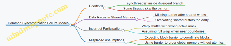
Example: Fixing a Divergent Barrier Bug
Suppose you guard a shared-memory load with bounds checks, but still call __syncthreads() only in the “in bounds” path. The fix is to ensure every thread reaches the barrier, while out-of-bounds threads write safe dummy values.
// Safe barrier placement with dummy writes
if (globalIdx < N) shared[tid] = input[globalIdx];
else shared[tid] = 0.0f;
__syncthreads();
// Now all threads can safely read shared[tid]
This keeps the barrier behavior consistent and makes the subsequent computation deterministic for the threads that participate.
2.4 Error Handling, Debugging, and Deterministic Verification
CUDA debugging is mostly about separating three things: whether the kernel launched, whether it ran correctly, and whether the results are reproducible. The trick is to check each layer at the right time, with the smallest possible perturbation to performance.
Error Handling Foundations
Start with a simple rule: every CUDA API call should be checked, and kernel failures must be surfaced after the launch. CUDA errors are sticky, meaning one failure can cause later calls to report the same issue even if they succeeded.
A practical pattern is:
- Check the return value of every CUDA runtime call.
- After a kernel launch, call
cudaGetLastError()to catch launch configuration issues. - Then call
cudaDeviceSynchronize()(or synchronize on the relevant stream) to catch runtime faults like illegal memory access.
Here is a compact helper that keeps the code readable:
#define CUDA_CHECK(call) do { \
  cudaError_t err = (call); \
  if (err != cudaSuccess) { \
    fprintf(stderr, "CUDA error %s at %s:%d\n", \
      cudaGetErrorString(err), __FILE__, __LINE__); \
    std::exit(EXIT_FAILURE); \
  } \
} while(0)
Use it like this:
CUDA_CHECK(cudaMemcpy(d_in, h_in, bytes, cudaMemcpyHostToDevice));
myKernel<<<grid, block, 0, stream>>>(d_in, d_out, n);
CUDA_CHECK(cudaGetLastError());
CUDA_CHECK(cudaStreamSynchronize(stream));
This sequence catches both “launch-time” and “run-time” problems without guessing.
Debugging Strategy That Scales
When something goes wrong, you want to narrow the fault domain quickly.
- Reproduce with minimal inputs. Reduce the problem size until the failure still occurs. If the bug disappears at smaller sizes, you likely have an indexing or bounds issue.
- Use deterministic launch geometry. Keep grid and block sizes fixed while debugging. Changing geometry can hide race conditions or expose them.
- Turn failures into assertions. For example, validate indices inside the kernel and write a sentinel value when an invalid index is detected.
- Inspect memory behavior. Illegal accesses often originate from incorrect pointer arithmetic, wrong element sizes, or mismatched host/device types.
A simple in-kernel guard for bounds:
__global__ void myKernel(const float* in, float* out, int n){
  int i = blockIdx.x * blockDim.x + threadIdx.x;
  if (i >= n) return;
  out[i] = in[i] * 2.0f;
}
This doesn’t fix every bug, but it prevents the most common “works for my size” failure.
Deterministic Verification Concepts
Determinism means the same inputs produce the same outputs across runs. GPUs can be nondeterministic due to race conditions, atomics, and floating-point reduction order.
A deterministic verification workflow has three layers:
- Reference correctness: compute expected results on the CPU with a clear, slow-but-trustworthy implementation.
- Numerical tolerance policy: compare with an error metric that matches the algorithm’s sensitivity.
- Execution determinism: ensure the kernel has no data races and that reductions use a stable strategy.
For floating-point comparisons, use a policy like:
- Absolute tolerance for near-zero values.
- Relative tolerance for larger magnitudes.
Example comparison logic:
- If
abs(a-b) <= atol + rtol*abs(b), treat as equal.
Mind Map: Debugging and Verification Workflow
Example: Catching a Race and Verifying Results
Suppose you compute a sum into a single output using multiple threads. If you write to the same location without synchronization, you’ll get nondeterministic results.
A deterministic approach is to:
- Accumulate partial sums per block into an intermediate array.
- Then reduce those partial sums in a second stage with a consistent order.
Verification then becomes meaningful: you compare against the CPU reference with the tolerance policy. If the comparison fails consistently, it’s a correctness issue; if it fails intermittently, it’s likely nondeterminism.
Example: Turning Kernel Failures into Actionable Reports
When a kernel fails, the error code alone is rarely enough. A useful pattern is to also record a small amount of diagnostic data:
- A counter of invalid indices.
- The first offending index (or a small ring buffer of offenders).
Then your host code can print a concise summary after synchronization. This keeps debugging focused: you learn what went wrong, not just that something went wrong.
Deterministic Verification Checklist
Before you trust performance results, run a deterministic verification pass:
- Same inputs, same launch geometry.
- No kernel errors after launch and synchronization.
- CPU reference comparison within the chosen tolerance policy.
- No nondeterministic reductions without a stable strategy.
If any item fails, fix correctness first. Performance work on incorrect or nondeterministic kernels is like measuring a stopwatch while the clock is broken.
2.5 Writing Reusable Kernel Interfaces for Engineering Workflows
Reusable kernel interfaces are less about clever abstractions and more about making the “contract” between host code and device code unambiguous. A good interface answers: what inputs are required, what shapes and strides are assumed, how errors are reported, and what guarantees the kernel makes about outputs. When those answers are consistent, you can swap implementations without rewriting the whole workflow.
Interface Goals That Prevent Engineering Headaches
Start with four goals. First, make indexing rules explicit so engineers don’t guess whether a kernel expects row-major or column-major layouts. Second, keep data movement predictable by stating whether pointers are device pointers, unified pointers, or host pointers. Third, separate configuration from computation: launch parameters and problem geometry should be passed in a structured way, not scattered across call sites. Fourth, ensure correctness checks are easy to run by returning status information and keeping deterministic validation paths.
Define a Kernel Contract with Clear Geometry
A reusable interface typically takes a small “problem descriptor” plus raw pointers. The descriptor should include dimensions, leading dimensions (stride), and any boundary parameters. For example, a 2D operator often needs width, height, and pitch/stride so the kernel can compute addresses without assuming contiguous storage.
A practical rule: if the kernel uses an index formula, the interface should provide every term in that formula. If you hardcode assumptions like contiguous rows, document them in the interface name or in a dedicated struct field.
Choose Parameter Types That Match Real Engineering Data
Use types that reflect how the data is produced. If your solver stores grid spacing as floats, don’t force double everywhere “just in case.” If your engineering pipeline uses 32-bit indices for memory footprint, keep indices 32-bit in the interface and only widen inside the kernel when needed for address arithmetic.
Also decide early whether the kernel supports in-place operation. In-place can be a performance win, but it changes aliasing assumptions. Your interface should either forbid aliasing or explicitly allow it.
Build a Launch Wrapper That Encodes Policy
A kernel interface should not force every caller to reinvent launch policy. Provide a host-side wrapper that computes grid and block sizes from the descriptor and selects shared memory usage. This wrapper becomes the single place where you encode “how we run this kernel.”
To keep it reusable, the wrapper should accept a stream and return a status code. That way, the same kernel can be used in synchronous tests and asynchronous pipelines without rewriting call sites.
Mind Map: Reusable Kernel Interface Components
Example: A Geometry Descriptor and a Host Wrapper
Below is a compact pattern for a 2D stencil-like kernel interface. The key idea is that the kernel never guesses strides or dimensions; it reads them from the descriptor.
struct Grid2D {
  int width;
  int height;
  int stride; // elements between rows
};

__global__ void apply_op(const Grid2D g,
                          const float* in,
                          float* out) {
  int x = blockIdx.x * blockDim.x + threadIdx.x;
  int y = blockIdx.y * blockDim.y + threadIdx.y;
  if (x >= g.width || y >= g.height) return;
  int idx = y * g.stride + x;
  out[idx] = in[idx];
}
Now the wrapper encodes launch policy and stream usage. It also centralizes error checking so callers stay clean.
int apply_op_launch(const Grid2D& g,
                     const float* d_in,
                     float* d_out,
                     cudaStream_t stream) {
  dim3 block(16, 16);
  dim3 grid((g.width + block.x - 1) / block.x,
            (g.height + block.y - 1) / block.y);
  apply_op<<<grid, block, 0, stream>>>(g, d_in, d_out);
  auto err = cudaGetLastError();
  if (err != cudaSuccess) return (int)err;
  return 0;
}
Interface Details That Make Kernels Composable
When kernels are composed, interfaces must agree on memory layout and synchronization. If kernel A writes into a buffer that kernel B reads, the interface should document whether the caller must synchronize or whether the wrapper enqueues operations on the same stream. The simplest rule: if both wrappers accept a stream and use it consistently, then ordering is preserved without extra device-wide synchronization.
Also, keep parameter naming consistent across kernels. If one kernel uses stride as “elements between rows,” another should not use pitchBytes without a clear conversion step.
Validation Hooks Without Polluting Production Code
A reusable interface should support lightweight validation. One approach is to include optional debug checks in the wrapper, not inside the kernel. For example, verify that stride >= width on the host, and that pointers are non-null. For correctness testing, provide a reference CPU function that uses the same descriptor and indexing formula, so mismatches show up as real bugs rather than “different assumptions.”
Mind Map: Validation and Debug Workflow
Summary of the Reuse Checklist
A reusable kernel interface: (1) passes geometry and strides explicitly, (2) uses consistent data types and aliasing rules, (3) centralizes launch policy in a wrapper that accepts a stream, and (4) provides validation hooks that keep production kernels uncluttered. When those pieces are stable, engineering workflows become a matter of swapping descriptors and pointers, not rewriting indexing logic every time.
3. Performance Engineering Workflow with Profiling and Metrics
3.1 Establishing Baselines with Representative Inputs
A baseline is your “known-good” performance and correctness snapshot before you change anything. For CUDA kernel work, that snapshot must be tied to inputs that resemble real runs, because performance often depends more on data shape and memory behavior than on the kernel code alone.
What a Baseline Must Capture
Start by defining four measurements for the same kernel build and runtime configuration:
- Correctness: bitwise match when possible, otherwise tolerance-based checks for floating-point results.
- Timing: kernel-only time and end-to-end time (including transfers if they matter to your workflow).
- Resource behavior: achieved occupancy, memory throughput, and stall reasons from profiling.
- Stability: repeatability across multiple runs to avoid optimizing noise.
A baseline that only records one number is like a map with no roads. You can still move, but you’ll guess where the bottlenecks are.
Choosing Representative Inputs
Representative inputs mean they exercise the same memory access patterns, boundary conditions, and workload mix as production. The trick is to avoid “average-looking” data that hides worst-case behavior.
Use three input categories:
- Typical: matches the most common sizes and distributions.
- Stress: hits extremes that affect memory coalescing, divergence, or reduction imbalance.
- Boundary: smallest sizes that still run correctly, plus sizes that trigger edge handling.
For example, if your kernel processes a 3D grid, choose dimensions that cover:
- non-multiples of block sizes (to test bounds checks)
- both small and large halos (to test shared memory tiling assumptions)
- cases where the last block is partially full (to test divergence and wasted work)
Systematic Baseline Procedure
- Fix the environment: lock GPU clocks if your workflow allows it, keep the same driver/runtime versions, and avoid background GPU load.
- Fix the launch configuration: record grid and block sizes, shared memory usage, and any compile-time flags.
- Warm up: run a few iterations before timing so caches, JIT compilation, and memory allocation effects settle.
- Measure with synchronization: ensure timing brackets include the right synchronization points so you’re not timing asynchronous launches.
- Repeat and summarize: collect at least 10 timing samples and report median plus spread.
Here’s a minimal timing pattern for kernel-only measurement:
// Pseudocode for kernel-only timing
warmup<<<grid, block, shmem, stream>>>(...);
cudaDeviceSynchronize();

for (int i = 0; i < N; i++) {
  cudaEventRecord(start, stream);
  kernel<<<grid, block, shmem, stream>>>(...);
  cudaEventRecord(stop, stream);
  cudaEventSynchronize(stop);
  times[i] = elapsed_ms(start, stop);
}
Use the same pattern for every candidate optimization so comparisons stay fair.
Mind Map: Baseline Inputs and Metrics
Concrete Example for Input Selection
Suppose you’re optimizing a reduction kernel that sums values per block and then reduces across blocks. Performance depends on how many elements each block processes and how balanced the partial sums are.
- Typical: N = 10,000,000 elements with uniformly random values.
- Stress: N = 10,000,003 elements so the last block is partial; values arranged so many threads contribute near-zero while a few contribute large magnitudes (to test numerical behavior and reduction imbalance).
- Boundary: N = 1, 2, 256, and 257 elements to validate edge handling and ensure the kernel doesn’t assume full blocks.
Your baseline should include all three categories, because a “fast” kernel on typical sizes can still be slow or incorrect on partial blocks.
What to Record in the Baseline Log
For each input category, record:
- input sizes and layout (dimensions, strides, alignment)
- data distribution summary (uniform, clustered, sparse density)
- kernel launch parameters (grid, block, shared memory)
- correctness result (pass/fail, max error)
- timing summary (median, min/max or interquartile range)
- key profiler metrics (memory throughput and dominant stalls)
When you later change one thing—say, a tiling factor or a memory layout—you’ll know whether the improvement is real, and whether it came with a correctness or stability cost.
3.2 Using Nsight Systems for Timeline and Concurrency Analysis
Nsight Systems helps you answer two practical questions: what ran, and when it ran relative to other work. For CUDA engineering, that means correlating CPU activity (kernel launches, memory copies, synchronization) with GPU activity (kernel execution, copy engines, and idle gaps). The goal is not to stare at a timeline until it feels meaningful; it’s to turn gaps and overlaps into specific, testable changes.
What You See on the Timeline
A typical Nsight Systems capture shows:
- CPU threads: where your host code issues work and waits.
- CUDA API calls: kernel launches, memory operations, and synchronization.
- GPU queues: where kernels and copies actually execute.
- Copy engines: whether H2D, D2H, and D2D transfers overlap with compute.
A useful mental model is a set of queues fed by the CPU. If the CPU is late, the GPU starves. If the GPU is busy but copies are serialized, you may be leaving bandwidth on the table.
Establishing a Baseline Capture
Start with a run that represents real workload shape: same input sizes, same iteration count, same stream usage. Then capture with enough duration to include steady-state behavior, not just warm-up.
A baseline capture should include:
- At least one full iteration of your main loop.
- Any one-time setup (so you can ignore it later).
- The region where you expect overlap between compute and transfers.
If you see only a single kernel launch, you’re likely missing the concurrency story. If you see many launches but no overlap, you may have a synchronization barrier in the wrong place.
Reading Concurrency Like a Checklist
Use this sequence when interpreting a capture.
-
Confirm kernel launch cadence
- Look for regular spacing between kernel launches on the CPU timeline.
- If launches bunch up and then stall, the host may be blocked on synchronization or memory allocation.
-
Check GPU queue overlap
- If kernels appear back-to-back with no gaps, the GPU is saturated.
- If there are gaps, identify whether the CPU is waiting or whether the GPU queue is empty.
-
Verify copy and compute overlap
- Transfers on different engines can overlap with compute if they are issued in separate streams and not blocked by dependencies.
- If H2D and compute never overlap, check for implicit synchronization points.
-
Inspect synchronization calls
- Calls like device-wide synchronization or stream synchronization can force ordering that removes concurrency.
- Prefer stream-scoped synchronization when you only need ordering within one stream.
Example: Overlap That Isn’t Actually Overlap
Suppose you intend to pipeline batches: while batch N computes, batch N+1 transfers.
A common accidental pattern is synchronizing after each transfer:
for (int i = 0; i < numBatches; i++) {
  cudaMemcpyAsync(d_in[i], h_in[i], bytes, cudaMemcpyHostToDevice, stream);
  cudaMemcpyAsync(d_out[i], h_out[i], bytes, cudaMemcpyDeviceToHost, stream);
  cudaStreamSynchronize(stream); // removes overlap
  kernel<<<grid, block, 0, stream>>>(d_in[i], d_out[i]);
}
In Nsight Systems, you’ll see transfers and kernels serialized on the same stream, with the CPU thread waiting at the synchronization call. The fix is to remove the per-iteration stream sync and instead synchronize only after the pipeline completes, or use events to enforce only the needed dependencies.
Example: Stream Dependencies That Preserve Overlap
If you need ordering between a specific transfer and its corresponding kernel, use events rather than global waits:
cudaEvent_t ready;
cudaEventCreate(&ready);

for (int i = 0; i < numBatches; i++) {
  cudaMemcpyAsync(d_in[i], h_in[i], bytes, cudaMemcpyHostToDevice, sCopy);
  cudaEventRecord(ready, sCopy);
  cudaStreamWaitEvent(sCompute, ready, 0);
  kernel<<<grid, block, 0, sCompute>>>(d_in[i], d_out[i]);
  cudaMemcpyAsync(h_out[i], d_out[i], bytes, cudaMemcpyDeviceToHost, sCopy);
}

cudaEventDestroy(ready);
On the timeline, you should observe that while batch i is computing on the compute stream, batch i+1 can be transferring on the copy stream. The event creates a precise dependency without forcing the entire device to idle.
Mind Map: Timeline and Concurrency Analysis
Turning Observations into Engineering Actions
Once you locate the first “why” on the timeline, the next step is to change one variable and recapture. If you remove a synchronization call, confirm that overlap returns in the same region of the timeline. If you add event-based dependencies, verify that only the intended ordering remains.
A good capture ends with a clear statement you can test: “This gap is caused by host waiting at stream synchronization,” or “Copies are serialized because they share a stream with compute.” Nsight Systems is most useful when it narrows the problem to a specific ordering constraint rather than a vague sense that “performance could be better.”
3.3 Using Nsight Compute for Kernel Level Bottleneck Diagnosis
Nsight Compute answers one practical question: where did the kernel spend its time, and what constraint caused it? The workflow is systematic: (1) collect a focused profile for one kernel configuration, (2) identify the limiting resource using section summaries, (3) confirm with metric relationships, and (4) apply one change at a time.
Start with a Clean, Representative Run
Use the same input sizes and launch geometry you care about, and profile only the kernel under test. If your kernel is called many times, profile a single representative call so the results match the steady behavior.
A good habit is to record three launch parameters: grid size, block size, and shared memory usage. Nsight Compute metrics often explain performance only when these are known.
Read the Report Like a Map, Not Like a Novel
Nsight Compute groups metrics into sections. Treat the “Top” or “Summary” view as a triage stage. Look for:
- Memory throughput limits: global load/store throughput, cache hit rates, and memory transaction counts.
- Execution efficiency limits: warp stall reasons, instruction mix, and occupancy-related signals.
- Synchronization limits: barriers and long-latency waits.
If you see high “Stall” time, the next step is to identify which stall reason dominates. A kernel can be “slow” for different reasons: waiting on memory, waiting on dependencies, or waiting on synchronization.
Use Warp Stall Reasons to Pinpoint the Constraint
Warp stall reasons are especially useful because they connect directly to what the hardware is doing. Common patterns:
- Memory dependency stalls: loads are not ready when needed; often fixed by improving locality or reducing redundant loads.
- Long scoreboard stalls: arithmetic depends on prior operations; often fixed by reordering computations or reducing register pressure.
- Barrier stalls: threads wait at
__syncthreads(); often fixed by reducing barrier frequency or restructuring tiles.
A quick sanity check: if stall reasons point to memory, don’t start by changing arithmetic intensity. Fix data movement first.
Confirm with Memory Transaction Metrics
Memory bottlenecks are rarely just “bandwidth.” Nsight Compute can show whether your loads are inefficient due to:
- Uncoalesced accesses causing extra transactions.
- Misaligned accesses increasing transaction count.
- Cache behavior that suggests poor reuse.
When global memory transactions are high relative to useful bytes, you likely have an indexing or layout issue. When transactions are reasonable but throughput is low, you may be limited by latency and insufficient parallelism.
Apply One Change and Reprofile
A single change should target the diagnosed constraint. Examples:
- If stall reasons show memory dependency, try tiling into shared memory and ensure coalesced global loads.
- If barrier stalls dominate, reduce the number of synchronization points or fuse operations within a tile.
- If register pressure reduces effective occupancy, simplify expressions and avoid large live ranges.
Reprofile the same kernel with the same input size so the comparison is meaningful.
Mind Map for Bottleneck Diagnosis
Example: From Stall Reasons to a Concrete Fix
Suppose a 2D stencil kernel shows:
- High warp stall time attributed to memory dependency.
- Many global load transactions per useful element.
The likely cause is that each thread loads neighbors with a pattern that is not coalesced. A practical fix is to load a tile plus halo into shared memory using coalesced accesses, then compute from shared memory.
// Shared-memory tiling sketch for a 2D stencil
__global__ void stencil(const float* in, float* out, int W, int H) {
  __shared__ float tile[BLOCK_Y+2][BLOCK_X+2];
  int x = blockIdx.x * BLOCK_X + threadIdx.x;
  int y = blockIdx.y * BLOCK_Y + threadIdx.y;

  // Load center and halo cooperatively
  tile[threadIdx.y+1][threadIdx.x+1] = in[y*W + x];
  if (threadIdx.x == 0) tile[threadIdx.y+1][0] = in[y*W + (x-1)];
  if (threadIdx.x == BLOCK_X-1) tile[threadIdx.y+1][BLOCK_X+1] = in[y*W + (x+1)];
  if (threadIdx.y == 0) tile[0][threadIdx.x+1] = in[(y-1)*W + x];
  if (threadIdx.y == BLOCK_Y-1) tile[BLOCK_Y+1][threadIdx.x+1] = in[(y+1)*W + x];

  __syncthreads();
  // Compute from shared memory
  float c = tile[threadIdx.y+1][threadIdx.x+1];
  float n = tile[threadIdx.y][threadIdx.x+1];
  float s = tile[threadIdx.y+2][threadIdx.x+1];
  float w = tile[threadIdx.y+1][threadIdx.x];
  float e = tile[threadIdx.y+1][threadIdx.x+2];
  out[y*W + x] = 0.2f*(c+n+s+w+e);
}
After this change, you should expect fewer global transactions and a shift in stall reasons away from memory dependency. If stalls remain high, the next suspect is insufficient parallelism or excessive register pressure, which Nsight Compute can also reveal.
Example: Barrier Stalls and a Less Synchronization-Heavy Layout
If Nsight Compute shows barrier stalls dominating, you can often restructure so multiple computations happen within one shared-memory tile lifetime. Instead of synchronizing after every micro-step, compute a small pipeline of operations before the next barrier, keeping intermediate values in registers.
The key is to match the fix to the metric: barrier stalls should drop, and the warp stall breakdown should shift accordingly after reprofile.
3.4 Interpreting Key Metrics Such as Occupancy and Memory Throughput
Occupancy and memory throughput are two different stories about performance. Occupancy describes how many warps can be resident on a streaming multiprocessor (SM) at once. Memory throughput describes how effectively the kernel turns memory requests into useful data per second. A kernel can have high occupancy and still be slow if it issues inefficient memory transactions; it can also be limited by memory even with moderate occupancy.
Occupancy Metrics That Actually Matter
Start with what occupancy means in practice: the GPU can switch between warps when one warp stalls (often on memory). Higher occupancy can hide latency, but only if there are enough independent warps and the scheduler can keep them progressing.
Key metrics to interpret:
- Achieved occupancy: the fraction of the theoretical maximum resident warps. This is influenced by registers per thread, shared memory per block, and the block size.
- Active warps per SM: a more direct view of how many warps are ready to run.
- Register pressure: high register usage can reduce resident blocks, lowering active warps.
- Shared memory usage: large shared allocations can cap the number of concurrent blocks.
A useful mental model: occupancy is a capacity constraint. Throughput is the result of how well warps use that capacity.
Memory Throughput Metrics That Tell You Where Time Goes
Memory throughput is usually limited by one of three things: bandwidth, transaction efficiency, or access pattern.
Key metrics to interpret:
- Global memory throughput: how many bytes per second are transferred.
- Memory transaction efficiency: whether loads/stores are coalesced into fewer, larger transactions.
- L2 hit rate and cache behavior: whether data is reused and whether the cache helps.
- Stall reasons: whether warps are waiting on memory, execution dependencies, or synchronization.
If throughput is low and stall reasons point to memory, you likely have an access-pattern problem (strided indexing, misalignment, or scattered gathers). If throughput is decent but stalls remain high, you may be limited by instruction dependencies or synchronization.
A Systematic Interpretation Workflow
- Confirm the bottleneck category: check stall reasons first. If memory stalls dominate, focus on memory metrics; if not, look at instruction and dependency metrics.
- Check whether occupancy is the limiting factor: if achieved occupancy is low, inspect register and shared memory usage. Then verify whether increasing occupancy is likely to help by seeing whether memory stalls are high.
- Evaluate transaction efficiency: compare effective bytes moved to requested bytes. Poor coalescing often shows up as low effective throughput even when bandwidth is available.
- Validate with a controlled change: adjust one variable at a time (block size, tile size, data layout, or loop structure) and re-check the same metrics.
This workflow prevents the classic mistake: optimizing occupancy when the kernel is actually limited by memory transaction inefficiency.
Mind Map: How Metrics Connect to Kernel Behavior
Example: When High Occupancy Still Fails
Suppose a stencil kernel uses a large tile in shared memory. Achieved occupancy drops because shared memory per block is high. You might expect performance to suffer, and it does—but the more important question is why.
- If stall reasons show heavy memory dependency stalls, then lowering occupancy can hurt because fewer warps are available to cover latency.
- If stall reasons show execution dependency stalls instead, then occupancy changes may not help much; the kernel may be waiting on arithmetic or synchronization.
Now consider memory throughput. If global memory throughput is low and transaction efficiency is poor, the kernel is not just underutilizing latency hiding; it is also issuing inefficient memory requests. Fixing coalescing (for example, changing indexing so consecutive threads access consecutive elements) can raise throughput even if occupancy stays the same.
Example: When Low Occupancy Is Fine
A reduction kernel often has fewer independent memory accesses per instruction and may use warp-level primitives. Achieved occupancy might be moderate because registers are used for partial sums. If memory stalls are not dominant and throughput is already near the expected level for the access pattern, then pushing occupancy higher may not improve runtime. In that case, the kernel is limited by reduction steps and synchronization costs, not by memory latency.
Practical Checklist for Reading Metrics
- If memory stalls dominate and achieved occupancy is low, try reducing register usage or shared memory footprint, then re-check stall distribution.
- If memory stalls dominate but transaction efficiency is low, focus on coalescing and data layout before touching occupancy.
- If memory stalls are not dominant, treat occupancy as a secondary metric and look for dependency chains, branch divergence, or synchronization overhead.
- Always pair occupancy changes with throughput and stall reason checks; otherwise you might “fix” the wrong constraint.
3.5 Building Iterative Optimization Loops with Measured Changes
An optimization loop is just disciplined experimentation: change one thing, measure the effect, and keep the change only if it improves the outcome you care about. On GPUs, “one thing” is rarely a single line of code, so the loop needs a clear target metric, a controlled setup, and a way to attribute improvements to the change.
Step 1: Define the Optimization Goal and Success Metric
Start by choosing a metric that matches the bottleneck you suspect. Common choices include kernel time, achieved memory bandwidth, instruction throughput, occupancy, and end-to-end iteration time for an algorithm.
Example goal: “Reduce time per iteration of a Jacobi stencil.”
- Primary metric: total time per iteration (including halo exchange if applicable).
- Secondary metrics: kernel time for the stencil update, and achieved global memory bandwidth.
Write down the metric names exactly as they will appear in your profiling output. If you later switch metrics midstream, you’ll end up optimizing the wrong thing with confidence.
Step 2: Build a Reproducible Baseline
A baseline is not “whatever happens when I run it.” It is a repeatable configuration.
Baseline checklist:
- Fix input sizes and iteration counts.
- Use the same GPU clocks mode and driver settings.
- Warm up the run so caches and JIT compilation effects settle.
- Run multiple trials and record the median.
Example baseline procedure:
- Run 10 iterations of the stencil kernel update.
- Measure total time for those 10 iterations.
- Record median across 5 trials.
Step 3: Choose a Single Change and Predict Its Mechanism
Each loop iteration should change one hypothesis-driven aspect.
Good change candidates:
- Adjust block size to improve occupancy or reduce register pressure.
- Reorder data layout to improve coalescing.
- Introduce shared-memory tiling to reduce redundant global loads.
- Fuse kernels to reduce launch overhead and intermediate writes.
- Replace a naive reduction with a warp-level reduction.
Prediction format that keeps you honest:
- “If we tile into shared memory, global load transactions should drop, so achieved bandwidth should rise and kernel time should fall.”
Step 4: Measure the Change with the Same Instrumentation
Use the same profiling workflow for every iteration. If you change instrumentation, you change overhead and you lose comparability.
What to capture each time:
- Kernel time (or relevant section time).
- Memory throughput indicators (e.g., global load/store efficiency).
- Occupancy and stall reasons.
- Any correctness flags or residual norms.
Example: After switching to a tiled stencil, you expect fewer global loads. If kernel time drops but bandwidth metrics do not improve, you may have shifted the bottleneck to arithmetic or synchronization.
Step 5: Decide Keep, Revert, or Split the Change
Not every improvement is worth keeping, and not every regression is fatal.
Decision rules:
- Keep if primary metric improves and correctness is unchanged.
- Revert if primary metric regresses beyond measurement noise.
- Split if the change includes multiple effects (e.g., block size plus data layout). Separate them so you can attribute gains.
A practical noise guard:
- If the improvement is smaller than the typical variation across trials, treat it as inconclusive.
Step 6: Update the Model of the Bottleneck
After each measurement, update your understanding of what limits performance.
Example reasoning chain for a stencil:
- Baseline shows high “memory dependency” stalls.
- Tiling reduces global transactions and improves bandwidth.
- Kernel time drops, but stalls shift toward “execution dependency.”
- Next change targets instruction efficiency (e.g., reduce redundant address calculations or simplify boundary handling).
This is where the loop becomes systematic: you are not just trying options, you are refining a bottleneck model.
Mind Map: Iterative Optimization Loop
Example: A Measured Loop for a Stencil Kernel
Iteration 0 baseline:
- Block size: 16×16×1.
- Metric: 10-iteration time = 120 ms median.
- Observation: low global load efficiency and high memory stalls.
Iteration 1 change: shared-memory tiling.
- Tile size chosen to fit shared memory without spilling.
- Prediction: fewer global loads per output cell.
- Result: 10-iteration time = 98 ms median; bandwidth efficiency improves.
Iteration 2 change: adjust block size to reduce register pressure.
- Prediction: higher occupancy without increasing memory traffic.
- Result: 10-iteration time = 92 ms median; stalls shift toward execution dependency.
Iteration 3 change: simplify boundary condition handling.
- Prediction: fewer divergent branches and less instruction overhead.
- Result: 10-iteration time = 88 ms median; correctness checks match CPU reference within tolerance.
At this point, the loop has done its job: each change is tied to a measurable mechanism, and the bottleneck model has moved from memory to execution overhead.
Practical Loop Hygiene
Keep a small log per iteration:
- Change description.
- Metric deltas.
- Profiling highlights.
- Correctness outcome.
When you later revisit the code, you’ll know why a choice exists, not just that it “worked once.”
4. Memory Optimization Strategies for High Throughput Kernels
4.1 Coalesced Global Memory Access and Alignment Requirements
Coalescing is what happens when threads in a warp access global memory addresses that the hardware can combine into as few memory transactions as possible. The goal is simple: fewer transactions means less wasted bandwidth and fewer stalls. The tricky part is that “nearby” addresses in your code do not always mean “coalesced” addresses in memory.
What Coalescing Actually Depends On
A warp has 32 threads. For a typical 4-byte element type (like float), a perfectly coalesced access looks like a contiguous 128-byte segment: 32 threads × 4 bytes = 128 bytes. If your threads read a[i + lane], where lane is the thread’s position within the warp, the hardware can usually serve the whole warp with one transaction.
Coalescing breaks when:
- Threads access a stride larger than the element size.
- Threads access mixed or irregular indices.
- The starting address is misaligned relative to the transaction size.
- The access pattern crosses segment boundaries within the same warp.
Alignment Requirements in Practice
Alignment is about the starting address of the data. Even if threads access a contiguous range, an awkward starting pointer can force the hardware to touch multiple segments.
A practical rule of thumb: align allocations and leading dimensions so that the first element accessed by a warp begins on a boundary that matches the transaction granularity. For 4-byte elements, aligning the base pointer to 128 bytes is ideal for warp-sized contiguous accesses. For 8-byte elements, 128-byte alignment still helps, but you should expect coalescing to be more sensitive to how many bytes each thread reads.
In engineering terms: if you control the data layout, make it easy for the warp to land on clean boundaries.
A Systematic Way to Check Your Access Pattern
- Identify the warp dimension: which index varies fastest across threads.
- Write the address expression: determine what global address each thread touches.
- Compute the per-warp byte span: multiply element size by the number of contiguous elements accessed by the warp.
- Check stride: if the index step between adjacent lanes is not 1 element, coalescing likely degrades.
- Check alignment: confirm the base pointer and the effective starting index produce aligned segment boundaries.
Example: Contiguous Reads That Coalesce
Assume float* x points to an array. Each warp reads consecutive elements.
__global__ void readCoalesced(const float* x, float* out) {
  int i = blockIdx.x * blockDim.x + threadIdx.x;
  out[i] = x[i];
}
If threadIdx.x maps directly to the element index, lane 0 reads x[i0], lane 1 reads x[i0+1], and so on. For 4-byte floats, that’s the classic 128-byte contiguous segment per warp.
Example: Strided Access That Fails Coalescing
Now suppose you store a 2D array in row-major order but launch threads over columns.
__global__ void readStrided(const float* A, float* out, int rows, int cols) {
  int col = blockIdx.x * blockDim.x + threadIdx.x;
  int row = blockIdx.y;
  int idx = row * cols + col;
  out[col] = A[idx];
}
If row is fixed for a warp and col varies, you may still get coalescing because col is contiguous. But if you instead fix col and vary row, adjacent lanes jump by cols elements, turning a single warp into many scattered transactions.
Alignment Pitfalls with Structs and Mixed Types
If you use a struct like:
struct { float a; char b; float c; }
the compiler may insert padding. That padding changes the byte distance between fields across threads, which can ruin your mental model of “adjacent elements.” Even when the logical field is contiguous, the physical layout might not be.
A safer approach is to store frequently accessed numeric fields in separate arrays (structure-of-arrays) so each field has a predictable element size and alignment.
Practical Engineering Guidelines
- Prefer contiguous indexing for the fastest-changing thread dimension: make the thread index correspond to the element index.
- Use grid-stride loops carefully: the stride should preserve contiguity within each warp for each iteration.
- Ensure base pointers are aligned: allocate with alignment guarantees and avoid manual pointer arithmetic that offsets alignment.
- Match element sizes to access width: if you read
double, remember each lane touches 8 bytes, so the warp spans 256 bytes; coalescing still works, but alignment and segment boundaries matter more. - Avoid accidental misalignment from subviews: slicing like
x + kcan shift the starting address away from a clean boundary.
Mind Map: Coalescing and Alignment Requirements
Quick Mental Test
Ask: “If I freeze the warp’s lane index and look at the byte addresses each lane touches, do they form a mostly contiguous, well-aligned range?” If the answer is no, you likely need to change the indexing or data layout before you start tuning anything else.
4.2 Shared Memory Tiling and Bank Conflict Avoidance
Shared memory is the fast scratchpad that lets threads reuse data instead of repeatedly fetching it from global memory. Tiling is the engineering move that stages a small working region into shared memory, computes on it, then moves to the next region. Bank conflict avoidance is the part where you make sure those shared-memory accesses can happen in parallel rather than queuing behind each other.
From Global Loads to Shared Tiles
Start with the baseline: each thread loads its own input element from global memory, then computes. This often works but wastes bandwidth because neighboring threads repeatedly read overlapping regions.
Tiling changes the flow:
- Threads cooperatively load a tile into shared memory.
- Threads synchronize so the tile is fully available.
- Threads compute using shared memory, which is much faster.
- Threads move to the next tile.
A simple mental model: global memory is a busy highway; shared memory is a local street. Tiling turns many highway trips into a single neighborhood delivery.
Shared Memory Banks and What Conflicts Mean
Shared memory is divided into banks. When threads in the same warp access shared memory addresses that map to the same bank, the accesses serialize. The result is lower throughput even though the data is “in shared memory.”
Key idea: bank mapping depends on the address. For typical configurations, consecutive 32-bit words map to consecutive banks. That means patterns that stride by 1 word are usually conflict-free, while patterns that stride by a multiple of the number of banks can cause repeated bank hits.
Tiling Layout That Plays Nice with Banks
Consider a 2D tile stored in shared memory as tile[row][col]. If you access tile[row][col] with threads varying col across a warp, then col is the dimension that controls bank mapping.
A common pitfall is using a tile width that makes the stride align badly with bank count. The classic fix is padding: add one extra element to the leading dimension so that rows start at different bank offsets.
Padding Rule of Thumb
If your shared tile is TILE_DIM x TILE_DIM, store it as TILE_DIM x (TILE_DIM + 1). That extra column shifts each row’s bank alignment, breaking up repeated bank targeting.
Systematic Tiling Workflow
- Choose a tile size that fits shared memory budget with room for other arrays. If you oversize, you may reduce occupancy because shared memory per block becomes too large.
- Map threads to tile coordinates so each thread loads one element (or a small fixed number) from global memory into shared memory.
- Use coalesced global loads by ensuring consecutive threads read consecutive global addresses.
- Synchronize once per tile after the load phase.
- Compute using shared memory with access patterns that avoid bank conflicts.
- Synchronize only when needed before the next tile load.
Example: Matrix Multiply Tile with Conflict Avoidance
Below is a compact kernel sketch for C = A x B using shared memory tiling. The padding on As and Bs reduces the chance of bank conflicts when threads read columns.
__global__ void matmul_tiled(const float* A, const float* B, float* C,
                               int N) {
  const int TILE = 16;
  __shared__ float As[TILE][TILE + 1];
  __shared__ float Bs[TILE][TILE + 1];

  int row = blockIdx.y * TILE + threadIdx.y;
  int col = blockIdx.x * TILE + threadIdx.x;

  float acc = 0.0f;
  for (int k0 = 0; k0 < N; k0 += TILE) {
    As[threadIdx.y][threadIdx.x] = A[row * N + (k0 + threadIdx.x)];
    Bs[threadIdx.y][threadIdx.x] = B[(k0 + threadIdx.y) * N + col];
    __syncthreads();

    #Pragma Unroll
    for (int k = 0; k < TILE; k++)
      acc += As[threadIdx.y][k] * Bs[k][threadIdx.x];
    __syncthreads();
  }
  C[row * N + col] = acc;
}
Why this helps: during the inner loop, threads read As[threadIdx.y][k] and Bs[k][threadIdx.x]. Without padding, the “column-like” access can repeatedly target the same bank. With padding, each row starts at a shifted bank boundary, so the warp’s accesses spread out.
Mind Map: Shared Memory Tiling and Bank Conflicts
Debugging the “It Should Be Fast” Problem
If performance is disappointing, check whether the shared-memory access pattern is actually conflict-free. A tiling kernel can still underperform if the compute phase reads shared memory in a way that collapses many threads onto the same bank. Padding is the most common low-effort fix, but the deeper fix is to align your thread-to-data mapping so the varying index corresponds to the dimension that naturally spreads bank usage.
Finally, remember that tiling is not just about speed; it’s about making data reuse predictable. When the tile boundaries and access patterns are consistent, correctness stays straightforward and performance becomes measurable rather than mysterious.
4.3 Register Pressure Control and Compiler Friendly Coding Patterns
Register pressure is the quiet reason kernels slow down. When the compiler needs many registers per thread, fewer warps fit on a streaming multiprocessor, which reduces latency hiding. The result is often lower occupancy and more spilling to local memory, where performance goes to get a coffee and never comes back.
Foundations of Register Pressure
A CUDA thread has a fixed register budget per SM. The compiler decides how many registers each thread uses based on your code structure, types, and control flow. Two symptoms show up repeatedly:
- Low occupancy: the scheduler has fewer warps to switch between.
- Local memory spills: values that don’t fit in registers are stored in “local” memory, which is backed by global memory and is much slower.
The key engineering idea is simple: write code that gives the compiler a clear, stable plan for lifetimes and types, so it can reuse registers instead of hoarding them.
How the Compiler Chooses Registers
Register usage grows when the compiler must keep many live values at once. “Live” means the value may be needed later along some path. Common causes include:
- Long expressions that keep intermediate results alive.
- Multiple variables with overlapping lifetimes.
- Branch-heavy code where the compiler must preserve values across paths.
- Large structs or arrays in registers.
A practical mindset: treat registers like a small desk. If you keep too many papers out, you’ll start stacking them on the floor (spills).
Compiler Friendly Coding Patterns
Shorten Expression Lifetimes
Break large expressions into steps so intermediates can be reused or overwritten. This often reduces the number of simultaneously live temporaries.
// Less friendly: many intermediates may stay live
float t = a*b + c*d - e*f;

// More friendly: reuse a variable
float t1 = a*b;
float t2 = c*d;
float t3 = e*f;
float t = t1 + t2 - t3;
If you see no improvement, don’t force it—measure. Sometimes the compiler already optimizes this well.
Prefer Reuse over “Nice” Naming
Using many distinct variables can extend lifetimes. Reusing a variable name can encourage earlier overwrites.
float x = in[i];
float y = x * scale;
float z = y + bias;
// Friendly reuse
x = in[i];
x = x * scale;
x = x + bias;
This is not about aesthetics; it’s about giving the compiler fewer candidates for “still needed later.”
Control Branch Divergence and Live Ranges
Branches can force the compiler to keep values alive across both sides. When possible, move invariant computations outside conditionals and keep conditional blocks small.
A typical pattern for boundary handling:
- Compute indices and masks.
- Guard loads with conditions.
- Compute the main formula with values already normalized (e.g., set out-of-bounds loads to zero).
This keeps the core arithmetic path uniform and reduces the number of values that must survive across divergent paths.
Use Smaller Types Carefully
Using half or int32 can reduce register usage, but it can also introduce extra conversion instructions. The goal is not “smaller is always better.” The goal is “fewer registers without creating new bottlenecks.”
A safe approach is to start with the type that matches your data, then check register count and achieved throughput.
Avoid Large Per-Thread Arrays
Arrays declared inside kernels often force register allocation or spills. If you need temporary storage, consider:
- Using shared memory for block-scoped tiles.
- Using warp-level primitives for small reductions.
- Using scalar temporaries when the algorithm allows it.
Keep Structs Lean
Passing or storing large structs by value can inflate register usage. Prefer passing pointers/references and accessing only needed fields. If you must use structs, keep them small and avoid embedding large arrays.
Mind Map: Register Pressure Control
Systematic Verification Loop
- Inspect register count for the kernel build you care about.
- Check for spills by looking at compiler output or profiling signals.
- Apply one change at a time so you know what helped.
- Re-measure end-to-end time, not just occupancy, because memory behavior and instruction mix also matter.
A kernel can have fewer registers and still be slower if it increases memory traffic or adds conversions. The engineering job is to make the tradeoff net-positive.
Example: Boundary Guarding Without Register Bloat
A common pattern is to compute a value for every thread, but guard the load:
- If the index is valid, load from global memory.
- Otherwise, set the value to a neutral element (often zero).
This avoids having separate “valid” and “invalid” arithmetic paths that keep different sets of variables alive.
int idx = base + tid;
float val;
if (idx < n) {
  val = in[idx];
} else {
  val = 0.0f;
}
// Continue with uniform arithmetic
out[tid] = val * scale + bias;
The uniform arithmetic after the conditional is the part that keeps register lifetimes predictable.
Practical Checklist
- Split long expressions into steps when temporaries explode.
- Reuse variables to shorten lifetimes.
- Keep conditional blocks small and move invariants out.
- Avoid per-thread arrays and large structs.
- Use types that match the data, then verify register and spill behavior.
When you treat register pressure as a measurable constraint rather than a mystery, the compiler becomes a collaborator instead of a surprise party.
4.4 Cache Behavior With Read Only Data and Locality Management
GPUs have multiple cache-like structures, but the practical question is simpler: how do you reduce repeated global memory reads when many threads need the same inputs? Read-only data is a common case in scientific kernels—coefficients, lookup tables, boundary parameters, and small constants. Locality management is the discipline of arranging accesses so that reuse happens while the data is still “near” the threads that need it.
Core Cache Behavior Concepts
Start with the memory hierarchy you actually feel in kernels: registers for per-thread values, shared memory for per-block reuse, and global memory for everything else. Caches sit between global memory and the compute units, but they are not magic; they respond to access patterns.
Read-only data benefits when:
- Many threads in a warp read the same or nearby addresses.
- The working set fits in the cache capacity for the duration of the reuse.
- Accesses are not constantly evicting each other.
Locality management benefits when:
- Threads access memory in a predictable order.
- Reuse occurs within a short time window.
- You avoid patterns that scatter accesses across a huge address range.
Read Only Data Paths and What “Read Only” Means
On CUDA, marking data as read-only (for example, using the read-only cache path) helps when the hardware can treat those loads as non-modifying. The key is that read-only caching is most effective for repeated reads, not for one-time streaming.
A typical scenario: a stencil kernel where each block loads a small set of coefficients (like weights) that are reused across many grid points. If every thread fetches coefficients from global memory repeatedly, you pay the bandwidth cost over and over. If instead you route those loads through a read-only path or stage them into shared memory once per block, the cost drops.
Locality Management Through Access Geometry
Locality is mostly about mapping indices to addresses. Consider a 2D array stored in row-major order. If thread tx varies fastest and you map x to the contiguous dimension, then threads in a warp tend to read consecutive addresses. That pattern is friendly to caches and memory coalescing.
When you accidentally map threads so that tx jumps by a large stride, each thread touches a far-away cache line. Even if the data is “read only,” the cache can’t help much because reuse is low.
Practical Example: Coefficients for a Stencil
Suppose each output point computes:
- A weighted sum of neighbors using a small coefficient array
w[9]. - The same
wfor every point.
A simple engineering approach:
- Keep
win a read-only cache path so repeated loads across warps are cheaper. - Optionally stage
winto shared memory once per block if you want deterministic reuse and fewer cache interactions.
// Conceptual sketch: read-only coefficients used by all threads
__global__ void stencil(const float* __restrict__ in,
                          float* __restrict__ out,
                          const float* __restrict__ w) {
  int x = blockIdx.x * blockDim.x + threadIdx.x;
  int y = blockIdx.y * blockDim.y + threadIdx.y;

  // Each thread reads the same small coefficient set
  float c0 = w[0];
  float c1 = w[1];
  // ... c2..c8

  // Compute using in neighbors (not shown)
  // out[idx] = c0*in[idx] + c1*in[idx+...] + ...
}
If w is small and reused heavily, this pattern reduces redundant global traffic. If w were large and accessed with little repetition, read-only caching would not compensate for the sheer number of distinct addresses.
Mind Map: Cache Behavior with Read Only Data and Locality Management
Advanced Details Without the Hand-Waving
-
Choose the right reuse scope. If reuse is per-thread, registers win. If reuse is per-block, shared memory is usually the most controllable. If reuse is across many blocks, read-only caching can help, but it depends on how often the same addresses are touched concurrently.
-
Avoid cache-thrashing patterns. If each thread walks a long array with little overlap, the cache becomes a temporary holding area, not a reuse engine. In that case, focus on coalescing and reducing total loads rather than expecting cache hits.
-
Use consistent indexing and alignment. Misaligned or irregular indexing can turn a “mostly contiguous” access into many small, inefficient transactions. Even when the code is correct, the memory system may not be.
A Second Example: Lookup Table with Strided Access
Imagine a kernel that maps each grid point to a lookup table lut[1024] using an index derived from coordinates. If neighboring threads produce indices that are close, locality improves and caches can help. If neighboring threads produce indices that are effectively random, each thread touches different cache lines, and read-only caching offers limited benefit.
The engineering response is not to force caching. It is to restructure the computation so that threads process regions where lut indices are correlated, or to stage a small subset of lut into shared memory for the region a block is responsible for.
Summary of the Section’s Engineering Rules
- Read-only caching helps when reuse is real and the working set is small enough to stay relevant.
- Locality management is about mapping threads to addresses so that both spatial and temporal reuse happen.
- Shared memory staging is the most controllable way to guarantee reuse within a block.
- When access patterns are scattered, focus on reducing distinct loads and improving coalescing rather than expecting caches to fix everything.
4.5 Efficient Data Layout Choices for Multidimensional Arrays
Multidimensional arrays are where performance goes to hide. The GPU doesn’t care that your data is “3D”; it cares how threads walk through memory. Efficient layout means you choose an ordering that matches how threads index elements, so global memory accesses become coalesced and reuse becomes possible.
Start with the Linearization Rule
In C/C++, a multidimensional array is stored linearly in row-major order. For an array A[Z][Y][X], the fastest-changing index is X, then Y, then Z. That means consecutive X elements sit next to each other in memory.
A simple mental model: if your kernel’s threads vary X across the warp, then each thread reads a neighboring address. If threads vary Z instead, the warp jumps by large strides and coalescing collapses.
Match Layout to Thread Indexing
Assume a 3D grid where each thread computes one element. If your indexing is:
x = threadIdx.x + blockIdx.x * blockDim.xy = threadIdx.y + blockIdx.y * blockDim.yz = threadIdx.z + blockIdx.z * blockDim.z
Then you should store data so that the dimension you map to x is the fastest-changing one in memory. For row-major A[z][y][x], that is exactly x. If you instead store A[x][y][z] (or treat a buffer as if it were), you effectively reverse the stride pattern and hurt memory throughput.
Use Strides Explicitly When You Can
When you pass multidimensional data to kernels, prefer explicit strides over assuming a particular layout. A common pattern is to represent a 2D slice as a pointer plus a leading dimension (stride). For example, a Y x X tile stored with leading dimension ld lets you handle padding and subviews without rewriting indexing logic.
This matters because padding can align rows to cache-line or memory-transaction boundaries, improving coalescing. It also matters for halo regions in stencils, where you often allocate extra border elements.
Choose Between Array of Structures and Structure of Arrays
For multidimensional arrays of structs, layout choice can dominate performance. Suppose each grid point stores {u, v, w}. If you use an array of structs, threads reading only u still fetch the whole struct. With structure of arrays, each component is stored in its own contiguous buffer, so threads read only what they need.
A practical rule: if kernels operate on one or two fields at a time, Structure of Arrays usually wins. If kernels always touch all fields together, Array of Structures can be fine.
Plan for Shared Memory Tiling
Shared memory tiling works best when you can load a tile with coalesced global reads and then reuse it across multiple computations. For a 2D stencil, a typical tile is (tileY + 2*halo) x (tileX + 2*halo). The shared memory array should mirror the access pattern of the computation, not necessarily the original global layout.
To avoid bank conflicts, you sometimes add padding in shared memory. The padding is small and local, but it can prevent repeated serialization when threads access different columns.
Mind Map: Data Layout Decisions for Multidimensional Arrays
Example: 3D Stencil with Correct Ordering
Consider a stencil that updates A[z][y][x] using neighbors in x, y, and z. If your threads map x to threadIdx.x, store the grid as A[z][y][x] (row-major). Then each warp reads a contiguous run of x values for the center and for the x±1 neighbors.
If you accidentally treat the same buffer as A[x][y][z], then x becomes the slowest-changing dimension. Threads in a warp will stride by Y*Z elements, and the memory system will do a lot more work per useful byte.
Example: Padded Rows for Coalescing
For a 2D buffer B[y][x], you can allocate B with a leading dimension ld = X + pad. Then each row starts at ld elements, not X. If ld makes row starts align better with transaction sizes, each warp’s reads across x become more consistently coalesced.
This is especially useful when X is not a multiple of the transaction granularity. Padding changes only the indexing math; the kernel logic stays the same.
Example: Structure of Arrays for Component Updates
If you have u, v, and w at each grid point but your kernel computes a new u using only u and a few coefficients, store u in its own contiguous buffer. Then the kernel reads u with the same coalescing behavior as a plain scalar field, while v and w remain untouched.
When you later need all components, you can still load them, but you avoid paying the bandwidth cost on the common path.
Quick Checklist for Layout Decisions
- Map the dimension that varies within a warp to the fastest-changing memory index.
- Use explicit strides for subviews, halos, and padded allocations.
- Prefer Structure of Arrays when kernels touch a subset of fields.
- Mirror computation access patterns in shared memory tiles, and add small padding to reduce bank conflicts.
- Validate indexing assumptions with small test sizes where dimensions are not multiples of block sizes.
5. Kernel Design Patterns for Scientific Computation
5.1 Parallelizing Stencil Computations with Halo Regions
Stencil computations update each grid point from a fixed neighborhood, like a 3D 7-point stencil or a 2D 5-point stencil. On a GPU, the key engineering task is to ensure every thread can read its required neighbor values without stepping on data that belongs to other blocks or other time steps. Halo regions solve this by giving each block a small “border” of extra input cells.
Core Idea of Halo Regions
Consider a 2D grid u updated into u_next using the 5-point stencil:
u_next[i,j] = c0*u[i,j] + c1*(u[i-1,j] + u[i+1,j] + u[i,j-1] + u[i,j+1])
If a thread computes u_next[i,j], it needs u values at (i±1,j) and (i,j±1). When threads are grouped into blocks, the block’s interior threads can be computed from a contiguous tile of u, but the boundary threads also need neighbor values just outside the tile. Those outside values are the halo.
A practical pattern is:
- Each block loads its tile of
uinto shared memory. - Threads also load halo cells into shared memory.
- After a barrier, threads compute
u_nextfor the interior tile.
This avoids repeated global memory reads and prevents incorrect reads caused by missing neighbor data.
Mapping Threads to Tiles
Let a block cover TILE_X × TILE_Y output points. Shared memory then needs (TILE_X + 2) × (TILE_Y + 2) to include a one-cell halo on each side for the 5-point stencil.
A clean indexing scheme is:
- Global output index:
(x, y)foru_next. - Shared memory index:
(sx, sy)wheresx = tx + 1,sy = ty + 1for the interior. - Halo loads use
sx = 0orsx = TILE_X + 1(and similarly forsy).
The “+1” offset is the small trick that keeps interior and halo reads consistent.
Boundary Conditions Without Chaos
Halo loading must handle edges of the global domain. Common choices are:
- Clamp: treat out-of-bounds neighbors as the nearest valid cell.
- Zero: out-of-bounds neighbors are zero.
- Fixed: boundary values are stored separately.
In all cases, the halo load code checks whether the neighbor coordinate is inside the domain. Threads that would load outside simply write the chosen boundary value into shared memory.
This is where correctness usually breaks first, so it’s worth making the boundary rule explicit and consistent across all halo directions.
Example Kernel Skeleton
Below is a compact CUDA-style skeleton showing the halo load and compute phases. It assumes a one-cell halo for a 2D 5-point stencil.
__global__ void stencil5(const float* __restrict__ u,
                          float* __restrict__ u_next,
                          int nx, int ny) {
  const int TILE_X = blockDim.x;
  const int TILE_Y = blockDim.y;

  __shared__ float sh[TILE_X + 2][TILE_Y + 2];

  int tx = threadIdx.x, ty = threadIdx.y;
  int x0 = blockIdx.x * TILE_X;
  int y0 = blockIdx.y * TILE_Y;

  int x = x0 + tx;
  int y = y0 + ty;

  auto load = [&](int gx, int gy) {
    if (gx < 0 || gx >= nx || gy < 0 || gy >= ny) return 0.0f;
    return u[gy * nx + gx];
  };

  sh[tx + 1][ty + 1] = load(x, y);
  if (tx == 0) sh[0][ty + 1] = load(x - 1, y);
  if (tx == TILE_X - 1) sh[TILE_X + 1][ty + 1] = load(x + 1, y);
  if (ty == 0) sh[tx + 1][0] = load(x, y - 1);
  if (ty == TILE_Y - 1) sh[tx + 1][TILE_Y + 1] = load(x, y + 1);

  __syncthreads();

  if (x < nx && y < ny) {
    float center = sh[tx + 1][ty + 1];
    float up = sh[tx + 1][ty + 2];
    float down = sh[tx + 1][ty];
    float left = sh[tx][ty + 1];
    float right = sh[tx + 2][ty + 1];
    u_next[y * nx + x] = 0.0f + center + 0.1f * (up + down + left + right);
  }
}
This skeleton uses zero boundary values for out-of-range halo reads. The coefficients are placeholders; the important part is the halo-to-shared-memory mapping.
Mind Map: Halo Stencil Engineering
Advanced Details That Matter
For a 5-point stencil, corners are not required because no diagonal neighbor is used. For a 9-point stencil, you must load the four corner halo cells as well, which changes the shared memory fill logic.
Also note that the shared memory layout sh[TILE_X + 2][TILE_Y + 2] can affect bank conflicts. If you see performance issues, try swapping indices so that the fastest-changing dimension aligns with how threads access shared memory.
Finally, keep the compute phase free of conditional branches where possible. The boundary checks should happen during halo loads and the final write guard, not inside the arithmetic for every thread.
5.2 Reductions for Norms Dot Products and Aggregates
Reductions turn many values into one. On a GPU, that “one” is usually computed by combining partial results produced by many threads, then combining those partial results again until a final scalar (or a small vector) remains. This section focuses on reductions used for norms, dot products, and general aggregates, with examples that map cleanly to engineering workflows.
Foundations of Reduction on GPUs
A reduction has three recurring phases:
- Local accumulation: each thread processes a chunk of input and produces a partial sum.
- In-block reduction: threads in a block cooperate to combine partial sums into one value per block.
- Global reduction: block results are combined, either by a second kernel launch or by a final pass on the host.
The key engineering constraint is that threads cannot safely update a single global variable without synchronization and contention. Instead, reductions use shared memory and structured synchronization inside a block, then move to a second stage for global completion.
Norms and Dot Products as Reduction Forms
A dot product is a reduction of elementwise products:
- Dot: \(\text{dot}(a,b)=\sum_i a_i b_i\)
A norm is a reduction of squared magnitudes:
- L2 norm: \(|a|_2 = \sqrt{\sum_i a_i^2}\)
For complex numbers (if applicable), the reduction uses \(|a_i|^2 = a_{i,a}^2 + a_{i,b}^2\) and then takes the square root.
A practical detail: for performance and numerical stability, you often compute the sum in a wider type (e.g., accumulate float into double) when accuracy matters, then cast back.
Mind Map: Reduction Pipeline and Design Choices
Example: Dot Product Using Two-Stage Reduction
Assume arrays a and b of length n. Stage 1 computes one partial sum per block. Stage 2 reduces those partial sums to a single value.
Stage 1: Per-Block Partial Sums
Each thread accumulates a local sum over a grid-stride loop, then cooperatively reduces within the block using shared memory.
__global__ void dot_stage1(const float* a, const float* b,
                             float* block_sums, int n) {
  extern __shared__ float sdata[];
  int tid = threadIdx.x;
  int i = blockIdx.x * blockDim.x + tid;

  float sum = 0.0f;
  for (; i < n; i += gridDim.x * blockDim.x) {
    sum += a[i] * b[i];
  }
  sdata[tid] = sum;
  __syncthreads();

  for (int stride = blockDim.x / 2; stride > 0; stride >>= 1) {
    if (tid < stride) sdata[tid] += sdata[tid + stride];
    __syncthreads();
  }

  if (tid == 0) block_sums[blockIdx.x] = sdata[0];
}
Stage 2: Final Reduction
You can reuse the same kernel with a smaller n equal to the number of blocks from stage 1. If the partial array is small enough, you can also finish on the host after copying it back.
// Launch dot_stage1 again with block_sums as input.
// Or use a dedicated stage2 kernel that assumes small n.
// The same reduction logic applies.
A subtle but important engineering point: choose the number of blocks in stage 1 so that stage 2 has a manageable size. If stage 2 is too large, you pay extra kernel launches and memory traffic.
Example: L2 Norm from a Reduction
Compute \(\sum_i a_i^2\) with the dot product pattern by setting b to a. Then take the square root.
- If you need \(|a|_2\) only, compute sum of squares directly.
- If you need both \(|a|_2\) and \(a\cdot b\), consider fusing computations in one pass over the data to reduce memory reads.
Advanced Details That Matter
Choosing Block Size
Block size affects shared memory usage and the number of reduction steps. A common engineering approach is to start with 256 or 512 threads per block, then validate with profiling. The “best” value depends on register pressure and occupancy, not just raw throughput.
Avoiding Divergence and Reducing Synchronization Cost
The classic halving loop uses if (tid < stride) and a barrier each step. That’s correct and usually fast enough, but you can reduce overhead by using warp-level reduction for the final steps where synchronization is unnecessary. The engineering goal is to keep the reduction tree regular.
Numerical Stability and Accumulation Type
Reduction order changes results because floating-point addition is not associative. If your application is sensitive (e.g., convergence checks), accumulate in double even if inputs are float. For very large arrays, consider compensated summation in the per-thread accumulation stage, then reduce those partials.
Handling Large Arrays Efficiently
Grid-stride loops ensure every thread processes multiple elements when n is large. This keeps the GPU busy and avoids launching an impractically large grid.
Mind Map: Reduction Correctness and Performance Checks
Case-Ready Engineering Pattern
For norms, dot products, and aggregates, the reliable pattern is:
- Use a grid-stride loop for per-thread partial accumulation.
- Reduce within a block using shared memory and structured synchronization.
- Perform a second-stage reduction over block results.
- Validate numerics with a CPU reference and choose accumulation type based on tolerance.
This pattern scales from small vectors to large scientific arrays without changing the mental model: many threads compute partials, blocks combine partials, and a final pass produces the scalar you actually need.
5.3 Prefix Sums and Scan Based Building Blocks
Prefix sums, also called scans, turn “many-to-one” accumulation into “many-to-many” reuse. Given an input array x[0..n-1], an inclusive scan produces y[i] = x[0] + ... + x[i], while an exclusive scan produces y[i] = x[0] + ... + x[i-1] with y[0] = 0 (for addition). On GPUs, the key engineering challenge is that each output depends on earlier inputs, so we need a parallel strategy that avoids serial dependence.
Core Concepts That Make Scan Work
A scan can be expressed using an associative operator ⊕ (for addition, multiplication, min, max, etc.). Associativity matters because parallel algorithms reorder operations. For addition, a + (b + c) = (a + b) + c, so the result is well-defined.
Two practical building blocks appear everywhere:
- In-block scan: scan a chunk that fits in one thread block using shared memory.
- Block aggregation and fix-up: scan the per-block totals, then add the appropriate offset back into each block’s outputs.
This two-phase approach keeps global memory traffic predictable and makes performance tuning less of a guessing game.
Mind Map: Scan Building Blocks
In-Block Scan with Shared Memory
A common pattern is the Blelloch scan using an up-sweep (reduce) and down-sweep (distribute). For exclusive scan, the algorithm builds a binary tree of partial sums in shared memory.
A practical GPU implementation usually:
- Loads
2 * blockDim.xelements into shared memory to improve arithmetic intensity. - Performs the up-sweep to compute totals at internal nodes.
- Sets the last element to the identity (for exclusive scan, that’s
0for addition). - Performs the down-sweep to write exclusive results.
Inclusive scan can be derived by shifting or by writing inclusive values directly.
Here’s a minimal exclusive-scan kernel sketch for one block. It assumes n <= 2*blockDim.x for clarity.
__global__ void scanExclusiveOneBlock(const int* in, int* out, int n) {
  extern __shared__ int s[];
  int tid = threadIdx.x;
  int i0 = 2 * tid;
  int i1 = 2 * tid + 1;

  if (i0 < n) s[i0] = in[i0]; else s[i0] = 0;
  if (i1 < n) s[i1] = in[i1]; else s[i1] = 0;
  __syncthreads();

  for (int offset = 1; offset < 2 * blockDim.x; offset *= 2) {
    int idx = (tid + 1) * offset * 2 - 1;
    if (idx < 2 * blockDim.x) s[idx] += s[idx - offset];
    __syncthreads();
  }

  if (tid == 0) s[2 * blockDim.x - 1] = 0;
  __syncthreads();

  for (int offset = blockDim.x; offset >= 1; offset /= 2) {
    int idx = (tid + 1) * offset * 2 - 1;
    if (idx < 2 * blockDim.x) {
      int t = s[idx - offset];
      s[idx - offset] = s[idx];
      s[idx] += t;
    }
    __syncthreads();
  }

  if (i0 < n) out[i0] = s[i0];
  if (i1 < n) out[i1] = s[i1];
}
The bounds checks look boring, but they prevent out-of-range reads and make the kernel usable for arbitrary n.
Multi-Block Scan with Offsets
For arrays larger than one block, each block computes:
outfor its own elements (exclusive scan within the block)blockSumequal to the total of that block’s input
Then you scan the blockSum array (recursively if needed). Finally, each block adds the scanned offset to its local results.
A mental model helps: each block’s local scan gives correct results as if it started at zero. The fix-up step shifts those results to match the true global prefix.
Example: Building a Compaction Primitive
Suppose you have flags[i] where 1 means “keep” and 0 means “discard”. You want to pack kept elements into a dense output.
- Compute
prefix = exclusiveScan(flags). - Let
totalKept = prefix[n-1] + flags[n-1]. - For each
iwhereflags[i] == 1, writeout[prefix[i]] = in[i].
This is a classic example where scan turns irregular selection into regular writes. The output indices are computed independently per element, so the kernel can be straightforward and fast.
Engineering Details That Matter
- Operator identity: exclusive scan needs an identity element. For addition it’s
0; for multiplication it’s1. - Synchronization scope: only threads within a block coordinate via
__syncthreads(). Cross-block coordination happens through separate kernel launches. - Memory layout: load contiguous elements per thread to keep global memory accesses coalesced.
- Work efficiency: using
2*blockDim.xelements per block reduces overhead and improves throughput.
Once you can reason about the two-phase structure—local scan plus offset fix-up—you can implement scan-based building blocks for many higher-level GPU algorithms without re-inventing the dependency logic each time.
5.4 Sparse Computation With CSR And ELL Formats
Sparse matrices show up when most entries are zero, like a grid with obstacles or a graph with limited connections. On GPUs, the main engineering problem is not just “compute the math,” but “move the right data with as few wasted memory transactions as possible.” CSR and ELL are two common storage formats that trade off flexibility, memory footprint, and regularity.
Core Concepts Before Choosing a Format
A sparse matrix-vector multiply (SpMV) is the canonical starting point: for each row, sum products of nonzeros with the corresponding vector entries. In CSR, each row has a variable number of nonzeros; in ELL, each row is padded to a fixed width.
The GPU-friendly way to think about SpMV is: each thread (or warp) should do useful work with minimal divergence and coalesced memory accesses. Divergence happens when threads in a warp follow different control paths, often caused by different row lengths.
CSR Format and Its Engineering Implications
CSR stores three arrays:
row_ptr[r]androw_ptr[r+1]delimit the nonzeros for rowr.col_idx[nnz]stores the column index for each nonzero.val[nnz]stores the nonzero value.
A CSR SpMV kernel typically assigns one thread per row. Each thread loops from row_ptr[r] to row_ptr[r+1]. That loop length varies by row, so performance depends on how row lengths are distributed.
Easy Example with Uneven Row Lengths
Consider a 4×4 matrix with nonzeros:
- Row 0: (0, 10), (2, 3)
- Row 1: (1, 5)
- Row 2: (0, 2), (3, 7), (2, 1)
- Row 3: (3, 4)
CSR arrays:
row_ptr = [0, 2, 3, 6, 7]col_idx = [0, 2, 1, 0, 3, 2, 3]val = [10, 3, 5, 2, 7, 1, 4]
Thread for row 2 loops 3 times; thread for row 1 loops once. That mismatch is exactly where warp-level inefficiency can creep in.
CSR Kernel Skeleton
__global__ void spmv_csr(int nrows,
                          const int* row_ptr,
                          const int* col_idx,
                          const float* val,
                          const float* x,
                          float* y) {
  int r = blockIdx.x * blockDim.x + threadIdx.x;
  if (r >= nrows) return;
  float sum = 0.0f;
  int start = row_ptr[r];
  int end   = row_ptr[r + 1];
  for (int i = start; i < end; ++i) {
    sum += val[i] * x[col_idx[i]];
  }
  y[r] = sum;
}
ELL Format and Its Engineering Implications
ELL stores a fixed number of entries per row. Let max_cols be the maximum nonzeros in any row. ELL then uses:
ell_col[row * max_cols + k]ell_val[row * max_cols + k]
If a row has fewer than max_cols nonzeros, the remaining slots are padded with zeros (and typically a harmless column index).
This regular layout makes memory access patterns more predictable: threads in a warp often execute the same loop length, reducing divergence.
Easy Example with Padding
Using the same matrix, max_cols = 3.
Row 0 has 2 entries, so ELL stores one padded slot.
ELL arrays conceptually:
- Row 0:
(col 0,val 10), (col 2,val 3), (pad 0,val 0) - Row 1:
(col 1,val 5), (pad 0,val 0), (pad 0,val 0) - Row 2:
(col 0,val 2), (col 3,val 7), (col 2,val 1) - Row 3:
(col 3,val 4), (pad 0,val 0), (pad 0,val 0)
The cost is extra storage and extra multiply-adds with padded zeros. The benefit is uniform control flow.
Mind Map: Choosing Between CSR and ELL
Advanced Details That Matter in Practice
Memory Access Reality: The Vector x
Both CSR and ELL read x[col_idx]. Those reads are indirect and can be scattered. You can’t fully eliminate that, but you can reduce pain by:
- Keeping
col_idxas 32-bit integers for alignment and bandwidth. - Using
__ldg-style read-only caching patterns when appropriate (or relying on modern compiler behavior for read-only pointers). - Reordering rows/columns offline to improve locality, while keeping the format unchanged.
Warp-Level Work Assignment
One-thread-per-row is simple, but not always optimal. If you have many short rows, a warp may finish quickly while others still loop. A common engineering adjustment is to group work so that threads in a warp handle similar amounts of work, either by:
- Using a different mapping from rows to threads for CSR, or
- Choosing ELL when row lengths are naturally bounded.
When ELL Padding Becomes a Performance Bug
If max_cols is much larger than the typical row length, ELL spends time multiplying by zeros and moving padded data. In that case, CSR’s compactness usually wins, even with divergence.
Example: A Simple Decision Workflow
- Compute
max_colsand the average nonzeros per row. - If
max_colsis close to the average, ELL’s padding overhead is limited and divergence is reduced. - If
max_colsis far larger, CSR avoids padding waste and often becomes the better baseline. - In both cases, validate with profiling focused on memory throughput and stall reasons, not just kernel time.
Summary
CSR is compact and flexible, but variable row lengths can cause divergence. ELL is regular and warp-friendly, but padding can waste both memory bandwidth and arithmetic. The engineering move is to match the format to the row-length distribution and then verify that the bottleneck is what you think it is—usually indirect reads of the input vector.
5.5 Batched Linear Algebra Workflows with Kernel Composition
Batched linear algebra shows up whenever you solve the same kind of problem many times: many small matrices, many right-hand sides, or many independent systems. On GPUs, the trick is to treat “batch” as a first-class dimension and then compose kernels so intermediate results stay on the device with minimal round-trips.
Core Idea: Batch as a Dimension, Not a Loop
A typical workflow for each batch item might be: (1) prepare inputs, (2) factorize or transform, (3) apply the transform to one or more vectors, and (4) write outputs. If you launch separate kernels for each step and bounce data through the host, you pay overhead and bandwidth costs. Kernel composition keeps the pipeline on the GPU: each kernel produces exactly what the next kernel needs, using consistent layouts and indexing.
A practical mental model is a 3D indexing scheme:
- batch index selects the matrix instance
- row/column indices select the element within the matrix
- thread index selects which element a thread computes
When you design kernels this way, you can fuse logic across steps without forcing every thread to do everything.
Data Layout Choices That Make Composition Work
Kernel composition is easiest when the memory layout is consistent across steps.
- Strided batch layout: matrices are stored back-to-back in memory. For matrix A, element (i, j) of batch b is at
A[b*stride + i*ld + j]. - Leading dimension discipline: keep
ldconsistent across kernels so indexing math matches. - Contiguous small matrices: for small sizes, consider packing into a structure-of-arrays style if it improves coalescing for your access pattern.
A simple rule: if kernel 1 writes to a buffer that kernel 2 reads, use the same stride and leading dimension so kernel 2 can compute addresses without extra transforms.
Kernel Composition Patterns for Batched Workflows
Pattern 1: Prepare Then Compute
Use a “prepare” kernel to normalize or reorder inputs into the layout your compute kernel expects. Then run a compute kernel that assumes the prepared layout.
Example: if you need to apply a permutation to each matrix before multiplying by a vector, do the permutation once per batch item, then reuse the permuted matrix for multiple right-hand sides.
Pattern 2: Factor Then Apply
For systems where you can reuse a factorization across multiple vectors, split the pipeline into:
- Factor kernel: produces factors (or a compact representation)
- Apply kernel: consumes factors and computes solutions for each RHS
This composition reduces repeated work. It also keeps factor data resident on the device.
Pattern 3: Compute Blocks Then Reduce
For batched reductions (like norms or Gram matrices), compose kernels so partial results are produced in one kernel and finalized in another. The first kernel should write partial sums in a layout that makes the second kernel’s reduction straightforward.
Mind Map: Batched Linear Algebra Kernel Composition
Example: Batched Matrix-Vector Multiply with Two-Stage Composition
Suppose you want y = A * x for many small matrices, and you also need to scale x by a per-batch scalar alpha[b] before multiplication.
Instead of doing scaling on the host or inside the multiply kernel with messy branching, use two clean kernels:
- Scale kernel writes
x_scaled[b, j] = alpha[b] * x[b, j] - GEMV kernel computes
y[b, i] = sum_j A[b, i, j] * x_scaled[b, j]
This composition is easy to reason about:
- The scale kernel has a simple access pattern and predictable writes.
- The GEMV kernel reads a consistent
x_scaledlayout. - If you later need multiple operations using the same scaled vectors, you reuse
x_scaled.
Indexing Example for Strided Batch Layout
Let matrices be stored with:
A[b, i, j]atA_base + b*strideA + i*ldA + jx[b, j]atx_base + b*strideX + jy[b, i]aty_base + b*strideY + i
Both kernels use the same b mapping, so the output of the scale kernel lines up with the input of the GEMV kernel.
Correctness and Engineering Details That Prevent “It Runs but It’s Wrong”
- Bounds checks match the geometry: if matrix size is
N, ensure every kernel uses the sameNand guards threads withif (i < N && j < N). - Consistent strides across kernels: pass
ldA,strideA, andstrideXexplicitly so you don’t rely on accidental assumptions. - Validation per batch item: test a small batch with known matrices and compare results for several
bvalues, not just batch 0.
Example: Composing Factor Then Apply for Multiple Right-Hand Sides
If you have A[b] and multiple vectors X[b, k, :] for RHS index k, compose as:
- Factor kernel computes a factor representation
F[b]once per batch item. - Apply kernel loops over RHS index
k(or mapskto grid dimensions) and computes outputsY[b, k, :].
This avoids refactorization and keeps factor data reused. The apply kernel should treat k as another index dimension so threads access RHS data contiguously.
Summary Mindset
Kernel composition for batched linear algebra is mostly about discipline: consistent indexing, consistent strides, and buffers that flow cleanly from one kernel to the next. When those pieces line up, you get both correctness and performance without turning the code into a maze.
6. Numerical Correctness and Precision Engineering on GPUs
6.1 Floating Point Semantics and Reproducibility Considerations
Floating point math on GPUs is fast partly because it follows hardware-defined semantics. Those semantics can differ from CPU behavior, and they can also vary across optimization settings and execution order. Reproducibility is not a single switch; it’s a set of choices about precision, operation ordering, and reduction strategy.
Floating Point Basics That Matter in CUDA
A floating point value is stored with limited precision, so many real numbers cannot be represented exactly. Operations then round results to the nearest representable value using a rounding mode (typically round-to-nearest-even). Two consequences follow.
First, associativity breaks: (a + b) + c may not equal a + (b + c). Second, reductions depend on the order of summation, and GPU parallelism naturally changes that order.
GPU Execution Order and Why Results Drift
On a GPU, threads run concurrently, and partial sums are combined later. Even if each thread performs identical arithmetic, the final combination order can differ from a CPU loop and can differ between runs if scheduling changes. Drift shows up most clearly in:
- Reductions like sums, dot products, and norms
- Iterative solvers where small errors accumulate
- Any algorithm that relies on cancellation, where large terms subtract to produce a smaller result
Precision Choices and Their Practical Effects
CUDA supports multiple floating point types, including FP32 and FP64. FP64 usually reduces rounding error but costs throughput and may reduce occupancy. FP32 is often the default because it’s faster, but you must treat it as “approximate arithmetic,” not “exact arithmetic with rounding at the end.”
A common engineering pattern is mixed precision: store inputs in FP32, accumulate in FP64 for reductions, then convert back. This improves reproducibility of the reduction result without forcing the entire kernel to run in FP64.
Fused Multiply Add and Operation Semantics
Many GPUs implement fused multiply-add (FMA), which computes a*b + c with a single rounding step. That can change results compared to separate multiply then add, especially when values are close in magnitude. If you compare against a CPU reference that does not use FMA (or uses different contraction rules), you may see small but consistent differences.
To reason about this, treat FMA as a different arithmetic expression than “multiply then add.” If your correctness criteria are strict, align the expression form and compiler behavior between CPU and GPU.
Reduction Strategies That Control Summation Order
Parallel reductions typically use a tree structure. The tree shape determines summation order. Two runs can still differ if the reduction spans different blocks or if the kernel uses atomics.
Prefer deterministic reduction patterns when reproducibility matters:
- Use a fixed block size and a fixed reduction tree within each block.
- Combine block partials in a controlled second stage rather than relying on atomics.
- If you must use atomics, understand that the order is effectively nondeterministic.
Example: Dot Product with Controlled Accumulation
Below is a conceptual kernel pattern that accumulates in FP64 and performs a two-stage reduction. The first stage produces per-block partial sums; the second stage combines them in a deterministic order.
// Stage 1: per-block partial sums
__global__ void dot_stage1(const float* a, const float* b,
                             double* block_sums, int n) {
  __shared__ double sh[256];
  int tid = threadIdx.x;
  int i = blockIdx.x * blockDim.x + tid;
  double acc = 0.0;
  if (i < n) acc = (double)a[i] * (double)b[i];
  sh[tid] = acc;
  __syncthreads();
  for (int s = blockDim.x / 2; s > 0; s >>= 1) {
    if (tid < s) sh[tid] += sh[tid + s];
    __syncthreads();
  }
  if (tid == 0) block_sums[blockIdx.x] = sh[0];
}
The second stage can run on one block (or a fixed grid) so the final summation order is stable. This is slower than a fully parallel atomic approach, but it’s predictable.
Mind Map: Reproducibility Levers
Validation: What “Correct” Means for Floating Point
Reproducibility is often confused with bitwise identity. In practice, you usually need numerical agreement within a tolerance. Choose tolerances based on the operation type and magnitude of results.
A good workflow is:
- Build a CPU reference that mirrors the GPU expression form (including whether FMA is used).
- Use the same precision for inputs and the same accumulation type for reductions.
- Compare using both absolute and relative error, because small numbers can fail relative-only checks.
Example: Tolerance That Matches the Failure Mode
If you sum values that cancel, the result magnitude can be much smaller than intermediate terms. Relative error can explode even when the computation is “as accurate as expected.” In that case, include an absolute tolerance tied to the scale of the expected cancellation.
Engineering Checklist for Reproducible Kernels
- Accumulate reductions in a higher precision type when feasible.
- Use deterministic reduction trees and avoid atomics for strict reproducibility.
- Align CPU and GPU arithmetic expressions, especially around FMA.
- Validate with tolerance rules that reflect cancellation and scaling.
Mind Map: Common Sources of Mismatch
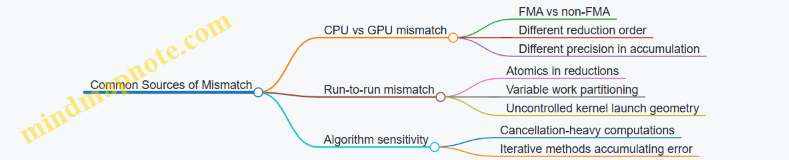
Reproducibility engineering is mostly about controlling order and precision. Once you treat floating point as defined arithmetic with rounding and ordering effects, the remaining work becomes systematic: match semantics, control reductions, and validate with tolerances that reflect how errors actually behave.
6.2 Choosing Precision Levels for Performance and Accuracy Tradeoffs
Precision choice is engineering, not philosophy. On GPUs, precision affects throughput, memory bandwidth, numerical behavior, and even which kernel optimizations are available. The goal is to pick the smallest precision that keeps your results within a defined tolerance.
Start with What Must Be Accurate
Define an acceptance criterion before touching types. For example, if you compute a pressure field, you might require that the relative error stays below 1e-5 in L2 norm. If you compute a convergence metric, you might require monotonic decrease of the residual for at least N iterations. These requirements determine whether you can tolerate rounding noise or whether you need extra guard digits.
A practical way to reason is to separate error sources:
- Discretization error from the model and grid.
- Iteration error from stopping early.
- Floating-point error from rounding and cancellation. If floating-point error is smaller than the other two, lower precision is usually safe.
Understand Precision Costs on GPUs
Lower precision typically improves:
- Compute throughput (more operations per second).
- Memory bandwidth usage (fewer bytes moved).
- Cache residency (more elements per cache line).
But it can reduce:
- Dynamic range (values may underflow or overflow sooner).
- Resolution (small increments may disappear).
- Stability in reductions and iterative updates.
A common engineering pattern is mixed precision: store inputs and intermediate states in lower precision, but accumulate in higher precision where rounding is most harmful.
Use a Precision Budget for Each Operation
Not every operation deserves the same precision.
- Elementwise operations like
y = a*x + boften tolerate lower precision if values are well-scaled. - Reductions like sums, dot products, and norms are sensitive because rounding accumulates across many terms.
- Iterative updates like
x_{k+1} = x_k + alpha * p_kcan amplify small errors over many iterations.
So you can choose:
- Lower precision for storage and elementwise math.
- Higher precision for accumulations and critical scalars.
Mind Map: Precision Decision Flow
Example: Dot Product with Mixed Precision
Suppose you compute a dot product s = sum_i x[i] * y[i]. If you store x and y as float but accumulate in float, rounding grows with the number of terms. If you accumulate in double, the sum is more stable, especially when terms vary in magnitude.
A mixed approach often works well:
- Load
xandyasfloat. - Multiply in
float. - Accumulate in
double(or use a higher-precision accumulator type).
// Conceptual kernel fragment
float xi = x[i];
float yi = y[i];
float prod = xi * yi;
double acc = (double)prod; // higher-precision accumulation
// Later: reduce acc across threads
Even if the final result is stored as float, the accumulator reduces error during the sum.
Example: Iterative Update with Guarded Accumulation
Consider a Jacobi-like update:
x_new = x_old + omega * (b - A*x_old) / diag
The subtraction b - A*x_old can suffer cancellation. If b and A*x_old are close, low precision can turn a meaningful residual into noise. A robust strategy is:
- Keep
x_oldandA*x_oldin lower precision. - Compute the residual and the update in higher precision.
- Store
x_newin lower precision if it still meets the tolerance.
Practical Rules That Prevent “Precision Whiplash”
- Cast once, early, and consistently: decide where higher precision begins and keep it there through the sensitive operation.
- Avoid accidental downcasts: if you compute in
doublebut store intofloattoo early, you lose the benefit. - Scale inputs: if values span many orders of magnitude, precision loss is inevitable; rescaling can make lower precision viable.
- Match precision to reduction structure: tree reductions and warp-level partial sums change rounding behavior, so test with the actual reduction pattern you use.
Validation Checklist for Precision Choices
Run a small, deterministic test suite:
- Compare against a high-precision reference for representative inputs.
- Test edge cases: near-zero values, large magnitudes, and worst-case cancellation.
- Measure both error and stability (e.g., whether residual decreases as expected).
If the error is within tolerance and stability holds, you can keep the lower precision. If not, increase precision only where it matters: accumulation for reductions, and residual/update computations for iterative methods.
6.3 Stable Summation Techniques for Reductions
Reductions add many floating-point values, and floating-point addition is not associative:
- (a + b) + c can differ from a + (b + c).
When you sum thousands or millions of terms, the ordering and the rounding error pattern matter. “Stable” summation aims to reduce error growth so results stay close to a higher-precision reference.
Foundations: Why Naive Reduction Drifts
A typical GPU reduction accumulates partial sums in a tree pattern. Even if the tree is deterministic, it still introduces rounding at every addition. The error can grow roughly with the number of additions, and it can be worse when magnitudes vary widely (for example, adding tiny corrections to large baseline values).
A quick mental model: if each addition rounds to the nearest representable float, then each step can introduce a small relative error. After many steps, those small errors can accumulate into a noticeable bias, especially in iterative solvers where reductions feed back into later computations.
Strategy One: Pairwise Summation for Better Ordering
Pairwise summation changes the reduction order to sum similar magnitudes together more often. The classic approach is to split the input into halves, recursively sum each half, then add the two results. This tends to reduce error compared to a long left-to-right chain.
On GPUs, tree reductions already resemble pairwise summation, but you can improve stability by ensuring the tree is balanced and by avoiding extra reordering steps that mix very different magnitudes early.
Example: Suppose you sum [1e8, 1, -1e8, 1]. A naive left-to-right sum can produce 0 due to rounding: (1e8 + 1) rounds to 1e8, then (1e8 + -1e8) becomes 0, and +1 yields 1. A different order can yield 2. Pairwise summation reduces the chance of losing the small terms early.
Strategy Two: Kahan Summation for Compensation
Kahan summation keeps a running compensation term that tracks lost low-order bits.
Maintain two variables:
sum: the running totalc: the compensation for lost bits
For each value x:
- Compute
y = x - c - Compute
t = sum + y - Update
c = (t - sum) - y - Set
sum = t
This reduces error dramatically for sequences where a long chain would otherwise drift.
Example: Summing values like [1.0, 1e-6, 1e-6, ...] in float can lose the tiny terms after a few additions. Kahan keeps c so those tiny contributions have a better chance to affect sum.
GPU note: Kahan is sequential by nature, so it’s not a perfect fit for massively parallel reductions. A practical compromise is to apply Kahan within each block (small sequential chunk), then combine block results using pairwise summation.
Strategy Three: Neumaier Variant for Mixed Magnitudes
Kahan can struggle when the next addend is much larger than the current sum. The Neumaier variant modifies the compensation update based on which magnitude dominates.
In Neumaier, when you compute t = sum + x, you update compensation using either sum or x depending on absolute values. This makes it more robust for reductions with large dynamic range.
Example: Summing [1e-3, 1e3, 1e-3, 1e3] benefits from Neumaier because the compensation logic accounts for the fact that the large terms dominate intermediate rounding.
Strategy Four: Use Higher Precision for Accumulation
Even if your inputs are float, you can accumulate in double (or use wider intermediate types). This reduces rounding at each addition step.
A common engineering pattern:
- Load inputs as float
- Convert to double for accumulation inside the reduction
- Convert back to float at the end
This is often the simplest stability improvement, though it costs more registers and bandwidth for intermediate values.
Example: In a dot product, accumulating a[i] * b[i] in double can noticeably improve the final residual compared to float accumulation, especially when vectors have components spanning several orders of magnitude.
Mind Map: Stable Reduction Options
Practical GPU Pattern: Block-Local Compensation Then Pairwise Combine
A stable and practical approach is:
- Each block reduces its chunk using either Kahan or Neumaier in a small sequential loop over the block’s assigned elements.
- Each block writes one partial sum.
- A second-stage reduction combines partial sums using pairwise ordering (tree reduction).
This keeps the compensation cost bounded while still improving global accuracy.
Example: For a large array x, you can reduce x to partial[blockId] using Neumaier inside each block, then reduce partial with a standard tree. The final result typically tracks a high-precision CPU sum more closely than a single-stage float reduction.
Choosing a Technique Without Guessing
Pick based on what dominates your error:
- If your reduction already uses a balanced tree and magnitudes are similar, pairwise summation is often enough.
- If you see drift from tiny terms being swallowed, use Kahan or Neumaier within blocks.
- If you need the most reliable accuracy and can afford it, accumulate in double.
A good engineering habit is to compare against a reference computed in higher precision on the CPU for a small representative dataset, then verify that the chosen method improves the specific failure mode you observe.
6.4 Handling Boundary Conditions and Indexing Robustness
Boundary conditions are where kernels go to misbehave: one off-by-one error can turn a correct stencil into a quiet memory scribbler. Indexing robustness means you design your index math so that every thread either computes a valid output or cleanly does nothing.
Boundary Conditions as Explicit Policies
Start by naming the boundary policy you want. Common choices include:
- Clamp: treat out-of-range coordinates as the nearest valid index.
- Zero Padding: out-of-range reads return 0.
- Mirror: reflect indices back into range.
- Periodic: wrap indices modulo the dimension.
A practical rule: implement the policy in one place, then reuse it. For example, a helper that maps an index to a valid index (or marks it invalid) keeps your stencil code readable and reduces the chance that one direction uses a different rule.
Indexing Foundations That Prevent Off-by-One Errors
For 1D, 2D, and 3D arrays, robust indexing follows the same pattern:
- Compute a global thread coordinate.
- Convert it to a linear index only after you know it is in range.
- Apply boundary policy for neighbor reads, not for the current cell write.
For a 2D row-major array with dimensions nx and ny, the linear index is i + j*nx. Robustness comes from checking 0 <= i < nx and 0 <= j < ny before writing out[i + j*nx].
A Safe Pattern for Stencil Neighbor Reads
Neighbor reads are the tricky part because they often involve i-1, i+1, j-1, j+1. A clean approach is:
- Validate the center coordinate for output.
- For each neighbor, apply the boundary policy to the neighbor coordinate.
- Read using the mapped neighbor coordinate.
Here is a compact example for a 2D 5-point stencil using zero padding. The key is that the center write is guarded, while neighbor reads are handled by a function.
__device__ __forceinline__ float readZeroPad(const float* a, int nx, int ny, int i, int j){
    if(i < 0 || i >= nx || j < 0 || j >= ny) return 0.0f;
    return a[i + j*nx];
}

__global__ void stencil5(const float* in, float* out, int nx, int ny){
    int i = blockIdx.x * blockDim.x + threadIdx.x;
    int j = blockIdx.y * blockDim.y + threadIdx.y;
    if(i >= nx || j >= ny) return;

    float c = readZeroPad(in, nx, ny, i, j);
    float l = readZeroPad(in, nx, ny, i-1, j);
    float r = readZeroPad(in, nx, ny, i+1, j);
    float u = readZeroPad(in, nx, ny, i, j-1);
    float d = readZeroPad(in, nx, ny, i, j+1);

    out[i + j*nx] = 0.2f * (c + l + r + u + d);
}
This pattern scales to 3D by extending the coordinate mapping and adding k neighbors. The important part is that the output guard remains simple and consistent.
Mind Map: Robust Boundary Handling
Advanced Details That Matter in Practice
1) Guard Writes, Not Reads. If you guard only the output write, neighbor reads can still be safe because they route through the boundary policy. Guarding both center and neighbors often duplicates logic and increases the chance of inconsistent rules.
2) Keep Dimension Variables Consistent. A common failure mode is mixing nx and ny in linearization or passing swapped dimensions from the host. Treat dimension parameters as part of the kernel’s contract and verify them with a tiny test grid.
3) Choose Branching vs. Mapping Intentionally. Zero padding uses branches in the neighbor read. Clamp and periodic can be implemented with index mapping, which may reduce branching but adds arithmetic. Either way, correctness comes first; then measure.
4) Validate With Edge-Heavy Tests. Use small sizes like nx=3, ny=2 and initialize arrays with distinct values per coordinate. Then check corners and edges explicitly, because interior points often mask indexing mistakes.
Example: Corner Behavior for Zero Padding
Consider nx=3, ny=2 with coordinates (i,j) where i is column and j is row. For the corner (0,0), the neighbors (i-1,j) and (i,j-1) are out of range, so they contribute 0. The stencil result depends only on (0,0), (1,0), and (0,1). If your output at (0,0) includes contributions from those missing neighbors, your boundary policy is not being applied correctly.
Example: Periodic Wrapping Without Surprises
For periodic boundaries, neighbor coordinates wrap into range. For instance, with nx=4, i-1 at i=0 becomes 3. Implementing this with modulo must handle negative values carefully; a robust mapping uses a normalization step so that (-1 % 4) becomes 3 rather than staying negative.
Case Study: Indexing Robustness in a 3D Stencil
In 3D, the same discipline applies: guard the center write with if(i>=nx||j>=ny||k>=nz) return;. For neighbor reads, route each (i±1,j,k), (i,j±1,k), (i,j,k±1) through a boundary policy mapper. This keeps the kernel’s write path uniform and makes boundary behavior consistent across all six directions.
Summary of Robustness Rules
- Define boundary behavior as a clear policy.
- Guard output writes using the center coordinate.
- Apply the boundary policy to neighbor coordinates.
- Linearize indices only after you know they are valid.
- Test with small, edge-heavy grids and compare against a CPU reference.
6.5 Validation Strategies Using CPU Reference Implementations
Validation is easiest when you treat the CPU version as a specification, not as a second implementation. The goal is to compare results in a way that respects floating-point realities while still catching real bugs like wrong indexing, missing boundary handling, or race conditions.
Define What “Correct” Means Before Comparing
Start by listing invariants your kernel must satisfy. For example, a stencil update should preserve known boundary rules, a reduction should match the expected aggregation order constraints, and a solver step should keep values finite. Then decide the comparison rule:
- Exact match for integer outputs or bitwise-stable operations.
- Tolerance-based match for floating-point results.
A practical default for floating-point is a combined absolute and relative tolerance:
- Absolute tolerance catches small-magnitude errors.
- Relative tolerance scales with the expected magnitude.
Build a CPU Reference That Mirrors Semantics
A CPU reference should match the GPU’s semantics, not just the math. Key details:
- Use the same data layout and indexing formula.
- Apply the same boundary conditions.
- Use the same reduction definition (sum order differs, so expect small discrepancies).
When the GPU uses fused operations or different rounding behavior, the CPU reference should use a consistent policy. If you cannot match rounding exactly, validate with tolerances and focus on detecting large deviations.
Compare Outputs Systematically with Error Localization
Instead of only checking a final scalar, compare intermediate structures when possible. For a stencil, compare per-cell updates; for a reduction, compare partial sums if you expose them.
Use a structured error report:
- Compute max absolute error and max relative error.
- Record the index of the worst element.
- Optionally compute an error histogram to see whether errors are localized (often indexing) or widespread (often precision or memory issues).
A common debugging pattern: if errors concentrate near boundaries, your halo or bounds checks are wrong. If errors appear in a checkerboard pattern, your indexing stride or layout is off.
Choose Test Inputs That Stress the Kernel
Validation is only as good as the inputs. Use a small set that covers distinct behaviors:
- Constant fields to catch incorrect arithmetic.
- Linear ramps to catch indexing and stride mistakes.
- Alternating patterns to expose coalescing-related bugs indirectly via wrong reads.
- Random values with fixed seeds to cover general cases.
For reductions, include cases where the expected result is near zero to test relative tolerance behavior.
Handle Floating-Point Differences Without Hiding Bugs
Floating-point differences can come from:
- Different summation order in reductions.
- Different instruction sequences due to compiler optimizations.
- Use of fast math settings.
Validation strategy:
- Start with looser tolerances to confirm the pipeline is wired correctly.
- Tighten tolerances once indexing and memory correctness are established.
- For reductions, consider validating against a CPU reference that uses a stable summation method when you need stricter checks.
Automate the Comparison in a Repeatable Harness
A good harness runs the same test set across devices and kernel variants, then fails with actionable diagnostics.
Example pseudocode for tolerance-based comparison:
bool compare(const float* gpu, const float* cpu, int n,
             float atol, float rtol, int& badIdx,
             float& maxAbs, float& maxRel) {
  maxAbs = 0.0f; maxRel = 0.0f; badIdx = -1;
  for (int i = 0; i < n; i++) {
    float a = cpu[i];
    float b = gpu[i];
    float absErr = fabsf(a - b);
    float relErr = absErr / (fabsf(a) + 1e-12f);
    if (absErr > atol && relErr > rtol) {
      if (absErr > maxAbs) { maxAbs = absErr; maxRel = relErr; badIdx = i; }
      return false;
    }
    maxAbs = fmaxf(maxAbs, absErr);
    maxRel = fmaxf(maxRel, relErr);
  }
  return true;
}
Mind Map: CPU Reference Validation Workflow
Example: Stencil Kernel Validation with Boundary Focus
Suppose your GPU stencil updates each cell using neighbors and a fixed boundary rule. Your CPU reference should apply the same rule explicitly for the first and last rows/columns. When validation fails:
- If only boundary cells mismatch, inspect bounds checks and halo indexing.
- If interior cells mismatch too, inspect the mapping from 2D indices to linear memory and verify stride calculations.
A small trick: run a tiny grid like 4×4 or 8×8. The worst error index becomes easy to reason about, and you can print the neighborhood values around that index to confirm which neighbor read is wrong.
Example: Reduction Validation with Stable Summation
For a reduction that sums many elements, GPU and CPU may differ due to summation order. Use tolerance-based comparison first. If failures persist beyond tolerance, switch the CPU reference to a stable summation approach so the CPU result becomes a better “truth” for comparison. Then re-check whether the GPU reduction tree matches the intended grouping logic.
Validation Checklist That Prevents the Usual Mistakes
- CPU and GPU use identical indexing and boundary rules.
- Comparison uses appropriate absolute and relative tolerances.
- Worst-element reporting is enabled so failures are actionable.
- Test inputs include structured patterns, not only random data.
- The harness runs the same tests across kernel variants.
When these pieces are in place, validation stops being a vague “it seems right” exercise and becomes a precise diagnostic tool—one that catches real bugs without punishing harmless floating-point differences.
7. Advanced Synchronization and Communication Within a GPU
7.1 Warp Level Operations for Efficient Intra Warp Collaboration
Warp-level operations let threads cooperate without full-block synchronization. The key idea is that threads within a warp execute in lockstep, so you can exchange values and compute results using warp intrinsics rather than shared memory and __syncthreads(). This reduces latency and avoids extra memory traffic—especially when your algorithm naturally forms “local” groups.
Foundations: What a Warp Gives You
A warp is a fixed group of 32 threads. Within a warp, lane IDs identify which thread is which. Because execution is synchronized at the warp level, operations like shuffle can move register values directly between lanes. That means you can implement reductions, broadcasts, and data-dependent selection with minimal overhead.
Start by mapping your computation to lanes. If each lane owns one element (or one partial sum), you can often reduce the problem to “combine lane values” or “pick a lane’s value and reuse it.” If your data is 2D or 3D, you can still assign a linear lane index and treat it as a small vector.
Shuffle Operations: Moving Values Without Shared Memory
The most common warp primitive is shuffle, which reads a value from another lane by lane index. A typical pattern is:
- each lane computes a local value in a register,
- lanes exchange registers using shuffle,
- lanes combine results using arithmetic.
A simple reduction example sums one value per lane. The code below assumes a full warp and uses a power-of-two reduction tree.
__inline__ __device__ float warp_reduce_sum(float x) {
  for (int offset = 16; offset > 0; offset >>= 1) {
    x += __shfl_down_sync(0xffffffff, x, offset);
  }
  return x;
}
Every lane performs the same loop, but only lanes that remain “active” contribute meaningful partial sums. After the loop, lane 0 holds the total.
Masking and Divergence: Keeping Results Correct
Warp intrinsics take an active mask. If some lanes are inactive due to branching, using the wrong mask can mix in garbage from lanes that should not participate. A safe approach is to compute an active mask based on your predicate, then pass it to shuffle.
For example, if you only want to reduce elements where valid is true, you can set active = __ballot_sync(mask, valid) and then use that mask in subsequent intrinsics. The important nuance: the mask must reflect which lanes are logically participating, not just which lanes exist.
Warp-Level Broadcast and Indexing
Broadcast is useful when one lane produces a value that all lanes need. You can fetch lane 0’s reduced sum with __shfl_sync.
float sum = warp_reduce_sum(x);
float total = __shfl_sync(0xffffffff, sum, 0);
Now every lane has total in a register. This is often faster than writing to shared memory and reading back, especially when the value is reused immediately.
Warp-Level Selection: Handling Irregular Work
Many scientific kernels have irregular boundaries, like masked stencils near edges. Instead of branching heavily, you can use warp-level predicates to select values.
A common technique is:
- compute a predicate per lane,
- use ballot to compact or at least count active lanes,
- use shuffle to fetch the value from a chosen lane.
Even without full compaction, you can reduce divergence by ensuring that all lanes execute the same control flow and only the data changes.
Mind Map: Warp Level Collaboration
Warp Level Operations Mind Map
Advanced Details: Building Block-Wide Results from Warps
Warp operations usually produce warp-local results. To get block-wide reductions, you combine warp results in a second stage. A practical approach:
- each warp reduces its lanes to one value,
- lane 0 of each warp writes its value to shared memory,
- a final warp reduces those warp results.
This keeps most work warp-local and limits shared memory usage to a small number of warp outputs.
Example: Warp Reduction Inside a Kernel
Consider a kernel where each thread computes a partial contribution x and you want the block sum. The warp stage returns a per-warp sum, then lane 0 writes it.
__global__ void block_sum_kernel(const float* in, float* out) {
  int tid = threadIdx.x;
  float x = in[tid];

  float wsum = warp_reduce_sum(x);
  int lane = threadIdx.x & 31;
  int warp = threadIdx.x >> 5;

  __shared__ float warp_sums[8];
  if (lane == 0) warp_sums[warp] = wsum;
  __syncthreads();

  if (warp == 0) {
    float y = (lane < (blockDim.x + 31) / 32) ? warp_sums[lane] : 0.0f;
    float bsum = warp_reduce_sum(y);
    if (lane == 0) out[blockIdx.x] = bsum;
  }
}
The subtle part is the second-stage bounds: the number of warps may not fill the first warp completely, so inactive lanes contribute zero.
Practical Checklist for Warp Intrinsics
- Use shuffle to move register values, not shared memory.
- Pass an active mask that matches your predicate.
- Prefer warp-local reductions and broadcasts when reuse is immediate.
- Combine warp results with a small shared-memory stage for block-wide outcomes.
When you follow that sequence, warp-level operations become a reliable tool for fast intra-warp collaboration rather than a collection of mysterious intrinsics.
7.2 Block Level Coordination With Shared Memory And Barriers
Block-level coordination is where you stop thinking “each thread does its own thing” and start thinking “threads cooperate to produce one block’s worth of results.” Shared memory is the cooperation space: it’s fast, visible to all threads in the same block, and organized so you can stage data, reuse it, and reduce global memory traffic. Barriers are the rules that keep the cooperation from turning into a race condition.
Shared Memory as a Block Scratchpad
Shared memory is allocated per block, so every block gets its own scratchpad. That means you can safely store intermediate tiles, partial sums, or neighbor data without cross-block interference.
A common pattern is tiling: each thread loads one or more elements from global memory into shared memory, then all threads compute using the shared tile. The key is that computation must not start until the tile is fully loaded.
Barriers and What They Actually Guarantee
A barrier such as __syncthreads() ensures that all threads in the block reach the same point before any thread proceeds past it. It does not magically make memory writes visible across blocks, and it does not fix incorrect indexing. It also requires that all threads in the block execute the barrier; placing it inside a branch where some threads skip it is a correctness bug.
A practical mental model: shared memory writes are like putting ingredients on the counter; the barrier is the moment everyone confirms the counter is ready before cooking.
Systematic Tiling Workflow
Use this sequence for most shared-memory tiling kernels:
- Compute thread-local indices for where each thread reads from global memory and where it writes in shared memory.
- Load into shared memory with bounds checks for edges.
- Barrier so every shared element is ready.
- Compute using shared memory.
- Optional second barrier if later phases reuse shared memory that earlier threads overwrite.
The “optional second barrier” is not superstition: it’s needed when you have multiple phases that overwrite shared memory and then read it again.
Example: 1D Stencil with Shared Memory
Consider a simple stencil where each output depends on itself and its immediate neighbors. Threads load a tile plus halo into shared memory, then compute outputs.
__global__ void stencil1d(const float* in, float* out, int n) {
  extern __shared__ float s[];
  int tid = threadIdx.x;
  int gid = blockIdx.x * blockDim.x + tid;

  int left = gid - 1;
  int right = gid + 1;

  s[tid] = (gid < n) ? in[gid] : 0.0f;
  if (tid == 0) s[tid - 1 + 1] = (left >= 0) ? in[left] : 0.0f;
  if (tid == blockDim.x - 1) s[tid + 1] = (right < n) ? in[right] : 0.0f;

  __syncthreads();

  if (gid < n) {
    float a = s[tid];
    float b = s[tid];
    float c = s[tid];
    if (tid > 0) b = s[tid - 1];
    if (tid + 1 < blockDim.x) c = s[tid + 1];
    out[gid] = (a + b + c) / 3.0f;
  }
}
This sketch shows the structure, but the indexing is intentionally compact. In real code, you’d allocate blockDim.x + 2 shared elements and map s[tid+1] to in[gid], with s[0] and s[blockDim.x+1] holding halos. The barrier is the correctness hinge: without it, some threads might read halo values before the halo loads complete.
Mind Map: Block Coordination with Shared Memory and Barriers
Advanced Details That Matter in Practice
1) Divergence and barrier placement. If any thread in the block skips the barrier, the program can deadlock. A safe rule is: barriers belong in straight-line code paths that all threads execute.
2) Multi-phase shared memory. If you load a tile, compute, then overwrite shared memory for a second tile, you need a barrier between phases. Otherwise, threads that finish early may start overwriting while others still read.
3) Shared memory bank behavior. Barriers don’t fix bank conflicts. If multiple threads access shared addresses that map to the same bank, performance drops even if correctness is perfect. The fix is usually data layout or padding, not synchronization.
4) Bounds checks without breaking barriers. You can guard loads with bounds checks, but the barrier must still be executed by all threads. Threads that are out of range should write a safe value into shared memory so later reads are defined.
A Clean Two-Phase Pattern
When you see code that loads, synchronizes, computes, then loads again, treat it as two separate “prepare then use” phases. The barrier belongs after each prepare stage.
// Phase 1: prepare shared tile
load_tile_to_shared();
__syncthreads();
compute_from_shared();

// Phase 2: prepare next tile
load_next_tile_to_shared();
__syncthreads();
compute_from_shared();
This pattern keeps the mental model consistent: shared memory is a shared workspace, and barriers are the checkpoints that make the workspace safe to use.
7.3 Avoiding Deadlocks and Ensuring Safe Synchronization
Deadlocks on GPUs usually come from one simple mismatch: threads that wait for something that other threads never reach. On CUDA, “waiting” can be explicit (barriers) or implicit (waiting on data that never gets produced). The goal of this section is to make synchronization rules concrete, then show how to structure kernels so every thread reaches every required synchronization point.
Core Synchronization Rules
- All threads in a synchronization scope must participate. A
__syncthreads()barrier is block-scoped; every thread in the block must execute it the same number of times. - No barrier inside divergent control flow. If some threads take a branch and others don’t, the barrier becomes a trap. Even “harmless” early returns can break the rule.
- Use the right barrier for the right scope.
__syncwarp()is warp-scoped;__syncthreads()is block-scoped. Mixing assumptions leads to waiting on the wrong group. - Prefer dataflow synchronization over “hope.” If a thread reads shared memory, ensure the writer runs before the reader, using barriers or warp-level primitives.
Mind Map: Deadlock Causes and Fixes
Safe Barrier Placement Strategy
A reliable pattern is: compute → stage data → synchronize → consume. The barrier sits between producer and consumer phases, and every thread reaches it.
Example: Shared Memory Producer Consumer Without Deadlock
__global__ void tileSum(const float* in, float* out, int n) {
  __shared__ float s[256];
  int tid = threadIdx.x;
  int gid = blockIdx.x * blockDim.x + tid;

  // Producer phase: every thread writes something to s
  float v = (gid < n) ? in[gid] : 0.0f;
  s[tid] = v;

  // Barrier: all threads in the block reach this line
  __syncthreads();

  // Consumer phase: reduction over s
  for (int stride = blockDim.x / 2; stride > 0; stride >>= 1) {
    if (tid < stride) s[tid] += s[tid + stride];
    __syncthreads();
  }

  if (tid == 0) out[blockIdx.x] = s[0];
}
Key detail: the bounds check is used to choose a value, not to skip the barrier. Threads that are “out of range” still participate by writing a neutral element.
Common Deadlock Triggers and How to Avoid Them
Divergent Branches Around Barriers
If you write:
- some threads return early,
- others continue to a barrier, then the continuing threads wait forever.
Fix: keep control flow uniform around barriers. Use predicates for work, not for barrier participation.
Barrier Count Mismatch
Deadlock can also happen when barriers are inside loops whose iteration counts differ per thread. For example, a loop conditioned on gid < n can cause some threads to execute fewer barriers.
Fix: structure loops so every thread executes the same barrier sequence. If work is conditional, guard the work inside the loop, not the loop itself.
Wrong Scope Assumptions
Warp-level operations are not automatically safe for block-level synchronization. __syncwarp() only coordinates threads within a warp; __syncthreads() coordinates the whole block.
Fix: if the data lives in shared memory and is shared across the block, use __syncthreads(). If the data is warp-local, use warp primitives and keep it warp-local.
Mind Map: Safe Patterns
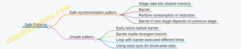
Warp-Level Coordination Without Block Barriers
When communication is limited to threads within a warp, block barriers are unnecessary and can reduce performance. A typical approach is to use warp shuffle or warp-synchronous programming.
Example: Warp Reduction with __syncwarp()
__inline__ __device__ float warpReduceSum(float x) {
  // Assumes all active lanes in the warp participate
  unsigned mask = 0xffffffff;
  for (int offset = 16; offset > 0; offset >>= 1) {
    x += __shfl_down_sync(mask, x, offset);
  }
  return x;
}
This avoids block barriers entirely. The important rule is that the warp-level mask and participation must match how you handle “active” lanes.
Practical Checklist for Safe Synchronization
- Every
__syncthreads()is reached by all threads in the block on every execution path. - No
return,break, or divergent branch bypasses a barrier. - Loops containing barriers have uniform iteration structure across threads.
- Shared memory reads happen only after the barrier that follows the writes.
- Warp-only communication uses warp primitives and does not rely on block barriers.
When these rules are followed, synchronization becomes predictable: barriers become “phase separators” rather than “waiting points that can go missing.”
7.4 Managing Producer Consumer Pipelines with Streams and Events
A producer-consumer pipeline on the GPU is about keeping work moving without forcing everyone to wait for everyone else. The producer stage generates inputs and launches kernels; the consumer stage transforms results and possibly launches follow-up kernels. The key engineering goal is to overlap independent work while preserving correct ordering where dependencies exist.
Core Concepts That Make Pipelines Work
A CUDA stream is an ordered queue of operations. Operations in the same stream execute in issue order; operations in different streams may overlap. Events are lightweight markers that can be recorded into a stream and later used to gate work in another stream.
A practical pipeline uses three rules:
- Use separate streams for independent stages so the GPU can schedule them concurrently.
- Record an event at the exact point data becomes ready in the producer stream.
- Make the consumer wait on that event before it touches the produced data.
This avoids the common mistake of using a global device synchronize, which kills overlap by waiting for everything.
A Systematic Pipeline Layout
Consider processing chunks of a large array. Each chunk goes through:
- Producer: copy or preprocess chunk, then run a “stage A” kernel.
- Consumer: wait for stage A completion, then run “stage B” kernel.
To keep the GPU busy, you process multiple chunks in flight. A typical pattern is double buffering: chunk 0 and chunk 1 alternate roles across streams.
Mind Map: Producer Consumer Pipeline with Streams and Events
Example: Double-Buffered Chunk Processing
Assume pinned host memory for transfers and device buffers sized for one chunk. Two sets of device buffers allow the producer to work on chunk i+1 while the consumer processes chunk i.
cudaStream_t prod, cons;
cudaEvent_t ready[2];

cudaStreamCreate(&prod);
cudaStreamCreate(&cons);
for (int b = 0; b < 2; b++) cudaEventCreateWithFlags(&ready[b], cudaEventDisableTiming);

for (int i = 0; i < numChunks; i++) {
  int b = i & 1;
  // Producer: H2D + stage A
  cudaMemcpyAsync(d_in[b], h_in[i], bytes, cudaMemcpyHostToDevice, prod);
  stageA<<<grid, block, 0, prod>>>(d_in[b], d_mid[b]);
  cudaEventRecord(ready[b], prod);

  // Consumer: wait + stage B
  cudaStreamWaitEvent(cons, ready[b], 0);
  stageB<<<grid2, block2, 0, cons>>>(d_mid[b], d_out[i]);
}

cudaStreamSynchronize(cons);
This works because the consumer stream is gated per buffer index. The event is recorded after stage A writes d_mid[b], and the consumer waits before reading it.
Choosing Where to Record Events
Record events at boundaries where the consumer truly needs completion. Recording too early can cause the consumer to read partially written data; recording too late reduces overlap because the consumer waits longer than necessary.
A good heuristic is: record immediately after the last operation in the producer stream that writes the shared data region for that chunk.
Handling Transfers and Compute Together
If you also overlap host-device transfers, use a dedicated transfer stream. The producer stream can depend on transfer completion via an event, then run stage A. The consumer stream can depend on stage A completion via another event.
cudaStream_t xfer, prod, cons;
cudaEvent_t xferDone[2], stageADone[2];

for (int i = 0; i < numChunks; i++) {
  int b = i & 1;
  cudaMemcpyAsync(d_in[b], h_in[i], bytes, cudaMemcpyHostToDevice, xfer);
  cudaEventRecord(xferDone[b], xfer);

  cudaStreamWaitEvent(prod, xferDone[b], 0);
  stageA<<<grid, block, 0, prod>>>(d_in[b], d_mid[b]);
  cudaEventRecord(stageADone[b], prod);

  cudaStreamWaitEvent(cons, stageADone[b], 0);
  stageB<<<grid2, block2, 0, cons>>>(d_mid[b], d_out[i]);
}
The transfer stream isolates copy scheduling, while events preserve correctness.
Common Failure Modes and Fixes
- Missing
cudaStreamWaitEvent: the consumer may start before data is ready. Fix by waiting on the correct event for the correct buffer index. - Reusing buffers too soon: if you only have one buffer but multiple chunks are in flight, you’ll overwrite data. Fix by using double buffering or more.
- Recording the event before the write completes: if stage A is asynchronous and you record too early, the event won’t protect the consumer. Fix by recording after the kernel launch in the same stream.
A Quick Mental Model
Think of each event as a “data ready ticket” tied to a specific buffer slot. Streams decide when operations are allowed to run; events decide which operations are allowed to run based on data readiness. When you keep those responsibilities separate, the pipeline stays both fast and correct.
7.5 Overlapping Compute and Transfers with Asynchronous Execution
Overlapping compute with data transfers is mostly about one thing: keeping the GPU busy while the CPU prepares the next chunk. In CUDA, the practical lever is asynchronous copies issued into streams, paired with kernels that run in those same streams. If the transfers and kernels are independent, the hardware can execute them concurrently.
Core Idea and Preconditions
- Use multiple streams so the GPU has independent work queues.
- Use asynchronous operations like
cudaMemcpyAsyncso the host thread does not block. - Ensure the data path supports overlap: host memory should be pinned (page-locked), otherwise transfers may serialize.
- Avoid implicit synchronization: calls that force device-wide ordering (for example, certain blocking syncs) will collapse overlap.
A simple mental model: stream A handles “copy chunk i” then “compute chunk i”, while stream B handles “copy chunk i+1” then “compute chunk i+1”. When chunk i is computing, chunk i+1 can be copying.
Mind Map: Overlap Strategy
Double Buffering with Two Streams
Chunk your workload so each chunk can be transferred and processed independently. Allocate two device buffers for inputs and outputs, and alternate which buffer each stream uses.
Key rule: operations in the same stream execute in order, but operations in different streams may overlap. That means you can safely enqueue copy-then-kernel pairs per stream without extra synchronization.
Example: Enqueue Copy and Kernel per Stream
// Assume pinned host buffers h_in, h_out and device buffers d_in[2], d_out[2]
cudaStream_t s[2];
cudaStreamCreate(&s[0]);
cudaStreamCreate(&s[1]);

for (int i = 0; i < numChunks; ++i) {
  int b = i & 1;                 // double buffer index
  size_t off = (size_t)i * chunkElems;
  size_t n = min(chunkElems, totalElems - off);

  cudaMemcpyAsync(d_in[b], h_in + off, n*sizeof(float),
                  cudaMemcpyHostToDevice, s[b]);

  myKernel<<<gridFor(n), block, 0, s[b]>>>(d_in[b], d_out[b], n);

  cudaMemcpyAsync(h_out + off, d_out[b], n*sizeof(float),
                  cudaMemcpyDeviceToHost, s[b]);
}

cudaDeviceSynchronize();
This pattern overlaps transfers for chunk i+1 with computation for chunk i, as long as the GPU and PCIe/NVLink path can run copy engines concurrently with kernels.
When You Need Dependencies: Events
Sometimes chunk i computation depends on results produced by chunk i-1 on the GPU. In that case, you cannot rely on stream ordering across streams. Use events to express a dependency without forcing a global sync.
cudaEvent_t done[2];
for (int b = 0; b < 2; ++b) cudaEventCreateWithFlags(&done[b], cudaEventDisableTiming);

// After enqueuing kernel for chunk i in stream s[b], record an event.
// Before starting dependent work for chunk i+1 in stream s[b2], make it wait.
// cudaEventRecord(done[b], s[b]);
// cudaStreamWaitEvent(s[b2], done[b], 0);
Record the event in the stream where the producing kernel runs, then make the consuming stream wait on that event. This keeps unrelated work overlapped while preserving correctness.
Avoiding Overlap Killers
- Synchronous copies (
cudaMemcpy) block the host and often serialize the timeline. - Unpinned host memory can prevent true overlap because the driver may stage through temporary buffers.
- Device-wide synchronization inside the loop collapses concurrency.
- Reusing the same staging buffers across streams without ordering guarantees can cause data races. Double buffering exists to prevent that.
Measuring Overlap Correctly
Use a timeline view to confirm concurrency. Look for regions where copy operations and kernels overlap in time. If you see a strict “copy then compute then copy then compute” pattern, check pinned memory, stream usage, and whether any sync calls occur between enqueues.
Practical Checklist for Engineering Use
- Split work into chunks that fit staging buffers.
- Allocate pinned host buffers for inputs and outputs.
- Create at least two streams and two sets of device staging buffers.
- Enqueue
MemcpyAsync→ kernel →MemcpyAsyncin the same stream. - Use events only when cross-stream dependencies exist.
- Validate correctness first with small sizes, then scale chunk counts.
Done carefully, overlap turns “waiting for data” into “useful work”, and the GPU spends more time computing than waiting for the CPU to catch up.
8. Host Side Engineering for Data Movement and Throughput
8.1 Pinned Memory Allocation and Transfer Optimization
Pinned (page-locked) host memory reduces transfer overhead by preventing the operating system from paging host buffers out while a DMA engine is moving data. The result is more predictable throughput and better overlap with GPU work when you use streams correctly. The trick is to pin only what you need, for as long as you need it, and to structure transfers so the GPU is never waiting on a slow host.
Foundational Concepts That Drive the Design
Pinned memory changes two things that matter for engineering:
- Transfer path stability: pageable memory may require staging through an internal buffer, adding extra copies and latency.
- Asynchronous behavior: pinned buffers can participate in truly asynchronous
cudaMemcpyAsynccalls, which lets you overlap copies with kernel execution.
A practical mental model: pageable memory is like sending a package that might be temporarily rerouted; pinned memory is like handing the courier a fixed address and a ready-to-ship crate.
Mind Map: Pinned Memory and Transfer Optimization
Allocating Pinned Memory Without Creating New Problems
Pinning is not free. Pinned pages reduce the flexibility of the OS memory manager, so pinning too much can hurt overall system performance. A good default is to pin buffers that:
- are reused across many iterations (e.g., per-timestep fields in a simulation),
- are large enough that copy overhead dominates,
- are contiguous and naturally aligned.
For small one-time transfers, pageable memory is often fine because the overhead of pinning and unpinning can outweigh the gains.
Example: Reusable Pinned Buffers with Streamed Transfers
// Allocate pinned host buffers once
cudaHostAlloc(&h_in,  bytes, cudaHostAllocDefault);
cudaHostAlloc(&h_out, bytes, cudaHostAllocDefault);

cudaStream_t s;
cudaStreamCreate(&s);

for (int iter = 0; iter < iters; ++iter) {
  fill_host_input(h_in, iter);

  cudaMemcpyAsync(d_in,  h_in,  bytes, cudaMemcpyHostToDevice, s);
  myKernel<<<grid, block, 0, s>>>(d_in, d_out);
  cudaMemcpyAsync(h_out, d_out, bytes, cudaMemcpyDeviceToHost, s);
}

cudaStreamSynchronize(s);

cudaFreeHost(h_in);
cudaFreeHost(h_out);
cudaStreamDestroy(s);
This pattern works because the host buffers are pinned and the operations are issued on a stream. If your kernel and copies are independent, the runtime can overlap them; if not, the stream ordering still guarantees correctness.
Transfer Geometry That Prevents Hidden Slowdowns
Pinned memory helps, but it cannot fix inefficient transfer geometry. Keep these rules in mind:
- Prefer contiguous layouts: copying strided slices forces extra work and may reduce effective bandwidth.
- Transfer in chunks that match your pipeline: if you stream through a large array, split it into chunks that are big enough to amortize overhead but small enough to overlap with compute.
- Use the right size types: transferring
floatarrays as bytes is fine, but ensure the byte count matches the element count timessizeof(T).
Example: Chunked Transfers for Overlap
size_t chunkElems = 1<<20; // tune for your workload
size_t chunkBytes = chunkElems * sizeof(float);

for (int k = 0; k < numChunks; ++k) {
  size_t offset = k * chunkElems;

  cudaMemcpyAsync(d_in + offset, h_in + offset,
                  chunkBytes, cudaMemcpyHostToDevice, s[k%2]);
  myKernel<<<grid, block, 0, s[k%2]>>>(d_in + offset, d_out + offset);
  cudaMemcpyAsync(h_out + offset, d_out + offset,
                  chunkBytes, cudaMemcpyDeviceToHost, s[k%2]);
}
Using two streams (s[0] and s[1]) implements a simple double-buffering scheme: while one chunk is copying, another can be computing.
Measuring Whether Overlap Actually Happens
Pinned memory is only useful if it improves end-to-end time. Measure three durations separately:
- host-to-device copy time,
- kernel time,
- device-to-host copy time.
Then check whether the timeline shows overlap. If copies and kernels are serialized, the issue is usually one of these:
- you reused the same stream for dependent stages,
- the kernel depends on data that is still transferring,
- the chunk sizes are too small to hide latency,
- the GPU is memory-bound and cannot run concurrently with copy.
Lifecycle Management That Keeps Systems Stable
Pinning should be treated like reserving a resource, not like a casual convenience. Allocate pinned buffers once per buffer lifetime, reuse them across iterations, and free them when the owning scope ends. If you repeatedly allocate and free pinned memory inside a loop, you pay overhead and risk memory pressure from pinned pages.
A clean engineering rule: pin at initialization, reuse during the hot loop, unpin at shutdown. Your transfer code stays simple, and your system stays predictable.
8.2 Stream Design for Concurrency Across Independent Work
Streams let you overlap work that does not depend on each other: independent kernel launches, independent memory transfers, and even independent stages of a pipeline. The trick is to design a schedule that respects dependencies while keeping the GPU busy and the PCIe bus useful.
Foundational Concepts for Stream Concurrency
A CUDA stream is an ordered queue of operations. Operations in the same stream execute in issue order; operations in different streams may overlap if the hardware has resources and if the operations are compatible with overlap. “Compatible” usually means: no cross-stream dependency that forces serialization, and enough copy engines or compute capacity to run concurrently.
Think in three layers:
- Dependency graph: what must happen before what.
- Placement: which stream each operation goes into.
- Resource fit: whether the GPU can run those operations at the same time.
A practical rule: start with a dependency graph, then assign each independent chain to its own stream, and finally verify overlap with profiling.
Designing a Dependency Graph That Actually Helps
Suppose you have three independent tasks per iteration: A computes, B transfers input, and C computes on transferred data. A common mistake is to put everything into one stream, which guarantees correctness but prevents overlap.
Instead, define dependencies explicitly:
Bmust finish beforeCstarts.Ahas no dependency onBorC.
This yields two streams:
- Stream 0:
A. - Stream 1:
BthenC.
If you also have output transfers, you can add a third stream for independent output copies, but only if those copies do not depend on the same buffers being written by kernels in conflicting ways.
Stream Assignment Patterns That Scale Beyond Toy Examples
Pattern 1: One Stream per Independent Chain
Use separate streams for independent chains of work. This is the simplest approach and often enough for engineering workloads.
Pattern 2: Double Buffering for Iterative Pipelines
For iterative solvers or time-stepping, you can overlap “iteration i transfer” with “iteration i compute” by alternating between two buffer sets. Stream assignment becomes systematic:
- Stream for H2D copy of buffer set 0 while compute uses buffer set 1.
- Swap roles next iteration.
Pattern 3: Staged Pipelines with Events
When you need cross-stream coordination, use events to avoid global synchronization. Record an event at the end of a producer operation, then make the consumer stream wait on that event.
Concrete Example with Two Streams and Double Buffering
Assume each iteration needs:
- Copy input chunk
in[k]to device. - Run kernel on that chunk.
- Copy results back.
You can use two device buffers d_in[2] and d_out[2] and two streams s0 and s1.
cudaStream_t s0, s1;
cudaStreamCreate(&s0);
cudaStreamCreate(&s1);

for (int i = 0; i < iters; ++i) {
  int buf = i & 1;
  cudaStream_t s = (buf == 0) ? s0 : s1;

  cudaMemcpyAsync(d_in[buf], h_in[i], bytes, cudaMemcpyHostToDevice, s);
  myKernel<<<grid, block, 0, s>>>(d_in[buf], d_out[buf]);
  cudaMemcpyAsync(h_out[i], d_out[buf], bytes, cudaMemcpyDeviceToHost, s);
}

cudaStreamSynchronize(s0);
cudaStreamSynchronize(s1);
This works because each stream uses its own buffer set, so operations do not fight over the same memory. The GPU can overlap copy and compute when hardware supports it.
Avoiding the Usual Concurrency Traps
- Accidental serialization via shared buffers: if two streams write the same device pointer, you reintroduce ordering constraints. Use separate buffers per stream or per pipeline stage.
- Host memory not pinned:
cudaMemcpyAsyncis only truly asynchronous for page-locked host memory. If host buffers are pageable, overlap shrinks dramatically. - Implicit sync from default stream usage: mixing the legacy default stream with other streams can cause surprising ordering. Use explicit streams consistently.
- Too many tiny operations: concurrency helps, but launch overhead still matters. Batch work when it is safe.
Mind Map: Stream Concurrency Design
A Systematic Checklist Before You Trust the Timeline
- Each independent chain has its own stream.
- Any cross-stream dependency is represented with events or buffer separation.
- Host buffers for async copies are pinned.
- You never reuse the same device buffer in two streams without a defined ordering.
- You validate overlap using a timeline view, not just total runtime.
When these conditions hold, stream design becomes less about “more streams” and more about a clean schedule that matches the hardware’s ability to run copies and kernels at the same time.
8.3 Unified Memory Usage with Explicit Prefetching and Guidance
Unified Memory (UM) lets you allocate data once and access it from both the CPU and GPU. The runtime migrates pages on demand, which is convenient but can be slow when the first touch happens inside a kernel. Explicit prefetching and guidance moves that cost to predictable points and nudges the runtime toward the access pattern you actually intend.
Core Concepts You Need Before Touching Prefetch
UM is page-based. Your arrays are split into pages, and each page has a current “residency” location. When a CPU or GPU first touches a page, the runtime may migrate it. If that first touch occurs during a kernel, you pay migration latency while the GPU is waiting.
Two practical rules follow.
- Make first touch happen on purpose. Prefetch pages to the device before launching kernels that will read or write them.
- Tell the runtime what you plan to do. Guidance hints help the runtime choose whether pages should stay on the GPU, be treated as read-mostly, or be migrated back.
A Systematic Workflow for Explicit Prefetching
Step 1: Allocate with UM
Use cudaMallocManaged for arrays shared across CPU and GPU. Keep allocations large enough to amortize overhead, but not so large that you thrash memory.
Step 2: Decide Residency per Phase
Most engineering workloads have phases: initialization on CPU, compute on GPU, and optional post-processing on CPU. Prefetching should match those phases.
- Initialization phase: prefetch to CPU (or just let CPU touch first).
- Compute phase: prefetch to the active GPU.
- Post-processing: prefetch back to CPU if you will read results there.
Step 3: Prefetch Before Kernel Launch
Prefetching is a host-side operation. Call it after you finish CPU writes and before you launch the kernel that will consume the data.
Step 4: Use Guidance for Access Patterns
Guidance is not magic; it’s a hint. Still, it can reduce unnecessary migrations and improve cache behavior.
Common guidance choices:
- Read-mostly: if the GPU reads a dataset repeatedly while the CPU rarely writes it.
- Preferred location: if a region should stay on the GPU for the duration of compute.
Step 5: Synchronize at the Right Boundaries
Prefetching and kernel execution are asynchronous with respect to the host unless you synchronize. Use cudaDeviceSynchronize() or stream synchronization when you must ensure residency before accessing results.
Mind Map: Unified Memory with Prefetching and Guidance
Example: Prefetching a Managed Array for a Compute Phase
// Allocate managed memory
float* a = nullptr;
size_t bytes = N * sizeof(float);
cudaMallocManaged(&a, bytes);

// CPU initialization
for (size_t i = 0; i < N; i++) a[i] = 1.0f;

// Prefetch to GPU before kernel touches it
int device = 0;
cudaGetDevice(&device);
cudaMemPrefetchAsync(a, bytes, device, 0);

// Kernel launch uses a on the GPU
myKernel<<<grid, block>>>(a, N);

// Ensure kernel completion before CPU reads
cudaDeviceSynchronize();

// Prefetch back if CPU will read results
cudaMemPrefetchAsync(a, bytes, cudaCpuDeviceId, 0);
This pattern avoids the “GPU first touch” penalty. Without prefetching, the first kernel access can trigger page migration while the GPU is already scheduled, which often shows up as a stall.
Example: Guidance for Read-Mostly Data
If you have a constant-ish lookup table used by many kernels, guidance can help keep it on the GPU.
float* table = nullptr;
cudaMallocManaged(&table, tableBytes);

// Initialize on CPU
initTable(table, M);

// Hint that GPU will read it frequently
cudaMemAdvise(table, tableBytes, cudaMemAdviseSetReadMostly, 0);

// Prefetch to GPU for the compute phase
cudaMemPrefetchAsync(table, tableBytes, 0, 0);

// Launch kernels that read table
for (int k = 0; k < K; k++)
  myLookupKernel<<<grid, block>>>(table, M);

cudaDeviceSynchronize();
The key is that guidance should match reality: if the CPU writes to table often, read-mostly hints can backfire by encouraging the runtime to keep stale pages around.
Practical Checks That Prevent Common Mistakes
- Bounds and indexing still matter. UM doesn’t protect you from out-of-range accesses; it just makes memory movement more forgiving.
- Measure first-touch timing. If you see stalls, confirm that prefetch happens after CPU writes and before the kernel.
- Avoid mixing conflicting advice. Preferred location and read-mostly hints should be consistent with your phase plan.
Integrated Summary for Engineering Use
Treat UM as a page-migration system you can steer. Prefetching sets the stage so kernels don’t pay migration latency mid-flight. Guidance refines the runtime’s decisions by reflecting your actual access pattern. When you combine both with phase-based residency planning and correct synchronization, UM becomes predictable enough for high-performance engineering rather than just convenient for demos.
8.4 Minimizing Launch Overhead with Kernel Fusion Techniques
Kernel launch overhead is the tax you pay every time the host asks the GPU to start work. For large kernels, the tax is small compared to execution time; for small or highly segmented workloads, it can dominate. Kernel fusion reduces the number of launches by combining multiple operations into one kernel, but it also changes resource usage and can make debugging harder. The engineering goal is to fuse safely and only when it improves end-to-end time.
Foundational Model of Launch Overhead
A typical pipeline looks like this: host prepares arguments, launches a kernel, GPU schedules blocks, and the host later synchronizes or enqueues dependent work in a stream. Launch overhead includes CPU-side work (building launch parameters, driver calls) and GPU-side setup (queueing and scheduling). If your workload is split into many kernels—say, elementwise transform, then reduction, then another transform—you may spend more time launching than computing.
A quick sanity check is to time a single fused candidate against the original sequence using the same input sizes and stream behavior. If the fused kernel is not faster, you likely increased register pressure, reduced occupancy, or introduced extra memory traffic.
Fusion Decision Rules That Prevent Accidental Slowdowns
Start with operations that:
- Are elementwise or have compatible iteration spaces (same indexing scheme).
- Can share intermediate values without writing them to global memory.
- Have simple dependency ordering (producer-to-consumer within the same thread or block).
- Do not require different synchronization scopes beyond what a single kernel can provide.
Avoid fusing when:
- The fused kernel would require large shared memory buffers for multiple stages.
- The stages have very different memory access patterns that would fight each other.
- You need global synchronization between stages; a single kernel cannot synchronize across all blocks.
Practical Fusion Patterns with Examples
Example: Fuse Two Elementwise Kernels
Suppose you currently do:
y = a*x + bz = y*y + c
Two launches write y to global memory and read it back. Fusion computes z directly:
__global__ void fused_ax2(const float* x, float* z, float a, float b, float c, int n){
  int i = blockIdx.x * blockDim.x + threadIdx.x;
  if(i >= n) return;
  float y = a * x[i] + b;
  z[i] = y * y + c;
}
This reduces global memory traffic and eliminates one launch. The fused kernel uses a couple extra registers for y, but the memory savings often outweigh it.
Example: Fuse Stencil Compute with Local Post-Processing
For a 2D stencil, you might compute u_next and then apply a clamp or boundary adjustment in a second kernel. If the post-processing depends only on the computed value for each output element, fuse it into the same kernel. The key is to keep halo loads and shared memory tiling unchanged, then apply the post-step before writing the final output.
Example: Fuse Reduction into a Block-Local Pipeline
Reductions are trickier because they often require multiple passes. A safe fusion target is block-local reduction steps that can be completed within one kernel stage. For instance, you can fuse “load + partial reduction + write partial sums” into one kernel, then keep the final global reduction as a separate kernel.
This is not “one kernel for everything”; it’s “fuse what fits the synchronization boundary.”
Mind Map: Fusion Engineering
Systematic Workflow for Choosing and Validating Fusion
- Measure the baseline: time the original sequence with the same stream and synchronization points.
- Identify intermediate writes: if a kernel writes an intermediate that the next kernel immediately reads, fusion is a prime candidate.
- Prototype one fusion step: fuse two adjacent kernels first, not the whole pipeline.
- Check resource pressure: if the fused kernel uses many more registers or shared memory, occupancy may drop and erase the benefit.
- Validate correctness: test boundaries, odd sizes, and alignment-sensitive cases.
- Re-measure end-to-end: compare total time, not just kernel time, because fewer launches can change scheduling and overlap.
A Small Engineering Example with a Realistic Outcome
If your pipeline is transform -> reduce -> transform, you might fuse the two transforms but keep the reduction separate. The fused transform kernel removes one launch and avoids writing an intermediate array. The reduction remains separate because it typically needs a different access pattern and may require multiple stages. This hybrid approach often beats both extremes: “no fusion” and “everything fused.”
Practical Debugging Without Losing Your Mind
When fused kernels misbehave, you need a way to isolate which stage is wrong. A practical technique is to temporarily add a compile-time switch that writes intermediate results to global memory for a small test size. Once correctness is confirmed, remove the intermediate writes and keep the fused fast path.
// Pseudocode sketch
// if(DEBUG) write y to global; else keep y in registers
This keeps the production kernel lean while giving you a controlled view of the intermediate values during development.
8.5 Building End-to-End Pipelines for Iterative Solvers
An iterative solver on the GPU is rarely “one kernel.” It’s a pipeline: prepare inputs, run compute kernels, reduce or communicate partial results, check convergence, and repeat. The engineering goal is to keep the GPU busy while keeping data movement predictable and correctness easy to verify.
Pipeline Mental Model
Think in stages with explicit data ownership. A typical Krylov-style loop has:
- Precompute: build or update vectors and any operator parameters.
- Apply Operator: compute (y = A x) (often sparse or stencil-like).
- Vector Updates: combine vectors using axpy-like operations.
- Reductions: compute dot products and norms for step sizes and stopping criteria.
- Convergence Check: decide whether to continue.
- Swap and Repeat: update (x), residuals, and any cached intermediates.
Each stage should either be fully on-device or have a clearly bounded host interaction. If the host needs a scalar for convergence, design the pipeline so the scalar arrives without stalling the entire GPU.
Data Flow and Memory Strategy
Start by deciding where each vector lives. A practical rule: keep all iteration vectors in device memory and only move scalars (like a single norm) to the host.
Use a consistent layout for vectors (flat 1D arrays) and for operators (CSR for sparse, structured grids for stencils). That consistency makes kernel indexing and correctness checks less error-prone.
For reductions, prefer a two-phase approach: kernel produces partial sums per block, then a second kernel (or a small reduction kernel) finalizes the result. This avoids forcing every thread to contend for a single global location.
Streams and Overlap Without Guesswork
Use multiple CUDA streams only when you can name what overlaps. A common pattern:
- Stream A runs the operator and vector update kernels.
- Stream B runs reductions that depend on completed updates.
- Host-side convergence check happens after the reduction scalar is ready.
To avoid accidental race conditions, enforce dependencies with events: record an event after the last kernel that produces inputs for a reduction, then make the reduction stream wait on that event.
Example Pipeline for a Simple Iterative Method
Below is a minimal structure for a loop that applies an operator, updates vectors, computes a norm, and stops.
for (int iter = 0; iter < maxIters; ++iter) {
  // 1) Apply operator: y = A * x
  applyOperator<<<grid, block, 0, streamA>>>(A, x, y);

  // 2) Vector update: r = b - y
  axpy<<<grid, block, 0, streamA>>>(b, y, r);

  // 3) Reduction: norm = ||r||
  cudaEventRecord(evReady, streamA);
  cudaStreamWaitEvent(streamB, evReady, 0);

  partialReduce<<<gridR, blockR, 0, streamB>>>(r, partial);
  finalizeReduce<<<1, 256, 0, streamB>>>(partial, normDev);

  // 4) Copy scalar for convergence
  cudaMemcpyAsync(&normHost, normDev, sizeof(double),
                  cudaMemcpyDeviceToHost, streamB);
  cudaStreamSynchronize(streamB);

  if (normHost < tol) break;

  // 5) Update x using r and step size
  updateX<<<grid, block, 0, streamA>>>(x, r, step);
}
The key detail is that only normHost is synchronized. Everything else stays asynchronous until it must be ordered.
Mind Map: End-to-End Iterative Solver Engineering
Convergence Check Without Pipeline Stalls
If you synchronize every iteration on the host, you’ll often throttle throughput. A better approach is to keep the convergence scalar on the host only as needed and ensure the GPU work for the next iteration doesn’t depend on the host decision.
For methods where the next iteration’s kernels require the convergence decision, you can still reduce stall time by:
- making the reduction scalar computation fast and predictable,
- using a single scalar copy per iteration,
- keeping the rest of the pipeline in device memory.
Practical Checklist for Integrated Correctness
Before optimizing, verify the pipeline as a whole:
- Confirm the residual definition matches the math you intend (signs and scaling matter).
- Validate that reductions compute the same scalar as a CPU reference for a small problem.
- Check that vector swaps are consistent with kernel expectations (no stale pointers).
- Ensure every kernel uses the same indexing convention and bounds logic.
Once correctness is stable, optimization becomes a matter of moving the bottleneck: memory bandwidth in operator kernels, reduction efficiency in dot products, or launch ordering in the pipeline. The pipeline structure above keeps those bottlenecks visible instead of hiding them behind accidental synchronization.
9. Multi-GPU Scaling with Explicit Partitioning and Communication
9.1 Selecting Multi-GPU Work Partitioning Strategies
Multi-GPU scaling starts with a boring question: how do you split the work so each GPU stays busy without drowning in communication? The best partitioning strategy depends on (1) where the data lives, (2) how much boundary data must move, and (3) whether the workload is naturally uniform or varies across the domain.
Foundational Partitioning Choices
Domain Decomposition
Domain decomposition splits the problem space into subdomains, one per GPU. Each GPU computes its interior cells and exchanges boundary (halo) regions with neighbors. This fits stencils, PDE solvers, and grid-based simulations.
A practical rule: if your computation needs nearby neighbors, domain decomposition is usually the cleanest mapping. If your computation is mostly independent per item, other strategies may reduce halo traffic.
Data Decomposition
Data decomposition splits arrays or batches across GPUs while keeping the same overall index space. Each GPU processes its chunk and later combines results. This fits embarrassingly parallel workloads like per-particle kernels, per-sample inference, or batched transforms.
A practical rule: if you can aggregate results with a small number of reductions, data decomposition can be efficient.
Task Decomposition
Task decomposition assigns different kernels or stages to different GPUs. This can work when stages have different costs, but it often complicates synchronization and data movement because intermediate results must move between devices.
A practical rule: use task decomposition when stages are clearly separable and the intermediate data is small or already replicated.
Strategy Selection Criteria
Communication Volume Versus Compute
For domain decomposition, communication scales with halo surface area, while compute scales with subdomain volume. If you double GPUs by slicing thinner slabs, halo-to-compute ratio rises and performance can flatten.
For data decomposition, communication scales with the size of the final reduction or gather. If you can keep reductions small, scaling is often smoother.
Load Balance
Even with perfect partitioning, real workloads can be uneven. For example, adaptive meshes or irregular sparsity produce hotspots. If one GPU finishes early, others wait at synchronization points.
A practical rule: measure per-GPU time for a few representative inputs, then adjust partition sizes or use finer-grained chunking.
Data Locality and Layout
Partitioning should match memory access patterns. If each GPU repeatedly touches the same neighbor regions, keep those regions contiguous in memory and minimize strided access.
A practical rule: when splitting multidimensional arrays, partition along the fastest-changing dimension only if it preserves coalesced access; otherwise partition along a dimension that keeps contiguous tiles per GPU.
Mind Map: Multi-GPU Partitioning Decision Flow
Example: 3D Stencil Domain Decomposition
Assume a 3D grid of size Nx * Ny * Nz and a 7-point stencil. With G GPUs, a common choice is to split along Nz into slabs.
- Each GPU owns a slab of
Nz/Gplanes. - Each iteration computes interior planes.
- Before computing boundary planes, GPUs exchange one halo plane with the neighbor GPUs.
If you instead split into 2D blocks (e.g., Nx and Nz), each GPU has more neighbors, and halo exchange grows. Sometimes that’s still worth it because each GPU’s subdomain becomes smaller and fits better in cache/shared memory, but you should expect more communication endpoints.
A practical rule: start with 1D slabs for simplicity, then move to 2D/3D blocks only if load balance or memory constraints demand it.
Example: Batched Independent Work with Reduction
Suppose you have B independent samples, each producing a scalar loss. With G GPUs, split the batch into chunks of size B/G.
- GPU
icomputes losses for samples[i*chunk, (i+1)*chunk). - Each GPU produces a partial sum.
- A final reduction combines partial sums.
This avoids halo exchange entirely. The only communication is the reduction of G scalars (or small arrays if you compute multiple metrics).
A practical rule: if your final aggregation is small, data decomposition is hard to beat.
Example: Handling Uneven Workloads
Consider a simulation where some regions are more active (e.g., higher refinement or more nonzeros). If you use fixed geometric partitions, some GPUs will spend more time.
A practical approach is to partition by work units rather than pure geometry. For instance, you can map tiles to GPUs using a simple greedy assignment based on estimated tile cost, then still exchange halos based on tile adjacency.
This keeps the halo logic intact while improving load balance.
Implementation Checklist
- Choose decomposition type based on dependency structure.
- Estimate communication volume: halo surface area for domain decomposition, reduction size for data decomposition.
- Ensure partitions preserve coalesced access and contiguous tiles.
- Validate load balance with timing on representative inputs.
- Keep synchronization minimal: overlap halo exchange with interior computation when possible.
When these pieces align, scaling stops being a guessing game and becomes an engineering exercise: measure, adjust partition geometry, and confirm that the communication pattern matches the workload’s dependency graph.
9.2 Peer To Peer Access And Topology Aware Data Paths
Peer to peer (P2P) access lets one GPU read or write another GPU’s memory without staging through host memory. That matters because host staging adds latency and burns PCIe bandwidth. Topology aware data paths go one step further: they choose the communication route that matches how your GPUs are physically connected, so you don’t accidentally route traffic through a slower hop.
Foundations: What P2P Actually Changes
When P2P is enabled, a kernel on GPU A can issue global memory loads/stores to pointers allocated on GPU B. The CUDA runtime maps those pointers to the correct device address space and uses the hardware path between devices. If P2P is not enabled, the same pointer usage is invalid or forces you to copy through host memory (depending on your API choices).
Two practical constraints drive the design:
- Reachability: Not every GPU pair can support direct access. Some systems require going through the host.
- Path quality: Even when P2P works, the effective bandwidth and latency depend on whether the GPUs share a PCIe switch, are connected via NVLink, or must traverse multiple links.
Mind Map: Peer to Peer and Topology Aware Paths
Enabling P2P Correctly
Start by checking whether each GPU pair supports P2P. In engineering terms, you want a matrix that tells you which pairs are safe and which are likely to be slow.
int canAccess = 0;
cudaDeviceCanAccessPeer(&canAccess, devA, devB);
if (canAccess) {
  cudaSetDevice(devA);
  cudaDeviceEnablePeerAccess(devB, 0);
}
A common mistake is enabling access only in one direction. Many applications need both directions for halo exchange or all-reduce style patterns, so treat the matrix as directional and enable what you need.
Topology Aware Routing: Choosing the Right Pairings
Topology aware routing begins with the observation that “GPU 0 to GPU 3” is not a single thing. It can be:
- Direct fast link (e.g., NVLink-like connectivity)
- Same PCIe switch (often good)
- Different switches (often slower)
- Host-mediated (worst case)
Your goal is to map communication-heavy neighbors in your domain decomposition onto the best-connected GPU pairs.
Practical Example: Halo Exchange Neighbor Selection
Suppose you decompose a 3D grid across 4 GPUs arranged in a logical ring for simplicity. If you blindly connect neighbors as (0↔1, 1↔2, 2↔3, 3↔0), you may place the heaviest halo exchange on a slow path.
Instead:
- Query topology and build a “link quality” score per GPU pair.
- Assign logical neighbors so that each GPU’s two halo partners use the best available links.
- Keep the domain mapping consistent with your indexing so you don’t add extra copies.
Even if your ring stays a ring, the GPU IDs behind each logical position can change.
Measuring and Verifying the Path
Topology queries tell you what the system can do, not what it will do under your workload. Verification should be part of the engineering loop.
A simple bandwidth test uses a large buffer on GPU B and measures copy or load/store throughput from GPU A. You don’t need a full benchmark suite to catch obvious problems like host-mediated transfers.
When you measure, keep these details consistent:
- Use pinned host memory only if you’re testing host staging; otherwise focus on device-to-device.
- Use the same transfer size and alignment.
- Run multiple iterations and take a stable median.
Example: Two-GPU P2P Halo Exchange Skeleton
The key idea is to allocate device buffers on each GPU, enable P2P, then exchange boundary slabs using device-to-device copies or direct kernel reads.
// Setup
cudaSetDevice(devA);
float* bufA = allocOnDevice(devA, bytes);

cudaSetDevice(devB);
float* bufB = allocOnDevice(devB, bytes);

// Enable P2P both ways if needed
cudaDeviceCanAccessPeer(&okAB, devA, devB);
cudaDeviceCanAccessPeer(&okBA, devB, devA);
if (okAB) { cudaSetDevice(devA); cudaDeviceEnablePeerAccess(devB, 0); }
if (okBA) { cudaSetDevice(devB); cudaDeviceEnablePeerAccess(devA, 0); }

// Exchange using device-to-device copy
cudaSetDevice(devA);
cudaMemcpyPeerAsync(dstOnA, devA, srcOnB, devB, bytes, streamA);
To avoid synchronization stalls, pair this with events: record completion on the sender stream, then wait on the receiver stream before launching the compute kernel that consumes the halo.
Engineering Checklist for Topology Aware P2P
- Build a pairwise capability matrix using device reachability checks.
- Enable peer access only for pairs you actually use.
- Choose domain neighbor mappings based on link quality, not GPU IDs.
- Use stream-based copies and event synchronization to overlap exchange with computation.
- Validate with a targeted bandwidth/latency test so you catch slow paths early.
With these steps, P2P becomes a controlled tool rather than a “works on my machine” feature. Your communication pattern stays correct, and your performance stops being a mystery box.
9.3 Using NCCL for Collective Operations Across Devices
When you scale a CUDA workload across multiple GPUs, you quickly run into the same question: how do you move and combine data efficiently without turning every iteration into a host-driven traffic jam? NCCL (NVIDIA Collective Communications Library) answers that by providing collective operations—broadcast, reduce, all-reduce, gather, and more—optimized for GPU-to-GPU communication.
Foundations of NCCL Collectives
A collective operation involves a group of ranks (one per GPU process) that participate in the same call sequence. The key engineering rule is simple: every rank must call the same collective with matching parameters (same communicator, same operation type, same tensor sizes). If one rank diverges, you get hangs that are painful to debug.
NCCL also assumes you are working with device pointers. That means you typically stage data on the GPU, then call NCCL so it can move bytes directly between devices.
A practical mental model is “one collective call, many coordinated transfers.” For example, all-reduce sums a tensor across all ranks and returns the result to every rank. That pattern shows up in distributed gradient aggregation and in global norm computations.
Communicator Setup and Rank Discipline
Before any collective, you create an NCCL communicator that defines the participating ranks and their mapping to devices. In engineering terms, this is where you prevent accidental cross-wiring.
A typical flow is:
- Choose a rank per process and set the active CUDA device.
- Create an NCCL unique ID on one process and broadcast it to all ranks.
- Initialize an
ncclComm_tper rank using that ID and the rank index. - Run collectives in a consistent order across ranks.
The “consistent order” part matters because NCCL uses internal state. If your code conditionally calls an all-reduce only on some ranks, you will eventually pay for it.
Choosing the Right Collective
Common collectives map cleanly to scientific and engineering tasks:
- All-Reduce: sum or max across ranks, result on all ranks. Use for global reductions and gradient-like aggregations.
- Reduce: combine to a single root rank. Use when only one GPU needs the final value.
- Broadcast: send one rank’s data to all ranks. Use for distributing parameters or initial conditions.
- All-Gather: collect distinct tensors from all ranks and distribute the concatenation to all ranks. Use for assembling distributed vectors.
For performance, prefer collectives that match your dataflow. If you need a global sum everywhere, all-reduce beats reduce+extra broadcast.
Stream Integration and Overlap
NCCL operations are asynchronous with respect to the host when launched on a CUDA stream. The engineering trick is to place NCCL calls on the same stream that produces the input data, or to use explicit stream synchronization so NCCL never reads incomplete buffers.
A common pattern is:
- Launch a kernel to compute a tensor on each GPU.
- Call NCCL on that tensor in the same stream.
- Launch the next kernel that consumes the reduced result.
This keeps dependencies on the GPU timeline rather than bouncing through the CPU.
Example All-Reduce for a Global Sum
Below is a minimal sketch of an all-reduce on device memory. The code assumes you already created comm, set cudaSetDevice, and have sendbuf and recvbuf allocated on the GPU.
// Assume: comm is initialized, sendbuf/recvbuf are device pointers.
// Assume: stream is a valid CUDA stream.

size_t count = N; // number of elements
ncclDataType_t dtype = ncclFloat32;

// Sum across ranks, result in recvbuf on every rank
ncclResult_t r = ncclAllReduce(
    sendbuf,
    recvbuf,
    count,
    dtype,
    ncclSum,
    comm,
    stream
);

if (r != ncclSuccess) {
  // Handle error
}

// Later: launch kernels that use recvbuf
If you want a global maximum instead, switch ncclSum to ncclMax. If your tensor is half precision, choose the matching NCCL datatype and ensure your computation semantics are acceptable.
Mind Map: NCCL Collective Engineering
Engineering Checklist for Collective Calls
Before you trust a collective in a tight iteration loop, verify these points:
- Every rank executes the same collective calls in the same order.
- The element count and datatype match exactly across ranks.
- The input buffer is fully produced on the GPU before NCCL reads it.
- The output buffer is consumed only after NCCL completes on the relevant stream.
Once those are in place, NCCL becomes a reliable building block: you write the math once, and the communication pattern stays consistent across GPUs without you manually orchestrating each transfer.
9.4 Implementing Domain Decomposition with Halo Exchange
Domain decomposition splits a large 3D or 2D grid across multiple GPUs. Each GPU owns a subdomain and also keeps a thin “halo” region around its boundary so it can compute stencil-like updates without waiting for every neighbor cell. The key engineering goal is to overlap communication with computation while keeping indexing and correctness airtight.
Core Concepts and Data Ownership
Start by defining a global grid of size \(N_x \times N_y \times N_z\). Choose a partition direction, commonly \(x\) for simplicity: GPU \(g\) owns \([x_{g0}, x_{g1})\). The halo thickness equals the stencil radius \(r\). For a 7-point stencil, \(r=1\); for a 27-point stencil with larger reach, \(r\) may be 2.
Each GPU stores its local array with extra halo layers. If the owned region is \(n_x\) in x, the allocated storage is \(n_x + 2r\). The interior region maps to indices \([r, r+n_x)\) in the local array. This convention makes halo updates a pure copy into the halo slots.
Halo Exchange Plan
For each time step (or iteration), you need neighbor boundary values before computing updates that depend on them.
- Pack or directly copy halo faces from the interior boundary of each GPU into send buffers.
- Exchange halos with neighbors using peer-to-peer copies or explicit device-to-device copies.
- Compute interior first, using data that does not depend on newly received halos.
- Compute boundary next, after halo data arrives.
For an \(x\)-partition, each GPU exchanges two faces: left neighbor and right neighbor. If a GPU is at the global boundary, it either uses fixed boundary conditions or mirrors values depending on your physics.
Mind Map: Domain Decomposition with Halo Exchange
Example: 1D Halo Exchange for a 3D Stencil
Assume you partition along \(x\) and update a field \(u\) using neighbors in \(x\), \(y\), and \(z\). The halo exchange only concerns \(x\) faces; \(y\) and \(z\) are local to each GPU.
Let \(r=1\). GPU \(g\) owns x indices \([x_{g0}, x_{g1})\) globally. In local storage, interior x runs from local index 1 to local index \(n_x\). The halo slots are local x=0 (left halo) and local x=\(n_x+1\) (right halo).
- Send left face: local x=1 values to neighbor’s right halo.
- Send right face: local x=\(n_x\) values to neighbor’s left halo.
A practical way to keep copies simple is to store the array in a layout where the x-face is contiguous. For example, use a structure like \(u[x][y][z]\) with x as the fastest-changing index in memory, or flatten indices so that the face stride is 1.
Example: Streamed Overlap with Interior and Boundary Kernels
Use two CUDA streams per GPU: one for halo exchange copies and one for computation. The pattern is:
- Launch halo exchange copies in the comm stream.
- Launch an interior kernel in the compute stream that only reads interior neighbors. For \(r=1\), the interior kernel can skip x indices 1 and \(n_x\) because those depend on halos.
- Synchronize on the comm stream completion.
- Launch a boundary kernel that computes x indices 1 and \(n_x\) using the updated halo.
This ordering avoids a full device-wide sync and keeps the GPU busy while data moves.
Indexing Rules That Prevent Off-by-One Bugs
Use a single mapping function conceptually:
- Global x index \(x\) maps to local \(x_{loc} = x - x_{g0} + r\).
- Interior region satisfies \(r \le x_{loc} < r+n_x\).
- Left halo corresponds to \(x_{loc}=0\), right halo to \(x_{loc}=r+n_x\).
When packing faces, always pack from the interior boundary indices that match what the neighbor expects. For \(r=1\), that means pack from \(x_{loc}=r\) and \(x_{loc}=r+n_x-1\) if you use zero-based interior indexing in your kernel.
Synchronization and Correctness Checks
Correctness hinges on two things: halos must be updated before boundary computations, and boundary conditions must be applied consistently.
- For internal GPUs, halos come from neighbors.
- For edge GPUs, halos come from boundary conditions. For example, Dirichlet boundaries set halo values to a constant; Neumann boundaries mirror the nearest interior value.
A simple sanity check is to run with two GPUs and compare against a single-GPU run on the same global grid. If the halo exchange and indexing are correct, the results match bitwise for deterministic operations.
Mind Map: Communication and Compute Ordering
Practical Engineering Notes
Minimize packing overhead by copying directly from the array if the face is contiguous. If it is not contiguous, consider a lightweight pack kernel that writes into a contiguous send buffer; then the exchange becomes a single contiguous copy per face. Either way, keep the halo thickness equal to the stencil radius so you never “almost” have the data you need.
9.5 Coordinating Streams and Events Across Multiple GPUs
When you scale to multiple GPUs, the hard part is rarely “making kernels run.” It’s making the whole timeline line up: transfers, halo exchange, and compute must overlap without reading data that hasn’t arrived yet. Streams and events give you that control, but only if you treat them as a dependency graph rather than a pile of queues.
Core Idea: Treat Streams as Lanes
Each GPU has its own default stream and additional streams. Operations issued to the same stream execute in order; operations in different streams can overlap. To coordinate across streams, you record an event in one stream and make another stream wait on it. On multi-GPU systems, you also need to decide where the dependency lives: on the producing GPU, on the consuming GPU, or both.
A practical rule: use one stream for each “stage” on each GPU (compute, H2D/D2H, halo send, halo receive). Then connect stages with events so the consumer stream starts only after the producer has completed the relevant copy.
Step 1: Choose a Communication Pattern
For domain decomposition with halo exchange, each GPU typically needs to:
- compute interior cells that do not depend on halo data,
- exchange boundary data with neighbors,
- compute boundary-adjacent cells once halos arrive.
That maps cleanly to two compute streams per GPU: one for interior and one for boundary. Transfers for halo send and receive can use dedicated copy streams.
Step 2: Use Events to Encode Dependencies
On each GPU, create events for:
- “halo receive complete”
- “halo send complete” (often optional if you only need the receive side to proceed)
- “interior compute complete” if boundary compute depends on it
Record events after the relevant operation in the producing stream. Then call cudaStreamWaitEvent in the consuming stream.
Step 3: Keep Copies and Compute Overlapped
A common timeline looks like this:
- GPU k starts interior compute in
compute_interior[k]. - In parallel, it starts halo receive in
copy_recv[k]and halo send incopy_send[k]. - When halo receive finishes,
compute_boundary[k]waits on the “halo receive complete” event. - If boundary compute also needs interior results (for example, shared buffers), it waits on “interior compute complete” too.
This avoids a global barrier that would stall every GPU.
Example: Two GPUs with Halo Exchange and Overlapped Compute
Assume GPU 0 sends its right halo to GPU 1, and GPU 1 sends its left halo to GPU 0. Each GPU has two compute streams and two copy streams.
// Pseudocode sketch for GPU 0 and GPU 1
// Streams: ci[k], cb[k], cs[k], cr[k]
// Events: eHaloRecv[k], eInteriorDone[k]

// GPU 0
cudaMemcpyAsync(sendBuf0, hostOrPeerSrc0, bytes, cudaMemcpyDeviceToDevice, cs[0]);
cudaEventRecord(eHaloRecv[0], cr[0]); // record after halo receive copy completes
launchInteriorKernel<<<... , ci[0]>>>(...);
cudaEventRecord(eInteriorDone[0], ci[0]);

cudaStreamWaitEvent(cb[0], eHaloRecv[0], 0);
cudaStreamWaitEvent(cb[0], eInteriorDone[0], 0);
launchBoundaryKernel<<<... , cb[0]>>>(...);

// GPU 1 mirrors the pattern with its own neighbor direction
The key detail is that boundary compute does not start when the program reaches it; it starts when the events it waits on become true.
Mind Map: Stream and Event Coordination
Step 4: Decide Where to Synchronize
You only need a device-wide synchronization when you need final results on the host or when a later phase truly depends on everything. For phase boundaries, prefer:
- stream-level synchronization for the streams that produce the required outputs,
- event-based synchronization for internal dependencies.
A clean pattern is: after launching all work for a phase, synchronize only the streams that write the final buffers for that phase, then proceed.
Step 5: Validate with Timeline Reasoning
Before you chase micro-optimizations, confirm that overlap actually happens. If boundary compute starts late, check whether:
- the event was recorded in the correct stream,
- the wait was issued to the correct consuming stream,
- the halo copy direction matches the neighbor mapping,
- the buffers used by the copy are not being overwritten early.
A good sanity check is to temporarily insert a deliberate delay in the copy stream and verify that only the boundary compute shifts, not the interior compute.
10. Multi-GPU Engineering for Distributed Scientific Workloads
10.1 Scaling Stencil Solvers with Overlap of Compute and Exchange
Stencil solvers spend time in two places: updating grid points (compute) and moving boundary data between partitions (exchange). Overlap means you start exchanging halo regions early, then keep the GPU busy computing interior points while communication is in flight. The trick is to structure both the kernel work and the host-side scheduling so neither side waits unnecessarily.
Core Idea and Work Decomposition
Assume a 3D 7-point stencil on a domain split across GPUs by subdomains with one-cell halos. Each iteration needs:
- Interior update: points whose stencil footprint stays entirely inside the local subdomain.
- Halo update: points adjacent to partition boundaries that depend on neighbor halo values.
To overlap effectively, you pipeline these steps:
- Launch a kernel for interior points.
- Pack and start halo exchange for the next iteration’s boundary values.
- Launch a kernel for halo-adjacent points after halos arrive.
This requires double buffering for grid arrays (e.g., u and u_next) so that interior computation for iteration k can proceed while halos for iteration k+1 are being transferred.
Mind Map: Overlap Pipeline and Data Dependencies
Step-by-Step Execution Strategy
1) Partition Geometry and Halo Packing
Define your local grid dimensions as nx, ny, nz excluding halos, and allocate arrays with halo padding like (nx+2) x (ny+2) x (nz+2). Halo packing extracts contiguous planes when possible. For example, for the x-direction neighbors:
- Send left halo:
u[1, :, :](first interior plane) - Send right halo:
u[nx, :, :](last interior plane) - Receive into:
u[0, :, :]andu[nx+1, :, :]
If your data layout makes these planes non-contiguous, consider reorganizing to keep halo regions contiguous so packing can be a single async copy rather than a scatter kernel.
2) Stream and Event Layout
Use at least two CUDA streams per GPU:
- Compute stream: runs interior and halo kernels.
- Transfer stream: runs async device-to-host (or device-to-device) copies and any packing kernels.
Then use events to connect them. The compute stream should not wait for halo exchange before interior work starts. The halo kernel should wait on a “halo received” event.
3) Interior Kernel Launch
Launch an interior kernel that updates indices that do not depend on halos. For a one-cell halo stencil, interior indices are:
i = 2..nx-1,j = 2..ny-1,k = 2..nz-1(adjust for your exact indexing)
This kernel reads only local u values and writes u_next. It can run immediately after the previous iteration’s buffer swap.
4) Start Halo Exchange Early
While the interior kernel runs, pack halo planes for the next iteration and start communication.
A common pattern is:
- Record an event after interior kernel begins (or after any writes to halo send buffers are complete).
- On the transfer stream, pack halo send buffers from
uinto contiguous buffers. - Start non-blocking sends/receives.
If you use GPU-aware MPI, you can often send directly from device buffers. If not, use pinned host buffers and async copies.
5) Halo Kernel After Receive Completion
When halo receives complete, signal an event that the halo data is ready. Then launch the halo-adjacent kernel that updates points whose stencil footprint touches halos.
For the same one-cell halo stencil, halo-adjacent indices include planes at i=1 and i=nx, and similarly for j and k.
6) Swap Buffers and Repeat
After halo kernel finishes, swap u and u_next and proceed to the next iteration. The swap is where correctness is enforced: interior and halo kernels must write to the same destination buffer for that iteration.
Example: Minimal Pipelined Loop Skeleton
for (int iter = 0; iter < iters; ++iter) {
  // 1) Interior compute
  launch_interior_kernel<<<grid, block, 0, computeStream>>>(u, u_next);

  // 2) Pack halos and start exchange
  pack_halos<<<packGrid, packBlock, 0, transferStream>>>(u, sendBuf);
  mpi_irecv(recvBuf, ...);
  mpi_isend(sendBuf, ...);

  // 3) Wait for halos then compute boundary-adjacent
  wait_for_mpi_receives_and_record_event(haloReadyEvent);
  cudaStreamWaitEvent(computeStream, haloReadyEvent, 0);
  launch_halo_kernel<<<grid, block, 0, computeStream>>>(u, u_next);

  // 4) Swap
  std::swap(u, u_next);
}
The key is that interior compute and halo exchange overlap in time. If your halo packing is slow or forces synchronization, the overlap shrinks and scaling suffers.
Correctness Checklist That Prevents “It Works on My Machine”
- No halo reads in interior kernel: interior indices must exclude any point whose stencil touches halo cells.
- Send buffers are stable: don’t overwrite
uor reuse send buffers until the send completes. - Halo kernel waits: boundary-adjacent kernel must not start until receives are complete and halo data is written.
- Consistent iteration semantics: halos exchanged must correspond to the same source buffer used by the next iteration’s kernels.
When these rules hold, overlap becomes a predictable performance lever rather than a lucky accident.
10.2 Scaling Reductions and Global Norm Computations
Reductions are where performance goes to be measured, not guessed. A “global norm” is a reduction over many elements, often followed by a scalar operation and sometimes a collective communication across GPUs. Scaling it means keeping three things under control: (1) how much work each GPU does, (2) how efficiently each GPU reduces locally, and (3) how cheaply GPUs combine their partial results.
Local Reduction Foundations
Start with the simplest decomposition: each GPU computes a partial sum (or partial sum of squares) for its assigned data, then the host or a device collective combines those partials into the final scalar.
A typical global L2 norm looks like this conceptually:
- Each GPU computes
partial = Σ x_i^2over its chunk. - GPUs combine partials into
total = Σ partial. - The norm is
sqrt(total).
The local kernel should reduce in two stages: intra-block reduction to produce one value per block, then a second kernel (or the same kernel with grid-stride and atomics, depending on constraints) to reduce block results. The key engineering choice is to avoid a long dependency chain where every thread waits on every other thread.
Choosing a Reduction Strategy That Scales
For dense reductions, a common pattern is:
- Use a block-level reduction in shared memory.
- Reduce within a warp using warp-level primitives to reduce synchronization overhead.
- Write one partial per block to global memory.
- Reduce the partials until a single value remains.
This structure scales because the expensive synchronization is limited to within a block, and the number of blocks shrinks quickly across stages.
Example Local Kernel Structure
Below is a compact sketch of a two-stage approach. It assumes the input is already on the device and uses a grid-stride loop to cover arbitrary sizes.
__global__ void partialSquares(const float* x, float* blockOut, int n) {
  extern __shared__ float s[];
  int tid = threadIdx.x;
  int gid = blockIdx.x * blockDim.x + tid;

  float sum = 0.0f;
  for (int i = gid; i < n; i += gridDim.x * blockDim.x) {
    float v = x[i];
    sum += v * v;
  }

  s[tid] = sum;
  __syncthreads();

  for (int stride = blockDim.x / 2; stride > 32; stride >>= 1) {
    if (tid < stride) s[tid] += s[tid + stride];
    __syncthreads();
  }

  // Final warp reduction without __syncthreads
  if (tid < 32) {
    // assume warpReduceSum is available
    float wsum = warpReduceSum(s[tid]);
    if (tid == 0) blockOut[blockIdx.x] = wsum;
  }
}
A second kernel reduces blockOut to a single scalar. If you keep the partial array small, the second stage is cheap and predictable.
Global Combination Across GPUs
Once each GPU has its partial sum, the global norm is just a collective reduction of scalars. The engineering goal is to minimize overhead and avoid unnecessary host-device round trips.
A practical workflow is:
- Partition the vector across GPUs with equal-sized chunks when possible.
- Launch the local partial reduction on each GPU in its own stream.
- Synchronize only where needed to ensure partial scalars are ready.
- Perform an all-reduce (sum) across devices for the partial scalars.
- Compute
sqrton the resulting scalar.
If you use NCCL for the all-reduce, the communication cost is mostly a function of the number of GPUs and the scalar size (one float or double). That means the local reduction quality matters more than the communication payload.
Mind Map: Scaling Reductions and Global Norms
Numerical and Validation Details
Global norms are sensitive to accumulation order. Even if the math is “the same,” floating-point associativity means results can differ slightly across GPU counts. For engineering sanity, validate with a tolerance and compare against a CPU reference using the same precision.
If you need tighter agreement, consider accumulating in double for the sum of squares even if the input is float. That increases arithmetic cost, but it often pays off in predictable error bounds.
Case-Driven Example: L2 Norm Across Multiple GPUs
Suppose you have n = 10^8 floats and g = 4 GPUs. Split the input into four contiguous chunks of size about n/4. Each GPU runs partialSquares to produce blockOut values, then reduces those to one partialSum[g]. Finally, all-reduce sums partialSum[0..3] into totalSum, and compute sqrt(totalSum).
The scaling behavior is straightforward: if local reduction is efficient, the all-reduce of a single scalar is rarely the bottleneck. If local reduction is inefficient (too many stages, excessive synchronization, or poor memory access), then scaling stalls because each GPU spends more time producing its partial.
The engineering takeaway is simple: treat the global norm as two problems—local reduction quality and global scalar combination—and optimize them separately without mixing concerns.
10.3 Scaling Sparse Matrix Operations with Partitioned Storage
Sparse matrix work scales well only when the data layout matches the computation. Partitioned storage is the practical bridge: you split the matrix into blocks that fit your execution and communication patterns, then store each block in a sparse format that minimizes wasted work.
Core Idea of Partitioned Storage
Start with a sparse matrix A and a vector x. The baseline operation is y = A x. The scaling problem appears when you distribute rows across devices: each device needs the x entries referenced by its local nonzeros. Partitioned storage tackles this by aligning three things: (1) row ownership, (2) where nonzeros live, and (3) which x segments must be available locally.
A common approach is row partitioning. Device k owns a contiguous range of rows. For each owned row, you store its nonzeros locally. Then you build an index set of required x elements, often called a gather list. This list drives communication and also guides how you pack x for faster device access.
Choosing a Partition Strategy
Row partitioning is usually the simplest because it keeps y ownership local. Two practical variants matter for engineering:
- Contiguous row blocks: easy to implement, stable mapping, good for predictable memory access.
- Graph-aware row blocks: reduce the size of gather lists by grouping rows that reference similar x indices.
Even if you start with contiguous blocks, you can still apply the same engineering steps: compute gather lists, pack x, and run a local sparse kernel.
Partitioned Storage Layout
Within each device, store the local submatrix A_k using a sparse format that matches your sparsity structure.
- CSR for irregular row lengths: each row has its own nonzero count, and CSR stores row pointers plus column indices.
- ELL or HYB for structured sparsity: if many rows share similar nonzero counts, ELL reduces index overhead.
For scaling, the key is that the local format should support fast traversal of nonzeros while keeping indices small and predictable.
A practical engineering trick is to remap global column indices to local x offsets. After you build the gather list, you create a mapping col_global -> col_local. Then your local sparse kernel reads x_local[col_local] instead of chasing global indices.
Data Flow and Execution Steps
A systematic pipeline for device k looks like this:
- Partition rows: determine row range [r0, r1) for device k.
- Extract local nonzeros: build A_k from A restricted to those rows.
- Build gather list: collect all global column indices referenced by A_k.
- Pack x: create x_local by gathering x_global[gather[i]].
- Remap indices: convert each nonzero’s column index to its position in gather.
- Compute: run y_local = A_k x_local.
- Scatter y: place y_local into the global y range owned by device k.
This pipeline keeps the sparse kernel focused on arithmetic and memory reads, while communication and indexing happen in preparation steps.
Mind Map: Scaling Mechanics
Example: Two-Device Row Partition with CSR
Assume A is stored in CSR globally. You split rows into two ranges: device 0 owns rows 0..R-1, device 1 owns rows R..N-1.
For device 0:
- Extract CSR arrays for rows 0..R-1 to form CSR\( A_0 \).
- While scanning A_0’s column indices, build gather_0 = unique(sorted(columns referenced)).
- Pack x_local_0 by reading x_global at gather_0.
- Remap each column index in A_0 to its position in gather_0.
Now the local SpMV kernel can do:
- For each local row i: sum over local nonzeros j in that row
- Read x_local_0[col_local(j)]
- Write y_local_0[i]
Device 1 repeats the same steps independently. After both devices finish, each writes its y_local into the global y range it owns. No device needs to write the other’s rows, so synchronization is straightforward.
Engineering Details That Prevent Slowdowns
- Unique gather lists: duplicates inflate x_local size and waste bandwidth. Use a uniqueness step when building gather.
- Remapping cost vs. kernel speed: remapping adds overhead, but it often pays off because the kernel avoids global index lookups.
- Load balance by nonzeros: equal row counts can still produce uneven work. Partition by nonzero counts when possible.
- Index width: if gather lists are small, store local column indices in narrower integer types to reduce memory traffic.
Case Study: When Partitioning Helps and When It Doesn’t
If your matrix is nearly dense in the sense that each row references most columns, gather lists become large. Partitioning still works, but communication and x packing dominate, and the sparse kernel may spend more time waiting on data than computing. In contrast, if each row references a limited neighborhood of columns, gather lists stay compact, remapping reduces index overhead, and scaling improves because each device can compute with mostly local data.
The engineering takeaway is simple: partitioning is effective when it reduces the size and fragmentation of the x data each device must fetch, not just when it splits rows evenly.
10.4 Scaling Batched Workloads with Device Local Scheduling
Batched workloads show up when you have many independent problems that share the same kernel logic: many right-hand sides in a linear solve, many small simulations, many short time windows, or many parameter sweeps. Scaling across multiple GPUs is easiest when each batch item can run mostly independently. The trick is to schedule those items so each GPU stays busy while minimizing cross-device traffic.
Core Idea: Keep Work Local
Device local scheduling means each GPU pulls work from its own queue and only exchanges data when it must. You partition the batch into chunks per GPU, then within each GPU you schedule the chunk using streams so transfers and compute overlap.
A practical mental model: each GPU has three lanes—H2D transfers, kernel compute, and D2D or D2H transfers for results. If you feed the compute lane with a steady stream of ready batch items, the GPU stops waiting. If you also overlap transfers for the next items, you hide latency behind useful work.
Work Partitioning Strategies
Start with a partitioning rule that matches your data layout.
- Contiguous batch slices: GPU 0 gets items
[0..B0), GPU 1 gets[B0..B1), etc. This is simplest when your batch dimension is stored contiguously. - Strided assignment: GPU
ggets itemsg, g+N, g+2N.... This can help when some items have different sizes and you want a rough load balance. - Two-level partitioning: first split by size class (small vs large items), then split each class across GPUs. This avoids one GPU getting stuck with all the heavy items.
A useful engineering check: measure per-item runtime variance on one GPU. If variance is high, prefer strided or two-level partitioning.
Device Local Scheduling with Streams
Within a GPU, you typically use multiple streams to pipeline batch items. Each stream handles one “stage” of the pipeline for a sequence of items.
A clean pattern is double buffering per stream: while stream 0 computes item k, stream 1 transfers item k+1 and stream 2 can transfer results for item k-1.
Example: Pipelined Batched Kernel Launch
Assume each batch item needs an input vector and produces an output vector. You allocate per-GPU pinned host buffers and per-GPU device buffers for two buffers per stream.
// Pseudocode sketch for one GPU
for (int s = 0; s < numStreams; ++s) {
  cudaStreamCreate(&streams[s]);
}
for (int i = start; i < end; ++i) {
  int buf = i % 2;
  int s = i % numStreams;

  // 1) Copy input for item i
  cudaMemcpyAsync(d_in[buf], h_in[i], bytes,
                  cudaMemcpyHostToDevice, streams[s]);

  // 2) Compute
  myKernel<<<grid, block, 0, streams[s]>>>(d_in[buf], d_out[buf]);

  // 3) Copy output back
  cudaMemcpyAsync(h_out[i], d_out[buf], bytes,
                  cudaMemcpyDeviceToHost, streams[s]);
}
for (int s = 0; s < numStreams; ++s) cudaStreamSynchronize(streams[s]);
The key is that buf prevents overwriting buffers still in flight, and s spreads work across streams so the GPU can overlap operations.
Mind Map: Device Local Scheduling
Handling Dependencies Without Breaking Locality
Sometimes batch items share read-only data, like a common matrix or geometry. If that data is identical across GPUs, you can replicate it once per GPU and keep the rest local. If batch items depend on each other, you must introduce ordering, but you can still keep most data local by exchanging only the minimal boundary state.
A common compromise: replicate read-only inputs, and only transfer small “control” results that determine the next steps. This keeps bandwidth usage predictable.
Example: Load Balancing with Strided Assignment
Suppose you have 10,000 batch items and each item runtime varies because some inputs trigger extra iterations. If you split contiguously, GPU 1 might get a cluster of “hard” items.
Use strided assignment: GPU g runs items g, g+N, g+2N... where N is the number of GPUs. This spreads hard items across devices without any runtime prediction. Then apply the same per-GPU stream pipeline to its assigned items.
Practical Tuning Checklist
- Choose buffer count: start with double buffering; increase only if you see stalls from overwriting or insufficient overlap.
- Tune stream count: too few streams underutilize overlap; too many can increase overhead and reduce cache locality.
- Align batch layout: ensure each batch item’s input and output are contiguous so transfers are large and efficient.
- Validate correctness per stream: if kernels write to shared device buffers, you must isolate buffers per in-flight item.
Device local scheduling is not magic; it’s disciplined bookkeeping. Partition the batch so each GPU gets a fair share, pipeline transfers and compute with streams, and keep data movement intentional. The result is scaling that looks boring—in the best way.
10.5 Measuring Scaling Efficiency with Controlled Experiments
Scaling efficiency answers a simple question: when you add more GPUs, how much of the extra work actually turns into extra throughput? The trick is to measure it under controlled conditions so you don’t accidentally reward faster hardware, luckier scheduling, or a different batch composition.
Core Definitions and What You Measure
Start by defining the quantities you will compute every time.
- Strong scaling: fixed total problem size, increasing number of GPUs. Efficiency should stay near 1 if the added GPUs help.
- Weak scaling: problem size grows with GPU count so each GPU gets the same amount of work. Efficiency is about whether overhead grows slower than the work.
Use a consistent time window. For iterative solvers, measure from the start of the first iteration to the end of the last iteration, excluding one-time setup like memory allocation. For multi-GPU runs, include communication that occurs during the measured window, not just the kernel time.
Compute:
- Speedup: \(S(N)=T(1)/T(N)\)
- Parallel efficiency: \(E(N)=S(N)/N\)
If \(E(N)\) drops, it’s not automatically “bad scaling.” It means overheads are consuming more of the total time.
Controlled Experiment Design
A controlled experiment keeps everything constant except the scaling variable.
- Fix the workload: same input data distribution, same stopping criteria, same number of iterations (or same residual threshold).
- Fix the batch composition: if your solver uses batches of right-hand sides, keep batch size and ordering identical.
- Fix the GPU mapping: pin processes to specific GPUs and keep the same device order across runs.
- Fix the communication pattern: same halo width, same partitioning scheme, same collective operations.
- Warm up: run a few iterations before timing to stabilize clocks, caches, and memory behavior.
A practical rule: if you can’t explain why two runs differ besides GPU count, you don’t have a controlled experiment.
Timing Strategy That Doesn’t Lie
Use two layers of timing.
- Wall-clock time: what the user experiences. Measure with a host timer around the synchronized region.
- Component timing: what the system spends time on. Use GPU events for kernel and device-to-device transfers, and host timers for orchestration overhead.
Synchronize carefully. For example, record a start event after the last dependency is enqueued, and record an end event after the last dependency is enqueued, then synchronize on the end event before reading elapsed time.
Mind Map: Scaling Efficiency Measurement
Example: Strong Scaling for a Halo Exchange Stencil
Suppose you solve a 3D stencil with domain decomposition. Each GPU updates its subdomain and exchanges halo planes.
Controlled setup:
- Same global grid size for all runs.
- Same halo width and same number of iterations.
- Same partitioning rule so each GPU gets the same number of interior cells.
Measurement plan:
- Time the full iteration loop.
- Record component times per iteration: compute kernels, halo pack/unpack, and halo exchange.
Interpretation:
- If compute time per iteration drops roughly like \(1/N\) but halo exchange stays flat, efficiency will fall at larger \(N\).
- If compute time doesn’t drop much, you likely have load imbalance or synchronization stalls.
Example: Weak Scaling for Batched Reductions
Now consider a batched reduction where each GPU handles a fixed number of vectors. Weak scaling keeps per-GPU work constant.
Controlled setup:
- Increase global batch size proportionally with GPU count.
- Keep the reduction tree structure consistent.
Measurement plan:
- Time only the reduction phase and any required inter-GPU collectives.
- Track both total time and the fraction spent in collectives.
Interpretation:
- If efficiency stays high, overhead grows slowly compared to work.
- If efficiency drops, the collective portion is growing faster than the local compute.
Repeatability and Statistical Sanity
Run multiple trials per \(N\) and report the median time. If the spread is large, you’re measuring scheduling noise or contention rather than scaling behavior. Also compare component timings: a consistent shift from compute to communication across trials is meaningful; random swings usually aren’t.
A Simple Efficiency Checklist
Before trusting \(E(N)\):
- The workload and stopping criteria match.
- The timing window includes communication and excludes setup.
- GPU mapping and partitioning are consistent.
- Warm-up is done.
- Trials are repeated and summarized consistently.
When these conditions hold, efficiency becomes a reliable diagnostic tool rather than a mystery score.
11. Practical Case Studies for CUDA Kernel Optimization
11.1 Optimizing a 3D Stencil Kernel With Tiling and Shared Memory
A 3D stencil computes each grid point from a neighborhood, commonly a 7-point or 27-point pattern. The performance challenge is usually memory traffic: each output point needs several input values, and naive kernels repeatedly fetch overlapping regions from global memory. Tiling plus shared memory reduces those redundant fetches by loading a block’s “working slab” once, then reusing it for many output points.
Mind Map: 3D Stencil Optimization Flow
Baseline Kernel: What You Start With
Assume a 3D grid nx * ny * nz stored in a flat array with idx = x + nx*(y + ny*z). A simple interior 7-point stencil might compute:
out[x,y,z] = c0*in[x,y,z] + c1*(in[x-1,y,z] + in[x+1,y,z] + in[x,y-1,z] + in[x,y+1,z] + in[x,y,z-1] + in[x,y,z+1])
In a naive kernel, each thread loads its center and all neighbors from global memory. Threads in the same block share neighbors, but the hardware cache may not capture enough reuse, especially when the working set is larger than cache capacity. The result is high global memory load count and low arithmetic intensity.
Tiling with Halo: The Core Idea
For a 7-point stencil, each output cell needs neighbors at ±1 in x, y, and z. If a thread block computes a tile of size (Bx, By, Bz) outputs, it also needs a halo of width 1 around that tile in all directions. That means shared memory must hold (Bx+2) * (By+2) * (Bz+2) input values.
A practical mapping is:
- Each thread corresponds to one output cell in the interior of the tile.
- Threads cooperatively load shared memory for both interior and halo cells.
- After a
__syncthreads(), each thread reads only from shared memory to compute its output.
This turns many global loads into one-time shared loads per block.
Shared Memory Staging: Cooperative Loading
Shared memory is limited, so tile sizes must fit. For float values, shared usage is 4 * (Bx+2)*(By+2)*(Bz+2) bytes. For example, Bx=By=Bz=8 uses (10^3)*4 = 4000 bytes, which is comfortable. Larger tiles can improve reuse but may increase register pressure and reduce occupancy.
The loading pattern should be simple and regular. One approach is to have each thread load one or more shared elements using a linear index over the shared array. The key is to cover the entire shared tile, including halo, before computing.
Example: Tiled 3D Stencil Kernel Skeleton
__global__ void stencil3d_tiled(
  const float* __restrict__ in,
  float* __restrict__ out,
  int nx, int ny, int nz,
  float c0, float c1)
{
  const int Bx = blockDim.x, By = blockDim.y, Bz = blockDim.z;
  __shared__ float sh[(8+2)*(8+2)*(8+2)];

  int tx = threadIdx.x, ty = threadIdx.y, tz = threadIdx.z;
  int x0 = blockIdx.x * Bx;
  int y0 = blockIdx.y * By;
  int z0 = blockIdx.z * Bz;

  int sx = tx + 1, sy = ty + 1, sz = tz + 1;
  int gx = x0 + tx, gy = y0 + ty, gz = z0 + tz;

  // Load center into shared
  if (gx < nx && gy < ny && gz < nz)
    sh[(sx) + (Bx+2)*(sy + (By+2)*sz)] = in[gx + nx*(gy + ny*gz)];

  __syncthreads();

  // Interior-only compute example
  if (gx > 0 && gx < nx-1 && gy > 0 && gy < ny-1 && gz > 0 && gz < nz-1) {
    float center = sh[sx + (Bx+2)*(sy + (By+2)*sz)];
    float xm = sh[(sx-1) + (Bx+2)*(sy + (By+2)*sz)];
    float xp = sh[(sx+1) + (Bx+2)*(sy + (By+2)*sz)];
    float ym = sh[sx + (Bx+2)*((sy-1) + (By+2)*sz)];
    float yp = sh[sx + (Bx+2)*((sy+1) + (By+2)*sz)];
    float zm = sh[sx + (Bx+2)*(sy + (By+2)*(sz-1))];
    float zp = sh[sx + (Bx+2)*(sy + (By+2)*(sz+1))];
    out[gx + nx*(gy + ny*gz)] = c0*center + c1*(xm+xp+ym+yp+zm+zp);
  }
}
This skeleton shows the indexing discipline and the shared-only compute phase. In a complete implementation, you must load halo values into sh as well, not just the centers. A common method is to loop over shared indices and map them back to global coordinates with bounds checks.
Boundary Handling Without Sloppy Branching
Branching inside the hot compute loop can cost more than it saves. A clean approach is:
- Run a fast interior kernel that assumes
x in [1, nx-2],y in [1, ny-2],z in [1, nz-2]. - Run a separate boundary kernel (or handle boundaries on the host) for the outer layers.
If you must keep one kernel, restrict conditionals to a single outer if that encloses the compute, and keep shared loading consistent.
Tuning Checklist That Actually Moves the Needle
- Confirm shared reuse by checking that global load counts drop sharply versus the baseline.
- Balance tile size and occupancy so shared memory and registers do not throttle active warps.
- Keep indexing cheap by precomputing strides and using
__restrict__pointers. - Use fixed stencil coefficients to encourage compiler optimization and reduce redundant loads.
- Validate numerics with a CPU reference on small grids, then scale up.
When tiling is correct, the kernel becomes limited by shared memory bandwidth and arithmetic rather than repeated global neighbor fetches. That shift is the whole point: fewer trips to global memory, more useful work per loaded value.
11.2 Optimizing a Reduction Kernel With Warp Level Primitives
Reduction kernels are the GPU equivalent of “sum everything, but do it fast and without losing correctness.” The baseline approach—one thread loads one element, then block-level reductions combine partial sums—works, but it often leaves performance on the table. Warp-level primitives help because they reduce communication overhead inside a warp, where threads execute in lockstep.
Mind Map: Reduction Optimization Path
Foundational Setup: What We Reduce and How Threads Map
Assume we want a sum of N floats. A common mapping is grid-stride looping: each thread processes multiple elements separated by the total number of threads. This keeps the kernel simple and avoids requiring N to match the grid size.
Each thread accumulates a local sum in a register. That local accumulation is the first optimization: it reduces the number of values that must participate in the reduction tree.
Baseline Block Reduction with Shared Memory
A typical baseline reduces within a block using shared memory and a power-of-two stride. It usually looks like: write each thread’s partial to shared memory, synchronize, then halve the active range repeatedly.
This works, but it pays two costs repeatedly: (1) shared memory traffic and (2) __syncthreads() barriers. Barriers are especially expensive when the reduction stage is already confined to a warp.
Warp-Level Primitives: Reduce Without Shared Memory
Warp-level reduction uses shuffle operations to exchange values between lanes without shared memory. The key idea is that a warp’s lanes can read each other’s registers directly.
A systematic approach:
- Perform a warp-level reduction on each lane’s register value.
- Only one lane per warp (often lane 0) writes the warp’s result to shared memory.
- Synchronize once per block.
- Let the first warp reduce those warp results.
This reduces synchronization frequency and shrinks shared memory usage to “one value per warp,” not “one value per thread.”
Example: Warp Shuffle Reduction Kernel Skeleton
__inline__ __device__ float warp_reduce_sum(float v) {
    for (int offset = 16; offset > 0; offset >>= 1) {
        v += __shfl_down_sync(0xffffffff, v, offset);
    }
    return v;
}

__global__ void reduce_sum(const float* x, float* blockSums, int N) {
    int tid = threadIdx.x;
    int gid = blockIdx.x * blockDim.x + tid;

    float sum = 0.0f;
    for (int i = gid; i < N; i += gridDim.x * blockDim.x) {
        sum += x[i];
    }

    sum = warp_reduce_sum(sum);

    __shared__ float warpSums[32];
    int lane = tid & 31;
    int warpId = tid >> 5;

    if (lane == 0) warpSums[warpId] = sum;
    __syncthreads();

    if (warpId == 0) {
        float v = (lane < (blockDim.x + 31) / 32) ? warpSums[lane] : 0.0f;
        v = warp_reduce_sum(v);
        if (lane == 0) blockSums[blockIdx.x] = v;
    }
}
This kernel produces one partial sum per block. A second kernel (or a final reduction on the CPU) combines blockSums until a single value remains.
Correctness Details That Matter
- Non-multiple sizes: The grid-stride loop naturally skips out-of-range indices.
- Warp size assumptions: The shuffle loop assumes 32-lane warps. That matches current NVIDIA GPUs.
- Floating-point order: Warp shuffles change the reduction order compared to a shared-memory tree. For strict reproducibility, you may need a deterministic reduction strategy, but for typical engineering workloads, the result is usually within expected floating-point error bounds.
Performance Reasoning: Why This Is Faster
Shared-memory reductions require multiple rounds of synchronization and reads/writes. The warp shuffle approach keeps most arithmetic in registers and removes barriers inside the warp. Shared memory is used only for warp leaders, so the shared memory footprint and traffic drop sharply.
A practical checklist:
- Ensure the input is accessed contiguously by threads in the first iteration to get coalesced loads.
- Keep block size reasonable so the number of warps fits the
warpSumsarray. - Watch register pressure; if local accumulation uses too many registers, occupancy can drop and performance can suffer.
Mind Map: Common Pitfalls
Example: Verifying Against a CPU Reference
Compute a CPU sum in double precision and compare the GPU result with a tolerance. Use the same input data and ensure the GPU kernel is fully synchronized before reading results. If the difference is larger than expected, inspect reduction order sensitivity and confirm that the second-stage reduction is correct.
Summary of the Optimization Ladder
Start with grid-stride accumulation in registers, reduce within each warp using shuffle primitives, store only warp results to shared memory, then finish the block reduction using a single warp. This sequence systematically removes the expensive parts of the baseline reduction while keeping the kernel structure easy to reason about.
11.3 Optimizing Sparse Matrix Multiply With Format Selection
Sparse matrix multiply (SpMM) computes C = A × B, where A is sparse and B is dense. The core engineering problem is that “sparse” can mean many different structures, and the best storage format depends on how nonzeros are distributed and how you want to traverse them. Format selection is not a cosmetic choice; it changes memory access patterns, branch behavior, and the amount of useful work per memory transaction.
From Structure to Format Choice
Start by classifying A along two axes: row density and regularity.
- Row density: how many nonzeros per row. If most rows have similar counts, you can use formats that assume a predictable row structure.
- Regularity: whether nonzeros cluster in a few columns or are scattered.
A practical workflow is to compute quick statistics on the host: average nnz per row, variance of nnz per row, and the distribution of column indices per row. Then map those observations to a format.
Format Options and What They Trade
CSR (Compressed Sparse Row) stores row pointers plus column indices and values. It is a strong default when you need straightforward row-wise traversal.
- Strength: efficient row iteration and easy integration with row-based kernels.
- Cost: irregular column indices can cause scattered reads from B.
ELL (ELLPACK) stores a fixed number of entries per row, padding shorter rows. It works best when row lengths are similar.
- Strength: more regular memory access and fewer branches.
- Cost: padding overhead when row lengths vary.
COO stores explicit (row, col) triplets.
- Strength: simple construction.
- Cost: slower SpMM kernels because you typically need extra work to group by row.
A useful rule of thumb: if nnz per row has low variance, ELL often improves throughput by reducing control divergence. If nnz per row varies widely, CSR usually avoids padding waste.
Mind Map: Format Selection for SpMM
Kernel Mapping That Makes Format Matter
For SpMM, each output element C[i, k] is a dot product over nonzeros in row i of A:
- For each row i, iterate over nonzeros (i, j) in A.
- Multiply A[i, j] × B[j, k] and accumulate.
A common GPU mapping is one thread block per row (or per group of rows), with threads covering the k dimension of B. This is where format selection pays off: the inner loop over nnz must be efficient, and the reads from B must have enough locality to avoid turning the kernel into a random-access benchmark.
Example: CSR SpMM with Row Blocks
Assume CSR arrays: row_ptr, col_idx, val. A CSR kernel typically does:
- block selects a row i from
blockIdx.x - each thread handles a subset of columns k in B
- loop over
pfromrow_ptr[i]torow_ptr[i+1] - load
j = col_idx[p],a = val[p] - accumulate
a * B[j, k]
To reduce wasted work, guard the k range and keep the inner loop tight. Also, if B is stored so that B[j, k] for consecutive k is contiguous, threads in a warp will read contiguous addresses, which improves memory efficiency.
Example: ELL SpMM When Row Lengths Are Uniform
ELL stores ell_col[ row ][ t ] and ell_val[ row ][ t ] for t in [0, max_nnz_per_row). If you choose max_nnz_per_row based on a percentile (for example, the 90th percentile), you reduce padding while keeping rows mostly aligned.
In the ELL kernel:
- each thread block processes a row
- threads iterate t from 0 to
max_nnz_per_row - if an entry is padded, skip using a sentinel or a separate mask
- accumulate into C
The key benefit is that the loop trip count is uniform, which reduces divergence. The key risk is padding overhead: if many rows are much shorter than max_nnz_per_row, you spend time multiplying by zeros (or checking sentinels).
Choosing Between CSR and ELL with a Concrete Decision
Compute:
mean_nnz = total_nnz / num_rowsvar_nnzor standard deviationmax_nnzand a trimmedp90_nnz
Decision logic:
- If
std_nnz / mean_nnzis small (rows are similar), set ELL’smax_nnz_per_rownearp90_nnzand use ELL. - If row lengths vary a lot, use CSR to avoid padding.
This decision is simple enough to automate, and it directly targets the two big costs: divergence (CSR) versus padding (ELL).
Practical Notes That Prevent “It Runs, but It’s Slow”
- Ensure B’s memory layout matches the thread mapping. If threads iterate over k, store B so k is contiguous.
- Keep index and value loads coalesced. CSR’s
col_idxandvalare contiguous within a row; mapping rows to blocks helps. - Avoid extra indirection. COO often needs grouping into CSR/ELL before a fast SpMM kernel.
Case Study: Format Selection for a Mixed Sparsity Matrix
Suppose A has 100k rows. You measure:
- mean nnz per row = 12
- standard deviation = 2.5
- p90 nnz per row = 15
This indicates fairly uniform row lengths. ELL with max_nnz_per_row = 15 will have limited padding, and uniform loop counts reduce divergence. If instead standard deviation were 10 and p90 were 40, padding would dominate, and CSR would likely be faster because it only iterates over actual nonzeros.
In both cases, the winning format is the one that minimizes wasted work in the inner loop: either wasted iterations (ELL padding) or wasted control flow (CSR divergence).
11.4 Optimizing Data Layout for Multidimensional Transformations
Multidimensional transformations—like 2D/3D FFT-like stages, separable filters, and tensor contractions—often fail for the same reason: the computation is fast, but the data walks around like it has somewhere better to be. Optimizing data layout means arranging memory so that threads read and write contiguous (or at least predictable) regions, while keeping index math simple enough that it doesn’t become the hidden tax.
Core Idea: Map Indices to Memory Once
Start with a clear rule: choose a layout first, then write kernels that follow it. For an array A[x][y][z] stored in row-major order, the last index varies fastest in memory. That means threads that vary the last index should get coalesced accesses.
A practical workflow:
- Pick the dimension that your kernel’s threads will iterate over most tightly.
- Ensure that dimension is the fastest-changing one in memory.
- For transforms that require different access patterns per stage, plan a layout change between stages (or use a transpose kernel).
Layout Choices for Multidimensional Arrays
Row-Major Versus Column-Major
In C/C++ with row-major storage, A[x][y][z] is contiguous in z. If your kernel uses threadIdx.x to cover z, each warp tends to hit consecutive addresses.
If instead threadIdx.x covers x, then each thread jumps by a large stride, and global memory transactions multiply.
Structure of Arrays Versus Array of Structures
When each element carries multiple fields (e.g., real and imaginary parts, or multiple channels), prefer Structure of Arrays (SoA):
real[idx],imag[idx]rather thancomplex[idx]with interleaved fields.
SoA makes it easier to load only what a stage needs, and it improves coalescing because each array is a dense block.
Designing Kernels Around the Layout
Use Contiguous Thread Dimensions
For a 2D transform A[i][j], if you launch threads so that j changes fastest, then reads and writes align with contiguous memory. A common pattern is:
threadIdx.xmaps tojblockIdx.xmaps toi
Then each block handles one row (or a tile of rows), and each warp reads a contiguous segment.
Tile for Shared Memory Staging
For operations that need neighbor values (stencils, local windows, separable filters), tile the input into shared memory. The tile shape should match the access pattern:
- If each thread reads
A[i][j + k], then shared memory should store a contiguous span inj.
This reduces repeated global reads and turns many scattered accesses into shared-memory hits.
Transpose as a Layout Tool
Many separable transforms alternate between “row-friendly” and “column-friendly” stages. Instead of forcing every stage to fight the layout, insert a transpose between stages.
A transpose kernel is usually worth it when:
- The next stage has a fundamentally different access direction.
- The transpose cost is amortized over many operations per element.
Avoiding Bank Conflicts in Shared Memory
When transposing tiles, shared memory indexing can cause bank conflicts. A simple fix is to pad the shared tile width by 1 element so that columns don’t map to the same bank repeatedly.
Example: 2D Separable Transform with Two Layouts
Assume A is NxM in row-major order. Stage 1 processes rows, stage 2 processes columns.
- Stage 1 kernel reads contiguous
A[i][j]. - Transpose
B[j][i] = A[i][j]. - Stage 2 kernel now treats
B[j][i]rows as the original columns.
This keeps both stages coalesced without complicated strided loads.
Minimal Indexing Pattern
Let idx = i*M + j for A[i][j].
- Stage 1: threads vary
j, soidxincrements by 1 across a warp. - Stage 2: after transpose: threads vary the new fast index, again producing contiguous accesses.
Example: 3D Transform and Dimension Reordering
For A[x][y][z] with row-major storage, z is contiguous. If your transform applies the same 1D operation along z first, you’re in luck: threads that vary z get coalesced reads.
If the next stage operates along x, you have two options:
- Reorder the tensor so that
xbecomes the fastest-changing dimension before that stage. - Or transpose between stages to bring the working dimension into the contiguous position.
In both cases, the goal is identical: make the dimension your threads iterate over match the memory’s fastest-changing index.
Mind Map: Data Layout for Multidimensional Transformations
Practical Checklist for Engineers
- Confirm which index is contiguous in memory for your chosen layout.
- Ensure the fastest-changing index is the one mapped to
threadIdx.x(or the closest equivalent). - Use SoA when kernels consume only subsets of fields.
- Insert transpose kernels when stage access patterns differ.
- Tile and pad shared memory to keep neighbor-heavy kernels efficient.
When these steps are followed, multidimensional transformations stop being a memory-access puzzle and start behaving like the arithmetic they were meant to perform.
11.5 End-to-End Optimization of an Iterative Solver Pipeline
An iterative solver pipeline is a loop with three recurring costs: (1) applying an operator, (2) reducing global quantities, and (3) updating vectors. Optimization works best when you treat the pipeline as a system rather than a collection of kernels.
Pipeline Map and Data Flow
The core idea is to keep data resident on the GPU, minimize synchronization points, and ensure each kernel has enough work to hide latency. A typical flow for a Krylov method looks like this:
- Start with vectors on device:
x,b,r,p. - Each iteration computes
Ap = A*p. - Compute scalars via reductions, then update
x,r, andp. - Stop when a norm criterion is met.
Mind Map: Iterative Solver Pipeline
Step 1: Establish a Baseline That Matches Reality
Use a representative matrix and right-hand side size, not a toy case. Record three numbers per iteration: time spent in operator application, time spent in reductions, and time spent in vector updates. If reductions dominate, you will chase the wrong bottleneck.
A practical baseline checklist:
- Confirm all vectors are allocated on device once.
- Ensure the loop does not force device-to-host transfers for convergence.
- Use the same stopping criterion for both CPU and GPU runs.
Step 2: Optimize the Operator Application Kernel
The operator kernel usually determines the memory traffic. For a stencil, tiling with shared memory reduces redundant global loads. For sparse CSR, the main win comes from choosing a layout that improves locality and from using a kernel that matches the sparsity structure.
Concrete example: a CSR SpMV kernel often benefits from:
- Assigning one thread block per row chunk to reduce divergence.
- Using a consistent indexing strategy so reads of
colIdxandvalare predictable. - Keeping
xreads as efficient as possible, even though reuse is limited.
After changes, verify that the kernel still produces the same Ap within tolerance. A fast kernel that is wrong is just a faster way to fail.
Step 3: Reduce Scalars Without Turning the GPU into a Waiting Room
Dot products and norms are reduction-heavy and can introduce frequent synchronization. The goal is to reduce the number of global synchronization events and to keep intermediate results on the device.
A common pattern:
- Each block computes a partial sum in shared memory.
- A second stage reduces partial sums.
- The final scalar stays on device for subsequent updates.
To avoid repeated kernel launches, consider fusing reduction outputs into the update step when the data dependencies allow it. If fusion is not possible, at least ensure the reduction pipeline uses the same stream and does not force a host sync.
Step 4: Vector Updates with Minimal Temporaries
Vector updates are often bandwidth bound. The best improvements usually come from:
- Using a single kernel that performs multiple AXPY-like operations when possible.
- Avoiding extra intermediate arrays like
tmp1,tmp2when you can compute in registers. - Ensuring contiguous memory access by using a structure-of-arrays layout for multiple right-hand sides.
Concrete example: if your iteration computes
x = x + alpha * pr = r - alpha * Ap
you can implement both in one kernel by reading p and Ap once per element and writing x and r once per element.
Step 5: Convergence Check Without Host Bottlenecks
If you copy a scalar to the host every iteration, you pay a synchronization tax. Instead, keep the convergence scalar on the device and structure the loop so the host only learns the result when you must stop.
A simple engineering approach:
- Compute the norm on device.
- Store it in a device scalar.
- Use a device-side decision mechanism or batch the checks so the host sync frequency is reduced.
Step 6: Measure, Change One Thing, Re-Validate
Optimization is iterative. After each change, re-run the same iteration count and compare:
- Residual history shape (not just the final residual).
- Kernel times for operator, reductions, and updates.
- GPU memory throughput and achieved occupancy.
Example: One Iteration Timing Breakdown
Iteration 1
- Operator application: 42% of time
- Reductions: 35% of time
- Vector updates: 23% of time

Action
- If reductions stay high, focus on reduction staging and fusion.
- If operator application grows, re-check memory access and tiling.
Step 7: Keep Correctness Tight While Performance Moves
Use a CPU reference for a small problem and a GPU run for the same inputs. Check:
- Dot product agreement within tolerance.
- Residual norm monotonicity where expected.
- No indexing mistakes at boundaries.
When you change kernel fusion or reduction order, numerical differences can appear. That’s normal; what matters is that the solver still converges and the residual behavior remains consistent.
Summary Mind Map: What to Optimize First
12. Engineering Tooling for Build, Test, and Maintainable CUDA Code
12.1 Project Structure With CMake and CUDA Compilation Targets
A maintainable CUDA project starts with a clean separation of concerns: host code, device code, and shared headers. CMake then becomes the “wiring diagram” that tells the compiler which files belong to which target, which flags apply, and how artifacts are organized. The goal is simple: when you add a new kernel file or a new executable, you should not edit five unrelated places.
Core Layout That Scales Past Hello World
A practical directory structure keeps responsibilities obvious:
src/for host and device implementation filesinclude/for headers shared across translation unitskernels/for CUDA.cufiles when you want a clear boundarytests/for correctness checkscmake/for helper CMake modules
A common pattern is to compile CUDA code into a library target, then link that library into one or more executables. This avoids duplicating compilation flags and makes it easier to test kernels through a single interface.
Target Strategy That Keeps Flags Local
Use three kinds of targets:
- A CUDA library for reusable kernels and device utilities.
- One or more executables for applications and benchmarks.
- Optional test executables that link the same library.
Each target should own its compile options. If you set -lineinfo or --use_fast_math, you want to know exactly which target got it.
CMake Essentials for CUDA Compilation
At minimum, you need:
project(... LANGUAGES CXX CUDA)to enable CUDA language supportadd_library(... LANGUAGES CUDA)oradd_librarywith.cusourcestarget_include_directoriesforinclude/target_compile_optionsfor target-specific flagsset_target_propertiesfor CUDA-specific properties when needed
Example Mind Map
Mind maps are useful here because they show the flow from files to targets to build outputs.
A Minimal, Correct CMake Skeleton
This example shows a library that compiles CUDA sources and an executable that links it. Keep it small so the structure is the lesson.
cmake_minimum_required(VERSION 3.25)
project(cuda_engineering LANGUAGES CXX CUDA)

set(CMAKE_CXX_STANDARD 17)
set(CMAKE_CUDA_STANDARD 17)

add_library(cuda_kernels STATIC
  kernels/vector_add.cu
  src/device_utils.cu
)

target_include_directories(cuda_kernels PUBLIC include)

add_executable(vector_add_app src/main.cpp)

target_link_libraries(vector_add_app PRIVATE cuda_kernels)
Example: Per-Target Flags Without Global Chaos
If you set flags globally, you eventually regret it. Prefer target_compile_options.
target_compile_options(cuda_kernels PRIVATE
  $<$<CONFIG:Debug>:-G>
  $<$<CONFIG:RelWithDebInfo>:--generate-line-info>
)

target_compile_options(vector_add_app PRIVATE
  $<$<CONFIG:Debug>:-O0>
  $<$<CONFIG:RelWithDebInfo>:-O2>
)
Organizing Device Code Interfaces
A clean interface keeps host code from knowing too much about device internals. A typical approach:
include/declares host-callable functions likevoid launch_vector_add(...);kernels/implements the kernels and the launch wrappersrc/contains host-side orchestration and validation
This separation matters because it reduces recompilation. When you change a kernel implementation, only the CUDA library rebuilds; the executable relinks.
Common Pitfalls and How the Structure Prevents Them
- Mixing headers and compilation units unintentionally: headers should not contain heavy device code unless you intentionally use header-only device utilities.
- Forgetting include visibility: if the executable cannot find headers, you’ll see it immediately. Use
PUBLICfor library headers. - Overusing one giant target: a single target works for tiny projects, but it makes flag changes and incremental builds harder.
- Debug flags applied everywhere:
-Gslows compilation and execution. Keep it scoped to the CUDA library target.
Mind Map: Build Flow

Practical Checklist for Adding a New Kernel File
When you add kernels/new_kernel.cu:
- Add the file to
cuda_kernelssources. - Keep the public launch wrapper declaration in
include/. - Ensure the executable calls only the wrapper, not the kernel directly.
- Run the existing test target or the smallest executable that exercises the new path.
This workflow keeps the build predictable and the codebase easy to navigate, even when the kernel count grows.
12.2 Automated Testing for Kernel Correctness and Edge Cases
Correctness tests for CUDA kernels should answer two questions: “Does it compute the right results?” and “Does it behave safely when inputs are awkward?” The second question is where most GPU bugs hide—off-by-one indexing, missing bounds checks, race conditions that only appear under certain launch sizes, and reductions that silently lose elements.
Testing Strategy from Foundations to Edge Cases
Start with a reference model on the CPU. For each kernel, define a pure function that matches the mathematical intent, including boundary handling. Then test the GPU kernel against that reference for a small set of deterministic inputs before you scale up.
Next, add property-style checks that don’t require exact floating-point equality. For example, for a stencil update you can verify invariants like “output at interior points matches reference” and “boundary points follow the chosen rule.” For reductions, verify that the sum of partial outputs equals the final output within a tolerance.
Finally, expand coverage with edge-case input generation. The goal is not to test every possible input, but to systematically stress the indexing and memory access patterns.
Mind Map: Test Coverage Plan
A Practical Test Harness Pattern
Use a parameterized test harness that runs the same kernel under multiple launch configurations. For each configuration, generate inputs, run the kernel, copy results back, and compare to the CPU reference.
Key detail: always include launch sizes that do not evenly divide the problem size. If your kernel uses grid-stride loops, test both small grids and large grids to ensure the loop termination logic is correct.
Also, record the launch configuration on failure. When a test fails, you want to know whether it was a specific block size, a specific grid size, or a specific input pattern.
Example: Bounds Checks with Grid-Stride Loops
Suppose you have a vector kernel that writes out[i] = f(in[i]) for i < N. A common bug is forgetting the bounds check when using grid-stride loops.
// Pseudocode for test logic
for (int N : {0, 1, 7, 256, 257, 1023, 1024, 1025}) {
  for (int block : {32, 64, 128, 256}) {
    int grid = (N + block - 1) / block;
    launch_kernel<<<grid, block>>>(d_in, d_out, N);
    cudaDeviceSynchronize();
    copy_back(out);
    ref = cpu_reference(in, N);
    assert_close(out, ref, tolerance);
  }
}
This test set hits the “just barely wrong” sizes: 0, 1, and values around block multiples. If the kernel accidentally writes past N, the test may fail immediately under memory checking or later as a mismatch.
Example: Reduction Edge Cases
Reductions are sensitive to missing elements and unstable accumulation order. Test at least three categories: empty input, single element, and sizes that are not powers of two.
for (int N : {0, 1, 2, 3, 31, 32, 33, 1000}) {
  fill(in, pattern);
  launch_reduction<<<grid, block, shared>>>(d_in, d_partial, N);
  launch_final<<<1, final_block>>>(d_partial, d_out, N);
  copy_back(out);
  ref = cpu_reference_sum(in, N);
  assert_close(out, ref, 1e-6f);
}
Use a tolerance that matches your precision choice. If you use half or mixed precision, tighten or loosen tolerances based on what your CPU reference computes.
Safety Checks That Catch “Correct Math, Wrong Memory”
Correctness comparisons won’t detect every memory bug. Add a safety layer that ensures the kernel doesn’t trigger illegal accesses. Run tests with a memory checking mode during development, and keep a smaller subset in continuous runs.
Also test with different pointer alignments and strides. A kernel that assumes contiguous layout may pass for one dataset and fail for another.
Failure Logging That Makes Debugging Fast
When a test fails, log: kernel name, launch configuration, problem size, input pattern identifier, and the first index where output diverges. For floating-point mismatches, log both values and the absolute and relative error. This turns a vague “it’s wrong” into a targeted investigation.
Mind Map: Debugging from Test Signals
Closing the Loop
Automated testing is most effective when it’s systematic: reference correctness first, then safety properties, then numerical robustness, and finally concurrency behavior across launch configurations. With that structure, edge cases stop being “rare surprises” and become routine, repeatable checks.
12.3 Profiling Automation with Repeatable Benchmark Harnesses
Profiling is only useful when you can reproduce it. A repeatable benchmark harness turns “it got faster” into a measurable, reviewable change. The goal is to control inputs, isolate the GPU work, and record enough metadata that another engineer can rerun the same experiment and get comparable results.
Mind Map: Profiling Automation Workflow
Benchmark Contract and Deterministic Inputs
Start by defining a benchmark contract: what the harness varies, what it holds constant, and what it reports. For example, if you benchmark a stencil kernel, fix the grid dimensions, halo size, and data type. Generate input data deterministically using a fixed seed, then reuse it across runs.
A practical pattern is to separate “data preparation” from “kernel execution.” Data preparation can run once per run, while kernel execution repeats many times. This prevents CPU-side variability from contaminating GPU timing.
Environment Control and Run Hygiene
Before each run, set the active device explicitly and reset any state that could affect results. If you use multiple streams, ensure the harness creates them consistently and uses the same stream ordering. Also decide whether you want to include transfer time or measure only kernel time; mixing both without labeling leads to confusion.
Timing should include a clear synchronization boundary. If you use CUDA events, record start and stop events on the same stream as the kernel launches, then synchronize on the stop event. If you use host timers, you must synchronize the device, which usually adds overhead and reduces precision.
Measurement Strategy Warmup and Steady State
GPU performance often changes over the first few iterations due to caching, instruction path stabilization, and memory allocator behavior. Use a warmup phase that you do not record, then measure a steady-state phase.
Example approach:
- Warmup: 10 iterations
- Measure: 100 iterations
- Report: median of measured iteration times
Median is robust to occasional hiccups caused by OS scheduling or background activity. If you want more rigor, compute both median and interquartile range and store them; later you can see whether a regression is a single outlier or a consistent shift.
Automated Tool Capture Without Guesswork
Nsight Systems and Nsight Compute answer different questions. Nsight Systems shows concurrency, stream behavior, and transfer overlap. Nsight Compute focuses on kernel-level metrics like memory throughput and instruction mix.
Automate capture by triggering tool runs based on the harness results. For instance, if a kernel time regresses beyond a threshold, automatically run Nsight Compute for that kernel and store the report with the same run identifier. This keeps profiling time proportional to the problem.
Data Logging Schema and Artifact Layout
Log everything needed to interpret a run: GPU model, driver version, CUDA version, kernel name, compile flags, input shapes, and timing statistics. Store artifacts in a structured directory so you can compare runs quickly.
A simple layout:
runs/
  run_2026-04-15_1530/
    metadata.json
    timings.csv
    nsys_report.qdrep
    ncu_report.ncu-rep
Use a stable run identifier format so scripts can find the right files.
Example Harness Pseudocode
// Pseudocode for repeatable timing
init_device(gpu_id);
set_deterministic_seed(seed);
prepare_inputs_once();
create_streams_consistently();

warmup(stream, warmup_iters);
for (i = 0; i < measure_iters; i++) {
  cudaEventRecord(start, stream);
  launch_kernels(stream, fixed_config);
  cudaEventRecord(stop, stream);
  cudaEventSynchronize(stop);
  times[i] = elapsed_ms(start, stop);
}

stats = compute_median_iqr(times);
write_metadata_and_csv(stats, run_id);
if (stats.regressed) {
  run_nsys_capture(run_id);
  run_ncu_capture(run_id, kernel_name);
}
Regression Gates and Triage Rules
Define thresholds that match your tolerance for noise. For example, if typical run-to-run variation is around 1%, a 5% regression is meaningful. Record the baseline run id and compare against it using the same input shapes.
When a regression triggers, triage in a deterministic order:
- Confirm the harness used the same launch configuration.
- Check whether transfer time changed or only kernel time.
- If kernel time changed, inspect Nsight Compute metrics for memory throughput and occupancy shifts.
This turns profiling automation into a controlled feedback loop rather than a collection of one-off screenshots.
12.4 Code Organization for Kernel Reuse and Parameterization
Kernel reuse is mostly about making the “shape” of a computation explicit: what varies, what stays fixed, and what must be known at compile time. Parameterization is the tool for that, but it only helps when the code layout makes the intent obvious and the call sites stay clean.
Core Principles for Reusable Kernel Code
Start by separating three layers:
- Kernel implementation: the device code that does the work.
- Kernel interface: the host-side wrapper that chooses launch geometry and binds parameters.
- Policy and configuration: compile-time knobs and runtime options that describe the computation.
A reusable kernel should accept data pointers and sizes as runtime parameters, while performance-critical choices (like tile sizes or unrolling factors) should be compile-time. When you mix them, you get either slow code (everything runtime) or brittle code (everything compile-time).
Parameterization Strategy
Use a consistent rule of thumb:
- Runtime parameters: problem sizes, pointers, strides, and flags that change per call.
- Compile-time parameters: tile dimensions, vector widths, and algorithm variants that affect control flow or memory access patterns.
For example, a stencil kernel might take nx, ny, nz at runtime, but choose TILE_X at compile time to match shared-memory usage. A reduction kernel might take the input length at runtime, but select a reduction strategy at compile time.
A Clean Kernel Interface Pattern
Keep the kernel signature stable and small. Put “extra” configuration into a struct so call sites don’t grow into a wall of arguments.
// Device kernel
template<int TILE_X, int TILE_Y>
__global__ void stencil2d_kernel(
    const float* __restrict__ in,
    float* __restrict__ out,
    int nx, int ny,
    int inPitch, int outPitch)
{
    int x = blockIdx.x * TILE_X + threadIdx.x;
    int y = blockIdx.y * TILE_Y + threadIdx.y;
    if (x <= 0 || x >= nx-1 || y <= 0 || y >= ny-1) return;

    int idxIn  = y * inPitch  + x;
    int idxOut = y * outPitch + x;

    float c = in[idxIn];
    float l = in[idxIn - 1];
    float r = in[idxIn + 1];
    float u = in[idxIn - inPitch];
    float d = in[idxIn + inPitch];

    out[idxOut] = 0.25f * (l + r + u + d) + 0.0f * c;
}
Now wrap it with a host function that computes launch dimensions and passes pitches. This keeps the kernel call readable and makes it easy to reuse across projects.
struct Stencil2DParams {
    const float* in;
    float* out;
    int nx, ny;
    int inPitch, outPitch;
};

template<int TILE_X, int TILE_Y>
void launch_stencil2d(cudaStream_t s, const Stencil2DParams& p) {
    dim3 block(TILE_X, TILE_Y);
    dim3 grid((p.nx + TILE_X - 1) / TILE_X,
              (p.ny + TILE_Y - 1) / TILE_Y);
    stencil2d_kernel<TILE_X, TILE_Y><<<grid, block, 0, s>>>(
        p.in, p.out, p.nx, p.ny, p.inPitch, p.outPitch);
}
Mind Map: Reuse and Parameterization
File Layout That Scales
A practical layout keeps compilation boundaries clear:
kernels/stencil2d.cuh: templated kernel(s) and small device helpers.kernels/stencil2d_launch.cuh: host wrapper(s) and parameter structs.kernels/common.cuh: shared utilities like index helpers.src/stencil2d_driver.cpp: application-specific orchestration.
This separation prevents the common failure mode where application code starts depending on device internals, and it also reduces rebuild time when only launch logic changes.
Example: One Kernel, Multiple Variants
Suppose you want two tile sizes for the same stencil. You can reuse the same kernel body by instantiating different template parameters at the call site.
- For small grids, use smaller tiles to reduce wasted threads.
- For large grids, use larger tiles to improve shared-memory reuse.
The key is that the kernel logic stays in one place, while the interface selects the variant.
Invariants and Documentation That Prevent Bugs
Reusable code needs explicit invariants. Document them near the interface, not in a distant comment block. For instance:
- “
inPitchandoutPitchare in elements, not bytes.” - “Input arrays include a one-cell halo on all sides.”
- “
nxandnymust be at least 3.”
These statements reduce the guesswork that otherwise creeps into parameterization.
Final Checklist for Reuse-Ready Kernels
- Kernel signature is stable and small.
- Runtime vs compile-time parameters are intentionally chosen.
- Host wrapper computes launch geometry and binds parameters.
- Parameter structs keep call sites readable.
- Device and host responsibilities live in separate files.
- Invariants are written next to the interface.
When these pieces are in place, reuse stops being a heroic refactor and becomes a routine instantiation problem.
12.5 Performance Regression Checks Using Stored Metrics
Performance regressions are rarely dramatic. They show up as a slow drift: a kernel that used to run in 2.1 ms now runs in 2.6 ms, or a memory-bound stage that used to hit 900 GB/s now lands at 780 GB/s. Stored metrics turn that drift into a measurable event, so you can catch it before it becomes a “mysterious” production slowdown.
Define What You Measure Before You Measure It
Start by choosing a small set of metrics that reflect the engineering intent. For CUDA kernels, a practical baseline set is:
- Kernel time distribution (mean and tail, not just average)
- Achieved memory throughput (GB/s) and achieved occupancy proxy metrics
- DRAM load/store efficiency indicators (e.g., memory transactions per request)
- Launch configuration stability (grid/block sizes used by the runtime)
Then decide the scope: single-kernel microbenchmarks for tight iteration, and end-to-end pipeline timings for integration confidence. Store both, because a kernel can improve while the pipeline gets worse due to scheduling or data movement.
Build a Repeatable Benchmark Harness
A regression check is only as good as its repeatability. Use fixed inputs, fixed problem sizes, and a controlled warm-up phase. Warm-up matters because caches, JIT compilation, and frequency scaling can skew the first run.
A simple harness strategy:
- Run a warm-up loop until metrics stabilize.
- Run N timed iterations.
- Record per-iteration kernel timings and key counters.
- Aggregate into a summary object and store it with build metadata.
Store build metadata alongside metrics: git commit hash, compiler flags, CUDA version, GPU model, and the exact kernel launch parameters. If you don’t store these, you’ll eventually compare apples to a fruit salad.
Store Metrics with Enough Structure to Compare
Use a structured record format so comparisons are deterministic. Each stored run should include:
- Environment: GPU name, driver/runtime versions
- Workload: problem dimensions, data types, batch sizes
- Execution: stream usage mode, number of warm-up iterations, N timed iterations
- Metrics: kernel time stats, throughput, and the counters you selected
- Hashes: source commit and build configuration
A minimal example schema in JSON helps keep the comparison logic simple.
{
  "run_id": "2026-03-11T10:00:00Z",
  "gpu": "NVIDIA_XX",
  "cuda_version": "12.x",
  "commit": "abcdef123",
  "workload": {"nx": 256, "ny": 256, "nz": 128},
  "kernels": [
    {"name": "stencil3d",
     "block": [16,8,1],
     "grid": [16,32,128],
     "time_ms": {"mean": 2.12, "p95": 2.35},
     "dram_gbs": 910.4}
  ]
}
Compare New Results Against Stored Baselines
Regression detection needs thresholds that match the metric’s noise level. For example, kernel time might tolerate a small variance, while a counter like “memory transactions per request” should not swing wildly.
A systematic comparison approach:
- Compute relative change: (new - baseline) / baseline
- Use metric-specific tolerances, e.g., time tolerance of 3–5%, throughput tolerance of 2–4%
- Require consistency across iterations: flag only if the change persists across most timed runs
When a regression triggers, store the diff report: which kernel changed, which metric moved, and whether launch parameters changed. This prevents the common trap of “fixing” the wrong layer.
Mind Map: Performance Regression Checks Using Stored Metrics
Example Regression Workflow with a Concrete Outcome
Assume a 3D stencil kernel regresses after a refactor.
- Baseline: mean 2.10 ms, p95 2.28 ms, dram_gbs 920
- New: mean 2.46 ms, p95 2.60 ms, dram_gbs 760
- Launch parameters: unchanged block and grid
The time and throughput both moved in the same direction, and the launch configuration stayed stable. That combination strongly suggests a memory-efficiency change rather than scheduling overhead. Next, compare the stored efficiency counters (e.g., memory transactions per request). If those counters increased, you likely introduced misaligned accesses or altered indexing that broke coalescing.
Finally, verify correctness with the same stored inputs. A regression check should not mask correctness issues; it should separate them. If correctness fails, you stop performance work and fix the logic first.
Keep the System Honest
A regression system should be strict about what it compares and flexible about what it tolerates. Strictness comes from storing metadata and launch parameters; flexibility comes from metric-specific thresholds and iteration consistency. When both are in place, the results become actionable rather than noisy, and the team spends time fixing causes instead of arguing about numbers.