Direct to Cell Satellite Communication Fundamentals
1. Scope and Terminology for Direct to Cell Satellite Communication
1.1 Defining Direct to Cell Satellite Communication and Its Service Boundaries
Direct to Cell Satellite Communication is a way for a normal mobile device to exchange data with a satellite link without requiring a dedicated satellite handset. In practice, it means the user terminal speaks the same general “language” as cellular systems, while the network adapts radio, timing, and reliability to the realities of space links. The key boundary is simple: the service is designed around what the satellite path can reliably carry, and what the terrestrial network can handle once the signal reaches the ground.
What “Direct to Cell” Means in Operational Terms
A direct-to-cell service typically includes three roles. First, the user equipment transmits and receives radio signals to a satellite. Second, the satellite relays those signals toward a ground segment. Third, the ground segment connects the traffic into a cellular core so that applications can use familiar IP-based services.
The “direct” part does not mean “no network.” It means the user does not need a separate satellite modem and does not need to manually aim an antenna at a satellite. The network still performs scheduling, authentication, and session control, but those functions are mapped onto an NTN-friendly architecture.
Service Boundaries You Must Define Up Front
Service boundaries are the rules that determine what the system will do, where it will do it, and how it will behave when conditions change. If you skip this step, you end up with a system that technically works in the lab but behaves unpredictably in the field.
Coverage Boundary
Coverage is not just “satellite visible.” It is the set of locations and orientations where the link budget supports the required performance. For mobile users, coverage also depends on terminal behavior such as antenna pattern, device orientation, and whether the terminal can maintain stable pointing.
Example: A handheld device may work reliably when held upright but struggle when tucked into a pocket if the antenna is partially blocked. The service boundary should state the expected operating conditions and the performance target.
Capability Boundary
Not every cellular capability is equally practical over a satellite path. Many direct-to-cell deployments focus on narrowband messaging, low-rate data, and control-plane signaling rather than high-throughput streaming.
Example: If the service boundary targets short text messages, the system can allocate resources for small payloads and use robust error control. If it targets continuous video, the same design choices would fail because the satellite link is constrained by bandwidth and latency.
Performance Boundary
Performance boundaries define acceptable latency, reliability, and throughput ranges. Satellite links introduce propagation delay and variable channel conditions, so the system must specify what “success” means.
Example: For an emergency text message, the boundary might require delivery within a certain time window with a defined probability. For non-critical telemetry, the boundary can be looser, allowing more aggressive resource sharing.
Mobility Boundary
Mobility boundaries specify how the system handles movement across beams or coverage regions. The network must know what handover behavior is supported and what happens at beam edges.
Example: A vehicle traveling through coverage may experience rapid changes in signal quality. If the service boundary says “session continuity is maintained for low-rate transfers,” then the design can prioritize stable delivery over perfect real-time throughput.
Operational Boundary
Operational boundaries include what the network can measure and control. The ground segment must support timing alignment, frequency management, and monitoring so that the service can meet its stated performance.
Example: If the system cannot reliably estimate uplink timing for a certain terminal class, then that terminal class should be excluded from the supported service profile.
A Mind Map of Service Boundaries
Mind Map: Direct to Cell Service Boundaries
Example: Turning Boundaries into a Simple Service Statement
A practical service statement can be written as a checklist. For instance, a messaging-focused service might specify: supported terminal types, minimum usable coverage conditions, maximum payload size, expected delivery time window, and what happens when the user is at the edge of coverage.
Example: “Short messages up to a defined size are supported in locations where the terminal can maintain a minimum signal quality for uplink and downlink. Delivery is attempted with retransmissions until a time budget expires. If the user moves out of coverage, the system reports failure after the time budget rather than keeping the session open indefinitely.”
This kind of statement is not paperwork for its own sake. It guides radio design, scheduling strategy, protocol behavior, and the user experience. When the boundaries are explicit, every later decision has a place to land, and troubleshooting becomes less guesswork and more engineering.
1.2 Key Terms for NTN, Satellite Access, and Mobile Connectivity
Direct to Cell NTN relies on a few core terms that show up everywhere: the user device, the satellite access link, the network functions that manage sessions, and the way mobility is handled when the radio path changes. If you can map these terms to a simple end-to-end story, the rest of the book becomes much easier.
Foundational Entities
User Equipment (UE) is the mobile device that sends and receives signals. In direct-to-cell NTN, the UE talks to the satellite directly, so it must support satellite-friendly features such as timing acquisition and Doppler tolerance.
Satellite Access Link is the radio path between UE and satellite. It includes uplink and downlink, plus the physical effects that shape performance: path loss, atmospheric attenuation, and Doppler shift from satellite motion.
Satellite is the space segment that relays or transmits the radio signals. Depending on the system, it may act as a transparent repeater or a regenerative node, but from the UE perspective it is still the “next hop” over the air.
Gateway is a ground segment node that connects the satellite access to the terrestrial network. It performs frequency conversion, filtering, and often terminates parts of the radio processing chain.
Network Control Function is the logical set of functions that manages registration, session setup, and mobility decisions. Think of it as the part that answers: “Which satellite resources should this UE use right now?”
Service and Bearer Terms
Registration is the process where the UE becomes known to the network. In practice, registration ties the UE identity to reachable network resources and helps the network select correct timing and access parameters.
Session is the ongoing communication context for a service. For example, a messaging session might keep state for the duration of a conversation, while a data session might persist across multiple packets.
Bearer is the logical transport path with defined quality characteristics. In NTN, bearers must account for link variability, so the network often maps service requirements to radio scheduling and link adaptation behavior.
Quality of Service (QoS) describes how the network treats different traffic classes. A low-latency control message and a bulk file transfer may share the same satellite access link but not the same scheduling priority.
Radio Link and Timing Terms
Uplink and Downlink are the two directions of communication. Uplink is UE to satellite; downlink is satellite to UE. Many troubleshooting steps start by separating these directions because impairments can differ.
Doppler Shift is the frequency change caused by relative motion. Mobile UEs experience time-varying Doppler, so the receiver must estimate and compensate it to keep demodulation stable.
Timing Advance and Synchronization are mechanisms that align the UE’s transmissions with the network’s expected timing. Because propagation delay is significant, the system cannot rely on “instant” alignment.
Link Adaptation is the selection of modulation and coding based on current link conditions. When the link degrades, the system uses more robust settings to preserve delivery, even if throughput drops.
Resource Allocation is how the network assigns radio resources to UEs. In direct-to-cell, resources are shared across a coverage footprint, so allocation must handle contention.
Mobility and Coverage Terms
Beam is a coverage region produced by the satellite antenna pattern. A UE may move between beams as it travels or as the satellite geometry changes.
Handover is the process of switching the UE’s serving resources from one beam or access configuration to another. A good handover avoids gaps in service and prevents the UE from “ping-ponging” at beam edges.
Coverage Footprint is the geographic region where the satellite access link meets minimum performance. It is not a hard boundary in practice; performance typically degrades gradually.
Availability is the probability that the service meets its target requirements at a given time. Availability depends on both radio conditions and network resource behavior.
Mind Map: Key Terms for Direct to Cell NTN
Integrated Example: Naming the Pieces in One Flow
Suppose a UE wants to send a short status message.
- The UE performs registration, so the network control function knows it is reachable.
- The UE acquires timing and compensates Doppler shift to demodulate the satellite downlink.
- The network assigns resources for the uplink and downlink, creating a bearer with a QoS profile suitable for short messages.
- If the UE moves and the serving beam changes, the network triggers handover so the session continues with minimal disruption.
A practical way to remember these terms is to treat them as roles in a relay story: UE speaks, satellite carries, gateway connects, and network control coordinates. Once you can label each step, later chapters on link budgets, protocols, and scheduling stop feeling like separate topics and start feeling like one system.
1.3 Reference Architectures and Interfaces Used in Practice
Direct to cell satellite communication sits at the intersection of satellite radio links and cellular-style session control. In practice, you can think of the system as two planes that must agree: the user plane that carries payload data, and the control plane that sets up, secures, and maintains sessions. Reference architectures describe where each function lives and which interfaces connect them, so engineers can swap components without breaking the whole chain.
Foundational View of Planes and Segments
A practical reference architecture usually splits responsibilities into three segments.
- User segment: the direct-to-cell user equipment (UE) that transmits and receives over the satellite link.
- Access segment: the satellite access network functions that terminate radio-related processing and map between satellite bearers and cellular bearers.
- Core segment: the 5G core functions that handle registration, authentication, policy, and session management.
Within those segments, the control plane handles registration and session establishment, while the user plane carries IP packets (or packetized service data) with quality-of-service behavior.
Interface Map You Can Actually Use
Interfaces are where “it works in a diagram” becomes “it works in a lab.” In practice, you will repeatedly encounter these interface categories.
- Radio-side interfaces between UE and the access network. These include timing, frequency, and link adaptation behavior that must tolerate Doppler and variable propagation.
- Access-to-core interfaces that carry signaling and user-plane traffic. These interfaces define how sessions are created, how bearers are established, and how QoS parameters are conveyed.
- Transport interfaces inside the access and core segments. These are often IP-based and must preserve latency and packet ordering expectations.
A useful mental model is: radio interfaces are about reliable delivery under motion; access-to-core interfaces are about consistent service semantics.
Mind Map: Reference Architecture Functions
How the Pieces Fit Together in a Typical Flow
Consider a straightforward scenario: a UE powers on, registers, and then sends a small burst of data.
- Registration begins when the UE establishes a control path through the satellite access network. The access segment translates radio-related signaling into core-understandable session requests.
- Authentication and security context are established in the core. The resulting security parameters must be applied to the user plane so that payload traffic is protected end-to-end from the UE perspective.
- Session establishment creates a PDU session (or equivalent service context) and selects QoS behavior. The access segment then configures the radio bearers to match the requested service characteristics.
- User-plane data transfer forwards packet payloads through the access segment to the core, which routes them to the appropriate service endpoint.
The key practical detail is that the access segment must maintain consistent mapping between radio bearers and core bearers. If the mapping is inconsistent, you may see symptoms like “the session exists but data stalls,” which is usually a bearer/QoS mismatch rather than a radio failure.
Interface Naming Without the Confusion
Different vendors and deployments use different labels, but the interface intent stays similar. When documenting your own system, name interfaces by what they carry and what they guarantee.
- Signaling interfaces: carry messages that create or modify sessions and security contexts.
- User-plane interfaces: carry packet data and QoS markings.
- Transport interfaces: carry the underlying packet transport with defined latency and reliability expectations.
This approach keeps your documentation stable even if internal function placement changes.
Example: Mapping QoS from Core to Radio
Suppose the core requests a service with higher priority for short messages and lower priority for background traffic. In a reference architecture, the access segment receives the QoS intent and translates it into radio scheduling behavior.
A concrete example:
- Core assigns priority level A to the messaging flow.
- Access segment maps priority A to a radio bearer with more favorable scheduling opportunities.
- During congestion, the access segment ensures that priority A traffic is granted resources first, while background traffic waits.
If priority A is not mapped correctly, you’ll observe that background traffic “wins” during contention, even though the core policy is correct. That mismatch is an interface-level problem, not a policy-level problem.
Practical Checklist for Reading a Reference Architecture
When you review an architecture diagram, verify these points in order.
- Where does bearer mapping happen between radio and core?
- Which interface carries QoS parameters and how are they represented?
- Where is security context applied to the user plane?
- Which transport assumptions (latency, ordering, loss handling) are required by the user-plane path?
- What triggers session changes when mobility or beam conditions change?
If you can answer those questions from the diagram, you can usually implement the system without guessing which component “owns” the behavior.
1.4 Service Scenarios for Voice Messaging and Data Over Satellite Links
Direct to cell satellite communication is easiest to understand by starting with what the user actually wants to do. Voice and messaging are not just “applications”; they impose timing, reliability, and buffering requirements that shape the radio design, scheduling, and error control.
Voice Services and Their Real Constraints
Voice over satellite typically uses one of two patterns: continuous conversational audio or short voice bursts. Continuous audio is sensitive to delay and jitter because the listener expects near-real-time turn-taking. Short bursts tolerate more delay because the user is effectively sending a “chunk” of speech and waiting for delivery.
A practical way to reason about voice is to separate three time budgets:
- Mouth-to-ear latency: how long until the other side hears speech.
- Silence and talk-spurt behavior: how often the user speaks and how long pauses last.
- Retransmission tolerance: whether lost packets can be recovered without making the audio worse.
For continuous voice, retransmissions are usually limited because waiting for missing packets can create gaps that are more annoying than occasional loss. For burst voice, retransmissions can be more acceptable because the user expects a “send then receive” experience.
Example: A field technician records a 10-second voice note. If one or two packets are lost, the system can either accept a small degradation or request a retransmission depending on the configured error-control mode. The correct choice depends on whether the note is treated like a burst (more tolerant) or a live call (less tolerant).
Messaging Services and Delivery Semantics
Messaging over satellite often includes text messages, short status updates, and confirmation receipts. These services care about delivery semantics more than audio smoothness.
Messaging can be modeled as a sequence of events:
- User submits content with an identifier.
- Network accepts the submission and returns an acknowledgement.
- Receiver obtains the content and optionally sends a delivery confirmation.
This event model matters because satellite links can introduce variable delay. The user experience improves when the system distinguishes “accepted by network” from “delivered to the recipient.”
Example: A driver sends a short “engine check” message. The app shows “sent” when the network acknowledges acceptance, and it shows “delivered” only when the recipient side confirms receipt. This avoids confusing the user when the link is busy.
Data Services and Traffic Shaping
Data over satellite ranges from small packets (telemetry, acknowledgements, location reports) to larger transfers (forms, logs, images). The key difference is how traffic interacts with scheduling and buffering.
Small-packet telemetry benefits from predictable scheduling and efficient header handling. Larger transfers benefit from segmentation and reassembly so that one lost segment does not force restarting the entire transfer.
A useful mental model is to classify data into three buckets:
- Latency-sensitive: needs quick delivery, tolerates small payloads.
- Throughput-oriented: cares about total delivered bytes over time.
- Bulk with checkpoints: can resume after interruption.
Example: A sensor sends a 200-byte reading every minute. That is latency-sensitive in the sense that the reading should arrive near its reporting window. A maintenance log upload might be throughput-oriented and can be chunked into segments with acknowledgements.
Integrated Service Mapping to Link Behavior
Voice and messaging share a common requirement: the system must decide what to do when the link is imperfect. The decision is not arbitrary; it follows from the service’s tolerance for delay and loss.
- If a service is loss-tolerant but delay-sensitive (typical for live audio), the system favors forward error correction and minimal retransmissions.
- If a service is delay-tolerant but loss-sensitive (typical for text messaging), the system favors retransmissions and robust acknowledgements.
- If a service is size-variable (typical for data), the system favors segmentation, reordering tolerance, and per-bearer quality handling.
Example: During a busy period, the scheduler may allocate fewer resources to a low-priority telemetry stream. The system can still deliver it reliably if the bearer is configured for retransmission and buffering, while a live voice bearer may instead reduce quality slightly to keep latency bounded.
Mind Map of Service Scenarios and Design Implications
Mind Map: Voice Messaging and Data over Satellite Links
Example Workflow for a Mixed Service Session
Consider a user who sends a text status update and then records a short voice note. The system can treat them as separate bearers with different reliability and latency targets.
- The text message is acknowledged quickly after acceptance.
- The voice note is buffered and delivered with a configuration that tolerates some retransmissions.
- If the link becomes congested, the scheduler prioritizes the voice note’s latency target while keeping the text message’s delivery semantics intact.
Example: On 2026-02-16, a rescue worker submits a “need assistance” text and then a 15-second voice note. The app shows the text as accepted immediately, and it shows the voice note as delivered once the network confirms receipt, even if the exact arrival time differs.
This scenario demonstrates the core idea: service scenarios are not separate chapters of the system; they are the driving constraints that determine how the satellite link is used.
1.5 Practical Requirements Mapping from Use Case to Network Capability
Turning a use case into a working direct-to-cell satellite service is mostly careful bookkeeping. You start with what the user needs, then translate it into measurable radio and network requirements, and finally verify that the end-to-end system can meet them under realistic conditions.
Step 1: Write the Use Case as Measurable Outcomes
Begin with a short “service contract” that includes: who uses it, what they send, how often, and what “good” means. For example, a roadside safety application might require short status messages every 30 seconds, with delivery within 10 seconds and a maximum acceptable failure rate of 1%.
A practical way to avoid vague requirements is to separate three layers:
- Service outcome: delivery success, latency, and continuity.
- Traffic shape: message size, periodicity, and burstiness.
- Operational context: mobility speed, antenna type, and typical blockage.
Step 2: Convert Outcomes into Link-Level Targets
Direct-to-cell depends on the radio link behaving well enough for the protocol stack to do its job. Translate service latency and reliability into link-layer behavior.
Key mapping rules:
- Latency target → scheduling and retransmission budget: If the service allows 10 seconds, you must ensure HARQ and any higher-layer retries fit inside that window.
- Reliability target → coding and diversity strategy: A 1% failure rate typically requires sufficient link margin plus robust coding and retransmission behavior.
- Coverage expectation → worst-case link budget: Decide what “coverage” means operationally, such as beam edge probability or specific elevation angles.
Concrete example: If status messages are 200 bytes and you allow up to two retransmissions, then the physical layer must support a modulation and coding scheme that can deliver each attempt with a probability high enough that the combined failure probability stays below 1%.
Step 3: Map Traffic Shape to Resource Requirements
Satellite access is shared, so capacity is not just “how strong is the signal,” but “how many users can be served per unit time.”
Use case traffic becomes resource demand:
- Uplink load: message size × reporting rate × number of active users.
- Downlink load: acknowledgments, control signaling, and any payload responses.
- Control overhead: registration, paging, and scheduling grants.
Then you map demand to radio resources:
- Time-frequency resources: how many resource units are needed per frame or scheduling interval.
- Grant strategy: whether you use fixed periodic grants, dynamic grants, or a hybrid.
- Contention handling: how you behave when many terminals transmit around the same time.
Example: If 50 vehicles report every 30 seconds in the same beam, that’s 100 messages per minute. If each message consumes 1.5 scheduling units including overhead, you can estimate the required scheduling units per minute and compare it to what the beam can supply.
Step 4: Add Mobility and Timing Constraints
Mobile terminals introduce Doppler and timing uncertainty. These constraints affect how quickly the system can establish and maintain stable communication.
Map mobility into requirements for:
- Frequency offset tolerance: how much Doppler the receiver must handle.
- Timing acquisition and tracking: how quickly the terminal can synchronize after beam entry.
- Handover behavior: what happens at beam edges, including how fast the system can reconfigure.
Example: For a vehicle at 100 km/h, Doppler changes noticeably during a short interval. If your protocol needs stable measurements before scheduling grants, then your latency budget must include acquisition time, not just payload transmission.
Step 5: Translate into Network Capability and Operational Parameters
Now you can express requirements as system capabilities:
- Radio capability: supported modulation/coding range, maximum retransmissions, and link adaptation behavior.
- Gateway capability: processing latency, buffering, and scheduling coordination.
- Core capability: session setup time, authentication handling time, and bearer establishment behavior.
- Monitoring capability: which counters confirm that the service contract is being met.
A useful checklist is to ensure every requirement has an owner and a measurable indicator. If “delivery within 10 seconds” is required, you need a way to measure end-to-end time from user send to successful delivery confirmation.
Mind Map: Use Case to Capability Mapping
Example: Mapping a Simple Status Messaging Service
Assume: 200-byte uplink messages every 30 seconds, up to 50 active terminals per beam, delivery within 10 seconds, and failure rate ≤ 1%.
- Latency budget: allocate time for registration (if needed), scheduling grant acquisition, payload transmission, and up to two retransmissions.
- Reliability budget: choose coding and link adaptation so that each attempt has a sufficiently low error probability; confirm that the combined probability after retransmissions stays under 1%.
- Capacity check: estimate uplink scheduling units per message including overhead, multiply by expected messages per minute, and verify the beam can supply that load with headroom for contention.
- Mobility check: ensure synchronization and Doppler tracking are fast enough that the terminal can participate in scheduling before the latency window expires.
When these steps align, the requirements stop being a wish list and become a set of constraints you can test, measure, and tune.
2. Fundamentals of Satellite Links for Mobile User Terminals
2.1 Link Budget Basics for Space to Ground and Ground to Space Paths
A link budget is a bookkeeping method for deciding whether a signal can be received with enough quality. For direct-to-cell satellite communication, you compute it separately for the uplink (user to satellite to gateway) and the downlink (gateway to satellite to user), because the transmit powers, antenna gains, losses, and receiver sensitivities are not the same.
Mind Map: Link Budget Flow
Step 1: Fix the Geometry and Frequency
Start with the carrier frequency and the slant range. Free-space loss depends on distance and frequency, so even a small change in elevation angle can matter. For a quick sanity check, compute the slant range from the satellite altitude and the user’s elevation angle, then use that range consistently for both uplink and downlink.
Step 2: Write the Core Budget Equation
A common form is:
Received power = Transmit EIRP + (antenna gain at receiver) − path losses − system losses.
In practice, you often work in dB units:
- EIRP (dBW) = transmit power (dBW) + transmit antenna gain (dBi) − transmit feeder losses (dB)
- Received power (dBW) = EIRP + receive antenna gain (dBi) − free-space loss (dB) − atmospheric loss (dB) − pointing loss (dB) − polarization mismatch (dB) − other implementation losses (dB)
Then you compare received power to what the receiver needs.
Step 3: Compute Noise and Receiver Threshold
Noise power in the receiver is:
Noise power = −174 dBm/Hz + 10·log10(BW in Hz) + Noise figure (dB).
If your receiver needs a certain SNR to support a modulation and coding scheme, then:
Required received power = noise power + required SNR.
If you prefer energy-per-bit form, use Eb/N0 and the data rate, but the SNR approach is usually easier for first-pass feasibility.
Step 4: Include Losses That Actually Show Up
Free-space path loss is the baseline. Atmospheric attenuation adds a frequency-dependent term, and rain can dominate at higher frequencies. Even when atmospheric loss is modest, pointing loss can be the quiet killer for direct-to-cell terminals because the user antenna may not track perfectly.
System losses include anything you can’t wish away:
- feeder and connector losses
- implementation losses in RF chains
- duplexer or filter insertion losses
- additional losses from beamforming or combining inefficiencies
Polarization mismatch matters when the transmit and receive polarizations are not aligned. Treat it as a loss term unless you have a verified polarization alignment strategy.
Example: Uplink Feasibility Check
Assume a simplified uplink budget for a user terminal sending to a satellite:
- Frequency: 2.0 GHz
- Slant range: 20,000 km
- UE transmit power: 23 dBm
- UE antenna gain: 0 dBi
- Feeder loss at UE: 2 dB
- Satellite receive antenna gain: 35 dBi
- Free-space loss: compute from distance and frequency (use consistent units)
- Atmospheric loss: 1 dB
- Pointing loss: 2 dB
- Polarization mismatch: 1 dB
- Other implementation losses: 2 dB
- Receiver noise figure at satellite: 3 dB
- Channel bandwidth: 200 kHz
- Required SNR for chosen modulation and coding: 6 dB
Compute:
- EIRP = 23 dBm + 0 dBi − 2 dB = 21 dBm
- Received power = EIRP + 35 − FSPL − 1 − 2 − 1 − 2
- Noise power = −174 dBm/Hz + 10·log10(200,000) + 3
- Required received power = noise power + 6 dB
If received power exceeds required received power by a comfortable margin, the uplink is feasible for that modulation and coding. If not, you adjust one of the controllable knobs: increase transmit power (if allowed), improve antenna gain, reduce bandwidth (if it matches the service), or select a more robust modulation and coding that lowers the required SNR.
Step 5: Add Link Margin Without Guessing
A link margin is not a random number; it covers uncertainties and variability. Typical contributors include:
- fade margin for atmospheric and rain variability
- implementation margin for calibration errors and aging
- margin for imperfect pointing and tracking
Use margins that match the assumptions you used in the propagation model. If your atmospheric loss term already includes a conservative worst-case, don’t double-count by adding an equally conservative fade margin.
Step 6: Repeat for Downlink and Compare
Downlink often differs because the gateway can transmit higher EIRP and the user receiver has different noise figure and antenna gain. The downlink may be the limiting direction for data-heavy services, while the uplink may be limiting for power-constrained terminals. Compute both, then identify the bottleneck direction for the chosen service parameters.
Mind Map: What Changes Between Uplink and Downlink
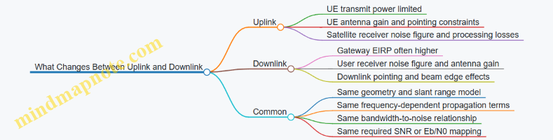
A good link budget ends with a clear decision: whether the received power meets the receiver threshold for the selected bandwidth and modulation and coding, and how much margin remains for real-world imperfections.
2.2 Propagation Effects Including Free Space Loss and Atmospheric Attenuation
Direct to cell satellite links live and die by propagation. Two effects dominate early link-budget thinking: free space loss, which is mostly geometric, and atmospheric attenuation, which is mostly environmental. Treat them separately first, then combine them so you can see what changes when frequency, elevation angle, or weather changes.
Free Space Loss as the Baseline
Free space loss (FSPL) describes how signal power spreads as it travels through space without additional losses. It depends on distance and frequency, so it is the first “sanity check” when a link budget looks off.
- Distance: as range increases, power density drops with the square of distance.
- Frequency: as frequency increases, the wavelength shrinks, so the same physical spreading causes more loss.
A practical way to use FSPL is to compute it at the carrier frequency and the estimated path length (often slant range for mobile terminals). If you later add antenna gains and receiver noise figures, FSPL tells you whether you’re starting from a plausible place.
Example: Suppose a terminal sees a slant range of 600 km at 2.0 GHz. FSPL will be large even before any atmospheric effects. If you double the frequency to 4.0 GHz while keeping range the same, FSPL increases by 6 dB. That 6 dB is not “mysterious”; it is the frequency dependence showing up.
Atmospheric Attenuation as the Environment
Atmospheric attenuation includes absorption and scattering by gases and hydrometeors. For terrestrial links it can be modest, but for satellite links the signal crosses a long atmospheric path near the terminal, and the path length changes with elevation angle.
Key drivers:
- Elevation angle: lower elevation means a longer path through the atmosphere, increasing attenuation.
- Frequency: attenuation can rise sharply near absorption lines of water vapor and oxygen.
- Weather: rain and cloud add additional loss, often the biggest variable during operations.
A useful modeling approach is to separate “gaseous absorption” from “rain attenuation.” Gaseous absorption is relatively predictable from frequency and temperature/humidity assumptions. Rain attenuation is more variable and often handled with statistical models or conservative margins.
Example: Two terminals use the same frequency and power. Terminal A operates at 70° elevation, Terminal B at 20°. Even if both are in the same region, Terminal B typically experiences higher atmospheric loss because the slant path through the atmosphere is longer. In link budgets, this is why elevation angle is treated as a first-class input, not an afterthought.
Combining Effects Without Double Counting
In a basic link budget, you can combine losses additively in dB:
- Total propagation loss ≈ FSPL + atmospheric attenuation + other minor terms
Be careful not to mix models that already include parts of FSPL. For instance, some “path loss” formulas may already embed free space behavior. The safe workflow is:
- Compute FSPL from geometry and frequency.
- Compute atmospheric attenuation from frequency and elevation angle.
- Add them in dB with any additional losses you explicitly model (e.g., polarization mismatch, implementation loss).
Mind Map: Propagation Effects
Worked Mini-Scenario for Intuition
Consider two frequencies, f1 and f2, and two elevation angles, e1 and e2.
- If f2 > f1 and range is unchanged, FSPL increases by 20·log10(f2/f1).
- If e2 < e1, atmospheric attenuation generally increases because the atmospheric path length grows.
So a higher frequency can hurt twice: it increases FSPL and may also increase atmospheric attenuation depending on where the carrier sits relative to absorption characteristics. This is why link budgets often show “frequency windows” where performance is more forgiving.
Practical Best Practices for Modeling
- Use slant range for mobile terminals, not just ground distance.
- Treat elevation angle as time-varying during movement; propagation loss changes even if transmit power stays fixed.
- Keep gaseous and rain terms separate so you can adjust margins when conditions differ.
- Validate your numbers with internal consistency checks: if a small frequency change causes a huge loss jump, confirm whether you crossed an absorption region.
Quick Reference Summary
- FSPL: mostly geometric, frequency-sensitive, predictable.
- Atmospheric attenuation: environment-sensitive, elevation-sensitive, frequency-dependent.
- Combine in dB carefully, with explicit inputs and no overlapping models.
2.3 Modulation Coding and Link Adaptation Concepts for Robust Delivery
Direct-to-cell satellite links behave like a moving target: path loss changes with geometry, Doppler shifts the carrier, and latency makes retransmission expensive. Modulation, coding, and link adaptation are the three knobs that keep delivery reliable without wasting spectrum.
Modulation Choices for Mobile Satellite Links
Modulation sets how many bits you pack into each symbol. Higher-order constellations (like 16-QAM) carry more bits per symbol but require a cleaner signal-to-noise ratio (SNR). Lower-order constellations (like QPSK) are more forgiving.
A practical way to think about it: if your receiver can reliably estimate the channel and compensate frequency offset, you can afford denser constellations. If the receiver is struggling—because the terminal is moving, the beam edge is near, or the link is fading—then robust constellations reduce bit errors.
Key implementation detail: modulation is not just “what you transmit.” It also determines how sensitive the demodulator is to residual frequency error and phase noise. In satellite systems, Doppler compensation reduces the problem, but it rarely makes it disappear.
Coding Fundamentals for Error Control
Coding adds redundancy so the receiver can correct errors rather than merely detect them. Two broad roles matter here.
First, forward error correction (FEC) corrects errors within a single transmission. This is crucial when round-trip time is large, because waiting for retransmissions is slow.
Second, coding rate controls the tradeoff between throughput and robustness. A lower code rate adds more redundancy, improving decoding success at lower SNR.
A concrete example: suppose you need to deliver a short status message. With a high code rate and 16-QAM, you might succeed when the link is strong but fail when it dips. With QPSK and a lower code rate, you may send fewer bits per second, but the message arrives more consistently.
Combining Modulation and Coding into a Transport Strategy
In practice, modulation and coding are paired as a set of transmission modes. Each mode corresponds to a specific constellation and coding rate, often with a target block error rate.
Think of each mode as a “seatbelt level.” When conditions are good, you use a lighter seatbelt to move faster. When conditions degrade, you switch to a heavier seatbelt.
The receiver estimates link quality using measurements such as reference signal quality and error statistics. The transmitter then selects a mode that matches the estimated capability.
Link Adaptation Logic for Robust Delivery
Link adaptation is the control loop that chooses the best transmission mode over time. It must respond to changing conditions while avoiding oscillation (switching modes too frequently).
A systematic adaptation approach uses three steps:
- Measure: obtain an estimate of effective SNR or a related metric.
- Select: map the metric to a mode using a table or function with margins.
- Apply: schedule transmissions using the chosen mode until the next update.
Margins matter because measurements are imperfect. If you choose the highest mode that barely fits the estimate, you’ll see bursts of block failures. Adding a margin reduces failures but costs throughput.
Practical Example of Mode Selection
Assume you have four modes:
- Mode A: QPSK, low code rate (most robust)
- Mode B: QPSK, higher code rate
- Mode C: 16-QAM, moderate code rate
- Mode D: 16-QAM, high code rate (least robust)
If the terminal reports a strong link quality, the system selects Mode D for efficiency. If the terminal moves toward a beam edge and the reported quality drops, the system steps down to Mode C or B. When the quality becomes very low, it switches to Mode A to keep block error rates within the target.
A useful operational detail: mode switching should be tied to block boundaries. That way, each block is decoded with a known configuration, and the receiver doesn’t have to guess.
Handling Latency and Retransmission Constraints
Satellite links often use hybrid automatic repeat request (HARQ) at the link layer. Even with HARQ, you want the first attempt to succeed often enough that retransmissions don’t dominate.
That leads to a design principle: choose coding and modulation so that the probability of needing retransmission stays manageable. If you rely too heavily on retransmissions, latency grows and buffers fill.
Mind Map: Modulation Coding and Link Adaptation
Advanced Details Without the Mystery
A robust adaptation table is usually built from measured or simulated performance curves that relate SNR (or effective SINR) to block error rate for each mode. The mapping is then adjusted with implementation margins for estimation error.
To prevent rapid toggling, systems commonly use hysteresis: the threshold to move to a higher mode is slightly higher than the threshold to move to a lower mode. That way, small measurement fluctuations don’t cause constant mode changes.
Finally, adaptation must consider what the receiver can actually decode. If the terminal’s capability is limited—due to power, antenna pattern, or processing—then the mode set should be restricted so the system never selects configurations the terminal cannot support.
In short: modulation sets the packing density, coding sets the error-correction strength, and link adaptation decides which combination fits the current link quality while respecting latency and receiver limits.
2.4 Doppler, Timing, and Frequency Offset Handling in Mobile Satellite Links
Mobile satellite links rarely behave like calm, stationary lab links. The satellite moves, the user moves, and the radio carrier you thought was “at frequency X” slowly drifts. This section explains how to estimate Doppler, keep timing aligned, and correct frequency offset so the receiver can demodulate reliably.
Doppler Basics and Why It Matters
Doppler shift is the change in observed carrier frequency caused by relative motion. In a direct-to-cell scenario, the satellite’s angular motion dominates, but terminal motion adds a smaller component. The practical effect is that the receiver’s local oscillator and the incoming signal no longer match, which reduces coherent demodulation performance.
A useful mental model: Doppler creates a moving target for frequency. If the receiver’s frequency correction is too slow or too inaccurate, the demodulator sees residual frequency error, and symbol decisions become noisier.
Timing Reference and Synchronization Goals
Timing synchronization aims to align the receiver’s sampling and symbol boundaries with the transmitted waveform. In satellite links, propagation delay is large and varies with geometry, so the receiver must estimate timing offset and track it as conditions change.
Timing has two distinct jobs. First, it must find the correct frame or slot boundary so the receiver knows where symbols start. Second, it must keep that alignment stable enough that channel estimation and equalization remain valid.
Frequency Offset Decomposition
Frequency offset in practice is a sum of multiple contributors:
- Doppler shift from satellite and terminal motion.
- Oscillator mismatch between transmitter and receiver.
- Any residual offsets from prior calibration steps.
Instead of treating these as one blob, receivers typically estimate a combined offset and then track it. The combined estimate is what matters for demodulation; the decomposition is what helps you reason about why the estimate changes over time.
Estimation Pipeline from Coarse to Fine
A systematic receiver approach uses stages:
- Coarse frequency estimation using a preamble or synchronization signal. This stage tolerates large initial error.
- Coarse timing estimation using correlation peaks and known reference structures.
- Fine frequency tracking using reference symbols embedded in the signal.
- Fine timing tracking using ongoing measurements and control loops.
Each stage narrows the error budget. If you skip a stage, later loops may start outside their capture range.
Mind Map: What the Receiver Must Do
Tracking Loops and Control Stability
Frequency tracking is usually implemented as a feedback loop that updates the receiver’s correction based on fresh measurements. The loop has a bandwidth: too narrow, and it can’t follow Doppler changes; too wide, and it chases noise.
Timing tracking similarly balances responsiveness and stability. A good rule of thumb is to update timing more frequently than you update large frequency corrections, because timing errors directly break symbol alignment, while frequency errors can often be partially tolerated until they accumulate.
Practical Example: Estimating Residual Frequency Error
Assume a receiver performs coarse frequency correction after synchronization. After that, it measures residual frequency error using reference symbols.
- If residual error is small, the demodulator can use it as a minor correction.
- If residual error is large, the receiver should re-enter acquisition or increase tracking aggressiveness.
A concrete check: compute the phase rotation over one symbol period caused by residual frequency error. If the rotation is a significant fraction of 360 degrees, you will see constellation smearing and higher error rates. That’s your signal that the correction is not keeping up.
Practical Example: Timing Acquisition with Variable Propagation Delay
Suppose the receiver correlates a known synchronization pattern and finds a peak. In satellite links, the peak position shifts as geometry changes. If the receiver only performs timing acquisition once, the peak will drift and eventually move away from the sampling instant.
A robust approach is to:
- Use correlation to get an initial timing estimate.
- Then apply a tracking update each time new reference information arrives.
This keeps the receiver aligned without requiring full re-acquisition.
Advanced Detail: Doppler Rate and Update Scheduling
Doppler is not constant; it changes with relative motion. That means the receiver must consider Doppler rate when choosing update intervals for frequency tracking.
If you update too slowly, the correction lags behind the true Doppler, leaving residual error. If you update too quickly, measurement noise dominates and the correction jitters. The best scheduling ties update timing to how often reference symbols are available and to the expected rate of Doppler change.
Practical Example: Choosing a Tracking Strategy for a Beam Edge
Near a beam edge, the link quality can drop and reference measurements become noisier. A sensible strategy is to keep the loop running but adjust how aggressively it reacts to noisy measurements.
For example:
- Maintain frequency tracking using the most reliable reference symbols.
- Reduce timing update aggressiveness if correlation peaks become less distinct.
This prevents the receiver from “over-correcting” based on weak signals.
Summary of Key Handling Principles
- Estimate coarse frequency and timing early, then refine.
- Track frequency and timing continuously with feedback loops sized to measurement quality.
- Treat Doppler as time-varying, not a single offset.
- Use reference symbols to measure residual errors and decide whether to keep tracking or re-acquire.
2.5 Antenna Considerations for Handheld and Vehicle Mounted Terminals
Direct to cell satellite links are often limited by geometry and link budget, but antennas decide whether the link budget survives real life. A good antenna choice balances gain, pattern stability, polarization match, and mechanical practicality—especially when the user is moving and the terminal is not perfectly aimed.
Handheld Terminals: Practical Constraints and Design Priorities
Handheld antennas must work with limited size, changing body blockage, and frequent orientation changes. Start with the radiation pattern: a terminal that can “see” the satellite across a range of elevations and azimuths reduces outages caused by small user movements. For many handheld designs, a controlled pattern with moderate gain is more reliable than a very high-gain antenna that needs precise pointing.
Polarization matters because satellite signals arrive with a polarization state that depends on the satellite and terminal orientation. If the terminal antenna polarization is mismatched, you lose effective signal power even when the link budget looks fine on paper. A practical approach is to use antennas that support polarization diversity or that maintain acceptable polarization alignment across typical device rotations.
Body blockage is the handheld’s silent saboteur. Human tissue attenuates and can depolarize signals, so antenna placement and ground clearance are not cosmetic. Placing the antenna near the top edge or away from the user’s palm often improves consistency. If the antenna is integrated into a device chassis, account for the chassis as part of the RF environment rather than treating it as a neutral housing.
Vehicle Mounted Terminals: Mounting Geometry and Stability
Vehicle installations trade portability for stability. A fixed mount can maintain a consistent antenna orientation relative to the sky, which improves polarization match and reduces fading caused by rapid orientation changes. The key constraint becomes mounting location: roof, trunk, hood, or side panels each introduce different reflections and shadowing.
A vehicle roof mount usually offers better sky visibility, but it can suffer from multipath due to nearby metal surfaces. This shows up as pattern ripples—small variations in gain versus angle—that can cause noticeable throughput swings when the vehicle changes heading. A well-designed mount uses a ground plane and spacing that shape the antenna’s pattern predictably.
Cable loss and connector quality become more important in vehicles because the antenna is farther from the radio. Even a small additional loss in the coax or feedline directly reduces received power. Keep cable runs short, use low-loss cable where needed, and verify connector insertion loss under temperature and vibration.
Pattern, Gain, and Coverage: Turning Antenna Specs into Link Behavior
Antenna gain is not just a number; it is angle-dependent. For satellite links, you care about gain across the elevation range where the satellite is visible. When you evaluate an antenna, map its gain pattern onto the expected sky track and check whether the worst-case angles still meet the required link margin.
Beamwidth also affects user experience. A narrow beam can increase gain but makes the link sensitive to pointing errors and terminal rotation. A wider beam reduces sensitivity but may lower peak gain. The “best” choice is the one that keeps the effective gain above the threshold for the majority of the pass, not just at the peak.
Polarization Matching and Diversity Strategies
Polarization mismatch can be quantified as an additional loss term. In practice, you reduce this risk by selecting antenna elements and feed structures that either align with the expected polarization or tolerate rotation. Diversity can be implemented as dual-polarized elements or by using two orthogonal elements with switching or combining.
For handhelds, polarization diversity often improves reliability because the user’s grip changes orientation. For vehicles, polarization diversity can still help, but stable mounting may already provide sufficient alignment, letting you prioritize pattern and mechanical robustness.
Mind Map: Antenna Considerations for Direct to Cell Terminals
Antenna Considerations Mind Map
Example: Choosing Between a Narrow and a Wide Pattern for a Handheld
Suppose a handheld antenna option A has higher peak gain but a narrow beam, while option B has slightly lower peak gain but a wider pattern. If the satellite is visible over a limited elevation window, option A might look better at the pass center. However, if user orientation changes frequently, the effective gain during the edges of the pass can drop below the required margin for option A. Option B, with its wider coverage, may keep the effective gain above threshold for more of the pass, improving message success rate even with lower peak gain.
Example: Vehicle Roof Mount with Feedline Loss Check
A vehicle design uses a roof-mounted antenna with a 3 m feedline. If the feedline has 0.5 dB loss at the operating band, that loss directly reduces received power. If the link budget is tight, you may need either a lower-loss cable, a shorter run, or a higher-gain antenna. Before changing antenna hardware, verify connector insertion loss and routing losses, because a “good” antenna paired with a lossy or poorly terminated feedline can erase the gains you paid for.
Summary of What to Verify Before Finalizing Hardware
For handhelds, verify pattern coverage, polarization tolerance, and body blockage effects in realistic grip and orientation tests. For vehicles, verify sky visibility from the chosen mount, quantify feedline and connector losses, and confirm that metal-induced multipath does not create unacceptable gain dips. Antenna selection is ultimately about keeping effective gain and polarization match within the margins that the rest of the link design assumes.
3. NTN Network Architecture and Functional Building Blocks
3.1 Core NTN Entities Including User Equipment, Gateway, and Network Control
Direct to cell NTN works because three roles cooperate: the User Equipment (UE) speaks radio, the Gateway (GW) anchors the satellite link to the terrestrial network, and Network Control (NC) coordinates access, sessions, and policy. Think of it as a three-part handshake: the UE can transmit and receive, the GW can translate and route, and the NC can decide who gets resources and how sessions stay consistent.
User Equipment
The UE is the mobile device that must survive a moving radio channel. In NTN, the UE typically includes:
- Satellite-capable radio: It generates uplink waveforms and demodulates downlink signals. It must tolerate Doppler and timing uncertainty.
- Antenna and beam interface: For direct to cell, the UE antenna pattern and pointing assumptions affect link quality. Even when the UE is “omnidirectional,” the effective gain varies with orientation.
- Protocol stack for constrained links: Satellite links often have higher latency and variable error rates, so the UE must manage retransmissions and buffering without stalling everything.
- Measurement and reporting logic: The UE measures reference signals, estimates frequency offset, and reports quality metrics used for access decisions.
Example: A field technician’s phone tries to send a short status message. The UE first synchronizes to the downlink, estimates Doppler-induced frequency shift, then requests uplink resources. If the UE is near a beam edge, it may use more robust modulation and coding to keep the message decodable.
Gateway
The Gateway is the bridge between satellite access and the terrestrial core. It usually performs:
- RF front-end and satellite link processing: Frequency conversion, filtering, and amplification for uplink and downlink.
- Baseband processing and framing: It aligns received signals to expected timing/frequency references and prepares data for higher layers.
- Transport connectivity to the core: It forwards user-plane traffic to the appropriate network functions with the right latency and reliability characteristics.
- Interface to network control: The GW receives configuration and policy inputs that affect scheduling, access parameters, and session handling.
Example: During the same technician’s message, the GW receives the uplink burst, performs synchronization and decoding, then forwards the payload to the core network. If the UE’s timing estimate drifts, the GW’s processing and feedback paths help keep subsequent bursts aligned.
Network Control
Network Control decides “what happens next” for access and sessions. It typically includes:
- Access management: It controls how UEs request resources, how contention is resolved, and how admission is granted.
- Session management: It establishes and maintains user sessions, mapping service requirements to radio bearers and core routing.
- Mobility and beam coordination: It uses UE measurements and network topology to support transitions between beams or coverage areas.
- Policy and security enforcement: It ensures only authorized UEs can establish service and that session parameters match service rules.
Example: If the UE moves from one coverage region to another, Network Control updates the session context so the UE continues using the correct access configuration. The UE may not need to restart the entire session; it needs the right parameters and continuity handling.
How the Three Entities Work Together
A practical way to understand the system is to follow a message from first contact to delivery.
- UE synchronization and measurement: The UE locks to downlink references and estimates timing/frequency.
- UE access request: The UE requests uplink resources using configured access procedures.
- Network Control decision: NC authorizes access, selects parameters, and coordinates with the GW.
- Gateway processing and forwarding: The GW decodes uplink, then routes user-plane data to the core.
- Session continuity handling: If conditions change, NC updates context and the GW applies it to subsequent bursts.
Mind Map: Core NTN Entities
Integrated Example Walkthrough
Consider a short burst message sent while the UE is moving.
- The UE synchronizes to the downlink and estimates Doppler, then prepares an uplink burst with parameters chosen to match current link quality.
- The UE sends an access request. Network Control checks authorization and decides whether to grant resources immediately or apply a contention resolution path.
- The GW receives the uplink burst, performs decoding, and forwards the payload to the core network.
- As the UE approaches a beam boundary, Network Control updates the session context so the next bursts use the correct access configuration. The UE continues sending without changing its application behavior.
This division of responsibilities keeps the system manageable: the UE focuses on radio correctness, the GW focuses on reliable translation and routing, and Network Control focuses on decisions that require global context.
3.2 Roles of Satellite and Terrestrial Segments in End to End Connectivity
Direct to cell services work because two very different worlds cooperate: the satellite segment carries radio connectivity over long distances, while the terrestrial segment provides the “plumbing” that makes sessions, routing, and policy enforcement practical. Think of the satellite as the long-haul bridge for radio reach, and the terrestrial network as the traffic controller that decides where packets go next.
Satellite Segment Responsibilities
The satellite segment’s job is to deliver radio access between the user terminal and the network entry point. It includes the spaceborne payload behavior and the radio link characteristics that shape what the system can reliably do.
- Radio coverage and link feasibility: The satellite determines which users can be served by creating coverage footprints and beam patterns. Link feasibility depends on geometry, elevation angle, and terminal antenna performance.
- Uplink and downlink transport over the air: The satellite payload receives uplink signals from user equipment and transmits downlink signals back. This is where propagation effects, Doppler shifts, and fading directly influence throughput and latency.
- Beam-level resource handling: Within the satellite access, scheduling and resource allocation are constrained by beam capacity and shared spectrum usage. When many users contend, the satellite segment must support mechanisms that keep service usable rather than merely possible.
- Timing and frequency stability support: Even when the terminal performs compensation, the satellite segment contributes reference behavior that affects synchronization quality.
A concrete example: a hiker at low elevation angle may still receive control messages, but data rates drop because the satellite link margin shrinks. The satellite segment is the reason the system can’t “wish” higher throughput into existence.
Terrestrial Segment Responsibilities
The terrestrial segment connects the satellite access to the rest of the communication system. It translates radio access into end-to-end service behavior by providing routing, session management, and policy enforcement.
- Gateway functions and demarcation: Gateways terminate satellite access links and interface them to the terrestrial network. They handle frequency conversion, baseband processing, and mapping between radio bearers and IP transport.
- Backhaul transport and reliability: Terrestrial links carry user traffic onward. Their latency and jitter characteristics influence how well higher-layer protocols can maintain stable sessions.
- Core network integration: The terrestrial core handles registration, authentication, session establishment, and mobility-related control. Without this, the satellite could “hear” the terminal but not provide service.
- Quality of Service enforcement: Terrestrial components classify traffic, apply QoS rules, and schedule resources in ways that match service requirements such as messaging priority versus bulk data.
- Monitoring and operational control: Performance counters, alarms, and logs help operators identify whether issues originate in the radio link, the gateway, or the core.
A concrete example: if a user can register but cannot send data, the issue is often not the satellite coverage itself. It may be a terrestrial policy rule, a session setup failure, or a QoS mapping mismatch.
How They Work Together End to End
End-to-end connectivity is a chain of responsibilities. The satellite segment creates the radio path; the terrestrial segment makes that path useful for applications.
- Access establishment: The terminal acquires timing and frequency references, then exchanges control signaling over the satellite link.
- Gateway termination and mapping: The gateway converts the satellite access into terrestrial transport, preserving identifiers needed for session continuity.
- Core-driven session creation: The core network authorizes the user and creates bearers with appropriate QoS.
- Data delivery with QoS: Traffic flows through terrestrial routing with the QoS rules that were negotiated during session setup.
- Mobility and continuity: When beam conditions change, the system coordinates handover or session adjustments so the user experiences continuity rather than repeated starts.
Mind Map: Satellite and Terrestrial Roles
Example: Diagnosing Where the Problem Lives
Suppose a direct-to-cell messaging service shows frequent delays. A systematic check separates radio-limited behavior from network-limited behavior.
- If control messages fail first: suspect satellite link margin, synchronization, or beam availability. The terminal may be able to “hear” but not reliably decode.
- If registration succeeds but user data stalls: suspect terrestrial session setup, bearer mapping, or QoS policy enforcement at the core or gateway.
- If both control and data are slow: suspect backhaul congestion or gateway processing delays, because the terrestrial segment can throttle end-to-end delivery even when the radio link is fine.
This division of labor keeps troubleshooting grounded: the satellite segment explains whether the radio path is viable, and the terrestrial segment explains whether the service path is correctly established and maintained.
3.3 Transport and Backhaul Requirements for Satellite Network Operation
Transport and backhaul are the “plumbing” that connect satellite access to the 5G core and to each other. In direct to cell satellite communication, the plumbing must handle long propagation delays, variable satellite link capacity, and strict timing for signaling and scheduling. If you treat backhaul like a simple pipe, you’ll eventually meet the reality of buffering, jitter, and congestion—usually at the worst possible moment.
Foundational Requirements for End to End Transport
Start with what must be carried: control-plane signaling (registration, session setup, mobility events) and user-plane traffic (data bearers, messaging payloads). Control-plane messages are small but timing-sensitive; user-plane traffic is larger but more tolerant of minor delay. Both must traverse transport segments that may include satellite feeder links, gateway processing, terrestrial backhaul, and core network interfaces.
A practical way to size transport is to separate three behaviors:
- Latency budget: propagation delay plus processing plus queuing. For NTN, propagation delay is not negotiable, so the transport must avoid adding avoidable queuing.
- Jitter budget: variation in packet arrival time. Jitter matters because it affects buffering and retransmission behavior at higher layers.
- Loss budget: packet loss can trigger retransmissions and reduce effective throughput. Loss is often caused by congestion rather than link errors in the terrestrial segment.
Capacity Planning with Variable Satellite Access
Satellite access capacity changes with beam loading, terminal geometry, and link adaptation. Backhaul must therefore support a bursty pattern rather than a steady rate. The key is to match backhaul behavior to satellite behavior:
- Peak-to-average ratio: if satellite access can temporarily deliver faster than average, backhaul must absorb short bursts without excessive queue growth.
- Queue management: use traffic classes and scheduling so user-plane bursts do not starve control-plane messages.
- Overbooking policy: if you overbook, do it with clear boundaries. For example, allow user-plane overbooking only when control-plane class remains protected.
A simple example: suppose a gateway serves 10,000 terminals with a typical user-plane load of 2 Mbps per beam on average, but occasional bursts reach 6 Mbps for short intervals. If backhaul is provisioned for 2 Mbps per beam with no burst tolerance, queues build quickly and jitter spikes. Provisioning for a higher burst rate or implementing strict shaping per beam prevents that.
Transport Topology and Interface Choices
Transport typically includes:
- Feeder link to gateway: may be satellite-to-ground or satellite-to-satellite depending on architecture.
- Gateway internal transport: between radio processing and packet processing.
- Terrestrial backhaul: from gateway to aggregation points and onward to the 5G core.
Interface selection affects operational complexity. For instance, packet-based transport with QoS markings can preserve service differentiation across hops, while a less capable transport may force you to re-map priorities at each boundary. The goal is consistent treatment of traffic classes end to end.
QoS, Traffic Classification, and Scheduling
Backhaul must carry at least two service categories: control-plane and user-plane. Within user-plane, you may further separate by bearer type or priority.
A workable QoS approach:
- Mark packets at the gateway according to their service class.
- Enforce per-class queuing so control-plane packets experience minimal queueing delay.
- Apply shaping or policing at ingress to prevent one beam from overwhelming shared links.
Example: if a beam experiences a sudden surge of user-plane traffic, policing at the beam ingress keeps the shared backhaul queues stable. Control-plane packets continue to flow, so session setup and mobility signaling do not stall.
Reliability, Redundancy, and Failure Containment
Backhaul reliability is not just “up or down.” You also need to contain partial failures. Common tactics include:
- Redundant paths between gateway and core with fast reroute.
- Failure domain separation so one congested segment does not cascade into all beams.
- Monitoring at boundaries: measure delay, jitter, and loss per hop, not only at the end.
A concrete workflow: when throughput drops, first check whether loss increased on the terrestrial backhaul. If loss stayed low but jitter increased, the issue is likely queueing or scheduling. If both increased, congestion or misconfiguration is more likely.
Mind Map: Transport and Backhaul Requirements
Example: Sizing Backhaul for a Gateway with Two Beams
Assume two beams share a terrestrial link. Beam A has average user-plane 3 Mbps with bursts to 8 Mbps; Beam B averages 2 Mbps with bursts to 5 Mbps. If you provision backhaul only for 5 Mbps average, bursts overlap and queues grow, increasing jitter and triggering retransmissions.
A better approach is to provision for a burst-safe rate and enforce class protection. For example, allocate control-plane capacity explicitly, then shape user-plane per beam so the combined burst does not exceed the link’s queue-safe threshold. The result is stable delay for signaling and predictable user-plane performance even when both beams peak.
3.4 Session Management and Mobility Support Across Satellite Coverage
Direct-to-cell satellite links behave differently from terrestrial ones: propagation delay is longer, coverage is shaped by beams, and link quality changes as the user moves. Session management and mobility support are the parts of the system that keep a user’s service usable while the radio path changes.
Session Foundations for NTN
A “session” is the set of network resources and state needed to deliver a particular service flow, such as a messaging bearer or an interactive data stream. In an NTN context, the session must track three things: (1) where the user is expected to be reachable, (2) how the network should route and schedule the user’s traffic, and (3) what radio parameters are currently safe to use.
A practical way to think about it is a control loop with two time scales. The slow loop handles reachability and routing state; the fast loop handles radio parameters like timing and link adaptation. If you only do the fast loop, the network may still send traffic to the wrong place. If you only do the slow loop, the radio may be “connected” but not deliver packets reliably.
Mobility Triggers and State Transitions
Mobility support starts with triggers. For satellite coverage, triggers are typically based on measured reference signal quality, beam availability, and timing/frequency stability. The key is to avoid thrashing: switching too often wastes resources and increases signaling.
When a user approaches a beam edge, the system should transition in a controlled order:
- Prepare the target reachability context.
- Adjust radio parameters to the new link conditions.
- Move the user’s active traffic to the new path.
- Release the old context after confirming delivery.
This ordering matters because satellite links can have transient periods where measurements are noisy. Preparing first reduces the chance that the user experiences a gap while the network is still “learning” where the user is.
Reachability and Routing State
Session management must ensure that downlink packets reach the user even as the satellite-to-user geometry changes. The network uses a combination of user identity, current serving area information, and routing rules to decide where to send packets.
A useful mental model is a mailroom with two addresses: a stable identity (the user) and a changing delivery zone (the current satellite/beam context). The session state tells the mailroom which delivery zone is currently valid.
Timing, Latency, and Retransmission Interaction
Because round-trip time is longer, retransmission behavior affects perceived mobility. If the system switches paths while there are outstanding retransmissions, the user can see duplicates or delays.
To manage this, the session layer and link layer coordinate on sequence handling. The session should tolerate reordering during transitions, while the radio layer should avoid unnecessary retransmissions once the new path is confirmed. In practice, this means the system treats mobility as a controlled change in the path, not as a sudden disconnect.
Example: Beam Edge Session Continuity
Consider a user sending a short burst of data while moving from Beam A to Beam B.
- At first, the session routes downlink traffic to Beam A’s context.
- Measurements show Beam B becoming usable, so the network creates a target context for Beam B and updates radio parameters.
- During the transition, the system keeps the session active and continues delivering using the best available path.
- Once Beam B is confirmed, new downlink traffic is routed to Beam B, and Beam A’s context is released.
From the user’s perspective, the burst may experience a small delay, but it should not fail outright. The system’s job is to ensure that “delivery intent” survives the path change.
Mind Map: Session Management and Mobility Support
Advanced Details That Prevent Real-World Pain
A session can fail during mobility even when the radio link is “mostly fine.” Common causes include stale routing state, mismatched sequence handling, and inconsistent timing assumptions between control and data paths.
To reduce these risks, the system should:
- Keep routing state changes aligned with confirmed radio readiness, not just early measurements.
- Use consistent sequence and reordering rules so that duplicates and out-of-order packets are handled deterministically.
- Ensure that session release happens only after the new path is confirmed to carry the traffic, not merely after the handover command is issued.
If you implement these rules, mobility becomes a sequence of deliberate state updates rather than a gamble on timing. The user gets continuity; the network gets fewer surprises.
3.5 Security and Authentication Components in NTN Deployments
Direct-to-cell satellite links change the security problem in three ways: the radio path is longer and noisier, the network is more distributed, and the user terminal may be far from any terrestrial base station. The goal of this section is to explain how authentication and security controls are composed so that only authorized users get service, and only authorized network entities can create or modify sessions.
Core Security Goals in NTN
Start with what must be true at the system level.
- Mutual trust for session setup: the terminal must verify it is talking to the right network, and the network must verify the terminal’s identity.
- Integrity and confidentiality for signaling: authentication messages and session control must not be altered in transit.
- Replay resistance: captured messages must not be reusable later, even if the satellite link introduces long delays.
- Key separation across functions: compromise of one key should not automatically expose everything else.
A helpful mental model is to treat NTN security as layered gates: identity proof, then key establishment, then protected signaling and protected user data.
Authentication Flow Components
In a 5G-integrated NTN deployment, the authentication logic typically involves the UE, the access network side, and the core network side. The satellite and gateway segments carry traffic, but they should not be trusted to make identity decisions.
Key components you will see in practice:
- UE credentials and identifiers: long-term identity material stored securely in the terminal.
- Authentication server in the core: generates challenge material and verifies responses.
- Access-side authentication relay: forwards messages between UE and core without interpreting secrets.
- Session key derivation: produces keys for signaling protection and for user-plane encryption.
- Security mode control: decides when encryption and integrity protection are enabled for a given session.
A concrete example: a field technician’s phone attempts to register while moving between satellite beams. The access side forwards the registration and authentication messages; the core decides whether the UE is allowed. The satellite link may be lossy, but the security decisions are still made by the core using fresh challenges.
Key Management and Protection Boundaries
Security is not just “encryption on.” It is also about where keys are used.
- Long-term keys: used to authenticate the UE to the core.
- Derived session keys: used to protect signaling and user data for a specific session or context.
- Separate keys for different protections: integrity protection keys differ from encryption keys, so an attacker cannot downgrade one protection by exploiting the other.
In NTN, boundaries matter because the path includes multiple hops: UE to satellite, satellite to gateway, gateway to core. The access-side components should treat the satellite hop as untrusted transport and rely on cryptographic protection for sensitive messages.
Integrity Protection for Signaling Under Latency
Satellite links can increase round-trip time, which makes replay and delay-based attacks more plausible. Integrity protection and replay checks address this.
Practical mechanisms include:
- Freshness tokens or nonces in authentication challenges.
- Sequence numbers or counters for protected messages.
- Strict validation rules: if a message fails freshness or counter checks, it is rejected even if it decrypts correctly.
Example: suppose an attacker records a valid protected signaling message during a registration attempt. When replayed later, the receiver compares counters/freshness data against what it expects for that UE context and discards the message.
Security Mode Control and Session Establishment
After authentication succeeds, the network must decide what protections to apply.
- Security mode negotiation: selects which algorithms and which protections are enabled.
- Protected NAS and RRC signaling: ensures that session setup and mobility-related signaling cannot be modified.
- User-plane protection: encrypts user data so that payloads are not readable on the satellite hop.
Example: a direct-to-cell messaging session starts with protected signaling. If the UE later moves and the access side changes beam or gateway routing, the session continuity mechanism must keep the same security context or re-establish it according to policy. Either way, the UE should not accept unprotected control messages that would change session parameters.
Mind Map: Security and Authentication Components in NTN Deployments
Operational Checks That Prevent “It Works on My Link” Problems
Security failures often appear as connectivity issues, so operational discipline matters.
- Log security-relevant events: authentication success/failure, security mode decisions, and counter validation outcomes.
- Validate algorithm compatibility: mismatched capabilities can lead to weaker protection or failed sessions.
- Confirm context binding: keys and counters must be tied to the correct UE and session context.
Example: during a trial on 2026-02-14, a team notices intermittent registration failures only when the UE is near beam edges. The radio link is fine, but logs show counter mismatches due to context re-selection timing. Fixing the context binding rules resolves both the security validation errors and the user-visible registration failures.
The takeaway is systematic: authenticate with fresh challenges, derive session keys with clear boundaries, protect signaling with integrity checks that tolerate latency, and enforce security mode decisions consistently across satellite access changes.
4. 5G System Integration for Direct to Cell Services
4.1 Mapping NTN Concepts into 5G System Components
Direct to cell satellite communication (NTN) changes the radio environment, but the 5G system still needs to do the same core jobs: identify the user, establish sessions, schedule radio resources, protect data, and keep timing and mobility sane. This section maps NTN concepts to concrete 5G components so you can reason about what goes where.
Foundational Mapping: What Changes and What Stays
Start with the invariants. 5G still uses a user identity, a control plane for registration and session setup, and a user plane for data forwarding. What changes is the path: the satellite introduces long propagation delay, Doppler shifts, and coverage that behaves like moving beams rather than fixed cell sectors.
A useful mental model is to treat NTN as a radio access variant. The 5G core remains responsible for policy, authentication, and routing, while the NTN-specific behavior concentrates in the access network functions and the radio protocol timing.
Mind Map: NTN Concepts to 5G Components
UE Side Mapping: Making the Radio Behave
In 5G, the UE runs RRC procedures for registration, capability signaling, and measurement reporting. For NTN, the UE must also manage radio impairments that are mostly invisible in terrestrial cells.
Timing and frequency control map to UE physical layer and MAC behaviors that support synchronization under Doppler. Practically, the UE uses reference signals to estimate frequency offset and applies correction so demodulation stays stable across beam movement.
Measurement reporting maps to RRC measurement configuration and reporting triggers. Instead of only tracking neighbor cell reference signals, the UE may report beam-related metrics that reflect availability and signal quality at beam edges.
Example: A vehicle-mounted UE enters a satellite beam footprint. It performs initial access using NTN-aware timing parameters, then reports updated signal quality as Doppler changes. The network uses those reports to maintain the right radio configuration for the current beam.
Access Network Mapping: gNB Functions with NTN-Aware Radio
In 5G, the gNB is where radio scheduling, HARQ behavior, and radio configuration live. For NTN, the gNB must incorporate satellite-specific constraints into those functions.
Scheduling and resource allocation map to the gNB scheduler. The scheduler must handle variable link quality caused by geometry and atmospheric effects, and it must coordinate uplink grants in a way that respects propagation delay.
HARQ and retransmissions map to link-layer reliability mechanisms. Because round-trip time is longer, retransmission timing and buffer sizing must be tuned so the system does not waste resources on doomed retransmissions.
Beam management maps to how the access network represents coverage. Even if the satellite is a single platform, the system can treat beams as logical coverage areas with their own availability and configuration.
Example: During a busy hour, many UEs share the same beam. The gNB scheduler prioritizes control-plane traffic and time-critical user-plane flows, while bulk data uses lower priority grants. If uplink timing uncertainty increases near the beam edge, the scheduler reduces grant aggressiveness to avoid repeated failures.
Core Network Mapping: Keeping Control Plane Responsibilities Clear
The 5G core components keep their roles, but NTN changes the timing and the kinds of events the access network reports.
AMF handles registration and mobility-related control. It relies on access network status and UE reports to decide how to maintain reachability.
SMF manages session establishment and policy-driven behavior. It selects user-plane routing and service parameters that match the expected bearer characteristics.
UPF forwards user-plane traffic. For NTN, the UPF must tolerate longer effective latency, but it still performs routing, QoS enforcement, and buffering according to standard 5G mechanisms.
Example: A UE registers while moving between beam footprints. The access network signals availability changes, AMF updates the control-plane context, and SMF ensures the session bearer remains consistent so user traffic can continue without a full teardown.
Interfaces and Transport Mapping: Delay Is a First-Class Constraint
Mapping NTN concepts into 5G also means respecting where delay shows up. Signaling paths between UE, access network, and core must account for longer radio round-trip times. Transport links between gateway and core must be provisioned so that jitter does not turn into radio instability.
Example: If the gateway-to-core transport experiences bursts of latency, the access network may see delayed acknowledgments or delayed status updates. The system then compensates by using stable radio parameters and conservative scheduling until transport conditions normalize.
Putting It Together: A Coherent End-to-End Flow
A clean mapping is easiest to validate with a single flow: registration, session setup, and data delivery.
- UE uses NTN-aware RRC and synchronization to access the satellite-served coverage.
- gNB scheduler and link-layer reliability mechanisms adapt to Doppler and propagation delay.
- AMF and SMF maintain control-plane context and set up the right bearer behavior.
- UPF forwards user-plane traffic with QoS enforcement, while the access network continues to manage radio conditions.
When each component keeps its job and only the NTN-specific behavior is added where it belongs, the system stays understandable—even when the sky is doing the moving.
4.2 Radio Access Network Integration With Satellite Access Links
Direct-to-cell satellite service still needs the same basic job as any cellular radio access network: schedule radio resources, manage link adaptation, and keep user sessions stable while the radio environment changes. The difference is that the “radio environment” includes long propagation delays, Doppler shifts from satellite motion, and coverage that may be beam-shaped rather than cell-shaped.
Core Integration Idea
The RAN must treat the satellite access link as a first-class radio bearer with its own timing, link adaptation, and error-control behavior. Practically, that means the RAN scheduler and protocol stack cannot assume the same round-trip timing and channel coherence used in terrestrial-only deployments.
A useful mental model is a two-layer mapping:
- Radio bearer mapping: how a service flow becomes one or more radio bearers over the satellite link.
- Control mapping: how RAN control messages reach the UE reliably despite delay and mobility.
System Components and Responsibilities
In a typical 5G-style split, the RAN side includes the gNB functions that coordinate radio scheduling and radio protocol handling. For satellite access, the RAN also needs satellite-aware behaviors in the radio protocol and scheduler.
- UE: measures reference signals, reports measurements, and performs timing/frequency corrections.
- gNB RAN functions: allocate resources, configure modulation and coding, and manage HARQ and retransmissions.
- Satellite access interface: carries the radio signals between the gNB and the satellite segment, including any frequency translation and buffering required by the transport.
- Gateway and transport: provide the path for user-plane and control-plane traffic with predictable latency and jitter.
Timing and Scheduling Integration
Satellite links force the RAN to be explicit about timing. If the scheduler assumes terrestrial-like timing, grants and HARQ feedback can miss their intended windows.
Key integration steps:
- Align grant timing with propagation delay so the UE transmits in the expected receive window at the gNB.
- Use Doppler-aware frequency handling so the UE’s uplink and downlink remain within receiver tracking capability.
- Configure HARQ timing to match the longer round-trip over the satellite path.
A concrete example: imagine a UE at the edge of a beam where the link is weaker. The RAN may choose a lower modulation order and enable more robust coding. If HARQ feedback timing is not adjusted for satellite delay, the gNB may treat valid feedback as late and trigger unnecessary retransmissions, increasing load and reducing throughput.
Radio Bearer and QoS Mapping
Satellite access links often have constrained capacity per beam. The RAN must map QoS requirements to radio bearers that reflect that constraint.
- Latency-sensitive flows: use smaller packetization and conservative retransmission behavior so the RAN does not spend too long waiting for HARQ.
- Best-effort flows: can tolerate retransmissions and may be scheduled opportunistically when link quality improves.
Example: a messaging service with short packets benefits from predictable scheduling intervals. If the RAN treats it like a bulk file transfer bearer, it may get queued behind larger transmissions, causing avoidable delays.
Mobility and Beam-Edge Behavior
Beam coverage can change more abruptly than terrestrial cell boundaries. Integration must ensure that handover-like procedures do not depend on assumptions about smooth signal variation.
Practical behaviors:
- Measurement reporting tuned to beam dynamics so the UE reports meaningful changes rather than noisy fluctuations.
- Handover decision logic that considers availability of the target beam and the expected timing of control messages.
Example: a vehicle moving under a narrow beam may experience rapid changes in signal quality. If the RAN waits for a very specific threshold pattern before switching, the UE can drop into a coverage gap. A more robust approach is to base decisions on a combination of availability indicators and measurement trends.
Control-Plane Robustness
Control messages include scheduling grants, configuration updates, and measurement requests. Over satellite, these messages must be delivered with reliability mechanisms that match the delay.
Integration checklist:
- Ensure retransmission timers for control messages are consistent with satellite propagation.
- Ensure the UE state machine tolerates delayed responses without entering invalid states.
- Ensure buffering at the satellite access interface does not reorder control messages.
Mind Map: RAN Integration with Satellite Access Links
Example Walkthrough: From Registration to Data Delivery
- Registration: the UE establishes initial access using satellite-aware timing so the gNB can interpret uplink responses in the correct receive window.
- Bearer setup: the RAN maps the requested service QoS to a radio bearer configured for satellite link adaptation and appropriate retransmission behavior.
- Scheduling: the scheduler issues grants using propagation-aligned timing, and the UE transmits with Doppler-compensated frequency.
- Data delivery: the RAN applies HARQ and error control tuned for satellite delay, so retransmissions occur when feedback can realistically arrive.
- Mobility: as the UE moves, measurement reports trigger beam-aware scheduling changes without forcing the UE into a coverage gap.
The result is not a different “kind” of RAN, but a RAN whose timing, reliability, and bearer mapping are consistent with the physics of satellite links. That consistency is what keeps the system from behaving like it works in theory and fails in practice.
4.3 Core Network Integration for Session Establishment and Service Continuity
Direct to cell satellite access changes the “shape” of the radio link: higher latency, intermittent coverage at beam edges, and timing uncertainty from Doppler. The core network still needs to create sessions, keep them stable, and recover gracefully when the radio side hiccups. This section focuses on how session establishment and service continuity are handled when the access path is satellite-based but the service experience must remain consistent.
Foundational Concepts for Session Establishment
A session is the set of control-plane state and user-plane forwarding rules that make a specific service work for a specific user. In a 5G-style core, session establishment typically includes:
- Identity and access context: the network binds a user’s identity to an access context that can survive mobility.
- Policy and QoS intent: the network decides what kind of traffic this session carries and what performance it should receive.
- User-plane anchoring: the network selects where user data is forwarded and how it is routed.
- Radio access coordination: the core provides parameters that the access side uses to configure bearers.
In direct to cell, the core must treat the access link as “variable quality,” not as a stable pipe. That means session setup should be robust to delayed acknowledgments and should avoid tight coupling between radio timing and core state transitions.
Session Establishment Flow with Satellite Access
A practical flow can be understood as four phases.
-
Registration and access context creation
- The UE registers and the core establishes an access context that includes the serving access node information.
- Example: a field worker powers on a direct-to-cell handset in a vehicle. Registration succeeds even if the first beam is weak; the core stores the context so the next radio measurement can still map to the same session policy.
-
Service request and session policy decision
- The core receives a request (e.g., messaging, data session) and selects policy rules for QoS, charging, and routing.
- Example: for a low-rate text message service, the core chooses a bearer profile that tolerates retransmissions and prioritizes delivery over peak throughput.
-
Session creation and user-plane rule installation
- The core creates the session and installs forwarding rules so user-plane packets reach the correct destination.
- Example: when the UE starts a data session, the core ensures that packets are routed to the correct anchor and that the access side can map them to the right bearer.
-
Radio bearer activation and confirmation
- The core coordinates with the access side so the UE can activate the radio bearers needed for the session.
- Example: if the satellite link is temporarily degraded, the core should not tear down the session immediately; it should wait for radio-side activation outcomes within defined timers.
Service Continuity Under Mobility and Coverage Changes
Service continuity is the art of keeping the session usable while the access path changes. In direct to cell, the most common continuity challenges are beam edge behavior and intermittent link availability.
Key mechanisms include:
-
Mobility support with stable session anchors
- The core keeps the session anchored so that mobility primarily changes access routing rather than rebuilding the entire session.
- Example: as the UE moves from one satellite beam footprint to another, the core updates the access mapping while keeping the same session policy.
-
Session state retention and controlled release
- The core uses timers and state machines to decide when a session is truly lost versus temporarily unreachable.
- Example: a short outage during a handover should not trigger full session release; instead, the core maintains state until the radio link recovers or the inactivity threshold is reached.
-
QoS continuity across access changes
- QoS rules should remain consistent even if the radio scheduler changes grant patterns.
- Example: a session marked for “priority messaging” should keep its QoS intent so that when the link returns, the UE can resume with the expected priority.
Mind Map: Core Network Session and Continuity
Example: Messaging Session Through a Beam Edge
Consider a messaging service that sends a short text and expects delivery confirmation.
- The UE registers and the core creates a session with a QoS profile suited for small payloads.
- The user sends the message. The core has already installed user-plane forwarding rules, so the packet can be queued and forwarded according to the user-plane path.
- The UE approaches a beam edge. The radio link becomes intermittent, so acknowledgments may be delayed.
- Instead of releasing the session immediately, the core relies on continuity timers and retains session state long enough for the radio side to re-establish bearers.
- Once the UE re-enters a usable beam footprint, the access side activates the bearer mapping again, and the message delivery proceeds without requiring a full re-registration.
This example highlights the core principle: session continuity is preserved by separating “radio reachability” from “session existence,” using timers and stable anchoring so that temporary link problems do not force unnecessary control-plane churn.
Example: Data Session with QoS Preservation
For a data session carrying a small stream (e.g., telemetry bursts), the core assigns QoS intent that matches bursty behavior. When mobility changes the access path, the core keeps the session policy intact so the UE can resume transmission with the same priority and bearer mapping. The result is consistent behavior from the application’s perspective: fewer surprises, fewer full session rebuilds, and a predictable mapping between service requirements and network treatment.
4.4 QoS Handling for Satellite Bearers Including Priority and Scheduling
Quality of Service (QoS) in direct to cell satellite links is mostly about deciding who gets airtime and how much reliability you can afford, given long propagation delays and variable link conditions. In practice, QoS is implemented as a chain: application intent becomes service requirements, which become bearer parameters, which become scheduler decisions at the radio access layer.
QoS Foundations for Satellite Bearers
Start with two constraints that shape everything else.
- Latency is not negotiable: propagation delay dominates, so QoS can’t “fix” round-trip time. Instead, QoS controls how long packets wait in queues.
- Capacity is bursty: rain, shadowing, and beam geometry change the usable modulation and coding, so the scheduler must adapt.
A useful mental model is to treat each bearer as a set of packets with a target profile:
- Priority: relative importance when multiple bearers contend.
- Reliability expectation: how aggressively you retransmit or how much redundancy you allocate.
- Rate behavior: whether traffic is steady, bursty, or event-driven.
Mapping Service Intent to Bearer Parameters
In a 5G-integrated NTN system, QoS handling typically follows a mapping flow:
- Application class becomes a QoS flow with a defined priority level.
- Traffic characteristics determine whether the bearer should be shaped (smooth bursts) or left to burst.
- Radio link behavior determines scheduling granularity and retransmission policy.
A concrete example helps. Suppose you have:
- Emergency text messages (high priority, small payloads)
- Field telemetry (medium priority, periodic)
- Background status updates (low priority, tolerant)
You would assign higher priority to emergency messages and ensure they are not trapped behind large telemetry bursts. You might also allow telemetry to use efficient bulk scheduling when conditions are good, while background updates can be rate-limited.
Priority Handling Without Starvation
Priority alone is not enough; a high-priority bearer can still cause starvation if it always wins. A practical approach is weighted scheduling with minimum service guarantees.
- Give each bearer a weight that reflects priority.
- Enforce a cap on how much consecutive airtime any one bearer can consume.
- Maintain a small reserved budget for lower-priority bearers so they can make progress.
Example: If emergency messages are rare but urgent, you can allocate them a high weight and a short “service window.” If emergency traffic suddenly spikes, the cap prevents it from completely blocking telemetry.
Scheduling Under Variable Link Conditions
Satellite links change the effective data rate. The scheduler should therefore consider both queue urgency and current link quality.
A systematic scheduling policy uses two inputs:
- Queue state: how long packets have waited and how full the queue is.
- Link state: which modulation and coding are currently feasible.
When link quality is good, the scheduler can serve larger packets efficiently. When link quality drops, it may switch to smaller, more robust transmissions to avoid excessive retransmissions.
Reliability and Retransmission Tradeoffs
Retransmissions interact with QoS because they consume resources and increase queueing delay. For satellite bearers, you typically balance:
- Fewer retransmissions to protect latency for interactive traffic.
- More retransmissions to protect delivery for small but critical messages.
Example: For emergency text messages, you might allow a limited number of retransmissions to improve delivery probability without letting the queue grow unbounded. For background updates, you can reduce retransmissions and accept occasional loss, since the application can retry later.
Mind Map: QoS Handling for Satellite Bearers
Example: Priority and Scheduling in a Mixed Traffic Beam
Assume three bearers share a beam:
- Bearer A emergency text: priority 3
- Bearer B telemetry: priority 2
- Bearer C background updates: priority 1
At time slot boundaries, the scheduler computes a service score for each bearer using:
- urgency from queue length and packet age
- feasibility from current link quality
- weight from priority
If the link quality supports high throughput, the scheduler serves the bearer with the best combined score, which often means A when it has packets waiting. If the link quality degrades, the scheduler may still serve A first, but it will choose more robust transmission settings to prevent repeated retransmissions from blocking the entire beam.
To keep C from being stuck, the scheduler enforces a minimum service share. Even when A is active, C receives occasional slots, which prevents queue overflow and reduces drops.
Practical Verification Metrics
QoS is only “working” if the measured outcomes match the intent. Track per bearer:
- Queueing delay distribution (not just average)
- Delivery ratio and retransmission counts
- Drop rate and queue occupancy
- Service fairness across priority classes
If emergency messages show high queueing delay, the issue is likely scheduling or admission, not the radio link alone. If background updates have near-zero delivery, the issue is starvation or overly aggressive rate limiting.
In short, QoS handling for satellite bearers is a disciplined combination of priority, scheduling policy, and reliability tradeoffs, all driven by real queue and link state rather than fixed assumptions.
4.5 Practical Example: End to End Service Flow From Registration to Data Delivery
This example walks through a direct-to-cell NTN service using a 5G core with an NTN-capable access path. The goal is simple: a user equipment (UE) registers, requests a data session, and delivers a small message to an application server. Along the way, each step shows what information is created, where it goes, and what can go wrong.
Mind Map: End to End Service Flow
Step 1: UE Initial Access and Measurements
When the UE powers on, it first performs timing and frequency acquisition. In an NTN setting, Doppler and propagation delay vary with satellite motion, so the UE measures reference signals and estimates frequency offset before it attempts any uplink transmission. A practical sanity check is to log the estimated offset and the received signal quality for the top candidate beams; if the offset is wildly inconsistent, the UE should avoid starting random access.
Next, the UE selects a beam and a serving cell. Beam selection is not just “strongest signal wins.” The UE also considers whether the beam is configured for direct-to-cell access and whether the expected timing advance range can be supported by its hardware.
Step 2: Random Access and Contention Resolution
The UE sends a random access preamble on the uplink. Multiple UEs may choose the same preamble, so the network responds with timing and scheduling grants that allow the UE to align its uplink and identify itself. The UE then completes contention resolution by matching the response to its preamble identity.
Easy-to-understand example: imagine three UEs in the same beam edge region. Two of them pick the same preamble. The first UE receives a grant and proceeds; the second UE times out, retries with a different preamble, and succeeds. This retry behavior is normal and should be reflected in access performance counters.
Step 3: Registration Signaling and Security Setup
After initial access, the UE performs registration with the 5G core. The UE provides identity and capability information, including whether it supports the NTN-specific access parameters. The core then runs authentication and establishes security context so that subsequent signaling and user data are protected.
A useful implementation detail is to separate “registration success” from “data readiness.” Registration can complete even if the user’s requested service parameters are not yet authorized or if the access bearer cannot be created with the desired QoS.
Step 4: Session Establishment with QoS and Bearers
The UE requests a data session for a specific application. The core evaluates policy, selects QoS parameters, and creates the necessary bearers. For direct-to-cell, QoS must account for variable link conditions and latency. The network maps the application’s needs to radio bearers that define priority, scheduling behavior, and packet handling.
Example: the UE requests a messaging service with small payloads and moderate reliability. The network chooses a bearer profile that supports retransmissions at the link layer and sets a priority that prevents the message from being starved during contention.
Step 5: Uplink Data Transfer over the Satellite Access
With bearers active, the UE sends the message. At the radio side, packets are segmented, scheduled, and protected. Link-layer retransmission mechanisms handle errors without requiring the application to manage every lost packet. Because satellite links introduce additional delay, retransmission timers and HARQ timing must be configured so that the UE does not declare failure too early.
Concrete example: the UE sends a 200-byte message. The stack segments it into smaller units, transmits them, and waits for acknowledgments. If one segment is corrupted, only that segment is retransmitted, reducing unnecessary airtime.
Step 6: Downlink Delivery and Application Confirmation
On the downlink, the network delivers the message to the application server. The UE verifies integrity and reorders segments if needed. The application then receives the payload and sends an acknowledgment at the application layer.
A practical check is to compare three timestamps: UE transmit time, gateway receive time, and UE application receive time. Large gaps usually indicate scheduling delays, transport congestion, or beam-related access instability.
Step 7: Logging and Performance Validation
To confirm the end-to-end flow, record counters and events at each boundary:
- Access layer: random access attempts, contention resolution outcomes
- Core signaling: registration success, bearer creation results
- Radio link: retransmission counts, scheduling grants, HARQ outcomes
- Transport and gateway: processing latency and error rates
If registration succeeds but data delivery fails, the most common causes are bearer policy mismatch, QoS mapping errors, or link-layer configuration that does not match the expected timing and Doppler behavior.
Mind Map: What to Verify at Each Boundary
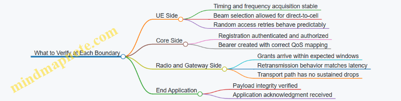
This flow is intentionally linear: initial access, registration, bearer creation, uplink transfer, downlink delivery, and confirmation. When you test it, treat each boundary as a gate with its own success criteria, so failures are localized instead of guessed.
5. Radio Resource Management for Satellite Access Links
5.1 Resource Allocation Principles for Shared Satellite Spectrum
Shared satellite spectrum means multiple users and services must share the same radio resources without stepping on each other. The core job of resource allocation is to decide who transmits, when they transmit, and at what rate, while keeping interference under control and meeting service requirements. Think of it as traffic control on a single-lane bridge: you can let more cars through only if you manage spacing, speed, and lane discipline.
Foundational Concepts for Shared Spectrum
Start with three constraints that shape every decision.
- Interference is the limiting factor. In direct-to-cell satellite access, users in the same beam and frequency region can interfere. Allocation must reduce overlap in time, frequency, or power.
- Propagation and scheduling latency matter. Round-trip time is longer than in terrestrial networks, so the system benefits from allocations that remain valid for a scheduling window.
- User demand is uneven. Some users send small messages; others stream data. Allocation must avoid wasting capacity on low-need users while still serving them reliably.
A practical way to reason about allocation is to separate resource dimensions (time, frequency, code, power) from goals (throughput, latency, fairness, reliability). Each allocation policy chooses a trade-off.
Resource Dimensions and What They Control
- Time division (slotting): Limits how many users transmit simultaneously. It is simple and effective when interference dominates.
- Frequency division (subcarriers or channels): Reduces interference by separating users across frequency. It works well when channel conditions differ across users.
- Code division (if applicable): Uses different spreading or coding structures. It can improve spectral efficiency but increases receiver complexity.
- Power control: Adjusts transmit power to meet link quality while limiting interference. It is often constrained by terminal capability and regulatory limits.
In practice, systems combine these dimensions. For example, a scheduler may assign a time slot and frequency block, then apply power control within that assignment.
Mind Map: Allocation Building Blocks
Allocation Inputs That Actually Matter
Resource allocation is only as good as its inputs. For direct-to-cell, the most useful inputs are:
- Queue state: How much data is waiting per user and per service class.
- Channel quality indicators: A proxy for expected SINR on candidate resources.
- Geometry and beam context: Users near beam edges often have worse link quality and different interference patterns.
- Service requirements: Latency tolerance and reliability targets determine whether the scheduler should spend resources on robust settings or higher rates.
A common mistake is to allocate purely on instantaneous channel quality. That can starve users with consistently poor conditions. A good scheduler uses channel quality but also accounts for waiting time and service class.
Core Principles for Systematic Allocation
Start with Interference Management
The first principle is to limit harmful overlap. If two users are likely to interfere strongly, the scheduler should avoid assigning them the same time-frequency region. This can be done through:
- Orthogonalization: Separate users in time or frequency when their interference coupling is high.
- Reuse planning: Use frequency reuse patterns across beams so that co-channel beams are sufficiently separated.
Match Modulation and Coding to the Assignment
Once a time-frequency region is chosen, select the modulation and coding scheme (MCS) based on expected SINR. The scheduler should prefer robust MCS for users with uncertain or low SINR, especially for latency-sensitive messaging.
Example: If User A reports stable SINR and User B reports fluctuating SINR, the scheduler can assign both the same time slot but choose different MCS levels. User B gets a lower rate with higher reliability, preventing repeated retransmissions that would otherwise consume shared resources.
Use Fairness That Respects Service Classes
Fairness should not mean “everyone gets the same.” Instead, fairness should be service-aware:
- For best-effort data, proportional fairness can balance throughput and waiting time.
- For urgent messages, priority scheduling can reserve a small fraction of resources.
A practical rule: allocate a baseline share to each active user or service class, then distribute remaining capacity based on channel quality and backlog.
Keep Scheduling Decisions Stable over the Validity Window
Because of longer propagation, the scheduler should avoid overly fine-grained decisions that become stale before they take effect. Use a scheduling window where channel estimates remain meaningful, and keep grant sizes aligned with expected traffic bursts.
Example: For periodic status updates, allocate recurring resources or semi-static grants. For sporadic traffic, use dynamic grants but keep them within a window that matches the system’s measurement-to-transmission timing.
Worked Example: Simple Beam Scheduler
Assume one beam with 12 resource blocks (RBs) per frame and three users:
- User 1: high SINR, large backlog, best-effort
- User 2: medium SINR, small backlog, best-effort
- User 3: low SINR, urgent message, latency sensitive
A systematic allocation could be:
- Reserve 2 RBs for User 3 using robust MCS to meet latency.
- Allocate the remaining 10 RBs using proportional fairness between Users 1 and 2.
- Apply higher MCS to User 1 and a more conservative MCS to User 2.
Result: User 3 gets predictable delivery without forcing repeated retransmissions that would reduce overall throughput. Users 1 and 2 share the rest based on backlog and channel quality, so neither user is ignored.
Practical Checklist for Implementing Allocation
- Identify interference-prone user pairs and avoid co-channel overlap.
- Reserve a small, reliable resource slice for latency-sensitive traffic.
- Choose MCS per assignment using expected SINR, not optimism.
- Combine fairness with service class so waiting time is handled intentionally.
- Ensure grants remain valid for the scheduling window given measurement timing.
5.2 Beam Management and Coverage Partitioning for Mobile Users
Beam management is the practical art of deciding which users share which satellite resources, and when. Coverage partitioning is the planning side of that art: how the service area is split into manageable regions that align with beams, scheduling, and terminal behavior. Together, they keep link quality predictable enough to run a network without constant firefighting.
Foundational Concepts for Partitioning
Start with three inputs: user distribution, beam footprint geometry, and link budget margins. User distribution can be uneven even within a small area, such as a roadside corridor or a stadium. Beam footprints overlap, and overlap is not a bug; it is a tool for continuity. Link budget margins determine how much overlap you can afford before edge users become unreliable.
A useful mental model is to treat each beam as a “resource container” with a coverage region and a capacity budget. Partitioning assigns users to containers based on where they are likely to be during the next scheduling interval.
Coverage Partitioning Strategies
Single-beam assignment assigns each user to one beam at a time. It is simple and reduces cross-beam complexity, but it can cause abrupt changes near beam edges.
Multi-beam assignment allows a user to be served by more than one beam, either simultaneously or in a make-before-break sequence. This improves continuity but increases coordination needs and can raise interference or resource duplication if not controlled.
Overlapping-region partitioning explicitly defines overlap zones where the network expects handover activity. Instead of reacting only after quality drops, you predefine where decisions should occur.
A practical rule: choose partition boundaries so that the expected signal quality stays above the minimum threshold for at least one scheduling cycle after a boundary crossing. That prevents “ping-pong” behavior where a user flips beams every few seconds.
Beam Management Control Loop
Beam management typically runs as a loop:
- Measure: the terminal reports reference signal quality and timing-related measurements.
- Classify: the network maps measurements to candidate beams and determines whether the current beam remains acceptable.
- Decide: the network selects the serving beam(s) and updates scheduling grants.
- Execute: the radio layer applies the change with timing and buffering rules.
The key detail is that measurement-to-decision latency must be accounted for. If the terminal reports quality that is already outdated, the network may assign a user to a beam that is no longer the best choice.
Handover-Friendly Partition Boundaries
Partition boundaries should be defined using quality margins, not just geometry. Geometry tells you where beams overlap; quality tells you how usable that overlap is.
To make this concrete, consider a highway scenario. If the terminal moves quickly along the corridor, the network should use wider overlap zones along the corridor direction and narrower zones elsewhere. That reduces the number of handovers while keeping edge users above the minimum modulation and coding capability.
Scheduling Implications of Partitioning
Once users are assigned to beams, scheduling can be beam-local. Beam-local scheduling reduces coordination overhead and makes capacity planning easier. However, it can create unfairness if one beam becomes crowded while adjacent beams are underutilized.
A common mitigation is load-aware beam selection: when multiple beams are acceptable, the network prefers the beam with more available resource blocks. This is not about “fairness for its own sake”; it directly reduces packet delay and retransmissions.
Mind Map: Beam Management and Coverage Partitioning
Example: Partitioning for a Mixed Urban Corridor
Assume a satellite system with three overlapping beams covering an urban corridor and surrounding blocks. The corridor has higher user density because of offices and transit stops.
A workable partition plan:
- Define overlap zones primarily along the corridor direction.
- Use single-beam assignment in the outer blocks where density is low.
- Use multi-beam make-before-break only inside the corridor overlap zones to smooth transitions at beam edges.
Operationally, the network keeps a user on the current beam until the reported quality drops below a threshold that accounts for measurement latency. If two beams are both acceptable, it selects the beam with lower load to reduce queue buildup. The result is fewer handovers during stop-and-go movement and more stable throughput when users cluster near transit hubs.
Example: Avoiding Ping-Pong at Beam Edges
Ping-pong happens when a user repeatedly crosses a boundary faster than the system can settle. The fix is to combine three controls:
- Hysteresis: require a quality improvement before switching back.
- Time-to-trigger: wait a short duration before executing the change.
- Boundary placement: ensure the overlap zone covers the expected movement during the measurement-to-decision delay.
If you implement only hysteresis, a fast-moving terminal can still trigger repeated switches. If you implement only time-to-trigger, a slow terminal may stay on a degrading beam too long. Using all three makes the behavior stable and predictable, which is exactly what mobile users notice when they stop thinking about beams and start thinking about their app working.
5.3 Scheduling and Grant Strategies Under Variable Propagation Conditions
Direct to cell scheduling has a simple enemy: the radio channel changes while you’re trying to decide who transmits. In NTN, that change is driven by geometry (satellite motion), atmosphere, and beam edge effects. The scheduler’s job is to turn those variations into predictable service by combining three ideas: measure channel state, choose a grant that fits the moment, and adapt retransmissions when the moment was unlucky.
Foundational Inputs the Scheduler Needs
A practical scheduler starts with a small set of per-user measurements and constraints:
- Channel quality indicators such as SINR or an equivalent metric derived from reference signals.
- Timing and frequency uncertainty indicators, since Doppler and offset can reduce effective demodulation quality.
- Queue state for each logical flow, including how long packets have waited.
- Terminal capability such as maximum modulation and coding supported, and whether the terminal can handle higher HARQ rounds.
- Resource limits including available bandwidth per beam and any configured priority rules.
A useful mental model is to treat each grant as a bet: the scheduler chooses modulation/coding and allocation size based on what it believes the channel will support for that user during the grant’s effective time window.
Variable Propagation and Why It Breaks Naive Scheduling
If you schedule purely by “best current SINR,” you can starve users near beam edges. If you schedule purely by fairness, you may waste resources on low-probability decodes. Variable propagation creates both problems at once because the ranking of users changes quickly.
So the scheduler needs a policy that balances:
- Throughput efficiency (use resources where decoding is likely)
- Reliability (avoid repeated failures that burn HARQ budget)
- Fairness (prevent persistent disadvantage for edge users)
- Latency (avoid letting small packets wait behind large ones)
Grant Strategy: Choose Size, MCS, and Retransmission Behavior Together
A grant is more than “who gets time.” It includes how aggressively you transmit.
- Initial transmission aggressiveness: pick modulation and coding based on the user’s estimated channel quality.
- Grant size: allocate enough symbols to carry the payload without forcing excessive segmentation when the channel is poor.
- HARQ coupling: if the system supports HARQ, the scheduler should reserve or prioritize resources for retransmissions so that failures don’t cascade into queue growth.
A simple rule that works well in practice: when propagation conditions worsen, reduce the payload per grant rather than only lowering MCS. Smaller payloads shorten the time the receiver needs to accumulate enough reliable information, which helps keep latency stable.
Scheduling Policy Under Changing Conditions
A common approach is to compute a priority score per user each scheduling interval. The score can combine:
- Expected spectral efficiency from the channel estimate
- Probability of successful decode for the chosen MCS
- Head-of-line delay for queued packets
- Service class weight (for example, messaging vs. bulk data)
Then the scheduler allocates resources to maximize a weighted objective. The key is that the “expected decode probability” must be tied to the propagation state, not just the raw SINR.
Beam-Aware and Time-Aware Allocation
Because direct to cell uses beams, treat the scheduler as having two layers:
- Beam layer: decide how much total resource each beam gets.
- User layer: within a beam, decide which users get grants.
Time awareness matters because the channel estimate is only valid for a short interval. If the scheduler’s interval is long relative to channel variation, it should be more conservative: use lower MCS and smaller grants to reduce the chance of HARQ-heavy outcomes.
Example: Two Users at Different Beam Positions
Assume one beam with 10 ms scheduling intervals. User A is near beam center, user B near the edge.
- At interval 1, A estimates SINR high enough for MCS 12 with high decode probability. B estimates low SINR; MCS 6 would decode with moderate probability.
- A naive “best SINR first” scheduler gives most resources to A. B’s small packets wait.
- A balanced scheduler computes priority including head-of-line delay. It gives B a smaller grant using MCS 6, enough to carry one message segment.
In interval 2, geometry shifts slightly and B’s SINR improves. The scheduler then increases B’s grant size and MCS, while A’s priority drops because its queue is already served. The result is that B experiences fewer long waits without forcing the system into repeated retransmissions.
Mind Map: Scheduling and Grants Under Variable Propagation
Practical Checklist for Robust Scheduling
- Update channel-based priority frequently enough that grants match the estimate’s validity window.
- Tie MCS selection to decode probability, not just SINR ranking.
- When conditions degrade, prefer smaller payload grants plus lower MCS rather than only lowering MCS.
- Ensure retransmissions have a clear resource path so failures don’t turn into unbounded latency.
- Use beam-aware allocation so edge users are not permanently disadvantaged by center-heavy scheduling.
With these pieces aligned, the scheduler behaves like a careful dispatcher: it doesn’t try to guess the future perfectly, but it does make decisions that remain sensible when the channel refuses to stay still.
5.4 Handling Contention and Congestion in Direct to Cell Scenarios
Direct to Cell links share spectrum across many users and beams, so contention shows up as collisions, retransmissions, and queue buildup. Congestion shows up when the system can’t drain buffers fast enough, even if individual transmissions are “correct.” The practical goal is to keep the system stable: reduce wasted airtime, protect latency-sensitive traffic, and prevent buffer growth from turning into a reliability problem.
Core Concepts That Drive Contention
Contention begins at the moment multiple UEs try to transmit in overlapping resources. In a satellite direct-to-cell setting, the round-trip time is longer than in terrestrial networks, so feedback arrives later and retransmissions cost more airtime. Congestion then compounds the issue: if scheduling keeps granting resources to already-backlogged flows, the backlog grows and the channel spends more time on retries than on new successful deliveries.
A useful mental model is “airtime accounting.” Every failed attempt consumes airtime and increases waiting time for everyone else. If the scheduler keeps trying the same approach under load, the system becomes self-defeating.
Mind Map: Contention and Congestion Control Loop
Stepwise Strategy from Foundations to Advanced Details
1) Measure Load Where It Matters
Start by distinguishing “many users with little traffic” from “few users with heavy traffic.” Use beam-level load indicators (active UE count, grant utilization, retransmission rate) and queue indicators (pending bytes per bearer, HARQ occupancy). If you only look at throughput, you may miss rising latency caused by retries.
Easy example: In a beam where average SINR looks acceptable, but retransmissions jump from 5% to 25%, the system is already spending airtime on recovery. Throughput might still look okay for a moment, but latency will climb and congestion will follow.
2) Control Contention at the Entry Point
Random access and initial transmissions are where collisions are most expensive. Use contention-aware backoff so that when the system detects high collision probability, new attempts spread out instead of synchronizing.
Easy example: Suppose 200 UEs attempt to send a short status message after a power restoration event. Without tuned backoff, they pick similar timing windows and collide repeatedly. With adaptive backoff, the same 200 UEs spread their attempts across more frames, reducing collisions and lowering total airtime wasted.
3) Make Scheduling Load-Aware, Not Just Fair
Fairness alone can be harmful under congestion. If every UE gets a small slice, none of the slices are large enough to clear queues, especially for users at the edge of coverage. A better approach is “priority-aware fairness”: protect latency-sensitive flows while granting enough resources to clear at least some backlog per scheduling interval.
Concrete rule of thumb: if retransmission rate is rising, temporarily bias grants toward users with stable link quality and toward flows that can complete quickly. This increases successful deliveries per unit airtime and reduces the retry pile.
4) Use Link Adaptation to Prevent Retry Spirals
When link quality is variable, aggressive modulation and coding can increase error probability, which increases retransmissions, which increases congestion. Under load, choose a more conservative operating point so that the system spends less airtime on failed attempts.
Easy example: Two UEs have similar average SNR, but one has frequent fades due to movement. If both are scheduled with the same high-rate configuration, the moving UE triggers more HARQ failures. Reducing its rate slightly can improve overall beam efficiency because it stops generating repeated failures.
5) Bound Queues with Admission and Shaping
Congestion management is partly about preventing infinite waiting. Apply admission control for non-critical traffic and shape or cap per-flow queues so that one heavy sender can’t consume all scheduling opportunities.
Easy example: If background telemetry is allowed to queue indefinitely, it can occupy buffer space and delay emergency messaging. A simple per-bearer quota ensures that emergency traffic always has room to be scheduled and transmitted.
6) Manage Retransmissions with Practical Limits
HARQ can help, but it can also saturate. If too many retransmissions are pending, the scheduler keeps serving “old” packets while new packets wait. Use limits such as maximum retransmission attempts and fallback behavior that either reduces rate or switches to a more robust configuration.
Easy example: For short messages, after a small number of failed attempts, switching to a more robust configuration can be better than repeating the same configuration. The goal is to avoid spending multiple frames on a packet that is unlikely to succeed.
Example: A Beam Under Sudden Load
Assume a beam receives a burst of 1,000 short messages over a few seconds. The system observes rising grant utilization, increasing retransmissions, and growing UE queues.
- Collision control: increase contention backoff for new access attempts.
- Scheduling: prioritize flows that can complete quickly and reserve resources for priority messaging.
- Link adaptation: reduce MCS for users with unstable measurements to lower error probability.
- Queue management: cap background traffic queues and admit only a limited number of new background flows.
- Retransmission limits: after a small number of failures, switch to a more robust configuration.
The expected outcome is not “maximum throughput at any cost,” but stable delivery: fewer retries, bounded latency for priority traffic, and queues that stop growing.
Quick Checklist for Operators and Engineers
- Track collision rate, retransmission rate, and queue growth separately.
- Tune contention backoff when collision probability rises.
- Use priority-aware fairness so edge users don’t starve, but the system also doesn’t stall.
- Choose conservative link adaptation under high load to avoid retry spirals.
- Bound queues with admission control and per-flow quotas.
- Apply retransmission limits with fallback behavior.
5.5 Practical Example: Designing a Resource Plan for a Given Coverage Footprint
You’re given a direct to cell coverage footprint shaped like an irregular polygon on the ground, plus a target service mix: small messages for IoT-like users and occasional larger data bursts for field staff. The goal of a resource plan is simple to state and tricky to execute: allocate radio resources so that most users meet their latency and reliability needs while the system stays stable when users cluster.
Step 1: Translate Coverage into Beam and Cell Geometry
Start by converting the ground footprint into the satellite’s beam layout. For each beam, compute which portion of the footprint it covers and how the beam edge affects link quality. A practical rule is to treat the beam edge as a “quality gradient” zone rather than a hard boundary.
Example: Suppose the footprint spans three beams: Beam A covers 45%, Beam B covers 40%, Beam C covers 15%. If Beam C is mostly edge-of-beam, assume its effective throughput is lower even if the geometry says it covers users. You’ll reflect that later in scheduling weights.
Step 2: Define Traffic Classes and Their Resource Demands
Create traffic classes with clear radio implications. For instance:
- Class M: small messages, strict latency, low payload.
- Class D: data bursts, moderate latency, higher payload.
- Class S: signaling and keep-alives, very small payload, frequent.
Assign each class a target performance profile: maximum acceptable delay, minimum reliability, and typical packet size. Then translate those into required link adaptation margin. If Class M must succeed quickly, it needs more robust modulation and coding or more retransmission budget.
Step 3: Choose a Scheduling Strategy That Matches the Footprint
Resource planning depends on how you share resources among users within a beam. A common approach is time-frequency scheduling with per-user grants, but you must decide how to handle contention.
A workable baseline:
- Reserve a small fraction of resources for Class S so control traffic doesn’t get stuck behind user data.
- Use priority-aware scheduling for Class M to protect latency.
- Allow Class D to use remaining capacity with a cap on how much it can consume per scheduling interval.
Example: If the beam has 100 resource units per frame, allocate 10 units to Class S, 50 to Class M, and 40 to Class D. If Class M demand drops, unused units can be borrowed by Class D, but only up to a defined limit to prevent starvation.
Step 4: Build a Link Quality Map and Convert It to Weights
For each beam, estimate expected signal quality distribution across the footprint. Use a link-quality metric such as expected SINR bins. Then convert those bins into scheduling weights.
Example: In Beam B, assume 60% of users are in a “good” bin, 30% in “fair,” and 10% in “edge.” If edge users require roughly 2× more robust coding to meet reliability, you can reflect that by giving edge users a larger share of grants per successful message attempt. The exact factor comes from your link adaptation curves, but the planning method stays the same.
Step 5: Apply a Load Model and Check Stability
Now combine geometry, traffic demand, and weights into a load estimate per beam. You’re checking whether the system can serve the offered load without persistent queue growth.
A simple stability check:
- For each class, compute expected resource consumption per user per interval.
- Multiply by expected active users in each quality bin.
- Sum across bins and classes.
- Ensure the total expected consumption stays below available resources, with headroom for variability.
Example: Beam A has 200 active users, mostly in good quality. Beam C has 60 active users but mostly edge quality. Even with fewer users, Beam C may consume more resources per successful delivery, so you might increase its reserved share or reduce its Class D cap.
Step 6: Produce the Resource Allocation Plan
The output should be operational, not theoretical: per beam, per class, per quality bin. Keep it explicit so you can test it.
Example Resource Plan Table (illustrative numbers):
| Beam | Class S Reserve | Class M Share | Class D Share | Class D Cap | Edge Weight Effect |
|---|---|---|---|---|---|
| A | 10% | 50% | 40% | 30% | baseline |
| B | 10% | 55% | 35% | 25% | moderate reduction |
| C | 12% | 60% | 28% | 15% | strong robustness factor |
Interpretation: Beam C gets a slightly higher signaling reserve and a larger share for latency-sensitive messages, while Class D is constrained to prevent edge users from being overwhelmed.
Step 7: Validate with Two Concrete Scenarios
Scenario 1: Uniform user distribution across the footprint.
- Expect Beam A and B to carry most Class D.
- Confirm Class M meets delay targets without excessive retransmissions.
Scenario 2: Clustered users in the beam edge zone.
- Expect increased resource use in edge bins.
- Confirm the plan’s caps prevent queue buildup for Class M and signaling.
If either scenario fails, adjust one lever at a time: class shares first, then borrowing rules, then quality-bin weights. This keeps the debugging process sane—like using a map instead of guessing which way “feels right.”
6. Link Layer Protocols and Error Control for Space Based Connectivity
6.1 Physical Layer to MAC Layer Responsibilities in Satellite Links
Satellite links behave like a long, moving hallway: signals travel far, arrive late, and shift in frequency as the spacecraft moves. Because of that, the physical layer and MAC layer must cooperate tightly, with each layer owning specific jobs and exposing the right knobs to the next layer.
Physical Layer Responsibilities
The physical layer turns bits into radio wave behavior and back again. In satellite direct-to-cell links, its responsibilities include:
- Modulation and Demodulation: Choose a modulation scheme that matches the expected signal quality. For example, if the link margin is tight, the system may use a more robust modulation so the receiver can still recover symbols.
- Forward Error Correction: Apply coding that can correct errors without waiting for retransmissions. A practical example is using a code rate that trades throughput for reliability when the channel is harsh.
- Channel Estimation and Equalization: Estimate how the channel distorts the signal. In satellite links, this includes coping with time-varying effects caused by motion and propagation.
- Timing and Frequency Recovery: Estimate and correct timing offset and carrier frequency offset. Doppler causes frequency drift, so the receiver must track it continuously.
- Power and Beam Awareness Hooks: Provide measurements such as received signal strength, error vector magnitude, or block error indicators. These metrics become inputs to MAC decisions.
A useful way to think about the physical layer is: it produces reliable “deliverability signals”. Not just bits, but also quality indicators that tell MAC whether it should schedule more aggressively, back off, or request retransmission.
MAC Layer Responsibilities
The MAC layer decides who transmits, when they transmit, and how transmissions are packaged for the physical layer. In satellite links, its responsibilities include:
- Channel Access and Scheduling: Coordinate multiple users sharing the same satellite resources. For a simple example, if two users transmit simultaneously in the same time-frequency slot, their signals collide; MAC prevents that by assigning distinct resources.
- Transport Unit Framing: Map higher-layer packets into MAC transport blocks sized for the physical layer. This includes respecting constraints like maximum payload size and coding block structure.
- Link Adaptation Control: Select modulation and coding parameters based on physical-layer feedback. Example: if the receiver reports rising block error rates, MAC can request a more robust configuration.
- Retransmission Strategy: Manage retransmissions when errors remain after coding. Because satellite round-trip time is long, MAC must avoid overly chatty retransmission loops.
- HARQ Coordination: Coordinate hybrid automatic repeat request behavior, including what constitutes an acknowledgment, negative acknowledgment, or implicit success.
- Buffering and Queueing: Handle variable arrival rates from the core network and variable service opportunities due to scheduling.
In short, MAC owns resource discipline. It keeps the shared channel from turning into a group project where everyone talks at once.
The Handoff Between Physical and MAC
The boundary between layers is where most practical bugs live, so it helps to be explicit about the interface:
- Physical Layer → MAC: Quality and outcome metrics.
- Example metrics: block success/failure, estimated SNR, timing error magnitude, and frequency offset estimates.
- MAC → Physical Layer: Transmission configuration and transport block parameters.
- Example parameters: modulation and coding selection, transmit power targets, and transport block size.
A systematic workflow for one transmission opportunity looks like this:
- MAC schedules a user and chooses a transport block size.
- MAC requests a physical-layer configuration (modulation/coding) consistent with expected channel quality.
- The physical layer transmits and later reports whether blocks were decoded successfully.
- MAC uses the outcome to update scheduling priorities and decide whether to retransmit.
Mind Map: Physical to MAC Responsibilities
Example: Scheduling with Physical Feedback
Assume a direct-to-cell system assigns a user a downlink slot. The physical layer decodes the received transport block and reports a block error indicator plus an estimated quality metric.
- If decoding succeeds consistently, MAC can schedule the user more frequently or allocate larger transport blocks.
- If decoding fails intermittently, MAC can reduce transport block size and request a more robust modulation/coding configuration.
- If failures persist, MAC can trigger retransmission behavior while also lowering the user’s priority to protect overall throughput.
This example shows why both layers must be precise: physical-layer metrics must be trustworthy enough for MAC to act, and MAC must translate those actions into valid physical-layer configurations.
Example: Why Retransmission Timing Matters
Satellite round-trip time is long, so MAC cannot treat retransmissions like a fast local link. If MAC retransmits too aggressively, it can waste resources on transmissions that would have succeeded with a slightly different physical configuration. If it retransmits too conservatively, queues build up and latency grows. The practical balance comes from physical-layer feedback: MAC uses decoding outcomes and quality trends to decide whether to retransmit, adapt, or reschedule.
6.2 HARQ Concepts and Retransmission Behavior Under Latency Constraints
HARQ—Hybrid Automatic Repeat reQuest—combines forward error correction with selective retransmissions. In direct-to-cell satellite links, the “hybrid” part matters because you often have enough redundancy to recover many corrupted packets immediately, but not all of them. The “repeat” part matters because retransmissions are expensive when round-trip time is long.
Core Idea of HARQ in One Pass
A typical HARQ flow sends a transport block (TB) with coding redundancy. The receiver attempts decoding right away. If decoding succeeds, it sends an acknowledgment. If decoding fails, it requests retransmission, usually using incremental redundancy so the second transmission adds useful information rather than repeating the same bits.
The key design tension is simple: retransmissions improve reliability, but they consume time and radio resources. Under satellite latency, waiting for a negative acknowledgment can stall the pipeline, so the system must be careful about when it decides to retransmit and how many times it does.
Timing Constraints That Shape Retransmission
In terrestrial systems, HARQ can often react quickly enough to keep the scheduler busy. In satellite direct-to-cell scenarios, the feedback loop is slower. That means:
- The transmitter may have already scheduled subsequent transmissions before it knows whether earlier ones succeeded.
- The receiver’s feedback arrives late, so the transmitter must buffer state for multiple in-flight HARQ processes.
- Retransmission decisions must be made with limited knowledge of what will succeed, so the protocol relies on explicit feedback and strict process identifiers.
A practical consequence is that HARQ behaves like a pipeline with multiple “slots.” Each slot corresponds to a HARQ process, and each process tracks redundancy versions, acknowledgments, and whether the maximum number of attempts has been reached.
HARQ Process Structure and Redundancy Versions
HARQ processes prevent confusion when multiple packets are in flight. Each process is associated with a specific transport block and a sequence of redundancy versions (RVs). A common pattern is:
- Send RV0.
- If decoding fails, send RV1 or RV2 that reuses the same code structure but with different parity contributions.
- Continue until success or until the attempt limit is reached.
Incremental redundancy is efficient because the second transmission is not wasted even if the first attempt failed. It also reduces the probability that a retransmission is “all or nothing” compared to repeating identical bits.
A Mind Map of HARQ Behavior Under Latency
Mind Map: HARQ Concepts and Retransmission Behavior
Retransmission Outcomes and Their System-Level Effects
When HARQ succeeds on the first attempt, latency is minimal and radio resources are used efficiently. When it succeeds after one or more retransmissions, latency increases roughly by the feedback and retransmission timing, and the scheduler must allocate additional grants.
If decoding fails after the maximum number of attempts, the transport block is dropped. The higher layers then decide what to do next—often by retransmitting at a different layer or by accepting loss for certain message types. This separation is important: HARQ is tuned for radio reliability, while upper layers handle end-to-end delivery semantics.
Example: Messaging with Tight Latency Budget
Assume a messaging service where each user message should be delivered quickly, but occasional loss is acceptable only if it doesn’t cause long waits.
- The system configures HARQ with a small attempt limit to avoid long stalls.
- The receiver uses decoding results to send feedback as soon as possible.
- The transmitter schedules new transmissions in other HARQ processes while waiting for feedback.
Concrete behavior:
- If the first transmission decodes successfully, the message is delivered with one transmission grant.
- If it fails, the message is delivered after a retransmission grant, but only for the affected HARQ process.
- If it fails repeatedly until the attempt limit, the message is dropped at the radio layer, and the application layer can decide whether to retry immediately or report failure.
This setup prevents a single bad link moment from locking the entire scheduling pipeline.
Example: Incremental Redundancy vs Repetition
Consider two strategies for a failed TB:
- Repetition: retransmit the exact same coded bits.
- Incremental redundancy: retransmit additional parity that complements the first attempt.
With incremental redundancy, the receiver’s second decoding attempt has more independent information, so the probability of success increases more smoothly. With repetition, the receiver may gain less new information, which can lead to either quick success or repeated failure depending on the channel realization.
In latency-constrained satellite links, incremental redundancy is usually the more predictable choice because it maximizes the value of each retransmission grant.
Practical Design Rules for Latency-Constrained HARQ
- Keep the number of HARQ attempts bounded so NACK storms do not dominate time.
- Use multiple HARQ processes to maintain a pipeline even when feedback is delayed.
- Prefer incremental redundancy so each retransmission has measurable decoding benefit.
- Ensure strict process identification so ACK/NACK feedback updates the correct transport block.
- Align HARQ behavior with upper-layer expectations so dropped TBs do not cause silent, long delays.
When these rules are followed, HARQ becomes a controlled trade: it improves reliability without turning latency into a hostage situation.
6.3 RLC and PDCP Functions Including Segmentation and Reordering
RLC and PDCP sit between the radio bearer and the IP layer, translating “what the radio can deliver” into “what higher layers expect.” In direct-to-cell satellite links, the translation has to handle two realities at once: variable delay and occasional out-of-order delivery caused by propagation changes and scheduling.
Foundational Roles of RLC and PDCP
PDCP (Packet Data Convergence Protocol) focuses on functions that are mostly independent of the exact radio scheduling, such as header compression, ciphering, and sequence-number-based delivery control. RLC (Radio Link Control) focuses on reliable transfer over a bearer, including segmentation, reassembly, and retransmission behavior.
A useful mental model: PDCP is the “session-aware translator,” while RLC is the “radio-aware courier.” PDCP assigns sequence numbers to PDUs so the receiver can place them in order. RLC then breaks large PDUs into smaller pieces that fit the transport blocks and reassembles them at the receiver.
Segmentation: Making Big Packets Fit Small Radio Pieces
Segmentation happens when a PDCP PDU is larger than what the MAC can carry in a single transmission. RLC splits the payload into multiple RLC data segments, each mapped to a radio transmission opportunity.
Key detail: segmentation is not just slicing bytes. RLC must preserve enough information to reassemble the original PDCP PDU correctly. That means each segment carries identifiers and offsets so the receiver can reconstruct the exact byte sequence.
Example: Suppose PDCP produces a 1200-byte PDU, but the radio can carry 400 bytes per transmission. RLC segments it into three parts: 400 + 400 + 400. If the second segment arrives first, the receiver buffers it until the first and third segments arrive, then reassembles the full 1200-byte unit.
In satellite NTN, segmentation also interacts with latency. More segments mean more opportunities for scheduling delays and more buffering at the receiver. That’s why RLC configuration should align with expected transport block sizes and typical scheduling granularity.
Reordering: Putting Pieces Back in the Right Sequence
Reordering occurs when segments or PDCP PDUs arrive out of order. This can happen when different transmissions experience different effective delays, or when retransmissions are scheduled later than the original attempt.
RLC reordering is primarily about reassembling segments into the correct PDCP PDU. PDCP reordering is about ordering PDCP PDUs for delivery to upper layers.
Example: Two PDCP PDUs, A and B, are sent in sequence. Due to link dynamics, B’s segments arrive before A’s. PDCP uses sequence numbers to hold B until A is available, ensuring the application sees A then B.
This “hold until missing data arrives” is not free. It trades ordering correctness for buffering and potential delay. In practice, the system uses timers and thresholds to decide when to release what it has.
How RLC and PDCP Work Together
RLC and PDCP coordinate through sequence numbering boundaries. PDCP sequence numbers identify PDCP PDUs. RLC segmentation identifiers identify how a PDCP PDU is split across radio transmissions.
When RLC reassembles a complete PDCP PDU, it passes it upward to PDCP. PDCP then decides whether it can deliver it immediately or must wait for earlier sequence numbers.
The result is a two-stage pipeline:
- RLC stage: ensure bytes for each PDCP PDU are complete and correctly ordered within that PDU.
- PDCP stage: ensure PDCP PDUs are delivered to upper layers in sequence.
Mind Map: Segmentation and Reordering Flow
Practical Walkthrough with a Timing Twist
Consider a direct-to-cell scenario where the UE transmits two PDCP PDUs, A then B. RLC segments each PDCP PDU into multiple radio-sized pieces.
- Transmit: RLC sends A1, A2, A3 and then B1, B2, B3.
- Receive: Due to scheduling and propagation changes, B2 arrives early.
- RLC action: RLC buffers B2 until B1 and B3 (or the missing parts) arrive, then reassembles B.
- PDCP action: PDCP sees that A is still incomplete or not yet delivered, so it holds B until A is ready.
- Release: Once A is reassembled and delivered in order, PDCP releases A then B to the upper layer.
This sequence shows why segmentation and reordering must be treated as a coordinated system. RLC can be “perfect” at reassembly while PDCP still delays delivery to preserve ordering.
Configuration Implications for Satellite NTN Links
Segmentation granularity affects buffering pressure at the receiver. Reordering behavior affects how long PDCP waits for missing sequence numbers. Together, these choices influence user-perceived latency and reliability.
A practical rule of thumb: if your link frequently produces out-of-order arrivals, you should expect PDCP buffering to matter more than raw retransmission counts. If your transport block sizes are small relative to typical PDCP PDU sizes, segmentation overhead and reassembly delay will dominate.
In short, RLC and PDCP turn an imperfect radio delivery pattern into a consistent byte stream for applications—by splitting large units, reassembling them correctly, and enforcing delivery order with sequence numbers.
6.4 Packet Loss and Out of Order Delivery Handling Strategies
Packet loss and out of order delivery are normal side effects of satellite access links: propagation delay is large, retransmissions take time, and mobility plus Doppler can cause occasional decoding failures. The goal is not to “avoid” loss entirely, but to handle it predictably so upper layers see stable service behavior.
Foundational View of What Goes Wrong
At the receiver, a packet can be lost for several reasons: the radio frame fails decoding, the MAC grant is missed, or the link layer discards due to buffer limits. Out of order delivery happens when later packets arrive successfully while earlier ones are delayed or retransmitted. In direct-to-cell scenarios, this is especially noticeable during beam edge transitions or when the terminal’s timing and frequency estimates briefly drift.
A practical way to reason about this is to separate three layers of responsibility:
- Radio and link reliability: decide whether to retransmit and how many times.
- In-order delivery mechanisms: decide whether to reorder or tolerate gaps.
- End-to-end transport behavior: decide how to react to missing data.
Mind Map: Packet Loss and Out of Order Handling
Link Layer Tactics for Loss
HARQ behavior is the first line of defense. When a transport block fails CRC, the receiver sends a negative acknowledgment (or equivalent status) and the transmitter schedules a retransmission. The key is to treat HARQ as a bounded reliability mechanism: too many retries waste time and can worsen perceived latency.
A concrete example: suppose a messaging packet is segmented into two transport blocks. The first block fails CRC, the second succeeds. With HARQ, only the failed block is retransmitted. If the receiver’s reassembly waits for the missing block, the message delivery is delayed but still correct. If the system instead delivers partial data immediately, the application might see corrupted or incomplete content. So the link layer should align with the segmentation model used by the higher layers.
Duplicate handling matters because retransmissions can arrive after the original packet was already accepted by the receiver. Sequence numbers and HARQ process identifiers allow the receiver to recognize duplicates and discard them without confusing reordering logic.
Reordering Strategies for Out of Order Delivery
Out of order delivery is best handled with a small reordering buffer and a clear policy for when to release data.
A typical policy:
- Maintain an expected sequence number.
- Store successfully received packets that are ahead of the expected number.
- When the missing packet arrives, release the contiguous run.
- If the buffer fills or a timer expires, release what you have and mark gaps.
Example: packets 10, 11, 13 arrive, but 12 is lost. The receiver buffers 13 while waiting for 12. If 12 is recovered via retransmission, packets 10–13 are released in order. If 12 never arrives within the timer window, the receiver releases 10–11 and then 13 with a gap indication so upper layers can decide whether to request retransmission or tolerate the loss.
This is where “gap-tolerant” behavior becomes important. For some services, missing data can be handled by higher layers using their own retransmission or error recovery. For others, the link layer must ensure completeness before delivery.
Coordinating with Segmentation and Reassembly
Satellite links often use segmentation to fit payloads into radio transport blocks. That means a single application packet may map to multiple link-layer units. If one segment is lost, reassembly cannot complete.
A systematic approach is:
- Use sequence numbers at the segment level so the receiver can detect missing segments.
- Use reassembly timers that match the expected round-trip time plus scheduling variability.
- Apply discard rules when reassembly buffers overflow, so stale partial data does not block newer traffic.
Example: an application message is split into segments A, B, C. A and C arrive, B is lost. The receiver starts a reassembly timer when A arrives. If B is recovered before the timer expires, the message is delivered once. If not, the receiver discards the partial message and signals loss upward, preventing the application from waiting indefinitely.
Practical Parameter Choices Without Guesswork
Parameter selection should be driven by measurable constraints:
- Latency budget: how long you can wait for missing data before it becomes useless.
- Buffer size: how many out-of-order packets you can store.
- Retransmission budget: how many HARQ attempts you allow before giving up.
A simple tuning exercise: start with a conservative reordering timer that covers typical retransmission delay under normal mobility. Then verify behavior at beam edge by checking whether gaps frequently trigger timer expiry. If they do, increase timer slightly or reduce how aggressively you buffer ahead-of-expected packets.
End-to-End Interaction with Transport Behavior
Even with link-layer reliability, some losses will remain. Upper layers must interpret them correctly. If the transport protocol expects in-order delivery, frequent out-of-order releases can trigger unnecessary retransmissions or congestion responses.
So the receiver should ensure that reordering and gap signaling are consistent: either deliver in order whenever possible, or deliver with explicit gap handling so the transport layer can react based on real missing data rather than timing artifacts.
In practice, the best results come from aligning three decisions: HARQ retry limits, reordering buffer policy, and reassembly timers. When those are consistent, packet loss looks like “missing data” rather than “random chaos,” and the system behaves like a predictable machine instead of a guessing game.
6.5 Practical Example: Selecting Coding and Retransmission Parameters for Messaging
You’re designing a direct-to-cell messaging service where small packets (text, status updates, or sensor readings) must arrive reliably even when the satellite link is noisy and latency is non-trivial. The goal is to pick coding and retransmission settings that match the link’s behavior without wasting airtime.
Step 1: Start with What You Can Measure
Before choosing parameters, define three inputs:
- Packet size and payload structure: e.g., 200-byte payload plus headers.
- Latency budget: e.g., “deliver within 10 seconds” for user-visible messages.
- Channel variability: e.g., you expect frequent fades near beam edges and occasional deep fades.
A practical way to estimate variability is to collect SNR or BLER vs. time from test logs or field measurements. If you don’t have that yet, use a conservative assumption: BLER will be higher at beam edges and during mobility.
Step 2: Choose Coding Strategy Based on Error Patterns
For messaging, you typically want strong forward error correction (FEC) so that most packets succeed without retransmission. The trade is that stronger coding reduces throughput but increases success probability.
Use this rule of thumb:
- If your latency budget is tight, prefer more FEC and fewer retransmissions.
- If airtime is scarce but latency is flexible, prefer moderate FEC and retransmissions.
Concrete example assumptions:
- Payload: 200 bytes
- Target: high delivery probability
- Expected BLER at chosen modulation: around 0.2 in good conditions and 0.6 in bad conditions
If BLER is already high, coding must do more work. You can model the effect of coding by thinking in terms of “effective BLER after FEC.” For instance, moving to a stronger code might reduce BLER from 0.6 to 0.2 in bad conditions.
Step 3: Compute Retransmission Budget from Latency
Retransmission adds time. In a satellite link, the round-trip time is dominated by propagation plus scheduling delays. So you should cap the number of retransmissions.
Example timing:
- One-way propagation plus processing: ~1.5 seconds
- Scheduling and processing overhead per attempt: ~0.2 seconds
- Round-trip per retransmission opportunity: ~3.4 seconds
If your latency budget is 10 seconds, then:
- Initial transmission: attempt 1
- Retransmissions: at most 2 (attempts 2 and 3)
So you might set max retransmissions = 2 (meaning up to 3 total transmissions).
Step 4: Pick Parameters Using a Simple Success Probability Model
Let p be the probability a packet succeeds on one transmission attempt. If BLER is the failure probability, then p = 1 − BLER.
In good conditions:
- BLER = 0.2 → p = 0.8
- With max retransmissions = 2, success probability is:
- P(success) = 1 − (1 − p)^3 = 1 − (0.2)^3 = 0.992
In bad conditions:
- Suppose stronger coding reduces BLER from 0.6 to 0.2 → p = 0.8 again
- You get the same 0.992 success probability.
If stronger coding is not enough and BLER stays at 0.4 → p = 0.6:
- P(success) = 1 − (0.4)^3 = 0.936
This is the key decision point: if you can afford stronger coding, it often beats relying on retransmissions that may not fit the latency budget.
Step 5: Validate with Airtime Efficiency
Retransmissions consume resources. If you choose parameters that cause frequent retransmissions, you’ll see congestion and queueing, which then increases latency further.
A practical check is to estimate expected transmissions:
- Expected number of attempts ≈ 1 + failure probability + failure probability squared
- In good conditions with BLER 0.2: 1 + 0.2 + 0.04 = 1.24 attempts
- In bad conditions with BLER 0.2 after stronger coding: also 1.24 attempts
That’s a manageable overhead. If BLER were 0.4: 1 + 0.4 + 0.16 = 1.56 attempts, which can start to strain scheduling.
Step 6: Mind Map of the Decision Flow
Mind Map: Selecting Coding and Retransmission Parameters
Step 7: Final Parameter Set for the Messaging Example
A reasonable integrated choice for the scenario above:
- Coding: select a stronger FEC mode that targets post-FEC BLER ≈ 0.2 in both good and bad conditions.
- Retransmissions: set max retransmissions = 2, allowing up to 3 total transmissions.
- Scheduling behavior: keep retransmission grants predictable so the second and third attempts actually occur before the latency budget expires.
If your measurements show that post-FEC BLER cannot be pushed near 0.2 in bad conditions, then you should either reduce the modulation/coding rate (to lower BLER) or reduce the payload size (to reduce the probability of failure per packet). The model stays the same; only the knobs change.
Step 8: Quick Worked Summary
- Latency budget: 10 seconds
- RTT per attempt: ~3.4 seconds
- Max retransmissions: 2
- Target BLER after coding: ~0.2
- Success probability: 1 − (0.2)^3 = 0.992
- Expected attempts: 1 + 0.2 + 0.04 = 1.24
That combination gives high delivery probability without relying on too many retransmissions that would arrive late or overload the scheduler.
7. Timing Synchronization and Doppler Compensation Techniques
7.1 Timing Advance and Synchronization Requirements for NTN
Direct-to-cell NTN links behave like terrestrial links that forgot to stay still. The satellite moves, the propagation delay changes, and the user terminal can be anywhere from a few meters to a few hundred kilometers of slant range away. Timing advance (TA) and synchronization are the tools that keep uplink transmissions aligned enough for the network to decode them reliably.
Core Timing Concepts for NTN
Timing advance is the network’s way of compensating for variable propagation delay so that the terminal’s uplink arrives near the expected time at the receiver. In practice, the receiver does not “wait for the signal”; it correlates and demodulates within a timing window. If the window is missed, the signal energy spreads across symbols and the error rate rises.
Synchronization in NTN has two layers. First is time and frequency alignment so that demodulation reference signals line up. Second is link-specific timing control so that scheduling grants map to the correct physical resources. TA mainly addresses the first layer’s time component, while frequency offset handling and reference signal tracking support the second.
Why Timing Advance Is Harder in Space
In terrestrial networks, propagation delay changes slowly with mobility. In NTN, delay changes continuously because the satellite’s position relative to the user changes. Even if the terminal is stationary, the slant range changes, so TA must track the dynamics.
A second complication is that the network may not have perfect knowledge of the terminal’s position. TA computation depends on estimated range and timing reference assumptions. If the terminal location estimate is off, TA will be biased, and the residual timing error will remain.
Timing Advance Workflow
A practical NTN TA workflow looks like this:
- The terminal acquires downlink timing and frequency using synchronization signals and reference signals.
- The terminal measures timing-related quantities needed to infer the uplink arrival time at the gateway or gNB receiver.
- The network provides TA commands or TA parameters tied to the current timing reference and scheduling context.
- The terminal applies TA to its uplink transmission timing so that the uplink lands in the receiver’s expected window.
- The terminal continues tracking and updates TA as the satellite geometry changes.
The key is that TA is not a one-time setting. It is a control loop with measurement, computation, and application.
Mind Map: Timing Advance and Synchronization Requirements
Example: TA Calculation with Residual Error
Assume the network expects the uplink to arrive after a nominal propagation delay \( T_{nom} \). The terminal estimates the actual delay as \( T_{est} \) and applies TA to shift its transmit time by
\[ TA = T_{est} - T_{nom}. \]
If the estimate is imperfect by \(\Delta T = T_{actual} - T_{est}\), then the residual timing error at the receiver is \(T_{actual} - (T_{nom} + TA) = \Delta T\). If \(\Delta T\) is small relative to the receiver’s timing tolerance, decoding works. If \(\Delta T\) grows, the receiver’s correlation peak broadens and the demodulator sees effectively lower signal-to-noise.
A concrete way to think about tolerance is to compare \(\Delta T\) to a fraction of the OFDM symbol duration. When residual timing error approaches a significant fraction of the cyclic prefix budget, inter-symbol interference and loss of orthogonality start to dominate.
Synchronization Requirements Beyond TA
Even with perfect TA, frequency mismatch can ruin coherent demodulation. Doppler shifts change the carrier frequency as the satellite moves, and the terminal oscillator adds additional offset. The receiver relies on reference signals to estimate and correct frequency. If reference signal quality is poor, TA updates may be technically correct but practically ineffective because the terminal’s timing measurements are noisy.
Practical Implementation Checks
A stable NTN TA system usually shows three observable behaviors during operation:
- Timing error distribution stays centered near zero with limited spread, indicating that TA bias is controlled.
- Uplink demodulation success rate improves when TA updates are applied, showing that the control loop is doing useful work.
- Reference signal quality remains sufficient during TA updates, preventing noisy measurements from feeding the loop.
When these conditions fail, the first suspect is often not the TA formula but the measurement chain: reference signal reception, beam association context, and the freshness of the timing reference used for TA computation.
7.2 Frequency Offset Estimation and Correction Under Doppler Dynamics
Frequency offset in direct-to-cell satellite links is rarely a single, fixed number. Doppler shifts change with relative motion, and the user terminal’s oscillator adds its own drift. The receiver’s job is to estimate the instantaneous offset well enough to keep demodulation stable, then correct it in real time.
Core Ideas Before the Math
A Doppler shift moves the received carrier frequency away from what the receiver expects. If the offset is large, the demodulator’s local oscillator no longer matches the incoming signal, causing constellation rotation, degraded correlation, and ultimately higher error rates.
In practice, the receiver treats the total offset as:
- Doppler component that varies with time due to geometry and motion.
- Clock/oscillator component that varies more slowly but still drifts.
- Residual component after correction, which should be small enough for the chosen modulation and coding.
A useful mental model is a “tracking loop”: estimate offset from received pilots or reference signals, update a correction oscillator, and repeat often enough that the residual stays within tolerance.
Mind Map: Frequency Offset Estimation and Correction
Step 1: Separate Capture from Tracking
Most receivers use two stages.
Coarse acquisition finds an offset within a wide capture range. A common approach is to try a grid of candidate frequency hypotheses, correlate with known reference symbols, and pick the hypothesis that maximizes correlation magnitude. This stage is tolerant of noise but doesn’t need precision.
Fine tracking refines the estimate continuously. Here, the receiver uses the fact that a frequency offset produces a predictable phase change over time. If you observe the reference signal phase at two instants separated by \(\Delta t\), the phase difference \(\Delta\phi\) relates to frequency offset \(\Delta f\) by:
\[\Delta f \approx \frac{\Delta\phi}{2\pi\Delta t}\]
This is the “phase slope” idea: frequency offset becomes a slope in phase versus time.
Step 2: Estimate Doppler as a Time-Varying Quantity
Doppler dynamics are often smooth over short intervals. A practical receiver assumes the offset is approximately constant over a small window, then updates. If the window is too long, the assumption breaks and residual error grows.
A more robust method models the offset as piecewise linear over short segments. You estimate an initial offset and a rate term (how fast it changes). Even a simple linear model can reduce residual rotation during the segment.
A concrete example: suppose your reference symbols arrive every 1 ms. If the Doppler changes enough that the offset drifts by 50 Hz over 10 ms, then using a 10 ms window for fine estimation may leave a noticeable residual. Using 1–2 ms windows keeps the drift small, at the cost of more frequent updates.
Step 3: Correct Using a Numerically Controlled Oscillator
Correction is typically implemented by mixing the received signal with a complex exponential at the estimated offset. In digital form, an NCO advances phase by \(2\pi\hat{f} / f_s\) each sample.
The key design choice is loop bandwidth. If the loop updates too slowly, residual offset remains large and demodulation suffers. If it updates too quickly, it chases noise in the phase measurements, injecting jitter.
A simple rule of thumb is to set the update interval so that the expected Doppler change between updates is smaller than the receiver’s tolerable residual frequency error. For many modulation schemes, this tolerable residual is tied to how much constellation rotation you can accept over one symbol.
Example: Phase-Slope Estimation with Pilot Spacing
Assume:
- Pilot phase is measured at \(t_0\) and \(t_1\).
- \(\Delta t = 2\text{ ms}\).
- Measured phase difference \(\Delta\phi = 0.628\text{ rad}\).
Then: \[\Delta f \approx \frac{0.628}{2\pi\cdot 0.002} \approx 50\text{ Hz}\]
If your receiver corrects by mixing out 50 Hz, the remaining residual should be closer to zero. If you still see rotating constellations, the residual likely comes from either an incorrect window assumption (Doppler not constant) or timing misalignment that biases phase measurements.
Step 4: Guard Against Timing-Frequency Coupling
Timing errors can bias phase measurements because the receiver samples the reference at the wrong points in time. That bias can look like a frequency offset, especially when the receiver is already near acquisition.
A practical mitigation is to iterate: estimate timing first (or jointly with frequency), then estimate frequency using corrected timing. In systems where timing is already stable, you can keep frequency tracking running continuously and only re-check timing when pilot metrics degrade.
Validation Checklist
After correction, validate with three signals:
- Residual frequency error: estimate again and confirm it clusters near zero.
- Pilot phase consistency: the phase evolution should match the corrected model.
- Demodulation quality: constellation rotation should reduce, and error rates should improve.
If residual estimates remain biased, revisit window length, loop bandwidth, and whether timing is sufficiently aligned. In Doppler-heavy conditions, the most common fix is not “more averaging,” but shorter estimation windows with stable tracking updates.
7.3 Reference Signals and Measurement Procedures for Mobile Terminals
Reference signals are the terminal’s way of asking, “Where am I in the link, and how good is it right now?” In direct to cell satellite communication, that question is harder because the channel changes quickly with motion, beam edges, and Doppler. A good measurement procedure turns those changes into stable estimates that the receiver can use for demodulation, timing alignment, and link adaptation.
What Mobile Terminals Measure and Why
A mobile terminal typically needs four categories of information:
- Timing: where the symbol boundaries are, so the receiver samples the right moments.
- Frequency: the residual offset after coarse acquisition, mainly driven by Doppler.
- Channel quality: signal strength and quality indicators used for scheduling decisions and link adaptation.
- Channel state: enough detail to equalize the received waveform, especially when the channel varies across time and frequency.
In practice, timing and frequency estimates are tightly coupled. If timing is off, frequency estimation becomes noisy; if frequency is off, channel estimates smear. That’s why reference signals are designed to support both estimation and tracking.
Reference Signal Types and Their Roles
Reference signals can be thought of as “known patterns” inserted into the transmission so the terminal can compare what it receives against what it expects.
- Synchronization reference signals help the terminal lock to the carrier and symbol timing. They are used early in the process and must be robust under low signal conditions.
- Channel state reference signals support estimation of the radio channel for demodulation. They are used repeatedly so the terminal can track changes.
- Measurement reference signals are used to derive metrics such as reference signal received power and quality indicators. These metrics feed higher-layer decisions.
A useful mental model is to separate “lock” from “track.” Locking gets you aligned; tracking keeps you aligned as the satellite and terminal move.
Measurement Workflow from Acquisition to Tracking
A systematic procedure keeps the terminal from mixing stale estimates with fresh ones.
- Initial acquisition: perform coarse frequency and timing estimation using synchronization reference signals. The goal is to get within the receiver’s capture range.
- Fine synchronization: refine timing and frequency using dedicated reference patterns. This step reduces residual Doppler error.
- Channel estimation: compute channel coefficients using channel state reference signals. The receiver uses these coefficients for equalization and demodulation.
- Metric computation: derive measurement metrics from measurement reference signals. Typical metrics include received power and quality indicators.
- Tracking loop: periodically repeat fine synchronization and channel estimation. The update interval should match how fast the channel changes for the terminal’s expected motion.
The terminal should also maintain a small history buffer so that sudden metric jumps can be correlated with beam edge effects rather than treated as random noise.
Doppler and Mobility Effects on Reference Signal Measurements
Doppler causes frequency rotation across the observation window. If the terminal estimates frequency using reference signals but the channel changes faster than the estimation window, the estimate lags and equalization suffers.
To manage this:
- Use shorter coherent measurement windows when motion is high.
- Apply frequency tracking so the receiver corrects residual offset continuously rather than only at acquisition.
- Treat beam edge behavior carefully: signal quality can drop because of geometry, not because the terminal is broken.
A practical check is to compare frequency offset estimates across consecutive reference occasions. If timing is stable but frequency drifts rapidly, Doppler tracking is the likely issue.
Example Procedure for a Vehicle Mounted Terminal
Assume a terminal in a vehicle traveling through a satellite beam. The terminal performs:
- Coarse acquisition using synchronization reference signals.
- Fine synchronization every reference occasion.
- Channel estimation and equalization for each downlink burst.
- Metric reporting every few occasions to smooth short-term fluctuations.
If the vehicle approaches a beam edge, you may observe:
- Received power decreases gradually.
- Quality indicators degrade faster than power, because equalization becomes less effective.
- Frequency estimates remain consistent, indicating the issue is geometry rather than Doppler failure.
The terminal can then reduce modulation and coding aggressiveness based on the quality metrics, while continuing frequency tracking to avoid compounding errors.
Mind Map of Reference Signal Measurements
Mind Map: Reference Signals and Measurement Procedures
Practical Measurement Integrity Checks
To keep measurements trustworthy, the terminal should apply consistency checks:
- Timing consistency: if timing error grows while frequency error stays stable, the issue may be multipath or scheduling changes rather than Doppler.
- Frequency consistency: if frequency estimates jump abruptly, verify that the terminal is still aligned to the correct reference occasion.
- Metric sanity: if quality collapses while power remains steady, equalization may be failing due to incorrect channel estimation or insufficient tracking rate.
These checks prevent the terminal from reacting to measurement artifacts, which is especially important when the link is already operating near its practical limits.
7.4 Impact of Satellite Motion on Link Stability and Handover Triggers
Satellite motion changes the radio link in ways that matter for both stability and handover timing. Even when the satellite is “in view,” its movement continuously alters geometry, which shifts path loss, Doppler, and timing. The result is a link that behaves like a moving target: predictable in physics, but not static in measurements.
What Motion Changes in the Link
As the satellite moves relative to the user terminal, the slant range changes. That directly affects free-space loss and therefore received signal strength. Motion also changes the relative radial velocity, which creates Doppler shift. Doppler is not just a frequency offset; it also affects how well the receiver’s tracking loops can stay locked.
Timing is impacted too. Propagation delay varies with slant range, so the terminal’s timing reference must keep up. If timing and frequency tracking drift beyond tolerances, the link can degrade abruptly even though the satellite remains visible.
A useful mental model is to separate effects into three measurement streams:
- Signal strength trend from changing range and antenna patterns.
- Frequency trend from Doppler and oscillator offsets.
- Timing trend from changing propagation delay.
Each stream has its own “rate of change,” so a handover trigger based on only one measurement can be late or premature.
Link Stability Mechanisms Under Motion
Link stability depends on whether the receiver can maintain synchronization and decoding performance while measurements evolve. In practice, stability is governed by:
- Tracking loop margins for frequency and timing.
- Coding and retransmission behavior that tolerates short bursts of errors.
- Scheduling continuity so the terminal keeps getting resources when conditions fluctuate.
When Doppler changes quickly, the receiver’s frequency estimation can lag. That increases residual error, which raises demodulation error rates. If the error bursts exceed the link’s recovery capacity, higher layers experience packet loss or delays.
Timing drift can cause reference signal misalignment. Even small misalignment can reduce coherent combining gain, which shows up as a drop in effective SINR.
How Motion Drives Handover Triggers
Handover triggers are usually based on measured quality and availability. Motion changes those measurements continuously, so the trigger logic must avoid oscillation and avoid missing the moment when the target becomes better.
A stable handover strategy typically uses multiple guardrails:
- Thresholds that reflect decoding quality, not just raw signal strength.
- Hysteresis so the terminal does not bounce between beams or gateways when measurements hover near a boundary.
- Time-to-trigger so short dips caused by geometry or tracking transients do not cause immediate switching.
Motion also affects the rate at which measurements cross thresholds. If the terminal is moving fast or the beam boundary is steep, the measurement slope is high. In that case, a fixed time-to-trigger can be too long, causing the handover to occur after the link has already degraded.
Conversely, if the slope is low, a short time-to-trigger can cause unnecessary handovers. The trigger logic should therefore consider both the measurement value and how quickly it is changing.
Practical Example of Trigger Behavior
Consider a terminal moving across a beam edge. Early in the crossing, the received power decreases gradually. Doppler continues to change smoothly, so tracking remains stable. The quality metric might stay above the handover threshold for a while.
Near the edge, the antenna gain drops faster and the effective SINR falls. At the same time, the frequency tracking residual may increase slightly because the Doppler rate is higher for that geometry. The quality metric crosses the threshold.
If the system uses:
- a hysteresis of 2 dB,
- a time-to-trigger of 200 ms,
- and a minimum quality requirement for the target, then the handover will not trigger on the first brief dip. It will trigger when the target beam’s quality is consistently better and the current beam’s quality remains below threshold long enough to indicate a real boundary crossing.
If hysteresis is removed, the terminal can oscillate: one measurement moment favors the current beam, the next favors the target, and the handover repeats. If time-to-trigger is too short, tracking transients can masquerade as a boundary crossing.
Mind Map of Motion Effects and Trigger Controls
Mind Map: Satellite Motion Impact on Link Stability and Handover Triggers
Summary of the Cause-and-Effect Chain
Satellite motion changes geometry, velocity, and delay. Those changes alter received power, Doppler behavior, and timing alignment. Link stability holds only while tracking and decoding remain within margins. Handover triggers must therefore use quality-based thresholds with hysteresis and time-to-trigger, and they should account for how quickly measurements move when the terminal crosses a beam boundary.
7.5 Practical Example: Building a Synchronization Workflow for a Direct to Cell UE
A Direct to Cell UE needs to lock onto timing and frequency well enough to decode control information, then keep that lock stable while the satellite moves and the user terminal changes orientation. The workflow below is written as a practical checklist you can implement in software or validate in a lab.
Step 1: Start with What You Can Measure
The UE begins in a “search” state and measures what the receiver can reliably estimate: coarse time, coarse frequency offset, and signal quality metrics. In practice, you treat the first pass as a rough map, not a final answer.
- Coarse frequency offset: estimate from a known reference structure (or a preamble) using a wide capture window.
- Coarse timing: find the strongest correlation peak across candidate delays.
- Signal quality: record RSRP-like and SINR-like metrics for later decision thresholds.
Example: If the UE sees multiple correlation peaks, pick the earliest peak that exceeds a minimum threshold. This reduces the chance of locking to a delayed echo.
Step 2: Apply Doppler-Aware Frequency Correction
Satellite motion creates a time-varying Doppler shift. Instead of assuming a constant offset, you estimate an initial correction and then refine it using ongoing measurements.
- Initial correction: apply the coarse frequency estimate immediately to bring the receiver into the right demodulation range.
- Refinement loop: after decoding any available reference or control symbols, update the frequency estimate.
- Rate limiting: constrain how fast the correction can change between updates to avoid chasing noise.
Example: If your update interval is 10 ms and the estimated offset jumps by 200 Hz due to a weak reference, clamp the change to a smaller step (for instance 50 Hz) until quality improves.
Step 3: Establish Timing Using Reference Signals
Once frequency is close, timing estimation becomes sharper. The UE uses reference signals to compute a timing offset and then aligns its receiver window.
- Fine timing estimation: compute the delay that maximizes correlation with the reference.
- Timing advance behavior: if the UE transmits, apply timing advance so the uplink arrives aligned at the gateway.
- Window selection: choose a receive window that covers expected residual timing error.
Example: If the fine estimate lands near the edge of your receive window, expand the window for the next attempt rather than forcing a lock that will fail intermittently.
Step 4: Validate Lock with Decode-Driven Checks
Synchronization is not “done” when you compute offsets; it’s done when decoding succeeds consistently.
- Control channel decode check: verify CRC on the first critical messages.
- Reference residuals: confirm that residual frequency error is small enough for demodulation.
- Stability window: require success across multiple consecutive frames or slots.
Example: If CRC fails once but reference residuals look good, retry with the last known good timing and a slightly adjusted frequency rather than restarting the full search.
Step 5: Maintain Synchronization During Mobility
As the UE moves, Doppler and timing drift. Maintenance should be incremental.
- Continuous measurement: periodically re-estimate frequency and timing offsets.
- Handover readiness: when beam or coverage changes, increase measurement frequency before the handover completes.
- Graceful degradation: if quality drops, keep the last good parameters and widen search only when decode checks fail.
Example: When SINR drops below a threshold, switch from “tight tracking” to “robust tracking” by relaxing update constraints and increasing the number of candidate timing hypotheses.
Step 6: Put It into a Workflow You Can Test
Use a state machine so behavior is predictable.
- States: Search → Coarse Lock → Fine Lock → Decode Verify → Track
- Transitions: driven by measurement thresholds and decode success counters
Mind Map: Synchronization Workflow for Direct to Cell UE
Example: Parameter Set for a Repeatable Test
- Coarse search window: cover expected delay spread plus margin.
- Frequency update interval: short enough to follow Doppler drift.
- Stability requirement: e.g., 3 consecutive successful decodes.
- Retry policy: 2 incremental retries before widening the search.
Example: In a lab replay, start with a known initial offset and inject a controlled Doppler ramp. Confirm that the UE transitions from Fine Lock to Decode Verify within a fixed number of frames and that it stays in Track without frequent resets.
Step 7: A Minimal Pseudocode Outline
state = SEARCH
last_good = {freq: 0, time: 0}
crc_passes = 0
fail_count = 0

while true:
  meas = measure_reference()

  if state == SEARCH:
    freq0, time0 = coarse_estimate(meas)
    apply(freq0)
    state = COARSE_LOCK

  elif state == COARSE_LOCK:
    time1 = fine_timing_estimate(meas)
    apply_timing(time1)
    state = FINE_LOCK

  elif state == FINE_LOCK:
    ok = decode_and_check_crc()
    if ok:
      crc_passes += 1
      last_good = current_params()
      if crc_passes >= 3:
        state = TRACK
    else:
      fail_count += 1
      if fail_count <= 2:
        restore(last_good)
      else:
        state = SEARCH

  elif state == TRACK:
    update = periodic_refinement(meas)
    apply(update)
    if decode_fails_repeatedly():
      state = SEARCH
This workflow keeps the UE from doing expensive full searches when it can recover with small corrections, while still guaranteeing that synchronization is only considered valid after decoding checks confirm it.
8. Mobility Management and Handover Across Satellite Coverage
8.1 Mobility Models for Users Moving Through Satellite Beams
Mobility models describe how a user terminal’s position, velocity, and direction evolve over time, and how that motion translates into changes in satellite beam coverage, link quality, and timing. For direct to cell satellite communication, the key is that beam footprints are not static rectangles; they are shaped by antenna patterns, pointing, and satellite motion, so the user experiences entry, dwell, and exit events that drive scheduling, handover, and link adaptation.
Foundational Building Blocks
Start with a coordinate model. Represent the user position in a global frame (latitude, longitude, altitude) and convert to a satellite-centric view when computing angles of arrival and path geometry. Then define motion. A practical model uses a piecewise trajectory: constant velocity segments separated by turns or speed changes. Even if you don’t model every road detail, capturing direction changes matters because beam edges are angle-sensitive.
Next define the beam interaction. A beam can be treated as a region where a minimum reference signal quality is satisfied. In a simplified model, the beam boundary is a threshold on received power or on elevation angle. In a more realistic model, the boundary is a threshold on beam gain plus propagation loss, which makes the “edge” depend on both position and time.
Finally define time granularity. Mobility models can be continuous, but network decisions are discrete. Choose a step size that matches your control loop: for example, update position every few milliseconds for timing-related effects, but update beam membership and scheduling parameters every tens of milliseconds.
Common Mobility Models and What They Capture
1) Constant Velocity Model Use it for straight-line movement such as a vehicle traveling on a highway. The user enters a beam, stays for a predictable duration, and exits. This model is good for validating that your beam membership logic and timing tracking behave consistently.
2) Random Walk Model Use it for pedestrians or mixed indoor-outdoor movement where direction changes are frequent. The user may re-enter the same beam multiple times, which stresses session continuity and buffering behavior when link quality fluctuates.
3) Gauss–Markov Mobility Model This is a “random walk with memory.” Speed and direction are correlated over time, which better matches real movement than independent random steps. It’s useful when you want realistic dwell-time variability without simulating a full map.
4) Road-Constrained Mobility Model For vehicles, constrain motion to lanes or road segments. Even a coarse road graph improves realism because it reduces impossible turns and produces smoother angle evolution. This matters because beam edges can be crossed quickly if the direction changes abruptly.
Beam Crossing as the Core Event
Instead of focusing only on position, define beam crossing events. A beam crossing event occurs when the user’s computed beam membership changes from “in” to “out” or vice versa. For direct to cell, these events are the moments that typically trigger measurement updates, scheduling reconfiguration, and potential handover decisions.
A useful metric is dwell time: the duration the user remains above the beam threshold. Dwell time distributions help you test whether your system can handle short visits (frequent edge crossings) or long stays (stable links). Another metric is edge crossing speed, which is the rate of change of beam gain or reference signal quality near the boundary. High edge crossing speed increases the risk of abrupt quality drops between decision points.
Mind Map: Mobility Modeling to Network Effects
Example: Comparing Two Mobility Models on the Same Beam
Assume a single beam with a threshold that the received reference signal must exceed. Consider a user starting outside the beam and moving through it.
-
Constant Velocity Example: The user moves at 20 m/s in a straight line. The beam membership becomes true at time \( t_1 \), stays true until \( t_2 \), then becomes false. Because direction is fixed, the rate of change of beam gain near the edge is relatively steady, so scheduling decisions can be updated predictably.
-
Random Walk Example: The user moves with the same average speed but changes direction every second. Even if the average dwell time is similar, the beam membership can toggle multiple times. That produces repeated edge crossings, which increases the number of measurement updates and can cause more frequent reconfiguration of link parameters.
The takeaway is not that one model is “better,” but that each model stresses different parts of the system: constant velocity tests stability, while random walk tests robustness to rapid membership changes.
Example: Choosing a Step Size Without Guesswork
Suppose your network updates beam-related parameters every 100 ms. If your mobility step is 1 ms, you may waste computation without improving decisions. If your mobility step is 200 ms, you can miss the exact moment the user crosses the threshold, leading to delayed or premature beam membership changes.
A practical rule is to make the mobility step small enough that the beam gain changes by only a modest fraction between steps near the boundary. You can estimate this by computing beam gain at consecutive steps along a representative trajectory and checking that the difference is within your acceptable tolerance.
Advanced Detail: Modeling Direction Changes at Beam Edges
Direction changes are especially important near beam edges because they alter the angle of arrival quickly. In a Gauss–Markov model, you can control how sharply direction can change by tuning the correlation time. A shorter correlation time produces more abrupt angle evolution, which increases edge crossing speed and makes measurement noise more consequential.
To keep the model systematic, separate two effects: (1) geometric motion that changes beam gain deterministically, and (2) measurement uncertainty that adds randomness to observed quality. This separation helps you determine whether handover or scheduling instability comes from the mobility pattern itself or from noisy measurements interacting with a fast-changing beam edge.
Summary of Modeling Choices
Use constant velocity to validate baseline beam entry and exit behavior, random walk to test frequent edge toggling, Gauss–Markov to represent correlated real movement, and road-constrained motion to improve vehicle realism. Define beam crossing events explicitly, measure dwell time and edge crossing speed, and choose time steps that align with your network decision cadence. When these pieces fit together, mobility modeling becomes a reliable tool for explaining observed behavior rather than a source of mysterious variability.
8.2 Handover Decision Criteria Including Signal Quality and Availability
A handover decision in direct-to-cell NTN is mostly about two questions: “Is the target beam likely to deliver usable service?” and “Will switching cause a service gap?” The criteria should be evaluated in a consistent order so the UE does not bounce between beams when signal quality is near the edge.
Core Inputs the UE Uses
Signal quality is the primary driver. In practice it is represented by measurements such as reference signal quality, demodulation metrics, or an estimated transport block success probability. For NTN, quality must be interpreted alongside Doppler and timing stability, because a beam can look “strong” while still being hard to decode.
Availability is the second driver. Availability includes whether the UE can access the target beam resources in time, whether timing and frequency can be acquired quickly, and whether the network indicates the target is currently schedulable for the UE’s service type.
Handover margin is the buffer that prevents ping-pong. It is the minimum advantage the target must have over the serving beam before a switch is allowed.
Decision Logic from Simple to Robust
Start with a baseline rule: the UE should prefer the beam whose predicted link performance is best for the current modulation and coding configuration. Then add guardrails.
- Measure and filter: Use a time window to smooth measurements. For example, if the UE averages quality over 200–500 ms, a brief fade near the beam edge won’t trigger a switch.
- Check target eligibility: Confirm the target beam is not barred for the UE, and that required synchronization and access procedures are feasible.
- Apply hysteresis: Require the target quality to exceed the serving quality by a margin. A typical margin might be 3–6 dB in terms of quality metric, but the exact value should be tied to the observed error-rate curve.
- Verify availability timing: Ensure the UE can complete the handover procedure before the serving beam quality drops below a minimum threshold.
- Select the best candidate: If multiple beams qualify, pick the one with the highest predicted success probability, not just the strongest received power.
This order matters. If you pick the strongest beam first, you can end up switching to a beam that is measurable but not schedulable for the UE’s current traffic pattern.
Signal Quality Criteria That Actually Work
Use quality thresholds that map to service outcomes. A practical approach is to define two thresholds: Q_enter and Q_exit.
- Q_enter: the target must be above this to start handover evaluation.
- Q_exit: the serving beam must remain above this to avoid unnecessary switching.
For messaging services with small packets, Q_enter can be slightly lower because short transmissions tolerate brief degradation. For continuous data, Q_enter should be higher because retransmissions can accumulate and increase latency.
Also include a “decode stability” check. If the UE detects frequent demodulation failures or unstable timing estimates, it should treat quality as effectively worse even when received power is high.
Availability Criteria for NTN Beams
Availability is not just “beam exists.” It includes:
- Resource readiness: whether the target beam can grant uplink and downlink resources for the UE’s next transmission opportunity.
- Synchronization feasibility: whether the UE can reacquire timing and frequency within the handover timeline.
- Procedure budget: whether the handover signaling and access steps fit within the time the serving beam remains usable.
A simple way to operationalize this is to compute a handover deadline: the latest time the UE can start the handover such that the target is ready before serving quality falls below Q_exit.
Mind Map: Handover Decision Criteria
Example: Beam Edge with Messaging Traffic
Assume the UE is sending short status messages every second. Measurements show serving beam quality is slowly decreasing as the UE approaches a beam boundary. The UE computes a filtered quality metric.
- Serving quality drops toward Q_exit.
- A neighboring beam’s filtered quality rises above Q_enter.
- The target is eligible and the network indicates it can schedule the next downlink opportunity.
The UE then checks hysteresis: the target must exceed the serving metric by the handover margin. If it does, the UE starts handover early enough that the handover deadline is not violated. If the target quality briefly spikes but does not stay above Q_enter for the filter window, the UE does not switch.
Result: the UE avoids switching during a short fade and still completes handover before the serving link becomes unreliable.
Example: Continuous Data with Tight Latency
Now consider a continuous data session where retransmissions directly increase latency. The UE uses a higher Q_enter and a stricter decode stability check. Even if the target beam is slightly better in received power, the UE may delay handover until the predicted success probability improves enough to justify the switching overhead.
If the target beam is eligible but resource readiness is uncertain, the UE may keep the serving beam until the next scheduling cycle confirms availability. This prevents a handover that technically “works” but causes a noticeable pause in throughput.
Practical Summary of the Criteria
A good handover decision combines: filtered signal quality, decode stability awareness, hysteresis margins, and an availability check tied to a handover deadline. When these criteria are evaluated in a consistent sequence, the UE switches beams when it is likely to improve delivery and avoids switching when it would mostly create extra work.
8.3 Session Continuity Mechanisms for Ongoing Data Transfers
When a user moves across satellite beams, the network must keep ongoing transfers usable even as radio conditions and routing paths change. “Session continuity” means the application keeps its logical session while the network quietly adjusts the radio and transport details underneath. In direct-to-cell satellite communication, continuity is harder because propagation delay is large and Doppler changes quickly as the satellite moves.
Core Idea of Continuity
A session is usually anchored in the core network, while the radio access path can change. Continuity mechanisms therefore focus on two things: (1) keeping the session context so the core knows the user is still the same logical entity, and (2) minimizing disruption during beam changes by coordinating radio handover and data forwarding.
A practical way to think about it is “make the user identity stable, make the path flexible.” The user equipment (UE) remains the same from the core’s perspective, while the access link may switch between beams or gateways.
Session Context Preservation
Session continuity starts with context preservation. The network stores enough state to resume data flow without forcing a full re-establishment. Typical context elements include security state, bearer identifiers, quality-of-service parameters, and sequence tracking for reliable delivery.
In a direct-to-cell setup, the UE may report measurements that trigger a beam change. The network then updates the radio-side mapping while keeping the same core-side session identifiers. If the UE must temporarily suspend transmission due to timing or scheduling changes, the network uses buffering so the application does not see a hard break.
Make Handover Predictable for Ongoing Transfers
Beam changes can be treated like handovers, but with satellite-specific constraints. The key is to coordinate three timelines: measurement reporting, radio resource availability in the target beam, and the moment the UE can transmit with correct timing and frequency.
To reduce gaps, the network can prepare the target resources before the UE fully switches. This preparation can include reserving scheduling opportunities and ensuring that the UE’s timing advance and frequency correction parameters are valid for the new beam.
A concrete example: a vehicle streams telemetry at a steady rate. As it approaches a beam edge, the UE reports rising reference-signal measurements for the next beam. The network schedules a short “make-before-break” window where the UE can send in the target beam while the source beam still carries earlier packets. The application sees continuous throughput because the receiver can reorder or absorb minor timing differences.
Buffering and In-Flight Data Handling
Even with careful coordination, some packets are in flight during the transition. Continuity mechanisms therefore rely on buffering and controlled retransmission.
At the radio protocol level, reliable mechanisms can retransmit lost segments, but satellite latency makes retransmission expensive. So the system often combines: (1) buffering at the network side to bridge the handover gap, and (2) limited retransmission for truly missing data.
At the transport level, continuity can also use sequence numbers so the receiver can reorder packets that arrive out of order due to path changes. The goal is not to eliminate every disorder event, but to keep the application from interpreting reordering as a session failure.
Security and Key Continuity
Security continuity prevents unnecessary re-authentication during mobility. If security context is preserved across the handover, the UE can continue using existing keys for integrity and encryption. That reduces signaling overhead and avoids delays that would otherwise stall data transfer.
A simple example: a messaging session uses protected signaling and user-plane data. During a beam switch, the UE should not need to restart the entire security procedure. Instead, the network updates only the radio routing while keeping the security context valid for the session.
QoS Continuity and Scheduling Behavior
Ongoing transfers often depend on QoS. Continuity therefore includes preserving QoS parameters so the target beam applies the same priority and scheduling treatment.
Consider a scenario with two concurrent flows: a low-rate control channel and a higher-rate file transfer. If the file transfer suddenly drops priority during beam change, it may starve and trigger application-level timeouts. QoS continuity avoids that by carrying the bearer’s QoS profile into the target scheduling context.
Mind Map: Session Continuity Mechanisms
Example: Telemetry Stream Through Multiple Beam Edges
A telemetry stream uses a dedicated bearer with a fixed QoS profile. As the UE approaches the first beam edge, it reports measurements for the next beam. The network prepares target scheduling and updates the radio mapping while keeping the core session unchanged.
During the transition, the network buffers a small amount of data so the receiver can continue without a long pause. Any packets that arrive out of order are handled by sequence-aware reordering. The UE continues sending with updated timing and frequency correction parameters, and the bearer remains protected with the existing security context.
The result is a session that stays logically intact: the application keeps its session identifiers and does not need to restart, even though the radio path changed multiple times.
8.4 Managing Coverage Gaps and Beam Edge Behavior Without Speculation
Coverage gaps and beam edges are where direct to cell links stop behaving like a neat textbook diagram and start behaving like real radio. The goal is not to guess what will happen next, but to design behavior that stays correct when signal quality changes quickly.
Foundational Concepts for Beam Edges
A beam edge is not a cliff; it is a region where received power, interference, and timing stability change with user position. In practice, the edge region is shaped by antenna patterns, satellite pointing, polarization mismatch, and the user terminal’s own orientation. The same user can experience different link margins over short distances, especially when the terminal is moving and the satellite geometry changes.
A coverage gap is a location where the link cannot meet the minimum required performance for the chosen service. “Cannot” can mean insufficient signal-to-noise ratio, excessive block error rate, or inability to maintain synchronization and timing advance. Treat gaps as measurable outcomes, not surprises.
Deterministic Design Inputs
Start with three measurable inputs: link margin versus position, beam footprint geometry, and terminal capability limits. Link margin comes from the link budget and the expected propagation losses. Footprint geometry comes from the beam maps used by the network scheduler. Terminal capability limits include maximum supported modulation and coding, receiver sensitivity, and whether the terminal can reacquire timing quickly after degradation.
Then define what “good enough” means. For example, a messaging service might require a maximum block error rate and a maximum end-to-end delay. A voice-like service might require more consistent scheduling and tighter latency bounds. These thresholds drive the handover and fallback behavior.
Beam Edge Behavior Management
Beam edge management is mostly about controlling transitions.
- Monitor the right measurements. Use measurements that reflect both quality and stability, such as reference signal quality and timing error indicators. If you only watch received power, you can miss cases where the channel is noisy but power is still high.
- Use hysteresis and time-to-trigger. Without hysteresis, the system can oscillate between beams. Without time-to-trigger, it can react to short fades that would pass naturally.
- Coordinate scheduling with mobility state. When the terminal is near the edge, allocate resources with a bias toward robustness. That can mean more conservative modulation and coding, or more retransmission budget at the link layer.
- Keep the session behavior consistent. If the network changes bearers or service parameters during edge crossing, do it in a way that the user experience remains coherent. For packet services, this often means maintaining sequence handling and avoiding unnecessary resets.
Coverage Gap Handling Without Guessing
When a gap is unavoidable, the system should fail gracefully.
A practical approach is to define three states: Connected, Degrading, and Out of Coverage. Transitions are triggered by thresholds and timers.
- Connected: Measurements meet the service requirements.
- Degrading: Measurements fall below a “comfort” threshold but still allow successful delivery with the current configuration.
- Out of Coverage: Measurements indicate that successful delivery is unlikely or synchronization cannot be maintained.
In Degrading, the system should attempt to improve robustness using link adaptation and scheduling priority. In Out of Coverage, it should stop wasting resources on transmissions that are likely to fail and instead switch to a recovery procedure that is bounded in time.
Mind Map: Coverage Gaps and Beam Edge Behavior
Example: Messaging Session Crossing an Edge
Assume a direct to cell messaging service uses small packets with link-layer retransmissions.
- At first, the terminal is Connected and uses a higher modulation and coding for efficiency.
- As it approaches the beam edge, reference signal quality drops and timing error increases. The system enters Degrading after a time-to-trigger of, say, 200 ms.
- In Degrading, the scheduler grants more robust resources and the link layer increases retransmission allowance. The message still completes, but with higher airtime.
- If measurements remain below the out-of-coverage threshold for a bounded interval, the system transitions to Out of Coverage. It stops attempting new message transmissions and starts a recovery procedure that includes periodic synchronization attempts.
The key detail is that the system does not “predict” where the terminal will be. It reacts to observed measurements and uses bounded timers so behavior is repeatable.
Example: Vehicle Movement and Oscillation Prevention
A vehicle moving along a road can repeatedly skim the edge of two adjacent beams. Without hysteresis, the terminal can bounce between beams every few hundred milliseconds, causing repeated reconfiguration and failed deliveries.
With hysteresis, the terminal requires a stronger condition to switch beams than to stay in the current one. With time-to-trigger, it waits for the condition to persist before switching. The result is fewer transitions and more stable delivery, even if the vehicle’s position fluctuates around the edge.
Validation Checklist for Real Deployments
To ensure the behavior is correct, validate with logged measurements and outcomes.
- Confirm that each state transition aligns with measured thresholds.
- Verify that oscillation is reduced when hysteresis and time-to-trigger are enabled.
- Check that Out of Coverage behavior conserves resources and triggers recovery within the intended bounds.
- Ensure that session continuity mechanisms handle edge crossing without unnecessary resets.
Coverage gaps and beam edges are unavoidable. What matters is that the system’s response is measurable, bounded, and consistent with the service requirements—so the radio can be unpredictable while the behavior remains reliable.
8.5 Practical Example: Tracing a Handover Sequence With Logged Measurements
This example walks through a single handover for a direct-to-cell UE moving across satellite beams. The goal is to show how logged measurements map to decisions, and how those decisions show up later as user-visible behavior.
Scenario Setup
Assume a UE travels from Beam A toward Beam B. The network uses beam-specific reference signals, and the UE reports measurements every 200 ms. The logs include:
- UE measurements: RSRP/RSRQ-like metrics per beam, timing advance estimate, and frequency offset estimate.
- Network decisions: candidate beam selection, handover trigger, and target beam activation.
- Radio outcomes: grant success rate, HARQ retransmissions, and scheduling delays.
To keep the example concrete, use these thresholds:
- Handover trigger: target beam metric exceeds serving beam metric by 3 dB for at least 2 consecutive reports.
- Handover execution: target beam becomes active within 1 scheduling interval after trigger.
- Edge guard: if timing advance error exceeds a limit, delay execution by one interval.
Mind Map: What You Log and Why
Step 1: Align the Timeline
Start by choosing a common time base. In practice, logs often use different clocks, so you first align them using a known event such as “measurement report sent” or “grant received.” Once aligned, create a table of key timestamps:
- t0: last report where serving beam clearly dominates
- t1: first report where target beam surpasses serving by 3 dB
- t2: second consecutive report meeting the margin
- t3: handover trigger issued
- t4: target beam activation confirmed
- t5: first successful uplink grant on target beam
If your logs are messy, don’t panic. The trick is to anchor on events that must exist in both UE and network logs, like measurement report transmission and grant reception.
Step 2: Verify the Trigger Condition
At t0, Beam A metric is higher than Beam B by 2 dB. Over the next two reports, the UE moves closer to Beam B’s footprint. At t1, Beam B exceeds Beam A by 3.2 dB, but the trigger requires two consecutive reports. At t2, the margin is 3.6 dB again, so the trigger condition is satisfied.
A common mistake is to treat the first crossover as the trigger. In this example, the network waits for the second report, which reduces ping-pong when the UE is near the beam edge.
Step 3: Check Execution Gating with Timing Advance
Even when the trigger fires, execution can be delayed. At t3, the network issues the handover trigger, but it also checks the timing advance guard. Suppose the UE’s timing advance error spikes at t3 due to rapid geometry change. The network delays execution by one interval, so target activation shifts from t4 to t4+Δ.
This is where the logs become useful: you should see a gap where the target beam is “prepared” but not yet “active,” and you should see the UE’s timing advance estimate stabilize right before the first target grant.
Step 4: Confirm Radio Outcomes After Activation
At t4, the target beam becomes active. The first uplink grant on the target beam occurs at t5. Validate the handover by checking that radio outcomes improve or at least behave consistently:
- Grant success rate should recover after the activation.
- HARQ retransmissions should spike briefly during the transition, then settle.
- Scheduling delay should return to the baseline for that beam.
If grants fail repeatedly after activation, the handover may have executed but not fully synchronized. In that case, revisit timing advance and frequency offset logs around t4–t5.
Example: Correlated Log Snippet (Conceptual)
t1 UE report: BeamA=-92 dBm, BeamB=-88.8 dBm, margin=3.2 dB
t2 UE report: BeamA=-93 dBm, BeamB=-89.4 dBm, margin=3.6 dB
t3 Network: Handover trigger issued to BeamB
t3 UE TA error: 1.8 us exceeds guard 1.5 us
t4 Network: Execution delayed one interval
t4+Δ UE TA error: 1.1 us
t4+Δ Network: Target BeamB active
t5 UE: First uplink grant received on BeamB
t5+1 HARQ: retransmissions drop toward baseline
Step 5: Summarize the Handover in One Paragraph
In this trace, the UE crossed the beam edge at t1, met the two-report margin requirement by t2, and triggered handover at t3. Execution was delayed because timing advance error exceeded the guard, then proceeded once timing stabilized at t4+Δ. The first successful uplink grant on Beam B at t5 confirms that the radio path was usable again, and the brief HARQ retransmission increase matches the expected transition behavior.
Mind Map: Validation Checklist

9. Gateway and Ground Segment Operations for NTN Networks
9.1 Gateway Placement and Coverage Planning for Practical Deployments
Gateway placement is where “it works in a lab” turns into “it works in the field.” In direct-to-cell satellite communication, the gateway is not just a radio site; it is the anchor for timing, link quality, routing, and operational control. Good planning starts with geometry and ends with measurable acceptance criteria.
Foundational Inputs for Placement Decisions
Begin with the service footprint and the satellite access method. For each user region, define:
- Elevation angle constraints for user terminals and for the satellite-to-ground path.
- Expected user density and typical movement patterns, since beam loading changes how much margin you need.
- Link budget assumptions including rain attenuation models, terminal antenna patterns, and polarization losses.
- Latency and transport constraints from gateway to core network, because retransmissions and scheduling depend on end-to-end timing.
A practical trick: create a small table of “must-have” thresholds (for example, minimum downlink SNR at beam edge, maximum acceptable outage duration, and target availability). These thresholds later become your acceptance tests.
Coverage Planning Using Geometry and Link Margins
Coverage planning is fundamentally about ensuring that the worst-case path still meets the required margin. Use the following workflow:
- Map satellite visibility over time for candidate gateway locations. Even if a gateway “sees” the satellite at one moment, it may not maintain stable link conditions across the service window.
- Compute path loss and atmospheric losses for the elevation angles you expect at the gateway. Low elevation increases attenuation and multipath effects.
- Include antenna pattern effects. Gateway antennas rarely behave like ideal isotropic radiators; sidelobes and pointing errors can dominate at the edges.
- Account for frequency and timing stability. If the gateway’s reference and tracking chain cannot support the required Doppler and timing accuracy, the radio link may fail before the raw power budget looks bad.
When you compare candidate sites, prioritize the one that improves the distribution of link quality, not only the best-case point. A site with slightly lower peak performance but fewer deep fades is usually the better operational choice.
Candidate Site Selection and Practical Constraints
A gateway site must satisfy radio, transport, and operations constraints simultaneously:
- Radio line-of-sight and mounting: ensure clear horizons for the relevant elevation range and verify structural suitability for the antenna size.
- Backhaul diversity: plan at least two independent transport paths to reduce single-point outages.
- Power and grounding: stable power and correct grounding reduce downtime and protect sensitive RF components.
- Regulatory and coordination: confirm spectrum permissions, antenna registration, and any coordination requirements early.
A common planning mistake is optimizing only RF. If the transport path adds jitter or drops under load, the gateway can still “hear” the satellite but fail to deliver consistent service.
Gateway Redundancy and Coverage Continuity
For practical deployments, plan for redundancy rather than assuming perfect conditions. Two patterns are common:
- Geographic redundancy: multiple gateways cover overlapping regions so that if one site degrades, the other maintains service.
- Functional redundancy: duplicate critical components such as reference clocks, modems, and monitoring systems.
Overlap is not free; it consumes capacity and operational effort. Use overlap where it matters: around beam edges, where elevation angles are lowest and link margins are tight.
Mind Map: Placement and Coverage Planning
Example: Comparing Two Candidate Gateway Locations
Assume two candidate sites, Site A and Site B, both within the same general region. Site A has better average elevation angle to the satellite, but Site B has stronger backhaul and lower risk of transport congestion.
A sensible comparison uses the same acceptance thresholds for both sites:
- Downlink SNR at beam edge must exceed the required value for at least 99% of the observation window.
- Uplink availability must remain above the target during peak user activity.
- End-to-end latency must stay within the limit that your retransmission strategy can tolerate.
If Site A meets the SNR threshold but occasionally violates latency due to transport jitter, the system may still underperform because scheduling and retransmissions become less effective. In that case, Site B can be the better choice even with slightly lower average elevation, because it preserves consistent delivery.
Validation Plan and Operational Monitoring
After selecting a site, validate with measurements that mirror real conditions:
- RF measurements: received signal quality across the service window, including pointing and tracking behavior.
- Transport measurements: packet delay variation and loss between gateway and core.
- Operational checks: alarms for reference stability, modem health, and antenna pointing drift.
Define pass/fail criteria before testing. For example, require that link quality stays above the threshold during scheduled peak periods and that monitoring counters remain within expected ranges. This keeps the decision grounded in evidence rather than hope.
9.2 Uplink and Downlink Processing Including Frequency Conversion and Filtering
Uplink and downlink processing turns a messy radio world into something the rest of the network can schedule, decode, and route. The key idea is simple: frequency conversion moves signals to a convenient intermediate frequency (IF) or baseband, and filtering keeps out-of-band energy from poisoning the receiver. In direct to cell satellite links, the “mess” includes Doppler shifts, wide dynamic range, and strong adjacent signals from other beams.
Uplink Processing from UE Transmission to Gateway Baseband
An uplink chain typically starts at the user equipment (UE) with a modulated waveform that already accounts for its own timing and frequency estimates. At the gateway, the received signal first goes through low-noise amplification to preserve weak signals. Frequency conversion then maps the RF signal to an IF or directly to baseband using a local oscillator (LO). Because satellite motion changes the received carrier frequency, the LO is either tuned dynamically or the system uses a tracking loop that updates LO frequency based on measured offsets.
After conversion, filtering performs two jobs. First, it limits bandwidth so the analog-to-digital converter (ADC) sees only what it can represent. Second, it reduces interference that would otherwise fold into the sampled band. A practical filter choice balances selectivity with group delay, because excessive delay can complicate timing alignment across beams.
Next, the gateway performs synchronization and channel estimation. These steps depend on having a clean enough spectrum that reference signals remain detectable. If filtering is too lax, reference symbols get buried under adjacent-channel leakage, and channel estimation becomes unstable.
Finally, the gateway extracts the uplink transport blocks, performs error control decoding, and forwards the resulting data to the core network or to the NTN control functions. The important nuance is that frequency conversion and filtering affect not only signal quality but also the reliability of the decoding pipeline.
Downlink Processing from Gateway Baseband to UE Reception
Downlink processing is the mirror image with a few extra constraints. The gateway starts with baseband symbols and maps them to the appropriate modulation and coding. Before transmission, the signal passes through digital filtering and pulse shaping to control spectral spillover. This matters because downlink adjacent beams can overlap in frequency and space, and uncontrolled sidelobes increase interference.
Frequency conversion then shifts the baseband signal up to RF for satellite transmission. The LO plan must be consistent with the UE’s expected frequency plan. If the system uses a fixed LO at the gateway, the satellite transponder and the UE must jointly handle Doppler and residual offsets. If the system uses dynamic LO tuning, the gateway must coordinate updates so that the UE’s tracking loops do not chase unnecessary frequency steps.
After upconversion, analog filtering again limits bandwidth and suppresses harmonics. A common practical goal is to keep emissions within regulatory and system masks while maintaining enough passband flatness for the modulation’s spectral shape.
Frequency Conversion and Filtering Mind Map
Mind Map: Uplink and Downlink Processing
Example: Choosing Filter Bandwidth for a Shared Spectrum Link
Assume a gateway receives multiple beams that partially overlap in frequency. The ADC sampling rate sets the maximum usable bandwidth, but the analog anti-alias filter must be narrower than that to prevent out-of-band energy from folding. Suppose the desired signal occupies 10 MHz of effective bandwidth after modulation and pulse shaping.
A reasonable starting point is to set the analog filter passband slightly above 10 MHz, such as 12 MHz, while ensuring steep attenuation outside the passband. If you instead choose a very wide filter, say 20 MHz, adjacent-beam leakage enters the sampled band. The receiver may still decode, but channel estimation quality drops because reference symbols sit in a noisier effective spectrum. The result is lower throughput even when the nominal signal-to-noise ratio looks acceptable.
Now flip the problem: if the filter is too narrow, such as 8 MHz, it clips the modulation spectrum. That increases distortion and can raise the error rate even in clean conditions. The practical lesson is that filtering is not just “cleaning”; it shapes the signal in a way that the demodulator expects.
Example: Frequency Conversion Strategy Under Doppler
Consider a UE moving relative to the satellite so the uplink carrier drifts by several kilohertz over a scheduling interval. If the gateway uses a fixed LO, the residual frequency error must be handled entirely by digital correction after conversion. That can work, but it increases the burden on frequency offset estimation and can reduce reference signal coherence.
If the gateway instead tracks the Doppler by updating the LO using measured offsets, the residual error after conversion becomes smaller and more stable. The receiver then spends more effort on channel estimation and decoding rather than constantly re-estimating frequency. The benefit is not magic; it’s simply better alignment between what the receiver assumes and what the signal actually does.
Practical Checks for Implementation Correctness
A robust implementation verifies three things in order. First, the LO plan and tracking loop produce a residual frequency error within the demodulator’s estimation range. Second, filtering prevents aliasing and reduces adjacent leakage without excessive passband distortion. Third, synchronization succeeds under realistic interference levels, because reference signals must remain detectable after filtering and conversion. When these checks pass, uplink and downlink processing becomes predictable enough for the rest of the NTN and 5G integration to behave.
9.3 Transport Network Considerations Including Latency and Reliability
Transport is the “middle mile” between the NTN radio access and the 5G core. In direct-to-cell satellite systems, the transport network must tolerate long propagation delays, variable scheduling, and occasional bursts of retransmissions without turning every packet into a waiting game.
Foundational Concepts for Transport Paths
A typical end-to-end path looks like: User Equipment to satellite to gateway, then over terrestrial transport to the 5G core, and back for downlink scheduling and control. Transport latency matters twice: first for user-plane data delivery, and second for control-plane responsiveness such as session setup, bearer modification, and paging-related signaling.
Reliability is not just “no drops.” It is the combination of loss rate, reordering behavior, jitter, and how quickly the system recovers when something goes wrong. For NTN, jitter often comes from contention on the satellite access and from buffering differences across transport segments.
Latency Budgeting That Actually Helps
Start with a simple latency budget broken into segments: radio processing, satellite propagation, gateway processing, transport transit, and core processing. The key is to treat transport as a measurable component rather than a vague “network delay.”
A practical way to budget is to define target one-way latency for user-plane packets and separate targets for control-plane messages. For example, you might aim for:
- User-plane one-way latency: dominated by propagation plus transport transit.
- Control-plane one-way latency: tighter, because signaling timeouts can be triggered by slow paths.
Then map those targets to transport choices: link speed, hop count, queueing policy, and whether the path includes any buffering-heavy elements.
Reliability Mechanisms and Their Side Effects
Transport reliability usually comes from a mix of link-layer protection and end-to-end mechanisms. Common patterns include:
- Forward error correction or link-layer retransmissions on some terrestrial segments.
- End-to-end retransmissions at higher layers when packets are lost.
- Buffering and traffic shaping to smooth bursts.
The side effect to watch is head-of-line blocking. If a transport segment uses a single queue for multiple traffic types, a burst of one class can delay another class. That is why separating traffic classes and applying consistent queue behavior across the path is often more effective than simply increasing bandwidth.
Jitter, Queueing, and Scheduling Alignment
Even when average latency is acceptable, jitter can break timing assumptions. Transport queues should be configured so that jitter stays within the tolerances expected by the radio and core scheduling.
A systematic approach is:
- Identify traffic classes: user-plane data, control-plane signaling, and management/telemetry.
- Assign each class a queue with a defined priority and shaping policy.
- Ensure the gateway-to-core path uses consistent behavior so that bursts do not create long reordering windows.
If the transport introduces reordering, higher layers may compensate, but that compensation consumes buffer space and can increase effective latency.
Mind Map: Transport Latency and Reliability
Transport Latency and Reliability Mind Map
Example: Designing a Gateway-to-Core Transport Path
Assume a gateway forwards both user-plane packets and control-plane messages to the core over a terrestrial network. You observe that user-plane throughput is fine on average, but session setup sometimes times out.
A likely cause is that control-plane messages share queues with bulk user-plane traffic. Fix it by:
- Creating separate queues for signaling and data.
- Applying a strict priority or guaranteed minimum service for signaling.
- Limiting buffering for signaling so that it does not wait behind large data bursts.
To validate, measure one-way delay and jitter for control-plane messages during peak user-plane load. If the transport is the culprit, you will see control-plane jitter spikes aligned with user-plane bursts, while user-plane average latency remains acceptable.
Example: Reliability Under Burst Loss
Consider a scenario where the satellite access occasionally produces bursts of retransmission requests. Those retransmissions can create sudden increases in traffic toward the core.
A transport network that only optimizes for average throughput may drop packets during these bursts. The fix is to configure queue sizes and shaping so that burst traffic is absorbed without excessive drops, while still preventing data traffic from starving control traffic.
Validation is straightforward: compare packet loss and queue occupancy during normal operation versus burst periods. If loss rises sharply when queue occupancy approaches capacity, you have a queueing mismatch rather than a radio-only issue.
Advanced Details Without the Mystery
Two advanced considerations keep transport behavior predictable:
-
Consistent Path Behavior Across Segments If one segment performs aggressive buffering while another drops early, the combined effect can be oscillatory. Align queue policies so that the system experiences either controlled buffering or early drop consistently, not a mix that causes repeated retransmission cycles.
-
Correlation With Radio Events Transport metrics become meaningful when correlated with gateway-side radio events such as beam changes, scheduling congestion, or retransmission bursts. Without correlation, you may “fix” transport while the real driver is radio scheduling behavior.
When transport latency and reliability are treated as engineered, measurable properties—rather than assumed—they stop being the silent reason for intermittent issues and start behaving like a stable foundation for the rest of the NTN system.
9.4 Operations and Monitoring Including Performance Counters and Alarms
Operations for direct-to-cell satellite communication are mostly about two things: knowing what the network is doing right now, and catching the “why” early enough to fix it before users notice. Because satellite links add latency and variability, monitoring must be both precise (so alarms point to a real issue) and forgiving (so transient fades don’t trigger panic).
Mind Map: Operations and Monitoring
Monitoring Layers That Actually Help
Start with a layered view so you can localize faults quickly.
-
Radio link health: Track BLER, retransmission counts, and the distribution of modulation and coding settings. If BLER rises while MCS stays conservative, the issue is often propagation or synchronization rather than scheduling policy.
-
MAC and scheduling behavior: Monitor grant success rate, queue occupancy, and scheduling fairness indicators. A common failure mode is “radio is fine but grants aren’t landing,” which shows up as rising HARQ attempts and growing buffers.
-
Transport and backhaul: Measure transport delay, packet drops, and jitter between gateway components. Satellite links can be stable while backhaul becomes congested, so user-plane latency spikes with flat radio counters is a strong hint.
-
Core signaling and sessions: Track registration success rate, session setup time, and teardown frequency. If signaling errors increase without radio degradation, the problem is likely authentication, policy, or gateway-to-core connectivity.
-
Security and authentication: Monitor authentication failure rate and key management errors. These counters should be treated as “impactful but not noisy,” meaning alarms should require sustained failure, not single events.
Performance Counters with Practical Interpretation
Use counters in pairs, not in isolation.
- BLER and retransmissions: Rising BLER with rising retransmissions indicates the link is struggling and the system is trying to recover. Rising BLER with flat retransmissions can indicate a configuration or capability mismatch.
- Frequency offset and timing advance errors: If frequency offset estimates drift while user-plane throughput drops, you likely have a synchronization problem. If timing errors spike only during handovers, the handover procedure or reference measurement timing may be misaligned.
- Handover success rate and beam edge events: A falling handover success rate alongside increased beam edge events points to coverage partitioning or beam boundary behavior. If handovers fail but beam edge events remain normal, focus on measurement reporting and decision thresholds.
- End-to-end delay and jitter: Compare user-plane delay against transport delay. If transport delay rises, the radio may be innocent. If radio counters look stable while delay rises, inspect buffering and scheduling at the gateway.
Alarm Strategy That Avoids False Positives
Good alarms are specific and time-aware.
- Thresholds with context: For example, trigger a critical alarm when BLER exceeds a threshold for a sustained window, not a single interval. Pair it with a second condition like retransmissions increasing, so you don’t alarm on brief fades.
- Rate-of-change alarms: Use alarms when a counter changes quickly relative to its baseline. This catches sudden transport congestion even if absolute values are still within nominal limits.
- Correlation rules: If radio BLER increases and transport drops increase simultaneously, treat it as a single incident with two contributing causes. If only transport drops increase, suppress radio-related alarms to reduce noise.
- Severity and suppression windows: Warnings can be short-lived; critical alarms should require evidence of user impact, such as sustained throughput reduction or rising session failures.
Operational Workflow for Triage and Diagnosis
When an alarm fires, follow a repeatable sequence.
-
Confirm scope and impact: Identify affected beams, gateways, and time window. If only one beam is affected, start with radio and beam management counters.
-
Check recent changes: Look for configuration updates or maintenance actions in the last 60 days, such as scheduling parameter changes or gateway software updates. If the alarm aligns with a change window, prioritize rollback or targeted adjustment.
-
Localize the fault:
- Radio-first: BLER, retransmissions, frequency offset, timing advance.
- Transport-first: transport delay, jitter, packet drops.
- Core-first: registration and session setup failures.
-
Mitigate with minimal disruption: Prefer parameter adjustments (for scheduling or link adaptation) before restarts. If mitigation requires a restart, do it only after you confirm the counters indicate a component-level fault.
-
Verify with counters and user-plane KPIs: Confirm BLER and retransmissions return toward baseline, and that end-to-end delay stabilizes. A fix that improves radio counters but leaves transport jitter high is not complete.
Example: Low Throughput Alarm with Conflicting Clues
An operations team receives a critical alarm: “User-plane throughput below target” for a set of beams.
- Radio counters show BLER slightly elevated but stable, and retransmissions are not increasing.
- Transport counters show a sharp rise in jitter and packet drops.
- Core session counters remain normal.
Triage conclusion: the issue is transport congestion or packet loss, not link adaptation. The mitigation focuses on transport path capacity and gateway interface health rather than changing radio parameters. After adjustment, transport jitter drops first, followed by throughput recovery, confirming the diagnosis.
Example: Handover Failures at Beam Edges
A warning alarm escalates to critical: “Handover success rate below threshold” during specific beam boundary periods.
- Beam edge events increase.
- Frequency offset estimates show larger variance during the same window.
- Timing advance errors spike only around handover moments.
Triage conclusion: the measurement-to-decision timing during handover is misaligned with the synchronization behavior. The team verifies measurement reporting timing and reference signal processing, then rechecks handover success rate and timing counters. Once timing advance errors normalize, handover success returns to baseline without needing broader restarts.
9.5 Practical Example: Designing Ground Segment Interfaces for a Service Trial
A service trial needs ground segment interfaces that are predictable under stress: variable satellite delay, intermittent link availability, and strict timing requirements. The goal is to define what each interface carries, who owns it, and how you verify it without guessing.
Start with Interface Inventory and Ownership
List every interface between the NTN gateway, transport network, and 5G core. For each interface, capture:
- Direction (uplink, downlink, or control)
- Data type (user plane bearer, signaling, timing/measurement, management)
- Latency tolerance (tight for timing, looser for management)
- Reliability expectation (best effort vs acknowledged)
- Security boundary (where encryption/authentication is applied)
A practical way to avoid confusion is to assign an owner per interface: gateway team for radio-facing functions, transport team for IP routing and QoS, and core team for session and policy behavior.
Define Trial Use Cases and Map Them to Interfaces
Pick one primary and one secondary use case. Example:
- Primary: short text messaging with acknowledgments
- Secondary: periodic status updates with moderate size
Then map each use case to interface flows:
- Registration and session setup rely on signaling interfaces between access and core.
- User plane delivery relies on bearer interfaces with QoS marking.
- Measurements and timing rely on gateway-to-access control and terminal synchronization support.
Concrete example: if messaging requires delivery confirmation, ensure the user plane path supports retransmission behavior at the appropriate layer, and ensure the signaling path can correlate acknowledgments to the correct session.
Specify Message and Media Contracts
Interfaces fail most often because teams disagree on what a “message” contains. Write compact contracts for each interface:
- Schema: required fields, allowed ranges, and identifier formats
- Semantics: what each field means, including units and time bases
- Error handling: how failures are reported and retried
Example contract decisions:
- Use a single time base for gateway measurements and core timestamps.
- Define how sequence numbers are carried so the core can match acknowledgments to user-plane packets.
- Specify whether management interfaces are read-only during the trial or can change parameters live.
Plan QoS and Packet Treatment End to End
Ground interfaces must preserve QoS intent. Define:
- Traffic classes for signaling, user plane, and management
- Marking strategy at the gateway boundary
- Queueing behavior in the transport network
Concrete example: if signaling and user plane share a path, a burst of user traffic can delay session updates. In the trial, set signaling to a higher priority class and verify it by generating a controlled burst while observing session establishment time.
Build a Verification Matrix with Pass Criteria
Create a matrix that links each interface to tests and measurable outcomes.
| Interface | Test | Pass Criteria |
|---|---|---|
| Signaling control | Session setup under normal link | Setup completes within target window |
| Signaling control | Session setup during link interruption | Clear failure or successful recovery |
| User plane bearer | Messaging delivery with ack | Ack correlates to correct message |
| User plane bearer | Packet loss scenario | Retransmission behavior matches design |
| Timing/measurement | Synchronization stability | No sustained timing drift |
| Management | Parameter read/write | Changes apply and are logged |
Use a fixed trial date for logs and configuration snapshots, such as 2026-02-14, to keep comparisons consistent across teams.
Mind Map: Ground Segment Interfaces for a Service Trial
Example Trial Walkthrough from Interface Bring-Up to Acceptance
- Bring up signaling: establish a minimal session flow and confirm that core receives the expected identifiers and state transitions.
- Bring up user plane: send a small payload and verify that acknowledgments map to the correct session and message sequence.
- Introduce controlled impairment: simulate packet loss or short link interruptions and confirm that the system behavior matches the contract, not just “it works.”
- Validate QoS behavior: run a burst of user traffic while initiating new sessions; signaling should remain responsive.
- Finalize acceptance: compare gateway logs, transport counters, and core session records for consistency.
A good acceptance check is simple: every message that the terminal reports as acknowledged should have a corresponding core-side record with matching identifiers, and every failure should produce a clear error cause rather than a silent timeout.
10. Security and Privacy Fundamentals for Direct to Cell Connectivity
10.1 Threat Model Elements for Satellite Enabled Mobile Services
A threat model for direct-to-cell satellite services starts with a simple question: what can go wrong for a user, a network, and the messages traveling between them? In satellite-enabled mobile systems, the answer is shaped by long propagation delays, wide-area coverage, and the fact that radio links are exposed to anyone with the right equipment.
Core Assets and Security Goals
Begin by listing assets that must be protected:
- User identity and credentials used during registration and session setup.
- Signaling messages that control attachment, bearer setup, and mobility.
- User data carried over radio bearers and transported through gateways and core.
- Network configuration such as beam parameters, access policies, and routing rules.
- Operational telemetry used for monitoring and incident response.
For each asset, define security goals:
- Confidentiality prevents eavesdropping on identity and data.
- Integrity prevents tampering with signaling and payloads.
- Availability ensures service continuity despite interference and load.
- Authenticity ensures the network and user are who they claim to be.
A practical way to keep this grounded is to map each goal to a concrete failure mode. For example, if integrity fails on signaling, a user might be redirected to the wrong service context, even if the payload encryption remains intact.
Actors and Trust Boundaries
Next, define actors and where trust changes:
- User Equipment: the terminal that transmits and receives over the satellite link.
- Satellite and space segment: typically treated as a relay, but still part of the end-to-end path.
- Gateway and ground segment: where radio processing, authentication checks, and routing occur.
- Core network functions: where sessions are anchored and policy is enforced.
- External adversaries: eavesdroppers, jammers, spoofers, and malicious insiders with limited access.
Trust boundaries are where data transitions between protection domains. Common boundaries include:
- Radio link boundary between UE and satellite access.
- Gateway boundary between radio processing and transport to core.
- Core boundary between access control and user-plane handling.
When you place boundaries explicitly, you avoid the common mistake of assuming that encryption on one hop automatically covers the next.
Threat Categories Mapped to Satellite Realities
Use a structured set of threat categories so you don’t miss the “boring” ones that cause real outages.
-
Eavesdropping and traffic analysis
- Even when payloads are encrypted, metadata such as timing and message sizes can leak patterns.
- Example: an attacker records uplink bursts from a vehicle and correlates them with known movement schedules.
-
Impersonation and unauthorized access
- Attackers may attempt to masquerade as a legitimate UE or as a network component.
- Example: replaying captured registration-related messages to trigger repeated attach attempts.
-
Jamming and denial of service
- Satellite links are wide-area; interference can be broad and persistent.
- Example: a jammer targets a beam footprint, causing repeated access failures and forcing retries.
-
Spoofing and signal injection
- Adversaries can transmit crafted signals that confuse synchronization, measurements, or decoding.
- Example: injecting uplink-like waveforms to increase error rates and degrade throughput.
-
Man-in-the-middle on signaling paths
- If any hop lacks proper authentication and integrity, signaling can be altered.
- Example: tampering with session establishment parameters so the user-plane routes incorrectly.
-
Replay and rollback
- Old messages can be resent to re-trigger state changes.
- Example: replaying a previously valid control message after a mobility event.
-
Resource exhaustion
- Attackers can force expensive operations such as authentication attempts or state creation.
- Example: sending many bogus access attempts that consume gateway processing capacity.
Mind Map: Threat Model Elements
Evidence and Detection Signals
A threat model is incomplete without “what would we see.” Define detection evidence at each boundary:
- At the UE: repeated synchronization failures, abnormal measurement variance, and repeated access attempts.
- At the gateway: spikes in authentication failures, unusual uplink error rates, and sudden changes in beam-level load.
- In the core: integrity check failures on signaling, abnormal session setup rates, and inconsistent state transitions.
For example, if jamming is present, you typically see a combination of elevated physical-layer errors and increased retry behavior, while integrity failures remain low because the attacker is disrupting reception rather than forging authenticated messages.
Example Threat Model Walkthrough for One Session
Consider a user attempting to start a data session.
- Asset focus: session establishment signaling and the first user-plane packets.
- Boundary focus: UE-to-satellite radio and gateway-to-core transport.
- Threat focus: replay of signaling, impersonation during attach, and resource exhaustion via repeated bogus requests.
- Mitigation evidence: successful authentication with fresh nonces, integrity-protected signaling, and rate-limited state creation at the gateway.
This walkthrough keeps the model concrete: you can test whether protections actually prevent the specific failure modes you listed, rather than hoping that “security” is doing the work somewhere else.
10.2 Authentication and Key Management Concepts in 5G Based Systems
Authentication in a 5G-based system answers a simple question: “Is this user and device really who they claim to be?” Key management answers the follow-up: “How do we create, protect, and rotate the secrets used to secure signaling and user data?” In direct-to-cell satellite scenarios, these basics matter even more because radio conditions can be harsher and retransmissions more common.
Core Ideas Behind 5G Authentication
A 5G system typically separates authentication from authorization. Authentication proves identity; authorization decides what the authenticated entity may do. In practice, the network uses a challenge-response flow where the network and the user equipment (UE) derive shared cryptographic keys from a common secret held by the subscriber’s home environment.
The subscriber’s long-term secret is stored in the home side (often called the home network or home environment). The serving side (where the UE is currently connected) does not need to store the long-term secret; it relies on derived session material. This reduces the blast radius if a serving component is compromised.
Key Types and Where They Are Used
Think of keys as belonging to layers. Some keys protect integrity of signaling so attackers cannot modify control messages without detection. Other keys protect confidentiality so eavesdroppers cannot read user data. A third category supports integrity and confidentiality for different protocol segments.
In a 5G system, keys are derived from a master secret and then expanded into specific session keys. This derivation is designed so that compromise of one session key does not automatically reveal other sessions. It also allows the system to use different keys for different purposes, which limits the impact of a single cryptographic failure.
Authentication Flow with Derived Session Keys
A typical flow has these stages:
- The UE and network agree on authentication parameters.
- The network sends a challenge to the UE.
- The UE computes a response using subscriber secrets and returns it.
- The network verifies the response.
- Both sides derive the same session keys.
- The UE and network use those keys to protect subsequent signaling and data.
A practical way to understand this is to map it to a “shared recipe” model. The home environment and UE share a long-term ingredient. The network provides a challenge like a specific measurement cup. The UE and network combine the ingredient with the cup to produce the same session “baking mix,” which then secures the session.
Key Management Responsibilities Across Components
Key management is not one job; it is a set of responsibilities distributed across components.
- The home environment generates authentication vectors and ensures subscriber secrets remain protected.
- The access side coordinates the authentication procedure and installs the resulting session keys into the relevant protocol entities.
- The UE stores session keys in secure memory and uses them to compute message authentication codes and encryption.
In direct-to-cell deployments, the access side may include satellite-specific radio access functions, but the key lifecycle still follows the same principle: derive once per session (or per re-authentication event), then use consistently until the session ends or keys are refreshed.
Key Freshness, Re-Authentication, and Lifetimes
Session keys have lifetimes. Keys are refreshed when the system needs to reduce the risk of long-term exposure, such as after a period of inactivity, after certain mobility events, or when policy requires re-authentication. The exact triggers depend on configuration, but the goal stays consistent: limit how long any one key protects traffic.
A concrete example: imagine a UE that stays in coverage for hours. If it never re-authenticates, a single key protects a very large amount of traffic. If it re-authenticates periodically, each key protects a smaller slice, which makes it harder for an attacker to accumulate enough material to attempt cryptanalysis.
Mind Map: Authentication and Key Management
Example: Integrity Protection During Signaling
Suppose the UE sends a registration request. Without integrity protection, an attacker could modify fields such as capability indicators or routing-related parameters. With integrity protection, the network verifies a cryptographic tag computed over the message using the session integrity key. If the attacker changes even a single bit, the tag check fails and the network rejects the message.
Example: Confidentiality Protection for User Data
After authentication, the UE and network use a confidentiality key to encrypt user-plane payloads. If an eavesdropper captures radio transmissions, they see ciphertext rather than readable content. Even if the attacker can record many packets, the encryption key is session-scoped and refreshed according to policy, which limits how much data is protected by any single key.
Example: Re-Authentication After Mobility
Consider a UE moving between coverage areas where the serving side changes. The system may trigger re-authentication to ensure the new serving side has the correct session keys and that the UE’s security context remains consistent. The result is a fresh set of session keys tied to the new context, so the UE does not continue using keys that were derived for a different serving environment.
Summary of the Practical Model
Authentication establishes trust; key management establishes secure communication. In a 5G-based system, the home environment anchors identity, the serving side coordinates the session, and the UE uses derived session keys to protect signaling integrity and user data confidentiality. The system’s safety comes from scoping keys to sessions, separating purposes by key type, and refreshing keys when the context changes.
10.3 Encryption and Integrity Protection Across Radio and Core Paths
Direct to cell links carry user data and control signaling over a path that includes a satellite hop, variable propagation, and multiple processing stages. Encryption and integrity protection must therefore cover two different realities: (1) the radio link is exposed to eavesdropping and tampering, and (2) the core path is exposed to misrouting, replay, and corrupted state. The goal is to ensure that only the intended receiver can read the content, and that any receiver can detect whether the content was modified or replayed.
Foundational Concepts for Protection
Encryption provides confidentiality by transforming plaintext into ciphertext using keys shared between authorized endpoints. Integrity protection provides tamper detection by attaching a cryptographic check value (often called a MAC or integrity tag) so the receiver can verify the message was not altered.
In practice, you also need replay resistance. A receiver must reject old packets that an attacker resends to confuse session state or waste resources. Replay resistance is typically achieved with sequence numbers, counters, and freshness checks.
Finally, you must decide where protection is applied. Some protections are applied at the radio bearer level, others at the transport or application layer, and signaling often has its own protection rules. If you protect only one segment, the unprotected segment becomes the weak link.
Radio Path Protection: What Must Be True
On the radio side, the system protects both user-plane payloads and control-plane signaling. The radio protocol stack typically provides:
- Confidentiality for payloads so a listener cannot reconstruct traffic patterns into readable content.
- Integrity for payloads so bit flips and malicious modifications are detected.
- Freshness using sequence numbers or similar mechanisms so replayed bursts are rejected.
A practical way to think about this is: the receiver should be able to verify three things before accepting a packet—who it claims to be, whether it is fresh, and whether it matches what was sent.
Example: A field technician sends a short status message. The UE encrypts the message and computes an integrity tag over the ciphertext plus relevant header fields. If an attacker captures the burst and replays it later, the receiver’s freshness check fails because the sequence number is outside the acceptable window.
Core Path Protection: Keeping State Honest
The core path includes gateways, routing functions, and the 5G core. Here, integrity protection matters for signaling correctness and for preventing silent corruption. Encryption still matters, but the emphasis often shifts toward protecting session setup, bearer establishment, and policy enforcement.
Core protection typically ensures:
- Signaling authenticity so only authorized entities can create or modify session state.
- Integrity for control messages so corrupted or tampered messages do not trigger incorrect behavior.
- Replay resistance for signaling so old registration or session requests cannot be re-applied.
Example: During session establishment, a control message requests a bearer with specific QoS parameters. If integrity is missing, a corrupted message could cause the core to accept wrong parameters. With integrity, the receiver detects the mismatch and rejects the message.
Key Management and Separation of Duties
Encryption and integrity are only as good as the key management around them. Keys must be derived from a trusted root, distributed to the correct endpoints, and rotated or updated according to the system’s security model.
A key separation principle helps avoid accidental cross-use. Keys used for confidentiality should not be reused for integrity in a way that creates exploitable relationships. Likewise, keys for radio protection should be distinct from keys used for core signaling protection.
Example: If the same key and algorithm were used for both radio payload encryption and core signaling integrity, a vulnerability in one context could potentially leak information usable in the other. Separation reduces the blast radius.
End-to-End Coverage Without Double-Encrypting Everything
You do not need to encrypt the same bytes multiple times across every layer, but you do need to ensure that every hop that could expose data is covered by at least one strong protection layer.
A common integrated approach is:
- Radio bearer protection for user-plane payloads and radio control messages.
- Core signaling protection for session management and policy enforcement.
- Optional additional protection at higher layers when required by application constraints.
The system design should document which layer protects which fields, so debugging focuses on the right layer rather than guessing.
Mind Map: Encryption and Integrity Across Radio and Core Paths
Practical Validation Checklist with Examples
- Modified Packet Test: Flip one bit in a captured radio burst. The receiver should discard it due to integrity failure.
- Replay Test: Re-send an earlier burst with the same sequence number. The receiver should reject it as stale.
- Signaling Corruption Test: Corrupt a core signaling message field such as a bearer identifier. The core should reject the message due to integrity verification.
- Key Context Test: Use keys from the wrong context (for example, radio vs core). Verification should fail because the receiver cannot validate tags under the expected key context.
When these checks are wired into test automation, the system becomes easier to reason about: failures point to the exact missing property—confidentiality, integrity, or freshness—rather than leaving engineers to interpret symptoms.
10.4 Secure Handling of Signaling and User Data in NTN Contexts
Direct to cell satellite networks carry both signaling (registration, session setup, mobility events) and user data (messages, IP traffic). Security has to work even when links have higher latency, intermittent coverage, and more challenging timing behavior than terrestrial-only networks. The goal is simple: only authorized users can access services, and messages can’t be read or altered in transit.
Threat Model for NTN Signaling and Data
Start with what can go wrong, then map protections to those risks.
- Eavesdropping: An attacker listens to downlink traffic and tries to infer content or identifiers.
- Message tampering: An attacker modifies signaling fields or user payloads to change behavior.
- Impersonation: A rogue device or relay attempts to masquerade as a legitimate user or network function.
- Replay: Captured packets are resent later to trigger duplicate actions.
- Denial of service: Flooding or resource exhaustion targets access procedures.
In NTN, the same risks exist, but the attack surface is wider because satellite links can be harder to confine physically, and timing uncertainty can make naive replay detection less effective.
Security Foundations in a 5G Integrated View
In a 5G-based system, security is built around authentication, key establishment, and protected transport of signaling and user plane data.
- Authentication and key management ensure the network and UE agree on fresh cryptographic keys.
- Integrity protection prevents undetected modification of signaling messages.
- Confidentiality protection prevents reading user data and sensitive signaling fields.
- Replay protection ensures old messages can’t be reused to force actions.
- Key separation limits the blast radius if one context is compromised.
A practical way to think about it: signaling needs integrity first, user data needs confidentiality and integrity, and both need replay resistance.
Protecting Signaling in NTN Contexts
Signaling includes access-layer procedures and core-network signaling. In NTN, the main practical issues are message ordering and timing variability.
- Integrity on control messages: Registration, session establishment, and mobility-related signaling should be integrity protected so that an attacker can’t change identifiers, capabilities, or routing decisions.
- Freshness and replay resistance: Use sequence numbers or equivalent freshness mechanisms tied to the security context. The UE and network should reject messages that fall outside an acceptable window.
- Context binding: Security context should be bound to the correct serving beam or access context so that a message captured in one context can’t be replayed into another.
Example: A UE sends a registration request. An attacker replays an older request that previously succeeded. With replay protection and freshness checks, the network rejects it because the message’s freshness token or sequence number no longer matches the current context.
Protecting User Data over Satellite Links
User data protection must handle fragmentation, retransmissions, and variable link quality.
- Confidentiality for payloads: Encrypt user-plane traffic so that intercepted packets reveal nothing useful.
- Integrity for user-plane packets: Add integrity checks so corrupted or modified packets are detected rather than silently accepted.
- Robustness to retransmission: Integrity mechanisms should tolerate retransmissions without allowing replay to be treated as new data.
Example: A text message is segmented into multiple packets. Some packets arrive late due to link conditions. Integrity checks ensure only unmodified segments are accepted, and replay protection prevents an attacker from injecting previously captured segments.
Key Management and Separation
Key management is where many real deployments succeed or fail. NTN adds operational complexity, so the system should keep key usage disciplined.
- Separate keys by purpose: Use distinct keys for signaling integrity, user-plane encryption, and integrity, rather than reusing one key everywhere.
- Rotate keys on context changes: When the UE moves between access contexts, update keys so that old keys can’t be used indefinitely.
- Limit key exposure in logs and diagnostics: Operational teams need visibility, but sensitive material should never be written to persistent logs.
Example: During a beam change, the UE establishes a new access security context. Even if an attacker recorded earlier traffic, the new context uses different keys, so captured packets can’t be decrypted or validated.
Operational Controls for Secure Signaling Handling
Security isn’t only cryptography; it’s also how systems behave under stress.
- Rate limiting for access attempts: Throttle repeated failed authentication or malformed signaling to reduce denial-of-service impact.
- Strict validation of message structure: Reject messages with invalid lengths, missing fields, or inconsistent capability indicators.
- Monitoring for security-relevant events: Track authentication failures, replay detections, and integrity check failures to support incident response.
Mind Map: Secure Handling of Signaling and User Data
Putting It Together with a Coherent Flow
A secure NTN session typically follows a consistent logic: authenticate and establish keys, protect signaling with integrity and freshness, protect user data with confidentiality and integrity, and enforce replay resistance throughout. When a UE changes access context, the system updates security context so that old captured traffic remains useless. This approach keeps the security properties stable even when the radio path behaves like a moody roommate: sometimes late, sometimes noisy, but still predictable enough for correct checks.
10.5 Practical Example: Verifying Security Controls With Test Vectors And Logs
This example verifies that a Direct to Cell NTN service actually enforces the security controls you configured, using repeatable test vectors and evidence from logs. The goal is simple: prove that the system rejects wrong keys, protects integrity, and records the right events when things go right or wrong.
Step 1: Define What Must Be Verified
Start by listing the security properties you expect to hold for the user plane and control plane.
- Authentication: the UE is accepted only when it can prove possession of the correct keys.
- Key derivation: session keys are derived deterministically from the agreed inputs.
- Confidentiality: ciphertext changes when keys change.
- Integrity protection: tampering causes verification failure.
- Replay resistance: old sequence numbers do not validate.
A practical way to keep this grounded is to map each property to an observable artifact: a computed value (from a test vector) or a log event (from the running system).
Step 2: Prepare Test Vectors for Deterministic Checks
Use fixed inputs so the expected outputs are stable. Pick a single test session and freeze these fields for the exercise.
- UE identity and serving cell identifiers
- Nonce or challenge value used in the authentication flow
- Security algorithm identifiers
- A known plaintext payload for the user plane
- A known sequence number for integrity checks
Then compute expected results using the same algorithm and parameter set your implementation uses. You do not need to trust the implementation yet; you just need a reference target.
Mind Map: Security Verification Evidence
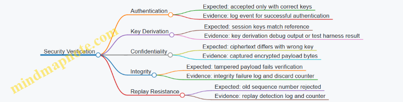
Step 3: Run Three Controlled Experiments
Run the same traffic pattern three times, changing only one security input each time.
Experiment A: Correct Keys
Send one short user-plane message and one control-plane signaling message.
- Expected outcome: both are accepted.
- Expected artifacts:
- The computed session keys match the reference test vector.
- The ciphertext matches the expected encryption output.
- Integrity verification passes and the message is delivered.
Experiment B: Wrong Integrity Key
Keep everything the same, but substitute the integrity key with a single-bit-flipped variant.
- Expected outcome: user-plane message is discarded.
- Expected artifacts:
- Ciphertext may still look plausible, but integrity verification fails.
- Logs show an integrity failure event and an increment in discard counters.
Experiment C: Tampered Payload with Correct Keys
Use correct keys, but flip one byte in the protected payload before it reaches the integrity check.
- Expected outcome: integrity verification fails.
- Expected artifacts:
- Logs indicate integrity mismatch.
- The system does not deliver the tampered plaintext.
Step 4: Validate Logs Against Expected Event Semantics
Logs should be treated like a contract. For each experiment, define the exact event types you expect and the counters you expect to move.
A typical verification checklist looks like this:
- Authentication success event appears only in Experiment A.
- Key derivation event shows matching derived values in all experiments where inputs are correct.
- Integrity failure event appears in Experiments B and C.
- Discard counters increase only when integrity fails.
- Replay detection event appears when you intentionally reuse an old sequence number.
Example: Minimal Log Assertions
Experiment A
- AUTH_SUCCESS: present
- INTEGRITY_FAIL: absent
- DISCARD_COUNT: unchanged

Experiment B
- AUTH_SUCCESS: present
- INTEGRITY_FAIL: present
- DISCARD_COUNT: incremented by 1

Experiment C
- AUTH_SUCCESS: present
- INTEGRITY_FAIL: present
- DELIVERED_PAYLOAD: absent
Step 5: Confirm Sequence Handling with Replay Checks
To verify replay resistance, resend the same protected message using the same sequence number.
- Expected outcome: the second attempt is rejected.
- Expected artifacts:
- A replay detection or sequence window violation log.
- No delivery event for the replayed message.
Step 6: Tie It Together with One Evidence Table
Create a compact table that links each security property to both a computed check and a log check.
| Security Property | Test Vector Check | Log Evidence |
|---|---|---|
| Authentication | Derived session keys match | AUTH_SUCCESS or AUTH_FAIL |
| Confidentiality | Ciphertext matches expected | Encrypted payload captured |
| Integrity | MAC matches expected | INTEGRITY_FAIL or INTEGRITY_OK |
| Replay Resistance | Sequence validation outcome | REPLAY_DETECTED and no delivery |
When all rows match their expected outcomes across Experiments A, B, and C, you have evidence that the security controls are not just configured, but enforced end to end. And yes, it is satisfying when the wrong key fails exactly where the logs say it should.
11. Performance Engineering and Troubleshooting Workflows
11.1 Defining KPIs for Coverage Throughput Latency and Reliability
KPIs for direct to cell satellite communication should be defined from the user experience backward to the radio link forward. Start with what “good” means for a specific service, then translate it into measurable network behaviors, and finally map those behaviors to radio and protocol knobs.
Coverage KPIs
Coverage is not just “signal exists.” For mobile terminals, coverage must include usability at the beam edge and during movement.
Coverage KPIs to measure
- Availability of usable signal: Percentage of time a terminal can meet a minimum receive quality threshold (for example, reference signal quality or demodulation success rate) while in motion.
- Geographic coverage footprint: Area where the minimum threshold is met under representative terminal heights and antenna orientations.
- Beam edge margin: How far the received quality falls below the target at the edge, measured as a distribution rather than a single worst point.
Easy example If your messaging service requires successful decoding with a target block error rate, define coverage as “% of drive-test samples where decoding succeeds within the first attempt.” A beam that looks fine on average but fails frequently at the edge will show up immediately.
Throughput KPIs
Throughput depends on scheduling, contention, and link adaptation. For satellite links, throughput should be measured per service class, not only as a raw peak rate.
Throughput KPIs to measure
- User throughput percentile: For example, 5th and 50th percentile user throughput over time windows.
- Cell or beam throughput efficiency: Delivered payload rate divided by allocated radio resources.
- Goodput: Application payload delivered successfully per second, excluding retransmissions and protocol overhead.
Easy example Two configurations can have the same average throughput. If one causes many retransmissions, goodput will be lower and latency will rise. Goodput prevents you from rewarding “busy radios” that don’t deliver.
Latency KPIs
Latency in NTN is shaped by propagation, scheduling, retransmissions, and processing delays. Separate one-way and end-to-end metrics so you can pinpoint which part is misbehaving.
Latency KPIs to measure
- End-to-end latency distribution: Median and 95th percentile from application send to application receive.
- Radio access latency: Time from scheduling grant to successful delivery at the link layer.
- Retransmission-induced delay: Extra time added by HARQ or link-layer recovery.
Easy example If end-to-end latency spikes only at certain times, check whether radio access latency grows (scheduling contention) or whether retransmission-induced delay grows (link quality drops).
Reliability KPIs
Reliability should reflect success probability under realistic mobility and channel variation.
Reliability KPIs to measure
- Delivery success rate: Fraction of attempts that complete successfully within a defined deadline.
- Block success rate: Link-layer decoding success probability per transport block.
- Session continuity success: Probability that a session remains usable across beam transitions without user-visible failure.
Easy example For a short burst message, define reliability as “% of messages delivered within 10 seconds.” For a streaming-like flow, define reliability as “% of segments delivered without exceeding a maximum rebuffer threshold.” Same network, different KPI definitions.
Translating KPIs into Measurable Signals
KPIs become useful when each one maps to counters, logs, and measurement procedures.
Mind Map: KPI Definition Flow
KPI Measurement Method
Use a measurement plan that matches the KPI definition.
Recommended measurement approach
- Define the time window for each KPI (for example, per minute for throughput, per session for reliability).
- Collect synchronized timestamps at the application and at the network boundary.
- Record radio conditions alongside outcomes (beam ID, terminal speed, received quality, scheduling grants).
- Compute distributions rather than single averages.
Mind Map: What To Log For Each KPI
Practical KPI Set for a Direct to Cell Messaging Service
A coherent KPI set should be mutually consistent: coverage supports reliability, reliability supports latency, and latency supports throughput.
Example KPI set
- Coverage: Usable decoding availability ≥ 99% of drive-test samples at the target threshold.
- Reliability: Message delivery success ≥ 98% within 10 seconds.
- Latency: 95th percentile end-to-end latency ≤ 8 seconds.
- Throughput: 5th percentile goodput ≥ a minimum payload rate during moderate contention.
How the logic holds If coverage availability drops, block success rate drops, which reduces delivery success and increases latency via retransmissions. If scheduling contention rises, throughput falls and latency grows, but coverage availability may remain stable.
Common KPI Pitfalls to Avoid
- Using only averages: Averages hide edge failures and intermittent outages.
- Mixing layers: Don’t treat radio access latency and application latency as the same KPI.
- Ignoring deadlines: Reliability without a deadline is ambiguous for user experience.
KPI Review Checklist
- Each KPI has a clear target, time window, and percentile or deadline.
- Each KPI maps to specific measurements and counters.
- Each KPI is validated under both stationary and moving terminal scenarios.
- Each KPI set supports a single service objective without contradictions.
11.2 Measurement Methodologies Including Drive Tests and Lab Emulation
Measurement is where theory meets reality, and reality is annoyingly specific. This section lays out a systematic approach to measuring direct-to-cell satellite performance using two complementary methods: drive tests in the field and lab emulation in controlled environments. The goal is not to collect numbers for their own sake, but to produce evidence you can trace back to link behavior, scheduling behavior, and protocol behavior.
Measurement Foundations and What You Can Actually Learn
Start by defining what you want to measure and what decision it supports. Coverage maps answer “where can a terminal work,” while throughput and latency measurements answer “how well does it work under load.” Reliability metrics answer “how often does it fail,” which is different from “how fast it usually works.”
A practical measurement plan ties each KPI to a measurement artifact:
- Coverage: received signal quality distributions and availability over time.
- Throughput: user-plane goodput under representative traffic.
- Latency: end-to-end delay distribution, not just average.
- Reliability: packet success rate and retransmission behavior.
- Mobility: handover success rate and time-to-reconnect.
Drive Tests for Real-World Behavior
Drive tests capture the messy parts: antenna orientation changes, multipath from buildings, vehicle motion, and real scheduling contention. Use a repeatable route and a repeatable test script.
1) Prepare the test setup
- Use a consistent terminal model and firmware configuration.
- Log time-synchronized measurements (radio metrics, GPS position, and application-level events).
- Fix the traffic pattern: for example, periodic small messages plus occasional bursts.
2) Choose routes and sampling strategy
- Include representative environments: open areas, urban canyons, and near obstacles.
- Run the same route multiple times to separate “route effects” from “system effects.”
3) Control variables
- Keep speed ranges consistent, or log speed so you can stratify results.
- Record antenna orientation if possible; if not, at least standardize mounting.
4) Interpret results with causality When throughput drops, check whether the cause is link quality, contention, or protocol retransmissions. A useful workflow is to align application events with radio logs around each drop window.
Lab Emulation for Controlled Root Cause Analysis
Lab emulation isolates variables so you can test hypotheses without the route changing under your feet. It is especially useful for timing, Doppler, and protocol parameter tuning.
1) Build an emulation model
- Represent the satellite channel with configurable impairments: path loss, fading, Doppler shift, and timing offsets.
- Include realistic propagation dynamics for mobility scenarios.
2) Use scenario-based testing Run a small set of scenarios that map to field observations. For example:
- Stable link with mild Doppler.
- Beam-edge-like conditions with rapid quality variation.
- High contention with multiple simulated users.
3) Validate measurement integrity Confirm that the emulation produces the intended impairment profiles by checking measurement traces at the radio interface. If the impairment model is wrong, the conclusions will be wrong too, just faster.
Mind Map: Measurement Workflow
Measurement Methodologies Mind Map
Example: From Field Dropouts to Lab Explanations
Suppose a drive test shows intermittent message delays in a specific corridor. First, segment the route into “normal” and “delay” intervals using application timestamps. Next, inspect radio logs for those intervals: if retransmission counts spike and link adaptation reports degraded quality, the delay is likely protocol-driven rather than application-driven.
Then mirror the corridor behavior in the lab. Configure the channel model to reproduce the observed quality variation rate and Doppler range. Run the same traffic pattern and compare:
- If delay distribution matches, you have a credible explanation.
- If it does not, adjust the impairment model or include contention by adding simulated users until the behavior aligns.
Example: Measuring Reliability Without Lying to Yourself
Reliability measurements often fail because the test duration is too short or the traffic pattern is unrealistic. Use a traffic script that generates enough events to estimate packet success rate with reasonable confidence. Also separate “no service” periods from “service with losses,” since they come from different causes and require different fixes.
Practical Measurement Checklist
- Define KPIs and map each to a loggable measurement artifact.
- Use repeatable traffic patterns in both field and lab.
- Time-align application events with radio measurements.
- Attribute performance drops using evidence, not assumptions.
- Use field results to choose lab scenarios, and lab results to explain field behavior.
This two-lane approach keeps measurements honest: drive tests show what happens, lab emulation explains why it happens, and the combination supports parameter decisions you can defend.
11.3 Interpreting Link Budget and Live Telemetry Together
A link budget tells you what should happen if the assumptions are correct; live telemetry tells you what is happening in the real world. The trick is to compare them using the same variables, at the same points in the chain, and with the same time granularity. If you compare a static budget to a rolling average, you’ll end up arguing with yourself.
Mind Map: What to Compare and Where
Step 1: Align the Reference Points
Start by matching the budget’s “receiver input” to the telemetry’s “receiver measurement.” For example, a budget might compute received power at the demodulator input after feeder losses, while telemetry might report a calibrated RSRP-like value at the RF front end. If those reference points differ, the delta will look like a mystery even when nothing is wrong.
Practical alignment checklist:
- Use the same beam and direction as the budget (uplink vs downlink).
- Confirm the terminal antenna gain model used in the budget matches the terminal class in telemetry.
- Ensure the telemetry metric is tied to the same bandwidth and reference signal type.
Step 2: Compare Margins, Not Just Levels
Received power alone rarely explains performance. A link budget usually converts power into an SNR/SINR margin against a required threshold for a chosen modulation and coding scheme (MCS). Telemetry gives you the selected MCS and the resulting error behavior.
Compute three deltas for the same time window and beam:
- Pr delta: observed received level minus budget predicted level.
- SNR delta: observed effective SNR minus budget predicted effective SNR.
- Margin delta: required threshold minus observed effective SNR.
If Pr is low but SNR behaves normally, the issue may be calibration or measurement scaling. If Pr matches but BLER spikes, the issue is more likely interference, timing/frequency errors, or incorrect assumptions about noise figure.
Step 3: Use Mode Switching as a Truth Serum
Live systems adapt. When geometry degrades, the scheduler and link adaptation should step down MCS in a predictable way. Compare the pattern of MCS changes to the budget’s expected thresholds.
Example: Suppose the budget says MCS 12 requires an SINR of 10 dB, and MCS 9 requires 7 dB. If telemetry shows frequent toggling between MCS 12 and 9 while BLER remains high, that suggests the effective SINR is oscillating faster than the adaptation logic expects—often due to timing drift, Doppler residuals, or bursty interference.
If telemetry stays at a high MCS even when BLER is rising, adaptation may be constrained by policy, reporting delays, or stale CQI.
Step 4: Interpret HARQ Like a Timeline, Not a Score
HARQ statistics reveal whether failures are random noise or structured problems.
- Many first-transmission failures with few successful retransmissions: likely insufficient SINR or persistent interference.
- Successful retransmissions after one or two attempts: likely marginal link conditions where coding gain helps.
- Retransmissions clustered in time: often points to geometry crossing, beam edge effects, or transient interference.
Example: During a beam-edge pass, you might see retransmissions jump exactly when the terminal’s estimated timing advance changes abruptly. That pattern points to synchronization sensitivity rather than a pure power shortfall.
Step 5: Attribute the Delta with Minimal Guessing
Once you have deltas and patterns, map them to likely causes:
- Pr delta consistent across many terminals: model mismatch in path loss, antenna gain, or feeder losses.
- SNR delta larger than Pr delta: noise figure mismatch, implementation losses, or interference not represented in the budget.
- Margin delta appears only for certain beams: beam pattern or pointing errors, or localized interference.
- Error bursts without large Pr changes: timing/frequency offset residuals or receiver processing constraints.
Worked Example: One Beam, Two Windows
Assume a budget for a specific beam predicts an effective SNR of 9 dB at a certain geometry point, giving a small margin above the MCS threshold. You observe two telemetry windows:
- Window A: MCS stays at the expected level, BLER is low, HARQ retransmissions are rare.
- Window B: MCS remains high longer than expected, BLER rises, and retransmissions increase.
Because Window A matches the budget, the budget assumptions are not wildly wrong. The difference in Window B suggests a change in conditions not captured by the static budget: either interference increased, CQI/reporting lag delayed adaptation, or synchronization degraded due to a timing/frequency behavior change.
The goal is not to “find the culprit” in one leap; it’s to narrow the set of explanations until the remaining ones explain both the level (Pr/SNR) and the behavior (MCS switching and HARQ timing).
11.4 Common Failure Modes and Diagnostic Steps Without Predictions
Direct-to-cell links fail in recognizable patterns. The trick is to diagnose by what changed between a known-good state and the current state, then map symptoms to the most likely layer: radio, timing, link adaptation, scheduling, or core/session behavior. This section gives a systematic workflow that avoids guesswork.
Mind Map: Failure Modes to Diagnostic Paths
Step 1: Classify the Symptom by Layer
Start with the user-visible symptom and translate it into a layer hypothesis.
- Registration never completes usually points to acquisition, coverage/beam selection, or signaling rejection.
- Registration completes but data stalls often indicates link adaptation, HARQ effectiveness, or scheduling contention.
- Drops and reconnect loops frequently correlate with mobility/beam edge behavior or session timer mismatches.
A practical way to keep this grounded is to create a small “evidence table” for each test run: time of event, uplink/downlink counters, BLER, retransmissions, and any rejection cause codes.
Step 2: Confirm Radio Reachability Before Blaming Protocols
Before touching protocol knobs, verify that the UE can reach the network.
Example: A field test shows “no service” in a vehicle. The first check is not the core logs; it’s whether the UE is actually seeing usable signal.
- If reference signal measurements are near the receiver sensitivity threshold, the UE may fail to lock timing or frequency.
- If measurements look healthy but registration still fails, then focus on synchronization quality and signaling causes.
Diagnostic steps
- Compare RSRP/SINR during a known-good location versus the failing location.
- Check whether the UE reports stable timing and frequency offset estimates.
- Verify antenna orientation and polarization by repeating the test with a controlled mounting angle.
Step 3: Use Counter Patterns to Separate “Bad Link” from “Bad Scheduling”
When throughput collapses, you want to know whether the link is failing repeatedly or the network is starving the UE.
- Bad link pattern: BLER rises, and retransmission counters climb, with grant sizes that don’t recover performance.
- Bad scheduling pattern: BLER may be moderate, but the UE receives too few opportunities, or grants are too small relative to the packetization.
Example: Messaging takes 30–60 seconds instead of a few seconds. BLER is high and HARQ retransmissions spike right after each grant. That points to link adaptation and/or coding selection being mismatched to the instantaneous channel, not to a core routing issue.
Diagnostic steps
- Plot BLER over time alongside retransmission counts.
- Compare uplink and downlink behavior; asymmetry often indicates RF chain or power control limits.
- Review grant timing relative to the UE’s reported channel quality.
Step 4: Diagnose Timing and Doppler as “Silent Saboteurs”
Timing errors can look like random packet loss.
Example: A test lab run shows stable signal strength, yet packet error rates oscillate quickly. That pattern often matches frequency offset or timing drift issues.
Diagnostic steps
- Check frequency offset estimation stability during the failing interval.
- Verify synchronization reference quality and whether the UE reports frequent reacquisition.
- Confirm that timing advance behavior matches expected propagation changes.
Step 5: Interpret Mobility and Session Events Together
Intermittent drops are best handled by correlating radio events with session-layer outcomes.
Example: A session drops exactly when the UE approaches the beam edge. Handover events occur, but the session resumes with a delay and PDCP discard counters increase. That suggests reordering/discard behavior is being triggered by timing gaps during the transition.
Diagnostic steps
- Align handover start/end times with drop and reconnect timestamps.
- Inspect PDCP discard and reordering indicators around the transition.
- Check whether session timers expire during periods of reduced radio opportunity.
Step 6: Run a Minimal Reproduction Checklist
To avoid “fixing” the wrong thing, reproduce with controlled variables.
- Keep terminal model and mounting constant.
- Repeat the same location and time window.
- Change only one factor per run: antenna angle, terminal orientation, or test profile.
Example: If rotating the terminal by 30 degrees immediately restores uplink but not downlink, the issue is likely RF/polarization or power control limits rather than core configuration.
Step 7: Produce a Single Root-Cause Hypothesis with Evidence
End each diagnostic with one clear statement: which layer is failing and why, supported by counters and event correlation. If the evidence supports multiple layers, choose the earliest failing point in the chain and document the alternative as a secondary hypothesis.
A good diagnostic ends with a checklist of “what to verify next” rather than a list of guesses. That keeps the next test focused and prevents the classic cycle of changing five things and learning nothing.
11.5 Practical Example: Root Cause Analysis for Low Throughput in a Beam
Low throughput in a single satellite beam is usually a “many small things” problem: one parameter nudges another, and the chain ends at the user experience. The goal of this workflow is to identify the first measurable constraint, not to collect every possible metric.
Step 1: Confirm the Symptom and Localize the Scope
Start by separating “low throughput” into what kind of low it is.
- Low average rate: throughput drops across most users.
- High retransmissions: throughput drops but retransmission counters spike.
- Burstiness: throughput is fine in some time windows, then collapses.
Example observation set for a beam:
- Downlink throughput averages 35% below baseline.
- HARQ retransmissions increase from 2% to 18%.
- Scheduling utilization is near normal, so the scheduler is not simply starving the beam.
This combination strongly suggests a link quality or timing issue rather than pure congestion.
Step 2: Build a Minimal Hypothesis List
Create hypotheses that map to measurable signals. Keep it short.
- Link budget degradation: higher path loss, mispointing, or unexpected attenuation.
- Timing and frequency errors: residual Doppler or synchronization drift causing decoding failures.
- Resource mismatch: wrong modulation/coding selection or beam-to-user mapping errors.
- Interference or contention: uplink power control issues or adjacent-beam leakage.
Step 3: Check the Fastest Signals First
Use the metrics that typically move first.
3.1 Physical Layer Quality Indicators
- Verify RSRP/RSRQ-like measurements (or their NTN equivalents) for a sample of UEs.
- Compare SNR distribution for the affected beam versus a neighboring beam.
Example:
- Affected beam shows median SNR 3–4 dB lower than adjacent beam.
- Retransmissions correlate with the lower SNR tail.
That points to link budget or interference rather than a purely protocol-layer problem.
3.2 Timing and Doppler Compensation Health Check whether the UE and gateway are meeting their synchronization targets.
- Look for rising frequency offset estimates.
- Look for increased timing advance corrections or failures to lock.
Example:
- Frequency offset variance increases during a specific pass segment.
- The increase aligns with the time window where throughput collapses.
This suggests Doppler compensation is not tracking as expected.
Step 4: Use a Mind Map to Drive the Next Measurements
Mind Map: Root Cause Analysis Flow for Beam Throughput
Step 5: Narrow Down with Controlled Comparisons
Do not change everything at once. Compare like with like.
5.1 Adjacent Beam Comparison
- If adjacent beams are normal, the issue is likely beam-specific: pointing, beamforming weights, or local interference.
Example:
- Adjacent beam throughput matches baseline.
- Only the affected beam shows SNR drop and retransmission spike.
5.2 UE Class Comparison Split UEs by terminal type or antenna configuration.
- Handheld vs vehicle-mounted
- High-gain vs low-gain
Example:
- Vehicle-mounted UEs show smaller SNR drop than handheld UEs.
- Retransmissions still rise, but less severely.
This pattern fits a link quality issue rather than a universal protocol failure.
5.3 Pass Segment Comparison Plot throughput and frequency offset variance versus time along the satellite pass.
Example:
- The worst throughput occurs when frequency offset variance peaks.
- After that window, throughput partially recovers.
Step 6: Convert Evidence into a Concrete Root Cause
At this point, you should be able to state a root cause in one sentence tied to a measurement.
Example root cause statement:
- Residual Doppler tracking error increases during a pass segment, causing decoding failures and triggering frequent HARQ retransmissions, which reduces effective throughput.
Step 7: Validate the Fix with a Re-Measurement Plan
A good fix is one you can prove quickly.
- Apply a controlled adjustment (e.g., update Doppler compensation parameters or synchronization thresholds) for the affected beam.
- Re-run the same pass segment and compare:
- retransmission rate
- SNR distribution
- throughput distribution
Example validation results:
- HARQ retransmissions drop from 18% to 6%.
- Median throughput returns to within 10% of baseline.
- The throughput collapse window shrinks to a smaller time interval.
Step 8: Document the Decision Logic
Write down the chain from symptom to root cause.
- Symptom: throughput down, retransmissions up.
- Localization: beam-specific, adjacent beam normal.
- Evidence: SNR shift and Doppler variance correlation.
- Root cause: residual Doppler tracking error.
- Proof: retransmissions and throughput recover after parameter adjustment.
That documentation matters because the next incident will reuse the same reasoning, not just the same numbers.
12. Practical Implementation Guide for End to End Direct to Cell Services
12.1 Planning Inputs Including Spectrum, Coverage, and Terminal Capability
Planning a direct to cell service starts with three inputs that constrain everything else: spectrum, coverage, and terminal capability. Treat them like the three legs of a stool—if one is off, the system wobbles no matter how good the rest of the design is.
Spectrum Inputs
Begin by listing the available frequency bands and the regulatory constraints that apply to your deployment area. For each band, capture: uplink and downlink frequency ranges, channel bandwidth, duplexing approach, and any limits on transmit power spectral density. Then translate those constraints into practical radio parameters: maximum effective isotropic radiated power at the terminal, allowable EIRP at the gateway, and any guard-band requirements.
Next, decide how the spectrum will be used across beams. If you plan to reuse spectrum across multiple beams, you must account for inter-beam interference and the receiver’s ability to separate signals. A simple way to reason about this is to write down the worst-case co-channel scenario you expect at the beam edge, then confirm that your link budget and receiver design still meet the target block error rate.
Example: Suppose your uplink uses a 5 MHz channel and your terminal can support only a limited transmit power. You may find that the modulation and coding scheme you want for good throughput is not feasible at the beam edge. The planning fix is not “try harder,” it is to adjust the service definition: reduce the target rate, change the scheduling strategy, or narrow the coverage footprint for the high-rate mode.
Coverage Inputs
Coverage planning is more than drawing footprints. You need a map of where service is required, how long users stay within each region, and what “good enough” means at the boundary.
Capture these items:
- Coverage area definition, including excluded zones if regulations or site constraints require them.
- Beam layout and pointing strategy, including overlap regions.
- Elevation angle constraints, because low elevation often drives worse link budgets and more pronounced Doppler dynamics.
- Mobility assumptions, such as typical user speed and expected dwell time in a beam.
Then define performance targets per region: minimum downlink/uplink throughput, maximum acceptable latency for small messages, and reliability targets for control signaling. Reliability targets should be tied to the service type. For example, a short acknowledgment message can tolerate different error behavior than a file transfer.
Example: If your service requires reliable delivery of small status updates, you can set a stricter reliability target for those packets while allowing lower throughput for bulk data. This keeps the system honest: you are not forcing one performance number to fit every traffic type.
Terminal Capability Inputs
Terminal capability determines what the network can safely assume. Start with hardware and implementation limits: maximum transmit power, receiver sensitivity, supported antenna patterns, and supported bandwidth. Then include protocol and processing limits: maximum supported modulation and coding schemes, buffer sizes, and how quickly the terminal can measure and report channel conditions.
Also capture operational constraints that affect real deployments: power-saving modes, whether the terminal can maintain timing reference during movement, and how the terminal behaves when signal quality fluctuates near the beam edge.
A useful planning habit is to create a capability matrix that lists each terminal class and the exact features it supports. If you later discover that a subset of terminals cannot support a certain configuration, you can route them to a more robust mode rather than failing silently.
Example: If a low-cost terminal cannot support the highest-order modulation, you should plan a fallback mode with a lower rate but higher robustness. The coverage plan should reflect that fallback mode’s link budget so the user experience degrades gracefully instead of abruptly.
Integrated Planning Mind Map
Turning Inputs into Planning Decisions
Once the three input sets are captured, convert them into a consistent set of radio and service decisions. First, compute link budgets for the required regions using the terminal capability limits and the spectrum constraints. Second, define mode selection rules that map channel conditions and terminal class to an appropriate modulation/coding and resource allocation approach. Third, verify that control-plane signaling can be carried reliably under the same assumptions, because registration and session setup often fail before data does.
Finally, document the assumptions explicitly. A planning document that states “we assumed terminals support X” and “we assumed users remain above Y elevation for Z seconds” is easier to validate and easier to troubleshoot later. The goal is not to predict everything; it is to make the system’s behavior understandable when reality shows up.
12.2 Step by Step Service Design From Requirements to Radio Parameters
Start with what the service must do, then translate those needs into radio parameters you can actually configure and test. The trick is to keep a single chain of reasoning from user experience to link behavior.
Step 1: Lock the Service Requirements into Measurable Targets
Write requirements as testable statements, not vibes. For a direct to cell service, typical targets include:
- Coverage: minimum probability of successful reception at the beam edge.
- Latency: end to end time budget for a message or interactive session.
- Reliability: block error rate or message success rate under defined mobility.
- Capacity: average and peak throughput per cell/beam area.
- Terminal constraints: max transmit power, antenna gain assumptions, and supported bandwidth.
Example: “A 200-byte status message must succeed 95% of the time for a handheld moving at 3 m/s, with a 2-second application-level deadline.” That immediately implies a link budget margin, a retransmission strategy, and a scheduling window.
Step 2: Choose the Service Model and Map It to Bearers
Decide whether the service is best-effort data, prioritized messaging, or a mix. Then map it to bearer types with clear QoS behavior.
- Messaging: small packets, tolerate some retransmissions, strict deadline.
- Streaming: larger packets, needs sustained throughput and stable scheduling.
- Control signaling: low volume, but must be robust for session continuity.
Example: For messaging, set a tight latency budget and allow HARQ retransmissions within that budget. For control signaling, prioritize access and initial link establishment.
Step 3: Define the Radio Environment Assumptions
You cannot design radio parameters without assumptions. Capture:
- Geometry: satellite altitude, elevation angle ranges, and beam footprint.
- Propagation: atmospheric attenuation model and worst-case weather margin.
- Mobility: UE speed and expected Doppler range.
- Interference: co-channel assumptions, adjacent channel leakage, and noise figure.
Example: If the requirement assumes “beam edge,” define what “edge” means in terms of elevation angle and path loss percentile. Otherwise, your link budget will be a guessing game with math.
Step 4: Build the Link Budget and Convert It into Required Signal Quality
Compute the received power and required SINR for the chosen modulation and coding. Then translate that into a target SNR at the receiver.
- Start from UE transmit power, antenna gain, feeder losses.
- Add path loss and atmospheric losses.
- Include receiver noise figure and bandwidth.
- Apply implementation margins for frequency offset and imperfect channel estimation.
Example: If your selected coding needs 6 dB effective SNR for the target BLER, then your link budget must deliver at least that SNR at the defined coverage percentile, after all margins.
Step 5: Select Waveform, Bandwidth, and Numerology
Choose parameters that match both the service and the channel dynamics.
- Bandwidth affects noise floor and achievable throughput.
- Numerology affects timing granularity and how you handle Doppler and scheduling.
- Guard intervals and reference signal density affect acquisition and tracking.
Example: For handheld terminals with limited processing, pick a configuration that keeps reference overhead reasonable while still supporting reliable measurement under Doppler.
Step 6: Determine HARQ and Retransmission Timing
HARQ behavior must respect the latency budget and the round-trip time constraints.
- Set maximum retransmissions based on deadline.
- Choose transport block sizing so that retransmissions are efficient.
- Ensure the scheduler can allocate resources for potential reattempts.
Example: If the application deadline is 2 seconds and the system round-trip plus processing consumes 1.2 seconds, allow at most one retransmission for the message payload, then rely on link adaptation for the next attempt.
Step 7: Configure Link Adaptation and MCS Mapping
Link adaptation decides which modulation and coding scheme to use for a given measured channel quality.
- Define CQI-to-MCS mapping rules.
- Set hysteresis to avoid rapid switching.
- Constrain the adaptation range to protect reliability at the coverage edge.
Example: If CQI reports are noisy near the edge, use conservative MCS thresholds so that the “95% success” requirement is met even when measurements fluctuate.
Step 8: Set Scheduling and Resource Allocation Rules
Scheduling converts “radio capability” into “service delivery.” Define:
- Grant strategy for uplink and downlink.
- Priority handling for control vs user data.
- How you allocate resources across beams or coverage partitions.
- Contention handling when many UEs transmit simultaneously.
Example: For messaging, allocate small periodic opportunities for uplink grants to reduce access delay, and reserve higher priority resources for session-critical signaling.
Step 9: Translate Everything into Concrete Radio Parameters
At this point, you can produce a parameter set that a radio engineer can implement:
- Carrier frequency and channel bandwidth.
- Frame structure and numerology.
- Reference signal configuration for measurement and tracking.
- HARQ process count, retransmission limits, and timing.
- MCS tables and CQI mapping.
- Power control targets and limits.
- Beam management parameters and coverage partitioning.
Example: If the link budget requires a 2 dB additional margin at the edge, increase power control headroom or adjust MCS thresholds rather than pretending the margin will appear magically.
Step 10: Validate with End to End Simulations and Targeted Tests
Validation should check both link-layer success and service-layer outcomes.
- Verify BLER and message success rate at the defined percentiles.
- Confirm latency distribution meets the deadline.
- Stress with mobility and frequency offset scenarios.
- Check scheduler behavior under contention.
Example: Run a scenario where 30% of UEs are near beam edge while others are closer, then confirm that the edge group still meets the 95% message success target.
Mind Map: Requirements to Radio Parameters Flow
Example: A Complete Walkthrough for a 200-Byte Status Message
- Requirements: 95% success, 2-second deadline, handheld at 3 m/s, beam edge defined by a specific elevation percentile.
- Service model: messaging bearer with strict latency priority.
- Environment: set worst-case atmospheric loss and receiver noise figure; include Doppler range for tracking.
- Link budget: compute required effective SNR for the chosen MCS; confirm margin at the edge.
- Radio parameters: select bandwidth and numerology that support reliable measurement; configure reference signals for Doppler tracking.
- HARQ: allow one retransmission within the 2-second budget; set transport block size to fit 200 bytes efficiently.
- Adaptation: map CQI to MCS conservatively near edge; add hysteresis.
- Scheduling: reserve small uplink opportunities for prioritized messaging and ensure grant timing supports the HARQ cycle.
- Validation: simulate mobility and contention; confirm message success and latency distributions meet targets.
This workflow keeps the design grounded: every radio choice traces back to a requirement, and every requirement is checked against the radio reality.
12.3 Integration Checklist for 5G Core and NTN Radio Access Components
This checklist is organized from “things that must be true” to “things you can verify,” so integration doesn’t turn into a scavenger hunt. Each item includes a concrete example of what “done” looks like.
Baseline Assumptions and Interface Contracts
Start by writing down the integration contracts before touching configuration.
- Define the service type and bearer mapping. Example: For a messaging service, map user data to a dedicated bearer with a latency target, while keeping signaling on a separate control path.
- Confirm NTN access mode and terminal capabilities. Example: If the UE supports only a specific modulation/coding set, ensure the radio parameters and link adaptation profiles do not request unsupported modes.
- Lock down addressing and identifiers. Example: Verify that the UE identity used for registration matches the one used for authorization, so you don’t end up with “registered but not allowed” behavior.
5G Core Integration Points
Integrate the core functions with explicit expectations for signaling, session setup, and policy.
- Registration and mobility context. Example: During beam transitions, confirm the core receives consistent location and access information so session continuity rules apply correctly.
- Session establishment flow. Example: When a UE requests a data session, verify that the core selects the correct QoS profile and returns it to the access side.
- Policy control and QoS enforcement. Example: If a user enters a coverage area with lower expected capacity, ensure the policy can adjust the QoS parameters without breaking the session.
NTN Radio Access Integration Points
Treat the radio access side as a system with measurable inputs and outputs.
- Radio bearer setup and parameter propagation. Example: Confirm that the QoS parameters chosen by the core are translated into the radio scheduler inputs used for grant decisions.
- Timing and frequency handling alignment. Example: Ensure the UE timing advance procedure and the network reference timing agree on units and update cadence.
- HARQ and retransmission behavior consistency. Example: If the radio layer uses a specific retransmission window, verify the core does not assume immediate delivery for application-level acknowledgments.
QoS, Scheduling, and Resource Coordination
This is where “it connects” becomes “it performs.”
- Map QoS to scheduler behavior. Example: For a high-priority bearer, verify it receives earlier grants under contention and that the scheduler uses the correct priority weights.
- Handle variable propagation conditions. Example: During periods of worse link quality, confirm the system uses link adaptation rather than dropping sessions.
- Define contention strategy for shared resources. Example: If multiple UEs share a beam, confirm the scheduler enforces fairness rules so one UE doesn’t monopolize grants.
Security Integration Checks
Security failures often show up as “mysterious access denials.” Make them explicit.
- Authentication and key derivation alignment. Example: Validate that the derived keys used by the access side match the keys expected by the core for integrity protection.
- Encryption and integrity coverage. Example: Confirm that user-plane traffic is encrypted end-to-end across the access segment and that signaling integrity is enforced.
- Key lifetime and rekey triggers. Example: During long sessions, verify that rekey events do not cause session teardown.
Observability and Operational Readiness
If you can’t measure it, you can’t integrate it.
- End-to-end trace points. Example: Ensure you can correlate a UE registration event in the core with the corresponding access-side radio state transitions.
- Performance counters with clear ownership. Example: Define which system reports HARQ retransmissions, which reports scheduling delays, and which reports session setup time.
- Alarm thresholds tied to integration assumptions. Example: If timing sync fails, confirm the alarm indicates whether it is a reference timing mismatch or a UE measurement issue.
Validation Scenarios That Prove the Integration
Use scenarios that cover the full path, not just isolated components.
- Registration and initial session. Example: Bring up a UE, register, establish a data session, and verify QoS parameters match what the core selected.
- Beam transition with active traffic. Example: Start a file transfer, then force a beam edge transition and confirm the session remains stable.
- Congestion test under shared resources. Example: Simulate multiple UEs and verify high-priority traffic retains its target behavior while others degrade gracefully.
- Security verification under normal and error cases. Example: Attempt a session with invalid credentials and confirm the failure is clean and does not leak partial context.
Mind Map: Integration Checklist Flow
Example: Integration Acceptance Criteria
Use pass/fail statements tied to logs and measurements.
- Pass: A UE registration results in a core session with the expected QoS profile, and the access side confirms the corresponding radio bearer parameters.
- Pass: During a forced beam transition, the session remains active and user-plane throughput shows no sustained collapse beyond the configured adaptation behavior.
- Pass: Security failures produce a deterministic rejection with no partial user-plane context.
- Pass: Traces show consistent correlation IDs across core and access for registration, session setup, and bearer changes.
Example: Minimal Configuration Sanity Checks
Check 1: QoS profile IDs match across core and access
- Input: core-selected profile
- Output: radio bearer uses same profile

Check 2: Timing units match
- Input: reference timing update interval
- Output: UE timing advance update cadence

Check 3: Retransmission window alignment
- Input: HARQ retransmission settings
- Output: RLC/PDCP behavior does not assume instant delivery
This section ends with a practical rule: every integration decision should be traceable to a measurable outcome, otherwise it’s just a configuration story.
12.4 Test and Validation Procedures Including Interoperability Checks
A good validation plan for direct to cell services treats interoperability as a chain of contracts: radio behavior, protocol expectations, timing assumptions, and security handshakes. If any link in the chain is ambiguous, the test results will look like “it works on my setup,” which is not a useful outcome.
Define Test Objectives and Acceptance Criteria
Start by writing acceptance criteria in measurable terms before touching a test tool. For example, specify target ranges for:
- Registration success rate within a time budget (e.g., 95% within 30 seconds under defined signal conditions).
- Packet delivery ratio for a fixed payload size under controlled mobility.
- End-to-end latency distribution for a small message flow.
- Security handshake success rate and absence of downgrade behavior.
Then map each criterion to a specific component boundary: UE-to-RAN, RAN-to-core, and core-to-application. This prevents “global” pass/fail results that hide which interface is misbehaving.
Build a Test Matrix That Covers Interface Contracts
Create a matrix that varies the parameters that actually change behavior:
- Signal conditions: clear sky vs. edge-of-coverage, and uplink vs. downlink stress.
- Mobility: stationary, slow movement, and beam-edge crossing.
- Load: single UE vs. multiple UEs sharing resources.
- Feature toggles: security on/off, QoS profiles, and retransmission settings.
For interoperability, include at least one “mismatched” pairing on purpose: different vendor implementations of UE firmware, gateway software, or core network releases. The goal is not to break things; it’s to confirm that the system behaves correctly when assumptions differ.
Validate Radio and Timing Behavior First
Before protocol-level checks, confirm that the radio link is stable enough to carry signaling.
- Run synchronization checks by verifying reference signal measurements and timing alignment stability.
- Verify Doppler handling by observing frequency offset estimates and whether the receiver maintains lock during mobility.
- Confirm that link adaptation does not oscillate excessively at beam edges.
A practical example: transmit a short periodic control message while moving the UE through a beam edge. If the message interval stretches or delivery becomes bursty, you likely have timing or resource scheduling instability rather than a core-network issue.
Validate Protocol Flows End to End
Once the radio layer is stable, validate the full signaling and data path.
- Registration and session establishment: confirm that the UE reaches the expected state transitions and that bearer setup matches the requested QoS.
- User plane delivery: send a sequence of numbered payloads and verify ordering rules, duplication behavior, and retransmission effects.
- Teardown and recovery: force a controlled interruption and confirm that the system recovers without leaving stale sessions.
Use a deterministic payload pattern so you can detect subtle issues. For instance, embed a monotonically increasing sequence number and a checksum in each payload. If you see gaps, duplicates, or checksum mismatches, you can classify the issue as transport loss, retransmission misconfiguration, or data corruption.
Perform Interoperability Checks Across Implementations
Interoperability is easiest to test when you treat each interface as a contract with explicit expectations.
Mind Map: Interoperability Validation Focus
A concrete interoperability example: pair a UE that advertises one set of capability flags with a gateway that expects a slightly different parameter set. The correct behavior is either graceful acceptance with compatible defaults or a clear rejection with an actionable cause. Silent fallback that changes QoS without notice is a validation failure.
Use Traceability to Localize Failures
When a test fails, you need to know where it failed, not just that it failed.
- Correlate UE logs, RAN logs, and core logs using shared identifiers.
- Capture message traces for signaling flows and packet captures for user-plane flows.
- Record radio measurements around the failure window.
If registration fails, check whether the failure occurs before or after security negotiation. If user-plane delivery fails, check whether bearer setup succeeded and whether retransmission counters behave consistently with the observed packet loss.
Run Regression and Repeatability Checks
Repeatability matters because satellite links can be sensitive to conditions.
- Re-run the same scenario at least three times with identical test scripts.
- Compare distributions, not just averages.
- Confirm that results are consistent across different test days and different operator sessions.
A simple operational example: use the same mobility route and the same payload pattern, then compare the packet delivery ratio and latency percentiles across runs. If only one run deviates, the issue may be environmental or procedural rather than a systemic interoperability defect.
Document Results in a Decision-Ready Format
Finish by producing a compact report that supports go/no-go decisions:
- Scenario list with parameter values.
- For each scenario, pass/fail per interface boundary.
- Evidence pointers: which logs and traces support the conclusion.
- A short remediation note describing what to change and where.
Keep the report factual. If you can’t point to a specific interface contract and a specific observation, the validation is not complete.
12.5 Practical Example: Complete Walkthrough for a Messaging Service Deployment
Define the Messaging Service and Success Criteria
Start with a concrete service: “Direct to Cell text messaging” where a user sends a short message and the recipient receives it when coverage exists. Set measurable targets before touching radio parameters.
- Message size: 200 bytes payload plus headers.
- Delivery behavior: store-and-forward at the network side if the recipient is temporarily unreachable.
- Latency target: 30 seconds typical, 2 minutes worst-case under normal coverage.
- Reliability target: 99% successful delivery within the latency target.
A practical way to avoid scope creep is to list what is explicitly out of scope: attachments, group chat, and streaming media.
Choose the NTN and 5G Integration Mapping
Direct to Cell messaging needs an end-to-end path that can tolerate intermittent link quality. In a 5G-integrated NTN design, the user equipment (UE) talks over the satellite access link, while the 5G core handles session setup, security, and messaging logic.
- UE side: supports satellite access procedures, timing/frequency acquisition, and link adaptation.
- Access side: satellite gateway terminates radio and forwards traffic over the transport network.
- Core side: messaging service uses standard 5G core functions for authentication, policy, and routing.
Keep the mapping simple: treat the satellite access link as the “radio bearer” that carries signaling and user data, while the core provides the “delivery brain.”
Plan the Radio Parameters from Link Budget to Scheduling
Messaging is small, but it is sensitive to outages and retransmissions. Use a link budget to decide whether the chosen modulation and coding can meet the reliability target.
- Compute baseline link margin for the worst-case beam edge and expected terminal antenna gain.
- Select a conservative initial MCS that can survive moderate fading.
- Enable link adaptation so the network can raise or lower coding rate based on measured quality.
- Account for Doppler by ensuring the UE can track frequency and timing during movement.
Then translate that into scheduling rules. For example, allocate a minimum number of uplink resources for signaling and a separate pool for user data. This prevents a busy uplink from starving message delivery.
Implement the End-to-End Signaling and Data Flow
The walkthrough below assumes a UE registers, then sends a message.
- Registration: UE performs satellite access acquisition, establishes timing, and completes network registration.
- Security: UE and core exchange keys and establish integrity protection for signaling.
- Session and bearer setup: core authorizes a messaging bearer with appropriate QoS.
- Message submission: UE sends the message over the satellite uplink; the gateway forwards to the core.
- Delivery handling: core stores the message if the recipient is not currently reachable.
- Recipient retrieval: when the recipient registers again, the core delivers pending messages.
A useful sanity check is to log the timestamps at three points: UE transmit time, gateway receive time, and core enqueue time. If latency is high, you can immediately see whether the bottleneck is radio, transport, or core processing.
Mind Map for the Deployment Workflow
Messaging Service Deployment Mind Map
Validation Test Cases That Actually Prove Delivery
Use a small set of tests that cover the failure modes you care about.
- Beam edge test: place the UE at the edge of coverage and send 100 messages. Confirm delivery rate and average latency.
- Mobility test: drive through a beam boundary and send messages every 5 seconds. Confirm that handover and timing remain stable.
- Intermittent coverage test: create a short outage window and send messages during it. Confirm store-and-forward behavior and eventual delivery.
- Congestion test: simulate multiple UEs sending simultaneously. Confirm that scheduling prevents starvation.
For each test, record: success/failure, number of retransmissions, and whether failures correlate with timing acquisition or with radio quality drops.
Practical Example Walkthrough with Concrete Numbers
Assume the link budget supports an initial MCS that yields an estimated block error rate of 1% under nominal conditions at the chosen beam edge. With HARQ enabled, most messages succeed after 0–2 retransmissions.
Run a pilot: 20 UEs send 10 messages each over 30 minutes. You observe:
- 198 out of 200 messages delivered within 30 seconds.
- 2 messages delivered within 90 seconds due to a short coverage outage.
- Retransmissions average 1.1 per message.
Interpretation: radio reliability is meeting the target, and the few slow deliveries align with outage windows rather than persistent link failure. Next, adjust scheduling to slightly increase uplink grants for the messaging bearer during congestion, then rerun the congestion test to confirm the improvement.
Deployment Checklist for Day One
Before you declare success, verify these items in order:
- UE can register and establish a protected signaling path.
- Messaging bearer is created with the intended QoS.
- Gateway forwards uplink data without excessive transport delay.
- Core stores and later releases messages correctly.
- Logs show consistent timestamps across UE, gateway, and core.
If any one item fails, fix it at the layer where the evidence points, not where the symptoms look loud.