Dynamic Pricing and Revenue Algorithms
1. Foundations of Revenue Management and Dynamic Pricing
1.1 Core Objectives of Revenue Management and Pricing
Revenue management is the practice of deciding what to sell, to whom, for how much, and under what conditions—using limited capacity and uncertain demand. Pricing is the lever; revenue management is the system that decides how and when to pull it.
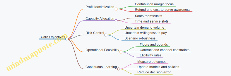
The Core Objectives
Maximize Expected Profit, Not Just Revenue. Revenue management often starts with revenue because it is easy to measure, but profit depends on costs, refunds, and service effort. A $120 booking that triggers heavy variable costs can be worse than a $110 booking with lower cost-to-serve.
Allocate Limited Capacity Intelligently. Capacity is not only seats, rooms, or units. It is also time on a service line, production slots, or bandwidth for delivery. The objective is to reserve capacity for higher-value demand while still selling enough to avoid empty capacity.
Control Risk Under Demand Uncertainty. Demand is uncertain in timing, volume, and willingness to pay. The system should avoid “all-or-nothing” decisions that look great in one scenario and fail badly in another.
Maintain Operational Feasibility. Pricing decisions must respect constraints like minimum margins, contractual rates, channel rules, and inventory availability. A theoretically optimal price that cannot be executed is just a fancy spreadsheet.
Improve Decision Quality Over Time. Objectives include learning from outcomes: if a price change consistently underperforms for a segment, the system should adjust. Learning is not a separate project; it is built into measurement and feedback.
Mind Map: Objectives and How They Connect
From Objectives to Decisions
A useful way to connect objectives to day-to-day decisions is to map each objective to a decision variable.
- Profit Maximization → Price and offer selection. If you can choose between a higher price with lower conversion and a lower price with higher conversion, you are optimizing expected profit.
- Capacity Allocation → Protection levels and inventory controls. You decide how much capacity to hold back for later or for higher-value segments.
- Risk Control → Guardrails and conservative policies. You limit how aggressively you change prices when uncertainty is high.
- Operational Feasibility → Constraints and eligibility logic. You ensure the system only proposes prices that can be honored.
- Continuous Learning → Measurement and feedback loops. You track whether the chosen policy actually performed as expected.
Example: A Simple Booking Scenario
Imagine an airline flight with 100 seats. You can offer two fare classes:
- Saver: $200, expected 60% chance of purchase if offered.
- Flex: $260, expected 35% chance of purchase if offered.
If you sell all seats at Saver, expected revenue is 100 × 0.60 × $200 = $12,000 (ignoring no-shows and assuming demand arrives until seats fill). If you restrict Saver and reserve seats for Flex, you trade off lower probability of selling each seat against higher value when demand is willing to pay.
A revenue-only mindset might chase the highest expected revenue per seat in isolation. A profit-aware mindset checks contribution margin and operational effects. For instance, if Flex bookings have lower refund rates or lower handling costs, Flex can be more attractive even when its raw purchase probability is lower.
Example: Capacity Allocation as a Protection Level
Suppose you expect two demand waves: early bookings are price-sensitive, late bookings are less price-sensitive. A protection level policy might reserve 20 seats for late demand.
- If early demand is strong, you still sell most early seats but stop selling Saver once you reach the protection threshold.
- If early demand is weak, you sell more early seats to avoid empty capacity.
This is risk control in action: you are not guessing one perfect outcome; you are choosing a rule that performs reasonably across multiple demand paths.
Objective Trade-Offs You Must Make Explicit
Revenue management is full of trade-offs, so the objectives should be stated in measurable terms.
- Revenue vs Profit: A higher price can reduce refunds or costs, improving profit even if revenue per seat drops.
- Sell-Through vs Value: Aggressive discounting increases sell-through but can cannibalize higher-value demand.
- Stability vs Responsiveness: Frequent price changes can improve fit but may create operational complexity and customer confusion.
When objectives are explicit, the system can justify decisions. When they are vague, the system becomes a collection of knobs with no clear target.
1.2 Demand Uncertainty and Capacity Constraints
Revenue management lives at the intersection of two realities: demand is not perfectly predictable, and capacity is not perfectly flexible. When you combine those, you get a simple but unforgiving rule—every unit of capacity you allocate today can’t be used later, and every pricing decision changes how many customers show up.
Demand Uncertainty as a Distribution, Not a Number
Instead of treating demand as a single forecast value, treat it as a range of outcomes. For a given time window (say, the next 14 days), demand might be 90, 110, or 140 units depending on seasonality, marketing effects, competitor actions, and random variation.
A practical way to think about this is: you choose a price, which influences demand, and then demand realizes from a distribution. Uncertainty matters because the “best” price under the average outcome can be worse under the tails.
Example: A hotel sets a nightly price for a weekend. If the price is too low, demand spikes and rooms sell out early, leaving later high-value demand unserved. If the price is too high, you may leave rooms empty, and empty rooms are lost revenue.
Capacity Constraints as a Hard Budget
Capacity constraints are usually modeled as a finite number of sellable units. The constraint is hard: you can’t sell more rooms than you have, and you can’t retroactively create capacity after the booking window closes.
There are two common forms of capacity constraints:
- Total capacity over a period: e.g., 500 seats available for a flight.
- Capacity by resource type: e.g., rooms by room type, or inventory by SKU and location.
When capacity is hard, the system must decide not only “what price should I offer,” but also “how much of my capacity should I reserve for later or for higher-value customers.”
The Booking Horizon and Time Coupling
Demand uncertainty is coupled across time. Early bookings reduce remaining capacity for later dates. That means your decision today affects the feasible set of decisions tomorrow.
A useful mental model is a booking horizon with a remaining inventory state. Each booking event updates the state, and future prices should be computed from the updated state.
Example: If you accept many low-fare bookings early, you may be forced to offer lower prices later because you still need to clear remaining inventory. If you protect capacity early, you can maintain higher prices later, but you risk unsold capacity if demand doesn’t materialize.
Protection Levels and Marginal Value
Protection levels convert uncertainty into a rule. The idea is to reserve some capacity for scenarios where demand is strong or customers are willing to pay more.
A common approach is to compare the expected value of selling one more unit now versus saving it for later. If the expected marginal value of selling now is lower than the value of keeping capacity, you protect.
Example: Suppose you have 100 seats. If you expect that later demand will likely support a higher fare, you might protect 20 seats. When a booking request arrives, you accept only if the fare exceeds the implied value of the protected seats.
Modeling Demand Under Capacity Limits
Demand models must respect capacity. If your demand model predicts 140 bookings for a 100-seat flight, the system can’t accept all 140. The accepted demand becomes the minimum of demand and remaining capacity.
This matters for evaluation. If you compute revenue using unconstrained demand, you’ll overestimate performance. You need constrained simulation or constrained optimization.
Example: A pricing policy might look great in a spreadsheet that assumes all demand converts. In reality, once capacity is exhausted, additional demand is lost. Your evaluation must include the “sell-out” behavior.
Practical Best Practices for Handling Uncertainty
- Use scenario-aware forecasts: Maintain multiple demand scenarios (low, base, high) rather than a single point estimate. Then compute expected outcomes across scenarios.
- Track uncertainty by segment: Uncertainty is not uniform. A last-minute business segment might be more predictable than a leisure segment that depends on travel plans.
- Update beliefs with new data: As the booking window progresses, observed bookings reduce uncertainty. Your system should incorporate this update rather than sticking to a static forecast.
- Separate demand drivers from capacity effects: Capacity changes acceptance rates, which can look like demand changes. Keep these effects distinct in your measurement.
Mind Map: Demand Uncertainty and Capacity Constraints
Worked Mini-Example with Constraints
Assume 10 units of capacity and two price options.
- Price A: expected demand 8 units, but could be 5–11.
- Price B: expected demand 6 units, but could be 3–9.
If you ignore capacity, Price A seems better because its average demand is higher. With capacity, the high-demand tail for Price A causes sell-out, and the low-demand tail leaves units unused. Price B may yield steadier accepted volume, which can translate into higher expected revenue when the marginal value of late capacity is high.
The key point is not which price wins in this toy example; it’s that capacity converts demand uncertainty into a nonlinear outcome. Your algorithm must model both the distribution of demand and the hard cap on accepted units.
1.3 Price Elasticity and Revenue Sensitivity Concepts
Price elasticity tells you how much demand changes when price changes. Revenue sensitivity tells you how revenue responds to that same price move. They’re related, but not identical: elasticity is about quantity, sensitivity is about money.
Elasticity Basics Without the Math Panic
Elasticity is usually expressed as a ratio of percentage changes. If price goes up by 1% and quantity drops by 2%, demand is more elastic than if quantity drops by only 0.5%. In practice, you’ll estimate elasticity from historical data or experiments, then use it to reason about pricing moves.
A key sign convention: demand typically falls when price rises, so elasticity is often negative. Many teams use the absolute value for “how responsive” and keep the sign implicit.
Point Elasticity Versus Average Elasticity
Point elasticity describes responsiveness at a specific price level. Average elasticity summarizes across a range, which can hide important curvature. For example, a product might be fairly inelastic near the current price but elastic at higher prices where customers switch to alternatives.
The Demand Curve Shape Matters
Elasticity changes as you move along the demand curve. Near the steep part of the curve, small price changes can cause large quantity shifts. Near the flat part, quantity barely moves. This is why “one elasticity number” can be misleading if your pricing policy makes large jumps.
Revenue Sensitivity: When Quantity Loss Beats Price Gain
Revenue is price times quantity. If you raise price, revenue increases only if the quantity loss is not too large. A useful intuition: revenue is most sensitive when demand is near the boundary between “price wins” and “quantity wins.”
A Simple Rule of Thumb
For many smooth demand relationships, revenue tends to increase with price when demand is relatively inelastic and decrease with price when demand is relatively elastic. The exact threshold depends on how elasticity is defined and how the demand curve behaves, but the practical takeaway is consistent: elasticity magnitude determines whether price increases are likely to help or hurt revenue.
Local Sensitivity Versus Global Outcomes
Revenue sensitivity is local: it describes what happens for small changes around the current price. If you plan to move price a lot, you need to consider how elasticity changes across the range, not just at one point.
Connecting Elasticity to Revenue with Concrete Examples
Example: A Subscription with Low Elasticity
Suppose a subscription costs $20/month. Historical data suggests that a 1% price increase reduces monthly subscribers by about 0.3% (absolute elasticity 0.3). If you raise price by 1% to $20.20, revenue per month changes approximately by +1% from price and −0.3% from quantity, netting about +0.7% revenue. The quantity loss is small enough that price gain dominates.
Example: A Ticketed Event with Higher Elasticity
Now consider event tickets. If a 1% price increase reduces attendance by 1.6% (absolute elasticity 1.6), then the −1.6% quantity effect outweighs the +1% price effect. Revenue would likely drop for small price increases. This doesn’t mean “never raise price,” but it signals that you should expect revenue to be fragile around the current price.
Example: Elasticity Differences Across Segments
Elasticity is rarely uniform. Business travelers might have low elasticity because they value schedule certainty, while leisure customers might have higher elasticity because they can wait for discounts. If you average elasticity across both groups, you can end up with a policy that looks reasonable on paper but underperforms because one segment is harmed more than the other benefits.
Estimating Elasticity in a Way That Supports Decisions
Elasticity estimates are only useful if they match the decision you’re making.
Observational Estimation Pitfalls
If price changes are correlated with demand shocks (for example, you raise price during high-demand periods), naive estimates can confuse “demand caused by seasonality” with “demand caused by price.” A good best practice is to control for time effects, promotions, and availability so the remaining variation is closer to price-driven.
Experiment-Based Estimation
When you run a controlled test, you can compare demand under different prices while holding other factors steady. Even then, be careful about eligibility rules: if only certain users see the price, your elasticity is conditional on that selection.
Mind Map: Price Elasticity and Revenue Sensitivity
Practical Checklist for Using Elasticity
- Use elasticity that matches your price move size: local estimates for small adjustments, curve-aware reasoning for larger ones.
- Keep segment-level elasticity when segments have different behaviors; averages can mislead.
- Verify that your estimation controls for promotions, time effects, and availability so price effects aren’t mixed with other drivers.
- Translate elasticity into revenue sensitivity using the “price gain versus quantity loss” intuition, then sanity-check with a small numerical scenario.
Quick Numerical Sanity Check
If you’re unsure whether a price increase helps, do a one-line calculation: assume a 1% price increase causes an x% quantity decrease where x is the absolute elasticity. Net revenue change is roughly +1% − x%. If that number is negative, revenue is likely to fall for small increases; if positive, it’s likely to rise.
1.4 Data Requirements for Pricing and Yield Systems
Pricing and yield algorithms are only as good as the inputs they trust. This section lays out what data you need, why each piece matters, and how to structure it so decisions can be made consistently in real time.
What “Good Data” Means for Pricing
For pricing and yield systems, “good” usually means three things: (1) the data describes the decision context accurately, (2) it is aligned in time so the model sees what the decision-maker saw, and (3) it can be audited after the fact.
A simple test: pick one offer shown to a customer, then trace backward to the exact features used and forward to the outcome. If you cannot reconstruct that chain, you will struggle to debug revenue dips or explain why a policy changed.
Core Data Domains
Demand and Outcome Signals
You need outcomes that reflect customer response and inventory consumption.
- Impressions or offer exposures: when an offer was eligible and shown.
- Selections or bookings: what the customer chose, including “no purchase” when available.
- Cancellations and refunds: revenue is not final until these are settled.
- Time stamps: offer time, decision time, booking time, and cancellation time.
Easy example: a hotel shows two room rates. If you only log bookings, you miss that the cheaper rate was shown but not chosen. That missing “no” is often the difference between learning and guessing.
Inventory and Capacity State
Yield systems require a precise view of what can still be sold.
- Capacity by resource: rooms, seats, inventory units.
- Availability by time window: how many units remain for each stay date or departure.
- Release and hold rules: when inventory becomes sellable and when it is reserved.
- Overbooking policy parameters: limits and risk thresholds.
Easy example: if 10 seats remain but your system thinks 12 do, your algorithm will happily sell too much and then scramble later.
Offer Catalog and Eligibility Rules
Pricing decisions depend on what offers are allowed.
- Offer definitions: price, included terms, restrictions, and validity.
- Eligibility logic: channel, customer segment, geography, device, loyalty status.
- Lifecycle events: when an offer is created, updated, paused, or retired.
Easy example: if a promotion ends at 18:00 but your data still marks it active until midnight, you will attribute demand lift to the wrong policy.
Customer and Context Features
Features describe who the customer is and what situation they are in.
- Customer attributes: segment, loyalty tier, historical behavior.
- Session context: device, channel, referrer, search parameters.
- Temporal context: day of week, lead time, holiday flags.
- Geographic context: origin market, region, currency.
Easy example: lead time is not just “days until travel.” It must be computed consistently from the same time basis used in the decision.
Cost and Margin Inputs
If you optimize margin, you need cost to go with revenue.
- Variable costs: per unit sold, per booking, per service.
- Semi-variable costs: costs that scale with volume but not perfectly linearly.
- Refund and chargeback costs: expected impact on contribution.
- Ancillary costs and fees: what you keep versus what you pass through.
Easy example: a low ticket price might still be profitable if the average cost is lower for that route or customer segment.
Data Quality Requirements That Prevent Silent Failures
Time Alignment and Event Ordering
Every training row should represent a decision at a specific time with a specific inventory state. If you join data by date only, you will mix “before” and “after” outcomes.
Consistent Identifiers and Join Keys
Use stable keys for customers, offers, inventory units, and transactions. If offer IDs change between systems, you will lose the ability to compare policies.
Coverage of the “No Decision” Case
You need a way to record when no offer was shown or when a customer was not eligible. Otherwise, the model learns that “missing” means “no demand,” which is rarely true.
Mind Map: Data Requirements for Pricing and Yield Systems
Example: Building a Single Training Row
Suppose you price a flight for a customer searching 30 days before departure.
- Decision time: record the exact moment the offer was generated.
- Inventory state: record remaining seats for that departure date and fare family.
- Offer details: record the exact price and restrictions shown.
- Customer context: record segment, channel, and lead time computed from the same time basis.
- Outcome: record whether the customer booked, and if so, capture cancellation later.
- Margin: attach expected variable cost and refund impact for that itinerary class.
If any of these fields are missing, you either drop the row or mark it explicitly. Dropping without tracking can bias results toward “easy” cases.
Practical Data Schema Checklist
- Event tables: offers shown, offers eligible, bookings, cancellations.
- State tables: inventory snapshots keyed by resource and time window.
- Reference tables: offer catalog, eligibility rules, cost tables.
- Feature store outputs: versioned features tied to decision timestamps.
- Decision logs: what the system recommended and what was actually served.
A pricing system is a chain. Data requirements are about making every link measurable, joinable, and explainable—so the algorithm can learn from reality instead of guessing at it.
1.5 Practical Example: Mapping Goals to Metrics
A revenue management system usually starts with a goal that sounds simple, like “maximize profit” or “improve fill rate.” The hard part is translating that goal into metrics that (1) can be measured reliably, (2) move when the pricing policy changes, and (3) don’t accidentally reward the wrong behavior. This example walks through a complete mapping from goals to metrics for a seat-based travel product.
Step 1: Write Goals in Decision Language
Assume the business goal is: increase contribution margin per departure while keeping customer experience stable. Break it into decision-relevant subgoals:
- Sell more seats at acceptable prices without exhausting inventory too early.
- Avoid selling at prices that are too low relative to variable costs and expected future demand.
- Prevent customer-visible issues like excessive price changes on the same itinerary.
Each subgoal should correspond to a lever the system can control: offer prices, offer eligibility, and booking limits.
Step 2: Choose Metric Families That Cover the Whole Loop
Use three metric families so you can see whether the system is winning for the right reasons.
- Outcome metrics measure what happened.
- Mechanism metrics measure how the system behaved.
- Guardrail metrics measure what must not degrade.
Here is the mapping for our example.
-
Outcome goal: contribution margin per departure
- Primary metric: contribution margin = (ticket price − variable cost − per-booking fees) × accepted bookings
- Secondary metric: margin per available seat (MPAS)
-
Outcome goal: sell more seats
- Primary metric: load factor (accepted bookings / available seats)
- Secondary metric: booking rate by time-to-departure bucket
-
Outcome goal: avoid too-low sales
- Primary metric: realized average price (or realized yield)
- Secondary metric: share of bookings in “low-price” bands
-
Guardrail goal: stable customer experience
- Primary metric: price change frequency for the same itinerary within a window
- Secondary metric: cancellation or refund rate attributable to price dissatisfaction signals (measured carefully)
-
Guardrail goal: operational safety
- Primary metric: offer rejection rate due to constraint violations
- Secondary metric: latency and decision failure rate
Step 3: Define Metrics with Clear Numerators and Denominators
Ambiguity is where good intentions go to die. For each metric, specify exactly what counts.
- Load factor: accepted bookings / total sellable seats for that departure.
- Realized average price: sum of accepted ticket prices / accepted bookings.
- Low-price band share: accepted bookings with price < threshold / accepted bookings.
- Price change frequency: number of distinct price updates shown to customers for an itinerary / number of itinerary views in the same window.
Pick thresholds using business policy, not vibes. For example, “low-price band” might be defined as below the variable-cost-plus-min-margin floor.
Step 4: Add a Small Example with Numbers
Suppose a departure has 100 seats. Over the booking horizon, the system accepts 78 bookings.
- Average accepted ticket price: 220
- Variable cost per booking: 60
- Per-booking fee: 5
Contribution margin = (220 − 60 − 5) × 78 = 155 × 78 = 12,090.
Now compare two pricing policies:
- Policy A: 78 bookings, realized average price 220 → margin 12,090
- Policy B: 80 bookings, realized average price 210 → margin = (210 − 65) × 80 = 145 × 80 = 11,600
Policy B sells more but earns less margin. That’s why you need both outcome and mechanism metrics: load factor alone would have picked the wrong winner.
Step 5: Mind Map of the Mapping Process
Mind Map: Mapping Goals to Metrics
Step 6: Sanity Checks Before You Trust the Metrics
Before running a full policy comparison, verify three things:
- Metric sensitivity: when you change the pricing policy in a controlled way, the metric moves in the expected direction.
- Metric integrity: the metric can be recomputed from logs without missing fields.
- Metric alignment: improving one metric doesn’t systematically worsen a guardrail.
If a metric fails any of these, it’s not “wrong” forever, but it is not ready to be a decision driver yet. In practice, this step prevents the system from optimizing a scoreboard that doesn’t match the business goal.
2. Pricing Data Engineering and Feature Construction
2.1 Event and Transaction Data Modeling for Pricing
Pricing systems live or die by the quality of their inputs. “Modeling” here means turning raw logs into a consistent set of entities, events, and measurements that can be joined, replayed, and audited. The goal is simple: every decision the system makes must be explainable in terms of what it knew at the time.
Start with the Decision Loop
A pricing decision usually follows this loop: an offer is shown, a user responds, and the system updates future decisions. To model this cleanly, define a decision timestamp and treat everything after it as outcome data.
Key modeling rule: store the decision context separately from the outcome. For example, the offer shown at 10:03:12 should not silently change if the user’s later session attributes are corrected.
Define Core Entities
Most pricing domains can be represented with a small set of entities.
- Subject: the thing being priced (seat, room night, SKU, subscription term).
- Customer: the identity or anonymous key used for segmentation.
- Channel: where the offer is surfaced (web, app, call center).
- Offer: the concrete price and terms presented (price, currency, fees included/excluded, restrictions).
- Transaction: the completed purchase or booking, including quantity and final paid amount.
Each entity needs a stable identifier and a time window. If you cannot define the window, you will eventually join the wrong facts.
Model Events with Clear Semantics
Events are what happened, in order. For pricing, you typically need:
- Offer Display Event: when an offer becomes eligible and is actually shown.
- Offer Interaction Event: clicks, add-to-cart, selection, or quote requests.
- Offer Acceptance Event: the moment the user commits to the offer terms.
- Transaction Completion Event: payment success, booking confirmation, or fulfillment start.
- Cancellation or Refund Event: reversals that affect realized margin.
A practical best practice is to attach a decision_id to each offer display and interaction. That way, you can trace outcomes back to the exact pricing logic that produced the offer.
Separate Offer Terms from Price Numbers
Offers are more than a single price. Two offers with the same price can differ in fees, cancellation rules, or included taxes. Model:
- Price components: base price, taxes, service fees, discounts.
- Terms: refundability, minimum stay, inventory rules.
- Eligibility: which segments and channels can see it.
Example: A hotel might show “$200 + $25 service fee” versus “$225 all-in.” If you store only one paid amount, you lose the ability to compute margin correctly when costs attach to specific components.
Build a Transaction Fact Table
A transaction fact table should represent realized outcomes, not just intent. Include:
- transaction_id
- subject_id and quantity
- final_paid_amount and currency
- cost components used for margin (variable fulfillment cost, payment processing, support cost)
- status (completed, canceled, refunded)
- timestamps (created, completed, refunded)
Then link it to the offer via offer_id or decision_id. If you only link by customer_id and time proximity, you will eventually misattribute outcomes.
Handle Time Zones and Late Arrivals
Pricing logs often arrive late due to buffering, retries, or batch exports. Use two timestamps:
- event_time: when the event occurred.
- ingest_time: when it was recorded.
For joins, prefer event_time for business logic and ingest_time for pipeline correctness. Also normalize time zones at ingestion so “10:00” means the same moment across systems.
Mind Map: Data Model for Pricing
Example: Joining Offer Displays to Realized Margin
Suppose a pricing service generates an offer for a seat. You store an offer_display event with decision_id, subject_id, and price components. Later, the transaction completes and you store final_paid_amount plus costs.
To compute realized margin for that decision, join:
- offer_display (decision_id, subject_id, event_time)
- transaction_facts (decision_id or offer_id, status, completion_time)
- cost components (variable_cost, processing_fee)
Then calculate margin as: final_paid_amount − variable_cost − processing_fee − refunds_adjustment. If a refund event arrives later, update the adjustment using refund timestamps, not the original completion timestamp.
Example: Preventing “Context Drift”
A common failure mode is recomputing features after the fact. If you store only raw customer attributes and rebuild features later, you might change the offer context for past decisions.
Best practice: snapshot the feature set used for the decision (or at least the key features) alongside decision_id. Then your audit trail can answer: “What did the system know when it chose this price?”
Validation Checklist for Modeling
Before you trust any pricing algorithm, validate the data model with checks that catch structural issues:
- Every offer_display has a decision_id.
- Every transaction links to exactly one accepted offer (or has a defined attribution rule).
- Currency is consistent within a transaction fact.
- Refunds and cancellations reduce realized margin using event_time ordering.
- No joins rely on “nearest timestamp” without an explicit rule.
When these constraints hold, your pricing analytics stop being a guessing game and become a measurable system.
2.2 Building Customer, Segment, and Channel Features
Good pricing decisions depend on features that describe who the customer is, what they are likely to do, and how they arrived. This section builds those features in a way that stays consistent from data collection to model input.
Customer Identity Features
Start with stable identifiers and basic behavioral summaries. Use them to create features that are meaningful even when some events are missing.
- Customer tenure: days since first purchase or first account creation.
- Recency: days since last purchase or last meaningful interaction.
- Purchase history counts: number of orders in the last 30/90/180 days.
- Typical basket size: rolling average of order value, plus a count of orders used to compute it.
- Product affinity: share of purchases in the last 90 days that belong to each major category.
Best practice: compute rolling windows with explicit denominators. For example, “average order value last 90 days” should also carry “number of orders last 90 days,” so the model can treat sparse customers differently.
Example: A customer with one order in the last 90 days gets a less confident “typical basket size” than a customer with 20 orders. The second feature (order count) lets the model learn that difference.
Segment Features That Generalize
Segments are not just labels; they are structured summaries that reduce noise. Build segments using rules that match how demand differs.
Common segment dimensions:
- Value tier: based on lifetime spend or average margin contribution.
- Engagement tier: based on browsing or search activity frequency.
- Price sensitivity proxy: based on historical response to discounts.
- Risk tier: based on refund rate, chargebacks, or cancellation frequency.
Best practice: keep segment definitions versioned. If you change the rule that defines “value tier,” you must know which definition was used for each training row.
Example: If “value tier” is defined by lifetime spend thresholds, store both the tier and the raw lifetime spend. The tier helps generalization; the raw value preserves ordering within tiers.
Channel Features That Explain Context
Channel features capture the path to the offer, which often changes both intent and constraints.
Channel dimensions to model:
- Acquisition channel: organic search, paid search, email, affiliate, direct.
- Device and platform: mobile web, iOS app, Android app, desktop.
- Session context: landing page type, referrer category, campaign identifier.
- Fulfillment context: delivery speed selection, pickup vs delivery.
Best practice: separate “channel” from “campaign.” Campaign identifiers can be sparse and short-lived; channel is usually more stable. When you include campaign, also include channel so the model can fall back when campaign data is missing.
Example: Two customers both arrive via “email,” but one is from a “10% off” campaign and the other is from a “back in stock” message. Channel features describe the shared baseline; campaign features describe the specific incentive.
Feature Engineering with Guardrails
Pricing features often fail in predictable ways: leakage, inconsistent timestamps, and mixing training and serving logic. Use these guardrails.
- Timestamp discipline: every feature must be computed using events strictly before the decision time.
- Missingness as information: include explicit flags like “no recent purchases” rather than imputing silently.
- Scale consistency: normalize continuous features (e.g., log-transform order value) and keep the same transformation at training and serving.
- Cardinality control: for high-cardinality fields (e.g., campaign id), use hashing or target-encoding with careful leakage prevention.
Example: If you compute “orders in last 30 days” at training time using the full dataset, you may accidentally include orders that happened after the price was shown. The fix is to compute features from an event stream with a strict cutoff at the decision timestamp.
Mind Map: Customer, Segment, and Channel Features
Practical Example: One Offer, Three Feature Views
Suppose you show a discount offer for a product category. Build three aligned feature sets for the same decision time.
- Customer view: recency, last 90-day category affinity, and order count in the last 90 days.
- Segment view: value tier and price sensitivity proxy derived from historical discount response.
- Channel view: acquisition channel, device type, and fulfillment context.
Then add guardrail features: a missingness flag for “no orders in last 90 days,” and a “feature computed from available history length” indicator. This makes the model robust when customers are new or when event logs are incomplete.
The result is a feature design that is interpretable, consistent, and resilient. It also gives the model multiple ways to explain demand differences without forcing one brittle definition to do all the work.
2.3 Handling Inventory, Availability, and Offer Lifecycles
Inventory and availability are the “what can be sold” layer, while offer lifecycles are the “how and when it can be sold” layer. If you treat them as one thing, you’ll eventually sell the wrong thing at the wrong time. The goal is to keep these concepts separate in your system design and then connect them with clear rules.
Inventory as State, Not a Number
Start with inventory as a state machine. A seat, room, or unit is either available, reserved, sold, or blocked. The system should track transitions, not just a remaining count. For example, a flight seat might be:
- Available: eligible for offers.
- Reserved: held for a user session or payment window.
- Sold: committed and no longer eligible.
- Blocked: unavailable due to operational reasons (crew changes, maintenance, manual holds).
Best practice: represent inventory events (reserve, release, sell, block) as append-only logs, then compute current availability from those events. This makes debugging far less painful than trying to infer history from a single number.
Availability as Eligibility Logic
Availability answers: “Given the current inventory state, which offers are eligible for a given user and context?” Eligibility depends on more than remaining units. It typically includes:
- Time windows: booking open/close, cutoff times, check-in deadlines.
- Channel rules: direct vs. partner access, contract restrictions.
- Offer validity: start/end timestamps, minimum stay or length-of-use.
- Segment constraints: age bands, membership tiers, corporate agreements.
Easy example: Suppose a hotel has 10 rooms. If 3 are reserved for a group that only accepts refundable rates, then the remaining 7 rooms may still not be eligible for a nonrefundable offer if the offer requires a specific cancellation policy.
Offer Lifecycles as Controlled Lifetimes
An offer is a priced, bookable option with a defined lifetime. Offers should not live forever, even if inventory does. Common lifecycle stages:
- Draft: computed but not yet shown.
- Published: visible to users and eligible for selection.
- Committed: selected and payment is underway.
- Expired: lifetime ended without commitment.
- Superseded: replaced by a newer offer due to inventory or price updates.
Best practice: tie offer expiration to both time and state changes. If inventory changes materially (e.g., a unit is sold elsewhere), mark affected offers as superseded immediately rather than waiting for their timer.
Reservation Windows and Consistency
Reservations prevent overselling during the gap between “user clicks” and “payment confirms.” The tricky part is consistency across services.
A practical approach:
- When an offer is selected, create a reservation with an expiration timestamp.
- Lock the reservation to the exact inventory unit(s) or to a capacity bucket with a clear reconciliation rule.
- If payment fails or the reservation expires, release inventory back to availability.
Example: A booking request arrives at 10:00:05. You reserve capacity for 90 seconds. If payment confirms at 10:01:20, the reservation becomes a sale. If it confirms at 10:02:10, the reservation has expired, so the system must reject or reprice.
Handling Cancellations and Repricing Safely
Cancellations create new inventory, but they also create new opportunities for offers. The safe rule is: inventory release should trigger availability recomputation, and availability recomputation should trigger offer refresh only for impacted segments.
Example: If a cancellation returns 1 seat to a fare family, you may need to:
- Update the remaining capacity for that fare family.
- Recompute bid prices or protection levels for the affected time bucket.
- Invalidate offers that depended on the previous capacity.
Do not silently keep old offers active. Users will notice when the system “accepts” a selection and then fails at confirmation.
Mind Map: Inventory, Availability, and Offer Lifecycles
Example: End-to-End Flow for a Single Offer
Consider a train ticket offer for a specific departure date.
- Compute eligibility: check booking window, channel access, and segment constraints.
- Check inventory state: confirm capacity is available for the relevant fare bucket.
- Publish offer: assign a price and an expiration time (e.g., 2 minutes).
- User selects: create a reservation tied to the offer and inventory bucket.
- Payment confirms: convert reservation to sold and finalize the booking.
- Payment fails or expires: release reservation and mark the offer expired.
- Concurrent updates: if another sale reduces capacity before confirmation, supersede the offer so the user must see updated eligibility.
This flow keeps the system honest: inventory changes drive availability, availability drives offer eligibility, and offer lifecycles control what users can actually do at any moment.
2.4 Data Quality Controls for Real Time Pricing Inputs
Real time pricing decisions are only as good as the inputs they consume. In practice, “data quality” means more than accuracy; it includes timeliness, completeness, consistency, and whether the data matches the decision being made. This section lays out a systematic control stack that starts with basic checks and ends with decision-time safeguards.
Data Quality Goals for Pricing Decisions
A pricing engine typically needs features such as availability, demand signals, customer context, and offer eligibility. Quality controls should therefore target four failure modes:
- Wrong value: a feature is incorrect (e.g., inventory shows 12 when 2 are actually sellable).
- Missing value: a feature is absent (e.g., channel is null, so eligibility rules can’t run).
- Stale value: a feature is old (e.g., inventory updated 30 minutes ago but the decision is now).
- Inconsistent meaning: the same field is interpreted differently across systems (e.g., “booking date” means local time in one pipeline and UTC in another).
A useful mindset is to treat each feature as having a “contract”: what it represents, its allowed range, its freshness expectation, and how it should be handled when it fails.
Foundational Checks Before Any Modeling
Start with checks that are cheap and deterministic.
Schema and type validation ensures the incoming payload matches expectations. For example, if price_floor arrives as a string instead of a number, the engine should fail fast or coerce safely.
Range and constraint checks catch impossible values. If availability can’t be negative, enforce availability >= 0. If lead time is computed from timestamps, enforce lead_time_minutes >= 0.
Completeness checks verify required fields exist for the decision path. If the pricing policy depends on customer_segment, then missing segment should trigger a defined fallback segment or a “no-offer” response.
Freshness checks compare event timestamps to the decision timestamp. A practical rule is to define a maximum acceptable delay per feature. Inventory might tolerate seconds; a weekly promotion flag might tolerate hours.
Consistency Controls Across Systems
Consistency problems are subtle because each system can be “correct” locally.
Key alignment ensures joins use the same identifiers. A classic failure is joining by product_id in one table and sku_id in another, producing silent mismatches.
Time zone normalization prevents off-by-one-day errors. If a booking window is defined in local time, convert all timestamps into that same frame before computing lead time or cutoff eligibility.
Unit normalization avoids mixing currencies, weights, or quantities. If costs are stored in cents but revenue features are in dollars, you’ll get confidently wrong margins.
Decision-Time Guardrails
Even with pipeline controls, you still need safeguards at the moment of decision.
Eligibility gating should be the first step. If required inputs fail validation, do not attempt to optimize; instead, apply a conservative policy such as returning the last known safe offer or withholding offers.
Fallback strategies must be explicit and testable. Example: if demand_signal is missing, use a neutral default (e.g., baseline demand index) rather than reusing an old value.
Rate limiting for updates prevents thrashing when upstream systems briefly glitch. If inventory changes by an extreme amount in a short window, clamp the change and log the anomaly.
Logging and Traceability That Actually Helps
Controls without observability are just hope with extra steps.
Log the following for every pricing decision:
- Feature validation outcomes (pass/fail per feature)
- Freshness deltas (how late each feature was)
- Fallbacks used (which defaults were applied)
- The final offer inputs (so you can reproduce the decision)
A simple rule: if you can’t explain why an offer was withheld, you don’t have enough logging.
Mind Map: Data Quality Controls for Real Time Pricing Inputs
Example: Inventory Freshness and Fallback
Suppose an airline pricing request arrives at 2026-02-26 10:05:00 UTC. The pricing engine requires sellable_seats and expects inventory freshness within 60 seconds.
- Upstream inventory timestamp: 10:03:00 UTC
- Freshness delta: 120 seconds
- Validation result: stale inventory
Best practice: do not use the stale value. Instead, apply a fallback such as:
- Use the last inventory snapshot that is within freshness tolerance, if available.
- If none exists, withhold offers for that cabin and log the reason.
This avoids a common failure where the system “works” but sells seats that are already gone.
Example: Unit Normalization for Margin Inputs
A hotel margin policy needs variable cost per booking. Costs arrive from finance in cents, while the pricing engine expects dollars.
- Incoming
variable_cost_cents = 1250 - Engine expects
variable_cost_dollars
Control: enforce a unit contract at ingestion. Convert cents to dollars (12.50) before any margin computation. If conversion is missing, margin optimization can systematically bias prices while still producing plausible numbers.
Example: Consistency Through Time Zone Normalization
A retail promotion ends at 23:00 local time. The promotion service stores timestamps in local time; the pricing engine uses UTC.
Control: normalize both to the same time zone before computing whether the offer is eligible. Without this, customers near midnight can see offers that should have expired, and the engine will “correct” itself later with inconsistent behavior.
Summary of the Control Stack
Use deterministic checks first, then cross-system consistency, then decision-time guardrails, and finally traceability. When each feature has a contract and every failure path is defined, real time pricing becomes predictable in the only way that matters: the system behaves the same way under both normal and messy inputs.
2.5 Practical Example: Designing a Pricing Feature Store
A pricing feature store is the place where raw signals become consistent, reusable inputs for forecasting, optimization, and real time price control. The goal is simple: the same customer, time, and context should produce the same features across teams and systems, with clear freshness rules.
Step 1: Define Feature Contracts
Start with a contract that every downstream model can trust. For each feature, specify: meaning, grain, allowed values, time window, and update cadence.
- Meaning: what the feature measures (e.g., “days until departure”).
- Grain: the unit each row represents (e.g., offer_id × request_time).
- Time window: how far back history is used (e.g., last 7 days).
- Freshness: when the feature becomes valid (e.g., updated every 15 minutes).
Example: If you store days_to_event, compute it at the request timestamp, not at midnight. Otherwise, two requests a few hours apart can disagree.
Step 2: Choose the Store Layout
A practical layout separates features by purpose and update frequency.
- Static attributes: rarely change (e.g., customer tier, route). Update daily.
- Slow changing: update hourly or daily (e.g., rolling average conversion rate).
- Fast changing: update near real time (e.g., current inventory availability, active promotions).
This separation prevents a common failure mode: recomputing everything for every request.
Step 3: Build a Minimal Feature Set First
Resist the urge to store every possible metric. Start with features that map cleanly to pricing decisions.
Core demand context
days_to_eventday_of_weekseason_bucketlead_time_bucket
Offer and channel context
channel_idoffer_typeprice_position_in_ladderis_promo_active
Inventory and availability context
remaining_capacitycapacity_utilizationsold_out_flag
Customer and segment context
segment_idloyalty_statusrecent_purchase_count_30d
Example: For a travel product, capacity_utilization might be sold / (sold + remaining) computed at the same time window as remaining_capacity so the model doesn’t see contradictory signals.
Step 4: Implement Time-Aware Joins
Features often come from different pipelines. The store must join them using the request timestamp.
- Use as-of joins: each feature value must be the latest one not after the request time.
- Apply lookback windows consistently (e.g., “last 14 days” means 14×24 hours ending at request time).
Example: If promotions are logged with start and end times, compute is_promo_active by checking whether request_time falls within the interval.
Step 5: Add Guardrails for Data Quality
Quality checks should run before features are served.
- Schema checks: correct types, no missing required fields.
- Range checks:
days_to_eventmust be non-negative for future events. - Distribution drift checks: detect sudden spikes in missingness.
When a check fails, decide a policy: drop the request, fall back to last known good, or use a default with a “fallback_used” flag.
Mind Map: Pricing Feature Store Design
Step 6: Version Features and Log Decisions
Versioning prevents silent changes from breaking model behavior.
- Feature version: increment when logic changes.
- Model version: record which model consumed which feature version.
- Decision logging: store request context, features used, and chosen price.
Example: If you change capacity_utilization from “sold/(sold+remaining)” to “sold/total_capacity,” you must bump the feature version and keep old values for backtesting.
Step 7: Example Feature Store Schema
A simple schema keeps things understandable.
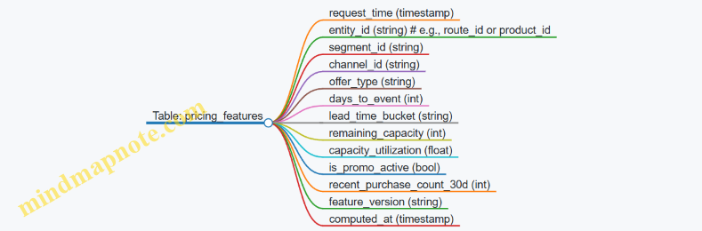
Step 8: End-to-End Example Flow
- A pricing request arrives with
request_time,entity_id,segment_id, andchannel_id. - The store retrieves static, slow, and fast features using as-of logic.
- Guardrails validate ranges and missingness; if needed, a fallback flag is set.
- The pricing model consumes the feature vector and outputs a candidate price.
- The system logs the feature_version and the chosen price for later evaluation.
This workflow makes debugging practical: if revenue drops, you can check whether the feature inputs changed, whether freshness lagged, or whether the model saw a different capacity state.
3. Demand Forecasting for Yield Management
3.1 Forecasting Targets and Granularity Choices
Forecasting starts with two decisions that quietly control everything else: what you forecast (the target) and at what level you forecast it (the granularity). If either is wrong, the model can be perfectly trained and still produce decisions that miss the mark—like measuring a marathon with a ruler.
Define Forecasting Targets
A forecasting target is the quantity your system will use downstream to choose prices, protect capacity, or decide which offers to show. Common targets include:
- Demand volume: expected number of bookings or units sold in a time window.
- Arrival process: expected number of customers arriving per day or per hour.
- Conversion rate: probability an eligible user books given an offer.
- Revenue or margin per booking: expected value conditional on booking.
In yield and dynamic pricing, demand volume and conversion rate are usually the workhorses. Revenue and margin are often computed after the fact using the chosen price and cost rules, because those depend on the decision you’re trying to make.
A practical best practice is to forecast the “decision-relevant” quantity. For example, if your pricing algorithm selects among discrete price points, you typically need demand (or conversion) as a function of price. If you only forecast total revenue historically, you’ll struggle to attribute changes to price versus mix.
Choose Granularity Levels
Granularity is the “where” and “when” of the forecast. Typical axes are:
- Time: day, hour, or booking horizon buckets (e.g., 0–3 days before arrival).
- Customer segment: channel, geography, loyalty tier, device type, or past behavior bucket.
- Product or offer: SKU, fare family, room type, seat bucket, or bundle.
- Channel: direct web, call center, partner marketplace.
The goal is to match granularity to operational control. If your system can only change prices once per day, forecasting hourly demand won’t help much; it may even create noise that looks like signal. Conversely, if you update offers every few minutes, daily granularity can hide short-lived demand spikes.
A useful rule: forecast at the finest granularity you can support with stable data, then aggregate upward for decisions that don’t require finer control.
Mind Map: Target and Granularity Design
Booking Horizon Versus Calendar Time
Many revenue systems forecast by booking horizon—time remaining until the service date—because demand patterns often change as the departure date approaches. Calendar time captures seasonality, but horizon captures urgency and planning behavior.
A systematic approach is to include both:
- Use calendar time features to represent macro effects like weekends.
- Use horizon buckets to represent the “how close are we” effect.
Example: A hotel might see strong weekend demand, but the last 3 days before check-in also behave differently from 30 days out. If you forecast only by calendar day, you’ll mix these effects and force the model to learn a complicated relationship it doesn’t need.
Segment Granularity and Data Sufficiency
Segmenting too aggressively creates sparse data. Sparse data leads to unstable estimates of conversion or demand, which then causes erratic pricing.
A best practice is to start with a segmentation that is both operationally meaningful and statistically supported. For instance:
- If you can route customers by channel, start with channel.
- If you can only observe loyalty tier reliably for returning customers, keep a “known loyalty” bucket and an “unknown” bucket.
Example: Suppose you split web traffic into 20 micro-segments by device and referrer. If each segment has only a few thousand eligible impressions per week, conversion estimates will swing with random variation. A safer approach is to group devices into fewer buckets and keep referrer categories broader.
Target Choice: Volume Versus Conversion
When you have clear eligibility rules (who sees which offer), conversion rate can be more stable than raw demand volume because it factors out exposure.
Example: Two channels may generate the same number of impressions, but one channel’s users are more likely to book. Forecasting conversion rate per channel lets your pricing logic respond to willingness to pay rather than being distracted by differences in traffic volume.
If you forecast volume directly, you must ensure the model accounts for both traffic and conversion. That’s doable, but it increases the number of moving parts.
Evaluation at Multiple Levels
Granularity choices should be validated where decisions happen. Backtesting only at the most aggregated level can hide problems.
Example: A model might predict total bookings correctly for the week, but fail for a specific fare family near the end of the booking horizon. The aggregated metric looks fine, while the protection logic quietly breaks.
A systematic evaluation set includes:
- Accuracy metrics at the decision granularity (e.g., fare family by horizon bucket).
- Calibration checks for conversion probabilities.
- Error decomposition by segment to locate where the model is consistently off.
Practical Example: Designing a Forecasting Setup
Imagine an airline with discrete fare classes and frequent offer updates. A coherent setup is:
- Target: conversion rate per fare class and booking horizon bucket.
- Granularity:
- Time: booking horizon buckets (e.g., 0–3, 4–7, 8–14, 15–30 days).
- Segment: channel (direct vs partner) and a coarse loyalty tier.
- Product: fare class.
Then compute expected bookings by multiplying predicted conversion by eligible impressions (or eligible customer arrivals) for each bucket. This keeps the forecast aligned with what the pricing system actually controls: which fare class is offered and at what price.
The result is a forecast that is not just accurate in hindsight, but useful in the exact places where pricing decisions are made.
3.2 Time Series Models for Booking and Arrival Processes
Booking and arrival processes are time-indexed systems: demand arrives over time, inventory is consumed, and the remaining capacity changes what future demand can do. A good time series model respects three realities: (1) arrivals are not evenly spaced, (2) booking behavior changes as the departure date approaches, and (3) price and availability affect what gets booked, even if you model them separately.
Core Time Axis Choices
Start by deciding what “time” means in your dataset. For bookings, common axes are booking timestamp (when the customer books) and stay/usage start date (when the customer uses the product). For arrivals, you often model the usage start date as the event time.
A practical rule: use one axis for the event you care about (arrival or usage start) and another for the lead time (days before arrival). Lead time is usually the more stable structure because it captures the approach to departure.
Modeling Arrival Counts
Let \( A_t \) be the number of arrivals in time bucket \(t\) (for example, per day). The simplest baseline treats (A_t) as a count process. A Poisson model assumes the variance equals the mean; real booking data usually has extra variance, so a Negative Binomial model is often a better starting point.
Best practice: fit a baseline model per segment or per route/channel, then check residual patterns by lead time. If residuals cluster near the departure date, your model is missing the “last-minute” shape.
Lead Time Effects and Nonstationarity
Booking behavior is strongly nonstationary: early lead times look different from late lead times. Instead of forcing one stationary process across all lead times, represent time as lead time \(L\) and model \(A(L)\) or booking intensity as a function of \(L\).
A simple and effective approach is a two-stage structure:
- Model the arrival intensity by lead time.
- Convert intensity into expected arrivals for each future day.
This keeps the model interpretable and makes it easier to apply booking controls later.
Intensity Models for Booking Curves
Many revenue systems use an intensity view: the probability of a booking happening in a small interval depends on the current lead time and current conditions (like price and remaining inventory). Even if you don’t model inventory directly, you can still model the baseline intensity.
A common form is:
- Expected arrivals in bucket \(t\): \(\mathbb{E}[A_t] = \lambda(t)\)
- Where \(\lambda(t)\) is a smooth function of lead time and calendar features.
Calendar features matter because demand has weekly and seasonal cycles. Include day-of-week and holiday indicators, and treat them as exogenous inputs rather than letting the model “discover” them from noise.
Seasonality and Calendar Features
Seasonality can be handled with either explicit features or seasonal components. Explicit features are often easier to debug:
- Day of week (categorical)
- Month or week-of-year (categorical or cyclic)
- Holiday flags
- Local events if you have them
Best practice: keep holiday effects separate from general seasonality. Otherwise, the model may smear a sharp holiday spike into nearby days and distort protection levels.
Autocorrelation and Residual Structure
Arrivals are correlated across time buckets because demand is not independent. If you ignore autocorrelation, your forecast intervals will be too narrow and your booking control will be overconfident.
A standard approach is to use autoregressive terms on residuals or to adopt a state-space model. For example, an AR component can capture short-term correlation after accounting for lead time and calendar.
Check this systematically:
- Fit the model.
- Plot residuals by lead time and by calendar position.
- If residuals show a repeating pattern, your seasonality representation is incomplete.
State-Space Models for Evolving Behavior
State-space models represent the system as a hidden state that evolves over time. In booking, the hidden state can represent “current demand level” or “market momentum” after controlling for lead time and calendar.
A useful mental model: the observed arrivals are noisy measurements of an underlying demand state. As new data arrives, the state updates, which naturally supports rolling forecasts.
This is especially helpful when you need forecasts that update frequently during the booking horizon.
Practical Example: Modeling Daily Arrivals by Lead Time
Suppose you forecast arrivals for a product with departure date \(D\). For each historical booking, compute lead time (\(L = D - \text{booking date}\)). Aggregate arrivals by lead time bucket (e.g., 0–6 days, 7–13 days, etc.) and by day-of-week of departure.
Then:
- Fit \(\lambda(L, \text{dow})\) using a Negative Binomial regression.
- Include holiday indicators for departure date.
- Add a small autoregressive correction on daily residuals within each departure day-of-week group.
Finally, generate expected arrivals for each future departure day by summing expected intensity across lead time buckets.
Mind Map: Time Series Modeling for Booking and Arrival Processes
Validation Checklist That Actually Helps
Before you trust the forecast, verify that the model reproduces the booking curve shape. A quick sanity test is to compare predicted and actual arrivals aggregated by lead time buckets. If the model matches the curve but misses day-to-day variation, you can still use it for booking control, provided your uncertainty estimates reflect the remaining variance.
If the model matches day-to-day variation but misses the curve shape, your protection levels will be wrong near the departure date. In that case, fix lead time representation first, then revisit autocorrelation.
Example: A Simple Baseline with Clear Failure Modes
Start with a Negative Binomial regression for arrival counts using lead time buckets and day-of-week of departure. If forecasts systematically underpredict late lead times, add a flexible term for lead time (more buckets or a smooth spline). If forecasts overpredict holiday spikes, separate holiday indicators from general seasonality and refit.
This “fit, inspect, adjust” loop keeps the model grounded in observable structure rather than hoping the algorithm figures out the booking curve on its own.
3.3 Incorporating Price and Promotion Effects in Forecasts
Forecasting demand without accounting for price and promotions is like planning a trip while ignoring traffic lights. You can still arrive, but you’ll keep “mysteriously” missing your timing. This section explains how to incorporate price and promotion effects systematically, from basic modeling choices to practical validation.
Price and Promotion Effects as Forecast Inputs
Start by separating two roles that price and promotions play in forecasting:
- They shift demand: a higher effective price usually reduces quantity demanded, while promotions can increase it.
- They change the composition of buyers: promotions may attract more price-sensitive customers or different purchase timing.
In practice, you need forecast features that represent the effective price customers face at the moment they decide, plus promotion context such as discount depth, duration, and whether the offer is active.
Defining Effective Price and Promotion Variables
Effective price should reflect what the customer actually pays after discounts and fees. A simple example for retail:
- List price: $100
- Coupon: 20% off
- Net price: $80
For forecasting, represent this as a numeric feature (net price) rather than only a “promo yes/no” flag. Promotions also need structure:
- Discount depth: percent off or absolute off
- Promo type: coupon, , bundle, free shipping
- Promo phase: first day, middle, last day
- Promo intensity: discount depth multiplied by availability (if you have it)
If you only have a binary promo indicator, you can still model lift, but you’ll lose the ability to forecast different discount levels accurately.
Modeling Approaches That Work in Real Systems
Use a modeling approach that matches your data and decision granularity.
Baseline Demand Model
First build a baseline that captures non-price effects:
- seasonality (day-of-week, month)
- trend (slow drift)
- calendar effects (holidays)
- channel effects (web vs store)
This baseline should forecast demand when price and promotions are “normal.”
Additive Lift Model
A straightforward method is:
- Forecast = Baseline + Promotion Lift
Price can be included as an additional term, for example:
- Forecast = Baseline + α · (Net Price) + β · (Promo Indicator)
This is easy to interpret, but it assumes linear relationships and can struggle when demand response is nonlinear.
Multiplicative Response Model
A more stable alternative is to model demand as a multiplier:
- Forecast = Baseline × (1 + Promotion Lift Rate)
For price, you can use a log-linear form:
- log(Demand) = baseline terms + γ · log(Net Price) + …
This often behaves better because demand changes tend to scale rather than shift by a constant amount.
Avoiding Common Data Traps
Price and promotions are rarely random. They are often set in response to demand signals, which can bias estimates.
- Confounding by intent: if promotions are triggered when demand is already weak, a naive model may think promotions reduce demand.
- Selection effects: certain segments see different offers, so “promo” is not comparable across customers.
- Stockouts and availability: if items are out of stock during a promo, observed demand won’t reflect the offer’s true effect.
Practical mitigations:
- Include availability indicators or filter out periods with stockouts.
- Use lagged price/promo features when decisions are made before purchase.
- Fit at the right level of aggregation so that price/promo exposure is comparable.
Example: Forecasting with Net Price and Promo Depth
Suppose you forecast weekly units for a product. You have:
- Baseline seasonality already modeled.
- Net price varies due to s.
- Promotions occur for 2 weeks with varying discount depth.
A workable feature set for each week:
- NetPrice
- PromoDepthPercent (0 when no promo)
- PromoWeekIndex (1, 2 during the promo, 0 otherwise)
- DaysSinceLastPromo
- AvailabilityRate
Then you fit a response model where promotion lift depends on depth and phase. For instance, you might find:
- Each additional 5% discount increases units by a smaller amount later in the promo window.
- The first promo week has higher lift because customers notice and act sooner.
This matters because your forecast for a future promo must reflect the phase, not just the discount.
Mind Map: Price and Promotion Effects in Forecasts
Validation That Confirms You’re Modeling the Right Thing
After fitting, validate in ways that directly test price and promo behavior.
- Scenario backtests: compare forecasts under historical promo depths to actual outcomes.
- Residual patterns: check whether errors systematically grow during promo periods or at specific discount levels.
- Stability checks: verify that the model’s response to price doesn’t flip sign when you change aggregation level.
A model that predicts “average lift” but fails at different discount depths is still useful for rough planning, but it will mislead when you need to forecast specific offers.
Practical Integration into the Forecast Pipeline
To keep the system coherent:
- Compute effective price and promo features at the same time granularity as the demand target.
- Ensure the baseline model is trained with consistent definitions of “normal” periods.
- Fit the response layer using the same exposure logic you will use in production.
- Log the exact features used for each forecast so you can reproduce results when a promo changes.
If you do these steps, your forecast becomes a controlled calculation rather than a black box that happens to match last month.
3.4 Calibration and Backtesting for Forecast Reliability
Forecasts are only useful if they behave like the truth when you test them. Calibration answers “are we systematically too high or too low?” Backtesting answers “does the forecast drive good decisions when the world changes?” Together they turn a demand model from a number generator into a decision tool.
Calibration Targets and Error Types
Start by defining what “reliable” means for your use case. For yield management, you usually care about booking volume by time bucket and the implied availability consumption.
Common calibration checks:
- Level calibration: predicted totals match observed totals.
- Distribution calibration: predicted uncertainty bands contain the right fraction of outcomes.
- Segment calibration: errors are not concentrated in one channel or customer group.
Use two complementary error views:
- Point accuracy: compare predicted mean demand to realized demand.
- Probabilistic accuracy: compare predicted quantiles or intervals to realized demand.
A practical rule: if your point forecasts are biased, your optimization will consistently protect too much or too little capacity.
Backtesting Design That Respects Time
Backtesting fails when it accidentally “peeks” at the future. Use a rolling-origin design.
- Choose an evaluation horizon, such as the next 14 days of bookings.
- Pick multiple cutoffs spaced through time, for example weekly.
- For each cutoff, train using only data available up to that cutoff.
- Generate forecasts for the horizon and compare to what actually happened.
This produces a set of forecast errors across time, which you can summarize with stability metrics.
Building a Backtesting Dataset
Your dataset should mirror production inputs. That means the same feature logic, the same price/promo encoding, and the same handling of missing values.
Best practices that prevent silent failures:
- Lock feature definitions: freeze transformations used during training.
- Reproduce availability logic: if inventory constraints affect observed bookings, ensure the model sees the same constraints.
- Separate training and evaluation segments: do not mix post-cutoff outcomes into feature aggregates.
Concrete example: if you compute “recent search volume” using a rolling window, ensure the window ends at the cutoff date for each backtest run.
Calibration Metrics That Actually Help
For point forecasts, use metrics that align with operational decisions.
- MAE for interpretability in units of bookings.
- Weighted MAPE when some buckets matter more, such as near departure.
- Bias as mean(predicted − actual) to detect systematic over/under forecasting.
For probabilistic forecasts, use:
- Coverage: fraction of actuals within predicted 80% or 90% intervals.
- Calibration curves: group predictions by predicted quantile levels and compare empirical frequencies.
If you only track one number, track bias plus coverage. Bias tells you which direction to correct; coverage tells you whether your uncertainty is too tight or too wide.
Correcting Miscalibration Without Breaking the Model
Calibration is not just a report card; it can be a fix.
Two common correction layers:
- Post-hoc bias correction: adjust predicted means by a learned offset per segment or per horizon bucket.
- Uncertainty scaling: widen or narrow prediction intervals using an error-based scale factor.
Example: suppose your model predicts demand too high for last-minute bookings. You can estimate a horizon-specific bias term by averaging residuals for the last 3 days before arrival, then subtract it from future predictions for that horizon.
Keep corrections simple and auditable. Overfitting calibration to a single backtest window is a classic way to get “good-looking” metrics that fail in production.
Mind Map: Calibration and Backtesting Workflow
Example: Rolling Backtest with Horizon Buckets
Assume you forecast daily bookings for the next 7 days. You run backtests with weekly cutoffs for 8 weeks.
For each cutoff:
- Predict bookings for day 1 through day 7.
- Store predicted mean and predicted 80% interval.
After collecting all runs, compute:
- Bias by day: average residual for day 1, day 2, … day 7.
- Coverage by day: fraction of actuals within the 80% interval for each day.
Interpretation example:
- If day 1 bias is +6 bookings and day 1 coverage is 90%, your model is too high and also too uncertain. Bias correction should reduce the mean; uncertainty scaling should narrow intervals.
- If bias is near zero but coverage is 60%, your mean is fine but your uncertainty is too optimistic. Increase interval width.
Example: Decision-Linked Backtesting
Forecast reliability matters because it feeds optimization. A forecast that is “accurate” by MAE can still cause poor capacity decisions.
To connect forecasts to decisions:
- For each backtest cutoff, run your booking control policy using the forecast.
- Compare realized outcomes to a baseline policy.
- Track decision quality metrics such as accepted bookings vs. lost sales, and margin impact if costs vary.
This catches cases where errors cancel out numerically but still shift the timing of protection levels.
Practical Checklist for Reliability
- Use rolling-origin backtests with fixed horizons.
- Ensure feature and availability logic match production.
- Track bias and coverage by horizon bucket.
- Apply minimal correction layers when calibration fails.
- Validate that decision-linked backtesting improves outcomes, not just forecast metrics.
When calibration and backtesting agree—errors are small, intervals contain the right outcomes, and decisions improve—you can trust the forecast enough to optimize with confidence.
3.5 Practical Example: Forecasting Demand Under Multiple Price Scenarios
A good demand forecast for dynamic pricing answers one question: “If we change the price, what happens to bookings or sales volume, and how does that ripple through inventory and time?” This example builds that capability step by step, using a small but realistic workflow.
Step 1: Define the Decision Set and the Time Grain
Pick a time grain that matches how you sell. Suppose you sell seats for a route with departures every day. You decide prices once per day for the next 14 days.
Create a price scenario table for each day t:
- Scenario A: Keep current price
- Scenario B: Reduce price by 5%
- Scenario C: Increase price by 5%
Best practice: keep scenarios small and interpretable. A 5% move is large enough to measure, but not so large that demand behavior changes in weird ways.
Step 2: Choose the Demand Target and the Modeling Form
Let y(t) be daily demand (bookings) for a given segment, say “business travelers.” You also track price p(t) and a few drivers that affect demand regardless of price: day-of-week, lead time, and a simple availability proxy.
A practical modeling form is a log-linear response:
- log(E[y(t)]) = β0 + βp log(p(t)) + βdow[dow(t)] + βL leadTime(t) + βa availability(t)
Why this works well in practice: the coefficient βp behaves like an elasticity. If βp is -1.2, then a 1% price increase reduces expected demand by about 1.2% (before accounting for other terms).
Step 3: Fit the Model on Historical Data with Consistent Features
Use historical days where you know the realized price and the same feature set. Ensure that availability(t) is computed the same way as in production; otherwise the model learns a mismatch.
Guardrails that prevent silent errors:
- Normalize or cap extreme prices before log transforms
- Encode day-of-week consistently
- Use the same segment definition as your pricing policy
Step 4: Generate scenario-specific forecasts
For each future day t and each scenario s, compute the scenario price p_s(t). Then plug p_s(t) into the model while holding non-price features fixed at their forecasted or planned values.
Concretely, for each scenario s:
- Compute log(p_s(t))
- Compute the linear predictor η_s(t)
- Convert to expected demand E[y_s(t)] = exp(η_s(t))
Best practice: treat non-price drivers as “common inputs” across scenarios. If you let them vary too, you can’t tell whether demand changes came from price or from something else.
Step 5: Convert Demand Forecasts into Booking Curves
If your system uses yield management, you need cumulative demand over time. For each scenario, compute cumulative expected bookings up to day k:
- C_s(k) = Σ_{t=1..k} E[y_s(t)]
Then compare C_s(k) to capacity to understand how quickly you’ll fill.
Step 6: Evaluate Scenario Outcomes with a Simple Profit Lens
Even if the chapter focus is forecasting, you should sanity-check the direction using margin.
Assume a seat sells at price p and has variable cost c per seat. Expected contribution for scenario s over the horizon is:
- Profit_s = Σ_t E[y_s(t)] · (p_s(t) - c)
This is not the final optimization, but it catches modeling mistakes. If a higher price scenario predicts both higher demand and higher profit, you should verify the elasticity sign and feature handling.
Mind Map: Forecasting Demand Under Multiple Price Scenarios
Example: A Small Numerical Walkthrough
Suppose for a particular segment on a given future day t, the model yields:
- η = β0 + βdow + βL + βa + βp log(p)
- βp = -1.1
- Current price p0 = 200
- Variable cost c = 120
- Non-price terms sum to 1.5 (everything except βp log(p))
Compute scenario prices:
- Scenario A: pA = 200
- Scenario B: pB = 190
- Scenario C: pC = 210
For each scenario:
- η_s = 1.5 + (-1.1) log(p_s)
- E[y_s] = exp(η_s)
Even without exact logs shown, the ordering is determined by βp’s sign: higher price lowers expected demand. Then profit per seat is p_s - c, so Scenario C has higher per-seat margin but fewer expected bookings. The model forecast tells you which effect dominates.
Finally, you repeat this for each day in the 14-day horizon and sum profits or build booking curves. That’s the practical point: scenario forecasting turns “what if we change price?” into a consistent set of demand and capacity implications you can feed into the next step of yield and margin optimization.
4. Yield Management Fundamentals and Booking Control
4.1 Booking Curves and Protection Levels
Booking curves describe how demand arrives over time for a fixed inventory horizon. Protection levels are the operational rule that turns those curves into decisions: when to accept bookings in each fare class and when to hold capacity for later, higher-value demand.
Booking Curves from First Principles
Start with a simple setting: one route, one booking horizon, and multiple fare classes. For each fare class, you can estimate the probability that a unit sells before a given time, assuming the current price and offer rules. When you aggregate across time, you get a curve that typically rises as the departure date approaches.
A practical way to think about the curve is as a cumulative demand distribution. If you have 100 seats and a curve says that 60 units are expected to be sold by T minus 30 days, then the remaining 40 units are “at risk” of being sold later. That risk is not evenly distributed; it concentrates near the departure date.
To make this operational, you also need a booking horizon timeline and a mapping from “time remaining” to “expected remaining demand.” In practice, you estimate this from historical bookings using the same segmentation logic you will use in production.
Protection Levels as Capacity Reservations
Protection levels convert forecasts into a capacity allocation policy. The core idea is to reserve some seats for later demand that is likely to be more valuable. If you protect too much, you leave money on the table by rejecting demand that would have been profitable. If you protect too little, you sell early at lower fares and later you face a sold-out plane with no seats for higher fares.
Protection is usually defined per fare class. For two fare classes—low (L) and high (H)—a common rule is:
- Accept low-fare bookings until the remaining capacity falls to a protection threshold.
- Once capacity is at or below that threshold, only accept high-fare bookings.
The threshold is not arbitrary. It is derived from the marginal value of capacity: the expected contribution of keeping one more seat for later versus selling it now.
The Marginal Value View
Imagine you are deciding whether to accept a low-fare booking at some time. Accepting consumes one unit of capacity and yields immediate contribution. Rejecting keeps the seat available for future bookings, whose expected value depends on the remaining time and the booking curve.
So the decision compares:
- Immediate gain from accepting now.
- Expected future gain from keeping the seat.
Protection levels are the set of capacity states where these two quantities balance. That balance point shifts over time because the future becomes less uncertain as departure approaches.
Mind Map: Booking Curves and Protection Levels
Worked Example with Two Fare Classes
Suppose a flight has 100 seats. Low fare contributes $80 per seat sold, high fare contributes $140 per seat sold. You estimate booking curves for the two classes under current rules.
At a certain time T, you forecast that if you keep selling low fares, you will likely sell about 70 seats total by departure, leaving 30 seats for later demand. But later high-fare demand is uncertain. If you accept low-fare bookings aggressively, you risk filling those 30 seats with low fares.
Protection level logic says: reserve enough seats so that the expected value of keeping a seat for high demand exceeds the value of selling it now at low fare. If the marginal expected future value of a seat at time T is $110, then:
- Accepting low yields $80.
- Keeping yields $110.
Since $110 > $80, you should protect capacity at that time. Concretely, if you currently have 35 seats remaining, and the protection threshold for low is 30 at time T, then you accept low fares only while remaining seats are above 30. Once you reach 30, low-fare acceptance stops and high-fare acceptance continues.
Multi-Class Intuition Without Math Gymnastics
With more than two fare classes, protection levels stack. Higher fare classes typically have higher protection thresholds because they are more valuable and more sensitive to being crowded out by early sales. The thresholds are time-dependent because the remaining booking horizon shrinks the uncertainty window.
A useful operational check is to ensure monotonicity: as time advances toward departure, protection for a given class should generally decrease because there is less future demand left to protect against. If your thresholds behave wildly, it usually signals a mismatch between how curves were estimated and how offers are actually sold.
Common Implementation Pitfalls
First, inconsistent definitions: if your historical booking curves were built using a different availability policy than your production policy, the protection levels can be systematically wrong. Second, segmentation drift: if the mix of channels or customer types changes, the curve for each segment no longer matches reality. Third, ignoring contribution details: if refunds, fees, or variable costs differ by fare class, using raw ticket price instead of contribution can flip the accept-or-protect decision.
Protection levels are a disciplined way to manage uncertainty, but they only work when the booking curves and the operational rules agree. When they do, the policy becomes straightforward: accept what you can sell without stealing seats from what you should sell later.
4.2 Fare Class Controls and Capacity Allocation Logic
Fare class controls decide which customers get which inventory when demand arrives. Capacity allocation logic decides how much of each resource to reserve for different fare classes so the system can earn more overall profit, not just more bookings. The key idea is simple: you don’t sell all inventory to everyone; you ration it using rules that balance current sales against future opportunity.
The Building Blocks of Fare Class Control
A fare class is an offer bucket with a specific price and set of restrictions. In practice, it maps to a product configuration such as booking rules, refundability, and included services. Capacity is the limited resource, like seats on a flight, rooms in a hotel night, or units in a rental window.
To allocate capacity, you need three ingredients:
- Demand arrival by class: how many requests you expect for each fare class at each time-to-event.
- Bid price or value of capacity: the minimum “worth” of one unit of capacity in terms of expected contribution.
- Protection levels: how many units you keep back for higher-value demand.
A practical best practice is to define fare classes so they are meaningfully ordered by contribution margin, not just by price. A “cheaper” class can still be better if it has lower variable costs or fewer refunds.
Ordering Fare Classes by Marginal Value
Start by ranking fare classes from highest to lowest expected contribution per unit. For each class (i), compute an expected contribution:
- Expected selling price minus expected variable costs minus expected refunds and credits.
Then sort classes by this expected contribution. If two classes have similar value, keep them separate only if their demand patterns differ enough to matter. Otherwise, merging them reduces noise and makes the control policy easier to explain.
Protection Levels and Booking Curves
The classic capacity allocation approach uses protection levels. Imagine you have 100 seats. You might protect 20 seats for higher-value demand and allow lower-value sales to consume the remaining 80.
In a multi-class setting, you define protection for each class boundary. A common mental model is a booking curve: as time passes and capacity shrinks, the system becomes less selective. Early on, you protect more capacity for high-value classes; late in the horizon, you relax protections because the future has less time to materialize.
A concrete example:
- Fare class A: high value, expected contribution 200 per seat
- Fare class B: medium value, expected contribution 140 per seat
- Fare class C: low value, expected contribution 90 per seat
- Total capacity: 100 seats
Suppose the policy sets protection levels so that:
- Protect 25 seats for A
- Protect 10 additional seats for B after reserving for A
That means:
- A can sell until 25 seats remain
- B can sell until 10 seats remain after A’s protection is satisfied
- C can sell only when neither A nor B protections are active
This is not “first come, first served.” It’s “first come, served if it doesn’t violate the protection logic.”
Capacity Allocation Logic in Decision Terms
When a request arrives for fare class (i), the system checks whether accepting it would reduce capacity below the protection threshold for that class boundary. If it would, the request is rejected or offered an alternative (like a different fare class with different rules).
A best practice is to implement this as a deterministic decision with explicit guardrails:
- Eligibility checks: inventory availability, customer rules, and channel constraints.
- Protection check: compare remaining capacity to the protection level for the requested class.
- Fallback logic: if rejected, decide whether to offer a lower class, a different product, or no offer.
This prevents “soft failures” where the system partially accepts requests and creates accounting mismatches.
Handling Multiple Resources and Segmented Capacity
Many real systems allocate capacity across more than one dimension: for flights, seats across legs; for hotels, rooms across nights; for rentals, units across pickup and return windows.
A systematic approach is to compute an effective capacity for the request based on the tightest constraint. For a multi-leg journey, the limiting leg determines how many itineraries can be supported. Then apply the same fare class protection logic to that effective capacity.
If you segment capacity by route, property, or time window, keep the segmentation consistent with how demand is forecasted. Mismatched granularity is a common source of “the policy looks right but behaves wrong.”
Example: Two-Level Control with Clear Outcomes
Assume 50 rooms for a specific night. You have two fare classes:
- Class H: refundable, expected contribution 160
- Class L: nonrefundable, expected contribution 110
Set a protection level for H of 12 rooms. The logic is:
- If remaining rooms > 12, accept H requests.
- If remaining rooms <= 12, reject H and accept L.
Walkthrough:
- Start with 50 rooms. Remaining is 50, so H is accepted.
- After 39 H bookings, remaining becomes 11. Now H is rejected to preserve capacity for the last few units that are expected to be more valuable.
- L bookings consume the remaining 11 rooms.
The policy’s behavior is easy to audit: every decision is explainable as “capacity would fall below protection.”
Mind Map: Fare Class Controls and Capacity Allocation Logic
Practical Checklist for Correctness
- Rank fare classes by expected contribution, not only by sticker price.
- Define protection levels per class boundary and apply them to remaining capacity.
- Ensure fallback behavior is explicit so accounting stays consistent.
- Use effective capacity when multiple constraints exist, then apply the same logic.
- Log each decision with the protection threshold used, so you can explain outcomes without guesswork.
4.3 Overbooking and Risk Management Mechanics
Overbooking is the practice of selling more capacity than you physically have, based on the fact that not every buyer will show up or complete the transaction. The risk is straightforward: if too many buyers arrive, you must deny service, rebook, or refund. The mechanics are about turning that risk into a controlled trade-off between expected profit and acceptable service failure.
Core Idea from Probability to Decisions
Start with a simple model: each sold unit has a probability of “no-show” (or cancellation) and a probability of “show” (or completion). If you sell S units for capacity C, then the number of shows X is random. Overbooking is choosing S so that the expected value of revenue (or margin) minus the expected cost of failures is maximized, subject to a service constraint.
A practical best practice is to separate two layers of risk:
- Demand risk: how many buyers show up.
- Operational risk: how well you can handle failures when they happen (rebooking speed, customer support capacity, refund policy strictness).
Risk Metrics That Actually Drive Policy
You need metrics that map to decisions, not just dashboards.
- Service failure probability: \(P(X > C)\). This is the chance you cannot accommodate all shows.
- Expected spill or denied units: \(E[(X - C)^+]\). This estimates how many customers you will fail to serve.
- Expected cost of failure: \(E[(X - C)^+] \times \text{cost per failure}\). Cost per failure can be a blend of refunds, compensation, and operational burden.
- Tail risk: focus on the upper tail of X, because the worst outcomes dominate customer harm.
A useful rule of thumb: if your policy only targets average show rates, it will underreact to variability. Overbooking is a variability problem wearing a probability hat.
Building the Show-Up Distribution
To compute \(P(X > C)\), you need a distribution for X. The simplest approach assumes each sold unit independently shows with probability p, giving a binomial distribution. In real systems, probabilities differ by segment, booking time, and offer type.
A systematic approach:
- Estimate show probability per unit or per segment: p1, p2, …
- Approximate X as a sum of Bernoulli variables.
- Use a computationally convenient method (exact for small counts, approximation for large counts).
Best practice: calibrate show probabilities using recent data and include covariates that reflect operational reality, such as lead time and channel.
Risk Management Mechanics in Practice
Overbooking policies typically combine three controls: capacity protection, dynamic adjustment, and failure handling.
Capacity Protection
Instead of selling up to C, you reserve some capacity for late or high-priority demand. In booking control terms, you set a protection level C* and allow overbooking only against the remaining capacity.
Example: Capacity C = 100 seats. You protect C* = 15 seats for high-priority arrivals. Effective capacity for overbooking decisions is 85.
Dynamic Adjustment
Overbooking should change as the departure date approaches and as observed no-show behavior updates. A simple mechanism is to recompute show probabilities daily (or hourly) and re-optimize S.
Best practice: apply smoothing so that a short-term anomaly doesn’t cause a large overbooking swing. For instance, blend the last 7 days of show rates with the prior baseline.
Failure Handling
Even with good probabilities, failures happen. You must define what “failure” means operationally:
- Denied boarding with compensation
- Rebooking to later departures
- Refunds with or without penalties
Then translate that into a cost per failure unit. If rebooking is available, the cost depends on rebooking success rate and customer impact.
Mind Map: Overbooking Risk Management
Worked Example with Guardrails
Assume capacity C = 100. You estimate that each sold unit shows with probability p = 0.92. You consider selling S = 110 units.
- Expected shows: E[X] = S × p = 110 × 0.92 = 101.2
- The risk is that X exceeds 100.
If your computed \(P(X > 100)\) is 6% and your cost per denied unit is $250, then the expected failure cost depends on \(E[(X - 100)^+]\). Suppose that expectation is 0.35 denied units per departure. Expected failure cost is 0.35 × 250 = $87.50.
Now compare to the incremental margin from selling 10 extra units. If the incremental expected margin is $140 per departure, then the net gain is about $52.50, assuming the cost model is accurate.
Guardrails matter: if your service target is “failure probability must be below 5%,” then S = 110 is rejected even if the expected value is positive. This is how you prevent the policy from buying a small expected gain with a large chance of a bad day.
Summary of the Mechanics
Overbooking works when you (1) model show-up behavior with enough granularity to capture variability, (2) compute tail risk and expected denied units, (3) optimize expected margin while enforcing service constraints, and (4) define failure handling so the cost model matches reality. When these pieces align, the policy becomes a controlled bet rather than a hope-based spreadsheet.
4.4 Bid Price and Marginal Value Concepts
Bid price is the price (or value) you are willing to “pay” in capacity terms when deciding whether to accept a booking. Marginal value is the incremental contribution of using one more unit of capacity right now, compared with saving it for later. In yield management, these ideas connect demand uncertainty to concrete booking controls.
From Capacity Scarcity to Bid Decisions
Capacity is limited, so every accepted booking consumes capacity that could have been used by future customers. The key question is not only “What revenue does this booking bring?” but also “What is the opportunity cost of consuming capacity?”
A simple mental model: imagine one seat left. If you accept a $200 booking now, you forgo the chance to sell that seat later at a potentially higher price. Bid price formalizes the minimum acceptable value that makes the acceptance decision rational under uncertainty.
Marginal Value as Opportunity Cost
Marginal value answers: if we had one additional unit of capacity, how much more expected profit would we make? In practice, we estimate marginal value for each time-to-departure state and each remaining capacity level.
For a booking request with expected contribution margin m (revenue minus variable costs, refunds, and service costs attributable to that booking), the decision rule becomes:
- Accept if m is at least the marginal value of one unit of capacity at that moment.
- Otherwise, reject to preserve capacity for potentially better future demand.
This is why bid price is often described as a “shadow price” of capacity: it is not a market price, but an internal value derived from expected future opportunities.
The Bid Price Rule in Booking Control
In a two-fare-class setting, you can think of each fare class as generating a margin m_i when sold. The system compares m_i to the bid price b(t) for the current time state t.
- If m_i ≥ b(t), accept the booking and reduce remaining capacity.
- If m_i < b(t), reject and keep capacity for later.
This rule is systematic: it turns a complex future problem into a local decision using a state-dependent threshold.
Estimating Marginal Value from Forecasts
Marginal value is computed from demand forecasts and the current capacity. A common approach uses expected future value functions over time and remaining capacity.
A practical way to reason without heavy math is to build a “protection logic” from the forecast:
- Forecast demand by fare class over time.
- Compute how much capacity you want to reserve for higher-margin demand.
- Translate that reservation level into a bid price threshold.
If you reserve enough capacity so that the probability of selling out before higher-margin demand arrives is controlled, the implied threshold behaves like the marginal value.
Discrete Fare Classes and Bid Price Levels
With discrete fare classes, marginal value typically forms a step function over time and capacity. Early in the selling horizon, marginal value is lower because there is more time for high-paying demand to arrive. Closer to departure, marginal value rises because remaining capacity is more likely to go unused.
This step behavior is useful operationally: you can store bid prices per time bucket and apply them to fare classes.
Mind Map: How Bid Price Connects Everything
Example: One Seat, Two Fare Classes
Assume one seat remains at time t. There are two possible booking types:
- Low fare class margin: m_L = $120
- High fare class margin: m_H = $220
Suppose your current marginal value of the seat is b(t) = $180. Then:
- If a low fare booking arrives, m_L = $120 < $180, so you reject it.
- If a high fare booking arrives, m_H = $220 ≥ $180, so you accept it.
Notice what happened: the system is not “trying to be picky” for its own sake. It is using the forecasted chance of later high-margin demand to decide whether consuming the seat now is worth it.
Example: Two Seats and Capacity Effects
Now suppose two seats remain, and the marginal value for the first unit is b1(t) = $190 while the marginal value for the second unit is b2(t) = $150. This difference reflects diminishing value as capacity becomes scarce.
If a low fare booking arrives with m_L = $160:
- For the first unit, m_L = $160 < b1(t) = $190, so you would reject if the system treats acceptance as consuming the most valuable unit.
- For the second unit, m_L = $160 ≥ b2(t) = $150, so you might accept if the policy allows partial acceptance logic.
In practice, policies typically use a consistent marginal value approximation per unit or per capacity state, but the example shows why marginal value can vary with remaining capacity.
Practical Best Practices for Using Bid Prices
- Use contribution margin, not gross revenue, when refunds and variable costs matter; otherwise the threshold is systematically biased.
- Compute bid prices per time bucket so the threshold changes as departure approaches; a single static threshold usually performs poorly.
- Keep the mapping from fare class to margin explicit and versioned, so operational teams can explain why a class was accepted or rejected.
- Validate the bid price logic with backtests that mirror your real booking arrival patterns, not just historical totals.
Bid price and marginal value are the bridge between forecasting and booking control. Once you treat capacity as a scarce resource with an opportunity cost, the acceptance rule becomes a clean comparison between a booking’s margin and the value of preserving capacity.
4.5 Practical Example: Implementing a Two Fare Class Control Policy
A two fare class control policy is a clean way to start yield management: you protect capacity for a higher-value class while still selling the lower-value class when it is likely to clear. The “two” refers to two demand streams, not two prices on the same stream.
Mind Map: Two Fare Class Control Policy
Step 1: Define the Classes and Capacity
Assume a flight with capacity C = 100 seats. There are two fare classes:
- High class: fare H = 300 per seat
- Low class: fare L = 180 per seat
You will treat high and low as separate booking requests arriving over the booking window. In a simple implementation, each request is labeled as high or low based on the customer’s chosen product.
Step 2: Choose a Protection Level Logic
The protection level answers one question: “How many seats should remain for high class when low requests arrive?” A standard approach uses the expected demand for high class to set a threshold.
Let λH be the expected number of high-class arrivals over the horizon. Suppose λH = 60. A practical approximation is to compute a protection quantity p such that you accept low only when remaining capacity is greater than p.
A common starting point is:
- Compute the expected number of high bookings you want to protect against being displaced.
- Set p near the “bid price” logic for high class.
For this example, use a simple and transparent target: protect enough seats so that high class can fill most of its expected demand. If high demand is 60 on average, protecting p = 45 seats is a reasonable starting point.
That means: when a low request arrives, you accept it only if remaining seats > 45.
Step 3: Implement the Booking Decision Rule
At any moment, track remaining capacity R. Initialize R = C.
Decision rule for each incoming request:
- If request is High: accept if R > 0, then set R = R - 1.
- If request is Low: accept only if R > p, then set R = R - 1.
- If the rule says reject, do not decrement capacity.
This is intentionally strict: low is blocked when you are “close enough” to the protected zone.
Step 4: Walk Through a Concrete Sequence
Let p = 45 and C = 100.
- Start: R = 100. A low request arrives. Since 100 > 45, accept. Now R = 99.
- Several low requests arrive; suppose after some time R = 46.
- A low request arrives when R = 46. Since 46 > 45, accept. Now R = 45.
- Next low request arrives when R = 45. Since 45 > 45 is false, reject. R stays 45.
- A high request arrives. Since R > 0, accept. Now R = 44.
Notice what happened: low sales stopped exactly at the boundary, but high sales continued to consume protected seats.
Step 5: Add a Simple Margin Maximization Twist
Revenue is not always the objective. If you have variable costs per sold seat, you can convert fares into contribution margins.
Assume variable cost per seat v = 40 for both classes. Then:
- High contribution Hc = 300 - 40 = 260
- Low contribution Lc = 180 - 40 = 140
The control policy should protect based on the higher contribution class, not the raw fare. In this example, the protection logic remains the same form, but you would set p using the relative value of high versus low. If you keep the same p = 45, you are implicitly assuming the protection level was computed with the high class being more valuable, which still holds.
A practical best practice is to recompute p using the same method you used for revenue, but with contribution values.
Step 6: Handle Cancellations Without Overcomplicating
If cancellations occur, you can treat them as capacity returns. A simple operational approach:
- When a cancellation happens, increment R by 1.
- Keep the same p during the booking window.
This works because the policy is defined in terms of remaining capacity, and cancellations restore that capacity.
Step 7: Validate with Two Quick Checks
- Threshold sanity: ensure 0 ≤ p ≤ C. If p = 0, you accept low whenever possible; if p = C, you never accept low.
- Policy behavior: confirm that low acceptance probability decreases as R approaches p, and high acceptance continues until R = 0.
That’s the whole two fare class policy: a single protection threshold, a simple accept/reject rule, and careful bookkeeping of remaining capacity. It’s small enough to implement correctly, and structured enough to explain why it works.
5. Margin Maximization and Profit Based Optimization
5.1 From Revenue to Contribution Margin Objectives
Revenue is what you collect; contribution margin is what you keep after variable costs. Moving from revenue to contribution margin matters because two pricing decisions can produce the same revenue while consuming very different amounts of cost. A simple example: a hotel room sold with a high discount may still require the same cleaning and guest services, but it can also trigger extra refunds or fee waivers. If you optimize only revenue, you may systematically choose offers that look good on the invoice and bad on the profit-and-loss statement.
Core Definitions That Drive the Objective
Contribution margin is typically computed as:
- Contribution margin = Price − Variable costs − Variable service adjustments
Variable costs are those that scale with each unit sold or each transaction processed. In many businesses, they include payment processing, per-order fulfillment, customer support tied to the transaction, and certain refund-related costs. Some costs are fixed in the short run (like building rent), and they should not steer the pricing decision at the unit level.
A practical rule: if the cost changes when you sell one more unit, it belongs in contribution margin. If it stays the same, it belongs outside the pricing objective.
Why Revenue Optimization Can Mislead
Revenue optimization assumes that every incremental sale has the same cost structure. That assumption breaks when:
- Refund rates change with price or promotion intensity.
- Service levels differ by offer type (for example, premium support included in some packages).
- Variable fees depend on the transaction amount or payment method.
Consider two offers for the same product:
- Offer A: $100 price, $70 variable cost, $5 expected refund cost → margin $25
- Offer B: $110 price, $80 variable cost, $15 expected refund cost → margin $15
Offer B wins on revenue ($110 vs $100) but loses on contribution margin ($15 vs $25). The pricing system should prefer Offer A.
Translating Business Logic into a Margin Model
A contribution margin objective needs a cost model that is consistent with how offers are actually fulfilled.
-
Identify variable cost drivers
- Per-unit fulfillment cost
- Per-transaction processing cost
- Expected refund or chargeback cost
- Offer-specific service add-ons
-
Compute expected adjustments
- Refunds are probabilistic. Use an expected value approach: expected refund cost = refund probability × refund amount × cost rate.
-
Align cost timing with decision timing
- If refunds are recognized later, you still estimate them now using historical patterns by offer and segment.
-
Keep the model auditable
- Each cost component should be traceable to a measurable metric, not a vague “cost factor.”
Mind Map: Revenue Versus Contribution Margin
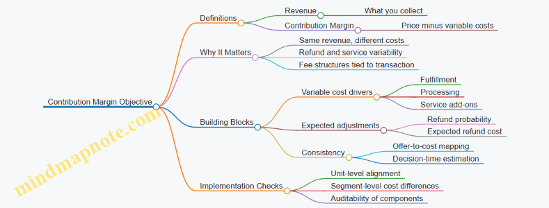
Systematic Objective Formulation for Optimization
Once you have contribution margin per unit, you can define the optimization target. In yield and pricing, the decision is often “which offer to show” or “which inventory to allocate.” The objective becomes maximizing expected total contribution margin over the horizon.
A typical structure looks like this:
- For each candidate offer (i):
- Estimate demand probability or expected bookings under that offer.
- Compute expected contribution margin per booking.
- Multiply to get expected contribution margin contribution.
Then choose the offer or allocation that maximizes total expected contribution margin subject to constraints (capacity, eligibility, and operational rules).
Example: Two Offers with Different Cost Profiles
Assume a product with limited inventory. You consider two price points for the same segment.
-
Offer 1: $80 price
- Variable cost: $45
- Expected refund cost: $3
- Contribution margin per sale: $80 − $45 − $3 = $32
- Expected probability of sale: 0.40
- Expected contribution margin: 0.40 × $32 = $12.80
-
Offer 2: $90 price
- Variable cost: $50
- Expected refund cost: $8
- Contribution margin per sale: $90 − $50 − $8 = $32
- Expected probability of sale: 0.30
- Expected contribution margin: 0.30 × $32 = $9.60
Even though both offers have the same margin per sale, Offer 1 wins because it sells more often. This example highlights a key point: contribution margin objectives combine per-sale economics and expected sales volume.
Practical Best Practices for Margin-First Objectives
- Separate fixed and variable costs explicitly so the objective doesn’t “double count” business overhead.
- Model expected refunds and service adjustments by offer and segment rather than using one global rate.
- Use consistent units: if your demand model predicts bookings, your cost model must predict costs per booking.
- Validate with backtests using margin, not revenue to confirm that the system’s ranking of offers changes in the direction you expect.
When revenue and margin disagree, contribution margin provides the more honest target for pricing decisions. It turns “what we sold” into “what we kept,” which is the only part that can pay for the next decision.
5.2 Cost Modeling for Variable and Semi Variable Costs
Cost modeling turns “we sold more” into “we kept more.” In yield and dynamic pricing, the goal is to estimate contribution margin per unit (or per booking) while accounting for costs that change with volume and costs that change with activity but not strictly one-for-one.
Core Concepts for Cost Behavior
Start by classifying costs by how they move when demand changes.
- Variable costs change roughly in proportion to units sold or served. If you sell 1 more ticket, you incur cost for that ticket.
- Semi variable costs have a fixed component plus a variable component. They move with volume, but not from zero.
A practical rule: if the cost line item exists even when volume is zero, it likely has a fixed part. If it scales with each transaction, it likely has a variable part.
Building Blocks for a Margin Objective
For each offer or booking decision, compute expected contribution margin:
- Contribution margin per unit = Price − Variable cost per unit − Variable portion of semi variable costs per unit − Direct per-transaction fees
- Expected margin = Probability of booking × Contribution margin per booked unit − Any expected penalties tied to the decision
This is the bridge between optimization and accounting reality. Revenue algorithms often optimize price; margin algorithms optimize the net that survives after costs.
Modeling Variable Costs
Variable costs are usually the easiest to model because they map cleanly to units.
Common examples
- Payment processing fees per transaction
- Per-item fulfillment costs in retail
- Per-seat catering or per-ride operating costs in transport
Best practice: use a per-unit cost that matches the decision granularity. If your algorithm decides at the offer level but fulfillment happens per booked unit, convert to “per booked unit.” If costs are per order, aggregate accordingly.
Example:
A hotel charges a nightly rate. For each booked room-night, there is a cleaning cost of $18 and a payment fee of 2.5% of the nightly rate.
If the nightly price is $140, variable cost per room-night is:
- Cleaning: $18
- Payment fee: 0.025 × 140 = $3.50
- Total variable cost: $21.50
Contribution margin per booked room-night becomes $140 − $21.50 = $118.50, before considering semi variable costs.
Modeling Semi Variable Costs
Semi variable costs require splitting into fixed and variable components. A common approach is:
- Choose a time window where you have stable operations.
- Collect historical totals of the cost line item and the activity driver (rooms sold, rides taken, orders shipped).
- Fit a simple model: Cost = Fixed + Variable × Activity.
Even if you use a regression, keep the interpretation simple so the cost split can be audited.
Activity driver selection
Semi variable costs often respond to activity, not time alone. Examples:
- Call center staffing costs rise with booking volume
- Maintenance costs rise with usage hours
- Customer support costs rise with number of tickets handled
Pick the driver that best matches how operations scale.
Example:
A subscription service has a support cost line item. Monthly support cost averages $12,000 plus $3.20 per active subscriber.
If a pricing policy expects 5,000 active subscribers in a month:
- Fixed component: $12,000
- Variable component: 3.20 × 5,000 = $16,000
- Total support cost: $28,000
To use this in per-booking margin, convert to a per-subscriber variable portion of $3.20 and decide how to allocate the fixed component. Two common allocation methods are:
- Per-activity allocation: treat fixed cost as spread across expected activity, so fixed-per-unit = Fixed / Expected Activity.
- Decision-time handling: keep fixed cost outside the optimization objective if it is truly unaffected by the decision horizon.
In yield settings, the second method is often safer when the fixed component is stable across competing pricing actions.
Allocation Choices That Avoid Hidden Bugs
Fixed cost allocation can quietly distort optimization.
- If fixed costs do not change between pricing options, excluding them from the objective is correct for comparing options.
- If fixed costs change with capacity usage (e.g., overtime triggered by higher volume), then part of the “fixed” line item is actually variable over the relevant range.
Best practice: document which cost components are included in the optimization objective and which are treated as constants for the decision window.
Mind Map: Cost Modeling Workflow
Practical Implementation Notes
When you compute expected margin inside a pricing algorithm, keep the cost model consistent with the decision unit:
- If the algorithm evaluates an offer for a single booking, compute costs per booked unit.
- If it evaluates a bundle or cart, compute costs per bundle and avoid mixing per-unit and per-order numbers.
Finally, validate the cost model with a sanity check: plug in historical average volume and confirm that the modeled total cost is close to observed totals. If it is not, the issue is usually driver mismatch or an incorrect split between fixed and variable components.
Example: Sanity Check
If modeled variable cost per booking is $21.50 and historical average bookings are 10,000, variable cost should be about $215,000. If observed variable-like costs are closer to $260,000, revisit the per-booking mapping (maybe a cost is per order, not per booking, or a fee is missing).
5.3 Incorporating Refunds, Fees, and Service Costs
Revenue is only half the story when customers can cancel, when transactions carry fixed and variable charges, and when serving an order has real operational cost. This section builds a practical way to convert “expected bookings” into “expected contribution margin” by modeling refunds, fees, and service costs as first-class inputs to your optimization.
Refunds as Negative Sales with Timing
Refunds are not just a percentage of price; they have timing, eligibility rules, and sometimes partial refunds. Start by separating three quantities:
- Refund rate by offer type and customer segment (e.g., refundable vs nonrefundable).
- Refund timing distribution (immediate, within a window, or after fulfillment).
- Refund amount rules (full, partial, minus penalties).
A simple baseline model treats expected refund cost as:
- Expected refund = (Refund rate) × (Refundable portion of price) × (Refund timing discount factor)
The timing discount factor matters because cash and accounting recognition differ. If your system optimizes for near-term margin, a refund that arrives later should be weighted less than one that arrives immediately.
Example: A hotel sells a room for $200. If 20% of bookings are refundable with a full refund and refunds typically process 10 days later, while nonrefundable bookings are 2% refundable with a $50 penalty, then expected refund outflow is:
- Refundable: 0.20 × 200 = $40
- Nonrefundable: 0.02 × (200 − 50) = $3
- Total expected refund = $43, then apply your timing weight (e.g., 0.99 for near-term cash impact).
Fees as Transaction-Level Adjustments
Fees often come from payment processing, channel commissions, taxes, and administrative charges. The key is to classify fees by how they behave:
- Proportional fees: a percentage of the charged amount.
- Fixed fees: per transaction, per booking, or per invoice.
- Conditional fees: only when a refund occurs, or only for certain payment methods.
When optimizing margin, you should compute fees on the same base as the cash you expect to receive. If a fee is charged on the original payment but not reversed on refund, it becomes a cost even when the customer cancels.
Example: Suppose a marketplace charges 3% commission on the sale price and does not reverse it on refunds. If the expected refund rate is 20% on a $200 price, then commission cost persists on the refunded portion. Expected commission cost becomes:
- Commission on full sale: 0.03 × 200 = $6
- No reversal on refunds means you keep the $6 even though $40 is refunded.
This is why “refund rate × price” is not enough; you must align fee reversal behavior with your accounting reality.
Service Costs as Fulfillment and Support Expenses
Service costs include costs to deliver the product or provide the service, plus customer support and handling. These costs can be:
- Variable with fulfillment: e.g., cleaning per occupied room, shipping per delivered order.
- Partially variable: e.g., customer support effort increases with cancellations but not linearly.
- Fixed per active capacity: e.g., staffing that scales with expected load.
For margin optimization, the most actionable approach is to model service costs at the decision level you control. If your pricing decision affects booking probability, then service cost should be weighted by expected fulfillment probability.
Example: If serving a booked room costs $65 when the guest stays, but cancellations still incur $10 for processing and rebooking, then expected service cost is:
- Expected stay cost: P(stay) × 65
- Expected cancellation handling: P(cancel) × 10
If your refund model implies P(cancel) = 20%, then expected service cost = 0.80 × 65 + 0.20 × 10 = $53 + $2 = $55.
Integrating Everything into Expected Contribution Margin
To keep the logic consistent, compute expected margin per offer as:
- Expected net cash from sale = price × (1 − refund rate) minus any non-reversed fees.
- Expected service cost = cost_if_fulfilled × P(fulfilled) + cost_if_canceled × P(canceled).
- Expected contribution margin = expected net cash − expected service cost.
The important practice is to ensure every term uses the same probability definitions. If your refund rate is conditional on “booking occurs,” then your service-cost probabilities must be conditional on the same event.
Mind Map: Refunds, Fees, and Service Costs
Practical Implementation Checklist
- Use one probability backbone: define P(fulfill) and P(cancel) once, then reuse them.
- Model fee reversal explicitly: “fee on sale” is not the same as “fee on net received.”
- Include refund timing weights when optimizing for near-term cash or short accounting windows.
- Validate with a reconciliation report: sum expected refunds, fees, and service costs for a sample period and compare to observed totals.
Example: If your expected margin is consistently higher than realized margin, the usual suspects are non-reversed fees, undercounted cancellation handling costs, or refund timing weights that are too optimistic for your cash cycle.
5.4 Optimization Constraints and Feasibility Checks
Revenue and margin optimization are only useful if the solution can actually be executed. Constraints turn “best price on paper” into “best price you can safely offer.” Feasibility checks prevent the optimizer from choosing combinations that violate capacity, policy, or operational rules.
Constraint Types That Matter in Practice
Start by classifying constraints, because each class needs a different check.
- Capacity and allocation constraints: You cannot sell more than available inventory, and you may need to reserve capacity for higher-value demand.
- Offer eligibility constraints: Some customers, channels, or times are not allowed to see certain offers.
- Price and change constraints: Prices must stay within bounds, and you may limit how fast prices can move to avoid churn or operational issues.
- Margin and cost constraints: Contribution margin must remain non-negative after refunds, fees, and variable service costs.
- Business logic constraints: For example, you might require that a bundle price is at least the sum of its components minus an allowed discount.
A good rule of thumb: if a constraint can be written as “must be true for every decision,” it belongs in feasibility checks; if it’s a “preference,” it belongs in the objective or regularization.
Feasibility Checks as a Pipeline
Treat feasibility as a sequence of filters that progressively narrow the candidate decisions.
- Normalize the decision space: Convert candidate prices, fare classes, and allocations into a consistent representation (e.g., discrete price ladder indices and booking limits).
- Apply hard constraints first: Bounds, eligibility, and capacity rules should eliminate invalid options before any scoring.
- Compute margin feasibility: For each remaining candidate, compute expected contribution margin using the same cost model used in optimization.
- Check allocation feasibility: Ensure the chosen allocation does not exceed remaining capacity and respects protection levels.
- Validate operational constraints: Confirm the decision can be served by the pricing system and logged correctly.
This order matters: it’s cheaper to reject impossible options early than to waste compute on candidates that will be thrown away later.
Mind Map: Constraints and Feasibility Checks
Example: Capacity and Protection Level Checks
Suppose you have 100 seats remaining for a flight. You use a two-fare-class policy:
- Fare Class A: sells to price-sensitive demand.
- Fare Class B: sells to higher-value demand.
- Protection rule: keep 20 seats for Fare Class B.
A candidate allocation might propose selling 90 seats to Fare Class A and 15 to Fare Class B. That totals 105 seats, which is impossible.
Feasibility checks catch this immediately:
- Available for A = 100 − 20 = 80
- Proposed A = 90 → violates capacity
- Proposed B = 15 → even if B is fine, the combined allocation fails
The optimizer should either discard this candidate or adjust it using a deterministic repair rule (e.g., cap A at 80) only if your policy explicitly allows repairs.
Example: Margin Feasibility with Refunds and Variable Costs
Consider a hotel night offer with:
- Candidate price: $200
- Variable service cost: $35 per booking
- Expected refund rate: 10% with full refund of the room rate
- Expected contribution margin per booking:
- Contribution = (1 − 0.10) × 200 − 35
- Contribution = 180 − 35 = $145
Now test a lower price candidate, $30:
- Contribution = (1 − 0.10) × 30 − 35
- Contribution = 27 − 35 = −$8
Even if demand is high at $30, the decision is infeasible under a “non-negative expected contribution” rule. The feasibility check should remove it before comparing expected revenue or margin.
Example: Price Change Constraints and Rounding
Assume the system updates prices every hour. You require:
- Price must be within [base × 0.8, base × 1.2]
- Max change per update: no more than 5% from the current displayed price
- Prices must be rounded to the nearest $1
If the current price is $120 and the optimizer suggests $130.50:
- Max allowed = $120 × 1.05 = $126
- Suggested $130.50 exceeds the max change
- Even if rounding would bring it down, feasibility must be evaluated before or after rounding consistently with your policy
A practical best practice: define rounding and bound logic in one place so every component agrees on what “$126” means after rounding.
Implementation Practices That Prevent Silent Failures
- Make constraints deterministic: The same inputs should always yield the same feasibility result.
- Use one cost model everywhere: If feasibility uses a different refund assumption than the objective, you’ll get “optimal but infeasible” outcomes.
- Log the reason for rejection: Store which constraint failed (e.g., “capacity,” “margin,” “eligibility”) so debugging is fast.
- Unit test edge cases: Zero inventory, exactly-at-floor prices, and allocations that sum to capacity are where bugs hide.
Feasibility checks are not a bureaucratic step; they’re the bridge between mathematical optimization and decisions that can be executed without breaking policy or economics.
5.5 Practical Example: Switching From Revenue To Margin Optimality
Revenue optimization chooses the offer with the highest expected selling price times expected probability of sale. Margin optimization chooses the offer with the highest expected contribution margin, which subtracts variable costs and accounts for refunds, fees, and service costs. The switch matters because two offers can have similar revenue but very different costs, or similar revenue but different likelihoods of triggering refunds.
Step 1: Define the Objective Precisely
Assume a booking system offers two fare classes for the same seat inventory: Saver and Flex. For each class, you can estimate demand probability as a function of price and segment.
- Revenue objective: maximize \(E[\text{Revenue}] = p\text{(buy)} \times \text{Price}\)
- Margin objective: maximize \(E[\text{Margin}] = p\text{(buy)} \times \text{(Price} - \text{VarCost} - \text{ServiceCost}) - p\text{(refund)} \times \text{RefundAmount}\)
A practical best practice is to keep the cost model aligned with what actually changes per transaction. If a cost is fixed per day, it should not influence the per-offer choice.
Step 2: Build a Tiny Cost Model That Matches Reality
Let variable costs and service costs be per booking. Refunds are modeled as a probability of refund conditioned on purchase.
- Saver: Price = 120, VarCost = 35, ServiceCost = 8, RefundAmount = 60, RefundProb = 0.06
- Flex: Price = 150, VarCost = 35, ServiceCost = 12, RefundAmount = 70, RefundProb = 0.03
Note the costs are not identical: Flex costs more to serve, and refunds are smaller and less likely.
Step 3: Use the Same Demand Estimates for Both Objectives
Suppose for a given segment and time-to-departure, your demand model estimates purchase probabilities:
- Saver purchase probability \(p(\text{buy}|\text{Saver}) = 0.40\)
- Flex purchase probability \(p(\text{buy}|\text{Flex}) = 0.30\)
Revenue would favor Saver because it sells more often and has lower price.
Step 4: Compute Expected Revenue for Each Offer
- Saver expected revenue: \(0.40 \times 120 = 48\)
- Flex expected revenue: \(0.30 \times 150 = 45\)
Revenue optimal choice is Saver.
Step 5: Compute Expected Margin for Each Offer
First compute contribution margin per sale excluding refunds.
- Saver per-sale margin: \(120 - 35 - 8 = 77\)
- Flex per-sale margin: \(150 - 35 - 12 = 103\)
Now subtract expected refund impact. Refund probability is applied only when a purchase happens.
- Saver expected margin: \(0.40 \times 77 - 0.40 \times 0.06 \times 60\)
- \(= 30.8 - 1.44 = 29.36\)
- Flex expected margin: \(0.30 \times 103 - 0.30 \times 0.03 \times 70\)
- \(= 30.9 - 0.63 = 30.27\)
Margin optimal choice is Flex, even though it has lower expected revenue.
This is the key reasoning: Flex’s higher per-sale margin outweighs its lower purchase probability and its refund risk.
Step 6: Mind Map of the Switching Logic
Mind Map: Revenue to Margin Switching
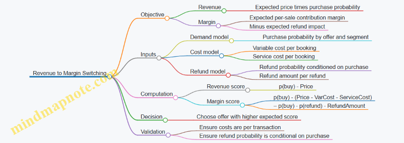
Step 7: Operational Best Practices That Prevent Common Mistakes
- Keep units consistent. If costs are per passenger but demand is per booking, scale accordingly.
- Condition refund probability correctly. Using an unconditional refund probability can double-count purchase likelihood.
- Use the same segmentation for demand and costs. If costs vary by channel but demand varies by segment, you still need a mapping from segment to channel cost assumptions.
- Sanity-check with a quick spreadsheet. In production, the math is the same; the spreadsheet is just your early warning system.
Step 8: A Small Sensitivity Check
If Flex’s purchase probability drops from 0.30 to 0.29, its expected margin becomes \(0.29 \times 103 - 0.29 \times 0.03 \times 70 = 29.87 - 0.61 = 29.26\), which is slightly below Saver’s 29.36. That boundary tells you where the decision flips, so you can focus monitoring on the demand estimates that matter most.
In short, switching from revenue to margin optimality is not a new algorithm so much as a corrected score function. Once the score reflects what you actually keep after costs and refunds, the “best” offer can change in a way that matches operational reality.
6. Real Time Price Control Systems
6.1 Real Time Decision Architecture and Latency Budgets
Real time price control is a pipeline problem: you need the right inputs, a decision policy that can run fast, and guardrails that keep the system from making “technically correct but operationally disastrous” choices. A good architecture treats latency as a budgeted resource, not a vague performance goal.
Decision Loop from Trigger to Offer
Start with the trigger. Common triggers include a user search, a cart update, a booking attempt, or an inventory change. Each trigger should map to a single decision request with a clear output: an offer set, a price, or a recommendation of which price to show.
A practical loop looks like this:
- Request intake: Validate identifiers (product, channel, segment), normalize timestamps, and attach context like device and locale.
- Feature retrieval: Pull precomputed features (segment attributes, historical demand signals, inventory state) from a low-latency store.
- Policy evaluation: Compute the candidate price(s) and expected value or margin objective.
- Constraint enforcement: Apply floors, ceilings, rate limits, and eligibility rules.
- Response assembly: Produce the offer payload and log the decision inputs and outputs for later analysis.
The key is that each stage has a measurable cost and a defined failure mode. If feature retrieval fails, you should return a safe fallback rather than block the user.
Latency Budgets That Match Human Expectations
Latency budgets should be expressed in milliseconds per stage, with a total target that matches the user-facing interaction. For example, if the UI can tolerate about 120 ms end-to-end, you might allocate:
- Intake and validation: 5 ms
- Feature retrieval: 45 ms
- Policy evaluation: 40 ms
- Constraint checks: 10 ms
- Response assembly and serialization: 10 ms
- Logging overhead: 10 ms
This is not about being exact; it’s about preventing one stage from silently consuming the whole budget. If feature retrieval regularly spikes, you either cache more aggressively, reduce feature count, or move computation earlier.
Mind Map: Architecture Components
Policy Evaluation Under Time Pressure
The policy layer should be designed for predictable runtime. If you use a model, keep inference bounded: fixed-size feature vectors, limited branching, and precomputed lookups where possible.
A common pattern is two-step pricing:
- Generate candidates from a small set of plausible prices (for instance, a price ladder around the current price).
- Score candidates using a fast objective such as expected contribution margin.
Example: Suppose a hotel room has a current price of $180. You might generate candidates at $170, $180, $190, and $200. For each candidate, you estimate expected bookings using a demand model and compute expected margin as:
- expected margin = (expected bookings) × (price − variable cost) − (expected cancellation impact)
Then you pick the best candidate that passes constraints. This avoids scanning thousands of prices and keeps runtime stable.
Constraint Enforcement That Prevents “Correct” Mistakes
Constraints are part of the decision, not an afterthought. Rate limits stop the system from changing prices too frequently, which can cause customer confusion and operational load.
Example: A rule might say “no more than one price change per SKU per 10 minutes per channel.” If the policy wants to jump from $180 to $210, the constraint layer can either cap the change to $190 or revert to the last allowed price, depending on business rules.
Observability and Stage-Level Accountability
You need metrics that answer two questions: “Was the decision fast enough?” and “Where did time go?” Track latency per stage and include correlation IDs so you can reconstruct a decision path.
Also log the decision inputs that matter: the candidate prices, the objective scores, and which constraints were triggered. This makes debugging practical. If a constraint blocks a price, you want to know whether it was the floor, the rate limit, or eligibility.
Example Decision Budget with Failure Modes
Consider a retail SKU pricing request with a 120 ms target. If feature retrieval times out, you can switch to a degraded mode that uses cached inventory and a simpler demand estimate. The response still returns an offer, but you mark it as degraded in logs.
This keeps the user experience stable and prevents the system from turning a data issue into a customer-facing outage. The system remains boring, which is exactly what you want when money is involved.
6.2 Offer Generation and Eligibility Rules
Offer generation turns a pricing decision into something customers can actually buy: a concrete offer with a price, rules, and constraints. Eligibility rules decide who can see or purchase that offer, and under what conditions. Treat these as two halves of the same system: offer generation creates candidates, eligibility rules filter them into the final set.
Offer Objects and Decision Inputs
An offer should be represented as a structured object so downstream systems can validate it consistently. At minimum, include:
- Price and currency
- Validity window (start/end timestamps)
- Inventory or capacity reference (what it consumes)
- Purchase constraints (min/max quantity, stay length, booking lead time)
- Eligibility keys (segment, channel, membership tier, geography)
- Policy identifiers (which guardrails and experiments produced it)
Decision inputs typically include current availability, customer context, and the pricing model output. A practical best practice is to log the full set of inputs used to build each offer, even if the final price is later adjusted by guardrails. That log becomes your “why” trail when something looks off.
Eligibility Rules as a Filter Pipeline
Eligibility is easiest to reason about as a pipeline with short-circuiting. Start with fast, deterministic checks; then apply slower checks that require more computation.
Common pipeline stages
- Hard exclusions: blocked users, fraud flags, contract-ineligible geographies.
- Channel and device constraints: some offers are only valid on specific channels.
- Customer eligibility: membership tier, loyalty status, age restrictions, corporate agreements.
- Offer compatibility: does the offer match the requested product attributes (date, duration, class)?
- Time validity: offer timestamps must overlap the customer’s shopping session.
- Capacity and inventory checks: ensure the offer can be fulfilled.
- Policy guardrails: enforce floors, ceilings, rate limits, and rounding rules.
A useful mental model: eligibility rules answer “should this offer exist for this customer right now?” Guardrails answer “even if it exists, is it allowed to be shown or sold?”
Mind Map: Offer Generation and Eligibility Rules
Deterministic Offer Ordering and Selection
If multiple offers survive eligibility, you still need a selection rule. Deterministic ordering prevents “same inputs, different outputs” bugs.
A straightforward approach:
- Rank offers by fulfillment priority (e.g., those consuming scarce capacity last)
- Then by net margin (or expected contribution)
- Then by stability preference (avoid unnecessary price churn)
Example: A travel site generates three offers for the same itinerary: a standard fare, a flexible fare, and a member-only fare. Eligibility removes the member-only fare for non-members. Between the remaining two, the system ranks by expected contribution margin, but also prefers the offer that matches the customer’s previously viewed fare class to reduce confusion.
Guardrails Embedded in Eligibility
Eligibility rules should include guardrails that are logically tied to “can we show or sell this offer?” Examples:
- Price bounds: never show below a minimum or above a maximum for that product.
- Rate limits: restrict how fast price can change within a short window.
- Rounding compliance: ensure the final displayed price matches allowed increments.
- Promotion stacking rules: prevent incompatible discounts from combining.
Example: Suppose a model suggests a price that is within bounds but would violate a rate limit because it is 12% lower than the last price shown in the same session. Eligibility can either (a) reject the offer and fall back to the previous allowed price, or (b) clamp the price to the nearest allowed change magnitude. The key is to make the behavior deterministic and logged.
Validation Checks That Prevent Silent Failures
Before offers reach the customer, validate them:
- Schema validation: required fields present and correctly typed.
- Time overlap: validity window intersects the session window.
- Inventory feasibility: capacity reference exists and is not already reserved beyond limits.
- Constraint consistency: min/max quantity and duration rules are coherent.
Example: If an offer says “valid for 3–5 nights” but the customer searched for 7 nights, compatibility checks should remove it early. Without this, you might show an offer that later fails at checkout, which is a fast way to create support tickets.
Diagram: Eligibility Filter Pipeline
    flowchart TD
  A[Start with Offer Candidates] --> B[Hard Exclusions]
  B --> C[Channel Constraints]
  C --> D[Customer Eligibility]
  D --> E[Offer Compatibility]
  E --> F[Time Validity]
  F --> G[Capacity and Inventory Checks]
  G --> H[Policy Guardrails]
  H --> I[Rank and Select Final Offers]
  I --> J[Return Eligible Offers]
Practical Example with Concrete Rules
Assume today’s system run uses a pricing policy effective on 2026-02-26. A customer searches for a hotel for 4 nights, booking lead time 10 days, channel is mobile web, and the customer is not a loyalty member.
Offer generation produces:
- Offer 1: member-only discount, valid for 3–7 nights
- Offer 2: standard fare, valid for 2–5 nights
- Offer 3: flexible fare, valid for 1–10 nights
Eligibility rules then:
- Remove Offer 1 due to customer eligibility.
- Remove Offer 2 if its lead-time constraint requires 14+ days.
- Keep Offer 3 if it passes time validity and capacity checks.
Finally, ranking selects Offer 3 as the only eligible option, and the system logs which checks removed the others. That log makes debugging straightforward: you can see whether the issue was eligibility, compatibility, or capacity rather than guessing.
6.3 Price Update Policies and Change Management
Price updates are where good models meet messy reality: stale data, partial outages, and competing business rules. A solid policy defines when updates happen, how they’re computed, and what happens when something goes wrong. The goal is simple: every offer shown to a customer should be explainable from the system’s inputs and rules.
Update Cadence and Triggering
Start with two questions: how often can you safely change prices, and what events must force an update.
- Fixed cadence updates every N minutes, using the latest features and forecasts.
- Event-driven updates trigger on inventory changes, campaign starts, or sudden demand shifts.
- Hybrid systems run on cadence but also trigger immediately on high-impact events.
Best practice: define a maximum staleness window for each input. For example, if booking pace is computed from the last 30 minutes of transactions, then a 60-minute update cadence means you must either recompute pace at update time or accept that the pace feature is stale.
Example: A hotel updates room rates every 15 minutes. If a last-minute cancellation increases available rooms, an event-driven trigger recalculates protection levels immediately, while the rest of the inventory classes wait for the next 15-minute cycle.
Decision Scope and Eligibility Rules
Not every price update should touch every offer. Define scope using eligibility rules that prevent accidental changes.
- Offer eligibility: only offers currently sellable under business constraints.
- Segment eligibility: only segments with sufficient data quality and coverage.
- Time eligibility: only future travel dates beyond a cutoff where forecasts are reliable.
Best practice: keep eligibility logic centralized so the same rules apply to both real-time serving and offline backtesting.
Example: If a flight’s fare class is restricted to members, the pricing service must not update public offers using member-only margin targets.
Rate Limits, Floors, and Guardrails
Guardrails convert “mathematically optimal” into “operationally safe.”
- Rate limits cap how much price can move per update window.
- Absolute bounds enforce minimum and maximum prices.
- Change frequency limits prevent oscillation when demand signals are noisy.
- Inventory-aware floors prevent pricing below a level that would cause systematic losses when capacity is scarce.
Example: If the algorithm suggests moving from $120 to $95 in one step, a rate limit of 10% forces an intermediate $108. The next update can move further only if evidence persists.
Change Management Workflow
Treat each update like a controlled release. A practical workflow has four stages.
- Compute: generate candidate prices for eligible offers.
- Validate: run guardrails, schema checks, and consistency tests.
- Publish: atomically swap the active price table used by serving.
- Verify: confirm that serving logs match the published version.
Best practice: use versioned price artifacts. Every served offer should reference a price version ID so you can trace outcomes.
Example: On 2026-02-26, a pricing job computes new offers for the next 7 days. Validation rejects one fare class due to missing cost inputs. Publishing proceeds for the other classes, and logs record the partial acceptance.
Observability and Rollback
You need fast answers to two questions: did we publish the right thing, and did it behave.
- Pre-publish checks: null rates, feature completeness, and constraint satisfaction.
- Post-publish checks: distribution shifts in offered prices, error rates, and conversion deltas.
- Rollback triggers: if guardrails are violated, if serving fails, or if anomalies exceed thresholds.
Best practice: rollback should be deterministic. Keep the last known-good price version and revert serving to it without recomputation.
Mind Map: Price Update Policies and Change Management
Putting It Together with a Concrete Scenario
Imagine a retail assortment with 500 SKUs and multiple channels. The system runs every 10 minutes, but a sudden stockout triggers an immediate recompute for affected SKUs only. Candidate prices are validated against SKU-specific floors and a 12% per-step rate limit. Publishing swaps the active price table using a new version ID. If monitoring detects an abnormal spike in “below-floor” rejections or a serving error rate above a threshold, the system rolls back to the previous version and stops further publishes until the validation pipeline is healthy.
This is change management that behaves like engineering: explicit scope, explicit constraints, explicit versions, and explicit failure handling.
6.4 Guardrails for Bounds, Floors, and Rate Limits
Real time price control is a lot like driving with a GPS: the route matters, but so do the brakes. Guardrails prevent the system from making technically “reasonable” decisions that are operationally unsafe, financially harmful, or simply impossible to honor.
Guardrail Goals and Failure Modes
Guardrails typically cover three categories of risk.
- Bounds stop the system from proposing prices outside allowed ranges. Example: a hotel room price cannot go below a contractual minimum or above a display cap.
- Floors protect minimum profitability or minimum customer value. Example: if variable costs rise due to last-minute logistics, the floor ensures contribution margin stays non-negative.
- Rate limits control how fast prices can change. Example: an airline fare cannot be updated more than once every 15 minutes to avoid downstream cache churn and customer confusion.
A good guardrail design starts by mapping each failure mode to a measurable rule. If you can’t measure it, you can’t guard it.
Bounds: Hard Limits That Keep Offers Honest
Bounds are the simplest to reason about because they are absolute.
- Static bounds come from policy: minimum and maximum allowed prices per product, market, and channel.
- Dynamic bounds come from operational context: temporary outages, inventory state changes, or payment method constraints.
Example: A retail SKU has allowed prices from $10 to $25. The optimizer suggests $9.50 because it expects high demand at lower prices. Bounds reject it and return $10.00.
Best practice: apply bounds after the optimizer computes the candidate price, not before. That way you can log the “raw” suggestion and learn whether the optimizer is drifting toward invalid regions.
Floors: Profit and Value Constraints That Preserve Margin
Floors turn business intent into math.
Common floor types:
- Contribution margin floor: ensure
price - variable_cost - fulfillment_cost >= 0. - Discount floor: ensure the discount does not exceed what the business can sustain.
- Customer value floor: ensure the price stays within a perceived value band for that segment.
Example: A delivery fee is $4.20 and variable cost is $6.10. If the floor requires non-negative contribution, then price >= 10.30. If the optimizer proposes $9.99, the floor lifts it to $10.30.
Best practice: compute floors using the same cost inputs that the fulfillment system will actually use. If costs are stale, the floor becomes a polite suggestion rather than a safety mechanism.
Rate Limits: Controlling Change Frequency and Change Magnitude
Even correct prices can be wrong if they change too often.
Rate limits usually include two controls:
- Time-based limits: minimum time between updates for the same offer.
- Magnitude-based limits: maximum percent or absolute change per update.
Example: A pricing service updates every minute, but rate limits say “no more than 5% change per minute.” If the current price is $100 and the optimizer suggests $92, the system caps the change to $95.
Best practice: rate limits should be enforced per offer identity (product + market + channel + eligibility set). Otherwise, the system may oscillate between similar offers and still violate customer expectations.
Guardrail Evaluation Order
The order matters because each guardrail changes the candidate value.
A practical sequence:
- Generate candidate price from the pricing model.
- Apply bounds to ensure legality.
- Apply floors to ensure profitability or value constraints.
- Apply rate limits to ensure operational stability.
- If any rule modifies the value, log the reason and the inputs used.
This order keeps the system from “fixing” an illegal price with a floor, then later discovering it violates bounds again.
Mind Map: Guardrail Components and Checks
Example: Putting It All Together in One Decision
Assume a market where:
- Bounds are $10 to $25.
- Floor requires non-negative contribution with variable cost $6.10 and fulfillment $4.20, so floor is $10.30.
- Rate limit allows at most +0% to +3% per update, and the last published price is $20.00.
The optimizer suggests $9.50.
- Bounds: clamp to $10.00.
- Floors: lift to $10.30.
- Rate limit: $10.30 is a -48.5% change, which violates the “no more than +3%” rule if the rule is directional. If the rate limit is symmetric, it would cap the decrease instead. The system must define whether the limit is symmetric or directional.
Best practice: make rate limit rules explicit: symmetric (max absolute change up or down) or directional (different caps for increases vs decreases). Then the system behaves consistently and logs match expectations.
Implementation Checklist for Guardrails
- Define guardrails per product-market-channel offer identity.
- Use consistent cost and eligibility inputs across model and guardrails.
- Enforce guardrails in a fixed evaluation order.
- Log every modification with the rule triggered and the computed thresholds.
- Validate with unit tests using edge cases: near bounds, near floors, and rapid update sequences.
6.5 Practical Example: Designing a Real Time Price Update Workflow
A real time price update workflow turns incoming signals into safe, auditable price changes. The goal is simple: update offers fast enough to matter, but never in a way that breaks business rules or creates inconsistent customer experiences.
Define the Decision Boundary
Start by stating what the system is allowed to change. In this example, the workflow updates the price of a single product per store for a given sales channel.
Inputs
- Inventory availability snapshot (units on hand, units reserved, lead time)
- Demand signals (recent sales velocity, search interest, cancellation rate)
- Cost and margin parameters (base cost, variable fulfillment cost, target contribution margin)
- Business rules (price floors, maximum discount, competitor caps, contract restrictions)
Outputs
- Price for each eligible offer
- Reason codes for why the price changed
- A versioned decision record for audit
Set Latency Budgets and Staging
Real time does not mean “everything happens in one breath.” Use stages so each part can be optimized and monitored.
- Stage A: Feature assembly (target 50–150 ms): fetch inventory, compute availability, normalize demand metrics
- Stage B: Eligibility and constraints (target 10–30 ms): filter offers that violate rules
- Stage C: Price optimization (target 20–80 ms): compute candidate prices and expected margin
- Stage D: Guardrails and commit (target 10–40 ms): enforce bounds, rate limits, and change thresholds
- Stage E: Logging (target 5–20 ms): write decision record asynchronously
Eligibility Rules Before Optimization
Optimization should not waste time on offers that cannot be sold.
Example eligibility checks for a store offer:
- If available units after reservations are below a minimum sellable threshold, mark offer as “not eligible.”
- If the contract requires a fixed price for certain customer tiers, exclude those tiers.
- If the channel is “member only,” apply member-specific floors.
A practical trick: compute an eligibility mask once per request, then pass it to downstream steps.
Candidate Generation with Discrete Ladders
Even if you ultimately choose a single price, generate a small set of candidates.
Example price ladder for a product with current price $120:
- $110, $115, $120, $125, $130
For each candidate, estimate expected demand using a simple response model (elasticity or learned response) and compute expected contribution margin:
- Expected units sold = f(demand signals, price)
- Expected margin = (price − variable cost) × expected units sold − fixed handling adjustments
Guardrails That Prevent “Price Thrash”
Guardrails are not optional; they are the difference between “dynamic” and “chaotic.”
Use three layers:
- Absolute bounds: floor and ceiling per store and channel
- Rate limits: maximum number of price changes per hour per product
- Change thresholds: only commit if the improvement exceeds a minimum delta
Example: if the best candidate improves expected margin by less than $0.80 per 1000 impressions, keep the current price. This avoids tiny oscillations caused by noisy demand signals.
Consistency Across Services
A common failure mode is inconsistent views: one service updates price while another still serves the old offer.
Use a single “commit” point:
- The pricing service produces a decision object containing price, reason codes, and a decision timestamp.
- The offer service applies the decision atomically for the relevant store and channel.
- The customer-facing API reads from the committed offer state.
Logging and Audit Records
Every committed decision should be traceable.
Log fields to include:
- Decision ID, product ID, store ID, channel
- Inputs summary (inventory snapshot ID, demand window)
- Candidate set and chosen price
- Guardrail outcomes (which constraints were active)
- Reason codes (e.g., “inventory tightened,” “margin target adjustment”)
This makes debugging straightforward: you can answer “what did we know, when did we know it, and why did we choose that price?”
Worked Example with Concrete Numbers
Assume a store has 40 units on hand, 10 reserved, so 30 sellable units. Variable fulfillment cost is $72. Current price is $120.
Demand response model estimates expected units sold for each candidate:
- $110 → 34 units
- $115 → 32 units
- $120 → 28 units
- $125 → 25 units
- $130 → 22 units
Expected contribution margin per candidate (ignoring small fixed terms):
- $110: (110−72)×34 = 38×34 = 1292
- $115: 43×32 = 1376
- $120: 48×28 = 1344
- $125: 53×25 = 1325
- $130: 58×22 = 1276
Best candidate is $115 with margin 1376. Now apply guardrails:
- Floor is $108, ceiling is $135 → $115 passes
- Max change per hour is 10% → current $120 to $115 is 4.17% → passes
- Minimum improvement threshold is $0.80 per 1000 impressions; expected improvement vs $120 is 1376−1344 = 32 margin units → passes
Commit decision: update offer price to $115 with reason code “inventory tightened and margin optimization.”
Mind Map: Real Time Price Update Workflow
Example: Decision Object Schema
{
  "decisionId": "dec_2026_03_01_1045_7f2a",
  "productId": "SKU_1842",
  "storeId": "ST_019",
  "channel": "web",
  "timestamp": "2026-03-01T10:45:00Z",
  "chosenPrice": 115.0,
  "reasonCodes": ["inventory_tightened", "margin_optimal"],
  "constraints": {
    "floorPassed": true,
    "ceilingPassed": true,
    "rateLimitPassed": true,
    "deltaThresholdPassed": true
  },
  "candidatePrices": [110.0, 115.0, 120.0, 125.0, 130.0]
}
This workflow stays systematic: it filters first, optimizes second, and only then commits under explicit guardrails with a complete audit trail.
7. Estimation of Price Response and Elasticity
7.1 Estimating Elasticity With Observational Data
Elasticity tells you how much demand changes when price changes. With observational data, you don’t get clean “price was randomly set” experiments, so the main challenge is separating price effects from everything else that moves demand at the same time.
Core Idea and Definition
Price elasticity of demand at a point is the percent change in quantity demanded divided by the percent change in price. In practice, you estimate it from historical variation in price and demand, using a model that controls for confounders.
A useful mental check: if price rises because demand is already strong (a common pattern), a naive model may report elasticity that looks too small or even positive. Your job is to prevent that “demand drives price” story from masquerading as “price drives demand.”
Observational Data Setup
Start by defining the unit of analysis. For example, you might use daily store-level sales for a product, or hourly site-level bookings for a fare family. Then define:
- Demand metric: units sold, bookings, or conversion rate.
- Price metric: the effective price customers faced (not just the list price).
- Time window: how far back you use for features and how you align price to demand.
- Granularity: segment by channel, geography, device type, or customer cohort if behavior differs.
Best practice: compute effective price from actual offers shown and accepted. If you only use the posted price, you’ll mix in selection effects where customers self-select into different offers.
Confounding and Identification
In observational pricing, at least three forces move together:
- Demand shocks (weather, events, seasonality)
- Operational changes (inventory, staffing, assortment)
- Pricing decisions (promotions, rules)
To estimate elasticity, you need variation in price that is not just a reflection of demand shocks. Common identification strategies include:
- Fixed effects to absorb stable differences across stores, SKUs, or segments.
- Time controls to absorb seasonality and day-of-week patterns.
- Instrument-like variables when available, such as cost changes or competitor price updates that affect your price but not demand directly.
- Policy-aware features that capture how pricing rules respond to demand signals.
Even without a formal instrument, you can reduce bias by modeling the pricing policy explicitly.
Modeling Approach That Stays Interpretable
A standard starting point is a log-log demand model:
- Let y be demand (often log(y + small_constant) to handle zeros).
- Let p be effective price (log p).
- Include controls for time and segment.
Then the coefficient on log price approximates elasticity: a 1% price change corresponds to an estimated elasticity percent change in demand.
Best practice: estimate elasticity per segment when segments have different baseline demand levels and different price sensitivity. If you pool everything, the model averages away meaningful differences.
Practical Example with Simple Numbers
Suppose a retailer tracks a SKU in one region. Over two weeks, effective price changes from 10 to 11 (a +10% change). Sales units change from 200 to 180 (a -10% change). A rough elasticity estimate is:
- elasticity ≈ (-10%) / (+10%) = -1.0
Now add the missing context: those weeks also had a local event that increased foot traffic. If the event boosted demand, the observed -10% might understate the true price effect. A controlled model would include event indicators or proxies (like traffic) so the price coefficient reflects price-driven movement rather than event-driven movement.
Mind Map: Estimating Elasticity with Observational Data
Advanced Details Without Making It Complicated
1) Exposure alignment: if customers see prices throughout the day, but you aggregate sales daily, you need a consistent mapping from price to demand. A common approach is to use the average effective price weighted by offer exposure.
2) Selection effects: if higher prices reduce who clicks, then conversion and demand are jointly affected. If your demand metric is conversion rate, elasticity mixes price effects on both click and purchase. Decide whether you want elasticity for conversion or for purchase quantity, and model accordingly.
3) Nonlinearities: elasticity may vary by price level. You can allow this by adding interactions, such as price with segment or with promotion intensity.
4) Robustness checks: re-estimate elasticity after removing extreme promotions or after excluding days with known stockouts. If elasticity flips sign when you remove stockouts, you’ve learned something important: the model was using stockout-driven demand changes as a proxy for price effects.
Validation with a Concrete Workflow
- Fit the model on an earlier period.
- Predict demand for a later period using the later period’s prices and controls.
- Compare predicted vs observed demand and check whether the implied elasticity is stable across segments.
If predictions are good but elasticity is unstable, you may be fitting demand shocks through controls while price coefficients compensate. If elasticity is stable but predictions are poor, you likely need better price measurement or additional confounders.
A final practical note: elasticity is only as useful as the price variation you actually observe. If your historical prices barely move, your estimate will be precise-looking but fragile. In that case, focus on improving effective price measurement and segmenting so you capture meaningful variation.
7.2 Causal Considerations for Price Effects
Price effects are not just “what happened when we changed price.” They are “what would have happened if we changed price, holding everything else constant.” Causal thinking is what keeps your model from learning the difference between a price move and the reason the price moved.
The Causal Question Behind Price Effects
Start with two worlds for the same customer or segment at the same time: one where the price is set to P, and one where it is set to P’. Only one world is observed. The causal task is to estimate the missing world using assumptions that are testable in practice.
A useful mental model is: price is a decision variable, while demand is an outcome. If the decision is influenced by demand signals (like bookings trending up), then price and demand are entangled. That entanglement is confounding.
Confounding from Decision Policies
In many systems, price changes are triggered by inventory risk, forecast updates, competitor signals, or marketing plans. Those drivers also affect demand directly.
Example: Suppose you raise price because bookings are strong. You observe higher demand after the raise, but the higher demand may have been coming anyway. The observed correlation is biased upward for price’s effect.
To reason systematically, separate:
- Price assignment: how the system chooses P.
- Demand generation: how customers decide to buy.
- Shared causes: variables that influence both.
Shared causes often include time-to-event, seasonality, channel mix, and operational constraints like capacity releases.
Common Sources of Bias
- Time confounding: Price changes cluster around certain times (weekends, promotions, day-of-week). If you only compare before vs after without controlling time structure, you’ll attribute seasonality to price.
- Inventory confounding: When inventory tightens, you both raise price and reduce availability. Demand shifts for both reasons.
- Marketing confounding: A promotion might coincide with a price change, and the promotion affects demand regardless of the price.
- Selection bias: You may only observe price effects for customers who see the offer. If offer visibility changes with demand, the sample is not representative.
A Practical Causal Framework
Use a three-step workflow that stays grounded in data reality.
Step 1: Define the Unit and Time Window
Pick a unit where “price” is well-defined: a user-session, a search impression, a booking window, or an offer exposure. Then define the time window for outcomes, like purchase within 24 hours.
Best practice: keep the window consistent across experiments and production logs. If one segment’s outcome window is longer, you’ll accidentally measure different behaviors.
Step 2: Identify Backdoor Paths
A backdoor path is any route from price to demand that goes through a shared cause. You block it by conditioning on the right variables.
Typical conditioning set for price effects includes:
- time features (day-of-week, holiday flags)
- inventory/availability state
- offer eligibility and visibility
- segment identifiers and channel
- baseline demand indicators used by the pricing policy
Step 3: Choose an Estimation Strategy That Matches Assumptions
- Randomized experiments: best for causal identification when feasible.
- Quasi-experiments: use policy changes or discontinuities when randomization is not possible.
- Observational adjustment: model-based methods that rely on “no unmeasured confounding” after conditioning.
Observational adjustment can work well, but only if your conditioning set captures the variables the pricing policy uses.
Mind Map: Causal Considerations for Price Effects
Example: Inventory-Triggered Price Changes
Assume a travel booking system updates prices daily. When remaining seats drop below a threshold, the system increases price and also tightens fare availability.
If you estimate price effect by comparing high-price days to low-price days, you’ll likely overstate price’s impact because the low availability also reduces purchases.
Causal fix:
- Use a conditioning set that includes remaining seats and fare availability.
- Compare within similar inventory states, not across wildly different ones.
- Ensure time features are aligned so day-of-week differences don’t masquerade as price effects.
A quick sanity check: after adjustment, the residual demand pattern should not systematically rise or fall with the same inventory thresholds that triggered pricing.
Example: Offer Visibility and Selection Bias
Consider an e-commerce platform that shows different prices depending on user engagement. Highly engaged users are more likely to see discounted offers.
If you regress purchases on the observed price without accounting for exposure, you’ll confuse “discounted users buy more” with “discount causes more buying.”
Causal fix:
- Model exposure/eligibility as part of the data-generating process.
- Estimate price effects among comparable exposures, using features that determine visibility.
- Track outcomes from the moment of exposure, not from the start of the browsing session.
Validation That Respects Causality
Causal assumptions are not magic; they need friction tests.
- Covariate balance: after adjustment, price groups should look similar on the variables that drive the pricing policy.
- Placebo checks: test whether “price” predicts outcomes it should not affect, like purchases in a window before the offer is shown.
- Policy-consistent residuals: if the pricing policy uses a signal, your model should not leave that signal as a strong predictor of demand.
When these checks fail, the issue is usually missing confounders or misaligned time windows, not “the model is wrong in a mysterious way.”
7.3 Segment Level Versus Aggregate Elasticity Modeling
Elasticity is the link between price changes and demand changes. The key modeling choice is whether you estimate that link for the whole market (aggregate) or for specific customer groups and contexts (segments). Both can work, but they answer different questions.
What Aggregate Elasticity Answers
Aggregate elasticity treats demand as one combined pool. You estimate one response curve using total sales and average price. This is often the first model you build because it’s simple and stable: more data per estimate, fewer missing values, and fewer modeling knobs.
A practical example: a retailer sells one product across all channels. If you compute elasticity from total weekly units and the weighted average price, you might find that a 1% price increase reduces units by 0.8%. That number is useful for high-level planning, especially when you only change prices uniformly across channels.
The limitation is that aggregate elasticity hides opposing behaviors. Suppose online customers are price sensitive (elasticity -1.5) while in-store customers are less sensitive (elasticity -0.3). If online and in-store prices move together, the aggregate estimate might land near -0.9. It will look reasonable, but it won’t tell you which segment is driving the effect.
What Segment Level Elasticity Answers
Segment level elasticity estimates separate response curves for groups such as customer type, geography, device, loyalty tier, booking lead time, or channel. The goal is to predict how demand changes when you change price for a specific audience.
A concrete example: an airline offers two customer segments—business travelers and leisure travelers. Business travelers book closer to departure and are less price sensitive. Leisure travelers book earlier and respond strongly to discounts. If you estimate elasticity separately, you might get -0.2 for business and -1.6 for leisure. Now your pricing policy can protect margin on business while using discounts to stimulate leisure demand.
Segment models also handle different baselines. Even if both segments have the same elasticity, their absolute demand levels differ, which affects optimal price decisions under capacity constraints.
Why the Choice Matters for Real Time Pricing
Real time price control rarely changes “the market average.” It changes an offer for a particular user, session, or inventory context. If your elasticity is aggregate, your model assumes the same response for everyone. That mismatch can cause systematic errors: you may discount too much for low-sensitivity segments or raise prices too aggressively for high-sensitivity segments.
Segment elasticity reduces that mismatch, but it introduces variance. Fewer observations per segment means noisier estimates, especially for rare segments or short time windows.
Mind Map: Modeling Elasticity at Different Levels
A Systematic Comparison Framework
Start with three questions.
-
Are price changes uniform across the market? If yes, aggregate elasticity is often adequate. If no, segment elasticity is closer to the decision you actually make.
-
Do segments behave differently? You can test this by comparing observed demand shifts when price changes occur in different contexts. If the direction or magnitude differs, aggregate modeling will average away the signal.
-
Is there enough data per segment to estimate reliably? If segments are small, pure segment models can overfit. In that case, you still want segment structure, but you need pooling or smoothing.
Example: When Aggregate Elasticity Misleads
Imagine a hotel with two channels: direct and OTA. Direct customers are less price sensitive; OTA customers are more price sensitive. Over a month, the hotel runs promotions mostly on the OTA channel.
If you estimate aggregate elasticity using total bookings and average price across both channels, the estimate will reflect the OTA-heavy promotion pattern. You might conclude that demand is very elastic overall. Then you apply that elasticity to direct offers, discounting more than necessary and leaving money on the table.
A segment model would prevent this by estimating elasticity separately for direct and OTA, even if the direct segment has fewer observations.
Example: When Segment Elasticity Is Too Noisy
Now flip the scenario. Suppose you create many fine-grained segments, like “device type × loyalty tier × region × lead-time bucket.” Some combinations have few observations, and price changes are rare within each segment.
A segment elasticity model might produce extreme values simply because of limited data. Your pricing decisions become unstable: small random fluctuations in observed demand look like strong price effects. The fix is not to abandon segment modeling, but to reduce variance through pooling (for example, sharing information across similar segments) and by using regularization.
Practical Modeling Takeaway
Aggregate elasticity is a good baseline when decisions are broad and data is limited. Segment elasticity is the right tool when offers are targeted and customer responses differ. The best systems align the modeling level with the level at which price decisions are applied, while controlling variance so segment estimates don’t turn into guesswork.
7.4 Regularization and Stability for Elasticity Estimates
Elasticity estimates are fragile because they sit at the intersection of noise (few observations), confounding (price moves for reasons other than demand), and model mismatch (the true response curve is rarely the one you assumed). Regularization helps by adding controlled bias so the estimate doesn’t swing wildly when data are thin or features are correlated. Stability helps by ensuring the estimate changes smoothly when you retrain, refresh data, or adjust segments.
The Core Problem with Unregularized Elasticity
Suppose you estimate a log-demand model where the coefficient on log-price is your elasticity. If price and other drivers (seasonality, promotions, inventory constraints) are correlated, the price coefficient can absorb effects that belong elsewhere. With limited data, the coefficient can also overfit idiosyncrasies: one week of unusual behavior can dominate the fit.
A simple symptom: two nearby price points produce very different implied elasticities, even though the underlying customer behavior should be similar. Another symptom: the elasticity estimate jumps when you change the training window by a small amount.
Regularization Targets That Actually Matter
Regularization can be applied at three levels: parameters, features, and segments.
- Parameter shrinkage: Penalize large coefficients so the elasticity doesn’t become extreme without strong evidence.
- Feature shrinkage: Reduce the influence of noisy or highly collinear features so price doesn’t borrow their explanatory power.
- Segment pooling: Borrow strength across segments so small segments don’t get their own wildly noisy elasticity.
A practical rule: if your elasticity is used downstream for pricing decisions, you want it to be stable enough that small data changes don’t trigger large price swings.
A Systematic Workflow for Stable Elasticity
Step 1: Choose a Response Form and Interpretability
Start with a model you can reason about. For many pricing problems, a log-log form is interpretable: elasticity is the slope of log-demand versus log-price. If you expect curvature, consider adding a nonlinear term (for example, price squared in log space) but regularize it more strongly.
Step 2: Add Parameter Shrinkage
Use ridge-style penalties for continuous coefficients. If you have multiple elasticity-related parameters (baseline, promo interaction, curvature), shrink them all, but allow the baseline price effect to be less constrained than higher-order terms.
Concrete example: you estimate elasticity for a SKU across 12 weeks. Without shrinkage, the model returns elasticity −3.8 for one segment with only 40 transactions. With ridge regularization, it might return −2.1, reflecting that the data are insufficient to justify a very steep response.
Step 3: Stabilize Feature Effects
If you include many correlated features (weekday, holiday flags, campaign intensity), the model can trade off coefficients. Regularize those coefficients too, and standardize features so the penalty is comparable across variables. This prevents the optimizer from “preferring” one feature just because it has a larger numeric scale.
Step 4: Pool Segments with Hierarchical Priors
For segment-level elasticity, use partial pooling: each segment elasticity is pulled toward a global mean, with the pull strength depending on segment size. Small segments move toward the global estimate; large segments can deviate when evidence is strong.
Example: Segment A has 5,000 observations and Segment B has 120. If both show a negative price effect, pooling ensures Segment B doesn’t produce an elasticity that is effectively random.
Step 5: Validate Stability, Not Just Accuracy
Evaluate elasticity stability by checking how it changes across:
- training windows (for example, rolling last 8 weeks)
- bootstrap resamples
- segment redefinitions (merge/split rules)
A stable estimate should vary within a reasonable band. If it doesn’t, your regularization is too weak, your model form is too rigid, or your features are missing key drivers.
Mind Map: Regularization and Stability for Elasticity Estimates
Example: Regularization with a Two-Segment Setup
Imagine two segments for the same product: “commuters” and “families.” Families have fewer observations because fewer bookings occur in that group. You fit a log-demand model with log-price.
- Without regularization: families elasticity becomes −4.5 because a handful of weeks coincide with a promotion that also changes demand.
- With shrinkage and pooling: families elasticity becomes −2.3, closer to the global pattern, while commuters elasticity stays around −2.0 because it’s supported by more data.
The key is not that the estimate is “more correct” in a single run; it’s that it behaves sensibly when the dataset changes. That behavior is what keeps real-time pricing from reacting to statistical ghosts.
Guardrails for Downstream Use
Even with regularization, you should bound elasticity inputs used by optimization. If your elasticity estimate is used to compute expected demand under candidate prices, cap extreme values and enforce sign expectations when justified by business logic. This prevents a rare estimation glitch from producing nonsensical price moves.
Finally, log the elasticity estimate with its uncertainty proxy (for example, standard error from the fitted model or variability from bootstrap). When uncertainty is high, the pricing policy should rely more on conservative assumptions, rather than treating the point estimate as gospel.
7.5 Practical Example: Estimating Elasticity for a Retail SKU Assortment
Imagine a retailer selling a set of related SKUs—say, three sizes of the same cereal. You want elasticity estimates that tell you how demand changes when you change price, but you also need them to be stable enough to use in pricing decisions. The goal of this example is to estimate own-price elasticity for each SKU while accounting for substitution across SKUs and for promotions.
Step 1: Define the Demand Model You Can Actually Fit
Start with a log-log demand model at the daily level. For SKU i on day t:
- Let \(y_{it}\) be units sold.
- Let \(p_{it}\) be the effective price (after discounts).
- Let \(promo_{it}\) be a promotion indicator or discount depth.
- Let \(x_{t}\) be shared controls like day-of-week and weather.
A workable specification is:
\(\log(y_{it}) = \alpha_i + \beta_i \log(p_{it}) + \sum_{j\neq i} \gamma_{ij} \log(p_{jt}) + \delta_i,promo_{it} + \theta_i^T x_t + \epsilon_{it}\)
Here, \(\beta_i\) is the own-price elasticity: a 1% price increase changes units by \(\beta_i\)%.
Step 2: Build the Dataset with Consistent Price and Demand
Elasticity estimates are fragile when inputs are inconsistent. Use these best practices:
- Use effective price, not shelf price. If a SKU is discounted, \(p_{it}\) must reflect what customers actually pay.
- Handle zero sales carefully. If \(y_{it}=0\), log transforms break. A common fix is to model \(\log(1+y_{it})\) or to exclude days with persistent zero demand.
- Align time windows. If promotions start mid-day, aggregate to the same daily boundary for all SKUs.
- Keep assortment constant when possible. If the retailer adds or removes SKUs, include an availability flag or restrict to stable periods.
Concrete example: Suppose SKU A, B, and C are available for 120 days. You compute effective prices daily and create a table with 360 rows (3 SKUs × 120 days), plus shared controls.
Step 3: Include Substitution Instead of Pretending SKUs Are Independent
If SKU A and B are substitutes, ignoring \(\gamma_{ij}\) can bias \(\beta_i\). For the cereal example, when price of A rises, some demand shifts to B and C. Including cross-price terms captures that shift.
Practical simplification: If you have many SKUs, you can group them into a small number of substitute clusters (e.g., same brand, same size family). Then estimate cross effects within clusters rather than for every pair.
Step 4: Estimate Elasticity with Regularization for Stability
With only 120 days, a full cross-price matrix might be too noisy. Use regularization so the model doesn’t chase random fluctuations.
A simple approach is to estimate the model with ridge regression on the \(\gamma_{ij}\) terms while leaving \(\beta_i\) less penalized. This keeps cross effects from becoming extreme when data is thin.
Step 5: Validate the Estimates Using Sanity Checks
Before using elasticities, run checks that catch common failure modes:
- Sign check: Own-price elasticity should usually be negative for normal demand.
- Magnitude check: Extremely large elasticities (like -20) often indicate data issues or promotion confounding.
- Promotion separation: If promotions are frequent, ensure promo effects are not being absorbed into price elasticity.
- Residual behavior: Look for systematic errors by day-of-week or by store traffic level.
Concrete example: If SKU A shows \(\beta_A=-1.35\), a 5% price increase predicts about a 6.75% unit drop, holding other prices and promotions constant. If the observed drop is closer to 1%, you likely have missing controls or price measurement problems.
Step 6: Turn Coefficients into Decision-Ready Elasticities
Elasticity depends on the operating point. With log-log models, \(\beta_i\) is constant, but your effective price changes and promotion mix vary. Use these practices:
- Compute elasticity at the same definition of price used in the model (effective price).
- Report elasticity with uncertainty (confidence intervals) so you know how much to trust it.
- If you must choose a single number, use the median elasticity across stores or across time windows rather than a single fit.
Mind Map: Elasticity Estimation Workflow for a Retail Assortment
Example: From Estimated Elasticities to a Price Test
Suppose you estimate:
- SKU A own elasticity \(\beta_A=-1.35\)
- SKU B own elasticity \(\beta_B=-1.10\)
- Cross effects: \(\gamma_{AB}=0.25\) and \(\gamma_{AC}=0.10\)
You plan to increase A’s effective price by 4% while holding B and C prices constant. The model predicts:
- Units for A: \(-1.35\times 4\% \approx -5.4\%\)
- Units for B: \(0.25\times 4\% \approx +1.0\%\)
- Units for C: \(0.10\times 4\% \approx +0.4\%\)
Best practice: compute both SKU-level and assortment-level impact on margin, because substitution can soften the revenue hit even when A’s own demand drops.
Step 7: Practical Guardrails for Using Elasticity Estimates
Elasticity estimates are not truth; they are a compact summary of past behavior. Use guardrails:
- Apply elasticity only within the price range where you have data.
- If promotions are common, prefer elasticity estimates from periods with similar promo intensity.
- When uncertainty is high, shrink elasticities toward zero for safer pricing moves.
That’s the full loop: define a fit-able model, build consistent price and demand inputs, estimate own and cross effects with stability, validate with sanity checks, and translate coefficients into assortment-aware price decisions.
8. Algorithmic Pricing Models for Discrete and Continuous Prices
8.1 Discrete Price Ladders and Offer Sets
Discrete price ladders turn “set any price you want” into “choose from a controlled menu.” That menu is an offer set: each offer bundles a price with eligibility rules, quantity limits, and sometimes terms like refunds or bundles. This chapter section focuses on how to design ladders that are expressive enough to capture demand differences, but constrained enough to keep operations, reporting, and customer experience sane.
Why Discreteness Helps
A continuous price can be theoretically optimal, but in practice you need guardrails. Discrete ladders reduce decision noise because the system compares a finite set of options. They also make experiments easier: when you test one ladder step, you know exactly what changed. Finally, offer sets align with how inventory and policies work. For example, a hotel might not be able to offer “any” nightly rate due to contract rules, channel constraints, or rate plan structures.
Building Blocks of a Ladder
A discrete price ladder is defined by three elements.
- Price steps: the actual prices offered, usually increasing in consistent increments.
- Step granularity: how close adjacent prices are. Too coarse and you miss revenue; too fine and you create operational complexity.
- Offer mapping: which products, segments, and inventory states can use which steps.
A practical best practice is to start with a ladder that matches your existing catalog structure. If your system already has rate plans or SKU price points, reuse them as ladder steps before inventing new ones.
Choosing Step Size Without Guessing
Step size should reflect how much demand changes when price moves by one step. A simple approach is to estimate local price sensitivity from historical data: compute revenue impact for small price changes within a segment and time window. If moving from $120 to $130 often flips purchase probability sharply, you need finer steps. If changes barely move outcomes, coarser steps are fine.
When you don’t have reliable sensitivity estimates, use a conservative rule: set step size so that the maximum number of steps per product remains manageable for operations and reporting. For instance, if you can comfortably manage 20 steps across a typical range, you can allocate them across the expected price band rather than letting the ladder explode.
Offer Sets as Eligibility and Packaging
An offer set is more than a price list. Each offer typically includes:
- Price: one ladder step.
- Eligibility: who can see it, based on segment, channel, device, loyalty status, or booking lead time.
- Inventory rules: how many units are available at that offer, and whether it consumes capacity.
- Terms: cancellation windows, refundability, or bundle inclusions.
A clean design principle is to keep offer definitions stable over time. If you frequently change terms, you make it harder to attribute demand changes to price versus policy.
Mind Map: Discrete Ladders and Offer Sets
Example: Retail SKU with Three Offer Tiers
Suppose a retailer sells a single SKU with a target price band of $80 to $120. You choose 9 ladder steps: $80, $85, $90, $95, $100, $105, $110, $115, $120.
Now define three offer tiers, each with different eligibility and terms:
- Tier A: Standard
- Eligibility: all customers
- Terms: standard return window
- Ladder: all 9 steps
- Tier B: Loyalty
- Eligibility: loyalty members only
- Terms: same as standard
- Ladder: $80 to $110 only
- Tier C: Limited-Time
- Eligibility: non-loyalty, specific channel
- Terms: stricter returns
- Ladder: $90 to $120 only
The integrated logic is that the ladder steps are shared building blocks, while offer sets decide which steps are reachable for each group. This prevents the system from offering $80 to customers who are unlikely to accept it anyway, and it keeps reporting coherent because each tier has consistent terms.
Example: Capacity-Constrained Booking with Fare Classes
Consider a flight with two fare classes, Economy and Flex. You create a ladder for each class, but you also allocate capacity.
- Economy offer set includes steps from $200 to $260.
- Flex offer set includes steps from $240 to $320.
At any moment, the system chooses the best step within each offer set subject to remaining capacity. If Economy sells out at lower steps, the algorithm shifts eligible offers upward within the Economy ladder rather than switching to Flex too early. That behavior matters because Flex typically has higher margin and different customer mix.
Common Pitfalls and How to Avoid Them
- Changing ladder definitions midstream: if you alter step values or terms, you contaminate measurement. Keep ladder structure stable.
- Ignoring eligibility complexity: a ladder that is simple on paper can become messy if eligibility rules differ for every step. Prefer rules that apply to ranges or tiers.
- Overfitting step granularity: adding steps because “it seems more precise” often increases operational burden without improving outcomes. Start with a reasonable number of steps and validate.
Practical Checklist for Designing a Ladder
- Define the price band and operational floors and caps.
- Choose a step count that your teams can manage.
- Map ladder steps into offer sets with stable terms.
- Validate that eligibility rules are implementable and testable.
- Evaluate performance by segment and inventory state, not only overall revenue.
8.2 Continuous Price Optimization and Practical Discretization
Continuous price optimization treats price as a real number, then chooses the value that maximizes an objective like expected margin or expected contribution. In practice, you still ship a finite set of prices, because offers, rounding rules, and channel constraints make “any real number” impossible. The trick is to optimize in a continuous mindset while discretizing in a controlled, auditable way.
The Continuous Optimization View
Start with a demand model that maps price to expected demand for a given context (segment, channel, inventory state). Let expected demand be \(\mu(p)\). If unit contribution margin is \(m(p) = p - c\) (or more generally \(m(p)\) includes variable fees and refunds), then the expected objective is:
\(J(p) = \mathbb{E}[\text{margin} \mid p] = m(p)\cdot \mathbb{E}[\min(\text{demand}, \text{capacity})]\).
Even if you don’t model the full distribution, you can approximate the expected sales with a smooth function of demand and remaining capacity. The key is that \(J(p)\) should be computable and differentiable enough to support search.
A practical best practice: constrain the search domain to feasible prices \([p_{min}, p_{max}]\) and enforce monotonic guardrails on components like refunds or eligibility. Otherwise, the optimizer may “find” a mathematically good price that violates business rules.
From Continuous Candidates to Discrete Offers
Discretization converts a continuous candidate price \(p^*\) into an offer price that exists in your system. Common discretization methods include:
- Rounding to a grid: choose \(\Delta\) (e.g., $0.50 or 1% steps) and map \(p\) to the nearest grid point.
- Rounding with direction: floor or ceil depending on whether you prefer protecting margin or protecting conversion.
- Assortment-limited prices: restrict to an explicit list of allowed prices per channel or promotion.
The best practice is to discretize after optimization, but evaluate the discretized objective, not just the continuous one. In other words, compute \(J(p)\) for the discrete set near \(p^*\) and pick the best among them.
Practical Discretization Mind Map
Example: Continuous Search Then Discrete Choice
Assume a single product with variable cost \(c = 40\). Capacity is 120 units. For a given context, expected demand follows a simple log-linear form:
\(\mu(p) = 200\cdot e^{-0.03(p-60)}\).
Use a smooth capacity approximation for expected sales: \(\mathbb{E}[\text{sales}] \approx \frac{\text{capacity}\cdot \mu(p)}{\text{capacity} + \mu(p)}\). Then:
\(J(p) = (p-40)\cdot \frac{120\cdot \mu(p)}{120 + \mu(p)}\).
Suppose the continuous optimizer returns \(p^* = 73.27\). Your system only allows prices in $1 increments. A naive approach would round to $73 or $74 and stop. A better approach is to evaluate both feasible neighbors and pick the best.
- Discrete candidates: $73 and $74.
- Compute \(J(73)\) and \(J(74)\) using the same formula.
- Select the higher value, and record that mapping for audit.
This small step prevents a common failure mode: the continuous optimum can sit between grid points, and the “nearest” choice may not maximize the discretized objective.
Example: Discretization Direction Matters
If your business goal is to protect margin during low-stock moments, you might prefer floor rounding (choose the lower grid point) when \(p^*\) is near a boundary. If your goal is to protect conversion when demand is highly price-sensitive, you might prefer ceil rounding (choose the higher grid point) only when it doesn’t violate a minimum conversion constraint.
A concrete rule that stays simple: when inventory is below a threshold, use floor rounding; otherwise use nearest rounding. The rule is easy to explain, easy to test, and easy to reverse if it doesn’t behave.
Implementation Notes That Avoid Surprises
When you discretize, keep the following consistent:
- Use the same demand and margin computations for both continuous and discrete evaluation.
- Apply eligibility constraints before scoring, not after.
- Log \(p^*\), the discretization rule, the final \(p\), and the scored objective value.
That logging makes debugging straightforward: if performance drops, you can tell whether the optimizer moved but the discrete mapping didn’t, or whether the mapping changed the chosen offer.
Summary
Continuous optimization gives you a clean way to search for a best price under a modeled objective. Discretization turns that candidate into an implementable offer. The practical best practice is to discretize with a controlled rule and then re-score the discrete candidates so the final choice truly maximizes the objective under real offer constraints.
8.3 Expected Value Computation Under Demand Uncertainty
Expected value (EV) is the workhorse for turning “we’re not sure how many customers will buy” into a single number you can optimize. In pricing, EV typically means: for each candidate price (or offer), compute the average profit you expect across plausible demand outcomes, then pick the option with the best EV.
The Core Setup
Assume you choose a price (p) from a discrete set (a price ladder) or from a continuous range that you later discretize. Demand is uncertain, so represent it as a random variable (D). For a given price, you also need a payoff function that maps demand to profit.
A common payoff for a single product with limited inventory (I) is:
- Units sold: \(\min(D, I)\)
- Contribution margin per unit: \(m(p) = p - c\) (or a more detailed margin model)
- Profit: \(\Pi(p, D) = m(p) \cdot \min(D, I) - \text{fixed costs}\)
Then the expected value is:
\[ EV(p) = \mathbb{E}[\Pi(p, D) ] = \sum_{d} \Pi(p, d),P(D=d) \]
If demand is continuous, replace the sum with an integral.
From Demand Distribution to EV
You rarely have a perfect demand distribution. In practice, you build it from a forecast model that outputs either:
- A full predictive distribution (e.g., quantiles or samples), or
- A point forecast plus an uncertainty model (e.g., a variance estimate).
To compute EV, you need probabilities for demand outcomes. A practical approach is to discretize demand into bins (for example, 0–9, 10–19, etc.) and approximate \(P(D\in\text{bin})\). This keeps the computation stable and aligns with how inventory caps sales.
Inventory Effects That Matter
Inventory makes EV non-linear in demand. If inventory is large relative to demand, \(\min(D, I)\) behaves like \(D\), and EV mostly tracks expected demand. If inventory is tight, EV saturates: once demand exceeds inventory, extra demand doesn’t increase sales, so higher prices may become less risky than they would be with unlimited stock.
A quick example: inventory \(I=100\). If you compare two prices, the lower price may increase expected demand, but if both prices already imply demand above 100 in most scenarios, the EV difference will come mainly from margin \(m(p)\), not from demand.
Discrete Price Ladder Example
Suppose you consider two prices for a single product.
- Inventory \(I=50\)
- Unit cost \(c=40\)
- Price A: \(p_A=60\) so margin \(m_A=20\)
- Price B: \(p_B=70\) so margin \(m_B=30\)
Assume demand scenarios (already discretized) for each price are represented by probabilities:
- Demand outcomes: \(d\in{0, 30, 60}\)
- For Price A: \(P(D=0)=0.1, P(D=30)=0.6, P(D=60)=0.3\)
- For Price B: \(P(D=0)=0.2, P(D=30)=0.5, P(D=60)=0.3\)
Compute profit \(\Pi(p,d)=m(p)\cdot\min(d,50)\):
-
Price A:
- \(d=0\): profit 0
- \(d=30\): profit \(20\cdot 30=600\)
- \(d=60\): profit \(20\cdot 50=1000\)
- \(EV_A=0.1\cdot 0 + 0.6\cdot 600 + 0.3\cdot 1000=60+360+300=720\)
-
Price B:
- \(d=0\): profit 0
- \(d=30\): profit \(30\cdot 30=900\)
- \(d=60\): profit \(30\cdot 50=1500\)
- \(EV_B=0.2\cdot 0 + 0.5\cdot 900 + 0.3\cdot 1500=0+450+450=900\)
EV favors Price B, even though it has lower probability of selling at \(d=30\). The higher margin wins because inventory caps sales at 50 in the high-demand scenario.
Mind Map: Expected Value Computation
Practical Guardrails for Correct EV
- Probability sanity checks: probabilities must sum to 1 after discretization; otherwise EV becomes a weighted sum with hidden scaling.
- Unit consistency: margin and inventory units must match the demand unit (per day, per session, per booking window).
- Granularity alignment: if demand is forecast per hour but inventory is tracked per day, you must aggregate demand uncertainty consistently before computing EV.
- Payoff correctness: include refunds, fees, or cancellation effects directly in \(\Pi(p,d)\) so EV reflects contribution, not just gross revenue.
A Small Implementation Sketch
The computation is straightforward: loop over prices, loop over demand bins, accumulate probability-weighted profit.
For each price p in price_set:
  EV = 0
  For each demand bin b:
    d_mid = representative demand for bin b
    prob = P(D in bin b)
    units_sold = min(d_mid, inventory)
    profit = margin(p) * units_sold
    EV += prob * profit
  record EV(p)
Choose p with highest EV
This is the “math-to-decision” bridge: once you have a demand distribution and a payoff model, EV turns uncertainty into a single comparable score per price.
8.4 Handling Nonlinearities and Threshold Effects
Linear pricing models assume demand changes smoothly with price. Real systems rarely cooperate: discounts can trigger different customer behaviors, inventory rules can create step changes, and operational constraints can cap outcomes. Nonlinearities and threshold effects are how those “rules of the world” show up in your pricing optimization.
Nonlinearities in Demand and Value
Start by separating two sources of nonlinearity.
-
Demand nonlinearities: the probability of purchase or booking does not change linearly with price. A common pattern is diminishing sensitivity: early price cuts increase demand a lot, but later cuts add fewer incremental bookings.
-
Value nonlinearities: the contribution from a booking changes nonlinearly with conditions. Examples include refunds that depend on fare type, variable service costs that kick in only above certain basket sizes, or margin floors that prevent certain offers from being profitable.
A practical way to model both is to write the expected objective as a function of price and state, then allow nonlinear components:
- Expected bookings:
E[Q | p, s]can be nonlinear inp. - Expected margin per booking:
E[M | p, s]can be nonlinear inp. - Feasibility: some prices are invalid in some states, creating hard discontinuities.
Threshold Effects from Eligibility, Rules, and Inventory
Threshold effects are discontinuities: a tiny change in price or state flips an outcome category.
Typical threshold sources:
- Offer eligibility: a price is only shown if it clears a minimum margin or passes a compliance rule.
- Capacity protection: when remaining capacity crosses a protection level, the system switches from “protect” to “sell,” changing which fare classes are available.
- Customer segmentation gates: some segments only respond when price crosses a psychological boundary (e.g., “under $50” behavior).
- Rounding and ladders: discrete price steps create stepwise changes in demand and conversion.
When optimizing, treat thresholds as part of the decision logic, not as noise. If you ignore them, the optimizer may recommend prices that look good in a smooth model but fail in production.
Mind Map: Nonlinearities and Threshold Effects
Modeling Approaches That Match the Shape
Use the simplest model that matches the discontinuity pattern.
1) Piecewise models for regime changes If demand behaves differently above and below a price boundary, split the price axis into regions and fit separate curves. For example, conversion might be steep from $60 to $50, then flatten from $50 to $40.
2) Discrete price optimization for discrete ladders If your system only offers prices from a ladder, optimize over the ladder directly. This prevents the optimizer from “hitting” a price that never exists.
3) Constraint-aware expected value When eligibility depends on margin, compute expected value only for feasible offers. If an offer is infeasible, set its expected objective to negative infinity (or exclude it). This avoids the classic mistake of optimizing a number that your system will later refuse.
4) State-dependent models Thresholds often depend on state: remaining inventory, days to departure, or current protection level. Include those state variables so the model learns the step behavior rather than averaging it away.
Example: Psychological Threshold with Eligibility Gate
Suppose a hotel sets nightly prices from a ladder: $80, $85, $90. A promotion is only applied if the projected margin stays above $20 per room.
- At $90, demand is low but margin is high.
- At $85, demand rises moderately and margin stays above $20.
- At $80, demand rises sharply, but after fees and expected refunds, margin drops below $20, so the promotion is not eligible.
A smooth model might predict that $80 is best because it sees higher demand. A threshold-aware approach does this instead:
- Compute expected bookings for each ladder price.
- Compute expected margin with the refund/fee logic.
- Apply eligibility: if margin < $20, the promotion-adjusted offer is excluded.
- Compare feasible expected contribution.
Result: $85 can outperform $80 even if $80 has higher raw demand, because the system’s rules create a discontinuity in the realized offer.
Example: Inventory Protection Creates Stepwise Booking Curves
Consider a flight with two fare classes. When remaining seats are above 20, the system sells both classes. When remaining seats drop to 20 or below, it protects the higher fare class.
If you fit a single smooth booking curve across all inventory levels, you’ll smear the step change and misestimate marginal value near the boundary. The fix is to model expected bookings by inventory regime:
- Regime A: seats > 20, both classes available.
- Regime B: seats ≤ 20, only lower fare class available.
Then optimize bid prices or fare-class controls using the regime-specific expected values.
Validation Checks That Catch Threshold Mistakes
- Threshold neighborhood tests: compare predicted versus actual outcomes for states just above and just below the boundary.
- Feasibility audits: verify that the optimizer’s chosen offers are feasible under the same eligibility logic used in production.
- Segment calibration: ensure curvature and thresholds differ by segment; otherwise, one segment’s behavior can dominate the fit.
Nonlinearities and thresholds are not modeling imperfections; they are the system’s rules showing up in data. Handle them explicitly, and your pricing decisions stop being “mathematically plausible” and start being operationally correct.
8.5 Practical Example: Optimizing Price for a Limited Inventory Product
A limited-inventory product forces a simple truth: you cannot sell everything to everyone. Your job is to choose prices that balance two competing goals—sell enough units before stock runs out, and earn enough margin per unit. This example walks through a complete, practical workflow using a discrete price ladder and a protection-style inventory policy.
Set Up the Problem with Concrete Inputs
Assume a one-week sale for a product with 1,000 units. You show offers to two segments:
- Segment A: price-sensitive, higher volume
- Segment B: lower volume, higher willingness to pay
You maintain a price ladder with three discrete prices:
- $80, $90, $100
For each segment, you have historical estimates of demand per offer exposure (expected units sold per 1,000 exposures) at each price. You also estimate contribution margin per unit after variable costs:
- Margin at $80: $60
- Margin at $90: $68
- Margin at $100: $75
Finally, you track remaining inventory and the number of exposures you expect in each day. The key operational constraint: you can update prices once per day, not continuously.
Build a Simple Demand-to-Sales Mapping
For each segment s and price p, compute expected units sold in the remaining horizon:
- Expected demand = exposures_remaining(s) × demand_rate(s, p)
Example day 3 of 7:
- Remaining inventory: 420 units
- Expected exposures remaining: A = 30,000; B = 8,000
- Demand rates (units per 1,000 exposures):
- Segment A: at $80 → 0.90, $90 → 0.70, $100 → 0.50
- Segment B: at $80 → 0.40, $90 → 0.55, $100 → 0.65
Compute expected units:
- Segment A: $80 → 27, $90 → 21, $100 → 15
- Segment B: $80 → 3.2, $90 → 4.4, $100 → 5.2
Total expected units if you set a single price for both segments:
- $80 → 30.2 units
- $90 → 25.4 units
- $100 → 20.2 units
This mapping is intentionally basic. It keeps the example readable while still capturing the real tradeoff: higher prices reduce expected volume.
Add Inventory Protection Using Marginal Value
Inventory protection means you avoid selling too much at low prices early when you might need inventory for higher-value demand later. A practical way to do this with discrete prices is to compute a “shadow price” threshold.
Let V be the marginal value of one unit of inventory at the current decision point. If you sell a unit at price p with contribution margin M(p), you should accept it only if M(p) is at least V. In practice, V is estimated from remaining time and expected future demand.
For this example, suppose your policy estimates V = $70 at day 3. Then:
- $80 margin $60 is below V → treat as low-value
- $90 margin $68 is slightly below V → borderline
- $100 margin $75 is above V → high-value
So you prefer $100, but you still need to sell enough units to avoid ending the sale with unsold inventory.
Choose a Price with Expected Profit Under Stock Limits
Now evaluate each candidate price p by capping sales at remaining inventory.
Expected profit at price p:
- Profit(p) = min(Inventory_remaining, Expected_units(p)) × Margin(p)
At day 3, inventory is 420, and expected units are far below 420, so the cap won’t bind yet. Still, you should check later days in the same way; here we focus on the decision at day 3.
Compute profit:
- $80: 30.2 × $60 = $1,812
- $90: 25.4 × $68 = $1,727.2
- $100: 20.2 × $75 = $1,515
Despite $100 being “high-value” relative to V, the immediate expected profit is highest at $80 because you have plenty of inventory left and the volume drop is too steep. This is the kind of outcome that makes protection logic useful: it prevents you from always choosing the highest margin price, but it doesn’t force it.
Mind Map of the Decision Logic
Mind Map: Limited Inventory Price Optimization
Operational Best Practices Embedded in the Example
-
Use a discrete ladder that matches your offer system. If you can only change prices daily and offers are discrete, optimize over the same discrete set. That avoids “model says $93” problems.
-
Compute profit with the inventory cap. Even if it doesn’t bind today, it will later. The cap is what keeps the system honest.
-
Separate segment demand estimation from inventory policy. Demand rates tell you how many units you expect; the inventory policy decides which prices you can afford.
-
Log the decision inputs, not just the final price. Store inventory remaining, chosen price, expected units, and the estimated V. When results look off, you can identify whether the issue was demand estimation or the protection threshold.
Final Decision for This Day
At day 3, with inventory still ample relative to expected demand, the best choice among $80, $90, and $100 is $80, because it yields the highest expected contribution profit under the stock cap.
The next day, you repeat the same calculations using the updated inventory remaining and updated exposures. That repetition is the practical “science” part: the method stays consistent while the state changes.
9. Reinforcement Learning and Bandit Methods for Pricing
9.1 Problem Formulation for Sequential Pricing Decisions
Sequential pricing is what happens when today’s price choice changes what you can sell tomorrow. Instead of treating each offer as an isolated event, you model a chain of decisions tied together by inventory, customer behavior, and time.
The Core Decision Loop
At each decision time \(t\), the system observes a state \(s_t\), chooses an action \(a_t\) (a price or offer set), receives a reward \(r_t\) (profit or margin), and transitions to a new state \(s_{t+1}\). The goal is to maximize expected total reward over a horizon.
A practical formulation starts with four explicit objects:
- State: what you know and what matters for future sales.
- Action: what you can change.
- Reward: what you want to optimize.
- Transition: how the world evolves after your action.
State Design That Actually Works
A state should be sufficient for decision-making without being so large that it becomes noisy. Common state components include:
- Time features: days to departure, hour of day, day-of-week.
- Inventory and availability: remaining units per fare class or SKU.
- Market context: observed demand signals, competitor price bands, promo flags.
- Customer context: segment, channel, device type, loyalty tier.
- Offer context: which price ladder you are using, eligibility rules.
Best practice: define state at the same granularity as your decision. If you update prices every 15 minutes, don’t build state only at daily resolution.
Action Space Choices
Actions can be:
- Discrete: choose one price from a ladder, or choose one offer from a set.
- Structured: choose a vector of prices across multiple products under constraints.
- Continuous: choose a real-valued price, then map it to allowed increments.
Best practice: keep actions aligned with operational reality. If your system can only publish prices in $0.50 steps, model actions as those steps.
Reward That Matches Business Reality
Reward should reflect what you care about, not just top-line revenue.
Typical reward definitions:
- Contribution margin: (price − variable cost) × units sold − service and fulfillment costs.
- Net margin: margin minus expected refunds and chargebacks.
- Risk-adjusted margin: margin penalized by stockout probability or SLA violations.
Example: If a hotel room yields $120 revenue but variable cost is $35 and expected refund rate is 3% for that segment, then expected net contribution is (120 − 35) × (1 − 0.03) = $82.95 per booked room.
Transition Dynamics and What You Can Assume
Transitions describe how state changes after an action. In pricing, transitions are driven by:
- Demand realization: whether customers buy at the offered price.
- Inventory depletion: units sold reduce future availability.
- Learning signals: observed outcomes update your belief about demand.
You can model transitions in two ways:
- Environment model: explicitly simulate demand given price and context.
- Model-free learning: learn action values directly from observed outcomes.
Best practice: even if you use model-free methods, you still need a transition-aware state. Inventory depletion is not optional.
Objective over a Horizon
Let V be the expected return. A common objective is:
- maximize expected discounted sum of rewards: \(\sum_{t=0}^{T} \gamma^t r_t\)
Discounting is a knob for how strongly you prioritize near-term profit over later profit. In many yield settings, you can set \(\gamma\) close to 1 and rely on the finite horizon to handle time.
Mind Map: Sequential Pricing Components
Example: Booking Offers with Two Fare Classes
Suppose you sell seats with two fare classes: A (higher price) and B (lower price). You update every hour.
- State: (hours_to_departure, seats_A_left, seats_B_left, segment_mix_indicator).
- Action: choose one of three offer policies:
- protect A heavily (offer A to most segments, limit B),
- balanced protection,
- protect A lightly (offer B more often).
- Reward: expected net margin from bookings minus expected refund costs.
- Transition: if a segment buys, inventory for the chosen fare class decreases; if not, inventory stays.
If you choose policy 3 (more B offers) early, you may sell more seats quickly, but you also reduce the chance to sell high-margin A later when demand is stronger. The sequential formulation captures that tradeoff because the state at later times depends on earlier actions.
Example: Single SKU with Discrete Prices
For a retail SKU with allowed prices {10, 12, 14}, decisions happen daily.
- State: (day_index, inventory_left, recent sales velocity).
- Action: pick one price from the set.
- Reward: (price − unit_cost) × units_sold.
- Transition: inventory_left decreases by units_sold; sales velocity updates based on observed demand.
Here, the sequential nature is clear: a low price today can increase sales velocity but may also exhaust inventory before later demand spikes. The formulation makes both effects explicit.
Practical Modeling Checklist
Before choosing an algorithm, verify:
- Your state includes inventory and time.
- Your action set matches what the system can publish.
- Your reward matches margin after refunds and relevant costs.
- Your transition logic accounts for demand-driven inventory depletion.
Once those four pieces are coherent, the sequential pricing problem becomes well-posed enough to learn or optimize without guessing what the future will do.
9.2 Multi Armed Bandits for Discrete Price Choices
Multi armed bandits solve a simple but annoying problem: you have several discrete price options, and each time you show one, you observe a noisy outcome. The goal is to earn more total profit over many rounds while still learning which prices work best.
The Core Setup
You define a finite set of price “arms,” such as {90, 100, 110}. Each arm i has an unknown reward distribution. A reward might be contribution margin per offer, not just revenue. For a single offer, you can compute reward as:
- If a purchase happens: margin = price − variable_cost − expected fulfillment_cost
- If no purchase happens: margin = 0 (or a small negative value if you model service or payment costs)
Each round corresponds to an offer opportunity: a user session, a booking request, or a product page view that can convert. You choose one arm, observe reward, and update your beliefs.
What “Learning” Means
Learning is not about predicting demand perfectly. It’s about estimating which arm yields higher expected reward under uncertainty. If one price is clearly better, the bandit should choose it more often. If differences are small, the bandit should keep sampling to avoid being fooled by randomness.
A practical best practice is to keep the reward definition consistent with your optimization target. If your business cares about margin, don’t train on revenue and hope the math behaves.
Mind Map: Discrete Bandit Pricing
Epsilon Greedy with a Pricing Example
Epsilon greedy is the simplest approach: with probability ε, pick a random price; otherwise pick the price with the highest estimated average reward.
Example: You offer three prices: 90, 100, 110. After 200 offers, your observed average rewards are:
- 90: 8.0
- 100: 8.8
- 110: 8.6
With ε = 0.05, you choose 100 about 95% of the time, but you still sample 90 and 110 about 5% of the time to catch shifts in behavior or initial estimation errors.
Best practice: choose ε based on how quickly you can afford learning mistakes. If a wrong price costs real margin, keep ε small and ensure you have enough traffic to learn.
Upper Confidence Bound for Discrete Prices
UCB chooses the arm with the highest upper confidence estimate. Intuition: an arm with high average reward is attractive, but an arm with fewer samples gets a bonus for uncertainty.
Example: Suppose after 50 offers, price 110 has fewer samples than 100. Even if its average reward is slightly lower, UCB may still pick 110 because the uncertainty bonus is large enough to justify more testing.
Best practice: use confidence calculations that match your reward type. If rewards are bounded (like margin capped by business rules), UCB-style methods behave more predictably.
Thompson Sampling with Bernoulli Purchases
When purchase is binary, Thompson sampling is a clean fit. Model each arm’s probability of purchase with a Beta distribution. Each time you observe a purchase, you update the Beta parameters for that arm.
Example: For price 100, start with Beta(1,1). After 30 offers, you see 9 purchases, so you update to Beta(1+9, 1+21) = Beta(10,22). For each new offer, you sample a purchase probability from each arm’s Beta distribution, compute expected margin = price × sampled_probability (minus costs), and pick the arm with the highest sampled expected margin.
This naturally balances exploration and exploitation: arms with uncertain probabilities get sampled more often early, then settle as evidence accumulates.
Best practice: if margin depends on more than purchase probability (refunds, partial cancellations, or different fulfillment costs by price), incorporate those into the reward calculation rather than forcing a simplistic purchase-only model.
Reward Engineering That Avoids Silent Bugs
Discrete bandits are sensitive to reward noise and missingness. Three common pitfalls:
- Delayed outcomes: If refunds arrive later, don’t update with revenue-only at purchase time unless you can reconcile later. Use a reward that reflects what you can observe at update time.
- Selection bias: You only observe outcomes for the arm you chose. That’s fine for online learning, but it makes offline evaluation tricky.
- Inconsistent eligibility: If some prices are unavailable for certain sessions, treat eligibility as part of the decision policy. Otherwise the bandit learns from a distorted set of opportunities.
Evaluation with Replay and Guardrails
For offline evaluation, you can replay logged data only when you can correct for the fact that the logged policy chose arms. A simple sanity check is to compare bandit-chosen arms against historical frequencies and ensure you’re not relying on arms that were rarely shown.
In production, guardrails matter even for bandits:
- Enforce price floors and ceilings.
- Limit how often you change price for the same user or session.
- Stop updates when data quality drops (for example, missing purchase events).
A Minimal Implementation Flow
- Define arms as discrete prices.
- Define reward as margin per offer with consistent timing.
- Initialize per-arm parameters (counts and reward sums, or Beta priors).
- For each offer, select an arm using the chosen bandit rule.
- Log arm, context fields needed for eligibility, and the eventual reward.
- Update the selected arm’s parameters.
This is the whole loop. The rest is careful bookkeeping so the bandit learns from the same world your business measures.
9.3 Contextual Bandits for Segment Aware Pricing
Contextual bandits choose an action (a price or offer) using features (context) and learn from observed outcomes. The key difference from plain bandits is that “who is buying” and “what is happening now” are inputs, not afterthoughts. In segment-aware pricing, context might include customer history, device type, time-to-event, channel, and inventory pressure.
The Core Setup
At each decision time, you observe a context vector \(x\). You choose one action \(a\) from a finite set of price points \({p_1,\dots,p_K}\). You then observe a reward \(r\), such as contribution margin from the resulting transaction (or zero if no purchase). The learning goal is to maximize expected reward over time.
A practical best practice is to define reward so it matches your business objective. If you optimize revenue but later discover refunds and variable costs dominate, you’ll train a system that “wins” the wrong game. For example, if a $120 ticket has a $25 variable service cost and a typical refund rate of 2% for a segment, then a simple reward might be \(r = (120 - 25)\times(1-0.02)\) when purchased, and 0 otherwise.
Segment Aware Context Design
Contextual bandits work best when segments are represented as features rather than hard-coded rules. Hard rules can still exist as eligibility constraints, but the bandit should decide among allowed prices.
A systematic feature approach:
- Customer intent proxies: prior browsing depth, loyalty tier, recent purchase frequency.
- Session and channel: device, referral source, logged-in status.
- Time and availability: days to departure, current remaining inventory, lead time bucket.
- Offer context: product variant, bundle eligibility, payment method.
Example: Suppose you sell a limited inventory item with three price points. A “deal-seeker” segment might be characterized by high coupon usage and short time-on-page. A contextual bandit can learn that this context tends to respond to lower prices, while “last-minute planners” (high urgency signals) respond to mid prices.
Exploration That Doesn’t Waste Money
Bandits must explore, but exploration should be controlled. A common approach is \(\epsilon\)-greedy: with probability \(\epsilon\), pick a random price; otherwise pick the best predicted price. This is easy to implement, but it can be inefficient if some prices are clearly bad for certain contexts.
A more segment-aware alternative is to use an exploration strategy that accounts for uncertainty per context. One practical method is Thompson sampling: sample a plausible reward model from a posterior distribution and choose the action with the highest sampled reward. The result is more exploration where the model is unsure, less where it is confident.
A Concrete Example with Context
Consider a retailer with two context features: \(x_1\) = time-to-delivery bucket (0–2 days, 3–5 days, 6–10 days) and \(x_2\) = customer type (new vs returning). Actions are prices \({90, 110, 130}\). Reward is margin if purchased.
- Returning customers with short delivery windows often buy at $110.
- New customers with long delivery windows often wait unless price is $90.
The bandit learns this by comparing observed rewards across contexts. If a returning customer sees $90 and still buys, the bandit records a lower reward than $110 and reduces the probability of choosing $90 for that context. If a new customer sees $130 and doesn’t buy, the bandit records zero reward and shifts probability away from $130 for that context.
Mind Map: Contextual Bandits for Segment Aware Pricing
Practical Implementation Details
1. Logging for learning. You must log the context, the chosen action, and the reward outcome. If you only log outcomes for the chosen price, you still can learn, but you need the logging policy information for unbiased evaluation.
2. Offline evaluation with propensity. If your exploration policy sometimes chooses non-greedy prices, use propensity scores (the probability of choosing each action given context) to estimate what would have happened under a new policy. This prevents the classic mistake of “evaluating” on data that never tested the alternative.
3. Guardrails as hard constraints. Put floors, ceilings, and contract rules outside the bandit. For instance, if a price must stay within $95–$125 for a segment, the bandit’s action set should only include allowed prices. That way, exploration never violates policy.
A Simple Pseudocode Sketch
For each request t:
  Observe context x_t
  Build allowed actions A_t via constraints
  For each action a in A_t:
    Estimate reward distribution using model(x_t, a)
  Select action a_t using exploration rule
  Serve price p(a_t)
  Observe purchase outcome and compute reward r_t
  Update model with (x_t, a_t, r_t)
  Log (x_t, a_t, r_t, propensity)
Common Failure Modes and Fixes
If rewards are delayed (e.g., refunds processed later), use a consistent reward definition window or incorporate expected refund adjustments at decision time. If context features are sparse or noisy, the model may overfit; reduce feature cardinality by bucketing and ensure every feature is available at decision time. Finally, if exploration is too aggressive, you’ll see purchase-rate volatility; if it’s too timid, the model won’t learn segment differences. The goal is steady learning with controlled variance, not constant experimentation.
9.4 Offline Evaluation and Policy Comparison Methods
Offline evaluation answers a practical question: “If we had used policy B instead of policy A on past traffic, what would have happened?” The trick is that you only observe one action per request in historical logs, so you must estimate counterfactual outcomes carefully.
Offline Evaluation Goals and What You Can Trust
Start by separating three targets. First, estimate expected outcomes like revenue or margin per request. Second, compare policies on the same logged dataset without needing to rerun production. Third, quantify uncertainty so you know when a difference is meaningful.
A good offline setup makes two promises. It uses the same feature pipeline and decision logic that production would use, and it measures outcomes with the same definitions used by business reporting. If your “offline revenue” counts refunds differently than production, the comparison will be confidently wrong.
Logging Requirements for Counterfactual Evaluation
Offline policy comparison depends on how actions were chosen in the logs.
- Action logging: store the offered price or price bucket, eligibility set, and the chosen action.
- Propensity or exploration probability: record the probability of selecting each action under the behavior policy.
- Outcome labeling: capture whether the user accepted, purchased, or booked, plus realized margin components.
- Context: store features used for decisioning at the time of the offer.
If you lack propensities, you can still do “replay” evaluation for deterministic policies that always choose the same action as the log, but you lose generality. For broader comparisons, propensities are the difference between “interesting” and “defensible.”
Replay Evaluation and Its Limits
Replay evaluation simulates a new policy by matching logged contexts to the action the new policy would have taken.
- Deterministic replay: if the new policy selects the same action as the logged one, you can reuse the observed outcome.
- Coverage problem: if the new policy chooses actions rarely taken in logs, you get sparse matches and high variance.
A simple sanity check is to compute action coverage: the fraction of requests where the new policy’s chosen action appears in the logged action set. Low coverage means your results are mostly “we didn’t see it.”
Inverse Propensity Scoring for Off-Policy Estimation
Inverse propensity scoring (IPS) reweights observed outcomes to estimate what would happen under a target policy.
For each logged request \(i\):
- observed action \(a_i\)
- target policy action \(\pi(x_i)\)
- reward \(r_i\)
- behavior propensity \(p_i = P(a_i \mid x_i)\)
If \(a_i = \pi(x_i)\), include \(r_i / p_i\); otherwise include 0. The estimate is the average of these weighted rewards.
Best practice: clip propensities or use stabilized variants to reduce variance. For example, if a rare action has propensity 0.001, a single purchase can dominate the estimate. Clipping keeps the estimator from turning one lucky log into a whole business plan.
Doubly Robust Estimation for Better Stability
Doubly robust (DR) combines IPS with a learned reward model.
- Train a model \(\hat{q}(x,a)\) predicting expected reward for context-action pairs.
- Use IPS weighting to correct bias from the model.
DR is attractive because it can remain reliable when either the propensity model or the reward model is imperfect. In practice, you still validate both components: propensity calibration and prediction error by segment.
Policy Comparison Protocol That Doesn’t Lie
Use a consistent workflow:
- Define the target policy precisely: price ladder, eligibility rules, and tie-breaking.
- Use the same feature snapshot as in logs.
- Compute offline metrics: expected revenue, expected margin, acceptance rate, and cancellation/refund-adjusted outcomes.
- Estimate uncertainty: bootstrap over sessions or days, not individual rows, to respect correlation.
- Check overlap: compare action distributions between behavior and target policies.
A useful “don’t get fooled” metric is effective sample size under IPS/DR. If it’s tiny, the estimate is mostly noise wearing a suit.
Mind Map: Offline Evaluation and Policy Comparison
Example: Comparing Two Price Policies Offline
Assume you logged 100,000 requests for a product with two price actions: $90 and $110.
- Behavior policy chose $90 with propensity 0.7 and $110 with propensity 0.3.
- Policy A always picks $90.
- Policy B picks $110 for a segment where predicted acceptance is higher.
Replay result: Policy B matches only 30% of logs because it chooses $110, so its replay estimate has high variance.
IPS result: For each request where Policy B chooses $110, you weight reward by \(1/0.3\). If $110 purchases are rare, clipping propensities at 0.1 prevents a few purchases from dominating.
DR result: You train \(\hat{q}(x,a)\) to predict margin. DR uses both the model prediction and IPS correction, typically producing a smoother estimate across segments.
Finally, you compare policies using bootstrap confidence intervals. If Policy B’s margin lift is within the interval width of Policy A, you treat it as “no clear improvement,” not “a win with vibes.”
Example: Segment-Aware Diagnostics
Suppose Policy B improves margin overall but harms acceptance in one segment.
You should break down metrics by segment and by price action. If the reward model error is concentrated in that segment, DR may be overconfident. If propensities are low there, IPS variance may be the real culprit. Either way, the diagnostics tell you whether the issue is modeling, logging coverage, or both.
9.5 Practical Example: Running a Contextual Bandit for Booking Offers
A contextual bandit chooses one action at a time, observes a reward, and uses that feedback to improve future choices. In booking offers, the “action” is the offer configuration (price, refundability, seat class, or bundle), and the “context” is everything you know at decision time (customer segment, device, time to departure, inventory state, and recent browsing behavior).
Mind Map: Contextual Bandit Booking Offers
Step 1: Define Actions and Context
Start with a discrete offer set so the bandit can choose among a manageable number of options. For example, define five booking offers:
- A1: Price $120, refundable
- A2: Price $120, nonrefundable
- A3: Price $135, refundable
- A4: Price $135, nonrefundable
- A5: Price $150, nonrefundable
Context features should be available before the offer is shown. A practical set:
- Time to departure bucket: 0–7 days, 8–21, 22–60, 60+
- Customer segment: loyalty tier and acquisition channel
- Session intent proxy: searches in last 10 minutes
- Inventory state: remaining seats in the relevant fare bucket
- Competitor pressure proxy: recent price index for the route
A simple best practice is to keep context stable and interpretable. If you can’t explain why a feature should matter, it often won’t help the bandit.
Step 2: Design Reward That Matches Margin Goals
If you optimize raw revenue, you can accidentally reward offers that increase cancellations or refunds. Use contribution margin as the reward:
- Reward = (Ticket price − variable service cost − expected refund cost) if purchase occurs
- Reward = 0 if no purchase occurs
Example numbers for one route:
- Variable service cost: $8 per ticket
- Expected refund cost: 0 for nonrefundable, $6 for refundable times an estimated refund probability
If a customer buys with offer A2 at $120, reward = 120 − 8 = $112. If they buy with A1 at $120 and refund probability is 10%, expected refund cost = 0.10 × 6 = $0.60, reward ≈ 120 − 8 − 0.60 = $111.40.
This small difference matters because the bandit will learn that “refundable” may be slightly less profitable even when it boosts conversion.
Step 3: Choose an Exploration Strategy
You need exploration so the bandit doesn’t get stuck always picking the first offer that looked good. A straightforward approach is epsilon-greedy with contextual estimates:
- With probability ε, pick a random eligible offer
- With probability 1−ε, pick the offer with the highest predicted expected reward for the current context
Eligibility rules are essential. If inventory is insufficient for a fare class, that offer is not an action. This prevents the bandit from learning from outcomes that should never happen.
Step 4: Run the Loop with Logging and Updates
For each booking page load:
- Compute context features.
- Filter eligible actions.
- Select an action using the policy.
- Serve the offer.
- Log context, action, and policy probability.
- After outcome, compute reward and update the model.
Here is a compact pseudo-implementation of the decision and logging flow:
def choose_offer(context, eligible_actions, model, eps):
    if random() < eps:
        a = random_choice(eligible_actions)
        p = eps / len(eligible_actions)
        return a, p
    scores = {a: model.predict(context, a) for a in eligible_actions}
    a = argmax(scores)
    p = 1 - eps
    return a, p

def update_model(context, action, reward, model):
    model.learn(context, action, reward)
Step 5: Concrete Example over Several Sessions
Assume a context C1: time to departure 8–21 days, loyalty tier Silver, inventory moderate, and intent proxy high. Initially, the model is uncertain and exploration is active.
- Session 1: policy explores and shows A3 ($135 refundable). Customer buys. Reward ≈ 135 − 8 − (0.10×6)=126.40. Model updates that A3 can work for C1.
- Session 2: policy exploits and shows A2 ($120 nonrefundable). Customer does not buy. Reward 0. Model learns that A2 underperforms for C1’s intent level.
- Session 3: policy exploits and shows A4 ($135 nonrefundable). Customer buys. Reward = 127. Model updates A4 as strong.
- Session 4: policy explores again and shows A5 ($150 nonrefundable). Customer buys at lower probability; suppose no purchase. Reward 0. Model reduces confidence in A5 for C1.
After enough sessions, the policy probability mass concentrates on the offer with the best expected reward for that context. The key is that the bandit learns from the actual outcomes of the offers it chose, not from offers it never served.
Step 6: Evaluate with Logged Data and Guardrails
Before going live, evaluate offline using logged decisions from an earlier policy. You must account for the fact that the bandit only observes rewards for the actions it selected. Use logged policy probabilities to reweight outcomes.
Guardrails should include:
- Conversion rate stability by segment
- Average contribution margin per offer shown
- No-purchase rate spikes for specific contexts
If a segment’s conversion drops while margin rises, verify it isn’t caused by eligibility mistakes or missing inventory updates.
Step 7: Operational Checks That Prevent Silent Failures
Two practical checks:
- Feature freshness: context must reflect the same moment the offer is chosen.
- Logging integrity: every served offer must record context, action, and policy probability so reward attribution is possible.
When these are correct, the contextual bandit becomes a disciplined way to choose booking offers that balance conversion and margin without pretending the world is perfectly predictable.
10. Experimentation, Measurement, and Model Governance
10.1 Designing Controlled Experiments for Pricing Changes
Controlled experiments answer a simple question with boring precision: if you change price, what happens to outcomes, and how much of that change is caused by the price change rather than by time, seasonality, or other operational shifts? In pricing, that “boring precision” is the difference between a useful decision rule and a confident guess.
Start with a Clear Causal Target
Define the treatment and the outcome before touching data. Treatment is the pricing change you control, such as moving a product from $49 to $52 for a specific segment. Outcome is what you care about, such as contribution margin per session, conversion rate, or refund rate. Also specify the unit of randomization: session, user, order, or market-day. If you randomize at the order level while customers can place multiple orders, you risk contamination where one customer experiences both prices.
A practical target statement looks like: “For new customers in Region A, changing the displayed price ladder for SKU X for 14 days increases contribution margin per visit, holding inventory and promotions constant.” That last clause matters because it tells you what you must monitor or control.
Choose an Experimental Design That Matches Reality
Pricing systems often face constraints like limited inventory, multiple channels, and eligibility rules. Pick a design that respects those constraints.
- A/B test with user-level randomization when you can keep each user on one price policy for the experiment window.
- Geo-split when you can isolate markets and avoid cross-region leakage.
- Time-split when you cannot isolate users, but you must model time effects carefully.
- Staggered rollouts when you need operational safety and can accept a slightly more complex analysis.
If you use multiple price points, prefer a structured approach like a multi-armed bandit only when you can still evaluate causally; otherwise, stick to fixed arms for clean interpretation.
Build Guardrails Around What You Must Keep Stable
Controlled experiments fail when other variables move with the treatment. Common culprits include:
- Inventory availability changing during the test window.
- Promotion rules altering eligibility or discount stacking.
- Assortment changes affecting what customers see.
- Customer service policy changing refund handling.
Create a “stability checklist” and log it daily. For example, if SKU X goes out of stock for 3% of sessions in the treatment arm but 0.5% in control, your conversion and margin results are no longer a pure price effect.
Randomization, Stratification, and Balance
Randomization reduces bias, but stratification reduces variance. If you know demand differs by device type and day-of-week, stratify by those dimensions so each arm has comparable mix.
A simple rule: randomize within strata where you expect the biggest outcome swings. Then verify balance with pre-experiment metrics like baseline conversion and average order value.
Define the Measurement Plan and Metrics
Use a primary metric and a small set of guard metrics.
- Primary metric: contribution margin per eligible session.
- Guard metrics: conversion rate, refund rate, and share of sessions with “no offer available.”
Guard metrics prevent a classic failure mode: price increases margin per order but collapses conversion so badly that overall margin falls, or refund rate spikes due to mismatched expectations.
Mind Map: Experiment Design Flow
Example: Two-Arm Test for a Fare Ladder
Suppose an airline tests a new fare ladder for a route. Treatment shows fares $120, $150, $180 by booking class; control uses $125, $155, $185. Randomize at the customer itinerary level so a traveler sees only one ladder.
- Primary metric: expected contribution margin per itinerary.
- Guard metrics: seat inventory left at departure, refund rate, and average load factor.
Stability checklist items: ensure the route’s schedule changes are identical across arms, and confirm that no other fare rules (like corporate discounts) differ.
During the run, monitor exposure counts. If one arm has far fewer eligible itineraries because of a bug in eligibility logic, stop and fix; otherwise, your comparison is biased by selection.
Example: Handling Seasonality with Time-Split
A retailer cannot randomize users because pricing is cached at the store level. Use a time-split: compare Store A week 1 vs Store B week 1, then swap in week 2. This “cross-over” reduces the impact of week-specific demand shocks.
Primary metric: contribution margin per transaction. Guard metrics: average discount depth and return rate. If return rate rises in the higher-price week, you treat margin changes as incomplete until you account for refunds.
Analysis That Respects the Design
Estimate lift as the difference in primary metric between treatment and control, normalized if needed. Use confidence intervals to quantify uncertainty, and always report sample sizes and exposure definitions. Finally, check assumptions that matter for your unit of randomization, such as independence within arms.
A clean experiment ends with a decision rule tied to the primary metric. If the guard metrics worsen beyond acceptable thresholds, you do not “win” just because the primary metric moved in the right direction. In pricing, the margin is rarely the only thing that gets a vote.
10.2 Metrics for Revenue, Margin, and Customer Experience
Metrics are easiest to manage when they answer three questions: What did we earn, what did we keep after costs, and how did customers react. In pricing and yield systems, the trick is that these questions often move in different directions, so you need a small set of metrics that are comparable across time, segments, and channels.
Revenue Metrics That Stay Comparable
Start with revenue because it is the direct outcome of demand and price decisions.
- Gross Booking Revenue: Sum of transaction amounts before refunds and after taxes if your business treats taxes as pass-through. Example: If a hotel room sells for $200 and taxes are $30, decide whether your revenue metric includes taxes; keep it consistent.
- Net Revenue: Gross revenue minus refunds and chargebacks. Example: A $200 booking later refunds $80; net revenue reflects the $120 you actually retained.
- Revenue Per Available Unit: Revenue divided by available capacity (rooms, seats, inventory slots). Example: If you had 100 rooms available and sold 60 at an average of $180, revenue per available room is $108.
- Take Rate by Offer: Share of eligible sessions that accept a specific offer. Example: If 10,000 users see three price points and 1,200 buy the middle one, take rate is 12% for that offer.
Best practice: pair each revenue metric with a denominator that matches the decision scope. If your algorithm chooses among offers per session, use session-based denominators, not global capacity.
Margin Metrics That Respect Costs
Revenue can look great while margin quietly collapses due to costs that vary by booking type, channel, or customer behavior.
- Contribution Margin: (Net revenue) minus variable costs tied to the transaction. Example: If each booking triggers $25 payment processing and $10 customer support cost, contribution margin subtracts $35 from net revenue.
- Contribution Margin Per Available Unit: Contribution margin divided by available capacity. Example: If you had 100 rooms available and contribution margin totals $9,400, the metric is $94 per available room.
- Cost-to-Serve Rate: Variable cost per booking or per unit of usage. Example: Two channels both sell 1,000 units, but one has higher support costs; this metric reveals the difference.
- Refund and Adjustment Rate: Refund amount divided by gross revenue for the same cohort. Example: If refunds are 6% of gross revenue for a segment, margin erosion is likely to track that rate.
Best practice: define cost categories once and map them to margin metrics consistently. If you treat some costs as fixed in one report and variable in another, you will chase ghosts.
Customer Experience Metrics That Connect to Decisions
Customer experience metrics should be measurable from the same events you already log for pricing decisions.
- Acceptance Quality: Acceptance rate weighted by downstream satisfaction signals. Example: If offer A converts at 8% but leads to 2% complaints, and offer B converts at 7% with 0.5% complaints, acceptance quality favors B.
- Time-to-Decision: Median time from offer display to purchase. Example: If a higher price reduces conversion but also reduces time-to-decision, you may be filtering out indecisive shoppers.
- Rebooking or Cancellation Behavior: Cancellation rate and rebooking rate within a defined window. Example: If a price increase raises cancellations from 3% to 4%, net revenue may fall even if gross revenue rises.
- Customer Support Contact Rate: Contacts per booking for pricing-related issues. Example: If “price mismatch” contacts spike after a new offer ladder, your price presentation or eligibility rules may be confusing.
- Net Promoter Proxy: If you cannot use surveys, use a proxy like post-stay rating distribution. Example: Track share of ratings below a threshold for each offer.
Best practice: keep experience metrics cohort-aligned with revenue and margin. If you measure complaints for customers who saw offers but did not buy, you will mix intent with outcome.
Mind Map: Metric Design
Integrated Example: One Offer, Three Outcomes
Imagine a flight offer ladder with three prices: $120, $140, $160. For a given day and segment:
- Revenue: $140 yields the highest gross revenue because it converts best.
- Margin: $160 yields higher contribution margin because the $140 cohort has higher refund rate (5% vs 2%) and higher variable support cost.
- Experience: $120 has the lowest complaints but also the lowest acceptance quality because many buyers cancel later.
A practical reporting approach is to compute all three metrics for each price point, then summarize with a decision-ready view:
- Choose the price that maximizes contribution margin per available unit subject to experience guardrails (for example, cancellation rate and support contact rate not exceeding thresholds).
Measurement Mechanics That Prevent Misleading Results
To keep metrics trustworthy, enforce three rules.
- Cohort definition: Use the same cohort for revenue, margin, and experience, typically “customers who were eligible and saw the offer.”
- Netting consistency: Apply refunds and adjustments using the same timing window across metrics. Example: If you net refunds after 30 days for revenue, do the same for margin.
- Attribution clarity: When multiple factors change (inventory, promotions, channel mix), record the context so you can interpret metric shifts without guessing.
When these rules are followed, the metric set becomes a shared language between pricing logic and operations. You stop arguing about whether the system “felt better” and start pointing to numbers that explain why it did.
10.3 Attribution and Lift Measurement for Pricing Policies
Attribution answers a simple question: which pricing policy change caused the observed outcome? Lift measurement answers a slightly different question: how much better (or worse) were treated users compared to a comparable baseline. In pricing, both matter because demand is noisy, seasonality is real, and customers are not stationary creatures.
The Core Setup for Pricing Experiments
A pricing policy is usually deployed as an assignment to an offer or price rule. You then observe outcomes like bookings, revenue, and margin. The cleanest attribution comes from randomized assignment, where treatment and control are comparable by design.
Best practice: define the unit of assignment clearly. For example, assign at the customer-session level for web offers, or at the booking-eligibility level for travel inventory. If you assign at one level but measure at another, you’ll get “mystery lift” that’s really measurement mismatch.
Example: A retailer tests a 5% discount rule for a subset of shoppers. If you assign discounts at the shopper ID level but measure at the order level, you must ensure each order inherits the correct assignment.
Attribution with Randomization
With randomized control, attribution is straightforward: the difference in outcomes is attributed to the policy, assuming no major interference. Interference happens when control users are indirectly affected, such as when inventory is shared and treatment users consume capacity.
Best practice: track exposure and eligibility. Exposure means the user saw an offer under the policy. Eligibility means the user could have been offered something under the policy rules. If a user was not eligible, they should not be counted as treated or control for that policy.
Concrete example: In airline pricing, a treatment policy might only apply to certain fare classes. If you compare all passengers, including those who could never buy the treated fare class, you dilute the effect and bias attribution toward zero.
Lift Metrics That Match Business Decisions
Lift should be measured on the same economic basis you optimize. Revenue lift is common, but margin lift is often more relevant.
Common lift definitions:
- Absolute lift: treated minus control.
- Relative lift: (treated − control) / control.
- Per-exposure lift: average outcome per eligible exposure.
- Per-converter lift: average outcome among those who converted, useful when conversion is the bottleneck.
Best practice: report at least two views. If conversion rate drops but average order value rises, revenue lift might look fine while margin or customer experience suffers.
Example: A pricing policy increases average order value by $6 but reduces conversion by 2%. Revenue lift could be positive for high-intent segments and negative for low-intent segments. Segment-level lift prevents one number from hiding the tradeoff.
Handling Time, Seasonality, and Carryover
Pricing effects often unfold over time. A policy applied today may influence bookings over the next week, while control users may still book later under their baseline.
Best practice: use a consistent observation window and align it to the decision timestamp. For booking systems, define a booking horizon like “28 days from offer exposure.”
Example: If you measure revenue only within 24 hours, you may attribute short-term browsing effects to the policy while missing delayed purchases.
Dealing with Unequal Exposure and Missingness
Not every eligible user becomes an exposed user. If exposure depends on behavior, you can get selection bias.
Best practice: distinguish three groups:
- Eligible under the policy rules.
- Exposed to the offer.
- Converted to a purchase.
Then measure lift for each stage. If attribution is correct at the exposure stage but not at conversion, the policy may be showing offers that don’t convert.
Example: A dynamic price rule might only be shown after a user clicks. If click-through differs between treatment and control, you should interpret conversion lift as conditional on exposure.
A Practical Measurement Workflow
- Define assignment: who is treated, and at what unit.
- Define exposure: what counts as seeing the offer.
- Define outcomes: revenue, margin, refunds, and time windows.
- Compute lift: absolute and relative, per exposure and per converter.
- Check balance: compare baseline covariates between groups.
- Validate interference: monitor inventory or capacity effects.
Mind Map: Attribution and Lift Measurement for Pricing Policies
Worked Example with Clear Attribution
Suppose you run a two-week test for a hotel booking engine. Treatment applies a new price rule to eligible searches. You track outcomes for 14 days after exposure.
- Control: 10,000 eligible searches, 1,200 bookings, $240,000 revenue.
- Treatment: 10,000 eligible searches, 1,260 bookings, $252,000 revenue.
Attribution: because assignment is randomized at search-session level and eligibility is enforced, the revenue difference is attributed to the policy.
Lift:
- Booking rate lift = (1260/10000 − 1200/10000) = 0.006 = 0.6 percentage points.
- Revenue lift = (252,000 − 240,000) / 240,000 = 5% relative lift.
If margin per booking differs due to refunds or variable costs, you repeat the same lift calculation on contribution margin. If revenue lift is positive but margin lift is negative, attribution is still correct, but the policy fails the economic objective.
Interpreting Results Without Fooling Yourself
Attribution tells you the policy caused the change under the experiment conditions. Lift tells you the magnitude. The final sanity check is consistency across metrics: conversion, average value, and cost components should move in a coherent direction. If they don’t, you likely have a measurement definition issue, an eligibility mismatch, or interference from shared constraints.
10.4 Model Monitoring for Drift and Performance Degradation
Monitoring is the boring part that keeps pricing decisions from quietly turning into expensive guesses. The goal is to detect when the model’s inputs, relationships, or decision outcomes no longer match what the model was trained for, and to do it fast enough to matter.
What Drift Means in Pricing Systems
Drift shows up in three places. First, data drift: feature distributions shift, like a new booking channel changing typical lead times. Second, label drift: the target behavior changes, such as refunds becoming more common or service fees changing customer willingness to pay. Third, relationship drift: the mapping from features to outcomes changes, like elasticity estimates becoming less stable because promotions now target different segments.
A practical monitoring plan treats these as separate checks with different thresholds and different remediation paths.
Monitoring Inputs and Data Quality
Start with input sanity before statistical tests. Track missingness, schema changes, and out-of-range values. If a feature suddenly becomes null for 30% of requests, the model will still run, but it will run on guesses.
Then monitor distribution shifts for key features used in pricing decisions: price history, time-to-event, device or channel indicators, and inventory availability signals. Use simple baselines: compare today’s rolling window to the training window using stable metrics like population stability index (PSI) or normalized histogram distance.
Example: If “time_to_departure” is now computed in hours instead of days due to a unit bug, the model will see values 24× larger. A range check catches it immediately; a distribution shift check confirms it even if the range still falls within allowed bounds.
Monitoring Model Outputs and Decision Behavior
Even if inputs look fine, outputs can degrade. Monitor the distribution of predicted demand, predicted conversion probability, or predicted margin contribution. Watch for sudden tightening or widening of predictions, which often indicates feature issues or changes in the underlying market.
Next, monitor decision behavior: how often the system selects each price tier, whether it hits floors or ceilings more frequently, and how often it declines to offer due to eligibility rules. A model can be “accurate” on paper while still producing unhelpful decisions because constraints are being triggered more often.
Example: If the model’s recommended price is frequently clamped to the same floor, you may be seeing either a genuine market shift or a calibration mismatch. Monitoring the clamp rate tells you which.
Monitoring Performance with Causal-Aware Metrics
Performance monitoring should separate “model quality” from “policy effects.” If you changed the offer selection policy, the observed outcomes may change even when the model is fine.
Use two layers of metrics:
- Model-centric metrics computed on logged data with consistent evaluation logic, such as calibration error for predicted demand or ranking quality for booking likelihood.
- Business metrics computed from actual transactions, such as realized margin per request, cancellation-adjusted revenue, and take-rate.
To reduce confounding, compare against a stable baseline policy and use stratified reporting by segment, channel, and time-to-event bucket.
Example: Suppose realized margin drops in the last week. Stratification shows the drop is concentrated in one channel where a new payment method reduced conversion. The model may still be fine elsewhere.
Mind Map: Monitoring Signals and Actions
Alerting, Thresholds, and Triage Workflow
Set thresholds that reflect what you can fix quickly. Data quality alerts should be strict and near-instant. Statistical drift alerts can be more tolerant but should trigger investigation when they persist.
Use severity levels:
- Level 1: data integrity issues, schema/unit changes, extreme missingness.
- Level 2: distribution shifts in critical features.
- Level 3: output distribution or calibration drift.
- Level 4: business metric degradation without matching model signals, which often points to policy changes or logging differences.
Triage should follow a consistent order: verify logging and feature computation, confirm eligibility and constraint logic, then inspect model output distributions, and only then question the learned relationships.
Example: On 2026-02-26, margin per request drops by 2.5%. Input monitoring shows no missingness change. Output monitoring shows predicted demand is lower across all segments. Decision monitoring shows fewer high-price offers are being selected. That pattern points to relationship drift or a systematic change in demand drivers rather than a logging bug.
Practical Monitoring Checklist
- Confirm feature computation units and schema compatibility.
- Track missingness and out-of-range rates for every critical feature.
- Monitor distribution shift for top drivers of pricing decisions.
- Monitor prediction distributions and calibration stability.
- Monitor constraint clamp rates and offer eligibility rates.
- Track business metrics stratified by segment and channel.
- Use a triage workflow that starts with data integrity.
When monitoring is systematic, you spend less time arguing about what changed and more time fixing the right thing. The model can be wrong, but it shouldn’t be wrong silently.
10.5 Practical Example: Building a Pricing Experiment Scorecard
A pricing experiment scorecard turns messy results into a decision-ready summary. The goal is simple: measure whether the new pricing policy improves the right outcomes for the right reasons, while catching failure modes early.
Step 1: Define the Decision and the Primary Metric
Start with a single decision: “Should we roll out the new pricing policy to all eligible traffic?” Then pick one primary metric that matches the decision. For a pricing policy, a common choice is expected contribution margin per eligible session.
Example: A travel site tests a new real-time offer rule. Each session may see multiple offers, but only one offer is accepted. The primary metric is computed as:
- Contribution margin = (accepted price − variable fulfillment cost − payment fees) − expected refund cost
- Session contribution margin = contribution margin for accepted offer, or 0 if no acceptance
Best practice: keep the primary metric aligned with what operations can actually influence. If refunds are material, include them; if they are negligible, don’t pretend they matter.
Step 2: Choose Guardrail Metrics That Prevent “Wins” With Hidden Losses
Guardrails ensure the experiment doesn’t improve the primary metric by harming other constraints.
Example guardrails for pricing:
- Offer acceptance rate (to detect “higher price, fewer sales” tradeoffs)
- Refund rate (to catch policy-induced mismatch)
- Customer support contacts per 1,000 orders (proxy for confusion or dissatisfaction)
- Price change frequency (to detect excessive churn that annoys users)
- Eligibility error rate (to catch logic bugs that silently block offers)
Best practice: guardrails should be measured on the same unit of analysis as the primary metric where possible (session vs order), otherwise you end up comparing apples to “apples that got lost.”
Step 3: Specify the Experiment Design and Analysis Window
Document the experiment scope and timing so results are interpretable.
Example:
- Start date: 2026-02-20
- End date: 2026-03-05
- Traffic split: 90% control, 10% treatment
- Eligibility: only users in Region A, device types {mobile, desktop}
- Randomization unit: user_id
Best practice: use a consistent randomization unit across metrics. If you randomize by session but analyze by user, you can accidentally contaminate groups.
Step 4: Build the Scorecard Layout
A scorecard should read top-to-bottom like a checklist: metric, result, uncertainty, and decision.
Mind Map: Pricing Experiment Scorecard
Step 5: Compute Effect Sizes and Confidence Intervals
Report both statistical and practical significance.
Example output fields:
- Primary metric lift: +1.8%
- 95% confidence interval: [+0.6%, +3.0%]
- Practical threshold: at least +1.0% lift
Best practice: define the practical threshold before looking at results. Otherwise, you’re basically negotiating with the data.
Step 6: Add Diagnostics to Catch Data and Logic Failures
Before trusting results, verify that the experiment behaved.
Example diagnostics:
- Exposure balance: treatment and control should see similar distributions of baseline price bands.
- Logging completeness: missing acceptance events should be below a set limit (e.g., <0.1%).
- Eligibility error rate: if treatment has higher eligibility errors, lower margin could be a bug, not a policy.
Step 7: Use a Decision Rule That Is Explicit
A clear rule prevents “interpretation drift.”
Example decision rule:
- Approve if:
- Primary metric lift ≥ +1.0%
- 95% CI lower bound ≥ +0.5%
- All guardrails within allowed limits
- Reject if:
- Any guardrail violates a hard limit (e.g., refund rate increases by >0.3 percentage points)
- Otherwise:
- Mark as inconclusive and require a targeted follow-up analysis by segment
Example: Scorecard Summary Table
| Section | Metric | Control | Treatment | Lift | 95% CI | Decision Rule |
|---|---|---|---|---|---|---|
| Primary | Margin per eligible session | 12.40 | 12.62 | +1.8% | [+0.6%, +3.0%] | Pass if ≥ +1.0% |
| Guardrail | Acceptance rate | 0.214 | 0.210 | -1.9% | [-3.8%, +0.1%] | Must not drop > -3% |
| Guardrail | Refund rate | 0.041 | 0.043 | +0.2 pp | [+0.0, +0.4] | Hard limit +0.3 pp |
| Diagnostic | Eligibility error rate | 0.0012 | 0.0011 | -0.1 pp | — | Must be <0.2% |
Step 8: Write the Final Narrative in Three Sentences
The narrative should connect the numbers to the decision.
Example narrative:
- The treatment improved contribution margin per eligible session by +1.8% with a 95% CI lower bound above the practical threshold.
- Acceptance rate declined slightly but stayed within the allowed guardrail range, and refund rate did not breach the hard limit.
- Diagnostics show balanced exposure and stable eligibility logging, so the result is consistent with the pricing policy rather than measurement issues.
11. Constraints, Fairness, and Operational Risk Controls
11.1 Business Constraints on Price and Offer Eligibility
Business constraints keep pricing decisions from becoming mathematically optimal but operationally impossible. They also protect customer trust by preventing offers that violate rules customers can reasonably expect. In practice, constraints come in layers: eligibility rules first, then pricing bounds, then change and channel controls, and finally auditability.
Constraint Categories and Their Roles
Eligibility Constraints
Eligibility constraints decide who can see or buy an offer. They typically include:
- Customer eligibility: membership tier, corporate agreement, loyalty status, age restrictions, residency rules.
- Context eligibility: device type, channel (web vs. call center), region, time window, event date.
- Inventory eligibility: minimum remaining quantity, blackout dates, seat/room type compatibility.
- Contract eligibility: rate plans with negotiated ceilings or minimums.
A simple way to think about eligibility is as a filter that runs before any optimization. If a customer is not eligible, the algorithm should not waste effort computing a price for them.
Pricing Constraints
Pricing constraints bound the numeric output:
- Floors and ceilings: minimum price to cover contribution margin after variable costs, maximum to respect contracts.
- Step sizes: prices must be on a ladder (e.g., increments of $1 or $0.50).
- Rounding rules: currency rounding, tax-inclusive vs. tax-exclusive display.
- Offer-specific constraints: some offers require a minimum discount relative to a reference price.
These constraints are usually applied after the optimizer proposes a candidate price.
Operational and Channel Constraints
Even a valid price can be invalid in the real world:
- Rate limits: maximum number of price changes per hour/day.
- Propagation delays: if downstream systems update every 15 minutes, the decision must align.
- Channel parity: avoid showing materially different prices across channels for the same eligible customer segment.
- Promotion stacking rules: prevent combining discounts that exceed allowed total savings.
Governance Constraints
Governance constraints ensure the system can explain itself:
- Decision logging: store inputs, chosen offer, applied constraints, and final price.
- Override tracking: record manual changes and who approved them.
- Audit-friendly reasons: capture which constraint blocked or adjusted a proposal.
Mind Map: Constraint Flow
Systematic Implementation Pattern
Step 1: Build an Eligibility Set
Start by computing an eligibility set for each request. For example, a hotel booking engine might receive: customer tier = Silver, region = EU, channel = mobile app, check-in date = 2026-06-10, and room type = Standard.
Rules might say:
- Silver customers can use “Member Rate” only if check-in is within 60 days.
- EU customers cannot see “Resident Only” offers.
- Mobile app cannot show “Call Center Exclusive” offers.
The result is a list of eligible offers. If the list is empty, the system falls back to a default offer that is always eligible.
Step 2: Optimize Within Bounds
Next, run optimization only for eligible offers. Suppose the optimizer proposes a price of $142.37 for a Member Rate offer.
Constraints then apply:
- Floor: $130 (to maintain contribution margin after variable costs)
- Ceiling: $150 (contract cap)
- Step size: $1 increments
- Rounding: round to nearest $1, tax-inclusive display
The final price becomes $142 (rounded) and remains within bounds. If the proposal were $151.20, it would be capped to $150 before rounding.
Step 3: Enforce Operational Controls
Now check operational constraints. If the system can only change prices twice per day for this route, and it already changed at 09:00 and 13:00, a new decision at 14:10 must either:
- keep the last published price, or
- defer the update until the next allowed window.
This prevents “price thrashing,” where the optimizer keeps changing its mind faster than customers or systems can absorb.
Step 4: Log Constraint Outcomes
For auditability, log at least:
- request identifiers
- eligible offers considered
- proposed price
- constraints applied and their results
- final price and reason codes
A reason code like CEILING_APPLIED is more useful than a vague “adjusted.”
Example: Constraint-Aware Offer Selection
A ride-share platform offers two fare types: “Standard” and “Priority.” Priority is only eligible for customers with verified payment and for trips longer than 8 km.
A request arrives with trip distance = 6.5 km and payment status = unverified.
Eligibility filter removes Priority, leaving Standard. The optimizer then computes a Standard price within its bounds. Even if Priority would have produced higher expected revenue, the system must not show it because eligibility constraints are absolute.
Example: When Constraints Conflict
Sometimes constraints disagree. Imagine a contract ceiling of $120, but a margin floor implies at least $125.
The system must follow a precedence rule defined in policy. A common approach is:
- Apply contract ceilings first to avoid legal or contractual breach.
- If margin floor cannot be met, mark the offer as “non-viable” and exclude it from eligibility.
That turns a numeric conflict into a clear eligibility outcome, which is easier to explain and easier to audit.
Practical Checklist for Constraint Design
- Define which constraints are filters (eligibility) versus adjusters (price bounds).
- Specify precedence when constraints conflict.
- Ensure every constraint has a machine-checkable rule and a human-readable reason code.
- Validate constraints with small, realistic scenarios before connecting them to live pricing.
- Confirm fallback behavior when no offers remain eligible.
11.2 Regulatory and Contractual Compliance Requirements
Compliance is the boring part that keeps the interesting parts from getting you sued. In dynamic pricing and yield systems, compliance shows up as constraints on what you can charge, how you can target, what you must disclose, and how you must record decisions. The goal is not to “avoid risk” in general; it is to make pricing decisions that remain valid under specific rules and contracts.
Start with the Rules You Actually Have
Begin by separating requirements into three buckets:
- Legal requirements: laws and regulations that apply regardless of customer contract.
- Contractual requirements: obligations in airline, hotel, platform, or reseller agreements.
- Operational requirements: internal policies that are enforceable because they are written into processes or controls.
A practical best practice is to build a compliance inventory that maps each rule to a measurable control. For example, if a rule says “no discriminatory pricing,” the measurable control might be “pricing must not vary based on protected attributes,” plus “we must log the features used for the decision.”
Translate Compliance into Decision Constraints
Regulatory and contractual language is rarely in a form your optimizer can read. Convert it into constraints at the decision layer.
Common constraint types include:
- Eligibility constraints: which offers can be shown to which users.
- Pricing bounds: floors and ceilings by market, channel, or product.
- Prohibited feature constraints: disallow use of protected attributes or sensitive proxies.
- Disclosure constraints: ensure required terms are present before purchase.
- Audit constraints: retain logs for a defined retention period.
A concrete example: suppose a contract requires that “member rates cannot be lower than the published public rate for the same inventory.” Your system should enforce this by comparing the computed member offer price against the public offer price for the same SKU and time window, then rejecting or adjusting the member offer if it violates the rule.
Build a Compliance Mind Map for Pricing Systems
Compliance Mind Map
Feature Governance Without Guesswork
Compliance often fails when teams treat “we don’t use protected attributes” as sufficient. In practice, proxies can sneak in through seemingly harmless features like location granularity, device identifiers, or browsing patterns.
A systematic approach:
- Define allowed feature lists for each pricing use case.
- Define prohibited feature lists for protected attributes.
- Run proxy checks using documented criteria, such as whether a feature can be used to infer protected characteristics.
- Log feature sets used for each decision so audits can reproduce the logic.
Example: if “postal code” is restricted, you can still use “market region” if it is coarse enough and approved. The compliance control is not the name of the field; it is the approved level of granularity and the documented mapping.
Contractual Parity and Rate Rules
Contracts frequently impose parity or minimum-offer rules. These are tricky because dynamic pricing can change public and private offers at different times.
Best practice: enforce parity at the moment of offer creation, not after the fact. For instance, when generating a member offer, compute the corresponding public offer for the same product and time bucket, then apply the parity rule immediately.
Example: A hotel contract requires that “direct bookings must not be priced above the OTA price for the same room type and dates.” If the OTA price feed is delayed, you should define a safe behavior: either block the direct offer update until the feed is fresh enough, or use the last known OTA price with an explicit “staleness” rule. The key is that the behavior is written and testable.
Logging, Retention, and Audit Readiness
Auditors want three things: what was decided, why it was decided, and what inputs were used.
Minimum evidence set for each pricing decision:
- Offer identifiers and final price.
- Model or ruleset version.
- Feature values or a reference to an immutable feature snapshot.
- Eligibility checks performed.
- Constraint outcomes (e.g., “price adjusted to floor”).
Retention should follow the applicable requirement. If a contract specifies retention starting from a date like 2026-02-01, store logs accordingly and ensure deletion processes do not break referential integrity.
Failure Handling That Stays Compliant
When constraints are violated, the system must behave predictably. A good pattern is:
- Reject offers that cannot be made compliant.
- Fallback to a safe default offer that satisfies bounds and eligibility.
- Alert the right team with enough context to fix the root cause.
Example: if a computed price would breach a contractual ceiling, do not silently publish the violating price. Instead, publish the ceiling-compliant price and log the adjustment reason so the audit trail is complete.
Putting It Together with a Worked Example
Consider a travel platform with three constraints:
- Protected attributes cannot be used.
- Member rates must respect a parity rule against public rates.
- Decision logs must be retained for audit.
A compliant flow is: validate the feature set against allowed lists, generate the member offer candidate, compute the matching public offer price for parity comparison, apply the parity rule immediately, then write a decision log containing the final price, model version, feature snapshot reference, and whether any constraint adjustments occurred. This makes compliance a property of the decision pipeline, not a post-hoc explanation.
11.3 Fairness Considerations in Segmented Pricing Systems
Segmented pricing systems often decide who sees which price, offer, or restriction. Fairness is not a single rule; it’s a set of constraints that keep the system from producing avoidable harm, inconsistent treatment, or legally risky outcomes. The goal is to make pricing differences explainable, proportionate, and consistent with the business purpose.
What Fairness Means in Practice
Fairness starts with defining the decision and the harm. A pricing decision might be “show price A vs price B,” “allow booking with refund option,” or “enable a discount eligibility rule.” The harm can be financial (overpaying), procedural (being blocked without a clear reason), or informational (receiving misleading expectations). A practical fairness definition ties each harm to a measurable symptom, such as systematic price uplift for a protected group, higher rejection rates for a segment, or higher complaint rates after a policy change.
A useful baseline is “business-relevant differences only.” If two customers are similar with respect to the variables that truly drive cost or demand, they should not be treated differently in ways that cannot be justified. For example, seat availability and booking horizon are business-relevant; a customer’s neighborhood is often not, unless it is a proxy for logistics costs and you can justify that link.
Segmentation Design and Proxy Risk
Segmentation usually uses features like device type, channel, loyalty tier, or booking history. Fairness issues arise when features act as proxies for protected attributes. Even if you never include a protected attribute directly, correlated variables can recreate the same pattern.
A systematic approach:
- List candidate features and label their intended business purpose.
- Check proxy pathways by reviewing correlations and segment outcomes across demographic proxies where legally permissible.
- Apply feature constraints: remove or cap features that have no clear causal role in cost or demand.
- Use monotonic or bounded rules where possible so the system can’t create extreme differences from small feature shifts.
Example: Suppose you use “zip code” to estimate delivery cost for a physical product. If the model also uses zip code to predict willingness-to-pay, you may end up charging more in areas with higher predicted demand even when delivery cost is unchanged. A fairness fix is to separate cost estimation from demand estimation and restrict the demand model from using zip code.
Fairness Metrics That Match Real Decisions
Fairness metrics should reflect the actual decision points. Common metrics include:
- Price parity: compare average offered prices for comparable customers.
- Eligibility parity: compare the share of customers who receive discounts or flexible terms.
- Outcome parity: compare conversion or acceptance rates after controlling for legitimate drivers.
- Error rate parity: if you have a classifier for “discount eligible,” compare false positives and false negatives across segments.
Best practice is to compute metrics at the same granularity as the pricing decision. If your system chooses among offer sets, measure fairness on offer eligibility and final offer selection, not just on downstream purchases.
Guardrails for Segmented Policies
Guardrails prevent the system from “gaming” fairness constraints.
- Bounded price changes: limit how far a price can move within a time window for a segment.
- Eligibility floors: ensure a minimum discount access rate when business rules allow.
- Consistency checks: if two segments are defined by irrelevant differences, enforce similar treatment.
- Explainability for denials: when a customer is blocked from an offer, store the rule that caused it so support teams can answer accurately.
Example: A loyalty-based discount policy might deny discounts to “new accounts.” If the system also denies due to a fraud score that is updated frequently, fairness can degrade because the denial reason becomes opaque. A fix is to separate “loyalty eligibility” from “fraud risk,” then require that denial messaging and logging reflect both components clearly.
Mind Map: Fairness Controls in Segmented Pricing
Case Example: Fairness Review Workflow
Imagine a travel booking system that offers refundable fares to some customers. The system uses channel and booking history, but also includes a feature derived from browsing behavior.
- Define the decision: refundable fare eligibility.
- Identify fairness symptoms: refundable eligibility rate differs sharply between two customer segments that share similar booking history.
- Trace the driver: browsing-derived feature correlates with the segment difference while not affecting refund cost.
- Apply a constraint: remove browsing-derived feature from eligibility scoring, keep it only for non-refund perks.
- Recompute metrics: confirm eligibility parity improves while overall margin remains within acceptable bounds.
This workflow keeps fairness grounded in what the system actually does, not in abstract intentions.
Governance and Accountability
Fairness controls require ownership. Document the purpose of each feature, the fairness metrics used, and the thresholds that trigger review. When a fairness regression occurs, the response should focus on the specific rule or feature change that caused it, using decision logs to reproduce the behavior. That’s how fairness becomes a controllable property rather than a periodic debate.
11.4 Fraud, Abuse, and Manipulation Resistance Mechanisms
Fraud and manipulation in dynamic pricing and yield systems usually share one trait: the attacker tries to influence the decision inputs or the decision outputs. Resistance starts with a clear threat model, then moves to controls that are measurable, enforceable, and explainable to operations.
Threat Model and Attack Surfaces
Begin by listing where pricing decisions can be nudged.
- Input manipulation: fake identity, spoofed device signals, altered geolocation, or fabricated intent signals.
- Inventory and availability gaming: creating conditions that make an offer look scarce or more valuable than it is.
- Channel abuse: using one channel to probe prices while buying through another.
- Timing attacks: repeated rapid requests to exploit update cadence or caching.
- Policy circumvention: bypassing eligibility rules through edge cases in segmentation.
A practical best practice is to map each attack to the specific data fields and services that feed the pricing decision. If you cannot name the field, you cannot instrument it.
Foundational Controls That Reduce Attack Value
-
Strong identity and session integrity
- Use stable identifiers with risk scoring rather than trusting a single signal.
- Example: if a user changes device identifiers mid-session, treat it as a risk event and reduce trust in that session’s segment features.
-
Eligibility checks before optimization
- Guardrails should run before any optimization or offer generation.
- Example: if a user is not eligible for a fare class due to contract rules, do not compute a “best” price for them; return a denial reason and log it.
-
Rate limiting and request shaping
- Throttle repeated quote requests, especially when the quote is not purchased.
- Example: allow 10 quote attempts per hour per account, but 2 per minute per anonymous session; excess attempts increase risk score.
-
Consistency constraints across the funnel
- Compare quote-time attributes to purchase-time attributes.
- Example: if the quote was generated for a “mobile app” channel but the purchase arrives as “web,” either reconcile the channel or flag the transaction for review.
Detection Signals and How to Use Them
Detection works best when signals are tied to actions.
- Behavioral anomalies: unusual request frequency, repeated failures, or rapid switching between segments.
- Graph signals: shared payment instruments across many accounts, shared device fingerprints across unrelated identities.
- Outcome-based signals: high quote-to-purchase mismatch, repeated cancellations after acceptance.
- Data quality signals: missing fields, conflicting location signals, or impossible timelines.
A simple operational approach is to compute a risk score and route actions:
- Low risk: normal pricing and booking control.
- Medium risk: restrict to safer offer sets or require additional verification.
- High risk: deny offers or force manual review.
Manipulation Resistance in Real Time Price Control
Real time systems are vulnerable because they react quickly. Resistance means controlling what can change and how often.
- Bounded price movement: limit how far a price can move per update cycle.
- Example: if the current price is 120, disallow jumps above 132 in the next cycle unless a verified promotion flag is present.
- Rate-limited model updates: prevent adversaries from forcing frequent recomputation.
- Example: cache eligibility and feature bundles for a short window; only refresh when key identity fields change.
- Offer set stability: keep the candidate offer ladder stable for a session.
- Example: if a user probes multiple prices, they should still see the same ladder until a meaningful event occurs (e.g., verified identity change).
Logging, Auditability, and Explainable Enforcement
Controls fail when teams cannot reconstruct why an offer was denied or altered.
- Log inputs, eligibility decisions, risk score components, and final offer selection.
- Store a compact “decision trail” so customer support can answer: “What rule blocked this?”
- Example: if a booking was denied, record that the account exceeded quote rate limits and that device fingerprint changed twice within 15 minutes.
Mind Map: Fraud and Manipulation Resistance
Example: Quote Probing and Risk Routing
A user repeatedly requests quotes for the same product, changing only a single attribute that influences eligibility. The system detects a high quote-to-purchase ratio and a pattern of segment switching.
- Risk score increases due to rate limit breaches and segment inconsistency.
- The system switches from full optimization to a restricted offer set with tighter bounds.
- If the behavior continues, the system denies further quotes for that session and logs the exact triggers.
This approach avoids punishing normal customers while making probing expensive in time and effort.
Example: Payment Instrument Reuse Across Accounts
Multiple accounts share the same payment instrument and show similar cancellation patterns. The system flags the accounts via graph signals.
- Medium risk accounts receive additional verification before purchase completion.
- High risk accounts are denied at eligibility time.
- The decision trail records the shared instrument signal and the cancellation pattern, so operations can review without guessing.
When enforcement is tied to specific, logged signals, resistance becomes a system behavior rather than a manual judgment call.
11.5 Practical Example: Implementing Constraint Aware Price Optimization
Constraint-aware price optimization means you choose prices that maximize your objective (revenue or margin) while obeying rules that keep the business, customers, and systems from getting weird. In practice, constraints are not an afterthought; they shape the feasible set of prices, which changes the “best” answer.
Step 1: Define the Objective and the Decision Variables
Suppose an airline sells a single fare product with three candidate prices: $120, $140, and $160. Your decision variable is the chosen price for each market segment (e.g., business vs. leisure) and each time bucket (e.g., booking window day -30 to -1). Your objective is expected contribution margin:
- Expected demand depends on price and segment.
- Contribution margin per booking equals fare minus variable costs and expected service/refund costs.
A simple expected margin calculation for a segment at a time bucket is:
- For each candidate price p: expected_bookings(p) × margin_per_booking(p)
- Choose p that maximizes the sum across segments.
Step 2: List Constraints in Plain Business Terms
You typically need constraints in four categories.
- Price bounds: keep prices within contractual and brand limits.
- Example: $110 ≤ price ≤ $170.
- Rate limits: prevent sudden jumps that break customer expectations or internal policies.
- Example: price can change by at most 10% versus the last published price.
- Offer eligibility: only certain prices are allowed for certain segments or channels.
- Example: leisure customers cannot see $160 due to a promotion rule.
- Capacity and yield consistency: ensure the pricing policy doesn’t violate booking controls.
- Example: if remaining seats are low, you must protect inventory by avoiding low prices that would overfill.
Step 3: Build a Feasibility Filter Before Optimization
A reliable pattern is to filter candidate prices first, then optimize only over what remains.
Example data
- Last published price: $140
- Candidate prices: $120, $140, $160
- Rate limit: ±10% → allowed range is $126 to $154
- Bounds: $110 to $170 (not binding here)
- Eligibility: leisure allowed only $120 and $140
- Business allowed all candidates
Feasibility results:
- Business: $120 is outside rate range, $140 allowed, $160 outside rate range → only $140 remains.
- Leisure: $120 and $140 are eligible, but $120 is outside rate range → only $140 remains.
Now the optimization is trivial: both segments must use $140. This is exactly why feasibility filtering matters; it prevents the optimizer from “winning” by choosing a price your policy forbids.
Step 4: Add Soft Constraints When Hard Constraints Are Too Restrictive
Sometimes constraints are real but not absolute. For example, you may prefer not to change price too much, but you can if the margin gain is large.
Use a penalty term for constraint violations. For each candidate price p, compute:
- Score(p) = expected_margin(p) − penalty(p)
A practical penalty for rate limits:
- If p is within ±10%, penalty = 0
- If p is above the limit, penalty = k × (p − upper_limit)
- If p is below the limit, penalty = k × (lower_limit − p)
Pick k so that small violations are tolerated but large ones are effectively blocked.
Step 5: Enforce Capacity Consistency with a Booking-Curve Guardrail
Capacity constraints often require a guardrail rather than a full-blown optimization across every future booking. A common approach:
- Compute expected bookings for each candidate price.
- Compare expected bookings to remaining capacity and a protection level.
Example:
- Remaining seats: 50
- Protection level: 15 seats reserved for late high-value demand
- Usable seats: 35
If expected bookings at $140 for the next time bucket is 28, it’s feasible. If expected bookings at $120 is 45, it violates the guardrail and gets removed (hard) or penalized (soft).
Step 6: Implement the Constraint-Aware Selection Logic
Below is a compact decision procedure for one market segment and time bucket.
candidates = [120, 140, 160]
last_price = 140
rate_low = last_price * 0.90
rate_high = last_price * 1.10
bounds_low = 110
bounds_high = 170

feasible = []
for p in candidates:
  if p < bounds_low or p > bounds_high: continue
  if p < rate_low or p > rate_high: continue
  if not eligible(segment, channel, p): continue
  if violates_capacity_guardrail(p): continue
  feasible.append(p)

if feasible is empty:
  feasible = fallback_prices(segment, channel, last_price)

best = argmax_p_in(feasible) expected_margin(p)
publish_price(best)
log_decision(segment, time_bucket, best, feasible)
Step 7: Validate with “Constraint Coverage” Checks
Before trusting results, measure how often constraints bind.
- If rate limits eliminate most candidates, your system will look “stuck” at the last price.
- If eligibility rules remove many options, you may be underutilizing the price ladder.
- If capacity guardrails frequently trigger, your demand model may be overestimating bookings at low prices.
A simple coverage report per segment:
- Total candidate prices considered
- Count removed by each constraint type
- Final chosen price frequency
Mind Map: Constraint Aware Price Optimization
Example: Putting It All Together in One Minute
If both segments end up with only $140 feasible due to rate limits, the system should still behave correctly: it selects $140, logs which constraints removed $120 and $160, and confirms capacity guardrails were satisfied for $140. That log is the difference between “the optimizer picked a price” and “the optimizer followed policy with evidence.”
12. End-to-End Implementation and System Integration
12.1 Reference Architecture for Pricing and Yield Platforms
A pricing and yield platform needs to turn messy, fast-changing inputs into decisions that are explainable, testable, and safe. The reference architecture below is organized around a simple loop: ingest signals, compute candidate offers, score them against objectives, apply constraints and guardrails, then log everything so you can learn from what happened.
Core Components and Data Flow
-
Data Ingestion and Normalization
- Collect events such as searches, page views, quote requests, bookings, cancellations, and inventory updates.
- Normalize identifiers (customer, device, route, date, channel) so the same entity is consistent across systems.
- Best practice: maintain an “event contract” that defines required fields and allowed value ranges; reject or quarantine events that violate it.
-
Feature Store and Context Assembly
- Build features for demand context (time to departure, day-of-week), offer context (current price, remaining inventory), and customer context (segment, loyalty tier).
- Best practice: separate static attributes (e.g., route) from dynamic attributes (e.g., remaining seats) so refresh logic is predictable.
-
Forecast and Capacity Modules
- Forecast demand at the granularity your control policy uses.
- Translate forecasts into capacity-aware booking curves or expected remaining demand.
- Best practice: run the same granularity mapping in training and serving to avoid “it worked offline” surprises.
-
Offer Generation and Eligibility
- Generate a set of candidate offers: price points, fare classes, bundles, or seat allocations.
- Apply eligibility rules: channel restrictions, minimum stay, contractual limits, and inventory availability.
- Example: if a fare class is sold out, it should disappear from candidates immediately rather than being scored as “bad.”
-
Optimization and Scoring Engine
- Compute expected objective value per candidate offer.
- Objectives can be revenue, contribution margin, or a blended score that includes penalties for refunds, service costs, or churn risk.
- Best practice: keep the scoring function deterministic given the same inputs; randomness belongs in exploration policies, not in production scoring.
-
Constraint and Guardrail Layer
- Enforce bounds: price floors and ceilings, maximum change per update, and rate limits.
- Add stability rules: avoid oscillation by requiring a minimum expected lift before switching.
- Example: if the recommended price differs by 12% from the last published price but the allowed change is 5%, clamp to the maximum allowed and re-score feasibility.
-
Decision Service and Offer Publishing
- Serve the chosen offer to the requesting system with a decision ID.
- Ensure idempotency: repeated requests with the same decision context should yield the same output.
-
Logging, Evaluation, and Feedback
- Log inputs, features, candidate sets, chosen offer, constraints applied, and the final score.
- Best practice: store the “why” fields, such as which constraint triggered a clamp, so postmortems are grounded.
Mind Map: Reference Architecture
Integrated Example: From Signal to Published Offer
Assume a travel booking flow where a customer searches for a route on a specific date.
- Ingestion captures the search event and the latest inventory snapshot.
- Feature assembly computes time-to-departure, remaining seats by fare class, and segment indicators.
- Forecast module provides expected demand for the remaining booking window.
- Offer generation creates candidates: three price points for two fare classes, but removes the sold-out class.
- Scoring engine estimates expected contribution margin for each candidate using demand response to price and expected refund/service costs.
- Guardrail layer clamps any recommendation outside allowed bounds and limits the change from the last published price.
- Decision service returns the selected offer and logs: candidate scores, the chosen offer ID, and which guardrail triggered any clamp.
The result is a system where each layer has a clear responsibility, and the logs let you verify that the decision followed the intended logic rather than a mystery chain of side effects.
Operational Boundaries That Keep It Working
- Latency budget: define which steps must be fast (feature retrieval, scoring) and which can be slower (forecast refresh), then design accordingly.
- Consistency rules: ensure the inventory snapshot used for eligibility matches the one used for scoring.
- Failure modes: if forecast data is stale, fall back to a safe baseline policy rather than producing arbitrary scores.
This architecture is intentionally modular: you can swap forecasting methods, change the objective from revenue to margin, or adjust guardrails without rewriting the entire platform.
12.2 Model Serving, Feature Retrieval, and Decision Logging
A pricing and yield system only works as well as the decisions it can reproduce. That means the serving layer must (1) fetch the right features, (2) run the right model version with the right parameters, and (3) record enough context to explain what happened later. The goal is not just to “get a price,” but to make the price traceable down to inputs, model identity, and business rules.
Serving Architecture and Decision Contracts
Start with a clear decision contract: given an offer request, the system returns an offer set (or a single price) plus metadata. The contract should specify required fields such as inventory state, customer segment, channel, and eligibility flags. A practical best practice is to treat the contract like an API schema with validation rules; if a field is missing, the system should fail closed to a safe fallback price rather than guessing.
A typical flow is:
- Receive an offer request.
- Resolve eligibility and constraints.
- Retrieve features for the exact decision time.
- Run models for demand and/or price optimization.
- Apply guardrails and rounding.
- Log the decision with traceable identifiers.
Feature Retrieval with Consistent Semantics
Feature retrieval is where many “it worked yesterday” incidents are born. The system must guarantee that feature definitions used in training match those used in serving. That includes time windows, aggregation logic, and handling of missing values.
Key practices:
- Point-in-time correctness: compute features as of the decision timestamp, not “now.” For example, if you compute “last 7 days bookings,” the window should end at the request time.
- Deterministic transformations: if training used log transforms or clipping, serving must apply the same steps.
- Versioned feature sets: store a feature set ID that corresponds to the training pipeline.
Example: Suppose a model uses “customer historical spend last 30 days.” If the serving job accidentally uses a rolling window ending at midnight instead of the request time, two customers making requests at 11:50 PM and 12:10 AM could be assigned different spend values even though they share the same last 30 days of transactions. The decision contract should include the decision timestamp so feature windows are unambiguous.
Model Invocation and Reproducibility
Serving must record which model produced the output. That includes model ID, model version, and any runtime configuration such as feature set ID, normalization parameters, and inference settings. If you use multiple models (forecasting plus optimization), log the full chain.
A useful operational rule: the decision log should be sufficient to rerun the same inference offline. That means storing either the raw features used or a compact feature snapshot keyed by feature set ID.
Decision Logging Design
Decision logging should capture three categories of information: inputs, outputs, and context.
- Inputs: request identifiers, decision timestamp, segment/channel, inventory snapshot ID, and feature snapshot ID.
- Outputs: chosen price(s), offer IDs, expected demand or value estimates if available, and guardrail adjustments.
- Context: model IDs, constraint policy version, rounding rules, and fallback reason if triggered.
A practical example: If a guardrail enforces a minimum price, the log should record both the model’s raw suggested price and the post-guardrail price. Otherwise, later analysis can’t tell whether the model was wrong or the policy was protective.
Mind Map: Model Serving, Feature Retrieval, and Decision Logging
Example: End-to-End Decision Trace
Consider a hotel booking offer request at 2026-02-26 21:15. The system:
- Resolves eligibility: the room type is available and the customer qualifies for the channel.
- Retrieves features using a point-in-time window ending at 21:15, including “recent booking pace” computed from the inventory events up to that time.
- Runs the pricing model with model ID
pricing_v14and feature set IDfeatset_2026_02_20. - Applies a minimum margin guardrail that caps the discount.
- Logs a record containing: request ID
req_8841, decision timestamp2026-02-26T21:15, inventory snapshot IDinv_snap_773, feature snapshot IDfs_2190, model IDs, raw suggested price, final price, and the guardrail rule that modified it.
This trace makes debugging straightforward: if performance drops, you can check whether the feature snapshot changed, whether the model version changed, or whether guardrails started firing more often.
Operational Checks for Serving Reliability
Finally, treat serving like a production system with measurable guarantees. Validate schema and required fields, monitor feature retrieval latency, and alert on abnormal fallback rates. Most importantly, verify that every decision log entry can be joined back to the exact model and feature versions used, because that join is the difference between “we think it changed” and “we know what changed.”
12.3 Backtesting Pipelines and Offline Simulation Environments
Backtesting answers a simple question: “If we had run this pricing and yield policy on past data, what would have happened?” Offline simulation answers a slightly harder one: “What happens when decisions change the future, not just the past?” In pricing, that second part matters because an offer you show now affects what inventory remains later.
A solid backtesting pipeline starts with three inputs: historical events, a decision policy, and an environment model. Historical events are the ground truth of what customers did when they encountered offers. The policy is your algorithm plus guardrails. The environment model translates decisions into outcomes such as bookings, cancellations, and remaining capacity. If you skip the environment model and only score decisions against logged outcomes, you risk overestimating performance.
Mind Map: Backtesting Pipeline Components
Building the Data Spine
First, normalize your logs into a consistent “decision timeline.” Each row should represent an offer opportunity: who the customer was, what offers were eligible, what prices were shown, and what happened next. For yield systems, you also need inventory state at that moment. A common best practice is to reconstruct capacity by replaying bookings in chronological order, using the same booking rules as production. If your reconstructed capacity differs from production by even a small amount, later comparisons become misleading.
Example: Suppose a hotel has 100 rooms. Your log shows 12 bookings in the first week. If your backtest reconstructs only 11 because one cancellation was filtered out, your simulated protection levels will trigger earlier, and the policy will appear more conservative than it should.
Offline Simulation Environment
An offline simulation environment must model how decisions affect future states. There are two practical approaches.
-
Replay with acceptance modeling: Use logged exposures to estimate acceptance probabilities for each offer price and context, then simulate whether a booking occurs. This is useful when you have rich exposure data.
-
Counterfactual choice modeling: When multiple offers are shown, customers choose among them. A choice model estimates the probability of selecting each offer given price and context, then updates inventory accordingly.
Both approaches require careful handling of selection bias. If your logs only contain prices from one policy, your model may struggle when you test a policy that proposes very different prices. A best practice is to restrict the offline action space to the overlap region where the model has support, and to explicitly track when the policy proposes out-of-distribution prices.
Policy Evaluation Loop
The evaluation loop is deterministic given inputs: for each time step, compute eligible offers, apply the policy and guardrails, simulate outcomes, update inventory, and record metrics.
For each simulation run
  Initialize inventory and time state
  For each event opportunity in chronological order
    Build features from event and current state
    Generate candidate offers
    Apply constraints and pricing bounds
    Simulate customer outcome using environment model
    If booking occurs
      Update inventory and any booking-class state
    Log decision, outcome, and state snapshot
  Aggregate metrics across horizon
To keep results interpretable, run multiple seeds or bootstrap samples when your environment model includes randomness. Then compare against baselines such as static pricing, a legacy policy, and a simple elasticity-based rule.
Metrics That Actually Matter
Revenue and margin are the headline metrics, but you also need operational metrics that explain why performance changes.
- Margin per booking: catches cases where revenue rises but costs rise faster.
- Capacity utilization by lead time: shows whether you’re selling too early or too late.
- Protection level adherence: measures whether the policy respects booking-class or segment constraints.
- Guardrail violation rate: counts pricing bound breaches and rate-limit triggers.
Example: A policy might increase revenue by offering discounts late in the horizon. If your margin metric drops and utilization shifts toward low-margin segments, you’ve learned something actionable even if revenue looks good.
Validation and Reproducibility
Use time-based splits: train on earlier periods, validate on a middle window, and backtest on a later window. Keep feature definitions identical across training, validation, and backtesting. Version your feature code and environment model parameters, and store decision traces so you can inspect a single event end-to-end.
A practical sanity check is “no-change consistency.” If you run the policy equal to the logging policy (or a close approximation), the simulation should reproduce logged aggregate outcomes within a tolerance. When it doesn’t, the issue is usually in capacity reconstruction, eligibility rules, or the acceptance/choice model.
Finally, treat backtesting as a pipeline with failure modes. If the simulation produces NaNs, empty offer sets, or impossible inventory states, stop the run and surface the offending step. Quiet failures are how you end up optimizing a ghost.
12.4 Deployment Checklists for Production Readiness
A production deployment for dynamic pricing is less about “going live” and more about proving that the system behaves correctly under real traffic, real data delays, and real business constraints. Use this checklist as a sequence: verify inputs, verify decisions, verify outputs, then verify operations.
Mind Map: Production Readiness Checklist
Preconditions That Must Be True Before Any Switch Flips
-
Feature freshness and completeness: Confirm that every required feature is available within the latency budget. Example: if “days until departure” is computed from an event timestamp, test what happens when the event arrives 30 seconds late; the system should either use a safe default with a clear reason code or skip the decision.
-
Schema validation at the boundary: Enforce strict input checks before scoring. Example: if a segment id is expected as an integer, reject or map invalid values rather than letting them silently coerce to null and distort demand estimates.
-
Model version pinning: Ensure the serving service uses a specific model artifact and feature definition set. Example: if you update the feature store but forget to update the model’s expected feature list, the system should fail fast with a readable error.
Decision Correctness with Guardrails That Actually Guard
- Bounds, floors, and rate limits: Guardrails prevent “reasonable math” from becoming unreasonable outcomes.
- Example: if the allowed price range is $80–$200 and the model suggests $240, clamp to $200.
- Example: if the last published price was $120 and the maximum change per hour is 10%, cap the new price at $132.
- Eligibility rules: Decisions must respect offer constraints like inventory availability, channel restrictions, and customer eligibility.
- Example: if inventory for a fare class is exhausted, the system should not generate offers for that class even if the model predicts high demand.
- Objective alignment: Verify that the optimization objective matches the business definition.
- Example: switching from revenue to margin means refunds and variable service costs must be included consistently in the expected value calculation.
- Deterministic behavior for replays: For the same request and the same model inputs, the system should produce the same decision.
- Example: if two prices tie on expected margin, use a deterministic tie-breaker like “lowest price first” or “highest offer id first.”
Operational Reliability Checks That Prevent Quiet Failures
- Latency budget measurement: Measure end-to-end time from request receipt to decision publication.
- Example: if the target is 80 ms, test under peak load with realistic payload sizes and feature retrieval times.
- Timeouts and fallbacks: Define what happens when dependencies fail.
- Example: if the feature store times out, fall back to a cached feature snapshot for that segment for up to N minutes, and mark the decision as “fallback used.”
- Circuit breakers: If error rates spike, stop hammering failing services.
- Example: after 5 consecutive timeouts to inventory, temporarily switch to “no-offer” or “last-known safe offer” mode.
- Decision logging with traceability: Every decision should be explainable after the fact.
- Example: log request id, model version, feature hash, predicted demand summary, chosen price, applied guardrails, and the final published offer set.
Compliance and Safety Checks That Keep the System Auditable
- Audit trails for policy changes: Record when guardrail parameters, eligibility rules, and model versions changed.
- Example: store a policy snapshot id alongside every decision log.
- PII handling: Ensure that logs and analytics outputs do not store raw personal data.
- Example: store hashed customer identifiers and avoid logging free-form text fields.
- Abuse resistance: Validate that unusual request patterns do not cause unstable pricing.
- Example: if a single client generates abnormal volumes, rate-limit decisions and require stronger eligibility checks.
Launch Execution with Staged Rollout and Rollback Criteria
- Shadow mode parity: Run the new system without publishing decisions, and compare outputs to the current system.
- Example: compute the distribution of proposed prices and ensure guardrail hit rates are within expected bounds.
- Canary rollout with clear success metrics: Enable for a small slice of traffic.
- Example: success criteria might include stable latency, acceptable guardrail clamp frequency, and no increase in error rates.
- Rollback plan with safe revert behavior: Define exact triggers and what “rollback” means.
- Example: if latency exceeds 120 ms for 10 minutes or decision error rate crosses a threshold, revert to the last known good model and policy snapshot, and continue logging.
Example: Minimal Go Live Checklist
- Input schema validation enabled
- Feature freshness checks passing for all required fields
- Model and feature definitions version pinned
- Guardrails configured and tested with clamp and rate-limit scenarios
- Eligibility rules enforced with inventory exhaustion tests
- Deterministic tie-breaking verified
- Latency measured under peak load
- Timeouts, fallbacks, and circuit breakers configured
- Decision logs include trace id, model version, and guardrail reasons
- Audit snapshot ids recorded for every decision
- Shadow mode comparisons completed
- Canary success metrics defined and monitored
- Rollback triggers and revert procedure documented
12.5 Practical Example: Integrating Forecasting, Optimization, and Guardrails
Consider a mid-sized airline that sells seats on a single route. The system must decide, every 15 minutes, which fare offers to show for each booking channel (web, call center) and each cabin (economy, business). The goal is not just to maximize revenue; it must also protect margin after refunds, change fees, and variable service costs.
Step 1: Forecasting Inputs with Booking Granularity
Start with a booking horizon split into time buckets (e.g., 0–7 days, 8–14 days, 15–30 days) and a separate arrival process for each segment (leisure vs. business). For each bucket and segment, produce:
- Expected demand by fare class under a baseline price.
- Expected no-show and cancellation rates.
- Expected mix shift when price changes (kept simple at first: a segment-level elasticity estimate).
Best practice: keep the forecast target aligned with the decision unit. If you optimize per cabin and channel, forecast at the same level or aggregate carefully with documented rules.
Example: For the next 14 days, leisure demand is forecast at 420 seats economy with a baseline average fare of $180. Business demand is forecast at 260 seats economy with baseline $260. Cancellations are expected at 6% leisure and 3% business.
Step 2: Optimization That Uses Contribution Margin
Convert each fare offer into expected contribution margin per seat. Use:
- Fare price minus variable service cost per ticket.
- Expected refund impact (refund rate times refundable portion).
- Expected change fee revenue (if changes are common, include it as a positive term).
Then run an optimization that chooses which offers to activate subject to capacity and protection rules.
Best practice: include feasibility checks before optimization results are accepted. If the optimizer suggests an offer set that violates capacity protection, the system should fall back to the nearest feasible plan.
Example: Economy variable service cost is $22 per ticket. Refundable portion is 40% of fare for leisure and 20% for business. If an economy offer is $200, expected contribution margin for leisure is:
- $200 − $22 − (0.06 × 0.40 × $200) = $200 − $22 − $4.80 = $173.20
Step 3: Real Time Offer Selection with Guardrails
Guardrails prevent the system from making “technically optimal but operationally risky” moves.
Use four layers:
- Bounds: enforce min and max price per fare class and channel.
- Rate Limits: cap how much the price can change per update window.
- Eligibility Rules: block offers that violate inventory status or contractual restrictions.
- Stability Checks: require that the expected improvement over the current plan exceeds a threshold.
Example: The web economy fare for leisure has a floor of $160 and a ceiling of $220. The system can change at most ±5% every 15 minutes. If the optimizer proposes $150, it is clipped to $160. If it proposes $214 but the last published price was $200, the ±5% limit may cap it at $210.
Step 4: Integrated Mind Map
Mind Map: Integrating Forecasting, Optimization, and Guardrails
Step 5: A Concrete End-to-End Walkthrough
Assume current published leisure economy web fare is $200. The latest forecast update (for the next 14 days) slightly increases leisure demand but also increases cancellations.
- Forecast update: leisure expected demand rises from 420 to 435 seats, cancellations rise from 6% to 7%.
- Optimization: using contribution margin, the optimizer prefers a modest increase because higher demand outweighs higher cancellation impact. It proposes $210.
- Guardrails:
- Bounds allow $210 (between $160 and $220).
- Rate limit allows at most +5% from $200, which is $210. Exactly on the limit, so it passes.
- Stability check compares expected margin improvement to a threshold; if improvement is too small, keep $200.
- Publish and log: publish $210 for leisure economy web, keep call center unchanged if its rate limit is tighter.
The key integration detail is that guardrails are applied after optimization but before publishing, and the system records both the raw optimizer proposal and the final guarded decision. That makes debugging straightforward: if performance drops, you can tell whether the issue came from forecasting, optimization, or constraint handling.
Step 6: Minimal Monitoring Signals That Close the Loop
Track three signals per cycle:
- Guardrail activations: how often clipping or rate limiting occurred.
- Feasibility rate: fraction of cycles where fallback was needed.
- Observed lift proxy: realized margin per booking compared to the baseline plan for the same segment and channel.
If guardrails trigger frequently, the optimizer is likely operating outside realistic operational space, which usually means the forecast or economics inputs need adjustment. If feasibility fallbacks are rare but lift is weak, the offer selection logic may be too conservative or the price response parameters may be miscalibrated.