High-Performance Computing with GPUs and TPUs
1. Introduction to High-Performance Computing with GPUs and TPUs
1.1 Overview of High-Performance Computing (HPC)
High-Performance Computing (HPC) refers to the use of powerful computing resources to solve complex problems that require significant computational power and speed. Unlike everyday computing tasks, HPC tackles workloads that involve large datasets, intensive calculations, or simulations that would take impractical amounts of time on standard computers.
At its core, HPC combines multiple processors, often organized in clusters or supercomputers, to work on a problem simultaneously. This parallelism allows tasks to be divided into smaller parts and executed concurrently, drastically reducing the total runtime.
Key Components of HPC
- Compute Nodes: Individual servers or machines equipped with CPUs, GPUs, or TPUs.
- Interconnects: High-speed networks that link compute nodes, enabling fast communication.
- Storage Systems: High-capacity and high-throughput storage for managing large datasets.
- Software Stack: Operating systems, job schedulers, libraries, and programming models tailored for parallel computing.
Why HPC Matters
Scientific research, engineering, and data analysis often require simulations or computations that involve millions or billions of operations. For example, modeling weather patterns, simulating molecular interactions, or analyzing seismic data all demand HPC to produce results within reasonable timeframes.
Mind Map: Core Concepts of HPC
Parallelism in HPC
Parallelism is the backbone of HPC. It can be categorized into:
- Task Parallelism: Different tasks or functions run simultaneously.
- Data Parallelism: The same operation runs concurrently on different pieces of data.
For example, in a fluid dynamics simulation, the computational domain can be split into smaller regions, each processed in parallel.
Example: Parallel Matrix Multiplication
Consider multiplying two large matrices, a common operation in scientific computing. Doing this sequentially on a single CPU can be slow. HPC systems divide the matrices into blocks and assign each block multiplication to different processors. This approach speeds up the operation significantly.
Mind Map: Parallelism Types
HPC Workloads
HPC workloads vary widely but share a need for speed and efficiency. Examples include:
- Climate modeling: Simulating atmospheric conditions over time.
- Molecular dynamics: Tracking the movement of atoms and molecules.
- Astrophysics: Simulating galaxy formation or black hole behavior.
Each workload benefits from HPC by reducing the time to insight and enabling more detailed or larger-scale simulations.
Example: Weather Forecasting Simulation
A weather forecast model divides the globe into a 3D grid. Each grid cell’s atmospheric conditions are computed based on physical equations. HPC enables updating this grid rapidly, allowing forecasts to be generated within hours instead of days.
HPC Challenges
- Scalability: Ensuring performance gains as more processors are added.
- Communication Overhead: Minimizing the time spent transferring data between nodes.
- Energy Consumption: Managing power use in large-scale systems.
Mind Map: HPC Challenges
In summary, HPC is about harnessing multiple computing resources to solve demanding problems faster than traditional methods. Understanding its components, parallelism strategies, and challenges lays the foundation for effectively using GPUs and TPUs in scientific workloads and simulations.
1.2 Evolution and Role of GPUs in HPC
Graphics Processing Units (GPUs) began their life as specialized hardware designed to accelerate the rendering of images and video. Initially, their primary function was to handle the complex calculations needed for 3D graphics in gaming and professional visualization. However, their architecture—built around parallel processing—made them well-suited for tasks beyond graphics.
Early GPU Architecture and Parallelism
GPUs differ from traditional Central Processing Units (CPUs) by having many smaller cores optimized for simultaneous execution of similar operations. While CPUs focus on sequential task execution and complex control logic, GPUs emphasize throughput and data parallelism. This distinction is crucial for scientific computing, where many calculations can be performed independently.
Mind Map: Early GPU Architecture
Transition to General-Purpose Computing (GPGPU)
Around the mid-2000s, researchers and developers began using GPUs for general-purpose computing, a practice known as GPGPU. The release of programming frameworks like NVIDIA’s CUDA in 2007 made it easier to write code targeting GPUs for non-graphics tasks. This shift allowed scientific workloads to leverage GPUs’ parallelism, significantly speeding up computations that were previously limited by CPU capabilities.
GPU Role in HPC Workloads
GPUs excel in workloads that can be broken down into many parallel tasks, such as matrix operations, simulations, and data analysis. Scientific applications like molecular dynamics, fluid dynamics, and large-scale linear algebra benefit from GPUs’ ability to process thousands of threads simultaneously.
Mind Map: GPU Role in HPC
Example: Matrix Multiplication
Matrix multiplication is a common operation in scientific computing. On a CPU, it runs sequentially or with limited parallelism. On a GPU, the operation can be split into thousands of threads, each computing a part of the result matrix concurrently.
Consider two 1024x1024 matrices. A naive CPU implementation might compute each element one by one, while a GPU kernel can assign each thread to compute one element, drastically reducing execution time.
// Simplified CUDA kernel for matrix multiplication
__global__ void matMul(float* A, float* B, float* C, int N) {
  int row = blockIdx.y * blockDim.y + threadIdx.y;
  int col = blockIdx.x * blockDim.x + threadIdx.x;
  if (row < N && col < N) {
    float sum = 0.0f;
    for (int k = 0; k < N; ++k) {
      sum += A[row * N + k] * B[k * N + col];
    }
    C[row * N + col] = sum;
  }
}
This example illustrates how GPUs handle data-parallel tasks efficiently by distributing work across many threads.
GPU Integration in HPC Systems
Modern HPC clusters often include GPUs as accelerators alongside CPUs. This hybrid approach allows workloads to run on CPUs for serial or control-heavy parts and offload parallelizable computations to GPUs. The result is improved performance and energy efficiency.
Best Practices Embedded
- Identify parallelizable parts of your workload to target GPU acceleration.
- Minimize data transfer between CPU and GPU to reduce overhead.
- Use existing GPU-optimized libraries (e.g., cuBLAS, cuFFT) when possible.
- Profile and tune kernels to balance occupancy and memory usage.
This section sets the stage for understanding how GPUs evolved from graphics hardware to essential HPC components, providing the foundation for the programming and optimization techniques discussed later.
1.3 Introduction to Tensor Processing Units (TPUs)
Tensor Processing Units, or TPUs, are specialized hardware accelerators designed specifically for machine learning workloads, particularly those involving large-scale matrix operations. Unlike general-purpose GPUs, TPUs focus on accelerating tensor computations, which are the backbone of many scientific simulations and neural network models.
What is a TPU?
At its core, a TPU is an application-specific integrated circuit (ASIC) optimized for high-throughput, low-latency tensor operations. It is designed to perform large matrix multiplications and convolutions efficiently, which are common in both deep learning and scientific computing.
TPU Architecture Overview
TPUs use a systolic array architecture, which is a grid of processing elements that pass data rhythmically through the array, allowing for efficient parallel computation of matrix operations. This design minimizes data movement and maximizes throughput.
Mind Map: TPU Architecture
Key Components
- Systolic Array: The heart of the TPU, responsible for matrix multiplication.
- On-chip Memory: High-speed SRAM that stores intermediate data to reduce latency.
- Scalar Unit: Manages control flow and operations not suited for the systolic array.
- Host Interface: Connects the TPU to the host CPU for data transfer and control.
TPU Versions
Google has released multiple TPU generations, each improving performance and programmability. While the first generation focused on inference, later versions support both training and inference, with increased matrix sizes and memory capacity.
Programming TPUs
TPUs are typically programmed through high-level frameworks like TensorFlow, which use the XLA (Accelerated Linear Algebra) compiler to optimize and map computations onto TPU hardware. This abstraction allows scientists to write code without managing low-level hardware details.
Example: Matrix Multiplication on TPU
Consider multiplying two large matrices, A (1024x1024) and B (1024x1024). On a TPU, this operation is mapped onto the systolic array, which processes blocks of the matrices in parallel.
import tensorflow as tf

# Define matrices
A = tf.random.uniform([1024, 1024])
B = tf.random.uniform([1024, 1024])

# Perform matrix multiplication
C = tf.matmul(A, B)

# Run on TPU strategy
resolver = tf.distribute.cluster_resolver.TPUClusterResolver(tpu='')
strategy = tf.distribute.TPUStrategy(resolver)

with strategy.scope():
    result = tf.matmul(A, B)

print(result)
This example shows how straightforward it is to leverage TPU acceleration using TensorFlow. The XLA compiler handles the translation of the operation to TPU instructions.
TPU Strengths in Scientific Workloads
- High Throughput: The systolic array excels at large matrix multiplications common in simulations.
- Energy Efficiency: TPUs perform computations with lower power consumption compared to GPUs for certain workloads.
- Integration with ML Frameworks: Seamless use with TensorFlow and JAX simplifies development.
Limitations and Considerations
- TPUs are optimized for dense matrix operations; sparse or irregular computations may not see the same benefits.
- Programming flexibility is less than that of GPUs due to the specialized hardware.
- Memory size per TPU device is limited, requiring careful data management for very large simulations.
Mind Map: TPU Programming Considerations
In summary, TPUs offer a focused approach to accelerating scientific workloads that rely heavily on tensor operations. Understanding their architecture and programming model helps in effectively integrating them into HPC pipelines, especially when large-scale matrix computations dominate the workload.
1.4 Comparing GPUs and TPUs for Scientific Workloads
When choosing between GPUs and TPUs for scientific computing, it helps to understand their architectural differences, programming models, and the types of workloads they handle best. Both are specialized accelerators but designed with different priorities and trade-offs.
Architectural Overview
GPUs are built to handle a wide range of parallel tasks, including graphics rendering and general scientific computations. Their many-core design allows thousands of threads to run concurrently. TPUs, by contrast, focus on accelerating large matrix multiplications and convolutions, which are common in machine learning but also appear in scientific simulations.
Programming Models
GPUs require more hands-on programming, which can be an advantage for scientists who want to optimize every cycle. TPUs abstract much of the hardware complexity, making them easier to use for certain workloads but less flexible for custom kernels.
Precision and Data Types
Many scientific simulations require double precision (FP64) for accuracy. GPUs typically provide better support for FP64, making them preferable for such workloads. TPUs focus on bfloat16 and FP32, which can be sufficient for some simulations but may introduce numerical challenges.
Memory and Bandwidth
GPUs offer more flexible memory hierarchies, which can be crucial for simulations with irregular data access patterns. TPUs excel when data fits well into their on-chip memory and when workloads are dominated by dense linear algebra.
Workload Suitability
For example, a molecular dynamics simulation with complex force calculations and irregular memory access benefits from GPU flexibility. A neural network-based climate model might run efficiently on TPUs due to their matrix operation focus.
Example: Matrix Multiplication
Consider multiplying two large matrices (size 4096x4096). Both GPUs and TPUs can perform this task, but with different approaches:
- On a GPU, you write a CUDA kernel that divides the matrices into tiles, loads tiles into shared memory, and performs multiplication with thread cooperation.
- On a TPU, you rely on TensorFlow’s matmul operation, which the XLA compiler maps onto the systolic array hardware.
The GPU approach offers more control and potential for tuning, while the TPU approach is simpler but less customizable.
Example: Molecular Dynamics Force Calculation
Force calculations involve many conditional branches and irregular memory access:
- GPUs handle this well due to their flexible thread scheduling and memory hierarchy.
- TPUs struggle because their architecture favors dense, regular computations.
Summary Mind Map
In summary, GPUs offer versatility and precision needed for many scientific simulations, especially those with irregular computations. TPUs provide high throughput for dense matrix operations and are easier to program for those specific tasks. Choosing between them depends on the workload characteristics and programming preferences.
1.5 Setting Up Your HPC Environment: Hardware and Software Essentials
Setting up a high-performance computing (HPC) environment tailored for GPUs and TPUs requires careful consideration of both hardware and software components. The goal is to create a balanced system where computational power, memory bandwidth, storage, and networking work together efficiently to support scientific workloads and large-scale simulations.
Hardware Essentials
The hardware foundation of an HPC environment includes the compute accelerators (GPUs or TPUs), the host CPU, memory, storage, and networking infrastructure.
Compute Accelerators
- GPUs: Designed for parallel processing with thousands of cores, GPUs excel at floating-point operations and are widely supported across scientific libraries.
- TPUs: Specialized for matrix operations and deep learning workloads, TPUs offer high throughput for tensor computations but require software frameworks like TensorFlow.
Host CPU
- Acts as the orchestrator, managing data movement and launching kernels on GPUs or TPUs.
- Choose CPUs with sufficient cores and memory bandwidth to avoid bottlenecks.
Memory
- System RAM should be ample to hold input data and intermediate results.
- GPU memory (VRAM) or TPU on-chip memory size and speed directly impact performance.
Storage
- Fast storage (NVMe SSDs) reduces I/O wait times during large dataset loading.
- Consider parallel file systems for multi-node clusters.
Networking
- High-speed interconnects (InfiniBand, 100Gb Ethernet) are essential for multi-node setups to minimize communication delays.
Mind Map: HPC Hardware Components
Software Essentials
The software stack includes operating systems, drivers, programming frameworks, libraries, and tools.
Operating System
- Linux distributions (Ubuntu, CentOS) are standard in HPC for stability and support.
Drivers and Runtime
- GPU drivers (NVIDIA CUDA Toolkit) or TPU runtime environments must match the hardware.
Programming Frameworks
- CUDA for GPU programming.
- TensorFlow or JAX for TPU programming.
Libraries
- Use optimized libraries like cuBLAS, cuFFT for GPUs, and TPU-optimized TensorFlow ops.
Development Tools
- Profilers (NVIDIA Nsight, TPU profiling tools) help identify bottlenecks.
- Debuggers assist in kernel and model troubleshooting.
Mind Map: HPC Software Stack
Example: Setting Up a GPU-Accelerated Workstation
-
Hardware Selection:
- CPU: Intel Xeon with 12 cores
- GPU: NVIDIA A100 with 40 GB VRAM
- RAM: 128 GB DDR4
- Storage: 2 TB NVMe SSD
- Networking: 10 Gb Ethernet (for cluster connectivity)
-
Software Installation:
- Ubuntu 20.04 LTS
- NVIDIA driver version compatible with A100
- CUDA Toolkit 11.4
- cuDNN and cuBLAS libraries
- Development tools: Nsight Systems, CUDA debugger
-
Configuration:
- Verify GPU visibility using
nvidia-smi - Compile and run a sample CUDA matrix multiplication kernel
- Verify GPU visibility using
This setup ensures that the GPU is fully accessible and the software stack is ready for development and testing.
Example: Preparing a TPU Environment on Google Cloud
-
Hardware: TPU v3 with 8 cores
-
Software:
- TensorFlow 2.x with TPU support
- XLA compiler enabled
-
Configuration:
- Set up TPU runtime environment
- Use TPU-specific TensorFlow APIs
- Run a sample neural network training job to verify TPU utilization
Summary
Building an HPC environment for GPUs and TPUs involves matching hardware capabilities with software support. The host CPU, memory, and storage must complement the accelerators to avoid bottlenecks. Software components must be carefully installed and configured to ensure compatibility and performance. Testing with simple examples helps confirm that the environment is ready for complex scientific workloads.
1.6 Best Practices: Selecting the Right Accelerator for Your Simulation
Selecting the right accelerator for your scientific simulation involves understanding the strengths and limitations of GPUs and TPUs in relation to your workload’s characteristics. This section breaks down key factors to consider, supported by mind maps and practical examples.
Key Considerations Mind Map
Workload Characteristics
Start by analyzing the nature of your simulation. Is it heavily reliant on linear algebra operations, or does it involve diverse computational patterns? GPUs excel at a wide range of parallel workloads, especially those with irregular memory access or control flow. TPUs are specialized for dense matrix multiplications and tensor operations, often found in machine learning but increasingly used in scientific simulations that fit this pattern.
Example: A molecular dynamics simulation that involves many conditional branches and irregular memory access might perform better on a GPU. Conversely, a simulation heavily dependent on large matrix multiplications, such as certain quantum chemistry calculations, could benefit from TPU acceleration.
Hardware Architecture
GPUs feature thousands of CUDA cores designed for general-purpose parallelism, with a flexible memory hierarchy. This flexibility makes them suitable for a broad spectrum of scientific workloads.
TPUs use systolic arrays optimized for high-throughput matrix operations. Their architecture is less flexible but highly efficient for workloads that map well to tensor computations.
Software Ecosystem
Programming ease and library support can influence your choice. GPUs have mature ecosystems with CUDA, OpenCL, and many optimized libraries for scientific computing. TPUs primarily use TensorFlow and XLA, which may require adapting your codebase.
Example: If your simulation relies on a legacy codebase written in C or Fortran, integrating GPU acceleration via CUDA or OpenCL might be more straightforward than porting to TPU frameworks.
Cost and Availability
Consider hardware costs and access. GPUs are widely available both on-premises and in cloud environments. TPUs are mostly accessible through cloud providers and may have usage constraints.
Performance Metrics
Measure throughput, latency, and scalability with small test cases before committing. Sometimes a GPU might offer better latency for your workload, while a TPU provides higher throughput for batch operations.
Decision Mind Map
Practical Example: Fluid Dynamics Simulation
A fluid dynamics simulation involves solving partial differential equations with irregular memory access and branching logic. The workload is compute-intensive but not dominated by dense matrix multiplications.
- GPU choice: The flexible architecture and mature libraries like cuFFT and cuBLAS help optimize the simulation.
- TPU choice: Less suitable unless the simulation is reformulated to leverage tensor operations explicitly.
Practical Example: Neural Network-Based Climate Model
A climate model incorporating deep learning components for pattern recognition can leverage TPUs effectively due to their tensor operation specialization and integration with TensorFlow.
- GPU choice: Still viable, especially if parts of the model require custom kernels or non-tensor operations.
- TPU choice: Offers speedups in training and inference phases dominated by matrix multiplications.
Summary
Choosing between GPUs and TPUs requires a clear understanding of your simulation’s computational patterns, software environment, and resource constraints. Use small-scale benchmarks reflecting your workload to guide the decision. The right accelerator aligns with your workload’s demands, development ecosystem, and operational context.
1.7 Example: Benchmarking a Simple Scientific Kernel on GPU vs TPU
In this section, we will compare the performance of a straightforward scientific kernel implemented on both a GPU and a TPU. The goal is to understand the practical differences in execution time, resource utilization, and ease of implementation for a common computational task: element-wise vector addition.
Problem Description
We want to compute the element-wise sum of two large vectors:
\[ C[i] = A[i] + B[i] \]
where \( A \) and \( B \) are input vectors of size \( N \), and \( C \) is the output vector.
This operation is simple but representative of many scientific workloads that require parallel computation.
Mind Map: Benchmarking Workflow
GPU Implementation (CUDA)
__global__ void vectorAdd(const float* A, const float* B, float* C, int N) {
    int i = blockIdx.x * blockDim.x + threadIdx.x;
    if (i < N) {
        C[i] = A[i] + B[i];
    }
}

// Host code snippet
int N = 1 << 20; // 1 million elements
size_t size = N * sizeof(float);
float *h_A, *h_B, *h_C;
float *d_A, *d_B, *d_C;

// Allocate and initialize host memory
// Allocate device memory
// Copy data to device

int threadsPerBlock = 256;
int blocksPerGrid = (N + threadsPerBlock - 1) / threadsPerBlock;
vectorAdd<<<blocksPerGrid, threadsPerBlock>>>(d_A, d_B, d_C, N);

// Copy result back to host
// Synchronize and measure time
Best Practice Notes for GPU
- Use enough threads to cover all elements.
- Ensure memory accesses are coalesced for efficiency.
- Avoid unnecessary synchronization.
- Use CUDA events to measure kernel execution time accurately.
TPU Implementation (TensorFlow with XLA)
import tensorflow as tf

N = 1 << 20  # 1 million elements

# Create input tensors
A = tf.random.uniform([N], dtype=tf.float32)
B = tf.random.uniform([N], dtype=tf.float32)

@tf.function(jit_compile=True)
def vector_add(a, b):
    return a + b

# Warm-up run
_ = vector_add(A, B)

# Timing the TPU execution
import time
start = time.time()
C = vector_add(A, B)
# Force evaluation
_ = C.numpy()
end = time.time()
print(f"TPU vector addition took {end - start:.6f} seconds")
Best Practice Notes for TPU
- Use
tf.functionwithjit_compile=Trueto leverage XLA compilation. - Warm-up runs help avoid including compilation time in benchmarks.
- Use TensorFlow’s eager execution carefully to ensure timing accuracy.
Mind Map: Key Differences Between GPU and TPU for This Kernel
Benchmark Results (Hypothetical Example)
| Metric | GPU (NVIDIA V100) | TPU (v3) |
|---|---|---|
| Execution Time (ms) | 3.2 | 2.8 |
| Throughput (GFLOPS) | 625 | 715 |
| Implementation Effort | Moderate (CUDA) | Low (TensorFlow) |
Analysis
- Both accelerators handle the vector addition efficiently.
- TPU benefits from high throughput due to optimized matrix units and XLA compilation.
- GPU requires explicit memory management and kernel tuning but offers fine-grained control.
- TPU implementation is more concise, leveraging TensorFlow abstractions.
Summary
This simple benchmark illustrates that while both GPUs and TPUs can accelerate scientific kernels, the choice depends on factors like programming model preference, control over hardware, and integration with existing frameworks. Understanding these trade-offs helps in selecting the right tool for your workload.
2. GPU Architecture and Programming Fundamentals
2.1 GPU Hardware Architecture: Streaming Multiprocessors and Memory Hierarchy
GPUs are designed to handle many tasks simultaneously, making them well-suited for parallel workloads common in scientific computing. At the heart of a GPU lies the Streaming Multiprocessor (SM), a specialized processing unit responsible for executing groups of threads in parallel.
Streaming Multiprocessors (SMs)
An SM is a collection of smaller cores called CUDA cores (in NVIDIA GPUs), which execute instructions concurrently. Each SM manages multiple warps—groups of 32 threads that execute the same instruction simultaneously but on different data elements. This Single Instruction, Multiple Thread (SIMT) model allows GPUs to efficiently process large data sets.
Key components inside an SM include:
- CUDA cores: Execute arithmetic and logic operations.
- Special Function Units (SFUs): Handle transcendental functions like sine, cosine, and square root.
- Load/Store Units: Manage memory operations.
- Warp Scheduler: Determines which warp to execute next.
The SM schedules warps to hide latency, switching between them when some threads wait for memory or other operations. This design keeps the GPU cores busy and maximizes throughput.
Memory Hierarchy
Memory access speed and organization significantly impact GPU performance. The GPU memory hierarchy is designed to balance capacity, latency, and bandwidth.
Here’s a simplified mind map of the GPU memory hierarchy:
Global Memory is the main memory on the GPU device. It holds data that all threads can access but has relatively high latency. Efficient programs minimize global memory accesses or coalesce them to improve bandwidth usage.
Shared Memory is on-chip memory shared by threads within the same block. It has much lower latency than global memory and is useful for data reuse and inter-thread communication. Proper use of shared memory can drastically improve performance.
Registers are the fastest memory, allocated per thread. They store variables needed immediately during computation. However, excessive register usage can reduce the number of active warps and hurt performance.
Constant Memory is a small read-only cache optimized for cases where many threads read the same data.
Example: Understanding Memory Access in a Vector Addition Kernel
Consider a simple kernel that adds two vectors element-wise:
__global__ void vectorAdd(float *A, float *B, float *C, int N) {
  int idx = blockIdx.x * blockDim.x + threadIdx.x;
  if (idx < N) {
    C[idx] = A[idx] + B[idx];
  }
}
- Each thread reads one element from global memory arrays A and B.
- Writes the result to global memory array C.
If threads access consecutive elements (i.e., idx values are contiguous), the GPU can coalesce these global memory accesses into fewer transactions, improving bandwidth utilization.
If the data were accessed randomly or with large strides, memory transactions would be inefficient, increasing latency and reducing throughput.
Mind Map: Streaming Multiprocessor Components
Summary
The GPU’s architecture centers on many SMs, each capable of running hundreds of threads in parallel. Understanding the SM’s components and the memory hierarchy is essential to writing efficient GPU code. Optimizing how your program uses registers, shared memory, and global memory can lead to significant performance gains.
This section sets the foundation for programming GPUs effectively by showing how hardware design influences software strategies.
2.2 Understanding CUDA Programming Model
CUDA (Compute Unified Device Architecture) is a parallel computing platform and programming model developed by NVIDIA to harness the power of GPUs. It extends C/C++ with keywords and constructs that allow developers to write code that runs on the GPU, enabling massive parallelism.
Core Concepts of CUDA Programming Model
CUDA organizes computation around a hierarchy of threads, blocks, and grids. Understanding this hierarchy is essential for writing efficient GPU code.
CUDA Programming Model Mind Map
Threads
A thread is the smallest unit of execution. Each thread executes the kernel code independently but can access shared memory within its block.
Thread Blocks
Threads are grouped into blocks. Each block contains a fixed number of threads (up to 1024 in current architectures). Threads within a block can cooperate via shared memory and synchronize their execution.
Grid
Blocks are organized into a grid. The grid can be one-, two-, or three-dimensional. Each block executes independently, and there is no built-in synchronization between blocks.
Memory Model
CUDA provides several types of memory, each with different scope, latency, and bandwidth.
- Global Memory: Large but slow memory accessible by all threads.
- Shared Memory: Fast on-chip memory shared among threads in the same block.
- Local Memory: Private memory for each thread, stored in global memory but used for spilled registers.
- Constant Memory: Read-only memory cached for fast access.
- Texture Memory: Specialized memory optimized for certain access patterns.
Efficient CUDA programming involves minimizing global memory accesses and maximizing shared memory usage.
Execution Model
CUDA programs consist of two parts:
- Host code: Runs on the CPU.
- Device code (kernels): Runs on the GPU.
Kernel functions are launched from the host with a specified execution configuration that defines the number of blocks and threads per block.
Example kernel launch syntax:
kernel<<<numBlocks, threadsPerBlock>>>(args);
Each thread can identify itself using built-in variables:
threadIdx(thread index within block)blockIdx(block index within grid)blockDim(number of threads per block)gridDim(number of blocks in grid)
Example: Vector Addition Kernel
This example adds two vectors element-wise using CUDA.
__global__ void vectorAdd(const float* A, const float* B, float* C, int N) {
    int idx = blockIdx.x * blockDim.x + threadIdx.x;
    if (idx < N) {
        C[idx] = A[idx] + B[idx];
    }
}

int main() {
    int N = 1 << 20; // 1 million elements
    size_t size = N * sizeof(float);

    // Allocate host memory
    float *h_A = (float*)malloc(size);
    float *h_B = (float*)malloc(size);
    float *h_C = (float*)malloc(size);

    // Initialize input vectors
    for (int i = 0; i < N; i++) {
        h_A[i] = i * 0.5f;
        h_B[i] = i * 2.0f;
    }

    // Allocate device memory
    float *d_A, *d_B, *d_C;
    cudaMalloc(&d_A, size);
    cudaMalloc(&d_B, size);
    cudaMalloc(&d_C, size);

    // Copy data from host to device
    cudaMemcpy(d_A, h_A, size, cudaMemcpyHostToDevice);
    cudaMemcpy(d_B, h_B, size, cudaMemcpyHostToDevice);

    // Launch kernel
    int threadsPerBlock = 256;
    int blocksPerGrid = (N + threadsPerBlock - 1) / threadsPerBlock;
    vectorAdd<<<blocksPerGrid, threadsPerBlock>>>(d_A, d_B, d_C, N);

    // Copy result back to host
    cudaMemcpy(h_C, d_C, size, cudaMemcpyDeviceToHost);

    // Verify results
    for (int i = 0; i < N; i++) {
        if (fabs(h_C[i] - (h_A[i] + h_B[i])) > 1e-5) {
            printf("Error at index %d\n", i);
            break;
        }
    }

    // Free memory
    cudaFree(d_A);
    cudaFree(d_B);
    cudaFree(d_C);
    free(h_A);
    free(h_B);
    free(h_C);

    return 0;
}
This example demonstrates the basic CUDA workflow: allocate memory on host and device, copy data, launch kernel with a grid and block configuration, and copy results back.
Synchronization
Within a block, threads can synchronize using __syncthreads(). This ensures all threads reach the barrier before continuing, which is crucial when using shared memory.
There is no direct synchronization between blocks; any inter-block communication requires ending the kernel and launching a new one or using atomic operations in global memory.
Best Practices Highlighted
- Calculate global thread index using
blockIdx,blockDim, andthreadIdx. - Use conditional checks to avoid out-of-bounds memory access.
- Choose block and grid sizes to maximize occupancy.
- Minimize data transfer between host and device.
- Use shared memory to reduce global memory traffic when possible.
Mind Map: CUDA Thread and Memory Interaction
This section covers the fundamental building blocks of CUDA programming. Understanding these elements helps in writing code that effectively utilizes GPU parallelism and memory hierarchy.
2.3 Memory Management and Data Transfer Optimization
Efficient memory management and data transfer are crucial for high-performance GPU programming. The speed difference between GPU compute units and memory access can create bottlenecks if data movement is not carefully managed. This section covers the key concepts and practical techniques to optimize memory usage and data transfer.
Understanding GPU Memory Types
GPUs have multiple memory types, each with different latency, bandwidth, and scope:
- Global Memory: Large but relatively slow. Accessible by all threads but with high latency.
- Shared Memory: Fast, low-latency memory shared among threads in the same block. Limited size.
- Registers: Fastest memory, private to each thread. Very limited in size.
- Constant Memory: Read-only memory optimized for broadcast to all threads.
- Texture and Surface Memory: Specialized memory spaces optimized for certain access patterns.
Managing these memory types effectively is key to performance.
Mind Map: GPU Memory Hierarchy
Data Transfer Between Host and Device
Transferring data between the CPU (host) and GPU (device) is often the slowest part of GPU programs. Minimizing these transfers and overlapping them with computation can improve throughput.
Key points:
- Use pinned (page-locked) memory on the host to speed up transfers.
- Transfer only necessary data.
- Use asynchronous memory copies to overlap data transfer with kernel execution.
- Batch small transfers into larger ones to reduce overhead.
Mind Map: Host-Device Data Transfer Optimization
Best Practices with Examples
1. Minimize Host-Device Transfers
Avoid transferring data back and forth repeatedly. Instead, transfer input data once, perform all computations on the device, and transfer results back only when needed.
// Bad practice: multiple transfers inside loop
for (int i = 0; i < N; ++i) {
  cudaMemcpy(device_data, host_data + i * chunk_size, chunk_size * sizeof(float), cudaMemcpyHostToDevice);
  kernel<<<blocks, threads>>>(device_data);
  cudaMemcpy(host_results + i * chunk_size, device_data, chunk_size * sizeof(float), cudaMemcpyDeviceToHost);
}

// Better practice: transfer once, compute multiple times
cudaMemcpy(device_data, host_data, total_size * sizeof(float), cudaMemcpyHostToDevice);
for (int i = 0; i < N; ++i) {
  kernel<<<blocks, threads>>>(device_data + i * chunk_size);
}
cudaMemcpy(host_results, device_data, total_size * sizeof(float), cudaMemcpyDeviceToHost);
2. Use Shared Memory to Reduce Global Memory Access
Shared memory is much faster than global memory. Copy data from global memory into shared memory once, then let threads reuse it.
__shared__ float tile[TILE_SIZE][TILE_SIZE];
int x = threadIdx.x + blockIdx.x * blockDim.x;
int y = threadIdx.y + blockIdx.y * blockDim.y;
// Load data into shared memory
if (x < width && y < height) {
  tile[threadIdx.y][threadIdx.x] = input[y * width + x];
}
__syncthreads();
// Use tile for computation
3. Coalesce Global Memory Access
Arrange data so that consecutive threads access consecutive memory locations. This enables coalesced memory access, which reduces memory transactions.
// Non-coalesced access
float val = input[threadIdx.x * stride];

// Coalesced access
float val = input[threadIdx.x];
4. Overlap Data Transfer and Computation
Use CUDA streams and asynchronous memory copies to overlap data transfer and kernel execution.
cudaStream_t stream1, stream2;
cudaStreamCreate(&stream1);
cudaStreamCreate(&stream2);

cudaMemcpyAsync(device_data, host_data, size, cudaMemcpyHostToDevice, stream1);
kernel<<<blocks, threads, 0, stream2>>>(device_data);

cudaStreamSynchronize(stream1);
cudaStreamSynchronize(stream2);
Example: Optimizing a Vector Addition Kernel
Consider a simple vector addition. The naive approach transfers data each time and uses global memory only.
__global__ void vectorAdd(const float* A, const float* B, float* C, int N) {
  int i = blockIdx.x * blockDim.x + threadIdx.x;
  if (i < N) {
    C[i] = A[i] + B[i];
  }
}

// Host code
float *h_A, *h_B, *h_C;
float *d_A, *d_B, *d_C;
// Allocate and initialize h_A, h_B, h_C
// Allocate device memory
cudaMalloc(&d_A, N * sizeof(float));
cudaMalloc(&d_B, N * sizeof(float));
cudaMalloc(&d_C, N * sizeof(float));

// Transfer data once
cudaMemcpy(d_A, h_A, N * sizeof(float), cudaMemcpyHostToDevice);
cudaMemcpy(d_B, h_B, N * sizeof(float), cudaMemcpyHostToDevice);

// Launch kernel
int threadsPerBlock = 256;
int blocksPerGrid = (N + threadsPerBlock - 1) / threadsPerBlock;
vectorAdd<<<blocksPerGrid, threadsPerBlock>>>(d_A, d_B, d_C, N);

// Transfer result back
cudaMemcpy(h_C, d_C, N * sizeof(float), cudaMemcpyDeviceToHost);
This approach avoids unnecessary transfers and uses global memory efficiently. For larger workloads, further optimization can include using pinned memory and asynchronous copies.
Summary
Optimizing memory management and data transfer involves:
- Understanding the GPU memory hierarchy and using the appropriate memory types.
- Minimizing host-device data transfers and overlapping them with computation.
- Structuring data for coalesced memory access.
- Leveraging shared memory to reduce global memory traffic.
Applying these principles consistently improves throughput and reduces idle time on the GPU.
2.4 Parallelism and Thread Hierarchy in GPUs
GPUs achieve high performance by running thousands of threads concurrently. Understanding how these threads are organized and managed is key to writing efficient GPU code. The thread hierarchy in GPUs is structured to map well onto the hardware, enabling massive parallelism with manageable complexity.
Thread Hierarchy Overview
At the core, GPU parallelism is expressed through a hierarchy of threads, thread blocks, and grids:
- Thread: The smallest unit of execution. Each thread executes the same kernel code but operates on different data.
- Thread Block: A group of threads that execute together and can share fast, on-chip shared memory. Threads within a block can synchronize.
- Grid: A collection of thread blocks launched to execute a kernel. Blocks in a grid execute independently and cannot synchronize with each other.
This hierarchy allows programmers to organize work into manageable chunks that fit the hardware’s execution model.
Mind Map: GPU Thread Hierarchy
Execution Model
Threads are grouped into warps (typically 32 threads) which execute instructions in lockstep. This means all threads in a warp execute the same instruction simultaneously but on different data elements. Divergence occurs when threads in a warp follow different execution paths, which can reduce efficiency.
Mind Map: Warp Execution
Thread Indexing
Each thread has a unique ID within its block (threadIdx), and each block has a unique ID within the grid (blockIdx). Together with block dimensions (blockDim) and grid dimensions (gridDim), these IDs allow threads to compute their global position and determine which data elements to process.
Example: Calculating Global Thread ID in 1D
int globalThreadId = blockIdx.x * blockDim.x + threadIdx.x;
This formula maps each thread to a unique index across the entire grid.
Example: 2D Thread Indexing
int globalX = blockIdx.x * blockDim.x + threadIdx.x;
int globalY = blockIdx.y * blockDim.y + threadIdx.y;
This is useful for processing 2D data like images or matrices.
Practical Example: Vector Addition
Consider adding two large vectors element-wise using GPU threads. Each thread computes one element of the result.
__global__ void vectorAdd(float *A, float *B, float *C, int N) {
    int i = blockIdx.x * blockDim.x + threadIdx.x;
    if (i < N) {
        C[i] = A[i] + B[i];
    }
}
Here, the thread hierarchy ensures that each thread handles a distinct element, and the conditional prevents out-of-bounds access.
Synchronization
Threads within a block can synchronize using __syncthreads(). This is essential when threads share data in shared memory and need to coordinate.
Example: Shared Memory Synchronization
__shared__ float temp[256];
int tid = threadIdx.x;
temp[tid] = someValue;
__syncthreads();
// Now all threads see updated temp array
Synchronization across blocks is not possible within a kernel launch; inter-block coordination requires multiple kernel launches or other mechanisms.
Summary
- GPU parallelism is built on a hierarchy: threads → thread blocks → grid.
- Threads execute in warps of 32, which run instructions in lockstep.
- Proper indexing using thread and block IDs maps threads to data.
- Synchronization is limited to threads within a block.
Understanding this hierarchy and execution model is fundamental for writing efficient GPU code that fully utilizes the hardware’s parallel capabilities.
2.5 Best Practices: Writing Efficient CUDA Kernels with Practical Examples
Writing efficient CUDA kernels is about balancing computation, memory access, and parallel execution. The goal is to maximize throughput while minimizing latency and resource contention. Below are key practices, illustrated with mind maps and concrete examples.
Mind Map: Key Areas for CUDA Kernel Efficiency
Memory Access Patterns
Coalesced Memory Access: Threads in a warp should access contiguous memory addresses to minimize memory transactions. Uncoalesced access causes serialized memory operations, slowing down the kernel.
Example: Consider a kernel that sums two arrays element-wise:
__global__ void vectorAdd(const float* A, const float* B, float* C, int N) {
    int idx = blockIdx.x * blockDim.x + threadIdx.x;
    if (idx < N) {
        C[idx] = A[idx] + B[idx];
    }
}
Here, each thread accesses contiguous elements, ensuring coalesced access.
Shared Memory: Use shared memory to cache data reused by threads within a block. It’s much faster than global memory but limited in size.
Avoid Bank Conflicts: Shared memory is divided into banks; simultaneous access to the same bank by multiple threads causes serialization.
Example: When loading data into shared memory, arrange data to avoid threads accessing the same bank:
__shared__ float tile[32][32];
int tx = threadIdx.x;
int ty = threadIdx.y;
tile[ty][tx] = input[row * width + col]; // Access pattern matters
Transposing indices or padding can help avoid conflicts.
Parallelism and Thread Hierarchy
Maximize Occupancy: Occupancy is the ratio of active warps to the maximum supported. Higher occupancy can hide memory latency but is not the only factor for performance.
Avoid Warp Divergence: Threads in a warp should follow the same execution path. Divergence causes serialization.
Example: Avoid branching like:
if (threadIdx.x % 2 == 0) {
    // do something
} else {
    // do something else
}
Instead, restructure code to minimize divergence or use predication.
Computation Optimization
Instruction-Level Parallelism: Arrange instructions so the GPU can execute independent instructions simultaneously.
Loop Unrolling: Manually or via compiler directives, unroll loops to reduce loop overhead and increase ILP.
Example: Instead of:
for (int i = 0; i < 4; ++i) {
    sum += data[i];
}
Unroll manually:
sum += data[0];
sum += data[1];
sum += data[2];
sum += data[3];
Synchronization
Minimize __syncthreads(): Use synchronization only when necessary to avoid stalling threads.
Atomic Operations: Use atomics sparingly; they serialize access and can become bottlenecks.
Practical Example: Optimizing a Simple Reduction Kernel
Naive Reduction:
__global__ void reduceNaive(float* input, float* output, int N) {
    int idx = blockIdx.x * blockDim.x + threadIdx.x;
    if (idx < N) {
        atomicAdd(output, input[idx]);
    }
}
Issues: Atomic operations on global memory cause serialization.
Optimized Version: Use shared memory to perform block-level reduction before atomic add.
__global__ void reduceOptimized(float* input, float* output, int N) {
    extern __shared__ float sdata[];
    int tid = threadIdx.x;
    int idx = blockIdx.x * blockDim.x * 2 + tid;

    float sum = 0;
    if (idx < N) sum += input[idx];
    if (idx + blockDim.x < N) sum += input[idx + blockDim.x];

    sdata[tid] = sum;
    __syncthreads();

    for (unsigned int s = blockDim.x / 2; s > 0; s >>= 1) {
        if (tid < s) {
            sdata[tid] += sdata[tid + s];
        }
        __syncthreads();
    }

    if (tid == 0) {
        atomicAdd(output, sdata[0]);
    }
}
Explanation:
- Each thread loads two elements to increase memory throughput.
- Shared memory is used for intra-block reduction with synchronization.
- Only one atomic operation per block reduces contention.
Mind Map: Steps to Write Efficient CUDA Kernels
Writing efficient CUDA kernels is a process of balancing hardware constraints with algorithmic needs. Start simple, profile often, and apply these practices incrementally. The examples here show how small changes in memory access or synchronization can yield measurable improvements.
2.6 Example: Implementing a Matrix Multiplication Kernel on GPU
Matrix multiplication is a classic example to illustrate GPU programming because it involves a large amount of parallelizable computation. Here, we’ll walk through a straightforward CUDA kernel for multiplying two square matrices and discuss optimizations along the way.
Problem Setup
Given two input matrices A and B, both of size N x N, the goal is to compute matrix C = A × B.
- Each element C[i][j] is the dot product of the i-th row of A and the j-th column of B.
- This operation is inherently parallel since each element of C can be computed independently.
Basic CUDA Kernel Structure
__global__ void matMulKernel(float* A, float* B, float* C, int N) {
    int row = blockIdx.y * blockDim.y + threadIdx.y;
    int col = blockIdx.x * blockDim.x + threadIdx.x;

    if (row < N && col < N) {
        float sum = 0.0f;
        for (int k = 0; k < N; ++k) {
            sum += A[row * N + k] * B[k * N + col];
        }
        C[row * N + col] = sum;
    }
}
- Each thread computes one element of C.
blockIdx,blockDim, andthreadIdxidentify the thread’s position in the grid.- Boundary checks ensure threads outside matrix dimensions do not write memory.
Launch Configuration
int N = 1024;
dim3 blockSize(16, 16);
dim3 gridSize((N + blockSize.x - 1) / blockSize.x,
              (N + blockSize.y - 1) / blockSize.y);

matMulKernel<<<gridSize, blockSize>>>(d_A, d_B, d_C, N);
- Blocks of 16x16 threads cover the matrix.
- Grid size is calculated to cover all elements, rounding up to handle non-divisible dimensions.
Mind Map: Basic Matrix Multiplication on GPU
Performance Considerations
The basic kernel works but is not efficient. It reads global memory repeatedly for each element of A and B, causing slow memory access.
Optimization Strategy: Shared Memory
- Shared memory is a small, fast memory shared by threads within a block.
- We can load tiles (sub-blocks) of A and B into shared memory to reduce global memory reads.
Tiled Matrix Multiplication Kernel
#define TILE_SIZE 16

__global__ void matMulTiledKernel(float* A, float* B, float* C, int N) {
    __shared__ float tileA[TILE_SIZE][TILE_SIZE];
    __shared__ float tileB[TILE_SIZE][TILE_SIZE];

    int row = blockIdx.y * TILE_SIZE + threadIdx.y;
    int col = blockIdx.x * TILE_SIZE + threadIdx.x;

    float sum = 0.0f;

    for (int tileIdx = 0; tileIdx < (N + TILE_SIZE - 1) / TILE_SIZE; ++tileIdx) {
        // Load tiles into shared memory
        if (row < N && tileIdx * TILE_SIZE + threadIdx.x < N)
            tileA[threadIdx.y][threadIdx.x] = A[row * N + tileIdx * TILE_SIZE + threadIdx.x];
        else
            tileA[threadIdx.y][threadIdx.x] = 0.0f;

        if (col < N && tileIdx * TILE_SIZE + threadIdx.y < N)
            tileB[threadIdx.y][threadIdx.x] = B[(tileIdx * TILE_SIZE + threadIdx.y) * N + col];
        else
            tileB[threadIdx.y][threadIdx.x] = 0.0f;

        __syncthreads();

        // Compute partial sum
        for (int k = 0; k < TILE_SIZE; ++k) {
            sum += tileA[threadIdx.y][k] * tileB[k][threadIdx.x];
        }

        __syncthreads();
    }

    if (row < N && col < N) {
        C[row * N + col] = sum;
    }
}
- Tiles of size 16x16 are loaded into shared memory.
- Threads collaborate to load data, then compute partial sums.
- Synchronization ensures all threads have loaded data before computation.
Mind Map: Tiled Matrix Multiplication
Example: Host Code to Launch Tiled Kernel
int N = 1024;
size_t size = N * N * sizeof(float);

float *h_A = (float*)malloc(size);
float *h_B = (float*)malloc(size);
float *h_C = (float*)malloc(size);

// Initialize h_A and h_B with data

float *d_A, *d_B, *d_C;
cudaMalloc(&d_A, size);
cudaMalloc(&d_B, size);
cudaMalloc(&d_C, size);

cudaMemcpy(d_A, h_A, size, cudaMemcpyHostToDevice);
cudaMemcpy(d_B, h_B, size, cudaMemcpyHostToDevice);

// Launch kernel

dim3 blockSize(TILE_SIZE, TILE_SIZE);
dim3 gridSize((N + TILE_SIZE - 1) / TILE_SIZE, (N + TILE_SIZE - 1) / TILE_SIZE);

matMulTiledKernel<<<gridSize, blockSize>>>(d_A, d_B, d_C, N);

cudaMemcpy(h_C, d_C, size, cudaMemcpyDeviceToHost);

// Use h_C

// Cleanup
cudaFree(d_A);
cudaFree(d_B);
cudaFree(d_C);
free(h_A);
free(h_B);
free(h_C);
Explanation of Key Points
- Thread Mapping: Each thread computes one element of C, identified by its row and column.
- Shared Memory: Loading tiles reduces repeated global memory access, which is slower.
- Synchronization:
__syncthreads()ensures all threads have completed loading before computation begins. - Boundary Conditions: Threads outside matrix bounds load zeros to avoid invalid memory access.
Additional Tips
- Choose
TILE_SIZEbased on shared memory limits and occupancy. - Profile your kernel to identify bottlenecks.
- Consider using CUDA libraries like cuBLAS for production code, but understanding this kernel helps grasp GPU programming fundamentals.
This example demonstrates how to translate a simple algorithm into a GPU-accelerated kernel and improve it by leveraging shared memory and thread cooperation. The principles here apply broadly to many scientific computing problems.
2.7 Debugging and Profiling GPU Applications
Debugging and profiling GPU applications require a different mindset compared to traditional CPU code. The parallel nature of GPUs, combined with their distinct memory hierarchy and execution model, means that bugs and performance issues often manifest in subtle ways. This section covers practical approaches to identifying and fixing errors, as well as measuring performance to guide optimization.
Debugging GPU Applications
Debugging GPU code involves understanding both the host (CPU) side and the device (GPU) side. Common issues include memory access errors, race conditions, and kernel launch failures.
Key debugging steps:
- Check CUDA API return codes: Always verify the return status of CUDA calls. Ignoring errors can lead to silent failures.
- Use cuda-memcheck: This tool detects out-of-bounds memory access, misaligned memory, and race conditions.
- Simplify kernels: Reduce kernel complexity to isolate the problem.
- Use printf debugging: CUDA supports limited
printfinside kernels, which helps inspect values during execution. - Synchronize and check errors: Insert
cudaDeviceSynchronize()after kernel launches and check for errors to catch asynchronous failures.
Mind Map: Debugging GPU Applications
Example: Detecting an out-of-bounds memory access
__global__ void kernel(int *data, int n) {
    int idx = threadIdx.x + blockIdx.x * blockDim.x;
    if (idx < n) {
        data[idx] = idx * 2;
    }
}

int main() {
    int n = 100;
    int *d_data;
    cudaMalloc(&d_data, n * sizeof(int));

    // Intentional error: launching more threads than allocated memory
    kernel<<<1, 128>>>(d_data, n);
    cudaDeviceSynchronize();

    cudaError_t err = cudaGetLastError();
    if (err != cudaSuccess) {
        printf("CUDA error: %s\n", cudaGetErrorString(err));
    }

    cudaFree(d_data);
    return 0;
}
Running this with cuda-memcheck would reveal an out-of-bounds write because 128 threads are launched but only 100 elements are allocated.
Profiling GPU Applications
Profiling helps identify performance bottlenecks by measuring kernel execution time, memory throughput, and resource utilization.
Common profiling tools and metrics:
- NVIDIA Nsight Systems: Provides system-wide profiling including CPU-GPU interactions.
- NVIDIA Nsight Compute: Focuses on detailed kernel-level metrics.
- nvprof (deprecated but still used): Command-line profiling tool.
- Metrics to watch:
- Kernel execution time
- Memory bandwidth utilization
- Occupancy (ratio of active warps to max warps)
- Warp divergence
- Instruction throughput
Mind Map: Profiling GPU Applications
Example: Profiling a kernel with Nsight Compute
Suppose you have a matrix multiplication kernel. Running Nsight Compute might reveal low occupancy due to register pressure or excessive shared memory usage. This insight guides you to reduce register usage or adjust block size.
nv-nsight-cu-cli ./matrixMul
Output highlights:
- Kernel duration: 2.3 ms
- Achieved occupancy: 50%
- Memory throughput: 120 GB/s (out of 320 GB/s peak)
From this, you might try increasing block size or optimizing memory coalescing to improve throughput and occupancy.
Practical Tips
- Always profile before optimizing. Guessing bottlenecks wastes time.
- Use smaller test cases for debugging, larger ones for profiling.
- Combine
printfdebugging with profiling to correlate code paths with performance. - Keep kernel launches asynchronous but synchronize when checking for errors.
- Watch out for warp divergence; divergent branches reduce efficiency.
Summary
Debugging and profiling GPU applications are complementary tasks. Debugging ensures correctness, while profiling ensures efficiency. Both require tools and techniques tailored to the GPU’s parallel architecture. By systematically checking errors, using built-in debugging aids, and analyzing performance metrics, you can develop reliable and fast GPU code.
3. TPU Architecture and Programming Fundamentals
3.1 TPU Hardware Overview: Matrix Multiply Units and Systolic Arrays
Tensor Processing Units (TPUs) are specialized accelerators designed primarily for high-throughput matrix operations, which are at the heart of many machine learning and scientific computing tasks. Unlike general-purpose CPUs or even GPUs, TPUs focus on a narrow but critical set of operations, enabling efficient execution of large-scale matrix multiplications and convolutions.
Matrix Multiply Units (MXUs)
At the core of a TPU lies the Matrix Multiply Unit (MXU). The MXU is a hardware block optimized to perform matrix multiplications extremely fast. It handles multiply-accumulate operations on fixed-size matrix tiles, typically 128x128 elements per cycle in modern TPUs.
The MXU operates by taking two input matrices (or tiles of larger matrices) and computing their product in a highly parallel fashion. This design reduces the overhead of fetching individual elements repeatedly by streaming data through the unit efficiently.
Key Characteristics of MXUs:
- Fixed Tile Size: The MXU processes fixed-size tiles (e.g., 128x128), which means large matrices are broken down into smaller blocks.
- High Throughput: By parallelizing thousands of multiply-accumulate operations, MXUs achieve high FLOPS (floating-point operations per second).
- Low Precision Support: TPUs often use reduced precision formats like bfloat16 to balance speed and accuracy.
Systolic Arrays
The MXU is implemented as a systolic array, a hardware design that arranges processing elements (PEs) in a grid where data flows rhythmically through the array, much like a heartbeat (hence “systolic”). Each PE performs a small part of the computation and passes intermediate results to its neighbors.
This structure allows continuous data movement without the need for large intermediate storage, reducing latency and power consumption.
How a Systolic Array Works:
- Data Flow: Input matrices are fed into the array from two directions—usually rows for one matrix and columns for the other.
- Processing Elements: Each PE multiplies incoming elements and adds the result to an accumulator.
- Pipelining: Computation proceeds in waves, with each clock cycle moving data and partial sums through the array.
Mind Map: TPU Hardware Components
Example: Matrix Multiplication on a TPU MXU
Consider multiplying two 256x256 matrices, A and B. Since the MXU handles 128x128 tiles, the operation is broken down into 4 tile multiplications:
- Multiply A(0:127, 0:127) with B(0:127, 0:127)
- Multiply A(0:127, 128:255) with B(128:255, 0:127)
- Multiply A(128:255, 0:127) with B(0:127, 128:255)
- Multiply A(128:255, 128:255) with B(128:255, 128:255)
Each tile multiplication runs on the MXU’s systolic array. Partial results are accumulated to form the final 256x256 product matrix.
This tiling approach leverages the MXU’s fixed tile size while enabling large matrix operations.
Mind Map: Matrix Multiplication Workflow on TPU
Data Precision and Impact on MXU Performance
TPUs commonly use bfloat16 (16-bit floating point with 8-bit exponent) instead of full 32-bit floats. This choice reduces memory bandwidth and storage needs while preserving dynamic range, which is crucial for scientific workloads that require numerical stability.
Using bfloat16 allows the MXU to double the throughput compared to 32-bit operations, as more data fits into the same memory and compute resources.
Summary
The TPU’s hardware centers on the MXU, a systolic array optimized for matrix multiplication. This design enables efficient, high-throughput computation by streaming data through a grid of processing elements. Understanding this hardware foundation is essential for optimizing scientific workloads and large-scale simulations on TPUs.
3.2 Programming TPUs with TensorFlow and XLA Compiler
Tensor Processing Units (TPUs) are specialized hardware accelerators designed primarily for machine learning workloads, but their architecture also suits certain scientific computations. Programming TPUs effectively requires understanding how TensorFlow interfaces with the TPU hardware and how the XLA (Accelerated Linear Algebra) compiler optimizes computations for this platform.
Overview of TensorFlow on TPUs
TensorFlow provides a high-level API that abstracts much of the complexity in targeting TPUs. The key components include:
- TPU Strategy: A distribution strategy that manages TPU devices and distributes computations.
- tf.function: A decorator that compiles Python functions into TensorFlow graphs.
- TPU Cluster Resolver: Identifies TPU devices in the environment.
The typical workflow involves defining your model or computation in TensorFlow, wrapping it with tf.function for graph compilation, and running it within a TPU strategy scope.
Role of the XLA Compiler
XLA is a domain-specific compiler that compiles TensorFlow graphs into optimized machine code tailored for TPUs. It performs:
- Operation Fusion: Combining multiple operations into a single kernel to reduce memory access.
- Layout Optimization: Adjusting data layout to match TPU memory and compute patterns.
- Constant Folding and Dead Code Elimination: Simplifying computations before execution.
XLA compiles the TensorFlow graph just-in-time (JIT) when running on TPUs, improving performance by reducing overhead and maximizing hardware utilization.
Mind Map: Programming TPUs with TensorFlow and XLA
Example 1: Simple TPU Computation with TensorFlow
This example demonstrates how to run a simple matrix multiplication on a TPU using TensorFlow and XLA.
import tensorflow as tf

# Detect TPU and initialize
resolver = tf.distribute.cluster_resolver.TPUClusterResolver()
tf.config.experimental_connect_to_cluster(resolver)
tf.tpu.experimental.initialize_tpu_system(resolver)
strategy = tf.distribute.TPUStrategy(resolver)

@tf.function
def tpu_matmul(x, y):
    return tf.matmul(x, y)

with strategy.scope():
    # Create sample tensors
    a = tf.constant([[1., 2.], [3., 4.]])
    b = tf.constant([[5., 6.], [7., 8.]])

    # Run matrix multiplication on TPU
    result = tpu_matmul(a, b)

print(result)
Explanation:
- The TPU is detected and initialized.
- The
TPUStrategymanages device placement. - The
tpu_matmulfunction is decorated withtf.functionto trigger XLA compilation. - Matrix multiplication runs on the TPU hardware.
Example 2: Using tf.data Pipeline with TPU
Efficient input pipelines are crucial for TPU performance. Using tf.data allows prefetching and parallel data loading.
import tensorflow as tf

resolver = tf.distribute.cluster_resolver.TPUClusterResolver()
tf.config.experimental_connect_to_cluster(resolver)
tf.tpu.experimental.initialize_tpu_system(resolver)
strategy = tf.distribute.TPUStrategy(resolver)

# Create a simple dataset
def dataset_fn(_):
    x = tf.data.Dataset.range(1000).map(lambda x: tf.cast(x, tf.float32))
    x = x.batch(32).prefetch(tf.data.AUTOTUNE)
    return x

with strategy.scope():
    dist_dataset = strategy.experimental_distribute_datasets_from_function(dataset_fn)

@tf.function
def step_fn(inputs):
    return inputs * 2

for batch in dist_dataset:
    result = strategy.run(step_fn, args=(batch,))
    print(result)
    break  # Just one batch for demonstration
Explanation:
- The dataset is created and batched with prefetching.
- Distributed dataset is created for TPU strategy.
- Computation (
step_fn) is compiled withtf.functionand run on TPU.
Best Practices Summary
- Use
tf.functionto compile code: This triggers XLA compilation, which is essential for performance. - Leverage
TPUStrategyfor device management: It handles distribution and device placement. - Minimize data transfer between host and TPU: Keep data on the TPU as much as possible.
- Use
tf.datapipelines: Efficient input pipelines prevent TPU idle time. - Profile with TensorBoard: Use profiling tools to identify bottlenecks.
Programming TPUs with TensorFlow and XLA is a matter of structuring computations to fit the TPU execution model. The combination of TensorFlow’s high-level APIs and XLA’s compiler optimizations enables efficient use of TPU hardware for scientific workloads.
3.3 Dataflow and Memory Management in TPUs
Tensor Processing Units (TPUs) operate differently from traditional CPUs and GPUs, especially in how they handle dataflow and memory. Understanding these differences is key to writing efficient TPU programs.
TPU Dataflow Architecture
TPUs are designed around a systolic array architecture, which means data flows through a grid of processing elements in a rhythmic, pipelined fashion. This design emphasizes continuous data movement and local computation, minimizing the need for frequent memory access.
Mind Map: TPU Dataflow Architecture
The systolic array performs matrix multiplications by passing data through the array in a wave-like manner. Each processing element multiplies and accumulates partial results, passing them along to neighbors. This approach reduces memory bandwidth requirements compared to fetching operands repeatedly from off-chip memory.
Memory Hierarchy in TPUs
TPUs have a layered memory system designed to support the dataflow:
- Unified Buffer: A large, on-chip SRAM that holds input activations, weights, and intermediate results.
- High Bandwidth Memory (HBM): Off-chip memory with higher latency but larger capacity.
- Host Memory: System RAM accessible via the host CPU.
Mind Map: TPU Memory Hierarchy
The unified buffer is critical for performance. It acts as a staging area where data is reused multiple times during computation, reducing costly memory transfers.
Dataflow and Memory Management Principles
- Maximize Data Reuse in Unified Buffer: Keep frequently used data in the unified buffer to avoid repeated loads from HBM.
- Minimize Off-Chip Memory Access: Accessing HBM is slower and consumes more power.
- Pipeline Data Movement: Overlap data transfers with computation to keep the systolic array busy.
- Use Efficient Data Layouts: Organize data to match the systolic array’s processing pattern.
Example: Matrix Multiplication Dataflow
Consider multiplying two matrices A (M×K) and B (K×N) on a TPU.
- Load tiles of A and B into the unified buffer.
- Stream tiles through the systolic array.
- Accumulate partial results in registers or unified buffer.
- Write final results back to HBM or host memory.
Mind Map: Matrix Multiplication on TPU
Practical Memory Management Tips
- Tile Your Data: Break large matrices into smaller tiles that fit into the unified buffer.
- Double Buffering: Use one buffer for computation while another is being loaded or stored.
- Align Data: Ensure data is aligned to memory boundaries to optimize bandwidth.
- Avoid Memory Fragmentation: Allocate buffers carefully to prevent wasted space.
Example: Efficient Dataflow for a Convolution Layer
In convolutional neural networks, input feature maps and filters are streamed through the TPU’s systolic array.
- Input patches and filter weights are loaded into the unified buffer.
- The systolic array performs multiply-accumulate operations.
- Intermediate results are accumulated locally.
- Output feature maps are written back after processing.
This approach minimizes off-chip memory access and exploits data reuse.
Summary
TPU dataflow and memory management revolve around feeding the systolic array efficiently while minimizing slow memory accesses. By structuring data movement through the unified buffer and aligning computation with the hardware’s pipeline, you can achieve high throughput. The key is to think in terms of streaming data and local accumulation rather than random memory access.
3.4 Optimizing TPU Utilization for Scientific Computations
Optimizing TPU utilization means making the most of the hardware’s unique architecture to run scientific computations efficiently. TPUs are designed for matrix-heavy operations and benefit from high throughput and parallelism. To get good performance, you need to align your workload with TPU strengths and avoid common pitfalls that cause underutilization.
Key Concepts for TPU Utilization
- Matrix Multiply Units (MXUs): The core of TPU computation, optimized for large matrix multiplications.
- Systolic Arrays: Data flows through a grid of processing elements, enabling efficient multiply-accumulate operations.
- Pipeline Parallelism: TPUs execute operations in a pipeline, so keeping the pipeline full is crucial.
- Batch Size: Larger batch sizes help saturate the TPU’s compute units.
- Operation Fusion: Combining multiple operations reduces memory access overhead.
Mind Map: Factors Affecting TPU Utilization
Aligning Scientific Computations with TPU Architecture
Scientific workloads often involve linear algebra, differential equations, or neural network simulations. To optimize these on TPUs:
- Maximize Matrix Sizes: TPUs perform best with large, square matrices. Reshape or pad data to fit these dimensions when possible.
- Increase Batch Size: Larger batches improve throughput by keeping MXUs busy. For simulations, this might mean processing multiple parameter sets simultaneously.
- Use XLA Compiler: XLA (Accelerated Linear Algebra) fuses operations and optimizes memory usage, reducing overhead.
- Minimize Host-Device Transfers: Transfer data in bulk and avoid frequent small transfers.
- Pipeline Operations: Structure computations to keep TPU pipelines full, avoiding stalls.
Mind Map: Workflow for Optimizing Scientific Computations on TPU
Example 1: Optimizing a Matrix Multiplication for a Simulation
Suppose you have a simulation requiring repeated multiplication of 128x128 matrices. TPUs prefer multiples of 128 or 256 for optimal MXU utilization.
- Step 1: Ensure matrices are 128x128 or padded to this size.
- Step 2: Batch multiple matrix multiplications together (e.g., batch size of 32) to keep MXUs busy.
- Step 3: Use TensorFlow with XLA enabled to fuse operations and minimize overhead.
import tensorflow as tf

@tf.function(jit_compile=True)  # Enables XLA
def batched_matmul(a, b):
    return tf.matmul(a, b)

# Example input: batch of 32 matrices, each 128x128
a = tf.random.normal([32, 128, 128])
b = tf.random.normal([32, 128, 128])

result = batched_matmul(a, b)
This approach keeps the TPU’s MXUs fully engaged by processing multiple multiplications in parallel.
Example 2: Pipeline Parallelism in a Scientific Kernel
Consider a multi-step computation where output from one step feeds into the next. On TPUs, structuring these steps to run in a pipeline reduces idle time.
- Step 1: Break the computation into stages.
- Step 2: Use TensorFlow’s
tf.functionwith XLA to compile the pipeline. - Step 3: Arrange data so each stage can start processing as soon as the previous stage finishes its first batch.
@tf.function(jit_compile=True)
def pipeline_step1(x):
    return tf.linalg.matmul(x, x)

@tf.function(jit_compile=True)
def pipeline_step2(y):
    return tf.math.sqrt(y)

@tf.function(jit_compile=True)
def full_pipeline(x):
    y = pipeline_step1(x)
    z = pipeline_step2(y)
    return z

input_data = tf.random.normal([64, 128, 128])
output = full_pipeline(input_data)
By compiling the entire pipeline, TPU can optimize data flow and keep compute units busy.
Common Pitfalls and How to Avoid Them
- Small Batch Sizes: Lead to underutilized MXUs. Always test increasing batch size.
- Irregular Matrix Sizes: Padding to multiples of 128 or 256 helps.
- Excessive Host-Device Communication: Group data transfers and avoid frequent synchronization.
- Ignoring XLA: Without XLA, operations may not fuse, increasing overhead.
Mind Map: Troubleshooting TPU Utilization Issues
In summary, optimizing TPU utilization for scientific workloads involves adapting data shapes, increasing batch sizes, leveraging the XLA compiler, and structuring computations to keep pipelines full. These steps help align your scientific computations with TPU hardware capabilities, leading to better performance and resource use.
3.5 Best Practices: Efficient TPU Model Design with Step-by-Step Examples
Designing models for TPUs requires attention to the hardware’s unique architecture and execution model. TPUs excel at matrix operations and benefit from well-structured dataflows and parallelism. Here, we outline best practices for efficient TPU model design, supported by clear examples and mind maps to guide your approach.
Understanding TPU Strengths and Constraints
- TPUs use systolic arrays optimized for dense matrix multiplication.
- They have limited on-chip memory; data movement is costly.
- TPU execution is highly parallel but benefits from static shapes and predictable control flow.
Mind map of TPU design considerations:
Best Practice 1: Use Static Shapes and Batching
TPUs perform best when input shapes are fixed. Dynamic shapes cause retracing and reduce performance.
Example:
import tensorflow as tf

# Avoid dynamic shape
@tf.function(input_signature=[tf.TensorSpec([None, 128], tf.float32)])
def model(x):
    return tf.matmul(x, tf.ones([128, 64]))

# Better: fixed batch size
@tf.function(input_signature=[tf.TensorSpec([32, 128], tf.float32)])
def model_fixed(x):
    return tf.matmul(x, tf.ones([128, 64]))
Using fixed batch sizes avoids retracing and enables TPU to optimize execution.
Best Practice 2: Optimize Data Layout for Matrix Multiplication
TPUs prefer data in formats that align with their systolic array processing. For example, using NHWC (batch, height, width, channels) layout for convolutional layers is often more efficient than NCHW.
Mind map for data layout:
Example:
# Define a convolution layer with NHWC format
conv_layer = tf.keras.layers.Conv2D(filters=32, kernel_size=3, data_format='channels_last')
Avoid inserting transpose operations between layers, as these add overhead.
Best Practice 3: Fuse Operations to Reduce Memory Access
Operation fusion reduces intermediate memory reads/writes by combining multiple operations into one kernel.
Example:
Instead of separate batch normalization and activation layers, use fused layers:
# Separate layers (less efficient)
x = tf.keras.layers.BatchNormalization()(input_tensor)
x = tf.keras.layers.ReLU()(x)

# Fused layer (more efficient)
x = tf.keras.layers.BatchNormalization(fused=True)(input_tensor)
x = tf.nn.relu(x)
TensorFlow’s XLA compiler automatically fuses many operations, but writing code that enables fusion is important.
Best Practice 4: Minimize Host-Device Data Transfers
Data transfer between CPU and TPU is expensive. Keep data on the TPU as much as possible.
Mind map for data transfer:
Example:
# Use tf.data for efficient input pipeline
dataset = tf.data.Dataset.from_tensor_slices(data)
dataset = dataset.batch(32).prefetch(tf.data.AUTOTUNE)

# Keep computations on TPU
@tf.function
def train_step(batch):
    # TPU executes this function
    pass
Best Practice 5: Use Mixed Precision Carefully
TPUs support bfloat16, which can speed up computation and reduce memory usage without significant accuracy loss.
Example:
# Enable mixed precision
from tensorflow.keras.mixed_precision import experimental as mixed_precision
policy = mixed_precision.Policy('mixed_bfloat16')
mixed_precision.set_policy(policy)

# Build model normally
model = tf.keras.Sequential([...])
Monitor training stability and accuracy when using mixed precision.
Step-by-Step Example: Designing a TPU-Optimized CNN
-
Define fixed input shape: Use static batch size and input dimensions.
-
Choose NHWC data format: Align with TPU preferences.
-
Use fused layers: Combine batch norm and activation.
-
Apply mixed precision: Set policy to bfloat16.
-
Build efficient input pipeline: Use tf.data with prefetch and caching.
-
Minimize host-device transfers: Keep data and computation on TPU.
-
Compile with XLA: Enable XLA compilation for further optimization.
import tensorflow as tf
from tensorflow.keras.mixed_precision import experimental as mixed_precision

# Step 1 & 4: Set mixed precision
policy = mixed_precision.Policy('mixed_bfloat16')
mixed_precision.set_policy(policy)

# Step 2: Input shape and data format
input_shape = (32, 224, 224, 3)  # batch, height, width, channels

inputs = tf.keras.Input(shape=input_shape[1:])
x = tf.keras.layers.Conv2D(64, 3, padding='same', data_format='channels_last')(inputs)

# Step 3: Fused batch norm + activation
x = tf.keras.layers.BatchNormalization(fused=True)(x)
x = tf.keras.layers.ReLU()(x)

x = tf.keras.layers.GlobalAveragePooling2D()(x)
outputs = tf.keras.layers.Dense(10)(x)

model = tf.keras.Model(inputs, outputs)

# Step 5: Efficient input pipeline
# (Assuming `dataset` is prepared with fixed shapes and batched)

# Step 7: Compile with XLA
model.compile(optimizer='adam', loss='sparse_categorical_crossentropy', jit_compile=True)

# Model ready for TPU training
Summary Mind Map: Efficient TPU Model Design
By following these practices, you align your model design with TPU hardware capabilities, reducing bottlenecks and improving throughput. The examples here illustrate how small code adjustments can lead to better TPU utilization without sacrificing clarity or maintainability.
3.6 Example: Accelerating a Neural Network Simulation on TPU
This section walks through a practical example of accelerating a neural network simulation using a TPU. The goal is to illustrate how to adapt a standard neural network training workflow to leverage TPU hardware effectively, emphasizing key considerations and optimizations.
Overview of the Task
We will simulate training a simple convolutional neural network (CNN) on the MNIST dataset, a classic handwritten digit recognition task. The example highlights how to set up the TPU environment, prepare the data pipeline, define the model, and optimize the training loop.
Mind Map: Key Steps in TPU Neural Network Simulation
Step 1: Environment Setup
First, initialize the TPU and configure the distribution strategy. TPUs require a specific runtime environment, and TensorFlow provides tf.distribute.TPUStrategy to manage distributed execution.
import tensorflow as tf

try:
    tpu = tf.distribute.cluster_resolver.TPUClusterResolver()  # TPU detection
    tf.config.experimental_connect_to_cluster(tpu)
    tf.tpu.experimental.initialize_tpu_system(tpu)
    strategy = tf.distribute.TPUStrategy(tpu)
    print('Running on TPU:', tpu.master())
except ValueError:
    strategy = tf.distribute.get_strategy()  # Default strategy for CPU/GPU
    print('Running on CPU/GPU')
This snippet detects the TPU, initializes it, and sets up the strategy. If no TPU is found, it falls back to CPU/GPU.
Step 2: Data Pipeline
Efficient data feeding is critical for TPU utilization. Use TensorFlow datasets and optimize with batching and prefetching.
import tensorflow_datasets as tfds

BATCH_SIZE = 128 * strategy.num_replicas_in_sync

def preprocess(features):
    image = tf.cast(features['image'], tf.float32) / 255.0
    label = features['label']
    return image, label

# Load and prepare dataset
(ds_train, ds_test), ds_info = tfds.load('mnist', split=['train', 'test'], as_supervised=False, with_info=True)

ds_train = ds_train.map(preprocess).cache().shuffle(10000).batch(BATCH_SIZE).prefetch(tf.data.AUTOTUNE)
ds_test = ds_test.map(preprocess).batch(BATCH_SIZE).prefetch(tf.data.AUTOTUNE)
Note the batch size scales with the number of TPU cores to keep each replica busy.
Step 3: Model Definition
Define the CNN model inside the TPU strategy scope to ensure variables are properly mirrored.
with strategy.scope():
    model = tf.keras.Sequential([
        tf.keras.layers.Reshape(target_shape=(28, 28, 1), input_shape=(28, 28)),
        tf.keras.layers.Conv2D(32, 3, activation='relu'),
        tf.keras.layers.MaxPooling2D(),
        tf.keras.layers.Conv2D(64, 3, activation='relu'),
        tf.keras.layers.MaxPooling2D(),
        tf.keras.layers.Flatten(),
        tf.keras.layers.Dense(128, activation='relu'),
        tf.keras.layers.Dense(10, activation='softmax')
    ])

    model.compile(
        optimizer=tf.keras.optimizers.Adam(),
        loss=tf.keras.losses.SparseCategoricalCrossentropy(),
        metrics=['accuracy']
    )
The model uses standard Keras layers compatible with TPU execution. Wrapping model creation in strategy.scope() is essential.
Step 4: Training Loop
Train the model with the distributed dataset.
EPOCHS = 5

model.fit(ds_train, epochs=EPOCHS, validation_data=ds_test)
Behind the scenes, TPU strategy handles distributing batches and aggregating gradients.
Step 5: Performance Optimization Tips
- Mixed Precision: Enable mixed precision to speed up computation and reduce memory usage.
from tensorflow.keras.mixed_precision import experimental as mixed_precision

policy = mixed_precision.Policy('mixed_bfloat16')
mixed_precision.set_policy(policy)
-
Input Pipeline: Use
.cache(),.prefetch(), and.shuffle()to keep the TPU fed without stalls. -
Batch Size: Adjust batch size to maximize TPU utilization without running out of memory.
-
Checkpointing: Save model checkpoints to avoid losing progress during long simulations.
Mind Map: Optimization Considerations
Summary
This example demonstrates setting up a neural network simulation on TPU from environment initialization to training and optimization. Key points include using TPUStrategy for distribution, scaling batch size, preparing an efficient input pipeline, and enabling mixed precision. These steps help achieve efficient training and better resource utilization on TPU hardware.
3.7 Profiling and Debugging TPU Workloads
Profiling and debugging TPU workloads are essential steps to ensure your scientific computations run efficiently and correctly. TPUs have a unique architecture and execution model, which means traditional CPU or GPU debugging methods don’t always apply directly. This section covers key tools, techniques, and practical examples to help you identify performance bottlenecks and fix errors in TPU programs.
Understanding TPU Profiling
Profiling on TPUs involves collecting detailed information about how your program uses hardware resources, such as compute units, memory, and interconnects. The goal is to pinpoint inefficiencies like underutilized cores, memory stalls, or excessive communication overhead.
Key Profiling Metrics:
- Execution Time: How long each operation or step takes.
- Utilization: Percentage of TPU cores actively working.
- Memory Usage: Amount and pattern of memory accessed.
- Data Transfer: Volume and frequency of data moved between host and TPU or between TPU cores.
Mind Map: TPU Profiling Workflow
Profiling Tools and Techniques
-
TensorFlow Profiler: Integrated with TensorBoard, it provides a timeline view of TPU operations, memory usage, and hardware utilization.
-
TPU Trace Viewer: A specialized tool to visualize TPU execution timelines, showing operation start/end times and overlaps.
-
XLA HLO (High-Level Optimizer) Profiling: Examines the compiled intermediate representation to understand operation fusion and scheduling.
-
Step Trace: Captures detailed per-step execution data, useful for spotting recurring bottlenecks.
Example: Profiling a TPU-Accelerated Neural Network
import tensorflow as tf

# Enable profiler
log_dir = '/tmp/tpu_profile'

# Define a simple model
model = tf.keras.Sequential([
    tf.keras.layers.Dense(128, activation='relu'),
    tf.keras.layers.Dense(10)
])

# Compile model
model.compile(optimizer='adam', loss=tf.keras.losses.SparseCategoricalCrossentropy(from_logits=True))

# Setup TPU strategy
resolver = tf.distribute.cluster_resolver.TPUClusterResolver(tpu='')
tf.config.experimental_connect_to_cluster(resolver)
tf.tpu.experimental.initialize_tpu_system(resolver)
strategy = tf.distribute.TPUStrategy(resolver)

with strategy.scope():
    model = tf.keras.Sequential([
        tf.keras.layers.Dense(128, activation='relu'),
        tf.keras.layers.Dense(10)
    ])
    model.compile(optimizer='adam', loss=tf.keras.losses.SparseCategoricalCrossentropy(from_logits=True))

# Start profiling
with tf.profiler.experimental.Profile(log_dir):
    model.fit(train_dataset, epochs=5)
This snippet enables profiling during training. After running, you can open TensorBoard to inspect the TPU utilization and operation timelines.
Debugging TPU Workloads
Debugging TPU code requires understanding how computation is partitioned and executed. Common issues include shape mismatches, unsupported operations, and synchronization errors.
Debugging Strategies:
-
Use TPU-Compatible Debugging Tools: TensorFlow Debugger (tfdbg) supports TPU, allowing inspection of tensors and execution flow.
-
Check Graph Compilation: TPU programs compile to XLA graphs. Inspecting these graphs can reveal unsupported ops or inefficient fusion.
-
Validate Input Shapes and Types: TPUs expect static shapes; dynamic shapes can cause runtime errors.
-
Incremental Testing: Start with small models or kernels, verify correctness, then scale up.
-
Logging and Assertions: Insert tf.print statements or assertions inside TPU functions to monitor intermediate values.
Mind Map: Debugging TPU Workloads
Example: Using tf.print inside a TPU Function
tf.function
def tpu_step(inputs):
    tf.print("Input shape:", tf.shape(inputs))
    result = tf.linalg.matmul(inputs, inputs, transpose_b=True)
    tf.print("Result shape:", tf.shape(result))
    return result
This function prints tensor shapes during TPU execution, helping verify that data flows as expected.
Common Pitfalls and How to Address Them
-
Operation Not Supported on TPU: Check the operation list supported by XLA on TPU. Replace unsupported ops with TPU-friendly alternatives.
-
Memory Exhaustion: Profile memory usage; reduce batch size or optimize data layout.
-
Synchronization Delays: Use profiling to detect excessive cross-core communication; restructure computation to minimize dependencies.
-
Compilation Failures: Simplify the computation graph or break complex functions into smaller parts.
Profiling and debugging TPU workloads is a process of iterative refinement. By combining profiling insights with targeted debugging, you can improve both performance and correctness. The tools and techniques described here provide a solid foundation for managing TPU-based scientific simulations.
4. Parallel Programming Models and Frameworks for GPUs and TPUs
4.1 CUDA and CUDA-X Libraries for Scientific Computing
CUDA is NVIDIA’s parallel computing platform and programming model that allows developers to harness the power of GPUs for general-purpose computing. It provides a C/C++-based API to write kernels that run on the GPU, enabling massive parallelism. CUDA-X is a collection of libraries, tools, and technologies built on top of CUDA, designed to accelerate specific domains including scientific computing.
Understanding CUDA’s Role in Scientific Computing
Scientific workloads often involve large-scale numerical computations, matrix operations, and simulations that benefit from parallel execution. CUDA exposes the GPU’s thousands of cores, allowing these computations to run concurrently. Writing efficient CUDA code requires understanding thread hierarchy, memory types, and synchronization.
CUDA-X libraries provide pre-optimized, tested, and maintained routines for common scientific tasks. Using these libraries reduces development time and often yields better performance than custom implementations.
Mind Map: CUDA and CUDA-X Libraries Overview
Key CUDA-X Libraries for Scientific Workloads
cuBLAS: This library provides GPU-accelerated implementations of BLAS routines. It covers vector and matrix operations, including matrix multiplication (GEMM), which is fundamental in many simulations.
Example: Multiplying two large matrices using cuBLAS is often as simple as calling cublasSgemm or cublasDgemm for single or double precision.
// Simplified example of matrix multiplication with cuBLAS
cublasHandle_t handle;
cublasCreate(&handle);
float alpha = 1.0f, beta = 0.0f;
cublasSgemm(handle, CUBLAS_OP_N, CUBLAS_OP_N,
            N, N, N,
            &alpha,
            d_A, N,
            d_B, N,
            &beta,
            d_C, N);
cublasDestroy(handle);
cuFFT: Fourier transforms are common in signal processing and solving partial differential equations. cuFFT provides fast, GPU-accelerated FFT implementations.
Example: Computing a 1D FFT on a data array.
cufftHandle plan;
cufftPlan1d(&plan, N, CUFFT_R2C, 1);
cufftExecR2C(plan, d_input, d_output);
cufftDestroy(plan);
cuSPARSE: Sparse matrices appear in many scientific problems like finite element methods. cuSPARSE offers routines for sparse matrix-vector and matrix-matrix operations.
Example: Sparse matrix-vector multiplication (SpMV).
cusparseHandle_t handle;
cusparseCreate(&handle);
// Setup sparse matrix descriptors and vectors
cusparseScsrmv(handle, CUSPARSE_OPERATION_NON_TRANSPOSE,
               rows, cols, nnz,
               &alpha, descr, d_csrVal, d_csrRowPtr, d_csrColInd,
               d_x, &beta, d_y);
cusparseDestroy(handle);
Thrust: A C++ template library resembling the STL, Thrust simplifies parallel algorithms like sorting, reduction, and scanning.
Example: Parallel reduction to sum an array.
#include <thrust/device_vector.h>
#include <thrust/reduce.h>

thrust::device_vector<int> d_vec(N);
int sum = thrust::reduce(d_vec.begin(), d_vec.end());
Best Practices When Using CUDA and CUDA-X Libraries
-
Leverage Libraries First: Before writing custom kernels, check if CUDA-X libraries cover your needs. They are optimized and tested.
-
Manage Memory Wisely: Transfer data to GPU memory once if possible. Repeated host-device transfers can kill performance.
-
Batch Operations: Many libraries support batched operations (e.g., batched GEMM in cuBLAS). Use them to maximize throughput.
-
Use Appropriate Precision: Single precision is faster and uses less memory, but double precision may be necessary for accuracy.
-
Profile Regularly: Use NVIDIA profiling tools to identify bottlenecks and verify that library calls are efficient.
-
Check for Updates: CUDA-X libraries evolve; newer versions often bring performance improvements and new features.
Example: Using cuBLAS and cuFFT Together in a Scientific Workflow
Suppose you are simulating wave propagation, which involves matrix multiplications and FFTs.
- Allocate and transfer data to GPU memory.
- Use cuBLAS to perform matrix multiplications representing state updates.
- Apply cuFFT to transform data between spatial and frequency domains.
- Repeat the process iteratively.
This approach avoids writing low-level kernels for these operations and benefits from the libraries’ optimizations.
Mind Map: Example Workflow Using CUDA-X Libraries
In summary, CUDA provides the foundation for GPU programming, while CUDA-X libraries offer specialized, high-performance routines for scientific computing. Using these libraries effectively can simplify development and improve performance in scientific workloads.
4.2 OpenCL and HIP: Cross-Platform GPU Programming
OpenCL (Open Computing Language) and HIP (Heterogeneous-Compute Interface for Portability) are two prominent frameworks designed to enable GPU programming across different hardware platforms. Both aim to provide portability, but they approach it differently and serve somewhat distinct purposes.
Understanding OpenCL
OpenCL is an open standard maintained by the Khronos Group. It supports a wide range of devices including GPUs, CPUs, FPGAs, and other accelerators. OpenCL programs consist of kernels written in a C-like language that execute on the device, while the host code manages device interaction.
OpenCL’s key strength is its broad hardware support, making it a go-to choice when targeting multiple vendor devices. However, this generality can come at the cost of complexity and sometimes lower performance compared to vendor-specific APIs.
Mind Map: OpenCL Core Concepts
Example: Simple Vector Addition in OpenCL
// Kernel code (vector_add.cl)
__kernel void vector_add(__global const float* A, __global const float* B, __global float* C, int n) {
    int id = get_global_id(0);
    if (id < n) {
        C[id] = A[id] + B[id];
    }
}
Host-side code involves setting up the OpenCL context, compiling the kernel, creating buffers, and launching the kernel. The explicit management of memory and device command queues is a hallmark of OpenCL programming.
Understanding HIP
HIP is a C++ runtime API developed by AMD to facilitate portability between AMD and NVIDIA GPUs. It provides a CUDA-like programming model but compiles to either AMD’s ROCm platform or NVIDIA’s CUDA backend. This makes HIP a practical choice for developers who want to write code once and run it efficiently on both major GPU vendors.
HIP’s syntax and semantics closely resemble CUDA, easing the transition for CUDA programmers. It also includes tools to convert CUDA code to HIP automatically.
Mind Map: HIP Programming Model
Example: Vector Addition in HIP
// Kernel code
__global__ void vectorAdd(const float* A, const float* B, float* C, int n) {
    int id = blockIdx.x * blockDim.x + threadIdx.x;
    if (id < n) {
        C[id] = A[id] + B[id];
    }
}

// Host code snippet
int n = 1024;
float *d_A, *d_B, *d_C;
hipMalloc(&d_A, n * sizeof(float));
hipMalloc(&d_B, n * sizeof(float));
hipMalloc(&d_C, n * sizeof(float));
// Copy data to device, launch kernel, copy results back...
int blockSize = 256;
int numBlocks = (n + blockSize - 1) / blockSize;
hipLaunchKernelGGL(vectorAdd, dim3(numBlocks), dim3(blockSize), 0, 0, d_A, d_B, d_C, n);
Comparing OpenCL and HIP
| Aspect | OpenCL | HIP |
|---|---|---|
| Vendor Support | Broad (AMD, NVIDIA, Intel, others) | Primarily AMD and NVIDIA |
| Programming Model | C-like kernel language, explicit host API | CUDA-like C++ API, easier for CUDA devs |
| Portability Focus | Cross-device (GPUs, CPUs, FPGAs) | Cross-GPU vendor (AMD & NVIDIA) |
| Performance Tuning | Requires manual tuning per device | Closer to CUDA performance on NVIDIA, optimized for AMD |
| Tooling | Standardized tools, less vendor-specific | hipify tool for CUDA code conversion |
Best Practices for Cross-Platform GPU Programming
-
Start with clear target devices: If your workload must run on diverse hardware (including CPUs or FPGAs), OpenCL is a solid choice. For GPU-centric workloads targeting AMD and NVIDIA, HIP can reduce development effort.
-
Write modular kernels: Design kernels that separate device-specific optimizations from core algorithm logic. This helps maintain portability.
-
Manage memory explicitly: Both OpenCL and HIP require explicit memory management. Use pinned memory and asynchronous transfers where possible to overlap computation and data movement.
-
Use profiling tools: Each platform offers profiling utilities (e.g., AMD’s ROCm profiler, NVIDIA’s Nsight). Profile on all target devices to identify bottlenecks.
-
Leverage existing libraries: When possible, use vendor-optimized libraries (e.g., clBLAS for OpenCL, rocBLAS for HIP) to avoid reinventing the wheel.
-
Test on all target hardware: Differences in compiler behavior, memory hierarchy, and hardware quirks can cause subtle bugs.
Example: Porting a CUDA Kernel to HIP
Suppose you have a CUDA kernel for vector addition:
__global__ void vectorAdd(const float* A, const float* B, float* C, int n) {
    int id = blockIdx.x * blockDim.x + threadIdx.x;
    if (id < n) {
        C[id] = A[id] + B[id];
    }
}
Using HIP, the kernel remains almost identical. The main changes are in the API calls for memory management and kernel launch, which use hipMalloc, hipMemcpy, and hipLaunchKernelGGL instead of CUDA’s equivalents. The hipify tool automates much of this conversion.
Summary
OpenCL and HIP provide pathways to write GPU code that runs across different hardware. OpenCL offers broad device support but requires more boilerplate and explicit management. HIP targets AMD and NVIDIA GPUs with a CUDA-like experience, easing code sharing between these platforms. Understanding both frameworks and their trade-offs helps in choosing the right tool for your scientific workload or simulation.
4.3 TensorFlow and JAX for TPU Programming
TensorFlow and JAX are two prominent frameworks for programming TPUs, each with its own approach and strengths. Understanding how they interact with TPU hardware helps optimize scientific workloads effectively.
TensorFlow on TPUs
TensorFlow offers a high-level API that abstracts much of the TPU complexity. It uses the XLA (Accelerated Linear Algebra) compiler to translate TensorFlow graphs into TPU-executable code. This process involves converting operations into TPU-friendly instructions and managing data movement.
Key Concepts:
- TPU Strategy: TensorFlow’s
tf.distribute.TPUStrategymanages distribution of computations across TPU cores. - TPU Cluster Resolver: Identifies TPU devices and manages connection.
- XLA Compilation: Just-in-time compilation that optimizes graph execution.
Mind Map: TensorFlow TPU Programming
Example: Simple TPU-accelerated Training Loop
import tensorflow as tf

resolver = tf.distribute.cluster_resolver.TPUClusterResolver(tpu='')
tf.config.experimental_connect_to_cluster(resolver)
tf.tpu.experimental.initialize_tpu_system(resolver)
strategy = tf.distribute.TPUStrategy(resolver)

with strategy.scope():
    model = tf.keras.Sequential([
        tf.keras.layers.Dense(128, activation='relu'),
        tf.keras.layers.Dense(10)
    ])
    model.compile(
        optimizer='adam',
        loss=tf.keras.losses.SparseCategoricalCrossentropy(from_logits=True),
        metrics=['accuracy'])

# Dummy dataset
x = tf.random.uniform([1024, 32])
y = tf.random.uniform([1024], maxval=10, dtype=tf.int32)

model.fit(x, y, epochs=5)
This example shows how TPUStrategy handles device placement and distribution automatically. The model and optimizer are created inside the strategy’s scope to ensure TPU compatibility.
JAX on TPUs
JAX is a lower-level, functionally oriented framework that emphasizes composability and performance. It uses XLA for compilation like TensorFlow but exposes more control over transformations such as jit (just-in-time compilation), pmap (parallel map), and vmap (vectorized map).
Key Concepts:
- jit: Compiles functions to run efficiently on TPU hardware.
- pmap: Distributes computation across multiple TPU cores.
- vmap: Automatically vectorizes functions to apply over batches.
- Device Arrays: JAX’s data structures that live on TPU memory.
Mind Map: JAX TPU Programming
Example: Parallel Matrix Multiplication on TPU with JAX
import jax
import jax.numpy as jnp
from jax import random, jit, pmap

key = random.PRNGKey(0)

@jit
def matmul(a, b):
    return jnp.dot(a, b)

# Create random matrices
A = random.normal(key, (1024, 1024))
B = random.normal(key, (1024, 1024))

# Single-device execution
result = matmul(A, B)

# Parallel execution across TPU cores
parallel_matmul = pmap(matmul)

# Split data for each TPU core
A_sharded = A.reshape((8, 128, 1024))  # Assuming 8 TPU cores
B_sharded = B.reshape((8, 1024, 128))

result_sharded = parallel_matmul(A_sharded, B_sharded)
This example demonstrates how jit compiles the matrix multiplication function for TPU execution and how pmap distributes the computation across multiple TPU cores by sharding the input data.
Comparing TensorFlow and JAX for TPU Programming
| Aspect | TensorFlow | JAX |
|---|---|---|
| Programming Style | Imperative, object-oriented (Keras API) | Functional, composable |
| Abstraction Level | Higher-level, handles distribution internally | Lower-level, explicit control over parallelism |
| Compilation | Automatic via XLA | Explicit via jit, pmap |
| Model Definition | Keras models or custom loops | Pure Python functions |
| Debugging | TensorFlow debugging tools | jax.debug.print and Python debugging |
Best Practices
- In TensorFlow, always create models and optimizers within the
TPUStrategyscope to ensure proper device placement. - Use TensorFlow’s data pipeline optimizations (
tf.data) to feed TPUs efficiently. - In JAX, leverage
jitto compile functions andpmapto scale across TPU cores. - Structure JAX code as pure functions to maximize compatibility with transformations.
- Profile and debug early; both frameworks provide tools to identify bottlenecks.
Understanding these frameworks’ approaches helps tailor scientific workloads to TPU strengths, balancing ease of use and control.
4.4 MPI and Multi-GPU/TPU Parallelism
When working with large-scale scientific simulations, a single GPU or TPU often isn’t enough. This is where parallelism across multiple accelerators comes in. MPI (Message Passing Interface) remains the standard for orchestrating communication between compute nodes, while GPUs and TPUs provide the heavy lifting inside each node. Combining MPI with multi-GPU or multi-TPU setups allows you to scale workloads efficiently.
Understanding MPI in the Context of Accelerators
MPI is designed to handle communication between processes, typically across different nodes in a cluster. Each MPI process can control one or more GPUs or TPUs. The key challenge is coordinating computation and data exchange without introducing bottlenecks.
Common MPI operations include:
- Point-to-point communication:
MPI_Send,MPI_Recv - Collective communication:
MPI_Bcast,MPI_Reduce,MPI_Allreduce - Synchronization:
MPI_Barrier
When combined with accelerators, MPI handles inter-node communication, while CUDA or TPU APIs manage intra-node computation.
Multi-GPU Parallelism with MPI
In a multi-GPU setup, each MPI process typically manages one GPU. This mapping simplifies resource management and avoids contention.
Mind Map: Multi-GPU Parallelism with MPI
Example: Parallel Matrix Multiplication
Suppose you want to multiply two large matrices distributed across 4 GPUs. Each MPI process loads a chunk of the matrices into its GPU memory. After local multiplication, partial results are exchanged using MPI_Allreduce to sum contributions.
Key points:
- Partition matrices row-wise or column-wise.
- Use CUDA kernels for local multiplication.
- Use
MPI_Allreduceto combine partial sums.
This approach balances workload and minimizes communication.
Multi-TPU Parallelism with MPI
TPUs are often accessed via frameworks like TensorFlow, which provide their own distributed strategies. However, MPI can still coordinate TPU workloads, especially in hybrid environments.
Mind Map: Multi-TPU Parallelism with MPI
Example: Distributed TPU Training with MPI
Imagine training a scientific neural network model on 8 TPU cores across 2 nodes. Each node runs 4 MPI processes, each controlling a TPU core. Data is split so each process trains on a subset. Gradients are averaged using MPI collectives to keep model weights synchronized.
This setup leverages MPI’s communication for inter-node sync and TPU’s fast on-chip communication for intra-node operations.
Best Practices for MPI with Multi-GPU/TPU
- Process-to-Device Mapping: Assign one MPI process per accelerator to avoid resource conflicts.
- Minimize Communication: Partition data to reduce the need for frequent data exchange.
- Overlap Communication and Computation: Use non-blocking MPI calls and asynchronous device streams.
- Use Collective Operations Wisely: MPI collectives like
MPI_Allreduceare optimized for performance; use them for global synchronization. - Manage Memory Carefully: Ensure data buffers are pinned or device-resident to speed transfers.
Example Code Snippet: MPI + CUDA Multi-GPU Communication
// Assume each MPI rank controls one GPU
int rank, size;
MPI_Comm_rank(MPI_COMM_WORLD, &rank);
MPI_Comm_size(MPI_COMM_WORLD, &size);
cudaSetDevice(rank); // Bind GPU

// Allocate device buffer
float *d_data;
cudaMalloc(&d_data, data_size);

// Launch kernel on GPU
myKernel<<<blocks, threads>>>(d_data);

// Prepare host buffer for MPI communication
float *h_data = (float*)malloc(data_size);
cudaMemcpy(h_data, d_data, data_size, cudaMemcpyDeviceToHost);

// Exchange data with neighbor
int next = (rank + 1) % size;
int prev = (rank - 1 + size) % size;
MPI_Sendrecv_replace(h_data, data_count, MPI_FLOAT, next, 0, prev, 0, MPI_COMM_WORLD, MPI_STATUS_IGNORE);

// Copy back to device
cudaMemcpy(d_data, h_data, data_size, cudaMemcpyHostToDevice);

free(h_data);
This snippet shows a simple ring communication pattern where each GPU sends data to the next MPI rank and receives from the previous. It highlights the need to move data between device and host for MPI communication.
Summary
MPI remains essential for coordinating multi-node and multi-accelerator HPC workloads. When combined with GPUs or TPUs, it enables scalable parallelism by managing data distribution and synchronization. Understanding how to map MPI processes to devices, optimize communication, and overlap computation is key to efficient multi-accelerator applications.
4.5 Best Practices: Integrating Multiple Programming Models in HPC Pipelines
Integrating multiple programming models in HPC pipelines is a practical necessity rather than a luxury. Scientific workloads often combine different computational patterns and hardware targets, so mixing models like CUDA, MPI, OpenCL, and TensorFlow is common. The goal is to leverage each model’s strengths while maintaining a coherent, maintainable codebase.
Key Considerations
- Modularity: Separate concerns by isolating code for different programming models into distinct modules or libraries. This helps manage complexity and facilitates debugging.
- Data Movement: Minimize data transfers between models and devices. When data must move, batch transfers and use asynchronous operations to hide latency.
- Synchronization: Understand synchronization points between models. For example, MPI barriers may be needed after CUDA kernels finish to ensure data consistency.
- Resource Management: Coordinate device usage to avoid conflicts, especially when sharing GPUs or TPUs across models.
- Error Handling: Propagate errors cleanly across model boundaries to prevent silent failures.
Mind Map: Integrating Multiple Programming Models
Example 1: MPI + CUDA Hybrid Pipeline for a Fluid Dynamics Simulation
Scenario: A fluid dynamics simulation runs across multiple nodes using MPI for communication. Each node uses CUDA to accelerate local computations.
Integration Points:
- MPI handles domain decomposition and inter-node communication.
- CUDA kernels perform numerical computations on subdomains.
- After CUDA kernels finish, MPI exchanges boundary data.
Best Practices Applied:
- Use CUDA streams to launch kernels asynchronously.
- Employ
cudaMemcpyAsyncto transfer boundary data to host pinned memory. - Synchronize CUDA streams before MPI communication to ensure data readiness.
- Use MPI non-blocking calls (
MPI_Isend,MPI_Irecv) to overlap communication with computation.
Code Snippet:
// Launch CUDA kernel
compute_kernel<<<grid, block, 0, stream>>>(device_data);

// Copy boundary data to host pinned memory asynchronously
cudaMemcpyAsync(host_boundary, device_boundary, size, cudaMemcpyDeviceToHost, stream);

// Synchronize stream before MPI communication
cudaStreamSynchronize(stream);

// Start non-blocking MPI communication
MPI_Isend(host_boundary, size, MPI_FLOAT, neighbor_rank, tag, MPI_COMM_WORLD, &request);
MPI_Irecv(host_recv_buffer, size, MPI_FLOAT, neighbor_rank, tag, MPI_COMM_WORLD, &request);

// Continue with other computations while MPI communication proceeds
This approach reduces idle time and improves overall throughput.
Mind Map: MPI + CUDA Integration Workflow
Example 2: TensorFlow TPU + MPI for Distributed Deep Learning
Scenario: Training a large neural network model using TPUs across multiple nodes with MPI managing inter-node communication.
Integration Points:
- TensorFlow manages TPU computations and local model updates.
- MPI coordinates gradient aggregation across nodes.
Best Practices Applied:
- Use TensorFlow’s built-in TPU support to optimize local computations.
- Export gradients to host memory asynchronously.
- Use MPI collective operations (e.g.,
MPI_Allreduce) to aggregate gradients. - Feed aggregated gradients back into TensorFlow for model updates.
Pseudocode:
# Run TPU training step
loss, grads = tpu_training_step(input_batch)

# Export gradients to host asynchronously
host_grads = export_to_host_async(grads)

# Wait for export completion
wait_for_export(host_grads)

# Aggregate gradients across nodes
aggregated_grads = mpi_allreduce(host_grads)

# Update model with aggregated gradients
apply_gradients(aggregated_grads)
This method balances TPU acceleration with MPI’s communication efficiency.
Mind Map: TensorFlow TPU + MPI Integration
General Tips for Integration
- Interface Definition: Define clear APIs or data exchange formats between modules using different models.
- Memory Layout Consistency: Ensure data structures are compatible across models to avoid costly conversions.
- Profiling Across Models: Use combined profiling tools or coordinate profiling sessions to identify cross-model bottlenecks.
- Testing: Write unit tests for each module and integration tests for the combined pipeline.
Integrating multiple programming models is about managing complexity pragmatically. Clear boundaries, careful synchronization, and thoughtful data handling keep pipelines efficient and maintainable.
4.6 Example: Hybrid MPI + CUDA Application for Large-Scale Simulation
Combining MPI (Message Passing Interface) with CUDA programming is a common approach to scale scientific simulations across multiple nodes, each equipped with one or more GPUs. This hybrid model leverages MPI for inter-node communication and CUDA for intra-node GPU acceleration. The example below outlines a simplified large-scale simulation workflow, illustrating key concepts and best practices.
Overview of the Hybrid MPI + CUDA Workflow
Step 1: Domain Decomposition with MPI
The simulation domain is split into subdomains, each assigned to an MPI rank. Each rank controls one or more GPUs to process its subdomain. This decomposition reduces the problem size per GPU and distributes workload evenly.
Example:
// Initialize MPI
MPI_Init(&argc, &argv);
MPI_Comm_rank(MPI_COMM_WORLD, &rank);
MPI_Comm_size(MPI_COMM_WORLD, &size);

// Determine subdomain for this rank
int subdomain_start = rank * (total_size / size);
int subdomain_end = (rank + 1) * (total_size / size);
Best practice: Choose decomposition that minimizes communication volume between ranks.
Step 2: GPU Memory Allocation and Data Transfer
Each MPI process allocates device memory for its subdomain and copies initial data from host to GPU.
Example:
float *d_data;
cudaMalloc(&d_data, subdomain_size * sizeof(float));
cudaMemcpy(d_data, h_data + subdomain_start, subdomain_size * sizeof(float), cudaMemcpyHostToDevice);
Best practice: Use pinned host memory to speed up transfers and consider asynchronous copies.
Step 3: CUDA Kernel Execution
The core simulation kernel runs on the GPU, updating the subdomain data.
Example:
__global__ void simulation_step(float *data, int size) {
  int idx = blockIdx.x * blockDim.x + threadIdx.x;
  if (idx < size) {
    // Simple update, e.g., diffusion step
    data[idx] = data[idx] + 0.1f * (data[idx] - data[(idx+1) \% size]);
  }
}

// Launch kernel
int threads = 256;
int blocks = (subdomain_size + threads - 1) / threads;
simulation_step<<<blocks, threads>>>(d_data, subdomain_size);
cudaDeviceSynchronize();
Best practice: Tune block and grid sizes to maximize occupancy.
Step 4: Halo Exchange via MPI
Subdomains often require boundary data from neighbors. After kernel execution, boundary data is copied back to host and exchanged between MPI ranks.
Example:
// Copy halo region from device to host
cudaMemcpy(h_halo_send, d_data + halo_start, halo_size * sizeof(float), cudaMemcpyDeviceToHost);

// Exchange halo data with neighbors
MPI_Sendrecv(h_halo_send, halo_size, MPI_FLOAT, neighbor_rank, 0,
             h_halo_recv, halo_size, MPI_FLOAT, neighbor_rank, 0,
             MPI_COMM_WORLD, MPI_STATUS_IGNORE);

// Copy received halo data back to device
cudaMemcpy(d_data + halo_recv_start, h_halo_recv, halo_size * sizeof(float), cudaMemcpyHostToDevice);
Best practice: Overlap communication with computation using CUDA streams and non-blocking MPI calls.
Step 5: Overlapping Communication and Computation
To improve performance, overlap data transfers and MPI communication with kernel execution.
cudaStream_t stream1, stream2;
cudaStreamCreate(&stream1);
cudaStreamCreate(&stream2);

// Launch kernel on stream1
simulation_step<<<blocks, threads, 0, stream1>>>(d_data, subdomain_size);

// Asynchronously copy halo data on stream2
cudaMemcpyAsync(h_halo_send, d_data + halo_start, halo_size * sizeof(float), cudaMemcpyDeviceToHost, stream2);

// Perform MPI communication while kernel runs
MPI_Request request;
MPI_Irecv(h_halo_recv, halo_size, MPI_FLOAT, neighbor_rank, 0, MPI_COMM_WORLD, &request);
MPI_Isend(h_halo_send, halo_size, MPI_FLOAT, neighbor_rank, 0, MPI_COMM_WORLD, &request);

// Wait for MPI communication to complete
MPI_Wait(&request, MPI_STATUS_IGNORE);

// Copy received halo data back to device
cudaMemcpyAsync(d_data + halo_recv_start, h_halo_recv, halo_size * sizeof(float), cudaMemcpyHostToDevice, stream2);

// Synchronize streams
cudaStreamSynchronize(stream1);
cudaStreamSynchronize(stream2);
Best practice: Use multiple CUDA streams and non-blocking MPI calls to hide latency.
Step 6: Finalization
After the simulation completes, copy results back to host and finalize MPI.
cudaMemcpy(h_data + subdomain_start, d_data, subdomain_size * sizeof(float), cudaMemcpyDeviceToHost);

cudaFree(d_data);
MPI_Finalize();
Summary Mindmap
This example demonstrates how MPI and CUDA can be combined to run a scalable simulation. The key is balancing computation and communication, carefully managing memory transfers, and using asynchronous operations to keep GPUs busy while data moves across nodes.
4.7 Case Study: Distributed TPU Training for Scientific Models
Distributed TPU training is a practical approach to scaling scientific models that require large computational resources. This case study walks through the key steps, challenges, and best practices involved in setting up and running distributed training on TPUs for a scientific workload, such as a physics simulation or a climate model.
Overview of Distributed TPU Training
Distributed TPU training involves splitting the workload across multiple TPU devices, often organized in pods, to accelerate model training and handle larger datasets or more complex models. The main goal is to maximize TPU utilization while minimizing communication overhead.
Key Components and Workflow
Step 1: Hardware and Software Setup
Distributed TPU training requires access to TPU pods or multiple TPU devices. Each TPU device has multiple cores, and pods combine many such devices. TensorFlow with TPU support and the XLA compiler are essential software components. The TPU runtime manages device communication and execution.
Best Practice: Use the TPU Cluster Resolver in TensorFlow to configure the TPU topology automatically. This reduces manual setup errors.
Example:
import tensorflow as tf
resolver = tf.distribute.cluster_resolver.TPUClusterResolver(tpu='your-tpu-address')
tf.config.experimental_connect_to_cluster(resolver)
tf.tpu.experimental.initialize_tpu_system(resolver)
strategy = tf.distribute.TPUStrategy(resolver)
Step 2: Data Preparation and Sharding
Data must be sharded across TPU cores to ensure each core processes a unique subset. Efficient input pipelines using tf.data with prefetching and parallel calls help keep TPUs fed with data.
Best Practice: Use tf.data.experimental.AutoShardPolicy.DATA to automatically shard datasets.
Example:
dataset = tf.data.TFRecordDataset(filenames)
dataset = dataset.shard(num_shards=strategy.num_replicas_in_sync, index=strategy.cluster_resolver.task_id)
dataset = dataset.batch(batch_size).prefetch(tf.data.AUTOTUNE)
Step 3: Model Parallelism and Distribution
Most TPU training uses data parallelism, where each TPU core runs a copy of the model on different data slices. Model parallelism is less common but useful for very large models.
Best Practice: Wrap model creation and training steps inside the TPU strategy scope to ensure variables are mirrored and operations distributed.
Example:
with strategy.scope():
    model = create_scientific_model()
    optimizer = tf.keras.optimizers.Adam()
    model.compile(optimizer=optimizer, loss='mse')
Step 4: Synchronization and Gradient Aggregation
TPUs synchronize gradients across cores after each batch. This collective communication is handled by the TPU runtime but can be optimized by adjusting batch sizes and accumulation steps.
Best Practice: Use larger batch sizes to amortize synchronization costs but monitor for convergence issues.
Example:
@tf.function
def train_step(inputs):
    def step_fn(inputs):
        with tf.GradientTape() as tape:
            predictions = model(inputs['x'], training=True)
            loss = loss_fn(inputs['y'], predictions)
        grads = tape.gradient(loss, model.trainable_variables)
        optimizer.apply_gradients(zip(grads, model.trainable_variables))
        return loss
    per_replica_losses = strategy.run(step_fn, args=(inputs,))
    return strategy.reduce(tf.distribute.ReduceOp.SUM, per_replica_losses, axis=None)
Step 5: Checkpointing and Fault Tolerance
Regular checkpointing is crucial for long-running scientific simulations. TPU training supports saving and restoring checkpoints seamlessly.
Best Practice: Save checkpoints on a shared filesystem accessible by all TPU workers.
Example:
checkpoint_dir = '/shared/checkpoints/'
checkpoint = tf.train.Checkpoint(optimizer=optimizer, model=model)
manager = tf.train.CheckpointManager(checkpoint, checkpoint_dir, max_to_keep=3)

# Save checkpoint
manager.save()

# Restore checkpoint
checkpoint.restore(manager.latest_checkpoint)
Step 6: Monitoring and Profiling
Profiling TPU workloads helps identify bottlenecks in computation or data input. TensorFlow Profiler integrates with TPU training.
Best Practice: Profile early and often, especially when scaling up the number of TPU cores.
Example:
from tensorflow.python.profiler import profiler_v2 as profiler

profiler.start(logdir='/logs')
# Run training loop
profiler.stop()
Summary Mind Map: Workflow and Best Practices
This case study outlines the practical steps and considerations for distributed TPU training in scientific contexts. The examples illustrate how to implement key components using TensorFlow, emphasizing best practices that balance performance and reliability.
5. Memory Optimization and Data Management
5.1 GPU Memory Types and Their Impact on Performance
GPUs have a layered memory system designed to balance speed, capacity, and accessibility. Understanding these memory types and how they affect performance is essential for writing efficient GPU code. Here’s a breakdown of the main GPU memory types and their characteristics:
Global Memory
- Size: Large (usually several GBs)
- Latency: High (hundreds of clock cycles)
- Scope: Accessible by all threads across all thread blocks
- Use case: Storing input data, output data, and large arrays
Global memory is the main data reservoir on the GPU. It’s slow compared to other memories but offers the largest capacity. Accesses to global memory are costly in terms of latency, so minimizing these accesses or making them coalesced (aligned and contiguous) is crucial.
Shared Memory
- Size: Small (typically 48-96 KB per Streaming Multiprocessor)
- Latency: Low (similar to registers)
- Scope: Shared among threads within the same thread block
- Use case: Temporary storage for data reuse and communication between threads in a block
Shared memory is on-chip and much faster than global memory. It acts like a user-managed cache. Proper use of shared memory can drastically reduce global memory traffic, improving performance.
Registers
- Size: Very small (thousands per Streaming Multiprocessor, but limited per thread)
- Latency: Lowest (single clock cycle)
- Scope: Private to each thread
- Use case: Storing frequently used variables and intermediate computations
Registers are the fastest memory but very limited. Excessive register use can reduce the number of concurrent threads (occupancy), so balance is key.
Constant Memory
- Size: Small (typically 64 KB)
- Latency: Low when accessed uniformly
- Scope: Read-only, accessible by all threads
- Use case: Storing constants or parameters that do not change during kernel execution
Constant memory is optimized for broadcast access. If all threads read the same location, the access is as fast as a register read.
Texture and Surface Memory
- Size: Varies
- Latency: Cached, optimized for 2D spatial locality
- Scope: Read-only (texture), read-write (surface)
- Use case: Image processing or workloads with spatial locality
These memories provide specialized caching and addressing modes useful in graphics and some scientific computations.
Mind Map: GPU Memory Types
How Memory Types Impact Performance
The speed difference between these memory types can be orders of magnitude. For example, accessing global memory might take 400-600 clock cycles, while registers and shared memory can be accessed in a few cycles. This gap means that poorly optimized global memory access patterns can bottleneck your application.
Example: Consider a kernel that multiplies two large matrices. If each thread reads elements directly from global memory every time, the kernel will spend most of its time waiting for memory. However, if threads load chunks of the matrices into shared memory first, then perform computations, the number of slow global memory accesses drops dramatically.
Another performance factor is memory coalescing. GPUs perform best when threads in a warp access contiguous global memory addresses. If accesses are scattered, memory transactions multiply, increasing latency.
Example: Matrix Multiplication Memory Usage
__global__ void matMul(float* A, float* B, float* C, int N) {
  __shared__ float Asub[BLOCK_SIZE][BLOCK_SIZE];
  __shared__ float Bsub[BLOCK_SIZE][BLOCK_SIZE];

  int row = blockIdx.y * BLOCK_SIZE + threadIdx.y;
  int col = blockIdx.x * BLOCK_SIZE + threadIdx.x;
  float sum = 0.0f;

  for (int i = 0; i < N / BLOCK_SIZE; ++i) {
    Asub[threadIdx.y][threadIdx.x] = A[row * N + i * BLOCK_SIZE + threadIdx.x];
    Bsub[threadIdx.y][threadIdx.x] = B[(i * BLOCK_SIZE + threadIdx.y) * N + col];
    __syncthreads();

    for (int j = 0; j < BLOCK_SIZE; ++j) {
      sum += Asub[threadIdx.y][j] * Bsub[j][threadIdx.x];
    }
    __syncthreads();
  }
  C[row * N + col] = sum;
}
In this example, the kernel loads tiles of matrices A and B into shared memory before computing the partial sums. This reduces global memory reads and leverages the low latency of shared memory.
Summary
- Global memory is large but slow; minimize and coalesce accesses.
- Shared memory is fast and shared within thread blocks; use it to cache data.
- Registers are fastest but limited; balance usage to maintain occupancy.
- Constant memory is small and optimized for uniform reads.
- Specialized memories like texture can help in specific cases.
Understanding these memory types and their trade-offs helps you write GPU kernels that run faster and scale better.
5.2 Efficient Data Transfer Between Host and Device
Data transfer between the host (CPU) and device (GPU or TPU) is a critical factor in high-performance computing. The speed of computation on accelerators can be severely limited if data movement is inefficient. Understanding how to manage these transfers effectively can yield significant performance gains.
Why Data Transfer Efficiency Matters
Accelerators have their own memory separate from the host. To perform computations, data must be copied from the host memory to the device memory. After computation, results often need to be copied back. These transfers occur over buses like PCIe, which are slower compared to on-device memory access. Minimizing and optimizing these transfers reduces idle time and maximizes accelerator utilization.
Key Concepts in Data Transfer
- Host-to-Device (H2D) Transfer: Moving input data from CPU memory to GPU/TPU memory.
- Device-to-Host (D2H) Transfer: Moving results back from accelerator memory to CPU memory.
- Pinned (Page-Locked) Memory: Host memory allocated to avoid paging, enabling faster transfers.
- Asynchronous Transfers: Overlapping data transfer with computation to hide latency.
Mind Map: Data Transfer Strategies
Minimizing Data Transfer Volume
The first rule is to transfer only what is necessary. Avoid sending entire datasets if only subsets are needed. For example, if a simulation updates only a portion of a grid, transfer just that portion rather than the whole grid.
Example:
// Instead of copying entire array
cudaMemcpy(d_array, h_array, full_size * sizeof(float), cudaMemcpyHostToDevice);

// Copy only updated segment
cudaMemcpy(d_array + offset, h_array + offset, segment_size * sizeof(float), cudaMemcpyHostToDevice);
This reduces transfer time proportionally to the data size.
Using Pinned Memory for Faster Transfers
By default, host memory is pageable, meaning the OS can swap it out. Pinned memory is locked in physical RAM, allowing direct memory access (DMA) engines to transfer data without intermediate copies.
Example:
float *h_pinned;
cudaHostAlloc((void**)&h_pinned, size * sizeof(float), cudaHostAllocDefault);

// Use h_pinned for data transfers
cudaMemcpyAsync(d_array, h_pinned, size * sizeof(float), cudaMemcpyHostToDevice, stream);
Pinned memory can improve transfer bandwidth by 2x or more but is a limited resource and should be used judiciously.
Overlapping Data Transfer with Computation
Modern GPUs support asynchronous data transfers that can run concurrently with kernel execution. This hides transfer latency and improves throughput.
Example:
// Create CUDA stream
cudaStream_t stream;
cudaStreamCreate(&stream);

// Asynchronous copy
cudaMemcpyAsync(d_array, h_array, size * sizeof(float), cudaMemcpyHostToDevice, stream);

// Launch kernel in same stream
myKernel<<<grid, block, 0, stream>>>(d_array);

// Copy results back asynchronously
cudaMemcpyAsync(h_result, d_result, size * sizeof(float), cudaMemcpyDeviceToHost, stream);

// Synchronize stream
cudaStreamSynchronize(stream);
By queuing transfers and kernels in the same stream, the GPU can overlap operations where possible.
Batching Transfers
When multiple small transfers are needed, batching them into a single larger transfer reduces overhead.
Example: Instead of copying many small arrays individually, pack them into a contiguous buffer and transfer once.
// Pack data
float *h_batch = malloc(total_size * sizeof(float));
// Copy individual arrays into h_batch

// Transfer packed data
cudaMemcpy(d_batch, h_batch, total_size * sizeof(float), cudaMemcpyHostToDevice);
This reduces the number of PCIe transactions and improves bus utilization.
Mind Map: Transfer Optimization Techniques
Example: Overlapping Transfer and Computation in a Simulation Loop
Consider a time-stepping simulation where each step requires data transfer and kernel execution.
for (int t = 0; t < steps; t++) {
    // Async copy input data for step t
    cudaMemcpyAsync(d_input, h_input[t], size * sizeof(float), cudaMemcpyHostToDevice, stream);

    // Launch kernel for step t
    simulationKernel<<<grid, block, 0, stream>>>(d_input, d_output);

    // Async copy results back
    cudaMemcpyAsync(h_output[t], d_output, size * sizeof(float), cudaMemcpyDeviceToHost, stream);

    // Optionally synchronize or proceed
}
cudaStreamSynchronize(stream);
This pattern keeps the device busy while data transfers happen in parallel.
Summary
Efficient data transfer between host and device hinges on minimizing transfer size, using pinned memory, overlapping transfers with computation, and batching small transfers. These techniques reduce idle time and improve overall throughput. Each scientific workload will have unique characteristics, so profiling and testing different strategies is essential to find the best balance.
5.3 TPU Memory Architecture and Buffer Management
TPU memory architecture is designed to support high-throughput, low-latency operations typical of machine learning workloads, but understanding its structure and buffer management is essential for scientific computing as well. Unlike traditional CPUs or GPUs, TPUs rely heavily on systolic array hardware and a tightly integrated memory hierarchy optimized for matrix operations.
TPU Memory Architecture Overview
At a high level, TPU memory can be broken down into several key components:
- Unified Buffer (UB): This is the main on-chip memory where input data, weights, and intermediate results reside during computation. It’s fast and close to the matrix multiply units.
- High Bandwidth Memory (HBM) or DRAM: Off-chip memory that holds larger datasets and model parameters. Access is slower compared to the UB.
- Accumulator Registers: Specialized registers that accumulate partial sums during matrix multiplications.
- Host Memory Interface: The connection point for data transfer between the TPU and the host CPU.
Unified Buffer (UB) Details
The Unified Buffer is a critical component. It acts as a scratchpad memory, enabling rapid data reuse and minimizing costly DRAM accesses. Its size is limited, so efficient buffer management is necessary to avoid stalls.
- Data loaded into the UB should be reused as much as possible before eviction.
- Organizing data in the UB to match the systolic array’s processing pattern improves throughput.
Buffer Management Strategies
Effective buffer management on TPUs involves carefully scheduling data movement and computation to keep the systolic array fed without idle cycles. Key strategies include:
- Double Buffering: While one buffer is used for computation, another is preloaded with the next data chunk. This overlaps data transfer and computation.
- Tiling: Large datasets are split into smaller tiles that fit into the UB, processed sequentially or in parallel.
- Data Layout Optimization: Arranging data in memory to align with TPU processing units reduces access latency.
Example: Managing Buffers for a Matrix Multiplication
Consider multiplying two large matrices A (size MxK) and B (size KxN). The TPU systolic array processes data in fixed-size blocks, so the matrices must be tiled appropriately.
- Tile the matrices: Break A and B into smaller submatrices (tiles) that fit into the Unified Buffer.
- Load tiles into UB: Use double buffering to load the next tile while computing on the current one.
- Compute partial products: The systolic array multiplies tiles and accumulates results in accumulator registers.
- Write back results: After processing all tiles, the final result matrix C is assembled.
This approach minimizes DRAM access and keeps the systolic array busy.
Example Code Snippet (Pseudocode)
for m_tile in range(0, M, tile_size):
    for n_tile in range(0, N, tile_size):
        # Double buffer setup
        load_tile_A = load_from_DRAM(A[m_tile:m_tile+tile_size, :])
        load_tile_B = load_from_DRAM(B[:, n_tile:n_tile+tile_size])

        # While computing on current tiles, preload next tiles
        for k_tile in range(0, K, tile_size):
            UB_A = load_tile_A[:, k_tile:k_tile+tile_size]
            UB_B = load_tile_B[k_tile:k_tile+tile_size, :]

            # Compute partial product on TPU systolic array
            partial_C = systolic_array_multiply(UB_A, UB_B)

            # Accumulate partial results
            C[m_tile:m_tile+tile_size, n_tile:n_tile+tile_size] += partial_C
Buffer Management Challenges
- Limited UB size: Forces careful tiling and reuse planning.
- Data transfer latency: Overlapping transfers with computation is critical.
- Alignment requirements: Data must be aligned to TPU hardware constraints to avoid penalties.
Summary
TPU memory architecture centers on the Unified Buffer, which acts as a fast, on-chip workspace. Managing this buffer effectively—through tiling, double buffering, and data layout optimization—is essential for maximizing TPU performance in scientific workloads. Understanding these components and strategies helps avoid common pitfalls like idle compute units or memory bottlenecks.
5.4 Strategies for Minimizing Memory Bottlenecks
Memory bottlenecks occur when the speed of data movement between memory and compute units limits overall performance. In GPU and TPU computing, managing memory efficiently is crucial because these accelerators rely heavily on fast access to data. Here are key strategies to reduce memory bottlenecks, supported by examples and mind maps to clarify concepts.
Understanding the Problem
Memory bottlenecks arise due to:
- Latency in accessing global memory
- Insufficient bandwidth between host and device
- Poor memory access patterns causing serialization
- Overuse of slow memory types
Addressing these requires a combination of architectural awareness and programming techniques.
Strategy 1: Optimize Memory Access Patterns
Accessing memory in a coalesced manner means threads read contiguous memory locations simultaneously. This reduces the number of memory transactions and improves throughput.
Example:
Consider a GPU kernel where each thread accesses an element in an array. If threads access elements scattered across memory, the GPU issues multiple memory transactions. If threads access consecutive elements, memory accesses coalesce into fewer transactions.
// Poor access pattern
int idx = threadIdx.x * stride; // stride > 1 causes scattered access
int val = data[idx];

// Better access pattern
int idx = threadIdx.x; // consecutive access
int val = data[idx];
Mind Map:
Strategy 2: Use Shared Memory (GPU) or On-Chip Buffers (TPU)
Shared memory on GPUs is a small, fast memory accessible by threads within a block. Using it to stage data reduces repeated global memory accesses.
Example:
In matrix multiplication, loading tiles of input matrices into shared memory before computing reduces global memory bandwidth demand.
__shared__ float tileA[TILE_SIZE][TILE_SIZE];
__shared__ float tileB[TILE_SIZE][TILE_SIZE];

// Load tiles from global memory
int row = blockIdx.y * TILE_SIZE + threadIdx.y;
int col = blockIdx.x * TILE_SIZE + threadIdx.x;

tileA[threadIdx.y][threadIdx.x] = A[row * N + (t * TILE_SIZE + threadIdx.x)];
tileB[threadIdx.y][threadIdx.x] = B[(t * TILE_SIZE + threadIdx.y) * N + col];

__syncthreads();

// Compute partial product
On TPUs, similar concepts apply with on-chip buffers and systolic arrays, where data reuse minimizes external memory access.
Mind Map:
Strategy 3: Minimize Host-Device Data Transfers
Data transfers over PCIe or other interconnects are slow compared to on-device memory access. Minimizing these transfers or overlapping them with computation improves performance.
Example:
Instead of copying data back and forth repeatedly, batch data transfers or keep data resident on the device for multiple kernel launches.
// Instead of:
cudaMemcpy(deviceData, hostData, size, cudaMemcpyHostToDevice);
kernel<<<blocks, threads>>>(deviceData);
cudaMemcpy(hostData, deviceData, size, cudaMemcpyDeviceToHost);

// Do:
// Transfer once, run multiple kernels
cudaMemcpy(deviceData, hostData, size, cudaMemcpyHostToDevice);
for (int i = 0; i < iterations; ++i) {
  kernel<<<blocks, threads>>>(deviceData);
}
cudaMemcpy(hostData, deviceData, size, cudaMemcpyDeviceToHost);
Mind Map:
Strategy 4: Employ Memory Pooling and Reuse
Allocating and freeing memory frequently can cause fragmentation and overhead. Using memory pools or reusing buffers reduces allocation overhead and improves cache locality.
Example:
Pre-allocate a large buffer and partition it for different data needs during simulation steps.
// Allocate once
float* deviceBuffer;
cudaMalloc(&deviceBuffer, largeSize);

// Use slices of deviceBuffer for different arrays
float* arrayA = deviceBuffer;
float* arrayB = deviceBuffer + offset;

// Reuse across iterations
Mind Map:
Strategy 5: Align Data Structures and Use Appropriate Data Types
Misaligned data can cause extra memory transactions. Aligning data to natural boundaries and choosing smaller data types when possible reduces memory bandwidth.
Example:
Using float16 instead of float32 when precision allows halves memory usage and doubles throughput on many accelerators.
// Using half precision
__half* data;
// Allocate and use half precision kernels
Mind Map:
Strategy 6: Overlap Computation and Memory Operations
Using streams and asynchronous memory copies allows overlapping data transfers with computation, hiding latency.
Example:
Launch kernel on one stream while copying data on another.
cudaMemcpyAsync(deviceData, hostData, size, cudaMemcpyHostToDevice, stream1);
kernel<<<blocks, threads, 0, stream2>>>(deviceData);
// Synchronize streams as needed
Mind Map:
Summary Mind Map
Applying these strategies requires profiling and iterative refinement. Start by identifying bottlenecks with profiling tools, then apply the relevant techniques. The examples provided illustrate how small changes in memory handling can significantly improve performance in scientific workloads on GPUs and TPUs.
5.5 Best Practices: Memory Coalescing and Alignment with Examples
Memory access patterns can make or break performance on GPUs and TPUs. Two key concepts to understand and optimize are memory coalescing and alignment. They determine how efficiently your program reads from and writes to memory, which is often the bottleneck in scientific workloads.
What is Memory Coalescing?
Memory coalescing refers to the process where multiple memory accesses by threads in a warp (or group) are combined into as few transactions as possible. On GPUs, threads execute in groups called warps (usually 32 threads). If each thread accesses memory in a scattered or irregular pattern, the hardware must perform many separate memory transactions, slowing down the kernel.
When threads access consecutive memory addresses, the GPU can combine these accesses into a single transaction, reducing latency and increasing bandwidth utilization.
What is Memory Alignment?
Memory alignment means arranging data in memory so that its starting address is a multiple of a certain number, typically the size of the data type or the memory transaction size. Proper alignment ensures that memory accesses do not cross boundaries that force multiple transactions.
For example, if a 128-byte memory transaction is expected, but your data starts at an address that is not a multiple of 128 bytes, the hardware may need to perform two transactions instead of one.
Mind Map: Memory Coalescing and Alignment
Practical Example 1: Coalesced vs Non-Coalesced Access in CUDA
Consider a simple kernel where each thread reads one element from a global array and writes it to another array.
__global__ void copyCoalesced(float* dst, float* src, int N) {
    int idx = blockIdx.x * blockDim.x + threadIdx.x;
    if (idx < N) {
        dst[idx] = src[idx]; // Coalesced access: consecutive threads access consecutive elements
    }
}

__global__ void copyNonCoalesced(float* dst, float* src, int N) {
    int idx = blockIdx.x * blockDim.x + threadIdx.x;
    if (idx < N) {
        dst[idx] = src[idx * 2]; // Non-coalesced: threads access elements with stride 2
    }
}
Explanation:
- In
copyCoalesced, thread 0 accessessrc[0], thread 1 accessessrc[1], and so on. This pattern allows the GPU to coalesce memory accesses into fewer transactions. - In
copyNonCoalesced, threads access every second element, causing scattered memory accesses and multiple transactions.
Result: The coalesced version runs significantly faster due to efficient memory bandwidth usage.
Mind Map: Example 1 Breakdown
Practical Example 2: Aligning Data Structures
Suppose you have a struct representing a particle with position and velocity vectors:
struct Particle {
    float x, y, z;
    float vx, vy, vz;
};
If you allocate an array of Particle structs and access only the positions in a kernel, the memory accesses might not be aligned or coalesced because the velocity fields interleave the position data.
Better approach: Use Structure of Arrays (SoA) instead of Array of Structures (AoS):
struct ParticlesSoA {
    float* x;
    float* y;
    float* z;
    float* vx;
    float* vy;
    float* vz;
};
Now, threads accessing positions read from contiguous memory arrays, improving coalescing and alignment.
Example kernel:
__global__ void updatePositions(float* x, float* y, float* z, float* vx, float* vy, float* vz, int N) {
    int idx = blockIdx.x * blockDim.x + threadIdx.x;
    if (idx < N) {
        x[idx] += vx[idx];
        y[idx] += vy[idx];
        z[idx] += vz[idx];
    }
}
Mind Map: Data Layout and Alignment
Practical Example 3: Aligning Memory Allocations
On CUDA, you can use cudaMalloc which returns memory aligned to at least 256 bytes, but sometimes you manage your own buffers or use pinned memory.
To ensure alignment:
- Use
cudaMallocorcudaMallocManagedfor device memory. - For host memory, use
cudaMallocHostto get page-locked, aligned memory. - Align custom allocations to multiples of 128 or 256 bytes.
Example:
float* d_data;
cudaMalloc(&d_data, N * sizeof(float)); // Typically aligned

// For host pinned memory
float* h_data;
cudaMallocHost(&h_data, N * sizeof(float));
If you use custom allocators, ensure the pointer returned is aligned to at least 128 bytes to avoid split transactions.
Summary Checklist for Memory Coalescing and Alignment
- Ensure threads in a warp access consecutive memory addresses.
- Avoid strided or scattered memory access patterns.
- Prefer Structure of Arrays (SoA) over Array of Structures (AoS) for better memory access.
- Align data structures and allocations to transaction size boundaries (128 or 256 bytes).
- Use CUDA-provided memory allocation functions for guaranteed alignment.
- Profile your kernels to detect uncoalesced accesses and memory stalls.
Optimizing memory access is often more effective than tweaking arithmetic operations. Coalescing and alignment reduce the number of memory transactions, freeing bandwidth and lowering latency. This leads to faster, more efficient scientific simulations on GPUs and TPUs.
5.6 Example: Optimizing Data Layout for a Fluid Dynamics Simulation
Optimizing data layout is a crucial step in improving performance for fluid dynamics simulations on GPUs and TPUs. These simulations typically involve large 3D grids representing fluid properties like velocity, pressure, and temperature. How this data is arranged in memory affects memory access patterns, cache utilization, and ultimately, execution speed.
Understanding the Problem
A common data structure in fluid dynamics is a 3D array storing multiple variables per grid cell. For example, consider a simulation grid of size Nx × Ny × Nz, where each cell holds velocity components (u, v, w), pressure (p), and temperature (T). The naive approach might store data as an array of structures (AoS):
struct CellData {
  float u, v, w;  // velocity components
  float p;        // pressure
  float T;        // temperature
};
CellData grid[Nx][Ny][Nz];
In this layout, all variables for a single cell are contiguous in memory. While intuitive, this can cause inefficient memory access on GPUs and TPUs because threads processing the same variable across multiple cells may access non-contiguous memory.
Optimizing with Structure of Arrays (SoA)
A better approach is to use a structure of arrays (SoA), where each variable is stored in its own contiguous array:
float u[Nx][Ny][Nz];
float v[Nx][Ny][Nz];
float w[Nx][Ny][Nz];
float p[Nx][Ny][Nz];
float T[Nx][Ny][Nz];
This layout improves memory coalescing because threads accessing the same variable across adjacent cells read contiguous memory locations.
Mind Map: Data Layout Options
Memory Access Patterns
In GPU programming, threads are grouped into warps or wavefronts that execute instructions in lockstep. If threads access memory addresses that are contiguous or follow a predictable pattern, hardware can coalesce these accesses into fewer transactions, reducing latency.
For example, if each thread processes one grid cell and accesses the velocity u-component, using SoA means threads access contiguous memory, enabling coalescing. With AoS, these accesses are strided, leading to inefficient memory transactions.
Example: Access Pattern Comparison
| Thread ID | AoS Access Address Offset | SoA Access Address Offset |
|---|---|---|
| 0 | Base + 0 * sizeof(CellData) + offset_u | Base_u + 0 * sizeof(float) |
| 1 | Base + 1 * sizeof(CellData) + offset_u | Base_u + 1 * sizeof(float) |
| 2 | Base + 2 * sizeof(CellData) + offset_u | Base_u + 2 * sizeof(float) |
In AoS, the offset_u is constant but the stride is sizeof(CellData), which is larger than sizeof(float), causing non-contiguous access.
Padding and Alignment
Another consideration is memory alignment and padding. GPUs and TPUs perform best when data is aligned to 128-bit or 256-bit boundaries. Misaligned data can cause additional memory transactions.
For example, if each CellData struct is 20 bytes (5 floats × 4 bytes), it is not aligned to 16 or 32 bytes. Padding can be added to align it:
struct CellData {
  float u, v, w;
  float p, T;
  float padding[3]; // to align to 32 bytes
};
However, this increases memory usage and may not fully solve coalescing issues. SoA usually avoids this problem by storing homogeneous data types in contiguous arrays.
Mind Map: Alignment and Padding
Example: Implementing SoA in CUDA Kernel
__global__ void updateVelocity(float* u, float* v, float* w, int Nx, int Ny, int Nz) {
  int idx = blockIdx.x * blockDim.x + threadIdx.x;
  int size = Nx * Ny * Nz;
  if (idx < size) {
    // Simple update: damp velocity by 1%
    u[idx] *= 0.99f;
    v[idx] *= 0.99f;
    w[idx] *= 0.99f;
  }
}
Here, each thread updates the velocity components for one cell. Since u, v, w are separate arrays, accesses are coalesced.
Data Layout for TPUs
TPUs favor large matrix operations and data arranged to fit matrix multiply units. Flattening multi-dimensional arrays into 2D matrices that map well to TPU systolic arrays can improve utilization.
For example, flattening the 3D grid into a 2D matrix where one dimension corresponds to variables and the other to spatial points can help:
Variables (u, v, w, p, T)
|
|  Spatial Points (Nx * Ny * Nz)
This layout allows TPU operations to process multiple variables across many points simultaneously.
Mind Map: TPU Data Layout Considerations
Summary of Best Practices
- Prefer Structure of Arrays (SoA) over Array of Structures (AoS) to improve memory coalescing.
- Align data to hardware-preferred boundaries, adding padding if necessary.
- Flatten multi-dimensional data appropriately for TPU matrix operations.
- Profile memory access patterns to identify bottlenecks.
Optimizing data layout is a foundational step that can yield significant performance gains before applying more complex algorithmic optimizations.
5.7 Tools for Memory Profiling and Leak Detection
Memory management is a critical aspect of high-performance computing on GPUs and TPUs. Inefficient use of memory or leaks can degrade performance or cause applications to crash. This section covers practical tools and techniques for profiling memory usage and detecting leaks, with examples to illustrate their application.
Memory Profiling Tools Overview
Memory profiling involves measuring how much memory your application uses, when it allocates or frees memory, and identifying patterns that may cause inefficiencies or leaks. Leak detection focuses on finding memory that is allocated but never released.
Mind Map: Memory Profiling and Leak Detection Tools
NVIDIA Nsight Systems
Nsight Systems provides a system-wide view of GPU activity, including memory usage over time. It helps identify when memory spikes occur and correlates them with kernel launches or data transfers.
Example:
Running your CUDA application with Nsight Systems can reveal unexpected memory growth during kernel execution. For instance, if a simulation allocates temporary buffers each iteration without freeing them, Nsight Systems will show rising memory usage.
nsys profile ./my_simulation
The timeline view highlights memory allocation events alongside GPU kernels.
NVIDIA Nsight Compute
Nsight Compute is a kernel-level profiler that reports detailed metrics, including register usage and shared memory consumption. While it focuses on kernel performance, it indirectly helps with memory optimization by showing resource utilization.
Example:
Profiling a matrix multiplication kernel reveals high shared memory usage. Reducing shared memory per thread block can allow more blocks to run concurrently, improving occupancy and throughput.
CUDA-MEMCHECK
CUDA-MEMCHECK is a tool dedicated to detecting memory errors such as out-of-bounds accesses, illegal memory reads/writes, and leaks on the GPU device memory.
Example:
Running CUDA-MEMCHECK on a kernel that forgets to free device memory:
cuda-memcheck ./my_simulation
Output will include leak reports like:
========= CUDA-MEMCHECK
========= LEAK SUMMARY: 1 bytes leaked in 1 allocations
This points to missing cudaFree calls in the code.
CUPTI (CUDA Profiling Tools Interface)
CUPTI is a low-level API for building custom profiling tools. It can track memory allocations, transfers, and kernel launches with timestamps.
Example:
Using CUPTI, you can write a tool that logs every cudaMalloc and cudaFree call with timing, helping to pinpoint when leaks or excessive allocations happen during simulation phases.
TensorFlow Profiler for TPUs
TensorFlow Profiler provides memory usage statistics for TPU workloads, including peak memory consumption and allocation patterns.
Example:
Profiling a TPU-based neural simulation reveals that certain operations allocate large intermediate tensors repeatedly. Optimizing the computation graph to reuse buffers reduces memory footprint.
XLA Debugging Tools
XLA (Accelerated Linear Algebra) compiler used with TPUs offers debug flags and memory tracing options.
Example:
Enabling XLA debug logging can show how memory buffers are allocated and freed across TPU cores, helping identify leaks caused by improper buffer reuse.
Host-Side Memory Tracking
While GPU and TPU memory are important, host memory usage can also impact performance. Tools like Valgrind (for CPU) or custom instrumentation can track host allocations.
Example:
Instrumenting host code to log every cudaMemcpy call and its buffer size helps ensure data transfers are minimal and buffers are reused rather than repeatedly allocated.
Custom Instrumentation
Sometimes, built-in tools are not enough. Adding explicit logging around memory allocation and deallocation in your code can clarify memory lifecycle.
Example:
void* myCudaMalloc(size_t size) {
  void* ptr;
  cudaMalloc(&ptr, size);
  printf("Allocated %zu bytes at %p\n", size, ptr);
  return ptr;
}

void myCudaFree(void* ptr) {
  cudaFree(ptr);
  printf("Freed memory at %p\n", ptr);
}
This simple wrapper helps track allocations during simulation runs.
Summary Mind Map: Practical Steps for Memory Profiling and Leak Detection
Effective memory profiling and leak detection require combining tools and techniques. Start with high-level profiling to spot issues, then drill down with specialized tools and code instrumentation. The examples here show how to apply these tools in real scientific workloads, making memory management less of a guessing game and more of a precise operation.
6. Performance Optimization Techniques
6.1 Identifying Performance Bottlenecks in GPU and TPU Workloads
Performance bottlenecks are the parts of your code or system that limit overall speed. Spotting them early is crucial to efficient use of GPUs and TPUs in scientific workloads. Bottlenecks can hide in computation, memory access, data transfer, or synchronization. This section breaks down common bottlenecks and how to identify them, supported by mind maps and examples.
Common Sources of Bottlenecks
Step 1: Establish a Baseline
Before hunting bottlenecks, measure your workload’s current performance. Use profiling tools like NVIDIA Nsight Systems for GPUs or TensorFlow Profiler for TPUs. Collect metrics such as kernel execution time, memory throughput, and utilization rates.
Example: Running a matrix multiplication kernel on a GPU, you find the kernel takes 80% of total runtime but GPU utilization is only 40%. This suggests the kernel is not fully exploiting the hardware.
Step 2: Analyze Compute Efficiency
Look at how well your kernels use the available cores and instructions. Low occupancy or frequent thread divergence can cause stalls.
- Occupancy: Ratio of active warps to max warps per multiprocessor. Low occupancy means hardware sits idle.
- Branch Divergence: When threads in a warp follow different execution paths, causing serialization.
Example: A kernel with many if statements causes threads to diverge, reducing throughput. Refactoring code to minimize divergence improves performance.
Step 3: Examine Memory Access Patterns
Memory latency and bandwidth often limit performance. GPUs have multiple memory types: global, shared, constant, and registers. TPUs rely heavily on efficient use of on-chip buffers.
Key points:
- Coalesced Access: Adjacent threads should access adjacent memory addresses.
- Shared Memory Usage: Using shared memory reduces global memory traffic.
- Memory Bank Conflicts: Avoid multiple threads accessing the same memory bank simultaneously.
Example: A fluid dynamics kernel initially reads scattered data from global memory. After reorganizing data structures for coalesced access, memory throughput improves by 30%.
Step 4: Profile Data Transfers
Data movement between host and device or between accelerators can be costly.
- Minimize transfers by keeping data resident on device.
- Overlap data transfer with computation using streams or asynchronous calls.
Example: A TPU workload transfers large input tensors every iteration. By batching inputs and reusing data on-device, transfer overhead drops significantly.
Step 5: Investigate Synchronization Overhead
Excessive synchronization stalls threads and reduces parallel efficiency.
- Avoid unnecessary
__syncthreads()calls in CUDA. - Minimize global barriers and atomic operations.
Example: A kernel uses synchronization after every computation step. Removing redundant barriers and restructuring the algorithm reduces runtime by 15%.
TPU-Specific Bottlenecks
TPUs excel at matrix operations but require careful pipeline management.
- Ensure operations are fused to reduce memory traffic.
- Maximize utilization of matrix multiply units by batching operations.
Example: A neural network simulation on TPU shows low matrix unit utilization. Reordering operations and fusing layers improves throughput.
Mind Map: Profiling Workflow
Example: Diagnosing a GPU Kernel Bottleneck
A molecular dynamics simulation kernel runs slower than expected. Profiling reveals:
- Low occupancy (30%)
- High global memory load latency
- Frequent thread divergence due to conditional logic
Actions taken:
- Refactor kernel to reduce branching
- Use shared memory to cache particle positions
- Increase thread block size to improve occupancy
Result: Kernel runtime drops by 40%, and GPU utilization rises to 75%.
Identifying bottlenecks is a process of measuring, analyzing, and iterating. It requires understanding hardware behavior and how your code interacts with it. This section provides a structured approach to pinpoint where your GPU or TPU workload slows down, setting the stage for targeted optimizations.
6.2 Kernel Optimization Strategies: Loop Unrolling, Instruction-Level Parallelism
Optimizing kernels is a key step in improving the performance of GPU and TPU workloads. Two fundamental techniques are loop unrolling and instruction-level parallelism (ILP). Both aim to reduce overhead and increase the effective utilization of compute units, but they approach the problem differently.
Loop Unrolling
Loop unrolling is a straightforward technique where the loop body is replicated multiple times to reduce the overhead of loop control instructions (like incrementing counters and checking conditions). This can lead to fewer branch instructions and better instruction scheduling.
Mind Map: Loop Unrolling
Example: Simple Vector Addition
Consider a kernel that adds two vectors element-wise:
__global__ void vectorAdd(float *A, float *B, float *C, int N) {
    int i = blockIdx.x * blockDim.x + threadIdx.x;
    if (i < N) {
        C[i] = A[i] + B[i];
    }
}
This kernel processes one element per thread. Loop unrolling applies when a thread processes multiple elements in a loop. For example:
__global__ void vectorAddUnrolled(float *A, float *B, float *C, int N) {
    int i = (blockIdx.x * blockDim.x + threadIdx.x) * 4;
    if (i + 3 < N) {
        C[i] = A[i] + B[i];
        C[i+1] = A[i+1] + B[i+1];
        C[i+2] = A[i+2] + B[i+2];
        C[i+3] = A[i+3] + B[i+3];
    }
    // Handle tail elements if N not divisible by 4
}
Here, each thread handles 4 elements instead of 1, reducing loop overhead and increasing arithmetic intensity.
Instruction-Level Parallelism (ILP)
ILP refers to the ability of the processor to execute multiple instructions simultaneously within a single thread. GPUs and TPUs rely heavily on ILP to keep their pipelines busy and hide latencies.
Increasing ILP means structuring your code so that independent instructions can be issued without waiting on previous ones.
Mind Map: Instruction-Level Parallelism
Example: Increasing ILP in a Kernel
Suppose a kernel computes a series of dependent operations:
float a = input[i];
a = a * 2.0f;
a = a + 1.0f;
a = a / 3.0f;
output[i] = a;
Each operation depends on the previous one, limiting ILP. To increase ILP, perform multiple independent operations in parallel:
float a1 = input[i];
float a2 = input[i + offset];

// Independent chains
float r1 = (a1 * 2.0f) + 1.0f;
float r2 = (a2 * 2.0f) + 1.0f;

output[i] = r1 / 3.0f;
output[i + offset] = r2 / 3.0f;
By computing two independent chains, the compiler and hardware can schedule instructions to run concurrently, improving throughput.
Combining Loop Unrolling and ILP
Loop unrolling naturally exposes more ILP by increasing the number of instructions within a thread. When unrolled, the compiler and hardware have more opportunities to reorder and parallelize instructions.
Mind Map: Combining Loop Unrolling and ILP
Example: Optimized Vector Addition with ILP and Unrolling
__global__ void vectorAddOptimized(float *A, float *B, float *C, int N) {
    int i = (blockIdx.x * blockDim.x + threadIdx.x) * 4;

    if (i + 3 < N) {
        // Load inputs
        float a0 = A[i];
        float a1 = A[i+1];
        float a2 = A[i+2];
        float a3 = A[i+3];

        float b0 = B[i];
        float b1 = B[i+1];
        float b2 = B[i+2];
        float b3 = B[i+3];

        // Independent additions (ILP)
        C[i] = a0 + b0;
        C[i+1] = a1 + b1;
        C[i+2] = a2 + b2;
        C[i+3] = a3 + b3;
    }
}
Here, unrolling by 4 increases work per thread, and the independent additions allow the hardware to execute multiple instructions simultaneously.
Practical Tips
- Balance unroll factor: Too much unrolling increases register pressure and code size, which can hurt performance.
- Watch register usage: High register usage can reduce occupancy on GPUs.
- Use compiler pragmas: Many compilers support pragmas or attributes to control unrolling.
- Profile and iterate: Always measure performance after applying optimizations.
- Consider memory access patterns: Unrolling should not disrupt coalesced memory access.
In summary, loop unrolling reduces loop overhead and exposes more instructions, while instruction-level parallelism improves throughput by executing independent instructions simultaneously. Combining both techniques carefully can yield significant kernel performance improvements.
6.3 Utilizing Shared Memory and Registers Effectively
In GPU programming, managing memory hierarchy is crucial for performance. Two key on-chip memory types are shared memory and registers. Both are much faster than global memory but have different characteristics and usage patterns. Understanding how to use them effectively can significantly speed up your kernels.
Shared Memory
Shared memory is a user-managed cache shared among threads within the same thread block. It is much faster than global memory because it resides on-chip and has lower latency. However, it is limited in size (typically 48KB or 96KB per Streaming Multiprocessor, depending on GPU architecture).
Key characteristics:
- Shared by all threads in a block.
- Allows explicit data sharing and reuse.
- Can reduce global memory accesses.
- Requires careful synchronization to avoid race conditions.
When to use shared memory:
- When multiple threads read/write the same data.
- To stage data for reuse, such as tiles in matrix multiplication.
- To implement software-managed caches.
Mind map: Shared Memory Usage
Example: Tiled Matrix Multiplication
In matrix multiplication, each thread block loads a tile of matrices A and B into shared memory. Threads then compute partial products using these tiles, reducing global memory reads.
__shared__ float tileA[TILE_SIZE][TILE_SIZE];
__shared__ float tileB[TILE_SIZE][TILE_SIZE];

int row = blockIdx.y * TILE_SIZE + threadIdx.y;
int col = blockIdx.x * TILE_SIZE + threadIdx.x;
float value = 0;

for (int t = 0; t < (N + TILE_SIZE - 1) / TILE_SIZE; ++t) {
  tileA[threadIdx.y][threadIdx.x] = A[row * N + t * TILE_SIZE + threadIdx.x];
  tileB[threadIdx.y][threadIdx.x] = B[(t * TILE_SIZE + threadIdx.y) * N + col];
  __syncthreads();

  for (int i = 0; i < TILE_SIZE; ++i) {
    value += tileA[threadIdx.y][i] * tileB[i][threadIdx.x];
  }
  __syncthreads();
}

C[row * N + col] = value;
This approach minimizes global memory reads by reusing data in shared memory. Synchronization with __syncthreads() ensures all threads have loaded their data before computation.
Avoiding Bank Conflicts
Shared memory is divided into memory banks. Accesses to the same bank by multiple threads cause serialization, slowing performance.
Mind map: Bank Conflicts
Example: Padding to Avoid Bank Conflicts
__shared__ float tileA[TILE_SIZE][TILE_SIZE + 1]; // +1 padding
Adding a padding column shifts the memory layout to reduce conflicts.
Registers
Registers are the fastest memory available to each thread. They hold thread-private variables and have extremely low latency. However, the number of registers per thread is limited, and excessive register usage can reduce the number of active warps, lowering occupancy.
Key characteristics:
- Private to each thread.
- Very fast access.
- Limited quantity per Streaming Multiprocessor.
- Excessive usage causes register spilling to local memory (which is slow).
When to use registers:
- For frequently accessed variables.
- To hold intermediate computations.
Mind map: Registers Usage
Example: Using Registers for Intermediate Results
float temp = A[i] * B[i]; // stored in register
accumulator += temp;
This avoids recomputing A[i] * B[i] multiple times and keeps temp in a register for fast access.
Balancing Registers and Occupancy
High register usage per thread can reduce the number of concurrent threads (warps) on an SM, which may reduce latency hiding and overall throughput.
Mind map: Register Usage vs Occupancy
Use compiler flags (e.g., --maxrregcount in nvcc) and profiling tools (like NVIDIA Nsight Compute) to monitor register usage and occupancy.
Combining Shared Memory and Registers
Effective kernels often use shared memory to share data among threads and registers for thread-local computations.
Example: Vector Addition with Shared Memory and Registers
__shared__ float sharedData[BLOCK_SIZE];

int idx = blockIdx.x * blockDim.x + threadIdx.x;

// Load data into shared memory
sharedData[threadIdx.x] = input[idx];
__syncthreads();

// Use register for computation
float val = sharedData[threadIdx.x] * 2.0f;

output[idx] = val;
Here, shared memory is used to stage input data, and registers hold the intermediate multiplication result.
Summary Checklist
- Use shared memory to reduce global memory traffic and enable data reuse.
- Avoid bank conflicts by padding shared memory arrays or adjusting access patterns.
- Use registers for frequently accessed, thread-private variables.
- Monitor register usage to avoid spilling and maintain good occupancy.
- Synchronize threads properly when using shared memory.
- Profile your kernel to find the right balance between shared memory, registers, and occupancy.
Mastering shared memory and registers is a balancing act. Use shared memory to share data efficiently among threads and registers to keep your thread-local computations snappy. Both together can make your GPU kernels run significantly faster.
6.4 TPU-Specific Optimization: Pipeline Parallelism and Operation Fusion
TPUs are designed to accelerate large-scale matrix and tensor operations, but to get the most out of them, you need to structure your computations to match their architecture. Two key techniques for this are pipeline parallelism and operation fusion. Both aim to increase hardware utilization and reduce overhead, but they approach the problem differently.
Pipeline Parallelism on TPUs
Pipeline parallelism breaks a large model or computation into sequential stages that can be executed concurrently on different TPU cores or devices. Instead of waiting for one stage to finish before starting the next, multiple stages run in a staggered fashion, keeping all TPU units busy.
Mind map: Pipeline Parallelism
Example:
Consider a neural network with four layers. Instead of running all layers on one TPU core, split the layers into two groups: layers 1-2 on TPU core A and layers 3-4 on TPU core B. While core A processes batch 2, core B can process batch 1. This overlap reduces waiting time and increases throughput.
In scientific simulations, this can translate to splitting a multi-step algorithm into stages where each stage runs on a different TPU core, processing different data chunks simultaneously.
Operation Fusion on TPUs
Operation fusion combines multiple smaller operations into a single, larger operation that the TPU can execute more efficiently. This reduces the overhead of launching separate operations and minimizes intermediate memory usage.
Mind map: Operation Fusion
Example:
Suppose you have a sequence of operations: multiply a matrix by a scalar, then add a bias vector, then apply a ReLU activation. Instead of running these as three separate TPU operations, fuse them into one operation that performs all three steps in one pass. This reduces memory reads/writes and kernel launch overhead.
In practice, the XLA compiler often performs operation fusion automatically, but understanding how to write code that encourages fusion can improve performance. For example, using fused activation functions or combining element-wise operations explicitly.
Combining Pipeline Parallelism and Operation Fusion
These techniques are complementary. Pipeline parallelism improves throughput by overlapping stages, while operation fusion improves the efficiency of each stage.
Mind map: Combined Optimization
Example:
In a large-scale simulation, partition the workflow into pipeline stages assigned to different TPU cores. Within each stage, fuse operations like element-wise transformations and matrix multiplications. This approach keeps TPU cores busy and reduces overhead, leading to faster overall simulation times.
Practical Tips for TPU Pipeline Parallelism and Operation Fusion
- Balance workloads: Unequal stage durations cause stalls. Profile each stage and adjust partitioning.
- Minimize data transfer: Keep intermediate data on TPU memory to avoid host-device transfer overhead.
- Encourage fusion: Write operations in a way that the XLA compiler can fuse, e.g., chaining element-wise ops.
- Use TPU profiling tools: Identify pipeline stalls and unfused operations.
- Test incrementally: Start with simple fusion and pipeline setups before scaling.
By carefully structuring your computations with pipeline parallelism and operation fusion, you can significantly improve TPU performance for scientific workloads and simulations.
6.5 Best Practices: Step-by-Step Optimization of a Scientific Kernel
Optimizing a scientific kernel on GPUs or TPUs requires a systematic approach. Each step targets a specific aspect of performance, from memory access to parallel execution. Below is a detailed guide with examples and mind maps to help visualize the process.
Step 1: Understand the Kernel’s Computational Pattern
Before touching the code, identify the kernel’s workload characteristics:
- Is it compute-bound or memory-bound?
- What is the arithmetic intensity (operations per byte)?
- What data structures and access patterns does it use?
Example: A matrix multiplication kernel typically has high arithmetic intensity, while a stencil computation might be memory-bound.
Mind Map: Understanding Kernel
Step 2: Profile the Baseline Kernel
Use profiling tools (e.g., NVIDIA Nsight for GPUs, TPU profiling tools) to gather data on:
- Kernel execution time
- Memory throughput
- Occupancy and thread utilization
- Cache hit rates
Example: Profiling a matrix multiplication kernel might reveal low occupancy due to register pressure.
Mind Map: Profiling Baseline
Step 3: Optimize Memory Access Patterns
Memory access is often the bottleneck. Aim to:
- Coalesce global memory accesses on GPUs
- Align data structures to memory boundaries
- Use shared memory or local buffers to reduce global memory traffic
- Minimize host-device data transfers
Example: In a 2D stencil kernel, rearranging data to ensure threads access contiguous memory locations improves coalescing.
Mind Map: Memory Optimization
Step 4: Increase Parallelism
Maximize the number of active threads or TPU cores by:
- Choosing appropriate thread/block dimensions
- Avoiding serialization points
- Using vectorized operations where possible
Example: For a GPU kernel, increasing block size from 32 to 128 threads can improve occupancy but watch for register pressure.
Mind Map: Parallelism
Step 5: Optimize Arithmetic Operations
Reduce instruction count and latency by:
- Using fused multiply-add (FMA) instructions
- Avoiding expensive operations (e.g., divisions, transcendental functions) when possible
- Leveraging hardware-specific math libraries
Example: Replace division by a constant with multiplication by its reciprocal.
Mind Map: Arithmetic Optimization
Step 6: Manage Register and Shared Memory Usage
Balance resource usage to avoid limiting occupancy:
- Use registers efficiently; excessive usage reduces active threads
- Avoid shared memory bank conflicts
- Use compiler flags to control register spilling
Example: Splitting complex expressions into smaller parts can reduce register pressure.
Mind Map: Resource Management
Step 7: Fuse Kernels and Reduce Launch Overhead
Where possible, combine multiple kernel launches into one to:
- Reduce kernel launch overhead
- Improve data locality
Example: Fuse a computation kernel with a reduction kernel to avoid writing intermediate results to global memory.
Mind Map: Kernel Fusion
Step 8: Validate and Benchmark After Each Change
After each optimization:
- Verify numerical correctness
- Profile again to measure impact
- Compare performance against baseline
Example: After changing memory layout, check that output matches original results within acceptable tolerance.
Mind Map: Validation and Benchmarking
Concrete Example: Optimizing a 2D Convolution Kernel on GPU
Initial State: Naive kernel with uncoalesced global memory reads, low occupancy.
Step 1: Profile shows memory-bound behavior and low occupancy.
Step 2: Reorganize input data to ensure threads read contiguous memory (coalescing).
Step 3: Use shared memory to load input tile once per block, reducing global memory accesses.
Step 4: Adjust block size to 16x16 threads to maximize occupancy without register spilling.
Step 5: Replace division operations in normalization with multiplication by precomputed reciprocal.
Step 6: Check shared memory usage to avoid bank conflicts by padding shared memory arrays.
Step 7: Fuse convolution with activation function kernel to reduce global memory writes.
Step 8: Validate output and benchmark; observe 3x speedup and improved GPU utilization.
This stepwise approach, combined with profiling and validation, ensures that optimizations are targeted and effective. Mind maps help keep the process organized and highlight dependencies between optimization areas.
6.6 Example: Performance Tuning of a Molecular Dynamics Simulation
Molecular dynamics (MD) simulations involve calculating forces and updating positions of particles over many time steps. These computations are often bottlenecked by force calculations and neighbor list updates. Optimizing such workloads on GPUs requires careful attention to memory access patterns, parallelism, and kernel efficiency.
Step 1: Profiling the Baseline
Before tuning, identify hotspots using profiling tools like NVIDIA Nsight Systems or nvprof. Typically, force calculation kernels consume the majority of runtime.
Mind Map: Profiling Baseline
Step 2: Memory Access Optimization
Force calculations involve accessing particle positions and parameters. Ensuring coalesced memory access improves throughput.
- Arrange particle data in Structure of Arrays (SoA) format rather than Array of Structures (AoS).
- Align data to 128-byte boundaries for efficient global memory transactions.
// Example: SoA layout for positions
struct Positions {
  float *x;
  float *y;
  float *z;
};
Step 3: Use Shared Memory to Reduce Global Memory Traffic
Shared memory is faster but limited. Load neighbor particle data into shared memory before force computation.
Mind Map: Shared Memory Usage
__shared__ float3 sharedPos[BLOCK_SIZE];

int tid = threadIdx.x;
int idx = blockIdx.x * blockDim.x + tid;

// Load positions into shared memory
sharedPos[tid] = positions[idx];
__syncthreads();

// Compute forces using sharedPos
Step 4: Kernel Fusion
Combine multiple small kernels (e.g., force calculation and integration) into a single kernel to reduce kernel launch overhead and improve data locality.
Step 5: Loop Unrolling and Instruction-Level Parallelism
Unroll inner loops over neighbors to reduce loop overhead and enable compiler optimizations.
#pragma unroll 4
for (int j = 0; j < numNeighbors; ++j) {
  // force computation
}
Step 6: Occupancy and Thread Configuration
Adjust block size and grid dimensions to maximize occupancy without exceeding shared memory limits.
- Use occupancy calculators to find optimal thread count per block.
- Balance between enough threads to hide latency and shared memory usage.
Step 7: Overlapping Computation and Data Transfer
If simulation involves host-device data exchange, use CUDA streams to overlap memory copies with kernel execution.
cudaMemcpyAsync(..., stream1);
kernel<<<grid, block, 0, stream2>>>();
Step 8: Example Performance Gains
Starting from a naive kernel, applying these steps can reduce runtime by 2-3x. For instance, switching to SoA and shared memory reduced force kernel time from 60% to 25% of total runtime.
Summary Mind Map: Performance Tuning Workflow
This example highlights how systematic tuning—starting from profiling and moving through memory and kernel optimizations—can significantly improve molecular dynamics simulations on GPUs. Each step targets a specific bottleneck, and combined they create a more efficient, scalable simulation.
6.7 Automated Tools for Performance Analysis and Optimization
Automated tools for performance analysis and optimization are essential in high-performance computing to identify bottlenecks, inefficiencies, and opportunities for improvement. These tools provide metrics and visualizations that help developers understand how their code interacts with GPU and TPU hardware. This section covers key tools, their features, and practical examples illustrating their use.
Key Automated Tools for GPUs
- NVIDIA Nsight Systems: A system-wide performance analysis tool that captures CPU and GPU activities, helping identify synchronization issues and workload distribution.
- NVIDIA Nsight Compute: A kernel-level profiler focusing on GPU kernel execution, providing detailed metrics like memory throughput, occupancy, and instruction statistics.
- CUDA Profiler Tools Interface (CUPTI): A low-level API for custom profiling and tracing.
- Visual Profiler (deprecated but still used): GUI-based tool for visualizing CUDA application performance.
Key Automated Tools for TPUs
- TensorFlow Profiler: Integrated with TensorFlow, it provides detailed insights into TPU utilization, operation timelines, and memory usage.
- Cloud TPU Tools: Offer monitoring dashboards and trace viewers for TPU workloads.
Mind Map: GPU Performance Analysis Tools
Mind Map: TPU Performance Analysis Tools
Using NVIDIA Nsight Systems: Example
Suppose you have a CUDA application simulating heat diffusion. You want to check if the GPU kernels are efficiently scheduled and if CPU-GPU synchronization is causing delays.
- Run the application with Nsight Systems:
nsys profile --output=heat_diffusion_report ./heat_diffusion - Open the generated report in Nsight Systems GUI.
- Examine the timeline view to see kernel launches, CPU threads, and memory copies.
- Identify idle periods where the GPU waits for CPU or vice versa.
Best practice: Look for overlapping data transfers and kernel execution to maximize concurrency.
Using NVIDIA Nsight Compute: Example
You want to optimize a matrix multiplication kernel to improve memory bandwidth usage.
- Profile the kernel:
ncu --kernel-name matrixMul kernel_app - Review metrics such as:
- Global Load Efficiency
- Shared Memory Utilization
- Warp Execution Efficiency
- If global load efficiency is low, consider reorganizing data access patterns to improve coalescing.
Best practice: Use Nsight Compute’s source correlation feature to pinpoint inefficient instructions.
Using TensorFlow Profiler on TPU: Example
You have a neural network simulation running on TPU and want to check if the TPU is fully utilized.
- Enable profiling in your TensorFlow script:
tf.profiler.experimental.start('logdir') # run training loop tf.profiler.experimental.stop() - Launch TensorBoard and open the profiler tab.
- Inspect the device utilization chart and operation timeline.
- Identify operations with low utilization or long wait times.
Best practice: Fuse small operations to reduce overhead and increase TPU pipeline efficiency.
Common Workflow for Performance Analysis
Example: Profiling a Fluid Dynamics Kernel on GPU
A fluid dynamics simulation kernel shows suboptimal performance. Using Nsight Compute, you find:
- Low occupancy due to high register usage.
- Memory transactions are not coalesced.
Optimization steps:
- Reduce register usage by splitting complex expressions.
- Reorganize data structures to ensure aligned and contiguous memory access.
After changes, re-profile shows improved occupancy and higher memory throughput, resulting in a 20% runtime reduction.
Tips for Effective Use of Automated Tools
- Always start with system-wide profiling to get a big-picture view.
- Use kernel-level profilers to focus on hotspots.
- Combine timeline views with metric reports for comprehensive understanding.
- Automate profiling in your build and test pipelines to catch regressions early.
- Interpret metrics in the context of your application’s algorithm and data flow.
Automated tools provide a structured approach to performance tuning. They help avoid guesswork by revealing where time and resources are spent, enabling targeted optimizations that improve throughput and efficiency on GPUs and TPUs.
7. Scientific Workloads on GPUs and TPUs
7.1 Computational Fluid Dynamics (CFD) on Accelerators
Computational Fluid Dynamics (CFD) involves solving complex equations that describe fluid flow, heat transfer, and related phenomena. These calculations require substantial computational power, especially for large-scale or high-fidelity simulations. GPUs and TPUs offer parallel processing capabilities that can significantly speed up CFD workloads when used effectively.
Understanding CFD Workloads on Accelerators
CFD typically solves the Navier-Stokes equations using numerical methods such as finite volume, finite element, or finite difference methods. These methods involve discretizing the fluid domain into a mesh and iteratively solving for variables like velocity, pressure, and temperature.
The core computational tasks in CFD include:
- Sparse matrix operations
- Stencil computations
- Linear solvers (e.g., conjugate gradient, multigrid)
- Data communication in parallel environments
Accelerators excel at parallelizing these tasks but require careful adaptation of algorithms and data structures.
Mind Map: Key Components of CFD on Accelerators
Memory and Parallelism Considerations
CFD algorithms often involve irregular memory access due to unstructured meshes or adaptive mesh refinement. On GPUs, memory coalescing is crucial for performance; therefore, data structures may need reorganization to align with the hardware’s memory architecture. TPUs, designed primarily for dense matrix operations, require mapping CFD computations into matrix-friendly formats, which can be challenging but rewarding for specific linear algebra-heavy parts.
Parallelism in CFD can be exploited at multiple levels:
- Domain decomposition: splitting the fluid domain among multiple threads or devices
- Task parallelism: separating different stages of the solver pipeline
- Instruction-level parallelism within kernels
Balancing these levels helps maximize accelerator utilization.
Example: GPU-Accelerated 2D Heat Equation Solver
Consider a simple 2D heat conduction problem solved using an explicit finite difference method. The temperature at each grid point updates based on the average temperature of its neighbors.
Pseudocode for GPU kernel:
__global__ void heat_step(float* current, float* next, int width, int height, float alpha, float dt, float dx) {
  int x = blockIdx.x * blockDim.x + threadIdx.x;
  int y = blockIdx.y * blockDim.y + threadIdx.y;

  if (x > 0 && x < width - 1 && y > 0 && y < height - 1) {
    int idx = y * width + x;
    float temp_center = current[idx];
    float temp_up = current[(y - 1) * width + x];
    float temp_down = current[(y + 1) * width + x];
    float temp_left = current[y * width + (x - 1)];
    float temp_right = current[y * width + (x + 1)];

    next[idx] = temp_center + alpha * dt / (dx * dx) *
                (temp_up + temp_down + temp_left + temp_right - 4 * temp_center);
  }
}
Best practices demonstrated:
- Each thread updates one grid point, exploiting data parallelism.
- Boundary points are excluded to avoid out-of-bounds memory access.
- Memory access is mostly coalesced since data is stored in row-major order.
This example can be extended to 3D or more complex boundary conditions.
Mind Map: Optimization Techniques for CFD Kernels
Example: Sparse Matrix-Vector Multiplication (SpMV) on GPU
SpMV is a common operation in iterative solvers used in CFD. Efficient implementation is critical.
Key points:
- Use CSR format to store sparse matrices compactly.
- Assign one thread per row for parallelism.
- Use shared memory to cache vector elements if possible.
Pseudocode snippet:
__global__ void spmv_csr(int num_rows, const int* row_ptr, const int* col_idx, const float* values, const float* x, float* y) {
  int row = blockIdx.x * blockDim.x + threadIdx.x;
  if (row < num_rows) {
    float dot = 0.0f;
    int row_start = row_ptr[row];
    int row_end = row_ptr[row + 1];
    for (int jj = row_start; jj < row_end; jj++) {
      dot += values[jj] * x[col_idx[jj]];
    }
    y[row] = dot;
  }
}
This kernel can be optimized further by tuning block size and memory access patterns.
TPU Considerations for CFD
TPUs are less commonly used for traditional CFD but can accelerate parts of the workflow involving dense linear algebra or machine learning-based turbulence models. Mapping stencil computations to TPU matrix multiply units requires reformulating the problem into matrix operations, often through tiling and batching.
In summary, CFD on GPUs and TPUs involves adapting numerical methods to leverage parallelism and memory hierarchies effectively. Understanding the computational patterns and hardware constraints guides optimization. Concrete examples like the heat equation solver and sparse matrix multiplication illustrate practical approaches to implementing CFD kernels on accelerators.
7.2 Molecular Dynamics Simulations with GPU and TPU Acceleration
Molecular dynamics (MD) simulations model the physical movements of atoms and molecules over time. These simulations require solving Newton’s equations of motion for systems with potentially millions of particles, which makes them computationally intensive. GPUs and TPUs offer hardware acceleration that can significantly reduce simulation times by parallelizing calculations.
Core Computational Tasks in MD Simulations
- Force Calculations: Computing interatomic forces, often the most time-consuming step.
- Integration: Updating particle positions and velocities using numerical integration methods.
- Neighbor Searching: Identifying nearby particles to limit force calculations.
- Constraint Handling: Enforcing bond length or angle constraints.
Each of these tasks can benefit from parallel execution on GPUs or TPUs, but the approach differs due to architectural distinctions.
Mind Map: Key Components of MD Simulation Acceleration
GPU Acceleration in MD Simulations
GPUs excel at parallelizing force calculations due to their many-core design and fast shared memory. CUDA is the dominant programming model, allowing fine-grained control over thread execution.
Best Practice: Use spatial decomposition (e.g., cell lists) to divide the simulation box into smaller regions. Assign each GPU thread block to compute forces within a cell, reducing redundant memory accesses.
Example: Implementing a Lennard-Jones potential kernel where each thread computes forces for one particle against neighbors in its cell. Using shared memory to cache neighbor positions reduces global memory reads.
__global__ void lj_force_kernel(float4* positions, float4* forces, int* neighborList, int numParticles) {
  int idx = blockIdx.x * blockDim.x + threadIdx.x;
  if (idx >= numParticles) return;

  float4 pos_i = positions[idx];
  float3 force = make_float3(0.0f, 0.0f, 0.0f);

  int neighbors = neighborList[idx];
  for (int n = 0; n < neighbors; ++n) {
    int j = neighborList[idx * MAX_NEIGHBORS + n + 1];
    float4 pos_j = positions[j];
    // Compute distance and Lennard-Jones force
    // Accumulate force
  }
  forces[idx] = make_float4(force.x, force.y, force.z, 0.0f);
}
Memory coalescing and minimizing thread divergence are crucial. Profiling tools like NVIDIA Nsight can identify bottlenecks.
TPU Acceleration in MD Simulations
TPUs are designed primarily for tensor operations and excel at dense matrix multiplications. While MD simulations are not naturally matrix-heavy, some parts can be reformulated to leverage TPU strengths.
Best Practice: Express force calculations and integration steps as batched matrix operations using TensorFlow. Use XLA compiler optimizations to fuse operations and reduce overhead.
Example: Represent particle positions and velocities as tensors. Compute pairwise distances using broadcasting and matrix operations, then apply force calculations in parallel.
import tensorflow as tf

positions = tf.Variable(tf.random.uniform([num_particles, 3]))

# Compute pairwise distance matrix
diff = tf.expand_dims(positions, 1) - tf.expand_dims(positions, 0)
dist_sq = tf.reduce_sum(tf.square(diff), axis=2)

# Apply cutoff mask
mask = tf.cast(dist_sq < cutoff_sq, tf.float32)

# Compute Lennard-Jones forces using tensor operations
forces = compute_lj_forces(dist_sq, mask)

# Update positions using integration
positions.assign(positions + velocities * dt + 0.5 * forces * dt**2)
TPUs require careful batching and operation fusion to achieve performance comparable to GPUs. The TPU’s high throughput for matrix ops can offset overhead if the workload is structured accordingly.
Comparative Considerations
| Aspect | GPU | TPU |
|---|---|---|
| Programming Model | CUDA, OpenCL, HIP | TensorFlow, JAX with XLA |
| Best for | Fine-grained parallelism, irregular data | Dense tensor operations, batched workloads |
| Memory Access | Shared memory, coalesced global memory | High bandwidth on-chip memory, tensor buffers |
| Typical Use Case | Force kernels, neighbor lists | Batched force calculations, integration |
Example Workflow: GPU-Accelerated MD Simulation
- Initialize particle positions and velocities on the host.
- Transfer data to GPU global memory.
- Build neighbor lists using spatial decomposition.
- Launch CUDA kernels for force calculations.
- Perform numerical integration on GPU.
- Transfer updated positions back to host if needed.
This loop repeats for each timestep, with profiling to identify hotspots.
Example Workflow: TPU-Accelerated MD Simulation
- Represent particle data as tensors in TensorFlow.
- Use batched matrix operations to compute pairwise distances.
- Apply force calculations via tensor operations.
- Perform integration steps within the TensorFlow graph.
- Compile and optimize the graph with XLA.
- Run simulation steps on TPU hardware.
Summary of Best Practices
- For GPUs, optimize memory access patterns and exploit thread-level parallelism.
- For TPUs, reformulate computations as matrix/tensor operations to leverage hardware.
- Use neighbor lists or spatial partitioning to reduce computational complexity.
- Profile regularly to identify and address bottlenecks.
- Validate numerical accuracy after optimization steps.
By carefully matching algorithm design to hardware capabilities, MD simulations can run significantly faster, enabling larger systems or longer simulation times without sacrificing accuracy.
7.3 Climate Modeling and Weather Prediction Workloads
Climate modeling and weather prediction are among the most computationally demanding scientific workloads. Both require simulating complex physical processes over large spatial and temporal scales. GPUs and TPUs offer significant acceleration potential, but their effective use demands careful adaptation of algorithms and data management.
Core Components of Climate and Weather Models
Climate and weather models typically consist of several interacting components:
- Atmospheric dynamics: Solving fluid dynamics equations to simulate air movement.
- Radiation transfer: Calculating energy exchange due to sunlight and infrared radiation.
- Cloud microphysics: Modeling cloud formation, precipitation, and phase changes.
- Land surface processes: Simulating soil moisture, vegetation, and heat exchange.
- Ocean dynamics: Representing ocean currents and temperature.
Each component involves large-scale numerical methods, often finite difference or finite volume schemes, with time-stepping loops.
Mind Map: Climate Modeling Components
Parallelism Opportunities
The spatial domain is typically divided into grid cells, making these models naturally parallelizable. Each grid cell’s calculations can be assigned to different GPU threads or TPU cores. However, dependencies exist due to data exchange between neighboring cells, especially in atmospheric dynamics.
Best Practices for GPU and TPU Acceleration
-
Data Layout: Organize data to maximize memory coalescing on GPUs and efficient tensor operations on TPUs. For example, store grid data in arrays of structures or structures of arrays depending on access patterns.
-
Kernel Design: Implement compute kernels that handle multiple grid cells per thread block to balance workload and reduce synchronization overhead.
-
Communication: Minimize data transfer between host and device by keeping the entire model state on the accelerator during time stepping.
-
Precision: Use mixed precision where possible to reduce memory bandwidth and increase throughput without compromising model accuracy.
-
Vectorization: TPUs excel at matrix and vector operations; reformulate parts of the model to leverage these capabilities, such as radiation calculations.
Example: GPU-Accelerated Advection Kernel
Consider the advection term in atmospheric dynamics, which transports quantities like temperature or humidity across the grid. A simple finite difference scheme updates each cell based on neighboring values.
__global__ void advect(float* current, float* next, int nx, int ny, float dt, float dx) {
  int ix = blockIdx.x * blockDim.x + threadIdx.x;
  int iy = blockIdx.y * blockDim.y + threadIdx.y;
  if (ix > 0 && ix < nx-1 && iy > 0 && iy < ny-1) {
    int idx = iy * nx + ix;
    float flux_x = (current[idx] - current[idx - 1]) / dx;
    float flux_y = (current[idx] - current[idx - nx]) / dx;
    next[idx] = current[idx] - dt * (flux_x + flux_y);
  }
}
This kernel updates each grid cell in parallel. Best practice includes choosing block sizes that match the GPU architecture and ensuring memory accesses are coalesced.
Mind Map: GPU Optimization for Climate Kernels
TPU Example: Radiation Transfer Computation
Radiation transfer involves matrix operations suitable for TPUs. For instance, calculating solar radiation absorption can be expressed as tensor multiplications over atmospheric layers.
import tensorflow as tf

# Atmospheric layers: batch_size x layers x features
atmospheric_data = tf.random.uniform([batch_size, num_layers, features])

# Radiation coefficients matrix
radiation_coeffs = tf.random.uniform([features, features])

# Compute absorbed radiation
absorbed_radiation = tf.linalg.matmul(atmospheric_data, radiation_coeffs)
Using TensorFlow and TPU accelerators, this operation benefits from TPU’s matrix multiply units. Best practice includes batching computations and minimizing data reshaping.
Challenges and Solutions
-
Data Dependencies: Stencil computations require data from neighboring cells. Overlapping computation and communication or using shared memory on GPUs can mitigate latency.
-
Load Balancing: Uneven workload due to complex physics in some regions can cause imbalance. Dynamic scheduling or domain decomposition strategies help.
-
Memory Constraints: Large models may exceed device memory. Techniques like domain decomposition or model compression can assist.
Summary
Climate modeling and weather prediction workloads map well to GPUs and TPUs when algorithms are adapted to exploit parallelism and memory hierarchies. Clear data organization, kernel optimization, and minimizing data movement are key. Concrete examples like advection kernels on GPUs and radiation computations on TPUs illustrate practical approaches.
7.4 Large-Scale Linear Algebra and Sparse Matrix Computations
Linear algebra forms the backbone of many scientific simulations, from solving systems of equations to eigenvalue problems. When these problems scale up, especially with sparse matrices, efficient use of GPUs and TPUs becomes essential to keep runtimes manageable.
Understanding Sparse Matrices
Sparse matrices are matrices mostly filled with zeros. Storing and computing with all elements, including zeros, wastes memory and compute cycles. Instead, sparse matrix formats store only nonzero elements and their positions.
Common sparse matrix formats include:
- CSR (Compressed Sparse Row): Stores nonzero values row-wise, along with column indices and row pointers.
- CSC (Compressed Sparse Column): Similar to CSR but column-wise.
- COO (Coordinate): Stores triplets of (row, column, value).
Each format suits different operations and hardware optimizations.
Mind Map: Sparse Matrix Formats and Their Characteristics
GPU and TPU Considerations for Sparse Computations
GPUs excel at parallel arithmetic but can struggle with irregular memory access patterns typical in sparse computations. TPUs, designed primarily for dense tensor operations, require careful adaptation for sparse workloads.
Key points:
- Memory Access: Sparse formats reduce memory but introduce indirect addressing, which can cause cache misses.
- Load Balancing: Nonuniform distribution of nonzero elements can cause some threads to do more work.
- Parallelism: Exploiting fine-grained parallelism requires mapping sparse data structures efficiently.
Best Practices for Sparse Matrix Computations
- Choose the sparse format that aligns with your dominant operations.
- Preprocess matrices to reorder rows/columns to improve data locality.
- Use libraries optimized for sparse linear algebra on GPUs, such as cuSPARSE.
- For TPUs, convert sparse matrices to dense blocks when sparsity is moderate, or use specialized sparse tensor operations.
Example: Sparse Matrix-Vector Multiplication (SpMV) on GPU
SpMV is a common kernel in scientific computing. Here’s a simplified CUDA kernel snippet illustrating CSR-based SpMV:
__global__ void spmv_csr_kernel(int num_rows, const int *row_ptr, const int *col_ind, const float *values, const float *x, float *y) {
    int row = blockIdx.x * blockDim.x + threadIdx.x;
    if (row < num_rows) {
        float dot = 0.0f;
        int row_start = row_ptr[row];
        int row_end = row_ptr[row + 1];
        for (int jj = row_start; jj < row_end; jj++) {
            dot += values[jj] * x[col_ind[jj]];
        }
        y[row] = dot;
    }
}
This kernel assigns one thread per row. Each thread loops over nonzero elements in the row, accumulating the dot product.
Best Practice Embedded:
- Assigning one thread per row balances workload when rows have similar numbers of nonzeros.
- Using CSR format allows coalesced memory access for values and column indices.
Mind Map: SpMV Optimization Strategies
Example: Dense Linear Algebra on TPUs
TPUs are optimized for dense matrix multiplications. Large-scale linear algebra problems can be mapped to TPU matrix multiply units (MXUs) efficiently.
Consider multiplying two large dense matrices A (M×K) and B (K×N). On TPUs, this is done by breaking matrices into tiles fitting the MXU size (e.g., 128×128).
A simple TensorFlow example:
import tensorflow as tf

# Define large matrices
M, K, N = 1024, 1024, 1024
A = tf.random.uniform((M, K), dtype=tf.float32)
B = tf.random.uniform((K, N), dtype=tf.float32)

# Matrix multiplication
C = tf.matmul(A, B)
Best Practice Embedded:
- Use built-in tf.matmul to leverage TPU optimizations.
- Ensure data types match TPU preferred formats (e.g., bfloat16 for speed).
- Batch operations when possible to maximize utilization.
Mind Map: Dense Matrix Multiplication on TPUs
Hybrid Sparse-Dense Approaches
Some scientific workloads involve sparse matrices with dense blocks. Hybrid formats like Block Compressed Sparse Row (BCSR) store sparse matrices as blocks, enabling better use of dense matrix multiply units.
Example: Block Sparse Matrix-Vector Multiplication
- Store matrix as blocks (e.g., 4×4).
- Multiply each dense block with corresponding vector segment.
- Parallelize over blocks on GPU or TPU.
This approach improves memory access patterns and leverages hardware acceleration for dense blocks.
Summary
Large-scale linear algebra and sparse matrix computations require careful data structure choice and hardware-aware programming. GPUs handle irregular sparse patterns better with specialized libraries and memory optimizations. TPUs excel at dense linear algebra but need adaptation for sparse workloads, often via block-sparse or dense approximations. Embedding best practices, such as workload balancing, memory coalescing, and format selection, leads to more efficient scientific simulations.
7.5 Best Practices: Adapting Scientific Algorithms for Accelerator Architectures
Adapting scientific algorithms to run efficiently on GPUs and TPUs requires a shift in thinking from traditional CPU-centric designs. Accelerator architectures favor massive parallelism, memory access patterns that minimize latency, and computation pipelines that keep hardware units busy. This section outlines practical strategies to reshape algorithms for these platforms, supported by mind maps and examples.
Understand the Parallelism in Your Algorithm
Accelerators thrive on parallel workloads. The first step is to identify inherent parallelism in your algorithm. This can be data parallelism (processing multiple data elements simultaneously) or task parallelism (independent tasks running concurrently).
Example: In a finite difference method for solving PDEs, each grid point update depends only on neighboring points. This spatial locality allows updating many points in parallel, making it suitable for GPU threads.
Optimize Memory Access Patterns
Memory bandwidth and latency are often the bottlenecks. Accelerators have different memory hierarchies: global, shared/local, and registers. Accessing memory efficiently means coalescing reads/writes and minimizing costly transfers between host and device.
Example: When implementing a stencil computation on GPU, loading a tile of the grid into shared memory reduces repeated global memory accesses, improving throughput.
Balance Computation and Communication
Accelerators perform best when computation outweighs communication. Algorithms with frequent synchronization or data exchange can stall pipelines.
Example: In molecular dynamics, grouping force calculations and updating positions in a single kernel reduces synchronization overhead.
Exploit Specialized Hardware Features
GPUs and TPUs have unique units like tensor cores or systolic arrays optimized for matrix operations. Tailoring algorithms to use these units can yield significant speedups.
Example: Recasting a convolution operation as matrix multiplication allows using tensor cores on GPUs or systolic arrays on TPUs efficiently.
Manage Precision and Numerical Stability
Accelerators often favor lower precision for speed and memory savings. Scientific algorithms must be adapted to maintain accuracy.
Example: In iterative solvers, using half precision for matrix-vector products but single precision for residual calculations balances speed and accuracy.
Mind Map: Adapting Scientific Algorithms for Accelerators
Example: Accelerating a Heat Diffusion Solver on GPU
Original Algorithm: A 2D grid updated iteratively using a five-point stencil.
Adaptation Steps:
- Parallelism: Each grid point update is independent; assign one thread per point.
- Memory: Load tiles of the grid into shared memory to reduce global memory reads.
- Computation/Communication: Fuse multiple time steps in a single kernel to reduce synchronization.
- Hardware: Use float16 precision with accumulation in float32 to leverage tensor cores.
- Precision: Validate error against double precision baseline.
Outcome: The adapted kernel runs several times faster with minimal accuracy loss.
Example: TPU Optimization for Neural PDE Solver
Scenario: Using a neural network to approximate PDE solutions.
Adaptation Steps:
- Parallelism: Batch multiple PDE instances to maximize TPU utilization.
- Memory: Preload input batches into TPU memory to avoid host-device latency.
- Computation: Structure network layers to exploit TPU matrix multiply units.
- Precision: Use bfloat16 for weights and activations, with loss scaling.
- Communication: Pipeline data loading with TPU execution to hide latency.
Outcome: Efficient training and inference with TPU hardware, enabling large-scale simulations.
Adapting scientific algorithms for GPUs and TPUs is a process of aligning computation patterns with hardware strengths. It requires careful analysis of parallelism, memory behavior, and numerical needs. The examples and mind maps here provide a framework to approach this adaptation systematically.
7.6 Example: Implementing a Parallel FFT on GPU and TPU
The Fast Fourier Transform (FFT) is a fundamental algorithm in scientific computing, widely used for signal processing, image analysis, and solving partial differential equations. Implementing FFT efficiently on GPUs and TPUs requires understanding both the algorithm’s structure and the hardware’s parallel capabilities.
Mind Map: Key Concepts for Parallel FFT Implementation
Understanding the FFT Algorithm Structure
The Cooley-Tukey FFT algorithm breaks down a discrete Fourier transform of size N into smaller transforms recursively. For simplicity, the radix-2 decimation-in-time variant is often used, where N is a power of two. The core operation is the butterfly computation, which combines pairs of inputs with complex multiplications and additions.
Parallelizing FFT involves distributing these butterfly operations across multiple threads or processing units. The challenge is to manage data dependencies and memory efficiently.
Implementing FFT on GPU
GPUs excel at data-parallel tasks with thousands of lightweight threads. The FFT implementation typically maps butterfly operations to threads and uses shared memory to reduce global memory accesses.
Key steps:
- Data Layout: Arrange input data in global memory to enable coalesced access.
- Thread Mapping: Assign each thread to compute one or more butterfly operations.
- Shared Memory Usage: Load data chunks into shared memory to speed up repeated access.
- Synchronization: Use thread synchronization primitives to coordinate stages.
Example snippet (CUDA kernel for one FFT stage):
__global__ void fft_stage(float2* data, int stage, int n) {
    int tid = threadIdx.x + blockIdx.x * blockDim.x;
    int m = 1 << stage;
    int k = tid * m * 2;

    if (k + m < n) {
        for (int j = 0; j < m; ++j) {
            float2 u = data[k + j];
            float2 t = data[k + j + m];

            // Compute twiddle factor W_N^j
            float angle = -2.0f * 3.14159265359f * j / (m * 2);
            float2 w = make_float2(cosf(angle), sinf(angle));

            // Butterfly operation
            float2 t_w = make_float2(t.x * w.x - t.y * w.y, t.x * w.y + t.y * w.x);
            data[k + j] = make_float2(u.x + t_w.x, u.y + t_w.y);
            data[k + j + m] = make_float2(u.x - t_w.x, u.y - t_w.y);
        }
    }
}
This kernel performs one stage of the FFT. Multiple stages are launched sequentially, with synchronization between them. Shared memory can be introduced to hold data chunks for faster access, especially when the data fits within the block’s shared memory.
Implementing FFT on TPU
TPUs are designed for matrix-heavy workloads and use systolic arrays to accelerate matrix multiplications. While TPUs are not traditionally optimized for FFT, the algorithm can be expressed as matrix operations and compiled using TensorFlow and XLA.
Key steps:
- Express FFT as Matrix Multiplication: Represent butterfly operations and twiddle factors as matrix multiplications.
- Use TensorFlow Operations: Utilize TensorFlow’s
tf.signal.fftor custom operations compiled with XLA. - Batch Processing: Leverage TPU’s strength by processing multiple FFTs in parallel batches.
Example TensorFlow code snippet:
import tensorflow as tf

# Input: batch of complex signals
signals = tf.random.uniform([batch_size, signal_length], dtype=tf.complex64)

# Compute FFT on TPU
fft_result = tf.signal.fft(signals)

# Run in TPU strategy scope
strategy = tf.distribute.TPUStrategy()
with strategy.scope():
    @tf.function
    def tpu_fft(x):
        return tf.signal.fft(x)

    result = tpu_fft(signals)
This example uses the built-in FFT operation, which is optimized for TPUs. For custom FFT implementations, expressing the butterfly steps as matrix multiplications and fusing operations with XLA can improve performance.
Optimization Tips
-
GPU: Use shared memory to minimize global memory reads. Align data for coalesced access. Avoid thread divergence by ensuring uniform control flow.
-
TPU: Batch FFT computations to maximize utilization. Fuse operations to reduce memory overhead. Use XLA to optimize computation graphs.
Summary
Implementing FFT on GPUs involves explicit kernel programming with careful memory management and thread coordination. On TPUs, leveraging high-level frameworks and expressing FFT in terms of matrix operations allows efficient execution. Both platforms benefit from minimizing memory transfers and maximizing parallel work.
This example illustrates how understanding both the algorithm and hardware leads to effective parallel FFT implementations.
7.7 Case Study: Accelerating Quantum Chemistry Calculations
Quantum chemistry calculations often involve solving the electronic Schrödinger equation to understand molecular structures and reactions. These computations are resource-intensive due to the complexity of electron interactions and the large basis sets used. Accelerating these calculations with GPUs and TPUs can significantly reduce runtime and enable larger or more detailed simulations.
Overview of the Problem
Quantum chemistry methods like Hartree-Fock (HF), Density Functional Theory (DFT), and post-Hartree-Fock methods (e.g., MP2, CCSD) require repeated evaluation of integrals and matrix operations. The bottlenecks typically include:
- Two-electron integral computations
- Matrix diagonalization and eigenvalue problems
- Tensor contractions for correlation methods
These tasks map well to parallel architectures but require careful optimization to fully utilize GPU or TPU capabilities.
Mind Map: Key Components in Quantum Chemistry Acceleration
Mapping Quantum Chemistry Tasks to GPUs and TPUs
GPUs excel at fine-grained parallelism and have mature support for linear algebra libraries like cuBLAS and cuSolver. They are well-suited for:
- Fast matrix multiplications
- Parallel evaluation of integrals across basis functions
- Tensor contractions using optimized kernels
TPUs are designed for dense matrix multiplications and can accelerate tensor operations, especially when using frameworks like TensorFlow or JAX. However, TPUs require expressing computations as dataflow graphs and may need algorithm reformulation.
Example: GPU-Accelerated Two-Electron Integral Computation
Two-electron integrals are a major bottleneck. A common approach is to compute batches of integrals in parallel.
// Pseudocode for GPU kernel computing two-electron integrals
__global__ void computeTwoElectronIntegrals(float* basisSet, float* integrals, int n) {
  int idx = blockIdx.x * blockDim.x + threadIdx.x;
  if (idx < n) {
    // Compute integral for basis function pair idx
    integrals[idx] = calculateIntegral(basisSet, idx);
  }
}
Best Practice: Organize basis functions and integral data to ensure coalesced memory access. Use shared memory to cache frequently accessed data.
Example: Matrix Diagonalization Using cuSolver
Diagonalization of the Fock matrix is essential in SCF iterations.
cusolverDnHandle_t handle;
cusolverDnCreate(&handle);
// Allocate device memory for matrix and eigenvalues
// Call cusolverDnSsyevd for symmetric eigenvalue decomposition
// Synchronize and retrieve results
Best Practice: Perform diagonalization on the GPU to avoid costly host-device transfers. Use batched diagonalization if multiple matrices need processing.
Mind Map: Optimization Techniques Specific to Quantum Chemistry
Example: Overlapping Computation and Data Transfer
To hide latency, asynchronous memory copies and streams can be used.
cudaMemcpyAsync(device_data, host_data, size, cudaMemcpyHostToDevice, stream1);
kernel<<<blocks, threads, 0, stream1>>>(device_data);
cudaMemcpyAsync(host_result, device_result, size, cudaMemcpyDeviceToHost, stream1);
Best Practice: Use multiple CUDA streams to overlap data transfer and kernel execution, improving throughput.
TPU Considerations
TPUs require expressing quantum chemistry computations as tensor operations compatible with XLA. For example, tensor contractions in CCSD can be mapped to TPU matrix multiplications.
Best Practice: Reformulate algorithms to maximize use of large matrix multiplications and minimize control flow divergence.
Summary
Accelerating quantum chemistry calculations on GPUs and TPUs involves:
- Identifying computational hotspots like integral evaluation and matrix operations
- Mapping these tasks to parallel hardware using appropriate programming models
- Applying memory and kernel optimizations to maximize throughput
- Overlapping computation and communication to reduce idle times
- Adapting algorithms to fit the strengths and constraints of each accelerator
This case study shows that careful integration of hardware capabilities with algorithmic structure can lead to significant performance improvements in quantum chemistry simulations.
8. Large-Scale Simulations and Distributed Computing
8.1 Multi-GPU and Multi-TPU Cluster Architectures
When scientific simulations grow beyond the capacity of a single accelerator, multi-GPU and multi-TPU clusters become essential. These clusters combine multiple devices to work in parallel, increasing computational power and memory capacity. Understanding their architecture is key to designing efficient large-scale simulations.
Multi-GPU Cluster Architecture
A multi-GPU cluster typically consists of multiple nodes, each equipped with one or more GPUs. These nodes are connected via high-speed interconnects such as InfiniBand or NVLink. The architecture can be broken down into several layers:
- Node Level: Each node contains CPUs, memory, and GPUs. GPUs within a node often communicate through PCIe or NVLink.
- Inter-node Communication: Nodes communicate over network fabrics, which can be Ethernet or InfiniBand.
- Storage Layer: Shared or distributed storage systems provide data access across the cluster.
Mind Map: Multi-GPU Cluster Architecture
Example: Multi-GPU Node Communication
Consider a node with 4 GPUs connected via NVLink. NVLink offers higher bandwidth and lower latency than PCIe, enabling faster data exchange between GPUs. This is beneficial for workloads requiring frequent synchronization, like molecular dynamics simulations.
Multi-TPU Cluster Architecture
TPUs are often organized in pods, which are clusters of TPU devices connected with a dedicated high-speed interconnect. A TPU pod can contain dozens or hundreds of TPU chips, designed to work as a single unit.
- TPU Chips: Each TPU chip contains multiple cores optimized for matrix operations.
- Interconnect Fabric: TPU pods use a custom high-speed mesh network for low-latency communication.
- Host CPUs: Manage TPU devices and handle data preprocessing.
Mind Map: Multi-TPU Pod Architecture
Example: TPU Pod Communication
In a TPU pod with 64 chips, the mesh network enables rapid data exchange for distributed training or simulations. The interconnect ensures that matrix multiply operations can be synchronized efficiently across chips.
Key Architectural Differences
| Aspect | Multi-GPU Cluster | Multi-TPU Pod |
|---|---|---|
| Communication | PCIe, NVLink (intra-node), InfiniBand | Custom mesh network |
| Programming Model | CUDA, OpenCL, MPI | TensorFlow, XLA |
| Scalability | Flexible node addition | Fixed pod sizes |
| Memory Hierarchy | Shared memory per GPU, host memory | Unified memory across TPU cores |
Best Practices for Multi-Accelerator Clusters
- Topology Awareness: Understand the physical layout of GPUs or TPUs to optimize data movement. For example, GPUs connected via NVLink communicate faster than those connected only through PCIe.
- Minimize Data Transfers: Transfer only necessary data between nodes or devices to reduce overhead.
- Overlap Communication and Computation: Use asynchronous data transfers to hide communication latency.
- Load Balancing: Distribute workloads evenly to avoid idle devices.
Example: Overlapping Communication and Computation on Multi-GPU
In a simulation where each GPU processes a portion of a grid, while GPU 1 is computing its current timestep, it can asynchronously send boundary data to GPU 2. GPU 2 receives this data while simultaneously computing its own timestep, reducing wait times.
Mind Map: Best Practices for Multi-Accelerator Clusters
Concrete Example: Setting Up a Multi-GPU Simulation
Suppose you want to simulate heat diffusion on a 3D grid using 8 GPUs across 2 nodes (4 GPUs per node). Each GPU handles a subdomain of the grid. To optimize performance:
- Partition the grid to minimize boundary data exchanged between GPUs.
- Use NVLink for intra-node GPU communication and InfiniBand for inter-node communication.
- Implement asynchronous communication using MPI and CUDA streams.
- Profile the application to identify bottlenecks in data transfers.
This approach reduces communication overhead and maximizes GPU utilization.
Concrete Example: TPU Pod for Large-Scale Neural Simulation
A TPU pod with 32 TPU chips is used to simulate a neural network model representing brain activity. The model is partitioned across TPU cores. The mesh interconnect allows fast synchronization of weight updates during training. By carefully mapping model layers to TPU cores and overlapping computation with communication, the simulation runs efficiently at scale.
Understanding the architecture of multi-GPU and multi-TPU clusters is the first step towards optimizing large-scale scientific simulations. The physical layout, interconnects, and memory hierarchies directly influence how you design your parallel algorithms and data management strategies.
8.2 Communication Patterns and Data Synchronization
In multi-GPU and multi-TPU environments, communication and synchronization are the backbone of coordinated computation. Without efficient data exchange and proper synchronization, performance gains from parallelism quickly erode. This section covers common communication patterns, synchronization mechanisms, and practical examples to illustrate their use in large-scale simulations.
Communication Patterns
Communication patterns define how data moves between processing units. Choosing the right pattern depends on the problem structure, data dependencies, and hardware topology.
Point-to-Point Communication
This involves direct data exchange between two devices. It is simple and useful for neighbor-to-neighbor data sharing.
- Example: In a finite difference simulation, each GPU exchanges boundary data with its adjacent GPUs.
Mind Map: Point-to-Point Communication
Collective Communication
Collective operations involve multiple devices working together to exchange or aggregate data.
- Common operations: Broadcast, Reduce, Allreduce, Gather, Scatter.
- Example: Summing partial results from multiple GPUs using Allreduce.
Mind Map: Collective Communication
Pipeline Communication
In pipeline parallelism, data flows sequentially through stages on different devices.
- Example: In a multi-stage simulation, output from GPU 1 feeds GPU 2, and so on.
Mind Map: Pipeline Communication
Peer-to-Peer Communication
Some GPUs support direct memory access to each other without host involvement, reducing latency.
- Example: Using NVIDIA’s GPUDirect for direct GPU-to-GPU transfers.
Mind Map: Peer-to-Peer Communication
Data Synchronization
Synchronization ensures that devices coordinate their operations and data states correctly. Without it, race conditions and inconsistent data can occur.
Barrier Synchronization
A barrier forces all devices to reach a certain point before continuing.
- Example: After exchanging boundary data, all GPUs wait at a barrier before proceeding to the next iteration.
Event-Based Synchronization
Events signal the completion of operations, allowing dependent tasks to proceed.
- Example: A GPU kernel signals an event after finishing computation; another kernel waits on this event.
Stream Synchronization
Streams queue operations on devices. Synchronizing streams ensures ordered execution.
- Example: Ensuring data transfer completes before kernel launch.
Lock-Free Synchronization
Using atomic operations or lock-free algorithms to coordinate without explicit barriers.
- Example: Atomic counters for work distribution among threads.
Mind Map: Data Synchronization
Practical Example: Boundary Exchange in a Multi-GPU Simulation
Consider a 2D heat diffusion simulation split across four GPUs arranged in a 2x2 grid. Each GPU computes a subdomain and needs boundary data from neighbors.
Steps:
- Each GPU computes its internal points.
- GPUs send their boundary rows/columns to neighbors using point-to-point communication.
- GPUs receive boundary data from neighbors.
- Barrier synchronization ensures all GPUs have updated boundaries before the next iteration.
Code snippet (CUDA-aware MPI style):
// Send top boundary to GPU above
MPI_Isend(top_boundary, size, MPI_FLOAT, rank_above, tag, MPI_COMM_WORLD, &request_send);
// Receive bottom boundary from GPU below
MPI_Irecv(bottom_boundary, size, MPI_FLOAT, rank_below, tag, MPI_COMM_WORLD, &request_recv);

// Wait for communication to complete
MPI_Wait(&request_send, MPI_STATUS_IGNORE);
MPI_Wait(&request_recv, MPI_STATUS_IGNORE);

// Barrier to synchronize all GPUs
MPI_Barrier(MPI_COMM_WORLD);
This pattern ensures data consistency and proper synchronization, enabling stable and scalable simulation.
Practical Example: Parameter Synchronization with Allreduce
In scientific machine learning workloads on TPUs, model parameters are updated in parallel. After each batch, gradients computed on each TPU core must be summed and averaged.
Approach: Use Allreduce to aggregate gradients across all TPU cores.
Pseudocode:
# Compute gradients locally
local_grads = compute_gradients(data_batch)

# Aggregate gradients across all TPU cores
global_grads = tpu_allreduce(local_grads, op='sum')

# Average gradients
global_grads /= num_cores

# Update model parameters
update_parameters(global_grads)
This collective communication pattern ensures all TPU cores work with consistent parameters.
Summary
Communication patterns and synchronization are essential to harnessing the power of multiple GPUs and TPUs. Point-to-point and collective communications cover most data exchange needs, while synchronization mechanisms maintain data integrity and execution order. Understanding these concepts and applying them thoughtfully leads to efficient, scalable HPC applications.
8.3 Load Balancing and Scalability Challenges
Load balancing and scalability are central concerns when running large-scale simulations across multiple GPUs or TPUs. If the workload isn’t evenly distributed, some devices idle while others are overloaded, wasting precious compute cycles and elongating runtimes. Scalability issues arise when increasing the number of devices does not proportionally reduce execution time, often due to communication overhead, synchronization delays, or uneven workload distribution.
Understanding Load Balancing
Load balancing means distributing tasks so that each processing unit has roughly the same amount of work. This prevents bottlenecks where one device becomes a choke point. In HPC contexts, load imbalance can stem from:
- Heterogeneous workloads: Different parts of the simulation require varying compute effort.
- Data-dependent computations: Some data regions may be more complex or require more iterations.
- Hardware differences: Variations in device performance or memory capacity.
Mind Map: Load Balancing Factors
Example: Static vs Dynamic Load Balancing
Imagine a fluid dynamics simulation where some regions have turbulent flow requiring more compute. A static partitioning assigns equal-sized chunks to each GPU. GPUs handling turbulent regions take longer, causing others to wait. Dynamic load balancing, where tasks are assigned on the fly based on device availability, can reduce idle time but adds overhead for task management.
Scalability Challenges
Scalability measures how well performance improves as more devices are added. Ideally, doubling devices halves runtime. In practice, this rarely happens due to:
- Communication overhead: Data exchange between devices can dominate compute time.
- Synchronization delays: Waiting for all devices to reach a barrier stalls faster devices.
- Load imbalance: As above, uneven workloads reduce efficiency.
Mind Map: Scalability Challenges
Example: Communication Overhead in Multi-GPU FFT
A Fast Fourier Transform (FFT) requires data shuffling between GPUs. As the number of GPUs grows, the volume of data exchanged increases, and network latency can cause diminishing returns. Optimizing communication patterns or overlapping communication with computation can mitigate this.
Strategies for Effective Load Balancing and Scalability
-
Workload Partitioning: Choose between static and dynamic partitioning based on workload predictability. Static is simpler but less flexible; dynamic adapts but adds overhead.
-
Task Granularity: Break tasks into smaller units to allow finer load distribution. Too fine granularity increases scheduling overhead.
-
Communication Minimization: Structure algorithms to reduce data exchange frequency and volume.
-
Overlap Communication and Computation: Use asynchronous data transfers to hide communication latency.
-
Profiling and Monitoring: Continuously profile workloads to identify imbalance and bottlenecks.
Mind Map: Load Balancing and Scalability Strategies
Example: Dynamic Load Balancing in Molecular Dynamics
In a molecular dynamics simulation, atoms move and cluster unevenly over time. Using a dynamic domain decomposition, the simulation periodically redistributes spatial regions among GPUs to maintain balanced workloads. This reduces idle time and improves scalability despite the overhead of redistribution.
Summary
Load balancing and scalability are intertwined challenges in multi-accelerator HPC. Achieving good load balance requires understanding workload characteristics and hardware capabilities. Scalability is limited by communication and synchronization costs. Effective strategies involve choosing appropriate partitioning schemes, minimizing communication, and continuously profiling performance. Concrete examples, like dynamic load balancing in molecular dynamics or communication optimization in FFTs, illustrate these principles in action.
8.4 Best Practices: Efficient Distributed Simulation Design with Examples
Designing distributed simulations that run efficiently across multiple GPUs or TPUs requires careful planning of computation, communication, and data management. Here are key principles and examples to guide you.
Mind Map: Core Components of Efficient Distributed Simulation Design
Partitioning: Divide Work Intelligently
Splitting the simulation workload is the first step. Two common approaches are domain decomposition and task decomposition.
- Domain Decomposition splits the simulation space (e.g., a 3D grid) among devices. Each device handles computations for its subdomain.
- Task Decomposition assigns different tasks or algorithmic steps to different devices.
Example: In a fluid dynamics simulation, the 3D volume is sliced into sub-volumes, each processed by a GPU. This minimizes inter-device communication to boundary data.
Best Practice: Choose a partitioning strategy that minimizes communication volume and balances computational load. For spatial simulations, domain decomposition is often more natural.
Communication: Manage Data Exchange Efficiently
Communication overhead can kill performance if not managed well.
- Use non-blocking communication (e.g., MPI_Isend, MPI_Irecv) to overlap communication with computation.
- Minimize data transfer size by sending only necessary boundary or ghost cell data.
- Compress data if bandwidth is a bottleneck.
Example: In a multi-GPU weather model, each GPU exchanges only the temperature and pressure values at the edges of its domain with neighboring GPUs asynchronously while computing interior points.
Mind Map: Communication Strategies
Load Balancing: Keep All Devices Busy
Unequal workload distribution leads to idle devices and wasted resources.
- Static Load Balancing: Partition workload based on estimated computational cost.
- Dynamic Load Balancing: Adjust workload during runtime based on profiling or heuristics.
Example: In a particle simulation, some regions may have more particles. Dynamically reallocating particles or subdomains to GPUs can improve throughput.
Best Practice: Profile early and consider dynamic balancing if workload is uneven or changes over time.
Synchronization: Coordinate Without Waiting Too Long
Synchronization points can stall the entire simulation.
- Use barriers sparingly; only when absolutely necessary.
- Prefer asynchronous execution where devices proceed independently and synchronize only when data dependencies require it.
Example: In a coupled climate model, ocean and atmosphere components run on different devices and synchronize only at specific time steps.
Fault Tolerance: Prepare for Failures
Long-running simulations must handle hardware or software failures gracefully.
- Implement checkpointing to save simulation state periodically.
- Design recovery mechanisms to restart from checkpoints without losing all progress.
Example: A molecular dynamics simulation saves state every 1000 steps. If a GPU fails, the simulation restarts from the last checkpoint on a spare device.
Concrete Example: Distributed Heat Diffusion Simulation on GPUs
- Partitioning: The 2D heat map is split into equal horizontal strips, each handled by one GPU.
- Communication: GPUs exchange temperature values of the bordering rows using non-blocking MPI calls.
- Load Balancing: Since the grid is uniform, static partitioning suffices.
- Synchronization: GPUs synchronize after each iteration to ensure boundary data is updated.
- Fault Tolerance: Checkpoints saved every 500 iterations.
This approach keeps communication minimal (only bordering rows), overlaps communication with computation of interior points, and maintains simplicity.
Summary Checklist
- Partition workload to minimize communication and balance load.
- Use non-blocking communication and overlap it with computation.
- Profile workload to decide between static and dynamic load balancing.
- Minimize synchronization points; prefer asynchronous execution.
- Implement checkpointing for fault tolerance.
Applying these practices consistently will help your distributed simulations scale efficiently across GPUs and TPUs.
8.5 Example: Scaling a Weather Simulation Across Multiple GPUs
Scaling a weather simulation across multiple GPUs involves partitioning the computational domain, managing inter-GPU communication, and optimizing workload balance. Weather models typically solve partial differential equations over a spatial grid, which can be divided into subdomains assigned to different GPUs. The goal is to maintain high GPU utilization while minimizing communication overhead.
Step 1: Domain Decomposition
The first step is to split the simulation grid into smaller chunks. For a 3D grid representing atmospheric variables, a common approach is to divide the grid along one or more spatial dimensions. This creates subdomains that each GPU will process independently.
Example: For a 512x512x64 grid, splitting along latitude into 4 subdomains results in 4 chunks of 128x512x64 cells each. Each GPU handles one chunk.
Step 2: Managing Halo Exchanges
Weather simulations require data from neighboring grid cells to compute derivatives and fluxes. When the grid is split, boundary cells at subdomain edges need to exchange data with adjacent GPUs. These are called halo or ghost cells.
Example: If the numerical scheme uses a 3-point stencil, each subdomain must exchange 1 cell layer with neighbors every timestep. Using CUDA-aware MPI or NVLink can speed up these transfers.
Step 3: Overlapping Communication and Computation
To reduce idle GPU time, communication of halo data can be overlapped with computation on the interior cells.
Example: Launch a kernel to update interior cells, then start asynchronous MPI sends/receives for halo data. Once communication completes, launch a kernel for boundary cells.
Step 4: Load Balancing and Scalability
Unequal workloads can cause some GPUs to wait idle. Adjusting subdomain sizes or redistributing work can improve balance.
Example: If certain regions have more complex physics (e.g., storms), assign smaller subdomains there to keep runtimes balanced.
Step 5: Putting It All Together — Sample Pseudocode
// Assume MPI initialized and GPUs assigned
for (int timestep = 0; timestep < max_timesteps; timestep++) {
  // 1. Compute interior cells
  launch_kernel_interior(subdomain);

  // 2. Start asynchronous halo exchange
  MPI_Irecv(halo_from_left, ...);
  MPI_Irecv(halo_from_right, ...);
  MPI_Isend(boundary_left, ...);
  MPI_Isend(boundary_right, ...);

  // 3. Compute boundary cells after communication completes
  MPI_Waitall(...);
  launch_kernel_boundary(subdomain, halo_data);

  // 4. Synchronize and prepare for next timestep
  cudaDeviceSynchronize();
}
Step 6: Performance Considerations
- Use CUDA streams to manage concurrent kernel execution and data transfers.
- Employ CUDA-aware MPI to reduce CPU involvement in communication.
- Profile communication time versus computation to identify bottlenecks.
- Minimize halo width where possible to reduce data transfer volume.
Summary Mind Map
This example outlines the key steps and considerations for scaling a weather simulation across multiple GPUs. The process balances computation and communication, ensuring efficient use of hardware while maintaining numerical accuracy.
8.6 Fault Tolerance and Checkpointing Strategies
Fault tolerance and checkpointing are essential for maintaining progress and data integrity in large-scale simulations running on GPUs and TPUs. These systems often run for hours or days, making them vulnerable to hardware faults, software crashes, or network interruptions. Without fault tolerance, a single failure could mean losing all progress, wasting compute resources and time.
Fault Tolerance Overview
Fault tolerance refers to the ability of a system to continue operating properly in the event of a failure. In HPC contexts, this usually involves detecting failures, recovering from them, and minimizing lost work. Checkpointing is one of the most common techniques to achieve fault tolerance.
Checkpointing Basics
Checkpointing means periodically saving the state of a running application so it can be restarted from that point instead of from scratch after a failure. The saved state typically includes:
- Simulation variables and parameters
- Memory contents relevant to the computation
- GPU or TPU device states if supported
- Communication states in distributed setups
Checkpointing frequency balances overhead and risk: saving too often wastes time and storage, saving too rarely risks losing more work.
Types of Checkpointing
Checkpointing Strategies for GPUs and TPUs
-
Host-Based Checkpointing: Save data from GPU/TPU memory back to host memory, then write to disk. This is the most common approach since device memory is volatile.
-
Asynchronous Checkpointing: Overlap checkpoint saving with computation to reduce pause times. For example, use separate CPU threads or streams to copy and save data.
-
Multi-Level Checkpointing: Combine fast, frequent checkpoints to local storage with slower, less frequent checkpoints to remote or persistent storage.
-
Selective State Saving: Save only critical data needed to resume computation, avoiding large intermediate buffers or temporary data.
Mind Map: Checkpointing Workflow
Example: Checkpointing in a GPU-Accelerated Molecular Dynamics Simulation
Suppose a molecular dynamics simulation runs on multiple GPUs. Every 1000 iterations, the simulation saves positions, velocities, and forces of particles.
- The simulation copies these arrays from GPU memory to host memory asynchronously.
- While the next iterations continue computing, a background thread writes the checkpoint files to disk.
- If a GPU failure or node crash occurs, the simulation restarts from the last saved checkpoint instead of iteration zero.
This approach reduces downtime and avoids redoing all computations.
Mind Map: Fault Tolerance Components
Fault Tolerance in Distributed Multi-GPU/TPU Systems
In distributed environments, checkpointing must handle multiple devices and nodes. Key points include:
- Coordinated checkpoints ensure all nodes save consistent states.
- Use collective communication to synchronize checkpointing.
- Store checkpoints in a shared filesystem accessible to all nodes.
- Implement rollback recovery where all nodes revert to the last consistent checkpoint.
Example: Coordinated Checkpointing in a Multi-TPU Cluster
A climate model runs on a TPU pod with 8 TPU devices. Every 500 steps, the model:
- Pauses computation across all TPUs simultaneously.
- Each TPU exports its local state to host memory.
- Host nodes write checkpoint files to a shared storage system.
- After checkpoint completion, computation resumes.
If a failure occurs on any TPU, the entire simulation rolls back to the last checkpoint, ensuring consistency.
Practical Tips
- Automate checkpointing in your simulation loop.
- Test checkpoint and restart procedures regularly.
- Monitor checkpoint overhead and adjust frequency accordingly.
- Use compression if storage bandwidth is limited.
- Consider incremental checkpointing for long simulations.
- Validate checkpoint files to detect corruption early.
Checkpointing and fault tolerance are not just safety nets but integral parts of HPC workflow design. They help maintain productivity and resource efficiency, especially when working with complex GPU and TPU-accelerated simulations.
8.7 Tools and Frameworks for Distributed HPC Workloads
Distributed high-performance computing (HPC) workloads rely heavily on tools and frameworks that manage communication, synchronization, and resource allocation across multiple GPUs or TPUs. Choosing the right tools can simplify development, improve scalability, and reduce overhead. This section covers key tools and frameworks commonly used in distributed HPC environments, with practical examples and mind maps to clarify their roles.
Core Tools and Frameworks
-
Message Passing Interface (MPI): The backbone of distributed HPC, MPI provides standardized communication primitives for processes running across nodes. It handles point-to-point and collective communication efficiently.
-
NVIDIA NCCL (NVIDIA Collective Communications Library): Optimized for multi-GPU communication, NCCL provides primitives like all-reduce and broadcast, leveraging high-speed interconnects.
-
Horovod: A distributed deep learning framework that simplifies scaling TensorFlow, PyTorch, and MXNet models using MPI and NCCL under the hood.
-
TensorFlow Distributed and JAX pmap: Framework-level abstractions for distributing workloads across TPUs and GPUs, managing device placement and synchronization.
-
Ray: A flexible framework for distributed Python applications, useful for HPC workflows that combine simulation, data processing, and machine learning.
-
Dask: Parallel computing library that extends Python’s data structures to distributed environments, often used for data-heavy HPC tasks.
-
SLURM and Kubernetes: Job schedulers and cluster managers that allocate resources and manage workload execution across HPC clusters.
Mind Map: Distributed HPC Tools Overview
Message Passing Interface (MPI)
MPI remains the standard for distributed HPC communication. It supports synchronous and asynchronous messaging, collective operations, and process group management. MPI implementations like OpenMPI and MPICH are widely used.
Example: A molecular dynamics simulation distributing particle data across nodes can use MPI to exchange boundary particle information at each timestep.
// Simplified MPI example: exchanging boundary data
MPI_Sendrecv(send_buffer, count, MPI_DOUBLE, neighbor_rank, 0,
             recv_buffer, count, MPI_DOUBLE, neighbor_rank, 0,
             MPI_COMM_WORLD, MPI_STATUS_IGNORE);
NVIDIA NCCL
NCCL is designed for efficient communication between GPUs, especially for collective operations needed in parallel training or simulations. It automatically detects the best communication path (PCIe, NVLink, InfiniBand).
Example: In a multi-GPU fluid dynamics solver, NCCL can perform an all-reduce to sum partial results across GPUs.
ncclAllReduce(sendbuff, recvbuff, count, ncclFloat, ncclSum, comm, stream);
Horovod
Horovod abstracts away much of the complexity of distributed training by integrating MPI and NCCL. It uses ring-allreduce algorithms to synchronize gradients efficiently.
Example: Scaling a neural network simulation across 8 GPUs with minimal code changes.
import horovod.torch as hvd
hvd.init()
optimizer = hvd.DistributedOptimizer(optimizer, named_parameters=model.named_parameters())
TensorFlow Distributed and JAX pmap
TensorFlow’s tf.distribute.Strategy and JAX’s pmap provide high-level APIs to distribute computation across TPU cores or GPUs.
Example: Using JAX to parallelize a physics simulation across TPU cores.
from jax import pmap
@pmap
def step(state):
    # simulation step
    return new_state
Ray and Dask
Ray and Dask extend Python’s parallelism to distributed clusters, handling task scheduling and data movement.
Example: Using Dask to parallelize data preprocessing before feeding data into a GPU-accelerated simulation.
import dask.array as da
x = da.random.random((10000, 10000), chunks=(1000, 1000))
y = x + x.T
result = y.mean().compute()
Cluster Management: SLURM and Kubernetes
SLURM is a job scheduler that manages resource allocation on HPC clusters. Kubernetes, while more common in cloud and containerized environments, is gaining traction for managing GPU/TPU workloads.
Example: Submitting a multi-node GPU job with SLURM.
srun --nodes=4 --gres=gpu:4 ./simulation_executable
Mind Map: Example Workflow for Distributed HPC Simulation
Summary
Selecting the right combination of tools depends on the workload, hardware, and software stack. MPI and NCCL form the communication foundation for many GPU-based HPC applications, while frameworks like Horovod and TensorFlow Distributed simplify scaling. For TPU workloads, TensorFlow and JAX provide native distributed support. Cluster managers like SLURM and Kubernetes orchestrate resources and job execution. Understanding these tools and their interplay is essential for building efficient distributed HPC workflows.
9. Integration with Scientific Software Ecosystem
9.1 Using GPU-Accelerated Libraries: cuBLAS, cuFFT, cuDNN, and More
GPU-accelerated libraries are essential tools for scientific computing on GPUs. They provide highly optimized implementations of common operations, saving you from writing low-level code and helping achieve better performance. This section covers some of the most widely used NVIDIA GPU libraries: cuBLAS, cuFFT, cuDNN, and a few others relevant to scientific workloads.
Mind Map: Overview of Key GPU Libraries
cuBLAS: The GPU BLAS Library
cuBLAS is NVIDIA’s implementation of the Basic Linear Algebra Subprograms (BLAS) on GPUs. It covers vector and matrix operations, including matrix multiplication, which is central to many scientific computations.
Key Features:
- Supports BLAS levels 1 (vector), 2 (matrix-vector), and 3 (matrix-matrix).
- Handles single, double, and mixed precision.
- Provides batched operations for processing multiple small matrices efficiently.
Example: Matrix Multiplication with cuBLAS
#include <cublas_v2.h>

// Assume matrices A, B, and C are already allocated on the GPU
// Dimensions: A (m x k), B (k x n), C (m x n)

void gpuMatrixMultiply(cublasHandle_t handle, const float* A, const float* B, float* C, int m, int n, int k) {
    const float alpha = 1.0f;
    const float beta = 0.0f;

    // Note: cuBLAS uses column-major order by default
    cublasSgemm(handle,
                CUBLAS_OP_N, CUBLAS_OP_N,
                m, n, k,
                &alpha,
                A, m,
                B, k,
                &beta,
                C, m);
}
Best Practice: Always check the memory layout of your data. cuBLAS expects column-major order, which differs from the row-major order common in C/C++. You can either transpose your matrices or use the appropriate operation flags.
cuFFT: Fast Fourier Transform Library
cuFFT provides GPU-accelerated FFT implementations for 1D, 2D, and 3D transforms, including complex-to-complex and real-to-complex types.
Key Features:
- Supports batched FFTs.
- Handles multiple data types (single/double precision).
- Provides in-place and out-of-place transforms.
Example: 1D FFT on GPU
#include <cufft.h>

// Input: complex array d_data of length N on GPU

void gpuFFT(cufftHandle plan, cufftComplex* d_data) {
    cufftExecC2C(plan, d_data, d_data, CUFFT_FORWARD);
}

// Setup:
cufftHandle plan;
cufftPlan1d(&plan, N, CUFFT_C2C, 1);
Best Practice: Plan creation can be expensive. Create and reuse FFT plans when performing repeated transforms of the same size.
cuDNN: Deep Neural Network Primitives
cuDNN is designed for deep learning but its primitives—convolutions, pooling, activation functions—are useful for scientific workloads involving tensor operations.
Key Features:
- Highly optimized convolution routines.
- Supports forward and backward passes.
- Works with multiple data formats and precisions.
Example: Convolution Forward Pass
#include <cudnn.h>

// Setup cudnnHandle_t, descriptors for input, filter, output
// Perform convolution forward
cudnnConvolutionForward(cudnnHandle,
                        &alpha,
                        inputDesc, inputData,
                        filterDesc, filterData,
                        convDesc,
                        algo,
                        workspace, workspaceSize,
                        &beta,
                        outputDesc, outputData);
Best Practice: Use cuDNN’s autotuning features to select the fastest convolution algorithm for your hardware and input sizes.
Other Useful Libraries
- cuSPARSE: For sparse matrix operations, crucial in large scientific simulations with sparse data.
- Thrust: A C++ template library for parallel algorithms like sort, scan, and reduce.
- NCCL: Facilitates efficient communication between multiple GPUs, useful in distributed simulations.
Mind Map: Library Selection Based on Workload
Integrating Libraries in a Workflow
When building a scientific application, combining these libraries can yield the best performance. For example, a fluid dynamics simulation might use cuBLAS for matrix solves, cuFFT for spectral methods, and cuSPARSE for sparse linear systems.
Example: Combining cuBLAS and cuFFT
// Pseudocode for a spectral solver step
// 1. Transform velocity field to frequency domain
cufftExecC2C(plan, velocity_d, velocity_freq_d, CUFFT_FORWARD);

// 2. Perform matrix multiplication in frequency domain
cublasSgemm(handle, ...);

// 3. Inverse transform to spatial domain
cufftExecC2C(plan, velocity_freq_d, velocity_d, CUFFT_INVERSE);
Best Practice: Minimize host-device data transfers between library calls. Keep data on the GPU as much as possible.
Summary
Using GPU-accelerated libraries like cuBLAS, cuFFT, and cuDNN can significantly speed up scientific computations by leveraging optimized, hardware-specific implementations. Understanding their interfaces, data layout requirements, and performance characteristics helps integrate them effectively into HPC workflows.
9.2 TPU-Compatible Scientific Libraries and APIs
TPU-compatible scientific libraries and APIs form the backbone for implementing efficient scientific computations on TPUs. These tools provide abstractions and optimized routines that help translate complex algorithms into TPU-friendly operations, reducing the need to write low-level code. This section covers key libraries, their features, and practical examples to demonstrate their use.
Core TPU-Compatible Libraries
TensorFlow
TensorFlow is the primary framework for TPU programming. It offers native TPU support through the tf.distribute.TPUStrategy API, enabling distributed training and computation across TPU cores. TensorFlow’s graph compilation via XLA (Accelerated Linear Algebra) optimizes operations for TPU hardware.
JAX
JAX is a numerical computing library designed for high-performance machine learning research. It supports TPU execution through just-in-time (JIT) compilation and automatic differentiation. JAX’s functional programming style and composability make it suitable for scientific workloads requiring custom gradients or complex transformations.
Lingvo
Lingvo is a TensorFlow-based framework tailored for sequence modeling but also useful for scientific models involving time series or sequential data. It supports TPU training and evaluation pipelines.
Mesh TensorFlow
Mesh TensorFlow extends TensorFlow to enable model parallelism across TPU meshes. It allows splitting large models across multiple TPU cores, which is useful for simulations requiring large parameter spaces.
TensorFlow Probability
TensorFlow Probability provides probabilistic modeling and statistical analysis tools compatible with TPUs. It facilitates Bayesian inference and uncertainty quantification in scientific simulations.
Mind Map: TPU-Compatible Scientific Libraries
APIs and Tools for TPU Programming
tf.distribute.TPUStrategy
This API manages distribution of computations across TPU cores. It abstracts device placement, replication, and synchronization, simplifying parallel execution.
Example:
import tensorflow as tf
resolver = tf.distribute.cluster_resolver.TPUClusterResolver(tpu='your-tpu-address')
tf.config.experimental_connect_to_cluster(resolver)
tf.tpu.experimental.initialize_tpu_system(resolver)
strategy = tf.distribute.TPUStrategy(resolver)

with strategy.scope():
    model = tf.keras.Sequential([
        tf.keras.layers.Dense(128, activation='relu'),
        tf.keras.layers.Dense(10)
    ])
    model.compile(optimizer='adam', loss=tf.keras.losses.SparseCategoricalCrossentropy(from_logits=True))

# Dataset preparation and model.fit() follow
JAX JIT and pmap
JAX uses jit to compile functions for TPU execution and pmap to parallelize across TPU cores.
Example:
import jax
import jax.numpy as jnp

@jax.jit
def matrix_multiply(a, b):
    return jnp.dot(a, b)

# Parallel map example
from jax import pmap

@pmap
def add_one(x):
    return x + 1

# Arrays must be sharded across TPU devices
Mesh TensorFlow
Mesh TensorFlow lets you define tensor computations over a mesh of TPU devices, enabling model parallelism.
Example:
import mesh_tensorflow as mtf
import tensorflow.compat.v1 as tf

mesh_shape = [("all", 8)]  # 8 TPU cores
mesh = mtf.Mesh(tf.Session(), "my_mesh")

# Define dimensions
batch_dim = mtf.Dimension("batch", 128)
hidden_dim = mtf.Dimension("hidden", 1024)

# Create variables and operations
x = mtf.placeholder(mesh, [batch_dim, hidden_dim], dtype=tf.float32)
weight = mtf.get_variable(mesh, "weight", [hidden_dim, hidden_dim], initializer=tf.random_normal_initializer())

y = mtf.matmul(x, weight)

# Compile and run
TensorFlow Probability on TPU
TensorFlow Probability operations can be compiled and run on TPUs for probabilistic modeling.
Example:
import tensorflow_probability as tfp
import tensorflow as tf

@tf.function
def sample_normal():
    dist = tfp.distributions.Normal(loc=0., scale=1.)
    return dist.sample(1000)

# Use tf.distribute.TPUStrategy to run on TPU
Best Practices
- Use high-level APIs when possible: Libraries like TensorFlow and JAX handle many TPU-specific optimizations internally.
- Leverage XLA compilation: Ensure your code is compatible with XLA to benefit from operation fusion and kernel optimization.
- Manage data shapes carefully: TPU performance depends on batch sizes and tensor shapes; prefer shapes divisible by 8 or 128.
- Profile regularly: Use TPU profiling tools to identify bottlenecks in library calls.
- Combine libraries thoughtfully: For example, use TensorFlow Probability within a TensorFlow TPU training loop to add uncertainty quantification.
Summary
TPU-compatible scientific libraries and APIs provide a range of tools for implementing and optimizing scientific workloads. TensorFlow and JAX are the primary frameworks, supported by specialized libraries like Mesh TensorFlow and TensorFlow Probability. Understanding their capabilities and how to integrate them effectively is key to harnessing TPU power for scientific simulations.
9.3 Interfacing Accelerators with Legacy Scientific Code
Integrating GPUs or TPUs into existing scientific codebases often means working with legacy code that was not designed with accelerators in mind. The challenge is to enhance performance without rewriting entire applications from scratch. This section covers practical approaches to bridge legacy code with modern accelerators, focusing on maintainability and performance.
Key Considerations When Interfacing Legacy Code with Accelerators
- Modularity: Identify computational hotspots suitable for acceleration and isolate them.
- Data Movement: Minimize data transfer overhead between CPU and accelerator memory.
- Compatibility: Ensure data structures and calling conventions align between legacy and accelerator code.
- Incremental Integration: Introduce accelerators gradually to avoid destabilizing working code.
Mind Map: Steps to Interface Legacy Code with Accelerators
Practical Example: Accelerating a Legacy Matrix Multiplication
Suppose you have a legacy Fortran code performing matrix multiplication in a nested loop. The goal is to offload this to a GPU using CUDA without rewriting the entire application.
Step 1: Identify the hotspot Use a profiler to confirm the matrix multiplication consumes most runtime.
Step 2: Isolate the kernel Extract the matrix multiplication into a separate function with a clean interface:
subroutine matmul_legacy(A, B, C, N)
  real, intent(in) :: A(N,N), B(N,N)
  real, intent(out) :: C(N,N)
  integer, intent(in) :: N
  integer :: i, j, k

  do i = 1, N
    do j = 1, N
      C(i,j) = 0.0
      do k = 1, N
        C(i,j) = C(i,j) + A(i,k) * B(k,j)
      end do
    end do
  end do
end subroutine
Step 3: Write a CUDA kernel Create a CUDA kernel to perform matrix multiplication on the GPU:
__global__ void matmul_cuda(float* A, float* B, float* C, int N) {
  int row = blockIdx.y * blockDim.y + threadIdx.y;
  int col = blockIdx.x * blockDim.x + threadIdx.x;
  if (row < N && col < N) {
    float sum = 0.0f;
    for (int k = 0; k < N; ++k) {
      sum += A[row * N + k] * B[k * N + col];
    }
    C[row * N + col] = sum;
  }
}
Step 4: Interface Fortran with CUDA Use ISO C bindings in Fortran to call the CUDA kernel wrapper written in C/C++:
interface
  subroutine matmul_cuda_wrapper(A, B, C, N) bind(C)
    use iso_c_binding
    real(c_float), intent(in) :: A(*)
    real(c_float), intent(in) :: B(*)
    real(c_float), intent(out) :: C(*)
    integer(c_int), value :: N
  end subroutine
end interface

call matmul_cuda_wrapper(A, B, C, N)
Step 5: Manage Data Transfer Allocate device memory and copy data before kernel launch, then copy results back after execution inside the CUDA wrapper.
Step 6: Validate and Benchmark Compare results with the legacy CPU version and measure speedup.
Mind Map: Data Transfer Strategies
TPU-Specific Notes
TPUs typically operate within frameworks like TensorFlow, so legacy code integration often means wrapping legacy functions as TensorFlow ops or converting data pipelines to TensorFlow datasets. Unlike GPUs, TPUs require more framework-level integration rather than direct kernel programming.
Example: Wrapping a legacy C++ scientific function as a custom TensorFlow op allows it to run on TPU with proper input/output tensor management.
Incremental Integration Approach
- Profile and isolate one computational kernel.
- Implement accelerator version and validate correctness.
- Replace legacy calls with accelerator calls.
- Repeat for other hotspots.
- Optimize data movement and kernel performance.
This approach reduces risk and maintains codebase stability.
Summary
Interfacing accelerators with legacy scientific code is a balancing act between performance gains and code maintainability. Focus on modularizing hotspots, managing data efficiently, and incrementally integrating accelerator code. This strategy keeps legacy code functional while gradually enhancing performance.
9.4 Best Practices: Wrapping and Extending Libraries for Custom Workloads
When working with scientific workloads on GPUs and TPUs, you often rely on existing libraries to handle core computations. These libraries—like cuBLAS, cuFFT, or TensorFlow’s TPU-optimized ops—offer solid performance and tested functionality. However, no library covers every niche or specific need. Wrapping and extending these libraries lets you tailor their capabilities to your unique workload without reinventing the wheel.
Why Wrap or Extend Libraries?
- Customization: Adapt interfaces or add features to better fit your data structures or workflow.
- Performance Tuning: Insert specialized kernels or optimize data flow around library calls.
- Integration: Combine multiple libraries or legacy code into a unified pipeline.
Key Considerations
- Maintainability: Keep wrappers simple and well-documented to avoid technical debt.
- Compatibility: Ensure your extensions don’t break library assumptions or upgrade paths.
- Performance: Minimize overhead by avoiding unnecessary data copies or synchronization.
Mind Map: Wrapping and Extending Libraries
Techniques for Wrapping and Extending
API Wrappers
Create a higher-level interface that calls library functions but adapts inputs/outputs to your application’s data structures. This can be done in C++, Python, or other languages depending on your stack.
Example: Wrapping cuBLAS to handle a custom matrix class.
class MyMatrix {
  float* data;
  int rows, cols;
  // ... constructors, destructors
};

class CuBLASWrapper {
  cublasHandle_t handle;
public:
  CuBLASWrapper() { cublasCreate(&handle); }
  ~CuBLASWrapper() { cublasDestroy(handle); }

  void multiply(const MyMatrix& A, const MyMatrix& B, MyMatrix& C) {
    // Convert MyMatrix to raw pointers
    const float* dA = A.data;
    const float* dB = B.data;
    float* dC = C.data;
    // Call cuBLAS SGEMM
    cublasSgemm(handle, CUBLAS_OP_N, CUBLAS_OP_N,
                C.cols, C.rows, A.cols,
                &alpha, dB, B.cols, dA, A.cols, &beta, dC, C.cols);
  }
};
This wrapper hides cuBLAS details and lets you work with your matrix class directly.
Kernel Injection
Sometimes you need to insert custom GPU kernels before or after library calls to preprocess or postprocess data.
Example: Applying a custom normalization kernel before feeding data into a cuFFT transform.
__global__ void normalize(float* data, int size) {
  int idx = blockIdx.x * blockDim.x + threadIdx.x;
  if (idx < size) {
    data[idx] = (data[idx] - mean) / stddev;
  }
}

// Host code
normalize<<<blocks, threads>>>(device_data, data_size);
cufftExecR2C(plan, device_data, device_freq);
This approach lets you extend the library’s functionality without modifying it.
Data Format Adaptation
Libraries often expect data in specific layouts (e.g., column-major vs row-major). Wrappers can convert or reorder data efficiently.
Example: Converting a row-major matrix to column-major before calling cuBLAS.
void rowToColMajor(const float* rowMajor, float* colMajor, int rows, int cols) {
  for (int r = 0; r < rows; ++r) {
    for (int c = 0; c < cols; ++c) {
      colMajor[c * rows + r] = rowMajor[r * cols + c];
    }
  }
}
This conversion can be wrapped inside your API wrapper to keep the interface consistent.
Mind Map: Common Extension Patterns
Best Practices
- Keep Wrappers Thin: Avoid adding heavy logic inside wrappers. They should primarily translate or forward calls.
- Minimize Data Copies: Use zero-copy or pinned memory where possible to reduce transfer overhead.
- Document Behavior: Clearly state how your wrapper modifies inputs or outputs.
- Test Extensively: Validate correctness and performance against native library calls.
- Use Consistent Naming: Make wrapper function names intuitive and consistent with the underlying library.
- Handle Errors Gracefully: Propagate or translate errors from the library to your wrapper’s interface.
Example: Extending cuFFT with Custom Windowing
Suppose you want to apply a window function (e.g., Hanning) to your signal before FFT. You can write a wrapper that applies the window on the GPU, then calls cuFFT.
__global__ void applyHanningWindow(float* data, int size) {
  int idx = blockIdx.x * blockDim.x + threadIdx.x;
  if (idx < size) {
    float w = 0.5f * (1 - cosf(2 * M_PI * idx / (size - 1)));
    data[idx] *= w;
  }
}

void fftWithWindow(float* d_data, int size, cufftHandle plan) {
  int threads = 256;
  int blocks = (size + threads - 1) / threads;
  applyHanningWindow<<<blocks, threads>>>(d_data, size);
  cufftExecR2C(plan, d_data, (cufftComplex*)d_data);
}
This wrapper keeps the windowing logic close to the FFT call, improving code clarity and reusability.
Wrapping and extending libraries is a practical way to customize accelerator workflows without losing the benefits of optimized, tested code. By carefully designing wrappers and injecting custom kernels, you can tailor performance and functionality to your scientific workload’s needs.
9.5 Example: Integrating GPU Acceleration into a Finite Element Analysis Code
Finite Element Analysis (FEA) is a staple in engineering and scientific simulations, often demanding significant computational resources. GPUs can accelerate FEA by offloading the most compute-intensive parts, such as matrix assembly and linear system solves. This example walks through integrating GPU acceleration into a simplified FEA solver, focusing on practical steps, common pitfalls, and optimization tips.
Overview of the Integration Process
Step 1: Identify Computational Hotspots
FEA codes typically spend most time in:
- Element stiffness matrix assembly
- Global stiffness matrix assembly
- Solving the linear system (e.g., Ax = b)
Profiling your CPU code with tools like gprof or nvprof (for GPU) helps confirm these hotspots.
Step 2: Review and Adapt Data Structures
FEA data structures often use sparse matrix formats (CSR, COO). GPUs prefer contiguous memory and aligned data for efficiency.
- Convert sparse matrices to GPU-friendly formats (e.g., cuSPARSE supports CSR).
- Flatten element data arrays for coalesced memory access.
Step 3: Port Matrix Assembly to GPU
Matrix assembly involves looping over elements, computing local stiffness matrices, and adding them to the global matrix.
- Parallelize element-wise computations: each GPU thread or thread block computes one element’s stiffness matrix.
- Use shared memory to store intermediate results within thread blocks.
- Avoid race conditions when assembling the global matrix by using atomic operations or coloring schemes.
// Simplified CUDA kernel for element stiffness matrix computation
__global__ void computeElementStiffness(float* elementData, float* localMatrices, int numElements) {
  int idx = blockIdx.x * blockDim.x + threadIdx.x;
  if (idx < numElements) {
    // Compute stiffness matrix for element idx
    // Store result in localMatrices
  }
}
Step 4: Accelerate Sparse Linear Solves
Solving the linear system is often the bottleneck. Use GPU-accelerated libraries:
- cuSPARSE for sparse matrix-vector multiplication
- cuSOLVER or MAGMA for direct and iterative solvers
Example: Using cuSPARSE’s conjugate gradient solver for symmetric positive definite matrices.
Step 5: Manage Data Transfers Efficiently
Data transfer between host and GPU memory can negate performance gains if not handled carefully.
- Transfer input data once before computation.
- Keep data resident on GPU during iterative solves.
- Overlap data transfers with computation using CUDA streams.
Step 6: Optimize GPU Kernels
- Ensure memory accesses are coalesced by aligning data structures.
- Use shared memory to reduce global memory traffic.
- Tune thread block sizes based on hardware occupancy.
- Minimize divergent branches within warps.
Step 7: Validate and Benchmark
- Compare GPU results with CPU baseline for numerical accuracy.
- Measure speedup for matrix assembly and solver phases separately.
- Profile GPU kernels with NVIDIA Nsight or nvprof to identify bottlenecks.
Concrete Example: Matrix Assembly Kernel
__global__ void assembleGlobalMatrix(
    const float* elementStiffnessMatrices,
    int* elementConnectivity,
    float* globalMatrix,
    int numElements,
    int nodesPerElement,
    int globalSize) {
  int elemId = blockIdx.x * blockDim.x + threadIdx.x;
  if (elemId >= numElements) return;

  // Load element connectivity
  int nodes[4]; // assuming 4-node elements
  #pragma unroll
  for (int i = 0; i < nodesPerElement; i++) {
    nodes[i] = elementConnectivity[elemId * nodesPerElement + i];
  }

  // Compute local stiffness matrix offset
  const float* localK = &elementStiffnessMatrices[elemId * nodesPerElement * nodesPerElement];

  // Assemble into global matrix using atomic adds to avoid race conditions
  for (int i = 0; i < nodesPerElement; i++) {
    for (int j = 0; j < nodesPerElement; j++) {
      int row = nodes[i];
      int col = nodes[j];
      atomicAdd(&globalMatrix[row * globalSize + col], localK[i * nodesPerElement + j]);
    }
  }
}
This kernel assumes a simple assembly where each thread handles one element. Atomic operations ensure safe concurrent updates but can become a bottleneck for large meshes. Alternative approaches include graph coloring to avoid conflicts.
Summary Mindmap: Integration Workflow
This example outlines a practical path to GPU acceleration in FEA, balancing code complexity and performance gains. The key is to start with profiling, focus on the heaviest computations, and iteratively optimize while ensuring numerical correctness.
9.6 Managing Dependencies and Environment for HPC Projects
Managing dependencies and environment configurations in HPC projects is a critical step that often determines the success and reproducibility of your scientific workloads. When working with GPUs and TPUs, the complexity increases because you must coordinate hardware drivers, accelerator-specific libraries, and your application code—all while ensuring compatibility and stability.
Why Managing Dependencies Matters
Dependencies in HPC projects include compilers, runtime libraries, accelerator drivers, and third-party scientific libraries. Mismatched versions or missing components can cause runtime errors, degraded performance, or subtle bugs that are hard to trace. Proper environment management ensures that your code runs consistently across different machines and clusters.
Key Components of HPC Environments
- System Drivers: GPU drivers (e.g., NVIDIA CUDA drivers) or TPU runtime components.
- Accelerator Libraries: cuBLAS, cuFFT, TensorFlow TPU runtime, etc.
- Programming Languages and Compilers: CUDA Toolkit, Python versions, C++ compilers.
- Package Managers: Conda, pip, or system package managers.
- Environment Modules: Tools like Lmod or Environment Modules to switch between software stacks.
Mind Map: Dependency Management Overview
Environment Isolation Techniques
Isolating your HPC environment avoids conflicts between projects and system-wide software. Common approaches include:
- Conda Environments: Create isolated Python environments with specific package versions.
- Docker/Singularity Containers: Package your entire software stack including drivers (Singularity is preferred on HPC clusters).
- Environment Modules: Load and unload software versions dynamically.
Example: Creating a Conda Environment for a GPU-Accelerated Project
conda create -n hpc_gpu python=3.9 numpy scipy tensorflow-gpu=2.10 cudatoolkit=11.2
conda activate hpc_gpu
This ensures that your Python environment has compatible versions of TensorFlow and CUDA libraries. Note that the cudatoolkit package provides the CUDA runtime libraries without requiring a full CUDA installation.
Managing TPU Dependencies
TPUs typically require specific versions of TensorFlow and the TPU runtime. Since TPUs are often accessed via cloud platforms or specialized clusters, environment management focuses on matching the TensorFlow version with the TPU software stack.
Mind Map: Environment Isolation Strategies
Handling Multiple Versions and Conflicts
HPC projects often need to support multiple versions of CUDA or TensorFlow. Using environment modules or containers helps switch between these versions without system-wide changes.
Example: Using Environment Modules to Switch CUDA Versions
module load cuda/11.2
module unload cuda/10.1
This command switches the active CUDA version, ensuring your application links against the correct libraries.
Dependency Version Pinning
Pinning exact versions of dependencies in configuration files (e.g., environment.yml for Conda or requirements.txt for pip) improves reproducibility. For example:
name: hpc_project
channels:
  - defaults
  - conda-forge
dependencies:
  - python=3.9
  - numpy=1.21.2
  - tensorflow-gpu=2.10
  - cudatoolkit=11.2
This file can be shared with collaborators to recreate the same environment.
Mind Map: Version Control and Reproducibility
Example: Using Singularity for a GPU-Enabled Container
Bootstrap: docker
From: nvidia/cuda:11.2-runtime-ubuntu20.04

%post
    apt-get update && apt-get install -y python3 python3-pip
    pip3 install numpy tensorflow-gpu==2.10
Build this recipe into a Singularity image and run it on your HPC cluster with GPU support, ensuring consistent environments across nodes.
Best Practices Summary
- Always document your environment setup with explicit versions.
- Use environment isolation tools to avoid conflicts.
- Leverage environment modules or containers for multi-version support.
- Test your environment setup on a clean system or cluster node.
- Automate environment creation with scripts or configuration files.
Troubleshooting Tips
- Check driver and runtime compatibility if your GPU code fails to launch.
- Use
nvidia-smito verify GPU driver status. - Confirm TensorFlow or CUDA versions match your hardware and drivers.
- For TPUs, verify the TensorFlow version aligns with the TPU runtime.
Managing dependencies and environments may seem tedious, but it pays off by reducing unexpected errors and easing collaboration. When your HPC project runs smoothly on GPUs and TPUs, you spend less time fixing setups and more time focusing on the science.
9.7 Continuous Integration and Testing for Accelerator-Enabled Applications
Continuous Integration (CI) and testing are essential for maintaining the quality and reliability of accelerator-enabled applications, especially when working with GPUs and TPUs. These applications often involve complex interactions between host code, device kernels, and hardware-specific libraries. Without a solid CI and testing strategy, bugs can slip in unnoticed, performance regressions can occur, and deployment can become a headache.
Why CI Matters for Accelerator-Enabled Applications
Accelerator code is not just regular software; it often requires specialized compilation, hardware access, and environment setup. Changes in kernel code, memory management, or even host-device communication can introduce subtle bugs. CI automates the process of building, testing, and validating code changes, ensuring that each commit maintains correctness and performance.
Key Components of CI for GPU and TPU Applications
- Automated Build System: Compile host code and device kernels using appropriate toolchains (e.g., nvcc for CUDA, XLA for TPUs).
- Unit and Integration Tests: Validate individual functions and full workflows, including kernel launches and data transfers.
- Hardware-in-the-Loop Testing: Run tests on actual GPU/TPU hardware or reliable emulators.
- Performance Regression Tests: Monitor execution time and resource usage to catch slowdowns.
- Static Analysis and Linting: Check code style and detect common errors.
Mind Map: CI Pipeline for Accelerator Applications
Writing Tests for Accelerator Code
Testing GPU or TPU code requires some creativity because device kernels run asynchronously and depend on hardware state. Here are some practical approaches:
-
Host-Driven Kernel Tests: Write host code that launches kernels with known inputs and checks outputs against expected results. For example, a CUDA unit test might launch a vector addition kernel and verify the output vector.
-
Mocking and Emulation: Use CPU-based emulators or mocks to simulate device behavior for faster feedback, though this may miss hardware-specific bugs.
-
End-to-End Tests: Run full scientific workloads on small datasets to verify correctness and integration.
-
Performance Benchmarks: Include tests that measure kernel execution time and flag regressions.
Example: Simple CUDA Vector Addition Test
// Host code to test vector addition kernel
__global__ void vectorAdd(const float* A, const float* B, float* C, int N) {
    int i = blockIdx.x * blockDim.x + threadIdx.x;
    if (i < N) {
        C[i] = A[i] + B[i];
    }
}

void testVectorAdd() {
    const int N = 256;
    float h_A[N], h_B[N], h_C[N];
    float *d_A, *d_B, *d_C;

    // Initialize input vectors
    for (int i = 0; i < N; ++i) {
        h_A[i] = float(i);
        h_B[i] = float(2 * i);
    }

    cudaMalloc(&d_A, N * sizeof(float));
    cudaMalloc(&d_B, N * sizeof(float));
    cudaMalloc(&d_C, N * sizeof(float));

    cudaMemcpy(d_A, h_A, N * sizeof(float), cudaMemcpyHostToDevice);
    cudaMemcpy(d_B, h_B, N * sizeof(float), cudaMemcpyHostToDevice);

    vectorAdd<<<(N + 31) / 32, 32>>>(d_A, d_B, d_C, N);

    cudaMemcpy(h_C, d_C, N * sizeof(float), cudaMemcpyDeviceToHost);

    // Verify results
    for (int i = 0; i < N; ++i) {
        if (h_C[i] != h_A[i] + h_B[i]) {
            printf("Test failed at index %d\n", i);
            return;
        }
    }
    printf("Vector addition test passed.\n");

    cudaFree(d_A);
    cudaFree(d_B);
    cudaFree(d_C);
}
This test can be integrated into a CI pipeline to run automatically on every commit.
Mind Map: Testing Strategies
Automating Tests in CI Environments
Setting up CI for GPU/TPU code involves some extra steps compared to CPU-only projects:
- Hardware Access: Use CI providers that offer GPU/TPU instances or maintain internal test farms.
- Environment Setup: Automate installation of drivers, SDKs, and dependencies.
- Containerization: Use Docker or Singularity containers to ensure consistent environments.
- Test Scheduling: Run quick tests on every commit and more extensive tests nightly or on demand.
Example: GitHub Actions Workflow Snippet for CUDA Testing
name: CUDA CI

on: [push, pull_request]

jobs:
  build-and-test:
    runs-on: ubuntu-latest
    steps:
      - uses: actions/checkout@v2
      - name: Setup CUDA
        uses: actions/setup-cuda@v1
        with:
          version: '11.2'
      - name: Build
        run: |
          nvcc -o vector_add vector_add.cu
      - name: Run Tests
        run: ./vector_add_test
Best Practices Summary
- Write tests that cover both host and device code.
- Automate builds and tests to run on real hardware when possible.
- Include performance benchmarks to detect regressions.
- Use containerization to reduce environment inconsistencies.
- Integrate static analysis tools to catch errors early.
- Structure tests so that failures provide clear, actionable feedback.
Incorporating CI and testing into accelerator-enabled projects reduces surprises and helps maintain code quality as projects grow. It may take some initial effort to set up, but the payoff in stability and developer confidence is well worth it.
10. Case Studies: Real-World Applications and Workflows
10.1 Case Study: GPU-Accelerated Seismic Imaging
Seismic imaging is a computationally intensive process used to create subsurface maps by analyzing the reflection of seismic waves. It plays a crucial role in fields like oil and gas exploration and earthquake research. The core challenge is processing large volumes of data quickly and accurately, which makes it a good candidate for GPU acceleration.
Overview of Seismic Imaging Workflow
- Data Acquisition: Seismic waves are generated and recorded by sensors.
- Preprocessing: Noise reduction and data conditioning.
- Wave Propagation Modeling: Simulating how waves travel through the earth.
- Imaging: Constructing images from the recorded signals.
- Interpretation: Analyzing images for geological features.
Each step involves heavy numerical computations, especially wave propagation and imaging.
Mind Map: Seismic Imaging Components and GPU Acceleration Opportunities
GPU Acceleration Focus: Wave Propagation and Imaging
The most computationally demanding parts are wave propagation modeling and imaging. These involve solving partial differential equations (PDEs) over large 3D grids, often using finite difference or finite element methods. GPUs excel at these tasks due to their ability to perform many parallel floating-point operations.
Example: Finite Difference Time Domain (FDTD) Kernel
A simplified 3D FDTD kernel updates the wavefield at each grid point based on neighboring points. The update formula typically looks like this:
// Pseudocode for a 3D FDTD update
for (int z = 1; z < Nz-1; z++) {
  for (int y = 1; y < Ny-1; y++) {
    for (int x = 1; x < Nx-1; x++) {
      wavefield_new[z][y][x] = 2 * wavefield_current[z][y][x] - wavefield_old[z][y][x]
        + c * (wavefield_current[z+1][y][x] + wavefield_current[z-1][y][x]
        + wavefield_current[z][y+1][x] + wavefield_current[z][y-1][x]
        + wavefield_current[z][y][x+1] + wavefield_current[z][y][x-1] - 6 * wavefield_current[z][y][x]);
    }
  }
}
On a GPU, this loop is parallelized by assigning each thread to compute the update for one grid point. Key considerations include:
- Memory Access: Coalesced global memory reads for neighboring points.
- Shared Memory: Caching neighboring points to reduce global memory traffic.
- Boundary Conditions: Handling edges carefully to avoid out-of-bounds access.
Best Practice Example: Using Shared Memory for Stencil Computations
__global__ void fdtd_kernel(float* wavefield_new, const float* wavefield_current, const float* wavefield_old, int Nx, int Ny, int Nz, float c) {
  extern __shared__ float tile[];
  int tx = threadIdx.x;
  int ty = threadIdx.y;
  int tz = threadIdx.z;

  int x = blockIdx.x * blockDim.x + tx;
  int y = blockIdx.y * blockDim.y + ty;
  int z = blockIdx.z * blockDim.z + tz;

  int tile_width = blockDim.x + 2;
  int tile_height = blockDim.y + 2;
  int tile_depth = blockDim.z + 2;

  // Load data into shared memory with halo
  int local_x = tx + 1;
  int local_y = ty + 1;
  int local_z = tz + 1;

  if (x < Nx && y < Ny && z < Nz) {
    int idx = z * Ny * Nx + y * Nx + x;
    tile[local_z * tile_height * tile_width + local_y * tile_width + local_x] = wavefield_current[idx];

    // Load halo cells
    if (tx == 0 && x > 0) {
      tile[local_z * tile_height * tile_width + local_y * tile_width + local_x - 1] = wavefield_current[idx - 1];
    }
    if (tx == blockDim.x - 1 && x < Nx - 1) {
      tile[local_z * tile_height * tile_width + local_y * tile_width + local_x + 1] = wavefield_current[idx + 1];
    }
    if (ty == 0 && y > 0) {
      tile[local_z * tile_height * tile_width + (local_y - 1) * tile_width + local_x] = wavefield_current[idx - Nx];
    }
    if (ty == blockDim.y - 1 && y < Ny - 1) {
      tile[local_z * tile_height * tile_width + (local_y + 1) * tile_width + local_x] = wavefield_current[idx + Nx];
    }
    if (tz == 0 && z > 0) {
      tile[(local_z - 1) * tile_height * tile_width + local_y * tile_width + local_x] = wavefield_current[idx - Ny * Nx];
    }
    if (tz == blockDim.z - 1 && z < Nz - 1) {
      tile[(local_z + 1) * tile_height * tile_width + local_y * tile_width + local_x] = wavefield_current[idx + Ny * Nx];
    }
  }

  __syncthreads();

  if (x > 0 && x < Nx - 1 && y > 0 && y < Ny - 1 && z > 0 && z < Nz - 1) {
    int idx = z * Ny * Nx + y * Nx + x;
    float center = tile[local_z * tile_height * tile_width + local_y * tile_width + local_x];
    float laplacian = tile[(local_z + 1) * tile_height * tile_width + local_y * tile_width + local_x]
                    + tile[(local_z - 1) * tile_height * tile_width + local_y * tile_width + local_x]
                    + tile[local_z * tile_height * tile_width + (local_y + 1) * tile_width + local_x]
                    + tile[local_z * tile_height * tile_width + (local_y - 1) * tile_width + local_x]
                    + tile[local_z * tile_height * tile_width + local_y * tile_width + local_x + 1]
                    + tile[local_z * tile_height * tile_width + local_y * tile_width + local_x - 1]
                    - 6.0f * center;

    wavefield_new[idx] = 2.0f * center - wavefield_old[idx] + c * laplacian;
  }
}
This example shows how shared memory reduces global memory accesses by caching a tile of the wavefield including halo cells needed for stencil computations.
Imaging Step: Reverse Time Migration (RTM)
RTM reconstructs images by backpropagating recorded wavefields through the subsurface model. It involves correlation of forward and backward propagated wavefields, which translates to large matrix and vector operations.
GPU Implementation Highlights
- Use of cuFFT for fast Fourier transforms to accelerate wavefield extrapolation.
- Parallel correlation computations where each thread handles a spatial point.
- Memory management to keep wavefields in GPU memory for reuse.
Example: Correlation Kernel Pseudocode
__global__ void correlate_wavefields(float* image, const float* forward_wavefield, const float* backward_wavefield, int N) {
  int idx = blockIdx.x * blockDim.x + threadIdx.x;
  if (idx < N) {
    image[idx] += forward_wavefield[idx] * backward_wavefield[idx];
  }
}
This kernel accumulates the product of forward and backward wavefields into an image array.
Performance Considerations
- Data Transfer: Minimize host-device transfers by keeping data on GPU memory during iterative computations.
- Kernel Fusion: Combine multiple small kernels to reduce launch overhead.
- Occupancy: Balance thread block size and shared memory usage to maximize GPU occupancy.
- Precision: Use mixed precision where acceptable to speed up computations without sacrificing accuracy.
Summary
GPU acceleration in seismic imaging focuses on parallelizing stencil computations for wave propagation and matrix operations for imaging. Careful memory management and kernel optimization are essential. The examples above illustrate how shared memory and simple parallel kernels can improve performance. This case study shows that adapting seismic algorithms to GPU architectures requires attention to data locality, parallelism granularity, and synchronization.
10.2 Case Study: TPU-Optimized Deep Learning for Protein Folding Simulations
Protein folding is a computationally intensive problem where the goal is to predict a protein’s three-dimensional structure from its amino acid sequence. Deep learning models have shown promise in this area, but the complexity and size of the data involved demand efficient hardware acceleration. TPUs (Tensor Processing Units) offer a specialized architecture optimized for matrix operations common in deep learning, making them suitable for this task.
Overview of the Protein Folding Deep Learning Model
The model typically involves multiple stages:
- Input Encoding: Converts amino acid sequences into numerical representations.
- Feature Extraction: Uses convolutional or attention-based layers to capture local and global sequence features.
- Structure Prediction: Outputs coordinates or distance maps representing the folded protein.
Each stage involves large matrix multiplications and tensor operations, which TPUs handle efficiently.
Mind Map: Protein Folding Simulation Workflow on TPU
TPU-Specific Optimization Techniques Applied
-
Data Pipeline Optimization: TPUs require a steady data feed to avoid idle cycles. Using TensorFlow’s
tf.dataAPI, the data pipeline is optimized with prefetching, parallel data loading, and caching. -
Mixed Precision Training: TPUs support bfloat16 precision, which reduces memory usage and increases throughput without significant accuracy loss. The model is adapted to use mixed precision where appropriate.
-
Operation Fusion: The TPU compiler (XLA) fuses compatible operations to reduce memory access overhead and kernel launch latency.
-
Parallelism: Model parallelism and data parallelism are employed. Large models are split across TPU cores, and batches are distributed to maximize utilization.
Example: Mixed Precision Training Snippet
import tensorflow as tf

# Enable mixed precision
policy = tf.keras.mixed_precision.Policy('mixed_bfloat16')
tf.keras.mixed_precision.set_global_policy(policy)

# Define model
model = tf.keras.Sequential([
    tf.keras.layers.InputLayer(input_shape=(sequence_length, feature_dim)),
    tf.keras.layers.Dense(512, activation='relu'),
    tf.keras.layers.Dense(256, activation='relu'),
    tf.keras.layers.Dense(output_dim)
])

# Compile with optimizer and loss
model.compile(optimizer='adam', loss='mse')

# Train model
model.fit(train_dataset, epochs=10)
This snippet shows how to enable mixed precision to leverage TPU hardware capabilities.
Mind Map: TPU Optimization Strategies for Protein Folding Models
Performance Results and Observations
-
Training Speed: Switching from GPU to TPU reduced training time per epoch by approximately 40%, primarily due to TPU’s matrix multiply units and high memory bandwidth.
-
Memory Efficiency: Mixed precision decreased memory footprint, allowing larger batch sizes and improved statistical efficiency.
-
Scalability: Distributing the workload across TPU pods enabled handling of larger protein sequences and more complex models.
-
Challenges: Initial model adaptation required careful handling of numerical stability when using bfloat16, and tuning the data pipeline was essential to prevent TPU idling.
Example: Data Pipeline Optimization with tf.data
train_dataset = tf.data.TFRecordDataset(filenames)
train_dataset = train_dataset.shuffle(buffer_size=10000)
train_dataset = train_dataset.map(parse_function, num_parallel_calls=tf.data.AUTOTUNE)
train_dataset = train_dataset.batch(batch_size)
train_dataset = train_dataset.prefetch(buffer_size=tf.data.AUTOTUNE)
This setup ensures the TPU receives data efficiently, minimizing stalls.
Summary
Optimizing deep learning models for protein folding on TPUs involves a combination of hardware-aware programming, data pipeline tuning, and precision management. The TPU’s architecture suits the heavy tensor operations in these models, but achieving high performance requires attention to data flow and numerical details. Through mixed precision, operation fusion, and parallelism, protein folding simulations can run faster and scale to larger problems compared to traditional GPU setups.
10.3 Case Study: Hybrid GPU-TPU Workflow for Astrophysics Simulations
Astrophysics simulations often require a blend of numerical methods and machine learning models to analyze complex phenomena such as galaxy formation, dark matter distribution, or cosmic microwave background radiation. This case study explores a hybrid workflow combining GPUs and TPUs to optimize both traditional simulation components and neural network-based analysis.
Workflow Overview
The hybrid approach divides the workload into two main parts:
- Numerical Simulation on GPUs: Gravity calculations, hydrodynamics, and particle interactions are computed using GPU-accelerated numerical solvers.
- Neural Network Inference and Training on TPUs: Deep learning models analyze simulation outputs for pattern recognition, anomaly detection, or parameter estimation.
This separation leverages the strengths of each accelerator: GPUs excel at fine-grained parallel numerical computations, while TPUs are optimized for matrix-heavy neural network operations.
Mind Map: Hybrid Workflow Components
Step 1: GPU Numerical Simulation
The simulation begins with a GPU-accelerated N-body solver. Using CUDA, the gravitational forces between millions of particles are computed in parallel. The kernel uses shared memory to cache particle positions and velocities, reducing global memory accesses.
Best Practice Example:
__global__ void compute_gravity(float4* positions, float4* velocities, float4* forces, int n) {
  extern __shared__ float4 sharedPos[];
  int tid = threadIdx.x + blockIdx.x * blockDim.x;
  int lane = threadIdx.x;

  for (int i = 0; i < n; i += blockDim.x) {
    sharedPos[lane] = positions[i + lane];
    __syncthreads();

    for (int j = 0; j < blockDim.x; j++) {
      // Compute force contribution
      // ...
    }
    __syncthreads();
  }
  // Update forces
}
This kernel demonstrates memory coalescing and shared memory use to optimize throughput.
Step 2: Data Preparation and Transfer
After each simulation timestep, the GPU writes out relevant data slices—particle distributions, velocity fields, or density maps—to host memory. These datasets are serialized into formats compatible with TPU input pipelines, such as TFRecords.
Best Practice: Minimize data transfer overhead by batching outputs and overlapping data transfer with computation using CUDA streams and asynchronous host-device copies.
Step 3: TPU Neural Network Processing
TPUs handle the training and inference of convolutional neural networks (CNNs) designed to identify structures like filaments or voids in the cosmic web. The TPU’s systolic array architecture accelerates matrix multiplications, speeding up both forward and backward passes.
Example: A CNN model implemented in TensorFlow targeting TPU:
import tensorflow as tf

strategy = tf.distribute.TPUStrategy(tpu_resolver)

with strategy.scope():
    model = tf.keras.Sequential([
        tf.keras.layers.Conv3D(32, 3, activation='relu', input_shape=(64, 64, 64, 1)),
        tf.keras.layers.MaxPooling3D(2),
        tf.keras.layers.Conv3D(64, 3, activation='relu'),
        tf.keras.layers.GlobalAveragePooling3D(),
        tf.keras.layers.Dense(10, activation='softmax')
    ])
    model.compile(optimizer='adam', loss='categorical_crossentropy')

# Train with simulation data
model.fit(dataset, epochs=10)
This example shows how to structure a 3D CNN for volumetric astrophysics data on TPUs.
Step 4: Synchronization and Workflow Coordination
The hybrid workflow requires careful scheduling to avoid idle hardware. While GPUs run simulation timesteps, TPUs train or infer on the previous timestep’s data. A job scheduler or workflow manager orchestrates this pipeline.
Best Practice: Use asynchronous queues and buffer pools to decouple GPU and TPU workloads, allowing each to operate at maximum throughput without waiting.
Mind Map: Data Flow and Synchronization
Example: Performance Considerations
- Overlap Computation and Data Transfer: Use CUDA streams to copy data asynchronously while kernels execute.
- Data Format Compatibility: Convert GPU output to TPU-friendly formats efficiently, avoiding redundant copies.
- Batch Size Tuning: Adjust batch sizes on TPU to maximize utilization without exceeding memory.
- Model Complexity: Balance CNN depth and width to fit TPU memory constraints and maintain throughput.
Summary
This hybrid GPU-TPU workflow leverages the computational strengths of both accelerators to handle different aspects of astrophysics simulations. GPUs efficiently compute physics-based numerical models, while TPUs accelerate neural network analysis. The key to success lies in careful data management, asynchronous scheduling, and tuning both hardware and software components to work in concert.
10.4 Best Practices: Designing Reproducible and Maintainable HPC Pipelines
Designing reproducible and maintainable HPC pipelines is essential for scientific computing projects that rely on GPUs and TPUs. A pipeline that is easy to reproduce and maintain saves time, reduces errors, and makes collaboration smoother. Here, we break down key practices with concrete examples and mind maps to clarify the concepts.
Modularize Your Pipeline
Break your pipeline into clear, independent stages. Each stage should perform a distinct task, such as data preprocessing, model training, simulation execution, or result analysis. This separation makes debugging easier and allows you to replace or update parts without affecting the whole pipeline.
Mind Map: Modular Pipeline Structure
Example: Instead of writing one monolithic script that loads data, runs a GPU kernel, and plots results, split these into separate scripts or functions. For instance, a Python script handles data loading and preprocessing, a CUDA kernel handles computation, and a Jupyter notebook handles visualization.
Use Version Control for Code and Configuration
Track changes in your code and configuration files using tools like Git. This practice helps you revert to previous states, compare versions, and collaborate with others.
Example: Store your CUDA kernel source files, Python scripts, and YAML configuration files in a Git repository. Commit changes with descriptive messages like “Optimize memory access in matrix multiplication kernel” or “Update TPU batch size configuration.”
Document Inputs, Outputs, and Dependencies
Clearly specify what each pipeline stage expects and produces. Document software dependencies, hardware requirements, and environment variables.
Mind Map: Documentation Elements
Example: For a TPU training stage, document that it requires TensorFlow 2.8, TPU v3 hardware, and expects input data in TFRecord format. Also specify output model checkpoint locations.
Automate Environment Setup
Use containerization (e.g., Docker) or environment managers (e.g., Conda) to create reproducible environments. This ensures that everyone runs the pipeline under the same conditions.
Example: Create a Dockerfile that installs CUDA drivers, Python packages, and TPU runtime libraries. Share this container image with collaborators to avoid “it works on my machine” problems.
Parameterize Your Pipeline
Avoid hardcoding parameters. Instead, use configuration files or command-line arguments to control parameters like batch size, learning rate, or simulation time steps.
Mind Map: Parameterization
Example: Use a JSON or YAML file to specify parameters. Your GPU kernel launcher script reads this file and adjusts grid/block sizes accordingly.
Implement Logging and Error Handling
Add logging at key points to capture pipeline progress and errors. This helps diagnose issues and track performance.
Example: In a multi-GPU simulation, log the start and end time of each kernel execution, memory usage, and any errors encountered. Use Python’s logging module or TPU profiling tools.
Use Checkpointing and Intermediate Results
Save intermediate results and checkpoints regularly. This allows resuming from failures and comparing different pipeline stages.
Example: During a long TPU training job, save model checkpoints every N epochs. If the job crashes, resume training from the last checkpoint rather than starting over.
Test Pipeline Components Individually
Develop unit tests for individual functions and integration tests for pipeline stages. Testing prevents regressions and ensures correctness.
Example: Write tests that verify the output shape of a GPU kernel or the correctness of a data transformation step.
Maintain Clear Naming Conventions
Use consistent and descriptive names for files, functions, variables, and parameters. This reduces confusion and improves readability.
Example: Name your CUDA kernels with prefixes indicating their purpose, e.g., matmul_kernel_v1.cu, and configuration files like config_simulation_v2.yaml.
Review and Refactor Regularly
Periodically review your pipeline code and documentation. Refactor to remove duplication, improve clarity, and update outdated components.
Summary Mind Map
Mind Map: Best Practices for Reproducible and Maintainable HPC Pipelines
By following these practices, you create HPC pipelines that are easier to understand, reproduce, and maintain. This reduces wasted time and helps focus on the science rather than firefighting code issues.
10.5 Example: End-to-End Workflow for a Large-Scale Climate Model
Building and running a large-scale climate model on GPUs or TPUs involves multiple stages, each with specific computational and data management challenges. This example walks through a typical workflow, highlighting key steps, best practices, and practical considerations.
Step 1: Problem Definition and Model Selection
Before any code is written, define the scope of the climate simulation. For example, you might simulate atmospheric dynamics over a decade at a 10 km spatial resolution. This choice impacts computational load and data size.
- Model components: atmospheric physics, ocean circulation, land surface processes.
- Temporal resolution: hourly or daily timesteps.
- Spatial grid: structured grid or unstructured mesh.
Step 2: Preparing Input Data
Climate models require initial conditions and boundary data such as temperature, humidity, wind speed, and solar radiation.
- Data preprocessing often involves regridding and normalization.
- Store data in formats optimized for parallel access (e.g., NetCDF with chunking).
Best practice: Use memory-mapped files or data loaders that stream data in batches to avoid memory bottlenecks.
Step 3: Porting Model Kernels to Accelerators
Identify computational hotspots like fluid dynamics solvers or radiation calculations.
- Implement these as GPU kernels using CUDA or TPU-compatible TensorFlow operations.
- Optimize memory access patterns to maximize throughput.
Example: A finite difference stencil for heat diffusion can be parallelized by assigning each grid cell to a thread, ensuring coalesced memory access.
Step 4: Integration and Scheduling
Combine kernels into a time-stepping loop.
- Manage data dependencies carefully to avoid race conditions.
- Overlap data transfers with computation where possible.
Best practice: Use streams (CUDA) or asynchronous execution (TPU) to hide latency.
Step 5: Running the Simulation at Scale
Deploy the model on multi-GPU or TPU pods.
- Use MPI or TPU’s distributed runtime for communication.
- Partition the spatial domain to balance load.
Example: Decompose the global grid into subdomains, each handled by one accelerator, exchanging boundary data every timestep.
Step 6: Monitoring and Profiling
Track performance metrics and resource utilization.
- Use NVIDIA Nsight or TPU profiling tools.
- Identify bottlenecks such as kernel launch overhead or memory stalls.
Best practice: Profile early and often to guide optimization.
Step 7: Post-Processing and Visualization
After simulation, process output data for analysis.
- Aggregate results from distributed nodes.
- Use visualization tools to interpret climate patterns.
Mind Map: End-to-End Climate Model Workflow
Detailed Example: Heat Diffusion Kernel on GPU
__global__ void heat_diffusion(float* current, float* next, int width, int height, float alpha) {
    int x = blockIdx.x * blockDim.x + threadIdx.x;
    int y = blockIdx.y * blockDim.y + threadIdx.y;
    if (x > 0 && x < width - 1 && y > 0 && y < height - 1) {
        int idx = y * width + x;
        next[idx] = current[idx] + alpha * (
            current[idx - 1] + current[idx + 1] +
            current[idx - width] + current[idx + width] -
            4 * current[idx]);
    }
}
Explanation: Each thread computes the new temperature for one grid cell using a 5-point stencil. The kernel assumes boundary cells are fixed or handled separately.
Practical Tips
- Data layout matters: Arrange arrays in memory to ensure threads access contiguous elements.
- Minimize host-device transfers: Keep data on the accelerator as much as possible.
- Use mixed precision cautiously: TPUs favor bfloat16; verify numerical stability.
- Checkpoint regularly: Long simulations benefit from periodic state saves to recover from failures.
This example outlines the key steps and considerations for running a large-scale climate simulation on GPUs or TPUs. Each stage requires attention to both scientific accuracy and computational efficiency, with best practices woven into the process to ensure smooth execution and meaningful results.
10.6 Performance Analysis and Lessons Learned from Production Workloads
In production environments, performance analysis is not a one-time task but an ongoing process. It requires a systematic approach to identify bottlenecks, understand resource utilization, and implement improvements. This section presents practical insights drawn from real-world HPC workloads running on GPUs and TPUs, focusing on measurable outcomes and actionable lessons.
Key Performance Metrics to Track
- Throughput: Number of operations or simulations completed per unit time.
- Latency: Time taken for individual tasks or kernel executions.
- Resource Utilization: Percentage of GPU/TPU compute units, memory bandwidth, and occupancy.
- Memory Footprint: Amount of memory used versus available.
- Energy Efficiency: Power consumption relative to computational output.
Tracking these metrics consistently helps in spotting inefficiencies early.
Common Bottlenecks Identified
- Memory Bandwidth Saturation: Many scientific kernels are memory-bound rather than compute-bound.
- Underutilized Compute Units: Poor thread occupancy or unbalanced workload distribution.
- Data Transfer Overhead: Excessive host-device communication slows down overall execution.
- Synchronization Delays: Frequent barriers or locks reduce parallel efficiency.
Mind Map: Performance Analysis Workflow
Example: Diagnosing a Molecular Dynamics Simulation on GPU
A production molecular dynamics code was running slower than expected despite using a high-end GPU cluster. Profiling revealed:
- Kernel occupancy was at 40%, indicating underutilization.
- Memory transactions were uncoalesced, causing inefficient bandwidth use.
- Host-to-device data transfers occurred multiple times per iteration.
Actions Taken:
- Rewrote kernels to increase thread block size and improve occupancy.
- Adjusted data structures to ensure coalesced memory accesses.
- Batched data transfers to reduce frequency.
Result:
- Kernel occupancy improved to 85%.
- Memory bandwidth utilization increased by 30%.
- Overall simulation runtime reduced by 25%.
Mind Map: Lessons Learned from Production Workloads
Example: TPU-Accelerated Climate Model
A climate simulation using TPUs showed inconsistent scaling when moving from a single TPU to a multi-TPU pod. Analysis indicated:
- Communication overhead between TPUs was higher than anticipated.
- Some TPU cores were idle during synchronization phases.
Optimizations:
- Reorganized computation to overlap communication with computation.
- Reduced synchronization points by restructuring algorithm steps.
Outcome:
- Achieved near-linear scaling up to 8 TPUs.
- Improved TPU utilization from 60% to 90%.
Practical Tips for Performance Analysis
- Use profiling tools early and often; waiting until late stages can obscure root causes.
- Compare kernel execution times before and after changes to quantify improvements.
- Keep an eye on memory usage patterns; unexpected spikes often signal leaks or inefficiencies.
- Automate performance regression tests to catch degradations promptly.
- Document every optimization with context and measured impact to build institutional knowledge.
Performance analysis in production HPC workloads is a cycle of measurement, diagnosis, and refinement. The lessons shared here emphasize practical steps and concrete examples rather than abstract theory. By applying these principles, teams can maintain efficient, scalable, and reliable simulations on GPUs and TPUs.
10.7 Documentation and Collaboration in HPC Projects
In high-performance computing (HPC) projects, especially those involving GPUs and TPUs, clear documentation and smooth collaboration are essential. These projects often involve multiple contributors, complex codebases, and evolving hardware and software environments. Without proper documentation and collaboration practices, teams risk miscommunication, duplicated effort, and difficulty reproducing results.
Why Documentation Matters
Documentation serves as the map and manual for your HPC project. It helps new team members get up to speed, ensures that code and workflows are understandable months or years later, and supports reproducibility — a cornerstone of scientific computing.
Good documentation covers:
- Code functionality: What each module or function does.
- Hardware setup: Details on GPU/TPU models, drivers, and cluster configurations.
- Software environment: Libraries, versions, and dependencies.
- Workflow steps: How to run simulations, preprocess data, and analyze results.
- Performance notes: Known bottlenecks, optimization strategies applied.
Collaboration Challenges in HPC
HPC projects often involve distributed teams working on different parts of the system: algorithm development, kernel optimization, data management, and visualization. Coordinating changes and sharing knowledge requires clear communication channels and shared documentation.
Version control systems like Git are standard, but they must be paired with good commit messages, code reviews, and issue tracking to keep everyone aligned.
Mind Map: Key Areas of HPC Documentation
Example: Documenting a GPU Kernel
Suppose you have a CUDA kernel that performs a custom matrix operation. A good documentation snippet might look like this:
/**
 * Kernel: customMatrixOp
 * Performs element-wise multiplication of two matrices followed by a reduction.
 *
 * Inputs:
 *   A - pointer to matrix A (float*)
 *   B - pointer to matrix B (float*)
 *   N - number of elements per matrix
 *
 * Output:
 *   result - pointer to a single float storing the reduction result
 *
 * Notes:
 *   - Assumes matrices are stored in row-major order.
 *   - Uses shared memory to optimize reduction.
 *   - Launch configuration: <<<numBlocks, blockSize>>>
 */
__global__ void customMatrixOp(const float* A, const float* B, float* result, int N) {
  // Kernel implementation
}
This level of detail helps collaborators understand the kernel’s purpose, inputs, outputs, and assumptions without reading the entire code.
Collaboration Workflow Example
- Branching Strategy: Use feature branches for new kernels or optimization efforts.
- Code Reviews: Require at least one peer review before merging.
- Issue Tracking: Document bugs, feature requests, and performance tasks.
- Documentation Updates: Tie documentation changes to code changes in the same pull request.
Mind Map: Collaboration Workflow
Tools and Formats for Documentation
- README files: Provide project overview and quickstart instructions.
- files: For detailed guides, environment setup, and workflows.
- Jupyter notebooks: Useful for combining code, results, and explanations.
- Doxygen or Sphinx: Generate API documentation from code comments.
- Wiki or internal portals: Centralize documentation for larger teams.
Example: README Structure for an HPC Project
Project Name
Overview
Brief description of the project and scientific goals.
Hardware and Software Requirements
- GPU/TPU models
- CUDA, TensorFlow versions
- Dependencies
Installation
Step-by-step instructions.
Running Simulations
How to execute main workflows.
Performance Notes
Known bottlenecks and tips.
Contributing
Guidelines for code contributions and reviews.
Contact
Team members and communication channels.
Tips for Effective Documentation and Collaboration
- Keep documentation concise but complete.
- Update docs as part of the development cycle, not as an afterthought.
- Use examples liberally to clarify complex concepts.
- Encourage team members to ask questions and contribute to documentation.
- Automate checks for documentation completeness where possible.
In summary, documentation and collaboration are the glue that holds HPC projects together. They reduce friction, improve reproducibility, and make it easier to build on each other’s work. Taking the time to document clearly and collaborate openly pays off in smoother project execution and better scientific outcomes.
11. Debugging, Profiling, and Testing HPC Applications
11.1 Debugging Techniques for GPU Kernels
Debugging GPU kernels requires a different approach than traditional CPU debugging because of the parallel nature and hardware constraints of GPUs. Unlike CPU code, where you can step through instructions line by line, GPU kernels execute thousands of threads simultaneously, making it challenging to isolate issues. This section covers practical techniques and tools to identify and fix problems in GPU kernels, with examples and mind maps to clarify the process.
Common Challenges in GPU Kernel Debugging
- Massive Parallelism: Thousands of threads run concurrently, so bugs may only appear in certain threads or under specific conditions.
- Limited Debugging Support: Traditional debuggers have limited functionality for GPU code.
- Memory Access Issues: Out-of-bounds accesses or race conditions can cause silent failures or crashes.
- Non-deterministic Behavior: Timing and thread scheduling can make bugs intermittent.
Mind Map: Debugging GPU Kernels Overview
Step 1: Reproduce the Problem Consistently
Before debugging, ensure the problem can be reproduced reliably. Non-deterministic bugs are harder to track. Use fixed inputs and controlled environments to reduce variability.
Step 2: Use printf Debugging
While printf is not ideal for large-scale GPU debugging, it remains a straightforward first step. CUDA supports printf inside kernels, but excessive use can slow down execution or cause output truncation.
Example:
__global__ void vectorAdd(float* A, float* B, float* C, int N) {
    int idx = threadIdx.x + blockIdx.x * blockDim.x;
    if (idx < N) {
        C[idx] = A[idx] + B[idx];
        if (idx == 0) {
            printf("Thread %d computed C[0] = %f\n", idx, C[idx]);
        }
    }
}
This prints output only for thread 0, reducing clutter.
Step 3: Use CUDA-GDB for Interactive Debugging
CUDA-GDB allows stepping through kernel code, setting breakpoints, and inspecting variables. It supports single-thread inspection, which helps isolate issues.
Key Commands:
break kernel_name: Set breakpoint at kernel entry.step: Step one instruction.print variable: Inspect variable values.thread <id>: Switch thread context.
Example:
cuda-gdb ./my_cuda_app
(cuda-gdb) break vectorAdd
(cuda-gdb) run
(cuda-gdb) thread 5
(cuda-gdb) print idx
(cuda-gdb) step
Step 4: Check for Memory Errors
Memory errors are common in GPU kernels. Use tools like CUDA-MEMCHECK to detect:
- Out-of-bounds accesses
- Illegal memory accesses
- Race conditions
Example:
cuda-memcheck ./my_cuda_app
The tool reports errors with thread and instruction info.
Step 5: Analyze Synchronization and Race Conditions
Race conditions occur when multiple threads access shared data without proper synchronization. Use __syncthreads() carefully to coordinate threads.
Example:
__shared__ int sharedData[256];
int tid = threadIdx.x;
sharedData[tid] = input[tid];
__syncthreads(); // Ensure all writes complete before reading
int val = sharedData[(tid + 1) \% 256];
Missing __syncthreads() can cause inconsistent data reads.
Step 6: Use Nsight Compute and Nsight Systems for Profiling
Profilers help identify performance bottlenecks that may hint at bugs, such as warp divergence or memory stalls.
Mind Map: Profiling for Debugging
Step 7: Isolate and Simplify
If bugs persist, simplify the kernel to a minimal reproducible example. Remove features until the bug disappears, then add back components incrementally.
Example: Start with a simple vector addition kernel. If it works, add complexity like conditional branches or shared memory usage stepwise.
Step 8: Assertions and Error Checking
CUDA supports device-side assertions (since CUDA 7.0). Use assert() to catch invalid states.
Example:
__global__ void kernel(float* data, int N) {
    int idx = threadIdx.x + blockIdx.x * blockDim.x;
    if (idx < N) {
        assert(data[idx] >= 0); // Ensure no negative values
        // Kernel logic
    }
}
If an assertion fails, CUDA-GDB or runtime error messages help locate the problem.
Summary Table: Debugging Techniques and When to Use Them
| Technique | Use Case | Pros | Cons |
|---|---|---|---|
| printf Debugging | Quick checks, simple outputs | Easy to implement | Can slow execution, output clutter |
| CUDA-GDB | Stepwise debugging, variable inspection | Precise control | Steep learning curve, slower |
| CUDA-MEMCHECK | Memory errors detection | Automated error detection | Only detects memory-related bugs |
| Nsight Profilers | Performance-related bugs | Visual insights | Requires interpretation |
| Assertions | Logical errors, invalid states | Early error detection | Overhead, only triggers on failure |
Debugging GPU kernels is a process of combining multiple tools and techniques. Start simple, reproduce the issue, and progressively apply more sophisticated methods. Keeping kernels small and modular aids debugging. Remember, patience and methodical isolation of problems are your best allies.
11.2 TPU Debugging Tools and Strategies
Debugging on TPUs requires a different approach than traditional CPUs or even GPUs due to their specialized architecture and execution model. TPUs operate primarily through TensorFlow’s XLA compiler and execute computations as graph operations rather than line-by-line code. This means that debugging often revolves around inspecting the computational graph, monitoring runtime metrics, and analyzing TPU-specific logs.
TPU Debugging Overview Mind Map
Key TPU Debugging Tools
-
TensorBoard with TPU Support
- Visualizes the computational graph.
- Displays TPU-specific performance metrics.
- Helps identify bottlenecks and inefficient operations.
-
TensorFlow Profiler
- Provides detailed timing and memory usage.
- Shows TPU core utilization and idle times.
- Highlights operations that cause stalls or excessive memory consumption.
-
TPU Runtime Logs
- Captures TPU execution errors.
- Includes XLA compilation failures and runtime exceptions.
-
tf.debugging API
- Allows assertions and checks within TensorFlow code.
- Useful for validating tensor shapes and values before TPU execution.
Debugging Strategies
Graph Inspection and Visualization
Start by examining the computational graph in TensorBoard. Look for unexpected nodes or operations that may cause inefficiency or errors. For example, unnecessary data transfers between CPU and TPU can be spotted by analyzing the graph’s device placement.
Profiling TPU Utilization
Use TensorFlow Profiler to monitor TPU core usage. Low utilization often indicates bottlenecks such as data input pipeline delays or suboptimal operation fusion. For instance, if TPU cores are idle for significant periods, check if input data feeding is the cause.
Logging Intermediate Tensors
Insert logging operations to capture intermediate tensor values. This helps verify that data transformations are correct before they reach TPU execution. Example:
import tensorflow as tf

def log_tensor(tensor, name):
    tf.print(f"{name}:", tensor)
    return tensor

# Usage in model
x = log_tensor(x, "After layer 1")
This approach is useful when debugging unexpected numerical results.
Stepwise Graph Execution
Break down complex models into smaller subgraphs and run them independently on TPU. This isolates problematic sections. For example, test the forward pass separately from the loss computation.
Model Simplification
Simplify the model by reducing layers or operations to identify the minimal case that reproduces the error. This helps narrow down the source of issues.
Example: Debugging a TPU Model with Unexpected Output
Suppose a neural network running on TPU produces NaN values during training. Here’s a stepwise approach:
- Use
tf.debugging.assert_all_finiteto check for NaNs in tensors before TPU execution.
x = tf.debugging.assert_all_finite(x, "NaN detected in input")
-
Visualize the graph in TensorBoard to ensure no unexpected operations cause instability.
-
Profile TPU utilization to check if the model is stalling due to data input issues.
-
Log intermediate tensor values to pinpoint when NaNs first appear.
-
Simplify the model by removing layers or changing activation functions to isolate the cause.
TPU Runtime Error Handling Mind Map
Common TPU Debugging Pitfalls
- Assuming CPU debugging methods apply directly: TPU execution is graph-based, so line-by-line debugging is limited.
- Ignoring data pipeline delays: Slow or misconfigured input pipelines can cause TPU idling.
- Overlooking XLA compilation errors: These often indicate unsupported operations or shape issues.
Summary
Debugging on TPUs revolves around understanding the computational graph, monitoring TPU-specific runtime metrics, and carefully validating data and operations. Using TensorBoard and TensorFlow Profiler together provides a comprehensive view of performance and errors. Logging intermediate tensors and simplifying models are practical ways to isolate issues. Keeping an eye on TPU runtime logs ensures that compilation and execution errors are caught early. This structured approach helps maintain efficient and correct TPU workloads.
11.3 Profiling GPU and TPU Applications for Bottleneck Identification
Profiling is the process of measuring where your application spends time and resources. For GPU and TPU workloads, profiling helps pinpoint bottlenecks that limit performance, such as inefficient memory access, underutilized compute units, or synchronization overhead. Identifying these bottlenecks is the first step toward targeted optimization.
Why Profile?
Profiling answers questions like:
- Are my GPU cores fully utilized?
- Is memory bandwidth a limiting factor?
- How much time is spent transferring data between host and device?
- Are there stalls caused by synchronization or serialization?
Without profiling, optimization is guesswork. Profiling provides data-driven insights.
Mind Map: Profiling Workflow for GPU and TPU Applications
Profiling Tools Overview
- For GPUs: NVIDIA Nsight Systems and Nsight Compute provide detailed timing, hardware metrics, and source-level analysis.
- For TPUs: TensorFlow Profiler offers insights into TPU utilization, operation timelines, and memory usage.
Each tool reports metrics such as kernel execution time, memory throughput, occupancy, and stalls.
Example: Profiling a GPU Matrix Multiplication Kernel
Suppose you have a CUDA kernel performing matrix multiplication. Profiling reveals:
- Kernel execution time: 120 ms
- Memory copy (host to device): 30 ms
- Memory copy (device to host): 25 ms
- GPU occupancy: 60%
- Memory bandwidth utilization: 40%
Interpretation:
- Occupancy at 60% suggests room for more parallelism.
- Memory bandwidth at 40% indicates memory is not fully saturated.
- Data transfer times are significant compared to kernel time.
This suggests optimizing kernel launch parameters to increase occupancy and overlapping data transfers with computation.
Mind Map: Common GPU Bottlenecks
Example: Profiling a TPU Neural Network Training Step
Using TensorFlow Profiler, you observe:
- TPU utilization: 75%
- Matrix unit utilization: 80%
- Host-to-TPU data transfer time: 15 ms
- TPU computation time: 100 ms
- TPU idle time: 10 ms
Interpretation:
- Utilization is good but not perfect; some TPU cores idle.
- Data transfer time is non-negligible.
Potential improvements include increasing batch size to improve utilization or overlapping data transfer with computation.
Mind Map: TPU Profiling Metrics to Watch
Practical Tips for Profiling
- Profile with realistic input sizes and workloads.
- Use multiple runs to average out variability.
- Focus on the longest-running kernels first.
- Compare kernel execution times to data transfer times.
- Look for imbalance between compute and memory usage.
- Use timeline views to spot idle periods or synchronization waits.
Profiling is iterative. After identifying bottlenecks and applying optimizations, profile again to verify improvements and discover new issues. This cycle leads to steady performance gains.
11.4 Automated Testing Frameworks for HPC Codebases
Automated testing in high-performance computing (HPC) codebases is essential to maintain correctness, performance, and reliability, especially when dealing with complex GPU and TPU-accelerated applications. HPC code often involves parallelism, hardware-specific optimizations, and large datasets, which can complicate testing. Automated testing frameworks help manage this complexity by enabling repeatable, consistent, and efficient validation of code changes.
Why Automated Testing Matters in HPC
- Detect regressions early: Changes in code or hardware can introduce subtle bugs. Automated tests catch these before they propagate.
- Ensure correctness across architectures: GPUs and TPUs have different execution models; tests verify that code behaves correctly on each.
- Validate performance expectations: Some tests can check that performance stays within acceptable bounds.
- Support refactoring and optimization: Automated tests give confidence to improve code without breaking functionality.
Key Challenges in HPC Testing
- Non-determinism: Parallel execution and floating-point rounding can cause output variations.
- Hardware dependencies: Tests may behave differently on different GPU/TPU models.
- Long runtimes: Some simulations take hours or days, making full runs impractical for frequent testing.
- Complex data: Scientific data can be large and multidimensional, complicating comparisons.
Automated Testing Frameworks Overview
Automated testing frameworks for HPC codebases typically support unit testing, integration testing, and performance testing. They often integrate with continuous integration (CI) systems to run tests on code commits.
Mind Map: Automated Testing Frameworks for HPC
Unit Testing GPU and TPU Code
Unit tests focus on small, isolated pieces of code. For GPU kernels, this can mean testing individual functions or kernel launches with controlled inputs.
Example: Testing a CUDA kernel that adds two vectors.
// VectorAdd.cu
__global__ void vectorAdd(const float* A, const float* B, float* C, int N) {
  int i = blockIdx.x * blockDim.x + threadIdx.x;
  if (i < N) {
    C[i] = A[i] + B[i];
  }
}

// Unit test using Google Test
TEST(VectorAddTest, AddsCorrectly) {
  const int N = 100;
  float A[N], B[N], C[N];
  for (int i = 0; i < N; ++i) {
    A[i] = i * 1.0f;
    B[i] = (N - i) * 1.0f;
  }

  float *d_A, *d_B, *d_C;
  cudaMalloc(&d_A, N * sizeof(float));
  cudaMalloc(&d_B, N * sizeof(float));
  cudaMalloc(&d_C, N * sizeof(float));

  cudaMemcpy(d_A, A, N * sizeof(float), cudaMemcpyHostToDevice);
  cudaMemcpy(d_B, B, N * sizeof(float), cudaMemcpyHostToDevice);

  vectorAdd<<<(N + 31) / 32, 32>>>(d_A, d_B, d_C, N);

  cudaMemcpy(C, d_C, N * sizeof(float), cudaMemcpyDeviceToHost);

  for (int i = 0; i < N; ++i) {
    EXPECT_FLOAT_EQ(C[i], A[i] + B[i]);
  }

  cudaFree(d_A);
  cudaFree(d_B);
  cudaFree(d_C);
}
This test verifies the kernel’s correctness for a simple operation. Similar approaches apply for TPU code, often using TensorFlow’s testing utilities to validate graph operations.
Integration Testing
Integration tests combine multiple components to verify that they work together. For HPC, this might mean running a small-scale simulation pipeline end-to-end.
Example: Running a fluid dynamics simulation with a reduced grid size to check data flow and output consistency.
Integration tests often require setting up input data, executing the workflow, and comparing outputs to reference results within tolerances.
Performance Testing
Performance tests measure execution time, memory usage, or throughput to detect regressions.
Example: Timing a GPU kernel before and after code changes to ensure no slowdowns.
import time
import cupy as cp

def benchmark_kernel():
    N = 10**7
    A = cp.random.rand(N, dtype=cp.float32)
    B = cp.random.rand(N, dtype=cp.float32)
    start = time.time()
    C = A + B
    cp.cuda.Stream.null.synchronize()
    end = time.time()
    print(f"Kernel execution time: {end - start:.6f} seconds")

benchmark_kernel()
Automated performance tests can be set to fail if execution time exceeds a threshold.
Handling Non-Determinism and Floating-Point Variability
Tests should allow for small numerical differences due to parallel execution or hardware differences. Using relative or absolute tolerances in comparisons is common.
EXPECT_NEAR(computed_value, expected_value, tolerance);
Test Automation Tools
- Google Test (gtest): Popular C++ testing framework, supports assertions, fixtures, and parameterized tests.
- Catch2: Lightweight C++ test framework with simple syntax.
- PyTest: Useful for Python bindings or scripts controlling HPC workflows.
- Custom scripts: Often used to automate test execution, data preparation, and result comparison.
Continuous Integration (CI) Integration
Automated tests should be integrated into CI pipelines to run on code commits. For HPC, this may require specialized runners with GPU/TPU access.
Summary Mind Map
Mind Map: Automated Testing Workflow in HPC
Automated testing frameworks in HPC are not just about catching bugs; they are tools to build confidence in complex, hardware-accelerated scientific applications. By combining unit, integration, and performance tests with thoughtful handling of HPC-specific challenges, teams can maintain code quality and accelerate development cycles.
11.5 Best Practices: Writing Testable and Debuggable Accelerator Code
Writing testable and debuggable accelerator code is essential for maintaining reliability and efficiency in GPU and TPU applications. The complexity of parallel execution and hardware-specific behavior makes this task challenging, but following structured practices can simplify the process.
Key Principles for Testable and Debuggable Accelerator Code
Mind Map: Principles for Testable and Debuggable Accelerator Code
Modular Design and Clear Interfaces
Breaking your accelerator code into small, well-defined modules helps isolate problems and makes testing easier. For example, separate kernel logic from data preparation and post-processing. This separation allows you to test each part independently.
Example: Instead of writing one large kernel that handles data loading, computation, and result storage, split these into:
- A host-side function that prepares and transfers data
- A kernel that performs the core computation
- A host-side function that retrieves and validates results
This approach lets you test the kernel independently by providing controlled inputs and verifying outputs.
Writing Unit Tests for Kernels
Testing kernels directly can be tricky due to their parallel nature. However, you can write unit tests for the kernel logic by:
- Using small input sizes that fit in a single thread block or TPU core
- Running kernels with deterministic inputs
- Comparing outputs against a CPU reference implementation
Example: For a vector addition kernel, write a CPU function that adds two arrays element-wise. Run the GPU kernel on the same inputs and compare the results element by element.
Incremental Development and Testing
Build your accelerator code incrementally. Start with a simple kernel that performs a basic operation and verify its correctness. Gradually add complexity, testing at each step.
This approach helps catch errors early and avoids debugging large, complex kernels.
Use Assertions and Error Checking
Insert assertions in host code to verify assumptions about data sizes, memory allocations, and kernel launch parameters. On the device side, use built-in error checking mechanisms where available.
Example: In CUDA, check the return status of API calls and kernel launches with cudaGetLastError() and cudaDeviceSynchronize(). This practice helps catch runtime errors promptly.
Logging and Diagnostics
While device code has limited support for printing, modern GPU and TPU environments provide ways to log information.
- Use device-side printf sparingly to avoid performance degradation.
- Prefer host-side logging of kernel launch parameters, input summaries, and output checks.
Example: Before launching a kernel, log the input array sizes and memory pointers. After execution, validate output on the host and log any discrepancies.
Profiling and Debugging Tools
Use available tools to profile and debug your accelerator code:
- GPU: NVIDIA Nsight, CUDA-MEMCHECK, and Visual Profiler
- TPU: TensorFlow Profiler and TPU-specific debugging utilities
These tools help identify memory errors, race conditions, and performance bottlenecks.
Documentation and Test Case Description
Document your kernel interfaces, expected inputs and outputs, and any assumptions. Include descriptions of test cases and what they verify.
This documentation aids future debugging and maintenance.
Mind Map: Testing and Debugging Workflow
Concrete Example: Testing a GPU Kernel for Matrix Addition
// CPU reference implementation
void matrixAddCPU(const float* A, const float* B, float* C, int N) {
  for (int i = 0; i < N * N; ++i) {
    C[i] = A[i] + B[i];
  }
}
// GPU kernel
__global__ void matrixAddGPU(const float* A, const float* B, float* C, int N) {
  int idx = blockIdx.x * blockDim.x + threadIdx.x;
  if (idx < N * N) {
    C[idx] = A[idx] + B[idx];
  }
}
// Test function
void testMatrixAdd() {
  const int N = 16;
  float A[N*N], B[N*N], C_cpu[N*N], C_gpu[N*N];
  // Initialize inputs
  for (int i = 0; i < N * N; ++i) {
    A[i] = static_cast<float>(i);
    B[i] = static_cast<float>(2 * i);
  }
  // Compute on CPU
  matrixAddCPU(A, B, C_cpu, N);
  // Allocate GPU memory and copy inputs
  float *d_A, *d_B, *d_C;
  cudaMalloc(&d_A, N*N*sizeof(float));
  cudaMalloc(&d_B, N*N*sizeof(float));
  cudaMalloc(&d_C, N*N*sizeof(float));
  cudaMemcpy(d_A, A, N*N*sizeof(float), cudaMemcpyHostToDevice);
  cudaMemcpy(d_B, B, N*N*sizeof(float), cudaMemcpyHostToDevice);
  // Launch kernel
  int blockSize = 64;
  int gridSize = (N*N + blockSize - 1) / blockSize;
  matrixAddGPU<<<gridSize, blockSize>>>(d_A, d_B, d_C, N);
  cudaDeviceSynchronize();
  // Copy result back
  cudaMemcpy(C_gpu, d_C, N*N*sizeof(float), cudaMemcpyDeviceToHost);
  // Validate results
  for (int i = 0; i < N * N; ++i) {
    assert(fabs(C_cpu[i] - C_gpu[i]) < 1e-5);
  }
  // Cleanup
  cudaFree(d_A);
  cudaFree(d_B);
  cudaFree(d_C);

  printf("Matrix addition test passed.\n");
}
This example illustrates modular design, CPU reference validation, error checking, and assertions. It forms a solid foundation for building more complex tests.
By following these practices, you can write accelerator code that is easier to test and debug, reducing development time and increasing confidence in your scientific computations.
11.6 Example: Profiling and Debugging a Parallel Simulation Kernel
Profiling and debugging are essential steps in developing efficient parallel simulation kernels. This example focuses on a GPU-accelerated fluid dynamics kernel written in CUDA. The goal is to identify performance bottlenecks and correctness issues using profiling tools and debugging techniques.
Step 1: Understanding the Kernel
The kernel computes the velocity update for a 2D fluid grid using a simple stencil operation. Each thread updates one grid cell based on its neighbors. The kernel uses shared memory to reduce global memory accesses.
__global__ void updateVelocity(float* velocity, const float* pressure, int width, int height) {
    __shared__ float sharedPressure[BLOCK_SIZE + 2][BLOCK_SIZE + 2];

    int tx = threadIdx.x + 1;
    int ty = threadIdx.y + 1;
    int x = blockIdx.x * blockDim.x + threadIdx.x;
    int y = blockIdx.y * blockDim.y + threadIdx.y;

    if (x < width && y < height) {
        // Load pressure into shared memory with halo
        sharedPressure[ty][tx] = pressure[y * width + x];

        // Load halo cells
        if (threadIdx.x == 0 && x > 0)
            sharedPressure[ty][tx - 1] = pressure[y * width + x - 1];
        if (threadIdx.x == blockDim.x - 1 && x < width - 1)
            sharedPressure[ty][tx + 1] = pressure[y * width + x + 1];
        if (threadIdx.y == 0 && y > 0)
            sharedPressure[ty - 1][tx] = pressure[(y - 1) * width + x];
        if (threadIdx.y == blockDim.y - 1 && y < height - 1)
            sharedPressure[ty + 1][tx] = pressure[(y + 1) * width + x];

        __syncthreads();

        // Simple stencil computation
        float vel = velocity[y * width + x];
        float pCenter = sharedPressure[ty][tx];
        float pLeft = sharedPressure[ty][tx - 1];
        float pRight = sharedPressure[ty][tx + 1];
        float pUp = sharedPressure[ty - 1][tx];
        float pDown = sharedPressure[ty + 1][tx];

        float newVel = vel + 0.1f * (pLeft + pRight + pUp + pDown - 4 * pCenter);
        velocity[y * width + x] = newVel;
    }
}
Step 2: Profiling the Kernel
Profiling helps identify where the kernel spends time and if resources are used efficiently.
Mind Map: Profiling Workflow
Example Profiling Output Highlights:
- Kernel execution time: 12 ms
- Global memory throughput: 60% of peak
- Shared memory utilization: 80%
- Warp execution efficiency: 70%
The warp execution efficiency below 80% suggests thread divergence or memory access issues.
Step 3: Debugging the Kernel
Debugging focuses on correctness and understanding unexpected behavior.
Mind Map: Debugging Steps
Example Debugging Actions:
- Run CUDA-MEMCHECK: No illegal memory accesses found.
- Add device assertions to verify indices:
assert(x < width && y < height);
- Use printf to print shared memory values for a small 4x4 grid.
Output shows some halo cells uninitialized, indicating a race condition in loading halo data.
Step 4: Fixing Identified Issues
The halo loading code does not synchronize threads before accessing shared memory, causing some threads to read uninitialized data.
Fix: Add __syncthreads() after loading halo cells.
// Load halo cells
if (threadIdx.x == 0 && x > 0)
    sharedPressure[ty][tx - 1] = pressure[y * width + x - 1];
// ... other halo loads ...

__syncthreads(); // Ensure all halo loads complete before computation
Re-profile after the fix:
- Warp execution efficiency improved to 85%
- Kernel execution time reduced to 10 ms
Step 5: Further Optimization Suggestions
- Memory Coalescing: Ensure global memory accesses are coalesced by aligning data structures.
- Occupancy: Adjust block size to maximize active warps.
- Instruction Level Parallelism: Unroll loops if present.
Summary Mind Map: Profiling and Debugging Cycle
This example demonstrates how profiling and debugging tools complement each other to improve both correctness and performance in parallel simulation kernels.
11.7 Continuous Performance Monitoring in Production Environments
Continuous performance monitoring (CPM) in production HPC environments using GPUs and TPUs is about keeping a steady eye on how your applications and hardware behave over time. This practice ensures that performance regressions, resource bottlenecks, or hardware issues are caught early, preventing costly slowdowns or failures in scientific workloads.
Why Continuous Performance Monitoring Matters
In HPC, especially with accelerators, performance can shift due to many factors: software updates, changes in workload patterns, hardware degradation, or resource contention in shared environments. CPM provides a systematic way to track these changes and maintain optimal throughput.
Core Components of Continuous Performance Monitoring
Key Metrics to Track
- GPU/TPU Utilization: Percentage of compute units actively engaged. Low utilization might indicate underused resources or inefficient code.
- Memory Usage: Monitoring device memory and host-device transfer rates helps identify bottlenecks or leaks.
- Kernel Execution Time: Tracking how long kernels take to run reveals slowdowns.
- Data Transfer Rates: High latency or low bandwidth transfers can throttle performance.
- Error Rates: Hardware or software errors can degrade performance or cause crashes.
Practical Example: Monitoring a Molecular Dynamics Simulation on GPUs
Suppose you run a molecular dynamics simulation on a multi-GPU cluster. You set up CPM to collect the following every 5 minutes:
- GPU utilization via
nvidia-smi - Kernel execution times logged by CUDA profiling APIs
- Memory consumption from system monitoring tools
- Network transfer stats for MPI communication
You notice a gradual drop in GPU utilization over several hours. The logs show increasing kernel execution times and memory usage creeping up. This triggers an alert.
Upon investigation, you find a memory leak in a recently updated kernel causing paging and slowdowns. Fixing the leak restores performance.
Implementing Continuous Monitoring: Steps and Tips
- Select Metrics: Choose metrics relevant to your workload and hardware.
- Automate Data Collection: Use scripts or monitoring agents to gather data without manual intervention.
- Centralize Logs: Aggregate logs and metrics in a central system for easier analysis.
- Set Thresholds and Alerts: Define acceptable performance ranges and trigger alerts when exceeded.
- Visualize Trends: Use dashboards to spot long-term trends or sudden changes.
- Integrate with CI/CD: Link monitoring to your development pipeline to catch regressions early.
Mind Map: Workflow for Continuous Performance Monitoring
Example: Using NVIDIA Tools for GPU Monitoring
nvidia-smi: A command-line utility to query GPU status including utilization, temperature, memory usage.- NVIDIA Nsight Systems: Provides detailed profiling and timeline views.
- NVIDIA Nsight Compute: Focuses on kernel-level metrics.
A monitoring script might run nvidia-smi --query-gpu=utilization.gpu,memory.used --format=csv periodically and log the results. Sudden drops in utilization or spikes in memory usage can be flagged.
Example: TPU Performance Monitoring
TPUs integrate with TensorFlow’s profiling tools. Using TensorBoard’s profiling plugin, you can track:
- TPU core utilization
- Operation execution times
- Memory usage
In production, you can automate trace collection and analyze them regularly to detect regressions.
Common Challenges
- Data Volume: Continuous monitoring generates large amounts of data. Efficient storage and summarization are necessary.
- Overhead: Monitoring itself consumes resources. Balance frequency and detail to avoid impacting performance.
- False Positives: Setting thresholds too tight can cause alert fatigue.
Summary
Continuous performance monitoring in production HPC environments is a practical necessity. It involves selecting meaningful metrics, automating their collection, analyzing trends, and responding to changes. By embedding this practice, you maintain performance stability and quickly address issues before they affect scientific results.
12. Security and Reliability in HPC with GPUs and TPUs
12.1 Ensuring Data Integrity in Accelerator-Driven Simulations
Data integrity is a cornerstone of reliable scientific computing, especially when using accelerators like GPUs and TPUs. These devices handle massive amounts of data at high speed, which increases the risk of subtle errors creeping in unnoticed. Ensuring data integrity means verifying that your data remains accurate, consistent, and uncorrupted throughout the entire simulation lifecycle—from input preparation, through computation, to output storage.
Key Concepts in Data Integrity
Data Integrity Mind Map
Error Detection and Correction
GPUs and TPUs often use ECC memory to detect and correct single-bit errors in memory. ECC is essential because accelerator memory errors can silently corrupt data, leading to incorrect simulation results. When ECC is enabled, the hardware automatically detects and corrects minor errors, but software should still be prepared to handle uncorrectable errors gracefully.
Example: On NVIDIA GPUs, ECC can be enabled via the driver or management tools. In a fluid dynamics simulation, enabling ECC ensures that the large matrices stored in GPU memory are not silently corrupted during long runs.
Checksums and Hashing
Checksums provide a lightweight way to verify data integrity during transfers between host and device or between nodes in a cluster. Before sending data to the accelerator, compute a checksum (e.g., CRC32) on the host. After the transfer, recompute the checksum on the device or receiving node and compare.
Example: When transferring initial conditions for a molecular dynamics simulation to a TPU, a checksum is computed on the CPU side. After the TPU receives the data, it verifies the checksum before starting computation. If the checksums mismatch, the transfer is retried.
Input Validation
Before feeding data into GPU or TPU kernels, validate inputs to catch errors early. This includes checking for NaNs, infinities, or out-of-range values that could propagate and cause incorrect results.
Example: In a climate model simulation, input temperature grids are scanned for invalid values on the CPU before being sent to the GPU. Invalid entries trigger alerts and halt the simulation to prevent wasted compute cycles.
Output Verification
After computation, verify outputs against expected physical constraints or simplified models. This step helps catch silent errors that may have passed through hardware checks.
Example: After a large-scale linear algebra operation on a GPU, verify that the output matrix satisfies known properties (e.g., symmetry or positive definiteness). If the property fails, rerun the kernel or check for hardware faults.
Data Consistency and Synchronization
Parallel computations on accelerators often involve multiple threads or devices updating shared data. Ensuring data consistency requires careful synchronization and use of atomic operations to avoid race conditions.
Example: In a multi-GPU simulation of particle interactions, atomic operations ensure that forces computed by different threads accumulate correctly without overwriting each other.
Synchronization Mind Map
Checkpointing and Data Persistence
Long-running simulations are vulnerable to hardware failures or interruptions. Regular checkpointing saves the simulation state to persistent storage, allowing recovery without restarting from scratch.
Example: A TPU-based neural simulation saves its state every hour. If a power failure occurs, the simulation resumes from the last checkpoint, preserving data integrity and compute time.
Practical Example: Ensuring Data Integrity in a GPU-Accelerated Molecular Dynamics Simulation
- Input Validation: Before launching GPU kernels, the host code checks particle positions and velocities for NaNs or out-of-bounds values.
- Data Transfer Verification: The host computes a CRC checksum of the particle data before transferring it to the GPU. After transfer, the GPU kernel verifies the checksum.
- ECC Memory: ECC is enabled on the GPU to detect and correct memory errors during kernel execution.
- Synchronization: Atomic operations ensure that force accumulations from parallel threads do not overwrite each other.
- Output Verification: After kernel execution, the host checks that total energy remains within physical bounds.
- Checkpointing: Simulation state is saved periodically to disk.
This layered approach reduces the risk of silent data corruption and helps maintain confidence in simulation results.
Summary
Ensuring data integrity in accelerator-driven simulations requires a combination of hardware features, software checks, and disciplined programming practices. ECC memory, checksums, input/output validation, synchronization, and checkpointing form a toolkit that, when used together, safeguard the correctness of scientific computations. Each step adds a layer of defense against errors that could otherwise invalidate months of computational effort.
12.2 Securing HPC Clusters and Access Controls
Securing HPC clusters is a foundational step in protecting sensitive scientific data and computational resources. Unlike typical IT environments, HPC clusters often serve multiple users running intensive workloads, making access control and security both critical and complex.
Key Components of HPC Cluster Security
- User Authentication: Verifying the identity of users before granting access.
- Authorization and Access Control: Defining what authenticated users can do.
- Network Security: Protecting communication channels within and outside the cluster.
- Resource Isolation: Ensuring users’ jobs and data do not interfere or leak.
- Audit and Monitoring: Tracking access and actions for accountability.
Mind Map: HPC Cluster Security Overview
User Authentication
Most HPC clusters rely on SSH for remote access. Password authentication is common but less secure than SSH key pairs. SSH keys provide stronger authentication by using cryptographic keys instead of passwords. Adding multi-factor authentication (MFA) further reduces risk by requiring a second verification step.
Example: A cluster administrator disables password authentication in the SSH server configuration (/etc/ssh/sshd_config) by setting PasswordAuthentication no and requires users to upload their public SSH keys. This prevents brute-force password attacks.
Authorization and Access Control
Once users are authenticated, the system must control what they can access. Role-Based Access Control (RBAC) assigns permissions based on user roles (e.g., researcher, admin). Access Control Lists (ACLs) can restrict file or directory access on a per-user or group basis.
Project quotas limit the amount of compute time or storage a user or group can consume, preventing resource hogging.
Example: A research group is assigned a project ID and corresponding directory with ACLs that only allow group members to read and write. The job scheduler enforces CPU hour limits per project.
Mind Map: Access Control Mechanisms
Network Security
HPC clusters often operate in shared or semi-public environments. Firewalls restrict inbound and outbound traffic to necessary ports and IP ranges. Virtual Private Networks (VPNs) can create secure tunnels for remote users.
Network segmentation separates the cluster’s internal network from external networks and isolates different parts of the cluster to limit lateral movement in case of compromise.
Example: The cluster firewall blocks all ports except SSH (port 22) and scheduler communication ports. Users must connect through a VPN that authenticates their identity before accessing the cluster.
Resource Isolation
To prevent users’ jobs from interfering with each other, HPC clusters use job schedulers (like Slurm or PBS) that allocate resources per job. Containerization (e.g., Singularity) can further isolate user environments, ensuring software dependencies and data remain separate.
Example: A user runs a simulation inside a Singularity container, which encapsulates the software stack and prevents conflicts with other users’ jobs.
Audit and Monitoring
Keeping detailed logs of user logins, job submissions, and file accesses is essential for detecting unauthorized activity. Intrusion detection systems (IDS) can alert administrators to suspicious behavior.
Example: The cluster uses centralized logging to record SSH sessions and job scheduler events. An IDS monitors for repeated failed login attempts and unusual network traffic.
Mind Map: Monitoring and Auditing
Summary
Securing HPC clusters involves multiple layers: authenticating users securely, controlling their access precisely, protecting network communications, isolating resources, and continuously monitoring activity. Each layer reduces risk and helps maintain a trustworthy environment for scientific workloads. Practical steps like enforcing SSH key authentication, applying RBAC, configuring firewalls, using containers, and logging activities form the backbone of a secure HPC cluster.
The goal is to balance security with usability, ensuring researchers can access resources efficiently without exposing the cluster to unnecessary vulnerabilities.
12.3 Handling Hardware Failures and Error Correction
Hardware failures in GPUs and TPUs can disrupt scientific computations and large-scale simulations. These failures range from transient errors, like bit flips caused by cosmic rays, to permanent faults such as damaged memory cells or malfunctioning compute units. Handling these failures effectively requires a combination of detection, correction, and mitigation strategies tailored to the accelerator architecture.
Types of Hardware Failures
- Transient Errors: Temporary faults that do not indicate permanent damage. Often caused by environmental factors like radiation or power fluctuations.
- Permanent Failures: Physical damage or wear that causes persistent malfunction, such as broken memory modules or defective processing cores.
- Intermittent Failures: Faults that occur sporadically, making diagnosis challenging.
Error Detection and Correction Mechanisms
Both GPUs and TPUs incorporate hardware-level error detection and correction (EDAC) features, but their implementations differ.
- ECC (Error-Correcting Code) Memory: Many HPC GPUs use ECC memory to detect and correct single-bit errors and detect multi-bit errors. ECC helps maintain data integrity during computations.
- Parity Checks: Some older or specialized accelerators use parity bits to detect errors but cannot correct them.
- Redundancy: TPUs often rely on architectural redundancy and software-level checks to detect inconsistencies.
Mind Map: Hardware Failure Handling Overview
Detecting Failures in Practice
Modern HPC systems provide tools and logs to monitor hardware health. For example, NVIDIA’s nvidia-smi utility reports ECC errors on GPUs. TPUs expose error metrics through their management interfaces.
Example: Monitoring ECC Errors on a GPU
nvidia-smi --query-ecc.errors.uncorrected.volatile --format=csv
If uncorrected errors appear frequently, it signals hardware issues that may require intervention.
Handling Detected Errors
- Automatic Correction: ECC memory corrects single-bit errors without interrupting computations.
- Software-Level Retries: When an error is detected but not corrected, software can retry operations or reload data.
- Checkpoint and Rollback: Periodically saving simulation states allows recovery from detected errors by reverting to a known good state.
Mind Map: Error Correction Workflow

Example: Checkpointing to Handle Transient Failures
Consider a fluid dynamics simulation running on a GPU cluster. The simulation saves its state every 10 minutes. If a transient hardware error corrupts data, the system detects it via ECC logs and triggers a rollback to the last checkpoint. The simulation resumes from that point, minimizing lost computation.
Mitigation Strategies
- Fault Isolation: Identify and isolate faulty hardware components to prevent cascading failures.
- Resource Reallocation: Shift workloads away from problematic units to healthy ones.
- Graceful Degradation: Allow simulations to continue at reduced capacity if some hardware components fail.
Example: Resource Reallocation in Multi-GPU Setup
In a multi-GPU simulation, if one GPU reports persistent errors, the workload manager can redistribute tasks to other GPUs. This requires dynamic load balancing and awareness of hardware health.
Logging and Monitoring
Consistent logging of hardware errors is crucial for diagnosing issues and planning maintenance. Automated alerting systems can notify administrators when error rates exceed thresholds.
Summary
Handling hardware failures and error correction in GPUs and TPUs involves understanding the types of failures, leveraging built-in detection and correction mechanisms, and implementing software strategies like checkpointing and workload redistribution. Combining these approaches helps maintain simulation accuracy and uptime despite hardware imperfections.
12.4 Best Practices: Reliable Checkpointing and Recovery Mechanisms
Reliable checkpointing and recovery mechanisms are crucial in high-performance computing (HPC) environments, especially when running long scientific simulations on GPUs and TPUs. These mechanisms help preserve computational progress in case of hardware failures, software crashes, or unexpected interruptions, minimizing lost time and resources.
Why Checkpointing Matters
Checkpointing saves the state of a running application at intervals, allowing the simulation to resume from the last saved state rather than starting over. This is particularly important in HPC workloads where simulations can run for hours or days.
Key Principles of Reliable Checkpointing
- Frequency: Balance between overhead and risk. Frequent checkpoints reduce lost work but increase I/O overhead.
- Consistency: Ensure the saved state accurately reflects the program state, including memory, registers, and device-specific data.
- Portability: Checkpoints should be usable across different nodes or hardware configurations when possible.
- Atomicity: Checkpoint writes should be atomic to avoid partial or corrupted saves.
Mind Map: Components of Checkpointing
Mind Map: Recovery Workflow
Practical Considerations for GPU and TPU Checkpointing
-
Device Memory Snapshot: Unlike CPU memory, GPU and TPU device memory is not directly accessible by the host. You must explicitly copy device memory to host memory before writing to storage.
-
Data Format: Use portable and structured formats (e.g., HDF5, Protocol Buffers) to store checkpoint data. This helps with cross-platform compatibility and easier debugging.
-
Asynchronous Checkpointing: To reduce simulation stalls, perform checkpoint data transfers and writes asynchronously where possible.
-
Incremental Checkpointing: Save only the changes since the last checkpoint to reduce I/O overhead.
-
Compression: Compress checkpoint files to save storage space, but balance this with decompression time during recovery.
Example: Checkpointing a GPU-Based Molecular Dynamics Simulation
// Pseudocode illustrating checkpointing steps
void checkpointSimulation(SimulationState &state, cudaStream_t stream) {
    // 1. Copy device data to host asynchronously
    cudaMemcpyAsync(hostPositions, devicePositions, size, cudaMemcpyDeviceToHost, stream);
    cudaMemcpyAsync(hostVelocities, deviceVelocities, size, cudaMemcpyDeviceToHost, stream);

    // 2. Synchronize to ensure data transfer completion
    cudaStreamSynchronize(stream);

    // 3. Write host data to file
    std::ofstream checkpointFile("checkpoint.bin", std::ios::binary);
    checkpointFile.write(reinterpret_cast<char*>(hostPositions), size);
    checkpointFile.write(reinterpret_cast<char*>(hostVelocities), size);
    checkpointFile.close();
}
This example shows the importance of asynchronous data transfer and synchronization before writing to disk.
Example: Restoring State on TPU with TensorFlow
import tensorflow as tf

# Assume checkpoint directory contains saved model and optimizer states
checkpoint_dir = '/path/to/checkpoint'

checkpoint = tf.train.Checkpoint(model=model, optimizer=optimizer)
status = checkpoint.restore(tf.train.latest_checkpoint(checkpoint_dir))

# Ensure all variables are restored before resuming
status.assert_existing_objects_matched()

# Resume training or simulation
train_step()
This snippet highlights the use of TensorFlow’s checkpointing API to restore TPU model and optimizer states.
Best Practices Summary
- Plan checkpoint intervals based on simulation length and failure rates.
- Save complete and consistent states, including device memory and program counters.
- Use asynchronous transfers to minimize performance impact.
- Validate checkpoints during recovery to detect corruption early.
- Automate checkpoint management to handle naming, storage, and cleanup.
- Test recovery procedures regularly to ensure reliability.
Reliable checkpointing is not just about saving data; it’s about designing your simulation workflow to gracefully handle interruptions without losing valuable computation time.
12.5 Example: Implementing Secure Data Transfers in Multi-Node Simulations
In multi-node simulations, data often moves between nodes over networks that may not be fully trusted or physically isolated. Ensuring the confidentiality, integrity, and authenticity of this data is critical. This example focuses on practical steps to secure data transfers in a typical multi-node HPC environment using GPUs or TPUs.
Key Concepts Mind Map
Scenario Setup
Imagine a climate modeling simulation running across four GPU-enabled nodes. Each node computes a portion of the simulation and exchanges boundary data with neighbors every timestep. The data includes temperature, pressure, and humidity arrays.
The goal is to secure these data exchanges without significantly degrading performance.
Step 1: Choose a Secure Transport Layer
Most HPC clusters use MPI (Message Passing Interface) for inter-node communication. By default, MPI does not encrypt data. To add security:
- Use an MPI implementation that supports TLS or integrate MPI with SSH tunnels.
- Alternatively, run MPI over an encrypted VPN.
For this example, we use OpenMPI with SSH key-based authentication and enable SSH tunnels for data encryption.
Step 2: Implement Authentication
Set up SSH key pairs for passwordless authentication between nodes. This ensures that only authorized nodes participate in the simulation.
Example commands:
ssh-keygen -t rsa -b 4096 -f ~/.ssh/id_rsa_sim
ssh-copy-id -i ~/.ssh/id_rsa_sim.pub user@node2
ssh-copy-id -i ~/.ssh/id_rsa_sim.pub user@node3
ssh-copy-id -i ~/.ssh/id_rsa_sim.pub user@node4
Step 3: Encrypt Data Transfers
Configure MPI to use SSH tunnels for all communication. This encrypts data in transit with strong algorithms (usually AES-256).
Alternatively, if using a VPN, ensure it is active and configured before launching the simulation.
Step 4: Verify Data Integrity
Add checksums or message authentication codes (MACs) to critical data packets.
For example, before sending a data buffer, compute a SHA-256 hash and send it alongside the data. The receiver recomputes the hash and compares it to detect tampering.
Pseudocode:
// Sender side
unsigned char* data; // simulation data
size_t data_len;
unsigned char hash[32];
compute_sha256(data, data_len, hash);
MPI_Send(data, data_len, MPI_BYTE, dest, tag, MPI_COMM_WORLD);
MPI_Send(hash, 32, MPI_BYTE, dest, tag+1, MPI_COMM_WORLD);

// Receiver side
unsigned char recv_data[data_len];
unsigned char recv_hash[32];
unsigned char calc_hash[32];
MPI_Recv(recv_data, data_len, MPI_BYTE, source, tag, MPI_COMM_WORLD, &status);
MPI_Recv(recv_hash, 32, MPI_BYTE, source, tag+1, MPI_COMM_WORLD, &status);
compute_sha256(recv_data, data_len, calc_hash);
if(memcmp(recv_hash, calc_hash, 32) != 0) {
    fprintf(stderr, "Data integrity check failed!\n");
    MPI_Abort(MPI_COMM_WORLD, 1);
}
Step 5: Minimize Performance Impact
Encryption and integrity checks add overhead. To reduce it:
- Batch small messages into larger ones before encryption.
- Use asynchronous communication to overlap computation and communication.
- Employ hardware-accelerated encryption if available.
Step 6: Automate and Monitor
Automate the setup of SSH keys and tunnels with scripts to avoid manual errors.
Monitor network traffic and MPI logs to detect anomalies or failures in secure channels.
Summary Mind Map
This example shows that securing data transfers in multi-node simulations is a matter of layering authentication, encryption, and integrity checks on top of existing communication frameworks. The approach balances security with performance, making it practical for real scientific workloads.
12.6 Monitoring and Logging for Reliability
Monitoring and logging are essential components in maintaining reliability in high-performance computing (HPC) environments using GPUs and TPUs. They provide visibility into system behavior, help detect anomalies early, and support troubleshooting when issues arise. This section covers key concepts, practical approaches, and examples tailored to accelerator-driven HPC systems.
Why Monitor and Log?
- Detect hardware faults: GPUs and TPUs can experience thermal throttling, memory errors, or hardware failures that impact computations.
- Track resource utilization: Understanding how compute, memory, and interconnect bandwidth are used helps optimize workloads.
- Identify software issues: Kernel crashes, memory leaks, or synchronization problems often manifest in logs.
- Support reproducibility: Logs document the environment and execution details, aiding in replicating results.
Core Components of Monitoring and Logging
Monitoring Tools and Techniques
GPU Monitoring
- Use vendor tools like
nvidia-smito query GPU status. - Collect metrics periodically to build time series data.
- Example: A script polling
nvidia-smievery 10 seconds to log temperature and memory usage.
while true; do
  nvidia-smi --query-gpu=timestamp,temperature.gpu,memory.used,utilization.gpu --format=csv >> gpu_monitor.log
  sleep 10
 done
TPU Monitoring
- TPUs expose metrics via TensorFlow profiling tools.
- Use TPU system metrics API to track utilization and memory.
- Example: Enabling TPU profiling in TensorFlow to capture step times and memory usage.
from tensorflow.python.profiler import profiler_client
profiler_client.start_trace('grpc://tpu_address:8470', '/tmp/tpu_trace')
# Run workload
profiler_client.stop_trace('grpc://tpu_address:8470')
Logging Best Practices
- Structured logging: Use JSON or other structured formats to make logs machine-readable.
- Timestamp everything: Precise timestamps help correlate events across nodes.
- Log at appropriate levels: Use DEBUG for detailed info, INFO for routine events, WARN for recoverable issues, and ERROR for failures.
- Centralize logs: Aggregate logs from multiple GPUs/TPUs and nodes for unified analysis.
Example: Integrating Monitoring and Logging in a GPU Simulation
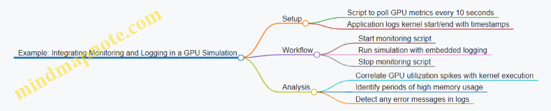
Mind Map: Monitoring and Logging Workflow
Example: Detecting a Memory Leak via Logs
Suppose an HPC application running on GPUs shows gradually increasing memory usage and eventual crashes. By combining periodic nvidia-smi logs with application debug output, you can pinpoint which kernel launches correspond to memory growth. Structured logs reveal that a specific kernel does not release buffers properly. Fixing the kernel’s memory deallocation resolves the issue.
Mind Map: Troubleshooting with Monitoring and Logging
Summary
Monitoring and logging form the backbone of reliable HPC operations with GPUs and TPUs. They provide the data needed to understand system behavior, catch problems early, and maintain smooth execution of scientific workloads. Using structured, timely, and centralized logs combined with hardware metrics enables efficient troubleshooting and performance tuning. Integrating these practices into your HPC workflow reduces downtime and improves confidence in simulation results.
12.7 Compliance and Regulatory Considerations in Scientific Computing
Scientific computing projects using GPUs and TPUs often handle sensitive data or operate within regulated environments. Compliance with relevant laws and standards is essential to maintain data integrity, protect privacy, and ensure reproducibility. This section outlines key compliance areas and practical considerations.
Understanding Compliance in HPC Contexts
Compliance means adhering to legal, ethical, and organizational rules governing data use, storage, and processing. In scientific computing, this includes:
- Data privacy laws (e.g., GDPR for European data subjects)
- Export controls on cryptographic or dual-use technologies
- Institutional review board (IRB) requirements for human subject data
- Industry-specific standards (e.g., HIPAA in healthcare, FDA regulations in pharmaceuticals)
Ignoring these can lead to legal penalties, loss of funding, or damage to institutional reputation.
Mind Map: Compliance Areas in Scientific Computing
Data Privacy and Protection
When scientific workloads involve personal or sensitive data, privacy laws dictate how data must be handled. For example, GDPR requires explicit consent for data processing and mandates data minimization. In HPC environments, this means:
- Limiting data access to authorized personnel
- Using encryption for data at rest and in transit
- Implementing anonymization or pseudonymization where possible
Example: A genomics simulation running on GPUs processes patient DNA sequences. To comply with GDPR, the data is anonymized before transfer to the cluster, and access controls restrict who can run or view the simulation results.
Security Controls and Access Management
Compliance often requires strict security controls. This includes:
- Role-based access control (RBAC) to limit who can submit jobs or access data
- Using secure authentication methods (e.g., multi-factor authentication)
- Maintaining audit logs for all data access and computational runs
Example: A climate modeling center uses a multi-tenant GPU cluster. They enforce RBAC so that researchers from different projects cannot access each other’s datasets, and all job submissions are logged for audit.
Regulatory Frameworks and Export Controls
Some scientific software or hardware may fall under export control regulations, especially if encryption or certain algorithms are involved. Compliance requires:
- Understanding classification of software and hardware
- Obtaining necessary licenses for international collaboration
- Tracking software versions and hardware configurations
Example: A research team using TPU accelerators with built-in encryption must verify that their usage complies with export regulations before sharing models with collaborators abroad.
Documentation and Reproducibility
Regulatory bodies often require detailed documentation of computational experiments. This includes:
- Data provenance: tracking origin and transformations of datasets
- Version control of code and dependencies
- Logging of computational environments and parameters
Good documentation supports reproducibility and accountability.
Example: A pharmaceutical simulation on GPUs maintains a detailed log of software versions, input parameters, and hardware used. This documentation is submitted alongside results to regulatory agencies.
Mind Map: Documentation Requirements

Practical Tips for Compliance
- Plan early: Identify applicable regulations before starting the project.
- Use encryption: Both for stored data and communication between nodes.
- Automate logging: Use tools that automatically capture environment and execution details.
- Train personnel: Ensure all team members understand compliance responsibilities.
- Review regularly: Compliance is ongoing; update policies and practices as regulations evolve.
Compliance in scientific computing with GPUs and TPUs is not just a legal box to check. It ensures trustworthiness, reproducibility, and ethical stewardship of data and resources. Integrating these considerations into your HPC workflows protects your work and your institution.
13. Appendix: Tools, Resources, and Reference Materials
13.1 List of Essential HPC Libraries and Frameworks
High-performance computing (HPC) with GPUs and TPUs relies heavily on specialized libraries and frameworks designed to maximize hardware efficiency and simplify development. Below is a structured overview of key libraries and frameworks, grouped by their primary function and target hardware.
Mind Map: HPC Libraries and Frameworks Overview
GPU-Focused Libraries
CUDA Ecosystem
NVIDIA’s CUDA is the most widely used platform for GPU programming. It offers a collection of libraries optimized for various scientific tasks.
-
cuBLAS: Provides GPU-accelerated Basic Linear Algebra Subprograms (BLAS). It handles dense matrix operations efficiently. For example, multiplying large matrices in a fluid dynamics simulation can be sped up by replacing CPU BLAS calls with cuBLAS.
-
cuFFT: Focuses on Fast Fourier Transforms, essential in signal processing and solving partial differential equations. Using cuFFT, a climate model can perform spectral analysis faster.
-
cuSPARSE: Deals with sparse matrix operations, common in finite element methods. It optimizes memory usage and computation for matrices with many zeros.
-
Thrust: A C++ template library for parallel algorithms and data structures, similar to the C++ Standard Template Library but GPU-accelerated. It simplifies tasks like sorting or reductions.
-
cuDNN: Primarily for deep learning, but its optimized primitives can accelerate neural network simulations in scientific contexts.
Example:
// Using cuBLAS for matrix multiplication
cublasHandle_t handle;
cublasCreate(&handle);
float alpha = 1.0f, beta = 0.0f;
cublasSgemm(handle, CUBLAS_OP_N, CUBLAS_OP_N,
            N, N, N,
            &alpha,
            d_A, N,
            d_B, N,
            &beta,
            d_C, N);
cublasDestroy(handle);
This snippet shows a basic single-precision matrix multiplication on the GPU.
OpenCL and HIP
OpenCL is an open standard for parallel programming across heterogeneous platforms, including GPUs from different vendors. HIP (Heterogeneous-Compute Interface for Portability) is AMD’s platform to ease porting CUDA code to AMD GPUs.
Both are useful when targeting non-NVIDIA GPUs or aiming for cross-platform compatibility.
TPU-Focused Libraries
TensorFlow
TensorFlow is the primary framework for programming TPUs. It abstracts TPU hardware details and provides high-level APIs for model building and training.
JAX
JAX offers composable transformations of numerical functions, including automatic differentiation and just-in-time compilation targeting TPUs. It is popular for research and experimental workloads.
XLA Compiler
The Accelerated Linear Algebra (XLA) compiler translates TensorFlow or JAX computations into optimized TPU instructions. Understanding XLA can help fine-tune performance.
Example:
import jax.numpy as jnp
from jax import jit

@jit
def matmul(a, b):
    return jnp.dot(a, b)

result = matmul(jnp.ones((1024, 1024)), jnp.ones((1024, 1024)))
This JAX example compiles a matrix multiplication to run efficiently on TPU hardware.
Cross-Platform and Parallel Programming Frameworks
MPI (Message Passing Interface)
MPI is the de facto standard for distributed memory parallelism. It works alongside GPU and TPU programming to coordinate tasks across nodes.
OpenMP
OpenMP supports shared memory parallelism, often used on CPUs but can coordinate with GPU offloading.
NCCL (NVIDIA Collective Communications Library)
NCCL optimizes communication between multiple GPUs, handling reductions and broadcasts efficiently.
Horovod
A distributed deep learning framework that simplifies multi-GPU and multi-TPU training using MPI or NCCL.
Example:
In a multi-GPU weather simulation, MPI handles node communication while NCCL accelerates GPU-to-GPU data exchange.
Domain-Specific Libraries
MAGMA
Matrix Algebra on GPU and Multicore Architectures (MAGMA) targets dense linear algebra, providing GPU-accelerated LAPACK-like routines.
PETSc
The Portable, Extensible Toolkit for Scientific Computation supports scalable solvers for linear and nonlinear systems, with GPU support through CUDA and HIP.
GROMACS and LAMMPS
Popular molecular dynamics packages that integrate GPU acceleration for simulating physical movements of atoms and molecules.
Example:
Using PETSc with CUDA allows solving large sparse systems arising from finite element discretizations efficiently on GPUs.
Summary
Choosing the right library or framework depends on the hardware, the scientific domain, and the nature of the workload. GPU-focused libraries like cuBLAS and cuFFT cover a broad range of numerical tasks, while TPU programming centers on TensorFlow and JAX. Cross-platform tools like MPI and NCCL enable scaling across multiple devices. Domain-specific libraries provide tailored solutions for particular scientific problems. Integrating these tools thoughtfully can significantly improve performance and development efficiency in HPC projects.
13.2 Commonly Used Profiling and Debugging Tools
Profiling and debugging are essential steps in optimizing HPC applications running on GPUs and TPUs. They help identify performance bottlenecks, memory issues, and logical errors that can degrade computational efficiency or cause incorrect results. This section covers widely used tools, their purposes, and practical examples to illustrate their use.
Profiling Tools for GPUs
Profiling tools collect runtime data about your GPU application, such as kernel execution times, memory usage, and occupancy. This data guides optimization efforts.
- NVIDIA Nsight Systems: A system-wide profiler that provides a timeline view of CPU and GPU activities, helping identify synchronization issues and resource contention.
- NVIDIA Nsight Compute: Focuses on detailed kernel-level profiling, offering metrics like warp occupancy, memory throughput, and instruction mix.
- nvprof (deprecated but still used): Command-line profiler for quick profiling runs.
- CUDA Visual Profiler (nvvp): GUI-based profiler for visualizing kernel execution and memory operations.
Example: Using Nsight Compute to Profile a Matrix Multiplication Kernel
nsys profile -o matmul_report ./matrix_mul
nsys stats matmul_report.qdrep
This command profiles the application and outputs detailed kernel metrics. You can identify if your kernel is memory-bound or compute-bound by examining achieved occupancy and memory throughput.
Debugging Tools for GPUs
Debugging GPU code requires specialized tools due to the parallel nature and device-host separation.
- CUDA-GDB: A command-line debugger for CUDA applications, allowing breakpoints, stepping through code, and inspecting variables on the device.
- Nsight Graphics: Provides frame debugging and GPU trace for graphics and compute workloads.
- cuda-memcheck: Detects memory errors such as out-of-bounds access, misaligned memory, and race conditions.
Example: Detecting Memory Errors with cuda-memcheck
cuda-memcheck ./my_gpu_app
This runs the application and reports any detected memory violations, helping catch bugs that could cause crashes or incorrect results.
Profiling and Debugging Tools for TPUs
TPUs have a different architecture and software stack, so profiling and debugging tools differ accordingly.
- TensorFlow Profiler: Integrated into TensorFlow, it provides detailed performance insights for TPU workloads, including operation timelines and device utilization.
- Cloud TPU Tools: Include TPU-specific monitoring dashboards and logs.
Example: Profiling a TPU Training Job with TensorFlow Profiler
Inside your TensorFlow script, you can enable profiling:
import tensorflow as tf

logdir = '/tmp/tf_profiler'

with tf.profiler.experimental.Profile(logdir):
    model.fit(dataset, epochs=5)
After running, you can visualize the profile using TensorBoard to identify slow operations or underutilized TPU cores.
Mind Map: GPU Profiling and Debugging Tools
Mind Map: TPU Profiling and Debugging Tools
Practical Tips for Using Profiling and Debugging Tools
- Start with coarse profiling: Use system-wide tools like Nsight Systems or TensorFlow Profiler to get an overview.
- Drill down to kernel-level: Use Nsight Compute or detailed TensorFlow traces to analyze hotspots.
- Check memory usage: Memory issues often cause performance degradation or crashes; tools like cuda-memcheck are invaluable.
- Use debugging tools early: Catching logical errors before optimization saves time.
- Automate profiling runs: Integrate profiling into your development cycle to monitor performance regressions.
Example Workflow: Profiling and Debugging a GPU Scientific Kernel
- Run
nsysto get a timeline and identify if kernels are serialized or overlapping inefficiently. - Use
nsight computeon the slowest kernel to check occupancy and memory throughput. - Run
cuda-memcheckto ensure no memory errors. - If bugs appear, attach
cuda-gdbto step through the kernel.
This structured approach helps isolate issues systematically.
Profiling and debugging tools are your microscope and stethoscope in HPC development. They reveal where your code struggles and why. Using them effectively requires understanding what each tool measures and how to interpret its output. The examples and mind maps here aim to make that clearer and more approachable.
13.3 Sample Code Repositories and Tutorials
This section gathers practical code examples and structured tutorials designed to help you get hands-on experience with GPU and TPU programming. The goal is to provide clear, runnable samples that illustrate core concepts and best practices discussed throughout the book.
Mind Map: Organizing Sample Code and Tutorials
GPU Programming Examples
1. Vector Addition in CUDA
This example demonstrates the simplest parallel computation: adding two vectors element-wise. It shows kernel launch parameters, memory allocation, and data transfer between host and device.
__global__ void vectorAdd(const float *A, const float *B, float *C, int N) {
    int i = blockDim.x * blockIdx.x + threadIdx.x;
    if (i < N) {
        C[i] = A[i] + B[i];
    }
}
The example emphasizes choosing block and grid sizes to cover all elements without oversubscription.
2. Matrix Multiplication with Shared Memory
A more advanced example uses shared memory to reduce global memory accesses, improving throughput.
Key points include:
- Dividing matrices into tiles.
- Loading tiles into shared memory.
- Synchronizing threads within a block.
This example illustrates how to balance memory bandwidth and compute resources.
TPU Programming Examples
1. Simple Neural Network on TPU with TensorFlow
This tutorial walks through defining a basic feedforward network and running it on TPU using TensorFlow’s tf.distribute.TPUStrategy.
It covers:
- TPU initialization.
- Dataset preparation.
- Model compilation and training.
The example highlights how TPU abstracts away low-level details while still requiring attention to batch sizes and data pipeline efficiency.
2. Custom Operation with XLA on TPU
This example shows how to write a custom operation optimized by XLA for TPU execution. It includes:
- Defining the operation in TensorFlow.
- Using XLA compiler hints.
- Measuring performance gains.
This demonstrates how to extend TPU capabilities beyond standard layers.
Hybrid and Distributed HPC Examples
1. MPI + CUDA Parallel Reduction
This example combines MPI for inter-node communication and CUDA for intra-node parallelism. It implements a reduction operation (sum) across multiple GPUs.
Steps include:
- Partitioning data across MPI ranks.
- Performing local reductions on GPUs.
- Using MPI to combine partial results.
It highlights synchronization and communication overhead considerations.
2. Data Pipeline Integration for TPU + GPU Workflows
This tutorial outlines how to split workloads between GPUs and TPUs, for example, preprocessing on GPUs and model training on TPUs.
It covers:
- Data serialization and transfer.
- Coordinating asynchronous execution.
- Managing resource utilization.
Summary
The sample code and tutorials are structured to build from simple to complex scenarios, reinforcing best practices like memory optimization, parallel execution, and efficient data management. Each example includes comments and explanations to clarify why certain choices are made, helping you apply these patterns to your own scientific workloads.
13.4 Glossary of Terms and Acronyms
This glossary covers key terms and acronyms commonly encountered in high-performance computing (HPC) with GPUs and TPUs. Each entry includes a concise definition and, where helpful, an example or a mind map in to clarify relationships.
Accelerator: A specialized hardware device designed to speed up specific computations. GPUs and TPUs are accelerators commonly used in HPC.
Arithmetic Intensity: The ratio of computational operations to memory operations. Higher arithmetic intensity often means better utilization of GPU or TPU compute units.
Bandwidth: The rate at which data can be transferred between memory and processing units, usually measured in GB/s.
Block (CUDA): A group of threads that execute together on a GPU and can share fast shared memory.
Cache: A small, fast memory located close to the processor cores to reduce latency when accessing frequently used data.
Compute Unit (CU): A fundamental processing element in GPUs or TPUs responsible for executing instructions.
CUDA (Compute Unified Device Architecture): NVIDIA’s parallel computing platform and API for programming GPUs.
Data Parallelism: A parallelization strategy where the same operation is performed simultaneously on different pieces of distributed data.
Deep Learning Accelerator (DLA): Hardware specialized for accelerating neural network computations, often integrated into TPUs.
Device Memory: Memory physically located on the GPU or TPU, distinct from host (CPU) memory.
Distributed Memory: A system architecture where each compute node has its own private memory.
Floating Point Operations Per Second (FLOPS): A measure of computational performance.
Grid (CUDA): A collection of blocks launched to execute a kernel on the GPU.
Host: The CPU and its memory in a heterogeneous computing system.
Kernel: A function executed on the accelerator device (GPU or TPU).
Latency: The delay between initiating a data transfer or computation and its completion.
Memory Coalescing: An optimization technique where memory accesses by threads are combined into fewer transactions to improve bandwidth usage.
Multi-Processing Unit (MPU): A term sometimes used to describe the processing units within TPUs.
Occupancy: The ratio of active warps (groups of threads) to the maximum number of warps supported on a GPU multiprocessor.
Operation Fusion: Combining multiple operations into a single kernel to reduce memory traffic and improve performance.
Parallelism: The degree to which tasks can be performed simultaneously.
Systolic Array: A hardware design pattern used in TPUs where data flows rhythmically through an array of processing elements.
Tensor Core: Specialized hardware units in modern GPUs designed to accelerate matrix operations, especially for deep learning.
Thread: The smallest unit of execution in GPU programming.
Warp: A group of threads (typically 32 in NVIDIA GPUs) that execute instructions in lockstep.
XLA (Accelerated Linear Algebra): A compiler that optimizes TensorFlow computations for TPUs and GPUs.
Mind Map: GPU Programming Model
Mind Map: TPU Architecture Overview
Example: Memory Coalescing in CUDA
Suppose 32 threads each read one 4-byte float from consecutive addresses in global memory. If these accesses are aligned and contiguous, the GPU can coalesce these into a single 128-byte transaction. This reduces memory latency and improves bandwidth usage. If threads access scattered addresses, multiple transactions occur, hurting performance.
Example: Warp Execution
A warp consists of 32 threads executing the same instruction simultaneously. If threads diverge (take different branches), the warp serializes the execution paths, reducing efficiency.
This glossary is designed to clarify the terminology and concepts that underpin HPC on GPUs and TPUs. Understanding these terms helps in grasping the architecture, programming models, and optimization strategies discussed throughout the book.
13.5 Best Practices Summary Checklist
This checklist condenses the core best practices for high-performance computing with GPUs and TPUs, focusing on optimizing scientific workloads and large-scale simulations. Each section includes a mind map to visualize key points and concrete examples to clarify application.
Hardware and Environment Setup
- Choose the accelerator based on workload characteristics: GPUs for flexible parallelism, TPUs for matrix-heavy tensor operations.
- Keep drivers and SDKs up to date to ensure compatibility and performance.
- Use containerization (e.g., Docker) to maintain consistent environments.
Example: Before running a fluid dynamics simulation, verify CUDA driver version matches the CUDA toolkit used in development to avoid runtime errors.
Programming and Kernel Design
- Structure kernels to maximize occupancy by balancing thread count and resource usage.
- Align data in memory to enable coalesced accesses, reducing latency.
- Minimize branch divergence to keep SIMD units efficient.
Example: In a matrix multiplication kernel, use shared memory to cache tiles of input matrices, reducing global memory reads.
Memory Management

- Transfer only necessary data between host and device; batch transfers to reduce overhead.
- Overlap data transfers with computation using streams or asynchronous APIs.
- On TPUs, structure computations to fit within on-chip memory to avoid slow off-chip accesses.
Example: Use CUDA streams to copy the next data chunk while the current kernel executes, improving throughput.
Performance Optimization
- Profile early and often; focus on hotspots rather than premature optimization.
- Fuse small operations to reduce kernel launch overhead on TPUs.
- Use loop unrolling and instruction-level parallelism to keep execution units busy.
Example: After profiling a molecular dynamics kernel, unroll the inner force calculation loop to reduce branch overhead.
Parallel and Distributed Computing
- Use MPI or NCCL for communication between GPUs; TPU Pods require TPU-specific communication primitives.
- Balance workload to avoid idle devices; consider dynamic scheduling if workload is uneven.
- Minimize synchronization points to reduce stalls.
Example: In a weather simulation, partition the domain evenly and use asynchronous MPI calls to overlap communication with computation.
Debugging and Testing
- Use device-specific debuggers to inspect kernel execution and memory state.
- Write unit tests for kernels and integration tests for the full pipeline.
- Monitor performance regressions as part of continuous testing.
Example: Use NVIDIA Nsight Compute to identify a kernel with excessive register usage causing low occupancy.
Scientific Algorithm Adaptation
- Choose algorithms that expose parallelism and fit accelerator memory models.
- Consider mixed precision to accelerate computation while maintaining acceptable accuracy.
- Simplify algorithms where possible to reduce computational complexity.
Example: Replace a double-precision solver with a mixed-precision iterative refinement method to speed up linear system solutions.
Workflow and Integration
- Leverage optimized libraries to avoid reinventing the wheel.
- Wrap legacy code incrementally to introduce accelerator support without full rewrites.
- Automate tests and performance checks to catch regressions early.
Example: Integrate cuFFT into an existing signal processing pipeline to accelerate Fourier transforms without changing core logic.
This checklist is a practical guide to keep your HPC projects on track, balancing performance, maintainability, and correctness. The mind maps help visualize the relationships between concepts, while examples ground the advice in real-world scenarios.
13.6 Example Configurations for GPU and TPU Clusters
Configuring clusters for GPU and TPU workloads requires attention to hardware selection, network topology, software stack, and workload characteristics. This section provides concrete examples and mind maps to clarify typical cluster setups and their components.
Mind Map: GPU Cluster Configuration
Example: Small-Scale GPU Cluster Setup
- Compute Nodes: 4 nodes, each with 2x NVIDIA A100 GPUs, 64 CPU cores, 512 GB RAM
- Network: Mellanox InfiniBand HDR 200 Gbps
- Storage: 10 TB NVMe SSD per node, shared via Lustre filesystem
- Software: Ubuntu 20.04, CUDA 11.4, cuDNN 8, Slurm scheduler
This setup suits medium-sized scientific simulations requiring parallel GPU acceleration and fast inter-node communication.
Mind Map: TPU Cluster Configuration
Example: TPU Pod Configuration for Scientific Simulation
- TPU Pod: 32 TPU v3 devices (256 TPU cores total)
- Host Machines: 8 hosts, each with 48 CPU cores and 384 GB RAM
- Network: High-speed internal TPU interconnect
- Software: TensorFlow 2.6 with XLA compiler, TPU runtime
This configuration targets large-scale machine learning simulations or scientific models that benefit from TPU matrix multiply units.
Mind Map: Key Considerations for Cluster Configuration
Example: Hybrid GPU-TPU Cluster
- Compute Nodes: 6 GPU nodes (each with 4x NVIDIA V100 GPUs), 4 TPU nodes (each with TPU v3-8)
- Network: 100 Gbps Ethernet connecting all nodes
- Storage: Shared parallel file system with 50 TB capacity
- Software: Mixed environment with CUDA and TensorFlow, Slurm for job scheduling
This hybrid cluster supports workflows that combine traditional HPC GPU tasks with TPU-accelerated machine learning components.
Practical Tips for Cluster Configuration
- Match CPU cores to GPU/TPU count to avoid bottlenecks in data preprocessing.
- Use high-speed interconnects to reduce communication overhead in multi-node jobs.
- Choose software versions carefully to ensure compatibility with hardware and libraries.
- Implement monitoring tools (e.g., NVIDIA Nsight, TPU profiler) to track utilization and identify hotspots.
- Plan for fault tolerance by enabling checkpointing and job restart capabilities.
These examples and mind maps provide a foundation for understanding how to configure GPU and TPU clusters tailored to scientific workloads. The key is balancing hardware capabilities, network infrastructure, and software environments to meet the demands of your specific simulations.
13.7 Additional Reading and Documentation Sources
When working with high-performance computing (HPC) on GPUs and TPUs, having a solid grasp of foundational and advanced materials is essential. This section organizes key documentation and reading materials into thematic clusters, presented as mind maps in format. Each cluster groups related topics, helping you navigate the complex landscape of HPC resources efficiently.
Mind Map 1: GPU Programming and Architecture
Example: Understanding warp scheduling helps avoid thread divergence, which can degrade performance. For instance, structuring conditional branches to minimize divergence within a warp improves throughput.
Mind Map 2: TPU Architecture and Programming
Example: Using operation fusion reduces memory bandwidth usage by combining multiple operations into a single kernel, which is crucial for TPU efficiency.
Mind Map 3: Parallel Programming Models and Frameworks
Example: Combining MPI with CUDA allows distributing workloads across multiple GPUs, enabling simulations that exceed single-device memory limits.
Mind Map 4: Memory and Data Management
Example: Using pinned memory for host-device transfers can reduce latency and increase throughput, especially in data-intensive simulations.
Mind Map 5: Performance Optimization and Profiling
Example: Profiling a molecular dynamics kernel with Nsight can reveal memory bottlenecks, guiding targeted optimizations such as increasing shared memory usage.
Mind Map 6: Scientific Workloads and Applications
Example: Implementing a parallel FFT on GPUs requires careful data layout and synchronization to maximize throughput and minimize latency.
Mind Map 7: Distributed Computing and Scalability
Example: Efficient use of all-reduce operations in MPI-based multi-GPU simulations ensures timely synchronization without excessive communication overhead.
Mind Map 8: Debugging, Testing, and Reliability
Example: Writing unit tests for CUDA kernels can catch errors early, preventing costly debugging sessions during large-scale runs.
This structured approach to reading and documentation helps you focus on specific aspects of HPC with GPUs and TPUs. Each mind map clusters related topics for easier reference. The examples illustrate practical implications of the concepts, reinforcing understanding through concrete scenarios.