Holographic Display Systems Explained
1. Foundations of Holographic Display
1.1 What Holography Produces and Why It Differs from Stereoscopy
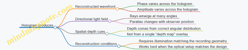
What Holography Produces
A hologram is a record of how light’s wavefront looks, not just where objects appear in a picture. When you illuminate a hologram with the right reference light, the hologram reconstructs a wavefront that propagates through space as if the original scene were there. The key output is a spatially varying optical field: different points on the hologram contribute different phase and amplitude, so the reconstructed light carries direction information.
A useful way to think about it is: stereoscopy stores two images for two viewpoints, while holography stores enough information to recreate many viewpoints at once—because the wavefront itself encodes direction.
Mind Map: Holography Output
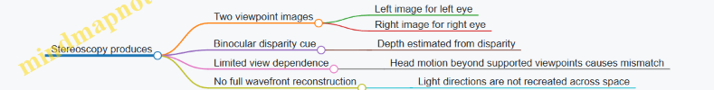
How That Differs from Stereoscopy
Stereoscopy aims to trick your eyes by presenting a different image to each eye. It typically uses two slightly different camera views, then relies on binocular vision to interpret the disparity as depth. The images are still flat in the sense that each eye receives a 2D projection; the system does not inherently generate a full 3D wavefront.
That difference shows up in what happens when you move your head. With stereoscopy, the view changes only for the discrete viewpoints the system is designed to support. With holography, the reconstructed field naturally changes with position because the light directions are physically present in the reconstructed wavefront.
Mind Map: Stereoscopy Output
Concrete Example: A Coin on a Table
Imagine a coin at a known distance from the viewer.
-
In stereoscopy, the system renders two images: one where the coin appears slightly shifted left, and one where it appears slightly shifted right. Your brain uses the disparity between these images to estimate depth. If you move your head sideways, the images may not update continuously for the new viewpoint, so the coin can “stick” to the screen plane or show incorrect motion parallax.
-
In holography, the reconstructed wavefront for the coin includes angular information. As you move laterally, the light reaching your eyes comes from different directions that were encoded in the hologram. The coin’s apparent position and motion parallax change in a way that matches the geometry of the reconstructed field.
The practical takeaway: stereoscopy can be convincing for small head motions around the intended viewing zone, while holography is designed to reproduce the spatial structure of light so that viewpoint changes are handled by the physics of reconstruction.
Concrete Example: A Point Light Source
Consider a point source at a specific location in space.
-
A stereoscopic system can show the point at a depth by placing it at different pixel coordinates in the left and right images. But the light reaching each eye is still an image projection; it does not behave like a true point source that emits spherical wavefronts.
-
A hologram aims to reconstruct the wavefront that a point source would generate. If the reconstruction is correct, the light field near the hologram behaves like the original spherical wavefront, which is why the point can appear to occupy space rather than just a screen depth cue.
Why the Difference Matters in Practice
The distinction between “image-based depth” and “field-based reconstruction” affects what you can measure and debug.
- With stereoscopy, you can evaluate performance by checking disparity consistency, image alignment, and how well the system updates with viewpoint.
- With holography, you evaluate whether the reconstructed wavefront matches the intended geometry: phase accuracy, diffraction order control, and whether the reconstructed directions align with the viewing conditions.
In short: stereoscopy produces images that your eyes interpret as depth; holography produces a reconstructed optical field that your eyes sample as depth.
1.2 Wavefronts, Phase, and Amplitude in Practical Display Terms
A holographic display is easiest to understand as a device that controls how light waves arrive at the viewer. The “wavefront” is the geometric shape of equal phase—think of it as the set of points where the wave is at the same stage of its cycle. If you can shape wavefronts, you can steer where light constructively adds and where it cancels.
Wavefronts as “Where the Light Wants to Be”
A wavefront alone doesn’t tell you brightness; it tells you timing. Suppose two rays reach a point on the viewer’s retina. If their phases match, they add strongly. If they differ by half a cycle, they subtract. In practice, holograms create a pattern of phase delays across the modulator so that, after propagation through the optics, the viewer receives the intended phase relationships.
A useful mental model: wavefronts are like road signs for the wave. They don’t carry energy by themselves; they specify the schedule of oscillation across space.
Phase as the Display’s Main Dial
Phase is the position within a repeating cycle. For a monochromatic wave, you can write the complex field as:
- Amplitude: how strong the wave is
- Phase: where in the cycle it is
In holography, phase control is often the most important because small phase errors can turn a sharp reconstruction into a blurry one. For example, if a hologram is designed to focus light to a point, a phase error across the aperture changes the interference pattern that creates that focus.
Practical Example: Phase Error as “Focus Drift”
Imagine you want a bright spot at a target distance. The hologram encodes a phase pattern that makes the wavefronts converge there. If you add a constant phase offset everywhere, the spot stays bright because relative phase between points is unchanged. If instead you introduce a phase ramp error across the aperture, the convergence point shifts—your “spot” moves.
Amplitude as “How Much Light You Send”
Amplitude controls the strength of the field. In many holographic setups, amplitude is harder to control directly than phase, so systems often approximate amplitude using phase-only modulation plus optical filtering. Still, amplitude matters: if amplitude is too low, the reconstruction is dim; if amplitude is uneven, the image can show contrast problems.
Practical Example: Amplitude Weighting for Edges
Consider a simple scene: a bright square on a dark background. If you encode only phase and ignore amplitude, the reconstruction may still appear, but the edge contrast can be weaker because the field magnitude doesn’t match the intended distribution. A practical approach is to compute a complex field for the target (with both magnitude and phase), then map it onto what the modulator can represent.
Complex Field in Display Terms
A hologram typically starts from a desired complex field at some plane. The modulator then applies a transformation so that, after propagation, the viewer sees that field.
Mind Map: Wavefront, Phase, Amplitude
Interference: The Bridge Between Theory and What You See
What the viewer perceives is not amplitude at one point, but the result of interference across many paths. A hologram works because it creates consistent phase relationships across the aperture. When those relationships match the design, the viewer receives a strong reconstructed wavefront.
Practical Example: Why “More Light” Isn’t the Same as “Better”
If you increase illumination intensity uniformly, the reconstruction gets brighter, but phase mistakes remain. The image can still be washed out or misfocused because the interference pattern is wrong. Conversely, a well-encoded phase pattern can produce a recognizable image even at moderate brightness, because the relative timing is correct.
Phase and Amplitude in a Single Sentence That Actually Helps
In a holographic display, phase decides the geometry of interference, while amplitude decides how strongly that geometry shows up as brightness and contrast.
Quick Checklist for Interpreting a Holographic Result
- If the image is in the wrong place: suspect phase ramp or alignment errors.
- If the image is faint: suspect amplitude mismatch or efficiency loss.
- If edges look smeared: suspect phase quantization, bandwidth limits, or propagation mismatch.
- If contrast is low: suspect amplitude approximation or unwanted background orders.
1.3 Coherence, Bandwidth, and Illumination Constraints
Holographic displays are picky about three things: how consistent the light’s phase is (coherence), how much data you can push per second (bandwidth), and how much usable light you can afford to deliver (illumination). These constraints show up as visible artifacts: speckle, washed-out contrast, blur, flicker, and depth errors.
Coherence Constraints
Coherence describes how stable the phase relationship is over time and distance. In practice, it sets how well the system can interfere light from different parts of the scene.
- Temporal coherence limits interference when path lengths differ too much. If your illumination has a short coherence length, interference fringes wash out, and reconstructions lose contrast.
- Spatial coherence limits interference across the modulator aperture. If spatial coherence is insufficient, the reconstructed wavefront becomes inconsistent across the field.
Easy example: Imagine two beams that should interfere to form a bright spot. If the phase difference jitters faster than the camera or eye integration time, the spot becomes a gray smear. That jitter can come from a light source with short coherence or from mechanical vibration that changes optical path length.
Practical best practice: Keep optical paths stable and minimize unnecessary path-length differences between reference and object wave paths. When using an SLM, ensure the illumination and relay optics do not introduce strong phase noise across the modulator plane.
Bandwidth Constraints
Bandwidth is both optical and computational. Optical bandwidth affects coherence (spectral width), while computational bandwidth affects how quickly you can update holograms or view-dependent light-field data.
- Spectral bandwidth tradeoff: A broader spectrum reduces temporal coherence, which can reduce interference contrast. Narrowing the spectrum improves coherence but reduces available power.
- Data bandwidth tradeoff: Real-time holography often needs frequent updates. If your system can’t refresh fast enough, motion causes temporal artifacts and depth cues lag behind head or object motion.
Easy example: Suppose you render a hologram at 60 Hz but the user turns their head quickly. The reconstructed image corresponds to an earlier viewpoint, so parallax feels “off.” Even if the hologram is perfect for its intended view, the mismatch in time makes the scene look wrong.
Practical best practice: Budget latency end-to-end: tracking update time, rendering time, modulator settling time, and synchronization. Then choose a refresh rate that the pipeline can sustain without dropping frames.
Illumination Constraints
Illumination constraints are about brightness, efficiency, and how much light survives the optical chain.
- Source power and safety limits cap how bright the system can be.
- Optical throughput drops due to losses in lenses, polarizers, diffraction orders, and apertures.
- Modulation efficiency matters because many holographic encodings waste light into unwanted diffraction orders.
Easy example: If half your light goes into the wrong diffraction order, your “useful” reconstruction is dimmer by roughly a factor of two. Dim reconstructions force you to increase exposure or gain, which also amplifies noise and makes speckle more noticeable.
Practical best practice: Treat brightness like a budget. Identify where light is lost: polarizers (especially with phase-only modulation), diffraction order selection, and any spatial filtering. Then tune encoding and optical filtering so the desired order gets the most energy.
Mind Map: Coherence, Bandwidth, Illumination
Integrated Example: Choosing Illumination and Update Rate
Consider a system targeting a moderate eye box and a 3D scene with noticeable motion. If you choose a very broad-spectrum source to maximize power, temporal coherence drops and interference contrast falls, making depth cues harder to read. If you instead narrow the spectrum to improve coherence, you may lose power, which can reduce brightness and increase perceived noise.
Now add computation: if your pipeline can only sustain the hologram update rate at a lower frame rate, motion causes viewpoint mismatch. The result is a reconstruction that is both low-contrast (from coherence limits) and temporally inconsistent (from bandwidth limits). The fix is not one knob; it’s balancing illumination spectrum, optical stability, and a refresh rate your pipeline can maintain.
Quick Checklist
- Coherence: Are path-length differences controlled, and is the source spectrum narrow enough for visible interference?
- Bandwidth: Can the system update holograms at a rate that matches motion and avoids frame drops?
- Illumination: Is the desired diffraction order receiving enough light after polarizers, filtering, and losses?
1.4 Viewing Geometry, Parallax, and Eye Box Requirements
Viewing geometry is the set of spatial relationships that determine where each eye receives light from the display. In holographic and light-field-like systems, those relationships directly control parallax, perceived depth, and whether the image stays stable as the viewer moves.
What “Viewing Geometry” Means in Practice
Start with three points: the viewer’s eyes, the display plane, and the reconstructed image points. If the system is designed so that a reconstructed point sends light toward the correct eye positions, then moving your head changes which rays you receive. That change is parallax. If the system sends light toward only a narrow range of angles, the image will shift or dim outside that range.
A useful mental model is to treat the display as a source of many directional “channels.” Each channel corresponds to a small range of angles. The eye box is the region in space where enough channels overlap with the eye’s pupil to produce a coherent reconstruction.
Parallax: Correct Motion Versus Wrong Motion
Parallax is not just “the image moves when you move.” It should move in a way consistent with the scene’s depth. For a simple example, imagine two reconstructed points: one near, one far. When you shift laterally, the near point should shift more than the far point. If both shift equally, depth cues collapse into a flat look.
In practice, parallax errors come from mismatches between:
- The assumed eye position used during rendering or hologram generation.
- The actual optical path through the modulator and reconstruction optics.
- The effective pupil location, which can differ from where the eye tracker thinks it is.
A quick check: pick a single high-contrast edge at a known depth. Move your head slowly left and right. If the edge “slides” sideways at the wrong rate, your geometry mapping is off.
Eye Box Requirements and How to Size Them
The eye box is usually specified as a 3D volume with a lateral extent (left-right), vertical extent (up-down), and depth extent (front-back). The required size depends on the intended use case.
Example: workstation viewing.
- Typical head motion might be about ±5 cm laterally and ±3 cm vertically.
- The system might target a comfortable viewing distance where the eye box depth is limited by optics and coherence.
- If the eye box is smaller than the user’s motion, the image will drift, lose brightness, or show order-dependent artifacts.
Sizing the eye box is a balancing act. A larger eye box demands more angular coverage from the display and more careful control of reconstruction. That increases computational load and can reduce per-angle intensity.
Mapping Eye Position to Rendering or Modulation
Most systems need a mapping from measured eye pose to the parameters used to generate the displayed hologram or light-field content. Even if the system is “static,” the optical reconstruction still depends on where the eye is.
A practical approach is to define a coordinate system:
- Display coordinates: origin at the modulator center, with axes aligned to the optical layout.
- Eye coordinates: measured eye center or pupil center in the same reference frame.
- View parameters: derived quantities such as lateral offsets and viewing direction.
Then, for each view update, the system selects or computes the content that best matches those view parameters.
Example: discrete view sampling.
If you precompute holograms for a grid of eye positions, you can choose the nearest view or interpolate between two. Nearest-view selection is simple but can cause small jumps when the eye crosses a grid boundary. Interpolation reduces jumps but requires careful blending to avoid ghosting.
Mind Map: Viewing Geometry and Eye Box
Example: A Simple Eye Box Calculation Workflow
- Choose a target viewing distance \(D\) from the display to the nominal eye plane.
- Decide lateral comfort range \( \Delta x \) (e.g., 10 cm total span).
- Convert lateral range to angular coverage using \( \theta \approx \arctan(\Delta x / (2D)) \).
- Ensure the system’s reconstruction supports that angular range with sufficient intensity.
If your supported angular range is smaller than the required one, you will see parallax errors and brightness falloff near the edges of the eye box.
Common Failure Modes to Watch For
- Depth-dependent drift: near objects appear to “swim” more than expected, indicating incorrect depth-to-parallax mapping.
- Order-dependent artifacts: unwanted diffraction orders become more visible as the eye moves, suggesting insufficient order suppression across the eye box.
- Boundary jumps: discrete view selection causes sudden changes at certain head positions.
A good workflow is to test with a scene containing both near and far features, then sweep the head position across the intended eye box while monitoring edge alignment and brightness consistency.
1.5 System-Level Signal Chain from Scene to Screen
A holographic display is picky about timing, geometry, and how the light is modulated. The signal chain is the set of steps that turns a 3D scene into a modulator pattern that reconstructs the intended wavefronts at the intended viewing positions.
Scene Inputs and Coordinate Conventions
Start with a scene description: meshes, materials, and camera pose. Even before rendering, lock down coordinate conventions. If your renderer uses meters but your optics model uses millimeters, you will get the right shape at the wrong depth. A practical habit is to define one “source of truth” unit and convert everything else to it at the boundaries.
Example: You model a 200 mm cube. Your renderer outputs depth in meters. If you forget to divide by 1000 when computing hologram propagation distances, the cube will appear 1000× farther away, and the eye box will not behave as expected.
View Selection and View-Dependent Rendering
Most holographic systems are view-dependent: the modulator pattern changes with where the viewer is. The pipeline therefore begins with view selection.
- If you have eye tracking, you map eye pose to a discrete set of view parameters.
- If you don’t, you choose a fixed view or a small set of views and accept reduced comfort.
Best practice: quantize view updates to the modulator frame rate. If you update view parameters mid-frame, you create temporal inconsistency that shows up as shimmering or depth wobble.
Example: A system runs at 60 Hz. If your tracking updates at 120 Hz but the hologram only changes at 60 Hz, you should sample the latest eye pose at each hologram frame boundary rather than interpolating continuously.
Rendering to an Intermediate Light Representation
Instead of jumping straight to a hologram, many pipelines render to an intermediate representation that matches the physics of the next step.
Common intermediates:
- Light field samples (angular and spatial samples)
- Disparity-layered images (depth slices)
- Complex field samples on a plane (amplitude and phase)
Best practice: keep the intermediate aligned with the optical propagation model. If your hologram generator assumes a particular plane location, render the intermediate as if that plane is where the field lives.
Example: If your optical model propagates from a “virtual object plane” to the modulator, render your depth layers relative to that plane, not relative to the mesh origin.
Hologram Synthesis and Encoding
Hologram synthesis converts the intermediate representation into a modulator pattern. This step includes propagation, interference, and encoding.
Key sub-steps:
- Propagate the intermediate field to the modulator plane.
- Compute the complex field at the modulator.
- Convert complex field to what the modulator can display (often phase-only, sometimes amplitude via tricks).
- Encode into discrete pixels with quantization.
Best practice: include a “zero-order and unwanted order” strategy. If you do nothing, the reconstruction can be dominated by the direct term.
Example: A phase-only encoding might add a carrier grating to shift the desired reconstruction away from the zero order. You then filter or design the optics so the shifted order lands in the eye box.
Modulator Calibration and Driver Output
The modulator does not respond ideally to commanded values. Calibration maps commanded gray levels to actual phase (or amplitude) response.
Practical calibration workflow:
- Measure phase response versus gray level.
- Fit a function or build a lookup table.
- Apply the inverse mapping in the driver.
Best practice: calibrate at the operating temperature and include a periodic re-check. Liquid crystal devices drift with temperature, and the “same” gray value can mean a different phase later.
Example: Without inverse mapping, a 2π phase wrap might occur at gray 180 in the lab but at gray 170 during operation. The hologram still updates, but the reconstructed depth shifts and contrast drops.
Optical Transfer and Alignment Constraints
The optical system transforms the modulator pattern into the reconstructed field. This includes lens focal lengths, distances, aperture stops, and alignment.
Best practice: treat alignment as part of the signal chain. If the modulator is shifted by a few hundred micrometers, the reconstruction geometry changes, and your view mapping becomes wrong.
Example: If the modulator is laterally misaligned, the reconstructed image shifts sideways. Your eye-tracking mapping might still be correct in software, but the physical reconstruction no longer matches the assumed coordinates.
Timing, Synchronization, and Frame Scheduling
Holographic displays are sensitive to timing. The driver, modulator refresh, and any tracking input must be synchronized.
A robust scheduling approach:
- Capture tracking pose.
- Render hologram for the next modulator update.
- Upload pattern before the modulator’s sample-and-hold moment.
Best practice: measure end-to-end latency and budget it. If the pipeline takes longer than one frame, you will effectively display an older view.
Example: If rendering takes 20 ms but the modulator updates every 16.7 ms, you will miss deadlines. The system will show a lagging view, which often presents as eye-box instability.
Mind Map of the Signal Chain
Mind Map: System-Level Signal Chain from Scene to Screen
A Concrete End-to-End Example
Assume a 3D scene with a tracked viewer.
- The renderer receives the latest eye pose at the start of a frame.
- The system maps eye pose to a discrete view index and selects the corresponding rendering parameters.
- The renderer outputs a depth-sliced intermediate aligned to the virtual object plane used by the propagation model.
- The hologram generator propagates each slice to the modulator plane, combines them, and applies an encoding strategy that shifts the desired order.
- The driver converts the encoded phase to modulator gray values using the calibrated inverse mapping.
- The optical system reconstructs the shifted order into the eye box, assuming alignment parameters match the ones used in view mapping.
- The scheduler ensures the pattern is uploaded before the modulator’s update moment, so the displayed hologram corresponds to the intended view.
When any one of these steps is off—units, view quantization, calibration, alignment, or timing—the failure mode is usually consistent and diagnosable: wrong depth, wrong lateral position, reduced contrast, or unstable eye-box behavior.
2. Light Field Rendering for Display-Ready Imagery
2.1 Light Field Parameterizations for Rendering Pipelines
A light field describes how light rays vary with both direction and position. In rendering pipelines, the key question is not “what is a light field,” but “which coordinates make it easy to sample, store, and transform.” Different parameterizations trade off memory, aliasing risk, and how naturally they connect to your display model.
1) The Three Coordinates You Keep Reusing
Most practical parameterizations can be understood as choosing:
- A spatial coordinate for where the ray is “sampled” (often a point on a plane).
- An angular coordinate for the ray direction (often represented by another coordinate on a different plane).
- A depth or propagation model for how you interpret those rays when reconstructing images.
If you pick coordinates that align with your optics, you spend less time converting between representations.
2) Common Parameterizations
A) Two-Plane Parameterization
You represent rays by their intersection points with two parallel planes. Let the planes be at positions \(z=z_0\) and \(z=z_1\). A ray is then \(r(u,v,s,t)\), where \((u,v)\) is the hit point on the first plane and \((s,t)\) is the hit point on the second plane.
Why it’s useful: it maps cleanly to view synthesis because changing the “virtual camera” corresponds to selecting rays with consistent angular structure.
Pipeline-friendly example: Suppose you want 9 views across an eye box. If you store rays on a grid of angular samples, you can render each view by selecting rays whose direction matches that view’s camera center.
Practical caution: if your angular sampling is too coarse, you get view-to-view jumps that look like stepping parallax.
B) Angular-First Parameterization
Instead of storing both plane intersections, you store rays as a set of direction bins plus a spatial sample per direction. Conceptually, it’s like: for each direction \(\omega\), store a 2D image of radiance over space.
Why it’s useful: it can reduce wasted storage when many directions are irrelevant (for example, if your display only supports a limited range of angles).
Pipeline-friendly example: If your optical system only reconstructs within a cone of angles, you can pre-filter directions and avoid computing rays outside that cone.
Practical caution: direction bins must be consistent with the reconstruction geometry; otherwise, you’ll get incorrect depth scaling.
C) Pixel-Centric Parameterization
You store rays relative to a pixel grid on a sensor or intermediate plane. Each pixel corresponds to a set of rays with different directions.
Why it’s useful: it aligns with how cameras and many intermediate buffers naturally output data.
Pipeline-friendly example: If you already have a renderer that outputs per-pixel depth and normal, you can generate rays per pixel and then map them into direction bins for the light field.
Practical caution: pixel-centric layouts can hide uneven sampling density across the field, which shows up as uneven blur or aliasing.
3) How Parameterization Affects Rendering Steps
A rendering pipeline typically does three things: sample, transform, and reconstruct.
- Sample: generate rays from your scene. Your parameterization decides what “sample grid” means.
- Transform: convert between your ray storage and the coordinates your reconstruction expects.
- Reconstruct: produce images for specific viewpoints or hologram inputs.
A good parameterization minimizes transforms. For example, if your reconstruction uses a two-plane geometry, storing in two-plane form avoids repeated coordinate remapping.
4) Mind Map of Parameterization Choices
5) Concrete Example: Choosing a Layout for 3×3 Views
Assume you need 9 views (3×3) across an eye box. You can do this two ways:
- Two-plane storage: pick angular samples so that each view corresponds to a consistent direction subset. Rendering each view becomes selecting rays whose direction matches that view.
- Angular-first storage: store only the directions that map to the 9 views. Rendering becomes projecting each stored direction image into the view.
If your eye box is narrow, option 2 often wastes less storage because it avoids directions you’ll never use. If your eye box is wide but your reconstruction geometry is fixed, option 1 often reduces transform errors because the coordinate mapping stays consistent.
6) A Simple Rule for Picking Coordinates
Choose parameterization coordinates that make your reconstruction step a selection rather than a re-derivation.
- If reconstruction expects two-plane intersections, store two-plane.
- If reconstruction expects a limited angular cone, store direction bins and pre-filter.
- If your upstream data is pixel-aligned, start pixel-centric and convert once.
That rule keeps your pipeline predictable: fewer conversions means fewer opportunities to introduce subtle geometric mistakes.
2.2 Sampling Strategies for Angular and Spatial Resolution
Sampling decides whether a holographic or light-field pipeline produces a clean reconstruction or a blurry, aliased mess. The trick is to treat angular and spatial sampling as two coupled budgets: angular sampling controls how many viewing directions you can represent, while spatial sampling controls how finely you can represent structure within each direction.
Angular Sampling for View Coverage
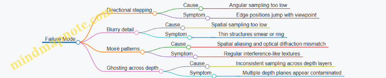
Angular sampling describes how densely you sample rays (or view directions) across the eye box. If you sample too sparsely, the reconstruction shows “directional stepping,” where object edges shift in discrete jumps as the viewer moves.
A practical way to reason about angular sampling is to start from the maximum lateral eye-box shift, \(\Delta x\), and the distance to the reconstruction plane, \(z\). The corresponding angular span is approximately \(\Delta \theta \approx \Delta x / z\). If you want the viewer to perceive smooth motion, you choose an angular step \(\delta \theta\) small enough that the induced lateral shift at the reconstruction plane is below your tolerance.
Easy example: Suppose the eye box spans \(\Delta x = 20,\text{mm}\) and the reconstruction plane is \(z = 200,\text{mm}\). Then \(\Delta \theta \approx 0.1,\text{rad}\). If you can tolerate about \(0.5,\text{mm}\) of lateral “jump” at the plane, then \(\delta \theta \approx 0.5/200 = 0.0025,\text{rad}\). That suggests about \(0.1/0.0025 = 40\) angular samples across the span. In a 2D angular grid, you’ll need roughly \(40 \times 40\) directional samples if you cover both horizontal and vertical.
Spatial Sampling for Detail Preservation
Spatial sampling describes how finely you sample the scene across the display aperture or intermediate representation. Too coarse a spatial grid causes loss of high-frequency detail and can create moiré patterns when combined with the optical system’s diffraction.
A useful mental model is: spatial sampling sets the smallest feature size you can represent without aliasing. If your effective sampling pitch is \(p\) at the plane where you encode rays or hologram content, then the highest representable spatial frequency is on the order of \(1/(2p)\). Features smaller than roughly \(2p\) will be poorly represented.
Easy example: If your modulator pixel pitch maps to an effective sampling pitch of \(p = 6.4,\mu\text{m}\) at the encoding plane, then the smallest reliably representable feature is on the order of \(2p \approx 12.8,\mu\text{m}\). If your rendering includes thin structures or sharp edges that project to smaller scales, you should expect edge thickening or ringing.
Coupling Angular and Spatial Sampling
Angular and spatial sampling are not independent. A ray-based representation can be thought of as a 4D sampling problem: two spatial coordinates (\(x,y\)) and two angular coordinates (\(\theta_x,\theta_y\)). Increasing angular resolution without enough spatial resolution can still fail, because each angular slice carries spatial detail that must be sampled consistently.
A concrete way to see the coupling: when you increase angular sampling, you effectively increase the number of distinct views that must be reconstructed. If the spatial sampling is fixed, each view has limited bandwidth, so fine angular changes may appear smooth but still lack crisp edges.
Choosing Sampling Rates with a Simple Workflow
- Define the reconstruction plane and eye box. Use \(z\) and \(\Delta x,\Delta y\) to estimate angular span.
- Set a lateral tolerance. Decide the maximum acceptable shift at the reconstruction plane between adjacent angular samples.
- Compute angular sample counts. Use \(\delta \theta \approx \text{tolerance}/z\) and \(N \approx \Delta \theta/\delta \theta\).
- Estimate spatial sampling pitch. Use modulator pixel pitch and your optical mapping to get effective \(p\).
- Check feature bandwidth. Ensure the smallest projected features are not far below \(2p\).
- Validate with a test pattern. Use a grid of slanted edges or a checkerboard at multiple depths to reveal both aliasing and directional stepping.
Mind Map: Sampling Decisions for Angular and Spatial Resolution
Example: Diagnosing Angular vs Spatial Undersampling
Imagine you render a scene with a thin vertical bar and move the viewpoint horizontally across the eye box.
- If the bar’s position “snaps” between a few discrete locations, the angular sampling is too low. Spatial sampling might still be adequate, because each view’s internal structure looks sharp.
- If the bar stays in roughly the right place but looks fuzzy or develops ringing, the spatial sampling is too low. Angular sampling might be fine, because the motion is continuous.
A simple test pattern helps separate the causes: use a bar that is thin enough to expose spatial bandwidth limits, and also use a slanted edge that reveals directional stepping when the viewpoint changes.
Example: Practical Sampling Grid Selection
Suppose you need an eye box of \(\pm 10,\text{mm}\) at \(z = 250,\text{mm}\), and you choose a tolerance of \(0.4,\text{mm}\) for lateral stepping. Then \(\Delta x = 20,\text{mm}\), \(\Delta \theta \approx 20/250 = 0.08,\text{rad}\), and \(\delta \theta \approx 0.4/250 = 0.0016,\text{rad}\). That yields \(N \approx 0.08/0.0016 = 50\) samples across the horizontal span. If you also cover vertical similarly, you plan for about \(50 \times 50\) angular samples.
Now check spatial sampling: if your effective pitch is \(p = 8,\mu\text{m}\), then the smallest feature you can represent is about \(16,\mu\text{m}\). If your rendering includes features that project smaller than that at the encoding plane, you should reduce the effective spatial frequency (for example, by limiting detail or applying controlled smoothing) so the sampling budgets match what the optics can actually reconstruct.
Mind Map: Common Sampling Failure Modes
Summary
Angular sampling controls how smoothly the reconstruction responds to viewpoint changes, while spatial sampling controls how faithfully each view represents fine structure. The best results come from choosing both budgets together: compute angular counts from eye-box geometry and tolerance, estimate spatial pitch from your encoding mapping, then verify with test patterns that expose each failure mode.
2.3 Depth Handling with Disparity and Layered Representations
Depth is where holographic display pipelines either behave nicely or start producing “almost right” geometry. In this section, depth handling means turning a 3D scene into a representation that preserves correct parallax while staying compatible with how holograms are computed and reconstructed.
Disparity as a Practical Depth Handle
For display systems that reconstruct multiple viewing angles, disparity is the most direct bridge between depth and perceived motion. Disparity describes how much an image point shifts between two viewpoints. In practice, you can treat disparity as a depth-dependent mapping that tells the renderer how far to move features across views.
A concrete example: imagine a sphere centered at 0.5 m from the display plane and another at 1.0 m. If you render both as flat images without depth-aware disparity, they will appear to “slide” incorrectly when the viewer moves. If you instead compute disparity for each depth and apply it consistently across views, the near sphere will shift more than the far one, matching expected parallax.
Key detail: disparity is not a free parameter. It depends on the display geometry (eye box position, reconstruction distance, and optical scaling). So the renderer should compute disparity from depth using the system’s geometry model, not from a guessed constant.
Layered Representations for Depth Slices
Layering breaks the continuous depth range into discrete planes or bands. Each layer is rendered as if it lies on a specific depth. Later, the hologram synthesis combines these layers so that reconstruction forms a 3D-like volume.
A simple layered workflow:
- Choose depth planes (for example, every 10 cm between 0.5 m and 1.5 m).
- For each plane, render only the contribution that belongs to that depth band.
- Encode each layer into the hologram with the correct propagation model.
- Sum layers in the hologram domain.
Why this works: hologram reconstruction is sensitive to propagation distance. If you render a surface at the wrong depth plane, it will reconstruct at the wrong focus and show incorrect parallax. Layering reduces that mismatch by aligning each contribution with its intended propagation.
Tradeoff with a concrete consequence: if you use too few layers, depth discontinuities become visible as “stepping” in focus and parallax. If you use too many layers, computation and modulation bandwidth increase, and quantization errors accumulate across layers.
Combining Disparity and Layers Without Double-Counting
A common mistake is applying disparity twice: once during view synthesis and again during layer propagation. The fix is to define responsibilities.
A practical rule:
- Use disparity to generate view-dependent sampling of the scene.
- Use layers to assign propagation distance for reconstruction.
Example: Suppose you render a point light at depth z. In a view-based renderer, you compute where that point lands in each view image using disparity derived from z. Then, when you convert those view images into hologram contributions, you propagate them using the layer’s depth plane that corresponds to z. If you also shift the point again during propagation, you effectively change its depth.
Mind Map: Depth Handling with Disparity and Layering
Example: Two Planes and a Moving Viewer
Consider a scene with two textured cards: one at 0.8 m and one at 1.2 m. Choose two depth layers matching those planes.
- Render view images for each layer using disparity computed from depth.
- Convert each layer’s view images into hologram contributions using propagation distance for that layer.
- Sum contributions.
Now move the viewer laterally within the eye box. The near card should show larger lateral motion relative to the far card. If the motion magnitudes are swapped, the disparity-depth mapping is wrong. If both cards move correctly but the focus looks inconsistent across depth, the layer-to-depth assignment or propagation model is off.
Example: Depth Banding for Smooth Surfaces
For a smooth object like a curved surface, hard depth planes can produce visible banding. A practical improvement is depth bands with weighting.
Instead of assigning each pixel to exactly one layer, compute weights based on distance to neighboring depth planes. For a pixel with depth z, determine the two nearest planes z1 and z2 and blend contributions proportionally to closeness.
Concrete effect: edges remain crisp because the disparity mapping still follows the pixel’s depth, while the reconstruction becomes smoother because propagation is blended across adjacent layers.
Case Study: Debugging a Depth Mismatch
If a holographic reconstruction shows correct parallax but incorrect depth ordering, focus on the mapping between depth and propagation.
A quick diagnostic:
- Render a single bright point at known depths (for example, 0.9 m and 1.1 m).
- Verify that the point appears at the correct reconstruction depth when only one layer is enabled.
- If the point appears at the wrong depth, the layer depth values or propagation scaling are incorrect.
- If the point appears at the correct depth but shifts incorrectly with viewer motion, the disparity-depth mapping or view geometry is incorrect.
This separation keeps the debugging focused: disparity errors show up as wrong view-dependent motion, while layer propagation errors show up as wrong reconstruction depth.
2.4 Converting Rendered Light Fields into Display Signals
A rendered light field is usually a set of samples that describe how rays (or ray directions) carry radiance. A display, however, needs a specific electrical drive pattern for its modulator(s) and a specific optical arrangement to reconstruct the intended wavefront. Converting between the two is mostly bookkeeping: choosing what to sample, mapping samples to spatial locations on the modulator, and enforcing constraints like phase wrapping, diffraction order selection, and timing.
What “Display Signals” Mean in Practice
For most holographic display systems, the “signal” is a 2D array written to a spatial light modulator (SLM) each frame. That array might represent phase only, complex amplitude via encoding, or a multiplexed mixture of multiple views. Even if your renderer outputs a light field, the display ultimately consumes a modulator pattern plus synchronization signals.
A useful mental model is: light field → wavefront targets → modulator pixels → optical reconstruction. The conversion step decides how wavefront targets are approximated with the modulator’s discrete pixels and how those targets are scheduled across time.
Step 1: Choose a Target Representation
Common renderer outputs include:
- Angular light field samples: radiance indexed by position and direction.
- Disparity-layered images: multiple depth slices, each with an image.
- Ray bundles: sparse rays used for importance sampling.
A display signal needs a representation that matches the modulator’s degrees of freedom. If your system reconstructs via Fourier optics, you often want a wavefront or hologram-like target in the modulator plane. If your system uses a lenslet or similar angular mapping, you may instead want a set of sub-aperture images that correspond to different view directions.
Easy example: Suppose your renderer gives 9×9 angular samples for a single depth plane. If your optical system uses a 9×9 view grid, you can map each angular sample to one sub-aperture region on the modulator. If it uses a different view grid, you resample the angular data before mapping.
Step 2: Resample to Match the Display’s Sampling Grid
Mismatch between renderer sampling and display sampling creates blur, missing directions, or repeated artifacts. Resampling is not just resizing; it changes which rays are represented.
A practical approach is:
- Convert renderer samples into a continuous model (often by interpolation in disparity or direction).
- Sample that model at the display’s required angular and spatial coordinates.
- Apply a window function to reduce ringing from sharp cutoffs.
Easy example: If your renderer uses a wider angular range than the eye box, crop the angular domain before resampling. Cropping prevents energy from being mapped into directions the optics can’t reconstruct.
Step 3: Map Light Field Samples to Modulator Coordinates
The mapping depends on the optical architecture. In many setups, each modulator pixel contributes to a range of reconstructed directions through diffraction.
A generic mapping pipeline looks like:
- Determine the modulator plane coordinate system.
- For each target ray direction, compute the corresponding phase slope (or spatial frequency) needed at the modulator.
- Accumulate contributions from all rays or depth layers.
If you use depth layers, you typically compute a hologram contribution per layer and sum them.
Easy example: For a two-layer scene (near and far planes), compute two phase patterns: one that reconstructs the near plane at the correct depth, and one for the far plane. Then add them in the complex domain (or add phase-encoded contributions using the encoding method you chose). The result is a single modulator pattern that reconstructs both depths.
Step 4: Encode the Target into Phase or Complex Amplitude
If the modulator is phase-only, you must encode complex amplitude into phase. A common method is to use an encoding that trades amplitude accuracy for reconstruction stability, then rely on optical filtering to select the desired order.
Key practical constraints:
- Phase wrapping: modulator values are periodic, so you wrap phase to the device range.
- Quantization: limited phase levels cause banding and reduced contrast.
- Order selection: you often add a carrier to shift the desired reconstruction away from the zero order.
Easy example: If your computed complex field is \(E(x,y)=A(x,y)e^{j\phi(x,y)}\) but the SLM only accepts phase, you can encode using a carrier so that the desired reconstruction appears in a filtered diffraction order. The carrier frequency must be chosen so the order lands within the optical passband.
Step 5: Apply Temporal Scheduling and Synchronization
When the display uses time multiplexing (for example, multiple subframes for different views or for amplitude encoding), each subframe must correspond to a consistent slice of the light field.
A robust rule is: keep the mapping from view index to modulator pattern deterministic, and keep the timing aligned with the modulator’s update latency. If the renderer assumes frame boundaries but the modulator updates mid-frame, the reconstructed view can “swim.”
Easy example: If you split a 9×9 view grid into three temporal groups of 3×9 views, ensure each group uses the same spatial mapping and only changes the view subset. Then verify that the display’s frame sync signal triggers the pattern swap at the same time the modulator actually updates.
Mind Map: Conversion Pipeline
Example: Two Depth Layers to a Phase-Only SLM
Assume your renderer outputs two disparity-layer images at depths \(z_1\) and \(z_2\). You want one phase-only SLM pattern per frame.
- Compute a complex field per layer in the modulator plane: \(E_1(x,y)\) and \(E_2(x,y)\).
- Sum them: \(E(x,y)=E_1(x,y)+E_2(x,y)\).
- Add a carrier term to shift the desired reconstruction order: \(E_c(x,y)=E(x,y)e^{j2\pi(f_x x+f_y y)}\).
- Encode phase only: set the SLM phase to \(\angle E_c(x,y)\) wrapped to the device range.
- Use optical filtering aligned to the carrier so the reconstruction corresponds to the intended order.
If the near layer appears too sharp or the far layer looks washed out, the usual culprits are incorrect depth-to-phase mapping, insufficient sampling density, or a carrier frequency that pushes the desired order near the edge of the optical passband.
Example: Angular Resampling for Eye Box Fit
Your renderer produces angular samples covering a wider range than the eye box. If you directly map them, energy goes into directions that the optics can’t reconstruct, which often shows up as extra haze or ghosting.
A practical fix is to:
- Determine the eye box angular limits.
- Crop the renderer’s angular domain to those limits.
- Resample onto the display’s view grid.
Then map each view to its corresponding sub-aperture region or direction index. The reconstruction becomes cleaner because the modulator receives only the directions the system can actually use.
2.5 Practical Quality Metrics for Light Field Outputs
Light field outputs are only “good” relative to what the display and optics can actually reproduce. This section turns that idea into measurable metrics you can compute from rendered light fields and compare across pipeline changes.
What You Measure and Why
Start with three buckets: (1) geometric correctness, (2) photometric correctness, and (3) perceptual stability. A light field can look sharp in one view and fall apart in another, so metrics should be view-aware.
- Geometric correctness checks whether rays land at the intended image locations across angles.
- Photometric correctness checks whether brightness and contrast behave consistently.
- Perceptual stability checks whether small changes in view or time cause large visual swings.
Mind Map: Quality Metrics for Light Field Outputs
Geometric Correctness Metrics
1) Ray-to-View Mapping Error Pick a set of test points in the scene (or synthetic targets like a checkerboard plane). For each view direction, trace the light field rays that should intersect the image plane at known pixel coordinates. Compute the average pixel displacement.
- Example: Render a single fronto-parallel plane at depth Z with a grid pattern. For each view angle, compute where the grid corners reconstruct. If the mean displacement grows linearly with angle, your angular sampling or mapping is off.
2) Parallax Slope Error For a slanted edge or a depth step, measure how the edge shifts across views. Compare the measured shift slope to the expected slope from camera geometry.
- Example: Use a two-depth scene: a near plane and a far plane separated by a crisp boundary. Track the boundary position across views. A slope mismatch shows up as “depth drift,” where the boundary seems to slide at the wrong rate.
3) Disparity Error vs Target Depth Convert disparity estimates back to depth and compute error statistics.
- Example: If you know the near plane depth exactly, estimate disparity from the light field by finding the best match along the angular dimension. Report mean absolute depth error for each plane.
Photometric Correctness Metrics
4) Mean Intensity Consistency Compute mean luminance (or per-channel mean) over a stable region for each view. Then measure variance across views.
- Example: Render a uniform gray patch. If the mean intensity changes with view, your pipeline likely applies angle-dependent weighting or normalization.
5) Local Contrast Preservation Compute a local contrast metric such as the standard deviation of luminance in small windows, then compare to a reference light field or ground truth.
- Example: Use a high-frequency texture patch (not too small). If contrast collapses only at extreme angles, your angular sampling is too sparse for those rays.
6) Clipping and Dynamic Range Use Count how often values saturate after any tone mapping or normalization step.
- Example: If 5% of pixels clip in the center view but 30% clip at the edges, your display-ready scaling is view-dependent. Fix by applying a consistent normalization strategy before view slicing.
Perceptual Stability Metrics
7) View-to-View Smoothness Proxy Measure the difference between adjacent views in a perceptually relevant space (luminance or edge maps). Use an L1 or SSIM-like score across view indices.
- Example: For a static scene, compute edge-map differences between neighboring angular samples. Spikes indicate that small view changes cause large structural changes, which often shows up as flicker-like behavior.
8) Noise and Speckle Variance in Uniform Regions In a region that should be uniform, compute variance and optionally the fraction of energy in high-frequency bands.
- Example: Render a flat white patch with no texture. If variance is high, the light field contains structured noise from sampling, filtering, or numerical steps.
9) Artifact Localization Scores Use targeted masks to quantify known failure modes: ghosting near edges, ringing around depth steps, or leakage across occlusion boundaries.
- Example: Create a depth step with a sharp silhouette. Define a narrow band around the silhouette and measure excess energy there compared to a reference. This isolates ringing without being confused by the rest of the image.
A Simple Evaluation Workflow
- Render test scenes: uniform patch, depth step, slanted plane with texture.
- Slice into views matching your intended angular sampling.
- Compute metrics per view and then summarize across views with mean and worst-case.
- Compare pipeline variants using the same normalization and window sizes.
Practical tip: Always report both mean and worst-case. A light field that averages well but fails at extreme angles will still produce visible issues when the eye moves.
Example Metric Summary Table
| Metric | What It Catches | Typical Symptom | Good Target |
|---|---|---|---|
| Ray-to-View Mapping Error | Angular mapping issues | Grid corners drift | Low mean, low worst-case |
| Parallax Slope Error | Depth drift | Boundary slides at wrong rate | Near-zero slope difference |
| Disparity Error vs Depth | Depth reconstruction mismatch | Planes feel at wrong depth | Small MAE per plane |
| Mean Intensity Consistency | View-dependent brightness | Patch gets darker/brighter | Low variance across views |
| Local Contrast Preservation | Over-smoothing or undersampling | Texture loses detail | Close to reference |
| View-to-View Smoothness Proxy | Flicker risk | Edge structure changes abruptly | Smooth score curve |
| Uniform-Region Variance | Noise and speckle | Grain in flat areas | Low variance |
| Artifact Localization Score | Ghosting/ringing | Halo near silhouette | Low band energy |
3. From Light Field to Hologram Generation
3.1 Mapping Between Rays and Wavefronts
A holographic display ultimately needs a phase pattern, but many rendering pipelines start with rays. Mapping between rays and wavefronts is the bridge: it tells you how a set of geometric directions becomes a continuous surface of equal phase.
The Core Idea
A ray is a direction of propagation. A wavefront is a surface where the optical phase is constant. If you know where rays originate (or how they are constrained) and how they travel, you can construct the wavefronts they imply.
A practical way to think about this mapping is to pick a reference plane and ask: “At each point on the reference plane, what phase would a wave have if it were composed of rays that pass through that point?” The answer gives you a phase function, and that phase function is what you encode.
From Rays to Phase
Consider a monochromatic field with wavelength λ. Let k = 2π/λ be the wavenumber. If a wave travels a distance s from a source point to an observation point, the phase accumulates as k·s (modulo 2π).
Now replace “one source point” with “a family of rays.” For each pixel location (x, y) on a modulator or intermediate plane, you can compute the optical path length to the target point(s) you want to reconstruct. The phase at (x, y) is then proportional to that path length.
Two details matter for correctness:
- Reference choice: Phase is only meaningful relative to a reference. Different references shift the phase by a constant, which does not change interference patterns.
- Path consistency: If you mix rays that imply different path lengths without accounting for them, you get the wrong wavefront curvature and the reconstruction appears at the wrong depth.
Wavefront Curvature as Geometry
A useful mental model is that wavefront curvature encodes depth.
- Plane wave: Rays are parallel; wavefronts are parallel planes.
- Spherical wave: Rays emanate from a point; wavefronts are concentric spheres.
- General case: Rays form a bundle; wavefronts become a family of surfaces whose shape is determined by the optical path lengths.
In holography, you often want a specific wavefront shape at the modulator plane so that, after propagation through the optics, it matches the desired reconstruction geometry.
Mind Map: Rays to Wavefronts
Example: Single Point Reconstruction
Suppose you want the display to reconstruct a bright point at position P = (X, Y, Z) in space. Pick a modulator plane at z = 0. A point on the modulator is M = (x, y, 0).
The ray from M to P has path length
- s(x, y) = √((X − x)² + (Y − y)² + Z²)
The phase you need at (x, y) is
- φ(x, y) = k·s(x, y) + φ0
If you encode φ(x, y) (wrapped to 0…2π), the outgoing field has wavefronts that are spherical around P. When the optics propagate that field, the spherical wave converges at the intended point.
A quick sanity check: if Z increases, s(x, y) changes more slowly with x and y, so the wavefront curvature decreases. That matches the intuition that a farther point looks “less curved” at the modulator.
Example: Planar Wave from Parallel Rays
Now consider rays that are parallel, traveling in direction d. At the modulator plane, the wavefronts must be planes perpendicular to d.
If d makes an angle with the z-axis, then the phase across the modulator varies linearly with position. In practice, you can represent the phase as
- φ(x, y) = k·\( d_x x + d_y y \) + φ0
This linear phase produces a wavefront that is flat in the propagation direction. If you accidentally use a spherical mapping here, the reconstruction will drift or blur because the implied wavefront curvature is wrong.
Example: From a Light Field Slice to Wavefronts
A light field slice can be described by rays parameterized by angle (or direction) and position on a plane. To map it to wavefronts, you treat each ray direction as contributing a phase gradient.
For a fixed target depth Z, you can compute the implied phase at the modulator for rays that intersect the target plane at corresponding coordinates. The result is a phase map that varies across (x, y) according to the geometry of those ray intersections.
This is where “ray-based” and “wave-based” descriptions meet: the light field tells you which directions exist; the wavefront mapping tells you what phase those directions require at the modulator.
Practical Takeaway
When you map rays to wavefronts, you are not just converting units. You are enforcing that every point on your modulator corresponds to a consistent optical path length for the rays you chose. Get the path geometry right, and the phase pattern will reconstruct the intended wavefront shape. Get it wrong, and the system will still produce interference—just not where you asked it to.
3.2 Hologram Synthesis Methods for Real-Time Use
Real-time hologram synthesis is mostly an exercise in choosing what to approximate, what to precompute, and what to accept as “good enough” for the eye box. The core job is to turn a scene description into a phase (or complex) pattern on a modulator, fast enough to update every frame.
Direct Wavefront Synthesis with Practical Limits
Direct synthesis computes the interference contribution of each scene point to every modulator pixel. In its simplest form, each point adds a phase term based on optical path length.
Best practice: Use a point-based representation only when the number of points is manageable. For example, render a small set of bright landmarks (like a few LEDs or sparse particles) and synthesize a hologram from those points. You’ll see immediate wins in speed because the cost scales with point count.
Easy example: Suppose you have 200 point emitters. If your modulator has 1920×1080 pixels, direct synthesis is still too heavy. But if you downsample the hologram for prototyping (e.g., 480×270) and then test reconstruction quality, you can validate the phase model before scaling up.
Fourier Optics Approaches for Speed
Many holographic setups behave like a Fourier transform system between the modulator and the reconstruction plane. When the geometry matches, you can synthesize holograms by working in the spatial frequency domain.
Best practice: Choose an optical configuration where the mapping from scene depth to spatial frequency is consistent. Then you can reuse FFTs across frames.
Easy example: If you render a single depth plane (a “card” at one z), you can compute the complex field on that plane, apply a Fourier transform, and map it to the modulator. When the scene stays near that plane, the result stays stable and the pipeline stays fast.
Multi-Plane and Layered Depth Synthesis
Real scenes are not single planes, so layered methods approximate depth by splitting the scene into discrete z-slices.
Best practice: Use fewer planes than you think, but place them where depth changes matter. A common heuristic is to allocate more slices near the viewer’s expected focus range and fewer slices elsewhere.
Easy example: For a tabletop scene, you might use 5 planes spanning 0.5 m to 1.0 m. Objects at 0.6 m and 0.9 m get different phase contributions, while background beyond 1.0 m can be merged into the last plane to keep computation bounded.
Complex Amplitude Encoding and Phase-Only Conversion
Most spatial light modulators are phase-only or near phase-only. If your synthesis produces complex amplitude, you must convert it into a phase pattern.
Best practice: Use an encoding rule that preserves the most important part of the field for your application. If your priority is correct bright regions, phase-only encoding with amplitude weighting can work well.
Easy example: Take a small 64×64 complex field for a single plane. Compute its phase, then scale the phase contribution by a normalized amplitude mask. In practice, you’ll see that bright areas reconstruct more cleanly than dim areas, which is often acceptable for visualization.
Precomputation and Reuse Strategies
Real-time performance improves dramatically when you avoid recomputing geometry-heavy terms.
Best practice: Precompute per-depth or per-view constants. For instance, if your optical geometry is fixed, you can precompute phase kernels for each depth slice and reuse them across frames.
Easy example: If you use 8 depth planes, precompute 8 phase kernels once at startup. Each frame then becomes a weighted sum of those kernels using the current scene’s slice intensities.
Practical Pipeline: A Minimal Real-Time Recipe
A typical fast pipeline looks like this:
- Render the scene into a small set of depth slices.
- For each slice, compute a 2D complex field (or intensity-weighted phase term).
- Apply precomputed depth kernels to map slice fields onto the modulator plane.
- Combine slices into one complex hologram.
- Convert to phase-only, then apply order-suppression and normalization.
Easy example: If you render 6 slices, each slice field is 256×256. You can compute slice-to-hologram contributions using precomputed kernels and then sum them. Even with modest hardware, this stays within frame budgets because the heavy lifting is mostly array operations.
Mind Map: Real-Time Hologram Synthesis Methods
Debugging with Small Tests
When synthesis fails, it’s usually a mismatch between the assumed model and the actual geometry.
Best practice: Test with controlled scenes: a single point, a single plane, and two planes. If a single point reconstructs at the wrong location, the geometry or scaling is off. If two planes smear into each other, the depth slicing or kernel mapping is inconsistent.
Easy example: Render a single bright point at a known depth. Synthesize a hologram and check whether the reconstruction peak appears at the expected lateral position and depth. Then repeat at a second depth. Once both depths work, you can add more points and slices with confidence.
3.3 Phase Retrieval and Phase Encoding Basics
Holograms care about phase because phase controls where light constructively and destructively interferes. In many practical systems you don’t directly measure the complex wavefront (amplitude and phase) at the modulator plane, so you estimate phase from intensity measurements, then you encode that phase into the device.
Phase Retrieval in Plain Terms
Phase retrieval is the process of recovering phase from intensity-only data. A common setup measures how an unknown wavefront changes after known propagation distances or optical transformations. The key idea is simple: intensity depends on the squared magnitude of a complex field, but by observing intensity under multiple conditions you constrain the missing phase.
A typical workflow looks like this:
- Start with an initial guess for the complex field at the modulator plane.
- Propagate it to a measurement plane using a known model (often Fresnel or angular spectrum propagation).
- Replace the predicted amplitude at the measurement plane with the measured amplitude while keeping the predicted phase.
- Propagate back to the modulator plane.
- Apply constraints in the modulator plane (for example, support limits or known amplitude behavior).
- Repeat until the predicted intensities match the measurements well enough.
Constraints That Make Retrieval Work
Without constraints, phase is underdetermined. Constraints turn “many possible phases” into “a smaller set that fits.” Useful constraints include:
- Support constraint: the object or hologram content occupies a known region. Example: if your target is a small patch on a screen, you set the field to zero outside that patch.
- Amplitude constraint: if you know the amplitude should be uniform or follow a measured profile, you enforce it. Example: a calibrated SLM often has a known amplitude response; you can correct for it.
- Nonnegativity or real-valued constraints: sometimes the object transmission is real-valued (or nearly so) in a chosen model. Example: certain amplitude masks can be treated as real-valued, reducing ambiguity.
A Concrete Example: Two-Plane Intensity Measurements
Suppose you want the phase of a wavefront that illuminates your hologram. You measure intensity at two propagation distances, z1 and z2. You then run an iterative algorithm:
- At z1, you enforce the measured amplitude and keep the current phase.
- Propagate back to the hologram plane.
- Propagate forward to z2, enforce the measured amplitude again.
- Repeat.
Why two planes? With one plane, many phases can produce the same intensity. With two planes, the phase must be consistent with how the field evolves under propagation. The propagation model acts like a “translator” between planes.
Phase Encoding Basics for Modulators
After you have a phase map, you must convert it into something the modulator can display. Most phase-only devices implement a phase delay per pixel, often by driving a voltage that yields a phase shift.
Key practical steps:
- Wrap the phase: devices usually accept phase modulo 2π. Example: if your computed phase is 7π/2, you wrap it to π/2.
- Quantize to device levels: if the modulator has discrete phase states, you map the wrapped phase to the nearest level.
- Calibrate the phase response: the same voltage may not always produce the same phase shift across the panel. Example: you measure a phase ramp and fit a per-pixel or global phase-voltage curve.
- Handle unwanted orders: encoding often includes strategies to suppress the zero order or select a reconstruction order.
Mind Map: Phase Retrieval and Phase Encoding
Example: Encoding a Simple Phase Pattern
Imagine you want a hologram that produces a focused spot. A basic phase encoding approach uses a phase profile that approximates the required wavefront curvature. If your computed phase at pixel (x, y) is:
- φ(x, y) = (2π/λ) * (r(x, y) - r0)
where r(x, y) is the distance from the pixel to the intended focal point and r0 is a reference distance, then:
- You wrap φ to the range [0, 2π).
- You quantize it to the nearest of N phase levels.
If N = 8, each level spans π/4. A pixel with φ = 1.1 rad maps to the nearest level (0, π/4, π/2, …). The quantization error slightly blurs the reconstruction, but the overall focus can remain usable if the phase steps are fine enough.
Common Failure Modes and How to Spot Them
- Stagnation: the iterative retrieval stops improving. Often caused by weak constraints or an incorrect propagation model.
- Phase wrapping mistakes: encoding without proper modulo handling can cause discontinuities that scatter light.
- Calibration mismatch: if the phase-voltage curve is wrong, the encoded phase differs from the intended one, shifting focus and reducing contrast.
The practical takeaway is that phase retrieval and phase encoding are two halves of the same job: retrieval estimates phase consistent with measured intensities, and encoding turns that estimate into the phase delays your modulator can actually produce.
3.4 Depth-Resolved Hologram Construction Techniques
Depth-resolved holograms build the final wavefront by treating depth as a first-class dimension. Instead of trying to encode everything at one plane, you generate contributions from multiple depth layers and then combine them into a single modulator pattern. The trick is choosing a depth parameterization that matches your optics and keeping the combination numerically stable.
Depth Layering Strategies
A practical starting point is to discretize the scene into Z layers. Each layer represents a set of points that share a depth bin. For each bin, you compute a hologram contribution as if all points in that bin lie on one plane. Then you sum the complex fields from all bins.
Example: layered point cloud. Suppose you have 3D points with depths ranging from 0.5 m to 1.0 m. Pick 16 depth bins. For each point, assign it to the nearest bin center Zk. Compute its complex contribution at the modulator using the wavefront corresponding to Zk, then add it to the bin’s accumulator. After processing all points, sum all bin accumulators into the final hologram.
Layering works well when your depth bins are fine enough that the phase variation within a bin is not wildly different. A useful rule of thumb is to choose bin thickness so that the phase change across the bin stays within a fraction of 2π for the spatial frequencies you care about.
Angular Spectrum Assembly
One robust method is to use the angular spectrum view of propagation. You compute a complex field at the modulator plane for each depth layer, then propagate it to the reconstruction plane using a transfer function. In practice, you can reverse the order: compute the field at the modulator directly from each depth layer’s object field, then sum.
Example: two depth planes. Let Z1 and Z2 be two planes. You compute object fields E1(x,y) and E2(x,y) on their respective planes. For each plane, you map it to the modulator using the appropriate propagation operator (often implemented with FFT-based transfer functions). You then add the two modulator fields: E_mod = E_mod1 + E_mod2. The resulting hologram encodes both depths simultaneously.
This approach naturally handles different depths without inventing special cases, but it can be sensitive to sampling. If your modulator pixel pitch and reconstruction distance do not match the assumed sampling grid, the transfer function will “wrap” spatial frequencies incorrectly.
Fresnel-Based Layer Summation
When distances are not extreme and paraxial assumptions are acceptable, Fresnel propagation is a simpler alternative. For each depth bin, you compute a Fresnel kernel and convolve (or multiply in the frequency domain) with the layer’s object field.
Example: depth-resolved image slices. Imagine a volumetric dataset stored as grayscale slices. For each slice k at depth Zk, treat the slice as an amplitude map Ak(u,v). Multiply by a depth-dependent phase factor if needed, propagate to the modulator using Fresnel, and accumulate. If you use 32 slices, you get a depth-resolved hologram that reconstructs a stack of slices.
Fresnel methods are computationally efficient, but they assume a certain relationship between propagation distance, wavelength, and sampling. If you see depth-dependent blur or systematic shifts, it often means the Fresnel approximation is being used outside its comfort zone or the sampling grid is inconsistent.
Complex Amplitude Versus Phase-Only Encoding
Depth-resolved construction produces a complex field. Real modulators often require phase-only patterns, so you convert complex amplitude into a phase command while managing efficiency loss.
A common workflow is:
- Build the complex hologram field H(x,y) by summing depth-layer contributions.
- Convert to phase-only: φ(x,y) = arg(H(x,y)).
- Optionally apply amplitude weighting through encoding tricks (for example, splitting into multiple frames or using a carrier to trade amplitude accuracy for reconstruction contrast).
Example: phase-only conversion with depth layers. If H is the sum of 20 depth contributions, the magnitude |H| carries information about how strongly each spatial frequency is supported. Taking only arg(H) discards magnitude, which can reduce brightness and contrast. To compensate, you can normalize contributions per depth bin so that no single bin dominates the sum.
Depth Weighting and Normalization
When you sum many layers, the dynamic range can explode. Depth weighting prevents far layers (which may map to different spatial frequency content) from being under- or over-represented.
Example: equalizing layer energy. For each depth bin k, compute the RMS magnitude of its modulator contribution Ek_mod. Scale the contribution by 1/RMS(Ek_mod) before summing. This keeps the combined hologram from being dominated by one depth region. The result is often a more uniform reconstruction across depth, especially when the scene has uneven depth density.
Mind Map: Depth-Resolved Hologram Construction
Practical Checklist for Depth-Resolved Builds
- Pick depth bins so that phase does not vary too much within a bin for the spatial frequencies you expect.
- Ensure your propagation operator uses the same sampling grid as your modulator.
- Normalize per-layer contributions when depth density or energy varies across Z.
- Convert to phase-only carefully, because magnitude information affects contrast.
- Test with a simple two-depth scene first, then scale to more layers once the depth positions reconstruct correctly.
3.5 Managing Aliasing, Speckle, and Reconstruction Artifacts
Aliasing, speckle, and reconstruction artifacts all come from the same basic tension: you’re trying to represent a continuous wavefront with finite samples, limited bandwidth, and imperfect optics. The fixes are practical and measurable, not mysterious.
Aliasing in Hologram Sampling and Propagation
Aliasing shows up when the hologram encodes spatial frequencies your optical system cannot faithfully reconstruct. A common symptom is “shimmering” edges or repeating patterns that don’t match the intended object.
Best practice: enforce a sampling budget before you encode. Start with the intended reconstruction distance and the modulator pixel pitch. If your encoding requires higher spatial frequencies than the system can support, the reconstruction folds those frequencies into lower ones.
Easy example:
- You encode a sharp checkerboard at a near depth.
- The hologram uses a pixel pitch that’s too large for that depth.
- In reconstruction, the checkerboard appears as a lower-frequency pattern that seems to “swap” as you change depth slightly.
What to do:
- Reduce the highest spatial frequency in the scene representation (e.g., blur only the far-field high-frequency components).
- Increase angular coverage carefully by adjusting the reconstruction geometry (within the optical constraints).
- Use band-limited encoding: clamp or filter the complex field so it doesn’t contain frequencies beyond what the propagation model and optics can support.
Speckle from Coherent Illumination and Finite Aperture
Speckle is the grainy intensity pattern caused by interference of coherent waves with random relative phases. It’s not a “bug”; it’s what coherent light does when you have limited spatial and angular diversity.
Best practice: reduce coherence in a controlled way. You can’t remove coherence entirely without changing the illumination source, but you can reduce speckle contrast by adding diversity.
Easy example:
- A hologram reconstructs a flat uniform patch.
- Instead of a smooth patch, you see a mottled texture.
- If you slightly vary the illumination angle or wavelength over time and average, the mottling reduces.
Practical levers:
- Temporal averaging: update the hologram with small, known perturbations (angle or phase) and average camera frames or integrate over time.
- Spatial averaging: use a larger effective source or apply a controlled diffuser so the reconstruction averages over multiple realizations.
- Order management: suppress unwanted diffraction orders that can interfere with the desired order and amplify speckle.
Reconstruction Artifacts from Phase Quantization and Optical Mismatch
Artifacts include ghost images, incorrect depth, reduced contrast, and unwanted bright spots. They often come from phase quantization, calibration errors, and misalignment.
Best practice: treat calibration as part of the encoding pipeline. If your modulator phase response is off by even a fraction of a cycle, the reconstructed wavefront accumulates systematic error.
Easy example:
- You encode a single point at a known depth.
- The reconstruction shows a point plus a secondary blurred spot at a different depth.
- After measuring the modulator phase curve, you find the phase-to-voltage mapping is nonlinear.
What to do:
- Measure the modulator phase response and build an inverse mapping for encoding.
- Calibrate geometric alignment so the propagation model matches the real optical path.
- Validate with test targets: point, edge, and slanted-plane patterns are fast to interpret.
Artifact Triage Workflow
When something looks wrong, don’t guess. Use a short sequence of checks that isolates the cause.
- Check sampling/aliasing first: reconstruct a band-limited version of the scene (e.g., blur the highest frequencies). If artifacts reduce, aliasing is likely.
- Check speckle next: reconstruct a uniform patch and compare single-frame versus averaged frames. If grain reduces with averaging, speckle dominates.
- Check calibration last: reconstruct a point target at multiple depths. If depth shifts or ghosts persist, phase or geometry mismatch is likely.
Mind Map: Aliasing, Speckle, and Reconstruction Artifacts
Example: A Unified Fix for a “Wrong Depth with Grain” Problem
Suppose a holographic scene shows two issues: a grainy look on flat surfaces and a slight depth offset on edges.
- Step A: isolate speckle. Reconstruct a uniform plane and capture multiple frames while applying small, deterministic perturbations. If the grain decreases with averaging, speckle is the main contributor to the texture.
- Step B: isolate depth error. Reconstruct a point target at the intended depth and one nearby depth. If the peak shifts consistently, it’s not speckle; it’s calibration or propagation mismatch.
- Step C: apply targeted fixes. Use the measured phase response inverse mapping for encoding, then re-run the point test. Keep the speckle reduction method (temporal averaging) for the uniform plane.
This approach avoids the common trap of applying a single “quality” tweak to everything and then wondering which part actually helped.
4. Spatial Light Modulators and Optical Modulators
4.1 SLM Operating Principles for Phase and Amplitude Control
Spatial light modulators (SLMs) are programmable optical surfaces. Each pixel changes how it treats incoming light, typically by adding a controllable phase delay, and sometimes by also changing amplitude. The key idea is simple: the SLM does not “create” the image by itself; it reshapes the wavefront so that, after propagation through optics, the desired field appears at the reconstruction plane.
How Phase Control Works
Most common SLMs for holography are phase modulators. For a monochromatic field with wavelength \(\lambda\), a pixel that imposes phase \(\phi\) multiplies the complex field by \(e^{i\phi}\). In practice, the SLM is driven with a voltage (or current) that produces a phase shift through the device’s electro-optic or thermo-optic mechanism.
A useful mental model is a “pixel-by-pixel wavefront stamp.” If you want a flat wavefront, you drive pixels so that \(\phi\) is constant. If you want a tilted wavefront, you vary \(\phi\) linearly across pixels. That linear phase becomes an angle after Fourier propagation, which is why holography often uses Fourier optics.
Best practice: treat phase control as a calibration problem first, not a rendering problem. The same digital gray level rarely maps to the same phase shift across the panel, temperature, or time.
Example: Suppose you want a single diffraction order to carry your hologram. You can encode a phase pattern that suppresses the zero order by adding a carrier phase ramp. If your phase calibration is off by even a few degrees, the carrier’s intended diffraction angle shifts, and the reconstruction blurs or drifts.
How Amplitude Control Works
Pure amplitude modulation is harder because most SLMs are naturally phase devices. However, amplitude control can be achieved indirectly by converting phase modulation into amplitude changes using interferometry or polarization.
Two common approaches are:
- Polarization-based amplitude modulation: The SLM is used in a polarization interferometer. The pixel’s phase retardation rotates polarization components differently, and an analyzer converts that into intensity modulation.
- Complex amplitude via phase-only with filtering: You encode phase-only patterns and then use spatial filtering (apertures or order selection) so that only a chosen interference term contributes to the output.
Best practice: when you need amplitude, decide whether you truly need it or whether phase-only plus filtering is sufficient. Amplitude control usually costs efficiency and can increase sensitivity to alignment.
Example: If you want a bright object region and a dark background, you might try to directly modulate amplitude. With a phase-only SLM, you can instead encode a phase pattern that creates destructive interference in the background region after propagation. The result looks like amplitude modulation, but the underlying mechanism is still phase shaping.
Complex Field View and Pixel Limits
An SLM pixel can be modeled as producing a complex transmittance \(t = A e^{i\phi}\). For an ideal phase-only device, \(A\) is constant and only \(\phi\) varies. Real devices deviate: the amplitude may vary slightly with gray level, and the phase response may be nonlinear.
Pixel pitch, fill factor, and surface gaps matter. Light that falls between pixels can diffract, creating unwanted orders. The practical consequence is that your hologram encoding should respect the device’s effective aperture and the optical system’s spatial filtering.
Best practice: include a “device-aware” encoding step. If your optical setup selects only a certain diffraction order, encode with that order in mind rather than assuming every part of the spectrum will be used.
Phase Quantization and Gray-Level Mapping
SLMs typically accept discrete gray levels. If the phase response spans \(2\pi\) over \(N\) levels, the phase step is roughly \(\Delta\phi \approx 2\pi/N\). Quantization introduces phase errors that appear as speckle increase, reduced contrast, and more energy leaking into unintended orders.
Example: A 6-bit phase map gives 64 levels. If the phase calibration is linear, the quantization error is small enough that fine fringes survive. If the phase map is nonlinear, the effective phase step varies across the range, and the hologram’s fine structure becomes inconsistent.
Mind Map: Phase and Amplitude Control
Example: Designing a Phase-Only Carrier
A simple way to control where the hologram energy goes is to add a carrier phase ramp:
- Choose a spatial frequency that maps to the desired diffraction angle.
- Add the ramp to your object phase pattern.
- Use the optics to select the first order.
Concrete workflow:
- Compute the object phase \(\phi_{obj}(x,y)\) for your target plane.
- Add a carrier \(\phi_{carrier}(x,y) = 2\pi( f_x x + f_y y )\).
- Send \(\phi = \mathrm{wrap}(\phi_{obj}+\phi_{carrier})\) through your calibrated gray-level lookup.
- Verify by capturing the Fourier plane and checking that the selected order sits where you expect.
If the captured order is offset, the issue is usually calibration (phase-to-gray mapping) or optical alignment, not the math of the carrier.
Example: Turning Phase into Amplitude with Polarization
If your SLM can act as a variable waveplate, you can use it with polarizers:
- Input polarizer sets a known polarization state.
- Each pixel changes retardation, altering how much light passes the output analyzer.
- The analyzer converts retardation differences into intensity differences.
Best practice: calibrate amplitude response separately from phase response, because the mapping from gray level to transmitted intensity is not the same as the mapping to phase delay.
In short, phase control is the direct lever: it changes the wavefront. Amplitude control is usually a second-order effect: it requires polarization or interference plus filtering. Once you treat the SLM as a calibrated complex transmittance device, the rest of holographic design becomes consistent and testable.
4.2 Pixel Pitch, Fill Factor, and Fill-Related Diffraction Effects
Pixel pitch is the physical spacing between neighboring modulator elements (often pixels on an SLM). Fill factor is how much of each pixel area is actually active for modulation. Together, they shape the “aperture” of the display: not just how much light you can modulate, but also how that light gets diffracted.
Pixel Pitch as a Built-In Diffraction Grating
A pixelated modulator behaves like a periodic structure. Even if you try to display a smooth phase pattern, the underlying sampling grid creates diffraction orders at angles determined by pitch and wavelength.
A practical way to reason about it: imagine the modulator as a mask with repeating cells. The Fourier transform of a repeating structure contains discrete peaks. In an optical reconstruction, those peaks appear as unwanted replicas (ghost images) or as reduced contrast if they overlap with the desired reconstruction.
Example: Suppose you use a wavelength of 532 nm and a pixel pitch of 6.4 µm. The grating-like behavior means the first-order diffraction angle is roughly on the order of \(\theta \approx \lambda/p\) for small angles, giving \(\theta \approx 0.083\) rad (about 4.8°). If your optical system collects only a limited angular range, those orders may land outside the reconstruction plane; if it collects them, they can show up as extra images.
Fill Factor as a Secondary Aperture
Fill factor is less about “brightness” and more about the shape of the effective pixel aperture. If the active region covers only part of the pixel, the pixel acts like a smaller window with edges. Those edges introduce additional high spatial frequencies, which translate into more diffraction spreading.
A high fill factor means the pixel’s transmission/phase modulation is closer to the ideal “square cell” you assumed in many simplified models. A low fill factor means the modulation is effectively apodized by dead areas (gaps, electrodes, trenches), which changes the diffraction pattern.
Example: Consider two modulators with the same pixel pitch but different fill factors: 90% vs 60%. The 60% case has larger dead gaps, so each pixel’s effective aperture is narrower and more sharply bounded. In reconstruction, you typically see increased background and lower contrast because energy leaks into more angular components.
How Fill-Related Diffraction Shows Up in Real Reconstructions
Fill-related diffraction effects usually appear as one or more of these symptoms:
- Reduced contrast: The desired image still forms, but the background rises because extra diffraction orders contribute.
- Sharper speckle texture: Edge-induced spatial frequencies can alter interference statistics.
- Order-dependent artifacts: Some patterns look fine while others produce stronger ghosts, because the pattern’s spatial frequency content interacts with the pixel grid and the pixel aperture.
Example: Display a uniform phase (a “flat” wavefront). Ideally, you want a single reconstruction order. With low fill factor, the uniform pattern still produces multiple angular components because the pixel aperture has its own diffraction signature. The result is a faint haze around the main image.
Mind Map: Pixel Pitch and Fill Factor Effects
Concrete Design Practices
-
Use pitch to predict order angles before you build the optics. If your desired reconstruction occupies a limited angular region, choose pitch so unwanted orders fall outside what your optics can pass.
-
Treat fill factor as an aperture function, not a footnote. When you model the modulator, include an aperture term that represents the active area. Even a simple rectangular window can explain why contrast drops.
-
Validate with two simple tests. A uniform phase pattern reveals baseline leakage and background. A single-frequency grating pattern reveals how strongly the system passes specific diffraction orders.
Example: If a uniform phase test shows a bright central reconstruction plus a noticeable halo, you can often trace it to fill-factor-induced spreading. If the halo grows when you increase the spatial frequency of your displayed content, the pixel aperture is likely contributing additional angular components that overlap the reconstruction.
A Quick Mental Model for Engineers
Think of the modulator as two layers of structure:
- The pixel pitch grid sets where energy can go in angle (discrete order locations).
- The fill factor aperture sets how much energy spreads within and around those locations (background and contrast).
When you remember that separation, troubleshooting becomes less mysterious: if artifacts move with wavelength or pitch, suspect the grid; if artifacts persist even for low spatial frequency patterns, suspect the fill-factor aperture and its edges.
4.3 Refresh Rate, Latency, and Frame Synchronization
Refresh rate and latency decide whether a holographic display feels stable or “swims” when the viewer moves. Refresh rate sets how often the modulator updates; latency is the time from input change to optical update; synchronization ensures the modulator, camera/eye tracking, and rendering stay aligned so the wrong view doesn’t get displayed for a fraction of a cycle.
Refresh Rate as a Budget, Not a Number
A useful way to think about refresh rate is as a frame budget. If the display refreshes at 60 Hz, you have 16.67 ms per displayed frame. That budget must cover:
- View acquisition (tracking or camera capture)
- Rendering or hologram computation
- Data transfer to the modulator
- Modulator settling and optical reconstruction
A common best practice is to measure end-to-end latency with a simple “blink test”: render a high-contrast pattern that toggles every frame, record the modulator drive (or a proxy like a photodiode), and compare it to the displayed optical change. The measured delay tells you whether your pipeline fits the budget or silently overflows.
Latency Components and Why They Matter Differently
Latency isn’t one lump; each part affects a different failure mode.
- Tracking latency: the view you compute is already outdated when it reaches the renderer.
- Compute latency: the hologram corresponds to an older scene state.
- Transfer and hold latency: the modulator updates late, so the displayed view lags behind the intended frame.
For holographic systems, a small view error can cause noticeable parallax mismatch. That’s why you should treat latency as a view alignment problem, not just a responsiveness metric.
Frame Synchronization Strategies
Synchronization means deciding what “frame N” refers to across the system. Three practical strategies are common.
-
Lock Rendering to Display VBlank Render only when the display signals a safe update window. This reduces tearing-like artifacts in time, but it can increase latency if rendering misses the window.
-
Use a Fixed-Delay Pipeline Introduce a deliberate, fixed delay so that tracking samples correspond to the frame you will display. For example, if the pipeline takes 10 ms and the refresh period is 16.67 ms, you can sample tracking at time t, render immediately, and display at the next scheduled update. The key is consistency: the same delay every frame keeps view mapping predictable.
-
Double Buffer With Deterministic Swap Maintain two hologram buffers: one currently displayed and one being prepared. Swap buffers only at a known synchronization point. This prevents partial updates and makes timing behavior repeatable.
Mind Map: Timing Relationships
Example: A Timing Diagram for a Double-Buffered Pipeline
Assume 60 Hz refresh, double buffering, and a compute time of 9 ms.
- t = 0 ms: tracking sample captured (timestamp T0)
- t = 0–9 ms: render hologram for T0
- t = 9 ms: hologram ready in back buffer
- t = 16.67 ms: modulator latches back buffer (frame displayed)
- t = 16.67 ms: next tracking sample captured (timestamp T1)
If you instead latch at 12 ms due to an unsynchronized swap, you display a hologram that was computed for the correct tracking sample but displayed earlier than intended. That shifts the effective mapping between tracking time and displayed time, which can look like parallax drift.
Example: Detecting a Synchronization Bug with a Moving Edge
Render a simple scene: a high-contrast vertical edge at a known depth. Move the viewer laterally at a steady speed. If synchronization is correct, the edge should move smoothly with consistent depth cues. If synchronization is wrong, you’ll see:
- Edge “jumps” at frame boundaries (swap timing mismatch)
- Edge motion that lags behind expected parallax (timestamp mismatch)
- Occasional ghosting (partial buffer update or late latch)
To debug, log three timestamps per frame: tracking capture time, render completion time, and modulator latch time. Then compute the difference between expected and actual latch times. The bug usually shows up as a consistent offset or a jitter pattern that correlates with missed windows.
Practical Best Practices for Stable Timing
- Use a single timebase across tracking, rendering, and modulator latch so frame indices map to real timestamps.
- Prefer deterministic swaps over “whenever ready” updates for modulator buffers.
- Measure worst-case compute time, not average, and ensure it fits the frame budget with margin.
- Keep the hologram data path predictable by using fixed-size transfers and avoiding variable stalls.
- Validate with a time-sensitive test scene (moving edge or moving checkerboard) and confirm that artifacts correlate with specific timing events.
When refresh rate, latency, and synchronization are treated as one system, the display stops fighting the viewer’s motion and starts behaving like a coherent instrument.
4.4 Calibration Workflows for Accurate Phase Response
Accurate phase response calibration means you can predict what phase the modulator will produce for a given input command. Without it, your hologram encoding quietly “works” while reconstruction quality drifts: depth shifts, contrast drops, and phase-dependent artifacts appear.
What You Are Calibrating
Most phase-only calibration workflows target three relationships:
- Command to phase: phase(\(V\)) or phase(\(I\)) for each pixel.
- Phase uniformity: how much phase differs across the panel at the same command.
- Temporal stability: how phase changes with refresh, temperature, or settling time.
A practical goal is to build a per-pixel (or grouped-pixel) mapping from command values to phase, then validate it by measuring reconstruction behavior with known patterns.
Mind Map: Calibration Workflow
Step 1: Lock Down Measurement Conditions
Phase measurements are sensitive to polarization and wavelength. If your modulator is polarization-dependent, measure with the same polarization state you will use in the display system. Also ensure the optical path difference in the interferometer is stable during acquisition; even small drift can masquerade as phase error.
A simple sanity check: display a uniform command pattern (all pixels set to the same value) and confirm the measured phase is spatially smooth. If you see strong spatial structure, you likely have alignment or polarization mismatch rather than true device behavior.
Step 2: Measure Phase Using Interferometry
A common approach uses a Mach–Zehnder or Michelson interferometer. You record at least two intensity frames with known phase shifts, then compute the phase from the interference fringes.
Example: Two-frame phase extraction
- Set command \(V\) on the modulator.
- Acquire intensity \(I_0\) with reference phase near 0.
- Apply a small, controlled reference phase shift and acquire \(I_1\).
- Compute the wrapped phase \(\phi_w\) from the intensity pair using the known phase shift.
In practice, you will average multiple frames to reduce noise. If your phase extraction includes unwrapping, keep the unwrapping method consistent across all command values.
Step 3: Sweep Commands and Build the Mapping
Sweep the command range with enough resolution to capture nonlinearity. Many devices show regions where phase changes quickly and others where it flattens. If you sample too coarsely, your mapping will fit poorly and your hologram will show systematic phase errors.
Example: Per-pixel lookup table
- Choose command values \(V_k\) across the usable range.
- For each pixel \(p\), measure \(\phi_p(V_k)\).
- Unwrap and normalize phase so it increases monotonically over the region you will use.
- Store a lookup table that maps desired phase \(\phi\) to the nearest command \(V\).
If per-pixel calibration is too slow, group pixels by similar response. A safe grouping method is to cluster pixels by measured phase at a few key commands (for example, low, mid, and high). Then fit one mapping per group.
Step 4: Handle Offsets and Modulo Effects
Phase is inherently modulo \(2\pi\), but hologram encoding often assumes a continuous phase model over a limited range. Decide which range you will use for encoding and calibrate only that range.
Example: Offset correction
If your measured phase at a “zero” command is not exactly 0, compute an offset \(\Delta\phi\) and subtract it from the measured curve before building the mapping. This prevents a constant phase bias from turning into a depth shift.
Also check whether the device introduces amplitude changes when you change command. Even if the system is intended to be phase-only, residual amplitude coupling can affect reconstruction contrast. You can detect this by measuring the intensity of a uniform beam through the modulator at each command.
Step 5: Validate with Known Patterns
Calibration is only useful if it predicts reconstruction outcomes. Validate in two layers: device-level and system-level.
Device-level validation
- Display a uniform phase target by commanding a phase value you expect.
- Confirm the interferometer-derived phase matches the target within tolerance.
System-level validation
- Display a simple hologram that should reconstruct a known plane or known interference pattern.
- Compare reconstructed depth or fringe spacing before and after applying the calibration mapping.
Example: Two-point depth check
Create two holograms intended to reconstruct at depths \(z_1\) and \(z_2\). After applying calibration, the measured depth difference should match the design. If both depths shift by the same amount, you likely have a global offset issue. If the shift differs between depths, your mapping may be nonlinear or your phase range selection may be inconsistent.
Step 6: Repeatability and Logging
Repeat the calibration measurement at a later time using the same setup. If the phase curve drifts, record the conditions (temperature, time since power-on, and any mechanical changes). Even a small drift can matter when encoding fine phase gradients.
Example: Minimal repeat test
- Measure phase at three commands: low, mid, high.
- Compute the phase difference from the original calibration.
- If the deviation exceeds your tolerance, rerun the full sweep.
Practical Tolerances and Failure Modes
Common failure modes are easy to diagnose:
- Non-monotonic phase vs command: your mapping will be ambiguous; restrict the encoding range or refine the sweep.
- Spatial phase “patches”: alignment or polarization mismatch; verify uniform command response.
- Good interferometer phase, poor reconstruction: amplitude coupling or optical path differences between calibration and display.
A calibration workflow is successful when the mapping produces consistent phase behavior under the exact conditions used for hologram generation, and when validation patterns confirm the reconstruction you designed.
4.5 Polarization, Modulation Depth, and Efficiency Tradeoffs
Holographic displays often use a spatial light modulator (SLM) that changes the phase of light. The catch is that the modulator usually works best for one polarization state, and the amount of phase change you can apply depends on how much “modulation depth” the device can deliver. Efficiency is what’s left after you account for polarization mismatch, diffraction order selection, and optical losses.
Polarization Basics That Actually Matter
Most phase-only SLMs are polarization-sensitive. If the incoming light polarization is not aligned to the modulator’s preferred axis, the effective phase modulation shrinks and the device may behave more like a weak attenuator than a phase shifter.
Practical example: Suppose an SLM can provide a full 2π phase swing for the correct polarization. If you rotate the input polarization so it’s at 45° to the preferred axis, the phase modulation amplitude typically drops to about half. That means your hologram encoding produces less phase contrast, and reconstruction contrast falls. You may also see more energy in unwanted orders because the encoding no longer matches the assumed phase model.
Best practice: Use a polarizer and, if needed, a half-wave plate to set polarization before the SLM. Then verify by measuring reconstruction contrast while sweeping the wave plate angle in small steps.
Modulation Depth as a Budget, Not a Constant
Modulation depth is the maximum phase change (or amplitude change) the SLM can apply under real operating conditions: wavelength, temperature, drive voltage range, and calibration accuracy. Even if the device is rated for 2π, the usable depth can be smaller once you include non-idealities.
Concrete reasoning: Hologram synthesis assumes a certain phase response. If the actual phase response is φ(V) = k·V with k smaller than expected, then the encoded phase is scaled down. In many encoding schemes, that scaling reduces the strength of the desired diffraction order relative to background.
Best practice: Calibrate the phase response at the wavelength you will use, and confirm that the drive voltages you plan to use stay within the region where the phase response is monotonic and repeatable.
Efficiency: Where Light Goes When You Encode Phase
Efficiency in holography is not one number. It’s a chain of factors:
- Polarization efficiency: fraction of light that the SLM actually modulates.
- Diffraction efficiency: fraction of modulated light that lands in the selected reconstruction order.
- Optical throughput: losses from lenses, apertures, and any filtering.
- Order suppression: how well you remove the zero order and other unwanted orders.
Practical example: If polarization mismatch reduces modulation depth by 50%, the hologram’s effective phase contrast drops. Many encoding methods rely on phase contrast to steer energy into the target order. Lower contrast often means lower diffraction efficiency, even if the optical system is perfect.
Tradeoffs You Can Manage
-
Higher modulation depth vs. stability
- Pushing the SLM near its voltage extremes can increase phase nonlinearity and temperature sensitivity.
- A slightly reduced phase swing used consistently can outperform a “maxed-out” drive that drifts.
-
Polarization purity vs. optical loss
- Adding polarizers improves polarization alignment but reduces throughput.
- The goal is not maximum throughput; it’s maximum useful modulated light in the correct polarization.
-
Order selection vs. field of view
- Strong filtering can improve reconstruction cleanliness but may limit the usable spatial bandwidth.
- If you filter too aggressively, you can lose detail or reduce brightness in the periphery.
Mind Map: Polarization, Modulation Depth, Efficiency
Example: Choosing a Drive Strategy for Better Reconstruction
Imagine two drive strategies for the same scene:
- Strategy A: Use the full voltage range to attempt a near-2π phase swing.
- Strategy B: Use a reduced voltage range that yields a stable, repeatable phase swing of, say, 1.6π.
If Strategy A introduces phase nonlinearity, the hologram encoding deviates from the assumed phase model. That deviation can spread energy into background orders and reduce contrast. Strategy B may produce slightly lower theoretical steering, but it keeps the phase response predictable, so the encoding matches the model more closely.
Best practice: Compare reconstruction contrast and background level for both strategies using the same test pattern. Choose the one that improves contrast-to-background, not just the one that claims the largest phase swing.
Example: Polarization Alignment Check with a Simple Sweep
Set up a wave plate before the SLM and keep everything else fixed. Display a hologram that produces a strong target order when polarization is correct. Then sweep the wave plate angle in small increments and record:
- target order brightness
- background level
- any visible increase in ghost images
You’ll typically find a clear maximum where modulation depth is highest. Use that angle as your operating point, and lock it mechanically to avoid drift.
Summary of What to Optimize
Optimize for useful modulated phase contrast in the selected reconstruction order, while keeping the system calibrated and stable. Polarization alignment sets the ceiling, modulation depth sets the effective encoding strength, and efficiency tells you how much of that strength survives the optical chain.
5. Optical Architectures for Holographic Displays
5.1 Off-Axis Versus In-Line Geometries
Holographic optical layouts often differ in how the reference beam relates to the reconstruction beam. Two common choices are off-axis and in-line geometries. The difference sounds small, but it changes where unwanted diffraction orders land, how alignment behaves, and how much effort goes into filtering.
Off-Axis Geometry
In an off-axis setup, the reference beam arrives at an angle relative to the object beam. During recording, the interference pattern contains the desired hologram information plus cross-terms that encode the reference-object angle. During reconstruction, those terms separate spatially, so the correct image appears in a specific region while other orders shift away.
A practical way to think about it: the hologram acts like a grating. The reference angle sets the grating period, and the grating period sets where the reconstruction orders go.
Key benefits
- Better order separation: The desired reconstruction is typically separated from the zero-order and conjugate image.
- Simpler filtering: You can often block unwanted orders with an aperture or spatial filter.
- More forgiving viewing: Since the correct image is spatially located, small misalignments usually cause less “image overlap” than in-line designs.
Key costs
- More complex alignment: The reference angle must be stable and repeatable.
- Potentially reduced field uniformity: If the optical system is not designed for the chosen angle, parts of the field can show uneven brightness or contrast.
Concrete example Suppose you want a clean reconstruction of a single depth plane. You set the reference beam at a modest angle so the first-order reconstruction lands on-axis through your imaging optics. If you then place a spatial filter at the Fourier plane, you can pass only that order. The result is a reconstruction with fewer ghost images, and the filter also suppresses the zero-order that otherwise looks like a bright haze.
In-Line Geometry
In an in-line setup, the reference beam travels nearly collinearly with the object beam. The interference pattern then mixes terms that reconstruct the desired image and its conjugate in the same general spatial region. That makes the hologram compact and alignment-friendly in one sense: you don’t need a deliberate reference angle.
Key benefits
- Simpler geometry: Fewer angular degrees of freedom.
- Potentially higher efficiency in some implementations: When you cannot afford to waste light on separation, in-line can be attractive.
Key costs
- Harder order separation: The desired and conjugate images overlap more strongly.
- More sensitivity to phase errors: Small phase or wavefront differences can change the balance between terms, which can show up as reduced contrast.
Concrete example Imagine recording a hologram of a small test target. During reconstruction, you observe both the real image and its mirror-like conjugate superimposed. If you try to remove the conjugate with an aperture, you may also clip the desired image because they occupy the same region. You can sometimes improve results by using phase-shifting or amplitude balancing, but the geometry itself offers less built-in separation.
Mind Map: Off-Axis Geometry, In-Line Geometry, Practical Selection Criteria
Choosing Between Them in a Display System
A display system usually cares about where the reconstructed light ends up relative to the eye box and optics. Off-axis geometry gives you a lever: you can choose the reference angle so the desired order lands where your imaging chain expects it. That often reduces the burden on later filtering stages.
In-line geometry can be attractive when the optical layout strongly limits angular freedom or when you want a compact arrangement. However, you should plan for overlap management: contrast may require better phase control, and you may need more careful design of the reconstruction optics.
Quick Comparison Example
Consider two designs that both aim to reconstruct a single object point.
- Off-axis: The point reconstructs at a chosen location in the image plane. The conjugate shifts to a different location, so a small aperture can suppress it.
- In-line: The point reconstructs, but the conjugate lands in nearly the same location. Any aperture that blocks the conjugate also blocks part of the desired signal.
In other words, off-axis geometry trades some alignment effort for cleaner spatial separation, while in-line geometry trades separation for geometric simplicity and relies more on phase quality and optical design to maintain contrast.
5.2 Lens-Based Fourier Optics for Hologram Reconstruction
Lens-based Fourier optics is the practical bridge between a hologram pattern on a modulator and a reconstructed 3D wavefront in space. The core idea is simple: a lens performs a spatial Fourier transform of the field at its input plane, so the hologram’s spatial frequencies map to angles and positions in the reconstruction.
The Fourier Optics Picture in Plain Terms
Start with a complex field U(x, y) at the hologram plane. A thin lens of focal length f takes that field and produces, at its back focal plane, a field proportional to the Fourier transform of U(x, y). In reconstruction terms, each spatial frequency component corresponds to a propagation direction. That’s why holograms can steer light without moving the source.
A useful mental model is “angles in, positions out.” If the lens focuses a plane wave component at an angle θ to a point in the focal plane, then the hologram’s pattern decides which angles are present, and the lens decides where those angles land.
Optical Layout That Actually Works
A common reconstruction layout uses:
- A coherent laser source.
- A modulator holding the hologram pattern.
- A lens to carry out the Fourier transform.
- A screen or camera placed at a focal plane for angular inspection, or at a relayed plane for spatial reconstruction.
If you place a camera at the back focal plane, you effectively see the angular spectrum. If you place it at a plane conjugate to the desired reconstruction depth, you see the reconstructed image.
Mapping Hologram Coordinates to Reconstruction Angles
Let k = 2π/λ be the wavenumber. A spatial frequency component (fx, fy) in the hologram plane corresponds to transverse wavevector components (kx, ky) where kx = 2πfx and ky = 2πfy. The lens converts those transverse components into positions (X, Y) in the focal plane:
- X ≈ f * kx / k
- Y ≈ f * ky / k
This relation is the reason you can predict where the “useful order” will appear. It also explains why pixel pitch matters: smaller pixels support higher spatial frequencies, which can steer light to larger angles.
Practical Example: Verifying the Fourier Plane
Suppose you display a hologram that contains a single carrier grating, so the field includes a term like exp(i 2π f0 x). In the Fourier plane, that carrier produces two bright spots at ±f0 in frequency space. With a lens, those spots appear at ±X in the focal plane.
A practical workflow:
- Put a camera at the back focal plane.
- Display a simple grating hologram.
- Measure the spot separation ΔX.
- Use the lens focal length f and wavelength λ to estimate the effective spatial frequency.
If the measured spot location doesn’t match, the usual culprits are incorrect lens focal length assumptions, wavelength mismatch, or a misaligned optical axis.
Practical Example: Reconstructing a Single Depth Point
To reconstruct a point at depth z, hologram synthesis typically encodes a phase curvature so that the outgoing wavefront converges as if it originated from that point. Lens-based reconstruction then turns that encoded curvature into a focused spot at the corresponding plane.
A concrete check uses a “point target” test scene:
- Synthesize a hologram for one point at a known depth.
- Reconstruct with the lens system.
- Move the camera along the optical axis until the spot is sharp.
The depth where the spot sharpens is your effective reconstruction plane. If it shifts systematically, you can compensate by adjusting the reconstruction distance in the hologram generation or by rechecking the relay geometry.
Mind Map: Lens-Based Fourier Optics for Reconstruction
Common Failure Modes and How to Diagnose Them
- Orders appear in the wrong place. Check wavelength and lens focal length, then verify that the hologram plane is at the lens input focal distance.
- Reconstruction is blurry at the intended depth. Confirm the camera’s axial position and ensure the relay optics preserve the intended conjugate planes.
- Unexpected extra spots. These often come from imperfect modulation, residual DC terms, or higher-order components from the hologram encoding. A quick grating test usually reveals whether the lens mapping is behaving as expected.
Lens-based Fourier optics is powerful because it turns a complicated wave problem into a coordinate mapping problem. Once you can predict where a known spatial frequency lands in the focal plane, the rest of the reconstruction pipeline becomes a sequence of controlled geometry choices rather than guesswork.
5.3 Beam Expansion, Filtering, and Diffraction Order Management
Beam expansion and filtering decide how much light actually reaches the intended reconstruction, and diffraction order management decides which parts of the modulator pattern survive the optical system. If you treat the modulator as “the image,” you’ll be surprised when the optics quietly edits it.
Beam Expansion for Matching Spatial Frequencies
A hologram modulator has a finite pixel pitch, so it can only represent spatial frequencies up to a practical limit. Beam expansion changes how many modulator pixels are illuminated by the optical beam.
- Too small a beam: only a subset of pixels is active, which reduces effective aperture and increases blur. Example: if your hologram target needs a 20 mm illuminated width but you illuminate 10 mm, the reconstructed spot size grows roughly in proportion to the aperture reduction.
- Too large a beam: the beam spills beyond the active area, causing vignetting and uneven phase response. Example: if the beam overfills the SLM by 10%, the outer region may be clipped, producing a ring-like contrast loss.
A practical way to choose expansion is to start from the desired illuminated width on the modulator, then compute the required magnification from your relay optics. Use a beam profiler or a simple card-and-measure method to verify the actual illuminated region at the modulator plane.
Filtering to Control Unwanted Diffraction Orders
A phase-only hologram typically generates multiple diffraction orders. Filtering uses apertures or spatial filtering at a Fourier plane to keep the order that reconstructs correctly and reject the rest.
- Fourier plane placement: the lens that performs the Fourier transform must be positioned so that the hologram plane is conjugate to the Fourier plane. If the filter is not at the true Fourier plane, you filter the wrong thing and lose efficiency.
- Aperture size selection: choose the aperture to pass the desired order lobe while blocking neighboring lobes. Example: if the desired order occupies a diameter of 2 mm at the Fourier plane and the next order starts at 2.5 mm, an aperture around 2.2–2.3 mm can improve contrast without killing brightness.
- Tradeoff: tighter filtering increases contrast but reduces throughput. If your system is already dim, start with a slightly larger aperture and tighten only after you see ghost orders.
A quick diagnostic is to remove the filter and observe the reconstruction with a camera at the intended depth. Then insert the filter and compare: if the main image stays but ghosts shrink, you filtered correctly.
Diffraction Order Management with Geometry and Phase Encoding
Order management is not only optical filtering; it also depends on how the hologram is encoded.
- Carrier frequency: adding a linear phase ramp shifts the desired reconstruction away from the zero order. Example: if the zero order overlaps the reconstruction, you can apply a carrier so the desired order moves to a distinct angle that your Fourier filter can isolate.
- Order separation vs. aperture: increasing the carrier separates orders more, but it also pushes the desired order toward the edge of the optical pupil. Example: a carrier that shifts the desired order close to the pupil edge can cause clipping, which looks like reduced brightness and asymmetric artifacts.
- Phase-only vs. complex amplitude: phase-only encoding often spreads energy across orders. Complex-amplitude approaches can concentrate energy, but they require amplitude control or equivalent techniques. In practice, you still need filtering because “concentration” is never perfect.
Mind Map: Beam Expansion, Filtering, and Order Management
Example: Choosing an Aperture for a Known Order Layout
Suppose your Fourier-plane image shows three bright lobes: zero order at the center, desired order at +x, and a neighboring unwanted order at +x2. Measure the lobe diameters at the Fourier plane using a camera.
- Measure the desired lobe diameter \( D_d \) at a consistent intensity threshold (for example, where intensity drops to 50% of peak).
- Measure the gap between the desired lobe edge and the unwanted lobe edge, (G).
- Set the aperture diameter (A) to pass the desired lobe plus a small margin but not the unwanted lobe: \( A \approx D_d + 0.3G \).
If (G) is small, you’ll either accept ghosting (larger aperture) or lose brightness (smaller aperture). In that case, adjust the carrier frequency so the lobes separate more before you change the aperture again.
Example: Debugging a Reconstruction That Looks “Correct but Dim”
A dim reconstruction often points to filtering or clipping rather than encoding.
- If the reconstruction is dim but sharp, the desired order is likely passing, but throughput is low. Check whether the aperture is too small or the beam is underfilling the modulator.
- If the reconstruction is dim and has a clipped or asymmetric shape, the desired order may be hitting the pupil edge. Reduce carrier frequency or realign the relay optics so the order lands in the pupil center.
- If the reconstruction has strong ghosts, the aperture is likely too large or not at the Fourier plane. Reconfirm lens placement and tighten the aperture while watching the main image.
Beam expansion, filtering, and order management work best as a loop: measure the illuminated region, observe the order distribution, set the carrier and geometry so the desired order lands where the optics can pass it, then use filtering to remove the rest without starving the system.
5.4 Eye-Tracking Integration for View-Dependent Rendering
Eye tracking turns a static holographic render into a view-dependent one: the system updates the hologram (or light-field-to-hologram mapping) based on where the viewer’s eyes are. The key engineering idea is simple: you only need enough eye information to choose the correct view parameters, not to “understand” the user.
What to Track and Why
Most holographic view-dependent pipelines need three quantities:
- Eye position in display coordinates to select the correct reconstruction geometry.
- Eye direction or gaze proxy to refine which rays or wavefronts are emphasized.
- Confidence or validity to avoid updating with bad measurements.
A practical approach is to treat eye tracking as a measurement with noise and occasional dropouts. Your renderer should accept “good” samples and gracefully hold the last stable view when confidence is low.
Coordinate Systems and Calibration
Eye trackers report gaze in their own coordinate frame. Your holographic renderer expects coordinates in the optical system frame. Integration is mostly about mapping between frames:
- Tracker-to-head transform: aligns the eye tracker with the user’s head pose.
- Head-to-display transform: aligns head pose with the display optics.
- Display-to-render mapping: converts eye position into view parameters used by the hologram computation.
A concrete example: if your display uses an off-axis geometry, a small lateral eye shift changes the effective viewing angle. If you skip the head-to-display transform, the hologram will “follow” the wrong direction, producing a consistent ghosting pattern that looks like crosstalk but is actually geometry error.
Sampling Strategy and Update Rate
Eye tracking has latency, and hologram rendering has latency. The integration goal is to keep the total latency within the tolerance where the reconstruction appears stable.
A common best practice is sample-and-hold with prediction-lite:
- Sample eye position at the tracker rate.
- Reject samples that jump beyond a physically plausible bound.
- Use the most recent accepted sample for rendering.
- Optionally apply a small linear extrapolation over the measured system latency.
Example: if the tracker reports 120 Hz and your hologram update runs at 60 Hz, you can average two samples for stability, then apply a one-step extrapolation using the last two accepted positions. This reduces jitter without making the view overshoot.
View Parameterization for Holographic Rendering
Eye position typically maps to one or more rendering parameters. Depending on your pipeline, these might be:
- Viewpoint for light-field slicing
- Angular selection for ray groups
- Propagation distance or reconstruction plane alignment
- Cropping or windowing region in the hologram computation
Example: In a light-field-to-hologram pipeline, you can select a subset of angular samples that best match the eye’s viewpoint. If the eye moves right, you shift the angular window right. If you instead keep the angular window fixed and only change propagation, the result often looks like the image “slides” incorrectly across depth.
Confidence Gating and Fallback Behavior
Eye trackers often output a confidence score. Use it as a control signal:
- High confidence: update view parameters every frame.
- Medium confidence: update at a reduced rate or smooth more aggressively.
- Low confidence: hold the last good view and reduce temporal changes.
Example: when the user blinks or looks away, confidence drops. If you keep updating with those samples, the hologram will visibly “swim.” Holding the last good view prevents that, and the user perceives stability even during brief tracking loss.
Smoothing Without Lag
Smoothing is necessary because eye position is noisy, but too much smoothing creates lag that the user feels as delayed response.
A practical method is separate filtering for position and velocity:
- Apply a low-pass filter to position.
- Estimate velocity from recent accepted samples.
- Use velocity only for small extrapolation, not for aggressive prediction.
Example: if the user makes a quick head turn, position filtering alone may lag behind. Velocity-based small extrapolation can keep the hologram aligned without causing overshoot.
Mind Map: Eye Tracking Integration
Example: End-To-End Update Loop
Below is a minimal logic sketch for integrating eye tracking into a view-dependent renderer.
For each render frame:
  read latest eye sample(s)
  if confidence < threshold:
    use last_good_view
  else:
    transform eye position to display coords
    reject outliers using max motion bound
    smooth position
    compute view parameters from eye position
    last_good_view = view parameters
  render hologram using current view parameters
  output to modulator
The important part is not the exact math; it’s the control flow. Confidence gating and outlier rejection prevent the renderer from reacting to measurement glitches.
Example: Debugging a Coordinate Mismatch
If the hologram appears to shift in the wrong direction when the user moves, suspect transforms first. A quick diagnostic is to ask the user to move only laterally by a known amount while keeping head pose stable. If the reconstructed image moves opposite to expectation, the sign convention in the display-to-render mapping is likely flipped. Fixing that usually resolves the issue without touching rendering quality settings.
Practical Checklist for Integration
- Calibrate transforms and verify sign conventions with controlled eye motion.
- Use confidence gating to avoid updates during blinks or loss.
- Reject outliers with a physically plausible motion bound.
- Smooth position enough to reduce jitter, but keep lag small.
- Map eye position to view parameters that directly affect angular selection or propagation, depending on your pipeline.
- Validate with a simple lateral sweep test before adding complex scenes.
5.5 Alignment Procedures for Stable Reconstruction
Stable reconstruction is mostly about making the optical system agree with the assumptions used during hologram generation. If the modulator plane, Fourier optics, and reconstruction distance don’t match what your pipeline expects, you get the right scene at the wrong depth, or the right depth with the wrong scale. The goal of alignment is to measure those mismatches, then either correct them in hardware or compensate them in the hologram.
Alignment Mind Map
Define Targets and Metrics
Start with test patterns that make errors obvious. A single bright point target is good for checking lateral position and focus. A slanted edge is good for checking magnification and whether the system is behaving like a linear imaging model. For depth, use a small set of known axial planes (for example, three distances around your intended reconstruction distance) and record where the point target appears sharpest.
A simple metric set keeps you from “fixing” the wrong thing:
- Lateral shift: pixel-to-mm mapping at the reconstruction plane.
- Axial focus: which reconstruction distance yields the smallest spot size.
- Order balance: how much energy lands in the desired diffraction order versus zero order.
Mechanical Alignment
Mechanical alignment is the boring part that saves hours later. Use a rigid mount for the modulator and optics so that tightening screws doesn’t shift the optical axis. Square the modulator to the optical axis using a straight reference beam and a target card at the intended reconstruction plane. If the beam hits the target off-center, you’ll see it later as a consistent lateral error across all holograms.
Set distances using a repeatable method: measure from the same physical reference surfaces each time. For example, if you measure from the modulator’s active area plane to the first lens reference, keep that convention throughout the project. Changing the reference point midstream is a common source of scale drift.
Optical Alignment
Optical alignment focuses on the Fourier optics assumptions. If your hologram generation assumes a particular Fourier plane, you must place the lens and any filtering elements so that the actual Fourier plane matches.
A practical method uses a lens and a pinhole:
- Place a pinhole at the modulator output (or approximate it with a small aperture).
- Adjust the lens position until the pinhole image at the reconstruction plane is minimized and stable.
- Move the pinhole laterally and confirm that the image moves linearly without unexpected rotation.
Then verify pupil overlap and beam expansion. If the beam underfills the modulator, diffraction efficiency changes and the effective scaling can shift. If it overfills, you clip the pupil and distort the reconstruction. Use a beam profiler or a simple card at the modulator plane to confirm the beam footprint covers the active area with a comfortable margin.
Phase and Calibration Alignment
Even with perfect geometry, phase encoding depends on the modulator’s phase response. Alignment here means making the modulator behave predictably.
Measure phase response by displaying a uniform pattern that sweeps the driving level and observing interference with a reference beam or by using a diffraction-order method. The key is to find the mapping from drive value to phase shift that your system actually produces.
Also calibrate the zero-order behavior. Many systems produce a strong undiffracted component if the hologram encoding doesn’t suppress it. During alignment, adjust encoding parameters (such as bias terms or order-selection masks) while watching the reconstruction: you want the desired order to dominate without introducing a systematic depth offset.
Reconstruction Verification Loop
Alignment is iterative because you’re correcting multiple coupled errors. Use a loop with clear stopping conditions.
Example loop:
- Display a point-target hologram intended for depth Z0.
- Measure the axial position where the spot is sharpest; call it Zmeas.
- If Zmeas is consistently offset, adjust the optical distance that controls reconstruction depth (often the modulator-to-lens or lens-to-reconstruction-plane spacing).
- Re-encode and repeat until Zmeas ≈ Z0 within your tolerance.
For lateral alignment, repeat with a point target at multiple x positions. If the mapping is linear but scaled incorrectly, you adjust magnification-related distances. If it’s nonlinear, you likely have an angular misalignment or a lens placement issue.
Common Failure Modes
- Depth inversion: the reconstructed plane appears on the wrong side of the expected depth. This often comes from a sign convention mismatch between encoding and optical propagation.
- Scale drift: the scene looks consistently too large or too small. This usually traces back to an incorrect distance measurement or an incorrect effective wavelength assumption.
- Ghost images: faint replicas appear at predictable offsets. These can come from stray reflections, imperfect order suppression, or misplacement of spatial filtering.
Example: Aligning for a Three-Plane Depth Test
Suppose your hologram pipeline targets three depths: 0.95 m, 1.00 m, and 1.05 m. You display the same point target at each depth and record where the spot is sharpest.
- If the sharpest spots occur at 0.96 m, 1.01 m, and 1.06 m, your system has a consistent depth scaling error. Adjust the reconstruction distance parameter in the optical path by the same factor.
- If all three sharpest spots shift by the same amount (for example, +0.02 m), you likely have a fixed offset in the reconstruction plane reference, such as the physical distance to the measurement surface.
- If the ordering flips (the 0.95 m hologram focuses behind the 1.05 m plane), revisit sign conventions and lens orientation before changing distances.
Once the three-plane test passes, you can move to more complex scenes with confidence that the geometry is stable enough for practical use.
6. Hologram Encoding, Quantization, and Efficiency
6.1 Phase Quantization Effects on Reconstruction Fidelity
Phase quantization happens when a hologram’s continuous phase values are forced into a limited set of discrete levels, usually because the modulator reports or accepts only a finite number of phase steps. The result is not just “less accurate phase”; it changes the interference pattern that forms the reconstructed wavefront.
What Quantization Does to the Wavefront
Assume the ideal phase at a pixel is \(\phi\), but the device can only output \(\hat{\phi}=\phi+\Delta\phi\), where \(\Delta\phi\) is the quantization error. The complex field contribution from that pixel is proportional to \(e^{j\phi}\) versus \(e^{j\hat{\phi}}\). For small errors, the magnitude of the error in the field is roughly proportional to \(|\Delta\phi|\), but the visual impact depends on how those errors add across the aperture.
A useful mental model: quantization turns a smooth phase map into a “staircase.” Each step is still a phase, so the hologram remains a hologram, but the staircase introduces extra phase noise. That noise spreads energy into unintended spatial frequencies, which shows up as reduced contrast and more visible background.
How Many Phase Levels You Need
If the phase is quantized into \(N\) levels over \([0,2\pi)\), the step size is \(\Delta=2\pi/N\). With round-to-nearest quantization, the error is typically within \(\pm\Delta/2\). A practical rule of thumb is that more levels reduce the average phase error, which improves reconstruction fidelity, but returns diminish once the phase error is already small compared to other system limits like alignment and optical aberrations.
Concrete example: compare 4-level and 16-level phase control.
- 4 levels: step size \(\Delta=\pi/2\). A pixel can be off by about \(\pm\pi/4\). That’s large enough to noticeably wash out fine details.
- 16 levels: step size \(\Delta=\pi/8\). Typical error is about \(\pm\pi/16\), which is much gentler and usually preserves sharper reconstruction.
Where Fidelity Loss Shows Up
Quantization affects multiple observable qualities:
- Contrast reduction: The desired image energy competes with energy redistributed by phase errors. The background rises, so the peak-to-sidelobe ratio drops.
- Edge softening: High spatial frequency content relies on precise phase relationships. Staircasing makes those relationships less consistent, so edges look less crisp.
- Depth-dependent changes: In multi-depth holograms, phase errors interact with propagation. Some depths may degrade more than others because the mapping from phase to reconstructed location is not uniform.
Mind Map: Quantization Path to Artifacts
Example: Measuring the Difference Between 8 and 16 Levels
Suppose you encode a simple planar wavefront target at a fixed reconstruction distance. You render the hologram, then quantize the phase to either 8 or 16 levels before displaying.
What you should see:
- Peak intensity stays similar for both cases if the encoding is normalized, because the hologram still roughly matches the target.
- Background increases more for 8 levels, because phase noise spreads energy into nearby spatial frequencies.
- Fine features degrade first: small text-like structures or thin lines lose sharpness earlier than large blobs.
A simple metric is to compare the mean intensity in a region around the target (background) to the mean intensity inside the target (peak). The ratio improves as phase levels increase.
Example: Quantization Error and Order Selection
Many holographic setups rely on selecting a diffraction order using spatial filtering. Quantization can leak energy into multiple orders because the phase errors perturb the intended interference pattern. If your filter is tight, the leakage may be partially rejected, improving apparent contrast. If the filter is loose, the leakage raises the background.
So, quantization and filtering are coupled: increasing phase levels reduces leakage, but a well-chosen filter can also mask some of the damage.
Practical Takeaway
Phase quantization is best treated as an additional phase-noise term that redistributes energy away from the intended reconstruction. The most direct improvement is more phase levels, but calibration and encoding choices determine how effectively those levels translate into accurate phase on the optical path.
6.2 Encoding Schemes for Complex Amplitude Control
A hologram needs a complex field: amplitude and phase. Many displays modulate phase only, some modulate amplitude too, and most real systems have non-ideal response. Encoding schemes are the practical rules that translate a desired complex field into what the modulator can actually produce.
What “Complex Amplitude” Means in Practice
Think of the target field at the modulator plane as \(U(x,y)=A(x,y)e^{j\phi(x,y)}\). The encoding scheme decides how to represent \(A\) and \(\phi\) using the available control knobs.
- If you can control phase only, you must “hide” amplitude control inside phase patterns.
- If you can control both phase and amplitude, you can map \(A\) and \(\phi\) more directly, but you still face efficiency limits and quantization.
Mind Map: Encoding Schemes for Complex Amplitude Control
Double-Phase Method for Phase-Only Modulation
The double-phase method converts a complex target \(A e^{j\phi}\) into the sum of two phase-only terms. The key idea is that two unit-magnitude phasors can add up to a phasor with a controllable magnitude.
A common form uses two phases \(\theta_1\) and \(\theta_2\) such that:
- The average phase sets the target phase.
- The phase difference sets the target amplitude.
A practical recipe:
- Normalize amplitude: \(a = A/A_{max}\) clipped to \([0,1]\).
- Set \(\theta_1 = \phi + \arccos(a)\) and \(\theta_2 = \phi - \arccos(a)\).
- Encode using a carrier strategy so both phases contribute to the same diffraction order.
Example: Suppose you want amplitude \(A=0.25A_{max}\) and phase \(\phi=\pi/2\).
- \(a=0.25\)
- \(\arccos(0.25)\approx 1.318\)
- \(\theta_1\approx 1.571+1.318=2.889\) rad
- \(\theta_2\approx 1.571-1.318=0.253\) rad You then place these phases in a way that their interference reconstructs the desired magnitude in the selected order.
Why it works: the vector sum of two equal-length phasors has a magnitude determined by the angle between them. The method uses that geometry to emulate amplitude.
Interference-Based Encoding with Carrier Grids
When you only modulate phase, you often add a carrier so the desired field lands in a chosen diffraction order. A simple approach uses a periodic phase grating.
Example: You want to encode a complex field over a region. You can:
- Multiply the target field by a complex carrier \(e^{j2\pi(u_0 x+v_0 y)}\).
- Encode the resulting phase-only pattern so that, after propagation, the carrier shifts the reconstruction to a known order.
Then amplitude emulation can be done by choosing the local phase to control how much energy goes into that order. The carrier grid also helps separate the desired reconstruction from the zero-order and other orders.
A concrete check: if your reconstruction shows a strong bright background, your order separation is weak. Increase carrier frequency (within the system’s sampling limits) or refine order filtering in the optical setup.
Lee-Style Holograms for Amplitude Approximation
Lee holograms approximate complex amplitude using a phase pattern derived from the target field and a reference wave. The reference wave acts like a built-in interferometer.
A typical workflow:
- Choose a reference phase \(\phi_r\) and reference amplitude.
- Compute a hologram phase from the target complex amplitude so that interference produces the desired intensity distribution in the selected order.
Example: If the target amplitude is high in one region and low in another, the encoding should steer more energy into the reconstruction where amplitude is high. With Lee-style encoding, that steering happens through the local phase relative to the reference.
Tradeoff: Lee-style methods can be simpler to implement, but they often yield lower efficiency or more sensitivity to calibration than double-phase methods.
Quantization-Aware Encoding and Phase Steps
Real modulators have finite phase levels. If you quantize phase naively, you introduce systematic errors that show up as speckle changes and contrast loss.
Best practice:
- Use a phase lookup table from calibration rather than assuming linear phase vs. voltage.
- Quantize the encoded phase to the nearest achievable level.
- If the system supports it, use temporal dithering: alternate between two adjacent phase levels across frames to approximate an intermediate phase.
Example: Suppose your modulator has 8 phase levels. A desired phase of 1.2 rad might map to either 1.0 rad or 1.57 rad. Temporal dithering can average the field over time, improving perceived amplitude smoothness.
Efficiency and Order Selection as Part of Encoding
Encoding is not only about matching \(A\) and \(\phi\); it’s also about where the energy goes. Many schemes inherently split energy among multiple diffraction orders.
Best practice:
- Choose an encoding that concentrates energy into one order.
- Use spatial filtering or optical apertures aligned to that order.
- Validate by measuring reconstruction intensity while varying carrier frequency and filter position.
Example: If you see two reconstructions symmetrically placed, you likely selected a carrier that produces multiple strong orders. Adjust the carrier or the filter to suppress the unwanted one.
Summary of When to Use Which Scheme
- Use double-phase when you need phase-only amplitude emulation with good control.
- Use carrier-interference strategies when you need robust order separation.
- Use Lee-style holograms when implementation simplicity matters and some efficiency loss is acceptable.
- Always incorporate calibration and quantization into the encoding step, not as an afterthought.
6.3 Zero-Order Suppression and Order Selection Methods
When a hologram is displayed, it doesn’t just reconstruct the intended image. It also produces a “zero order” (often called the DC or undiffracted term) that can appear as a bright haze, wash out contrast, and reduce usable dynamic range. Order selection is the practical art of choosing which diffraction orders you keep, and which you intentionally throw away.
Why Zero Order Shows Up
A phase-only hologram typically encodes the desired wavefront by modulating phase across the SLM pixels. But the average phase pattern still has a component that doesn’t steer light into the reconstruction direction. In Fourier terms, that component lands near the optical axis, so it overlaps the region where you want clean reconstruction.
A simple way to picture it: if you print a pattern that has a strong “baseline,” the baseline contributes a bright central spot in the Fourier plane. Even if the baseline is not perfectly constant, it can still create a dominant low-spatial-frequency term.
Mind Map: Zero-Order Suppression and Order Selection
Encoding-Based Suppression
Mean Phase Removal
A practical first step is to remove the average phase offset from the hologram pattern. If your phase map is \(\phi(x,y)\) then compute \(\bar{\phi}\) as the mean over the active area and use \(\phi’(x,y)=\phi(x,y)-\bar{\phi}\)
Example: Suppose your computed phase map has values mostly around 1.2 rad because of a bias in your encoding. Subtracting the mean centers the phase distribution, reducing the DC component that would otherwise dominate the Fourier plane.
Carrier-Based Encoding and Order Separation
A more robust approach is to add a carrier so the desired reconstruction shifts away from the optical axis. The hologram is encoded as a phase pattern that includes a linear phase ramp.
Example: If you add a ramp \(\phi_c(x)=2\pi f x\), the intended image shifts by an angle proportional to \(f\). In the Fourier plane, the desired order moves away from the center, so a physical stop can block the zero order while passing the shifted order.
A key detail: the carrier frequency must be chosen so the target order lands within the optical system’s passband and doesn’t overlap with other orders. If the carrier is too small, the orders remain too close to the center and filtering becomes ineffective. If it’s too large, the target order may clip at the aperture.
Optical Filtering in the Fourier Plane
Even with good encoding, you still want an optical “bouncer” that blocks the unwanted central term.
Fourier-Plane Spatial Filter
Place an aperture (or spatial filter) at the Fourier plane where diffraction orders are spatially separated. The filter passes the region containing the selected order and blocks the rest.
Example: If your carrier shifts the first order to a ring at radius R in the Fourier plane, you can use a slit or small circular aperture centered on that ring. The zero order at the center is blocked, and the reconstruction contrast improves because the background haze drops.
Aperture Sizing and Tradeoffs
A smaller aperture increases rejection of unwanted orders but also reduces throughput and can increase ringing or speckle contrast due to truncation. A larger aperture passes more light but may leak zero order or neighboring orders.
A practical method: start with an aperture that covers the full width of the target order spot measured at the Fourier plane, then tighten until the reconstruction background stops improving.
Order Selection Logic for Real Systems
Order selection is not just “pick the first order.” It’s a decision based on overlap, efficiency, and system bandwidth.
Choose the Order That Fits the Optics
Orders are separated by the carrier and by the hologram’s spatial frequency content. Your optics has a finite numerical aperture, so only certain spatial frequencies reach the image plane.
Example: If your system’s pupil only passes a limited range of angles, a higher-order reconstruction may never reach the screen clearly. In that case, selecting a lower-order (closer to the axis) might yield a sharper image even if it has more zero-order leakage—provided filtering suppresses the DC term.
Reject Overlapping Orders
If two orders overlap in the Fourier plane, filtering can’t separate them cleanly. The fix is usually upstream: adjust carrier frequency, change encoding scaling, or modify the reconstruction geometry.
Example: If you see a ghost image offset in depth or lateral position, it often corresponds to an unintended order. Increase the carrier slightly so the ghost order moves away from the aperture pass region, then re-measure.
Validation Checks That Actually Help
- Measure diffraction efficiency per order by capturing the Fourier-plane intensity and integrating within the aperture region for the selected order.
- Check reconstruction contrast by comparing the mean intensity in a background region versus the mean intensity in the reconstructed object region.
- Verify stability under small alignment changes. If a tiny tilt of the SLM causes the reconstruction to jump, your order selection is likely too tight or too close to overlap.
Common Failure Modes
- Zero order still dominates: mean phase bias remains, carrier is too small, or the Fourier filter is mis-centered.
- Target order is dim: aperture is too small, carrier pushes the order near the pupil edge, or modulator efficiency is low at that operating point.
- Ghosts persist: overlapping orders cannot be separated by filtering; adjust carrier frequency or encoding scaling.
Zero-order suppression and order selection work best as a combined strategy: encode to move the desired order away from the center, then filter to remove what the encoding couldn’t fully eliminate. When both are tuned together, the reconstruction stops looking like a bright fog and starts behaving like a controlled optical signal.
6.4 Diffraction Efficiency Optimization with Practical Constraints
Diffraction efficiency is the fraction of optical power that ends up in the diffraction order you actually want. In holographic displays, you rarely get to optimize efficiency in isolation: you also need enough phase accuracy, enough brightness, and enough stability that the reconstruction looks consistent across the eye box. This section focuses on practical ways to raise useful power while respecting the constraints that usually cause “efficiency” to drop in real systems.
What Efficiency Means in a Hologram Pipeline
A phase-only hologram typically controls the complex field by modulating phase across the modulator. The optical system then performs a Fourier transform (or a related mapping), so the hologram’s spatial frequency content determines where light goes. Efficiency is therefore tied to:
- Order selection: how much energy lands in the chosen diffraction order.
- Modulation depth: phase-only devices can’t always create the full complex amplitude you’d like.
- Sampling and quantization: discretization spreads energy into neighboring orders.
- Optical filtering: apertures and pupil sizes decide what survives.
A useful mental model: you’re not just “making it brighter,” you’re shaping where the power goes so the optics can keep it.
Mind Map: Efficiency Levers and Constraints
Practical Constraint 1: Phase-Only Limits and What to Do About It
If your modulator is phase-only, you can’t directly set both amplitude and phase of the reconstructed field. A common workaround is to encode complex amplitude indirectly using phase-only methods (for example, by using a carrier and letting the reconstruction filter select the desired order).
Example: Suppose you want a bright object region and a dim background. With phase-only modulation, you can’t simply “turn down amplitude.” Instead, you encode a carrier so that the desired object information appears in a selected diffraction order, while the unwanted components land elsewhere. Then you place a spatial filter at the Fourier plane to pass only the order that carries the object.
Constraint-aware rule: If you increase carrier frequency to separate orders, you may exceed the system’s optical bandwidth or push the desired order toward the edge of the pupil, which reduces throughput. Efficiency gains from better order separation can be canceled by optical losses.
Practical Constraint 2: Quantization Spreads Power into Unwanted Orders
Phase quantization turns a smooth phase map into steps. Those steps act like additional spatial frequencies, which scatter energy into neighboring orders and raise background.
Example: Imagine a hologram that ideally uses continuous phase from 0 to 2π. With 8-bit phase control, the phase step is small, so the order remains concentrated. With 4-bit control, the phase steps are larger, and the Fourier spectrum broadens. The “useful” order power drops even if the optical alignment is perfect.
Constraint-aware rule: Don’t treat quantization as a purely digital issue. If your optical system already has limited numerical aperture, the broadened spectrum may be partially clipped, which can either help (by rejecting background) or hurt (by rejecting the useful order). Measure order power, not just reconstruction appearance.
Practical Constraint 3: Filtering Improves Order Power but Can Reduce Total Throughput
Spatial filtering at the Fourier plane is one of the most direct ways to increase diffraction efficiency into the selected order. However, a tighter filter also discards parts of the useful spectrum, especially when the hologram content has high spatial bandwidth.
Example: You render a scene with fine edges. Those edges require higher spatial frequencies in the hologram. If you use a narrow aperture that only passes the center of the desired order, the reconstruction becomes dimmer and blurrier. If you widen the aperture, you recover brightness but also pass more background.
Constraint-aware rule: Choose filter size based on the hologram’s expected spectrum, not on a single “pretty” frame. A practical approach is to test with a scene that contains the highest spatial detail you plan to display, then tune the filter until the useful order is strong without letting background dominate.
Practical Constraint 4: Zero-Order Suppression Has a Cost
Zero-order light is the part that reconstructs near the optical axis without carrying the intended scene information. Suppressing it often requires adding a carrier or modifying the encoding so that the desired content shifts away from the zero-order.
Example: If you add a carrier to move the scene away from the zero-order, you may increase separation and make filtering easier. But the carrier also redistributes energy: some power goes into the carrier’s sidebands, and the chosen order may not capture all of it.
Constraint-aware rule: Suppression should be evaluated as a ratio: useful order power divided by total power that reaches the reconstruction plane. A method that reduces zero-order but spreads the useful content across multiple orders can lower the ratio even if the zero-order visually disappears.
A Simple Optimization Workflow That Stays Grounded
- Pick a metric: measure the power in the selected order relative to total transmitted power.
- Lock optics first: alignment and focus affect order concentration; fix them before changing encoding.
- Tune encoding parameters: carrier frequency, phase quantization settings, and encoding method.
- Tune filter last: adjust Fourier-plane aperture to match the spectrum of the chosen encoding.
- Validate across content: test with both smooth and high-detail scenes to ensure the efficiency doesn’t collapse when bandwidth increases.
Example: Carrier Frequency Tuning Under a Fixed Pupil
Assume the optical system has a fixed pupil size that limits the maximum spatial frequency it can pass. You test three carrier frequencies:
- Low carrier: the desired order overlaps with background and leaks into the zero-order region.
- Medium carrier: the desired order fits comfortably inside the pupil; background is reduced.
- High carrier: the desired order shifts toward the pupil edge; part of the order is clipped.
The best efficiency typically occurs at the medium setting because it balances separation against pupil throughput. The “right” answer depends on your pupil and your hologram bandwidth, so the tuning must be measured, not assumed.
Summary of Constraint-Aware Efficiency Principles
- Efficiency is an order-and-filter problem, not just a hologram problem.
- Phase quantization and sampling broaden spectra, which changes what the optics can pass.
- Filtering can raise the useful ratio but may reduce total useful power if it clips the spectrum.
- Zero-order suppression often trades one kind of loss for another, so evaluate ratios.
When you optimize diffraction efficiency this way, you end up with a reconstruction that is brighter where it matters and less sensitive to small practical mismatches—exactly what you want when the system is doing real work, not just producing a good-looking snapshot.
6.5 Temporal Dithering and Frame Interleaving for Quality
Temporal dithering uses time as an extra dimension: instead of forcing one frame to represent the full target field, you split the representation across multiple frames and let the eye (and the reconstruction optics) integrate the result. Frame interleaving is the practical sibling: you alternate subsets of hologram samples, view slices, or depth layers across frames so that each frame stays within hardware limits.
Why Temporal Methods Help
Most holographic encodings are constrained by discrete phase levels, limited diffraction efficiency, and finite refresh rate. Temporal methods reduce visible quantization and reduce “stair-step” artifacts by distributing error over time. The key is to distribute error in a way that is consistent with the eye’s integration window and the display’s motion behavior.
A useful mental model: each pixel’s encoded phase is a noisy estimate of the ideal phase. Spatial quantization makes that noise fixed in space; temporal dithering makes it move in time. Moving noise is usually less objectionable than static noise.
Temporal Dithering for Phase Quantization
If your modulator supports only M phase states, the ideal phase ϕ is approximated by one of M discrete values. Temporal dithering represents ϕ as a weighted mixture of the two nearest phase states.
Example: Suppose the ideal phase is halfway between two states, ϕa and ϕb. Over two frames, encode ϕa in frame 1 and ϕb in frame 2. Over many frames, the average complex modulation approaches the ideal more closely than picking either state every time.
To avoid flicker, use a deterministic pattern rather than random choices. A simple 2-frame alternation works for static scenes; for motion, use a longer cycle so the eye averages smoothly while the scene changes.
Frame Interleaving for Bandwidth and Depth
Frame interleaving splits what you cannot fit into one frame. Common splits include:
- View interleaving: alternate angular samples or view tiles across frames.
- Depth interleaving: alternate depth planes or depth bins.
- Amplitude/phase interleaving: alternate which component is emphasized per frame.
Example: If you render 16 depth planes but can only update 8 per frame, render planes 0–7 in frame 1 and 8–15 in frame 2. The reconstruction integrates contributions across time, reducing depth banding.
Choosing a Temporal Pattern
A good temporal pattern balances three constraints: (1) avoid obvious flicker, (2) keep the average field accurate, and (3) prevent structured artifacts from repeating.
A practical approach is to use a small cycle length with low discrepancy in time. For instance, a 4-frame cycle can distribute phase-state choices evenly rather than clumping them.
Mind Map: Temporal Dithering and Frame Interleaving
Implementation Notes That Matter
-
Match the accumulation model. If your reconstruction effectively integrates over N frames, choose a dithering cycle length near N. If the cycle is too short, artifacts can lock in; too long, flicker becomes visible.
-
Keep phase continuity across frames. Sudden jumps between unrelated phase states can create temporal “sparkle.” Prefer alternating between the two nearest states or between neighboring depth bins.
-
Synchronize with tracking and rendering. If the view changes between frames, interleaving can smear the intended view-dependent content. Use interleaving only for components that tolerate the view change, or update the interleaved subset with the correct view for that frame.
Concrete Example Workflow
Example: Phase dithering with 8-bit target phase but 6 phase states.
- Compute ideal phase ϕ for each pixel.
- Find the two nearest modulator states ϕk and ϕk+1.
- Compute weights w and 1-w based on proximity.
- Use a 4-frame cycle where the pixel uses ϕk for ⌊4w⌋ frames and ϕk+1 for the remaining frames.
This produces the correct average phase over the cycle while keeping the per-frame phase choice stable enough to avoid random flicker.
Debugging Artifacts
- Flicker: cycle too short or weights changing too abruptly with motion. Smooth the weights over time or increase cycle length.
- Ghosting: interleaving subsets are not consistent with the reconstruction geometry. Verify that the optical reconstruction maps each subset to the intended depth/view.
- Depth banding persists: interleaving depth planes but with insufficient plane spacing or too few planes per cycle. Increase the number of planes per cycle or adjust depth binning.
Temporal dithering and frame interleaving work best when you treat time as a controlled averaging window, not as randomness. When the average complex field is right and the per-frame changes are structured, the reconstruction looks cleaner without paying a brightness or resolution penalty.
7. Real-Time Rendering Pipelines for 3D Visualization
7.1 Scene Representation Choices for Holographic Rendering
A holographic renderer needs a scene representation that can answer one question reliably: “What light should reach each point in the hologram plane for the current view?” The representation you choose determines how easily you can compute that answer, how well you can control depth, and how much you have to fight artifacts.
Mind Map: Scene Representation Choices
Geometry First Representations
Triangle meshes are the most practical starting point because most 3D assets are already triangulated and visibility tests are well understood. For holographic rendering, the mesh alone is not enough; you still need a strategy for converting surfaces into depth-resolved contributions. A common approach is to render the mesh into depth layers: for each pixel, you estimate which depth slice it belongs to, then accumulate contributions per slice. This turns “surface geometry” into something closer to what a hologram needs: depth-separated light.
Example: Suppose you have a chair model. If you render it as a single surface pass, thin parts like chair legs can alias in depth. If you instead quantize depth into, say, 32 slices and assign each triangle to slices based on its projected depth range, the chair’s legs become more stable in reconstruction because the renderer can place energy at the correct depth bands.
Point clouds can work when you need to display scanned objects quickly. The catch is that holograms are sensitive to missing samples: gaps in the point cloud become holes in the reconstructed wavefront. A practical best practice is to densify and smooth the point cloud before rendering, then treat each point as a small disk or Gaussian footprint in the hologram computation. This gives the renderer a controllable “spread” that reduces speckle-like discontinuities.
Example: A scanned bust with sparse hair points will produce patchy reconstructions. If you expand each point to a footprint whose radius matches the expected angular resolution, the hair becomes a coherent texture rather than scattered dots.
Light Field First Representations
A light field representation stores radiance as a function of position and direction. For holographic rendering, you can use it in two ways: either you directly synthesize view-dependent images from the light field, or you convert it into depth layers that match the hologram’s reconstruction geometry.
Layered depth images are often the most workable compromise. You store multiple depth slices, each with an image-like representation of radiance. During hologram generation, you map each slice to the corresponding propagation distance.
Example: For a scene with a foreground plane and a background plane, layered depth images let you prevent “depth bleeding.” If you keep only one depth estimate per pixel, the renderer may smear energy across both planes when the view changes. With two or more layers, the foreground stays near its slice while the background remains separated.
The downside is occlusion. If two surfaces overlap in screen space, a single layered image per pixel can struggle to represent which surface should dominate for a given view. A practical fix is to use visibility-aware layering: generate layers from a depth-sorted visibility pass rather than from a naive depth quantization.
Radiance First Representations
Materials matter because holographic reconstruction depends on the phase and amplitude of light, and shading models determine those quantities. A BRDF/BSDF-based approach is useful for computing intensity and color, but you must be careful not to assume that “more realistic shading” automatically improves reconstruction. What matters is consistency between how you compute radiance and how you propagate it.
Example: If you use a glossy BRDF for a metallic surface, the specular highlights concentrate energy into small regions. If your hologram sampling grid is coarse, those highlights can produce structured artifacts. A practical practice is to clamp or remap very high-frequency specular terms so the energy distribution matches the hologram’s spatial bandwidth.
For volumetric media, you represent the scene as a density field and compute participating light. This can be done, but it is computationally heavier because you integrate along rays (or along propagation paths) and you must decide how scattering affects phase.
Example: For fog in front of a logo, a simple density field with single-scattering approximation can produce convincing depth haze. If you ignore scattering and treat fog as a transparent surface, the logo may look correct in intensity but the depth cues will be weaker.
Hybrid Strategies That Work in Practice
Most real systems benefit from combining representations. A common hybrid is mesh for visibility plus depth layers for hologram mapping. Visibility from the mesh gives you correct occlusion ordering, while depth layers give you a stable way to place energy at multiple propagation distances.
Example: For a hand holding a card, the hand occludes parts of the card depending on the view. If you rely only on layered depth images without visibility ordering, you can get ghosting where both surfaces contribute. If you generate layers using a depth-sorted visibility pass from the mesh, the card appears only where it should.
Another hybrid is implicit surfaces for smoothness plus sampling for hologram computation. Implicits help with clean silhouettes and reduce jagged depth transitions, while sampling controls how much detail the hologram can actually support.
Choosing with Constraints in Mind
When deciding between representations, start from three constraints: (1) how many depth slices you can afford, (2) how many view samples you need for the eye box, and (3) the hologram’s spatial sampling limits. A representation that is mathematically elegant but mismatched to these constraints will usually fail in predictable ways: depth bleeding from too few slices, shimmering from insufficient angular sampling, and structured artifacts from trying to render details the hologram cannot represent.
7.2 GPU-Accelerated Light Field and Hologram Computation
GPU acceleration matters because holographic rendering is mostly “same math, many pixels/rays.” The trick is to keep data movement predictable and to structure computations so the GPU can run them in large, regular batches.
Core Pipeline on the GPU
A practical pipeline usually separates work into three stages: (1) build or update the scene representation, (2) compute light field samples or hologram fields, and (3) post-process for encoding and display.
Stage 1: Scene to Sampling Parameters
Instead of pushing full geometry into every kernel, precompute compact buffers: per-primitive transforms, material parameters, and a depth representation suitable for your chosen sampling scheme. For light fields, you also precompute the mapping from camera/view indices to ray directions. For holograms, you precompute pixel-to-wavefront geometry (for example, the spatial frequency grid or propagation distances).
Easy example: Render a rotating cube. Precompute the cube’s vertex transforms for each frame on the CPU, then upload only the transformed vertices and a small index buffer. The GPU kernels then operate on those buffers without redoing matrix math per sample.
Stage 2: Light Field Computation
Light field rendering can be treated as “evaluate radiance along many rays.” On the GPU, each thread (or small thread group) can handle one ray sample: compute intersection, shading, and store radiance into a 4D-like layout (two spatial coordinates and two angular coordinates).
To keep memory efficient, store light field samples in a layout that matches your next step. If you will convert rays to hologram contributions immediately, store in an order that avoids costly transposes.
Easy example: For a 9×9 angular grid and an 512×512 spatial grid, store as LF[ax][ay][sx][sy] if your conversion kernel iterates over angles first. If your conversion iterates over spatial first, swap the order. The math is the same; the performance isn’t.
Stage 3: Hologram Field Accumulation
Hologram computation often becomes a sum of complex contributions. Each hologram pixel accumulates contributions from many scene samples or light field rays. On the GPU, this is typically implemented as either:
- Forward accumulation: each thread computes contributions for one hologram pixel.
- Ray-driven accumulation: each thread processes one ray and atomically adds to affected hologram pixels.
Forward accumulation usually avoids atomics but can be heavier per thread. Ray-driven accumulation can be faster when each ray affects a limited region, but atomics and contention can bite.
Easy example: If you approximate each object point as a small set of depth layers, each ray contribution spreads across a predictable band of hologram pixels. If that band is narrow, ray-driven accumulation can work well.
Memory and Scheduling Practices
Use Coalesced Writes and Predictable Reads
GPUs like contiguous memory access. When writing light field samples, ensure adjacent threads write adjacent addresses. When reading, avoid strided patterns that force many cache misses.
Easy example: If your kernel assigns threads to sy first, but your buffer is laid out with sx contiguous, you’ll see a performance drop. Reorder indices or change the thread mapping.
Batch by Propagation Distance or Depth Layer
Propagation steps can be expensive. If you use layered depth representations, group rays by layer so each kernel launch handles one layer with the same propagation parameters.
Easy example: For 32 depth layers, launch 32 kernels rather than one kernel that branches per layer. Branching inside a kernel can cause threads to diverge and waste cycles.
Prefer Fused Operations Where It Helps
Many steps are “compute then multiply then add.” Fusing them reduces intermediate buffers and bandwidth. Keep an eye on register pressure; too much fusion can reduce occupancy.
Mind Map: GPU Computation Structure
Example: Choosing Between Forward and Ray-Driven Accumulation
Assume you have a light field with N_rays rays and a hologram with N_h pixels.
- Forward accumulation: cost is roughly proportional to
N_h × samples_per_pixel. - Ray-driven accumulation: cost is roughly proportional to
N_rays × pixels_affected_per_ray.
If each ray affects only a small region (for example, due to depth layering and limited angular spread), ray-driven accumulation can be cheaper. If each ray affects most pixels, forward accumulation is often more stable.
Easy example: A near object point produces a tight contribution on the hologram. If your scene is mostly near objects, ray-driven accumulation can outperform forward accumulation because pixels_affected_per_ray stays small.
Example: Practical Kernel Decomposition
A common decomposition for a single frame:
- Kernel A: compute ray directions for the angular grid and store them.
- Kernel B: intersect rays with a depth representation and compute radiance.
- Kernel C: convert radiance samples to complex hologram contributions.
- Kernel D: encode phase (and optionally amplitude) into the modulator-ready format.
This separation keeps each kernel’s job clear and makes it easier to profile. If Kernel B is slow, you optimize intersection and shading. If Kernel C is slow, you optimize accumulation strategy and memory layout.
Debugging Checks That Save Time
- Energy sanity check: sum magnitudes (or a proxy) of intermediate fields and confirm it scales with scene brightness.
- Indexing check: render a single point source and verify the hologram’s expected symmetry.
- Resolution scaling check: double the light field angular resolution and confirm the hologram quality improves without exploding runtime.
These checks catch the usual mistakes: swapped indices, incorrect geometry mapping, and accidental transposes that still “look plausible” but are wrong.
7.3 View Synthesis Scheduling with Latency Budgets
View synthesis is where “what the user sees” meets “what the system can compute.” Scheduling turns that meeting into a plan: decide which computations must finish before a deadline, which can be approximated, and which can be skipped when the user moves.
Latency Budget Basics
Start with a simple timeline per display update. If the display refresh is 60 Hz, you have 16.67 ms from the moment you begin rendering until the modulator update is ready. That budget is usually split into:
- Input capture: head/eye pose timestamping and filtering (often 0.5–2 ms)
- View selection: mapping pose to a discrete view index or interpolation weights (often 0.1–0.5 ms)
- Rendering compute: light field or hologram generation (the big chunk)
- Encoding and modulation prep: phase quantization, order selection, and buffer formatting (often 0.5–2 ms)
- Transfer and synchronization: copying to device memory, waiting for the next safe modulator window (often 1–4 ms)
A practical rule: treat the budget as a chain. If rendering occasionally spikes by 5 ms, you don’t “average it out”; you miss the deadline and the view becomes stale.
Scheduling Strategy
Use a two-layer approach: predict what view you need, then prioritize computations that affect that view.
-
Predict the target view
- Timestamp the pose at capture time.
- Estimate where the user will be at the modulator update time.
- Convert that estimate into a view index (or two indices for interpolation).
-
Prioritize the work that changes with view
- Many pipelines reuse scene-dependent terms (geometry buffers, precomputed textures, depth layers).
- Only the view-dependent part (ray directions, wavefront mapping, or view-specific warps) must be recomputed every frame.
-
Use a “good enough now” fallback
- If the system detects it is behind schedule, it should degrade gracefully.
- Typical degradations: reduce angular samples, lower depth-layer count, or switch from full hologram synthesis to a cheaper approximation for one frame.
Mind Map: Latency Budget Scheduling
Example: 60 Hz Pipeline with a Rendering Spike
Assume rendering normally takes 9 ms, encoding 1 ms, and transfer/sync 3 ms. That totals 13 ms, leaving 3.67 ms slack. Now suppose a complex scene causes rendering to take 15 ms for one frame.
A good scheduler does two things:
- Detect the spike early: measure rendering time and compare against a threshold like “must finish by 11 ms to stay safe.”
- Switch to a fallback: for that frame, render fewer depth layers (for example, 32 instead of 64) while keeping the same view index.
The result is not perfect, but it avoids a full deadline miss. The user sees a slightly less detailed reconstruction rather than a jump to an older view.
Example: Discrete View Selection for Eye-Box Management
If the eye box is covered by 16 discrete views, you can map the predicted pose to the nearest view index. Scheduling becomes simpler:
- Precompute per-view constants (like mapping matrices) for all 16 views.
- Each frame, only select the constants and run the view-dependent synthesis.
This reduces branching and makes timing more stable. It also makes fallback easier: if you must degrade, you can keep the same view index and reduce sampling density.
Example: Interpolation Between Two Views
When you interpolate between view A and view B, you need weights that depend on pose. A scheduling-friendly approach is:
- Compute the expensive shared terms once.
- Compute view-dependent terms for A and B only when you have time.
- If you’re behind, skip B and use A with weight 1.0.
This avoids a common failure mode: spending extra time on interpolation when the system is already late.
Debugging Checks That Keep Scheduling Honest
- Per-stage timing logs: record input capture, view selection, rendering, encoding, and transfer separately.
- Deadline miss counters: count how often each stage causes a miss.
- Visual staleness indicators: track the pose timestamp used for the displayed frame; if it lags too far behind, scheduling is failing even if average timing looks fine.
Scheduling is not just about speed. It’s about making sure the computations that matter for the current view finish before the display asks for them, every time.
7.4 Multi-Resolution Strategies for Performance Control
Real-time holographic rendering is expensive because you’re trying to represent many rays, many depths, or both. Multi-resolution strategies control cost by spending computation where it matters most for the current view and by using cheaper approximations where it doesn’t.
Core idea
Use different spatial and angular resolutions for different parts of the scene, then blend the results so transitions don’t look like someone turned down a setting. A practical rule: allocate higher resolution to regions that contribute more to perceived structure—edges, silhouettes, high-contrast surfaces, and near-depth layers that dominate parallax.
Mind Map: Multi-Resolution Levers
Spatial multi-resolution
Start with a scene buffer that marks where detail is likely to matter. A simple approach uses screen-space gradients: compute an edge mask from the rendered color or normal buffer, then use it to choose resolution.
Example: edge-driven tiling
- Divide the image into tiles (e.g., 16×16 pixels).
- For each tile, compute an edge score from gradient magnitude.
- If the score is high, render that tile at full resolution; otherwise render at half resolution and upsample.
Why it works: hologram reconstruction is sensitive to phase discontinuities, which often coincide with edges. Smooth regions tolerate approximation because small phase errors average out.
Practical blending
Upsampling alone can create visible seams. Use a feathered mask so the high-res and low-res contributions overlap by a few pixels. Keep the feather width tied to the tile size so the seam location doesn’t drift with motion.
Angular multi-resolution
If your pipeline uses light field representations, angular sampling is a direct knob for cost. You can allocate more angular samples around the current eye direction and fewer elsewhere.
Example: eye-centered ray budget
- Define a cone around the eye ray direction.
- Allocate dense angular samples inside the cone.
- Allocate sparse samples outside the cone.
Implementation detail: keep the cone fixed in view space, not world space. That way, when the user moves, the “expensive” region moves smoothly with them.
Seam control
Angular sparsity can cause missing rays to show up as reduced contrast or slight blur. Blend angular reconstructions using weights that taper with angle, rather than switching abruptly.
Depth multi-resolution
Depth is where many systems pay the most. Instead of treating all depths equally, vary the number of depth slices or the depth sampling density.
Example: focus band slicing
- Choose a focus band around the depth range that contributes most to the current view.
- Use more depth slices inside the band.
- Merge slices outside the band into thicker layers.
Why it works: near the focus-critical region, small depth errors shift where light reconstructs. Farther away, the same error tends to smear rather than sharply misplace structure.
Layer merging rule of thumb
Merge depths when the expected disparity change across the slice is below a threshold tied to your target pixel pitch and viewing geometry. This keeps the merged layers from “jumping” during view updates.
Temporal multi-resolution
Not every region needs a full update every frame. If the user motion is smooth, you can update high-importance regions more frequently and reuse low-importance results.
Example: staggered updates
- Split the scene into two sets of tiles: high-importance and low-importance.
- Update high-importance tiles every frame.
- Update low-importance tiles every other frame.
- For low-importance tiles, interpolate using the last two updates and the current view transform.
This reduces compute while keeping perceived stability where the eye looks for detail.
Quality metrics that actually guide decisions
Multi-resolution without measurement turns into guesswork. Use lightweight per-tile metrics:
- Edge score from gradients.
- Phase sensitivity proxy from depth discontinuity magnitude.
- Reconstruction error proxy from difference between a cheap preview and the last full-quality result.
Example: decision pipeline
- Render a low-cost preview at reduced resolution.
- Compute per-tile error proxy.
- Promote tiles whose error exceeds a threshold to higher resolution for the next frame.
- Demote tiles after they remain below threshold for a few frames to avoid flicker.
Putting it together: a practical scheduling pattern
A common pattern is to combine spatial and depth multi-resolution first, then add angular refinement only where it’s needed.
Example: budgeted rendering schedule
- Allocate 60% of compute to full-res spatial tiles.
- Allocate 30% to extra depth slices in the focus band.
- Allocate 10% to angular refinement inside the eye cone.
- Apply temporal staggering to low-importance tiles.
The result is predictable performance: you can change the budget percentages without rewriting the whole pipeline, and you can explain why a given frame used more or less compute based on the tile and depth importance maps.
7.5 End-To-End Pipeline Profiling and Bottleneck Removal
A holographic pipeline usually fails in predictable places: data movement, synchronization, and “almost real-time” compute that quietly slips past the frame budget. Profiling works best when you measure time at the same granularity as your rendering decisions.
Frame Budget First, Then Timing
Start by writing a budget table for one displayed frame. If you target 60 Hz, you have 16.67 ms from “input ready” to “modulator update.” If your system uses double buffering, the budget splits into compute time and transfer time, but the sum still must fit.
Example budget (single pipeline, one eye):
- View update and tracking read: 0.5 ms
- Scene update and culling: 1.5 ms
- Light field or hologram computation: 10.0 ms
- Encoding, quantization, and order selection: 1.0 ms
- Modulator upload and synchronization: 3.0 ms
- Margin for jitter: 0.67 ms
If any stage exceeds its slice, you either reduce work, overlap work, or change the representation.
Measure the Right Boundaries
Time each stage at boundaries that match data ownership. For instance, measure “end of GPU compute” separately from “start of GPU-to-device transfer,” because those can be decoupled with asynchronous copies.
A practical checklist:
- Timestamp before and after each kernel group, not just the whole frame.
- Separate CPU-side preparation from GPU execution.
- Track queue depth: if the GPU is idle waiting for the CPU, you have a CPU bottleneck; if the CPU waits on GPU completion, you have a GPU bottleneck.
Mind Map of Profiling Signals
Mind Map: End-To-End Profiling Signals
Example: Finding a Hidden Transfer Bottleneck
Suppose hologram computation is 9 ms, encoding is 1 ms, and the rest “should be fine.” Yet frames occasionally miss deadlines. Profiling shows the modulator upload takes 4.5 ms, and it happens after compute finishes, with no overlap.
Fix sequence:
- Switch the upload to an asynchronous transfer so encoding and upload can overlap with the next frame’s compute.
- Ensure the hologram buffer is in a layout that avoids extra copies (for example, avoid converting between two different memory layouts on the CPU).
- Reduce payload size: if you currently upload full-resolution complex arrays, upload only what the modulator needs (often phase-only plus a small correction term).
After changes, the upload time might remain 4.5 ms, but the overlap hides it, and the end-to-end time drops under budget.
Example: Kernel Launch Overhead and Small Work Units
Another common issue is many tiny kernels. Each kernel launch has overhead, and the GPU spends time on administration rather than math.
Symptoms:
- GPU utilization looks low even when compute is “supposed” to be heavy.
- Stage timing shows many short kernels.
Fix sequence:
- Fuse adjacent operations into fewer kernels (for example, combine phase computation and quantization into one pass).
- Batch per-object work into per-tile work so the GPU sees larger contiguous regions.
- Replace CPU loops that enqueue work item-by-item with a single GPU dispatch that processes a structured list.
Bottleneck Removal as a Controlled Experiment
Treat each change like a hypothesis test.
- Pick one bottleneck category (compute, transfer, sync, or data).
- Change one thing at a time.
- Keep the same scene input and the same view update cadence.
- Record stage timings before and after.
A simple “before/after” table for one stage:
- GPU compute: 10.2 ms → 8.9 ms
- Encoding: 1.1 ms → 1.0 ms
- Upload: 3.2 ms → 2.6 ms
- Total: 16.7 ms → 14.5 ms
If total improves but one stage worsens, check whether the overlap changed; the goal is end-to-end fit, not local perfection.
Practical Debugging Hooks
Add lightweight counters that help you interpret timing without guessing:
- Number of active depth layers per frame.
- Number of tiles processed versus skipped.
- Average and worst-case kernel time for the largest kernel group.
- Count of synchronization waits per frame.
When a deadline miss happens, you want to know whether it was “more work” or “less overlap.” That distinction determines whether you reduce sampling or restructure scheduling.
End-To-End Profiling Output That Engineers Actually Use
At the end, produce a single report per configuration:
- Stage timing breakdown with min/avg/max across at least 100 frames.
- A note on overlap effectiveness (for example, whether upload overlaps compute).
- The top three contributors to worst-case frame time.
- The exact change that reduced the worst-case, not just the average.
This keeps the team from chasing the wrong number. Average performance can look fine while worst-case timing still breaks the modulator update cadence.
8. Calibration and Measurement of Holographic Systems
8.1 Measuring Phase Response of Modulators
Phase response tells you how much optical phase the modulator adds for each drive value. For holographic systems, “close enough” often fails in predictable ways: depth shifts, reduced contrast, and phase-wrapping artifacts that look like ghosts. This section focuses on measuring phase versus gray level (or voltage) in a way that supports later hologram encoding.
What You Are Actually Measuring
A typical phase modulator is not perfectly linear. You want a mapping like:
- Input drive value → phase delay at the target wavelength
- Optional: phase delay versus temperature or time (if drift matters)
- Optional: amplitude change versus drive value (because real devices rarely keep amplitude constant)
A practical measurement separates three effects:
- Phase slope: how quickly phase changes with drive.
- Phase offset: where phase starts at the chosen reference.
- Nonlinearity: deviations from a straight line across the usable range.
Experimental Setup That Doesn’t Lie
Use a stable interferometer so phase changes become measurable intensity changes. A common approach is a Mach–Zehnder interferometer with one arm passing through the modulator.
Key choices:
- Wavelength: match the display laser or the closest available line.
- Polarization: set it to the modulator’s intended axis. If polarization is off by even a little, you measure a mixture of phase and amplitude behavior.
- Reference stability: keep path lengths fixed during the sweep. If the interferometer drifts, your “phase curve” becomes a moving target.
A simple sanity check: with the modulator held at a constant drive, the measured intensity should be stable over the time it takes to record a few frames.
Step-by-Step Measurement Procedure
-
Choose a drive sweep
- For an 8-bit device, sweep 0–255.
- If the device saturates early, sweep only the region that covers the full phase span you need.
-
Record interferograms
- For each drive value, capture multiple frames.
- Average frames to reduce noise and speckle fluctuations.
-
Extract phase from intensity
- In a two-beam interferometer, intensity follows a sinusoid with phase.
- Fit the measured intensity to a model of the form:
- \(I = I_0 + I_1 \cos(\phi + \phi_0)\)
- The fitted phase \(\phi\) is the modulator-induced phase relative to the reference.
-
Unwrap the phase
- The fitted phase is modulo \( 2\pi \).
- Unwrap by enforcing continuity across the drive sweep.
-
Build the mapping
- Store a table: drive value → unwrapped phase.
- Also store amplitude change if you measure it (see next section).
Measuring Amplitude Coupling Along the Way
Many modulators change amplitude slightly as phase changes. If you ignore this, your encoded complex field won’t match the intended one.
A practical method:
- Measure interferometer visibility (contrast) as a function of drive.
- If visibility drops, amplitude modulation or polarization mismatch is likely.
If you want a direct amplitude mapping, use a second measurement path that measures transmitted intensity without interference, normalized to a reference.
Handling Phase Wrapping and Nonlinearity
Phase wrapping is normal: a modulator might add more than \( 2\pi \) across the full drive range. The unwrapping step is where mistakes happen.
Rules that keep it sane:
- Use a monotonic assumption only if the device is known to be monotonic in your operating region.
- If the curve has reversals, unwrap using the smallest phase jump between neighboring drive values.
- Record the drive values in the exact order you sweep; random ordering makes unwrapping harder.
Example: Building a Phase Lookup Table
Suppose you sweep drive values 0–255 and fit each to obtain wrapped phase. After unwrapping, you get a phase curve that roughly spans 0 to 6.3 radians.
You then create a lookup table for encoding:
- Input: desired phase \(\phi_d\) in radians
- Output: drive value that best matches \(\phi_d\)
Because the mapping is not perfectly linear, use interpolation:
- For each \(\phi_d\), find the two neighboring measured phases \(\phi_i \le \phi_d \le \phi_{i+1}\)
- Interpolate drive linearly between the corresponding drive values
This reduces quantization errors and prevents systematic phase bias.
Mind Map: Phase Response Measurement
Quality Checks That Catch Common Failures
- Repeatability: run the sweep twice without changing alignment. The phase curve should match closely after accounting for any constant offset.
- Residual sinusoid fit error: large fit residuals suggest polarization mismatch, poor interferometer alignment, or insufficient averaging.
- Phase span coverage: if your measured phase range is smaller than required, later encoding will clip and produce visible artifacts.
Practical Notes for Real Devices
- Use the modulator’s intended operating temperature and bias conditions. Phase response can shift with temperature.
- If the device has a “reset” or calibration bias, include it in the measurement so the lookup table matches the actual encoding conditions.
- Keep the measurement beam size and incidence angle consistent with the display optics. Phase response can vary with angle and spatial nonuniformity.
When done carefully, the phase response curve becomes a reliable ingredient in the encoding pipeline. It turns “drive values” into “optical phase,” which is the only language holographic reconstruction really cares about.
8.2 Geometric Calibration for Correct Reconstruction Depth
Geometric calibration makes the reconstructed 3D scene land at the depth you think it does. Without it, a hologram that is “correct” in phase can still reconstruct too near, too far, or with depth-dependent scale errors.
What “Correct Depth” Means in Practice
Depth correctness has two parts: (1) the reconstruction plane position along the optical axis, and (2) the mapping from scene depth to hologram encoding depth. If either part is off, objects appear at the wrong distance or change size as you move them.
A useful mental model is to treat the system as a chain of transforms: scene coordinates → hologram coordinates → optical propagation → reconstructed coordinates. Geometric calibration estimates the missing parameters in that chain.
Calibration Targets and Measurement Setup
Use targets with known geometry so you can measure depth error directly.
- Single-plane target: a sharp pattern (e.g., a printed checkerboard or a pinhole array) placed at a known distance. You adjust system parameters until the pattern is sharpest at the expected reconstruction plane.
- Multi-plane target: the same pattern at two or more known depths. This reveals whether you have a constant depth offset or a depth scaling error.
Keep the measurement method consistent: same illumination, same modulator settings, same reconstruction optics, and the same method for judging “sharpest” (for example, maximizing contrast in a region of interest).
Parameterizing the Depth Error
Most depth errors come from a small set of geometry parameters:
- Effective propagation distance: the distance used in the hologram-to-reconstruction model.
- Modulator plane position: the actual optical location of the SLM/LCOS relative to the assumed plane.
- Reconstruction lens focal length and placement: small focal length or mounting errors shift the reconstruction depth.
- Magnification and pixel pitch mapping: errors in how pixel coordinates map to physical coordinates can create depth-dependent scaling.
You can often start with a simplified model: assume lateral scaling is correct and solve only for axial distance. Then expand if multi-plane measurements show nonlinearity.
Step-by-Step Calibration Workflow
1) Align the Optical Axis First
Before touching depth parameters, ensure the reconstruction is centered and not tilted. A tilted reconstruction plane can masquerade as a depth error when you judge sharpness.
A practical check: display a simple test pattern and verify that the reconstructed pattern is symmetric and centered across the field.
2) Solve for Axial Offset Using One Plane
Pick a target at depth Z₀. Generate a hologram using your current geometry model, reconstruct it, and measure the depth Ẑ where the target is sharpest.
Update the effective propagation distance by the difference:
- If your model uses an assumed distance d, and the reconstruction is sharp at d̂, then set d ← d̂.
This works because, for small errors, the propagation model behaves like a shift in the reconstruction plane.
3) Check for Depth Scaling Using Two Planes
Repeat the procedure for a second target at depth Z₁. If the corrected model places both planes correctly, you likely had only an axial offset.
If plane 0 is correct but plane 1 is still off, you have a scaling or lens placement issue. A common cause is an incorrect focal length or an incorrect mapping between pixel coordinates and physical coordinates.
A simple two-point correction is:
- Compute the measured sharpness depths Z a0 and Z a1 for the two targets.
- Fit a linear mapping from encoded depth to reconstructed depth: Z_recon = a·Z_encoded + b.
- Apply the inverse mapping in your encoding stage so that encoded depths produce the desired reconstructed depths.
4) Validate with a Depth Sweep
Use a third target depth Z₂ (not used in fitting). If it lands correctly, your calibration is consistent across depth.
If it doesn’t, revisit assumptions: lateral scaling, lens position, and any non-parallelism between modulator and optical elements.
Mind Map: Geometric Calibration for Depth
Example: Two-Plane Correction with a Linear Mapping
Assume your encoding uses depth values Z_encoded. You place the same target at Z₀ = 200 mm and Z₁ = 300 mm.
After reconstruction, you find the sharpness peaks at:
- For Z₀, sharp at Ẑ₀ = 230 mm
- For Z₁, sharp at Ẑ₁ = 330 mm
Both are 30 mm too far, suggesting an offset. A linear mapping Z_recon = a·Z_encoded + b gives:
- a = (330 - 230) / (300 - 200) = 1.0
- b = 230 - 1.0·200 = 30 mm
So you correct by encoding depth as:
- Z_encoded_corrected = Z_target - 30 mm
Then test at Z₂ = 250 mm. If it reconstructs at 250 mm (within your measurement tolerance), the calibration is consistent.
Example: When Scaling Appears
Now suppose instead:
- Z₀ = 200 mm reconstructs at Ẑ₀ = 240 mm
- Z₁ = 300 mm reconstructs at Ẑ₁ = 360 mm
The error grows with depth, indicating scaling. Compute:
- a = (360 - 240) / (300 - 200) = 1.2
- b = 240 - 1.2·200 = 0 mm
So Z_recon = 1.2·Z_encoded. To hit a target depth Z_target, encode Z_encoded = Z_target / 1.2.
Practical Notes That Prevent Wasted Iterations
- Use the same region of interest for sharpness scoring across depths.
- Keep the target orientation fixed; rotating the target can change perceived sharpness.
- If you see lateral shifts when you change depth, treat pixel-to-physical mapping as a suspect, not just axial distance.
Geometric calibration is successful when a depth sweep produces a monotonic, repeatable mapping from intended depth to reconstructed depth, with residual error that stays within your system’s tolerance.
8.3 Characterizing System Transfer Functions in Practice
A holographic system’s transfer function describes how an input you command (phase patterns, amplitude modulation, timing) turns into what the optics and display actually produce at the reconstruction plane. In practice, you treat it like a measurement problem: excite the system with known patterns, measure the output field (or a proxy), then fit a model you can use for correction.
What You Measure and Why It Matters
Start by separating three “transfer” layers:
- Modulator transfer: how commanded phase maps to actual phase delay and how uniformity varies across pixels.
- Optical transfer: how the optical train maps the modulator plane to the reconstruction plane, including scaling, aberrations, and diffraction order behavior.
- System timing transfer: how synchronization errors and latency shift the effective view or depth content.
A simple rule: if you can’t predict where a feature lands, you can’t correct it. So your characterization should include both amplitude/phase behavior and geometric mapping.
A Practical Measurement Workflow
-
Lock the geometry first
- Put a target at a known distance from the modulator plane.
- Use a low-complexity pattern (single grating or a small set of tilted plane waves) to locate the reconstruction plane and determine scaling.
- Record the mapping from commanded spatial frequency to observed angle.
-
Measure modulator phase response
- Drive each pixel (or a small region) through a phase sweep while keeping the rest constant.
- Use an interferometric setup or a diffraction-order intensity method to infer phase.
- Fit a per-pixel or per-region curve: phase(command) → phase(actual).
-
Measure spatial nonuniformity and cross-coupling
- Apply a uniform phase pattern and measure reconstructed intensity uniformity.
- Apply localized phase “patches” and check whether neighboring pixels leak into the reconstruction.
- Summarize results as a correction map and a blur/crosstalk model.
-
Estimate the optical transfer function
- Use a set of known holograms that produce distinct, isolated features at the reconstruction plane.
- Compare measured feature shapes to the ideal model and fit aberration parameters (often low-order) plus a global magnification.
-
Validate with a closed-loop test
- Use the fitted model to pre-distort a pattern.
- Measure the reconstruction again and quantify improvement using a metric like peak-to-background ratio or depth-plane sharpness.
Mind Map: Transfer Function Components
Example: Measuring Phase Response with a Diffraction-Order Method
Use a grating pattern so the reconstruction contains a strong first diffraction order. Command a phase offset across a region while keeping the grating constant.
- Setup: apply a 1D grating with known period so the first order is separated from the zero order.
- Procedure: for each commanded phase value, capture the intensity in the first order region.
- Reasoning: the first-order intensity depends on the relative phase between the grating and the phase-shifted region.
- Fit: map commanded phase to inferred phase by fitting a sinusoid-like relationship.
A concrete check: if the fitted curve is monotonic over your operating range, you can safely invert it for pre-distortion. If it wraps early, reduce the phase sweep range or adjust the encoding so the operating region stays within the monotonic segment.
Example: Optical Scaling from Tilted Plane Waves
Command a sequence of holograms that correspond to tilted plane waves. Measure where the bright spot (or line) appears in the reconstruction plane.
- Setup: choose several tilt angles by changing the grating frequency.
- Procedure: for each commanded tilt, record the observed angle or spot position.
- Reasoning: the slope of observed position vs commanded spatial frequency gives the effective scaling.
- Correction: update your rendering-to-display mapping so that depth and lateral placement align.
A common failure mode: using the wrong reconstruction plane distance. If your measured spot positions curve instead of forming a straight line, re-check the plane where you measure and confirm the optical path length.
Example: Validating the Fitted Model with a Pre-Distorted Test Pattern
After fitting modulator and optical effects, generate a test hologram that should produce a known set of features (for instance, three points at known lateral offsets and a known depth).
- Baseline: measure the reconstruction without correction.
- Corrected: apply pre-distortion using the inverse of your fitted transfer model.
- Metric: compare the lateral error of each feature and the peak-to-background ratio.
If lateral errors shrink but depth sharpness does not, your model likely captures geometry but not depth-dependent aberrations or phase quantization effects. In that case, refine the optical transfer function using measurements taken at multiple depth planes.
Practical Tips That Prevent Wasted Hours
- Keep illumination and alignment stable during sweeps; small changes look like “transfer function changes.”
- Use consistent regions of interest for intensity measurements; drifting ROI boundaries can mimic nonuniformity.
- Fit with enough samples to capture nonlinearity, but not so many that you average over mechanical drift.
Characterizing transfer functions is mostly careful bookkeeping: define what “input” means, measure what “output” actually is, then use a model that predicts both where features go and how they look.
8.4 Measuring Speckle, Contrast, and Artifacts Quantitatively
Speckle, contrast loss, and visible artifacts are not just “looks bad.” They are measurable effects tied to coherence, modulation accuracy, and reconstruction geometry. This section gives practical metrics, simple measurement setups, and example calculations you can repeat.
Speckle Metrics That Actually Help
Speckle is intensity variation caused by interference of coherent components. In holographic displays it often shows up as grainy texture that changes with viewpoint and time.
Core metric: normalized speckle contrast
- Capture a short exposure image of a uniform patch (or a flat test target at a fixed depth).
- Compute mean intensity \(\mu\) and standard deviation \(\sigma\) over a region of interest (ROI).
- Use \(C = \sigma/\mu\).
Interpretation
- Higher \(C\) means stronger graininess.
- If your ROI includes edges or residual structure, \(C\) inflates. Use a mask that excludes boundaries.
Example
- ROI mean \(\mu = 120\) (arbitrary camera units)
- ROI standard deviation \(\sigma = 36\)
- Speckle contrast \(C = 36/120 = 0.30\) If you later apply temporal averaging or spatial averaging, \(C\) should drop.
Averaging sanity check
- If you average \(N\) independent frames (e.g., by dithering phase or using view-dependent updates), speckle contrast often scales roughly like \(1/\sqrt{N}\) when the frames are sufficiently decorrelated.
- Example: if \(C_1 = 0.30\) and \(N=4\), expect \(C_4\) near \(0.30/2 = 0.15\). Real systems deviate, but the direction should be correct.
Contrast Metrics for Reconstruction Quality
Contrast answers a different question: how well does the display separate bright and dark content.
Local Michelson contrast For a line pair or small feature, compute \[ K = \frac{I_{max} - I_{min}}{I_{max} + I_{min}} \] Use it on a region where the target is supposed to be binary or high-contrast.
Global contrast via histogram spread
- Compute a histogram of intensities in a region that should be mostly empty except the reconstructed object.
- Report percentile-based contrast, such as \(P_{95} - P_{5}\) normalized by \(P_{95}\). This is more robust than a single \(I_{max}\) that can be noisy.
Example
- In an ROI, \(P_{95} = 200\), \(P_{5} = 40\)
- Normalized spread \(= (200-40)/200 = 0.80\) If you change encoding or alignment, this number moves with both contrast and noise.
Artifact Taxonomy and How to Measure Each
Artifacts are not one thing. Treat them as categories with targeted measurements.
1) Zero-order and unwanted orders
- Use a dark-field test: display a single point or uniform plane.
- Measure energy in a known “bad” region in the reconstruction plane where the unwanted order lands.
- Define an order suppression ratio \(R = E_{good}/E_{bad}\).
2) Ghost images and crosstalk
- Render two depths or two objects separated in depth.
- Measure intensity at the “wrong” depth plane.
- Define crosstalk \(X = I_{wrong}/I_{correct}\) using matched ROIs.
3) Focus and depth errors
- Sweep the reconstruction plane position (or adjust the optical focus) and record intensity sharpness.
- Use a focus score such as the variance of a Laplacian-filtered image (higher means sharper edges).
- Report the peak focus score and the full-width at half-maximum (FWHM) of the focus curve.
4) Motion artifacts from latency
- For a moving test pattern, compute frame-to-frame difference in the ROI.
- Report mean absolute difference (MAD) normalized by mean intensity. This quantifies “smear” without guessing what the eye thinks.
Mind Map of Measurement Workflow
Mind Map: Quantitative Measurement of Speckle, Contrast, and Artifacts
Example Measurement Plan You Can Run
- Speckle run: show a uniform patch at the target depth, capture 20 frames at fixed exposure, compute \(C\) for each frame and report mean \(\pm\) standard deviation. Then average every 4 frames and recompute \(C\).
- Contrast run: show a binary line target, compute Michelson contrast on a fixed ROI around the line pair. Repeat for at least three different line orientations to catch direction-dependent issues.
- Artifact run: show a two-depth scene. Measure \(X\) by sampling the “wrong” depth plane ROI. Then render a single point and compute \(R\) by comparing energy in the intended spot versus the unwanted order region.
Common Pitfalls That Skew Numbers
- Nonlinear camera response: if the camera saturates, both \(\sigma\) and \(\mu\) distort. Keep intensities in the linear range.
- ROI contamination: including edges or residual background structure inflates speckle contrast and reduces interpretability.
- Changing exposure between conditions: contrast and speckle metrics depend on noise and scaling. Keep exposure and gain fixed when comparing.
- Insufficient decorrelation for averaging: if frames are too similar, speckle contrast won’t drop as expected, and you may misattribute the result to encoding.
Quantitative measurement is mostly about controlling what changes. Once camera settings, ROIs, and test patterns are consistent, the metrics above let you compare systems and settings without relying on subjective impressions.
8.5 Validation Workflows Using Known Test Targets
Validation is where “it looks right” becomes “it measures right.” The goal is to confirm that your system reproduces known geometry, phase behavior, and depth placement—under the same conditions you’ll use for real content.
Define What You Are Validating
Start by writing down three measurable claims. For example: (1) lateral position is correct within a tolerance, (2) reconstructed depth matches the target plane, and (3) contrast or speckle level stays within an expected range.
A practical way to keep this grounded is to map each claim to a test target:
- Lateral accuracy: use a grid or dot array with known spacing.
- Depth accuracy: use a single plane target at a known distance.
- Phase/encoding sanity: use a checkerboard or phase-step pattern that stresses encoding.
Build a Test Target Set
Use targets that isolate failure modes.
Recommended targets
- Dot array: evenly spaced points for lateral scaling and distortion.
- Checkerboard: alternating blocks for contrast and order selection.
- Single-plane depth target: a pattern intended to reconstruct at one depth.
- Multi-plane step target: two or three planes with different depths to test depth ordering.
Easy example If your display shows a “soft” reconstruction, start with a dot array. If dots smear equally in all directions, it often points to focus or calibration. If dots shift sideways, it often points to geometric mapping or alignment.
Capture Data Consistently
Validation fails when capture conditions drift.
Use the same camera position, exposure, and illumination settings for every run. If you use an eye-tracking or view-dependent pipeline, lock the view during validation so you’re not mixing rendering changes with measurement noise.
A simple capture checklist:
- Camera intrinsics and focus set once.
- Exposure fixed; avoid auto-exposure.
- Record raw frames, not only processed images.
- Save the exact reconstruction parameters used for each capture.
Measure Against Ground Truth
Turn images into numbers.
Lateral metrics
- Detect dot centroids and compare measured spacing to expected spacing.
- Compute mean absolute error in pixels, then convert to millimeters using your calibration.
Depth metrics
- For a single-plane target, scan reconstruction distance by adjusting the propagation or reconstruction parameter.
- Choose the parameter that maximizes a sharpness metric (for example, edge contrast) and compare it to the known target depth.
Encoding sanity metrics
- For a checkerboard, measure contrast between bright and dark regions.
- If contrast collapses, suspect order selection, quantization, or phase response mismatch.
Mind Map: Validation Workflow Using Known Test Targets
Example Workflow with Pass/Fail Criteria
Scenario: You want to validate lateral scaling and depth placement.
-
Dot array run
- Expected: dot spacing of 1.0 mm in the reconstructed plane.
- Measure: centroid spacing across the array.
- Pass: mean absolute spacing error < 2%.
-
Single-plane depth run
- Expected: reconstruction at 300 mm.
- Measure: scan reconstruction distance and compute sharpness.
- Pass: best-focus distance within ±5 mm.
-
Checkerboard run
- Expected: alternating regions remain distinguishable.
- Measure: contrast ratio between high and low regions.
- Pass: contrast ratio above a threshold you establish from a known-good configuration.
If dot spacing passes but depth fails, you likely have a depth mapping or propagation calibration issue rather than a global scaling issue. If checkerboard contrast fails while dot spacing passes, the problem is more likely encoding-related than geometric.
Repeatability and Error Attribution
Repeatability is not optional; it’s the difference between “works today” and “works reliably.” Run the same target three times without changing hardware settings. If results drift, log the drift source: modulator temperature, mechanical alignment, or capture exposure.
When a metric fails, attribute the error by using the target that isolates it:
- Lateral-only failure: dot array.
- Depth-only failure: single-plane depth target.
- Encoding/order failure: checkerboard.
This keeps debugging efficient: you fix the most likely subsystem first, then re-run the smallest set of tests that can confirm the fix.
9. Reconstruction Quality and Artifact Mitigation
9.1 Speckle Sources and Practical Reduction Techniques
Speckle is the visible “grain” you get when coherent light interferes after scattering or after being modulated with limited degrees of freedom. In holographic displays it shows up as high-contrast intensity fluctuations that can be distracting even when the reconstructed geometry looks correct. The key is to reduce the coherence of the interference pattern that reaches the eye, or to average it out over time and space.
Mind Map: Speckle Origins and Levers
Common Speckle Sources in Practice
1) Laser coherence and spectral width. If the illumination has a long coherence length, the interference survives across many optical paths, so the intensity pattern becomes stable and grainy. A simple check is to compare speckle visibility when you swap between a narrowband and a broader source at the same power; the broader source typically reduces speckle contrast.
2) Phase modulation quantization and nonlinearity. When an SLM or similar modulator can only output discrete phase levels, the reconstructed field becomes a sum of imperfectly controlled contributions. Those imperfections can increase contrast in the interference pattern, especially in regions with fine detail.
3) Optical surface roughness and micro-structure. Even “good” optics have microscopic roughness. Light scattered from these surfaces mixes with the main beam and produces a stable speckle pattern if the path lengths are stable.
4) Coherent propagation through multiple planes. Holographic reconstruction often involves Fourier filtering and propagation. Any unintended reflections or residual orders can interfere with the desired field, adding extra speckle components.
Practical Reduction Techniques
Reduce Coherence with Spectral Broadening
If you can control the illumination spectrum, broaden it enough that the coherence length is shorter than the effective path-length differences that contribute to interference at the eye. A practical example: keep the optical layout fixed, then adjust the source bandwidth in steps (or use a source with different linewidth settings) and measure speckle contrast on a camera placed at the eye-equivalent plane. You should see contrast drop as bandwidth increases, while overall brightness may also change.
Use Temporal Decorrelation with Controlled Dithering
Temporal averaging works when the speckle pattern changes faster than the eye integrates it. A common approach is to introduce a small, repeatable phase or wavelength modulation so the reconstructed field fluctuates between frames.
Example: apply a tiny phase offset to the hologram each frame, cycling through values that are small enough to keep geometry stable. For instance, if the phase quantization step is 2π/256, try offsets of a few steps rather than large jumps. Then verify that the reconstructed depth and lateral position remain consistent while speckle contrast decreases.
Add Spatial Averaging via Pupil Sampling
Speckle contrast falls when the eye effectively averages over multiple uncorrelated speckle realizations across the pupil. In practice, you can encourage this by ensuring the system uses a pupil region that samples more than one speckle grain.
Example: if your eye box is larger than the pupil you assume, intentionally design the reconstruction so the pupil sees a range of angles rather than a single narrow direction. You can test this by measuring speckle contrast at different pupil positions (or simulated pupil masks) and confirming that contrast decreases as the pupil samples a wider angular spread.
Improve Phase Calibration and Encoding Order Control
Speckle often worsens when the modulator response is inconsistent across pixels. Calibrate the phase response so that the intended phase map actually produces the intended phase.
Example: run a calibration that maps each pixel’s phase versus drive value, then rebuild holograms using the corrected phase map. Compare speckle contrast before and after calibration while keeping the same scene and encoding. If contrast drops without losing reconstruction sharpness, the modulator nonlinearity was a major contributor.
Also suppress unwanted diffraction orders that can interfere with the main reconstruction. Even a small residual order can act like a coherent “ghost” that increases graininess.
Example: apply a zero-order suppression method and measure speckle contrast in a region with uniform intensity in the reconstructed image. If the uniform region becomes smoother while edges remain sharp, the suppression likely reduced interfering components.
Measuring Speckle Reduction Without Guesswork
Use a consistent metric. A practical method is to compute speckle contrast as the standard deviation divided by the mean intensity over a region of interest in the reconstructed plane. Keep illumination power, exposure time, and region size fixed while you vary one reduction lever at a time.
Example workflow: (1) capture baseline hologram reconstruction, (2) apply only spectral broadening, (3) capture again, (4) revert and apply only temporal dithering, (5) capture again. The comparison tells you which lever actually reduces contrast for your specific optical path and encoding.
Quick Troubleshooting Checklist
- If speckle is strong everywhere, suspect coherence length and residual coherent orders.
- If speckle is worse in fine-detail regions, suspect encoding quantization and phase calibration.
- If speckle changes when you touch the mount, suspect mechanical stability and stray reflections.
- If temporal dithering reduces speckle but shifts geometry, reduce the dither amplitude and re-check synchronization.
Speckle reduction is mostly about controlling what interferes with what, and how quickly the interference pattern changes relative to the observer. When you treat it like an engineering measurement problem instead of a visual mystery, the fixes become straightforward.
9.2 Ghost Images, Crosstalk, and Unwanted Diffraction Orders
Ghost images are the “almost right” reconstructions that appear when the hologram contains energy that reconstructs at the wrong place, wrong depth, or wrong time. Crosstalk is what happens when multiple intended components interfere with each other more than you planned. Unwanted diffraction orders are the specific mechanism behind both: the modulator and optics do not send all light into the single reconstruction you want.
How Ghost Images Form
Ghosts usually come from one of three sources.
- Residual energy in the zero order: If the hologram encoding does not suppress the undiffracted component, you get a bright background or a faint copy near the optical axis.
- Energy in the wrong diffraction order: Phase-only encoding produces multiple orders because the hologram is a sampled grating. Each order reconstructs as a shifted image.
- Depth-plane mixing: When you encode multiple depths (or a depth range) using layered or multiplexed methods, imperfect separation causes partial reconstruction at neighboring depths.
A quick sanity check: if the ghost shifts laterally when you change the reconstruction angle or viewing geometry, it’s likely an order issue. If it stays fixed in depth but changes with focus or propagation distance, it’s likely depth-plane mixing.
Mind Map: Ghosts and Their Causes
Unwanted Diffraction Orders in Practice
Consider a simple phase-only hologram that encodes a single point at a target location. If you reconstruct and see multiple point-like spots, those are diffraction orders. Their relative positions are predictable: they correspond to different spatial frequency components of the hologram.
Example: Carrier Frequency Too Small
- You encode with a carrier that is barely large enough to separate the desired order from the zero order.
- Result: the desired order and an unwanted order overlap in the optical system’s acceptance.
- Fix: increase the carrier so the desired order moves farther away in spatial frequency, then use an aperture or Fourier filter to select it.
Example: Carrier Frequency Too Large
- You increase the carrier aggressively.
- Result: the desired order walks outside the system’s numerical aperture or the modulator-to-optics mapping.
- Fix: choose a carrier that fits within the optical pupil and the modulator’s usable spatial frequency range.
Crosstalk Between Multiplexed Components
Crosstalk often appears when you combine multiple hologram components, such as:
- multiple depths in one frame,
- multiple views,
- polarization channels,
- or multiple objects encoded with different carriers.
A practical rule: if two components share overlapping spatial-frequency support, they will interfere in reconstruction.
Example: Two Depth Layers With Overlapping Spectra
- You encode depth A and depth B using the same carrier and similar encoding windows.
- Result: each layer reconstructs partially at the other depth, creating a “double depth” ghost.
- Fix: separate the layers using either different carriers (spectral separation) or different encoding windows with guard bands, and reduce sharp transitions using apodization.
Debugging Workflow That Actually Narrows the Problem
- Start with a single object at one depth. If ghosts appear, they’re likely order-related rather than depth-multiplexing related.
- Toggle encoding features. For instance, compare reconstructions with and without zero-order suppression (or with a different carrier). If the ghost changes dramatically, you’ve identified the mechanism.
- Change reconstruction distance slightly. If the ghost depth tracks the propagation distance differently from the main image, it’s depth-plane mixing.
- Use a “flat test”. Encode a uniform plane or a simple checkerboard. Order artifacts often show up as structured replicas rather than random noise.
Practical Mitigations with Clear Tradeoffs
- Zero-Order Suppression: Helps brightness and background, but can reduce usable efficiency if the encoding sacrifices dynamic range.
- Order Selection With Apertures: Removes unwanted orders, but reduces throughput and can increase sensitivity to alignment.
- Guard Bands and Windowing: Reduces spectral overlap, but can lower contrast or require more careful parameter tuning.
- Depth Separation and Apodization: Improves depth isolation, but may blur fine details if the windowing is too aggressive.
A good engineering mindset is to treat ghosts as measurable “energy routing” problems. Once you can predict whether an artifact is tied to zero order, a specific diffraction order, or depth mixing, the fixes become targeted rather than guessy.
9.3 Depth Bandwidth Limits and Focus Errors
Depth bandwidth is the range of scene depths a holographic system can reproduce with acceptable sharpness and correct focus. It is limited by how finely the system can encode depth-dependent wavefront curvature, and by how much angular and spatial frequency content the optics and modulator can support.
A useful way to think about it: each depth plane requires a different phase pattern. If your system can only represent phase patterns up to a certain “detail level,” then far depths will look soft, near depths may shift, and intermediate depths may show a mix of sharp and blurry regions.
What Limits Depth Bandwidth
-
Finite modulator resolution and pixel pitch: The modulator samples the hologram. Sampling sets a maximum spatial frequency, which translates into a maximum range of wavefront curvatures you can represent without severe aliasing.
-
Optical transfer limits: The reconstruction optics act like a filter. Even if the hologram contains the right frequencies, the optics may block them or send them to the wrong angles.
-
Depth discretization in the rendering model: Many pipelines approximate a continuous scene with a set of depth layers. If the layer spacing is too coarse, the system cannot “interpolate” focus smoothly between layers.
-
System geometry and calibration errors: A small mismatch in distances (SLM-to-lens, lens-to-target, or effective focal length) changes the phase-to-depth mapping. The result is focus error: the plane that should be sharp is sharp at the wrong depth.
Focus Error: How It Shows Up
Focus error is often perceived as one of these patterns:
- Global focus shift: Everything appears sharp but at a different depth than intended. This usually points to a geometry or calibration mismatch.
- Depth-dependent blur: Near and far planes both blur, but not equally. This suggests a bandwidth problem where the system can’t represent the required curvature at those depths.
- Ghost planes: Additional faint depth layers appear. This can come from residual unwanted diffraction orders or from how depth layers are encoded.
A practical diagnostic is to render a single bright point at multiple known depths and measure where it reconstructs. If the reconstructed depth vs. commanded depth is linear but offset, you likely have a calibration shift. If the curve bends or compresses, you likely have bandwidth limits.
Mind Map: Depth Bandwidth and Focus Errors
Example: Layer Spacing vs. Focus Smoothness
Suppose you render a scene with depth layers every 10 mm. If your system’s acceptable focus tolerance corresponds to about 6 mm of depth change, then the “true” focus will fall between layers for many points. The reconstruction becomes a weighted blend of neighboring layers, which looks like blur rather than a crisp plane.
A simple fix is to reduce layer spacing to 2–3 mm for the depth range you care about. The cost is more computation and more hologram content per frame, but the benefit is that the system can represent the depth variation with fewer gaps.
Example: Calibration Shift Produces Consistent Offset
Imagine a point target placed at 300 mm from the reconstruction reference plane. After calibration, you observe that it reconstructs sharply at 310 mm for multiple points at different lateral positions but the same depth.
That pattern suggests a consistent mapping error. If you correct the geometry parameter that controls phase curvature (for instance, the effective propagation distance used in the hologram synthesis), the sharp plane should move back toward 300 mm without changing the overall depth bandwidth.
Example: Bandwidth Limit Bends the Depth Response
Now place points at 200 mm, 300 mm, and 400 mm. You measure reconstructed depths of 210 mm, 330 mm, and 470 mm. The offset grows with depth, which is not what a simple constant calibration shift would do.
This bending indicates that the system cannot represent the required curvature at deeper planes. In practice, you can mitigate it by narrowing the depth range for high-quality rendering, using a depth-dependent encoding strategy (different parameters per depth band), or adjusting optical filtering so the reconstruction accepts the frequencies that correspond to the target depth range.
Practical Measurement Workflow
- Render a single point at a sequence of commanded depths.
- For each depth, capture the reconstruction and find the depth where intensity is maximal.
- Plot reconstructed depth vs. commanded depth.
- Interpret the curve:
- Near-straight line with offset → calibration shift.
- Curved or expanding slope → bandwidth limit.
- Multiple peaks → ghost planes or order leakage.
Depth bandwidth and focus errors are not separate problems; they interact through the mapping from phase to depth. When you measure the depth response curve, you get a clear answer about whether you should adjust geometry, adjust depth sampling, or adjust how the system filters and encodes the hologram.
9.4 Motion Artifacts from Latency and Temporal Sampling
When a holographic display updates late, the viewer’s eyes and head are already somewhere else. The result is not just “a delayed picture,” but a mismatch between where the light field appears to be and where the user is looking. Motion artifacts show up as swimming edges, depth-dependent jitter, and occasional “order hopping” where the reconstruction seems to jump between nearby depth cues.
What Latency Breaks in a Holographic Pipeline
A holographic system typically has three time-sensitive steps: tracking (pose estimation), rendering (view-dependent hologram computation), and modulation (SLM update plus optical settling). Latency means the hologram corresponds to an older pose than the one currently driving the viewer’s eye position.
A useful mental model is a simple error budget:
- Pose error: how far the eye moved since the pose was captured.
- View sensitivity: how strongly the hologram changes per unit pose change.
- Optical sensitivity: how reconstruction shifts with small phase or alignment changes.
If pose error is small but view sensitivity is high, you still get visible artifacts. For example, a near object with strong parallax will change significantly with head motion, even if the head moves only a few millimeters.
Temporal Sampling and Why Frame Rate Isn’t the Whole Story
Temporal sampling refers to how often you update the hologram and how you choose which pose to render. Two systems can have the same average frame rate but different artifact behavior depending on:
- Update timing: whether the SLM is driven immediately after rendering or waits for a sync boundary.
- Pose sampling strategy: nearest-sample, interpolated, or predicted pose.
- Motion bandwidth: how quickly the user’s head motion changes.
A concrete example: suppose head yaw changes smoothly at 2 Hz. If you update at 60 Hz, you get 30 samples per cycle, which is usually fine. But if the pipeline adds 25–30 ms of latency, the effective sampling phase shifts, and the hologram can lag enough to cause depth-dependent jitter.
Artifact Signatures You Can Diagnose
You can often tell which problem dominates by looking at how artifacts behave:
- Global smear: looks like the whole scene drifts. Often caused by consistent latency plus slow pose changes.
- Depth shimmer: edges at certain depths flicker more than others. Often caused by depth-dependent view sensitivity and insufficient temporal sampling.
- Directional artifacts: motion in one axis causes stronger issues. Often caused by asymmetric optical geometry or tracking axis scaling.
A practical test is a controlled motion: move your head left-right while keeping translation minimal. If shimmer is stronger for near objects, the system is likely view-sensitive in depth and not updating fast enough.
Mitigation Techniques That Actually Map to the Problem
Pose prediction with caution: Predicting pose can reduce perceived lag, but it can also introduce overshoot when motion changes abruptly. A safe approach is to predict only within a short horizon and clamp the maximum correction.
Time-stamped rendering: Render for a specific target time rather than “render as soon as possible.” If your SLM update occurs at time T, render the hologram for the pose at T, not for the pose at render start.
Temporal smoothing for pose, not for hologram: Smoothing pose estimates can reduce jitter, but smoothing the hologram itself can blur parallax cues. Prefer filtering the pose signal (with a small window) and keep hologram updates responsive.
Motion-aware view selection: If your eye box is discretized into view bins, choose the bin based on the pose at the target time. This reduces order hopping when the user crosses bin boundaries.
Example: Head Rotation with a Fixed Latency
Assume a head yaw of 10 degrees over 0.5 seconds (a smooth motion). With 30 ms latency, the hologram corresponds to the pose about 6% of the motion cycle earlier. For a near object, that can translate into a noticeable parallax shift.
A simple way to validate: record the tracking pose timestamps and the SLM update timestamps. Compute the average pose difference between “pose at render start” and “pose at SLM update.” If the difference is consistently larger than your system’s acceptable view error, you’ll see shimmer.
Example: Temporal Aliasing from Irregular Updates
If your pipeline sometimes drops frames, the effective sampling becomes irregular. Irregular sampling can cause visible stutter even when the average frame rate looks fine.
A practical mitigation is to enforce a stable update cadence for modulation, even if rendering occasionally finishes early. When rendering finishes early, wait until the next modulation slot rather than pushing updates immediately and breaking timing consistency.
Mind Map: Motion Artifacts from Latency and Temporal Sampling
Example: A Minimal Debug Checklist
- Log pose timestamps and SLM update timestamps.
- Compute pose error at the target modulation time.
- Test left-right head motion with fixed translation.
- Compare shimmer strength at near and far depths.
- If artifacts correlate with dropped frames, enforce stable modulation cadence.
This section’s core idea is straightforward: motion artifacts are the visible consequence of time mismatch. Fixing them means aligning the hologram’s “intended pose time” with the display’s “actual light emission time,” then ensuring updates are temporally consistent.
9.5 Robust Post-Processing for Display-Ready Outputs
Post-processing turns a mathematically correct hologram into something that survives real hardware: quantization, imperfect calibration, and the fact that light does not care about your intentions. The goal is simple—reduce visible artifacts while preserving intended depth and edges.
Start with a Debug-First Output Contract
Before you “beautify” anything, define what success means for your pipeline. A practical contract includes: (1) target reconstruction depth planes, (2) acceptable error in lateral position, (3) maximum allowed speckle contrast, and (4) a rule for handling pixels that saturate the modulator.
Example: Render a test scene with three known depth planes (near, mid, far). Run post-processing on the hologram, then measure peak intensity at each plane. If near-plane contrast improves but far-plane energy collapses, you tuned the wrong knob.
Normalize Intensity Without Breaking Phase
Many artifacts come from amplitude scaling done at the wrong stage. If your hologram encoding expects a specific complex amplitude range, normalize in a way that preserves relative phase.
Practice: Apply normalization to the complex field magnitude before encoding, not after phase quantization. If you must adjust after encoding, do it with a global gain that does not change per-pixel phase ordering.
Example: If your encoded phase uses 8-bit steps, scaling the encoded phase map after quantization just remaps values and creates banding. Scaling the complex field before quantization keeps phase relationships intact.
Order Selection and Zero-Order Suppression
Unwanted diffraction orders often look like a bright “sheet” or a ghost layer. Post-processing can reduce this by shaping the hologram spectrum.
Practice: Use a spatial carrier and then filter in the Fourier domain to keep the desired order. If your system already uses an optical filter, keep post-processing consistent with that assumption.
Example: If you see a strong on-axis glow, increase carrier strength slightly and re-run order selection. Then verify that the desired order still lands inside the aperture.
Speckle Control Through Deterministic Averaging
Speckle is not a bug; it’s interference. Post-processing can reduce it by averaging multiple reconstructions that differ in a controlled way.
Practice: Use small, deterministic perturbations such as phase dithering patterns that preserve mean intensity. Average in reconstruction space rather than trying to “smooth” the hologram directly.
Example: Generate four holograms with tiny phase offsets applied to a checkerboard mask. Reconstruct each, then average the intensity images. The result typically looks less grainy while edges remain sharper than with heavy spatial blurs.
Depth-Edge Preservation with Guided Filtering
Depth discontinuities are where naive smoothing causes halos. Use edge-aware filtering that respects intensity gradients in reconstruction space.
Practice: Apply guided filtering or bilateral filtering to the reconstructed intensity map, using a guidance image that correlates with depth edges (often the unfiltered reconstruction).
Example: If a foreground object creates a bright rim behind it, reduce smoothing strength near high-gradient regions. You’ll keep the rim from smearing into the background.
Quantization-Aware Phase Dithering
Quantization introduces phase steps that can create structured artifacts. Dithering can distribute quantization error.
Practice: Add a small, zero-mean dither to the phase before quantization. Ensure the dither amplitude is below one quantization step so you don’t change the intended phase too much.
Example: With 256 phase levels, use a dither amplitude around 0.3 of a step. Then check whether the reconstruction’s background speckle becomes less structured without shifting object boundaries.
Artifact Triage Using a Minimal Checklist
When something looks wrong, avoid random parameter changes. Use a checklist that maps symptoms to likely causes.
Example checklist:
- Bright sheet at all depths: order selection or carrier mismatch.
- Ghost image offset laterally: geometric calibration or phase-to-depth mapping error.
- Edges look “melted”: filtering too aggressive or applied in hologram space.
- Background too grainy: speckle control insufficient or averaging not applied in reconstruction space.
Mind Map: Post-Processing Pipeline
Example: A Practical Post-Processing Sequence
- Reconstruct a baseline hologram and capture intensity at the three test depths.
- Apply global complex magnitude normalization before phase quantization.
- Encode with phase dithering below one quantization step.
- Suppress unwanted orders using Fourier-domain filtering consistent with your optical setup.
- Reconstruct multiple deterministic holograms with tiny phase perturbations and average intensities.
- Apply guided filtering to the averaged reconstruction intensity, using the unfiltered reconstruction as guidance.
- Re-check depth-plane peaks and edge sharpness.
This sequence is robust because it separates concerns: encoding correctness first, order cleanup second, and artifact reduction last. Each step has a measurable effect, so you can stop when the reconstruction meets the output contract.
10. Interaction, View Management, and Tracking Workflows
10.1 Mapping User Pose to View-Dependent Hologram Updates
A view-dependent holographic display needs a clean mapping from where the user is (pose) to what the hologram should show (updated wavefront content). The mapping is easiest to reason about when you treat it as a pipeline of coordinate transforms, sampling decisions, and update scheduling.
Pose Inputs and Coordinate Frames
Start by defining the pose in a consistent frame. Typical inputs include head position and orientation, sometimes eye position separately from head. You also need the display’s coordinate frame: where the modulator plane is, where the optical reconstruction plane is, and where the eye box center lies.
A practical approach is to maintain these transforms:
- World to Display: where the user pose is expressed in the display coordinate system.
- Display to Optical: mapping from modulator coordinates to the reconstruction geometry.
- Optical to Rendering: mapping into the renderer’s camera model.
A simple sanity check prevents many “it looks shifted” problems: render a known test point at a known depth, then move the user pose by a small amount and confirm the reconstructed point moves in the expected direction.
From Pose to View Parameters
Once you have the user pose in the display frame, convert it into view parameters used by your hologram generator. Common parameters are:
- Eye position relative to the reconstruction volume.
- View direction (unit vector from the eye toward the display or toward a reference plane).
- Parallax offset across the modulator aperture.
For light-field style rendering, you can think in terms of sampling rays that pass through the eye. For hologram synthesis, you can think in terms of which wavefronts should be emphasized so that reconstruction aligns with the eye.
A concrete example: if the eye moves right by 10 mm, the parallax across the aperture shifts so that features appear to move left relative to the display. Your mapping should produce a corresponding change in the view parameters, not just a translation of the final image.
View Sampling and Eye Box Management
You rarely update a hologram for every possible pose continuously. Instead, you sample the eye box into discrete view points and interpolate or select among them.
A robust strategy is:
- Define an eye box grid in 3D (or a 2D grid if depth is fixed).
- For each grid node, precompute or quickly generate a hologram basis.
- For a live pose, select the nearest node(s) and blend or re-render with view parameters.
Example: Suppose the eye box spans 60 mm horizontally and you can tolerate 5 mm view error. That suggests about 13 samples across. If your system can only update at a certain rate, you may choose fewer samples and rely on interpolation, accepting some residual mismatch.
Update Scheduling and Latency Budgeting
Mapping pose to hologram updates must respect latency. If pose updates arrive late, the hologram will correspond to an older head position.
A practical method is to maintain a small pose history with timestamps and use the most recent pose that matches the hologram’s expected display time. If your pipeline has a known processing delay, you can select the pose sample closest to “now minus delay.”
Concrete example: If rendering plus modulation takes 12 ms and your pose sensor timestamp is reliable, then at display time you should use the pose from 12 ms earlier. This reduces the “swimmy” effect where the reconstructed content lags behind head motion.
Implementation Sketch
The mapping can be expressed as a deterministic function from pose to view parameters to hologram update inputs.
Inputs:
  pose_world (position, orientation)
  T_world_to_display
  eye_model (optional eye offset)
  view_grid (discrete nodes)
  latency_estimate_ms

Steps:
  pose_display = T_world_to_display * pose_world
  eye_display = pose_display.position + eye_model.offset
  view_dir = normalize(reference_point - eye_display)
  view_params = {eye_display, view_dir}
  node = nearest_view_node(view_params, view_grid)
  hologram_update = render_or_select(node, view_params)
  schedule(hologram_update, pose_timestamp - latency_estimate_ms)
Mind Map: Pose to Hologram Mapping
Example: Debugging a Left-Right Reversal
If moving your head right makes the reconstructed object move right instead of left, the mapping likely has a sign error in one transform or in the parallax computation. A quick fix workflow is:
- Freeze everything except the pose input.
- Move the pose by +Δx in display coordinates.
- Confirm whether the computed view direction changes sign as expected.
- Verify the nearest-node selection uses the same axis convention as the renderer.
This kind of check is faster than tweaking hologram parameters blindly, because it isolates the mapping layer.
Example: Handling Noisy Pose
Pose sensors often jitter. If you feed raw pose directly into view selection, the hologram may flicker between neighboring nodes.
A simple mitigation is to apply a small temporal smoothing to pose position and orientation before mapping. Another approach is hysteresis in node selection: keep the current node until the pose is clearly closer to a neighbor by a margin. Both methods reduce unnecessary view switching while preserving real head motion.
Key Takeaways
A good pose-to-hologram mapping is predictable: define frames, compute view parameters consistently, sample the eye box intentionally, and align pose timestamps to hologram display time. When something looks wrong, start with transform sign checks and timestamp alignment before touching the hologram math.
10.2 Eye Box Management with Discrete View Sampling
An eye box is the range of viewer positions where the reconstructed 3D content looks correct enough to be comfortable. In many holographic systems, you cannot update the hologram continuously for every micro-movement of the eyes, so you sample discrete views and switch or blend between them. The goal is to choose sampling so that the mismatch between the viewer’s actual position and the nearest sampled view stays within tolerable limits.
Discrete View Sampling Model
Treat the viewer position as a parameter, typically using horizontal and vertical offsets relative to the display’s optical axis. For each sampled view, you precompute a hologram (or a light-field-derived representation) that assumes that eye position. During use, you estimate the current eye position and select the closest view index.
A practical rule: if the eye moves by more than a “phase-sensitive” amount, the reconstructed wavefront no longer matches the intended geometry, and you see errors like lateral image drift, depth plane shift, or contrast loss. Discrete sampling turns that continuous error into a bounded one.
Choosing View Samples
Start with the eye box size you want to support, then decide how many samples you can afford in compute and memory.
- Step size from geometry: If the eye box width is (W) and you use (N) samples across, the average spacing is about (W/(N-1)). Smaller spacing reduces mismatch.
- Step size from optical sensitivity: The same spatial step can be more or less noticeable depending on wavelength, reconstruction distance, and system magnification. You can estimate sensitivity by testing a single object at a known depth and measuring drift versus view offset.
- Non-uniform sampling: If your system is more sensitive in one direction (often horizontal due to typical mounting and alignment), you can use denser sampling there and coarser sampling vertically.
Selection and Blending
Hard switching between two nearest views is simple but can create visible “stepping” when the eye crosses the midline between samples. A common improvement is blending.
- Nearest-neighbor selection: Choose the closest view. Works when the step size is small or when the system is tolerant.
- Linear blending: Blend between two adjacent views based on normalized distance. This reduces stepping but can soften contrast if the representations are not perfectly consistent.
- Barycentric blending on a grid: For 2D sampling (x and y), blend among the four surrounding views using bilinear weights.
A useful sanity check: if blending produces ghosting, it usually means the holograms are not aligned in phase or the optical pipeline introduces view-dependent scaling that the blending does not account for.
Mind Map: Eye Box Management with Discrete View Sampling
Example: 1D Horizontal Sampling for a Fixed Depth Scene
Assume your eye box spans 30 mm horizontally at the eye plane. You decide on 7 discrete views across the box, giving a spacing of roughly 30/(7-1) = 5 mm.
You render a test target: a bright point at 1.0 m reconstruction distance. During use, when the eye is at the center of a sample region, the point appears sharp. When the eye moves halfway toward the next sample, the point shifts laterally and its peak intensity drops slightly. If the shift becomes noticeable at 2.5 mm offset, then 5 mm spacing is too coarse; you would increase the number of views (smaller spacing) or add blending.
Now add linear blending between the two nearest views. The point’s lateral position becomes smoother as the eye moves, and the intensity dip reduces. If you still see a “double image” during blending, you likely need to ensure the view-dependent coordinate mapping is consistent between precomputation and runtime.
Example: 2D Grid Sampling with Hysteresis
For a 2D eye box, suppose you sample 5 positions horizontally and 4 vertically, forming a 20-view grid. At runtime, you compute the nearest grid cell and blend the four corner views.
Add hysteresis to prevent rapid index changes when the eye estimate jitters. For instance, only update the selected cell if the eye position moves more than 1 mm from the previous cell boundary. This keeps the blend weights from oscillating frame-to-frame, which otherwise shows up as subtle shimmer.
Example: Coordinate Mapping Pitfall
A common mistake is mixing coordinate conventions: precomputing views using eye position measured at one plane, while runtime tracking reports position at another plane. Even if both are “the same” in a casual sense, the mapping changes with geometry. The symptom is consistent reconstruction error across all views, not just at boundaries.
Fix by defining a single reference plane for eye offsets and applying the same transformation in both precomputation and runtime. After correction, blending should behave predictably: as the eye moves smoothly, the reconstructed point should move smoothly too.
Practical Checklist
- Define the eye box in the same coordinate plane used for view generation.
- Start with a coarse grid, then measure drift at known depths to refine spacing.
- Prefer blending when stepping is visible, but verify it does not introduce ghosting.
- Use hysteresis near view boundaries to handle tracking noise.
- Validate with both a sharp target and a textured scene, since artifacts can hide in simple tests.
10.3 Handling Occlusions in View-Dependent Rendering
Occlusion is what keeps a 3D scene from looking like a stack of transparent sheets. In view-dependent holographic rendering, occlusion must be handled twice: first in the scene-to-image computation (what should be visible from the current eye position), and again in the hologram update (so hidden geometry does not leak into the reconstruction).
Occlusion Basics That Matter for Rendering
In a typical renderer, an object is visible if, along a ray from the eye through the pixel, it is the first surface hit. For holographic pipelines, the “first hit” concept still applies, but you must decide what representation you render: a depth buffer, a layered light field, or a set of depth slices. Each choice changes how occlusion errors show up.
A useful mental model: occlusion errors become either (1) wrong depth ordering, which causes ghosting, or (2) missing visibility masks, which causes “see-through” artifacts.
Mind Map: Occlusion Handling Workflow
Practical Strategy: Visibility Masks per View
When the eye moves, the set of visible surfaces changes. The simplest robust approach is to compute a visibility mask for each rendered view (or view sample) and apply it before hologram synthesis.
Example: Two Boxes With One Partially Blocking the Other
Imagine a near box and a far box, aligned so the near box covers part of the far box from the current eye position.
- Render the scene from the eye sample.
- Produce a depth buffer and a visibility mask: visible pixels are those where the near box is the first hit.
- When generating hologram contributions, multiply the far box’s contribution by the visibility mask complement.
If you skip the mask and render both boxes, the far box will appear as a faint overlay in the covered region. With the mask, the far box disappears cleanly behind the near one.
Practical Strategy: Layered Depth Slices with Occlusion-Aware Compositing
Layered representations are common because they map well to depth-resolved hologram construction. The catch is that layers can overlap in depth, so you need a compositing rule.
Example: A Rod Behind a Wall
Suppose a thin rod sits behind a wall. In a layered system, the rod might occupy depth slice k, while the wall occupies slice k-1 or k+1 depending on discretization.
Use an occlusion-aware rule:
- For each pixel, keep only the nearest non-empty layer among the slices.
- If multiple layers contain energy, select the one with the smallest depth (or smallest depth bin index).
This prevents the rod from “bleeding” through the wall when slice boundaries are coarse.
A small refinement helps at edges: if depth values are close, blend between the two nearest layers using a narrow depth threshold. This reduces flicker when the occlusion boundary moves across pixels.
Handling Occlusion Boundaries Without Shimmer
Occlusion boundaries are where small view changes cause large visibility changes. In real-time view-dependent rendering, this can create shimmering.
A practical mitigation is edge-aware hysteresis:
- Track the visibility state per pixel across consecutive view updates.
- Only switch from “hidden” to “visible” when the depth difference exceeds a threshold.
- Only switch from “visible” to “hidden” when the depth difference falls below a (possibly different) threshold.
Example: A Door Edge Moving Past a Wall
As the door swings, the visible region grows and shrinks. Without hysteresis, the boundary toggles rapidly, producing a crawling edge. With hysteresis, the boundary moves smoothly because it requires a meaningful depth change before flipping.
Occlusion in the Hologram Domain
Even with correct visibility masks, hologram synthesis can reintroduce hidden contributions if you treat all geometry as if it were visible.
A practical rule: apply visibility before computing complex amplitude contributions. If your pipeline uses per-object or per-slice accumulation, multiply each object’s (or slice’s) contribution by its visibility mask.
Example: Foreground Face and Background Face
If the foreground face blocks the background face, the background should not contribute to the hologram region corresponding to those pixels. Masking at the amplitude stage prevents hidden faces from generating reconstruction energy.
Debugging Occlusion Errors Efficiently
When occlusion is wrong, the artifact often points to the failure mode.
- Ghosting behind occluders: visibility mask missing or applied too late.
- Depth inversion: wrong nearest-layer selection rule.
- Flickering edges: no hysteresis or too-aggressive depth threshold.
- Edge halos: depth discretization too coarse; add narrow blending near boundaries.
Example: Diagnostic Overlay
Render three debug images for the current view:
- Depth buffer grayscale.
- Visibility mask (visible=white, hidden=black).
- Selected layer index per pixel.
If the mask looks correct but the reconstruction still shows hidden geometry, the issue is likely in hologram-domain accumulation rather than visibility computation.
Summary of Best Practices
Handle occlusion by computing per-view visibility, selecting the nearest depth layer per pixel in layered systems, applying masks before hologram contribution accumulation, and stabilizing occlusion boundaries with hysteresis or narrow blending near depth ties. This keeps hidden geometry from leaking into the reconstruction while preserving crisp occlusion edges.
10.4 Synchronizing Tracking, Rendering, and Modulation
A holographic display is a three-way handshake: tracking tells you where the viewer is, rendering computes what the viewer should see, and modulation turns that computed result into light. Synchronization is what keeps those steps from disagreeing about time.
Timing Model That Matches Reality
Start by writing a simple timeline with explicit delays:
- Tracking latency: time from sensor measurement to pose output.
- Render latency: time from pose input to generated hologram or light-field representation.
- Modulation latency: time from sending the pattern to the modulator until the optical field reflects it.
- Optical propagation: usually constant, but it affects where depth cues land.
Best practice: treat the pose used for rendering as pose-at-render-start, not pose-at-render-end. If your pipeline takes 12 ms and your modulator adds 2 ms, then the hologram you display at time t should correspond to the viewer pose around t − (render + modulator).
Example: If tracking output arrives at 60 Hz (16.7 ms period) but your render runs at 120 Hz, you should not reuse the same pose blindly. Instead, interpolate pose between the two nearest tracking samples, then render using the interpolated pose timestamp that aligns with your display update.
Timestamp Discipline Across the Pipeline
Every stage should carry timestamps, even if you later ignore some of them.
- Tracking produces:
poseplust_pose. - Renderer consumes:
pose(t_render_start)and outputspatternplust_pattern_ready. - Modulation consumes:
patternplust_sendand recordst_appliedwhen possible.
Best practice: define a single time origin (e.g., system monotonic clock) and convert all sensor and device times into that domain.
Example: If your tracking system timestamps in its own clock domain, you’ll see “micro-jitter” in reconstructed depth. The fix is not smoothing the image; it’s aligning clocks so the renderer uses the correct pose for the pattern it will display.
Double Buffering and Phase-Consistent Updates
Use buffering so modulation always has a pattern ready.
- Front buffer: currently displayed pattern.
- Back buffer: next pattern being computed.
- Swap buffers on a known boundary tied to the modulator update.
This prevents the renderer from writing into the same memory the modulator is reading.
Example: With a 240 Hz modulator update, you can render at 240 Hz using a back buffer. If rendering occasionally overruns, keep the last valid back buffer and log the miss. The viewer will notice a small motion mismatch, but you avoid corrupted patterns.
View Prediction That Prevents “Lagged Parallax”
If your system shows parallax that trails head motion, you’re effectively displaying a pose from too far in the past. A practical approach is short-horizon prediction using recent motion.
Mind Map: View Prediction
Example: Suppose tracking latency is 6 ms, rendering is 8 ms, and modulation is 1 ms. Total delay is 15 ms. If head motion is roughly smooth over that window, predict pose at t_now + (display_time - now) using a constant-velocity model from the last two pose samples.
Handling Dropped Frames Without Breaking Coherence
When tracking drops a sample, you have two options: hold or predict.
- Hold: reuse the last pose and render with the correct timestamp mapping.
- Predict: estimate pose for the needed render timestamp.
Best practice: choose based on measured motion. If the user is mostly still, holding is fine. If motion is frequent, prediction reduces visible lag.
Example: For a lab test where the head moves slowly, holding avoids sudden jumps. For a demo where users turn quickly, prediction keeps the hologram aligned with the expected view.
Modulation Scheduling and Pattern Validity Windows
Modulators often have a “settling” behavior: the optical field corresponds to the pattern after some internal time. Define a validity window for each pattern.
Best practice: only swap buffers when the modulator is ready for the next pattern, not when the renderer finishes. If your modulator update is driven by a hardware sync signal, tie the swap to that signal.
Example: If the modulator updates at 120 Hz and your renderer finishes at random times, you should queue the newest completed pattern and apply it at the next sync boundary. If multiple patterns are ready, keep the most recent one and discard older ones to avoid applying stale view information.
Concrete Synchronization Checklist
- Confirm end-to-end delay: tracking → render → modulation.
- Align timestamps to one clock domain.
- Render using pose at render-start (or the pose timestamp that maps to display time).
- Use double buffering with swap on modulator sync.
- Predict pose only over the short horizon that covers known latency.
- On dropped frames, hold or predict based on measured motion.
- Log overruns and timestamp deltas; fix the pipeline, not the visuals.
Example: A common debugging workflow is to intentionally freeze tracking pose. If the reconstruction still “moves,” the issue is not tracking—it’s buffer swapping, modulation timing, or a mismatch between pattern timestamps and application time.
10.5 Designing Interaction Tests for Usability and Stability
Interaction tests answer two practical questions: “Can people use it without fighting the system?” and “Does it stay predictable when conditions change?” For holographic display systems, “conditions” includes latency, view-dependent rendering, tracking noise, and optical alignment drift. The goal is to test the whole loop: user motion → tracking → view selection → rendering → modulation → reconstruction.
Test Goals That Map to Real Failures
Start by listing failure modes you can actually observe.
- Usability failures: users can’t find the sweet spot, objects jump when they move, or controls feel inconsistent.
- Stability failures: reconstruction flickers, depth cues drift, or the system produces intermittent artifacts under motion.
- Operational failures: the system locks up, frame drops spike, or synchronization breaks during long sessions.
A good test plan ties each failure mode to a measurable symptom and a trigger condition.
Mind Map: Interaction Test Plan
Usability Tests with Concrete Tasks
Use tasks that force the system to exercise view dependence.
-
Sweet Spot Acquisition Task
- Setup: place a simple target (e.g., a floating cube) at a mid depth.
- Task: user starts outside the eye box, then moves to “where the cube looks solid.”
- What to measure: time to settle, number of corrective head movements, and whether the cube appears to “slide” during approach.
- Best practice: run the same motion path for multiple users, but keep the target depth constant to isolate eye-box behavior.
-
Depth Consistency Task
- Setup: show two planes at different depths with a clear edge pattern.
- Task: user aligns the edges so they appear at the same depth.
- What to measure: perceived depth mismatch frequency and how it changes with head position.
- Best practice: include both slow and medium head motion so you can separate tracking noise from latency.
-
Occlusion Reacquisition Task
- Setup: track a user’s head or eyes.
- Task: briefly block tracking (e.g., turn behind a panel) and then return.
- What to measure: whether the hologram “jumps” to a new view abruptly, and how long it takes to regain stable reconstruction.
- Best practice: log the exact moment tracking confidence drops and returns.
Stability Tests That Stress Timing and Geometry
Stability tests should be repeatable and harsh in controlled ways.
-
Latency Sensitivity Sweep
- Method: introduce controlled delays in the view update path (or simulate them) while keeping optics fixed.
- What to measure: artifact onset threshold, such as ghosting intensity increase or edge shimmer.
- Example: if you see shimmer begin when view updates lag by a certain number of milliseconds, treat that as a gating requirement for performance.
-
Tracking Noise Injection
- Method: add recorded tracking jitter to a playback pipeline.
- What to measure: how often the system produces noticeable parallax errors or depth flicker.
- Best practice: keep the same user motion recording so you can compare changes after each fix.
-
Long-Session Drift Test
- Method: run a 30–60 minute loop with periodic head motion and constant scene content.
- What to measure: changes in reconstruction contrast, alignment stability, and frame timing drift.
- Example: if contrast gradually drops while frame rate stays stable, suspect optical or calibration drift rather than compute load.
Test Design Rules That Prevent “Good Luck” Results
- Use identical scenes and motion scripts for regression. Humans are inconsistent; scripts are not.
- Vary one factor at a time: change head speed without changing depth, or change depth without changing speed.
- Define pass/fail gates before testing. For example: “no more than X visible jumps per minute” for occlusion re-acquisition.
- Separate perception from telemetry: telemetry tells you what happened; user reports tell you what it felt like. Both are needed.
Example Test Matrix
| Scenario | Variable | Expected Stability Signal | Usability Signal |
|---|---|---|---|
| Eye-box traverse | Head speed | No edge shimmer beyond threshold | Short time to settle |
| Depth alignment | Depth separation | Planes remain consistently separated | Few corrections |
| Occlusion | Tracking confidence drop | No abrupt view jump | Smooth re-acquisition |
| Motion burst | Direction change | No ghosting spike | No disorientation |
Reporting That Leads to Fixes
For each test run, record: scenario, user motion script, scene parameters, tracking metrics, timing metrics, and a short observation log tied to timestamps. When you find an issue, correlate it to the closest telemetry event. If the artifact appears only during fast direction changes, focus on view update scheduling and smoothing. If it appears mainly after occlusion, focus on re-acquisition logic and view continuity.
A well-designed interaction test suite is small enough to run often, but structured enough that every failure points to a specific component or assumption.
11. Implementation Case Studies and System Recipes
11.1 Building a Light Field to Hologram Prototype Step By Step
This section walks through a small, testable pipeline: start with a simple light field representation, convert it into a hologram, and verify reconstruction quality with measurements you can repeat.
Step 1: Choose a Minimal Scene That Teaches You Something
Start with one depth layer and one moving viewpoint. For example, render a white square plane at z = 0.5 m, with a second test run using a second plane at z = 0.7 m. The two-depth case quickly reveals whether your depth mapping and reconstruction are behaving.
Best practice: keep the scene texture simple. A flat square makes it obvious when you have wrong scaling, wrong sign, or incorrect propagation distance.
Step 2: Define Light Field Sampling That Matches Your Display
Pick a light field parameterization that you can compute and that your hologram stage can consume. A practical choice is a grid of rays indexed by angular samples (u, v) and spatial samples (x, y).
Example: use 9×9 angular samples and 64×64 spatial samples. If your hologram SLM is 1920×1080, you are not matching resolutions yet; you are matching conceptual sampling. Later, you will resample to the SLM grid.
Best practice: document the mapping from light field coordinates to physical units (meters) early. If you postpone units, you will spend time debugging “it looks close” errors.
Step 3: Render Light Field Views Consistently
Render the scene from each angular sample as if you were capturing a set of perspective images. Each view should share the same camera intrinsics and differ only by viewpoint.
Easy example workflow:
- For each angular index, render the scene to a texture.
- Convert each rendered view into a complex field approximation if your hologram method expects complex amplitude; otherwise keep intensity and use a method that can operate with it.
Best practice: enforce identical exposure and normalization across views. If one view is brighter, your hologram will carry that imbalance as unwanted artifacts.
Step 4: Convert Light Field Data into a Hologram-Compatible Representation
Most hologram synthesis methods need a mapping from rays to wavefront contributions at the modulator plane. A common approach is to treat each ray as a contribution that propagates to the SLM plane.
Concrete example: for each angular sample, compute the phase term that aligns the ray to the SLM plane location. Sum contributions across all rays to form the complex hologram field.
Best practice: start with a single depth plane so you can verify that the reconstructed plane lands at the intended distance.
Step 5: Encode Complex Hologram into Modulator Commands
If your SLM is phase-only, you typically encode the phase of the complex hologram and manage amplitude indirectly.
Example encoding strategy:
- Compute complex hologram H(x, y).
- Set SLM phase command to angle(H(x, y)).
- Apply a zero-order suppression method if your optical setup produces a strong undiffracted term.
Best practice: use a known test pattern hologram first (like a single plane wave target). It helps you confirm sign conventions and phase wrapping.
Step 6: Resample and Align to the SLM Grid
Your hologram grid must match the SLM pixel pitch and active area. Resample the hologram field to the SLM resolution and ensure the optical center aligns with the SLM center.
Example: if your hologram is computed on 512×512 but the SLM is 1024×768, resample with care and preserve coordinate origin. A one-pixel shift can look like a systematic tilt.
Best practice: include an alignment check using a reconstruction of a centered point or centered plane.
Step 7: Simulate Reconstruction Before You Touch Hardware
Run a propagation simulation from the SLM plane to your target depth. Compare the reconstructed intensity distribution to what you expect from the original scene.
Example checks:
- Does the square plane appear at the correct depth?
- Does it appear centered?
- Does adding a second depth plane produce two distinct planes rather than a smeared blur?
Best practice: quantify focus error by scanning propagation distance and selecting the distance that maximizes contrast.
Step 8: Hardware Bring-Up with a Controlled Sequence
When you move to the real system, keep the sequence simple:
- Display a hologram for a single plane.
- Verify reconstruction position and orientation.
- Add the second plane.
- Only then test viewpoint changes.
Example: if the first plane reconstructs but the second plane collapses into the first, your depth mapping or propagation model likely uses inconsistent distances.
Step 9: Measure and Iterate Using a Small Checklist
Use a checklist that targets the most common failure modes:
- Wrong sign in phase propagation.
- Incorrect scaling between light field units and optical units.
- Phase wrapping causing discontinuities.
- Zero-order term dominating.
- Misalignment between SLM and optical axis.
Best practice: change one variable per iteration and log the result. “It got better” is not enough; you need to know what changed.
Mind Map: Prototype Pipeline Overview
Example: Single-Plane Then Two-Plane Test
Use this exact sequence to keep debugging focused.
- Run A: one plane at z = 0.5 m.
- Expected: one sharp square at the target depth.
- Run B: two planes at z = 0.5 m and z = 0.7 m.
- Expected: two squares at their respective depths with reduced cross-talk.
If Run A fails, do not proceed to Run B. If Run A passes but Run B smears, your depth handling is inconsistent between the light field mapping and the hologram propagation model.
Step 10: Document the Parameter Set You Actually Used
Write down the exact values you used for sampling counts, depth distances, and coordinate mappings. This is not paperwork; it is how you avoid repeating the same mistake with different filenames.
Example log fields:
- Angular samples: 9×9
- Spatial samples: 64×64
- Target depths: 0.5 m and 0.7 m
- SLM resolution: 1024×768
- Resampling method: nearest vs bilinear
- Encoding: phase-only with zero-order suppression on/off
When you can reproduce the same reconstruction twice, you have a prototype worth extending.
11.2 Implementing a Real-Time Pipeline With Performance Targets
A real-time holographic pipeline is mostly about budgeting. You decide what must happen every frame, how long each step is allowed to take, and what quality knobs can be turned when the budget gets tight. The goal is not “maximum quality,” but “consistent reconstruction that stays stable while the user moves.”
Define Targets That Match the Display
Start with three numbers: frame rate, end-to-end latency, and eye-box update rate. If your display refreshes at 60 Hz, you typically want the hologram modulation to be ready slightly before the next scan, not exactly at the deadline. A practical target is:
- Frame time budget: 16.67 ms at 60 Hz
- Latency budget: split into render time, transfer time, and modulator settling time
- View update budget: how often you recompute for a new eye position
Example: If tracking updates at 120 Hz but the modulator runs at 60 Hz, you can sample tracking twice per frame and use the most recent pose for the next hologram. That keeps motion smooth without doubling the heavy compute.
Build a Pipeline Map Before Writing Code
Treat the pipeline as stages with explicit inputs and outputs. This prevents “mystery time” where data conversion or synchronization quietly dominates.
Mind Map: Pipeline Stages and Budgets
Choose a Scheduling Strategy That Avoids Stalls
A common failure mode is blocking: waiting for the modulator buffer or waiting for GPU work to finish before starting the next frame. Use a double-buffer or triple-buffer approach so rendering can proceed while the previous hologram is being displayed.
Example: With triple buffering, you keep three hologram buffers in rotation. Frame N renders into buffer A while buffer B is being sent to the modulator and buffer C is currently displayed. This reduces “bubble time” when one stage occasionally runs long.
Instrument Timing at the Right Granularity
Measure each stage separately, not just total frame time. You want to know whether you are compute-bound, transfer-bound, or synchronization-bound.
Use a timing breakdown like:
- Pose update and culling: 0.2–0.8 ms
- View-dependent rendering: 6–10 ms
- Hologram mapping: 3–7 ms
- Encoding and quantization: 0.5–1.5 ms
- Data transfer and upload: 0.5–2 ms
- Modulator synchronization overhead: 0.2–1 ms
Example: If total time is 18 ms at 60 Hz, but rendering is 12 ms and everything else is under 3 ms, you scale rendering quality first. If transfer is 4 ms, you reduce CPU-GPU copies or compress intermediate representations.
Implement Quality Knobs That Degrade Gracefully
When you miss the budget, you need predictable behavior. Quality knobs should reduce compute cost in a way that doesn’t cause sudden reconstruction changes.
Recommended knobs, in the order they usually help:
- Resolution scaling: reduce hologram or intermediate grid size by 10–25%
- Depth layer count: fewer layers reduce mapping work
- Sampling density: reduce angular or spatial sampling
- Quantization and dithering: adjust encoding complexity and artifact balance
Example: If depth layers are 16 and you drop to 12, you reduce mapping cost while keeping the overall depth range. Users notice less “depth popping” than if you abruptly change the near/far mapping.
Keep Encoding Deterministic and Consistent
Encoding should be stable frame-to-frame. If quantization thresholds or normalization depend on per-frame statistics, the hologram can shimmer even when timing is perfect.
Example: Use a fixed normalization range derived from calibration or from a running average with a slow update rate. Then quantize phase using the same mapping each frame. The reconstruction may be slightly less optimal, but it will look steadier.
Diagram: Timing and Buffer Rotation
    flowchart LR
  A[Frame N Pose] --> B[Render View]
  B --> C[Hologram Mapping]
  C --> D[Encode and Quantize]
  D --> E[Upload to Modulator Buffer]

  subgraph Buffers
    F1[Buffer 1 Displaying]
    F2[Buffer 2 Uploading]
    F3[Buffer 3 Rendering]
  end

  E --> F2
  B --> F3
  F1 -->|Next refresh| F2
  F2 -->|Next refresh| F1
Validate with Timing-Driven Test Scenes
Use test scenes that stress the pipeline in controlled ways. A good set includes:
- A static scene with fine geometry to test compute stability
- A moving viewpoint to test view-dependent updates
- A scene with many depth layers to test mapping cost
Example: Run 300 frames and record min/median/max stage times. If median is within budget but max spikes exceed it, you likely have occasional stalls from synchronization or memory allocation. Fix by preallocating buffers and removing per-frame allocations.
A Concrete Implementation Checklist
- Preallocate all buffers for hologram, intermediate grids, and modulator frames
- Use double or triple buffering for upload and display
- Keep stage boundaries explicit and measured
- Apply quality knobs only at frame boundaries
- Ensure encoding normalization is stable across frames
- Confirm that the modulator update is synchronized with the frame you think you’re displaying
When these pieces are in place, performance targets stop being guesses. You get a pipeline that either meets the budget or fails in a controlled, diagnosable way, which is exactly what you want when the user is moving and the optics are doing their own strict interpretation of your math.
11.3 Choosing Parameters for a Given Eye Box and Resolution
A good holographic setup starts with two numbers you can’t wish away: the eye box geometry (where viewers can move) and the target resolution (how finely you want the scene to look). Everything else—rendering sampling, hologram size, optical scaling, and update rate—should be chosen to satisfy those constraints without wasting computation or light.
Start with Eye Box Geometry and Viewing Modes
Define the eye box as a rectangular region in space, typically described by lateral width, vertical height, and depth (how far the eye can move forward/back). Then decide whether you want a single fixed viewpoint, a small set of discrete viewpoints, or continuous tracking.
Example: If your eye box is 60 mm wide and 40 mm tall at a nominal distance of 500 mm, you can treat it as a set of view positions. If you plan to update for 9×5 view samples, each step is about 7.5 mm laterally and 8 mm vertically. That step size becomes a hard limit on how much parallax error you can tolerate between updates.
Translate Eye Box into Angular Coverage
Holographic reconstruction depends on angles. Convert eye box extents into angular ranges relative to the optical axis.
A practical approximation for small angles:
- Horizontal angle range: \(\Delta\theta_x \approx \arctan(\frac{W/2}{D})\)
- Vertical angle range: \(\Delta\theta_y \approx \arctan(\frac{H/2}{D})\)
Example: With \(W=60\) mm and \(D=500\) mm, \(\Delta\theta_x \approx \arctan(0.06) \approx 3.4^\circ\). That means your system must support rays spanning roughly ±3.4° horizontally.
Choose Spatial Sampling from Hologram Size and Pixel Pitch
The modulator pixel pitch and active area determine the hologram’s spatial sampling. The key is to ensure the hologram can represent the angular content you need.
A common rule of thumb links spatial frequency to diffraction angle. If you push too much angular content into a hologram that is undersampled, you get aliasing that shows up as wrong image placement or extra ghost structure.
Example: Suppose your SLM has pixel pitch 8 µm and an active width of 15 mm. That gives about 1875 pixels across. If your optical setup maps hologram spatial frequencies to angles, you must confirm that the maximum supported angle exceeds your eye box angular range with margin for calibration errors.
Match Resolution Targets to Sampling Budgets
“Resolution” in holography is not just pixel count. It’s the combined effect of:
- Scene depth range (how many depths you represent)
- Angular sampling (how many view directions you support)
- Spatial sampling (how finely the hologram encodes phase)
- Optical magnification (how hologram features map to the reconstructed image)
A useful workflow is to pick a target for the smallest feature you want to resolve at a representative depth \(Z\). Then estimate the required angular and spatial sampling.
Example: If you want to resolve 2 mm features at \(Z=600\) mm, the corresponding angular scale is about \(\arctan(2/600)\approx 0.19^\circ\). If your view sampling step causes parallax changes larger than that scale, the feature will smear even if the hologram encoding is perfect.
Mind Map: Parameter Coupling
Practical Selection Procedure
- Fix eye box and viewing mode. Decide whether you can afford discrete views or need continuous tracking.
- Compute angular coverage. Convert eye box extents into \(\Delta\theta_x\) and \(\Delta\theta_y\).
- Check hologram support. Verify that the modulator pixel pitch and active size can represent the required spatial frequencies without severe aliasing.
- Set view sampling density. Choose the number of view steps so parallax error stays below your resolution tolerance.
- Validate with a diagnostic scene. Use a simple target with known depth planes and high-contrast edges to reveal whether errors come from sampling, optics, or depth mapping.
Example: Discrete View Choice for a 60 mm Eye Box
Assume the same eye box as earlier: 60 mm wide at 500 mm distance, giving ±3.4°. If you use 9 horizontal view samples, the step is about 7.5 mm. The parallax-induced angular change between adjacent views is roughly \(\Delta\theta \approx \arctan(7.5/500)\approx 0.86^\circ\). If your smallest target feature corresponds to ~0.2° angular scale, then 0.86° is too coarse and you should increase the number of view samples or reduce the eye box depth.
Example: Resolution vs. Depth Range
If you widen the depth range you must render, you increase the burden on depth encoding. Even if the lateral resolution looks fine at one depth plane, depth-dependent phase errors can reduce contrast elsewhere. A practical compromise is to allocate more encoding precision to the depth interval where the user’s content lives, rather than spreading effort uniformly across a large depth range.
Validation Checklist
- Does the reconstructed image stay correctly positioned across the eye box without “swimming” artifacts?
- Do edges remain sharp at the intended depth planes?
- Are ghost orders visible when you increase view sampling density?
- Does changing view step size improve parallax consistency as expected?
When these checks pass, the chosen parameters are consistent: the eye box is supported by angular coverage, the hologram sampling can represent that coverage, and the rendering sampling matches the resolution you actually care about.
11.4 Debugging Reconstruction Failures With Diagnostic Checks
When a holographic reconstruction looks wrong, the fastest path to a fix is to treat the system like a chain of assumptions. Each diagnostic check should answer one question: “Is this stage producing what the next stage expects?” The checks below are ordered from least invasive to most invasive.
Triage by Symptom
Start by classifying the failure mode. This prevents you from chasing phase when the real issue is geometry.
- Everything is blurred and low contrast: likely coherence/illumination mismatch, wrong propagation distance, or phase response scaling.
- A sharp image appears but at the wrong depth: likely depth mapping error, incorrect reconstruction distance, or calibration drift.
- Strong ghost images or multiple planes: likely order leakage, insufficient zero-order suppression, or incorrect filtering.
- Images “swim” with small changes in view: likely latency mismatch, synchronization issues, or tracking-to-render timing errors.
- Random speckle changes frame-to-frame: expected speckle exists, but if it changes too abruptly, check temporal modulation and exposure timing.
Verify the Input Signal Assumptions
Before touching optics, confirm the digital inputs match the display’s expectations.
- Check phase range and wrapping: If your phase encoder outputs values outside the modulator’s accepted range, the reconstruction can collapse into noise. Example: if the SLM expects phase in [0, 2π) but you feed [-π, π), the effective phase offset can shift the reconstruction.
- Confirm complex amplitude mapping: If you use amplitude-to-phase tricks, validate that the mapping is consistent with your modulator mode (phase-only vs amplitude-capable). Example: a “phase-only” pipeline that assumes complex amplitude will often produce correct outlines but wrong brightness distribution.
- Validate frame timing: If the hologram updates late relative to the illumination or camera trigger, the reconstruction can smear. Example: a 16.7 ms frame budget with a 2 ms jitter can be enough to shift the apparent plane during fast view changes.
Run a Minimal Optical Test
Use a simple scene that isolates variables.
- Single point source at known depth: Render a point (or a small bright disk) at one depth plane. If the point reconstructs at the wrong location, your depth calibration is off.
- Single plane grating: Display a known carrier grating. You should see energy in the expected diffraction order. Example: if the carrier is correct but the order is missing, your filtering or alignment is wrong.
- Uniform field test: Display a constant phase pattern (or a flat phase). The reconstruction should show a predictable background behavior. Example: if uniform input yields structured artifacts, the modulator has residual phase curvature or the optical system is misaligned.
Check Calibration with Targeted Measurements
Calibration errors often masquerade as rendering errors.
- Phase response scaling: Measure how many gray levels correspond to a 2π phase shift. Example: if your encoder assumes 2π occurs at 255 but the real device reaches it at 220, the reconstruction will appear defocused or shifted.
- Geometric calibration: Verify the mapping from pixel coordinates to physical angles. Example: a small angular scale error can move the reconstructed image laterally even when depth looks plausible.
- Transfer function sanity: If you apply a system transfer function in software, confirm it matches the optical setup. Example: using the wrong pupil size in the model can reduce contrast and increase ghosting.
Order Management and Filtering Checks
Many “mystery artifacts” are just the wrong diffraction order making it through.
- Zero-order suppression: If the zero order is strong, it can wash out the image. Example: a point source reconstruction with a bright background blob usually indicates insufficient suppression or incorrect spatial filtering.
- Fourier plane alignment: If your spatial filter is slightly off, you may pass the wrong band. Example: a filter centered 5% off can turn a clean single-plane reconstruction into a multi-plane mess.
Synchronization and View-Dependent Rendering Checks
If the failure depends on view, focus on timing and mapping.
- Pose-to-render mapping: Confirm that the coordinate frames match. Example: swapping axes can produce reconstructions that look “almost right” but drift systematically.
- Latency budget: Log timestamps for tracking update, render start, modulator update, and illumination exposure. Example: if the hologram corresponds to an older pose, the reconstruction appears to lag behind head motion.
Mind Map for Debugging Flow
Example Diagnostic Sequence
- Show a single point at one depth. If it appears at the wrong depth, stop and fix depth calibration.
- If depth is correct but contrast is low, display a uniform field. If artifacts appear, check phase response scaling and alignment.
- If you see ghost planes, switch to a plane grating and verify the expected diffraction order is present. Then re-check Fourier-plane filtering alignment.
- If the reconstruction “swims” during head motion, log timestamps and confirm the hologram update corresponds to the pose used for rendering.
This sequence keeps you from changing three things at once. Each step narrows the problem to a specific stage, which is exactly what debugging needs: fewer guesses, more evidence.
11.5 Reproducible Test Scenes for Comparing Configurations
Reproducible test scenes let you compare configurations without arguing about whether the scene was “harder” or “easier.” The goal is not to mimic every real workload; it is to control variables so differences in reconstruction come from the configuration, not the content.
Test Scene Design Principles
- Control depth complexity. Use a small set of known depths (for example, 0.5 m, 1.0 m, 1.5 m) and keep the same depth ordering across scenes. This makes focus errors and depth band limits easier to spot.
- Control spatial frequency. Include both low-frequency shapes (planes, large disks) and high-frequency edges (thin bars, checkerboards). High-frequency content stresses sampling and quantization.
- Control occlusion and silhouettes. Use a foreground object that partially covers a background object. This reveals whether crosstalk or ghosting breaks the intended layering.
- Control motion and temporal sampling. For real-time comparisons, keep motion simple: a single object translating laterally at a fixed speed. If you vary frame rate or latency, the scene should still be unambiguous.
- Use deterministic geometry and materials. Prefer flat colors and simple reflectance models. If you must use shading, keep it consistent and avoid stochastic textures.
Mind Map: Scene Components and What They Stress
Scene 1: Depth Ladder with Controlled Edges
Purpose: Compare depth accuracy and focus consistency across configurations.
Scene: Three fronto-parallel planes at 0.5 m, 1.0 m, and 1.5 m. Each plane contains a centered disk and a thin horizontal bar. The disk radius and bar thickness stay fixed.
Best-practice setup:
- Render the same scene with identical camera/view parameters.
- Keep the hologram encoding settings constant except for the configuration under test.
- Evaluate whether the disk edges sharpen at the correct depth and whether the bar shows ringing at incorrect depths.
Easy example reasoning: If one configuration shows the 1.0 m disk crisp but the 0.5 m disk blurred, you likely have a depth bandwidth or reconstruction geometry mismatch, not a content issue.
Scene 2: Occlusion Stack for Crosstalk Detection
Purpose: Reveal ghost images and incorrect layering.
Scene: A foreground rectangle at 0.75 m partially covers a background checkerboard at 1.25 m. The checkerboard uses large squares to avoid ambiguity about which depth should dominate.
Best-practice setup:
- Use the same occlusion ratio in every run.
- Ensure the checkerboard contrast is consistent so you can judge whether unwanted orders appear as faint replicas.
Easy example reasoning: If the background pattern appears “through” the foreground more strongly in one configuration, that configuration is producing higher crosstalk or insufficient order suppression.
Scene 3: Spatial Frequency Stress Strip
Purpose: Compare sampling, quantization, and edge fidelity.
Scene: A single depth plane containing vertical bars with decreasing spacing: wide bars, medium bars, and narrow bars. Keep the total width constant so the scene area does not change.
Best-practice setup:
- Use a static scene to isolate spatial effects from temporal effects.
- Compare edge sharpness and whether thin bars collapse into thicker blobs.
Easy example reasoning: If only the narrow bars degrade while wide bars remain stable, the configuration is failing at higher spatial frequencies rather than overall alignment.
Scene 4: Lateral Motion with Fixed Speed
Purpose: Compare latency sensitivity and view-dependent update quality.
Scene: A disk translating left to right across a fixed depth plane. The disk crosses a vertical reference line at known times.
Best-practice setup:
- Use the same motion path and speed across configurations.
- Record the time offset between expected and observed disk position.
Easy example reasoning: If one configuration consistently lags by the same pixel amount, the issue is likely synchronization or pipeline delay, not rendering math.
Evaluation Checklist for Fair Comparisons
- Same depth set: confirm plane depths match exactly.
- Same angular/view sampling: ensure view parameters are identical.
- Same output scaling: verify display sampling and cropping are consistent.
- Same test duration: for motion, compare equal frame counts.
- Same metrics targets: decide in advance what you measure (edge sharpness, ghost strength, depth correctness).
Practical Mind Map: Run Protocol
A good test scene is boring in the best way: it makes the reconstruction differences show up as differences in the system, not as differences in what you happened to render.
12. Practical Design Constraints and Engineering Tradeoffs
12.1 Bandwidth, Coherence, and Illumination Compatibility
Bandwidth is the shared bottleneck across the whole holographic chain: the modulator update rate, the data you can stream, the optical bandwidth you can support, and the angular sampling you can reconstruct. Coherence and illumination compatibility decide whether the math you compute turns into a stable interference pattern instead of a polite blur.
Bandwidth Budgeting That Actually Matches the Hardware
Start by separating “how fast you can compute” from “how fast you can display.” A common failure mode is assuming a GPU can render at 120 frames per second, while the modulator can only accept 60 updates per second, or while the optical system needs multiple subframes per displayed frame.
A practical bandwidth checklist:
- Modulator refresh rate sets the maximum subframe rate.
- Subframe count per displayed frame multiplies the required update throughput.
- Pixel count and bit depth determine the streaming load.
- Latency budget limits how far behind the user pose you can be.
Example: Suppose your modulator is 1920×1080 at 60 Hz. If you use 2 subframes per displayed frame for temporal dithering, your effective displayed frame rate is 30 Hz, and your data pipeline must sustain 60 subframes per second. If your renderer outputs 16-bit phase maps but your modulator interface expects 8-bit, you either compress (with quantization loss) or you add conversion steps that can stall the pipeline.
Coherence Requirements for Stable Reconstruction
Holographic reconstruction relies on interference between light that has a consistent phase relationship over the relevant path differences. Two coherence types matter:
- Temporal coherence relates to spectral width. Narrower linewidth increases the maximum usable optical path difference.
- Spatial coherence relates to source size and beam quality. Insufficient spatial coherence reduces contrast and increases speckle variability.
Example: If you use a laser with a linewidth that supports only a few millimeters of effective path difference, but your optical layout introduces larger delays between reference and object wavefronts, the reconstructed image will look washed out or inconsistent across the field.
A simple way to reason about it: treat coherence as the “phase memory length.” If your system’s optical path differences exceed that length, phase encoding becomes unreliable, even if the modulator is perfect.
Illumination Compatibility with Modulation and Optics
Illumination compatibility is about matching the light source to the modulator’s optical response and the reconstruction optics.
Key constraints:
- Wavelength matching: many SLMs and phase modulators are optimized for a specific wavelength range.
- Polarization matching: phase-only behavior often depends on polarization state.
- Intensity and dynamic range: the system must operate where the modulator response is linear enough for your encoding.
- Spectral purity: broadband sources reduce interference contrast and can shift effective phase behavior.
Example: If your modulator is calibrated for 532 nm but you illuminate with a source that has significant spectral components away from that wavelength, the phase response becomes inconsistent across the spectrum. The result is reduced diffraction efficiency and more “fog” in the reconstruction.
Bandwidth, Coherence, and Illumination Together
These three constraints interact, so it helps to plan them as a single compatibility problem.
- If you increase bandwidth by using more subframes, you may demand higher temporal coherence stability because the reconstruction depends on consistent phase across subframes.
- If you broaden illumination to gain brightness, you reduce temporal coherence, which can lower contrast and make phase errors more visible.
- If you tighten coherence by using a very narrow linewidth, you may reduce available optical power, forcing you to raise exposure or accept lower signal-to-noise.
Mind Map: Compatibility Checklist
Example Workflow: Make One Change, Measure the Right Thing
- Lock the modulator mode: keep bit depth, subframe count, and update timing fixed.
- Change only illumination bandwidth: for instance, compare a narrow-line laser setting versus a broader spectral setting.
- Measure reconstruction contrast: use a consistent region-of-interest and compare peak-to-background.
- Change only optical alignment: adjust path matching while keeping source and encoding constant.
If contrast drops when you broaden illumination but improves when you restore coherence, you’ve confirmed that temporal coherence is limiting. If contrast stays stable but the image shifts or defocuses, the issue is more likely geometric alignment or calibration rather than coherence.
Practical Rules of Thumb
- Treat “effective frame rate” as refresh rate divided by subframes per frame.
- Assume coherence limits show up as contrast loss before they show up as obvious geometric errors.
- Ensure illumination matches the modulator’s wavelength and polarization before you spend time optimizing encoding.
Bandwidth tells you whether you can keep up; coherence tells you whether the interference math holds; illumination compatibility tells you whether the modulator and optics respond the way your encoding assumes.
12.2 Optical Throughput, Efficiency, and Brightness Budgeting
Optical throughput is the fraction of useful light that survives the journey from laser or lamp to the reconstructed image. In holographic systems, “useful” is not just “bright”; it also means the light ends up in the correct diffraction orders, with the right polarization, and at the right angles for the eye box.
Throughput Budgeting Mind Map
Defining Useful Light
A common mistake is to budget “total optical power” while ignoring that holograms typically send most of the incident light into unwanted orders. If your encoding suppresses the zero order by 20 dB, that is not a small detail; it is a direct brightness decision. Likewise, if the modulator expects a specific polarization and you feed it the wrong one, you can lose half the light before the hologram even starts doing its job.
A practical way to define useful light is to write it as a product:
- Useful fraction = (polarization match) × (modulator transmission) × (order selection) × (optical transmission) × (aperture acceptance)
Each term should be measurable or at least bounded with conservative assumptions.
Loss Mechanisms That Actually Matter
Modulator insertion loss. Even when the modulator is “on,” it has finite transmission. If it is 70% efficient in amplitude terms, that is 49% in power terms. The system can still look fine in a lab, then disappoint in a real brightness budget.
Polarizers and analyzers. Polarization optics often dominate when you use multiple elements. Two imperfect polarizers can easily cost more than the modulator itself. For example, if each polarizer transmits 90% of the desired polarization, two in series give 81%.
Order selection and filtering. Spatial filtering after the modulator can be necessary to remove unwanted orders. But every filter has an acceptance angle and a throughput. If your filter passes 60% of the desired order’s power, that is a 0.6 factor you must include.
Aperture clipping and vignetting. The eye box is not a magic place; it is limited by apertures. If the optical train clips rays needed for off-axis views, brightness becomes view-dependent. You can measure this by scanning a test pattern across the intended view angles and recording reconstructed intensity.
Efficiency and Brightness Budgeting Example
Assume a system with the following measured or specified factors:
- Polarization match: 0.90
- Modulator power transmission: 0.70
- Order selection and filtering: 0.60
- Lens and window transmission: 0.95
- Aperture acceptance: 0.80
Useful fraction = 0.90 × 0.70 × 0.60 × 0.95 × 0.80 ≈ 0.29
So only about 29% of the incident power becomes light that can contribute to the intended reconstruction.
Now include view sampling. If you time-multiplex 16 views and each view is displayed for 1/16 of the frame time, the per-view brightness drops by 16× compared to a hypothetical single-view continuous display. If your target luminance assumes a certain exposure, you must either increase incident power, reduce view count, or improve efficiency terms.
Brightness Budget with Refresh Rate and Exposure
Brightness at the eye depends on both optical power and temporal behavior. If the modulator refresh is high but your view update rate is low, the eye sees less energy per view. A simple budgeting approach is to treat each view as receiving an “exposure budget” proportional to its duty cycle.
For instance, if you need 1.0 units of effective brightness per view and you have a duty cycle of 1/8, then your required optical useful power must be 8× higher than what would be needed for a full-time single-view display. This is why throughput improvements are valuable: they reduce the required incident power without changing the duty cycle.
Verification Workflow
Measure power at key planes rather than trusting component datasheets. A good sequence is:
- Measure incident power on the modulator.
- Measure power after the modulator with the correct polarization.
- Measure power after order filtering.
- Measure reconstructed intensity uniformity across the eye box using a fixed test hologram.
If reconstructed brightness varies strongly with view angle, the culprit is usually aperture acceptance or misalignment, not “mysterious hologram physics.”
Mind Map Summary
12.3 Thermal, Power, and Stability Considerations for Operation
Thermal, power, and stability constraints decide whether a holographic system behaves like a lab instrument or like a temperamental appliance. The goal is simple: keep optical alignment, modulator performance, and timing behavior within tolerances long enough to deliver consistent reconstructions.
Thermal Management That Protects Optical Alignment
Heat moves. It changes refractive indices, expands mounts, and shifts optical elements by tiny amounts that still matter at holographic distances.
Start with a thermal map of the system: identify where heat is generated (modulators, drivers, illumination sources, electronics) and where it can cause optical drift (lens mounts, beam paths, alignment-critical stages). Then choose a strategy that matches the dominant heat path.
- Conductive path: Use thermally conductive interfaces between heat sources and a chassis. Example: if an SLM runs hot, mount its controller board to a metal baseplate with a controlled contact pressure so the baseplate becomes the heat sink.
- Convective path: Add airflow only where it won’t disturb optical alignment. Example: place fans so the airflow doesn’t create vibration at the optical bench; use rubber isolation mounts for the fan assembly.
- Radiative path: Shield sensitive optics from direct radiation from high-power LEDs or lasers. Example: add a simple reflective baffle between the illumination module and the modulator optics.
Measure temperatures at the points that correlate with drift. A practical rule: if you can’t explain which sensor reading predicts reconstruction quality, you don’t yet have a useful thermal model.
Power Budgeting with Real Operating Loads
Power budgeting is not just about total watts; it’s about voltage stability, ripple, and transient behavior.
Break the budget into rails: illumination, modulator drive, camera or eye-tracking sensors, and compute. For each rail, note the allowed tolerance and the expected peak current during frame updates.
- Example: modulator drive ripple. If the modulator driver draws current in bursts synchronized to frame refresh, ripple can couple into the phase response. Mitigation: add local bulk capacitance near the driver and route the modulator power separately from noisy digital supplies.
- Example: illumination sag. If an LED array is powered from a supply that droops under load, brightness changes can alter perceived contrast. Mitigation: use a constant-current driver and monitor photodiode output to normalize intensity.
Also plan for startup. Many systems experience a brief period where temperatures and voltages are out of equilibrium. If you need stable reconstructions, define a warm-up window and only enable modulation after the key temperatures settle.
Stability Targets for Timing and Control Loops
Stability includes timing alignment, synchronization, and control-loop behavior. A hologram that updates at the wrong moment can look like it’s “almost right,” which is the hardest kind of wrong.
Define stability targets in three layers:
- Electrical timing: ensure modulator updates, illumination gating, and any synchronization signals share a common reference.
- Optical timing: confirm that the optical path doesn’t introduce variable delays (for example, from moving shutters or variable-focus elements).
- Control stability: keep feedback loops from hunting. Example: if you use temperature control for a laser or illumination module, tune the controller so it reaches setpoint without overshoot that could shift alignment.
A simple diagnostic is to log timestamps for every stage: tracking input, rendering output, modulator command, and illumination enable. Then compare the measured end-to-end latency against your allowed budget.
Mind Map: Thermal, Power, and Stability Considerations
Example: A Practical Warm-Up and Enable Sequence
A reliable enable sequence reduces “first seconds” failures.
- Turn on illumination and allow current regulation to settle.
- Start temperature control for the modulator and any alignment-critical mounts.
- Wait until two conditions are met: key temperatures are within a narrow band and the modulator phase response has stabilized (measured via a quick calibration pattern).
- Only then begin view-dependent updates and eye-tracking-driven rendering.
This sequence turns an unpredictable start into a repeatable one, which matters when you’re comparing system configurations.
Example: Diagnosing Drift After 20 Minutes
If reconstructions degrade after a fixed time, treat it like a measurement problem.
- Compare temperature logs from before and after the degradation point.
- Check whether the drift correlates with a specific component temperature or a power rail change.
- Verify mechanical stability: inspect mounts for looseness and confirm vibration isolation is intact.
- Re-run a short phase calibration and see whether the issue is phase shift (electrical/thermal) or alignment shift (mechanical/optical).
By separating electrical effects from mechanical effects, you avoid chasing the wrong knob.
Operational Practices That Keep Systems Consistent
- Use consistent ambient conditions during testing so thermal baselines match.
- Keep cable routing stable to avoid micro-movements that can couple into mounts.
- Record power supply settings and driver firmware versions with each test run.
- Define an operational mode for “calibration” versus “display,” so the system doesn’t mix control behaviors.
These practices are unglamorous, but they directly reduce the number of times you have to ask, “Is it the hologram, or is it the system behaving differently today?”
12.4 Data Formats, Synchronization, and System Integration
Holographic systems fail in predictable ways: the data is correct but arrives late, the format is correct but interpreted differently, or the optical path expects one timing while the electronics deliver another. This section treats those issues as engineering problems with concrete checks.
Data Formats That Survive Reality
A practical holographic pipeline usually carries three kinds of data: scene geometry, intermediate optical representations (often light-field samples or wavefront parameters), and final modulator frames.
Scene geometry formats should be explicit about units and coordinate handedness. A common best practice is to store transforms as 4×4 matrices and keep a single “world” coordinate convention end-to-end. Example: if your renderer outputs meters but your calibration assumes millimeters, the hologram depth will shift even if everything “looks” aligned in 2D.
Intermediate representations need clear definitions of what each sample means. For light-field style inputs, specify whether samples are angular, spatial, or disparity-based, and whether they map to rays or to layered depth slices. Example: two teams can both say “light field,” but one stores (u, v, s, t) ray coordinates while the other stores (x, y, disparity) layers; the conversion step must be deterministic.
Modulator frames should define:
- pixel ordering (row-major vs column-major)
- phase range and wrapping convention (e.g., 0..2π mapped to 0..N-1)
- whether the frame includes zero-order suppression masks
- bit depth and packing order (8-bit, 10-bit, or 16-bit)
A simple integration practice is to include a small “frame header” in your internal buffers: version, coordinate convention ID, and expected frame rate. It’s not glamorous, but it prevents silent mismatches.
Synchronization Across the Whole Chain
Synchronization is about aligning three clocks: rendering, modulator update, and camera or sensor timing (if you measure reconstruction).
Frame timing: decide whether the modulator is driven by a fixed-rate clock (e.g., 60 Hz) or by “update when ready.” Fixed-rate is easier to reason about. Example: if your renderer produces frames at 58–62 Hz, you still need a policy for what happens on the two slow frames—either reuse the last frame or drop to keep phase continuity.
Latency budgeting: track the time from pose input to modulator output. If eye tracking updates at 120 Hz but modulator updates at 60 Hz, you must define whether you sample the newest pose at each modulator tick or interpolate. Example: nearest-pose sampling can cause small jumps in parallax; interpolation smooths motion but requires consistent timestamping.
Triggering and determinism: use hardware triggers or a single timebase when possible. If you must use software scheduling, log timestamps at every boundary: pose acquisition, render start, render end, frame enqueue, modulator latch, and (optionally) camera exposure.
System Integration Patterns That Reduce Bugs
Integration is easier when you standardize interfaces between modules.
1) Single Source of Truth for Timing Pick one component to define “frame time.” Everything else converts to it.
2) Versioned Data Contracts Every buffer type should carry a version number and a checksum for critical fields like phase mapping.
3) Calibration as Data, Not a One-Off Calibration results should be stored as structured parameters: geometric transforms, phase response curves, and any masks. Example: if phase response is stored as a lookup table, keep the LUT resolution and interpolation method with it.
Mind Map: Data Formats, Synchronization, and Integration
Example: A Frame Contract That Prevents Phase Errors
Suppose your modulator expects phase mapped as:
- input phase φ in radians
- wrap to [0, 2π)
- map to integer code c = round(φ / 2π * (2^N - 1))
Your renderer outputs φ in [-π, π). If you forget the wrap, the hologram can look like it has the wrong depth or contrast, even though the pattern is “reasonable.” The fix is to enforce a contract: the renderer must output wrapped phase, or the modulator encoder must wrap before quantization. Either way, the rule must be explicit and testable.
Example: Synchronization with Logged Timestamps
A minimal integration test runs a static scene with a moving virtual camera. You log timestamps for each stage and verify:
- render end time is consistently before modulator latch by a safe margin
- pose timestamps are monotonic
- frame IDs match between renderer output and modulator latch
If you see occasional mismatches, you don’t guess—you inspect the queue behavior. Common causes include multiple producer threads, buffer reuse without clearing, or a modulator driver that latches on a different edge than you assumed.
Example: Integration Test Scenes
Use small, deterministic scenes to validate data and timing together:
- A single planar checkerboard at known depth
- Two planes with a known disparity gap
- A phase-only test pattern that should reconstruct with uniform brightness
These scenes make it obvious whether the issue is format interpretation (wrong depth, wrong phase) or synchronization (motion smearing, inconsistent parallax).
12.5 Documentation Standards for Repeatable Experiments
Repeatable experiments in holographic display systems depend less on heroic memory and more on boring consistency. The goal is simple: someone else should be able to reproduce your setup, understand why you made a choice, and verify results without guessing.
Core Documentation Principles
Start with a one-page experiment record that answers five questions: what you tested, where it ran, what inputs you used, what you measured, and what you concluded. Then attach the supporting details so the record stays readable.
Use a stable naming scheme for every artifact: raw captures, calibration outputs, rendered frames, hologram files, and measurement logs. Include date, system configuration ID, and scene ID. If you change one parameter, create a new configuration ID rather than overwriting files.
Write down the “assumptions you didn’t test.” For example, if you assume the modulator phase response is linear over the full gray range, document the calibration method and the valid range. If you assume the optical alignment is unchanged, record the alignment check you performed and the tolerance.
Experiment Record Template
Use the same template for every run so comparisons are mechanical, not interpretive.
- Experiment ID: Unique identifier
- System Configuration ID: Optical layout, modulator model, firmware version
- Scene ID: Geometry source, material assumptions, lighting model
- Render Parameters: Light field sampling, depth discretization, encoding settings
- Acquisition Parameters: Exposure, camera gain, frame rate, synchronization method
- Calibration State: Latest calibration timestamps and validity checks
- Measured Metrics: Contrast, efficiency, reconstruction depth error, speckle statistics
- Results Summary: What changed, what improved, what got worse
- Known Deviations: Anything that broke the plan (and how)
A practical trick: include a “re-run checklist” at the bottom. If a run cannot pass the checklist, it is not comparable to other runs.
Configuration Management
Treat configuration like code. Store parameter files in versioned form and record the exact parameter set used for each hologram generation. For optical systems, document alignment states with measurable proxies: beam spot positions, order filtering aperture settings, and measured reconstruction plane location.
When you calibrate, save both the calibration data and the calibration procedure. The data alone can become meaningless if the procedure changes (for instance, different background subtraction or different phase unwrapping rules).
Measurement Traceability
Every measurement should specify the instrument and the method. If you compute a metric from images, document the image processing pipeline: cropping rules, normalization, thresholding, and any denoising.
For camera-based measurements, record whether the camera is calibrated for response linearity and how you handled saturation. For phase-related measurements, record the reference method and the unwrapping strategy.
If you use multiple cameras or sensors, document their synchronization method. A one-frame offset can look like a rendering error, especially when motion or view-dependent updates are involved.
Mind Map: What to Record
Example: A Repeatable Run for Depth Accuracy
Experiment ID: HDS-2026-02-18-A12
System Configuration ID: S-Optics-3, Modulator FW 1.8.2, order filter aperture 0.8 mm
Scene ID: Planes-3D-DepthSweep
Render Parameters:
- Depth planes: 0.8 m to 1.2 m in 5 cm steps
- Light field sampling: fixed angular grid
- Encoding: phase-only, zero-order suppressed
Acquisition Parameters:
- Camera: model X, exposure 12 ms, gain 1.5
- Synchronization: trigger from modulator frame counter
Calibration State:
- Phase response calibration performed 2 days prior
- Valid gray range: 10–245
- Alignment check: reconstruction plane within ±0.5 mm of last baseline
Measured Metrics:
- Reconstruction depth error per plane
- Contrast at each plane
Results Summary:
- Depth error reduced after updating the depth-to-wavefront mapping
- Contrast dropped slightly due to stronger order filtering
Known Deviations:
- One plane capture required re-exposure because of saturation; excluded from contrast averaging
Re-run Checklist:
- Confirm aperture setting matches 0.8 mm
- Confirm modulator firmware and parameter file hash
- Confirm alignment check passes tolerance
- Confirm camera exposure and gain match
Example: Artifact Naming That Prevents Confusion
Use a consistent pattern like:
EXPID_CONFIGID_SCENEID_DATE_INPUTTYPE_PARAMSETID_OUTPUTTYPE.ext
Example:
HDS-2026-02-18-A12_S-Optics-3_Planes-3D-DepthSweep_2026-02-18_render_holoEncP1_v3.binHDS-2026-02-18-A12_S-Optics-3_Planes-3D-DepthSweep_2026-02-18_cam_reconPlane_0p95m.png
This makes it possible to locate the exact hologram that produced a specific reconstruction image.
Final Quality Gate
Before you call a run “done,” verify that the record contains enough detail to re-run it without asking you. If a reader cannot identify the exact parameter set, calibration state, and measurement pipeline, the documentation is incomplete. The best documentation is the kind that turns future questions into quick file lookups.