Integrated Finance with Effective Tax Rate Safe Harbour
1. Purpose Scope and Pillar Two Context for Effective Tax Rate Safe Harbour
1.1 Overview of Pillar Two and the Role of Effective Tax Rate Safe Harbour
Pillar Two is a group-level framework designed to reduce incentives to shift profits to low-tax jurisdictions. In practice, it asks a multinational group to compare its taxes to a baseline measure of profit for each relevant jurisdiction. If the comparison shows that the group’s effective tax rate is too low, additional top-up tax may be due.
The key idea is simple: Pillar Two does not start from “what tax did we pay?” alone. It starts from “what profit measure should we consider?” and then asks whether the taxes associated with that profit are sufficient under the framework’s rules. That means finance teams need a repeatable way to translate financial statement information into Pillar Two inputs.
How Pillar Two Creates a Calculation Chain
A practical way to understand the mechanics is to view them as a chain with checkpoints:
- Identify the scope: which entities and jurisdictions are in scope, and which reporting units matter.
- Build the profit measure: a standardized profit concept derived from financial statements with specified adjustments.
- Compute covered taxes: taxes that count for Pillar Two, mapped from tax expense and other tax-related items.
- Calculate an effective tax rate: covered taxes divided by the profit measure.
- Determine whether top-up applies: compare the effective tax rate to the relevant threshold.
Each step has failure modes. For example, if profit is measured inconsistently across entities, the effective tax rate comparison becomes unreliable even when the underlying tax payments are correct.
Where Safe Harbour Fits
Effective Tax Rate Safe Harbour is a simplification mechanism. Instead of performing the full, detailed Pillar Two computation for every jurisdiction, a group can use a standardized effective tax rate approach—provided it meets eligibility conditions and documentation requirements.
Think of it as a “fast lane” that still requires proof of fitness. The safe harbour does not remove the need for accurate data; it changes the method and reduces the number of moving parts. That matters because the detailed approach often requires more granular adjustments, more reconciliations, and more interpretation.
Mind Map: Pillar Two Logic and Safe Harbour Role
A Concrete Example of the Calculation Chain
Assume a jurisdiction has the following simplified inputs for the year:
- Profit measure: 100
- Covered taxes: 15
- Effective tax rate: 15 / 100 = 15%
If the relevant threshold is 15%, the jurisdiction meets the test and no top-up is expected under the effective tax rate approach. If covered taxes were 12 instead, the effective tax rate would be 12%, and the group would need to evaluate top-up tax under the framework.
Now consider why safe harbour is useful. In a detailed computation, the group might need to identify and treat multiple categories of adjustments and tax items carefully. With safe harbour, the group uses a standardized effective tax rate method, but it must still show that the inputs used are eligible and properly supported.
What Finance Teams Must Get Right
Safe harbour shifts effort rather than eliminating it. The most important work becomes:
- Mapping: ensuring the profit measure and covered taxes are derived from the same underlying financial statement logic every time.
- Consistency: using stable definitions for denominators and numerators across entities within the jurisdiction.
- Evidence: retaining reconciliations that show how tax expense and related items were transformed into covered taxes.
- Eligibility checks: confirming that the jurisdiction and reporting unit meet the safe harbour conditions before relying on it.
A small mapping error can still cause a misleading effective tax rate. For instance, if a tax item that should not be included in covered taxes is accidentally included, the effective tax rate may appear higher than it should be, leading to an incorrect conclusion.
A Simple Safe Harbour Workflow
A workable workflow for a single jurisdiction looks like this:
- Extract local trial balance and tax reporting data.
- Reconcile statutory tax expense to the components used for covered taxes.
- Compute the effective tax rate using the standardized safe harbour method.
- Run eligibility checks and document the basis.
- Produce a calculation pack with traceable links from source data to outputs.
This is the practical role of effective tax rate safe harbour: it reduces complexity in the calculation itself, while increasing the importance of disciplined data mapping, eligibility verification, and documentation quality.
1.2 Definitions That Drive Eligibility and Measurement
Effective Tax Rate Safe Harbour depends on definitions that are precise enough to be computed consistently, yet practical enough to be documented. This section sets the terms you will repeatedly use: what “covered” means, what “tax” includes, what “profit” measures, and how eligibility is checked.
Core Terms That Control Eligibility
Covered Taxes are the taxes you include in the numerator of an effective tax rate calculation. In practice, teams often start from the tax expense line items in the financial statements, then apply a filter: include taxes that are part of the group’s income tax burden for the period, and exclude items that do not represent income taxes on profits (for example, certain penalties or taxes that are not income-based). A simple rule of thumb is: if it is an income tax that would be expected to move with profit, it belongs; if it is a charge with a different economic purpose, it usually does not.
Profit Measure is the denominator used to compute the effective tax rate. It is not “revenue” and not “cash.” It is a profit concept that aligns with the Pillar Two measurement approach, typically based on accounting profit adjusted for relevant items. The key definition is that the denominator must be consistent with the numerator’s period and scope.
Relevant Period is the reporting period for which you compute the effective tax rate. Eligibility is assessed for that period, so mixing periods between numerator and denominator breaks the logic even if the numbers look reasonable.
Safe Harbour Outcome is the result of applying the eligibility test and then using the safe harbour conclusion in the Pillar Two computation workflow. The safe harbour is not a separate tax; it is a measurement shortcut that depends on the definitions above.
Measurement Definitions That Prevent “Good-Looking Wrong”
Effective Tax Rate is the ratio of Covered Taxes to the Profit Measure for the relevant period. The definition matters because sign conventions and zero-profit cases can change the interpretation. For example, if profit is negative, the effective tax rate can become misleading or undefined depending on the denominator rule used in your calculation pack.
Current Versus Deferred Components: Covered Taxes may include both current and deferred tax elements depending on the measurement definition used in your mapping. The practical implication is that you must define, in writing, which tax components are included and how they reconcile to the financial statement tax note.
Jurisdiction Scope: Eligibility is assessed at the level required by the safe harbour mechanics. Your definition must state whether you are testing per jurisdiction, per reporting unit, or another grouping. The easiest way to avoid confusion is to define the “unit of account” once and then enforce it in your data model.
Mind Map: Eligibility and Measurement Definitions
Example: Turning Financial Statement Lines Into Definitions
Assume an entity reports income tax expense of 120, made up of current tax of 140 and deferred tax credit of 20. Your definition register states that Covered Taxes include both current and deferred components that represent income taxes on profits for the period. Then Covered Taxes for the numerator are 120.
Next, your profit measure definition states that the denominator uses accounting profit before tax adjusted for specific items required by the Pillar Two measurement approach. Suppose adjusted profit is 600. The effective tax rate is 120 / 600 = 20%.
Now eligibility: if the safe harbour threshold test is based on this effective tax rate and the jurisdiction scope is “per jurisdiction for the relevant period,” you document that the test is applied to the jurisdiction totals for the same period. If your team accidentally uses profit measure from a different consolidation version or period, the effective tax rate will not match the documented reconciliation, and the safe harbour conclusion becomes hard to defend.
Example: Zero Profit and Sign Conventions
Consider a jurisdiction where adjusted profit measure is 0 because profit is fully offset by defined adjustments. If Covered Taxes are also 0, the effective tax rate is not informative, but the eligibility test still needs a defined rule. Your definition should specify how you treat this case in the calculation pack: whether you treat it as eligible by a specific rule, or whether you require additional checks. The point is not the arithmetic; it is that the definition removes ambiguity.
Definition Register Checklist
A definition register is the practical artifact that keeps teams aligned. It should state: (1) which tax lines map to Covered Taxes, (2) which profit concept forms the denominator, (3) how current and deferred components are treated, (4) the jurisdiction scope rule, and (5) the handling of zero or negative profit scenarios. When these five items are explicit, eligibility checks become repeatable rather than interpretive.
1.3 Mapping Financial Statement Concepts to Tax Computation Inputs
Mapping is the step where “what the accounts say” becomes “what the tax computation needs.” The goal is not to replicate the tax return, but to produce consistent inputs for the Effective Tax Rate Safe Harbour calculation.
Start with the Computation Inputs, Not the Accounts
Begin by listing the tax computation fields you must populate, then trace each field back to the most reliable source in the financial statements. A practical approach is to create a one-page mapping table with three columns: Computation Field, Financial Statement Source, and Mapping Rule. The mapping rule should be explicit about whether you use a balance, a movement, or a component.
Example mapping decisions:
- Covered Taxes numerator often draws from tax expense components, but may require separating current tax from deferred tax depending on the safe harbour definition used in your methodology.
- Denominator profit measure typically uses a profit figure from the financial statements, adjusted for items that are excluded or treated differently for the computation.
Translate Financial Statement Components Into Tax Components
Financial statements group items by accounting logic, while tax computations group items by tax logic. The bridge is a set of consistent translations.
-
Tax Expense Line Items
- If your income statement shows a single “Income tax expense,” split it into current tax and deferred tax using the tax note disclosures.
- If the tax note provides only net deferred tax movement, ensure you can still identify the current tax amount used for the computation.
-
Deferred Tax Balances and Movements
- Deferred tax balances explain timing differences; the computation may require only the movement that corresponds to covered taxes.
- When the tax note includes valuation allowance or recognition changes, map those to the correct tax component so you do not accidentally double count.
-
Profit Before Tax and Adjustments
- Use profit before tax as a starting point, then apply computation-specific adjustments.
- Keep adjustments tied to identifiable financial statement lines, such as impairment, equity method results, or non-recurring items.
Use a “Source of Truth” Hierarchy
Not all accounting data is equally trustworthy for tax mapping. Set a hierarchy so the team knows what to use when numbers disagree.
- Primary source: audited trial balance and tax note reconciliations.
- Secondary source: consolidation adjustments and elimination schedules.
- Tertiary source: management accounts or reclassifications, only if they are reconciled to the primary source.
A simple rule prevents chaos: if a tax note reconciliation exists, it beats a spreadsheet reclass. If both exist, the mapping rule should state which one wins and why.
Mind Map: the Mapping Logic
Worked Example: From Tax Expense to Covered Taxes
Assume the income statement shows Income tax expense = 120. The tax note provides:
- Current tax = 90
- Deferred tax movement = 30
If your safe harbour numerator uses covered taxes equal to current tax plus qualifying deferred tax, you map:
- Covered taxes = 90 + 30 = 120
If instead your approach uses only current tax, then:
- Covered taxes = 90
The key is that the mapping rule must state which definition you are using. Otherwise, two teams can both be “correct” relative to their own assumptions, and the computation will not reconcile.
Worked Example: From Profit Before Tax to Denominator
Suppose profit before tax is 500. Your computation requires excluding a non-taxable equity method gain of 40.
- Denominator profit = 500 − 40 = 460
To keep this systematic, the mapping rule should point to the exact financial statement line where the equity method gain sits, and specify whether the exclusion is gross or net of related expenses.
Validation Checks That Catch Mapping Errors Early
Use three checks that are hard to argue with:
- Tie-out check: mapped tax components should reconcile to the tax note totals.
- Sign check: losses and credits should follow the computation’s sign convention.
- Completeness check: every computation field has a documented source and rule.
When mapping is done this way, the safe harbour calculation becomes a controlled translation rather than a mystery tour through spreadsheets.
1.4 Boundaries Between Accounting Tax Expense and Covered Taxes
A clean boundary between accounting tax expense and Pillar Two covered taxes prevents the classic problem: the numbers look close, but the logic is different. Accounting tax expense is built for financial reporting, using accounting standards and presentation choices. Covered taxes are built for Pillar Two, using a defined set of taxes and a defined way to measure them.
What Accounting Tax Expense Is Measuring
Accounting tax expense typically includes current tax and deferred tax movements recognized in the income statement. It is influenced by items such as:
- Recognition timing of deferred tax assets and liabilities.
- Valuation allowances and recoverability assessments.
- Accounting classification and presentation choices.
Example: If a company records a deferred tax expense because a temporary difference reverses later than expected, the accounting tax expense changes even when the cash tax paid this period does not.
What Covered Taxes Are Measuring
Covered taxes focus on taxes that are relevant for Pillar Two calculations, measured using Pillar Two rules. They aim to represent the tax burden on profits in a consistent way across jurisdictions. Covered taxes are not automatically equal to the tax line in the financial statements because Pillar Two excludes or includes specific components.
Example: A jurisdiction may impose a levy that is recorded in accounting as part of operating expenses rather than income tax. Pillar Two may treat it as a covered tax if it meets the definition.
The Boundary Rule of Thumb
Use this rule of thumb to avoid mixing layers:
- Accounting tax expense is a financial reporting outcome.
- Covered taxes are a Pillar Two input.
Your job is to translate from the outcome to the input, using a mapping that is explicit, repeatable, and auditable.
Mind Map: Mapping Boundaries from Financial Statements to Covered Taxes
Systematic Boundary Workflow
- Start with the tax expense bridge: break the accounting tax expense into current and deferred components using the entity’s tax note or tax reconciliation.
- Identify the covered tax candidates: list taxes that could plausibly be covered based on jurisdictional tax types and how they are booked.
- Apply inclusion and exclusion logic: decide which components become covered taxes and which do not.
- Measure using Pillar Two measurement rules: adjust for differences in how accounting recognizes timing and classification.
- Reconcile back to the starting point: produce a schedule that explains every difference.
This workflow matters because it forces traceability. If you skip step 5, you may still compute a number, but you lose the ability to defend it.
Concrete Example: Current Tax Looks Right, Deferred Tax Does Not
Assume a company has:
- Accounting current tax expense: 120
- Accounting deferred tax expense: 30
- Total accounting tax expense: 150
In the Pillar Two covered taxes mapping, suppose only current taxes are included for the relevant measure, while deferred tax effects are excluded for the covered tax input.
Result:
- Covered taxes from this starting point: 120
- Difference explanation: 30 deferred tax excluded because it reflects accounting timing rather than the defined covered tax measure.
A common mistake is to use the full 150 because it is the “tax expense” line. That line includes deferred tax movements that are not meant to be treated as covered taxes.
Concrete Example: A Tax Expense Line Hides a Covered Tax
Assume the company records a “business tax” of 10 within operating expenses, not within income tax expense. The tax is legally linked to profits and meets the covered tax definition.
Boundary action:
- Do not rely on the accounting classification.
- Add 10 to covered taxes if it meets the definition.
Result:
- Covered taxes = mapped income tax components + 10 business tax
- Difference explanation: accounting classification differs from Pillar Two scope.
Advanced Boundary Detail: Sign Conventions and Netting
Covered taxes mapping should be consistent about signs:
- Tax expense increases are positive inputs.
- Tax credits and refunds reduce covered taxes, but only when they meet the covered tax definition.
Also watch for netting. Accounting may present net tax expense after offsets. Pillar Two schedules often need gross components so you can apply inclusion/exclusion rules correctly.
Practical Checklist for the Boundary
- Every covered tax input has a documented source line or tax note reference.
- Every excluded component has a documented reason tied to the boundary logic.
- The reconciliation schedule ties covered taxes back to accounting tax expense with no unexplained gaps.
- Sign conventions are applied consistently across entities and jurisdictions.
When boundaries are treated as a mapping problem rather than a guess, the rest of the safe harbour computation becomes much easier to trust.
1.5 Practical Workflow From Data Capture to Safe Harbour Conclusion
A practical workflow for Effective Tax Rate Safe Harbour starts with collecting the right inputs once, then transforming them through a controlled sequence of checks until the final conclusion is defensible. Think of it as a pipeline: each stage produces outputs that the next stage can trust.
Step 1: Data Capture with Clear Ownership
Begin with a data request pack that lists exactly what you need, where it lives, and who signs off. For example, for the denominator you typically need profit measures from the reporting package, while for the numerator you need covered taxes aligned to the same scope.
Concrete example: Entity A reports profit before tax of 120 in local currency. Its tax expense in the statutory accounts is 28, but the covered taxes input requires separating items that are not in scope (for instance, certain penalties or non-income taxes). Your capture sheet should therefore include both the raw tax expense and the mapping to covered taxes.
Key control: every captured number must have a source pointer (trial balance line, tax return schedule, or consolidation adjustment reference) and a date-stamped extraction.
Step 2: Data Normalization Into a Standard Working Model
Once captured, normalize the data into a working model that uses consistent sign conventions, currency handling, and entity-to-reporting-unit mapping.
Concrete example: If Entity B has a tax credit recorded as a negative tax expense, your model should convert it into the covered taxes sign convention used for the safe harbour calculation. Otherwise, the effective tax rate can look “wrong” for reasons that are purely mechanical.
Key control: run a normalization checklist that verifies currency translation method, elimination of intercompany effects where required, and consistent treatment of losses.
Step 3: Reconciliation Between Financial Statements and Safe Harbour Inputs
This is where many teams lose time. The goal is not to force every number to match perfectly; it is to explain every difference.
Concrete example: Suppose statutory tax expense is 30, covered taxes are 26, and the difference is 4. Your reconciliation should break the 4 into categories such as non-covered taxes, permanent differences, and timing-related items that are treated differently in the safe harbour computation.
Key control: require a reconciliation “bridge” that ties each covered taxes component back to a captured source line or adjustment.
Step 4: Effective Tax Rate Computation with Guardrails
Compute the effective tax rate using the standardized numerator and denominator. Add guardrails so the calculation fails loudly when inputs are inconsistent.
Concrete example: If the denominator profit measure is zero or negative, document the chosen handling rule and ensure the output is flagged for review. A safe harbour conclusion should not be produced from a silent edge case.
Key control: implement checks such as denominator not missing, covered taxes not outside expected ranges, and rate inputs consistent with the jurisdiction mapping.
Step 5: Safe Harbour Eligibility Check with Evidence Assembly
Eligibility is not just a yes/no. It is a set of conditions that must be supported by evidence.
Concrete example: If the group uses a standardized reporting approach, you still need to confirm that the entity is within the scope of the safe harbour method and that the relevant tax profile meets the stated conditions. Your evidence pack should include the eligibility checklist, the computed effective tax rate, and the reconciliation bridge.
Key control: store evidence in a structured folder aligned to the checklist items, so reviewers can trace from conclusion back to inputs.
Step 6: Conclusion Drafting with Reviewable Logic
Draft the conclusion as a short narrative tied to the computation outputs and eligibility evidence. The conclusion should state what was calculated, which method was used, and why the eligibility conditions were met.
Concrete example: “Based on the standardized working model, Entity A’s effective tax rate safe harbour computation uses covered taxes of 26 and a profit denominator of 120, resulting in an effective tax rate of 21.7%. Eligibility conditions were met as evidenced by the completed eligibility checklist and reconciliation bridge.”
Key control: include a sign-off section with reviewer comments and resolution status for any exceptions.
Mind Map: End-to-End Workflow
Example: Mini Workflow for One Entity
- Capture: Entity A trial balance tax expense 30 and tax return schedules showing non-covered items 4.
- Normalize: convert tax credit signs to covered taxes convention; translate to group currency using the agreed rate.
- Reconcile: build a bridge showing 30 → 26 covered taxes with categories that match the capture pack.
- Compute: covered taxes 26 / profit denominator 120 = 21.7% effective tax rate.
- Check eligibility: complete the eligibility checklist and attach the reconciliation bridge.
- Conclude: produce a short conclusion statement and record reviewer sign-off.
This workflow keeps the process auditable without turning it into paperwork theater. Each step produces outputs that are both usable and reviewable, so the final safe harbour conclusion is grounded in traceable logic rather than guesswork.
2. Governance Operating Model and Controls for Integrated Finance
2.1 Responsibility Matrix for Tax Reporting Data Ownership
A responsibility matrix prevents the classic problem: everyone “owns” tax data in theory, and nobody can produce evidence in practice. For Effective Tax Rate Safe Harbour, the goal is simple—each input used in the computation has a named owner, a defined control, and a clear escalation path when numbers do not reconcile.
Foundational Ownership Principles
Start with three rules that keep the model stable across cycles:
- Ownership follows the data source, not the spreadsheet. If the trial balance is produced by Group Reporting, Group Reporting owns the base numbers.
- Every computation input has one accountable owner. If two teams can change the same cell, you will eventually get two different answers.
- Controls are attached to risk, not to convenience. Higher-risk fields—like covered taxes, profit measures, and rate inputs—require stronger evidence and review.
Responsibility Matrix Structure
Use a RACI-style matrix with roles that match how your organization actually works. Typical roles include:
- Data Owner: accountable for accuracy and completeness of a dataset.
- Process Owner: accountable for the end-to-end workflow and deadlines.
- Reviewer: verifies reasonableness and reconciliation outcomes.
- Approver: signs off on the final Safe Harbour pack.
- Consulted: provides technical interpretation of tax rules.
- Informed: receives outputs and status updates.
Responsibility Matrix Example
| Data Element | Data Owner | Process Owner | Reviewer | Approver | Evidence to Retain |
|---|---|---|---|---|---|
| Local trial balance totals | Group Reporting | Tax Reporting Lead | Tax Ops Reviewer | CFO or delegate | Trial balance extract, version ID |
| Current tax expense | Tax Accounting | Tax Reporting Lead | Tax Ops Reviewer | CFO or delegate | Tax return summary, GL mapping |
| Covered taxes adjustments | Tax Accounting | Tax Reporting Lead | Tax Ops Reviewer | CFO or delegate | Adjustment log, rationale |
| Denominator profit measure | Group Reporting | Tax Reporting Lead | Tax Ops Reviewer | CFO or delegate | Reconciliation to reporting profit |
| Safe Harbour eligibility checks | Tax Technical | Tax Reporting Lead | Tax Ops Reviewer | CFO or delegate | Eligibility checklist, sign-offs |
| Tax rate inputs | Tax Technical | Tax Reporting Lead | Tax Ops Reviewer | CFO or delegate | Rate source, calculation method |
Mind Map: Ownership and Controls
Workflow That Makes the Matrix Work
A matrix is only useful when paired with a workflow. A practical sequence:
- Data freeze date: lock the trial balance and tax return extracts for the cycle. For example, use a freeze date of two months ago from your current planning cadence, then keep it consistent.
- Mapping step: Data Owners map source lines to Safe Harbour inputs using a controlled mapping table.
- Computation build: Process Owner assembles the calculation pack from mapped inputs.
- Review step: Reviewer checks reconciliations and flags anomalies (for example, covered taxes that do not track with tax expense).
- Approval step: Approver signs off only after exceptions are resolved or formally accepted.
Concrete Example: Who Fixes a Broken Reconciliation
Assume the Safe Harbour pack shows covered taxes of 12.0 million, but the reconciliation to current tax expense shows a 0.6 million gap.
- Group Reporting (Data Owner) confirms whether the profit measure denominator was translated correctly and whether any consolidation eliminations were applied.
- Tax Accounting (Data Owner) checks whether current tax expense includes a one-off adjustment that should be excluded or reclassified for covered taxes.
- Tax Ops Reviewer verifies the adjustment log and ensures the gap is explained with evidence.
- Tax Reporting Lead (Process Owner) coordinates the fix, updates the mapping table if needed, and ensures the calculation pack version is consistent.
- Approver confirms the final numbers and records the resolution in the issue register.
Advanced Details Without the Headaches
To avoid ownership drift over time, add two practical mechanisms:
- Change control for mappings: if a mapping rule changes, require a short impact note and re-run the reconciliation for affected entities.
- Evidence completeness checks: before sign-off, run a checklist that confirms each input has a retained source document and a traceable mapping.
When these are in place, the responsibility matrix becomes a working tool: it tells people what to do, what to keep, and what to do when the numbers refuse to behave.
2.2 Control Objectives for Data Quality and Auditability
Control objectives for data quality and auditability answer two practical questions: “Can we trust this number?” and “Can we prove how we got it?” In Pillar Two effective tax rate safe harbour calculations, those questions apply to both the inputs (tax expense, covered taxes, profit measures) and the transformations (mapping, reclassifications, consolidations, and safe harbour eligibility checks).
Foundational Control Objectives
Accuracy and Completeness
- Every covered tax component used in the computation must be present and correctly classified.
- Example: If current tax expense is split across two GL accounts, the control should verify that both accounts are included in the covered taxes numerator, not just the one that “looks like tax.”
Consistency Across Periods and Entities
- The same mapping rules should produce comparable results across reporting periods and reporting units.
- Example: If an entity’s tax provision was previously mapped using a specific account range, a control should flag when the account range changes without an approved mapping update.
Traceability and Reproducibility
- A reviewer should be able to start from the final safe harbour calculation and trace back to source documents, mappings, and adjustments.
- Example: For an adjustment that moves deferred tax from one line to another, the control should retain the adjustment rationale and the source amounts used.
Timeliness and Controlled Change
- Data should be captured and transformed within defined cut-offs, and changes should be logged.
- Example: If a late consolidation adjustment is posted after the data freeze, the control should require a documented impact assessment and a recalculation of the affected schedules.
Auditability Controls That Make Reviews Efficient
Auditability is not just “having documents.” It is having the right documents in the right order, with enough structure to avoid detective work.
Evidence Packaging
- Maintain a calculation pack that includes: source trial balance extracts, mapping tables, adjustment schedules, rate selections, and reconciliation bridges.
- Example: A reconciliation bridge from statutory tax expense to covered taxes should show each reconciling item with sign conventions and a short reason.
Independent Review and Challenge
- Use a two-step review: a preparer check for completeness and a reviewer check for reasonableness.
- Example: The reviewer verifies that the effective tax rate denominator is not zero or negative without an explicit documented handling approach.
Reconciliation and Control Totals
- Use control totals to catch missing lines and mis-signing.
- Example: Sum of mapped covered taxes should reconcile to the total tax expense used in the group tax reporting pack within an agreed tolerance, with exceptions listed.
Mind Map: Data Quality and Auditability Controls
Systematic Control Design from Input to Output
Step 1: Define the “Data Contract”
- Specify which fields are required, where they come from, and how they are transformed.
- Example: “Covered taxes numerator” must be sourced from a defined set of GL accounts and adjustment schedules, not from a free-text spreadsheet entry.
Step 2: Validate Mappings Before Calculations
- Controls should confirm that each required input line has a mapping and that unmapped lines are either excluded with a reason or included via an exception workflow.
- Example: If a tax credit account appears in the trial balance but has no mapping, the control should stop the pack from finalizing until resolved.
Step 3: Reconcile Transformations
- Every transformation should have a reconciliation bridge: what went in, what came out, and why.
- Example: If intercompany tax effects are reclassified, the bridge should show the original amounts and the destination lines.
Step 4: Perform Output Reasonableness Checks
- Reasonableness checks should be tied to the computation logic, not generic “does it look right?”
- Example: If the effective tax rate safe harbour result implies a covered tax amount that is materially inconsistent with the reconciled tax expense, the control should require investigation.
Example Control Objective Set for One Entity
For a single reporting unit, a practical control objective set could be:
- Completeness: All mapped current and deferred tax components are included in covered taxes.
- Correctness: Signs and classifications match the mapping rules.
- Traceability: Each mapped component traces to a GL extract and, where applicable, an adjustment schedule.
- Consistency: Mapping rules match the prior period unless an approved change exists.
- Auditability: The reconciliation bridge from statutory tax expense to covered taxes is complete and documented.
When these objectives are met, the reviewer can reproduce the calculation from the source data without guessing, and the organization can explain any difference between statutory reporting and safe harbour inputs with clear, checkable evidence.
2.3 Standard Operating Procedures for Tax Data Collection
Standard Operating Procedures (SOPs) for tax data collection exist to prevent the classic problems: missing inputs, inconsistent definitions, and “we thought someone else had that file.” This SOP section sets a repeatable path from source data to the tax computation pack used for Effective Tax Rate Safe Harbour.
Purpose and Scope
The SOP defines who collects what, from where, and how the data is checked before it enters the computation. It covers covered taxes inputs, profit or loss denominators, and the rate inputs needed to interpret the effective tax rate. It applies to group reporting cycles and local statutory reporting cycles when those results feed the safe harbour pack.
Roles and Responsibilities
Assign roles so handoffs are explicit.
- Data Owner: provides source numbers and confirms definitions match the SOP.
- Tax Data Collector: extracts, maps, and prepares the calculation-ready dataset.
- Tax Reviewer: performs reconciliation checks and signs off on completeness.
- Finance Ops Coordinator: manages deadlines, versioning, and evidence storage.
A practical rule: the person who extracts data should not be the only person who reconciles it. That separation catches both arithmetic mistakes and mapping errors.
Inputs and Definitions
Before collecting, lock definitions in a short “input dictionary.” Each input should state:
- Source (trial balance, tax return, tax provision workpaper)
- Measure (current tax, deferred tax, total tax expense)
- Sign convention (tax expense positive, tax benefit negative)
- Scope (covered taxes only, excluding items outside the safe harbour computation)
Example: If the tax provision workpaper shows “income tax expense” as a net figure, the SOP must specify whether the collector uses that net figure directly or splits it into current and deferred components for mapping.
Collection Steps from Source to Staging
Use a consistent sequence so checks happen at the right time.
- Freeze the source: capture the trial balance and tax provision versions used for the reporting cycle.
- Extract covered tax components: pull current tax, deferred tax, and any relevant adjustments per the input dictionary.
- Extract denominator measures: pull the profit or loss measure used for the effective tax rate computation.
- Capture tax rate inputs: record the relevant statutory or effective rates used for interpretation, including how multiple taxes are handled.
- Stage in a controlled workbook or database: keep raw extracts separate from mapped fields.
A good SOP makes it hard to “fix” numbers silently. If a value changes, the evidence and reason must be recorded.
Mapping Rules and Reconciliation
Mapping rules translate financial statement lines into computation inputs.
- Chart of accounts mapping: map trial balance lines to computation categories.
- Tax return mapping: map tax return lines to current tax and adjustments.
- Provision mapping: map tax provision workpaper lines to covered taxes.
Reconciliation checks should be systematic:
- Balance check: mapped totals equal the source totals (within defined tolerances).
- Bridge check: differences are explained by known adjustments (for example, non-covered items).
- Completeness check: every required input has a value or a documented “not applicable” reason.
Example: Suppose trial balance shows income tax expense of 120, but the tax return indicates current tax of 110 and deferred tax of 15. The SOP requires a bridge explaining why the net differs from the mapped covered taxes (for example, excluded items or classification differences).
Evidence Capture and Audit Trail
Evidence should be collected at the same time as the numbers.
- Store the source version identifiers (reporting period, workbook version, tax return version).
- Save mapping outputs showing the transformation from source to computation fields.
- Record review notes with dates and reviewer names.
If a date is required in the evidence log, use a stable reference such as 2026-03-15.
Quality Checks and Sign Off
Quality checks prevent late surprises.
- Consistency checks: sign conventions, currency, and entity identifiers match the input dictionary.
- Outlier checks: flag unusual ratios or zero denominators for review.
- Reperformance: reviewer recalculates key totals from staged inputs.
Sign off should be explicit: the reviewer confirms completeness, reconciliation, and correct mapping, then approves the dataset for the safe harbour computation pack.
Mind Map: Tax Data Collection SOP
Example Workflow for One Entity and One Jurisdiction
Assume Entity A in Jurisdiction X.
- The collector freezes the trial balance version used for group reporting.
- The collector extracts current tax and deferred tax from the tax provision workpaper and records sign conventions.
- The collector maps trial balance tax expense lines to covered taxes categories and stages both raw and mapped values.
- The reviewer reconciles mapped covered taxes to the tax provision totals and documents any bridge items.
- The reviewer confirms the denominator measure is present and not zero without a documented reason.
- The reviewer signs off, and the dataset is released to the safe harbour calculation pack.
This workflow keeps the “why” attached to the “what,” so the computation pack can be trusted without heroic detective work.
2.4 Evidence Requirements for Supporting Calculations
Evidence requirements are what make a calculation defensible when someone asks, “Where did that number come from?” In Effective Tax Rate Safe Harbour work, evidence must support both the inputs (data) and the logic (how the data became the calculation).
Evidence Principles That Keep Audits Calm
Start with three principles. First, traceability: every figure in the calculation should map to a source document or system extract. Second, completeness: the evidence set should cover the full scope of covered taxes and the profit measure used in the computation. Third, consistency: the same mapping rules should be applied across entities and periods, so reviewers see a repeatable method rather than a one-off effort.
A practical way to test these principles is to pick any line item in the safe harbour pack and follow it backward to its origin, then forward to its final use. If you cannot do that in one sitting, the evidence is not yet ready.
Evidence Inventory from Source to Submission
Build an evidence inventory that mirrors the calculation pack structure.
-
Source evidence for financial statement numbers
- Trial balance extracts by entity and period.
- General ledger detail for tax expense and relevant profit components.
- Consolidation adjustments that affect the profit measure.
-
Source evidence for covered taxes
- Current tax computation schedules used for statutory reporting.
- Tax return summaries showing tax paid or payable where applicable.
- Deferred tax roll-forward supporting any deferred components included in the computation.
-
Evidence for adjustments and reclassifications
- Mapping tables showing how each statutory line maps to covered tax categories.
- Reclassification worksheets explaining why an amount was included or excluded.
-
Evidence for rate inputs
- Jurisdiction tax rate documentation used for the computation.
- Selection rationale when multiple rates apply.
-
Evidence for controls and review
- Completed checklists and sign-offs.
- Review notes resolving discrepancies.
- Version history showing what changed and why.
Mind Map: Evidence Chain for Safe Harbour Calculations
How to Make Evidence Traceable Without Creating Paperwork Purgatory
Evidence should be organized so a reviewer can reperform the calculation without guessing.
- Use stable identifiers: entity code, jurisdiction code, reporting period, and a calculation pack version.
- Name files to match the pack: if the pack has “Covered Taxes Reconciliation,” the evidence should contain the same phrase so the mapping is obvious.
- Keep reconciliation totals aligned: totals in the reconciliation should tie to the underlying financial statement totals, with differences explained.
A common failure mode is having detailed evidence for each component but missing the bridge totals. Reviewers can tolerate complexity; they cannot tolerate missing bridges.
Example: Evidence for a Covered Taxes Reconciliation
Assume an entity reports tax expense of 120 in the local financial statements. The safe harbour computation requires covered taxes of 110.
Evidence set should include:
- A reconciliation worksheet showing:
- Starting point: tax expense 120.
- Adjustments: exclusions of 10 due to non-covered items.
- Ending point: covered taxes 110.
- Supporting evidence for the 10 exclusion:
- A mapping table linking the excluded statutory line to the non-covered category.
- A short reclassification note stating the reason for exclusion.
- A tie-out to the general ledger:
- The tax expense total 120 traced to the relevant GL accounts.
If the reconciliation worksheet exists but the GL tie-out does not, the evidence chain breaks at the first question.
Example: Evidence for Rate Selection When Multiple Rates Apply
Suppose two tax rates apply in the same jurisdiction due to different activities. The safe harbour pack uses a blended rate for the profit measure.
Evidence should include:
- The rate selection worksheet showing the basis for weighting (for example, profit by activity).
- The activity-level profit source from management reporting or statutory segmentation.
- A check that the weighted rate reproduces the blended rate used in the computation.
This prevents a reviewer from concluding the blended rate was chosen by convenience rather than method.
Advanced Details Reviewers Expect to See
Evidence quality improves when you include “how we know” notes for edge cases.
- Loss or near-zero profit: show the denominator logic and confirm whether any special handling was applied.
- Currency translation: include the exchange rate source and the translation method used for both profit and tax amounts.
- Intercompany effects: show whether elimination entries affect the profit measure and whether the evidence reflects the final consolidated position.
Finally, evidence should be complete for the period and scope claimed. If the pack states it covers all reporting units in a jurisdiction, the evidence inventory should show coverage for each unit, not just the ones with material amounts.
Evidence Mindset for Review Sign-Off
A sign-off is credible when it is backed by evidence coverage and a repeatable method. The goal is simple: if someone else repeats the steps using the evidence set, they should arrive at the same safe harbour computation.
2.5 Change Management for Tax Rates and Reporting Templates
Change management for tax rates and reporting templates is where “we calculated it once” turns into “we can calculate it again, consistently, and with evidence.” This section sets a practical approach that connects governance, template design, rate data, and control testing.
Start with What Changes and Why It Matters
Tax rate changes typically come from statutory updates, administrative guidance, or internal re-mapping of which rate applies to which income stream. Reporting template changes come from new schedules, revised mapping logic, or altered reconciliation steps.
A useful first step is to classify each change request into one of three types:
- Rate logic change: the rate selection rule changes (for example, different treatment for withholding taxes).
- Rate data change: the rule stays the same, but the numeric rate input changes.
- Template change: the computation structure changes (for example, new lines for covered taxes or a different denominator input).
Example: If a jurisdiction introduces a reduced corporate rate for qualifying profits, that is a rate data change if the selection rule already supports “qualifying vs non-qualifying.” If the template previously assumed one rate per jurisdiction, it becomes a template change plus a rate data change.
Define Ownership and Decision Rights
Assign clear roles before touching spreadsheets.
- Rate owner: validates statutory basis and rate effective dates.
- Template owner: ensures the reporting structure matches the computation logic.
- Finance controller: approves the change package and confirms controls are updated.
- Reporting operator: implements the change in the calculation pack.
A simple rule prevents chaos: no one role can both change logic and approve it. The operator prepares; the controller signs.
Use a Standard Change Package
Every change should be traceable through a consistent package. Include:
- Change summary: what changed and where it appears in the pack.
- Effective period: which reporting periods are impacted.
- Source evidence: statutory text or internal interpretation memo.
- Mapping impact: which entities, jurisdictions, or tax components are affected.
- Control impact: which checks must be updated or re-run.
Example: A template update that adds a new “withholding taxes included in covered taxes” line requires updating the reconciliation check that previously compared only two totals.
Manage Effective Dates and Versioning
Effective dates are where mistakes hide. Use a versioning convention that ties template and rate inputs together.
- Template version: changes to schedules, line items, or mapping logic.
- Rate version: changes to rate values or selection rules.
When both change, keep them aligned by using a single “submission-ready” bundle. If you must separate them, document the dependency explicitly.
Example: For a reporting cycle covering 2025, a rate reduction effective 2025-04-01 means the pack must support partial-year logic or a documented approximation rule. If the pack cannot support partial-year, the change request should include a decision on how to handle it, not just the new rate number.
Update Templates Without Breaking Reconciliations
Template changes should preserve the ability to reconcile old and new outputs.
A safe approach is to introduce changes in layers:
- Add new lines or schedules while keeping existing totals intact.
- Update mapping logic to populate the new lines.
- Re-run reconciliation checks to confirm totals still tie.
- Only then retire old lines in the next cycle.
Example: If you add a new schedule for “covered taxes adjustments,” keep the original “covered taxes total” line for one cycle so you can compare outputs and explain differences.
Test Controls and Evidence Before Approval
Controls should be tested at two levels.
- Data controls: rate inputs exist, are within expected ranges, and match the effective date.
- Computation controls: totals tie, sign conventions are consistent, and denominator inputs are not accidentally swapped.
Run a “before vs after” test for a small set of entities. The goal is not to prove the math is correct in theory; it is to prove the pack behaves correctly with real data.
Example: If a rate selection rule changes from “jurisdiction-level” to “entity-level,” test one entity that previously used the jurisdiction rate and one that had a different local tax profile.
Communicate Changes in a Way Operators Can Follow
Operators need instructions that map to actions.
- What to update (which cells, which tabs, which schedules).
- What to verify (which checks and expected outcomes).
- What to document (which evidence to attach).
Keep the communication short and operational. If a change requires a judgment call, specify the exact decision rule.
Mind Map: Change Management for Tax Rates and Reporting Templates
Worked Example for a Controlled Template Update
Assume a template update adds a new schedule for “covered taxes adjustments.” The change request states that the schedule must roll into the existing “covered taxes total” line.
- Before: covered taxes total equals current tax expense plus/minus a single adjustment.
- After: covered taxes total equals current tax expense plus/minus the same adjustment, but split into two components for clarity.
Testing steps:
- Select one entity in the affected jurisdiction.
- Populate the new schedule using the same underlying inputs.
- Confirm covered taxes total matches the before version within rounding.
- Update the reconciliation check to compare the new split components to the original adjustment total.
If the totals do not tie, the pack should fail the control check and require a fix before approval. That’s the point: the evidence trail should be boring, consistent, and complete.
3. Data Architecture for Standardized Reporting Across Entities
3.1 Entity Mapping from Legal Entities to Reporting Units
Entity mapping is the bridge between what the legal entities do and what Pillar Two reporting units need. If the bridge is shaky, the calculations will still run, but the numbers will be attached to the wrong people—an error that is hard to spot because it looks tidy in spreadsheets.
Foundational Concepts
A legal entity is the statutory company that files local accounts and pays local taxes. A reporting unit is the unit used for Pillar Two measurement and safe harbour computations. Mapping is the controlled process of assigning each legal entity’s relevant financial and tax inputs to the correct reporting unit.
Start with a simple rule: every legal entity must have exactly one primary reporting unit mapping for a given reporting period, unless your methodology explicitly supports split mappings with documented rationale and consistent data handling.
Inputs and Outputs
Inputs typically include:
- Legal entity master data (name, tax identifiers, jurisdiction, consolidation status)
- Local trial balance and tax expense components
- Entity-level tax attributes used for covered taxes and rate inputs
- Group consolidation structure and elimination logic
Outputs typically include:
- A mapping table from legal entity to reporting unit
- A mapping rationale log for exceptions
- A control-ready dataset that downstream templates can consume
Systematic Mapping Workflow
Step 1: Establish the Mapping Key
Use a stable key such as legal entity ID plus reporting period. Avoid relying on names alone; names change, IDs usually do not.
Step 2: Determine the Reporting Unit Basis
Define the basis your group uses for reporting units. In practice, this often aligns with how the group groups entities for Pillar Two measurement, which may be jurisdictional or based on a defined set of reporting boundaries.
Step 3: Perform the Default Mapping
Apply the default rule to most entities. For example, if your reporting unit is jurisdiction-based, map all legal entities in Germany to the Germany reporting unit.
Step 4: Handle Exceptions with Evidence
Exceptions are where mapping quality is won or lost. Examples include:
- Entities with different tax profiles than their jurisdiction peers
- Entities that are consolidated but have distinct reporting boundaries
- Entities with discontinued operations where you still need consistent period treatment
For each exception, record:
- Why the default mapping is not appropriate
- What alternative reporting unit is used
- Which data fields are affected (financials, covered taxes, or both)
Step 5: Validate Completeness and Uniqueness
Run two checks:
- Completeness: every legal entity in scope has a mapping
- Uniqueness: no legal entity maps to multiple reporting units without an approved split method
Step 6: Lock the Mapping for the Cycle
Freeze the mapping before calculation packs are finalized. If changes occur, require a controlled re-run and an audit trail of what changed and why.
Mind Map: Entity Mapping Logic
Concrete Example: Default Mapping with One Exception
Assume a group has three legal entities:
- DECo GmbH (Germany)
- DEHold GmbH (Germany)
- FRCo SARL (France)
Your reporting unit basis is jurisdiction-based, so the default mapping is:
- DECo GmbH → Germany reporting unit
- DEHold GmbH → Germany reporting unit
- FRCo SARL → France reporting unit
Now suppose DEHold GmbH has a distinct tax treatment because it is a holding entity with a different covered taxes profile and you apply a documented split method for reporting units. The exception mapping becomes:
- DEHold GmbH → Germany holding reporting unit
The mapping table must reflect this split, and the rationale log must state the basis for the split and confirm which inputs are routed to each reporting unit.
Control Checklist for Mapping Quality
- Mapping table includes all in-scope legal entities
- No duplicate mappings without approved split logic
- Jurisdiction and reporting unit labels are consistent across cycles
- Exception rationale is complete and references the affected entities
- Downstream templates reference the mapping by ID, not by name
Example: Mapping Table Structure
A practical mapping table contains:
- LegalEntityID
- LegalEntityName
- Jurisdiction
- ReportingUnitID
- ReportingUnitName
- MappingMethod (Default or Exception)
- ExceptionReasonCode (blank if Default)
- EffectiveFromPeriod
- EffectiveToPeriod (blank if current)
This structure supports both calculation and audit. When someone asks, “Why did this entity land in that reporting unit?”, the answer is already in the table instead of living in someone’s memory.
3.2 Chart of Accounts Alignment With Tax Data Needs
A chart of accounts (CoA) is the bridge between accounting results and tax computations. If the CoA is aligned to tax data needs, you can produce consistent inputs for Effective Tax Rate Safe Harbour without heroic spreadsheet surgery. The goal is not to redesign accounting, but to ensure that the accounts you already post to can be reliably mapped to the “covered taxes” and the profit denominator used in Pillar Two calculations.
Foundational Principle: Map Once, Reuse Often
Start by defining what the tax computation needs at the level of granularity you can support from the CoA. For Safe Harbour, you typically need covered taxes by jurisdiction and a profit measure that corresponds to the computation base. Then you create a mapping layer that links CoA accounts to tax input categories. Once the mapping is stable, every reporting cycle becomes a controlled extraction rather than a fresh interpretation.
Step 1: Identify Tax Input Categories
Create a short list of tax input categories that your computation requires, such as:
- Current tax expense
- Deferred tax movements that affect the covered tax view (if applicable to your approach)
- Withholding taxes and other taxes that qualify as covered taxes
- Tax credits or reliefs that reduce taxes (captured consistently)
- Profit denominator components (the profit measure you use for the effective tax rate)
Example: If your CoA has “Income tax expense” and “Deferred tax expense,” you can map them to current and deferred categories. If you also have “Withholding tax on dividends,” map that to the withholding category.
Step 2: Classify CoA Accounts by Tax Role
For each CoA account, assign a tax role:
- Direct tax input account: already represents a tax line you need
- Tax adjustment account: represents an item that must be reclassified into a tax input category
- Profit denominator account: represents profit components used in the base
- Non-relevant account: does not feed the computation
Example: “Legal and professional fees” is non-relevant for covered taxes, even though it may affect profit. “Tax penalties” might be non-covered or excluded; you decide the role based on your covered tax definition and document it.
Step 3: Define Mapping Rules and Sign Conventions
Mapping is where errors breed. Document rules for:
- Sign conventions (expenses as positive or negative)
- Treatment of reversals and credit notes
- Whether the mapping is based on account only or account plus transaction attributes
Example: If your system posts tax refunds as negative “Income tax expense,” your mapping rule must still place them in the correct covered tax category. Otherwise, the effective tax rate denominator might look fine while the numerator flips.
Step 4: Use Dimensions to Avoid CoA Explosion
Instead of creating dozens of new CoA lines for every tax nuance, use dimensions such as jurisdiction, tax type, and entity. Keep CoA stable and let dimensions carry the tax specificity.
Example: “Income tax expense” stays one account. Jurisdiction is captured via a dimension. Withholding taxes can be separated by a “tax type” dimension rather than by creating separate CoA accounts for each withholding category.
Step 5: Validate with Reconciliations
Validation should be systematic:
- Reconcile mapped tax inputs back to the tax-related ledger totals
- Reconcile profit denominator mapped accounts back to the profit measure used in the computation
- Check that excluded accounts do not leak into the numerator
Example: If the ledger shows total “Income tax expense” of 10,000, but your mapped covered taxes sum to 9,200, you need a documented reason for the 800 difference (e.g., excluded penalties or non-covered taxes).
Mind Map: CoA Alignment Workflow
Example: Practical Mapping Table
| CoA Account | Typical Description | Tax Role | Mapping Category | Notes |
|---|---|---|---|---|
| 4000 | Income tax expense | Direct tax input | Current tax | Use jurisdiction dimension |
| 4100 | Deferred tax expense | Tax adjustment | Deferred component | Include only if your covered tax definition requires it |
| 4200 | Withholding tax on dividends | Direct tax input | Withholding taxes | Map refunds using same category |
| 4300 | Tax penalties | Tax adjustment | Excluded from covered taxes | Document exclusion rule |
| 8000 | Revenue | Profit denominator | Profit base | Included via profit measure mapping |
| 8100 | Operating expenses | Profit denominator | Profit base | Included net of exclusions |
Step 6: Handle Edge Cases Without Breaking the Model
Edge cases usually come from mixed postings:
- A single account used for both covered and non-covered taxes
- Tax items posted through journals that bypass standard dimensions
- Intercompany tax settlements posted to non-tax accounts
Example: If “Other taxes” includes both covered and non-covered items, split by a “tax type” dimension and enforce it in journal templates. If you cannot enforce it, create a temporary mapping override with documented criteria and a reconciliation check.
When the CoA alignment is done this way, the tax computation becomes a repeatable extraction plus a small set of documented adjustments. That’s the difference between “we can calculate it” and “we can calculate it consistently under review.”
3.3 Data Dictionaries for Covered Taxes and Relevant Adjustments
A data dictionary is the group’s single source of truth for what “covered taxes” means in your calculations, how each number is sourced, and how adjustments are classified. Without it, teams end up with spreadsheets that look consistent but quietly disagree on definitions. The goal here is practical: make every field in your safe harbour pack traceable to a financial system object and a documented rule.
Start with the Covered Taxes Vocabulary
Begin by listing the tax concepts you will actually compute. For each concept, define three things: (1) the accounting source, (2) the computation role, and (3) the sign convention.
Example vocabulary entries:
- Current tax expense: sourced from the income tax note or tax provision ledger; used as a base component; typically positive when expense increases profit.
- Deferred tax movements: sourced from deferred tax rollforward; used only if your covered taxes definition includes it; sign must match the computation template.
- Withholding taxes: sourced from tax withholding ledgers; used depending on whether they are treated as covered taxes in your mapping.
A good dictionary also states what is not included. If a tax is excluded, record the reason category (for example, “not a covered tax type” or “excluded due to jurisdiction mapping”).
Define Fields as “Business Meaning + System Path”
For each dictionary field, include:
- Field name: the label used in the calculation pack.
- Definition: one sentence describing the business meaning.
- Source system and object: where the number comes from (trial balance account, tax ledger, subledger journal type).
- Transformation rule: how raw data becomes the field value (currency conversion, aggregation level, sign flip).
- Validation checks: what must be true for the value to be accepted.
- Owner and evidence: who confirms it and what document proves it.
This structure prevents the classic problem where two teams both say “tax expense” but one uses the tax provision and the other uses the tax payable movement.
Classify Relevant Adjustments with Rule Types
Adjustments should not be a pile of one-off exceptions. Classify them into rule types so the pack can be reviewed consistently.
Common rule types:
- Reclassification: move amounts between categories without changing the underlying economic amount.
- Inclusion/Exclusion: remove or add specific components based on covered tax rules.
- Timing alignment: map items to the correct reporting period when systems post differently.
- Aggregation standardization: combine multiple accounts into a single dictionary field.
Example adjustment rule:
- Rule type: Reclassification
- Dictionary field affected: “Current tax expense included in covered taxes”
- Trigger: tax provision ledger includes a component booked to a non-covered account
- Action: re-map that component to the covered category using a mapping table.
Mind Map for Dictionary Design
Example Dictionary Entries That Work in Practice
Example: “Covered Taxes Current”
- Definition: the portion of current tax expense included in the covered taxes numerator.
- Source: income tax provision ledger account group “Current Tax”.
- Transformation: sum by reporting unit and period; convert to reporting currency using the group average rate used in the safe harbour pack; apply sign convention so expense is positive.
- Validation: value must reconcile to the tax expense line within a tolerance; if not, require a mapping break explanation.
- Evidence: tax provision trial balance extract and the mapping table version used.
Example: “Excluded Taxes Category”
- Definition: amounts that are tax-like but not included in covered taxes.
- Source: tax ledger account group “Non-covered levies”.
- Transformation: carry forward as excluded; no sign flip.
- Validation: excluded total must equal the sum of excluded account balances; if a new account appears, block submission until it is classified.
Validation Logic That Prevents Silent Errors
A dictionary is only as good as its checks. Build validations around three failure modes:
- Mapping gaps: an account exists in the ledger but has no dictionary field mapping.
- Sign mismatches: a credit/debit convention flips the numerator or denominator.
- Reconciliation drift: totals no longer tie to the tax note or provision ledger.
Use dictionary-driven checks inside your pack so reviewers see issues as soon as data is loaded, not after calculations are finalized.
Versioning and Change Records
Store a dictionary version with each safe harbour calculation cycle. Record what changed, why it changed, and which entities it affects. A simple change log entry should include the affected field names and the mapping table version. This keeps reviews grounded: when numbers move, you can point to the rule change rather than guessing.
A dictionary that is consistent, testable, and versioned turns tax data from “spreadsheet content” into “controlled inputs,” which is exactly what integrated finance needs.
3.4 Handling Currency Translation and Consolidation Effects
Currency translation is where “same numbers, different stories” tends to happen. For Effective Tax Rate Safe Harbour inputs, the goal is not to mirror consolidation accounting perfectly; it is to produce consistent, traceable covered-tax and profit measures in the reporting currency used for Pillar Two calculations.
Foundational Principles for Safe Harbour Currency Consistency
Start with two rules.
-
Choose the measurement currency early. Decide whether the Safe Harbour computation is performed in the group reporting currency (common) or in local currency per jurisdiction and then translated. Either approach can work, but mixing approaches across entities creates avoidable reconciliation noise.
-
Translate components using the same logic every time. Covered taxes and the profit denominator must follow a consistent translation method across the group. If you translate taxes at one rate and profit at another without a documented rationale, your effective tax rate can shift even when underlying economics did not.
A practical baseline is:
- Profit denominator: translate using the average rate for the period.
- Covered taxes: translate using the rate applicable to the tax amount recognition basis (often the average rate for the period for simplicity, or a weighted approach if your tax amounts are materially time-phased).
Consolidation Effects That Change the Inputs
Consolidation can affect both numerator and denominator through eliminations and reclassifications.
Intercompany Transactions
Intercompany interest, royalties, and service charges can move profit between entities. If the Safe Harbour inputs are built from local financial statements before eliminations, the denominator may reflect local profit allocation rather than group profit.
Best practice is to align the Safe Harbour inputs with the consolidation stage you use for Pillar Two:
- If Pillar Two is computed on consolidated covered taxes and consolidated profit, then build inputs from the consolidation ledger after intercompany eliminations.
- If Pillar Two is computed per jurisdiction, then keep local profit and local covered taxes, but still apply jurisdiction-level eliminations consistently.
Foreign Exchange Differences
FX differences can appear in profit but may not correspond to tax effects in a clean way. For Safe Harbour, treat FX differences as part of the profit denominator if they are included in the consolidated profit measure you are using. The key is to ensure the tax numerator corresponds to the same profit basis.
Deferred Tax and Translation
Deferred tax balances are often translated using closing rates, but Safe Harbour focuses on covered taxes for the period. Avoid translating deferred tax movements directly into covered taxes unless your mapping explicitly supports it. Instead, map covered taxes from the period tax expense/current tax components that your reporting framework defines.
Systematic Workflow for Translation and Consolidation
- Lock the rate set for the reporting period (average and closing rates, plus any weighted rates used for tax timing).
- Translate local trial balance to the computation currency using the chosen method.
- Apply consolidation adjustments that affect profit and taxes (intercompany eliminations, reclassifications).
- Reconcile to consolidation totals using control checks: numerator totals, denominator totals, and sign conventions.
- Document the mapping from local line items to covered taxes and profit denominator, including the translation method used for each component.
Mind Map: Currency Translation and Consolidation Effects
Example: Two Entities, One Reporting Currency
Assume the group reporting currency is EUR.
-
Entity A (functional currency EUR):
- Profit denominator (local): 10,000 EUR
- Covered taxes (local): 2,000 EUR
-
Entity B (functional currency USD):
- Profit denominator (local): 12,000 USD
- Covered taxes (local): 3,000 USD
- Average rate for the period: 0.90 EUR per USD
Translation using the baseline method:
- Entity B profit denominator: 12,000 × 0.90 = 10,800 EUR
- Entity B covered taxes: 3,000 × 0.90 = 2,700 EUR
Group totals before intercompany eliminations:
- Denominator: 10,000 + 10,800 = 20,800 EUR
- Numerator: 2,000 + 2,700 = 4,700 EUR
- Effective tax rate: 4,700 / 20,800 = 22.60%
Now suppose there is an intercompany service fee from A to B that increases B profit by 500 USD and reduces A profit by the equivalent amount, with no direct tax effect in the mapping used for covered taxes. After consolidation eliminations, the denominator changes, but the covered taxes remain the same. Your effective tax rate moves because the denominator moved—this is correct as long as both numerator and denominator come from the same consolidation stage.
Control Checks That Prevent Silent Errors
- Rate consistency check: confirm the same average rate set is used for all profit denominator translations in the period.
- Component alignment check: verify that covered taxes are translated using the same rate logic as defined in your mapping.
- Sign and rounding check: ensure negative profits and tax credits follow the same sign convention across currencies.
- Reconciliation check: tie translated totals back to the consolidation pack totals within an agreed tolerance.
A good rule of thumb: if a change in exchange rates alone moves the effective tax rate, you should be able to point to exactly which component was translated and which rate method was applied.
3.5 Building a Reusable Data Model for Safe Harbour Computations
A reusable data model turns Safe Harbour calculations from a one-off spreadsheet exercise into a repeatable pipeline. The goal is simple: the same definitions, mappings, and checks should work across entities, jurisdictions, and reporting cycles, with minimal manual rework.
Foundational Design Principles
Start with stable “source-of-truth” tables. For Safe Harbour, the model needs (1) financial statement amounts, (2) tax amounts that qualify as covered taxes, (3) profit measures used as denominators, and (4) tax rate inputs where required. If you treat these as separate layers, you can change mappings without rewriting calculations.
Next, define canonical keys. Use consistent identifiers for entity, reporting unit, jurisdiction, and period. A common mistake is to let the same entity appear under different names across systems; the model should normalize names into keys once, then reuse them everywhere.
Finally, design for traceability. Every computed output should be explainable back to input lines and adjustment rules. That means storing not only final numbers, but also the rule used to produce them.
Data Model Layers
Layer 1: Raw Inputs
- Trial balance or statutory tax return extracts by entity and period.
- Consolidation adjustments that affect profit measures.
- Tax expense components and current/deferred splits where available.
Layer 2: Standardized Measures
- Covered taxes measure, built from eligible tax components.
- Profit measure used for the effective tax rate denominator.
- Optional components for reconciliation, such as “tax expense per accounts” and “covered taxes per model.”
Layer 3: Safe Harbour Calculation Outputs
- Effective tax rate computation.
- Eligibility flags and documentation completeness indicators.
- Output schedules that can be exported into a calculation pack.
Layer 4: Controls and Evidence
- Mapping confidence checks (for example, missing jurisdiction tags).
- Reconciliation tolerances.
- Evidence pointers to supporting schedules.
Canonical Definitions and Mapping Rules
Define covered taxes once, then reuse. For example, if your group includes current corporate income tax and excludes certain penalties, represent that as a rule: “Covered taxes = current tax + qualifying taxes − excluded items.”
Example: Suppose Entity A reports tax expense of 120, made of current tax 110 and deferred tax 10. If your Safe Harbour covered taxes definition includes only current tax, then covered taxes becomes 110, not 120. The model should store both numbers so the reconciliation is automatic rather than reconstructed later.
For the denominator, decide whether you use profit before tax, profit after tax, or another profit measure consistent with your Safe Harbour approach. The model should treat the denominator as a standardized measure, not a direct copy from one report.
Example: If consolidation introduces an intercompany elimination that reduces profit before tax by 5, the standardized profit measure should reflect the consolidated view used for Safe Harbour. Keep the local profit and the consolidation-adjusted profit as separate standardized measures so you can explain differences.
Reusability Through Parameterization
Parameterize by jurisdiction and reporting unit. The same calculation logic can run for multiple jurisdictions if you store jurisdiction-specific items as parameters: tax rate selection rules, included tax types, and exclusions.
Example: Jurisdiction B has both corporate income tax and a payroll-related levy that is excluded from covered taxes. Instead of hardcoding exclusions in formulas, store “levy excluded” as a parameter tied to tax type codes.
Mind Map: Data Model Components
Worked Example: Minimal End-to-End Flow
Assume a reporting period of 2026-03-31 and Entity A in Jurisdiction X.
- Raw inputs load trial balance lines for profit before tax and tax expense components.
- Mapping rules convert tax expense lines into tax type codes.
- Covered taxes rule selects only current tax lines, excluding penalties.
- Denominator rule selects the consolidated profit measure for the reporting unit.
- Effective tax rate is computed as covered taxes divided by the denominator.
- Controls verify that covered taxes reconcile to tax expense per accounts within tolerance and that jurisdiction tags are present.
If the denominator is zero, the model should still produce an output record with a clear status (for example, “denominator zero”) rather than leaving blanks. That keeps downstream reporting consistent.
Implementation Notes That Prevent Rework
Use versioned mapping tables. When tax type codes or chart of accounts change, you want the model to apply the correct mapping for the period, not the latest mapping.
Store sign conventions explicitly. A surprising number of Safe Harbour issues come from negative amounts being treated as positive. Put sign normalization in one place, then keep formulas sign-agnostic.
Finally, treat reconciliation as a first-class output. If your model can generate “tax expense per accounts vs covered taxes per model” automatically, review time drops because questions have answers attached.
4. Effective Tax Rate Computation Foundations
4.1 Core Formula Components and Interpretation
Effective Tax Rate Safe Harbour starts with one simple idea: you compare a group’s covered taxes to a profit measure, then interpret the ratio against a safe harbour threshold. The trick is that the ratio only means something if each component is defined consistently and interpreted with the right sign and scope.
Core Ratio Structure
At the heart of the computation is:
- Numerator: Covered Taxes for the period
- Denominator: Profit measure used for the safe harbour test
- Result: Effective Tax Rate (ETR) = Covered Taxes ÷ Profit
Covered Taxes are not “whatever tax expense looks like.” They are the taxes that the Pillar Two calculation expects, after aligning financial statement amounts to the covered tax definition.
Profit is also not “any profit.” It is the profit measure used to compute the ETR, typically derived from accounting profit and then adjusted to match the safe harbour approach.
Mind Map: Formula Components and Interpretation
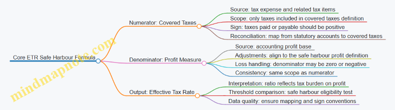
Covered Taxes Numerator
Covered Taxes usually come from a reconciliation that begins with the group’s tax expense and then adjusts it to the covered tax definition. A practical way to keep this from turning into a guessing game is to separate three buckets:
- Current tax: the tax payable for the period.
- Deferred tax movements: changes in deferred tax that may or may not be included depending on the covered tax definition.
- Other tax items: items that look tax-like but must be included or excluded deliberately.
Example: Mapping tax expense to covered taxes
Assume a reporting unit has:
- Income tax expense in the financial statements: 30
- Deferred tax expense movement: 10
- Non-covered taxes included in tax expense: 4
If the covered tax definition includes current tax but excludes the non-covered taxes and excludes the deferred tax movement for this safe harbour computation, then:
- Covered Taxes = 30 − 4 − 10 = 16
The key interpretation point: the numerator is a curated number. If you treat tax expense as covered taxes without reconciliation, your ETR ratio can be systematically biased.
Profit Denominator
The denominator should represent the profit base used for the safe harbour test. Even when teams start from accounting profit, they must ensure the profit measure’s scope matches the covered taxes scope.
Common denominator pitfalls include:
- Using a profit measure that includes items excluded from the covered taxes mapping.
- Mixing consolidated and local figures without consistent adjustments.
- Mishandling sign conventions when profit is negative.
Example: Profit measure with sign handling
Suppose the profit measure for the period is 50. Covered Taxes are 16. Then:
- ETR = 16 ÷ 50 = 32%
Now suppose profit is −20 (a loss). A ratio like 16 ÷ (−20) gives −80%, but that does not behave like a normal “tax burden on profit” interpretation. In practice, teams must follow the safe harbour approach for loss or zero profit scenarios rather than forcing a standard ratio narrative.
Interpretation Against the Safe Harbour Test
Once you have the ETR, interpretation is straightforward but only after two checks:
- Scope check: numerator and denominator come from the same reporting scope and period.
- Sign and edge-case check: loss or zero profit scenarios are handled according to the safe harbour rules.
Example: Threshold comparison
If the safe harbour threshold for the relevant jurisdiction is 15% and the computed ETR is 32%, the reporting unit does not meet the safe harbour condition based on this test.
If the computed ETR is 12%, it meets the condition, assuming eligibility requirements are satisfied and the mapping is supportable.
Practical Consistency Rules
To keep the formula meaningful across entities and periods, apply these consistency rules:
- Use one mapping method per period: the same reconciliation logic should produce the same covered taxes definition each time.
- Lock sign conventions early: decide whether taxes are positive when they increase the numerator and keep it consistent.
- Reconcile before you compute: build a bridge from financial statement lines to covered taxes and from profit lines to the denominator, then compute the ratio.
Quick Reference Mind Map for Interpretation

When these components are treated as defined inputs rather than “numbers that look right,” the ETR becomes a reliable indicator for safe harbour testing instead of a ratio that merely reflects accounting noise.
4.2 Covered Taxes Identification from Tax Expense and Current Tax
Covered taxes are the taxes you use to compute the Effective Tax Rate Safe Harbour. The tricky part is not the arithmetic; it is deciding which amounts in your financial statements actually represent the “covered” numerator inputs. This section builds a practical path from tax expense and current tax to a defensible covered taxes figure.
Start with the Two Anchors in Your Financials
Most groups have two related numbers in their tax note: income tax expense and current tax (often shown as current tax expense or current tax payable). Think of them as anchors:
- Tax expense is the total tax cost recognized in profit or loss.
- Current tax is the tax payable or receivable for the period based on taxable profit.
For covered taxes identification, you typically begin with current tax because it is the most direct link to the period’s tax liability. Then you adjust for items that are included in tax expense but should or should not be treated as covered taxes.
Mind Map: Covered Taxes Identification Flow
Step 1: Choose the Starting Point: Current Tax First
If your tax note provides current tax expense by jurisdiction, start there. Example: Entity A in Jurisdiction X reports:
- Current tax expense: 120
- Deferred tax expense: 30
- Total income tax expense: 150
A clean starting point for covered taxes is 120. You then check whether any portion of the current tax includes items that are not “covered” (for example, interest on late payment or penalties). If the tax note does not break those out, you use the underlying tax computation or ledger detail to isolate them.
Step 2: When Current Tax Is Not Clearly Available
Sometimes the tax note shows only total tax expense and a deferred tax movement, without a separate current tax line. In that case, you can derive current tax as:
- Current tax ≈ Tax expense − Deferred tax expense
Example: Entity B reports:
- Income tax expense: 200
- Deferred tax expense: 70
Derived current tax is 130. You still need to verify that the deferred tax figure is truly the movement in deferred tax recognized in profit or loss, not a reclassification or a one-off presentation change.
Step 3: Separate Covered from Non-Covered Components
Covered taxes are not “whatever sits under the tax line.” You must filter out amounts that do not represent income-based taxes for the period.
Common exclusions to test for:
- Penalties and interest: often included in tax expense but not part of the income tax computation.
- Taxes not based on income: for example, payroll taxes or VAT-like taxes booked in tax expense.
- Uncertain tax positions: the treatment can differ depending on how the group presents and measures them. The safe approach is to use the tax computation that shows the amount attributable to current period tax.
Concrete example: Entity C has current tax expense of 90, but the tax computation shows:
- Income tax on taxable profit: 85
- Interest on late payment: 5
Covered taxes should start from 85, not 90. The reconciliation should show the 5 as an explicit adjustment.
Step 4: Reconcile to the Tax Note Bridge
A good reconciliation is not just a tie-out; it is a narrative that explains every difference.
Use a simple bridge structure:
- Start with current tax (or derived current tax)
- Add or subtract identified adjustments
- Arrive at covered taxes
Example bridge for Entity D:
- Current tax expense: 140
- Less penalties and interest: (8)
- Less non-income taxes booked in tax expense: (2)
- Covered taxes: 130
Then confirm that the bridge aligns with the tax note’s total tax expense reconciliation by showing where deferred tax sits (it should not be treated as covered taxes unless your covered taxes definition requires a specific inclusion).
Step 5: Document Evidence and Mapping Logic
To make the identification defensible, document three things:
- Ledger mapping: which GL accounts feed current tax and tax expense.
- Computation support: the tax computation schedule that produces the current tax amount.
- Adjustment rationale: why each excluded component is excluded, with sign and currency conventions.
A small but important detail: ensure the sign convention matches your computation pack. If your tax note reports expenses as positive and your computation expects taxes as positive in the numerator, keep it consistent. If not, document the sign flip once, then apply it everywhere.
Advanced Detail: Multi-Jurisdiction and Mixed Presentations
When multiple jurisdictions roll up into one group tax note, avoid using only the consolidated tax expense. Instead, identify covered taxes per jurisdiction using the tax computation or jurisdictional tax note breakdown.
If a jurisdiction reports a tax credit that reduces current tax, include the net effect only after confirming the credit is part of the income tax computation for the period. Credits that are booked through other lines (for example, as reductions of revenue) should not be pulled into covered taxes unless the mapping rules explicitly support it.
Quick Check Before You Move On
Before finalizing covered taxes, verify:
- You used current tax as the anchor when available.
- You excluded penalties, interest, and non-income taxes with explicit adjustments.
- Your reconciliation can be traced from tax note to computation to covered taxes.
If any of these fail, the safe harbour calculation will be “accurate” in the way a neatly typed wrong address is still wrong.
4.3 Denominator Construction Using Profit Measures
The denominator is where most “why is this number so weird?” moments begin. In an effective tax rate safe harbour context, the denominator is built from a profit measure that represents the earnings base to which covered taxes are compared. The goal is consistency: the profit measure should be defined, sourced, and treated in a way that matches how the numerator is assembled.
Profit Measure Foundations
Start with the profit measure conceptually. You need a single number that reflects profitability for the period, typically derived from financial statement results. In practice, teams often use a profit before tax measure because it is naturally aligned with tax expense mechanics.
A workable approach is:
- Choose the profit measure definition once (for example, profit before tax).
- Ensure it is calculated for the same scope as the covered taxes numerator.
- Apply the same entity and jurisdiction mapping rules used for the numerator.
Example: If covered taxes are based on current tax plus certain adjustments tied to profit, then the denominator should reflect the profit base those taxes relate to, not a different accounting profit measure.
Selecting the Profit Base
Profit measures can be constructed from several candidates, but the denominator must be stable and auditable. Common candidates include:
- Profit before tax from the income statement
- Profit after tax (usually less suitable because it already reflects tax effects)
- Operating profit (often misaligned with tax computations)
Best practice is to use profit before tax because it keeps the tax comparison “clean”: the numerator represents tax, and the denominator represents the earnings that tax is applied to.
Aligning Scope with Covered Taxes
Denominator construction fails when scope differs. If the numerator includes only covered taxes for specific jurisdictions or reporting units, the denominator must reflect the same scope.
Practical checks:
- Confirm the profit measure is taken from the same set of entities used to compute covered taxes.
- Confirm intercompany eliminations are handled consistently. If covered taxes are computed on a consolidated basis, the profit measure should reflect the consolidated profit base used in that computation.
- Confirm currency translation rules match the numerator’s currency treatment.
Example: Suppose Entity A and Entity B are in the same jurisdiction. If covered taxes are computed after consolidation eliminations, but the denominator uses each entity’s standalone profit before tax, the effective tax rate will be distorted.
Handling Losses and Zero Profit Scenarios
Losses are the denominator’s stress test. When the profit measure is negative or zero, the effective tax rate comparison can become meaningless or produce unstable ratios.
A systematic method:
- Identify whether the denominator is positive, zero, or negative.
- Apply the safe harbour rule logic consistently for each category.
- Document the sign convention and the treatment of losses in the calculation pack.
Example: If profit before tax is -10 and covered taxes are 2, the ratio is -0.2, which is not a helpful “tax burden” indicator. Teams should follow the safe harbour mechanics for loss years rather than forcing a ratio.
Adjusting the Profit Measure for Consistency
Even when you start from profit before tax, you may need adjustments so the denominator matches the numerator’s covered scope.
Typical adjustment categories:
- Reclassifications between discontinued operations and continuing operations
- Treatment of non-recurring items if the numerator excludes or includes them differently
- Alignment of accounting policy differences that affect profit before tax
Example: If covered taxes exclude taxes related to discontinued operations, but the denominator includes profit before tax from discontinued operations, the effective tax rate will look artificially high or low.
Worked Example with Clear Steps
Assume a reporting unit has:
- Profit before tax: 100
- Covered taxes: 25
Step 1: Confirm the profit measure definition is profit before tax.
Step 2: Confirm the profit measure scope matches the covered taxes scope.
Step 3: Confirm currency and sign conventions.
Step 4: Compute denominator = 100.
Effective tax rate safe harbour comparison uses:
- Numerator (covered taxes) = 25
- Denominator (profit measure) = 100
Result: 25 / 100 = 25%.
Now change only one input:
- Profit before tax: 0
- Covered taxes: 5
Here, the denominator is zero. The ratio cannot be interpreted as a burden. The calculation pack should flag this case and apply the safe harbour logic for zero profit years.
Mind Map: Denominator Construction
Control Checklist for the Denominator
Use a short checklist so the denominator is not a “trust me” number:
- Tie profit before tax to the income statement line used in reporting.
- Reconcile profit before tax to the trial balance movement for the same scope.
- Verify intercompany eliminations and discontinued operations treatment match the numerator.
- Confirm currency translation method matches the covered taxes currency.
- Flag zero and loss cases and record the rule applied.
When these steps are done consistently, the denominator becomes a dependable anchor for the effective tax rate safe harbour calculation—less mystery, more math.
4.4 Treatment of Losses and Zero Profit Scenarios
Effective Tax Rate (ETR) safe harbour calculations often assume there is a meaningful profit base. Losses and zero-profit outcomes break that assumption, so the computation needs clear rules for what to include, how to treat signs, and when the safe harbour result becomes unusable.
Foundational Idea: Why Losses Are Tricky
ETR is typically computed as covered taxes divided by a profit measure. When the denominator is negative (loss) or zero (no profit), the ratio can become misleading or undefined. A negative denominator can flip the sign of the ETR, while a zero denominator can create division-by-zero problems. The goal is not to “force” a number, but to produce a result that is mathematically stable and consistent with the safe harbour intent.
Step 1: Define the Denominator and Its Sign
Start by locking the denominator definition used in your template. For example, if your denominator is “profit before tax” (PBT) from the financial statement mapping, then:
- If PBT is positive, ETR is a normal ratio.
- If PBT is negative, ETR becomes a ratio with a negative denominator.
- If PBT is zero, ETR is undefined.
A practical control is to store both the raw denominator and its sign classification (Positive, Negative, Zero) before any ratio logic runs.
Step 2: Treat Covered Taxes Consistently with the Denominator
Covered taxes should be derived consistently from the same mapping logic used in profitable cases. The key is to avoid mixing “tax expense” concepts with “cash tax” concepts.
Example: Loss year with tax benefit
- Covered taxes: -10 (a tax benefit reflected in the computation input)
- Denominator (PBT): -100
- ETR = (-10) / (-100) = 10%
This produces a positive ETR, which may look counterintuitive at first glance. The sign logic is doing its job: both numerator and denominator are negative, so the ratio is positive. The important nuance is that the ETR here is a mathematical outcome, not a statement that the company “paid” tax.
Step 3: Handle Zero Profit Scenarios Without Inventing Numbers
When the denominator is zero, ETR cannot be computed as a ratio. In practice, you have two common approaches in templates:
- Mark the ETR as “Not Applicable” and exclude the entity/jurisdiction from safe harbour reliance for that period.
- Use an alternative rule set defined in your methodology for zero-profit cases, if permitted by your internal policy and the safe harbour framework you follow.
Example: Zero profit with tax expense
- Covered taxes: 6
- Denominator (PBT): 0
- ETR: undefined
Even though there is tax expense, the ratio still cannot be computed. A common mistake is to set ETR to 0% because the denominator is zero; that turns an undefined ratio into a fabricated rate.
Step 4: Document the Classification and the Reason Code
To keep the reporting audit-friendly, record a reason code for each entity/jurisdiction outcome:
- Loss year with computable ratio
- Loss year with unusual sign pattern
- Zero profit with undefined ratio
- Missing denominator input
This turns a calculation problem into a traceable decision.
Mind Map: Losses and Zero Profit Treatment
Example: Loss Year with Tax Expense
- Covered taxes: 8
- Denominator (PBT): -120
- ETR = 8 / (-120) = -6.67%
A negative ETR can occur when the numerator is positive (tax expense) but the denominator is negative (loss). Instead of “fixing” the sign, keep the ratio and flag it in the reason code as an unusual sign pattern. That flag helps reviewers focus on whether the mapping is correct.
Example: Zero Profit with Tax Benefit
- Covered taxes: -3
- Denominator (PBT): 0
- ETR: undefined
Again, the ratio is not computable. The presence of a tax benefit does not resolve the division-by-zero issue.
Step 5: Reconcile and Sanity-Check the Mapped Inputs
Before finalizing the classification, reconcile the mapped denominator and covered taxes back to the source financial statement lines used in your mapping. For loss and zero-profit cases, reviewers should specifically check:
- Whether the profit measure is truly zero after consolidation adjustments.
- Whether tax benefits are captured as negative covered taxes consistently.
- Whether sign conventions match across entities and currencies.
A small but effective sanity check is to compare the mapped denominator to the trial balance PBT for the same reporting unit and period, then confirm that any consolidation adjustments are applied before the denominator is classified as Zero or Negative.
4.5 Reconciliation Templates Between Statutory Accounts and Pillar Two Inputs
A reconciliation template is the bridge between what statutory accounts say and what Pillar Two needs. The goal is not to “make numbers match,” but to show exactly why they differ and which differences are relevant for the Effective Tax Rate (ETR) safe harbour inputs.
Foundational Mapping Principles
Start with three anchors that every template should carry:
- Source anchor: the statutory line item (for example, current tax expense, deferred tax expense, or profit before tax).
- Pillar Two anchor: the Pillar Two input bucket (for example, covered taxes, denominator profit measure).
- Transformation logic: the rule that moves the source to the Pillar Two bucket (for example, reclassify, exclude, or adjust).
A good template makes these anchors visible on one page, so reviewers can trace a figure without hunting across spreadsheets.
Template Structure That Works in Practice
Use a consistent layout across entities and jurisdictions:
Header and Scope Block
Include reporting period, entity, currency, and the safe harbour basis used. Add a short scope statement such as “Reconciliation of statutory tax expense to covered taxes for ETR computation.”
Covered Taxes Reconciliation Table
Create a table with columns for:
- Statutory tax components (current tax, deferred tax, tax related to discontinued operations if applicable)
- Adjustments (exclusions and inclusions)
- Pillar Two covered taxes result
- Evidence reference (trial balance line, tax computation schedule, or consolidation adjustment note)
Denominator Reconciliation Table
Denominator profit measures often differ from statutory profit before tax due to specific inclusions/exclusions. Mirror the same column pattern: statutory profit measure, adjustments, and Pillar Two denominator.
Control Checks Block
Add checks that catch common errors:
- Sign conventions consistent across tax expense and covered taxes
- No missing jurisdictions or tax types
- Reconciliation totals tie to the final Pillar Two input pack
Mind Map: Reconciliation Template Logic
Example: Covered Taxes Reconciliation in One Page
Assume an entity reports statutory tax expense of 120 in local currency:
- Current tax expense: 100
- Deferred tax expense: 20
Pillar Two covered taxes require excluding a non-covered component, say a tax credit treated differently in the statutory accounts. The template would record:
- Statutory current tax expense: 100
- Statutory deferred tax expense: 20
- Less: excluded tax credit impact: (10)
- Plus: included withholding tax treated as covered: 5
Resulting covered taxes: 115.
The key is that the template explicitly labels each adjustment as excluded or included, and links it to evidence. If the tax credit is supported by a tax computation schedule, reference that schedule line rather than a vague “tax notes” cell.
Example: Denominator Reconciliation with a Simple Adjustment
Suppose statutory profit before tax is 1,000. Pillar Two denominator may require excluding a one-off gain that is not part of the denominator measure.
- Statutory profit before tax: 1,000
- Less: excluded one-off gain: (60)
- Plus: included restructuring cost treatment difference: 10
Denominator profit measure: 950.
This is where reviewers appreciate clarity: the template shows the direction of each adjustment and why it exists.
Advanced Details Without the Usual Headaches
Evidence Reference Discipline
Use a consistent evidence key format, such as:
- TB for trial balance
- TC for tax computation
- FX for currency translation support
- CO for consolidation adjustments
Then, every adjustment line must have exactly one evidence key.
Sign and Rounding Controls
Add a control row that checks whether covered taxes are presented with the same sign convention as the Pillar Two input pack. Also include a rounding check that confirms the sum of rounded lines equals the rounded total.
Reconciliation Narrative That Explains the “Why”
Include a short narrative field for each major adjustment category. For example: “Excluded tax credit because statutory presentation netted it against current tax, while Pillar Two treats it as non-covered.” One sentence is enough if it points to the rule.
Diagram: Reconciliation Flow
    flowchart TD
  A[Statutory Tax Expense and Profit] --> B[Identify Pillar Two Input Buckets]
  B --> C[Populate Covered Taxes Table]
  C --> D[Populate Denominator Table]
  D --> E[Apply Adjustments with Evidence Keys]
  E --> F[Run Tie-Outs and Sign Checks]
  F --> G[Produce Pillar Two Input Outputs]
A well-built reconciliation template turns a tax story into a traceable set of decisions. It is the difference between “we think it matches” and “we can show why it matches.”
5. Safe Harbour Eligibility Mechanics and Documentation Requirements
5.1 Eligibility Conditions and How to Verify Them
Effective Tax Rate Safe Harbour is only useful if you can prove eligibility quickly and consistently. This section turns the eligibility conditions into a verification routine: what to check, where the evidence comes from, and how to handle common “almost eligible” situations.
Start with the Eligibility Checklist
Eligibility is typically assessed at the level required by the safe harbour rule (often jurisdictional, but confirm your group’s application approach). Your checklist should include:
- Scope match: the entity and jurisdiction are within the safe harbour population.
- Covered taxes availability: you can identify the covered taxes needed for the effective tax rate computation.
- Denominator availability: you can compute the profit or loss measure used in the safe harbour test.
- Rate and period consistency: the period matches the reporting cycle and the tax amounts tie to the same accounting period.
- Documentation completeness: you can produce a trace from financial statements to the safe harbour inputs.
A practical way to avoid missed items is to require a “green-light” sign-off before calculations begin. If any checklist item is red, you stop early and switch to the non-safe-harbour path.
Verify Scope Match Using Entity-Jurisdiction Mapping
Eligibility verification starts with mapping. Build a table that links:
- legal entity
- reporting unit
- jurisdiction
- reporting currency
- tax reporting basis used locally
Example: Entity A is legally in Country X but reports under a regional consolidation entity. Eligibility is tested for Country X, not the consolidation entity. Your mapping should therefore show Country X as the jurisdiction for the safe harbour input set.
Verification steps:
- Reconcile the entity-jurisdiction mapping to the group’s tax registration list.
- Confirm that any permanent establishments or special tax regimes are reflected in the jurisdiction mapping.
- Ensure the safe harbour input set includes only the entities intended for that jurisdiction.
Confirm Covered Taxes and Denominator Inputs Are Computable
Eligibility fails quietly when inputs are missing or not comparable.
Covered taxes checks
- Identify the tax expense components you will treat as covered taxes.
- Confirm you can separate covered taxes from non-covered items (for example, certain penalties or taxes that do not meet the covered definition).
- Ensure sign conventions are consistent (tax expense as positive, refunds as negative, or vice versa—pick one and enforce it).
Denominator checks
- Confirm the profit measure used in the safe harbour test is available for the same period.
- If the measure is based on accounting profit, verify that consolidation adjustments do not break the linkage to local results.
Example: If a group has a large deferred tax movement, the accounting profit measure may still be computable, but the covered taxes may require reclassification. Eligibility is not about whether the numbers look “nice”; it is about whether the required components can be identified and supported.
Validate Period Alignment and Evidence Trace
Eligibility verification is strongest when every input has a traceable evidence trail.
Create a trace matrix with three columns:
- safe harbour input line
- source document or schedule
- control evidence (who prepared, who reviewed, when)
Example: The covered taxes input is sourced from the tax expense note in the statutory accounts plus a reconciliation schedule. The evidence includes the reconciliation workbook version, review sign-off, and the mapping rules used.
Period alignment rules to enforce:
- The safe harbour computation period must match the financial reporting period.
- Any reclassifications must be applied consistently across all entities in the jurisdiction set.
- If a currency translation step is used, document the exchange rate source and the timing.
Handle Edge Cases Without Guessing
Edge cases are where eligibility verification becomes a discipline.
Common edge cases:
- Loss-making entities: confirm how the safe harbour rule treats zero or negative denominators and whether the jurisdiction set aggregates them.
- Tax rate changes within the period: verify whether the rule requires an average rate or a specific approach.
- One-off tax items: confirm whether they are included or excluded from covered taxes and document the rationale.
Example: A jurisdiction has one entity with a tax refund that flips the sign of covered taxes. Your verification should confirm that the safe harbour computation accepts negative covered taxes and that the reconciliation schedule clearly shows the refund’s origin.
Mind Map: Eligibility Conditions and Verification
A Simple Verification Workflow That Stays Auditable
- Confirm scope using the entity-jurisdiction mapping.
- Check computability of covered taxes and denominator inputs.
- Reconcile and trace each input to source schedules.
- Run eligibility test inputs only after checklist items are green.
- Document edge case decisions with the same trace matrix used for normal cases.
If you can complete steps 1–3 without exceptions, eligibility verification is usually straightforward. If you cannot, the issue is not the safe harbour outcome—it is the data readiness, and that should be fixed before you compute anything.
5.2 Jurisdiction Level Versus Entity Level Considerations
Safe harbour calculations look simple on paper, but the inputs can sit in different places depending on how your group is organized. The key question is: are you measuring taxes and profits for a jurisdiction (where the tax rules apply) or for an entity (where the accounting records live)? Getting that distinction right prevents mismatched denominators, inconsistent tax rates, and documentation gaps.
Foundational Distinction
At jurisdiction level, you aggregate covered taxes and profit measures for entities that are subject to the same tax regime in a given jurisdiction. At entity level, you compute or collect the same items from each legal entity’s financial statements, then map them upward.
A practical way to think about it: entity-level numbers are your “raw ingredients,” while jurisdiction-level numbers are your “recipe output.” Safe harbour eligibility and the effective tax rate computation must use the recipe output.
Why the Distinction Matters in Practice
-
Different tax profiles inside one jurisdiction: Two entities in the same country may have different tax incentives, permanent differences, or withholding patterns. If you treat them as identical without aggregation logic, your effective tax rate can be distorted.
-
One entity spanning multiple tax outcomes: An entity may have multiple activities (for example, domestic sales and cross-border royalties) that trigger different tax treatments. Even if the accounting is consolidated at entity level, the safe harbour inputs may need jurisdiction-level grouping rules.
-
Denominator consistency: The profit measure used in the effective tax rate calculation must align with the same scope as the covered taxes. If you compute profit at entity level but taxes at jurisdiction level without a clear mapping, the ratio becomes a “mix-and-match” calculation.
Mapping Rules That Keep You Sane
Use a mapping approach that is explicit and testable.
Step 1: Define the Jurisdiction Scope
Create a jurisdiction list that matches the tax regimes you will use for safe harbour. For each jurisdiction, define which entities are included.
Step 2: Define the Entity-to-Jurisdiction Mapping
For each entity, specify the jurisdiction(s) it belongs to for safe harbour purposes. Most groups can start with a single jurisdiction per entity, then add exceptions where needed.
Step 3: Define How to Aggregate Covered Taxes and Profit
Aggregation should follow the same grouping keys. If covered taxes are allocated by activity, ensure the profit measure is allocated using the same activity logic.
Step 4: Document the Mapping Logic
Your documentation should explain the “why,” not just the “what.” For example, state whether mapping is based on statutory filing, tax registration, or operational substance.
Example: One Jurisdiction, Multiple Entities
Assume Jurisdiction A contains two entities:
- Entity E1: Profit before tax = 100; covered taxes = 18
- Entity E2: Profit before tax = 50; covered taxes = 5
Jurisdiction-level aggregation:
- Total profit = 150
- Total covered taxes = 23
- Effective tax rate = 23 / 150 = 15.33%
Entity-level effective tax rates would be 18% for E1 and 10% for E2, but safe harbour uses the jurisdiction-level ratio. The weighted approach is automatic when you aggregate first.
Example: One Entity with Mixed Outcomes
Entity E3 operates in Jurisdiction B but has a portion of income taxed under a different regime (for instance, a special rate for qualifying income). If your accounting reports profit at entity level without splitting, you need an allocation method.
A simple allocation method:
- Split profit by activity based on revenue or segment profit.
- Allocate covered taxes using the same activity split.
If E3 has total profit 200, with 120 qualifying and 80 non-qualifying, and covered taxes are 30 total, then allocate taxes proportionally to the activity split unless you have a better tax-specific allocation.
Jurisdiction-level safe harbour inputs then use the allocated figures, not the unallocated entity totals.
Mind Map: Jurisdiction Versus Entity Inputs
Control Checks That Prevent Common Errors
-
Numerator-denominator alignment test: For each jurisdiction, confirm that the covered taxes and profit measure were aggregated using the same entity set and allocation logic.
-
Mapping completeness test: Ensure every entity in the group is either mapped to a jurisdiction or explicitly excluded with a documented reason.
-
Sign and rounding consistency: Verify that losses, credits, and negative adjustments follow the same sign conventions at both entity and jurisdiction levels.
-
Reconciliation checkpoint: Tie jurisdiction-level totals back to an entity-level roll-up that you can reproduce from source data.
Practical Documentation Example
In your calculation pack, include a one-page mapping summary:
- Jurisdiction A: Entities E1, E2
- Jurisdiction B: Entity E3 with activity split into qualifying and non-qualifying
- Allocation basis: segment profit by activity
- Evidence: local tax filings and segment reporting extracts dated 2026-03-15
This turns a potentially fuzzy mapping exercise into a controlled, reviewable process.
5.3 Documentation Pack Structure and Retention Practices
A documentation pack is the evidence trail that lets a reviewer reproduce the effective tax rate safe harbour conclusion without chasing spreadsheets across folders. The pack should be complete enough to answer three questions: what inputs were used, how they were transformed, and who approved the result.
Documentation Pack Structure
Start with a one-page index, then attach evidence in the same order the calculation is performed.
-
Cover Page and Index
- Reporting period, group name, reporting unit scope, and jurisdiction list.
- Safe harbour basis selected and the high-level conclusion (eligible or not eligible).
- Index that maps each calculation step to an attachment.
-
Eligibility Evidence
- A checklist showing eligibility conditions met, with references to supporting documents.
- Examples of supporting evidence: tax registration status, ownership structure summary, and confirmation of covered taxes scope.
-
Financial Inputs Evidence
- Trial balance extracts or consolidated tax-relevant ledgers used for covered taxes and profit measures.
- Reconciliation from statutory financial statements to the pack’s computation inputs.
- Currency translation approach used for the period, including exchange rate source and method.
-
Tax Computation Evidence
- Covered taxes schedule showing each component used in the numerator, including current tax and any other included taxes.
- Denominator schedule showing the profit measure used, including sign conventions and loss handling.
- Adjustment schedules that explain reclassifications, exclusions, and inclusions.
-
Effective Tax Rate Safe Harbour Calculation
- The final computation workbook or calculation sheet with locked formulas.
- A summary table that states numerator, denominator, resulting effective tax rate, and whether the safe harbour threshold is met.
-
Quality Controls and Review Evidence
- Control checklist completed by preparer and reviewer.
- Evidence of review actions: variance explanations, mapping checks, and sign-off records.
-
Approval and Audit Trail
- Approval record with names, roles, and approval date.
- Version history: what changed, why it changed, and which attachments were updated.
Retention Practices
Retention should match the risk profile of the pack: the more it drives a tax position, the longer it should be retained and the stricter the access controls should be.
- Retention period: follow the group’s legal and tax retention requirements for tax documentation and financial records. If local rules differ, retain the longest applicable period.
- Access control: restrict editing rights to named roles; keep read-only access for reviewers.
- Immutability for final versions: store the final approved pack in a controlled repository with a unique identifier.
- Separation of drafts and finals: drafts can be edited freely, but final packs should be frozen and not overwritten.
- Evidence integrity: keep source extracts and reconciliations that feed the final calculation, not just the final numbers.
A practical rule: if a reviewer can’t trace a number back to a source extract within five minutes, the pack is missing something.
Mind Map: Documentation Pack and Retention
Example: What “Good” Looks Like in Practice
Assume a group prepares safe harbour for Jurisdiction A for the year ended 30 April 2026, using a computation pack created on 2026-03-15.
- The index lists “Step 2 Covered Taxes Schedule” and points to Attachment B.
- Attachment B includes a table with line items: current tax expense, adjustments for non-covered taxes, and any included levies.
- The pack’s reconciliation shows that statutory tax expense includes a non-covered component of 2.0 million, which is excluded in the covered taxes schedule.
- The final calculation sheet references Attachment B and Attachment C (denominator schedule) and displays the effective tax rate result.
- The reviewer checklist confirms that the excluded component matches the statutory note disclosure and that the sign convention for profit is consistent across entities.
If the reviewer asks, “Where did the 2.0 million go?”, the answer is immediate: it is explicitly shown in the adjustment schedule and referenced in the reconciliation.
Example: Retention and Versioning That Prevents Confusion
A common failure mode is overwriting a workbook after review. A better approach is:
- Save Draft v1, Draft v2, then Final v1.
- Store Final v1 as a read-only file in the controlled repository.
- Record in the change log that Draft v2 updated the currency translation method due to a corrected exchange rate source.
- Keep both the corrected and original exchange rate documentation as attachments, so the reviewer can see the reason for the change.
This structure keeps the pack usable months later, even when the team that built it has moved on to other tasks.
5.4 Common Eligibility Pitfalls And How To Prevent Them
Effective Tax Rate Safe Harbour decisions are often derailed by small, avoidable mismatches between what the group reports and what the safe harbour expects. The goal of this section is to move from the basics of eligibility evidence to the practical traps that show up during real calculations.
Pitfall: Using the Wrong Denominator Basis
A common failure is building the effective tax rate using a denominator that does not match the safe harbour definition for the relevant period. For example, teams sometimes divide covered taxes by accounting profit before tax, even when the safe harbour expects a different profit measure.
Prevention approach
- Start with a single “denominator spec” document that states the exact line items and sign conventions.
- Reconcile the denominator to the group reporting pack before any safe harbour logic is applied.
Example:
An entity reports profit before tax of 100 in local accounts. Covered taxes computed from tax expense and adjustments total 18. If the safe harbour denominator should be profit after certain exclusions, but the team uses 100, the effective tax rate becomes 18%. If the correct denominator is 80, the rate is 22.5%, which can change eligibility.
Pitfall: Mixing Covered Taxes with Non-Covered Amounts
Eligibility can fail when the numerator includes amounts that are not part of covered taxes, such as certain penalties, interest, or taxes outside the safe harbour scope.
Prevention approach
- Maintain a “covered vs excluded” mapping for every tax line in the chart of accounts.
- Require a reconciliation from tax expense to covered taxes with explicit inclusion/exclusion flags.
Example:
Tax expense is 25, but includes a 3 penalty. If the safe harbour expects only taxes on income, including the penalty inflates covered taxes to 25 and may push the effective tax rate above the threshold.
Pitfall: Losing Track of Currency and Consolidation Effects
Teams sometimes compute safe harbour inputs in local currency and then consolidate inconsistently, or they translate at different rates for numerator and denominator.
Prevention approach
- Choose one translation method for both covered taxes and the denominator, and document it.
- Perform a “translation sanity check” by comparing the consolidated result to the sum of translated components.
Example:
Covered taxes are translated at the average rate, but profit is translated at the closing rate. The effective tax rate becomes distorted because both components are not measured on the same basis.
Pitfall: Eligibility Evidence That Cannot Be Reproduced
A safe harbour conclusion is only as good as its audit trail. If the team cannot reproduce the computation from source data, eligibility becomes fragile.
Prevention approach
- Store calculation packs with version control and immutable source references.
- Require evidence for each mapping step, not just the final rate.
Example:
A spreadsheet includes manual overrides for certain tax lines, but the rationale and source are missing. During review, the override cannot be validated, so the conclusion cannot be supported.
Pitfall: Sign Errors and Loss Period Edge Cases
Eligibility logic is sensitive to whether amounts are treated as positive or negative. Loss periods add another layer: a denominator near zero or negative can produce misleading rates or trigger special handling.
Prevention approach
- Implement sign checks that validate whether profit and taxes are expected to be positive/negative for the period.
- Use a dedicated “edge case worksheet” for zero or loss scenarios with explicit rules.
Example:
If profit is -10 and covered taxes are 2, a naive division yields -20%. If the safe harbour requires a different treatment for loss periods, the naive result can incorrectly suggest eligibility.
Pitfall: Jurisdiction Scope Confusion
Eligibility can be misapplied when teams treat jurisdiction-level conditions as entity-level facts, or when they aggregate entities that should be evaluated separately.
Prevention approach
- Define the evaluation unit clearly: which entities roll into which jurisdiction safe harbour assessment.
- Lock the mapping between legal entities, reporting units, and jurisdiction tags.
Example:
Two entities in the same jurisdiction have different tax profiles due to different incentives. If they are combined without respecting the safe harbour’s scope rules, the effective tax rate may not represent either entity’s eligibility.
Pitfall: Incomplete Reconciliation Between Financial Reporting and Tax Inputs
Eligibility often fails not because the formula is wrong, but because the inputs are incomplete. Missing adjustments, stale data, or partial mapping from the trial balance to covered taxes can quietly skew results.
Prevention approach
- Use a three-way reconciliation: trial balance tax lines, statutory tax expense, and covered taxes.
- Require a completeness check that every tax line is either included or excluded with a reason.
Example:
A deferred tax movement is booked in the tax ledger, but the mapping excludes it by default. If the safe harbour expects it to be treated in a specific way, the covered taxes are understated.
Mind Map of Eligibility Pitfalls and Controls
Practical Checklist for the First Review Pass
Before finalizing eligibility, verify that (1) the denominator matches the spec, (2) covered taxes are derived from a documented bridge, (3) translation and consolidation are consistent, (4) every tax line is classified, and (5) loss or near-zero scenarios follow the edge case rules. If any item fails, treat it as a data problem first, not a “calculation tweak” problem.
5.5 Sign Off Process for Safe Harbour Determinations
A safe harbour determination is only as strong as the chain of evidence behind it. The sign-off process should therefore be designed like a controlled handover: clear responsibilities, repeatable checks, and a documented conclusion that someone else can follow without guessing.
Define the Decision and the Sign-Off Boundary
Start by writing down what the sign-off covers and what it does not. For example, the sign-off may cover the jurisdiction-level effective tax rate safe harbour conclusion for a reporting year, including the covered taxes inputs, the denominator, and the eligibility checks. It should not silently include unrelated computations such as Pillar Two top-up logic, unless explicitly stated.
A practical boundary statement helps prevent “almost the same” sign-offs. If the safe harbour pack is used for multiple reporting units, the sign-off should specify whether it is per reporting unit, per jurisdiction, or per group, and which mapping is assumed.
Assign Roles and Evidence Ownership
Use a simple RACI-style approach so each step has an accountable owner. A typical split looks like this:
- Preparation owner: compiles the safe harbour pack, performs initial reconciliations, and resolves data mapping issues.
- Review owner: checks logic, verifies calculations, and challenges assumptions.
- Approver: confirms the final conclusion and signs the determination.
- Tax data owner: confirms covered taxes inputs and rate inputs are consistent with the approved accounting and tax positions.
To keep it concrete, require that every numeric input in the pack has a traceable source (trial balance line, tax return figure, or approved adjustment schedule).
Use a Two-Stage Review Before Approval
A two-stage review reduces the chance that the approver becomes the first line of defense.
Stage 1: Completeness and Consistency Checks
- All required schedules are present for each jurisdiction.
- Covered taxes tie to the agreed tax expense/current tax components according to the pack’s reconciliation template.
- Denominator profit measure is populated and uses the same sign convention across entities.
- Any exclusions or inclusions are explicitly listed and linked to the supporting adjustment.
Stage 2: Reasonableness and Eligibility Checks
- Verify the eligibility conditions are met using the documented criteria.
- Perform targeted reasonableness checks, such as comparing the effective tax rate to prior-year patterns and to the jurisdiction’s typical tax profile.
- Confirm that loss or near-zero profit scenarios are handled using the pack’s defined approach.
If a check fails, the pack should not proceed to approval until the issue is resolved or formally waived with documented rationale.
Document the Conclusion and the Audit Trail
The sign-off record should include:
- The reporting year and jurisdiction scope.
- The safe harbour method applied (as defined by the pack).
- The computed effective tax rate and the eligibility outcome.
- A short list of key assumptions that materially affect the result.
- The evidence references used for each key input.
A good rule: if someone asked “Why did you conclude safe harbour applies?”, the answer should be visible in the sign-off record without searching through every spreadsheet tab.
Example Sign-Off Pack Walkthrough
Assume a group has a jurisdiction pack for FY2025. The preparation owner completes:
- Covered taxes reconciliation: tax expense to covered taxes with two adjustments (one exclusion for non-covered levies, one inclusion for a specific tax credit).
- Denominator schedule: profit measure derived from group reporting profit with a defined mapping.
- Eligibility checklist: confirms the jurisdiction meets the required conditions.
Stage 1 review finds that one entity’s currency translation was applied using the wrong rate type. The review owner flags it, the preparation owner corrects the translation, and the pack is reissued with a version number.
Stage 2 review then confirms the corrected effective tax rate remains within the safe harbour threshold and that loss handling rules were applied consistently. The approver signs on 2026-03-15, referencing the final version of the pack and the resolved issue log.
Mind Map for Sign Off Process
Practical Control Tips That Prevent Common Failures
Keep the sign-off checklist aligned to the pack structure so reviewers don’t rely on memory. Require re-approval when any of the following changes: covered taxes inputs, denominator mapping, eligibility criteria evidence, or sign convention rules. Finally, ensure the approver receives a single consolidated view of outcomes and exceptions, not a folder of spreadsheets—because the goal is a decision, not a scavenger hunt.
6. Standardized Reporting Templates and Calculation Packs
6.1 Template Design Principles for Consistency and Traceability
A safe harbour calculation pack lives or dies by how easily someone else can reproduce it. “Consistency” means the same inputs produce the same outputs across entities and cycles. “Traceability” means every number can be traced to a source, a rule, and a reviewer.
Start with a Single Source of Truth for Each Input
Define a small set of input fields that are never retyped. For example, “Covered Taxes” should be pulled from a controlled schedule, not re-entered in the template. If you need a manual adjustment, create a dedicated line called “Manual Adjustment” with a reason code and evidence link.
Example: Entity A has current tax expense of 120. Covered Taxes requires excluding non-covered items of 10. The template should show:
- Current tax expense (sourced)
- Less: Excluded items (sourced or coded)
- Manual adjustment (optional)
- Covered Taxes (calculated)
This prevents the classic spreadsheet problem where the same concept is calculated three different ways.
Use a Stable Layout with Predictable Blocks
Organize the template into fixed regions so reviewers know where to look:
- Inputs block (raw and controlled)
- Calculation block (formulas only)
- Reconciliation block (bridges to financial statements)
- Outputs block (safe harbour result and supporting metrics)
- Controls block (checks, sign-offs, and version metadata)
When the layout is stable, you can compare packs across periods without hunting.
Design for Traceability with Explicit Lineage
Every calculated line should have a “lineage rule” that states what it depends on. In practice, add a column such as “Derivation” with short, human-readable rules.
Example derivation rules:
- Covered Taxes = Current tax expense − Excluded items + Manual adjustment
- Denominator Profit = Accounting profit before tax adjusted for excluded income/expense
- Effective Tax Rate = Covered Taxes ÷ Denominator Profit
Then add a “Source” field for each input line, pointing to the schedule or trial balance reference.
Standardize Naming Conventions and Units
Use consistent labels for the same concept across entities and jurisdictions. Include units in the header, such as “Currency: EUR” and “Amounts: Thousands.” If you translate currencies, show the exchange rate source and the translation method used.
Example: If the template supports both local and group currency, include two separate fields:
- Covered Taxes Local Currency
- Covered Taxes Group Currency
Avoid mixing them in one column; it’s how silent errors happen.
Build in Control Checks That Catch Errors Early
Controls should be simple, deterministic, and visible. Common checks include:
- Sign checks: Covered Taxes should not flip sign unexpectedly versus the source schedule
- Balance checks: Reconciliation totals must match the financial statement line within a defined tolerance
- Formula checks: Denominator Profit must be non-zero when computing an effective tax rate
- Rate checks: Selected safe harbour rate must match the documented eligibility basis
Example: If Denominator Profit is 0, the template should display “ETR not computed” rather than dividing by zero and producing nonsense.
Separate Assumptions from Calculations
Assumptions include eligibility flags, rate selection rationale, and treatment choices. Calculations include arithmetic and mapping rules. Keep them in different sections so a reviewer can confirm assumptions without reading formulas.
Example: Put “Safe Harbour Rate Selected: 15%” in the assumptions block with a reason code. The calculation block then uses that rate only.
Make Versioning and Evidence Part of the Template
Include fields for:
- Template version
- Data freeze date
- Prepared by and reviewed by
- Evidence pack identifier
Use a consistent evidence naming pattern such as “EtrSH_Entity_Jurisdiction_Period_Evidence_vX”. This reduces the time spent matching files to numbers.
Provide Worked Examples Inside the Pack
A template should include one small “Example” worksheet that demonstrates the mapping and reconciliation logic using sample numbers. This is not for training; it’s for sanity.
Example mapping snippet:
- Trial balance line: Income tax expense 120
- Excluded items: Non-deductible penalties 10
- Covered Taxes: 110
- Denominator Profit: 600
- Effective Tax Rate: 110 ÷ 600 = 18.33%
If the example and the live calculations disagree, you’ve found a template defect.
Mind Map: Template Design Principles for Consistency and Traceability
Example: Minimal Template Skeleton for a Safe Harbour Pack
Inputs
- Entity
- Period
- Currency and units
- Current tax expense (source)
- Excluded items (source)
- Manual adjustment (optional)
- Denominator profit (source)
Assumptions
- Safe harbour eligibility flag
- Selected safe harbour rate
- Rate selection rationale
Calculations
- Covered Taxes
- Effective Tax Rate
- Safe harbour outcome indicator
Reconciliation
- Bridge from tax expense to covered taxes
- Bridge from profit to denominator profit
Controls
- Balance checks
- Sign checks
- Denominator zero rule
- Reviewer sign-off
A good template is boring in the best way: it tells the story of each number without requiring the reviewer to guess.
6.2 Required Schedules for Effective Tax Rate Safe Harbour
Effective Tax Rate Safe Harbour reporting lives or dies by schedules that are consistent, traceable, and easy to reconcile. Think of the schedules as a set of “inputs with receipts”: each one states what you used, where it came from, and how it connects to the next schedule.
Schedule 1: Covered Taxes Summary
This schedule aggregates the covered taxes used in the effective tax rate computation. It should separate taxes by type so reviewers can spot mismatches quickly.
Minimum columns
- Jurisdiction
- Tax type (current tax, deferred tax, withholding, other)
- Amount used for safe harbour
- Source reference (trial balance line, tax provision workpaper, or consolidation adjustment)
- Sign convention (positive/negative)
Example:
For Jurisdiction A, current tax expense is 120, deferred tax expense is 10, and withholding tax is 5. If the safe harbour computation uses total covered taxes of 135, the schedule should show 120, 10, and 5 as components that sum to 135.
Schedule 2: Profit Denominator Summary
This schedule provides the profit measure used as the denominator. It must align with the same scope and sign conventions as the covered taxes schedule.
Minimum columns
- Jurisdiction
- Profit measure name (as defined in your methodology)
- Amount used for safe harbour
- Source reference
- Adjustments applied
Example:
If the profit measure starts from accounting profit before tax of 300, and you apply a standard adjustment of -20 to reach 280, the schedule should show both the starting point and the adjustment so the denominator is not a black box.
Schedule 3: Effective Tax Rate Computation
This schedule ties Schedule 1 and Schedule 2 together and produces the effective tax rate used for safe harbour.
Minimum columns
- Jurisdiction
- Covered taxes (from Schedule 1)
- Denominator profit (from Schedule 2)
- Effective tax rate
- Zero or loss handling flag
- Calculation notes
Example:
If covered taxes are 135 and denominator profit is 280, the effective tax rate is 48.21%. If denominator profit is zero, the schedule should not attempt a division; it should mark the scenario explicitly and route the case to your defined handling rule.
Schedule 4: Reconciliation to Financial Statements
This schedule proves that the safe harbour inputs are grounded in the group’s financial reporting. It should reconcile from consolidated or local financial statement lines to the safe harbour schedules.
Minimum columns
- Financial statement line item
- Amount
- Mapping to safe harbour component
- Consolidation adjustments impact
- Net amount used
Example:
Tax expense in the financial statements might be 130, but covered taxes used for safe harbour might be 135 due to a specific inclusion (for example, a tax type reclassified into covered taxes). The reconciliation should show the exact bridge.
Schedule 5: Rate Inputs and Tax Type Mapping
Even when the safe harbour is computed from effective tax rate, you still need schedules that document how tax types and rates were interpreted for the computation.
Minimum columns
- Jurisdiction
- Tax type
- Rate basis or classification basis
- Source reference
- Mapping to covered taxes components
Example:
Withholding tax might be treated as covered taxes in your methodology. This schedule should show how you classified it and where the amount came from.
Schedule 6: Eligibility Evidence Summary
Eligibility is not a vibe; it is a checklist backed by evidence. This schedule records the eligibility conditions and the proof that they were met.
Minimum columns
- Eligibility condition
- Status (met/not met)
- Evidence reference
- Owner
- Review date
Example:
If an eligibility condition requires consistent reporting for the relevant period, the schedule should reference the reporting package version and the sign-off record.
Mind Map: Schedule Set and Data Flow
Practical Integration Example
A clean workflow for one jurisdiction looks like this: Schedule 4 reconciles financial statement tax expense and profit to the mapped components; Schedule 1 extracts covered taxes by type; Schedule 2 builds the denominator profit with the same scope; Schedule 3 calculates the effective tax rate and flags edge cases; Schedule 5 documents how each tax type was classified; Schedule 6 confirms eligibility with evidence references. When a reviewer asks “why is the effective tax rate different from the tax expense ratio?”, Schedule 4 and Schedule 3 provide the answer without forcing anyone to hunt through spreadsheets.
Schedule Quality Checks
Before you finalize, ensure each schedule has a consistent sign convention, a complete source reference, and a deterministic bridge to the next schedule. If any schedule cannot be reproduced from its sources, treat it as a defect, not a formatting issue.
6.3 Standard Reconciliation Steps and Control Checks
A standardized reconciliation is the bridge between what finance reports and what Pillar Two needs for the Effective Tax Rate Safe Harbour. The goal is not to “make numbers match,” but to explain every difference with a traceable reason and evidence.
Core Reconciliation Flow
-
Start with the financial statement tax line
- Use the group reporting tax expense (or the local tax expense that will be mapped to covered taxes).
- Example: If tax expense is 120, split it into current tax and deferred tax components using the tax note.
-
Identify covered taxes versus non-covered items
- Covered taxes typically align to taxes on income and similar items included in the Pillar Two covered taxes definition.
- Example: If 15 relates to penalties or interest, exclude it from covered taxes and keep it in a “non-covered” bucket with a short description.
-
Reclassify and adjust to the safe harbour computation basis
- Apply standardized adjustments for items that are in the tax expense but not in covered taxes, or vice versa.
- Example: If a tax credit is netted in the tax expense but should be treated gross for the computation, re-express it consistently.
-
Reconcile the denominator profit measure
- Ensure the profit measure used for the effective tax rate denominator is aligned to the same reporting scope and sign convention.
- Example: If profit before tax is 500 but includes discontinued operations, confirm whether the safe harbour basis requires excluding them and document the decision.
-
Perform a control check that differences are explainable
- Every reconciling item must have: a category, a reason, and a link to source evidence.
- Example: “Deferred tax movement” is not enough; specify whether it is due to temporary differences, rate changes, or remeasurements.
-
Tie out to the final safe harbour inputs
- Confirm the final covered taxes figure equals the sum of: covered current taxes + covered adjustments + covered deferred tax components as applicable.
- Example: If final covered taxes are 105, show the roll-forward from 120 tax expense to 105 with a controlled bridge.
Standard Control Checks
-
Check 1: Scope and entity mapping
- Confirm the reconciliation is performed for the correct reporting unit and jurisdiction grouping.
- Example: If an entity is excluded from the safe harbour population, its tax lines must not appear in the computation pack.
-
Check 2: Sign conventions
- Covered taxes should follow a consistent sign rule (commonly positive for tax expense). Negative values must be justified.
- Example: A tax benefit of -8 should be supported by the underlying tax credit or refund documentation.
-
Check 3: Completeness of adjustments
- Use a checklist of adjustment categories: credits, withholding, penalties, interest, uncertain tax positions, and deferred tax components.
- Example: If uncertain tax positions are included in tax expense, either include them in covered taxes per policy or explicitly exclude them with evidence.
-
Check 4: Reconciliation arithmetic
- Validate that bridges sum correctly and that rounding does not hide a material mismatch.
- Example: If the bridge totals differ by 1 due to rounding, document the rounding method and confirm it is within tolerance.
-
Check 5: Consistency across periods
- Compare current period reconciling categories to prior period to spot unusual reclassifications.
- Example: If penalties moved from excluded to included, confirm the policy or classification change and capture the approval.
Mind Map: Reconciliation Steps and Controls
Example: Simple Bridge from Tax Expense to Covered Taxes
Assume tax expense is 120.
- Current tax included in covered taxes: 110
- Deferred tax component: 10
- Penalties and interest included in tax expense: (15)
- Tax credits netted in tax expense but treated gross in computation: + (10) adjustment to align basis
Reconciliation bridge:
- Start: 120 tax expense
- Less non-covered penalties and interest: -15 → 105
- Basis alignment adjustment for credits: 0 net effect after gross/net re-expression → 105
Control checks:
- Sign: covered taxes shown as +105
- Completeness: all adjustment categories present (credits, penalties/interest)
- Evidence: penalties/interest extracted from tax note; credit treatment confirmed from tax credit schedule
Example: Control Check for Denominator Consistency
If profit before tax is 500 but includes discontinued operations of 40, and the safe harbour basis excludes discontinued operations, then denominator profit becomes 460. The reconciliation pack should show the line item in the segment or disclosure note, and the check should confirm that the same exclusion is applied consistently across entities in the reporting unit.
6.4 Versioning and Audit Trail Practices for Calculation Packs
A calculation pack is only as trustworthy as the story it tells about how the numbers were produced. Versioning and audit trails make that story consistent: who changed what, why it changed, and how the change affects the safe harbour effective tax rate inputs.
Versioning Foundations That Prevent “Which File Is Correct?”
Start with a clear version scheme that matches how work actually happens.
- Pack version: increments when the pack’s outputs change (for example, effective tax rate numerator or denominator).
- Draft status: distinguishes working drafts from submission-ready packs.
- Immutable inputs: once a source dataset is frozen for a cycle, it should not be silently edited.
Example: On 2026-03-15, Entity A’s tax expense mapping is updated due to a reclassification from “other income” to “covered taxes.” The pack version increments because the covered taxes numerator changes. The draft status moves from “Draft” to “Ready for Review,” and the audit trail records the mapping change and the reason.
Audit Trail Design That Stays Useful Under Pressure
An audit trail should be structured so reviewers can trace from output back to inputs without hunting.
Include these minimum elements in every pack:
- Source references: trial balance extract ID, tax ledger extract ID, consolidation package ID.
- Transformation log: each mapping, filter, and adjustment step with a short rationale.
- Assumption register: items like denominator profit treatment, loss handling, and rate selection logic.
- Evidence pointers: where the supporting documents live, such as signed tax computations or reconciliation worksheets.
Example: If a temporary difference is excluded from covered taxes, the audit trail should point to the exact account mapping rule and the reconciliation line where the exclusion is applied.
Change Control Workflow That Matches Real Team Behavior
Use a workflow that separates preparation from approval.
- Create a new pack version when any output-affecting input changes.
- Lock frozen inputs for the cycle so reviewers can reproduce results.
- Record the change in a structured log: field changed, old value, new value, reason, and impacted schedules.
- Perform review sign-off before submission.
- Retain prior versions so you can explain differences between submissions.
Example: A denominator profit figure changes because currency translation rates were updated in the consolidation system. The pack version increments, the transformation log notes the translation source ID, and the review sign-off confirms the recalculation.
Standardized Naming and Metadata That Make Sorting Automatic
Adopt naming conventions that encode cycle, entity, and status.
- File name pattern:
Pack_{Entity}_{JurisdictionOrGroup}_{Cycle}_{Status}_v{Major}.{Minor} - Metadata fields: preparation date, preparer, reviewer, source IDs, and safe harbour determination date.
Example: Pack_EntityA_GroupCycle_Q1_Ready_v1.2 plus metadata showing source extract IDs and reviewer name. Even if someone downloads the file without context, the metadata still tells the story.
Mind Map: Versioning and Audit Trail Practices
Worked Example: From Draft to Submission Without Losing the Plot
Suppose a pack is prepared for a group cycle.
- Draft v1.0 uses trial balance extract TB-1042 and tax ledger extract TL-778.
- During review, you find that an account mapping rule incorrectly classifies a levy as non-covered.
- You update the mapping rule and rerun calculations.
- Submission v1.1 is created, inputs remain frozen (TB-1042 and TL-778 unchanged), and the transformation log records:
- Mapping rule ID
- Affected accounts
- Old vs new covered taxes amounts
- Impacted schedules (effective tax rate numerator and reconciliation)
The key detail is that the audit trail explains the difference without forcing the reviewer to guess.
Practical Checks Reviewers Should Perform Every Time
- Reproducibility check: can the pack be recalculated from the frozen source IDs?
- Completeness check: does every output line have a transformation log entry?
- Consistency check: do rate inputs and covered taxes references match the same cycle snapshot?
- Version difference check: is the change log sufficient to explain why v1.1 differs from v1.0?
When these checks are routine, versioning stops being paperwork and starts being a reliable way to answer one question: “How did we get these numbers, and why are they different from last time?”
6.5 Example Calculation Pack Walkthrough with Commentary
This walkthrough shows a complete Effective Tax Rate Safe Harbour calculation pack for one reporting unit in one jurisdiction. The goal is not to produce a single “magic number,” but to make every input traceable back to financial reporting and every step explainable to a reviewer.
Scenario Setup
Assume the group prepares consolidated financial statements for FY2025. The reporting unit is in Country A. Management wants to test whether the reporting unit can use an Effective Tax Rate Safe Harbour approach based on a standardized effective tax rate computation.
Given (from financial reporting):
- Profit before tax (PBT): 100,000
- Income tax expense (total): 24,000
- Current tax expense: 22,000
- Deferred tax expense: 2,000
- Withholding taxes on dividends paid to non-residents: 1,500
- Tax credits related to qualifying R&D: 3,000
- Loss carryforward utilization: none
Assumption for the pack: Covered taxes will be aligned to the Pillar Two covered taxes concept using a consistent mapping from financial statement tax lines and specified inclusions/exclusions.
Mind Map: Pack Components and Flow
Step 1: Build the Covered Taxes Schedule
Start with a schedule that reconciles from the tax expense lines to the covered taxes figure used in the effective tax rate computation.
Start from income tax expense
- Income tax expense (total): 24,000
Identify components
- Current tax: 22,000
- Deferred tax: 2,000
Apply inclusions and exclusions
For this example, the pack treats the following as covered taxes inputs:
- Include current tax and deferred tax that are part of the income tax expense.
- Include withholding taxes if they are within the covered taxes scope for the computation.
- Treat tax credits as reducing covered taxes when they are reflected in the tax expense; if credits are presented separately, the pack adjusts to reach the same net effect.
Apply the example adjustments
- Add withholding taxes on dividends: +1,500
- Tax credits related to R&D: assume they are already netted in the income tax expense of 24,000, so no additional adjustment is needed in this example.
Covered taxes total (example):
- Covered taxes = 24,000 + 1,500 = 25,500
Step 2: Construct the Denominator Profit Measure
The denominator should be the profit measure used for the effective tax rate computation. In this pack, use PBT as the starting point.
- Profit before tax (PBT): 100,000
Sign check: PBT is positive, so the effective tax rate is meaningful for the safe harbour test.
Step 3: Compute the Effective Tax Rate
Now compute the effective tax rate using the standardized formula.
- Effective tax rate = Covered taxes / PBT
- Effective tax rate = 25,500 / 100,000 = 25.5%
Step 4: Reconcile and Validate
A reviewer should be able to follow the numbers without hunting through spreadsheets.
Reconciliation to tax expense
Show a simple bridge:
- Income tax expense: 24,000
- + Withholding taxes included in covered taxes: 1,500
- = Covered taxes: 25,500
Evidence traceability
Each line item in the bridge should point to a source:
- Income tax expense lines from the trial balance or consolidation tax note.
- Withholding taxes from tax withholding reports or statutory filings.
Rounding and sign conventions
- Use consistent rounding for the effective tax rate (e.g., one decimal place).
- Confirm that covered taxes are treated as positive amounts when they represent tax cost.
Mind Map: Validation Checks

Step 5: Produce the Pack Output
The pack outputs two things: the computed effective tax rate and the safe harbour eligibility conclusion based on the standardized threshold logic used by the organization.
Output (example):
- Effective tax rate: 25.5%
- Safe harbour eligibility: determined by comparing 25.5% to the applicable safe harbour threshold for the reporting unit and period.
Example Calculation Pack Layout
Section a Inputs
- PBT: 100,000
- Income tax expense: 24,000
- Current tax: 22,000
- Deferred tax: 2,000
- Withholding taxes: 1,500
Section B Covered Taxes Bridge
- Income tax expense: 24,000
- + Withholding taxes included: 1,500
- = Covered taxes: 25,500
Section C Effective Tax Rate
- Covered taxes / PBT = 25,500 / 100,000 = 25.5%
Section D Validation
- Bridge reconciles to tax expense
- Denominator positive and non-zero
- Evidence links present for each line
This example is intentionally small. In real packs, the same structure scales: more jurisdictions, more tax components, and more mapping rules, but the logic stays the same—bridge first, compute second, validate always.
7. Adjustments and Reclassifications from Financial Results to Covered Taxes
7.1 Identifying Temporary Differences and Permanent Differences
Temporary differences are timing differences: the tax base of an asset or liability differs from its carrying amount in the financial statements, but the gap reverses in later periods. Permanent differences are structural differences: they affect taxable profit in one period but never reverse, so they do not create deferred tax.
Core Idea from One Trial Balance Line
Start with a single item and ask two questions.
- Does the item affect accounting profit and taxable profit in the same period? If not, you likely have a temporary difference.
- If it affects taxable profit now, will it affect it again later in the opposite direction? If yes, it is temporary. If no, it is permanent.
A practical way to keep the logic consistent is to classify each difference by its “reversal behavior,” not by its label in the tax computation.
Mind Map: Difference Types
Temporary Differences with Concrete Examples
Example 1: Depreciation method mismatch
- Financial statements: Depreciation for the year is 100.
- Tax computation: Tax depreciation is 70.
- Result: Accounting profit is lower by 100, taxable profit is lower by 70.
- Difference: 30 increases taxable profit relative to accounting profit for the year.
- Why it is temporary: In later years, tax depreciation may exceed accounting depreciation, reversing the gap.
- What you do next: Compute the deferred tax using the tax rate applicable to the reversal period assumptions, and document the depreciation schedule that supports the reversal.
Example 2: Provision recognized in accounts but deductible later
- Financial statements recognize a provision for 40 (expense in profit or loss).
- Tax allows deduction only when paid, so no deduction this year.
- Result: Taxable profit is higher by 40 this year.
- Why it is temporary: When the claim is settled and paid, the tax deduction occurs, reversing the earlier difference.
- What you do next: Track the provision’s expected settlement pattern and link it to the deferred tax movement.
Example 3: Accrued revenue taxed on receipt
- Financial statements include accrued revenue of 25.
- Tax taxes revenue only when received.
- Result: Taxable profit is lower by 25 this year.
- Why it is temporary: When cash is received, taxable profit increases, reversing the earlier difference.
- What you do next: Reconcile the accrual aging to cash receipt evidence.
Permanent Differences with Concrete Examples
Example 4: Non-deductible penalties
- Accounting records a penalty expense of 10.
- Tax law does not allow deduction for penalties.
- Result: Taxable profit is higher by 10.
- Why it is permanent: There is no later period where the tax deduction will occur.
- What you do next: Do not create deferred tax. Instead, keep a clear mapping from the expense account to the tax adjustment line.
Example 5: Tax-exempt dividend income
- Accounting includes dividend income of 60.
- Tax exempts qualifying dividends.
- Result: Taxable profit is lower by 60.
- Why it is permanent: The exemption does not reverse in later periods.
- What you do next: Ensure the dividend is consistently classified as exempt, and document the eligibility basis.
A Systematic Classification Workflow
- Start from accounting carrying amounts for the relevant balance sheet items (assets and liabilities that can have tax bases).
- Determine the tax base for each item using the tax rules that govern future deductibility or future taxation.
- Compute the difference between carrying amount and tax base.
- Assess reversal behavior:
- If the difference reverses through future taxable profit or future deductions, classify as temporary.
- If the difference affects taxable profit without a future offset, classify as permanent.
- Link to the tax computation by mapping each adjustment to either:
- a balance sheet-driven deferred tax movement (temporary), or
- a profit-and-loss adjustment with no deferred tax (permanent).
Common Traps and How to Avoid Them
- Trap: Treating “timing” as “temporary” without evidence. A difference can look timing-related but still be permanent if the tax rule never allows a future deduction.
- Trap: Mixing income statement adjustments with balance sheet differences. Temporary differences usually originate from balance sheet items with different tax bases; permanent differences often come from specific income statement items with fixed tax treatment.
- Trap: Using the wrong tax base for provisions. The tax base depends on when the tax deduction is allowed, not on when the accounting provision is recognized.
Quick Worked Mini-Check
Suppose an expense is recognized in accounts in Year 1 for 100, but tax deduction is allowed only in Year 3 when paid.
- Year 1: Taxable profit increases by 100 (per the adjustment).
- Year 3: Taxable profit decreases by 100 when paid.
- Because the offset happens later, the difference is temporary and supports deferred tax in Year 1.
If instead the tax rule permanently disallows the expense, there is no Year 3 offset, so it is permanent and no deferred tax is recorded.
7.2 Exclusions and Inclusions That Affect Covered Taxes
Covered taxes are not just “tax expense.” They are a curated set of tax amounts used for Effective Tax Rate Safe Harbour calculations. The core idea is simple: include what Pillar Two needs for comparability, exclude what would distort the effective rate because it is not part of the recurring tax burden.
Foundational Rule for Deciding Inclusion
Start with two questions for each tax line item:
- Is it a tax cost that reflects income or profit taxation?
- Is it measured in a way that is consistent across entities and jurisdictions?
If the answer to (1) is yes but (2) is unclear, you treat it as a mapping problem, not a math problem. The mapping determines whether the amount belongs in covered taxes.
What Is Typically Included
In practice, covered taxes usually include amounts that represent the group’s tax burden on profits, such as:
- Current tax expense for the period, based on the local tax return.
- Deferred tax expense or benefit where it reflects income tax effects that are part of the Pillar Two covered tax concept.
- Taxes paid or payable that are economically equivalent to income taxes, even if presented differently in financial statements.
Example 1: Current tax included
A company reports current tax expense of 120 in its local accounts. The tax return shows the same 120 as current tax payable. For covered taxes, you include 120.
What Is Typically Excluded
Exclusions prevent the effective tax rate from being skewed by items that are not comparable across groups or that do not represent profit taxation.
Common exclusions include:
- Value-added tax, sales tax, and similar consumption taxes because they are collected from customers, not borne as profit tax.
- Penalties and interest for late payment or non-compliance, because they reflect enforcement outcomes rather than the underlying tax burden.
- Taxes that are not income or profit taxes, such as payroll taxes or property taxes, unless your covered tax definition explicitly captures them.
- Certain tax benefits that are not part of the covered tax concept, such as some credits that are presented net of tax expense in ways that break comparability.
Example 2: Penalties excluded
Financial statements show income tax expense of 200, including a 15 penalty for a filing error. The tax return separates the penalty. Covered taxes include 185, not 200.
Inclusions and Exclusions That Depend on Presentation
Some items are included or excluded based on how they appear in the accounts.
Netting and Grossing Issues
If the accounts present tax amounts net of credits, you may need to reconstruct the gross components to apply the correct inclusion logic.
Example 3: Tax credit presentation
Entity A reports “income tax expense” of 90 after a tax credit of 30. The credit relates to qualifying R&D expenditures and is treated as part of the covered tax concept in the mapping. If the credit is netted, you may need to gross up to ensure the covered tax amount reflects the intended concept. Suppose current tax before credit is 120; covered taxes should reflect 120 minus the credit effect according to the mapping rules you apply consistently.
Foreign Withholding Taxes
Withholding taxes can be tricky because they may be shown as part of income tax expense, as part of operating expenses, or as a separate line.
Example 4: Withholding tax inclusion depends on mapping
A dividend paid to a parent triggers withholding tax of 25. In the subsidiary’s accounts, it is recorded as “withholding tax expense.” If your covered tax mapping includes withholding taxes that are economically borne by the group, you include 25 in covered taxes. If it is treated as a pass-through or not part of the covered tax concept, you exclude it.
Mind Map: Exclusions and Inclusions That Affect Covered Taxes
Systematic Workflow for Mapping Exclusions and Inclusions
- Extract tax-related lines from the trial balance and tax provision schedules.
- Classify each line into one of three buckets: included, excluded, or mapping-required.
- For mapping-required items, reconcile to the tax return or supporting schedules to identify the underlying nature (e.g., penalty vs tax).
- Apply consistent reconstruction for netted credits and withholding taxes so the covered tax concept is measured the same way across entities.
- Document the rationale in the calculation pack so reviewers can trace why an amount moved in or out.
Example 5: One-page mapping outcome
A tax provision schedule lists:
- Current tax expense: 300
- Deferred tax benefit: (40)
- Penalty: 10
- Payroll taxes: 18
- Withholding tax: 22
Mapping outcome:
- Included: 300 and (40) if deferred tax is within scope for your covered tax concept; include withholding tax if mapped as borne by the group.
- Excluded: penalty 10 and payroll taxes 18.
Covered taxes become: 300 − 40 + 22 = 282 (based on the inclusion mapping for withholding and deferred tax).
Common Pitfalls to Avoid
- Assuming “income tax expense” is automatically covered taxes. It often includes excluded items like penalties.
- Forgetting netting effects. A credit can hide the gross tax base and lead to inconsistent mapping.
- Treating withholding taxes inconsistently across entities because they sit in different financial statement lines.
When exclusions and inclusions are mapped with the same logic every time, the effective tax rate calculation becomes stable enough to support safe harbour reporting without turning every period into a detective story.
7.3 Deferred Tax Components and Their Treatment in Computations
Deferred tax is where accounting meets patience. In Pillar Two effective tax rate safe harbour computations, the goal is not to reproduce the full deferred tax accounting model, but to use the right deferred tax components so the covered taxes numerator stays consistent with the underlying tax reality.
Foundational Concepts for Deferred Tax Inputs
Deferred tax arises from temporary differences between the carrying amount of assets and liabilities in the financial statements and their tax bases. For safe harbour computations, you typically need to decide which deferred tax movements are relevant to “covered taxes” and which should be excluded because they do not represent current-period tax cost.
A practical way to keep this straight is to separate three layers:
- Deferred tax balance: the cumulative difference at period end.
- Deferred tax movement: the change in the deferred tax balance during the period.
- Tax expense components: current tax plus deferred tax movement, often split into continuing operations and other comprehensive income.
Safe harbour computations usually focus on the tax expense components that correspond to covered taxes, while ensuring you do not double-count items that are already reflected elsewhere.
What to Include in Computations
Start from the tax expense bridge used in your reporting pack. Then map deferred tax movement into computation buckets.
Include deferred tax components that are part of the period’s tax expense for the relevant jurisdiction and that correspond to the covered taxes definition you are using in your standardized reporting template.
Exclude deferred tax components that are not part of covered taxes in your template logic, such as amounts that are reclassified through equity or other lines that your covered taxes definition treats differently. If your template already includes certain deferred tax movements in the covered taxes numerator, do not add them again via a separate adjustment.
Treatment by Source of Deferred Tax Movement
Deferred tax movement can come from several sources. Each source has a different “story,” so your treatment should follow the story.
- Profit or loss temporary differences: movements tied to items recognized in profit or loss generally follow the same inclusion logic as the related tax expense line.
- Other comprehensive income movements: if your covered taxes definition excludes those, keep them out of the numerator even if they change the deferred tax balance.
- Business combinations and remeasurements: movements that originate from acquisition accounting or remeasurement events should be handled consistently with your covered taxes mapping rules. The key is whether your template treats them as part of tax expense for covered taxes.
Mind Map: Deferred Tax Components
Worked Example with Clear Mapping
Assume a jurisdictional reporting unit has the following tax expense for the year (all amounts in currency units):
- Current tax expense: 40
- Deferred tax movement recognized in profit or loss: 10
- Deferred tax movement recognized in other comprehensive income: 6
Your standardized covered taxes mapping for safe harbour might include current tax plus deferred tax movement in profit or loss, but exclude deferred tax movement in other comprehensive income.
Covered taxes numerator (mapped): 40 + 10 = 50
Excluded from numerator: 6
Now check the common mistake: if your template also includes a “total tax expense” line that already contains the 6, you must subtract it to avoid double counting. The reconciliation should show both the inclusion logic and the exclusion logic in one place.
Advanced Detail: Sign Conventions and Denominator Independence
Deferred tax movement can be negative when temporary differences reverse. Your computation should preserve sign conventions consistently across the tax expense bridge and the covered taxes mapping.
Also, deferred tax treatment does not change the denominator construction (the profit measure you use for the effective tax rate). The denominator is driven by the profit measure rules in your safe harbour template, while deferred tax affects only the numerator through covered taxes.
Control Checks That Prevent Silent Errors
Use three checks that are simple but effective:
- Bridge completeness: every deferred tax movement line in the tax expense bridge must be mapped to either included or excluded.
- No double counting: if a “total tax expense” line is used, ensure deferred tax components are not added again through separate adjustments.
- Consistency across periods: the mapping rules should not change between reporting cycles without a documented reason and a template update.
When these checks are in place, deferred tax becomes a controlled input rather than a surprise guest at the calculation table.
7.4 Intercompany Transactions and Their Impact on Inputs
Intercompany transactions are the quiet source of most “why doesn’t this tie out?” moments in Effective Tax Rate Safe Harbour inputs. The core issue is simple: Pillar Two inputs are computed from covered taxes and profit measures that ultimately reflect the group’s economic position, while intercompany activity starts life as separate legal-entity numbers.
Foundational Concept: What Changes When You Eliminate Intercompany?
Start with two layers of data:
- Local layer: each entity records revenue, expenses, and tax expense based on its own books.
- Group layer: consolidation removes intercompany balances and results so the group’s profit is not inflated by internal trading.
Safe Harbour computations should use group-consistent profit and covered taxes. That means intercompany eliminations can affect both the denominator (profit measure) and the tax numerator (covered taxes), depending on how tax is booked and how adjustments are mapped.
Input Path: From Local Intercompany to Safe Harbour Numbers
A practical way to reason about impact is to trace three items through the workflow:
- Intercompany profit effects: do eliminations change the profit measure used in the ETR calculation?
- Tax booking effects: does the tax expense in the seller or buyer entity reflect internal pricing?
- Mapping effects: are the tax and profit components mapped to the same reporting unit and period?
If you keep these three in sync, most discrepancies become obvious.
Common Intercompany Patterns and Their Effects
Pattern A: Intercompany Sales and Cost of Sales
Local reality: Seller books revenue; buyer books expense. Group consolidation eliminates both.
- Denominator impact: profit measure should be unchanged at group level, because internal revenue and expense cancel.
- Practical risk: if your Safe Harbour profit input is pulled from a local trial balance without applying the consolidation elimination, the denominator will be wrong.
Example: Entity A sells goods to Entity B for 120. Entity B records cost of sales 120. In consolidation, revenue 120 and expense 120 are eliminated. If the Safe Harbour denominator is built from consolidated profit, it will reflect the true external profit. If it is built from Entity A’s local profit only, the denominator will be overstated.
Pattern B: Intercompany Services and Markups
Services often include recurring fees, so the mapping risk is operational rather than conceptual.
- Denominator impact: should cancel at group level if eliminations are applied.
- Tax numerator risk: tax expense is usually booked locally and may not cancel cleanly, especially when tax attributes differ by entity.
Example: Entity A charges Entity B a service fee of 30. Group eliminates the fee and expense. Entity A’s local taxable profit increases and its local tax expense increases. Entity B’s taxable profit decreases and its local tax expense decreases. At group level, the net covered taxes depend on how covered taxes are defined and mapped; the elimination does not automatically “undo” tax expense.
Pattern C: Intercompany Financing and Interest
Interest is a classic place where the profit measure cancels, but tax can behave differently.
- Denominator impact: interest income and expense eliminate at group level.
- Tax numerator risk: withholding taxes, tax credits, or limitations can cause covered taxes to differ across entities.
Example: Entity A lends 1,000 to Entity B. Entity B pays interest 50 to Entity A. Consolidation eliminates interest income and expense. If Entity B withholds tax 10 on the interest, that withholding may be included in covered taxes depending on your mapping rules. The group’s covered taxes can therefore be higher even though the group profit is unchanged.
Systematic Control Approach
Use a three-step control that mirrors the input path.
-
Elimination coverage check
- Confirm that intercompany revenue/expense and balance sheet items used in the profit measure are eliminated in the dataset feeding the Safe Harbour pack.
-
Tax mapping alignment check
- Confirm that covered taxes are sourced from the same consolidation scope and period as the profit measure.
- Verify that withholding taxes and other levies are treated consistently with your covered taxes definition.
-
Entity-to-reporting-unit traceability check
- Ensure each intercompany-affected entity is mapped to the correct reporting unit used for Safe Harbour eligibility and computation.
Mind Map: Intercompany Impact on Safe Harbour Inputs
Worked Example: One Intercompany Chain, Two Entities
Assume a group has only internal activity for simplicity.
- Entity A sells goods to Entity B for 120.
- Entity B buys the goods and records cost of sales 120.
- Consolidation eliminates revenue 120 and cost of sales 120.
- Entity A’s local tax expense is 18; Entity B’s local tax expense is 2 (because local taxable profits differ due to internal pricing and local tax rules).
What should happen:
- The group profit measure used in the ETR denominator should reflect the elimination, so internal trading does not inflate profit.
- The covered taxes used in the ETR numerator should reflect the group’s mapped covered taxes. Even though profit cancels, the taxes booked by each entity do not automatically cancel.
The practical takeaway: intercompany eliminations are essential for the profit measure, while the tax numerator requires careful mapping to covered taxes rather than assuming “elimination equals zero tax impact.”
7.5 Worked Examples for Common Adjustment Scenarios
This section shows how to move from financial statement numbers to the covered-taxes inputs used for Effective Tax Rate Safe Harbour. The pattern is consistent: start with a clear base (tax expense or current tax), apply only the adjustments that change the covered-taxes measure, then reconcile back to the source so reviewers can follow the trail.
Mind Map: Adjustment Scenarios to Covered Taxes
Scenario 1: Non-Deductible Expenses That Inflate Tax Expense
Assume Entity A has local profit before tax of 100, and statutory tax expense of 30. The tax computation includes non-deductible expenses of 20 (for example, entertainment above the limit). The tax rate is 30%.
- Determine the covered-taxes starting point.
- Use current tax where available: current tax equals 30 in this simplified case.
- Identify what must be adjusted.
- The non-deductible expenses increase taxable profit, but they do not create a separate tax line item. They are already reflected in the current tax amount.
- Apply the rule.
- No adjustment is needed to covered taxes if the starting point is current tax and the covered-taxes definition aligns with the tax actually paid or payable.
- Reconciliation check.
- Covered taxes = 30.
- Reconcile to tax computation: taxable profit = 120, tax = 36, but assume credits of 6 reduce tax to 30. Those credits must be reflected consistently in the covered-taxes measure.
Key takeaway: when you start from current tax, many “difference” drivers are already baked into the tax amount. The adjustment work is mainly about exclusions or inclusions relative to the covered-taxes definition.
Scenario 2: Deferred Tax Movements That Should Not Distort Covered Taxes
Entity B reports total tax expense of 25, made of current tax of 20 and deferred tax of 5. Covered taxes for Safe Harbour should use the covered-taxes measure consistent with the effective tax rate approach, typically based on current tax rather than the full accounting tax expense.
- Starting point decision.
- If your template expects covered taxes from current tax, you must remove deferred tax.
- Adjustment.
- Covered taxes = total tax expense − deferred tax = 25 − 5 = 20.
- Rate-change nuance.
- Suppose deferred tax of 5 includes a rate-change component of 2. Even if the rate change is “real,” it still belongs to deferred tax, so it is excluded from covered taxes under the current-tax approach.
- Reconciliation.
- Show a two-line bridge: total tax expense 25 to current tax 20, with deferred tax 5 as the adjustment.
Key takeaway: the bridge is not about whether deferred tax is “important.” It is about whether the covered-taxes definition includes it.
Scenario 3: Withholding Taxes and Levies with Mixed Treatment
Entity C has current corporate tax of 18 and withholding tax (WHT) of 4 on cross-border dividends received. The group’s covered-taxes definition includes WHT only when it is borne by the entity and not creditable or when it is treated as part of the effective tax burden.
Assume the WHT is creditable against the entity’s corporate tax in its jurisdiction.
- Determine creditability.
- If creditable, the WHT should generally not be double-counted in covered taxes when corporate tax already reflects the net burden.
- Adjustment.
- Covered taxes = current corporate tax 18 (exclude WHT 4).
- Alternative if not creditable.
- If WHT is not creditable, then covered taxes = 18 + 4 = 22.
- Evidence.
- Attach the tax computation note showing credit treatment or the tax authority guidance used internally.
Key takeaway: WHT treatment is a definition question plus a creditability fact pattern.
Scenario 4: Intercompany Recharges That Create Mapping Breaks
Entity D receives a management recharge from a related party. In local accounts, the recharge is expensed and reduces profit. In the group consolidation, the recharge is eliminated, but the tax computation remains local.
Assume local current tax is 12. The recharge is deductible locally and does not change taxable profit beyond what is already in the local tax computation.
- Starting point.
- Use local current tax as covered taxes for the jurisdiction.
- Adjustment.
- Do not adjust covered taxes just because the recharge is eliminated in consolidation. Covered taxes are measured at the jurisdictional tax level based on local tax outcomes.
- Control check.
- Ensure your template does not attempt to “rebuild” taxable profit from consolidated profit. Instead, map covered taxes directly from the tax computation or current tax line.
Key takeaway: consolidation eliminations change financial statement presentation; they do not automatically change the jurisdiction’s tax computation.
Scenario 5: Currency Translation on Tax Balances
Entity E reports in EUR but has a local functional currency of USD. Local current tax payable is USD 10. The average exchange rate for the period is 0.92 EUR per USD.
- Translate tax balances consistently.
- Covered taxes in EUR = 10 × 0.92 = 9.2.
- Avoid double FX effects.
- Do not also adjust for FX differences that already sit in the profit measure denominator. Keep the tax translation aligned to the accounting policy used for tax balances.
- Reconciliation.
- Bridge local current tax (USD) to group covered taxes (EUR) using the exact rate source and method.
Key takeaway: translation is a mechanics step, not a conceptual adjustment.
Worked Bridge Template: One Page per Scenario
Use the same bridge structure each time:
- Source line: current tax or total tax expense
- Included components: items that belong in covered taxes
- Excluded components: items that do not belong
- Covered taxes output: final number per jurisdiction
- Reconciliation notes: one sentence per adjustment explaining the rule
This consistency keeps reviewers from playing “spot the difference” across spreadsheets.
8. Rate Inputs and Effective Tax Rate Safe Harbour Rate Handling
8.1 Determining Relevant Tax Rates for Computation Purposes
A relevant tax rate is the rate you actually use to compute the effective tax rate safe harbour inputs. In practice, that means you must pick the right taxes, the right base, and the right “rate version” that matches how the group measures covered taxes. If you pick the wrong rate, everything downstream looks tidy and still ends up wrong—like balancing a checkbook using the wrong currency.
Start with What You Are Rate-Driving
Before touching any rate table, confirm what the computation needs. For effective tax rate safe harbour, the computation is driven by covered taxes and the profit measure used as the denominator. The tax rate you “determine” is therefore not a random statutory headline rate; it is the rate that corresponds to the covered taxes you will report for that jurisdiction and period.
Example: If your covered taxes include current tax expense only, but your rate source assumes you are also capturing deferred tax effects, you will misalign the rate with the tax base.
Define the Jurisdiction and Period Scope
Tax rates must be determined at the same scope level as the safe harbour measurement. Usually, this is jurisdictional, not legal-entity level. The period must match the reporting period for the safe harbour computation.
Example: A group reports quarterly. If the safe harbour computation uses the full year, do not mix a year-to-date rate with a full-year tax expense unless you have a documented method to reconcile the mismatch.
Choose the Rate Type That Matches Your Covered Taxes
Groups often have multiple “rates” available: statutory corporate income tax rates, blended rates across multiple taxes, and effective rates derived from financial statements. For safe harbour, you need a rate that is consistent with the covered taxes definition.
A practical hierarchy works well:
- Primary rate: the statutory rate(s) applicable to the income category that generates the covered taxes.
- Blended rate: when multiple taxes apply in the same jurisdiction and both are included in covered taxes.
- Fallback rate: only when statutory rates cannot be applied cleanly, supported by a reconciliation to the covered taxes.
Example: Jurisdiction A has corporate income tax plus a payroll-related tax that is included in covered taxes. You cannot use only the corporate income tax rate; you need a blended rate reflecting both taxes, or you need a documented fallback method.
Map Taxes Included in Covered Taxes to Rate Sources
Create a mapping from each covered tax component to its rate source and base. This mapping prevents the classic error of using a rate for a tax you did not include.
Example mapping logic:
- Current corporate income tax expense → corporate income tax statutory rate.
- Withholding taxes included in covered taxes → withholding rate applicable to the relevant income type.
- Penalties and interest excluded from covered taxes → exclude their rates entirely.
Handle Multiple Taxes and Mixed Regimes Systematically
When multiple taxes apply, avoid “averaging by vibes.” Use a weighted approach aligned to the tax base.
Simple weighted blended rate method:
- Compute each tax’s expected share using the relevant profit or income base.
- Apply each tax’s statutory rate to that share.
- Sum to get the blended rate.
Example: If corporate income tax applies to 80% of taxable profit at 20%, and a secondary tax applies to 20% at 10%, the blended rate is 0.8×20% + 0.2×10% = 18%.
Treat Withholding Taxes Carefully
Withholding taxes often relate to cross-border payments and may not track the same profit measure as domestic taxes. If withholding taxes are included in covered taxes, you must ensure the rate corresponds to the withholding tax base and the payment type.
Example: A group includes withholding tax on dividends in covered taxes. Use the withholding rate applicable to dividends for the relevant treaty or domestic rule, not the corporate income tax rate.
Validate Rate Selection with Reconciliation Checks
A rate is “relevant” only if it produces a coherent relationship to the covered taxes. Use reconciliation checks that are quick to perform and hard to game.
Recommended checks:
- Rate-to-tax sanity: covered taxes divided by the profit base should roughly align with the selected rate, allowing for known timing and exclusions.
- Sign and magnitude: ensure negative profits do not create misleading rate interpretations.
- Component consistency: the taxes driving the rate must match the taxes driving covered taxes.
Example: Covered taxes are 9 million on a profit base of 50 million. The implied rate is 18%. If your selected blended statutory rate is 25% with no documented exclusions, you likely selected the wrong rate or included the wrong tax components.
Document the Decision So It Survives Review
Documentation should answer three questions: what rate, why that rate, and what evidence supports it. Keep the narrative short and the evidence specific.
Example documentation structure:
- Jurisdiction: A
- Period: FY ending 2026-03-31
- Covered taxes included: current corporate income tax and withholding on dividends
- Rate selection: blended statutory rates using treaty withholding rate of X%
- Reconciliation: implied rate vs covered taxes with explanation of exclusions
Mind Map: Determining Relevant Tax Rates
Example: End-to-End Rate Selection for One Jurisdiction
Assume Jurisdiction B includes current corporate income tax and a withholding tax on dividends in covered taxes. Corporate income tax applies at 22%. The dividend withholding rate under the applicable treaty is 5%.
Step 1: Confirm both taxes are included in covered taxes for the period.
Step 2: Select the corporate income tax rate for the domestic profit base.
Step 3: Select the withholding rate for the dividend payment base.
Step 4: Compute an implied combined effect using the covered taxes reconciliation approach (for example, compare covered taxes divided by the relevant profit base to the blended expectation).
Step 5: Document the treaty basis and the mapping from each covered tax component to its rate.
This approach keeps the rate selection tied to the same components that generate the covered taxes, which is the whole point of being “relevant.”
8.2 Handling Multiple Taxes and Mixed Tax Regimes
When an entity faces more than one tax type in a jurisdiction, the effective tax rate safe harbour calculation needs a consistent way to treat each tax so the numerator and denominator stay aligned. The goal is not to guess what the “right” tax is, but to apply a repeatable mapping from financial reporting to the safe harbour inputs.
Foundational Idea: Treat Taxes as a Controlled Set
Start by listing every tax that could reasonably appear in the covered taxes numerator for the period. In practice, this list is usually broader than “income tax.” For example, a group might have corporate income tax plus payroll-related taxes, local surcharges, and withholding taxes on certain payments.
A useful rule of thumb: include only taxes that your safe harbour mapping policy explicitly classifies as covered taxes, and exclude taxes that your policy classifies as out of scope. If you cannot explain why a tax is included or excluded using your policy, it belongs in the “needs review” bucket.
Step 1: Classify Each Tax Into One of Three Buckets
Create a simple classification that finance teams can apply consistently:
- Income taxes: taxes measured on profits or taxable income.
- Surcharges and top-ups: additional charges calculated as a function of income taxes or the same tax base.
- Other taxes: levies not based on profit, such as payroll taxes, property taxes, or transaction taxes.
Example: A company has corporate income tax of 25% and a 5% municipal surcharge calculated on the same taxable profit. Both are income-tax-linked and usually treated together as “income taxes” for the numerator mapping. A payroll tax of 2% of gross salaries is “other taxes” and typically excluded unless your policy defines it as covered.
Step 2: Decide Whether Each Bucket Is Included in the Numerator
Your safe harbour numerator should reflect the taxes that match the covered taxes definition used in your computation framework. Mixed tax regimes often create confusion because some taxes look like income taxes but are legally separate.
Example: A “minimum tax” that is computed as a floor on income tax based on turnover rather than profit might still be reported in the income tax line in local accounts. The classification should follow the computation logic, not the label in the financial statements.
Step 3: Handle Withholding Taxes Without Breaking the Logic
Withholding taxes (WHT) can be tricky because they may be borne by the payer but economically relate to the recipient’s income. For safe harbour calculations, apply your policy consistently:
- If WHT is treated as part of covered taxes for the relevant jurisdiction mapping, include it in the numerator for the period it is incurred or recognized per your mapping.
- If WHT is excluded, ensure it is not accidentally pulled in via broad “tax expense” extracts.
Example: A parent receives dividends from a subsidiary and the jurisdiction withholds 10%. If your policy includes WHT as covered taxes, the numerator includes the WHT amount; if excluded, the numerator includes only the income tax components tied to the entity’s taxable profits.
Step 4: Reconcile Multiple Taxes to a Single Numerator
Once classification is done, reconcile the numerator back to the financial statement tax expense to prove completeness.
Example reconciliation (illustrative):
- Income tax expense in the trial balance: 120
- Less: excluded other taxes (payroll tax): 15
- Add: included WHT recognized in tax expense mapping: 8
- Add: included surcharge not booked as “income tax” but calculated on taxable profit: 7
Resulting covered taxes numerator: 120 - 15 + 8 + 7 = 120. The point is not the number; it is that every movement has a reason.
Step 5: Ensure Denominator Alignment Across Mixed Regimes
The denominator is typically a profit measure. Multiple taxes do not change the denominator, but they can tempt teams to use different profit bases (e.g., accounting profit vs taxable profit). For safe harbour consistency, use the denominator defined by your computation framework and keep it consistent across entities in the same reporting cycle.
Example: If your denominator uses profit before tax from the group reporting package, do not switch to taxable profit for one entity just because its tax regime is complex. Instead, adjust the numerator mapping to reflect the covered taxes definition.
Mind Map: Multiple Taxes and Mixed Tax Regimes
Worked Example: Mixed Regime in One Jurisdiction
Assume a subsidiary has:
- Corporate income tax booked: 200
- Municipal surcharge booked separately: 20
- Payroll tax booked in operating expenses: 12
- WHT on service payments recognized in tax expense mapping: 6
- Profit before tax (denominator base): 1,000
If your policy includes income taxes and surcharges, but excludes payroll tax and includes WHT:
- Covered taxes numerator = 200 + 20 + 6 = 226
- Excluded items = payroll tax 12
- Denominator = 1,000
The effective tax rate safe harbour computation then uses 226/1,000. The “mixed regime” part is handled by classification and inclusion rules, while the denominator remains stable.
Practical Control Checks That Prevent Common Errors
- Label check: confirm that each included tax is included because of policy classification, not because it appears in a particular financial statement line.
- Bridge check: every included tax should have a traceable bridge from source data to the numerator.
- Timing check: withholding taxes should follow the same period logic as the rest of the covered taxes mapping.
- Denominator check: verify that the profit measure used is identical across entities within the same reporting unit cycle.
These checks keep the calculation explainable even when the tax regime is messy—because the mess is handled in mapping, not in improvisation.
8.3 Treatment of Withholding Taxes and Other Levies
Withholding taxes (WHT) and other levies can quietly distort an Effective Tax Rate (ETR) safe harbour calculation if you treat them like ordinary income taxes. The goal here is simple: classify what the group actually pays or bears, then map it consistently into the “covered taxes” inputs used for the ETR.
Start with the Core Question
Ask two questions for each levy:
- Is it a tax on income that the entity bears? If the tax is withheld from the entity’s payment, the entity may bear the cost even if it is remitted by the payer.
- Is it part of the tax expense line you already reconcile? If it appears in tax expense, you have a starting point; if it does not, you need a deliberate bridge.
Example: A parent receives royalties from a subsidiary. The payer withholds 10% WHT on the royalty and remits it to the tax authority. The parent’s cash receipt is net of WHT. Even though the payer remits the WHT, the parent typically bears the economic cost, so you treat it as a covered tax if it is an income tax under the safe harbour definition.
Separate Withholding Taxes from Sales Taxes and Fees
WHT is often confused with value-added tax (VAT), goods and services tax (GST), or customs duties. Those are usually not income taxes and generally should not be included in covered taxes.
Example: A supplier charges VAT on services. VAT is collected and remitted by the supplier, and the group usually recovers it. That is not an income tax, so it should not flow into the ETR safe harbour covered taxes.
Decide the Inclusion Rule for Covered Taxes
Use a consistent inclusion rule:
- Include WHT that is an income tax borne by the tested entity (directly or economically).
- Exclude levies that are not income taxes even if they are remitted through payroll or invoicing systems.
- Avoid double counting when the same tax is reflected both as a withholding and as part of current tax expense.
Example: Suppose an entity has current tax expense of 100 and also suffers WHT of 15 on cross-border interest. If the tax expense already includes the WHT as part of the current tax computation, adding 15 again would inflate covered taxes. Your reconciliation should show whether WHT is embedded in the current tax figure or presented separately.
Map WHT to the Correct Jurisdiction and Reporting Unit
For safe harbour, jurisdiction mapping matters because rates and eligibility are jurisdiction-specific.
- WHT is typically linked to the jurisdiction that imposes the withholding.
- The tested unit is the entity that bears the cost.
Example: A subsidiary in Country A pays interest to a lender in Country B. Country A withholds WHT at 12%. The lender bears the cost, but the withholding is imposed by Country A. In your reporting pack, you assign the WHT to the jurisdiction that imposed it, while attributing it to the entity that suffered the net-of-tax payment.
Handle Treaty Relief and Gross-Up Effects
Treaty relief changes the WHT rate, and gross-up clauses can change the economic burden.
- If treaty documentation supports a reduced WHT rate, use the reduced rate in the computation inputs.
- If contracts require the payer to gross up so the recipient receives a net amount, the payer’s cost increases and may appear in tax expense or other lines.
Example: A service fee is contractually grossed up. The nominal WHT rate is 20%, but the contract ensures the recipient receives the agreed net amount. The payer remits more than it would under a non-gross-up arrangement. Your reconciliation should capture the gross-up as part of the tax cost borne by the group, not as a separate “fee” adjustment.
Reconcile WHT and Other Levies to Financial Statement Evidence
A practical reconciliation sequence:
- Extract WHT from tax withholding statements (or payroll/withholding registers).
- Trace to the tax expense bridge used for covered taxes.
- Confirm whether WHT is included in current tax expense or presented separately.
- Check sign conventions (refunds reduce covered taxes; additional assessments increase them).
Example: If the entity receives a WHT refund of 3 in the current period, it should reduce covered taxes for that period if it is clearly tied to prior-year tax and recognized in the tax reconciliation.
Mind Map of WHT and Other Levies Treatment
Mind Map: WHT and Other Levies in Covered Taxes
Worked Mini-Example for a Calculation Pack
Assume an entity in Country X has:
- Current tax expense: 120
- WHT suffered on interest in Country X: 18
- WHT suffered on royalties in Country Y: 7
- VAT on services: 9 (excluded)
Reconciliation outcome:
- Covered taxes include 120 + 18 + 7 = 145 if WHT is not already embedded in current tax expense.
- VAT is excluded because it is not an income tax.
If your tax expense bridge shows that the 18 is already included in the 120, then covered taxes become 120 + 7 = 127 instead. The pack should show this decision explicitly so the reviewer can follow the logic without guessing.
8.4 Linking Tax Rate Data to Entity Level Financials
Linking tax rate data to entity-level financials is where many effective tax rate safe harbour calculations either become clean and repeatable—or quietly drift. The goal is simple: ensure the tax rate you use is the one that actually applies to the covered taxes and profit measure for each entity and reporting unit.
Start with What You Are Linking
Before touching rates, lock down three items at the entity level:
- Denominator base: the profit measure used for the effective tax rate computation (for example, accounting profit before tax adjusted to the safe harbour basis).
- Covered taxes numerator: the taxes that feed the effective tax rate calculation (typically current tax plus relevant adjustments, excluding items outside the covered scope).
- Tax rate source: the rate(s) used to interpret or validate the covered taxes and to support safe harbour mechanics.
A practical way to keep this tight is to create an Entity Tax Rate Link Sheet per entity per jurisdiction, with one row per tax type and one column per financial input it ties to.
Choose the Rate Granularity That Matches the Data
Tax rate data can exist at multiple granularities:
- Jurisdiction statutory rate (often a single headline rate)
- Entity-specific effective rate (derived from entity tax expense and profit)
- Tax type rate (e.g., corporate income tax versus withholding taxes)
For safe harbour linking, you usually need jurisdiction-level rates to support validation and tax-type separation to avoid mixing taxes that behave differently. If your numerator includes withholding taxes, you must ensure the rate logic treats them consistently with how the numerator was constructed.
Example: Entity A has profit before tax of 100. Its corporate income tax expense is 20, and it also has withholding taxes of 3. If you apply only the corporate income tax statutory rate to the full numerator, you will overstate the implied rate. Instead, keep withholding taxes in their own line item and link them to their own rate treatment.
Map Financial Statement Lines to Rate Drivers
Rates should not be linked to “profit” in the abstract. They should be linked to the drivers that determine the tax outcome.
Common rate drivers include:
- Taxable income base differences from accounting profit
- Permanent differences that change the tax without changing the profit measure
- Loss utilization that reduces tax even when profit is low or negative
- Tax credits that reduce tax expense
To make this operational, define a mapping from financial statement lines to rate drivers:
- Trial balance lines → tax computation components → rate driver category.
Example: Suppose Entity B has accounting profit before tax of 50, but a tax credit of 5 reduces current tax. If you link the statutory rate directly to the accounting profit without accounting for the credit driver, the implied rate will look “too low,” and reviewers may question the safe harbour inputs. The fix is to link the credit to a “rate reduction driver” category and ensure the rate logic reflects that separation.
Handle Multiple Taxes Without Mixing Apples and Tax Oranges
When more than one tax applies in a jurisdiction, you need a consistent approach:
- Identify which taxes are included in the covered taxes numerator.
- For each included tax, specify the rate logic used for validation and linking.
- Keep exclusions explicit.
A simple control is to compute an implied rate by tax type:
- Implied corporate income tax rate = corporate income tax / denominator base (or the relevant tax base if your method requires it).
- Implied withholding rate = withholding taxes / relevant base used for withholding treatment.
If the implied rate is wildly different from the expected rate, investigate mapping first (wrong entity, wrong currency, wrong tax type), then investigate computation.
Reconcile Entity-Level Rate Links to Consolidation Outputs
Entity-level financials feed consolidation, and consolidation adjustments can change the inputs you think you linked. The linking process should therefore include a reconciliation step:
- Confirm the entity-level denominator used in the safe harbour pack matches the entity-level profit measure after any required local-to-group adjustments.
- Confirm the covered taxes used in the numerator are the same amounts that were consolidated and then allocated back (if allocation is used).
Example: Entity C is in a jurisdiction with a functional currency different from the group reporting currency. If your tax rate data is stored in local currency terms but your denominator is in group currency, the implied rate can shift due to translation effects. The linking sheet should state the currency basis for each input and enforce consistent translation rules.
Mind Map: Linking Tax Rate Data to Entity Level Financials
Worked Example with a Clean Linking Outcome
Assume reporting period 2025-03-15 to 2025-03-31 for Entity D in Jurisdiction X.
- Denominator base (safe harbour basis): 200
- Covered taxes numerator:
- Corporate income tax: 34
- Withholding taxes included in covered taxes: 6
- Tax rate data:
- Corporate income tax statutory rate: 17%
- Withholding tax rate treatment: 5% of the relevant withholding base (handled separately)
Linking steps:
- Create two numerator lines tied to two tax-type categories.
- Compute implied corporate income tax rate: 34 / 200 = 17%, matching the statutory rate.
- Compute implied withholding rate using the withholding base used in the numerator build (not the denominator base). If the withholding base is 120, implied withholding rate = 6 / 120 = 5%.
- If both implied rates align, the rate linking is consistent with the numerator construction.
The result is not just a number; it is a traceable chain from entity financials to the tax rate logic used in the safe harbour pack.
8.5 Quality Checks for Rate Selection and Consistency
Rate selection is where “looks right” can quietly become “is wrong.” This section turns that risk into a set of repeatable checks that connect the chosen tax rate back to the underlying financial and tax data.
Define the Rate Selection Rule Before You Touch Data
Start with a written rule that answers three questions: which rate type to use, which scope to apply, and what to do when multiple rates exist.
- Rate type: use the rate that matches the computation basis for the effective tax rate safe harbour (typically a covered-taxes rate linked to the profit denominator).
- Scope: decide whether the rate is applied at jurisdiction level or entity level based on your group’s reporting unit mapping.
- Multiplicity: specify how to handle multiple taxes (for example, corporate income tax plus non-income levies) and how to treat withholding taxes.
Example: Jurisdiction A has corporate income tax at 20% and a payroll-related levy that is not part of covered taxes. Your rule should explicitly exclude the levy from the rate base, even if it appears in the tax expense roll-forward.
Validate Rate Inputs Against the Source Tax Profile
Once the rule exists, check that the selected rate is consistent with the source profile.
- Statutory rate agreement: confirm the statutory rate used matches the jurisdiction’s enacted rate for the relevant period.
- Tax regime mapping: verify that any preferential regimes used in the safe harbour computation are supported by eligibility documentation.
- Currency and period alignment: ensure the rate period matches the financial reporting period used for the denominator.
Example: If the financials are prepared for a year ending 31 March, but the rate profile is taken from a calendar-year update, you may accidentally mix regimes. The check is simple: compare the rate effective dates to the reporting period.
Reconcile Rate Choice to Covered Taxes and Denominator
A rate is only “correct” if it explains the relationship between covered taxes and the profit denominator.
- Implied rate check: compute an implied rate using your covered taxes and denominator. It doesn’t need to match exactly, but it should fall within a reasonable band.
- Sign conventions: confirm that losses and negative denominators are handled consistently with your computation logic.
- Denominator consistency: ensure the profit measure used for the safe harbour matches the one used to select the rate.
Example: Entity B has covered taxes of 4.0m and a denominator of 20.0m, implying 20%. If your selected rate is 25% because you used a different regime, the implied-rate check flags the mismatch immediately.
Handle Multiple Taxes Without Double Counting
When multiple taxes exist, consistency checks must prevent accidental inclusion twice.
- Covered vs non-covered separation: confirm each tax component is tagged to either covered taxes or excluded taxes.
- Rate component logic: if you compute a blended rate, document the weights and ensure the weights tie back to the tax components.
- Withholding taxes: verify whether withholding taxes are included in covered taxes for your computation basis; if they are excluded, they must not influence the rate.
Example: A group includes withholding taxes in the tax expense line but excludes them from covered taxes. The rate selection check should show that the blended rate is derived only from covered components.
Consistency Checks Across Entities and Periods
Consistency is not sameness; it’s controlled variation.
- Entity-to-jurisdiction consistency: if two entities share the same jurisdiction and tax regime, their selected rates should match unless there is a documented reason.
- Period-to-period stability: if the rate changes, confirm it is driven by an enacted change or a regime eligibility update.
- Mapping completeness: ensure every reporting unit has a rate assigned and that no fallback default rate is used without approval.
Example: Entity C and Entity D both operate in Jurisdiction E. Entity C uses 18% and Entity D uses 20%. The check requires a documented regime difference; otherwise, it’s a mapping error.
Mind Map for Rate Quality Checks
Worked Example with a Simple Quality Checklist
Scenario: Jurisdiction F has a statutory rate of 22%. Entity E reports covered taxes of 5.5m and a denominator of 25.0m.
- Rule check: confirm you use the covered-taxes rate at jurisdiction scope.
- Source validation: confirm the 22% statutory rate applies for the reporting period.
- Implied rate: 5.5m / 25.0m = 22%. Pass.
- Multiple taxes: confirm no excluded levies were included in covered taxes.
- Cross-entity: if another entity in Jurisdiction F uses a different rate, require documented regime differences.
Result: All checks pass, so the selected rate is consistent with both the source profile and the computation relationship.
Exception Handling That Stays Auditable
When a check fails, treat it as a controlled exception, not a silent override.
- Classify the failure: wrong rate source, wrong scope, wrong component tagging, or denominator mismatch.
- Correct the root cause: update mapping, revise covered taxes tagging, or reselect the rate based on eligibility evidence.
- Document the exception: record what changed and why, including the evidence used to justify the final rate.
Example: The implied rate is 19% but the selected rate is 22%. Root cause is a denominator mapping error where a non-covered profit component was included. After correction, the implied rate returns to 22% and the exception closes.
9. Integration with Consolidation Reporting and Group Level Processes
9.1 Consolidation Adjustments That Influence Safe Harbour Inputs
Safe harbour calculations start with local tax and profit numbers, but consolidation adjustments can quietly change the inputs. The goal is not to “recalculate tax in consolidation,” but to ensure the safe harbour inputs reflect the same economic base the group uses for Pillar Two reporting.
Foundational Principle
Consolidation adjustments affect three safe harbour input buckets: (1) the profit denominator, (2) the covered taxes numerator, and (3) the mapping between entity-level tax expense and group-level reporting units. If an adjustment changes any of these, it must be reflected consistently in the safe harbour calculation pack.
Where Consolidation Adjustments Show Up
- Intercompany eliminations: remove intra-group revenue, expenses, and related tax effects that would otherwise distort profit.
- Foreign currency translation: changes the reporting-currency amounts used for profit and tax.
- Consolidation entries for ownership differences: affects attribution of profit and taxes to the reporting unit.
- Purchase price allocation and fair value adjustments: can change depreciation/amortisation and therefore profit.
- Equity method and non-controlling interests: changes the portion of profit and taxes included in the group view.
Step-by-Step Integration Logic
Start with local trial balances and tax computations, then apply consolidation adjustments in a controlled order.
Step 1: Build an entity-level “safe harbour input staging” view
Create a staging table per entity and jurisdiction with:
- Profit measure used for the effective tax rate denominator
- Covered taxes measure used for the numerator
- A trace key linking each line to the local source (trial balance line, tax computation line, or adjustment schedule)
Step 2: Apply consolidation adjustments to the profit denominator
Intercompany eliminations are the most common. Example: Entity A sells goods to Entity B. In local books, A records revenue and cost of sales; B records purchases and inventory. In consolidation, revenue and cost of sales are eliminated, and the inventory movement remains only to the extent it reflects the group’s external position.
Example (simplified):
- Local profit before consolidation: A = 100, B = 40
- Intercompany revenue elimination reduces A profit by 30 and reduces B profit by 30 via matching elimination of cost
- Consolidated profit denominator becomes 110 (100 + 40 − 30)
If your safe harbour pack uses the denominator from consolidated profit, this elimination must be reflected. If it uses entity-level profit, you must still ensure the denominator is not double-counted across entities.
Step 3: Determine whether covered taxes need consolidation-aware treatment
Covered taxes are based on taxes of the group’s reporting units, not on eliminated intra-group items. However, consolidation can change the tax mapping through reclassification and attribution.
Example: Entity A pays withholding tax on a payment to Entity B. In consolidation, the payment is eliminated, but the withholding tax is still a real tax cost borne by the group. The safe harbour numerator should keep the withholding tax in the jurisdiction where it was incurred, unless your group policy explicitly reclassifies it through a documented mapping rule.
Step 4: Apply foreign currency translation consistently
If local tax and profit are in different currencies, translation rates used in consolidation must be mirrored in the safe harbour pack. A common control failure is translating profit at average rates but translating tax at closing rates, creating a mismatch that looks like a tax rate change.
Example:
- Local profit: 1,000 EUR at average rate 1.10 = 1,100 USD
- Local current tax: 110 EUR at closing rate 1.12 = 123.2 USD If consolidation uses those same conventions, the safe harbour pack should match them. If not, you need a documented translation approach for both numerator and denominator.
Step 5: Handle ownership and attribution
For non-controlling interests, consolidation includes only the parent’s share of profit in the group view. Taxes are typically attributed using the same ownership logic so the effective tax rate remains coherent.
Example:
- Parent share of consolidated profit: 80% of 200 = 160
- Taxes incurred by the subsidiary: 50
- Safe harbour numerator for the reporting unit: 80% of 50 = 40
Mind Map: Consolidation Adjustments to Safe Harbour Inputs
Practical Control Checks
- Denominator reconciliation: consolidated denominator equals the sum of staged denominators adjusted for eliminations and attribution.
- Numerator reconciliation: covered taxes remain linked to the correct jurisdiction tags after consolidation entries.
- Translation consistency: numerator and denominator use the same translation convention as consolidation.
- Traceability: every consolidation adjustment line has a trace key back to the staging view.
Worked Mini-Example: End-to-End
Assume two entities in one jurisdiction, with intercompany sales and a withholding tax.
- Entity A local profit: 120
- Entity B local profit: 30
- Intercompany elimination reduces group profit by 40
- Consolidated profit denominator: 120 + 30 − 40 = 110
- Withholding tax incurred by Entity A: 12
- Consolidated covered taxes numerator: 12 (not eliminated)
Effective tax rate safe harbour input becomes 12 / 110 = 10.91% using the consolidation-aware denominator and the jurisdiction-tagged tax.
The key is discipline: consolidation changes the economic base for the denominator and the attribution of amounts, while covered taxes keep their jurisdictional reality. When those rules are applied consistently, the safe harbour calculation stops being a guessing game and starts being a traceable workflow.
9.2 Intercompany Eliminations and Their Downstream Effects
Intercompany eliminations remove internal activity so Pillar Two inputs reflect the group’s external economics. The tricky part is that eliminations happen in consolidation, while Safe Harbour inputs often start from local tax and finance data. If you eliminate too early, too late, or with inconsistent mapping, your effective tax rate calculation can drift in ways that are hard to explain.
Foundational Idea: What Eliminations Change
At consolidation, you typically eliminate:
- Intercompany revenue and expense (so group profit is not inflated by internal trading).
- Intercompany balances (so net assets and leverage measures are not distorted).
- Intercompany tax-related items when they are booked locally but do not represent group-level taxes.
For Safe Harbour, the downstream effect is mainly on the denominator (profit measure) and on the numerator (covered taxes), but the numerator is usually less affected than the denominator. Still, some tax-linked items are booked on intercompany flows, so you must treat them carefully.
Step-by-Step Elimination Flow That Avoids Mismatches
- Start from local trial balances: capture local profit before tax and local tax expense/current tax as separate fields.
- Apply consolidation adjustments: include intercompany eliminations and any consolidation reclassifications.
- Freeze the mapping: ensure the profit measure used for Safe Harbour is sourced from the same consolidation layer used for eliminations.
- Reconcile covered taxes to the same layer: if covered taxes are derived from local tax expense, confirm whether any intercompany-linked tax entries were eliminated or reclassified.
- Run a control check: compare group-level profit before tax after eliminations to the sum of external-only profit components.
A practical rule: if an elimination changes the profit measure, it must be reflected in the denominator used for the effective tax rate Safe Harbour calculation.
Mind Map: Elimination Impacts on Safe Harbour Inputs
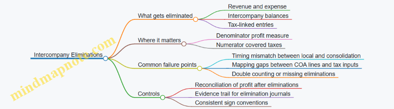
Example: Internal Service Fee and the Denominator
Assume:
- Entity A (Jurisdiction X) sells services to Entity B (Jurisdiction Y).
- Local books:
- A records revenue of 100 and expense of 40, so profit before tax is 60.
- B records expense of 100 and revenue of 20, so profit before tax is -80.
- Local tax expense is booked based on local profits.
If you consolidate without eliminations, group profit before tax becomes 60 + (-80) = -20, but it is distorted because internal revenue and expense remain.
With intercompany elimination:
- Remove A’s intercompany revenue 100 and B’s intercompany expense 100.
- Group profit before tax becomes (A profit 60 - 100) + (B profit -80 + 100) = 60 + 20 = 80.
Downstream effect: the effective tax rate denominator increases from -20 (wrong) to 80 (right). Even if covered taxes are unchanged, the effective tax rate result changes materially because the denominator moved.
Example: Tax-Linked Entries and the Numerator
Consider a scenario where Entity A books a withholding tax on an intercompany payment, and Entity B records a corresponding tax credit or gross-up locally.
At group level, the withholding tax may still be a real tax cost depending on the group’s tax position, but the key is that the local accounting may include intercompany-linked gross-ups that are not “covered taxes” in the same way.
A safe approach:
- Identify which local tax lines are included in covered taxes for Safe Harbour.
- Apply eliminations only to the components that represent internal recharges, not to the actual tax paid to authorities.
- Document the mapping rule so reviewers can trace why a tax line was included or excluded.
Control Checklist for Elimination-Driven Downstream Effects
- Denominator traceability: confirm the profit measure used for Safe Harbour is taken after intercompany eliminations.
- Elimination completeness: ensure every intercompany revenue line has a matching elimination entry.
- Sign convention consistency: verify that revenue/expense eliminations flip signs correctly across entities.
- Tax mapping stability: keep a fixed mapping between local tax expense/current tax lines and covered taxes, then apply elimination logic only where it truly affects the covered tax definition.
- Evidence trail: store the elimination journal reference and the consolidation version used for the Safe Harbour pack.
Practical Mini-Worked Reconciliation
If your group profit before tax after eliminations is 80, and covered taxes are 16, the effective tax rate is 16/80 = 20%.
If you accidentally use a denominator computed before eliminations (-20), you get 16/(-20) = -80%, which is not just “different,” it is structurally inconsistent with the group’s external profit picture. That is the kind of error a reconciliation control should catch early.
Summary of the Downstream Logic
Intercompany eliminations primarily reshape the denominator by removing internal trading effects. They can also affect the numerator when tax-linked accounting entries are tied to intercompany flows. The integrated best practice is to align the consolidation layer used for eliminations with the layer used for Safe Harbour inputs, then enforce traceable mappings and reconciliation checks so the result is explainable rather than merely computable.
9.3 Group Reporting Calendar and Data Freeze Controls
A group reporting calendar is the shared rhythm that keeps local finance teams, consolidation, tax reporting, and safe harbour calculations from stepping on each other’s toes. Data freeze controls are the guardrails that define when numbers stop moving for a given cycle, so downstream calculations remain traceable.
Foundational Concepts for Timing and Traceability
Start with three dates per cycle: the data cut-off, the freeze date, and the submission date. The cut-off is when local systems stop accepting routine postings for the reporting period. The freeze date is when the group locks the dataset used for consolidation and Pillar Two inputs. The submission date is when the final pack is sent to the next internal or external recipient.
A practical rule: every dataset used for safe harbour computations must have a named version, such as “FY2025-Q4 Safe Harbour Pack v1.0 (Frozen 2025-03-15)”. Even if the numbers are identical, the label prevents confusion during review.
Designing the Calendar from Upstream Inputs
Build the calendar backwards from the consolidation deadline. If consolidation needs trial balances by entity and currency, then local teams must receive a mapping checklist early enough to correct chart of accounts issues.
A typical sequence:
- T-6 to T-4 weeks: local reporting packs and mapping templates issued; data dictionary sign-off.
- T-3 weeks: first reconciliation window for tax-related lines (tax expense, current tax, deferred tax movements).
- T-2 weeks: consolidation dry run using last cycle’s templates to test completeness.
- T-1 week: final local adjustments window.
- T-0: freeze date and lock of the dataset.
Example: If the group freeze is 2025-03-15, local teams should aim to complete tax line reconciliations by 2025-03-08, leaving a week for consolidation mapping fixes.
Data Freeze Controls That Actually Work
Freeze controls should cover both data and changes.
Data freeze means the group stops pulling updated numbers for the frozen dataset. This includes trial balances, consolidation adjustments, and any tax line extracts used for effective tax rate safe harbour.
Change control means exceptions are allowed only through a defined path. Use three categories:
- Routine corrections before freeze: allowed without special approvals.
- Post-freeze corrections: allowed only via an exception ticket with reason, impact, and approval.
- Recalculations: if a post-freeze change affects safe harbour inputs, the pack must be reissued with a new version.
A simple control checklist for the freeze day:
- All entities have submitted trial balances in the required format.
- Tax line mappings are complete for covered taxes.
- Currency translation inputs are consistent with the consolidation method.
- Evidence files for key tax lines are present for audit trail.
Mind Map: Group Reporting Calendar and Data Freeze Controls
Example: From Local Submission to Frozen Safe Harbour Inputs
Assume Entity A submits its local trial balance on 2025-03-10. The group freeze is 2025-03-15.
- 2025-03-10 to 2025-03-12: consolidation team runs completeness checks. Entity A’s tax expense line is mapped, but current tax is missing a supporting schedule.
- 2025-03-13: Entity A provides the missing schedule. The group updates the dataset because the freeze has not occurred.
- 2025-03-15 freeze: the group locks the dataset. The safe harbour pack is generated as v1.0.
- 2025-03-16 post-freeze: a correction is requested because a tax rate was keyed incorrectly. The change is logged as an exception, approved, and the safe harbour pack is reissued as v1.1.
The key point is not that changes never happen; it’s that each change has a controlled path and a visible impact on the safe harbour pack version.
Operationalizing the Controls for Review Efficiency
To keep review efficient, align the freeze with the review workflow. If reviewers need time to test effective tax rate inputs, schedule the first review window immediately after freeze, using the frozen dataset only. Any issues found during review should be handled as exceptions, not silent edits.
Finally, ensure the freeze controls are consistent across cycles. A stable pattern reduces training overhead and prevents teams from guessing which numbers are safe to use.
9.4 Managing Differences Between Local Statutory and Group Reporting
Local statutory reporting and group reporting rarely match perfectly. For Effective Tax Rate Safe Harbour inputs, the goal is not to force identical numbers; it is to ensure that the group-level covered taxes and profit measures are computed from consistent definitions, with differences explained and controlled.
Foundational Concept: Two Ledgers, One Tax Story
Start by separating three layers:
- Local statutory numbers: produced under local accounting rules and statutory filing requirements.
- Group reporting numbers: produced under group accounting policies and consolidation adjustments.
- Safe Harbour inputs: a tax-focused view that selects and adjusts items from local and group numbers to match Pillar Two covered tax definitions.
A simple rule keeps teams sane: every Safe Harbour input must trace back to either a local statutory line, a group consolidation adjustment, or a controlled tax mapping rule.
Step 1: Identify Difference Types That Matter
Not all differences affect Safe Harbour inputs. Classify them so you know what to reconcile and what to document.
- Measurement differences: different depreciation methods, provisions, or revenue recognition.
- Timing differences: recognition occurs in different periods due to policy differences.
- Presentation differences: same economics, different line items.
- Consolidation differences: intercompany eliminations, FX translation, and ownership adjustments.
Example: Entity A records a provision for doubtful debts under local rules. In group reporting, the provision is measured differently. For Safe Harbour, you may need to adjust covered taxes if the group policy changes the tax expense linkage.
Step 2: Build a Mapping Bridge Between Local and Group
Create a mapping bridge that links local trial balance lines to group reporting lines and then to Safe Harbour inputs.
A practical approach:
- Map tax expense components (current and deferred) from local reporting to group reporting.
- Map profit measures used in the effective tax rate denominator to the group basis required for the safe harbour computation.
- Record which consolidation adjustments change the profit measure or covered taxes.
Keep the mapping bridge “boring” and explicit. If a mapping relies on judgment, write the rule and the evidence needed.
Step 3: Reconcile Using a Controlled Waterfall
Use a reconciliation waterfall that shows how the group basis is reached.
Example waterfall for a single jurisdiction:
- Local statutory profit before tax: 100
- Group policy remeasurement adjustment: +10
- Intercompany elimination impact on profit: -6
- FX translation impact on profit: +2
- Group profit before tax: 106
Then reconcile covered taxes:
- Local current tax expense: 18
- Local deferred tax movement: -3
- Group policy adjustment to tax expense linkage: +1
- Intercompany elimination effect on tax: 0
- Group covered taxes for Safe Harbour: 16
If the numbers don’t tie, the reconciliation should point to the first break, not the last one.
Mind Map: Local to Group to Safe Harbour Flow
Step 4: Handle FX and Intercompany Eliminations Without Guessing
FX translation and intercompany eliminations are common sources of “mystery differences.” Treat them as first-class reconciliation steps.
Example: Entity B has local profit before tax of 50 in local currency. Group translates it into reporting currency using an average rate, resulting in 60. If covered taxes are also translated, ensure the translation method matches the group policy used for the safe harbour denominator and numerator.
For intercompany eliminations, document whether the elimination affects:
- the profit measure used in the denominator,
- the covered taxes numerator, or
- both.
In many setups, intercompany eliminations change profit but not the underlying tax paid by each entity; however, the group-level tax expense presentation can still shift due to consolidation mechanics.
Step 5: Document Differences as “What Changed” Not “Why It Feels Different”
For each material difference, record:
- the source (local policy, consolidation adjustment, mapping rule),
- the direction and magnitude,
- the period impact,
- the evidence (trial balance lines, consolidation adjustment schedules, tax computation outputs).
A good control note reads like a recipe: “From local deferred tax movement line X, apply group policy adjustment Y, then include in covered taxes as component Z.”
Step 6: Use a Review Checklist That Matches the Reconciliation Logic
A review should confirm that:
- every Safe Harbour input has a trace to local or group sources,
- the reconciliation waterfall ties at each step,
- difference classifications are consistent across entities,
- mapping tables are versioned and approved.
Example checklist item: “Profit measure tie-out: local profit before tax plus all group adjustments equals group profit before tax used in the safe harbour denominator, with no unclassified adjustments.”
Integrated Example: One Entity with Three Difference Drivers
Entity C shows a safe harbour effective tax rate that looks “off” compared to local intuition.
- Measurement difference: group policy reduces deductible expenses by 5.
- Timing difference: deferred tax movement differs by +2 due to recognition timing.
- Consolidation difference: intercompany elimination reduces profit by 8.
After applying the mapping bridge and waterfall, the covered taxes numerator and denominator both align to the group basis. The safe harbour result is no longer a surprise; it is a computed outcome with a clear trail from local statutory lines through group reporting adjustments.
9.5 Example: End-to-End Integration from Local Trial Balance to Group Pack
This example shows how a group turns local trial balance data into a standardized Effective Tax Rate Safe Harbour pack for one reporting cycle. The goal is not just to compute a number, but to produce an auditable chain from source entries to the final group submission.
Step 1: Define the Input Map Before Touching Numbers
Start with a simple input map that links each Safe Harbour input to a source system object.
- Denominator profit measure: typically derived from local P&L lines that feed the group’s consolidated profit measure.
- Covered taxes: derived from local tax expense components and reconciled to current tax where required.
- Tax rate inputs: derived from jurisdiction tax rules and applied to the covered tax base consistently.
A practical rule: if an input cannot be traced to a specific local ledger line or tax schedule, it does not belong in the pack yet.
Step 2: Extract Local Trial Balance with Control Fields
For each entity, extract the local trial balance for the reporting period and include control fields needed for later reconciliation.
- Entity identifier and legal entity name
- Reporting currency and translation method
- Period start and end dates
- Version and posting status (e.g., “final statutory” vs “management accounts”)
Example: Entity A posts tax expense in local currency. The extraction includes the tax expense account codes and the tax authority reference used in the tax provision.
Step 3: Build the Local Safe Harbour Working Schedule
Convert trial balance lines into the working schedule using a fixed mapping table.
- Pull tax expense into “covered taxes candidates.”
- Separate current tax and deferred tax components if the group requires that split for reconciliation.
- Apply inclusion/exclusion rules (for example, remove non-covered levies if the group’s policy defines them as excluded).
Concrete example: If Entity A has tax expense of 120, of which 90 is current tax and 30 is deferred tax, the working schedule records both components and flags any adjustments needed to align with the covered taxes definition.
Step 4: Reconcile Local Working Schedule to Local Financial Statements
Reconciliation is where most integration errors hide, so keep it mechanical.
- Reconcile totals: working schedule tax totals must tie to the local tax expense total.
- Reconcile sign conventions: ensure expenses are positive or negative consistently across entities.
- Reconcile timing: confirm the period matches the trial balance extraction.
Example: If the working schedule shows covered taxes of 110 but local tax expense is 120, the difference must be explained by a documented adjustment (e.g., excluded levy of 10).
Step 5: Apply Standardization Rules for Group Pack Consistency
Standardization ensures the group pack is comparable across entities.
- Use a consistent profit measure denominator definition.
- Standardize currency translation: translate profit and tax using the group’s consolidation approach.
- Normalize rate handling: store the selected tax rate and the basis for selection.
Example: Entity A’s profit is translated at average rates, while tax is translated at closing rates per group policy. The pack stores both the local amounts and the translated amounts.
Step 6: Consolidate Into the Group Pack with Clear Eliminations
Group consolidation introduces eliminations that can affect inputs.
- Apply intercompany eliminations to the profit measure denominator.
- Confirm whether covered taxes are affected by eliminations or remain entity-level.
- Ensure the group pack reflects the same consolidation scope used for financial reporting.
Example: If Entity A and Entity B have intercompany charges, the group elimination reduces the consolidated profit denominator. The pack records the elimination impact so the safe harbour computation remains consistent.
Step 7: Produce the Group Pack Outputs and Evidence Set
The final group pack should include both results and evidence.
- Safe Harbour computation summary per jurisdiction
- Entity-level working schedules
- Reconciliation statements tying to local trial balance and local financial statements
- Control logs showing extraction version, mapping version, and sign-off
A good sanity check: totals in the group pack should reconcile to consolidated financial statement totals within defined tolerances, with differences explained.
Mind Map: End-to-End Integration Flow
Step 8: Mini Example with Numbers to Show the Chain
Assume Entity A (jurisdiction X) has:
- Local profit measure denominator: 1,000
- Local tax expense: 120
- Excluded levy: 10
- Covered taxes after adjustment: 110
Group consolidation eliminates intercompany profit of 200, so the consolidated denominator for jurisdiction X becomes 800. The group pack stores:
- Local covered taxes: 110
- Translated covered taxes: (translated amount)
- Consolidated denominator: 800
- The final safe harbour computation inputs used for the jurisdiction result
The key integration discipline is that every transformation step is recorded: mapping, adjustments, translation, and eliminations. If a reviewer can follow the chain without guessing, the pack is ready.
10. Practical Case Studies with Step-by-Step Safe Harbour Calculations
10.1 Case Study: A Single Jurisdiction with Standard Tax Profile
Case Setup
A group has one reporting unit in a single jurisdiction, Country A. The goal is to compute the Effective Tax Rate (ETR) inputs used for the Effective Tax Rate Safe Harbour and to document them so the numbers can be traced back to the financial statements.
Assume the group’s local trial balance for the year ended 2026-03-15 includes:
- Profit before tax: 100,000
- Current tax expense: 22,000
- Deferred tax expense: 3,000
- Total tax expense in the income statement: 25,000
- Statutory tax rate: 22%
The safe harbour computation needs covered taxes and a profit denominator. The key integration task is to ensure the covered taxes figure is consistent with the group’s definition, not just the accounting tax expense.
Step 1: Map Financial Statement Items to Computation Inputs
Start by separating “what the accounts show” from “what the safe harbour asks for.” In this case, the tax profile is standard, meaning there are no unusual permanent differences and no special regimes.
- Covered taxes: use the taxes that correspond to the safe harbour definition. For this case, assume covered taxes equal total tax expense (current + deferred) because the jurisdiction’s tax system and the group’s mapping align.
- Denominator: use profit before tax or an equivalent profit measure as required by the safe harbour mechanics.
Example mapping table
| Financial statement line | Amount | Role in safe harbour | Notes |
|---|---|---|---|
| Profit before tax | 100,000 | Denominator | Use the same sign convention as the template |
| Current tax expense | 22,000 | Covered taxes | Trace to tax return support |
| Deferred tax expense | 3,000 | Covered taxes | Trace to deferred tax roll-forward |
| Total tax expense | 25,000 | Covered taxes | Sum of current and deferred |
Step 2: Compute Effective Tax Rate
Compute ETR as covered taxes divided by the denominator.
- Covered taxes: 25,000
- Denominator: 100,000
- ETR: 25,000 / 100,000 = 25%
Now compare the computed ETR to the safe harbour threshold logic used in your approach. In a “standard tax profile” case, the expectation is that the ETR will be close to the statutory rate, but it can differ due to timing effects captured in deferred tax.
Reasoning check: if deferred tax expense is positive, ETR rises above the statutory rate; if it were negative, ETR would fall. This is a quick sanity check that catches sign errors.
Step 3: Validate Eligibility and Documentation
Even with one jurisdiction, eligibility still needs evidence. The documentation pack should show:
- The jurisdiction identification and reporting unit mapping
- The profit denominator source (income statement or consolidation schedule)
- The covered taxes components (current and deferred)
- The reconciliation from local statutory tax expense to covered taxes
Example reconciliation
| Reconciliation item | Amount | Why it matters |
|---|---|---|
| Total tax expense per income statement | 25,000 | Starting point |
| Adjustments to reach covered taxes | 0 | Confirms standard profile |
| Covered taxes for safe harbour | 25,000 | Final input |
Step 4: Control Checks That Prevent Common Mistakes
Use a small set of checks that are easy to perform and hard to “accidentally” pass.
- Sign convention check: profit denominator should be positive in this case; taxes should be positive expenses.
- Component tie-out: covered taxes must equal current + deferred.
- Reconciliation completeness: if adjustments are zero, still document why (e.g., no permanent differences identified).
- Rate consistency check: the statutory rate used for narrative and threshold comparison should match the jurisdiction’s documented tax rate.
Mind Map: Single Jurisdiction Safe Harbour Case
Step 5: Final Output Pack Structure
A practical pack for this case includes one calculation sheet and one reconciliation sheet, plus evidence pointers.
- Calculation sheet: denominator, covered taxes components, ETR result, and template tie-outs.
- Reconciliation sheet: income statement tax expense to covered taxes with explicit “no adjustments” support.
- Evidence index: trial balance extract, tax return summary for current tax, deferred tax roll-forward for deferred tax, and the documented statutory rate.
This case is intentionally simple: the value is in showing that “standard” still requires disciplined mapping, clean arithmetic, and a reconciliation that explains why the mapping required no adjustments.
10.2 Case Study: Multiple Taxes With Reconciliations to Tax Expense
Case Setup and Goal
A group has one reporting unit in Jurisdiction A. The entity’s statutory accounts show tax expense, but Pillar Two inputs require “covered taxes” and a clean bridge to the effective tax rate safe harbour computation. The goal is to reconcile multiple tax components—current tax, deferred tax movements, and a withholding tax—back to the tax expense line items, while keeping the safe harbour calculation auditable.
Assume the reporting period ended 2026-03-31. The entity reports profit before tax of 10,000. Statutory tax expense is 2,050. The group also has a withholding tax of 120 related to payments to non-residents.
Step 1: Identify Tax Components That Contribute to Covered Taxes
Start by listing tax components from the tax note and mapping each to either covered taxes or excluded items.
- Current tax expense: 1,980
- Deferred tax expense (net movement): 70
- Withholding tax: 120
- Tax penalties and interest: 0
Best practice: treat penalties and interest as exclusions unless your covered taxes definition explicitly includes them. In this case, none exist, so the mapping is straightforward.
Step 2: Build the Reconciliation Bridge to Tax Expense
Create a bridge that shows how the statutory tax expense line becomes the covered taxes figure used in the safe harbour computation.
Tax expense in the statutory income statement is 2,050. It equals current tax (1,980) plus deferred tax (70). The withholding tax is not always included in the statutory income statement tax expense, so you reconcile it separately.
Reconciliation logic
- Covered taxes for the safe harbour computation = current tax + deferred tax + withholding tax (if included in your covered taxes definition)
- Tax expense line = current tax + deferred tax
Here, covered taxes = 1,980 + 70 + 120 = 2,170.
Step 3: Confirm Denominator Inputs for Effective Tax Rate
The safe harbour effective tax rate uses a profit measure as the denominator. For this case, use profit before tax of 10,000.
Effective tax rate = 2,170 / 10,000 = 21.7%.
Best practice: ensure the denominator is aligned to the same scope as the covered taxes. If the group uses a different profit measure for Pillar Two, the reconciliation bridge must extend to that profit measure, not just tax.
Step 4: Document the “Why” Behind Each Number
Numbers without reasons are just numbers. Document the drivers:
- Current tax (1,980): based on taxable profit after adjustments.
- Deferred tax movement (70): arises from temporary differences reversing during the period.
- Withholding tax (120): based on gross payments and applicable withholding rates.
A practical control is to require a short evidence note per component:
- Current tax: tax return computation summary
- Deferred tax: movement schedule by temporary difference
- Withholding tax: payment register and withholding certificates
Step 5: Mind Map of the Reconciliation Workflow
Mind Map: Multiple Taxes Reconciliation to Tax Expense
Step 6: Worked Example Table for the Bridge
| Line Item | Amount | Included in Covered Taxes | Evidence to Attach |
|---|---|---|---|
| Current tax expense | 1,980 | Yes | Tax return computation summary |
| Deferred tax expense (net) | 70 | Yes | Deferred tax movement schedule |
| Statutory tax expense total | 2,050 | Yes | Income statement tax note |
| Withholding tax | 120 | Yes | Payment register and certificates |
| Covered taxes total | 2,170 | Yes | Reconciliation worksheet |
Step 7: Common Pitfalls and How This Case Avoids Them
- Double counting withholding tax: If withholding tax is already included in statutory tax expense in your local accounts, you must not add it again. Here, it is separate, so adding is correct.
- Mixing sign conventions: Deferred tax can be negative in some periods. This case uses positive net expense; the worksheet should still handle negative values without manual edits.
- Denominator mismatch: If profit before tax includes discontinued operations, but covered taxes exclude them, the rate becomes misleading. This case assumes consistent scope.
Step 8: Final Safe Harbour Computation Output
Covered taxes: 2,170
Denominator profit measure: 10,000
Effective tax rate: 21.7%
The reconciliation bridge and evidence notes form a complete audit trail from statutory tax expense to the safe harbour inputs, with each tax component explained and traceable.
10.3 Case Study: Loss Making Entity With Denominator Considerations
This case study shows how to compute an Effective Tax Rate (ETR) safe harbour when the entity is loss-making, so the denominator can be zero or negative. The goal is to keep the calculation consistent, auditable, and explainable to someone who did not build the spreadsheet.
Case Setup and Inputs
Assume a single entity in Jurisdiction A with the following local financial results for Year X:
- Profit before tax (PBT): -€40m (loss)
- Income tax expense in the financial statements: €6m
- Current tax expense: €2m
- Deferred tax expense: €4m
- Covered taxes for Pillar Two mapping: €6m (current + deferred, after agreed mapping rules)
- Relevant tax rate input: 20% statutory rate (used only for rate-related checks, not to force an ETR)
Key point: the safe harbour ETR computation uses a profit-based denominator. With PBT at -€40m, the denominator is negative, which can break naive ETR formulas.
Step 1: Confirm the Denominator Definition
Start by writing the denominator definition in plain language and then applying it consistently:
- Denominator = Profit measure used for ETR safe harbour (commonly based on PBT or a closely aligned profit figure)
- If the denominator is zero or negative, the ETR is not meaningful as a ratio in the usual sense
Practical check: do not “fix” the sign by taking absolute values. If the denominator is negative, the computation must follow the safe harbour rules for loss scenarios.
Step 2: Compute the Numerator and Identify the Loss Scenario
Numerator = Covered taxes = €6m.
Denominator = Profit measure = -€40m.
A ratio would be €6m / -€40m = -15%. That number is mathematically valid but conceptually unhelpful for safe harbour eligibility, because it implies a “negative tax rate” interpretation that does not align with how the safe harbour is meant to be applied.
So the workflow should branch here:
- If denominator > 0: compute ETR as ratio
- If denominator <= 0: apply the loss-making handling approach defined in your methodology and document why ETR is not used as a ratio
Step 3: Apply Loss-Making Handling with Documentation
In this case, denominator is negative, so you apply the loss-making handling approach.
A robust approach for an integrated finance workflow is to record two outputs:
- “ETR Ratio” field: leave blank or mark “Not Applicable due to loss denominator”
- “Safe Harbour Outcome” field: record the rule-based outcome for loss-making entities
Example documentation note (short and specific):
- “Denominator equals -€40m (loss). ETR ratio not computed because the denominator is non-positive. Covered taxes mapped to €6m per reconciliation schedule. Safe harbour outcome determined under loss-making rule for Year X.”
Step 4: Reconcile Covered Taxes to Explain the Tax Expense
Even if the ETR ratio is not computed, the covered taxes still need to be explainable.
Use a reconciliation table:
- Financial tax expense: €6m
- Current tax: €2m
- Deferred tax: €4m
- Mapping adjustments: €0m
- Covered taxes for safe harbour: €6m
Concrete reason this matters: auditors often ask whether deferred tax should be included, excluded, or adjusted. Your reconciliation answers that question without forcing them to interpret your mapping logic from scratch.
Step 5: Validate Edge Cases That Commonly Confuse Teams
Check these items in order:
- Sign conventions: confirm losses are negative in the profit measure, not positive with a “loss flag”
- Denominator source: confirm the profit measure comes from the same reporting basis as the covered taxes mapping
- Rounding: ensure the denominator is not accidentally rounded to zero in intermediate steps
- Intercompany effects: if PBT includes intercompany profits eliminated elsewhere, confirm which basis your safe harbour computation uses
Mind Map: Loss Making Denominator Workflow
Mini Example: Near-Zero Denominator
If PBT were -€0.2m instead of -€40m, the denominator is still non-positive. The correct handling remains the same: do not compute a ratio just because the loss is small. Instead, document that the denominator is non-positive and apply the loss-making rule.
Output Summary for Year X
- Covered taxes: €6m (reconciled)
- Denominator: -€40m (loss)
- ETR ratio: Not Applicable due to non-positive denominator
- Safe harbour outcome: determined under the loss-making rule for the methodology
The spreadsheet should therefore look “quiet” in the ETR ratio cell, but “loud” in the reconciliation and documentation cells. That is the point: the calculation is not trying to force a ratio where the denominator rules say it should not be used.
10.4 Case Study: Complex Group With Intercompany And Currency Effects
This case study shows how a group can produce an effective tax rate safe harbour computation when intercompany flows and currency translation complicate the inputs. The goal is not to “get a number fast,” but to get a number that ties back to controlled source data.
Scenario Setup
Assume a group with two reporting units in different jurisdictions:
- Jurisdiction A: Functional currency EUR. Parent owns 100% of Sub A.
- Jurisdiction B: Functional currency USD. Parent owns 100% of Sub B.
For the year, the group prepares consolidated financial statements in EUR. Sub A and Sub B both have local statutory tax expense, and both also have intercompany charges from the Parent.
Key facts (local books):
- Sub A has profit before tax of €120m and current tax expense of €24m.
- Sub B has profit before tax of $90m and current tax expense of $18m.
- Parent charges Sub A and Sub B for services. In consolidation, those intercompany revenues and expenses are eliminated.
- Exchange rates used for consolidation: average rate 1.10 USD per EUR and closing rate 1.12 USD per EUR.
Step 1: Define the Safe Harbour Inputs You Will Actually Use
For effective tax rate safe harbour, you need a consistent pair:
- Covered Taxes: the taxes that correspond to the safe harbour definition.
- Profit Measure: the denominator measure used for the effective tax rate.
Best practice here is to decide early whether your group uses current tax only or current plus deferred for the covered taxes mapping. In this case, assume the group uses current tax expense as covered taxes because it is directly traceable and stable across reporting cycles.
Example mapping rule used in this case:
- Covered Taxes = Current tax expense from the local tax note.
- Profit Measure = Profit before tax from the local income statement.
Step 2: Handle Intercompany Effects Without Breaking Traceability
Intercompany eliminations affect consolidated profit, but safe harbour computations are typically prepared at the jurisdiction level using local profit measures that already include intercompany effects in local books. The group’s approach is:
- Compute safe harbour inputs per reporting unit using local profit before tax and local current tax expense.
- Do not attempt to “rebuild” local profit after elimination for the safe harbour calculation.
Why this works: the tax expense is already incurred in the jurisdiction based on local taxable results, and the safe harbour computation is designed to reflect that jurisdictional tax position.
Concrete example:
- Sub A’s local profit before tax includes Parent service income net of its service expense. The consolidation elimination removes the matching revenue/expense pair from the group totals, but Sub A’s local tax expense remains tied to Sub A’s local taxable base.
Step 3: Convert Currency in a Controlled Way
Because the safe harbour computation pack is reported in EUR, you must translate both numerator and denominator consistently.
Rule applied in this case:
- Translate profit before tax using the average rate.
- Translate current tax expense using the average rate as well, because both represent flows for the period.
Example:
- Sub B profit before tax: $90m ÷ 1.10 = €81.82m
- Sub B current tax expense: $18m ÷ 1.10 = €16.36m
Avoid a common mistake: using the closing rate for tax expense. Closing rates belong to balance sheet items; tax expense is a period flow.
Step 4: Compute Effective Tax Rates per Reporting Unit
Jurisdiction A:
- Covered Taxes = €24m
- Profit Measure = €120m
- Effective tax rate = 24 / 120 = 20.0%
Jurisdiction B:
- Covered Taxes = €16.36m
- Profit Measure = €81.82m
- Effective tax rate = 16.36 / 81.82 = 20.0%
In this example, both jurisdictions land at the same effective rate, which makes the safe harbour conclusion straightforward.
Step 5: Aggregate for Group-Level Presentation Without Mixing Concepts
If the group presents a combined effective tax rate for reporting convenience, it should be a weighted result:
- Total Covered Taxes = €24m + €16.36m = €40.36m
- Total Profit Measure = €120m + €81.82m = €201.82m
- Combined effective tax rate = 40.36 / 201.82 = 20.0%
This avoids the error of averaging 20.0% and 20.0% without weights. In other cases, those would differ.
Step 6: Documentation That Survives Review
Your calculation pack should include:
- A mapping table from local tax note line items to covered taxes.
- A mapping table from local income statement line items to the profit measure.
- A currency translation table showing average rate usage for both numerator and denominator.
- A reconciliation bridge showing how local figures were extracted from the trial balance or tax working papers.
Here is a compact mind map of the logic chain.
Mind Map: Complex Group Safe Harbour with Intercompany and Currency
Step 7: Control Checks That Catch Real Problems
Use three quick checks:
- Sign check: profit and tax expense should align with expected sign conventions.
- Rate consistency check: confirm the same exchange rate basis is used for both numerator and denominator.
- Extraction check: ensure the tax expense used matches the tax note, not a reclassified management figure.
Summary of the Case
By computing safe harbour inputs at the reporting-unit level, translating period flows with the average rate, and aggregating using weights, the group produces a consistent effective tax rate of 20.0% despite intercompany eliminations and cross-currency reporting.
10.5 Case Study: Documentation Assembly and Control Evidence Review
This case study shows how a group prepares a complete Effective Tax Rate Safe Harbour documentation pack and then reviews it with a control-evidence mindset. The goal is simple: when someone asks “why this number?”, the pack should answer without hunting across spreadsheets, emails, and half-labeled tabs.
Case Setup and Inputs
Assume the reporting unit is “Entity A” in Jurisdiction X. The pack must support the effective tax rate computation used for Safe Harbour. The group uses a standardized template with three calculation layers:
- Financial layer: trial balance, tax expense, current tax, and deferred tax movements.
- Mapping layer: how each tax line maps to “covered taxes” and to the denominator profit measure.
- Computation layer: the final effective tax rate and the Safe Harbour conclusion.
A control-evidence review starts by confirming that each layer has traceable sources and consistent sign conventions. For example, if tax expense is presented as a positive number in the trial balance but covered taxes require a negative sign, the pack must show the transformation explicitly.
Documentation Assembly Sequence
Step 1: Create the pack index. The pack begins with a one-page index listing every required schedule and the location of its source data. This prevents the classic “we have the numbers, but not the proof” problem.
Step 2: Attach source evidence for each input. For Entity A, the pack includes:
- Trial balance extract for the period.
- Tax note extracts showing current tax and deferred tax.
- A reconciliation from statutory tax expense to covered taxes.
- The denominator schedule used for the effective tax rate.
Step 3: Capture mapping decisions. The mapping layer includes a short mapping log. It records why certain items are included or excluded. Example: a tax credit that offsets current tax is included in covered taxes if it reduces the net tax burden; a VAT-like levy is excluded because it is not an income tax.
Step 4: Record assumptions and exceptions. If Entity A has a loss-making year, the pack includes the loss handling logic and shows how the denominator is treated. If there are multiple tax types, the pack lists each tax type and the rate or classification used.
Step 5: Lock versions and approvals. The pack includes a version control sheet with preparation date (for this case, use 2026-03-15), preparer name, reviewer name, and approval status. The pack also stores the template version used.
Control Evidence Review Method
The review is performed in two passes: completeness checks first, then reasonableness checks.
Pass A: Completeness and traceability. The reviewer verifies that:
- Every computation cell that feeds the effective tax rate links to a source schedule.
- Every mapping rule has an evidence reference.
- Every reconciliation has a tie-out to the trial balance or tax note.
- Any manual adjustments are documented with a reason and an evidence link.
Pass B: Reasonableness and consistency. The reviewer checks:
- Sign conventions across schedules.
- Whether covered taxes and denominator profit use the same scope and entity.
- Whether rounding rules are consistent with the template.
A practical example: if the effective tax rate is unusually high, the reviewer does not assume an error. Instead, they trace whether the denominator profit is small due to timing differences, or whether a tax credit was excluded incorrectly.
Mind Map: Documentation Pack and Evidence Review
Worked Example: What “Good Evidence” Looks Like
Suppose the reconciliation from statutory tax expense to covered taxes shows a difference of 12.0. The pack includes:
- A line-by-line bridge explaining that 12.0 is a non-income levy excluded from covered taxes.
- A reference to the tax note line where the levy is described.
- A control check showing that the excluded amount does not appear in the denominator profit measure.
If the reviewer finds the bridge but not the tax note reference, the issue is not “the number is wrong.” The issue is “the evidence is incomplete,” and the pack is updated before approval.
Final Assembly Checklist
Before sign-off, the reviewer confirms that the pack can be understood by a new reader in one sitting: the index points to every schedule, each schedule ties to a source, and every conclusion is supported by a documented rule. That’s the difference between a pack that contains numbers and a pack that contains answers.
11. Review Testing and Issue Resolution for Reliable Outcomes
11.1 Review Checklist for Safe Harbour Computations
A good review is not a second calculation; it is a structured way to prove the calculation is built on the right inputs, uses them consistently, and produces a result that makes sense. Use the checklist below in order, so you catch foundational issues before you spend time on arithmetic.
Scope and Eligibility Confirmation
- Confirm the computation is for the correct reporting period and the correct reporting unit set.
- Verify the safe harbour basis being applied matches the group’s stated approach for that period.
- Check that the jurisdiction and entity mapping used in the pack matches the governance decision for safe harbour eligibility.
Example: If an entity is excluded from safe harbour due to a specific condition, ensure its covered taxes and profit measure are excluded from the safe harbour computation rather than merely flagged.
Input Completeness and Traceability
- Ensure every required input line has a source reference to the underlying financial system extract.
- Confirm the pack includes both numerator and denominator components, not just the final effective tax rate.
- Validate that sign conventions are consistent across all schedules.
Example: A denominator built from profit before tax should not be negative if the methodology expects a positive base; if it is negative, the review should stop and escalate to the methodology owner.
Covered Taxes Reconciliation
- Reconcile covered taxes used in the safe harbour computation to the group’s tax expense components.
- Confirm exclusions and inclusions are applied exactly once, not both in the source mapping and again in the computation.
- Check that any deferred tax components included or excluded follow the documented rule.
Example: If current tax is mapped from statutory accounts and deferred tax is excluded, the review should confirm that the deferred tax line is not still present in an adjustment schedule.
Denominator Construction Checks
- Verify the denominator profit measure is built from the correct financial statement line items.
- Confirm adjustments that affect the denominator are applied consistently with the numerator methodology.
- Check treatment of losses and zero-profit scenarios per the safe harbour approach.
Example: For a loss-making entity, confirm whether the methodology uses a zero denominator, a special handling rule, or exclusion. The review should match the chosen rule every time.
Tax Rate Input Validation
- Confirm the relevant tax rate inputs used for any rate-related steps match the jurisdiction and period.
- Check that withholding taxes or other levies are treated according to the same inclusion/exclusion logic used for covered taxes.
- Validate that rate selection is not overridden by stale master data.
Example: If a jurisdiction has a temporary rate change, ensure the rate table used in the pack reflects the period dates, not the last known rate.
Calculation Integrity and Arithmetic
- Perform a line-by-line re-check of the effective tax rate formula using the pack’s own intermediate values.
- Confirm rounding rules are applied at the correct stage and do not cause inconsistent totals.
- Check that totals equal the sum of components after any eliminations or reclassifications.
Example: If rounding is applied per entity and then summed, totals may differ from rounding at group level. The review should confirm the pack follows the documented approach.
Consistency Across Entities and Consolidation Effects
- Verify intercompany eliminations do not leave orphan amounts in either numerator or denominator.
- Confirm currency translation effects are applied consistently across all schedules.
- Check that entity-level computations roll up to the group-level safe harbour computation without missing entities.
Example: If an entity’s local currency profit is translated using an average rate, ensure the same translated basis is used for the denominator and any related adjustments.
Evidence, Review Trail, and Sign-Off Readiness
- Confirm each exception has a documented resolution and an owner.
- Ensure the review trail includes who checked what, when, and against which version of the pack.
- Verify that the final pack is the approved version and not a working draft.
Example: If an exception is resolved by changing a mapping rule, the review should confirm the change is reflected in the calculation pack version and the evidence folder.
Issue Handling and Escalation Triggers
Escalate immediately when you see any of the following:
- Missing source references for required inputs.
- Denominator sign or loss handling that contradicts the methodology.
- Double-counting indicators such as the same adjustment appearing in two schedules.
- Rate inputs that do not match the jurisdiction-period mapping.
Mind Map: Review Checklist Flow
Example: Mini Review Walkthrough for One Entity
- Eligibility: Confirm entity is included for the period.
- Inputs: Check covered taxes numerator lines each link to a source extract.
- Reconciliation: Ensure covered taxes equal mapped current tax plus/minus documented adjustments, with deferred tax excluded.
- Denominator: Confirm profit measure uses the correct financial statement lines and applies loss handling rule.
- Arithmetic: Recompute effective tax rate from intermediate values and confirm rounding matches the pack.
- Evidence: Confirm the reviewer notes any exceptions and that the pack version is the approved one.
Example: Common Failure Pattern and How the Checklist Catches It
Failure pattern: An adjustment is applied in the mapping layer and again in the computation layer.
- The checklist catches it at Covered Taxes reconciliation by comparing intermediate totals to the expected mapped components.
- It also catches it at Calculation integrity by showing totals that do not tie to the sum of components after eliminations.
Review Output Format
- Record the final effective tax rate result.
- List exceptions with resolution notes.
- Confirm sign-off readiness: evidence complete, version approved, and tie-outs passed.
11.2 Analytical Procedures for Detecting Data Anomalies
Analytical procedures are how you catch “data that looks plausible but isn’t.” The goal is not to prove a number wrong immediately; it’s to identify which parts of the safe harbour computation deserve deeper checking. Start with simple comparisons, then move to ratio and movement analysis, and finish with targeted tests that connect anomalies back to specific source data.
Foundational Concepts for Anomaly Detection
Begin by separating anomalies into three buckets:
- Level anomalies: a value is unusually high or low versus expectation.
- Movement anomalies: the change from prior period is unusual even if the level is not.
- Composition anomalies: the mix of components shifts, such as covered taxes changing relative to profit.
A practical mindset helps: if an anomaly appears in the safe harbour pack, it should be traceable to either (1) financial statement inputs, (2) mapping rules, (3) rate selection, or (4) consolidation adjustments. If you cannot trace it, you do not yet have an anomaly—you have a mystery.
Step 1: Establish Expectations Using Baselines
Create baselines before you compare anything. Use at least two of the following:
- Prior period effective tax rate (ETR) by reporting unit.
- Multi-year average ETR for stable jurisdictions.
- Budget or forecast ETR if available.
- Peer comparison across similar entities within the same tax regime.
Example: Entity A has an ETR of 14% last year and 15% average over three years. In the current period, the computed ETR is 28%. Even without knowing the reason, you now have a clear target for investigation.
Step 2: Perform Level and Movement Tests
Use a small set of tests consistently so results are comparable across entities.
- ETR level test: Compare current ETR to baseline.
- Covered taxes movement test: Compare covered taxes to prior period.
- Denominator movement test: Compare profit measure to prior period.
- Sign and zero tests: Flag cases where profit is near zero, or where losses flip the sign of the denominator.
Example: Entity B shows profit down 40%, but covered taxes down only 5%. The ETR rises sharply. That pattern often points to mapping issues (e.g., taxes included that should be excluded) or rate selection problems.
Step 3: Use Ratio and Bridge Analysis to Isolate Drivers
ETR alone rarely explains itself. Add a bridge that decomposes the ETR change into drivers:
- Change in covered taxes components (current vs deferred-related elements as applicable to your mapping).
- Change in profit measure.
- Change in applied rates or tax regime inputs.
- Change in consolidation effects such as eliminations.
Example: Entity C’s ETR increases from 10% to 13%. A bridge shows covered taxes increased by 20 while profit increased by only 5. A second bridge shows that the increase is concentrated in one component mapped from a specific GL account range. Now the investigation has a direction.
Step 4: Validate Data Quality Through Consistency Checks
Consistency checks catch errors that look like “real” numbers.
- GL-to-pack completeness: every relevant GL account mapped to covered taxes must appear in the pack.
- Reconciliation sanity: differences between trial balance tax expense and covered taxes should reconcile to documented adjustments.
- Rate alignment: the rate used must match the jurisdiction and period basis.
- Currency translation: ensure the same currency basis is used for both numerator and denominator.
Example: Entity D uses a local currency profit measure but translates covered taxes using a different exchange rate. The ETR becomes slightly off in a way that repeats each period—an excellent clue that the issue is systematic, not random.
Step 5: Prioritize Findings Using a Triage Logic
Not every anomaly deserves the same effort. Triage by:
- Magnitude: how far from baseline.
- Impact: how much it affects the safe harbour outcome.
- Traceability: whether the anomaly can be linked to a small set of source inputs.
- Repeatability: whether it occurs across entities or only one.
A simple rule works: if the anomaly is large and traceable to one mapping rule, fix the mapping first; if it’s large and not traceable, start with source data completeness.
Mind Map: Analytical Procedures for Detecting Data Anomalies
Example: From Anomaly Flag to Root Cause
Entity E has an ETR jump from 9% to 17%. Level tests flag it as high magnitude. Movement tests show profit is stable, but covered taxes increased. Bridge analysis shows the increase is entirely in one component mapped from a specific tax expense GL bucket. Consistency checks confirm that the bucket includes a levy that should be excluded under the covered taxes definition. The fix is to adjust the mapping rule and rerun the computation, then re-check the reconciliation to ensure the change is fully explained.
Practical Output for the Review Record
Your review record should capture three things for each anomaly: the test that triggered it, the direction of the driver (numerator, denominator, rate, or mapping), and the evidence link to the source data or adjustment schedule. That structure keeps the process efficient and makes the next review faster, not harder.
11.3 Resolving Data Gaps and Mapping Breaks
Data gaps and mapping breaks are the quiet reasons safe harbour results go sideways. The goal here is not to “fix” numbers blindly, but to restore traceability: every input used in the effective tax rate computation should have a clear origin, a documented transformation, and a defensible treatment when it is missing.
Foundations for Diagnosing the Problem
Start with a simple classification. A gap is usually one of three types: missing source data, missing mapping rules, or missing transformation logic.
- Missing source data means the underlying trial balance or tax schedule line is absent (for example, a tax code never posted).
- Missing mapping rules means the data exists but cannot be linked to the covered taxes denominator or numerator (for example, a tax line sits under an unexpected account).
- Missing transformation logic means the mapping exists, but the computation step is incomplete (for example, currency translation applied to revenue but not to tax).
A practical diagnostic step is to compare three counts for each reporting unit and jurisdiction: number of expected tax lines, number of mapped tax lines, and number of lines that successfully pass reconciliation checks. When these counts diverge, you know exactly where the break occurred.
Mind Map: Gap Resolution Workflow
Containment Before Correction
Before changing anything, contain the issue. Freeze the current calculation pack inputs and record which reporting units and jurisdictions are affected. This prevents “fixes” from being mixed with untracked changes. Assign a severity level based on impact to the effective tax rate numerator or denominator. A missing denominator component is usually more severe than a missing disclosure line because it changes the ratio.
Systematic Diagnosis from Template to Source
Use a reverse trace. Take one unmapped tax line from the safe harbour template and follow it backward:
- Template line: identify the intended covered tax category.
- Mapping key: confirm the account number, tax code, and jurisdiction tag used to map.
- Source ledger: locate the trial balance line and verify posting period and sign.
- Transformation: confirm whether any adjustments were required, such as intercompany eliminations or currency translation.
Example: Mapping Break Due to Account Reclassification
Suppose the template expects “Current tax expense” mapped from account TAX_CURR. In one entity, the trial balance posts current tax under TAX_CURRENT after a chart of accounts update.
- Symptom: the template shows a gap for covered taxes numerator.
- Diagnosis: mapping rules still reference TAX_CURR only.
- Resolution: extend the mapping to include TAX_CURRENT, then re-run reconciliation.
- Verification: confirm the mapped amount equals the trial balance current tax for the period and that the sign matches the template convention.
Example: Missing Source Data from a Tax Code Posting Issue
An entity reports a tax line in the statutory return but not in the ledger. The safe harbour pack expects ledger-based covered taxes.
- Symptom: source extraction returns zero for the expected tax code.
- Diagnosis: the tax code was disabled in the posting configuration for that month.
- Resolution: re-extract after correcting the posting configuration and ensure the corrected entries are included in the same reporting period.
- Verification: reconcile the corrected ledger total to the tax schedule used for statutory reporting.
Resolving Transformation Logic Gaps
Transformation gaps often hide in consolidation and currency handling.
- Currency translation: ensure the same exchange rate basis is used for both numerator and denominator components when they are computed in different currencies.
- Intercompany eliminations: confirm that eliminated profits do not leave behind tax effects that should have been eliminated or reclassified.
Example: Currency Translation Applied to Profit but Not Tax
If profit is translated using the average rate but tax is translated using the closing rate, the effective tax rate can be distorted.
- Symptom: reconciliation passes, but the effective tax rate is materially inconsistent with prior periods.
- Diagnosis: transformation logic uses different rate types for tax and profit.
- Resolution: align the translation method to the defined computation policy for covered taxes inputs.
- Verification: re-run the computation and confirm the numerator and denominator are now translated consistently.
Verification and Evidence Closure
After each resolution, re-run the same checks that detected the gap: mapping completeness, reconciliation totals, and sign conventions. Evidence closure means you store the corrected mapping rule, the extraction output, and the reconciliation worksheet showing the before-and-after impact. When a manual override is unavoidable, document the reason and attach the source evidence used to justify it.
Finally, ensure the calculation pack version is locked so the next review cycle starts from a stable baseline. That’s how you keep “fixed” from turning into “mysteriously different.”
11.4 Handling Rounding, Sign Conventions, and Edge Cases
Safe harbour computations look simple until numbers start disagreeing by a few units, signs flip during reclassifications, or edge cases (losses, zero denominators, mixed tax types) show up like uninvited guests. This section gives practical rules to keep results consistent, explainable, and reviewable.
Rounding Rules That Stay Reviewable
Rounding should be applied at the latest possible stage, after all intermediate arithmetic is complete. If you round early, you create tiny differences that later reconciliation steps cannot justify.
A practical approach:
- Keep source amounts in full precision from the trial balance and tax ledger.
- Perform calculations using full precision.
- Round only the final outputs used for safe harbour eligibility and reporting.
- Use a single rounding convention across entities and jurisdictions.
Example: Suppose covered taxes are 12,345.67 and profit is 98,765.43.
- Exact ETR = 12,345.67 / 98,765.43 = 0.124999…
- If you round covered taxes to 12,346 and profit to 98,765 first, ETR becomes 0.125010…
- That difference can move a result across a threshold when the safe harbour boundary is tight.
Sign Conventions That Prevent Silent Errors
Sign conventions must be consistent across three places: financial statements, tax computations, and reporting templates.
Common pitfalls:
- Tax expense reported as positive in the financial statement, but covered taxes treated as positive for payments and negative for refunds.
- Denominator profit treated as positive for profit and negative for loss, while the computation expects profit as an absolute measure.
- Reclassifications that reverse sign during mapping from tax accounts to covered taxes.
A simple rule set:
- Define one “positive direction” for each input: profit measure, covered taxes, and adjustments.
- Document the direction in the template header and enforce it with control checks.
- When an adjustment is described as “increase covered taxes,” it must change the covered taxes sign in the same direction every time.
Example: An entity receives a tax refund of 300. If your covered taxes convention treats refunds as negative, then covered taxes decrease by 300. If someone instead records the refund as +300, the ETR increases, and the safe harbour conclusion may change.
Edge Cases That Need Explicit Handling
Edge cases are not rare; they are just under-documented. Treat them as first-class scenarios with explicit logic.
Losses and Negative Denominators
When the profit measure is negative, the ETR ratio can become misleading or undefined depending on the safe harbour method. The computation should follow the method’s definition for negative or zero profit.
Example: Profit = -50,000 and covered taxes = 5,000.
- A naive ETR = 5,000 / -50,000 = -10% looks “clean,” but it may not be meaningful for eligibility.
- Instead, the template should route the scenario to the defined loss handling logic and record the reason.
Zero Profit Scenarios
If the denominator is zero, the ETR ratio cannot be computed. Your process should detect this early and stop the ratio calculation.
Example: Profit = 0 and covered taxes = 2,000.
- The template should flag “Zero Denominator” and store covered taxes for documentation.
- The safe harbour outcome should follow the defined rule for zero profit rather than forcing a ratio.
Mixed Tax Types and Offsetting
Covered taxes can include multiple components that may offset each other (e.g., current tax expense and refunds). Offsetting is valid, but only if the sign conventions are correct.
Example: Current tax expense = 4,000; refund = -1,200.
- Covered taxes = 4,000 + (-1,200) = 2,800.
- If the refund is mistakenly entered as +1,200, covered taxes become 5,200, inflating the ETR.
Currency Translation Effects
If local amounts are translated into a reporting currency, rounding and sign issues can compound.
Example: A refund of 1,000 local currency translates to -1,003.50 at one rate and -1,004.00 at a slightly different rate due to rounding. Keep translation precision consistent and round only at the final stage.
Mind Map: Rounding, Sign, and Edge Case Controls
Practical Control Checklist for Review
Use these checks during review testing:
- Final outputs are rounded once, at the end, and match the template’s rounding settings.
- Covered taxes and profit inputs follow the defined sign direction.
- Scenario flags exist for negative profit and zero profit, with no ratio forced.
- Refunds and offsets change covered taxes in the correct direction.
- Currency translation uses consistent precision before final rounding.
Example control outcome: If a jurisdiction shows a small ETR difference versus the prior version, the reviewer first checks whether rounding moved the final output, then checks whether any sign mapping changed, and only then investigates deeper data differences.
11.5 Preparing Responses for Internal Audit and External Review
A good response package is less about having the “right story” and more about making it easy for a reviewer to trace inputs to outputs. Start by treating every question as a path: what they will ask, what evidence supports it, and how you will show the link without forcing them to guess.
Build a Response Strategy That Mirrors Reviewer Questions
Most review questions fall into four buckets: eligibility, calculation accuracy, data integrity, and control effectiveness. For each bucket, define (1) the claim you are making, (2) the evidence you will cite, and (3) the person who can explain it.
Example: If asked why an entity qualified for effective tax rate safe harbour, your claim is the eligibility conditions were met for the relevant reporting period. Your evidence is the eligibility checklist, jurisdiction mapping, and sign-off record. Your explainer is the tax reporting owner who can walk through the checklist line by line.
Organize Evidence So It Can Be Traced in Minutes
Use a consistent folder structure and a single index document. The index should list every schedule, the purpose of the schedule, the source system, the reporting period, and the owner. Reviewers often lose time when they must hunt for the “same” file under different names.
A practical rule: every number in a calculation pack should have a sibling reference. If the pack shows “Covered Taxes,” the evidence should show where that figure came from, including any reclassifications.
Prepare Calculation Explanations That Are Short but Complete
When reviewers ask “how did you compute this,” they want a controlled summary, not a novel. Provide a one-page calculation narrative per safe harbour submission that covers:
- Inputs used and where they were sourced
- Key adjustments and why they were applied
- Denominator logic and how loss or zero-profit cases were handled
- Reconciliation to financial statement tax expense or covered tax components
Example: For a loss-making entity, your narrative should state whether the computation uses the prescribed profit measure and how you treated negative denominators. If you applied a rule that results in a zero or alternative treatment, cite the exact policy step and show the resulting numbers.
Anticipate Common Reviewer Requests and Pre-Answer Them
Create a question bank with your top recurring issues. Keep answers factual and tied to evidence. Typical requests include:
- “Show the mapping from legal entities to reporting units.”
- “Explain any material differences between statutory tax expense and covered taxes.”
- “Confirm the tax rate source and selection logic.”
- “Demonstrate control performance for the period.”
Example: If a reviewer asks about tax rate selection, include a rate selection sheet that lists each jurisdiction, the rate used, the source document, and the validation check (for instance, agreement to the approved rate master).
Document Control Effectiveness Without Overclaiming
Control evidence should show that the control ran, not just that it exists. For each key control, provide:
- Control description in plain language
- Frequency and timing for the period
- Who performed it
- What was checked
- The outcome (pass/fail) and any remediation steps
If a control had exceptions, explain the exception handling and show the corrected output. Reviewers are usually more comfortable with “we found an issue and fixed it” than with silence.
Use a Review-Ready Timeline and Version Trail
A timeline helps reviewers understand sequencing: data freeze, mapping finalization, calculation run, review sign-off, and submission. Include version identifiers for the calculation pack and the data model so it is clear which version produced the final numbers.
Example: If a mapping change occurred after the first calculation run, show the change log entry, the reason, the updated mapping table, and the recalculated outputs.
Mind Map: Preparing Responses for Internal Audit and External Review
Example Response Pack Layout
Use a consistent pack layout so reviewers know where to look.
- Cover page: reporting period, scope, and safe harbour basis
- Index: schedule list with owners and sources
- Eligibility: checklist, jurisdiction mapping, sign-off
- Calculations: computation schedules and reconciliation tables
- Rates: rate master extract, selection logic, validation checks
- Controls: control matrix, evidence of performance, exception log
- Version trail: change log and final version identifiers
Final Pre-Submission Checks
Before sending anything, run a “reviewer walk-through” on one entity end to end. Start at the final safe harbour conclusion, then trace backward to the underlying tax expense or covered tax components, then forward to the final submission number. If you cannot complete the walk-through quickly, the reviewer will struggle too.
Also verify that every explanation references a specific schedule or control record. A response that says “we followed the process” without pointing to the performed control record is like a map with no streets.
12. Implementation Guide for Finance Teams and Reporting Owners
12.1 Implementation Phases From Scoping To First Submission
This section turns the safe harbour workflow into a sequence of practical phases. Each phase produces tangible outputs you can hand to the next team, which is the main antidote to “we thought someone else had it.”
Phase 1: Scoping and Decision Boundaries
Start by fixing what “first submission” means for your group. Confirm the reporting period, the covered jurisdictions, and whether you will compute at entity level, reporting unit level, or both. Then define the decision boundaries: what is in scope for the effective tax rate safe harbour calculation pack, and what is out of scope (for example, separate computations for other Pillar Two outcomes).
Example: If your group has 12 entities across 3 jurisdictions, you may decide to compute safe harbour at jurisdiction level but still require entity-level evidence for eligibility checks. That choice affects data granularity and review effort.
Deliverables
- Scope register listing jurisdictions, entities, and reporting units
- Input inventory mapping each required number to a source system
- Assumption log with explicit “we will not do X” statements
Phase 2: Data Readiness and Mapping
Next, validate that the finance data needed for covered taxes and profit measures exists in a form you can reconcile. Build a mapping from chart of accounts lines to computation inputs, including sign conventions. Also confirm how consolidation adjustments will be treated before the safe harbour calculation.
Example: Trial balance “income tax expense” might include both current and deferred components. If your computation requires covered taxes aligned to current tax, you need a mapping to split current tax from deferred tax using your tax accounting schedules.
Deliverables
- Data dictionary for covered taxes and profit denominator
- Mapping rules from GL accounts to computation lines
- Reconciliation plan showing expected ties and tolerances
Phase 3: Control Design and Evidence Strategy
Controls should be designed around failure modes: missing data, wrong rates, incorrect eligibility flags, and broken traceability. Define who performs each control, how often it runs, and what evidence proves it.
A useful approach is to separate controls into three layers:
- Completeness checks (all entities and jurisdictions present)
- Accuracy checks (reconciliations and rate selection)
- Eligibility checks (safe harbour conditions and sign-offs)
Example: A completeness control can compare the list of reporting units in the calculation pack against the consolidation reporting population. An accuracy control can require that covered taxes reconcile to tax expense within a defined tolerance.
Deliverables
- Control matrix with evidence requirements
- Evidence folder structure for audit-ready traceability
Phase 4: Build the Standard Calculation Pack
Now create the standardized templates and calculation packs. Keep them consistent: same line items, same ordering, same reconciliation tabs, and the same review fields. Include a “data quality” section that records missing items and the reason they are missing.
Example: If an entity lacks a current tax breakdown, the pack should not silently proceed. It should flag the gap, require a manual entry justification, and record the source used.
Deliverables
- Standard pack template with locked formulas
- Reconciliation schedules and review checklists embedded
- Versioning rules for each submission cycle
Phase 5: Dry Runs and Reconciliation Tightening
Run the pack using last period data or a pilot subset of entities. Focus on reconciling differences rather than achieving perfection on day one. Track issues by category: mapping gaps, sign errors, rate mismatches, and consolidation timing differences.
Example: If the denominator uses profit before tax from group reporting, but your local trial balance uses a different basis, you’ll see systematic differences. Fix the mapping or add a controlled bridge schedule.
Deliverables
- Issue log with root cause and resolution status
- Updated mappings and tolerances
Phase 6: Eligibility Confirmation and Final Review
Perform eligibility checks using the documented conditions and evidence. Then run the final review cycle: completeness, accuracy, and eligibility sign-off. The goal is to ensure the submission is consistent, not just numerically plausible.
Example: If a jurisdiction fails an eligibility condition due to a specific tax profile, the pack should clearly show the failing criterion and the supporting evidence, so the decision is repeatable.
Deliverables
- Eligibility sign-off record per jurisdiction
- Final review checklist completed and stored with evidence
Phase 7: First Submission Execution
Execute the submission using the finalized pack. Freeze the data inputs, confirm the final rate inputs, and ensure the submission output matches the pack totals. After submission, store the final “as submitted” version so later questions don’t trigger a scavenger hunt.
Deliverables
- As-submitted calculation pack version
- Submission reconciliation summary tying pack totals to submitted outputs
Mind Map: Implementation Phases
Example: End-to-End Mini Timeline
Assume a group wants first submission for a quarter ending on 2026-03-31. A practical sequence is: scoping in week 1, mapping in weeks 2–3, control design in week 3, pack build in weeks 4–5, dry run in week 6, final review in week 7, and submission execution in week 8. The exact dates vary, but the order matters because later phases depend on earlier decisions and mappings.
12.2 Roles Training and Competency for Integrated Finance Workflows
Integrated finance for Effective Tax Rate Safe Harbour is a team sport: finance operations produce inputs, tax specialists validate tax logic, and reporting owners ensure the outputs are consistent, documented, and reviewable. Training should therefore be role-based, but the competency model must be shared so everyone understands what “good” looks like.
Competency Model That Everyone Shares
Start with a simple three-layer model.
- Data competence: knowing where inputs come from, how they are transformed, and what can go wrong.
- Computation competence: applying the safe harbour logic correctly, including sign conventions, denominators, and exclusions.
- Evidence competence: producing traceable support that survives review, not just internal confidence.
A useful rule: if a person can’t point to the source line item and the mapping step that produced a number, they don’t yet have computation competence.
Role Map and Training Tracks
Training works best when each role has a clear “minimum viable” scope.
- Finance data owners (local close, consolidation coordinators): focus on data completeness, mapping accuracy, and reconciliation discipline.
- Tax computation owners (tax accounting and tax reporting): focus on covered taxes identification, adjustment logic, and safe harbour eligibility checks.
- Reporting pack owners (group reporting, pillar two reporting leads): focus on template consistency, version control, and review readiness.
- Reviewers (internal audit, finance controllers): focus on challenge questions, evidence sufficiency, and defect categorization.
Foundational Training Sequence
Use a staged curriculum so people build mental models before they touch spreadsheets.
- Workflow orientation: walk through the end-to-end cycle from trial balance to safe harbour conclusion. Include one deliberate “bad data” example, such as a missing tax expense line, and show how it propagates.
- Mapping fundamentals: teach how chart of accounts items map to covered taxes and profit measures. Include a worked example where the same amount appears under different labels across entities.
- Computation mechanics: train the safe harbour effective tax rate calculation using a consistent denominator rule. Example: if covered taxes are 12 and profit measure is 60, the effective tax rate is 20%.
- Eligibility and documentation: teach how eligibility is verified and how evidence is packaged. Example: demonstrate a documentation pack where the tax expense reconciliation ties to the covered taxes figure with clear sign handling.
- Review and remediation: train reviewers to use a checklist and to request specific evidence, not vague assurances.
Advanced Training Topics That Prevent Real Errors
Once the basics are stable, add targeted depth.
- Denominator edge cases: train how to handle zero or negative profit measures. Example: profit measure of -10 with covered taxes of 2 requires special handling; the training should specify the expected outcome in the template.
- Intercompany and consolidation effects: train how eliminations change the inputs. Example: local tax expense includes an intercompany service fee; after elimination, the covered taxes mapping must still reconcile.
- Rate selection discipline: train how relevant tax rates are chosen and how mismatches are flagged. Example: two jurisdictions with different rates but one combined reporting line requires explicit split logic.
Mind Map: Roles Competency and Training Flow
Example Training Exercise with Clear Pass Criteria
Run a short practical using one entity and one reporting cycle.
- Provide a mini dataset: trial balance lines, tax expense reconciliation, and a draft safe harbour pack.
- Ask participants to (a) map inputs, (b) compute the effective tax rate, and (c) list the evidence they would attach.
- Pass criteria should be explicit: correct mapping to covered taxes, correct denominator handling, and evidence that links each computed figure to a source.
Competency Assessment and Ongoing Calibration
Assessments should be consistent across roles.
- Knowledge checks: short scenario questions on mapping and eligibility.
- Practical checks: participants produce a mini pack for review.
- Calibration sessions: reviewers compare scoring decisions so “pass” means the same thing for everyone.
A practical cadence is to run the first full assessment on a cycle dated two months ago, then repeat a smaller calibration after the first two reporting cycles to tighten interpretation of edge cases.
12.3 Building and Validating Standard Operating Procedures
A Standard Operating Procedure (SOP) is the group’s “single source of truth” for how Safe Harbour inputs are produced, checked, and evidenced. For Effective Tax Rate Safe Harbour, the SOP should be written so a new team member can reproduce the same calculation pack from the same source data, with the same outcomes.
SOP Design Principles
Start with a clear purpose statement and a scope boundary. For example: the SOP covers the end-to-end process from trial balance extraction to final Safe Harbour conclusion for each reporting unit and jurisdiction, but it does not cover statutory tax return filing.
Define roles and handoffs. A practical pattern is: data owner prepares inputs, preparer runs the computation pack, reviewer validates logic and evidence, and approver signs off eligibility and submission readiness.
Use “inputs, actions, outputs” language in every step. Each step should name the input (e.g., tax expense, current tax, deferred tax movement), the action (e.g., mapping, reclassification, reconciliation), and the output (e.g., completed schedule with control totals).
SOP Structure That Works
-
Process Overview
- Purpose, scope, and key outputs (calculation pack, reconciliation, eligibility memo).
- Timing and data freeze points.
-
Data Inputs and Ownership
- Source systems and extraction owners.
- Required fields and acceptable formats.
- Evidence location rules (where supporting documents live).
-
Computation Steps
- Denominator build and sign conventions.
- Covered taxes identification and adjustment logic.
- Rate selection rules and how to handle multiple taxes.
-
Validation and Control Checks
- Reconciliation checks between financial statements and computation inputs.
- Arithmetic checks and reasonableness checks.
- Eligibility checks and documentation completeness.
-
Issue Handling
- How to log breaks in mapping, missing data, or control failures.
- Escalation thresholds and approval requirements.
-
Versioning and Audit Trail
- Template version, change log, and who can modify mappings.
Mind Map: SOP Components and Validation Flow
Validation Method That Prevents “Looks Right” Errors
Validation should be layered. First, verify that the computation is internally consistent. Second, verify that it ties back to the financial statements. Third, verify that eligibility documentation is complete.
Example: Reconciliation Control Step
Suppose the computation pack uses “covered taxes” derived from tax expense. The SOP should require a reconciliation schedule that ties:
- Tax expense per financial statements
- Less excluded components (e.g., certain non-covered levies)
- Plus included components (e.g., specific adjustments defined in the SOP)
- Equals covered taxes used in the numerator
A simple control total can be used: the reconciliation should show the net difference between tax expense and covered taxes, and the SOP should state acceptable thresholds (for example, exact tie or a documented explanation for immaterial differences).
Example: Denominator Sign Convention
If the denominator uses profit measures, the SOP must state how to treat losses. For instance, if an entity has a negative profit measure, the SOP should specify whether the denominator is set to zero for the Safe Harbour computation or handled via a defined alternative approach, and it should require a clear flag in the pack.
SOP Validation Through Walkthroughs and Reperformance
Validation is not just reviewing the document; it is testing the procedure.
-
Walkthrough
- Select one reporting unit and one jurisdiction.
- The reviewer follows the SOP step-by-step while the preparer demonstrates the exact actions.
- Any ambiguity becomes a documented change request.
-
Reperformance
- A second person reruns the calculation pack using the same inputs.
- The SOP should require that outputs match within defined tolerances, and that any differences are explained and approved.
-
Evidence Completeness Check
- Confirm that every schedule has its supporting evidence referenced.
- Ensure sign-offs exist for eligibility and submission readiness.
SOP Templates and Standard Language
To reduce variation, the SOP should include template headings and standard phrases for common outcomes. For example:
- “Mapping break resolved by reclassifying accounts X and Y to covered taxes category A.”
- “Denominator flagged due to negative profit measure; eligibility memo updated accordingly.”
This keeps the pack readable and makes review faster without relying on reviewer memory.
Validation Checklist Embedded in the SOP
Include a checklist section that the reviewer completes for every cycle. The checklist should cover: input completeness, mapping coverage, reconciliation tie, arithmetic checks, eligibility criteria, evidence references, and final sign-off readiness. When the checklist is present, the SOP becomes enforceable rather than merely informative.
12.4 Automation Opportunities Within Controlled Boundaries
Automation helps when it reduces repetitive work without reducing traceability. In a safe harbour effective tax rate workflow, the goal is simple: standardize inputs, calculations, and evidence so the result is repeatable and explainable. The trick is to automate the parts that are stable, while keeping human review where judgment or interpretation lives.
Automation Principles That Keep Controls Intact
Start with a “what can be trusted” mindset. Automate only when you can define inputs, rules, and outputs precisely.
- Deterministic calculations: If the same inputs always produce the same outputs, automation is safe. Example: summing covered taxes from a mapped schedule.
- Explicit mappings: If a mapping from chart of accounts to covered taxes is documented, automation can apply it consistently. Example: mapping “Current tax expense” and “Deferred tax expense” to separate lines.
- Evidence-first outputs: Every automated number should point to a source range and a rule. Example: the tool stores the trial balance line IDs used for the denominator.
- Controlled exceptions: When data is missing or ambiguous, the system should stop and request clarification rather than guessing. Example: if a jurisdiction has multiple tax rates and the rate selection rule can’t decide, it flags the row.
A Practical Automation Scope Map
A good scope is layered: data preparation first, then computation, then packaging.
- Data staging: Pull trial balance, tax expense components, and tax rate tables into a standardized staging area.
- Rule application: Apply mapping rules for covered taxes and profit measures.
- Computation engine: Calculate effective tax rate and safe harbour indicators using fixed formulas.
- Reconciliation checks: Run variance checks between automated outputs and statutory totals.
- Reporting pack assembly: Generate the calculation pack with versioned outputs and evidence links.
Mind Map: Controlled Automation for Safe Harbour
Example: Automating a Covered Taxes Schedule Without Losing the Plot
Assume a group has two accounts: “Current tax expense” and “Deferred tax expense.” The safe harbour computation needs covered taxes as a specific combination, excluding certain items.
Manual approach: Analysts copy numbers into a template, then adjust for exclusions. This works until the next quarter, when the mapping changes or an account is reclassified.
Automated approach: The system:
- pulls the trial balance lines for the reporting unit and period,
- applies a mapping table that tags each line as “covered” or “excluded,”
- calculates covered taxes as the sum of covered lines,
- writes a reconciliation line showing the difference between total tax expense and covered taxes.
If the mapping table is missing a tag for a new account, the automation produces an exception row instead of silently treating it as zero. That single behavior prevents the most common “looks fine until it doesn’t” failure.
Example: Exception Handling for Rate Selection
Suppose a jurisdiction has both corporate income tax and a separate levy. The safe harbour computation requires a defined approach to combine or select rates.
Automation should implement the rule, but also enforce data completeness:
- If the levy base is present and mapped, include it.
- If the levy base is absent, stop and request confirmation.
- If multiple rate records exist for the same period, require a selection rationale.
This keeps the workflow consistent while still respecting that rate selection can involve judgment.
Control Checks That Belong Inside the Automation
Automate checks that are easy to define and hard to do consistently by hand.
- Balance checks: Covered taxes + excluded taxes = total tax expense for the mapped scope.
- Denominator sanity: Denominator should not be negative when the rule expects a profit measure; if it is, flag it.
- Rate consistency: The selected rate must match the jurisdiction-period record used in the pack.
- Reproducibility: Re-running the same inputs produces the same outputs for the same version.
Implementation Mechanics That Keep Everything Auditable
Use three artifacts: a mapping table, a rules sheet, and an output pack.
- Mapping table: account-to-category tags with effective dates.
- Rules sheet: formulas and inclusion/exclusion logic in plain language and testable form.
- Output pack: schedules with evidence links and a change log.
When these artifacts are versioned together, reviewers can trace a number back to a rule and a source range without playing detective.
12.5 Final Readiness Checklist for Safe Harbour Reporting Cycles
This checklist is designed to be used at the end of each reporting cycle, after calculations are complete and before sign-off. It moves from foundational inputs to evidence quality, then to submission readiness.
Confirm Scope and Eligibility Inputs
- Reporting units and jurisdictions are locked. Verify the entity-to-jurisdiction mapping used for the safe harbour computation matches the latest approved structure.
- Covered taxes inputs are complete. Ensure the dataset includes all taxes that qualify as covered taxes for the effective tax rate computation, and that exclusions are documented.
- Denominator profit measure is defined consistently. Confirm the profit measure used is the same across entities and matches the template logic.
Example: If Entity A has tax expense but the profit measure is missing due to a mapping gap, the safe harbour outcome becomes meaningless. Fix the mapping before any recalculation.
Validate Data Quality with Targeted Checks
- Trial balance tie-out. Confirm that the tax-related general ledger balances used in the computation reconcile to the trial balance (or consolidation tax ledger) within agreed tolerances.
- Sign conventions are consistent. Check that losses, credits, and refunds follow the same sign logic across the pack.
- Currency handling is correct. Ensure local currency amounts are translated using the same rates and timing rules as the rest of the reporting pack.
Example: A common failure mode is translating taxes but not translating the profit measure, which can distort the effective tax rate even when both inputs are individually “correct.”
Reconcile Computation Outputs to Supporting Schedules
- Effective tax rate calculation ties. Reperform the key arithmetic steps: covered taxes divided by the profit measure, including any zero-profit handling rules.
- Reconciliation schedules are complete. Confirm there is a clear bridge from financial statement tax expense to covered taxes used in the computation.
- Adjustments are traceable. For each adjustment, verify the source line item, the reason code, and the direction of impact.
Example: If a deferred tax component is excluded, the pack should show where it came from and why it was excluded, not just that it was excluded.
Evidence and Documentation Readiness
- Eligibility evidence is present. Confirm the documentation pack includes the eligibility basis, the method used to verify conditions, and the sign-off record.
- Control evidence is attached. Include outputs from the data quality checks, tie-out results, and any exception logs.
- Version control is clean. Ensure the calculation pack version matches the final numbers and that prior versions are archived.
Example: If an exception was resolved by changing a mapping table, the evidence should show the before/after mapping and the reason for the change.
Review Testing and Issue Closure
- Review checklist completed. Confirm each reviewer item has a status and a resolution note where applicable.
- Exceptions are closed, not parked. Any open items must have an owner, a due date, and a documented impact assessment.
- Rounding and edge cases are handled. Verify behavior for zero profit, negative profit, and small denominators matches the template rules.
Example: If rounding causes a borderline eligibility threshold to flip, the pack should show the rounding approach and the exact inputs used.
Submission and Sign-Off Readiness
- Final pack completeness check. Confirm all required schedules, calculation tabs, and reconciliation tabs are present for every reporting unit.
- Consistency across the group pack. Ensure the safe harbour inputs align with the consolidated reporting figures used elsewhere in the group submission.
- Sign-off sequence is followed. Verify approvals are obtained in the required order, with evidence of reviewer independence where required.
Mind Map: Final Readiness Checklist Flow
Quick Execution Plan for the Last Day
- Hour 1: Run tie-outs and sign/currency checks; fix mapping issues immediately.
- Hour 2: Reconcile tax expense to covered taxes and confirm effective tax rate arithmetic.
- Hour 3: Complete evidence attachment and version control verification.
- Hour 4: Close exceptions, validate edge cases, and complete sign-off workflow.
Example: If you discover a missing adjustment after evidence attachment, treat it as a new exception: update the calculation, update the reconciliation, and reattach the evidence so the record stays consistent.