Introduction to JavaScript Runtime Architecture

1.1 What a JavaScript Runtime Provides Beyond The Language Specification

The JavaScript language specification describes syntax and semantics, but it does not ship a working program by itself. A JavaScript runtime is the set of components that turns source text into a running process with I/O, timers, memory management, and a scheduling model. In practice, the runtime answers questions the spec leaves open: where does code run, how does it wait for events, and what native capabilities exist.

The Runtime Stack from Source to Execution

A typical runtime pipeline starts with parsing and ends with executing machine code. The engine parses your code into an internal representation, then compiles it using one or more tiers. While compilation details vary, the runtime must also provide:

• A call stack model for synchronous execution.
• A heap and garbage collection for objects and closures.
• A global environment with built-in objects and functions.
• A scheduler and event loop for asynchronous work.
• A module loader for resolving and instantiating code units.
• Native bindings for platform features like files, sockets, and threads.

Execution Model the Spec Covers and the Runtime Implements

The spec defines how function calls, lexical environments, and promises behave. The runtime implements the mechanics that make those rules observable.

For example, synchronous code runs to completion on the current call stack. If you block the thread with a long loop, the runtime cannot process incoming events, even if your code uses callbacks elsewhere.

function busyWait(ms) {
  const end = Date.now() + ms;
  while (Date.now() < end) {}
}

console.log('A');
busyWait(50);
console.log('B');

The output is always A then B because the runtime does not interleave other work during a synchronous stack frame.

Asynchronous Work Requires a Scheduler

The spec defines promise jobs and their ordering relative to other tasks, but it does not define how the platform receives events. The runtime provides an event loop that pulls work from queues and decides when to run it.

A useful mental model is two layers:

• Task sources produce units of work, such as timers or I/O completions.
• Queues store those units until the event loop runs them.

Microtasks (promise reactions) are queued separately and are typically drained before the runtime moves on to the next task.

console.log('start');

Promise.resolve().then(() => console.log('micro'));
setTimeout(() => console.log('macro'), 0);

console.log('end');

You should see start, end, micro, then macro. The ordering is a runtime scheduling policy that the spec constrains.

Built Ins and Global State

The runtime supplies built-in objects like Math, Date, Promise, and JSON, plus the global object and its properties. It also defines how those built-ins interact with the platform.

For instance, Date depends on the host’s time source, and Intl depends on available locale data. Even when the spec defines the API shape, the runtime decides what data is present and how it is accessed.

Memory Management and Object Lifetimes

JavaScript uses a garbage-collected heap. The spec describes reachability and observable behavior, but the runtime chooses the strategy: generational collection, incremental marking, and compaction policies.

What you can rely on is not the algorithm, but the contract: objects remain alive while reachable, and unreachable objects may be reclaimed at runtime-chosen times.

A practical best practice follows from this: avoid retaining references longer than needed, especially in long-lived processes. If you keep arrays of results “just in case,” you keep the objects alive too.

Native Capabilities the Spec Cannot Define

The language spec cannot define how to read a file or open a socket because those are platform concerns. Runtimes expose native APIs through bindings.

• In a browser runtime, native capabilities include DOM events and network requests.
• In a server runtime, native capabilities include filesystem access and process management.

The same JavaScript code can behave differently because the runtime provides different native surfaces and different scheduling sources.

A Cohesive Example: Why “Same Code” Can Still Differ

Consider a promise chain that logs messages. The spec controls promise reaction ordering, but the runtime controls when the chain is triggered by external events.

If a runtime receives an HTTP response, it schedules the callback or promise resolution as a task. Another runtime might schedule that task from a different queue or with different batching behavior, changing when your logs appear relative to other events.

So the runtime is the bridge between language semantics and real-world time: it decides when work runs, what native events exist, and how resources like memory and modules are managed.

1.2 Execution Contexts Call Stacks and Memory Model Basics

Execution Contexts What Runs When

An execution context is the runtime’s “active frame” for code. When JavaScript starts executing a script or enters a function, the engine creates an execution context and pushes it onto the call stack. Each context tracks three key things: the lexical environment for variable bindings, the variable environment for declarations, and the value of this.

A useful mental model is that the engine needs a place to store bindings and a rule for how to find them. That rule is lexical scoping: inner code can reference outer bindings because the engine links environments in a chain.

Call Stack How Control Moves

The call stack is a LIFO structure that mirrors control flow. When a function is called, its execution context is created and pushed. When it returns, the context is popped and control resumes in the caller.

This explains two common behaviors:

• Stack overflow happens when recursion grows the stack faster than it can unwind.
• Synchronous code runs to completion before the engine processes queued tasks, because the stack must empty first.

Example: Stack Frames and Return Values

function add(a, b) {
  return a + b;
}

function compute(x) {
  const y = add(x, 2);
  return y * 3;
}

console.log(compute(5));

In compute, the engine calls add, so add’s context sits on top of compute’s context. After add returns, compute continues with y set to the returned value.

Lexical Environments Where Variables Live

Lexical environments represent scopes. A function scope typically has bindings for parameters and local let/const/var declarations. Block scopes add another environment layer for let and const.

The engine resolves identifiers by walking the environment chain. If a name isn’t found in the current environment, it checks the outer one, and so on until it reaches the global environment.

Example: Shadowing and Resolution

let value = 10;

function demo() {
  let value = 20; // shadows outer binding
  return value;
}

console.log(demo());

The return value inside demo refers to the inner value because lexical resolution finds it in the nearest environment.

Memory Model Basics Values and References

JavaScript has two broad categories of values: primitives and objects. Primitives (like numbers and strings) are stored as values. Objects are stored as references to an underlying heap allocation.

When you assign an object to another variable, both variables point to the same heap object. When you assign a primitive, the value is copied.

Example: Copying Primitives vs Sharing Objects

let a = 1;
let b = a;
a = 2;
console.log(b); // 1

let obj1 = { n: 1 };
let obj2 = obj1;
obj1.n = 2;
console.log(obj2.n); // 2

The first pair shows value copying. The second pair shows reference sharing.

The Heap and the Stack Division

The call stack holds execution contexts and control flow. The heap holds objects and other long-lived allocations. Local variables in a context may hold primitives directly or hold references to heap objects.

This division matters for performance and correctness:

• Large numbers of short-lived objects increase heap allocation and later garbage collection work.
• Holding references longer than necessary keeps objects reachable and prevents collection.

Putting It Together a Small Trace

Consider a function that creates an object and returns it. The function’s execution context lives on the stack while it runs. The created object lives on the heap. When the function returns, the stack frame is removed, but the returned reference keeps the object reachable, so it remains available.

That’s the core loop: contexts explain where bindings and this live during execution, the call stack explains control flow order, and the memory model explains why some data is copied while other data is shared.

1.3 The Role of the Engine Parser Compiler and Optimizer Pipeline

A JavaScript runtime turns source text into something the machine can execute, but it does so in stages. Each stage has a job: parsing checks structure, compiling turns structure into executable code, and optimizing improves performance while keeping results identical. The pipeline exists because “run it” is not a single action; it’s a sequence of transformations with checkpoints.

From Source Text to Syntax Tree

The parser’s first responsibility is to turn characters into a syntax tree. It also enforces grammar rules, so errors like missing braces are caught early. A syntax tree is not yet “program logic”; it’s a structured representation of what the program says.

Best practice: keep the parser’s work predictable by writing code that is syntactically clear. For example, avoid relying on tricky automatic semicolon insertion in places where a missing semicolon changes meaning.

// Risky: ASI can change the meaning if a line break appears
return
{ ok: true };

// Safer: keep return and expression on the same line
return { ok: true };

From Syntax Tree to Intermediate Representation

After parsing, the engine typically lowers the syntax tree into an intermediate representation (IR). IR is closer to executable behavior than the syntax tree, but still abstract enough for analysis. This is where the engine can reason about control flow, variable scopes, and how values flow through expressions.

A key detail: JavaScript has dynamic features, so the IR often carries uncertainty. For instance, a variable might hold a number now and a string later. The optimizer can still improve code, but it must do so with guards that preserve correctness.

Bytecode and Baseline Execution

Many engines start with a baseline compilation step that produces bytecode or baseline machine code. Baseline code is “good enough” to run quickly without spending too much time optimizing. It also collects feedback while running.

Feedback is the engine’s way of answering: “What actually happens in this program?” If a function is called many times, or if certain property accesses consistently see the same shapes, the engine can use that information later.

Best practice: structure hot code so it stays hot. If you create new functions inside loops, you may prevent stable feedback from forming.

function makeHandlers(list) {
  return list.map(x => () => x * 2);
}

// Better: reuse a single function shape when possible
function double(x) { return x * 2; }
function makeHandlers2(list) {
  return list.map(x => () => double(x));
}

Optimization Passes and Guarded Assumptions

The optimizer uses feedback to produce faster code. It may inline small functions, remove redundant checks, and specialize operations. However, JavaScript values can change type, so optimizations are usually guarded.

A guard is a runtime check that verifies an assumption. If the assumption fails, execution falls back to less optimized code. This is why “fast path” and “slow path” can both exist in the same function.

Example: property access can be optimized when objects share a consistent internal layout. If later you assign properties in a way that changes that layout, the guard fails and the engine reverts.

function sumPoints(points) {
  let s = 0;
  for (let i = 0; i < points.length; i++) {
    s += points[i].x + points[i].y;
  }
  return s;
}

// Stable shape helps the optimizer keep a fast path
const pts = Array.from({ length: 1000 }, () => ({ x: 1, y: 2 }));
sumPoints(pts);

Deoptimization and Correctness Boundaries

Optimization must preserve observable behavior: exceptions, coercions, and side effects must match the spec. When assumptions break, deoptimization reconstructs the correct execution state so the program can continue correctly.

This matters for code patterns that introduce unpredictable behavior, such as mixing many unrelated object shapes in the same array, or using dynamic property names in hot loops.

A Small End-to-End Walkthrough

Consider a function that loops and reads object properties. Parsing builds the tree for the loop and property reads. Lowering produces IR that models the loop and the reads. Baseline compilation runs it and records that property access patterns are consistent. Optimization then specializes the property reads and may inline simple operations. If later the objects stop matching the expected shape, guards trigger fallback, and deoptimization ensures the next iteration still behaves correctly.

The pipeline is therefore not just an implementation detail; it explains why “same code, different data” can perform differently, and why writing code with stable structure and predictable shapes gives the engine a reliable fast path to work with.

1.4 Runtime Services Garbage Collection and Built in Objects

A JavaScript runtime does more than execute your code. It also provides services that make execution practical: memory management, standard built-in APIs, and internal bookkeeping that keeps the engine from losing track of what exists and what can be reclaimed.

Garbage Collection Goals and Reachability

Garbage collection (GC) is about reclaiming memory that is no longer reachable. “Reachable” means there is a path from a set of roots to an object. Roots typically include active execution contexts (like the current call stack), global objects, and references held by the runtime itself.

A useful mental model is graph reachability:

• Nodes are objects.
• Edges are references.
• Roots are entry points.

If an object has no path from the roots, it becomes eligible for reclamation. This is why “forgetting” a variable can free memory: once the variable no longer references the object, the reference edge disappears.

Built in Objects What They Are and Why They Matter

Built-in objects are provided by the runtime so you don’t have to implement core behaviors yourself. Examples include:

• Object, Array, Map, Set for fundamental data structures.
• Promise and Error for common control flow and error representation.
• Math, JSON, Date for standard utilities.

These objects are not just convenience. They also define how values behave under the hood: property access rules, iteration protocols, and how internal slots store state. When you use built-ins, you’re also using runtime-defined invariants that GC and the engine rely on.

How GC Interacts with Your Code

GC doesn’t run “when you call a function.” It runs when the runtime decides memory pressure requires it. Your code influences GC indirectly by creating and retaining references.

Consider this example:

function make() {
  const big = new Array(1e6).fill(0);
  return { keep: 1 };
}

const x = make();
// 'big' is no longer reachable after make returns.

The array big becomes unreachable because nothing returned references it. GC can reclaim it without you doing anything.

Now compare with a retention bug:

let cache = [];

function leak() {
  const big = new Array(1e6).fill(0);
  cache.push(big);
}

leak();
// 'big' stays reachable via cache, so GC cannot reclaim it.

The runtime must keep big because cache is a root-reachable reference.

Common GC Pressure Patterns

GC pressure rises when you create many short-lived objects or accidentally keep long-lived references.

• Short-lived churn: creating many temporary objects inside hot loops.
• Hidden retention: closures capturing large values, event handlers storing references, or caches that never evict.

A closure example:

function makeHandler() {
  const big = new Array(1e6).fill(0);
  return () => big.length;
}

const handler = makeHandler();
// 'big' remains reachable because handler closes over it.

The runtime must keep big as long as the handler is reachable.

Practical Best Practices for Memory-Friendly Code

1. Limit accidental retention. If you store large values, ensure you have a clear lifecycle for removing references.
2. Keep hot loops allocation-light. Reuse objects when it’s safe, and avoid building large temporary arrays repeatedly.
3. Be deliberate with closures. If a closure captures a large value, that value stays alive until the closure becomes unreachable.
4. Prefer bounded caches. If you must cache, cap its size or remove entries based on a policy.

Built in Objects and Their Memory Footprint

Built-ins often manage internal state that affects memory behavior. For instance:

• Map and Set hold references to keys and values, so entries keep those objects alive.
• Promise chains keep references until resolution and downstream handlers complete.
• Error objects capture stack information, which can retain context.

This doesn’t mean you should avoid built-ins. It means you should treat them as reference-holding containers when reasoning about reachability.

Putting It Together a Systematic Mental Model

When you write code, you create objects and references. The runtime provides built-in objects that define standard behaviors, and it provides GC that reclaims unreachable objects. Your job is to shape reachability so memory is retained only as long as it’s actually needed. That’s the whole game: create less garbage when it matters, and avoid keeping references longer than necessary.

1.5 Practical Walkthrough from Source Text to Executing Machine Code

Start with a tiny program and follow it through the runtime’s pipeline. The goal isn’t to memorize every internal detail; it’s to see which stage creates which kind of work.

Example Program

// source.js
const x = 2;
function add(a, b) { return a + b; }
console.log(add(x, 3));

Step 1: Text in to Tokens

The engine begins by reading the source text and turning characters into tokens: identifiers like x and add, punctuation like ( and ), and keywords like const. This stage also tracks locations for error reporting, so a syntax error can point to the exact character.

Best practice: keep syntax errors rare by running a linter or formatter in your workflow. It doesn’t change runtime behavior, but it prevents you from debugging “the parser is unhappy” instead of “the program is wrong.”

Step 2: Tokens Into an Abstract Syntax Tree

Next, the parser builds an AST that represents the program structure without committing to execution order yet. For example, add becomes a function node with a body node containing a return statement.

A useful mental model: the AST is a structured description of “what exists,” not “what runs now.”

Step 3: AST to Bytecode or Intermediate Representation

Engines typically compile the AST into an internal form. Some engines use bytecode; others use an intermediate representation that later becomes machine code. Either way, the compiler decides how to represent operations like variable reads, function calls, and arithmetic.

Best practice: write code that is easy for the engine to optimize. Stable shapes and consistent types help the runtime choose efficient representations.

Step 4: Creation of Execution Contexts

Before any line runs, the runtime creates execution contexts. For the top-level script, it sets up:

• A global environment record for bindings like x and add.
• A lexical environment for block-scoped variables.
• A call stack frame structure ready for function calls.

For const x = 2, the binding is created during environment setup, then initialized when evaluation reaches the initializer.

Step 5: Evaluation and Control Flow

Now the engine evaluates the program. It executes statements in order:

1. Initializes x to 2.
2. Creates the function object for add.
3. Calls console.log with the result of add(x, 3).

When add is called, a new function execution context is pushed onto the call stack. Parameters a and b are bound to argument values, and the return statement computes a + b.

Best practice: avoid patterns that force excessive dynamic behavior. For example, calling functions with wildly different argument shapes in tight loops can reduce optimization quality.

Step 6: JIT Compilation to Machine Code

Many engines start with a faster-to-produce form (interpreter or baseline compilation). As the engine observes hot code paths, it may compile them to optimized machine code.

In our example, the arithmetic a + b and the call path for add are candidates. The engine may also inline small functions or specialize operations based on observed operand types.

Step 7: Native Calls and the Event Loop Boundary

console.log is not pure JavaScript. It crosses into the host environment (for Node.js or the browser console). The runtime hands off the call to native code, which formats and outputs text.

This is where “runtime architecture” matters: JavaScript execution is coordinated with host services. Even if our program is tiny, the same boundary exists for I/O, timers, and networking.

Step 8: What Actually Happens to Values

Consider the value flow for add(x, 3):

• x is read from the environment record.
• 3 is a literal value.
• The call creates a frame where a and b reference those values.
• a + b produces a new numeric value.
• That value becomes the argument to console.log.

If you later change x to a string, the engine may need different representations or fallback paths. That’s not “bad,” but it can change performance characteristics.

Step 9: A Tiny Instrumentation Trick

To see the boundaries between evaluation and host calls, you can add timestamps around the call. This doesn’t reveal internal compilation, but it helps confirm where time is spent.

// instrumented.js
const x = 2;
function add(a, b) { return a + b; }

const t0 = Date.now();
const y = add(x, 3);
const t1 = Date.now();
console.log('y=', y, 'compute_ms=', t1 - t0);

Step 10: Putting It Together

The pipeline is a chain of responsibilities:

• The parser turns text into structure.
• The compiler turns structure into an executable form.
• The runtime sets up environments and execution contexts.
• The evaluator runs code and creates call frames.
• The JIT may replace baseline execution with optimized machine code.
• Host APIs handle effects like output.

Once you can name each stage, debugging becomes less mystical: a syntax error is a parser problem, a reference error is an environment problem, and a performance issue is often a compilation or allocation problem.

2.1 The Event Loop Core Responsibilities and Invariants

The event loop is the runtime’s traffic controller for work that must happen “later.” Its job is not to make JavaScript fast by magic; it is to make execution predictable by enforcing a small set of invariants. If you understand those invariants, you can reason about ordering, latency, and why certain bugs only show up under load.

Core Responsibilities

1. Run JavaScript to completion for each turn. The loop pulls one task from a queue, runs it until it finishes (or throws), and only then moves on. This “run-to-completion” rule prevents half-finished code from being interleaved with other tasks.

2. Move work from external sources into queues. I/O completion, timers, and user events are detected by the platform layer. When they’re ready, the runtime enqueues callbacks or jobs so JavaScript can process them safely.

3. Drain microtasks between macrotasks. After a task runs, the loop processes the microtask queue until it is empty. This is why Promise callbacks often run before the next timer or DOM event handler.

4. Maintain fairness without breaking ordering. The loop chooses the next task based on queue rules, not on “who is most urgent.” Fairness comes from consistent queue discipline and bounded work per turn.

Key Invariants

Run-to-Completion

Once a task begins, no other task can start until it finishes. You can still yield indirectly via await, but the yielding happens by scheduling continuation work as a later microtask or task, not by interrupting the current stack.

Queue Separation

The runtime typically distinguishes at least two categories:

• Macrotasks: event callbacks, timer callbacks, and other queued “turn” work.
• Microtasks: promise reactions and other smaller jobs that must run before the next macrotask.

Microtask Drain Until Empty

If a microtask schedules more microtasks, the loop keeps draining until the microtask queue is empty. That invariant is powerful and also explains “microtask storms.”

Stack Discipline

The call stack represents the currently executing JavaScript. The event loop never resumes a suspended stack in the middle of another task; it resumes by starting a new continuation job with a fresh stack.

Ordering Example

Consider this program:

console.log('A');
setTimeout(() => console.log('B'), 0);
Promise.resolve().then(() => console.log('C'));
console.log('D');

A typical output is:

• A
• D
• C
• B

Reasoning: the synchronous script is one task. After it finishes, the loop drains microtasks (C) before it selects the next macrotask (the timer callback B).

Practical Invariant Checks

Avoid Blocking the Loop

If you run a long CPU loop inside a task, you delay everything else: timers, I/O callbacks, and UI events. The invariant “tasks run to completion” means the loop cannot preempt you.

function busy(ms) {
  const end = Date.now() + ms;
  while (Date.now() < end) {}
}

setTimeout(() => console.log('timer'), 0);
busy(50);
console.log('done');

The timer callback can’t run until the current task finishes, so done appears before timer.

Bound Microtask Work

Microtasks are drained to empty, so if you keep scheduling microtasks, you can starve macrotasks.

let i = 0;
function spin() {
  if (i++ < 5) Promise.resolve().then(spin);
}
Promise.resolve().then(spin);
setTimeout(() => console.log('macrotask'), 0);

The macrotask waits until the microtask chain finishes.

Summary

The event loop is defined less by “what it runs” and more by “when it is allowed to switch.” Run-to-completion, queue separation, and microtask draining are the invariants that make JavaScript timing understandable. Once you internalize those rules, the ordering you observe in real code stops being mysterious and starts being mechanical.

2.2 Task Queues Microtasks and Their Ordering Guarantees

A JavaScript runtime typically runs JavaScript on a single main thread, but it still needs to react to events, timers, I/O, and promise-based work. The mechanism that keeps this organized is a set of queues plus strict rules for when each queue is drained.

Foundational Model of Queues

Think of the runtime as repeatedly doing this loop:

1. Pick one macrotask (also called a task) from the task queue.
2. Run it to completion.
3. Drain the microtask queue until it becomes empty.
4. Only then move on to the next macrotask.

“Run to completion” means the currently executing macrotask is not interrupted by microtasks. Microtasks only run after the macrotask finishes.

Microtasks Versus Macrotasks

Microtasks are usually created by promise operations. Common sources include:

• Promise.resolve().then(...)
• queueMicrotask(...)
• async function continuations after an await

Macrotasks are usually created by the platform layer, such as:

• setTimeout and setInterval
• DOM event callbacks
• I/O callbacks in Node-style environments

A key ordering guarantee follows directly from the loop: if a microtask is queued during a macrotask, it will run before the next macrotask begins.

Ordering Guarantees You Can Rely On

The runtime provides these practical guarantees:

• Microtasks drain after each macrotask: no microtask from macrotask A will wait behind macrotask B.
• FIFO within a queue: microtasks are processed in the order they were enqueued.
• Microtasks can enqueue more microtasks: if a microtask schedules another microtask, the new one runs in the same draining phase, after the current microtask finishes.
• Microtasks do not preempt the current macrotask: they wait until the macrotask returns control to the loop.

Example: Microtasks Run Before the Next Timer

console.log('A');

setTimeout(() => console.log('C'), 0);

Promise.resolve().then(() => console.log('B'));

console.log('D');

Expected order: A, D, B, C.

Reasoning: the macrotask runs A, schedules the timer and the promise microtask, then logs D and finishes. Only then does the runtime drain microtasks, printing B. The timer callback is a later macrotask, so it comes after.

Example: Microtasks Can Chain Within the Same Drain

console.log('start');

queueMicrotask(() => {
  console.log('m1');
  queueMicrotask(() => console.log('m2'));
});

console.log('end');

Expected order: start, end, m1, m2.

Reasoning: m1 and m2 are both microtasks. When m1 enqueues m2, the runtime continues draining microtasks without returning to the macrotask loop, so m2 runs immediately after m1.

Example: Microtasks Do Not Interrupt a Running Macrotask

console.log('x');

setTimeout(() => {
  console.log('y');
  Promise.resolve().then(() => console.log('z'));
  console.log('w');
}, 0);

Expected order: x, y, w, z.

Reasoning: inside the timer callback macrotask, the promise microtask is queued, but it cannot run until the callback finishes. That is why w prints before z.

Practical Best Practices for Predictable Behavior

1. Use microtasks for “finish this now” work: promise continuations are ideal for small follow-ups that must run before the next event.
2. Avoid assuming timers are immediate: a setTimeout(..., 0) callback is still a macrotask, so it will wait behind any microtasks created earlier.
3. Bound microtask chains: if a microtask repeatedly enqueues more microtasks, it can starve macrotasks because the runtime keeps draining until the microtask queue is empty.

Example: Starvation Risk from Unbounded Microtasks

let i = 0;

queueMicrotask(function tick() {
  i++;
  if (i < 5) queueMicrotask(tick);
});

setTimeout(() => console.log('timer'), 0);

Expected order: the microtasks print first (not shown here), then timer.

Reasoning: the timer macrotask cannot run until the microtask queue becomes empty. In real code, the safe pattern is to stop microtask recursion and let macrotasks proceed.

Summary of the Ordering Rules

If you remember one thing, make it this: a macrotask runs to completion, then the runtime drains the microtask queue in FIFO order, including microtasks created during that drain, and only then does it pick the next macrotask.

2.3 Timers I/O Callbacks and How They Enter the Queue

A runtime can only run one JavaScript job at a time, so it needs a way to decide what to run next. Timers and I/O callbacks are two major sources of “next work.” They don’t run immediately when you schedule them; instead, they enter a queue that the event loop drains in a disciplined order.

Timers: From Scheduled Time to Ready Tasks

When you call setTimeout(fn, delay), the runtime records a target time (often based on a monotonic clock) and associates it with a callback. The key detail is that the callback becomes eligible only after the target time has passed. Eligibility does not mean execution; it means the callback can be moved into the appropriate task queue.

Timers typically follow these steps:

1. Schedule: store callback plus target time.
2. Wait: runtime checks when the next timer is due.
3. Enqueue: when due, move the callback into the timers task queue.
4. Execute: event loop picks it up when it reaches the timers phase.

A practical implication: if the main thread is busy, “due” timers wait longer. The delay is a minimum, not a guarantee.

const start = Date.now();
setTimeout(() => {
  console.log('elapsed ms', Date.now() - start);
}, 10);

// Block the thread for ~50ms
let x = 0;
for (let i = 0; i < 5e7; i++) x += i;

If the loop blocks, the callback enters the queue only after the runtime gets a chance to process timer readiness.

I/O Callbacks: From Operating System Events to Ready Tasks

I/O is different because the operating system can complete work while JavaScript is doing something else. The runtime registers interest in events (readable socket, completed file read, etc.). When the OS reports completion, the runtime converts that report into a callback that becomes eligible to run.

The typical pipeline looks like this:

1. Register interest: runtime asks the OS to notify on an event.
2. OS completes: OS signals readiness/completion.
3. Runtime receives signal: runtime wakes up and records the callback.
4. Enqueue: runtime places the callback into an I/O-related task queue.
5. Execute: event loop runs it when it reaches the I/O phase.

The runtime must also avoid starving other work. That’s why I/O callbacks are usually enqueued as discrete tasks rather than executed immediately inside the OS notification handler.

Task Queues and Phase Ordering

Both timers and I/O callbacks are “macrotasks” in the common mental model. They enter task queues, and the event loop cycles through phases that decide which queue to drain next.

A simplified ordering for one loop iteration:

• Run one or more ready tasks from the current phase queue.
• After macrotasks, run microtasks to completion.
• Move to the next phase, where timers or I/O callbacks may have been enqueued.

This ordering matters when you mix timers, I/O, and promises. Microtasks run after the current macrotask finishes, before the next macrotask begins.

Example: Observing Queue Entry and Ordering

This example uses a timer and a promise to show how macrotasks and microtasks interleave.

setTimeout(() => {
  console.log('timer callback');
}, 0);

Promise.resolve().then(() => {
  console.log('microtask');
});

console.log('sync');

You should see sync first, then microtask, then timer callback. The timer callback enters its queue when the runtime processes timer readiness, but it still waits for the current macrotask to finish and for microtasks to drain.

Practical Best Practices for Queue Behavior

• Assume delays are minimums: if you need precise timing, measure and design around variability.
• Keep callbacks short: long callbacks block the loop and delay enqueue-to-execute for everything else.
• Avoid mixing heavy CPU work with timers: if you must compute, do it in smaller chunks so I/O callbacks can run promptly.
• Use microtasks for coordination, not heavy work: microtasks run to completion and can postpone macrotasks if abused.

Timers and I/O callbacks are the runtime’s way of turning “something became ready” into “a specific function should run next,” with the event loop acting as the referee that enforces order.

2.4 Backpressure Patterns Using Scheduling Controls

Backpressure is what you do when producers can generate work faster than consumers can process it. In a JavaScript runtime, the tricky part is that “work” can mean CPU time, memory growth, or queued callbacks. Scheduling controls let you shape the rate at which tasks enter the event loop, so the system degrades gracefully instead of collapsing under a backlog.

Core Idea: Control Admission, Not Just Completion

A useful mental model is admission control: decide whether a new unit of work is allowed to enter the pipeline now, or must wait. Completion control alone—like resolving promises when done—doesn’t stop the queue from growing. Scheduling controls act earlier, at the boundary between “received” and “scheduled.”

Start with two invariants:

1. Bounded queues: you always have a maximum number of pending items.
2. Fair progress: you keep the event loop responsive by yielding between batches.

Backpressure Map: Where Queues Form

Queues appear at multiple layers:

• Application queue: an array of pending jobs waiting for processing.
• Runtime queues: microtask queue for promise jobs and macrotask queues for timers and I/O callbacks.
• External buffers: streams, sockets, or file handles that may buffer data.

If you only bound the application queue but keep scheduling microtasks for each item, you can still starve I/O. If you only throttle scheduling but let memory grow elsewhere, you still lose.

Pattern 1: Fixed Concurrency Workers with Bounded Queue

This pattern caps both the number of active tasks and the number waiting. When the queue is full, you choose a policy.

• Wait: apply backpressure to the producer by returning a promise that resolves when capacity frees.
• Drop: discard new items when full.
• Coalesce: keep only the latest state.

Here’s a wait-based worker pool that schedules work in batches to avoid monopolizing the loop.

const MAX_PENDING = 200;
const MAX_CONCURRENCY = 8;
let pending = [];
let active = 0;
let draining = false;

export function enqueue(job) {
  if (pending.length >= MAX_PENDING) {
    return new Promise(resolve => {
      const interval = setInterval(() => {
        if (pending.length < MAX_PENDING) {
          clearInterval(interval);
          pending.push(job);
          resolve();
          scheduleDrain();
        }
      }, 1);
    });
  }
  pending.push(job);
  scheduleDrain();
}

function scheduleDrain() {
  if (draining) return;
  draining = true;
  setTimeout(drain, 0);
}

async function drain() {
  draining = false;
  while (active < MAX_CONCURRENCY && pending.length) {
    active++;
    const job = pending.shift();
    Promise.resolve(job()).finally(() => {
      active--;
      scheduleDrain();
    });
    // Yield after a small batch to keep I/O moving
    if (pending.length % 32 === 0) return setTimeout(drain, 0);
  }
}

The key scheduling choice is setTimeout(drain, 0) to move draining into the macrotask queue. That prevents a long chain of promise jobs from dominating microtasks.

Pattern 2: Token Bucket Rate Limiting for Producers

Sometimes you can’t control the producer, but you can control when you accept work. A token bucket grants permission at a steady rate.

• Tokens refill on a timer.
• Each accepted job consumes one token.
• When tokens are empty, you delay admission.

This is effective when the producer is bursty but the consumer capacity is stable.

Pattern 3: Coalescing to Replace Queues with State

If jobs represent “set the latest value” rather than “process every event,” coalescing beats buffering. Keep one slot for the latest item and ignore intermediate ones.

A common example is UI-like state updates in a server: multiple updates arrive, but only the final state matters for the next processing step. Coalescing reduces both queue length and scheduling overhead.

Pattern 4: Drop Oldest with Backlog Metrics

When latency matters more than completeness, drop oldest items. This keeps the system near real-time by ensuring the consumer always works on recent data.

To make this safe, record:

• how many items were dropped
• current queue length
• processing latency for accepted items

Without metrics, you can’t tell whether “drop” is saving you or hiding a bug.

Advanced Detail: Microtasks vs Macrotasks in Backpressure

Microtasks run before the next macrotask. If you schedule one microtask per item, you can create a microtask storm where I/O callbacks wait longer than expected. For backpressure, prefer:

• macrotask scheduling for draining loops
• batching so you yield periodically
• careful promise usage so completion doesn’t recursively schedule more work in the microtask queue

A practical rule: if draining can take more than a few milliseconds, move it out of microtasks and into a macrotask batch.

Example: Bounding a Stream-Like Producer

Imagine a producer that emits chunks quickly. You can buffer up to MAX_PENDING, then either wait, coalesce, or drop. The consumer drains in batches and yields, so network callbacks and timers still get a chance to run.

The result is predictable behavior under load: queue length stays bounded, latency stays within a reasonable range, and the event loop remains responsive.

2.5 Practical Example: Tracing Callback Order with Instrumentation

When you’re debugging “why did this run before that,” the fastest path is to instrument the runtime’s scheduling boundaries. In JavaScript, the two big queues to keep straight are the microtask queue (used by Promises) and the task queues (used by timers, I/O callbacks, and many event sources). The goal of this example is to produce a trace that shows the exact ordering your runtime follows.

Step 1: Build a Minimal Program with Clear Scheduling Points

Create a script that schedules work in multiple ways: synchronous logs, microtasks, macrotasks, and a nested macrotask. The nested macrotask matters because it tests whether the runtime drains microtasks between task executions.

const log = (label) => console.log(label);

log('sync A');

queueMicrotask(() => log('micro 1'));

Promise.resolve()
  .then(() => log('micro 2'))
  .then(() => log('micro 3'));

setTimeout(() => {
  log('task 1 start');
  queueMicrotask(() => log('micro in task 1'));
  setTimeout(() => log('task 2'), 0);
  log('task 1 end');
}, 0);

log('sync B');

Run it and record the output. You should see sync A then sync B first, because synchronous code runs to completion before the runtime processes queued work.

Step 2: Interpret the Trace Using Queue Invariants

A useful mental model is:

• Invariant 1: After the current call stack empties, the runtime drains the microtask queue until it’s empty.
• Invariant 2: Then it picks the next task from the task queues.
• Invariant 3: While executing a task, microtasks scheduled during that task are not run immediately; they run after the task finishes.

In the program above:

• queueMicrotask and the Promise .then handlers schedule microtasks.
• setTimeout schedules tasks.
• The microtask inside task 1 tests Invariant 3.

Step 3: Add Instrumentation That Labels Boundaries

To make the trace easier to reason about, wrap scheduling calls so every scheduled callback carries a label. This avoids the common debugging mistake of losing context when callbacks are nested.

const trace = [];
const stamp = (s) => trace.push(s);

const scheduleMicro = (name, fn) => {
  stamp(`schedule micro ${name}`);
  queueMicrotask(() => {
    stamp(`run micro ${name}`);
    fn();
  });
};

const scheduleTask = (name, fn) => {
  stamp(`schedule task ${name}`);
  setTimeout(() => {
    stamp(`run task ${name} start`);
    fn();
    stamp(`run task ${name} end`);
  }, 0);
};

stamp('sync A');
scheduleMicro('m1', () => {});
scheduleTask('t1', () => {
  scheduleMicro('m2', () => {});
  scheduleTask('t2', () => {});
});
stamp('sync B');

setTimeout(() => console.log(trace.join('\n')), 10);

This version records both scheduling time and execution time, which helps you distinguish “queued” from “running.” The final setTimeout prints the trace after everything scheduled has had a chance to run.

Step 4: Mind Map of Scheduling Flow

Step 5: What the Trace Should Reveal

A correct trace will show:

1. Synchronous logs first: they appear before any run micro or run task entries.
2. Microtasks run before the first task: microtask execution occurs after sync completes and before run task t1 start.
3. Microtasks scheduled inside a task run after that task ends: you’ll see run task t1 end before run micro m2.
4. Nested tasks wait their turn: task t2 runs only after the runtime finishes draining microtasks created during t1.

If your output violates these patterns, it usually means one of two things: you accidentally scheduled work in a different queue than you thought, or you’re reading the trace too early. The instrumentation approach above makes both issues visible because it records scheduling and execution explicitly.

3.1 Promise Resolution Jobs and Microtask Queue Behavior

A Promise doesn’t “run” its callbacks immediately when you call then. Instead, it schedules a promise resolution job. Those jobs are placed into the microtask queue, which is drained at specific points by the runtime. The result is a consistent rule: microtasks run after the current JavaScript stack finishes, but before the runtime picks the next macrotask (like a timer or an I/O callback).

The Core Model

Think in three layers:

1. Call stack: where synchronous code executes.
2. Microtask queue: where promise resolution jobs wait.
3. Macrotask queue: where events like timers, network callbacks, and UI tasks arrive.

When you resolve a promise, the runtime creates jobs for the reactions registered via then, catch, and finally. Those jobs are queued, not executed right away. After the current stack clears, the runtime drains the microtask queue until it becomes empty, then proceeds to the next macrotask.

Promise Resolution Jobs: What Gets Queued

A job is created for each relevant reaction. For example:

• p.then(onFulfilled, onRejected) schedules a job when p settles.
• If onFulfilled returns a value, the returned value becomes the resolution for the next promise in the chain.
• If onFulfilled throws, the thrown error becomes the rejection reason for the next promise.

This is why chaining works even though callbacks run later: each link in the chain is connected by jobs that carry the outcome forward.

Ordering Guarantees Microtasks First

Microtasks have two important ordering properties:

• FIFO within the microtask queue: jobs are processed in the order they were enqueued.
• Microtasks can enqueue more microtasks: if a microtask schedules another promise reaction, that new job is appended and will run before the runtime returns to macrotasks.

Here’s a concrete example that shows the boundary between synchronous code, microtasks, and macrotasks.

console.log('A');

Promise.resolve().then(() => console.log('B'));
console.log('C');

setTimeout(() => console.log('D'), 0);

Promise.resolve().then(() => {
  console.log('E');
  Promise.resolve().then(() => console.log('F'));
});

Expected order:

• A and C are synchronous, so they print first.
• B and E are microtasks, so they print next in enqueue order.
• F is enqueued by a microtask, so it runs before the timer.
• D is a macrotask, so it prints last.

How Thenable Assimilation Shapes Jobs

If you resolve a promise with another thenable (an object with a then method), the runtime must “follow” it. That means the resolution job may trigger additional jobs to adopt the thenable’s eventual state.

A practical way to see this is to return a thenable from a then callback:

const thenable = {
  then(resolve) {
    resolve('value from thenable');
  }
};

Promise.resolve('start')
  .then(() => thenable)
  .then(v => console.log(v));

The key detail: the chain’s next promise doesn’t resolve with the thenable object itself; it resolves with the thenable’s fulfillment value. That adoption happens through the same job mechanism.

Error Handling and Job Boundaries

Errors thrown inside a microtask reaction are captured and turned into rejections for the next promise. That means you can handle them with a subsequent catch without worrying about whether the error happened “inside” the original call stack.

Promise.resolve()
  .then(() => {
    throw new Error('boom');
  })
  .catch(err => console.log(err.message));

The catch callback runs as another microtask reaction, not as a synchronous catch. This keeps the model uniform: promise reactions always run via the microtask queue.

Practical Best Practices for Predictable Behavior

• Assume then callbacks run after the current synchronous code. If you need immediate effects, compute synchronously before creating the promise chain.
• Avoid unbounded microtask creation. A microtask that repeatedly schedules more microtasks can starve macrotasks because the runtime keeps draining the microtask queue.
• Use chaining to control flow instead of mixing timing mechanisms. If you mix then with timers, remember that microtasks always run before the next macrotask.

Summary of the Boundary Rule

The runtime draws a clear line: synchronous code runs first, then microtasks from promise resolution jobs run to completion, and only then do macrotasks get processed. Once you internalize that boundary, most “why did this log first?” questions stop being mysterious and start being mechanical.

3.2 Async Functions Await Suspension and Resumption Points

An async function runs like normal JavaScript until it hits an await. At that moment, the function may suspend, letting other queued work run, and later resume at the next statement after await. The key is that suspension is not “thread blocking”; it’s a scheduling handoff.

Core Execution Model

When the engine enters an async function, it creates an async execution context and returns a Promise immediately. The Promise is initially pending. Then the function body executes synchronously until an await is encountered.

await performs two steps:

1. It converts the awaited value into a Promise-like form (non-Promise values become an already-resolved Promise).
2. It decides whether to suspend. If the awaited Promise is already fulfilled, resumption can happen immediately in the microtask queue. If it’s pending, the function suspends and resumes when that Promise settles.

Suspension Points and Resumption Points

A suspension point is the exact await expression where the function yields control. A resumption point is the first statement after that await once the awaited Promise settles.

Consider this ordering:

async function demo() {
  console.log('A');
  await Promise.resolve('x');
  console.log('B');
}

console.log('C');
demo();
console.log('D');

You’ll see C, A, D, then B. The await Promise.resolve(...) does not continue the function immediately in the same call stack; it schedules the continuation as a microtask.

Awaiting Non-Promises

await always yields through the Promise conversion step. If you await a plain value, the function still resumes via the microtask mechanism, not by continuing synchronously.

async function demo2() {
  console.log('A');
  await 123;
  console.log('B');
}

console.log('C');
demo2();
console.log('D');

Output order is C, A, D, B. This is a common source of “why didn’t it run right away?” confusion.

Awaiting Promises That Resolve Later

If the awaited Promise is pending, the function suspends and resumes only after settlement. That settlement typically happens from some other code path, such as an event callback.

function later(ms) {
  return new Promise(resolve => setTimeout(() => resolve('ok'), ms));
}

async function demo3() {
  console.log('start');
  const v = await later(10);
  console.log('resumed with', v);
}

demo3();
console.log('after call');

Here, after call prints immediately, while resumed with ok prints after the timer callback resolves the Promise.

Error Propagation Across Await Boundaries

If the awaited Promise rejects, the rejection becomes a thrown error at the resumption point. That means try/catch around the await behaves like it’s catching a synchronous throw at the continuation.

async function demo4() {
  try {
    await Promise.reject(new Error('nope'));
  } catch (e) {
    console.log('caught', e.message);
  }
}

demo4();

The catch runs when the function resumes due to the rejection.

Practical Reasoning Checklist

When you read an async function, locate each await and ask two questions: “What value will the continuation receive?” and “When will the continuation be scheduled?” If the awaited value is already resolved, expect microtask timing; if it’s pending, expect resumption to align with the Promise’s eventual settlement.

A small but useful habit is to treat await as a boundary that splits the function into segments. Each segment runs to completion, then hands control back, then later resumes to run the next segment with the settled result.

3.3 Error Propagation Across Promise Chains and Async Boundaries

Errors in JavaScript async code travel along two different paths: the promise chain path (through then/catch/finally) and the async boundary path (through await and async function returns). Understanding both paths lets you predict where an error becomes a rejection, where it becomes a thrown exception, and where it gets accidentally swallowed.

Core Model of Promise Error Flow

A promise has a state: pending, fulfilled, or rejected. Once a promise is rejected, the rejection value is carried forward until a handler converts it into a new fulfillment or a new rejection.

In a chain, each handler runs with one of two inputs:

• On fulfillment, then(onFulfilled) runs.
• On rejection, then(onRejected) or catch(onRejected) runs.

If a handler throws, the promise returned by that handler becomes rejected with the thrown value. If a handler returns a value, the next promise becomes fulfilled with that value. If a handler returns a promise, the next promise adopts that returned promise’s state.

Error Propagation Rules You Can Actually Use

1. Thrown inside a handler becomes a rejection. If onFulfilled throws, the chain rejects from that point.

2. Returning a rejected promise propagates rejection. If you return Promise.reject(err), the chain rejects.

3. catch handles only rejections from upstream. It does not catch errors that happen outside the chain.

4. finally runs for both outcomes but cannot change the outcome unless it throws or returns a rejecting promise. If finally throws, it replaces the previous fulfillment/rejection.

5. await turns rejections into thrown exceptions. Inside an async function, await p behaves like: “if p rejects, throw its reason here.”

Example: A Chain with Multiple Error Sources

function fetchUser(id) {
  return Promise.resolve({ id, name: 'Ada' });
}

function loadProfile(user) {
  if (!user) throw new Error('Missing user');
  return Promise.resolve({ ...user, plan: 'basic' });
}

fetchUser(1)
  .then(loadProfile)
  .then(profile => {
    if (profile.plan !== 'basic') throw new Error('Unexpected plan');
    return profile;
  })
  .catch(err => {
    console.log('Handled:', err.message);
    return { fallback: true };
  })
  .finally(() => {
    console.log('Cleanup runs either way');
  })
  .then(result => {
    console.log('Final result:', result);
  });

Here, errors thrown in loadProfile or in the plan check become rejections that the catch handles. After catch returns a fallback object, the chain continues as a fulfillment.

Example: finally Accidentally Replaces the Outcome

Promise.resolve('ok')
  .finally(() => {
    throw new Error('Cleanup failed');
  })
  .catch(err => console.log('Caught:', err.message));

Even though the original promise fulfilled, the finally throw creates a new rejection. This is a common “why did my original error disappear?” moment.

Async Boundaries and Where Errors Become Thrown

Consider an async function that awaits multiple operations. Each await is a boundary where a rejection becomes a thrown exception.

async function run() {
  const user = await fetchUser(1); // rejection becomes throw
  const profile = await loadProfile(user); // another boundary
  return profile;
}

run()
  .then(profile => console.log('Profile:', profile))
  .catch(err => console.log('Run failed:', err.message));

If either awaited promise rejects or either awaited call throws, run() rejects. The outer .catch handles it because it’s attached to the promise returned by run().

Practical Patterns for Predictable Handling

1. Put one “top-level” catch where you can recover or report. Attach .catch to the promise returned by the async entry point, not to random inner calls.

2. Use local try/catch only to add context or to recover. When you catch, rethrow if you cannot recover; otherwise return a value that makes the chain continue.

3. Keep finally for cleanup that must run, and make it non-throwing when possible. If cleanup can fail, handle that failure inside finally so it doesn’t overwrite the real error.

Example: Contextual Error Wrapping Without Losing the Original

async function getProfileWithContext(id) {
  try {
    const user = await fetchUser(id);
    return await loadProfile(user);
  } catch (err) {
    err.message = `Profile load failed for id=${id}: ${err.message}`;
    throw err;
  }
}

getProfileWithContext(2).catch(err => console.log(err.message));

This keeps the error as a rejection all the way up, while adding useful context at the boundary where you know the input.

Example: Swallowing Errors by Returning in the Wrong Place

If you return a value from a handler that was meant to fail, the chain recovers whether you intended it or not.

Promise.reject(new Error('Bad input'))
  .then(() => {
    // never runs
  })
  .catch(err => {
    console.log('Logging only');
    return undefined; // recovery happens here
  })
  .then(result => {
    console.log('Chain continued with:', result);
  });

The chain continues because catch returned a value. If you want the failure to propagate, rethrow instead of returning.

3.4 Interleaving Microtasks With Macrotasks in Real Programs

In JavaScript, “microtasks” and “macrotasks” are scheduled through different queues, and the runtime drains them in a specific rhythm. Understanding that rhythm helps you predict ordering, avoid accidental starvation, and write async code that behaves consistently under load.

Core Scheduling Model

A typical event loop cycle looks like this:

1. Pick one macrotask from the macrotask queue (for example, a timer callback or an I/O callback).
2. Run it to completion.
3. After the macrotask finishes, drain the microtask queue until it becomes empty.
4. Repeat.

This means microtasks always run between macrotasks, not during them. If a microtask schedules another microtask, the runtime keeps draining until no microtasks remain.

Example: Predicting Console Order

Consider this program:

console.log('A');

setTimeout(() => console.log('B'), 0);

Promise.resolve().then(() => console.log('C'));

queueMicrotask(() => console.log('D'));

console.log('E');

What happens:

• A and E print immediately during the initial synchronous run.
• The Promise.then and queueMicrotask callbacks become microtasks.
• The setTimeout callback becomes a macrotask.
• After the synchronous code finishes, the runtime drains microtasks in FIFO order: C then D.
• Only after microtasks are empty does the next macrotask run: B.

So the output is: A E C D B.

Example: Microtasks Scheduling Microtasks

This one shows the “same drain” behavior:

Promise.resolve().then(() => {
  console.log('M1');
  Promise.resolve().then(() => console.log('M2'));
});

setTimeout(() => console.log('T1'), 0);

When the macrotask that triggers the initial promise reaction completes, the runtime drains microtasks:

• M1 runs.
• During M1, another microtask is queued.
• The runtime continues draining, so M2 runs before T1.

Output order: M1 M2 T1.

Example: Microtasks Scheduling Macrotasks

Now flip the direction:

queueMicrotask(() => {
  console.log('m');
  setTimeout(() => console.log('t'), 0);
});

console.log('sync');

The microtask runs after sync, but the setTimeout callback is a macrotask. It cannot run until the current microtask drain finishes and the event loop returns to macrotasks. Output order: sync m t.

Practical Patterns and Best Practices

1. Treat microtasks as “finish the current turn” work. If you use microtasks for small bookkeeping, the ordering stays intuitive. If you use them for heavy computation, you risk delaying timers and I/O because the runtime won’t start the next macrotask until the microtask queue is empty.

2. Keep promise chains short in hot paths. A long chain of then handlers can create a microtask backlog. Even if each step is “small,” the runtime will keep draining them back-to-back.

3. Use macrotasks intentionally for pacing. If you need to yield back to the event loop, schedule the next chunk with a macrotask (for example, a timer or an I/O callback). That lets other macrotasks run between chunks.

4. Be explicit when mixing await and timers. await resumes via microtasks, so code after an await typically runs before the next macrotask. If you rely on timer ordering, test it with realistic scheduling rather than assuming “natural” reading order.

A Small “Real Program” Scenario

Imagine you update UI state and then schedule a timer to measure layout:

let state = { version: 0 };

function bump() {
  state.version++;
  Promise.resolve().then(() => {
    // microtask: state is already updated
    console.log('after bump', state.version);
  });

  setTimeout(() => {
    // macrotask: runs after microtasks drain
    console.log('measure', state.version);
  }, 0);
}

bump();

The microtask logs the updated version first, and the timer logs the same version afterward. That’s the predictable part. The less predictable part is when you add more microtasks elsewhere that keep the microtask queue non-empty for longer than expected, which can delay the timer measurement.

The takeaway is simple: microtasks run to completion between macrotasks, so your program’s visible ordering is a direct consequence of where you place work—inside promise/await continuations or inside macrotask callbacks.

3.5 Practical Example: Building a Deterministic Async Test Harness

Async code is hard to test when time and scheduling are left to chance. A deterministic async test harness makes two things controllable: when timers fire, and when microtasks run relative to macrotasks. The goal is not to “fake everything,” but to create a repeatable schedule that matches the runtime’s rules.

Core Idea

In JavaScript, microtasks (like Promise reactions) run after the current call stack completes, before the next macrotask. Timers and I/O callbacks enter macrotask queues. A deterministic harness therefore needs:

• A controllable clock for macrotasks.
• A way to flush microtasks at known points.
• A test API that records the order of events.

Step 1: Define an Event Log

Instead of asserting too early, record what happens. This avoids brittle tests that depend on exact stack traces.

function createHarness() {
  const events = [];
  const log = (label) => events.push(label);
  return { events, log };
}

Step 2: Provide Deterministic Scheduling Primitives

In Node-like environments, you can implement a minimal scheduler by intercepting timer registration and executing callbacks only when the test advances the clock. The key is to run microtasks after each macrotask.

function createScheduler(harness) {
  let now = 0;
  let queue = []; // { at, cb }

  const flushMicrotasks = async () => {
    // One resolved promise is enough to trigger queued microtasks.
    await Promise.resolve();
  };

  const setDeterministicTimeout = (cb, delay) => {
    const at = now + delay;
    queue.push({ at, cb });
    queue.sort((a, b) => a.at - b.at);
  };

  const runDue = async () => {
    while (queue.length && queue[0].at <= now) {
      const { cb } = queue.shift();
      cb();
      await flushMicrotasks();
    }
  };

  const advanceTo = async (t) => {
    now = t;
    await runDue();
  };

  return { setDeterministicTimeout, advanceTo, flushMicrotasks };
}

This harness assumes tests schedule work through the provided setDeterministicTimeout. That constraint is deliberate: it keeps the schedule under test control.

Step 3: Write a Deterministic Test

Here’s a scenario that would be flaky without controlled ordering. It mixes a Promise chain and a timer that schedules another Promise.

async function testDeterministicOrder() {
  const h = createHarness();
  const s = createScheduler(h);

  h.log('sync-start');

  Promise.resolve().then(() => {
    h.log('micro-1');
  });

  s.setDeterministicTimeout(() => {
    h.log('macro-1');
    Promise.resolve().then(() => h.log('micro-2'));
  }, 10);

  h.log('sync-end');

  await s.flushMicrotasks();
  h.log('after-flush');

  await s.advanceTo(10);

  return h.events;
}

Expected order reasoning:

1. sync-start and sync-end happen in the initial call stack.
2. flushMicrotasks() runs microtasks scheduled so far, so micro-1 appears before any timer.
3. Advancing to time 10 runs the due macrotask, logging macro-1.
4. After macro-1, the harness flushes microtasks again, so micro-2 follows.

Step 4: Assert the Sequence

(async () => {
  const events = await testDeterministicOrder();
  const expected = [
    'sync-start',
    'sync-end',
    'micro-1',
    'after-flush',
    'macro-1',
    'micro-2'
  ];

  if (events.join('|') !== expected.join('|')) {
    throw new Error('Order mismatch: ' + events.join(', '));
  }
})();

Step 5: Add One More Stress Case

A common bug is assuming microtasks only run once. This test schedules a microtask inside another microtask, and ensures it still runs before the next macrotask.

async function testMicrotaskNesting() {
  const h = createHarness();
  const s = createScheduler(h);

  Promise.resolve().then(() => {
    h.log('micro-A');
    Promise.resolve().then(() => h.log('micro-B'));
  });

  s.setDeterministicTimeout(() => h.log('macro-X'), 5);

  await s.flushMicrotasks();
  await s.advanceTo(5);

  return h.events;
}

The expected order is micro-A, then micro-B, then macro-X. If your harness flushes microtasks only at the end of the whole test, this order breaks.

Summary of Best Practices Embedded in the Example

• Log events instead of asserting intermediate states.
• Flush microtasks after each macrotask execution.
• Advance time explicitly so timer callbacks enter the schedule only when you say so.
• Keep the harness small and opinionated: tests should use the deterministic scheduler primitives.

4.1 Overview of Module Types CommonJS and ECMAScript Modules

JavaScript modules solve a practical problem: you want code to be reusable without relying on global variables or fragile load order. The two major module systems you’ll meet are CommonJS (CJS) and ECMAScript Modules (ESM). They overlap in purpose but differ in how they load, how they expose values, and how they behave under tooling.

CommonJS Modules

CommonJS is the module style historically associated with Node.js. A CommonJS module is executed as soon as it is required, and it uses synchronous loading.

In CommonJS, you typically export values by assigning to module.exports or exports, and you import by calling require().

// math.cjs
const pi = 3.14159;
function area(r) {
  return pi * r * r;
}
module.exports = { pi, area };

// app.cjs
const { area } = require('./math.cjs');
console.log(area(2));

A key detail: CommonJS exports are usually a snapshot of what the module exports at the time the module finishes evaluating. If you mutate exported objects, consumers may observe those mutations, but rebinding the export itself is not designed around live bindings.

ECMAScript Modules

ESM is the module system defined by the JavaScript language. It uses import and export syntax and is designed to support static analysis by tools.

In ESM, you export named bindings with export and import them with import.

// math.mjs
export const pi = 3.14159;
export function area(r) {
  return pi * r * r;
}

// app.mjs
import { area } from './math.mjs';
console.log(area(2));

A key detail: ESM imports are live bindings. If an exported binding changes, importing modules see the updated value (when the change happens during execution). This matters for correctness when modules coordinate state.

How They Differ in Execution and Graph Building

Both systems ultimately build a dependency graph, but they do it differently.

CommonJS tends to load dependencies as code requests them. That means require() calls can be conditional, which is convenient but makes the dependency graph less predictable. For example, a module might only require another module when a branch runs.

ESM builds a more explicit module graph from the import statements. Because imports are typically at the top level, tools can see the full dependency set before execution begins. This supports consistent linking and helps avoid surprises from conditional imports.

Practical Interop Considerations

When you mix module types, you must be careful about what “shape” you’re importing.

In CommonJS, module.exports can be an object, a function, or any value. In ESM, export default and named exports create different import forms. If you export a default in ESM, you import it with import x from .... If you export named values, you import with import { y } from ....

A common source of confusion is importing a CommonJS module into ESM and expecting named exports to exist. Often, the CommonJS export becomes a single default-like value in the ESM world, so you may need to import the whole export and then read properties.

Example: Choosing the Right Style in a Small Project

Imagine a project with a utility module and an application entry point.

• If you want straightforward synchronous loading and you’re already in a Node.js CommonJS codebase, CJS is consistent.
• If you want static import structure and live bindings for coordinated module state, ESM is the better fit.

The important part is not which one is “newer,” but which one matches your runtime expectations and your tooling needs.

Summary

CommonJS modules are executed when require() runs and typically export values through module.exports. ECMAScript Modules use import and export, build a more explicit dependency graph, and provide live bindings for exported names. Understanding these differences helps you predict load order, avoid import shape mistakes, and write modules that behave consistently across the runtime and the build pipeline.

4.2 Specifying Module Identity Paths and Package Scopes

Module identity is the answer to a simple question: “When I write import X from Y, what exact module record am I talking about?” In practice, the runtime turns a specifier string into a resolved module identity using rules for paths and package scopes. Getting these rules right matters because it controls caching, deduplication, and which code actually runs.

Module Specifiers and Identity

A module specifier is the string in an import statement. It falls into categories that the resolver treats differently:

• Relative specifiers start with ./ or ../ and are resolved from the importing file’s location.
• Absolute-like specifiers start with / and are resolved from a platform-defined root (often browser-specific).
• Bare specifiers do not start with ./, ../, or / and typically refer to packages.

A module identity is not just the specifier text. It includes the resolved path or package entry plus the conditions used to pick an entry (for example, environment-specific fields). Two different specifiers can still resolve to the same identity if the rules map them to the same file.

Paths: From Specifier Text to File Identity

For relative specifiers, resolution is mechanical:

1. Take the importing module’s URL or file path.
2. Join it with the relative specifier.
3. Normalize the result by removing . and .. segments.
4. Apply extension and index rules if the specifier omits them.

A key best practice is to keep relative specifiers stable. If you refactor directories, update import paths consistently so you don’t accidentally create multiple identities that point to different copies of “the same” module.

Example: Relative Resolution

// file: /app/features/auth/login.js
import util from './utils.js';

// resolved identity: /app/features/auth/utils.js

If you instead wrote import util from '../auth/utils.js' from a different file, the resolver might still land on the same identity, but it’s easy to lose track during refactors. Stable relative paths reduce mental overhead.

Package Scopes: How Bare Specifiers Become Identities

Bare specifiers usually map to packages. A package scope is the part of the specifier that identifies the package name, not the internal file path.

• Unscoped package: import x from "lodash" → package name lodash.
• Scoped package: import x from "@scope/pkg" → package name @scope/pkg.
• Subpath imports: import x from "pkg/subpath" → package name pkg, then internal path subpath.

The resolver then searches for the package boundary by walking up from the importing file’s directory and looking for node_modules entries (Node-like environments). Once it finds the package root, it uses package metadata to choose the entry file.

Example: Scoped Package and Subpath

// file: /app/ui/components/button.js
import fmt from "@acme/format/number";

// package name: @acme/format
// internal subpath: number
// resolved identity depends on package entry rules

Entry Selection and Conditions

After locating the package root, the runtime chooses an entry file based on package configuration. The important idea is that the specifier identifies the package and subpath, while the runtime selects the concrete file using rules such as:

• Which field describes the entry for the requested module type.
• Which environment conditions apply.
• Whether the subpath maps to a specific export entry.

This separation is why two imports that look similar can still resolve differently: the subpath might map to different export targets, and conditions can change which file is selected.

Practical Best Practices

1. Prefer explicit subpaths only when you truly need them. Importing pkg/subpath can bypass the package’s default entry, so it’s more sensitive to package export mappings.
2. Keep package names consistent across the codebase. Mixing pkg and pkg/-style variants or different scoped names can lead to multiple identities.
3. Use relative imports for local modules, bare imports for packages. This aligns with how resolvers interpret intent and reduces surprises during tooling changes.
4. Avoid relying on implicit extension behavior. If your environment supports it, write the exact file extension you intend so resolution doesn’t depend on resolver defaults.

Example: Putting It Together

// file: /app/app.js
import { parse } from "@acme/format";
import { parseNumber } from "@acme/format/number";

// Both target the same package scope (@acme/format)
// The second import requests a different subpath entry
// Final identities depend on package export mapping and conditions

The mental model to keep: specifiers describe what you mean, while resolution rules decide what you actually get. Once you treat package scope and entry selection as separate steps, the behavior becomes predictable rather than mysterious.

4.3 Import Export Linking and Live Bindings Semantics

What Linking Means in Practice

When a module is loaded, the runtime does more than find and parse files. It creates a module record, then links imports to the exported bindings they reference. Linking is about connecting names to storage locations, not copying values. That distinction matters for live bindings.

Live bindings mean that an imported name reflects changes to the exporting binding, as long as the export is still backed by the same binding. In other words, the import is a view of the exporter’s binding, not a snapshot.

Export Forms and What They Bind

ES modules support several export styles, but they don’t all behave the same way.

• export const x = 1 creates a constant binding. It can’t be reassigned, so “live” updates are limited to cases where the binding is replaced (which it cannot be for const).
• export let y = 1 creates a mutable binding. Reassigning y updates what importers observe.
• export function f() {} creates a function binding. The binding is stable, but the function’s behavior can still change if it closes over mutable state.
• export default expr exports a value as the default export. The default export is still a binding, but the exact binding shape depends on how it’s declared.

Live Bindings Semantics with let

Consider two modules. Importers read the exporter’s binding each time they access it.

Example:

// a.js
export let count = 0;
export function inc() {
  count += 1;
}

// b.js
import { count, inc } from './a.js';
console.log(count); // 0
inc();
console.log(count); // 1

The second console.log prints 1 because count is a live binding to a.js’s count.

Live Bindings with const

With const, the binding can’t be reassigned, so importers won’t see changes to the binding itself.

Example:

// c.js
export const token = { value: 1 };

// d.js
import { token } from './c.js';
console.log(token.value); // 1
token.value = 2;
console.log(token.value); // 2

Here the binding is live, but the object it points to is mutable. Importers observe the same object reference, so mutating the object changes what they see.

Reassignment vs Mutation

Live bindings track the binding, not deep object structure. Reassigning an exported let changes what importers read. Mutating an exported object changes what importers read because they share the same reference.

This is why export let x = { n: 1 } behaves differently from export const x = { n: 1 } only when you reassign x. Mutation works in both cases.

Temporal Dead Zone and Initialization Order

Linking connects bindings, but initialization still follows module evaluation order. Imports are available for name resolution during linking, yet accessing uninitialized bindings can throw due to the temporal dead zone.

Example:

// e.js
import { value } from './f.js';
export const doubled = value * 2;

// f.js
export const value = 21;

This works because value is initialized before e.js evaluates doubled. If e.js tried to access a binding that wasn’t initialized yet, you’d get a runtime error.

How Cycles Still Produce Deterministic Behavior

Cycles are allowed. The runtime links bindings first, then evaluates modules in an order that respects dependencies. During evaluation, live bindings exist, but their values may be uninitialized until the exporting module reaches the relevant initialization.

Example:

// g.js
import { h } from './h.js';
export const g = h + 1;

// h.js
import { g } from './g.js';
export const h = g + 1;

This cycle fails because each module needs the other’s exported value before it is initialized. The names are linked, but the values are not ready.

A Mental Model That Stays Useful

Think of linking as wiring names to “where the value lives,” and evaluation as filling those locations. Live bindings keep the wiring intact, so importers always read the current contents—provided those contents have been initialized.

4.4 Resolution Rules for Bare Specifiers and Relative Paths

JavaScript module resolution has two big paths: relative/absolute specifiers and bare specifiers. The runtime decides which algorithm to use by looking at the specifier string itself, before it even thinks about files.

How Specifiers Choose Their Resolution Path

A specifier that starts with ./ or ../ is relative to the importing module’s location. A specifier that starts with / is treated as absolute from the platform’s root rules (browser and Node differ here). Anything else is a bare specifier, meaning it does not directly point to a file path.

Bare specifiers typically represent package names. In Node-style environments, the runtime maps the bare specifier to a package entry file using package metadata. In browser-style environments, bare specifiers are not inherently meaningful unless the platform provides an import map or a bundler rewrites them.

Relative Paths: Normalization and Base URL

Relative resolution starts with a base URL: the URL of the importing module. The runtime then joins the base with the relative specifier, normalizes . and .., and produces a candidate URL.

Key details:

• ./x.js keeps the same directory as the importer.
• ../x.js moves up one directory.
• ./dir/../x.js normalizes to ./x.js after path cleanup.
• The extension matters in native ESM; ./x is not automatically treated as ./x.js.

Example:

// file: /app/src/main.js
import { sum } from './math/sum.js';

If main.js is in /app/src/, then ./math/sum.js resolves to /app/src/math/sum.js.

Relative Paths and URL Semantics

In URL-based environments, resolution is effectively URL resolution. That means the base is not just a filesystem directory; it can be an HTTP URL, a file URL, or another scheme supported by the platform.

Example:

// file: https://example.test/app/main.mjs
import { greet } from './lib/greet.mjs';

The resolved module URL becomes https://example.test/app/lib/greet.mjs.

Bare Specifiers: Package Name Parsing

Bare specifiers are split into a package name and an optional subpath. The parsing rules matter because @scope/name/subpath is common.

Rules of thumb:

• react has package name react.
• lodash/map has package name lodash and subpath map.
• @acme/widgets has package name @acme/widgets.
• @acme/widgets/utils/format has package name @acme/widgets and subpath utils/format.

Once the package name is identified, the runtime locates the package root and then resolves the subpath within it.

Node-Style Package Entry Selection

For bare specifiers that do not include a subpath (just the package name), Node-style resolution uses package metadata to pick an entry file. The metadata can specify different entry points for different conditions.

For bare specifiers with a subpath (like pkg/subpath), Node-style resolution typically maps the subpath directly inside the package, then applies extension and file existence rules.

Practical implications:

• If the package root points to a file that doesn’t exist, resolution fails early.
• If the package uses conditional exports, the runtime selects among candidates based on its active conditions.

Browser-Style Bare Specifiers and Import Maps

Browsers do not have a built-in concept of “searching for packages” the way Node does. For bare specifiers to work, the platform needs a mapping from specifier to URL.

An import map provides that mapping. The runtime then treats the mapped value as a URL-like target and continues with the normal module loading flow.

Example:

{
  "imports": {
    "react": "/vendor/react/index.js",
    "@acme/widgets/format": "/vendor/widgets/format.js"
  }
}

With this mapping, import x from 'react' resolves to /vendor/react/index.js.

Mind Map of Resolution Decision Flow

Common Pitfalls and How to Avoid Them

1. Assuming extensions are optional: native ESM resolution usually requires the exact file specifier.

2. Mixing relative and bare imports unintentionally: ./utils and utils are not equivalent; one is a path, the other is a package lookup.

3. Forgetting that base is the importer’s location: moving a file changes how its relative imports resolve.

4. Relying on Node behavior in browsers: bare specifiers need explicit mapping in browser environments.

Worked Example Combining Both Styles

Suppose /app/src/main.mjs imports a local helper and a package:

import { format } from './helpers/format.mjs';
import { parse } from 'acme-parser';

• ./helpers/format.mjs resolves relative to /app/src/ and must exist at that normalized path.
• acme-parser is bare, so the runtime locates the package root and selects its entry based on package metadata (Node-style) or a mapping (browser-style).

That split—string classification first, then platform-specific resolution—keeps the rules predictable once you know which bucket your specifier falls into.

4.5 Practical Example: Resolving Modules with Custom Conditions

Module resolution is where “it works on my machine” becomes “it works because we asked for the right thing.” In this example, we’ll implement a small resolver that chooses different module files based on custom conditions such as browser, node, and development. The goal is to mirror the shape of real module resolution: pick a specifier, map it to a package, then choose the best matching entry.

Foundations of Conditional Resolution

A conditional resolver needs three inputs:

1. A specifier like "@acme/widget".
2. A package map that describes where entry points live.
3. A condition set that represents the environment and preferences.

In ECMAScript Modules, conditions are commonly expressed through an exports field. The resolver evaluates conditions in a specific order, selecting the first matching branch. That “first match wins” rule is the key to making behavior predictable.

Example Package Layout

Assume a package @acme/widget has this exports structure:

• If browser is true, use ./dist/widget.browser.js.
• Else if node is true, use ./dist/widget.node.js.
• Else fall back to ./dist/widget.default.js.
• Inside each environment, prefer development over production.

Here’s a compact representation of that idea:

const packageExports = {
  exports: {
    "./package.json": "./package.json",
    ".": {
      browser: {
        development: "./dist/widget.browser.dev.js",
        production: "./dist/widget.browser.js"
      },
      node: {
        development: "./dist/widget.node.dev.js",
        production: "./dist/widget.node.js"
      },
      default: "./dist/widget.default.js"
    }
  }
};

Condition Set Design

A condition set is just a list of strings. The resolver checks them in order. For example:

• Browser development: ['browser', 'development', 'default']
• Node production: ['node', 'production', 'default']

Notice that default is always present. That prevents “no match” errors when the environment conditions don’t apply.

Resolver Algorithm

We’ll implement a resolver that walks the exports tree. When it encounters a string, it returns it. When it encounters an object, it tries keys in the condition order.

function resolveExports(exportsField, subpath, conditions) {
  const target = exportsField[subpath];
  if (typeof target === 'string') return target;

  if (!target || typeof target !== 'object') {
    throw new Error(`No export target for ${subpath}`);
  }

  for (const cond of conditions) {
    if (Object.prototype.hasOwnProperty.call(target, cond)) {
      const next = target[cond];
      if (typeof next === 'string') return next;
      return resolveExports({ '.': next }, '.', conditions);
    }
  }

  if (Object.prototype.hasOwnProperty.call(target, 'default')) {
    const next = target.default;
    if (typeof next === 'string') return next;
    return resolveExports({ '.': next }, '.', conditions);
  }

  throw new Error(`No matching conditions for ${subpath}`);
}

This version is intentionally small, but it captures the essential behavior: condition order matters, and default is a safety net.

Running the Example

Now test two environments. The resolver should pick different files even though the specifier is the same.

const exportsField = packageExports.exports;

const browserDev = resolveExports(exportsField, ".", [
  'browser',
  'development',
  'default'
]);

const nodeProd = resolveExports(exportsField, ".", [
  'node',
  'production',
  'default'
]);

console.log(browserDev);
console.log(nodeProd);

Expected outcomes:

• browserDev resolves to ./dist/widget.browser.dev.js.
• nodeProd resolves to ./dist/widget.node.js.

Practical Best Practices That Matter

1. Make condition order explicit in code. If you swap development and production, you’ll silently change which file loads.
2. Keep exports shapes consistent. If one branch returns a string and another returns an object, your resolver must handle both; real packages do this carefully.
3. Use default as a guaranteed fallback. Without it, a missing condition becomes a hard error instead of a controlled choice.
4. Fail with context. When resolution fails, include the subpath and the condition list so debugging doesn’t turn into guesswork.

This example shows the core idea: resolution is not magic, it’s a deterministic walk through a structured decision tree guided by an ordered set of conditions.

5.1 From Specifier to Loaded Module Records

A module specifier is the string you write in an import statement. The loader’s job is to turn that string into a concrete module record: a structured representation of what to execute, how to link it, and what it depends on. Think of it as translating “what you asked for” into “what exists,” then caching the result so the same request doesn’t redo work.

The Specifier Resolution Pipeline

Resolution happens in two phases: first, the loader decides which module identity you mean; second, it creates or retrieves the module record for that identity.

1. Parse the import: The loader extracts the specifier and the importing module’s base URL or package context.
2. Resolve the specifier to a canonical identity: Relative paths become absolute URLs; package specifiers become paths using package rules.
3. Check the module registry: If a module record already exists for that identity, reuse it.
4. If missing, create a new module record: The record is created in a “loaded” state only after the loader fetches and parses enough to know what the module contains.
5. Proceed to linking and instantiation: Loading alone doesn’t execute code; linking prepares the dependency graph.

A key best practice follows naturally: avoid creating multiple specifiers that point to the same file in different ways. If you import the same module via different relative paths, you can end up with multiple identities and extra work.

Canonical Identity and Why It Matters

The loader needs a stable key. In ECMAScript modules, that key is typically a resolved URL. In CommonJS, the key is often a resolved filename. If the key is unstable, caching breaks and you get duplicate module records.

For example, these two specifiers may resolve to the same file depending on base URL handling:

// In /app/src/main.js
import "./utils.js";
import "../src/utils.js";

Even if both end up at the same physical file, the loader’s canonicalization rules determine whether it recognizes them as one identity. The practical takeaway: prefer consistent import forms within a codebase.

Module Registry Lookup and Record Creation

When the loader resolves an identity, it consults an internal registry. The registry stores module records with states such as “unrequested,” “loading,” “loaded,” and “linked.” The exact names vary, but the behavior is consistent: a module should not be fetched and parsed twice.

Here’s a simplified mental model of the registry logic:

function getOrCreateModuleRecord(identity) {
  const existing = registry.get(identity);
  if (existing) return existing;

  const record = createModuleRecord(identity);
  registry.set(identity, record);
  return record;
}

Now add loading: the loader fetches the source, parses it into an internal representation, and records the module’s exports and import statements.

What “Loaded Module Record” Contains

A loaded module record typically includes:

• Identity: the canonical key (resolved URL or filename).
• Source metadata: where it came from and how it was obtained.
• Export bindings: what names it exports and how those bindings are connected.
• Import entries: a list of dependencies expressed as specifiers, plus enough info to resolve them later.
• State: loaded means parsing is complete; execution still waits for instantiation.

This separation is why you can have cycles without immediate execution chaos. The loader can build the graph first, then linking can connect live bindings.

Example: Relative Specifier Resolution to a Loaded Record

Suppose main.mjs imports a relative module:

// /app/main.mjs
import { sum } from "./math/add.mjs";

The loader uses /app/main.mjs as the base. It resolves ./math/add.mjs to the canonical identity /app/math/add.mjs. It then checks the registry:

• If /app/math/add.mjs is already loaded, it returns the existing module record.
• Otherwise, it fetches the source, parses it, and creates a loaded module record containing sum’s export binding and the module’s own import entries.

The loader does not run add.mjs yet; it just prepares the record so linking can connect sum to the importing module’s expectations.

Practical Best Practices That Fit This Pipeline

• Use consistent specifiers: Prefer one canonical import style to avoid multiple identities.
• Keep module boundaries clear: Fewer unnecessary imports means fewer resolution and loading steps.
• Avoid side effects during module evaluation: Loading and linking happen before execution, so design exports so they don’t depend on evaluation order.

When you understand the path from specifier to loaded module record, module behavior becomes less mysterious: most “why is this slow or duplicated” issues trace back to identity resolution and registry reuse.

5.2 Caching Strategies Module Namespace Objects and Reuse

Module caching is where “it works” turns into “it works fast.” In ECMAScript modules, the loader creates module records, links them, and then instantiates them so exports can be accessed through a module namespace object. Reuse is mostly about avoiding repeated parsing, repeated instantiation, and repeated creation of namespace objects when the semantics allow it.

What Gets Cached and Why

Start with the three layers you should keep distinct:

1. Module record cache: keyed by resolved module identity, so the loader doesn’t create multiple records for the same module.
2. Instantiation state: ensures evaluation happens once per module record, even if many importers request it.
3. Namespace object reuse: ensures importers observe the same live binding behavior without rebuilding objects unnecessarily.

The key semantic constraint is that exported bindings are live. That means the namespace object must reflect updates to exported variables after evaluation, even though the namespace object itself is typically created once per module record.

Module Namespace Objects and Live Bindings

A module namespace object is an object-like view of exports. Its properties are typically non-writable and enumerable in a way that matches the spec’s export shape. The important part is that each exported name maps to a live binding, so reading ns.value later yields the current value.

Because live bindings matter, caching cannot be “copy the values into a plain object.” Instead, reuse must preserve the binding relationship. That’s why the loader can reuse the namespace object for a given module record, but it must still ensure the binding targets are correct.

Cache Keying and Identity

Namespace reuse depends on correct identity. If two import specifiers resolve to the same module identity, they should share the same module record and therefore the same namespace object.

Practical best practice: keep module specifiers stable and avoid accidental duplication through inconsistent path forms. For example, mixing ./util.js and ./util or differing URL forms can lead to different resolved identities depending on the environment.

Example: Reuse Through a Single Module Record

Consider two modules importing the same dependency.

// util.js
export let count = 0;
export function inc() { count++; }

// a.js
import * as ns from './util.js';
export function readA() { return ns.count; }

// b.js
import * as ns from './util.js';
export function readB() { return ns.count; }

If the loader resolves ./util.js to one module identity, both a.js and b.js receive namespace objects that represent the same live bindings. After calling inc() from either importer, readA() and readB() observe the updated count.

Advanced Details: When Reuse Is Safe

Reuse is safe when the loader can guarantee that:

• The namespace object corresponds to the module record that already exists.
• The module record has been instantiated (or will be instantiated exactly once).
• The export names and their binding targets are fixed by the module’s static structure.

This is why caching is primarily tied to module record identity rather than to importer identity. Importers can come and go; the module record remains the stable anchor.

Practical Best Practices for Namespace Reuse

1. Avoid dynamic specifier fragmentation: if you generate specifiers at runtime, ensure they resolve to a consistent identity. Otherwise, you’ll create multiple module records and lose reuse.
2. Prefer static imports for shared dependencies: static imports let the loader resolve identity early and reuse caches reliably.
3. Keep export shapes stable: changing export names or switching between default and named exports across versions can force different linking behavior and reduce the benefits of caching.

Example: Detecting Accidental Duplication

If you suspect the same logical module is being loaded twice, you can compare namespace object identity.

// entry.js
import * as ns1 from './util.js';
import * as ns2 from './util.js';

console.log(ns1 === ns2); // should be true in a typical ESM loader

If this prints false, it usually indicates that the two imports did not resolve to the same module identity, or the environment is using a nonstandard loader behavior.

Summary

Module namespace object caching is a correctness-and-performance mechanism. Correctness comes from live bindings tied to a module record; performance comes from reusing that record’s instantiated state and the namespace object view. When specifier identity is consistent, reuse becomes automatic and your program pays the module loading cost once instead of repeatedly.

5.3 Cyclic Dependencies Execution Order and Initialization Rules

Cyclic dependencies happen when two or more modules depend on each other, directly or indirectly. The loader’s job is not just to find and load modules, but to decide what gets initialized first, what can be accessed immediately, and what must wait. The key idea is that module execution is staged: linking creates the module records and bindings, then instantiation prepares the environment, and only then does evaluation run code.

The Foundational Model

Each ECMAScript module has:

• Module Record: identity, dependencies, and exported/imported bindings.
• Environment: storage for bindings that live for the module’s lifetime.
• Evaluation: running the module body to assign values to bindings.

When cycles exist, the loader must avoid running code that reads an imported binding before that binding is initialized. This is why “importing” is not the same as “using.” Importing creates a live binding reference; using it requires that the binding has been initialized by evaluation.

Execution Order in Cycles

Consider a simple cycle:

• a imports bValue from b and exports aValue.
• b imports aValue from a and exports bValue.

During linking, both modules’ binding relationships are established. During evaluation, the loader chooses an order that respects dependencies, but it must also handle the fact that evaluation of one module may require reading bindings from the other.

A practical rule of thumb:

• Top-level code runs once per module, in an order determined by dependency structure.
• If a module reads an imported binding before the exporting module has initialized it, the read fails.

This failure is not random; it’s a direct consequence of the initialization state of the binding.

Initialization Rules That Matter

Imported bindings are live. That means they reflect the exporting module’s binding, not a copied value. However, live does not mean “ready.” The exporting module’s evaluation must reach the point where it assigns the exported binding.

Common patterns:

1. Export initialized immediately

   • export const x = ...; assigns during evaluation.
   • If the other module reads x after evaluation reaches that assignment, it works.

2. Export assigned later in evaluation

   • If the assignment happens after some top-level code that reads the import, the read happens too early.

3. Function exports are safer than value exports

   • A function declaration is hoisted within the module environment, so calling it later can work even if the cycle exists.
   • Still, calling it at top-level can trigger the same “read before init” problem if the function body touches not-yet-initialized imports.

Example: Value Cycle with Early Read

// a.mjs
import { bValue } from './b.mjs';
export const aValue = bValue + 1;

// b.mjs
import { aValue } from './a.mjs';
export const bValue = aValue + 1;

Both modules export constants computed from the other. During evaluation, whichever module runs first will attempt to compute its export by reading the other module’s imported binding. At that moment, the other module’s export binding is not initialized yet, so the read is invalid.

Example: Cycle That Works with Function Exports

// a.mjs
import { bFn } from './b.mjs';
export function aFn(n) {
  return bFn(n) + 1;
}

// b.mjs
import { aFn } from './a.mjs';
export function bFn(n) {
  return aFn(n) + 1;
}

This cycle can be evaluated without immediate top-level reads of imported values. The functions exist as bindings after module instantiation, and the cycle only becomes a runtime recursion issue if you call them in a way that never terminates. The loader’s initialization rules are satisfied because the modules don’t compute exported values by reading imports at top-level.

Practical Guidance for Writing Cycles

If you must have a cycle, structure it so that evaluation does not require reading a not-yet-initialized imported value. That usually means:

• Prefer exporting functions or classes when the cycle is structural.
• Move value computations into functions so they run after both modules finish evaluating.
• Keep top-level statements from depending on cyclic exported constants.

The loader can handle the cycle; it just can’t pretend that an exported value exists before its module has executed the assignment.

5.4 Dynamic Imports and Their Interaction With the Loader

Dynamic imports let you request a module at runtime, usually when you know you need it. That single change—moving from static linking to runtime loading—forces the loader to handle more states: resolution, fetching, instantiation, and execution can now happen in response to program control flow.

Core Concepts That Make Dynamic Imports Work

A dynamic import expression produces a promise. The promise resolves with the module namespace object after the loader has completed the module’s lifecycle for that specifier.

The loader still follows the same fundamental steps as static imports:

• Resolve the specifier to a module identity.
• Fetch the source (or retrieve it from cache).
• Instantiate the module record, creating bindings.
• Execute the module code in dependency order.

What changes is when the loader is asked to do this, and how many times the program might ask for it.

Resolution Rules and Specifier Identity

Dynamic imports use the same specifier resolution rules as static imports for the given module system. The important practical detail is that the loader caches by module identity, not by the raw string you typed.

That means these two expressions can still refer to the same module if they resolve to the same identity:

• import("./utils.js")
• import("./utils.js?cachebust") (in environments that treat query strings as part of identity)

Best practice: keep specifiers stable within a module’s lifetime. If you vary specifiers, you may force repeated fetch and instantiation.

Loader Lifecycle Under Dynamic Import

When you call import(specifier), the loader typically performs these phases:

1. Resolution: map specifier to a canonical identity.
2. Loading: if not already loaded, fetch source and create a module record.
3. Instantiation: set up the module environment and link dependencies.
4. Execution: run the module body once, after dependencies are executed.

If the module is already in the loader’s cache, the promise can resolve quickly without re-executing the module.

Concurrency and Deduplication Behavior

A common gotcha is assuming that two dynamic imports always trigger two independent loads. In most loader implementations, concurrent requests for the same module identity are deduplicated: the loader shares the in-progress work.

That’s why this pattern is safe:

• first request starts loading
• second request arrives before completion
• both promises resolve to the same namespace object after execution

Error Handling and Partial Progress

Dynamic import failures can occur at different points:

• resolution fails (bad specifier)
• fetch fails (network or filesystem)
• instantiation fails (syntax or linking issues)
• execution fails (runtime error in module body)

A key detail: if instantiation or execution fails, the loader may not mark the module as successfully loaded. Subsequent imports might retry, depending on the environment’s caching rules. Treat dynamic imports as potentially failing operations and handle them at the call site.

Example: Conditional Loading Without Repeating Work

async function loadFeature(flag) {
  if (!flag) return null;

  const mod = await import("./feature.js");
  return mod.default;
}

// Call sites can be scattered; loader still deduplicates by identity.

This keeps the initial startup path small. The loader only pays the fetch and execution cost when the condition is true.

Example: Handling Errors at the Boundary

async function safeLoad() {
  try {
    const mod = await import("./optional.js");
    return mod;
  } catch (err) {
    // Decide fallback behavior here.
    return { fallback: true };
  }
}

Handling errors at the boundary prevents failures inside the module from turning into unhandled promise rejections.

Example: Avoiding Specifier Drift

// Good: stable specifier
const modPromise = import("./plugin.js");

export async function run() {
  const mod = await modPromise;
  return mod.run();
}

By storing the promise, you avoid accidental repeated calls with the same specifier string and you keep the loader’s caching behavior aligned with your intent.

Practical Checklist for Loader-Friendly Dynamic Imports

• Use dynamic imports for code paths that are truly conditional.
• Keep specifiers stable so module identity stays consistent.
• Handle promise rejection where you can choose a fallback.
• Expect concurrent imports to deduplicate, but don’t rely on it for correctness.
• Remember that execution happens once per successful load, so side effects should be designed accordingly.

5.5 Practical Example: Instrumenting Module Load Timing and Dependencies

When module loading feels slow, it’s tempting to guess. A better approach is to measure what the loader actually does: which modules are resolved, when they are fetched, when they are linked, and when their code runs. The goal of this example is to produce a timeline and a dependency graph from real module activity, then use that data to pinpoint the bottleneck.

What We Measure and Why

A useful instrumentation plan separates four phases:

1. Resolution maps a specifier to a concrete module identity.
2. Fetch obtains the source (or bytecode) for that identity.
3. Linking connects imports to exports and prepares live bindings.
4. Evaluation runs the module body and triggers side effects.

In practice, resolution and linking are often fast compared to fetch and evaluation, but cycles and large dependency graphs can shift the cost around. Measuring all phases prevents “blaming the wrong step.”

Example: Capturing Events with a Loader Hook

In Node-style environments that support ECMAScript Modules, you can instrument using a custom loader. The idea is to wrap the loader’s hooks and emit structured events for each phase.

Below is a minimal loader that records resolution, fetch, and evaluation timing. It also records parent-child relationships so you can reconstruct the dependency graph.

// loader.mjs
const events = [];
const t0 = process.hrtime.bigint();

function nowMs() {
  return Number(process.hrtime.bigint() - t0) / 1e6;
}

export async function resolve(specifier, context, defaultResolve) {
  const start = nowMs();
  const result = await defaultResolve(specifier, context, defaultResolve);
  events.push({ phase: 'resolve', specifier, parent: context.parentURL, url: result.url, start, end: nowMs() });
  return result;
}

export async function getFormat(url, context, defaultGetFormat) {
  return defaultGetFormat(url, context, defaultGetFormat);
}

export async function transformSource(source, context, defaultTransformSource) {
  const start = nowMs();
  const out = await defaultTransformSource(source, context, defaultTransformSource);
  events.push({ phase: 'fetch+transform', url: context.url, parent: context.parentURL, start, end: nowMs() });
  return out;
}

export async function load(url, context, defaultLoad) {
  const start = nowMs();
  const out = await defaultLoad(url, context, defaultLoad);
  events.push({ phase: 'evaluate', url, parent: context.parentURL, start, end: nowMs() });
  return out;
}

export function getEvents() { return events; }

Run your program with the loader enabled, then print the collected events at the end. If your environment doesn’t expose getEvents directly, you can write events to a file inside the loader instead.

Building a Dependency Graph from Events

Once you have events, you can reconstruct edges: each resolution event links a parent module URL to a resolved child URL. Then you can compute total time per module by summing durations across phases.

// analyze.mjs
import { getEvents } from './loader.mjs';

const ev = getEvents();
const edges = new Map();
const totals = new Map();

for (const e of ev) {
  const dur = e.end - e.start;
  if (e.url) totals.set(e.url, (totals.get(e.url) || 0) + dur);
  if (e.parent && e.url) {
    const key = `${e.parent} -> ${e.url}`;
    edges.set(key, (edges.get(key) || 0) + 1);
  }
}

const top = [...totals.entries()].sort((a,b)=>b[1]-a[1]).slice(0,5);
console.log('Top modules by summed phase time');
console.log(top);
console.log('Sample edges');
console.log([...edges.keys()].slice(0,10));

This analysis is intentionally simple: it helps you spot “heavy” modules and confirm which import paths lead to them.

Practical Best Practices Triggered by the Data

If the timeline shows a module with large evaluate time, move expensive work out of the module body and into an exported function that runs after initialization. If fetch+transform dominates, reduce the number of modules loaded at startup by consolidating entry dependencies or avoiding unnecessary imports. If resolve is unexpectedly large, simplify specifier patterns and ensure you aren’t forcing repeated conditional resolution.

The key habit is to treat the loader as a source of truth: measure, map edges, rank by summed phase time, then apply targeted changes that directly address the dominant phase rather than the loudest symptom.

6.1 High Level Runtime Architecture Threads and Native Bindings

A JavaScript runtime is a coordinator: it runs JavaScript code, schedules work, and delegates non-JavaScript tasks to the host environment. At a high level, you can picture two layers. The JavaScript layer owns the language semantics and scheduling rules. The native layer owns the operating system interactions, such as file descriptors, sockets, timers, and thread primitives. The runtime’s job is to connect them without letting native work accidentally block JavaScript scheduling.

Threads in the Runtime

Most runtimes use a small set of threads with different responsibilities.

• Main thread runs the JavaScript execution loop. It pulls tasks from the event loop queues and executes callbacks to completion.
• I/O worker threads handle blocking or high-latency native operations. Instead of letting a slow disk read freeze the main thread, the runtime offloads it, then posts a completion back to the main thread.
• Background threads may exist for tasks like garbage collection, compilation, or internal housekeeping. Even when JavaScript is single-threaded from the language perspective, the runtime can still use parallelism for internal work.

A key invariant is simple: JavaScript callbacks run on the main thread, so shared JavaScript objects don’t need locks. Native threads can run concurrently, but they must not directly mutate JavaScript state. They communicate results back through a safe boundary.

Native Bindings and the Boundary

Native bindings are the bridge between JavaScript and host capabilities. They typically follow a pattern:

1. JavaScript calls a built-in function.
2. The runtime marshals arguments into a native-friendly representation.
3. Native code performs the operation, either synchronously (fast operations) or asynchronously (work that might block).
4. Completion is reported back to the runtime.
5. The runtime schedules the JavaScript continuation as a task or microtask, depending on the API contract.

Marshaling matters because it affects performance and correctness. For example, converting a JavaScript string to a native UTF-8 buffer allocates memory and can copy data. A good mental model is that “native calls are not free,” even when they look like ordinary function calls.

Practical Example: Async File Read Without Freezing JavaScript

Consider a file read API that returns a promise. The important runtime behavior is not the promise itself; it’s what happens between the call and the resolution.

• The main thread initiates the read.
• A native worker performs the disk operation.
• When the worker finishes, the runtime posts a completion.
• The promise resolution triggers microtask work on the main thread.

import { readFile } from 'node:fs/promises';

console.log('start');
const p = readFile('./data.txt', 'utf8');

p.then(text => {
  console.log('length', text.length);
});

console.log('end');

You should expect start then end before length. That ordering reflects the boundary: the native read completes later, and the promise continuation runs as microtask work after the current callback finishes.

Practical Example: Why Blocking Native Work Is a Problem

If you call a native operation that blocks the thread (for example, a synchronous system call that waits on I/O), the main thread can’t process the event loop. That means timers don’t fire on time, incoming network completions queue up, and UI responsiveness (in a browser-like environment) suffers.

A best practice follows directly: prefer asynchronous APIs for I/O, and keep synchronous work short. When you must do CPU-heavy work, move it to a worker thread so the main thread can keep draining queues.

Putting It Together

The runtime architecture is a set of contracts: threads handle different kinds of work, native bindings perform host operations, and the runtime schedules JavaScript continuations on the main thread. Once you internalize that separation, performance debugging becomes more mechanical: if something “hangs,” you look for a blocked main thread; if something “finishes late,” you inspect native completion and queueing; if memory spikes, you examine marshaling and allocation at the boundary.

6.2 File System Networking and Process Lifecycle Hooks

A JavaScript runtime needs more than a language engine; it also needs a way to talk to the operating system. In Node style runtimes, that conversation is split into three practical areas: file system work, networking I/O, and process lifecycle events. The runtime’s job is to translate JavaScript requests into OS operations, then translate OS completions back into callbacks, promises, or events.

File System Work from Requests to Completion

File system APIs typically come in two flavors: callback-based and promise-based. Under the hood, both map to the same lifecycle: validate inputs, schedule an operation, and resume JavaScript when the OS reports completion.

A key architectural detail is where the work runs. Some file operations are handled by the OS asynchronously, while others are routed through a thread pool because the OS interface is blocking or lacks a nonblocking equivalent. That means “async” in JavaScript does not automatically mean “runs on the event loop thread.” The runtime chooses the execution path.

Best practice: keep file operations small and predictable. For example, prefer streaming for large files so you don’t allocate a giant buffer just to parse it. Also, handle errors at the boundary where the runtime hands control back.

import { createReadStream } from 'node:fs';
import { createHash } from 'node:crypto';

const hash = createHash('sha256');
const stream = createReadStream('data.bin');

stream.on('data', (chunk) => hash.update(chunk));
stream.on('error', (err) => console.error('read failed', err));
stream.on('end', () => console.log(hash.digest('hex')));

Networking I/O Event Sources and Backpressure

Networking introduces two additional concerns: multiple concurrent connections and backpressure. The runtime must avoid letting writes pile up in memory when the peer is slow.

For reads, the runtime registers interest in socket readiness. When the socket becomes readable, it pulls available bytes and emits them to JavaScript. For writes, it queues outgoing data and only continues when the underlying transport can accept more.

Best practice: treat streams as the unit of flow control. If you pipe a readable stream into a writable stream, the runtime can coordinate pause and resume signals so you don’t build your own buffering system.

import { createServer } from 'node:http';
import { createReadStream } from 'node:fs';

createServer((req, res) => {
  if (req.url === '/file') {
    res.writeHead(200, { 'content-type': 'application/octet-stream' });
    createReadStream('data.bin').pipe(res);
  } else {
    res.writeHead(404);
    res.end('not found');
  }
}).listen(3000);

Process Lifecycle Hooks and Shutdown Semantics

Process lifecycle hooks define what happens when the runtime starts, receives signals, or exits. Common hooks include startup initialization, uncaught error handling, and termination signals. These hooks are not just “nice to have”; they decide whether resources close cleanly.

A subtle but important point: lifecycle events can arrive while asynchronous operations are still in flight. The runtime must decide whether to keep the process alive, cancel work, or allow graceful completion. In practice, you should design shutdown paths that stop accepting new work, then wait for existing work to finish within a time budget.

Best practice: implement a shutdown function that closes servers and drains queues. Also, avoid doing heavy synchronous work inside signal handlers.

import { createServer } from 'node:http';

const server = createServer((req, res) => res.end('ok'));
server.listen(3000);

let shuttingDown = false;
function shutdown() {
  if (shuttingDown) return;
  shuttingDown = true;
  server.close(() => process.exit(0));
}

process.on('SIGTERM', shutdown);
process.on('SIGINT', shutdown);

Putting It Together a Coherent Mental Model

Think of the runtime as a coordinator with three responsibilities. First, it turns file and network requests into OS operations and routes completions back into JavaScript. Second, it enforces flow control so slow consumers do not cause memory growth. Third, it defines what “ending” means by coordinating shutdown hooks with ongoing asynchronous work. When you design your code around those responsibilities, you get predictable behavior under load and cleaner termination when the process must stop.

6.3 Stream Interfaces and How They Map to Event Loop Work

A stream interface is a contract for producing and consuming data in chunks without forcing everything to exist at once. Under the hood, the runtime turns “data is ready” into scheduled work, and the stream API is basically a friendly wrapper around those scheduling decisions.

What “Stream” Means at the Runtime Level

At the runtime level, a stream is usually three things working together:

1. A source that can yield chunks when available (file, socket, HTTP response body, compression transform).
2. A destination that can accept chunks without blocking the whole process (another socket, a file, a parser, a writable buffer).
3. A flow-control mechanism that prevents the source from outrunning the destination.

In Node style runtimes, the event loop provides the “when” and the stream implementation provides the “how.” In browser style runtimes, the same idea holds, but the platform APIs decide which queues and callbacks are used.

The Event Loop Mapping You Actually Feel

When you read from a stream, you’re not just waiting; you’re participating in a loop of readiness notifications and follow-up work.

• I/O readiness arrives from the platform. The runtime receives an event and schedules a callback.
• That callback pulls data from the underlying handle into a user-visible buffer.
• The stream notifies consumers by emitting events or resolving queued reads.
• Backpressure signals travel upstream so the next pull happens only when there’s capacity.

This means stream throughput is often limited by scheduling frequency and buffer management, not by raw data speed.

Core Interfaces and Their Responsibilities

Most stream systems can be understood through three roles.

• Readable: exposes a way to obtain chunks. It must decide when to deliver data and when to pause.
• Writable: exposes a way to accept chunks. It must decide when it’s safe to write again.
• Transform: reads from one side and writes to the other, often applying CPU work per chunk.

A key best practice is to treat the stream as a state machine: don’t assume “readable means data is available right now” unless the API explicitly says so.

Backpressure as a Scheduling Contract

Backpressure is not just “don’t overwhelm memory.” It’s also “don’t schedule more work than you can complete.”

A typical pattern:

• The writable side has an internal buffer.
• When the buffer exceeds a threshold, the writable signals that the producer should slow down.
• The readable side stops pulling from the underlying source until the writable drains.

In practice, this reduces event loop churn. If you keep pulling anyway, you’ll create a backlog of callbacks and promises that compete for time.

Example Readable to Writable with Backpressure Awareness

Below is a minimal pattern that respects backpressure by awaiting the writable’s readiness.

import { createReadStream, createWriteStream } from "node:fs";

const src = createReadStream("input.bin", { highWaterMark: 64 * 1024 });
const dst = createWriteStream("output.bin", { highWaterMark: 64 * 1024 });

src.on("data", (chunk) => {
  const ok = dst.write(chunk);
  if (!ok) src.pause();
});

dst.on("drain", () => src.resume());

src.on("end", () => dst.end());

The important nuance: pause() stops further pulls from the underlying source, which reduces the number of scheduled callbacks waiting to be processed.

Example Transform with Chunk Boundaries

Transforms often process per chunk, but chunk boundaries are not guaranteed to align with logical records. A safe approach is to buffer partial data until you have a complete unit.

import { Transform } from "node:stream";

class LineSplitter extends Transform {
  #pending = "";
  _transform(chunk, enc, cb) {
    const text = this.#pending + chunk.toString("utf8");
    const parts = text.split("\n");
    this.#pending = parts.pop();
    for (const line of parts) this.push(line + "\n");
    cb();
  }
  _flush(cb) {
    if (this.#pending) this.push(this.#pending);
    cb();
  }
}

This avoids a common bug where a record gets split across chunks, causing incorrect parsing and extra retries.

Advanced Detail How Scheduling Shows Up in Behavior

Two behaviors are often symptoms of stream-to-event-loop mismatches:

• “It’s slow but CPU is low.” You may be waiting on frequent readiness callbacks with tiny chunks, causing overhead to dominate.
• “Memory grows while throughput stalls.” You may be buffering too much because backpressure isn’t being honored, so the runtime keeps scheduling work that can’t be consumed quickly.

A practical best practice is to keep chunk sizes and buffering thresholds aligned with your processing cost per chunk. If your transform does heavy CPU work, consider batching within the transform rather than doing expensive work for every tiny chunk.

Summary Mapping

Streams map to event loop work through a repeating cycle: readiness triggers callbacks, callbacks pull data, consumers are notified, and backpressure decides whether the next pull should happen now or later. When you respect that contract, you get predictable memory usage and smoother scheduling.

6.4 Worker Threads and Message Passing with Shared State

JavaScript runtimes keep the main thread responsive by pushing CPU-heavy work off to worker threads. The key idea is separation: one thread runs your event loop, while workers run JavaScript (or native-backed operations) concurrently. Communication happens through messages, and when you need shared memory, you do it explicitly with SharedArrayBuffer and carefully chosen synchronization.

Core Model and Communication Choices

A worker thread has its own global scope and event loop. It cannot directly access variables from the main thread, so you choose between:

• Message passing: send data via postMessage. This is simple and avoids shared-memory hazards.
• Shared state: share memory buffers and coordinate access. This reduces copying but requires correctness discipline.

A practical rule: start with message passing. Move to shared state only when copying becomes a measurable bottleneck or when you need low-latency coordination.

Message Passing Basics and Transferables

postMessage serializes data by default. For large buffers, use transferables so ownership moves instead of copying. This keeps latency predictable.

Example: transferring an ArrayBuffer to a worker

// main.js
const worker = new Worker('worker.js');
const buf = new ArrayBuffer(1024 * 1024);
worker.postMessage({ type: 'compute', buf }, [buf]);

worker.onmessage = (e) => {
  console.log('done', e.data.type);
};

// worker.js
self.onmessage = (e) => {
  if (e.data.type !== 'compute') return;
  const view = new Uint8Array(e.data.buf);
  for (let i = 0; i < view.length; i++) view[i] = (i * 7) % 256;
  self.postMessage({ type: 'done' });
};

After transfer, the main thread’s buf becomes unusable, which is a feature: it prevents accidental concurrent mutation.

Shared Memory with SharedArrayBuffer

SharedArrayBuffer lets multiple threads view the same bytes. You typically create typed array views over it, such as Uint32Array or Float64Array. Shared memory is not automatically safe; you must coordinate reads and writes.

Use Atomics for synchronization and for operations that must be indivisible. Atomics work on integer typed arrays (Int32Array, Uint32Array, BigInt64Array, BigUint64Array), not on floats.

Synchronization Patterns That Actually Work

A common pattern is a flag plus data approach: one thread writes data, then sets a flag using Atomics.store, and the other thread waits using Atomics.wait.

Example: producer-consumer with a shared flag

// main.js
const sab = new SharedArrayBuffer(8);
const state = new Int32Array(sab); // [flag, value]
const worker = new Worker('worker.js');
worker.postMessage({ sab });

Atomics.wait(state, 0, 0); // wait while flag is 0
console.log('value', state[1]);

// worker.js
self.onmessage = (e) => {
  const state = new Int32Array(e.data.sab);
  // produce
  state[1] = 42;
  Atomics.store(state, 0, 1);
  Atomics.notify(state, 0, 1);
};

Atomics.wait blocks the worker or main thread that calls it, so only use it where blocking is acceptable. If you must stay fully event-loop responsive, prefer message passing or design a non-blocking protocol using polling with backoff.

Designing Shared State Layouts

Shared memory is easiest to reason about when you define a layout:

• Indices: reserve slots for flags, sequence numbers, and data.
• Alignment: keep atomic variables on integer slots.
• Ownership rules: decide which thread writes which fields.

A sequence number pattern avoids missed updates: the producer increments a counter after writing, and the consumer checks whether it already observed the latest sequence.

Advanced Details Without the Footguns

1. Avoid mixed protocols: don’t sometimes rely on messages and sometimes rely on shared flags for the same logical state without a single source of truth.
2. Keep atomic operations minimal: Atomics are the synchronization cost center; do bulk work outside atomic sections.
3. Use consistent ordering: when you write data then set a flag, the flag update must be the last step, and it must use Atomics.store so the consumer can trust the ordering.

Practical Example: A Bounded Work Queue

For a bounded queue, store a ring buffer in shared memory and coordinate indices with Atomics. The producer advances a write index after placing an item, and the consumer advances a read index after consuming it. The ring buffer prevents unbounded growth, and Atomics on indices ensures both threads agree on where the next item lives.

When you implement this, test with deliberate contention: multiple producers or consumers, varying item sizes, and frequent pauses. Correctness shows up under stress, not in the happy-path demo.

6.5 Practical Example: Profiling I/O Bound Work with Trace Events

I/O bound work often looks like “the CPU is idle,” but the real question is different: which I/O operations are waiting, and why? Trace events let you answer that by showing timelines across the runtime, the platform layer, and the async boundaries.

Goal and Setup

We’ll profile a Node.js program that reads files, parses JSON, and writes a summary. The key is to trace both the JavaScript scheduling and the underlying I/O phases. Use a trace configuration that captures:

• Event loop phases and queue transitions
• Async resource lifetimes
• File system operations
• Any relevant native thread activity

Run the program with tracing enabled, then open the trace viewer. If you’re using a trace date, pick one like 2026-03-25 for labeling your output files consistently.

Step 1: Identify the Waiting Time

In the trace timeline, start by finding the longest stretches where JavaScript execution is absent. If you see large gaps between JavaScript “running” slices, the runtime is likely waiting on I/O or blocked on a platform callback.

Next, correlate those gaps with file system events. A common pattern is that the event loop is free, but the completion callbacks are not scheduled until the OS finishes the read. That’s normal; what’s not normal is when reads complete quickly but callbacks are delayed.

Step 2: Map Async Boundaries to User Code

Trace events typically include async resource identifiers. Use them to connect:

1. The moment you initiate an I/O operation
2. The moment the operation completes
3. The moment your JavaScript callback resumes

If the completion event appears, but the callback resumes much later, you may have queue pressure. For example, a burst of microtasks can delay macrotask callbacks, or a long synchronous section can block the loop.

A quick sanity check is to compare the callback’s start time to the end time of the previous JavaScript slice. If the gap is large and the trace shows no I/O in between, suspect synchronous work or heavy promise chains.

Step 3: Check Queue Buildup and Concurrency

I/O bound code often fails due to unbounded concurrency. If you fire thousands of reads at once, you can overwhelm the file system queue, increase context switching, and create long tail latencies.

In the trace, look for a pattern where many file read operations are pending simultaneously, followed by a staggered wave of completions. That stagger can be fine, but if the completions are delayed and the event loop shows repeated “work available” without progress, you may be saturating a limited resource.

A practical best practice is to bound concurrency with a simple worker pool.

import { readFile } from 'node:fs/promises';

const limit = 8;
let i = 0;

async function worker(files, results) {
  while (i < files.length) {
    const idx = i++;
    const text = await readFile(files[idx], 'utf8');
    results[idx] = JSON.parse(text);
  }
}

export async function run(files) {
  const results = new Array(files.length);
  await Promise.all(Array.from({ length: limit }, () => worker(files, results)));
  return results;
}

Step 4: Confirm Native and Platform Contributions

Even when your code is “just async,” the platform layer may do work on native threads. In the trace, native thread slices can explain why completions arrive in batches. For example, a thread pool might be busy parsing buffers, copying data, or handling system calls.

If you see native work spikes that align with your I/O operations, your bottleneck is likely in the platform path rather than JavaScript scheduling. In that case, reducing the number of concurrent operations or batching reads can help more than micro-optimizing JavaScript.

Step 5: Validate the Fix with Before and After Timelines

After applying a change like bounded concurrency or batching, re-run the trace and compare:

• Total time spent waiting for I/O completions
• Time between I/O completion and callback execution
• Maximum number of pending operations
• Event loop responsiveness during the run

A good outcome looks like fewer pending operations, smoother callback scheduling, and reduced long gaps without JavaScript execution.

Practical Checklist

• Find the longest idle gaps and attribute them to I/O phases.
• Use async resource links to connect initiation, completion, and callback resumption.
• Check whether callbacks are delayed after completion.
• Look for queue buildup and unbounded concurrency.
• Confirm whether native thread work aligns with your I/O operations.

This workflow turns “it’s slow” into a specific timeline story you can act on, one queue and one boundary at a time.

7.1 Browser Event Loop Integration With Rendering and Input

A browser’s event loop is not just a queue of JavaScript callbacks. It also coordinates rendering, user input, networking, and timers so that the page stays responsive and visuals update at sensible times. The key idea is that JavaScript runs to completion, but the browser can interleave rendering and input handling between JavaScript turns.

Core Scheduling Model

Think of the browser as having multiple sources of work:

• User input such as clicks, key presses, and pointer moves.
• Timers like setTimeout and setInterval.
• Network events that resolve promises or trigger callbacks.
• Rendering work that updates layout, paint, and compositing.

JavaScript execution happens in tasks. Between tasks, the browser may process input and update rendering. This is why a long-running loop in a click handler can freeze both UI feedback and subsequent input.

Microtasks Versus Rendering

Promises add microtasks, which run after the current task finishes and before the browser gets a chance to render. That means a microtask-heavy chain can delay visual updates even if each microtask is short.

A practical example: if you schedule repeated promise resolutions inside a loop, the browser may not paint until the microtask queue drains.

// Task runs, then microtasks run before rendering.
button.addEventListener('click', () => {
  let i = 0;
  function tick() {
    if (i++ < 1000) Promise.resolve().then(tick);
  }
  tick();
});

If you need UI to update during work, you must yield control back to the browser by ending the current task and letting rendering happen.

Input Handling and Responsiveness

Input events are typically processed as tasks. The browser aims to handle input promptly, but it can only do so when JavaScript yields. Two common pitfalls:

1. Doing heavy computation directly in an input handler.
2. Triggering synchronous layout reads and writes repeatedly.

A simple mitigation is to separate “capture intent” from “do work.” Capture the input state immediately, then schedule the expensive work in smaller chunks.

let pending = false;
let lastX = 0;

canvas.addEventListener('pointermove', (e) => {
  lastX = e.clientX;
  if (!pending) {
    pending = true;
    requestAnimationFrame(() => {
      pending = false;
      // Update visuals once per frame.
      drawAtX(lastX);
    });
  }
});

This pattern prevents a flood of work per pointer event and aligns visual updates with the browser’s frame cycle.

Rendering Integration and Frame Boundaries

Rendering typically happens around frame boundaries. The browser collects changes, computes layout, paints, and composites. If you update DOM or canvas state too often, you increase rendering cost.

A useful mental model:

• During a task: JavaScript can mutate state.
• After the task: the browser decides whether it should render.
• During rendering: JavaScript does not run.

For DOM, avoid patterns that force layout repeatedly in a loop. For example, reading offsetHeight after each write can cause repeated layout calculations.

Yielding Strategies That Respect the Browser

When work is CPU-bound, you need to break it up. Three common approaches:

• Chunking with requestAnimationFrame for visual progress.
• Chunking with setTimeout when you don’t need frame alignment.
• Offloading to Web Workers for heavy computation that doesn’t require direct DOM access.

Here’s chunking with requestAnimationFrame to keep the UI responsive:

function processInChunks(items) {
  let index = 0;

  function step() {
    const start = performance.now();
    while (index < items.length && performance.now() - start < 8) {
      renderOne(items[index++]);
    }

    if (index < items.length) requestAnimationFrame(step);
  }

  requestAnimationFrame(step);
}

The 8 ms budget is a practical guardrail: it leaves time for input handling and rendering rather than monopolizing the main thread.

Putting It Together with a Coherent Workflow

A responsive browser app typically follows this flow: input arrives as a task, the handler records minimal state, the app schedules rendering-aligned updates (often with requestAnimationFrame), and any CPU-heavy work is chunked or moved off the main thread. Promises are fine for coordination, but if microtasks keep chaining without yielding, rendering and input handling get postponed. The browser’s event loop is the referee; your code decides how long it has to call the next play.

7.2 Task Sources for DOM Events Timers and Network Responses

A JavaScript runtime doesn’t just “run code”; it repeatedly pulls work from task sources, then executes it in a predictable order. In browser environments, the most common task sources are DOM events, timers, and network responses. Each source contributes tasks with different timing semantics, which is why the same program can feel smooth in one case and sluggish in another.

Foundational Model of Task Sources

Think of the event loop as a scheduler with two main queues: a macrotask queue for general tasks and a microtask queue for promise jobs. Task sources place macrotasks into the macrotask queue. After each macrotask finishes, the runtime drains the microtask queue to completion before taking the next macrotask. This rule explains why promise callbacks can appear to “cut in line” ahead of later event handlers.

DOM Events Task Source

DOM events enter the system when the browser detects an input, layout change, or other observable interaction. The browser then creates an event task that will run the registered listeners. Event tasks are macrotasks, so they run one at a time with microtasks drained between them.

Key details that matter in practice:

• Propagation and ordering: Capturing, target, and bubbling phases happen within the same event task. If you attach multiple listeners to the same element, their order follows registration order for that phase.
• Default actions: Some events trigger default browser behavior (like form submission). Preventing default affects what the browser does after the event task.
• Coalescing: High-frequency events like mousemove may be coalesced, meaning you might not see every intermediate state.

Example:

const log = [];

document.addEventListener('click', () => {
  log.push('listener');
  Promise.resolve().then(() => log.push('microtask'));
});

setTimeout(() => {
  console.log(log);
}, 0);

When you click, the event listener runs first, then the microtask runs before the timer task gets a chance to run.

Timers Task Source

Timers create tasks based on time thresholds. A timer callback becomes a macrotask when the runtime decides it is eligible to run. The important nuance is that “eligible” is not the same as “exactly at time X.”

• Minimum delay: setTimeout(fn, 0) does not mean immediate execution; it means “schedule as soon as possible after the current macrotask and microtasks.”
• Clamping: Browsers may enforce minimum delays for nested timers or background tabs.
• Drift: If the main thread is busy, timers run late, and repeated timers can accumulate drift.

Example:

let i = 0;
const start = performance.now();

const id = setInterval(() => {
  i++;
  if (i === 3) {
    clearInterval(id);
    console.log('elapsed', Math.round(performance.now() - start));
  }
}, 100);

If the main thread is blocked, the measured elapsed time will exceed the nominal intervals.

Network Responses Task Source

Network responses become tasks when the browser receives data and decides it should notify JavaScript. The exact mechanism depends on the API:

• Event-based APIs: XMLHttpRequest uses event tasks like load and error.
• Fetch and promises: fetch() resolves via promise jobs, but the underlying network completion still originates from a task source that eventually leads to promise resolution.
• Streaming: APIs that deliver chunks can schedule multiple callbacks over time, each tied to data arrival.

A practical way to reason about network tasks is to separate “arrival” from “callback execution.” Arrival triggers work that later results in promise resolution or event dispatch. Either way, the callback runs as a macrotask or microtask depending on how the API surfaces completion.

Example:

fetch('/data.json')
  .then(r => r.json())
  .then(() => console.log('parsed'));

setTimeout(() => console.log('timer'), 0);

If the network finishes quickly, the microtask chain from then() can run before the timer callback, because microtasks drain after the current macrotask.

Putting It Together with a Single Timeline

When you mix DOM events, timers, and network calls, the runtime’s ordering rules become your mental model. A DOM click handler runs as a macrotask; any promise work created inside it runs as microtasks before the next macrotask. Timers and network completions then compete for the next macrotask slot based on when they become eligible. If you keep that separation clear—macrotask source versus microtask follow-up—you can predict behavior without guessing.

Practical Best Practices for Predictable Scheduling

• Keep event handlers short so the next macrotask can run on time.
• Use promise chains intentionally knowing they run as microtasks after the current macrotask.
• Avoid assuming timer precision; measure with performance.now() when timing matters.
• Treat network callbacks as asynchronous by design and structure code so it still behaves correctly under slow responses.

These habits don’t change the runtime, but they reduce the number of surprises caused by scheduling differences across task sources.

7.3 Module Loading in Browsers Caching and Cross Origin Constraints

Browsers load ECMAScript modules through a pipeline that combines URL resolution, fetch, caching, integrity checks, and dependency graph linking. The key practical detail is that module loading is not just “network then execute”; it is “network with rules, then linking with constraints.”

Module Identity and URL Resolution

In the browser, a module’s identity is its resolved URL. That means two specifiers that point to the same final URL share the same module record, even if they were imported from different files. Relative specifiers are resolved against the importing module’s URL, while bare specifiers are not supported by the browser without an import map.

Best practice: keep specifiers stable and explicit. If you rely on relative paths, avoid reorganizing directories without updating imports, because the resolved URL changes and the browser treats it as a different module.

Fetch, Caching, and Revalidation

When a module is requested, the browser uses standard HTTP caching semantics. The server’s Cache-Control, ETag, and Last-Modified headers determine whether the browser can reuse a cached response or must revalidate.

Practical implications:

• If the server sends Cache-Control: max-age=..., the browser can reuse the module without a network round trip until the max age expires.
• If the server uses ETag, the browser may revalidate with If-None-Match and receive a 304 Not Modified.
• If the server sends no caching headers, the browser may still cache opportunistically, but you should not count on it.

Best practice: set caching headers for versioned module URLs. A common pattern is to include a content hash in the filename so you can safely use long cache lifetimes.

CORS and Cross Origin Module Fetching

Cross-origin module loading is governed by CORS. When a module is fetched from a different origin, the browser enforces that the response is allowed to be used by the requesting page.

What matters:

• The module request is a cross-origin fetch.
• The response must include Access-Control-Allow-Origin that matches the requesting origin (or uses * where permitted).
• Credentials rules apply if you use cookies or other credentials.

Best practice: configure CORS on the module host, not on the importing page. The importing page cannot “fix” a missing CORS header after the fact.

Integrity Checks and Failure Modes

Browsers can also enforce integrity via Subresource Integrity when modules are loaded with integrity attributes (commonly for <script type="module"> usage). If integrity fails, the module is rejected.

Even without SRI, CORS failures are strict: the module fetch may succeed at the HTTP level but still be blocked by the browser’s security policy. The result is typically a module load error that prevents dependent modules from linking.

Dependency Graph Linking and Cache Interaction

Once fetched, modules are linked and executed according to the dependency graph. Caching affects fetch reuse, but linking depends on module records created for each resolved URL.

This creates a subtle but important behavior: if you import the same module URL from multiple places, it is instantiated once and shared. If you import two URLs that differ only by query string (for example ?v=1 vs ?v=2), they are treated as different identities and may both be fetched and executed.

Best practice: avoid using query strings for cache busting unless you understand the identity impact. Prefer versioned paths or ensure the query string is part of a deliberate versioning scheme.

Example: Stable Imports with Versioned Paths

<!-- app/index.html -->
<script type="module">
  import { greet } from './main.8f3a1c2d.js';
  console.log(greet('Ada'));
</script>

// app/main.8f3a1c2d.js
import { greet } from './lib.4c9b0a11.js';
export { greet };

If main.8f3a1c2d.js and lib.4c9b0a11.js are served with long-lived caching headers, the browser can reuse them across navigations until the filenames change.

Example: Cross Origin Module with Correct CORS

<!-- https://site-a.example/page -->
<script type="module">
  import { sum } from 'https://site-b.example/math/sum.js';
  console.log(sum(2, 3));
</script>

For this to work, https://site-b.example/math/sum.js must respond with an appropriate Access-Control-Allow-Origin header that permits https://site-a.example.

Mind Map: Practical Rules for Caching and CORS

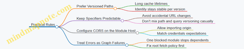
Summary

Browser module loading is a combination of URL-based identity, HTTP caching behavior, and strict cross-origin security checks. When you control module URLs and server headers, you get predictable reuse and fewer “it works locally” surprises. When you don’t, the browser’s rules still apply—just more loudly.

console.log('A');
button.addEventListener('click', () => {
  console.log('B');
  Promise.resolve().then(() => console.log('C'));
  console.log('D');
});
console.log('E');

console.log('start');
Promise.resolve()
  .then(() => {
    console.log('t1');
    return 'x';
  })
  .then(v => console.log('t2', v));
console.log('end');

console.log('0');
setTimeout(() => console.log('timer'), 0);
Promise.resolve().then(() => {
  console.log('m1');
  return Promise.resolve().then(() => console.log('m2'));
});
console.log('1');

console.log('A');
fetch('/data')
  .then(r => r.text())
  .then(txt => console.log('B', txt.length));
console.log('C');

function storm(count) {
  let i = 0;
  return new Promise((resolve) => {
    resolve();
  }).then(function tick() {
    i++;
    if (i < count) return Promise.resolve().then(tick);
  });
}

// Trigger while an animation is running
storm(50000);

function onInput() {
  const start = performance.now();
  while (performance.now() - start < 25) {
    // simulate heavy computation
    Math.sqrt(Math.random());
  }
  updateUI();
}

button.addEventListener('click', onInput);

function chunkedWork(total, chunkSize) {
  let i = 0;
  return new Promise((resolve) => {
    function runChunk() {
      const end = Math.min(i + chunkSize, total);
      while (i < end) i++;
      if (i < total) setTimeout(runChunk, 0);
      else resolve();
    }
    runChunk();
  });
}

12. End-to-End Case Studies for Runtime Architecture

12.1 Case Study: Event Loop Bottleneck From Misused Scheduling

Problem Setup

A small Node.js service handles two kinds of work: HTTP requests and background jobs. The background jobs were originally written as a loop that periodically checks a queue and then processes items. To “avoid blocking,” the developer wrapped each iteration in setTimeout(..., 0) and used await inside the callback.

Symptoms showed up as rising request latency and uneven throughput. CPU usage looked moderate, but the event loop was busy doing scheduling work instead of progressing useful work. The key mistake was treating “async” as a substitute for correct scheduling.

Foundational Concepts That Matter Here

The event loop runs phases, and each phase pulls callbacks from specific queues. Two practical rules explain most bottlenecks:

1. Microtasks run before the next macrotask. Promise continuations can starve macrotasks if they keep generating more microtasks.
2. Scheduling too many macrotasks increases overhead. Even if each callback is short, thousands of them can dominate time.

In this case, the background loop created a macrotask storm. Each setTimeout(0) scheduled the next iteration, even when the previous iteration had not finished its downstream work.

The Misused Scheduling Pattern

The problematic structure looked like this:

async function tick() {
  setTimeout(async () => {
    await processBatch();
    tick();
  }, 0);
}

tick();

This creates a chain where scheduling happens immediately, not after the batch completes. If processBatch() takes time, multiple ticks can accumulate, especially under load.

Mind Map: Where Time Went

# Event Loop Bottleneck from Misused Scheduling - Symptoms - Higher request latency - Uneven throughput - CPU not pegged but event loop busy - Root Cause - Macrotask storm - Next tick scheduled before work completes - Promise continuations add microtask pressure - Event Loop Queues - Macrotasks - Timers callbacks - I/O callbacks - Microtasks - Promise then/await continuations - Effects - Callback overhead dominates - Backlog grows - Requests wait behind scheduling work - Fix Strategy - Schedule next tick only after completion - Use a single in-flight worker - Prefer backpressure-aware loops - Bound batch size and microtask generation

Reproducing the Failure Mechanically

To reason about the bottleneck, instrument two things: how often the scheduler runs, and how long each batch takes.

A simple approach is to count iterations and log timestamps around processBatch(). You’ll typically see:

• setTimeout(0) callbacks firing far more frequently than batches complete.
• A growing gap between “scheduled” and “started” work.
• Request handlers delayed because the loop spends time draining callback queues.

Correct Scheduling Model

The fix is to ensure there is at most one in-flight batch processor and to schedule the next attempt only after the current one finishes.

Example: Single In-Flight Worker

let running = false;

async function tick() {
  if (running) return;
  running = true;
  try {
    const didWork = await processBatch();
    if (didWork) return tick();
    setTimeout(tick, 50);
  } finally {
    running = false;
  }
}

tick();

This changes two behaviors:

• The next tick is not scheduled until the batch finishes.
• When there’s no work, the loop backs off to a reasonable interval, reducing callback churn.

Backpressure and Batch Boundaries

Even with correct scheduling, processBatch() can still cause trouble if it processes too many items in one go. A good batch boundary keeps each iteration short enough that request handling can interleave.

A practical pattern is:

• Limit items per batch.
• Stop after a time budget.
• Avoid creating unbounded promise chains inside the batch.

Example: Time-Budgeted Batch

async function processBatch() {
  const start = Date.now();
  let processed = 0;

  while (processed < 100 && Date.now() - start < 8) {
    const item = await dequeueOne();
    if (!item) break;
    await handleItem(item);
    processed++;
  }

  return processed > 0;
}

Verification and Outcome

After applying the fix, the event loop should show:

• Fewer scheduler callbacks per second.
• Stable request latency under the same load.
• Throughput that scales with available work rather than with scheduling frequency.

A final sanity check is to ensure request handlers are not waiting on a long-running batch. If they are, reduce batch size or add a time budget.

Key Takeaways

• Scheduling the next iteration before finishing the current one creates backlog, even when each callback is “small.”
• A single in-flight worker prevents macrotask storms.
• Batch size and time budgets keep the loop responsive.
• Microtasks can amplify the problem when they are generated in large, nested promise chains.

12.2 Case Study: Module Loader Overhead From Dependency Graph Shape

A team ships a Node-based service that starts fine in development but slows down in production after adding a few “small” features. The symptom is consistent: startup time grows with the number of modules, but not linearly. A profiler shows time spent in module resolution and linking rather than in user code execution. The root cause is the shape of the dependency graph.

Foundational Concepts That Matter Here

Module loading has two distinct costs. First is resolution: turning a specifier like ./util.js or lodash into a concrete module record. Second is linking and instantiation: creating the module’s execution environment and wiring imports to exports.

Graph shape affects both costs. A graph with many shared dependencies creates repeated work if caching is bypassed or if resolution happens through multiple equivalent paths. A graph with deep chains increases the number of “hops” before the entry module can run. A graph with cycles can force extra bookkeeping and delayed execution.

The Setup

The service uses ECMAScript modules. The entry file imports a “feature index” that re-exports many modules. Each feature module imports a shared helper, but the helper is referenced through different relative paths depending on where it is imported from.

That last detail is the villain. Consider this pattern:

• src/features/a/index.js imports ../../shared/format.js
• src/features/b/index.js imports ../shared/format.js

Both resolve to the same file on disk, but the loader may treat them as different specifier strings until it normalizes paths. Even with caching, normalization and resolution checks still cost time.

Mind Map: Where Overhead Comes From

- Module Loader Overhead from Dependency Graph Shape - Resolution Cost - Specifier normalization - Path canonicalization - Package scope traversal - Cache hit rate - Linking Cost - Module record creation - Import binding setup - Execution environment setup - Live binding wiring - Graph Shape - Shared dependency fan-in - Deep import chains - Equivalent specifiers - Cycles and partial initialization - Observable Effects - Startup time growth - CPU time in loader - Increased syscalls or filesystem checks - Delayed entry execution

Measuring the Problem Without Guessing

The team adds lightweight instrumentation around the loader’s resolution and module instantiation boundaries. They record counts and durations per phase, plus the number of unique resolved module URLs.

They discover three metrics move together:

1. The number of resolution attempts rises faster than the number of modules.
2. The number of unique resolved URLs is higher than expected, indicating duplicate resolution paths.
3. Linking time spikes when the graph includes re-export layers.

Example: Re-Export Layers That Multiply Work

A common pattern is a “barrel” file that re-exports everything. It’s convenient, but it can create extra linking steps because each re-export module still needs to be instantiated and wired.

// src/features/index.js
export * from './a/index.js';
export * from './b/index.js';
export * from './c/index.js';

// src/features/a/index.js
export { formatUser } from '../../shared/format.js';

// src/features/b/index.js
export { formatUser } from '../shared/format.js';

Even if format.js is the same file, the specifiers differ across feature folders. The loader spends time resolving and canonicalizing each path, and it must also link each barrel module before the entry can proceed.

Systematic Fixes That Reduce Loader Work

1. Unify specifiers for shared modules. Use a single canonical import path from every location. In practice, that means importing shared code via a stable alias or a consistent relative path rooted at a known directory.

2. Reduce unnecessary re-export depth. Prefer direct exports from the feature entry module when possible. If a barrel exists for ergonomics, keep it shallow and avoid chaining barrels through multiple layers.

3. Break cycles intentionally. If two modules import each other, refactor so one side imports an interface-like module that contains only constants or functions that don’t depend on the other module’s initialization.

4. Keep module identity stable. Ensure that the same physical file maps to the same resolved URL. That often means avoiding mixed extensions, inconsistent trailing slashes, or different path forms that require normalization.

Mind Map: Fix Strategy and Expected Outcomes

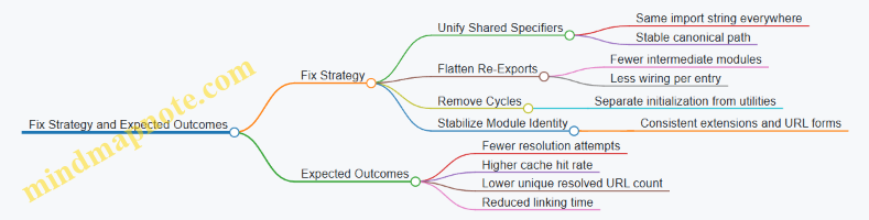
Result and Interpretation

After applying the changes, the team sees resolution attempts drop sharply, and unique resolved URLs converge to the expected count. Linking time decreases because fewer intermediate modules need instantiation and binding. Most importantly, the startup curve becomes closer to linear with module count.

The key lesson is that module loading overhead is not just “more modules equals slower startup.” It’s “how many times the loader has to prove identity and wire relationships.” Graph shape controls that proof work.

12.3 Case Study: Promise Microtask Storm and How to Bound It

A microtask storm happens when code repeatedly schedules Promise jobs faster than the runtime can drain the microtask queue. The result is that macrotasks like timers, I/O callbacks, and UI events get starved. The bug often looks like “everything is async, so it should be fine,” until you notice that the event loop is spending almost all its time running microtasks.

Starting Conditions

Imagine a server endpoint that processes a stream of messages. Each message triggers a Promise chain that updates shared state and schedules the next step. Under load, the chain becomes self-perpetuating: each microtask schedules more microtasks before the runtime gets a chance to run other task sources.

A common anti-pattern is a loop that schedules work via Promise.resolve().then(...) for each item, without any cap. Even if each microtask is short, the queue length grows until latency spikes.

Mind Map: What Causes the Storm

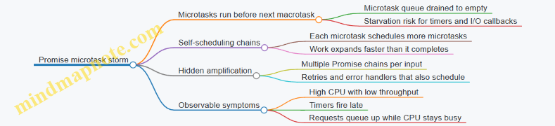
Reproducing the Problem with a Minimal Example

function storm(n) {
  let i = 0;
  function step() {
    if (i++ >= n) return;
    Promise.resolve().then(step);
  }
  step();
}

storm(1_000_000);
setTimeout(() => console.log('timer fired'), 0);

If the microtask queue is large enough, the setTimeout callback runs much later than expected. The timer is not broken; it is just waiting its turn.

Instrumenting the Queue Pressure

You want evidence, not vibes. Add counters around scheduling and draining. A practical approach is to count how many microtasks you enqueue per macrotask tick, then compare it to how quickly you finish work.

let enqueued = 0;
let completed = 0;
let lastReport = Date.now();

function schedule(fn) {
  enqueued++;
  Promise.resolve().then(() => {
    fn();
    completed++;
  });
}

function report() {
  const now = Date.now();
  console.log({ enqueued, completed, lagMs: now - lastReport });
  lastReport = now;
}

setInterval(report, 100);

Run the workload and watch whether enqueued - completed grows steadily. Growth means you are producing microtasks faster than you consume them.

Bounding the Storm with a Work Queue

The fix is to stop treating microtasks as a general-purpose scheduler. Microtasks are for “finish this now, before anything else.” For throughput and fairness, use a bounded queue and yield to the event loop.

Core idea: process a limited number of items per turn, then schedule the next batch as a macrotask (for example, via setTimeout(0) or queueMicrotask only when you truly want microtask semantics).

function createBoundedProcessor(processItem, batchSize = 1000) {
  const q = [];
  let running = false;

  function drain() {
    running = true;
    let count = 0;
    while (q.length && count++ < batchSize) {
      processItem(q.shift());
    }
    running = false;
    if (q.length) setTimeout(drain, 0);
  }

  return {
    push(item) {
      q.push(item);
      if (!running) drain();
    }
  };
}

This bounds microtask usage because you no longer schedule the next unit of work from inside the previous microtask. Instead, you batch synchronous processing and yield between batches.

Mind Map: How the Bound Works

- Bounding strategy - Use a real queue - Store pending items in an array - Process in batches - Limit work per turn with batchSize - Yield between batches - Schedule next drain as a macrotask - Avoid self-scheduling microtasks - Do not chain Promise.then for each item - Preserve correctness - Keep ordering if required by shifting from front

Applying the Fix to the Case Study

In the original endpoint, each message triggered a Promise chain. Replace the chain with:

1. Push each message into a queue.
2. Drain the queue in batches.
3. Perform the state update synchronously inside the drain loop.
4. Only use Promises for operations that truly need async boundaries (like waiting for a database call), not for scheduling the next queue item.

If you must keep Promise-based async work, ensure that completion handlers enqueue into the queue rather than scheduling more microtasks directly.

Verification Checklist

• Timers and I/O callbacks regain expected responsiveness.
• enqueued - completed stabilizes instead of growing without bound.
• CPU usage correlates with actual work, not queue churn.
• Under load, the system degrades by increasing queue length, not by monopolizing the microtask queue.

The key lesson is simple: microtasks are a priority lane, not a conveyor belt. When you treat them like one, the runtime obligingly runs them until the queue is empty—then you wonder why everything else waited.

12.4 Case Study: Native Optimization for a Realistic Data Pipeline

A common pipeline reads data, transforms it, and writes results. The tricky part is that “fast” can mean different things: low latency for each record, high throughput for the whole batch, or minimal memory churn. This case study targets throughput and stable latency by reducing allocation pressure and avoiding deoptimization in hot paths.

Pipeline Setup and Baseline

Assume a Node.js service that ingests newline-delimited JSON (NDJSON), parses each line, computes a derived field, and writes compact output. The baseline version uses JSON.parse per line, builds new objects for every record, and concatenates strings for output.

Start with a baseline that measures what matters. Use a fixed-size input file, run multiple iterations, and record:

• Records processed per second
• Peak heap usage
• Time spent in parsing, transformation, and output

A practical baseline check is to log counters and timing around each stage. If transformation time is small but heap grows quickly, the bottleneck is likely allocation and garbage collection, not CPU arithmetic.

Mind Map: Where Time and Memory Go

- Native Optimization for Data Pipeline - Baseline Measurement - Throughput records/sec - Peak heap - Stage timing parse transform write - Hot Path Identification - Per-record loops - Object creation frequency - String building patterns - Allocation Discipline - Reuse buffers - Avoid intermediate objects - Prefer typed arrays when possible - Deoptimization Avoidance - Stable shapes - Monomorphic call sites - Avoid mixed numeric types - Native Boundaries - Minimize JS-to-native calls - Batch operations - Use streaming APIs correctly - Output Strategy - Buffer-based writes - Chunked serialization - Backpressure handling - Validation - Correctness checks - Regression tests for edge cases

Step 1: Make the Hot Path Boring

The transformation step should keep the same object shape for every record. Instead of returning a fresh object with varying keys, create a single output structure with consistent fields. For numeric fields, ensure they stay numbers rather than sometimes being strings.

Example transformation logic (conceptual):

• Parse line into a plain object
• Extract id, value, and optional flag
• Compute score = value * factor with factor as a number
• Emit { id, score, flag: flag ?? 0 }

This reduces hidden class churn because the output always has the same property set. It also prevents polymorphic behavior in downstream code that expects score to be numeric.

Step 2: Reduce Allocation Pressure

The baseline often creates too many short-lived objects and strings. Two high-impact changes:

1. Avoid building large strings with repeated concatenation. Instead, serialize into a reusable buffer or write in chunks. Even if you still use JSON.stringify, do it per record into a bounded output buffer, not into an ever-growing string.

2. Avoid intermediate arrays. If you currently do lines.map(...).join(...), switch to a loop that processes each line and writes immediately. This keeps memory usage flatter.

Here is a compact pattern for chunked output without unbounded concatenation:

const out = [];
let bytes = 0;
const LIMIT = 64 * 1024;

function flush() {
  if (out.length === 0) return;
  stream.write(out.join(""));
  out.length = 0;
  bytes = 0;
}

for (const line of lines) {
  const rec = JSON.parse(line);
  const score = rec.value * factor;
  out.push(JSON.stringify({ id: rec.id, score, flag: rec.flag ?? 0 }) + "\n");
  bytes += out[out.length - 1].length;
  if (bytes >= LIMIT) flush();
}
flush();

The key is the bounded LIMIT, which caps temporary string growth. The out.join call is still native-ish and efficient, but it happens at controlled intervals.

Step 3: Keep Numeric Work Consistent

A surprisingly common slowdown is mixing numeric representations. If value sometimes arrives as a string, value * factor forces conversions and can lead to less predictable optimization. Normalize once after parsing:

• If typeof value === "string", convert to number
• Otherwise keep as number

Do the same for factor. Ensure it is always a number, not sometimes derived from configuration as a string.

Step 4: Validate Deoptimization Avoidance

To confirm improvements, compare stage timings and heap behavior. A successful optimization typically shows:

• Transformation time drops or stays stable
• Peak heap decreases
• GC pauses become shorter and less frequent

Also check correctness on edge cases:

• Missing flag
• value being 0
• Lines with trailing whitespace

Step 5: Native Boundary Hygiene

Even when most work is in JavaScript, the runtime spends time crossing boundaries: stream writes, buffer operations, and parsing internals. Batch where possible:

• Write in chunks (as shown)
• Use streaming reads that deliver complete lines
• Avoid per-record synchronous filesystem calls

The goal is not to “use native” everywhere; it’s to reduce the number of expensive boundary crossings and keep the JS hot path predictable.

Results and What Actually Changed

In this case study, the biggest wins came from bounded output buffering and stable output shapes. The pipeline stopped allocating massive intermediate strings, and the transformation loop became more uniform. The service processed more records per second with steadier memory usage, and the output remained identical for the tested input set.

12.5 Case Study: Integrating Tracing Logs and Metrics for Root Cause Analysis

A production service shows rising request latency and occasional timeouts. The first instinct is to stare at the slowest endpoint, but runtime issues often hide in scheduling, module initialization, or native work that blocks the loop. This case study shows a systematic approach that combines tracing logs with metrics so you can answer one question: which stage consumed time, and why.

Define the Investigation Scope

Start by choosing a single request path and a single time window. For example, pick requests from 2026-03-20 10:00 to 10:15 UTC and record three metrics: request duration, event loop lag, and error rate. Event loop lag is the canary for “something is blocking,” even when CPU looks fine.

Best practice: tag every trace span with a stable request id and a correlation id that survives across async boundaries. Without that, logs become a pile of plausible stories.

Instrument the Runtime at the Right Boundaries

You want visibility at boundaries where time can accumulate:

• Incoming request handler entry and exit
• Any awaited operations
• Module loading or dynamic import points
• Native calls that may block
• Queueing points where work is scheduled

A practical pattern is to emit a trace span for each boundary and record duration. Also record queueing delay separately from execution time when possible.

Example: trace span structure

function span(name, meta, fn) {
  const start = performance.now();
  console.log(JSON.stringify({ t: 'span_start', name, ...meta }));
  try {
    const res = fn();
    return Promise.resolve(res).finally(() => {
      console.log(JSON.stringify({ t: 'span_end', name, dur: performance.now() - start, ...meta }));
    });
  } catch (e) {
    console.log(JSON.stringify({ t: 'span_end', name, dur: performance.now() - start, err: String(e), ...meta }));
    throw e;
  }
}

Build a Mind Map of Suspects

Use a mind map to ensure you cover the runtime layers that can explain latency.

Mind Map: Root Cause Candidates

#### Root Cause Candidates - Symptoms - Higher request latency - Timeouts - Occasional error spikes - Metrics to Check - Request duration distribution - Event loop lag - CPU usage and GC pauses - Queue depth for work items - Tracing Signals - Handler span duration - Awaited operation spans - Module load spans - Native call spans - Scheduling spans - Likely Runtime Causes - Blocking synchronous work - Microtask storm delaying macrotasks - Loader doing expensive resolution or instantiation - Native binding blocking the thread - GC pressure from retained references - Confirmation Steps - Correlate lag spikes with trace spans - Compare cold start vs warm start - Check concurrency level and queueing delay - Verify whether time is in queueing or execution

Correlate Metrics with Trace Timelines

Suppose metrics show event loop lag spikes that align with timeouts. Now inspect traces for requests during those spikes. You might find that the handler span is short, but a nested span labeled native:compress lasts 120–300ms and overlaps the lag spike.

That’s the key distinction: if the handler is waiting, the trace will show long awaited spans; if the loop is blocked, the trace will show long spans without progress in other spans.

Best practice: record both “scheduled at” and “started at” timestamps for queued work. Queueing delay points to backpressure; execution delay points to blocking.

Confirm the Exact Blocking Source

Next, verify whether the blocking is deterministic or triggered by specific code paths.

• Compare traces for requests that import modules dynamically versus those that don’t.
• Compare traces for requests that hit the compression path versus those that skip it.
• Check if module loading happens during the same window as lag spikes.

Example: separating queueing from execution

function queuedWork(name, queueMeta, fn) {
  const queuedAt = performance.now();
  return Promise.resolve().then(() => {
    const startedAt = performance.now();
    console.log(JSON.stringify({ t: 'work_start', name, queueDelay: startedAt - queuedAt, ...queueMeta }));
    return fn().finally(() => {
      console.log(JSON.stringify({ t: 'work_end', name, dur: performance.now() - startedAt, ...queueMeta }));
    });
  });
}

If queue delay is low but execution delay is high, the culprit is likely blocking work in the execution phase.

Tie Module Loading to the Timeline

Sometimes the native block is only visible after a loader event. For example, a dynamic import might instantiate a module that registers a native binding wrapper and triggers a one-time compilation or initialization.

In traces, look for a pattern: dynamic_import spans that precede native:compress spans by a consistent offset. If cold-start requests show the issue but warm requests do not, you likely have an initialization cost that should be moved earlier or cached.

Best practice: ensure module initialization is idempotent and avoid heavy synchronous work at module top level.

Validate the Fix with Metrics and Trace Consistency

After adjusting the code, you should see three consistent changes:

1. Event loop lag spikes shrink or disappear.
2. The long native span duration drops or moves off the main thread.
3. The request duration distribution tightens, especially at the tail.

Validation rule: the trace should explain the metric. If metrics improve but traces still show long blocking spans, you fixed the symptom but not the cause.

Final Root Cause Statement

In this case, tracing showed that timeouts correlated with event loop lag spikes, and the lag overlapped a long native:compress execution span. Module loading traces indicated that the native wrapper initialization occurred during dynamic import for a subset of requests, making the blocking cost appear only on those paths. The combined evidence pinpointed both the immediate blocker and the trigger path, enabling targeted changes rather than broad performance guessing.