No-Till Farming and Soil Regeneration Economics
1. Scope and Definitions for No-Till Soil Regeneration Economics
1.1 Defining No-Till and Related Systems for Economic Accounting
No-till is an operational choice, not a moral one: it changes what you do with residue, how you place seed, and how you manage weeds and fertility. For economic accounting, the key is to define the system in ways that map to costs, yields, and risk—so two farms can compare apples to apples even when their equipment and weather differ.
What Counts as No-Till in Accounting Terms
For budgeting, define no-till by three measurable behaviors:
- Soil disturbance rule: seed is placed with minimal soil movement, and tillage is not used as a routine operation for seedbed preparation.
- Residue rule: crop residue remains on the surface to the extent that seeding can occur through it.
- Weed control rule: weeds are managed primarily through herbicide programs and/or targeted mechanical actions that do not function as full seedbed tillage.
A practical example: if a field is seeded with a no-till drill into residue, but the farmer also runs a moldboard plow every spring “just to clean it up,” that is not no-till for economic comparisons. The costs and yield risks come from the plow operation, and the residue benefits are interrupted.
Related Systems and How They Differ
Economic accounting needs clear boundaries because “near no-till” can behave very differently in cost and yield.
- Strip-Till: only narrow strips are disturbed for seed placement; residue remains between rows. This often changes fertilizer placement economics because nutrients can be placed in the strip.
- Reduced Tillage: some tillage occurs, but less than conventional. The economic impact depends on how often and how deep.
- Minimum Tillage: a broad term; in accounting, you must specify the actual operations (tool type, depth, timing) to avoid mixing systems.
- Conventional Tillage: routine tillage for seedbed preparation. This is the baseline for many comparisons.
A simple rule for your budget spreadsheet: if the operation list includes a full-width tillage pass for seedbed preparation, treat it as reduced or conventional, not no-till.
The System Boundary for Costs and Benefits
To avoid double counting, define what is inside and outside the system boundary.
Inside the boundary typically includes:
- seeding operation and any residue handling required for seeding
- weed control operations and timing constraints
- fertility placement operations and any changes in input types
- field passes that occur because of residue or weed pressure
Outside the boundary might include:
- general overhead not tied to field operations
- land rent changes that are negotiated separately from management
Example: if no-till reduces the number of tillage passes but increases herbicide applications, your “no-till savings” is not the difference in tillage fuel alone. It is the net of all operations and inputs that change.
Mapping Agronomic Actions to Economic Categories
No-till economics becomes manageable when you translate agronomy into cost categories.
- Labor: seeding speed, scouting frequency, and time spent managing residue-related issues.
- Fuel and maintenance: fewer tillage passes, but potentially more attention to seeding depth control and residue flow.
- Inputs: herbicides, seed, fertility placement products, and cover crop termination costs.
- Yield and variability: not just average yield, but how often yields fall below your break-even threshold.
A concrete example: a farmer switches to no-till and sees similar average yield, but weed escapes increase in wet springs. The economic risk shows up as higher “low-yield tail” years, not as a shift in the mean.
Mind Map: No-Till Definition for Economic Accounting
Example: Classifying a Field for Your Budget
Suppose Field A has these operations in the transition year:
- spring burndown herbicide
- no-till seeding into residue
- one pass with a cultivator between rows for weed suppression
For economic accounting, you can classify this as no-till if the cultivator is not used as full-width seedbed preparation and the residue remains largely on the surface. If instead the cultivator is used to break up the entire surface to create a seedbed, then the system behaves more like reduced tillage, and the cost comparison should reflect that.
A Simple Accounting Checklist
Before you label a practice “no-till” in your model, confirm:
- the operation list does not include routine full-width seedbed tillage
- seeding is performed through residue
- weed control is primarily chemical and/or targeted, not seedbed-forming
- your cost categories include every operation that changes
When these conditions are met, your economic comparisons stop being arguments and start being measurements—still imperfect, but at least consistent.
1.2 Distinguishing Soil Regeneration Outcomes from Yield Outcomes
Soil regeneration and yield are related, but they are not the same scoreboard. Yield outcomes describe what the crop produces in a given season. Soil regeneration outcomes describe how the soil system changes over time—often in ways that may not show up as higher yield immediately.
Foundational Distinctions That Prevent Budget Confusion
Yield outcomes are typically measured as grain, forage, or biomass per acre, plus quality traits that affect price. They respond quickly to weather, planting date, pest pressure, and nutrient availability.
Soil regeneration outcomes are measured as changes in soil structure, organic matter, biological activity, infiltration, and erosion resistance. These changes can influence yield later by improving water availability, root growth conditions, and nutrient cycling.
A practical way to keep them separate is to treat yield as a performance result and soil regeneration as a system condition. When you mix them, you can accidentally attribute a weather-driven yield dip to “soil health” or credit a good season to long-term carbon gains.
What Each Outcome Looks Like in Real Fields
Soil regeneration outcomes often show up as operationally relevant shifts:
- Infiltration and traffic tolerance: After a few seasons of residue cover and reduced disturbance, fields may accept rainfall better and recover from compaction faster.
- Erosion control: Less bare soil means less sediment movement, which protects topsoil where yield potential lives.
- Biological activity: More residue and less disturbance can increase earthworm activity and microbial turnover, which supports nutrient cycling.
Yield outcomes show up as measurable crop results:
- Stand establishment: Emergence uniformity affects early growth and final yield.
- Water use efficiency: Better infiltration can support yield during dry spells, but the effect depends on timing.
- Nutrient availability: Soil changes can improve nutrient supply, yet yield still depends on whether nutrients are available when the crop needs them.
A Simple Causal Chain That Keeps Expectations Honest
Use this chain to separate what causes what:
- Management inputs (residue, tillage intensity, cover crop timing, nutrient placement)
- Soil condition changes (structure, organic matter dynamics, infiltration, biological activity)
- Crop response (root environment, water access, nutrient cycling)
- Yield and quality (grain per acre, test weight, protein, forage quality)
Notice that step 2 is not step 4. Soil condition changes can occur without an immediate yield increase, especially during transition years when weed control and residue management are being tuned.
Mind Map: Outcome Separation for Better Economics
Example: The Same Yield, Different Soil Story
Imagine two fields both averaging 160 bushels per acre this year.
- Field A: Achieved yield through timely rain and a strong nutrient program, but residue was frequently removed and tillage remained frequent.
- Field B: Achieved yield with consistent residue cover and reduced disturbance, plus a cover crop that was terminated with a planned sequence.
Yield alone can’t tell you which field is regenerating. Field B may show improved infiltration and reduced erosion risk even if this year’s yield is similar. Economically, that matters because future yield stability and input requirements depend on soil condition, not just last season’s output.
Example: A Soil Win That Doesn’t Pay Off Yet
Consider a transition year where a grower reduces tillage and increases residue. Weed pressure may rise temporarily if burndown timing and seeding depth aren’t dialed in. The field might still show improved infiltration after heavy rains because residue protects the surface.
In this case:
- Soil regeneration outcomes improve (less runoff, better aggregation).
- Yield outcomes may lag (weed competition and early stress).
A good budget separates these outcomes so the grower can see whether the system is moving in the right direction even when the crop is still learning the new routine.
A Measurement Approach That Keeps Both Scoreboards Useful
When tracking outcomes, use two columns in your analysis:
- Seasonal column: yield and quality, plus the in-season factors that explain them.
- Multi-season column: soil condition indicators and management practices that plausibly drive them.
Then connect them with evidence: if infiltration improves and yield stability improves later, you have a coherent story. If yield changes without soil indicators moving, you likely have a management or weather explanation rather than a soil regeneration explanation.
This separation is the foundation for credible economics: it prevents attributing every yield fluctuation to soil health, and it prevents dismissing soil progress just because one season didn’t cooperate.
1.3 Mapping Carbon Recovery Mechanisms to Measurable Farm Inputs
Carbon recovery on farms is not a single switch. It happens through multiple mechanisms that change soil carbon over time, and each mechanism can be tied to inputs you already control: residue quantity, residue quality, disturbance level, soil moisture conditions, and nutrient availability. The goal of this section is to translate “what improves soil carbon” into “what you can measure, record, and cost.”
Foundational Mechanisms and Their Input Levers
Start by separating mechanisms into two buckets: inputs that add carbon and management that slows carbon loss.
- Residue inputs add carbon through roots and aboveground biomass. Measurable inputs include cover crop species, seeding rate, termination timing, and residue retention.
- Reduced disturbance slows decomposition and erosion. Measurable inputs include tillage passes, implement type, and seeding method.
- Nutrient and moisture conditions influence how quickly residues decompose and how much biomass plants produce. Measurable inputs include nitrogen timing, irrigation or rainfall capture practices, and drainage management.
A practical way to avoid gaps is to map each mechanism to a small set of farm records that are both available and decision-relevant.
From Mechanism to Measurable Inputs
Use a consistent mapping template for every field and season.
- Mechanism: What part of the carbon cycle is being affected?
- Input lever: Which management choice changes it?
- Measurable proxy: What record stands in for the mechanism?
- Expected direction: Does the proxy increase or decrease carbon gain?
- Uncertainty note: What could break the link?
Example mapping choices:
- Residue quantity → proxy: total biomass estimate from species mix and termination date; record seeding rate and termination method.
- Residue quality → proxy: C:N ratio class from species selection and termination timing; record growth stage at termination.
- Disturbance level → proxy: number of tillage operations and depth class; record whether seeding is true no-till or shallow disturbance.
- Decomposition control → proxy: soil moisture window management; record irrigation timing or drainage interventions and seeding dates.
Mind Map: Mechanism to Inputs
Concrete Example: Two Fields, Same Crop, Different Carbon Path
Consider Field A and Field B both growing corn, but with different transition choices.
- Field A: winter rye cover crop, terminated at early flowering, residue left on the surface, no-till seeding, and nitrogen applied in split doses.
- Field B: no cover crop, residue removed for bedding, one shallow tillage pass before planting, and nitrogen applied as a single pre-plant application.
Mapping to inputs:
- Residue inputs: Field A has higher biomass and typically more consistent residue coverage; Field B has near-zero cover crop residue and less surface protection.
- Disturbance: Field A uses zero tillage passes; Field B includes a disturbance event that increases contact between residue and soil.
- Nutrient timing: Field A’s split application supports crop uptake while reducing the chance of excess nitrogen being available during residue decomposition peaks.
Even without running a full carbon model, these differences create a clear, recordable story: Field A supplies more carbon and reduces loss pathways, while Field B does the opposite.
Turning Records Into Carbon-Accounting Variables
To make this usable in economics, convert proxies into variables you can cost and compare.
- Residue coverage variable: percent ground cover at planting, estimated from cover crop stage and termination date.
- Disturbance variable: tillage pass count and depth class, recorded per operation.
- Residue quality variable: a simple class based on species and termination stage, used consistently across fields.
- Moisture window variable: seeding and termination dates relative to rainfall or irrigation events, recorded as “wet window” or “dry window” categories.
Keep the variable set small. If you track ten things, you will eventually stop tracking them. If you track four well, you can explain the carbon mechanism without hand-waving.
Common Breaks in the Mapping Link
A mapping is only as good as its weakest assumption. Watch for:
- Residue removal: baling or heavy grazing can erase the residue input you assumed.
- Inconsistent termination: terminating too late can change residue quality and seedbank dynamics.
- Hidden disturbance: “no-till” that includes repeated shallow passes can behave like a different system.
- Nutrient mismatch: applying nitrogen in a way that increases decomposition during residue peaks can weaken the expected carbon gain.
When you record these operational details, you can explain why a field’s carbon outcome did or did not match the mechanism you planned. That’s the bridge between agronomy and economics.
1.4 Establishing a Consistent Cost and Benefit Framework for Comparisons
A comparison fails when it mixes apples and slightly different apples. This section builds a framework that keeps costs and benefits aligned across fields, years, and management choices so you can trust the numbers.
Start with the Decision You Are Actually Making
Write a single-sentence decision statement before touching spreadsheets. Example: “Should we transition 40 acres from conventional tillage to no-till with cover crops over two seasons, given equipment constraints and expected yield variability?” This forces you to define the comparison set: the baseline system, the candidate system, the time horizon, and the unit of measure (typically per acre per year).
Define the Comparison Boundary and Unit
Use the same boundary for every option.
- Farm boundary: include on-farm operations and inputs; exclude off-farm processing unless you truly control it.
- Field boundary: decide whether you include only the acres changing management or also shared equipment and labor.
- Time boundary: pick a horizon long enough to cover transition effects. If you choose 3 years, every option gets 3 years.
- Unit boundary: use “per acre” for field economics, and “per hour” or “per machine-day” for capacity constraints.
Example: If the baseline uses a moldboard plow and the no-till option uses a strip-till fertility pass plus a no-till seeder, both must be costed for the same acres and the same calendar windows.
Separate Costs Into Categories That Behave Differently
Costs do not all move the same way, so treat them differently.
- Variable costs move with acres: seed, fertilizer, herbicide, custom passes, fuel per acre.
- Fixed costs exist regardless of acres: land rent, baseline insurance, some overhead.
- Capacity costs show up when you add or remove operations: extra labor hours, seeding window bottlenecks, downtime.
- Transition costs are one-time or front-loaded: equipment purchase, repair spikes, learning curve effects you can measure as rework or slower throughput.
Example: If a new no-till drill reduces throughput by 10% during the first season, that is not “seed cost.” It is a capacity cost that may force custom hiring or delayed planting.
Define Benefits with the Same Precision as Costs
Benefits should be measurable and tied to management.
- Yield benefits: average yield and yield stability (risk-adjusted returns).
- Input efficiency benefits: changes in nutrient use efficiency, reduced passes, or improved stand uniformity.
- Carbon recovery benefits: only include what your framework can justify with consistent assumptions and documentation.
- Operational benefits: fewer tillage passes, reduced labor variability, or improved timeliness.
Example: If soil structure improves infiltration, you may see fewer “failed planting” events. In the framework, that becomes a yield stability benefit, not a vague “soil health” credit.
Use a Consistent Accounting Method for Multi-Year Comparisons
Pick one method and apply it to all options.
- Cash-flow view: track when money leaves and enters.
- Accrual view: spread certain costs across useful life when appropriate.
- Discounting: if you discount, discount every option with the same rate.
Example: Equipment depreciation can be treated as an economic cost in an accrual view, while custom hiring is a cash cost. Mixing views without clarity leads to misleading comparisons.
Build a “What Changes” Inventory Before Calculating Anything
Create a list of every operational difference between baseline and candidate systems.
- Tillage operations: type, depth, number of passes.
- Seeding: seeder model, seeding rate, calibration steps.
- Weed control: burndown timing, residual programs, mechanical additions.
- Fertility: placement method, timing, application rate changes.
- Cover crops: species, seeding method, termination method.
Then map each item to a cost category and a benefit channel.
Example: Cover crop termination by roller-crimper changes both weed control costs (labor, fuel) and potential yield outcomes (stand vigor). Both must be represented.
Mind Map of the Framework
Mind Map: Consistent Cost and Benefit Framework
Worked Example with a Clean Comparison Table
Assume you compare two systems on 100 acres for 3 years.
- Baseline: conventional tillage + standard herbicide program.
- Candidate: no-till seeding + cover crops + residual herbicide.
You compute:
- Per-acre variable costs for each year (seed, fertilizer, herbicide, fuel).
- Capacity costs in year 1 if throughput drops (extra custom hours or delayed planting penalties).
- Transition costs for equipment changes (purchase amortized or lease payments, plus repair spikes).
- Benefits as yield and stability differences, plus any carbon recovery values you can support with consistent assumptions.
The key is that every line item is either “changes because of management” or “does not change and can be ignored.” If a cost is identical across options, it cancels out and should not clutter the comparison.
Common Failure Points to Avoid
- Using different time horizons for baseline and candidate.
- Treating capacity constraints as if they were variable costs.
- Including carbon benefits without a matching measurement and documentation logic.
- Forgetting that transition effects often concentrate in year 1.
A consistent framework is less about perfect numbers and more about consistent assumptions. When the assumptions match, the comparison becomes a tool rather than a guess.
1.5 Setting Boundaries for Farm Level Analysis Across Crops and Years
Farm-level economics gets messy fast because “the farm” is not one crop, one soil type, or one season. Setting boundaries means deciding what you include, what you exclude, and how you keep comparisons fair across crops and years. Done well, it prevents two common mistakes: mixing apples and soybeans, and treating one good year as if it were a permanent policy.
Define the Decision You Are Supporting
Start with a single decision statement. Examples:
- “Should we adopt no-till on Fields A–C starting this fall?”
- “Which rotation and residue plan gives the best risk-adjusted return over five years?” Your boundary choices should serve that decision, not the other way around.
Choose the Spatial Unit and the Aggregation Rule
Pick a unit that matches how operations actually happen.
- Field-level unit when equipment passes, residue, and weed pressure differ by field.
- Management-zone unit when soils and slope are similar and operations are standardized. Then define how you roll up to farm totals: weighted by acres, by labor hours, or by expected throughput constraints. If you use acres, say so and keep it consistent.
Example: If Field A is 120 acres and Field B is 80 acres, farm-level averages should weight by 120/200 and 80/200. If you instead weight by “time in the shop,” you must use the same time basis for every scenario.
Choose the Temporal Horizon and the Treatment of Transition Years
No-till changes don’t land all at once. Boundaries must specify the time window and how you handle transition.
- Pre-transition baseline period: typically 1–3 years of historical operations and yields.
- Transition window: the years where management changes but the system is still stabilizing.
- Steady-state window: years where you assume practices have settled into a repeatable pattern.
A practical boundary rule: keep the same horizon length for every scenario you compare. If one scenario includes two transition years and another includes five, you are comparing policies plus time, not policies alone.
Standardize What Counts as “The Same” Across Crops
Cross-crop comparisons fail when you treat different crops as if they share the same yield drivers and cost structure. Your boundary should separate:
- Crop-specific economics: seed, fertility program, crop insurance, harvest costs, and market price assumptions.
- System-specific economics: tillage passes, residue handling, weed control sequences, and equipment wear.
Example: If wheat and corn both move to no-till, the system-specific savings might be similar in tillage passes, but the crop-specific herbicide timing and fertility placement can differ. Your budget should reflect that difference rather than averaging it away.
Decide Which Costs Are Included and Which Are Deferred
Farm-level analysis often mixes “cash out now” with “costs that show up later.” Boundaries should specify categories:
- Included: variable cash costs (seed, fertilizer, herbicides), labor, fuel, repairs, custom hire, and any incremental equipment operating costs.
- Included with explicit treatment: depreciation or opportunity cost of equipment, using a consistent method.
- Excluded: one-time administrative overhead unless it changes materially by scenario.
If you exclude something, do it consistently. Otherwise, you can accidentally make the “cheaper” scenario look cheaper simply because it shifts costs into categories you ignored.
Handle Risk and Variability Without Breaking Comparability
Boundaries should define how you represent uncertainty across years.
Use the same approach for every scenario:
- Yield variability: use historical yield distributions for each crop and field (or zone), not one pooled number.
- Input variability: decide whether you hold prices constant or use historical ranges.
- Weather-dependent operations: if a no-till plan requires a specific seeding window, represent the operational failure rate using your own records.
Example: If your no-till seeding plan fails 10% of the time in wet springs due to residue and seedbed conditions, that failure rate belongs in the scenario budget. It is not “bad luck”; it is part of the operational reality you are comparing.
Create a Boundary Map for Every Scenario
A boundary map is a short checklist that prevents silent scope creep.
Mind Map: Farm Level Analysis Boundaries
Worked Example Using Simple Numbers
Suppose you compare two scenarios on a 200-acre farm with wheat and corn.
- Scenario A: conventional tillage for 3 years, then partial no-till.
- Scenario B: full no-till for 3 years.
Boundary choices:
- Same 5-year horizon for both scenarios.
- Field-weighted aggregation by acres.
- Include labor, fuel, repairs, seed, fertilizer, herbicides, and harvest.
- Depreciation treated the same way for both scenarios.
- Transition years explicitly labeled, so yields in years 1–2 are allowed to differ without being averaged into “steady-state.”
If you do this, the comparison answers the real question: which scenario produces better returns given the same scope, time window, and accounting rules.
Quick Boundary Checklist
Before you compute anything, confirm:
- The decision statement is written.
- The spatial unit and aggregation rule are fixed.
- The horizon and transition handling are identical across scenarios.
- Crop-specific and system-specific costs are separated.
- Included and excluded cost categories are consistent.
- Risk methods are applied the same way for every scenario.
2. Baseline Farm Diagnostics for Costing and Risk Management
2.1 Inventorying Current Field Operations and Equipment Utilization
Start by treating your current system like a machine with inputs, outputs, and failure points. The goal is not to judge the past; it’s to measure what you actually do so the economics in later chapters have something solid to stand on.
Step 1: List Field Operations with Realistic Boundaries
Write down every operation you perform from seedbed prep through harvest, including “small” tasks that quietly consume time. Use a consistent boundary for each operation so two people would record the same thing.
Example: If you do a light tillage pass in spring “just to help the drill,” record it as a separate operation with its own fuel, labor, and time. If you instead fold it into seeding, you’ll never see how much that pass costs.
Include these categories:
- Soil and residue actions (tillage, residue management, rolling)
- Seeding actions (drill/planter, depth control, seed treatment application)
- Nutrient actions (fertilizer placement, sidedress, foliar)
- Crop protection actions (spraying, burndown, spot treatments)
- Harvest and post-harvest actions (combining, baling, chopping, spreading)
- Transport and setup actions (moving equipment, calibration, cleanup)
Step 2: Capture Equipment Utilization as Time, Not Vibes
Equipment utilization is usually reported as “hours used,” but for economics you need time broken into productive and non-productive components.
For each machine, record:
- Work rate (acres per hour) under typical conditions
- Effective field time (minutes actually working)
- Setup and calibration time per day or per field
- Travel time between fields
- Downtime causes (clogs, sensor errors, hydraulic issues, weather delays)
Example: A sprayer might cover 80 acres per day on paper, but if it spends 45 minutes per day waiting for a tow truck or reloading, your effective acres per hour drops. Later, that drop becomes labor and custom-hire costs.
Step 3: Build a Field-Operation Matrix
Create a matrix that links fields, crops, and operations. This prevents the common mistake of averaging everything together.
Example: Field A might get a burndown plus two herbicide passes, while Field B gets one pass and a different seeding date. If you average herbicide time across both fields, you’ll misprice weed-control budgets.
Use the matrix to compute:
- Acres per operation per field
- Total machine hours per operation per field
- Labor hours per operation per field
- Fuel and consumables per operation per field
Step 4: Identify Bottlenecks and Constraint Patterns
Once you have time and acres, look for where the system repeatedly slows down.
Common bottlenecks:
- Seeding window pressure when multiple fields share one planter
- Sprayer capacity when weed-control timing overlaps with harvest logistics
- Residue conditions that reduce seeding speed or increase plugging
- Fertility timing that conflicts with harvest or weather windows
Example: If seeding speed drops after heavy residue years, you’ll see it as lower effective acres per hour for the drill. That’s not a “mystery performance issue”; it’s a measurable constraint.
Step 5: Normalize Data Into Cost-Ready Units
Convert raw notes into consistent units so later chapters can calculate budgets.
Recommended normalization:
- Acres per hour for each machine-operation pair
- Labor hours per acre (including setup and cleanup)
- Fuel per acre (or per hour with a conversion)
- Consumables per acre (seed, fertilizer, chemical, wear parts)
Example: If one operator logs “about two tanks” of diesel per day, convert it to gallons per hour using the day’s machine hours, then to gallons per acre using acres covered.
Mind Map: Inventorying Operations and Utilization
Example: A Simple One-Field Log That Stays Useful
For Field 12, Soybean, record one week of activity like this:
- Day 1: Burndown spray, 18 acres, 2.0 hours machine time, 0.5 hours setup/loading, 0.25 hours travel
- Day 2: Seeding, 22 acres, 2.4 hours machine time, 0.4 hours setup, 0.2 hours calibration, 0.3 hours downtime for a sensor reset
- Day 3: Fertility, 20 acres, 1.6 hours machine time, 0.3 hours setup
Then compute effective acres per hour for each machine and operation. That single field-week becomes a template for similar fields, instead of a one-off story.
Step 6: Validate the Inventory Against Reality
Do a quick consistency check before moving on:
- Total acres by operation should match your planting and harvest records.
- Total machine hours should roughly align with your maintenance logs and operator schedules.
- If a number looks off, fix the recording method rather than ignoring it.
Example: If your inventory shows 10 hours of seeding but your maintenance log shows 25 hours for the same period, you likely mixed machine time with labor time or included a different attachment.
By the end of this section, you should be able to answer, for each field and crop: what happened, when it happened, how long it took, and which equipment did the work. That’s the foundation for both yield stability analysis and the equipment transition cost calculations that follow.
2.2 Measuring Soil Condition Indicators That Affect Economics
Soil condition indicators matter economically because they change how reliably you can produce a crop with the inputs you already budget. The trick is to measure indicators that connect to operations, not just to soil science curiosity. A practical measurement plan links each indicator to a decision: seeding depth, residue handling, fertilizer placement, weed control timing, irrigation scheduling, and harvestability.
Foundational Concept: Indicators with Decision Links
Start by grouping indicators into three economic pathways:
- Establishment pathway: how quickly and evenly seedlings emerge.
- Input efficiency pathway: how much of your fertilizer and water actually becomes plant growth.
- Operational pathway: how easily equipment can work and whether you lose time to compaction, crusting, or uneven residue.
If an indicator doesn’t change a decision, it’s usually not worth the measurement effort.
Core Indicators and What They Signal
Measure indicators that reflect structure, water behavior, biological activity, and compaction. Use a consistent sampling pattern so year-to-year comparisons mean something.
Soil Structure and Aggregate Stability
Look for indicators that describe how soil holds together under tillage-free traffic and rainfall.
- Aggregate stability (simple field proxy): after rainfall or irrigation, observe whether the surface breaks into stable crumbs or slakes into a paste.
- Penetrometer resistance: high readings at seeding depth often predict poor root penetration and uneven emergence.
Example: Two fields have the same soil test phosphorus and potassium. Field A has lower penetrometer readings in the top 4 inches and forms crumbs after rain; Field B crusts and shows resistance spikes. Even if fertilizer rates match, Field B often needs a re-seed or suffers patchy stands, which raises per-acre cost and reduces yield.
Infiltration and Water Holding Behavior
Water behavior affects both yield stability and the number of trips you make.
- Infiltration rate: use a basic infiltration test (ring or cup) to compare spots within a field.
- Surface crusting and ponding: record where water stands after a typical storm.
- Root-zone moisture availability: measure soil moisture at consistent depths during key growth stages.
Example: If infiltration is slow, you may see delayed planting after rain because fields stay too wet. That delay can force you to seed into less favorable temperatures, which increases stand risk. The economic impact shows up as both lost planting days and higher weed pressure from uneven emergence.
Compaction and Traffic Effects
Compaction is measurable and directly tied to equipment passes.
- Bulk density: useful for comparing management zones.
- Penetrometer depth profiles: track compaction layers.
- Wheel-track observations: note whether tracks remain visible after rain or whether they smear and seal.
Example: A no-till field that was trafficked when wet can develop a compacted layer at 6–10 inches. Even with good residue cover, roots struggle to access water, and the crop shows stress earlier in dry spells. Your irrigation or yield protection costs rise, and yield stability drops.
Biological Activity and Organic Matter Function
Organic matter isn’t just a number; it’s part of how soil aggregates form and how nutrients cycle.
- Soil organic matter (SOM): track changes over time with consistent sampling depth.
- Active carbon or respiration tests: more lab-based, but can help explain why two soils with similar SOM behave differently.
- Earthworm counts and residue breakdown observations: simple field checks that correlate with biological activity.
Example: Two fields both test at similar SOM. One has faster residue breakdown and more earthworm activity. That field often supports better seedbed conditions and fewer emergence failures, which reduces replanting and herbicide re-treatment costs.
Measurement Design That Stays Honest
A measurement plan should be repeatable, not heroic.
- Define management zones: use slope, soil type, and past yield maps to avoid averaging away problems.
- Choose sampling depth by decision: seeding depth for emergence indicators; 6–10 inches for compaction and water access.
- Time measurements to crop stages: structure and crusting matter around planting and early growth; moisture and resistance matter during stress periods.
- Use paired measurements: compare “good” and “problem” spots to identify what actually differs.
Mind Map: Soil Condition Indicators Linked to Economics
Practical Example Workflow for One Field
Pick one field and run a baseline measurement before you change anything.
- Step 1: Map three zones: low spot, mid slope, and high spot.
- Step 2: At each zone, measure penetrometer profiles at seeding depth and at 6–10 inches.
- Step 3: Run a simple infiltration test in each zone.
- Step 4: During planting, record seedbed conditions and emergence uniformity.
- Step 5: After a typical storm, note crusting and ponding locations.
Example: If low spots show ponding and high penetrometer resistance at 6–10 inches, your economic focus shifts. You may prioritize drainage fixes, traffic timing, or residue adjustments rather than immediately changing fertilizer rates. The measurements tell you which lever affects yield stability and which one mostly changes paperwork.
Turning Measurements Into Economic Variables
Finally, translate indicators into variables you can budget.
- Stand risk from emergence uniformity and crusting observations.
- Replant and reseed probability from historical emergence failures tied to measured conditions.
- Fuel and labor variability from trafficability and equipment plugging patterns.
- Water-related yield variability from infiltration and root-zone moisture behavior.
When measurements are tied to these variables, soil condition becomes a cost-and-risk story you can actually manage.
2.3 Characterizing Weed Pressure and Residue Dynamics for Transition Costs
Transitioning to no-till is often less about “no till” and more about managing what used to be buried. Two forces drive most early transition costs: weed pressure and residue dynamics. Weed pressure determines how much control you must buy and apply; residue dynamics determine whether your seeding system can place seed and establish stands without extra passes.
Foundational Concepts That Translate Into Costs
Weed pressure is the combination of weed species present, their life cycles, and how well your current system suppresses them. Residue dynamics describe how much plant material remains on the surface, how fast it breaks down, and how it interacts with seeding depth, soil contact, and moisture.
A simple way to connect these to dollars is to treat each field as a “constraint system.” Weed pressure constrains your herbicide and mechanical options; residue dynamics constrain your seeding speed and accuracy. When either constraint is tight, you pay through extra product, extra labor, or extra equipment time.
Mind Map: What Drives Transition Weed and Residue Costs
Characterizing Weed Pressure Systematically
Start with a weed inventory that is practical for budgeting. Walk each field at two times: once before your primary burndown and once after emergence. Record dominant species, approximate density, and growth stage. Growth stage matters because it determines whether you can use a single-pass program or need a follow-up.
Next, classify weeds by control pathway. Annual grasses often respond well to timely burndown and residual programs, while perennials frequently require more targeted sequences. If you have a history of resistance, treat “same herbicide, same rate” as a budgeting mistake. Instead, estimate control success as a range and plan for the cost of a second pass if the first pass underperforms.
A concrete example: Field A has mostly annual broadleaf and a small patch of perennial thistle. Your plan might work with one burndown plus residual for the annuals, but the thistle patch may need spot treatment. Budgeting should include the spot-treatment labor and the extra spray time, not just the main-pass product.
Characterizing Residue Dynamics Systematically
Residue characterization should answer three questions: how much residue is present, what it is made of, and how it behaves in your conditions. Measure residue load using a simple frame method: place a square frame on the ground, clip residue inside, weigh it, and convert to pounds per acre. Do this in representative zones, not just the cleanest areas.
Then note residue type. Cereal straw tends to persist longer and can slow breakdown, especially when moisture is limited. Legume residue often breaks down faster but can still create surface matting if it is thick.
Finally, connect residue to seeding performance. If residue is high, you may see furrow closure issues, seed placement variability, and plugging. Those problems translate into transition costs through reduced seeding speed, more frequent adjustments, and sometimes re-seeding where emergence fails.
A concrete example: Field B has heavy rye residue. During the first no-till seeding, the row unit struggles to cut through the mat, and emergence is uneven. The direct costs include extra planter downtime and an additional herbicide application to manage early escapes. The indirect cost is that uneven stands create more weed-friendly gaps, increasing later control needs.
Turning Observations Into Transition Cost Estimates
Use a field worksheet with two columns: “Weed pressure risk” and “Residue seeding risk.” For each, assign a low, medium, or high rating based on your inventory and residue measurements. Then map each rating to cost pathways.
- High weed pressure risk usually increases the number of passes and the likelihood of follow-up treatments.
- High residue seeding risk usually increases equipment time and the chance of stand repair.
Keep the logic tight: if you rate weed pressure as high because of multiple flushes, the budget should include a second timing window. If you rate residue seeding risk as high because of matting, the budget should include planter adjustment time and potential re-seeding costs.
Practical Mindset for the Transition Year
Treat the first no-till season as a controlled experiment on your own fields. Your goal is not to “win” every weed or every emergence attempt; it is to quantify where your system is stressed so you can account for the real costs. When weed pressure and residue dynamics are characterized well, the transition budget stops being a guess and becomes a set of defensible assumptions.
2.4 Documenting Yield Variability and Input Response Patterns
Yield variability is not just “some years are better.” It’s a pattern you can measure, explain, and price into decisions. The goal of documentation here is simple: connect what you did (inputs and operations) to what happened (yield and quality), while separating real cause from coincidence.
Foundational Concepts for Recording Variability
Start with three layers of data.
- Outcome layer: yield by field and date range, plus quality proxies you can measure consistently (test weight, protein, moisture, grade). If you only track bushels, you’ll miss shifts in how the crop filled.
- Management layer: seeding rate, variety, planting date, row spacing, fertilizer rates and placement, herbicide program, irrigation or drainage actions, and residue management. Record the “what” and the “when,” not just the totals.
- Condition layer: soil test results, soil type map, slope/low spots, compaction notes, and weather summaries that matter for that field (rain timing, heat waves, frost dates). You don’t need a weather station; you need consistent field-relevant signals.
A practical rule: if two fields have different soil or different planting dates, treat them as different experiments even when the crop and inputs look similar.
Building a Yield Variability Record That Can Be Used
Use a template that forces consistency. For each field-year, capture:
- Yield summary: average yield, yield range across zones, and any harvest issues (uneven maturity, lodging, skips).
- Input timeline: application dates and rates, plus seeding and termination dates for cover crops.
- Operational notes: equipment settings changes, missed passes, re-seeding, or delays due to weather.
- Zone mapping: at least 3–5 zones per field based on soil and topography, so you can see patterns instead of averages.
Example: In a 120-acre field, the north zone yields 8% higher than the south zone for three years. If the south zone also received later planting and had higher compaction scores, you’ve got a candidate explanation. If the south zone was treated identically for inputs but still lags, the condition layer becomes the suspect.
Documenting Input Response Patterns Without Guessing
Input response patterns describe how yield changes when an input changes, while other factors are held as constant as your farm reality allows.
There are three documentation approaches, from simplest to more rigorous.
- Within-Field Comparisons: Use zones or strips where management differed. Example: If you applied nitrogen at 90 lb/ac in one strip and 120 lb/ac in another, compare yield differences by zone, not by gut feel.
- Between-Field Comparisons: Compare fields with similar soil and management. Example: Two fields planted within two days, similar residue, same variety, and similar weed control. If one field consistently responds more to fertilizer, you’ve learned something about soil supply or placement effectiveness.
- Year-Over-Year Comparisons: Track how the same input behaves across weather variation. Example: A herbicide program that works in wet springs but struggles in dry springs suggests timing sensitivity. Document the weather around application and the crop stage.
To avoid false conclusions, record “input intensity” and “input timing” separately. A rate change without a timing change is different from a timing change without a rate change.
Mind Map: Yield Variability Documentation Workflow
Example: Turning Notes Into a Usable Pattern
Suppose you notice yield drops in low spots during dry spells. You document that low spots also received:
- later planting by 3–5 days due to access,
- higher residue load because cover crop termination was delayed,
- and a different nitrogen placement method.
Instead of concluding “no-till causes drought loss,” you test the pattern in your record:
- Compare low spots vs. uplands for years with similar rainfall timing.
- Compare low spots across years where termination date was the same.
- Compare nitrogen placement methods in the same zone when weather was similar.
If the yield gap shrinks when termination timing matches, residue and early-season conditions likely matter more than the tillage system itself. If the gap persists across termination timing, focus shifts to planting delay, compaction, or water movement.
Documentation Outputs That Feed Economics
Good documentation ends in numbers you can use:
- Sensitivity estimates: how much yield moves per unit change in an input within a zone.
- Variance estimates: how wide the yield distribution is for each zone under your management.
- Cost-to-fix mapping: which input changes reduce variability most cheaply (for example, better seeding depth consistency may cost less than reworking drainage).
When you later build budgets, you’ll have defensible assumptions for both expected yield and the range around it. That’s where economics stops being a spreadsheet exercise and starts being a decision tool.
2.5 Building a Baseline Budget With Field Level Granularity
A baseline budget is your “before” snapshot: what you spend, what you produce, and what you assume about variability. Field-level granularity matters because no-till economics are rarely uniform across a farm; one field can be a smooth transition, while another turns into a weed-and-residue obstacle course.
Step 1: Choose the Budget Unit and Time Window
Start with a consistent unit: typically per acre per crop year, then roll up to field totals. Use a time window that matches your decision cycle. For example, if you plan equipment changes in spring 2025, build the baseline for the 2024–2025 crop year so the cash timing aligns with your transition plan.
Step 2: Build a Field Inventory That Drives Costs
Create a field card for each field. Include soil texture class, drainage notes, slope, typical residue level, and last three years of crop sequence. This is not paperwork for its own sake; it determines which operations are likely to change under no-till.
Example: Field A has heavy residue after corn and slow spring drying. You should expect higher burndown and seeding timing sensitivity than Field B, which is lighter and drains quickly.
Step 3: Separate Costs Into Operation, Input, and Overhead Buckets
A practical baseline budget uses three buckets:
- Operation costs: fuel, labor, custom rates, and machinery wear tied to specific passes.
- Input costs: seed, fertilizer, lime, herbicides, adjuvants, cover crop seed, and biologicals if used.
- Overhead costs: insurance, management, shop overhead, and general admin. Overhead is allocated, not directly tied to each pass.
Example: If you currently do two tillage passes, those passes belong in operation costs. If you switch to one pass, you can see the savings without guessing.
Step 4: Create a Pass-by-Pass Budget Template
For each field and crop, list operations in chronological order. Include the “why” in plain language so later adjustments are grounded.
Example template (for one crop year):
- Residue management: burndown application (timing window)
- Seeding: seeder/planter pass (seed depth and spacing)
- Fertility: placement method and timing
- Weed control: post-emerge sprays and/or spot treatments
- Harvest: combine and hauling assumptions
When you fill this in, use your actual practice where possible. If you must estimate, record the assumption and the reason.
Step 5: Add Yield and Quality Assumptions at Field Level
Yield is not a single number. Use a baseline distribution approach with three values: expected yield, low yield, and high yield. Keep it simple: derive from your last 5–7 years of field yield records, adjusting for known changes like drainage improvements or major variety shifts.
Example: Field A expected yield is 165 bu/ac, low is 140, high is 185. Field B expected yield is 155, low is 145, high is 170. This difference will later affect risk-adjusted returns.
Step 6: Model Variability Without Overcomplicating
To keep the baseline usable, link variability to drivers you can control or measure.
- Weed pressure variability: tied to residue and prior crop
- Seeding success variability: tied to spring soil moisture and residue cover
- Nutrient response variability: tied to soil test and placement method
Example: If Field A often misses the seeding window due to slow drying, you can represent that by increasing the probability of a lower-yield outcome rather than inventing a new cost category.
Step 7: Allocate Overhead and Compute Field Net Return
Allocate overhead using a consistent rule such as acres farmed or labor hours. Then compute:
- Total variable costs per acre
- Total allocated overhead per acre
- Net return per acre = revenue minus total costs
Example: If overhead is allocated at $35/ac and variable costs are $520/ac, total cost is $555/ac. Multiply by expected yield and price to get expected net return.
Mind Map: Baseline Budget Inputs and Flow
Step 8: Produce a Baseline Comparison Table
Finish by creating a table that will later support “before vs after” comparisons. Include columns for each field: acres, expected yield, low/high yield, revenue assumptions, variable costs, allocated overhead, and net return.
Example: Field A may show higher expected costs due to more weed control passes, but also higher expected revenue if yield potential is strong. Field B may show lower costs and tighter yield range. These patterns are the starting point for evaluating no-till changes without surprises.
3. Transition Planning and Operational Design for No-Till Systems
3.1 Selecting Transition Strategies That Match Soil and Crop Context
A good transition plan starts with matching three things: what your soil is doing now, what your crop needs at each growth stage, and what your field operations can reliably deliver. No-till is not one switch; it’s a sequence of choices that reduce disturbance while keeping planting, fertility, and weed control working together.
Step 1: Classify Soil Constraints with Field-Useful Signals
Begin with a short list of constraints that actually affect operations.
- Surface residue and seed-to-soil contact: If residue is heavy or uneven, emergence can be patchy. A practical signal is visible residue thickness and how well seed rows “open” during seeding.
- Compaction and infiltration limits: If water ponds or drains slowly, roots and early growth suffer. A practical signal is where runoff concentrates after a rain.
- Soil biology and structure: If tilth is poor and crusting happens, emergence and root penetration are harder. A practical signal is crust formation and how quickly the surface breaks after rain.
Example: In a field where water ponds in low spots, a full no-till push without addressing drainage timing can turn into a yield stability problem. The transition strategy should prioritize seeding windows and residue management in those zones.
Step 2: Match Crop Timing to Transition Operations
Crops differ in how sensitive they are to stand establishment.
- Small grains and many legumes often tolerate slower early growth, but still need consistent emergence.
- Row crops usually demand precise seed placement and uniform depth.
Example: If you grow corn after a residue-heavy cover crop, you may need a more aggressive residue termination and a seeding setup that maintains depth consistency. If you grow soybeans after a lighter residue, you can often transition with fewer changes.
Step 3: Choose a Transition Path by Disturbance Level
Think in terms of how much disturbance you can reduce without breaking planting and weed control.
-
Full No-Till Transition
- Use when soil infiltration is adequate, residue can be managed, and weed control is already strong.
- Example: A farm with reliable burndown timing and a planter that consistently places seed can move directly to no-till for most fields.
-
Strip-Till or Controlled Disturbance Transition
- Use when you need help with seedbed conditions while still reducing tillage.
- Example: If compaction is localized, strip-till can create a consistent planting zone while leaving most residue undisturbed.
-
Zone-Based Phased Transition
- Use when fields vary in constraints.
- Example: Transition the best-draining, easiest-to-seed zones first. Keep the toughest zones on a reduced-disturbance plan until residue and infiltration issues are solved.
-
Crop-Sequence Phased Transition
- Use when one crop is more forgiving during the first year.
- Example: Transition with a crop that tolerates slight emergence variability, then tighten the system for the more sensitive crop once weed control and planting consistency improve.
Step 4: Build the Strategy Around Weed Control Reality
Weed pressure is often the limiting factor, not the planter.
- If you have perennial weeds, you need a plan that targets them across growth stages, not just a single burndown.
- If you have annual weeds, timing and residue effects matter most.
Example: Suppose a field has heavy winter annual pressure. A transition plan that relies on a single spring application may fail because residue slows soil warming and delays emergence, shifting weed timing. Adjusting termination timing and seeding window can reduce the “weed gap” between crop emergence and control.
Step 5: Use a Simple Decision Logic to Keep Choices Coherent
The goal is consistency: the same strategy should explain residue handling, seeding performance, and weed control.
- If residue is heavy, your plan must specify how termination and seeding depth will stay consistent.
- If infiltration is limited, your plan must specify how you’ll avoid seeding into wet spots and how you’ll manage runoff.
- If weed pressure is high, your plan must specify the sequence and timing of control actions.
Mind Map: Transition Strategy Selection
Example: Putting It Together in One Field
A mixed field has moderate residue, occasional ponding, and strong annual weed pressure.
- Soil choice: Use zone-based phasing so the ponding-prone areas are not the first to go fully no-till.
- Crop choice: Transition the less sensitive crop first if your rotation allows.
- Operational choice: Tighten residue termination timing and ensure seeding depth consistency in the zones you transition.
- Weed choice: Plan weed control around the expected emergence window created by residue and soil warming, not around a fixed calendar date.
This approach keeps the transition strategy grounded in what the field actually does, while still reducing disturbance in a controlled, measurable way.
3.2 Designing Residue Management Plans for Seeding Success
Residue management is the part of no-till that decides whether your seed lands where it should and stays there long enough to matter. The goal is simple: create a consistent seedbed environment across fields and across passes, even when residue amount, residue type, and weather vary.
Start with Residue Reality
Begin by classifying residue into three practical buckets: amount, type, and distribution.
- Amount: light, moderate, heavy. A quick field check is to compare residue height to the seeding depth target; if residue is taller than the depth you need, you will likely need more aggressive handling.
- Type: cereal straw, corn stalks, broadleaf stems, or mixed. Straw tends to mat; stalks can bridge; mixed residue can create uneven contact.
- Distribution: uniform across the row, concentrated in windrows, or patchy due to harvest patterns.
Example: After combining wheat, you notice straw is evenly spread but thick enough that it covers the soil surface. Your plan should focus on cutting and distributing residue so the opener can reach mineral soil.
Define Seeding Success Requirements
Translate agronomy into measurable requirements for the seeding system.
- Seed-to-soil contact: the furrow must close enough to press residue aside without leaving a gap.
- Depth consistency: residue should not cause the opener to ride up.
- Seed zone cleanliness: residue should not sit directly on the seed, especially in cool or wet conditions.
- Row unit stability: residue should not clog closing wheels or create uneven downforce.
Write these as constraints for equipment settings. If your opener cannot maintain depth under heavy residue, no amount of “good intentions” will fix the outcome.
Choose a Residue Handling Strategy
Most farms can meet the requirements using one of four integrated approaches. Use them in combination rather than in isolation.
-
Chop and Spread at Harvest
- Objective: reduce long pieces and create a more uniform layer.
- Easy example: If corn stalks are coming off in long strips, adjust combine chopper settings and ensure discharge is well distributed.
-
Surface Management With Targeted Cutting
- Objective: reduce matting and improve opener access.
- Easy example: In heavy wheat straw, use a residue manager or row cleaner that lifts and moves residue away from the seed trench.
-
Row-Only Clearing
- Objective: clear only where the seed goes, keeping the rest covered.
- Easy example: For moderate residue, set row cleaners to skim the surface rather than digging; you get contact without exposing too much soil.
-
Residue Reduction Through Termination Timing
- Objective: manage how residue behaves after termination.
- Easy example: If cover crop residue is tough and springy, terminate earlier so it lays down and breaks more readily during seeding.
Build the Plan Around Field Variability
A residue plan should include field-specific settings and decision rules.
- If residue is heavy and uniform: prioritize cutting and row-only clearing so the opener stays at depth.
- If residue is patchy: prioritize stability and clog prevention; adjust downforce and consider multiple passes of row cleaning rather than trying to “over-clear” everything.
- If residue is concentrated in windrows: treat windrows as a separate case; you may need to re-distribute residue before seeding or adjust seeding speed and opener pressure.
Example: Field A has heavy, uniform straw; Field B has windrowed residue from uneven harvest. In Field A, you run row cleaners to keep the seed trench open. In Field B, you slow down and increase residue movement so the opener does not ride over the windrow.
Translate Strategy Into Operational Settings
Use a simple settings worksheet tied to your equipment.
- Row cleaner height and angle: aim for residue movement away from the opener, not soil scraping.
- Downforce and gauge wheel pressure: ensure depth consistency when residue is thick.
- Opener type and closing pressure: match residue conditions so the furrow closes and seed zone contact is maintained.
- Seeding speed: reduce speed when residue is heavy to prevent bounce and clogging.
Example: If you see seeds sitting on residue rather than in contact with soil, reduce speed and increase closing pressure slightly, then re-check depth and furrow closure.
Use a Field Test Loop Before Committing
Run a short “measure and adjust” loop.
- Seed a small section.
- Inspect depth and seed placement by digging a few spots.
- Check for residue clogging and furrow closure.
- Adjust one variable at a time.
This prevents the classic mistake: changing three settings at once and then not knowing which one fixed the problem.
Mind Map: Residue Management Plan for Seeding Success
Example Plan Snapshot
For a moderate-to-heavy wheat straw field, you might: ensure harvest chopping and spreading, set row cleaners to skim and move residue away from the opener, run a slightly slower seeding speed, and perform a short trial strip to confirm depth and furrow closure. If seeds are found resting on residue, you adjust closing pressure and row cleaner height before seeding the rest of the field.
3.3 Planning Fertility Placement and Timing Under No-Till Constraints
No-till changes where nutrients land, how they move, and how quickly roots can access them. The goal is simple: place nutrients where the seedling or crop roots can reach them, and time applications so the crop actually uses them instead of feeding weeds or sitting in the wrong soil layer.
Core Principles for Placement
Start with three constraints that no-till makes more visible.
-
Residue changes the “delivery channel.” Fertilizer can contact residue and slow down infiltration. For example, broadcasting urea on a field with heavy cover can increase losses if it sits on the surface. In contrast, banding near the seed row reduces the distance nutrients must travel to reach roots.
-
Soil stratification becomes more likely. With repeated no-till, nutrients can accumulate near the surface. If you always apply the same way, you may create a top layer that is “fertile on paper” but not where roots are active.
-
Seed-zone safety matters. Many no-till planters place fertilizer close to seed. If rates are too high or placement is too close, seedlings can suffer salt stress. A practical approach is to treat the seed row like a narrow hallway: you can carry fertilizer there, but you cannot stack it.
Timing Logic That Matches Crop Demand
Timing is about matching nutrient availability to crop uptake windows.
-
Starter nutrients for early root establishment. In corn and small grains, early growth depends on readily available phosphorus and some nitrogen. A common no-till pattern is a small starter band at planting, then follow-up nitrogen later when the crop can use it.
-
Nitrogen timing to reduce losses and improve uptake. In no-till, surface-applied nitrogen can be more exposed to weather and residue effects. For instance, applying nitrogen right before a forecasted rain that reliably wets the top layer can improve infiltration and reduce the chance of fertilizer sitting on residue.
-
Potassium and sulfur often tolerate later placement better. These nutrients can be managed with fewer “seedling critical” constraints, though they still benefit from placement that supports root access.
Placement Options and When They Make Sense
Use placement methods as tools, not dogma.
-
Seed-row banding. Best for starter phosphorus and small nitrogen amounts. Example: If your soil tests show low phosphorus, band a modest rate at planting rather than relying on surface broadcast.
-
In-furrow or near-furrow. Similar intent to seed-row banding, but you must manage planter settings carefully to avoid seedling stress.
-
Side-dress banding. Useful for nitrogen after emergence. Example: After a uniform stand is established, side-dress between rows to reduce contact with residue and keep fertilizer closer to active roots.
-
Surface broadcast with incorporation alternatives. In no-till, you cannot count on tillage. Example: If you broadcast and then get a dry spell, the crop may wait. If you broadcast and then receive timely rainfall, the fertilizer can move into the top rooting zone.
A Practical Decision Workflow
-
Start with soil test depth and stratification. If your sampling only measures the top few inches, you may miss deeper nutrient limitations. Adjust sampling depth to reflect where roots are likely to forage.
-
Match placement to the limiting nutrient. If phosphorus is limiting, prioritize seed-row or near-row placement. If nitrogen is limiting, prioritize timing and delivery method.
-
Check equipment capability and spacing. No-till planters vary in how consistently they place bands. If your planter can’t maintain consistent depth and spacing, reduce reliance on tight seed-zone placement and shift more nitrogen to later side-dress.
-
Use a simple “root access” map. Think in layers: seed zone, top rooting zone, and deeper rooting zone. Placement should land nutrients in the layer the crop can reach during the uptake window.
Mind Map: Fertility Placement and Timing Under No-Till Constraints
Example: Corn with Low Phosphorus and Moderate Nitrogen
Assume soil tests show low phosphorus in the top layer and nitrogen is uncertain.
- At planting: apply a phosphorus starter band near the seed row to support early root growth. Keep nitrogen in the starter modest to avoid seedling stress.
- After emergence: once the stand is uniform, side-dress nitrogen between rows. This reduces residue contact and places nitrogen closer to active roots.
- During the season: if potassium is adequate but sulfur is low, consider timing sulfur so it is available during active uptake rather than only at the surface.
The economic effect is straightforward: you spend more precision where it matters early, and you spend less precision where the crop can still access nutrients later.
Example: Wheat After a Heavy Cover Crop
With heavy residue, surface-applied nitrogen can sit too long.
- At planting: use a near-row starter for phosphorus and a small nitrogen amount.
- For nitrogen top-up: prefer a timing that follows a reliable wetting event or use a placement method that reduces surface residence.
This keeps nitrogen from becoming a “residue roommate” instead of a nutrient the crop can use.
3.4 Developing Weed Control Sequences That Fit Equipment and Labor
A weed control sequence is a calendar plus a machine plan. The calendar decides what you target and when; the machine plan decides whether you can actually do it on time without turning your week into a parking lot. Start by listing your likely weed problems by season stage: early-emerging annuals, late-emerging annuals, perennial regrowth, and any troublesome escapes that show up in wet pockets.
Step 1: Build a Weed Pressure Map by Field Reality
Use field history and scouting notes to rank weed pressure in zones. For example, a low spot that stays damp may favor early germination and require earlier burndown. A ridge with fast drying may need a later follow-up because weeds emerge in waves. Then match each zone to a practical action window based on your equipment schedule.
Step 2: Choose the Sequence Logic
Most no-till sequences follow one of three logics:
- Burndown first, then in-crop control: Works well when you can seed into residue and still apply a reliable burndown.
- Residual first, then targeted follow-up: Works when you can apply residuals at seeding or shortly before and then clean up escapes.
- Perennial-focused sequence: Uses repeated hits on regrowth and timing around carbohydrate movement and leaf area.
A simple rule: if your seeding date is fixed by labor or contracts, work backward from that date to set the latest acceptable burndown and the earliest acceptable residual timing.
Step 3: Fit the Plan to Equipment Throughput
Weed control is often limited by application capacity, not by agronomy. If you have one sprayer and one seeding unit, a tight window can force you to skip a step or rush it. Write your sequence as an ordered list of operations with estimated hours per field.
Example: You want burndown, seeding, and a post-emerge pass. If burndown and seeding overlap, you may need to seed only the fields that are ready for residue flow and depth control, then return for the remaining fields when the sprayer is free.
Step 4: Fit the Plan to Labor and Skill
Different steps require different skill levels. Calibration and correct nozzle selection matter most for burndown and residual timing. Post-emerge spot control can be more forgiving on timing but less forgiving on identification. Assign responsibilities: one person scouts and tags escapes, another runs calibration, and a third handles mixing and recordkeeping.
Step 5: Use a Mind Map to Keep the Sequence Coherent
Mind Map: Weed Control Sequence That Fits Equipment and Labor
Step 6: Add Concrete Examples for Common No-Till Scenarios
Example 1: Early Annuals With a Tight Seeding Window
- Burndown: Apply when weeds are actively growing and before the seeding crew starts. Keep residue management in mind so the seeder can place seed consistently.
- Residual: Apply at seeding or immediately after, depending on your equipment setup and label timing.
- Cleanup: Scout 10–14 days after emergence. If escapes are patchy, use targeted post-emerge rather than a full-field repeat.
Example 2: Late Flushes After a Cool Spring
- Burndown: Do not over-apply early if weeds are small and slow. Focus on getting a reliable kill on the first flush.
- Residual: Prioritize coverage during the period when the second flush is likely to germinate.
- Cleanup: Plan a post-emerge pass only if scouting confirms emergence and density that would threaten yield stability.
Example 3: Perennial Regrowth in Field Corners
- Sequence: Use a regrowth trigger. After the first hit, return when new leaves have enough size to intercept spray and support translocation.
- Equipment fit: Corner patches often get missed when crews are rushing. Build a separate small-field route so those areas are not sacrificed.
- Labor fit: Assign scouting to those corners because perennials can look “fine” until regrowth is obvious.
Step 7: Lock in Decision Rules So You Do Not Guess Under Pressure
Before the season, define what triggers each step: weed size thresholds, emergence confirmation timing, and escape density thresholds for spot versus full-field action. When weather compresses your schedule, these rules prevent random changes that break the sequence logic.
A good weed control sequence is not the one with the most steps. It is the one that matches your weed biology, your calendar, and your actual sprayer-and-labor capacity—so the plan survives contact with real life.
3.5 Scheduling Operations to Reduce Bottlenecks and Downtime
No-till success often fails in the boring parts: the calendar, the sequence, and the queue at the fuel pump. Scheduling for reduced bottlenecks means you treat operations like a system with constraints, not like a list of tasks.
Start with three foundational inputs: (1) field readiness windows, (2) equipment capacity, and (3) labor availability. Field readiness is not “the day it’s dry,” but a range defined by residue condition, soil trafficability, and weed stage. Equipment capacity is not just “we own a seeder,” but how many acres per hour you can seed at the required depth and spacing without rework. Labor availability is not just headcount, but whether the same people can handle calibration, hitching, and in-field adjustments.
Step 1: Build a Constraint Map for Each Field
Create a simple table for each field with the operations that must happen in order: residue management, seeding, fertility placement, and weed control. Then mark the constraint for each operation: time window, speed limit, or dependency on another operation.
Example: Field A has heavy residue. The constraint for seeding is residue distribution quality, which depends on the residue management pass finishing early enough to allow uniform coverage. If you seed immediately after a late pass, you may get uneven seed-to-soil contact and patchy emergence, which later forces extra weed control passes.
Step 2: Sequence Operations to Avoid “Waiting on the Wrong Thing”
A common scheduling mistake is to schedule the first operation as early as possible, even when it creates a dependency that blocks later steps. Instead, schedule by dependency chains.
Use this rule: if Operation B cannot start until Operation A is complete, then Operation A should be scheduled to finish with enough buffer for calibration and transport, not just to finish before the day ends.
Example: If your burndown must be applied before seeding, schedule burndown based on the earliest safe interval for seeding, not on when you can physically drive the sprayer. If the interval is 7–10 days, plan burndown so that seeding lands inside that window with weather flexibility.
Step 3: Allocate Capacity Using a Throughput View
Treat each machine as a bottleneck candidate. For each operation, estimate effective acres per hour including common delays: turning, refilling, calibration checks, and minor troubleshooting. Then compute daily capacity as:
Daily capacity = (available hours × effective acres per hour) − (planned downtime hours)
Planned downtime includes scheduled maintenance and the realistic time to swap worn parts before they fail in the field. If you ignore this, your schedule will “work” on paper and fail at the first clogged coulter or worn gauge wheel.
Example: If the seeder averages 35 acres/hour effective and you have 6 productive hours, daily capacity is about 210 acres. If you assign 300 acres of seeding to that day, you are not planning—you are hoping.
Step 4: Create a Buffer Strategy That Matches the Failure Mode
Buffers are not one-size-fits-all. Choose buffer type based on what usually breaks.
- Weather-sensitive operations need calendar buffer. Example: burndown and post-emergence herbicide timing.
- Equipment-sensitive operations need mechanical buffer. Example: seeder wear parts and hydraulic hoses.
- Labor-sensitive operations need staffing buffer. Example: calibration and seed handling.
A practical approach is to buffer the operation that, if delayed, forces the next operation to be rescheduled into a worse window. That’s often seeding, because it anchors emergence timing and later weed control.
Step 5: Use a Rolling Schedule with a “Go/No-Go” Threshold
Instead of a fixed plan for the whole week, use a rolling schedule updated daily. Define go/no-go thresholds for key conditions: soil trafficability, residue moisture, and weed stage.
Example: If soil sticks to tires or forms clods under light traffic, delay seeding even if the calendar says “go.” The cost of rework and uneven emergence usually exceeds the cost of waiting.
Step 6: Reduce Downtime with Micro-Standardization
Downtime shrinks when the team follows the same small routines.
- Pre-stage parts and tools by operation. Example: keep gauge wheel assemblies and seed meter spares at the field staging point.
- Standardize calibration checks. Example: verify depth and downforce at the start of each field and after any major adjustment.
- Plan transport routes. Example: group fields by distance so the seeder is not idle between short runs.
Mind Map: Scheduling Levers for No-Till Operations
Example: A Two-Day No-Till Sequence That Doesn’t Collapse
Day 1: Finish residue management on Field A early enough to allow uniform coverage. Apply burndown to Field B so seeding lands inside the safe interval. Keep the sprayer on a route that minimizes travel time.
Day 2: Seed Field A first if residue distribution is uniform and soil trafficability meets the threshold. Seed Field B next, but only after confirming downforce and depth settings match the soil test expectations. If the seeder needs a part swap, pause seeding and fix immediately rather than continuing with degraded performance.
The key is that each decision ties back to a constraint, a dependency, or a capacity limit. When you schedule this way, downtime becomes an exception rather than the plan’s hidden author.
4. Yield Stability Economics Under No-Till Management
4.1 Yield Components That Drive Profit Under No-Till Practices
No-till profit usually comes from a simple idea: you can’t treat yield as one number. Profit depends on how many plants establish, how well they survive early stress, how efficiently they convert resources into grain, and how much of the crop you actually harvest. No-till changes several of those pieces at once, so the best budgeting starts by breaking yield into components you can manage.
Core Yield Components and What No-Till Changes
-
Stand Establishment
Stand establishment is the fraction of planted seeds that become productive plants. In no-till, the biggest drivers are seed-to-soil contact, residue interference, and emergence timing. A practical example: if a field has 30% more residue than usual and your seeding depth varies, emergence can drop even when seeding rate stays the same. That loss shows up as fewer heads or pods later. -
Early Growth And Stress Tolerance
Early season stress includes cold, crusting, waterlogging, and nutrient availability. No-till often improves infiltration over time, but the transition year can be uneven by zone. Example: in low spots, residue can slow drying and delay planting, leading to uneven emergence. Profit impact is not just lower yield; it’s also higher input use trying to rescue the crop. -
Resource Capture
Resource capture is how much sunlight, water, and nutrients the crop intercepts during vegetative and reproductive stages. No-till can change root architecture and water dynamics, which affects how long the crop stays green and how well it fills grain. Example: if residue increases soil moisture retention, you may see better grain fill during a dry spell, even if early emergence was average. -
Yield Formation And Grain Fill
Yield formation includes the number of reproductive structures and the grain fill rate. No-till management affects nitrogen availability timing, canopy microclimate, and disease pressure. Example: if nitrogen is applied too early relative to mineralization, early growth may look fine but grain fill can stall when the crop needs nitrogen most. -
Harvestable Yield And Losses
Harvestable yield is what survives to harvest and what the combine can pick up cleanly. No-till can increase residue on the surface, which may affect harvest efficiency and increase lodging in some situations. Example: if residue is heavy and lodging occurs, you might lose yield to shatter and header losses even when the crop “looks” similar in late season.
Mind Map: Yield Components Under No-Till Profit Logic
Turning Components Into Practical Field Checks
A useful approach is to assign each component a measurable proxy you can check without turning your farm into a lab.
- Stand Establishment proxy: emergence uniformity across the first 2–3 weeks. If emergence is patchy, treat it as a stand problem before assuming a fertility problem.
- Early Stress proxy: plant vigor and leaf color at a consistent growth stage. If low vigor clusters match wet or compacted zones, the issue is often water movement and root access.
- Resource Capture proxy: canopy closure timing and how quickly the crop shades the soil. If canopy closure is slow, grain fill potential is usually reduced.
- Grain Fill proxy: late-season leaf retention and grain moisture at maturity. If grain moisture stays high longer than expected, filling may have been constrained.
- Harvestable yield proxy: combine losses and lodging notes. If you see more residue-related pickup issues, the “yield” you measure may be lower than the yield the crop actually produced.
Example: A Simple Component-Based Profit Diagnosis
Imagine two no-till fields, both seeded at the same rate.
- Field A: emergence is uniform, canopy closes on time, and grain fill looks steady. Yield is close to your target. Profit differences likely come from input costs, not yield components.
- Field B: emergence is uneven, with thin spots that later become headless areas. Even if the rest of the field performs well, the thin zones cap yield. In this case, the stand establishment component is the profit driver, and the fix is usually seeding depth consistency, residue management at the row, or seedbed firmness.
Profit Connection Without Guessing
When you break yield into components, you stop paying for “average” assumptions. You can connect management choices to the specific component they influence, then estimate how much yield you gain or lose per acre. No-till doesn’t remove risk; it changes where risk shows up. The goal is to identify which component is currently doing the heavy lifting for your profit, and which one is quietly leaking it.
4.2 Managing Stand Establishment and Early Season Stress
Stand establishment is where no-till economics either start paying rent or start collecting late fees. In practical terms, you’re trying to get uniform emergence, protect seedlings from early stress, and avoid the “patchy field” problem that turns later weed control and fertility into a scavenger hunt.
Foundational Goals for Early Establishment
Begin with three measurable targets: (1) consistent seed-to-soil contact, (2) timely emergence, and (3) a seedling environment that doesn’t swing wildly between waterlogged and bone-dry. In no-till, residue and soil structure do the heavy lifting, but they also create the main failure modes. For example, if residue is thick and seeding depth varies, you may see uneven emergence even when the seeding rate is correct.
A simple way to think about it is “placement plus protection.” Placement is depth and contact; protection is moisture, temperature, and weed competition during the first few weeks.
Seed Placement Mechanics That Prevent Uneven Emergence
Uniform depth matters more than people expect. If your opener runs too shallow, seeds sit in dry residue contact zones and germination stalls. If it runs too deep, seedlings spend extra energy reaching the surface, and emergence becomes slower and less uniform.
Use a field check after seeding: pick 10 random spots, dig to the seed depth, and record actual depth and residue contact. If you find a pattern—say, deeper in wheel tracks or shallower on ridges—adjust downforce, gauge wheel settings, or residue management rather than blaming the seed.
Seed-to-soil contact is also affected by residue. A practical best practice is to manage residue distribution so the seeding row has a cleaner path. For instance, if you’re using a high-biomass cover crop, crimping or rolling can reduce residue thickness at the row while still leaving enough cover between rows to limit erosion.
Moisture and Temperature Management Without Tillage
Early-season stress is often water stress in disguise. In no-till, infiltration can improve over time, but the transition years can be uneven across fields. Low spots may stay saturated longer, while knolls dry out quickly.
To manage this, treat the field as zones rather than one uniform block. Identify drainage patterns from past seasons and current observation: where water stands after rain, where residue traps moisture, and where soil crusts. Then match seeding timing and seeding depth to those zones.
Example: In a field with a wet pocket, seeding the whole area on the same day can create a split stand. Instead, you can seed the better-drained portion first and delay the wet pocket until the surface firms and the row can close properly.
Temperature also matters. Cold, wet seedbeds slow germination and extend the window for weed competition. If you’re forced to seed into marginal conditions, prioritize uniform depth and good row closure to reduce the chance that seeds sit in a cold, oxygen-poor layer.
Weed Competition During the First Weeks
Weeds are the early-season stress multiplier. Even if your crop emerges, uneven emergence gives weeds a head start. The economic consequence is straightforward: you pay for extra herbicide passes or you accept yield loss from competition.
A practical approach is to plan weed control around crop emergence timing. If you expect slower emergence due to cool conditions, tighten the weed control window so you don’t rely on a single post-emergence application.
Example: Suppose your crop emerges in 7–10 days in normal weather but 14–18 days in a cool spring. If your weed program assumes the shorter window, you may see early weed biomass that later becomes harder to control. Adjust timing based on observed emergence pace rather than the calendar.
Nutrient Stress and Root Establishment
Seedlings can suffer nutrient stress even when the overall fertility plan is correct. In no-till, nutrient availability near the seed can be slower, and residue can temporarily tie up nitrogen.
Two management levers help: (1) ensure fertility placement supports early root growth, and (2) avoid creating salt or ammonia injury near the seed. If you use starter fertilizer, keep rates modest and place it where roots can access it without direct contact.
Example: If you apply a higher-than-usual starter rate because the soil test looks low, but residue is heavy and soil is cool, the seedling may show stunting and pale leaves. Reducing starter rate and improving placement can restore early vigor without changing the whole-season fertility plan.
Mind Map: Stand Establishment and Early Season Stress
A Systematic Field Workflow for the First 30 Days
- Before seeding: confirm residue distribution at the row and verify opener settings on a short test pass.
- Immediately after seeding: check depth and contact at multiple points; look for wheel-track effects.
- Within 7–10 days: score emergence uniformity and note where it’s delayed.
- During the first herbicide window: adjust timing based on observed emergence pace, not assumptions.
- By day 20–30: inspect root vigor and leaf color; if stress is patchy, link it back to moisture zones, depth variation, or nutrient placement.
A good stand is not just “more plants.” It’s plants that start at the same time, in the same conditions, with enough early protection that later management doesn’t have to compensate for avoidable gaps.
4.3 Handling Water Infiltration and Drainage Effects on Yield
Water affects yield through two linked processes: infiltration (how fast water enters the soil) and drainage (how long excess water stays). When either process is off, plants pay in stand quality, root function, and nutrient availability. The economics show up later as yield variability, input inefficiency, and sometimes replanting.
Foundations: What Infiltration and Drainage Mean for Plants
Infiltration is the soil’s ability to absorb rainfall or irrigation. Fast infiltration helps prevent surface runoff and keeps more water in the root zone. Slow infiltration can create ponding, which reduces oxygen in the root zone.
Drainage is how quickly water leaves the root zone after a wetting event. Good drainage prevents prolonged saturation, which limits root respiration and can trigger nutrient losses. In no-till systems, residue and soil structure often improve infiltration over time, but the first years can be uneven across fields and even within fields.
A practical way to think about it: infiltration controls how much water enters; drainage controls how long it stays. Yield depends on both, not just one.
Diagnosing the Problem Without Guessing
Start with field evidence. Look for patterns that repeat after rain:
- Ponding or crusting suggests infiltration limits.
- Yellowing or stunting in low spots suggests drainage limits.
- Uneven emergence can reflect both water distribution and seedbed conditions.
Then connect symptoms to likely causes:
- Compaction layers reduce infiltration and slow drainage.
- Poor residue-soil contact can limit infiltration pathways.
- High clay content or low organic matter can slow water movement.
- Surface sealing from fine particles can reduce infiltration even when the subsoil is fine.
Example: In a field where low areas stay wet for two extra days, you may see patchy growth even if the rest of the field looks normal. That points to drainage time, not total rainfall.
Infiltration Management in No-Till Systems
No-till changes the infiltration story by keeping residue on the surface and reducing disturbance. The goal is to maintain continuous pores and avoid creating surface barriers.
Key practices:
- Residue distribution: Aim for even residue coverage. If residue is piled in strips, water can run along those strips instead of infiltrating.
- Seeding depth consistency: If seed is too shallow in a wet year, it can sit in a saturated zone longer. If it’s too deep, emergence slows and roots spend more time in low-oxygen conditions.
- Targeted compaction relief: If you find wheel-track compaction or a persistent hardpan, address it where it matters. One pass in the worst zones can be more effective than broad tillage.
Easy-to-understand example: Suppose you have a 40-acre field with a 6-acre low strip that repeatedly ponds. Broad tillage across all 40 acres may cost more and disrupt soil structure. A targeted approach focuses on the 6 acres where infiltration and drainage are actually failing.
Drainage Management and Root-Zone Oxygen
Drainage is often the yield limiter when water lingers. Roots need oxygen to function; saturated soils reduce oxygen diffusion.
Management options depend on severity:
- Surface water control: Maintain gentle flow paths and avoid creating depressions that trap water.
- Subsurface constraints: If water movement is blocked by a compacted layer, improving infiltration above it may not fix the drainage problem.
- Field layout decisions: In some cases, changing traffic patterns and seeding direction helps reduce repeated compaction in wettest zones.
Example: A grower notices that corn in the same topographic pockets always lags after heavy rains. Soil tests show similar fertility across the field, but infiltration tests indicate slower intake in those pockets. The yield difference is likely oxygen and root function, not nutrient supply.
Linking Water Behavior to Yield Components
Water stress shows up in specific yield components:
- Stand establishment: Saturation delays emergence and increases unevenness.
- Early root growth: Poor oxygen slows root development, reducing access to water later.
- Nutrient availability: Wet soils can reduce nitrogen availability and increase losses.
A systematic approach is to track yield by zone. If yield correlates with wetness maps or low-spot locations, you can treat water as a primary driver rather than an afterthought.
Mind Map: Infiltration and Drainage to Yield
Example Workflow for a Wet-Spot Field
- Mark zones: Identify low spots and wheel-track areas.
- Observe after rain: Note which zones pond and for how long.
- Check seedbed and emergence: Compare emergence timing across zones.
- Test infiltration where it matters: Focus on the zones that repeatedly fail.
- Choose targeted fixes: Improve residue distribution, adjust traffic, and address compaction only in constrained areas.
This workflow keeps the logic tight: symptoms lead to diagnosis, diagnosis leads to a specific water mechanism, and the mechanism connects directly to yield components.
4.4 Quantifying Yield Variability Using Historical Field Data
Yield stability is not a vibe; it’s a number you can compute from field history. The goal here is to quantify how much yield moves around, where it moves, and which management choices are most likely to be responsible. You’ll use historical field data to estimate variability for each field and crop, then translate that variability into practical risk for budgeting.
Foundational Concepts for Variability Metrics
Start by separating three ideas: average yield, variability around that average, and the pattern of variability across time.
- Average yield answers “How much do we usually get?”
- Variability answers “How far can we be from usual?”
- Pattern answers “Does the field swing randomly or in a consistent way tied to seasons or operations?”
A simple example: Field A averages 160 bu/ac over 10 years. If it ranges from 120 to 200, it’s not just “average”; it’s a wide swing. If it ranges from 150 to 170, it’s steadier even if the average is similar.
Building a Clean Historical Dataset
Before calculating anything, make the dataset usable.
- Standardize units and yield basis so all records are comparable (for example, bushels per acre on the same moisture basis).
- Align the geography by using the same field boundary or management zone. If boundaries changed, treat the new area as a separate series.
- Handle missing or questionable yields. If a year’s yield is missing because the crop failed early, keep it but tag it as “crop failure” so you can analyze it separately from normal seasons.
- Record context variables that often explain variability: planting date, seeding rate, soil test category, drainage class, and major weed pressure notes.
A practical rule: if you can’t explain why a record exists, you probably shouldn’t use it for variability comparisons.
Choosing Metrics That Match Farm Decisions
Use at least two metrics: one for spread and one for relative risk.
- Range: max minus min. Easy, but it’s sensitive to outliers.
- Standard deviation (SD): average distance from the mean. Useful for comparing fields with similar yield levels.
- Coefficient of variation (CV): SD divided by mean, expressed as a percent. This lets you compare variability across fields with different average yields.
Example: Field B averages 120 bu/ac with SD 18 (CV 15%). Field C averages 180 bu/ac with SD 27 (CV 15%). Even though the absolute swings differ, the relative risk is similar.
To capture “bad years” specifically, compute lower-tail performance:
- Percent below a threshold (for example, years below 90% of the field’s mean).
- Quantiles such as the 10th percentile yield.
If your budget depends on avoiding low yields, quantiles are more informative than SD alone.
Calculating Variability by Field and Crop
Work field-by-field so you don’t average away problems.
- Filter to a single crop and field.
- Compute mean, SD, and CV.
- Compute lower-tail metrics like the 10th percentile.
- Repeat for each crop season type if you have enough data (for example, irrigated vs. non-irrigated, or different drainage classes).
If you have only 5–7 years of data, SD can be unstable. In that case, rely more on quantiles and on grouping by similar conditions (same soil test category and drainage class).
Separating Weather-Driven Variability from Management-Driven Variability
Historical data often mixes causes. You can still separate them with simple structure.
- Season grouping: classify years by rainfall or temperature category (for example, “wet,” “normal,” “dry” based on your local records). Then compute variability within each group.
- Operation grouping: compare yields for years with similar planting windows and similar residue/weed control conditions.
Example: If Field D shows high CV overall, but within “normal rainfall” years CV drops sharply, then weather dominates. If CV stays high within each rainfall group, management or soil constraints likely contribute more.
Mind Map: Yield Variability Quantification Workflow
Example: From Raw Yields to a Budget-Ready Summary
Suppose Field E has 12 years of soybean yields (bu/ac). After cleaning, you compute:
- Mean: 48 bu/ac
- SD: 6 bu/ac
- CV: 12.5%
- 10th percentile: 39 bu/ac
- Percent of years below 90% of mean (43.2 bu/ac): 25%
Interpretation: Field E is moderately variable, but the low tail is meaningful. If your no-till transition plan assumes yields rarely fall below 43 bu/ac, your historical data says that assumption is wrong one quarter of the time.
Now connect this to operations: if the low-yield years coincide with delayed planting and heavy early weed pressure, you can target those steps in the transition plan. If low-yield years align with drought seasons regardless of planting date, then the variability is mostly weather-driven, and your budget should reflect that.
Common Pitfalls That Distort Variability
- Mixing crops or varieties without separating them.
- Averaging across fields when you need field-level risk.
- Ignoring crop failures or treating them as normal yields.
- Using only range when outliers dominate.
A good variability summary is boring in the best way: it’s consistent, explainable, and directly tied to decisions you actually make.
4.5 Calculating Risk Adjusted Returns with Practical Methods
Risk-adjusted returns answer a simple question: “Which plan pays better when you account for the chance that yields, costs, or timing won’t behave?” No-till transitions often change both the average outcome and the spread of outcomes, so using only average profit can mislead.
Core Idea: Profit Is a Distribution, Not a Single Number
Start with a baseline profit model for each field-year option.
- Define profit per acre:
- Profit = (Expected yield × Expected price) − (Variable costs + Allocated fixed costs) − (Risk penalties if you use them)
- Replace single-point inputs with distributions:
- Yield: use historical field yield variability by crop and management stage (conventional vs transition vs established no-till).
- Costs: model uncertain items like herbicide timing sensitivity, custom work, repairs, and labor overtime.
- Timing: if cash flow matters, treat delays as a cost via interest or opportunity cost.
- Choose a risk-adjustment method that matches your decision style.
Method 1: Coefficient of Variation and “Return per Unit Variability”
This method is quick and works well when you have enough historical data.
- Compute mean profit (μ) and standard deviation of profit (σ) across comparable years.
- Compute a risk-adjusted score such as:
- Sharpe-like score = (μ − target) / σ
- Or simpler: μ / σ
Example: Two plans for the same field.
- Plan A: mean profit $180/acre, σ = $30 → μ/σ = 6.0
- Plan B: mean profit $200/acre, σ = $60 → μ/σ = 3.3 Even though Plan B averages higher, Plan A is more consistent, so the risk-adjusted score favors Plan A.
Method 2: Downside Risk with Lower Partial Moments
Yield losses hurt more than equivalent gains help, especially during transition years. Lower partial moments focus on outcomes below a threshold.
- Choose a threshold profit level, such as your break-even profit or a minimum acceptable return.
- Measure variability only for profits below that threshold.
Example: Threshold = $120/acre.
- Plan A: 2 of 10 years fall below threshold, average shortfall $15
- Plan B: 5 of 10 years fall below threshold, average shortfall $25 Plan A has fewer and smaller “bad years,” which matters for cash planning and lender comfort.
Method 3: Monte Carlo Simulation with Practical Inputs
When you want realism without pretending you know everything, simulate profit using distributions.
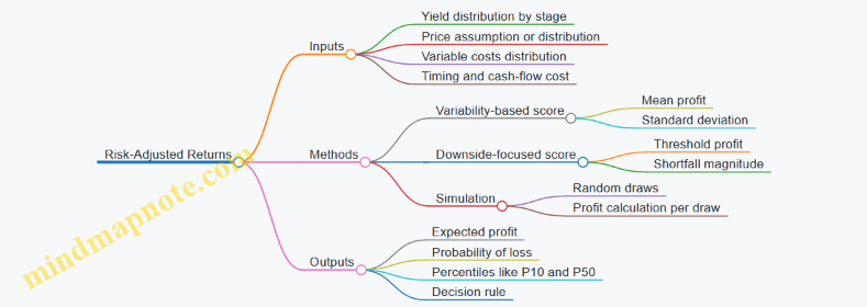
Simulation steps:
- Build distributions.
- Yield: use historical yields for the crop and field, then adjust the mean and spread for transition stage.
- Costs: assign ranges for herbicide and repairs based on past variability.
- Price: keep it fixed if you’re comparing agronomic risk only; use a distribution if you want combined risk.
- Run many trials (e.g., 5,000).
- For each trial, compute profit.
- Summarize results with percentiles and probabilities.
Example decision outputs:
- Plan A: P10 profit = $95/acre, probability of loss = 20%
- Plan B: P10 profit = $70/acre, probability of loss = 45% If your rule is “avoid plans with more than 30% loss probability,” Plan A wins.
Method 4: Certainty Equivalent Using Utility Curves
If you want a single number that reflects how you personally dislike risk, use a certainty equivalent.
- Convert profit outcomes into a utility value.
- Certainty equivalent is the guaranteed profit that gives the same utility.
A simple practical approach uses a risk aversion parameter. You don’t need a fancy formula; you need consistency. For example, set a stronger penalty for low profits during transition years because those are the years that strain equipment schedules and cash flow.
Choosing a Decision Rule That Fits No-Till Reality
No-till economics often changes the shape of outcomes: fewer “catastrophic” failures are possible once residue and seeding are dialed in, but early transition can increase variability. Use a rule that matches that pattern.
Common rules:
- If you must protect cash: compare probability of profit below break-even.
- If you can absorb variability: compare mean profit adjusted by standard deviation.
- If you care about worst-case planning: compare P10 or P5 profit.
Worked Mini-Example Combining Two Metrics
Assume both plans have the same mean profit $190/acre.
- Plan A: σ = $25, P10 = $120
- Plan B: σ = $55, P10 = $85 Even with equal averages, Plan A has a tighter spread and a higher worst-case percentile. If your operation is sensitive to bad years, Plan A is the safer choice.
Practical Checklist for Risk-Adjusted Calculations
- Use stage-specific yield variability, not one generic spread.
- Include timing-sensitive costs if operations can slip.
- Keep price treatment consistent across plans.
- Report at least one downside metric (probability of loss or P10).
- Use one decision rule and apply it the same way to every option.
5. Carbon Recovery Accounting at the Farm Level
5.1 Translating Soil Organic Matter Changes Into Economic Variables
Soil organic matter (SOM) changes matter economically because they alter how reliably a field produces and how much it costs to keep it producing. The trick is translating agronomy language into accounting language without pretending the relationship is perfectly linear.
Foundational Mapping from SOM to Farm Outcomes
Start with what SOM can influence in a no-till system: water storage, infiltration, nutrient retention, soil structure, and biological activity. Each of these affects at least one economic variable.
- Water availability affects yield stability and irrigation or drainage costs.
- Nutrient retention affects fertilizer efficiency and the risk of nutrient loss.
- Soil structure affects emergence uniformity and stand establishment costs.
- Biological activity affects residue breakdown timing and weed pressure indirectly.
A practical approach is to define a small set of economic variables you will actually budget and measure. For most farms, that set includes: net return per acre, yield and yield variability, input costs per acre, and risk-adjusted returns.
Stepwise Translation Method
Use a three-step chain: SOM change → agronomic effect → economic variable.
- Quantify SOM change using soil tests, sampling depth consistency, and trend direction. If you cannot measure change precisely, use a conservative range and focus on directionality.
- Assign agronomic effects to specific mechanisms. For example, a modest SOM increase often improves water holding and infiltration, which reduces yield penalties during dry spells.
- Convert agronomic effects to economics using field-level relationships you can defend.
For yield stability, the economic variable is not just average yield; it is the cost of variability. Variability shows up as lower average revenue, higher replanting risk, and sometimes higher input rates to rescue performance.
Economic Variables You Can Build Directly
Below is a concrete set of variables that connect to SOM.
- Yield level effect: SOM-driven improvements in stand establishment and water availability can raise average yield.
- Yield variability effect: SOM can reduce the size of yield dips in stress years.
- Fertilizer efficiency effect: Better nutrient retention can reduce the amount of nutrient needed to reach the same yield.
- Operational cost effect: Improved residue breakdown and soil structure can reduce the need for costly interventions like extra passes or emergency re-seeding.
- Risk cost effect: Even when average yield is similar, reduced downside yield lowers risk-adjusted costs.
Example: Turning a Soil Test Trend Into Budget Inputs
Assume a field has consistent sampling at 0–6 inches. Over three years, SOM rises from 2.2% to 2.3%. You do not claim a guaranteed yield response. Instead, you translate the change into a defensible range of agronomic improvements.
- Mechanism assumption: slightly improved water holding and infiltration.
- Agronomic effect: reduced yield penalty in dry years and slightly better emergence uniformity.
- Economic conversion:
- Dry-year yield penalty reduction by 2–3 bushels per acre.
- Average yield increase by 0–1 bushel per acre.
Now convert to dollars using your crop price and your cost structure. If the crop price is $4.50 per bushel, then a 2–3 bushel reduction in dry-year penalty is worth $9–$13.50 per acre in those years. You then weight by the frequency of dry years in your historical record, and you compare that value to the costs of practices that drove SOM change.
Mind Map: SOM Change to Economic Variables
Practical Guardrails for Credible Translation
Keep the translation honest by separating what you know from what you assume. Use ranges where uncertainty is real, and tie assumptions to measurable farm outcomes like yield maps, stand counts, and fertilizer application records. When you cannot link SOM change to a specific economic variable, do not force it into the budget—track it as a mechanism you expect to matter, but only monetize what you can justify with field evidence.
5.2 Selecting Measurement Approaches for Soil Carbon Inputs and Outputs
Soil carbon accounting works best when you measure the things you can control and observe: carbon inputs (what you add) and carbon outputs (what leaves or is transformed). The trick is choosing methods that match your farm’s scale, recordkeeping ability, and the level of certainty you need for economic decisions.
Start with the Accounting Boundary
Before selecting a measurement method, define what counts as “soil carbon” in your budget. A practical boundary is the topsoil layer you manage (often 0–15 cm or 0–20 cm) and the carbon pathways you can reasonably track. For no-till systems, the most relevant inputs are crop residues and cover crop biomass, while outputs include decomposition losses and any carbon removed with harvested biomass.
Example: If you grow corn and harvest grain, you can treat grain carbon as an output leaving the field, while residue carbon remains an input that either decomposes in place or contributes to longer-lived pools.
Choose Between Direct Measurement and Proxy Measurement
Direct measurement aims to estimate soil carbon change by sampling soil and analyzing it in a lab. Proxy measurement estimates carbon inputs and outputs using agronomic records and models, then infers soil carbon change.
- Direct measurement is strongest for verifying whether soil carbon is actually moving.
- Proxy measurement is strongest for budgeting and comparing management options when you need results quickly.
A common integrated approach is to use proxy methods for routine accounting and direct sampling for periodic calibration.
Map Carbon Inputs You Can Measure On-Farm
Carbon inputs typically come from:
- Crop residues (stover, straw, chaff)
- Cover crop biomass (roots and aboveground material)
- Manure or compost if used
- Fertilizer carbon is usually negligible for soil carbon budgets in most farm contexts, so it’s often excluded unless you have a specific reason.
Example: For a wheat field after harvest, you can estimate residue input using yield and a residue-to-grain ratio. If wheat yield is 60 bu/ac and the residue ratio is 1.2, you can estimate residue mass, then convert to carbon using a standard carbon fraction for plant material.
Map Carbon Outputs You Can Measure or Bound
Outputs include:
- Harvested biomass leaving the field (grain, hay)
- Erosion losses if soil is moving off-site
- Gaseous carbon losses from decomposition (often not measured directly on farms)
Because gaseous losses are hard to measure directly, many farm budgets treat them as the “difference” between inputs and measured soil carbon change, or they use model-based decomposition factors.
Example: If soil carbon measured over a year shows little change despite high residue inputs, that suggests decomposition and/or erosion offset gains. You can then check residue management, sampling depth consistency, and whether runoff is moving soil.
Select Soil Sampling Designs That Don’t Lie
Soil sampling is where good intentions go to die, mostly because sampling error is real. Use a design that reduces noise:
- Depth consistency: sample the same depth interval every time.
- Replicate strategy: multiple cores per management unit, composited or analyzed separately.
- Timing: sample at comparable points in the crop cycle.
- Spatial logic: follow management zones, not just random points.
Example: If you switch from conventional tillage to no-till, mixing soil from different depths or sampling after a heavy disturbance can create apparent “carbon changes” that are really sampling artifacts.
Decide What to Measure in the Lab
Common lab targets include soil organic carbon (SOC) concentration and bulk density. SOC alone can mislead because carbon concentration can change without a real change in carbon mass per area.
To estimate carbon stock, you typically need:
- SOC concentration
- Bulk density
- Soil depth thickness
Example: Two fields can have the same SOC concentration, but if one has lower bulk density due to improved structure, the carbon stock per acre may be higher.
Use Mind Maps to Keep Methods Coherent
Mind Map: Selecting Measurement Approaches for Soil Carbon
Build an Integrated Workflow for Farm Use
A workable workflow is:
- Create an input ledger for each field: yields, residue ratios, cover crop species, termination dates, and any amendments.
- Estimate carbon inputs from the ledger using consistent conversion factors.
- Estimate outputs using harvested biomass and erosion risk flags.
- Run proxy carbon accounting to compare management options.
- Schedule direct soil sampling at defined intervals to measure SOC and bulk density.
- Reconcile proxy assumptions with measured carbon stock changes by management zone.
Example: If proxy accounting suggests a cover crop should raise soil carbon but measured SOC stock stays flat, you can check whether termination timing reduced biomass, whether residue was removed, or whether sampling depth and bulk density procedures were inconsistent.
Keep the Measurement Choice Tied to Economic Use
Measurement approaches should serve the economic question: which practices improve carbon recovery without destabilizing yield. If you only need relative comparisons between no-till variants, proxy methods with careful recordkeeping may be enough. If you need verification for a carbon-related payment or internal performance tracking, direct sampling becomes non-negotiable.
Example: Comparing two residue management strategies can be done with proxy accounting every year, while direct sampling every few years can confirm whether the differences are showing up in carbon stock rather than just in calculations.
5.3 Linking Cover Crops Residue Inputs and Management Intensity to Carbon Accounting
Carbon accounting needs a bridge between what you physically add to the field and what the accounting method can credibly count. For cover crops, that bridge is the residue input and how you manage it—because residue quantity, residue quality, and the timing of decomposition all affect how much carbon is retained in soil versus released.
Foundational Concepts for Residue-Based Carbon Accounting
Start with three measurable ideas:
- Residue input: how much plant material reaches the soil surface or is incorporated.
- Residue quality: how easily microbes break it down, influenced by species and growth stage.
- Management intensity: how you terminate, disturb, and protect residue, which changes decomposition speed and soil contact.
A practical way to think about it: carbon accounting is not just “cover crop planted yes/no.” It is “how much carbon entered the residue pool, how fast it was offered to microbes, and whether soil structure helped protect part of it.”
Residue Inputs That Can Be Counted
Residue input is usually estimated from biomass and residue fraction. A simple workflow:
- Estimate aboveground biomass at termination using a consistent method (for example, clipped quadrats in representative spots).
- Convert biomass to residue mass using a fraction that represents what remains as residue after termination and handling.
- Track root contribution separately if your accounting method supports it; roots can matter even when aboveground residue is modest.
Example: A rye cover crop produces 2.5 tons/acre of aboveground dry biomass at termination. If your residue accounting uses a residue retention factor of 0.9 (meaning 10% is lost to handling or weather before measurement), the residue input becomes 2.25 tons/acre.
Management Intensity as a Control Knob
Management intensity affects decomposition and soil protection through at least four levers:
- Termination method: roller-crimping versus mowing versus herbicide termination can change residue contact and regrowth.
- Timing relative to growth stage: earlier termination often yields more labile residue; later termination can increase biomass but may also increase lignin and slow decomposition.
- Soil disturbance: no-till termination leaves residue on the surface; shallow incorporation increases soil contact and can accelerate mineralization.
- Residue coverage and duration: how long residue stays intact before the next crop shades it, breaks it down, or is incorporated.
Example: Two fields both plant clover. Field A terminates at early flowering with a roller and leaves residue on the surface for several weeks. Field B terminates later and incorporates with a shallow pass. Even if biomass is similar, Field B typically offers residue to microbes faster because it is mixed into soil.
Linking Residue Quality to Accounting Variables
Residue quality is often represented indirectly through species and termination stage. You can make this operational without turning it into a chemistry project:
- Use species groups (legumes, grasses, brassicas) and termination stage to assign a decomposition category in your accounting spreadsheet.
- Record termination date and growth stage consistently so the same rule applies each year.
Example: A grass-dominant cover terminated at boot stage is treated as “more readily decomposed” than the same grass terminated after heading. Your accounting method may not need exact lignin values, but it does need consistent category assignments.
Mind Map: Residue Inputs and Management Intensity to Carbon Accounting
Integrated Example: From Field Actions to Accounting Inputs
Imagine a 40-acre field with the same cover crop species used across two years.
- Year 1: rye planted after harvest, terminated with a roller at pre-heading, no incorporation, seeding into residue the next week.
- Year 2: rye planted similarly, terminated with mowing at early heading, then a shallow pass incorporates residue before seeding.
To link this to carbon accounting, you would:
- Use the measured biomass from each year to set residue quantity.
- Assign residue quality categories based on termination stage.
- Set management intensity flags: surface residue with minimal disturbance in Year 1 versus incorporation in Year 2.
- Ensure the timing between termination and next seeding is recorded, because it affects how long residue remains available on the surface.
The accounting model then has the inputs it needs to treat Year 1 as slower decomposition with more residue-soil protection, and Year 2 as faster decomposition due to soil mixing.
Practical Data Discipline That Prevents Accounting Drift
Carbon accounting fails most often when records are inconsistent. Keep three items tight:
- Termination stage definition: decide what “pre-heading” means in your field and stick to it.
- Biomass sampling representativeness: sample the same way each time, using similar locations and quadrat sizes.
- Operation timing: record dates for termination, incorporation (if any), and seeding so residue duration is not guessed.
If you do those three things, linking cover crop residue inputs and management intensity becomes a repeatable process rather than a yearly scramble.
5.4 Documenting Practices for Verification Ready Records
Verification-ready records are simply well-organized evidence that your soil and management claims can be checked without guessing. The goal is not to write a novel; it is to make every claim trace back to a specific field, date, input, and operation.
Foundational Principles for Evidence
Start with three rules. First, record what you did, not what you meant to do. Second, keep the “why” tied to the “what,” such as linking a weed control decision to the target species and growth stage. Third, use consistent identifiers so the same field is never a different field in different spreadsheets.
A practical example: if you claim a cover crop was established on Field 12, your record set should include the seeding date, seeding rate, seed mix, method, and the person or contractor who performed it. If you later adjust the plan due to weather, you document the change and the reason.
Record Architecture from Field to Claim
Build records in layers.
- Field identity layer: field name/number, soil type or management zone, and boundary reference.
- Operation layer: each pass with date, time window, equipment, operator, and location.
- Input layer: seed, fertilizer, lime, herbicide, and amendments with product, rate, and application method.
- Management layer: cover crop termination method, grazing status, residue handling, and any deviations.
- Measurement layer: soil sampling plan, lab results, and any calibration or QA notes.
- Outcome layer: yield records, stand counts, and notes that explain anomalies.
When these layers are consistent, verification becomes a matter of matching records to claims rather than reconstructing history.
What to Capture for No-Till and Soil Regeneration
No-till verification typically hinges on residue continuity, seeding method, and weed management consistency.
For each field and season, capture:
- Tillage status: confirm whether any tillage occurred, including “spot” tillage. If you did a one-time correction pass, record it with date and depth.
- Seeding details: planter model, row spacing, seeding depth setting, downforce or gauge settings if available, and whether residue was present.
- Residue and cover crop status: species, seeding date, termination date, and termination method (roller, crimping, herbicide, or mowing).
- Weed control actions: product, rate, carrier volume, nozzle type if known, application timing, and target stage.
- Fertilizer and amendments: placement method (band, dribble, broadcast), timing, and soil test basis.
A simple example: if you terminate a rye cover crop with a roller-crimper, record the termination date, the growth stage at termination, and the seeding date of the cash crop. If you used herbicide instead, record the product and rate and note why the roller alone was insufficient.
Mind Map: Verification-Ready Records
Example Record Set for One Field Season
Use a consistent naming convention such as Field12_2026_CoverRye_Seeding and Field12_2026_CashCrop_Seeding. For a concrete set, include:
- Cover crop establishment: seeding date (for example, March 15), species and seeding rate, seeding method, and residue condition at seeding.
- Termination: termination date (for example, May 20), method, and notes on growth stage.
- Cash crop seeding: seeding date, planter model, seeding depth setting, and whether residue was present.
- Weed control: burndown timing and product details, plus any follow-up post-emergence application.
- Soil sampling: sampling date, depth, number of cores, and lab report ID.
- Yield: combine yield monitor export summary and any adjustments explained in notes.
If you keep photos, take them consistently: one wide shot of the field and one close shot of residue or stand condition on the same day as key operations.
Verification-Ready Quality Checks
Before you finalize a claim, run three checks.
- Completeness check: every claim has at least one supporting record in each relevant layer (operation, inputs, and measurement when applicable).
- Consistency check: field IDs, dates, and units match across documents. If fertilizer is recorded in pounds of nutrient in one file and kilograms in another, convert once and keep the conversion note.
- Plausibility check: stand and yield notes should explain major deviations. If yield drops sharply, your records should show whether weed pressure, equipment issues, or water constraints were documented.
A small habit helps: after each operation day, enter the essentials immediately, then do a weekly cleanup pass to correct typos and fill missing units. That way, the record set stays accurate without becoming a last-minute scramble.
5.5 Valuing Carbon Benefits Using Farm Relevant Payment Structures
Farmers don’t get paid for “carbon” in the abstract. They get paid for specific, auditable outcomes under a particular contract. Valuing carbon benefits well means translating soil changes into contract-usable metrics, then matching those metrics to the payment structure you actually face.
Core Payment Structures and What They Pay For
Most farm-relevant carbon payments fall into four buckets:
- Practice-based payments pay for doing defined actions (for example, planting cover crops and maintaining residue). The value is usually easier to calculate because it depends on records, not on measured soil carbon.
- Performance-based payments pay for measured or modeled outcomes (for example, estimated soil organic carbon change). The value depends on measurement protocols and uncertainty handling.
- Stacked or tiered payments combine both. A base payment covers practices, and an additional payment is tied to performance thresholds.
- Shared-risk payments adjust payouts if outcomes miss targets. This matters because it changes the expected value, not just the headline rate.
A practical way to think about it: practice-based payments reduce measurement friction; performance-based payments can increase upside but add verification cost and variability.
Translating Soil Regeneration Into Contract Variables
Contracts typically require you to report variables that connect to soil regeneration. Common examples include:
- Field area and eligibility (which acres qualify, and which management history is required)
- Management events (cover crop species, planting dates, termination method, seeding rate)
- Tillage and residue rules (what counts as no-till, how residue is handled at planting)
- Baseline assumptions (what your “before” condition is)
- Verification method (soil sampling, modeling, remote sensing, or a mix)
Example: If your contract requires “continuous living cover for 8–10 weeks,” you need a plan that reliably meets that window. If you miss it, you may lose the practice payment even if soil benefits still occur.
Valuation Mechanics That Keep You Honest
To value carbon benefits, compute expected net benefits per acre using the payment formula and the costs of meeting requirements.
- Gross carbon payment: rate × eligible acres × performance factor (if any)
- Verification and administration costs: sampling, lab fees, documentation time, and any third-party support
- Risk adjustment: reduce expected value if payments depend on thresholds or shared-risk rules
- Net carbon benefit: gross payment minus costs
Example: Suppose a program pays $18/acre for verified practice compliance and adds $6/acre when modeled carbon gain exceeds a threshold. If your field history suggests you will meet the practice requirement 95% of the time and the threshold 70% of the time, your expected gross is:
- Practice: $18 × 1.00 × 0.95
- Performance bonus: $6 × 1.00 × 0.70
Then subtract verification costs. This turns “maybe” into a number you can compare to yield stability and equipment transition costs.
Mind Map: Payment Structure to Farm Decision
Example: Two Programs, Same “Carbon Rate,” Different Net Value
Consider two hypothetical programs for the same 1,000-acre farm.
- Program A pays $20/acre for practice compliance with low verification cost.
- Program B pays $26/acre for modeled performance but requires more documentation and soil sampling, and it reduces payouts if modeled gains fall below a threshold.
If Program B’s verification costs are $6/acre and the probability of meeting the performance threshold is 0.6, then the expected gross is $26 × 0.6 = $15.60/acre. Net expected carbon benefit becomes $15.60 − $6 = $9.60/acre.
Program A’s net is $20 − (say) $2 verification = $18/acre. Even with a higher headline rate, Program B can underperform because the contract shifts risk and adds cost.
Practical Checklist for Contract-Ready Valuation
Before you sign anything, make sure your valuation includes:
- Eligibility rules that could exclude acres (for example, field history requirements)
- Compliance timing that affects whether practices count (planting and termination windows)
- Verification costs that are not covered by the program
- Threshold definitions and how shortfalls are handled
- Payment timing and whether it affects cash flow relative to transition costs
Example: If your equipment transition causes a one-season delay in cover crop establishment, you may lose practice compliance for that season. That loss can be larger than the carbon benefit you hoped to earn.
Valuing carbon benefits is ultimately a budgeting exercise with agronomy attached. When you treat the contract like a set of measurable rules, the numbers become comparable to yield stability and equipment transition costs—on the same spreadsheet, with the same assumptions.
6. Cost Structure Analysis for No-Till Adoption
6.1 Categorizing Costs Into Fixed Variable And Semi Variable Components
No-till economics gets messy fast if you treat every expense as “per acre.” Some costs behave like a subscription (they show up whether you plant or not), others behave like a volume knob (they scale with acres), and many sit in between. This section gives you a practical way to sort costs so your budgets stay honest when yields, weather, or equipment schedules change.
Foundational Cost Logic
Start with three categories:
- Fixed costs: you pay them even if you farm fewer acres. They are tied to owning capacity, not using it.
- Variable costs: they change with the amount of work or inputs applied. If acres go down, these usually go down.
- Semi-variable costs: they include a fixed base plus a variable portion. Think “minimum charge plus usage.”
A quick test: if you could reduce acres by 20% and still expect the same cost, it’s likely fixed. If the cost rises roughly in proportion to acres, it’s variable. If it has a minimum level and then increases, it’s semi-variable.
Mind Map: Cost Categories and What Drives Them
Fixed Costs That Commonly Appear in No-Till Budgets
Fixed costs are often overlooked because they don’t change with acres. In no-till transition years, they still matter because you may pay for new equipment while acres or yields temporarily wobble.
Common fixed items:
- Equipment depreciation or lease minimums: If you lease a no-till planter with a monthly minimum, that cost doesn’t wait for good planting conditions.
- Insurance and permits: Crop insurance premiums and equipment insurance typically don’t scale with acres planted.
- Management and overhead: Office expenses, bookkeeping, and a portion of labor for planning and compliance.
Example: If your planter lease has a $600/month minimum and you plant 1,000 acres in one month and 800 acres in another, the lease minimum is still $600. The per-acre cost changes only because the denominator changed.
Variable Costs That Scale with Work and Inputs
Variable costs are the easiest to misclassify when you use “per acre” numbers without checking what actually drives them.
Common variable items:
- Seed rate and quality: Higher seeding rates increase seed cost per acre.
- Fertilizer and placement: If you apply more nitrogen or use more expensive placement methods, variable costs rise.
- Herbicide program: Costs scale with application rate and number of passes.
- Fuel and lubricants: Often proportional to acres and passes.
- Custom work per acre: If a contractor charges $18/acre for seeding, it scales with acres.
Example: Suppose burndown herbicide is $22/acre and you apply it once. If you seed 900 acres instead of 1,000, herbicide drops by $2,200. That’s variable behavior.
Semi-Variable Costs That Mix Minimums with Usage
Semi-variable costs are where real farms live. They include a base level and then additional cost as activity increases.
Common semi-variable items:
- Labor: You may have a baseline of supervision and equipment setup time, then extra labor during peak days.
- Maintenance: There’s usually a baseline inspection and seasonal service, plus wear-related repairs that increase with hours.
- Contracting: Many contracts include a mobilization fee plus a per-acre charge.
Example: A contractor charges $250 mobilization plus $14/acre for seeding. If you seed 600 acres, the total is $250 + (14×600) = $8,650. If you seed 900 acres, total becomes $250 + (14×900) = $12,850. The $250 is the fixed base; the $14/acre is the variable portion.
Practical Method to Classify Costs Without Guessing
Use a two-step approach:
- Find the driver: acres, passes, hours, or time. For instance, fuel is driven by hours and field distance, while seed is driven by acres.
- Check the minimum: if there’s a minimum charge, retainer, or seasonal baseline, it’s likely fixed or semi-variable.
Then record each cost with:
- Category: fixed, variable, or semi-variable
- Driver: acres, hours, passes, or months
- Unit basis: per month, per acre, per hour, or per job
Turning Categories Into Better Decisions
Once costs are categorized, you can compute two useful views:
- Per-acre cost at different activity levels: Fixed costs spread over fewer acres raise per-acre numbers even if variable costs stay the same.
- Break-even acres for equipment changes: If a new seeding setup adds fixed lease costs, you can see how many acres must run to cover the fixed base.
Example: If fixed costs rise by $12,000/year due to a new no-till planter lease, and variable costs are unchanged, then the break-even acres depend on your margin per acre. If your contribution margin is $40/acre, you need 12,000/40 = 300 acres to cover the fixed increase.
Categorizing costs isn’t about being perfect; it’s about being consistent. When you classify costs by their real drivers, your no-till budgets stop “moving the goalposts” every time acres or timing shift.
6.2 Estimating Labor Changes and Seasonal Workload Shifts
No-till often changes when labor happens more than how much labor exists in total. The goal of this section is to estimate labor hours by season, then translate those hours into cost and risk (like “we’re short on seeding day”). Start with a baseline year, then adjust for the specific no-till practices you’re adopting.
Core Labor Logic for No-Till Transitions
Begin with three labor buckets:
- Field operations labor: driving, hitching, turning, seeding, spraying, and any in-field adjustments.
- Support labor: loading seed and chemicals, calibrating equipment, cleaning, moving hoses, and recordkeeping.
- Contingency labor: extra trips for rework, waiting for weather windows, or fixing performance issues.
A useful rule: no-till usually reduces some operations (like tillage passes) but increases others (like residue handling planning, more careful seeding setup, and often more attention to weed control timing). The net effect depends on your starting point.
Foundational Step: Build a Seasonal Labor Calendar
Create a calendar by week (or by 10-day blocks) for your baseline year. For each field operation, record:
- Acreage covered
- Hours per acre (or hours per day and acres per day)
- Crew size (people on the job)
- Equipment count (how many machines are running)
- Weather sensitivity (low/medium/high)
Then compute total labor hours per block. This gives you a baseline workload shape, not just a total number.
Example Baseline Calendar Snapshot
Assume a 1,000-acre farm with two crops. In the baseline year, you might see:
- Spring tillage and seedbed prep: 120 labor hours in weeks 1–3
- Seeding: 80 labor hours in weeks 3–4
- Spraying: 60 labor hours in weeks 5–8
- Harvest: 140 labor hours in weeks 20–22
No-till changes the spring curve more than harvest, unless you also change harvest logistics.
Estimating Labor Changes by Operation Type
Reduced Tillage Passes
If you remove two tillage passes, you remove their field operation labor and some support labor (like fuel handling and equipment cleaning after tillage). However, you may add time for:
- residue assessment and seeding depth checks
- more frequent calibration during the first few seeding days
Estimate this by comparing your baseline “tillage days” to your new “seeding setup days.”
Seeding and Planting Setup Time
No-till seeders often require more careful setup early in the season. Split seeding labor into:
- Setup and calibration (one-time per season per machine)
- Production seeding (hours per acre)
- Troubleshooting (extra passes or adjustments)
A practical approach is to add a fixed setup allowance (for example, 6–10 labor hours per seeder) plus a per-acre production adjustment (for example, +0.05 to +0.15 hours/acre during the transition year).
Weed Control Timing and Application Windows
Weed control can shift from “one broad window” to “more precise windows.” Labor changes come from:
- additional scouting days
- more frequent sprayer calibration
- waiting for conditions that allow effective application
To estimate this, keep the same total acres sprayed, but adjust hours per acre upward for higher weather sensitivity and add a scouting/support allowance.
Advanced Details That Prevent Budget Surprises
Crew Scheduling and Equipment Bottlenecks
Labor cost is not just hours; it’s whether the crew can physically do the work when it appears. Create a simple capacity check:
- Determine maximum crew availability per week (people × hours)
- Determine required labor per week from your calendar
- Flag weeks where required labor exceeds capacity
If you’re short in a specific week, you either hire help, slow down, or shift operations. Each option changes cost and risk.
Contingency Labor as a Percentage
Instead of guessing “extra hours,” estimate contingency as a percentage of field operation labor for weather-sensitive tasks. For example:
- low sensitivity: +2–4%
- medium sensitivity: +5–8%
- high sensitivity: +10–15%
Apply this only to the operations that actually face weather constraints.
Mind Map: Labor Estimation Workflow
Integrated Example: One Transition Season Labor Estimate
Suppose your baseline spring includes 200 labor hours across tillage and seeding. In the transition year you:
- remove two tillage passes: -70 hours
- add seeder setup and calibration: +10 hours
- increase seeding production time by +0.10 hours/acre on 400 acres: +40 hours
- add scouting and tighter weed timing: +25 hours
Net spring change: -70 + 10 + 40 + 25 = +5 labor hours. That looks small, but the weekly distribution matters. If those +25 hours land in weeks 5–6 while your crew is already near capacity, you may still need help or a slower pace.
Practical Output Format for Your Budget
For each season block, report:
- required labor hours by operation
- crew capacity and any shortfalls
- contingency allowance by sensitivity level
- resulting labor cost using your chosen wage rate and overhead assumptions
This keeps the labor estimate grounded in what actually happens in the field, not just what the equipment list suggests.
6.3 Modeling Fuel and Lubricant Changes from Reduced Tillage
Reduced tillage often cuts the number of passes, but fuel use can also shift because implement choice changes working depth, draft, and travel speed. Modeling fuel and lubricants well means you track both the obvious pass-count savings and the less obvious “how hard the tractor works” effects.
Core Concepts for Fuel Modeling
Start with a simple accounting identity:
- Fuel per acre depends on engine load, time per acre, and idling.
- Time per acre depends on field speed, turn time, and overlap.
- Engine load depends on draft (pulling force) and hydraulics.
A practical way to model this is to separate operations into three buckets: primary tillage, secondary tillage, and seeding/finishing. Reduced tillage usually eliminates or shrinks the first two buckets, while seeding may gain complexity (for example, residue handling or downforce).
Mind Map: Fuel and Lubricant Modeling Inputs
Step 1: Build an Operation-Level Worksheet
For each field operation, record:
- Implement width (ft or m).
- Working speed (mph or km/h).
- Field efficiency (a fraction capturing turns and overlap). If you don’t have data, use a starting value like 0.85 for many row-crop fields, then adjust after you observe a season.
- Fuel rate under load (gal/hour). If you lack a measurement, you can estimate from tractor specs and typical load, but keep it as a parameter.
- Idling time fraction (for example, 5–15% depending on how often you wait for adjustments).
Compute hours per acre as:
- hours/acre = 1 / (width × speed × efficiency)
Then compute fuel/acre:
- fuel/acre = (fuel rate × hours/acre) × (1 + idling fraction)
This is the backbone. Everything else—draft changes, residue effects, and lubricant intervals—adds nuance.
Step 2: Model Draft and Load Changes from Reduced Tillage
Reduced tillage changes the draft profile. Two common patterns:
- Fewer passes reduces total working time.
- Different implement changes draft per pass. A no-till opener may require less overall soil disruption, but residue can increase resistance and require higher downforce.
Model draft effects by adjusting either:
- Fuel rate under load (preferred if you have any logged data), or
- Effective working speed (if the tractor slows because the opener struggles).
Example: Two Passes vs One Pass
Assume a conventional system uses two tillage passes before seeding, while a reduced tillage system uses one pass plus seeding.
- Conventional: 2 passes, each at 4.5 mph, 20 ft implement width, efficiency 0.85.
- Reduced: 1 pass at 5.0 mph, same width, efficiency 0.85.
- Fuel rate under load: 10 gal/hour for conventional tillage, 9 gal/hour for reduced tillage.
- Idling fraction: 0.10.
Hours/acre conventional per pass = 1 / (20 × 4.5 × 0.85) ≈ 0.0131. Two passes ≈ 0.0262.
Fuel/acre conventional ≈ 10 × 0.0262 × 1.10 ≈ 0.288 gal/acre.
Hours/acre reduced ≈ 1 / (20 × 5.0 × 0.85) ≈ 0.0118.
Fuel/acre reduced ≈ 9 × 0.0118 × 1.10 ≈ 0.117 gal/acre.
The difference here is mostly pass count, but the slightly lower fuel rate and higher speed add extra savings.
Step 3: Include Lubricants as “Per Hour” and “Per Acre” Costs
Fuel is usually the largest energy cost, but lubricants matter when you compare systems with different operating hours.
Track lubricants with two layers:
- Per operating hour: engine oil, hydraulic oil, and filter changes tied to hours.
- Per acre or per operation: grease points that you service on a schedule (often linked to days or hours, but you can convert to acres using your throughput).
A simple conversion:
- oil cost/acre = (oil cost per hour × hours/acre)
If reduced tillage cuts total hours, lubricant costs drop proportionally. If it changes implement type, grease frequency might change slightly; for example, residue-heavy conditions can increase wear and grease demand.
Example: Oil and Filter Changes
Suppose engine oil and filter costs are $18 per hour-equivalent when averaged over change intervals (including labor). If conventional tillage uses 0.0262 hours/acre and reduced uses 0.0118 hours/acre for the tillage portion:
- Conventional lubricant cost ≈ 18 × 0.0262 ≈ $0.47/acre
- Reduced lubricant cost ≈ 18 × 0.0118 ≈ $0.21/acre
You can add a small adjustment for extra grease on a specialized opener if your maintenance logs show it.
Step 4: Validate with Field Reality
Model outputs should be checked against at least one of:
- tractor fuel receipts for the season divided by total acres worked,
- logged engine hours by operation,
- or a short “spot measurement” where you record fuel used and acres covered for one day.
If your model consistently overestimates fuel, the usual culprits are inflated idling fractions, overly pessimistic efficiency, or fuel rates assumed too high for the actual load.
Step 5: Sensitivity That Actually Helps Decisions
For decision-making, vary the parameters that move the result:
- working speed (mph)
- field efficiency (turns and overlap)
- fuel rate under load (gal/hour)
- idling fraction
Keep the rest fixed. If the model is stable across reasonable ranges, you can trust the relative comparison between systems even if the absolute gallons are approximate.
6.4 Capturing Input Changes for Herbicides Fertility and Seed
No-till changes what you buy, when you buy it, and how reliably it performs. Capturing those input changes means building a budget that tracks each input by product, rate, timing, and placement method—then linking those details to the agronomic reason they changed. If you skip the “why,” your numbers will look precise and still be wrong.
Foundations for Input Change Tracking
Start with a baseline year under conventional tillage. For each field and crop, list the herbicide program, fertility program, and seeding plan as they were actually executed: active ingredients, product names, application dates, target weeds or growth stages, seeding date, seeding rate, row spacing, seedbed conditions, and any placement differences. Then create a second layer for no-till: what changed and why.
A practical rule: every input line item in your budget must have a matching operational record. If the budget says “nitrogen applied at V4,” your log should show the date, product, rate, and equipment used.
Herbicide Inputs Under No-Till
No-till often shifts weed control from “bury and reset” to “manage residue and timing.” That usually changes herbicide inputs in three ways.
-
Burndown timing and coverage. Residue can slow soil contact and keep weeds cooler longer. Example: if you previously used a single spring burndown, you may now split it into a residue-friendly burndown plus a follow-up post-emergence pass. Your budget should reflect both applications, including water volume and nozzle setup if you track it.
-
Residual herbicide selection and rate. Residual products may be used to cover the gap between burndown and crop canopy. Example: a field with heavy rye residue might require a higher residual rate or a different active ingredient to maintain early-season weed suppression. Capture the active ingredient, not just the product label.
-
Weed resistance management costs. Even when total herbicide dollars stay similar, the mix changes. Example: you rotate modes of action by adding a different active ingredient at a specific growth stage. Budget the added cost and record the target stage so you can compare like-for-like.
Fertility Inputs Under No-Till
Fertility changes are often less visible than herbicide changes, but they matter for yield stability. No-till can alter nutrient availability, stratify nutrients near the surface, and change how quickly residue decomposes.
Track fertility inputs by placement and timing.
-
Placement method. Example: if you switch from broadcast plus incorporation to banding with a no-till planter, your budget should reflect the banded application rate and the equipment cost assumptions tied to that method.
-
Timing. Example: you may apply some nitrogen earlier to support early growth because stand establishment can be slower in cool, wet springs. Record the date relative to seeding.
-
Soil test interpretation. Example: if surface stratification leads to different test results, you might adjust phosphorus or potassium rates. Capture the soil test date, the lab method if you track it, and the resulting rate change.
Also capture “small” line items that often change: micronutrients, starter fertilizer, lime or gypsum, and cover-crop termination nutrients.
Seed Inputs Under No-Till
Seed costs change through rate, treatment, and seeding system performance.
-
Seeding rate and spacing. Example: if you reduce tillage and expect more variable emergence, you might increase seeding rate slightly or adjust row spacing to improve stand uniformity. Record the exact rate and any planter calibration changes.
-
Seed treatment. Example: if you add fungicide or insecticide seed treatment to manage residue-associated disease or early pests, budget the per-unit treatment cost and the treated seed quantity.
-
Planter and seed-to-soil contact. Example: if residue causes inconsistent depth, you may adjust downforce or change closing wheel settings. Those changes can affect emergence and may lead to replant decisions. Capture replant probability using your own historical notes, not guesses.
Mind Map: Input Changes to Capture
Example: Converting Field Notes Into Budget Lines
Assume a 120-acre field moving to no-till corn.
-
Herbicides: In the baseline year, you used one burndown application at 1.0 qt/acre of a glyphosate product plus a single residual. In the no-till year, you record two passes: a burndown at seeding week and a post-emergence spot treatment when weeds reach 2–4 inches. Your budget should show three herbicide line items: burndown product, residual product, and post-emergence product, each with date and rate.
-
Fertility: Baseline used broadcast nitrogen in spring. No-till uses banded nitrogen at seeding plus a small starter. Your budget should separate banded N and starter rather than lumping them into “nitrogen.”
-
Seed: Baseline seeding rate was 32,000 seeds/acre without treatment. No-till increases to 34,000 seeds/acre and adds a seed treatment. Your budget should show treated seed cost per unit and the adjusted seed quantity.
When you do this consistently, you can compare net returns without pretending the only difference is “no-till vs tillage.” The difference is the input system you actually ran.
Quality Checks for Budget Integrity
Before finalizing, reconcile totals against purchase records and application logs. Then run a simple sanity check: if herbicide acres match field acres but application dates don’t match your operational calendar, you likely missed a pass or mis-coded a field. If seed rate changes but planter calibration notes are blank, you may be paying for a change you never implemented. In no-till economics, the budget is only as good as the operational truth underneath it.
6.5 Building Field Level Cost Curves for Multiple Management Options
Field-level cost curves show how total cost per acre changes as you vary a management lever—like residue handling intensity, weed control program complexity, or seeding speed—while holding other assumptions steady. They’re useful because no-till economics rarely hinge on one input; they hinge on how several inputs scale together across acres, seasons, and field conditions.
Step 1: Choose the Comparison Set and the “Fixed” Assumptions
Start by listing the management options you will compare, such as:
- Option A: Conventional tillage baseline
- Option B: No-till with standard residue management
- Option C: No-till with enhanced residue management and tighter weed control
Then lock the assumptions that should not change inside the cost-curve exercise: crop rotation year, target yield goal, land rent treatment, and the same field area and soil test interpretation method. If you change those, the curve becomes a story about changing assumptions rather than changing management.
Easy example: You compare Options B and C for the same field and crop year. You keep seed rate, fertilizer rates, and harvest method identical. Only residue handling and weed control sequence differ.
Step 2: Define the Cost Components That Actually Move
Break costs into categories that respond differently to management changes:
- Direct variable costs: seed, fertilizer, herbicides, custom passes, fuel per operation.
- Labor and equipment operating costs: hours, operator wages, maintenance per hour.
- Capacity and downtime costs: lost planting days, backlog, or extra days to finish.
- Risk-linked costs: costs that occur when establishment or weed control fails, modeled as expected value.
A common mistake is to lump everything into “miscellaneous.” Cost curves need components that scale differently, or the curve will look smooth while reality is lumpy.
Easy example: Enhanced residue management might add one extra pass (variable cost), but it can also reduce rework from poor emergence (risk-linked cost). Those two effects should appear separately.
Step 3: Pick the X-Axis Lever and Build the Curve Logic
Select one lever for the x-axis. Good choices are measurable and controllable:
- Number of field passes per season
- Herbicide program “steps” (burndown + residual + post)
- Seeding speed class (e.g., 4, 5, 6 mph) tied to planter performance
- Residue handling intensity (none, light, heavy)
For each lever value, compute total cost per acre:
- Total variable cost = sum of (rate per acre × acres) for each input and operation
- Total operating cost = (hours per acre × cost per hour)
- Expected rework cost = (probability of failure × cost of rework) per acre
- Capacity cost = (days delayed × daily cost of finishing) allocated per acre
Step 4: Use a Field-Level Unit-Of-Work Approach
Instead of guessing “cost per acre” directly, compute from units of work:
- Operation time per acre (minutes/acre)
- Equipment cost per hour (fuel + maintenance + depreciation allocation)
- Labor cost per hour
Then convert to per-acre totals. This keeps your curve consistent when you change assumptions about speed or field size.
Easy example: If residue management adds 12 minutes/acre and your all-in operating cost is $85/hour, that pass adds about $17/acre before considering any risk reduction.
Step 5: Create the Mind Map for the Cost-Curve Workflow
Mind Map: Field Level Cost Curves
Step 6: Build a Simple Numeric Example That Shows Curve Shape
Assume the x-axis lever is number of passes for residue and weed setup. You model three points:
- 1 pass: No-till with minimal residue handling
- 2 passes: No-till with added residue management
- 3 passes: No-till with added residue management plus tighter weed sequence
For a representative acre:
- Direct variable costs: $120 (1 pass), $135 (2 passes), $165 (3 passes)
- Operating costs: $25 (1 pass), $40 (2 passes), $55 (3 passes)
- Expected rework costs: $18 (1 pass), $10 (2 passes), $6 (3 passes)
- Capacity cost: $0 (1 pass), $4 (2 passes), $8 (3 passes)
Total cost per acre becomes:
- 1 pass: $163
- 2 passes: $189
- 3 passes: $234
The curve rises here because added passes cost more than the risk reduction saves. In other fields, the curve can flatten or even dip if the baseline failure probability is high and the extra passes prevent expensive rework.
Step 7: Interpret Intersections Without Pretending the World Is Linear
When you compare two options, look for:
- Dominance range: where one option is cheaper across lever values.
- Intersection point: where extra management stops paying for itself.
Easy example: If Option B is cheaper at 1–2 passes but Option C becomes cheaper at 3 passes due to much lower expected rework, your decision rule should reflect that lever range rather than a single “best” answer.
Step 8: Keep the Curve Honest with Validation Checks
Before finalizing, verify:
- Throughput assumptions match realistic field conditions (minutes/acre should be plausible).
- Herbicide step counts reflect actual sequences you can execute in the timing window.
- Risk-linked probabilities are consistent with your own history or documented field observations.
A cost curve is only as good as its units of work and its separation of variable, capacity, and risk-linked costs. When those are cleanly modeled, the curve becomes a practical decision tool rather than a spreadsheet decoration.
7. Equipment Transition Economics and Implementation Constraints
7.1 Identifying Equipment Gaps for No-Till Seeding and Residue Handling
No-till economics often hinge on a boring truth: the field doesn’t care what you planned, only what your equipment can physically do. Equipment gaps show up as missed seed placement depth, uneven residue flow, poor seed-to-soil contact, or application patterns that don’t match the weed and residue reality. The goal of this section is to identify those gaps systematically, using a repeatable field-to-shop checklist.
Start with the Two Jobs No-Till Must Do
No-till seeding equipment must complete two jobs at the same time:
- Move residue out of the way without clogging. Residue is bulk, friction, and sometimes wet matting. If residue handling fails, seeding units skip, bounce, or ride over the soil.
- Place seed at a consistent depth with good contact. Seed depth variability and poor contact can look like “mysterious yield loss,” but it’s usually mechanical.
A practical way to frame the audit is to ask: Where does residue go, and where does seed go? Everything else—fertility placement, downforce, closing wheels—supports those two answers.
Build a Gap Inventory from Your Current Setup
Begin with a baseline inventory of what you have and how it behaves in your fields.
- Seeding system type: drill, planter, air seeder, or strip-till variant.
- Row unit design: opener type, gauge wheels, closing system, and residue management features.
- Downforce and depth control: hydraulic or mechanical downforce, depth wheels, and how units respond when residue is heavy.
- Seed metering and singulation: especially important when residue causes uneven opener load.
- Speed range: many no-till failures are speed-related, not design-related.
Then record what you observe during a test pass. Use simple notes like “row unit #4 rides over residue” or “seed depth shallow on wheel tracks.” Those observations become your gap list.
Diagnose Residue Handling Gaps
Residue handling gaps usually show up in three patterns.
Clogging or Bridging
If residue accumulates at the opener throat or between components, you’ll see skipped seed rows or inconsistent opener engagement. Common causes include insufficient clearance, wrong residue flow angle, or too little agitation.
Example: In a corn stover field, a planter with marginal clearance seeds fine at 3.5 mph but clogs at 4.5 mph. The gap isn’t just “speed”; it’s that residue mass needs more time and space to pass.
Uneven Residue Distribution
If residue is heavier in some zones (windrows, headlands, or harvest swaths), opener load changes across the pass.
Example: On a field with uneven swathing, the left half shows better emergence because residue is lighter. The gap is that your system lacks consistent residue management across variable residue loads.
Opener ride-over
When residue is thick, openers may float, reducing depth control.
Example: After a wet harvest, residue forms a mat. Even with depth wheels set, the opener rides over the mat and seed lands too shallow. The gap is mechanical engagement under mat conditions.
Diagnose Seed Placement Gaps
Seed placement gaps are easier to measure than to argue about.
- Depth consistency: check multiple locations per pass.
- Seed-to-soil contact: lift a few seed furrows and inspect closure and packing.
- Row unit uniformity: compare rows with different residue loads.
Example: If average depth is acceptable but variability is high, you may have adequate settings for light residue but not for heavy residue pockets. That points to downforce response, opener design, or closing wheel performance.
Map Equipment Gaps to Specific Field Constraints
Use a constraint-to-gap mapping so you don’t treat symptoms as separate problems.
Mind Map: Equipment Gap Identification
Run a Focused Field Test to Confirm Gaps
A good test is short, structured, and measurable.
- Choose two residue conditions (light and heavy pockets) and one moisture condition.
- Run at your normal speed and one slower speed. If performance changes dramatically, you’ve found a speed-residue interaction gap.
- Inspect depth and contact at multiple points per pass.
- Check for residue accumulation at the opener and along the row unit.
Example: If depth is shallow only in heavy residue pockets, the gap is likely opener engagement and downforce response, not seed settings alone.
Translate Gaps Into Actionable Fix Categories
Once gaps are identified, group them into fix categories so decisions are clear.
- Adjustment gaps: downforce, depth wheel settings, closing wheel pressure, row unit leveling.
- Component gaps: residue managers, opener type, gauge wheels, closing wheels, seed firmers.
- Capacity gaps: throughput limits that force speed changes, or row spacing that doesn’t match residue flow.
- System gaps: missing integration between seeding and residue control operations.
Example: If residue accumulates at the opener throat, an adjustment may help briefly, but a component gap (clearance or residue manager design) is the more reliable fix.
Create a One-Page Gap Scorecard
To keep the audit usable, summarize each gap with evidence and the likely category.
| Gap Area | What You See | Where It Happens | Evidence Check | Likely Fix Category |
|---|---|---|---|---|
| Residue clogging | Skipped rows, buildup | Heavy stover pockets | Visual inspection + emergence notes | Component or Capacity |
| Opener ride-over | Shallow depth despite settings | Wet mat zones | Depth sampling across rows | Adjustment or Component |
| Poor closure | Loose furrow, weak contact | Wheel tracks | Furrow inspection | Component |
| Row variability | Some rows deeper than others | Uneven residue distribution | Depth variance by row | Adjustment or System |
This scorecard becomes the foundation for later sections on transition planning and equipment transition costs, because it separates “we hope it works” from “we know what must change.”
7.2 Comparing Purchase Lease and Custom Hiring for Seeders and Planters
Choosing between purchase, lease, or custom hiring is mostly a question of capacity, cash timing, and how much risk you can tolerate when weather and field conditions refuse to cooperate. The goal is to compare options using the same yardstick: total delivered seeding performance per acre, with downtime and operating constraints treated as real costs.
Foundational Concepts for Like-for-Like Comparisons
Start with three numbers for each option: (1) cost per acre delivered, (2) probability of meeting your seeding window, and (3) throughput per day under your typical residue and soil conditions.
- Cost per acre delivered includes ownership or lease payments, maintenance, repairs, fuel, operator labor, and any per-acre charges from custom providers.
- Probability of meeting your seeding window reflects whether you can seed when you need to, not when the calendar says you should.
- Throughput per day matters because a seeding window is a constraint, not a suggestion. If you can’t cover your acres fast enough, yield stability suffers.
A simple example: you have 600 acres to seed in a 10-day window. If your practical field speed averages 4 acres per hour and you can run 8 hours per day, you can cover about 320 acres in 10 days. That gap forces either overtime, additional equipment, or custom help.
Mind Map: Decision Inputs and Cost Drivers
Purchase Option: When Ownership Makes Sense
Purchase tends to win when you have consistent acreage, stable crop plans, and enough margin to absorb repairs without breaking your seeding schedule.
Example: You buy a no-till planter for $180,000. You expect 8 years of use and 1,000 acres per year. Straight-line depreciation is $22,500 per year. Add estimated maintenance and repairs of $8,000 per year, plus insurance and storage of $2,000. If you seed 1,000 acres, fixed ownership costs alone are about $32.50 per acre before fuel and labor. If your practical speed is reliable, you also reduce the chance of late seeding.
Ownership can still be expensive if your repair history is unpredictable. A planter that needs a major part during a narrow window effectively converts a “cost” into a “schedule failure.” Treat that as a cost even if it never shows up on an invoice.
Lease Option: When Flexibility Beats Commitment
Leasing is often a good fit when acreage is moderate, crop plans shift, or you want to reduce the risk of being stuck with equipment that doesn’t match your next season’s needs.
Example: You lease for $28,000 per year with service included, seed calibration support, and no major repair surprises. If you seed 900 acres, lease cost is about $31.10 per acre before fuel and labor. The key is whether the lease terms protect your schedule: hours limits, delivery timing, and service response time matter more than the headline payment.
A practical check: ask how quickly the lessor can provide a replacement unit if yours is down. If the answer is “not quickly,” the lease may be cheaper on paper and more expensive in missed acres.
Custom Hiring: When Time and Expertise Are the Product
Custom hiring is best when you need guaranteed capacity for a short window, your fields are highly variable, or you lack the labor and calibration time to run equipment efficiently.
Example: A custom operator charges $65 per acre including operator and fertilizer placement. If you would otherwise spend $32 per acre on ownership costs plus $20 per acre on your labor and fuel, you might think custom is too expensive. But if your own capacity would leave 150 acres seeded late, and late seeding costs you even 5% yield on those acres, the math changes fast.
Also compare calibration time. If residue conditions require frequent adjustments, custom operators who do this daily may reduce downtime. Your job is to ensure the custom service matches your agronomic requirements, not just their standard settings.
Mind Map: Comparing Options Using a Simple Scorecard
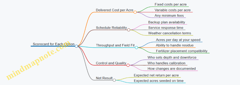
Integrated Recommendation Method
- Compute your on-time acres for each option using realistic field speed and available hours.
- Convert late acres into a cost using your own yield penalty estimate.
- Add delivered cost per acre for each option, including downtime risk as a schedule failure cost.
- Choose the option that minimizes expected total cost while meeting your on-time acres target.
If you want one rule of thumb: purchase is a control strategy, lease is a risk-sharing strategy, and custom hiring is a capacity strategy. The best choice is the one that matches the constraint you actually have—usually time, not money.
7.3 Estimating Depreciation Repair and Maintenance Under New Workloads
When you change tillage intensity, you change how machines wear. Estimating depreciation, repair, and maintenance under new workloads is mostly about translating “what will run more” and “what will run less” into dollars per acre and dollars per year. The goal is not perfect prediction; it’s a defensible baseline you can update after the first season.
Foundational Concepts That Drive the Numbers
Start with three buckets that often get mixed up:
- Depreciation is the value you lose as the machine ages, regardless of whether it breaks. It’s usually modeled as straight-line or declining balance.
- Maintenance is planned work like lubrication, wear-part replacement, and routine inspections.
- Repair is unplanned work like a broken gauge wheel, a hydraulic hose failure, or a bearing replacement after it overheats.
A simple rule: if it happens because time passes, it’s depreciation; if it happens because you used it, it’s maintenance or repair; if it happens because something failed, it’s repair.
Step 1: Define the New Workload in Operational Terms
Workload is not just acres. It’s also how hard the machine works.
Create a workload table for each key implement and tractor combination:
- Annual acres by field type (stubble, cover crop residue, wet spots)
- Operation hours (seeding, rolling, spraying, transport)
- Depth or aggressiveness (for tillage tools, residue managers, and closing systems)
- Field conditions frequency (how often you hit heavy residue or compaction)
Example: If you switch from chisel to no-till, your seeding pass may run at similar acres, but residue management might add an extra pass in some fields. That extra pass increases wear on bearings, belts, and hydraulic components even if tillage depth drops.
Step 2: Estimate Depreciation Under Changed Utilization
Depreciation depends on purchase price, salvage value, and useful life. Under new workloads, the useful life may change because wear patterns shift.
Use a practical approach:
- Estimate hours per year under the new system.
- Convert the machine’s useful life from “years” into hours if the manufacturer provides it, or use your own historical hours-to-replacement.
- Compute annual depreciation as:
Annual depreciation = (Purchase price − Salvage value) ÷ Useful life in years
If you expect replacement sooner due to higher hours, reduce the useful life in years proportionally.
Example: A seeder used to run 600 hours/year and now runs 900 hours/year. If your historical replacement happened at 6,000 hours, then useful life becomes 6,000 ÷ 900 = 6.7 years instead of 10 years. That increases annual depreciation even if repairs stay stable.
Step 3: Build Maintenance Costs from Wear-Item Cycles
Maintenance is easiest to estimate because it’s repeatable. Break it into:
- Scheduled service (oil changes, grease intervals, filter swaps)
- Wear parts (blades, discs, gauge wheels, closing wheels, hydraulic hoses inspection)
- Consumables (belts, bearings, fasteners, hydraulic fittings)
For each wear item, estimate:
- Replacement interval in hours or acres
- Unit cost installed or parts-only
- Labor cost per replacement
Example: If gauge wheels used to be replaced every 1,200 acres and no-till residue increases abrasive wear, you might replace them every 900 acres. If parts cost $55 each and you have 10 wheels, that’s $550 per replacement. Add labor, say $40 per replacement. Then maintenance per acre becomes (550+40) ÷ 900.
Step 4: Model Repairs Using Failure Rates and Severity
Repairs are harder because failures are lumpy. The best method is to use a “last time it happened” dataset from your own logs.
Create a repair list for each machine:
- Component (hydraulics, bearings, electrical, frame welds)
- Typical failure frequency (events per 100 hours or per 1,000 acres)
- Typical cost range (parts + labor)
- Downtime cost if you track it
If you lack data, start with conservative averages from your own history and adjust for workload differences. For instance, higher residue can increase plugging-related stress, which raises the chance of shear pin replacements and hydraulic strain.
Example: If you previously averaged 0.3 hydraulic hose failures per year at 600 hours/year, and new workload is 900 hours/year, scale frequency by hours: 0.3 × (900/600) = 0.45 failures/year. Multiply by expected cost per failure.
Step 5: Combine Into an Acre and Year Cost Summary
For each machine, compute:
- Annual depreciation
- Annual maintenance
- Annual repair
- Total annual cost ÷ annual acres = cost per acre
Then allocate costs to the relevant operations. A tractor’s depreciation might be shared across seeding and spraying, while a seeder’s wear parts belong mostly to seeding.
Mind Map: Depreciation Repair and Maintenance Estimation
Mini Example: Putting It Together for a Seeder
Assume a no-till seeder with 1,000 acres/year.
- Depreciation: $24,000 purchase, $4,000 salvage, 6.7-year life → ($24,000−$4,000)/6.7 ≈ $2,985/year.
- Maintenance: wear parts and scheduled service average $18/acre → $18,000/year.
- Repairs: expected $6,500/year based on scaled failure history.
Total machine cost ≈ $2,985 + $18,000 + $6,500 = $27,485/year, or $27.49/acre. That number becomes a line item you can compare against the alternative system’s seeding and residue approach.
Practical Checks That Prevent Common Estimation Errors
- If maintenance per acre rises but repairs fall, verify you didn’t accidentally move repair items into wear-part categories.
- If depreciation rises sharply, confirm the useful life change is justified by hours, not by wishful thinking.
- If cost per acre looks too low, check whether you allocated labor and downtime or only parts.
A good estimate is consistent with how the machine actually works in your fields. If the math contradicts the operating reality, the spreadsheet is lying, not the soil.
7.4 Assessing Tradeoffs Between Speed Accuracy and Throughput
Speed, accuracy, and throughput are a three-legged stool: improve one and the other two usually wobble. In no-till equipment planning, the goal is not “maximum speed,” but “enough speed to keep the system fed without turning measurement noise into bad decisions.”
Foundational Concepts for Tradeoff Thinking
Throughput is how many acres you can cover per day at acceptable quality. Accuracy is how closely the operation matches the target spec, such as seeding depth, row spacing, and residue handling. Speed is the travel rate that drives both throughput and the risk of quality drift.
A useful mental model is to treat quality as a probability distribution, not a single number. At low speed, the distribution is tight; at higher speed, it spreads. If your agronomic target has a “tolerance band,” then throughput is profitable only when the fraction of passes inside that band stays high enough.
Where Speed Hurts Accuracy in No-Till
Most no-till operations have a mechanical “contact problem”: the implement must manage residue, maintain depth, and place seed or fertilizer consistently while the ground surface varies.
Common failure modes that scale with speed:
- Depth variability: gauge wheels and openers can bounce more, especially on uneven residue mats.
- Seed placement inconsistency: closing wheels may not firm soil uniformly, increasing emergence variability.
- Row unit bounce and singulation drift: higher vibration can worsen metering performance.
- Residue flow and plugging: faster travel can overwhelm residue management, leading to intermittent skips or uneven cutting.
A practical rule: if your operation already struggles at “comfortable” speed, pushing faster usually increases the number of “bad acres,” not just the average quality.
Throughput Math That Doesn’t Lie
Start with a simple daily capacity equation:
- Effective field hours = available hours − setup − calibration − breaks − delays.
- Acres per day = effective hours × (width × speed) × field efficiency.
Field efficiency captures the reality that you won’t run at target speed the entire day. It drops when you must slow down for residue, adjust downforce, or handle skips.
Then connect throughput to accuracy by using a quality factor:
- Effective acres = acres per day × quality pass rate.
Quality pass rate can be estimated from short calibration checks and a few representative runs, not from vibes.
A Systematic Method to Find the “Right Speed”
- Define the target specs: depth range, singulation/spacing tolerance, and residue handling outcomes you can observe.
- Pick 3 speed settings: one conservative, one mid, one aggressive.
- Hold everything else constant: same downforce, same seedbed prep approach, same tire pressure, same residue condition.
- Measure quality on each speed: sample multiple locations across the field, not just the easiest patch.
- Convert measurements into pass/fail: count how many samples meet tolerance.
- Compute effective acres: acres per day × pass rate.
- Choose the speed that maximizes effective acres, subject to your risk tolerance.
This method keeps the tradeoff honest: you’re not optimizing speed in isolation, you’re optimizing the system’s usable output.
Mind Map: Speed, Accuracy, Throughput Links
Example: Seeding Speed Choice on a Residue-Heavy Field
Assume a planter width of 12 rows at 7.5 inches spacing, giving an effective working width of about 7.5 feet. You have 8 hours available, but only 6.5 hours are effective after setup and breaks.
- At 4.5 mph, you cover about 6.5 × (7.5/5280) × 4.5 × 0.90 ≈ 7.4 acres.
- At 5.5 mph, you cover about 6.5 × (7.5/5280) × 5.5 × 0.85 ≈ 8.1 acres.
Now add quality pass rates from sampling:
- 4.5 mph: 90% of samples within depth and placement tolerance → effective acres = 7.4 × 0.90 = 6.7.
- 5.5 mph: 75% within tolerance because residue mat bounce increases depth spread → effective acres = 8.1 × 0.75 = 6.1.
Even though 5.5 mph covers more acres, 4.5 mph produces more usable acres. The “winner” is the speed that maximizes effective acres, not the speed that looks fastest on paper.
Example: When Speed Can Increase Without Losing Accuracy
If your conservative speed is limited by setup inefficiency rather than mechanical limits, you can raise throughput without harming accuracy. For instance, if you currently calibrate too often because you lack a repeatable residue and downforce baseline, then improving calibration workflow can reduce downtime.
In that case, the quality pass rate stays similar because the implement dynamics are unchanged; the gain comes from higher effective field hours and fewer interruptions.
Practical Adjustment Triggers
Use clear stop-and-adjust rules so speed doesn’t quietly degrade quality:
- If depth samples drift beyond tolerance in two consecutive checks, slow down or adjust downforce.
- If residue plugging occurs, reduce speed until residue flow is stable, then re-check placement.
- If emergence risk indicators rise (for example, inconsistent seed-to-soil contact you can observe), treat it as a quality problem, not a “later problem.”
The point is simple: speed is a lever, but it needs measurement feedback. When you connect speed to pass rate, the tradeoff becomes a decision you can defend.
7.5 Planning Downtime and Backlog Costs During Equipment Transition
Equipment transition is where good agronomy plans meet the real world: machines break, schedules slip, and fields wait. Downtime is not just lost hours; it creates backlog that pushes later operations into less forgiving weather windows. The goal is to plan the transition so that the farm’s critical path stays critical, not chaotic.
Core Concepts for Downtime and Backlog
Start by separating three time buckets:
- Planned downtime: time you intentionally allocate for setup, calibration, and operator training.
- Unplanned downtime: breakdowns, parts delays, and troubleshooting.
- Backlog time: the spillover when a later operation cannot start because an earlier one is incomplete.
A simple way to think about backlog is “waiting cost.” If seeding slips, weeds and residue management may become harder, and fertility timing can miss the window where it matters most.
Build a Transition Timeline That Shows the Critical Path
List operations in order for each crop and field group. Then mark which operations are preceding constraints.
- If seeding is delayed, harvest timing may still be fine, but emergence and early weed control can suffer.
- If residue handling is delayed, seeding depth and seed-to-soil contact can become inconsistent.
Use a field grouping approach so you can model capacity realistically. For example, group fields by similar residue load and soil type, then assign each group to a seeding day range based on equipment throughput.
Estimate Downtime Using a Practical Method
For each key machine (planter/seeder, residue manager, sprayer, tractor/implement match), estimate:
- Setup hours per season (calibration, row unit checks, seed singulation verification)
- Average repair hours per week during transition (higher than steady-state)
- Parts lead time risk (how many days you can tolerate without the machine)
Example: If a new no-till drill requires 6 hours of setup and calibration in week 1, plus an expected 2 hours of minor adjustments during the seeding window, planned downtime might be 8 hours. If a hydraulic hose replacement typically takes 3 days to source, unplanned downtime risk becomes a scheduling constraint, not just a time loss.
Convert Lost Time Into Backlog Costs
Backlog costs come from three sources:
- Direct cost: extra labor overtime, custom hiring, additional fuel for rework.
- Yield and quality risk: uneven emergence, delayed weed control, and inconsistent stand.
- Operational friction: missed windows that force less ideal settings (higher seeding rates, more aggressive herbicide programs, or slower passes).
To keep this grounded, quantify each cost driver with a small set of measurable proxies.
- For yield risk, use historical sensitivity: “If seeding is delayed by X days, yield drops by Y% in similar years.”
- For weed control friction, use a cost proxy: “If burndown timing slips, add Z dollars per acre in additional applications or labor.”
Example: Suppose your sprayer can cover 120 acres per day. If seeding backlog pushes early post-emergence spraying from day 3 to day 8, you might need an extra day of spraying plus a second pass for patchy weeds. That becomes a backlog cost per acre based on acres affected.
Capacity Planning with Buffer Rules
A transition plan should include buffers that are tied to reality, not optimism. Use two buffers:
- Machine buffer: reserve a small number of hours each week for troubleshooting.
- Weather buffer: avoid scheduling the entire window at full capacity.
Example buffer rule: If your seeding capacity is 300 acres per day under normal conditions, schedule only 250 acres per day during the transition weeks. The remaining 50 acres worth of time is your “fix it” buffer.
Mind Map: Downtime and Backlog Planning
Example Workflow for a Two-Week Seeding Window
Assume you have 1,000 acres to seed across two weeks, and your seeder can cover 250 acres per day in ideal conditions. During transition, you schedule 2.5 days of work in week 1 and 2.5 days in week 2, leaving 1 day worth of buffer total.
- Week 1: complete setup and calibration on day 1 morning; seed the first field group by mid-day.
- Mid-week check: measure depth and emergence uniformity on a small sample area; adjust settings before backlog forms.
- Backlog trigger: if seeding falls behind by more than one field group by day 3, activate the response plan: shift labor, prioritize fields with lower residue risk, and schedule custom seeding for the most time-sensitive acres.
- Spraying alignment: lock the sprayer schedule to the expected emergence window, not the calendar. If seeding slips, you reschedule by emergence stage.
This approach keeps the plan operational: it uses measurable triggers, not vague “we’ll catch up later.”
Response Plan That Prevents Backlog from Spreading
When downtime happens, backlog spreads because tasks are interdependent. Your response plan should specify:
- Which fields get priority (those that preserve emergence timing)
- Which operations can be done in parallel (for example, fertility prep while seeding waits)
- What gets paused (non-critical adjustments that can wait until the machine is stable)
- How you document changes so the budget reflects reality rather than hope
Example: If the seeder is down, don’t spend the day “optimizing” settings on paper. Use the time for residue staging, seed lot checks, and sprayer calibration so that once the machine is running, you regain throughput quickly.
8. Herbicide and Weed Control Costing with No-Till Systems
8.1 Building Weed Control Budgets by Species and Growth Stage
A weed control budget is a field-by-field plan that turns weed biology into dollars. The core idea is simple: different species emerge at different times, respond differently to herbicide modes of action, and require different follow-up actions. When you budget by species and growth stage, you stop paying for “average weeds” and start paying for the weeds you actually have.
Step 1: Define the Weed Inventory by Species
Start with a practical inventory, not a perfect one. Use last season’s scouting notes and identify the dominant species by frequency and impact. Group minor species into a single “other” line item if they rarely drive yield loss.
Example: In a corn field, you might list:
- Giant foxtail (dominant summer grass)
- Waterhemp (dominant broadleaf, late emergence)
- Ragweed (early broadleaf)
- Volunteer rye (residual grass from cover)
For each species, record typical emergence timing in your region and the growth stage you usually see at the time of each planned operation.
Step 2: Map Growth Stages to Control Windows
Weed control works best when the product meets the weed at the right stage. Build a timeline with your operational windows: pre-plant, pre-emerge, early post, and late post. Then attach each species to the windows where it is most vulnerable.
A useful rule: if a species regularly escapes a window, you budget a second chance rather than hoping it behaves.
Step 3: Build Line Items for Each Species and Window
For each species, create a row of actions that could realistically occur in that window. Each action becomes a cost line item.
Common action types:
- Residual herbicide application (pre-emerge or early post)
- Burndown herbicide application (pre-plant or at planting)
- Post-emergence herbicide application (stage-specific)
- Spot treatment (sprayer time and labor)
- Mechanical touch-up (cultivation or inter-row tools where allowed)
Each action line item should include:
- Product cost per acre
- Application cost per acre (labor, fuel, wear)
- Adjuvant cost if required
- Any extra pass cost (if you must slow down or change equipment)
Example budget logic for waterhemp:
- Pre-emerge residual: targets early cohorts
- Early post: targets plants that emerged before crop canopy closes
- Late post or spot: targets late-emerging plants that residual missed
Step 4: Add Weed-Stage-Specific Quantities
Budgets become more accurate when you estimate coverage and dose based on stage. Two practical adjustments:
- If weeds are larger than the label’s ideal stage, you may need a higher rate or a different product, which changes cost.
- If you expect patchy emergence, you may plan spot treatments instead of full-field passes.
Example: If giant foxtail usually emerges in flushes, you might budget one full-field early post plus a smaller spot-treatment fraction later.
Step 5: Include Failure Modes as Explicit Costs
Instead of treating “control failure” as a surprise, budget for it as a conditional line item. The conditional part can be simple: “If escapes exceed threshold, apply follow-up.” You still keep it grounded by using a scouting threshold and a realistic follow-up action.
Example threshold approach:
- If waterhemp density exceeds your set level at the late post window, budget a second post application on the affected fraction.
Step 6: Summarize Into a Field Total and a Species Total
Once each species has its window-based actions, sum costs to get:
- Total weed control cost per acre
- Species contribution to that total
- Pass count and labor hours per acre
This species total is valuable because it shows whether your biggest cost is a single late-emerging species or a repeated early flush.
Mind Map: Weed Budgets by Species and Growth Stage
Example: Turning a Species Timeline Into Costs
Assume a 200-acre field with these planned windows:
- Pre-emerge residual applied at planting
- Early post at 2–4 inch weed stage
- Late post only if scouting shows escapes
For waterhemp, you budget:
- Residual pass (full field)
- Early post pass (full field)
- Late post spot treatment (fractional acres based on scouting)
For ragweed, you budget:
- Burndown at pre-plant
- No late post unless scouting shows unusual late cohorts
For giant foxtail, you budget:
- Residual pass
- Early post full field
- Spot treatment only after a second flush is confirmed
The result is a budget that mirrors how weeds actually behave, while keeping costs tied to specific decisions rather than vague averages.
8.2 Accounting for Application Timing and Weather Dependent Constraints
No-till weed control and fertility placement are less forgiving than conventional tillage because you’re relying on residue, soil structure, and crop stand to do more of the work. Timing and weather determine whether an application lands where it should, stays there long enough, and doesn’t accidentally pay the wrong bill.
Core Idea: Match the Application’s Job to the Window
Every input has a “job” and a “delivery requirement.” Herbicides often need contact with target tissue or a residual layer in the top inch. Fertility often needs moisture to move nutrients into the root zone or conditions that prevent volatilization and runoff. Weather constraints are the practical limits on meeting those requirements.
A simple way to account for timing is to treat each field operation as a sequence of gates:
- Can you apply safely and legally under conditions?
- Can you apply at the right crop stage or weed stage?
- Will the product reach the target (spray coverage, soil contact, infiltration)?
- Will it remain effective long enough (rainfastness, evaporation, wind drift)?
- Will it avoid damage pathways (runoff, drift to sensitive areas, stand stress)?
Weather Constraints That Change Effectiveness
Account for weather in two categories: immediate performance and downstream impact.
Immediate performance includes wind speed and direction, temperature, humidity, and the likelihood of rain soon after application. For example, a burndown herbicide applied on a warm, dry afternoon may evaporate faster than expected, reducing contact performance. A residual herbicide applied right before a heavy rain may wash too deeply, weakening the shallow residual zone.
Downstream impact includes soil moisture and infiltration rate. If the field is already saturated, a pre-emergence or residual program may create patchy weed control because water movement is uneven. If the soil is very dry, post-emergence uptake can be slow, and fertilizer placed without moisture may sit where roots can’t reach it.
Timing Constraints That Change the Biology
Weather is only half the story. Timing also depends on growth stages.
For weed control, the “right stage” is usually when weeds are small enough for the chosen mode of action to work efficiently. In no-till, residue can delay soil warming and emergence, so the same calendar date can produce different weed sizes across fields. That means your budget should be stage-based, not date-based.
For fertility, timing is about matching nutrient availability to crop demand. If you apply nitrogen too early and conditions favor loss pathways, you pay for nitrogen that never becomes plant-available. If you apply too late, the crop may show deficiency symptoms and you pay again through yield loss.
Accounting Method: Build a Timing-And-Weather Adjustment Factor
Use a field-level adjustment factor that modifies expected efficacy and expected yield impact.
- Start with a baseline efficacy assumption for the product at the correct stage.
- Apply a weather factor based on whether key constraints were met.
- Apply a timing factor based on whether the target stage alignment was within your acceptable window.
- Convert reduced efficacy into expected weed pressure or nutrient stress, then into yield impact.
Keep the factors simple and defensible. For instance, if rain occurred sooner than the product’s rainfast window, reduce expected residual performance. If wind exceeded your drift threshold, assume coverage gaps and increase the probability of escapes.
Mind Map: Timing and Weather Constraints Accounting
Example: Two Herbicide Applications with Different Weather Outcomes
Assume a 120-acre farm uses a two-pass system: a burndown plus a residual. Baseline expectation is 90% weed control from the residual when applied at the right weed stage with adequate soil contact.
-
Field A: Applied at early weed stage. Wind stayed below the drift threshold. No rain occurred for the rainfast window. You record good residue coverage and uniform spray pattern. Your efficacy factor stays near baseline, so you budget for minimal escapes.
-
Field B: Applied at the same calendar date, but weeds were slightly larger because emergence was delayed by cooler nights. Wind briefly exceeded the threshold and a light rain arrived sooner than expected. You adjust the residual efficacy downward and increase the probability of escapes. In the budget, you include a higher chance of a follow-up spot treatment and a small yield risk from early competition.
The key accounting move is that both fields share the same product and rate, but different timing alignment and weather gates change expected outcomes.
Example: Fertility Timing Under Moisture Constraints
Consider nitrogen placement on a no-till field with variable soil moisture.
-
Field C: Soil is moist and infiltration is good. You apply at a crop stage where roots can access the nutrient. Your budget assumes high nutrient use efficiency.
-
Field D: Soil surface is dry and the forecast shows no meaningful rainfall before the next growth stage. Even if the application is technically “on time,” the delivery requirement isn’t met. You reduce expected nutrient availability and account for a higher chance of yield loss or the need for an additional corrective application.
Practical Recordkeeping That Makes the Numbers Hold Up
To keep the economics honest, record three things for each application: the target stage observed in the field, the weather gates that were met or missed, and the operational details that affect delivery (spray pattern, nozzle setup, and whether residue coverage was adequate). When you do this, your timing-and-weather adjustment factors stop being guesses and start being measurable farm reality.
8.3 Evaluating Residual Programs and Burndown Sequences Economically
Residual herbicide programs and burndown sequences are where no-till economics get real: you’re paying for weed control now to avoid yield loss later, and you’re also paying for operational fit—timing, weather windows, and equipment capability. The goal is to choose a sequence that controls the target weeds with the least total cost per acre, while protecting stand establishment and reducing the chance of expensive “fix-it” passes.
Foundations for Economic Evaluation
Start by separating weed control into three cost buckets.
-
Application costs: fuel, labor, chemical cost, and any custom hire. If you add a second pass, you add more than chemical—think sprayer setup time and field traffic.
-
Yield risk costs: expected loss from inadequate control, delayed emergence, or crop stress. Even if you don’t measure yield loss directly, you can quantify risk using historical outcomes and stand counts.
-
Resistance and compliance costs: costs show up as higher future herbicide rates, additional modes of action, and the administrative burden of documenting what you used and when.
A practical way to keep this systematic is to compute expected cost per acre:
- Expected total cost = (direct costs) + (probability of failure × cost of failure)
Where “cost of failure” can be modeled as a yield loss value plus the cost of a rescue application.
Residual Programs: What You’re Actually Buying
Residual herbicides aim to control weeds as they germinate after burndown. Economically, they’re attractive when:
- You can seed into a relatively stable residue and soil surface.
- Rainfall or irrigation reliably activates the residual.
- Weed flushes are predictable enough that one residual step covers the critical early window.
They’re less attractive when:
- Activation is uncertain, such as long dry spells after application.
- Soil conditions reduce herbicide performance, including heavy residue that blocks contact and uneven incorporation.
- You face multiple weed cohorts with different emergence timing.
Example: A farm applies a residual program on April 5 and plans to seed April 10. If the forecasted activation window doesn’t materialize, the residual may underperform. The economic consequence is not just “weeds show up”—it’s that the crop may compete during establishment, forcing a later, more expensive post-emergence rescue.
Burndown Sequences: Timing and Targeting
Burndown is the “front door” treatment. It reduces existing weeds and sets the stage for residual performance. Economically, burndown sequences should be evaluated by how well they:
- Kill emerged weeds before seeding.
- Prevent regrowth that would compete with the crop.
- Avoid antagonism with residual products.
A common decision is whether to use a single burndown pass or a layered approach (for example, a contact burndown plus a residual component). The layered approach can reduce later weed pressure, but it increases direct costs and tightens timing windows.
Example: If rye cover is thick, a contact burndown alone may leave regrowth. That regrowth can force either a later burndown repeat or a post-emergence correction. A layered sequence can be cheaper overall if it prevents the rescue pass.
Building an Economic Comparison Framework
Use a field-by-field worksheet with these inputs.
-
Weed pressure profile: species, growth stage at application, and expected emergence timing.
-
Weather and activation risk: probability of adequate rainfall/irrigation within the residual activation window.
-
Crop and seeding constraints: seeding depth, emergence speed, and sensitivity to early competition.
-
Operational constraints: how many days you can shift seeding, and whether you can apply and seed without creating bottlenecks.
Then compare at least two options:
- Option A: burndown only, no residual.
- Option B: burndown plus residual.
For each option, estimate:
- Direct cost per acre.
- Probability of inadequate control.
- Expected rescue cost if control fails.
Example: Suppose Option A costs $28/acre in direct inputs, while Option B costs $45/acre. If Option A has a 25% chance of needing a $22/acre rescue and Option B has a 10% chance of rescue, expected rescue costs are:
- Option A: 0.25 × 22 = $5.50
- Option B: 0.10 × 22 = $2.20
So expected totals become $33.50 vs. $47.20. In this simplified case, Option A wins economically, but only if the yield loss from early competition is truly captured by the rescue assumption. If historical data shows larger yield penalties when residual fails, the balance can flip.
Mind Map: Economic Logic for Residual and Burndown Choices
Practical “Sequence Fit” Rules
-
Match residual to the weed emergence window: if weeds emerge in two distinct waves, a single residual may not cover both.
-
Protect the crop’s early competition window: if the crop is slow to emerge, the economic value of residual control rises because early weed pressure is more costly.
-
Use rescue triggers to avoid guesswork: define a threshold such as “weed density above X at crop stage Y” so rescue decisions are consistent and measurable.
Example: A farm sets a rule: if volunteer rye or broadleaf weeds exceed a set density by the crop’s 2-leaf stage, they apply a targeted post-emergence treatment. This turns “we’ll see” into a controlled cost decision, making the original residual choice easier to evaluate next season.
Worked Example: Comparing Two Sequences
Assume a field with mixed broadleaf weeds and a thick residue mat.
- Sequence 1: burndown only at $30/acre.
- Sequence 2: burndown plus residual at $48/acre.
From past seasons, Sequence 1 fails to keep weeds below threshold 30% of the time, and rescue costs average $25/acre. Sequence 2 fails 15% of the time with the same rescue cost.
Expected totals:
- Sequence 1: 30 + (0.30 × 25) = $37.50
- Sequence 2: 48 + (0.15 × 25) = $51.75
If the farm’s historical yield penalty from early competition is already reflected in the rescue cost, Sequence 1 is cheaper. If not, you add an additional yield loss term to the failure cost, and the comparison becomes more sensitive to early-season weed control quality.
The economic takeaway is straightforward: residual programs are worth paying for when they reliably reduce the probability and severity of failure during the crop’s most vulnerable establishment period, and when the operational timing supports activation rather than hoping for it.
8.4 Incorporating Mechanical Options Without Breaking No-Till Boundaries
Mechanical weed control can fit inside no-till, but only if you treat it as a system constraint rather than a one-off fix. The boundary is simple: you can disturb the soil surface enough to cut weeds, but you should avoid turning, burying residue, or creating a seedbed that behaves like tilled ground.
Foundational Boundary Rules
Start with three practical rules that keep the system coherent.
- Residue stays on top. If your operation consistently drags residue into furrows, you’re effectively re-creating tillage. A good mechanical setup leaves a continuous mulch layer, even if it’s slightly shredded.
- Seed contact stays limited. Mechanical tools can expose weed seeds to light and warmth. That’s fine when you’re targeting existing weeds, but it’s costly if you also create new germination windows.
- Depth stays shallow and consistent. Most no-till weed cutting happens at or near the surface. If you need repeated passes to get control, the problem is usually timing, tool choice, or residue interference—not “more depth.”
A quick example: suppose a field has heavy rye residue and you run a shallow rotary hoe. If the residue mat blocks the blades, you’ll either miss weeds or you’ll push deeper to compensate. Either way, the no-till boundary gets crossed. The fix is to adjust residue management and timing so the tool can work at its intended depth.
Mind Map: Mechanical Options Inside No-Till
Timing and Targeting: The Part That Actually Determines Success
Mechanical control is mostly about timing. Weeds are easiest to stop when they’re small and still have limited stored energy. If you wait until weeds are tall, you’ll need multiple passes or deeper cutting, which increases residue disturbance and crop risk.
Example: In a corn field with a cover crop, you plan to seed into a thick mat. If you terminate the cover crop too early, it regrows and you end up cutting larger weeds later. The rotary hoe then has to work harder, and residue gets lifted and redistributed. If you terminate closer to seeding and seed into a uniform mulch, the same rotary hoe pass can cut weeds at the right stage with less residue disruption.
Tool Choice by Crop Stage and Row Geometry
Mechanical options differ in where they can operate.
- Between-row tools (stirrup hoe, row cultivator) rely on crop rows being distinct. If emergence is uneven, the tool can hit plants or leave weeds untouched.
- Surface tools (rotary hoe) can work across the row, but they are more likely to disturb residue and expose soil if the crop canopy is fragile.
- Top-kill tools (mower-style cutting) are often best before seeding or during fallow periods because they reduce weed biomass while leaving the mulch layer largely intact.
Example: If you have a soybean field with wide rows, a stirrup hoe can run after emergence when plants are established and the inter-row space is clear. If you try the same approach in a narrow-row crop, you’ll either miss weeds or risk plant damage.
Keeping the No-Till Boundary Intact During Passes
Mechanical passes should be treated like controlled experiments: one change at a time, with clear success criteria.
- Set depth to the minimum that cuts. Use a consistent depth setting and verify it across the field. If you see soil smearing or residue burial, depth is too aggressive.
- Limit pass count. Two well-timed passes often beat three late ones. Extra passes increase fuel, labor, and the chance of residue disruption.
- Match residue to tool clearance. If residue is too thick, the tool may bounce and fail to cut. If residue is too sparse, you lose mulch protection and increase soil exposure.
Example: A farm runs a rotary hoe after seeding but before crop emergence. The weeds are small, so control is good. However, the residue is so sparse that the soil surface dries and crusts, and the crop struggles to emerge uniformly. The boundary wasn’t broken by tillage depth, but it was broken by residue management. The fix is to adjust cover crop termination so you keep enough mulch for emergence while still allowing weed cutting.
Economic Integration: Costing Mechanical Control as a System Variable
Mechanical weed control costs are not just fuel and wear. They include the risk of yield loss from crop disturbance and the cost of additional herbicide or rework if control is inconsistent.
A practical budgeting approach:
- Estimate passes per season by field and crop stage.
- Assign a disturbance risk factor based on crop stage sensitivity and expected residue interference.
- Compare against herbicide-only or hybrid plans using the same weed-control target date.
Example: If a mechanical plan reduces herbicide cost but forces an extra pass because control is unreliable, the net benefit may disappear once labor and yield risk are included. The “best” plan is the one that reliably hits the weed target with the fewest system disruptions.
Implementation Checklist for Mechanical Options
- Confirm row spacing and emergence uniformity before choosing between-row tools.
- Terminate cover crops so weed cutting happens at small growth stages.
- Set shallow, consistent depth and verify residue behavior after the first pass.
- Use pass count limits and treat each pass as a measurable decision.
- Budget mechanical control as disturbance plus labor plus fuel, not only equipment time.
8.5 Documenting Resistance Management Costs and Operational Tradeoffs
Resistance management is mostly a bookkeeping problem with a field reality attached. You’re trying to record what you did, what it cost, and what it changed—so you can tell whether the plan is working or just spending money politely.
Core Documentation Goals
Start by separating three things in your records: (1) herbicide inputs, (2) operational choices, and (3) outcomes. Herbicide inputs include product, rate, carrier, adjuvants, and application timing. Operational choices include sprayer setup, travel speed, boom height, nozzle type, and whether you used a burndown plus residual sequence. Outcomes include weed control scores, escapes by species, stand impacts, and any crop injury notes.
A practical rule: if you can’t connect a cost line to a specific operational decision and a specific weed-control event, it won’t help you manage resistance.
Cost Categories That Actually Matter
Record costs in categories that map to resistance risk.
- Active ingredient and adjuvant costs: product price, adjuvant rate, and any tank-mix components.
- Application labor and machinery: operator time, fuel, and maintenance tied to that pass.
- Operational overhead: calibration time, extra passes, and downtime caused by residue or weather windows.
- Non-chemical control costs: mowing, tillage spot work, cultivation, or additional cover crop termination steps.
- Learning and verification costs: sampling time for weed counts and control scoring, plus any re-sprays.
Example: If you add a mechanical pass to reduce reliance on one herbicide group, you should record that pass as a resistance-management cost, not as “general field work.” Otherwise, the budget will look artificially cheap.
Operational Tradeoffs to Record
Resistance management often trades one kind of risk for another. Document the tradeoff explicitly.
- Timing tradeoff: Earlier burndown may cost more in labor or require different equipment scheduling, but it can reduce the chance that weeds survive to seed.
- Coverage tradeoff: Higher water volume or slower travel improves coverage, but it increases time and fuel.
- Sequence tradeoff: Using a different mode of action later can protect the earlier product, but it may require a second application window.
- Crop safety tradeoff: Some residual programs reduce weed pressure but can increase crop injury risk under stress; record injury observations and weather context.
Mind Map: Resistance Management Records
Example: Turning Field Notes Into a Costed Decision
Suppose you manage a field with heavy waterhemp pressure. Your plan uses a burndown plus residual sequence, then a post-emergence option only if escapes exceed a threshold.
- Event 1: Burndown with Group A at labeled rate plus an adjuvant. Record calibration time (e.g., 45 minutes), water volume, and travel speed.
- Event 2: Residual with Group B. Record whether you had to delay due to rain and whether the delay changed weed size at application.
- Event 3: Post-emergence rescue with Group C only on spots where control scores were below your threshold.
Now cost it properly. If you spent extra labor to apply at the right weed stage, that labor is part of resistance management. If you skipped a second pass because the first sequence held, record the savings as “avoided re-spray cost,” not as “no cost.”
Example: Operational Tradeoff That Looks Like a Savings
You might be tempted to reduce water volume to save time. If you do, document the outcome. If control scores drop or escapes increase, the “savings” becomes a later cost: more rescue applications, more spot mechanical work, and more sampling time. The record should show the chain from operational choice to weed survival to added management.
Building a Simple Resistance Cost Ledger
Use one ledger row per herbicide event and one per non-chemical event. Each row should include the weed species targeted, the mode of action group, the operational settings, and the verification result.
A clean ledger lets you compute two useful metrics without guessing:
- Cost per effective control event: total resistance-management cost divided by the number of events that met your control threshold.
- Cost per escape: total cost divided by the number of escapes by species in the scored area.
If cost per escape rises after a change in sequence or application settings, you’ve learned something concrete—even if the total spend stayed the same.
Verification Notes That Prevent Confusing Data
Record what you observed, not what you hope happened. Include:
- Weed growth stage at application
- Weather conditions during and after spraying
- Any crop stress (wet spots, compaction, nutrient deficiency)
- Whether escapes were clustered (suggesting coverage issues) or scattered (suggesting survival)
This prevents a common mix-up: coverage problems can mimic resistance, and resistance can be mistaken for poor timing. Your notes should help you tell the difference.
Mind Map: What to Write Down After Each Pass

Closing Principle
Documenting resistance management costs is not about making the spreadsheet look impressive. It’s about making the next decision easier: you want to know which operational choices reduced survivors, which increased them, and which costs were paid to prevent resistance rather than to clean up after it.
9. Fertility and Nutrient Management Economics Under Soil Regeneration Goals
9.1 Comparing Fertility Placement Methods for No-Till Profitability
No-till changes where nutrients end up, how fast they move, and how reliably roots can access them. Fertility placement is the lever that most directly affects early root growth, stand uniformity, and nutrient use efficiency—especially during the transition years when residue and soil structure are still settling into a new rhythm.
Core Idea: Placement Controls Root Access
Nutrients are only profitable when roots can reach them at the right time. In no-till, residue can slow soil warming and water infiltration patterns can shift, so early-season access matters more than in tilled systems. Placement methods mainly differ in three ways: (1) distance from the seed or root zone, (2) concentration in a small band versus spread over the field, and (3) timing relative to crop uptake.
Mind Map: Fertility Placement Compared
Step 1: Define What “Profitability” Means for Placement
Start with a simple scorecard per acre:
- Net return = expected yield × price − all fertility and application costs.
- Risk adjustment = how much yield drops when conditions are poor (cold, wet, dry, or weedy).
- Operational fit = whether the placement method can be executed at the right time without slowing seeding.
Example: If a banded program costs $12/acre more than broadcast but reduces yield variability enough to keep returns above break-even in most years, it can win even with a smaller average yield gain.
Step 2: Compare Broadcast Fertility in No-Till
Broadcast fertilizer spreads nutrients across the surface. In no-till, the nutrient must move downward through rainfall, irrigation, or biological activity.
- Best fit: fields with reliable early moisture and residue management that doesn’t trap water.
- Common failure mode: nutrients stay near the surface when early rainfall is limited, so roots encounter them later than the crop needs.
Easy example: Apply phosphorus broadcast before seeding. If the first month is dry, roots may grow but not find much available P in the top inch. A band placed at seeding would have put P where roots start.
Step 3: Compare Band at Seeding for Early Access
Band placement concentrates nutrients in a narrow zone near where roots will grow.
- Best fit: crops that need early growth, and fields where residue delays nutrient movement.
- Key tradeoff: higher local concentration can increase injury risk if rates are too high or if fertilizer chemistry is harsh near the seed.
Easy example: Use a starter band with a modest nitrogen-phosphorus rate. In a cool spring, seedlings often grow slowly. The band helps them access phosphorus immediately, improving early root branching and reducing the chance of a thin stand.
Step 4: Compare In-Row or Seed-Adjacent Placement
In-row placement puts fertilizer extremely close to the seed.
- Best fit: when equipment precision is high and rates are conservative.
- Main risk: salt injury or ammonia-related stress, especially in dry conditions where fertilizer solution is concentrated.
Practical example: If you run higher nitrogen in the furrow during a dry week, you can see uneven emergence. The same setup in a wetter week may look fine. Profitability depends on matching placement chemistry and rate to expected early moisture.
Step 5: Compare Deep Placement for Moisture-Driven Uptake
Deep placement targets nutrients below the surface where moisture may persist.
- Best fit: fields with dry topsoil patterns or where subsoil moisture is consistently available.
- Main limitation: roots must reach the deeper zone; if the crop stays shallow early, nutrients may be underused.
Easy example: Deep-placed potassium can help in sandy soils where surface K is prone to leaching or where roots struggle to find K in the top layer during droughty springs.
Step 6: Compare Split Applications for Matching Uptake
Splitting places part of the nutrient early and part later.
- Best fit: nitrogen management where uptake timing is critical.
- Economic logic: you reduce the chance of early loss while still supporting early growth.
Example: Apply a smaller starter nitrogen amount at seeding, then topdress after stand establishment. If early weather is wet, less nitrogen is exposed to loss; if early weather is dry, the starter still supports growth.
Step 7: Use a Side-by-Side Evaluation Method
To compare methods without guesswork, evaluate by field zones:
- Choose zones with similar soil texture and residue levels.
- Keep everything else constant: seed variety, seeding rate, weed control timing.
- Track emergence uniformity and early vigor, not just yield.
- Compute per-acre economics using actual application costs and realistic yield ranges.
A simple rule: if a placement method improves early uniformity, it often improves yield stability too. That stability is a real economic asset, not just a nice agronomic outcome.
9.2 Estimating Nutrient Use Efficiency Changes from Soil Condition Shifts
Nutrient use efficiency (NUE) is the bridge between soil condition and profit. When soil structure, organic matter, and biological activity improve, nutrients often become easier to access and losses often shrink. The tricky part is estimating how much of that change is real and how much is just weather doing weather things.
Foundational Concepts That Make NUE Measurable
Start with what you can observe and what you can calculate.
- NUE as a ratio: A common farm-level form is “nutrient recovered” divided by “nutrient applied.” If you don’t measure plant uptake directly, you estimate it from yield and tissue or from yield response curves.
- Soil condition shifts: Improvements like better aggregation, infiltration, and residue decomposition change the timing and location of nutrient availability. That affects both how much crop can use and how much escapes.
- Loss pathways: Nitrogen losses often include leaching, denitrification, and volatilization. Phosphorus losses are more tied to erosion and runoff. Potassium losses are usually linked to erosion and crop removal patterns.
A useful mental model is: soil condition changes the “delivery system,” and NUE measures how well the crop receives the delivery.
A Systematic Estimation Workflow
-
Define the nutrient and the efficiency metric
- For nitrogen, choose either grain yield response efficiency (yield per unit N) or a recovery-style estimate using tissue tests.
- For phosphorus and potassium, use yield per unit applied and adjust for soil test levels.
-
Separate soil-driven effects from management and weather
- Keep seeding rate, variety, and planting date as consistent as possible in your comparison fields.
- Use multi-year yield records to reduce the “one wet spring fooled me” problem.
-
Quantify soil condition change using practical indicators
- Look for measurable shifts like improved infiltration (faster water entry), reduced crusting, more uniform emergence, and soil test trends.
- If you track infiltration or compaction proxies, treat them as explanatory variables, not as the final answer.
-
Estimate nutrient availability and uptake changes
- If you have tissue tests, compare nutrient concentration and sufficiency ranges at key growth stages.
- If you don’t, use yield response and soil test baselines to infer whether the crop is using applied nutrients more effectively.
-
Compute NUE change as a difference in response, not just a difference in yield
- Example: If yield rises but N rates also changed, you need to normalize. NUE change is about “more yield per unit nutrient,” not “more yield.”
Mind Map: Linking Soil Condition to Nutrient Use Efficiency
Concrete Example: Nitrogen Efficiency After Better Soil Structure
Assume a farm compares two no-till management blocks over three years.
- Block A (baseline soil condition): average yield 140 bu/ac with 160 lb N/ac applied.
- Block B (improved soil condition): average yield 152 bu/ac with 160 lb N/ac applied.
If N rates were the same, the NUE change is straightforward: yield per unit N rises.
- Yield per lb N in A: 140 / 160 = 0.875 bu per lb N
- Yield per lb N in B: 152 / 160 = 0.950 bu per lb N
- Relative NUE improvement: (0.950 − 0.875) / 0.875 ≈ 8.6%
Now add nuance. If Block B also had better emergence and less early waterlogging, that likely improved uptake efficiency and reduced losses. If you also have tissue data showing higher N concentration at V6–V8 without higher N rate, that supports the uptake explanation rather than a “just a better year” explanation.
Concrete Example: Phosphorus Efficiency with Soil Test Trends
Phosphorus often behaves differently because soil test P reflects a pool, not just a delivery event. Suppose:
- Block A: soil test P (Mehlich-3) averages 18 ppm; yield response to P is modest.
- Block B: soil test P averages 24 ppm after consistent residue cover and reduced erosion; yield increases at the same P rate.
To estimate NUE change, normalize yield by P applied and check whether the soil test increase explains the response. If yield rises more than expected from soil test alone, that suggests improved root access and reduced runoff losses. If yield rises less, it may indicate that P is abundant but not reaching roots due to localized compaction or poor early root growth.
Practical Guardrails That Prevent Bad Estimates
- Don’t treat soil test numbers as direct NUE: they describe pools; NUE is about recovery and response.
- Use matched comparisons: same crop, similar planting windows, and comparable residue and weed control.
- Watch for confounders: if improved soil condition coincides with a different N timing or a different hybrid, your NUE attribution gets messy.
- Quantify uncertainty: use the spread across fields or years to express a range, not a single magic percent.
When you estimate NUE change this way, you end up with a defensible number you can plug into budgets—one that reflects how soil condition changes nutrient delivery and crop recovery, not just how the season treated you.
9.3 Costing Cover Crop Termination and Nutrient Contribution Accounting
Cover crop termination is where agronomy meets accounting. You’re not just ending growth; you’re converting biomass into future nutrient availability, weed suppression, and soil cover. The goal of this section is to cost termination actions accurately and then translate nutrient contributions into numbers you can compare across fields and years.
Core Concepts for Termination Costing
Termination has three cost buckets: (1) direct operation costs, (2) timing and risk costs, and (3) downstream nutrient and weed effects that change the next crop’s input needs.
Start with a simple rule: if the termination step changes what you do next (herbicide timing, fertilizer rate, seeding depth, or stand quality), it belongs in the economic model. If it only changes how you feel about the cover crop, it doesn’t.
Termination Methods and What They Usually Cost
Common termination methods include rolling/crimping, mowing, herbicide burndown, and mechanical cultivation. Each method has a different mix of fuel, labor, chemical, and equipment wear.
- Herbicide burndown often costs more in chemical and application time, but it can be faster and more consistent when weather is cooperative.
- Rolling/crimping can reduce herbicide use, but it may require specific growth stage and may increase the chance of incomplete kill if moisture and maturity don’t cooperate.
- Mowing can be cheaper per pass, yet it may require additional passes or follow-up control if regrowth occurs.
- Mechanical cultivation can be effective but can also increase soil disturbance, which may conflict with no-till goals and can raise fuel and labor costs.
Step-by-Step Termination Cost Build
Use a field-year worksheet with line items. For each termination action, record the date, field, method, rate, and pass count. Then attach unit costs.
1) Direct Operation Costs
Direct costs include:
- Labor: hours × wage rate (include supervision if you track it).
- Fuel and lubrication: fuel burn per hour × fuel price.
- Equipment: depreciation or ownership cost per hour plus repair and maintenance per hour.
- Chemicals: product cost plus adjuvants and any tank-mix components.
- Application: if you use custom work, use the custom rate per acre.
Example: If you terminate 120 acres with a burndown pass that takes 0.6 machine-hours per acre, and your all-in machine cost is $55 per machine-hour, the base operation cost is 120 × 0.6 × 55 = $3,960. Add herbicide cost per acre and labor if labor is not already included in the machine rate.
2) Timing and Risk Costs
Timing affects whether the next crop establishes cleanly. Risk costs are not guesses; they’re budgeted based on measurable outcomes you’ve seen.
Track two practical risk drivers:
- Incomplete termination leading to higher weed control needs or stand losses.
- Seedbed conditions affecting seeding depth, emergence uniformity, and replant likelihood.
Example: If in the last three years, fields terminated with a late roll required an extra herbicide pass on 30% of acres, you can budget an expected extra cost: extra pass cost per acre × 0.30.
Nutrient Contribution Accounting That Doesn’t Pretend
Cover crop nutrient contribution accounting should be conservative and operational. You’re estimating what the next crop can use, not what the cover crop “contains.”
The Two-Stage Approach
- Estimate nutrient in biomass at termination.
- Estimate plant-available fraction that actually becomes available to the next crop.
Biomass estimation can come from local sampling, extension-style yield tables, or your own historical measurements. If you don’t have measurements, use a consistent assumption and keep it field-specific by cover type and termination stage.
Nutrient Fractions by Nutrient Type
- Nitrogen (N): availability depends on residue carbon-to-nitrogen ratio, moisture, temperature, and time between termination and seeding. Use a fraction that reflects your conditions and termination timing.
- Phosphorus (P) and potassium (K): these are less about mineralization timing and more about whether roots and residue placement make them accessible. Still, not all nutrient becomes available immediately.
A practical method is to use a “credit” that reduces fertilizer needs only when it’s supported by your soil test and yield response history.
Integrated Example Worksheet
Assume a rye cover crop terminated 10 days before planting corn.
- Estimated biomass N at termination: 60 lb N/acre
- Plant-available fraction to corn: 25%
- Estimated N credit: 60 × 0.25 = 15 lb N/acre
If your usual starter plus sidedress plan applies 160 lb N/acre and you can reduce by 15 lb without hurting yield, your N credit is worth the fertilizer cost of 15 lb N.
If urea-equivalent cost is $0.70 per lb N, the nutrient credit is 15 × 0.70 = $10.50/acre.
Now integrate termination costs. Suppose termination costs are $28/acre for burndown and $18/acre for rolling. If rolling has a 10% chance of extra weed control costing $12/acre, expected rolling cost is 18 + 0.10 × 12 = $19.20/acre.
Net difference per acre: rolling termination cost advantage is 28 − 19.20 = $8.80/acre. If both methods yield the same N credit, rolling wins on cost. If rolling reduces termination completeness and forces higher N due to stand variability, you adjust the N credit downward or add a risk cost.
Mind Map: Termination Cost and Nutrient Accounting
Practical Accounting Controls
To keep the numbers honest, standardize three items across fields: termination stage definition, pass counting rules, and how you treat fertilizer credits when soil tests show low or high baseline nutrients. When those controls are consistent, your comparisons stop being arguments and start being calculations.
Finally, record the termination date and method in your worksheet. Even if you don’t use the date directly in the model, it helps you explain why a fraction or risk probability changed when it did.
9.4 Managing pH and Soil Test Driven Amendments in No-Till Contexts
Why pH Changes Behave Differently Under No-Till
In no-till, you still manage pH, but you manage the path by which amendments reach roots. Tillage mixes lime and soil; no-till relies on natural movement, residue contact, and time. That means pH correction is usually slower and more uneven across a field, especially where residue concentrates or where wheel tracks and compaction create micro-zones.
A practical starting point is to treat soil tests as a map of where pH is off, not just a single number. If you sample only once per field, you may correct the average while missing the pockets that limit yield. If you sample by management zones, you can target amendments and avoid over-liming areas already near target.
Interpreting Soil Tests for Amendment Decisions
Soil test reports typically include pH, buffer pH, base saturation, and sometimes exchangeable acidity and cation levels. For no-till, the key is matching the amendment to the limiting mechanism:
- If pH is low and buffer pH is also low, lime is usually the correct lever.
- If pH is acceptable but calcium or magnesium is low, you may need a nutrient-focused amendment rather than more lime.
- If pH is low but the soil test shows low buffering capacity, smaller doses may move pH faster, but they can also require more frequent re-checking.
Example: A field tests pH 5.2 with low base saturation in the low spots. The same field tests pH 6.0 on the knolls. Applying one uniform lime rate risks wasting money on knolls while leaving low spots under-corrected.
Choosing Amendment Type and Rate
Lime materials differ in neutralizing value and particle size. Finer material reacts faster, but it can also be more variable in application if spreading is inconsistent. Rate selection should be based on the target pH and the soil’s buffering response, not just the current pH.
A no-till-friendly approach is to split the correction into phases:
- Apply the portion needed to reach the target in the most limiting zones.
- Re-test after a reasonable interval to confirm movement.
- Apply a follow-up adjustment if needed.
This reduces the chance of overshooting pH in already-correct zones.
Timing Amendments Around Residue and Seeding
Residue can affect amendment contact. Lime spread on heavy residue may not reach soil uniformly, and broadcast incorporation is limited. Timing should therefore align with conditions that improve contact and distribution:
- Apply before a period with moisture that supports movement.
- Avoid applying right before a long dry spell.
- Coordinate with seeding so you don’t create a residue-and-amendment “stack” that stays on the surface.
Example: If you plan to seed in early spring, applying lime in late fall can allow contact and movement before seeding. If you must apply in spring, choose a window where rainfall or irrigation can help move lime off the residue and into the soil surface layer.
Placement and Application Quality in No-Till
Because no-till limits mixing, application uniformity matters more. Calibrate spreaders, verify output across the swath, and check for overlap patterns. If you use variable-rate application, base it on soil test zones and keep the rate map aligned with how you actually drive the field.
A simple quality check: after spreading, look for consistent color and coverage patterns. If you see streaks, you likely have rate variation that will show up later as patchy pH.
Managing Acidifying Inputs Without Fighting Yourself
Some fertilizers and nutrient programs can push pH downward over time. Under no-till, the correction burden can accumulate because mixing is limited. The integrated move is to pair amendment planning with nutrient management:
- Use soil tests to set nutrient rates rather than assuming the same rates every year.
- Match nitrogen form and rate to crop needs.
- Keep an eye on long-term trends in pH and base saturation by zone.
Example: A field repeatedly receives high rates of ammonium-based nitrogen. Even if lime is applied once, pH may drift back faster in the zones where nitrogen demand is highest and residue contact is lower.
Mind Map: Soil Test Driven Amendment Workflow
Case Example: Zone-Based Lime with Follow-Up Adjustment
A farm samples a 200-acre field in three management zones. Zone A (low spots) tests pH 5.0; Zone B tests pH 5.6; Zone C tests pH 6.1. The plan is to apply a higher lime rate to Zone A and a lower rate to Zones B and C using variable-rate spreading. Lime is applied in late fall, then the field is seeded in spring.
After the next soil sampling cycle, Zone A reaches the target range, while Zone C remains near target. The follow-up action is limited to Zone B only, using a smaller adjustment rate. The economics improve because the farm avoids paying for lime where pH was already acceptable, and the agronomy improves because the limiting zones are corrected first.
Practical Checklist for No-Till pH Management
- Sample and interpret by zone, not just field average.
- Choose amendment type based on neutralizing value and particle size.
- Use phased correction when pH is far from target.
- Apply when moisture can help move lime off residue and into the surface layer.
- Calibrate and verify spreader uniformity.
- Coordinate lime with nitrogen and fertility plans to prevent repeated acidification.
- Re-test by zone and adjust with targeted follow-up rates.
Example date reference: Soil sampling conducted on 2026-03-20 can be used to anchor the amendment verification interval for the following crop season.
9.5 Tracking Nutrient Carryover Effects on Multi Year Budgets
No-till changes how nutrients move through the system. Some nutrients become easier to keep in the root zone because soil structure improves; others can become harder to manage because residues, stratification, and timing effects shift where and when nutrients show up. Multi-year budgeting is where these differences stop being “interesting” and start being money.
Core Idea for Carryover
Nutrient carryover is the portion of nutrients applied in one year that still influences crop performance and costs in later years. In budgets, you track it as a balance: what you applied, what the crop removed, what stayed in soil pools, and what you may need to apply again.
A practical way to think about it is three buckets:
- Crop removal: nutrients leaving the field in harvested product.
- Short-term soil availability: nutrients that affect the next season’s crop.
- Longer-term pools: nutrients that may matter later, especially when soil organic matter and pH stabilize.
Step 1: Build a Nutrient Ledger by Field and Year
Start with a simple ledger for each field and each nutrient you care about (often N, P, K, and sometimes S and micronutrients). For each year, record:
- Applied nutrients by source and timing (fertilizer, manure, compost, cover crop termination).
- Crop yield and nutrient removal estimates (based on typical nutrient content for your crop and yield).
- Soil test results at consistent intervals.
Example: A field grows corn in Year 1 and soybeans in Year 2. In Year 1 you apply 180 lb N/acre split into two applications. In Year 2 you apply 0 lb N/acre for soybeans (or a small starter amount). Your ledger should still include Year 1 N as a potential contributor to Year 2 soil availability, even if soybeans don’t “need” N the same way corn does.
Step 2: Separate carryover into “availability” and “availability timing”
Carryover isn’t only how much nutrient remains; it’s also when it becomes available.
- Availability: how much nutrient is in forms plants can use.
- Timing: whether it becomes available early enough for the crop’s critical growth stages.
No-till can shift timing because residues slow soil warming and can change mineralization rates. That means a nutrient may be present but not useful when the crop needs it.
Example: You apply P in Year 1. If no-till causes P stratification near the surface, the next crop may show different early growth than expected, even if total P levels look similar. Your budget should treat this as a timing effect, not just a quantity effect.
Step 3: Use Soil Tests and Yield Response as Calibration Signals
Soil tests are snapshots; yield response is the field’s report card. Combine them to estimate how your system is behaving.
- If soil test P is stable but yields rise, you may be improving nutrient use efficiency.
- If soil test K is stable but yields drop, timing or placement may be off.
Keep the logic consistent: soil tests guide the direction of nutrient balances, while yield response helps you decide whether the nutrient was actually available when needed.
Mind Map: Nutrient Carryover Tracking Logic
Step 4: Convert Carryover Into Budget “Credits” Without Pretending Certainty
In budgets, carryover credits should be conservative and tied to evidence. Use a range rather than a single number when you have limited history.
A simple method:
- Start with a baseline nutrient recommendation for the target crop.
- Estimate a carryover credit from prior-year applications and soil test trends.
- Reduce the current-year application by the credit amount.
- Keep a contingency line in the budget for re-application if early-season indicators show the nutrient isn’t available.
Example: Year 1 K application is 120 lb K2O/acre. Year 2 soil test K is similar to Year 1 and yields are steady. You might credit part of the K carryover (say 30–50 lb K2O/acre) toward Year 2 needs, while still planning a small adjustment option if early growth is weak.
Step 5: Track Interactions That Change Carryover Behavior
Nutrients rarely act alone. Two interactions matter most for no-till budgeting:
- N with residue and mineralization: residue can increase microbial demand early, affecting how much N is available.
- P with placement and soil stratification: surface accumulation can change early uptake.
Example: If you increase residue from a cover crop in Year 1, you may see lower early N availability in Year 2 even when total N inputs are unchanged. Your ledger should reflect that the carryover credit for N is smaller in the early part of the season.
Step 6: Build a Field-Level Multi-Year Table That Shows the Logic
Use a table structure in your budget workbook:
- Rows: years (Year 1, Year 2, Year 3)
- Columns: nutrient applied, estimated removal, carryover credit, current-year application, soil test trend notes
Example structure for one nutrient (K):
- Year 1: apply 120, removal 80, carryover credit estimate 40
- Year 2: apply 60 (after credit), removal 70, carryover credit estimate 20
- Year 3: apply 80 (after credit), removal 75, carryover credit estimate 15
The key is that the carryover credit is an accounting tool tied to your observed soil and yield signals, not a wish.
Step 7: Validate with a “No-Surprises” Review After Harvest
After each harvest, update the ledger with actual yield and revised removal estimates. Then adjust carryover credit assumptions for the next planning cycle. This keeps your multi-year budget from drifting into fantasy math.
Example: If yields in Year 2 were lower than expected despite a carryover credit, reduce the credit next time or shift it from “amount” to “timing” by changing application timing or placement in the budget assumptions.
10. Multi Year Budgeting and Cash Flow Under Transition Periods
10.1 Constructing Multi Year Budgets with Year Specific Assumptions
A multi-year budget is a field-by-field plan that treats each year as its own mini-world. You keep the same accounting structure, but you allow assumptions to change because soil regeneration, weed pressure, and equipment wear do not follow a neat calendar. The goal is not to predict the future perfectly; it is to build a budget that explains how costs and returns move as management changes.
Step 1: Lock the Budget Skeleton Before You Fill Numbers
Start with a consistent set of categories so you can compare Year 1 to Year 3 without mixing apples and slightly different apples.
- Revenue: yield, price, quality adjustments, and any carbon payments you are accounting for.
- Variable costs: seed, fertility, herbicides, cover crop costs, custom work, fuel, and repairs tied to field operations.
- Fixed costs: land rent, insurance, overhead, and equipment ownership costs that do not change with acres in the short run.
- Transition costs: one-time or front-loaded expenses like new seeding equipment, extra passes during establishment, or soil testing that happens more frequently.
Example: If you include “repairs” in variable costs for Year 1, keep it there for Year 2 and Year 3 so the comparison stays honest.
Step 2: Create Year Specific Assumption Sheets
For each year, write assumptions in plain language and then translate them into numbers. The most common year-specific drivers in no-till transitions are yield shape, weed control intensity, residue management, and equipment throughput.
Key assumption groups:
- Agronomy assumptions: expected yield and yield variability, stand establishment success, and nutrient response.
- Weed control assumptions: herbicide program intensity, timing constraints, and whether additional mechanical steps are needed.
- Residue and cover crop assumptions: termination method, seeding window, and any extra passes.
- Equipment assumptions: seeding speed, downtime, and maintenance intensity.
- Cash timing assumptions: when inputs are purchased and when custom services are paid.
A simple rule: if an assumption changes because of the transition, it belongs in the year-specific sheet.
Step 3: Build the Year-by-Year Budget Logic
Use a repeatable workflow for each year.
- Determine acres and field sequence for the year.
- Set yield expectation for each field based on the transition stage.
- Assign operations and inputs by field and timing.
- Compute variable costs per acre and multiply by acres.
- Add fixed costs and allocate them consistently across fields.
- Apply transition costs in the year they actually occur.
- Produce a per-acre and total farm view.
Example: Year 1 might include extra passes for residue management on heavier fields. Year 2 may reduce those passes as residue handling stabilizes. The budget should show that change explicitly.
Step 4: Integrate Carbon Accounting Without Distorting the Farm Budget
If you include carbon recovery payments, treat them as a separate revenue line with its own measurement assumptions. Do not blend carbon benefits into yield or fertilizer savings.
- Carbon revenue assumptions: what practices are counted, how measurement is handled, and when payments are received.
- Cost linkages: cover crop seed and termination labor remain costs in the year incurred.
Example: A cover crop planted in Year 1 may generate carbon revenue in Year 2 or later. The budget should show the cost in Year 1 and the payment in the year it is received.
Step 5: Use a Mind Map to Keep the System Coherent
Mind Map: Multi-Year Budget Construction
Step 6: Run a Small Worked Example
Assume one field, 200 acres, and three years of transition.
- Year 1: yield expectation is lower due to stand establishment risk; weed control is more intensive; equipment maintenance is higher.
- Year 2: yield stabilizes; herbicide program may shift to fewer applications; residue handling improves.
- Year 3: yield variability narrows; costs settle into a steady pattern.
You would compute:
- Revenue per acre each year = yield × price (plus carbon line if applicable).
- Variable costs per acre each year = seed + fertility + weed control + cover crop + fuel + variable repairs.
- Transition costs added only in the year they occur.
- Total farm results = (per-acre totals × 200) + fixed cost allocation.
The budget becomes useful when you can point to a specific year driver. For instance, if Year 1 net return is weak, the budget should show whether it is mostly yield, weed control, or equipment downtime—not a vague “transition effect.”
Step 7: Validate the Budget with Internal Consistency Checks
Before finalizing, check three things.
- Category consistency: every cost appears in the same category across years.
- Timing consistency: cash outflows align with purchase and service dates.
- Mechanism consistency: if residue management improves, the budget should show reduced passes or reduced labor in later years.
If any of these fail, the budget may still balance mathematically, but it will not explain the economics of the transition.
10.2 Handling Transition Year Yield and Cost Variability
Transition years are where budgets meet reality and both sides learn something. Yield and cost variability happen because the farm is changing how it manages residue, weeds, fertility, and equipment. The goal is not to predict a single outcome; it is to structure assumptions so your plan survives the messy middle.
Foundational Idea: Separate Variability Types
Start by splitting variability into three buckets:
- Biological variability: weather-driven growth differences, stand establishment, and weed pressure.
- Management variability: learning curve effects, timing errors, and residue or fertility placement adjustments.
- Operational variability: equipment throughput limits, downtime, and input delivery timing.
A practical way to keep this systematic is to build your transition-year budget with separate lines for each bucket, then assign ranges rather than point estimates.
Yield Variability Mechanics During Transition
Yield changes in the transition year usually come from predictable bottlenecks:
- Stand establishment: No-till seeding can face residue interference and seed-to-soil contact issues. Example: If you seed into heavy corn stalk residue, you may see uneven emergence in low spots where residue stays thicker.
- Weed competition: Weed control often needs a tighter sequence than in long-established no-till. Example: If burndown is delayed by a few days, early-season weeds can steal nitrogen and light before the crop canopy closes.
- Water dynamics: In some fields, infiltration improves; in others, residue can slow warming or affect drainage. Example: A spring with cool nights may reduce early growth where residue remains thick.
- Nutrient availability: Nutrients may not be immediately available in the same way as under frequent tillage. Example: If you reduce nitrogen rates too quickly, you can see yield drag even when soil tests look acceptable.
Cost Variability Mechanics During Transition
Costs vary because the farm is doing new things with existing constraints:
- Herbicide and application timing: More passes or tighter windows can raise both cost and risk. Example: A burndown plus a post-emerge cleanup can become necessary when emergence is uneven.
- Fertility placement and rate changes: You may adjust placement depth or timing, which can change both equipment needs and nutrient efficiency.
- Equipment wear and maintenance: Seeders and residue managers may run differently, increasing wear. Example: A new closing system may require more adjustments during the first season.
- Labor and scheduling: Throughput limits can shift labor from “planned” to “emergency.” Example: If seeding gets delayed, you may pay for overtime or custom help.
Building a Transition-Year Budget with Ranges
Use a simple structure that still feels usable:
- Base case: your best estimate for yield and each cost line.
- Low case: assume biological stress and management learning both underperform.
- High case: assume timing works and equipment performs as intended.
Then apply ranges to the lines that actually move. For instance, fuel might vary less than herbicide timing or custom seeding costs.
Mind Map: Transition Year Drivers and Budget Levers
Example: Two Fields, One Transition Plan
Assume you transition 200 acres. Field A has light residue and good drainage; Field B has heavy residue and a history of patchy emergence.
- Field A: Use a base-case yield drop of 0–5% and assume herbicide costs stay near baseline because burndown timing is usually reliable.
- Field B: Use a low-case yield drop of 10–15% and include a contingency herbicide pass because uneven emergence is likely.
Costs also differ. Field B may require more seeding adjustments and possibly custom help if throughput drops during the first week of seeding.
Example: A Simple Contingency Rule
Instead of adding a vague “miscellaneous” line, tie contingency to a specific failure mode:
- If seeding throughput falls below your target for more than two days, budget a fixed amount for custom seeding or overtime.
- If burndown is delayed beyond your planned window, budget an additional application line.
This keeps contingency from becoming a catch-all that hides weak assumptions.
Operational Notes That Reduce Variability
You can’t control weather, but you can reduce avoidable variability:
- Pre-season calibration: Run the seeder on a representative residue level and verify depth and closing performance.
- Field-by-field residue planning: Treat heavy-residue fields as a separate operational category with different expectations.
- Weed sequence discipline: Write down the sequence and the trigger conditions for cleanup rather than relying on memory.
- Cost tracking during the season: Record actual application dates, rates, and downtime hours so your next budget is grounded.
Mind Map: Budgeting with Base, Low, and High Cases
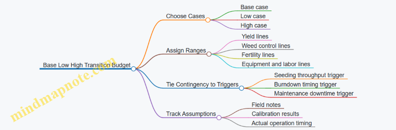
Closing the Loop in the Transition Year
At season end, compare actuals to the assumptions by bucket: biological, management, and operational. If yield missed the base case but costs matched, the issue is likely biological or management timing. If costs rose without yield gains, the issue is often operational inefficiency or equipment mismatch. This separation makes the next year’s budget tighter and less argumentative.
10.3 Incorporating Financing Costs and Timing of Cash Outflows
No-till transitions often change when money leaves the farm more than how much money leaves. Financing costs and cash timing matter because lenders and landlords don’t accept “later” as a payment plan. The goal here is to model (1) the timing of each outflow, (2) the interest or financing charge applied to unpaid balances, and (3) the timing of inflows from sales and any carbon payments you choose to include.
Core Concepts for Cash Timing
Start with a simple timeline for each year: land preparation and seeding costs early, weed and fertility costs around key growth stages, and revenue at harvest. Then add financing: if you borrow to cover early-season costs, interest accrues while the loan balance remains outstanding.
Two practical rules keep the model grounded:
- Accrue interest on the average outstanding balance, not on the total annual cost. If you borrow $50,000 and repay $20,000 mid-year, interest is not computed as if the full $50,000 stayed unpaid all year.
- Treat timing as a first-class input. A budget that spreads costs evenly across months can be “accurate on paper” and wrong in cash reality.
Step-by-Step Method
- List cash outflows by operation date: seed purchase, herbicide applications, fertilizer, custom work, repairs, and any equipment payments.
- Assign payment timing: paid at purchase, paid on delivery, or paid after invoicing. If you don’t know, use your farm’s last three seasons as a reference for typical invoice lag.
- Define financing structure: operating line, term loan, or equipment lease. Each has different interest rules and repayment schedules.
- Compute interest charges: apply the lender’s annual rate to the outstanding balance, using monthly or weekly periods.
- Build a cash flow statement: beginning cash + inflows − outflows − interest = ending cash. If ending cash goes negative, you need additional borrowing or cost deferral.
Mind Map: Cash Timing and Financing Mechanics
Example: Operating Line During Transition Year
Assume a transition field plan where early costs are heavier than the following year.
- March: seed and planting supplies paid $18,000
- April: herbicide and application paid $9,000
- May: fertilizer paid $12,000
- August: additional weed control paid $4,000
- October: grain sold and cash received $55,000
Suppose the farm uses an operating line at 9% annual interest, with monthly interest calculation, and repays the line from harvest proceeds.
A timing-aware approach estimates outstanding balances month by month. If the line is drawn in March and remains outstanding until October, interest accrues across those months. If instead you make partial repayments after April invoices are settled, the average outstanding balance drops and interest falls.
The key insight: two budgets with identical annual totals can produce different interest costs if one spreads outflows earlier.
Example: Equipment Transition with Lease Payments
Equipment changes can shift cash outflows from “pay when used” to “pay on schedule.” Consider a no-till drill upgrade financed via a lease.
- Lease payment due monthly starting January: $1,200
- Drill used for seeding starting September
- Repairs and wear parts paid after use: $2,000 in October
Even though the drill is only used late in the year, the lease payment begins immediately. In a cash flow model, that means you may borrow earlier than you would under a pay-as-you-go repair plan.
This is why equipment transition economics should include financing timing, not just depreciation or purchase price.
Practical Checks That Prevent Budget Errors
- No negative cash surprises: if ending cash becomes negative in a month, you must increase borrowing or adjust payment timing assumptions.
- Separate interest from principal: interest is a cost; principal repayment is a cash movement. Mixing them can distort profitability comparisons.
- Keep carbon accounting consistent: if you include carbon payments, place them on the same timeline basis as crop revenue. If you exclude them, don’t let the model “assume” they arrive.
Mini Template for Implementation
Use a monthly table for each year:
- Columns: Month, Outflows, Inflows, Borrowing Needed, Outstanding Balance, Interest, Ending Cash
- Rows: January through December
Then repeat for each scenario (baseline tillage, year-1 transition, year-2 stabilized). The scenario with the best net return can still lose on cash if it requires more early borrowing.
Summary
Incorporating financing costs and cash timing turns a static budget into a cash-flow reality check. By tracking outflows by date, applying interest to outstanding balances, and aligning inflows to actual receipt timing, you get a more reliable comparison of no-till transition strategies—especially in the year when the farm is paying for change before it receives the full payoff.
10.4 Evaluating Break Even Points for Equipment and Practice Changes
Break-even analysis answers one practical question: when do the cumulative savings and added returns catch up with the cumulative costs? In no-till transitions, the costs often hit early (equipment, downtime, extra weed control), while benefits show up as steadier yields, lower erosion losses, and sometimes carbon payments. The trick is to model timing, not just totals.
Core Break-Even Concepts
Start with three building blocks.
- Cash outflows and inflows by year: Equipment purchases, repairs, custom hire, and extra inputs are usually front-loaded. Yield stability benefits may appear in the transition year and then improve.
- Incremental comparison: Break-even is about the difference between the no-till plan and the baseline plan, not about absolute profit.
- Cumulative net position: You track cumulative incremental cash flow until it crosses zero.
A simple rule: if the cumulative incremental net return becomes positive in year N, that is the break-even year. If it never crosses, you still learn something—your plan needs a different cost structure, a different practice mix, or a different field portfolio.
Step-by-Step Method
Step 1: Define the Alternatives
Pick two scenarios with consistent assumptions:
- Baseline: current tillage and current equipment approach.
- Change plan: no-till practices plus the specific equipment transition path.
Example: Baseline uses a conventional planter and spring tillage. Change plan uses a no-till drill, residue management, and a herbicide program that differs in timing and product mix.
Step 2: Build an Incremental Cash Flow Table
For each year, compute:
- Incremental costs: added equipment payments, repairs, custom work, extra labor hours valued at your rate, and any extra inputs.
- Incremental returns: yield change times price, plus any carbon payment if you are modeling it as a cash inflow.
Example values (illustrative):
- Year 0 (purchase year): +$18,000 equipment cost, +$2,000 extra weed control, -$3,000 yield drag.
- Year 1: -$1,500 extra labor and repairs, +$4,000 yield improvement.
- Year 2: +$2,500 yield stability benefit, +$1,200 carbon payment.
Step 3: Compute Cumulative Net Incremental Position
Add incremental net cash flow each year to a running total.
- Break-even occurs when cumulative net becomes ≥ 0.
If you want a more precise estimate than whole years, interpolate between the last negative year and the first positive year.
Step 4: Add Discounting When Timing Matters
If you finance equipment or want to reflect the time value of money, discount future incremental cash flows. The break-even year may shift, especially when benefits arrive later.
Mind Map: Break-Even Logic for Equipment and Practice Changes
Example: Two Break-Even Paths
Example 1: Buying a Seeder vs. Using Custom Hire
Assume you can either:
- Buy a no-till drill now: higher Year 0 cost, lower later custom fees.
- Hire custom for two years: lower Year 0 cost, higher Year 1–2 cost.
If the transition year yield drag is large, the plan with lower Year 0 cash outflow may break even sooner in cash terms, even if total cost over five years is higher.
Example 2: Practice Change Without Full Equipment Replacement
Sometimes you can reduce costs without buying new equipment by adjusting residue management and seeding speed constraints. In that case, break-even may occur quickly because incremental equipment costs are near zero. The analysis still needs incremental labor and input changes, because those can quietly dominate.
Sensitivity Checks That Actually Matter
Break-even results are only as good as the uncertain inputs. Focus sensitivity on the variables that move the cumulative curve the most:
- Transition-year yield impact: even a small yield change can outweigh modest cost differences.
- Downtime and repair costs: equipment transition often creates “hidden” costs through missed windows.
- Weed control cost and timing: a delayed burndown or a resistance-driven program can shift costs across years.
- Carbon payment structure: if modeled, treat it as cash inflow with a clear timing assumption.
A practical way to test sensitivity is to rerun the cumulative table with three scenarios: low, expected, and high for the top two uncertain variables. If break-even flips from year 2 to year 4, you know where to tighten your assumptions.
Common Pitfalls
- Using average annual profit instead of cumulative cash flow: break-even is about the path, not the mean.
- Ignoring labor and downtime: equipment changes often change who does what, and when.
- Comparing different field mixes without normalization: if the change plan shifts acres to easier fields, incremental returns may look better than the true practice effect.
When you finish the table and the cumulative curve, you should be able to point to the exact year where the plan stops “costing you” and starts “paying you.” That clarity is the whole point of break-even analysis.
10.5 Using Sensitivity Analysis With Farm Relevant Parameters
Sensitivity analysis answers a practical question: “Which assumptions actually move my decision?” In no-till transitions, the biggest cost and risk levers often sit in a few places—yield stability, weed control intensity, equipment throughput, and cash timing. Instead of changing everything at once, you vary one or a small set of parameters while keeping the rest fixed, then watch how net return and risk metrics respond.
Start with a baseline model for the transition year and a steady-state year. Use the same field list, same crop rotation, and the same operation schedule you used in your multi-year budget. Then define farm-relevant parameters that you can measure or credibly estimate. A good rule: if you cannot explain how you’d update the parameter after one season of data, it’s probably not farm-relevant.
Step 1: Choose Parameters That Matter in Your System
Common high-impact parameters include:
- Yield level shift from stand establishment differences. Example: assume a 3% yield drop in year one, then test 0%, -3%, and -6%.
- Yield variability measured as standard deviation or range. Example: test whether no-till reduces variability (tighter stands) or increases it (more weather sensitivity).
- Weed control cost per acre by program intensity. Example: compare a “standard” residual + burndown plan to a “tight” plan with an extra pass.
- Herbicide efficacy factor under weather and residue. Example: model a 90% vs 100% effective kill rate, which changes re-treatment needs.
- Seeding speed and downtime for equipment transition. Example: if the new seeder is slower, throughput drops and custom hire or delayed planting costs appear.
- Fuel and labor hours per acre. Example: test whether reduced tillage saves 10% fuel but increases labor due to residue handling.
- Cash timing for inputs and returns. Example: move fertilizer purchase two weeks later and see how interest and working capital change.
Step 2: Define Ranges Using Farm Evidence
Ranges should come from your own records or realistic agronomic constraints. For instance, if your planting window is typically 10 days, a scenario that delays seeding by 20 days is not a “small change,” it’s a different operational plan. Keep ranges tight enough to reflect plausible management outcomes.
A concrete way to set ranges:
- Use last 3–5 years of field yield history to bound yield shifts.
- Use last season’s weed escapes to bound efficacy and re-treatment probability.
- Use maintenance logs and operator notes to bound downtime.
- Use your invoice dates to bound cash timing.
Step 3: Run One-Way Sensitivity First
One-way sensitivity changes one parameter at a time. Track two outputs: net return per acre and risk-adjusted return (for example, net return minus a penalty for yield shortfall). Example: if net return barely changes when herbicide efficacy varies, you can focus attention elsewhere.
A simple workflow:
- Compute baseline net return.
- Increase parameter by a small step and recompute.
- Decrease parameter by the same step.
- Record the change in net return.
Step 4: Use Two-Way Sensitivity for Interactions
No-till economics often has interactions. Weed control cost and yield are linked: a weaker residual program can force extra passes, which also affects planting speed and yield. Equipment downtime and planting date interact: delays can reduce yield even if weed control is perfect.
Use a grid for two parameters. Example grid:
- Yield shift: 0%, -3%, -6%
- Weed program intensity: standard vs tight Then compute net return for each cell. The “worst” cell is not the only one that matters; you also want to see whether the decision is robust across the plausible range.
Step 5: Rank Parameters with a Practical Output
Instead of ranking by statistical importance, rank by decision impact. A parameter is important if it changes your choice of management option. Example: if the “tight weed” option only wins when yield is at least -2% and efficacy is near 100%, then your decision depends on whether you can reliably achieve that efficacy.
Mind Map: Sensitivity Analysis Flow
Example: A Field-Level Decision That Depends on Two Levers
Suppose you compare two no-till seeding setups: a standard setup and a higher-throughput setup that costs more to run. Baseline shows the higher-throughput option has slightly better net return, but sensitivity reveals the story:
- If downtime stays within your maintenance range, the higher-throughput option wins.
- If downtime doubles, the planting delay penalty wipes out the advantage.
- Weed program intensity matters too, but only when herbicide efficacy drops below your assumed threshold.
This tells you what to verify early in the season: equipment reliability and whether your residue conditions allow the herbicide plan to perform as expected.
Step 6: Tie Results Back to Monitoring
Sensitivity analysis is useful only if it guides what you measure. After running scenarios, select 2–4 “watch items” tied to the most sensitive parameters. Example watch items:
- Actual seeding speed and time lost to adjustments.
- Weed counts at a consistent growth stage.
- Stand density or emergence uniformity.
- Invoice timing for key inputs.
When the season data arrives, you update the sensitive parameters and re-run the same sensitivity structure. That keeps the model honest and prevents the budget from becoming a work of fiction—complete with confident numbers and no receipts.
11. Decision Tools for Comparing No-Till Options by Field and Crop
11.1 Defining Comparable Alternatives With Consistent Assumptions
Comparable alternatives are the ones you can argue about without arguing about the math. In no-till economics, that means every option must be compared using the same field boundaries, time horizon, measurement rules, and accounting conventions—so differences come from management choices, not from inconsistent bookkeeping.
Step 1: Lock the Comparison Frame
Start by writing down the “unit of comparison” in plain language: one acre of a specific field, for one crop year, under a specified rotation position. If you compare two fields, you must either normalize them (same soil class, slope, drainage category) or treat them as separate comparisons.
Example: Field A and Field B both grow corn, but Field A has heavier clay and slower infiltration. If you compare no-till on Field A to conventional tillage on Field B, you are not comparing tillage; you are comparing soils.
Step 2: Standardize the Rotation and Calendar
No-till decisions usually span multiple operations across the rotation. To keep alternatives comparable, define the rotation slot and the sequence of key events: residue management, termination timing, seeding date window, nutrient application timing, and weed control windows.
A practical rule: if two alternatives use different termination dates, you must either (a) keep the dates the same and accept different biological outcomes, or (b) explicitly model the date difference as part of the alternative. Mixing both approaches creates “mystery profit.”
Step 3: Use Consistent Agronomic Assumptions
Comparable alternatives require the same baseline expectations for stand establishment and weed pressure measurement. You don’t need identical yields, but you do need consistent assumptions about how yields are generated.
Common assumption set:
- Seeding depth and row spacing are the same unless the alternative changes them.
- Weed pressure is measured using the same scouting method and timing.
- Soil test interpretation rules are identical across options.
Example: If Alternative 1 assumes a uniform 95% stand and Alternative 2 uses a 70% stand because it “expects more stress,” then yield differences may be partly assumption-driven. Instead, model stand establishment as an outcome of the management choice, not as a preloaded conclusion.
Step 4: Harmonize Input and Cost Accounting
Costs must be defined with the same categories and the same inclusion rules.
Use a fixed chart of accounts for every alternative:
- Variable costs: seed, fertilizer, herbicides, cover crop seed, custom services, fuel per acre.
- Labor: hours per acre by operation.
- Equipment: ownership (depreciation or lease), maintenance, repairs, and opportunity cost of downtime.
- Overhead: decide whether to include it. If you include overhead in one alternative, include it in all.
Example: If you include custom application fees in one option but treat them as “already in overhead” in another, the comparison becomes a spreadsheet prank.
Step 5: Define Yield and Risk Consistently
Yield stability is not just “average yield.” Decide how you will represent variability: historical distribution, scenario ranges, or field-specific variability estimates.
Comparable risk methods:
- Use the same yield distribution shape and same number of years.
- Apply the same risk metric (for example, downside-focused returns) across alternatives.
Example: If one alternative uses 10 years of yield history and another uses 3 years, the risk comparison is biased toward the alternative with more stable data.
Step 6: Keep Carbon Accounting Comparable
If carbon recovery is part of the decision, the accounting rules must match across alternatives.
Consistency requirements:
- Same measurement boundary (what practices count and what doesn’t).
- Same method for converting practice intensity into carbon-related variables.
- Same verification-ready record expectations.
Example: If Alternative 1 counts cover crop biomass inputs but Alternative 2 counts only termination timing, you are comparing two different carbon models.
Mind Map: Comparable Alternatives with Consistent Assumptions
Example: Two Alternatives Compared Correctly
Alternative A: No-till with residue retention and a winter cover crop.
Alternative B: Reduced tillage with residue removal and no cover crop.
To keep them comparable, you define:
- Same field, same crop year, same seeding window.
- Same weed scouting timing and thresholds.
- Same fertilizer plan logic, with differences only where residue and cover crop change nutrient availability.
- Same cost categories and inclusion rules.
- Same yield variability method using the same historical years for that field.
Then the differences in net return and stability can be attributed to the management choices, not to a mismatch in assumptions.
Practical Consistency Checklist
Before comparing net returns, verify that each alternative has the same: unit of comparison, calendar windows, agronomic measurement rules, cost categories, yield variability method, and carbon accounting boundary.
11.2 Calculating Net Returns per Acre With Full Cost Inclusion
Net returns per acre answer one practical question: after paying every relevant cost, how much money is left from the crop enterprise? “Full cost inclusion” means you don’t stop at seed and fertilizer. You also include labor, equipment, land, overhead, and the costs created by transition choices—especially those that show up only in certain years.
Step 1: Define the Unit of Analysis and the Time Window
Start with a clear unit: one acre of one crop in one season, or one acre averaged across a rotation year. Then decide whether your numbers are cash-only or full economic. For this section, use full economic costs so comparisons between no-till and conventional don’t get distorted.
Example: You compare two systems for corn on 100 acres. System A uses conventional tillage. System B uses no-till with cover crop residue and a different herbicide program. You calculate net returns per acre for each system for the same calendar season.
Step 2: Write the Net Returns Equation
Use a structure that forces completeness:
Net Returns per Acre = Revenue − Cash Costs − Allocated Noncash Costs
Cash costs include items you pay during the season. Allocated noncash costs include depreciation, opportunity cost of land, and sometimes management labor if you want a consistent “what it really costs” view.
Step 3: Build Revenue with Crop-Realistic Assumptions
Revenue usually equals yield × price, but keep it grounded in how you actually sell.
Example: Corn yield is 170 bu/acre for System A and 165 bu/acre for System B. If your effective price is $4.50/bu for both systems, revenue is:
- System A: 170 × 4.50 = $765/acre
- System B: 165 × 4.50 = $742.50/acre
If you use different grades or contract terms, reflect the effective price, not a generic one.
Step 4: List Cash Costs by Operation and Input
Organize cash costs so you can trace them back to field activities.
Common cash cost buckets:
- Seed and planting materials
- Fertilizer and soil amendments
- Herbicides and adjuvants
- Cover crop seed and termination inputs
- Fuel and lubricants
- Custom hire or contractor costs
- Labor wages and payroll burden
- Crop insurance premiums if you treat them as enterprise costs
- Drying, storage, and hauling if they differ by system
Example: No-till may reduce fuel and tillage labor, but it can increase herbicide and cover crop costs.
Step 5: Add Allocated Noncash Costs Without Making Them Vague
Noncash costs are where “full cost inclusion” earns its keep.
Include at least:
- Equipment depreciation and repairs allocated per acre
- Opportunity cost of land (rent or land value-based return)
- Management labor if you want a true economic comparison
Equipment allocation method: compute an hourly or per-acre cost from annual ownership costs divided by expected usable hours or acres.
Example: If a no-till planter costs $60,000, has a useful life of 10 years, and you expect to cover 2,000 acres/year, straight-line depreciation is $60,000/10/2,000 = $3/acre. Add repairs and maintenance allocated similarly.
Step 6: Include Transition-Specific Costs Correctly
Transition years often have costs that don’t repeat every year.
Typical transition costs:
- Extra weed control passes while residue and weed seedbank equilibrate
- Additional cover crop management or termination adjustments
- Equipment changes such as buying a new seeder or paying for custom seeding during downtime
- Learning curve costs like slower planting speed
Example: In year one, System B requires an extra burndown application and a slightly higher seeding rate. In year two, those costs drop. If you compare systems using only steady-state costs, you’ll misjudge the transition.
Step 7: Compute Net Returns per Acre for Each System
Example numbers (illustrative):
- System A revenue: $765/acre
- Cash costs: $520/acre
- Allocated noncash costs: $140/acre
- Net returns: 765 − 520 − 140 = $105/acre
- System B revenue: $742.50/acre
- Cash costs: $485/acre
- Allocated noncash costs: $160/acre
- Net returns: 742.50 − 485 − 160 = $97.50/acre
Even with lower revenue, System B can still be competitive if cash costs fall enough. Here, it’s slightly lower.
Step 8: Sanity-Check the Result with a Cost Share View
Before trusting the number, check whether the biggest cost categories behave as expected.
- If no-till shows higher net returns but your herbicide and equipment lines are missing, the math is lying.
- If no-till shows lower net returns but only because you forgot land opportunity cost in one system, the comparison is inconsistent.
Mind Map: Full Cost Net Returns Workflow
Example: A Clean Cost Table You Can Reuse
Use a simple structure so every line item has a source.
| Category | System A Conventional | System B No-Till | Notes |
|---|---|---|---|
| Revenue | $765.00 | $742.50 | Yield × effective price |
| Seed | Same crop, different rates | ||
| Fertility | Placement and timing | ||
| Herbicides | Burndown and residual | ||
| Cover Crop | 0.00 | Seed and termination | |
| Fuel and Lubricants | Tillage reduction | ||
| Labor | Operation count and speed | ||
| Equipment Depreciation | Allocated per acre | ||
| Repairs and Maintenance | Allocated per acre | ||
| Land Opportunity Cost | Consistent rent basis | ||
| Total Cash Costs | 520.00 | 485.00 | Sum of cash lines |
| Total Noncash Costs | 140.00 | 160.00 | Depreciation plus land |
| Net Returns | 105.00 | 97.50 | Revenue − cash − noncash |
When you keep the table consistent, you can swap one assumption at a time—like herbicide timing or planting speed—without breaking the logic of the comparison.
11.3 Incorporating Labor and Equipment Capacity Constraints Into Choices
No-till decisions often fail for a simple reason: the plan fits on paper, but not on the calendar. Capacity constraints show up as labor shortages, equipment bottlenecks, and timing conflicts between seeding, residue management, and weed control. The goal is not to “do everything,” but to choose an option set that can be executed reliably with the resources you actually have.
Foundational Concepts for Capacity-Aware Comparisons
Start by separating three constraints that behave differently.
-
Labor availability limits how many acres can be covered per day for tasks like seeding, spraying, and monitoring. If one operator can only run the sprayer for 6 hours before fatigue or shift changes, that’s a hard cap.
-
Equipment throughput limits acres per day based on implement width, travel speed, and setup time. A 12-row seeder that averages 4.5 mph may look fast, but headlands, calibration, and turning time can cut effective speed.
-
Timing windows limit when tasks can occur. Burndown timing, soil moisture for seeding, and weed stage for herbicide all create “must-do-by” dates.
A practical way to keep these from mixing together is to build a simple capacity table for each critical operation: acres per day, labor hours per acre, and the earliest and latest workable dates.
Mind Map: Capacity Constraints and Decision Inputs
Step 1: Translate Each Operation Into Acres per Day
For each critical operation, estimate effective acres per day rather than relying on marketing specs.
Example: Your no-till seeding plan uses a 30-foot drill. You can seed 5 hours of productive time per day after calibration and headland passes. If average field speed is 4 mph, then productive area is:
- 30 ft × 4 mph = 120 ft/min = 0.0273 acres/min
- 5 hours = 300 minutes → 8.2 acres/day (before accounting for turns and delays)
If you add 15% for turning, refueling, and minor stops, you get about 7.0 acres/day. That number goes into your schedule.
Step 2: Match Labor Hours to Equipment Hours
If the seeder requires one operator and one helper for seed monitoring and plugging response, labor becomes the binding constraint when the helper is also needed for spraying or loading.
Example: You have 1 trained seeding operator and 1 helper available for 10 hours/day. Seeding needs 6 hours/day of helper time to keep up with monitoring and quick fixes. Spraying needs the helper for loading and boom checks for 3 hours/day. If both operations are scheduled on the same day, you exceed the helper’s 10-hour capacity even if the tractor operator is available.
In capacity-aware planning, you either (a) stagger tasks, (b) reduce the number of fields attempted that day, or (c) change the equipment plan so one person can cover both roles.
Step 3: Build a Simple Schedule with Bottlenecks
Create a week-by-week plan for the season using your timing windows. Mark which operation is the bottleneck by comparing required acres to available acres.
Example: Suppose you must seed 280 acres within a 10-day window. At 7 acres/day, seeding capacity is 70 acres/week, or 140 acres in 10 days. You are short by 140 acres, so either:
- you increase throughput (wider implement, more days, or custom seeding),
- you narrow the plan (seed fewer fields in the window and accept later planting for the rest), or
- you change the system (for instance, adjust residue strategy to reduce delays from plugging or rework).
The key is that the constraint identifies which decision variable matters.
Step 4: Price the Cost of Delays and Rework
Capacity shortfalls create economic costs beyond lost time.
- Delay costs: later planting can reduce yield; later weed control can increase competition.
- Rework costs: if seeding is rushed into marginal moisture, you may need a second pass for stand repair.
- Opportunity costs: time spent fixing one field can steal capacity from another.
Example: If a rushed seeding day causes 5% of acres to require re-seeding, and re-seeding costs $35/acre in seed, fuel, and labor, then the rework cost is $1.75/acre across the original acres attempted that day. Add delay-related yield risk using your own historical patterns, not generic assumptions.
Step 5: Choose Option Sets That Fit Together
A no-till option is not just a seeding method. It’s the whole sequence: residue handling, fertility placement timing, and weed control steps. Capacity-aware choices aim for sequences where the same equipment and crew are not repeatedly overloaded.
Example: If your plan uses a heavy residue burndown plus a separate mechanical pass, you may create a labor bottleneck that forces seeding into the tail end of the window. A capacity-fit alternative might be a residue plan that reduces mechanical passes, even if it slightly changes herbicide timing, because it keeps seeding on schedule.
Quick Capacity Checklist for Field-Level Decisions
- For each critical operation, compute acres per day and labor hours per acre.
- Identify the tightest timing window and compare required acres to available capacity.
- Check whether the same people are needed simultaneously for multiple tasks.
- Add rework and delay costs when the schedule is forced.
- Select the option set that stays feasible without “hero days.”
11.4 Comparing Cover Crop and Residue Strategies Using Costed Inputs
Cover crop and residue strategies change both the agronomy inputs you buy and the operational steps you run. The goal of this section is to compare options using the same costed inputs and the same decision boundaries, so the numbers actually mean something.
Step 1: Define the Comparison Frame
Start by choosing a single “decision unit,” usually a field-year, and lock the baseline assumptions: crop, seeding date window, soil type class, and the weed pressure level you expect. Then list the outcomes you will score. For economics, you typically need at least:
- Net return per acre (yield × price minus all variable costs)
- Yield stability risk (how much yield swings when weather or weed control varies)
- Transition friction (extra passes, labor peaks, and equipment wear)
Example: If Field A is corn-after-soy, compare three options for the same fallow period: (1) no cover crop, (2) cereal rye cover crop terminated early, (3) cereal rye cover crop terminated late with heavier residue. Keep the corn seeding equipment and planting speed assumptions identical.
Step 2: Build a Costed Input List That Matches the Field Reality
Create a line-item list for each option. Use the same categories every time:
- Establishment costs: seed, seeding method, passes, and fuel.
- Termination costs: herbicide, mechanical termination, and application timing labor.
- Residue and seeding impacts: any changes to seeding depth, downforce needs, or seed-to-soil contact adjustments.
- Weed control costs: burndown, residual herbicides, and any follow-up applications.
- Fertility and amendments: nutrient additions tied to cover crop biomass or residue decomposition.
- Equipment and maintenance: wear items and downtime from slower seeding or clogged residue.
A practical way to avoid missing costs is to write the operations as a mini schedule. If Option 2 requires an extra pass for termination or a slower seeding speed due to residue, that must show up as labor and equipment time.
Step 3: Translate Agronomy Effects Into Economic Variables
Cover crops and residue change three economic levers.
Lever A: Weed pressure and control timing
- Early termination can reduce biomass and make burndown easier.
- Heavy residue can suppress weeds but may require more careful seeding and potentially different herbicide timing.
Example: If heavy residue delays planting by three days, you may pay for an extra labor day and risk a small yield penalty. Even if weed suppression is better, the delayed seeding can still dominate the net return.
Lever B: Nitrogen dynamics and fertility timing
- Legumes can add nitrogen, but they also change the timing of nitrogen availability.
- High-carbon residues can temporarily tie up nitrogen, affecting early crop vigor.
Example: If a rye cover crop is terminated late and you see slower early growth, you might add a starter nitrogen dose. That cost belongs in the cover crop option, not the baseline.
Lever C: Yield stability through stand establishment
Residue can improve moisture retention and soil structure, but it can also increase planting difficulty. Yield stability is often driven by whether the crop establishes uniformly.
Example: If one option produces uneven emergence due to residue matting, yield variability increases even when the average yield looks similar.
Step 4: Use a Simple Scorecard with Costed Inputs
For each option, compute:
- Variable cost total per acre
- Expected yield per acre
- Expected net return per acre
- A stability adjustment based on yield variability and weed-control reliability
To keep it systematic, treat stability as a cost of uncertainty. One simple method is to apply a “risk haircut” to expected net return using historical variability for that field and management style.
Step 5: Mind Map of the Costed Comparison Logic
Mind Map: Comparing Cover Crop and Residue Strategies
Step 6: Worked Example with Three Options
Assume Field A has the same expected corn yield under all options, but weed control reliability differs.
- Option 1: No cover crop
- Lower establishment cost, but higher chance of a late weed flush requiring an extra application.
- Option 2: Rye terminated early
- Moderate establishment and termination costs.
- Weed control is more predictable; seeding is faster because residue is lighter.
- Option 3: Rye terminated late with heavier residue
- Higher establishment and termination costs.
- Better weed suppression, but seeding speed drops and you may need a starter nitrogen top-up.
Even if Option 3 has the lowest weed-control cost, it can lose on net return if the seeding delay and added fertility push variable costs above the savings. The comparison stays fair because every extra pass, every added input, and every timing-driven adjustment is included as a costed input.
Step 7: Sanity Checks That Prevent Costing Errors
Before choosing, verify three common failure points:
- Missing passes: termination, burndown, and follow-up applications must all be counted.
- Timing mismatch: if an option changes planting date, reflect the operational and yield implications.
- Equipment reality: if residue slows seeding, convert that into labor and depreciation time.
When these checks are done, the numbers become a tool for choosing, not a spreadsheet exercise. You can then compare options field-by-field and crop-by-crop without pretending every field behaves the same.
11.5 Selecting a Portfolio of Fields to Balance Yield Stability and Costs
A portfolio approach treats your farm like a set of interacting bets. Instead of asking, “Which field is best for no-till?” you ask, “Which combination of fields keeps total profit steadier while staying within equipment and cash limits?” The logic is simple: yield risk varies by field, and costs vary by field, but your constraints—seeding capacity, labor timing, and cash flow—apply across the whole operation.
Step 1: Build a Field Scorecard That Separates Risk from Cost
Start with two numbers per field: an expected net return and a risk measure. Use your baseline budgets and at least two years of yield history if available.
- Expected net return per acre: include seed, fertility, weed control, fuel, labor, and equipment ownership or custom rates. Add transition-year costs separately so you don’t mix “learning curve” with “steady state.”
- Yield stability: use a practical proxy such as the standard deviation of yield or a simpler range metric like “yield in the bottom 25% of years.”
Example: Field A has slightly lower expected yield than Field B, but it has much smaller yield swings. If your no-till plan increases weed-control costs in Field B during wet springs, Field A may improve portfolio stability even with a modest yield penalty.
Step 2: Identify Operational Couplings That Create Hidden Costs
Costs don’t only depend on agronomy; they depend on timing. Group fields by constraints:
- Seeding window pressure: fields that must be seeded early (poor drainage or residue-heavy situations) compete for the same days.
- Weed-control timing: burndown and early post-emergence windows can overlap across fields.
- Equipment availability: if you have one no-till drill and one sprayer, throughput matters.
Example: If Field C and Field D both require a tight burndown-to-seed gap, a rainy week can force you to either delay seeding (yield risk) or rush herbicide timing (weed risk and cost). Portfolio selection should avoid stacking multiple “timing-sensitive” fields in the same season.
Step 3: Classify Fields Into Management Bands
Create bands based on how no-till changes their risk and cost.
- Band 1: Low transition friction: fields with manageable residue, consistent stand history, and moderate weed pressure.
- Band 2: Moderate friction: fields with either higher weed pressure or more challenging residue, but still workable with your current equipment.
- Band 3: High friction: fields likely to require extra passes, special seeding setups, or higher herbicide intensity during transition.
Example: Field E might be Band 3 because it has heavy residue and a history of patchy emergence. If you plant it alongside several Band 1 fields, you can absorb the learning and operational stress without letting the whole farm’s seeding schedule collapse.
Step 4: Set Portfolio Targets for Stability and Capacity
Choose targets that reflect your actual constraints.
- Stability target: limit how much of your total acreage sits in high-variance fields.
- Capacity target: cap the acreage that requires the same equipment in the same week.
- Cash-flow target: restrict how much transition-year spending lands in the same month.
A practical rule: keep at least one “buffer” block of Band 1 fields so that if a timing-sensitive field slips, you still complete a meaningful portion of seeding and weed-control operations.
Step 5: Use a Simple Optimization Mindset
You can do this without fancy software by ranking fields and then selecting acreage blocks.
- Rank fields by risk-adjusted net return: expected net return minus a penalty for yield variability.
- Apply capacity filters: remove fields that would exceed seeding or spraying throughput in the same window.
- Apply transition filters: ensure you spread Band 3 acreage so transition-year costs and operational strain don’t peak simultaneously.
Example: Suppose you can seed 600 acres in your optimal window. If Field F (Band 3) and Field G (Band 3) both demand extra setup time, you might choose only one of them that year and keep the other for the next transition cycle.
Step 6: Validate with “What If” Scenarios Using Your Own Data
Run three scenarios using your historical weather and operation timing patterns:
- Wet spring: higher weed pressure and delayed seeding.
- Dry spring: stand establishment stress and slower residue breakdown.
- Normal year: baseline performance.
Check whether your selected portfolio keeps total net return within an acceptable range in each scenario. If the portfolio fails only in one scenario, adjust by shifting acreage between bands rather than changing everything.
Mind Map: Portfolio Selection Logic
Example Portfolio for One Season
Imagine 1,000 acres total with one no-till seeder and one sprayer. You might choose:
- 500 acres Band 1 to anchor throughput and reduce timing risk.
- 350 acres Band 2 to capture upside where conditions are favorable.
- 150 acres Band 3 to learn and manage transition friction without overwhelming setup time.
If your wet-spring scenario shows weed-control costs spike on Band 2 fields, you shift 50 acres from Band 2 to Band 1 next year. The key is that the portfolio changes are targeted: you adjust the mix that drives the failure mode, not the entire plan.
A good portfolio doesn’t eliminate risk; it distributes it across fields and seasons in a way your operation can handle.
12. Implementation Checklists and Recordkeeping for Economic Verification
12.1 Creating Practice Logs That Support Both Agronomy and Economics
A practice log is the bridge between what happened in the field and what you can defend in a budget. The goal is simple: every agronomic decision you make should be traceable to a measurable input, an operation, and an outcome you can cost.
Foundational Log Design
Start with a consistent unit of record: one field, one crop, one season, and one operation event. If you mix events across fields, you’ll end up averaging away the very differences that matter for yield stability and cost.
Use three layers of detail.
- Event layer captures the operation itself: date, field, crop stage, implement, pass count, and weather notes that explain performance.
- Input layer captures what went into the event: seed lot, rate, fertilizer product and placement, herbicide product and carrier, and calibration checks.
- Outcome layer captures what resulted: stand counts or emergence notes, weed observations, residue condition, soil test results when available, and yield data.
A slightly playful rule: if you can’t attach a cost to a log entry, either it belongs in a different layer or it needs a measurable proxy.
Minimum Viable Fields and Why They Matter
At minimum, each entry should include:
- Field ID and crop year so you can compare apples to apples.
- Operation type (seeding, burndown, fertilizing, rolling, spraying, harvest).
- Timing relative to crop stage (e.g., “V3” or “before emergence”), not only calendar date.
- Rate and method (lb/ac and broadcast, banded, or placed).
- Equipment identity (seeder model, spray boom width, nozzle type) because performance and downtime costs differ.
- Weather snapshot (wind, rainfall within 24–48 hours, soil moisture condition) because it explains why a plan didn’t match reality.
- Labor hours and pass count so your labor and capacity assumptions stay grounded.
Integrated Workflow from Field Notes to Budget Numbers
A practical workflow keeps the log from becoming a junk drawer.
- During the operation: record the event layer and the input layer. If you only have time for one thing, record rates and pass count.
- Within a week: record early outcomes like emergence uniformity, residue distribution, and weed escapes.
- After harvest: record yield, harvest moisture, and any rework events (spot reseeding, additional passes, equipment issues).
- After soil tests: attach soil test results to the correct field-year and link them to the practices used.
When you later build a budget, you can map each log entry to a cost line item without guessing.
Mind Map: Practice Log Components and Links
Example Entries That Stay Costable
Example: No-till seeding event
- Field: 14, Crop: corn, Year: 2025
- Timing: “after burndown, before emergence”
- Equipment: 12-row no-till drill, coulter type noted
- Pass count: 1
- Seed lot: brand and germination recorded
- Rate: 32,000 seeds/ac
- Calibration: target vs actual seed rate written down
- Labor: 5.5 hours, including setup
- Weather: soil moist, no rainfall for 36 hours
- Outcome: emergence uniformity “good” with stand estimate
This entry supports both agronomy (stand establishment) and economics (seed cost, labor hours, and the likelihood of needing rework).
Example: Herbicide sequence event
- Operation: burndown at V0–V1 window
- Products and rates: written with carrier and nozzle type
- Weather: wind speed and rainfall timing
- Pass count: 1
- Outcome: weed escapes counted in fixed transects
Weed escape counts let you connect the event to later costs, such as additional spraying or yield impacts.
Data Quality Checks That Prevent Budget Drift
Before you finalize the season’s log, do three checks.
- Unit consistency: confirm rates are all in the same units (lb/ac, gal/ac, seeds/ac).
- Totals cross-check: sum input quantities from the log and compare to purchase records for the field-year.
- Missing data flags: if labor hours are missing, record a placeholder and the reason, then decide whether to estimate using a documented method.
A log that is slightly incomplete but clearly labeled is far more useful than a log that looks complete but hides assumptions.
Closing the Loop Without Guessing
At the end of the season, review each field-year and ask one question per operation: “What did this event change, and what did it cost?” If the answer is supported by the log, you can update budgets confidently. If it isn’t, you know exactly what to improve next time—rates, timing, equipment notes, or outcome measurements.
12.2 Standardizing Input and Operation Coding for Accurate Budgets
Accurate budgets depend on one unglamorous skill: consistent coding. If “glyphosate” sometimes appears as “Roundup,” or if “seeding” is split across three operation names, your spreadsheet will do math on mismatched categories and call it truth. Standardization fixes that by making every input and operation land in the same place every time.
Foundational Coding Principles
Start with a coding system that separates three things: what you used, what you did, and where it happened.
- Inputs are consumables and services that change costs: seed, fertilizer, herbicide, fuel, custom work.
- Operations are actions with timing and equipment: burndown spray, seeding, rolling, sidedress.
- Locations are the unit of budgeting: field, zone, crop year, and sometimes soil type.
A practical rule: every transaction should map to exactly one input code and exactly one operation code, plus one location code. If you can’t do that, your categories are too fuzzy.
The Coding Structure
Use a simple hierarchy so codes remain readable.
- Field code:
F01,F02 - Crop-year code:
CR24_WHT,CR24_CORN - Operation code:
OP_SEED,OP_BURNDOWN,OP_SIDEDRESS - Input code:
IN_SEED,IN_N,IN_HERB_GLY,IN_FUEL_DSL - Unit of measure:
ac,lb,gal,hr
Then add attributes that explain why costs differ without changing the code itself:
- For operations: date window, equipment used, pass count, application rate.
- For inputs: product concentration, active ingredient, nutrient form, wastage factor.
Mind Map: Coding Components
Controlled Vocabulary That Doesn’t Drift
Create a controlled list for operation names and input names. The goal is not to capture every brand label; it’s to capture the cost driver.
Example: instead of coding by brand, code by active ingredient and formulation.
- Input code
IN_HERB_GLYwith attributeform=SLandstrength=41% - If you switch brands later, you keep the same input code and update only the attributes.
Example: for fertilizer, code by nutrient form.
IN_N_UANfor 28% UANIN_N_ANHfor ammonium nitrate
This prevents “same nutrient, different product” from turning into “different cost category.”
Operation Coding with Timing and Pass Logic
Operations should reflect how labor and equipment time actually accumulate.
A seeding operation often has multiple passes: calibration, actual seeding, and sometimes a light packing pass. If you lump them into one line item, your labor and fuel assumptions get messy.
Use operation codes that match the pass logic you record.
OP_SEEDfor the seeding passOP_PACKfor packing/rolling passOP_CALIBfor calibration time if you track it
If you don’t track calibration time, don’t create a code for it. Standardization should match your measurement reality.
Example: From Messy Notes to Budget-Ready Lines
Imagine a field log entry:
- “Sprayed 30 acres with glyphosate, 20 gal, used 2 tanks, fuel burned.”
Turn it into structured lines:
- Location:
F03,CR24_CORN - Operation:
OP_BURNDOWN - Input:
IN_HERB_GLYwith attributerate=??andunits=gal - Fuel: either
IN_FUEL_DSLtied toOP_BURNDOWNor a separate fuel allocation rule tied to equipment hours
If you only know total gallons of herbicide and not the application rate, you can still code it, but you must store the missing attribute as “unknown” rather than guessing. Budgets can include unknowns; they just can’t include invented numbers.
Quality Control Checks That Catch Errors Early
Before finalizing budgets, run three checks.
- Required fields check: every line must have field code, crop-year code, operation code, input code, quantity, and unit.
- Unit consistency check:
lbnever mixes withkgwithout conversion. - Category coverage check: every cost line in your bank or invoice list must map to at least one coded transaction.
Example: Reconciliation Rule
If an invoice lists “seeding service” as a lump sum, you still code it as an operation (OP_SEED) and allocate the total across inputs only if you have itemized quantities. Otherwise, store it as a service input code like IN_CUSTOM_SEED so the budget remains honest.
Implementation Workflow
- Build the controlled lists for operation and input codes.
- Define the mapping rules so each transaction has one operation and one input.
- Convert last season’s records into the new structure for a pilot field.
- Run the three quality checks and fix the categories that cause repeated “unknowns.”
Once the system is stable, your budgets stop being a one-time spreadsheet exercise and become a consistent accounting layer for every field and year.
12.3 Building a Soil Sampling and Test Interpretation Workflow
A good soil workflow does two jobs: it produces samples that represent the field, and it turns lab numbers into decisions you can defend. The trick is to treat sampling like data collection, not like a one-off chore.
Step 1: Define the Decision Before You Take Samples
Start with the question your budget needs answered. Examples:
- “Will we need to adjust nitrogen rate next season?”
- “Is compaction limiting infiltration and yield stability?”
- “Are pH and phosphorus trending enough to change placement?”
Then choose the depth and timing that match the decision. For most crop planning, common depths are 0–6 inches (surface fertility and residue effects) and 6–12 inches (root zone and longer-term trends). If you’re diagnosing compaction or water movement, you’ll often add deeper observations, but keep the fertility sampling separate so you don’t mix purposes.
Step 2: Create Sampling Zones That Make Agronomic Sense
Avoid sampling the whole farm as one blob. Split fields by factors that change soil behavior:
- soil type or texture changes
- slope and drainage differences
- management history (old headlands, eroded areas, unusual manure zones)
- yield maps or persistent problem areas
A practical rule: each zone should be large enough to be useful, but small enough that you’re not averaging away the problem. If a zone is too variable, you’ll get “average” results that don’t help.
Step 3: Choose a Sampling Pattern and Keep It Consistent
Within each zone, use a pattern that reduces bias. Common options:
- grid sampling for uniform fields
- zigzag or W-pattern for general coverage
- targeted sampling for known problem spots
Collect multiple cores per zone and combine them into one composite sample. The composite reduces the noise from random variability. Consistency matters more than perfection: if you sample the same zones the same way each year, trends become interpretable.
Step 4: Standardize Handling So Lab Results Mean Something
Soil is perishable data. Keep these controls tight:
- remove surface residue clumps so you’re sampling soil, not mulch
- air-dry only if the lab requests it; otherwise follow lab instructions
- label clearly with zone, depth, date, and intended tests
- avoid contamination from tools by cleaning between zones
If you’re sampling right after heavy rain, note it. Wet conditions can change how easily soil clumps form and how representative the composite feels.
Step 5: Select Tests That Match Your Economics
Not every lab panel is useful for every decision. A typical workflow for no-till soil regeneration economics includes:
- pH and buffer pH for lime decisions
- phosphorus and potassium for fertility planning
- organic matter or soil carbon indicators for tracking soil regeneration direction
- nitrate or mineral nitrogen when you need near-term nitrogen decisions
- texture or bulk density when water movement and compaction are suspected
Example: If your main concern is yield stability during early season, prioritize pH, mineral N timing, and infiltration-related diagnostics rather than chasing every possible micronutrient.
Step 6: Interpret Results Using a Decision Lens
Lab numbers are not decisions by themselves. Convert them into actions using thresholds and your management context.
- pH interpretation: If pH is low, lime cost and timing become the economic question. In no-till, lime incorporation is slower, so you’re planning for gradual change rather than immediate correction.
- phosphorus interpretation: If P is low in a zone, placement and rate matter. If P is high, you can often reduce inputs and redirect cash.
- organic matter interpretation: Treat it as a trend signal. One test rarely explains a season’s yield; it’s the multi-year direction that supports soil regeneration economics.
- mineral nitrogen interpretation: Use it to adjust nitrogen rate and timing. If mineral N is higher than expected, you can reduce early-season N without gambling.
A simple way to avoid confusion: write a one-sentence “meaning statement” for each test result, then attach the action it triggers.
Step 7: Build a Field Record That Supports Budgeting
Create a sampling log that links zone → tests → results → decisions → outcomes. This is where interpretation becomes defensible.
Example workflow for one zone:
- Zone A sampled 0–6 inches and 6–12 inches
- pH low in 0–6, acceptable in 6–12
- decision: lime application planned with a focus on surface correction
- budget note: lime cost included, yield impact treated as gradual
- next season: compare early vigor and soil test trend
Mind Map: Soil Sampling and Test Interpretation Workflow
Example: A Two-Zone Sampling Plan That Stays Practical
Zone A is a well-drained area with stable yields; Zone B is a low spot that shows delayed emergence. Sample both zones at 0–6 and 6–12 inches using the same pattern each year. In Zone B, add a bulk density or infiltration observation if water movement is the suspected limiter. Then interpret results separately: Zone A guides fertility rate decisions, while Zone B guides both fertility and the operational choices that affect stand establishment.
This workflow keeps sampling tied to decisions, and it keeps interpretation tied to economics. When you can point from a lab result to a specific action and a specific budget line, you’re doing soil regeneration management with receipts.
12.4 Maintaining Equipment Performance Records for Cost Control
Cost control in no-till is less about guessing and more about measuring what your machines actually do. When you record equipment performance consistently, you can separate “bad luck” from “avoidable wear,” and you can price repairs and downtime with the same discipline you use for seed and fertilizer.
What to Record First
Start with the minimum set that explains most cost swings: time, throughput, quality, and failure mode.
- Operational time: hours engaged, hours idle, and reasons for idle (waiting on seed delivery, weather hold, hydraulic issue).
- Throughput: acres per hour by field and operation, using the same method each time (GPS swath area or implement width × calibrated speed).
- Quality checks: seeding depth distribution, residue flow observations, and uniformity notes (for example, “skips in wheel track” or “row unit bounce after compaction”).
- Failure and maintenance: what failed, when it failed, parts used, labor hours, and whether the failure repeated.
A practical rule: if you cannot connect a record to an acre, a row, or a downtime event, it will be hard to use for cost control.
A Simple Recording Workflow
Use a two-layer system: quick capture in the field, then structured entry after the day.
- Field capture: one-page log per day per machine. Record start/stop times, acres, and any deviations.
- Daily consolidation: enter the same fields into a spreadsheet or farm management system. Attach photos only when they explain a problem (for example, a worn gauge wheel causing depth drift).
- Monthly review: summarize by machine and operation to find patterns in parts consumption and downtime.
Example: If a no-till drill averages 120 acres/day in April but drops to 80 acres/day in May, your records should show whether the cause is weed residue buildup, seed singulation issues, or repeated hydraulic leaks.
Mind Map: Equipment Records That Control Costs
Cost Attribution That Actually Works
To control costs, convert records into per-acre and per-hour metrics.
- Repair cost per acre = (parts + labor + service call) ÷ acres completed since the last major service.
- Downtime cost per hour = (lost contribution margin ÷ available working hours) or a simpler internal rate you apply consistently.
- Consumables per acre = gauge wheel bearings, blades, shear bolts, hydraulic hoses, and any wear items.
Example: If gauge wheel bearings cost $180 and you complete 300 acres since replacement, the wear cost is $0.60/acre. If the same bearing set lasts only 150 acres after a residue-heavy transition year, you can link the change to residue management rather than treating it as random.
Calibration and Settings Records
Many “mystery” cost increases come from silent changes in settings.
Record:
- seeding depth target and how it was achieved (gauge wheel setting, downforce, row unit adjustments)
- seed rate calibration method and date
- hydraulic pressure settings for downforce or residue management
- tire pressure and track width settings
Use a consistent calibration cadence. For example, after a major maintenance event or when switching seed lots, re-check depth and singulation and record the outcome.
Failure Mode Coding for Better Repairs
When you log failures, use a consistent failure code so you can compare like with like.
Example failure codes:
- Hydraulic leak: hose, fitting, cylinder seal
- Drive issue: gearbox noise, belt slip, chain wear
- Metering issue: blockage, singulation drift, seed bridging
- Row unit wear: gauge wheel bearing, coulter blade wear, closing wheel damage
Then record whether the same code appears again within a defined window, such as the next 30 working hours. If it does, you are not just paying for repairs; you are paying for the same root cause twice.
Case Example: Depth Drift and Closing Wheel Wear
A crew notices uneven emergence after switching from a lighter residue field to a heavier one. The equipment log shows:
- depth distribution shifted shallow by 0.5–1.0 cm
- closing wheel vibration increased
- bearing replacements occurred 20 hours earlier than the previous season
Because the records tie residue conditions to depth drift and wear, the fix is operational: adjust downforce and residue handling settings, then verify depth distribution on the next pass. The cost control win is that you prevent repeated bearing wear caused by abnormal vibration.
Minimum Record Template
Keep it short enough that it gets used.
- Date: 2026-03-31
- Machine and implement
- Field and operation
- Acres completed
- Engaged hours and idle hours with reasons
- Throughput acres/hour
- Quality checks summary
- Maintenance actions and parts list
- Failure code and brief description
- Notes on settings changes
This template turns equipment from a black box into an accountable system. When the numbers are consistent, cost control becomes a matter of correcting specific causes rather than arguing about impressions.
12.5 Using Post Season Reviews to Update Assumptions Without Speculation
A post-season review is where you replace guesses with evidence. The goal is not to “feel confident,” but to tighten the numbers you’ll use next season: yields, input rates, labor timing, equipment capacity, and the soil-related assumptions that sit underneath your economics.
Step 1: Lock the Review Scope and Use One Version of Reality
Start by choosing the boundaries of the review. Pick the same fields and crop years you used in your budgets, and use one consistent unit system (acres, bushels, gallons, hours). If you ran two different seeding setups on the same day, separate them by field or pass, not by “it seemed similar.”
Example: If Field 12 had two seeding passes due to a planter issue, record the actual seeding date, seeding depth setting, and any skip areas. Then compare those specifics to the budget assumptions for stand establishment.
Step 2: Build a Timeline That Matches Operations to Outcomes
Create a simple operation timeline from harvest backward. Include planting, residue management, herbicide applications, fertility placement, and any irrigation or rainfall events you tracked. Then attach outcomes to each stage: emergence uniformity, weed escapes, disease notes, and yield by zone.
This prevents a common budgeting error: attributing yield differences to the wrong intervention window. Soil regeneration practices often show effects through multiple steps, so the timeline keeps you honest about cause and timing.
Step 3: Separate Measurement from Interpretation
Use three buckets:
- Measured: soil tests, yield monitor data, application records, equipment downtime logs, seed rates, and actual input invoices.
- Derived: calculations you performed from measured data, like yield variability metrics or cost per acre.
- Interpreted: your agronomic explanation for what happened.
Only the first two buckets should directly change your economic assumptions. The interpretation bucket should guide what you investigate next, not what you assume.
Example: If soil organic matter rose in a sampled zone, that’s measured. If you conclude the rise was caused by a specific cover crop termination method, that’s interpretation. You can update carbon accounting inputs with the measured change, while keeping the management-cause link as a hypothesis to test with better records next season.
Step 4: Update Assumptions Using a Controlled Change Log
Create a change log with four columns: Assumption, Original Value, Evidence, and New Value. Evidence must point to a record type (yield monitor summary, invoice, equipment log, soil test report). Avoid “we think” entries.
Example: If your budget assumed 0.5 hours per acre for seeding but your downtime log shows 0.7 hours per acre in transition fields, update the labor and equipment capacity assumptions for those fields. Keep the original value for fields that did not experience the same constraints.
Step 5: Review Yield Stability Like a Budget Line Item
Yield stability is not a vibe; it’s a distribution. Use your zone or field-level yield history to compute variability metrics you can reuse in risk-adjusted returns. Then check whether variability changed after no-till practices.
Concrete checks:
- Did stand establishment improve or worsen in early season?
- Did weed pressure increase variability even when average yield stayed similar?
- Did fertility timing reduce yield drops in dry spells?
Example: If average yield stayed flat but low-yield zones improved, your risk-adjusted return may improve even without a headline yield gain. Update the variability assumption accordingly.
Step 6: Reconcile Carbon Recovery Inputs with What You Actually Did
Carbon accounting assumptions should reflect management reality: cover crop species, seeding dates, termination method, residue coverage, and any missed applications. If you used a model or accounting method, update the management input parameters based on records, not intentions.
Example: If a cover crop was planted but terminated later than planned due to weather, record the actual termination date and method. Then adjust the carbon input assumptions tied to that management window.
Step 7: Equipment Transition Review That Separates Throughput from Quality
Equipment economics often fail because throughput and performance get mixed. Review:
- Throughput: acres per hour including delays.
- Quality: seeding depth consistency, emergence uniformity notes, residue flow issues.
- Maintenance: repairs, wear parts, and recurring failures.
Update assumptions separately. If throughput fell but quality improved, you may still justify the change for certain fields.
Step 8: Mind Map for the Whole Review Workflow
Step 9: Close with a “No Speculation” Rule and One Practical Output
End the review by producing two outputs:
- A revised assumption sheet for next season’s budgets.
- A short list of questions that require better measurement next time.
The no-speculation rule is simple: if you cannot cite a record, you do not change the number. You can still change the plan, but the plan change must be tied to what you will measure to confirm it.
Example: If you suspect herbicide timing caused weed escapes, keep the weed-control cost assumption unchanged until you can link escapes to application records and weather timing. Instead, add a measurement task for next season: record application start/stop times and wind conditions at the field edge.