Precision Loitering Drone Platforms
1. Mission Requirements for Persistent Strike Platforms
1.1 Defining Operational Objectives and Success Criteria
Operational objectives describe what the system must accomplish in real missions, not what it can do in a lab. Success criteria translate those objectives into measurable outcomes that teams can test, verify, and review. When these are written well, engineering decisions stop being debates and start being checklists.
Operational Objectives
Start with a single-sentence objective that includes the mission phase and the intended effect. For persistent loitering platforms, the objective usually spans multiple phases: loiter, search, identify, confirm, and deliver. A good objective also states the operational boundary, such as the allowed altitude band, weather limits, and communication posture.
A practical way to structure objectives is by separating “what” from “where and when.”
- What: the effect type (e.g., precision strike on a specified target class) and the required level of certainty.
- Where and when: the operating region, time-on-station window, and any constraints on target motion or illumination.
Example objective (plain and testable): “Maintain station for up to 2 hours, detect and classify the target within the designated area, and deliver a precision effect only when identification confidence and aimpoint quality meet defined thresholds.”
Success Criteria
Success criteria should be observable and tied to evidence. If a criterion cannot be measured from logged data, it will drift into opinions during reviews.
Use three layers:
- Performance outcomes: what numbers must be achieved.
- Quality gates: what must be true before proceeding to the next phase.
- Safety and constraint compliance: what must never be violated.
Performance Outcomes
Define metrics for each phase.
- Loiter performance: time-on-station achieved, orbit stability (e.g., maximum radial deviation), and energy margin remaining at the end of the mission.
- Sensor performance: detection probability under specified visibility, classification accuracy for the target class, and false alarm rate.
- Precision performance: aimpoint error distribution at the moment of delivery, including how error changes with range and angle.
- End-to-end performance: probability of completing the full sequence from search to delivery under the stated conditions.
Quality Gates
Quality gates prevent the system from “doing the right thing for the wrong reason.” Common gates include:
- Identification gate: minimum confidence score and minimum supporting evidence count.
- Aimpoint gate: minimum measurement quality (e.g., rangefinding geometry quality, image sharpness, or target pose stability).
- Terminal readiness gate: confirmation that guidance and control are within allowable envelopes.
Example gate phrasing: “Proceed to terminal delivery only if identification confidence exceeds threshold A for at least N consecutive frames and aimpoint measurement quality exceeds threshold B.”
Safety and Constraint Compliance
Safety criteria are not optional add-ons; they are part of success. Include:
- Geofencing compliance: never enter prohibited airspace volumes.
- Kinematic limits: maximum bank angle, descent rate, and control saturation behavior.
- Arming and interlock logic: delivery is permitted only when all safety conditions are satisfied and faults are cleared.
A useful habit is to list “stop conditions” explicitly. For example: “If sensor confidence drops below threshold C for more than T seconds, abort delivery and return to a safe loiter pattern.”
Traceability from Objectives to Tests
Every objective should map to at least one testable criterion, and every criterion should map to at least one verification method.
- Simulation verifies logic and control behavior across many scenarios.
- Ground testing verifies sensor calibration, timing, and interface correctness.
- Flight testing verifies integrated performance under real dynamics.
To keep this systematic, write a short trace table in your planning document: objective → phase → metric → threshold → evidence source.
Mind Map: Operational Objectives and Success Criteria
Example: Writing a Complete Objective Set
A cohesive set might include:
- Objective: “Maintain station for up to 2 hours and deliver a precision effect only after identification and aimpoint quality gates are satisfied.”
- Success criteria:
- Loiter: “≥ 95% of planned time-on-station achieved within radial deviation limit R.”
- Identification: “Classification accuracy ≥ P under visibility V; false alarms ≤ F per mission hour.”
- Delivery: “Aimpoint error median ≤ E with 90th percentile ≤ E90.”
- Safety: “Never violate geofence; abort delivery if confidence < C for longer than T.”
When you can read these statements and immediately picture the logs and plots you will generate, you have the right level of specificity. The rest of the program can then focus on engineering, not interpretation.
1.2 Selecting Engagement Concepts and Targeting Constraints
Selecting an engagement concept is choosing how the system will move from “we have a mission” to “we have a precise effect,” while targeting constraints define what must never happen. Think of it as two rails: the engagement concept determines the route, and the constraints determine the guardrails.
Engagement Concepts as End-to-End Patterns
An engagement concept is a repeatable pattern that ties together sensing, decision logic, and terminal delivery. Start with the simplest decomposition: (1) detect and localize, (2) confirm identity and intent, (3) compute a delivery solution, (4) execute with safety checks, (5) record evidence.
A practical way to compare concepts is to list the “handoffs” between components. For example, if the concept relies on a human to approve a final shot, the handoff is a decision gate. If it relies on onboard confirmation, the handoff is a confidence threshold plus a verification step. Each handoff has measurable failure modes: wrong inputs, ambiguous outputs, or timing mismatches.
Common engagement concept families include:
- Single-pass precision: the platform loiters near a stable observation geometry, confirms the target, and delivers in one continuous sequence.
- Reacquisition loop: the platform confirms, pauses for additional observation, then re-confirms before delivery to reduce ambiguity.
- Staged delivery: the system performs a non-final action (e.g., marking or ranging) to improve measurement geometry, then performs the final delivery.
Each family trades time, sensor exposure, and risk. Single-pass precision is efficient but sensitive to measurement noise. Reacquisition loop reduces identity uncertainty but increases the chance that the environment changes. Staged delivery can improve geometry, but it introduces extra steps that must be verified and logged.
Targeting Constraints as Explicit Rules
Targeting constraints are not “nice to have” requirements; they are operational rules that shape what the system is allowed to do. Organize constraints into four groups.
- Legal and policy constraints: who may be targeted, under what conditions, and what approvals are required. In practice, these constraints map to decision gates in the autonomy stack.
- Geometric constraints: minimum standoff, approach angle limits, and no-fly or no-approach zones. These constraints often come from safety and platform controllability.
- Environmental constraints: visibility limits, wind and turbulence bounds, and sensor performance thresholds. These determine whether the system can produce a delivery solution with acceptable uncertainty.
- Effects constraints: acceptable collateral risk, fuzing and arming logic requirements, and impact point accuracy limits.
A useful best practice is to express each constraint as a checkable condition with a clear pass/fail outcome. For example, “wind must be below X” is checkable; “wind should be manageable” is not.
From Mission Context to Constraint-Driven Concept Selection
Start with the mission context: target type, expected motion, and the surrounding environment. Then map context to constraints.
- If the target is likely to move during the engagement window, a reacquisition loop with a defined re-confirmation interval reduces the chance of acting on stale information.
- If the environment includes clutter or similar-looking objects, the engagement concept should include an explicit identity confirmation step that requires multiple observations or sensor modalities.
- If the platform must operate near restricted airspace, the concept should minimize terminal maneuvering and rely on earlier geometry planning.
A coherent concept also defines what happens when constraints fail. The system should either hold, re-observe, or abort based on the specific constraint violated. “Abort” is not a single behavior; it should be parameterized by reason so operators can interpret outcomes correctly.
Confidence, Uncertainty, and Decision Gates
Precision loitering depends on uncertainty management. The engagement concept should specify where uncertainty is reduced and where it is tolerated.
A common integrated approach is:
- Use sensor processing to produce a target hypothesis with a confidence score.
- Use navigation and measurement models to produce a delivery solution with an uncertainty bound.
- Apply constraints to decide whether the solution is acceptable.
For example, if identity confidence is high but delivery uncertainty is too large due to wind, the concept should trigger a re-observation or a geometry change rather than forcing execution.
Mind Map: Engagement Concepts and Targeting Constraints
Example: Choosing Between Single-Pass and Reacquisition
Assume a target with moderate movement and a cluttered background. A single-pass concept might confirm identity once and proceed if confidence exceeds a threshold. If the background causes occasional false matches, the concept should require a second observation after a short hold, using the same identity pipeline but with a different observation angle. The targeting constraints then become the trigger: if identity confidence remains ambiguous after the second observation, the system aborts with a reason code tied to the identity constraint rather than a generic failure.
Example: Constraint Failure Handling
Suppose environmental constraints are violated because wind exceeds the allowable bound for the delivery solution. The engagement concept should specify whether the platform should (1) loiter longer to wait for a calmer interval, (2) reposition to reduce crosswind effects, or (3) abort immediately. The correct choice depends on geometric constraints and the acceptable time window for the target. The key is that the behavior is deterministic and traceable to the specific constraint that failed.
1.3 Establishing Endurance, Range, and Payload Tradeoffs
Endurance, range, and payload are not three independent knobs. They are coupled through energy, mass, aerodynamics, and mission geometry. A good trade study starts by writing down what “success” means in time-on-station and effect delivery, then works backward to the energy budget and the mass budget.
Foundational Definitions That Prevent Confusion
Endurance is how long the platform can remain operational under defined conditions. Range is how far it can travel while meeting a mission profile, often including loiter. Payload is the useful mass and power allocated to sensors, communications, and effects. In practice, payload also changes drag and power draw, which then changes endurance and range.
A simple way to keep the trade grounded is to separate mission time into segments: transit to area, loiter/search, terminal approach, and recovery or safe exit. Each segment has a characteristic power demand and a characteristic energy consumption.
Energy Budgeting from First Principles
Start with the energy available from the power source. For electric systems, energy is proportional to battery capacity or generator output integrated over time. For fuel systems, energy is proportional to fuel mass times effective specific energy, adjusted for engine efficiency.
Then allocate energy to each segment. If loiter dominates, endurance is the primary constraint; if transit dominates, range becomes the limiter. If terminal effects require peak power or strict timing, payload power and control authority can become the bottleneck even when average power looks fine.
A practical best practice is to compute both average and peak power needs. Average power predicts endurance; peak power predicts whether the system can actually perform the maneuver or run the payload during the critical window.
Mass Budgeting and the “Payload Tax”
Adding payload increases mass, which increases required lift and often drag. That raises power demand, which reduces endurance. The “payload tax” is the extra energy required per unit payload mass.
To quantify it without getting lost in equations, use a sensitivity approach: estimate how power changes with total mass using either flight data or a validated performance model. Then compute endurance impact for a few payload mass points. Even a coarse curve helps you avoid designing a platform that only works at one payload weight.
Aerodynamics and Mission Geometry
Loiter is where aerodynamics quietly takes the wheel. Orbit shape, bank angle, airspeed, and altitude determine induced drag and control losses. A tighter loiter can improve coverage but may increase power draw due to higher maneuvering loads.
Range depends on how efficiently the platform transitions between loiter and transit. If the mission requires long loiter at high altitude, you may trade range for endurance by choosing a cruise speed that minimizes drag. If the mission requires frequent repositioning, the “move time” becomes a hidden endurance killer.
Communications and Payload Power Coupling
Payloads rarely consume only their own power. Data rates can increase onboard processing load, which increases compute power. Link requirements can also drive antenna placement and pointing constraints, which can affect drag and control margins.
A best practice is to define payload operating modes with explicit power states: idle, detection/track, and high-rate capture. Then map those modes to mission segments. This prevents the common mistake of assuming payload power is constant when it is not.
A Systematic Trade Method That Stays Usable
Use a three-step workflow.
- Define mission segments and constraints: time-on-station targets, maximum speed, minimum loiter altitude, and any hard deadlines.
- Build an energy and power table: for each segment, estimate average power and peak power, then compute energy consumption.
- Iterate mass and payload allocations: adjust payload mass and power, then recompute endurance and range.
If the results show that endurance is short, do not immediately cut payload. First check whether loiter assumptions are realistic, whether the chosen loiter speed is efficient, and whether the payload is running at full power longer than necessary.
Mind Map: Endurance, Range, and Payload Coupling
Example: Two Payload Options with the Same Total Mass
Assume the platform has enough energy for 90 minutes at a baseline payload. Option A uses a sensor suite that draws 120 W during detection and 40 W during idle. Option B uses a different suite that draws 90 W during detection but 70 W during idle.
If the mission spends 60 minutes in detection and 20 minutes in idle, Option A consumes more energy during detection but less during idle. If the mission spends most of its time waiting for cues, Option B can win even with lower detection power. The key is that “payload efficiency” depends on the time distribution across modes, not just on one headline power number.
Example: Loiter Speed Choice Changes Range Even When Energy Looks Similar
Suppose two loiter speeds both fit within the same average power estimate, but one requires more frequent repositioning due to wider coverage gaps. The repositioning segments add extra transit energy, reducing effective range. This is why the trade must include the mission geometry and not only the loiter segment in isolation.
Practical Margins That Keep the Design Honest
Finally, include margins for navigation uncertainty, control losses, and payload operating variability. A common rule of thumb is to reserve energy for unexpected maneuvering and to reserve power for peak loads. The goal is not to be conservative for its own sake; it is to ensure the platform can complete the mission profile when the real world refuses to match the spreadsheet perfectly.
1.4 Specifying Environmental Operating Limits and Mission Profiles
A persistent loitering platform lives or dies by how well its mission profile respects the environment. “Environment” here means more than weather reports; it includes the full set of conditions that shape energy use, sensor performance, navigation accuracy, and safe control margins. The goal is to translate real-world variability into explicit operating limits, then build mission profiles that never ask the system to do something outside those limits.
Environmental Limits as System Contracts
Start by defining limits as contracts between subsystems. For each environmental factor, specify (1) what it affects, (2) the measurable quantity that represents it, (3) the threshold values, and (4) the required system response when approaching or crossing thresholds.
Common factors include wind speed and gustiness, temperature range, precipitation type and intensity, cloud cover and visibility, solar loading, icing conditions, and electromagnetic interference levels. Each factor should map to at least one measurable sensor or actuator constraint. For example, wind affects loiter station-keeping and energy consumption; temperature affects battery and motor efficiency; precipitation affects optical contrast and laser ranging reliability.
A practical best practice is to write limits in the same units used by test instrumentation. If your wind limit is “strong wind,” operators will interpret it differently. If it is “sustained wind 12 m/s with gusts up to 18 m/s,” everyone is looking at the same numbers.
Building Mission Profiles from Limits
Once limits exist, mission profiles become structured sequences of phases. A phase is a time-bounded activity with a defined objective and an expected resource draw. Typical phases for persistent strike operations include pre-launch checks, takeoff and climb, loiter entry, station-keeping, search and identification, terminal approach, and post-event safe recovery.
For each phase, specify:
- Duration and geometry: how long and at what altitude bands.
- Energy budget: expected power draw and reserve margin.
- Sensor operating mode: exposure settings, filtering assumptions, and any constraints on target acquisition.
- Navigation assumptions: which sensors are trusted and under what signal conditions.
- Control margins: maximum allowable tracking error before the system must switch modes or abort.
A simple example: if gusts can exceed the station-keeping controller’s designed disturbance rejection, then the mission profile should either reduce loiter speed/altitude to improve stability or schedule a loiter pattern that tolerates drift while maintaining coverage. The key is that the profile changes because the limit says so, not because someone “feels like it.”
Sensor and Navigation Constraints by Weather
Environmental limits should be expressed in ways that connect directly to sensing and navigation.
- Optical imaging: low visibility and precipitation reduce contrast and increase false positives. A limit might specify minimum visibility for reliable identification, plus a rule for switching to a different sensor mode or pausing search.
- Laser ranging: fog, heavy rain, and dust can attenuate the beam and destabilize returns. A limit should define when ranging is considered valid and when the system must rely on alternative measurements.
- Navigation: high multipath environments and electromagnetic interference can degrade satellite-based solutions. A limit should specify acceptable interference levels and define fallback behavior, such as switching to inertial-dominant navigation with conservative control gains.
Concrete example: if cloud base is below a threshold, the mission profile can still loiter above the cloud layer, but the terminal approach phase may be constrained by line-of-sight to the target. The profile should reflect that by separating “search altitude” from “approach altitude,” rather than pretending one altitude solves everything.
Reserve Margins and Abort Logic
A mission profile must include reserve margins that account for uncertainty. Uncertainty comes from wind estimation error, battery state estimation error, sensor mode switching overhead, and navigation drift. Reserve margins should be expressed as time, distance, or energy, and they should be consumed by specific events.
Abort logic should be deterministic: when a limit is approached, the system performs a defined action; when a limit is exceeded, it performs a safer defined action. For example, if wind gusts exceed the station-keeping limit during loiter, the system can reduce maneuver aggressiveness and increase loiter radius. If gusts exceed a higher threshold, it can exit the loiter pattern and proceed to a recovery phase.
Mind Map: Limits to Mission Phases
Example Mission Profile with Explicit Limits
Assume a mission profile is built around three altitude bands: 300 m for search, 200 m for identification, and 150 m for terminal approach. Environmental limits specify:
- Wind: sustained 10 m/s, gusts up to 15 m/s for station-keeping; above that, exit loiter.
- Visibility: minimum 3 km for reliable identification; below that, identification is paused.
- Temperature: -5°C to 35°C for full power operations; outside that range, climb and loiter power budgets are reduced.
In execution, the system continuously checks environment estimates. If gusts rise but remain below the station-keeping threshold, it widens the loiter pattern to reduce control effort. If gusts exceed the threshold, it transitions directly to recovery rather than attempting identification at lower altitude. If visibility drops below 3 km during search, it holds position at the search altitude and waits for conditions to improve, while preserving energy reserves for recovery.
This approach keeps the mission profile coherent: every phase has a reason to exist, every reason is tied to a measurable limit, and every limit has a defined system response. The result is not just safer operation; it is also clearer operator expectations and more predictable system behavior.
1.5 Mapping Requirements to System Level Interfaces and Data Flows
Turning mission requirements into working interfaces is mostly bookkeeping with a strong sense of physics. The goal is to ensure every requirement has a clear owner, a measurable behavior, and a path for data to move from where it is sensed to where it is used.
Start with a Requirement-to-Function Trace
A practical mapping begins by converting each requirement into a function and then into an interface contract. For example, a requirement like “maintain loiter stability within specified position error” becomes functions for navigation state estimation, loiter guidance law computation, and actuator command generation. Each function then maps to system components and the data they exchange.
Best practice: write a one-line “contract” for each interface: what goes in, what comes out, timing expectations, and what happens when inputs are missing or inconsistent. If you cannot state timing, you will eventually guess during integration.
Define System Data Products and Their Lifetimes
Data flows are easier to design when you name the data products and specify their lifetimes. Common products include:
- Navigation state: position, velocity, attitude, and uncertainty.
- Target track: estimated target position and confidence.
- Sensor measurements: raw detections with calibration metadata.
- Engagement solution: predicted impact point and constraints.
- Health and evidence logs: time-stamped records for review.
For each product, specify:
- Source (which sensor or estimator),
- Transform chain (calibration, fusion, filtering),
- Consumer (guidance, operator display, safety logic),
- Update rate and latency budget,
- Validity rules (when it is safe to use).
Easy example: If the guidance loop runs at 50 Hz, but the target track updates at 10 Hz, then the guidance consumer must either hold the last valid track or blend it with a prediction model. The interface contract should state which behavior is required.
Establish Timing, Synchronization, and Rate Contracts
Interfaces fail in boring ways: dropped packets, stale timestamps, and mismatched sample rates. To prevent that, define:
- Sampling rates for each sensor and estimator.
- Control loop rates for guidance and actuation.
- Timestamping rules so every data product can be aligned in time.
- Latency budgets from measurement to decision.
Best practice: include a “maximum staleness” field in interface definitions. For instance, “target track is valid for 300 ms after last update.” This turns a vague integration issue into a testable condition.
Map Interfaces to Safety and Fault Handling
Not all consumers are equal. Safety-critical logic needs stricter validity rules than operator displays. Split interfaces into tiers:
- Safety-critical: arming logic, safe-state triggers, hard fault detection.
- Control-critical: guidance inputs and actuator commands.
- Mission-critical: target confirmation and engagement decision support.
- Observability: logs and displays.
Easy example: If sensor fusion confidence drops below a threshold, the mission-critical engagement decision interface may refuse to authorize, while observability continues to log raw measurements for later review.
Use a Mind Map to Keep the System Coherent
Provide an Integrated Example of the Mapping
Consider a requirement: “Engagement authorization requires target confirmation with confidence above a threshold and must be inhibited when navigation uncertainty exceeds a limit.”
A clean mapping looks like this:
- Sensor measurement interface provides detections with calibration metadata.
- Target track estimator interface outputs track position and confidence, with a validity flag.
- Navigation state estimator interface outputs uncertainty metrics and a validity flag.
- Engagement authorization interface consumes both track confidence and navigation uncertainty, then outputs an authorization token.
- Safety-critical inhibit interface consumes the authorization token and navigation validity to either permit or block terminal control.
Best practice: make the authorization token a single-purpose data product with explicit states: AUTHORIZED, INHIBITED, UNKNOWN. That prevents “almost authorized” ambiguity from creeping into control logic.
Verify the Mapping with Interface-Level Tests
Once interfaces are defined, verification should test the contracts, not just the final outcome. Include:
- Rate tests to confirm update frequencies.
- Latency tests to confirm end-to-end timing.
- Validity tests to confirm behavior under missing or inconsistent inputs.
- Fault injection tests to confirm safety-critical inhibit paths.
When the mapping is correct, integration becomes less of a guessing game and more of a checklist: every requirement has a data path, every data path has a contract, and every contract has a test.
2. Platform Architectures for Loitering and Precision Effects
2.1 Airframe Configurations and Their Impact on Aerodynamics
Airframe configuration is the first aerodynamic decision you make, and it quietly shapes everything that follows: how much power you spend staying aloft, how stable you feel in turbulence, how well you can carry sensors, and how predictable your control response is when you’re trying to hold a loiter pattern. A good way to think about it is to separate the airframe into three aerodynamic jobs: generate lift efficiently, manage drag across the speed range you actually fly, and keep the airflow around control surfaces and sensors behaving.
Foundational Concepts That Drive Configuration Choice
Lift and Drag Balance
For a loitering platform, the “best” configuration is usually the one that minimizes total drag at the operating point, not the one that looks sleek. Lift is tied to wing loading and induced drag, while drag is tied to form drag, skin friction, and interference drag where components meet. If you increase wing area to reduce induced drag, you may also increase wetted area and structural weight, which can raise parasitic drag and reduce endurance. The configuration is therefore a trade between induced and parasitic drag.
Stability and Control Authority
Aerodynamic stability depends on how the center of gravity (CG) relates to the aerodynamic center, and on how the tail or control surfaces produce restoring moments. A configuration that is stable in calm air can become “mushy” in gusts if airflow separation occurs near control surfaces. Conversely, a configuration that is highly responsive can become hard to fly if it couples roll and yaw in unexpected ways.
Propulsion Integration Effects
Propellers and ducted fans don’t just add thrust; they reshape the local airflow. A prop wash interacting with wings, tails, or control surfaces can reduce effective control authority or create nonlinear response. For persistent loiter, where you may spend long periods at similar throttle settings, you want predictable thrust-to-airflow coupling.
Common Airframe Configurations and Their Aerodynamic Impacts
Fixed-Wing with Conventional Tail
A conventional tailplane tends to provide clear pitch authority and straightforward stability tuning. Aerodynamically, the wing generates lift and the tail trims it, so you can optimize the wing for endurance while keeping tail sizing modest. The main aerodynamic penalty is interference drag at the wing-fuselage junction and the additional wetted area.
Easy example: If you reduce the tail incidence to improve cruise efficiency, you might find that pitch trim becomes sensitive during loiter when the CG shifts due to payload usage or battery depletion. The wing still flies well, but the trim margin shrinks.
Flying-Wing and Blended-Wing Designs
Blended designs can reduce wetted area and interference drag, which helps endurance. They also change how control surfaces generate moments, often requiring careful placement of elevons or split surfaces. The aerodynamic center can move with angle of attack, which makes stability tuning more sensitive to CG.
Easy example: A blended wing that feels stable at one CG position may become oscillatory at another because the restoring moment slope changes. You can still fly it, but your control laws must account for that shift.
V-Tail and Twin-Tail Variants
V-tails can reduce drag by replacing two tails with one structure, but they introduce coupling between yaw and pitch. Aerodynamically, that coupling means a rudder input can create pitch moment as well, which can complicate loiter control if your guidance system assumes decoupled axes.
Easy example: During a crosswind hold, the controller commands yaw to correct heading. If the V-tail coupling is strong, the aircraft may also pitch slightly, changing angle of attack and increasing drag, which then makes the heading correction harder.
Canard Configurations
Canards can improve lift distribution and potentially reduce trim drag by generating lift forward of the CG. However, canards can also increase interference effects and may stall earlier depending on planform and incidence scheduling.
Easy example: If the canard stalls before the main wing, you may get a sudden loss of pitch authority. For loiter, that matters because you might operate near higher angles of attack during turns or when holding a tight orbit.
Multirotor and Lift-Plus-Drag Hybrids
Multirotors trade aerodynamic efficiency for control simplicity. Their “drag” is dominated by rotor induced power rather than wing drag, and their efficiency drops quickly when you move forward at speed. Hybrids that combine rotors with wings can reduce that penalty, but the aerodynamic interaction between rotors and wings becomes a design challenge.
Easy example: A lift-plus-wing craft may hover efficiently enough for short transitions, but during loiter at moderate speed the wing carries lift and the rotors should be throttled down. If rotor down-throttle is too aggressive, airflow over the wing can change and the aircraft may require larger control inputs to hold orbit.
Aerodynamic Design Checks That Prevent Surprises
Planform and Wing Loading
Choose planform to match the loiter speed and expected turn rates. Higher wing loading reduces induced drag but increases stall speed and reduces margin during gusty turns.
Interference and Fairing Strategy
Most “mystery drag” comes from junctions: wing-to-fuselage, tail-to-fuselage, and sensor pods. Fairings and smooth transitions reduce interference drag and also smooth airflow over control surfaces.
Control Surface Placement and Flow Quality
Verify that control surfaces operate in attached flow across the angles of attack you use in loiter. If you rely on a control surface that sits in a disturbed wake, you’ll see inconsistent response and higher control effort.
Mind Map: Airframe Configuration to Aerodynamic Consequences
Integrated Example: Choosing Between Two Layouts
Imagine two fixed-wing candidates for the same loiter mission. Layout A uses a conventional tail with a larger wing area; Layout B uses a blended wing with smaller wetted area but tighter CG sensitivity. If your payload mass changes significantly during the mission, Layout A may keep trim margin more forgiving, while Layout B may require more careful CG management and more robust control tuning. If your loiter speed is low and turns are frequent, Layout A’s induced-drag advantage may matter more. If your loiter speed is moderate and you prioritize lower parasitic drag, Layout B’s reduced wetted area can help—provided you validate control response near the angles of attack used in orbit.
The point isn’t that one configuration is always better. It’s that each configuration makes different aerodynamic promises, and your job is to match those promises to the actual operating envelope you will fly.
2.2 Propulsion Choices and Power Budgeting for Endurance
Endurance is rarely limited by “how much fuel you can carry.” It’s usually limited by how efficiently you turn stored energy into thrust while keeping the rest of the system fed: avionics, sensors, computing, and the payload. A good propulsion choice starts with a simple question: what fraction of total electrical and thermal energy ends up as useful aerodynamic work?
Foundational Energy Accounting
Begin with a power budget that separates propulsion power from everything else.
- Propulsion power is the rate at which the platform produces thrust and overcomes drag.
- Hotel power is the steady draw for sensors, processors, radios, and control actuation.
- Peak power covers short bursts like sensor gimbals, cooling pumps, or high-rate data transmission.
A practical habit is to compute three numbers: average power, peak power, and energy required over the mission profile. For example, if a platform averages 120 W for propulsion and 60 W for hotel loads, total average power is 180 W. If the mission includes a 10-minute high-rate sensor mode that adds 80 W above baseline, you treat it as an energy add-on rather than inflating the whole mission average.
Propulsion Options and Their Tradeoffs
Most loitering drone platforms fall into one of three propulsion families: electric, internal combustion, or hybrid.
Electric Propulsion
Electric systems convert stored energy through a motor and propeller, with losses in the battery, power electronics, and motor. Their strengths are straightforward control and clean power delivery. Their constraints are energy density and voltage sag under load.
A useful rule of thumb for endurance work: if your motor draws near its maximum often, battery voltage will drop, current will rise, and efficiency will worsen. That’s why designers often choose a motor with headroom and size the propeller so cruise thrust occurs at a comfortable operating point.
Example: Suppose cruise requires 6 N of thrust at a propeller efficiency of 0.65. Mechanical power at the propeller is roughly thrust times velocity. At 15 m/s, mechanical power is 90 W. If overall electrical-to-mechanical efficiency is 0.85, electrical propulsion power becomes about 106 W. Add hotel loads, and you can see how quickly the margin shrinks.
Internal Combustion Propulsion
Small engines can offer better energy density than batteries, which helps with long loiter times. The trade is that efficiency varies with operating point, and engine start/idle behavior can dominate short missions.
For endurance, the key is specific fuel consumption at the cruise throttle setting. If the engine is tuned to run efficiently at a narrow RPM band, the guidance system should avoid frequent thrust changes that push the engine away from that band.
Example: If an engine consumes 0.25 g/s at cruise and the mission requires 3 hours, fuel mass needed is 0.25 × 3600 = 900 g, before reserves. If a control strategy causes frequent climbs that raise average throttle by 10%, fuel rises by roughly the same percentage, which can erase the intended endurance.
Hybrid Propulsion
Hybrid approaches combine an energy-dense source with an electrical distribution layer. The advantage is that you can run the energy source at a more efficient point while using batteries for peaks and transient loads.
The budgeting challenge is that you now have two conversion chains: source-to-electric and electric-to-propulsion. You must include both sets of losses, plus any power management inefficiencies.
Example: If the generator-to-electric efficiency is 0.80 and the motor chain is 0.85, the combined efficiency is 0.68. That’s not automatically bad, but it must be compared to the alternative of running the engine directly at the required thrust.
Power Budgeting Method That Doesn’t Lie
Use a mission profile with segments, not a single average.
- Define segments: loiter cruise, loiter maneuver, sensor high-rate mode, and any climb or descent.
- For each segment, estimate propulsion power from required thrust and propeller efficiency, then add hotel power.
- Compute energy per segment: energy = power × time.
- Add reserves for battery capacity limits, fuel unusable fraction, and margin for performance degradation.
A common mistake is to size the battery or fuel for average power only. Real systems experience inefficiencies that worsen at high current draw, cold starts, or higher-than-modeled drag.
Propeller and Motor Sizing Logic
Propeller efficiency depends on operating point: RPM, airspeed, and blade loading. Motor efficiency depends on torque and current. The best endurance design finds a cruise point where both are reasonably efficient.
A systematic approach is to map required thrust to propeller RPM and then compute electrical power at that RPM. If the required thrust forces the propeller into a region with low efficiency, you can often regain endurance by changing propeller diameter, pitch, or both—within structural and clearance limits.
Mind Map: Propulsion Choices and Power Budgeting
Integrated Example: Segment-Based Budget
Assume a mission with three segments:
- Cruise loiter: 2.0 hours at 110 W propulsion and 55 W hotel.
- Maneuver loiter: 0.5 hours at 140 W propulsion and 60 W hotel.
- High-rate sensor mode: 0.25 hours at 120 W propulsion and 95 W hotel.
Segment energies are:
- Cruise: (110 + 55) W × 2.0 h = 330 Wh
- Maneuver: (140 + 60) W × 0.5 h = 100 Wh
- Sensor mode: (120 + 95) W × 0.25 h = 53.75 Wh
Total mission energy is 483.75 Wh. If you apply a reserve factor of 1.2 to cover inefficiencies and unusable capacity, the required stored energy becomes about 581 Wh. That number directly informs battery sizing or fuel mass conversion, and it stays consistent with how the platform actually flies.
The takeaway is simple: propulsion choice and power budgeting are inseparable. Pick the propulsion family that matches the energy source constraints, then budget by segments so the system’s real operating points—not just a spreadsheet average—determine endurance.
2.3 Payload Integration Approaches for Sensors and Effects
Payload integration is where “it works in a lab” meets “it works on a moving platform with limited power, space, and patience.” The goal is to connect sensors and effects to the airframe and autonomy stack in a way that preserves performance, safety, and maintainability. A good integration approach starts with interfaces, then moves to mechanical fit, electrical power and data, and finally to software timing and calibration.
Foundational Interface Thinking
Begin by treating every payload as three layers: mechanical mounting, electrical/power delivery, and data/control interfaces. If you skip the interface map, you usually end up compensating with software hacks, which then become the new source of surprises.
A practical best practice is to define a payload “contract” before hardware arrives. The contract lists: required power rails and peak draw, allowable voltage ripple, data rates and message types, command/response timing expectations, and fault behaviors. For example, a sensor might require a stable 12 V rail within ±5% during acquisition, while an effect payload might demand an arming command followed by a time-locked enable.
Mechanical Integration Approaches
Mechanical integration is not just “bolt it on.” It determines vibration environment, field-of-view alignment, thermal paths, and service access.
-
Rigid mount with alignment features: Use dowel pins or machined reference surfaces so the sensor optical axis can be re-established after removal. Example: a gimbal-less EO/IR turret mounted to a reference plate with two locating pins and one adjustable shim set.
-
Vibration isolation with defined stiffness: Isolate sensitive optics from airframe vibration, but keep isolation predictable. Example: mount a laser rangefinder module on elastomer isolators selected for a target resonance well below the platform’s dominant vibration band.
-
Thermal management as a first-class constraint: Sensors often drift with temperature. Example: route a heat path from an IR detector housing to a heat spreader, and place a temperature sensor where it reflects the detector’s operating region.
A systematic check is to verify that mechanical changes do not break the sensor’s calibration assumptions. If the payload can be removed, define a repeatable alignment procedure and record the calibration parameters that must be reloaded.
Electrical Power and Signal Integration
Power integration should be designed around worst-case peaks, not average draw. Many payloads have short bursts: sensor warm-up, laser firing, or actuator movement.
-
Power budgeting: Reserve headroom for peak current and inrush. Example: if the platform power system can supply 40 A continuous but the payload draws 55 A for 200 ms, you need either a buffer capacitor/supercap strategy or a power management sequence that staggers loads.
-
Grounding and noise control: Separate “dirty” loads (actuators, igniters) from “clean” sensor grounds when possible. Example: run a dedicated return path for an effect actuator driver and connect it to the main ground at a single star point.
-
Signal integrity: Choose data interfaces that tolerate the platform environment. Example: if you use high-speed serial links, ensure proper shielding and connector strain relief, and validate bit error rate under vibration.
A helpful rule: every electrical interface should have a measurable acceptance test. If you cannot measure it, you cannot verify it.
Data and Control Integration Patterns
Payloads need both data (telemetry, imagery, measurements) and control (configuration, mode selection, arming). Integration patterns keep these flows predictable.
-
Synchronous command/response for safety-critical actions: Effects should use explicit state transitions. Example: the payload controller accepts
ARM_REQUEST, returnsARM_READYonly after internal checks, then acceptsFIREwith a strict time window. -
Asynchronous streaming for sensor data: Sensors typically stream frames or measurement packets. Example: EO/IR frames arrive at a fixed rate, while range measurements are timestamped and sent as separate packets for fusion.
-
Event-driven mode switching: Autonomy can request “search,” “track,” or “measure” modes, and the payload acknowledges when it is actually ready. Example: the guidance stack requests “measure,” but the payload only confirms readiness after focus and exposure settle.
Timing matters because sensor fusion and guidance control depend on timestamps. A best practice is to standardize time bases across payloads and the flight computer, then verify timestamp monotonicity in logs.
Calibration and Alignment Integration
Calibration is where integration becomes real. You are not just calibrating the sensor; you are calibrating the entire chain from payload measurement to effect placement.
-
Optical alignment calibration: Determine the transformation between sensor coordinates and platform body coordinates. Example: use a known target grid and solve for boresight offsets, then store the transform in a configuration block.
-
Measurement-to-action calibration: For effects, map guidance outputs to impact point. Example: if the effect requires a specific aim point in sensor coordinates, compute the transform from sensor frame to effect release frame and validate with drop tests or ground ballistic checks.
-
Recalibration triggers: Define what events require recalibration. Example: after payload removal, after connector replacement, or after a thermal soak beyond a threshold.
Mind Map: Payload Integration Workflow
Integrated Example: Sensor + Effect Payload Pairing
Imagine a payload set with an EO/IR sensor and a precision effect mechanism. The sensor contract specifies a stable power rail and a measurement packet format with timestamps. The effect contract specifies arming states and a time-locked enable.
Mechanically, the sensor mounts to a reference plate with repeatable alignment pins, while the effect mechanism mounts to a separate structural bracket to reduce vibration coupling. Electrically, the effect driver uses a dedicated return path and filtered power to limit noise on the sensor rail. Data-wise, the sensor streams frames and measurement packets, while the effect controller exposes a small command interface with explicit readiness acknowledgments.
Calibration ties it together: you compute the sensor-to-body transform, then compute the body-to-effect aiming transform. During integration tests, you verify that a known target measurement produces the expected aim command and that the effect controller only transitions to FIRE within the allowed readiness window.
When these pieces are integrated as a system, you get something rare: predictable behavior under real constraints, not just correct behavior in ideal conditions.
2.4 Guidance Navigation and Control Architecture Patterns
Guidance, navigation, and control (GNC) is easiest to reason about when you treat it as three cooperating layers with clear contracts. Navigation estimates where the platform is and how it moves. Guidance decides what motion you should aim for to satisfy the mission. Control turns that aim into actuator commands that keep the vehicle stable and within limits. When these responsibilities blur, you get systems that work in simulation but misbehave when sensors drift or commands saturate.
Foundational Contracts Between Layers
A practical architecture starts with explicit interfaces:
- Navigation outputs: position, velocity, attitude, and uncertainty (at least as a covariance or a confidence score). For example, if GPS drops out, the navigation layer should still output an estimate plus “how much to trust it.”
- Guidance inputs: target geometry, mission phase, navigation state, and constraints like minimum standoff or maximum bank angle.
- Guidance outputs: a reference for control, such as desired heading, desired flight path angle, or desired orbit parameters.
- Control outputs: actuator commands (or intermediate commands like desired angular rates) with saturation handling.
A simple example: during loiter, guidance might request “hold a circular orbit at radius R with along-track speed V.” Navigation provides current state and uncertainty; guidance computes the orbit error; control converts the resulting desired heading and speed into roll and throttle commands.
Pattern 1: Reference-Tracking with Phase-Scoped Guidance
In this pattern, guidance is organized by mission phase, and each phase produces a reference that the controller tracks.
- Phase examples: acquire, loiter, search, terminal approach, and post-engagement safe state.
- Reference examples: desired yaw rate, desired bank angle, desired climb rate, or desired line-of-sight (LOS) angles.
Why it works: controllers remain stable because they always track a well-defined reference, while guidance logic can change between phases without rewriting the control laws.
Easy example: In terminal approach, guidance switches from “orbit hold” to “LOS to impact point.” The controller still tracks a reference, but the reference source changes. You can test the controller separately from the guidance logic by feeding it recorded references.
Pattern 2: Outer Guidance Loop with Inner Stabilization Loop
This is the classic separation: an outer loop computes motion references, while an inner loop stabilizes attitude and rates.
- Inner loop: attitude stabilization using gyro and attitude estimate; typically includes rate damping and actuator saturation logic.
- Outer loop: guidance-to-attitude mapping, such as converting desired heading and flight path angle into desired roll and pitch.
Easy example: Suppose guidance wants to reduce cross-track error. It computes a desired heading correction. The outer loop maps that heading correction into a desired roll angle. The inner loop then tracks roll angle using measured attitude and rate feedback.
A key best practice is to ensure the inner loop bandwidth is higher than the outer loop bandwidth. If the outer loop asks for aggressive corrections faster than the inner loop can respond, you get oscillations that look like “navigation noise” but are actually control timing.
Pattern 3: Error-State Guidance Using Geometry and Constraints
Instead of commanding absolute angles directly, guidance often works with errors defined in mission geometry.
- Orbit error: difference between current radius and desired radius, plus along-track phase error.
- Terminal geometry error: LOS angle error and range-to-go error.
- Constraint handling: clamp commands based on bank limits, speed limits, and minimum sensor look angles.
Easy example: For orbit hold, compute radial error e_r = r − R and tangential error e_t from along-track phase. Guidance uses these errors to generate a correction that is then limited by maximum bank angle. The controller never needs to know the orbit math; it just tracks the resulting reference.
Pattern 4: Mode Switching with Hysteresis and Guard Conditions
Mode switching is where architectures usually get messy. A robust pattern uses guard conditions and hysteresis so the system doesn’t bounce between modes.
- Guard conditions: “Switch to terminal approach only when range < X and target confidence > Y.”
- Hysteresis: require stronger evidence to enter a mode than to exit it.
- Fallback behavior: if navigation uncertainty exceeds a threshold, guidance should revert to a safe loiter or hold pattern.
Easy example: If target detection confidence flickers around a threshold, hysteresis prevents rapid switching between “search” and “track.” That reduces control chatter and makes logs easier to interpret.
Mind Map: Guidance Navigation and Control Architecture Patterns
Integrated Example Flow from Navigation to Control
- Navigation estimates state and uncertainty. If uncertainty grows, guidance receives that signal and reduces aggressiveness.
- Guidance selects a phase-scoped logic block. During loiter, it computes orbit error; during terminal approach, it computes LOS and range-to-go errors.
- Guidance converts errors into a reference that the controller can track, such as desired heading and flight path angle.
- The controller maps references into attitude and rate commands, then applies saturation limits.
- Mode switching uses guard conditions and hysteresis so the system transitions cleanly.
This architecture keeps each component testable: you can replay navigation states into guidance, replay guidance references into control, and verify that the combined behavior matches the intended constraints without relying on lucky timing.
2.5 Communications Links and Onboard Autonomy Partitioning
Persistent loitering platforms live or die by how they split responsibilities between the radio link and onboard autonomy. The goal is simple: keep the mission safe and useful even when the link is weak, delayed, or temporarily unavailable.
Link Roles and Data Classes
Start by classifying what must cross the link. Treat every message as belonging to one of three buckets:
- Control-critical commands: actions that must be executed immediately and deterministically, such as “abort” or “enter safe loiter.” These should be short, authenticated, and designed for low bandwidth.
- Operator situational awareness: maps, tracks, and sensor thumbnails that help humans decide next steps. These can tolerate lower update rates.
- Evidence and logs: raw or summarized sensor products and system telemetry for later review. These can be buffered onboard and transmitted after the mission.
A practical best practice is to define a maximum acceptable latency per bucket. For example, if an operator needs to stop an effect quickly, you design that path for near-real-time delivery; if they only need to review what happened, you design for delayed transfer.
Partitioning Autonomy by Time Horizon
Next, partition autonomy by how quickly decisions must be made.
- Milliseconds to seconds: stabilization, collision avoidance, and sensor stabilization. These run locally because the link is too slow and too variable.
- Seconds to minutes: loiter pattern management, search sequencing, and target candidate handling. These can use onboard logic with occasional operator inputs.
- Minutes and beyond: mission replanning, engagement authorization, and post-mission reporting. These are where the link is most useful.
A good rule of thumb: if a decision affects immediate flight safety or actuator commands, it should not depend on a live link.
Communications Architecture Patterns
Use a layered approach so that losing one layer does not collapse the whole system.
Command Path
- Keep command messages minimal.
- Use explicit state transitions rather than free-form instructions.
- Require acknowledgements for state changes, but allow retries without re-triggering actions.
Example: Instead of sending “engage that target,” send a structured command like “enter engage-ready state for track ID 17,” where the onboard system already has the track and sensor context.
Telemetry Path
Telemetry should be designed for graceful degradation.
- Send high-priority health data more frequently.
- Downsample lower-priority sensor summaries.
- Include a link-quality indicator so the ground side can interpret gaps correctly.
Example: If bandwidth drops, the system continues sending battery, GPS health, and navigation status at a steady rate, while image thumbnails switch to lower resolution.
Payload Data Path
For evidence and payload products, buffer onboard and transmit summaries first.
- Send metadata early: timestamps, confidence scores, and bounding boxes.
- Send heavier data later: full frames, tracks, or logs.
Example: During the mission, transmit “detection confidence 0.82 at 14:03:22Z” and only later upload the corresponding image set.
Loss of Link Handling Without Confusion
Define what the platform does when the link is lost. The key is to avoid ambiguous behavior.
- Fail-safe: enter a safe loiter or hold pattern.
- Fail-operational: continue non-effect tasks like search and tracking if safety margins remain satisfied.
- Fail-closed for effects: do not initiate effect delivery without the required authorization path.
Example: If the link drops during a search, the platform keeps flying the search pattern and continues generating candidate tracks, but it pauses any effect arming logic until authorization is re-established.
Onboard Autonomy Partitioning Interfaces
Partitioning is only real when interfaces are explicit.
- State machine boundary: define which states require operator authorization.
- Data ownership: decide which subsystem owns track IDs, confidence values, and sensor calibration parameters.
- Time synchronization: ensure timestamps used for evidence and guidance are consistent.
A concrete best practice is to log every transition with the triggering condition, including whether it came from onboard logic or a received command.
Mind Map: Communications and Autonomy Partitioning
Example: End-to-End Message Flow
Consider a mission where the operator requests a change in search area.
- Operator sends a structured command: “set search region to polygon A.”
- Autonomy validates the command against safety constraints and current state.
- Autonomy updates the search pattern locally and confirms the transition.
- Telemetry continues at the health rate; search summaries update at a lower rate.
- If the link drops, the platform keeps the last validated search region and suspends any effect authorization steps.
This flow keeps the system predictable: the link can guide decisions, but it does not have to be present for the platform to behave safely.
3. Guidance Navigation and Control for Autonomous Loitering
3.1 State Estimation Using Inertial and Satellite Measurements
State estimation is the job of turning noisy sensor readings into a best-guess of where the platform is, how fast it is moving, and how it is oriented. For loitering drones, the estimate must stay stable for long periods, even when satellite signals weaken or drop out. The core idea is simple: inertial sensors provide smooth short-term motion, while satellite measurements correct long-term drift.
Foundational Concepts
An inertial measurement unit typically provides angular rate and specific force. Angular rate helps update attitude, while specific force helps update velocity after subtracting gravity in the correct frame. The satellite receiver provides position and sometimes velocity relative to Earth. Those measurements are accurate when available, but they can be delayed, noisy, or unavailable.
A practical state vector for navigation often includes position, velocity, attitude (or attitude error), and sensor biases. Biases matter because even small gyro and accelerometer offsets integrate into large errors over time. If you do not estimate biases, the filter will try to “explain away” drift using attitude or velocity, which eventually breaks consistency.
Integrated Estimation Flow
A common approach is a prediction-correction loop.
- Predict using inertial data at high rate. Integrate angular rate to propagate attitude, then rotate accelerometer measurements into the navigation frame, subtract gravity, and integrate to update velocity and position.
- Correct when satellite data arrives. Compare predicted satellite observables with measured ones, compute residuals, and update the state and covariance.
- Manage time alignment. Satellite measurements may arrive out of order or with latency. The filter must apply them at the correct measurement time, or you will “correct the past” incorrectly.
A slightly playful rule of thumb: inertial propagation is like walking with a metronome; satellite fixes are like checking your map. If you never check the map, you drift. If you check too often without a metronome, you jitter.
Mind Map: Estimation Ingredients
Measurement Modeling That Actually Works
Satellite measurements relate to the platform through geometry. If the satellite antenna is not at the IMU location, you need a lever-arm model. Otherwise, the filter will “correct” position using an offset that changes with attitude, creating a persistent wobble.
Satellite observables are also not purely position. Many systems provide quality indicators such as estimated uncertainty or satellite geometry effects. Those should scale the measurement noise in the filter so that low-quality fixes correct less aggressively.
Example: GNSS Dropout During Loiter
Assume a drone loiters at constant altitude. During normal operation, satellite updates arrive at 1–5 Hz. The filter predicts at 200 Hz using inertial data. When satellite signal drops out for 30 seconds, the filter runs prediction-only.
What changes? The covariance grows because uncertainty accumulates from accelerometer noise, gyro noise, and unmodeled bias. The position estimate may still be usable for control, but the confidence decreases. When satellite returns, the filter resumes correction and reduces covariance.
A concrete check: compare predicted altitude from inertial propagation against any onboard barometer or radar altimeter if available. Even if you do not fuse them in this section, you can use them as a sanity monitor to detect gross modeling errors like wrong gravity magnitude or frame misalignment.
Advanced Details Without the Mystery
Bias Estimation
Biases are modeled as slowly varying states. During satellite availability, residuals drive bias updates. During outage, bias uncertainty grows, which is why covariance inflation is not optional.
Consistency and Residual Gating
Residuals should behave like noise with a known spread. If a residual is too large compared to its predicted covariance, treat it as an outlier rather than forcing the filter to contort. This prevents a single bad satellite fix from corrupting attitude and velocity.
Time Alignment
If satellite measurements are timestamped at the receiver but processed later, the filter must either buffer inertial propagation to the measurement time or use a delayed-state update method. A timing offset of even tens of milliseconds can create systematic errors during fast turns.
Summary
Good state estimation is not just “fusing sensors.” It is maintaining a coherent model of how inertial motion evolves, how satellite measurements constrain that evolution, and how uncertainty changes when measurements are missing. When the model is consistent, loitering stays smooth; when it is inconsistent, the filter will either jitter or quietly lose trust in itself.
3.2 Navigation Under Degraded Signal Conditions and Sensor Fusion
Persistent loitering depends on navigation that keeps working when the usual help—satellite signals, clean sensor readings, or stable communications—doesn’t show up on schedule. Degraded conditions are rarely binary. They look more like “sometimes good, sometimes not,” which is why the navigation stack needs both robust estimation and disciplined decision logic.
Foundational Concepts for Degraded Navigation
Start with what “degraded” means in practice. Satellite navigation can be unavailable (no fix), weak (large errors), or inconsistent (multipath or interference). Inertial sensors can drift slowly, but they do not stop being useful. Cameras and radars can provide relative motion cues, but they may fail under blur, low texture, or clutter. The key idea is to treat each sensor as a contributor with a known reliability profile, then fuse them into a single best estimate.
A practical mental model is: navigation is an estimator, not a calculator. The estimator maintains a state (position, velocity, attitude, sensor biases) and updates it whenever measurements arrive. When measurements degrade, the estimator should reduce their influence rather than pretend they are still trustworthy.
Sensor Fusion Strategy Under Uncertainty
Sensor fusion typically uses a prediction-update loop. Prediction uses the inertial measurement unit (IMU) to propagate the state forward in time. Update uses external measurements—GNSS, magnetometer, barometer, optical flow, or radar—to correct the drift.
When GNSS quality drops, the update step should become conservative. That means two things:
- Downweight bad measurements using quality indicators such as estimated position covariance, number of satellites, signal-to-noise, or consistency checks.
- Reject inconsistent measurements when they fail gating tests, like innovation magnitude exceeding a threshold or residuals that don’t match the assumed noise model.
A common best practice is to compute an innovation (the difference between predicted measurement and actual measurement) and use it to decide whether the measurement is plausible. If the innovation is too large, the estimator can skip the update and rely on inertial prediction for a while.
Degradation Modes and What to Do About Them
No GNSS fix: Continue inertial propagation and use other sensors for stabilization. If you have a magnetometer, it helps with heading, but it can be corrupted by local magnetic disturbances. That’s why heading updates should also be gated.
Weak GNSS with large errors: Keep updating, but with reduced weight. A simple example is scaling measurement covariance based on reported GNSS quality. If the covariance doubles, the filter should treat the measurement as half as informative in each dimension.
Multipath or interference: The measurement may be biased rather than just noisy. Gating helps, but bias can still slip through if it looks “consistent.” A robust approach is to monitor long-term residual trends and compare them against expected motion patterns.
Optical or radar relative cues failing: Relative sensors can be excellent when they track features, but they can also jump when the scene changes. Use measurement validity flags and require temporal consistency before trusting updates.
Mind Map: Navigation Under Degraded Signal Conditions
Example: GNSS Dropout During Loiter
Assume the platform is holding a loiter circle. For the first two minutes, GNSS provides position updates. Then GNSS drops out for 30 seconds.
- During dropout, the estimator runs prediction using IMU. Position error grows because inertial drift accumulates.
- The system should still output a navigation solution, but confidence should decrease. Confidence can be represented by the state covariance from the filter.
- When GNSS returns, the first few updates should be handled carefully. If the platform moved significantly during dropout, the innovation will be larger than usual. A good practice is to allow a larger initial gate for reacquisition, then tighten it once residuals stabilize.
This approach avoids the classic failure mode where a filter “snaps” to a bad measurement because it never checked plausibility.
Example: Weak GNSS with Consistency Checks
Suppose GNSS reports a fix but with poor quality. Instead of trusting it at full strength, scale its covariance upward. Then apply a gating rule: if the innovation exceeds a threshold for several consecutive updates, temporarily reduce GNSS weight further or switch to a mode that relies more on inertial and relative sensors.
A concrete rule of thumb for implementation is to use two thresholds: a soft threshold that reduces weight and a hard threshold that rejects the measurement. That keeps the estimator responsive without letting outliers dominate.
Advanced Detail Without the Mess
Two implementation details make the difference between “works in the lab” and “works in the real world.” First, keep time alignment tight. Sensor fusion fails quietly when timestamps drift; the filter then attributes motion to the wrong sensor.
Second, log the right quantities: innovation, measurement quality, gating decisions, and mode transitions. Those logs let you diagnose whether the system is conservative because it should be, or conservative because something is misconfigured.
When degraded signals are handled through weighting, gating, and explicit mode logic, the navigation solution remains usable and predictable. That predictability is what makes persistent loitering practical rather than merely possible.
3.3 Loiter Control Laws for Stable Orbits and Waypoint Holding
Stable loitering is mostly about keeping the vehicle’s energy and geometry consistent: you want it to arrive at the desired orbit, stay near it despite disturbances, and transition cleanly between orbit segments and waypoint holds. A good control law starts with a clear orbit definition, then uses guidance to generate commands, and finally uses control loops to track those commands.
Foundational Geometry and Error Definitions
An orbit can be represented by a center point and a desired radius, or by a sequence of waypoints with a specified turn radius. For control, you need measurable errors:
- Radial error: the difference between current distance to the orbit center and desired radius.
- Along-track error: how far the vehicle is ahead or behind the desired path position.
- Heading error: difference between current heading and the tangent direction of the desired orbit.
A practical approach is to compute a desired tangent direction and a desired turn rate from the orbit geometry, then let the inner loops handle attitude and rate tracking.
Guidance Layer for Orbit Stability
A common stable pattern is to drive the vehicle toward the orbit radius while commanding motion along the orbit. One robust method is a radial correction plus tangential guidance:
- Compute radial error \(e_r\).
- Command a lateral acceleration component proportional to \(e_r\) to push the vehicle back toward the radius.
- Command tangential acceleration or turn rate to maintain progress around the orbit.
To avoid oscillations, the radial correction should be damped. If you only push based on position error, the vehicle can “chase” the orbit and overshoot. Damping uses radial velocity (or an equivalent derivative term) so the controller reacts less when the vehicle is already moving back toward the correct radius.
Inner-Loop Tracking and Command Shaping
Guidance outputs typically become commands for bank angle, yaw rate, or lateral acceleration. The inner loops should be designed so that command changes are smooth and actuator limits are respected.
- Saturation handling: if the commanded lateral acceleration exceeds what the airframe can produce, the controller must not keep integrating error blindly. Use anti-windup so the system recovers quickly when saturation ends.
- Rate limiting: abrupt turn-rate changes can excite oscillations. Apply a maximum change per second to the commanded turn rate or bank angle.
- Cross-coupling awareness: in fixed-wing vehicles, speed changes affect turn radius. If speed control is separate, ensure the loiter controller does not assume constant speed without checking.
Waypoint Holding as a Special Case
Waypoint holding differs from orbiting because the desired path is a point with a dwell condition. A clean method is to use a capture radius and a hold timer:
- When the vehicle enters the capture radius, switch to a hold mode.
- In hold mode, command a small loiter circle or a heading hold while maintaining altitude and speed.
- Exit hold when the timer completes or when a higher-level state machine requests the next segment.
This avoids the “hovering at a point” problem that doesn’t exist for fixed-wing dynamics. Instead, you accept that the vehicle must circle slightly, but you keep that circle small and predictable.
Mind Map: Loiter Control Laws
Example: Stable Radius Capture Then Hold
Assume a vehicle is commanded to loiter around a point with desired radius 300 m at a nominal ground speed of 25 m/s. The controller computes radial error \(e_r\) and radial velocity \(\dot{e}_r\). The guidance layer applies a lateral acceleration command that increases when \(|e_r|\) is large, but reduces when \(\dot{e}_r\) indicates the vehicle is already returning.
If the vehicle starts 80 m outside the orbit, the radial correction pushes it inward while the tangential component keeps it moving around the center. Within a few seconds, the radial error shrinks and the damping term reduces the lateral acceleration demand, preventing repeated overshoot. Once the vehicle is within a steady-state tolerance band, the controller maintains the orbit with small corrections.
For waypoint holding, suppose the next task is a hold at a waypoint with a 40 m capture radius. When the vehicle enters that radius, the system switches to hold mode and commands a small loiter circle, say 25 m radius, with a fixed dwell time. The vehicle does not need to stop at the exact point; it needs to remain within the capture region long enough for the mission logic to complete.
Example: Transition from Orbit Segment to Next Waypoint
A frequent failure mode is a sloppy transition that causes a radius jump. To prevent this, the orbit controller should align the tangential direction at the end of the segment with the initial direction required for the next waypoint leg. Practically, you compute the desired tangent at the transition point and feed it into the guidance layer so the inner loop sees a continuous command. The result is a smooth change in curvature rather than a sudden turn-rate step.
Practical Validation Checks
After implementing the control law, verify it with metrics that correspond to the errors you actually control:
- Radius convergence time from multiple initial offsets.
- Steady-state radius error under constant disturbances like wind.
- Oscillation amplitude after capture, especially when actuator saturation occurs.
- Hold-mode containment: fraction of time spent inside the capture radius during dwell.
If these checks look good, the loiter behavior is usually stable enough for waypoint holding to feel consistent to operators and predictable to the mission logic.
3.4 Guidance Strategies for Precision Approach and Terminal Control
Precision approach and terminal control are where “good enough” guidance stops being good enough. The goal is to drive the vehicle to a tight impact condition while respecting sensor limits, actuator limits, and safety constraints. The strategy is easiest to understand as a pipeline: establish a stable approach geometry, reduce uncertainty with each sensor update, then switch to a terminal controller that is tuned for the final seconds.
Foundational Concepts for Terminal Precision
Start with three quantities that every terminal strategy must manage: line-of-sight (LOS) error, time-to-go, and impact-point uncertainty. LOS error is the angular mismatch between where the vehicle is pointing and where the target is expected to be. Time-to-go is the remaining time until the terminal event, which determines how aggressively you can correct without overshooting. Impact-point uncertainty is the combined effect of navigation error, sensor measurement noise, and target motion uncertainty.
A practical best practice is to define acceptance gates. For example, you might require that LOS error be below a threshold before entering terminal control, and that time-to-go be within a window where your controller remains stable. This prevents the system from trying to do precision work while it is still “learning” the geometry.
Approach Geometry and Mode Switching
A common structure uses two guidance modes. The approach mode focuses on stability and coverage: it keeps the vehicle on a predictable path so the seeker or imaging sensor has consistent viewing angles. The terminal mode focuses on accuracy: it uses the most current target state estimate to command the final trajectory.
Mode switching should be based on measurable conditions, not operator feel. A clean example is switching when both of these are true: (1) the target is within the sensor’s effective field of view and (2) the estimated impact-point uncertainty is below a configured bound. If either condition fails, the system returns to approach mode and re-establishes geometry.
Precision Approach Control Laws
Precision approach typically uses guidance that converts LOS error into lateral acceleration commands. A simple, robust pattern is proportional navigation style logic, where the command depends on how quickly the LOS angle is changing. The key is to tune gains so that the controller reduces LOS error without exciting oscillations.
To make this concrete, consider a vehicle approaching a stationary target. If the LOS angle is decreasing smoothly, the controller commands lateral acceleration that “leans into” the correction. If the LOS angle starts to oscillate, the controller gain is effectively too high for the current time-to-go or sensor update rate. A best practice is to adapt gain scheduling by time-to-go: higher authority earlier, lower authority near the terminal event to avoid last-moment overshoot.
Terminal Control with Updated Target Estimates
Terminal control is where you fuse the latest target measurement into the final commands. The controller should use a target state estimate that includes both position and, when relevant, motion. If the target is moving, the guidance must account for relative motion so that the impact condition is computed for the correct future time.
A systematic approach is to compute a desired impact point in the navigation frame, then generate a trajectory that reaches it with feasible dynamics. The controller then tracks that trajectory using attitude and rate commands. This separation—guidance computes the desired condition, control tracks it—keeps the logic testable.
Sensor Update Timing and Latency Handling
Precision guidance is sensitive to latency. If the sensor update arrives late, the controller may chase an outdated target position. A practical method is to timestamp measurements and propagate the target estimate forward to the current control time. Even for a stationary target, this matters because platform motion changes the viewing geometry and can bias measurement association.
A simple example: if the seeker provides a bearing measurement at 20 Hz and the guidance loop runs at 100 Hz, you should hold the last measurement but also propagate the expected bearing using the current navigation state. That prevents the controller from “stuttering” between stale and updated estimates.
Safety-Critical Constraints During Terminal Phases
Terminal control must respect hard constraints: maximum bank angle, maximum lateral acceleration, minimum standoff where the sensor remains reliable, and safe arming conditions. These constraints should be enforced in the command generation stage, not after the fact.
One easy-to-implement practice is command limiting with rate limiting. If the guidance law requests an acceleration step that exceeds actuator capability, the limiter should smoothly cap the command so the vehicle remains controllable and the sensor keeps a stable view.
Mind Map: Precision Approach and Terminal Control
Example: Two-Stage Guidance for a Precision Terminal Event
Assume a vehicle is approaching a target with a seeker that outputs bearing and range estimate at 20 Hz. The approach mode commands a gentle turn to keep the target centered in the sensor field of view while maintaining a stable descent profile. The system monitors two gates: the estimated impact-point uncertainty must fall below a set value, and the target must remain within the effective viewing region.
When both gates pass, the system switches to terminal mode. Terminal mode computes a desired impact point using the latest propagated target estimate and the current navigation state. The guidance law then outputs lateral acceleration commands, which are converted into attitude and rate targets. If the commanded acceleration exceeds actuator limits, the rate limiter caps the change, preserving controllability and preventing the seeker from losing lock.
The result is a controlled sequence: geometry first, uncertainty reduction second, and precision tracking last. That ordering is the difference between “we can aim” and “we can arrive.”
3.5 Control System Verification Using Simulation and Hardware in the Loop
Control system verification answers one question: “Does the controller behave the way the requirements say it should, under the conditions we actually care about?” The trick is to test the same behaviors at increasing fidelity, so you catch both logic errors and integration surprises.
Foundational Verification Targets
Start by turning requirements into measurable behaviors. Typical targets include: orbit stability (hold radius and heading without oscillation), terminal approach accuracy (bounded miss distance), robustness to sensor noise (no runaway corrections), and safe handling of faults (defined safe state, not “whatever happens”). For each target, define:
- Stimulus: what you vary (wind gust, sensor dropout, target motion).
- Metric: what you measure (steady-state error, overshoot, settling time, control saturation rate).
- Acceptance band: what “good enough” means (e.g., radius error < 2% for 95% of the loiter window).
A practical habit: write a short “behavior contract” for each mode. Example: “In Loiter Hold, the controller must keep lateral acceleration within limits and maintain yaw rate below a threshold while rejecting a step disturbance.” This prevents the common failure mode where tests check the wrong thing.
Simulation Verification Workflow
Use simulation to validate control logic quickly and repeatedly. Begin with a simplified plant model, then increase realism.
- Nominal closed-loop tests: verify stability and tracking with ideal sensors. Confirm that the controller reaches the expected equilibrium and that gains produce the intended damping.
- Model mismatch tests: introduce parameter errors (mass, drag, actuator gain) and confirm performance degrades gracefully rather than catastrophically.
- Sensor realism tests: add noise, bias, latency, and quantization. The goal is to ensure the estimator and controller don’t “fight” each other.
- Scenario tests: run representative mission segments such as loiter entry, loiter hold, search pattern transitions, and terminal approach.
When a metric fails, don’t jump straight to retuning. First identify whether the failure is caused by guidance commands, estimator outputs, actuator limits, or timing. A good simulation setup logs the full chain: reference → guidance output → estimator state → controller output → actuator command → plant response.
Hardware in the Loop Purpose and Setup
Hardware in the loop (HIL) replaces the plant with a real-time simulator while keeping the flight controller hardware and software in the loop. This catches issues simulation can miss: timing jitter, numeric overflow, unit conversion mistakes, saturations in real actuator models, and integration bugs between estimator and control tasks.
A clean HIL setup includes:
- Real-time plant model running at a fixed step size.
- I/O interface that feeds sensor signals to the controller (often via simulated IMU, GPS-like measurements, and magnetometer-like data).
- Actuator interface that accepts controller outputs and applies them to the plant model.
- Deterministic logging with timestamps from both the controller and the plant.
A systematic approach is to start with “controller-only” HIL: feed recorded sensor streams and verify that control outputs match expected patterns. Then move to closed-loop HIL where the plant model responds to actuator commands.
Mind Map: Verification Layers and Evidence
Example: Loiter Hold Verification with Step Disturbance
Define a loiter hold test where the vehicle is already established in a stable orbit. Apply a step disturbance representing a sudden crosswind change.
- Simulation: inject the disturbance at time t0 and verify that radius error returns to the acceptance band within a defined settling time. Track control saturation rate; if it spikes, you may be demanding more lateral acceleration than the actuators can provide.
- HIL: repeat the same scenario using the controller hardware. Confirm that the estimator latency and task scheduling do not introduce oscillations. If simulation shows smooth recovery but HIL shows a limit-cycle, the likely culprits are timing jitter, discretization differences, or sensor update rate mismatches.
A useful sanity check: compare the controller output time series between simulation and HIL. If the command shapes differ, the issue is upstream (estimator timing or unit scaling). If command shapes match but the response differs, the plant interface or actuator model is inconsistent.
Example: Fault Handling Verification Without Guesswork
Pick a fault that is easy to model and easy to detect, such as a simulated sensor dropout for a fixed duration.
- Simulation: confirm the fault detector triggers within a specified window and that the controller transitions to the defined safe behavior. Measure the time spent outside safe bounds.
- HIL: verify the same timing on real hardware. Fault detection often depends on counters, filtering windows, and task rates, so HIL is where “it works in simulation” becomes “it works in the real software loop.”
Advanced Details That Prevent Late Surprises
- Discretization alignment: ensure the controller sample time matches the plant update step or that the rate conversion is explicit.
- Actuator saturation modeling: include rate limits and magnitude limits in both simulation and HIL so the controller’s anti-windup or integrator logic is exercised.
- Estimator-controller interface: verify coordinate frames and sign conventions by running a static test where the vehicle is held still and the expected acceleration and attitude corrections are near zero.
- Regression discipline: keep a fixed suite of scenarios and metrics so changes in code or parameters produce comparable evidence.
The end goal is a coherent evidence trail: simulation proves the logic and tuning under controlled variations, while HIL proves the same behaviors survive real timing, real I/O, and real software execution.
4. Sensor Suites for Identification and Precision Targeting
4.1 Electro Optical and Infrared Imaging Fundamentals for Detection
Electro optical (EO) and infrared (IR) imaging turn light into pixels, then pixels into decisions. Detection is the part where you decide whether something is present at all; later sections can handle classification and precision measurement. The core idea is simple: a sensor collects photons, converts them to an electrical signal, and compares that signal to noise. The details—wavelength, optics, detector behavior, and processing—determine how reliably that comparison works.
What the Sensor Sees and Why It Matters
EO imaging usually refers to visible and near-infrared wavelengths, where contrast often comes from reflectance differences. IR imaging refers to longer wavelengths, where contrast often comes from emitted radiation (thermal) or absorption/emission effects. A practical consequence: a target that looks distinct in visible may blend into the background in IR, and vice versa. Detection performance therefore depends on matching the sensor’s wavelength band to the physical contrast mechanism.
Imaging Geometry and Resolution
Resolution is not one number; it’s a chain. Start with the instantaneous field of view (IFOV), which depends on pixel size and focal length. Then consider the modulation transfer function (MTF), which describes how well the optics preserve contrast at different spatial frequencies. Finally, account for motion blur and atmospheric effects (for EO, especially). A useful rule of thumb for intuition: if the target occupies only a few pixels, small registration errors or slight defocus can erase the contrast you were counting on.
Signal, Noise, and the Detection Threshold
A detector produces a signal proportional to collected photons. Noise includes shot noise (from the randomness of photon arrival), read noise (electronics), and background noise (sky, sun glint, thermal background). Detection is often framed as a signal-to-noise ratio (SNR) problem: you need enough contrast above the background to exceed a threshold chosen for an acceptable false alarm rate.
A concrete example: imagine a dark vehicle against a bright road. In EO, the vehicle may be lower reflectance, so the contrast is negative relative to background. In IR, the vehicle may be warmer than the road, producing positive contrast. The same threshold logic applies, but the sign and magnitude of contrast change, which changes how often the detector crosses the threshold.
Optical Design Choices That Affect Detection
Optics control both how much light reaches the detector and how that light is distributed. Key parameters include aperture size (affects photon collection and diffraction), focal length (affects angular resolution), and lens coatings (affect transmission in the chosen band). For IR, detector sensitivity and cooling strategy also matter because thermal noise can dominate if the detector is not managed.
A practical best practice: treat “brightness” as a system property. If you change focal length or aperture, you change both resolution and SNR. That means you should not tune thresholds or processing settings in isolation.
Detector Behavior and Calibration
Detectors have non-idealities: fixed pattern noise (pixel-to-pixel gain differences), dark current drift, and nonlinearity at high signal levels. Calibration reduces these artifacts so that detection logic responds to real scene content rather than sensor quirks.
A simple calibration workflow for detection readiness:
- Capture dark frames to estimate offset and dark noise.
- Capture flat-field or uniform scenes to estimate pixel gain variations.
- Apply radiometric correction so that thresholds correspond to physical signal changes.
Contrast Mechanisms and Background Management
Detection depends on how the target differs from its surroundings. In EO, contrast may come from edges, specular highlights, or texture. In IR, contrast may come from temperature differences, emissivity differences, or wake effects. Background management is therefore not optional: clouds, sun angle, and terrain thermal properties can shift the baseline signal.
An easy-to-understand example: a warm object near a warm background may produce only a small temperature delta. Even if the object is “hot,” the sensor sees mostly background. Detection then relies on subtle spatial structure—edges and gradients—rather than absolute brightness.
Processing Steps from Raw Pixels to Candidate Detections
A typical detection pipeline includes:
- Radiometric normalization to reduce sensor artifacts.
- Background estimation to track slowly varying illumination or thermal baselines.
- Contrast enhancement or filtering matched to expected target scale.
- Thresholding with a rule that accounts for local noise conditions.
- Post-threshold logic to reduce isolated pixel false alarms.
The key integration point: background estimation and thresholding must be consistent. If you enhance contrast aggressively but estimate noise poorly, you’ll get a flood of false alarms. If you estimate noise well but filter too weakly, you’ll miss faint targets.
Mind Map: EO and IR Detection Fundamentals
Example: Choosing Between EO and IR for Detection
Suppose you need to detect a small vehicle at dusk. In EO, the vehicle may be visible due to headlights or residual illumination, but shadows and glare can dominate the background. In IR, the vehicle’s temperature contrast relative to the ground may be stronger, but if the ground is also warm, the delta shrinks. A systematic approach is to compare expected contrast mechanisms: if the scene provides stable thermal contrast, IR detection is often more reliable; if thermal contrast is weak but reflectance edges are strong, EO can win. The “best” choice is the one where the target-background difference is largest relative to the noise you can actually control.
Example: Threshold Tuning Without Guesswork
If you tune a detection threshold by trial and error on one scene, you risk breaking it on another. Instead, estimate local noise statistics after normalization and set the threshold to meet a target false alarm rate. For instance, if your background estimation yields a near-Gaussian noise distribution, you can choose a threshold corresponding to a fixed tail probability. Then validate on multiple scenes with different illumination or thermal baselines to ensure the background model is doing its job.
4.2 Laser Rangefinding and Measurement Geometry for Precision
Laser rangefinding turns “where is the target?” into a geometry problem with a stopwatch. The core idea is simple: measure the time-of-flight (or phase) of a laser pulse, then convert that measurement into distance using the speed of light and the measurement geometry. Precision comes from understanding what the geometry does to errors, not just from having a fancy sensor.
Foundations of Laser Rangefinding
Most precision systems use either time-of-flight (ToF) or phase-based ranging.
- ToF ranging measures the round-trip time of a pulse. Distance is proportional to time, so any timing bias becomes a distance bias.
- Phase ranging compares the phase shift of a modulated signal. It can be fast, but it must handle ambiguity and requires stable modulation and signal processing.
In both cases, the sensor reports a distance along the laser line-of-sight (LOS). That LOS is rarely perfectly aligned with the target’s “true” point you care about, so geometry is where precision is won or lost.
Measurement Geometry and Coordinate Frames
Think in frames: the laser measures along its own LOS, but the navigation and targeting system reasons in a vehicle frame and then in a world frame.
Key geometric elements:
- LOS direction: a unit vector from the laser aperture through the optical center.
- Range: the distance from the aperture to the intersection point with the target.
- Boresight alignment: the fixed transform between the laser optical axis and the sensor or gimbal axes.
- Pointing angles: the angles that define where the laser is aimed relative to the vehicle frame.
A practical way to keep this straight is to model the target point as:
- Target point = aperture position + range × LOS unit vector
If boresight is off by even a small angle, the LOS unit vector rotates, and the intersection point shifts sideways.
Error Propagation Through Geometry
Laser timing noise is only one contributor. Geometry converts angular errors into lateral position errors.
For small angles, a useful approximation is:
- Lateral error ≈ range × angular error
Example: if range is 2,000 m and angular error is 50 microradians, lateral error is about 0.1 m. That’s already “precision-relevant.” Now add that angular error can come from gimbal encoder noise, platform attitude uncertainty, and boresight misalignment.
Range error also matters, especially when you need accurate impact points. Range error scales directly with distance, while angular error scales with distance too, so both must be budgeted together.
Beam Footprint and Target Interaction
The laser does not hit a mathematical point; it hits a footprint whose size grows with range and optics.
- Footprint diameter increases roughly with range and beam divergence.
- Surface reflectivity changes the return strength, which can bias the detected “first return” or centroid.
- Partial occlusion can cause the measured point to land on a nearby edge rather than the intended feature.
Example: imagine a target with a bright corner and a darker face. If the beam footprint overlaps both, the receiver may lock onto the brighter portion, shifting the effective measurement point. Precision improves when the system uses gating (accept only returns consistent with expected geometry) and when the targeting logic chooses aim points that reduce mixed returns.
Measurement Geometry for Precision Targeting
Precision targeting typically needs more than one range sample.
- Single-point ranging is useful for coarse verification, but it is sensitive to footprint and alignment.
- Multi-sample ranging improves robustness by averaging out noise and detecting outliers.
- Cross-checking with imaging helps ensure the laser is aimed at the intended feature.
A common best practice is to treat each measurement as a constraint with a confidence value. The confidence should reflect return quality, beam footprint overlap likelihood, and alignment quality.
Mind Map: Laser Rangefinding Geometry
Worked Example: From Range to Target Point
Assume:
- Aperture position in vehicle frame: p = [0, 0, 1.2] m
- Laser LOS unit vector in vehicle frame: u = [0.01, 0.02, 0.9997]
- Measured range: r = 1500 m
The estimated target point is:
- x = p + r × u
So:
- x ≈ [0, 0, 1.2] + 1500 × [0.01, 0.02, 0.9997]
- x ≈ [15, 30, 1500.65] m
Now consider angular error. If the LOS direction has an angular error of 20 microradians, the lateral shift is about:
- 1500 × 20e-6 = 0.03 m
That 3 cm shift is not a rounding error; it is a geometry-driven effect that must be reflected in the targeting solution’s uncertainty.
Practical Measurement Geometry Checklist
A precision system benefits from disciplined geometry hygiene:
- Verify boresight alignment using repeatable calibration targets and record the transform with uncertainty.
- Use confidence-weighted fusion rather than treating every range as equally trustworthy.
- Reject returns that are inconsistent with expected aim direction and footprint behavior.
- Keep the full chain of transforms explicit so you can trace where each error enters.
When these practices are applied, laser rangefinding stops being “a number from a sensor” and becomes a well-behaved geometric constraint that the rest of the system can use confidently.
4.3 Automatic Target Recognition Pipelines and Confidence Scoring
Automatic Target Recognition (ATR) pipelines turn sensor imagery into candidate target hypotheses, then attach a confidence score that operators can interpret consistently. The pipeline is easiest to reason about when you separate three jobs: (1) propose what might be present, (2) verify it with additional evidence, and (3) express uncertainty in a way that matches the mission’s decision logic.
Pipeline Foundations and Data Flow
Start with a clear input contract: each frame or track segment should arrive with timestamps, sensor pose metadata, and calibration state. Without that, confidence scores become “confidence in the sensor being honest,” which is not what you want.
A practical pipeline has these stages:
-
Preprocessing and normalization: correct lens distortion, apply radiometric normalization, and align channels (for example, EO and IR). A simple example is resizing while preserving aspect ratio, then padding with a neutral value so the model does not treat borders as meaningful.
-
Candidate generation: run a detector or segmentation model to produce bounding boxes or masks. Example: a detector outputs five boxes with class labels like “vehicle” and “structure,” each with a raw score.
-
Track association: link detections across time using motion cues and appearance similarity. Example: if a box jumps 200 pixels between frames, association logic can down-rank it unless the motion model supports the change.
-
Feature extraction for verification: crop candidate regions and compute higher-resolution features, sometimes using a second-stage model. Example: a first-stage detector might be fast but coarse; the verifier re-evaluates the same candidate at higher detail.
-
Confidence scoring and calibration: convert raw model outputs into calibrated probabilities or calibrated risk scores.
-
Decision packaging: output a structured hypothesis list with confidence, supporting evidence, and gating flags (for example, “insufficient illumination” or “pose uncertainty high”).
Confidence Scoring That Operators Can Use
A confidence score should answer: “Given what we observed and what we know about sensor conditions, how likely is this hypothesis correct?” To make that statement true, you need calibration and gating.
Calibration aligns model scores with real-world frequencies. If the system says 0.90 confidence for 100 cases, about 90 should be correct under the same conditions. A common method is temperature scaling or isotonic regression trained on a validation set.
Gating prevents confident nonsense. Example: if IR contrast is low due to cloud cover, the pipeline can cap confidence at 0.4 even if the classifier is enthusiastic. This is not punishment; it’s honest accounting for missing evidence.
Evidence-aware scoring combines multiple sources. Example: confidence can be computed from detector score, track consistency, and verifier agreement. If the detector and verifier disagree, the final score should reflect that tension.
Mind Map: Pipeline Components and Scoring Inputs
Example: From Raw Detections to Calibrated Confidence
Suppose a loitering platform processes a short track segment and produces three candidate hypotheses for a “vehicle” class.
- Candidate A: detector score 0.78, verifier agreement high, track consistency strong.
- Candidate B: detector score 0.92, verifier agreement moderate, track consistency weak.
- Candidate C: detector score 0.70, verifier agreement high, but illumination gate triggers low-contrast conditions.
A sensible scoring approach might:
- Calibrate detector and verifier outputs separately so their scores are comparable.
- Compute a fusion score that rewards agreement and track consistency.
- Apply gating: Candidate C’s confidence is capped because the evidence quality is limited.
The result is a ranked list where Candidate A can outrank Candidate B if B’s high detector score is contradicted by verification and track behavior. That ranking is the point: confidence reflects the full story, not just the loudest model.
Example: Confidence Packaging for Decision Logic
Instead of a single number, package confidence with interpretable fields:
- Calibrated confidence: a probability-like value.
- Primary evidence: detector, verifier, and track consistency contributions.
- Condition flags: low contrast, high pose uncertainty, motion blur.
- Action recommendation: not a command, but a gating outcome such as “requires additional frames” when evidence is insufficient.
This structure keeps the pipeline systematic: every confidence score has a traceable basis, and every operator-facing decision has a clear reason for why the system is confident, cautious, or both.
4.4 Sensor Calibration, Alignment, and Ground Truth Collection
Precision targeting depends on a boring truth: sensors only measure what their geometry and timing allow. Calibration fixes the “how,” alignment fixes the “where,” and ground truth fixes the “what really happened.” Together they turn raw detections into measurements you can trust.
Calibration Foundations for Measurement Integrity
Start with the measurement chain: optics and electronics produce pixel coordinates, which become rays in the sensor frame, which become lines in the navigation frame, which become estimates in the world frame. Calibration assigns numbers to each transformation. If any link is wrong, the rest of the chain faithfully computes the wrong answer.
A practical calibration plan separates three error sources:
- Intrinsic errors: focal length, lens distortion, sensor scaling, and pixel aspect ratio.
- Extrinsic errors: the rigid transform between sensor and platform frames.
- Temporal errors: time offsets between sensor timestamps and the platform state used for projection.
A simple example: if a camera is mounted with a 1° yaw error relative to the navigation frame, a target at 1 km can shift by roughly 17 m laterally. That’s not a rounding error; it’s a calibration failure.
Intrinsic Calibration for Cameras and Range Sensors
Intrinsic calibration uses known patterns or known geometry to estimate how the sensor maps the world to its output.
For cameras, use a calibration target with measured dimensions and capture multiple views that cover the full field of view. Fit distortion parameters so straight lines in the scene map to straight lines in the image. Verify by reprojecting calibration points and checking residuals across the image, not just near the center.
For range sensors, calibrate scale and bias. A laser rangefinder can show systematic bias from atmospheric effects, mounting height, or beam divergence. Measure against a set of known distances and record residuals versus distance and angle.
Best practice: keep calibration data organized by sensor serial number, firmware version, and mounting configuration. If you change a cable or update a driver, you want to know whether the calibration still matches reality.
Extrinsic Alignment for Sensor-to-Platform Geometry
Extrinsic alignment estimates the rigid transform from sensor frame to platform frame. Use methods that constrain rotation and translation independently.
A common workflow:
- Rotation alignment: place the platform on a stable mount, point the sensor at a set of known landmarks, and solve for orientation that minimizes reprojection error.
- Translation alignment: measure mounting offsets physically when possible, then refine using observations that include parallax.
Example: if a camera is offset 50 mm from the assumed mounting point, the effect grows with range. At 200 m, a 50 mm lateral offset corresponds to about 0.014°; that can still matter for tight impact-point requirements.
Temporal Calibration for Sensor Timing and Motion
Temporal calibration estimates the time offset between sensor measurements and the navigation state used to interpret them. Motion makes timing errors visible.
A straightforward method uses a controlled motion segment: move the platform through a known angular rate while observing a high-contrast target. If the projected target consistently leads or lags the observed position, adjust the time offset and repeat until the residuals stop trending with time.
Best practice: treat timestamp handling as part of calibration. Confirm that the sensor timestamp is generated at acquisition, not at buffer write, and that the system clock is consistent across components.
Ground Truth Collection for Reference Measurements
Ground truth is the reference that tells you whether your calibration is correct. It must be measured with enough accuracy and in the same coordinate conventions used by the system.
Use a layered approach:
- Geometric ground truth: surveyed target coordinates, measured with a known datum.
- Observation ground truth: the sensor’s measured output for those targets under repeatable conditions.
- Context ground truth: weather, lighting, and platform configuration that affect measurement quality.
Example: for camera-based identification, ground truth includes not only target location but also target appearance conditions. If you calibrate on sunny images and validate on overcast images, you may see systematic detection shifts caused by contrast changes, not geometry.
Validation Metrics and Acceptance Checks
Calibration is not “done” when parameters are computed; it’s done when residuals behave.
Use metrics that map to operational needs:
- Reprojection error for cameras in pixels and as angular error.
- Range residuals for range sensors in meters versus distance.
- Projection error in world coordinates after full chain transformation.
Acceptance checks should include:
- Residuals that are small and not biased in a particular direction.
- Performance across the field of view, not only where the calibration target was placed.
- Repeatability after reboots and after swapping payload connectors.
Mind Map: Calibration Alignment and Ground Truth
Example: A Practical Calibration and Validation Run
- Prepare a calibration target with measured dimensions and mark its coordinates in the world frame.
- Collect intrinsic data by capturing images across the full field of view and fitting distortion parameters.
- Align extrinsics by observing the same landmarks from multiple platform orientations and solving for the sensor-to-platform transform.
- Calibrate timing by running a short motion segment while tracking a fixed target and adjusting the time offset until the target projection residual stops drifting.
- Collect ground truth by measuring several target points at different ranges and angles, then compute world projection error.
- Validate acceptance by checking that errors are consistent across the image and that repeat runs produce similar residual distributions.
If any step fails, don’t guess which one is wrong. Use the residual patterns: intrinsic problems often distort across the image, extrinsic problems shift directionally, and timing problems create lead-lag trends during motion.
4.5 Multi Sensor Data Association for Robust Target Confirmation
Robust target confirmation is less about having “more sensors” and more about deciding which measurements belong to the same real-world object. Multi-sensor data association answers a simple question repeatedly: when two sensors report something at similar times and places, are they describing the same target or different ones? The answer must hold up when measurements are noisy, targets maneuver, and some sensors occasionally miss.
Foundational Concepts and Inputs
Start with a clear measurement model. Each sensor produces detections with a timestamp, a state estimate (often position and velocity in some coordinate frame), and an uncertainty description. Uncertainty might be a covariance matrix, a range/angle error model, or a simpler “gate size” derived from calibration.
Next define the association problem. At each update cycle, you have a set of tracks (hypotheses about existing targets) and a set of new detections. The goal is to assign detections to tracks, possibly creating new tracks or terminating old ones.
A practical best practice is to standardize everything into one time base and one coordinate frame before association. For example, if one sensor reports in local ENU coordinates and another in ECEF, convert both to a common frame and interpolate states to the same timestamp. This prevents “association by accident” where geometry looks consistent only because frames were mixed.
Gating to Reduce False Matches
Before any assignment, apply gating. Gating uses predicted track state and uncertainty to define a region where a detection is plausible. If a detection falls outside the gate, it cannot belong to that track.
Example: Track A predicts a target at (x, y) with a 1-sigma position uncertainty of 50 m. If Sensor 1 reports a detection 300 m away, it fails the gate and is not considered for Track A. This single step often removes the majority of incorrect pairings.
Gates should be based on the full uncertainty, not just distance. If a sensor measures bearing more accurately than range, the gate should reflect that anisotropy. A circular gate can be “technically correct” yet still waste time and increase confusion.
Scoring Hypotheses with Measurement Likelihood
After gating, compute a score for each candidate track–detection pair. A common approach is a likelihood based on the innovation: the difference between the predicted measurement and the actual measurement, normalized by expected noise.
Example: Suppose Track B predicts that Sensor 2 should see a target at bearing 12.0° with expected standard deviation 0.5°. A detection arrives at 13.2°. The innovation is 1.2°, which is 2.4 sigma. If your likelihood model maps 2.4 sigma to a low probability, the score reflects that the match is unlikely.
Keep the scoring consistent across sensors. If Sensor 3 reports confidence values that are not calibrated to the same statistical meaning, do not mix them directly into likelihood without calibration. Instead, convert sensor confidence into an uncertainty or a measurement noise parameter.
Assignment Strategies for Multiple Targets
Once you have scores, you need an assignment rule. The simplest is greedy: repeatedly pick the highest score pair, remove the track and detection, and continue. Greedy works when targets are well separated, but it can fail when multiple tracks compete for the same detections.
A more robust approach is global assignment, such as the Hungarian algorithm, which finds the set of pairings that maximizes total score under one-to-one constraints. One-to-one constraints matter because a single detection should not update multiple tracks.
Example: Two tracks, C and D, both gate around the same detection from Sensor 1. Greedy might assign that detection to C because it has the slightly higher score, leaving D unmatched even though Sensor 2’s detection would have fit D well. Global assignment considers all pairings together and avoids that kind of “local optimum” mistake.
Track Management and Hypothesis Lifecycles
Association is not only about matching; it’s also about what happens when nothing matches. Define rules for:
- Track initiation: require a minimum number of consistent detections across sensors or time.
- Track continuation: update tracks only when association likelihood exceeds a threshold.
- Track termination: drop tracks after consecutive misses.
Example: A new detection appears from Sensor 4 but fails to associate with any existing track. Initiate a tentative track, but only promote it to confirmed status after it associates again in the next two cycles. This prevents a single noisy detection from becoming a “real” target.
Handling Sensor-Specific Failure Modes
Sensors fail in different ways. A camera might produce false positives from clutter; a radar might produce ghost tracks from multipath; an IR sensor might miss targets when they cool.
A best practice is to model these failure modes in the association logic. For instance, if Sensor 4 is prone to clutter in a specific region, widen its gate carefully but reduce its likelihood weight using a clutter rate model. If Sensor 2 occasionally drops detections, allow tracks to persist through a limited number of misses without forcing association.
Mind Map: Association Workflow
Integrated Example Cycle
Consider three sensors at the same update rate. Sensor A provides high-rate position estimates with moderate noise. Sensor B provides lower-rate but more accurate bearing. Sensor C occasionally produces detections in clutter-heavy backgrounds.
- Convert all detections to the common frame and align timestamps.
- Predict each existing track state and covariance.
- Gate detections for each track using innovation distance.
- Score remaining candidates using likelihood from each sensor’s noise model.
- Run global assignment to pair detections to tracks without double-use.
- Initiate tentative tracks for unassigned detections that pass a minimum plausibility threshold.
- Update confirmed tracks; keep tentative tracks alive only if they associate again.
The result is not just “a match,” but a controlled chain of decisions that reduces false confirmations while still allowing true targets to survive sensor dropouts. When the logic is consistent, the system behaves predictably even when the world is messy—because the association rules are explicit about what counts as plausible, likely, and worth keeping.
5. Autonomy Software Stacks for Persistent Strike Operations
5.1 Task Decomposition from Mission Planning to Execution
Task decomposition turns a mission goal into a chain of verifiable actions. For loitering platforms, the chain must survive imperfect sensors, changing target geometry, and intermittent communications—without turning the operator into a full-time autopilot.
From Mission Goals to Executable Tasks
Start with three artifacts that stay consistent as you move downward:
- Mission intent: what outcome matters (e.g., “confirm and deliver to a specified aim point within tolerance”).
- Constraints: what must never be violated (airspace, altitude bands, minimum standoff, safety interlocks).
- Evidence requirements: what must be recorded to justify each decision (sensor snapshots, geolocation, timestamps, confidence values).
A practical best practice is to write each constraint as a testable statement. Example: “Do not descend below 150 m AGL during loiter” becomes a logged check against barometric altitude and geofenced terrain model.
The Decomposition Ladder
Use a ladder that maps cleanly from planning to runtime:
- Mission phase: coarse timeline segments such as transit, loiter, search, terminal approach, and post-event safe state.
- Task: a unit of work that produces a measurable output, like “hold orbit at radius R” or “generate candidate target list.”
- Action: the concrete command set for a task, such as “set loiter controller gains,” “trigger sensor sweep,” or “compute aim point from range and bearing.”
- Guard condition: a rule that decides whether to proceed, repeat, or abort, such as “if confidence < threshold, expand search pattern.”
This structure prevents the common failure mode where a “task” is really a vague intention and the system has no clear completion criteria.
Mind Map: the Task Chain
Task Decomposition Mind Map
Example: Loiter to Terminal Approach
Consider a mission where the operator provides a target area and the system must confirm a specific aim point before any terminal delivery.
Phase: Loiter
- Task: hold orbit and maintain sensor coverage.
- Action: select an orbit geometry that keeps the sensor line-of-sight within a gimbal envelope; run state estimation continuously.
- Guard condition: if orbit tracking error exceeds a bound for more than N seconds, switch to a recovery orbit and re-stabilize.
- Output: logged navigation state and sensor coverage metrics.
Phase: Search
- Task: generate candidate targets.
- Action: run a sweep pattern that balances revisit rate and image quality; store detections with geolocation estimates.
- Guard condition: if detections are too sparse, expand the search footprint; if too dense, narrow by region-of-interest.
- Output: ranked candidate list with confidence scores.
Phase: Confirmation
- Task: confirm the correct target and compute aim point.
- Action: fuse detections across sensors, then compute aim point using measurement geometry and calibration parameters.
- Guard condition: if aim point uncertainty exceeds tolerance, request additional observations by repeating the search segment.
- Output: aim point solution, uncertainty bounds, and evidence package.
Phase: Terminal Approach
- Task: execute approach profile.
- Action: command guidance to follow a constrained trajectory while keeping the effector within safe limits.
- Guard condition: if safety interlocks fail or confidence drops below threshold, abort to a safe loiter pattern.
- Output: final delivery authorization record and terminal state log.
Execution Semantics and Completion Criteria
Each task should have a clear “done” condition. For example, “target confirmation” is done when (a) confidence is above threshold, (b) aim point uncertainty is within tolerance, and (c) required evidence fields are present in the log.
A helpful rule: if a task can’t be marked complete without operator judgment, it’s not decomposed enough. The operator can approve decisions, but the system should still be able to state what it is waiting for.
Diagram: Phase-to-Task Flow
    flowchart TD
  A[Mission Intent and Constraints] --> B[Transit Phase]
  B --> C[Loiter Phase]
  C --> D[Search Task]
  D --> E[Candidate List]
  E --> F[Confirmation Task]
  F --> G{Guard Conditions Met?}
  G -- No --> D
  G -- Yes --> H[Terminal Approach Task]
  H --> I{Safety Interlocks OK?}
  I -- No --> C
  I -- Yes --> J[Effects Task]
  J --> K[Safe State and Evidence Finalization]
Practical Implementation Notes
- Parameter ownership: define which module owns thresholds and tolerances so the same numbers appear in planning checks and runtime guards.
- Logging discipline: record the inputs to each decision, not just the decision. When a guard aborts, you want to know which measurement or confidence value triggered it.
- Repeatability: ensure that repeating a task uses the same task definition but may vary action parameters (like search footprint size) based on guard outcomes.
A well-decomposed system reads like a checklist with receipts: each step has a purpose, a measurable completion condition, and a rule for what happens when reality refuses to cooperate.
5.2 Behavior Management for Loiter, Search, and Engage Modes
Behavior management is the part of the autonomy stack that decides what the vehicle should do next, based on mission state, sensor inputs, and safety constraints. A useful way to think about it is as a set of modes with clear entry and exit rules, plus a small set of “guardrails” that prevent the system from doing the wrong thing quickly.
Foundational Concepts for Mode-Based Autonomy
A mode is a named behavior with predictable outputs: what the vehicle tries to achieve, what it expects from sensors, and what it does when conditions change. For persistent loitering, searching, and engaging, you want three properties.
First, each mode must have a single primary objective. Loiter aims to hold a stable orbit or track pattern; Search aims to maximize coverage or detection opportunities; Engage aims to execute a terminal action with tight timing and accuracy.
Second, each mode must define “handoff conditions.” For example, Loiter should transition to Search when target confidence is below a threshold and the coverage plan calls for expansion. Search should transition to Engage when identification and measurement quality meet acceptance criteria. Engage should transition back to Loiter or Search depending on whether the mission requires additional attempts.
Third, safety constraints must be evaluated continuously, not only at mode boundaries. If a geofence, altitude limit, or payload arming condition fails, the behavior manager should override the current mode and force a safe state.
Mode Definitions with Practical Entry and Exit Rules
Loiter Mode
- Objective: maintain position and timing over a planned pattern.
- Entry: after takeoff and stabilization, or after Engage completes.
- Exit: when the coverage plan indicates a new search segment, or when sensor quality drops below a minimum for reliable detection.
- Best practice: keep the loiter controller’s target (orbit center, radius, or waypoint) stable for a short dwell time so the sensor platform doesn’t “chase” noise.
Search Mode
- Objective: improve the probability of detection by scanning the relevant region.
- Entry: from Loiter when detection confidence is insufficient and the plan calls for scanning.
- Exit: when target candidates are confirmed with sufficient confidence and measurement quality, or when the search area is exhausted.
- Best practice: separate “candidate generation” from “candidate confirmation.” The vehicle can keep scanning while it refines confidence, but it should not switch to Engage until both identification and geometry are acceptable.
Engage Mode
- Objective: execute the terminal action with controlled timing and accuracy.
- Entry: only when identification confidence, range/angle geometry, and measurement stability meet thresholds.
- Exit: after the action is completed, or immediately if safety checks fail.
- Best practice: require a short measurement hold window. If the sensor solution is still moving, the system should wait rather than commit to a poor estimate.
Guardrails That Prevent Mode Thrashing
Mode thrashing happens when the system rapidly flips between behaviors due to noisy thresholds. A simple fix is hysteresis: use different thresholds for entering vs. leaving a mode. For instance, Engage entry might require confidence ≥ 0.85, while returning to Search might require confidence ≤ 0.70.
Another fix is dwell time. If the system must remain in Search for at least 10 seconds before it can attempt Engage, you reduce oscillations caused by brief sensor artifacts.
Finally, define a “priority override” list. Safety and arming constraints should outrank mission logic. If arming is not permitted, Engage should never be reachable, even if identification looks perfect.
Mind Map: Behavior Management
Behavior Management Mind Map
Example: Integrated Mode Flow for One Mission Segment
Assume a mission segment starts with the vehicle holding an orbit over a designated area.
- Loiter runs first. The behavior manager keeps the orbit stable and streams sensor data into the detection pipeline.
- Search triggers on low confidence. After a coverage timer expires, the manager switches to Search and begins scanning subregions in a planned order.
- Candidate confirmation gates Engage. When a candidate appears, the system does not immediately switch modes. It waits until identification confidence is high and the measurement solution is steady for a short hold window.
- Engage executes with safety overrides. If arming interlocks are satisfied and safety checks remain valid, Engage performs the terminal action. If any safety check fails mid-action, the manager aborts to a safe state.
- Post-engage returns to mission logic. If the mission requires additional attempts, it returns to Search for the next candidate. If the segment is complete, it returns to Loiter for the next planned area.
Example: Threshold Design That Avoids Oscillation
Suppose confidence is computed every second. Use hysteresis: enter Engage at confidence ≥ 0.85, but only return to Search when confidence ≤ 0.70. Add a dwell time of 5 seconds in Engage before allowing a transition back. This prevents the system from “hovering” between modes when confidence briefly dips due to lighting changes or partial occlusion.
Example: Reason Codes for Operator Clarity
When a mode transition occurs, the behavior manager should record a reason code tied to the rule that fired. For example: “Search entered: coverage segment 3 active” or “Engage inhibited: arming interlock not satisfied.” This makes it easier to verify that the autonomy behaved according to the intended logic, not just according to whatever the sensors happened to say at that moment.
5.3 Human in the Loop Control Points and Approval Workflows
Human-in-the-loop (HITL) design is about deciding where a person must be involved, where the system can proceed independently, and how the handoff is recorded. In persistent loitering platforms, the tricky part is that the mission can run for hours, sensors can drift, and communications can be intermittent. Good workflows reduce surprises by making each approval meaningful, time-bounded, and tied to specific evidence.
Foundational Concepts for HITL Placement
Start with three questions. First, what decision is being made: navigation, identification, selection of an effect, or authorization to execute? Second, what information is required to make that decision safely and correctly? Third, what happens if the required information is missing or inconsistent?
A practical rule is to place HITL at transitions between “state changes” that are hard to reverse. For example, switching from loiter to terminal approach changes the geometry and timing of the engagement. Similarly, authorizing a payload action changes the physical world and should not be triggered by ambiguous sensor data.
Control Points Across the Mission Loop
Think of the mission as a loop with checkpoints. Each checkpoint has (1) inputs, (2) system decision support, (3) operator action, and (4) logging.
- Loiter Entry Approval: The system proposes a loiter pattern and altitude band based on wind, terrain clearance, and sensor coverage. The operator confirms the plan matches the mission brief and that the platform is within allowable operating limits.
- Target Candidate Confirmation: The system presents candidate tracks with confidence scores and sensor evidence. The operator approves the candidate set that will be used for subsequent classification and measurement.
- Terminal Approach Authorization: The system computes an approach corridor and timing window. The operator authorizes entry only if the evidence quality meets thresholds and the predicted impact conditions are within limits.
- Effect Execution Authorization: The operator gives the final “go” for the payload action. This step should require explicit confirmation and should be blocked if required measurements are stale or inconsistent.
- Post-Action Review: The system records what was authorized, what was observed, and what the system believed at the moment of authorization.
Each control point should have a clear “no” path. If the operator declines, the system should return to a safe mode such as continued loiter, re-acquisition, or a sensor re-calibration routine, rather than attempting to improvise.
Approval Workflows That Stay Usable Under Stress
Approval workflows must be designed for real operator attention limits. A common failure mode is requiring too many confirmations during high workload moments. Instead, use staged approvals with decreasing frequency but increasing specificity.
- Staged Evidence: Early approvals rely on coarse evidence (track stability, coverage, basic identification). Later approvals rely on higher-resolution evidence (measurement geometry, classification confidence, and consistency across sensors).
- Time-Bound Validity: Each approval should expire. For example, a terminal approach authorization might be valid only while the navigation solution and measurement geometry remain within tolerance.
- Explicit Preconditions: The interface should show which preconditions are satisfied, such as “navigation solution stable,” “sensor alignment within tolerance,” and “measurement freshness under threshold.”
- Operator Intent Capture: The system should record not just the button press, but the selected candidate, the authorized action, and the evidence snapshot.
Mind Map: HITL Control Points and Evidence
Example: A Clean Terminal Approach Authorization
Assume the system detects a candidate track and begins classification. The operator sees two candidates with similar track quality, but only one has consistent identification cues across two sensor modalities. The operator approves that candidate set.
When the system proposes terminal approach, it displays three items: predicted corridor, estimated time-to-go, and evidence quality indicators. The interface also shows a validity timer tied to measurement freshness. The operator authorizes terminal approach only if the navigation solution is stable and the evidence quality indicators are green. If the timer expires before authorization, the system requires re-approval because the geometry has changed.
Example: Effect Execution with Guardrails
At the moment of execution, the system performs final checks: sensor alignment, measurement consistency, and safety interlocks. The operator is presented with a single “go” action that is enabled only when all blockers are cleared. If one sensor disagrees beyond tolerance, the system disables the go action and offers a controlled alternative such as re-measurement while maintaining safe loiter.
Example: Logging That Supports Accountability
A good log entry answers four questions: what was authorized, based on what evidence, under what system state, and for how long it remained valid. For instance, the log might record “terminal approach authorized for candidate X,” include the evidence snapshot used for that decision, note the corridor parameters, and record the expiration time. This makes later review straightforward and reduces the need to reconstruct context from scattered screens.
5.4 Data Management for Evidence Capture and Post Mission Review
Evidence capture is not an afterthought; it is a design constraint that shapes what the system measures, how it timestamps data, and how it proves what happened. A good workflow makes it hard to lose context and easy to reconstruct decisions without relying on memory.
Evidence Goals and What Counts
Start by defining evidence goals in plain terms: identify the target area, justify the identification confidence, document the selected action, and record the safety checks that prevented unsafe outcomes. Evidence should answer four questions: What did the sensors see? What did the autonomy decide? What did the operator approve? What safeguards were active at the time.
A practical best practice is to treat evidence as a chain of custody. Each data item should have a clear origin (sensor, estimator, decision module, operator interface), a time reference, and a link to the mission state that produced it.
Example: During a loiter hold, the system logs raw imagery plus derived detections. If the operator later reviews a decision to engage, the evidence package should show the detection confidence at that moment, the navigation state used for terminal control, and the arming logic inputs that were true.
Data Taxonomy and Capture Strategy
Organize captured data into layers so you can store what you need without drowning in everything.
- Raw sensor data: imagery, infrared frames, laser measurements, and any unprocessed signals.
- Derived products: detections, tracks, confidence scores, geolocation estimates, and effect-point estimates.
- Decision records: mode transitions, gating conditions, thresholds, and operator approvals.
- Safety and health logs: fault flags, interlock states, watchdog events, and link-quality indicators.
A systematic approach is to capture raw data selectively. For example, store full-resolution raw imagery only when detections exceed a confidence gate, while still keeping lower-rate summaries for the entire mission.
Time Synchronization and Mission State Binding
Evidence becomes trustworthy when timestamps are consistent across modules. Use a single time base for all logs, and record the mapping between onboard time and any external reference used for mission planning.
Bind every evidence item to a mission state identifier such as LOITER, SEARCH, TRACK, APPROACH, TERMINAL, HOLD, or ABORT. This prevents the common failure mode where a reviewer sees a detection log but cannot tell which guidance mode it belonged to.
Example: If a terminal approach is aborted due to a safety interlock, the evidence package should show the exact interlock transition time and the guidance mode at that same timestamp.
Evidence Packaging and Integrity Controls
Package evidence into a structured bundle that can be verified later. Include:
- A manifest listing every file, its size, and a cryptographic hash.
- A schema version for logs and derived products.
- A mission metadata block with platform configuration identifiers.
Integrity controls matter because evidence is often reviewed long after the mission. Hash verification detects accidental corruption and helps confirm that the package is complete.
Best practice: store both the manifest and the data in a way that prevents silent partial uploads. If the package is missing a required log category, the review tool should flag it immediately.
Post Mission Review Workflow
A review should follow the same order as the system’s reasoning.
- Reconstruct timeline: plot mode changes, operator approvals, and safety events.
- Validate perception: review detections and track quality metrics, not just final labels.
- Validate navigation: check state estimates, sensor fusion health, and any degraded-signal notes.
- Validate decision logic: confirm that the selected action matched the gating conditions.
- Validate effects and safety: verify arming inputs, interlock states, and effect-point computations.
Example: If identification confidence was high but the system did not proceed, the review should show which gating condition failed—such as a range constraint, a safety interlock, or a terminal control readiness flag.
Mind Map: Evidence Capture and Review
Example Evidence Bundle Layout
A simple, review-friendly layout improves consistency across missions.
manifest.jsonmetadata/mission.jsonlogs/decision/(mode transitions, approvals, gating results)logs/safety/(interlocks, faults, watchdog events)sensors/raw/(imagery and laser data segments)products/perception/(detections, tracks, confidence)products/navigation/(state estimates, covariance summaries)products/effects/(impact point estimates, effect-point inputs)
Example: If a reviewer opens products/perception/track_042.json, the file should reference the exact time window and the mission state ID so it can be cross-checked against logs/decision without guesswork.
Practical Quality Checks
Before archiving, run checks that catch common issues early:
- Every evidence file has a timestamp and mission state ID.
- Derived products reference the raw data segment they came from.
- Required categories exist for any mission that reached
APPROACHorTERMINAL. - Hashes in the manifest match the stored files.
These checks keep evidence review grounded in facts instead of interpretation, and they make the post-mission process faster for both operators and engineers.
5.5 Software Architecture Patterns for Reliability and Maintainability
Reliability starts with architecture that makes failure boring. Maintainability starts with architecture that makes change predictable. In persistent loitering systems, those goals matter because the software runs through long missions, intermittent links, and repeated sensor/actuator cycles.
Foundational Principles That Shape the Architecture
A dependable system separates concerns so that a bug in one area cannot silently corrupt another. A practical way to do this is to define clear boundaries: perception produces estimates, guidance consumes estimates, control commands actuators, and safety logic can override everything. Each boundary should have explicit data contracts (units, ranges, timestamps) and explicit ownership (who can write, who can read).
A second principle is deterministic behavior where it matters. For example, the control loop should not wait on slow sensor processing. Instead, it should consume the latest valid estimate and degrade gracefully when updates stop.
Core Patterns for Reliability
1. Layered Pipeline With Data Contracts Organize the software into layers: input acquisition, state estimation, mission logic, guidance, control, and safety. Each layer publishes typed messages with metadata such as validity flags and time tags. A simple example: if the camera confidence drops below a threshold, the perception layer publishes an estimate marked “stale,” and guidance switches to a loiter-hold mode that does not assume fresh target geometry.
2. Health Monitoring and Fault Containment Treat every subsystem as potentially unreliable. A health monitor aggregates signals like sensor freshness, estimator residuals, actuator command saturation, and link status. When a fault triggers, the system transitions to a defined safe behavior rather than continuing with questionable inputs.
3. State Machines for Mode Control Use explicit modes for loiter, search, approach, and engage. Each mode defines allowed transitions and required inputs. This prevents “mode drift,” where the system behaves like it is in one mode while internal variables say another.
4. Idempotent Command Handling Command interfaces should tolerate retries. If a command arrives twice due to a link glitch, the handler should either ignore the duplicate or apply the same effect without compounding. This is especially useful for operator approvals and payload arming steps.
Core Patterns for Maintainability
1. Configuration Over Code Keep mission parameters, thresholds, and timing settings in configuration files with versioning. When a test changes the loiter radius or sensor gating thresholds, the code stays the same and the change is auditable.
2. Interface-First Development
Define message schemas and service contracts early. For instance, the estimator publishes PositionEstimate with fields for latitude/longitude/altitude, covariance, and timestamp. Guidance code should depend only on that contract, not on how the estimator was implemented.
3. Testable Units and Simulation Hooks Design modules so they can run with recorded inputs. A practical approach is to separate “logic” from “I/O.” The logic module can be tested with a replay of sensor streams and expected state transitions.
Mind Map: Reliability and Maintainability Architecture
Example: Mode-Control Skeleton with Safety Override
stateDiagram-v2
  [*] --> Loiter
  Loiter --> Search: target_search_requested
  Search --> Approach: target_confirmed
  Approach --> Engage: terminal_conditions_met
  Engage --> Loiter: mission_complete
  Loiter --> Safe: health_fault
  Search --> Safe: health_fault
  Approach --> Safe: health_fault
  Engage --> Safe: health_fault
  Safe --> Loiter: fault_cleared_and_operator_ok
In this structure, “Safe” is not a vague concept. It is a concrete mode with defined outputs: hold position, reduce actuator aggressiveness, and stop any payload actions that require arming conditions.
Example: Data Contract for Sensor-to-Estimator Handoff
A maintainable contract prevents silent unit mistakes. For example, perception should publish pixel measurements with camera frame identifiers, while the estimator publishes geodetic position with covariance in meters. Guidance should never guess units; it should only read the estimator’s contract fields.
Observability That Supports Debugging Without Guesswork
Reliability improves when you can explain behavior after the fact. Use structured logs that record mode transitions, health triggers, and key inputs to decisions (like “target confidence below threshold at time T”). Keep logs consistent with the data contracts so that a single event can be traced across layers.
A small but effective habit: every safety transition should include the specific reason code and the measured value that caused it. That turns debugging from archaeology into arithmetic.
6. Communications, Data Links, and Resilient Mission Connectivity
6.1 Link Budgeting and Antenna Placement for Range and Coverage
A link budget is a bookkeeping system for radio energy: it starts with what the transmitter can produce, subtracts losses along the path, and checks whether the receiver can still decode the signal. Antenna placement is where the math meets reality, because the same radio can behave very differently depending on how the antenna “sees” the world.
Start with the Receiver’s Job
Begin with the minimum signal quality the receiver needs. Define the required received power (or equivalently required signal-to-noise ratio) based on the modulation, coding, and receiver noise figure. A practical way to keep this concrete is to treat the receiver as having a sensitivity threshold: if the received power drops below that threshold, packets fail.
Example: If the receiver sensitivity is −100 dBm for the chosen waveform, your budget must ensure the received power stays above −100 dBm for the worst-case geometry and environment.
Build the Link Budget from Transmit to Receive
A typical budget tracks these terms:
- Transmit power: the power delivered to the antenna.
- Antenna gains: how directionality concentrates energy.
- Free-space path loss: spreading loss with distance.
- Additional losses: cable loss, connector loss, polarization mismatch, and atmospheric effects.
- Receiver noise figure: how much extra noise the receiver adds.
The core check is whether received power exceeds the sensitivity, with margin for fading and implementation tolerances.
Example: Suppose transmit power is 20 dBm, transmit antenna gain is 6 dBi, and receive antenna gain is 3 dBi. At a given range, free-space path loss might be 110 dB. If cable and connector losses total 2 dB on both ends, the received power is:
20 + 6 + 3 − 110 − 2 − 2 = −85 dBm.
If sensitivity is −100 dBm, you have 15 dB of headroom before considering fading margin.
Add Margin for Fading and Real Hardware
Real links fluctuate due to multipath, body blockage, and small attitude changes. Budget margin is not a vibe; it’s a quantified allowance for uncertainty. Use a fading margin appropriate to the environment and a tolerance margin for component variation.
Example: If you add 10 dB fading margin and 3 dB implementation margin, your effective requirement becomes −100 dBm + 13 dB = −87 dBm. In the earlier example, −85 dBm still clears the bar, but only barely.
Antenna Placement Rules That Actually Matter
Antenna placement controls three things: radiation pattern, polarization alignment, and blockage.
-
Radiation pattern: Place antennas where the platform’s structure does not shadow the main lobe toward the expected ground station direction. If the antenna is mounted on a surface that frequently faces away from the link partner, you lose gain twice: once in pattern and again in orientation.
-
Polarization alignment: Ensure the antenna polarization matches the counterpart as much as possible. For linearly polarized antennas, a 90° mismatch can be catastrophic. For circular polarization, mismatch sensitivity is reduced, but placement still affects axial ratio and pattern.
-
Blockage and near-field effects: Avoid mounting near large metal surfaces that detune the antenna or create strong near-field coupling. Even if the antenna “works” on the bench, the platform can shift the effective impedance and pattern.
Example: A patch antenna mounted under a carbon-fiber fairing may show acceptable bench performance, but in flight the fairing can change the effective dielectric environment and reduce realized gain in the direction that matters.
Use Geometry to Turn Placement into Coverage
Coverage is not just range; it’s range across attitudes. Model the link as a function of elevation angle, azimuth, and platform orientation. Then map the resulting link margin over the operational envelope.
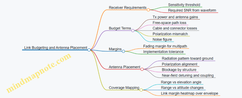
Validate with Measurement, Not Hope
After calculations, verify with measurements that mirror the real geometry. Use a test setup that includes the actual antenna mount, the same cabling, and representative platform materials. Measure realized gain or received power versus angle, then compare to the predicted link margin.
Example: If the predicted received power at a 30° elevation angle is −90 dBm but the measured value is −98 dBm, you likely have an unmodeled loss such as detuning, unexpected blockage, or polarization mismatch. Fixing the antenna mount or adjusting orientation can recover several dB—often more efficiently than increasing transmit power.
Practical Checklist for Range and Coverage
- Confirm receiver sensitivity for the exact modulation and coding.
- Compute free-space path loss at the worst-case range and include all known losses.
- Add fading and implementation margins before declaring success.
- Place antennas to minimize shadowing and preserve polarization alignment.
- Validate with angle-dependent measurements using the real mounting hardware.
When these steps are followed in order, link budgeting stops being a spreadsheet exercise and becomes a repeatable method for ensuring coverage where it counts.
6.2 Telemetry, Command, and Payload Data Prioritization
Persistent loitering systems generate three kinds of information that must coexist: telemetry (health and status), command (operator or mission directives), and payload data (sensor imagery, measurements, and derived products). Prioritization is not just about bandwidth; it’s about ensuring the right thing arrives in time for the right decision. A good rule of thumb is simple: if a message affects safety or control, it outranks everything else; if it affects targeting quality, it outranks routine monitoring.
Foundational Concepts for Prioritization
Telemetry is periodic and event-driven. Periodic telemetry answers “Is the platform still itself?” Event-driven telemetry answers “Something changed.” Command is usually sparse but time-critical; it answers “Do this now.” Payload data is often large and can be bursty; it answers “What do you see and what do you measure?”
A practical prioritization model uses three queues per link direction: control, status, and payload. Control includes arming state changes, mode transitions, and navigation-critical updates. Status includes battery, GPS quality, sensor health, and link quality. Payload includes raw imagery, cropped imagery, detection metadata, and measurement packets.
Designing a Priority Policy That Operators Can Reason About
Start with a policy matrix that maps message types to priority and allowed latency. For example, a navigation mode change might require delivery within 200 ms, while a periodic temperature report can tolerate seconds. Payload packets can be assigned “soft deadlines” tied to mission phases.
A common best practice is phase-aware payload throttling. During loiter, send low-rate thumbnails and detection metadata; during terminal approach, increase measurement rate and send only the fields needed for precision targeting. This prevents the link from being clogged by full-resolution imagery when the system is busy doing geometry and confirmation.
Telemetry Prioritization Details
Telemetry should be structured so that the receiver can quickly decide whether to trust it. Include sequence numbers and timestamps, and separate “heartbeat” from “fault.” If the link degrades, the system should continue sending heartbeat and minimal fault codes rather than stopping entirely.
Example: if the payload computer detects a sensor alignment drift, it emits an event telemetry packet immediately with a fault code and confidence score. The receiver can then reduce payload data rate or request recalibration, while still maintaining control and navigation telemetry.
Command Prioritization Details
Commands should be idempotent where possible and acknowledged with explicit results. Use a small set of command categories: immediate control, mission management, and payload requests. Immediate control commands preempt other traffic.
Example: an operator issues “Hold orbit” while the system is streaming imagery. The command is placed in the control queue and transmitted first. Payload streaming continues only after the command is acknowledged, preventing a “busy link” from delaying the control decision.
Payload Data Prioritization Details
Payload data is best treated as layered information. Send the smallest useful unit first, then add detail.
A simple layering scheme:
- Layer 0: detection metadata (bounding boxes, class, confidence, timestamps)
- Layer 1: measurement products (range estimates, pose, target coordinates)
- Layer 2: compressed imagery tiles
- Layer 3: full-resolution frames or video segments
When bandwidth shrinks, the system drops the highest layers first. When bandwidth improves, it resumes from the appropriate layer for the current mission phase.
Example: during search, transmit Layer 0 at a steady rate. Once a candidate target is confirmed, transmit Layer 1 more frequently and request a limited set of Layer 2 tiles around the candidate region. Full frames are only sent if they improve operator review or evidence quality.
Mind Map: Telemetry, Command, and Payload Prioritization
Integrated Example Workflow
Consider a mission segment where the platform is loitering and periodically checking for a target. The system sends telemetry heartbeat and link quality every second. Detection metadata is sent at a low rate, such as 1–2 updates per minute per candidate. If a candidate appears, the system increases measurement packet frequency and requests a small set of image tiles. If the operator issues “Engage hold,” the command preempts payload transmissions until acknowledged. If a sensor fault occurs, the system immediately reports the fault code and confidence, then reduces payload layers to metadata only.
Implementation Checks That Prevent Common Failure Modes
First, ensure preemption is real: control queue packets must bypass payload queue serialization. Second, ensure receivers can reconstruct order: sequence numbers and timestamps must be included for every queue type. Third, ensure payload throttling is deterministic: the same mission phase and link quality should produce the same prioritization behavior, so operators can predict what they will see without guessing.
6.3 Network Topologies for Swarm Like Coordination Without Speculation
Swarm-like coordination is easiest to get wrong when the network is treated as a magic spell. A practical approach starts with topology: who talks to whom, how messages are routed, and what happens when links degrade. The goal here is coordination that is deterministic enough for operators to reason about, while still resilient enough to keep missions moving when connectivity is imperfect.
Foundational Concepts for Topology Choice
A topology is not just a diagram; it defines latency, reliability, and who can make decisions. Three properties matter most.
First, message scope: is the message intended for one drone, a subset, or everyone in the group. Second, routing behavior: does traffic follow a fixed path, or does it adapt based on link quality. Third, state ownership: which node is considered the source of truth for shared variables like formation geometry, target lock status, or loiter phase.
A simple rule keeps things sane: minimize shared state. If every drone must agree on everything, coordination becomes a network problem instead of a mission problem.
Topology Patterns That Work in Practice
Star topology uses a single coordinator (often the ground station or a lead drone). It is straightforward for operators because the coordinator can enforce ordering and resolve conflicts. The tradeoff is a single point of failure and heavier uplink/downlink load.
Leader-follower topology reduces load by letting the leader distribute only what followers need. Followers report local observations upward, while the leader computes formation adjustments. This is a good fit when the leader has better sensors or more reliable connectivity.
Mesh topology improves resilience because multiple paths exist. However, it increases complexity: you must prevent message storms and define how conflicting updates are handled. Mesh is most effective when drones exchange small, frequent status messages and avoid large payload transfers.
Hybrid topology combines the strengths: a leader handles coordination-critical messages, while mesh links carry lower-priority telemetry and local health checks.
Mind Map: Topology Decisions and Message Discipline
Message Types and How They Flow
To keep coordination stable, treat messages as categories with different reliability requirements.
-
Coordination commands: formation changes, loiter phase transitions, and engagement gating. These should be small, versioned, and acknowledged. If an acknowledgement is not received within a bounded time, the sender retries a limited number of times, then the system falls back to a safe behavior.
-
Local observations: sensor detections, confidence scores, and health metrics. These can be less strictly reliable; missing one report should not stall the entire group.
-
Shared context: target identifiers, coordinate frames, and timing references. This should be updated at a controlled rate and only when changes are meaningful.
A practical example: each drone periodically broadcasts a compact “phase status” message containing its current loiter phase ID and a timestamp. The leader uses these to decide whether the group is synchronized. If one drone’s phase status is missing, the leader does not assume it is wrong; it marks the drone as “unknown” and continues with the rest.
Example: Leader-Follower with Bounded Coordination
Assume five drones coordinate around a target area. The leader maintains formation geometry and assigns each follower a relative position offset.
- Followers send local observation packets every 500 ms.
- The leader sends coordination commands only when offsets change, not continuously.
- Each command includes a sequence number and a phase ID.
If a follower misses two consecutive command acknowledgements, it enters a “hold last safe offset” mode. It keeps reporting local observations, so the leader can later re-synchronize it when connectivity returns.
This avoids speculation because the system never assumes the follower is where it last was; it uses explicit status and bounded timers.
Failure Handling Without Guesswork
Topology becomes useful only when you define failure behavior. Use link-loss timers tied to message categories. Coordination commands should have shorter timers than health telemetry.
When connectivity degrades:
- The coordinator or leader continues operating with the drones it can hear.
- Drones that lose the leader do not invent formation updates; they follow a local fallback policy based on the last acknowledged command.
- Rejoin requires a handshake that includes the current phase ID and sequence number, so stale commands do not get applied.
Example: Mesh for Health, Leader for Coordination
In a hybrid setup, drones exchange health and neighbor quality over mesh. Coordination-critical messages still come from the leader.
A concrete benefit: if two drones can’t reach the leader but can reach each other, they can still share health metrics and avoid redundant sensor checks. Meanwhile, they do not attempt to coordinate formation changes without the leader’s authoritative phase ID.
Summary of Integrated Best Practices
Choose a topology that matches your state ownership model. Keep shared state small, version it, and acknowledge only what must be acknowledged. Use bounded retries and explicit link-loss timers. With those rules, swarm-like coordination becomes a disciplined communications design rather than a network gamble.
6.4 Loss of Link Handling Using Defined Autonomy Behaviors
When the data link drops, the platform must stop improvising. The goal is predictable behavior that preserves safety, maintains mission intent as far as possible, and produces logs that explain what happened. “Defined autonomy behaviors” means the system has pre-validated actions tied to specific link-loss states, not a single generic fallback.
Link-Loss States and Triggers
Start by defining what “loss” means in measurable terms. Common triggers include: no valid command packets for a timeout window, telemetry heartbeat missing for N seconds, or loss of authenticated session keys. Each trigger maps to a link-loss state such as Degraded, Lost, or Recovered. A practical best practice is to require two independent indicators before declaring full loss, so brief fades don’t cause unnecessary mode changes.
Example: If the command channel heartbeat is missing for 3 seconds but telemetry is still flowing, the system enters Degraded. It reduces nonessential transmissions, keeps navigation running, and waits for recovery. If both channels fail for 10 seconds, it enters Lost and executes the loss plan.
Behavior Set and Mode Transitions
A robust behavior set usually includes four phases: Hold, Search, Safety, and Report. The platform chooses among them based on mission phase, altitude, geofence status, and remaining energy.
- Hold: Maintain the last safe loiter pattern or a stable orbit while continuing onboard sensing. This is appropriate when the platform is already in a terminal-relevant area and the risk of drifting is low.
- Search: If the platform needs target reacquisition, it performs constrained search patterns that respect airspace limits and sensor geometry.
- Safety: If constraints are violated or the platform cannot guarantee safe operation, it transitions to a predefined safe state such as loitering at a conservative altitude band or initiating a controlled descent profile.
- Report: Even without the link, the system records structured events so that when communications return, the operator sees a coherent timeline.
Mode transitions should be monotonic: once the system escalates to Safety, it should not automatically downgrade to Hold without explicit recovery logic. This prevents oscillation during intermittent connectivity.
State Machine Design for Predictability
A simple state machine makes behavior auditable. Each state has entry conditions, exit conditions, and a small set of actions. Keep the actions deterministic where possible.
Concrete Example: Terminal Approach Without Commands
Assume the platform is in the final minutes of a mission and is tracking a candidate target using onboard sensors. The command link drops, but the platform still has enough power to loiter.
- Degraded: The system stops requesting additional mission updates, but continues target tracking and maintains the current orbit.
- Lost: After the full timeout, it enters Hold if it remains within a predefined approach corridor. If it drifts outside that corridor, it switches to Safety and re-centers into a safe loiter volume.
- Report: It logs the last known target track quality, the time link was lost, and the reason for any safety transition.
When the link returns, the system does not “snap back” to an armed terminal action. Instead, it requires operator confirmation and revalidates the current state against the same safety checks used during normal operation.
Logging and Operator Clarity
Loss-of-link handling fails when logs are vague. Use structured event records: timestamps, state transitions, trigger values, and the active behavior. Include sensor confidence summaries so the operator can understand whether the platform was holding position, searching, or forced into safety.
A helpful best practice is to log the exact trigger that caused the transition. If the system entered Lost because the command heartbeat timed out, that should be explicit in the event record.
Verification Through Scenario Coverage
Test the behavior set with scenarios that mirror real link behavior: short fades, long outages, intermittent packet loss, and recovery after safety escalation. The key metric is not just “did it stay safe,” but “did it choose the correct behavior for the correct link-loss state.”
A good acceptance check is to confirm that every link-loss trigger maps to exactly one expected state transition, and that no transition occurs when triggers are not met. That’s how you keep autonomy from turning into guesswork when the link goes quiet.
6.5 Security Controls for Authentication, Integrity, and Access Control
Persistent loitering systems live and die by trust in their messages. A command that arrives late is annoying; a command that arrives from the wrong source is dangerous. This section builds a practical security baseline around three goals: prove who is sending, prove the message wasn’t altered, and prove the receiver is allowed to act.
Foundations of Trust Boundaries
Start by drawing trust boundaries between components that exchange commands and data: operator console to mission computer, mission computer to payload controller, and mission computer to datalink modem. Each boundary needs its own controls because compromise at one boundary should not automatically grant control everywhere.
A simple best practice is to classify every message by intent and consequence. For example, “request sensor snapshot” is lower consequence than “arm payload” or “change terminal guidance mode.” Then map each class to required security properties: authentication only, or authentication plus integrity, or authentication plus integrity plus strict authorization checks.
Authentication Controls for Message Origin
Authentication answers: “Is this message from a legitimate entity?” Use a two-part approach: identity and freshness.
- Identity: Each sender has a cryptographic identity (key or certificate) provisioned during integration. The receiver verifies that identity before processing.
- Freshness: Include a monotonically increasing counter or a time window marker so replayed messages are rejected.
Easy example: the console sends “enter loiter mode.” If an attacker replays an old “enter loiter mode” packet, the mission computer should reject it because the counter is stale.
Implementation detail that matters: counters must be stored persistently across reboots or you risk accepting old messages after a restart.
Integrity Controls for Tamper Resistance
Integrity answers: “Was this message modified in transit?” Apply a message authentication code (MAC) or a digital signature over the full message, including critical fields like mode identifiers, target identifiers, and arming-related parameters.
Best practice: authenticate the exact bytes that the receiver will parse. If you authenticate only a subset of fields, an attacker can sometimes change the unprotected fields while keeping the protected ones valid.
Easy example: a “payload configuration” message includes a fuse setting and a safety interlock flag. If only the fuse setting is protected, the interlock flag could be flipped to bypass safety logic.
Access Control for Authorized Actions
Authentication and integrity tell you the message is genuine; access control tells you the receiver should act on it.
Use role-based authorization with explicit permissions. Roles might include operator, test engineer, and automated safety supervisor. Permissions should be granular and tied to message classes.
A practical pattern is “allow lists” for high-consequence actions. For instance, only the operator role can request arming, while the safety supervisor role can command safe-state transitions.
Easy example: if the operator requests “arm payload,” the mission computer checks both the authenticated sender identity and whether the current mission state permits arming. Even a valid operator message should be denied if the platform is not in the correct flight envelope.
Defense in Depth Through State-Aware Checks
Security controls should be state-aware. A message that is cryptographically valid can still be logically invalid. Combine security checks with mission state constraints such as: altitude limits, geofenced areas, sensor readiness, and interlock status.
This is where “security” becomes operationally useful: it prevents valid-but-wrong commands from causing unintended behavior.
Mind Map: Authentication, Integrity, and Access Control
Example: Securing a Mode Change Command
Consider a command to switch from loiter to terminal approach.
- The console sends a mode-change message containing: mode ID, a target reference, a freshness counter, and a signature/MAC.
- The mission computer verifies authentication and freshness.
- It verifies integrity over all fields.
- It checks authorization: does the console role have permission for terminal approach?
- It checks state: are sensors calibrated, is the platform within the allowed envelope, and are safety interlocks satisfied?
- Only then does it apply the mode change.
If any step fails, the system should respond with a controlled denial and log the reason code for later review. That log should not include sensitive key material, and it should be protected against tampering as well.
Example: Preventing Replay After a Restart
Suppose the mission computer reboots mid-mission. If it resets its freshness counter to zero, an old authenticated message could become “fresh” again. The fix is to persist the last accepted counter value in non-volatile storage and require incoming counters to be greater than the stored value.
This turns a common engineering nuisance into a security feature: the system remains strict even when power cycles happen.
7. Precision Effects Integration and Safety Critical Design
7.1 Payload Types and Integration Constraints for Platform Compatibility
A loitering drone platform is only as precise as the payload stack it carries. Payload integration is not just “bolt-on hardware”; it is a chain of mechanical fit, power delivery, data bandwidth, thermal behavior, and safety logic that must all agree with the airframe and mission profile. The goal of this section is to help you reason from payload type to the platform constraints that decide whether the system behaves predictably.
Payload Types That Drive Different Constraints
Most payloads fall into a few functional families, each with distinct integration demands.
- Electro-Optical and Infrared Imaging
- Needs stable optical alignment, vibration control, and careful power regulation.
- Produces high-rate data streams when recording video or running onboard processing.
- Laser Rangefinding and Designation
- Requires precise pointing, timing discipline, and often tighter safety interlocks.
- May need additional cooling or duty-cycle limits to avoid overheating the emitter.
- Communications and Data Relay Payloads
- Prioritizes antenna placement, RF isolation, and link budgeting.
- Can be sensitive to airframe shielding and grounding quality.
- Effects Payloads
- Adds strict arming, fuzing, and safe-state requirements.
- Often imposes mass distribution constraints and mechanical release tolerances.
- Navigation and Targeting Support Sensors
- Includes additional measurement devices that improve geometry or identification.
- Typically less power-hungry than imaging, but can be sensitive to mounting angles and calibration.
A practical way to avoid surprises is to treat each payload as a set of “interfaces”: mechanical interface, electrical interface, data interface, thermal interface, and safety interface.
Platform Compatibility Constraints You Must Check
Mechanical compatibility covers mounting stiffness, center-of-gravity shift, and vibration transmission. A payload that is “light” on paper can still cause pointing errors if it sits on a flexible bracket.
Electrical compatibility includes voltage rails, peak current draw, inrush current at startup, and electromagnetic interference. Imaging payloads can create noisy power demand during sensor exposure changes; effects payloads can draw current in short bursts that stress regulators.
Data compatibility is about throughput and latency. A camera streaming full resolution may saturate a link that otherwise seems adequate for telemetry. If onboard processing reduces data, you must verify that the compute budget and storage behavior match the mission.
Thermal compatibility matters because endurance missions often run near steady-state. A payload that warms the airframe can shift sensor calibration, degrade optics, or trigger thermal throttling.
Safety-critical compatibility is the most unforgiving. Effects payloads require arming logic that prevents unintended activation, even during faults, resets, or loss of control. Imaging and ranging payloads also benefit from safety logic, such as laser inhibit conditions when pointing uncertainty is high.
Integration Workflow That Prevents Rework
Start with a compatibility matrix, then validate each interface with tests that mirror real operation.
- Define payload interface requirements: mass, dimensions, mounting pattern, connector types, voltage rails, data rates, and thermal limits.
- Map platform resources: payload bay volume, allowable center-of-gravity envelope, available power rails, compute capacity, and link capacity.
- Design for isolation: vibration damping for optics, RF shielding for radios, and separation of high-current switching from sensitive sensors.
- Implement safety logic: define inhibit conditions, safe states, and fault handling paths.
- Verify with integration tests: run vibration checks, power transient checks, thermal soak, and end-to-end pointing and data tests.
Mind Map: Payload Integration Interfaces and Checks
Example: Imaging Payload Integration Without Pointing Drift
Suppose you mount an EO/IR turret with a flexible bracket. During loiter, the drone’s propeller harmonics excite the bracket, causing small angular jitter. Even if the camera stabilizer corrects for some motion, the correction can saturate, leading to blur and reduced target confidence. The fix is not “increase stabilization gain”; it is to improve mount stiffness, add damping, and confirm the vibration spectrum at the optical reference point.
A good integration check is to log stabilized pointing error while the drone performs a representative loiter pattern. If the error grows with payload temperature, you also need to verify thermal expansion effects on alignment.
Example: Effects Payload Integration with Safety-First Electrical Design
An effects payload often uses a separate arming circuit with strict inhibit conditions. A common integration mistake is sharing a power rail without accounting for switching noise from other payloads. If the arming circuit sees spurious voltage transients during sensor exposure or radio transmission, it may enter a fault state or, worse, behave unpredictably.
The corrective approach is to allocate dedicated power conditioning for the effects arming path, separate high-current switching grounds, and test fault injection scenarios: payload connector disconnect, controller reset, and loss of command. The acceptance criterion is simple: the payload must remain in safe state under every defined fault.
Example: Laser Rangefinding Integration with Pointing Uncertainty Handling
Laser rangefinding accuracy depends on where the laser actually points relative to the target. If the platform’s pointing solution has higher uncertainty near the edge of the gimbal limits, the system should inhibit ranging or mark the measurement as low confidence. This is an integration constraint because it requires the payload to accept uncertainty metadata from the guidance and control stack, not just raw pointing angles.
When you test, include scenarios with reduced visibility and higher attitude rates. The goal is to confirm that the inhibit and confidence behavior matches the mission’s operational envelope, not just ideal lab conditions.
Summary of Integration Constraints
Payload integration succeeds when you treat each payload type as a bundle of interface requirements and then verify that the platform’s mechanical, electrical, data, thermal, and safety resources can satisfy them simultaneously. The best systems are the ones that fail safely, log what happened, and keep precision stable under the conditions that actually occur during persistent loiter.
7.2 Fuzing Concepts and Arming Safety Logic Requirements
Fuzing is the chain of decisions that turns a payload from “carried” into “effective.” Arming safety logic is the part that prevents that transition from happening accidentally, early, or under unsafe conditions. In a loitering platform, the logic must also tolerate long dwell times, sensor drift, and operator interaction without turning the system into a guessing game.
Core Concepts and Failure Modes
A typical fuzing system has three states: safe, armed, and fired. Safe means the initiator cannot produce the effect even if power is applied. Armed means the initiator is enabled but still constrained by additional conditions. Fired means the effect has been commanded and the initiator has executed.
The safety logic should explicitly guard against four common failure modes:
- Premature arming: arming occurs before the platform is in the intended delivery geometry.
- Unintended arming due to faults: a sensor glitch or software fault satisfies arming conditions.
- Unintended firing: arming happens correctly, but firing conditions are met without operator intent.
- Stuck unsafe or stuck armed: the system never transitions, or it transitions and cannot recover.
A practical best practice is to design arming as a monotonic progression with clear exit criteria. If the system can move from safe to armed, it should also have a defined path for returning to safe when conditions become invalid, unless the design intentionally latches armed for reliability.
Arming Conditions and Gating Strategy
Arming logic is usually built as a set of gates that must all be satisfied. Each gate should be independently checkable and time-bounded.
Gate categories commonly include:
- Platform state gates: altitude, attitude, airspeed, and attitude stability.
- Navigation and geometry gates: position uncertainty bounds and predicted impact point validity.
- Environmental gates: temperature or vibration thresholds that affect sensor reliability.
- System health gates: self-test results, sensor plausibility checks, and power rail status.
- Operator intent gates: explicit approval or a command that is only accepted in valid states.
A concrete example: the system may require that the platform’s pitch and roll remain within limits for a continuous 2-second window, and that the navigation solution uncertainty is below a threshold for the same window. This “continuous validity” requirement prevents a brief moment of good data from arming the payload.
Safety Interlocks and Two-Step Intent
Safety interlocks reduce the chance that a single bug or single sensor failure triggers the wrong transition. Two-step intent is a common pattern: one step arms, another step fires.
For instance:
- Step 1: Arm request is accepted only when all platform and health gates pass.
- Step 2: Fire command is accepted only after arming has been achieved and additional terminal conditions are met, such as a valid terminal time window or a confirmed aimpoint measurement.
This separation helps because arming can be treated as “enablement,” while firing is treated as “execution.” If the system loses link or the operator cancels, the logic should be able to prevent Step 2 without needing to re-validate every Step 1 detail.
Timing, Debounce, and Latch Behavior
Long loiter times create a subtle issue: conditions can oscillate around thresholds. Without debounce logic, the system could repeatedly enter and exit arming eligibility.
A systematic approach uses:
- Debounce timers for each gate (e.g., 1–3 seconds of continuous satisfaction).
- Hysteresis for thresholds (e.g., uncertainty must be below 0.5 m to arm, but must rise above 0.8 m to disarm).
- Defined latch rules: either “armed is reversible” or “armed is latched until safe-state reset.”
A simple example of hysteresis: if impact-point uncertainty is allowed up to 0.5 m for arming, the system disarms only when uncertainty exceeds 0.8 m. That prevents arming from flickering when uncertainty hovers near the boundary.
Mind Map: Fuzing and Arming Safety Logic
Example: Gate-Based Arming with Continuous Validity
Assume the system uses three gates for arming: health, geometry, and intent.
- Health gate: self-test must pass and sensor plausibility must remain true.
- Geometry gate: predicted impact point must be within an accuracy bound, and the platform must maintain stable attitude.
- Intent gate: operator approval must be present.
Arming occurs only if all three gates remain satisfied for 2 seconds continuously. If any gate fails for even 0.2 seconds, the timer resets. This design makes arming robust against brief sensor spikes and avoids “threshold surfing.”
Verification Requirements for Safety Logic
Safety logic should be verified with traceable evidence that each gate behaves correctly under both normal and fault conditions. A good verification set includes:
- Boundary tests: values just inside and just outside thresholds.
- Temporal tests: conditions that satisfy gates intermittently.
- Fault tests: stuck sensors, biased measurements, and health-test failures.
- State-machine tests: ensuring transitions follow the intended safe → armed → fired rules.
The goal is not just to show that the system works, but to show that it fails safely and predictably when reality gets messy.
7.3 Impact Point Accuracy Considerations for Terminal Delivery
Impact point accuracy is the chain of small errors that finally show up as “where it hit.” Terminal delivery makes that chain tighter because the last seconds compress time for sensing, computing, and correcting. The goal is not perfection; it is predictable accuracy with known bounds.
Foundations of Impact Point Accuracy
Start with a simple mental model: the impact point equals the predicted aim point plus error from (1) target location, (2) platform state, (3) sensor-to-body alignment, (4) guidance and control execution, and (5) effect delivery dispersion. Each term can be measured, bounded, and reduced.
A practical best practice is to separate errors into “known at launch,” “learned during terminal,” and “unavoidable.” For example, target coordinates from an earlier sensor pass are “known at launch” but may drift; platform state at the start of terminal is “known at launch” but can degrade; terminal sensor measurements are “learned during terminal.” This separation prevents the common mistake of treating everything as equally correct.
Geometry and Coordinate Consistency
Impact point math is unforgiving when coordinate frames disagree. The platform navigation frame, sensor frame, and effect aim frame must share a consistent definition of axes, sign conventions, and units. A small rotation error in sensor-to-body calibration can create a systematic miss that looks random in logs.
A concrete example: if a camera is yaw-misaligned by 0.2° and the target is 2 km away, the lateral pointing error is roughly 7 m (2,000 m × tan(0.2°)). That miss can be larger than the guidance correction authority near the end of flight.
Best practice: verify frame alignment with a “static sighting” procedure where the platform holds attitude while a known target marker is observed. Record the pixel-to-bearing mapping and confirm that the computed bearing matches the measured bearing within a tight tolerance.
Sensor Measurement Quality at the End
Terminal delivery often relies on the most recent sensor measurements. Those measurements have their own uncertainty: image blur, atmospheric effects, rolling shutter timing, and target motion between frames.
A systematic approach is to treat sensor output as a measurement with covariance, not a single best guess. If your system can estimate bearing and range uncertainty, you can propagate that uncertainty into the aim point. If it cannot, you can still use conservative bounds derived from repeated trials.
Example: suppose bearing uncertainty is ±0.05° and range uncertainty is ±50 m at 1.5 km. The lateral position uncertainty from bearing alone is about 1.5 km × tan(0.05°) ≈ 1.3 m. Range uncertainty contributes directly along the line of sight, affecting predicted intercept timing and terminal aim.
Guidance, Control, and Execution Limits
Even with perfect sensing, the vehicle must execute the commanded motion. Impact point accuracy depends on guidance law assumptions matching real actuator behavior.
Key contributors include:
- Control loop latency and sampling jitter
- Actuator saturation near the end of flight
- Rate limits that prevent the vehicle from tracking the commanded line
- Modeling mismatch in drag or thrust
A useful check is to compute the “achievable correction envelope” during terminal: the maximum lateral acceleration or turn rate the platform can produce given its speed and configuration. If the required correction exceeds that envelope, the miss becomes predictable and should be reflected in the accuracy budget.
Effect Delivery Dispersion and Aim Point Mapping
The effect delivery stage adds dispersion from release/trigger timing, mechanical tolerances, and environmental variability. Even when guidance aims correctly, the delivered effect may land within a pattern.
Best practice: characterize dispersion empirically under representative conditions and map it to the same coordinate system used for impact point prediction. For instance, if the effect has a typical cross-range standard deviation of 2 m at the relevant altitude, that value belongs in the final impact point uncertainty, not in a separate “payload section” that never meets the guidance math.
Building an Accuracy Budget Without Hand-Waving
An accuracy budget combines uncertainties into a final bound. A common method is root-sum-square for independent terms, plus worst-case handling for correlated terms.
Terminal Delivery Verification Through Repeatable Scenarios
Verification should test the whole chain, not isolated components. Use repeatable terminal geometries: similar approach angles, similar ranges, and similar sensor viewing conditions. Then compare predicted impact distributions to observed impacts.
Example: run ten trials with identical terminal start conditions and record the miss vectors in a consistent frame. If the mean miss is offset, suspect systematic calibration or frame issues. If the mean is near zero but spread is wide, suspect sensor noise, control authority limits, or effect dispersion.
A final best practice is to define acceptance criteria in terms of impact point bounds that match the operational decision. If the system must reliably place within a radius, evaluate that radius directly from the miss vectors rather than relying on intermediate metrics that may not correlate with the final outcome.
7.4 Blast Fragmentation Modeling for Planning and Risk Reduction
Blast fragmentation modeling turns “we think it will be close” into “we can bound what happens if it is close.” The goal is not to predict a single perfect outcome; it is to estimate fragment distributions, impact likelihood, and resulting hazard zones so planning decisions can be made with known assumptions.
Foundational Concepts for Fragment Hazard Modeling
Start with three inputs: the explosive energy release, the fragmentation mechanism, and the geometry of the target and surroundings. Fragmentation mechanism matters because it determines fragment size, mass distribution, and initial velocity. A simple way to keep planning grounded is to separate effects into (1) fragment generation and (2) fragment flight and impact.
For generation, you typically model a fragment mass distribution and an initial velocity distribution. For flight, you model drag and gravity, then compute where fragments intersect surfaces. Even when you use simplified physics, you should track uncertainty: if the model assumes a certain casing thickness or fill mass, the hazard zone should widen when those inputs are uncertain.
A practical planning habit is to define hazard outputs that map to decisions. Examples include “probability of fragment strike on a specific structure,” “distance to the 1% lethality contour,” or “maximum expected fragment energy at a given standoff.” Pick one or two outputs and keep them consistent across scenarios.
Modeling Workflow from Geometry to Hazard Zones
- Define the scenario geometry. Specify standoff distance, relative orientation, and any cover or barriers. If the environment includes walls, vehicles, or terrain features, represent them as surfaces that can block or redirect fragments.
- Choose a fragmentation representation. Use either a discrete fragment set (many fragments with sampled masses and velocities) or a continuous distribution (fewer parameters, faster but less detailed).
- Compute fragment trajectories. Apply drag and gravity to propagate each fragment until it hits a surface or falls below an effective range.
- Compute impact and hazard metrics. Convert impact velocity and fragment mass into an energy or penetration proxy, then map that to a hazard threshold.
- Aggregate results into zones. Convert many simulated impacts into contours such as “hazard probability by distance” or “expected number of impacts per square meter.”
A key risk-reduction step is to run sensitivity cases. Change one input at a time—standoff, casing assumptions, or barrier placement—and observe which uncertainty dominates the hazard zone. If the hazard zone barely moves when you vary casing thickness slightly, you can focus on other uncertainties.
Fragment Generation Assumptions That Affect Planning
Fragment size distribution is often the biggest driver. If you assume fragments are mostly small, the model may show many low-energy impacts; if you assume fewer large fragments, you may get a smaller but more severe hazard zone. Initial velocity distribution also matters because it shifts the entire range of fragments.
To keep assumptions transparent, record them as explicit parameters in the planning dataset. For example, store: fragment count model type, mass distribution parameters, and initial velocity scaling. Then you can compare scenarios without silently changing the underlying physics.
Flight Modeling and Environmental Effects
Drag modeling determines how quickly fragments slow down. A simple approach uses a ballistic coefficient or an effective drag term calibrated to fragment-like objects. If you have no calibration, treat drag uncertainty as a planning margin.
Barriers and cover are handled by surface intersection logic. When a fragment hits a barrier, you can either stop it (conservative for hazard) or apply a reduced-energy continuation model (more realistic but requires more assumptions). For risk reduction, conservative stopping is often appropriate for planning near protected areas.
Example Mind Map for Planning Inputs and Outputs
Mind Map: Blast Fragmentation Modeling for Risk Reduction
Example Scenario with Clear Decision Use
Assume a planning team needs an exclusion zone for a structure at a known standoff. They run a baseline simulation with a fragment mass distribution that includes a long tail of larger fragments. The resulting hazard contour shows a steep drop after a certain distance.
Next, they run a sensitivity case that increases the assumed initial velocity spread. The hazard contour expands slightly farther, but the steep drop remains. That tells the team the model is robust to velocity spread for the chosen threshold, so the main risk driver is standoff accuracy rather than velocity uncertainty.
Finally, they test barrier placement. If adding a barrier reduces hazard probability by an order of magnitude, they can justify a smaller exclusion zone on the barrier-protected side, while keeping a conservative zone on the unprotected side. The decision is grounded in modeled geometry and explicit assumptions, not vibes.
Practical Verification Checks
Before using results for planning, sanity-check the model outputs. Confirm that fragment ranges scale reasonably with standoff and that impact counts decrease with distance. Also verify that barrier logic behaves correctly: fragments should not “pass through” a barrier surface in the conservative stopping mode.
When these checks pass, the hazard zones become a reliable planning artifact. They provide a consistent way to compare scenarios, quantify uncertainty, and reduce risk through geometry, standoff control, and barrier placement.
7.5 Safety Interlocks, Fault Detection, and Safe State Procedures
Safety for precision loitering platforms is mostly about preventing “almost” from becoming “oops.” The core idea is simple: before any hazardous action, the system must verify that required conditions are true, and if they are not, it must move to a safe state that reduces risk rather than improvising.
Foundational Concepts for Interlocks
Start with three layers that work together.
-
Arming and enablement gates: The system should not allow a hazardous payload action unless explicit arming steps have been completed and verified. A practical example is a two-step arming sequence where the operator first selects the payload mode, then confirms a second prompt after reviewing sensor readiness and safety status.
-
Environmental and platform constraints: Even if the operator asks for action, the platform should refuse when conditions violate limits. Example: if the navigation solution quality drops below a threshold, the system should block terminal delivery and instead continue loitering or return to a safe orbit.
-
Fault-aware permissions: Interlocks must incorporate fault states. Example: if a sensor alignment check fails, the system should prevent precision targeting from being used for hazardous effects, even if other subsystems look healthy.
Fault Detection That Produces Actionable Decisions
Fault detection should be designed around what the system can do next, not just what it can detect.
Detection categories
- Sensor plausibility faults: Values that are inconsistent with expected behavior. Example: an inertial sensor bias estimate that jumps abruptly while the platform is steady.
- Timing and data integrity faults: Missing messages, stale timestamps, or corrupted packets. Example: a target coordinate update that arrives late enough to invalidate the guidance solution.
- Actuator and control faults: Commands that do not produce expected response. Example: a control surface position sensor reporting movement that contradicts commanded deflection.
- Power and thermal faults: Conditions that degrade performance. Example: payload cooling reaching a limit that would reduce measurement reliability.
Decision logic
Fault detection should map to a small set of outcomes: continue, degrade, or stop hazardous actions. A useful practice is to define thresholds and hysteresis so the system does not “chatter” between states. Example: if GPS quality drops, require sustained degradation for a few seconds before blocking precision delivery.
Safe State Procedures That Reduce Risk
A safe state is not just “do nothing.” It is a defined behavior that keeps the platform stable and prevents escalation.
Typical safe state behaviors
- Hazard action inhibit: Payload effects remain disabled.
- Guidance fallback: Switch to a conservative loiter pattern with reduced maneuvering.
- Stability priority: Maintain attitude and altitude margins to avoid uncontrolled flight.
- Operator notification: Provide clear status so the operator knows what is blocked and why.
Example safe state sequence
- Fault detected in target measurement confidence.
- Interlock blocks hazardous action.
- Guidance switches to a stable orbit with minimal control effort.
- System logs the fault, the confidence score, and the last valid targeting solution.
- Operator receives a single actionable message: “Precision delivery inhibited due to measurement confidence below threshold.”
Mind Map: Safety Interlocks, Fault Detection, and Safe State
Interlock Implementation Patterns
Reason codes and traceability: Each inhibit should carry a reason code that ties back to a specific check. Example: “INHIBIT_NAV_QUALITY” is more useful than “INHIBIT_GENERAL,” because it tells the operator whether waiting for recovery is reasonable.
Two-channel confirmation for critical transitions: For arming, require both operator intent and system readiness. Example: the operator selects “ARM,” but the system also verifies payload safety logic, sensor calibration status, and effect authorization state.
Fail-closed for hazardous permissions: If a required input is missing, treat it as not satisfied. Example: if the effect authorization message is absent, the system should not proceed.
Example: End-to-End Safety Flow
A coherent flow prevents gaps between detection and action.
- Pre-engagement: Interlocks verify arming steps, sensor calibration status, and navigation quality.
- During loiter: Fault detection monitors data integrity and plausibility.
- At terminal decision: The system checks confidence thresholds and ensures no active faults are marked as “inhibit.”
- If blocked: Safe state procedures maintain stability, inhibit hazardous action, and log the exact condition that triggered the block.
The result is a system that behaves predictably under stress: it refuses hazardous actions when it should, explains why in plain terms, and keeps the platform controllable while the operator decides the next step.
8. Mission Planning, Rehearsal, and Execution Workflows
8.1 Building Mission Plans From Terrain, Weather, and Constraints
A mission plan is a set of decisions that remain true when reality gets messy. The goal of this section is to show how terrain, weather, and constraints turn into a workable route, timing plan, and decision logic—before the aircraft ever leaves the ground.
Foundational Inputs That Drive Everything
Start with three input groups, because they constrain each other.
- Terrain and airspace geometry
- Define the operating area polygon, no-fly zones, altitude bands, and any required corridors.
- Convert terrain into practical limits: maximum safe climb rate, minimum terrain clearance, and areas where sensor line-of-sight is poor.
- Weather and environmental effects
- Use forecast layers for wind (speed and direction by altitude), visibility, precipitation, and cloud base.
- Translate weather into operational impacts: expected sensor performance windows, loiter stability margins, and communications reliability.
- Mission constraints and rules
- Include legal and safety constraints: altitude ceilings, geofencing, speed limits, and arming or release conditions.
- Include system constraints: battery or fuel limits, payload temperature limits, and maximum allowable maneuver rates.
A good practice is to write each constraint as a measurable statement. “Maintain safe clearance” becomes “Maintain at least X meters above the highest relevant terrain point within the planned corridor.”
Turning Inputs into a Route That Can Be Flown
Route planning is not just drawing lines. It is selecting segments that satisfy clearance, performance, and timing.
- Choose a loiter concept first
- Decide whether loitering is centered on a target, a sensor coverage region, or a navigation waypoint grid.
- Pick a loiter altitude that balances clearance with sensor quality. Higher altitude can improve coverage but may reduce target detail.
- Build the route as a sequence of segments
- Ingress: from current position to the loiter entry point while respecting airspace and climb limits.
- Stationing: holding patterns that keep the aircraft within clearance margins despite wind.
- Search and cueing: expanding coverage when the target is not immediately trackable.
- Terminal approach: a controlled geometry that supports measurement accuracy.
- Apply wind-aware timing
- For each segment, estimate ground speed and loiter drift using forecast winds.
- Use this to compute arrival time windows for sensor tasks, not just total mission duration.
Example: Converting Weather into Segment Times
Assume a loiter altitude where wind is forecast at 18 m/s from the west. If the loiter pattern is a racetrack aligned north-south, the aircraft will experience different ground speeds on each leg. Instead of using a single average speed, compute leg-by-leg times and verify that the sensor task still fits within the battery and payload duty limits.
Constraints as a Decision Tree, Not a Checklist
A mission plan should specify what happens when conditions change. That means defining decision points tied to measurable triggers.
- If visibility drops below threshold Y, switch from identification mode to broader search mode or abort with a safe return.
- If wind exceeds margin M, reduce loiter radius or change loiter altitude within allowed bands.
- If communications degrade, rely on pre-approved autonomy behaviors and restrict actions that require continuous operator approval.
This approach prevents “operator improvisation under stress,” which is a fancy way of saying the plan should already know the safe options.
Mind Map: Mission Planning Inputs to Execution Logic
Verification That Prevents Surprises
Before finalizing, validate the plan in three passes.
- Geometric pass: confirm clearance and corridor compliance for every segment, including turns and loiter extremes.
- Performance pass: check that energy and payload limits hold under worst-case wind within the forecast uncertainty band you choose.
- Operational pass: ensure the sensor tasks fit the timing windows created by the route and weather.
Example: Clearance Validation with Loiter Extremes
If the loiter radius is set to maintain sensor geometry, the aircraft’s actual path will still vary with wind. Validate clearance using the maximum expected lateral drift and the tightest turn rates allowed by the control system, not just the nominal centerline.
Integrated Planning Example with Concrete Steps
- Define the operating polygon and corridors, then compute a terrain clearance surface.
- Select a loiter altitude that satisfies clearance and preserves expected target detail given forecast visibility.
- Create ingress and egress segments that avoid no-fly zones and respect climb limits.
- Compute segment times using wind-by-altitude estimates.
- Add decision triggers: visibility threshold for mode switching, wind margin for loiter adjustment, and a comms-loss behavior that limits actions to pre-approved states.
- Run a simulation pass to confirm sensor task feasibility and clearance under loiter extremes.
A mission plan built this way reads like a set of engineering constraints with human-readable intent. It is easier to operate, easier to test, and harder to break when the environment refuses to cooperate.
8.2 Route Generation for Loiter Patterns and Coverage Optimization
Route generation turns a mission plan into a set of flyable, sensor-aware trajectories. The goal is not just “cover the area,” but cover it in a way that matches sensor geometry, dwell needs, and safety limits. A good route generator starts with constraints, then chooses a pattern family, then tunes parameters using measurable coverage metrics.
Foundations for Coverage-Aware Routing
Begin with a coverage model that answers three questions: What must be observed, for how long, and from what viewing angles? For loitering platforms, observation quality depends on slant range, look angle, and platform motion. A practical approach is to represent the target area as a grid of cells, each cell having a required dwell time or minimum detection confidence.
Next, define hard constraints that the route must respect. Typical ones include maximum bank angle, minimum altitude above terrain, geofence boundaries, speed limits, and minimum standoff distances for safety. If the sensor has a field-of-view cone, also include a constraint on how quickly the line of sight can move across the scene without degrading tracking.
Finally, decide what “coverage” means operationally. Coverage can be defined as the fraction of cells that receive at least the required dwell, or as an accumulated score where each cell earns points per second of acceptable viewing. This score-based view is handy when some cells are easier to observe than others.
Pattern Families and When to Use Them
Common loiter pattern families include circular orbits, racetracks, figure-eight variants, and waypoint-based “lawnmower” passes adapted for persistence. Each pattern has a predictable relationship between time-on-stare and geometry.
- Circular orbits are simple and stable, good when the target region is compact and you want consistent look angles.
- Racetracks handle elongated regions well, because the straight segments improve coverage of a corridor while turns keep the platform from drifting away.
- Waypoint-based sweeps are useful when you need to respect complex boundaries or when the sensor must repeatedly revisit specific subregions.
A best practice is to select the pattern family based on the shape of the required observation region. If the region is roughly round, start with circles. If it is a corridor, start with racetracks. If it is irregular, use waypoint sweeps with local loiters.
Coverage Metrics That Actually Guide Tuning
Use metrics that can be computed from the planned trajectory and sensor model.
- Dwell Coverage: For each cell, compute the total time where the sensor meets viewing constraints.
- Minimum View Quality: Track the worst-case view quality over time, such as maximum slant range or minimum look angle.
- Revisit Rate: For moving targets, measure how often the route returns to cells within a time window.
A simple example: suppose a grid cell requires 20 seconds of acceptable viewing. If a circular orbit gives 12 seconds per pass, you can either increase orbit time, adjust orbit radius to improve geometry, or switch to a racetrack that spends more time over the cell.
Route Generation Workflow
A systematic workflow keeps the process from becoming a pile of “try this and see.”
- Discretize the Area: Create a grid over the region of interest and mark cells that are mandatory versus optional.
- Seed Candidate Patterns: Generate initial parameters such as orbit radius, track length, turn radius, and center location.
- Simulate Sensor Visibility: For each candidate, compute which cells are visible within the sensor constraints and how long.
- Score and Rank: Use a weighted objective, for example: mandatory dwell coverage first, then overall score, then revisit rate.
- Enforce Constraints: Reject candidates that violate geofence, altitude, or maneuver limits.
- Parameter Refinement: Adjust parameters using the score gradients. For instance, if edge cells are under-covered, increase track length or shift the center.
- Finalize for Execution: Convert the chosen pattern into a time-parameterized trajectory with guidance-friendly segments.
Example: Tuning a Racetrack for Corridor Coverage
Assume a corridor-shaped target area 6 km long and 1 km wide. The sensor requires look angles between 20° and 45° and slant range under 4 km for reliable identification.
Start with a racetrack centered on the corridor. Choose a track length close to the corridor length and set turn radius to satisfy bank limits. Simulate the route: if the straight segments cover the corridor but the turns underperform, reduce turn sharpness by increasing turn radius and slightly widening the corridor alignment. If the straight segments are too far from the corridor centerline, shift the racetrack laterally by half the corridor width so the sensor spends more time within the acceptable look-angle band.
The key is to change one parameter at a time and observe which coverage metric improves. That keeps tuning from turning into guesswork.
Mind Map: Route Generation and Coverage Optimization
Practical Best Practices That Keep Routes Honest
First, always validate coverage against the same sensor model used in planning. If you plan with one set of visibility rules and execute with another, the route will look good on paper and behave differently in the air.
Second, include a “coverage margin” by requiring cells to exceed dwell thresholds by a small buffer. Real-world factors like wind drift and small navigation errors reduce effective dwell, and the buffer prevents borderline routes.
Third, keep the route generator deterministic for a given mission input. When two planners produce different routes for the same constraints, it becomes hard to debug why coverage changed.
Fourth, log the coverage score breakdown by cell group. If mandatory cells are covered but optional ones are not, you want to know that distinction immediately rather than after the mission ends.
With these elements in place, route generation becomes a controlled process: choose a pattern family that matches the region, compute coverage using explicit metrics, then tune parameters until the route meets the observation requirements without violating constraints.
8.3 Target Data Preparation Including Coordinates and Metadata
Target data preparation turns “we know where the target is” into “the system can use the target consistently.” The goal is not just to store coordinates, but to package them with the context needed for navigation, sensor alignment, and decision logic. A good workflow reduces ambiguity, prevents silent unit mistakes, and makes later review possible.
Foundational Coordinate Concepts
Start with a clear coordinate frame story. Most failures come from mixing frames without noticing. Decide the primary representation for planning and execution, then record the transformation chain.
- Geodetic coordinates (latitude, longitude, altitude) describe a point on the Earth model.
- Local coordinates (e.g., NED or ENU) describe motion relative to a chosen origin.
- Image coordinates (pixel rows and columns) describe where a target appears in a sensor frame.
Example: A target is provided as 37.4219999°N, -122.0840575°E, 30 m AGL. If the platform uses a local NED frame, you compute the local coordinates from a defined origin (often the takeoff point or a mission reference point) and store both the geodetic input and the derived local output.
Coordinate Quality and Uncertainty
Coordinates should include uncertainty, not just values. Uncertainty affects how tight the system can be without overconfidence.
- Horizontal uncertainty (meters) captures map and geolocation error.
- Vertical uncertainty captures altitude ambiguity and terrain model mismatch.
- Confidence level indicates how the uncertainty was estimated (survey-grade vs. inferred).
Example: If the target altitude comes from a digital elevation model, record the vertical uncertainty as larger than the horizontal one. During terminal approach, the guidance can then avoid treating altitude as perfectly known.
Metadata That Actually Matters
Metadata is useful when it changes how the system behaves or how humans interpret results. Include fields that support repeatability and traceability.
Common metadata categories:
- Reference model identifiers: Earth ellipsoid, geoid/height model, terrain model version.
- Time references: timestamp of target creation and the time basis used for any motion compensation.
- Target classification and constraints: what the target is expected to look like, and any constraints on engagement geometry.
- Sensor alignment context: which calibration set was assumed when mapping sensor observations to world coordinates.
Example: If the targeting package assumes a specific camera calibration and mounting alignment, store the calibration ID. Later, when reviewing why the image-to-world projection was off by a few pixels, you can connect the error to the calibration set rather than guessing.
Data Normalization and Validation Checks
Before the target enters mission planning, normalize units and validate ranges.
- Convert all angles to a consistent unit (degrees or radians) and all distances to meters.
- Validate latitude in [-90, 90], longitude in [-180, 180], and altitude sign conventions.
- Check that AGL vs. MSL is explicit. If you store both, ensure the conversion uses the same terrain and geoid models.
A practical rule: every numeric field should have an associated unit and a source. If a field is derived, record the derivation method and inputs.
Building a Target Package for Planning and Execution
A target package should support at least three consumers: mission planning, onboard navigation/guidance, and operator review.
- Planning consumer needs stable world coordinates and uncertainty.
- Onboard consumer needs the coordinate frame transformation inputs and any constraints.
- Review consumer needs provenance: where the data came from, when it was created, and which models were used.
Example: Store a target package with:
geodetic: lat, lon, altitude with uncertaintylocal_ned: derived coordinates relative to a named originframe_transforms: origin definition and transformation parametersmetadata: model IDs, calibration IDs, timestamp, and source
Mind Map: Target Data Preparation Flow
Example: From Provided Coordinates to Mission-Ready Inputs
Assume a target is provided as geodetic coordinates with altitude above mean sea level (MSL). The mission uses a local NED frame with origin at the planned takeoff point.
- Convert MSL altitude to an internal altitude reference using the recorded geoid model ID.
- Compute local NED coordinates from the mission origin and store both the derived values and the transformation parameters.
- Attach uncertainty: use tighter horizontal uncertainty if the coordinates came from a survey, and looser vertical uncertainty if altitude was inferred from terrain.
- Attach metadata: timestamp of target creation, terrain model version, and calibration ID used for any sensor-to-world mapping.
The result is a target package that can be used consistently across planning, execution, and review—without relying on someone remembering which model or unit system was assumed.
8.4 Operator Interfaces for Monitoring and Controlled Engagement
Operator interfaces are the cockpit of the process: they translate system state into readable cues and translate operator intent into constrained actions. A good interface reduces ambiguity, makes failures obvious, and keeps the operator from having to memorize the system’s internal logic.
Foundational Interface Goals
Start with three goals that drive every screen and workflow.
- Clarity of current mode: The operator should know what the platform is doing now, not what it was doing five minutes ago. For example, a single “Mode” field with a short description like “Loitering at holding pattern, sensor tracking active” beats a cryptic label.
- Confidence and evidence visibility: Identification and targeting should show what the system used, not just the final decision. A practical pattern is to display the top candidate(s) with confidence bars and the key supporting measurements (e.g., range estimate, image quality score, and track stability).
- Controlled action with guardrails: Engagement actions must require explicit operator steps and must be blocked when preconditions are not met. A simple example is a two-step “Arm” then “Engage” flow where “Engage” is disabled until safety checks, terminal conditions, and authorization are satisfied.
Information Architecture That Prevents Cognitive Overload
Use a consistent layout so the operator’s eyes know where to look.
- Top status strip: Current mode, link health, navigation quality, and safety state.
- Center evidence panel: Sensor imagery thumbnails, track overlays, and identification summary.
- Right-side action panel: Available commands, required approvals, and why commands are disabled.
- Bottom log strip: Time-ordered events with severity levels.
A small but effective practice is to show “last update age” for each critical input. If the sensor track is stale, the interface should say so plainly, like “Track updated 18s ago.”
Monitoring Workflows for Loiter and Search
Monitoring is not passive watching; it is structured checking.
- Verify the platform is behaving as expected: Confirm loiter geometry is stable and that the navigation solution is within acceptable bounds. If the interface shows “Orbit error: 42 m,” the operator can decide whether to wait for stabilization or request a corrective action.
- Check sensor readiness: Display sensor health and calibration status. Example: “IR calibration valid for 2h 10m” helps the operator avoid relying on outdated alignment.
- Track quality gating: Show track stability metrics and require a minimum threshold before the system can propose an engagement candidate. If stability drops, the interface should automatically demote the candidate confidence rather than leaving it unchanged.
Controlled Engagement Workflow with Explicit Preconditions
A controlled engagement flow should be deterministic and auditable.
Example flow
- Step 1: Candidate selection. The system proposes a candidate; the operator reviews evidence and selects it. The interface highlights which measurements contributed to the candidate.
- Step 2: Pre-engagement checks. The interface lists each required condition with a pass/fail indicator and a short reason. Example items: “Authorization: Granted,” “Safety interlocks: Clear,” “Terminal solution: Within limits,” “Effect parameters: Valid.”
- Step 3: Arm. Arm is enabled only when all conditions are met. The interface requires a deliberate action such as holding a button for two seconds or confirming a typed code.
- Step 4: Engage. Engage is enabled only after the terminal conditions remain valid for a defined window. If conditions drift, the interface should revert “Engage” to disabled and explain what changed.
This approach prevents the classic failure mode where an operator sees “ready” and assumes nothing will change between readiness and action.
Human Factors Practices That Make Interfaces Safer
- Make disabled buttons informative: A disabled “Engage” should say why it is disabled. “Safety interlock active” is more useful than “Unavailable.”
- Use consistent terminology across panels: If the top strip says “Navigation degraded,” the action panel should not say “Nav warning” or “Position uncertain.”
- Separate “system suggestion” from “operator approval”: Candidate confidence is not the same as operator authorization. The interface should visually distinguish them.
- Provide a clear abort path: Abort should be always available and should not require navigating through menus. Example: a persistent “Abort to Safe State” button with a confirmation step.
Mind Map: Operator Interface Elements and Flow
Example Screen Logic for Pre-Engagement Checks
A practical interface pattern is a checklist with live status.
- Authorization: Granted
- Safety interlocks: Clear
- Target track stability: Pass (stability score 0.86)
- Terminal solution: Pass (impact point error 18 m)
- Effect parameters: Valid (range setting 6.2 km)
If any item fails, the interface should update immediately and prevent Arm/Engage. The operator then knows whether to wait, reselect a candidate, or request a different mission action.
Integrated Summary of the Operator’s Job
The operator’s role is to supervise state, validate evidence, and authorize constrained actions. When the interface shows mode, evidence, and preconditions in a consistent structure, the operator can make decisions quickly without guessing what the system is doing or why a command is blocked.
8.5 Rehearsal Using Recorded Data and Scenario Based Testing
Rehearsal is where you practice the mission without burning airframes. The goal is not to “see if it works,” but to prove that the system behaves predictably when the world behaves messily. Recorded data rehearsal and scenario based testing complement each other: recorded data checks realism, while scenarios check coverage.
Foundational Setup for Recorded Data Rehearsal
Start by defining what “rehearsal fidelity” means for your use case. For navigation and loiter control, fidelity is mainly timing alignment between sensor streams, estimator updates, and guidance commands. For sensor processing, fidelity is mainly image geometry, exposure variability, and target motion relative to the camera. A simple practice is to run the same recorded log through the full stack and through each subsystem in isolation, then compare outputs at the interfaces.
A practical workflow begins with log hygiene. Verify timestamps, units, coordinate frames, and calibration states. If your log includes camera metadata, confirm intrinsics and distortion parameters match the configuration used during the run. If your log includes attitude and position, confirm the reference frame and time base are consistent. A good sanity check is to replay the log and ensure that “no-op” actions produce identical state trajectories.
Scenario Design That Forces Useful Stress
Scenario based testing turns rehearsal into coverage. Build scenarios from mission building blocks: loiter entry, search pattern execution, target reacquisition, terminal approach, and abort or hold. For each block, specify measurable acceptance criteria. Examples include “loiter radius error stays within X meters for Y seconds,” “target confidence remains above threshold for Z frames,” and “abort triggers within T seconds of a defined condition.”
Use scenario parameters that map directly to system sensitivities. For instance, vary target aspect angle, platform altitude, and sensor occlusion duration. Vary communications quality to test autonomy behavior when telemetry is delayed or missing. Keep parameters bounded so results remain interpretable.
Mind Map: Rehearsal and Scenario Based Testing
Integrated Example Workflow
Example: You have a recorded log from a prior loiter flight and want to test terminal approach behavior under intermittent sensor dropouts.
- Replay the log as-is to establish a baseline. Record the estimator state, guidance commands, and target confidence over time.
- Inject a controlled dropout by masking a defined time window of the sensor stream. Keep the vehicle dynamics from the log unchanged so the only difference is the perception availability.
- Run the full stack and verify that the system transitions to the intended behavior, such as holding position or switching to a degraded confidence rule.
- Compare decision traces to ensure the abort or hold trigger is driven by the intended condition, not by an unrelated timing mismatch.
A useful twist is to repeat the same injection at two different loiter phases. If the system is robust, the behavior should be consistent even when the geometry and relative motion differ.
Advanced Details for Reliable Results
Recorded data rehearsal can hide problems if the system depends on internal randomness. If your software uses sampling or non-deterministic scheduling, capture seeds and enforce deterministic execution where possible. When determinism is not feasible, compare distributions of metrics rather than single-run outcomes.
Also watch for “silent success.” A replay might complete without errors while still violating mission intent. That’s why acceptance criteria should include both performance and behavior. Performance metrics cover accuracy and stability; behavior metrics cover mode transitions, trigger timing, and safe-state entry.
Finally, treat evidence capture as part of the test. Store the exact configuration, parameter set, and calibration state used for each run. When a test fails, you should be able to reproduce it without hunting through notes like it’s a scavenger hunt.
Practical Acceptance Checklist
- Recorded logs replay with correct frame transforms and aligned timestamps.
- Full stack and subsystem outputs match at defined interfaces.
- Scenarios include phase transitions, not just steady-state segments.
- Metrics cover navigation, perception confidence, and decision timing.
- Evidence includes decision traces and configuration fingerprints.
- Failures are reproducible with the same scenario parameters and seeds.
9. Test, Evaluation, and Verification of Precision Loitering Systems
9.1 Verification Planning for Requirements Traceability
Verification planning turns a requirements document into a testable, reviewable chain of evidence. The goal is simple: every requirement has a defined verification method, and every verification result can be traced back to the requirement it supports. When this is done well, you can answer two questions quickly: “What proves this works?” and “What would we do if it doesn’t?”
Foundations of Requirements Traceability
Start by classifying requirements so you know what kind of proof each one needs. Functional requirements describe what the system must do, performance requirements describe how well it must do it, interface requirements describe what it must exchange, and safety requirements describe what it must prevent. A practical best practice is to assign each requirement a unique identifier and keep it stable across revisions.
Next, define a verification scope map. Verification evidence should cover the full chain: software behavior, sensor measurement quality, navigation stability, guidance logic, payload interface behavior, and safety interlocks. If you skip a link, traceability becomes a paper trail instead of a proof trail.
Building the Verification Matrix
Create a verification matrix that links each requirement to one or more verification methods. Use methods that match the risk and observability of the requirement.
- Analysis fits requirements that can be proven mathematically or by deterministic reasoning, such as timing budgets or control loop stability margins.
- Inspection fits requirements that are about structure and correctness, such as interface definitions, configuration management rules, or documented safety logic.
- Test fits requirements that depend on real behavior, such as sensor fusion performance under noise or payload arming logic under fault injection.
- Demonstration fits end-to-end scenarios where multiple subsystems interact and the requirement is about integrated behavior.
A good matrix also includes acceptance criteria. Without explicit thresholds, traceability becomes “we tested it” rather than “we met it.”
Traceability Workflow from Requirement to Evidence
Use a workflow that is easy to audit. One effective pattern is:
- Requirement baseline: freeze the set of requirement IDs and text for the verification campaign.
- Test design: for each requirement, define test steps, stimuli, and expected outcomes.
- Execution: run tests in simulation, hardware-in-the-loop, and flight where appropriate.
- Result capture: record measured values, logs, and pass/fail decisions.
- Evidence linking: attach results to requirement IDs in a single traceability database.
- Review: conduct a verification review that checks coverage and acceptance criteria alignment.
To keep the chain tight, require that every test case references the requirement IDs it covers, and every result references the test case ID it came from.
Mind Map: Verification Planning
Verification Planning Mind Map
Concrete Example of a Traceable Requirement
Consider a navigation performance requirement: “When GPS signal is degraded to intermittent availability, the system shall maintain loiter position error below 25 m RMS for 10 minutes.”
A traceable plan might include:
- Analysis: verify that the estimator update rate and process noise assumptions can support the error bound under intermittent measurement intervals.
- Test: run a simulation campaign with controlled GPS dropouts and compare estimator outputs to the acceptance threshold.
- Demonstration: execute a hardware-in-the-loop test where sensor timing jitter matches the target platform.
The acceptance criteria should specify what “position error” means (e.g., horizontal RMS relative to loiter center), how it is computed, and which time window is used. The evidence record should include the exact scenario configuration, estimator version, and the metrics extraction script version.
Coverage Checks That Prevent Common Failure Modes
Two common problems are missing coverage and ambiguous acceptance criteria. Missing coverage happens when a requirement is listed but no test case references it. Ambiguity happens when multiple tests claim to cover a requirement but none states the exact threshold.
A simple coverage check is to generate a report that lists each requirement ID and the verification methods assigned. A second check is to ensure that every pass/fail decision references the acceptance criteria used at the time of execution. If the criteria changed, the evidence must link to the criteria version, not just the requirement ID.
Practical Tips for Keeping Traceability Usable
Treat traceability as a living artifact, not a one-time spreadsheet. Use consistent naming for test cases, keep scenario definitions versioned, and require that logs include timestamps and configuration identifiers. If you do this, a verification review becomes a straightforward walk through evidence rather than a scavenger hunt.
Finally, document the verification plan with a baseline date such as 2026-03-01 so reviewers can confirm which requirement set and acceptance criteria were in effect during the campaign.
9.2 Ground Testing for Sensors, Navigation, and Payload Interfaces
Ground testing is where you earn the right to trust the air vehicle. The goal is not to “prove it works” in one heroic run; it’s to verify that each interface behaves correctly under controlled conditions, then to confirm that the combined system still makes sense when signals, timing, and coordinate frames all meet.
Foundations for Interface Ground Tests
Start by writing down three things for every interface: the expected signal type (analog, digital, message), the expected timing behavior (rate, latency, jitter tolerance), and the expected coordinate or reference frame (body frame, NED/ENU, camera frame, slant range geometry). A simple example: a navigation solution message might arrive at 50 Hz with a maximum 20 ms latency, expressed in NED meters relative to a local origin. If the payload expects ENU millimeters relative to a different origin, you will see “precision” that is actually just consistent confusion.
Next, define a test harness that can replay sensor inputs and capture outputs. For sensors, this often means calibrated targets or simulators; for navigation, it means repeatable motion cues or recorded datasets; for payloads, it means controlled triggers and known target geometries.
Sensor Interface Verification
Verify sensor interfaces in three layers.
First, validate physical and electrical behavior: connector pinouts, power rails, grounding, and signal integrity. A practical check is to log raw sensor status flags while you gently vary cable routing and strain relief. If a status bit flickers when the cable moves, you have a mechanical problem masquerading as a software problem.
Second, validate data correctness: units, scaling, byte order, and timestamp alignment. Example: a temperature sensor reported in tenths of degrees but interpreted as whole degrees will shift thermal models and degrade image stabilization. Catch this by comparing one or two known reference points from calibration.
Third, validate timing: confirm that timestamps are monotonic and that message rates match configuration. If your camera frames are nominally 30 Hz but arrive in bursts, your sensor fusion may “work” in the lab and then misbehave when the system is loaded.
Navigation Interface Verification
Navigation ground tests should focus on reference frames, time synchronization, and consistency.
Begin with frame sanity checks. Example: if the navigation system outputs yaw in degrees but the guidance module assumes radians, your loiter controller will command a turn that looks like a slow-motion comedy. Detect this by feeding a static scenario where the vehicle is known to be level and stationary; the attitude and position outputs should remain stable within defined tolerances.
Then test time alignment. Many navigation pipelines assume that inertial data and external measurements share a common time base. A clean method is to introduce a known delay in the external measurement stream and verify that the estimator either compensates or flags the mismatch. If it silently accepts the delay, you will later see “precision” that is actually time-warped.
Finally, validate estimator outputs against recorded truth. Use a dataset from a controlled run and compare outputs to expected trajectories or known landmarks. The key is to check residuals and covariance behavior, not just the final position number.
Payload Interface Verification
Payload interfaces include command/control, measurement outputs, and safety logic.
For command/control, test arming and inhibit paths first. Example: issue an engage command while the safety interlock is intentionally set to “not ready.” The payload should refuse the action and return a clear status. If it accepts the command but later fails, you have a sequencing bug.
For measurement outputs, validate geometry and metadata. A common failure is mismatched camera intrinsics or incorrect mounting transforms. Example: if the payload reports a bearing relative to the camera optical axis but the targeting software assumes it is relative to the body x-axis, the computed line of sight will drift systematically. Catch this by aiming at a known target location and checking whether the reported bearing matches the expected bearing from the mounting model.
For timing, confirm that payload measurements are tagged with the correct acquisition time and that downstream consumers use that time consistently. If the payload reports “time of exposure” but the consumer treats it as “time of receipt,” the targeting solution will lag.
Integrated Interface Tests and Acceptance Criteria
Once individual interfaces behave, run integrated tests that exercise the boundaries: sensor-to-navigation-to-payload.
A practical integrated scenario is “stationary platform with known target.” Keep the vehicle fixed on a mount, feed sensor data, run navigation estimation, and trigger payload measurement. Acceptance criteria should be explicit: maximum allowable frame error, maximum timestamp skew, and maximum deviation between expected and computed target geometry.
Example criteria set:
- Timestamp skew between payload measurement and navigation state below a defined threshold.
- Target bearing error below a defined angular tolerance for a known target.
- No safety interlock violations during inhibited command tests.
Mind Map: Ground Testing Flow
Example Test Matrix for a Single Scenario
Use one scenario to test many interfaces without changing the world.
- Setup: fixed mount, known target position, calibrated mounting transforms.
- Sensor tests: verify raw outputs and timestamps for each sensor.
- Navigation tests: verify stable attitude and consistent position estimate.
- Payload tests: verify inhibited commands, then allowed measurement outputs.
- Integrated checks: verify that the payload’s computed line of sight matches the expected geometry when expressed in the same reference frame.
If any check fails, do not jump straight to “fix the code.” First confirm the interface contract: signal units, frame transforms, and timing assumptions. Most ground-test failures are boring in the best way—wrong assumptions, not mysterious physics.
9.3 Flight Testing Methodologies for Endurance and Precision Metrics
Flight testing for loitering and precision effects is easiest when you treat it like two linked experiments: endurance performance and precision performance. Endurance tells you whether the platform can stay in the right place long enough; precision tells you whether it can repeatedly observe, compute, and deliver with acceptable error. The best test plans measure both continuously, then separate root causes when something drifts.
Foundational Test Philosophy
Start with a requirements-to-metrics mapping. For endurance, define measurable outputs such as time-on-station, loiter stability (track-keeping error), and energy margins (battery or fuel state versus predicted consumption). For precision, define measurable outputs such as line-of-sight pointing error, geolocation error at the moment of measurement, and terminal delivery error relative to a defined aim point.
A practical rule: every metric needs a reference frame. For example, “time-on-station” must specify whether station is a circle, a racetrack, or a waypoint hold, and what tolerance defines “on station.” “Precision” must specify whether error is reported in inertial coordinates, local tangent plane coordinates, or image-plane coordinates converted to ground.
Test Matrix Design
Build a matrix that varies one factor at a time while keeping others stable. Common axes include wind level, loiter altitude, sensor mode, and communications conditions. If you test under multiple winds, keep the loiter pattern and target geometry consistent so you can attribute changes to wind rather than to a different geometry.
Use staged complexity. Stage 1 validates endurance and navigation in benign conditions with inertial-only or low-rate sensor usage. Stage 2 adds the full sensor chain and data logging. Stage 3 introduces the precision workflow end-to-end, including measurement capture, computation, and delivery logic.
Instrumentation and Data Integrity
Precision metrics are only as good as the timestamps and coordinate transforms. Ensure all onboard sensors and ground references share a consistent time base. Record raw sensor data, not just derived products, so you can recompute metrics after you discover a calibration issue.
For endurance, log power draw and actuator duty cycles. If you only log “battery percent,” you will miss the difference between efficient loitering and a controller that is fighting the wind.
For precision, log the full chain: sensor pose, target measurement outputs, estimated target coordinates, and the final aim point used by the effect logic. This lets you compute where the error entered: sensing, estimation, or actuation.
Endurance Metrics and How to Measure Them
Define endurance metrics with clear acceptance bands. Examples:
- Time-on-Station: duration spent within a lateral tolerance of the commanded loiter track.
- Energy Margin: remaining usable energy at the end of the loiter segment compared to the predicted consumption.
- Loiter Stability: statistical distribution of cross-track error and heading error.
A simple example test: command a circular loiter at a fixed altitude and speed. Run three trials at the same pattern radius. If time-on-station drops in one trial while power draw rises, you likely have a control inefficiency or unmodeled wind shear rather than a “mysterious battery.”
Precision Metrics and How to Measure Them
Precision metrics should separate measurement accuracy from delivery accuracy.
- Measurement Accuracy: error between estimated target coordinates and a ground truth reference at the moment of capture.
- Pointing Accuracy: angular error between commanded and observed line-of-sight.
- Delivery Error: miss distance from the aim point at the effect time.
A concrete example: during a sensor-only pass, compute geolocation from the same target using two different sensor exposure settings. If pointing error stays constant but geolocation error changes, the issue is measurement quality, not navigation.
Mind Map: Endurance and Precision Flight Test Structure
Statistical Evaluation and Acceptance Criteria
Use distributions, not single numbers. Report median and percentiles for cross-track error, and report miss distance percentiles for delivery error. Define acceptance criteria before testing so you do not “move the goalposts” after you see results.
A useful approach is an error budget. For instance, if delivery miss distance exceeds the requirement, you can compare the measured pointing error and geolocation error to determine whether the dominant contributor is sensing or actuation. This prevents the common failure mode: fixing the wrong subsystem because the final error is all you looked at.
Example Test Run Workflow
- Preflight: verify calibration status, confirm time sync, and validate coordinate transform chain with a known reference.
- Stage 1 Segment: execute loiter pattern with minimal sensor load; confirm time-on-station and stability.
- Stage 2 Segment: enable full sensor logging; confirm measurement capture rate and data completeness.
- Stage 3 Segment: run precision workflow for a defined number of captures; compute measurement accuracy and delivery error.
- Postflight: recompute metrics from raw data, then attribute error using the logged chain.
If you need a date for documentation, use 2026-03-05 as the test campaign start marker.
9.4 Data Logging, Metrics Extraction, and Statistical Reporting
Persistent loitering systems generate a lot of data, but not all of it helps you answer the questions that matter: Did the navigation stay stable? Did the sensor track the intended target? Did the terminal guidance meet accuracy requirements? Good logging turns “we flew it” into evidence you can measure, compare, and defend.
Data Logging Foundations
Start by defining a logging contract that matches the verification plan. For each requirement, decide what must be observed, at what rate, and with what time alignment. A practical rule: log raw signals at the highest needed rate, then compute derived quantities in post-processing using the same formulas every time.
Core categories to log
- Time base and synchronization: a single monotonic clock, plus any GPS time markers.
- Navigation state: position, velocity, attitude, and covariance or uncertainty estimates.
- Guidance and control: commanded vs. actual trajectories, control surface or thrust commands, loop timing.
- Sensor measurements: detections, track states, range/angle measurements, confidence scores, and calibration parameters used.
- Payload and effects: arming state, fuzing logic inputs, impact point estimates, and safety interlock flags.
- System health: CPU load, sensor status, link quality, fault codes, and mode transitions.
Example: If your requirement is “hold loiter within a 50 m cross-track band for 10 minutes,” log the aircraft position in the loiter frame, the loiter center estimate, and the mode transition timestamps. Without the mode timestamps, you cannot tell whether a drift occurred during stable orbit or during a transition.
Metrics Extraction Pipeline
Treat metrics extraction like a small manufacturing line: consistent inputs, deterministic transformations, and explicit assumptions.
-
Segment the flight into analysis windows
- Use mode transitions and operator actions to define windows such as “search,” “track,” “terminal approach,” and “loiter hold.”
- Exclude windows with known sensor dropouts unless the requirement explicitly covers degraded operation.
-
Compute geometry and error metrics
- For navigation: cross-track error, along-track error, radial error, and orbit stability measures.
- For targeting: measurement residuals, track-to-measurement consistency, and time-to-first-stable-track.
- For terminal delivery: miss distance components in a defined coordinate frame.
-
Normalize and label
- Attach metadata such as configuration ID, software version, calibration set ID, and environmental tags used in the test plan.
- Ensure every metric includes units and coordinate frame definitions.
Example: For orbit stability, compute radial error relative to the loiter center estimate, then summarize with median absolute deviation and 95th percentile. Mean alone can hide occasional excursions that matter for safety and sensor geometry.
Statistical Reporting That Stays Honest
Statistical reporting should match the decision you need to make. If you are checking a threshold, report distribution summaries and the fraction of time within limits.
Recommended reporting set
- Per-run metrics: one row per flight or per analysis window.
- Aggregate summaries: median, interquartile range, and 95th percentile for key errors.
- Pass-rate metrics: percentage of samples or time within tolerance bands.
- Uncertainty handling: report whether variability is dominated by navigation, sensor measurement, or control mode.
Example: Suppose the requirement is “terminal miss distance under 20 m 90% of the time.” Report the empirical cumulative distribution at 20 m, plus the number of independent windows used. If you only have two flights, don’t pretend you have a population; report what you observed and how many windows contributed.
Mind Map: Logging to Reporting
Example Table Layout
Use a consistent table schema so reviewers can scan quickly.
| Flight ID | Window | Config ID | Metric Name | Units | Median | P95 | Pass Rate |
|---|---|---|---|---|---|---|---|
| F-014 | Loiter Hold | C-03 | Radial Error | m | 6.2 | 14.8 | 98.1% |
| F-014 | Terminal | C-03 | Miss Distance | m | 9.5 | 18.9 | 90.0% |
Practical Quality Checks
Before trusting results, verify that logging and extraction are aligned.
- Time alignment check: confirm sensor timestamps map correctly to navigation timestamps within a known tolerance.
- Formula consistency check: rerun extraction on the same log and confirm identical outputs.
- Sanity plots: plot commanded vs. actual trajectories and measurement residuals to catch sign errors or frame mix-ups.
Example: If residuals suddenly flip sign after a calibration update, you likely applied the new calibration parameters to derived outputs but not to raw measurement interpretation. The fix is to make calibration inputs explicit in the extraction pipeline.
Deliverables for Verification Review
Package results so they directly support requirement traceability.
- A metrics table per requirement with window definitions.
- A short summary of what variability source dominated each metric.
- A list of excluded windows with reasons tied to the test plan.
When logging is disciplined and metrics are computed consistently, statistical reporting becomes less about persuasion and more about clarity. The data can still be messy, but it stops being mysterious.
9.5 Acceptance Criteria for Software, Hardware, and Integrated Systems
Acceptance criteria are the concrete “pass/fail” statements that let teams stop arguing and start flying. They should be traceable to requirements, measurable in tests, and specific enough that two different engineers would reach the same conclusion. A good set of criteria covers three layers: software behavior, hardware performance, and integrated system outcomes.
Foundations of Traceable, Testable Criteria
Start by mapping each requirement to an observable artifact: a log entry, a sensor measurement, a timing budget, a fault flag, or a controlled physical response. Then define the test method and the tolerance. For example, if a requirement says “stable loiter,” the acceptance criterion should specify the metric (e.g., orbit radius error) and the environment (e.g., GPS-denied with IMU fusion).
A practical rule: every acceptance criterion should answer four questions—what is measured, how it is measured, what range is acceptable, and what evidence proves it.
Software Acceptance Criteria
Software acceptance focuses on deterministic behavior under defined inputs and repeatable handling of faults.
Core criteria examples
- Timing and scheduling: Control loop tasks meet their deadlines under worst-case CPU load. Evidence: timestamped logs showing jitter within a specified bound.
- State machine correctness: Mode transitions follow the defined rules, including safe fallbacks. Evidence: recorded mode history matching a truth table of transitions.
- Fault detection and containment: Each critical fault triggers the correct response (e.g., degrade, hold, or abort) within a maximum detection latency. Evidence: fault injection tests with measured latency.
- Data integrity: Telemetry and evidence logs include required fields with correct units and monotonic timestamps. Evidence: schema validation and checksum verification.
A simple example: if “loss of navigation” must trigger a loiter hold using inertial estimates, acceptance should require that the system enters the hold mode within a set time and that the commanded bank angle remains within limits.
Hardware Acceptance Criteria
Hardware acceptance ensures the physical system can support the software’s assumptions.
Core criteria examples
- Sensor performance: Calibration offsets and noise characteristics fall within bounds. Evidence: bench calibration reports and repeated measurement statistics.
- Actuator authority: Control surfaces or thrust commands achieve commanded responses without saturation beyond allowed margins. Evidence: step-response tests and limit checks.
- Power and thermal stability: Voltage rails and temperatures stay within specified ranges during endurance-relevant profiles. Evidence: power rail logging and thermal soak tests.
- Mechanical integrity and vibration tolerance: Structural mounts and wiring withstand vibration profiles without intermittent faults. Evidence: vibration testing with continuity monitoring.
Example: if the guidance algorithm assumes a certain IMU bias stability, acceptance should specify the maximum bias drift over the test duration, not just a one-time calibration.
Integrated System Acceptance Criteria
Integrated acceptance proves that the combined system meets mission-relevant outcomes, not just component metrics.
Core criteria examples
- Navigation and guidance performance: Under nominal and degraded conditions, the system maintains orbit/track with bounded position error. Evidence: flight logs and post-processed trajectories.
- Sensor-to-decision chain: Detection confidence thresholds and target association rules produce consistent outcomes across repeated runs. Evidence: scenario replay with labeled ground truth.
- Precision terminal behavior: Terminal control achieves required aimpoint accuracy with defined environmental constraints. Evidence: controlled drop/impact surrogate tests and measurement of miss distance.
- Safety behavior under faults: When injected faults occur (e.g., sensor dropout, actuator lag), the system transitions to the correct safe state and maintains constraints. Evidence: fault-in-the-loop tests with verified safe-state conditions.
A concrete example: for a “precision approach” criterion, acceptance should specify the maximum cross-track error at a defined range-to-go and the maximum control saturation duration during the approach window.
Mind Map: Acceptance Evidence and Metrics
Building a Complete Acceptance Matrix
Use an acceptance matrix that lists each criterion, its test type (analysis, bench, simulation, hardware-in-the-loop, flight), the pass threshold, and the evidence artifact name. Keep thresholds aligned across layers so the integrated system doesn’t “fix” a hardware shortfall with software magic.
Example matrix row (conceptual):
- Criterion: Control loop deadline met under worst-case load
- Threshold: Jitter ≤ X ms over Y minutes
- Test: Hardware-in-the-loop with CPU stress
- Evidence:
timing_report_v1plus raw log bundle
Practical Acceptance Workflow
- Draft criteria from requirements and confirm each has a measurable metric.
- Review assumptions between software and hardware teams, especially units, timing, and sensor validity windows.
- Run verification tests to collect evidence, then perform a formal acceptance review.
- Resolve borderline results by checking whether the test setup matches the acceptance environment and whether the metric definition is consistent.
A small but important detail: if a criterion depends on post-processing, acceptance should include the exact processing steps and versioned parameters so results are reproducible. For example, trajectory error computed with one coordinate frame can look “fine” while another frame reveals a systematic bias.
Example Acceptance Criteria Set for One Integrated Capability
For a single capability like “loiter hold with degraded navigation,” acceptance should include: (1) software mode transition within a time bound, (2) hardware sensor validity remaining within calibration limits, and (3) integrated orbit radius error staying within a mission-defined tolerance while respecting actuator saturation limits. When all three pass, you can trust the system’s behavior for that capability in the tested conditions—no hand-waving required.
10. Manufacturing, Quality Assurance, and Configuration Management
10.1 Production Processes for Airframes and Structural Consistency
Airframe production is where “design intent” meets reality. The goal is not just to build something that flies once, but to build something that stays within structural tolerances across repeated missions, handling, and maintenance. Structural consistency is achieved by controlling material, geometry, process conditions, and inspection evidence as a single chain.
Foundational Inputs That Control Structure
Start with the inputs that cannot be improvised on the shop floor: approved drawings, material certificates, and process specifications. Every airframe begins with a bill of materials that ties each part number to a material grade, batch identifier, and allowable property range. A practical best practice is to treat material traceability like a passport: if you cannot link a spar cap to its batch and cure record, you cannot confidently explain performance later.
Example: If a composite wing skin is produced from multiple prepreg rolls, the production traveler should record which roll IDs were used for each panel segment. During inspection, you can then correlate any localized stiffness variation to the specific roll history rather than guessing.
Tooling, Fixtures, and Datum Control
Structural accuracy depends on datums. Fixtures establish the reference surfaces used for layup, bonding, drilling, and assembly. Before production starts, verify fixture geometry against a master model and record the results. Fixtures also need maintenance intervals because wear changes alignment in ways that are easy to miss.
Example: A bonding jig that has shifted by 0.5 mm can create a systematic gap that later forces rework. Rework may preserve the external shape but can alter bondline thickness, which affects strength and fatigue behavior.
Process Control for Composite and Metallic Structures
Composite and metallic structures both benefit from process discipline, but the controls differ.
For composites, the critical variables are layup sequence, fiber orientation, resin content, cure temperature profile, pressure, and vacuum integrity. Production should log cure cycles and verify that the thermal profile stayed within limits. For metallic structures, controls focus on heat treatment, forming parameters, weld procedures, and surface preparation.
Example: During cure, a vacuum leak can cause voids that reduce compressive strength. A good production practice is to set acceptance criteria for void content and to sample coupons from representative panels when process parameters change.
Bonding, Fastening, and Interface Integrity
Interfaces are where structural consistency often breaks down. Bonded joints require controlled surface prep, correct adhesive mix ratio, and defined cure conditions. Fastened joints require correct torque or tensioning method, thread condition, and hole quality.
Example: If fasteners are installed with inconsistent lubrication or torque technique, clamp load varies. That can lead to fretting at interfaces even when the overall airframe dimensions look correct.
Dimensional Verification Through the Build
Use a staged inspection plan that matches the build sequence. Early checks catch alignment issues before they become expensive. Mid-build checks confirm geometry before bonding or closing access panels. Final checks confirm that the airframe meets the full tolerance stack.
A systematic approach is to define inspection points tied to datums and critical dimensions. Record measurement method, instrument ID, calibration status, and acceptance criteria.
Example: Measure wing root alignment after the primary structure is assembled but before skin closure. If the alignment is off, you can correct it while access is still available.
Nonconformance Handling and Rework Rules
Nonconformance is inevitable; uncontrolled rework is the real risk. Establish a decision workflow: identify the defect, determine whether it is repairable, and require engineering disposition when structural properties could be affected. Repairs should be documented with the exact procedure used and the inspection results that verify the repair.
Example: If a bondline thickness is out of tolerance, do not “eyeball” the fix. Use the approved repair procedure and re-inspect the joint with the same method used for acceptance.
Quality Evidence and Configuration Consistency
Quality is not just inspection; it is evidence. Maintain a production record that includes material traceability, process logs, inspection results, and configuration identifiers. Configuration control ensures that the same structural definition is built across serial numbers.
Practical Example Workflow from Start to Finish
A typical airframe build traveler can be organized as follows: (1) verify material batch IDs and issue parts to the correct station, (2) confirm fixture datum checks before layup or assembly, (3) log process parameters for each critical operation, (4) perform staged inspections at defined build milestones, (5) record any deviations and their dispositions, and (6) compile a final structural evidence packet.
Example: If a cure cycle deviates slightly but remains within the allowed window, record it and proceed with the planned inspection. If it exceeds limits, route the part to disposition before further assembly. This keeps the build moving while preventing “later fixes” from masking structural uncertainty.
10.2 Quality Assurance for Electronics, Wiring, and Connectors
Quality assurance here means making sure the electronics, wiring, and connectors behave the same way on the bench, in the hangar, and in the air. The goal is not just “it powers on,” but “it powers on the right way, with the right signals, under the right mechanical and environmental stresses.” A good QA program treats wiring and connectors as first-class components, because they often fail in ways that look like electronics problems.
Foundations of Electrical Quality Assurance
Start with a clear definition of what “good” means for each layer:
- Electrical performance: continuity, insulation resistance, correct pin mapping, signal integrity, and power stability.
- Mechanical integrity: strain relief, connector seating, retention features, and resistance to vibration loosening.
- Environmental robustness: temperature cycling effects, moisture ingress resistance, and corrosion control.
A practical best practice is to create a wiring and connector verification matrix that maps each requirement to a test method and acceptance criteria. For example, if a sensor line must not exceed a certain voltage drop at a specified current, the matrix should specify the measurement method and the maximum allowed drop.
Wiring Quality Assurance Workflow
A systematic workflow prevents “late surprises” by catching issues early.
- Design for testability: ensure harnesses include accessible test points or labeled measurement locations. If you cannot probe it without disassembly, you will eventually disassemble it.
- Material control: verify wire gauge, insulation type, shielding, and color coding match the harness drawing. A simple example: if a harness drawing calls for shielded twisted pair, substituting unshielded wire may still pass continuity but fail noise immunity.
- Assembly process control: define crimp tooling, insertion depth, and inspection steps. For instance, after crimping, inspect for correct conductor pull-out resistance and visual indicators like proper conductor strand capture.
- Harness continuity and mapping: perform end-to-end continuity checks and pin-to-pin mapping verification. A common easy-to-understand failure is swapped pins that still show continuity but route power to the wrong device.
- Insulation resistance and leakage checks: measure insulation resistance between conductors and to shield/ground. If insulation resistance is low, you may see intermittent faults that only appear after humidity exposure.
- Strain relief and routing verification: confirm bend radii, tie-down locations, and that connectors are not bearing harness loads.
Connector Quality Assurance Practices
Connectors are where “it fits” meets “it works.” QA should cover both installation and long-term reliability.
- Pin integrity: verify correct pin type, plating condition, and seating. Example: a partially seated pin can pass a static check but fail under vibration.
- Mating cycle discipline: control how many times connectors are unplugged during assembly and maintenance. If your process requires frequent disconnects, plan for inspection intervals.
- Contact resistance measurement: measure contact resistance under controlled conditions. If contact resistance drifts beyond limits, you may see voltage sag under load.
- Environmental sealing checks: verify backshell seals, gaskets, and potting where applicable. A simple example: a missing gasket can allow moisture ingress that later degrades insulation resistance.
Inspection and Test Mind Map
Mind Map: Quality Assurance for Electronics, Wiring, and Connectors
Evidence, Traceability, and Nonconformance Handling
QA is only as strong as its records. Each harness and connector set should have a unique identifier tied to:
- the build traveler or work order,
- the inspection results,
- the test equipment calibration status,
- and any deviations with disposition.
When something fails, handle it like a detective story with receipts, not a guessing game. Example: if insulation resistance fails between two conductors, first inspect for nicked insulation or incorrect wire routing, then re-test after corrective action. If the same failure repeats, escalate to tooling review or material lot inspection.
Example Acceptance Criteria Set
Use concrete thresholds so teams do not argue about interpretation.
- Continuity: each required conductor pair shows continuity within a defined resistance range.
- Pin mapping: every pin routes to the correct endpoint with no cross-connections.
- Insulation resistance: minimum value between conductors and to shield at specified test voltage and temperature.
- Contact resistance: maximum value per connector contact under defined current.
A small but effective best practice is to include a “known-good harness” baseline test. If a new harness passes its own criteria but deviates from the baseline in a measurable way, you investigate before it becomes a recurring mystery.
Practical QA Example: Harness Build to Release
A typical release sequence looks like this:
- Build harness using controlled materials and approved crimp tooling.
- Perform continuity and pin mapping verification.
- Perform insulation resistance checks.
- Install connectors with verified insertion depth and strain relief.
- Perform contact resistance checks and power-on functional verification.
- Record results against the wiring matrix and release only when all criteria are met.
This sequence keeps failures local. If a problem appears after release, you can trace it to the last verified step rather than re-litigating the entire build.
10.3 Calibration Procedures for Sensors and Navigation Components
Calibration is the boring part that keeps everything else from becoming creative. In a loitering navigation stack, small sensor biases turn into position drift, and small timing errors turn into wrong geometry. A good procedure reduces both, with evidence at each step.
Calibration Goals and What “Good” Looks Like
Start by defining measurable outcomes before touching hardware. For sensors, “good” means repeatable outputs under known conditions: correct scale, correct offset, correct alignment, and stable noise characteristics. For navigation components, “good” means the estimator converges quickly and stays consistent: residuals are bounded, and position error matches the expected uncertainty.
A practical checklist of targets:
- Bias stability: offsets remain within a specified tolerance across the calibration window.
- Scale accuracy: measured distances or rates match references within tolerance.
- Alignment accuracy: sensor axes are orthogonal and mapped to the navigation frame correctly.
- Time synchronization: sensor timestamps align to within the specified jitter budget.
- Estimator consistency: innovation or residual statistics match the model assumptions.
Foundational Setup and Safety Checks
Before calibration, verify the physical and operational baseline.
- Mechanical integrity: confirm mounts are tight, connectors are seated, and no cables tug on sensor housings.
- Thermal baseline: allow the platform to reach a stable temperature range; sensors drift with temperature, and you want to calibrate at a known state.
- Power quality: log voltage and current rails; noisy power can masquerade as sensor noise.
- Data integrity: confirm logging rates, timestamp sources, and that no samples are dropped.
Example: If an IMU shows a bias shift after connector reseating, you likely have a loose ground reference. Fix the hardware first; otherwise, calibration will “correct” the symptom and make the estimator fragile.
Sensor Calibration Workflow
Use a consistent order so later steps can assume earlier corrections.
-
Offset Calibration
- For accelerometers and gyros, keep the platform still and record raw outputs.
- Estimate bias as the mean over a stable interval.
- Repeat at multiple temperatures if your operating envelope is wide.
Example: Place the platform on a vibration-damped surface, wait for temperature stabilization, then record 60 seconds of stationary IMU data. If the bias changes noticeably between the first and last 10 seconds, your “still” condition is not still.
-
Scale Calibration
- For accelerometers, use known gravity vectors by orienting the platform so each axis experiences approximately +g and −g.
- For magnetometers, use controlled rotations and fit the ellipsoid model to remove scale and non-orthogonality.
Example: When gravity-based scale is performed, ensure the platform is not accelerating. A slight push during reorientation can contaminate the fit.
-
Axis Alignment Calibration
- Determine the rotation between sensor frames and the navigation frame.
- Use a combination of mechanical measurement (mount geometry) and observational fitting (e.g., comparing expected gravity direction to measured accelerometer direction).
Example: If the estimated gravity direction consistently tilts in the same direction across orientations, you likely have a mounting misalignment or a sensor board rotated relative to the expected frame.
-
Noise Characterization
- Measure noise density and bias instability parameters from stationary logs.
- Feed these into the estimator so it weights measurements correctly.
Example: If the estimator assumes low gyro noise but the measured noise is higher, the filter will overreact to gyro readings and underweight other sensors.
-
Time Synchronization Verification
- Confirm timestamp alignment between sensors and the estimator input.
- Measure end-to-end latency using a known event (e.g., a controlled impulse that triggers multiple sensors).
Example: If a camera trigger timestamp is consistently late by 20 ms relative to inertial data, the pose estimate will show systematic errors during fast maneuvers.
Navigation Component Calibration
Navigation components include GNSS receivers, barometers, wheel or airspeed sensors (if present), and any timing modules.
-
GNSS Calibration
- Verify antenna position relative to the navigation reference point.
- Confirm lever-arm offsets and coordinate frame conventions.
- Validate that reported velocities match expected motion during controlled ground runs.
-
Barometer Calibration
- Calibrate pressure-to-altitude mapping using a known reference or a stable ground station.
- Characterize drift over time so the estimator can separate slow pressure changes from true altitude changes.
-
Magnetometer Environment Checks
- Identify hard-iron and soft-iron effects from nearby structures and wiring.
- Repeat calibration after any hardware changes that could alter the magnetic environment.
Integrated Verification and Acceptance Criteria
Calibration is not complete until you test the estimator behavior.
- Run the navigation filter on recorded datasets from multiple conditions: stationary, slow motion, and controlled turns.
- Check residuals and innovation statistics against expected bounds.
- Confirm that position and attitude estimates remain stable when inputs should be stable.
Example: During a slow ground turn, attitude should change smoothly while position remains consistent with the motion model. If position “walks” while attitude behaves, the issue is often lever-arm, timing, or scale rather than attitude calibration.
Mind Map: Calibration Procedure Flow
Example: A Compact Calibration Plan for an IMU and GNSS Stack
- Day 1: Mechanical and thermal baseline checks, then IMU offset and noise characterization at two temperatures.
- Day 2: IMU scale and alignment using gravity orientations, then magnetometer calibration if present.
- Day 3: GNSS lever-arm verification and timing alignment using a controlled ground motion dataset.
- Final step: Replay all datasets through the estimator and confirm residuals and stability meet the acceptance thresholds.
This structure keeps the procedure systematic: each step produces parameters the next step can trust, and the final verification ties calibration back to estimator behavior rather than raw sensor plots.
10.4 Configuration Control for Software Versions and Parameter Sets
Configuration control is how you keep “the system that flew” aligned with “the system you can explain.” For persistent loitering platforms, the software version and the parameter sets that tune behavior are inseparable from mission outcomes. A change that looks harmless in a parameter file can shift loiter stability, sensor gating, or terminal timing.
Foundations of Configuration Control
Start with a simple rule: every executable and every parameter set used in testing or operations must be traceable to a specific, immutable record. In practice, you maintain three linked identifiers:
- Software build identifier for the compiled artifacts.
- Parameter set identifier for all tunable values that affect logic.
- Configuration record identifier that ties build + parameters + relevant documentation together.
A useful mental model is a “recipe card.” The build is the chef’s method, the parameter set is the ingredient amounts, and the configuration record is the printed recipe you can show after the meal.
Versioning Strategy That Prevents Confusion
Use versioning that answers two questions quickly: “What changed?” and “What was used?”
- Semantic versioning for major releases helps communicate compatibility boundaries.
- Build numbers for every compiled artifact prevent “same version, different binary” problems.
- Parameter sets versioned independently allow you to update tuning without recompiling.
A best practice is to treat parameter sets as first-class configuration items, not as optional extras. If a parameter set is missing, the system should refuse to run or should fall back to a clearly labeled safe default.
Parameter Set Design and Governance
Parameter sets typically include navigation gains, loiter geometry tolerances, sensor thresholds, and timing windows. To keep governance sane:
- Group parameters by subsystem so reviewers can focus on what matters.
- Name parameters consistently so logs and dashboards map cleanly.
- Define allowable ranges and enforce them at load time.
- Separate calibration constants from behavior tuning so you can audit changes without mixing intent.
Example: If you adjust an EO detection threshold, you should record whether the change was due to sensor recalibration or a deliberate behavior tuning decision. Those are different kinds of “why,” and they deserve different review paths.
Change Control Workflow
A systematic workflow reduces the chance that fixes and tuning edits get tangled.
- Request: describe the symptom or requirement that motivates the change.
- Impact assessment: identify affected subsystems and expected behavior changes.
- Review: require at least one reviewer who did not author the change.
- Test plan update: specify what must be re-verified.
- Approval: lock the configuration record once tests pass.
- Release: publish the configuration record identifier for use in integration.
A practical tip: require a short “behavior delta” statement in the change request. For instance, “Loiter hold will tighten radial tolerance from X to Y, expected effect is reduced orbit drift under wind.” This statement becomes a checklist for test evidence.
Traceability from Logs to Configuration Records
During operations, you want logs that can be mapped back to the exact configuration record. That means:
- The system writes the build identifier and parameter set identifier at startup.
- Every mission log includes the configuration record identifier.
- Post-mission analysis uses those identifiers as the primary key.
If you ever find yourself asking, “Which parameter file was on the bench unit?” you already lost the plot. The identifiers should answer that question automatically.
Mind Map: Configuration Control Scope
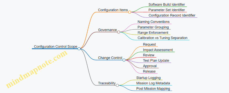
Example: Safe Parameter Update with Evidence
Assume a team wants to adjust a sensor gating parameter used to decide when to run a higher-cost identification routine. The parameter is part of the “Sensor Gating” group.
- They create a new parameter set version, e.g., PG-2026.03.14-02.
- The system validates ranges on load and rejects the set if any value is outside bounds.
- They run a regression suite that checks:
- identification trigger rate,
- false trigger behavior under known clutter conditions,
- timing budget to ensure loiter control loops remain unaffected.
- They approve a configuration record, e.g., CR-7F3A9C2B, that binds the parameter set to a specific build.
- In flight logs, the system records build ID + parameter set ID + configuration record ID at startup.
The key detail is that the evidence ties to the configuration record, not to a vague “we updated the file.”
Advanced Details That Matter in Practice
Two advanced practices prevent subtle failures:
- Deterministic parameter loading: ensure the parameter order and parsing rules are stable across builds, so the same parameter set yields the same internal representation.
- Compatibility checks: when a build expects certain parameter fields, it should verify presence and schema version. If the schema mismatches, the system should fail safely rather than guess.
A configuration record should be treated like a contract: it defines what the system was, what it was allowed to do, and what evidence supports that claim.
10.5 Documentation, Traceability, and Maintenance Readiness
Documentation is the system’s memory. Traceability is how you prove that memory is correct. Maintenance readiness is how you make sure the memory helps someone fix the right thing, quickly, with minimal guesswork.
Documentation Foundations That Prevent Confusion
Start with a single source of truth for each artifact type. Use a clear naming convention that encodes system, configuration, and document purpose. For example, a wiring diagram should identify the harness revision and the aircraft tail number range it applies to, not just the “latest” revision.
Define document roles and ownership. A sensor calibration procedure should be owned by the sensor team, while a maintenance checklist is owned by operations. When ownership is unclear, updates happen late, and the checklist quietly drifts away from the hardware.
Create a traceability map that links requirements to design artifacts, test evidence, and operational procedures. This is not paperwork for its own sake; it is how you answer questions like “Which software parameters affect arming logic?” without searching through five folders and a few emails.
Traceability That Connects Requirements to Evidence
Traceability should be bidirectional: from requirement to evidence, and from evidence back to what it supports.
A practical approach is a three-layer chain:
- Requirement: what must be true.
- Implementation: where it is realized.
- Verification: how it was shown.
Example: If a requirement states that the platform must enter a safe state when a critical sensor disagrees beyond a threshold, trace it to:
- the specific software module handling sensor fusion and fault detection,
- the parameter set that defines the threshold,
- the test report showing the fault injection results,
- the maintenance procedure that instructs how to confirm sensor health after replacement.
Use configuration identifiers consistently. If the system uses a configuration baseline like “CB-2026-03-12,” ensure every test record and maintenance action references that baseline. A date can be useful for human sorting; the configuration ID is what keeps the logic consistent.
Maintenance Readiness Through Actionable Procedures
Maintenance readiness means procedures are written for the person holding the tool, not for the person writing the report.
Write procedures with a predictable structure:
- Purpose: what outcome the procedure guarantees.
- Prerequisites: what must be true before starting.
- Steps: numbered actions with acceptance checks.
- Verification: how to confirm the work succeeded.
- Reversion: what to do if a check fails.
Include “decision points” where the technician must choose based on measured values. For instance, after replacing a navigation sensor, the procedure should instruct how to select the correct alignment routine based on the measured mounting offset range.
Also document consumables and tolerances. If a connector type requires a specific torque range, put it in the procedure and reference the applicable harness drawing. If a calibration fixture is required, list its part number and the acceptable condition of the fixture.
Mind Map: Documentation, Traceability, and Maintenance Readiness
Example: A Traceability Record That a Technician Can Use
Consider a maintenance action: replacing a laser rangefinder module.
A complete record ties together:
- Work Order: identifies the aircraft serial and the replaced part.
- Procedure Version: ensures the steps match the intended hardware.
- Calibration Evidence: includes the calibration results and pass/fail criteria.
- Software/Parameter Context: notes the configuration baseline used during the calibration run.
- Trace Links: references the requirement(s) that depend on range accuracy and the test evidence that established the acceptable error bounds.
This structure prevents a common failure mode: the module is replaced and calibrated, but the calibration was performed under a parameter set that the acceptance criteria assumed was different. When the record includes the configuration baseline, the mismatch becomes visible immediately.
Documentation Hygiene That Keeps Everything Sane
Finally, keep documentation synchronized with change control. When a wiring diagram changes, the maintenance checklist must reflect it, and the test evidence must be revalidated or explicitly justified as still applicable. If you cannot justify applicability, treat it as a new verification need.
A small but effective habit is to require that every procedure references the exact document versions it depends on. That way, “latest” cannot sneak in and quietly change the meaning of a step.
11. Operational Employment and Training for Precision Persistent Strike
11.1 Crew Roles, Responsibilities, and Standard Operating Procedures
Persistent loitering drone operations work best when roles are explicit and handoffs are boringly reliable. The crew is usually small, so each person’s responsibilities must map to specific decisions, approvals, and monitoring tasks.
Core Crew Roles
Mission Commander
- Owns mission authorization, risk posture, and final go/no-go decisions.
- Confirms that the planned engagement envelope matches current conditions (weather, comms quality, target data validity).
- Ensures the engagement chain is followed exactly as written in the mission plan.
Payload and Targeting Operator
- Manages sensor operation for identification, measurement, and evidence capture.
- Verifies target confirmation criteria are met before any terminal delivery step.
- Maintains a clear record of what was seen, when it was seen, and why it was accepted.
Navigation and Systems Operator
- Monitors health of navigation, power, propulsion, and safety interlocks.
- Tracks loiter pattern adherence and verifies that state estimation quality is within limits.
- Initiates safe-state procedures when thresholds are exceeded.
Communications and Data Operator
- Oversees link status, telemetry integrity, and command authorization.
- Ensures logs are complete and that critical messages are not overwritten or lost.
- Coordinates data prioritization so the most decision-relevant information arrives first.
Safety Officer
- Independent check on arming, inhibit logic, and procedural compliance.
- Confirms that all required confirmations are present before enabling any effect.
- Can pause or stop the mission if safety criteria are violated.
Not every mission uses all roles. If the crew is smaller, the SOP must still preserve separation between “target confirmation” and “effect authorization,” even if one person covers both with a second-person verification step.
Standard Operating Procedures
Pre-Mission Setup
- Verify mission configuration: confirm software version, parameter set, and payload configuration match the mission card.
- Perform calibration checks: validate sensor alignment, rangefinding calibration status, and navigation sensor health.
- Establish comms and logging: confirm command authentication, telemetry integrity checks, and that evidence logging is enabled.
- Brief the engagement chain: list the exact approvals required for each stage: loiter, search, track, terminal approach, and effect enable.
Example: If the payload operator reports “rangefinder warm-up complete” but the systems operator sees “calibration flag not set,” the mission does not proceed to terminal approach until the calibration flag is corrected and logged.
Loiter, Search, and Track
- Monitor orbit stability: navigation operator checks that loiter control is holding within defined tolerances.
- Quality-gate sensor data: payload operator confirms image clarity, stabilization status, and measurement confidence.
- Maintain evidence continuity: communications operator ensures the evidence stream is not interrupted during handoffs.
- Use explicit mode transitions: each transition (loiter → search → track) requires a checklist confirmation.
Example: During search, the payload operator may see multiple candidate objects. The SOP requires recording candidate IDs and confidence levels, then selecting only those that meet the mission’s confirmation thresholds for track.
Terminal Approach and Effect Authorization
- Confirm target and measurement: payload operator verifies identification criteria and measurement geometry quality.
- Check safety interlocks: navigation operator confirms safe-state conditions are satisfied and no inhibit flags are active.
- Run the arming sequence: safety officer verifies inhibit/arming logic and that required confirmations are present.
- Authorize effect: mission commander issues the final authorization only after the safety officer’s compliance check.
Example: If the safety officer notes that a “no-effect” inhibit is active due to an earlier fault, the mission commander cannot authorize effect even if the payload operator reports high target confidence.
Post-Engagement and Recovery
- Verify outcome and system state: navigation operator checks for expected post-event behavior and confirms safe-state entry.
- Preserve evidence: communications operator ensures logs and sensor recordings are stored with immutable identifiers.
- Conduct a structured debrief: each role reports what it observed, what it decided, and which checklist items were completed.
- Inspect and document: systems operator initiates inspection steps based on the mission’s fault/impact decision tree.
Example: If the debrief reveals that evidence capture stopped for 30 seconds during a critical measurement window, the SOP requires marking the engagement record as “evidence incomplete” and applying the mission’s review rules.
Mind Map: Crew Roles and SOP Flow
Practical Checklist Examples
Example: Mode Transition Gate
- Navigation operator confirms loiter tolerance within limits.
- Payload operator confirms sensor quality gate met.
- Communications operator confirms evidence logging active.
- Mission commander records the transition completion.
Example: Effect Enable Block
- Safety officer confirms all inhibits cleared.
- Payload operator confirms measurement confidence above threshold.
- Navigation operator confirms safe-state conditions satisfied.
- Mission commander issues the final authorization.
These procedures keep decisions traceable and reduce the chance that one good-looking sensor view overrides a safety or logging requirement.
11.2 Training Pipelines for Operators and Test Personnel
Training for persistent loitering platforms works best when it treats people like subsystems: each role has inputs, constraints, failure modes, and measurable outputs. Operators and test personnel share some foundations, but their pipelines diverge once the job shifts from “fly and decide” to “measure and prove.”
Foundations Before Role Separation
Start with a shared baseline that prevents mismatched assumptions. Everyone should be able to explain, in plain language, how mission phases relate to system states: preflight checks, launch, loiter, sensor tasking, terminal delivery, and post-mission recovery. The goal is not memorization; it is consistent mental models.
A practical way to teach this is a tabletop run using recorded telemetry. Trainees step through a mission log and answer three questions at each phase: What is the system trying to do? What data confirms it is doing that? What would look wrong if it were not?
Next, teach safety logic as a workflow, not a rule list. For example, show how arming conditions depend on multiple independent checks, then have trainees simulate a missing input and predict the safe state response.
Operator Pipeline
Operators need competence in controlled decision-making under imperfect information. Their training should emphasize repeatable procedures, not improvisation.
Core Skills
-
Preflight and configuration discipline: trainees verify mission parameters, payload selection, and geofencing constraints. Example: if a loiter pattern is loaded with the wrong coordinate frame, the operator should detect the mismatch by comparing expected ground track shape to a simple reference plot.
-
Sensor tasking and confidence handling: trainees learn to interpret detection confidence as a decision aid, not a guarantee. Example: when confidence drops due to glare, the operator follows a defined escalation path—adjust sensor settings, re-acquire, and only then proceed.
-
Engagement authorization workflow: trainees practice the sequence of “observe, confirm, request approval, execute,” including what to do when approvals are delayed. Example: if approval is pending, the operator maintains loiter stability and continues evidence capture rather than switching modes impulsively.
-
Loss-of-link behavior awareness: trainees learn what autonomy will do when communications degrade, and what they must still monitor. Example: if the system switches to a predefined search pattern, the operator checks that the pattern stays within safety boundaries.
Assessment Method
Use scenario-based checks with pass/fail criteria tied to procedure adherence and data interpretation. A good metric is “time to correct action” after a triggered anomaly. Example: when navigation confidence falls below a threshold, trainees should identify the cause category and initiate the correct recovery steps within a defined window.
Test Personnel Pipeline
Test personnel train for measurement integrity: repeatability, traceability, and clear separation between “what happened” and “why it happened.” Their pipeline should include both hardware test craft and software/data discipline.
Core Skills
-
Test planning and requirements traceability: trainees map each test objective to measurable signals. Example: if a requirement states terminal accuracy under wind, the test plan must define wind estimation method, acceptable error metrics, and logging coverage.
-
Instrumentation and calibration discipline: trainees verify sensor alignment, timing synchronization, and data quality before flight. Example: if a camera timestamp offset exists, they should detect it by comparing known event markers across logs.
-
Flight test execution under controlled variation: trainees learn to change one variable at a time. Example: to evaluate loiter stability, they vary only wind exposure while keeping guidance gains and payload settings constant.
-
Data reduction and evidence packaging: trainees produce a consistent report structure: raw logs, derived metrics, uncertainty notes, and anomaly timelines. Example: when a guidance correction spikes, the report should include the exact trigger signal, not just a narrative.
Assessment Method
Grade test personnel on the quality of their “replay package.” A replay package should allow another team to reconstruct the event sequence and verify computed metrics without asking the original tester for extra context.
Shared Training Practices That Reduce Friction
Operators and test personnel benefit from joint exercises that clarify handoffs.
-
Evidence capture rehearsal: both groups practice collecting the same set of logs and annotations during a simulated anomaly.
-
Common vocabulary drills: trainees standardize terms like “confidence,” “state,” “mode,” and “safe state,” so reports don’t become translation projects.
-
After-action reviews with structured causes: use a simple chain—trigger, system response, operator/test action, outcome—so discussions stay grounded.
Mind Map: Training Pipeline Structure
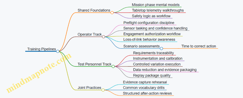
Example: One Week of Role-Appropriate Practice
Days 1–2 (shared): tabletop mission walkthroughs using recorded telemetry; safety logic simulations with missing inputs.
Days 3–4 (operators): sensor tasking drills with confidence drops; engagement workflow practice with delayed approvals.
Days 3–4 (test personnel): instrumentation checks; one-variable flight plan exercises using loiter stability metrics.
Day 5 (joint): anomaly scenario where operators must follow the defined procedure while test personnel verify logging completeness and compute the same metrics from the same dataset.
Example: A Clean Handoff Between Roles
After a flight, operators provide a phase-by-phase account of what they observed and what actions they took. Test personnel provide the computed timeline of triggers and responses, plus any gaps in data coverage. The combined record should answer the same three questions: what changed, what the system did, and whether the procedure matched the plan.
11.3 Evidence Handling for Targeting Review and Accountability
Evidence handling is the bridge between “what the system saw” and “what the organization can stand behind.” In practice, it means collecting the right artifacts, preserving them so they can be audited, and packaging them into a review workflow that supports accountability without turning operators into full-time archivists.
Foundational Concepts and Evidence Types
Start by separating evidence into three buckets:
- Sensor observations: raw or near-raw imagery, video frames, and measurement products (for example, georeferenced detections).
- System state and context: navigation solution logs, time synchronization records, mode transitions, and configuration identifiers.
- Decision artifacts: operator selections, targeting review outputs, and the rationale captured at the moment of approval.
A simple rule prevents most confusion: every decision must be traceable to at least one observation and the system state that produced it. If you cannot point to both, the decision is not reviewable.
Evidence Lifecycle from Capture to Review
1) Capture with Traceable Metadata
When evidence is captured, attach metadata immediately rather than later. Include:
- Time: a monotonic timestamp plus an absolute time reference.
- Platform identity: airframe ID or serial, software build ID, and configuration set.
- Sensor identity: camera/IR channel ID, calibration version, and lens or processing profile.
- Geometric context: estimated position, attitude, and any stabilization parameters.
Example: A review board asks why a target was classified as a specific type. The evidence package should show the exact frame timestamp, the navigation solution used for geolocation, and the software build that ran the classification.
2) Preserve Integrity with Controlled Storage
Integrity is about making tampering detectable and accidental corruption unlikely. Use:
- Write-once or append-only storage for raw evidence.
- Cryptographic hashes recorded in a manifest.
- Access controls that separate capture, review, and administrative roles.
Example: If a video clip is re-encoded for display, keep the original raw stream untouched. The manifest should link the display artifact back to the raw source.
3) Curate for Review Without Losing Traceability
Reviewers need readable products, but those products must remain linked to the underlying evidence. Create derived artifacts such as:
- annotated frames with bounding boxes,
- measurement summaries (range, bearing, uncertainty),
- geolocation overlays.
Each derived artifact should reference the raw evidence ID(s) and the processing parameters used.
Example: If an operator draws a region of interest, store the region coordinates and the coordinate system definition, not just a screenshot.
Targeting Review Workflow and Accountability
A good workflow makes “who approved what, based on which evidence” unambiguous.
Roles and Responsibilities
- Operator: records observations, proposes targeting actions, and confirms selections.
- Reviewer: verifies evidence quality, classification support, and consistency.
- Approver: authorizes the action under applicable rules.
- Custodian: manages evidence integrity, retention, and access logs.
Example: If the reviewer flags a mismatch between sensor time and navigation time, the approver should not proceed until the evidence package reflects the corrected alignment or the discrepancy is formally accepted.
Review Checklist That Prevents Common Failures
Use a checklist that maps directly to evidence types:
- Observation quality: focus, exposure, occlusion, and sensor health indicators.
- Measurement support: whether the geolocation and uncertainty are consistent with the sensor geometry.
- Decision traceability: the decision artifact references the exact observation IDs.
- Configuration correctness: software build and calibration versions match what was used.
- Mode and timing consistency: evidence shows the platform was in the expected mode during capture.
Mind Map: Evidence Handling for Targeting Review
Example Evidence Package Structure
A practical package is a folder-like structure with a manifest that ties everything together.
EvidencePackage/
  manifest.json
  raw/
    frame_000123.bin
    video_000045.raw
  state/
    nav_log_2025-03-01T1042Z.bin
    mode_transitions.json
  derived/
    annotated_frame_000123.png
    geolocation_overlay_000123.png
  decisions/
    operator_selection_000123.json
    reviewer_checklist_000123.json
    approval_record_000123.json
Discrepancy Handling Without Hand-Waving
When evidence conflicts, record the resolution path rather than smoothing it over. Typical resolutions include:
- Re-synchronization: update time alignment and regenerate derived products while preserving originals.
- Rejection: if observation quality is insufficient, mark the evidence as not meeting review thresholds.
- Qualified acceptance: if uncertainty is high but still within allowed bounds, document the uncertainty and why it is acceptable.
Example: A reviewer sees that the navigation solution drifted during the last seconds of capture. The package should show the drift indicator, the corrected alignment (or the rejection), and the resulting impact on geolocation uncertainty.
Practical Takeaway
Accountability comes from consistent linkage: raw observation → system state → decision artifact → review checklist → approval record, all bound by integrity checks. If any link is missing, the review becomes a story instead of an audit trail.
11.4 Post Mission Recovery, Inspection, and Data Archiving
A good post-mission routine turns “we got it back” into “we know what happened.” Recovery is not just physical retrieval; it is a controlled sequence that preserves evidence, prevents accidental damage, and produces clean inputs for the next planning cycle.
Recovery Priorities and Safe Handling
Start with safety and configuration control. Record the aircraft state at shutdown: flight mode, last commanded behavior, any warnings, and the reason for termination (planned end of mission, abort, or safety event). If the payload was armed or used, treat it as a hazardous subsystem even when the aircraft is otherwise safe.
Then secure the platform to prevent configuration drift. Lock or tag any removable components, capture serial numbers, and note software build identifiers. A common best practice is to photograph the aircraft in its as-recovered configuration before any covers are removed; it saves time when someone later asks, “Was that connector seated before?”
Inspection Workflow from External to Internal
Use a layered inspection approach so you don’t miss the obvious while chasing the subtle.
External Checks
Inspect airframe surfaces for impact marks, loose fasteners, abrasion on leading edges, and abnormal panel gaps. Verify control surface freedom of movement and look for signs of binding or foreign object intrusion. Check propulsor condition, including fan blades or propeller edges, for nicks and imbalance indicators.
Subsystem Checks
Move to power and avionics. Confirm battery condition indicators, connector seating, and any evidence of overheating such as discoloration or odor. For navigation sensors, verify mounting integrity and check for condensation or lens contamination.
Payload and Sensor Handling
For EO/IR and laser-related components, avoid wiping unless the procedure calls for it. Document sensor cleanliness state, then follow the approved cleaning steps if needed. If the laser subsystem was involved, inspect protective covers and interlocks, and verify that any safety pins or guards are present.
Functional Verification
Perform a short, structured check that does not require full flight readiness. Examples include sensor self-tests, gimbal calibration status checks, and control loop sanity checks. If a test fails, stop and record the failure mode rather than “trying again until it works.”
Evidence Preservation and Data Integrity
Data archiving is only useful if it remains trustworthy. Treat logs like they are part of the hardware.
What to Capture
Capture at minimum:
- Mission configuration snapshot: mission ID, target identifiers used, route/loiter parameters, and operator approvals.
- Navigation and guidance logs: state estimates, control outputs, mode transitions.
- Sensor outputs: detection tracks, confidence scores, and any measurement geometry used.
- Payload events: arming status, safety interlock states, and payload actuation timestamps.
- Health and fault logs: warnings, error codes, and subsystem temperatures.
How to Store
Use a consistent naming convention that includes aircraft ID, mission ID, and timestamp. Store raw logs before any processing, then create derived products in a separate folder. Record a checksum or equivalent integrity marker so you can detect accidental corruption.
Chain of Custody
Maintain a simple chain of custody: who handled the aircraft, who copied the data, and when. This can be as lightweight as a signed checklist plus a log of copy operations.
Structured Post-Mission Checklist
A checklist prevents “tribal knowledge” from replacing repeatable work. Keep it short enough to finish, but detailed enough to be actionable.
Mind Map: Post Mission Recovery
Concrete Example: Two Outcomes from One Mission
Example A: Planned end of mission. The aircraft returns with no warnings. External inspection shows no damage. Sensor self-tests pass. Logs are archived with a mission configuration snapshot and raw sensor tracks. The issue list is empty, and the disposition is “release for maintenance cycle.”
Example B: Abort due to navigation inconsistency. Shutdown state shows a mode transition to a safe loiter behavior. Inspection finds a loose connector on a navigation sensor harness. Functional verification reproduces the sensor fault until the connector is reseated. The data archive still stores raw logs first, and the derived analysis notes the exact timestamp where the inconsistency began. The disposition becomes “hold for repair and re-test,” not “looks fine now.”
Outputs That Make the Next Mission Easier
At the end, produce three artifacts:
- An inspection report with pass/fail results and any measurements taken.
- A data archive package containing raw logs, derived products, and integrity markers.
- An issue list with clear disposition: repaired and verified, repaired pending verification, or not repaired.
If you do this consistently, post-mission work becomes less about memory and more about evidence. That’s the whole point: the next operator should not have to guess what the last one saw.
11.5 Field Troubleshooting Using Defined Checklists and Diagnostics
Field troubleshooting works best when it is boring in the right places: repeatable steps, clear decision points, and evidence you can point to. The goal is not to “fix everything,” but to restore safe, predictable behavior by narrowing faults from symptoms to causes.
Foundational Approach
Start with three rules. First, confirm the symptom exactly as observed: what changed, when it changed, and what the operator saw on the console. Second, protect safety: if any arming, flight termination, or payload safety interlock is uncertain, stop and move to safe-state verification. Third, preserve data: record logs, switch positions, and any fault codes before power cycling.
A good checklist is organized by time and impact. Begin with power and configuration, then move to sensors and navigation, then to payload and effects interfaces, and finally to software behavior. Each stage has a “go/no-go” gate so you don’t chase ghosts.
Mind Map: Checklist Flow
Step 1: Safety and Evidence Capture
Use a short “stoplight” gate. If the system reports an interlock fault related to arming, payload safety, or flight termination, do not attempt to continue. Verify the safe state by checking that the payload is inhibited and that the flight controller is in a known safe mode. Capture logs and note the last known good behavior.
Example: During pre-launch checks, the console shows “payload inhibit active” plus a sensor alignment warning. The checklist directs you to keep the payload inhibited, record the warning code, and proceed to sensor calibration checks rather than attempting any arming-related troubleshooting.
Step 2: Configuration and Power
Most field issues are mundane. Confirm battery voltage under load, inspect connectors for seating and pin damage, and verify switch positions match the mission configuration. Then confirm software and parameter sets match the expected build for that airframe.
Example: A navigation drift complaint appears after a battery swap. The checklist has you verify the parameter set loaded with the new battery profile. In one common scenario, the wrong parameter file causes inconsistent sensor scaling, producing a drift that looks like a bad IMU.
Step 3: Fault Isolation by Subsystem
Treat each subsystem as a box with inputs and outputs.
Navigation: Check GNSS status, IMU health flags, and whether the fused solution is rejecting measurements. If the system reports “low confidence” but the raw sensors look normal, focus on calibration or alignment.
Guidance and Control: Confirm mode transitions and actuator feedback. If the controller is commanding stable loiter but the vehicle oscillates, look for actuator saturation, rate feedback mismatch, or a control loop timing issue.
Payload Interface: Verify readiness of the targeting sensor chain and any rangefinding subsystem. If the payload reports “not ready,” do not assume the sensor is broken; check power rails, interconnects, and inhibit logic.
Example: The operator reports that the targeting camera is “on” but no measurement is produced. The checklist routes you to payload interface diagnostics first, where you find a mismatch between the expected sensor handshake and the actual firmware revision.
Step 4: Diagnostic Tests
Run built-in tests before manual probing. If the system supports it, use ground checks for sensor outputs and bench checks for actuators. Keep tests short and repeatable, and record pass/fail results.
Example: IMU health passes, but fused navigation confidence is low. Ground sensor checks show a consistent bias in one axis after a recent transport event. The checklist then directs recalibration or alignment verification rather than replacing the IMU.
Step 5: Decision Points and Closure
When you reach a decision point, choose one action that matches the evidence.
- If a sensor output is consistently offset, recalibrate or realign.
- If a handshake or firmware mismatch is present, correct the configuration and verify again.
- If multiple subsystems fail simultaneously after a power event, suspect power distribution or a connector issue.
- If safety interlocks behave inconsistently, escalate after safe-state verification.
Closure requires three items: a root cause statement grounded in observed evidence, a summary of tests performed, and a preventive action that prevents recurrence (for example, connector inspection criteria after transport).
Example closure: “Payload inhibit remained active due to a targeting sensor handshake mismatch after parameter set load. Verified by log code X, corrected by matching firmware/parameter set, confirmed payload readiness and safe-state behavior.”
Practical Checklist Template
Use a one-page form with checkboxes and required log references.
| Stage | What To Check | Pass Criteria | Evidence To Record |
|---|---|---|---|
| Safety | Safe-state and payload inhibit | Inhibit confirmed, no arming allowed | Log codes, console screenshot |
| Power | Battery under load, rails | Voltage within spec, no brownout | Log timestamps, voltage readout |
| Config | Build and parameter match | Correct version and parameters | Build ID, parameter filename |
| Navigation | GNSS/IMU health and fusion | Confidence stable, no rejection storms | Health flags, fusion confidence |
| Control | Mode and actuator feedback | Commands match feedback | Mode history, actuator telemetry |
| Payload | Targeting chain readiness | Measurements produced when inhibited cleared | Payload readiness flags |
A defined checklist turns troubleshooting into a sequence of verifiable steps. That keeps the team aligned, reduces repeat failures, and makes the next troubleshooting session faster than the last one, even when the problem is new.
12. Case Studies of Platform Evolution Through Engineering Decisions
12.1 Case Study: Mission Requirement Changes And Their System Effects
A persistent loitering mission starts with a simple promise: stay on station long enough to observe, confirm, and deliver a precise effect. This case study shows what happens when that promise changes midstream—specifically, when the mission requirement shifts from “single-shot precision delivery” to “repeated observation and potential re-engagement within the same sortie.” The change sounds operational, but it forces concrete updates across navigation, sensing, autonomy logic, and safety.
Foundational Baseline
The original requirement assumed one engagement window. The platform was designed around:
- A single terminal approach profile.
- A sensor schedule that prioritized identification once, then switched to terminal measurement.
- A guidance mode that optimized for one impact point.
- A safety chain that armed only near the final approach.
A practical way to capture this baseline is to write down the mission as a timeline with explicit mode transitions: loiter → identify → confirm → approach → deliver → end. Each transition implies system behavior, timing budgets, and data products.
The Requirement Change
Two weeks into integration, the customer adds a constraint: the platform must support up to three engagement attempts if confirmation confidence drops or if the first delivery does not meet impact-point accuracy. The new requirement also tightens evidence expectations: each attempt must produce a traceable record of sensor readings, decision thresholds, and the final arming state.
This is not just “more tries.” It changes what the system must remember, what it must measure, and when it is allowed to act.
System Effects Across Subsystems
Guidance Navigation and Control
The original controller assumed a single terminal geometry. With multiple attempts, the platform needs repeatable loiter-to-approach transitions without accumulating bias.
- Best practice: define a “re-approach contract” that specifies the required state at approach start: position error bounds, heading error bounds, and allowable time-to-stabilize.
- Example: if the approach start requires heading within ±3°, the loiter controller must be tuned so that after a hold period the heading error returns to that bound, not just “stays small on average.”
Sensor Scheduling and Targeting
Multiple attempts require a sensor plan that can re-run identification and confirmation without exhausting power or degrading calibration.
- Best practice: separate “identification dwell” from “terminal measurement dwell,” and ensure the system can re-enter identification dwell after an aborted approach.
- Example: during attempt 1, the EO/IR system runs a wide-area scan for 90 seconds, then narrows to a tracking mode for 30 seconds. If attempt 1 aborts, attempt 2 repeats the wide-area scan but skips the long calibration step because the platform has not changed sensor mounting or temperature significantly.
Autonomy Logic and State Management
The autonomy stack must treat each attempt as a structured state machine, not a loop that reuses the same variables.
- Best practice: implement attempt-scoped data objects so that thresholds, confidence scores, and arming decisions are not overwritten.
- Example: attempt 1 stores
confidence=0.72andarming_gate_passed=false. Attempt 2 stores its ownconfidence=0.81andarming_gate_passed=true. The evidence record should show both attempts distinctly.
Safety Critical Design
Repeated engagement increases the risk of accidental arming or inconsistent safety interlocks.
- Best practice: require arming to depend on both proximity and a “mode legitimacy” flag that is set only when the system is in the correct attempt state.
- Example: even if the platform is physically near the terminal point, the safety logic refuses arming unless the system has completed the confirmation step for that specific attempt.
Mind Map: Requirement Change to System Impact
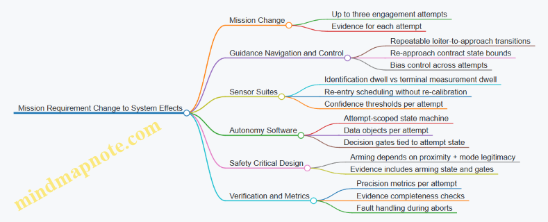
Verification Strategy That Matches the New Requirement
To avoid “it works once” testing, the verification plan must mirror the attempt structure.
- Best practice: define acceptance criteria per attempt, not only for the final attempt.
- Example: require that attempt 1 either delivers within impact-point error bounds or aborts with a logged reason code. Then require the same for attempt 2 and attempt 3.
Integrated Walkthrough of an Updated Sortie
A revised sortie timeline looks like this: loiter with periodic health checks → identification dwell → confirmation decision with confidence threshold → approach attempt 1 → either deliver or abort with reason → re-enter identification dwell (shortened where safe) → confirmation decision for attempt 2 → approach attempt 2 → deliver or abort → optional attempt 3 → end state with evidence packaging.
The key lesson is that a mission requirement change is really a contract update between time, state, and evidence. When you treat each attempt as its own accountable slice of behavior, the system becomes easier to test, easier to debug, and harder to surprise.
12.2 Case Study: Sensor Upgrade Paths And Integration Lessons
A sensor upgrade rarely fails because the new hardware is “bad.” It fails because the rest of the system keeps assuming the old sensor’s behavior. This case study uses a realistic sequence: replacing a legacy EO/IR turret with a higher-resolution unit while keeping the same loiter platform, mission software interfaces, and operator workflow.
Foundational Constraints That Drive the Upgrade
Start with the interfaces that must not change. In practice, that means preserving:
- Timing contracts: frame rate, latency bounds, and timestamp format.
- Coordinate conventions: boresight alignment, gimbal angles, and camera-to-body transforms.
- Data products: detection outputs, confidence fields, and track identifiers.
- Operational modes: search, designate, and confirm behaviors.
A simple example: if the new sensor outputs detections with a different confidence scale, the autonomy logic may still treat “0.6” as “high confidence,” even though the new sensor’s 0.6 means “maybe.” The system won’t crash; it will just be confidently wrong.
Upgrade Path A: Keep the Old Data Contract
The safest path is to adapt the new sensor to the existing data contract at the integration boundary.
What changes: raw imagery and internal processing. What stays: the format and semantics of the outputs consumed by guidance, tracking, and operator displays.
Example: The legacy pipeline produced a bounding box plus a confidence score per frame. The upgraded sensor might produce segmentation masks and a different confidence model. During integration, you convert masks to bounding boxes and remap confidence using a calibration dataset collected under the same mission lighting and viewing angles.
Lesson: treat the data contract as a product. Write it down, version it, and test it like you would test a protocol.
Upgrade Path B: Change the Data Contract with a Compatibility Layer
Sometimes the old contract is too limiting. Then you introduce a compatibility layer that supports both old and new products.
Example: The new sensor provides per-pixel target likelihood. The mission software expects a single confidence number. The compatibility layer computes confidence as a weighted average over the mask region, then applies the same thresholding logic the old system used.
This approach reduces risk because you can compare outputs side-by-side during flight tests. If the new sensor’s confidence distribution shifts, you see it immediately in logged metrics.
Integration Lessons from the “Small” Differences
-
Timestamp discipline matters more than you think If the new sensor’s timestamps are offset by even 50–100 ms, track-to-control alignment degrades. You may still get detections, but the loiter controller will chase stale target geometry.
-
Boresight alignment is not a one-time calibration Upgrades often change mounting stiffness, cable routing, or thermal behavior. Re-run alignment checks after installation and after any mechanical service.
-
Latency is a budget, not a number The system has a chain: sensor exposure → processing → transport → fusion → decision. When the new sensor increases processing time, you must either reduce other delays or adjust the fusion window.
-
Coordinate transforms must be validated with physical tests A transform that is mathematically correct can still be wrong in practice if the reference frames were interpreted differently. Use a repeatable pointing test: command known gimbal angles, observe where a fixed calibration target appears, and confirm the mapping.
Mind Map: Sensor Upgrade and Integration Flow
Example: A Practical Test Matrix for Integration
Use a matrix that isolates failure modes rather than testing everything at once.
- Timing test: record sensor timestamps and compare to fusion timestamps; verify offset stays within the agreed bound.
- Geometry test: point at a fixed target at multiple gimbal angles; verify pixel-to-angle mapping error stays within tolerance.
- Confidence test: run the same scenario through both old and new pipelines; compare confidence histograms and confirm thresholds still select the same targets.
- Mode test: execute search → designate → confirm with identical operator inputs; verify the autonomy state transitions occur at the same logical points.
Closing the Loop with Evidence Capture
After integration, log the exact inputs that drive decisions: raw sensor metadata, transform parameters, and the computed confidence used by the autonomy. When a mismatch appears, you can trace it to a specific contract violation instead of guessing. The upgrade then becomes an engineering change with receipts, not a mystery that shows up only during the last flight test.
12.3 Case Study: Autonomy Refactoring for Reliability and Operator Control
A team received a persistent loiter platform with autonomy that worked in tests but behaved inconsistently in field conditions. The symptoms were specific: occasional loiter orbit drift after long dwell, delayed operator response when switching modes, and rare sensor-fusion resets that forced the system into a conservative hold. The goal of the refactor was not “more autonomy,” but more predictable autonomy with clearer operator control boundaries.
Foundational Constraints and What They Meant
First, the team wrote down three constraints that guided every change.
- Operator intent must map to a small set of modes. Instead of letting operators indirectly influence many parameters, the system would expose a mode selector with well-defined behaviors.
- Autonomy must be restartable without losing mission context. If a module reset occurred, the platform should rejoin the same mode and continue with the same mission plan state.
- Safety logic must be independent of mission logic. Safety checks should run even if mission behaviors are paused or reconfigured.
A simple example clarified the intent mapping: “Loiter Hold” meant the orbit controller owns lateral motion, while “Search” meant the guidance layer owns a coverage pattern. The operator could not request “Search” while also expecting the orbit controller to remain active.
The Refactor Plan from Interfaces to Internals
The team started at interfaces because that’s where operator control usually gets messy.
Step 1: Define a Mode Contract. They created a mode contract that listed: allowed transitions, required sensor availability, and which outputs each mode owns (guidance commands, payload permissions, and telemetry priority). This prevented accidental cross-talk between behaviors.
Step 2: Split the Autonomy Stack Into Three Loops. They separated:
- Safety loop: monitors constraints and can override outputs into a safe state.
- Guidance loop: computes navigation commands for the current mode.
- Mission loop: decides which mode should be active based on mission state and operator input.
Step 3: Make State Explicit and Serializable. They replaced implicit state scattered across modules with a single mission state object that could be saved and restored. When sensor fusion reset happened, the mission loop reloaded the last known mode and continued.
Step 4: Add Deterministic Scheduling. The refactor removed “best effort” timing. Guidance updates ran at a fixed rate, while mission decisions ran slower. This reduced jitter that previously caused orbit drift.
Mind Map: Autonomy Refactoring Structure
Reliability Mechanisms with Concrete Examples
Example: Orbit Drift After Long Dwell. The old system updated orbit parameters opportunistically when new navigation estimates arrived. After hours, small timing differences accumulated, and the orbit controller effectively “walked.” In the refactor, the guidance loop used a fixed update rate and treated navigation estimates as inputs, not triggers. The orbit controller now recomputed commands every cycle, so drift stopped being a function of estimator arrival timing.
Example: Delayed Mode Switching. Previously, mode changes waited for multiple subsystems to finish their current tasks. The refactor introduced a mode transition handler that validated the request, acknowledged it to the operator, and then performed a controlled handoff at the next guidance cycle boundary. Operators experienced consistent responsiveness because the system had a defined latency budget.
Example: Rare Sensor-Fusion Resets. The old design let fusion resets ripple into mission logic, which sometimes caused the system to re-evaluate targeting and lose the last dwell context. The new design kept mission state separate. When fusion reset occurred, the safety loop could hold position if needed, while the mission loop preserved the active mode and resumed once navigation quality returned.
Operator Control Boundaries That Reduced Confusion
The team also tightened what operators could and could not influence.
- Operators could request mode changes, not internal controller parameters.
- The system displayed mode ownership: for example, “Guidance owns lateral motion” during Loiter Hold.
- The system required acknowledgement when a transition would reduce payload permissions, such as switching from Engage-ready to Search.
This prevented the common failure mode where an operator expects one behavior but the system is still finishing another. The platform behaved like a well-trained machine: predictable, boring in the best way.
Verification Checklist Used in the Case Study
The refactor was validated with scenario-driven tests that matched the reported symptoms.
- Long-dwell loiter with injected timing jitter
- Mode switching under link degradation
- Sensor-fusion reset during each mode
- Safety override during payload permission transitions
Each test checked not only whether the platform stayed stable, but whether it returned to the correct mode with the correct ownership rules.
Outcome Summary
After refactoring, the platform showed consistent loiter behavior over long dwells, mode switching latency became bounded and repeatable, and sensor-fusion resets no longer caused mission context loss. The operator experience improved because control mapped to a small, explicit set of modes with clear boundaries and deterministic handoffs.
12.4 Case Study: Navigation Improvements Using Updated Sensor Fusion
This case study follows a practical path: start with what was failing, identify why the navigation solution was fragile, then change the sensor fusion design so it stays accurate when conditions get messy. The goal is not “more sensors,” but better use of what already exists.
Problem Statement and Baseline
The platform used a strapdown inertial measurement unit (IMU) plus a satellite receiver for position and velocity. In calm conditions, the system held loiter waypoints acceptably. During low satellite geometry and intermittent signal degradation, the orbit drifted and the terminal approach point wandered. Operators noticed two symptoms: (1) the estimated position would slowly walk even when the aircraft appeared steady, and (2) the velocity estimate would show spikes that caused guidance to over-correct.
A baseline review showed the fusion filter treated satellite updates as uniformly reliable. When satellite quality dropped, the filter still trusted them enough to inject bias into the state estimate. Meanwhile, the IMU bias model was too slow to adapt, so it “explained away” errors as motion.
Foundational Concepts That Matter Here
Sensor fusion is a balancing act between prediction and correction. The IMU prediction is smooth but drifts due to bias and noise. The satellite correction is accurate when geometry is good, but can be biased or noisy when geometry is poor or signals are intermittent.
A robust fusion design therefore needs three things:
- Quality-aware measurement weighting so bad satellite data contributes less.
- A bias model that can adapt at the right pace so IMU drift does not masquerade as motion.
- Consistency checks so the filter can detect when its assumptions stop matching reality.
Updated Sensor Fusion Design
The update introduced a measurement quality metric and used it to scale the satellite observation covariance. Instead of a single “satellite measurement noise” value, the filter computed an effective noise based on receiver-reported geometry and signal health. When quality fell, the filter reduced the gain of satellite corrections.
Second, the IMU bias estimation was re-tuned. The bias random-walk parameters were increased slightly so the filter could adjust bias faster during degraded conditions, but not so fast that it chased noise.
Third, an innovation consistency gate was added. The innovation is the difference between predicted and measured observations. If the innovation magnitude exceeded a threshold for several consecutive updates, the filter marked the satellite measurement as suspect and temporarily relied more heavily on IMU propagation.
A small but important detail: the system also ensured time alignment between sensor streams. A consistent timing offset can look like a navigation error and will defeat any clever weighting.
Mind Map: Navigation Improvements Using Updated Sensor Fusion
Example: Quality-Aware Weighting in Practice
Imagine two satellite updates arriving 10 seconds apart. In the first, geometry is strong and the receiver reports high signal quality. In the second, geometry is weak and signal health drops. With the updated design, the second update gets a larger effective covariance.
Consequence: the filter still uses the measurement, but it does not yank the state estimate toward a potentially biased solution. Guidance then receives a steadier position and velocity estimate, so it does not “fight” the navigation solution.
Example: Bias Adaptation Without Overreaction
If the IMU bias random-walk is too small, the filter assumes bias is nearly constant. During degraded satellite conditions, that assumption forces the filter to interpret drift as motion, which shows up as orbit drift. If the random-walk is too large, the filter starts treating noise as bias changes, producing jitter.
The retune targeted a middle ground: bias can move when evidence accumulates, but it cannot jump every time the satellite quality dips.
Verification and Results
Verification used repeatable loiter patterns and logged innovation statistics. The updated system reduced the number of large innovation events during degraded reception. Orbit holding improved because the position estimate stopped walking at the same rate. Velocity spikes decreased because the filter stopped applying high-gain corrections from low-quality satellite updates.
A practical metric was “time on station” within a defined radius around the loiter point. After the change, the platform spent more of the loiter duration inside the radius without guidance saturation.
What Changed in the System Behavior
The navigation solution became less sensitive to satellite quality swings. Instead of treating satellite updates as always trustworthy, the fusion logic treated them as information with varying reliability. The IMU bias estimator then filled the gap during degraded periods, but with guardrails that prevented it from inventing motion.
The result was a navigation estimate that stayed consistent with the platform’s actual behavior, which made guidance tuning simpler and reduced operator workload during marginal reception windows.
12.5 Case Study: Test Campaign Design for Precision Delivery Validation
This case study shows how to design a test campaign that proves precision delivery performance without relying on wishful thinking. The core idea is simple: define measurable claims, build a test matrix that isolates error sources, and use acceptance criteria that match how the system will actually be used.
Start with Measurable Delivery Claims
Begin by translating “precision delivery” into specific, testable metrics. For example:
- Impact point accuracy: horizontal miss distance at the intended ground point.
- Terminal aim stability: variation of the predicted impact point when conditions are held constant.
- Time-to-commit: time from operator authorization to payload release or terminal trigger.
- Evidence completeness: whether sensor logs support post-run reconstruction for every engagement.
A practical best practice is to write each claim as a requirement with a unit, a tolerance, and a measurement method. If you cannot measure it consistently, you cannot validate it.
Build a Test Matrix That Separates Error Sources
Precision errors usually come from a few buckets: navigation state estimation, sensor measurement geometry, guidance control behavior, and payload/terminal mechanics. The test matrix should vary one bucket at a time.
A systematic matrix might include:
- Navigation quality: nominal GNSS, degraded GNSS, and GNSS-denied simulation.
- Sensor geometry: target range bands and look angles.
- Environmental conditions: wind levels and turbulence profiles.
- Platform configuration: payload mass and center-of-gravity variants.
- Operational mode: loiter hold quality and terminal approach profile.
Example: If you want to understand whether sensor geometry dominates miss distance, run multiple trials at fixed wind and fixed platform configuration while sweeping target range. If miss distance grows with range while other metrics remain stable, geometry is the likely driver.
Define Acceptance Criteria with Statistical Meaning
Acceptance criteria should not be a single “good run” threshold. Use a small set of metrics with clear statistical interpretation.
Example acceptance structure:
- Median miss distance must be below a specified value.
- 95th percentile miss distance must be below a larger bound to account for rare outliers.
- Terminal aim stability must show limited spread across repeated runs.
- Evidence completeness must be 100% for every run that reaches the terminal phase.
To keep it concrete, decide in advance how many runs are needed per matrix cell. If you only run one trial per cell, you are measuring luck, not performance.
Instrumentation and Data Integrity Checks
Before any precision claims are tested, verify that the measurement chain can support them.
Minimum instrumentation checks:
- Time synchronization across navigation, sensor, and payload logs.
- Coordinate frame consistency between onboard estimates and ground truth.
- Calibration status for sensors and any rangefinding geometry.
- Payload trigger logging that records the exact release/trigger event.
Example: If time stamps drift by even tens of milliseconds, the reconstructed impact point can shift enough to look like a guidance problem. A quick pre-test “dry run” that exercises logging end-to-end prevents that kind of confusion.
Stage the Campaign from Low Risk to High Fidelity
A good campaign is staged so you learn something every time.
- Ground and bench validation: confirm sensor calibration, trigger logic, and data logging.
- Closed-course flight validation: validate navigation and loiter stability with non-lethal payload behavior.
- Integrated precision runs: include full sensor-to-guidance-to-terminal behavior with controlled targets.
- Robustness runs: repeat key cells under degraded navigation or higher wind.
Example: If terminal aim stability fails in stage 3, you should not jump to stage 4. Instead, use stage 3 data to pinpoint whether the spread comes from state estimation, measurement association, or control response.
Use a Mind Map to Keep the Campaign Coherent
Mind Map: Precision Delivery Validation Test Campaign
Failure Triage and Iteration Without Guessing
When a run misses the acceptance criteria, the campaign should guide you to the next action. Use a structured triage:
- Compare onboard predicted impact point versus reconstructed impact point.
- Check whether sensor measurement confidence dropped.
- Inspect guidance mode transitions and control saturation indicators.
- Verify whether payload trigger timing matches the logged command.
Example: If predicted impact point is consistently offset in the same direction across trials, the issue may be a calibration or frame alignment problem. If predicted impact point varies widely while reconstructed impact follows it, the issue is likely state estimation or control behavior.
A Concrete Mini-Plan for One Week of Testing
Assume a focused campaign week with two matrix cells: nominal navigation and degraded navigation, each at two range bands. You would:
- Run bench checks on day 1 and confirm evidence completeness.
- Execute closed-course flights on day 2 to validate loiter stability.
- Perform integrated precision runs on days 3 and 4, collecting full logs.
- Use day 5 for robustness repeats of the worst-performing cell.
If the campaign begins on 2026-03-05, the schedule still works because the logic is about sequencing and isolation, not calendar drama.
The result of this design is not just a pass/fail outcome. It is a map of which error sources matter most, supported by repeatable measurements and acceptance criteria that mean something.