Saline-Alkali Soil Recovery
1. Understanding Saline Alkali Soil Constraints
1.1 Defining Salinity and Sodicity and How They Differ
Salinity and sodicity are often mentioned together, but they describe different problems with different fixes. Salinity is mainly about how much soluble salt is in the soil water. Sodicity is mainly about how much sodium is on the soil’s exchange sites, which changes how soil particles behave when wet.
Salinity: Too Many Dissolved Salts
Salinity is typically expressed using electrical conductivity of the soil solution (ECe for saturated paste or ECsw for irrigation water). High EC means plants must work against a “water-with-salt” situation: even when the soil looks moist, water is harder for roots to extract because the solution has lower effective water potential.
A practical way to picture it: imagine a sponge soaked in plain water versus a sponge soaked in salty water. The salty sponge may still feel wet, but it releases water more reluctantly. In saline soils, seeds may germinate slowly, and older plants may show leaf burn or stunting because water uptake and nutrient transport become less efficient.
Sodicity: Sodium That Breaks Soil Behavior
Sodicity is usually described using sodium adsorption ratio (SAR) for water, or exchangeable sodium percentage (ESP) and sodium percentage on the soil exchange complex. When sodium dominates, clay particles tend to disperse rather than stay flocculated. Dispersed clays clog pores, reduce infiltration, and promote crusting.
So sodicity is not just a chemistry issue; it’s a physical behavior issue. A field can have moderate salt levels but still fail because water can’t enter and roots can’t move through the surface and near-surface layers.
How They Differ in Symptoms and Soil Response
Salinity often shows up as a gradual reduction in growth with visible salt accumulation near the surface, especially after evaporation. Sodicity often shows up as poor infiltration, surface sealing, and patchy establishment even when irrigation water is not extremely salty.
A helpful rule of thumb: if the main complaint is “water won’t go in,” sodicity is a prime suspect. If the main complaint is “plants can’t get enough water even when the soil is wet,” salinity is a prime suspect.
The Overlap: Saline-Sodic Soils
Many real fields are both saline and sodic. In that case, you may see both symptoms: crusting and poor infiltration from sodium-driven dispersion, plus osmotic stress from dissolved salts. The order of operations matters because improving infiltration and reducing sodium effects can make leaching more effective, while reducing salts without addressing sodium behavior can leave the soil structure stubborn.
Mind Map: Salinity Versus Sodicity
Example: Two Fields, Two Diagnoses
Example 1: Saline field, decent infiltration. A farmer irrigates and water penetrates normally, but the crop stays short and leaves show burn. Soil EC is high, while ESP is moderate. The recovery plan focuses on managing leaching and salt removal, with careful irrigation scheduling so salts move below the root zone.
Example 2: Sodic field, infiltration problem. Another farmer irrigates and the surface turns into a slick crust within hours. Seedlings emerge in patches. Soil EC is not extreme, but ESP is high. The plan prioritizes reducing sodium effects and restoring aggregation so water can enter and roots can explore the soil.
Example: One Test, Two Numbers That Matter
When you see both EC and ESP/SAR reported, interpret them as two different bottlenecks. High EC points to osmotic stress; high ESP/SAR points to dispersion and infiltration limits. Treating only one bottleneck can leave the other one quietly doing damage.
Quick Concept Check
- Salinity is about dissolved salts in soil water.
- Sodicity is about sodium’s effect on soil particle behavior.
- Saline-sodic soils combine both, so recovery needs both water movement and sodium/structure management.
A soil can be wet and still be hostile; the trick is figuring out whether the hostility comes from salt concentration, sodium-driven structure breakdown, or both.
1.2 Soil Chemical Drivers Including Sodium Carbonate and Bicarbonate
Sodium Carbonate and Bicarbonate as Chemical Drivers
Saline alkali problems often start with the ions you can measure, but they persist because those ions change how soil particles behave. Sodium carbonate and bicarbonate are two common chemical drivers because they raise pH and supply sodium in forms that encourage dispersion and poor infiltration.
Foundational Chemistry of Carbonate and Bicarbonate
Carbonate (CO3^2−) and bicarbonate (HCO3−) are linked through the soil water pH. When pH is higher, bicarbonate tends to convert toward carbonate; when pH is lower, carbonate shifts toward bicarbonate. This matters because carbonate is more directly associated with high pH conditions, while bicarbonate can still contribute to alkalinity and sodium-related effects depending on the water chemistry and soil buffering.
In sodic soils, sodium is not just present; it is exchangeable. Sodium carbonate can supply sodium that replaces calcium and magnesium on the soil exchange sites. Once sodium dominates the exchange complex, clay particles repel each other, aggregates weaken, and water struggles to move through pore spaces.
Sodium Carbonate Pathways in Soil Water
Sodium carbonate can enter fields through irrigation water, saline groundwater, or dissolved salts in the soil profile. After application, it dissolves and creates a high-alkalinity solution. The high pH promotes two linked outcomes:
- Calcium and magnesium displacement: Sodium competes for exchange sites, reducing the concentration of divalent cations that help clay flocculate.
- Dispersion risk: With fewer calcium bridges, clay particles separate more easily, especially under wetting and drying cycles.
A practical way to picture this is to imagine clay aggregates as “stitching” held by calcium. Sodium carbonate swaps out the stitches for weaker ones, so aggregates unravel when water arrives.
Bicarbonate and Alkalinity Without Instant Carbonate
Bicarbonate is often present in irrigation water and groundwater. Even when it does not fully convert to carbonate immediately, it can still raise pH because the carbonate system buffers alkalinity. As soil CO2 conditions and microbial activity change, bicarbonate can shift toward carbonate, especially in zones where CO2 is low and pH rises.
This is why two fields with similar EC can behave differently: the bicarbonate fraction can create a persistent alkalinity environment that keeps pH high enough to sustain sodium-driven dispersion.
How High pH Changes Soil Chemistry and Biology
High pH affects more than clay behavior. It changes nutrient availability by altering solubility and reaction pathways. For example, phosphorus can become less available as pH increases, and micronutrients like iron and zinc can become harder for plants to access. Meanwhile, microbial communities that support nutrient cycling can be less active under sustained alkalinity, which reduces the natural “maintenance crew” that helps stabilize soil structure.
Soil chemistry and soil biology are connected through water chemistry: if alkalinity persists, the soil environment stays less favorable for the processes that build and maintain aggregates.
Sodium Carbonate Versus Sodium Bicarbonate in Practice
Both can contribute to sodicity, but their behavior differs across time and depth.
- Sodium carbonate tends to create stronger immediate alkalinity, so early infiltration problems and surface sealing can appear quickly after wetting.
- Sodium bicarbonate can act more gradually, with alkalinity maintained through buffering and conversion as soil conditions evolve.
In layered profiles, bicarbonate-driven alkalinity can also travel with the wetting front and then intensify where drainage is limited, because salts accumulate as water moves and evaporates.
Mind Map: Chemical Drivers
Example: Interpreting a Field Observation
A grower notices that after irrigation, water ponds briefly, then the surface becomes hard and crusted. Soil tests show high pH and elevated ESP in the top 10–20 cm, while EC is moderate. This pattern fits a scenario where bicarbonate and/or carbonate alkalinity is driving sodium exchange and dispersion more than salt concentration alone.
A simple check is to compare water alkalinity and soil pH trends across depth. If deeper layers show rising pH where drainage is limited, bicarbonate buffering and conversion can be sustaining alkalinity even when surface EC is not extreme.
Example: Linking Chemistry to Measurement Targets
When planning recovery, the chemical driver informs what to monitor. If sodium carbonate is suspected, prioritize tracking pH and ESP alongside EC because sodium exchange and dispersion can persist even when EC drops after leaching. If bicarbonate is suspected, also pay attention to how pH changes after irrigation events, since buffering can keep alkalinity high in the wetted zone.
In both cases, the goal is not just to reduce salts, but to reduce the chemical conditions that keep sodium on exchange sites and keep clay particles dispersed.
1.3 Soil Physical Drivers Including Dispersion, Crusting, and Infiltration Limits
Saline-alkali soils often fail not because water is absent, but because water can’t move in a useful way. Three physical drivers—dispersion, crusting, and infiltration limits—work together. Sodium on exchange sites weakens particle bonding, which makes the soil more likely to break apart when wet. Broken particles then clog pores near the surface, forming crusts that repel further infiltration. The result is a field that looks dry on top, yet stays waterlogged or salty in the root zone.
Dispersion: When Soil Particles Act Like They’re Trying to Leave
Dispersion is the separation of clay particles into fine suspended material when water contacts the soil. In sodic conditions, sodium reduces the “stickiness” between clay platelets. Water enters, but instead of forming stable aggregates, the soil releases particles into the flow. Those particles travel with infiltrating water and settle deeper or at pore throats.
A practical way to picture it: imagine a sponge made of tiny plates. With low sodium, the plates stay connected and water can pass through channels. With high sodium, the plates loosen, and the channels get lined with fine sediment that narrows the path.
What you see in the field
- Fine, muddy water during irrigation or rainfall, especially when the surface is disturbed.
- A “slick” feel after wetting, followed by a thin layer that dries hard.
- Patches where infiltration is much slower than nearby zones.
Crusting: The Surface Becomes a Gate That Closes
Crusting is the formation of a hardened layer at or near the soil surface. It can be structural (from aggregate breakdown) and/or chemical (from salt and sodium effects that promote particle rearrangement). Dispersion supplies the raw material—detached clay and silt—that can re-deposit as a dense skin.
Crusts reduce infiltration by two mechanisms. First, they physically block pores. Second, they change how water spreads: instead of soaking in, water runs along the crust and concentrates salts at the surface.
Simple field checks
- After irrigation, observe whether water infiltrates evenly or forms shallow puddles that persist.
- When the crust breaks under a boot, note whether it fractures into plates or powders into a thin layer.
Infiltration Limits: The Root Zone Gets the Wrong Kind of Water
Infiltration rate is the speed at which water enters the soil profile. In saline-alkali soils, infiltration limits often come from pore clogging and reduced hydraulic conductivity. Dispersion moves fine particles into the near-surface pore network; crusting then locks that network into a low-conductivity state.
Infiltration limits matter because they control leaching efficiency and oxygen availability. If water can’t enter, you either apply too much water (risking runoff and surface salt accumulation) or apply too little (leaving salts concentrated where roots grow). Even when irrigation is “on schedule,” the soil may not accept the water.
How the Three Drivers Connect
The sequence is usually: sodium-driven dispersion → particle transport → re-deposition → crust formation → reduced infiltration → poorer leaching and salt accumulation. This chain can repeat each wetting cycle, especially if the surface is repeatedly exposed and not protected by residue or cover.
Mind Map: Physical Drivers and Their Effects
Example: One Irrigation, Two Outcomes
Consider a field with two zones. Zone A has lower exchangeable sodium and stable aggregates. Zone B has higher sodium and a history of crusting.
- In Zone A, irrigation water infiltrates as a steady wetting front. Fine particles are limited, so pore spaces remain open. Roots later experience a gradual salt dilution.
- In Zone B, the first irrigation releases dispersed fines. Those fines settle near the surface and at pore throats, forming a crust as the water recedes. The second irrigation meets a hardened gate, so infiltration slows further. Even if the total water applied is similar, the water that reaches the root zone is less, and salts remain concentrated.
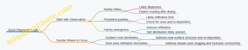
Example: Diagnosing the Limiting Step
If a grower sees crusting but not much muddy water, the limiting step may be more structural than dispersive, meaning aggregates are breaking but particle detachment is less intense. If muddy water is obvious and infiltration is slow from the first event, dispersion is likely dominant. If infiltration is slow even when the surface looks intact, pore clogging deeper in the profile may be the issue.
Mind Map: Quick Diagnostic Logic
Practical Implications for Recovery Planning
Physical drivers determine how well any biological amendment or carbon input can work, because those inputs need water movement to distribute and to support microbial activity. If infiltration is severely limited, treatments may stay near the surface and fail to reach the root zone. Therefore, recovery planning should treat dispersion, crusting, and infiltration limits as connected constraints, not separate problems—because the soil usually is not cooperating in neat categories.
1.4 Soil Biological Drivers Including Reduced Microbial Activity and Nutrient Cycling
Saline-alkali conditions don’t just change chemistry; they also change who lives in the soil and how they do their jobs. When sodium dominates and pH rises, many microbes slow down or shift their activity. The result is often a chain reaction: slower decomposition, weaker nutrient transformations, and less stable soil structure—exactly the combination that makes recovery harder.
Core Biological Effects of Saline Alkali Stress
Osmotic stress happens when soil water contains too many dissolved salts. Microbes must spend energy to keep their internal water balance, leaving less energy for growth and enzyme production.
Ionic stress is different: sodium and related ions can interfere with cell membranes and enzyme function. Even microbes that tolerate salt may not tolerate high sodium well, especially when sodium replaces calcium on particle surfaces.
High pH affects nutrient chemistry inside the microbe’s working environment. For example, nitrogen transformations depend on enzyme activity that is sensitive to pH, and phosphorus availability often drops when calcium and magnesium dominate.
A practical way to see this in the field is to compare “fresh residue” behavior. In healthier soil, plant residues darken and soften over weeks. In saline-alkali patches, residues often persist longer, and the soil surface can look more “strawy” than crumbly.
Nutrient Cycling Under Reduced Microbial Activity
Nutrient cycling is a set of linked steps. If one step slows, the next steps often stall too.
Carbon breakdown slows first. Microbial respiration and decomposition decline when microbes can’t access water easily or can’t function well at high pH. Less decomposition means less formation of microbial byproducts that help bind soil particles.
Nitrogen cycling becomes patchy. In many saline-alkali soils, ammonification and nitrification are reduced. Ammonium may accumulate in some spots while nitrate formation lags, producing uneven nitrogen availability across the field.
Phosphorus cycling loses momentum. Microbes contribute to organic phosphorus mineralization and can help mobilize nutrients through organic acids. When microbial activity drops, phosphorus can remain locked in forms that plants struggle to access.
Sulfur and micronutrient dynamics shift. Reduced microbial activity can alter sulfate reduction and the release of micronutrients from organic matter. Iron and zinc availability often remains low when pH is high, even if total nutrient content is not extremely low.
Soil Biology and Structure: The Hidden Link
Microbes don’t just feed plants; they also help build the physical habitat. Decomposition produces sticky compounds and microbial residues that support aggregation. When decomposition slows, aggregates can weaken, infiltration drops, and salts concentrate near the surface. That creates a feedback loop: poorer structure leads to more salt stress, which further reduces microbial activity.
A simple observation helps connect the dots. If you see surface crusting after irrigation and a “hard pan” feel at shallow depth, you’re likely also seeing reduced biological mixing and reduced breakdown of organic inputs.
Mind Map: Biological Drivers and Nutrient Cycling
Example: What Reduced Biology Looks Like in Practice
Imagine two adjacent strips receiving the same irrigation and residue. Strip A has better infiltration and a crumbly surface. Strip B crusts quickly and stays firm after irrigation.
Over a month, Strip A shows residue softening and a darker top layer, suggesting active decomposition and microbial processing. Strip B retains more intact residue and shows slower darkening, indicating reduced microbial breakdown. If you then sample soil, you often find more variability in nitrogen forms: Strip B may show less nitrate where nitrification is slowed, and phosphorus may remain less responsive to standard fertilization because microbial mineralization and mobilization are weaker.
Example: A Simple Field Check for Biological Function
Pick a small area and place a thin layer of fresh, chopped residue (or a small amount of compost) at shallow depth. Keep irrigation consistent. After a few weeks, compare:
- Residue condition: softened and fragmented versus mostly intact.
- Soil surface behavior: crusting versus stable granules.
- Plant response: more uniform emergence and early growth where decomposition is active.
This isn’t a lab test, but it links biology to outcomes you can see: if microbes are working, residues change and the soil surface behaves better.
Key Takeaways for Recovery Planning
Reduced microbial activity in saline-alkali soils is driven by osmotic stress, ionic stress, and high pH. That reduction slows decomposition and disrupts nitrogen and phosphorus cycling, which then weakens soil structure and intensifies salt stress. Recovery strategies that restore conditions for microbial work—especially water availability, sodium balance, and carbon processing—tend to improve nutrient cycling in a way that plants can actually use.
1.5 Field Symptoms and Diagnostic Clues from Plant and Soil Observations
Saline-alkali problems show up in the field as patterns, not as one-off surprises. The goal of observation is to connect what you see aboveground with what is happening in the root zone belowground, then decide what to measure next.
Plant Symptoms That Point to Salt and Sodium
Start with the crop because it integrates stress over time. In saline conditions, plants often show leaf burn at the margins, older leaves first, and patchy growth that follows low spots where water collects. Sodium stress linked to sodicity and dispersion more often shows stunted growth, poor stand establishment, and roots that struggle to penetrate compacted or crusted layers.
A useful field habit is to compare within-row and between-row variation. If the problem is strongest in areas that stay wet longer, salt and sodium are likely being transported and concentrated by water movement. If the problem is strongest where surface crusting forms, infiltration limits may be driving uneven leaching and uneven salt distribution.
Look for timing clues. If symptoms appear soon after germination or after irrigation events, the issue is likely tied to salt concentration in the wetting front or rapid surface evaporation that leaves salts behind. If symptoms build gradually through the season, the field may be experiencing ongoing salt accumulation or slow structural decline that reduces root access to water.
Soil Surface Clues That Reveal Physical Constraints
Walk the field after a light irrigation or rainfall and watch how water behaves. Crusting that forms quickly suggests dispersion and reduced infiltration, which can trap salts near the surface. Shallow wetting followed by dry cracking indicates that water cannot move downward efficiently, so salts concentrate where roots are shallow.
Check for white crusts on the surface or along furrows. White material can be salts, but the key diagnostic step is to note where it appears: near the surface points to evaporation-driven accumulation, while deeper salt layers suggest limited leaching and upward movement.
Root Zone Clues That Confirm the Mechanism
Soil pits or auger cores help you separate “salt is present” from “salt is limiting.” Sample at multiple depths, typically 0–15 cm, 15–30 cm, and 30–60 cm for a first pass. If EC or pH issues intensify with depth, the root zone may be encountering a concentrated layer that leaching cannot easily bypass.
Also observe structure. In sodic soils, you may find weak aggregates, smearing, or blocky layers that break into small fragments. These features align with dispersion and poor pore continuity, which reduces both infiltration and root penetration.
Mind Map: Field Observation Pathway
Integrated Example: Two Spots, Two Likely Causes
Spot A: Plants show marginal leaf burn and the worst patches sit in a shallow depression. After irrigation, water spreads slowly but eventually wets the surface; salts appear as a thin crust after evaporation. This pattern fits salt accumulation driven by water pooling and evaporation, so the next step is depth EC mapping and a leaching feasibility check.
Spot B: Plants are stunted even where surface crust is minimal, and roots appear sparse when you pull a plant. The soil feels dense and breaks into weak crumbs. This points toward sodium-driven structure problems limiting infiltration and root penetration, so you prioritize infiltration testing and depth structure observations alongside chemical sampling.
Quick Diagnostic Checklist for Field Teams
- Photograph the same patches from the same angle at each visit.
- Note whether symptoms align with topography, irrigation lines, or surface crust zones.
- Record plant stage when symptoms start.
- Take at least two depth cores in each symptom zone.
- Pair every “visual guess” with one confirmatory measurement you can do next.
A Simple Decision Rule for What to Measure First
If symptoms are strongest after irrigation or in low spots, measure EC by depth and verify water movement. If symptoms are strongest where infiltration is poor and soil structure is weak, measure infiltration and depth structure, then confirm with pH and sodium-related indices. This keeps the workflow grounded: observations guide measurements, and measurements explain the pattern you saw.
2. Soil Testing and Site Characterization for Recovery Planning
2.1 Sampling Design for Heterogeneous Salt and Sodium Patterns
Salinity and sodicity rarely form neat circles in a field. They follow water movement, soil texture, micro-topography, and irrigation patterns—so your sampling design has to “follow the story” of how water and ions travel. The goal is not to measure everything everywhere; it’s to capture the main patterns well enough to choose the right recovery actions.
Start with the Field Water Story
Begin by identifying likely pathways for salt and sodium: low spots where water collects, wheel tracks where infiltration differs, furrows or drip lines that concentrate wetting, and edges where irrigation or runoff enters. If you already know the irrigation layout, use it to predict where salts accumulate between wetting cycles.
A practical first step is a quick reconnaissance walk after irrigation or a light rain. Look for crusting, bare patches, stunted plants, and differences in soil color. Mark these areas on a simple sketch. Even without lab data, these clues help you decide where sampling density should be higher.
Use a Stratified Grid Instead of a Single Average
A common mistake is taking a uniform grid and then averaging the results. Averaging hides the worst zones that drive crop failure and treatment success.
Use stratification:
- By management zones: different irrigation blocks, soil types, or historical yield patterns.
- By landscape position: upper slope, mid-slope, depression.
- By visible symptoms: crusted areas, saline patches, sodic patches.
Within each stratum, sample on a grid or systematic pattern. If a stratum is small, you can sample more densely there and less elsewhere.
Decide Sample Count Using Variability, Not Hope
Sampling effort should reflect how patchy the field is. If symptoms are uniform, fewer samples may be enough. If you see strong patchiness, increase the number of points.
A workable rule for many farms is to collect composite samples within each stratum while keeping enough separate points to represent variability. For example, you might take 5–10 cores per composite, but keep 3–6 composites per stratum. This balances lab cost with pattern detection.
Choose Depths That Match Ion Movement
Salt and sodium often concentrate at different depths depending on leaching and drainage. Shallow sampling can miss the root-zone problem; deep sampling can waste effort if the issue is only near the surface.
A systematic approach is to sample at depth intervals that match root-zone recovery decisions:
- 0–10 cm for surface crusting and recent salt deposition
- 10–30 cm for early root establishment and structural effects
- 30–60 cm for whether leaching and amendments are reaching the active root zone
If you suspect shallow hardpan or compaction, add a depth around the suspected barrier (for example, 20–40 cm) because it can trap sodium and reduce infiltration.
Plan for Both “Where It Is” And “Why It Is”
Collecting only chemical data can lead to confusing results. Pair sampling with simple field measurements that explain patterns.
Include at least one of these per stratum:
- Infiltration check (spot test) to see whether sodium dispersion is limiting water entry
- Soil texture estimate (feel method) to anticipate cation exchange behavior
- EC or salinity proxy from a quick field method if available
These observations help interpret whether high sodium is tied to poor infiltration, irrigation concentration, or both.
Mind Map: Sampling Design Logic
Example: Designing Samples for a Patchy Sodic Clay Block
Imagine a 20-hectare block with three visible zones: a depression with crusting, a mid-slope area with patchy stunting, and an upper slope with relatively normal growth.
- Stratify into three zones based on symptoms and landscape position.
- Set sampling density: depression gets 6 composites, mid-slope gets 4, upper slope gets 3.
- Collect composites: each composite uses 6–8 cores taken within a 10–20 m area.
- Sample three depths: 0–10 cm, 10–30 cm, 30–60 cm.
- Add one infiltration check per zone using the same method each time.
If the depression shows high sodium indicators at 0–10 cm but lower values at 30–60 cm, you may prioritize surface management and targeted leaching. If high sodium persists at 30–60 cm, you likely need root-zone engineering and deeper amendment placement.
Example: Designing Samples for a Uniform-Looking Saline Field
On a field that looks uniform, you still sample by depth and keep enough points to confirm the pattern.
- Use a single stratum for the whole block.
- Take 8–12 composite points across the field.
- Keep the same three depth intervals.
- If results show consistent EC and sodium indicators across points, you can treat the field as one management unit. If one or two points are extreme, you can reclassify those areas as a separate stratum for targeted recovery.
Practical Output That Makes Sampling Worth It
Your sampling plan should produce maps or at least zone summaries that answer three questions: where salts and sodium are highest, whether the problem is shallow or extends into the root zone, and whether infiltration limitations align with the chemistry. When those answers are clear, the next steps—amendments, carbon inputs, and root-zone engineering—stop being guesswork and start being design.
2.2 Laboratory Measurements Including EC, SAR, ESP, pH, and Exchangeable Cations
Laboratory measurements turn “the field looks crusty” into numbers you can plan around. Saline-alkali soils are a mix of dissolved salts, sodium chemistry, and exchange reactions on clay surfaces, so you need a small set of tests that describe each piece.
Core Measurements and What They Represent
Electrical Conductivity (EC) measures total dissolved salts in a water extract. Higher EC means more ions in solution, which can stress plants by making it harder to take up water.
Sodium Adsorption Ratio (SAR) estimates how strongly sodium dominates relative to calcium and magnesium in the soil solution. SAR is computed from ion concentrations, so it depends on the extract you use.
Exchangeable Sodium Percentage (ESP) measures sodium held on exchange sites of soil particles. ESP is often more directly tied to dispersion and poor structure than SAR, because exchangeable sodium can trigger clay swelling and breakdown.
pH indicates alkalinity. High pH affects nutrient availability and can shift carbonate and bicarbonate chemistry, which influences both salinity behavior and sodium effects.
Exchangeable Cations (typically Na, Ca, Mg, K) quantify the ions on the soil exchange complex. These values support ESP calculation and help interpret why sodium is behaving the way it is.
Mind Map: Laboratory Measurement Logic
Sample Handling and Extract Choice
Results are only as good as the sample preparation. Air-drying and grinding are common for routine chemistry, but for EC and SAR you must follow a consistent extraction method because dilution and soil-to-water ratio change the measured concentrations.
A practical workflow is to run two extracts from the same dried, sieved soil: one for EC and pH, and one for cation analysis used in SAR. If your lab uses a fixed soil:water ratio, keep it consistent across all sampling points so comparisons are meaningful.
Measuring EC and PH
EC is measured on the soil extract using a conductivity meter calibrated with standard solutions. Report EC with the same unit basis your lab uses (often dS/m). pH is measured with a calibrated pH meter, typically on the same extract used for EC.
Example: A field zone with EC of 6 dS/m and pH 8.7 is likely experiencing strong osmotic stress plus alkalinity effects. If another zone has EC 3 dS/m but pH 9.4, the second zone may be more about sodium-carbonate chemistry and nutrient lockup than total salt load.
Measuring Exchangeable Cations and CEC
Exchangeable cations are extracted using a chemical extractant that displaces ions from exchange sites. The lab then quantifies Na, Ca, Mg, and often K using an instrument such as atomic absorption or ICP.
CEC is the total capacity of the soil to hold exchangeable cations. You can compute ESP once you have exchangeable Na and CEC.
Example: If exchangeable Na is 12 cmol(+)/kg and CEC is 30 cmol(+)/kg, then ESP = (12/30) × 100 = 40%. That high ESP aligns with a strong risk of dispersion, especially in fine-textured soils.
Calculating SAR and ESP Correctly
SAR is calculated from sodium, calcium, and magnesium concentrations in the soil solution extract. The standard form uses the square root of calcium and magnesium terms, so small measurement errors in Ca and Mg can shift SAR.
ESP is calculated from exchangeable sodium and CEC. ESP is less sensitive to the exact solution chemistry because it reflects the solid-phase exchange state.
Example: Two samples can show similar SAR but different ESP if one soil has a higher CEC that buffers sodium on exchange sites. That difference matters for structure because clays respond to what they hold, not only what is dissolved.
Quality Checks That Prevent “Good Numbers, Wrong Story”
- Charge balance sanity check: If the lab provides ionic analysis for the extract, verify that measured cations and anions are broadly consistent. Large imbalances suggest extraction or analytical issues.
- Replicate consistency: Run duplicates or triplicates for at least a subset of samples. If EC varies widely between replicates, the extraction process or mixing may be inconsistent.
- Depth consistency: If you sample by depth, keep the extraction and measurement method identical across depths. Sodium and salts often stratify, and mixing depths can blur the pattern.
Interpreting Patterns Without Guessing
Use EC, SAR, ESP, pH, and exchangeable cations together:
- High EC with moderate ESP points to salt-driven stress that may respond strongly to leaching.
- Moderate EC with high ESP points to structural risk from sodium on clays, where aggregation and exchange-site management become central.
- High pH with high sodium-related measures suggests carbonate-driven alkalinity effects that can also influence nutrient availability.
When you report results, include both the measured values (EC, pH, exchangeable cations) and the derived values (SAR, ESP). That keeps the chain of reasoning visible, which is exactly what you want when planning recovery steps.
2.3 Interpreting Texture and Cation Exchange Capacity for Treatment Selection
Texture and cation exchange capacity (CEC) tell you how the soil holds ions and how water moves through it. In saline-alkali recovery, that matters because sodium management depends on exchange sites, while infiltration and leaching depend on pore structure. Think of texture as the plumbing and CEC as the ion “parking lots.”
Texture as the Water-Movement Baseline
Start with the particle-size groups: sand, silt, and clay. Clay-rich soils have smaller pores, so water infiltrates more slowly and salts can linger near the surface. Sandy soils drain faster, which can help leaching but also increases the risk of losing applied nutrients before crops can use them.
Texture also shapes crusting and dispersion. Dispersive sodic clays break down into fine particles that clog pores, reducing infiltration further. A practical field check is the infiltration test: if water ponds and disappears slowly, you likely need structure-first steps (carbon and biological aggregation) and careful leaching scheduling.
Cation Exchange Capacity as the Sodium Buffer
CEC is the soil’s ability to hold positively charged ions like Ca2+, Mg2+, Na+, and K+. Higher CEC usually means more exchange sites, so sodium can be held and later displaced more effectively—provided you supply enough calcium and manage leaching. Lower CEC soils have fewer exchange sites, so sodium may not be buffered well; instead, you may see faster changes in soil solution after irrigation.
CEC is influenced by clay minerals and organic matter. Two soils with the same texture can differ in CEC if one has more organic matter or different mineralogy. That’s why treatment selection should not rely on texture alone.
Linking Texture and CEC to Treatment Choice
Use a simple decision logic:
- If texture is clayey and CEC is moderate to high: sodium can accumulate on exchange sites, and structure is often fragile. Prioritize calcium supply and aggregation-building inputs, then leach when infiltration improves.
- If texture is clayey but CEC is low: exchange buffering is limited. You may still need calcium, but expect faster shifts in soil solution and plan more frequent, smaller leaching events.
- If texture is sandy with low CEC: leaching is easier, but nutrients can wash out. Focus on targeted amendments, split nutrient applications, and avoid over-irrigation.
- If texture is mixed with moderate CEC: you can often combine biological aggregation with controlled leaching, using monitoring to adjust timing.
Interpreting Lab Results Without Getting Lost
When you receive a soil report, look for these items together:
- Texture class (sand/silt/clay percentages)
- CEC (often reported at a specified pH)
- pH and exchangeable sodium percentage or ESP if available
- Organic matter or total carbon
If pH is high, some measurements may reflect different exchange behavior than at crop root-zone pH. Still, the relative ranking of CEC across zones is useful for treatment planning.
Mind Map: Texture and CEC to Treatment Selection
Example: Two Zones, Different Choices
Zone A: 45% clay, CEC 22 cmol(+)/kg, ESP 18%, pH 8.6. Infiltration is slow and the surface seals after irrigation. This combination suggests sodium is sitting on exchange sites and structure is limiting water movement. A practical approach is to apply calcium-based amendment and carbon/biological inputs to encourage aggregation, then run leaching events only after infiltration improves. If you leach too early, you may just move salts into a still-dispersive surface layer.
Zone B: 20% clay, CEC 6 cmol(+)/kg, ESP 12%, pH 8.3. Water infiltrates quickly, but crop growth is patchy after fertilization. Here, sodium buffering is limited and nutrients can be lost with drainage. Use smaller, more frequent nutrient placements and keep amendment rates aligned with the measured salt movement, using soil solution or EC trends to confirm that salts are being flushed rather than redistributed.
Practical Takeaway for Treatment Selection
Texture tells you how water and salts travel. CEC tells you how ions are held and how easily sodium can be displaced. When you combine both, you can choose amendments and timing that match the soil’s “plumbing” and “ion parking,” instead of treating the field like it behaves uniformly.
2.4 Mapping Root Zone Conditions Using Depth Profiles and Infiltration Checks
Saline-alkali recovery fails most often when the plan is based on surface averages. Root problems usually start deeper than the top few centimeters, and water movement can change abruptly across a field. This section shows how to map root-zone conditions using two complementary tools: depth profiles (what the soil is like) and infiltration checks (how water actually moves).
Foundational Idea: Match Soil Chemistry to Water Pathways
Salinity and sodicity affect plants through the water they can access. If sodium disperses clay, infiltration slows, and salts concentrate where water evaporates. If the soil has a compacted layer, leaching water may bypass the root zone or pool above it. Depth profiles tell you where the chemistry shifts; infiltration checks tell you whether water can travel to the depth where you need it.
Planning the Field Sampling Layout
Start by dividing the field into zones that are likely to behave differently: low spots, ridges, known irrigation turns, and areas with different crop performance. Within each zone, choose 3–5 sampling points spaced far enough to capture variation but close enough to keep the map useful.
At each point, plan two “views”:
- A depth profile for EC, SAR/ESP-related indicators, pH, and exchangeable sodium or sodium proxy.
- An infiltration check at the same location to connect structure to water movement.
A practical depth scheme is 0–15 cm, 15–30 cm, 30–45 cm, and 45–60 cm. If the field has a known hardpan, add a sample just above and just below it.
Depth Profiles: What to Measure and How to Interpret It
Collect soil samples carefully to avoid mixing layers. Use a clean auger, discard the first small amount of soil from the hole, and label each depth immediately.
Measure at minimum:
- Electrical conductivity (EC) or a salinity proxy.
- pH.
- Sodium-related indicators such as SAR, ESP, or exchangeable sodium percentage.
- Texture or at least a quick field texture check, because infiltration behavior depends on it.
Interpretation logic:
- If EC is high mainly near the surface, salts are likely being brought up by evaporation or capillary rise. Your recovery needs surface crust and infiltration improvement.
- If EC stays high at depth, leaching water may not be reaching the root zone effectively, or salts are stored deeper and require deeper wetting and drainage.
- If pH and sodium indicators spike together at a particular depth, that layer is a likely barrier to root growth and nutrient uptake.
- If sodium indicators are high but EC is moderate, sodicity may be the dominant constraint, meaning structure and infiltration are the first targets.
Infiltration Checks: Simple Tests That Reveal Real Water Flow
Infiltration checks should be done on the same day as sampling if possible, because surface conditions change quickly after irrigation or rainfall.
Choose one method and standardize it across the field:
- A ring infiltrometer for more controlled measurements.
- A double-ring or ponding test if you need a practical approach.
- A simple infiltration test with a measured water depth and timed infiltration, as long as you record the method consistently.
Record:
- Time to reach a steady infiltration rate (or the time series if you cannot reach steady state).
- Whether water ponds, infiltrates slowly, or runs off.
- Surface crusting signs and whether the soil slakes when wetted.
Interpretation logic:
- Slow infiltration with surface crust suggests dispersion and sealing at the top layer.
- Slow infiltration that improves after breaking a compacted layer suggests a physical barrier.
- Fast initial infiltration followed by rapid slowdown suggests preferential flow that later encounters a dispersive or compacted horizon.
Linking the Two Views into a Root-Zone Map
Combine depth profile patterns with infiltration behavior to classify root-zone constraints. For example:
- High surface EC + very slow infiltration: prioritize crust removal and sodium-structure management near the surface.
- Moderate surface EC + high EC at 30–60 cm + slow infiltration: prioritize root-zone wetting pathways and drainage so salts can be displaced downward.
- High sodium indicators at 15–30 cm + infiltration slowdown at that depth: treat the barrier layer, not just the top.
Use the map to decide where to place amendments and where to focus engineering. If infiltration is blocked, adding carbon without improving water movement can leave salts behind while roots struggle.
Mind Map: Mapping Root Zone Constraints
Example: Two Points, Two Different Problems
Point A shows EC high at 0–15 cm, pH elevated, and sodium indicators elevated mainly in the top layer. Infiltration is very slow and water ponds. This points to surface sealing and dispersion. A recovery plan should focus on improving infiltration at the surface and reducing sodium-driven crusting so subsequent leaching can actually move salts.
Point B shows EC moderate at 0–15 cm but high at 30–45 cm, with sodium indicators peaking at 30–45 cm. Infiltration is slow overall, and water pools above a compacted horizon. This indicates a root-zone barrier that prevents effective wetting and salt displacement. The plan should target the barrier layer and ensure drainage or leaching pathways can carry salts away from the active root depth.
Quality Checks That Prevent Bad Maps
Before trusting the map, verify:
- Sampling consistency: same depth intervals and careful layer separation.
- Replication: at least 3 points per zone to avoid overfitting to one odd spot.
- Method consistency: infiltration test method and timing are the same across points.
- Coherence: chemistry patterns should make sense with infiltration behavior; if they do not, re-check sampling or consider micro-variability like buried debris or localized compaction.
A good root-zone map is not a perfect picture. It is a decision tool that tells you where water can go, where it cannot, and where salts and sodium are likely to follow.
2.5 Selecting Baseline Indicators and Establishing Measurement Protocols
A recovery plan lives or dies by measurement quality. Baseline indicators should answer three questions: What is limiting infiltration and plant growth right now? Where in the soil profile does the limitation sit? How will you tell, later, whether changes are real rather than just seasonal noise?
Foundational Indicators That Describe the Problem
Start with indicators that map directly to the two common constraints in saline-alkali soils: salt load and sodium-driven structure breakdown.
- Salinity load: Use electrical conductivity (ECe or EC1:5/ECw depending on lab method) to quantify total soluble salts. A simple field proxy is EC of a soil paste extract, but lab EC is the baseline standard.
- Sodium hazard: Measure SAR (for water) and ESP (for soil). If ESP is not available, exchangeable sodium percentage can be estimated from exchangeable cations.
- Alkalinity: Track pH and, when possible, bicarbonate (HCO3−) in irrigation water and carbonate/bicarbonate behavior in soil extracts. High pH without sodium symptoms can still affect nutrient availability.
- Soil structure and infiltration: Use infiltration rate (ring infiltrometer or field infiltration tests) and aggregate stability or slaking resistance. In sodic clays, infiltration often collapses before plants show severe stress.
- Plant response: Record stand establishment metrics (emergence %, uniformity), leaf greenness, and biomass at consistent growth stages. Plant data is not a replacement for soil data, but it helps interpret why a treatment is working or stalling.
Profile Depth Resolution That Prevents Guessing
Many failures come from sampling only the top layer. Sodium and salts often stratify by depth due to capillary rise and limited leaching.
Use a depth plan that matches the likely movement pathways:
- 0–10 cm for surface crusting and seed-zone conditions
- 10–30 cm for the main root zone in many annual crops
- 30–60 cm for subsoil constraints and leaching effectiveness
- Add 60–100 cm if drainage is limited or if deep salts are suspected
A practical baseline rule: if you cannot explain why you chose your depths, you probably chose them by habit rather than soil physics.
Establishing Measurement Protocols That Stay Consistent
Consistency matters more than sophistication. Your protocol should minimize variation from sampling, handling, and timing.
- Sampling design: Divide the field into zones using visible patterns, EC maps if available, and irrigation layout. Within each zone, sample multiple points and composite them for lab tests, while keeping structure tests as individual cores if possible.
- Sampling timing: Collect baseline samples at a consistent point in the season, ideally before major amendments and before the first heavy irrigation event that would redistribute salts.
- Sample handling: Keep samples sealed and cool to reduce chemical changes. For paste extracts and EC tests, follow the same soil-to-water ratio and mixing time every time.
- Replicate strategy: Use enough replicates to detect meaningful change. If you expect small improvements, increase replication rather than changing methods.
- Method pairing: Pair chemical indicators with physical indicators. For example, if EC drops but infiltration does not improve, the limitation may be structural dispersion rather than salt load.
Mind Map: Baseline Indicators and Protocol Logic
Example: Turning Baseline Data into a Measurement Plan
Assume a field with patchy emergence and surface crusts.
- Zone A (near irrigation inlet): sample EC and ESP at 0–10, 10–30, 30–60 cm; run infiltration tests in the same zones.
- Zone B (low spots): sample deeper (add 60–100 cm) because salts may accumulate where water stagnates.
- Protocol consistency: collect baseline samples on the same day across zones, then repeat the same sampling schedule after the first leaching-and-amendment cycle.
If Zone A shows high ESP at 0–10 cm but infiltration is already low, you prioritize structure recovery in the seed zone. If Zone B shows high EC at 30–60 cm with only moderate ESP, leaching depth and drainage become the first-order focus.
Example: A Simple Baseline Scorecard
Use a scorecard to keep decisions grounded in data rather than impressions.
- Salinity: EC high in which depth layer?
- Sodium: ESP high where dispersion risk is greatest?
- Alkalinity: pH extreme at surface or throughout profile?
- Infiltration: infiltration slow even after wetting?
- Plants: where does poor stand match the soil constraint depth?
A baseline scorecard is not a magic number. It is a structured way to ensure every later measurement has a clear meaning.
3. Recovery Objectives, Treatment Boundaries, and Management Targets
3.1 Setting Practical Goals for Crop Establishment and Yield Stability
Practical goals keep recovery work measurable and prevent “we added stuff, so it should work” thinking. In saline-alkali soils, establishment and yield stability depend on three linked outcomes: (1) seedlings survive the first stress window, (2) roots access water and nutrients without structural bottlenecks, and (3) salts and sodium do not return to the active root zone faster than they are removed.
Foundational Goal: Reliable Stand Establishment
Start with a goal you can observe within weeks: a target stand density and uniform emergence across the treated zone.
A simple way to set it is to define three thresholds:
- Emergence uniformity: how evenly plants appear across low, mid, and high-salt/sodicity patches.
- Early survival: percent of seedlings alive after the first irrigation-leaching cycle.
- Rooting progress: whether roots penetrate beyond the surface crust or compacted layer.
Example: If a field normally gives 40% emergence in the worst patches, set a first recovery target of 65% emergence in those patches and 80% in the better patches. You are not aiming for perfection immediately; you are aiming for enough plants that the next management step has something to work with.
Yield Stability Goal: Consistent Performance Across Cycles
Yield stability is not just “high yield once.” It means the crop produces similarly across irrigation events and seasonal variability.
Set stability goals using measurable proxies:
- Plant vigor consistency: similar canopy cover at key growth stages.
- Nutrient uptake consistency: less patchiness in leaf color and growth rate.
- Yield component stability: similar plant height range, tiller/panicle counts, or fruit set distribution.
Example: For a cereal, instead of targeting a single final yield number, set a goal that the coefficient of variation in plant height at flowering stays below a chosen level (for instance, half of what it is now). That keeps the management focused on uniform root-zone conditions.
System Goal: Keep Salts and Sodium from Winning the Root Zone
In saline-alkali recovery, salts can move back upward or sideways after leaching. Your goal should therefore include a root-zone “balance check.”
Define a practical root-zone target window:
- Active root-zone EC: a range where seedlings can grow without severe osmotic stress.
- Sodium hazard: an ESP or SAR-related target that supports soil aggregation and infiltration.
- pH stability: avoiding conditions that lock up nutrients.
You do not need perfect lab precision to set useful targets. You need targets that match your soil depth sampling plan and irrigation schedule.
Example: If your sampling shows the top 20 cm is the main problem, set a goal that EC and ESP in 0–20 cm improve enough to support emergence, while 20–40 cm improves enough to support early rooting. Then you adjust leaching timing and amendment placement based on whether the improvement stays after irrigation.
Mind Map: Goal Setting Logic for Establishment and Stability
Turning Goals into Zone-Based Targets
Saline-alkali fields are rarely uniform. Treating the whole field as one problem usually creates one of two outcomes: under-treatment where it is worst, and wasted inputs where it is best.
Create three management zones based on your earlier characterization:
- Zone A: highest hazard and poorest infiltration.
- Zone B: intermediate conditions.
- Zone C: relatively manageable conditions.
Then set different targets for each zone in the first season, with the same measurement method. This keeps the project fair and the data interpretable.
Example: Zone A might target 65% emergence and survival through early growth; Zone C might target 85–90% emergence and faster canopy closure. If Zone A fails, you know the issue is not “the crop variety” but the root-zone conditions or water management.
Practical Milestones and Decision Points
Use milestones that trigger decisions rather than just reporting progress.
A workable sequence:
- Pre-plant: confirm sampling depth plan and infiltration baseline.
- Week 2–3: count emergence and note patchiness patterns.
- After first leaching: re-check infiltration and observe any crusting return.
- Early vegetative stage: assess root-zone access via plant vigor uniformity.
- Mid-season: confirm nutrient-related symptoms are not reappearing in the same patches.
Example: If emergence is acceptable but early survival drops after irrigation, the goal is not “more seed” but “reduce the stress spike.” That usually points to leaching timing, water quality, or placement depth of amendments.
Summary of Goal Statements You Can Write in Your Field Plan
Write goals as short statements tied to measurements:
- “Achieve target emergence and survival by zone within the first leaching cycle.”
- “Reduce variability in plant vigor at a defined growth stage compared with baseline.”
- “Maintain improved EC and sodium hazard in the active root zone after irrigation, using depth-resolved checks.”
These statements keep the recovery process systematic: establish first, stabilize next, and manage the root zone so the field stays improved rather than briefly impressed.
3.2 Defining Treatment Boundaries by Depth, Field Zones, and Water Sources
Treatment boundaries are where good intentions meet physics. If you treat the wrong depth, the right amendment can still fail. If you treat the wrong zone, you may fix one problem while feeding another. And if you ignore water sources, you can accidentally re-salt the work you just did.
Foundational Idea: Boundaries Match the Cause
Start by separating three questions:
- Where does the salt or sodium problem sit in the soil profile?
- Where does it show up across the field?
- Where does the water that moves salts come from?
A practical boundary plan uses depth layers, field zones, and water pathways as a single system. You are not drawing lines for decoration; you are defining which parts of the field receive which treatment and when.
Depth Boundaries: Treat Where Ions and Structure Fail
Depth boundaries should reflect how salts and sodium behave under wetting and drying.
Step 1: Use depth profiles to locate the “active zone.” Sample at multiple depths (for example 0–15 cm, 15–30 cm, 30–60 cm, and deeper if needed). Look for:
- EC rising sharply with depth, suggesting salts accumulating below the surface.
- ESP or SAR-related indicators increasing with depth, suggesting sodium exchange and dispersion risk.
- Texture or structure changes that limit infiltration.
Step 2: Match treatment depth to the limiting process.
- If crusting and infiltration failure dominate near the surface, prioritize surface carbon and biological aggregation, plus a structure-friendly incorporation depth.
- If sodium and salts concentrate deeper, plan leaching and root-zone conditioning that reaches the depth where roots will actually grow.
- If the problem is mostly shallow, deep tillage may be unnecessary and can even bring salts upward.
Easy example: A field shows high EC in 0–15 cm but low EC below 30 cm. You focus on surface amendments and improved infiltration rather than deep mixing. After a couple of leaching cycles, the surface EC drops and the crop stand improves.
Field Zone Boundaries: Treat the Field Like a Set of Linked Mini-Sites
Field zones are based on repeating patterns in soil properties, topography, and management history.
Step 1: Create zones using three layers of evidence.
- Soil evidence: texture, CEC, and depth-profile indicators.
- Topography evidence: low spots, slopes, and drainage paths.
- Management evidence: irrigation method, past amendments, and where runoff or wheel tracks concentrate.
Step 2: Use zone size that matches your equipment and sampling resolution. If your spreader and applicator can’t treat uniformly across a large zone, split it. If your sampling grid is coarse, don’t pretend you know fine-scale boundaries.
Easy example: Two adjacent zones share the same irrigation source. The lower zone has higher EC and poorer infiltration because it receives lateral water. You apply the same amendment rate in both zones, but only the lower zone gets additional drainage conditioning and a tighter leaching schedule.
Water Source Boundaries: Water Decides Where Salts Go
Water sources define where salts enter and how they move.
Step 1: Identify water inputs and their chemistry. Separate:
- irrigation water EC and SAR,
- any canal seepage or groundwater contribution,
- rainfall runoff patterns that concentrate salts in depressions.
Step 2: Link water movement to depth and zone boundaries.
- If irrigation water is high in sodium hazard, sodium displacement and dispersion risk increase where wetting fronts repeatedly pass.
- If water is saline but not strongly sodic, EC management may dominate, and leaching depth becomes the key boundary.
Easy example: A farm uses two pumps: one draws from a deeper, saltier layer; the other from a fresher source. The zone irrigated by the saltier pump shows EC buildup at the depth where the wetting front stalls. Treatment boundaries follow the irrigation map, not the crop map.
Integrated Boundary Workflow: From Maps to Decisions
Use this sequence to keep boundaries consistent:
- Depth map: identify the active depth range where EC/ESP issues are strongest.
- Zone map: group the field into zones with similar soil and topographic behavior.
- Water map: assign each zone to its dominant water pathway and source.
- Treatment matrix: decide amendment type, incorporation depth, and leaching timing per zone and depth layer.
- Verification points: choose where you will sample after each treatment cycle to confirm the boundary logic.
Mind Map: Treatment Boundaries System
Example: Turning Boundaries into a Simple Treatment Plan
Assume three zones and two depth layers:
- Zone A (upland): active issues mainly in 0–15 cm.
- Zone B (mid-slope): issues in 0–30 cm.
- Zone C (low spot): issues in 0–60 cm with poor infiltration. Water sources: Zone A and B use fresher irrigation; Zone C receives additional lateral seepage.
Boundary-based plan:
- Zone A: surface biological amendment and carbon incorporation to 10–15 cm, plus light leaching events.
- Zone B: similar inputs but incorporated to 20–30 cm, with leaching designed to move salts through 0–30 cm.
- Zone C: deeper root-zone conditioning to 40–60 cm, drainage support to reduce lateral accumulation, and leaching that targets the 0–60 cm active zone.
The key is that each zone gets the right depth treatment for the water pathway that created the problem. When boundaries are defined this way, monitoring becomes straightforward: you measure whether the active zone shrinks and whether infiltration improves in the treated layers.
3.3 Establishing Target Ranges for EC, SAR, ESP, pH, and Soil Structure
Setting target ranges is where “we’ll improve the soil” becomes “we’ll measure progress.” The trick is to choose ranges that match (1) what the crop can tolerate, (2) what the soil can physically accept, and (3) what your water and amendments can realistically change within a season.
Step 1: Start with Crop Establishment Needs
Begin with the crop’s germination and early root growth sensitivity. For most crops, the first limiting factor is not the final yield potential; it’s whether seedlings can establish without osmotic stress or sodium-driven root damage. Use your current soil test as the baseline and set targets in two phases: an establishment target for the top root zone and a consolidation target for deeper layers.
Example: If surface EC is high enough to slow germination, your first target range focuses on reducing EC in the top 10–20 cm. Deeper EC may improve later as leaching and biological structure build infiltration.
Step 2: Translate Water Chemistry into Soil Targets
Salinity and sodicity are not just soil properties; they’re responses to irrigation water and drainage. EC in soil reflects total soluble salts, while SAR and ESP describe sodium’s dominance on exchange sites.
- EC (Electrical Conductivity): Target lower EC where roots are actively growing. Lower EC reduces osmotic stress.
- SAR (Sodium Adsorption Ratio): Use SAR to anticipate how irrigation sodium will behave in soil water.
- ESP (Exchangeable Sodium Percentage): ESP is the soil’s “memory” of sodium on exchange sites. ESP is often the more actionable target for structure.
- pH: High pH affects nutrient availability and microbial activity. It also influences how quickly amendments can shift chemistry.
Example: If your irrigation water has moderate SAR but the soil already shows high ESP, you still need a soil-focused target for ESP because exchange sites won’t reset instantly.
Step 3: Use Practical Target Ranges by Soil Function
Instead of chasing a single “perfect” number, set ranges that protect each soil function.
Mind Map: Target Ranges by Soil Function
Step 4: Set Two-Phase Targets for EC, SAR, ESP, and pH
A two-phase approach prevents the common mistake of setting overly ambitious targets for the first season.
-
Phase A: Establishment (Top Root Zone)
- EC: Aim for a range that allows germination and early growth without persistent salt stress.
- ESP: Aim to reduce sodicity risk enough to support infiltration and root penetration.
- pH: Aim to move pH toward a range where nutrients are less locked up, without assuming rapid correction.
- SAR: Use it to set leaching and drainage expectations.
-
** Phase B: Consolidation (Root Zone Expansion)**
- EC: Continue lowering EC where roots expand.
- ESP: Target further reduction to stabilize aggregates.
- pH: Continue gradual adjustment and nutrient management.
- SAR: Keep irrigation sodium risk controlled through water management.
Example: In a sodic clay, you may not fully “fix” ESP in one season, but you can still reach an establishment EC range and improve infiltration enough for roots to explore deeper layers.
Step 5: Tie Soil Structure Targets to Measurable Indicators
Soil structure is the bridge between chemistry and crop performance. You can’t reliably grow roots through a crusted, dispersed surface even if EC looks acceptable.
Set structure targets using simple field indicators:
- Infiltration: steady water entry rather than surface ponding.
- Crust behavior: reduced sealing after irrigation.
- Aggregate stability: improved clod behavior after wetting.
- Root penetration: fewer shallow roots and better rooting depth.
Example: If EC is within target but infiltration remains poor, your ESP and dispersion control targets are likely too loose, or your incorporation depth is too shallow to affect the crust-forming layer.
Step 6: Build a Target Table You Can Actually Use
Create a one-page table with ranges for each parameter, separated by depth (e.g., 0–10 cm, 10–20 cm, 20–40 cm) and by phase (A and B). Keep the ranges tied to your measurement plan.
Example Target Table Layout
| Parameter | Depth Focus | Phase A Establishment | Phase B Consolidation | Primary Reason |
|---|---|---|---|---|
| EC | 0–20 cm | Lower enough for germination | Lower for sustained growth | Osmotic stress |
| SAR | Irrigation planning | Controlled risk | Maintained control | Sodium input management |
| ESP | 0–20 cm | Reduced sodicity risk | Further reduction | Structure and infiltration |
| pH | 0–20 cm | Less nutrient lockup | More stable availability | Nutrient cycling |
| Soil Structure | Surface to rooting depth | Less crusting | Better infiltration and rooting | Root access |
Step 7: Add Decision Rules for When Targets Are Off Track
Targets should trigger actions, not just reporting.
- If EC improves but infiltration doesn’t, tighten ESP-related actions and adjust incorporation depth.
- If pH stays high, prioritize amendment choices and nutrient forms that remain usable at your measured pH.
- If roots remain shallow, revisit structure targets and leaching timing to ensure salts are actually moving out of the active root zone.
Example: After a leaching event, EC drops but seedlings still struggle. If the surface crust persists, sodium-driven dispersion may be blocking water entry, so the next step is structure-focused correction rather than repeating the same leaching schedule.
3.4 Choosing Compatible Inputs With Existing Fertility And Irrigation Plans
Compatible inputs are the ones that help the soil recover without fighting your current fertility program or irrigation water behavior. The trick is to treat amendments, carbon, and nutrients as a single system: they share the same water, the same root zone, and the same timing.
Step 1: Start with Your Current Fertility and Irrigation Baseline
List what you already do, then add what you know about the water and soil. For fertility, capture fertilizer type, placement method (broadcast, band, fertigation), application timing, and typical rates. For irrigation, capture water source, approximate EC and SAR, irrigation frequency, and whether you can drain excess water. For soil, capture surface crusting behavior, infiltration rate, and whether salts accumulate near the surface after irrigation.
Easy example: If you currently broadcast urea once before planting and irrigate lightly every few days, but the soil crusts and infiltration is slow, you should expect more ammonia loss and less uniform nutrient movement into the root zone. Compatibility means changing placement or timing, not just adding amendments.
Step 2: Match Input Chemistry to Water and Soil Chemistry
Saline-alkali soils often have high pH and sodium dominance, which affects nutrient availability and how amendments behave in water. Choose inputs that do not worsen salt concentration in the immediate application zone.
- If irrigation water has high EC, salts already move with the water. In that case, prioritize inputs that improve structure and infiltration so leaching can actually work.
- If irrigation water has high SAR, sodium can increase dispersion. Pair carbon and biological inputs with calcium-supporting strategies and root-zone pathways that reduce sodium buildup.
- If soil pH is high, avoid nutrient forms that become less available under alkalinity. Use placement and timing to keep nutrients near active roots rather than sitting in a high-pH surface layer.
Easy example: You want to apply compost. If your irrigation water is already salty, apply compost in a way that supports infiltration and reduces surface sealing, rather than relying on frequent shallow irrigation that keeps salts near the surface.
Step 3: Align Nutrient Supply with Amendment Effects
Biological amendments and carbon inputs can temporarily change nitrogen availability because microbes need nitrogen to break down organic material. Compatibility means planning nitrogen so crops don’t run short.
- For higher-carbon materials, consider split nitrogen applications or slightly higher early availability so seedlings establish while microbes do their aggregation work.
- For low-carbon, mineral-rich inputs, you may not need to adjust nitrogen much, but you still need to ensure placement doesn’t create a concentrated salt pocket.
Easy example: If you incorporate a bulky residue with a high carbon-to-nitrogen ratio, apply a smaller starter nitrogen dose near the seed or young roots, then follow with later splits once plants are established.
Step 4: Keep Placement and Timing Consistent with Leaching Reality
In saline-alkali recovery, leaching is often necessary, but only if water can move through the root zone. Compatibility means your irrigation schedule supports the leaching plan and your fertilizer placement supports plant uptake during that schedule.
- If you plan leaching events, avoid placing large nutrient doses right before a heavy leach unless you can capture and manage drainage.
- If infiltration is poor, prioritize structural improvement inputs early, then shift to more conventional fertilizer placement once infiltration improves.
Easy example: If you know you will do a leaching irrigation after amendment incorporation, place most nitrogen after the leaching window or in smaller splits that match the crop’s uptake rate.
Step 5: Use a Simple Compatibility Checklist Before You Commit
Run through these questions for each input:
- Does it increase soluble salts right where it is applied?
- Does it change pH in a direction that helps nutrient availability?
- Does it require nitrogen adjustment because of carbon-driven microbial demand?
- Does it fit your irrigation timing so nutrients and amendments move together?
- Can you place it uniformly enough to avoid patchy recovery?
Mind Map: Compatibility Logic for Inputs
Example: One Field, Two Fertility Strategies
Scenario A: Current practice stays the same
- Broadcast urea before planting.
- Irrigate lightly and frequently.
- Result: salts and sodium effects concentrate near the surface; seedlings struggle to access nutrients.
Scenario B: Compatible adjustments
- Apply carbon-supporting biological amendment early to improve infiltration.
- Use a small starter nitrogen dose near the seed or in bands.
- Split remaining nitrogen so a portion matches uptake after the first structural improvement and leaching window.
- Keep irrigation consistent with the leaching plan so nutrients don’t just get washed into the wrong place.
The difference is not “more inputs.” It is matching where nutrients go, when they go, and how water moves through the root zone.
3.5 Designing a Stepwise Recovery Sequence With Clear Decision Points
A stepwise recovery sequence turns a complicated field problem into a manageable set of actions. The key is to treat each step as a test: you apply a limited intervention, measure the response, and decide what to do next. This avoids the classic “we changed everything at once” problem, where you learn nothing except that the field is still difficult.
Step 0: Define the Starting Map and the First Pass Targets
Begin by splitting the field into zones that behave similarly in the root zone. Use depth-based sampling and simple infiltration checks to separate “surface crusting only” from “deep sodicity and poor drainage.” Then set first-pass targets that match the constraint you’re addressing.
- If infiltration is the bottleneck, the first target is improved water entry within the top 10–20 cm.
- If salt is the bottleneck, the first target is reduced EC in the root zone after leaching.
- If sodium dominance is the bottleneck, the first target is reduced ESP in the treated depth.
Decision point: If the zone is too saline to establish any crop, start with leaching and drainage conditioning before biological or carbon-heavy steps.
Step 1: Improve Water Movement Before You Ask Plants to Perform
In saline-alkali soils, water movement is the gatekeeper. If water can’t enter and move through the profile, amendments mostly sit where you put them, and salts can rebound.
Actions for this step:
- Correct surface crusting with incorporation of organic matter and gentle mechanical loosening where needed.
- Ensure there is a drainage pathway so leaching water can leave the root zone rather than re-circulating.
- Use irrigation scheduling that applies water in a way that actually reaches the target depth.
Easy example: A field with patchy emergence and a hard surface crust gets shallow incorporation of compost plus a targeted loosening pass. Infiltration is checked 24–72 hours after watering. If water still ponds, the next step is not “more compost,” it’s fixing drainage or soil structure deeper than the crust.
Decision point: After one leaching-and-drainage cycle, if EC in the top 20–30 cm drops but infiltration remains poor, continue structure work. If infiltration improves but EC rebounds quickly, adjust leaching volume and timing.
Step 2: Apply Biological Amendments and Carbon in a Controlled Order
Once water can move, you can use biology and carbon to stabilize structure and reduce sodium-related dispersion.
A practical order:
- Add biological amendments that support aggregation and surface stabilization.
- Add carbon inputs that feed microbial activity and build longer-lived structure.
- Maintain moisture and aeration so decomposition doesn’t stall or create temporary nutrient lockup.
Easy example: Instead of spreading high rates of compost everywhere, apply a moderate rate in the zone with the worst crusting, and pair it with a moisture plan that keeps the top layer active for microbial work. If you see improved crumb formation and better infiltration, you keep the same approach. If you see no structural change, you revisit incorporation depth and water management.
Decision point: If soil pH and ESP remain high but structure improves, you can proceed to crop establishment. If structure does not improve, increase the emphasis on root-zone engineering or adjust amendment placement depth.
Step 3: Leach Strategically to Displace Sodium and Manage Salt Rebound
Leaching is not just “more water.” It’s a timed exchange: you move salts out while preventing them from returning.
Actions:
- Use irrigation events timed to the period when plants are small or absent, if establishment is difficult.
- Ensure drainage capacity so displaced salts exit the system.
- Monitor EC trends at depth, not only at the surface.
Easy example: A zone shows high EC at 0–10 cm but moderate EC at 10–30 cm. You leach with a smaller, more frequent approach and confirm that EC at 10–30 cm declines after the event. If only the surface improves, salts are likely re-concentrating from below or lateral movement is occurring.
Decision point: If EC declines at depth and ESP trends improve, you can reduce the intensity of leaching and shift toward maintenance. If EC rebounds rapidly, you revisit drainage and water quality, and you avoid adding more carbon as a substitute.
Step 4: Establish Crops and Use Root Activity as a Recovery Tool
Crop establishment is both an outcome and a mechanism. Roots create channels, exude compounds that support aggregation, and help maintain soil structure.
Actions:
- Choose establishment-friendly crops or cover crops for the first phase.
- Place amendments where roots will reach early.
- Use split nutrient applications to reduce losses and improve uptake under variable conditions.
Easy example: In a zone with uneven emergence, you plant a tolerant crop with starter nutrition and place the most active amendments in bands. Stand counts and early vigor are tracked. If emergence is still patchy, you don’t assume “biology failed”; you check water distribution uniformity and seedbed condition.
Decision point: If stand establishment is acceptable and infiltration remains stable, you move to consolidation. If stand fails, you return to water movement and leaching logic before increasing amendment rates.
Step 5: Consolidate and Maintain with Measured Inputs
Consolidation means keeping structure stable and preventing re-sodification. You reduce the “big interventions” and focus on consistent moisture, residue management, and targeted nutrient support.
Decision point: If EC, ESP, and infiltration indicators stabilize across sampling rounds, you maintain. If any indicator worsens, you identify which step in the sequence is no longer working and correct that specific constraint.
Mind Map: Stepwise Recovery Sequence with Decision Points
Example Workflow: One Zone, Four Measurements, Three Decisions
Measure infiltration, EC at two depths, and ESP trend after each major action window. Decision 1: If infiltration fails, you fix structure and drainage before adding more carbon. Decision 2: If EC drops at depth but ESP stays high, you keep leaching logic and adjust sodium displacement support. Decision 3: If stand establishment improves and infiltration holds, you consolidate with lower-intensity inputs and consistent residue management.
4. Biological Amendments for Salt and Sodium Stress Reduction
4.1 Mechanisms of Biological Amendments Including EPS Production and Aggregation
Biological amendments help saline-alkali soils in two linked ways: they change how particles stick together, and they change how ions move through the pore network. The first effect is often visible as improved infiltration and reduced surface crusting. The second effect is less visible but shows up in slower salt rebound and more stable root access to water.
Foundational Concepts of EPS and Aggregation
EPS, or extracellular polymeric substances, are sticky materials that microbes release outside their cells. In saline-alkali conditions, EPS matters because it can bind water, coat mineral surfaces, and create microenvironments where microbes can keep functioning even when the soil solution is harsh.
Aggregation is the formation of stable clumps of soil particles. Aggregates create larger pores and more continuous flow paths. That improves infiltration and reduces the tendency for fine particles to disperse and clog pores.
In saline-sodic soils, sodium increases dispersion: clay particles repel each other less effectively and break apart under wetting. When dispersion dominates, infiltration drops and salts concentrate near the surface. EPS and aggregation counter this by helping particles remain in clumps rather than separating into a fine, mobile slurry.
How EPS Forms and What It Does
EPS production typically increases when microbes sense stress and when carbon and nutrients are available in usable forms. EPS can be thought of as a mix of sugars, proteins, and other polymers. Different microbes contribute different EPS chemistries, but the functional outcomes are similar: surface coating, water retention, and ion interactions.
EPS can:
- Increase water retention at the particle surface, reducing local drying and helping microbial activity persist through wet-dry cycles.
- Create a physical barrier that slows direct contact between sodium-rich solution and clay surfaces.
- Bind cations, including calcium and magnesium when present, which supports flocculation and reduces dispersion.
A practical way to picture this is to imagine a thin, sticky film on soil grains. When water arrives, the film helps grains clump and keeps the clay from turning into a fine suspension.
From EPS to Stable Aggregates
Aggregation is not a single step; it is a chain of events.
- EPS coats particles: Microbes release polymers that attach to mineral surfaces and to other EPS-coated particles.
- Cations bridge surfaces: Divalent cations such as Ca²⁺ can act like connectors between negatively charged sites on EPS and clay.
- Microbial growth reinforces structure: Biofilms and microbial colonies occupy pore spaces and help maintain the clump during wetting.
- Organic-mineral association strengthens aggregates: Over time, EPS and microbial residues become incorporated into the aggregate matrix, making the structure more resistant to breakdown.
This chain explains why biological amendments often work best when calcium is not completely limiting. If the soil has sodium dominance but lacks exchangeable calcium, EPS may coat particles yet still struggle to form strong, lasting bridges.
Mind Map: EPS and Aggregation Mechanisms
Integrated Example: What Changes in the Field
Consider a sodic clay patch that crusts after irrigation. Without biological amendments, water wets the surface, clay disperses, and fine particles move into pores. The surface becomes sealed, and salts ride upward with evaporation.
With a biological amendment that supports EPS production, the first irrigation after application often shows a different pattern: water infiltrates more evenly because clay particles remain in clumps. The surface still gets wet, but the fine fraction is less likely to detach and migrate. Over several wetting cycles, aggregates become more stable, so infiltration improves further and the soil solution becomes less concentrated at the surface.
A simple check for this mechanism is to compare infiltration and surface condition in treated versus untreated strips. If EPS-driven aggregation is working, you should see faster water entry and fewer crust breaks after the same irrigation volume.
Practical Implications for Using Biological Amendments
Biological amendments are not magic dust; they require conditions that let microbes produce EPS.
- Moisture timing matters: EPS production depends on microbial activity, which depends on having enough water for transport and metabolism.
- Carbon availability matters: microbes need usable carbon to build polymers. If carbon is absent, EPS production is limited.
- Calcium availability matters: cation bridging helps convert sticky coatings into durable aggregates.
When these conditions align, EPS and aggregation work together to reduce dispersion, improve pore structure, and create a more forgiving root zone for the next steps in recovery.
4.2 Microbial Inoculants Including Halotolerant and Alkalitolerant Strains
Saline-alkali soils challenge microbes in two ways at once: salt stresses cells by pulling water out, and alkalinity disrupts enzyme activity and nutrient availability. Inoculants help when they are matched to the stress pattern and when they are given a fair chance to survive long enough to do useful work.
Foundational Concepts for Strain Choice
Start with what the soil is doing, not what the label promises. Halotolerant strains are selected for salt survival and for maintaining activity under elevated electrical conductivity. Alkalitolerant strains are selected for functioning at higher pH and for supporting nutrient cycling when calcium and phosphorus chemistry becomes tricky.
A practical way to think about inoculants is by their job categories:
- Osmotic helpers: maintain cell water balance and stress tolerance.
- Structure builders: produce sticky substances that support aggregation.
- Nutrient managers: improve nitrogen availability, mobilize phosphorus, or influence iron and zinc uptake.
- Root partners: colonize root surfaces or the rhizosphere where conditions are less extreme than bulk soil.
If your field is mostly sodic with poor infiltration, prioritize inoculants that support aggregation and rhizosphere stability. If your field is mostly saline with crusting and salt movement, prioritize osmotic tolerance and survival under repeated wetting and drying.
Matching Inoculants to Soil Conditions
Before choosing strains, translate soil measurements into stress levels. Use EC and SAR/ESP to estimate salt and sodium pressure, and use pH to estimate alkalinity pressure. Then match inoculant traits to those pressures.
A simple decision logic for strain selection:
- High pH with nutrient lockup → include alkalitolerant functional groups for nutrient cycling.
- High EC with poor stand → include halotolerant survival traits.
- High sodium with dispersion → include structure builders that reduce dispersion risk.
- Both high pH and high EC → use a mixed inoculant strategy, but only if application timing and water management support survival.
Mind Map: Microbial Inoculant Selection and Use
Practical Inoculant Types and What They Do
Halotolerant Strains
Halotolerant strains are useful when salt stress limits early root growth. They help by keeping metabolic processes running while the crop establishes. In practice, they work best when you reduce the salt concentration around the seed or young roots through irrigation and, where feasible, leaching.
Example: A field with patchy emergence after irrigation shows crusting and high EC at the surface. Apply an inoculant at sowing using seed-row placement, then irrigate to move salts downward rather than letting them re-concentrate at the surface. The inoculant supports root establishment during the first weeks when the plant is most sensitive.
Alkalitolerant Strains
Alkalitolerant strains are useful when high pH slows nutrient cycling and reduces effective nutrient uptake. They can support processes that keep nutrients in forms plants can use, especially in the rhizosphere where root exudates slightly shift local chemistry.
Example: In a sodic field with high pH and yellowing despite fertilizer, inoculate at planting and pair it with a carbon input that is incorporated lightly into the topsoil. The carbon gives microbes energy to function, while alkalitolerant strains keep activity going in the higher-pH environment.
Mixed Strategies for Combined Stress
When both EC and pH are high, a mixed inoculant approach can be effective, but it requires careful placement and timing. If you apply only one type, the other stress may still suppress performance.
Example: A mixed-salinity zone shows both surface salt and high pH deeper down. Use a mixed inoculant and apply it after a leaching event that lowers surface EC. Then irrigate to keep the rhizosphere moist long enough for colonization.
Application Methods That Actually Matter
Inoculants are not magic dust; they need contact, moisture, and a short window of favorable conditions.
- Seed or furrow placement: puts microbes near roots where conditions are less extreme than bulk soil.
- Banding with organic amendments: supports early microbial activity by providing accessible carbon.
- Avoiding dry storage and harsh mixing: keeps cells viable and prevents immediate die-off.
Example: If you broadcast inoculant on a dry, crusted surface, most cells will not reach the rhizosphere. Instead, place it in the furrow or mix it into a shallow band with a compatible carbon source, then irrigate promptly.
Verification Without Guesswork
Track outcomes that reflect microbial function rather than hoping for a vague improvement.
- Early stand metrics: emergence rate and uniformity.
- Root-zone behavior: infiltration tests and reduced surface crusting.
- Soil trends: EC, SAR/ESP, and pH changes at relevant depths.
If stand improves but infiltration does not, the inoculant may be helping roots without enough structure support. If infiltration improves but stand remains poor, nutrient availability or water timing likely needs adjustment.
4.3 Organic Biological Inputs Including Compost, Manure, and Vermicompost
Organic biological inputs help saline-alkali soils in two linked ways: they feed soil microbes and they supply carbon that supports aggregation. In practice, the “biological” part matters because sodium-affected soils often have weaker microbial activity and slower nutrient cycling, so you want inputs that are stable enough to avoid oxygen crashes while still being biologically useful.
Foundational Concepts for Choosing Organic Inputs
Start by separating three roles that organic materials can play.
-
Carbon source: fuels microbial building and aggregation. In sodic soils, improved aggregation reduces dispersion and helps water move through pores instead of sealing them.
-
Biological starter: adds living microbes and enzymes, especially when the material is well processed. Vermicompost tends to be more microbially active than raw manure.
-
Nutrient carrier: supplies nitrogen, phosphorus, and micronutrients, but also introduces salts. Compost and vermicompost usually have lower soluble salt loads than fresh manure, though the exact numbers depend on feedstock and processing.
A simple rule for beginners: if the material smells strongly sour or looks “unfinished,” treat it as a risk for salt and nitrogen imbalance. If it is dark, crumbly, and earthy, it is more likely to be stable.
Compost as a Reliable Workhorse
Compost is fermented and stabilized organic matter that supports microbial activity without demanding immediate oxygen like fresh residues can. For saline-alkali recovery, compost is often used to improve structure and gradually enhance infiltration.
Easy example: In a field with crusting, apply compost as a surface incorporation layer (shallow mixing) before the first recovery irrigation. The goal is not to “wash away” salts in one go, but to build a better surface that resists sealing. After incorporation, follow with a leaching irrigation only if drainage is available.
Practical checks:
- Ask for or measure electrical conductivity (EC) and pH of the compost. High EC compost can add salts faster than you can leach them.
- Prefer compost made from mixed plant residues and avoid feeds that concentrate salts.
Manure as a Nutrient Tool with Guardrails
Manure can be effective because it adds nitrogen and carbon, but it is also the most variable input. Fresh or poorly managed manure can increase soluble salts, raise ammonia temporarily, and create uneven patches.
Easy example: If you have a sodic patch that stays wet and compacted, avoid dumping manure there. Instead, apply manure to better-drained zones first, then monitor infiltration and plant response before expanding.
Guardrails that prevent common failures:
- Use well-composted manure rather than raw manure when working on crusting and infiltration limits.
- Apply manure at rates that match your nutrient plan. Over-application increases salt load and can worsen sodium stress.
- Incorporate enough to reduce surface salt concentration, but don’t bury it so deep that it becomes biologically inaccessible.
Vermicompost for Faster Biological Support
Vermicompost is produced through earthworm digestion of organic matter. It typically has a finer structure, more readily available nutrients, and a strong microbial community. In saline-alkali soils, this can help jump-start nutrient cycling and support early aggregation.
Easy example: For establishing a cover crop, mix vermicompost into the topsoil band where seeds will germinate. This targets the zone that needs microbial activity first, while limiting the chance of adding salts to deeper layers that you want to leach.
What to watch:
- Vermicompost can still contain salts, especially if the feedstock was salty. Measure EC when possible.
- Because it is biologically active, apply it with a plan for moisture. Dry conditions slow microbial benefits.
Integrated Application Logic for Recovery Fields
Use a simple sequence that connects biology to soil chemistry.
- Stabilize the carbon input: choose compost or well-processed manure for bulk improvement.
- Add biological “support” where roots start: use vermicompost in bands or shallow incorporation near the seed zone.
- Coordinate with leaching and drainage: organic inputs help structure, but salts still need an exit route. If drainage is poor, the same salts you manage can accumulate.
Mind Map: Organic Biological Inputs
Example Field Plan for One Recovery Season
A practical approach is to use compost for structure and vermicompost for establishment.
- Before first recovery irrigation: incorporate compost into the top 5–10 cm in the whole field or in the most crust-prone zones.
- At planting: apply vermicompost in a narrow band near the seed row, then irrigate to ensure contact and moisture.
- If manure is available: use only well-composted manure, apply in smaller, controlled areas first, and compare infiltration and plant stand against an untreated strip.
This plan keeps the “salt risk” manageable while still giving microbes enough carbon and food to do their job.
4.4 Biochar with Biological Co Applications Including Inoculation and Compost Tea
Biochar helps saline-alkali soils in two ways: it provides a stable carbon surface that can hold nutrients and water, and it can create a friendlier habitat for microbes. The “biological co-application” idea is simple: apply biochar in a way that supports beneficial microbial activity immediately, rather than waiting for soil life to catch up.
Foundational Concepts for Biochar and Microbes
Biochar is porous, so it can physically protect microbes and microbial products from quick breakdown. Its surface also offers sites where dissolved ions and organic compounds can attach. In saline-alkali conditions, microbes often struggle because high pH and sodium stress disrupt enzyme function and reduce nutrient availability. Biological co-application aims to (1) seed the right functional microbes, (2) feed them with usable carbon and nitrogen, and (3) keep the biochar surface from becoming a “dry sponge” that adsorbs nutrients but doesn’t help biology.
A practical rule: treat biochar as a carrier and habitat, not as the whole solution. If you only add biochar, you may improve structure slowly; if you pair it with inoculation and a nutrient-containing tea, you often get faster biological activity and better early aggregation.
Choosing Biochar for Biological Pairing
Start with biochar that is not excessively dusty and has a reasonable pore structure. Very fresh biochar can be chemically reactive and may temporarily tie up nutrients. To reduce that risk, you can “pre-condition” biochar by wetting it and mixing it with a nutrient source before field application. The goal is to coat pores with benign organic matter so microbes can colonize.
Example: In a sodic clay patch where infiltration is poor, use biochar that can be incorporated into the top 10–15 cm. If you broadcast only on the surface, the pores may dry out and the biological benefit stays limited.
Inoculation Methods That Actually Meet the Microbes
Inoculation works best when microbes contact moisture and a food source. Three common approaches:
-
Direct soil inoculation with biochar as a carrier: mix biochar with the inoculant slurry and apply promptly. Keep the mixture shaded and moist.
-
Seed or furrow inoculation: apply inoculated biochar near the seed or root zone. This reduces the distance microbes must travel through harsh soil.
-
Spot treatment in problem zones: apply inoculated biochar only where crusting and sodium accumulation are worst. This is efficient when field variability is high.
Example: For a field with salt crust patches, apply inoculated biochar in bands along the row. After irrigation, the band stays wetter longer, giving microbes time to establish before the surface dries.
Compost Tea Co-Application for Nutrient and Microbial Support
Compost tea provides soluble nutrients and microbial metabolites that help inoculated organisms survive the first days. It also helps wet biochar pores so microbes can attach.
A workable approach is to prepare tea from mature compost, then use it to pre-wet biochar and to moisten the soil during application. The key is to avoid overly aggressive brewing that can create unstable, oxygen-poor conditions. Aim for a tea that smells like soil, not like fermentation gone sideways.
Example: If your soil tests show low available nitrogen and high pH, pre-wet biochar with compost tea and incorporate it lightly. Then follow with a modest nitrogen supplement in a form that won’t immediately precipitate under high alkalinity.
Integrated Application Workflow
Use this sequence to keep the biology and chemistry aligned:
- Pre-condition biochar by mixing with compost tea until evenly damp.
- Inoculate the damp biochar with the selected microbial culture.
- Apply soon after mixing to prevent drying and die-off.
- Irrigate to activate microbial movement and dissolve salts near the root zone.
- Avoid immediate high-salt bursts from concentrated fertilizers in the same micro-zone.
Example: On a clay field, incorporate inoculated biochar into the top 10–15 cm, irrigate lightly to settle soil, and then schedule leaching later so salts move away from the developing roots rather than concentrating them.
Mind Map: Biochar with Biological Co Applications
Troubleshooting Common Failure Points
If you see little improvement, check three bottlenecks. First, biochar may be too dry at application; microbes need moisture to attach and move. Second, the inoculant may not match the stress level; saline-alkali soils require organisms that tolerate high pH and sodium. Third, nutrients may be locked up; compost tea helps, but you still need a sensible nutrient plan so microbes and plants both have what they need.
Example: If infiltration improves but crop stand remains patchy, the issue may be uneven incorporation depth or irrigation distribution rather than the biochar itself. Adjust equipment calibration and application uniformity before changing products.
4.5 Application Methods Including Seed Treatment, Soil Incorporation, and Banding
Saline-alkali recovery works best when inputs land where the problem is happening: salts and sodium ions in the root zone, and the biological “helpers” that need close contact with soil surfaces and pores. The three practical application methods below—seed treatment, soil incorporation, and banding—differ mainly in where they place the amendment and how long they keep it in the active zone.
Seed Treatment for Early Root Establishment
Seed treatment is about protecting the first centimeters of growth. In saline conditions, seedlings often fail before roots reach deeper, less hostile layers. A good seed treatment targets two needs: (1) reduce early stress from osmotic pressure and (2) encourage root-associated microbes to colonize quickly.
A simple example: in a patchy field where EC is highest at the surface, treat seed with a microbial inoculant carrier plus a protective film (for example, a thin polymer or clay-based sticker). Apply at the manufacturer’s rate, then sow promptly so the microbes are not left to dry in the bag. If you also use an organic amendment, keep it fine and low in salt; coarse or salty mixes can worsen emergence.
Practical checks:
- Do a small germination test using your actual water and soil paste from the field.
- Ensure the treatment is compatible with your seed coating and any fungicide plan; some products can reduce microbial survival.
- Calibrate sowing speed so treated seed is not exposed to heat or long delays.
Soil Incorporation for Bulk Structural Change
Soil incorporation spreads amendments through a defined depth so they can influence aggregation, infiltration, and ion exchange across a larger volume. This method is useful when the whole topsoil layer is crusting, dispersing, or repeatedly re-salting after irrigation.
A systematic approach:
- Choose an incorporation depth that matches the limiting layer. If infiltration is poor only in the top 10–15 cm, incorporate there rather than deeper.
- Use a workable moisture level so the material mixes without creating clods. If the soil is too dry, incorporation becomes uneven; if too wet, it smears.
- Mix thoroughly enough to avoid “hot spots” of high amendment concentration.
Example: for a sodic clay field with surface crusting, incorporate compost plus a calcium-supporting amendment (where appropriate) into the top 15 cm before the first recovery irrigation. Then apply a light irrigation to settle the surface and reduce dusting. The goal is to create more stable aggregates and reduce dispersion so water can move instead of ponding.
Common mistakes:
- Over-applying carbon without addressing sodium displacement can improve structure but still leave roots struggling.
- Incorporating too deep can dilute benefits and increase the chance of bringing up salts from below.
Banding for Targeted Root Zone Delivery
Banding places amendments in narrow strips aligned with crop rows. It is especially effective when you want high biological activity and ion-exchange support near where roots will grow, while avoiding unnecessary salt or nutrient load across the entire field.
Banding works in two main ways:
- Concentration effect: more amendment per unit area in the band.
- Placement effect: amendments sit where roots will contact them first.
Example: in a field where EC is moderate but sodium effects dominate, place a calcium-supporting material and an inoculant in bands 5–8 cm to the side of the seed row and slightly below the seed depth. This encourages early root contact with improved exchange conditions. Keep band placement consistent; if bands drift upward, they can create localized high-salt zones.
Banding setup tips:
- Use equipment that meters consistently; uneven bands create uneven stands.
- Maintain a safe separation between fertilizer salts and biological inoculants. If you must combine, use compatible formulations and verify with a small strip test.
- Consider timing: banding before sowing is common, but banding during sowing can reduce handling steps if the system is calibrated.
Mind Map: Choosing the Right Placement
Integrated Example Workflow for One Planting Cycle
Use this sequence when you want early protection plus root-zone support:
- Treat seed with a low-salt inoculant film to stabilize early root growth.
- Incorporate compost into the top 10–15 cm if the surface layer is dispersive or crusting.
- Band a targeted amendment alongside the row at sowing to reinforce exchange conditions where roots will expand.
- Irrigate with a plan that moves salts downward without flooding the surface; then monitor stand uniformity and early root vigor.
This combination avoids the common “all-at-once” trap: seed treatment handles the first week, incorporation improves the water pathway, and banding focuses the most sensitive inputs where roots will actually touch them.
5. Carbon Inputs and Organic Matter Management for Structural Recovery
5.1 Selecting Carbon Sources Including Crop Residues, Compost, and Biochar
Choosing carbon sources for saline-alkali soil recovery is less about picking the “best” material and more about matching the material to the job: structure building, microbial support, or long-term stabilization. The key is to treat carbon as a tool with different speeds and side effects.
Foundational Criteria for Carbon Choice
Start with three practical questions.
First, what is the carbon’s decomposition pace? Crop residues often break down quickly, compost sits in the middle, and biochar is slow. Fast carbon can feed microbes and improve aggregation, but it can also temporarily increase oxygen demand and shift nitrogen availability. Slow carbon tends to be steadier, which helps when you need structure without large swings in nutrient demand.
Second, what is the material’s salt and sodium load? Some residues and composts can carry soluble salts. In saline soils, that matters because adding carbon that also adds salts can raise surface EC and delay plant establishment. The fix is simple: test inputs when possible, and apply higher-salt materials in ways that keep them off the seed zone.
Third, what is the target depth and mechanism? Surface crusting responds to near-surface aggregation and infiltration improvements. Subsurface sodicity issues respond better to carbon that can persist long enough to support stable pores and reduce dispersion over time.
Crop Residues as Carbon That Works Fast
Crop residues are usually the most available carbon source, and they can be effective when managed to avoid creating a salt-and-nitrogen bottleneck.
Use residues when you need quick microbial activity to improve aggregation. For example, after a cereal harvest, incorporate chopped straw lightly into the top 5–10 cm rather than burying thick layers deeper. In a sodic clay field, this helps microbes build sticky aggregates where crusting forms.
Manage residues to prevent nitrogen drawdown. If you incorporate a high-carbon residue, pair it with a modest nitrogen supplement or use a residue-to-nitrogen ratio approach in your nutrient plan. A practical example: if you are incorporating straw from a high-yield season, split nitrogen into two applications so early growth is not limited while decomposition ramps up.
Watch for salt concentration at the surface. Residues left in place can trap salts as water evaporates. If your field has strong surface salt accumulation, prioritize incorporation or cover management that reduces evaporation-driven salt rise.
Compost as Carbon That Balances Structure and Biology
Compost is a middle-speed carbon source that supports microbial communities and can improve soil structure without the sharp decomposition spikes of fresh residues.
Choose compost that is mature and stable. Mature compost tends to have lower risk of oxygen-demanding “hot” decomposition and usually behaves more predictably in saline-alkali soils. A simple field logic: if compost smells strongly of active fermentation or contains recognizable undecomposed material, it is less suitable for seed-adjacent placement.
Apply compost where you want aggregation and biological activity, typically in bands or shallow incorporation. Example: in a patchy field with crusting, apply compost in narrow bands between crop rows and irrigate lightly to move dissolved components into the aggregation zone rather than flooding the surface.
Account for nutrient content. Compost often brings nitrogen, phosphorus, and potassium, which can reduce fertilizer needs. But in alkaline conditions, phosphorus may still become less available, so compost should be treated as a contributor, not a replacement for all P management.
Biochar as Carbon That Persists and Supports Structure
Biochar is slow carbon with a strong role in long-term soil conditioning. It can help reduce dispersion risk and support aggregation by providing stable surfaces for microbial colonization and by improving water-stable structure.
Select biochar based on two practical properties: particle size and surface chemistry. Finer biochar mixes more uniformly, while larger particles can be harder to distribute evenly. For saline-alkali soils, biochar that has been “pre-conditioned” (for example, soaked or amended with nutrients) can reduce the chance of initial nutrient immobilization and can improve compatibility with your nutrient plan.
Use biochar when you need persistence. Example: in a field where sodicity effects persist below the surface, incorporate biochar into the top 10–20 cm in a controlled rate and combine it with a faster carbon source (like compost or residue) so microbes have something to work on while the biochar provides longer-term structure support.
Be cautious with application placement. Avoid direct contact with seeds. In practice, band biochar and cover it with soil or apply it after establishment using shallow incorporation.
Integrated Selection Logic for Real Fields
A good starting mix is often “fast + medium + slow,” but the exact proportions depend on your constraints.
- If infiltration is the main problem, prioritize residues or compost near the surface, then add biochar to stabilize the improved structure.
- If sodium-driven dispersion is persistent at depth, use biochar incorporated deeper and pair it with compost for biological support.
- If salts are high at the surface, keep higher-salt inputs away from the seed zone and rely on incorporation plus irrigation scheduling to manage soluble ions.
Mind Map: Carbon Source Selection
Example: Choosing Inputs for a Crusting Clay Field
A grower reports surface crusting, poor infiltration, and patchy stands. Soil tests show high ESP in the top 15 cm and elevated EC near the surface.
They choose chopped straw incorporated shallowly to feed aggregation where crust forms, add mature compost in row bands to support microbial activity without large decomposition spikes, and incorporate biochar into the top 10–20 cm to stabilize structure and reduce dispersion risk. Nitrogen is split to cover early crop demand while residues decompose. The result is a field where the carbon sources work on different timelines: residues improve the short-term infiltration window, compost supports biological continuity, and biochar helps the structure hold up after the first few irrigation cycles.
5.2 Managing Decomposition to Avoid Short Term Oxygen and Nitrogen Imbalances
Why Decomposition Can Trip You Up
When you add compost, manure, or crop residues, microbes start chewing. That’s good—until the chewing rate outruns oxygen supply and nitrogen availability. In saline-alkali soils, the problem is often sharper because structure is weaker, infiltration is slower, and salts can stress microbial communities. The result can be short-term oxygen shortage in the topsoil and nitrogen immobilization, where added carbon ties up available nitrogen.
A practical way to think about it: decomposition is a “demand” process. Microbes demand oxygen and nitrogen. Your soil must supply both, and it usually supplies oxygen better when it has stable pores and good drainage.
Foundations: Oxygen Supply and Microbial Demand
Oxygen availability depends on pore space continuity, soil moisture, and compaction. If the soil stays waterlogged after incorporation, diffusion slows and microbes switch to less efficient pathways. You may notice a sour smell, grayish zones, or a sudden drop in seedling vigor.
Microbial nitrogen demand depends on the carbon-to-nitrogen balance of what you added. High-carbon materials like straw and some biochars can push microbes to scavenge nitrogen from the soil solution. That immobilization can last weeks, especially when temperatures are moderate and the material is incorporated deeply.
Carbon Quality and Timing
Not all carbon behaves the same. Compost that is well matured usually decomposes more gradually than fresh residues. Fresh manure can be nitrogen-rich but also oxygen-demanding if applied thickly and kept wet.
Timing matters because decomposition speed rises with warmth and moisture. A simple field rule: avoid heavy incorporation right before a period of persistent wetting or irrigation that keeps the root zone saturated. If you must incorporate during a risky window, reduce the amount and improve aeration through shallower placement and better drainage.
Managing Moisture to Protect Oxygen
Aim for moisture that supports microbial activity without creating anaerobic pockets. After incorporation, use irrigation to wet the treated zone evenly, then allow partial drying between wetting events. In practice, this means shorter irrigation cycles and better distribution checks rather than one long soak.
If you see ponding or slow infiltration, treat the symptom first. Root-zone engineering steps like improving drainage pathways and reducing compaction often do more for oxygen than adding more amendments.
Managing Nitrogen to Prevent Immobilization
To reduce nitrogen immobilization, match nitrogen supply to the carbon you add. The goal is not to “overfeed” microbes; it’s to keep enough mineral nitrogen available for plants.
A straightforward approach is split nitrogen application. Apply a smaller portion at planting for crop establishment, then add the remainder after you confirm that plant growth is steady and soil conditions are not oxygen-limited. If you are using high-carbon residues, consider adding nitrogen in bands or shallow placements where roots can access it.
Also watch pH and salt effects. High pH can reduce nutrient availability, so even if nitrogen is present, plants may not use it well. That can make immobilization look worse than it is.
Depth and Mixing Strategy
Depth controls both oxygen and where nitrogen becomes available. Incorporating all residues deeply can create a low-oxygen zone that microbes dominate before roots can benefit. For many fields, a shallow incorporation band near the seedbed supports faster plant access and better aeration.
Mixing intensity matters too. Overly fine mixing can increase contact between carbon and soil, accelerating decomposition and oxygen demand. A moderate incorporation that improves contact without pulverizing the soil structure often reduces the risk.
Mind Map: Decomposition Controls
Example: Straw Incorporation Without Nitrogen Trouble
A farmer plans to incorporate 3 tons per hectare of wheat straw before planting a salt-tolerant crop. Straw is high-carbon, so they expect immobilization risk.
They do three things:
- Incorporate shallowly into the top 5–8 cm in the seedbed zone rather than deep throughout the field.
- Apply nitrogen in two splits: a modest starter dose at planting and the rest after seedlings establish.
- Use shorter irrigation events for the first two weeks, keeping the soil moist but not saturated.
If the field tends to crust and hold water, they also adjust tillage timing to avoid working the soil when it’s too wet, because compaction would reduce oxygen diffusion.
Example: Compost Addition During a Wet Spell
Another field receives compost before a forecasted stretch of frequent irrigation. Instead of incorporating a full rate, they reduce the amount and keep incorporation shallow. They also plan for a quick check after the first irrigation cycle: if infiltration is slow or the treated layer stays saturated, they pause further wetting and focus on drainage and distribution uniformity.
This prevents the “microbes win the oxygen race” scenario, where decomposition continues but plants lose the nitrogen and oxygen competition.
Practical Checklist for the First Weeks
- Incorporation is shallow in the seedbed zone.
- Irrigation keeps the treated layer moist but not continuously saturated.
- Nitrogen is split so plants have access during early growth.
- Field operations avoid compaction when soil is wet.
- You monitor seedling vigor and soil moisture behavior after the first wetting events.
5.3 Building Stable Aggregates Through Humification and Microbial Succession
Stable aggregates are the soil’s way of building “small rooms” that resist collapse. In saline-alkali soils, those rooms tend to fall apart because sodium promotes dispersion, surface crusting blocks infiltration, and high pH can slow microbial processes that normally glue particles together. Humification and microbial succession work together to counter these issues by forming persistent organic-mineral bonds and by maintaining a living system that keeps rebuilding structure after disturbance.
Foundations: What Makes Aggregates Stable
Aggregates persist when three conditions align: (1) particles are held together by binding agents, (2) water can enter without breaking the structure, and (3) the binding agents are protected from rapid decomposition. Binding agents include microbial exudates and fungal hyphae that physically bridge particles, plus humified organic matter that forms stronger associations with clay and calcium. In sodic soils, calcium availability is often the limiting factor, so humification is most effective when sodium is already being displaced or diluted through leaching and calcium-containing amendments.
Humification: Turning Fresh Carbon into Long-Lived Glue
Humification is the transformation of added organic material into more resistant compounds that persist in soil. Fresh residues and compost provide energy and building blocks, but they do not always create stable structure quickly. As decomposition proceeds, microbial communities convert labile carbon into more complex, less easily broken-down fractions. These humified fractions can increase aggregation by:
- Promoting clay-organic associations that reduce dispersion.
- Enhancing cation bridging, especially when calcium is present.
- Creating a more continuous organic coating on mineral surfaces.
A practical way to think about humification is “time plus chemistry.” Microbes need time to process carbon, and the chemistry of the soil determines whether the processed products can stick. High pH can slow some microbial pathways, so the goal is to keep carbon inputs steady enough for succession to establish, rather than relying on a single pulse.
Microbial Succession: Who Does the Work, When
Microbial succession is the orderly shift in community composition as available substrates change. In saline-alkali soils, the early community often focuses on tolerating stress and consuming the most accessible carbon. As those resources decline, organisms that can use more complex substrates increase, supporting the production of extracellular polymers and enzymes that contribute to aggregation.
Succession matters because aggregation is not a one-off event. After tillage, irrigation, or crust formation, the soil surface is reset. A succession-capable system can rebuild structure because it contains organisms suited to both fresh inputs and more processed carbon.
Integrated Mechanisms: How Humification and Succession Build Aggregates
Humification contributes the “durable mortar,” while succession supplies the “ongoing construction crew.” Microbes produce sticky substances such as extracellular polymeric substances (EPS) that help form initial micro-aggregates. Over time, humified organic matter strengthens these micro-aggregates into larger, more stable units. Calcium and other exchangeable cations influence whether the glue stays attached; when sodium dominates, dispersion competes with aggregation.
Field-Ready Practices with Clear Examples
Practice 1: Use a two-stage carbon strategy. Start with a modest, readily decomposable input to kick off microbial activity, then follow with a more stable carbon source to support humification. Example: apply compost at a moderate rate during the establishment phase, then incorporate a smaller amount of biochar-compost blend deeper in the root zone to support longer persistence.
Practice 2: Keep carbon where microbes can access it. Surface-only inputs can feed microbes but may not protect aggregates in the root zone. Example: incorporate compost into the top 10–15 cm for structure building, while placing a portion of more stable carbon slightly deeper to reduce rapid loss and to support aggregation around roots.
Practice 3: Avoid overdoing easily decomposable carbon when sodium is high. Too much labile carbon can increase microbial respiration and temporarily raise CO₂ and pH micro-gradients, which may not help structure if sodium remains. Example: if EC and ESP are both high, reduce the initial carbon rate and prioritize leaching and calcium availability first, then increase carbon inputs once infiltration improves.
Practice 4: Use minimal disturbance during the build-up window. Frequent tillage breaks forming aggregates and resets succession. Example: after incorporating compost, limit passes until you see improved infiltration and reduced surface crusting.
Mind Map: Humification and Microbial Succession for Aggregate Stability
Practical Monitoring That Confirms You’re Building Structure
Use simple checks that connect biology to structure. After irrigation, observe whether water infiltrates rather than ponding. During soil sampling, look for a shift from hard, blocky clods to crumbly aggregates that hold together when gently handled. If you see crusting persist, it usually means either dispersion pressure remains high or carbon inputs are not reaching the zones where aggregation is forming.
Example: A System That Works on Sodic Clay
A sodic clay field with poor infiltration receives a modest compost incorporation before the main growth period. Leaching is scheduled to reduce surface sodium concentration, improving calcium availability in the topsoil. Microbial activity increases, EPS helps form micro-aggregates, and humification gradually strengthens them. After infiltration improves, a smaller, more stable carbon input is added to support longer persistence, and tillage is minimized to avoid breaking the developing structure. Over successive sampling, aggregates become more crumb-like and crusting decreases, indicating that the “glue” is both forming and staying put.
5.4 Using Carbon to Improve Infiltration and Reduce Surface Crusting
Surface crusting in saline-alkali soils is often a “two-problem, one surface” situation: sodium-driven dispersion breaks aggregates, and salt plus high pH can slow the microbial and chemical processes that would normally rebuild structure. Carbon inputs help because they feed aggregation and create a more stable pore network, so water can enter instead of skimming and evaporating.
Core Principle: Carbon Builds Structure That Lets Water In
Carbon improves infiltration when it supports three linked outcomes:
- Aggregation: Microbes and organic compounds promote clumping of clay particles into stable aggregates.
- Pore Continuity: Aggregates create connected pores that reduce runoff and allow deeper wetting.
- Surface Protection: A more resilient surface resists sealing and crust formation after irrigation or rainfall.
A simple way to remember it: carbon is not just “food,” it is also “construction material” for the soil’s physical architecture.
What Crusting Looks Like and Why Carbon Helps
Crusting typically shows up as a hard, smooth layer after wetting, with reduced infiltration and patchy emergence. In practice, you can see it when water pools briefly, then infiltrates slowly, leaving a thin salt-rich film as water evaporates.
Carbon helps because it reduces the conditions that favor dispersion and sealing. When sodium dominates, dispersed clay can migrate and clog pores near the surface. Aggregation reduces that migration, and improved infiltration reduces the time water spends at the surface—less time for salt to concentrate.
Choosing the Right Carbon Form for Infiltration
Not all carbon behaves the same in saline-alkali soils.
- Compost and well-decomposed organic matter: Usually best for structure because they contain stable fractions that support aggregation without creating excessive short-term oxygen demand.
- Crop residues: Useful when managed to avoid creating a salty surface layer. Incorporation depth matters.
- Biochar: Often helpful for pore structure and water retention, but it works best when paired with biological activity (for example, compost or inoculated organic matter) so it does not remain inert.
A practical rule: if the soil is crusting badly, prioritize carbon that improves aggregation quickly enough to matter within the irrigation cycle.
Timing and Placement That Actually Reduce Crusting
Surface crusting is triggered by repeated wetting. That means carbon must be positioned where it can influence the surface layer and the first few centimeters of soil.
Best practice workflow
- Start with a surface assessment: Check infiltration by observing how fast water disappears from a small test area.
- Apply carbon before the first major wetting period: This gives microbes time to respond and helps the surface form aggregates before repeated irrigation.
- Incorporate shallowly when crusting is the main issue: Mix carbon into the top layer so it can stabilize the zone that seals.
- Avoid leaving salty, concentrated residues on the surface: If residues are high in salts, incorporate them or manage them so they do not form a crusty mulch.
Mind Map: Carbon Pathways to Better Infiltration
Example: Compost for a Crusting Clay Patch
A field section shows a hard crust after irrigation, with water pooling for several minutes. The soil is heavy clay with high exchangeable sodium in the top 10 cm.
Integrated approach
- Apply compost that is mature and not visibly hot or overly fibrous.
- Incorporate into the top 5–10 cm rather than leaving it as a surface layer.
- Use irrigation that wets the surface gently at first, so the developing aggregates are not immediately sheared apart.
What to watch
- After the next irrigation, water should infiltrate more quickly and leave less of a visible salt film.
- If crusting persists, the issue may be deeper sodium or compaction; carbon helps most when the crust zone is the main bottleneck.
Example: Biochar Paired with Compost for Infiltration Recovery
In another area, infiltration improves slightly after compost but stalls after a few wetting cycles. The soil has a tendency to re-seal.
Integrated approach
- Add biochar in a rate that does not overwhelm the surface with inert material.
- Pair it with compost so microbes can colonize and produce aggregation-promoting compounds.
- Incorporate shallowly to influence the sealing layer.
What to watch
- Look for reduced surface hardness and fewer “re-formed” crusts after irrigation.
- If infiltration remains poor, check whether compaction or drainage limits are preventing water from moving downward.
Practical Infiltration Checks to Guide Carbon Use
Use simple, repeatable checks:
- Infiltration observation: Time how long it takes for a measured amount of water to disappear from a small area.
- Surface condition after wetting: Note whether the surface becomes smooth and sealed or stays rough and porous.
- Salt film visibility: Less visible surface salt after irrigation usually means less evaporation-driven concentration.
Carbon works best when you treat it like a structural intervention, not just a nutrient input. When placement, timing, and soil response are aligned, infiltration improves and crusting becomes less of a recurring nuisance.
5.5 Practical Carbon Input Plans Including Rates, Timing, and Incorporation Depth
A good carbon plan for saline-alkali soils does three things in order: it feeds aggregation, it supports microbial activity without creating oxygen or nitrogen problems, and it places carbon where roots and water actually move. The tricky part is that “carbon” is not one ingredient. Compost, crop residues, and biochar behave differently, so the plan should match the material to the job.
Step 1: Start with Soil Texture and Water Movement
Clay soils often need more careful incorporation because carbon can sit in the wrong layer and do nothing for infiltration. Sandy patches may respond quickly, but salts can move fast, so timing matters. Before choosing rates, do two quick checks: (1) observe surface crusting after irrigation, and (2) measure infiltration with a simple ring or basin test. If infiltration is slow, prioritize incorporation depth and drainage-friendly placement.
Step 2: Choose a Carbon Mix That Matches the Recovery Phase
Use a two-track approach:
- Structure track: materials that build stable aggregates (often compost and well-processed organic matter).
- Persistence track: materials that last longer and buffer microbial swings (often biochar).
A practical baseline mix for many fields is:
- Compost: 5–10 t/ha (dry basis)
- Biochar: 0.5–2 t/ha
- Crop residues: managed to support cover and soil life, not to blanket the surface indefinitely
If your compost is salty or alkaline, reduce the compost rate and rely more on biochar plus targeted compost bands.
Step 3: Set Timing Around Leaching and Establishment
Carbon helps most when it is present during the period when sodium is being displaced and salts are being flushed. Plan timing around irrigation events and crop establishment.
A reliable sequence looks like this:
- Pre-leaching window: apply carbon, then irrigate to start moving salts downward.
- Establishment window: keep carbon near the root zone so seedlings get benefits immediately.
- Consolidation window: after stand establishment, add smaller follow-up inputs if needed.
For example, if you leach in early spring and plant soon after, apply compost and biochar shortly before the first leaching irrigation. If you have a late planting, split compost into two smaller applications so the root zone does not wait too long.
Step 4: Match Incorporation Depth to the Problem Layer
Think in layers, not in “one depth fits all.”
- Surface crusting and poor infiltration: incorporate a portion into the top 5–10 cm, and keep residue cover light enough to avoid sealing.
- Root-zone sodicity: incorporate into 10–20 cm where roots will actually explore during the first season.
- Deeper constraints: if EC/SAR/ESP remain high below 20 cm, carbon alone won’t fix it; pair with root-zone engineering and drainage.
A practical rule is to place most compost in the top 10–15 cm, while biochar can be placed slightly deeper (10–20 cm) because it is more stable and less likely to disappear quickly.
Step 5: Use Rates and Split Applications to Avoid Nitrogen and Oxygen Problems
Fresh, high-carbon residues can temporarily tie up nitrogen. Compost is usually safer, but still consider nitrogen balance.
A simple split plan:
- Apply 60–70% of compost before the first leaching irrigation.
- Apply 30–40% as a follow-up band or shallow incorporation before or during early establishment.
If you must use crop residues, chop and incorporate lightly (top 5–10 cm) rather than burying large amounts deep. Pair residue additions with adequate nitrogen supply so plants are not forced to compete with microbes.
Mind Map: Carbon Input Planning Logic
Example: Clay Field with Crusting and Patchy Stands
Assume a clay field with crusting after irrigation and poor emergence. Soil tests show elevated ESP in the top 15 cm.
Plan:
- Compost: 7 t/ha, split into 4.5 t/ha pre-leaching and 2.5 t/ha at early establishment.
- Biochar: 1 t/ha, incorporated to 10–20 cm.
- Residues: keep a thin residue layer, then incorporate chopped residues lightly to 5–10 cm.
Timing:
- Apply compost and biochar shortly before the first leaching irrigation.
- Plant after the leaching event when surface EC is lower and infiltration improves.
Expected outcome in practical terms: better infiltration reduces surface ponding, and carbon in the top 10–20 cm supports aggregation where roots begin, improving stand uniformity.
Example: Sandy Patch with Fast Salt Movement
Assume a sandy patch where salts move quickly and seedlings struggle after irrigation.
Plan:
- Compost: 5 t/ha (less total rate), incorporated to 10–15 cm.
- Biochar: 0.5–1 t/ha incorporated to 10–20 cm.
- Residues: use cover to protect the surface, but avoid heavy incorporation that can create uneven wetting.
Timing:
- Apply carbon just before a controlled irrigation that includes drainage, so salts move through rather than re-concentrate at the surface.
In both examples, the logic is the same: put carbon where water and roots will interact, apply it when leaching is happening, and use split rates to keep nitrogen and oxygen conditions plant-friendly.
6. Root Zone Engineering for Water Movement and Sodium Control
6.1 Root Zone Design Principles Including Drainage and Leaching Pathways
Saline-alkali recovery succeeds or fails in the root zone, not in the marketing brochure. Root zone design is about controlling where water goes, where dissolved salts travel, and how sodium-rich water is prevented from lingering near roots.
Core Idea: Manage Water Paths, Not Just Soil Chemistry
When irrigation water enters a sodic or poorly structured soil, it may move slowly, pond at the surface, or carve uneven channels. Each pattern changes how salts concentrate. If water moves quickly through a shallow layer, salts can be left behind near the surface. If water moves too slowly, salts accumulate as water evaporates or is taken up by plants.
A good root zone design therefore defines three pathways:
- Infiltration pathway: how water enters the soil profile.
- Leaching pathway: how water carries salts downward beyond the root depth.
- Drainage pathway: how salt-laden water exits the field so it does not re-enter the root zone.
Step 1: Set the Root Zone Depth and Leaching Target
Start by choosing a practical root depth for the crop and soil conditions. For many field crops, a working target is the effective rooting zone during establishment and early growth. Then define a leaching depth that is deeper than that rooting zone.
Easy example: If a crop’s effective rooting depth is about 30 cm, design leaching to move salts beyond 40–50 cm, assuming the subsoil can transmit water. If the subsoil is tight or waterlogged, leaching depth must be paired with drainage improvements.
Step 2: Diagnose Limiting Layers That Block Leaching
Root zone design fails when a restrictive layer traps water and salts. Common culprits include compacted horizons, clay lenses, or a crust that forces water to run laterally.
Practical checks:
- Infiltration test: compare intake rates across zones; a sharp drop with depth suggests a barrier.
- Soil penetrometer or simple resistance checks: identify compaction that limits downward flow.
- Observation after irrigation: ponding or lateral flow indicates infiltration problems.
If you find a barrier at 20–30 cm, you can either improve structure in that layer (carbon and biological amendments, plus controlled tillage where appropriate) or redesign leaching to avoid relying on downward movement through it.
Step 3: Choose Drainage Strategy That Matches the Water Table Risk
Drainage is not only for wet climates. In saline-alkali soils, drainage determines whether leached salts stay below the root zone or drift back upward.
Two common scenarios:
- Shallow water table or frequent saturation: prioritize subsurface drainage to lower the water table and provide a controlled exit.
- No water table problem but poor infiltration: focus on improving infiltration and creating a reliable leaching pathway, then ensure surface runoff is managed.
Easy example: In a field with low spots that stay wet after irrigation, leaching water may accumulate and later move upward by capillarity. Installing drainage in those low spots can be more effective than increasing leaching volume.
Step 4: Design Leaching Pathways with Controlled Lateral Movement
Even if water infiltrates, salts can still concentrate if water spreads sideways and evaporates before reaching depth.
Design principles:
- Avoid short-circuiting: prevent preferential channels that bypass the intended leaching zone.
- Promote uniform wetting: aim for consistent infiltration so leaching is predictable.
- Control runoff: keep irrigation water from escaping the target area before it infiltrates.
A simple field layout approach is to treat zones with different infiltration rates separately. If one zone infiltrates twice as fast, it will leach differently and should not be managed as if it were identical.
Step 5: Pair Root Zone Engineering with Water Quality and Scheduling
Leaching requires water that can carry salts downward. If irrigation water has high sodium or poor ionic balance, it can worsen sodicity even while you try to leach.
So root zone engineering must be paired with:
- Irrigation scheduling that prevents repeated cycles of evaporation-driven concentration.
- Leaching events that are timed when plants can tolerate temporary salt movement.
- Drainage capacity that can remove the leachate volume.
Mind Map: Root Zone Design Principles
Example: Designing for a Tight Layer at 25 cm
A field shows poor infiltration and high surface EC. After irrigation, water ponds for 30–60 minutes and then slowly infiltrates. Soil checks reveal a compacted layer at 25 cm.
Integrated design response:
- Zone the field: manage the ponding area separately.
- Improve the barrier layer: use biological amendments and carbon inputs to rebuild structure, and limit aggressive tillage to avoid creating new preferential channels.
- Adjust leaching strategy: do not assume deep leaching will work immediately; leaching should be paired with structural improvement so water can pass the 25 cm layer.
- Add drainage if low spots persist: if water remains saturated, subsurface drainage prevents salts from returning upward.
The result is a root zone that can accept water, move salts downward when you ask it to, and release leachate without letting it circle back into the root zone.
6.2 Surface and Subsurface Drainage Options Including Tile and Furrow Systems
Saline-alkali soils often fail not because water is absent, but because water moves the wrong way. When sodium disperses clays, infiltration slows and water spreads laterally near the surface. That shallow movement carries dissolved salts, then evaporates, leaving salts behind like a receipt you didn’t ask for. Drainage systems aim to create a predictable path for water: in, through the root zone, and out—without turning the field into a salt-slinging machine.
Foundational Concepts for Drainage Design
Start with three linked ideas.
-
Water balance: Drainage must remove enough water to prevent prolonged saturation, yet not so much that it strips nutrients faster than roots can use them.
-
Salt transport: Salts travel with water. If drainage lowers the water table, it can reduce upward salt movement. If drainage is poorly placed, it can concentrate salts in low spots.
-
Hydraulic pathways: Surface drainage handles runoff and ponding; subsurface drainage handles perched water and a high water table. In sodic clays, subsurface flow can be patchy until structure improves, so early designs should expect uneven performance.
Surface Drainage Options Including Furrows and Grassed Waterways
Surface drainage is the first line of defense when water ponds, flows across the surface, or follows compacted wheel tracks.
Furrow Systems
Furrows are shallow channels formed between crop rows or along field contours. They work best when:
- the field has a gentle, consistent slope or can be graded to create one,
- furrows can carry water away without eroding,
- the runoff path is protected with vegetation or stable lining.
How to think about it: Furrows are like gutters for the field. If they are too shallow, they overflow and still leave salts. If they are too deep or steep, they erode and carve new flow paths.
Easy example: In a field where water stands between rows after irrigation, a grower can reshape furrows to intercept that shallow flow. The key is to ensure furrows connect to a stable outlet, such as a grassed waterway, so the water leaves the field rather than re-entering low zones.
Grassed Waterways and Outlet Protection
Even a good furrow system fails if the outlet erodes. A grassed waterway slows water, encourages infiltration where appropriate, and prevents channel cutting. Outlet protection also reduces the chance that salts accumulate at the discharge point.
Subsurface Drainage Options Including Tile Drains
Subsurface drainage lowers the water table and removes excess water from the root zone. This is especially useful where irrigation and rainfall repeatedly create saturation, or where salts are concentrated by capillary rise.
Tile Drain Basics
Tile drains are buried conduits with openings or slots that collect water from the surrounding soil. Water then flows by gravity to an outlet.
Design logic:
- Depth: Set the drain depth to intercept the zone where water lingers. If drains are too shallow, they mainly collect surface seepage; if too deep, they may miss the perched layer.
- Spacing: Closer spacing removes water faster but costs more. Spacing should reflect soil permeability and the expected extent of the wetting front.
- Slope and outlet: The drain line must have enough gradient to move water. A blocked outlet turns the system into a buried pond.
How Sodic Soils Complicate Tile Performance
Sodic clays can swell and reduce conductivity when wet. That means tile drains may initially collect less water than expected. As structure improves through amendments and better infiltration, the soil around drains can become more conductive, and performance can improve.
Easy example: A field with patchy infiltration installs tile at a uniform depth. Early monitoring shows stronger drainage in sandy patches and weaker drainage in dense sodic lenses. The practical response is to verify outlet capacity and consider targeted adjustments in the worst-performing zones rather than assuming the entire system is wrong.
Choosing Between Surface and Subsurface Systems
Use a simple decision framework.
- If the main problem is runoff and ponding, start with surface drainage: furrows, grading, and protected outlets.
- If the main problem is high water table, persistent saturation, or salt rise, subsurface drainage is usually needed.
- Many recovery plans use both: surface drainage prevents water from spreading laterally, while subsurface drainage removes excess water from below.
Integrated Mind Map
Mind Map: Surface and Subsurface Drainage Options
Practical Example Workflow
- Observe where water goes: After irrigation, note whether water ponds on the surface, flows laterally, or remains wet below.
- Check outlets: Walk the discharge route. If the outlet can’t carry water, the best design won’t help.
- Match the tool to the problem: Use furrows for surface spread; use tile for persistent saturation and salt rise.
- Plan for uneven soils: In sodic fields, expect zone differences. Use monitoring to target adjustments rather than replacing everything.
Monitoring That Tells You It’s Working
Track simple indicators after drainage installation:
- time for surface water to disappear,
- soil moisture persistence at root depth,
- salt concentration changes in the upper profile,
- crop stand uniformity across low and high spots.
If surface water clears quickly but salts remain high, subsurface seepage or capillary rise may still be driving salt upward. If salts drop but plants still struggle, oxygen stress or nutrient availability may be the limiting factor. Drainage is a water solution, not a magic eraser—so the measurements should guide the next adjustment.
6.3 Leaching Management Including Irrigation Scheduling and Water Quality Checks
Leaching is the controlled movement of dissolved salts out of the root zone. In saline-alkali soils, the goal is not just “more water,” but water that dissolves salts, moves them downward, and then leaves the field drained enough that salts do not creep back up.
Foundations of Leaching Management
Start with three constraints: (1) the soil must allow water to infiltrate, (2) the irrigation must supply enough water to pass through the target depth, and (3) drainage must remove the salt-laden water from the root zone vicinity.
A simple way to think about leaching is the water balance in the root zone. If the applied water infiltrates but cannot drain, salts accumulate at the wetting front and later redistribute upward. If the soil crusts or disperses, infiltration slows, and the wetting pattern becomes shallow and patchy.
Water Quality Checks Before Scheduling
Irrigation water quality determines how much salt and sodium you add while trying to remove it.
Check these items before you schedule leaching events:
- Salinity level: Measure electrical conductivity (EC) of irrigation water. Higher EC means more dissolved salts enter each irrigation.
- Sodium hazard: Use SAR (sodium adsorption ratio) and/or sodium percentage. High sodium hazard increases dispersion risk, which can reduce infiltration and worsen structure.
- Alkalinity and bicarbonate: High bicarbonate can raise soil pH and contribute to sodicity problems even when salts are being leached.
- Consistency: Test multiple times across the season if possible. A water source that swings in quality can make leaching results hard to interpret.
Practical example: If your irrigation water EC is moderate but SAR is high, you may need stronger infiltration support (for instance, better soil structure from carbon inputs and biological amendments) so the leaching water can actually move downward.
Irrigation Scheduling for Leaching Events
Leaching scheduling is about timing and depth, not just total volume. Use a two-step approach: establish the infiltration capacity first, then apply leaching water in a controlled sequence.
-
Choose the leaching window
- Prefer periods when the crop can tolerate temporary salt movement away from the root zone.
- If the field is bare or newly established, you can leach more aggressively because there is less risk of salt stress during peak root activity.
-
Plan leaching depth
- Define a target depth based on where salts are concentrated (from soil EC/SAR/ESP profiles).
- The leaching water should wet and move through that depth, not just moisten the top few centimeters.
-
Use staged applications
- Instead of one long irrigation, split leaching into shorter sets with brief pauses. This helps infiltration and reduces runoff.
- After each set, check for surface sealing or ponding. If you see crusting, shorten the next set and improve infiltration support.
-
Coordinate with drainage
- If you have subsurface drainage, schedule leaching so the drainage system can carry away the salt-rich percolate.
- If drainage is limited, reduce leaching intensity and focus on improving infiltration and structure first.
Concrete example: In a clayey field with slow infiltration, apply a first irrigation set to wet the surface and reduce crusting stress, then apply a second set once infiltration improves. If you apply the full leaching volume in one shot, the wetting front may stall and salts may concentrate near the surface.
Managing Infiltration and Preventing Salt Rebound
Salt rebound happens when salts move back toward the root zone after leaching. The most common causes are insufficient drainage, shallow wetting, and repeated irrigation without enough downward movement.
To reduce rebound:
- Ensure downward movement by matching irrigation amount to infiltration capacity and target depth.
- Avoid frequent small irrigations that keep the wetting front shallow.
- Maintain soil structure so water pathways remain open. Dispersed clays can trap salts near the surface.
Mind Map: Leaching Scheduling and Water Quality Checks
Example: Building a Simple Leaching Plan
Assume soil profiles show high salts in the top 30–50 cm, and irrigation water EC is moderate while SAR is high.
- Before leaching: confirm water SAR and EC with at least two recent checks.
- During leaching: apply two staged irrigations rather than one long run. After the first set, inspect infiltration and surface condition.
- After leaching: allow drainage to work before the next irrigation cycle. Then resume normal irrigation with attention to keeping the wetting front deeper than the salt accumulation zone.
This plan treats leaching as a system: water quality sets the “input load,” scheduling controls the “movement,” and drainage determines whether salts stay where you put them.
6.4 Root Zone Conditioning Including Deep Tillage, Subsoiling, and Mixing Strategies
Saline-alkali problems often live below the surface, where sodium can accumulate and where water movement becomes sluggish. Root zone conditioning aims to create a workable “pathway” for roots and for the leaching water that carries salts downward. The key idea is simple: you are not just loosening soil; you are shaping how water, ions, and roots share the same space.
Foundational Principles for Conditioning
Start with the soil’s limiting layer. If infiltration is already poor at 0–15 cm, deep tillage alone can worsen things by breaking aggregates without improving water entry. If the limiting layer is deeper, say 25–45 cm, then subsoiling can help by restoring continuity of pores at the depth where roots will actually travel.
Conditioning should also respect the chemistry. In sodic soils, dispersion can smear particles and create a “sealed” layer after tillage if the soil is too wet or if salts are not being managed. That’s why conditioning is best paired with a leaching plan and with careful timing around irrigation and drainage.
Deep Tillage and Subsoiling: What Each Fixes
Deep tillage (turning or mixing deeper than normal plowing) is useful when you need to blend amendments into the root zone and when surface crusting is linked to a shallow, compacted, or chemically uniform layer.
Subsoiling (fracturing without fully inverting) is useful when you want to break compaction and restore pore channels while keeping the soil profile more intact. In many saline-alkali fields, this reduces the risk of bringing highly sodic material upward into the active root zone.
A practical rule: if your main issue is a hard pan or restricted rooting depth, subsoiling is usually the first choice. If your main issue is that amendments are not reaching the root zone, deep tillage or targeted mixing becomes more important.
Timing and Moisture Control
Conditioning works best when the soil is neither bone-dry nor saturated. Too dry leads to large clods and poor mixing; too wet encourages smearing and dispersion. A simple field check is to take a handful from the working depth and squeeze it: it should form a loose clump that breaks apart when you gently tap it. If it behaves like paste, wait for better moisture.
After conditioning, avoid leaving the soil bare and exposed to repeated wetting and drying cycles. A bare, freshly disturbed sodic layer can crust quickly, undoing the infiltration benefit.
Mixing Strategies That Don’t Create New Problems
Mixing is not automatically good. The goal is to place amendments where roots will grow and where sodium can be displaced and leached away. Three common approaches are:
- Targeted band mixing: Apply gypsum, compost, or biochar in bands and use a tool that mixes lightly around the band. This reduces the volume of soil you disturb.
- Layered incorporation: Incorporate amendments to a defined depth (for example 15–25 cm) when testing shows the main sodicity peak is there.
- Progressive conditioning: Condition one zone or one pass at a time, then leach and establish cover before repeating. This prevents repeated disruption of the same soil.
Example: In a clay field where ESP is highest at 20–35 cm, a grower can subsoil at 30–35 cm to restore pores, then incorporate amendments in a 15–25 cm band. Leaching follows within the same irrigation cycle window so displaced sodium has a clear route downward.
Tool Choice and Depth Logic
Choose depth based on root depth and the location of the limiting layer. If roots are expected to explore 0–40 cm, conditioning should address the 20–40 cm zone rather than only the top 10 cm.
Tool geometry matters. Narrow shanks can create focused fractures with less disturbance, while wider tools can mix more but may increase the risk of smearing in sodic clays. Adjusting speed and working depth often changes results more than switching brands.
Mind Map: Root Zone Conditioning Decision Flow
Example: Two-Stage Conditioning for a Patchy Field
A field shows patchy poor stands. Soil tests reveal that one area has a shallow crust and another has a deeper sodicity peak. The operator conditions both areas differently: the crusty zone receives shallow deep tillage plus amendment banding to improve surface infiltration, while the deeper zone receives subsoiling at the sodicity peak depth with minimal inversion. Leaching is scheduled so each zone receives water soon after conditioning, and cover is established to stabilize the disturbed layer.
Practical Checklist for Conditioning Success
- Confirm the limiting depth with simple infiltration checks and depth sampling.
- Match tool type to the limiting layer and to amendment placement needs.
- Condition at workable moisture to avoid smearing.
- Pair conditioning with leaching and drainage so displaced sodium can move.
- Protect the freshly conditioned surface with cover and timely establishment.
When these steps are followed together, conditioning becomes a controlled way to build a root-friendly zone rather than a one-time soil disturbance that needs rescuing later.
6.5 Preventing Recontamination Including Field Layout and Runoff Control
Recontamination happens when salts and sodium move back into the root zone after you’ve worked to reduce them. In saline-alkali recovery, the usual culprits are lateral salt movement from upslope areas, upward movement from a shallow water table, and runoff that carries dissolved salts into treated zones. The goal of this section is simple: keep salt-rich water from reaching the places you’re trying to improve, and keep treated soil from being re-wetted by salty inflows.
Foundational Principles for Salt Movement
Start by treating the field like a system of water paths. Water follows gravity, preferential flow channels, and compaction-related contrasts. Dissolved salts travel with that water, so controlling where water goes is the fastest route to controlling where salts go.
Two practical ideas guide layout decisions:
- Separate “salt sources” from “recovery targets.” Salt sources include saline seep areas, drainage outlets, field edges receiving runoff from roads or canals, and low spots where salts accumulate.
- Control the direction of runoff. If runoff crosses treated plots, it can deliver a salt dose even when irrigation water is clean.
Field Layout Strategies That Reduce Lateral Salt Inflow
Begin with a simple field walk after a rain or irrigation. Mark where water collects, where it flows, and where it disappears into cracks or wheel tracks. Then design layout features that interrupt those paths.
1. Place treated zones where water naturally leaves, not where it enters. If a corner consistently receives runoff, treat it as a source zone until you have drainage and diversion in place.
2. Use buffer strips between source and target areas. A buffer strip is not magic; it’s a controlled interception zone. Keep it vegetated and manage it so it doesn’t become a new salt reservoir. For example, if the north edge receives runoff, plant a dense grass strip there and keep the treated plots south of it.
3. Align furrows and ridges with the drainage plan. If furrows run downhill across treated blocks, salts can ride along the furrow flow. Where possible, orient furrows so that runoff is directed to a planned outlet rather than across the recovery area.
4. Avoid wheel-track shortcuts. Compacted tracks often become preferential channels. If you must travel through the field, keep traffic patterns consistent and consider stabilizing high-risk lanes with gravel or controlled surface management so runoff doesn’t carve new paths.
Runoff Control Measures That Stop Salt Transport
Runoff control is about capturing salty water before it reaches the root zone. Think in terms of interception, conveyance, and safe disposal.
Interception:
- Install shallow swales or berms upslope of treated plots to catch incoming sheet flow.
- Use contour bunds where the slope is gentle and consistent.
Conveyance:
- Route intercepted water through lined or well-vegetated channels to prevent erosion and salt concentration in random gullies.
- Ensure channels discharge into a designated drainage point rather than into low spots within the treated area.
Safe disposal:
- If you have a drainage system, connect controlled outlets to it.
- If you don’t, create a controlled evaporation or settling area where salt-laden water is managed away from crop roots.
A concrete example: in a field with a saline seep at the lower edge, a grower can build a shallow upslope diversion berm around the seep area and route intercepted flow to a separate ditch. Treated plots are then placed on the side that receives only irrigation water and rainfall that drains away from them.
Managing Water Table and Re-Wetting Risk
Even with good surface runoff control, a shallow water table can bring salts back upward. Layout helps here too.
- Keep treated plots away from persistent low depressions where groundwater rises after irrigation.
- Use drainage outlets at the right depth and location so that water is removed before it spreads laterally under the treated zone.
- Match irrigation timing to drainage capacity. If drainage is limited, smaller, more frequent irrigations reduce the chance of saturating the root zone and mobilizing salts.
Mind Map: Preventing Recontamination
Example Workflow for a Typical Field
- Map flow paths: After irrigation, note where water enters, where it crosses, and where it pools.
- Identify salt sources: Mark seep points, field edges receiving runoff, and low spots.
- Design layout changes: Add buffers and reposition treated blocks away from inflow corridors.
- Build runoff controls: Add swales or berms upslope, then route water to a planned outlet.
- Verify in the next wetting event: Walk the field again and confirm that runoff no longer crosses treated zones.
If you can’t change the entire field layout, you can still reduce recontamination by focusing on the dominant flow path. Fixing the one route that carries most of the salty water is usually more effective than spreading effort across many minor paths.
7. Integrated Leaching, Amendments, and Irrigation Scheduling
7.1 Planning Leaching Events Based on EC and Soil Depth Profiles
Leaching is the controlled movement of dissolved salts below the root zone. The trick is timing and targeting: you want salts to travel downward, not sideways into wetter, more productive patches. Planning starts with two inputs you can measure in the field: electrical conductivity (EC) and how EC changes with depth.
Foundational Concepts for Leaching Planning
EC tells you how much salt is in the soil water. In practice, you’ll see higher EC where salts accumulate, often near the surface in dry periods or at the depth where evaporation concentrates ions.
Depth profiles tell you where salts are sitting. If EC is high only in the top 0–15 cm, you can often use shallow leaching and then focus on keeping the surface from re-concentrating salts. If EC is high at 30–60 cm, you need deeper wetting and a drainage pathway, or leaching will mostly waste water.
Sodium and alkalinity complicate the picture. High sodium adsorption (often reflected by sodicity indicators) can reduce infiltration. That means the same irrigation amount may produce very different leaching results across the field.
Step 1: Build a Depth Profile That Actually Guides Decisions
Collect soil EC data at consistent depths, such as 0–15 cm, 15–30 cm, 30–60 cm, and 60–90 cm. If you can’t measure EC directly at all depths, use a practical proxy: soil saturation extract EC from depth cores, or a calibrated field EC method with depth sampling.
Record three things for each depth layer:
- Initial EC level (how salty it is now)
- Likely source (irrigation water, capillary rise, or fertilizer salts)
- Infiltration risk (surface crusting or compacted layers that limit downward flow)
A simple rule of thumb: the deepest layer with clearly elevated EC defines your leaching target depth. If EC spikes at 45–60 cm, leaching must wet at least to that zone and have somewhere for the displaced water to go.
Step 2: Choose Leaching Intensity and Duration
Leaching intensity is controlled by how much water you apply relative to the soil’s ability to move it downward. Rather than guessing, use a field check:
- Run a small test strip with a known irrigation volume.
- Measure EC before and after in the same depth intervals.
- Watch infiltration behavior during the event.
If EC drops in the top layer but stays high below, you applied enough water to flush the surface but not enough to reach the salt reservoir. If EC drops across multiple depths, you likely achieved the intended wetting front.
Step 3: Schedule Events Around Infiltration and Re-Concentration
Plan leaching when the soil can accept water and when evaporation is not immediately going to pull salts back upward.
A practical schedule example:
- Event date: 2026-03-05
- Morning irrigation to reduce early-day evaporation losses.
- Follow-up rest period long enough for drainage to occur, then reassess EC in the same depth intervals.
If you must leach during hot, windy conditions, shorten the irrigation pulses and increase the number of pulses so the soil doesn’t crust and seal.
Step 4: Use a Decision Logic Based on EC by Depth
The goal is to reduce EC in the root zone while keeping the displaced salts from returning.
Decision logic:
- If EC is high only at 0–15 cm, use a shallow leach and then protect the surface with residue or cover to slow evaporation.
- If EC is high at 15–30 cm, use a moderate leach and ensure infiltration isn’t blocked by crusting.
- If EC is high at 30–60 cm or deeper, use a deep leach only if drainage pathways exist; otherwise, you’ll mostly wet the profile without removing salts.
Mind Map: Leaching Planning Using EC and Depth Profiles
Example: Two Fields with the Same Surface EC
Field A: EC is high at 0–15 cm, moderate at 15–30 cm, and low below 30 cm. A shallow leach with careful pulse timing can remove the surface salt store. After drainage, you should see EC drop in the top layer without needing to push water deep.
Field B: EC is high at 0–15 cm and still high at 30–60 cm. If you apply only a shallow leach, the surface EC may fall temporarily, but salts remain stored deeper and can move upward again during drying. In this case, you need deeper wetting plus a drainage pathway, and you should expect leaching to be less efficient until infiltration improves.
Practical Quality Checks During and After Leaching
During the event, watch for surface sealing or rapid runoff; either signals that downward movement is limited. After the event, compare EC at the same depths. A successful leach shows a downward shift in EC reduction, not just a surface improvement.
If EC reduction is confined to the top layer, adjust wetting depth or infiltration constraints before increasing water volume. If EC drops across multiple layers but the field quickly returns to high root-zone EC, focus on evaporation control and drainage timing so the displaced salts don’t come back up.
7.2 Coordinating Biological Amendments with Leaching Windows
Biological amendments work best when the soil solution chemistry and water movement are predictable. Leaching windows are the periods when you can move dissolved salts downward without washing away the amendment before it has a chance to influence aggregation, microbial activity, and root-zone conditions. Think of it as timing two processes: (1) salt removal by water, and (2) biological stabilization of structure and nutrient cycling.
Foundational Logic for Timing
Start with two observations from your field plan: where salts and sodium accumulate (often the top 10–30 cm) and how fast water infiltrates. If infiltration is slow, a leaching event can pond and concentrate salts at the surface, which is the opposite of what you want. In that case, you coordinate timing so that biological inputs are applied when they can improve aggregation before the next major leaching.
Next, match amendment type to its “residence time.” Compost and microbial inoculants need contact time in the root zone. Biochar can persist longer, but its surface chemistry still benefits from being wetted and colonized before heavy leaching. If you leach immediately after applying a surface-only treatment, you may remove the very solution that helps microbes establish.
Stepwise Coordination Method
- Choose the leaching window first. Use your irrigation schedule and drainage capacity to pick a day or sequence when you can apply water and then drain or infiltrate it without leaving standing water.
- Apply biological amendments shortly before the window, not far ahead. A practical rule is to apply when you can follow with either the same day irrigation or the next irrigation cycle, giving microbes moisture and contact while limiting wash-off.
- Use a “gentle wetting” phase before the main leach. If the soil is crust-prone, start with a light irrigation that improves infiltration and reduces surface sealing. Then run the main leaching irrigation.
- Avoid nutrient shock. Some organic inputs can temporarily increase soluble carbon, which can shift nitrogen availability. Coordinate fertilizer timing so that nitrogen is not heavily applied right before the first leach unless you have a reason and monitoring to support it.
- Confirm with quick checks. After the leaching event, verify that EC in the top layer decreased and that infiltration did not worsen. If EC drops but infiltration stays poor, you likely need more structure-building contact time.
Mind Map: Leaching Window Coordination
Example: Sodic Clay with Crusting
Your soil forms a surface crust after irrigation, and EC is highest in the top 10 cm. You plan a leaching event after a forecasted low-wind day to reduce uneven application.
- Day 0 morning: Incorporate compost-based amendment into the top 10–15 cm using shallow tillage or banded placement. This creates contact without burying everything too deep.
- Day 0 afternoon: Apply a gentle wetting irrigation at a low rate until the surface stops cracking and water begins to move in. This is the “microbes get a drink” phase.
- Day 1: Run the main leaching irrigation with drainage pathways open. Monitor for ponding; if ponding occurs, reduce application rate next time and increase structure-building contact time.
Afterward, sample EC at 0–10 cm and 10–30 cm. If EC drops in 10–30 cm but not at the surface, the crust is still limiting infiltration, so you adjust the next cycle by improving aggregation before repeating the main leach.
Example: Saline Field with Good Drainage
Here infiltration is already decent, but salts are high due to irrigation water. You want to avoid washing away biological inputs.
- Irrigation cycle start: Apply microbial inoculant and a small amount of compost in bands or shallow incorporation.
- Same cycle: Follow with the main irrigation that will act as the leach. Because infiltration is good, the amendment stays in the active zone long enough to influence aggregation and microbial activity.
- Split the leach if needed: If salt levels are extreme, split the leaching into two smaller irrigations separated by a short drainage interval. This reduces the chance of moving a concentrated salt front through the root zone too quickly.
Practical Coordination Checklist
- Amendment placed so it contacts moist soil before heavy leaching.
- Gentle wetting used when crusting or ponding is likely.
- Main leach scheduled when drainage capacity is available.
- Fertilizer timing adjusted to avoid nitrogen losses during the first leach.
- Post-event sampling confirms EC reduction where roots will grow.
7.3 Managing Irrigation Water Quality Including SAR and Ion Balance Considerations
Saline-alkali recovery often fails for a simple reason: the field is treated, but the irrigation water keeps reloading sodium and alkalinity. Managing water quality means checking two things at once: (1) how sodium behaves in the soil (captured by SAR and related indices) and (2) whether the full ion mix supports or fights calcium-driven structure building.
Foundational Concepts for Water Quality
SAR and why it matters SAR estimates the relative dominance of sodium over calcium and magnesium in water. Higher SAR means sodium is more likely to displace calcium on soil exchange sites, which can worsen dispersion, crusting, and infiltration.
Ion balance and why SAR alone is not enough Two waters can share similar SAR but differ in sulfate, bicarbonate, calcium, or magnesium. Those differences change how much salt stays in solution, how much bicarbonate contributes to alkalinity, and how strongly calcium can counter sodium effects.
Practical target mindset Instead of chasing a single number, aim for water that (a) does not steadily increase ESP and (b) supports leaching without creating new structural problems. Think of irrigation as a controlled input stream, not a neutral rinse.
What to Measure and How to Interpret It
Core water parameters
- EC (electrical conductivity): indicates total dissolved salts.
- Na, Ca, Mg concentrations: needed for SAR.
- HCO3 and alkalinity: indicates bicarbonate-driven alkalinity risk.
- SO4 and Cl: help interpret salt type and leaching behavior.
Example interpretation Suppose Water A has moderate EC and SAR of 10, while Water B has similar SAR but higher bicarbonate. Water B can raise soil pH and reduce calcium availability at the exchange surface, making sodium effects more damaging even when SAR looks “okay.”
Using SAR in Recovery Planning
SAR-to-soil logic If SAR is high, each irrigation event tends to increase sodium pressure on exchange sites. In a recovering field, that pressure can slow aggregate formation and keep infiltration stubbornly low.
Easy field rule If you cannot change water quality, you must compensate with stronger leaching management and calcium-supporting amendments. If you can change water quality, you can reduce the intensity of other interventions.
Ion Balance Considerations That Matter in Real Fields
Calcium-to-sodium support Calcium in irrigation water can help maintain exchange balance. When calcium is present, sodium is less able to dominate the exchange complex.
Bicarbonate and alkalinity risk Bicarbonate can contribute to higher soil pH and carbonate formation, which can reduce the effectiveness of calcium-based structure improvement. The same SAR can behave differently under high bicarbonate.
Sulfate and chloride behavior Sulfate salts often leach more readily than some carbonate-associated salts, and chloride is generally more conservative in terms of pH influence. The practical takeaway is that salt type affects how quickly leaching clears the root zone.
A Systematic Decision Workflow for Irrigation Water
- Check EC and SAR to estimate salinity and sodium pressure.
- Check bicarbonate/alkalinity to assess pH and carbonate risk.
- Compare Ca and Mg to Na to judge exchange-site support.
- Match leaching strategy to water behavior so salts move out with drainage rather than cycling back.
- Set an irrigation schedule that avoids long dry periods that concentrate salts at the surface.
Example workflow
- Water: EC moderate, SAR moderate, bicarbonate high.
- Soil: recovering sodic layer with slow infiltration.
- Plan: use shorter irrigation cycles with better drainage capacity, and prioritize calcium-supporting inputs in the root zone rather than relying on leaching alone.
Managing Water Quality When You Cannot Fix It
Blend or switch sources If you have two water sources, blending can reduce SAR and bicarbonate exposure. Even a modest reduction can noticeably slow sodium buildup.
Use irrigation scheduling to control concentration Frequent, well-measured irrigations reduce salt concentration swings. The goal is to keep the root zone from repeatedly drying and concentrating salts.
Ensure drainage exists Leaching only works if salts can leave the root zone. If drainage is limited, irrigation water becomes a salt recycling system.
Example: the “leach but no exit” trap A field with shallow water tables may show temporary improvement after leaching, then rebound quickly because salts are pulled back upward. In that case, water quality management must be paired with drainage capacity.
Mind Map: Irrigation Water Quality to Soil Response
Worked Example: Comparing Two Waters
Water C: EC 2.0 dS/m, SAR 8, bicarbonate low, Ca moderate.
- Expected outcome: sodium pressure is manageable; leaching can gradually reduce ESP if drainage is adequate.
Water D: EC 2.0 dS/m, SAR 8, bicarbonate high, Ca low.
- Expected outcome: pH and carbonate effects can reduce calcium support, so sodium-driven dispersion can persist longer even with the same SAR.
The difference is not the SAR number; it is the ion balance that determines whether calcium can keep up with sodium’s exchange pressure.
Quick Checklist for Field Use
- Water EC measured and recorded.
- SAR calculated from Na, Ca, Mg.
- Bicarbonate or alkalinity checked.
- Ca relative to Na noted as exchange support.
- Leaching plan confirmed to have a drainage exit.
- Irrigation scheduling adjusted to prevent repeated concentration at the surface.
7.4 Avoiding Salt Rebound Through Timing, Drainage, and Crop Cover
Salt rebound happens when dissolved salts move back toward the root zone after you’ve pushed them downward with leaching. In saline-alkali soils, the rebound is often faster because sodium and bicarbonate-related chemistry can keep structure fragile, so water paths are inconsistent. The goal is simple: create a downward flushing route, keep it open long enough, and then prevent the next irrigation from dragging salts back up.
Core Principle: Separate Flushing from Refill
Flushing is the period when you apply enough water to move salts below the active root zone. Refill is the period when the soil profile re-wets from the surface. If refill starts before salts are safely out of reach, capillary rise and upward diffusion can bring ions back. This is why timing matters as much as total water.
Timing Leaching with Soil Water Status
Start leaching when the soil is not already near field capacity. If the profile is already wet, added water mainly spreads laterally or runs off, and the downward movement you want becomes less reliable. A practical field check is the “hand squeeze” and infiltration feel: if the surface is crusted and infiltration is slow, you may need a light pre-wet or surface conditioning before the main leaching event.
Use a two-step schedule for many fields:
- Pre-wet to break crust and restore infiltration.
- Main leach to move salts beyond the root zone.
Example: In a clay loam with crusting, apply a small irrigation to wet the top 5–10 cm, wait until infiltration improves, then apply the main leach. This reduces the chance that the main leach just creates shallow wetting fronts that later evaporate and pull salts back.
Drainage That Actually Removes Water
Leaching without drainage is like rinsing a sink with the drain closed. Water may move downward, but if it cannot exit, the salts remain in the profile and can re-enter the root zone during drying cycles.
Focus on three drainage layers:
- Surface drainage to prevent ponding and salt concentration at the surface.
- Subsurface drainage to carry saline water away from the root zone.
- Operational drainage to ensure outlets are functional when you need them.
Example: If you use furrows, keep them aligned with the natural slope and confirm that the end outlets are not blocked. A blocked outlet turns a leaching event into a temporary salt storage tank.
Crop Cover That Reduces Upward Salt Movement
Crop cover reduces rebound by lowering evaporation and by using water in a controlled way. Bare soil warms and dries quickly, which strengthens upward capillary flow. A living cover also improves near-surface structure over time, making infiltration more uniform.
Choose cover based on the recovery phase:
- Establishment phase: use quick cover or a tolerant crop that can survive the early salt stress while roots begin to occupy the profile.
- Consolidation phase: maintain continuous cover to keep the surface from drying between irrigations.
Example: After a leaching event, avoid leaving the field bare during the first dry-down period. Even a short window of bare soil can concentrate salts at the surface, which then dissolves again with the next irrigation.
Integrated Workflow for One Recovery Cycle
- Check infiltration and crust condition before leaching.
- Pre-wet if needed to restore water entry.
- Main leach with a plan for drainage exit.
- Maintain cover immediately after leaching to reduce evaporation.
- Irrigate next with a schedule that avoids re-wetting the profile too aggressively.
Mind Map: Salt Rebound Control
Quick Decision Rules You Can Use in the Field
- If infiltration is poor, leach results will be patchy; fix entry first.
- If water cannot leave the field, salts will stay in the profile; fix drainage before increasing leaching volume.
- If the surface is bare after leaching, rebound risk rises; keep cover on.
Example: Three Scenarios with Different Fixes
Scenario A: Salts return after leaching, surface is bare. Add crop cover immediately after leaching and keep irrigation intervals from creating long bare dry periods.
Scenario B: Salts remain high at depth, field has ponding. Improve surface drainage and ensure outlets are clear before repeating leaching.
Scenario C: Leaching creates shallow wetting, then salts concentrate again. Use a pre-wet step to improve infiltration, then apply the main leach once water entry is stable.
Salt rebound is not a mystery; it’s a timing-and-water-path problem. When flushing, drainage, and cover are coordinated, salts move where you want them to go and stay there long enough for roots to do their job.
7.5 Example Recovery Workflows for Different Field Conditions
A recovery workflow is a sequence of decisions, not a single product. The goal is to move salts and sodium out of the root zone, rebuild structure so water can move through the soil, and keep nutrients available while biology and carbon do their part. Below are three field-condition workflows that share the same logic but differ in the order and emphasis.
Mind Map: Core Workflow Logic
Mind Map: Workflow a Sodic Clay with Crusting and Slow Infiltration
Workflow A: Sodic clay with crusting and slow infiltration
- Diagnose and map: Take samples at 0–10, 10–20, and 20–40 cm. If EC is moderate but ESP is high, sodium-driven dispersion is likely the main barrier. Run a simple infiltration test on crusted spots and adjacent uncrusted spots.
- Prepare the water pathway: Use shallow loosening or targeted ripping to break the crust and reduce surface sealing. Avoid deep inversion if the subsoil is even more sodic; you want water to enter, not to mix worse material upward.
- Apply biological amendments with structure in mind: Incorporate compost or a well-matured organic amendment plus a microbial inoculant in bands or shallow zones where roots will first grow. Keep placement shallow enough to support early aggregation, but deep enough to avoid immediate surface re-crusting.
- Add carbon carefully: Use a carbon input that supports aggregation without creating a thick, water-repellent layer. Incorporate uniformly in the same zones as the biological amendment.
- Leach only after infiltration improves: Start with a small irrigation to confirm water entry. Then apply leaching events sized to move salts below the active root zone, using drainage pathways to prevent re-salting.
Easy example: If infiltration is near zero under a crust, leaching first just increases runoff. After banded carbon and biological amendment plus light loosening, infiltration improves, and the next leaching event actually carries salts downward.
Mind Map: Workflow B Saline Irrigated Field with Adequate Infiltration but High Salt Load
Workflow B: Saline irrigated field with adequate infiltration
- Diagnose salt balance: Measure soil EC by depth and check irrigation water EC and SAR. If infiltration is already fine, the limiting factor is often salt accumulation rather than structure.
- Set leaching fraction and timing: Plan leaching events around crop growth stages when roots can tolerate temporary salt movement. Use split irrigation to avoid long dry intervals that concentrate salts at the surface.
- Use calcium where sodium risk exists: If ESP is elevated or SAR is high, apply a calcium source to support sodium displacement. Place it where it can contact the root zone and leaching water.
- Support roots with carbon and biology: Apply carbon inputs to maintain consistent root growth and microbial activity, which helps maintain pore continuity. Keep rates moderate so you do not create excessive organic residues that temporarily tie up nutrients.
- Verify with depth sampling: After leaching, sample 0–10 and 10–20 cm. The target is not just lower surface EC, but reduced EC where roots actually feed.
Easy example: A field that “looks fine” at the surface can still have high EC in the 10–20 cm layer. Leaching that only wets the top inch won’t fix emergence problems.
Mind Map: Workflow C Mixed Salinity and Compaction with Uneven Drainage
Workflow C: Mixed salinity and compaction with uneven drainage
- Zone the field: Use infiltration checks and depth EC/ESP sampling to separate “fast-draining but salty” areas from “slow-draining and sodic” areas.
- Engineer the root zone where compaction blocks movement: Subsoil or deep loosen only in the compacted zones. If you loosen the whole field, you may spread sodic material and create new unevenness.
- Treat zones with matching leaching strategy: In slow-draining patches, improve drainage first so leaching water can actually move salts downward. In faster zones, focus on salt balance and calcium support.
- Use amendments as zone-specific insurance: Apply biological amendments and carbon in bands in compacted zones to encourage aggregation and root penetration. Where drainage is already good, keep amendment placement aligned with the active root depth.
- Track variability, not just averages: Compare EC and stand uniformity across zones. A successful workflow reduces patchiness because water movement becomes more predictable.
Easy example: If one corner of the field has standing water after irrigation, leaching there will concentrate salts at the surface unless drainage is corrected. Fixing drainage changes the entire outcome.
Across all workflows, the sequence is consistent: diagnose by depth, set targets for the root zone, restore water movement, apply biological and carbon inputs in the right placement window, then leach with controlled scheduling and verify with follow-up sampling.
8. Nutrient Management Under Saline Alkali Constraints
8.1 Nitrogen Availability Under High pH and Reduced Microbial Activity
High pH and low microbial activity often show up together in saline-alkali soils. The result is not just “less nitrogen,” but nitrogen that is present in the wrong chemical forms, in the wrong places, and at the wrong times for crops to use it.
Foundational Concepts of Nitrogen Forms in Soil
Most plant-available nitrogen comes from mineral nitrogen: ammonium (NH4+) and nitrate (NO3-). These forms are produced by mineralization, where organic nitrogen is converted into inorganic nitrogen, and by nitrification, where ammonium is converted into nitrate.
In saline-alkali conditions, two things commonly happen. First, high pH changes the balance of nitrogen reactions and can slow nitrification. Second, reduced microbial activity limits the conversion steps that generate NH4+ and NO3-. Even if you apply nitrogen fertilizer, the soil may not transform it into forms and locations that roots can access.
Why High pH Reduces Nitrogen Availability
High pH affects nitrogen availability through several linked mechanisms.
-
Nitrification slows: Nitrifying bacteria and archaea are sensitive to pH. When pH rises, their activity often drops, so ammonium accumulates while nitrate production lags.
-
Ammonium behavior changes: At higher pH, the equilibrium between NH4+ and ammonia (NH3) shifts toward NH3. NH3 is more likely to be lost to the atmosphere, especially when urea is applied and not incorporated.
-
Nutrient interactions tighten: High pH can increase the tendency for phosphorus to become less available, and that can indirectly limit nitrogen uptake because plants need adequate phosphorus to build roots and support nitrogen assimilation.
A practical way to see this in the field is to compare soil tests and plant response. If soil nitrate stays low while ammonium is present near the surface, and plants show slow early growth, nitrification limitation and nitrogen immobilization are likely contributors.
How Reduced Microbial Activity Compounds the Problem
Microbes drive mineralization and nitrification. When microbial activity is reduced—by salinity stress, sodicity-driven poor structure, crusting, or low oxygen in compacted zones—organic nitrogen conversion slows.
That means applied nitrogen can behave like a “waiting room” rather than a “fast lane.” If mineralization is slow, organic nitrogen stays locked. If nitrification is slow, ammonium stays where it is, and nitrate that would normally move with water may not form in time.
Reduced microbial activity also affects immobilization. When microbes are stressed, they may not immobilize nitrogen as strongly, but the net effect is still poor plant availability because the conversion to mineral forms is limited.
Practical Management Logic for Nitrogen Under These Conditions
The goal is to keep nitrogen in plant-available forms, reduce losses, and place nitrogen where roots and water can reach it.
Choose Nitrogen Forms That Match the Soil Chemistry
- Prefer nitrate-based sources when pH is high and nitrification is weak, because nitrate is already in the form plants can use.
- Use ammonium-based sources carefully. If ammonium accumulates and nitrification is limited, plants may still struggle unless placement and water management support uptake.
Reduce Ammonia Loss from Urea
Urea can lose nitrogen as NH3 when surface conditions are warm, dry, and high pH is present. Incorporation matters.
- Apply urea and incorporate it promptly, or use placement methods that move urea below the surface.
- Avoid heavy surface broadcasting right before hot, dry weather.
Use Split Applications to Match Limited Conversion
When conversion is slow, a single large dose can leave excess nitrogen unused. Split applications reduce the time nitrogen sits in vulnerable forms.
- Apply smaller amounts more frequently during periods when plants can take it up.
- Align timing with irrigation or rainfall that moves nitrogen into the root zone.
Pair Nitrogen with Root-Zone Conditions That Support Microbes
Even though this section focuses on nitrogen, the nitrogen story depends on the soil environment.
- Improve infiltration and reduce crusting so water reaches the active root zone.
- Avoid prolonged waterlogging in compacted layers, since low oxygen further suppresses microbial processes.
Mind Map: Nitrogen Availability Under High pH
Example: Interpreting a Field Pattern and Choosing a Fix
A farmer applies urea broadcast on a sodic field with surface pH around 9.5. Early growth is patchy. Soil nitrate tests show low NO3- in the top 10 cm, while ammonium is detectable near the surface.
A sensible response is to reduce ammonia loss and improve nitrogen placement. Next season, the farmer uses a split plan: a smaller urea dose incorporated into the top layer, followed by a nitrate-based application timed with irrigation that wets the root zone. If infiltration is poor, they also address crusting so the second dose actually reaches the active rooting depth.
The key reasoning is simple: high pH slows the conversion to nitrate, and surface urea is at risk of loss. Fixing placement and timing gives the crop nitrogen in the form and location it can use.
8.2 Phosphorus Fixation and Practical Strategies for Availability
Phosphorus (P) availability in saline-alkali soils is often limited not by total P, but by how quickly it gets tied up into forms plants cannot use. The main culprits are high pH, sodium-driven soil structure problems, and the chemistry of calcium, iron, and aluminum in the root zone. When pH rises, phosphate ions react with soil minerals and precipitate or adsorb strongly, so even a well-fed field can look nutritionally “hungry.”
How Fixation Happens in Saline Alkali Soils
In alkaline conditions, phosphate tends to form calcium phosphates when calcium is present, and it can also bind tightly to carbonates and other surfaces. In many saline-alkali fields, sodium contributes indirectly: poor aggregation reduces water movement and oxygen diffusion, so the root zone becomes a slow-moving chemistry lab where phosphate stays near the surface and keeps getting captured. Iron and aluminum can also bind phosphate strongly, especially where redox conditions fluctuate, such as in poorly drained patches.
A practical way to picture it: plants release small amounts of organic acids and protons at the root surface. In a neutral soil, that helps keep phosphate in a plant-available form. In a high-pH soil, the same protons are quickly neutralized, so phosphate still gets locked up.
Mind Map: Phosphorus Fixation Pathways and Levers
Practical Strategies for Availability
1) Place Phosphorus Where Roots Can Actually Reach It
Broadcasting P across a crust-prone surface often wastes fertilizer because phosphate stays near the top where fixation is strongest. Banding P a few centimeters to the side and slightly below the seed row concentrates it in the zone roots will explore first. In sodic soils, improving infiltration with earlier carbon and biological amendments helps water carry phosphate into the active root volume rather than letting it sit and react.
Easy example: In a field with patchy emergence, apply P in narrow bands at planting instead of spreading it. If stand establishment improves, you usually see better early P uptake because roots contact the fertilizer before it becomes fixed.
2) Use Phosphorus Forms That Behave Better at High pH
Not all P fertilizers react the same way. In alkaline soils, sources that create a more favorable micro-environment near the granule can reduce immediate precipitation. The goal is not magic chemistry; it’s reducing the time phosphate spends in the most reactive zone. If you use a P source that is less prone to rapid fixation, you still need good placement so the plant can access it before it locks up.
Easy example: If two P sources are applied at equal total P rates, the one that shows stronger early crop response often indicates better short-term availability, especially when pH is high and infiltration is limited.
3) Time Applications with Water Movement and Leaching
Leaching can help move soluble ions away from the surface and into deeper root-accessible zones, but it must be paired with drainage so salts do not rebound. Apply P when irrigation or rainfall will move it into the root zone without flooding. Split applications reduce the “one big dose” problem where fixation catches up faster than roots can use the P.
Easy example: Instead of applying all P at once, apply half at planting and half after early root establishment, using irrigation that wets the band area. This often improves uptake because the second portion arrives when roots are larger and can explore more volume.
4) Manage Calcium and Soil Structure to Reduce Fixation Intensity
Calcium is a double-edged sword: it can help displace sodium and improve structure, but it also supports calcium-phosphate formation under alkaline conditions. The practical approach is to improve aggregation and infiltration so the root zone becomes more dynamic, with less stagnant water and fewer long residence times for phosphate at the surface. Calcium management should be coordinated with sodicity correction steps, not treated as a standalone P trick.
Easy example: If you correct sodicity first and infiltration improves, the same P rate often performs better afterward because phosphate is transported and diluted in the active root zone.
Example: A Simple Field Decision Workflow
- If the soil test shows high pH and high ESP, prioritize infiltration and structure steps alongside P.
- If emergence is patchy, band P at planting rather than broadcasting.
- If early growth is weak despite adequate P rates, split P and align the second portion with a reliable wetting event.
- If P response is inconsistent across zones, sample by depth and zone because fixation can vary sharply within the same field.
Key Takeaways for Availability
Phosphorus fixation in saline-alkali soils is driven by chemistry (especially high pH) and by root-zone physics (water movement and oxygen). The most reliable improvements come from combining placement, timing, and soil conditioning so phosphate spends less time sitting in the most fixative parts of the soil and more time where roots can use it.
8.3 Potassium, Calcium, and Magnesium Balancing for Sodium Displacement
Sodium displacement is mostly a chemistry story, but it plays out in the soil’s everyday routines: which ions sit on exchange sites, which ions move with water, and which ions plants can actually use. Potassium, calcium, and magnesium matter because they compete with sodium for those exchange sites and because they influence how water behaves in the root zone.
Foundations: What “Displacement” Really Means
On many saline-alkali soils, sodium occupies a large share of cation exchange sites. When calcium is present in sufficient concentration, it can replace sodium on the exchange complex. The displaced sodium then leaves with the percolating water, provided drainage exists and the soil is not re-concentrating salts at the surface.
Potassium and magnesium also compete for exchange sites, but they do not behave like calcium in one key way: calcium is more effective at promoting stable aggregation and reducing dispersion when it is available in the right places and at the right time.
Calcium’s Role and Practical Targets
Calcium is the main “swap partner.” It can come from gypsum (calcium sulfate), lime (calcium carbonate or hydroxide), or other calcium-bearing amendments. The effectiveness depends on solubility and contact with the sodium-rich zones.
A practical way to think about targets is not just “add calcium,” but “add enough calcium to reduce exchangeable sodium percentage and support structure.” In field terms, you aim to lower ESP and improve infiltration so that leaching can carry sodium away. If infiltration stays poor, calcium may replace sodium on paper while sodium remains trapped in the soil matrix.
Easy example: In a sodic clay that crusts after irrigation, applying gypsum without improving drainage often yields limited progress. The calcium may react near the surface, but sodium can remain concentrated deeper where water movement is weak.
Potassium’s Role and How It Can Help or Get in the Way
Potassium competes with sodium for exchange sites, which can slightly reduce sodium dominance. It also supports plant function, especially stomatal regulation and overall vigor. However, potassium is not a substitute for calcium in sodicity control.
The balancing rule is simple: use potassium to meet crop needs, not as the primary displacement tool. Over-application can raise K in the soil solution and contribute to nutrient imbalance, while still leaving sodium exchange dominance largely unchanged.
Easy example: A field shows low potassium in leaf tests, so a grower applies potash. The crop greens up, but soil ESP barely changes. That outcome is consistent: potassium improved nutrition, yet calcium supply and leaching conditions were insufficient to replace sodium on exchange sites.
Magnesium’s Role and Why It Needs Attention
Magnesium can also occupy exchange sites. In some soils, high Mg relative to Ca can weaken aggregate stability and make dispersion more likely, especially when sodium is also present. Magnesium is not always harmful, but it becomes problematic when it crowds out calcium in the exchange complex.
Magnesium can enter from irrigation water, dolomitic amendments, or existing soil reserves. If Mg is already high, adding dolomitic lime may worsen the Ca:Mg balance even if pH rises.
Easy example: A sodic field irrigated with Mg-rich water shows persistent poor infiltration. Applying gypsum helps, but repeated use of dolomitic lime adds more Mg, slowing structural recovery. The fix is to prioritize calcium sources that do not add extra Mg and to manage irrigation quality when possible.
The Ca:Mg:K Balance as a Decision Framework
Use a three-part logic when planning amendments:
- Calcium availability for exchange replacement: choose a calcium source that can dissolve and reach the sodium-rich zone.
- Magnesium restraint: avoid inputs that increase Mg when Mg is already elevated.
- Potassium for crop performance: supply K based on soil tests and crop demand, while keeping it secondary to calcium for sodicity control.
A helpful mind map is below.
Mind Map: Ion Balancing for Sodium Displacement
Placement and Timing: Where the Ions Need to Go
Calcium must be present where sodium is. Surface-only applications can help if salts are shallow and water moves through the treated layer. In deeper sodic zones, deeper incorporation or repeated applications may be needed so calcium reaches the exchange sites that matter.
Timing matters because leaching carries displaced sodium away. Apply calcium before or during the period when you can provide controlled leaching and drainage. If you apply calcium but skip leaching, sodium can remain on exchange sites and salts can rebound after the next irrigation.
Easy example: A field receives gypsum right before a short irrigation interval with no drainage improvement. Infiltration improves slightly, but sodium concentration rebounds after the next cycle. The issue is not only calcium dose; it is the mismatch between calcium reaction and sodium removal.
Simple Field Checks to Keep the Plan Honest
After treatment, watch for indicators that reflect the ion balance working in practice:
- Infiltration and crust behavior: improving infiltration suggests exchange and structure are shifting.
- Soil ESP trends: confirm that exchange sites are actually changing.
- Plant K status and growth: ensure potassium is supporting the crop rather than masking a sodicity problem.
- Signs of Mg-driven structure issues: if infiltration stalls while pH rises, Mg may be crowding Ca.
Worked Example: Choosing Inputs for a Mixed Constraint
Suppose a soil test shows high ESP, moderate Mg, and low K. The plan is:
- Use a calcium source aimed at sodicity reduction (e.g., gypsum) to drive sodium off exchange sites.
- Apply potassium based on crop need to correct deficiency.
- Avoid dolomitic lime if Mg is already moderate to high, since it can worsen Ca:Mg.
If infiltration improves and ESP declines over subsequent sampling, the balance is working. If the crop improves but ESP stays high and infiltration remains poor, the limiting factor is likely calcium contact and leaching conditions, not potassium supply.
8.4 Micronutrient Constraints Including Iron and Zinc Under Alkalinity
Alkaline saline-alkali soils often trap micronutrients in forms plants can’t use well. Iron (Fe) and zinc (Zn) are the usual suspects because their solubility drops sharply as pH rises and because sodium-driven soil structure problems can limit root access to what remains soluble.
Foundational Chemistry and Plant Access
At higher pH, Fe tends to form insoluble hydroxides and oxides, so the soil solution Fe concentration falls. Zn also becomes less available as it precipitates or adsorbs strongly to carbonates and clay surfaces. Even when total Fe and Zn are present, plants mainly take up what is in the soil water at the root surface.
Root access matters too. If the soil crusts, infiltration slows, and water moves unevenly. That means roots may experience “dry pockets” even when the field looks wet, reducing mass flow of micronutrients toward roots. In sodic conditions, dispersion can further block pores, so micronutrients can’t travel from bulk soil to the rhizosphere.
Iron Behavior and Common Field Patterns
Iron deficiency under alkalinity often shows as interveinal chlorosis on young leaves because Fe is needed for chlorophyll formation and because Fe mobility in the plant is limited. A practical field check is to compare new growth color with older leaves: if older leaves stay greener while new leaves pale, Fe limitation is more likely than simple nitrogen shortage.
A simple soil-to-plant logic helps: if pH is high and Fe is low in soil tests, Fe deficiency is expected. If soil tests show moderate Fe but plants still show chlorosis, the issue is often that Fe is present in forms that are not readily soluble at the root surface.
Zinc Behavior and Common Field Patterns
Zinc deficiency commonly affects young leaves as well, but it can also show as small leaves, shortened internodes, and uneven growth. Zn is involved in enzyme function and growth regulation, so plants may look stunted even when macronutrients are adequate.
Under alkalinity, Zn can become strongly bound to soil particles. That binding is not just a lab curiosity; it reduces the fraction of Zn that can diffuse into the rhizosphere. If irrigation water is also high in bicarbonate, the pH near the root can rise further, worsening Zn availability.
Mind Map: Alkalinity Pathways to Fe and Zn Limitation
Practical Diagnosis and Decision Rules
Start with pH and bicarbonate context. If pH is consistently high, treat Fe and Zn as “availability problems,” not “total content problems.” Next, use plant symptoms as a map: young-leaf chlorosis points toward Fe or Zn, while uniform pale color across older and young leaves suggests broader nutrient issues.
Soil tests help, but interpret them through the lens of availability. A soil test that measures extractable Fe and Zn is more useful than total metal content. If extractable Fe and Zn are low, deficiency is likely. If extractable values are not extremely low but symptoms persist, root-zone access and local chemistry are probably limiting.
Management Options That Actually Fit the Problem
-
Correct the root-zone chemistry with calcium and leaching where appropriate. Calcium helps counter sodium effects and supports better structure, which improves water movement and root contact. Leaching reduces salt and bicarbonate load in the root zone, lowering the conditions that drive Fe and Zn into unavailable forms.
-
Use micronutrient sources that remain effective at higher pH. Chelated Fe is often more reliable than simple inorganic Fe salts because chelates keep Fe in a plant-available form longer. For Zn, consider sources designed for alkaline conditions and apply in a way that places Zn where roots can access it.
-
Apply in targeted placement rather than only broadcasting. Banding or localized placement near the active root zone improves contact and reduces the amount that gets immobilized on soil surfaces before roots can use it.
-
Time applications with periods of active root growth and adequate moisture. If the soil is dry or crusted, micronutrients won’t move into the rhizosphere. A good rule is to apply when you can also maintain wetting patterns that reach the root zone.
Example: Choosing an Approach for a High-pH Clay Field
A farmer reports pale new leaves and patchy growth in a sodic clay field. Soil pH is high, infiltration tests show slow intake, and irrigation water has bicarbonate. The plan combines (a) structural improvement through calcium-based amendments and (b) a leaching event to reduce bicarbonate influence in the root zone. In parallel, Fe is supplied using a chelated form and placed near the seedling zone, while Zn is applied locally to reduce immobilization. After establishment, the farmer monitors new leaf color and growth uniformity rather than relying on one-time soil test numbers.
Mind Map: Field Actions for Fe and Zn Under Alkalinity
Key Takeaways
Iron and zinc limitations under alkalinity are usually about availability at the root surface, not about whether the elements exist in the soil. Fixing root-zone chemistry and access, then supplying Fe and Zn in forms and placements that work at high pH, is the most consistent path to healthier young growth.
8.5 Fertilizer Placement and Form Selection Including Banding and Split Applications
Saline-alkali soils don’t just affect how much fertilizer you apply; they affect where it sits, how long it stays available, and whether roots can actually reach it. Placement and form selection are the two levers that help you feed the crop without feeding the salt problem.
Foundations for Placement Decisions
Start with three constraints. First, high pH and sodium can reduce nutrient availability, especially phosphorus and micronutrients. Second, salt stress can slow root growth, so nutrients placed too far from active roots may be missed. Third, poor infiltration and crusting can concentrate salts near the surface, making top-dressed nutrients less reliable.
A practical rule: place nutrients where water will move them into the root zone, not where you can physically spread them. If your infiltration is weak, you need placement that compensates for limited movement.
Fertilizer Form Selection Under High pH and Sodium
Choose forms that match the soil’s chemistry.
- Nitrogen: In alkaline conditions, ammonium-based sources can help maintain localized acidity, but they still need good placement to avoid rapid losses and uneven uptake. Nitrate forms are generally more mobile, which can be helpful when leaching is possible.
- Phosphorus: High pH often drives phosphorus into insoluble compounds. Use more available forms and place them close to roots. Banding is especially useful because it reduces contact with the bulk soil where fixation is strongest.
- Potassium: Potassium is usually more available than phosphorus in many saline-alkali settings, but sodium competition can still reduce uptake. Favor readily soluble K sources and avoid placing them where salt concentration will spike at the surface.
- Micronutrients: Iron, zinc, and manganese can become unavailable at high pH. Use chelated forms when needed and place them where roots can access them quickly.
Banding Placement for Better Root Access
Banding means applying fertilizer in a concentrated strip near the seed or crop row. This reduces the fertilizer-soil contact area and improves the odds that nutrients enter the root zone during early growth.
Example: A field with crusting and patchy emergence. Instead of broadcasting a full phosphorus dose, apply a smaller starter P band 5–7 cm to the side and slightly below the seed line. The band concentrates P where roots will grow, while the rest of the field remains less exposed to fixation.
Banding best practices
- Keep bands off the seed to reduce salt injury.
- Match band depth to your infiltration. If water barely moves downward, place bands slightly shallower but still below the seed zone.
- Use split banding for higher total rates to prevent local salt stress.
Split Applications for Timing and Salt Management
Split applications reduce the risk of applying too much nutrient at once when roots are small and water movement is limited.
A systematic approach is to align splits with crop demand and water availability:
- Starter dose: small amount at planting to support early root establishment.
- Early growth split: add nutrients when roots expand and can capture them.
- Mid-season split: supply remaining needs after structure and infiltration improve.
Example: For nitrogen on a sodic clay where surface salts build up. Apply a modest starter N near the row, then schedule the next split after an irrigation event that improves infiltration. Avoid heavy top-dressing right before a period when crusting will keep salts near the surface.
Mind Map: Placement and Form Logic
Putting It Together with a Simple Workflow
- Check your limiting nutrient: If phosphorus is limiting, prioritize banded P rather than heavy broadcast P.
- Match form to chemistry: Use chelated micronutrients when pH is high; choose N forms that fit your water movement.
- Match placement to water movement: If infiltration is poor, reduce reliance on broadcast and increase row-based placement.
- Split to reduce risk: Apply smaller doses more often so roots can actually capture what you put down.
Example: A grower plans to apply a full phosphorus rate at planting by broadcasting. After a crusting event, seedlings are uneven. The next season, they band only the starter P at planting and split the remainder into a later application after infiltration improves. The change is not magic; it’s better alignment between nutrient location, water movement, and root reach.
9. Crop and Cover Crop Selection for Recovery Phases
9.1 Selecting Salt and Sodicity Tolerant Crops by Establishment Requirements
Start with a simple rule: “tolerance” is not one number, it is a set of weak points. Salt stress often hits early growth through water uptake problems, while sodicity stress shows up as poor infiltration, crusting, and root-zone oxygen shortage. So crop choice must match the establishment bottleneck you are actually fighting.
Establishment Requirements First
1) Germination and early root growth Look at how the crop handles high soil solution EC and high pH/ESP right where the seedling lives. For many cereals and grasses, early vigor matters more than mature yield potential. A crop that survives later may still fail to establish if the seed zone stays too saline or too sodic.
2) Water movement into the root zone If infiltration is slow, the limiting factor becomes water distribution, not just salt tolerance. In sodic clays, a crop that tolerates sodium chemistry can still fail if the seedbed crusts and seedlings cannot emerge evenly.
3) Timing with leaching and irrigation Even a tolerant crop benefits from a window where salts are temporarily reduced. Plan establishment so the first irrigation after sowing supports uniform wetting and leaching, rather than just “watering and hoping.”
Matching Crop Traits to Soil Constraints
Salt-dominant fields Choose crops that maintain growth under osmotic stress. Practical signs include better stand persistence after irrigation and less leaf burn during early vegetative stages.
Sodicity-dominant fields Choose crops that tolerate higher pH and can grow through structural limitations. The best match is often a crop that can establish with minimal surface disturbance and that benefits from improved infiltration as biological amendments and carbon inputs start working.
Mixed salinity and sodicity Use a two-stage mindset: establish with the most forgiving crop for the seed zone, then transition to a higher-value crop once EC and ESP trends improve.
Crop Grouping by Establishment Strategy
Quick establishment for patchy fields Select crops with strong early emergence and fast canopy closure to reduce evaporation and salt concentration near the surface.
Rooting depth for uneven leaching If salts are deeper than the top 10–20 cm, prioritize crops that can root beyond the most saline layer once the root zone is conditioned.
Cover crops for structure building When infiltration is the main problem, cover crops with fibrous rooting can help stabilize aggregates and improve pore continuity, especially when residue management supports carbon inputs.
Practical Examples for Decision-Making
Example 1: Sodic clay with crusting and poor emergence If seedlings emerge unevenly after the first irrigation, treat infiltration as the primary constraint. Choose a crop that tolerates higher pH and can establish with minimal seedbed disturbance. Pair sowing with a plan for improved wetting uniformity, so the seed zone does not remain dry and salt-concentrated.
Example 2: Saline field with acceptable structure If the seedbed is workable and infiltration is fine, prioritize salt tolerance at germination. Use establishment irrigation to reduce seed-zone EC temporarily, then maintain a schedule that avoids letting salts rebound to the surface.
Example 3: Mixed field with variable EC and ESP Split the field into zones based on depth profiles and infiltration checks. Establish the most tolerant crop in the worst seed-zone zones, while using a slightly less tolerant crop in better zones. Transition only after measurements show improvement in the root-zone layer.
Mind Map: Crop Selection Logic
A Simple Establishment Checklist
- Confirm whether the main failure risk is germination, emergence uniformity, or early root oxygen.
- Choose a crop that matches that specific risk rather than the crop’s mature performance.
- Align sowing and the first irrigation with your leaching and water-quality plan.
- Use zone-based sowing when EC and ESP vary across the field.
If you do this, “tolerant crop” becomes a practical decision tied to what the seedling actually experiences, not a vague label.
9.2 Cover Crops for Soil Structure Including Root Architecture and Biomass Production
Saline-alkali soils often fail for two linked reasons: water moves poorly through the root zone, and the surface crust resists infiltration. Cover crops help by building a living “infrastructure” underground—roots create channels, residues feed soil organisms, and the resulting aggregates make the next irrigation event behave better.
Foundational Principles of Root Architecture
Start with the root job description. In sodic clays, dispersion breaks apart soil aggregates, so you want roots that (1) physically penetrate, (2) leave behind stable pores, and (3) encourage aggregation through biological activity.
- Taproots create deeper macropores that can persist after roots decay. They are useful when the main compaction or structural weakness sits below the top 10–20 cm.
- Fibrous roots spread through the topsoil and are good for rebuilding surface structure and improving infiltration where crusting is strongest.
- Rhizomes and dense root mats can be helpful when you need strong surface coverage quickly to reduce sealing by raindrop impact.
A practical way to choose is to match root depth to your problem depth. If infiltration tests show most resistance in the topsoil, prioritize fibrous cover crops. If water sits and then moves slowly below, add a taproot species.
Biomass Production That Supports Aggregation
Biomass is not just “more is better.” In saline-alkali soils, residues must be managed so they feed aggregation without worsening salt distribution.
- High residue mass supports microbial activity and aggregate formation, but excessive residue can slow drying and delay field access.
- Balanced carbon-to-nitrogen residues help microbes build stable organic matter rather than tie up nitrogen for the next crop.
- Residue placement matters. Incorporating residues near the surface improves biological aggregation where crust forms, while shallow incorporation can reduce the risk of moving salts deeper.
A simple rule: aim for enough biomass to cover the soil and feed microbes, then manage termination so residues are present when the next crop needs improved structure.
Matching Cover Crops to Soil Constraints
Cover crops should be selected for both salt tolerance and structural contribution.
- Sodicity and crusting: choose species that tolerate high pH and can produce roots that resist breakage in dispersive conditions.
- Salinity: choose species that can grow under elevated EC long enough to produce meaningful root biomass.
- Drainage limits: if leaching is constrained, avoid cover crops that require frequent irrigation beyond what your plan allows.
Root Architecture and Practical Examples
Example 1: Shallow crusting on a clay surface
- Use a fibrous cover crop to build a dense topsoil root network.
- Keep residue on the surface for a short period after termination to protect against sealing.
- After establishment, monitor infiltration; improved intake often appears before major changes in soil chemistry.
Example 2: Compaction and poor movement below 20 cm
- Use a taproot cover crop to create deeper channels.
- Terminate at a stage that still leaves roots intact enough to create pores, then manage residue so it doesn’t smother the next crop.
- Pair with a light soil disturbance only if needed to avoid breaking channels.
Example 3: Mixed constraints across the field
- Split the field into zones based on infiltration and salt/sodium patterns.
- In the worst zone, combine a taproot for depth with a fibrous component for surface coverage.
- In moderate zones, use the simpler option to reduce management complexity.
Mind Map: Root Architecture and Biomass Pathways
Termination Timing and Residue Handling
Termination is where structure gains can be lost. If you terminate too early, roots may not produce enough channels or residue. If you terminate too late, residues can become tough and slow decomposition.
A workable approach is to terminate when the cover crop has produced substantial biomass but before it becomes overly fibrous. Then manage residues to keep the soil protected while allowing the next crop to establish. In saline-alkali soils, this often means avoiding aggressive tillage that smears dispersive clay and destroys the pores you just paid for with root growth.
Quick Field Checklist for Choosing a Cover Crop
- What depth shows the biggest infiltration restriction?
- Do you need deeper pores, surface aggregation, or both?
- Can the cover crop establish with your available irrigation and water quality?
- Will termination timing leave residues that protect the surface without blocking the next crop?
- Are you zoning the field so each cover crop matches the local constraint?
When these choices line up, cover crops stop being “green background” and start acting like a structural tool—roots for pathways, residues for aggregation, and management for keeping the gains where you need them.
9.3 Managing Crop Residues to Support Carbon Inputs Without Excessive Salt Mobilization
Crop residues are a useful carbon source, but in saline-alkali soils they can also move salts in the wrong direction. The goal is simple: feed soil microbes and build structure while keeping salt concentration from rising in the root zone during decomposition.
Foundational Logic for Residue Management
Start with what residues do in these soils. As residues break down, they release dissolved organic compounds and create a temporary “wetting and transport” pathway. If the residue sits where water and salts concentrate, the breakdown products can carry ions along with the infiltrating water. In sodic conditions, dispersion can further worsen movement by breaking down aggregates, letting fine particles and associated salts travel.
So residue management has three linked targets:
- Carbon availability: enough residue-derived carbon to support aggregation and microbial activity.
- Salt control: prevent dissolved salts from accumulating near roots.
- Structure protection: avoid dispersion and surface sealing that trap salts.
Choose Residue Type and Adjust Expectations
Not all residues behave the same. High-salt residues (for example, from plants that took up lots of sodium and chloride) can increase the salt load added to the soil surface. Low-salt residues are easier to manage, but even they can mobilize salts if decomposition occurs during heavy wetting.
A practical approach is to treat residue as a variable input:
- If residue is visibly salty (crusty stems or leaves, strong salt odor after drying), plan for lower incorporation depth and more careful timing.
- If residue is relatively clean and fibrous, you can incorporate more confidently, but still coordinate with irrigation and drainage.
Timing Residues to Avoid Salt Spikes
Residues should not be decomposing at the same time as the soil is receiving the largest salt-transport pulses. Salt movement is driven by water flow and evaporation patterns.
Use this sequence:
- Prepare structure first: ensure the seedbed and surface are not sealing. If infiltration is poor, residues will mostly sit and decompose in place, increasing local salt concentration.
- Add carbon during controlled wetting: incorporate residues shortly before a period of irrigation that is sufficient to start decomposition but not so intense that it pushes salts upward.
- Keep a drainage path: if water cannot move downward, salts will concentrate where water evaporates.
A simple field rule: if you expect a long dry spell after residue incorporation, keep residues closer to the surface and avoid deep mixing that traps salts below the root zone.
Placement and Incorporation Depth
Depth is a salt-control lever. Surface residues reduce evaporation-driven upward salt movement because they shade the soil and slow crust formation. Deeper incorporation increases contact with soil moisture and can speed decomposition, which is helpful for aggregation but can also increase ion transport if salts are already concentrated.
Use a “match the problem” strategy:
- If the surface crusts and infiltration is limited: keep more residue on or near the surface, and focus on improving infiltration with residue plus gentle mechanical action.
- If salts are concentrated in the top 10–20 cm: avoid heavy deep incorporation. Instead, use shallow incorporation or banded placement so decomposition occurs where salts are less likely to accumulate.
- If salts are deeper and the surface is relatively stable: moderate incorporation depth can help build structure in the active root zone.
Manage Decomposition Rate with Residue-To-Soil Balance
Residues decompose faster when they are finely chopped and when nitrogen is available. Fast decomposition can be good for aggregation, but it can also increase the amount of dissolved material that carries salts.
To balance this:
- Chop residues to a moderate size rather than making a dust-like layer.
- Pair residue carbon with nitrogen in a way that supports microbial growth without creating excess soluble nitrogen that can move with water.
- If you see strong surface salt crusting after residue addition, slow decomposition by reducing chopping intensity and adjusting nitrogen timing.
Prevent Dispersion and Particle Movement
In sodic soils, dispersion can move fine particles and salts together. Residues help aggregation, but only if the soil has enough calcium and the surface is not repeatedly wetted and dried in a way that breaks aggregates.
Practical safeguards:
- Avoid repeated “small wettings” that repeatedly swell and disperse clays.
- Maintain residue cover to reduce evaporation cycles.
- Ensure the residue is not the only amendment; sodium displacement and structure-building often need calcium and biological activity working together.
Example: Residue Plan for a Patchy Sodic Field
A farmer has a field with crusted patches and better infiltration in the rest. They plan to apply residue from a previous cereal crop.
- In crusted patches, they keep residue mostly on the surface and use light incorporation only where infiltration tests show workable penetration.
- In better-infiltration zones, they incorporate more residue into the top 10–15 cm to support aggregation.
- They schedule the first irrigation after incorporation to be enough to moisten but not to flood, and they ensure water can drain away from the field.
- After two weeks, they check for surface crusting and salt sheen. If crusting increases, they reduce chopping and shift more residue back to surface cover.
This plan treats residue as a carbon input with a salt-management job description.
Mind Map: Residue Management for Carbon with Salt Control
Practical Checklist for the Next Residue Application
- Confirm infiltration and identify crusted zones.
- Estimate residue salt load from plant appearance and local history.
- Choose placement: surface cover for crusting, shallow incorporation for top-layer salts.
- Time irrigation to start decomposition without creating salt-transport pulses.
- Monitor crusting and salt sheen after the first decomposition window, then adjust chopping and depth.
9.4 Establishment Techniques Including Seedbed Preparation and Irrigation Starter Plans
Saline-alkali recovery often fails at the first handshake: seedbed preparation and the first irrigation. The goal is simple—create a seed zone that stays moist enough to germinate, but not so salty that seedlings wilt before roots reach safer soil depths.
Seedbed Preparation That Respects Salt Movement
Start with a practical layout. If the field has visible patches, treat them as separate “mini-fields” during establishment. Salt and sodium usually vary with microtopography, so one uniform seedbed plan rarely fits.
-
Choose the seedbed depth to match the problem depth. If EC and ESP are worst in the top 10–15 cm, focus incorporation and leveling so the seed sits in the least hostile slice. If the worst layer is deeper, you can still improve the top zone without trying to fix the entire profile in one pass.
-
Aim for stable tilth, not maximum fineness. Very fine seedbeds crust easily under sodic conditions. A medium tilth with good contact between soil particles and seed helps water move evenly. A quick field check: after a light irrigation, the surface should wet without forming a hard, sealed skin within the first day.
-
Use leveling to reduce ponding and salt pooling. Ponded water evaporates and leaves salts behind, often right where seedlings are. Light-to-moderate leveling and avoiding depressions reduces the “salt bathtub” effect.
-
Incorporate amendments where they matter for the seed zone. If you are using compost, biochar, or biological amendments, place them in bands or shallow incorporation zones that overlap the germination depth. Deep placement can be useful for structure, but seedlings need early benefits in the top layer.
-
Avoid working the soil when it is too wet. Sodic soils smear. Smearing creates a dense, low-infiltration layer that later blocks leaching water.
Irrigation Starter Plans That Prevent Germination Failure
A starter plan is a sequence, not a single irrigation. Germination needs water continuity, while early salt management needs controlled leaching.
Step 1: Pre-wet with a controlled event. If the soil is very dry, seedlings can fail even when salts are moderate. A light pre-wet brings the seed zone to uniform moisture.
Step 2: Follow with a germination irrigation that targets uniform wetting. Use the irrigation method that your field can distribute evenly. Uneven wetting creates uneven salt concentration: the driest spots become the saltiest.
Step 3: Add a leaching fraction only when infiltration allows it. Leaching works only if water can move through the seed zone. If infiltration is poor, a heavy leaching irrigation just increases surface evaporation and salt concentration.
Step 4: Manage water quality and timing together. If irrigation water has high sodium risk, the first irrigations should be timed when you can drain or move salts away from the seed zone. If you cannot drain, reduce the intensity of each irrigation and increase the number of smaller events.
Practical Example for a Patchy Sodic Clay Field
Imagine a field where the top 10 cm shows crusting and seedlings emerge unevenly. The plan could look like this:
- Prepare seedbeds with medium tilth and careful leveling to eliminate depressions.
- Apply a shallow, banded organic amendment so the seed zone receives biological and carbon inputs without burying everything too deep.
- Use smaller, more frequent irrigations during the first week to maintain moisture without creating ponding.
- After emergence, switch to a schedule that supports root penetration while still allowing periodic leaching when infiltration improves.
The “why” is straightforward: crusting reduces infiltration, so you prevent the crust from becoming the gatekeeper. Smaller irrigations keep the seed zone hydrated while avoiding salt concentration spikes from repeated evaporation.
Mind Map: Establishment Workflow
Mind Map: Decision Points for Irrigation Intensity

Example: Starter Plan for a Typical 0–15 cm Problem Zone
- Day 0: Seedbed leveled; seed placed at target depth; shallow amendment incorporated in bands.
- Day 1: Light pre-wet to bring the seed zone to consistent moisture.
- Days 2–6: Germination irrigations in smaller doses to avoid ponding and surface salt concentration.
- After emergence: Gradually increase irrigation size only when infiltration is stable; include leaching events when salts are likely to accumulate near the root zone.
This approach keeps the seed zone from swinging between too dry and too salty, which is the most common reason establishment stalls in saline-alkali soils.
9.5 Example Cropping Sequences for Establishment, Transition, and Consolidation
A good sequence for saline-alkali recovery has three jobs: (1) get plants established without wasting water, (2) rebuild soil structure while keeping salts from returning to the root zone, and (3) stabilize performance so you can manage nutrients and irrigation with less firefighting. The sequence below assumes you are already doing basic recovery work such as targeted leaching, biological amendments, and root-zone conditioning.
Establishment Phase Goals and Crop Logic
In the establishment phase, the limiting factor is usually stand failure: poor infiltration, crusting, and sodium stress make seedlings struggle even when nutrients are present. Choose crops that tolerate the current EC and ESP levels, and pair them with a management plan that reduces salt exposure during germination.
Example sequence A for establishment (one season):
- Crop: barley or triticale (fast emergence, decent tolerance)
- Companion cover: a short-lived forage legume only if infiltration is adequate
- Management: irrigate to wet the root zone evenly, then avoid repeated light irrigations that keep salts near the surface; use starter nutrients placed below the seed line to reduce early salt injury.
Easy-to-understand example: If your field has patchy crusting, treat the worst patches as “seedling zones.” Use a slightly higher seeding rate there and keep irrigation deeper and less frequent so the salts are carried downward rather than re-concentrated at the surface.
Transition Phase Goals and Crop Logic
The transition phase is where you trade “survival” for “soil rebuilding.” Roots and residue should help create stable aggregates and improve infiltration, while the crop canopy shades the surface and reduces evaporation-driven salt rise.
Example sequence B for transition (two seasons):
- Season 1: tolerant cereal (barley, sorghum, or millet depending on climate)
- Season 2: cereal-legume mix or legume-dominant stand if ESP is dropping and infiltration is improving
- Residue plan: leave residue in place or incorporate lightly after it has decomposed enough to avoid temporary nitrogen tie-up.
Easy-to-understand example: If you incorporate a lot of fresh residue right before a hot, dry period, the soil can temporarily “hold onto” nitrogen while microbes work. In practice, you can reduce this by incorporating earlier, splitting nitrogen, or using compost that is already mature.
Consolidation Phase Goals and Crop Logic
Consolidation means you maintain structure and nutrient availability while reducing the intensity of corrective actions. Crops with deeper or more aggressive rooting patterns help keep the root zone functioning, and rotation reduces pest pressure without relying on heavy inputs.
Example sequence C for consolidation (three seasons):
- Season 1: deep-rooting cereal or oilseed (where appropriate)
- Season 2: legume or legume-forward rotation to support nitrogen supply and biological activity
- Season 3: cash crop matched to your improved EC and ESP targets
- Cover crop rule: keep a cover between cash crops when possible, especially during fallow periods.
Easy-to-understand example: If you must leave land fallow, treat it like a “salt management job.” A bare surface evaporates water, pulling salts upward. A low-cost cover crop or residue mulch reduces that upward salt movement.
Mind Map: Cropping Sequence Design
Integrated Example Workflow for One Field
Assume your first season shows patchy emergence and crusting. You start with a tolerant cereal and manage irrigation to wet deeper rather than repeatedly wetting the surface. In the second season, you keep the cereal but add a legume only in zones where infiltration tests show improvement. By the third season, you rotate to a deeper-rooting crop and maintain a cover between cash crops. Each step is tied to a measurable soil response: emergence uniformity, infiltration rate, and the depth profile of EC and ESP.
Practical Decision Points
- If seedlings fail in the same zones, prioritize infiltration and surface crust control before changing crop type.
- If EC drops at depth but rises near the surface after irrigation, adjust irrigation timing and ensure drainage/leaching pathways are functioning.
- If plants look nitrogen-limited after heavy residue incorporation, reduce fresh residue load, split nitrogen, or use more mature compost.
This sequence approach keeps cropping and soil recovery working together: crops protect the surface and feed soil biology, while irrigation and residue management prevent salts from returning to the root zone.
10. Field Implementation Protocols and Quality Control
10.1 Preparing Inputs Including Compost Maturity and Biochar Handling
Saline-alkali recovery fails more often from “input problems” than from “soil problems.” Two common culprits are compost that is not mature and biochar that is applied without a plan for how it will interact with salt, sodium, and nitrogen. This section gives a practical workflow that starts with what to check, then moves to how to prepare, apply, and verify.
Compost Maturity Checks That Prevent Nitrogen and Salt Trouble
Start by treating compost like a living material that must be stabilized before it goes into a root zone that already struggles with nutrient availability.
-
Temperature history: If you have access to pile records, look for a sustained period of active heating followed by cooling. If you do not have records, assume the compost is immature unless you can confirm it was turned and held hot for long enough.
-
Odor and appearance: Mature compost smells earthy rather than sour, ammonia-like, or putrid. Fibers should be partially broken down, and the material should look dark and crumbly rather than like recognizable feedstock.
-
Simple germination test: Mix compost with a neutral medium (for example, sand or coco coir) at a moderate ratio and plant a fast-germinating seed. If germination is poor or roots are stunted, the compost may still contain phytotoxic compounds.
-
Salt load awareness: Compost can carry soluble salts from feedstock and water. If you know the compost EC, keep it in mind when planning leaching. If you do not know EC, treat the first application as a “test dose” in a small zone.
Easy example: A farmer applies fresh manure compost to a sodic patch. The soil crusts more, and seedlings look weak. The compost was still actively decomposing, consuming oxygen and tying up nitrogen while also adding soluble salts. Switching to mature compost and applying it after a light leaching event improves stand establishment.
Compost Preparation Steps That Make Application Predictable
- Screening: Remove large sticks and stones to improve uniformity and reduce uneven salt hotspots.
- Moisture adjustment: If compost is very dry, it will not mix well and can form clumps. If it is too wet, it can smear and clog spreaders.
- Pre-mixing for uniformity: For banded or targeted placement, blend compost with a carrier such as well-dried soil or fine sand to avoid streaking.
- Timing relative to leaching: Apply compost when you can follow with irrigation that moves salts downward rather than sideways.
Biochar Handling That Respects Root-Zone Chemistry
Biochar is stable, but it is not automatically “plant-friendly.” Fresh biochar can be alkaline and can adsorb nutrients, which is helpful in some contexts and harmful in others.
-
Source and production conditions: Biochar made at higher temperatures tends to be more stable and less reactive. That matters for how quickly it will interact with nutrients.
-
Particle size and dust control: Fine dust spreads unevenly and can be inhalation-unfriendly. Use appropriate handling and aim for a consistent particle size.
-
Pre-wetting and conditioning: If you can, condition biochar before field application by soaking it in a nutrient-containing liquid or compost extract so it does not “steal” nitrogen from the soil solution.
-
Salt and pH awareness: If your biochar is alkaline, it can raise pH locally. In saline-alkali soils, that can worsen nutrient lockup unless you coordinate with calcium sources, leaching, and biological activity.
Easy example: A field receives biochar right before planting without leaching. Seedlings emerge but then stall. The biochar adsorbed available nitrogen and increased local alkalinity. Conditioning the biochar and applying it with a planned leaching irrigation improves early growth.
Integrated Preparation Workflow for Field Use
Use this sequence to keep inputs consistent across zones.
- Verify compost maturity using odor, appearance, and a germination check.
- Measure or estimate salt load from compost EC if available.
- Condition biochar if it is fresh or very alkaline, and control dust.
- Blend for uniformity so application rate matches the plan.
- Coordinate with irrigation so salts move downward after application.
- Start with a small test strip in each distinct soil zone, then scale.
Mind Map: Preparing Inputs for Reliable Recovery
Practical Example: Two-Zone Plan with Different Inputs
Zone A has crusting and poor infiltration; Zone B has moderate infiltration but nutrient lockup.
- In Zone A, apply mature compost after a light leaching irrigation to reduce soluble salts at the surface, then incorporate shallowly to support aggregation.
- In Zone B, use conditioned biochar in bands to avoid local pH spikes, and pair it with a calcium-supporting nutrient plan so sodium displacement has a clear path.
The key is that compost and biochar preparation is not a separate task; it is part of the same logic as leaching, nutrient placement, and root-zone conditioning.
10.2 Mixing and Application Uniformity Including Equipment Calibration Checks
Uniformity is what turns a good recipe into a good field. If amendments or carbon sources land unevenly, you get patchy infiltration, uneven salt dilution, and inconsistent plant stands—often in the same row. The goal of calibration is simple: make the machine deliver the intended rate and placement across the whole working width, at the speed you will actually drive.
Foundational Concepts for Uniform Delivery
Start with three realities. First, most application errors come from flow and distribution, not from the “average” rate. Second, uniformity depends on both mixing and spreading, so you calibrate the whole chain: hopper → auger/pump → delivery tubes → spread pattern. Third, saline-alkali soils can be abrasive and sticky, so equipment that worked on a clean test pad may behave differently in the field.
A practical way to think about calibration is to separate it into two checks: (1) rate accuracy and (2) placement pattern. Rate accuracy answers “Did we apply the right amount?” Placement pattern answers “Did we apply it where we intended?”
Equipment Calibration Workflow That Works in Real Fields
-
Confirm the application plan: target rate (kg/ha), band width or broadcast width, incorporation depth, and whether the material is dry, slurry, or granular. If you plan banding, uniformity is judged within the band, not across the full broadcast width.
-
Inspect and clean contact surfaces: remove residue from hoppers, augers, belts, and spreader vanes. Residue changes flow behavior and can create a “first-load bias,” where the first few meters are heavier.
-
Set the working speed and verify it: calibration should be done at the same speed you will use. If you calibrate at 5 km/h and apply at 8 km/h, the machine’s delivery dynamics change.
-
Calibrate rate using a controlled test: run the equipment for a measured distance or time, collect the output, and weigh it. Convert to kg/ha using the actual swath width. Repeat at least two settings if you are near the edge of the machine’s operating range.
-
Check distribution pattern: place catch trays or shallow containers across the swath for a short run. Compare mass across positions. If the pattern is lopsided, adjust spreader settings, vane angles, or airflow (for pneumatic systems).
-
Verify mixing consistency: for blended amendments, confirm that the mix is homogeneous before loading. For dry blends, check for clumping; for slurries, check for settling by stirring and observing whether the mixture re-homogenizes quickly.
-
Run a short field verification: apply to a small section, then sample soil or collect material from known locations to confirm both rate and placement.
Mixing Practices That Reduce Segregation
Segregation is the enemy of uniformity. Fine particles and heavier granules separate during transport and augering.
- Dry materials: pre-mix in a clean container if possible, then load. If you must load directly, keep the hopper filled enough to avoid air gaps that cause surging.
- Slurries: maintain agitation during loading and application. If you see visible settling in the tank, remix before continuing.
- Biochar and compost blends: biochar often floats or flows differently than compost. Add biochar gradually while mixing, and avoid long pauses between mixing and application.
A simple field check: after loading, take small samples from different points in the hopper (near the front, middle, and rear) and compare appearance and moisture. If they look different, the mix is not ready.
Equipment-Specific Calibration Checks
- Spreader vanes and gate settings: adjust so the distribution is centered. If you see a consistent edge-heavy pattern, reduce speed or correct vane angle.
- Auger metering: check for wear and backlash. Worn flights can under-deliver at the start of a run.
- Pumps and hoses: confirm line blockage risk. In saline-alkali conditions, crusty residues can form; flush and inspect.
- Incorporation tools: depth uniformity matters as much as surface placement. If depth varies, salts and amendments move differently through the profile.
Example Calibration Scenario for a Dry Blend
A team plans to apply a dry biological amendment blend at 600 kg/ha using a broadcast spreader at 7 km/h.
- They clean the hopper and set the spreader according to the manufacturer baseline.
- They run a test over a measured distance, collect output, and weigh it. The first test yields 520 kg/ha, so they increase the gate opening slightly.
- A second test yields 610 kg/ha, which is close enough for field work.
- They then run distribution trays across the swath and find the left edge is 20% heavier than the right. They adjust vane angle and repeat the tray run until the difference is within an acceptable tolerance for their operation.
- Finally, they apply to a small verification strip and confirm that the stand establishment matches the expected uniformity.
Mind Map: Calibration and Uniformity Chain
Practical Calibration Tolerances and Decision Rules
Use decision rules so calibration doesn’t become endless tinkering. For example: if rate is within your operational tolerance and distribution is acceptably centered, proceed. If distribution is skewed, fix the spread pattern before you start the full job. If mixing checks show segregation, correct the mixing method first; adjusting spreader settings cannot compensate for a non-homogeneous load.
A final note that saves time: record the final settings and the test results. When the next load uses the same material batch and the same machine configuration, you can start from a known baseline instead of repeating the entire process.
10.3 Water Application Verification Including Infiltration and Distribution Tests
Good recovery work fails quietly when water doesn’t go where you think it goes. Verification is the step that turns “we irrigated” into “we actually leached and conditioned the root zone.” This subsection uses two complementary checks: infiltration behavior (how fast water enters) and distribution uniformity (how evenly water spreads).
Foundational Concepts for Verification
Start with the idea that saline-alkali soils often behave like two different soils: the surface may crust and repel water, while deeper layers may accept water if structure is improved. Infiltration tests reveal whether the surface is the bottleneck. Distribution tests reveal whether the bottleneck is local (a blocked emitter, a low spot, a clogged furrow) or field-wide.
Use a simple rule: if infiltration is poor, distribution tests can look “bad” even when the irrigation system is functioning. If infiltration is acceptable but distribution is uneven, you’ll see patchy leaching and patchy salt movement.
Infiltration Tests That Match Field Reality
Choose one method that fits your irrigation type and soil texture.
Option A: Infiltration rings or mini-basin tests. Place a ring or small basin on representative spots (not just the best-looking area). Apply water at the same rate you expect during irrigation. Record time to reach target wetting depth or record cumulative infiltration over a fixed period.
Option B: In-situ infiltration with a simple intake test. For furrow or border systems, measure how long it takes water to wet a set distance along the furrow. This is less “laboratory precise” and more “field honest.”
What to record every time.
- Water application rate (or approximate flow per area)
- Soil surface condition (crusted, smooth, bare, mulched)
- Time to first ponding and time to steady wetting
- Wetting depth estimate at a consistent time
Easy interpretation. If infiltration slows sharply after ponding begins, surface dispersion or crusting is likely. If infiltration stays steady, the limiting factor may be water distribution rather than entry.
Distribution Uniformity Tests That Reveal Patchiness
Distribution tests answer: did the whole field receive similar water, or did some zones get too little to leach salts?
For sprinkler systems. Use catch cans or collection points laid out in a grid. Run the system for a fixed duration, then measure collected depth. Calculate uniformity using the ratio of low-quarter average to overall average (or a similar uniformity metric your team already uses). The key is consistency: same grid spacing, same duration, same measurement method.
For drip or micro-irrigation. Check emitter discharge uniformity. Measure flow from a set of emitters across the line (upstream, middle, downstream). Also inspect for partial clogging, which often shows up as “looks fine from the road, not fine in the root zone.”
For furrow or border irrigation. Walk the field and verify advance and recession patterns. Measure how far water travels at set times during the run. Uneven advance indicates uneven inflow, roughness differences, or blocked sections.
Linking Infiltration and Distribution to Recovery Decisions
After you collect infiltration and distribution data, connect them to the recovery goal: leaching salts from the root zone while avoiding re-concentration.
If infiltration is the limiting factor:
- Reduce application intensity so water can enter without long ponding.
- Improve surface structure with carbon and biological amendments before relying on heavy leaching.
- Re-test after structural changes, because infiltration can improve even when EC hasn’t dropped yet.
If distribution is the limiting factor:
- Fix hydraulic issues first (pressure, filters, line leaks, emitter clogging).
- Adjust layout to address low spots and preferential flow paths.
- Use zone-based management so you don’t treat the whole field as one unit.
Example: Verifying a Leaching Irrigation in a Sodic Clay Patch
A field shows bare crusts and patchy emergence. The team runs a leaching irrigation.
- Infiltration check: Mini-basin tests show rapid intake for the first 10 minutes, then a slowdown as ponding persists. That suggests crust-driven infiltration decline.
- Distribution check: Catch points under sprinklers show acceptable uniformity, with only minor variation.
- Decision: Instead of increasing total water, they split the irrigation into shorter cycles with pauses, keeping application intensity low enough to reduce crust formation. They also incorporate carbon and biological amendments into the surface layer before the next leaching cycle.
- Verification repeat: A second infiltration check shows less slowdown, confirming that the water is now entering more consistently.
Mind Map: Water Application Verification Workflow
Practical Checklist for Field Teams
- Select test spots that represent the worst and best areas, not just the average.
- Use the same application rate and duration you plan for recovery leaching.
- Measure infiltration and distribution on the same day when possible, so you don’t chase changes caused by weather or soil drying.
- Document surface condition at the time of testing, because crust state can change within days.
- Repeat at least one infiltration and one distribution check after any major change in amendments, tillage, or irrigation hardware.
10.4 Monitoring During Recovery Including Soil and Plant Indicators
Monitoring is what turns a recovery plan into a measurable process. The goal is simple: confirm that sodium and salts are moving out of the root zone, structure is improving, and plants are actually using the improved conditions. Treat monitoring as a loop—measure, interpret, adjust—rather than a one-time check.
Foundational Soil Indicators and What They Mean
Start with a small set of soil indicators that connect directly to the problems you’re fixing.
- Electrical Conductivity (ECe or EC1:5): Tracks total soluble salts. If EC stays high after leaching, either the water isn’t reaching the target depth or drainage is insufficient.
- Sodium Hazard Indicators (SAR, ESP): Tracks sodium’s impact on structure. A drop in ESP after amendments suggests sodium is being displaced and stabilized.
- Soil pH and Buffering Behavior: High pH can slow nutrient availability even when salts are reduced. If pH remains high while EC falls, you may need stronger sodium displacement and better calcium supply.
- Infiltration and Crusting Behavior: Measures whether water can enter. If infiltration improves but EC rebounds quickly, salts may be migrating upward from deeper layers.
- Aggregate Stability and Surface Structure: Indicates whether carbon inputs and biological activity are building durable structure. Weak aggregates often correlate with crusting and poor emergence.
A practical rule: interpret chemical indicators alongside physical ones. Sodium can be “chemically present” but not causing dispersion if structure is protected; conversely, structure can fail even when EC looks moderate.
Root-Zone Sampling Design That Doesn’t Lie
Sampling must match the recovery mechanism. If your plan targets the top 20 cm for establishment and the 20–60 cm zone for long-term leaching, sample those depths separately.
Use a consistent pattern:
- Zone selection: Sample within the same management zones used for amendments and irrigation.
- Depth resolution: At minimum, use two depths (e.g., 0–20 cm and 20–60 cm). Add a deeper depth if you suspect a salt source layer.
- Timing: Sample before the first leaching event, then after a leaching-and-drainage cycle, and again after plant establishment stabilizes.
- Replicates: Use enough cores to represent variability; saline-alkali fields often vary over short distances.
Example: In a patchy field, you may find low EC in one area but high ESP in the same depth. That combination points to sodium-driven dispersion rather than salt-driven osmotic stress.
Plant Indicators That Reflect Soil Reality
Plants integrate multiple stresses, so use them as a diagnostic layer rather than a single “score.”
- Stand Establishment and Emergence Uniformity: Poor uniformity often signals crusting, uneven infiltration, or localized salt pockets.
- Leaf Color and Chlorosis Pattern: Yellowing can indicate nutrient lockup under high pH, especially iron and zinc. If chlorosis appears after emergence but EC is improving, nutrient availability is likely the limiting factor.
- Root Depth and Root Density: Simple excavation or core sampling can show whether roots are staying in the improved zone or avoiding it.
- Growth Rate and Biomass Partitioning: Slow early growth with later recovery can mean the plant is tolerating osmotic stress initially but benefiting once structure improves.
Example: If plants look stunted but roots are shallow and brittle, infiltration may still be failing even if surface EC has dropped.
Linking Indicators to Decisions
Monitoring becomes useful when it triggers specific adjustments.
- EC high after leaching: Check drainage capacity, irrigation distribution uniformity, and whether water is reaching the target depth.
- ESP not improving: Reassess calcium availability, amendment placement depth, and whether leaching water quality supports sodium displacement.
- pH remains high: Focus on sodium control and nutrient forms that remain available under alkaline conditions.
- Infiltration improves but plants still struggle: Look for nutrient limitations, compaction layers, or localized salt sources below the sampled depth.
Keep a short “if-then” log for each zone so decisions are consistent across the season.
Mind Map: Monitoring During Recovery
Monitoring During Recovery Mind Map
Example Monitoring Schedule for One Recovery Cycle
Use a schedule that matches the recovery steps. For instance, begin with baseline sampling, then run a leaching-and-drainage cycle, then sample again after water has had time to move through.
Example timeline:
- Baseline: Soil EC, SAR/ESP, pH at 0–20 cm and 20–60 cm; infiltration test at the same locations.
- After first leaching-and-drainage cycle: Repeat EC and pH at both depths; add infiltration check.
- During establishment: Record emergence uniformity and chlorosis pattern; do one root check in a representative spot.
- After establishment stabilizes: Confirm trends in soil chemistry and structure using the same sampling approach.
If you keep the schedule consistent, you can compare zones fairly and avoid the common mistake of “moving the goalposts” between measurements.
10.5 Troubleshooting Common Failures Including Patchiness and Poor Stand Establishment
Patchy stands and weak emergence are usually not one problem but a chain reaction. The chain starts with uneven salt and sodium conditions, then gets amplified by water movement problems, and finally shows up as poor germination, root restriction, or nutrient imbalance. Use this sequence to diagnose without guessing.
Start with Field Pattern Clues
Walk the field in a grid and note whether the problem is random or patterned. Random patchiness often points to uneven seed placement, variable soil contact, or localized crusting. Patterned issues—like bands aligned with irrigation flow or low spots that stay wet—usually trace back to water distribution, drainage, or salt transport.
A quick check is the “press-and-peel” test on crusted areas. If the surface breaks into plates and water beads on top, infiltration is failing. If the surface is loose but seedlings still struggle, the issue may be salinity at the seed zone or nutrient availability.
Confirm Seed Zone Conditions
Poor stands often come from the seed zone being harsher than the bulk soil. Sample the top 10–15 cm where seeds sit and compare EC, pH, and ESP/SAR indicators across good and bad patches. If you cannot sample immediately, use a practical proxy: measure infiltration rate on both zones and observe whether the bad zone forms a seal within minutes.
Example: A field shows thin stands only where irrigation water first enters. The likely cause is salt and sodium concentration at the leading edge plus reduced infiltration that prevents leaching into the seed zone.
Check Water Delivery and Leaching Logic
If water is not reaching the seed zone uniformly, amendments and carbon cannot compensate. Verify distribution by running a short irrigation and checking wetting depth with simple soil probes or auger checks. Also confirm that drainage is not backing up salts into the root zone.
Example: Furrows show good stands near the head ditch but poor stands farther down. The furrows likely lose flow before reaching the end, so salts accumulate where leaching is incomplete.
Diagnose Physical Barriers
Sodic soils can disperse and form crusts that block emergence. Look for a crust that is harder than the surrounding soil, especially after irrigation. If crusting is present, seedlings may emerge but then fail to establish roots.
Use a simple infiltration test: pour a measured amount of water into a ring and record time to percolation. Compare good and bad patches. A large difference indicates that root-zone engineering and surface structure work must be prioritized before expecting stand recovery.
Evaluate Biological and Carbon Inputs
Biological amendments and carbon inputs help when they are placed where roots will grow and when they are not competing with oxygen or nitrogen availability. If compost is immature, it can temporarily tie up nitrogen and create a hostile seedbed.
Example: After applying compost, emergence improves in some patches but stalls in others. The likely pattern is uneven incorporation depth or variable compost maturity, causing localized nitrogen immobilization and inconsistent aggregation.
Separate Germination Failure from Post-Emergence Failure
Germination failure shows up as missing seedlings. Post-emergence failure shows as seedlings that sprout but then thin out.
- If seedlings never emerge: focus on seed-zone salinity, crusting, and seed placement depth.
- If seedlings emerge then die back: focus on root restriction, nutrient lockup, and water stress caused by poor infiltration.
Example: Seedlings emerge uniformly but later yellow and stop growing in the same patches. That pattern fits nutrient availability issues under high pH or sodium-driven root stress rather than a pure germination problem.
Use a Mind Map to Keep the Logic Straight
Mind Map: Troubleshooting Patchiness And Poor Stand Establishment
A Systematic Fix Plan for the Most Common Scenarios
-
Crusting-driven patchiness: Improve surface structure first, then recheck infiltration. If crusting persists, adjust irrigation to reduce surface sealing and ensure leaching reaches the seed zone.
-
Salt-leading-edge failure: Rework water distribution so the leading edge does not become the most concentrated zone. Confirm wetting depth across the field before repeating amendment applications.
-
Immature compost or uneven incorporation: Stop treating the whole field the same way. Target incorporation depth and verify compost maturity so nitrogen immobilization does not coincide with germination.
-
Emergence then thinning: Reassess nutrient availability under high pH and sodium stress. Confirm that seedlings are not experiencing intermittent water stress due to infiltration failure.
Quick Decision Checklist
- Is the pattern random or aligned with water movement?
- Do bad patches have slower infiltration or stronger crusts?
- Is the seed zone harsher than the bulk soil?
- Did amendments reach the seed zone at consistent depth?
- Does failure occur at emergence or after sprouting?
Use these answers to choose the next action. When you fix the limiting link in the chain, stand establishment usually improves in the same patches where the measurements first pointed.
11. Case Studies of Integrated Recovery Approaches
11.1 Case Study of Sodic Clay with Poor Infiltration and Crusting
Site Snapshot and Symptoms
A 12-hectare field on heavy clay shows a familiar pattern: after irrigation or rain, the surface seals within hours, then forms a crust that cracks as it dries. Seedlings emerge unevenly, with patches that stay stunted even when fertilizer is applied uniformly. Soil tests confirm sodicity at the surface and upper root zone: pH is high, exchangeable sodium percentage is elevated, and infiltration is slow.
A practical first check is to compare infiltration across the crusted and non-crusted patches. In this case, the crusted zones take far longer to wet to 15 cm, which means salts and sodium remain concentrated near the surface. That concentration then keeps dispersion high, which keeps the crust intact. It’s a loop, not a mystery.
Root Cause Chain
Sodic clay tends to disperse when sodium dominates exchange sites. Dispersed clay particles clog pore spaces, reducing infiltration. Reduced infiltration increases surface water residence time, which concentrates dissolved salts at the surface as water evaporates. High pH also affects nutrient availability, so even when plants get water, they may struggle to use nutrients.
The recovery plan therefore targets three linked outcomes: (1) reduce sodium-driven dispersion, (2) restore infiltration so leaching can work, and (3) build stable structure so the surface stops sealing.
Mind Map: Problem to Levers
Treatment Design and Sequencing
The field is divided into three management zones based on crust severity and depth profiles: Zone A is worst at 0–15 cm, Zone B is moderate, and Zone C is relatively better. This matters because a single uniform treatment rate often wastes inputs in zones that need less and under-treats zones that need more.
Step 1: Prepare for infiltration before expecting leaching. If infiltration is extremely low, leaching water will mostly run off or sit on the surface. The plan includes a root-zone engineering action: targeted deep loosening in Zone A and B to break compacted layers that act like a barrier. The goal is not to “turn the soil upside down,” but to create channels that allow water to move beyond the crusted layer.
Step 2: Add biological and carbon inputs to rebuild structure. A compost-based biological amendment is incorporated into the top 10–15 cm where dispersion is most active. The compost is applied with enough incorporation to contact the crust-forming layer, not just the surface. A small amount of biochar is included in the same banding or incorporation pass to help retain nutrients and provide a habitat for beneficial microbes.
Step 3: Use controlled irrigation to move salts downward. After incorporation and loosening, irrigation is scheduled to wet the root zone without creating long surface ponding. The key is to apply water in a way that reaches the depth where sodium can be displaced and salts can be carried below the active root zone. Where drainage is limited, the plan includes furrow or shallow drainage adjustments so water has somewhere to go.
Example: A Simple Decision Workflow
- If infiltration tests show water barely reaches 10–15 cm, prioritize root-zone loosening and surface management first.
- If infiltration improves but EC remains high at 0–15 cm, adjust irrigation timing and ensure leaching water actually penetrates.
- If EC and ESP decline but plants still look poor, check nutrient availability under high pH and adjust placement and form.
This workflow prevents the common mistake of applying more amendments while the water still can’t move.
Monitoring and On-Farm Verification
Soil sampling is repeated at two depths: 0–15 cm and 15–30 cm. Infiltration is measured again using the same method as the baseline so the numbers are comparable. Plant stand uniformity is tracked by counting emerged plants in fixed transects.
In this case, the first visible improvement is not “greener leaves.” It’s faster wetting: infiltration increases, the crust becomes thinner and breaks more easily, and water penetrates deeper during irrigation. After that, EC at the surface declines and the difference between patches narrows.
Mind Map: What to Measure and Why
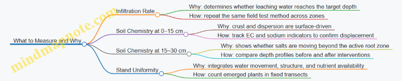
Practical Lessons from the Case
- Poor infiltration is not just a symptom; it controls whether any amendment can work.
- Zone-based treatment avoids input mismatch and reduces patchiness.
- Structure-building inputs are most effective when paired with water movement that can carry salts away from the surface.
- Monitoring should start with infiltration and depth-resolved chemistry, because plant appearance alone can lag behind the real changes.
By treating the crust as a system outcome—driven by sodium, dispersion, and water behavior—the field shifts from repeated surface sealing to a more stable wetting pattern that supports consistent emergence.
11.2 Case Study of Saline Irrigated Fields with Drainage Constraints
Field Setting and Starting Conditions
This case involves a flat, fine-textured field irrigated with water that has moderate salinity. Over several seasons, salts accumulated near the surface because drainage was weak and irrigation water had limited ability to move downward. The result was a patchy stand: seedlings emerged in low-salt pockets, then stalled as surface EC rose and sodium increased soil dispersion.
A practical baseline check used three measurements in the same week: (1) soil EC and pH at 0–15 cm and 15–30 cm, (2) infiltration rate using a simple ring test, and (3) a quick soil squeeze test to confirm dispersion risk. The key pattern was consistent: surface EC was highest, infiltration was slow, and the 15–30 cm layer showed delayed salt movement rather than clean leaching.
Root Cause Logic
Saline irrigation alone does not always fail; the failure comes from the combination of salt input plus restricted drainage. When infiltration is slow, water spreads laterally and evaporates near the surface. Sodium then promotes dispersion, which further reduces pore connectivity. That feedback loop explains why salts kept returning even when irrigation amounts were reduced.
Mind Map: Problem to Levers
Treatment Plan with Integrated Steps
The plan used a sequence so each step supported the next.
Step 1: Fix the drainage bottleneck first. Where feasible, shallow subsurface drainage was installed in the lowest parts of the field to create a consistent outlet. In areas where full drainage was not possible, furrow shaping and controlled field grading reduced ponding and lateral salt transport.
Step 2: Use leaching only when the soil can accept it. Leaching events were scheduled after the soil had improved infiltration. Instead of one large event, the team used smaller, well-timed leaching fractions during early growth when crop tolerance was higher and the field could be kept uniformly wet.
Step 3: Add biological amendments to improve structure, not just chemistry. Compost and a microbial inoculant were applied in bands to avoid overloading the entire surface with salts contained in some organic materials. The goal was to encourage aggregation and reduce dispersion so water could move downward during leaching.
Step 4: Add carbon inputs with incorporation depth in mind. Carbon was incorporated into the top 10–15 cm to support aggregate stability, while avoiding deep mixing that could bring up saltier subsoil. This mattered because the 15–30 cm layer already showed delayed salt movement.
Example: A Simple Decision Workflow
If surface EC is high but infiltration is very low, leaching will mostly spread salts sideways. The workflow below prevented that.
Example:
- If infiltration is below a practical threshold, apply structure-building inputs first and postpone heavy leaching.
- If infiltration improves, run a small leaching event and re-check EC at 0–15 cm after the next irrigation cycle.
- If 15–30 cm EC rises sharply, reduce leaching intensity and focus on maintaining aggregation and drainage pathways.
Monitoring and Quality Control
Soil sampling was repeated at the same depths after each two irrigation cycles. The team tracked three indicators together: surface EC decline, infiltration improvement, and whether the 15–30 cm layer stayed stable or increased slowly.
Plant observations were used as a sanity check. When infiltration improved, emergence became more uniform and early root growth looked less “surface-bound.” When infiltration stalled, the stand again became patchy, even if surface EC temporarily looked better.
Mind Map: What Success Looked Like
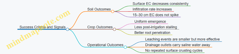
Results and Practical Takeaways
After the drainage improvements and a structured leaching schedule, surface EC stopped rebounding as quickly. Biological and carbon inputs reduced dispersion, which made each leaching event more efficient. The field still required careful irrigation management, but the system became controllable: salts moved downward when the soil could accept water, and they were carried away through drainage rather than lingering near the surface.
The main lesson was simple: in saline irrigated fields with drainage constraints, chemistry changes alone are not enough. The soil must be able to move water through the root zone, or the salts will keep taking the path of least resistance—usually straight back to the surface.
11.3 Case Study of Mixed Salinity and Alkalinity With Nutrient Lockup
A mixed-salt-and-alkali field often behaves like two problems wearing one trench coat. Salinity raises osmotic stress, while alkalinity (high pH plus sodium dominance) reduces nutrient availability, especially phosphorus and micronutrients. The result is a crop that looks hungry even when fertilizer was applied.
Field Snapshot and Symptoms
In a 40-hectare block, ECe readings ranged from 6 to 14 dS/m in the top 30 cm, while pH ranged from 8.4 to 9.1. SAR and ESP were highest in low spots where irrigation water pooled briefly after each application. Wheat emergence was patchy, and leaves showed pale striping consistent with iron and phosphorus issues. Soil tests also showed high total P but low plant-available P.
A practical clue came from infiltration checks: the surface crust broke easily in higher ground but stayed firm and smooth in the low spots. That matters because crusting limits water entry, which in turn limits leaching of salts and sodium.
Root Cause Chain
The lockup mechanism was not one single villain. Sodium disperses clay, which collapses pore structure and slows infiltration. Slow infiltration means salts and bicarbonates remain near the surface longer. High pH then promotes precipitation and adsorption of phosphorus, while iron and zinc become less soluble. Meanwhile, salt stress reduces root growth, so even “available” nutrients are harder to reach.
Mind Map: Problem to Measurement to Action
Treatment Design with Clear Boundaries
The team divided the field into three zones using EC and pH depth profiles:
- Zone A high EC, moderate pH: prioritize leaching and salt-tolerant establishment.
- Zone B moderate EC, high pH and ESP: prioritize sodium management and nutrient availability.
- Zone C low EC, high pH pockets: prioritize micronutrient and phosphorus availability with minimal salt movement.
They avoided a common mistake: applying the same amendment rate everywhere. In mixed fields, “more” in the wrong zone can worsen nutrient imbalance and waste inputs.
Biological Amendments and Carbon Inputs
For Zones B and C, they incorporated a mature compost plus a small, targeted dose of biochar that had been pre-loaded with nutrients and inoculated microbes. The goal was not to “feed the soil” in general terms; it was to improve aggregation and support microbial processes that help stabilize structure.
A simple example of timing: compost was applied before the first infiltration-focused irrigation so that improved structure could help water move downward. If compost is applied after crusting has already formed and water entry remains poor, the benefits stay near the surface.
Root-Zone Engineering and Leaching Management
In low spots, they corrected infiltration first. Shallow surface crusting was addressed with controlled tillage to break the hardpan layer, followed by a drainage-focused layout to prevent ponding. Then they scheduled leaching events using irrigation water that met basic SAR constraints.
A workable rule was to leach when the soil profile had room to accept salts. They monitored EC at 0–15 cm and 15–30 cm after irrigation. When EC in the top layer dropped but deeper EC rose, they knew salts were moving downward rather than just spreading laterally.
Nutrient Strategy Under High pH
Nutrient lockup was handled with placement and form, not just rate.
- Phosphorus: they used a placement approach (banding near the root zone) to reduce contact with high-pH soil surfaces. This improved early uptake even when total soil P was already high.
- Iron and Zinc: they selected forms that remain more soluble under alkaline conditions and applied them in a way that reached active root growth zones.
- Calcium support: they used calcium inputs in Zones B to counter sodium effects and help restore flocculation.
- Split nitrogen: they reduced the risk of losses and improved uptake as roots recovered.
Concrete example: in Zone B, a single broadcast application of phosphorus produced little response. After switching to banded placement plus sodium-structure improvements, leaf greenness improved within the next growth cycle, and root density increased in the treated bands.
Monitoring and Decision Points
They tracked three measurements at minimum:
- Depth EC to confirm salt movement below the root zone.
- Surface pH and ESP indicators to see whether alkalinity effects were easing.
- Plant tissue trends for P, Fe, and Zn to verify that “availability” translated into uptake.
When EC dropped but tissue P stayed low, they adjusted phosphorus placement rather than increasing total fertilizer. When tissue Fe improved but infiltration remained poor, they returned to crust and drainage fixes.
Outcome Summary
By treating sodium-driven structure first, then coordinating leaching with biological aggregation, and finally using nutrient placement and alkaline-tolerant forms, the field shifted from “fertilizer present but plant starved” to “nutrients reaching roots.” The patchiness reduced because water entry became more uniform, and the nutrient lockup eased because high-pH contact at the root surface decreased.
11.4 Case Study of Root Zone Compaction with Limited Leaching Efficiency
A 40-hectare field shows patchy crop stands after irrigation. Soil tests show moderate salinity and high sodicity in the top 20–40 cm, but the deeper layer is worse: EC rises with depth and infiltration tests slow dramatically below the plow pan. The farmer’s usual plan is “more irrigation to leach salts,” yet the field stays crusted and plants struggle. The core issue is not only chemistry; it is water movement. Compaction reduces infiltration and creates short, inefficient leaching paths, so salts concentrate where roots actually grow.
Foundational Diagnosis of Compaction and Leaching Limits
Start with three checks that connect physical structure to salt behavior.
-
Infiltration and ponding pattern: If water ponds at the surface and infiltration rate drops sharply after the first few centimeters, leaching water is not reaching the zone where it can carry salts downward.
-
Depth-specific structure: Use a simple profile description or a penetrometer transect to locate the plow pan or traffic pan. In this case, the barrier sits around 25–35 cm.
-
Salt distribution with depth: Take samples at 0–10, 10–20, 20–40, and 40–60 cm. Here, EC and ESP increase below the barrier, confirming that salts are being trapped in the root zone region.
A practical rule: if water cannot move through the barrier, leaching becomes a surface event, and salts rebound upward after irrigation stops.
Root Zone Engineering Strategy for Water Pathways
The recovery plan uses engineering to create controlled pathways for leaching water, then uses biological and carbon inputs to stabilize the improved structure.
Step 1: Break the compaction barrier selectively
- Use deep ripping or subsoiling only where the barrier is continuous, not across the whole field.
- Keep the working depth just below the compacted layer to avoid mixing sodic material into the surface.
- After ripping, avoid immediate heavy traffic while the structure is still open.
Easy example: If the barrier is at 30 cm, set the ripper to 35 cm and run on the same lanes each time. This limits disturbance and keeps the rest of the field from being re-compacted.
Step 2: Improve surface infiltration to prevent crusting
- Incorporate a carbon-rich amendment in bands or shallow incorporation zones to reduce surface sealing.
- Maintain residue cover between operations to protect aggregates from impact.
Step 3: Ensure drainage so leached salts have somewhere to go
- If the field has a high water table or poor lateral drainage, leaching water will accumulate and salts will remain.
- Add or repair shallow drainage where feasible, or adjust irrigation method to reduce waterlogging risk.
Integrated Recovery Sequence with Clear Decision Points
The sequence below ties each action to a measurable outcome.
- Pre-treatment measurement: Record infiltration rate, bulk density or penetrometer readings, and EC/ESP by depth.
- Engineering first: Subsoil/rip where infiltration is worst.
- Carbon and biological support: Apply compost or biochar-based amendments after mechanical loosening so microbes and organic matter can colonize the newly connected pores.
- Leaching events with controlled water: Schedule irrigation to wet the root zone without prolonged saturation.
- Re-check after each phase: If infiltration improves but EC at 20–40 cm does not drop, the barrier may still be limiting, or drainage may be insufficient.
Decision point example: After the first leaching cycle, if EC in 0–10 cm drops but 20–40 cm stays high, the water is moving downward only to the barrier. The next action is not “more water,” but additional targeted loosening or drainage correction.
Mind Map: the Case Study Logic
Practical Example Plan for One Irrigation Block
Divide the field into blocks based on infiltration and compaction depth. For the worst block, run a single targeted ripping pass, then apply compost in shallow bands. Follow with two irrigation cycles spaced to allow soil to drain, not remain saturated. After the second cycle, sample 0–10 and 20–40 cm. If EC at 20–40 cm has not moved, the barrier is still controlling flow, and the next step is additional targeted loosening or drainage correction rather than increasing irrigation volume.
This case shows a simple truth: when compaction limits water movement, chemistry treatments alone can’t do the job. The recovery becomes a water-path problem first, and a salt problem second.
11.5 Case Study of Smallholder Implementation with Practical Input Constraints
A smallholder farmer, Amina, manages 1.5 hectares of heavy clay with patchy crusting and salty patches that burn leaf edges. Her irrigation water has moderate salinity and occasional high sodium days. She cannot afford large quantities of gypsum, frequent lab testing, or specialized equipment. The goal is not “fix everything at once,” but to make the field more plantable by improving infiltration, reducing surface sodium risk, and keeping nutrients available.
Starting with What Can Be Measured
Amina begins with simple, repeatable checks: a handheld EC meter for irrigation and a soil test kit for pH and rough salinity. She also does two field observations each week: (1) infiltration time using a measured bucket pour into small spots, and (2) a quick stand check after emergence. She labels three zones: Zone A (worst crust), Zone B (moderate), and Zone C (best). This zoning matters because input constraints mean she must spend effort where it pays back fastest.
Mind Map: Smallholder Constraints to Field Actions
Phase 1: Make Water Enter the Soil
In Zone A, Amina focuses on infiltration. She cannot buy bulk structural amendments, so she uses a practical mix: mature compost plus a small amount of biochar that is pre-soaked in compost tea for several hours before application. She applies compost in shallow bands along planting rows rather than broadcasting across the whole field. The logic is simple: bands reduce input volume and target the root zone where sodium and salts most affect establishment.
She also creates shallow drainage furrows between rows in the lowest spots. The furrows are not deep engineering; they are just enough to prevent standing water that concentrates salts at the surface after evaporation.
Example: In Zone A, she marks a 20 m by 10 m area and applies compost bands at planting. After two irrigation cycles, she repeats the infiltration test. If infiltration improves by even a small margin, she keeps the same approach and repeats the banding strategy in the next season.
Phase 2: Reduce Sodium Risk During Establishment
Amina uses biological amendments where they matter most: at planting and early root development. She applies a modest dose of compost tea or a microbial-rich slurry into the furrow just before covering seed. The aim is to encourage aggregation and reduce surface dispersion, which is what turns crusting into a stand-killer.
She avoids over-irrigating right after planting. Too much water can move salts upward when evaporation follows. Instead, she schedules smaller irrigations more often, then performs a controlled leaching event only when the crop has enough root mass to tolerate temporary salt movement.
Example: If her irrigation schedule normally gives one heavy watering, she shifts to two lighter irrigations spaced by a day, then adds a single leaching irrigation after seedlings are established and the soil surface is no longer bare.
Phase 3: Nutrients That Don’t Get Trapped
High pH and sodium stress can reduce nutrient availability, especially phosphorus and micronutrients. With limited fertilizer budgets, Amina uses placement and timing rather than higher rates.
She applies phosphorus in a band near the seed row at planting, then uses split nitrogen doses after emergence. For micronutrients, she chooses small, targeted applications rather than large blanket amounts. If leaf symptoms appear in patches, she links them to the zone map and adjusts placement in that zone next time.
Example: In Zone B, she notices slower growth despite similar irrigation. She checks whether crusting is worse there and whether fertilizer was broadcast. She switches to band placement for the next crop and splits nitrogen into two doses.
Phase 4: Monitoring and Decision Rules
Amina keeps a one-page log: zone, input amounts, irrigation dates, infiltration time, and stand count at 14 and 30 days after emergence. Her decision rules are practical:
- If infiltration time does not improve in Zone A, increase surface organic cover using crop residues after emergence.
- If stand improves but leaf burn returns after a leaching event, reduce leaching intensity and increase irrigation frequency.
- If growth stalls without obvious burn, adjust nutrient placement and split timing rather than adding more fertilizer at once.
Integrated Outcome
By focusing on infiltration first, using low-cost carbon and biological support in targeted bands, and placing nutrients where roots can access them, Amina turns a difficult field into a field that can reliably establish crops. The recovery is not uniform across the farm, but it is measurable: better infiltration, fewer crust-driven stand failures, and more consistent early growth across the worst zone.
12. Documentation, Records, and Measurement for Recovery Verification
12.1 Building a Field Recovery Log Including Inputs, Dates, and Rates
A field recovery log is your “single source of truth” for what changed, when it changed, and how much you applied. In saline-alkali recovery, that matters because soil response is slow and uneven: one patch may improve after leaching while another stays stubborn due to depth-specific sodium accumulation. A good log lets you connect actions to outcomes without guessing.
What to Record Every Time
Record entries at the moment an operation is completed, not at the end of the season. For each input or management action, capture:
- Date and time window: Use the day you applied, plus the irrigation start and stop times if leaching occurred. Example date: 2026-03-05.
- Field identifier and zone: Include zone name or coordinates so you can compare like with like.
- Input name and grade: Compost type, biochar source, microbial product name, gypsum or amendment formulation.
- Rate and unit: Write the actual applied rate (e.g., kg/ha, t/ha, L/ha) and the unit you used.
- Application method: Broadcast, banded, incorporated to a depth, seed treatment, or foliar.
- Water details for leaching: Irrigation method, water EC and SAR if known, volume applied, and drainage status.
- Weather and field condition: Note soil surface wetness, wind, and whether the field was crusted or workable.
- Immediate observations: Any runoff, uneven spreading, odor from compost, or visible crust disruption.
A log that includes “what happened on the ground” prevents later confusion when lab results look contradictory.
A Simple Entry Template
Use one consistent structure for every operation. Keep it short enough that it gets filled.
- Operation: (e.g., compost incorporation)
- Date: (e.g., 2026-03-05)
- Zone: (e.g., North low spot)
- Rate: (e.g., 5 t/ha dry matter)
- Depth: (e.g., 10–15 cm)
- Equipment: (e.g., rotary tiller)
- Water plan: (e.g., light irrigation within 24 hours)
- Notes: (e.g., clods formed; next pass adjusted speed)
Mind Map: Field Recovery Log Components
Linking Inputs to Soil Depth and Timing
Saline-alkali issues often vary with depth, so your log should mirror that. When you sample, record the depth intervals and the zone. Then, when you apply amendments, note whether they were incorporated into the same depth band.
Example: If you incorporate compost to 10–15 cm but later sample only 0–5 cm, you may miss the improvement that actually occurred deeper. The log prevents that mismatch by forcing you to write down depth every time.
Example Log Entries That Stay Useful
Example 1: Biological amendment plus light irrigation
- Operation: Microbial inoculant applied with compost band
- Date: 2026-03-05
- Zone: East ridge
- Rate: 2.0 L/ha inoculant, compost 3 t/ha
- Method: Banding at seeding rows, followed by 20 mm irrigation
- Notes: No runoff observed; surface crust visible before irrigation
Example 2: Leaching event with drainage check
- Operation: Leaching irrigation
- Date: 2026-03-18
- Zone: North low spot
- Rate: 180 m³/ha applied
- Water notes: EC recorded at intake; SAR recorded if available
- Drainage: Furrow outlets flowed for 40 minutes
- Notes: After irrigation, infiltration improved in wheel tracks
These entries let you later answer practical questions like: “Did infiltration improve right after leaching, or only after the next carbon input?”
Quality Control Notes That Prevent Silent Errors
Add short QC lines whenever equipment or mixing could affect rate accuracy:
- “Spreader calibrated to target rate; test run completed.”
- “Compost moisture high; adjusted spreader speed to maintain coverage.”
- “Banded application verified by measuring band width and spacing.”
If you take photos, include a timestamp and the zone label. A photo is not a replacement for measurements, but it is excellent evidence for unevenness.
A Closing Rule for Consistency
If an entry cannot be tied to a later measurement or observation, it still belongs in the log—just label it clearly as context. That way, when soil chemistry and crop performance disagree, you can trace the disagreement to something concrete rather than to memory.
12.2 Soil Sampling and Data Management for Before After Comparisons
Before-after comparisons only work when the sampling plan is stable enough that differences reflect soil change, not sampling chaos. The goal is simple: measure the same soil processes in the same places, using the same methods, at the same depth logic, with enough replication to see real trends.
Foundational Sampling Logic
Start by defining what “before” means. Use a baseline campaign after the field has had a consistent management period (for example, after the last irrigation cycle and before the first amendment application). For “after,” schedule follow-ups at fixed intervals tied to crop stages and leaching events rather than calendar drift. A practical cadence is baseline, early response, and consolidation response.
Next, lock the sampling geometry. Saline-alkali patterns are patchy, so random sampling alone often compares different soil pockets. Use a grid or zone system that matches how you plan to treat the field. Mark sampling points permanently (GPS coordinates plus a physical reference) so the same spots are revisited.
Depth matters more than people expect. For saline and sodic issues, sample at least two depth bands: a surface band where crusting and root access are most affected, and a deeper band where leaching and sodium displacement show up. Keep depth intervals consistent across campaigns.
Sampling Design That Survives Reality
Use replication at two levels: within-point and within-zone. Within-point replication means multiple cores from a small radius around each marked location, composited into one sample per depth band. Within-zone replication means multiple marked locations per treatment zone.
A common field-friendly approach is:
- 5 to 10 locations per management zone
- 2 depth bands per location
- composite 3 to 5 cores per depth band
This balances labor with statistical usefulness. If a zone is highly variable, increase locations rather than increasing cores per location.
What to Measure and How to Keep It Comparable
Choose indicators that match the mechanisms you are targeting.
- Salinity: EC of the saturation extract or a consistent soil-water method
- Sodicity: SAR and/or ESP (exchangeable sodium percentage)
- Soil reaction: pH in a defined extract
- Structure proxy: infiltration rate or a simple crust strength observation
- Exchangeable cations: Ca, Mg, Na, and K to interpret displacement
Consistency rules:
- Use the same lab method each time.
- Use the same soil-to-water ratio and extraction time if you do field or on-farm tests.
- Record soil moisture at sampling because it affects EC readings.
- Label samples immediately with zone, point ID, depth band, and campaign.
Data Management Workflow
Treat data like a crop input: track it from receipt to interpretation.
- Create a sampling manifest before going to the field. It lists every point ID, depth band, and sample ID.
- Enter measurements into a structured sheet with controlled units and fixed column names.
- Store raw lab outputs as files linked to sample IDs, not as renamed copies.
- Keep a field notes log for anomalies: ponding, wheel tracks, unusual vegetation, or equipment issues.
When you compare before and after, compute change metrics per sample, such as ΔEC and ΔESP. Then summarize by zone using medians or trimmed means if outliers are common.
Mind Map: Before After Comparison System
Example: One Zone, Two Depths, Three Campaigns
Imagine a clay loam zone labeled Z3 with a biological amendment plus carbon input. You sample 7 permanent points in Z3.
- Campaign 1 (baseline): 7 points × 2 depths = 14 composite samples
- Campaign 2 (early response): repeat the same points and depths
- Campaign 3 (consolidation): repeat again
In the dataset, each row represents one sample ID with columns for zone, point ID, depth band, campaign, EC, ESP, and pH. Afterward, you calculate ΔEC = EC_after − EC_before and ΔESP = ESP_after − ESP_before for each point and depth. If Z3 shows consistent EC reduction at the surface depth but mixed ESP change at depth, that pattern tells you the sodium displacement is lagging behind salt removal, which guides the next management adjustment.
Quality Checks That Catch Mistakes Early
Before analyzing results, run three checks:
- Point match check: confirm the same point IDs were sampled at each campaign.
- Depth check: verify depth bands match the sampling template.
- Unit check: confirm EC and pH methods are identical across campaigns.
If any check fails, exclude that sample from change calculations rather than forcing it into the story. The field already provides enough surprises; the data should not add more.
12.3 Interpreting Trends in EC SAR ESP and pH With Depth Resolution
Depth resolution turns a confusing “field average” into a story with chapters. Salts, sodium, and alkalinity often move differently through the profile, so the same treatment can improve the topsoil while leaving deeper layers unchanged—or the reverse.
Foundational Idea: What Each Metric Is Telling You
EC (electrical conductivity) measures total dissolved salts in the soil solution. Higher EC usually means more osmotic stress for roots.
SAR (sodium adsorption ratio) estimates the relative dominance of sodium over calcium and magnesium in the water phase. It helps predict sodium hazard during irrigation and leaching.
ESP (exchangeable sodium percentage) measures sodium held on soil exchange sites. ESP is the “structural risk” metric: when it rises, dispersion and poor infiltration become more likely.
pH reflects alkalinity and the chemical environment that controls nutrient availability and microbial activity. In saline-alkali soils, pH can stay high even when EC drops, because sodium and carbonate/bicarbonate chemistry can persist.
Why Depth Matters in Practice
Topsoil (often 0–15 cm) responds quickly to amendments, irrigation, and surface crusting. Subsoil (15–60 cm or deeper) responds more slowly and is where leaching pathways either succeed or fail.
A useful rule: EC trends show salt movement; ESP trends show sodium exchange-site displacement; pH trends show alkalinity persistence; SAR helps interpret water-driven sodium pressure.
A Systematic Reading Workflow
- Start with the profile map, not the number. For each sampling date, compare EC, ESP, and pH at multiple depths. Look for gradients: surface-high vs subsoil-high patterns.
- Check whether changes are consistent across depths. If only the surface EC drops but subsoil EC stays high, salts are being redistributed rather than removed.
- Pair EC with ESP. EC can fall while ESP remains high if sodium is still on exchange sites. That combination often means structure may not fully recover yet.
- Pair ESP with pH. High pH alongside high ESP suggests carbonate/bicarbonate-driven sodium effects are still active.
- Use SAR to interpret irrigation influence. If SAR of applied water is high, sodium pressure can rebuild ESP even when EC temporarily improves.
- Confirm with a simple mass-balance mindset. Leaching should reduce EC in the wetted zone and move salts downward. If EC rises at depth after leaching, that is expected; if it rises at the surface, you likely have upward salt movement or poor drainage.
Example Patterns and What They Mean
Example 1: EC decreases at 0–15 cm, but ESP stays flat at 0–30 cm. This suggests salts are being flushed or diluted, yet sodium exchange sites are not being displaced. Biological amendments and carbon inputs may be improving infiltration, but calcium-driven sodium replacement (or sufficient leaching of sodium) may still be insufficient.
Example 2: EC decreases at all depths, ESP decreases only in the topsoil, and pH remains high. Salts are leaving the profile, but deeper exchange sites still hold sodium. The likely issue is that leaching water is not reaching enough depth, or the deeper layer lacks the calcium and structural conditions needed for sodium displacement.
Example 3: EC stays high at depth while pH drops slightly and ESP drops modestly. This can happen when alkalinity is easing faster than salt removal. It often points to carbonate chemistry changing (pH response) while total dissolved salts remain because drainage is limited.
Mind Map: Depth-Resolved Interpretation Logic
Practical Sampling and Interpretation Tips
- Use consistent depth intervals across dates so trends are real, not artifacts.
- Sample after comparable moisture conditions. EC and pH are sensitive to how much water is present; sampling too soon after irrigation can exaggerate differences.
- Track wetted depth. If irrigation infiltrates only to 20 cm, deeper ESP and pH may barely change even with strong surface improvements.
- Look for “cross-metric coherence.” The best recovery signals show EC and ESP improving together in the same depth zone, with pH easing in parallel when alkalinity is the limiting factor.
A depth-resolved profile is like a set of receipts: EC tells you what was in the solution, ESP tells you what was stuck to the soil, and pH tells you what chemical conditions were governing the whole transaction.
12.4 Linking Soil Indicators to Crop Performance and Stand Metrics
Soil indicators matter only when they explain what you see in the crop. The trick is to connect measurements to specific plant bottlenecks: water entry, root growth, nutrient availability, and salt exposure. A good linkage plan starts with a simple question for each indicator: “What plant process does this affect, and which stand metric should respond?”
Foundational Linkages Between Soil and Stand
1) EC and salt stress timing
- Indicator: Electrical conductivity (EC) in the root zone, ideally by depth.
- Plant process: Osmotic stress and reduced water uptake.
- Stand metrics: Germination rate, early stand count, leaf turgor, and biomass per plant.
- Example: If EC is highest at 0–15 cm and seedlings fail to establish, the issue is often early salt exposure near the seedling zone. If EC is high deeper but surface EC is lower, emergence may look fine while later growth stalls.
2) SAR, ESP, and sodium-driven structure problems
- Indicator: SAR and exchangeable sodium percentage (ESP) plus infiltration tests.
- Plant process: Dispersion, crusting, and reduced infiltration.
- Stand metrics: Patchy emergence, uneven plant size, runoff after irrigation, and reduced root depth.
- Example: Two plots can have similar EC, but the one with higher ESP shows crusting after irrigation and a thinner, more uneven stand.
3) pH and nutrient availability
- Indicator: Soil pH and, when possible, bicarbonate-related alkalinity.
- Plant process: Phosphorus fixation, micronutrient availability shifts, and reduced microbial activity.
- Stand metrics: Chlorosis patterns, slow early growth, and low tissue nutrient concentrations.
- Example: If plants look pale and phosphorus uptake is low while EC is moderate, pH-driven fixation is a likely contributor.
4) Physical structure and root-zone aeration
- Indicator: Bulk density, aggregate stability, infiltration rate, and compaction depth.
- Plant process: Root penetration limits and oxygen stress.
- Stand metrics: Root length density, root-to-shoot ratio changes, and reduced tillering or branching.
- Example: If infiltration is slow and roots stop at a compacted layer, you may see a “ceiling” on plant height even when nutrients are adequate.
Systematic Workflow for Linking Indicators to Metrics
Step 1: Choose stand metrics that match the growth stage.
- Establishment: emergence %, stand count, early vigor score.
- Vegetative growth: canopy cover rate, tiller count or branching, leaf area index.
- Reproductive stage: biomass partitioning, grain or fruit set, final yield.
Step 2: Pair each indicator with a likely mechanism. Create a one-to-one mapping from indicator → mechanism → metric. This prevents “data dumping” where you measure everything and explain nothing.
Step 3: Use depth logic. Seedlings respond to the top 0–20 cm; later growth reflects the whole effective rooting depth. If you only sample one depth, you’ll often misattribute the cause.
Step 4: Compare spatial patterns.
- If stand is patchy, check whether EC/ESP/pH also vary in patches.
- If stand is uniformly weak, check whether the whole field has a consistent constraint (often water entry or nutrient availability).
Step 5: Validate with simple field checks.
- Infiltration test results should align with crusting and patchiness.
- Tissue nutrient patterns should align with pH-related constraints.
Mind Map: Indicator to Mechanism to Stand Response
Example: Turning Measurements into a Clear Explanation
Assume a field shows uneven emergence. Soil tests show:
- EC is high in 0–10 cm in the weak patches.
- ESP is higher in those same patches.
- Infiltration is slower where crusting is visible.
A coherent explanation is: seedlings are exposed to both salt and sodium-driven infiltration failure at the seedling depth, reducing water availability and limiting early root establishment. The stand metric alignment is strong because emergence % drops first, while later growth differences follow the same spatial pattern.
If instead emergence is uniform but later growth diverges, you’d shift attention to deeper EC/ESP layers, rooting depth limits, or pH-driven nutrient availability that becomes more limiting as plants demand more nutrients.
Practical Stand Metric Targets for Interpretation
Use “directional targets” rather than absolute thresholds:
- If emergence % is low, prioritize seed-zone EC and infiltration.
- If early vigor is low but emergence is acceptable, prioritize pH-related nutrient availability and shallow root restriction.
- If canopy growth rate slows after establishment, prioritize deeper root-zone EC/ESP and physical constraints at the effective rooting depth.
This approach keeps the logic tight: each soil indicator earns its place by explaining a specific stand outcome, not by existing as a number on a report.
12.5 Verification Checklists for Completion of Recovery Milestones
A recovery plan is only as good as its checkpoints. This checklist turns “improving soil” into measurable milestones, so you can stop guessing and start confirming. Use it in order: first verify water movement, then chemistry, then biology and crop response.
Milestone 1: Field Readiness and Baseline Confirmation
Before any major input, confirm the field is testable and comparable.
- Sampling coverage confirmed: At least 3–5 representative zones per field block, with depth increments (e.g., 0–15 cm and 15–30 cm). Record GPS or grid IDs.
- Baseline infiltration check recorded: Run a simple infiltration test (ring or pit method) at each zone. Note time to a set depth or steady wetting.
- Baseline soil chemistry recorded: EC, SAR (or sodium adsorption proxy), ESP (or exchangeable sodium), pH, and exchangeable Ca/Mg/K/Na.
- Water source verified: Document irrigation EC and SAR, plus any seasonal changes.
- Operational constraints logged: Equipment limits for incorporation depth, drainage feasibility, and labor timing.
Example: If infiltration is near-zero in one zone, you treat that zone as a structural problem first, not a “nutrient problem.”
Milestone 2: Structural Improvement and Surface Stability
This milestone ensures water can enter and move through the root zone.
- Surface crusting reduced: After irrigation or rainfall, check for crust formation within 24–72 hours. Record whether seedlings can emerge without excessive crust cracking.
- Infiltration improved: Repeat infiltration tests. Target a clear improvement trend versus baseline, not perfection.
- Root-zone loosening verified: If subsoiling or deep mixing is used, confirm reduced compaction using penetrometer readings or root penetration observations.
- Drainage pathway confirmed: After a controlled irrigation, check whether water ponds or moves laterally. Note any persistent perched-water behavior.
Example: A field may show lower EC at the surface but still fail if water can’t reach 15–30 cm. That’s why infiltration is checked before celebrating chemistry.
Milestone 3: Salt and Sodium Targets Achieved in the Root Zone
This milestone confirms the ions are moving out or being displaced where roots actually grow.
- EC trend confirmed by depth: Re-sample after leaching windows. Look for EC reduction at 0–15 cm and 15–30 cm, not just the top 5 cm.
- ESP or exchangeable sodium reduced: Compare exchangeable Na and ESP against targets set in the plan.
- pH stabilized within workable range: If pH remains high, verify whether sodium displacement is progressing or whether alkalinity sources persist.
- No salt rebound after stopping leaching: Conduct a short “pause test” by monitoring EC after irrigation frequency returns to normal.
Example: If EC drops but ESP stays high, structure may still collapse under irrigation. That combination points to incomplete sodium management.
Milestone 4: Biological Activity and Carbon Integration Verified
This milestone checks whether amendments are doing useful work rather than just adding material.
- Organic matter placement verified: Confirm incorporation depth and uniformity. Uneven placement often creates patchy performance.
- Soil aggregation improved: Use a simple wet-sieving or aggregate stability observation after irrigation. Record whether aggregates resist slaking.
- N cycling indicators checked: Track mineral N availability trends (where measured) and plant response to split N applications.
- Odor and maturity checks for organics: Compost should not smell strongly anaerobic; manure should be stabilized enough to avoid nitrogen immobilization surprises.
Example: If biochar is applied but aggregation doesn’t improve, check whether it was inoculated or whether it was buried too shallow to interact with active roots.
Milestone 5: Crop Establishment and Yield Stability Confirmed
This milestone ties soil changes to practical outcomes.
- Stand establishment metrics: Record emergence rate, uniformity, and early vigor by zone.
- Root-zone performance observed: Use root sampling or careful excavation to see whether roots penetrate treated layers.
- Nutrient sufficiency signs checked: Compare leaf color and deficiency patterns against the nutrient management plan.
- Yield and quality recorded: Measure yield per zone and note whether variability matches remaining soil variability.
Example: If one zone yields well but another fails, compare their EC/ESP depth profiles and infiltration results rather than assuming the crop “didn’t like” the treatment.
Mind Map: Recovery Milestone Verification Flow
Example: One-Zone Pass or Fail Decision
- Pass: Infiltration improved, EC decreased at 15–30 cm, ESP decreased, aggregates improved, and stand is uniform.
- Fail: EC improves only at the surface, infiltration remains poor, or ESP stays high—then the next cycle focuses on structure and sodium displacement before increasing nutrient inputs.
Milestone Closure Checklist
When you close a milestone, record the following in the field log for each zone:
- Date of sampling and test method
- EC/SAR/ESP/pH values by depth
- Infiltration result summary
- Amendment type, rate, placement depth, and timing
- Crop stand metrics and root observations
- Decision outcome: continue, adjust, or stop leaching/amendment intensity
Use a consistent decision rule across zones. If you change the rule midstream, you’ll lose the ability to learn from the field—an expensive hobby no one needs.