Spectral Lighting Recipes for Indoor Farming
1. Scope and Lighting Fundamentals for Indoor Farming
1.1 Defining Lighting Recipes for Indoor Production
A lighting recipe is a repeatable set of instructions that turns LED hardware into a controlled light environment for a specific crop and production goal. In practice, it answers four questions: what wavelengths, how much light, when to deliver it, and how to keep it consistent across the room. If any of these are vague, you can still grow plants—but you cannot reliably control flavor, biomass, color, or harvest speed.
What a Recipe Must Specify
A usable recipe includes:
- Spectral recipe: the relative output of each LED channel (for example, blue, green, red, far red). This is usually expressed as a target spectral power distribution or as channel percentages tied to measured spectra.
- Intensity target: the delivered photosynthetic photon flux density (PPFD) at the canopy or at a defined measurement height.
- Timing schedule: photoperiod (hours on) and any stage-based changes (for example, different spectra during establishment versus production).
- Daily light integral target: the total light dose over 24 hours, typically in mol/m²/day, derived from PPFD and photoperiod.
- Spatial uniformity rules: how much variation is acceptable across benches, racks, or zones.
A good rule of thumb: if two growers could follow your recipe and measure the same PPFD and spectrum at the same canopy height, you have a recipe. If they would need to “adjust until it looks right,” you have a suggestion.
From Crop Goal to Light Inputs
Start with the production goal, then map it to light inputs. For example, if you want compact growth and consistent leaf color, you typically prioritize blue proportion and avoid excessive far red during early canopy formation. If you want faster harvest, you focus on delivering adequate daily light integral without pushing intensity so high that stress reduces quality.
This mapping is not magic; it’s cause-and-effect through plant physiology. Light drives photosynthesis, and the spectrum influences morphology and pigment development. Your job is to translate that into measurable targets.
Mind Map: Recipe Components and Their Dependencies
A Concrete Recipe Example
Suppose you grow culinary basil in a production room with multi-channel LEDs. You decide on a two-phase schedule: establishment and production.
- Establishment (days 1–7)
- Spectral mix: higher blue fraction to support sturdy early structure.
- Intensity: moderate PPFD so seedlings establish without bleaching.
- Timing: 16 hours on.
- Production (days 8–28)
- Spectral mix: slightly lower blue and higher red proportion to support biomass accumulation.
- Intensity: higher PPFD to maintain photosynthesis.
- Timing: 14 hours on.
Even without naming exact percentages, the recipe should state the measured PPFD at canopy height and the measured channel mix that produces that PPFD. Then you compute DLI from PPFD and photoperiod so you know the daily dose you are actually delivering.
The Measurement Anchor That Prevents Confusion
Recipes fail when “PPFD” means different things. Define:
- Measurement height (for example, 10 cm above the tallest expected canopy at each stage).
- Measurement method (sensor type and whether it’s corrected for spectrum).
- Reference point (center of each zone, or a grid average).
If you later change fixtures, replace LEDs, or alter optics, you re-check the anchor measurements. A recipe is only as stable as the calibration behind it.
Recipe Format That Scales from Pilot to Production
Use a consistent structure so you can compare batches:
- Crop and stage
- Spectral channel targets and verification method
- PPFD target and measurement height
- Photoperiod and any transitions
- DLI target and acceptance range
- Uniformity requirement across zones
- Notes on deviations and corrective actions
Here’s a compact template you can copy into your batch record:
Recipe Template
Crop/Stage:
Spectral Channels:
Measured Spectrum Check:
PPFD Target (canopy height):
Photoperiod:
DLI Target:
Uniformity Limit:
Zone Notes:
Acceptance Criteria:
When these fields are filled, the recipe becomes actionable. You can run it, measure it, and adjust it with confidence—without guessing whether the problem was the plants or the light.
1.2 Core Plant Light Responses and Practical Outcomes
Plants do not “see” light as a single thing. They respond to multiple signals at once: total photon supply, spectral balance, daily timing, and how evenly light reaches leaves. A lighting recipe is useful only when you can predict which response dominates under your settings.
Mind Map: Core Light Responses and What You Can Measure
Photosynthesis: From Photon Supply to Biomass
Photosynthesis depends on photons that plants can use, not on watts or even on “brightness” alone. In practice, you control photon supply using PPFD and DLI, then shape how efficiently plants use those photons with spectral balance.
Example: If two LED setups deliver the same PPFD at canopy, but one has a higher fraction of photons in red and the other has more in green, the red-leaning setup often produces faster leaf expansion because red photons are more directly effective for driving photosynthetic electron transport. The green-heavy setup can still grow plants, but you may need more total DLI to reach the same biomass target.
A practical recipe therefore starts with a DLI target for the crop stage, then uses spectrum to fine-tune efficiency and morphology rather than trying to fix everything with one knob.
Morphology: How Spectral Ratios Change Shape
Plants adjust architecture when spectral cues shift. Blue light generally supports compact growth by limiting stem elongation and encouraging leaf development that improves light capture. Red light supports photosynthesis and can increase biomass, but too little blue often leads to taller, thinner plants.
Far red affects the red-to-far-red balance, which plants interpret as a cue about shading. More far red relative to red can increase elongation and reduce compactness, which can be useful for some transitions but risky for market-ready compactness.
Example: For basil seedlings, a modest blue enrichment during early establishment can reduce stretch. If you later increase red proportion to raise DLI, you can maintain compactness while still pushing biomass. The key is stage separation: don’t keep the same spectrum and intensity for the entire cycle.
Pigment and Color: Why Leaves Look the Way They Do
Color is not only “cosmetic”; it reflects pigment investment. Chlorophyll supports green coloration and photosynthetic capacity. Blue light tends to support chloroplast development, while red supports chlorophyll maintenance. For red-purple traits, anthocyanins often increase when spectral cues and light intensity push plants toward protective pigments.
Example: If you want darker red tones in a specialty leafy crop, you can increase the proportion of red and add a controlled amount of blue while also ensuring the canopy receives enough PPFD. If the canopy is uneven, you’ll get red patches where leaves were brightest and greener leaves where they were dimmer, even if the fixture settings are correct.
Photoreceptor Signaling: Timing and Stage Consistency
Photoreceptors respond to spectral ratios and influence developmental timing. This is why two recipes with the same DLI can still produce different “feel” at harvest: one may yield thicker leaves and earlier canopy closure, while the other yields a more open structure.
Example: During the transition from vegetative growth to harvest-ready size, you can reduce blue slightly while maintaining DLI if your goal is faster canopy closure. If you reduce blue too much, you may see delayed leaf thickening and a looser canopy that slows uniform harvest.
Timing Effects: Photoperiod and Daily Rhythm
Photoperiod affects how quickly plants accumulate growth relative to the calendar. Longer photoperiods can increase daily photon capture, but only up to the point where plants can use the additional light without losing efficiency. The practical outcome is that harvest speed is often governed by DLI delivery across the day, not by “turning lights on longer” without checking canopy response.
Example: If you extend photoperiod but keep PPFD low, you may not reach the DLI needed for your target days-to-harvest. If you raise PPFD and shorten photoperiod, you can reach the same DLI while changing morphology slightly due to the different light rhythm.
Light Distribution: Uniformity Is Part of the Recipe
Even the best spectrum fails if the canopy experiences different PPFD. Uneven distribution creates variable morphology and color because leaves receive different photon totals and different spectral exposure.
Example: In a multi-tier rack, the top tier often receives higher PPFD. If you don’t zone or dim by tier, top plants may reach target size early but become over-compact or over-colored, while lower plants lag and show paler tones.
Practical Outcome Checklist for Recipe Design
- Start with a canopy DLI target for the stage.
- Use spectrum to adjust morphology and pigment investment, not to replace DLI.
- Keep photoperiod and intensity consistent with the crop’s growth pattern.
- Verify uniformity with a PPFD map before judging color or harvest timing.
- Compare outcomes using measurable proxies: internode length, leaf thickness, canopy closure, and color uniformity.
When you treat light as a set of interacting signals—photons, spectrum, timing, and distribution—you can predict outcomes instead of chasing them.
1.3 Key Photometric and Radiometric Terms for Growers
Indoor farming with LEDs is mostly a translation problem: you choose a light output, then you need terms that connect that output to what plants actually receive and what humans can measure. Photometric and radiometric quantities are the vocabulary for that translation. The trick is to use each term for the job it was designed for, instead of mixing them up and wondering why the numbers don’t agree.
Foundational Terms You Will Use Every Week
Radiometry describes light energy without caring how human eyes respond. Photometry weights light by human visual sensitivity, which is useful for lighting design but not for plant growth decisions. For plants, radiometric terms are the starting point, and photometric terms are mostly a sanity check for facility lighting.
Radiant Flux and Power
- Radiant flux (Φe) is total optical power emitted across all wavelengths, measured in watts (W). If you double the number of LEDs at the same drive current, radiant flux usually increases.
- Radiant intensity (Ie) describes power per solid angle (W/sr). It matters when you care about beam spread and fixture aiming.
Spectral Power Distribution
- Spectral power distribution (SPD) describes how radiant power is distributed across wavelength. Two fixtures can have the same total watts but different SPDs, and plants will respond differently because photosynthesis and photomorphogenesis depend on wavelength.
Terms That Connect Light to Plant-Relevant Energy
Photon Flux and Photosynthetic Photon Flux
Plants use photons, not watts. That’s why photon flux is central.
- Photon flux (Φp) is the number of photons per second (photons/s). It is wavelength-dependent because photon energy changes with wavelength.
- Photosynthetic photon flux (PPF) is photon flux in the photosynthetically relevant range, typically 400–700 nm, measured in micromoles per second (µmol/s). This is a bridge between electrical input and plant-usable photons.
Photosynthetic Photon Flux Density
- PPFD is PPF per unit area at the canopy, measured in µmol/m²/s. PPFD is the workhorse measurement for recipes because it tells you how many usable photons arrive each second at a specific location.
A practical example: if one bench averages 250 µmol/m²/s and another averages 350 µmol/m²/s under the same photoperiod, the second bench receives 40% more photons per second at the canopy. That difference often shows up as faster growth or earlier harvest—unless the spectrum or environment limits the response.
Daily Light and Timing Terms
Daily Light Integral
- DLI is the total photon dose delivered over a day, measured in mol/m²/day. It is essentially PPFD integrated over time.
A quick example: if PPFD is 200 µmol/m²/s for 16 hours, the daily photon dose is:
- 200 µmol/m²/s × 3600 s/hour × 16 hours = 11,520,000 µmol/m²/day
- Convert µmol to mol by dividing by 1,000,000 → 11.52 mol/m²/day
This is why two schedules can produce similar DLI even with different PPFD and photoperiod. Plants care about total dose and timing, not just one snapshot.
Photoperiod
- Photoperiod is the duration of light exposure per day. It affects morphology and can shift how efficiently plants use photons, especially when spectra include far red or blue.
Photometric Terms and Why They Usually Don’t Drive Recipes
Photometric quantities weight light by human eye sensitivity (the luminous efficiency function). They are measured in units like lumens (lm) and lux (lx).
- Luminous flux (Φv) is measured in lumens.
- Illuminance (E) is measured in lux (lm/m²).
For plant work, lux is not directly convertible to PPFD without knowing the spectrum. Two fixtures that look equally bright to humans can deliver very different photon flux to plants.
A practical example: a fixture with more red light can produce high PPFD with relatively fewer lumens, while a fixture with more green/yellow content can look brighter in lux but may not deliver the same photosynthetic photon density.
Advanced Details That Prevent Common Mistakes
Measurement Geometry and Sensor Response
PPFD meters often use a sensor designed to approximate 400–700 nm response. Still, sensor spectral response is not identical across brands, and the reading can shift with spectrum and angle.
- Measure at the canopy height you actually use.
- Check uniformity across the bench, because PPFD is not uniform just because the fixture looks centered.
Uniformity and Averaging
If you average PPFD across a bench, you hide extremes. Plants at the low end may become the bottleneck for harvest timing and uniformity.
A simple workflow: record PPFD at a grid of points, compute the average, and also track the minimum and maximum. If the minimum is far below the target, you’ll likely see uneven growth even when the average looks fine.
Mind Map: Grower-Relevant Light Terms
Example: Translating a Recipe Target into Measurements
Suppose your recipe target is DLI = 12 mol/m²/day with a 16-hour photoperiod. The average PPFD you need is:
- DLI (mol/m²/day) × 1,000,000 µmol/mol ÷ (seconds/day)
- 12 × 1,000,000 ÷ (16 × 3600) ≈ 231 µmol/m²/s
So you set the fixture channels, then verify with PPFD readings at canopy height. If the bench average is 231 but the minimum is 180, you adjust spacing, dimming, or fixture height until the low points meet the target.
When you keep these terms straight—watts for energy, µmol for photons, PPFD for instantaneous density, and DLI for daily dose—your lighting recipes stop being guesswork and start being measurable decisions.
1.4 Understanding Spectral Power Distribution and LED Binning
Spectral Power Distribution (SPD) describes how an LED’s output power is spread across wavelengths. Two fixtures can report the same “PPFD” yet produce different plant responses if their SPD differs, because photosynthesis and pigments depend on wavelength, not just total light. SPD is typically measured as a spectrum curve: wavelength on the horizontal axis, relative or absolute power on the vertical axis.
From SPD to What Plants Actually Receive
A plant does not see a single wavelength; it receives a weighted mix across the spectrum. The weighting comes from plant photoreceptors and pigment absorption. Practically, you can think of SPD as the “recipe ingredient profile,” while PPFD and DLI describe the “portion size.” If you change the ingredient profile (SPD) without changing the portion size (PPFD), the crop can still change—leaf thickness, color, and growth rate included.
SPD also matters for how you combine channels. A red channel and a blue channel might each be “on target,” but the combined SPD can shift because each channel has its own peak wavelength, bandwidth, and efficiency curve. That’s why recipe design should treat channels as spectral contributors rather than just intensity knobs.
LED Binning Explained Without the Hand-Waving
LED binning is how manufacturers group LEDs with similar spectral characteristics. Even LEDs from the same product line vary slightly in peak wavelength and output intensity. Bins are labeled by ranges, such as “bin A” for a wavelength window and “bin 1” for brightness. When you buy a fixture, you inherit the manufacturer’s binning decisions plus the fixture’s optical design.
The key idea: binning affects both the peak position and the distribution width. A narrow-band LED can look “similar” to another narrow-band LED on paper, but a small peak shift can change how much light falls into a pigment’s absorption region.
A Practical Mental Model for SPD and Bins
Imagine each LED as a bell curve. Binning selects which bell curves you get. SPD is the sum of those curves after optics and mixing. If you swap bins, you change the sum, even if the fixture still claims the same nominal wavelengths.
Mind Map: SPD and LED Binning
Dimming and SPD: The Hidden Variable
Dimming is often implemented by reducing current. That can slightly shift the spectrum and change relative channel contributions, especially when channels are driven differently. If your recipe uses dimming to hit a target DLI, you should confirm that the SPD at the operating dim level matches your assumptions.
A simple check is to measure spectra at two or three dim levels for each channel. If the peak wavelength or relative band shape changes meaningfully, your “recipe” should be defined at the dim level you actually run, not only at full power.
Example: Two “Red” Channels That Aren’t the Same
Suppose you design a lettuce recipe using a nominal 660 nm red channel and a 450 nm blue channel. You set both fixtures to the same PPFD at canopy height. In one fixture, the red LEDs are binned slightly toward 655 nm with a broader distribution; in the other, they cluster closer to 665 nm with a tighter distribution.
Even with equal PPFD, the second fixture can produce a different leaf tone and growth habit because the red band overlaps pigment absorption differently. The difference may be subtle at first, but it often shows up in canopy uniformity: some plants become slightly more elongated or show different leaf color distribution across the tray.
Example: Channel Mixing and Recipe Drift
If you later replace a panel and the supplier provides a different bin set for the blue channel, your “blue fraction” in the combined SPD can shift. You might keep the same blue channel intensity setting, but the actual spectral contribution changes. The result is recipe drift: the crop no longer matches the earlier batch even though your control settings are identical.
What to Record in Your Recipe Notes
To keep recipes reproducible, record the channel bin identifiers if available, the measured SPD or at least representative spectra at your operating dim levels, and the fixture-to-canopy geometry. This turns SPD and binning from a theoretical concern into a practical quality control step.
Quick Summary
SPD tells you how power is distributed across wavelengths; binning tells you how consistent that distribution is across LED units. Together, they explain why “same PPFD” does not guarantee “same crop outcome,” and why measuring or verifying spectra at the operating settings is worth the effort.
1.5 Mapping Light Inputs to Measurable Crop Targets
Indoor growers don’t “set a spectrum” and hope for the best. They translate light inputs into measurable crop targets, then verify those targets with repeatable measurements. The mapping is easiest when you treat lighting as a controllable input vector and crop outcomes as an output vector.
From Inputs to Targets
Start with three input categories:
- Spectral composition: how much power each wavelength band contributes.
- Intensity: how much photosynthetic photon flux reaches the canopy (often expressed as PPFD).
- Timing: photoperiod and any stage-based changes in spectrum or intensity.
Then define crop targets in measurable terms. For flavor, color, biomass, and harvest speed, targets typically include:
- Biomass: fresh mass, dry mass, leaf area, and dry matter percentage.
- Color: chlorophyll index proxies, anthocyanin-related color metrics, and visual grading with a consistent reference.
- Flavor proxies: soluble solids, specific metabolite indicators when available, and sensory panels only after you stabilize the lighting variables.
- Harvest speed: days to marketable size, growth rate, and uniformity across trays.
A practical mapping rule is: each target must have a measurement method that tolerates normal facility variation. If you can’t measure it consistently, you can’t map it.
Building the Mapping Model
A useful model is a layered chain:
- Light at the canopy → plant response signals → growth and quality outcomes.
The “light at the canopy” step matters because fixtures rarely deliver uniform spectra. Two benches can have the same nominal settings but different canopy PPFD and different spectral ratios due to distance, reflectance, and lensing.
Plant response signals are often summarized by effective drivers:
- Photosynthetic drive tied to photon availability across relevant wavelengths.
- Morphology drive tied to blue and far-red balance.
- Pigment drive tied to red/blue ratios and timing.
You don’t need a perfect mechanistic equation to start. You need a consistent operational mapping that you can test.
Converting Fixture Settings into Canopy Targets
Use a two-step conversion:
-
Fixture settings → canopy PPFD and spectral ratios
- Measure at representative canopy heights for each zone.
- Record PPFD and at least a few band ratios (for example, blue fraction and far-red fraction).
-
Canopy metrics → crop targets
- Translate canopy metrics into expected outcomes using your own facility history.
- If you’re new, begin with conservative baseline recipes and adjust one variable at a time.
A simple example for leafy greens: you want faster harvest without pale color. You might increase DLI by raising photoperiod while keeping blue fraction stable, then verify color at the usual harvest window. If color fades, you adjust spectrum rather than intensity.
Mind Map: Mapping Light to Measurable Outcomes
Example: A Controlled Mapping for Harvest Speed
Goal: reduce days to market size for basil while keeping leaf color consistent.
- Define the target: market size at day X ± 1, with a color grade that matches your reference photos.
- Measure baseline canopy inputs: PPFD at canopy height and blue fraction in each zone.
- Adjust one lever: increase photoperiod by 1–2 hours while holding spectral ratios constant.
- Verify outcomes: record growth rate daily, then measure soluble solids and color at the harvest day.
- If harvest speeds up but color dulls: reduce intensity slightly or restore the original blue fraction rather than cutting photoperiod back immediately.
This approach keeps the mapping honest: you learn which input changed the target, and you avoid mixing multiple changes that make the cause unclear.
Example: A Controlled Mapping for Color and Biomass
Goal: improve red-purple coloration in specialty greens without sacrificing dry matter.
- Target: a consistent color grade plus dry matter percentage within your acceptable range.
- Input mapping: keep total DLI stable, then adjust red-to-blue balance and timing of the spectrum shift.
- Verification: measure color at two points—early development and final harvest—to separate “color formation” from “late-stage thickening.”
When you map this way, you stop treating color as a single outcome and start treating it as a process with a measurable timeline.
Practical Mapping Checklist
- Targets are measurable and scheduled.
- Canopy inputs are measured, not assumed.
- Each recipe change affects one mapping variable at a time.
- Batch comparisons use the same harvest criteria.
- Notes include canopy height, zone, and any handling differences.
With this structure, light becomes a controlled input that you can connect to crop outcomes using evidence, not guesswork.
2. Measurement, Instrumentation, and Data Quality Control
2.1 Selecting Sensors for PAR PPFD and Spectral Measurements
A lighting recipe is only as good as the measurements behind it. In practice, you need two kinds of sensors: one that tells you how much usable light the plants receive (PAR PPFD), and one that tells you how that light is distributed across wavelengths (spectral measurement). The trick is choosing instruments that match your control goals and your facility reality, not just your budget.
1) Start with Your Measurement Job
First decide what you must control.
- If your recipe is mostly about intensity and daily light integral, PAR PPFD is the workhorse.
- If your recipe is about flavor compounds, color pigments, or morphology shifts tied to specific bands, you need spectral data.
- If you do both, you still don’t measure everything with the same sensor; you use each sensor for what it does best.
A practical rule: use PAR PPFD to verify delivery at the canopy, and use spectral measurements to verify that the delivery matches the intended spectrum.
2) Choose PAR PPFD Sensors That Match Canopy Reality
PAR PPFD sensors measure photon flux in the 400–700 nm range. For indoor farming, you want repeatable readings at the same height and angle.
Key selection points:
- Cosine response: Canopies are not point sources. A sensor with a good cosine response reduces errors when you move it slightly or when fixtures create non-uniform angles.
- Spectral response match: PAR sensors approximate the plant-relevant weighting across 400–700 nm. If your LEDs are heavy in narrow bands, a sensor with a well-characterized response matters.
- Integration time and stability: Fast changes from dimming or controller updates can confuse slow sensors. Choose an integration behavior that matches your measurement workflow.
- Form factor and mounting: A flat sensor head is easier to place consistently at canopy height than a bulky probe. If you use a boom or rail, ensure the sensor can be positioned without twisting.
Example: If you dim channels in steps (say 10% increments), measure PPFD after the system settles for a consistent dwell time. Otherwise, you’ll record a transient that looks like a recipe error.
3) Choose Spectral Sensors for What You Actually Need
Spectral measurement can mean two different things: a full spectrum across visible wavelengths, or a set of band estimates. For recipe development and verification, you generally want a spectrometer or a sensor array that can resolve wavelength-dependent output.
Key selection points:
- Wavelength range and resolution: You need enough resolution to distinguish your LED channels and any overlap between bands. If your recipe uses narrow peaks, coarse resolution can blur them together.
- Radiometric accuracy and calibration: Spectral sensors must be calibrated to convert raw counts into meaningful relative or absolute spectral power.
- Stray light and saturation behavior: High-intensity fixtures can saturate sensors. Saturation flattens peaks and makes spectra look “cleaner” than they are.
- Measurement geometry: Spectral readings depend on distance, angle, and whether the sensor sees direct light or a mix of direct and reflected light. Decide on a geometry and keep it consistent.
Example: If you measure at 30 cm above the canopy one day and 50 cm the next, the spectrum may shift due to fixture optics and reflections. Keep distance fixed, or at least record it and apply a consistent measurement protocol.
4) Decide on Relative Versus Absolute Use
You can use spectral sensors in two modes:
- Relative mode: You compare spectra across time or across fixtures. This is often enough for verifying that channel ratios are behaving.
- Absolute mode: You need calibrated spectra that can be compared across facilities or across years.
If your goal is to build a recipe library inside one facility, relative consistency can be more important than absolute accuracy. If you’re trying to reproduce results across different rooms, absolute calibration matters more.
5) Plan for Uniformity and Spatial Sampling
A single sensor reading can lie politely. Canopies have gradients from fixture layout, reflectance differences, and airflow-driven leaf movement.
A systematic approach:
- Map PPFD at a grid across the target area.
- Use spectral measurements at representative points, typically where PPFD is near the average and where it is near the low end.
- If your spectrum is controlled per fixture channel, verify that the spectral shape stays consistent across the area, not just the intensity.
Example: If one corner shows 20% lower PPFD but the spectrum shape is identical, you can fix it with intensity or zoning. If the corner also shows a different spectral balance, you likely have optical or mixing issues that require fixture-level attention.
6) Mind Map of Sensor Selection Logic
Mind Map: Selecting Sensors for PAR PPFD and Spectral Measurements
7) A Simple Example Workflow
- Set a measurement geometry: same sensor height, same distance, same angle.
- Verify PPFD delivery: take a grid of PPFD readings and compute average and minimum.
- Verify spectral correctness: measure spectra at the average PPFD point and at the lowest PPFD point.
- Check for mismatch patterns:
- If PPFD varies but spectrum shape stays consistent, adjust intensity/zoning.
- If spectrum shape varies, investigate fixture mixing, channel mapping, or optics.
This workflow prevents the most common mistake: treating intensity and spectrum as interchangeable when they are not. PPFD tells you “how much,” while spectral measurement tells you “what kind,” and both are needed for reliable recipes.
2.2 Calibrating Instruments and Verifying Readings
Calibration is the boring part that keeps your spectral recipes from becoming guesswork. The goal is simple: make sure your instruments measure what you think they measure, and confirm that the numbers you feed into your LED recipe are stable across time and space.
Establishing a Calibration Baseline
Start by separating two tasks: calibration of the sensor itself and verification of the measurement setup. Calibration answers, “Is the sensor reading correct?” Verification answers, “Is the setup producing repeatable readings under your operating conditions?”
Use a baseline day to define your reference behavior. For example, on 2026-03-05, measure a stable reference light source (or a known-good lamp/LED module) and record:
- Sensor serial number and firmware version
- Integration time and averaging settings
- Mounting height and orientation
- Ambient conditions (especially if your sensor is temperature-sensitive)
If you change any of those parameters later, treat it as a new baseline.
Calibrating PAR PPFD Sensors
PAR PPFD meters typically rely on a calibrated spectral response. Even if the meter is factory-calibrated, you still need to confirm it behaves consistently in your facility.
A practical workflow:
- Warm up the LED fixture long enough to reach steady output.
- Place the sensor at the intended canopy height.
- Measure at least five readings, then compute the mean and spread.
- Repeat after moving the sensor slightly (for example, 2–3 cm in each direction) to detect local effects.
A good verification target is repeatability: readings should cluster tightly. If your spread is large, fix the setup first—loose mounting, reflections, or inconsistent sensor angle can cause more trouble than the spectrum itself.
Calibrating Spectrometers for Spectral Power Distribution
Spectrometers are more sensitive to alignment and stray light. Before trusting spectral curves, confirm:
- Wavelength calibration using a known reference (if your device supports it)
- Intensity calibration using a reference source or internal calibration routine
- Correct integration time so the strongest peaks are not saturating
When you run a spectral measurement, keep the optical path consistent. A tiny change in distance between the LED and the sensor can alter the measured spectrum due to optics and geometry.
Verifying Readings with Cross-Checks
Cross-checks catch errors that single-instrument calibration misses. Use at least two independent checks:
- PPFD cross-check: Compare PPFD derived from the spectrometer against the PPFD meter reading under the same conditions.
- Spatial cross-check: Map a small grid (for example, 3×3 points) at your working height.
If the spectrometer-derived PPFD consistently reads higher than the PPFD meter, you likely have a conversion mismatch (spectral response assumptions) or a measurement geometry difference.
Building a Repeatable Measurement Routine
Consistency matters more than heroics. Create a routine that reduces human variability:
- Same fixture warm-up time every session
- Same sensor mounting method and leveling procedure
- Same averaging count and integration time
- Same grid layout and coordinate system
Then log results in a way that makes deviations obvious. A simple table with mean, standard deviation, and percent difference between instruments is enough.
Mind Map: Calibration and Verification Flow
Example: Detecting a Geometry Problem
You measure PPFD at the canopy height and get 420 µmol/m²/s. After remounting the sensor, the next session shows 390 µmol/m²/s even though the fixture settings are unchanged.
A quick cross-check reveals the sensor is now tilted by about 5 degrees. Because the sensor’s cosine response is not perfect, the tilt changes the effective collection. Correcting the leveling returns readings to within the expected repeatability range.
Example: Spectrometer Conversion Mismatch
Under a red-heavy spectrum, the spectrometer-derived PPFD is 10% higher than the PPFD meter. You repeat the measurement with the same geometry and see the same offset.
The likely cause is not the LEDs; it’s the conversion step from spectrum to PPFD. Confirm that the PPFD calculation uses the correct weighting function and that the spectrometer’s spectral units are interpreted correctly.
Acceptance Criteria for “Good Enough” Measurements
Define thresholds before you start recipe work. For routine production mapping, you might accept:
- Repeatability within a small percent range at each grid point
- Instrument-to-instrument agreement within a defined tolerance after geometry is matched
- No obvious outliers caused by reflections or sensor placement
When results fail criteria, fix the setup and re-measure rather than adjusting the recipe to compensate.
2.3 Converting Spectral Data into Usable Recipe Inputs
Spectral measurements tell you what the LEDs are actually doing, but recipes need inputs you can repeat: channel targets, timing, and intensity. This section turns a spectrum into a practical recipe by mapping measured wavelength content to controllable LED channels and then validating that the resulting light delivery matches the crop-relevant targets.
From Spectrum to Channel Contributions
Start with the measured spectral power distribution (SPD) at a known geometry: same fixture height, same distance to the sensor, and same optics state. If your SPD is measured at the canopy plane, you can treat it as “delivered light.” If it’s measured at the fixture, you must later account for distance and losses.
Next, express the SPD as a weighted sum of your LED channels’ spectra. In practice, you rarely have perfectly known spectra for every bin and temperature point, so you use a calibration matrix built from a few known channel settings. The goal is not mathematical perfection; it’s stable repeatability.
A simple mental model:
- Your sensor gives you intensity vs. wavelength.
- Your fixture has channels (for example: 450 nm, 660 nm, 730 nm, and white).
- Each channel has a characteristic SPD shape.
- The measured SPD is the mixture of those shapes.
Choosing Recipe Targets That Match Crop Goals
Recipes should be written in terms of what the plant responds to, not only what the instrument reports. Common targets include:
- PPFD or DLI for overall light quantity.
- Blue fraction or blue-weighted output for morphology and quality.
- Red dominance for biomass support.
- Far-red fraction for stretch and allocation signals.
- Color metrics when you care about pigment expression and visual uniformity.
To convert SPD into these targets, you apply weighting functions. For PPFD, you use the photometric response equivalent to photosynthesis-relevant weighting. For blue/red/far-red fractions, you integrate SPD over defined wavelength bands and normalize by total photosynthetically active output.
Practical Conversion Workflow
Use a workflow that can be repeated batch after batch.
-
Normalize the measurement
- Convert your SPD to consistent units.
- Integrate over the photosynthetically relevant range to compute total PPFD-equivalent.
-
Compute band integrals
- Integrate SPD over blue (for example 400–500 nm), red (for example 600–700 nm), and far-red (for example 700–800 nm).
- Convert each band integral into a fraction of total PPFD-equivalent.
-
Map fractions to channel settings
- Use your calibration matrix to estimate channel weights that would produce the measured band fractions.
- If the fixture includes a white channel, treat it as a broad-spectrum contributor that also affects band fractions.
-
Scale to the desired PPFD
- Once channel weights match the spectral shape, scale overall intensity to hit the target PPFD at the canopy plane.
-
Validate with a second measurement
- Re-measure after applying the computed channel settings.
- Compare predicted vs. measured band fractions and PPFD.
- If the error is systematic, update the calibration matrix; if it’s random, check sensor placement and fixture dimming stability.
Example: Turning a Measured Spectrum into a Recipe
Assume you measure an SPD at the canopy plane and compute:
- Total PPFD-equivalent: 280 µmol/m²/s
- Blue fraction: 18%
- Red fraction: 72%
- Far-red fraction: 10%
Your crop target for a compact leafy stage is:
- PPFD-equivalent: 300 µmol/m²/s
- Blue fraction: 20%
- Far-red fraction: 8%
You then:
- Use your calibration matrix to find channel weights that increase blue slightly and reduce far-red slightly while keeping red dominant.
- Scale the overall intensity so the integrated PPFD-equivalent becomes 300.
A realistic outcome might be:
- Increase the 450 nm channel by a small step.
- Reduce the 730 nm channel by a small step.
- Adjust the red channel to maintain total PPFD-equivalent.
The key is that you don’t guess channel changes from intuition; you compute them from the calibration mapping and then verify with a measurement.
Mind Map: Converting Spectral Data into Recipe Inputs
Common Failure Points and How to Avoid Them
- Sensor placement drift: Even a few centimeters can change the spectrum due to optics and angular response. Fix geometry before you trust conversions.
- Temperature and dimming nonlinearity: Channel spectra can shift with operating temperature and driver behavior. Calibration should reflect the operating range you actually use.
- Mixing “shape” and “quantity” incorrectly: Band fractions control spectral shape; PPFD controls quantity. If you adjust channels without re-scaling intensity, you’ll miss the target even when fractions look right.
Output Format for a Usable Recipe
A usable recipe input set includes:
- Channel targets (e.g., blue, red, far-red, white) as dimmer percentages or driver currents.
- Intensity target at canopy plane (PPFD-equivalent) and the method used to verify it.
- Timing parameters (photoperiod and any stage-based schedule).
When these are derived from measured SPD and validated with a second measurement, your recipe becomes a repeatable instruction rather than a one-off measurement story.
2.4 Measuring Uniformity Across Benches and Canopies
Uniformity is what turns a good spectral recipe into a consistent harvest. If one bench gets 10% more PPFD than another, you can end up with different growth rates, different color intensity, and different harvest timing—even when the recipe settings are identical. The goal is to measure spatial variation, quantify it, and then decide whether to adjust optics, layout, or control logic.
What Uniformity Means in Practice
Start with two layers of uniformity:
- Irradiance uniformity across the crop area (how PPFD and spectral distribution vary where plants actually sit).
- Canopy uniformity through height (how much the light changes from top leaves to lower leaves).
A bench can look uniform at the sensor height but still be uneven at the canopy. That’s why you measure at the plant plane and, when possible, at one additional height.
Measurement Plan Before You Measure
Pick a measurement grid that matches your geometry. For example, if your benches are 1.2 m by 2.4 m, a 6×12 grid gives 72 points, which is usually enough to see gradients without turning the day into a marathon.
Then decide what you will measure at each point:
- PPFD at the plant plane (fast, actionable).
- Spectral shape at a smaller subset of points (to confirm that “uniform PPFD” doesn’t hide “non-uniform spectrum”).
A practical approach is: measure PPFD everywhere, then measure full spectra at the grid corners and at the center of each bench zone.
Sensor Setup That Prevents False Uniformity
Uniformity measurements fail most often due to setup errors:
- Height consistency: keep the sensor at the same distance from the canopy across all points. If you can’t, record the height and correct later.
- Angular response: place the sensor so it faces the light source consistently. Tilting changes readings.
- Warm-up and stability: LEDs and drivers can drift slightly after power-up. Use a consistent warm-up time before starting.
- Cable and shadowing: route cables so they don’t cast shadows at low angles.
If you’re using a spectrometer, remember that it often has a smaller acceptance area than a PPFD sensor. That can make it more sensitive to local hotspots.
Quantifying Uniformity with Clear Metrics
Use metrics that map directly to recipe control decisions:
- Mean PPFD across the crop plane.
- Coefficient of variation (CV): standard deviation divided by mean. Lower CV means tighter uniformity.
- Uniformity ratio: often expressed as min-to-mean or min-to-max. Min-to-mean is useful because it highlights the “weakest” zones.
Example: Suppose a bench has mean PPFD of 300 µmol·m⁻²·s⁻¹, with a minimum of 255. The min-to-mean is 0.85, meaning the lowest zone receives 15% less light. If your recipe targets a tight DLI window, that 15% matters.
Mapping Uniformity Across Benches and Zones
Treat each bench as a system with zones. A zone might be “under a fixture row,” “between fixture rows,” or “near the aisle.” Measure and label zones so you can connect patterns to hardware.
If you see a repeating pattern aligned with fixture spacing, the cause is usually optical distribution or mounting height. If the pattern is irregular, check for obstructions, reflector differences, or uneven driver output.
Canopy-Height Checks Without Overcomplicating Life
For canopy uniformity, measure at two heights:
- Plant plane (where leaves are during the measurement window).
- Lower canopy plane (for example, 10–20 cm below the top leaf layer, depending on crop).
Example: If top leaves receive 300 PPFD but lower leaves average 210, then the canopy penetration ratio is 0.70. That ratio affects leaf thickness, stretch, and sometimes color development, even when top-plane uniformity looks good.
Mind Map: Uniformity Measurement Workflow
Example: Diagnosing a “Good Average, Bad Corners” Bench
You run a PPFD grid and find mean PPFD is on target, but the corners are low. You then measure spectra at the corners and center and discover the corners also have a different blue-to-red ratio. That combination suggests the corners are not just dimmer; they are receiving a different mix due to fixture geometry or reflector coverage.
Next, you check whether the dimming channels are truly uniform across the bench. If the corners fall under a different channel group, you can correct by applying zone-level scaling. After adjustment, re-measure only the corners and center first; if those match, you can decide whether a full grid is necessary.
Example: Canopy Penetration Explains Uneven Growth
Two benches have similar top-plane PPFD uniformity, but one bench shows slower lower-leaf development. A two-height check reveals lower-plane PPFD is 20% lower on that bench. The likely cause is canopy density differences during the measurement window or a fixture height/layout issue that affects penetration. The fix is not changing the top-plane recipe; it’s addressing canopy structure or light distribution so lower leaves receive comparable light.
Practical Checklist for Uniformity Runs
- Grid chosen and labeled by zone
- Sensor height and orientation standardized
- Warm-up completed before data capture
- PPFD measured across the full crop plane
- Spectra measured at corners and center zones
- Metrics computed: mean, CV, min-to-mean
- One additional canopy-height check when crop height varies
- Re-measure after any hardware or control changes
2.5 Recording Environmental Context for Reproducible Results
Reproducible lighting recipes depend on more than the LED spectrum and intensity. Plants respond to the whole room: air temperature, humidity, airflow, CO₂ level, substrate moisture, and even how long leaves spend in the dark during handling. If you record these conditions alongside your light settings, you can tell whether a result came from the recipe or from the environment doing its own thing.
Why Environmental Context Matters
Two runs can use the same wavelength mix and PPFD, yet differ in canopy temperature or stomatal behavior. For example, higher airflow can cool leaves and increase transpiration, which changes nutrient uptake and can shift color development. Similarly, a slightly higher humidity can reduce transpiration stress, affecting morphology and sometimes flavor-related compounds. Recording context lets you separate “light-caused” effects from “room-caused” effects.
What to Record Every Time
Record environmental variables at a consistent cadence, and keep the units and sensor locations fixed.
- Air temperature and leaf-zone temperature: Measure at canopy height. If you only have air sensors, note their height and distance from fixtures.
- Relative humidity and vapor pressure deficit: RH is useful, but VPD often explains plant responses more directly. If you compute VPD, store the formula and sensor inputs.
- Airflow: Note whether fans run continuously or cycle. If possible, record airflow speed near the canopy.
- CO₂ concentration: If you enrich CO₂, log setpoint and measured value. If you don’t, still record ambient CO₂ if your facility has variable ventilation.
- Substrate moisture and irrigation events: Log irrigation time, volume or duration, and drainage behavior. A recipe performed on a drier mat can look like a “spectrum effect.”
- Nutrient solution parameters: Record EC and pH at the time of irrigation, plus any changes in formulation.
- Photoperiod and dark handling: Log the exact light-on and light-off times, plus any blackout periods during transplanting or moving trays.
- Plant density and staging: Record seeding date, transplant date, and spacing. Even small density changes alter canopy light interception.
Where to Measure and How to Place Sensors
Sensor placement is a hidden variable. Use a repeatable layout:
- Create a measurement grid across the rack or room zone.
- Place at least one “representative” sensor near the center of the canopy.
- Place one “edge” sensor near the far end or near doors where airflow and temperature can differ.
- Keep sensor heights constant relative to the canopy, and update height when plants grow.
If you use multiple zones, label them clearly and record zone boundaries. A recipe that works in Zone A but not Zone B often reflects airflow or temperature differences, not the LED channels.
Logging Cadence and Data Integrity
Use a cadence that matches the variable’s dynamics:
- Temperature and RH: log every 1–5 minutes.
- CO₂: log every 1–10 minutes if controlled; otherwise log at least hourly.
- Irrigation and nutrient changes: log at event time with timestamps.
- Light settings: log when you change dimming levels or channel mixes.
Also record sensor health: battery status, calibration date, and any periods when a sensor was offline. If you later discover a sensor gap, you can exclude or interpret that segment correctly.
Mind Map: Environmental Context Recording
Example: Two Runs with the Same Spectrum
Run A uses the same LED recipe and PPFD. The log shows RH averaging 68% with steady airflow. Run B uses the same recipe, but RH averages 78% and airflow is reduced during the last two hours of the photoperiod. The plants in Run B show less leaf edge curling and slightly slower color development.
Because you recorded context, you can interpret the difference without guessing. You can check whether the VPD in Run B stayed lower, which would reduce transpiration-driven nutrient transport. Then you can decide whether to adjust airflow scheduling, irrigation timing, or the recipe’s timing within the photoperiod.
Example: Turning Logs into Actionable Notes
At harvest, you notice a batch is lighter in color than expected. Instead of changing the spectrum immediately, review the environmental log:
- Were there irrigation events that left trays wetter or drier than usual?
- Did temperature drift upward during the last growth stage?
- Did CO₂ control fail for a portion of the day?
- Did sensor placement accidentally shift when trays were moved?
When you find a mismatch, you can correct the process while keeping the lighting recipe constant. That’s the whole point of environmental context: it makes your next change smaller, smarter, and easier to justify.
3. Building Blocks of LED Spectral Recipes
3.1 Choosing Wavelength Bands and Their Intended Roles
A “wavelength band” is a slice of the spectrum you can control with LEDs or filters. A “recipe” is what you do with those slices: how much power you put into each band, how long you run it, and when you switch between bands. The first step is deciding what job each band should perform in the plant’s daily routine.
Start with the Plant’s Core Jobs
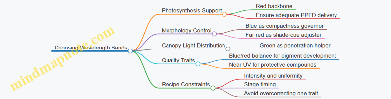
Plants use light for two broad purposes. The first is photosynthesis, which depends mainly on how much usable red and blue light reaches the leaves. The second is signaling, where specific wavelengths influence morphology and quality traits through photoreceptors. If you treat every band as “just more light,” you’ll often get tall plants, odd color, or slow harvest timing—because the signaling side is being ignored.
A practical way to choose bands is to map your production goal to one or more plant jobs:
- Biomass and photosynthesis: prioritize red-dominant energy with enough blue to keep structure compact.
- Compactness and leaf form: use blue as a structural governor.
- Color development: adjust blue and red balance, and include wavelengths that support pigment formation when needed.
- Harvest speed and uniformity: use stage-appropriate spectra and keep daily light delivery consistent.
The Main Wavelength Bands and Their Roles
Blue (roughly 400–500 nm) Blue light strongly affects leaf thickness, stomatal behavior, and stem elongation. In recipes, it often acts like a “shape control knob.” Too little blue can lead to stretching and softer canopy structure; too much can slow expansion if intensity is not managed.
Green (roughly 500–600 nm) Green is less efficient per photon for photosynthesis than red, but it can improve canopy penetration and visual uniformity. In practice, green is usually a supporting band: enough to smooth light distribution through layered canopies, not a replacement for red energy.
Red (roughly 600–700 nm) Red is the workhorse for photosynthesis and biomass accumulation. It also interacts with plant signaling pathways that influence growth rate and allocation. Most indoor recipes begin with a red backbone, then add blue and other bands to correct morphology and quality.
Far Red (roughly 700–750 nm) Far red affects the red-to-far-red ratio, which plants interpret as a cue about shading. In recipes, far red is a “timing and architecture” tool. It can increase leaf expansion and alter internode behavior, but it can also reduce compactness if overused.
Near Ultraviolet (roughly 380–400 nm) Near UV can influence protective compounds and surface traits. It is typically used sparingly because it can be harder to dose evenly and may increase stress responses if intensity is not carefully controlled.
Mind Map: Band Roles to Production Targets
Turn Roles into Band Selection Rules
Rule 1: Pick one primary band for energy, then add correction bands. For most leafy crops, red is the primary energy band. Blue is the most common correction band for structure.
Rule 2: Use far red only when you have a specific morphology or timing reason. If your plants are already compact and uniform, far red often adds complexity without clear benefit.
Rule 3: Treat green as distribution support, not the main driver. If canopy penetration is poor, green can help, but it should not replace red energy.
Rule 4: Use near UV as a targeted supplement, not a default. Start with low fractions and verify leaf response with simple visual and growth measurements.
Rule 5: Keep intensity and daily light integral stable while you change spectrum. Otherwise you can’t tell whether a change came from wavelength or from total delivered energy.
Example: Two Band Sets for the Same Crop Goal
Example 1: Compact Leafy Greens
- Red: primary energy
- Blue: structural correction
- Optional green: small fraction if the canopy is dense
- Far red: minimal or none during early establishment
Reasoning: you’re prioritizing photosynthesis while preventing elongation. If plants stretch, increase blue fraction before adding far red.
Example 2: Faster Canopy Closure
- Red: primary energy
- Blue: enough to keep form
- Far red: moderate during the phase when you want quicker canopy expansion
- Green: optional for uniformity across tiers
Reasoning: far red is used to influence architecture cues, but blue remains present so the canopy closes without turning into a tall, loose structure.
A Simple Checklist Before You Commit
- What is your dominant goal: biomass, compactness, color, or harvest speed?
- Which band will supply most of the photosynthetic energy?
- Which band will correct morphology without destabilizing growth?
- Are you changing spectrum while holding intensity and photoperiod constant?
- Do you have a measurement plan: height, leaf area, color score, and harvest timing?
When you choose wavelength bands this way, the recipe stops being a list of colors and becomes a set of controlled plant instructions—each band doing a specific job, at a dose you can justify.
3.2 Designing Spectral Combinations with Practical Constraints
Spectral recipes sound like they should be purely scientific, but indoor farming is mostly engineering with plants attached. “Designing combinations” means choosing wavelengths and proportions that hit your crop targets while respecting what your fixtures, power budget, and measurement setup can actually deliver.
Start with Your Constraints, Not Your Wish List
Before touching any spectrum, list the constraints that will shape the final recipe:
- Fixture channel limits: Many LEDs come as discrete channels (e.g., 450 nm, 660 nm, 730 nm). You can’t dial in arbitrary wavelengths.
- Power and thermal limits: Higher total intensity can force dimming on some channels to stay within driver limits.
- Optical mixing and uniformity: Some fixtures mix poorly, so the same channel setting yields different spectra across the bench.
- Measurement reality: Your spectrometer may have limited resolution or calibration accuracy, so you should avoid overfitting tiny spectral differences.
- Crop stage boundaries: Seedlings and mature plants often require different blue fractions and far-red handling.
A practical recipe design treats these as hard edges. If you ignore them, you’ll end up with a spectrum that looks right on paper and behaves differently in the room.
Translate Crop Goals into Band Roles
A helpful way to design is to assign each wavelength band a job. You don’t need a perfect biological model; you need consistent functional intent.
- Blue (around 430–470 nm): Often used to influence morphology and leaf thickness. In practice, it also helps you avoid overly stretched growth when red is dominant.
- Red (around 620–680 nm): The workhorse for photosynthesis and biomass accumulation.
- Far-red (around 700–740 nm): Used carefully to affect shade-avoidance signaling and canopy architecture.
- Green (around 500–570 nm): Sometimes added for perceived balance and penetration effects, but it’s frequently constrained by fixture availability.
- White (broadband): Useful when you need a stable baseline spectrum and consistent output across channels.
Once roles are set, the design becomes a constrained optimization problem: meet your target intensity and DLI, keep morphology within bounds, and maintain acceptable color and uniformity.
Use a Two-Layer Recipe: Baseline Plus Adjustments
A robust approach is to build a baseline spectrum that reliably supports photosynthesis, then add small adjustments for quality.
- Baseline layer: Choose a red-dominant mix that your fixture can deliver stably at the required PPFD.
- Adjustment layer: Add blue and far-red in controlled increments to steer morphology and canopy behavior.
This structure prevents “chasing” quality outcomes by changing everything at once. If you change red, blue, and far-red simultaneously, you can’t tell which lever mattered.
Practical Constraints as Design Rules
Use these rules to keep the recipe feasible:
- Rule 1: Keep total PPFD on target first. If PPFD is off, spectral comparisons are meaningless.
- Rule 2: Limit far-red changes to small steps. Far-red can strongly shift morphology, so large jumps often create unwanted stretch or uneven canopy.
- Rule 3: Treat blue as a fraction, not a vibe. Decide a starting blue fraction relative to red or relative to total photon flux, then adjust in increments.
- Rule 4: Avoid “channel starvation.” If one channel hits its driver ceiling, the recipe may clip and distort your intended proportions.
- Rule 5: Check spatial uniformity after spectrum changes. Some channels scatter differently; a spectrum that’s uniform in one setting may not be uniform in another.
Mind Map: Spectral Combination Design with Constraints
Example: Two Feasible Spectral Combinations for Leafy Greens
Assume you need a target PPFD of 250 µmol/m²/s at canopy height and you have channels at 450 nm, 660 nm, and 730 nm.
Example A: Compact Growth Baseline
- Start with a red-dominant baseline to hit PPFD.
- Add a modest blue fraction to reduce stretch.
- Keep far-red low to avoid excessive shade-avoidance.
A typical starting proportion might be:
- 660 nm: 85% of photon flux
- 450 nm: 12%
- 730 nm: 3%
If your fixture clips the 450 nm channel at high output, you reduce the total PPFD slightly during tuning or lower the blue fraction and compensate with a small increase in red while staying on PPFD.
Example B: Faster Canopy Closure Without Overstretch
- Keep red dominant.
- Increase far-red slightly to encourage canopy behavior that closes gaps.
- Reduce blue slightly if the plants become too compact and slow to expand.
A feasible starting proportion might be:
- 660 nm: 80%
- 450 nm: 10%
- 730 nm: 10%
Then you validate spatial uniformity: if 730 nm mixes unevenly, you may see patchy morphology even when the average spectrum matches.
Example: How to Iterate Without Confusing Yourself
When you test Example A vs. Example B, change only one lever at a time after the first comparison. For instance:
- If stretch increases, reduce far-red first.
- If leaves look pale or thin, increase blue fraction slightly.
- If yield drops while morphology improves, revisit PPFD calibration and channel clipping.
That disciplined iteration is what turns “spectral design” into a recipe you can reproduce across batches and rooms.
3.3 Managing Intensity Dimming and Output Stability
Intensity dimming is the practical bridge between a spectral recipe and what plants actually receive. A recipe that looks perfect on paper can still underperform if the LED output drifts, if dimming changes the spectrum, or if the facility’s control system introduces uneven timing. This section treats dimming as a measurable process: set a target, verify it, and keep it stable across time and space.
Foundational Concepts for Dimming Control
Start with two ideas: (1) dimming changes delivered photon flux, and (2) dimming can change spectral shape. Many LED systems dim by reducing current, which usually lowers intensity while keeping the spectrum close to the original. Some systems dim by altering drive behavior per channel, which can shift relative intensities between wavelengths. That matters because a “blue fraction” that was correct at full output may not stay correct at low output.
A useful way to think about intensity is to separate the recipe target from the control target. The recipe target is the canopy-level PPFD (or DLI) you want. The control target is the fixture setting you apply to reach that PPFD. The gap between them is where uniformity errors, sensor placement, and drift live.
Output Stability: What Can Go Wrong
Output stability issues typically fall into four buckets.
-
Thermal effects: LED efficacy and output can change as temperature rises. If your dimming schedule runs hotter at higher settings, the same “setting number” may yield different PPFD later in the day.
-
Driver behavior: Some drivers regulate current differently at low duty cycles, which can cause non-linear dimming. Two fixtures set to the same percentage may not deliver the same PPFD.
-
Aging and contamination: Over time, LEDs can lose output and optics can collect dust. This changes the mapping from fixture setting to delivered photons.
-
Channel imbalance: Multi-channel fixtures can drift differently per wavelength. Even if total PPFD is correct, the spectrum fraction can drift, affecting morphology and color.
A Systematic Workflow for Stable Dimming
Step 1: Define the measurement point. Choose a consistent measurement plane, such as canopy height or a fixed bench grid height. If you measure at fixture level, you’ll miss how plants and airflow change the effective distribution.
Step 2: Calibrate the mapping from setting to PPFD. For each fixture and each dimming channel group, measure PPFD at several output levels (for example 25%, 50%, 75%, 100%). Record the relationship between the control setting and measured PPFD. If the relationship is non-linear, use a correction curve rather than assuming linearity.
Step 3: Verify spectral stability at dimming points. At the same output levels, measure relative spectral output for the key channels. You don’t need a full spectral scan every minute, but you do need periodic checks that the blue-to-red ratio stays within your tolerance.
Step 4: Lock the control strategy. Use closed-loop control only if you can measure reliably and quickly. Otherwise, use open-loop control with scheduled verification. In either case, avoid changing multiple variables at once (for example, don’t adjust both dimming and photoperiod while troubleshooting).
Step 5: Manage timing and ramping. Sudden changes can cause transient behavior in drivers and temperature. A short ramp (seconds to a few minutes) can reduce overshoot and make measurements repeatable. Keep ramp profiles consistent between batches.
Practical Examples That Make It Concrete
Example: Keeping PPFD on target during a production day. Suppose your recipe calls for 250 µmol/m²/s at canopy level. You set the fixture to 60% output based on a prior calibration. After a few weeks, you notice the measured PPFD is 235 µmol/m²/s at the same canopy height. Rather than raising the setting blindly, re-measure PPFD at 60%, 70%, and 80% and update the mapping. This isolates drift from other variables.
Example: Preventing spectrum fraction drift at low output. A leafy greens recipe uses a specific blue fraction to control compactness. At high output, the blue fraction matches the target. At low output, the blue channel may dim more aggressively than red, shifting the ratio. The fix is to adjust channel-level dimming independently so that the measured spectral fractions remain within tolerance at the operating point.
Example: Uniformity across a bench. If the center of a bench receives 250 µmol/m²/s but the edges receive 220, plants at the edges will mature differently even if the recipe is “correct.” Use a grid measurement to compute correction factors per zone, then apply zone-level dimming offsets so the canopy PPFD distribution matches the recipe.
Mind Map: Dimming and Stability Checklist
Advanced Details Without the Headaches
When you update a dimming mapping, keep the recipe logic intact: the recipe should still specify canopy targets, not fixture percentages. Store both the recipe target and the current calibration parameters so you can reproduce past batches. If you use zone corrections for uniformity, document the zone geometry and measurement grid so the same “edge” remains the same location after any physical adjustments.
Finally, treat dimming stability as a system property, not a single number. A stable system delivers consistent PPFD and consistent spectral fractions at the same canopy plane, with predictable uniformity, even when the facility temperature and operating schedule vary within normal bounds.
3.4 Controlling Photoperiod and Daily Light Integral
Photoperiod and Daily Light Integral (DLI) are the two knobs most growers turn to control how much light plants receive over time. Photoperiod is the length of the light day; DLI is the total light energy delivered per day, usually expressed as mol·m⁻²·day⁻¹. A recipe can keep photoperiod constant while changing DLI, or keep DLI constant while shifting photoperiod and intensity. The plant usually cares about both the total and the timing, so it helps to treat them as a pair rather than separate chores.
Foundational Relationships Between Time and Light
Start with the practical conversion: DLI depends on average PPFD and the number of light hours.
- If PPFD is steady, then DLI ≈ PPFD (µmol·m⁻²·s⁻¹) × seconds of light per day ÷ 1,000,000.
- Example: 200 µmol·m⁻²·s⁻¹ for 16 hours gives DLI ≈ 200 × (16×3600) / 1,000,000 ≈ 11.5 mol·m⁻²·day⁻¹.
This means you can reach the same DLI with different combinations. For instance, 11.5 mol·m⁻²·day⁻¹ can be achieved with 200 µmol·m⁻²·s⁻¹ for 16 hours or 300 µmol·m⁻²·s⁻¹ for about 10.7 hours. Plants may respond differently because timing affects circadian signaling and stomatal behavior, even when the daily total matches.
Photoperiod as a Growth Signal
Photoperiod influences developmental timing and morphology through the plant’s internal clock. In leafy crops, the effect often shows up as changes in compactness and leaf expansion rate, especially when photoperiod is pushed shorter or longer than typical.
A useful rule of thumb for recipe design is: keep photoperiod within a crop-appropriate range, then use intensity to fine-tune DLI. If you must change photoperiod, do it gradually and watch for changes in leaf thickness, canopy uniformity, and the time to harvest.
DLI as the Daily Budget
DLI is the “money spent per day” on photosynthesis. When DLI is too low, plants typically show slower growth and lighter biomass. When DLI is too high for the crop stage or environment, you may see stress symptoms such as leaf edge burn, increased respiration costs, or reduced quality.
Quality is not only about total growth. For example, if you raise DLI by extending photoperiod, you may also increase the time plants spend under the same spectral conditions, which can shift pigment development and flavor-related compounds. That’s why photoperiod changes should be paired with a check of the rest of the recipe, not treated as a standalone adjustment.
Systematic Recipe Workflow
- Choose a target DLI for the growth stage and desired harvest speed.
- Select a photoperiod that fits facility scheduling and supports stable daily rhythms.
- Compute the required average PPFD from the DLI target.
- Verify uniformity at canopy height, because DLI is only as accurate as your PPFD map.
- Run a short calibration window with logging to confirm that the delivered DLI matches the plan.
If your facility uses dimming or multiple LED channels, calculate DLI using the expected PPFD at each channel setting, then confirm with a spectrally appropriate PPFD measurement method.
Mind Map: Photoperiod and DLI Control
Example: Matching DLI While Changing Photoperiod
Suppose you want to keep DLI at about 12 mol·m⁻²·day⁻¹ for a leafy green stage, but you need to shorten the light window due to labor or cooling constraints.
- Plan A: 200 µmol·m⁻²·s⁻¹ for 16 hours → ~11.5 mol·m⁻²·day⁻¹.
- Plan B: 300 µmol·m⁻²·s⁻¹ for 10.7 hours → ~11.5 mol·m⁻²·day⁻¹.
After switching, compare leaf expansion rate and canopy uniformity at the same calendar day. If plants become taller or less uniform under the shorter photoperiod, you likely need to adjust photoperiod back toward the original range and instead fine-tune DLI with intensity.
Example: Using Photoperiod to Stabilize Daily Operations
If your facility has a consistent temperature pattern, you can align the light period with the more stable part of the day. For instance, if cooling is strongest during the latter half of the light window, you may place the higher-intensity portion of the schedule there. Even when the total DLI stays the same, this can reduce heat-related quality issues because stomata and transpiration respond to both light and temperature together.
Troubleshooting with Measurable Checks
When results don’t match the recipe, start with the simplest checks:
- Delivered DLI mismatch: confirm PPFD at canopy height during the actual light window, not just at setup.
- Uniformity problems: if some zones receive less PPFD, the average DLI can look correct while growth becomes uneven.
- Timing-control lag: verify that dimming transitions happen at the scheduled times; a few minutes per hour can add up.
A good recipe is one you can reproduce. Photoperiod and DLI are the levers, but measurement discipline is what keeps the lever pulls from turning into guesswork.
3.5 Using White and Narrowband Mixes for Consistent Coverage
Consistent coverage is less about having “more light” and more about keeping the spectrum and intensity stable across space and time. White LEDs help with baseline coverage because they already include a broad mix of wavelengths, while narrowband channels let you correct specific plant responses without rebuilding the whole spectrum from scratch.
Start with a simple mental model: every fixture channel contributes two things—total photon delivery (how much) and spectral shape (which wavelengths). Coverage problems usually come from either uneven photon delivery across the canopy or spectral drift between fixtures and dimming levels. White plus narrowband mixes address both by giving you a dependable baseline (white) and a controlled adjustment layer (narrowband).
Step 1: Choose a Baseline White That Behaves Predictably
Not all “white” is equal. For recipe work, you want a white source whose spectral output stays reasonably consistent when you dim it. A practical check is to measure spectrum at two dimming points (for example, 50% and 100%) and compare the relative shape, not just the total PPFD. If the blue fraction changes a lot with dimming, your “baseline” will quietly become a different recipe.
A good baseline white also reduces the number of narrowband channels you need. If your crop needs a modest blue fraction for morphology and a modest red fraction for biomass, white can carry most of that load, leaving narrowband for fine-tuning.
Step 2: Add Narrowband Channels as Corrections, Not Crutches
Treat narrowband LEDs like calibration knobs. Common correction targets include:
- Blue correction for compactness and leaf thickness. If plants stretch, increase blue fraction slightly rather than increasing total intensity.
- Far-red correction for canopy architecture and allocation. Use it sparingly because it can change morphology even when PPFD is unchanged.
- Green correction when you need better penetration or you observe uneven lower-canopy appearance. Keep it modest so you don’t disrupt overall balance.
A useful rule: change one spectral knob at a time while holding PPFD and photoperiod constant. That way, your measurements map to causes instead of becoming a guessing game.
Step 3: Control Uniformity with Geometry and Channel Strategy
Uniformity failures often look like “some plants are greener” or “some are taller,” but the root cause is usually spatial intensity variation. White channels typically spread light more smoothly because they’re often mounted as a broader-emission set. Narrowband channels can be more directional depending on optics.
To reduce spatial mismatch, drive channels with the same dimming control logic and verify uniformity at the canopy plane. Measure PPFD at a grid of points and compute the coefficient of variation. If uniformity is poor, fix mounting height, reflector choice, and diffuser use before you blame the spectrum.
Step 4: Use a Recipe Format That Separates Baseline and Corrections
Write recipes in two layers:
- Baseline layer: white channel settings that establish your target PPFD and general spectral shape.
- Correction layer: narrowband adjustments that shift morphology or color without changing the baseline PPFD.
This separation makes it easier to reproduce results when you swap fixtures or when a channel ages. You can keep the baseline stable and re-tune only the correction layer.
Mind Map: White Plus Narrowband Coverage Workflow
Example: Two-Stage Recipe for Leafy Greens
Goal: compact leafy greens with consistent color across the bench.
- Baseline: set white to reach the target PPFD at canopy (for example, a measured target DLI-equivalent schedule), and keep photoperiod constant.
- Correction: if plants stretch or petioles elongate, increase blue narrowband by a small increment while reducing white slightly to keep total PPFD unchanged.
- Uniformity check: if lower-canopy leaves look pale, add a small green correction and re-measure PPFD uniformity. If uniformity is already good, the issue is likely spectral balance rather than light quantity.
This example works because it preserves the total photon budget while adjusting the spectral signals that influence morphology and appearance.
Example: Far-Red Without Changing Harvest Timing
Goal: adjust canopy architecture without shifting overall growth rate.
- Keep white PPFD and photoperiod fixed.
- Add far-red narrowband in small steps.
- After each step, verify that canopy height and leaf spacing change, but that harvest timing metrics remain within your acceptance window.
If harvest speed changes, the far-red increment was too large or your PPFD drifted during dimming. Return to the recipe format: baseline first, then corrections with PPFD held constant.
Practical Checklist for Consistent Coverage
- Measure spectrum at two dimming points for the white baseline.
- Use a grid to confirm PPFD uniformity before spectral tweaks.
- Hold PPFD constant when changing narrowband corrections.
- Record baseline and correction settings separately.
- Re-verify after fixture swaps or maintenance so “consistent” stays consistent.
4. Controlling Morphology with Spectral and Intensity Strategies
4.1 Regulating Stem Elongation With Blue and Far Red Balance
Stem elongation is mostly a light-timing and light-quality story. Plants use the ratio of red to far red to estimate how crowded they are, then adjust internode length to either stay compact or reach for more light. Blue light adds a second control lever by influencing leaf and stem architecture through photoreceptors that affect cell expansion and overall growth pattern.
Core Idea: Blue Sets Restraint, Far Red Sets Stretch
A practical way to think about it:
- Blue light tends to reduce elongation by promoting compact morphology and tighter growth.
- Far red light tends to increase elongation by shifting the plant’s red-to-far-red perception toward “shade.”
In recipes, you rarely change only one channel. You typically keep red as the main photosynthetic backbone, then tune blue for structure and far red for the shade signal.
Foundational Measurements That Make Tuning Work
Before changing spectra, confirm you’re controlling the right variables.
- PPFD and DLI: If total light is drifting, elongation changes may be caused by energy shortage rather than spectrum.
- Canopy height and distance to fixtures: Elongation responds to local light quality; uneven coverage can create “micro-shade” pockets.
- Stage timing: Seedlings and young transplants react strongly to early internode cues. Late-stage changes may alter appearance without fixing the underlying structure.
A simple check: measure PPFD at multiple points across the tray and confirm it’s within your facility’s target uniformity range. If PPFD varies widely, spectrum tuning will look inconsistent even when it’s correct.
Mind Map: Blue and Far Red Control Pathways
Stepwise Tuning Method for Real Crops
Use a controlled sequence so you can attribute outcomes.
-
Lock PPFD and DLI Keep total PPFD steady for at least several days while you adjust only blue and far red. If you change intensity and spectrum together, you lose causal clarity.
-
Start with Blue Restraint Increase blue in small increments until you see internode length decrease without making plants look overly stiff or reducing leaf expansion. A common symptom of “too little blue” is a tall, narrow look with longer gaps between leaves.
-
Then Adjust Far Red for Shade Signal If plants still stretch, reduce far red fraction. If they are too compact and slow to establish, slightly increase far red while keeping blue steady. The goal is not to eliminate stretch entirely; it’s to match the crop’s desired architecture.
-
Confirm with Two Metrics Measure internode length and canopy height at the same time each day. Canopy height alone can mislead if leaf angle changes; internode length tells you whether the stem is actually elongating.
Example: Compact Lettuce Transplants
Assume you’re growing lettuce from plug to transplant. You want short internodes and a sturdy stem.
- Baseline: Red-dominant spectrum with moderate blue, minimal far red.
- If stretching appears: reduce far red first by a small step, then increase blue slightly if needed.
- If plants look squat and slow: keep blue at the current level and reduce the far red reduction (move it back toward baseline).
A practical observation: when far red is too high, plants often show longer internodes even if PPFD is correct. When blue is too low, you may see both elongation and a looser canopy structure.
Example: Basil Establishment Without Leggy Stems
Basil tends to show leggy growth when early internodes stretch.
- During early establishment: use a blue-forward restraint and keep far red low.
- After establishment: you can maintain the same blue level while fine-tuning far red to avoid stalling leaf expansion.
If you only increase blue late, you may not fully correct internode length already formed. That’s why the timing of the blue-to-far-red balance matters.
Advanced Details: How to Avoid “Correct Spectrum, Wrong Outcome”
- Watch for channel drift: LED channels can change output with heat and age. If blue output drops, elongation can return even when the recipe settings are unchanged.
- Account for geometry: Far red effects depend on how much far red reaches the stem region. If plants are taller than expected, they may experience different red-to-far-red ratios than your measurements assumed.
- Use consistent sampling: Measure internodes on the same leaf positions across trays. Random sampling can hide real differences.
Practical Recipe Adjustment Checklist
- PPFD stable across treatments
- Blue adjusted in small steps
- Far red adjusted after blue is set
- Internode length measured alongside canopy height
- Same timing and sampling method every batch
When you follow that order, blue and far red stop being mysterious knobs and become predictable tools for controlling stem elongation.
4.2 Managing Leaf Expansion and Canopy Architecture
Leaf expansion is where spectral recipes stop being “light settings” and start becoming structure. Canopy architecture—leaf angle, overlap, and spacing—determines how much of your delivered light actually reaches photosynthetic tissue, and how quickly plants reach a marketable size without turning into a tangled green mat.
Foundational Concepts for Canopy Formation
Plants expand leaves by balancing two needs: capturing enough light to build biomass, and avoiding excessive self-shading that wastes energy. In practice, canopy architecture is shaped by three interacting levers:
- Leaf expansion rate: how fast new leaf area is produced.
- Leaf posture: how wide leaves spread versus how much they stay upright.
- Canopy packing: how quickly neighboring leaves overlap.
Spectral inputs influence these levers through photoreceptors that respond to blue, red, and far-red. Intensity and photoperiod set the overall energy budget, while spectrum steers how that energy is allocated to leaf area versus stem elongation.
Spectrum-to-Structure Mechanisms You Can Use
Blue light tends to support compact growth by encouraging tighter leaf expansion and stronger stomatal regulation. A practical way to think about it: blue helps plants “spend” more of their development on leaf form rather than stretching.
Red light supports photosynthesis and biomass accumulation, which indirectly drives canopy expansion. If red dominates without enough blue, leaves may expand but the canopy can become too open or too stretched depending on intensity and far-red content.
Far-red light affects perceived neighbor signals by shifting the red-to-far-red ratio. More far-red generally increases the tendency toward elongation and can reduce the compactness you need for uniform canopy coverage.
A useful rule of thumb for recipe design is to treat far-red as a posture tool, not a yield tool. If your goal is leaf area and even coverage, far-red should be limited and stage-specific.
Designing for Leaf Expansion Without Self-Shading
Start with a target canopy outcome, not a wavelength list. For leafy greens, a common outcome is “fast, uniform leaf area with minimal overlap in the first half of the cycle.” For that, you want:
- Enough red to drive photosynthesis.
- Enough blue to keep posture compact.
- Minimal far-red to prevent stretch that delays lateral leaf spread.
Then match intensity to the canopy stage. Early on, plants have low leaf area, so they can tolerate higher PPFD without immediate self-shading. Later, as leaves expand, the same PPFD can cause uneven light distribution because upper leaves intercept more.
Mind Map: Leaf Expansion and Canopy Architecture
Practical Recipe Patterns for Canopy Control
Pattern A: Compact leaf expansion for leafy greens
- Use a red-dominant base for photosynthesis.
- Add a moderate blue fraction to keep leaves from stretching.
- Keep far-red low during the phase when lateral leaf spread matters most.
Example: If your seedlings look tall and the canopy opens too slowly, increase blue slightly and reduce far-red rather than lowering intensity. Lowering intensity can slow everything, including leaf area.
Pattern B: Faster canopy closure for microgreens
- Use red to drive rapid leaf area.
- Keep blue present but not excessive, so leaves can expand quickly.
- Use minimal far-red to avoid elongation that creates a “leggy” look.
Example: If microgreens are reaching height but not filling the tray evenly, the issue is often posture and overlap timing. Reduce far-red first, then fine-tune blue.
Advanced Details That Matter in Real Benches
1) Uniformity beats perfection. If one zone receives more red or less blue than another, canopy architecture becomes uneven even when the average spectrum looks correct. Measure at multiple heights and positions, then adjust fixture spacing or diffuser settings before changing recipe targets.
2) Stage transitions should be gradual in effect. A sudden far-red change can shift posture quickly, but leaf expansion may lag. Instead of flipping channels abruptly, plan a transition window aligned with observable canopy traits like leaf angle and overlap.
3) Watch the overlap, not just the height. Two crops can have the same height but different canopy density. Track a simple metric: the fraction of leaves that touch neighboring leaves at a fixed day or PPFD exposure. That tells you whether your spectrum is steering expansion appropriately.
Quick Diagnostic Checklist for Canopy Problems
- Tall, narrow canopy: reduce far-red; increase blue fraction slightly.
- Slow lateral spread: increase red contribution modestly; confirm intensity is not limiting.
- Uneven coverage across the bench: verify spectral uniformity and fixture alignment before changing spectrum.
- Early self-shading: reduce intensity later in the cycle; keep blue adequate to maintain posture.
Case-Style Example: Fixing a Leggy Leafy-Green Batch
A batch reaches harvest size late and shows uneven leaf overlap. Height is acceptable, but the canopy is open, so lower leaves receive less light and develop slower.
- First adjustment: lower far-red during the expansion phase to reduce elongation pressure.
- Second adjustment: slightly increase blue to encourage broader, more compact leaf posture.
- Third adjustment: keep red steady so photosynthesis remains consistent.
After the change, the crop closes the canopy earlier, and the lower leaves catch up because the architecture improves light penetration. The key is that the fix targets structure (posture and overlap timing), not just total light.
4.3 Using Red to Support Biomass While Avoiding Stretch
Red light is the workhorse for photosynthesis, but it can also encourage plants to “reach” if the rest of the recipe is too permissive. The goal is simple: use red to build mass while keeping internodes compact and leaves properly layered.
Foundational Logic for Red and Stretch Control
Plants interpret light through multiple signals, not just total brightness. Two practical ideas guide recipe design:
- Red supports carbon gain. More usable photosynthetic photons generally mean more biomass potential.
- Red balance affects morphology. When plants perceive a light environment that resembles shade, they often elongate. In practice, this perception is influenced by the ratio of red to far-red and by how much blue is present.
A useful mental model is “biomass vs. posture.” Red helps biomass; blue and far-red balance help posture.
Mind Map: Red Role in Biomass and Morphology
Stepwise Recipe Strategy
Step 1: Set a Blue Baseline for Structure
Blue light is the main “keep it compact” lever in most indoor recipes. Start by choosing a blue fraction that prevents internode runaway under your facility’s typical intensity.
Example: For leafy greens at vegetative stage, begin with a recipe where red is dominant but blue is not negligible. If your current plants are stretching, increase blue fraction before reducing red.
Step 2: Use Red as the Biomass Engine, Not the Only Engine
Red can be increased to raise biomass, but it should be paired with structural support. If you push red too high while blue is low, you may get more growth that is also more stretched.
Example: Suppose two benches receive the same daily light integral (DLI). Bench A uses higher red and very low blue; Bench B uses slightly less red but maintains a consistent blue baseline. If Bench A shows longer stems and looser leaf spacing, the extra red helped carbon gain but the morphology signals were missing.
Step 3: Manage Far-Red with Intent
Far-red often nudges plants toward shade-like morphology. The key is not “far-red is bad,” but “far-red is a dial.” Use it when you need subtle canopy responses, and keep it limited when compactness matters.
Example: If you add far-red to encourage faster canopy closure, do it gradually and watch internode length. If internodes lengthen faster than leaf area increases, reduce far-red or raise blue slightly.
Step 4: Align Intensity and Timing to Stage
Stretch risk rises when plants receive high energy without the structural spectrum balance they need. Also, the same spectrum can behave differently at different growth stages.
Example: Seedlings often need stronger structural cues than mature plants. If you apply a “high-red biomass” recipe from day one, you may see early stretching that later cannot be fully corrected.
Practical Bench Examples
Example: Compact Lettuce for Faster Turnover
- Target: Short internodes, dense leaf rosette
- Approach: Keep red dominant for biomass, maintain a steady blue fraction, and use minimal far-red.
- What to measure: internode length at mid-cycle, leaf angle, and uniformity across the bench.
If internodes are too long, adjust in this order: blue up slightly → far-red down slightly → red down slightly.
Example: Higher Biomass Spinach Without Loose Growth
- Target: More dry matter while preserving tight canopy
- Approach: Increase red within a range that your blue baseline can “hold.” Keep far-red low-to-moderate.
- What to measure: fresh mass, dry mass ratio, and canopy thickness.
If biomass rises but canopy becomes airy, reduce far-red first, then fine-tune blue.
Quick Troubleshooting Map
Integrated Takeaway
Use red to build biomass, but keep posture signals in place. A stable blue baseline prevents most stretch problems, and far-red should be treated as a controlled ingredient rather than a default add-on. When you adjust, change one lever at a time and verify with internode length and canopy structure, not just total growth.
4.4 Adjusting Spectra for Different Growth Stages
A spectral recipe is not a single “set it and forget it” spectrum. Plants change their light needs as they move from establishing roots and leaves to building structure and finally filling out harvest quality. The practical goal is to keep the spectrum aligned with the plant’s current job: early establishment, vegetative expansion, and finishing.
Stage Logic from Plant Tasks to Spectral Choices
Seedling and early establishment prioritize leaf formation and efficient use of available light. Too little blue can lead to weak, stretched growth; too much can slow expansion. A common starting point is a red-dominant base with a modest blue fraction, then adjust intensity and photoperiod once you see canopy behavior.
Vegetative growth shifts toward maximizing leaf area and stable morphology. Here, blue helps keep internodes short and leaves flatter, while red supports biomass accumulation. Far red becomes a tool for subtle morphology changes, but it should be used carefully because it can also encourage elongation.
Finishing aims at the specific market target: color depth, leaf thickness, flavor-related compounds, and harvest speed. Many crops respond to a slight spectral “nudge” near the end—often by adjusting blue proportion, red-to-far-red balance, or adding narrowband components—while keeping total daily light integral (DLI) consistent.
A Simple Stage-Adjustment Workflow
- Lock DLI first. Keep daily light integral steady across stages unless your experiment is explicitly about DLI. Spectrum changes are easier to interpret when energy input is controlled.
- Start with a baseline spectrum. Use a red-dominant mix with enough blue to prevent stretching.
- Change one spectral lever at a time. For example, adjust blue fraction while holding red intensity constant, or adjust far-red fraction while holding total red+far-red output constant.
- Observe morphology within days, not weeks. Leaf angle, stem length, and canopy uniformity react quickly to blue and far red balance.
- Confirm quality near the end. Color and texture often need a finishing window, so evaluate during the last third of the crop cycle.
Mind Map: Growth Stages to Spectral Levers
Example: Lettuce from Seedling to Harvest
Assume a typical leafy crop cycle where you want compact heads and consistent leaf color.
Seedling (Days 0–7): Use a red-dominant spectrum with a moderate blue fraction. Keep far red low to avoid early elongation. If you see tall, narrow seedlings, increase blue slightly (for example, raise the blue channel by a small step) while reducing red intensity only if DLI drifts.
Vegetative (Days 8–21): Maintain red dominance to support biomass. Increase blue modestly if internodes lengthen or leaves tilt upward. If the canopy becomes too dense and leaves overlap excessively, reduce blue slightly or increase airflow rather than changing spectrum again.
Finishing (Last 5–7 days): Keep DLI stable and adjust the red-to-far-red balance to control final stretch. If leaves look too elongated at harvest, reduce far red or increase the red-to-far-red ratio. If color looks pale, fine-tune blue upward slightly and verify that intensity hasn’t dropped.
Example: Basil for Compact Growth and Aroma-Linked Quality
Basil often benefits from a spectrum that discourages stem elongation while supporting leaf expansion.
Seedling: Use red with enough blue to keep plants squat. Avoid heavy far red; basil can respond with unwanted height.
Vegetative: Keep blue steady and let red carry most of the photosynthetic load. If plants become leggy, adjust blue first before changing total intensity.
Finishing: Apply a short finishing window by slightly increasing blue fraction and tightening the red-to-far-red ratio. Evaluate leaf thickness and uniformity at harvest; if leaves become too small, revert the finishing adjustment and focus on maintaining consistent DLI.
Practical Checks That Prevent Confusing Results
- Uniformity check: If one zone is dimmer, it can mimic a “spectral effect.” Confirm PPFD uniformity before interpreting morphology.
- Stage boundary check: Make sure stage transitions are defined by plant age or developmental cues, not by calendar alone.
- Observation timing: Record morphology daily during early and mid stages, then record color and texture during finishing.
Quick Reference: What to Adjust First
- Stretch appears early: adjust blue fraction first; then check red-to-far-red balance.
- Canopy is too open: increase blue slightly or reduce far red.
- Color is weak near harvest: adjust blue or red-to-far-red ratio during the finishing window while holding DLI steady.
- Yield drops after changes: confirm you didn’t accidentally change DLI or photoperiod while swapping spectra.
4.5 Practical Recipe Templates for Seedling to Vegetative Phases
Seedling-to-vegetative recipes are about two things: getting roots and leaves established without stretching, and then building steady biomass while keeping color and texture on target. The templates below assume you already know your facility’s baseline PPFD uniformity and can measure at canopy height. If you can’t, start with a conservative version and tighten later.
Mind Map: Seedling to Vegetative Recipe Logic
Seedling Phase Template 1 Compact Establishment
Use this when transplants arrive small, leggy, or uneven. Keep the recipe simple: red for energy, blue for structure, and only a small far-red presence.
- Days: 7–10
- Photoperiod: 16 hours
- Target DLI: 8–12 mol/m²/day
- Canopy PPFD: 200–300 µmol/m²/s (adjust to hit DLI)
- Spectrum mix (example channel targets):
- 70–80% red (around 660 nm)
- 15–25% blue (around 450 nm)
- 0–5% far red (around 730 nm)
- 0–10% green (optional, low)
Easy example: If your canopy PPFD reads 240 µmol/m²/s at lights-on height, run 16 hours. That typically lands near the lower end of the DLI range for many leafy crops. If seedlings stretch within 3–4 days, reduce PPFD by 10–15% before increasing blue.
Adjustment rule: Change one lever at a time. First tune intensity (PPFD), then fine-tune blue percentage.
Seedling Phase Template 2 Balanced Growth with Faster Leaf Initiation
Use this when seedlings are compact but slow to expand leaves.
- Days: 7–10
- Photoperiod: 16 hours
- Target DLI: 10–14 mol/m²/day
- Canopy PPFD: 260–360 µmol/m²/s
- Spectrum mix:
- 75–85% red
- 10–20% blue
- 0–8% far red
- 0–10% green
Easy example: For basil or compact herbs, this template often increases leaf count without causing dramatic height gain. If you see leaf edges curling or pale color, raise PPFD slightly rather than adding far red.
Vegetative Phase Template 1 Steady Biomass and Uniform Canopy
This is the workhorse recipe for consistent harvest timing and predictable texture.
- Days: 14–21 (crop dependent)
- Photoperiod: 14–16 hours
- Target DLI: 14–20 mol/m²/day
- Canopy PPFD: 300–500 µmol/m²/s
- Spectrum mix:
- 80–90% red
- 8–15% blue
- 0–10% far red
- 0–10% green
Easy example: For lettuce, start at the low end of PPFD on day 1 of vegetative, then ramp 5–10% every 3–4 days until you reach your target DLI. This reduces shock and keeps internodes short.
Vegetative Phase Template 2 Color-Forward Leaves Without Overstressing
Use this when you need stronger pigment expression for market appearance while avoiding harsh, thin growth.
- Days: 10–18
- Photoperiod: 14–16 hours
- Target DLI: 15–22 mol/m²/day
- Canopy PPFD: 320–520 µmol/m²/s
- Spectrum mix:
- 70–85% red
- 12–20% blue
- 0–6% far red
- 5–15% green (optional, helps penetration)
Easy example: For brassicas or specialty greens, increasing blue within this range can improve visible color while keeping leaves thicker than a high-intensity red-only approach.
Far Red Use Guidelines Across Phases
Far red is a tool for morphology and allocation, but it’s easy to overdo. Keep it low during seedling establishment, then only increase if you observe overly compact plants that fail to fill canopy.
- Seedling: 0–5% far red
- Vegetative: 0–10% far red
- If stretching appears: reduce far red first, then reduce PPFD.
Practical Weekly Recipe Workflow
- Measure at canopy height at the same time each day, ideally mid-photoperiod.
- Confirm DLI by checking PPFD and photoperiod rather than guessing.
- Check morphology once per week: internode length, leaf thickness, and uniformity.
- Check color at a fixed time after lights-on to avoid lighting-cycle bias.
- Adjust intensity before spectrum when plants are generally underperforming.
Mind Map: Template Selection and Adjustment
Example: One Integrated Recipe Path
- Days 0–9: Seedling Template 1 at ~240 µmol/m²/s, 16 hours, red-heavy with moderate blue.
- Days 10–24: Vegetative Template 1 ramping from ~320 to ~420 µmol/m²/s, 15 hours.
- Final 7–10 days: If color needs strengthening, switch to Vegetative Template 2 by increasing blue and slightly reducing far red, while keeping DLI within your target band.
This path keeps morphology controlled early, then shifts emphasis to canopy fill and final appearance without changing everything at once.
5. Flavor and Phytochemical Outcomes Through Spectral Control
5.1 Linking Light Spectrum to Secondary Metabolite Pathways
Secondary metabolites are the compounds plants use for defense, signaling, and stress management. In indoor farming, the spectrum matters because many of the enzymes that build these compounds are regulated by light-sensing pathways, not just by total energy. The practical goal is to connect wavelength choices to measurable outcomes like bitterness, aroma intensity, pigment formation, and antioxidant capacity.
From Photons to Gene Expression
Plants perceive light through photoreceptors that respond to specific wavelength ranges. Blue light is strongly linked to cryptochromes and phototropins, which influence stomatal behavior and developmental programs. Red and far-red light are strongly linked to phytochromes, which regulate shade-avoidance signaling and can shift resource allocation. When these receptors activate, they change transcription factors, which then alter enzyme production for secondary metabolism.
A useful way to think about it: spectrum changes the “instruction set” (gene expression and enzyme availability), while intensity and timing change how strongly and how long those instructions are followed. That’s why two recipes with the same daily light integral can still produce different flavor or color.
Pathway Logic for Common Indoor Targets
Different metabolites cluster into different pathway logics. Phenolics and flavonoids often rise when plants experience spectral cues that mimic stress or high light quality. Carotenoids and related pigments depend on both light-driven biosynthesis and the plant’s developmental stage. Terpenes and many aroma compounds are influenced by light-regulated growth patterns and stress signaling.
To keep this systematic, map your target to a pathway category, then map that category to likely spectral drivers:
- Flavonoids and phenolics: often respond to blue enrichment and red/far-red balance that changes perceived canopy density.
- Anthocyanins and red-purple pigments: frequently increase with spectral cues that activate protective pigment programs, often involving blue and red components.
- Carotenoid-derived compounds: depend on red-driven photosynthetic support plus developmental timing.
- Terpenes and aroma volatiles: track with growth rate, leaf morphology, and stress signaling that spectra can influence.
The Role of Light Quality Versus Light Quantity
Light quantity sets the carbon supply for secondary metabolism. Light quality sets the regulation. If you raise intensity without adjusting spectrum, you may increase biomass but not necessarily increase the specific compounds you care about. If you adjust spectrum without enough intensity, the plant may prioritize survival over synthesis, leading to weak or inconsistent metabolite expression.
A concrete example: suppose you want more anthocyanin in a leafy crop. Increasing red alone may support growth, but it can also produce a canopy that doesn’t trigger the protective pigment program. Adding a controlled blue fraction and adjusting red/far-red can shift signaling toward pigment accumulation without collapsing yield.
Timing and Developmental Stage
Secondary metabolism is not evenly distributed across development. Early stages often emphasize establishment and leaf formation, while later stages can shift toward protective compounds as leaves mature. Photoperiod and stage-specific spectrum changes can therefore produce different metabolite profiles even when the total daily light integral is identical.
A practical approach is to treat spectrum as a stage-specific “recipe parameter.” For example, you might use a spectrum that supports compact growth during establishment, then shift toward a spectrum that encourages protective phenolics during the final days before harvest.
Mind Map: Spectrum to Secondary Metabolite Outcomes
Example: Designing a Spectrum Shift for Phenolic Flavor
Imagine a batch of leafy greens where you want stronger “bite” without making leaves tough. Start by keeping intensity and daily light integral steady so carbon supply stays comparable. Then adjust spectrum quality in the final production window.
- Baseline: a red-dominant mix that maintains steady growth.
- Flavor push: add a modest blue fraction during the last days to encourage phenolic accumulation.
- Avoid stretch: keep far-red low enough to prevent excessive elongation that can dilute leaf thickness and change perceived texture.
- Check consistency: measure color and a simple sensory proxy like bitterness level on the same harvest day.
If bitterness rises but leaves become less tender, reduce the blue fraction or shorten the timing window. If color stays pale, increase blue slightly or adjust red/far-red to strengthen the protective signaling.
Practical Measurement Tie-In
Because secondary metabolites are not directly visible from spectrum alone, you need a feedback loop. Use at least one quality proxy that matches your target: pigment intensity for anthocyanins, a bitterness or astringency score for phenolics, and a simple aroma intensity check for terpene-linked compounds. When the proxy changes in the direction you want after a controlled spectrum adjustment, you’ve confirmed the pathway logic rather than just the growth response.
5.2 Designing Blue Enrichment for Taste and Aroma Compounds
Blue light influences more than leaf shape; it steers metabolic pathways that affect flavor precursors and volatile compounds. The practical goal is to add enough blue to shift chemistry without paying for it in slower growth or uneven canopy behavior. Think of blue enrichment as a controlled “nudge,” not a blanket.
Foundational Logic for Blue Enrichment
Start with what blue does reliably. Blue photons are strongly absorbed by photoreceptors such as cryptochromes and phototropins, which regulate gene expression tied to secondary metabolites. In many leafy crops, this shows up as changes in phenolic content, antioxidant capacity, and sometimes the balance of sulfur- and nitrogen-derived volatiles that contribute to aroma.
Next, connect spectrum to plant structure. Blue tends to reduce internode elongation and can increase leaf thickness or alter stomatal behavior. Those structural shifts change how light penetrates the canopy and how gases move, which then affects volatile release and perceived aroma intensity at harvest.
Finally, remember that “taste” is not one compound. It is a mix of sugars, organic acids, amino acids, and phenolics. Blue enrichment can influence several of these at once, so you need a recipe that targets the whole outcome: flavor compounds plus the growth conditions that support them.
Recipe Design Workflow
- Choose the base spectrum first. Use a red-dominant or red-white base that reliably drives photosynthesis. Then add blue as an enrichment channel.
- Set a starting blue fraction. For many leafy crops, begin with a modest blue share (commonly in the low single-digit percent range of total photon flux) and keep it consistent across the day.
- Lock the daily light integral. Keep PPFD and photoperiod stable while you adjust blue fraction. Otherwise, you will confuse “more light” effects with “more blue” effects.
- Stage the enrichment. Apply stronger blue during the period when leaves are forming flavor-relevant tissues, then taper toward harvest to avoid excessive stress.
- Measure aroma-relevant proxies. Use simple, repeatable checks: leaf thickness, fresh mass per area, and a basic phenolic proxy if you have it. For aroma, rely on sensory panels only after you have consistent growth metrics.
Mind Map: Blue Enrichment Pathways to Flavor
Practical Examples You Can Run
Example: Basil for stronger aroma without harshness
- Base: red-white mix sized to hit your target DLI.
- Blue enrichment: add a small, steady blue fraction during early vegetative growth.
- Taper: reduce blue slightly in the final days before harvest.
- Why it works: early blue supports leaf development and metabolite formation; tapering reduces the risk of overly dry, thick leaves that can read as bitter or sharp.
- What to watch: if leaves become too compact and growth slows, reduce blue fraction or shorten the enrichment window.
Example: Lettuce for balanced sweetness and reduced blandness
- Base: red-dominant spectrum for consistent biomass.
- Blue enrichment: apply moderate blue during the canopy expansion phase.
- Keep DLI constant: do not raise PPFD when adding blue.
- Why it works: blue can shift phenolic accumulation and influence sugar-acid balance. Constant DLI isolates the spectral effect.
- What to watch: if you see increased bitterness, lower blue fraction or taper earlier.
Advanced Details That Prevent Common Mistakes
Uniformity matters more than you think. If blue is uneven across the canopy, you create mixed microclimates. That often shows up as inconsistent aroma intensity across trays even when average PPFD looks correct.
Avoid “blue spikes” from dimming artifacts. When controllers change channel outputs, some fixtures can momentarily alter spectral ratios. Use smooth ramping and verify that the blue fraction stays stable over the photoperiod.
Separate spectrum effects from stress effects. Blue enrichment can be beneficial, but excessive blue combined with high intensity can push plants into a stress response that changes flavor in unpredictable ways. Keep intensity and DLI controlled, then adjust blue.
Use a two-variable trial. When optimizing, change only blue fraction and timing. Keep everything else fixed, including temperature and CO₂ if you control it. This makes your results interpretable.
Example: A Simple Blue Enrichment Trial Plan
Trial Goal: Improve aroma while keeping growth rate stable

Keep constant: DLI, photoperiod, temperature, spacing

Treatments
- T1: Base spectrum only
- T2: Base + low blue fraction during days 7–14
- T3: Base + medium blue fraction during days 7–14
- T4: Base + medium blue fraction during days 10–14

Measurements
- Leaf thickness and fresh mass per area at harvest
- Sensory panel score for aroma intensity and bitterness
- Uniformity check: PPFD and blue fraction across trays
Practical Recipe Output Format
When you write the final recipe, include three numbers and one rule: the blue fraction, the stage window, the taper amount near harvest, and the rule that DLI stays constant across trials. That single rule prevents most “why did it taste different?” confusion.
A good blue enrichment recipe is the one that produces consistent flavor outcomes across batches because the plant experienced the same spectral signal, not because the facility happened to run a little brighter that week.
5.3 Using Red and Green Components for Balanced Development
Red light is the workhorse for photosynthesis and biomass accumulation, while green light can shape canopy architecture and light distribution. The goal of a balanced red–green recipe is not to “add green for fun,” but to manage how much usable light reaches leaves at different depths and how the plant allocates growth.
Foundational Roles of Red and Green
Red photons strongly drive photosynthetic electron transport and support leaf and stem mass. In practice, this means red-rich recipes often increase fresh weight and shorten the time to a marketable size when other factors are controlled.
Green photons are absorbed less efficiently than red by chlorophyll, so they tend to penetrate deeper into canopies. That deeper reach can improve lower-leaf illumination without raising surface PPFD as much. The trade-off is that green can also reduce the “effective” photosynthetic contribution per unit of total light if you overdo it.
A useful way to think about the balance is to separate two targets: (1) total daily energy delivered to the canopy and (2) how that energy is distributed across leaf layers. Red mainly supports the first target; green mainly supports the second.
Designing a Red–Green Recipe Without Guesswork
Start with a baseline red-dominant spectrum that already meets your PPFD and DLI targets for the growth stage. Then add green in small increments while keeping total PPFD constant.
A practical starting point for leafy greens is to allocate green as a fraction of the photosynthetically active output rather than as a fixed percentage of LED count. For example, you might begin with a spectrum that is roughly 90% red (including deep red) and 10% green by relative photon contribution, then adjust based on canopy response.
Watch for two common outcomes:
- If plants look stretched or thin, your red support may be too low or your DLI too conservative. Increase red fraction or total PPFD.
- If lower leaves look healthier but upper leaves become too dense, reduce green slightly or lower total PPFD to prevent excess canopy shading.
Canopy Architecture and Light Distribution
Balanced development depends on how leaves stack. When the top layer captures most of the light, lower leaves operate at a disadvantage, which can reduce overall uniformity and slow harvest readiness.
Green’s deeper penetration can help lower leaves maintain photosynthetic activity. However, canopy density still matters. If you run a high-density crop with insufficient airflow or too much nitrogen, even a good spectrum won’t fully fix uneven performance.
To integrate spectrum with plant spacing, treat red–green tuning as a “distribution lever.” If your crop is spaced widely and receives uniform illumination already, you may need less green. If your crop is dense or has a tall canopy, green becomes more valuable.
Stage-Specific Adjustments
During early establishment, plants benefit from stable red support to build functional leaf area. Green can be added modestly to reduce the risk of lower-leaf underperformance, but keep the fraction conservative so you don’t dilute photosynthetic drive.
During vegetative growth, the canopy thickens and self-shading increases. This is where green often shows clearer benefits: improved lower-leaf color and more even leaf thickness across the tray.
A simple operational rule is to increase green fraction only after the canopy has enough leaf area to create meaningful depth gradients. If you add green too early, you may simply shift the balance without improving distribution.
Example Recipes for Leafy Greens
Example: Compact Lettuce for Uniform Harvest
- Baseline: red-dominant spectrum meeting your target DLI
- Add green: small increment (about one tenth of the photosynthetic contribution)
- Keep photoperiod constant for the batch
- Evaluate after one week by checking lower-leaf color and leaf thickness uniformity
If lower leaves lag, increase green slightly while holding PPFD steady. If upper leaves become overly dense or pale, reduce green or slightly lower total PPFD.
Example: Dense Canopy Spinach for Lower-Leaf Performance
- Baseline: red-dominant spectrum with enough red to maintain biomass
- Add green: higher fraction than lettuce because the canopy is thicker
- Use the same DLI but monitor uniformity across the tray
If you see overall growth slowing, your green fraction is likely too high for the delivered DLI. Reduce green and compensate with red or a small PPFD increase.
Mind Map: Red–Green Balance for Development
Practical Checkpoints for Balanced Results
Use a consistent evaluation method: compare upper and lower leaves from the same tray position across batches. If the spectrum is working, you should see improved lower-leaf performance without a noticeable penalty in overall growth rate. If you only see changes in one leaf layer, adjust the red–green ratio rather than changing everything at once.
5.4 Managing Stress-Responsive Signals Without Yield Loss
Plants treat light as both energy and information. Stress-responsive pathways can be triggered by spectral cues (like blue and far-red balance), by intensity and timing (like sudden increases or long low-light gaps), and by the plant’s own developmental stage. The trick is to use those signals to steer quality traits while keeping the plant’s carbon budget and growth machinery intact.
Foundational Idea: Stress Signals Need a “Reason to Spend”
Stress responses are not free. When a plant shifts resources toward protective chemistry, it often reduces growth rate or leaf expansion. Yield loss happens when the stress signal is strong enough, long enough, or mistimed relative to the plant’s developmental needs.
A practical way to think about it is to separate three layers:
- Signal: the spectral and timing pattern that activates pathways.
- Constraint: what limits the plant’s ability to respond, such as low DLI, low CO₂ availability, or nutrient imbalance.
- Outcome: the measured change in morphology, color, flavor compounds, and harvest timing.
If the constraint is tight, even a “small” signal can become costly. If constraints are loose, the same signal may produce quality changes with minimal yield penalty.
Step 1: Identify Which Stress Pathway You’re Likely Activating
Different spectral patterns tend to correlate with different physiological responses. You don’t need to guess perfectly; you need to choose a hypothesis and test it with small, controlled changes.
- Blue enrichment often increases stomatal opening and can raise stress-like signaling when combined with high intensity or abrupt transitions. In practice, it can improve compactness and some flavor-related compounds, but it can also slow leaf expansion if overdone.
- Far-red presence and red-to-far-red balance influence shade-avoidance behavior. Too much far-red, especially early, can push elongation and reduce usable leaf thickness.
- Timing stress comes from photoperiod interruptions, rapid ramping, or uneven daily light distribution. Plants notice “wrong timing” quickly, and that can reduce uniformity.
Step 2: Use “gentle stress” design rules
Gentle stress is not about being timid; it’s about controlling dose and timing.
- Start with stage-appropriate baselines: keep the core spectrum and DLI aligned with the growth stage first. Stress recipes are overlays, not replacements.
- Change one variable at a time: adjust only blue fraction, or only far-red fraction, or only timing. Otherwise you can’t tell what caused the outcome.
- Avoid abrupt transitions: ramp intensity or spectral channel changes over a short window (for example, 30–60 minutes) rather than switching instantly.
- Cap the “stress window”: if you apply a stress-inducing spectral ratio, limit it to a defined portion of the photoperiod rather than the entire day.
Step 3: Protect the Carbon Budget
Yield loss often comes from insufficient carbon gain, not from the stress signal itself.
- Maintain adequate DLI: if you reduce intensity to make room for a spectral overlay, you may accidentally starve photosynthesis.
- Keep temperature and VPD stable: stomatal behavior and transpiration interact with light-driven signaling. Large swings can turn a manageable signal into a growth limiter.
- Ensure nutrient availability: nitrogen and potassium shortages can make plants more reactive to light cues, increasing the chance that “quality steering” becomes “growth suppression.”
Step 4: Measure the Right Indicators Early
Quality traits and yield traits respond on different clocks. Use early indicators to decide whether to back off.
- Morphology: leaf expansion rate, internode length, and canopy closure speed.
- Color trajectory: not just final color, but how quickly pigment levels reach market targets.
- Harvest timing: days to first harvestable leaves, plus uniformity across the tray.
If morphology slows while color improves, you may be trading yield for appearance. If both slow, you likely pushed the signal too hard or created a constraint.
Mind Map: Stress-Responsive Control Loop
Example: Blue Overlay for Compact Leafy Greens
Baseline: a red-forward spectrum with enough blue to support normal leaf development, delivering the target DLI for the stage.
Stress overlay: increase blue fraction only during the middle third of the photoperiod. Keep intensity the same as baseline and ramp the blue channel up over 45 minutes.
Decision rule: if leaf expansion rate drops noticeably compared with the baseline within the first week, reduce the blue overlay duration by half rather than lowering DLI.
Why this works: blue signaling is present, but the plant still gets consistent carbon gain during the rest of the day. The “middle third only” approach reduces the chance that blue becomes a constant growth limiter.
Example: Far-Red Restraint to Avoid Shade-Avoidance Yield Loss
Baseline: red and blue support compactness and photosynthesis.
Stress overlay: introduce far-red only briefly near the end of the photoperiod, keeping red-to-far-red close to baseline during the main growth window.
Decision rule: if internode length increases or leaf thickness decreases, shorten the far-red window first. If the issue persists, reduce far-red fraction next.
Why this works: shade-avoidance behavior is sensitive to perceived light quality over time. Limiting far-red exposure reduces the behavioral push while still allowing some spectral influence.
Example: Timing Correction After a Uniformity Problem
Symptom: some trays show slower canopy closure and uneven color.
Action: keep the spectrum constant, but smooth the daily ramp and eliminate photoperiod interruptions. Verify that all fixtures deliver the same daily pattern, not just the same total DLI.
Decision rule: if uniformity improves without changing spectral ratios, the “stress” was timing-related rather than spectrum-related.
Back-Off Rules That Prevent Yield Loss
When you see growth suppression, respond in the order that preserves carbon gain:
- Reduce stress window duration.
- Reduce stress fraction (blue or far-red) while keeping DLI constant.
- Only then adjust overall intensity or photoperiod.
This order matters because yield loss is most likely when photosynthesis is constrained. By protecting DLI first, you keep the plant’s response within a range where quality changes can occur without turning into a growth penalty.
5.5 Recipe Examples for Leafy Greens and Culinary Herbs
Leafy greens and culinary herbs are a great place to practice spectral “recipes” because their quality targets are visible quickly: leaf color, thickness, aroma intensity, and how fast you can harvest without sacrificing uniformity. The core idea is to treat spectrum as a set of levers that steer morphology and metabolism, then lock the lever positions to a measurable daily light integral (DLI) and a consistent photoperiod.
Foundational Recipe Targets
Start with two baseline targets you can reuse across crops.
- DLI target: choose a DLI that matches your harvest window and facility limits. For many leafy greens, a common working range is 12–18 mol·m⁻²·d⁻¹.
- Photoperiod target: keep it stable during a batch. A practical starting point is 14–16 hours; if you shorten the day, you must compensate with intensity to keep DLI steady.
Then add spectrum levers:
- Blue fraction influences compactness and leaf thickness.
- Red fraction drives biomass and photosynthetic efficiency.
- Far-red fraction can shift morphology and canopy dynamics, but it also changes how quickly plants “spend” their resources.
- Green fraction can improve perceived uniformity and canopy penetration, but it should not replace red as the main energy source.
Mind Map: Recipe Logic for Leafy Greens and Herbs
Example Recipe 1: Butterhead Lettuce for Compact Heads
Goal: compact rosette, good leaf color, harvest in a predictable window.
-
Stage 1: Establishment (days 1–7)
- Spectrum: Red-dominant with moderate blue.
- Practical starting mix: 70% red, 20% blue, 10% green.
- Timing: 16 hours.
- Intensity: set to hit your chosen DLI (e.g., ~14–16 mol·m⁻²·d⁻¹).
-
Stage 2: Vegetative Growth (days 8–21)
- Spectrum shift: slightly reduce blue to avoid overly thick, slow leaves.
- Practical starting mix: 75% red, 15% blue, 10% green.
- Timing: 15–16 hours.
-
Pre-harvest Finishing (last 3–4 days)
- Add a small far-red component only if you see canopy flattening or slow expansion.
- Practical starting mix: 72% red, 14% blue, 8% green, 6% far-red.
Easy-to-understand check: if plants look tall and loose, increase blue by a few percentage points or reduce far-red. If leaves are pale, raise DLI by increasing intensity while keeping photoperiod unchanged.
Example Recipe 2: Spinach for Thick Leaves and Fast Turnover
Goal: thick texture without sacrificing speed.
-
Stage 1: Establishment (days 1–5)
- Spectrum: higher blue to build structure early.
- Mix: 65% red, 25% blue, 10% green.
- Timing: 16 hours.
-
Stage 2: Growth (days 6–18)
- Spectrum: shift toward red for biomass.
- Mix: 78% red, 15% blue, 7% green.
- Timing: 15 hours.
-
Pre-harvest (last 2–3 days)
- Keep spectrum stable; adjust only intensity if needed.
- If leaves are too thin, raise DLI slightly rather than adding far-red.
Easy-to-understand check: spinach that’s thin usually needs more total light or more early blue, not a far-red boost.
Example Recipe 3: Basil for Aroma and Compact Canopies
Goal: compact growth with strong aroma, which often correlates with healthy leaf development and consistent light exposure.
-
Stage 1: Establishment (days 1–10)
- Mix: 60% red, 30% blue, 10% green.
- Timing: 16 hours.
-
Stage 2: Vegetative Growth (days 11–28)
- Mix: 70% red, 20% blue, 10% green.
- Timing: 14–15 hours.
-
Optional Finishing (last 3–5 days)
- If aroma seems muted and leaves are overly soft, add a small blue bump.
- Mix: 68% red, 24% blue, 8% green.
Easy-to-understand check: if basil stretches, blue is your first lever. If it looks stressed or slow, reduce blue slightly and keep DLI steady.
Example Recipe 4: Microgreens for Uniform Color and Quick Harvest
Goal: fast harvest with consistent appearance across trays.
- Spectrum: prioritize red and blue balance; keep far-red minimal.
- Mix: 80% red, 18% blue, 2% green.
- Timing: 14–16 hours depending on your DLI target.
- Intensity: set for the DLI that matches your harvest day.
Easy-to-understand check: if microgreens are uneven, the issue is often uniformity of PPFD across the tray rather than spectrum. Fix zoning and mounting first, then fine-tune blue.
Practical Adjustment Rules
When results don’t match expectations, change one lever at a time:
- Stretch or loose structure: increase blue fraction or reduce far-red.
- Pale color: increase red fraction or total DLI.
- Slow growth: raise intensity while keeping photoperiod constant.
- Too thick or slow: reduce blue slightly and keep DLI unchanged.
These recipes work best when you treat them as starting points tied to your facility’s measured PPFD and spectrum, not as fixed percentages carved in stone.
6. Color Development and Pigment Management
6.1 Chlorophyll and Carotenoid Formation with Spectral Inputs
Chlorophyll and carotenoids are not just “green pigments.” They are part of the plant’s light-harvesting and protection machinery, so their amounts and ratios respond to both wavelength and how much light the plant actually receives. A useful way to think about spectral recipes is: wavelength steers which photoreceptors and photosystems dominate, while intensity and timing decide how hard the machinery is working.
Foundational Pathways and What Spectra Influence
Chlorophyll formation depends on building blocks and enzymes that operate during active growth. Light is required for normal chloroplast development, and the balance between chlorophyll production and degradation shifts with light stress. Carotenoids are produced alongside chlorophyll-related development but also expand when plants need extra photoprotection.
A practical mapping looks like this:
- Blue light tends to support compact, functional chloroplast development and can increase chlorophyll accumulation when plants are otherwise light-limited.
- Red light drives photosynthesis efficiently and supports chlorophyll maintenance, especially when plants have enough total daily light.
- Green light penetrates deeper into canopies and can influence within-canopy distribution of photosynthetic activity, which indirectly affects pigment balance.
- Carotenoid emphasis often rises when plants experience higher light stress or when blue/red balance changes the excitation pressure on photosystems.
How Chlorophyll Changes Under Real Indoor Conditions
Chlorophyll content usually tracks with two things: how much photosynthetic capacity the plant can build and whether it is being forced to dissipate excess energy. If your recipe raises PPFD without adjusting spectrum or photoperiod, you may see chlorophyll plateau while carotenoids climb—an indicator that protection is being prioritized.
A concrete example: imagine two lettuce batches at the same DLI.
- Batch A uses a red-heavy spectrum with modest blue.
- Batch B uses a more balanced red plus blue mix. If Batch B shows slightly higher chlorophyll and steadier leaf color, it suggests the blue component supported chloroplast development without pushing the plant into strong protective mode.
How Carotenoids Respond to Spectral Inputs
Carotenoids include pigments that broaden the absorption of light and pigments that help manage excess energy. When excitation pressure increases, plants often increase carotenoids to protect photosystems and stabilize membranes.
A simple diagnostic is color behavior over time:
- Chlorophyll loss with stable carotenoids can indicate insufficient light for chloroplast maintenance.
- Carotenoid increase with reduced or stalled chlorophyll often points to higher stress or an imbalance that increases energy dissipation demands.
Example: basil under a high-intensity red-dominant recipe may look darker at first, then shift toward a slightly duller green if the plant is spending more effort on protection than on net pigment gain. Adding a measured blue fraction can restore chlorophyll stability without changing total DLI.
Mind Map: Spectral Levers for Chlorophyll and Carotenoids
Building an Integrated Spectral Recipe for Pigment Targets
Start with a target: “bright green” usually means chlorophyll is high relative to carotenoids, while “healthy green” means both are present in a stable ratio without signs of stress. Then control the two levers that matter most: spectrum balance and total light.
A practical approach for leafy greens:
- Set DLI first so the plant has enough energy to build and maintain chlorophyll.
- Add blue to stabilize chlorophyll and support functional chloroplast development.
- Use red as the workhorse for photosynthesis, but avoid pushing intensity so high that carotenoids surge.
- Include a small green component if canopy depth is an issue, because it can improve distribution without replacing red’s photosynthetic role.
Example: Two-Stage Recipe Logic for Leafy Greens
Seedling to early vegetative
- Goal: establish chloroplast function and steady chlorophyll accumulation.
- Recipe logic: moderate red with enough blue to prevent pale, thin growth; keep PPFD consistent with the stage so carotenoids do not dominate.
Vegetative growth
- Goal: maintain chlorophyll while avoiding stress-driven carotenoid dominance.
- Recipe logic: keep DLI stable, maintain blue fraction, and adjust red intensity in small steps if leaf color dulls or if carotenoids appear to rise.
A good operational check is to sample leaf color at the same canopy position each time. If pigment changes are consistent across positions, your spectrum is behaving predictably; if changes are position-specific, canopy distribution is likely the main driver, and green contribution or spacing may matter more than fine-tuning blue.
6.2 Anthocyanin and Red Purple Color Control with Wavelength Mixes
Anthocyanins are pigments that often show up as red, purple, or blue-black tones. In indoor farming, you can steer their formation by combining the right wavelengths with the right timing and intensity, then verifying the result with simple, repeatable measurements.
Foundations of Anthocyanin Signaling
Anthocyanin production is not just “more light equals more color.” It’s a response to specific light cues that interact with plant signaling pathways. Two practical ideas help you design recipes without guesswork:
- Short-wavelength light tends to increase anthocyanin-related signaling. Blue light is commonly effective because it influences photoreceptors that regulate pigment synthesis.
- Red and far-red ratios affect morphology and canopy microclimate. Even when red doesn’t directly “make purple,” it can change leaf thickness, posture, and how much light reaches pigment-rich tissues.
A useful mental model is to treat color as a balance between gene activation (driven by spectral cues) and resource availability (driven by overall photosynthesis and plant health).
Wavelength Mix Logic for Red Purple Outcomes
A practical wavelength mix usually includes three roles:
- Blue for signaling: Add enough blue to trigger anthocyanin pathways.
- Red for growth support: Keep red dominant enough to maintain photosynthesis and prevent color from being limited by low biomass.
- Optional far-red for canopy shaping: Use far-red sparingly to avoid excessive stretching that can reduce effective light on the target leaf layers.
Start with a baseline where red provides most of the PPFD and blue is a controlled fraction. Then adjust in small steps based on observed color and measured PPFD at the leaf surface.
Timing and Intensity That Actually Matter
Anthocyanins often respond strongly to light exposure patterns. Two timing strategies are common in production:
- Stage-based control: Apply a color-focused spectrum during the final growth window (for example, the last 3–7 days for many leafy crops). This reduces the risk of stunting earlier growth.
- Daily pattern control: Use a consistent photoperiod and avoid large day-to-day swings in PPFD. Plants interpret stable routines more predictably than chaotic ones.
Intensity matters because anthocyanin formation competes with other growth processes. If PPFD is too low, you may get pale leaves even with strong blue. If PPFD is too high, you can cause stress that changes texture and can reduce marketable uniformity.
Mind Map: Anthocyanin Control with Wavelength Mixes
Example: Leafy Greens Color Recipe Window
Assume you’re growing a red-leaning leafy green and want a noticeable purple tone by harvest. Use a two-phase approach:
- Phase 1 (growth): Red-dominant spectrum with modest blue to support healthy development.
- Phase 2 (color window): Increase blue fraction while keeping red high enough to avoid a growth slowdown.
A concrete starting point for Phase 2 is to raise blue relative to Phase 1 by a small, measurable amount (for example, increase the blue channel output by 10–30% while holding total PPFD constant). Then run the color window for a fixed number of days and compare batches.
If color is still weak, increase blue fraction again rather than immediately increasing PPFD. If color is strong but leaves look overly firm or show uneven stress, reduce PPFD slightly or shorten the color window.
Example: Balancing Red and Far-Red for Uniform Purple
Purple often looks patchy when light penetration differs across the canopy. If your canopy is tall or leaves overlap, far-red can change leaf posture and light distribution. A practical approach is:
- Keep far-red low or moderate during the color window.
- Ensure PPFD uniformity at leaf height by zoning and verifying with measurements.
- Adjust blue first for color intensity, then adjust far-red only if you see consistent patterns like “purple only on top leaves.”
Verification and Simple Scoring
Use a repeatable method so you can compare batches without arguing with your own eyes. A straightforward workflow:
- Take photos under consistent lighting and camera settings.
- Assign a color score using a fixed scale (for example, 1–5 based on red/purple intensity).
- Record PPFD at leaf height and the exact spectrum settings used.
If you want a more objective check, use a colorimeter to track a red-purple related metric consistently across batches.
Troubleshooting Map for Common Failures
- Weak purple despite high PPFD: Blue fraction may be too low, or the color window may be too short.
- Purple appears but yield drops: The spectrum may be too aggressive for that cultivar at that stage; reduce PPFD or shorten the color window.
- Purple is uneven across shelves: The issue is often uniformity, not the spectrum. Re-check zoning, dimming curves, and fixture height.
A good recipe is one you can reproduce. That means small spectral changes, fixed timing windows, and measurements at leaf level—so the next batch looks like the last one, only with better color.
6.3 Preventing Off Colors with Intensity and Timing Adjustments
Off colors usually come from a mismatch between what the spectrum is trying to do and what the plant can actually use at that moment. Two of the most common levers are light intensity and timing, because they change how much photosynthetic activity happens per day and how strongly photoreceptors are stimulated during key windows.
Foundational Logic for Color Stability
Start by separating three causes that often get mixed together:
- Spectrum mismatch: the wavelengths are present, but the balance is wrong for the crop stage.
- Dose mismatch: the spectrum is fine, but the plant receives too little or too much usable light.
- Timing mismatch: the plant receives the right dose overall, but the timing of intensity changes prevents consistent pigment development.
This section focuses on dose and timing. A practical way to think about it is: pigments are built and maintained by repeated daily signals, not by a single “perfect” day.
Intensity Adjustments That Prevent Off Hues
Off colors often show up as either washed-out greens or unexpected dull reds/purples. Both can be driven by intensity.
- Too low intensity: plants may fail to maintain chlorophyll and carotenoid balance, leading to pale leaf color. Example: if a lettuce batch looks lighter than the reference after switching to a lower PPFD setting, check whether the daily light integral dropped even if the photoperiod stayed the same.
- Too high intensity: pigments can shift toward stress-like patterns, including uneven anthocyanin distribution or leaf edge discoloration. Example: basil that suddenly shows patchy darker areas after raising PPFD may be receiving more light than the canopy can process uniformly.
A systematic approach is to adjust intensity in small steps and watch both color and growth rate. If color changes without a corresponding change in leaf expansion, you may be hitting a timing or uniformity issue rather than a pure dose issue.
Practical Intensity Recipe Checks
Use these checks before changing the spectrum:
- Confirm DLI: compute daily light integral from your PPFD and photoperiod. If DLI changed, color changes are expected.
- Check uniformity: if the center of the tray is brighter than the edges, you can get mixed pigment outcomes even with the same spectrum.
- Avoid abrupt jumps: step changes in PPFD can create transient pigment imbalance. A gradual ramp over several days often yields more consistent color.
Timing Adjustments That Prevent Off Colors
Timing issues are sneaky because the total daily dose can look correct while the plant’s internal signaling still gets confused.
Two timing patterns matter most:
- Photoperiod length: longer days increase total dose unless PPFD is reduced.
- Intensity scheduling within the day: splitting the day into segments can change how photoreceptors and photosynthesis interact.
Example Timing Patterns
- Single block timing: one continuous light period. This is often the most consistent for uniform pigment development.
- Two-block timing: two shorter light periods separated by a dark interval. This can help when you need to keep DLI stable but reduce peak stress.
Example: If your greens develop uneven purple spotting when you run a long photoperiod at high PPFD, try keeping DLI constant but splitting the photoperiod into two blocks with a short dark gap. The goal is to reduce peak stress while preserving daily signaling.
Mind Map: Intensity and Timing Controls for Color
Integrated Workflow for Diagnosis and Correction
- Compare to the reference: note whether the off color is uniform or patchy.
- Verify DLI and uniformity: confirm PPFD at multiple canopy points and recalculate DLI.
- Adjust intensity first if DLI is off: change PPFD in 5–10% increments and hold the schedule steady for at least one full growth day.
- Adjust timing if DLI is correct but color is inconsistent: switch from a single block to a two-block schedule or vice versa, keeping DLI constant.
- Re-check after pigment stabilization: pigment changes can lag behind the lighting change, so evaluate color at the same stage and time of day each batch.
Case Example: Lettuce Color Drift After a Schedule Change
A facility increased photoperiod by 2 hours to speed harvest. The spectrum stayed the same, but the leaves turned lighter than the usual market shade. The DLI increased because PPFD was unchanged. The correction was to reduce PPFD to restore the original DLI while keeping the new photoperiod. After two days, leaf color returned to the reference pattern, and the canopy stopped showing edge-to-center differences.
The key lesson is simple: when color drifts, first confirm whether the plant received the same daily dose and whether the light arrived in a consistent rhythm. Intensity and timing are the two knobs that most often explain “how did this happen?” without blaming the spectrum.
6.4 Stage Specific Color Recipes for Market Readiness
Color is not a single switch; it’s the result of how much light reaches the right tissues, when it arrives, and what the plant can do with it. For market readiness, you usually care about two things at once: the pigment you can see (chlorophyll, carotenoids, anthocyanins) and the uniformity across the leaf surface. Stage-specific recipes aim to hit both without accidentally trading color for slower growth or uneven canopy.
Foundational Logic for Stage Targeting
Start by separating three drivers:
- Pigment capacity: whether the plant has the biochemical “machinery” to build the pigment.
- Pigment expression: whether the light conditions signal the plant to allocate resources toward that pigment.
- Optical outcome: whether the canopy geometry and leaf thickness let the light reach the pigments.
A practical way to think about it: early stages set the plant’s structure and baseline pigment levels; mid stages build the visible target; late stages protect appearance by avoiding stress that causes dulling, bronzing, or patchy color.
Stage Map for Leafy Greens and Herbs
Use three stages for most leafy crops: establishment, color build, and finish. The exact timing depends on your crop and temperature, but the recipe logic stays consistent.
Establishment Stage
Goal: stable leaf formation and even coverage so later color signals aren’t wasted on uneven light.
- Spectrum emphasis: moderate blue to support compact growth and reduce excessive stretching.
- Red base: enough to maintain steady photosynthesis without pushing overly fast canopy closure.
- Timing: keep photoperiod consistent so plants don’t “learn” different schedules across zones.
Example: For a lettuce batch that will be harvested at day 28, run a steady red-heavy mix with a controlled blue fraction from day 0–10. Keep PPFD uniform across benches; if one zone is dimmer, it will show up as pale patches later.
Color Build Stage
Goal: drive the visible pigment you sell while keeping leaf texture and thickness within spec.
- Anthocyanin-leaning crops (some lettuces, mustards, specialty greens): increase the portion of wavelengths that support anthocyanin expression, and pair it with sufficient intensity so the signal is strong.
- Chlorophyll-leaning crops (many greens): avoid over-stressing; maintain a red/blue balance that supports chlorophyll retention.
- Canopy management: if leaves overlap heavily, lower leaves may receive less effective light, so you may need either higher overall intensity or a slightly different spectral mix to compensate.
Example: For red-leaf lettuce, shift from the establishment mix to a color build mix around day 10–18. Keep intensity high enough that the red/purple leaf areas develop uniformly, but don’t spike it so hard that leaves become thin or uneven.
Finish Stage
Goal: market appearance at harvest day with minimal variability.
- Spectrum emphasis: reduce the “push” that can cause stress while preserving the pigment already formed.
- Timing: keep daily light integral stable; sudden changes can cause patchiness.
- Avoiding common mistakes: don’t add far red late in the cycle without checking morphology, because it can change leaf posture and alter how light hits pigments.
Example: For herbs like basil, if you’re targeting a consistent green and tight leaf shape, keep the finish stage spectrum close to the color build baseline but slightly less intense. This helps prevent leaf edge browning that can appear when plants are pushed too hard at the end.
Mind Map: Stage Specific Color Recipe Workflow
Integrated Recipe Examples by Market Goal
Example: Red-Leaf Lettuce for Uniform Purple Tone
- Establishment (day 0–10): red-heavy base with moderate blue; steady photoperiod.
- Color build (day 10–18): increase the fraction of wavelengths that support anthocyanin expression and maintain higher PPFD than establishment.
- Finish (day 18–harvest): keep spectrum closer to the build stage but slightly lower intensity to reduce stress-driven dulling.
Example: Spinach for Deep Green Without Edge Stress
- Establishment: balanced red/blue for compact, even leaves.
- Color build: maintain chlorophyll-supporting balance; avoid excessive spectral pressure that can reduce leaf quality.
- Finish: hold DLI steady and slightly reduce intensity if you see edge browning or patchy tone.
Practical Stage Transition Rules
- Transition when leaves are structurally ready, not just when the calendar says so. If canopy is still thin, color signals won’t distribute well.
- Change one variable at a time during recipe development. If you adjust spectrum and intensity together, you won’t know which one caused the color shift.
- Verify uniformity before optimizing pigment intensity. A strong signal in one zone can’t fix a dim zone.
Quick Checklist for Market Readiness
- Pigment target matches spec across zones.
- No patchy leaf tone on the underside or shaded areas.
- Leaf posture and thickness remain within your handling requirements.
- Harvest-day appearance is consistent with the last 2–3 batches using the same stage timing.
6.5 Verification Methods for Color Consistency in Production
Color consistency starts with defining what “consistent” means in measurable terms. For indoor leafy crops, that usually includes pigment balance (chlorophyll, carotenoids, anthocyanins), surface appearance (leaf gloss and uniformity), and stage-appropriate hue. The trick is to verify these outcomes without accidentally changing the crop while you measure it.
Define Color Targets and Acceptance Rules
Begin by translating visual goals into practical acceptance criteria. For example, a red-leaf lettuce line might require a minimum anthocyanin-associated redness index and a maximum “brown edge” rate. A green herb line might require stable greenness across the tray and minimal yellowing at the tips.
Create a simple scorecard with three layers:
- Instrument metrics: a colorimeter reading (Lab* or similar) and/or a spectral reflectance ratio.
- Visual metrics: percent leaves with off-color patches beyond a set size.
- Process metrics: whether the batch met the intended DLI and spectrum timing window.
Example acceptance rule for a batch: “At least 90% of sampled leaves fall within ±2 units of the target a* value, and off-color patches exceed 5% area on no more than 2 leaves per tray.”
Build a Sampling Plan That Matches Real Variation
Color varies with microclimate and light distribution, so sampling must reflect where problems actually show up. Use a grid approach:
- Sample top, middle, and bottom canopy positions.
- Sample near, center, and far from fixture edges.
- Sample multiple trays across the rack, not just one.
A practical starting plan for verification is 5 trays per batch, with 3 leaves per tray chosen from the three canopy heights. If you see consistent edge effects, increase edge sampling and reduce canopy sampling to keep effort focused.
Instrument Checks Before Crop Checks
Before measuring leaves, verify the measurement system. Color instruments drift with temperature and handling, and reflectance setups can shift if the geometry changes.
Use a two-step routine:
- Reference check: measure a stable calibration tile or standard surface and confirm it returns within your tolerance.
- Geometry check: keep the probe distance, angle, and contact method consistent. If you press the probe on waxy leaves, you’ll change the reading.
Example: If your probe is handheld, mark a consistent placement spot on the leaf and always measure the same side. If leaves are wet, dry them gently and consistently; moisture changes reflectance more than most people expect.
Spectral Verification That Connects Light to Color
Color is the crop’s response, but you still need to confirm the light recipe delivered the intended spectral balance. Verify both spectrum and delivered intensity.
A workable workflow:
- Measure fixture output at representative points in the rack.
- Confirm channel ratios match the recipe within tolerance.
- Confirm PPFD and DLI targets were met during the photoperiod.
Then compare instrument color readings to the delivered light metrics. If color shifts correlate with a specific zone’s spectral imbalance, you’ve found the likely cause rather than guessing.
Data Handling That Prevents “Good Enough” Drift
Verification fails when data is averaged too aggressively. Mean values can hide a systematic problem like uneven anthocyanin development.
Use these rules:
- Track distribution (median and spread), not only averages.
- Flag outliers by zone so you can trace them to fixture layout.
- Record batch metadata: cultivar, transplant date, and any deviations in dimming or timer settings.
A simple internal rule: if the standard deviation of a* across sampled leaves increases by more than your historical threshold, treat the batch as “needs review” even if the mean is still within limits.
Visual Verification with Controlled Lighting
Instruments are great, but humans catch patterns instruments miss, like patchy discoloration or uneven gloss. Visual checks must be standardized.
Set a consistent viewing setup:
- Same ambient light level.
- Same background color.
- Same viewing distance.
Use a photo-based method with fixed camera settings and a consistent color reference card in every frame. Compare images using the same scoring rubric each time.
Root-Cause Mapping from Color Failures
When a batch fails color criteria, use a structured decision path rather than random troubleshooting.
Example Verification Routine for a Production Day
On a production day, run verification in a tight loop:
- Measure fixture output at three rack zones.
- Confirm channel ratios and PPFD are within tolerance.
- Sample leaves from top/middle/bottom across 5 trays.
- Take colorimeter readings using consistent probe placement.
- Perform a quick visual scan under standardized lighting and photograph any suspect leaves.
- Compare results to the batch scorecard and log deviations.
If the center zone passes but edges fail, you don’t need to rework the whole recipe. You adjust zoning, diffuser placement, or fixture height for the affected areas, then re-verify with the same sampling plan.
Documentation That Makes Rechecks Efficient
Keep a verification record that answers three questions: what was measured, where it was measured, and what decision was made. Include:
- Date of measurement (for example, 2026-03-05)
- Fixture IDs and measurement points
- Instrument settings and reference check results
- Sampling locations and leaf counts
- Pass/fail outcome and the specific criterion triggered
This turns verification from a one-time gate into a repeatable system, so color consistency becomes something you can manage rather than something you hope for.
7. Biomass Production and Yield Optimization with Spectral Recipes
7.1 Maximizing Dry Matter Accumulation with Red Dominant Spectra
Dry matter accumulation is the part of plant growth you can weigh without arguing with the water content. In indoor systems, red-dominant spectra are often the workhorse because red photons drive photosynthesis efficiently and support steady biomass formation. The trick is to use red in a way that keeps photosynthesis productive while preventing the common side effects: stretched internodes, thin leaves, and slow canopy closure.
Foundational Logic from Light to Dry Matter
Start with the chain: spectrum shapes photosynthetic performance and plant morphology, which then shapes canopy light capture, which then determines how much carbon becomes structural material.
- Red photons support photosynthesis by matching the action spectrum of photosynthetic pigments.
- Plant morphology responds to red balance through stem and leaf development signals.
- Canopy architecture controls light interception so more of the emitted light becomes absorbed by leaves.
- Carbon fixation becomes biomass when respiration and photorespiratory losses are kept reasonable for the environment.
A practical way to think about it: red helps you “pay the photosynthesis bill,” while morphology helps you “collect the light.” If morphology is off, you pay the bill but don’t collect enough.
What “Red Dominant” Means in Practice
Red dominant does not mean “only red.” It means the spectrum is weighted toward red wavelengths while still including enough blue and other bands to keep development on track.
- Red share: often the largest fraction of photon output.
- Blue presence: enough to prevent excessive elongation and to support leaf thickness.
- Far red: used sparingly when you want allocation shifts; it can reduce dry matter efficiency if overused.
A simple recipe mindset: choose a red-heavy baseline for biomass, then add small corrective bands based on the crop’s morphology and stage.
Dry Matter Targets and the Role of DLI
Dry matter accumulation is strongly tied to daily light integral (DLI). If DLI is too low, red photons cannot compensate for insufficient total energy. If DLI is too high, you can increase respiration and stress, which can reduce net biomass gain.
Use a two-step approach:
- Set a DLI window appropriate for the crop stage.
- Within that DLI, adjust spectrum to improve net dry matter rather than just total growth.
Example: If two batches receive the same DLI, the one with better leaf thickness and faster canopy closure often shows higher dry mass per unit time because more photons are absorbed by productive leaf area.
Mechanisms That Improve Dry Matter with Red Dominance
Leaf Thickness and Photosynthetic Capacity
Red-heavy spectra tend to support leaf expansion and biomass formation, but leaf thickness depends on the balance with blue. More blue often increases stomatal and leaf structural development, which can improve carbon gain per unit leaf area.
Canopy Closure and Light Capture
Dry matter benefits when the canopy closes quickly enough that lower leaves still receive useful light. Red supports growth, but if it causes excessive stretching, canopy closure slows and light distribution becomes less efficient.
Respiration and Energy Balance
Even with strong photosynthesis, respiration can eat into net gain. Maintaining stable temperature and avoiding excessive intensity spikes helps red-dominant systems convert fixed carbon into dry matter rather than “burning it off.”
Mind Map: Red Dominant Dry Matter Pathway
Example Recipe Strategy for a Leafy Green
Assume you want compact leafy growth with strong biomass. Use a red-heavy baseline and correct morphology with blue.
Step 1: Choose a red-heavy baseline
- Set your fixture to a red-dominant spectrum.
- Keep DLI in the normal production range for that stage.
Step 2: Add blue to control stretch
- If internodes lengthen or leaves look thin, increase blue fraction slightly while holding DLI constant.
Step 3: Watch canopy closure
- If lower leaves remain pale or underdeveloped, check uniformity first.
- If uniformity is fine, adjust spectrum toward slightly more blue or reduce any far-red contribution.
Step 4: Confirm with dry mass fraction
- At harvest, compare dry mass fraction between batches that share the same DLI.
- The batch with higher dry mass fraction is converting more fixed carbon into structural material.
Advanced Details Without Guesswork
Keep DLI Constant When Comparing Spectra
If DLI changes, you cannot attribute dry matter differences to spectrum. Hold DLI steady, then compare dry mass fraction and morphology metrics.
Use Bench Zoning to Separate Spectrum Effects from Uniformity
Red-dominant setups can reveal uniformity problems because plants may respond strongly where PPFD is highest. Measure PPFD across zones and ensure the “red recipe” is delivered consistently.
Interpret Morphology as a Diagnostic, Not a Goal by Itself
Compactness helps light capture, but extremely compact growth can sometimes reduce leaf area too early. The best dry matter outcomes usually come from a balance: enough leaf area to intercept light, enough structure to convert it into dry mass.
Practical Checklist for This Section
- Confirm DLI is in the crop stage window.
- Ensure red is dominant, not exclusive.
- Include enough blue to prevent stretching and support leaf structure.
- Keep far red minimal unless you have a specific allocation goal.
- Compare batches at the same DLI using dry mass fraction.
- Verify spatial uniformity before changing the spectrum again.
7.2 Balancing Blue and Red for Efficient Photosynthesis and Form
Blue and red are the “workhorse duo” of most indoor spectra, but they do different jobs. Red photons drive photosynthesis efficiently because chlorophyll absorbs strongly in the red region. Blue photons fine-tune plant form by influencing stomatal behavior, leaf thickness, and the balance between compact growth and stretching. The trick is to use enough blue to steer morphology without starving the crop of red-driven carbon gain.
Foundational Idea: Separate Carbon Gain from Growth Steering
Think of your spectrum as two levers:
- Carbon gain lever: mostly red intensity and the portion of the spectrum that chlorophyll can use effectively.
- Form steering lever: mostly blue fraction and timing, which affects morphology and gas exchange.
A common mistake is to treat “more blue” as automatically better. In practice, increasing blue often reduces the fraction of red at the same total light output, which can lower photosynthesis if the crop is already light-limited.
Step 1: Start with a Red-First Baseline for Photosynthesis
Begin with a red-dominant recipe that targets your intended PPFD and DLI. For leafy greens, a practical starting point is a spectrum where red contributes the majority of photon flux, with blue as a controlled supplement. Then verify that the canopy is not showing classic light limitation signs such as slow biomass accumulation or pale, thin leaves.
Easy example: If your target DLI is met but plants are stretching, you likely need more blue and/or a timing adjustment. If plants are compact but biomass is low, you may have pushed blue too far or reduced red too much.
Step 2: Add Blue as a Fraction, Not a Mood
Blue is most useful when it changes plant architecture in the direction you want. For many leafy crops, a moderate blue fraction improves leaf thickness and reduces excessive elongation. The goal is not to maximize blue; it’s to reach a stable morphology that still supports strong carbon gain.
A practical way to balance is to adjust blue in small increments while holding total PPFD constant. If you increase blue and see improved compactness without a drop in leaf expansion rate, you’re in the right neighborhood.
Step 3: Manage Intensity and Photoperiod Together
Blue effects are not only about percentage; they also depend on total daily light and how that light is distributed over time. If you use a long photoperiod, plants may respond differently than with a shorter one at the same DLI because stomatal behavior and growth allocation evolve over the day.
Easy example: Two batches receive the same DLI. Batch A uses higher PPFD for fewer hours; Batch B uses lower PPFD for more hours. If Batch B looks more elongated, you may need a slightly higher blue fraction or a different day schedule, even though DLI matches.
Step 4: Interpret Morphology Signals with a Simple Checklist
Use observable outcomes to decide whether to shift blue up or down:
- Too much stretch: increase blue fraction slightly, and consider whether red is dominating to the point of weak form control.
- Leaves too thick or slow to expand: reduce blue fraction slightly or check whether total PPFD is unnecessarily high.
- Stomatal stress signs: review blue timing and intensity; blue can increase stomatal opening, which interacts with humidity and airflow.
This checklist works best when you keep other variables stable: temperature, CO₂, substrate moisture, and spacing.
Mind Map: Blue and Red Balancing Logic
Example: Two Recipe Variants for the Same DLI
Assume both batches target the same DLI and total PPFD. Batch A uses a red-heavy mix with a modest blue fraction. Batch B increases blue fraction while keeping total PPFD constant.
- If Batch B shows shorter plants and thicker leaves while fresh mass remains similar, you improved form without sacrificing carbon gain.
- If Batch B shows reduced fresh mass and slower leaf expansion, you likely reduced the red contribution too much, making photosynthesis the limiting factor.
In that case, return blue toward Batch A and instead adjust form with timing (for example, shifting a portion of blue earlier in the photoperiod) or with a small intensity change rather than a large spectral shift.
Practical Recipe Logic for “Efficient Photosynthesis and Form”
Aim for a spectrum where red provides the bulk of photon-driven carbon gain, and blue provides enough steering to prevent unwanted elongation. Then confirm with measurements that matter: plant height, leaf area expansion, and fresh mass at harvest. If morphology improves but yield drops, you overshot blue. If yield is strong but plants stretch, you undershot blue. The balance is not a single number; it’s the point where both levers work together under your facility’s temperature, airflow, and daily light schedule.
7.3 Using Far Red Carefully to Influence Biomass Allocation
Far red (typically ~700–750 nm) is a small slice of the spectrum, but it can steer how plants decide to spend their growth budget. The key idea is that far red changes the perceived light environment, which affects stem elongation, leaf expansion, and the balance between building new tissue versus thickening existing tissue. In practice, you use far red as a controlled “nudge,” not a constant background.
Foundational Concepts That Matter in Recipes
Phytochrome State and Plant Decisions
Plants use phytochrome to sense red-to-far-red ratios. When far red increases relative to red, phytochrome shifts toward a form that generally promotes elongation and can reduce investment in compactness. The result is often a taller, sometimes looser canopy, with downstream effects on how efficiently plants intercept light.
Biomass Allocation: More Than Total Weight
Biomass allocation describes where mass goes: stems versus leaves, and how much dry matter accumulates per unit of plant size. Far red can increase total fresh growth in some cases, while dry matter efficiency may not rise proportionally. That’s why recipes should track both yield and morphology, not just height.
How to Use Far Red Without Creating a Stretchy Mess
Start with Ratios, Not Percentages
Instead of thinking “add 10% far red,” think “adjust red-to-far-red perception while keeping total PPFD stable.” A practical approach is to keep your target PPFD and DLI constant, then vary far red fraction in small steps. This isolates the effect of far red from simple intensity changes.
Use Stage-Appropriate Timing
Far red tends to have stronger morphological effects when plants are actively establishing structure. For many leafy crops, a short far-red pulse near the end of the light period can influence allocation while limiting long-term stretching. If your system supports it, keep far red off during the earliest seedling window unless you have a specific reason.
Keep Canopy Uniformity in Mind
Far red penetrates differently than shorter wavelengths. In uneven canopies, lower leaves can receive a different spectral mix than upper leaves, which can amplify variability. If you already struggle with uniform PPFD, fix that first; far red will not hide nonuniformity.
Systematic Recipe Workflow
Step 1: Define Your Biomass Target
Choose what “good” looks like for your crop: compactness, leaf thickness, stem length, or dry matter percentage. For example, basil for bunching often needs shorter internodes, while some microgreens prioritize rapid mass accumulation.
Step 2: Choose a Far-Red Dose Range
Use a conservative range and adjust in increments that your fixtures can reproduce. A common pattern is three levels: none, low, and moderate far red, each tested at the same PPFD and photoperiod.
Step 3: Measure the Right Outcomes
At minimum, record stem length, leaf area, fresh mass, and dry mass (or a proxy like dry matter percentage). Also note lodging risk and canopy closure timing.
Step 4: Interpret Results with a Simple Logic
- If plants get taller and looser with similar dry mass, far red is shifting allocation toward elongation.
- If dry mass increases and leaves thicken, far red is supporting biomass without excessive stretch.
- If fresh mass rises but dry mass lags, you may be increasing water content or reducing carbon efficiency.
Mind Map: Far Red to Biomass Allocation
Example: Leafy Greens with Controlled Far Red
Assume you run a lettuce program at constant PPFD and a fixed 16-hour photoperiod. You test three treatments for the last 5 days of growth:
- Treatment A: No far red
- Treatment B: Low far red fraction
- Treatment C: Moderate far red fraction
You keep PPFD identical across treatments by dimming the red channel as you add far red. After harvest, you compare stem length and dry matter percentage. If Treatment C increases stem length by 20% while dry matter percentage stays flat, you revert to Treatment B or shorten the far-red window by 1–2 days.
Case Study: Basil Bunching Without Stretch
A basil batch shows good leaf color but stems are too long for tight bunching. You reduce far red exposure by:
- Removing far red during the first half of the photoperiod.
- Keeping a small far-red contribution only during the final hours.
- Verifying that PPFD at canopy stays constant.
The expected outcome is shorter internodes with less canopy spacing, which improves bunch uniformity and reduces the need for trimming.
Practical Guardrails
- Change far red in small steps while holding PPFD and DLI steady.
- Use morphology plus dry matter metrics to judge success.
- Fix PPFD uniformity before adding spectral complexity.
- Treat far red as a timed lever, not a permanent background setting.
7.4 Recipe Calibration for Different Plant Density and Spacing
Plant density changes how much light each plant effectively receives, even when the fixture settings stay the same. Calibration is the process of adjusting your spectral recipe and intensity so the canopy gets the target daily light integral (DLI), the right blue-to-red balance, and the intended red-to-far-red ratio for morphology—without creating uneven color or patchy harvest timing.
Foundational Idea: Density Changes the Canopy’s Light Budget
Start with two facts. First, spacing changes leaf overlap, which changes how much of the spectrum reaches lower leaves. Second, density changes the canopy’s absorption, so the same PPFD at the top can produce different PPFD at the crop level. A practical way to think about it: your recipe targets the plant, but your measurements often start at the fixture.
A simple example: two lettuce trials use the same LED channels and the same photoperiod. Trial A has 16 plants per tray; Trial B has 36. If you measure only top-of-canopy PPFD, both trials may show the same number. Yet Trial B will likely have lower light penetration, leading to paler lower leaves and slower development in the shaded zone.
Step 1: Define the Calibration Targets by Growth Outcome
Choose targets that match what you want to control. For density calibration, you typically need three measurable outcomes:
- Canopy light distribution: PPFD at canopy height and, if possible, at mid-canopy.
- Morphology: internode length or leaf thickness proxy (for leafy greens, leaf posture is often enough).
- Quality timing: days to marketable harvest or a harvest readiness score.
Keep the targets stable while you adjust the recipe. If you change spectrum and intensity at the same time, you’ll learn less and troubleshoot more.
Step 2: Measure at the Right Height and Map the Spatial Pattern
Density affects not only average light but also uniformity. Measure PPFD at multiple points across the zone, then repeat at canopy height after the canopy expands.
A practical workflow:
- Measure fixture output and confirm channel stability.
- Place a sensor at canopy height for each spacing trial.
- Measure at least a 3×3 grid across the bench or zone.
- Record the coefficient of variation (CV) across points.
If spacing increases canopy height faster, your “canopy height” measurement timing matters. Measure when the canopy is at a comparable developmental stage, not just at the same day count.
Step 3: Adjust Intensity First, Then Spectrum
When density increases, you usually need less total intensity to avoid excessive top-layer light while still meeting the lower-layer needs. Adjust intensity before spectrum because intensity shifts DLI more predictably.
Example for basil: suppose your standard spacing recipe targets a canopy PPFD that yields compact growth and consistent leaf color. In a denser bed, you notice faster top growth and slightly stretched lower leaves. Reduce overall intensity by a small step (for instance, 5–10% channel dimming), then re-check canopy PPFD distribution. Only after the distribution looks closer should you tweak blue or far-red balance.
Spectrum adjustments should be smaller and targeted:
- Blue fraction: helps manage compactness and leaf posture. If dense canopies stretch, increase blue fraction slightly.
- Red-to-far-red balance: influences morphology via shade signaling. If lower leaves look etiolated, adjust far-red contribution carefully rather than adding lots of it.
- Green fraction: can affect perceived uniformity and penetration, but treat it as a fine-tuning lever, not a primary control knob.
Step 4: Use a Calibration Matrix Instead of One-Off Tweaks
Create a small matrix of trials that isolates variables. For each spacing level, test a baseline recipe and one adjusted recipe.
Mind Map: Density Calibration Logic
Step 5: Example Calibration for Three Spacing Levels
Assume three spacings for leafy greens: low, medium, high density. Keep photoperiod constant.
- Low density: You measure high uniformity and strong lower-leaf PPFD. If leaves are slightly too loose, reduce intensity a little or increase blue fraction slightly.
- Medium density: You hit targets with the baseline recipe. This becomes your reference.
- High density: You observe higher top-layer PPFD and lower mid-canopy PPFD, plus slower lower-leaf development.
Calibration actions:
- Reduce overall intensity so top-layer PPFD doesn’t overshoot.
- Increase blue fraction modestly to maintain posture in the shaded lower region.
- Adjust far-red contribution slightly to reduce shade-driven elongation.
Then verify with a second measurement pass after canopy expansion. If the lower leaves still lag, the issue may be uniformity rather than spectrum; in that case, revisit zoning or fixture height before changing wavelengths again.
Step 6: Acceptance Criteria That Prevent “Looks Fine” Mistakes
Use criteria that connect to both measurement and outcome:
- Uniformity: CV across the zone stays within your established tolerance.
- Color consistency: lower leaves match upper leaves within a defined visual or instrument-based threshold.
- Harvest timing: the densest spacing does not delay harvest beyond your acceptable window.
A good rule: if you can’t explain the result with your measurements (PPFD distribution and channel settings), you haven’t calibrated yet—you’ve guessed.
Example: Quick Calibration Checklist
- Confirm photoperiod and DLI targets are unchanged.
- Measure PPFD at canopy height for each spacing.
- Compare spatial CV across zones.
- Adjust intensity first to correct average canopy PPFD.
- Fine-tune blue and far-red only after distribution improves.
- Re-measure after canopy expansion.
- Decide pass/fail using uniformity, color, and harvest timing criteria.
7.5 Practical Yield Tracking and Batch Comparison Workflows
Yield tracking works best when it’s treated like a measurement system, not a spreadsheet hobby. The goal is to compare batches fairly, so you can tell whether a spectral recipe change caused the outcome.
Step 1: Define Yield Metrics That Match Your Market
Start by choosing metrics that you will actually use at harvest.
- Fresh weight per plant or per tray: simple, fast, and good for leafy crops.
- Marketable count: number of plants meeting size and appearance thresholds.
- Dry matter percentage: helps separate “bigger because wetter” from “bigger because more biomass.”
- Time to harvest: days from transplant or sowing to first acceptable harvest.
Example: For basil, you might track marketable bunch count and days to first harvest, then add dry matter on a subset to confirm that compactness isn’t just dehydration.
Step 2: Standardize Batch Structure and Sampling
A batch is not “everything under one light.” It’s a defined set of plants with consistent inputs.
- Use the same variety, starting material, and plant density.
- Keep environmental setpoints stable: temperature, humidity, CO₂ if used.
- Record recipe version and fixture settings as part of the batch ID.
Sampling rules prevent accidental bias.
- Sample from multiple positions: front/back and left/right.
- Use the same number of plants per batch, such as 10 plants for weight and 3 plants for dry matter.
- If you use multiple harvest cuts, track each cut separately.
Step 3: Build a Batch Record That Links Inputs to Outputs
Your batch record should connect three layers: light inputs, environment, and harvest results.
Minimum fields
- Batch ID, crop, cultivar, start date
- Recipe ID, photoperiod, target PPFD/DLI, spectrum channel settings
- Fixture ID and zoning layout
- Environmental logs summary (mean and range)
- Harvest dates and sampling counts
Use a consistent date format. If you need an example date, use 2026-03-05.
Step 4: Compare Batches Using a Clear Baseline
Pick a baseline batch that represents your “normal” production.
- Compare each new batch to the baseline, not to an average of many unrelated batches.
- Keep the baseline recipe unchanged during the comparison window.
Compute differences as both absolute and relative values.
- Yield difference = new batch mean − baseline mean
- Percent change = (difference / baseline mean) × 100
Example: If baseline marketable weight is 420 g/tray and the new batch is 455 g/tray, the gain is +35 g/tray or +8.3%.
Step 5: Use Simple Statistics to Avoid Overreacting
You don’t need advanced modeling to make good decisions.
- Report mean and standard deviation for each metric.
- Use a basic two-sample t-test when sample sizes are similar and data are roughly normal.
- If you can’t assume normality, use a median comparison and focus on practical thresholds.
Practical rule: if the improvement is smaller than your typical measurement noise, treat it as “not proven,” even if it looks nice on paper.
Step 6: Control for Position Effects and Fixture Drift
Indoor farms love to hide variability in plain sight.
- If you have multiple fixtures, treat each fixture as a block.
- If you have zones, compare zones separately before pooling.
- Confirm that spectrum and PPFD stayed within tolerance during the batch.
Example: Suppose batch A and B both show higher yield, but only in the left zone. That points to a fixture or airflow difference, not the spectrum.
Step 7: Turn Results into Actionable Recipe Notes
After comparison, write a short “what changed and what happened” note.
- Which channels changed (e.g., blue fraction up, far red down)
- Which metrics moved (yield, color, dry matter, harvest speed)
- Whether the effect was consistent across positions
Keep notes specific enough that someone could reproduce the batch without guessing.
Mind Map: Yield Tracking and Batch Comparison Workflow
Example: Two-Batch Comparison for Leafy Greens
Baseline batch: 420 g/tray marketable fresh weight, 28 days to first harvest, dry matter 6.2%.
New batch: 455 g/tray, 27 days to first harvest, dry matter 6.6%.
Interpretation steps:
- Yield improved by +35 g/tray (+8.3%).
- Harvest speed improved by 1 day, which matters if your schedule is tight.
- Dry matter increased, suggesting biomass gain rather than only water content.
- Check zone consistency: if both zones improved similarly, the recipe change is a strong candidate.
Example: When the Numbers Look Good but the Data Says “Not Yet”
New batch shows +10% marketable count, but only one zone improves while others match baseline.
- Likely causes: fixture output nonuniformity, airflow differences, or sampling imbalance.
- Action: repeat with the same recipe but enforce zone-blocked sampling and verify PPFD/spectrum uniformity during the batch.
Step 8: Close the Loop with Repeatable Batch Templates
Once a workflow works, lock it into a template.
- Same batch ID format
- Same sampling plan
- Same metric definitions
- Same tolerance checks for PPFD and spectrum
That’s how batch comparisons stay fair: the only meaningful difference is the recipe, not the paperwork.
8. Harvest Speed and Scheduling with Light Timing
8.1 Defining Harvest Speed Metrics and Acceptance Criteria
Harvest speed is not just “how fast you cut.” It’s the time from a defined starting point to a measurable, repeatable readiness state. If you define that state loosely, you’ll get fast batches that taste inconsistent, or slow batches that look perfect but miss the schedule.
Foundational Timing Definitions
Start by choosing a consistent clock. Use one of these:
- Calendar-based start: Day 0 is transplant or seeding. Harvest speed is measured from that day to harvest.
- Light-recipe start: Day 0 is when the crop receives the first scheduled spectrum and photoperiod.
- Establishment start: Day 0 is when seedlings reach a visual threshold, such as first true leaves or a minimum height.
Then define the harvest moment precisely. For leafy greens, harvest is often when plants reach a target fresh mass range and leaf structure suitable for packing. For microgreens, harvest is usually when cotyledon expansion and uniform height meet a threshold.
Core Metrics That Actually Matter
Use at least two metrics: one for speed and one for quality gating.
-
Days to Acceptance (DTA)
- Definition: number of days from Day 0 to the first day the batch meets acceptance criteria.
- Example: If lettuce meets the minimum fresh mass on Day 21, DTA is 21.
-
Time-to-First-Pick (TTFP)
- Definition: time from Day 0 to the earliest harvestable fraction.
- Example: If 70% of heads are harvestable on Day 19, TTFP is Day 19 even if the last 30% finishes on Day 21.
-
Harvest Window Width (HWW)
- Definition: how many days the batch stays within acceptance limits.
- Example: If acceptable color and mass occur from Day 20 to Day 22, HWW is 3 days.
-
Throughput Rate (TR)
- Definition: harvestable units per bench-day or per square meter-day.
- Example: If 40 trays are harvestable per week on a 10 m² zone, TR is 4 trays per m²-week.
Acceptance Criteria That Prevent “Fast but Wrong”
Acceptance criteria should include biological readiness and market handling readiness. Keep them measurable.
- Biomass threshold: minimum fresh mass per plant or per tray, plus an upper bound to avoid over-maturity.
- Morphology threshold: leaf count, leaf area proxy, stem length, or height range.
- Color threshold: chlorophyll-related greenness for greens, and pigment-related targets for red or purple varieties.
- Uniformity threshold: acceptable coefficient of variation (CV) for height or mass across the tray.
- Quality handling threshold: firmness proxy (for example, leaf thickness range) and absence of obvious defects like tip burn or severe chlorosis.
A practical way to set these is to run two pilot batches: one slightly under-target and one slightly over-target. Then choose limits that separate “packable” from “rejectable.”
Example Acceptance Sheet for Leafy Greens
Use a simple pass/fail structure with a small scoring buffer.
- Fresh mass per plant: 18–24 g
- Height: 14–18 cm
- Leaf count: 6–9 true leaves
- Color index: within the batch’s established green range
- Uniformity: height CV ≤ 12%
- Defects: no more than 2% of plants with visible damage
Harvest speed is then computed only for batches that pass the gating criteria. This avoids rewarding schedules that produce inconsistent quality.
Mind Map: Harvest Speed Metrics and Acceptance Criteria
Decision Rules That Keep Teams Aligned
When multiple criteria conflict, define a hierarchy. For example, if fresh mass is within range but color is off, you may delay harvest by one day rather than accept a rejectable batch. If height is too tall but mass is correct, you may harvest selectively (TTFP) and finish the rest later.
Finally, record the acceptance outcome for each batch on the same day you measure it. If you measure on Day 20 but decide on Day 21, your DTA will be wrong and your recipe comparisons will drift.
A Simple Computation Example
Suppose Day 0 is transplant. On Day 20, a batch meets biomass and morphology but fails uniformity (height CV is 15% instead of ≤12%). On Day 21, it passes all criteria. Then:
- DTA = 21
- If 60% of plants were already within height and mass on Day 20, TTFP = 20
- If it stays within limits through Day 22, HWW = 3 days (20–22)
This structure turns harvest speed into a controlled measurement, not a gut feeling.
8.2 Using Photoperiod and DLI to Shorten Production Cycles
Shortening a production cycle is mostly about delivering the right total light energy (DLI) early enough, without forcing plants into stress patterns that slow growth or reduce market quality. Photoperiod controls how long plants receive light each day; DLI controls the daily total energy they receive. When you adjust both together, you can often reduce calendar time while keeping morphology and quality consistent.
Foundational Relationships Between Photoperiod and DLI
DLI is commonly expressed as moles of photons per square meter per day (mol·m⁻²·d⁻¹). A practical way to think about it is:
- Higher PPFD means more photons per second.
- Longer photoperiod means more seconds.
- DLI is the combined result of PPFD and photoperiod.
A simple calculation many growers use is:
- DLI (mol·m⁻²·d⁻¹) ≈ PPFD (µmol·m⁻²·s⁻¹) × photoperiod (s) ÷ 1,000,000
Example: If your target PPFD is 250 µmol·m⁻²·s⁻¹ and you run 16 hours, photoperiod is 57,600 seconds.
- DLI ≈ 250 × 57,600 ÷ 1,000,000 ≈ 14.4 mol·m⁻²·d⁻¹.
To shorten cycles, you typically raise DLI during the early phase or reach a required cumulative light dose sooner. The catch is that plants still need a dark period for normal physiology, and too much daily light can push stomatal behavior and leaf temperature in ways that reduce growth efficiency.
Stepwise Method to Shorten Cycles Without Quality Loss
-
Define the “must-hit” targets for your crop. Decide what you will measure: fresh mass, leaf thickness, color, and harvest readiness days. For leafy greens, harvest readiness often correlates with leaf area expansion and dry matter accumulation.
-
Choose a baseline photoperiod that your plants tolerate. Many crops perform well with 14–18 hours. If you currently run 16 hours, start by testing 17–18 hours rather than jumping to 24.
-
Adjust PPFD and photoperiod together to hit the same DLI logic. If you extend photoperiod, you can often reduce PPFD slightly to keep leaf temperature and stress signals under control. If you increase PPFD, keep photoperiod moderate so you don’t overshoot DLI.
-
Use a “ramp” instead of a single daily setting. Early establishment can benefit from a slightly higher DLI to speed establishment, then settle into a maintenance DLI that supports steady growth.
-
Track cumulative light dose, not just daily numbers. If your crop needs roughly X mol·m⁻² to reach a harvestable size, you can reach that dose sooner by increasing early DLI. This is how you reduce calendar days while keeping the plant’s internal progress aligned.
Practical Example for Leafy Greens
Suppose your current program is 16 hours at 220 µmol·m⁻²·s⁻¹.
- DLI ≈ 220 × 57,600 ÷ 1,000,000 ≈ 12.7 mol·m⁻²·d⁻¹.
You want to shorten the cycle by about 2 days. A conservative approach is to raise early DLI while keeping later DLI close to baseline.
- Days 1–5: Increase photoperiod to 18 hours and PPFD to 230 µmol·m⁻²·s⁻¹.
- DLI ≈ 230 × 64,800 ÷ 1,000,000 ≈ 14.9 mol·m⁻²·d⁻¹.
- Days 6–end: Return to 16 hours at 220 µmol·m⁻²·s⁻¹.
This front-loads energy so plants accumulate the light dose earlier, while the later phase avoids pushing the canopy into unnecessary stress.
Mind Map: Photoperiod and DLI Levers
Common Failure Modes and How to Fix Them
-
Failure mode: faster growth but poorer texture. Often PPFD is too high for too long. Reduce PPFD slightly and compensate with a longer photoperiod, or shorten the high-DLI window.
-
Failure mode: uneven harvest timing. If zones receive different PPFD, the same photoperiod produces different DLI. Verify uniformity and ensure your recipe is applied per zone, not just per fixture model.
-
Failure mode: plants look “fine” but harvest takes longer. This can happen when DLI is high but early establishment is weak due to temperature or humidity mismatches. Keep the light changes paired with stable climate targets so the plant can convert photons into growth.
Example: A Two-Phase Schedule Template
Use this as a starting structure, then adjust based on your measurements.
- Phase A, Establishment: Slightly higher DLI using a modest photoperiod increase and a small PPFD lift.
- Phase B, Expansion: Return to a steady DLI that matches your baseline quality.
Example schedule logic for a crop currently at 16 hours:
- Phase A: 17–18 hours for the first 3–6 days
- Phase B: 16 hours for the remainder
The key is that the early phase changes are limited and measurable, so you can attribute improvements to light rather than to unrelated shifts in climate or spacing.
8.3 Spectral Shifts Across Growth Stages for Faster Turnover
Faster turnover usually comes from two levers: getting plants to establish quickly, and keeping them on a “productive” growth track without triggering slowdowns. Spectral shifts help because different wavelengths influence morphology, photosynthetic efficiency, and stress signaling. The trick is to shift spectra in sync with what the crop is actually doing that week, not just what stage the calendar says.
Stage Logic for Spectral Shifts
Start with a simple stage model you can observe in the room:
- Establishment: roots and first true leaves are forming; plants are sensitive to stretch and uneven emergence.
- Vegetative build: canopy is expanding; the goal is efficient carbon gain and stable leaf architecture.
- Pre-harvest readiness: plants are nearing market size; the goal is quality targets like color and texture, not just size.
Each stage gets a “recipe bias” that changes the balance among blue, red, and far red, while keeping total daily light consistent.
Establishment Stage for Rapid, Compact Start
For establishment, prioritize compact growth and uniformity. Blue light helps regulate stem elongation and can reduce the “reach for the light” behavior that wastes time. Red supports photosynthesis so seedlings don’t stall.
Practical example: If your seedlings are stretching and arriving at transplant size late, increase blue fraction during the first 7–10 days while holding PPFD steady. Keep far red low in this window to avoid encouraging elongation.
What to watch:
- If leaves are small and pale, you likely need more red intensity or a slightly higher DLI rather than more blue.
- If plants are compact but slow, reduce blue fraction and verify that your spectrum change didn’t accidentally lower total photon delivery.
Vegetative Build Stage for Efficient Canopy Expansion
During vegetative build, the crop needs enough red to drive photosynthesis while blue remains present to maintain leaf thickness and architecture. Far red can be used as a controlled “signal” to influence allocation and morphology, but it should be treated like a seasoning, not the main ingredient.
Practical example: For leafy greens, use a moderate red-heavy spectrum for most of the photoperiod, then add a brief far-red-enriched segment near the end of the light period. This can help manage canopy behavior without forcing elongation throughout the day.
What to watch:
- If canopy becomes too tall or internodes lengthen, reduce far red contribution or shorten the far-red segment.
- If leaves are thick but yield is low, check whether your spectrum change reduced effective photosynthesis (for instance, too much blue at the expense of red photons).
Pre-Harvest Readiness Stage for Quality Without Slowing
In the final stage, you’re balancing speed with market attributes. Color and texture often respond to spectrum timing and intensity. Blue can support compactness and leaf structure, while red maintains biomass accumulation. Far red is usually minimized here if elongation harms pack-out.
Practical example: If your lettuce is reaching size but looks pale, shift slightly toward wavelengths that support pigment formation while keeping DLI unchanged. If the crop is overshooting size and getting loose, reduce red fraction slightly and keep blue steady.
What to watch:
- If color improves but harvest size drops, you likely traded photons for pigment support.
- If harvest speed is unchanged but quality improves, your shift is doing its job.
Mind Map: Spectral Shifts by Stage
A Simple Shift Schedule You Can Run
Use a three-step schedule that changes only one or two channels at a time:
- Days 0–7: increase blue fraction; keep red-heavy; keep far red minimal.
- Days 8–end of vegetative: return to red-heavy baseline; keep blue moderate; add far red only as a short end-of-day segment if needed.
- Final 3–5 days: reduce far red to near zero; fine-tune blue for texture and red for final size.
Example: If your current cycle is 28 days and you want to cut 2 days, start by compressing establishment. Shift blue up for days 0–7 and keep DLI identical to the prior run. If plants still arrive late, the bottleneck is likely not spectrum but uniformity, temperature, or transplant timing.
Measurement Loop That Prevents Guesswork
Spectral shifts work best when you tie them to measurable signals:
- Stretch metric: internode length or height at day 7.
- Canopy metric: projected area or leaf count at mid-stage.
- Harvest readiness: days to target weight and pack-out quality.
Run the shift with consistent photoperiod and DLI, then adjust only the spectral balance. That discipline is what turns “faster turnover” from a hope into a repeatable outcome.
8.4 Managing Transplant Shock and Early Establishment
Transplant shock is the short period when plants recover from root disturbance, changes in water uptake, and a new light environment. In indoor farming, the light recipe can either help recovery or make it harder by pushing the plant into a mismatch between photosynthesis and water supply. The goal of early establishment is simple: keep the plant’s energy demand aligned with its ability to take up water and nutrients.
Core Mechanisms and What You Can Control
After transplanting, roots often have reduced hydraulic conductivity for several days. That means the plant may close stomata sooner, lowering CO₂ uptake. If you simultaneously raise light intensity or shift toward spectra that increase leaf demand, the plant can accumulate excess energy, leading to slower growth and sometimes leaf edge issues.
You can control three practical levers during establishment:
- Light intensity: start slightly below the target for the final stage, then ramp.
- Spectrum balance: use blue to support structure, but avoid sudden heavy blue or far red swings that change morphology faster than roots can support.
- Timing: keep photoperiod stable for the first days so the plant isn’t forced to re-synchronize daily metabolism.
A Systematic Establishment Workflow
Step 1: Set a recovery baseline. Choose an initial PPFD that is comfortable for the crop’s leaf area at transplant time. A common approach is to begin at about 70–85% of the eventual vegetative target PPFD, then increase once you see stable turgor and no new wilting.
Step 2: Use a gentle spectral transition. If your seedlings were grown under a different spectrum, shift gradually. For many leafy crops, a practical starting point is a red-dominant mix with moderate blue, keeping far red minimal in the first 2–3 days. This supports photosynthesis without encouraging rapid elongation that the weakened root system may not support.
Step 3: Keep photoperiod steady. Avoid changing day length during the first week. If you must adjust DLI, do it by PPFD ramping rather than turning the lights on and off differently.
Step 4: Watch plant signals that matter. Track three indicators daily: leaf posture (turgor), leaf expansion rate, and any visible stress at the leaf margins. If leaf posture improves but expansion is slow, you likely need a slightly higher PPFD ramp. If posture worsens after increasing light, reduce intensity and hold the spectrum constant.
Mind Map: Transplant Shock Management
Example: Leafy Greens After Plug Transplant
Assume you transplant lettuce plugs into a system where the final vegetative target is 200 µmol·m⁻²·s⁻¹ PPFD with a red-heavy spectrum and moderate blue. For the first three days:
- Days 0–1: run at 150 µmol·m⁻²·s⁻¹ PPFD, keep spectrum similar to the nursery but slightly reduce far red if it was high.
- Days 2–3: increase to 170–180 µmol·m⁻²·s⁻¹ if leaf posture is stable and new leaves are not curling.
- Day 4 onward: ramp to the full target over 2–4 days.
If you see leaf margins drying or curling right after the PPFD increase, hold intensity for 24 hours and keep spectrum unchanged. The plant is telling you the water supply and light demand are still out of sync.
Example: Basil Establishment Without Stretch
Basil often responds quickly to spectral cues. If seedlings were grown under a spectrum that encouraged compactness, a sudden shift to a more far red-heavy mix can cause elongation before roots fully recover.
A practical early recipe is:
- Start with a red-dominant mix and keep blue at a level that maintains compact leaves.
- Keep far red low for the first 3 days.
- Ramp PPFD gradually while maintaining the same photoperiod.
If stems begin to lengthen while leaves remain small, slow the PPFD ramp and reduce any far red component rather than increasing intensity.
Common Failure Modes and Fixes
- Failure mode: PPFD ramp too fast. Fix by holding intensity constant for a day and using the same spectrum until leaf posture stabilizes.
- Failure mode: Spectrum jump from nursery. Fix by matching the nursery spectrum more closely for 2–3 days, then transition.
- Failure mode: Photoperiod changes during recovery. Fix by keeping day length constant and adjusting only PPFD.
Practical Checklist for Early Establishment
- Confirm transplant day and record the nursery light conditions.
- Choose an initial PPFD at 70–85% of the final target.
- Keep photoperiod unchanged for at least the first week.
- Start with red-dominant light and moderate blue; keep far red minimal for 2–3 days.
- Review leaf posture and expansion daily; adjust PPFD before changing spectrum.
- Document every change with time and intensity so the next batch doesn’t repeat the same mistake.
8.5 Scheduling Recipes by Crop Calendar and Facility Constraints
Scheduling is where spectral recipes meet reality: plants grow on their own clocks, while fixtures, power, labor, and space run on yours. A good schedule starts with crop calendar anchors, then translates each anchor into light recipe phases, and finally checks whether the facility can actually deliver those phases without creating bottlenecks.
Foundational Scheduling Inputs
Start by listing four anchors for each crop: transplant date (or seeding date), target harvest window, quality acceptance criteria, and any known establishment constraints (for example, slower germination at lower temperatures). Next, define the facility constraints that can break the plan: fixture zoning limits, maximum simultaneous dimming changes, sensor availability for verification, and labor timing for harvest and trimming.
A practical rule: schedule light changes by phase boundaries, not by calendar days. If a crop needs a seedling-to-vegetative shift at day 10, schedule the shift on the day you expect the plants to reach that developmental stage, then verify with canopy height and leaf count.
Translating Crop Calendar into Light Phases
Most indoor leafy crops can be mapped into three to five phases: establishment, early growth, production, and finishing. Each phase typically uses a distinct spectrum balance and a defined daily light integral (DLI) target.
For example, a lettuce batch might use:
- Establishment: slightly higher blue fraction and moderate DLI to keep leaves compact.
- Production: red-dominant spectrum with steady DLI to drive biomass.
- Finishing: a small spectral adjustment and a DLI taper to support color and reduce overly fast, thin growth.
Instead of assigning exact wavelengths to every day, assign them to phase windows. Then schedule phase transitions as “events” that can be shifted by a day or two if germination or transplant timing slips.
Facility Constraint Checks That Actually Matter
- Zoning and fixture overlap: If your fixtures share drivers or channels, you may not be able to run two different spectra in adjacent zones simultaneously. Build the schedule around zones that can operate independently.
- Power and thermal limits: High output across many fixtures can push cooling systems. When that happens, dimming becomes a shared resource. Schedule high-output phases in staggered waves.
- Measurement capacity: If you only have one spectrometer or one reliable PAR sensor, you cannot verify every zone every day. Schedule verification at phase boundaries and at the start of production.
- Labor timing: Harvest and trimming are often the real limiter. Plan harvest windows first, then back-calculate phase start dates.
Mind Map: Scheduling Logic
Example: Two Batches, One Facility
Assume you run two lettuce batches in the same room but different zones. Batch A is planned for harvest in 28 days; Batch B in 35 days. Your facility can run two different spectra per day only if they are in separate zones and you avoid changing dimming levels more than once daily.
A workable schedule is:
- Batch A: Establishment days 1–7, Production days 8–21, Finishing days 22–28.
- Batch B: Establishment days 1–7, Production days 8–28, Finishing days 29–35.
Now check overlap. Batch A’s Production begins on day 8, while Batch B’s Production begins on its day 8. If both zones would hit maximum output on the same calendar day, you stagger the DLI by reducing output slightly for one zone during that overlap week, while keeping the same spectrum recipe. You preserve the spectral intent and adjust intensity within the facility’s power comfort.
Example: Handling a Slipped Establishment
If germination runs slow and Batch A reaches the expected leaf count two days later than planned, do not immediately rewrite the entire calendar. Instead, shift only the next phase boundary event. Keep the establishment recipe running until the checkpoint is met, then start Production. This approach prevents accidental quality drift caused by forcing a phase change on the wrong developmental stage.
Scheduling Output Format
Your schedule should produce a zone-by-zone timeline that includes: batch ID, phase name, DLI target, spectrum channel settings, photoperiod, and the date of the next checkpoint. Include a short “exception rule” for each crop, such as “If leaf count is behind by more than 2, extend establishment by 1 day and re-check before switching.”
Finally, record the schedule version used for each batch. When a harvest result looks off, you can trace whether the issue came from the recipe, the timing, or a constraint-driven adjustment. That’s the difference between guessing and learning with your eyes open.
9. Crop Specific Spectral Recipes for Common Indoor Species
9.1 Lettuce and Leafy Greens Recipes for Texture and Color
Lettuce quality is mostly about two things: leaf structure and pigment balance. Leaf structure depends on how much blue light you provide relative to red, plus the total daily light integral (DLI). Pigment balance depends on how long you run the spectrum and when you shift intensity during the day. A good recipe therefore specifies wavelength mix, target PPFD, photoperiod, and a simple stage plan from establishment to harvest.
Core Targets for Texture and Color
Start with measurable goals rather than guesses. For texture, growers usually want crisp leaves with moderate thickness and limited stretch. For color, they want consistent green with controlled edge browning and minimal dullness.
A practical way to set targets is to choose a baseline DLI for the crop and then tune blue fraction to adjust morphology. If you increase DLI without adjusting spectrum, you often get larger leaves but also softer texture. If you increase blue without enough red, you may get compact plants that look good but grow slowly.
Mind Map: Recipe Logic for Lettuce
Foundational Recipe Components
Red channel (workhorse): Use red as the main driver of photosynthesis. In practice, red-heavy mixes support biomass and keep growth steady. If red dominates too strongly while blue is low, leaves can become elongated and less crisp.
Blue channel (structure): Blue light suppresses stem elongation and encourages tighter leaf architecture. For lettuce, blue is the knob that most directly improves texture. The trick is to raise blue enough to control stretch without starving photosynthesis.
Far red channel (optional): Far red can change canopy behavior and perceived light environment. Use it sparingly for lettuce because too much can encourage unwanted elongation and reduce crispness.
Green channel (optional): Green light is not a primary driver of lettuce growth, but it can improve perceived uniformity across the canopy when fixtures are uneven. Treat it as a small correction, not a foundation.
Stage Plan That Avoids Common Mistakes
Establishment stage: Keep PPFD moderate and blue fraction slightly higher than later stages. This helps seedlings build structure before they start expanding rapidly.
Vegetative growth stage: Increase PPFD to reach the target DLI. Here, keep blue fraction stable and adjust only intensity if growth rate is off.
Pre-harvest finishing stage: Reduce PPFD slightly while maintaining spectrum. This often improves texture by lowering stress from high peaks and can stabilize color during the final days.
Example: Crisp Green Butterhead Lettuce Recipe
Assume a 21-day crop cycle with three stages.
- Days 0–7 establishment: Target canopy PPFD around 180 µmol/m²/s with a photoperiod of 14 hours. Use a spectrum mix of roughly 70% red, 20% blue, 5% green, and 5% far red.
- Days 8–14 vegetative: Raise canopy PPFD to about 240 µmol/m²/s for 14 hours. Adjust to 75% red, 18% blue, 5% green, and 2% far red.
- Days 15–21 finishing: Lower canopy PPFD to about 200 µmol/m²/s for 12 hours. Use 78% red, 18% blue, 4% green, and 0% far red.
Why this works: the early higher blue fraction limits stretch while the later reduction in far red helps preserve leaf firmness. The finishing stage reduces peak energy without removing the spectrum cues that maintain compactness.
Example: Faster Turnaround Leaf Lettuce Recipe
If you need quicker harvest while keeping acceptable texture, shorten the cycle by increasing intensity modestly and keeping blue fraction from dropping.
- Days 0–6 establishment: 200 µmol/m²/s for 14 hours, mix 72% red, 22% blue, 6% green, 0% far red.
- Days 7–13 growth: 260 µmol/m²/s for 14 hours, mix 78% red, 18% blue, 4% green, 0% far red.
- Days 14–16 finishing: 220 µmol/m²/s for 12 hours, mix 80% red, 17% blue, 3% green, 0% far red.
Why this works: the recipe keeps blue present so leaves stay structured even as total light increases. The finishing stage prevents the last days from becoming too energy-heavy, which often shows up as softer texture.
Measurement and Adjustment Rules
Measure leaf thickness and stretch at the same time each day. If leaves stretch, increase blue fraction by 2–4 percentage points or reduce far red first. If leaves are soft, lower DLI by reducing photoperiod by 1–2 hours or lowering PPFD by 10–15%. If color looks pale, increase red proportion slightly or extend photoperiod by 1 hour while keeping blue steady.
Practical Recipe Checklist
- Confirm canopy height and uniformity before changing spectrum.
- Set DLI targets first, then tune blue for texture.
- Use far red only if you have a specific canopy goal.
- Keep finishing stage lower in PPFD than the growth stage.
- Record stage dates, PPFD, photoperiod, and spectrum mix for every batch.
9.2 Spinach and Brassica Leaf Recipes for Flavor and Biomass
Spinach and many brassica leaves respond strongly to the balance between red for biomass and blue for compactness and quality. A useful way to think about recipes is to treat spectrum and timing as two knobs: spectrum shapes morphology and chemistry, while timing shapes how long the plant has to turn that light into edible tissue.
Core Targets and What “Good” Looks Like
For flavor and biomass, growers typically track three measurable outcomes: (1) fresh mass per plant or per tray area, (2) leaf color stability under harvest-day handling, and (3) sensory proxies such as perceived bitterness and “leafiness” (often linked to how much stress signaling the plant experiences). In practice, you can aim for a consistent canopy height and leaf thickness while keeping color within a narrow range.
A practical recipe philosophy is to start with a baseline that reliably produces biomass, then add controlled blue and timing adjustments to steer quality without stalling growth.
Mind Map: Spinach and Brassica Recipe Logic
Foundational Recipe Baseline for Biomass
Use a red-forward mix as the default for both spinach and brassicas. A common starting point is a red-heavy spectrum with a modest blue fraction and minimal far red. Keep the daily light integral (DLI) high enough to drive growth, but avoid pushing intensity so hard that leaves become thin or stressed.
Example baseline (seedling to early vegetative):
- Red: dominant channel
- Blue: low-to-moderate fraction
- Far red: near-zero or very small fraction
- Photoperiod: long enough to reach target DLI without overheating the canopy
If you want a simple operational check, measure PPFD at multiple points in the tray zone. If the bottom corners are consistently lower, your “recipe” becomes a “recipe plus a gradient,” and flavor uniformity will suffer.
Quality Steering with Blue Fraction
Blue influences leaf thickness, stomatal behavior, and the plant’s internal signaling balance. For spinach, too little blue can yield a softer canopy that looks fine but may taste flatter. Too much blue, especially if applied abruptly, can increase stress-like responses and shift flavor toward harsher notes.
Example quality adjustment:
- Keep the red level steady.
- Increase blue gradually over the first third of the growth window rather than jumping to the final value on day one.
- If you see compactness improve but fresh mass drops, reduce blue slightly and compensate with a small increase in red or photoperiod to restore DLI.
Far Red and Canopy Architecture
Far red affects perceived light quality and can change how plants allocate growth. For spinach and many brassicas, the goal is usually a compact canopy that shades itself appropriately without becoming crowded.
Example far red strategy:
- Use far red only as a fine-tuning tool.
- If plants stretch, reduce far red fraction or increase blue fraction slightly.
- If plants are too short and dense, reduce blue a touch and allow a small far red presence to improve leaf expansion.
Timing Recipes That Match Plant Phases
A spectrum that works at one stage can be inefficient at another. Seedlings need enough energy to establish quickly, while later stages benefit from steady support for biomass and stable leaf chemistry.
Example stage schedule (conceptual):
- Establishment phase: moderate DLI, stable red, modest blue
- Bulk growth phase: higher DLI, maintain blue at a level that preserves thickness
- Final days before harvest: avoid sudden stress-like changes; keep spectrum steady so leaves finish with consistent color and texture
This steady finish matters because leaf appearance and perceived flavor can shift when plants experience abrupt changes in light intensity or spectrum.
Practical Measurement and Batch Comparison
To keep recipes from drifting, log three things each batch: average PPFD, measured spectral channel outputs (or a verified proxy), and canopy uniformity. Then compare harvest-day outcomes against the same acceptance criteria.
Example batch workflow:
- Run the baseline recipe for one batch.
- Adjust only one variable for the next batch (for instance, blue fraction).
- Keep DLI within a tight band so you can attribute changes to spectrum rather than energy.
- Record leaf color consistency and fresh mass alongside any sensory notes you trust.
Troubleshooting Map for Common Failures
- Too tall, loose leaves: increase blue fraction slightly; reduce far red; confirm uniform PPFD.
- Pale leaves, slow growth: raise red intensity or extend photoperiod to restore DLI; check for underpowered zones.
- Harsh or overly bitter taste proxies: reduce blue fraction or smooth the blue ramp; keep timing steady.
- Good color but low biomass: verify DLI and uniformity first; then revisit red dominance before changing blue.
Example Integrated Recipe Template
Use this template as a starting structure, then fill in your facility’s verified channel settings.
Example template:
- Seedling to early vegetative: red-heavy, modest blue, minimal far red; steady photoperiod
- Bulk growth: maintain red dominance; slightly raise blue if leaves are too thin; keep far red low
- Final days: hold spectrum constant; avoid abrupt dimming changes
The key is consistency: spinach and brassicas reward recipes that are stable enough for the plant to build tissue predictably, while still allowing small, measured spectrum changes to steer flavor and texture.
9.3 Basil and Culinary Herbs Recipes for Aroma and Compact Growth
Basil and many culinary herbs are picky about two things at once: compact shape for easy harvesting, and enough spectral “signals” to build aroma compounds. The practical trick is to treat spectrum as a set of levers, not a single magic color. Start with a stable daily light integral (DLI), then adjust blue, red, and far red balance to steer morphology and secondary metabolism.
Foundational Targets for Aroma and Compactness
Aim for a consistent canopy environment before changing the spectrum. Basil responds strongly to light intensity and uniformity, so keep PPFD steady across the bench and avoid hot spots that cause uneven leaf thickness.
Use these baseline targets as a starting point:
- Daily Light Integral: keep it consistent across batches; adjust only after you confirm uniformity.
- Photoperiod: use a fixed schedule so plants experience the same light timing each day.
- Canopy height control: measure internode length or plant height weekly; compactness is a growth habit, not just a color.
A simple example workflow: run one week with a “standard leafy” spectrum, record height and leaf width, then change only one spectral lever (usually blue fraction) for the next week.
Spectral Roles in Basil
Basil aroma is tied to secondary metabolites that are influenced by light quality and stress-like cues. You can often get better results by using mild, controlled signals rather than pushing intensity.
- Blue (around 430–470 nm) supports compact growth by limiting excessive stem elongation and improving leaf thickness. It also tends to make plants look “tight,” with shorter internodes.
- Red (around 620–670 nm) drives photosynthesis efficiently, supporting biomass and leaf area. Too much red with too little blue can lead to stretch.
- Far red (around 700–740 nm) affects shade-avoidance signaling. In basil, small far red fractions can help maintain leaf expansion without forcing long stems, but large fractions usually push elongation.
Recipe a Compact Basil for Harvestable Tops
This recipe is designed for frequent harvesting of tops while keeping plants short enough to avoid lodging.
Day schedule
- Photoperiod: fixed daily hours
- Dimming: avoid large swings during the day; keep output stable
Spectrum mix
- Red-dominant base for photosynthesis
- Moderate blue fraction to restrain elongation
- Low far red fraction to prevent overly stiff, narrow growth
Easy-to-understand example If your plants are stretching and internodes are long, increase blue fraction slightly while holding total PPFD constant. If leaves are too thick and growth feels slow, reduce blue a touch and keep red steady.
Recipe B Aroma-Forward Basil Without Sacrificing Shape
For aroma, you want enough spectral “pressure” to encourage metabolite formation while still maintaining a harvest-friendly structure.
Core idea Use a two-phase approach: a stable growth phase, then a short adjustment phase near the end of the production window.
Phase 1
- Use the compact baseline spectrum to build structure.
Phase 2
- Keep red steady.
- Increase blue slightly and reduce far red slightly for the final days.
Easy-to-understand example If you notice strong aroma but plants are getting too short and slow, shorten the adjustment phase by a day or reduce the blue increase. If aroma is weak, extend the adjustment phase by one day rather than increasing intensity.
Recipe C Culinary Herbs Mix for Uniformity
When growing mixed herbs, uniformity matters more than perfection for each species. Many culinary herbs share similar spectral sensitivities, but their optimal blue fraction can differ.
Practical approach
- Choose a “middle” blue fraction that keeps basil compact and avoids excessive stretch in the other herbs.
- Use the same red base so all species photosynthesize similarly.
- Keep far red low to reduce shade-avoidance across the mix.
Easy-to-understand example If thyme or oregano is stretching while basil stays compact, your blue fraction is likely too low for the whole zone. Increase blue slightly and watch basil internodes; if basil becomes too slow, compensate by raising PPFD modestly while keeping the spectrum ratio stable.
Mind Map: Basil and Culinary Herbs Spectral Levers
Diagram: From Observation to Spectral Change
    flowchart TD
A[Observe plants weekly] --> B{What changed?}
B -->|Stretching| C[Increase blue fraction slightly]
B -->|Too slow| D[Reduce blue slightly]
B -->|Weak aroma| E[Extend end-phase adjustment]
B -->|Too short| F[Shorten end-phase adjustment]
C --> G[Keep PPFD and photoperiod stable]
D --> G
E --> G
F --> G
G --> H[Run next batch and compare metrics]
Compactness and Aroma Measurement That Actually Helps
Track two simple metrics: height or internode length for compactness, and harvest timing or leaf quality notes for aroma. If you only judge by smell at harvest, you’ll miss whether the spectrum change affected growth habit earlier. A practical compromise is to record leaf thickness and leaf color at the same time each week, then compare aroma notes at harvest.
A final operational tip: change one lever at a time. Basil can respond quickly, and if you adjust spectrum and intensity simultaneously, you won’t know which lever produced the result.
9.4 Microgreens Recipes for High Uniformity and Fast Turnover
Microgreens are small plants with big expectations: consistent height, even color, and a predictable harvest window. High uniformity starts with controlling the variables that affect emergence and early leaf expansion—especially spectrum, intensity, and timing—then it continues with simple operational checks.
Foundational Targets for Uniformity and Speed
Uniformity is easiest when you define measurable targets. For most trays, use three primary checks: (1) emergence timing across the tray, (2) canopy height at harvest, and (3) visual color consistency (no pale patches, no uneven redness). Fast turnover is mostly a scheduling problem: you want the crop to reach harvest criteria without pushing stress so hard that quality varies.
A practical starting point is a two-phase recipe. Phase 1 supports rapid, even establishment. Phase 2 supports leaf expansion and final appearance. Keep the photoperiod stable within each phase so plants don’t experience daily swings.
Mind Map: Microgreens Recipe System
Phase 1: Establishment Recipe
Use Phase 1 to reduce variability in emergence and early growth. Keep intensity moderate and spectrum slightly blue-leaning. Blue helps keep seedlings compact and can reduce the “tall-and-late” pattern that shows up when some areas receive more effective light than others.
Example Phase 1 settings
- Duration: 3–5 days depending on species and your substrate moisture consistency.
- Spectrum: 60–75% red, 20–35% blue, small green component (optional) to improve perceived uniformity.
- Intensity: target a PPFD that supports steady growth without forcing stress; start near the lower end of your facility’s microgreens range.
- Photoperiod: 16–18 hours/day with no mid-day interruptions.
Operational detail that matters: level the trays before lighting starts. A small tilt creates a PPFD gradient that becomes a height gradient by day 7.
Phase 2: Expansion Recipe
Phase 2 is where you earn the harvest speed. Increase intensity enough to drive leaf expansion, but keep blue present so plants don’t stretch and lose uniformity.
Example Phase 2 settings
- Duration: until harvest criteria are met, commonly 7–14 days total crop time depending on species.
- Spectrum: 70–85% red, 10–25% blue, optional green.
- Intensity: raise PPFD relative to Phase 1, then hold steady.
- Photoperiod: keep the same daily hours as Phase 1 for consistency.
Why this works: red supports photosynthesis and biomass accumulation, while blue acts like a stabilizer for morphology. If you remove blue entirely in Phase 2, you often see taller plants in brighter zones and shorter plants in dimmer zones, which looks like uneven growth even when total daily light is similar.
Zone-Based Uniformity Checks
Uniformity fails quietly when you only measure at the center. Do a simple zone audit on day 5 and again near harvest.
Example zone audit
- Divide each tray into 5 points: center plus four corners.
- Measure PPFD at each point at canopy height.
- If corner PPFD differs from center by more than your tolerance, correct by adjusting fixture height, dimming by zone, or repositioning trays.
Then pair the light check with a visual check: compare leaf color and height at the same points. If light is uniform but plants aren’t, the issue is usually substrate moisture distribution or airflow patterns.
Species-Specific Recipe Adjustments
Microgreens differ in how they respond to blue and how quickly they reach harvest.
Example adjustments
- For species that stretch easily: keep Phase 2 blue at the higher end of the range and avoid sudden intensity jumps.
- For species that stay compact: you can reduce blue slightly in Phase 2 while maintaining intensity for faster leaf expansion.
- For species with slower early growth: extend Phase 1 by 1 day rather than increasing intensity aggressively.
Mind Map: Troubleshooting Uniformity Without Guessing
Example: A Complete Two-Phase Microgreens Plan
Plan for a typical 10–14 day crop
- Days 1–4: Phase 1, 16–18 hours/day, red-dominant with meaningful blue, moderate PPFD.
- Days 5–harvest: Phase 2, same photoperiod, higher PPFD, slightly reduced blue fraction than Phase 1 if plants look compact.
- Harvest: pick when height and color match your acceptance range, then record the day and the zone results.
Practical Batch Notes That Keep Results Consistent
Keep a short log for each batch: tray type, substrate depth, seeding density, start date, Phase 1 and Phase 2 PPFD targets, and the day you first saw emergence uniformity. When a batch deviates, you can usually trace it to one of these items without rewriting the entire recipe.
9.5 Strawberry and Specialty Crops Recipes for Market Quality Targets
Market quality for strawberries and similar specialty crops depends on more than yield. Buyers notice color uniformity, sweetness balance, firmness, and how quickly plants reach a sellable stage. Spectral recipes help because light controls both photosynthesis and signaling pathways that influence pigment formation, leaf architecture, and stress responses.
Core Targets and Recipe Inputs
Start with four measurable targets: (1) canopy coverage, (2) daily light integral, (3) pigment and color readouts, and (4) harvest timing. For strawberries, you typically want compact, productive plants with consistent red color and stable firmness. For specialty crops like micro-berries, edible flowers, and compact ornamentals grown for edible use, the same logic applies: consistent color and predictable harvest windows.
Recipe inputs should be expressed as wavelength-channel intent plus timing. Use three levers: blue fraction for morphology and stomatal behavior, red fraction for biomass and photosynthesis, and far red fraction for canopy expansion and perceived “stretch.” Keep green modest unless you have a specific reason, since it can affect perceived color and canopy microclimate without being the main driver of photosynthesis.
Mind Map: Market Quality Drivers and Spectral Levers
Stage-Based Recipe Logic
Use a two-phase approach: establishment and fruiting. During establishment, prioritize compact growth and stable leaf function so the crop can support fruit development without excessive shading. During fruiting, prioritize consistent red color development and steady sugar accumulation.
A practical rule: change one major variable at a time. If you increase blue to tighten plants, keep DLI constant so you can attribute changes to morphology rather than total light.
Example: Strawberry Establishment Recipe for Compact, Productive Plants
Goal: uniform canopy, minimal stretch, and leaves that support fruit later.
- Photoperiod: 16 hours
- DLI target: set to your facility baseline for strawberries
- Spectrum intent:
- Red-dominant base for photosynthesis
- Moderate blue to control internode length
- Minimal far red to avoid early canopy overexpansion
Easy-to-understand implementation: if your fixture has separate channels, start with a red-heavy mix and add blue until plants stop getting leggy. Then hold that blue level steady while you fine-tune DLI to match your current growth rate.
Example: Strawberry Fruiting Recipe for Color and Firmness
Goal: consistent red color, balanced sweetness, and firmness that holds during handling.
- Photoperiod: 12 to 14 hours depending on your current cycle
- DLI target: maintain steady fruit filling without pushing stress
- Spectrum intent:
- Increase red fraction slightly relative to establishment
- Keep blue present but not excessive to avoid overly thick leaves that can reduce fruit exposure
- Use far red sparingly to prevent uneven canopy shading
Simple check: measure color uniformity across trays. If one side ripens earlier, it often indicates spatial light nonuniformity or canopy overlap, not a need for a completely different spectrum. Fix placement and uniformity first, then adjust spectral balance.
Specialty Crop Adaptation Patterns
For edible flowers and compact specialty greens, the same stage logic works, but the emphasis shifts. Color targets matter more than biomass, so you can keep red as the base while using blue to improve leaf structure and reduce weak, pale growth. For micro-berries and small fruiting ornamentals, prioritize uniform canopy coverage so fruit surfaces receive consistent light; uneven exposure creates patchy color even when total DLI is correct.
Measurement and Adjustment Workflow
- Verify PPFD and calculate DLI for each zone before changing spectrum.
- Take color readings at a fixed stage day, not “whenever it looks close.”
- Sample firmness consistently using the same handling method.
- Adjust spectrum in small steps: blue changes first for morphology, then far red for canopy behavior, and only then intensity.
Case Study: Fixing Uneven Ripening Without Overhauling the Spectrum
A batch shows early ripening on the front rows and delayed color on the back rows. Instead of increasing far red to “speed everything up,” you check uniformity and discover the back rows receive lower PPFD due to fixture height variation. After correcting spacing and confirming PPFD, you keep the fruiting spectrum the same and re-run the color check. Ripening becomes uniform, and firmness stays consistent because the plants experienced the intended spectrum at the intended dose.
Mind Map: Practical Decision Rules
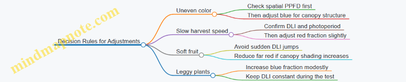
Recipe Summary You Can Run
Use establishment for compact, functional canopies, then switch to fruiting for consistent color and stable firmness. Keep DLI steady while you tune spectral balance, and treat uniformity as a first-order requirement. When quality issues appear, start with measurement and dose consistency; spectrum changes should be targeted, not reactive.
10. Implementation in Real Facilities with Fixtures and Controls
10.1 Translating Recipe Targets into Fixture Level Settings
A recipe usually starts as canopy-level targets: a spectral mix (by wavelength bands), an average PPFD, and a daily light integral schedule. Fixture-level settings are the practical knobs you can actually turn: channel dimming percentages, per-fixture offsets, and timing alignment. The translation is mostly bookkeeping, but the bookkeeping has to respect physics and measurement reality.
Start with What Your Recipe Means at the Canopy
First, restate the targets in the form your sensors can verify. If your recipe specifies “blue enrichment,” convert that into a band ratio plan (for example, 450 nm band fraction relative to total PAR) and pair it with a PPFD target at the crop plane. Then define the temporal plan: photoperiod and any stage-based spectral shifts. A simple check prevents a common mismatch: if the recipe assumes uniform canopy irradiance, your fixture plan must include zoning or correction factors.
Build a Fixture Model from Channels to Spectrum
Most LED fixtures expose multiple channels (for example, 450 nm, 660 nm, 730 nm, and white). To translate targets, you need a mapping from channel drive level to spectral output. Use either manufacturer spectral data or your own measured SPD at a few drive points. The key is to represent each channel’s contribution as a function of dimming.
A practical approach is piecewise linear fitting: measure each channel at 0%, 50%, and 100% (or fewer if you trust the driver linearity), then interpolate. If you have only one measurement per channel, assume proportionality and compensate later with canopy verification.
Convert Band Targets into Channel Dimming
Once you have channel SPDs, compute the combined SPD for a candidate set of channel dimming values. Then integrate to get band fractions and total PAR at the crop plane. Adjust dimming until the computed band fractions match the recipe and the computed PPFD matches the target.
A systematic workflow:
- Choose an initial channel set that roughly matches the recipe band ratios.
- Scale all channels together to hit PPFD.
- Fine-tune relative dimming to correct band fractions.
- Re-check uniformity assumptions and apply fixture offsets if needed.
Account for Geometry and Uniformity
Fixture-to-canopy distance, reflector shape, and lensing change how much each channel reaches the crop. Even if the spectrum at the center looks right, edges may drift. Treat uniformity as a separate layer: first match the spectrum and PPFD at a reference point, then verify across a grid.
If your facility uses multiple fixtures, you can apply per-fixture correction factors. For example, if the left zone reads 5% low PPFD at the crop plane, increase that zone’s overall dimming by a small percentage while keeping the band ratios fixed.
Use a Two-Stage Calibration Loop
Stage one is “spectral fit,” where you tune channel ratios. Stage two is “intensity fit,” where you tune overall output. This separation reduces confusion when both spectrum and PPFD are off.
Example: Your recipe calls for 20% blue-band fraction and 250 µmol/m²/s PPFD at the canopy.
- After initial tuning, your canopy PPFD reads 230 µmol/m²/s but blue fraction is close.
- Increase all channels proportionally by about 250/230 ≈ 1.09, then re-check blue fraction.
- If blue fraction shifts slightly, adjust only the blue channel relative to red/white while keeping PPFD near target.
Mind Map: Fixture Translation Logic
Example: From Band Fractions to Channel Percentages
Assume a fixture with three channels: 450 nm, 660 nm, and 730 nm. Your recipe for a vegetative phase specifies: 450 nm band fraction 18%, 660 nm 70%, 730 nm 12%, and canopy PPFD 300 µmol/m²/s.
- Use your channel SPD model to compute combined band fractions for a starting guess, such as 450:660:730 dimming at 20:70:10.
- If the computed 450 fraction is 15% instead of 18%, increase 450 relative to 660 while holding 730 roughly steady.
- After band fractions match, scale all channels together until canopy PPFD hits 300.
- Verify at a grid of points. If corners are low, apply per-zone intensity offsets rather than changing the spectral ratios.
Minimal Calculation Template
Use this checklist to keep the translation consistent across crops and batches.
- Inputs
- Recipe band fractions and PPFD target
- Channel SPDs at known dimming points
- Geometry and crop-plane measurement height
- Outputs
- Channel dimming levels per fixture or zone
- Expected canopy SPD and PPFD
- Checks
- Band fractions match within tolerance
- PPFD matches within tolerance
- Uniformity within allowed spread
- Timing channels start together
Timing Alignment Matters More Than It Sounds
Even when spectra and intensity are correct, timing errors can change morphology outcomes. Ensure channel start/stop times are synchronized across fixtures, especially if you use multiple controllers. A simple operational rule helps: set all fixtures to the same schedule reference, then confirm with a quick run and spot-check measurements at the same time offset after lights-on.
Integrated Output: What You Record for Production
For each recipe stage, store the fixture-level settings as a set of channel dimming values per zone, the measurement height used for canopy verification, and the acceptance tolerances for band fractions and PPFD. When a batch deviates, you can distinguish “recipe mismatch” from “fixture drift” without guessing.
10.2 Zoning Layouts for Uniformity and Efficient Power Use
Uniformity is mostly a geometry problem: where light lands depends on fixture height, beam spread, and how you divide the room into zones. Efficient power use is mostly a control problem: you avoid blasting every corner at the same intensity when plants only need specific targets at specific locations.
Foundational Layout Principles
Start by deciding what “uniform” means for your crop. For leafy greens, you might target a narrow PPFD band across the usable canopy area, while microgreens may tolerate slightly more variation if harvest is staged. Once the target is defined, treat zoning as a way to hit that target with fewer watts.
A practical workflow:
- Mark the usable plant footprint and exclude walkways, end walls, and any areas where you cannot measure reliably.
- Choose a zoning grid that matches fixture spacing. If fixtures are on a regular pattern, align zone boundaries to that pattern so each zone corresponds to a predictable light contribution.
- Plan for edge effects. The perimeter usually receives less overlap from neighboring fixtures, so edge zones need different dimming or slightly different fixture height.
Zoning Models That Work in Real Rooms
Use one of these models based on how your fixtures are arranged.
Single-Zone With Global Dimming This is simplest: one dimming level for the whole room. It works only when fixtures are dense enough that overlap is strong and the room is close to symmetrical.
Multi-Zone With Perimeter Compensation Divide the room into an interior zone and a perimeter ring. Interior zones usually run closer to the recipe PPFD, while perimeter zones run higher to compensate for reduced overlap.
Fixture-Group Zoning Group fixtures by rows or columns. Each group gets its own dimming channel. This model is effective when fixtures are evenly spaced and you can measure each group’s contribution.
Canopy-Height Zoning If your crop height varies across the footprint, zoning by height can reduce wasted light. For example, if one bench is consistently taller due to substrate depth, that zone may need less intensity to meet the same canopy PPFD.
Measurement-Driven Zoning
Before you commit to dimming settings, map the room.
- Measure PPFD at a consistent canopy reference height. If plants are at different heights, measure at the same relative stage (for example, “leaf tip level” rather than “floor height”).
- Use a grid fine enough to reveal gradients. A coarse grid hides the very edge and corner behavior you’re trying to correct.
- Record the average and the worst-case points per zone. Your control strategy should be based on the worst-case, not the average, because plants respond to the minimum light they receive.
Power Efficiency Without Guesswork
Efficient power use comes from matching output to need.
- Avoid overdriving the interior. If interior points exceed target while edges fall short, you’re paying for light that doesn’t improve quality.
- Use dimming resolution wisely. If your controller supports fine steps, you can tune zones tightly. If it only supports coarse steps, you may need fewer zones to avoid oscillating between “too low” and “too high.”
- Keep recipe changes separate from zoning changes. When you adjust spectra or photoperiod, keep the zoning map stable so you can interpret results.
Mind Map: Zoning Layout Logic
Example: Perimeter Ring Zoning for Leafy Greens
Assume a 2 m × 4 m grow area with fixtures spaced evenly. Measurements show:
- Interior zone average PPFD: 520 µmol/m²/s
- Interior worst-case: 480 µmol/m²/s
- Perimeter worst-case: 420 µmol/m²/s
If your target is 500 µmol/m²/s at canopy, you can set:
- Interior dimming to bring worst-case from 480 to 500 (about +4%).
- Perimeter dimming to bring worst-case from 420 to 500 (about +19%).
This avoids raising the entire room by 19%, which would waste power and likely push interior plants beyond the quality window.
Example: Fixture-Group Zoning for Uneven Wall Reflectance
If one side of the room has darker panels, that side receives less reflected light. Instead of adding more watts everywhere, split into left and right fixture groups.
After measurement:
- Left group worst-case: 460 µmol/m²/s
- Right group worst-case: 500 µmol/m²/s
Set left group dimming to raise worst-case by ~9% while keeping the right group near target. You get uniformity where it matters without turning the whole room into a single brightness level.
Advanced Details That Prevent “It Worked Once” Problems
- Lock the canopy reference. If you measure at floor height one week and at leaf height the next, your zoning settings won’t mean the same thing.
- Account for fixture aging consistently. If you re-check output after maintenance, re-measure by zone so you can see whether the drift is uniform or localized.
- Treat zone boundaries as operational, not theoretical. If plants spill across a boundary due to handling, adjust the boundary to match how the crop actually occupies space.
Mind Map: Common Failure Modes
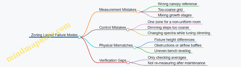
Practical Checklist for Implementation
- Define the usable footprint and exclude unreliable edges.
- Pick a zoning model that matches your fixture pattern.
- Measure PPFD at canopy height on a grid and compute worst-case per zone.
- Set dimming per zone to meet the worst-case target.
- Keep zoning stable while you test spectral recipes.
- Re-check after any fixture, mounting, or maintenance change.
10.3 Control Systems for Dimming and Spectral Channel Management
A spectral “recipe” only works if the facility can reproduce it day after day. That means your control system must translate targets (PPFD, spectrum ratios, photoperiod) into stable electrical outputs per channel, then verify the result with measurements.
Control Architecture from Targets to Light
Start with a simple loop: targets → controller outputs → fixture channels → measured light → adjustment. In practice, you’ll split responsibilities:
- Recipe layer stores wavelength-channel targets by stage and time window.
- Control layer converts targets into dimming commands and schedules.
- Feedback layer checks actual output using sensors and logs.
A useful mental model is “two clocks.” One clock is time (photoperiod and ramp profiles). The other clock is intensity (how quickly channels reach and hold their setpoints). If you only manage time, you get correct schedules with incorrect light.
Dimming Control Strategies That Don’t Drift
Most LED drivers accept dimming commands, but the mapping from command value to emitted photons is rarely perfectly linear. Use one of these approaches:
- Open-loop scaling: apply a pre-measured calibration curve per channel.
- Closed-loop intensity control: adjust commands based on PPFD feedback.
- Hybrid control: use calibration for fast response, then trim using feedback.
For spectral recipes, hybrid control is usually the sweet spot. It reduces hunting (oscillation) while correcting slow changes like temperature effects.
Practical Example: Two-Channel Trim
Suppose your recipe calls for 70% red channel power and 30% blue channel power at a total PPFD of 250 µmol/m²/s. You set initial driver commands using calibration curves. Then you measure PPFD and the red-to-blue ratio at the canopy. If measured red is 5% low, you increase only the red channel command slightly while keeping total PPFD near target. This prevents the common mistake of “fixing” ratio errors by changing overall intensity.
Spectral Channel Management Without Cross-Talk
Channel management is more than setting percentages. Consider these constraints:
- Driver resolution: small command steps can cause noticeable spectral ratio jumps.
- Thermal coupling: warming can change output differently per channel.
- Optical mixing: lenses and reflectors can blur spatial differences, making some sensors less representative.
To manage this, treat each channel as having its own calibration curve and stability window. Also, define a sensor-to-zone mapping so the feedback signal corresponds to the same plants you’re trying to control.
Scheduling Photoperiod and Ramps
Instant on/off creates unnecessary stress and can complicate measurements. Use ramp profiles:
- Morning ramp: 10–30 minutes to reach target PPFD.
- Steady phase: hold setpoints for the bulk of the photoperiod.
- Evening ramp: mirror the morning ramp.
If your recipe uses stage transitions, ramping helps keep morphology consistent. For example, a seedling stage that starts with a higher blue fraction benefits from a controlled ramp so the plant doesn’t experience a sudden spectral shock.
Feedback, Validation, and Logging
A control system should log at least:
- commanded dimming values per channel
- measured PPFD and spectral ratio proxies
- sensor status flags
- zone identifiers and recipe IDs
Validation checks should be routine, not heroic. For instance, run a daily quick check at a fixed time: confirm each channel can reach its expected relative output within tolerance. If one channel drifts, you correct the calibration or flag the fixture.
Mind Map: Dimming and Spectral Channel Control
Example: Minimal Control Logic
Inputs: recipe targets, sensor readings, calibration curves
For each zone:
  set photoperiod schedule
  for each time step:
    compute desired total PPFD
    compute desired channel ratios
    command channels using calibration curves
    if feedback enabled:
      adjust total PPFD using PPFD error
      adjust ratio using red/blue proxy error
    log commands and measurements
  run daily quick check and flag deviations
Case Study: Fixing a Ratio Error Without Changing Total Light
A leafy greens zone shows correct total PPFD but slightly too much green-yellow reflectance in canopy images. The control log reveals blue channel command steps are coarse, causing ratio quantization. The fix is to enable hybrid trimming: keep total PPFD on target via PPFD feedback, then apply smaller ratio trims using the spectral proxy sensor. The result is a stable overall light level with improved color consistency.
When your system is set up this way, “recipe execution” becomes a measurable process rather than a hope-and-pray routine. The plants get the spectrum you intended, at the intensity you intended, for the time you intended.
10.4 Safety, Electrical Considerations, and Operational Reliability
Indoor farms live and die by repeatability, and repeatability starts with safe, predictable power. This section treats electrical design and day-to-day operation as one system: wiring, protection, controls, and verification.
Foundational Safety Principles for LED Lighting Systems
Start with the reality that LED fixtures are electrical equipment, not “just lights.” Treat every connection as potentially energized until proven otherwise. Use grounded metal enclosures where applicable, strain relief for all cable runs, and cable routing that prevents abrasion from moving racks or cleaning tools.
A practical rule: if a component can fail, design so the failure mode is either non-hazardous or immediately detectable. For example, a loose connector should not become a hidden heat source. That means proper torque practices, locking connectors where vibration exists, and thermal checks during commissioning.
Power Architecture and Protection Layers
A reliable setup uses layered protection rather than one “magic breaker.” Typical layers include:
- Branch protection: correctly sized breakers or fuses for each circuit segment.
- Fixture protection: surge protection and appropriate overcurrent protection at the driver level.
- Grounding and bonding: continuous protective earth paths to prevent exposed metal from becoming energized.
- Isolation where needed: separation between control electronics and high-voltage sections.
Example: if a facility uses multiple LED channels for spectral recipes, each channel should be protected so a short in one channel does not take down the entire rack. That keeps production stable and reduces troubleshooting time.
Driver Selection, Dimming Behavior, and Thermal Limits
LED drivers convert electrical input into controlled current. Safety and reliability depend on matching driver specifications to the fixture design and operating environment.
Key checks:
- Input voltage range: confirm the facility supply stays within the driver’s allowed range.
- Output current and compliance: ensure the driver can deliver the intended LED current without exceeding voltage limits.
- Dimming method compatibility: analog dimming, PWM, or digital control can behave differently under load.
- Thermal derating: drivers and LEDs both age faster when run hot.
Operational example: if you dim a fixture to 30% for a seedling recipe, verify that the driver remains stable at that dimming level. Some drivers can show flicker or current ripple at low setpoints, which can affect plant response and complicate quality control.
Wiring Practices That Prevent Hidden Failures
Most electrical problems in farms are boring: loose terminations, damaged insulation, or moisture ingress. Prevent them with consistent installation standards.
- Use cable types rated for the environment and temperature.
- Keep connectors accessible for inspection without dismantling the entire fixture.
- Avoid cable loops that trap condensation.
- Label both ends of every cable and document the mapping to fixture zones.
A simple reliability habit: after installation, perform a visual inspection plus a continuity check for protective earth paths. Then repeat the same checks after any maintenance that involves moving fixtures or replacing drivers.
Operational Reliability Through Controls and Interlocks
Reliability is not only hardware; it’s also how the system behaves when something goes wrong.
Use control logic that fails safely:
- If a sensor fails, the system should revert to a conservative lighting state rather than continuing blindly.
- If a driver reports a fault, the controller should log the event and isolate the affected zone.
- If communication drops, define whether the last known recipe holds or the system returns to a safe baseline.
Example: during cleaning, a cable may be accidentally tugged. A robust system detects the resulting fault, turns off the affected zone, and records the incident so the team can restore service without guessing.
Maintenance, Inspection, and Verification Routines
Set a schedule that matches real usage: daily checks for obvious issues, periodic checks for electrical integrity, and deeper checks during planned downtime.
Daily
- Confirm all zones reach expected on/off states.
- Look for abnormal heat signs near drivers and connectors.
Monthly
- Inspect cable routing and connector tightness.
- Verify controller logs match operational records.
Quarterly or During Downtime
- Perform insulation and protective earth verification as appropriate.
- Check driver fans or cooling paths if present.
Example: Safe Commissioning Checklist for a Multi-Zone Rack
Use a commissioning flow that catches issues early and documents decisions.
Example checklist:
- Verify protective earth continuity for each rack enclosure.
- Confirm breaker sizing matches expected driver input current.
- Test each zone at 100% output and at a low dimming setpoint used in recipes.
- Trigger a controlled fault scenario by disconnecting a non-critical sensor input and confirm the system enters the defined safe state.
- Record driver serial numbers, channel-to-zone mapping, and baseline fault-free logs.
This approach turns “it seems fine” into evidence you can reuse when troubleshooting later.
Example: Handling a Driver Fault Without Losing the Whole Room
When a driver reports a fault, isolate only the affected zone. The controller should:
- Turn off the faulty zone.
- Keep other zones running their current recipes.
- Log the fault code with timestamp and zone ID.
Then the team can swap the driver or inspect the connector without pausing the entire production schedule. That’s operational reliability in practice: fewer surprises, faster recovery, and safer handling of the equipment.
10.5 Standard Operating Procedures for Recipe Execution and Logging
A good recipe is only as useful as the way it gets executed and recorded. This section gives a practical workflow that turns spectral targets into repeatable actions, then captures enough detail to explain results later.
Purpose and Scope
Use this SOP for any LED spectral recipe run in production: leafy greens, herbs, microgreens, and specialty crops. It covers setup, execution, logging, and end-of-run verification. If you change fixtures, controllers, or sensor hardware, treat that as a new “configuration” and run the SOP from the verification step.
Roles and Responsibilities
Assign one person as the “recipe operator” for day-to-day execution and one as the “data reviewer” for logging completeness. The operator runs the steps; the reviewer checks that logs match the physical setup and that key measurements are present.
Required Inputs Before Starting
Collect these before the first light-on:
- Fixture configuration: model, channel mapping, driver limits, and dimming range.
- Recipe definition: wavelength channel targets, intensity targets, photoperiod schedule, and any stage-based changes.
- Environmental baseline: target air temperature, RH range, CO₂ policy (if used), and airflow setting.
- Measurement plan: which sensor(s) will be used for PPFD and which method will be used for spectral verification.
A simple rule: if a log entry cannot be traced to a physical setting, it does not count as a valid record.
Execution Workflow from Setup to Harvest
Follow the same order every time.
Step 1: Pre-Run Fixture Verification
Confirm that each LED channel responds as expected.
- Run a short “sanity dim” at a known controller setting.
- Verify that measured PPFD is within your allowed tolerance of the expected value.
- Record any deviations and whether you adjusted the recipe or the fixture.
Example: If channel A (blue) is underperforming, you log the measured PPFD and decide whether to correct via controller output or flag the batch for reduced confidence.
Step 2: Load the Recipe and Lock the Schedule
Set the controller to the recipe’s photoperiod and DLI plan. Lock the schedule so it cannot be accidentally overwritten.
- Record the recipe ID and version.
- Record the start time and the intended “day count” convention.
Example: If your facility counts “Day 0” at transplant and another team counts “Day 0” at light-on, you will get mismatched logs. Pick one convention and record it.
Step 3: Place Crop and Confirm Zone Assignment
Map trays or beds to zones. Record:
- Zone ID, bench position, and spacing.
- Planting date, cultivar, and starting density.
- Any special handling like blackout periods or transplant timing.
Example: Two zones can share the same recipe but differ in airflow. Logging zone assignment prevents you from blaming spectrum for an airflow issue.
Step 4: Daily Execution Checks
Each day includes three quick checks:
- Controller status: no fault flags, correct schedule running.
- Environmental readings: temperature and RH at a consistent time.
- Light verification: PPFD spot check at the same locations.
If a check fails, document the action taken and the time window affected.
Step 5: Stage Transitions and Recipe Edits
When moving between growth stages, record:
- The exact time of transition.
- The reason for the transition if it differs from the plan.
- Any manual overrides.
Example: If you extend the seedling phase by 12 hours due to slow rooting, you log the reason and the new planned endpoint.
Step 6: End-of-Run Harvest Logging
At harvest, record:
- Harvest date and time.
- Yield metrics: fresh weight per tray, count, and any culls.
- Quality metrics: color notes, leaf thickness, and any sensory observations using a consistent rubric.
- Photos with filenames that include batch ID and zone.
Logging Template and Minimum Fields
Use a consistent schema so data review is fast.
Minimum fields per batch
- Batch ID, crop, cultivar, zone list
- Recipe ID and version
- Fixture configuration ID
- Start time, stage transition times
- Daily PPFD spot check values and locations
- Daily temperature and RH values
- Harvest metrics and cull reasons
Mind Map: SOP Execution and Logging
Example: One Batch with a Controlled Deviation
Batch L-042 uses Recipe R-Lettuce-BlueRed v3. Start time is logged at 08:00. On Day 2, the PPFD spot check in Zone B is 8% low versus expected. The operator records the measured value, checks controller output, and keeps the schedule unchanged. On harvest, the log includes yield per tray and a note that Zone B had slightly paler leaf edges. The reviewer can then compare Zone B against other zones using the same recipe and isolate the deviation to light delivery rather than spectrum intent.
Data Review Checklist for the Data Reviewer
Before approving the batch record, verify:
- Recipe ID/version matches the controller log.
- Stage transition times are present and consistent.
- Daily PPFD spot checks include location identifiers.
- Environmental readings exist for each day.
- Harvest metrics include cull reasons and photo naming.
When something is missing, fix the record immediately while the batch context is still fresh. This SOP is designed so “what happened” is answerable without guessing.
11. Experimental Design and Troubleshooting for Spectral Recipes
11.1 Designing Controlled Trials With Replication and Randomization
Controlled trials answer one question at a time: when you change the spectrum recipe, what changes in the crop, and how confidently can you say it’s because of the spectrum rather than something else? Replication and randomization are the two tools that make that answer defensible.
Core Goal and Unit of Analysis
Start by defining the experimental unit before you touch the LEDs. In indoor farming, the unit is often a bench zone, a rack shelf, or a tray position that receives a specific light setting. If you treat individual plants as independent units while they share airflow, spacing, and light mixing, your statistics will lie to you. A simple rule: if two plants are always exposed to the same light and handling, they should be analyzed together.
Example: You test three spectra on lettuce. If each spectrum is applied to an entire shelf, then shelf is the unit. If you can randomize individual trays within a shelf while maintaining identical light conditions, then tray can be the unit.
Replication That Actually Replicates
Replication means repeating the treatment across multiple independent units. Use two layers when possible: biological replication (multiple plant groups) and technical replication (repeat measurements within a group). Biological replication is what protects you from natural plant-to-plant variation.
A practical target is at least 3–5 independent units per treatment. If you only have one shelf per spectrum, you have no replication for shelf-level effects like temperature gradients or controller quirks.
Example: Spectrum A, B, and C. You place each spectrum on three different shelf positions across the room. Each shelf position holds one tray. Now you have 3 biological replicates per spectrum.
Randomization That Breaks Hidden Patterns
Randomization prevents systematic bias from creeping in through layout. Hidden patterns include edge effects, airflow differences, and uneven reflections from nearby surfaces.
Randomize at the level of the experimental unit. If shelves are your units, shuffle which shelf gets which spectrum. If trays are your units, shuffle tray positions within a shelf.
Example: You have 12 tray positions on a rack. Assign spectra to positions using a random draw, then rotate the trays daily only if your protocol keeps light exposure consistent. If you rotate, you must rotate all treatments the same way to avoid introducing a new variable.
Blocking for Facility Reality
Blocking reduces noise by grouping units that share nuisance conditions. A block might be a row, a shelf height, or a time window. Blocking is especially useful when you can’t fully randomize across the entire facility.
Example: You run the trial over two weeks. Week is a block because day-to-day temperature and humidity can shift. Within each week, you randomize spectrum assignments to the available shelf positions.
Treatment Structure and Controls
Include a control spectrum that represents your current standard recipe. Also decide whether you are testing one factor at a time (e.g., blue fraction) or multiple factors (e.g., blue fraction and far-red fraction). If you vary multiple wavelengths simultaneously, you must treat the treatment as a combined recipe rather than trying to infer which component caused the effect.
A clean design for beginners is a single-factor comparison: same PPFD and photoperiod across treatments, only spectrum changes.
Outcome Measures and Timing Windows
Predefine what you measure and when. For spectral trials, outcomes often include morphology (height, leaf area), quality proxies (color metrics, chlorophyll estimates), and harvest timing (days to marketable size). If you measure everything at every time point, you increase the chance of finding a “significant” result by accident.
Example schedule: day 0 baseline, day 7 morphology, day 14 quality and harvest readiness. Keep the same schedule for all treatments.
Mind Map: Trial Design Logic
Example: A Simple, Defensible Layout
You have 3 spectra (A, B, C) and 12 tray positions on two shelves. Each shelf is a block because shelf height affects temperature.
- Block 1: Shelf 1 has 6 positions.
- Block 2: Shelf 2 has 6 positions.
- Within each shelf, randomly assign A, B, C so each appears twice on that shelf.
- Each position holds one tray, and you keep tray handling identical.
This yields 4 biological replicates per spectrum total (2 per shelf × 2 shelves), while controlling for shelf-level nuisance effects.
Practical Checklist Before You Start
- Unit of analysis matches how light is actually delivered.
- Each treatment has multiple independent units.
- Randomization is done at the correct level.
- Blocking is used when full randomization is impossible.
- Control recipe is included.
- Outcomes and measurement days are fixed in advance.
When these pieces line up, your trial becomes less about hoping the spectrum “worked” and more about estimating how much it changed the crop, with a clear sense of uncertainty.
11.2 Interpreting Growth and Quality Metrics Without Confounding
When a spectral recipe trial produces unexpected results, the first question is rarely “Did the spectrum work?” It’s “What else changed at the same time?” Confounding happens when two factors move together, so the metric can’t tell you which factor caused the outcome. The goal here is to interpret growth and quality metrics using a disciplined chain: define the metric, map it to biology, identify plausible drivers, then check whether those drivers were controlled.
1) Start with Metric Definitions That Match Your Decision
Growth metrics should be tied to a specific production decision. For example, “fresh weight” supports harvest yield, while “leaf thickness” supports texture consistency. Quality metrics should be defined in observable terms before you measure. If “color” means “market-ready green,” decide whether you’ll use a colorimeter reading, a chart score, or both.
A practical rule: if two metrics are strongly correlated, treat them as a bundle and interpret them together. For instance, higher fresh weight often comes with larger leaf area, but not always with better texture. Separating “size” from “structure” prevents you from blaming spectrum for what was actually a density or hydration effect.
2) Map Each Metric to Likely Biological Drivers
Confounding is easier to spot when you know what should drive the metric. Use a driver map that connects spectrum and environment to plant responses.
- Biomass and growth rate: driven by total light delivered (PPFD and photoperiod), canopy temperature, and CO₂ availability.
- Morphology: driven by blue fraction, red:far-red balance, and intensity gradients.
- Color: driven by pigment synthesis pathways, but also by developmental stage and nitrogen status.
- Flavor-related proxies: driven by light-driven metabolism, but also by water status and harvest maturity.
If your driver map includes factors you didn’t control, you’ve found a potential confound.
Mind Map: Metric Interpretation Without Confounding
3) Check Co-Variation Patterns Instead of Single Outcomes
A single metric can mislead because confounders often affect multiple traits in characteristic ways.
Example: Suppose treatment A shows higher fresh weight but also taller plants with thinner leaves. That pattern can indicate either increased light delivery or a morphology shift from spectrum or gradients. If PPFD at canopy was not matched, you can’t claim the spectrum caused the biomass increase. If PPFD was matched but uniformity differed, the taller response may reflect edge or hotspot effects.
Example: Suppose anthocyanin-like purple increases while total dry mass decreases. That can happen when plants experience stress signals, but it can also happen if harvest maturity differs between treatments. If you harvested at different developmental stages, color changes may reflect stage rather than spectrum.
4) Control the “Hidden Variables” That Commonly Confound Trials
Confounders usually fall into four buckets.
- Environment: temperature and humidity affect transpiration and leaf water content, which can change fresh weight and texture. Even small airflow differences can alter canopy temperature.
- Handling: irrigation timing, nutrient delivery, and transplant age can shift developmental stage. A one-day mismatch can matter for fast crops.
- Measurement: sampling location (top vs bottom canopy), instrument calibration, and inconsistent sampling size can create apparent treatment effects.
- Layout: uneven PPFD across shelves produces gradients that mimic spectral effects. If you used dimming, verify that dimming didn’t change spectral ratios unintentionally.
5) Use a Simple Evidence Checklist Before You Conclude
Before attributing results to spectrum, verify these points:
- Light delivery matched: PPFD and DLI are comparable at the canopy level.
- Spectral ratios stayed stable: dimming or driver behavior didn’t shift the spectrum.
- Developmental stage matched: harvest timing and starting material were consistent.
- Uniformity was checked: measurements covered edges, centers, and representative canopy heights.
- Replicates agree: the direction of change is consistent across independent units.
Case Study: Interpreting a Confounded Color Result
In a lettuce trial, Treatment B used a higher blue fraction. Plants in B showed darker leaves, but also slightly delayed maturity. When the team compared leaf age at harvest, the darker color aligned with maturity differences rather than a pure pigment response. After re-analyzing using only leaves harvested at the same developmental stage, the color difference shrank, while morphology differences remained. The correct interpretation was: blue fraction influenced morphology, while the strong color change was partly confounded by harvest timing.
6) Turn Interpretation into Better Next Measurements
Once you identify likely confounders, adjust your measurement plan: sample multiple canopy positions, record canopy temperature and RH, and log irrigation events. Then interpret metrics as a set, not as isolated winners and losers. That approach keeps your conclusions tied to evidence rather than coincidence.
11.3 Troubleshooting Underperformance From Spectrum To Environment
When a crop underperforms, the spectrum is often blamed first. That’s fair—light is controllable—but it’s rarely the only variable. A systematic approach prevents you from “fixing” the spectrum while the real issue is humidity, temperature, or measurement.
Step 1: Confirm the Symptom with Measurable Signals
Start by separating “looks smaller” from “is actually receiving less effective light.” Compare three things across the affected area and a healthy control:
- Growth rate: days to target leaf size or fresh weight.
- Morphology: stretch, leaf thickness, and color drift.
- Light delivery: PPFD at canopy height and DLI over the photoperiod.
Example: If plants are pale and thin, check whether PPFD is low or whether the spectrum is missing blue that supports compact growth. If plants are dark but still slow, suspect temperature, CO₂, or root-zone limitations rather than wavelength.
Step 2: Verify the Recipe Is What the Plants Actually Received
A “correct” recipe can still be wrong in practice due to fixture behavior and control settings.
- Channel mapping: confirm each LED channel corresponds to the intended wavelength band.
- Dimming linearity: many drivers are not perfectly linear; 50% output may not equal half the photons.
- Thermal effects: LEDs can shift output as they warm; measure after stabilization.
Quick check: Measure PPFD at multiple points after the system reaches steady state. If the spatial pattern matches fixture layout rather than plant placement, the issue is delivery, not biology.
Step 3: Rule Out Measurement and Calibration Errors
Spectral recipes depend on accurate instrumentation. Common failure modes:
- Sensor mismatch: a PAR sensor may not represent your spectrum’s weighting.
- Dirty optics: dust on lenses changes transmission.
- Mounting height and angle: canopy height changes during growth; measurements taken once early can become misleading.
Example: Two benches use the same recipe. One bench has a slightly different sensor mounting angle. The PPFD reading looks similar, but the effective spectrum at canopy differs, leading to slower biomass accumulation.
Step 4: Connect Spectrum Symptoms to Likely Environmental Constraints
Spectrum and environment interact. Use symptom-to-cause logic rather than guessing.
- Stretch with low blue: can also happen with high temperature or low airflow that reduces stomatal conductance.
- Poor color: can be spectrum-related, but also caused by insufficient light uniformity or canopy shading.
- Slow harvest speed: can be DLI-related, but also limited by root-zone temperature or inconsistent watering.
A practical rule: if morphology suggests light stress but PPFD and DLI are correct, look at temperature and VPD next.
Step 5: Perform a controlled “one-change” test
Avoid changing everything at once. Pick the smallest change that tests a hypothesis.
- If PPFD is confirmed low: increase intensity by a fixed amount and keep spectrum ratios constant.
- If PPFD is correct but morphology is off: adjust blue fraction or red-to-blue balance while holding DLI constant.
- If both are correct: investigate environment (air temperature, VPD, CO₂, irrigation timing).
Example: Plants are leggy and slow. PPFD matches the target, but leaf thickness is low. Increase blue fraction slightly while keeping total DLI constant. If compactness improves without yield loss, the spectrum balance was the bottleneck.
Step 6: Use a Decision Tree to Avoid Circular Troubleshooting
A decision tree keeps you from “fixing” the spectrum repeatedly without evidence.
graph TD
A[Underperformance observed] --> B[Confirm symptom metrics]
B --> C[Compare PPFD and DLI vs target]
C -->|Low| D[Check fixture output and channel mapping]
C -->|On target| E[Check uniformity and canopy measurement]
E --> F[If uniformity poor]
F --> G[Fix zoning, spacing, or reflections]
E -->|Uniform| H[Check calibration and sensor setup]
H --> I[If measurement error]
I --> J[Recalibrate and remeasure]
H -->|No error| K[Evaluate environment]
K --> L[Temperature, VPD, CO2, irrigation]
L --> M[Run one-change test]
M --> N[Record results and lock the root cause]
Mind Map: Spectrum to Environment Troubleshooting
Step 7: Document the Chain of Evidence
Write down what you measured, what you changed, and what improved. This prevents repeating the same troubleshooting loop next batch.
Example: “PPFD was low on one bench after warm-up; channel mapping was correct; uniformity was poor due to fixture tilt; after correcting tilt, DLI matched target and harvest speed returned to baseline.” That single paragraph is more useful than a dozen guesses.
Step 8: Common Integrated Failure Scenarios
- Recipe correct, delivery wrong: channel mapping or dimming nonlinearity causes lower effective output.
- Delivery correct, environment limiting: VPD too high slows stomatal function; plants look light-stressed even when PPFD is right.
- Delivery and environment correct, measurement wrong: sensor mismatch or canopy height sampling error masks the real light exposure.
The goal is not to “find the culprit” instantly. It’s to narrow the cause with evidence, then test one variable at a time until the crop behaves like the recipe promised.
11.4 Correcting for Sensor Drift and Spatial Nonuniformity
A spectral recipe only works if the numbers you feed into it are trustworthy. Two common failure modes are sensor drift over time and spatial nonuniformity across the grow area. Drift makes the same lamp look different on different days; nonuniformity makes different spots look different on the same day. The fix is a workflow: detect, quantify, correct, and then verify with a simple acceptance test.
Foundations: What Drift and Nonuniformity Look Like
Sensor drift shows up as a slow change in readings when nothing in the facility changes. For example, if you measure PPFD at the same bench position every morning for a week and the values trend downward, the sensor or its electronics are likely drifting.
Spatial nonuniformity shows up as a pattern across the room. Even with identical fixtures, mounting height, reflector geometry, and airflow can create gradients. A practical symptom is that two plants receiving the same recipe still differ in color or growth rate because they were not actually receiving the same light.
Detection: Build a Baseline and Run Repeat Checks
Start with a baseline measurement plan that you can repeat without guesswork.
- Pick reference points: Choose 9 points in a 3×3 grid per zone, including corners and center. If the zone is large, use more points, but keep the grid logic consistent.
- Define a timing rule: Measure at the same time after lights-on, such as 15 minutes, to reduce warm-up effects.
- Record both spectrum and intensity: If you only track PPFD, you can miss spectral channel drift that still affects plant responses.
A simple drift check uses one reference point. Measure it daily for at least 5 days without changing recipes. If the readings move more than your tolerance, you have drift.
Mind Map: Sensor Drift and Spatial Nonuniformity Workflow
Quantification: Turn Patterns into Numbers
Drift Correction Factor
Compute a correction factor relative to a baseline day. If your baseline PPFD at the reference point is 450 µmol·m⁻²·s⁻¹ and today’s reading is 430, the factor to scale today’s measurements back to baseline is:
- Factor = 450 / 430 = 1.0465
Apply the factor to intensity-based recipe inputs. For spectral drift, do the same per wavelength band or per channel if your instrument provides calibrated channel outputs.
Uniformity Map and Interpolation
For spatial nonuniformity, create a map of measured PPFD across the grid. Convert each point into a ratio relative to the zone center (or the mean of all points). Then, when you place plants or trays, assign them the ratio for their location.
Example: If the center is 450 and a corner is 405, the corner ratio is 405/450 = 0.90. If your recipe target at the plant location is 450, you either raise intensity for that zone or adjust fixture height/angle so the corner reaches the target.
Correction: Apply Changes Without Breaking Consistency
Use two layers of correction: one for time (drift) and one for space (uniformity).
- Time correction first: Normalize today’s readings using the drift factor so the sensor behaves like it did on the baseline day.
- Space correction second: Use the uniformity ratios to adjust fixture settings or to interpret plant outcomes correctly.
If you cannot adjust fixtures for every location, you can still correct your recipe execution by zoning. For instance, split a large bay into two zones with separate target intensities. The goal is not perfect uniformity everywhere; it’s predictable delivery where plants actually sit.
Verification: Prove the Fix Works
After applying corrections, run a short verification.
- Measure the 9-point grid again in the same positions.
- Confirm that corrected PPFD values fall within your acceptance band, such as ±5% at most points.
- For spectral recipes, check that the key wavelengths used for your flavor and morphology goals remain within tolerance. If blue channel output is drifting, you can see correct PPFD while still getting the wrong plant response.
A practical acceptance test is to compare corrected readings to the recipe target at the center and at the worst-case corner. If the corner is still low, you need either fixture adjustment or a zone split.
Common Pitfalls and How to Avoid Them
- Measuring too soon after lights-on: Warm-up can masquerade as drift.
- Changing sensor orientation: Small angle differences can shift readings, especially for spectral sensors.
- Mixing zones with different mounting heights: A single uniformity map cannot cover different fixture geometries.
- Correcting only PPFD: Spectral channel drift can change plant outcomes even when total intensity looks stable.
Example: A Two-Step Correction in One Batch
On 2026-03-05, you set a baseline at the zone center: PPFD 450. On 2026-03-12, the center reads 430 with the same fixture settings. Drift factor is 450/430 = 1.0465.
You then measure the 3×3 grid and find the top-left corner reads 395. Correct it for drift: 395 × 1.0465 ≈ 413. If your target at corners is 450, that corner is still 8.2% low after drift correction. You either increase intensity for that zone or split the bay so the corner receives a higher setting.
Mind Map: Verification Checklist

When drift and spatial nonuniformity are handled as separate, measurable problems, recipe execution becomes repeatable. The plants still do their plant thing, but your light numbers stop moving under your feet.
11.5 Documenting Changes to Build Reproducible Recipe Libraries
Reproducible spectral recipes depend less on having “the perfect spectrum” and more on recording what changed, when it changed, and what evidence you used to decide the change. A good documentation habit turns each experiment into a reusable entry rather than a one-off story.
Start with a single source of truth: one recipe record per crop, stage, and target outcome. Each record should include the intended light plan and the operational reality. “Intended” covers wavelength channel targets and timing; “operational reality” covers what the fixtures actually delivered, including measured PPFD and spectral checks at representative canopy positions.
Change Log Foundations
A change log should answer five questions every time: what was changed, why it was changed, where it was applied, how it was verified, and what happened afterward. Keep the “why” grounded in measurements or observed failures, not in guesses. For example, “leaf edges browned after day 10” is actionable; “plants looked stressed” is not.
Use consistent identifiers so you can compare batches without hunting through spreadsheets. Recommended fields include:
- Recipe ID and version number
- Facility zone and fixture IDs
- Crop and stage definition (for example, “day since transplant” rather than “seedling size”)
- Light plan parameters (channel targets, photoperiod, DLI target)
- Measurement method (sensor model, placement height, number of points)
- Environmental conditions (air temperature, RH, CO2 if controlled)
- Outcome metrics (biomass, color score, harvest day, quality notes)
Versioning Rules That Prevent Confusion
Treat any change to wavelength targets, photoperiod, or intensity setpoints as a new version. Treat changes to logging, labeling, or file naming as documentation-only updates that do not affect the recipe’s biological intent. If you must adjust output due to LED aging or driver limits, record it as an operational deviation and either correct it back to the intended plan or create a separate “as-delivered” version.
A practical rule: if two batches could plausibly produce different results, they deserve different version numbers. This keeps your library honest.
Evidence Levels for Verification
Not every change deserves the same level of proof. Use evidence levels to keep effort proportional:
- Level 1: Fixture settings recorded and cross-checked against controller readouts
- Level 2: Spectral and PPFD measurements at multiple canopy points
- Level 3: Replicated crop trial with defined acceptance criteria
When a change is Level 1 only, label it clearly so later users know it is operationally plausible but not biologically confirmed.
Mind Map: Documentation Workflow
Example: A Controlled Change That Becomes Reusable
Suppose a lettuce batch shows slower color development than expected. You suspect the blue fraction is low or the delivered PPFD is under target.
- Record the baseline recipe version: channel targets, photoperiod, and DLI target, plus the measurement plan used for the baseline.
- Identify the change: increase the blue channel by a fixed percentage while keeping red and total PPFD targets constant.
- Verify operational delivery: measure PPFD and spectral distribution at the same canopy points used in the baseline.
- Run the trial with the same stage definition and the same environmental setpoints.
- Update the library only after outcomes are recorded: if color score improves without yield loss, promote the new version; if it improves color but reduces biomass, keep the version but mark the tradeoff in the outcome summary.
This turns a troubleshooting moment into a documented recipe option with known constraints.
Example: Handling As-Delivered Deviations
LED output can drift, and drivers can cap maximum current. If a scheduled recipe cannot reach its intended PPFD, document the delivered PPFD and the reason for the deviation. Then choose one of two paths:
- Corrective path: adjust fixture settings or replace components, then re-measure and keep the original version.
- Separate path: create an “as-delivered” version that records the delivered spectrum and intensity, so future users do not assume the recipe is biologically identical to the original.
Either way, the library remains usable because it reflects reality, not wishful settings.
Practical Checklist for Each Recipe Version
Before you close a batch record, confirm that the library entry includes:
- Version number and change summary in one paragraph
- Evidence level and measurement coverage
- Stage definition and batch identifiers
- Outcome metrics and any quality notes tied to the light plan
- Raw measurement files referenced by filename and date-stamped run ID
If you follow this checklist consistently, you can later compare versions without re-reading every experiment log. Your future self will thank you, mostly by not making you do detective work.
12. Recipe Libraries, Checklists, and Production Documentation
12.1 Standard Recipe Format for Wavelength Intensity and Timing
A standard lighting recipe is a written contract between your LEDs and your crop. The goal is simple: every batch should receive the same spectral intent, the same delivered intensity, and the same timing—despite fixture aging, dimmer quirks, and sensor drift.
Core Recipe Fields
Use a fixed order so technicians can fill it out quickly and consistently.
-
Crop and Stage
- Crop name, cultivar or line, and growth stage (seedling, vegetative, pre-harvest).
- Target outcomes: for example, “compact canopy” or “deep green with minimal stretch.”
-
Measurement Basis
- Specify whether intensity targets are based on PPFD (typical) and whether spectral targets are based on relative channel output or measured SPD.
- Record the measurement plane: canopy height, bench height, or a fixed reference grid.
-
Wavelength Channels and Targets
- List each LED channel (e.g., 450 nm, 660 nm, 730 nm, white) with a target output mode.
- For each channel, store either target relative ratio (e.g., 450:660:730 = 10:85:5) or target absolute intensity contribution (preferred when you have spectral measurement capability).
-
Intensity Setpoint and Dimming Law
- Store the total PPFD setpoint and the dimming strategy used to reach it.
- Include the dimming law type (linear, manufacturer curve, or calibrated curve) so “50%” means the same thing later.
-
Timing Block
- Photoperiod (hours on), ramp behavior (none, step, or ramp), and any mid-day adjustments.
- If you use a daily light integral target, include the DLI calculation basis and the expected PPFD during ramps.
-
Spatial Uniformity Rules
- Define how you compensate for edge effects: fixture zoning, per-zone correction factors, or a single uniform setting with acceptance limits.
-
Verification and Acceptance
- Minimum measurement frequency (e.g., at commissioning and after maintenance).
- Acceptance thresholds: PPFD tolerance, spectral ratio tolerance, and uniformity tolerance.
-
Change Control
- Record what changed: firmware, driver replacement, channel replacement, or sensor swap.
- Include a batch identifier and the date of last verification (use a date like 2026-03-05 if you need one).
Mind Map: Standard Recipe Components
Example: A Filled-Out Recipe Template
Below is a practical structure you can copy into your batch record.
- Recipe ID: LG-VEG-660-450-730-v3
- Crop/Stage: Lettuce, vegetative
- Target Outcomes: compact growth, strong leaf color
- Measurement Basis: canopy plane at 25 cm above bench; PPFD measured with calibrated quantum sensor; SPD measured at 1 m from fixture centerline
- Channels and Targets:
- 450 nm: 10% relative ratio
- 660 nm: 85% relative ratio
- 730 nm: 5% relative ratio
- White: 0% (disabled)
- Total PPFD Setpoint: 220 µmol/m²/s at canopy plane
- Dimming Law: calibrated channel-to-PPFD curve, driver rev A
- Timing Block:
- Photoperiod: 16 h
- Ramp: 30-minute linear ramp up, 30-minute linear ramp down
- Mid-day shift: none
- Spatial Uniformity: 9-zone layout; apply zone correction factors; acceptance uniformity CV ≤ 8%
- Verification: measure PPFD and channel ratios at 5 grid points per zone; PPFD tolerance ±10%; ratio tolerance ±15% relative
- Change Control: last verified 2026-03-05; sensor model QX-PPFD-01
Example: Converting Channel Ratios into Delivered Intensity
If your dimming system uses relative channel ratios, you still need a way to guarantee the total PPFD. A simple workflow is:
- Set channels to the target ratios.
- Adjust overall dimming until the total PPFD hits the setpoint.
- Re-check spectral ratio stability at the chosen dimming level.
Workflow
- Step 1: Set 450/660/730 to 10/85/5
- Step 2: Increase master dimmer until PPFD = 220
- Step 3: Measure SPD or channel output proxies
- Step 4: If ratios drift, update dimming law or apply per-channel trim
- Step 5: Store the final master dimmer value and trims in the recipe
Practical Notes That Prevent “Why Did This Batch Differ?”
- Treat “master dimmer” as a measured outcome, not a guess. Store the value that produced the target PPFD.
- Keep the measurement plane consistent. A 5 cm canopy-height change can shift delivered PPFD enough to matter.
- Record whether ramps are linear in time or in electrical output; the crop experiences light, not your intentions.
A good recipe format is boring in the best way: it makes differences traceable, so you can fix the cause instead of arguing about what the LEDs were “probably doing.”
12.2 Batch Records for Traceability From Setup to Harvest
Batch records are the paper trail that lets you answer three questions quickly: What did we run? What happened? What did we ship? For spectral lighting, the “what did we run” part is especially important because small differences in spectrum, timing, and intensity can change flavor, color, and harvest speed.
Foundational Batch Record Goals
A good batch record captures decisions and measurements in a way that survives real life: staff changes, equipment swaps, and sensor quirks. Traceability is achieved when every critical input has a unique identifier and every critical output has a matching measurement window.
Start with a batch ID and a scope statement. The scope should specify crop, cultivar or seed lot, production area or zone, and the growth stage covered by the record. If a batch spans multiple stages, split it into stage sub-batches so you can compare like with like.
Record Structure from Setup to Harvest
Use a consistent order so the record is easy to scan during audits and troubleshooting.
-
Setup Inputs
- Facility and zone: rack ID, bench ID, and fixture channel mapping.
- Plant material: seed lot, transplant date, and any pre-conditioning.
- Lighting recipe: channel setpoints by wavelength band, target PPFD or DLI, and photoperiod schedule.
- Hardware state: driver firmware version, dimming mode, and any recent maintenance.
-
Environmental Context
- Air temperature and humidity targets and actual readings.
- CO2 setpoint and monitoring method if used.
- Watering or nutrient program identifiers, including EC and pH targets.
-
Verification Measurements
- Initial light verification: PPFD at representative points and spectral check method.
- Uniformity notes: which points were used and what “acceptable” means for your facility.
- Sensor calibration references: last calibration date and calibration method.
-
In-Process Logs
- Daily or per-shift checks: actual photoperiod start/stop, dimming status, and any alarms.
- Any deviations: power interruptions, recipe changes, or fixture replacements.
- Quick crop observations: canopy height notes, visible color drift, and any pest or disease flags.
-
Harvest Outputs
- Harvest date and time window.
- Sample plan: how many plants were measured, where they were selected, and how they were labeled.
- Quality metrics: color score method, flavor-related proxies you use (for example, leaf maturity stage), and biomass measurements.
- Yield accounting: count, weight, and grade criteria.
Mind Map: Traceability Flow
Batch Traceability Mind Map
Example Batch Record Entries
Setup example:
- Batch ID: LG-2403-A
- Zone: Rack 3, Bench B
- Seed lot: L-1187
- Recipe: Blue/Red mix with far-red channel enabled during late phase; photoperiod 16 hours; target PPFD 220 µmol/m²/s
- Fixture mapping: Channel 1 = 450 nm band, Channel 2 = 660 nm band, Channel 3 = far-red band
Verification example:
- Initial PPFD check: 9-point grid, mean 218 µmol/m²/s, coefficient of variation 0.08
- Spectral check: handheld spectrometer method, confirm peak wavelengths within your tolerance
- Calibration reference: PAR sensor calibrated on 2026-03-05 using your facility standard
In-process example:
- Day 4 deviation: one fixture driver reported “dimming fault” for 12 minutes; recipe resumed automatically; log includes start/stop timestamps and affected fixture ID
- Corrective action: verified PPFD returned to target within the next measurement window
Harvest example:
- Harvest window: 2026-04-18 09:00–11:00
- Sample plan: 30 plants from three positions per tray, labeled T1–T10, T11–T20, T21–T30
- Outputs: fresh mass per plant, color score rubric used by two-person consensus, and grade assignment
Practical Rules That Prevent Traceability Breaks
Keep the record “single source of truth.” If you change a recipe, record the reason and the exact setpoint values that were applied, not just “adjusted.” If you replace a fixture, record the new fixture ID and confirm the mapping to wavelength channels.
Finally, ensure every measurement has a label that connects it to the batch and the stage. When you can trace from a leaf color score back to the exact lighting schedule and verification window, you can trust your comparisons—and you can fix problems without guessing.
12.3 Quality Control Checklists for Color Flavor and Yield
Quality control works best when it treats color, flavor proxies, and yield as a single system. If you only check one outcome, the others will quietly drift—usually because the spectrum, the delivered light dose, or the environment changed.
Foundational Checklist Logic
Start with three questions for every batch: What did we set? What did the plants actually receive? What did they produce?
- Set: Record fixture channel targets (blue, red, far red, green if used), photoperiod, and dimming schedule.
- Receive: Verify PPFD and spectral distribution at representative canopy heights, plus uniformity across zones.
- Produce: Measure color and growth metrics on a consistent sampling plan, then connect them to yield.
A practical rule: if PPFD is right but color is off, suspect spectrum balance or timing. If color is right but yield is low, suspect DLI shortfall, temperature/humidity mismatch, or plant density.
Mind Map: Quality Control Flow
Color Checklist with Concrete Pass Criteria
Color is easiest to control when you define “good” in measurable terms, not just “looks right.” Use a two-layer approach: a quick visual rubric for throughput, and a more objective check for disputes.
A. Visual rubric (fast, repeatable)
- Leaf color category: pale green, normal green, deep green, red/purple tint.
- Uniformity: even across the sampled area vs. patchy.
- Edge quality: scorched or bleached tips.
B. Objective pigment proxy (choose one per facility)
- For many leafy crops, a handheld chlorophyll proxy or standardized image capture works well.
- Record readings from the same leaf position each time (for example, the third fully expanded leaf).
C. Common spectrum-linked failures
- Too little blue often yields softer, less compact leaves and a flatter green tone.
- Too much far red relative to red can increase stretching and reduce the “tightness” that customers associate with freshness.
Flavor Checklist Using Proxies That Don’t Lie
Flavor is hard to measure directly, so QC uses proxies that correlate with the sensory outcome you care about.
A. Texture and structure proxies
- Leaf thickness or firmness (simple compression test or standardized thickness measurement).
- Water status indicators via fresh-to-dry ratio.
B. Secondary metabolite proxies
- For crops where bitterness or pungency matters, use a consistent internal scoring panel with the same sample handling.
- If you have a lab method for phenolics or related compounds, tie it to the same sampling plan.
C. Example: Leafy green batch decision
- If color is within range but firmness is low, check whether DLI was reduced by dimming drift or fixture fouling.
- If firmness is high but color is pale, check blue fraction and photoperiod timing rather than increasing total PPFD immediately.
Yield Checklist That Connects to Light Dose
Yield QC should separate “plants grew” from “plants grew efficiently.”
A. Fresh yield metrics
- Fresh mass per plant or per harvest unit.
- Size distribution: count how many plants fall into each market grade.
B. Efficiency metrics
- Dry matter percentage from a small, consistent subsample.
- Harvest timing consistency: record days from transplant or sowing.
C. Example: Fast harvest but low dry matter
- If harvest speed improved but dry matter dropped, the spectrum may have pushed rapid expansion without enough structural support.
- Correct by adjusting red-to-blue balance or tightening the photoperiod schedule so DLI matches the target stage.
Integrated QC Sampling Plan
Use the same sampling logic every batch.
- Zones: sample at least three zones (center, edge, and one intermediate).
- Replicates: minimum of 5 plants per zone for yield; 3 plants per zone for color and proxy flavor checks.
- Timing: measure color and proxies at a fixed stage marker (for example, first harvest readiness), not just “day X.”
Corrective Action Checklist Without Guesswork
When something fails, change one variable at a time.
- Confirm delivery: re-check PPFD and spectral mix at canopy height.
- Confirm timing: verify photoperiod and dimming logs match the recipe.
- Confirm environment: check temperature and humidity stability during the measurement window.
- Adjust spectrum or dose: only after steps 1–3 are clean.
Mind Map: Root Cause to Fix
Example: One-Page QC Record Template
Use a consistent record so deviations can be traced.
- Batch ID: ________ Crop: ________ Stage at harvest: ________
- Recipe targets: blue ___% red ___% far red ___% photoperiod ___h
- Delivered light: PPFD ___ at canopy; uniformity ___; spectral check date: 2026-03-05
- Environment window: temp ___–___; RH ___–___; airflow ___
- Color rubric result: pass/fail; notes: __________________________
- Flavor proxies: firmness ___; sensory score ___; pass/fail: ________
- Yield: fresh mass ___; dry matter ___%; grade distribution: ________
- Deviations and actions: ____________________________________________
Closing Principle
A good QC checklist doesn’t just say “pass or fail.” It forces you to connect the delivered spectrum and dose to the observed color, proxy flavor signals, and yield outcomes—so the next batch starts from evidence, not hope.
12.4 Maintenance and Reverification Schedules for LED Performance
A spectral lighting recipe is only as good as the hardware that delivers it. Maintenance keeps the optics clean and the electronics stable; reverification proves that the delivered spectrum still matches the recipe targets. The goal is simple: catch drift early, before it shows up as off-color leaves, slower harvest timing, or inconsistent flavor.
Foundational Concepts for Schedule Design
Start by separating three kinds of change. First is fast change, caused by loose wiring, controller faults, or a channel that stops responding. Second is gradual change, driven by LED aging, thermal stress, and driver behavior. Third is measurement change, caused by sensor drift, calibration errors, or mounting differences.
A good schedule addresses all three. Maintenance reduces fast and gradual change. Reverification quantifies both gradual change and measurement change, so you can distinguish “the lights changed” from “the measurement changed.”
Maintenance Cadence That Matches Failure Modes
Use a cadence with three layers: daily checks, monthly cleaning and inspection, and quarterly performance verification.
Daily checks (5–10 minutes per zone):
- Confirm each spectral channel responds to the expected dimming command by watching the controller readout and a quick visual reference panel.
- Verify cooling fans and heat sinks are unobstructed. If airflow is reduced, junction temperatures rise and spectra shift.
- Log any alarms, even if the system recovers automatically.
Monthly cleaning and inspection (1–2 hours per fixture group):
- Clean diffusers and lenses using the manufacturer’s recommended method. Residue changes scattering and can alter effective intensity at the canopy.
- Inspect mounting hardware and reflectors for looseness or corrosion.
- Check cable strain relief and connector seating. A slightly intermittent connection can create channel-specific drift.
Quarterly maintenance (half-day per facility zone):
- Re-check thermal contact surfaces and mounting pressure where applicable.
- Verify driver output stability by comparing current draw at a fixed dimming level across channels.
- Replace any components that show signs of wear before they become intermittent faults.
Reverification Cadence That Protects Recipe Integrity
Reverification should be frequent enough to catch gradual drift and consistent enough to be comparable.
After any hardware change:
- New driver, replaced LED board, controller firmware update, or fixture relocation triggers immediate reverification.
Monthly reverification for critical crops:
- Measure spectrum and PPFD at representative points in each zone.
- Compare against the last verified baseline using the same measurement geometry.
Quarterly reverification for standard production:
- Repeat the same measurement plan and update the “as-delivered” record if changes are within tolerance.
Annual full audit:
- Perform a deeper mapping across the full canopy area and verify uniformity assumptions.
A practical rule: if your recipe tolerances are tight for color or flavor, increase reverification frequency for those crops rather than tightening everything everywhere.
Tolerance Thinking and Decision Rules
Define tolerances per output type:
- Spectral shape tolerance: limits on relative band ratios (for example, blue-to-red balance) rather than only absolute intensity.
- Intensity tolerance: limits on PPFD at canopy height.
- Uniformity tolerance: limits on spatial spread across the measurement grid.
When a metric fails, decide whether to adjust the recipe or service the fixture. If the driver current draw is stable but the spectrum shifted, service optics or verify LED board health. If current draw is unstable, treat it as a hardware fault first.
Mind Map: Maintenance and Reverification Schedules
Example Schedule for a Two-Zone Facility
Assume Zone A grows leafy greens where color matters; Zone B grows herbs where harvest speed matters.
- Daily: both zones get channel response and airflow checks.
- Monthly: Zone A gets spectrum + PPFD at 9 grid points; Zone B gets spectrum + PPFD at 4 representative points.
- Quarterly: both zones get a full zone check at the same grid used for baselines.
- After any change: any fixture moved or any driver replaced triggers immediate measurement in that zone.
If Zone A’s blue-to-red ratio drifts beyond tolerance but PPFD stays stable, the schedule points you toward spectral-specific causes like LED bin variation, thermal contact changes, or optics contamination. If PPFD drifts with stable spectral ratios, you focus on output intensity and optical losses.
Measurement Consistency That Prevents False Alarms
Reverification only works if measurement conditions match the baseline. Record canopy height, fixture-to-sensor distance, sensor orientation, and whether diffusers are in place. Use the same sensor and the same warm-up time before readings. If you change any of these, treat the next measurement as a new baseline rather than a drift report.
Finally, keep a single “as-delivered” record per fixture group. When you service hardware, note exactly what changed and when. That turns maintenance from a routine chore into a traceable system that supports recipe reliability.
12.5 Practical Example Workflows for Scaling From Pilot to Production
Scaling a spectral lighting recipe is mostly about turning “what worked in the pilot” into “what will work every time” under tighter constraints: more benches, more plants, more variability, and fewer opportunities to babysit the system. A good workflow moves from measurement discipline to recipe packaging, then to controlled rollout and verification.
Step 1: Lock the Pilot Recipe into Measurable Targets
Start by converting your pilot notes into explicit targets: spectrum channels (or wavelength bands), intensity setpoints, photoperiod, and daily light integral (DLI). If your pilot used “about 70% red,” replace it with a measurable output like PPFD at canopy and a recorded spectral power distribution at fixture level.
Example workflow:
- Pick a canopy reference height and measure PPFD there at three points per bench.
- Record spectrum at the same points using your spectrometer, then compute the average and the spread.
- Define acceptance ranges, such as “PPFD within ±10% of target at 80% of measured points” and “blue fraction within ±0.5 of the pilot’s band ratio.”
This step prevents the classic failure mode: the recipe is correct in the lab, but the production canopy receives a different mix because fixtures, height, and reflectance changed.
Step 2: Create a Recipe Execution Sheet for Operators
A recipe is not just a set of LED channels. It’s a set of actions with checks. Your execution sheet should include: fixture mapping, dimming curve behavior, warm-up timing, sensor placement, and what to do when readings drift.
Example execution sheet fields:
- Fixture zones and channel mapping
- Warm-up duration before measurements
- Measurement schedule (start-of-day, mid-cycle, end-of-cycle)
- Sensor calibration status and last verification date (use your internal date, e.g., 2026-03-05)
- Pass/fail thresholds for PPFD and spectral band ratio
Keep the sheet short enough to be used during setup. If it’s too long, it won’t be followed.
Step 3: Build a Scale-Up Test Plan with Increasing Complexity
Instead of jumping straight from one bench to a whole room, use a staged rollout.
Example staged plan:
- Bench replication: run the recipe on two benches with the same plant density and canopy height as the pilot.
- Zone expansion: add a second fixture type or a different mounting height, then re-check uniformity.
- Full-room run: keep the recipe fixed, but increase the number of measurement points and tighten logging.
At each stage, you’re testing whether the recipe survives real-world differences in layout and handling.
Step 4: Use a Verification Matrix for Both Light and Crop
Light verification alone is not enough, because plants integrate light over time and respond to microclimate. Use a matrix that pairs light checks with crop checks.
Example verification matrix:
- Light checks: PPFD uniformity, spectral band ratio, DLI calculation from photoperiod and measured PPFD.
- Crop checks: canopy height at day 7, leaf color uniformity score, fresh mass per plant at harvest, and harvest day deviation from target.
If PPFD is correct but color is off, suspect timing (photoperiod start), canopy height drift, or reflectance changes from staging racks.
Step 5: Version Control and Controlled Changes
Once production starts, treat recipe changes like software releases. Assign a version number, record what changed (channels, dimming curve, sensor placement), and require a short verification run before full adoption.
Example change log entry:
- Version 1.2: adjusted blue channel dimming curve compensation after fixture aging check.
- Verification: two-bench run, PPFD within ±10%, color score within pilot acceptance.
This keeps your team from “fixing” the recipe informally and then losing the ability to explain outcomes.
Step 6: Close the Loop Using Root-Cause Categories
When results miss targets, categorize the cause so the fix is targeted.
Common root-cause categories:
- Measurement: sensor drift, wrong canopy height, inconsistent warm-up.
- Delivery: fixture mapping error, dimming channel mismatch, uneven spacing.
- Crop handling: transplant timing differences, density changes, airflow variation.
- Recipe execution: photoperiod timer misconfiguration, missed day-start checks.
Example: If harvest speed slows but PPFD matches, check whether the photoperiod schedule shifted by even an hour due to a controller reset. Plants notice.
Step 7: Freeze a Production-Ready Workflow
A production-ready workflow ends with a stable loop: setup checklist, measurement cadence, acceptance thresholds, and a documented response plan for failures. The goal is not perfection on day one; it’s predictable behavior under normal variation.
Example final workflow summary:
- Setup: warm-up, fixture mapping verification, start-of-day PPFD spot checks.
- During cycle: mid-cycle PPFD and spectral band ratio check.
- End of cycle: harvest metrics recorded against the verification matrix.
- If any threshold fails: pause, correct, and rerun the verification checks before continuing.
That’s how a pilot recipe becomes a production process: measurable targets, repeatable execution, staged rollout, and disciplined verification.