Tandem Solar Cell Systems
1. System Overview and Design Goals for Tandem Photovoltaics
1.1 Defining Tandem System Performance Targets for Commercial Applications
Commercial tandem targets start at the system level, not the lab cell. A practical target set balances energy yield, reliability, and manufacturability so that the module can survive real operating conditions while still delivering predictable annual kWh.
Start with the Job to Be Done
Define the installation context first, because it determines what “good” means. A rooftop string system with frequent partial shading needs different priorities than a ground-mount system with stable irradiance. For each use case, write three baseline requirements:
- Annual energy yield at a specified location and tilt range.
- Electrical compatibility with common string inverters and protection schemes.
- Operational lifetime with an explicit definition of acceptable performance drift.
A simple example: if a customer expects a 30-year warranty with no more than a certain percentage of power loss at year 25, your targets must include both initial power and long-term retention, not just peak efficiency.
Translate Cell Metrics into System Metrics
Tandem devices are usually characterized by current-voltage behavior and spectral response, but the system cares about energy. Convert cell-level goals into module-level and then into system-level metrics:
- Initial module power under standard test conditions.
- Temperature performance using a temperature coefficient that matches your module’s thermal behavior.
- Spectral sensitivity through how the tandem responds to varying spectrum across seasons and air mass.
- Mismatch and series behavior because tandem stacks are series-connected internally and will be limited by the weakest subcell.
Concrete example: if your tandem stack is designed for a specific current match, but your optical design or encapsulation shifts the spectrum reaching the perovskite, the module may show a smaller fill factor and lower current at off-design spectra. That reduces energy even if the STC efficiency looks fine.
Set Quantitative Target Ranges, Not Single Numbers
Use ranges to reflect manufacturing variation and field variability. A useful structure is:
- Target: the desired value.
- Minimum: the value that still meets warranty and energy expectations.
- Guardband: the margin reserved for measurement uncertainty, binning strategy, and degradation.
Example target set for a module:
- Initial power: target 100%, minimum 97% after production test.
- Power retention: minimum 90% at the end of the defined reliability period.
- Temperature coefficient: target a specific slope, with a maximum allowable magnitude so hot climates do not erase the gain.
Define Degradation Budgets Across Mechanisms
Reliability targets should be expressed as a budget across mechanisms that matter for tandem stacks. Break the total allowable loss into components you can test and control:
- Encapsulation barrier performance affecting moisture and oxygen ingress.
- Interlayer stability affecting charge transport and recombination.
- Optical stability affecting absorption and scattering.
- Mechanical stress effects from thermal cycling and lamination.
Example: if you allocate 3% of total allowable power loss to optical changes and 4% to electrical degradation, your qualification plan must include tests that can separate those contributions rather than only reporting a single end-of-test number.
Specify Electrical Behavior Under Real Operating Conditions
System targets must include behavior under non-ideal conditions:
- Partial shading and mismatch: series-connected tandem modules can show strong sensitivity to current-limiting regions.
- Hot spot risk: define acceptable limits for bypass protection response and current flow.
- Inverter operating window: ensure the module voltage-current curve supports stable MPPT tracking.
Example: if a module’s current collapses under partial shading, the string may force the inverter to operate at a less favorable point. Your target should include how much energy loss is acceptable for a defined shading scenario.
Mind Map: Performance Targets from System Down to Components
Example: Turning Requirements into a Target Sheet
Create a one-page target sheet that ties each requirement to a measurable quantity:
- Annual energy: specify a minimum kWh per kW installed at a defined site model.
- Initial power: set minimum power at production test with a guardband.
- Temperature behavior: set a maximum magnitude for the temperature coefficient.
- Lifetime retention: specify minimum retained power at the end of the qualification period.
- Shading tolerance: define an acceptable energy loss for a stated partial shading pattern.
- Electrical safety: set limits that bypass protection must satisfy during fault tests.
This approach keeps the team aligned: design choices can be judged by whether they protect the energy and reliability budgets, not by whether they look impressive on a single measurement condition.
1.2 Mapping Optical Electrical and Thermal Requirements to System Architecture
A tandem photovoltaic system is a set of constraints that must agree with each other. Optical requirements determine how much light reaches each subcell. Electrical requirements determine how that light turns into current and voltage without creating harmful mismatch. Thermal requirements determine how stable those optical and electrical conditions remain as the module warms up. System architecture is the design that satisfies all three at once, not one at the expense of the others.
Foundational Inputs That Drive Architecture
Start with measurable targets and boundary conditions:
- Site and operating envelope: irradiance range, ambient temperature range, wind conditions, mounting type, and expected soiling. These set the thermal operating point and the optical losses.
- Module-level performance targets: energy yield, efficiency, and acceptable degradation in the first years. These translate into allowable losses for optics, electrical mismatch, and thermal drift.
- Electrical interface constraints: string voltage limits, inverter MPPT behavior, and protection requirements. These affect how modules are wired and how bypass elements are placed.
- Optical stack constraints: front glass transmission, encapsulant absorption, and any spectral management elements. These determine the spectral split between subcells.
A practical rule: if you cannot measure or bound a loss mechanism, you cannot design around it. Architecture should be built from quantities you can test.
Optical Requirements Turn into Mechanical and Material Choices
Optical mapping begins with the tandem’s current matching logic. In a series-connected tandem, the subcell with the lower available current limits the total current. That means optical design must protect the current balance across angles, temperatures, and soiling.
Key optical-to-architecture links:
- Angle of incidence: Use optical modeling to estimate how reflection and absorption change with incidence. Architecture choices include glass thickness, anti-reflective coatings, and front surface texture.
- Spectral splitting: Ensure the optical stack supports the intended spectral partition. If the front layers absorb too much in the top-cell band, the bottom cell cannot compensate because series current is shared.
- Soiling and moisture effects: Encapsulation and front surface design influence how quickly optical transmission drops. Architecture should include a cleaning and inspection plan that matches the expected soiling rate.
Example: Current Matching Under Partial Shading
Suppose a row of tandem modules experiences partial shading from a nearby structure. Optical loss reduces top-cell current first if shading is wavelength-dependent due to sky conditions and surface reflections. Series connection forces the bottom cell to follow the reduced current. Architecture mitigates this by placing bypass protection so that shaded segments do not drag entire strings into low-current operation.
Electrical Requirements Determine Wiring, Protection, and Test Points
Electrical requirements are about controlling mismatch, preventing hot spots, and ensuring safe behavior under faults.
- Series interconnection strategy: Tandem subcells are series-connected internally; modules are then series-connected in strings. The architecture must ensure that internal series constraints do not amplify external mismatch.
- Bypass element placement: Bypass diodes or similar elements should be located to isolate module-level faults without creating excessive additional losses during normal operation.
- Hot spot prevention: Even with bypass protection, localized defects can create high local power dissipation. Architecture should include electrical layouts that minimize resistive heating paths.
- Measurement strategy: Define where you measure IV curves, where you capture spectral response, and how you log temperature during qualification. If you do not measure temperature at the relevant thermal boundary, you cannot attribute performance changes correctly.
Example: MPPT Interaction with Tandem IV Shape
Tandem modules often show an IV curve shape that changes with temperature and irradiance. If the inverter MPPT algorithm hunts aggressively, it can increase cycling around the knee region. Architecture addresses this by ensuring string sizing and electrical configuration keep operating points within stable MPPT behavior.
Thermal Requirements Constrain the Optical and Electrical Operating Point
Thermal mapping is not just about module temperature; it’s about how temperature changes both optics and electrical behavior.
- Temperature rise: Mounting configuration, heat sinking through the backsheet, and airflow determine the module temperature under load.
- Electrical temperature coefficients: Voltage typically decreases with temperature, while current changes less strongly. In a tandem, the voltage loss can be significant enough to affect the operating point and energy yield.
- Thermal gradients: Non-uniform heating can create local mismatch and accelerate degradation. Architecture should reduce gradients through uniform lamination, consistent materials, and controlled mounting pressure.
Example: Thermal Gradient from Uneven Mounting
If a module is mounted with uneven support, one corner may run hotter. In a series-connected tandem, the electrical output is limited by the weakest region. Even if the average temperature looks acceptable, the local hot region can reduce current and increase stress. Architecture should therefore include mounting hardware tolerances and installation checks.
Integrated Mapping Mind Map
Mind Map: Mapping Optical, Electrical, Thermal Requirements to Architecture
Architecture Output: A Coherent Specification
The final system architecture should read like a set of linked requirements with acceptance criteria:
- Optical acceptance: transmission and reflection targets that preserve current matching under defined incidence and soiling.
- Electrical acceptance: IV curve shape and mismatch behavior under temperature and irradiance, plus protection behavior under defined fault scenarios.
- Thermal acceptance: module temperature rise and gradient limits under mounting and airflow conditions.
When these three agree, the system behaves predictably. When they do not, you end up with a design that “meets efficiency on paper” but fails the real-world job description: turning light into stable energy without turning stress into damage.
1.3 Selecting System Use Cases Including Rooftop Ground Mount and Building Integrated Installations
Choosing a use case is not just about where the modules go. It sets the constraints for optics, wiring, mechanical loads, thermal behavior, maintenance access, and the way you verify performance. A good selection process starts with the site’s “physics and logistics,” then maps those realities to system architecture.
Foundational Inputs That Decide the Use Case
Begin with four inputs you can measure or bound early:
- Irradiance profile: annual tilt and azimuth, shading patterns, and expected soiling. A rooftop with intermittent shading behaves differently from an open ground mount with stable exposure.
- Temperature and airflow: rooftop surfaces can run hotter than ground mounts due to reduced convective cooling. That matters for tandem modules because voltage and current can shift with temperature.
- Mechanical constraints: wind uplift, snow load, roof structure capacity, and allowable roof penetrations. These determine mounting style and wiring routing.
- Electrical layout: available inverter locations, cable lengths, and whether you can keep string lengths consistent. Series-connected tandems are sensitive to mismatch and fault behavior, so layout choices affect both energy and reliability.
A practical best practice is to write these inputs as a short “site fact sheet” and attach it to the design package. When later decisions feel arbitrary, you can trace them back to the fact sheet.
Use Case 1: Rooftop Installations
Rooftops typically trade mechanical complexity for shorter cable runs and easier access to existing electrical infrastructure.
Key design implications
- Shading management: Rooftops often have chimneys, HVAC units, and parapet edges. Even small partial shading can create mismatch losses in series strings. Use a shading map and then decide whether to rely on bypass protection, string segmentation, or module-level optimization.
- Thermal behavior: Roof membranes and roof decks can trap heat. Favor mounting designs that improve airflow under the module while staying within wind load limits.
- Wiring and service access: Cable routing should avoid tight bends and minimize exposure to roof movement. Leave service loops where technicians can access junction points without removing large sections.
Easy example A commercial rooftop has a row of skylights that casts a narrow shadow band for two hours around midday. If you place all modules in one long string, the shadow band can reduce output more than expected. Splitting the array into two strings based on shading zones keeps the “shadow impact” localized and reduces mismatch energy loss.
Use Case 2: Ground Mount Installations
Ground mounts usually offer more uniform exposure and easier mechanical design, but they require land planning and longer cable runs.
Key design implications
- Optical uniformity: With fewer obstructions, you can design for more consistent irradiance across the array. That reduces mismatch risk and simplifies performance verification.
- Soiling and cleaning: Dust and pollen patterns can be more severe near ground level. Plan cleaning access and define how you will measure performance before and after cleaning.
- Electrical layout: Longer cable runs increase voltage drop. For tandem systems, voltage drop can change operating points, so you should calculate it using expected current at operating temperature, not just nameplate values.
Easy example A ground mount uses two inverters with long DC cable runs. During hot afternoons, the current rises and voltage drop increases, shifting the operating point. By selecting cable gauge based on worst-case current and temperature, you prevent avoidable fill factor loss.
Use Case 3: Building Integrated Installations
Building integrated installations include facade systems, roof-integrated laminates, and architectural skins. They prioritize aesthetics and integration, but they also introduce strict constraints on mounting, sealing, and inspection.
Key design implications
- Encapsulation and moisture control: The building envelope must remain watertight. Module edges, penetrations, and junction boxes become part of the weather barrier strategy.
- Mechanical movement: Buildings expand and contract. The system must tolerate differential movement without stressing interconnects.
- Maintenance access: Cleaning and inspection may require scaffolding or scheduled downtime. That affects how you set acceptance criteria for performance drift over time.
Easy example A facade installation uses modules mounted flush to a cladding system. If the design leaves no practical path to inspect junction boxes, a minor water ingress event can remain hidden until performance drops. Adding accessible service panels and clear inspection points prevents “mystery failures.”
Mind Map: Use Case Selection Logic
Integrated Selection Workflow
- Classify the site into rooftop, ground mount, or building integrated based on how the building envelope and access behave.
- Quantify constraints using the site fact sheet: shading map, thermal expectations, mechanical limits, and cable routing realities.
- Choose electrical segmentation to manage mismatch where shading is non-uniform, and to control voltage drop where cable runs are long.
- Select mounting and airflow strategy that respects wind and load requirements while keeping module temperatures within your design envelope.
- Define verification steps that match the use case: baseline measurements after commissioning, and additional checks after cleaning or any maintenance that could affect alignment or sealing.
A simple rule of thumb: if the use case makes inspection hard, design the system so that the first performance baseline is reliable and repeatable. If the use case makes shading variable, design the electrical segmentation so mismatch stays local. Both rules keep the system understandable when something changes.
1.4 Establishing Testable Acceptance Criteria for Module and System Level Qualification
Acceptance criteria turn “it seems good” into measurable pass fail decisions. For tandem perovskite silicon modules, the trick is to define criteria that connect device physics, manufacturing variability, and field stress into one coherent set of checks.
Start with Qualification Scope and Decision Points
Define what is being qualified: a module design, a manufacturing line, or a specific bill of materials plus process window. Then define the decision points: incoming release, lot acceptance, type qualification, and periodic requalification. A practical approach is to write a short “gate list” that maps each gate to the evidence required. Example: gate 1 checks basic electrical function; gate 2 checks environmental robustness; gate 3 checks system-relevant behavior like series string stability.
Build Criteria from Measurable Outputs
Use three layers of criteria.
- Baseline performance measured on fresh modules.
- Stability under stress measured after controlled exposure.
- System compatibility measured through electrical and mechanical interfaces.
For each criterion, specify the test method, sample size, acceptance threshold, and what constitutes a failure mode.
Define Baseline Electrical Acceptance Criteria
Baseline criteria should be tight enough to catch obvious issues but not so tight that normal process variation causes constant rejects.
- Power and efficiency proxy: Require a minimum module power at standard test conditions using a defined calibration method. Example: if your target is 1000 W/m² and 25°C, set a minimum based on the expected distribution minus a margin that reflects measurement uncertainty.
- Current voltage curve shape: Require a minimum fill factor and a maximum series resistance proxy derived from the curve. Example: a low fill factor with otherwise correct power often indicates interconnection or transport layer problems.
- Spectral response sanity check: Require that the tandem’s external quantum efficiency shape matches the expected split between subcells. Example: if the perovskite top cell is underperforming, the curve will show a reduced high-energy response even if the overall power looks acceptable.
Define Stability Acceptance Criteria Under Environmental Stress
Stability criteria should reflect the dominant degradation pathways: moisture ingress, ion migration, and interlayer or encapsulation stress.
- Damp heat: Set a maximum allowed relative power loss after a defined exposure. Example: if a module starts at 100%, require it to remain above a specified fraction after the test, and also require that the current mismatch does not worsen beyond a threshold.
- Thermal cycling: Set limits on power retention and on changes in electrical parameters like series resistance. Example: if thermal cycling causes microcracks, you often see increased series resistance and a steeper drop in fill factor.
- Light soaking: Require that performance after controlled illumination remains within limits. Example: if the top cell is sensitive to light-induced changes, you’ll see a shift in the curve shape before total power collapses.
To avoid “pass by accident,” include at least one criterion that checks curve shape, not only power. A module can retain power while hiding a growing mismatch that will show up later.
Define Mechanical and Encapsulation Acceptance Criteria
Mechanical criteria should be testable without destroying the module.
- Adhesion and barrier integrity proxies: Use tests that indicate encapsulation performance, such as insulation resistance thresholds and leakage-related electrical behavior.
- Lamination integrity: Require no delamination or visible defects beyond a defined size limit after mechanical stress.
- Edge and interconnect robustness: Include checks that specifically target series interconnect regions, since tandem failure often starts there.
Example: if you define a maximum allowed insulation resistance drop after cycling, you can catch early barrier degradation before it becomes a power issue.
Define System-Level Acceptance Criteria for Series Strings
System-level criteria ensure the module behaves predictably when connected in series.
- Hot spot risk indicators: Define electrical limits that prevent severe mismatch under partial shading. Example: require that bypass behavior and current limiting meet a defined response under a controlled mismatch condition.
- String-level power loss under shading: Use a standardized shading pattern and require that the module’s contribution stays within a threshold. Example: a module with hidden mismatch will show a disproportionate string power drop.
- Compatibility with inverter operating windows: Define acceptable voltage and current ranges under test conditions. Example: if the module’s voltage behavior shifts after stress, it can push strings outside inverter tracking assumptions.
Mind Map: Qualification Evidence and Criteria Flow
Example: Turning Criteria into a Simple Gate Sheet
A gate sheet keeps teams aligned and reduces argument time.
- Gate 1: Fresh Module Electrical
- Power at STC: pass if above minimum threshold
- Fill factor: pass if above minimum threshold
- Spectral shape: pass if top-cell response is within allowed deviation
- Gate 2: Environmental Stability
- Damp heat: pass if relative power loss is below limit
- Thermal cycling: pass if series resistance proxy change is below limit
- Light soaking: pass if curve shape change is below limit
- Gate 3: System Compatibility
- Series mismatch test: pass if string power loss stays below limit
- Insulation resistance: pass if above minimum threshold after stress
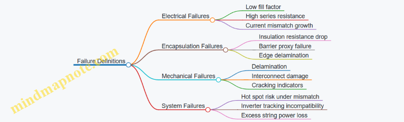
Mind Map: Failure Definitions That Prevent “Pass but Wrong”
Lock the Criteria with Traceability and Repeatability
Finally, acceptance criteria must be repeatable across labs and consistent across time. Specify calibration requirements for measurement equipment, define how you handle outliers, and require that test fixtures match the intended module geometry. When criteria are written this way, qualification becomes a controlled measurement exercise rather than a debate about what “good enough” means.
1.5 Translating Cell Level Metrics into Module Level Energy Yield Metrics
Cell metrics tell you how a device behaves under controlled conditions; module energy yield tells you what the same physics produces after optics, interconnects, encapsulation, temperature, and real-world soiling do their thing. The translation is not a single conversion factor—it’s a chain of adjustments that you can measure, model, and verify.
Start with What You Actually Measure at Cell Level
Begin with the cell’s electrical and optical inputs that will survive the journey to the module.
- Current capability: short-circuit current density (Jsc) and its spectral response. For tandem, also record how current matching changes with wavelength and angle.
- Voltage capability: open-circuit voltage (Voc) and how it shifts with temperature.
- Loss decomposition: series resistance (Rs), shunt resistance (Rsh), and fill factor (FF) drivers.
- Optical behavior: external quantum efficiency (EQE) and any angle-dependent response.
A practical best practice is to store these as functions, not single numbers: Jsc(λ), Voc(T), and FF(Rs, shunts). That makes later steps less hand-wavy.
Convert Cell Electrical Performance into Module Electrical Performance
Modules introduce three main electrical changes: area scaling, series interconnection, and bypass protection behavior.
-
Area and patterning
- If the cell area used in the module differs from the test cell area, scale current proportionally to active area, then re-check current density assumptions.
- If patterning reduces effective area or changes optical coupling, treat it as an optical loss term rather than an electrical one.
-
Series connection and current matching
- In a tandem, series operation already enforces current matching between subcells. In a module, additional series strings enforce matching across cells too.
- Use a “minimum current” rule at the string level: the string current is limited by the lowest-performing cell in the string under the operating spectrum.
-
Bypass diodes and partial shading
- Under uniform illumination, bypass diodes should be inactive; under partial shading, they change the effective circuit path.
- For yield modeling, represent bypass behavior with a simple rule set: when a cell group voltage drops below a threshold, bypass conducts and the group’s contribution changes.
A concrete example: if your cell-level tandem produces 28.0 mA/cm² at STC and your module string has 60 cells, a 2% current deficit in a subset of cells can reduce string current by roughly 2% for that operating condition, unless bypassing reroutes the current.
Translate Optical Response into Module-Level Irradiance Conversion
Optics changes in the module come from cover glass, encapsulant refractive effects, front-surface reflection, and any texture or scattering.
- Spectral conversion: module current is the integral of spectral irradiance times the module’s effective EQE.
- Optical loss budget: represent each optical element as a multiplicative factor on the cell EQE, such as T_glass(λ), T_encap(λ), and R_front(λ).
A simple calculation path:
- Compute cell current: Jsc_cell = ∫ E(λ)·EQE_cell(λ) dλ.
- Compute module current: Jsc_mod = ∫ E(λ)·EQE_cell(λ)·T_glass(λ)·T_encap(λ)·(1−R_front(λ)) dλ.
If you don’t have full spectral data, you can still do this with measured spectral response at the module level for a few representative conditions, then use those to calibrate the optical loss terms.
Incorporate Temperature Effects Without Guessing
Energy yield depends strongly on temperature because voltage drops with heat.
- Use a measured temperature coefficient of power or, better, Voc(T) and Rs(T) to compute P(T).
- For tandem modules, temperature affects both subcells, but the dominant effect is usually voltage-related.
Best practice: build a temperature model that maps irradiance and wind conditions to module temperature. Then compute IV curves at that temperature rather than applying a single blanket coefficient.
Example: if Voc drops by 0.25% per °C at the module level and the module runs 30°C above reference, that’s about a 7.5% voltage-related power reduction, before considering any temperature-dependent resistance changes.
Model Mismatch and Degradation of Yield Components
Module yield is sensitive to mismatch across cells and to performance drift.
- Mismatch: represent distributions of Jsc and Voc across cells. Even small spreads matter because series strings pick the minimum current.
- Degradation: treat it as a time-varying adjustment to cell-level parameters (often EQE and Voc). For yield translation, apply the degradation to the cell parameters first, then re-run the optical and electrical chain.
A practical approach is to separate “instantaneous yield” from “time-integrated yield.” Instantaneous uses current distributions and temperature; time-integrated applies parameter drift over the period of interest.
Validate the Translation with Module Measurements
Translation models should be checked against module-level data.
- Compare modeled and measured Pmax at multiple irradiance levels.
- Compare modeled and measured spectral response using controlled light sources or outdoor spectral proxies.
- Compare modeled and measured IV curve shape to ensure Rs and FF behavior are consistent.
If the model matches Pmax but not FF, you likely have the wrong electrical loss attribution. If it matches FF but not current, your optical terms or current matching assumptions are off.
Mind Map: Cell to Module Yield Translation
Example: A Systematic Mini-Workflow
- Take cell EQE(λ) and compute Jsc_cell under the site spectrum.
- Apply optical transmission and reflection terms to get Jsc_mod.
- Use Voc(T) and Rs(T) to compute module IV at the predicted module temperature.
- Apply series string current limiting using a measured or assumed distribution of cell currents.
- Apply bypass diode behavior for partial shading cases.
- Integrate Pmax over time using the site irradiance and temperature model.
This workflow keeps each assumption tied to a measurable parameter, so when results disagree, you know which link in the chain to inspect first.
2. Perovskite Silicon Tandem Device Fundamentals for System Engineers
2.1 Bandgap Selection and Current Matching in Practical Device Stacks
A tandem perovskite-silicon stack is only as good as its weakest electrical link. In practice, that means choosing a perovskite bandgap that produces a current close to the silicon bottom cell under the same optical conditions, then designing the stack so the two subcells actually operate near that matched point.
Foundational Idea: Current Matching Is an Optical-Electrical Constraint
In a series-connected tandem, the same current flows through both subcells. If the perovskite generates more current than silicon, the extra carriers cannot increase current; they mainly show up as reduced voltage and lower fill factor. If the perovskite generates less, it throttles the whole device. So “bandgap selection” is really “choose a bandgap that makes the perovskite’s usable photon flux align with the silicon’s usable photon flux.”
A practical way to think about it is to start with the incident spectrum and decide how much light each subcell can convert. The perovskite absorbs high-energy photons (above its bandgap), while silicon absorbs the remaining longer-wavelength photons. The perovskite’s bandgap sets the cutoff wavelength, which sets how much of the spectrum reaches silicon.
Step 1: Estimate Matched Current Using External Quantum Efficiency
Bandgap alone is not enough; real devices have wavelength-dependent losses. Use measured or modeled external quantum efficiency (EQE) for each subcell, then compute the tandem current under a reference spectrum (typically AM1.5G). The matched current is the minimum of the two subcell current integrals.
Easy example: Suppose a perovskite subcell EQE is high from 520–780 nm and drops sharply below 520 nm, while silicon EQE is strong from 650–1100 nm. If you pick a perovskite bandgap that cuts off around 750 nm, the overlap region where both could contribute becomes smaller. That reduces perovskite current and increases silicon’s share of photons, moving toward a match. If the cutoff is too short, silicon starves; if too long, perovskite dominates.
Step 2: Translate Bandgap Choice into a Cutoff Wavelength Window
A smaller bandgap shifts the perovskite cutoff to longer wavelengths, increasing perovskite current but reducing silicon current because more photons are absorbed before reaching silicon. A larger bandgap does the opposite. The “sweet spot” is where the two subcells’ current integrals cross.
Concrete rule of thumb for design iterations: treat bandgap as a knob that moves the perovskite cutoff, then re-check current matching after accounting for optical losses such as front contact absorption, reflection, and parasitic absorption in transport layers.
Step 3: Account for Practical Stack Effects That Break Ideal Matching
Even if the subcells match in isolation, the full stack can shift the balance.
- Optical parasitics: Transparent layers still absorb some light. If the perovskite stack has higher parasitic absorption than expected, its effective current drops.
- Spectral redistribution: Texturing and interference in multilayer stacks can change the local optical field, altering EQE shape.
- Voltage-dependent behavior: Current matching is about current, but the operating point depends on voltage. A design that matches at short circuit may not match at maximum power if one subcell’s recombination changes more strongly with bias.
Easy example: Imagine two perovskite compositions with similar bandgaps. One has slightly higher parasitic absorption in the transport layers. In isolation, it looks fine. In the tandem, its EQE curve is lower across the overlap region, so the tandem current becomes perovskite-limited even though the bandgap suggests otherwise.
Step 4: Use Thickness and Optical Management to Fine-Tune Matching
Bandgap sets the cutoff, but you can still tune the effective absorption profile.
- Perovskite thickness: Thicker layers absorb more near the band edge, increasing perovskite current but also increasing parasitic absorption and potentially affecting recombination.
- Front and rear reflectance: Adjusting reflectors and anti-reflection behavior can increase the number of photons that reach the perovskite or that are recycled into silicon.
- Interlayer absorption: Minimizing absorption in charge transport layers helps preserve the intended spectral split.
A practical workflow is to start with a bandgap that gives a near match, then adjust optical management so the tandem current stays matched across the intended operating conditions.
Mind Map: Bandgap Selection and Current Matching
Example: Diagnosing a Perovskite-Limited Tandem
You measure a tandem short-circuit current that is lower than expected from the perovskite bandgap choice. A systematic check:
- Compare perovskite EQE in the full stack versus in isolation. If the stacked EQE is reduced near the overlap region, optical parasitics or interface losses are likely.
- Check whether the silicon EQE in the stack increased as expected. If silicon EQE also drops, the issue may be broader optical loss or misalignment of the optical field.
- Verify that the perovskite cutoff is where you think it is by confirming the EQE roll-off wavelength. If it is shifted shorter, the effective bandgap may be larger than intended due to composition gradients or processing conditions.
The key point is that current matching is not a one-time calculation. It is a loop: choose bandgap, model with EQE, build the stack, measure EQE again, then adjust optical and recombination-related factors until the tandem current is limited by neither subcell.
2.2 Charge Transport Layers and Their Implications for Module Reliability
Charge transport layers sit between the perovskite absorber and the electrodes. In a tandem module, they do more than “help electrons and holes move.” They also control where recombination happens, how electric fields distribute, and how the stack tolerates heat, moisture, and mechanical stress. If you treat them like passive coatings, reliability will eventually correct your optimism.
Foundational Roles in a Tandem Stack
A perovskite-silicon tandem typically uses a series connection, so the top cell must deliver current efficiently while keeping losses low. Charge transport layers (CTLs) support this by:
- Selecting carriers: Electron transport layers favor electrons; hole transport layers favor holes.
- Reducing interfacial recombination: Better energy alignment and surface passivation reduce “short-circuit” pathways.
- Forming stable interfaces: The CTL must remain chemically and structurally compatible with both the perovskite and the adjacent electrode.
A practical way to think about reliability is to track three failure pathways: chemical degradation at interfaces, electrical degradation from field-driven processes, and mechanical degradation from swelling or delamination.
Energy Alignment and Recombination Control
Even small energy mismatches can increase recombination. In operation, the CTLs experience carrier injection and extraction under bias, so any barrier at the interface becomes a hotspot for non-radiative loss.
Easy example: Imagine a hole transport layer with slightly too deep a valence band. Holes then face a barrier at the perovskite interface, increasing the probability that electrons and holes meet and recombine. In a module, that shows up as reduced fill factor and a faster performance drop under stress, because the interface keeps “working harder” to move carriers.
Reliability implication: recombination-heavy interfaces tend to generate more local heating and accelerate chemical reactions, especially when moisture is present.
Interfacial Passivation and Ion Management
Perovskites can exchange ions and defects at interfaces. CTLs influence this by providing surfaces that either trap ions harmlessly or allow them to migrate toward electrodes.
Easy example: If a hole transport layer surface has poor passivation, mobile ions can accumulate near the interface. Over time, this can create local electric fields that promote further ion migration and degrade the perovskite/CTL contact.
Best practice: design CTLs so they both passivate defects and limit pathways for ion accumulation. In module qualification, this is reflected in how stable the CTL/perovskite interface remains after damp heat and thermal cycling.
Transport Properties and Field Distribution
CTLs must balance conductivity and selectivity. Too resistive, and the stack develops larger voltage drops across the CTL, increasing local electric fields. Too conductive without selectivity, and carriers leak, raising recombination.
Easy example: A slightly thicker electron transport layer can lower pinhole risk, but if it increases series resistance, the tandem current may become limited under real operating conditions. The module may still pass a quick lab measurement, then under field temperature and irradiance, the extra resistance shows up as reduced energy yield and higher stress.
Reliability implication: field concentration accelerates interfacial reactions and can worsen barrier formation over time.
Moisture and Oxygen Sensitivity at Interfaces
Many CTL materials are sensitive to moisture or oxygen, either directly or through reactions that form insulating or corrosive species. Even if the encapsulation is strong, micro-leaks, edge exposure, and permeation can bring small amounts of water to the stack.
Easy example: If a CTL absorbs moisture and changes its conductivity, the interface becomes less selective. That increases recombination and can shift the operating point, which then stresses the perovskite more aggressively.
Best practice: choose CTL chemistries and processing conditions that minimize residual solvents and avoid leaving reactive byproducts at interfaces. Reliability testing should include checks that performance loss correlates with interface degradation rather than only bulk perovskite changes.
Mechanical Compatibility and Delamination Risk
CTLs are thin, but they still experience strain from thermal expansion mismatch and from lamination pressure. If the CTL forms a weak interfacial bond, cycling can create micro-gaps that increase local resistance.
Easy example: A CTL that shrinks unevenly during drying can leave regions with poor contact. Under thermal cycling, those regions can become electrical bottlenecks, producing localized heating during operation.
Reliability implication: mechanical failure often appears electrically first—through rising series resistance or abnormal current-voltage behavior—before it becomes visible.
Mind Map: Charge Transport Layers to Reliability Links
Integrated Example Workflow for Reliability Diagnosis
When a tandem module shows performance decay, a systematic CTL-focused diagnosis helps avoid guesswork:
- Compare electrical signatures: If fill factor drops faster than current, suspect interfacial recombination or transport resistance changes.
- Check bias sensitivity: If degradation accelerates under higher bias, field-driven processes at CTL interfaces are likely.
- Correlate with environmental tests: Strong damp-heat correlation points toward moisture-related CTL or interface chemistry.
- Use microscopy where possible: Look for edge-related contact loss or signs of micro-gaps that would increase local resistance.
This approach keeps the story consistent: CTLs control interfaces, interfaces control recombination and fields, and those determine how the module responds to heat, moisture, and stress.
2.3 Interconnection Strategies for Series Tandem Operation
Series tandem operation means the same current must flow through both subcells, because they are electrically in series. That single constraint drives most interconnection choices: how you connect, how you route current, and how you manage mismatch and defects. In practice, you’re building a system that must behave predictably even when parts of the module are slightly different, slightly shaded, or slightly imperfect.
Foundational Principle of Series Current Matching
Start with the current-limiting step. Under a given spectrum and irradiance, the top subcell and bottom subcell each generate a current; the smaller one sets the series current. A useful mental model is to treat the tandem as a “current bottleneck.” Interconnection design should therefore minimize additional current losses that would otherwise reduce the already-limited current.
A simple example: if the top subcell can supply 18 mA/cm² and the bottom can supply 16 mA/cm² at a target condition, the series current is about 16 mA/cm². If your interconnect adds 1% extra resistive loss, the effective current at the operating voltage drops further, and the fill factor suffers. That’s why interconnection is not just wiring; it’s part of the electrical performance.
Interconnection Layout Options
Interconnection strategies usually fall into three practical categories.
-
Monolithic series connection: the subcells are connected through patterned interlayers so the series path is built into the device stack. This can reduce external wiring complexity, but it makes interlayer integrity and patterning yield critical.
-
Module-level series connection: each tandem cell is fabricated as a unit, then cells are connected in series across the module. This is common for manufacturability and testing, but it introduces more opportunities for mismatch due to cell-to-cell variation.
-
Hybrid approaches: partial monolithic features combined with module-level series routing. These can reduce the number of critical series interfaces while keeping layout manageable.
A practical rule of thumb: choose the approach that keeps the number of “high-risk” interfaces low while still allowing you to test and isolate faults.
Series Connection Implementation Details
Series interconnection requires two things: low resistance where current flows, and reliable insulation where it does not.
Low-resistance current paths
- Use conductive layers and contacts sized to keep voltage drop small at the expected current.
- Ensure uniform contact quality across the active area. A tiny contact defect can behave like a local current choke, which then forces current to redistribute through neighboring regions.
Insulation and isolation
- Maintain clean separation between adjacent conductive paths to prevent leakage.
- Plan for edge effects. Current crowding near busbars and cut lines can increase local heating, especially under partial shading.
Concrete example: imagine two adjacent series strings within a module. If one string has a slightly higher resistance due to a poorer contact, it will run at a slightly different current distribution. Under mismatch conditions, that difference can amplify into measurable performance loss.
Managing Mismatch and Partial Shading
Series tandems are sensitive to mismatch because current is shared. Interconnection design can reduce the impact of mismatch by controlling how current is distributed.
Stringing strategy
- Use consistent cell orientation and similar optical exposure within a string.
- Avoid mixing cells with very different expected irradiance profiles in the same series path.
Bypass protection
- Bypass elements are typically placed so that if a section becomes electrically inactive, current can route around it.
- The key is to define bypass regions that align with realistic failure modes, not with arbitrary layout boundaries.
Example: if a module is divided into two electrical sections, and the top subcell in one section degrades faster due to local moisture exposure, bypassing that section prevents the entire series string from being dragged down.
Reliability-Oriented Interconnection Practices
Interconnection choices affect failure modes.
- Thermal cycling: resistive contacts expand and contract. If the contact stack is too rigid or too thin, microcracks can form and increase resistance over time.
- Moisture ingress: even if the encapsulant is good, edges and interfaces are where trouble starts. Interconnect routing should avoid creating hard-to-seal geometries.
- Hot spot risk: series operation can concentrate current around a defect. Design current paths so that a localized defect does not force excessive current density elsewhere.
A practical example for quality control: measure resistance of each interconnect region before final lamination and again after. If the post-lamination resistance shift is larger than your tolerance, you likely have a mechanical or interfacial issue that will worsen under field cycling.
Mind Map: Series Tandem Interconnection
Worked Example: Choosing a Series Layout
Suppose you have a module with 10 tandem cells in series. You expect some shading from a nearby structure that affects only the left half of the module during morning hours.
- If all cells are in one long series string, the shaded cells limit current for the entire module.
- If you split the module into two series sections that share the same electrical rating and add bypass elements per section, the unshaded section can still contribute when the shaded section is current-limited.
The interconnection strategy here is not about adding complexity for its own sake. It’s about aligning the electrical segmentation with the dominant mismatch pattern so the series constraint doesn’t unnecessarily dominate the output.
2.4 Optical Management Using Texturing and Spectral Splitting Considerations
Optical management in perovskite-silicon tandems is about controlling where photons go, how they travel, and how much of the spectrum each subcell actually receives. In a series-connected tandem, current matching is unforgiving: if the perovskite layer absorbs too much or too little in the wrong wavelengths, the whole device is limited by the weaker subcell. The goal is therefore not just “high absorption,” but absorption that is spectrally and spatially well-behaved.
Foundational Concepts for Optical Allocation
Start with the basic chain: incident spectrum → front-surface reflection and transmission → absorption in perovskite → transmission to silicon → absorption in silicon → carrier collection. Each step has knobs.
- Front-surface optics set how many photons enter the stack. Texturing can reduce reflection and increase the optical path length, but it can also change angular response, which matters for real-world incidence angles.
- Spectral splitting is the deliberate partition of the spectrum between subcells. In practice, the perovskite’s bandgap and absorption coefficient define the natural split, while optical design shapes the effective split by altering field distribution and parasitic absorption.
- Spatial uniformity matters because local optical variations create local current variations. In series tandems, those variations translate into fill factor loss and sometimes premature failure under stress.
Texturing as a Practical Path-Length and Reflection Tool
Texturing is typically applied to the front side (or within the optical stack) to reduce reflection and increase effective optical path length. A useful way to think about it is: texture turns specular reflection into a mix of angles, and those angles increase the chance that photons are absorbed rather than reflected.
Best-practice example: texture pitch matched to wavelength scale. If the texture features are much smaller than the dominant wavelengths, the surface behaves more like a smooth layer and reflection reduction is limited. If features are much larger, scattering can become too strong, increasing haze and potentially reducing collection efficiency. A practical approach is to target feature sizes that are on the order of the relevant wavelengths in the perovskite absorption band, then verify with angle-resolved measurements.
What to measure. Use reflectance and external quantum efficiency (EQE) versus incidence angle. If the EQE peak shifts or the perovskite-to-silicon current ratio drifts with angle, the texture is altering the spectral allocation more than intended.
Spectral Splitting with Optical Stack Design
Spectral splitting is influenced by how the optical field is distributed across layers. Thin-film interference effects can enhance absorption in one region while suppressing it in another. In tandems, the “right” interference pattern is the one that supports current matching across the operating spectrum.
Best-practice example: controlling parasitic absorption in transport layers. Transport layers and electrodes can absorb light without generating useful carriers. If their absorption overlaps strongly with the perovskite’s intended absorption range, the perovskite receives less usable current. A simple diagnostic is to compare measured EQE with a model that includes layer absorption; if the model shows unexpected losses in non-active layers, adjust thicknesses or optical constants in the stack design.
Managing Angular Response and Current Matching
Real installations rarely see normal incidence only. Optical design must keep the perovskite and silicon subcell currents aligned across angles.
Best-practice example: check current matching at multiple angles, not just STC. Compute or measure the perovskite-limited and silicon-limited current densities under representative angle distributions. If current matching is only achieved at one angle, the tandem will show a fill factor penalty and power variability.
A practical workflow is:
- Measure angle-resolved reflectance.
- Measure or model EQE spectra for both subcells.
- Integrate each subcell’s effective current over the expected angle-weighted spectrum.
- Adjust texture parameters or optical thicknesses to reduce the spread.
Mind Map: Optical Management Logic
Example: A Systematic Tuning Sequence
Suppose initial measurements show strong perovskite absorption but silicon current is lower than expected, limiting the tandem. The first suspect is not always the perovskite bandgap; it can be optical losses before photons reach silicon.
- Confirm front reflection behavior. Compare measured reflectance to a smooth-surface baseline. If reflection is still high, texture may be insufficient or poorly matched.
- Check transmission into silicon. Use EQE of silicon and infer whether transmission is reduced across the silicon-relevant wavelengths.
- Inspect parasitic absorption. If transport layers or electrodes absorb in the transmitted band, reduce their optical thickness or adjust materials with lower extinction coefficients.
- Rebalance spectral allocation. Adjust optical thicknesses to shift interference so that more field energy resides in the silicon-absorbing region.
- Re-test angle dependence. If the fix improves normal incidence but worsens oblique angles, the texture or interference condition is too angle-sensitive.
This sequence keeps the reasoning grounded: each step targets a specific part of the optical chain, and each measurement tells you which knob to turn next.
2.5 Failure Mechanisms at the Device Level That Propagate to Modules
Device-level failures in perovskite-silicon tandems rarely stay politely inside the cell. They change local electrical behavior, create chemical pathways, and stress interfaces. The module then “inherits” the problem through series interconnection, encapsulation constraints, and optical and thermal coupling.
Start with What “Propagation” Means in Series Tandems
In a series tandem, the current is limited by the weakest subcell at each operating condition. A device defect that reduces local current or increases local resistance can become a module-level loss even if most of the area is fine. Propagation typically happens through three routes: (1) electrical mismatch and hot spots, (2) interfacial degradation that spreads laterally, and (3) moisture or ion transport that accelerates once a barrier is locally compromised.
Easy example: Imagine a small perovskite region with higher recombination. Under load, that region draws less current, so the series current is reduced across the entire cell area. The module output drops more than you’d expect from the defect’s physical size.
Recombination and Interface Degradation
Perovskite stacks include multiple interfaces where charge transfer must be both fast and selective. Failures that increase recombination—such as imperfect passivation, interlayer chemical reactions, or energy level misalignment—reduce the top-cell current and fill factor.
At the module level, this shows up as:
- Lower current at standard test conditions.
- Reduced fill factor that worsens under higher irradiance or temperature.
- Greater sensitivity to bias and light history.
Easy example: If the hole transport layer partially degrades, the top cell’s voltage may collapse slightly. In series, the silicon bottom cell still tries to deliver its current, but the tandem current is capped by the top cell, so the module underperforms across the whole string.
Ion Migration and Local Chemical Changes
Mobile ions can drift under electric fields and illumination. Even if the average device looks stable, ions can accumulate near interfaces, changing local composition and creating nonuniform recombination sites.
Propagation mechanisms include:
- Formation of “soft” shunts that grow with bias cycling.
- Increased leakage current that heats the local region.
- Chemical weakening of adjacent layers, making later moisture ingress more damaging.
Easy example: A tiny region becomes more conductive over time. During operation, that region draws disproportionate current, raising local temperature. The module then experiences a hot spot, which accelerates encapsulant stress and interface breakdown.
Shunts and Microcracks That Become Electrical Faults
Microcracks can originate from thermal expansion mismatch, mechanical handling, or lamination stress. In tandems, cracks can interrupt current paths or create conductive bridges if debris or ion-rich material fills the gap.
Module-level outcomes:
- Increased leakage and reduced shunt resistance.
- Nonlinear current-voltage behavior and early knee formation.
- Hot spot risk when bypass paths are absent or insufficient.
Easy example: A crack that slightly increases series resistance may look tolerable at low current. Under full sun, the voltage drop concentrates, and the module’s electrical protection may trigger earlier or the cell may heat enough to worsen the crack.
Optical and Thermal Feedback Loops
Device failures can alter optical absorption or scattering. A degraded perovskite region may absorb less light or change the refractive index locally. That changes how light reaches the silicon subcell and how heat is generated.
Propagation effects:
- Local temperature rise that accelerates ion migration.
- Increased thermal gradients that stress encapsulation and interfaces.
- Bias-dependent performance shifts that complicate acceptance testing.
Easy example: If a small area loses optical quality, it can reduce top-cell current there. The series current then limits the whole device, and the reduced current can shift the operating point so the silicon subcell runs at a different voltage, changing stress distribution.
Encapsulation-Adjacent Failures That Start at the Device
Even with good encapsulation, device-level defects can create pathways. For instance, pinholes, edge defects, or poor interlayer adhesion can allow moisture or oxygen to reach sensitive interfaces. Once chemistry changes, the failure can spread beyond the original defect.
Module-level signs:
- Gradual performance drift rather than an abrupt step change.
- Strong dependence on edge quality and lamination uniformity.
- Reliability test failures that correlate with early device-level anomalies.
Easy example: A small edge delamination at the cell level lets humidity reach the perovskite interface. The module then shows a slow decline in voltage and fill factor, even if the center area remains intact.
Mind Map of Device-to-Module Failure Propagation
Mind Map: Device-Level Failures That Propagate to Modules
Practical Diagnostic Logic for Engineers
A systematic way to connect device symptoms to module outcomes is to ask three questions in order: (1) Is the loss primarily current-limited or voltage-limited? (2) Does the behavior change with bias history or temperature? (3) Is the spatial pattern consistent with cracks, shunts, or edge-driven ingress?
Easy example: If the module shows a strong bias-history effect and gradual drift, ion migration or encapsulation-adjacent chemistry is a likely root. If the module shows abrupt knee behavior and localized heating, shunts or crack-related conductive paths are more likely.
3. Module Architecture and Encapsulation for Tandem Stability
3.1 Choosing Encapsulation Materials and Barrier Performance Requirements
Encapsulation in tandem modules is less about “sealing everything forever” and more about slowing down the specific ways moisture and oxygen ruin perovskite layers. A useful starting point is to treat the encapsulation stack as a set of barriers with measurable transmission rates, then connect those rates to the module’s expected operating conditions and lifetime targets.
Foundational Barrier Concepts
Barrier performance is usually described by transmission through the encapsulant: water vapor transmission rate and oxygen transmission rate. Lower transmission means fewer molecules reach the perovskite interface, which reduces ion migration and chemical reactions that create nonradiative recombination. In practice, you also care about how the barrier behaves after lamination, because heat and pressure can create microvoids or stress that later becomes a leak path.
A second concept is that barriers fail at defects, not in the average case. A tiny pinhole in a polymer layer can dominate the effective transmission. That’s why barrier requirements should include both bulk properties and defect tolerance, with inspection methods aligned to the failure modes you’re trying to prevent.
Material Selection Logic for Tandem Modules
Most tandem module stacks combine glass and polymer films. Glass typically provides excellent barrier performance, especially for water vapor, and it resists puncture better than many films. Polymer encapsulants can offer optical and mechanical benefits, but they must be chosen for low permeability, stable adhesion, and controlled outgassing during lamination.
When selecting materials, map each layer to a job:
- Front barrier layer: protects against environmental ingress and supports optical transmission.
- Interlayer encapsulant: provides adhesion and stress buffering between rigid components.
- Back barrier layer: completes the moisture and oxygen blocking path and supports electrical insulation.
A practical rule: if you can’t measure the barrier property for the exact formulation and thickness you will laminate, you can’t responsibly set a requirement. “Same family of material” is not a performance spec.
Barrier Performance Requirements That Actually Matter
Set requirements in terms of transmission rate and allowable defect density, then translate them into module-level risk. For example, if the encapsulant has a higher water vapor transmission rate, the module becomes more sensitive to edge sealing quality and to any microcracks that expose the periphery to humid air.
Also specify performance after processing. A material that looks good in a coupon test can degrade after lamination if it absorbs moisture, releases volatiles, or forms weak interfaces. Therefore, define acceptance criteria for:
- Pre-lamination properties: baseline transmission and optical clarity.
- Post-lamination properties: transmission after thermal exposure and adhesion integrity.
- Edge and seal performance: barrier continuity at the perimeter where ingress often starts.
Integrated Mind Map
Mind Map: Encapsulation Materials and Barrier Requirements
Concrete Examples of Requirement Setting
Example 1: Polymer Encapsulant Thickness Tradeoff If you increase encapsulant thickness to improve mechanical compliance, you might reduce defect-driven leakage but also increase residual stress and risk of interfacial debonding. A better approach is to keep thickness within a validated window and focus on controlling void formation during lamination. In qualification, compare transmission and adhesion before and after the same lamination profile used in production.
Example 2: Edge Seal as the Real Bottleneck Even with excellent bulk barrier performance, ingress often starts at the module perimeter. Suppose two encapsulant formulations have similar bulk water vapor transmission rates, but one produces a more consistent edge seal under the same sealant chemistry and cure profile. The module with the more reliable edge seal will typically show better stability because it reduces the number of pathways that bypass the bulk barrier.
Example 3: Optical Clarity vs Barrier Integrity Optical transmission matters because tandem current depends on how much light reaches the perovskite and silicon subcells. However, chasing maximum optical clarity by using a highly plasticized polymer can raise permeability. The integrated requirement is therefore a combined spec: optical transmission within a defined range and barrier transmission within a defined range, both measured on the final laminated stack.
Practical Acceptance Testing Strategy
To keep requirements grounded, align tests to the failure modes:
- Use transmission measurements on laminated coupons, not only raw films.
- Include adhesion checks after environmental preconditioning that mimics moisture exposure.
- Verify edge seal continuity with inspection methods that can detect discontinuities.
A module that passes bulk transmission tests but fails edge continuity is like a door with a great lock and a loose frame. The barrier stack is only as good as its weakest path.
3.2 Designing Glass Glass and Glass Backsheet Module Stacks for Tandems
A tandem module stack is a layered system that has to do three jobs at once: pass light to the right place, protect sensitive layers from moisture and oxygen, and survive heat, humidity, and mechanical stress. For perovskite silicon tandems, the “right place” is especially strict because the perovskite top cell is both optically selective and chemically fragile. The stack design therefore starts with optical intent, then locks in barrier performance, and only then addresses mechanical and electrical integration.
Foundational Stack Roles and Constraints
Begin by assigning each layer a clear function:
- Front cover glass: provides optical transmission, mechanical strength, and a first moisture barrier.
- Front encapsulant: bonds layers while limiting water vapor transmission.
- Tandem active stack: perovskite top cell and silicon bottom cell with their interconnects.
- Interlayer and series interconnect region: must avoid creating optical dead zones and must tolerate thermal cycling.
- Back encapsulation and backsheet or back glass: completes the barrier system and supports lamination.
- Back contact and electrical layout: must avoid corrosion paths and reduce hot-spot risk.
A practical constraint is that lamination pressure and temperature must be compatible with both the encapsulant chemistry and the perovskite stack. If the encapsulant softens too much, it can allow microvoids that later become moisture highways. If it does not flow enough, you get poor wetting and local delamination that shows up as performance drift.
Glass Glass Stack Design for Tandems
A glass glass module uses glass on both sides. This typically simplifies barrier strategy because the outer surfaces are already rigid and chemically stable.
Key design choices:
- Front glass selection: choose a glass type with stable transmission in the wavelengths used by the tandem. Also consider edge finish quality, because edge seals are where moisture often wins.
- Barrier encapsulant system: use encapsulants designed for low water vapor transmission and good adhesion to both glass and the cell stack. A common mistake is treating encapsulant as “just glue”; in tandems it is part of the barrier.
- Back glass and edge sealing: ensure the back glass and edge seal materials have compatible thermal expansion. If they don’t, cycling can open microscopic gaps.
- Optical management: keep refractive index transitions smooth. Rough interfaces can scatter light and reduce current matching, especially when the tandem is already sensitive to spectral balance.
Example: If you observe a consistent reduction in top-cell current after damp heat, inspect edge seal integrity and encapsulant void density near the perimeter. In many cases the center looks fine because moisture ingress starts at edges and then spreads.
Glass Backsheet Stack Design for Tandems
A glass backsheet module uses glass on the front and a polymer backsheet on the rear. This can reduce weight and cost, but the rear barrier must be engineered carefully.
Key design choices:
- Backsheet barrier layers: the backsheet is not one material; it is a stack of polymer and barrier films. The effective barrier depends on film continuity and lamination quality.
- Adhesion and wetting: polymer backsheets require encapsulant wetting that is uniform across the cell area. Poor wetting creates channels for moisture.
- Thermal expansion matching: polymer backsheets expand more than glass. Design the edge seal and encapsulant thickness to reduce stress concentration.
- Electrical corrosion control: ensure that any exposed conductor edges are sealed so that humidity cannot reach metal surfaces.
Example: If insulation resistance drops after thermal cycling, check whether the rear encapsulation has microcracks or delamination near string interconnect regions. Those are common paths for moisture to reach conductive traces.
Layer Stack Layouts and Decision Logic
Use a decision flow that starts with barrier needs and ends with mechanical feasibility.
graph TD
A[Define tandem sensitivity] --> B[Set barrier target for moisture and oxygen]
B --> C{Choose module type}
C -->|Glass glass| D[Use front and back glass with edge seal focus]
C -->|Glass backsheet| E[Use rear barrier backsheet with wetting focus]
D --> F[Select encapsulant system and thickness]
E --> F
F --> G[Design optical interfaces and avoid dead zones]
G --> H[Plan lamination pressure temperature and cure]
H --> I[Verify mechanical stress distribution]
I --> J[Validate electrical isolation and series interconnect integrity]
Mind Map: For Stack Design Considerations
Practical Verification Steps That Connect Design to Outcomes
After selecting the stack, verify it with tests that map to the failure modes you designed against:
- Moisture barrier checks: look for early signs of edge-driven ingress by comparing perimeter regions to the center.
- Lamination quality: use cross-sectional inspection to confirm encapsulant coverage and absence of voids at the interconnect region.
- Optical consistency: confirm that the stack does not add unexpected absorption or scattering that shifts current matching.
- Electrical isolation: track insulation resistance and leakage trends through thermal and humidity stress.
Example: If a glass backsheet module shows faster performance drift than a glass glass module under the same stress profile, the most common culprits are rear barrier film defects or encapsulant wetting gaps near the perimeter and interconnect zones, not the cell itself.
3.3 Managing Moisture Oxygen and Ion Migration Risks in Encapsulated Modules
Moisture, oxygen, and mobile ions are the three troublemakers that tend to travel through encapsulated tandem modules even when the device stack looks sealed. The goal of this section is not “perfect sealing,” but predictable barriers, measurable ingress, and controlled ion mobility so that performance loss stays slow and diagnosable.
Foundational Concepts That Drive Barrier Design
Moisture ingress matters because perovskite and adjacent interfaces can react with water, leading to chemical changes and increased nonradiative recombination. Oxygen ingress can accelerate oxidation of sensitive transport layers and metal interfaces. Ion migration matters because even trace mobile species can move under electric fields, creating local compositional changes and shunting pathways.
A useful mental model is to separate three pathways:
- Diffusion through barriers: molecules move by concentration gradients.
- Permeation through defects: pinholes, microcracks, and edge gaps act like shortcuts.
- Transport along interfaces: moisture or ions can follow delamination-prone regions.
This is why barrier performance is not just a material property; it is a system property that includes edge sealing, lamination quality, and adhesion.
Moisture and Oxygen Control in Encapsulated Stacks
Start with barrier requirements expressed as “what must not happen” at the device level. For example, if your acceptance criteria require that the module maintains stable current and voltage after damp heat exposure, then your encapsulation must limit both water uptake and oxygen availability at the perovskite interface.
Practical best practices
- Use a layered barrier strategy: combine low-permeability films with robust edge sealing. A single barrier layer rarely covers all failure modes.
- Engineer the edge seal geometry: moisture often enters at edges where stress concentrates. A wider seal land and consistent seal thickness reduce the chance of microgaps.
- Control lamination voids: trapped air pockets can become diffusion highways. Vacuum quality and wetting behavior during lamination should be treated as critical process parameters.
- Verify barrier integrity with targeted tests: measure water vapor transmission behavior indirectly through accelerated exposure and track performance drift, not just material datasheet values.
Easy example: If two module designs use the same barrier film but one has a thinner edge seal, the thinner one typically shows faster performance decline after damp heat because ingress concentrates at the perimeter. The device stack may be identical, but the system barrier is not.
Ion Migration Risk Management Under Real Operating Conditions
Ion migration is driven by electric fields, temperature, and the presence of mobile ionic species. In encapsulated modules, ions can originate from:
- Residual salts or impurities in precursor-related materials
- Metal diffusion or corrosion products
- Encapsulant additives that contain mobile ions
Practical best practices
- Minimize ionic contamination early: implement cleaning and process controls that reduce salt carryover into interlayers.
- Choose interlayers that block ion pathways: interfaces should be designed to reduce contact between mobile ions and the active stack.
- Avoid creating high-field hotspots: series-connected tandem layouts can concentrate fields near defects. Layout and contact design should distribute current more evenly.
- Use electrical stress tests to reveal migration: monitor changes in leakage current and shunt behavior during controlled bias and temperature conditions.
Easy example: A module that shows stable initial efficiency but develops increasing leakage current after bias-temperature exposure likely has ion mobility issues. The encapsulation may be “dry enough,” but ions are still moving and creating conductive paths.
Systematic Failure Modes and How to Detect Them
Moisture, oxygen, and ions often overlap, so detection should be systematic.
- Moisture-dominant signatures: gradual loss of voltage with increased recombination, often correlated with edge damage or lamination voids.
- Oxygen-dominant signatures: changes that align with oxidation-sensitive interfaces, sometimes showing faster degradation at higher temperatures.
- Ion-migration signatures: emergence of shunts, increased leakage current, and localized performance collapse under bias.
A good diagnostic workflow starts with module-level electrical trends, then narrows to encapsulation integrity and finally to device stack evidence.
Mind Map: Encapsulation Risks and Controls
Integrated Example: Turning Risks into Acceptance Criteria
Suppose your module qualification includes damp heat and bias-temperature steps. You can translate the above risks into measurable acceptance criteria:
- Damp heat: require limited efficiency drop and stable voltage trend, which indirectly constrains moisture and oxygen ingress.
- Bias-temperature: require controlled leakage current growth and no emergence of severe shunts, which constrains ion migration.
- Encapsulation checks: require consistent edge seal quality and low void fraction, which constrains diffusion shortcuts.
This approach keeps the encapsulation strategy tied to what matters at the module output, while still giving you actionable levers when something fails.
3.4 Thermal and Mechanical Design Considerations for Laminated Tandem Modules
Laminated tandem modules are a stack of materials that must survive heat, pressure, moisture exposure, and bending—while keeping electrical paths stable. The design job is to make the stack behave predictably under stress, not to make every layer perfectly happy. In practice, you design for the weakest link and for how stresses redistribute when the module flexes.
Thermal Design Foundations for Laminated Stacks
Start with the temperature story. During lamination and later in the field, the module experiences temperature gradients across the stack. Those gradients create differential expansion between glass, encapsulant, interlayers, and the active device layers. Even if the average temperature is within limits, local hot spots can occur near current flow paths or in regions with slightly different optical absorption.
A practical best practice is to treat thermal design as a chain of interfaces. For each interface, ask: what is the thermal resistance, what is the mechanical compliance, and what is the failure mode if the interface debonds? For example, if an encapsulant layer is too stiff, it can transfer stress into the device stack during thermal cycling. If it is too soft, it may allow excessive creep, changing alignment and increasing the chance of microcracks.
Next, define a temperature operating envelope for the module. Use it to set acceptance criteria for lamination cure and for post-lamination handling. A simple example: if your encapsulant requires a cure profile that peaks at 140°C, then your mechanical design must assume that the stack is temporarily at that temperature while pressure is applied. That pressure can compress layers unevenly if the tooling is not flat, leading to thickness variation that later becomes a stress concentrator.
Mechanical Design Foundations for Laminated Stacks
Mechanical stress in laminated modules comes from bending, wind loading, snow loading, and handling during installation. The key mechanical concept is strain distribution. The outer glass carries most bending stiffness, while the encapsulant and device layers experience shear and tensile/compressive strains depending on curvature.
A useful rule of thumb is to design the stack so that the encapsulant can accommodate strain without transferring large shear into the brittle device layers. That means selecting encapsulant modulus and thickness to reduce peak strain at the perovskite-silicon interface region. As a concrete example, if two designs have the same total encapsulant thickness but one places more of it near the device stack, the latter typically reduces strain peaks in the active layers because the compliant region is closer to where strain would otherwise concentrate.
Also consider edge effects. Module edges see higher stress due to constraints from frames, seals, and layup termination. If the edge seal is too rigid relative to the laminate, the stack can experience peel stresses during thermal expansion mismatch. A practical mitigation is to ensure the edge region has a controlled transition in stiffness, often by using a sealant system and layup geometry that avoids abrupt changes.
Interface Engineering for Stress Management
Interfaces are where thermal and mechanical design meet. Three interface failure modes show up repeatedly: debonding, interlayer cracking, and delamination propagation.
To reduce debonding, ensure surface energy and cleanliness are controlled before lamination. A simple example: if a glass surface has residues from cleaning, the encapsulant may wet poorly, creating voids. Those voids act like thermal insulation pockets, increasing local temperature during operation and raising the chance of mechanical separation under cycling.
To reduce cracking, manage thickness uniformity. Thickness variation creates local stiffness differences, which concentrate strain. Inline metrology for thickness and void detection supports this: if you see a recurring pattern of thicker regions near a squeegee path, you can adjust tooling or layup speed rather than blaming the device.
Lamination Process Windows and Mechanical Consequences
Lamination is not just a curing step; it is a mechanical shaping step. Pressure and temperature determine how the encapsulant flows and how voids are removed. If pressure is too low, trapped air remains; if too high, you can squeeze out material and create thin spots.
A systematic approach is to define a process window around three measurable outputs: final encapsulant thickness, void fraction, and warpage after cool-down. For example, if void fraction is acceptable but warpage exceeds limits, you likely have uneven cooling or non-uniform tooling contact. If warpage is fine but thickness is non-uniform, adjust layup alignment and flow behavior.
Mechanical Qualification and Design Verification
Qualification should mirror the stress types you designed for. Use a test matrix that includes thermal cycling and mechanical loading, but interpret results through the lens of stress transfer. If performance drops after cycling, correlate it with mechanical indicators like microcrack signatures or delamination evidence.
A practical example of integrated verification: after thermal cycling, perform electroluminescence mapping and compare it to pre-cycling maps. If crack patterns align with regions of higher thickness variation or edge constraints, you have a direct path to corrective action: improve layup uniformity or adjust edge stiffness transition.
Mind Map: Thermal and Mechanical Design Considerations
Example: Diagnosing a Post-Cycling Performance Drop
Suppose a batch shows reduced output after thermal cycling, while initial flash tests were fine. First, check for thickness variation and void indicators from lamination records. Next, inspect edge regions for signs of peel or delamination initiation. Finally, compare electroluminescence maps to pre-cycling maps. If cracks cluster near areas with known thickness non-uniformity, the corrective action is mechanical: tighten layup alignment, adjust pressure profile, and improve tooling flatness so the encapsulant flow is uniform.
The overall design principle is consistent: control temperature and pressure during lamination, manage stiffness transitions across the stack, and verify stress transfer with tests that match the real loading and cycling conditions.
3.5 Electrical Layout and Bypass Protection for Series Connected Tandem Cells
Series-connected tandem modules behave like a chain: the weakest illuminated segment sets the current. That’s fine when all cells see similar light, but it gets messy with partial shading, local defects, or non-uniform optical coupling. Electrical layout and bypass protection are the tools that keep the module from turning into a hot resistor when one cell (or a group of cells) can’t supply the matched current.
Foundational Concepts for Series Tandem Layout
Start with the current-matching reality. In a tandem, the top and bottom subcells are series-connected inside the device stack, so the device current is limited by the lower-current subcell under the local spectrum. At the module level, you then series-connect multiple tandem devices. If one tandem device experiences reduced irradiance or a spectrum shift, its current capability drops, and the string current is forced through it.
A bypass element provides an alternate path so the string current can flow without forcing the underperforming device to dissipate power as heat. The goal is not to “fix” the lost current; it’s to prevent excessive voltage drop and thermal stress.
Electrical Layout Principles That Reduce Stress
1) Minimize resistive losses in the current path. Use low-resistance interconnects and short bus routing between tandem devices. In practice, layout decisions that reduce series resistance also reduce localized heating during mismatch.
2) Keep current collection symmetric where possible. If one side of a cell string has longer routing, it can create uneven voltage distribution. Uneven distribution increases the chance that bypass activation happens earlier in one region than another.
3) Place bypass elements to match the physical mismatch scale. If shading or defect risk is localized to a few devices, bypassing a small group limits the area that can be forced into bypass. If you bypass too many devices together, you lose more power than necessary.
4) Design for predictable activation. Bypass diodes should turn on at a voltage that corresponds to a realistic mismatch condition, not during normal operation. That means selecting diode type and rating consistent with the module’s maximum system voltage and expected string currents.
Bypass Protection Architecture for Tandem Strings
Most module layouts use either diode bypassing or segmented bypassing. The key is to define “segments” that correspond to groups of tandem devices connected in series.
- Single bypass per string segment: One diode per segment that contains several tandem devices. Simple wiring, but a larger mismatch area can be bypassed.
- Multiple bypass per module: Several diodes, each covering a smaller segment. More wiring complexity, but better power retention under partial shading.
A practical rule of thumb: choose segment length so that typical partial shading patterns (like a narrow roof edge shadow) affect fewer devices than the segment size. That way, only the shaded segment bypasses.
Example Layout Decision with Numbers
Assume a module string current at full sun of 12 A. Suppose a shaded region reduces the local current capability of one tandem device so it can only support 6 A. Without bypass, the string current is still 12 A, so the underperforming device must dissipate the mismatch power. With bypass, the shaded device’s segment can be routed around once the diode forward voltage is reached.
If you bypass a segment containing 3 tandem devices, then the mismatch affects only those 3 devices. If you bypass a segment containing 9 devices, the bypass path carries more of the string’s current around a larger area, reducing power more than necessary.
Diode Selection and Placement Practices
Choose diode technology and rating to match the electrical environment. The diode must handle the maximum forward current during mismatch and the reverse voltage during normal operation. Also consider thermal behavior: a diode that is electrically correct but thermally stressed will fail early.
Place diodes close to the segment terminals. Long leads add resistance and inductance, which can delay activation and increase local heating. Close placement also improves the reliability of the thermal path.
Use consistent polarity and verify during assembly. A flipped diode doesn’t just reduce performance; it can remove bypass protection entirely. Build a test step that checks diode conduction direction at the module level.
Mind Map: Electrical Layout and Bypass Protection
Practical Checklist for Implementation
- Define segment size based on expected mismatch patterns and acceptable power loss.
- Route interconnects to reduce series resistance and avoid uneven voltage distribution.
- Select bypass diodes with forward and reverse ratings aligned to module operating conditions.
- Place diodes near segment terminals to ensure timely activation and stable thermal behavior.
- Add assembly verification for diode polarity and basic conduction behavior.
When these pieces work together, the module still loses power under mismatch, but it avoids the worst outcome: forcing a small, shaded region to carry the full string current and heat up beyond what the materials can tolerate.
4. Manufacturing Process Integration from Coating to Lamination
4.1 Process Flow Mapping from Substrate Preparation to Final Module Assembly
A tandem module is only as predictable as its process flow. Mapping the path from substrate cleaning to final lamination helps you see where yield is gained, where it is lost, and where measurement must happen to keep the line honest. The goal is not to list steps like a recipe; it is to define inputs, outputs, critical controls, and checks so each station knows what “good” looks like.
Process Flow Overview
Start with a substrate that is clean, dimensionally stable, and optically suitable. Then build the tandem stack in a controlled sequence, connect the series interconnects, and encapsulate the finished device so moisture and oxygen have a hard time getting in. Finally, test and label the module so field installation and warranty handling are straightforward.
Mind Map: End-to-End Module Build
Substrate Preparation and Readiness Gates
Substrate preparation is where many “mystery” performance losses begin. Define the substrate type and surface targets up front: for glass, specify thickness uniformity and edge quality; for any metal-supported approach, specify corrosion resistance and surface chemistry compatibility. Cleaning should remove organics and particulates without leaving residues that later interfere with wetting or adhesion.
A practical mapping includes inspection gates. For example, after cleaning, measure water contact angle or a comparable wetting indicator, then record it against a tolerance band. If the surface activation step is used, log the activation method and time window so you can correlate later adhesion or delamination issues with a specific process window.
Device Stack Formation with Defined Outputs
Treat each deposition or treatment step as producing a measurable output. For the bottom cell, confirm that the underlying layers meet thickness and uniformity targets before moving forward. For the perovskite layer, control the deposition environment and precursor handling, then verify film uniformity using in-line optical inspection or thickness mapping.
Charge transport layers should be treated as reliability-critical, not just functional. Map their deposition parameters to expected coverage and defect tolerance. A simple example: if a transport layer is applied by spin coating, record spin speed, time, and solution viscosity; if it is applied by coating or printing, record viscosity, nozzle or blade settings, and drying profile.
Optical management steps, such as texturing or anti-reflection coatings, should also have a measurable output. If you cannot measure it, you cannot control it, and the process map becomes a wish list.
Series Interconnection Formation and Electrical Checks
Series interconnection is where alignment and contact quality matter most. Map the patterning step to an alignment tolerance and define how you will verify it. A concrete example: after patterning, perform a microscopy check on a sample set to confirm that the interconnect overlaps the intended contact regions without shorting.
Then define the electrical continuity check immediately after interconnection formation. For instance, measure resistance between defined terminals on test coupons or sacrificial strips. If resistance is out of range, stop the flow before encapsulation locks in a problem.
Module Assembly and Encapsulation Controls
Module layup is not just stacking; it is controlled alignment and controlled pressure and temperature. Map the layup order, including any spacers, alignment pins, and temporary fixtures. Encapsulation materials should be treated as part of the process control system: specify cure temperature, ramp rate, and dwell time, and record them for each lamination batch.
Edge sealing deserves explicit attention in the flow map. A simple example is to define a visual inspection criterion for seal completeness and to record seal defects by location so you can trace them back to lamination pressure distribution or sealant dispensing.
Finalization, Testing, and Traceability
After lamination, map the final steps: trimming, routing, junction box attachment, and labeling. Then run electrical and visual tests that match the acceptance criteria defined in the system design goals.
A useful mapping practice is to include a “data handoff” step: the module test station should write results to a traceability record tied to the substrate lot and key process parameters. That way, when a module underperforms, you can identify whether the issue correlates with substrate wetting, perovskite deposition uniformity, interconnect resistance, or encapsulation cure conditions.
Example: A Practical Flow Map Entry Format
Use a consistent template for each station so the map is actionable:
- Station name
- Inputs
- Process parameters
- Outputs
- Critical control points
- In-line measurements
- Stop/go criteria
- Traceability fields
For example, for lamination you would list cure temperature and dwell time as parameters, encapsulant cure state and seal integrity as outputs, and define go criteria based on seal coverage and post-lamination electrical insulation resistance.
4.2 Deposition Methods for Perovskite Layers and Their Practical Throughput Constraints
Perovskite deposition is where lab recipes meet production reality. The method you choose determines not only film quality, but also cycle time, solvent handling, equipment footprint, and how easily you can keep thickness and composition consistent across a full module. A practical way to think about deposition is as a chain of steps: prepare the substrate surface, deposit a wet precursor layer, drive crystallization, then complete any post-treatments that lock in the desired phase.
Foundational Deposition Modes and What They Control
Most commercial-relevant approaches fall into two buckets: solution-based coating and vapor-based coating. Solution methods typically offer faster material use and simpler tooling, but they rely on solvent evaporation and crystallization kinetics that can be sensitive to humidity, airflow, and substrate temperature. Vapor methods can be more uniform and easier to control chemically, but they often require more complex hardware and can be slower per unit area.
A useful mental model is to map each method to the dominant constraint:
- If thickness uniformity is the hardest part, you care about wetting, spin or slot flow stability, and drying gradients.
- If composition uniformity is the hardest part, you care about precursor stoichiometry control and whether the process separates components during drying.
- If throughput is the hardest part, you care about how long the substrate must sit for crystallization and how quickly you can load, coat, and unload.
Spin Coating and Its Throughput Reality
Spin coating is excellent for learning and for small-area optimization because it produces repeatable thickness by balancing spin speed, solution viscosity, and solvent evaporation. The tradeoff is time: each substrate typically needs a dedicated spin program, and the drying/crystallization steps often require controlled environments.
Practical throughput constraints:
- Cycle time is dominated by spin, solvent evaporation, and any thermal or anti-solvent steps.
- Scaling from small coupons to large substrates increases the risk of edge effects and non-uniform drying.
- Solvent waste and exhaust requirements rise with larger batch sizes.
Example: If you run a two-step spin with an anti-solvent drip, you may get strong crystallinity on a 5–10 cm sample. On a larger substrate, the same anti-solvent timing can shift the nucleation rate across the surface, producing thickness gradients that later show up as current mismatch.
Blade Coating and Slot-Die Coating for Larger Areas
Blade coating and slot-die coating are closer to manufacturing because they can coat larger areas in a single pass. They also reduce the “start-stop” nature of spin coating. The key is controlling the fluid’s rheology so it spreads uniformly without streaks.
Practical throughput constraints:
- You must tune viscosity and surface tension so the film forms without dewetting.
- Drying is still a bottleneck; faster drying can trap defects, while slower drying can cause composition drift.
- Coating speed and gap height must be stable across the entire substrate.
Example: In blade coating, a small change in solution viscosity can shift the meniscus behavior, leading to thicker regions near the blade end. Those thicker regions can crystallize differently, creating local bandgap variations that reduce tandem current matching.
Inkjet and Aerosol Deposition for Patterned Coverage
Inkjet printing and aerosol deposition can be used when you need patterned deposition or when you want to reduce material usage. They are attractive for creating controlled precursor distribution, but throughput depends on droplet spacing, print head reliability, and how quickly the substrate can complete crystallization.
Practical throughput constraints:
- Printing time scales with pixel count; large-area full coverage can become slow.
- Droplet coalescence must be uniform to avoid pinholes.
- Post-crystallization steps still dominate total cycle time.
Example: If you print a grid pattern to reduce material usage, you may still need a full-area crystallization step that equalizes the film. If the pattern leaves solvent-rich regions, those regions can become defect hotspots.
Vapor-Assisted and Vacuum-Based Deposition
Vapor-assisted approaches can improve compositional control by limiting solvent evaporation variability. Vacuum-based deposition can yield highly uniform films, especially when the process is engineered for consistent flux and substrate temperature.
Practical throughput constraints:
- Vacuum pumping and chamber cycle time can be significant.
- Deposition rate must be high enough to offset pump-down and cooldown.
- Uniformity across large substrates depends on gas flow and source geometry.
Example: A vapor-assisted process that works well on a small substrate may show thickness non-uniformity on a larger one if the flux distribution is not corrected. That non-uniformity can translate into uneven series resistance and reduced fill factor.
Crystallization and Post-Treatment as the Hidden Bottleneck
Regardless of coating method, crystallization and post-treatment often determine both quality and throughput. Anti-solvent timing, solvent atmosphere, and thermal profiles can change grain size and defect density. In production, you also need repeatable thermal uniformity across the substrate.
A practical best practice is to treat crystallization as a controlled recipe with measurable endpoints. For instance, you can monitor film appearance and temperature profiles, then correlate them with thickness and device metrics.
Mind Map: Deposition Methods and Constraints
Practical Selection Checklist for Throughput
When choosing a deposition method for a module-scale line, start with the constraints you can measure:
- Total cycle time per substrate, including crystallization and any post-treatments.
- Expected uniformity across the full active area, not just the center.
- Solvent and exhaust capacity, since drying steps can dominate facility requirements.
- How sensitive the process is to small variations in viscosity, temperature, and airflow.
Example: If your line cannot support long crystallization holds, a method that requires extended thermal soaking may look good on paper but will lose throughput in practice. Conversely, a faster coating method can still underperform if drying creates composition gradients that later force rework.
Integrated Example Workflow for a Production-Style Run
A production-style run can be organized as follows: prepare substrate surfaces consistently, coat using a method aligned with area scale (slot-die for broad coverage), execute crystallization with a controlled thermal and atmosphere profile, then apply post-treatment steps that complete phase formation. After each run, measure thickness uniformity and defect indicators, then adjust only the parameters that directly affect the observed failure mode. This keeps the process from turning into a guessing game, which is the fastest way to lose both time and yield.
4.3 Quality Control for Film Uniformity Thickness and Defect Density
Uniformity and defect density are the two levers that most directly decide whether a perovskite-silicon tandem module behaves like a lab device or like a box of surprises. Quality control here is not just “measure and reject.” It is “measure, understand the cause, and prevent the next batch from repeating the same failure mode.”
Foundational Targets and What They Mean
Start by translating film properties into device-relevant outcomes.
- Thickness uniformity affects optical absorption and carrier collection. A small thickness bias can shift the optical balance between subcells, increasing current mismatch losses.
- Defect density includes pinholes, grain-boundary recombination sites, and interfacial voids. These defects often show up as lower fill factor and faster degradation under stress.
A practical approach is to define three tiers of control: process capability (can you consistently hit the target), spatial uniformity (does it vary across the substrate), and defect population (are there rare but fatal events).
Measurement Plan from Substrate to Device-Relevant Metrics
Quality control should follow a logical path: confirm the film is the right thickness, confirm it is uniform where it matters, and confirm defects are not concentrated in ways that create local electrical failure.
-
Thickness mapping across the substrate grid
- Use a method that can produce a map quickly enough for production. Optical thickness, profilometry on sacrificial sites, or inline ellipsometry can all work depending on your stack.
- Sample a grid that reflects your coating motion. If your coating head moves left-to-right, include more points near the ends where flow and drying dynamics differ.
-
Uniformity statistics
- Track mean thickness, standard deviation, and maximum deviation from the target.
- Use a “max deviation” metric because tandem stacks can fail locally even when the average looks fine.
-
Defect density assessment
- For pinholes and surface defects, use optical inspection with calibrated thresholds.
- For deeper defects or interfacial voids, use targeted cross-sectional checks on a reduced sample rate.
-
Linking to electrical behavior
- Correlate thickness and defect maps with device test results such as current-voltage curves and shunt resistance. The goal is not perfect causality; it is identifying which measurement signals predict yield loss.
Mind Map: Quality Control Workflow

Practical Examples That Make the Metrics Concrete
Example 1: Thickness uniformity drift across the substrate
- Observation: Heatmap shows thicker edges and thinner center.
- Likely causes: meniscus effects, drying gradients, or flow rate mismatch.
- Best practice: compare the thickness map to the coating head travel profile. If the thick edges align with slower travel segments, adjust motion timing or flow synchronization.
Example 2: Rare pinholes that dominate yield loss
- Observation: Average defect density is acceptable, but a small number of sites show high defect counts.
- Likely causes: occasional dust particles, intermittent wetting, or localized gelation.
- Best practice: treat “rare high-defect clusters” as a separate category. Add a rule that rejects or reprocesses when defect clusters exceed a spatial threshold, even if the global average passes.
Example 3: Defects concentrated near interconnect regions
- Observation: Defect density spikes near patterned edges or scribe lines.
- Likely causes: edge effects from capillary flow, different solvent evaporation, or local electric-field stress during subsequent steps.
- Best practice: include edge-focused sampling points and verify that patterning steps do not leave residues that change wetting.
Advanced Control: Turning Maps into Decisions
Once you can measure, the next step is deciding what to do with the information.
- Heatmap interpretation: Look for smooth gradients versus sharp localized spots. Smooth gradients often indicate process-level drift; sharp spots often indicate contamination or equipment intermittency.
- Control limits: Set limits using historical capability. If you only set limits based on “what passed last month,” you will eventually accept a slow drift until it becomes a big problem.
- Hold-and-release logic: Define actions for three categories: minor deviation (adjust and continue), major deviation (stop and investigate), and defect cluster exceedance (quarantine the batch).
Mind Map: Defect Taxonomy and Response
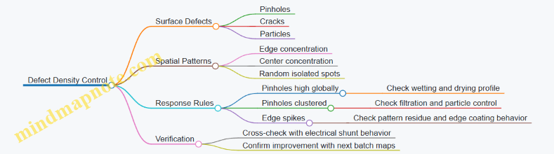
Documentation That Prevents Repeat Failures
For each batch, record: the thickness map summary statistics, the defect inspection settings and thresholds, the spatial heatmaps, and the decision outcome. Keep the records consistent so you can compare batches without reinterpreting everything from scratch. When a batch fails, the goal is to identify which measurement signal changed first, not to list every possible cause. That discipline is what turns quality control from a gate into a system.
4.4 Interlayer Deposition and Patterning for Reliable Series Connection
Series connection in perovskite silicon tandems is unforgiving: the electrical path is only as good as the narrowest, most resistive, or most poorly aligned interface. Interlayer deposition and patterning are where you turn a stack of layers into a repeatable circuit.
Foundational Concepts for Series Interconnects
A series tandem typically uses a shared current path through a top cell and a bottom cell. Electrically, that means the interconnect must provide:
- Low contact resistance at the interface where current transfers.
- Continuity across the intended overlap area.
- Isolation everywhere else so adjacent regions do not short.
- Mechanical and chemical compatibility with both the perovskite and the silicon-side layers.
A practical way to think about the interlayer is as a “bridge” with two jobs: it must conduct current where you want it, and it must not conduct where you do not.
Interlayer Deposition Strategy
Interlayer deposition is usually chosen to balance three constraints: conformal coverage over textured or patterned surfaces, controlled thickness for resistance, and chemical stability during subsequent steps.
Deposition Goals and Easy Checks
-
Thickness control: If the interlayer is too thin, pinholes and incomplete coverage raise contact resistance. If too thick, it adds series resistance and can trap voids.
- Example: During process development, target a deposition thickness window and verify it with cross-sectional imaging on test coupons. If you see “islands” instead of a continuous film, treat it as a coverage failure, not a measurement artifact.
-
Wetting and adhesion: Poor wetting creates discontinuities at the edges of the overlap region.
- Example: Compare two surface prep recipes on identical substrates. If one shows a sharper edge definition after patterning, it likely improves wetting and adhesion.
-
Compatibility with sensitive layers: Perovskite stacks can be sensitive to solvents, heat, and reactive species.
- Example: Run a short “soak” test where you expose a finished perovskite stack to the interlayer deposition conditions without patterning. If performance drops immediately, adjust chemistry or temperature before scaling.
Patterning Approaches
Patterning defines where the interlayer bridges the series connection and where it must be absent.
- Additive patterning: deposit only where needed using masks or printing-like approaches.
- Subtractive patterning: deposit a blanket film, then remove it where it should not exist.
For reliable series connection, subtractive patterning is common because it starts from a uniform film, but it must avoid damaging the underlying layers.
Patterning for Electrical Isolation and Edge Quality
The most common reliability issues in series interconnects are shorts from residual interlayer material and high resistance from damaged or undercut regions.
Alignment and Overlap Control
Series interconnects require overlap between the interlayer and the underlying electrodes or transport layers. Too little overlap increases resistance; too much can increase risk of unintended conduction.
- Example: Use alignment marks and define an overlap tolerance band. If your overlap distribution is wide, you will see a bimodal yield: one group with acceptable resistance and another with frequent open circuits.
Etch and Lift-Off Considerations
If you use subtractive patterning, the etch must stop cleanly without attacking the perovskite or the silicon-side layers.
-
Selectivity: choose etch chemistry that removes the interlayer much faster than the underlying layers.
-
Undercut control: undercut reduces effective overlap and can create a “thin neck” that fails under thermal cycling.
-
Residue management: residues can form conductive paths or increase contact resistance.
-
Example: After patterning, inspect for residue using optical microscopy and a simple electrical continuity test on dedicated test structures. If continuity appears where it should not, treat it as a patterning residue issue before changing deposition.
Process Integration Workflow
A systematic workflow reduces surprises:
- Deposit interlayer on test coupons using the intended process window.
- Pattern using the planned method and verify edge definition and isolation.
- Measure contact resistance proxies on test structures before building full tandems.
- Run a short thermal and environmental stress sequence consistent with downstream steps to catch early degradation.
- Only then integrate into full module flows.
This order matters because it isolates whether failures originate from deposition, patterning, or the interaction with the next layer.
Mind Map: Interlayer Deposition and Patterning
Example: Debugging a Series Short
Suppose a batch shows low series resistance but also frequent module-level shorts.
- Check pattern isolation on test structures that include the same interlayer pattern but stop before full stack completion.
- Inspect edges after patterning. If you see a faint film at the boundary, suspect residue or incomplete etch removal.
- Run a targeted cleaning comparison that changes only the post-pattern step. If shorts drop without changing deposition, the root cause is likely residue rather than film quality.
- Confirm with a continuity map across multiple sites. If shorts cluster around specific pattern geometries, adjust etch uniformity or mask contact quality.
This approach avoids changing everything at once, which is how you end up with a process that works only on good days.
Example: Fixing High Resistance from Undercut
If you observe high resistance and open circuits, undercut is a prime suspect.
- Measure effective overlap width after patterning.
- Compare etch time and selectivity settings while keeping deposition constant.
- If overlap shrinks with longer etch, reduce etch time or improve selectivity so the interlayer clears without attacking the edges.
When overlap is preserved, the series path becomes consistent, and yield typically stops behaving like a coin toss.
4.5 Lamination Process Windows Including Pressure Temperature and Cure Profiles
Lamination is where your module design meets reality: the stack must bond strongly without damaging sensitive layers, and the encapsulant must cure enough to block moisture while still allowing good optical and electrical performance. A “process window” is the range of pressure, temperature, and time where the module consistently meets acceptance criteria. The goal is not to find one perfect recipe; it is to define a robust region that tolerates normal equipment variation.
Foundational Concepts for Defining a Process Window
Start by separating three outcomes that lamination controls:
- Mechanical bonding: encapsulant wets interfaces and forms adhesion so the stack resists delamination under thermal cycling.
- Void suppression: trapped air and solvent residues expand with heat and can create bubbles that later become failure sites.
- Chemical curing: crosslinking determines barrier performance and long-term stability.
A practical way to define the window is to choose a baseline profile from prior experience, then map how performance changes when you shift one variable at a time. Pressure, temperature, and cure time interact, so you will later confirm the combined effect with a small factorial study.
Pressure Window and Its Practical Effects
Pressure influences intimate contact and void removal. Too little pressure leaves micro-gaps that can become channels for moisture. Too much pressure can squeeze out encapsulant unevenly, thinning regions near busbars or edges and increasing the risk of electrical hot spots.
Example: If you observe edge bubbles after lamination, increase pressure slightly and reduce ramp rate so air has time to escape. If you observe encapsulant starvation near the perimeter, reduce peak pressure or adjust layup alignment to prevent localized squeeze-out.
Key measurement signals include:
- Void fraction from optical inspection of witness coupons.
- Adhesion strength from peel tests on representative stacks.
- Thickness uniformity of encapsulant after lamination.
Temperature Window and Thermal Safety
Temperature affects both curing kinetics and thermal stress. Sensitive perovskite-related layers can degrade if overheated or held too long at elevated temperatures. Silicon cells tolerate heat better, but soldering and interconnect regions still need controlled thermal exposure.
Define temperature limits in two layers:
- Maximum temperature limit: the highest setpoint you allow anywhere in the stack.
- Soak temperature limit: the time at which the stack remains near the cure temperature.
Example: If performance drops after lamination but voids look fine, the issue is often thermal exposure. Reduce soak time while keeping cure completion by adjusting the ramp profile or cure temperature within the safe maximum.
Cure Profiles from Ramp to Hold to Cool
A cure profile is more than “heat for X minutes.” It is a sequence that manages solvent outgassing, encapsulant flow, crosslinking, and stress relaxation.
A systematic profile typically includes:
- Ramp-up phase: heat the stack gradually so trapped air expands and escapes before the encapsulant becomes too viscous.
- Flow and wetting phase: reach a temperature where encapsulant can wet interfaces under the chosen pressure.
- Cure hold phase: maintain temperature long enough for crosslinking to reach the target degree of cure.
- Controlled cool-down: reduce thermal gradients so the stack does not warp or create interfacial stresses.
Example: If you see bubbles only in thicker regions, slow the ramp-up so the thicker areas reach temperature later and have time to vent. If you see brittle encapsulant or poor adhesion, shorten the cure hold or adjust cool-down to reduce stress.
Mind Map: Lamination Process Window Drivers
Building the Window with a Small Experimental Plan
Use a staged approach:
- Single-variable screening: pick three levels for pressure, three for peak temperature, and two for cure hold time. Keep everything else fixed.
- Witness coupon strategy: run coupons with the same stack design and encapsulant lot to avoid misleading results from different geometry.
- Acceptance gating: define pass/fail criteria for voids, adhesion, and electrical performance before expanding the window.
Example: Suppose baseline voids are acceptable but adhesion is borderline. Increase pressure modestly and shorten cure hold slightly to reduce thermal stress, then confirm adhesion and voids together rather than separately.
Integrated Example Profile with Reasoned Targets
A typical integrated profile can be described as:
- Ramp-up: moderate slope to allow venting before encapsulant viscosity rises.
- Peak temperature: set below the maximum safe stack temperature.
- Pressure: apply during wetting and cure hold, with stable control at peak.
- Cure hold: long enough to reach target cure without excessive exposure.
- Cool-down: controlled to reduce thermal gradients.
If you document the profile, include the exact setpoints, the actual measured temperatures at representative stack locations, and the pressure trace. A good process window is one where the measured traces stay inside limits even when the equipment drifts slightly.
Documentation That Makes the Window Usable
Record the window as ranges, not single values. For each variable, list:
- allowed minimum and maximum pressure,
- allowed minimum and maximum peak temperature,
- allowed cure hold time range,
- ramp and cool-down constraints.
Example: Instead of “70°C for 20 minutes,” write “peak temperature within a safe band, cure hold within a time range, and ramp/cool constraints that keep measured stack gradients within limits.” That turns lamination from a recipe into a repeatable engineering control.
5. Yield Modeling and Process Control for Commercial Scale Production
5.1 Defining Yield Loss Sources Across Cell and Module Manufacturing Steps
Yield is what you keep, not what you start with. In tandem manufacturing, “loss” can happen as outright defects that fail test, or as performance drift that still passes but produces less energy than expected. A practical approach is to define yield at two levels: cell yield (devices that meet electrical and optical targets) and module yield (cells that survive interconnection, encapsulation, and module-level tests while delivering the expected power).
Foundational Yield Model
Start by separating losses into three buckets:
- Scrap: units fail a go/no-go criterion.
- Rework: units can be repaired and retested.
- Performance Yield: units pass but underperform due to parameter shifts.
A simple way to make this systematic is to track yield step-by-step with a “loss ledger.” For each manufacturing step, record the fraction of units lost to scrap, the fraction reworked, and the fraction that passes but shifts key metrics (for example, current matching, series resistance, or barrier integrity).
Mind Map: Yield Loss Sources
Cell Step Loss Sources with Examples
Substrate and cleaning often cause “silent” yield loss. Example: if cleaning leaves residues, the perovskite wetting becomes patchy, producing localized low-current regions. The cell may still show a reasonable average IV curve, but spectral response reveals a dip in the band of interest, which later worsens current matching in the tandem stack.
Perovskite deposition and crystallization typically dominate performance yield. Example: a small drift in precursor concentration can increase defect density. The device still forms, but the nonradiative recombination rises, reducing voltage. When you sort cells, you see more units falling into a lower power bin rather than outright failing.
Top electrode formation can create both scrap and performance loss. Example: incomplete coverage increases series resistance. The cell passes initial tests but fails module-level power targets because series resistance magnifies under tandem operating current.
Module Step Loss Sources with Examples
Cell layup and series connection is where “good cells” can become “bad modules.” Example: a conductive adhesive joint with a small void can pass early electrical checks, yet contact resistance grows after lamination thermal exposure. In module testing, the IV curve shows a reduced fill factor and a stronger sensitivity to temperature.
Encapsulation and barrier formation introduces reliability-related yield loss. Example: a microchannel at an edge seal can be invisible during visual inspection but shows up as early damp-heat failures. This is why module yield should include both immediate power tests and accelerated stress pre-screens.
Lamination and thermal stress can trigger mechanical damage. Example: if pressure distribution is uneven, one region experiences higher stress and develops microcracks. The module may still meet power at standard test conditions, but insulation resistance or post-stress IV measurements reveal the issue.
Turning Loss Sources into Actionable Metrics
For each step, define:
- Primary failure signatures (what you measure).
- Likely root causes (what process variables drive it).
- Where it shows up next (cell test vs module test).
Example ledger entry: “Perovskite crystallization drift” → signature: reduced voltage and broadened spectral response → root cause: precursor stoichiometry variation and drying profile shift → propagation: more cells land in lower power bins, increasing module performance loss.
Practical Yield Accounting Workflow
- Build a step list from cell fabrication through module final test.
- For each step, assign a loss type: scrap, rework, or performance.
- Link each loss to a measurable signature and a decision threshold.
- Review the ledger weekly using the same unit definitions for cell and module.
This keeps yield discussions grounded: instead of “we lost yield,” you can say “we lost performance yield at perovskite crystallization and scrap yield at series connection after lamination,” which is the difference between fixing a process and fixing a spreadsheet.
5.2 Statistical Process Control for Key Process Parameters
Statistical Process Control, or SPC, is how you keep a manufacturing process inside its intended behavior instead of discovering problems after yield drops. For tandem modules, the goal is practical: detect drift early, separate normal variation from real trouble, and document what you did so decisions are consistent across shifts.
Foundational Concepts That Make SPC Work
Start with three definitions that prevent most SPC confusion:
- Process parameter: a controllable input such as perovskite precursor concentration, coating speed, or lamination temperature.
- Key process parameter: a parameter that meaningfully affects device or module performance or reliability.
- Control chart: a plot of a statistic over time with rules for when to intervene.
SPC assumes the process has a “common cause” of variation when it is stable. When “special causes” appear—like a clogged nozzle, a miscalibrated balance, or a humidity excursion—the chart should flag it.
Choosing What to Measure and How to Summarize
A control chart needs a number. That number should represent the parameter in a way that is stable and comparable.
- If the parameter is approximately normal and continuous (e.g., coating thickness in nm), use X̄-R or X̄-S style charts.
- If the parameter is continuous but you care about the spread (e.g., variability of thickness), use charts that track dispersion.
- If the parameter is a pass/fail outcome (e.g., interlayer adhesion test), use p or np charts.
Example: Suppose you measure perovskite film thickness at 20 points per panel. You compute the mean thickness for each panel and track that mean with an X̄ chart. If the mean shifts, you investigate precursor delivery or spin speed. If only the spread increases, you investigate wetting, airflow, or edge effects.
Selecting Control Limits Without Guessing
Control limits are not the same as specification limits. Specification limits come from product requirements; control limits come from the process’s observed behavior.
A typical workflow:
- Run a baseline period where the process is believed stable.
- Compute the center line and control limits from that baseline.
- Use the chart rules to detect special causes.
- Reassess baseline only after confirmed corrective actions.
Example: If your lamination temperature setpoint is 120 °C with a specification of 118–122 °C, your control limits might be tighter or looser depending on what the baseline shows. If the chart flags a special cause at 121.5 °C, you still investigate even though it is inside the specification. That’s how you prevent slow drift from turning into a warranty event.
Mind Map: SPC in Tandem Module Manufacturing
Practical Sampling Plans That Don’t Waste Time
Sampling is where SPC becomes real. Too few samples and you miss drift; too many and you slow production.
A workable approach is stratified sampling:
- Sample more frequently during setup or after maintenance.
- Sample less frequently during steady production.
- Increase sampling when the chart shows warning patterns.
Example: During perovskite coating, measure thickness for every panel for the first 30 minutes after a recipe change. After stability is confirmed, reduce to one panel per hour while keeping a fast inline thickness check. If the chart flags a shift, immediately return to dense sampling until the process is back in control.
Interpreting Signals Without Overreacting
Control charts can be noisy, so use consistent rules.
- Out-of-control: a point beyond control limits. Investigate immediately.
- Run rules: patterns like several points trending upward can indicate a shift before limits are crossed.
Example: If lamination temperature shows a gentle upward trend over 8 consecutive lots, you may not exceed control limits yet. Investigate the heating system calibration or sensor drift. Waiting for a hard limit breach often means you discover the problem after multiple affected lots.
Linking SPC to Root Cause and Effectiveness
SPC flags special causes; it does not fix them. Your process should connect chart events to a structured response:
- Freeze affected lots for investigation.
- Check instrument health (calibration status, sensor drift, cleaning schedules).
- Review recent changes (materials lot, operator shift, recipe edits).
- Perform targeted verification tests.
- Resume production only after the chart returns to control.
Example: A series of thickness means shifts after a glass cleaning change. You verify cleaning conductivity and rinse time, then confirm thickness returns to baseline. Only then do you update the baseline limits if your quality team agrees the process is genuinely re-centered.
A Simple SPC Checklist for Daily Use
- Are control limits based on a stable baseline?
- Is the statistic chosen appropriate for the parameter type?
- Is sampling frequent enough to catch drift?
- Are chart signals tied to a defined escalation path?
- After corrective action, did the chart actually return to control?
When these are answered consistently, SPC becomes less about drawing lines and more about keeping the process predictable—so the module performance you expect is the module performance you get.
5.3 Inline Metrology for Early Detection of Defects and Drift
Inline metrology is the habit of measuring while the process is still fixable. In tandem module manufacturing, small shifts in film thickness, uniformity, or interlayer alignment can quietly reduce current matching and reliability. The goal is not to measure everything everywhere; it is to measure the few signals that correlate strongly with yield loss and to act quickly when those signals drift.
Foundational Principles for Inline Measurement
Start with a simple chain: process parameter changes → measurable film or interface change → electrical or reliability impact. Inline metrology should target the middle link. For example, if perovskite layer thickness drifts, you can often detect it as a change in optical interference fringes or reflectance before the device is fully assembled. If series interconnection alignment drifts, you can detect it as a change in overlay error or contact resistance after patterning.
Next, define what “early” means operationally. A measurement is early if it occurs before irreversible steps like final lamination or module sealing. That usually places inline checks around coating, drying, patterning, and pre-lamination inspection.
Finally, design the measurement to be robust to production realities. Inline tools must tolerate conveyor vibration, temperature variation, and partial coverage. A good practice is to include reference samples on every carrier so the system can normalize readings to the same baseline each run.
Measurement Strategy That Matches the Failure Modes
Inline metrology should be organized by where defects originate.
- Coating and drying defects: thickness nonuniformity, pinholes, edge beading, and solvent-related gradients.
- Interface and patterning defects: poor wetting, incomplete coverage, misalignment, and damaged underlying layers.
- Interconnection defects: contact voids, excessive series resistance, and short-risk regions.
- Encapsulation readiness: barrier integrity indicators and cleanliness before lamination.
A practical approach is to assign each metrology signal to a specific action. If reflectance uniformity drops below a threshold, you pause and check coating parameters. If overlay error increases, you verify alignment calibration and mask handling.
Example Workflow from Coating to Pre-Lamination
Consider a line that coats the perovskite top cell layer.
- After coating but before full drying completion, measure optical reflectance maps across the substrate. A typical signal is the spatial variation of reflectance at a fixed wavelength.
- Compute a uniformity metric such as the coefficient of variation across the active area.
- Compare to a control chart built from stable production weeks. If the metric shifts by a defined number of standard deviations, stop the run.
- Act on the likely cause: check dispense volume, meniscus behavior, and drying airflow. Then re-run a short batch with a known-good recipe.
For interconnection, a complementary workflow works well.
- After patterning, measure overlay error and line edge roughness using optical inspection.
- After metallization, perform localized resistance checks on test structures placed with the production layout.
- Trigger corrective actions: if contact resistance rises, inspect for incomplete wetting or contamination at the interface.
Mind Map: Inline Metrology Signals and Actions
Decision Rules That Prevent “Measuring for Measuring’s Sake”
Inline metrology becomes useful when it has clear decision rules.
- Use two thresholds: a warning level that prompts investigation and a stop level that prevents producing large quantities of likely-faulty modules.
- Require persistence: a single outlier can come from a transient event like a carrier mis-seat. A drift should persist across multiple substrates or minutes.
- Prefer relative metrics: uniformity ratios and normalized reflectance often outperform absolute values because they cancel out slow tool aging.
- Keep actions small and reversible: recalibration and recipe micro-adjustments are easier than changing hardware mid-run.
Example: Detecting Thickness Drift Before It Hits Performance
Suppose reflectance uniformity gradually worsens over a shift. The electrical impact might show up later as reduced fill factor due to current mismatch across the tandem stack. Instead of waiting for end-of-line current-voltage testing, you can detect the drift earlier.
A concrete practice is to track a “fringe shift” metric that correlates with optical thickness. When the metric trends upward for three consecutive carriers, you pause and check the drying airflow and substrate temperature. After correction, the metric returns to the prior distribution, and downstream electrical results stabilize.
Example: Catching Patterning Misalignment Early
If overlay error increases, series connection regions may experience partial contact or increased resistance. Inline optical inspection can catch this immediately after patterning. A practical rule is to compare overlay error distributions across the substrate: if the center remains stable but edges shift, the cause is often mechanical handling or mask-to-substrate skew rather than a global alignment calibration issue.
When the edge-shift pattern appears, you inspect carrier seating and verify that the mask frame is clamped consistently. This kind of targeted check avoids chasing unrelated coating parameters.
Operational Checklist for Inline Metrology
- Confirm each metrology signal has an assigned action.
- Normalize to per-carrier references.
- Use warning and stop thresholds with persistence rules.
- Capture measurement images and raw data for traceability.
- Review control charts at shift boundaries so drift doesn’t accumulate unnoticed.
Inline metrology is most effective when it behaves like a good safety system: it notices the problem early, explains it with measurable evidence, and triggers a specific response before the process turns into expensive history.
5.4 Root Cause Analysis Workflows for Performance and Reliability Deviations
When tandem perovskite-silicon modules underperform or fail reliability tests, the goal is not to find a single “culprit” quickly. The goal is to build a chain of evidence that explains what changed, where it changed, and why the change survived manufacturing and ended up in the field. A good workflow keeps the team honest: it forces measurements to agree with the proposed mechanism.
Step 1: Triage and Scope the Deviation
Start by separating performance deviations from reliability deviations, because they often point to different failure modes.
- Performance deviation examples: lower than expected power at STC, reduced fill factor, abnormal temperature coefficient, or mismatch between cell-level and module-level output.
- Reliability deviation examples: damp heat degradation, insulation resistance drop, delamination, or post-thermal-cycling power loss.
Create a short “scope statement” that includes affected lots, process steps, test conditions, and time since lamination. A practical rule: if the deviation appears across multiple unrelated lots, suspect measurement setup, incoming materials, or a shared upstream process.
Step 2: Collect Evidence Without Changing the Story
Evidence collection should be parallel, not sequential, so you don’t accidentally “fix” the problem while investigating it.
- Module electrical data: IV curves by string, series resistance estimates, and any bypass behavior.
- Optical data: EL images, reflectance, or simple visual inspection for bubbles, edge defects, and discoloration.
- Environmental context: humidity exposure history for encapsulant and any storage time beyond the defined shelf-life window.
Example: A lot shows a 12% power drop after damp heat. EL images show localized dark regions near interconnect edges. That pattern narrows the search toward interlayer integrity, edge sealing, or ion migration pathways rather than bulk optical mismatch.
Step 3: Build a Hypothesis Tree from Mechanisms
Turn observations into a hypothesis tree that maps symptoms to mechanisms. Keep it grounded in physics and process reality.
- If fill factor drops: suspect series resistance growth, contact degradation, or interconnect microcracks.
- If short-circuit current drops: suspect optical losses, parasitic absorption, or active layer degradation.
- If voltage loss increases: suspect recombination changes, transport layer degradation, or interface chemistry shifts.
- If insulation resistance drops: suspect moisture ingress, conductive pathways, or encapsulant barrier failure.
Mind Map: Root Cause Analysis Workflow
Root Cause Analysis Workflow Mind Map
Step 4: Verify with the Right Tests in the Right Order
Use a test ladder: start non-destructive, then move to targeted destructive analysis.
- Non-destructive: EL mapping, visual inspection under magnification, and basic IV by string to locate electrical non-uniformity.
- Targeted destructive: cross-section at defect coordinates, interconnect inspection, and barrier layer assessment.
- Material-level checks: verify whether the encapsulation stack shows signs consistent with moisture ingress or chemical interaction.
Example: If EL shows edge-localized darkening and cross-sections reveal voids at the seal line, the mechanism becomes moisture ingress at edges leading to interlayer degradation. That’s more actionable than “perovskite degraded,” because it points to sealing and lamination parameters.
Step 5: Correlate with Process Control Data
Root causes usually hide in process drift rather than in a single catastrophic event. Pull metrology and control charts for the relevant steps.
- Deposition uniformity trends for perovskite and transport layers
- Interlayer thickness and patterning alignment
- Lamination pressure and temperature profiles
- Encapsulant cure timing and batch-to-batch variability
A useful technique is “timeline alignment”: match the deviation’s onset to the last known stable process window. If the deviation first appears after a change in cure dwell time, the hypothesis tree should shift toward encapsulation chemistry and barrier performance.
Step 6: Confirm Root Cause and Close the Loop
Confirmation means the evidence supports causality, not just correlation.
- Reproduce the deviation by running a controlled process variation within safe lab bounds.
- Correlate the measured mechanism signature with the deviation signature.
- Verify effectiveness by re-testing modules from corrected lots under the same reliability protocol.
Example: After adjusting lamination dwell time and improving edge sealing, insulation resistance remains stable after damp heat, and EL darkening shifts from edge-localized to minimal uniform background. The workflow closes because the mechanism signature and the performance outcome both improve.
Step 7: Write Corrective Actions That Engineers Can Execute
Corrective actions should be specific enough to prevent “we changed something” outcomes.
- Define the exact parameter change and where it is controlled.
- Update acceptance criteria for incoming materials and in-line metrology.
- Add a containment step for suspect lots.
A good closure package includes: the scope statement, hypothesis tree, verification results, process data correlation, corrective action details, and effectiveness verification results. If any of these are missing, the next deviation will feel like déjà vu—just with different numbers.
5.5 Documentation and Traceability Systems for Production Accountability
A production accountability system answers three questions: What was made, when and where it was made, and which inputs and process settings produced it. For tandem perovskite-silicon modules, the “which inputs” part matters because performance and reliability are sensitive to film quality, interlayer interfaces, and encapsulation integrity. The goal is not paperwork for its own sake; it is fast, defensible root-cause analysis when a batch underperforms.
Foundational Concepts and Scope
Start by defining traceability scope at the right granularity. A practical baseline is:
- Material lot: supplier lot number for glass, encapsulant, interconnect foils, and critical chemicals.
- Process batch: the run identifier for coating, curing, and lamination steps.
- Unit identifier: module serial number and, if applicable, cell or subcell identifiers.
Then define the minimum dataset required to link these levels. For each critical step, capture: equipment ID, operator or shift, start and end timestamps, key setpoints, measured in-process values, and pass/fail outcomes. If a value is not measured, record why it is controlled indirectly (for example, by recipe lock and equipment qualification).
Data Model and Traceability Flow
A traceability system should follow the physical flow of the product. The simplest model is a chain:
- Inputs enter as material lots.
- Recipes and equipment settings transform inputs into intermediate films.
- Intermediate results are checked by metrology.
- Modules are assembled and tested.
- Final test results are tied back to all upstream identifiers.
To keep this manageable, classify data into three tiers:
- Tier 1: identifiers and timestamps needed for any investigation.
- Tier 2: measured process parameters and metrology results.
- Tier 3: optional notes such as deviations, rework actions, and calibration certificates.
Documentation Standards That Survive Real Investigations
Use controlled documents for work instructions and recipes, but keep the operational records separate from the instruction text. When a module fails, you want the exact recipe version and equipment configuration used, not the latest instruction.
A good practice is to require evidence fields for every deviation: what changed, what was measured afterward, and who approved the disposition. For example, if a lamination temperature profile deviates, the record should include the actual thermal log summary and the acceptance decision for that module.
Also standardize how you record test results. For each module test, store the raw curve or key extracted metrics (for example, current-voltage parameters, insulation resistance, and any spectral or imaging outputs). Store them with the same unit identifier used on the label so the investigation does not rely on manual matching.
Mind Map: Traceability System Components
Example: Linking a Module to Upstream Lots
Imagine Module TSP-24081-0142 fails an insulation resistance threshold during final test. The traceability record should immediately show:
- Material lots used for encapsulant and interconnect foils.
- Lamination process batch ID and equipment ID.
- The actual lamination profile summary and whether any alarms occurred.
- The intermediate metrology results for interlayer continuity and any rework steps.
A clean investigation path looks like this: first confirm whether the failure correlates to a specific lamination batch, then check whether that batch had a consistent deviation in thermal profile or dwell time, and finally verify whether modules from the same batch show similar trends in other electrical metrics.
Example: Deviation Handling with Evidence
Suppose a coating step is paused for 18 minutes due to a minor equipment fault. The deviation record should include:
- Start and end timestamps of the pause.
- Equipment ID and fault code.
- Whether the recipe was resumed with the same setpoints.
- In-process measurements after resumption.
- A disposition decision for the resulting intermediate and the modules built from it.
This avoids the common failure mode where the record says “paused” but not whether the film quality was re-verified.
Governance and Auditability
Traceability only works if records cannot be silently altered. Use role-based access, immutable audit trails, and clear retention rules. When a record is corrected, store the correction reason and the approving user. Keep the correction separate from the original entry so the history remains intact.
Finally, define an operational cadence for data completeness checks. A simple rule is: no module can be released without Tier 1 links present and Tier 2 required fields populated. That rule turns traceability from a best effort into a system behavior—less guesswork, fewer late surprises.
6. Reliability Engineering and Qualification Testing for Tandem Modules
6.1 Reliability Test Matrix Selection for Module Level Qualification
A reliability test matrix is a structured plan that answers one question: “Which stresses, in what order, at what severity, and with what pass criteria, prove the module can survive its intended life?” For perovskite-silicon tandem modules, the matrix must cover both the encapsulated stack and the electrical system, because failures often show up where moisture, heat, or bias stress meet.
Step 1: Start with Module Use Conditions
Build the matrix from the module’s real operating envelope: temperature range, humidity exposure, UV/visible irradiance, wind-driven mechanical loads, and electrical bias patterns. A practical way to keep this grounded is to define three operating bands—mild, typical, and worst-case—and assign each band a target stress severity. For example, if the module is expected to see frequent cool mornings and hot afternoons, thermal cycling should include both extremes rather than only the hottest day.
Step 2: Translate Failure Modes into Stress Types
Reliability tests are most effective when each stress maps to a likely failure mechanism. Use a simple mapping:
- Moisture ingress → damp heat, condensation cycling, and bias-assisted humidity where appropriate.
- Thermal expansion mismatch → thermal cycling and mechanical stress that simulates mounting constraints.
- Light induced degradation → UV exposure and light soaking while maintaining realistic temperature.
- Electrical stress → insulation resistance, hot spot risk checks, and bias-related tests that reflect series-connected behavior.
A key best practice is to avoid “one test to rule them all.” If you only run damp heat, you may miss light-driven interlayer changes; if you only run UV, you may miss moisture-assisted ion migration.
Step 3: Choose Standards-Like Durations with Clear Acceptance Criteria
Qualification matrices often borrow structure from common module reliability frameworks, but the acceptance criteria must be tailored to tandem specifics. Define measurable endpoints before testing:
- Performance retention: power at standard conditions compared to baseline.
- Electrical safety: insulation resistance and leakage current limits.
- Visual and structural integrity: delamination indicators, discoloration, and encapsulant cracking.
- Functional checks: continuity and bypass behavior under controlled stress.
Example: If baseline power is measured at STC and after damp heat you require at least 90% retention, also specify how you will handle outliers. A module that drops to 88% power but shows no electrical safety issues might indicate a performance-only degradation; a module that fails insulation resistance is a different category and should trigger a different root-cause workflow.
Step 4: Build the Matrix as a Sequence, Not a Random List
Order matters. Start with tests that establish baseline stability and reveal gross weaknesses, then move to combined stresses. A common sequence is:
- Pre-conditioning and baseline characterization (IV curve, spectral response if available, insulation resistance).
- Environmental exposure (damp heat and thermal cycling).
- Light exposure (UV/visible with controlled temperature).
- Electrical stress checks (bias-related insulation and hot spot risk verification).
- Post-test characterization using the same measurement methods as baseline.
This sequencing reduces ambiguity. If a module fails insulation resistance early, you don’t want to spend time interpreting power loss caused by a safety-relevant fault.
Step 5: Add Sampling Strategy and Traceability
Reliability qualification is only as good as its sampling plan. Use a tiered approach:
- Lot acceptance sampling for routine production checks.
- Qualification sampling for matrix execution.
- Failure investigation sampling for modules that deviate.
Traceability should link each module to key process parameters: encapsulation cure profile, interlayer deposition conditions, and lamination pressure-temperature history. Without that linkage, the matrix becomes a report of symptoms rather than a tool for fixing causes.
Mind Map: Reliability Test Matrix Logic
Example: A Practical Qualification Matrix Skeleton
A module qualification matrix can be organized into four blocks with consistent measurement checkpoints.
Block A: Baseline and Safety
- Measure IV curve, insulation resistance, and visual inspection.
- Record module serial identifiers and process traceability fields.
Block B: Thermal and Humidity
- Run thermal cycling across the defined temperature bands.
- Run damp heat at a severity aligned to the intended operating envelope.
- After each block, repeat insulation resistance and power measurement.
Block C: Light Exposure
- Apply UV/visible exposure while controlling temperature.
- Keep the electrical bias state consistent with the intended operating mode.
Block D: Electrical Stress Verification
- Perform insulation resistance and functional continuity checks.
- Confirm that bypass behavior and series interconnection remain stable.
Example: Interpreting Outcomes Without Guesswork
If power retention fails but insulation resistance remains within limits, focus on performance degradation pathways such as optical losses or interlayer changes. If insulation resistance fails, treat it as a safety and encapsulation integrity issue first, then investigate whether performance loss is secondary.
A good matrix is not just a list of tests; it is a decision system. When each stress has a defined purpose, a measurable endpoint, and a clear interpretation path, module qualification becomes repeatable rather than mysterious.
6.2 Damp Heat And Environmental Cycling Procedures And Acceptance Criteria
Damp heat testing checks whether encapsulation and interfaces can survive sustained moisture exposure without unacceptable performance drift. For tandem perovskite-silicon modules, the goal is not just “no visible damage,” but stable electrical output and controlled degradation pathways at the device stack and at the module edges.
Foundational Concepts for Damp Heat Stress
Start by separating three failure modes that damp heat can trigger:
- Barrier failure: moisture ingress through encapsulant or edge seals.
- Interfacial degradation: reactions at contacts, transport layers, or adhesive layers.
- System-level drift: changes in series resistance, shunt behavior, or insulation resistance.
A useful mental model is that damp heat is a “slow leak” test. If the barrier is good, moisture stays out and electrical parameters remain within limits. If the barrier is weak, the module may still look fine while internal parameters drift.
Test Setup and Conditioning Steps
Use a chamber that can control temperature and humidity uniformly. A common damp heat condition is 85°C and 85% relative humidity. Place modules on a non-reactive support so air can circulate around them. Avoid direct water droplets; the chamber should provide controlled humidity, not splashing.
Pre-conditioning matters because it reduces ambiguity:
- Measure baseline I-V curves and insulation resistance after stabilization.
- Record module temperature during measurement so later comparisons are apples-to-apples.
- If the module is laminated, ensure it has completed its normal post-lamination cure and any handling stabilization period.
During the test, periodically verify chamber stability. If the chamber drifts, you can end up measuring the chamber, not the module.
Environmental Cycling Procedure for Realistic Stress
Damp heat alone is slow. Environmental cycling adds mechanical and thermal stress that can open micro-pathways for moisture and stress interconnects.
A systematic cycling approach:
- Damp heat dwell at the target humidity and temperature.
- Thermal transitions between hot and cooler setpoints.
- Dry or lower-humidity dwell to create humidity gradients.
- Return to damp conditions to test whether the module “recovers” or continues degrading.
Keep the cycle count and dwell times consistent across lots. For example, if you use 10 cycles, do not mix 10-cycle and 30-cycle results in the same acceptance decision without separate criteria.
Measurement Plan and Parameter Selection
Acceptance should be based on parameters that detect both early drift and catastrophic failure.
Track at minimum:
- Power output at STC-equivalent conditions or a defined measurement condition.
- Fill factor and series resistance proxy derived from I-V curve shape.
- Short-circuit current and open-circuit voltage trends.
- Insulation resistance between electrical terminals and frame.
- Visual inspection for edge seal issues, bubbles, or delamination.
A practical example: if power drops mainly through fill factor reduction while voltage remains relatively stable, suspect increased series resistance or contact degradation. If voltage collapses while current stays closer to baseline, suspect interfacial or recombination changes.
Acceptance Criteria That Are Easy to Apply
Define criteria as pass/fail thresholds plus a “watch list” band.
Example acceptance framework (illustrative, to be set to your qualification standard):
- Power retention: module power after test must remain above a specified percentage of baseline.
- Insulation resistance: must remain above a minimum threshold; a sharp drop is a red flag even if power is still acceptable.
- I-V shape limits: fill factor and voltage changes must stay within defined bounds.
- No critical defects: no edge seal breach, no delamination that exposes internal layers, no corrosion at terminals.
Use a two-tier decision:
- Pass: all thresholds met.
- Conditional: one parameter in the watch band; require additional diagnostics such as cross-sectioning of representative samples.
Mind Map: The Damp Heat and Cycling Workflow
Concrete Example of Interpreting Results
Suppose a module shows power retention slightly below the pass threshold, while insulation resistance remains above the minimum. That combination suggests degradation is more likely within the optical/electrical stack rather than a gross barrier breach. Next, compare fill factor and series resistance proxy: if fill factor drops disproportionately, focus on interconnect and contact stability under cycling. If instead voltage drops strongly, focus on recombination changes in the tandem stack.
Finally, confirm whether the degradation is uniform across the module or localized. Localized changes often point to edge-related moisture pathways or non-uniform encapsulation, which is exactly what damp heat plus cycling is designed to reveal.
6.3 Thermal Cycling and Mechanical Stress Testing for Laminated Stacks
Thermal cycling and mechanical stress testing for laminated perovskite-silicon tandem modules are about one thing: proving the stack can survive repeated expansion and contraction without turning small stresses into big failures. In laminated designs, the weak links are rarely the bulk materials alone; they are the interfaces—adhesives, encapsulant edges, interconnect regions, and any area where stress concentrates.
Foundational Concepts That Drive Test Design
Start by translating real field stress into lab conditions. Temperature cycling produces mismatch strain because different layers expand differently. Mechanical stress adds bending and shear, especially at edges and near busbars or string interconnects. A practical approach is to define three stress paths:
- Thermal strain path: temperature change → layer expansion mismatch → interfacial shear and peel forces.
- Moisture-assisted path: cycling can move moisture and ions, changing interfacial adhesion and electrical behavior.
- Mechanical concentration path: mounting pressure, handling, and lamination shrinkage create local stress peaks.
A good test plan includes preconditioning, cycling, and post-cycling electrical and visual checks so you can separate “it looks fine” from “it still works.”
Test Setup and Instrumentation
Use a chamber that can control temperature uniformly across the sample area. Place thermocouples near representative locations: center, edge, and near any known stress concentrators such as interconnect zones. If the module is large, rotate samples or use multiple placements to avoid “center-only” results.
For mechanical stress, define whether you are testing:
- Bending from mounting and wind loads (fixture-based deflection),
- Compression from clamping and handling,
- Edge stress from frame design and lamination shrinkage.
A simple, effective practice is to record fixture geometry and clamp force, then keep them constant across batches. If you change the fixture, you change the stress distribution.
Thermal Cycling Protocol Structure
A systematic protocol typically includes:
- Preconditioning: stabilize samples at a controlled temperature and humidity state so initial moisture content is consistent.
- Baseline measurements: record IV curves, insulation resistance, and electroluminescence or other non-destructive imaging if available.
- Cycling: alternate between hot and cold plateaus with controlled ramp rates. Use dwell times long enough for the stack to approach thermal equilibrium; too-short dwell can under-represent interfacial stress.
- Inter-cycle checks: for long runs, perform periodic electrical checks to catch early degradation.
- Post-cycling measurements: repeat the baseline set and inspect for delamination, bubbles, edge whitening, or cracking.
A concrete example: if your module experiences daily temperature swings in service, choose a cycling profile that produces comparable strain energy in the stack. Then verify that the chamber’s ramp rate does not dominate the failure mode; otherwise you are testing the chamber, not the module.
Mechanical Stress Testing for Laminated Stacks
Mechanical testing should mirror how the module is actually supported. For laminated tandems, bending is often more informative than pure compression because it drives peel stress at interfaces.
A practical bending test workflow:
- Define support points matching the mounting system spacing.
- Apply controlled deflection to create repeatable curvature.
- Cycle the deflection if your use case includes repeated loading.
- Inspect after defined cycles rather than only at the end.
Example: if the field design uses a mid-span support, set the fixture so the sample’s center experiences the maximum curvature. Then compare failure locations to those seen in thermal cycling; consistent locations usually indicate a specific interface weakness.
Coupled Thermal and Mechanical Stress
Many failures come from the combination: thermal cycling weakens interfaces, and mechanical loading then accelerates separation or electrical discontinuities. If you can only run one combined test, prioritize the sequence that matches reality: thermal cycling first, then mechanical loading, or mechanical loading during cycling if your chamber allows it.
A simple decision rule: if post-thermal inspection shows edge lifting or interfacial haze, mechanical cycling is likely to reveal whether that damage is stable or progressing.
Acceptance Criteria and Failure Interpretation
Define acceptance criteria before testing. Typical criteria include:
- Electrical: limits on IV parameter shifts such as fill factor reduction and increased series resistance.
- Insulation: insulation resistance thresholds and absence of leakage growth.
- Visual and NDT: no new delamination patterns, no new cracks in encapsulant regions, and stable imaging signatures.
When failures occur, interpret them by location and timing. Edge failures after early cycles often point to moisture ingress pathways or poor edge adhesion. Center failures after many cycles often point to bulk-to-interface mismatch strain or lamination voids.
Mind Map: Thermal Cycling and Mechanical Stress Testing
Example Workflow for a Qualification Run
- Select representative laminated samples from the same lamination lot.
- Record baseline IV, insulation resistance, and imaging.
- Run thermal cycling with controlled ramp and dwell, sampling thermocouples at center and edge.
- Inspect after cycling for edge lifting, haze, and bubbles.
- Run bending cycles using a fixture that matches mounting support spacing.
- Repeat electrical and insulation checks, then compare failure locations to thermal inspection.
This workflow keeps the logic tight: baseline → stress → inspection → electrical verification. If the stack passes both thermal and mechanical stages, you have evidence that the interfaces are not just holding together today, but holding together under repeated stress.
6.4 UV Exposure and Light Soaking Protocols for Perovskite Sensitive Layers
Perovskite stacks are often sensitive to ultraviolet (UV) photons and to sustained illumination that can drive ion motion, interfacial reactions, and gradual changes in defect populations. A good protocol treats UV exposure and light soaking as two related but distinct stress modes: UV is the spectral trigger, while soaking is the time-and-environment driver. The goal is to measure how performance and stability shift under controlled conditions, not to “burn in” the device.
Foundational Concepts for Stress Design
Start by separating three variables that are easy to mix up:
- Spectral content: UV fraction matters more than total irradiance. Two lamps with the same sun-equivalent intensity can stress very differently if one has a stronger UV tail.
- Irradiance and temperature: Light can heat the sample. Temperature rise changes ion mobility and reaction rates, so you must record and control it.
- Environment: Oxygen and moisture accelerate many degradation pathways. Even if you encapsulate, testing should reflect the barrier’s real-world effectiveness.
A practical rule: keep one variable changing at a time. If you change UV intensity and temperature together, you will not know which one caused the shift.
UV Exposure Protocol Core Steps
Step 1: Define the test objective. Decide whether you are screening materials, qualifying an encapsulation stack, or comparing process variants. Screening often uses shorter exposures with tighter acceptance limits; qualification uses longer exposures and more measurements.
Step 2: Choose a UV-relevant light source. Use a calibrated lamp or filtered solar simulator where the UV band is known. Verify spectral output with a spectrometer, not just a lamp label.
Step 3: Control sample temperature. Mount samples on a thermally conductive stage with a sensor close to the active area. If the stage is at 25 °C but the device sits at 45 °C under illumination, your results are not comparable.
Step 4: Control atmosphere. For perovskite-sensitive layers, run tests in a controlled chamber with measured relative humidity and oxygen level. If you are testing encapsulated modules, include a “leakage representative” condition that matches your barrier assumptions.
Step 5: Use a measurement cadence. Measure current-voltage behavior and optical response at baseline, then at defined intervals. Early time points are important because some degradation is fast.
Step 6: Define pass-fail metrics. Common metrics include retention of initial efficiency, shift in open-circuit voltage, increase in series resistance, and changes in photoluminescence or external quantum efficiency. Use the same metrics across all samples.
Light Soaking Protocol for Sustained Illumination
Light soaking focuses on time under illumination, often at or near operating spectral conditions. The key is to avoid accidental “extra stress” from uncontrolled heating or drifting lamp output.
A systematic approach:
- Stabilize the light source before starting the timer.
- Maintain constant irradiance using feedback from a reference cell.
- Keep temperature constant with active control.
- Record environment continuously so you can correlate performance drift with humidity or oxygen changes.
Example: If you soak a perovskite-silicon tandem coupon at 1-sun equivalent for 500 hours, take measurements at 0, 50, 100, 200, and 500 hours. If you see a sharp voltage drop by 100 hours, you can shorten the next experiment to focus on the first 120 hours with finer time resolution.
Mind Map: UV Exposure and Light Soaking Workflow
Example Test Matrix That Avoids Confounded Results
Example: To separate UV effects from general illumination, run four conditions with the same irradiance and temperature:
- Condition A: full-spectrum with UV present
- Condition B: filtered to remove most UV while keeping visible similar
- Condition C: full-spectrum but in dry, oxygen-limited atmosphere
- Condition D: filtered UV-removed but in the same atmosphere as C
If A degrades faster than B, UV is a major driver. If C degrades slower than A, oxygen or moisture contributes. If D still degrades, then visible light or thermal effects are also involved.
Practical Acceptance and Documentation
Document the following for every run: lamp model, filter identifiers, spectral verification results, irradiance calibration method, temperature profile, chamber settings, sample layout, and measurement settings. When results disagree between batches, these details are often the fastest path to a real explanation.
Finally, treat the protocol itself as part of the product. A stable, repeatable UV and soaking method is what makes your stability comparisons meaningful—otherwise you are just comparing how different lamps and setups feel about your perovskite.
6.5 Electrical Reliability Testing Including Hot Spot and Insulation Resistance
Electrical reliability testing for tandem modules is about catching the boring-but-expensive failures early: local heating from current crowding and leakage paths that slowly drain performance or accelerate degradation. For perovskite-silicon tandems, series-connected stacks make the “weak link” problem more visible, so the test plan should treat hot spots and insulation resistance as linked symptoms rather than separate checkboxes.
Foundations: What Hot Spots and Insulation Resistance Mean
A hot spot is a localized region where current density rises above the surrounding area, producing higher temperature. In series tandems, this can happen when one subcell area has higher resistance, a micro-gap forms at an interconnect, or encapsulation defects allow moisture to change local conductivity.
Insulation resistance measures how well the module resists leakage between conductive parts and between the active stack and the frame or backsheet. Low insulation resistance can indicate moisture ingress, conductive contamination, or breakdown of insulating layers. The practical point: insulation issues often precede hot spots because leakage and partial shorts can increase local current flow.
Test Setup Principles That Prevent Misleading Results
Use a consistent test fixture and grounding scheme. A module that is clamped differently can show different leakage paths, especially at edges where encapsulation thickness varies. Keep test leads short and use clean contact points for any temporary electrodes.
Before stressing anything, record baseline measurements: insulation resistance at room conditions and a quick electrical check of continuity and polarity. If the baseline already looks poor, a “pass” later may only mean the failure mode changed, not that it improved.
Hot Spot Testing: From Electrical Stress to Temperature Evidence
Hot spot testing typically combines electrical stress with temperature observation. The goal is to detect localized heating under realistic current flow.
- Apply controlled forward bias or operating-equivalent current while monitoring voltage and current. Watch for unusual voltage drop behavior that can signal partial conduction.
- Measure temperature distribution using infrared imaging or embedded temperature sensors if available. Infrared imaging needs emissivity assumptions; calibrate using a reference area on the same module type.
- Define a hot spot criterion that is tied to temperature rise relative to the average module temperature, not just absolute temperature. Localized spikes are the target.
Easy example: If a module averages 55°C under test current but one corner reaches 75°C, the temperature rise is 20°C above average. If your criterion is, say, 15°C above average, that corner fails even if the absolute temperature is still below a “maximum” number.
Insulation Resistance Testing: Leakage Path Detection
Insulation resistance is commonly measured with a megohmmeter using a specified test voltage and dwell time. The key is to use the correct voltage level for the module design and to interpret results consistently.
- Measure between active conductors and the frame/back reference to detect leakage across the encapsulation and interfaces.
- Measure between series-connected regions if the fixture allows to localize where leakage is introduced.
- Use dwell time and record the trend rather than a single number. Leakage that decreases rapidly with time can indicate moisture-related conduction.
Easy example: Two modules both read 200 MΩ initially. After 60 seconds, Module A drops to 20 MΩ while Module B stays near 180 MΩ. Module A likely has a conductive path forming under the applied field.
Integrated Mind Map of the Test Logic
Mind Map: Electrical Reliability Testing for Hot Spots and Insulation Resistance
Advanced Details: Correlating Results Without Guessing
After you collect hot spot and insulation resistance data, correlate them using simple, defensible rules.
- If a module shows low insulation resistance and also exhibits hot spots at similar locations, treat the leakage path as the likely driver. The test evidence points to a shared defect region.
- If insulation resistance is acceptable but hot spots appear, focus on current crowding causes such as interconnect resistance variation or local contact issues.
Easy example: A module passes insulation resistance between active and frame, but fails hot spot criteria near a busbar edge. That pattern suggests a localized electrical resistance or contact geometry issue rather than a global moisture leakage path.
Practical Acceptance Criteria and Documentation
Set acceptance criteria that are measurable and repeatable: a temperature rise threshold for hot spots and a minimum insulation resistance value with a time-based rule. Document the test voltage, dwell time, fixture details, and imaging calibration method so results can be reproduced.
Finally, record the full measurement trace: current and voltage during hot spot tests, and resistance versus time during insulation tests. A single summary number is convenient, but the trace often explains why the module failed—without turning the report into a guessing game.
7. Electrical Characterization and Performance Verification
7.1 Measuring Current Voltage Curves Under Standard Test Conditions
A current voltage (IV) curve is the fastest way to see how a tandem device behaves under controlled light and temperature. For commercializing perovskite silicon tandems, the goal is not just to get a curve, but to get a curve you can compare across lots, tools, and days. Standard test conditions (STC) provide that common language: a defined irradiance, a defined spectrum, and a defined cell temperature.
What “Standard Test Conditions” Means in Practice
STC typically means 1000 W/m² irradiance, AM1.5G spectral distribution, and a cell temperature of 25 °C. In a tandem, the “cell temperature” is usually the temperature of the device under test, not the ambient lab temperature. A practical best practice is to record the temperature sensor location and mounting method, because small differences in thermal contact can shift the curve shape and the extracted parameters.
A useful mental model: the IV curve is the result of three coupled effects—optical generation (set by irradiance and spectrum), carrier collection (set by device physics and recombination), and electrical losses (set by series resistance and interconnection quality). STC controls the first effect tightly; the measurement setup and device handling control the other two.
Measurement Setup and Calibration Workflow
Start with the light source and calibration. Use a calibrated reference cell or reference module to verify irradiance at the plane of the device. Then verify spectral match if your lab uses a spectrum-corrected solar simulator; otherwise, expect systematic offsets in tandem current because perovskite layers respond differently across wavelengths.
Next, ensure electrical measurement integrity. Use four-wire sensing or equivalent practices to reduce lead resistance effects, especially when extracting fill factor. Confirm that the measurement system can sweep voltage in both directions or, if it only sweeps one direction, that you use a consistent sweep direction and settle time.
Finally, control the temperature. A common approach is to mount the device on a thermally conductive stage with a stable temperature controller, then wait until the device temperature stabilizes before starting the sweep. If you skip stabilization, you may still get a curve, but the extracted parameters will be “temperature-shaped,” not “device-shaped.”
Step by Step IV Curve Acquisition
- Prepare the device: clean the measurement window if needed, and handle the sample with consistent orientation. For tandems, avoid touching active areas.
- Stabilize temperature: wait until the device temperature reaches the target (25 °C for STC).
- Set irradiance: adjust the simulator until the reference reads 1000 W/m² at the device plane.
- Run the voltage sweep: sweep from short-circuit region toward open-circuit region with a defined step size and dwell time.
- Record current and voltage: sample at a consistent rate so the curve is smooth enough to locate knee regions.
- Repeat: take at least two sweeps to check for hysteresis or drift. If the second sweep differs materially, investigate before reporting.
Extracting Key Parameters Without Guesswork
From the IV curve, you extract short-circuit current (Isc), open-circuit voltage (Voc), maximum power point (MPP), fill factor (FF), and efficiency (η) when you have the active area and irradiance.
For tandems, the curve often shows a “knee” that reflects current matching between subcells. A practical example: if the top subcell current is lower than the bottom subcell current, the tandem behaves as if the series connection is limited by the weaker subcell. In the IV curve, this typically reduces the current level near the MPP and can lower FF due to increased relative impact of series resistance.
Common Measurement Pitfalls and How to Avoid Them
- Temperature mismatch: if your device is warmer than 25 °C, Voc will shift downward. Record temperature and reject measurements that did not stabilize.
- Spectral mismatch: a simulator that is “1000 W/m²” but not AM1.5G-matched can distort the tandem current balance. Use spectral correction or document the simulator class.
- Series resistance artifacts: poor wiring or contact resistance can make the curve look worse than the device. Use consistent contact pressure and clean contacts.
- Sweep-induced effects: perovskite devices can show time-dependent behavior. Use a consistent dwell time and compare repeated sweeps.
Mind Map: IV Curve Measurement Under STC
Example: Two Sweeps That Tell You Something
Suppose Sweep A shows a slightly higher Voc than Sweep B, while Isc stays nearly the same. That pattern often points to a temperature or stabilization issue rather than a gross electrical fault, because Voc is more sensitive to temperature than current. The fix is not “average the curves and move on,” but to verify that the device temperature reached 25 °C and that the dwell time is consistent.
Example: Current Limitation Visible in the Curve Shape
If you compare two tandem modules and Module 1 has a lower MPP current but similar Voc, the difference is likely current matching or optical generation efficiency rather than a major voltage loss mechanism. In practice, you confirm by checking the curve knee position and ensuring both devices were measured at the same irradiance and temperature with the same simulator settings.
A good IV measurement under STC is repeatable, traceable, and interpretable. When the setup is controlled, the curve stops being a mystery and becomes a diagnostic tool—especially for tandems where the series connection makes the “limiting subcell” show up in the shape of the power-producing region.
7.2 Spectral Response Measurement and Quantum Efficiency Mapping
Spectral response measurement tells you how a tandem device converts light at each wavelength into electrical current. Quantum efficiency mapping turns that idea into a map: not just “how much,” but “where” and “under what conditions.” For system engineers, this matters because tandem performance is often limited by mismatch, optical losses, and local defects that show up as wavelength-specific current shortfalls.
Core Concepts and What You Measure
Start with the definition: external quantum efficiency (EQE) is the fraction of incident photons at a given wavelength that produce collected charge. If you measure EQE across wavelength, you get a curve that can be integrated against a spectrum to predict current.
For a tandem, you typically measure:
- Top-cell EQE: photons absorbed in the perovskite stack that generate collected current.
- Bottom-cell EQE: photons transmitted through the top stack and absorbed in silicon.
- Device EQE: the combined series-limited response, which reflects current matching and interconnection constraints.
A practical rule: if the device EQE curve looks “smooth” but the top and bottom curves show a mismatch, the series connection is doing the damage quietly. The mapping helps you see where the mismatch originates.
Measurement Setup and Calibration
A standard EQE setup uses a monochromated light source, controlled beam spot, and a calibrated reference detector or calibrated photodiode. The key is to ensure that wavelength-dependent photon flux is known.
Best practices that prevent common mistakes:
- Use a wavelength-accurate monochromator and verify the wavelength axis with a known spectral line source.
- Calibrate photon flux at the device plane, not at the detector plane. Lens and window losses can be wavelength-dependent.
- Control bias conditions. EQE depends on operating point; for tandem characterization, record EQE at a consistent bias that matches how you plan to interpret current matching.
- Correct for reflectance and stray light only if your method requires it. If you use a reference-based approach, keep the correction model consistent across samples.
Example: Spot Size and Edge Effects
If your beam spot is larger than the active area, you average over inactive regions and get artificially low EQE near edges. If your spot is smaller, you can map local variations but must ensure the device is uniformly illuminated within the spot. A simple check is to scan the beam across the active area at one wavelength and confirm that EQE is stable in the interior.
From EQE Curves to Quantum Efficiency Mapping
EQE mapping extends the measurement by scanning the beam position across the module or cell. The output is a spatial grid of EQE values at selected wavelengths.
A systematic workflow:
- Pick wavelengths that represent the physics: one in the top-cell strong absorption region, one near the top-cell cutoff, and one in the bottom-cell dominant region.
- Map at those wavelengths to locate spatial nonuniformities tied to optical absorption and carrier collection.
- Optionally build a reduced spectral map by measuring a smaller set of wavelengths and interpolating EQE trends.
Example: Identifying a Local Interlayer Issue
Suppose the top-cell EQE map at a mid-perovskite wavelength shows a “dip” in one corner, while the bottom-cell map at a silicon-absorbing wavelength remains uniform. That pattern points to a top-cell collection or absorption issue localized to that region, such as a defect in the charge transport stack or a local optical barrier.
Tandem-Specific Interpretation
In a series-connected tandem, the measured device current is limited by the lower-current subcell at each operating condition. EQE mapping helps you separate three contributors:
- Optical mismatch: top-cell absorption too weak or too strong at certain wavelengths.
- Electrical mismatch: top or bottom collection efficiency varies spatially.
- Interconnection effects: series resistance or local shunts can distort the apparent EQE under bias.
A useful practice is to compare:
- Top EQE integrated under the incident spectrum
- Bottom EQE integrated under the transmitted spectrum
- Device EQE integrated
When the device EQE integration is lower than both subcell predictions, interconnection or bias-dependent collection is likely affecting the result.
Mind Map: Spectral Response to Spatial Diagnosis
Practical Quality Checks During Mapping
- Repeatability: measure the same wavelength at the same positions on two days. EQE drift can come from bias instability or illumination intensity changes.
- Consistency across wavelengths: a spatial defect should appear at wavelengths where that subcell contributes. If a “defect” appears everywhere equally, it may be a calibration or alignment artifact.
- Correlation with other signals: if you also have electroluminescence or reflectance images, use them to interpret whether a EQE dip is optical (absorption) or electrical (collection). The goal is not to prove a story, but to narrow the cause.
Example: A Simple Diagnostic Decision
- Top EQE dip only at perovskite wavelengths → likely top-cell collection/transport or local optical blocking.
- Bottom EQE dip only at silicon wavelengths → likely silicon collection or local optical transmission changes.
- Both dip together → likely illumination alignment, encapsulation barrier issues affecting both paths, or a series interconnection problem under the chosen bias.
Reporting the Results Clearly
Report at minimum:
- Wavelength range and step size
- Bias condition used for EQE
- Beam spot size and scan grid spacing
- Top, bottom, and device EQE curves
- EQE maps at the selected diagnostic wavelengths
Clear reporting prevents the classic “it looked fine in the plot” problem. In tandem devices, the plot is rarely the whole story; the map usually is.
7.3 Determining Fill Factor Losses and Series Resistance Contributions
Fill factor (FF) tells you how much of the ideal rectangular current-voltage shape survives real-world nonidealities. For tandem perovskite-silicon modules, the FF drop is often a mix of series resistance, recombination, and voltage-dependent losses. The goal here is to separate those contributions using measurements you can actually do, then connect them to design choices.
Foundational Concepts You Need Before Fitting
Start with the measured current-voltage curve at a fixed irradiance and temperature. The FF is computed from the maximum power point:
- \(FF = \frac{V_{mpp} I_{mpp}}{V_{oc} I_{sc}}\)
Series resistance \(R_s\) mainly reduces voltage at high current, so it bends the curve near the short-to-mid current region and lowers \( V_{mpp} \). Recombination and other voltage-dependent effects reduce \(V_{oc}\) and also change the curvature, but their signature is different: they tend to affect the low-current region more through changes in ideality and slope.
A practical way to think about it: \( R_s \) is a “tax on current,” while recombination is a “tax on voltage formation.” Both reduce FF, but they leave different fingerprints.
Measurement Setup and Data Hygiene
Use a four-wire (Kelvin) approach for module terminals when possible, or at least ensure the same lead configuration across tests. Record temperature at the module backsheet and keep it stable. If you sweep current using a source-measure unit, use consistent scan direction and settle time so the curve doesn’t pick up transient artifacts.
Before fitting, check that the curve is smooth near \(I_{sc}\) and \(V_{oc}\). A noisy curve can make the fitted \(R_s\) look like a random number generator.
Mind Map: What Drives Fill Factor Losses
Step-by-Step Extraction Using a Two-Stage Approach
Stage 1: Estimate \(R_s\) from the slope near high current.
Near the operating region where current is high, the terminal voltage can be approximated as:
- \(V \approx V_{ideal} - I R_s\)
Practically, you can estimate \(R_s\) by taking the derivative of the measured (V(I)) curve in a region close to (I_{mpp}) but not so close to (I_{sc}) that measurement compliance dominates. Choose a window such as 0.7–0.95 of (I_{sc}) (adjust if your curve shape differs).
Compute a local slope (dV/dI) and use its magnitude as an initial \(R_s\) guess.
Stage 2: Fit the full curve with a single-diode or two-diode model including \(R_s\).
Then refine \(R_s\) by fitting the entire curve, not just one region. Keep \(R_{sh}\) either fixed from the low-voltage region slope or fitted with constraints, because \(R_s\) and \(R_{sh}\) can trade off if the data quality is poor.
A good sanity check: the fitted \(R_s\) should reproduce the curvature near \(I_{mpp}\) without forcing unrealistic diode parameters.
Turning \(R_s\) Into Fill Factor Loss Numbers
Once you have \(R_s\), you can quantify how much FF loss is attributable to it by comparing two simulated curves:
- Use the fitted parameters including \(R_s\) to reproduce the measured \(V_{mpp}\) and FF.
- Set \(R_s = 0\) while keeping the diode-related parameters the same, then recompute FF.
The difference between the two FF values is an estimate of the FF loss due to series resistance. The remaining FF loss is attributed to voltage-dependent effects and shunt-related behavior (depending on your model).
Example: Interpreting a “Good Voc, Mediocre FF” Curve
Suppose a tandem module shows:
- \(V_{oc} = 1.80,\text{V}\)
- \(I_{sc} = 10.0,\text{A}\)
- \(FF = 0.78\)
You fit the curve and obtain \(R_s = 0.35,\Omega\). When you simulate with \(R_s = 0\), FF becomes 0.84. That suggests series resistance accounts for 0.06 FF points.
Now check the curve shape: if the voltage drop is strongest around 0.8–1.0 \( I_{sc} \), the \(R_s\) story is consistent. If instead the curve is already rounded near low current, recombination or transport limitations are likely contributing more than the \(R_s\) estimate alone.
Example: Distinguishing Rs from Shunt Effects
If a module has a low FF but also shows a noticeable slope change near low voltage (close to (V=0)), shunt pathways may be present. In that case, fitting only the high-current region can overestimate \( R_s \) because the model tries to explain curvature using the wrong parameter.
A simple diagnostic is to compare the fitted \(R_{sh}\) stability across fit windows. If \(R_s\) changes wildly when you shift the fit window but \(R_{sh}\) stays consistent, you likely have a series-dominated case. If both move together, you need better curve quality or a constrained fit.
Practical Best Practices for Reliable Rs Attribution
- Fit using a consistent irradiance and temperature point so FF changes reflect electrical effects, not thermal drift.
- Use a fit window that includes the region around \(I_{mpp}\), because that’s where FF is decided.
- Report \(R_s\) per module area or per cell equivalent so comparisons across designs are meaningful.
- Always include a curve-shape check: the fitted parameters should match the physical bending location, not just the numerical FF.
When done carefully, this workflow turns FF from a single number into a breakdown you can act on: whether to focus on contacts and interconnects (series resistance) or on recombination and transport (voltage-dependent losses).
7.4 Identifying Mismatch Losses in Tandem Operation From Test Data
Mismatch losses show up when the two subcells in a series tandem do not share current perfectly. Because series-connected current is limited by the weaker subcell, even small differences in current capability across the device area, spectrum, or operating point can reduce power. The goal of this section is to identify where the mismatch comes from and how to confirm it using standard test data.
Foundational Signals in Current Voltage Data
Start with the measured current voltage curve of the full tandem under a controlled spectrum and irradiance. In an ideal series tandem, the current is the same through both subcells at each operating point, so the power loss is dominated by resistive and optical factors. Mismatch adds a characteristic behavior: the tandem’s maximum power point (MPP) shifts and the fill factor drops more than expected from resistance alone.
A practical first check is to compare the tandem MPP current to the subcell current estimates derived from spectral response or separate characterization. If the tandem current is consistently lower than what either subcell could deliver at the same conditions, mismatch is likely.
Mind Map: Mismatch Sources and How to Prove Them
From Test Data to Current Balance
The most direct method uses spectral response. Measure or obtain EQE for the top and bottom subcells under the same optical configuration used for tandem testing. Then compute the expected short-circuit current for each subcell by integrating EQE against the incident spectrum. The mismatch metric is the difference between these predicted currents.
A simple workflow:
- Choose the spectrum used in the tandem test (for example, a calibrated simulator spectrum).
- Integrate top-cell EQE to get \(J_{sc,top}\) and bottom-cell EQE to get \(J_{sc,bot}\).
- Compute \(\Delta J = J_{sc,top} - J_{sc,bot}\).
- Compare the smaller of \(J_{sc,top}\) and \(J_{sc,bot}\) to the tandem current at MPP.
If \(\Delta J\) is large, mismatch is not subtle. If \(\Delta J\) is small but the tandem still shows a larger-than-expected power loss, the mismatch may be spatial or operating-point dependent.
Practical Example Using Two Illumination Levels
Suppose a tandem is tested at two irradiance levels, 1 sun and 0.5 sun, with the same spectrum. If mismatch is purely optical and current balance is fixed by the spectrum, the relative current limitation should scale similarly with irradiance. If mismatch is driven by recombination or transport differences that change with carrier density, the current balance can shift with irradiance.
Example reasoning:
- At 1 sun, the tandem MPP current is limited by the bottom subcell.
- At 0.5 sun, the bottom subcell’s current may drop less than the top due to different recombination mechanisms, reducing mismatch.
- You would observe a less severe fill factor loss at 0.5 sun than predicted by a resistance-only model.
To confirm, compare the tandem MPP current ratio \(I_{MPP}(0.5)/I_{MPP}(1)\) to the ratio predicted from EQE-based current scaling. Deviations indicate operating-point mismatch.
Advanced Details Using Temperature Sweeps
Temperature affects subcell currents differently because bandgap and recombination change with temperature. If the tandem mismatch is sensitive to temperature, the tandem MPP current and voltage will shift in a way that cannot be explained by a single temperature coefficient.
A systematic approach:
- Measure tandem IV curves at multiple temperatures.
- Extract MPP current and MPP voltage at each temperature.
- Use subcell temperature coefficients (from separate characterization or from temperature-dependent EQE if available) to predict how \(J_{sc,top}\) and \(J_{sc,bot}\) should change.
If the predicted current balance shifts toward one subcell at higher temperature and the tandem’s MPP current follows that trend, mismatch is confirmed as temperature-dependent.
Separating Mismatch from Resistive Loss
Mismatch and resistance both reduce fill factor, so you need a separation strategy. One method is to fit the tandem IV curve with a model that includes series resistance and recombination, then check whether the fitted parameters alone can reproduce the measured MPP current. If the model matches the shape but not the current balance, mismatch is the missing term.
A quick sanity check:
- If the inferred series resistance is reasonable but the MPP current is still lower than the smaller EQE-predicted subcell current, the limitation is not just resistive.
- If the MPP current tracks the smaller predicted subcell current across conditions, mismatch dominates.
What to Record in Your Test Report
To make mismatch identification actionable, record:
- Spectrum used for tandem testing and any deviations during measurement.
- EQE measurement conditions and integration assumptions.
- Predicted \(J_{sc,top}\), \(J_{sc,bot}\), and \(\Delta J\).
- MPP current and fill factor at each irradiance and temperature.
- The specific condition where mismatch impact is strongest.
This turns mismatch from a vague “performance loss” into a measurable current-balance problem with a clear cause you can trace back to optical, electrical, geometric, or operating conditions.
7.5 Temperature Coefficient Measurement and Thermal Performance Validation
Temperature affects tandem output in two ways: it changes the semiconductor band structure and it shifts how heat moves through the module stack. The goal of this section is to measure the temperature coefficient (typically in %/°C for power or mV/°C for voltage) and to validate that the module’s thermal behavior matches the assumptions used in energy-yield models.
Foundational Concepts for Temperature Coefficient
A temperature coefficient is not a single universal number; it depends on what you hold constant. For PV modules, you usually define:
- Power temperature coefficient: how module power changes with cell temperature.
- Voltage temperature coefficient: how open-circuit voltage or operating voltage changes with temperature.
- Current temperature coefficient: how current changes with temperature, often smaller in magnitude than voltage effects.
In practice, you measure under controlled irradiance and then relate electrical changes to cell temperature, not ambient temperature. Ambient temperature is convenient, but it is also a liar unless you model or measure the cell temperature.
Measuring Cell Temperature Without Guessing
Cell temperature can be estimated using thermocouples embedded near representative cells, or by using an infrared method calibrated to the stack. For tandem modules, the thermal path includes encapsulant, interlayers, and glass, so the “hot spot” can differ from the average.
Best practice is to define a temperature mapping plan before testing:
- Select representative locations for sensors, including at least one near the center and one near an edge where heat flow differs.
- If the module has multiple strings or zones, place sensors to capture any non-uniformity.
- Record sensor placement and thermal contact method, because a loose sensor can read several degrees low.
Example: Converting Ambient to Cell Temperature
Suppose a test run shows ambient rising from 20°C to 40°C. If your thermal model or calibrated sensor indicates cell temperature rises from 25°C to 47°C, then the effective temperature change is 22°C, not 20°C. Using ambient would slightly understate the magnitude of the coefficient.
Test Setup for Temperature Coefficient Measurement
A robust measurement setup keeps irradiance stable while temperature changes. Common approaches include thermal chambers, controlled airflow rigs, or outdoor tests with careful irradiance filtering.
Key measurement controls:
- Irradiance stability: use a reference cell and reject data outside a narrow irradiance band.
- Electrical measurement: use a source-measure unit or calibrated IV tester; ensure the measurement bandwidth matches the stabilization time.
- Stabilization time: wait until sensor readings and electrical parameters settle, especially after changing airflow or heater power.
Example: Data Filtering for a Clean Slope
If you plot measured power at the maximum power point versus measured cell temperature, you may see scatter from irradiance drift. A simple rule is to keep only points where irradiance is within ±2% of the target and where cell temperature is monotonic during the interval.
Extracting the Temperature Coefficient Systematically
Once you have paired data points of power and cell temperature, compute the slope using a linear fit over a defined temperature range. The range should cover the operating conditions you care about, typically from cool conditions up to the upper end of expected cell temperatures.
Practical details:
- Use cell temperature on the x-axis.
- Use power at maximum power point on the y-axis.
- Report the coefficient with the fitting method and the temperature range.
Example: Interpreting a Coefficient
If power decreases by 0.35% per °C, then a 10°C increase in cell temperature reduces power by about 3.5% under the same irradiance. In tandem modules, this number often reflects voltage loss dominating over current gain, so it is consistent with the physics of semiconductor behavior.
Thermal Performance Validation Beyond the Coefficient
A coefficient tells you “how much,” but validation checks “whether the module behaves as expected.” Validate thermal performance by comparing measured temperature rise under controlled heat loads to your thermal model.
What to validate:
- Thermal resistance from irradiance-driven heating to the measured sensor locations.
- Spatial non-uniformity between center and edge regions.
- Transient response: how quickly the module reaches steady state after a temperature or irradiance change.
Example: Steady State and Transient Checks
Run two phases: (1) step irradiance to a fixed level and observe how cell temperature approaches equilibrium, then (2) step ambient or airflow and repeat. If the steady-state rise matches but the transient time constant is off, your model may have incorrect heat capacity assumptions even if the coefficient looks reasonable.
Mind Map: Temperature Coefficient Measurement and Thermal Validation
Common Pitfalls and How to Avoid Them
- Using ambient temperature as a proxy: it mixes wind, mounting, and encapsulant effects into one number.
- Sensor placement that changes during testing: even small shifts alter thermal contact.
- Overfitting a narrow temperature band: a coefficient derived from a tiny range can look precise while being wrong elsewhere.
- Ignoring non-uniform heating: tandem stacks can show local differences, so a single sensor can miss hot spots.
Example: A Complete Validation Workflow in One Pass
- Mount the module in the test rig with documented sensor locations.
- Stabilize irradiance and step module temperature using controlled airflow or a thermal chamber.
- Record IV or power at steady state for multiple cell temperatures.
- Fit power versus cell temperature to obtain the temperature coefficient.
- Compare measured temperature rise and time constants to the thermal model.
- Confirm that center and edge sensors show consistent behavior within the defined acceptance criteria.
When these steps agree, the temperature coefficient becomes more than a number; it becomes a trustworthy input to system energy yield calculations and a check that the module’s thermal path is behaving the way you designed it to.
8. System Level Design for Energy Yield and Grid Compatibility
8.1 Designing String Layouts for Tandem Modules with Series Constraints
String layout is where “cell physics” meets “wiring reality.” In a perovskite-silicon tandem module, the series connection inside the module already forces current matching between subcells. At the system level, you then add another series constraint: modules in a string share the same string current, so any mismatch from temperature, irradiance, or partial shading shows up as voltage loss rather than current redistribution.
Foundational Constraints That Drive Layout
Start with three numbers for each module type: (1) the tandem current at the operating irradiance and temperature, (2) the tandem voltage at the same conditions, and (3) the module’s temperature coefficient for voltage. Even if two modules have identical nameplate ratings, their real operating points differ due to manufacturing spread and local conditions.
A practical layout rule is to group modules that experience similar irradiance and temperature. If you mix “hot and shaded” modules with “cool and sunny” modules in one string, the string current is set by the weaker group, and the stronger group wastes potential as reduced voltage.
Step-by-Step Workflow for String Design
-
Define the inverter operating window. Record the inverter’s MPPT voltage range and minimum start voltage. This determines how many modules you can place in series without falling below MPPT during cold conditions.
-
Choose a series count that respects cold voltage. Cold increases module voltage. Use the module’s temperature coefficient and the lowest expected ambient temperature to ensure the maximum string voltage stays below the inverter and system limits.
-
Check hot and low-irradiance behavior. Hot reduces voltage. Also consider early morning or late afternoon irradiance where current is lower; ensure the string still stays within MPPT.
-
Model mismatch sources. Include shading patterns, soiling gradients, and roof geometry. For tandem modules, partial shading can be especially punishing because the series path limits current through the whole string segment.
-
Select bypass protection strategy. Bypass diodes protect against localized hot spots. For series strings, they also define how much of the string can be electrically “skipped” under shading. The layout should ensure bypassing occurs in the intended segments.
Mind Map: String Layout Logic
Concrete Examples
Example 1: Roof with two irradiance zones Assume a roof where Zone A is mostly unobstructed and Zone B has a chimney shadow that covers the same module rows each day. If you place Zone A and Zone B modules in one string, the string current is limited by the shaded modules during the shadow window. A better approach is to create separate strings: one string for Zone A modules and one for Zone B modules. During shadow, only the Zone B string voltage collapses; Zone A continues operating closer to its own MPPT point.
Example 2: Temperature gradient from mounting height On a ground-mount site, modules closer to the ground may run cooler due to airflow and reduced radiative heating, while modules higher up run hotter. If you mix them in one string, the hotter modules pull the string voltage down more often, reducing the operating point for the cooler modules. Grouping by mounting height keeps the voltage-temperature behavior aligned, improving the stability of the string’s operating point.
Example 3: Partial shading and bypass diode behavior Consider a row of modules where a narrow obstruction shades only part of the row width. If the bypass diode groups inside the module are sized such that the shaded region triggers bypassing, the module voltage can drop sharply but safely. If the string layout instead forces multiple modules with different bypass states into series without segmentation, the string voltage may fall below MPPT during the shading window. The layout should align diode-triggering behavior with the expected shading footprint so that the string remains within MPPT as much as possible.
Advanced Details That Prevent “Works on Paper” Failures
- Use multiple operating points, not just STC. Check at least one cold high-voltage point and one hot low-voltage point, plus a reduced-irradiance point representing typical partial shading or morning conditions.
- Account for module-to-module spread. Treat current and voltage as distributions, not single values. A string is only as strong as its weakest segment under the chosen conditions.
- Plan for commissioning verification. Label strings by zone and expected behavior. During commissioning, compare measured string voltage at the same irradiance window; large deviations often indicate wiring mix-ups or unexpected shading.
A good string layout is boring in the best way: it keeps the series constraint from turning predictable site differences into avoidable performance loss.
8.2 Inverter Selection and Operating Window Matching
A tandem module’s electrical behavior is not just “a higher efficiency version” of a single-junction panel. The inverter must handle a narrower set of voltage and current combinations where the tandem stack delivers its expected power. Operating window matching means choosing an inverter and string configuration so that, across real temperatures and irradiance levels, the inverter can track maximum power without forcing the system into a corner.
Foundational Concepts That Drive the Choice
Start with three numbers from module datasheets: the maximum power point voltage range (often given as Vmp at STC), the open-circuit voltage (Voc), and the short-circuit current (Isc). For tandem systems, also pay attention to how current and voltage shift with temperature and spectrum. Even when the datasheet lists temperature coefficients, the practical effect is that voltage drops with heat while current changes more mildly.
Next, map those module values to inverter constraints. Inverter datasheets specify a maximum DC input voltage, a minimum MPPT voltage, and an MPPT current limit. A common mistake is to size only for maximum voltage at cold temperatures and forget the minimum MPPT voltage at hot temperatures. The result is an inverter that refuses to track properly when the array is warm.
Stepwise Matching Method
- Set the cold-weather voltage check: compute array Voc at the lowest expected module temperature. Ensure it stays below the inverter’s maximum DC input voltage with margin.
- Set the hot-weather MPPT check: compute array Vmp at the highest expected module temperature. Ensure it stays above the inverter’s minimum MPPT voltage so the inverter can actually reach the maximum power point.
- Check current limits: confirm that the string current at high irradiance stays within the MPPT current limit. For series-connected tandem cells, current mismatch and partial shading can reduce power, but they do not increase current beyond the electrical limits.
- Confirm MPPT count and string grouping: if you have different orientations, shading patterns, or soiling gradients, group strings so each MPPT sees a similar operating condition.
A quick sanity example: suppose a tandem module has Voc of 45 V at STC and a temperature coefficient that implies Voc rises at cold. If you place 10 modules in series, the array Voc might approach the inverter’s maximum DC voltage during winter mornings. If the inverter limit is tight, you reduce series count or choose an inverter with a higher DC rating.
Operating Window Matching Mind Map
Practical Inverter Selection Considerations
MPPT voltage range matters more than people think. If the minimum MPPT voltage is too high, the inverter may drop out during hot afternoons, even though the array is producing plenty of current. That creates a “flatline” in energy yield that looks like a wiring issue but is actually a tracking constraint.
Choose MPPT count based on real variability. If all strings share the same tilt, azimuth, and shading, one MPPT per string group is enough. If you have a roof with dormers or a ground mount with row-to-row shading, use multiple MPPTs so each group can settle into its own maximum power point.
Series count is a balancing act. More modules in series raises voltage and helps keep the operating point above the inverter’s minimum MPPT voltage at high temperatures. But it also raises Voc at cold, increasing the risk of exceeding the inverter’s maximum DC voltage. The “best” series count is the one that satisfies both constraints simultaneously.
Example: Matching with Temperature Extremes
Assume a tandem module has Vmp of 34 V at STC and a temperature coefficient that reduces Vmp by about 0.3% per °C. If the hottest module temperature is 70°C above STC reference, Vmp could drop by roughly 21% (0.3% × 70). That turns 34 V into about 27 V per module. With 12 modules in series, array Vmp becomes about 324 V. If the inverter’s minimum MPPT voltage is 300 V, you are barely safe; any additional losses from mismatch or wiring voltage drop could push you below the threshold.
Now check cold. If cold raises Voc enough that 12 modules in series exceed the inverter’s maximum DC voltage, you must reduce series count or choose a higher-voltage inverter. In practice, designers often iterate: adjust series count, re-check both cold and hot limits, then verify current limits and MPPT grouping.
Example: Handling Partial Shading Without Overcomplicating
Tandem modules are sensitive to operating point changes because the stack current is tied to optical conditions. If one portion of a string is shaded, the series nature forces the whole string to operate near the shaded constraint. The inverter can only track the maximum power point it is allowed to reach; it cannot “fix” series-limited current.
A practical approach is to avoid mixing heavily shaded and lightly shaded modules within the same string. Instead, use separate strings on different MPPTs or adjust layout so shading patterns align across strings. This keeps each MPPT’s operating window coherent, improving the chance that the inverter can track a stable maximum power point.
Summary Checks Before Finalizing
Before you lock the design, verify four items in order: cold Voc under maximum DC voltage, hot Vmp above minimum MPPT voltage, current under MPPT current limit, and MPPT grouping aligned with shading and soiling patterns. If any one item fails, change the series count, inverter model, or string grouping—do not rely on “it will probably work” assumptions. In tandem systems, the inverter is the referee, and it enforces the rules even when the modules are ready to play.
8.3 Modeling Shading Soiling and Partial Soiling Effects on Tandem Output
Tandem modules behave like two sub-cells in series, so anything that reduces one sub-cell’s current tends to limit the whole device. Shading and soiling are therefore not just “losses in power”; they are current-mismatch drivers that change the operating point of the tandem.
Foundational Modeling Inputs
Start with three inputs you can measure or estimate reliably:
- Irradiance by wavelength and angle: Use plane-of-array irradiance and, if available, spectral response or a spectral model. For practical engineering, you can approximate spectral shape with a standard sky model and then apply the device’s spectral response.
- Optical transmittance of the front stack: Glass, encapsulant, and any cover layers reduce and reshape light. Treat this as a baseline transmittance curve, then apply additional losses from soiling and shading.
- Device current-voltage behavior: For each sub-cell, you need a way to convert incident light into photocurrent and then into current-voltage curves. A common approach is to use measured single-junction or tandem sub-cell response curves and scale photocurrent with effective irradiance.
A simple but effective rule: compute effective photocurrent for the top and bottom sub-cells under the modified light, then solve the series tandem operating point where the two currents match.
Shading Geometry and Effective Irradiance
Shading is spatial. A module-level model must decide whether to treat shading as uniform or localized.
- Uniform shading: If the shade covers the whole module similarly, scale irradiance by a shading factor. This is often adequate for early design checks.
- Localized shading: If only part of the module is shaded, you must account for current collection across the affected area. In series-connected tandems, localized shading can create strong mismatch and may trigger bypass behavior depending on the module electrical design.
To model localized shading without overcomplicating, discretize the module area into a grid. For each cell segment, compute incident irradiance after shading and soiling, then aggregate the resulting currents using the module’s electrical topology.
Soiling as Time-Varying Optical Loss
Soiling reduces transmittance and can be treated as a multiplicative optical loss on the front stack. The key nuance is that soiling is often wavelength-dependent: dust and films scatter and absorb differently across the spectrum.
A practical modeling workflow:
- Represent soiling by a front transmittance factor \(\tau_{soil}(\lambda, t)\).
- Apply it to the baseline spectral irradiance \(E(\lambda)\) to get effective irradiance \(E_{eff}(\lambda, t)=E(\lambda)\tau_{soil}(\lambda,t)\).
- Convert \(E_{eff}\) into top and bottom photocurrents using the tandem’s spectral response.
If you only have total transmittance data, you can still proceed by using an approximate wavelength weighting derived from the device’s spectral response. The model will be less precise, but it remains consistent with the physics of current generation.
Partial Soiling and Mismatch Mechanisms
Partial soiling means the module surface is not uniformly affected. This can happen with rain-wash patterns, wind-driven dust streaks, or uneven cleaning.
There are two dominant mismatch mechanisms:
- Current reduction in one spectral band: If soiling preferentially reduces the wavelengths that the top sub-cell relies on, the top current drops more than the bottom. The series tandem then limits by the top sub-cell, reducing power more than a simple uniform scaling would predict.
- Spatial non-uniformity with series constraints: If soiling is localized, different module regions contribute different currents. With series operation, the lowest-current path can dominate the module output, especially when bypass elements are absent or not triggered.
To capture both effects, use a spatial grid model where each segment has its own \(\tau_{soil}(\lambda,t)\). Then compute segment currents and combine them according to the module’s series wiring.
Example: Uniform Soiling Versus Partial Soiling
Assume a tandem where, under clean conditions at a given irradiance, the top sub-cell generates 18.0 A/m² and the bottom generates 17.0 A/m². The tandem current is 17.0 A/m².
Uniform soiling reduces both sub-cells proportionally by 5% in effective irradiance. Then top becomes 17.1 A/m² and bottom becomes 16.15 A/m². Tandem current becomes 16.15 A/m².
Partial soiling reduces the top-effective irradiance by 8% and the bottom-effective irradiance by 3%. Top becomes 16.56 A/m² and bottom becomes 16.49 A/m². Now the tandem current becomes 16.49 A/m², which is higher than the uniform case despite the top being hit harder, because the bottom remains closer to the top. This illustrates why you should model spectral and mismatch effects rather than using a single “percent loss” number.
Mind Map: Modeling Shading and Soiling Effects
Practical Validation Checks
Before trusting results, run three sanity checks:
- Clean baseline consistency: The model should reproduce measured tandem current and voltage under a reference condition.
- Monotonic behavior: Increasing shading or soiling should not increase output power unless bypass topology changes the operating regime.
- Mismatch sensitivity: If you artificially change only the top-effective transmittance, the predicted power change should be larger than if you change only the bottom, when the top is the limiting sub-cell under clean conditions.
These checks keep the model grounded in what the tandem series constraint actually does, rather than what a single-junction intuition would suggest.
8.4 Electrical Protection Design Including Fusing and Grounding Practices
Electrical protection for tandem PV modules is mostly about controlling two things: what happens when current paths get weird, and how safely the system handles fault voltages. In a perovskite-silicon tandem, the series connection means a single weak link can throttle the whole string, so protection must be selective enough to avoid unnecessary shutdown while still preventing damage.
Core Principles for Tandem String Protection
Start with the operating reality: tandem modules in series produce higher string voltage than single-junction modules, and fault currents can be dominated by the weakest segment. Protection therefore needs to address both overcurrent and overvoltage, while grounding practices manage touch voltage and leakage current.
A practical best practice is to design protection around measured module parameters rather than nameplate guesses. Use the module’s measured short-circuit current and maximum system voltage rating, then apply conservative margins for temperature and irradiance conditions. If you skip this, you may end up with fuses that never blow when they should, or that blow too easily during normal operation.
Fusing Strategy for Series Tandem Modules
Fuses protect wiring and module interconnects from sustained overcurrent. For series strings, the most common approach is string-level fusing or module-level fusing depending on how your system is wired and how much selectivity you need.
String-level fusing is simpler and reduces parts count. It works best when the string wiring is robust and the system can tolerate losing an entire string during a fault. Module-level fusing increases selectivity by isolating the affected module, which is useful when you want to keep the rest of the string producing power.
A concrete example: suppose a junction box experiences a loose interconnect that creates a resistive hot spot. During the fault, current can rise locally and heat the interconnect. A correctly rated fuse should interrupt the current before insulation damage spreads. If the fuse rating is too high, the fault continues long enough to char encapsulant and degrade nearby contacts.
Key selection checks:
- Fuse type: Use PV-specific fuses designed for DC interruption.
- Current rating: Choose a rating that clears faults without nuisance blowing under expected maximum current.
- Voltage rating: Ensure the fuse withstands the maximum system voltage and DC arc behavior.
- Temperature derating: Apply derating if the fuse is in a warm enclosure.
Grounding Practices That Reduce Touch Voltage
Grounding is not just a compliance checkbox; it’s how you keep fault energy from becoming a “surprise voltage” on accessible metal parts. In PV systems, grounding also helps manage leakage currents through encapsulation and interlayer paths.
A good grounding design separates functions:
- Protective earth bonding for frames, mounting rails, and enclosures.
- Functional grounding only where required by the inverter or monitoring design.
Best practices:
- Bond all conductive parts with corrosion-resistant hardware and low-resistance connections.
- Use continuous grounding conductors sized for fault current and mechanical durability.
- Avoid relying on mounting bolts alone when paint or anodization could break continuity; use bonding jumpers or dedicated ground lugs.
- Verify insulation resistance and leakage during commissioning, then repeat after any repair.
A concrete example: if a module frame is bonded through a mounting rail that has intermittent contact due to coating, a fault can raise the frame potential. A person touching the frame could experience a hazardous touch voltage until the protective device clears. Proper bonding makes the fault current path predictable.
Coordination with Overvoltage Protection
Fusing and grounding are not enough when lightning-induced or switching-induced transients appear. Overvoltage protection devices (like surge protection components) should be coordinated with the system’s protective earth and the inverter’s input protection.
Coordination means the transient path is controlled: surge energy should flow to earth through the intended device, not through module interconnects or wiring insulation. In practice, you reduce loop area in DC wiring and keep surge device leads short and direct.
Mind Map: Electrical Protection Design
Example: Selecting Fuse Rating and Placement
Imagine a string of tandem modules with a maximum system voltage of 1000 V DC. You measure the module short-circuit current under expected conditions and determine the maximum string current. You then select PV-rated fuses with:
- a voltage rating exceeding the maximum system voltage with margin,
- a current rating that clears credible fault currents,
- and derating applied for the enclosure temperature.
If your layout places modules in a way that a single module fault could overheat its own interconnects, module-level fusing can prevent the entire string from going dark. If your layout already limits fault energy through robust wiring and you prefer fewer components, string-level fusing may be adequate.
Commissioning Checks That Confirm the Protection Works
Protection design is only as good as its verification. During commissioning:
- Measure grounding continuity and resistance for frames and enclosures.
- Confirm insulation resistance and leakage current behavior.
- Perform functional checks of protective devices and verify correct polarity and string mapping.
- Record fuse part numbers, ratings, and installation torque values.
A small but important habit: keep a fault evidence log for any protective trip events. When a fuse operates, note the string, module location, and any visible signs of heat at junction points. That information turns “it tripped” into a diagnosis you can act on.
8.5 Monitoring Strategy for Performance Verification in Field Installations
A monitoring strategy should answer two questions: “Is the system producing as expected?” and “If it isn’t, where should we look first?” For tandem perovskite-silicon modules, the goal is to verify both energy yield and stability signals without drowning in data. The best approach starts with a measurement plan, then ties each measurement to a decision rule.
Foundations for Field Verification
Begin with a baseline that reflects the site, not a generic datasheet. Use at least one month of commissioning data to establish normal behavior under local irradiance and temperature. A simple first baseline is daily energy versus a weather-normalized irradiance metric, then refine it by adding temperature correction.
Next, define what “expected” means. For example, set acceptance bands for:
- Daily energy yield relative to a reference model.
- Module string voltage and current consistency.
- Inverter clipping and curtailment flags.
- Temperature and irradiance ranges where the system should behave predictably.
A practical rule: if the system is within expected bands during stable weather, you can trust later anomalies more when they occur.
Measurement Architecture That Supports Decisions
Use a layered measurement stack:
- Inverter-level data for energy and operational state.
- String-level electrical data when available for mismatch and fault localization.
- Environmental data such as module backsheet temperature, ambient temperature, wind speed, and irradiance.
- Optional module-level signals like insulation resistance checks during commissioning and periodic service.
Keep sensors aligned with the physics. Tandem performance is sensitive to temperature and optical conditions, so temperature and irradiance are not “nice to have.” If you only measure ambient temperature, you’ll often misinterpret performance changes that are actually module-temperature changes.
Data Processing and Quality Checks
Raw monitoring data is rarely decision-ready. Apply a consistent pipeline:
- Remove periods with inverter curtailment, grid events, or shading from construction.
- Filter out nighttime and low-irradiance noise.
- Compute daily metrics such as energy, peak power, and normalized performance.
- Track data completeness so missing sensor streams don’t masquerade as performance drops.
A concrete example: if daily energy drops 8% but irradiance is 10% lower and module temperature is 3°C higher, the “drop” may be mostly temperature and weather. Normalization prevents false alarms.
Performance Metrics That Separate Yield Loss from Faults
Use metrics that map to likely causes:
- Normalized energy yield: detects gradual underperformance.
- Peak power ratio: highlights issues that affect the operating point.
- String consistency: identifies mismatch, interconnection problems, or localized failures.
- Voltage behavior under load: series-connected tandems can show characteristic shifts when a string is partially degraded.
Example workflow for a suspected issue:
- Daily normalized energy falls below the lower band for 5 consecutive days.
- String-level data shows one string has consistently lower peak power ratio while others remain stable.
- The string’s voltage at a given irradiance is shifted, suggesting electrical rather than purely optical causes.
- Schedule an on-site inspection focused on that string’s routing, connectors, and junction boxes.
Decision Rules and Escalation Paths
Monitoring should include thresholds and response steps. A simple escalation ladder works well:
- Level 1: Single-day deviation. Check data quality, weather, and curtailment flags.
- Level 2: Multi-day deviation. Compare strings; verify temperature sensor plausibility.
- Level 3: Persistent string-level anomaly. Perform targeted electrical checks and visual inspection.
- Level 4: Evidence of insulation or safety risk. Follow site safety procedures and isolate affected sections.
Use “evidence-based” escalation. For instance, don’t escalate to module-level inspection solely because energy is low; require at least one corroborating signal such as string mismatch or abnormal voltage behavior.
Mind Map: Monitoring Strategy
Integrated Example: A Week of Monitoring
Assume a system with four strings feeding one inverter. During week one, normalized energy stays within the expected band. In week two, day 3 shows a 6% energy drop. The pipeline filters out a short curtailment event, and normalized irradiance is within range. Peak power ratio also drops, but only for string B.
Because the anomaly is string-specific, the decision rule moves from Level 1 to Level 2. The next step is a plausibility check on module temperature readings; if temperature is normal, the likely causes shift toward electrical or local optical shading. A site visit focuses on string B’s junction box and connector terminations, where a loose connection can create higher losses without immediately triggering inverter alarms.
After corrective action, the monitoring baseline is updated using the same normalization method, so future comparisons remain consistent.
A good monitoring strategy is less about collecting everything and more about making each measurement earn its place by supporting a clear decision.
9. Field Deployment Planning and Installation Practices
9.1 Site Assessment for Irradiance Temperature Wind and Soiling Profiles
A good site assessment turns “we think it will perform” into “we can explain the numbers.” For tandem perovskite-silicon modules, the goal is not only to estimate energy yield, but also to anticipate stressors that affect reliability and operational stability. The assessment should cover four inputs—irradiance, temperature, wind, and soiling—then translate them into design choices for mounting, electrical layout, and maintenance.
Irradiance Profile and Its Practical Meaning
Start with irradiance as a time series, not a single annual average. Use historical weather data or on-site measurements to capture:
- Seasonal variation: winter low-angle sun changes optical path and module temperature.
- Cloud transients: short dips affect current matching in series strings and can increase mismatch losses.
- Spectral effects: while you may not measure spectrum directly, you can infer that air mass changes with sun angle and season.
Easy example: If a site has frequent morning clouds, your energy model should include rapid irradiance ramps. A string that performs well under steady conditions can show lower daily yield when ramps are common because the operating point moves quickly and mismatch losses fluctuate.
Temperature Profile and Module Stress Mapping
Temperature drives both efficiency and degradation mechanisms. Build a temperature profile that distinguishes:
- Ambient temperature
- Wind speed (cooling)
- Irradiance level (heating)
- Mounting configuration (airflow under the module)
Translate these into module temperature estimates using a thermal model or validated empirical approach. Then map temperature to operational constraints:
- Higher temperatures reduce power output.
- Thermal cycling amplitude depends on how fast the module heats and cools, which is influenced by wind and cloudiness.
Easy example: Two rooftops at the same latitude can differ by several degrees if one has a tight parapet that blocks airflow. That difference changes both daily energy and the rate of temperature cycling.
Wind Profile and Mechanical and Cooling Implications
Wind matters twice: it affects mechanical loads and cooling.
- For mechanical design, use wind speed and gust statistics aligned with your local code basis.
- For thermal behavior, use wind speed distribution to estimate how often the module runs cooler during high irradiance.
Easy example: A site with high gusts but low average wind can still impose strong mechanical stress while providing limited cooling most of the time. Don’t assume “gusty means always windy.”
Soiling Profile and Loss Mechanisms
Soiling is usually the most underestimated variable because it is slow and local. Assess it through:
- Rainfall frequency and intensity (cleaning effectiveness)
- Local dust sources (roads, construction, agriculture)
- Vegetation and bird activity
- Orientation and tilt (how easily rain sheets wash the surface)
Convert observations into a soiling loss curve: loss versus days since last effective cleaning. If you can’t measure immediately, use a structured sampling plan for the first few weeks.
Easy example: A south-facing array with a steep tilt may shed dust after light rain, while a shallow tilt array may retain a film that reduces output even after drizzle. The difference shows up as a faster-than-expected loss slope.
Integrated Assessment Workflow
Use a repeatable workflow so results are auditable.
- Collect baseline data: irradiance, ambient temperature, wind, precipitation.
- Measure on-site for calibration: at least one module-equivalent sensor set for temperature and irradiance.
- Characterize soiling: start with a simple grid-based inspection and periodic cleaning comparisons.
- Run energy and thermal simulations: include time series, not only annual totals.
- Translate findings into design: mounting airflow, string layout, and maintenance intervals.
Mind Map: Site Assessment Inputs and Outputs
Example: Turning Measurements into Decisions
Assume a commercial rooftop with frequent morning clouds and intermittent drizzle.
- Irradiance data show repeated ramps from 200 to 900 W/m² within minutes.
- Wind measurements show moderate average wind but low gust frequency.
- Soiling inspections show faster loss accumulation after drizzle events.
Design actions:
- Use an energy model that includes ramp behavior to avoid overestimating daily yield.
- Choose a mounting spacing that improves airflow under the module to reduce temperature peaks during clear intervals.
- Set a cleaning interval based on the observed soiling loss curve rather than a fixed seasonal schedule.
Documentation That Keeps Teams Aligned
Record assumptions and measurement methods so later troubleshooting can point back to site conditions. Include:
- Sensor locations and mounting details
- Data quality checks and gaps
- Soiling inspection method and sampling frequency
- The exact mapping from weather variables to module temperature and soiling loss
When the site assessment is done this way, the rest of the project—electrical design, commissioning, and maintenance—has a solid foundation instead of a collection of disconnected guesses.
9.2 Mounting Hardware Selection and Mechanical Load Considerations
Mounting hardware is where “the module is fine” meets “the roof is not.” For tandem perovskite-silicon modules, mechanical stress management matters because interlayers, encapsulants, and series interconnects can be sensitive to strain and local pressure. Good mounting starts with understanding the load paths, then choosing hardware that applies force evenly and avoids stress concentrations.
Foundational Load Concepts for Module Mounting
Begin with the loads the system will actually see: wind uplift, wind shear, snow or water accumulation, thermal expansion and contraction, and handling loads during installation. A practical way to reason about this is to trace where force goes: from the module frame into the mounting rail, from the rail into the roof attachment, and from the attachment into the structure. If any step introduces bending or twisting, the module experiences non-uniform pressure.
A simple rule of thumb: avoid point loads. If a clamp presses on a small area, the module stack behaves like a thin sandwich under compression, and the weakest layer in the stack becomes the limiting factor. Even when the module survives, repeated micro-stresses can accelerate interlayer degradation.
Hardware Selection Criteria That Prevent Stress Concentration
Choose mounting hardware that supports the module with distributed contact and controlled clamping force. For framed modules, use rail-to-frame interfaces that match the frame geometry and include compliant layers where appropriate. For frameless designs, the mounting system must provide a continuous support surface or a well-designed grid that limits bending moments.
Key selection checks:
- Contact area and compliance: Prefer wider contact pads or engineered compliant interfaces to reduce local pressure.
- Clamping force control: Use hardware that allows consistent torque and includes features that prevent over-tightening.
- Corrosion compatibility: Match metals and coatings to avoid galvanic corrosion that can loosen fasteners over time.
- Rail stiffness and alignment: Rails that flex under wind loads increase module bending; alignment errors create uneven support.
Mechanical Load Considerations for Real Installations
Wind loads create both uplift and shear. Uplift tends to pull the module upward, while shear tries to slide it sideways. If the mounting system resists uplift but allows rail-to-module slip, the module can experience cyclic micro-movement. That movement is small but persistent, and it is exactly the kind of stress that turns “fine once” into “fine until it isn’t.”
Thermal cycling adds another layer. Materials expand differently: module glass, encapsulant, frame, rails, and roof structure all have different coefficients of thermal expansion. Hardware should accommodate this mismatch without forcing the module to conform to the rail’s movement.
Practical Mounting Layout Example
Consider a rooftop array with modules mounted on two rails per module. If the rails are spaced too far apart, the module spans between supports and bends under wind uplift. If rails are too close, you may increase the number of clamp points and risk uneven pressure.
A balanced approach is to:
- Use the manufacturer’s recommended support spacing and clamp locations.
- Ensure rails are level and parallel before tightening.
- Apply torque using a calibrated tool and a repeatable sequence.
- Verify that clamps compress the frame consistently without crushing or deforming it.
Concrete example: during commissioning, measure the gap between module frame and rail at multiple points before final tightening. If one corner shows a larger gap, tightening will pull the module into alignment, creating a bending moment. Fix the rail alignment first; then tighten.
Mind Map: Mounting Hardware and Load Path
Mind Map: Failure Modes from Poor Mounting

Example: Clamp Force Verification Without Guesswork
If you can’t measure clamp force directly, you can still control it indirectly. Use a torque-controlled fastening process and record torque values per clamp type. Then perform a quick post-install check: run a visual inspection for uneven compression marks on the frame and confirm that all clamps sit flush. If you see one clamp with a noticeably different compression pattern, stop and correct rail alignment or clamp seating before continuing.
Example: Rail Alignment Check Before Tightening
Before final torque, place a straightedge along the rail and check for twist. A small twist can cause one end of a module to lift while the other end is clamped tightly. That creates a bending moment even before wind arrives. Correct the rail position, then tighten using the same sequence for every module so the array behaves consistently.
9.3 Wiring Practices for Minimizing Losses and Preventing Hot Spots
Hot spots in tandem PV systems usually start as ordinary electrical problems: extra resistance, poor contact, or a wiring layout that forces current through an unintended path. In series-connected tandems, those issues show up quickly because current is the same everywhere in the string, so a single weak connection can heat disproportionately.
Foundational Principles for Series Tandem Wiring
Start with two constraints: (1) the string current is fixed by the lowest-performing module in that string, and (2) voltage is the lever you use to reach system power. Wiring should therefore minimize resistive losses at the current level and ensure that any fault is handled by protection devices rather than by the module itself.
A practical way to think about it is to treat every conductor segment and contact as a small resistor. Power loss scales with current squared, so doubling current makes losses four times larger. Even if your design current is “only” a few amps, a milliohm-scale contact problem can still create enough heat to damage encapsulation or accelerate degradation.
Layout Practices That Reduce Resistive Loss
Use short, appropriately sized conductors for the high-current path. Keep the distance from module junction points to the string combiner or inverter input as small as the layout allows. If you must route longer runs, increase conductor cross-sectional area rather than relying on “good enough” cable lengths.
Route cables so they do not rub against sharp edges or module frames. Mechanical abrasion can create intermittent resistance changes that are hard to diagnose because they may only occur under wind loading or thermal cycling.
Maintain consistent polarity and labeling. A swapped polarity mistake can force bypass behavior in ways that look like “mysterious underperformance,” and the resulting current redistribution can create localized heating.
Connection Quality That Prevents Contact Heating
Most hot spots come from contacts, not from the cable itself. Use the correct connector type for the conductor material and insulation system, and follow the specified crimp tool and die set. A crimp that looks fine can still have a high-resistance interface if the conductor strands are not fully captured or if the insulation is trapped inside the contact.
Before assembly, inspect conductor ends for stray strands and oxidation. After crimping, verify pull strength and visual compression quality. If your process includes torque-based terminations, use calibrated tools and record torque checks as part of your quality routine.
When joining dissimilar metals, use the intended transition method. Avoid “field fixes” like improvised adapters; galvanic effects can raise resistance over time, which then turns into heat under load.
Protection and Bypass Coordination
Series tandems need protection that limits fault energy. Place fuses or string protection devices so that a short or severe mismatch is interrupted quickly. The goal is to prevent a faulted module from dissipating energy through internal resistive paths.
Bypass elements must be chosen and wired so they activate under the correct conditions. In practice, that means verifying that bypass wiring does not create unintended parallel paths that reduce string voltage in normal operation.
A useful check is to compare expected string voltage under normal conditions with the voltage behavior when a single module is shaded or disconnected. If the string voltage collapses more than expected, your wiring or bypass configuration may be forcing excessive current through a limited region.
Thermal and Mechanical Integration
Wiring should be secured to prevent movement. A cable that vibrates can gradually loosen terminations or fatigue strain relief. Use clamps and cable ties rated for outdoor use, and keep bend radii within the manufacturer’s limits.
Avoid trapping heat under cable bundles. If cables run tightly against the module surface, heat from resistive losses has fewer paths to dissipate. Provide spacing where the design allows, and keep cable routing consistent across the array so thermal behavior is predictable.
Mind Map: Wiring Practices for Hot Spot Prevention
Example: Diagnosing a Suspected Hot Spot
A rooftop system shows one string with lower energy and a higher-than-normal temperature at a specific module location during midday. The first step is not to assume the module is failing; it is to check the wiring path.
- Confirm string polarity and that the module is connected in the intended series position.
- Inspect the junction and connector at the hot location for looseness, discoloration, or mis-crimped contacts.
- Measure voltage across modules or use string-level diagnostics to see whether the voltage drop is localized.
- If the hot spot aligns with a connector, re-terminate using the correct connector and tool, then re-run the baseline measurement.
If the temperature remains elevated after re-termination, then the issue may be mechanical contact pressure or cable routing that concentrates heat. In that case, adjust cable support and ensure the termination is not under strain.
Example: Wiring Layout That Avoids Unnecessary Loss
Two array designs both meet power targets, but one routes long cable runs from the farthest module to the combiner. The longer design uses the same conductor gauge and adds extra junctions to reach the combiner. Even if the system passes initial tests, the higher resistive losses increase connector temperature during operation.
The fix is straightforward: shorten the run where possible, reduce junction count, and upsize conductors for the high-current segments. After changes, repeat baseline measurements so you can confirm that the string voltage and current behavior match the expected electrical model.
9.4 Commissioning Procedures Including Electrical Checks and Baseline Measurements
Commissioning is where the installation stops being a collection of parts and starts behaving like a system. For tandem perovskite-silicon modules, the goal is not only to confirm they work today, but to capture clean baseline data so later changes are easy to diagnose.
Pre-Commissioning Readiness Checks
Before any electrical test, verify the installation is mechanically and electrically safe. Confirm module string polarity, correct series wiring for tandem modules, and that bypass paths are installed exactly as designed. Inspect connectors for full seating and verify torque on terminations. A simple rule: if you can’t explain how current flows from the first module to the inverter input, stop and trace it.
Baseline measurements start with environmental context. Record irradiance conditions, module temperature, wind speed if available, and any persistent shading sources. For a practical reference date, use 2024-03-15 as the commissioning log date in your template.
Electrical Safety Verification
Perform insulation resistance and polarity checks before energizing the inverter. Use a megohmmeter on DC strings to detect moisture ingress or wiring faults. Then verify polarity at the inverter DC input and confirm grounding continuity at the module frames and mounting structure. If insulation resistance is low, do not proceed to performance testing; fix the cause first.
String-Level Electrical Checks
Start with string open-circuit voltage and short-circuit current measurements under stable conditions. Compare each string’s values to expected ranges derived from the module datasheet and your temperature/irradiance notes. In series tandem strings, a single weak module can drag current for the whole string, so string-level checks are your first mismatch detector.
Next, measure IV curves for a subset of strings if you have an IV tracer. Look for abnormal knee shape, excessive series resistance, or signs of partial shunting. A quick example: if String A shows a noticeably lower current at the same irradiance than String B, suspect either a wiring issue (wrong series count or polarity) or a module-level defect.
Inverter and AC-side commissioning
Verify inverter configuration: string mapping, maximum power point tracking settings, and protection thresholds. Confirm AC polarity, grid voltage, frequency, and protective device coordination. Then run a controlled start-up and check that the inverter reports expected string currents and voltages.
A useful sanity check is power consistency. If irradiance and temperature match your recorded conditions, total DC power should align with AC power within expected conversion losses. Large discrepancies often indicate configuration errors, missing strings, or incorrect sensor scaling.
Baseline Measurements for Later Comparison
Baseline is more than one number. Capture a small set of repeatable metrics that can be re-measured with the same method.
Recommended baseline set
- STC-equivalent or reference-condition IV curve parameters for representative strings.
- Module temperature at measurement time and corresponding irradiance.
- String voltage and current at a defined operating point.
- Insulation resistance values and grounding continuity results.
- Visual and electrical notes on any known shading or soiling patterns.
Example baseline log entry
- Date: 2024-03-15
- Conditions: clear sky, irradiance stable for 10 minutes, module temperature 42°C
- String 1: Voc within 2% of expected, Isc within 3%, IV curve shows normal knee
- String 2: Isc 8% low, Voc normal, no insulation fault detected
- Action: inspect connector seating and verify series count; re-test after correction
Mind Map: Commissioning Electrical Checks and Baseline Measurements
Common Commissioning Pitfalls and How to Avoid Them
- Comparing strings without matching conditions: If one measurement was taken under higher irradiance, current comparisons become meaningless. Always log irradiance and temperature.
- Skipping insulation resistance: A wiring fault can look like a performance issue. Insulation checks prevent chasing the wrong problem.
- Using only inverter-level power: Inverter output can hide which string is underperforming. Baseline string-level measurements make later troubleshooting targeted.
- Recording a single snapshot: Tandem systems can show changes that only become obvious when you compare the same metrics later. Baseline should be a small, consistent set.
When commissioning is done well, the site has a trustworthy starting point. Later, when something changes, you’re not guessing—you’re comparing against a baseline you actually measured.
9.5 Maintenance Planning for Cleaning Inspection and Performance Troubleshooting
A good maintenance plan for tandem perovskite-silicon modules starts with two facts: dirt changes optics, and moisture or mechanical stress changes reliability. The plan below is organized so you can move from routine tasks to targeted troubleshooting without guessing.
Define Maintenance Objectives and Boundaries
Start by writing three measurable goals: (1) keep optical losses low by controlling soiling, (2) prevent water ingress by protecting encapsulation integrity, and (3) detect performance drift early enough to avoid long periods of underproduction. Then define boundaries: what staff can do safely on-site, what requires trained technicians, and what triggers a module removal decision.
Example: If your baseline energy yield is 1.00, set a threshold such as 0.95 for “investigate” and 0.90 for “act,” but only after confirming the weather and irradiance normalization method used for reporting.
Cleaning Planning That Respects Module Stack Reality
Cleaning is not just “wash and go.” Tandem modules are sensitive to residues, abrasive contact, and water chemistry.
- Choose cleaning triggers: Use a soiling index approach based on measured energy deviation versus a reference string. Clean when deviation persists across multiple days, not after a single cloudy morning.
- Select water and tools: Use deionized or low-mineral water when available, and avoid brushes that can scratch glass or leave fibers.
- Control timing: Clean when module temperatures are moderate to reduce thermal stress and water spotting.
Easy example: If a site shows higher losses on windward rows, schedule row-specific cleaning rather than treating the whole array equally. That reduces water use and avoids unnecessary handling.
Inspection Plan with a Clear Evidence Trail
Inspections should produce evidence you can compare over time.
- Visual checks: Look for glass cracks, edge seal lifting, discoloration, delamination signs, and abnormal cable routing. Photograph each finding with a consistent angle and distance.
- Electrical checks: Verify string voltages, current consistency, and insulation resistance where your procedures allow it.
- Thermal checks: Use infrared imaging during stable irradiance to spot hot spots that indicate interconnect issues or partial shading.
Example: If one string consistently runs cooler than neighbors under the same irradiance, it may be current-limited by a fault rather than simply “dirty.” Thermal images plus string current data prevent misdiagnosis.
Performance Troubleshooting Workflow from Symptoms to Causes
Use a structured workflow so you don’t chase the wrong variable.
- Normalize the symptom: Compare measured performance to expected output using the same irradiance and temperature basis used in your monitoring.
- Localize the problem: Identify whether the issue is string-level, row-level, or module-level by checking electrical data and comparing adjacent strings.
- Check for non-fault causes: Confirm shading changes, new obstructions, snow patterns, or soiling differences. If cleaning was done recently, verify it was effective and residue-free.
- Run targeted diagnostics:
- If thermal imaging shows a localized hot spot, prioritize module and interconnect inspection.
- If the fault appears as reduced current across a string, suspect series connection issues or bypass behavior.
- Decide action: Repair, clean, retest, or remove based on evidence and your acceptance criteria.
Example: A string with lower current but normal voltage often points to current limitation rather than a complete open circuit. That guides you toward module-level optical or interconnect checks instead of replacing the inverter.
Maintenance Mind Map for Planning and Execution
Mind Map: Maintenance Planning for Cleaning, Inspection, and Troubleshooting
Example Maintenance Schedule with Practical Cadence
A balanced cadence avoids both neglect and overwork.
- Monthly: quick visual sweep plus monitoring review for sustained deviations.
- Quarterly: cleaning where triggers indicate it, plus infrared imaging for early hot spot detection.
- Semiannual: deeper inspection of cable management, connectors, and edge regions, followed by electrical checks per your procedures.
- After events: clean and inspect after storms with heavy debris, hail, or unusual dust events.
Example: If your monitoring shows a drift starting in one row after a maintenance outage, prioritize inspection of that row’s wiring and module edges before cleaning the entire array.
Documentation That Makes Troubleshooting Faster
Keep a decision log that links symptom → evidence → action. Include the cleaning method used, the inspection date, and the specific acceptance criteria applied. When the same pattern repeats, you can shorten the workflow because you already know which evidence matters for that site.
A simple rule: if you cannot point to the measurement that triggered the action, the action is not yet maintainable. That’s the difference between “we tried something” and “we improved the system.”
10. Failure Analysis and Corrective Actions in Commercial Operations
10.1 Structured Failure Reporting and Evidence Collection in Production and Field
A good failure report is not a story; it’s a map from observation to decision. The goal is to capture enough evidence to (1) classify the failure, (2) reproduce the likely conditions, and (3) choose corrective actions that can be verified. In production, the emphasis is on process traceability. In the field, it’s on installation context and operating history.
Foundations of Evidence Collection
Start with a consistent failure taxonomy so teams don’t invent categories mid-investigation. Use three layers: symptom, location, and mechanism hypothesis. For example, “power loss” is a symptom; “top cell interconnect region” is location; “series resistance rise from interlayer degradation” is a mechanism hypothesis.
Next, define what “evidence” means for each layer:
- Symptom evidence: IV curve shape, EL images, visual inspection notes, and environmental conditions at the time of measurement.
- Location evidence: where the defect appears, how it aligns with module layout, and whether it matches known stress points.
- Mechanism evidence: signs consistent with moisture ingress, interlayer delamination, ion migration, or electrical mismatch.
A practical rule: if an item can’t be tied to a measurement, a photo, or a trace record, it belongs in the “observations” section, not the “conclusions” section.
Production Reporting Workflow
In production, collect evidence in the order that preserves context. First, record the module identity and manufacturing history: line, shift, recipe version, and key process parameters for each step (coating, patterning, lamination, and final cure). Then capture the test results that triggered the failure classification.
A simple example: a module fails final insulation resistance. The report should include the exact test method, voltage level, dwell time, ambient conditions, and the measured value. Add the module’s lamination lot and cure profile so the team can check whether the failure correlates with a specific parameter drift.
Finally, attach “negative evidence.” If EL shows no obvious hot spots but IV indicates a series resistance increase, note that explicitly. It prevents later teams from assuming the defect must be visible.
Field Reporting Workflow
Field evidence must connect the module’s performance to its environment. Begin with a site record: mounting type, orientation, wiring configuration, string layout, and any known shading sources. Then capture the electrical measurements: module-level IV if available, or string-level data with clear identification of the affected module.
Include commissioning and maintenance history. If the module was cleaned recently, record the cleaning method and timing. If the inverter reported a fault, capture the fault code and timestamp. Even when the data is incomplete, the report should state what is missing and why.
A concrete example: a module shows intermittent output. The report should include whether the issue correlates with temperature, wind, or morning dew. If the module is in a row with others that remain stable, note the physical adjacency and whether bypass diodes are shared or independent.
Evidence Checklist for Consistent Reports
Use a checklist that is short enough to complete under time pressure:
- Identity: module serial number, production lot, and test station ID.
- Symptom: measured values with units, test conditions, and pass/fail thresholds.
- Location: photos of the full module, close-ups of suspect regions, and EL or other imaging results.
- Process trace: recipe versions, key parameter logs, and any rework steps.
- Field context: installation date, wiring diagram, string position, shading/soiling notes.
- Timeline: when the issue was first observed and what changed since.
- Data integrity: file names, timestamps, and who performed each measurement.
Mind Map: Evidence Collection Structure
Example: Production Failure Report Skeleton
Use a consistent structure so the next investigator can start fast.
Observation: Module S/N A12345 failed insulation resistance at 1000 V DC; measured 2.1 MΩ, below the 10 MΩ threshold.
Evidence: Test conditions recorded; EL images show no clear hot spot; visual inspection found a minor edge discoloration near the lamination seam.
Traceability: Lamination lot L-77; cure profile logged; coating recipe version R3.2; rework step performed on interconnect alignment.
Classification: Electrical insulation degradation; likely localized moisture or interfacial defect.
Next Actions: Perform targeted cross-section on the edge region; repeat insulation test after controlled conditioning; verify whether the rework step correlates with the discoloration.
Example: Field Failure Report Skeleton
Observation: Module in string 2 shows reduced output; intermittent behavior observed during morning hours.
Evidence: String data indicates mismatch-like behavior; module-level measurement confirms reduced current at higher irradiance; photos show no obvious cracking.
Context: Installed 2024-03-12; wiring matches approved diagram; adjacent modules show normal performance; site has frequent dew and periodic cleaning with a soft brush.
Classification: Intermittent series limitation; possible moisture-related interfacial degradation.
Next Actions: Inspect junction box and cable terminations; perform IR imaging of the module surface; compare results with modules from the same installation batch.
Advanced Details That Prevent Rework
Two details save weeks later. First, record measurement conditions every time, even if they seem routine; insulation and EL results are sensitive to temperature and dwell time. Second, keep a strict separation between “what we measured” and “what we think it means.” When teams mix them, corrective actions become guesswork dressed as certainty.
A structured report should end with a verification plan tied to the evidence. If the hypothesis is moisture ingress, the verification should test for moisture pathways or interfacial changes, not just re-run the same electrical test and hope the number improves.
10.2 Diagnostic Testing From Non Destructive Inspection to Cross Sectioning
When a tandem module underperforms or fails in the field, the fastest path to a fix is a disciplined sequence: confirm the symptom, localize it without damaging the evidence, then escalate to destructive analysis only when the non-destructive results point to a specific suspect.
Start with What You Know and What You Need
Begin by separating three questions: Is the problem electrical, optical, or environmental? Does it affect the whole module or a region? Is it consistent across strings and bypass paths? A practical checklist is to record the module’s operating conditions, the time since installation, and any visible signs such as discoloration, delamination edges, or connector damage.
Easy example: A module shows lower energy yield after a storm. Flash testing on a bench reveals reduced current but a near-normal voltage. That pattern suggests optical or collection issues rather than a complete open circuit.
Non Destructive Inspection That Actually Narrows the Search
Non-destructive inspection should produce actionable localization, not just pretty images.
Visual and Mechanical Checks
Inspect for connector looseness, cracked glass, edge seal defects, and bubbles. Use consistent lighting and document the same viewpoints each time.
Easy example: If only the top edge shows whitening, moisture ingress may be starting at the seal rather than the center.
Electroluminescence and Photoluminescence
Electroluminescence (EL) maps recombination and electrical continuity under bias. Photoluminescence (PL) can highlight optical and material changes when excited appropriately.
Easy example: A series-connected tandem module with a localized dark region in EL indicates a local electrical issue, such as a broken interconnect or a damaged subcell.
Infrared Thermography Under Load
Thermography reveals hot spots caused by increased resistance, partial shading, or poor contact. Use controlled irradiance and a stable electrical load so temperature differences are meaningful.
Easy example: A narrow hot line near a busbar suggests a contact problem rather than uniform aging.
Lock-In Style Approaches for Subtle Defects
Where available, modulation-based thermal or optical methods can improve contrast for small delaminations or weak interlayer regions. The key is to keep the excitation and measurement geometry consistent.
Electrical Diagnostics That Complement Imaging
Imaging tells you where to look; electrical tests tell you what kind of problem it is.
IV Curve Decomposition
Measure IV under controlled conditions and compare to a baseline. Look for changes in short-circuit current, open-circuit voltage, and fill factor. For tandem modules, a drop in current with relatively stable voltage often points to optical losses or collection issues.
Insulation Resistance and Ground Path Checks
Insulation resistance helps identify moisture-related leakage paths. Ground path anomalies can indicate connector or encapsulation failures.
Easy example: If insulation resistance is low and EL shows edge-localized defects, the likely culprit is moisture ingress at the perimeter.
Decision Logic for Escalation
Escalate to cross sectioning when non-destructive results agree on a location and failure mode category.
Use a simple triage rule:
- If EL/PL shows a localized electrical/material signature and thermography confirms a hot spot, cross section the region.
- If electrical tests show a global mismatch but imaging is uniform, cross section representative areas including edges and center.
- If visual inspection already shows seal failure, prioritize edge regions first.
Cross Sectioning with Evidence Integrity
Cross sectioning is destructive, so treat it like a forensic procedure.
Sample Selection and Marking
Mark the suspected region on the module exterior and preserve the mapping between images and the cut location. Take reference photos before cutting.
Controlled Sectioning and Layer Identification
Plan the cut so you can observe: encapsulant interfaces, interlayer stacks, and any series interconnect region. Use careful polishing to avoid smearing soft layers.
What to Look for in Tandem Modules
Focus on:
- Encapsulant barrier integrity and presence of voids
- Delamination at glass/encapsulant or encapsulant/interlayer boundaries
- Interlayer degradation products or discoloration
- Interconnect continuity and solder or conductive adhesive condition
- Perovskite and adjacent layer morphology changes
Easy example: If cross section shows a narrow delamination channel aligned with the EL dark region, the electrical loss likely comes from local separation and increased recombination or contact failure.
Mind Map of the Diagnostic Workflow
Mind Map: Diagnostic Testing Workflow
Mini Case Example from Start to Finish
A module returns with reduced output. EL shows a dark band running parallel to a string interconnect region, while thermography under load shows a matching hot band. Insulation resistance is normal, which reduces the likelihood of widespread moisture leakage. Cross sectioning of the band region reveals a partial delamination at an interlayer interface and degraded interconnect contact. The corrective action is then targeted to the interconnect formation and interface adhesion process rather than changing encapsulant materials.
Practical Output Format for Teams
Finish each investigation with a short, structured record: symptom summary, test results by method, localization coordinates, cross section observations by layer, and a single failure mode statement tied to evidence. This keeps the next diagnostic faster and prevents the team from arguing about what the images “might” mean.
10.3 Identifying Encapsulation Breach and Interlayer Degradation Signatures
Encapsulation breach and interlayer degradation usually show up first as “patterned weirdness” in electrical behavior, then as visible or measurable changes in optical and physical layers. The goal is to separate three common buckets: (1) moisture ingress through the encapsulant stack, (2) chemical or mechanical degradation at interfaces between perovskite and adjacent layers, and (3) purely electrical issues like series resistance or contact loss. You do this by linking symptoms across tests rather than trusting any single measurement.
Foundational Signatures to Watch First
Start with the simplest, repeatable observations.
- Encapsulation breach signatures
- Performance drift with time: a gradual loss in current and sometimes fill factor after environmental exposure, often with partial recovery only after drying or rest periods.
- Increased leakage or shunt-like behavior: current rises at low voltage, and the curve shape becomes less ideal.
- Spatial nonuniformity: some regions underperform consistently, especially near module edges, busbars, or seal lines.
- Interlayer degradation signatures
- Spectral imbalance: quantum efficiency drops more in one spectral region than the other, indicating selective loss of carrier collection rather than uniform optical blocking.
- Fill factor collapse without proportional current loss: series resistance and recombination increase, changing the slope near the maximum power point.
- Temperature sensitivity changes: the temperature coefficient becomes less stable, reflecting altered recombination pathways.
- Electrical-only signatures
- Consistent behavior across environments: if the curve shape stays similar after humidity/thermal cycling, the issue is more likely contact resistance, soldering, or interconnect layout.
Mind Map: Evidence Linking
Systematic Identification Workflow
Step 1: Confirm the symptom is real and repeatable. Run a baseline J-V and a second measurement after a short rest. If the curve changes significantly between runs, you may be dealing with measurement artifacts or unstable contacts rather than encapsulation or interlayer chemistry.
Step 2: Compare edge-biased versus uniform loss. Use a simple mapping approach: measure multiple sub-areas (or use a scanning method if available) and record where the worst performance appears. Edge-first loss strongly suggests barrier or seal weaknesses because moisture and oxygen typically enter from the perimeter.
Step 3: Use environmental contrast tests. Expose a small set of modules or coupons to controlled humidity and temperature cycling while keeping the electrical setup consistent. Encapsulation breach usually accelerates under humidity and shows stronger time dependence, while interlayer degradation can show a more immediate change in spectral response and fill factor.
Step 4: Separate recombination loss from shunt loss. Look at the low-voltage region of the J-V curve. A pronounced increase in current at low voltage points toward shunting, often linked to moisture-related pathways. If the low-voltage region stays relatively clean but the maximum power point collapses, interlayer recombination or transport issues are more likely.
Step 5: Tie electrical changes to spectral selectivity. If EQE loss is concentrated in the band associated with the top or bottom subcell, the interface responsible for carrier collection is a prime suspect. Uniform EQE reduction across bands is more consistent with optical attenuation or broad encapsulation effects.
Step 6: Validate with physical evidence. After electrical and spectral tests, inspect seal lines and edges for microcracks, voids, or discoloration. If you observe localized haze near the perimeter alongside shunt-like electrical behavior, you have a coherent encapsulation breach story.
Integrated Examples
Example 1: Edge-first shunt behavior A module shows stable performance for the first week, then after humidity exposure the J-V curve develops a higher low-voltage current and the fill factor drops. Mapping reveals the worst areas near the perimeter. The EQE reduction is broad rather than sharply selective. This combination—edge localization plus shunt-like curve shape—fits encapsulation breach.
Example 2: Spectral selectivity with stable leakage Another module exhibits a fill factor decline after thermal cycling, but the low-voltage region remains similar to baseline. EQE measurements show a stronger drop in one spectral region, and the temperature coefficient shifts. Spatial mapping shows no strong edge bias. This points toward interlayer degradation affecting carrier collection rather than moisture-driven shunting.
Example 3: Electrical-only contact issue A third module shows increased series resistance and reduced fill factor, but the behavior is unchanged after humidity and thermal cycling. Spatial mapping aligns with busbar or interconnect geometry. The low-voltage region does not show new shunt behavior, and EQE shape remains largely consistent. This is consistent with contact or interconnect degradation rather than encapsulation or interface chemistry.
Practical Checklist for Evidence Coherence
- Edge bias present? If yes, prioritize encapsulation pathways.
- Low-voltage leakage increased? If yes, prioritize shunt mechanisms from moisture ingress.
- EQE loss spectrally selective? If yes, prioritize interlayer carrier collection changes.
- Fill factor collapses without leakage change? If yes, prioritize recombination or transport at interfaces.
- Behavior stable across humidity contrast? If yes, prioritize electrical contacts and interconnects.
When these clues agree, the diagnosis becomes straightforward. When they conflict, treat the module like a data set: repeat measurements, tighten environmental control, and re-check spatial mapping before cutting into layers.
10.4 Electrical Fault Localization for Series Tandem Module Issues
Electrical Fault Localization for Series Tandem Module Issues
Series tandems fail in ways that are easy to miss if you only look at the module’s overall current. The goal of electrical fault localization is to separate three things: (1) whether the issue is in the series path, (2) whether it is a mismatch or a true open/short, and (3) whether the fault is repeatable across conditions. The workflow below starts with safe, low-effort checks and ends with targeted measurements that narrow the suspect area.
Foundational Signals and What They Mean
Start by recording the module’s electrical signature under controlled conditions: irradiance, temperature, and scan method. A series tandem module typically shows one current level because both subcells share the same current in series. If the module current collapses early, suspect an open in the series path or a severe shunt/short that forces current away. If the module current is near normal but voltage is low, suspect increased series resistance, interconnect degradation, or a partial shunt.
A practical rule:
- Current collapses with little voltage suggests open or strong series interruption.
- Voltage collapses while current remains suggests high resistance or partial shunt.
- Both degrade suggests multiple issues or a fault that changes with bias, temperature, or illumination.
Stepwise Localization Workflow
-
Verify the measurement setup Confirm polarity, string wiring, and that the IV curve is taken with stable temperature. A surprising number of “module faults” are actually measurement artifacts.
-
Compare IV curves at two irradiance levels Take IV curves at low and higher irradiance. If the module current scales normally but voltage drops disproportionately, the fault is likely resistive. If current fails to scale, the fault is likely a series interruption or a bias-dependent short.
-
Perform a dark IV check Measure in the dark to reveal shunt behavior. A strong dark leakage current often points to encapsulation breach, interlayer conduction paths, or damaged interconnects.
-
Use localized electroluminescence or thermal imaging as a guide Electrical tests tell you “something is wrong,” while imaging tells you “where.” Even a coarse map helps you choose which electrical test to run next.
-
Isolate series segments with controlled bypass behavior If the module design includes bypass elements, test whether bypass activation changes the IV shape in a consistent way. A bypass that activates too early can indicate a localized high-resistance region that behaves like a current-limiting element.
-
Run targeted resistance and continuity checks With the module safely disconnected, measure continuity across the series path and check for abnormal resistance. For series tandems, look for a resistance that is far above the baseline for similar modules.
-
Confirm with bias-dependent tests Repeat the IV curve after a brief controlled change in temperature or illumination. Faults in interconnects and interfaces often show stronger sensitivity than intact devices.
Mind Map: Electrical Fault Localization Logic
Example: Series Interruption vs High Resistance
Scenario A: Series interruption
- Observation: At low irradiance, module current is already much lower than expected, and voltage drops quickly.
- Dark IV: leakage is not unusually high.
- Localization: continuity across the series path shows an open or very high resistance at one segment.
- Likely mechanism: interconnect crack, delamination at a series joint, or a damaged solder/lamination interface.
Scenario B: High series resistance
- Observation: At both low and higher irradiance, current is closer to baseline, but voltage is consistently reduced, especially near the knee.
- Dark IV: leakage remains modest.
- Localization: continuity is intact, but resistance is elevated in one segment.
- Likely mechanism: degraded interlayer contact, partial delamination, or resistive corrosion at a junction.
Example: Shunt Behavior That Looks Like a Series Problem
Scenario C: Partial shunt
- Observation: IV curve shows a reduced fill factor and a voltage “flattening” region. Current may still appear nonzero but the knee is smeared.
- Dark IV: elevated leakage current compared to baseline.
- Localization: imaging highlights a localized area with higher emission loss or localized heating.
- Likely mechanism: microcrack with conductive path, moisture-driven leakage, or a damaged interconnect region creating a shunt.
Practical Output Format for Corrective Action
When you finish localization, record three items so the next step is unambiguous:
- Fault class (series interruption, high series resistance, shunt, or mixed).
- Electrical signature (current scaling behavior, knee shape, dark leakage level).
- Likely location (segment index, interconnect zone, or region indicated by imaging).
This keeps the investigation from turning into guesswork. The electrical tests narrow the class; the measurements and imaging narrow the location; the combination tells you what to fix and where to look first.
10.5 Corrective Action Implementation and Verification Protocols
Corrective actions work only if they are implemented in a controlled way and then verified with evidence. The goal is simple: stop the specific failure mode from recurring, without accidentally creating a new one elsewhere in the production or field workflow.
Define the Corrective Action Scope and Owner
Start by writing a one-page action record that states: what failed, where it failed, when it was detected, and which process step or installation practice is implicated. Assign a single owner who can coordinate across manufacturing, test, and reliability teams. Keep the scope tight at first; if the evidence points to a specific lot, tool, shift, or supplier batch, name it. If the evidence is broader, define a boundary using measurable criteria such as module serial ranges or production dates.
Example: A batch of tandem modules shows rapid encapsulant moisture ingress after damp-heat exposure. The action record specifies affected serial number ranges, the lamination press used, and the encapsulant lot. The owner confirms whether the same press and encapsulant lot were used in other products.
Translate Root Cause into Actionable Changes
Root causes often describe mechanisms, not instructions. Convert each root cause into a set of concrete changes: process parameter limits, material handling rules, inspection gates, or design tolerances. Each change should include acceptance criteria that can be checked.
A practical rule: every corrective action must have a “how we know it worked” line. For instance, if the root cause is poor barrier performance due to microvoids, the action might include a revised lamination pressure profile plus an inline void inspection threshold.
Implement Changes Using Controlled Release
Use a controlled release process so the change is not applied informally. Typical steps include: update work instructions, train operators, run a pilot build, and then release to full production. During the pilot, compare key metrics against a baseline using the same test methods.
Example: After identifying interlayer deposition nonuniformity, the team updates the deposition recipe and adds a new in-line thickness uniformity check. They run a pilot build for one week, then verify that the distribution of thickness and the resulting current matching metrics shift in the expected direction.
Prevent Recurrence with Process Controls and Guardrails
Corrective actions should include guardrails that catch the failure mode early. Add or tighten controls at the earliest practical point: incoming inspection for sensitive materials, tool calibration checks, environmental controls during sensitive steps, and test screening that correlates with the failure mechanism.
Verification Protocol with Evidence, Not Hope
Verification has two layers: confirmation that the change was applied correctly, and confirmation that it prevents the failure mode.
-
Implementation verification: check that the updated recipe, handling steps, and inspection gates were actually used. Evidence can include batch records, calibration logs, and test station settings.
-
Effectiveness verification: run the relevant qualification or screening tests that reproduce the failure mechanism. Use a comparison design: baseline modules versus modules built after the change, tested under the same conditions and evaluated with the same criteria.
Example: For encapsulant moisture ingress, the team compares damp-heat time-to-failure distributions for pre-change and post-change modules. They also verify barrier-related indicators such as interfacial integrity metrics from cross sections on a small sample.
Statistical Confirmation and Decision Rules
Define decision rules before testing. For example, require that post-change modules meet a minimum pass rate at a specified confidence level, or that a key metric shifts beyond a pre-set threshold. If results are mixed, do not “average it away”; instead, stratify by tool, shift, or material lot to find whether the fix is complete.
Documentation, Traceability, and Closure
Close the corrective action only when three documents are complete: the action record, the implementation evidence, and the verification report. Traceability should connect each affected serial number to the process revision and the test results used for acceptance.
    flowchart TD
A[Failure detected] --> B[Containment and evidence capture]
B --> C[Root cause analysis]
C --> D[Corrective action plan with acceptance criteria]
D --> E[Controlled release and pilot build]
E --> F[Implementation verification]
F --> G[Effectiveness testing under same conditions]
G --> H[Decision rules and statistical confirmation]
H --> I[Documentation and closure]
I --> J[Update controls and work instructions]
Mini Case Example from Start to Finish
A field cluster shows intermittent hot spots on series-connected tandem strings. Containment identifies affected installations wired with a specific connector model. Root cause analysis links the connector’s contact resistance increase to a handling step that left insulation residue.
Corrective action: update installation work instructions to include a residue check, add a torque verification step, and introduce an insulation resistance screening before commissioning. Verification: compare commissioning test pass rates and run targeted electrical stress tests on modules wired using the corrected procedure. Closure occurs only after both implementation evidence and effectiveness testing confirm the hot-spot signature no longer appears.
When corrective actions follow this sequence—scope, translation, controlled release, guardrails, and evidence-based verification—they become repeatable engineering work rather than a one-off scramble.
11. Supply Chain Qualification and Materials Management
11.1 Supplier Qualification for Glass Encapsulants Contacts and Interconnect Materials
Supplier qualification for tandem modules is less about collecting certificates and more about proving that incoming materials behave consistently inside your process and under your reliability targets. For glass encapsulants, contacts, and interconnect materials, the qualification plan should connect three things: material properties, process compatibility, and module-level outcomes.
Foundational Scope and Qualification Objectives
Start by listing exactly what you will qualify. For glass encapsulants, define the encapsulant system (glass type, thickness range, edge seal chemistry if applicable, and any interlayers). For contacts and interconnect materials, define the stack components you receive as inputs (conductive layers, metal foils or pastes, adhesion layers, and any solder or conductive adhesives used in interconnection). Then set objectives that are measurable: stable optical transmission after lamination, acceptable adhesion after thermal cycling, controlled electrical resistance growth, and no unacceptable corrosion or delamination under humidity exposure.
A practical way to keep scope tight is to qualify by “functional families.” Example: if two encapsulant suppliers provide glasses with the same nominal composition and barrier performance, you can qualify one family and require the other to demonstrate equivalence via the same test plan.
Qualification Workflow from Paper to Proof
- Document review: Verify material specifications, lot traceability, and declared processing limits (temperature, humidity, storage time). Require a consistent lot numbering scheme so you can link test results to production.
- Incoming inspection: Check dimensions, visual defects, and basic chemistry or coating presence using methods you can repeat. For contacts and interconnects, inspect for surface contamination and verify thickness or areal mass.
- Process compatibility trials: Run small-lot laminations and interconnection builds using your actual process windows. The goal is to catch failure modes that only appear when your stack is heated, pressed, and cured.
- Reliability-relevant testing: Test the material in the context of your module stack or a representative coupon.
- Qualification decision: Approve, approve with restrictions, or reject based on predefined acceptance criteria.
A good rule: if a supplier can meet spec but your process causes delamination or resistance drift, you do not have a qualified supplier for your use case.
Acceptance Criteria That Tie to Real Failure Modes
Define criteria that map to known risks.
- Glass encapsulants: Require stable optical transmission and haze after lamination, and verify barrier performance via moisture ingress proxies relevant to your module design. Also check edge seal integrity if your architecture includes it.
- Contacts and interconnect materials: Require electrical continuity after thermal stress and humidity exposure. Measure contact resistance before and after aging, and check for corrosion products that can increase resistance or break adhesion.
Example: If a conductive adhesive shows low initial resistance but fails after damp heat, you may still accept it for low-humidity applications, but you should not use it for modules targeting long-term outdoor exposure.
Mind Map: Qualification Inputs, Tests, and Decisions
Example: Qualification Plan for a Glass Encapsulant Lot
Assume you receive a new lot of encapsulant glass. You run three checks before full module trials: (1) optical transmission at incoming, (2) lamination compatibility by producing representative coupons at your normal pressure and temperature, and (3) adhesion after a short thermal cycle. If all three pass, you proceed to a longer aging test that includes humidity exposure and then measure optical change and any delamination indicators.
If the lot passes optical and adhesion but shows increased moisture ingress proxy, you can still reject it even though it “looks fine.” Glass can be visually perfect while still failing barrier performance.
Example: Qualification Plan for Interconnect Materials
For an interconnect metal or conductive adhesive, start with baseline electrical resistance and contact resistance in a representative interconnection build. Then run thermal cycling and humidity exposure on the same build type. Acceptance should include both electrical stability and evidence that failure is not creeping corrosion at interfaces.
If you observe resistance growth concentrated at edges or at a specific interface layer, you should require the supplier to provide root-cause evidence tied to composition, surface treatment, or storage handling.
Ongoing Qualification and Change Control
Qualification is not a one-time event. Put in place a sampling plan for incoming lots and define requalification triggers such as changes in supplier processing, coating chemistry, packaging method, or declared storage conditions. Require the supplier to notify you of changes early enough to run your process compatibility trials.
A simple but effective practice is to trend one or two “leading indicators” per material family, such as lamination adhesion strength for encapsulants and post-aging contact resistance for interconnects. When trends drift, you catch issues before they become warranty problems.
11.2 Incoming Inspection Plans for Critical Materials and Lot Variability
Incoming inspection is where you prevent “small” material differences from turning into “big” module headaches. The goal is not to test everything to death; it is to verify that what arrives matches the process assumptions used to build tandem modules, especially for perovskite-sensitive layers and moisture-sensitive encapsulation stacks.
Foundational Concepts for Lot Variability Control
Start by separating materials into three groups based on how variability shows up in the product.
- Direct performance drivers: items that strongly affect optical or electrical behavior, such as interfacial additives, transport layers, and conductive inks used in series interconnects.
- Reliability drivers: items that control degradation pathways, such as encapsulants, barrier films, and edge-seal components.
- Process enablers: items that mainly affect manufacturability, such as solvents, cleaning agents, and substrates.
A practical plan assigns each group a different inspection intensity. For example, a solvent with tight viscosity specs might need frequent checks, while a glass sheet might rely on dimensional and surface cleanliness verification.
Inspection Plan Architecture
A complete incoming inspection plan has five layers.
- Supplier qualification baseline: confirm the supplier can consistently meet specs using historical data.
- Lot acceptance sampling: define how many units to test per lot and what constitutes pass or fail.
- Identity and traceability checks: verify material identity before any performance testing.
- Process-relevant property verification: measure properties that map to your process window.
- Disposition and feedback loop: define quarantine, rework, or rejection rules and how results feed back to procurement and suppliers.
A good rule of thumb is: if a property affects your process window, it deserves a measurement; if it only affects paperwork, it does not.
Sampling Strategy That Does Not Waste Time
Use sampling that matches risk.
- High-risk materials: test every lot for key properties (e.g., barrier film water vapor transmission rate, encapsulant cure behavior, or conductive ink sheet resistance after curing).
- Medium-risk materials: test a subset of lots, with increased sampling when trends drift.
- Low-risk materials: rely on certificate checks plus periodic verification.
Example: If your encapsulation barrier is the reliability driver, you might test each incoming lot for barrier performance and edge-seal compatibility. If the substrate glass is a process enabler, you might check dimensions and surface energy every lot, but only run deeper surface defect inspection on a subset.
Identity, Traceability, and Handling Controls
Before testing, confirm identity using at least two independent checks such as label verification plus incoming barcode-to-MES traceability. Then control handling so the material does not change between receipt and testing.
Example: Moisture-sensitive components should be received into controlled storage, opened only in the specified environment, and tested within a defined time window. If you skip this, you end up measuring “storage life” instead of “lot quality.”
Property Tests Mapped to Process Windows
Tie each test to a specific manufacturing step.
- For perovskite-adjacent chemicals: verify purity indicators and solution properties that affect deposition uniformity, such as viscosity, solids content, or conductivity for doped solutions.
- For interconnect materials: verify curing response and electrical properties after the same thermal profile used in production.
- For encapsulation materials: verify cure kinetics, adhesion proxies, and barrier-related metrics.
Example: If your series interconnect relies on a narrow curing window, test a small cured coupon using the same cure profile. If the cured resistance is outside the process band, quarantine the lot before it reaches the line.
Lot Acceptance Criteria and Disposition Rules
Define acceptance criteria that are specific and actionable.
- Pass: all key properties within limits.
- Conditional release: properties within a broader band, but require additional in-line checks during the first production run.
- Quarantine: identity mismatch, missing documentation, or any critical property outside limits.
- Reject: repeated nonconformance or critical property failure.
Example: If barrier performance is outside spec, reject the lot outright. If a non-critical viscosity parameter is slightly off, you can allow conditional release while adjusting process parameters only if your process control plan permits it.
Mind Map: Incoming Inspection Planning
Example Workflow for a Reliability-Critical Lot
A barrier film lot arrives with documentation and a barcode. Identity is confirmed, then the film is tested for barrier-related performance and adhesion proxies. If results pass, the lot is released to production and traceability is linked to the first module test batch. If results are borderline, the lot is conditionally released while the first production run includes extra in-line checks of encapsulation adhesion and early electrical stability. If results fail critical barrier metrics, the lot is quarantined and the supplier is notified with the exact failing measurements so the next lot can be corrected at the source.
11.3 Managing Shelf Life and Storage Conditions for Sensitive Components
Perovskite-silicon tandem modules depend on materials that do not behave like ordinary electronics parts. Some layers degrade from moisture, others from oxygen, and many from heat and light exposure during idle time. Shelf life management is therefore not a paperwork exercise; it is a control system that keeps components inside their “do not spoil” envelope until they reach the line.
Foundations of Shelf Life Control
Start by separating components into risk classes based on what they can lose while sitting still:
- Moisture-sensitive: encapsulant precursors, hygroscopic salts, and some interlayers.
- Oxygen-sensitive: hole/electron transport materials and certain metal-organic species.
- Light-sensitive: perovskite-related intermediates and any photosensitive additives.
- Thermal-sensitive: adhesives, ion-containing layers, and polymeric films.
For each class, define three numbers before you store anything: maximum storage time, maximum storage temperature, and maximum exposure limits (humidity and light). Then connect those numbers to handling steps so the line does not accidentally “spend” shelf life during receiving, staging, or kitting.
Storage Conditions That Actually Matter
Humidity control is usually the biggest lever. Use desiccant systems with a defined change-out schedule and humidity monitoring at the storage location, not just inside a sealed bag. A practical rule is to treat any container that has been opened as a new exposure event: reseal immediately, log the opening time, and move it to a controlled staging area.
Temperature control prevents slow chemical changes and reduces viscosity drift in coating-related materials. Store at the specified temperature range and avoid cycling. If components must be transported to the production floor, use insulated containers and record the time outside the controlled area.
Light control matters even when materials are “sealed.” Many degradation pathways accelerate under ambient light, especially during long staging. Use opaque secondary packaging and minimize door-open time for storage cabinets.
Oxygen control is relevant when materials are shipped or stored under inert atmosphere. Verify that seals are intact and that purge systems are functioning. If inert storage is not feasible for a component, reduce exposure time and increase barrier packaging quality.
Integrated Workflow from Receiving to Line
A robust workflow ties storage to traceability and prevents silent mix-ups.
- Receiving inspection: verify packaging integrity, label readability, and lot identity. Check humidity indicator cards where applicable.
- Condition assignment: map each lot to a storage condition profile (temperature band, humidity target, light restriction).
- Time accounting: start a “shelf life clock” at the moment the component becomes storage-eligible. If the component is opened, pause and restart according to your defined procedure.
- Kitting discipline: prepare only what the line will consume within the allowed exposure window. This reduces the number of containers that get opened.
- Line-side staging: keep opened containers in a controlled staging station with local monitoring and a short, documented maximum dwell time.
Mind Map: Shelf Life and Storage Control
Example: Humidity-Sensitive Interlayer Material
A supplier ships an interlayer precursor in sealed pouches with a humidity indicator. On receipt, the indicator shows acceptable status, and the pouch is logged with a shelf life of 90 days at 15–25°C. The storage cabinet is set to keep humidity below the defined threshold, and the cabinet reading is recorded daily.
When the production team kitts for coating, they open only enough pouches for the shift. The opened pouch is kept in a local dry station, and the team records the opening time. If the shift ends early, the pouch is resealed immediately and returned to the dry station; the shelf life clock is adjusted based on the company rule for “opened and resealed” events.
If the humidity indicator turns color while the pouch is still sealed, the lot is quarantined. The decision is not based on guesswork; it is based on the pre-defined acceptance criteria tied to the indicator and cabinet readings.
Example: Thermal Cycling During Transport
A polymeric encapsulant film is specified for storage at 20°C. A warehouse uses a standard delivery box that sometimes warms during summer transit. Even if the film arrives “looking fine,” viscosity and adhesion behavior can drift.
The fix is straightforward: use insulated transport packaging, record the transit duration and estimated temperature exposure, and compare it to the allowed exposure window. If the recorded exposure exceeds the limit, the lot is either reconditioned according to the approved procedure or quarantined for evaluation.
Nonconformance Handling Without Guessing
When a component exceeds its storage limits, treat it as a controlled deviation. Quarantine the lot, document the reason (time, temperature, humidity, or light), and route it through the defined acceptance test or disposition rule. The goal is to keep the line moving while ensuring that only materials with known condition enter the process.
A good shelf life system is boring in the best way: it turns “we think it’s okay” into “we measured it, logged it, and followed the rule.”
11.4 Document Control for Material Specifications and Change Management
Document control is the boring part that keeps the interesting part from breaking. In tandem perovskite-silicon module manufacturing, small material changes can shift film formation, interlayer adhesion, barrier performance, and ultimately field reliability. This section explains a practical system for managing material specifications and changes so that every module is built from what the process says it is.
Foundational Concepts That Make Change Manageable
Start with three definitions that prevent most confusion:
- Specification: the measurable requirements for a material (composition, dimensions, purity, barrier metrics, electrical properties, allowable contaminants).
- Approved source: a supplier and lot handling method that has been qualified to meet the specification.
- Change: any modification that could affect performance, including supplier, grade, coating chemistry, packaging, storage conditions, or even a “minor” process adjustment at the supplier.
A good document control system links these definitions to the manufacturing steps that consume the material. If a specification is updated but the process steps are not, you have a paperwork win and a product loss.
Document Set and Ownership
A typical controlled document set includes:
- Material Specification Sheets: what the material must be.
- Approved Supplier List: who can provide it and under what conditions.
- Incoming Inspection Criteria: what you check at receipt.
- Process Work Instructions: how the material is used (mixing, deposition, cure, lamination, handling).
- Revision History and Change Records: what changed, when, and why.
Assign clear ownership:
- Materials Engineering owns specifications.
- Manufacturing Engineering owns work instructions.
- Quality owns document release, access control, and verification.
- Procurement owns supplier communication and lot traceability.
A simple rule: no document is “owned” by everyone, because then no one is accountable.
Change Management Workflow That Prevents Surprise
Use a staged workflow that matches risk. A lightweight change can still require evidence, just not the same evidence.
Step 1: Log the Proposed Change
Record the trigger: supplier notification, internal observation, or corrective action. Capture scope: which material, which process steps, which module designs.
Step 2: Classify the Change
Classify by potential impact on:
- Optical performance (spectral response, absorption, refractive index)
- Electrical performance (series resistance, contact behavior)
- Reliability (moisture/oxygen barrier, ion migration risk)
- Manufacturability (coating window, viscosity, cure behavior)
Step 3: Define Verification Requirements
Verification can be tiered:
- Paper checks: updated certificates, composition confirmation.
- Incoming testing: lot-level checks aligned to the specification.
- Process qualification: confirm the process still produces acceptable films and interfaces.
- Module-level verification: confirm performance and stability metrics for the impacted module stack.
Step 4: Update Controlled Documents
Update specification sheets first, then work instructions, then inspection criteria. Release documents in a controlled sequence so production never sees mismatched versions.
Step 5: Execute and Release
Run the verification plan, review results, and only then approve the new revision for production use.
Step 6: Maintain Traceability
Every module should be traceable to:
- material lot IDs
- document revision IDs used at the time
- key process parameters and test outcomes
If a module fails, traceability turns “mystery” into a solvable problem.
Practical Examples That Show How It Works
Example: Encapsulant Barrier Film Revision
A supplier updates the encapsulant barrier film formulation but keeps the same nominal thickness.
- Specification update: barrier metric limits and allowable defect density are revised.
- Incoming inspection update: add a barrier-related test at receipt.
- Process work instruction update: adjust lamination dwell time only if verification shows it is needed.
- Verification: run a small lot of modules to confirm no shift in adhesion and no increase in early degradation indicators.
The key is that thickness alone is not the specification; barrier performance is.
Example: Interlayer Adhesion Promoter Change
A contact layer additive is changed by the supplier. Certificates show the same supplier grade name.
- Change record: classify as high impact because adhesion affects series interconnection reliability.
- Verification: include adhesion-focused checks and module-level electrical stability tests.
- Document control: update the work instruction to include handling constraints if the new additive is more sensitive to moisture.
Even when the label looks the same, the behavior can differ.
Mind Map: Document Control and Change Management
Implementation Details That Keep the System Honest
- Revision numbering: use a consistent scheme so teams can quickly identify what changed.
- Effective dates: if a date is needed, use one like 2026-03-15 for the release effective date in your example change record.
- Access control: production should only see the latest released documents.
- Training records: when work instructions change, record who was trained and when.
- Audit trail: keep the rationale for classification and verification scope.
When the system is working, a change request reads like a clear checklist, not a scavenger hunt.
11.5 Building Redundancy in Procurement for Critical Process Inputs
Redundancy in procurement means you can keep producing when a supplier, material lot, or logistics path misbehaves. For perovskite silicon tandem modules, the goal is not to buy “more stuff”; it is to prevent single points of failure in the chain that turns sensitive layers into repeatable devices.
Start with a clear inventory of critical process inputs. A practical way is to classify each input by (1) process sensitivity, (2) performance impact, and (3) replacement difficulty. For example, a transparent conductive oxide used in a patterned interlayer may be sensitive to sheet resistance and deposition behavior, while a common solvent might be less sensitive if it is filtered and specified tightly. Redundancy should focus on items that can stop production or cause large yield swings.
Then define what “redundant” actually means for each item. There are three common levels:
- Dual sourcing: two qualified suppliers can deliver the same specification.
- Second source with equivalence testing: a second supplier is qualified to a defined test plan, but may require additional incoming checks.
- Process redundancy: the material is the same, but the process has an alternate route (for instance, a different drying or activation step) that keeps output within limits.
A good procurement plan ties these levels to lead time and risk. If a critical input has a long lead time, you need either higher safety stock or a second supplier that can ship faster. If it has short lead time but high sensitivity, you need stronger incoming inspection and tighter lot acceptance.
Mind Map: Procurement Redundancy System
Example: Dual Sourcing for Encapsulation Barrier Materials
Suppose you use a specific barrier film or encapsulant system to protect perovskite layers from moisture and oxygen. Redundancy begins with writing a specification that reflects what matters in your module, not what the supplier calls it. Include measurable parameters such as water vapor transmission rate, oxygen transmission rate, thickness tolerance, and adhesion behavior after lamination.
Next, qualify a second supplier using the same module-relevant test flow. A simple approach is to run a small matrix: two suppliers × two lots each × one representative lamination profile. Acceptance criteria should be tied to module-level indicators you can measure quickly, such as encapsulation integrity proxies and early electrical stability. If the second supplier passes, you can treat it as dual sourcing; if it only passes after extra incoming checks, you keep it at the “equivalence testing” level.
Finally, set an operational rule: if the primary supplier’s lot fails incoming inspection, production can switch to the alternate supplier without waiting for a full re-qualification. That rule must be backed by documented evidence and a clear deviation workflow.
Example: Second Source with Equivalence Testing for Interlayer Components
Consider an interlayer component that affects series resistance and optical coupling, such as a conductive interconnect paste or a transparent interlayer material. You may not be able to guarantee identical behavior across suppliers on day one. In that case, define an equivalence test plan.
A workable plan includes:
- Incoming checks for composition and key physical properties.
- A short process qualification run that measures the electrical signature you care about (for instance, contact resistance or sheet resistance after the relevant step).
- A lot acceptance rule that allows production to proceed only when results fall within your defined window.
This avoids the common failure mode where the alternate supplier is “approved” on paper but not operationally usable.
Example: Inventory and Logistics Redundancy for Long Lead Items
For items with long lead times—specialty glass, barrier films, or certain deposition consumables—dual sourcing alone may not prevent downtime. You can add logistics redundancy by mapping lead time variability and setting safety stock based on the worst-case delivery delay you can tolerate.
Also control storage conditions. If a material has shelf-life constraints, redundancy should include storage capacity and monitoring so that the alternate supply does not become unusable due to poor handling. A simple practice is to track received date, expiration date, and storage condition in the same traceability record used for production lots.
Change Control and Traceability That Make Redundancy Usable
Redundancy fails when teams cannot confidently switch. To prevent that, maintain an approved alternates list with the exact specification, qualification evidence, and the incoming inspection steps required. Tie every material lot used in production to the module test results so you can quickly see whether a supplier switch changes yield or reliability.
When a deviation occurs—such as a supplier lot that is within spec but behaves differently—use a structured response: isolate the lot, run the defined verification tests, decide whether to quarantine, accept with conditions, or reject. The point is to make the decision fast and consistent, not to reinvent judgment each time.
A final operational detail: run a periodic “switch drill.” It can be as simple as selecting an alternate supplier lot, performing the incoming checks, and confirming that the production line can execute the same work instructions without missing steps. If the drill reveals gaps, fix them before you need them.
12. Costing Quality and Documentation for Commercial Readiness
12.1 Cost Drivers Across Cell Processing Module Assembly and Balance of System
Cost Drivers Across Cell Processing, Module Assembly, And Balance Of System
Cost in tandem photovoltaics is not one big number; it is a chain of smaller ones that show up as scrap, rework, yield loss, and field energy shortfalls. For perovskite-silicon tandems, the chain is longer because you pay for two active stacks, more interfaces, and tighter reliability constraints. A useful way to manage cost is to separate it into three buckets: cell processing, module assembly, and balance of system (BOS). Each bucket has distinct cost drivers, but they interact through yield, test time, and system design.
Cell Processing Cost Drivers
Cell processing cost is dominated by throughput and yield. Throughput is set by how long each wafer spends in deposition, anneal, and curing steps, plus the time needed for handling and metrology. Yield is affected by defect density, thickness non-uniformity, and interface issues that reduce device performance or cause early degradation.
A practical example: if a deposition step takes 30 minutes per substrate and your line runs 8 hours per shift, you can estimate maximum daily capacity. Then apply a yield model: if 90% of substrates pass electrical screening and 80% pass reliability screening, the effective yield is 72%. That 28% loss is not just lost material; it also wastes deposition time, consumables, and operator attention.
Key cost levers include:
- Deposition utilization: downtime and batch scheduling can quietly double effective cost.
- Metrology intensity: more measurements can reduce scrap, but they also add labor and tool time.
- Rework rules: if a defect can be corrected without restarting the full stack, cost drops sharply.
Module Assembly Cost Drivers
Module assembly converts good cells into a product that survives handling, weather, and electrical stress. The biggest drivers are lamination yield, encapsulation barrier quality, and series interconnection reliability.
A concrete example: suppose lamination has a 95% yield and interconnection has a 98% yield. Combined module yield is 93.1%. If your target module cost assumes 99% yield, you will miss margin even if cell cost is on target.
Module assembly also has “hidden” time costs. Testing time per module affects throughput, and failure classification affects how much you can learn from rejects. If every reject is treated as a mystery, you pay for repeated trial-and-error.
Common cost levers include:
- Barrier and encapsulation process window: tighter windows reduce failures but may slow production.
- Interconnect patterning and alignment: misalignment increases series resistance and can trigger hot-spot risk.
- Test strategy: screening that catches the right failure modes early reduces downstream warranty exposure.
Balance of System Cost Drivers
BOS costs include mounting, wiring, inverters, protection devices, and installation labor. For tandems, BOS is influenced by electrical design choices and module performance under real conditions.
A practical example: if tandem modules have lower temperature coefficients than silicon-only modules, the energy yield improves at hot sites. That can reduce the number of modules needed for a given energy target, which reduces mounting and wiring quantities. Conversely, if module performance is more sensitive to partial shading due to series behavior, you may need more bypass protection complexity or more careful string layout, which increases BOS cost.
BOS cost levers include:
- String design constraints: series operation can limit flexibility and increase design effort.
- Protection and grounding: correct selection avoids costly field failures.
- Installation time: wiring practices and connector choices affect labor hours.
Mind Map: Integrated Cost Drivers
Example Cost Walkthrough with Simple Numbers
Assume you target a module output cost where cell cost and BOS cost both matter. If cell cost per processed substrate is $0.40 and effective cell yield after screening is 72%, then cost per accepted cell becomes $0.40 / 0.72 = $0.56. If module assembly adds $0.20 per module and lamination plus interconnect yield is 93.1%, then assembly cost per accepted module becomes $0.20 / 0.931 ≈ $0.215. Finally, if BOS is $0.30 per module installed, the total per accepted module is $0.56 + $0.215 + $0.30 = $1.075.
This arithmetic is intentionally boring, because it is the point: the largest savings usually come from improving the yield terms that sit in denominators, and from reducing the time that tools and people spend on units that will not pass.
Practical Takeaway for Cost Control
Treat cost drivers as a system: improving cell yield can reduce module rejects, which reduces assembly test time and lowers BOS risk by delivering consistent electrical behavior. Treating each stage independently often produces “wins” that get erased later by a different failure mode. The most reliable cost plan is the one that connects process parameters to yield, yield to test strategy, and test strategy to what the field actually sees.
12.2 Estimating Cost of Quality Including Scrap Rework and Warranty Reserves
Cost of quality is the accounting way of saying, “How much money do we spend to prevent bad outcomes, and what does it cost when prevention isn’t perfect?” For tandem perovskite-silicon modules, the answer is usually a mix of manufacturing scrap, rework labor and materials, and warranty reserves that cover field failures. The goal is not to predict the future with magic; it’s to build a consistent model that finance, engineering, and operations can use on the same numbers.
Core Definitions That Make the Numbers Comparable
Start by separating costs into three buckets.
- Prevention costs: activities that reduce defects before they occur, such as process development, operator training, and preventive maintenance.
- Appraisal costs: activities that detect defects, such as inline metrology, module test time, and incoming inspection.
- Failure costs: what happens when defects escape.
- Internal failure costs: scrap and rework before shipment.
- External failure costs: warranty reserves and replacement costs after shipment.
A practical best practice is to assign every cost line item to one bucket and one manufacturing stage. If a cost can’t be assigned, it’s a sign the cost tracking is too vague to support decisions.
Step 1: Build a Scrap and Rework Model by Stage
Treat the module as a sequence of stages with yields. For each stage, estimate:
- Stage yield: fraction of units passing without rework.
- Rework rate: fraction requiring rework but still recoverable.
- Scrap rate: fraction that cannot be recovered.
- Recovery yield: fraction of reworked units that pass after rework.
Then compute expected cost per good module.
Example with simple numbers:
- Assume 10,000 modules enter final assembly.
- Stage A yield is 0.90, so 1,000 units fail.
- Of those, 600 are reworked and 400 are scrapped.
- Rework recovery yield is 0.80, so 480 pass after rework.
- Total good modules from this stage = 9,000 + 480 = 9,480.
Now attach costs:
- Scrap cost per unit includes wasted materials, labor time, and disposal.
- Rework cost per unit includes additional labor, consumables, and extra test time.
A helpful sanity check is to compute cost per lost module and compare it across stages. If one stage shows a wildly higher cost per lost module than others, that stage likely has either a measurement issue or a hidden driver like long test dwell time.
Step 2: Estimate Appraisal Costs Without Inflating Them
Appraisal costs are often underestimated because they’re spread across equipment time and technician effort. A clean method is to express them as test minutes per module multiplied by a fully loaded cost rate.
Example:
- Module test time averages 12 minutes.
- Fully loaded test labor and equipment cost rate is $0.80 per minute.
- Appraisal cost per module = 12 × 0.80 = $9.60.
If a test is used both for screening and for diagnosing failures, split the cost: the portion used to decide “pass or fail” belongs to appraisal, while the portion used to investigate root causes belongs to prevention or internal failure analysis depending on how your accounting is set up.
Step 3: Build Warranty Reserves Using Observed Failure Modes
Warranty reserves should be tied to failure rates and costs, not to hope. Use historical field data if available; if not, use your most relevant internal reliability results and translate them into a failure probability model that matches your warranty period.
Reserve formula:
- Expected warranty cost per shipped module = (probability of failure during warranty) × (average replacement or repair cost per failure).
Example:
- Suppose you ship 50,000 modules.
- Estimated failure probability during warranty is 0.8%.
- Average warranty cost per failure is $220.
- Expected reserve = 50,000 × 0.008 × 220 = $88,000.
A best practice is to separate warranty costs into categories: replacement modules, labor for swaps, logistics, and administrative handling. This prevents a single “mystery bucket” from hiding which failure modes are actually driving cost.
Mind Map: Cost of Quality Estimation Flow
Step 4: Combine into a Single “Cost per Good Module” View
Once you have internal failure costs and appraisal costs, add them to prevention costs to get total manufacturing cost of quality per unit processed. Then divide by the number of good modules produced to get a cost per good module.
Example structure:
- Total CoQ per processed module = prevention + appraisal + internal failure.
- Warranty reserve per good module = (expected warranty cost per shipped module) / (good modules shipped).
Finally, reconcile the model with finance totals. If the model’s total differs from actual CoQ accounting by more than a small tolerance, fix the mapping or missing cost lines before trusting the stage-level insights.
Step 5: Use the Output to Improve Decisions
The model becomes useful when it points to actions. For instance:
- If scrap dominates at one stage, focus on reducing defect generation or improving that stage’s process window.
- If rework dominates, check whether the rework path is too broad and whether the screening test is catching the right defect signatures.
- If warranty reserve dominates, align reliability test evidence with the failure modes that actually cost money.
A good estimate is one that can be updated quickly after a process change and still produce consistent stage-level cost drivers. That’s the difference between a spreadsheet that looks correct and one that helps you run the line.
12.3 Creating Manufacturing Work Instructions and Standard Operating Procedures
Manufacturing work instructions (WI) and standard operating procedures (SOP) turn “how we make it” into repeatable actions. The goal is simple: when two people follow the same document, they should produce the same outcome, and when something goes wrong, the document should tell you where to look first.
Foundations and Document Roles
Start by separating three document types:
- SOP: the controlled, high-level procedure for a process step or workflow. It states purpose, scope, responsibilities, safety, required equipment, and acceptance criteria.
- WI: the detailed “do this, then that” instructions for a specific tool, line, or station. It includes settings, sequence, checks, and what to record.
- Work Records: the forms or electronic logs that capture evidence. If it isn’t recorded, it didn’t happen.
A practical rule: if the step can be performed incorrectly without obvious detection, it belongs in WI. If the step can be performed safely but with different interpretations, it belongs in SOP.
Structure That Prevents Confusion
Use a consistent template so operators can find what they need quickly.
- Purpose and Scope: what product family and which station(s).
- Responsibilities: who can start, who can release, who can approve deviations.
- Safety and Handling: PPE, chemical handling, ESD controls, and environmental constraints.
- Prerequisites: tool readiness, calibration status, material lot checks, and line conditions.
- Procedure: numbered steps with decision points.
- In-Process Checks: measurements, sampling plan, and stop/go rules.
- Acceptance Criteria: explicit pass/fail thresholds.
- Deviation and Rework Rules: what triggers a deviation, and what rework is allowed.
- Records and Traceability: exactly what fields must be completed.
- Revision Control: versioning and effective dates.
Mind Map: a Complete WI/SOP System
Example: SOP for a Deposition Station Workflow
An SOP for a deposition workflow should define the “shape” of the process, while the WI defines the exact sequence.
SOP content highlights:
- State that the station must operate within defined temperature and humidity limits.
- Require that material lots are verified against approved specifications before starting.
- Define stop/go rules: for example, if a key in-process metric fails, the run is paused and the deviation path is initiated.
- Specify who can approve a deviation and what evidence must be attached.
WI content highlights:
- Provide the step order: substrate loading, preconditioning, deposition start, timing control, and post-deposition handling.
- Include tool readiness checks: vacuum level, chuck temperature stabilization, and sensor status.
- List the exact records: operator ID, tool ID, recipe ID, start/stop timestamps, and measured values.
A small but important practice: write steps so they can be executed even by someone who is new to the line. If a step depends on “experience,” replace it with a measurable check.
Example: WI for In-Process Inspection and Decision Making
For inspections, the WI should prevent “interpretation drift.” Include:
- What to measure: thickness, uniformity proxy, defect count method.
- How to measure: instrument mode, calibration reference, and measurement locations.
- When to measure: after a defined process milestone.
- What to do with results:
- If within limits: proceed.
- If marginal: hold and escalate to a defined review.
- If out of limits: stop, quarantine, and start deviation.
Keep the decision logic in one place. Operators shouldn’t have to search multiple documents to know whether to continue.
Advanced Detail Without Overcomplication
As processes mature, add two layers of control:
- Start-of-Run Verification: confirm recipe version, calibration status, and material lot identity before the first substrate enters the process.
- End-of-Run Reconciliation: ensure the number of processed units matches records, and that any exceptions are explicitly logged.
This prevents the classic failure mode where the line “runs fine,” but the paperwork doesn’t match the physical reality.
Training and Revision Control That Actually Works
Document control is not just a filing system. When a WI changes, training must be tied to the affected steps, and the effectiveness check must confirm that the new instructions are being followed.
Use a revision history section that lists what changed and why, but keep it factual. For example, if a parameter was adjusted on 2026-03-16, record the reason as a process control outcome and link it to the acceptance criteria update.
Quick Checklist for Writing a New WI
- Every step is numbered.
- Every critical parameter has a recorded value.
- Every measurement has a defined method and threshold.
- Every failure path has a named action and responsible role.
- Every record field is required, not optional.
When these conditions are met, WIs and SOPs become a tool for consistency, not a bureaucratic obstacle. The documents guide the work, and the records prove it.
12.4 Establishing Traceability From Raw Materials to Final Module Test Results
Traceability is the ability to answer, quickly and accurately, “Which exact materials and process steps produced this exact module, and what evidence proves it?” For tandem perovskite-silicon modules, traceability matters because performance and reliability are shaped by many small decisions: film thickness, interlayer cleanliness, encapsulant barrier quality, and lamination conditions. A good system keeps those decisions connected without drowning the team in paperwork.
Foundations of Traceability
Start by defining the traceability scope at three levels: material lots, process batches, and hardware units.
- Material lots: glass, encapsulant films, interconnect materials, and any perovskite-related inputs. Each lot gets a unique identifier.
- Process batches: coating runs, drying/curing cycles, lamination batches, and any step that can shift properties across time.
- Hardware units: substrates, cell strings, and final modules. Each unit gets a serial number that persists through the line.
A practical rule: if a step can change outcomes measurably, it must be traceable. If it cannot, it should not consume traceability effort.
Data Model That Stays Usable
Traceability fails when data is captured but cannot be retrieved. Use a simple mapping: module serial → component serials → material lots and process batches → test results.
- Serial generation: create serials at the earliest point where identity matters, typically at substrate or cell-string formation.
- Linking events: every time a unit enters a process batch, record the batch ID and the timestamp window.
- Test evidence: store test results with the module serial, including measurement conditions and pass/fail criteria.
A slightly playful but effective check: try to reconstruct the module’s history from the test report alone. If you cannot, the traceability chain is missing a link.
Capturing Evidence Without Losing the Plot
Not all evidence is equal. Prioritize records that explain deviations.
- Incoming inspection: record lot acceptance status, key measurements, and any rework disposition.
- In-process metrology: capture thickness targets and actual values for critical layers, plus defect counts when available.
- Process parameters: record lamination pressure, temperature profile, dwell times, and cure conditions.
- Environmental controls: log humidity and oxygen exposure windows for steps where perovskite sensitivity is relevant.
Example: If a module shows reduced current at standard test conditions, traceability should let you quickly identify whether the encapsulant lot, lamination batch, or interlayer deposition batch correlates with the deviation.
Traceability Mind Map
End-to-End Example Workflow
Consider a module serial TS-2403-0197.
- Incoming: Encapsulant lot ECL-7782 passes inspection with a measured barrier proxy value within tolerance.
- Coating: The perovskite deposition step is performed in batch PRD-1120. The unit enters that batch during a defined time window.
- Interlayer and series connection: The interlayer deposition uses batch INT-0554, and the series connection uses batch CON-2031.
- Lamination: The module is laminated in batch LAM-331 with recorded pressure and temperature profile.
- Final tests: The module receives IV test results under specified conditions and passes insulation resistance checks.
If a later customer complaint indicates abnormal performance, you can trace TS-2403-0197 back to ECL-7782, PRD-1120, and LAM-331, then compare those batches against other modules with similar symptoms.
Practical Controls for Data Integrity
Traceability is only as strong as its consistency.
- Controlled identifiers: prevent manual retyping of IDs; use scanning at each handoff.
- Time stamping: record timestamps for batch entry and exit to support batch boundary disputes.
- Versioned test methods: store the test method version used for each result.
- Quarantine rules: define what triggers quarantine when a lot or batch fails acceptance.
Verification Through Traceability Tests
Before relying on the system, run traceability audits.
- Pick random modules and reconstruct their history from test records.
- Pick random material lots and list all modules they could have influenced.
- Confirm that reworked units have explicit rework records and updated test outcomes.
A traceability system that can survive these internal checks is ready for production reality—where questions arrive fast and answers must be precise.
12.5 Preparing Technical Documentation for Certification and Customer Acceptance
Technical documentation is the bridge between what you built in the lab and what a customer can safely operate in the field. For tandem perovskite silicon modules, the goal is not just to satisfy a checklist; it is to make every claim traceable to a test method, a measurement result, and a decision rule.
Start with a Documentation Map That Mirrors the Product
Build a “document set” that follows the same structure as the product: device stack behavior, module construction, electrical interfaces, environmental limits, and verification results. A practical approach is to define five document categories and keep them consistent across revisions.
- Product description and scope
- Installation and operating instructions
- Safety and compliance statements
- Test reports and qualification evidence
- Quality and traceability records
Example: If your module datasheet lists a temperature coefficient, the documentation set must also include the test method, the measurement uncertainty approach, and the conditions used to compute the coefficient.
Write Claims as if They Will Be Audited
Every performance or reliability statement should follow a simple pattern: claim → test method → acceptance criterion → result → traceability.
- Claim: “Power tolerance is ±X%.”
- Test method: STC measurement procedure and instrument settings.
- Acceptance criterion: pass/fail rule for production.
- Result: distribution summary from a defined lot.
- Traceability: link to lot ID, equipment ID, and calibration status.
This structure prevents the common failure mode where a datasheet number exists without the evidence that supports it.
Package Certification Evidence Without Mixing Levels
Certification and customer acceptance often require different granularity.
- Certification evidence usually focuses on standardized tests and compliance statements.
- Customer acceptance evidence often focuses on what will be verified at delivery and during commissioning.
Example: A certification report may show damp heat cycling results on representative samples, while customer acceptance may require an incoming inspection plan that checks insulation resistance and visual integrity on every delivered module.
Define the “Acceptance Story” for Incoming and Commissioning
Customers want to know what they will check, when they will check it, and what happens if something fails.
Include:
- Incoming inspection steps and pass/fail criteria
- Commissioning checks and baseline measurements
- Handling instructions for damaged packaging or suspected transport issues
- Re-test rules and escalation paths
Example: If a module fails insulation resistance at delivery, specify whether the customer should re-measure after drying time, whether the module is quarantined, and what evidence you need to authorize a replacement.
Make Test Reports Reproducible
A test report should be readable by someone who was not in the room. Include the “who, what, where, and how” details.
- Sample selection rules and number of specimens
- Environmental chamber settings and monitoring
- Measurement instruments and calibration dates
- Data processing steps, including how you compute derived metrics
- Any deviations from the standard and their impact
Example: If you compute power at a specific irradiance level, document the interpolation method and the criteria for rejecting outlier measurements.
Ensure Revision Control and Traceability Are Explicit
Tandem modules can be sensitive to changes in materials, process windows, and encapsulation quality. Your documentation should therefore state:
- What triggers a revision
- How you label module variants
- How you map revisions to manufacturing records
- How you preserve the ability to reproduce prior results
Example: If you change an encapsulant supplier, your revision notes should include the lot-to-lot comparison approach and which tests must be rerun before release.
Include a Customer-Facing Document That Matches the Technical Reality
A customer acceptance package typically includes:
- Datasheet with clearly defined test conditions
- Installation manual with wiring and grounding guidance
- Safety sheet with handling and disposal instructions
- Certificate of conformity and batch traceability
- Summary of qualification tests relevant to the customer’s use case
Keep the customer-facing documents consistent with the technical reports. If the datasheet says “measured at STC,” the test report must show the STC definition used by your organization.
Mind Map: Documentation Set for Certification and Acceptance
Example: A Minimal Yet Complete Acceptance Packet
- Datasheet: power, voltage current ranges, temperature coefficients, and defined test conditions.
- Incoming inspection sheet: insulation resistance method, visual inspection criteria, and required documentation from the customer.
- Commissioning checklist: baseline IV curve measurement instructions and how to record results.
- Batch traceability certificate: module serial range, manufacturing lot, and link to key test summaries.
- Qualification summary: a short table listing the relevant reliability tests and the acceptance outcomes.
The packet should be usable without hunting through internal documents. If a customer can’t find the “what to check” and “what pass means” in one place, the documentation is doing extra work instead of preventing misunderstandings.