Ultrashort Pulse Laser Design and Simulation
1. Fundamentals of Ultrashort Pulse Lasers
1.1 Introduction to Ultrashort Pulses: Definitions and Characteristics
Ultrashort pulses are bursts of electromagnetic energy with durations typically in the picosecond (10⁻¹² s) to femtosecond (10⁻¹⁵ s) range. These pulses are significantly shorter than the oscillation period of visible light waves, which means they contain only a few cycles of the optical carrier frequency. This brevity allows ultrashort pulses to probe and manipulate matter on extremely fast timescales.
Defining Ultrashort Pulses
- Pulse Duration: The full width at half maximum (FWHM) of the intensity envelope, often measured in femtoseconds or picoseconds.
- Spectral Bandwidth: Due to the Fourier transform relationship, shorter pulses have broader spectral bandwidths.
- Temporal Shape: Common pulse shapes include Gaussian, sech² (hyperbolic secant squared), and Lorentzian profiles.
- Carrier-Envelope Phase (CEP): The phase difference between the pulse envelope and the underlying carrier wave, important in few-cycle pulses.
Key Characteristics
- Time-Bandwidth Product: The product of pulse duration and spectral bandwidth has a lower limit determined by the pulse shape. For a Gaussian pulse, this minimum is approximately 0.44.
- Peak Power: Ultrashort pulses can achieve very high peak powers even if their average power is modest, due to their short duration.
- Coherence: High temporal coherence is typical, enabling precise interference and nonlinear optical effects.
Mind Map: Ultrashort Pulse Basics
Example 1: Calculating Spectral Bandwidth from Pulse Duration
Consider a Gaussian pulse with a duration of 100 fs. The time-bandwidth product for a Gaussian pulse is approximately 0.44.
\[ \Delta \nu = \frac{0.44}{\Delta t} = \frac{0.44}{100 \times 10^{-15} \text{s}} = 4.4 \times 10^{12} \text{Hz} \]
This means the pulse’s spectral bandwidth is about 4.4 THz, which corresponds to a wavelength spread depending on the central wavelength.
Example 2: Peak Power Estimation
A laser emits pulses with an average power of 1 W at a repetition rate of 80 MHz, and each pulse has a duration of 100 fs.
- Energy per pulse:
\[ E = \frac{P_{avg}}{f} = \frac{1 \text{ W}}{80 \times 10^{6} \text{Hz}} = 12.5 \times 10^{-9} \text{J} \]
- Peak power:
\[ P_{peak} = \frac{E}{\Delta t} = \frac{12.5 \times 10^{-9} \text{J}}{100 \times 10^{-15} \text{s}} = 125 \times 10^{3} \text{W} = 125 \text{kW} \]
Despite the modest average power, the peak power is 125 kW, illustrating how ultrashort pulses concentrate energy in time.
Mind Map: Ultrashort Pulse Parameters and Effects
Temporal and Spectral Relationship
The Fourier transform links the pulse’s temporal profile to its spectral content. Shortening the pulse in time broadens its spectrum. This interplay is fundamental in designing and simulating ultrashort pulse lasers, as managing dispersion and nonlinear effects depends on understanding this relationship.
Summary
Ultrashort pulses are defined by their extremely brief duration and broad spectral bandwidth. Their unique temporal and spectral properties enable applications requiring high peak powers and precise timing. Understanding these basic definitions and characteristics is the foundation for modeling nonlinear optics and pulse compression techniques.
1.2 Temporal and Spectral Properties of Ultrashort Pulses
Ultrashort laser pulses are bursts of electromagnetic energy lasting from picoseconds down to femtoseconds or even attoseconds. Understanding their temporal and spectral properties is essential for designing and simulating laser systems effectively.
Temporal Profile
The temporal profile describes how the pulse intensity varies over time. Common pulse shapes include Gaussian, sech² (hyperbolic secant squared), and Lorentzian. Each shape has unique mathematical descriptions and implications for pulse propagation and compression.
- Gaussian pulse: The intensity (I(t)) follows (I(t) = I_0 expleft(-4 ln 2 rac{t^2}{ au^2} ight)), where \(\tau\) is the full width at half maximum (FWHM) duration.
- Sech² pulse: Often arises in mode-locked lasers, described by (I(t) = I_0 operatorname{sech}^2left( rac{t}{ au} ight)).
The choice of pulse shape affects how the pulse interacts with dispersive and nonlinear media.
Spectral Profile
The spectral profile represents the distribution of the pulse’s energy across frequencies or wavelengths. It is the Fourier transform of the temporal profile. For example, a Gaussian temporal pulse corresponds to a Gaussian spectral profile.
- The spectral bandwidth (Delta u) is inversely related to the pulse duration ( au), a relationship quantified by the time-bandwidth product (TBP).
Time-Bandwidth Product (TBP)
The TBP is a fundamental limit expressing the trade-off between pulse duration and spectral bandwidth. It is defined as:
\[ \text{TBP} = \tau \times \Delta \nu \]
where \(\tau\) is the pulse duration (usually FWHM) and \(\Delta \nu\) is the spectral bandwidth (FWHM).
- For a Gaussian pulse, the minimum TBP is approximately 0.44.
- For a sech² pulse, the minimum TBP is about 0.315.
If the TBP equals the minimum, the pulse is called transform-limited, meaning it has the shortest possible duration for its spectral bandwidth.
Chirp and Pulse Broadening
A pulse is said to be chirped if its instantaneous frequency varies over time. Chirp increases the pulse duration beyond the transform limit.
- Positive chirp: Frequency increases with time.
- Negative chirp: Frequency decreases with time.
Chirp arises from dispersive elements in the laser system or nonlinear effects such as self-phase modulation.
Mind Map: Temporal and Spectral Properties
Example 1: Calculating Spectral Bandwidth for a Gaussian Pulse
Suppose you have a Gaussian pulse with a duration \(\tau = 100\) fs (FWHM). To find the minimum spectral bandwidth \(\Delta \nu\):
\[ \Delta \nu = \frac{\text{TBP}}{\tau} = \frac{0.44}{100 \times 10^{-15} \text{ s}} = 4.4 \times 10^{12} \text{ Hz} \]
This bandwidth corresponds to approximately 4.4 THz.
Example 2: Effect of Chirp on Pulse Duration
Consider a transform-limited Gaussian pulse of 50 fs duration that acquires a linear chirp. The chirped pulse duration \(\tau_c\) relates to the transform-limited duration \(\tau_0\) and chirp parameter \(C\) as:
\[ \tau_c = \tau_0 \sqrt{1 + C^2} \]
If \(C = 2\), then:
\[ \tau_c = 50 \text{ fs} \times \sqrt{1 + 4} = 50 \times \sqrt{5} \approx 112 \text{ fs} \]
The pulse more than doubles in duration due to chirp.
Mind Map: Chirp and Its Effects
Summary
Understanding the temporal and spectral properties of ultrashort pulses is crucial for controlling pulse duration, shape, and quality. The interplay between time and frequency domains, governed by Fourier relations and the time-bandwidth product, sets fundamental limits. Chirp introduces complexity but also opportunities for pulse shaping and compression. Practical laser design and simulation require careful consideration of these properties to achieve desired pulse characteristics.
1.3 Basic Laser Cavity Designs for Ultrashort Pulses
A laser cavity is the heart of any laser system, and its design directly influences the generation and quality of ultrashort pulses. The goal is to create a resonator that supports stable, short pulses by balancing gain, loss, dispersion, and nonlinear effects. Here, we explore fundamental cavity configurations commonly used in ultrashort pulse lasers, highlighting their components, advantages, and typical use cases.
Key Components of Ultrashort Pulse Laser Cavities
- Gain Medium: Provides amplification; examples include Ti:Sapphire crystals and doped fibers.
- Mirrors: Define the cavity length and feedback; can be flat, curved, or dispersive.
- Output Coupler: Partial reflector allowing some light to exit as the laser output.
- Dispersion Control Elements: Prisms or chirped mirrors to manage pulse broadening.
- Mode-Locking Mechanism: Passive (e.g., saturable absorbers) or active (e.g., acousto-optic modulators) to initiate and sustain ultrashort pulses.
Common Cavity Designs
Linear Cavity
A straightforward design where the beam bounces back and forth between two end mirrors. The gain medium is placed inside, often near one mirror.
- Advantages: Simple alignment, easy to integrate dispersion control.
- Limitations: Longer cavity length can limit repetition rate; less compact.
Ring Cavity
The beam circulates in one direction around a closed loop, typically using three or more mirrors.
- Advantages: Unidirectional operation reduces spatial hole burning, improving mode-locking stability.
- Limitations: More complex alignment, larger footprint.
Folded Cavity
A variation of the linear cavity where mirrors fold the optical path to reduce physical length.
- Advantages: Compact design, allows for insertion of multiple intracavity elements.
- Limitations: Slightly more complex alignment.
V-Shaped Cavity
Two arms form a V with the gain medium at the vertex; often used to incorporate dispersion compensating elements in one arm.
- Advantages: Flexible dispersion management, compact.
- Limitations: Alignment requires care to maintain beam quality.
Mind Map: Basic Ultrashort Pulse Laser Cavity Designs
Example: Designing a Linear Cavity for a Ti:Sapphire Laser
Objective: Create a linear cavity supporting ~100 fs pulses at 800 nm.
Components:
- Ti:Sapphire crystal as gain medium.
- High reflector mirror (HR) at one end.
- Output coupler with 1-5% transmission at 800 nm.
- Pair of chirped mirrors for dispersion compensation.
- Saturable absorber for passive mode-locking.
Design Notes:
- The cavity length determines the repetition rate; for 80 MHz, length ~1.875 m.
- Chirped mirrors compensate for group velocity dispersion introduced by the crystal and air.
- The saturable absorber initiates pulse shortening by preferentially absorbing low-intensity light.
Alignment Tips:
- Start by aligning the HR and output coupler for maximum feedback.
- Insert the gain medium and adjust position for optimal gain.
- Add dispersion compensation elements and verify pulse duration with an autocorrelator.
Example: Ring Cavity for Fiber-Based Ultrashort Pulses
Objective: Build a unidirectional ring cavity for mode-locked fiber laser at 1550 nm.
Components:
- Erbium-doped fiber as gain medium.
- Isolator to enforce unidirectional operation.
- Polarization controller for nonlinear polarization rotation mode-locking.
- Output coupler fiber coupler.
- Dispersion compensating fiber segments.
Design Notes:
- The isolator prevents back reflections, stabilizing the mode-locking.
- Polarization controller adjusts the nonlinear phase shift to favor pulse formation.
- Fiber segments are chosen to balance dispersion and nonlinearity.
Alignment Tips:
- Adjust polarization controller while monitoring output pulse shape.
- Fine-tune pump power for stable mode-locking.
Summary
Choosing a cavity design depends on the laser medium, desired pulse characteristics, and practical constraints like size and complexity. Linear cavities are straightforward and common in solid-state lasers, while ring cavities excel in fiber lasers due to their unidirectional operation. Folded and V-shaped cavities offer compactness and flexibility, especially when dispersion management is critical. Understanding these designs helps in tailoring laser systems for specific ultrashort pulse applications.
1.4 Mode Locking Techniques: Active and Passive Approaches
Mode locking is the process that enables the generation of ultrashort pulses by locking the phases of different longitudinal modes of a laser cavity. Without mode locking, a laser emits continuous wave (CW) or long pulses. With mode locking, these modes interfere constructively at regular intervals, producing a train of pulses much shorter than the cavity round-trip time.
There are two primary categories of mode locking: active and passive. Both achieve phase locking but differ in how the modulation or loss is introduced into the cavity.
Active Mode Locking
Active mode locking uses an external modulation source synchronized to the cavity round-trip time to force the modes to lock. This modulation can be amplitude or frequency based.
- Amplitude Modulation (AM): A modulator inside the cavity periodically modulates the intracavity intensity, favoring pulse formation at specific times.
- Frequency Modulation (FM): The modulator changes the phase or frequency of the intracavity light, indirectly locking modes.
Mind Map: Active Mode Locking
Example: Acousto-Optic Modulator in Active Mode Locking
Consider a laser cavity of length 1.5 meters, corresponding to a round-trip time of approximately 10 ns (speed of light in air ~3x10^8 m/s). The modulation frequency should be set to 100 MHz (1/10 ns) to synchronize with the cavity.
An AOM driven at 100 MHz modulates the intracavity intensity. This periodic modulation favors the formation of pulses every 10 ns. The modulation depth and bandwidth influence the pulse width and stability.
Key points:
- The modulator must be precisely synchronized.
- The pulse duration is often longer than passive mode locking pulses due to limited modulation speed.
Passive Mode Locking
Passive mode locking uses an intracavity element whose loss depends on the intensity of the light. This nonlinear loss mechanism favors the formation of short pulses without external modulation.
Common passive mode locking elements include saturable absorbers and Kerr-lens effects.
Mind Map: Passive Mode Locking
Example 1: SESAM-Based Passive Mode Locking
A SESAM is a mirror coated with a semiconductor layer whose absorption decreases with increasing light intensity. When intracavity light intensity is low, the SESAM absorbs more light, increasing loss. When a pulse forms with high peak intensity, the SESAM saturates, reducing loss and favoring pulse buildup.
Example parameters:
- Modulation depth: 1-5%
- Recovery time: 1-10 ps
The recovery time influences pulse duration and stability. Short recovery times support shorter pulses.
Example 2: Kerr-Lens Mode Locking (KLM)
KLM exploits the intensity-dependent refractive index n = n0 + n2 * I, where n2 is the nonlinear index coefficient and I is intensity. High-intensity pulses experience self-focusing inside the gain medium, effectively acting as an intensity-dependent lens.
This effect changes the mode size in the cavity, causing higher losses for low-intensity light and lower losses for pulses, favoring pulse formation.
Practical note:
- KLM requires precise cavity alignment.
- Often combined with hard or soft apertures to enhance mode discrimination.
Comparison of Active and Passive Mode Locking
| Feature | Active Mode Locking | Passive Mode Locking |
|---|---|---|
| Modulation Source | External modulator (AOM/EOM) | Intracavity nonlinear element (SESAM/KLM) |
| Synchronization | Requires precise frequency matching | Self-starting in many cases |
| Pulse Duration | Typically longer pulses (ps range) | Can achieve shorter pulses (fs range) |
| Complexity | Requires RF electronics and synchronization | Simpler setup but sensitive alignment |
| Stability | Good with stable electronics | Can be sensitive to environmental changes |
Summary
Mode locking is essential for generating ultrashort pulses. Active mode locking uses external modulation synchronized to the cavity, producing stable but often longer pulses. Passive mode locking relies on intracavity nonlinear loss mechanisms, enabling shorter pulses and often self-starting operation but requiring careful cavity design.
Both techniques have their place depending on the laser system requirements. Understanding their principles and practical implementation is key to designing and simulating ultrashort pulse lasers effectively.
1.5 Best Practices: Setting Up a Stable Mode-Locked Laser with Practical Examples
Setting up a stable mode-locked laser involves careful attention to both the physical components and the alignment process. Stability here means consistent pulse generation without mode hopping, amplitude fluctuations, or timing jitter. This section breaks down key steps and practical examples to help you achieve that.
Key Elements for Stability
- Cavity Alignment: Precise alignment of mirrors and gain medium is essential. Misalignment leads to increased losses and unstable mode locking.
- Mode Locking Mechanism: Passive mode locking (e.g., Kerr-lens or saturable absorber) requires fine-tuning of intracavity parameters.
- Dispersion Management: Proper dispersion compensation prevents pulse broadening and supports stable ultrashort pulses.
- Thermal Management: Temperature fluctuations can shift cavity length and refractive indices, destabilizing pulses.
Mind Map: Factors Affecting Mode-Locked Laser Stability
Step 1: Initial Cavity Setup
Start by assembling the laser cavity on a vibration-isolated optical table. Use mounts with fine adjustment screws for mirrors and the gain medium. Position the gain medium (e.g., Ti:Sapphire crystal) at the designed location, ensuring the pump beam is well focused into it.
Example: Align the pump beam to maximize fluorescence from the gain medium. Use an infrared viewer or beam profiler to verify the pump spot size and position.
Step 2: Aligning the Resonator
Adjust the cavity mirrors to form a stable resonator. Use the ABCD matrix method to calculate expected beam waist locations and sizes. Confirm alignment by observing the output beam profile and ensuring minimal clipping.
Example: Use a CCD camera to monitor the beam shape at the output coupler. Adjust mirrors to achieve a clean Gaussian mode.
Step 3: Initiating Mode Locking
For passive mode locking, insert the saturable absorber or adjust the Kerr-lens effect by fine-tuning the pump power and cavity alignment. Slowly increase pump power while monitoring the output spectrum and pulse train.
Example: Observe the transition from continuous-wave (CW) to mode-locked operation by watching the oscilloscope trace of the photodiode signal. Look for a stable pulse train with consistent amplitude.
Step 4: Dispersion Compensation
Introduce prism pairs or grating compressors to balance group velocity dispersion (GVD). Adjust the insertion length or prism separation to minimize pulse duration.
Example: Use an autocorrelator to measure pulse width. Iteratively tweak prism separation to achieve the shortest pulse.
Step 5: Thermal and Mechanical Stability
Ensure the gain medium mount includes heat sinking. Maintain room temperature within ±1°C. Use rigid mounts and minimize air currents.
Example: Place temperature sensors near the gain medium and monitor during operation. Use foam enclosures to reduce airflow.
Practical Example: Aligning a Kerr-Lens Mode-Locked Ti:Sapphire Laser
- Pump Alignment: Focus the pump laser into the Ti:Sapphire crystal. Adjust the pump beam to maximize fluorescence.
- Cavity Alignment: Set mirrors to form a stable cavity. Use a beam profiler to verify mode shape.
- Mode Locking Initiation: Increase pump power to threshold. Adjust the crystal position slightly to enhance Kerr-lens effect.
- Pulse Detection: Use a fast photodiode and oscilloscope to detect pulse train. Confirm repetition rate matches cavity length.
- Dispersion Tuning: Adjust prism pair separation to compress pulses. Verify with autocorrelation.
- Stability Check: Monitor output power and pulse shape over hours. Make minor adjustments to maintain stability.
Mind Map: Stepwise Procedure for Stable Mode-Locked Laser Setup
Troubleshooting Tips
- No Mode Locking: Check pump power and alignment. Ensure saturable absorber or Kerr-lens effect is active.
- Unstable Pulses: Verify mechanical stability and thermal control.
- Pulse Broadening: Re-examine dispersion compensation settings.
Summary
Stable mode locking demands a balance of precise alignment, controlled nonlinear effects, and environmental stability. By following a structured approach and verifying each step with practical measurements, you can reliably generate ultrashort pulses suitable for further experimentation or application.
2. Mathematical Foundations for Pulse Modeling
2.1 Wave Equation and Maxwell’s Equations in Nonlinear Media
The behavior of ultrashort pulses in nonlinear optical media is fundamentally governed by Maxwell’s equations. These equations describe how electric and magnetic fields propagate and interact with matter. To understand pulse propagation and nonlinear effects, we start with Maxwell’s equations and derive the wave equation adapted for nonlinear media.
Maxwell’s Equations Overview
Maxwell’s equations in differential form are:
- Gauss’s Law for Electricity: \[ \nabla \cdot \mathbf{D} = \rho \]
- Gauss’s Law for Magnetism: \[ \nabla \cdot \mathbf{B} = 0 \]
- Faraday’s Law of Induction: \[ \nabla \times \mathbf{E} = -\frac{\partial \mathbf{B}}{\partial t} \]
- Ampère-Maxwell Law: \[ \nabla \times \mathbf{H} = \mathbf{J} + \frac{\partial \mathbf{D}}{\partial t} \]
Here, \(\mathbf{E}\) and \(\mathbf{H}\) are the electric and magnetic fields, \(\mathbf{D}\) and \(\mathbf{B}\) are the electric displacement and magnetic induction fields, \(\rho\) is charge density, and \(\mathbf{J}\) is current density.
In optical media, especially dielectrics with negligible free charges and currents, \(\rho = 0\) and \(\mathbf{J} = 0\). This simplifies the equations and focuses the analysis on how the fields interact with the medium’s polarization.
Constitutive Relations and Nonlinearity
The medium’s response enters through constitutive relations:
- \(\mathbf{D} = \varepsilon_0 \mathbf{E} + \mathbf{P}\)
- \(\mathbf{B} = \mu_0 \mathbf{H}\)
Here, \(\mathbf{P}\) is the polarization vector representing the medium’s response to the electric field. In nonlinear optics, \(\mathbf{P}\) is not simply proportional to \(\mathbf{E}\) but includes higher-order terms:
\[ \mathbf{P} = \varepsilon_0 \left( \chi^{(1)} \mathbf{E} + \chi^{(2)} : \mathbf{E} \mathbf{E} + \chi^{(3)} \cdot \mathbf{E} \mathbf{E} \mathbf{E} + \cdots \right) \]
- \(\chi^{(1)}\) is the linear susceptibility.
- \(\chi^{(2)}\) and \(\chi^{(3)}\) are second- and third-order nonlinear susceptibilities.
For many ultrashort pulse applications, the dominant nonlinearity is third-order (\(\chi^{(3)}\)), responsible for effects like self-phase modulation and four-wave mixing.
Deriving the Wave Equation in Nonlinear Media
Starting from Maxwell’s curl equations and assuming no free charges or currents, we take the curl of Faraday’s law:
\[ \nabla \times (\nabla \times \mathbf{E}) = - \frac{\partial}{\partial t} (\nabla \times \mathbf{B}) \]
Using \(\mathbf{B} = \mu_0 \mathbf{H}\) and Ampère-Maxwell law:
\[ \nabla \times \mathbf{B} = \mu_0 \varepsilon_0 \frac{\partial \mathbf{E}}{\partial t} + \mu_0 \frac{\partial \mathbf{P}}{\partial t} \]
Substituting back:
\[ \nabla \times (\nabla \times \mathbf{E}) = - \mu_0 \varepsilon_0 \frac{\partial^2 \mathbf{E}}{\partial t^2} - \mu_0 \frac{\partial^2 \mathbf{P}}{\partial t^2} \]
Using the vector identity \(\nabla \times (\nabla \times \mathbf{E}) = \nabla (\nabla \cdot \mathbf{E}) - \nabla^2 \mathbf{E}\), and assuming negligible free charges so \(\nabla \cdot \mathbf{E} \approx 0\), the equation simplifies to:
\[ \nabla^2 \mathbf{E} - \mu_0 \varepsilon_0 \frac{\partial^2 \mathbf{E}}{\partial t^2} = \mu_0 \frac{\partial^2 \mathbf{P}}{\partial t^2} \]
This is the inhomogeneous wave equation where the polarization \(\mathbf{P}\) acts as a source term.
Mind Map: Maxwell’s Equations to Wave Equation in Nonlinear Media
Example: Linear vs Nonlinear Polarization Impact
Consider a linearly polarized plane wave propagating in a nonlinear medium. The electric field can be expressed as:
\[ \mathbf{E}(z,t) = \hat{x} E_0 \cos(kz - \omega t) \]
-
Linear Polarization: \[ \mathbf{P}_{\text{linear}} = \varepsilon_0 \chi^{(1)} \mathbf{E} \]
-
Nonlinear Polarization (Third Order): \[ \mathbf{P}_{\text{nonlinear}} = \varepsilon_0 \chi^{(3)} |\mathbf{E}|^2 \mathbf{E} \]
The nonlinear term depends on the intensity \(|E|^2\), causing intensity-dependent refractive index changes. This effect leads to phenomena such as self-phase modulation, which broadens the pulse spectrum.
Practical Note
When modeling ultrashort pulse propagation, the nonlinear polarization term is treated as a perturbation source in the wave equation. Numerical methods solve the wave equation iteratively, updating \(\mathbf{E}\) and \(\mathbf{P}\) at each step.
Mind Map: Nonlinear Polarization Effects
Summary
- Maxwell’s equations form the basis for describing electromagnetic wave propagation.
- In nonlinear media, the polarization \(\mathbf{P}\) includes nonlinear terms dependent on the electric field.
- The wave equation derived from Maxwell’s equations includes a source term from nonlinear polarization.
- This framework allows modeling of ultrashort pulse propagation and nonlinear optical effects.
Understanding these fundamentals is essential before moving to approximations and numerical methods tailored for ultrashort pulse simulations.
2.2 Slowly Varying Envelope Approximation (SVEA)
The Slowly Varying Envelope Approximation (SVEA) is a cornerstone concept in modeling ultrashort pulse propagation. It simplifies the full electromagnetic wave equation by separating the rapidly oscillating carrier wave from the slowly changing pulse envelope. This separation allows us to focus on the envelope dynamics without tracking every oscillation of the carrier frequency.
What is SVEA?
In mathematical terms, an electric field ( E(z,t) ) can be expressed as:
\[ E(z,t) = \frac{1}{2} \left[ A(z,t) e^{i(k_0 z - \omega_0 t)} + \text{c.c.} \right] \]
Here, ( A(z,t) ) is the complex envelope that varies slowly in space and time compared to the carrier oscillations ( e^{i(k_0 z - \omega_0 t)} ), where ( k_0 ) and ( \omega_0 ) are the central wavenumber and frequency respectively. The SVEA assumes that ( A(z,t) ) changes little over one optical cycle or one wavelength.
Why use SVEA?
Tracking the full field ( E(z,t) ) directly is computationally expensive and often unnecessary. The carrier oscillates at hundreds of terahertz, while the envelope evolves on picosecond or femtosecond scales. SVEA lets us ignore the carrier’s rapid oscillations and focus on the envelope’s evolution, which carries the pulse’s shape and energy.
Deriving the SVEA
Starting from the wave equation in a nonlinear medium:
\[ \nabla^2 E - \frac{1}{c^2} \frac{\partial^2 E}{\partial t^2} = \mu_0 \frac{\partial^2 P_{NL}}{\partial t^2} \]
where ( P_{NL} ) is the nonlinear polarization, we substitute the expression for ( E ) with the envelope ( A ). Applying the SVEA means neglecting second derivatives of ( A ) with respect to ( z ) and ( t ) that are small compared to first derivatives multiplied by ( k_0 ) or ( \omega_0 ). This leads to a first-order differential equation for ( A ), which is much easier to solve.
Key Assumptions of SVEA
- The envelope ( A ) varies slowly: ( |\partial A/\partial z| \ll k_0 |A| ) and ( |\partial A/\partial t| \ll \omega_0 |A| ).
- The medium is linear or weakly nonlinear so that higher-order derivatives and nonlinear terms remain manageable.
- The pulse bandwidth is narrow compared to the carrier frequency.
Mind Map: SVEA Core Concepts
Example 1: Applying SVEA to a Gaussian Pulse
Suppose we have a Gaussian pulse envelope at ( z=0 ):
\[ A(0,t) = A_0 e^{-t^2 / (2 \tau_0^2)} \]
where ( A_0 ) is the peak amplitude and ( \tau_0 ) is the pulse duration. Using SVEA, we can write the propagation equation for ( A(z,t) ) including dispersion and nonlinearity. The envelope evolves slowly, and the carrier oscillations are factored out. This lets us simulate how the pulse broadens or compresses as it travels through a medium.
Mind Map: Gaussian Pulse under SVEA
Example 2: Numerical Implementation of SVEA
In practice, the SVEA leads to equations like the Nonlinear Schrödinger Equation (NLSE), which can be solved numerically using methods such as the split-step Fourier method. The envelope ( A(z,t) ) is updated stepwise along ( z ), applying dispersion in the frequency domain and nonlinear effects in the time domain.
A simple Python pseudocode snippet for one propagation step might look like:
# A: envelope in time domain
# dz: propagation step
# beta2: GVD parameter
# gamma: nonlinearity coefficient

# Step 1: Apply dispersion in frequency domain
A_freq = fft(A)
A_freq = A_freq * exp(-1j * beta2 / 2 * omega**2 * dz)
A = ifft(A_freq)

# Step 2: Apply nonlinearity in time domain
A = A * exp(1j * gamma * abs(A)**2 * dz)
This approach relies on the SVEA to treat ( A ) as a slowly varying function, making the split-step method valid.
Mind Map: Numerical Simulation Using SVEA
Limitations of SVEA
SVEA breaks down when the envelope varies on timescales comparable to the optical period or when the pulse bandwidth approaches the carrier frequency. In such cases, full-field models or more advanced approximations are necessary.
Summary
The Slowly Varying Envelope Approximation simplifies ultrashort pulse modeling by separating the fast carrier oscillations from the envelope dynamics. It reduces the complexity of the wave equation, enabling efficient numerical simulations and analytical insights. Understanding SVEA is essential for anyone working with pulse propagation, nonlinear optics, or laser design.
2.3 Nonlinear Schrödinger Equation (NLSE) Derivation and Interpretation
The Nonlinear Schrödinger Equation (NLSE) is a fundamental equation describing the propagation of ultrashort pulses in nonlinear dispersive media, such as optical fibers or laser gain media. It captures the balance between dispersion and nonlinearity, which shapes the pulse evolution.
Starting Point: Maxwell’s Equations and the Wave Equation
The derivation begins with Maxwell’s equations in a nonlinear medium. Assuming a linearly polarized electric field ( E(z,t) ), the wave equation can be written as:
\[ \nabla^2 E - \frac{1}{c^2} \frac{\partial^2 E}{\partial t^2} = \mu_0 \frac{\partial^2 P_{NL}}{\partial t^2} \]
where ( P_{NL} ) is the nonlinear polarization induced by the medium.
Slowly Varying Envelope Approximation (SVEA)
To simplify, the electric field is expressed as an envelope ( A(z,t) ) modulating a carrier frequency ( \omega_0 ):
\[ E(z,t) = \frac{1}{2} \left( A(z,t) e^{i(k_0 z - \omega_0 t)} + c.c. \right) \]
The envelope ( A ) varies slowly compared to the optical period. Applying the SVEA reduces the wave equation to an evolution equation for ( A ).
Incorporating Dispersion and Nonlinearity
Expanding the propagation constant ( k(\omega) ) around ( \omega_0 ) using a Taylor series introduces dispersion terms:
\[ k(\omega) \approx k_0 + k_1 (\omega - \omega_0) + \frac{1}{2} k_2 (\omega - \omega_0)^2 + … \]
Here, \( k_1 = \frac{1}{v_g} \) relates to group velocity, and ( k_2 ) is the group velocity dispersion (GVD).
The nonlinear polarization ( P_{NL} ) is modeled primarily by the Kerr effect, where the refractive index depends on intensity:
\[ n = n_0 + n_2 |A|^2 \]
This leads to a nonlinear phase shift proportional to the pulse intensity.
The NLSE Formulation
Combining these effects, the NLSE in the time domain is:
\[ \frac{\partial A}{\partial z} + \frac{1}{v_g} \frac{\partial A}{\partial t} + \frac{i}{2} k_2 \frac{\partial^2 A}{\partial t^2} = i \gamma |A|^2 A \]
where:
- ( A(z,t) ) is the slowly varying envelope
- ( v_g ) is the group velocity
- ( k_2 ) is the second-order dispersion coefficient
- \( \gamma = \frac{\omega_0 n_2}{c A_{eff}} \) is the nonlinear coefficient, with ( A_{eff} ) the effective mode area
Often, the equation is expressed in a frame moving with the pulse at group velocity ( v_g ), eliminating the first-order time derivative:
\[ \frac{\partial A}{\partial z} + \frac{i}{2} k_2 \frac{\partial^2 A}{\partial t^2} = i \gamma |A|^2 A \]
This is the standard form of the NLSE.
Mind Map: NLSE Derivation
Physical Interpretation
-
Dispersion term ( \frac{i}{2} k_2 \frac{\partial^2 A}{\partial t^2} ): Causes pulse broadening or compression depending on the sign of ( k_2 ). Positive ( k_2 ) corresponds to normal dispersion, negative ( k_2 ) to anomalous dispersion.
-
Nonlinear term ( i \gamma |A|^2 A ): Represents self-phase modulation (SPM), where the pulse phase changes with intensity, leading to spectral broadening.
The NLSE balances these effects, allowing phenomena such as soliton formation when dispersion and nonlinearity exactly compensate.
Example 1: Simple Pulse Propagation Without Nonlinearity
Consider a Gaussian pulse ( A(0,t) = A_0 e^{-t^2 / T_0^2} ) propagating in a medium with ( \gamma = 0 ) (no nonlinearity) and positive ( k_2 ). The pulse broadens over distance ( z ) due to dispersion.
The pulse width ( T(z) ) evolves as:
\[ T(z) = T_0 \sqrt{1 + \left( \frac{z}{L_D} \right)^2} \]
where the dispersion length ( L_D = T_0^2 / |k_2| ).
This example shows how dispersion alone affects pulse shape.
Example 2: Self-Phase Modulation (SPM) in the Absence of Dispersion
Set ( k_2 = 0 ), so no dispersion. The NLSE reduces to:
\[ \frac{\partial A}{\partial z} = i \gamma |A|^2 A \]
The solution is:
\[ A(z,t) = A(0,t) e^{i \gamma |A(0,t)|^2 z} \]
The intensity profile remains unchanged, but the phase accumulates nonlinearly, causing spectral broadening.
Example 3: Soliton Solution
When ( k_2 < 0 ) (anomalous dispersion) and nonlinearity is present, the NLSE admits soliton solutions:
\[ A(z,t) = A_0 \sech \left( \frac{t}{T_0} \right) e^{i \frac{\gamma A_0^2}{2} z} \]
with the condition:
\[ T_0 = \sqrt{\frac{|k_2|}{\gamma A_0^2}} \]
Solitons maintain their shape during propagation due to the exact balance of dispersion and nonlinearity.
Mind Map: NLSE Physical Effects
Summary
The NLSE is a compact but powerful equation describing ultrashort pulse propagation in nonlinear dispersive media. Its derivation relies on Maxwell’s equations, the SVEA, and modeling of dispersion and Kerr nonlinearity. Understanding the NLSE helps predict pulse evolution, spectral changes, and special solutions like solitons. The examples illustrate how dispersion and nonlinearity individually and jointly affect pulses, providing a foundation for simulation and design of ultrashort pulse lasers.
2.4 Numerical Methods for Pulse Propagation: Finite Difference and Split-Step Fourier
Modeling ultrashort pulse propagation in nonlinear optical media requires solving partial differential equations that describe the evolution of the pulse envelope. Two widely used numerical methods are the Finite Difference Method (FDM) and the Split-Step Fourier Method (SSFM). Each has strengths and trade-offs depending on the problem specifics.
Finite Difference Method (FDM)
FDM approximates derivatives by differences on a discrete grid in time and space. For pulse propagation, this typically means discretizing the nonlinear Schrödinger equation (NLSE) or related equations on a mesh and updating the pulse envelope step-by-step.
Key points:
- The time domain is discretized into small intervals.
- Spatial propagation is treated as a marching problem, updating the pulse at each step along the propagation axis.
- Derivatives are replaced by finite differences, e.g., central difference for second derivatives.
Advantages:
- Conceptually straightforward and easy to implement.
- Flexible for complex boundary conditions or variable coefficients.
Disadvantages:
- Stability constraints limit step sizes (Courant condition).
- Computationally expensive for fine resolution.
- Numerical dispersion and dissipation can distort results if not carefully managed.
Example: Consider the NLSE in one dimension:
\[ \frac{\partial A}{\partial z} = i \frac{\beta_2}{2} \frac{\partial^2 A}{\partial t^2} + i \gamma |A|^2 A \]
Discretize time as \(t_j = j \Delta t\) and propagation distance as \(z_n = n \Delta z\). The second derivative in time is approximated by:
\[ \frac{\partial^2 A}{\partial t^2} \approx \frac{A_{j+1}^n - 2 A_j^n + A_{j-1}^n}{(\Delta t)^2} \]
The update for \(A_j^{n+1}\) can be computed explicitly or implicitly, depending on stability needs.
Mind map:
Split-Step Fourier Method (SSFM)
SSFM is a popular approach for solving the NLSE by splitting the propagation operator into linear and nonlinear parts. It alternates between applying dispersion effects in the frequency domain and nonlinear effects in the time domain.
How it works:
- The propagation over a small step \(\Delta z\) is split into two parts:
- Linear operator \(\hat{L}\) (dispersion) applied in frequency domain.
- Nonlinear operator \(\hat{N}\) (Kerr effect, etc.) applied in time domain.
- This splitting assumes that over a small step, the two effects act independently.
Algorithm steps:
-
Start with pulse envelope \(A(t, z)\).
-
Apply nonlinear phase shift:
\[ A(t, z + \frac{\Delta z}{2}) = A(t, z) \exp\left(i \gamma |A(t, z)|^2 \frac{\Delta z}{2}\right) \]
-
Fourier transform to frequency domain:
\[ \tilde{A}(\omega, z + \frac{\Delta z}{2}) = \mathcal{F}{A(t, z + \frac{\Delta z}{2})} \]
-
Apply linear operator:
\[ \tilde{A}(\omega, z + \Delta z) = \tilde{A}(\omega, z + \frac{\Delta z}{2}) \exp\left(i \frac{\beta_2}{2} \omega^2 \Delta z\right) \]
-
Inverse Fourier transform back to time domain:
\[ A(t, z + \Delta z) = \mathcal{F}^{-1}{\tilde{A}(\omega, z + \Delta z)} \]
-
Apply nonlinear phase shift again:
\[ A(t, z + \Delta z) = A(t, z + \Delta z) \exp\left(i \gamma |A(t, z + \Delta z)|^2 \frac{\Delta z}{2}\right) \]
This symmetric splitting improves accuracy.
Advantages:
- Efficient for long propagation distances.
- Naturally incorporates dispersion via FFT.
- Can handle higher-order dispersion and nonlinearities.
Disadvantages:
- Assumes weak coupling between linear and nonlinear effects over \(\Delta z\).
- Requires careful choice of step size to balance accuracy and speed.
Example: Simulate self-phase modulation (SPM) in a fiber with \(\beta_2 = 0\) (no dispersion). The SSFM reduces to applying nonlinear phase shifts in time domain:
- Start with Gaussian pulse \(A(t, 0) = A_0 \exp(-t^2 / T_0^2)\).
- At each step, update \(A(t)\) by \(\exp(i \gamma |A(t)|^2 \Delta z)\).
Observe spectral broadening as the pulse propagates.
Mind map:
Comparison and Practical Tips
| Aspect | Finite Difference Method | Split-Step Fourier Method |
|---|---|---|
| Implementation | Straightforward, but can be slow | Efficient with FFT libraries |
| Stability | Requires small steps for stability | More stable with symmetric splitting |
| Accuracy | Sensitive to discretization | Good for smooth pulses and spectra |
| Flexibility | Handles complex boundaries well | Assumes periodic boundary conditions |
| Computational cost | Higher for fine grids | Lower for large-scale simulations |
Best practice: Use SSFM for most ultrashort pulse propagation problems unless boundary conditions or media complexity force FDM.
Concrete Example: Implementing a Basic SSFM in Python (Pseudocode)
import numpy as np

# Parameters
Nz = 1000          # number of steps
Nt = 1024          # number of time points
Tmax = 10e-12      # time window (s)
beta2 = -20e-27    # s^2/m
gamma = 1.3e-3     # 1/(W*m)
Dz = 0.01          # step size (m)

# Time and frequency grids
dt = 2 * Tmax / Nt
t = np.linspace(-Tmax, Tmax - dt, Nt)
omega = 2 * np.pi * np.fft.fftfreq(Nt, dt)

# Initial pulse: Gaussian
A = np.exp(-t**2 / (2 * (0.5e-12)**2))

for _ in range(Nz):
    # Nonlinear half step
    A = A * np.exp(1j * gamma * np.abs(A)**2 * Dz / 2)

    # Linear full step
    A_w = np.fft.fft(A)
    A_w = A_w * np.exp(1j * beta2 / 2 * omega**2 * Dz)
    A = np.fft.ifft(A_w)

    # Nonlinear half step
    A = A * np.exp(1j * gamma * np.abs(A)**2 * Dz / 2)

# Result: A contains the pulse envelope after propagation
This example shows the core of the SSFM algorithm. Adjusting parameters like \(\Delta z\), time window, and grid size affects accuracy and computational load.
In summary, both FDM and SSFM are valuable tools for simulating ultrashort pulse propagation. FDM offers flexibility for complex problems but at a computational cost and stability risk. SSFM is efficient and well-suited for standard nonlinear Schrödinger-type problems, especially when combined with FFT techniques. Understanding their mechanics and limitations helps choose the right tool for your simulation needs.
2.5 Best Practices: Implementing a Split-Step Fourier Method with Step-by-Step Examples
The split-step Fourier method (SSFM) is a widely used numerical technique to solve the nonlinear Schrödinger equation (NLSE), which models ultrashort pulse propagation in nonlinear dispersive media. It breaks down the complex propagation into manageable linear and nonlinear steps, alternating between the time and frequency domains.
Mind Map: Overview of Split-Step Fourier Method
Step 1: Understand the NLSE and Its Components
The NLSE in its simplest form is:
\[ \frac{\partial A}{\partial z} = i \frac{\beta_2}{2} \frac{\partial^2 A}{\partial t^2} + i \gamma |A|^2 A \]
where:
- \( A(z,t) \) is the pulse envelope,
- \( z \) is the propagation distance,
- \( t \) is time in a frame moving with the pulse,
- \( \beta_2 \) represents group velocity dispersion (GVD),
- \( \gamma \) is the nonlinear coefficient.
The equation splits naturally into:
- Linear part: dispersion (second derivative in time)
- Nonlinear part: Kerr effect (intensity-dependent phase shift)
Step 2: Discretize the Problem
Choose:
- Temporal window size and resolution (number of points, \( N \))
- Propagation step size, \( \Delta z \)
Example:
- Temporal window \( T = 10 \) ps
- Number of points \( N = 1024 \) (time step \( \Delta t = T/N \))
- Propagation length \( L = 1 \) m
- Step size \( \Delta z = 0.001 \) m
Step 3: Initialize the Pulse
Example: Gaussian pulse
\[ A(0,t) = A_0 \exp\left(-\frac{t^2}{2 T_0^2}\right) \]
where \( T_0 \) is pulse width and \( A_0 \) is amplitude.
import numpy as np

T = 10e-12  # 10 ps
N = 1024
dt = T / N
t = np.linspace(-T/2, T/2, N)

T0 = 1e-12  # 1 ps pulse width
A0 = 1.0
A = A0 * np.exp(-t**2 / (2 * T0**2))
Step 4: Define the Linear Operator in Frequency Domain
Calculate frequency grid:
\[ \omega = 2 \pi f = 2 \pi \frac{n}{N \Delta t} \]
where \( n \) ranges from \( -N/2 \) to \( N/2 - 1 \).
The linear operator for dispersion over step \( \Delta z \) is:
\[ H(\omega) = \exp\left(i \frac{\beta_2}{2} \omega^2 \Delta z\right) \]
Example:
beta2 = -20e-27  # s^2/m (example value)

freq = np.fft.fftfreq(N, dt)  # frequency grid
omega = 2 * np.pi * freq

H = np.exp(1j * (beta2 / 2) * omega**2 * dz)
Step 5: Nonlinear Operator in Time Domain
The nonlinear phase shift over half-step \( \Delta z / 2 \) is:
\[ N(A) = \exp\left(i \gamma |A|^2 \frac{\Delta z}{2}\right) \]
Example:
gamma = 1.3e-3  # 1/(W*m), example value

N_op = lambda A: np.exp(1j * gamma * np.abs(A)**2 * dz / 2)
Step 6: Propagation Loop
The SSFM uses a symmetric split-step:
- Apply half nonlinear step in time domain
- Fourier transform to frequency domain
- Apply full linear step
- Inverse Fourier transform to time domain
- Apply half nonlinear step
Repeat for each \( \Delta z \).
Example code snippet:
for step in range(int(L / dz)):
    A = N_op(A) * A  # half nonlinear step
    A_w = np.fft.fft(A)
    A_w = H * A_w    # linear step
    A = np.fft.ifft(A_w)
    A = N_op(A) * A  # half nonlinear step
Step 7: Visualization and Verification
Plot initial and final pulse intensity and phase:
import matplotlib.pyplot as plt

plt.figure(figsize=(10,4))
plt.plot(t * 1e12, np.abs(A0 * np.exp(-t**2 / (2 * T0**2)))**2, label='Input Intensity')
plt.plot(t * 1e12, np.abs(A)**2, label='Output Intensity')
plt.xlabel('Time (ps)')
plt.ylabel('Intensity (a.u.)')
plt.legend()
plt.title('Pulse Intensity Before and After Propagation')
plt.show()
Mind Map: SSFM Implementation Workflow
Additional Tips and Best Practices
-
Step Size Selection: Choose \( \Delta z \) small enough to ensure numerical stability and accuracy. Smaller steps increase computation time but improve results.
-
Window Size and Resolution: Ensure the temporal window is wide enough to contain the entire pulse and any broadening during propagation. Higher resolution (larger \( N \)) improves accuracy but requires more memory.
-
Aliasing: Use zero-padding or larger windows if spectral broadening causes aliasing.
-
Boundary Conditions: The FFT assumes periodic boundary conditions; avoid pulse components reaching window edges.
-
Symmetric Split-Step: Applying half nonlinear steps at beginning and end of each step improves accuracy compared to asymmetric splitting.
-
Code Optimization: Use vectorized operations and efficient FFT libraries.
-
Validation: Compare with analytical solutions for simple cases (e.g., pure dispersion or pure nonlinear phase shift).
This step-by-step approach and the accompanying examples provide a solid foundation for implementing the split-step Fourier method. The method’s modular nature allows easy extension to include higher-order dispersion, Raman effects, or other nonlinearities by modifying the linear and nonlinear operators accordingly.
3. Nonlinear Optical Effects in Ultrashort Pulse Propagation
3.1 Kerr Nonlinearity and Self-Phase Modulation (SPM)
The Kerr effect is a fundamental nonlinear optical phenomenon where the refractive index of a material changes in response to the intensity of light passing through it. This intensity-dependent refractive index can be expressed as:
\[ n = n_0 + n_2 I \]
where \( n_0 \) is the linear refractive index, \( n_2 \) is the nonlinear refractive index coefficient, and \( I \) is the optical intensity. The Kerr effect is instantaneous and arises from the third-order nonlinear susceptibility \( \chi^{(3)} \) of the medium.
Self-Phase Modulation (SPM) is a direct consequence of the Kerr effect when an ultrashort pulse propagates through a nonlinear medium. Because the pulse intensity varies in time, the refractive index also varies temporally, causing a time-dependent phase shift on the pulse itself. This phase shift modifies the instantaneous frequency of the pulse, leading to spectral broadening.
Mind Map: Kerr Nonlinearity and SPM
Mathematical Description
Consider a pulse with electric field envelope \( A(t) \) propagating through a nonlinear medium of length \( L \). The nonlinear phase shift accumulated due to the Kerr effect is:
\[ \phi_{NL}(t) = k_0 n_2 L |A(t)|^2 \]
where \( k_0 = \frac{2 \pi}{\lambda} \) is the vacuum wavenumber. The instantaneous frequency shift is the time derivative of this phase:
\[ \delta \omega(t) = - \frac{d \phi_{NL}(t)}{dt} = - k_0 n_2 L \frac{d}{dt} |A(t)|^2 \]
This frequency shift causes the pulse spectrum to broaden symmetrically or asymmetrically depending on the pulse shape.
Example 1: Gaussian Pulse SPM
Assume a Gaussian pulse intensity:
\[ I(t) = I_0 \exp\left(-\frac{t^2}{\tau^2}\right) \]
The nonlinear phase shift is:
\[ \phi_{NL}(t) = k_0 n_2 L I_0 \exp\left(-\frac{t^2}{\tau^2}\right) \]
The instantaneous frequency shift becomes:
\[ \delta \omega(t) = - k_0 n_2 L I_0 \left(-\frac{2t}{\tau^2}\right) \exp\left(-\frac{t^2}{\tau^2}\right) = \frac{2 k_0 n_2 L I_0 t}{\tau^2} \exp\left(-\frac{t^2}{\tau^2}\right) \]
This means the leading edge of the pulse (negative \( t \)) experiences a red shift, while the trailing edge (positive \( t \)) experiences a blue shift, broadening the spectrum.
Example 2: Simple Python Code for SPM Phase Shift
import numpy as np
import matplotlib.pyplot as plt

# Parameters
lambda0 = 800e-9  # wavelength (m)
k0 = 2 * np.pi / lambda0
n2 = 3e-20        # nonlinear index (m^2/W)
L = 0.01          # medium length (m)
I0 = 1e14         # peak intensity (W/m^2)
tau = 50e-15      # pulse duration (s)

# Time array
t = np.linspace(-200e-15, 200e-15, 1000)

# Intensity profile
I = I0 * np.exp(- (t / tau)**2)

# Nonlinear phase shift
phi_NL = k0 * n2 * L * I

# Instantaneous frequency shift
delta_omega = -np.gradient(phi_NL, t)

# Plot
plt.figure(figsize=(10,6))
plt.subplot(2,1,1)
plt.plot(t*1e15, phi_NL)
plt.title('Nonlinear Phase Shift due to SPM')
plt.xlabel('Time (fs)')
plt.ylabel('Phase (rad)')

plt.subplot(2,1,2)
plt.plot(t*1e15, delta_omega*1e-12)
plt.title('Instantaneous Frequency Shift')
plt.xlabel('Time (fs)')
plt.ylabel('Frequency Shift (THz)')
plt.tight_layout()
plt.show()
This code calculates and plots the nonlinear phase shift and the instantaneous frequency shift for a Gaussian pulse propagating through a Kerr medium.
Physical Interpretation
SPM does not change the pulse envelope directly; instead, it imposes a time-dependent phase. Because frequency is the time derivative of phase, this phase modulation translates into a frequency chirp across the pulse. The chirp broadens the spectrum without energy loss, which can be exploited in pulse compression schemes.
Practical Considerations
- The magnitude of SPM depends on the product \( n_2 L I_0 \). Increasing any of these increases spectral broadening.
- SPM is instantaneous, so it affects ultrashort pulses effectively.
- In fibers or bulk media, SPM often acts together with dispersion; simulations must include both for accurate results.
- Excessive SPM can distort pulses, so balance is necessary in laser design.
Summary
Kerr nonlinearity causes an intensity-dependent refractive index change, leading to self-phase modulation when ultrashort pulses propagate through nonlinear media. SPM induces a time-dependent phase shift, resulting in frequency chirping and spectral broadening. Understanding and modeling SPM is essential for designing pulse compressors, amplifiers, and nonlinear optical devices.
3.2 Cross-Phase Modulation (XPM) and Four-Wave Mixing
Cross-Phase Modulation (XPM) and Four-Wave Mixing (FWM) are two nonlinear optical effects that play significant roles in ultrashort pulse propagation, especially in media with Kerr nonlinearity. Both phenomena arise from the intensity-dependent refractive index but affect the pulse dynamics in distinct ways.
Cross-Phase Modulation (XPM)
XPM occurs when the intensity of one optical field modulates the phase of another co-propagating field through the nonlinear refractive index. Unlike Self-Phase Modulation (SPM), which is a pulse modulating its own phase, XPM involves at least two pulses or frequency components interacting.
Key points:
- The refractive index change experienced by one pulse depends on the intensity of the other pulse(s).
- XPM can lead to spectral broadening, phase shifts, and temporal reshaping.
- It is polarization-dependent; pulses with orthogonal polarizations experience different XPM efficiencies.
Mathematical expression:
For two pulses (E_1) and (E_2), the nonlinear phase shift on (E_1) due to XPM is approximately twice that of SPM:
\[ \phi_{XPM} = 2 \gamma L |E_2|^2 \]
where \(\gamma\) is the nonlinear coefficient and \(L\) is the interaction length.
Four-Wave Mixing (FWM)
FWM is a parametric nonlinear process where interaction among three waves generates a fourth wave. Energy and momentum conservation (phase matching) govern the efficiency of this process.
Key points:
- FWM can generate new frequencies (sidebands) from existing ones.
- It requires phase matching to be efficient; dispersion plays a critical role.
- It can cause crosstalk in wavelength-division multiplexed systems but is also used for wavelength conversion.
Basic frequency relation:
\[ \omega_4 = \omega_1 + \omega_2 - \omega_3 \]
where \(\omega_i\) are the angular frequencies of the interacting waves.
Mind Map: Cross-Phase Modulation (XPM)
Mind Map: Four-Wave Mixing (FWM)
Example 1: Simulating XPM Between Two Pulses
Consider two Gaussian pulses, \(E_1(t)\) and \(E_2(t)\), co-propagating in a fiber. The nonlinear phase shift on \(E_1\) due to \(E_2\) can be modeled by adding a term in the nonlinear Schrödinger equation:
\[ \frac{\partial E_1}{\partial z} = i \gamma (|E_1|^2 + 2|E_2|^2) E_1 \]
Here, the factor 2 before \(|E_2|^2\) represents the XPM contribution. By numerically solving this equation using the split-step Fourier method, one observes that \(E_1\)’s spectrum broadens more than it would from SPM alone.
Practical tip: When simulating XPM, ensure the temporal overlap of pulses is sufficient; otherwise, the effect diminishes.
Example 2: Four-Wave Mixing in a Fiber
Suppose three continuous-wave (CW) signals at frequencies \(\omega_1\), \(\omega_2\), and \(\omega_3\) are launched into a highly nonlinear fiber. FWM generates a new signal at \(\omega_4 = \omega_1 + \omega_2 - \omega_3\).
To simulate this:
- Use coupled amplitude equations for each frequency component.
- Include phase mismatch \(\Delta k = k_1 + k_2 - k_3 - k_4\).
- The efficiency depends on \(\mathrm{sinc}^2(\Delta k L / 2)\).
Example parameters:
- Fiber length \(L = 1\) km
- Nonlinear coefficient \(\gamma = 2 \mathrm{W}^{-1} \mathrm{km}^{-1}\)
- Input powers \(P_i = 100\) mW
Running the simulation shows growth of the \(\omega_4\) component along the fiber, peaking when phase matching is optimized.
Summary
XPM and FWM are nonlinear interactions that extend the complexity of ultrashort pulse propagation. XPM modifies the phase of one pulse based on another’s intensity, often doubling the nonlinear phase shift compared to SPM. FWM generates new frequencies through energy exchange among waves, governed by phase matching. Both effects can be simulated using extensions of the nonlinear Schrödinger equation and require careful consideration of pulse overlap, polarization, and dispersion. Practical simulations help visualize spectral changes and guide design choices in ultrashort pulse laser systems.
3.3 Stimulated Raman Scattering and Raman-Induced Frequency Shift
Stimulated Raman Scattering (SRS) is a nonlinear optical process where incident photons interact with vibrational modes of a medium, resulting in frequency-shifted scattered light. Unlike spontaneous Raman scattering, which is weak and incoherent, SRS involves amplification of the scattered light when the incident intensity crosses a threshold, making it significant in ultrashort pulse propagation.
Physical Mechanism
When an intense laser pulse travels through a medium, it can excite molecular vibrations or phonons. The incident photons lose energy to these vibrations and are scattered at a lower frequency (Stokes shift). If the intensity is high enough, the Stokes wave grows exponentially by stimulated emission, drawing energy from the pump pulse.
This process can be summarized as:
- Pump photon at frequency \( \omega_p \)
- Scattered Stokes photon at frequency \( \omega_s = \omega_p - \Omega_R \)
- Vibrational mode (phonon) at frequency \( \Omega_R \)
Here, \( \Omega_R \) is the Raman shift characteristic of the medium.
Raman-Induced Frequency Shift in Ultrashort Pulses
For ultrashort pulses, the Raman effect causes a continuous redshift of the pulse spectrum during propagation, often called the Raman self-frequency shift. This shift arises because the trailing edge of the pulse experiences a delayed nonlinear response due to molecular vibrations, effectively transferring energy from higher to lower frequencies within the pulse.
This phenomenon is particularly pronounced in fibers and bulk media with strong Raman gain and can significantly alter pulse shape and spectrum.
Mind Map: Stimulated Raman Scattering Overview
Mathematical Description
The Raman contribution to the nonlinear polarization \( P_{NL} \) can be modeled by adding a delayed response function \( h_R(t) \) to the instantaneous Kerr nonlinearity. The nonlinear polarization becomes:
\[ P_{NL}(t) = \varepsilon_0 \chi^{(3)} \left( (1 - f_R) |E(t)|^2 E(t) + f_R E(t) \int_{-\infty}^t h_R(t - t’) |E(t’)|^2 dt’ \right) \]
where:
- \( E(t) \) is the electric field envelope,
- \( f_R \) is the fractional contribution of the Raman response,
- \( h_R(t) \) is the Raman response function, often approximated by a damped oscillator model.
This term leads to the delayed nonlinear response responsible for the frequency shift.
In the nonlinear Schrödinger equation (NLSE) framework, the Raman term adds a convolution integral, complicating numerical simulations but providing accurate modeling of the Raman-induced dynamics.
Example: Simulating Raman-Induced Frequency Shift in a Fiber
Consider a 100 fs Gaussian pulse centered at 800 nm propagating through a silica fiber. The Raman fraction \( f_R \) for silica is approximately 0.18. Using the generalized NLSE including the Raman term, one can observe the pulse spectrum shifting toward longer wavelengths as the pulse propagates.
Step-by-step outline:
- Define initial pulse envelope \( E(0,t) = \exp(-t^2 / 2 \tau^2) \) with \( \tau = 100 \text{ fs} / (2 \sqrt{\ln 2}) \).
- Set fiber parameters: dispersion, nonlinearity coefficient, and Raman response function.
- Implement split-step Fourier method including Raman convolution.
- Propagate pulse over several centimeters.
- Plot spectral evolution showing redshift.
This example highlights how Raman scattering can be incorporated into simulations and its impact on pulse characteristics.
Mind Map: Modeling Raman Effects in Pulse Propagation
Practical Considerations and Best Practices
-
Parameter Selection: Use accurate Raman response parameters for the medium. For silica fibers, \( f_R \approx 0.18 \), Raman frequency around 13 THz.
-
Numerical Stability: The convolution integral requires careful numerical treatment. Use sufficiently fine temporal grids to resolve the Raman response.
-
Pulse Duration: Raman effects become more significant for pulses shorter than ~200 fs due to the temporal overlap with molecular vibrations.
-
Interplay with Other Effects: Raman scattering often occurs alongside self-phase modulation and dispersion; simulations should include all relevant effects for realistic results.
-
Experimental Validation: Compare simulated spectral shifts with measured spectra to validate models.
Example Code Snippet (Conceptual, Python-like pseudocode)
import numpy as np

def raman_response(t, tau1=12.2e-15, tau2=32e-15):
    # Damped oscillator model for silica Raman response
    h = ((tau1**2 + tau2**2) / (tau1 * tau2**2)) * np.exp(-t / tau2) * np.sin(t / tau1)
    h[t < 0] = 0
    return h

# Define pulse, parameters, and implement split-step method including Raman convolution
# (Details omitted for brevity)
This snippet outlines how to define the Raman response function, a key step in including SRS in simulations.
In summary, stimulated Raman scattering is a crucial nonlinear effect in ultrashort pulse propagation. It causes a frequency downshift that modifies pulse spectra and shapes. Accurate modeling requires including a delayed nonlinear response in simulations. Understanding and simulating SRS helps in designing laser systems and pulse compression schemes that either mitigate or exploit this effect.
3.4 Self-Focusing and Filamentation Phenomena
Self-focusing and filamentation are nonlinear optical effects that occur when intense ultrashort laser pulses propagate through a medium. These phenomena arise primarily due to the intensity-dependent refractive index, which modifies the beam’s spatial profile during propagation. Understanding these effects is crucial for designing ultrashort pulse lasers and predicting pulse behavior in nonlinear media.
Self-Focusing: Basic Concept
Self-focusing happens when the refractive index of the medium increases with the light intensity, causing the beam to focus itself. This effect competes with natural diffraction, which tends to spread the beam out. When self-focusing dominates, the beam radius shrinks, potentially leading to very high intensities.
The refractive index ( n ) can be expressed as:
\[ n = n_0 + n_2 I \]
where:
- ( n_0 ) is the linear refractive index,
- ( n_2 ) is the nonlinear refractive index coefficient,
- ( I ) is the intensity of the laser beam.
The nonlinear term ( n_2 I ) acts like a lens with a focal length dependent on the beam intensity.
Mind Map: Self-Focusing Fundamentals
Critical Power for Self-Focusing
There is a threshold power, called the critical power ( P_{cr} ), above which self-focusing occurs:
\[ P_{cr} = \frac{3.77 \lambda^2}{8 \pi n_0 n_2} \]
where ( \lambda ) is the wavelength in vacuum. If the beam power exceeds ( P_{cr} ), self-focusing dominates diffraction.
Example: Calculating Critical Power
Consider a laser at 800 nm wavelength propagating in fused silica, where ( n_0 = 1.45 ) and ( n_2 = 2.5 \times 10^{-20} \text{ m}^2/\text{W} ). Calculate ( P_{cr} ):
\[ P_{cr} = \frac{3.77 \times (800 \times 10^{-9})^2}{8 \pi \times 1.45 \times 2.5 \times 10^{-20}} \approx 2.9 \text{ MW} \]
This means that pulses with peak power above 2.9 MW will self-focus in fused silica.
Filamentation: Extended Self-Focusing
Filamentation occurs when self-focusing is balanced by other effects, such as plasma generation or higher-order nonlinearities, preventing catastrophic collapse. The beam maintains a narrow, high-intensity core over distances much longer than the Rayleigh length.
Mind Map: Filamentation Overview
Physical Mechanisms Balancing Self-Focusing
- Plasma Defocusing: High intensities ionize the medium, creating free electrons that reduce the refractive index, acting as a defocusing lens.
- Multiphoton Absorption: Absorbs energy from the beam, limiting intensity growth.
Example: Simplified Numerical Model of Filamentation
A common approach to simulate filamentation is to solve the nonlinear Schrödinger equation (NLSE) with terms for Kerr nonlinearity, plasma generation, and absorption:
\[ \frac{\partial A}{\partial z} = \frac{i}{2 k_0} \nabla_\perp^2 A + i k_0 n_2 |A|^2 A - \frac{\sigma}{2} \rho A - \frac{\beta}{2} |A|^{2m-2} A \]
where:
- ( A ) is the complex envelope,
- ( k_0 ) is the wave number,
- ( \nabla_\perp^2 ) is the transverse Laplacian,
- ( \sigma ) is the plasma absorption cross-section,
- ( \rho ) is the plasma density,
- ( \beta ) is the multiphoton absorption coefficient,
- ( m ) is the order of multiphoton absorption.
Step-by-Step Example: Simulating Self-Focusing
- Initialize beam parameters: Gaussian beam with given waist and power above ( P_{cr} ).
- Set medium parameters: ( n_0, n_2, \beta, \sigma ), and plasma generation model.
- Propagate beam: Use split-step Fourier method to solve NLSE.
- Observe beam radius: Track beam narrowing due to self-focusing.
- Include plasma effects: Add plasma defocusing to prevent collapse.
- Result: Formation of a filament with stable core diameter.
Mind Map: Simulation Workflow
Practical Considerations
- Beam Quality: Imperfections and beam shape influence self-focusing thresholds.
- Pulse Duration: Shorter pulses have higher peak power, increasing nonlinear effects.
- Medium Properties: Dispersion and nonlinear coefficients vary with material and wavelength.
Summary
Self-focusing is the nonlinear lensing effect caused by intensity-dependent refractive index, leading to beam narrowing when power exceeds a critical threshold. Filamentation is the dynamic balance between self-focusing and defocusing effects like plasma generation, resulting in stable, narrow light channels. Both phenomena are key to understanding ultrashort pulse propagation in nonlinear media and require careful modeling to predict and control laser behavior.
3.5 Best Practices: Simulating SPM and Raman Effects with Practical Code Examples
Simulating nonlinear effects like Self-Phase Modulation (SPM) and Raman scattering is essential for understanding ultrashort pulse propagation. These effects shape the pulse spectrum and temporal profile, influencing laser performance and pulse compression. This section walks through practical steps and code snippets to simulate these phenomena effectively.
Mind Map: Key Concepts in Simulating SPM and Raman Effects
Step 1: Define the Physical Model
The pulse evolution in a nonlinear medium with Raman effect is often modeled by the generalized nonlinear Schrödinger equation (GNLSE):
\[ \frac{\partial A}{\partial z} = i \frac{\beta_2}{2} \frac{\partial^2 A}{\partial t^2} + i \gamma \left(1 - f_R\right) |A|^2 A + i \gamma f_R A \int_{-\infty}^{t} h_R(t - t’) |A(t’)|^2 dt’ \]
- \(A(z,t)\): pulse envelope
- \(\beta_2\): group velocity dispersion
- \(\gamma\): nonlinear coefficient
- \(f_R\): fractional contribution of Raman response
- \(h_R(t)\): Raman response function
The equation separates the instantaneous Kerr effect (SPM) and the delayed Raman response.
Step 2: Implement the Split-Step Fourier Method
The split-step method alternates between linear and nonlinear steps over small propagation distances \(\Delta z\). The nonlinear step includes both SPM and Raman effects.
Nonlinear step:
- Compute instantaneous nonlinear phase shift from SPM
- Calculate Raman convolution integral
- Update pulse envelope accordingly
Linear step:
- Apply dispersion in the frequency domain
Step 3: Practical Code Example (Python)
Below is a simplified example using NumPy. It simulates a Gaussian pulse propagating through a nonlinear fiber including SPM and Raman effects.
import numpy as np
import matplotlib.pyplot as plt

# Constants and parameters
c = 3e8  # speed of light (m/s)

# Simulation parameters
Nz = 100  # number of steps
z_max = 0.01  # propagation distance (m)
Nt = 2**12  # number of time points
T_max = 5e-12  # time window (s)

# Physical parameters
beta2 = -20e-27  # GVD (s^2/m)
gamma = 1.3  # nonlinear coefficient (1/(W*m))
f_R = 0.18  # Raman fraction

# Time and frequency grids
dt = 2 * T_max / Nt
t = np.linspace(-T_max, T_max - dt, Nt)

freq = np.fft.fftfreq(Nt, dt)
omega = 2 * np.pi * freq

# Input pulse: Gaussian
P0 = 1e4  # peak power (W)
T0 = 100e-15  # pulse width (s)
A0 = np.sqrt(P0) * np.exp(-t**2 / (2 * T0**2))

# Raman response function (simplified)
# Using a single exponential decay model
tau1 = 12.2e-15
tau2 = 32e-15

def h_R(t):
    return ((tau1**2 + tau2**2) / (tau1 * tau2**2)) * np.exp(-t / tau2) * np.sin(t / tau1) * (t > 0)

hR_t = h_R(t)

# Normalize Raman response
hR_t /= np.trapz(hR_t, t)

# Precompute dispersion operator
D = np.exp(-0.5j * beta2 * omega**2 * (z_max / Nz))

# Initialize pulse
A = A0.copy()

for step in range(Nz):
    # Nonlinear step (half step)
    intensity = np.abs(A)**2
    # Raman convolution
    conv = np.convolve(intensity, hR_t, mode='same') * dt
    nonlinear_phase = gamma * ((1 - f_R) * intensity + f_R * conv)
    A *= np.exp(1j * nonlinear_phase * (z_max / Nz / 2))

    # Linear step
    A_freq = np.fft.fft(A)
    A_freq *= D
    A = np.fft.ifft(A_freq)

    # Nonlinear step (half step)
    intensity = np.abs(A)**2
    conv = np.convolve(intensity, hR_t, mode='same') * dt
    nonlinear_phase = gamma * ((1 - f_R) * intensity + f_R * conv)
    A *= np.exp(1j * nonlinear_phase * (z_max / Nz / 2))

# Plot results
plt.figure(figsize=(12,5))
plt.subplot(1,2,1)
plt.plot(t * 1e12, np.abs(A0)**2, label='Input')
plt.plot(t * 1e12, np.abs(A)**2, label='Output')
plt.xlabel('Time (ps)')
plt.ylabel('Intensity (W)')
plt.legend()
plt.title('Temporal Intensity')

plt.subplot(1,2,2)
plt.plot(np.fft.fftshift(omega) / (2*np.pi*1e12), np.fft.fftshift(np.abs(np.fft.fft(A0))**2), label='Input')
plt.plot(np.fft.fftshift(omega) / (2*np.pi*1e12), np.fft.fftshift(np.abs(np.fft.fft(A))**2), label='Output')
plt.xlabel('Frequency (THz)')
plt.ylabel('Spectral Intensity (a.u.)')
plt.legend()
plt.title('Spectral Intensity')
plt.tight_layout()
plt.show()
Explanation of the Code
- The pulse starts as a Gaussian with peak power \(P_0\) and duration \(T_0\).
- The Raman response \(h_R(t)\) is modeled by a damped oscillation, normalized to unit area.
- The split-step method applies nonlinear phase shifts (including Raman convolution) in the time domain and dispersion in the frequency domain.
- The convolution integral for Raman is approximated by discrete convolution using NumPy’s
np.convolve. - The output shows temporal broadening and spectral broadening with characteristic Raman-induced frequency shifts.
Tips and Best Practices
- Time window and resolution: Choose \(T_{max}\) and \(N_t\) so the pulse fits well within the window and the sampling satisfies the Nyquist criterion for the pulse bandwidth.
- Step size \(\Delta z\): Smaller steps improve accuracy but increase computation time. Balance based on required precision.
- Raman response: More accurate models use multi-component response functions; start simple and refine as needed.
- Convolution efficiency: For large grids, use FFT-based convolution to speed up the Raman integral.
- Validation: Compare results with analytical solutions for pure SPM or experimental data when available.
Summary
Simulating SPM and Raman effects requires careful implementation of the nonlinear response in the pulse propagation model. The split-step Fourier method remains the workhorse technique, balancing accuracy and computational efficiency. Starting with a clear physical model and simple Raman response function helps build intuition. The provided code example demonstrates how to integrate these effects and visualize their impact on pulse shape and spectrum.
4. Dispersion Management in Ultrashort Pulses
4.1 Group Velocity Dispersion (GVD) and Higher-Order Dispersion
Group velocity dispersion (GVD) is a fundamental concept when working with ultrashort pulses. It describes how different frequency components of a pulse travel at different speeds through a medium, causing the pulse to spread out in time. This effect is crucial because it directly impacts pulse duration and shape, which are key parameters in laser design and applications.
Understanding Group Velocity and Dispersion
The group velocity (v_g) is the speed at which the envelope of the pulse travels. It is defined as:
\[ v_g = \frac{d\omega}{dk} \]
where \(\omega\) is the angular frequency and \(k\) is the wave number. Dispersion arises because \(v_g\) depends on frequency; different spectral components of the pulse move at different speeds, causing temporal broadening.
The group delay \(\tau_g\) over a length \(L\) is:
\[ \tau_g = \frac{d\phi}{d\omega} = L \frac{dk}{d\omega} \]
where \(\phi\) is the phase accumulated.
Group Velocity Dispersion (GVD)
GVD quantifies how the group velocity changes with frequency. It is the second derivative of the propagation constant \(k(\omega)\) with respect to angular frequency:
\[ \beta_2 = \frac{d^2 k}{d \omega^2} \]
Physically, \(\beta_2\) measures the curvature of the dispersion relation. A positive \(\beta_2\) means the medium is normal dispersive, causing longer wavelengths to travel faster; a negative \(\beta_2\) indicates anomalous dispersion, where shorter wavelengths travel faster.
The temporal broadening of a Gaussian pulse due to GVD over distance \(L\) can be expressed as:
\[ \Delta t(L) = \Delta t_0 \sqrt{1 + \left( \frac{4 \ln 2 \beta_2 L}{\Delta t_0^2} \right)^2 } \]
where \(\Delta t_0\) is the initial pulse duration.
Higher-Order Dispersion
While GVD captures the main dispersion effect, ultrashort pulses often have broad spectra that experience higher-order dispersion (HOD). These are captured by higher derivatives of \(k(\omega)\):
- Third-order dispersion (TOD): \(\beta_3 = \frac{d^3 k}{d \omega^3}\)
- Fourth-order dispersion (FOD): \(\beta_4 = \frac{d^4 k}{d \omega^4}\)
TOD causes asymmetric pulse distortion and can lead to pulse chirping and satellite pulses. FOD and beyond become significant for extremely short pulses or highly dispersive media.
Mind Map: Dispersion Effects Overview
Example 1: Calculating Pulse Broadening Due to GVD
Consider a 100 fs Gaussian pulse centered at 800 nm traveling through 1 mm of fused silica. The GVD parameter for fused silica at 800 nm is approximately \(\beta_2 = 36 \text{ fs}^2/\text{mm}\).
Calculate the broadened pulse duration.
- Initial pulse duration \(\Delta t_0 = 100 \text{ fs}\)
- Distance \(L = 1 \text{ mm}\)
- \(\beta_2 = 36 \text{ fs}^2/\text{mm}\)
Using the broadening formula:
\[ \Delta t(L) = 100 \times \sqrt{1 + \left( \frac{4 \ln 2 \times 36 \times 1}{100^2} \right)^2 } \approx 100 \times \sqrt{1 + (0.025)^2} \approx 100.03 \text{ fs} \]
The pulse broadens negligibly over 1 mm, but over longer distances, this effect accumulates.
Example 2: Effect of Third-Order Dispersion
Suppose the same pulse travels through a medium with significant TOD \(\beta_3 = 100 \text{ fs}^3/\text{mm}\). TOD introduces an asymmetric chirp, causing the pulse to develop a trailing edge.
A simple way to visualize TOD’s effect is by adding a cubic phase term to the spectral phase:
\[ \phi(\omega) = \frac{1}{6} \beta_3 L (\omega - \omega_0)^3 \]
This phase causes the instantaneous frequency to vary nonlinearly across the pulse, leading to distortion beyond simple broadening.
Mind Map: Dispersion Impact on Ultrashort Pulses
Best Practice: Incorporating Dispersion in Simulations
When simulating pulse propagation, include dispersion terms up to the order necessary for your pulse duration and bandwidth. For pulses longer than ~100 fs, GVD often suffices. For pulses below 50 fs, include TOD and possibly FOD.
Use the Taylor expansion of \(k(\omega)\) around the central frequency \(\omega_0\):
\[ k(\omega) = k_0 + \beta_1 (\omega - \omega_0) + \frac{1}{2} \beta_2 (\omega - \omega_0)^2 + \frac{1}{6} \beta_3 (\omega - \omega_0)^3 + … \]
Here, \(\beta_1\) corresponds to inverse group velocity and can be removed by moving to a frame traveling at the group velocity.
In numerical methods like the split-step Fourier method, apply dispersion as a phase factor in the frequency domain:
\[ E(\omega, z + \Delta z) = E(\omega, z) \times \exp\left( i \sum_{n \geq 2} \frac{\beta_n}{n!} (\omega - \omega_0)^n \Delta z \right) \]
This approach allows precise control over the dispersion orders included.
Summary
- GVD causes symmetric pulse broadening by different group velocities of spectral components.
- Higher-order dispersion introduces asymmetry and complex distortions.
- Accurate modeling requires including appropriate dispersion orders based on pulse duration and bandwidth.
- Practical calculations and simulations rely on Taylor expansions of \(k(\omega)\) and phase manipulation in the frequency domain.
Understanding and managing dispersion is key to preserving pulse quality in ultrashort pulse laser systems.
4.2 Dispersion Compensation Techniques: Prism Pairs and Gratings
Ultrashort pulses are highly sensitive to dispersion, which stretches the pulse in time and reduces peak intensity. Dispersion compensation is essential to restore pulse duration close to the transform limit. Two common techniques for dispersion compensation are prism pairs and diffraction gratings. Both rely on introducing negative group delay dispersion (GDD) to counteract the positive dispersion accumulated elsewhere in the system.
Prism Pair Dispersion Compensation
Prism pairs use the wavelength-dependent refractive index of glass to create a controllable amount of dispersion. When a pulse passes through a prism, different spectral components travel different optical paths due to refraction angles varying with wavelength. By arranging two prisms in sequence, the optical path length difference between colors can be adjusted to produce negative GDD.
Key features:
- Tunable dispersion by changing prism separation and insertion depth.
- Low loss compared to gratings.
- Compact and alignment-sensitive.
How it works:
- The pulse enters the first prism and refracts.
- It travels through air between the prisms, where different wavelengths take slightly different paths.
- The second prism recombines the beam, introducing a wavelength-dependent delay.
Mind map:
Example:
Suppose you have a Ti:Sapphire laser producing 100 fs pulses centered at 800 nm, but after traveling through 1 meter of fused silica (positive GVD ~ 36 fs²/mm), the pulse stretches to 300 fs. To compensate, you set up a prism pair with SF10 glass prisms (higher dispersion than fused silica) spaced 30 cm apart. By adjusting the insertion depth of the beam into the prisms, you introduce approximately -1000 fs² of GDD, effectively compressing the pulse back near 100 fs.
Best practice:
- Start with a rough calculation of required negative GDD based on material dispersion.
- Use ray-tracing software or analytical formulas to estimate prism pair parameters.
- Align prisms carefully to minimize beam deviation and optimize throughput.
Grating Pair Dispersion Compensation
Diffraction gratings separate spectral components by diffraction angle, producing a spatially dispersed beam. A pair of gratings arranged in a parallel or folded geometry can introduce negative dispersion by controlling the optical path length difference between wavelengths.
Key features:
- Larger negative dispersion range than prism pairs.
- Can handle broader bandwidths.
- Higher insertion loss due to diffraction efficiency.
How it works:
- The pulse diffracts off the first grating, spreading spectral components spatially.
- The beam reflects off a second grating, recombining spectral components with wavelength-dependent delay.
- The grating separation and incidence angle determine the amount of negative GDD.
Mind map:
Example:
Consider compressing a 50 fs pulse centered at 1030 nm after amplification in Yb-doped fiber, which introduces positive dispersion. Using a pair of 1200 lines/mm gratings spaced 50 cm apart, arranged in a double-pass configuration, you can introduce approximately -2000 fs² of GDD. Adjusting the grating separation fine-tunes the dispersion compensation, restoring pulse duration close to the original.
Best practice:
- Choose gratings with high diffraction efficiency at the operating wavelength.
- Use a folded geometry to reduce system footprint.
- Carefully align gratings to maintain beam quality and minimize angular dispersion.
Comparison and Integration
| Aspect | Prism Pair | Grating Pair |
|---|---|---|
| Dispersion Range | Moderate negative GDD | Large negative GDD |
| Insertion Loss | Low | Higher due to diffraction |
| Bandwidth Handling | Limited by prism material | Broad bandwidth possible |
| Alignment Sensitivity | High | Moderate |
| Physical Size | Compact | Larger, but folded designs help |
In practice, prism pairs are often preferred for fine-tuning dispersion in oscillators, while grating pairs suit high-energy amplifiers and broader bandwidths.
Concrete Example: Calculating Prism Pair GDD
Given:
- Prism material: BK7 glass
- Prism apex angle: 60°
- Center wavelength: 800 nm
- Prism separation: 20 cm
The GDD introduced by the prism pair can be approximated by:
\[ GDD = -\frac{\lambda^3}{2\pi c^2} \frac{d^2 n}{d \lambda^2} L_{eff} \]
where \( \frac{d^2 n}{d \lambda^2} \) is the second derivative of refractive index with respect to wavelength, and \( L_{eff} \) is the effective path length difference controlled by prism separation.
Using refractive index data for BK7, you calculate \( \frac{d^2 n}{d \lambda^2} \approx 0.02 \) µm⁻² at 800 nm. With \( L_{eff} = 0.2 \) m, the GDD is roughly -500 fs², enough to compensate moderate positive dispersion.
Summary
Prism and grating pairs are practical tools to manage dispersion in ultrashort pulse systems. Understanding their operating principles, parameter dependencies, and limitations helps design effective compensation schemes. Starting with simple calculations and progressing to simulations and alignment ensures reliable pulse compression and improved laser performance.
4.3 Chirped Pulse Amplification (CPA) Fundamentals
Chirped Pulse Amplification (CPA) is a technique designed to amplify ultrashort laser pulses to high peak powers without damaging the gain medium or optical components. The core idea is to stretch the pulse in time before amplification, reducing its peak power, then compress it back to a short duration after amplification.
Why Stretch the Pulse?
Ultrashort pulses have very high peak intensities. Amplifying them directly risks nonlinear effects and damage in the gain medium. By temporally stretching the pulse, the peak power drops, allowing safe amplification.
Basic CPA Process
- Pulse Stretching: The initial ultrashort pulse is passed through a dispersive element (like a grating pair or a fiber) that introduces positive group delay dispersion (GDD), spreading the pulse in time and creating a linear chirp.
- Amplification: The stretched pulse is amplified in a gain medium. Because the pulse is longer in time, the peak intensity is lower, reducing nonlinear effects and damage.
- Pulse Compression: After amplification, the pulse passes through a compressor that introduces negative dispersion, reversing the chirp and restoring the pulse to near its original duration.
Mind Map: CPA Workflow
Understanding Chirp
A chirp means the instantaneous frequency of the pulse changes over time. In CPA, the pulse is linearly chirped, meaning frequency changes linearly with time. This linear chirp is key because it allows the pulse to be compressed back effectively.
Example: Stretching a 100 fs Pulse
Suppose you start with a 100 fs pulse centered at 800 nm. Passing it through a grating stretcher with positive GDD of +20000 fs² might stretch it to about 100 ps. The peak power drops by roughly a factor of 1000, making amplification safer.
Mathematical Insight
If the initial pulse has an electric field envelope ( E_0(t) ), after stretching with GDD ( phi'' ), the pulse duration ( au ) increases approximately as:
\[ \tau = \tau_0 \sqrt{1 + \left( \frac{4 \ln 2 \cdot \phi''}{\tau_0^2} \right)^2} \]
where ( \tau_0 ) is the initial pulse duration. This formula shows how dispersion broadens the pulse.
Mind Map: Dispersion and Chirp in CPA
Practical Considerations
- Matching Stretcher and Compressor: The stretcher and compressor must have nearly equal and opposite dispersion to achieve good pulse compression.
- Nonlinear Effects During Amplification: Even with stretching, some nonlinear phase accumulation (self-phase modulation) can occur, affecting pulse quality.
- Gain Bandwidth: The gain medium’s bandwidth limits the shortest achievable pulse after compression.
Example: Simple Simulation of CPA Stretching and Compression
Consider a Gaussian pulse with initial duration 100 fs and central wavelength 800 nm.
- Stretch with GDD = +20000 fs² → pulse duration ~100 ps
- Amplify (simulate gain as amplitude increase)
- Compress with GDD = -20000 fs² → pulse duration close to original 100 fs
This simple model helps visualize how CPA preserves pulse duration while increasing energy.
Summary
CPA enables high-energy ultrashort pulses by temporally stretching, amplifying, and then compressing pulses. The key is controlling dispersion to manage chirp and avoid damage during amplification. Understanding the interplay between dispersion, chirp, and gain bandwidth is essential for effective CPA design.
4.4 Modeling Dispersion Effects in Pulse Propagation Simulations
Dispersion is a key factor shaping ultrashort pulse evolution as it causes different spectral components of a pulse to travel at different velocities. Properly modeling dispersion is essential to predict pulse broadening, compression, or distortion during propagation.
Understanding Dispersion in Simulations
Dispersion is typically characterized by the frequency dependence of the refractive index (n(omega)), which translates into a frequency-dependent phase velocity. In simulations, this is often expressed via the propagation constant \( \beta(\omega) \), expanded in a Taylor series around the central frequency \( \omega_0 \):
\[ \beta(\omega) = \beta_0 + \beta_1 (\omega - \omega_0) + \frac{1}{2} \beta_2 (\omega - \omega_0)^2 + \frac{1}{6} \beta_3 (\omega - \omega_0)^3 + \cdots \]
- \( \beta_1 \) corresponds to group delay (group velocity)
- \( \beta_2 \) is group velocity dispersion (GVD)
- \( \beta_3 \) and higher terms represent higher-order dispersion
In pulse propagation simulations, these coefficients determine how the pulse envelope evolves in time and frequency.
Incorporating Dispersion into the Nonlinear Schrödinger Equation (NLSE)
The generalized NLSE for pulse propagation in a dispersive medium is often written as:
\[ \frac{\partial A}{\partial z} + \sum_{k \geq 1} \frac{i^{k+1}}{k!} \beta_k \frac{\partial^k A}{\partial t^k} = i \gamma |A|^2 A \]
where:
- \( A(z,t) \) is the slowly varying pulse envelope
- \( \beta_k \) are dispersion coefficients
- \( \gamma \) is the nonlinear coefficient
For many simulations, including terms up to \( \beta_3 \) suffices to capture essential dispersion effects.
Mind Map: Dispersion Modeling Components
Numerical Implementation: Split-Step Fourier Method
The split-step Fourier method (SSFM) is widely used to simulate pulse propagation including dispersion and nonlinearity. It separates linear and nonlinear effects over small propagation steps \( \Delta z \).
- Linear Step (Dispersion): Applied in the frequency domain by multiplying the pulse spectrum by a phase factor:
\[ \tilde{A}(z + \Delta z, \omega) = \tilde{A}(z, \omega) \exp\left(i \beta(\omega) \Delta z\right) \]
where \( \tilde{A} \) is the Fourier transform of \( A \).
- Nonlinear Step: Applied in the time domain, accounting for instantaneous nonlinear effects like self-phase modulation.
This approach efficiently incorporates dispersion by using the exact frequency-dependent phase shift.
Example: Simulating GVD and TOD Effects
Consider a Gaussian pulse with central wavelength 800 nm and duration 50 fs propagating through a medium with known \( \beta_2 = 100 \ \mathrm{fs}^2/\mathrm{mm} \) and \( \beta_3 = 200 \ \mathrm{fs}^3/\mathrm{mm} \).
-
Step 1: Define the pulse envelope in time domain.
-
Step 2: Compute Fourier transform to frequency domain.
-
Step 3: Apply dispersion phase factor:
\[ \exp\left(i \left[ \frac{1}{2} \beta_2 (\omega - \omega_0)^2 + \frac{1}{6} \beta_3 (\omega - \omega_0)^3 \right] \Delta z \right) \]
-
Step 4: Inverse Fourier transform to get the new pulse shape.
This process can be iterated over multiple steps to simulate propagation over longer distances.
Mind Map: Simulation Workflow for Dispersion
Practical Tips and Best Practices
- Choose appropriate step size \( \Delta z \): Too large steps can miss dispersion details; too small steps increase computation time.
- Include higher-order dispersion terms when necessary: For pulses shorter than ~30 fs or broad spectra, \( \beta_3 \) and beyond become important.
- Validate dispersion parameters: Use measured or literature values for \( \beta_k \) to ensure realistic simulations.
- Monitor pulse energy and shape: Numerical errors can accumulate; check for unphysical results.
Example Code Snippet (Python-like Pseudocode)
import numpy as np

# Constants
c = 3e8  # speed of light (m/s)
lambda0 = 800e-9  # central wavelength (m)
omega0 = 2 * np.pi * c / lambda0

# Dispersion parameters (example values)
beta2 = 100e-30  # s^2/m
beta3 = 200e-45  # s^3/m

# Time grid
Nt = 2**12
T_max = 5e-12
dt = 2 * T_max / Nt
 t = np.linspace(-T_max, T_max, Nt)

# Frequency grid
freq = np.fft.fftfreq(Nt, dt)
omega = 2 * np.pi * freq

# Initial Gaussian pulse
pulse_duration = 50e-15
A0 = np.exp(-t**2 / (2 * pulse_duration**2))

# Propagation step
dz = 0.001  # meters

# Fourier transform
A_w = np.fft.fft(A0)

# Dispersion phase factor
phi = 0.5 * beta2 * (omega - omega0)**2 + (1/6) * beta3 * (omega - omega0)**3
H = np.exp(1j * phi * dz)

# Apply dispersion
A_w = A_w * H

# Inverse Fourier transform
A_z = np.fft.ifft(A_w)

# Result: A_z is the pulse envelope after propagation step dz
This example shows how to include second- and third-order dispersion in a single propagation step.
Summary
Modeling dispersion effects in pulse propagation simulations hinges on accurately representing the frequency-dependent phase shifts that different spectral components experience. Using the Taylor expansion of \( \beta(\omega) \), simulations incorporate GVD and higher-order terms to capture pulse broadening and distortion. The split-step Fourier method efficiently applies these effects in the frequency domain, alternating with nonlinear steps in the time domain. Careful selection of dispersion parameters and numerical settings ensures reliable and physically meaningful results.
4.5 Best Practices: Designing and Simulating Dispersion Compensation with Realistic Parameters
Dispersion compensation is a critical step in managing ultrashort pulses. Without it, pulses broaden and lose their peak intensity, undermining the performance of the laser system. This section covers practical approaches to designing and simulating dispersion compensation, focusing on realistic parameters and clear examples.
Understanding Dispersion Compensation
Dispersion compensation aims to counteract the pulse broadening caused by group velocity dispersion (GVD) and higher-order dispersion terms. Common devices include prism pairs, grating pairs, and chirped mirrors. Each has characteristic dispersion profiles and practical constraints.
Key Parameters to Consider
- Material Dispersion: The refractive index variation with wavelength for prisms or substrates.
- Geometric Dispersion: Path length differences introduced by the device geometry.
- Insertion Loss: Energy loss due to reflection, absorption, or scattering.
- Alignment Sensitivity: How small misalignments affect dispersion and throughput.
Mind Map: Components of Dispersion Compensation Design
Step 1: Define the Pulse and System Parameters
Start by specifying the pulse characteristics before compensation:
- Central wavelength (e.g., 800 nm)
- Initial pulse duration (e.g., 100 fs)
- Spectral bandwidth (e.g., 10 nm)
- Initial chirp or dispersion (e.g., +500 fs^2)
Example:
central_wavelength = 800e-9  # meters
pulse_duration = 100e-15     # seconds
spectral_bandwidth = 10e-9   # meters
initial_GVD = 500            # fs^2
Step 2: Choose a Dispersion Compensation Device
Suppose you select a prism pair made of fused silica. The material dispersion is well-characterized, and the geometry can be adjusted.
Parameters:
- Prism apex angle: 60 degrees
- Prism separation: variable
- Incident angle: near Brewster’s angle to reduce losses
Step 3: Calculate Material Dispersion
Use Sellmeier equations or tabulated refractive indices to compute the wavelength-dependent refractive index (n(lambda)). From this, calculate GVD and higher orders.
Example (simplified):
from scipy.constants import c
import numpy as np

# Sellmeier coefficients for fused silica
B1, B2, B3 = 0.6961663, 0.4079426, 0.8974794
C1, C2, C3 = 0.0684043**2, 0.1162414**2, 9.896161**2

def n_fused_silica(lambda_m):
    lambda_um = lambda_m * 1e6
    n_sq = 1 + B1*lambda_um**2/(lambda_um**2 - C1) + B2*lambda_um**2/(lambda_um**2 - C2) + B3*lambda_um**2/(lambda_um**2 - C3)
    return np.sqrt(n_sq)

# Calculate refractive index at central wavelength
n0 = n_fused_silica(central_wavelength)
Step 4: Model Geometric Dispersion
The prism pair introduces angular dispersion. Calculate the optical path difference for different wavelengths as a function of prism separation and apex angle.
Mind map snippet:
Example:
- Calculate deviation angles using Snell’s law
- Compute optical path length difference
Step 5: Simulate Pulse Propagation Through the Compensation Setup
Use the split-step Fourier method or equivalent to propagate the pulse through the dispersive medium.
Example outline:
- Define initial pulse electric field in time domain.
- Fourier transform to frequency domain.
- Apply phase shifts corresponding to calculated GVD and TOD.
- Inverse Fourier transform to time domain.
Example code snippet:
import numpy as np
from numpy.fft import fft, ifft, fftshift

# Time grid
N = 2**12
T = 5e-12  # total time window
dt = T/N

t = np.linspace(-T/2, T/2, N)

# Gaussian pulse
E_t = np.exp(-t**2/(2*(pulse_duration/2.355)**2))  # FWHM to sigma

# Frequency grid
freq = np.fft.fftfreq(N, dt)
omega = 2 * np.pi * freq

# Initial spectral field
E_w = fft(E_t)

# Dispersion phase term
beta2 = initial_GVD * 1e-30  # convert fs^2 to s^2
phi = np.exp(-1j * 0.5 * beta2 * omega**2)

# Apply dispersion compensation phase (example: negative beta2)
beta2_comp = -beta2
phi_comp = np.exp(-1j * 0.5 * beta2_comp * omega**2)

# Total phase
E_w_comp = E_w * phi * phi_comp

# Back to time domain
E_t_comp = ifft(E_w_comp)

# Calculate pulse duration after compensation
intensity = np.abs(E_t_comp)**2
pulse_duration_comp = np.sqrt(np.sum(t**2 * intensity) / np.sum(intensity)) * 2.355  # FWHM
print(f"Compensated pulse duration: {pulse_duration_comp*1e15:.2f} fs")
Step 6: Optimize Parameters
Adjust prism separation or grating spacing to minimize residual dispersion. Use iterative methods or simple parameter sweeps.
Mind map snippet:
Example:
- Sweep prism separation from 10 cm to 30 cm in 1 cm steps
- Calculate pulse duration for each
- Select minimum
Step 7: Account for Higher-Order Dispersion
Real devices introduce third-order dispersion (TOD) and beyond. Include these terms in the phase:
\[ \phi(\omega) = \exp\left(-i \frac{\beta_2}{2} \omega^2 - i \frac{\beta_3}{6} \omega^3 \right) \]
Calculate or estimate TOD from material data or device geometry.
Step 8: Validate with Experimental or Literature Data
Compare simulation results with known device performance or measured pulse durations to ensure realism.
Summary Checklist
- Define initial pulse parameters clearly.
- Select dispersion compensation device based on system constraints.
- Calculate material and geometric dispersion accurately.
- Simulate pulse propagation including GVD and TOD.
- Optimize device parameters iteratively.
- Validate simulation outcomes against realistic benchmarks.
This approach balances physical accuracy with computational efficiency. By incorporating realistic parameters and iterative optimization, you can design dispersion compensation schemes that maintain ultrashort pulse integrity in practical laser systems.
5. Pulse Compression Techniques
5.1 Principles of Pulse Compression
Pulse compression is a technique used to shorten the duration of an optical pulse, increasing its peak power without increasing the total energy. This is crucial in ultrashort pulse laser systems where high peak intensities are needed for applications like nonlinear optics or precision machining.
At its core, pulse compression relies on manipulating the spectral phase of a pulse. When a pulse travels through a dispersive medium, different frequency components travel at different speeds, causing the pulse to stretch in time. Pulse compression reverses this effect by introducing a complementary dispersion that realigns these frequency components, restoring or even shortening the pulse duration.
Key Concepts
- Chirp: A pulse whose frequency changes over time is said to be chirped. Positive chirp means frequency increases with time; negative chirp means it decreases.
- Group Delay Dispersion (GDD): The second derivative of the spectral phase with respect to angular frequency. It quantifies how different frequency components are delayed relative to each other.
- Fourier Transform Limit: The shortest possible pulse duration for a given spectral bandwidth, achieved when all frequency components are in phase.
Mind Map: Pulse Compression Fundamentals
How Pulse Compression Works
Imagine a pulse with a positive chirp: its lower frequencies arrive earlier than higher frequencies. If you send this pulse through a device that delays the higher frequencies more than the lower ones, the frequencies can be realigned in time, compressing the pulse.
This is often done using pairs of prisms or diffraction gratings arranged to introduce negative GDD. The pulse exiting such a compressor has a reduced temporal width, closer to the Fourier transform limit.
Example: Linear Pulse Compression
Suppose you have a Gaussian pulse with a duration of 200 fs that has acquired positive chirp due to propagation through glass. The spectral bandwidth remains the same, but the pulse duration has stretched to 400 fs.
By passing this chirped pulse through a grating pair compressor designed to introduce negative GDD matching the chirp, the pulse duration can be compressed back to near 200 fs.
This process involves:
- Measuring or estimating the chirp (GDD) introduced by the glass.
- Designing a compressor with equal and opposite GDD.
- Adjusting the compressor parameters (grating separation, angle) to fine-tune the dispersion compensation.
Mind Map: Linear Pulse Compression Example
Nonlinear Pulse Compression
In nonlinear compression, the pulse spectrum is broadened through nonlinear effects like self-phase modulation (SPM) in a medium such as a hollow-core fiber filled with gas. The broadened spectrum supports shorter pulses, but the pulse is chirped due to the nonlinear phase.
A subsequent linear compressor then removes this chirp, compressing the pulse to durations shorter than the original.
Example: Nonlinear Compression Using Hollow-Core Fiber
- Input pulse: 100 fs, moderate peak power.
- Pulse propagates through a gas-filled hollow-core fiber, experiencing SPM and spectral broadening.
- The broadened pulse is chirped and stretched in time.
- A grating compressor is used to compensate the chirp and compress the pulse to ~30 fs.
This method allows generation of pulses shorter than the initial pulse without increasing the energy.
Mind Map: Nonlinear Pulse Compression
Summary
Pulse compression is about controlling the spectral phase to shorten pulses. Whether linear or nonlinear, the principle is to introduce or compensate chirp to achieve the shortest possible pulse duration for a given spectral bandwidth. Understanding the interplay between dispersion, chirp, and nonlinear effects is key to designing effective compression schemes.
5.2 Grating and Prism-Based Compressors
Ultrashort pulses often broaden in time due to dispersion as they travel through optical components or media. To restore their short duration, pulse compressors are used. Two common types are grating compressors and prism compressors. Both rely on introducing negative dispersion to counteract positive dispersion accumulated earlier.
Grating Compressors
Grating compressors use diffraction gratings to spatially separate different frequency components of a pulse. Because different wavelengths diffract at different angles, the optical path length varies with wavelength, allowing control over the pulse’s group delay dispersion (GDD).
Key components:
- Two diffraction gratings arranged in a parallel or near-parallel configuration
- Mirrors to fold the beam path and control the effective path length
Working principle:
- The pulse hits the first grating and diffracts into its spectral components.
- These components travel different distances before recombining at the second grating.
- By adjusting the distance between gratings, the compressor introduces negative dispersion.
Advantages:
- High dispersion compensation capability
- Suitable for very short pulses (sub-50 fs)
Disadvantages:
- Bulkier setups
- Alignment sensitivity
- Losses due to diffraction efficiency
Example: Suppose a pulse has accumulated +2000 fs² of GDD after passing through a 10 cm fused silica block. A grating compressor with 1200 lines/mm gratings spaced 30 cm apart can introduce approximately -2000 fs² GDD, compressing the pulse back close to its transform limit.
Prism Compressors
Prism compressors use the wavelength-dependent refractive index of prisms to introduce negative dispersion. By passing the pulse through a pair of prisms arranged in a specific geometry, different spectral components experience different optical path lengths.
Key components:
- Two identical prisms made from a material with known dispersion (e.g., BK7 glass)
- Adjustable prism separation and insertion depth
Working principle:
- The pulse enters the first prism and disperses spatially.
- The beam travels through air between prisms, where longer wavelengths travel a shorter path.
- The second prism recombines the spectral components.
- Adjusting the prism separation changes the amount of negative GDD introduced.
Advantages:
- Lower insertion loss compared to gratings
- Compact and relatively easy to align
- Continuous tuning of dispersion by adjusting prism separation
Disadvantages:
- Limited compensation range compared to gratings
- Higher-order dispersion less controllable
Example: A pair of BK7 prisms with a 10 cm separation can compensate approximately -1000 fs² of GDD, suitable for pulses stretched by a few millimeters of glass.
Mind Map: Pulse Compression Using Gratings and Prisms
Practical Considerations
-
Alignment: Grating compressors require precise angular alignment to maintain diffraction efficiency and avoid pulse distortions. Prism compressors are more forgiving but still need careful beam centering.
-
Material choice: Prism material affects dispersion properties. BK7 and fused silica are common choices; fused silica offers lower absorption at shorter wavelengths.
-
Higher-order dispersion: Both compressors primarily address second-order dispersion (GVD). For pulses shorter than 20 fs, third-order dispersion (TOD) and beyond become significant and may require additional compensation.
-
Losses: Gratings introduce diffraction losses; efficiency depends on groove density and blaze angle. Prisms have lower losses but introduce material absorption and reflection losses.
Example Calculation: Designing a Grating Compressor
Given:
- Pulse central wavelength: 800 nm
- Required GDD compensation: -1500 fs²
- Grating groove density: 1200 lines/mm
Step 1: Calculate grating period, d:
\[ d = \frac{1}{1200 \times 10^3} = 833 \text{ nm} \]
Step 2: Use the grating equation for Littrow configuration:
\[ \sin \theta = \frac{\lambda}{2d} \]
\[ \theta = \arcsin \left( \frac{800}{2 \times 833} \right) \approx 28.7^\circ \]
Step 3: Calculate required grating separation L to achieve desired GDD using formula:
\[ \text{GDD} = -\frac{\lambda^3 L}{2 \pi c^2 d^2 \cos^3 \theta} \]
Rearranged for L:
\[ L = -\frac{2 \pi c^2 d^2 \cos^3 \theta \times \text{GDD}}{\lambda^3} \]
Plugging values (speed of light c = 3×10^8 m/s, convert units accordingly) yields approximately L ≈ 25 cm.
Adjusting the grating separation to 25 cm will introduce the required negative GDD.
Example Code Snippet: Simulating Prism Compressor GDD
import numpy as np

# Constants
c = 3e8  # Speed of light (m/s)
lambda0 = 800e-9  # Central wavelength (m)

# BK7 refractive index (Sellmeier coefficients simplified)
# For demonstration, use a simple dispersion model

def n_bk7(wavelength):
    # wavelength in meters
    wl_um = wavelength * 1e6
    return 1.5 + 0.005 / (wl_um**2 - 0.04)

# Prism parameters
prism_separation = 0.1  # meters

# Calculate GDD introduced by prism pair
# Simplified formula for demonstration

dn_dl = (n_bk7(lambda0 + 1e-9) - n_bk7(lambda0 - 1e-9)) / (2e-9)

d2n_dl2 = (n_bk7(lambda0 + 1e-9) - 2 * n_bk7(lambda0) + n_bk7(lambda0 - 1e-9)) / (1e-9**2)

GDD = -(prism_separation / c) * (lambda0**3) * d2n_dl2

print(f"Estimated GDD from prism compressor: {GDD*1e30:.2f} fs^2")
This code estimates the GDD introduced by a prism pair separated by 10 cm using a simplified refractive index model. Adjusting prism_separation tunes the GDD.
In summary, grating and prism compressors are essential tools for managing dispersion in ultrashort pulse systems. Gratings offer high compensation but require careful alignment and introduce losses. Prisms provide a more compact, lower-loss alternative with easier tuning but limited compensation range. Understanding their principles and trade-offs helps in designing effective pulse compression setups.
5.3 Nonlinear Pulse Compression Using Self-Phase Modulation
Nonlinear pulse compression leverages the intensity-dependent refractive index of a medium to broaden the pulse spectrum, which can then be compressed to shorter durations. Self-phase modulation (SPM) is the primary nonlinear effect exploited here. It occurs when the instantaneous intensity of a pulse changes the refractive index of the medium, inducing a time-dependent phase shift. This phase shift translates into spectral broadening, a prerequisite for effective pulse compression.
Understanding Self-Phase Modulation
SPM arises from the Kerr effect, where the refractive index ( n ) depends on the intensity ( I ) as:
\[ n = n_0 + n_2 I(t) \]
Here, ( n_0 ) is the linear refractive index and ( n_2 ) is the nonlinear index coefficient. The time-dependent intensity ( I(t) ) modulates the phase of the pulse envelope ( E(t) ) as:
\[ \phi_{NL}(t) = k_0 n_2 L I(t) \]
where ( k_0 ) is the vacuum wavenumber and ( L ) is the interaction length. This nonlinear phase shift causes a frequency chirp:
\[ \omega(t) = -\frac{d\phi_{NL}}{dt} \]
which broadens the spectrum.
Mind Map: Key Concepts in SPM-Based Pulse Compression
Practical Example: Simulating SPM-Induced Spectral Broadening
Consider a Gaussian pulse with an initial duration of 100 fs and a peak power sufficient to induce noticeable SPM in a 1 cm fused silica fiber segment. The nonlinear index ( n_2 ) for fused silica is approximately ( 2.6 imes 10^{-20} , mathrm{m}^2/mathrm{W} ).
-
Initial Pulse: \[ E(t) = E_0 \exp\left(-\frac{t^2}{2 \tau_0^2}\right) \] where ( \tau_0 = 100 , \mathrm{fs} \).
-
Calculate Intensity: \[ I(t) = |E(t)|^2 \]
-
Compute Nonlinear Phase: \[ \phi_{NL}(t) = k_0 n_2 L I(t) \]
-
Apply Phase to Pulse: \[ E_{out}(t) = E(t) \exp(i \phi_{NL}(t)) \]
-
Fourier Transform: Compute spectrum ( \tilde{E}_{out}(\omega) \) to observe broadening.
This simulation shows the initial narrow spectrum expanding due to the nonlinear phase modulation. The broadened spectrum can then be compressed using dispersive elements to achieve shorter pulse durations.
Mind Map: Simulation Workflow for SPM Compression
Best Practices in SPM-Based Compression
-
Choosing the Nonlinear Medium: The medium should have a high nonlinear coefficient ( n_2 ) and low linear and nonlinear losses to maximize spectral broadening without excessive attenuation.
-
Controlling Input Pulse Parameters: Peak power and pulse duration must be optimized to induce sufficient nonlinear phase without causing detrimental effects like self-focusing or damage.
-
Managing Dispersion: The medium’s dispersion affects the pulse shape during propagation. Ideally, the medium should have low or well-characterized dispersion, or dispersion compensation should be applied after spectral broadening.
-
Avoiding Higher-Order Nonlinearities: At very high intensities, effects like stimulated Raman scattering or multiphoton absorption can distort the pulse and reduce compression quality.
Example: Step-by-Step Compression Using SPM in a Hollow-Core Fiber
-
Input Pulse: 150 fs pulse at 800 nm with 1 MW peak power.
-
Propagation: The pulse travels through a 1 m hollow-core fiber filled with argon gas at controlled pressure.
-
SPM-Induced Broadening: The nonlinear interaction with the gas broadens the spectrum from ~10 nm to ~40 nm.
-
Chirp Characterization: The pulse acquires a positive chirp due to SPM.
-
Compression: A pair of diffraction gratings with negative group delay dispersion compensates the chirp.
-
Output Pulse: Compressed pulse duration reduces to ~30 fs.
This example highlights how SPM in a controlled nonlinear medium combined with appropriate dispersion compensation can effectively shorten pulses.
Mind Map: Components of SPM-Based Pulse Compression System
In summary, nonlinear pulse compression using self-phase modulation is a powerful technique to reduce pulse duration beyond the limits of the original laser system. The process hinges on controlled spectral broadening through intensity-dependent phase shifts, followed by precise dispersion compensation. Simulations based on the nonlinear Schrödinger equation and split-step Fourier methods provide valuable insights and guide design choices. Practical implementations require balancing nonlinear effects, dispersion, and input pulse parameters to achieve clean, short pulses.
5.4 Hollow-Core Fiber Compression and Gas-Filled Cells
Hollow-core fiber (HCF) compression is a widely used technique to shorten ultrashort laser pulses by exploiting nonlinear optical effects in a gas medium confined within a fiber. The basic idea is to send a relatively long pulse through a gas-filled hollow fiber, where nonlinear interactions broaden the spectrum. This broadened spectrum can then be compressed temporally using dispersive optics to achieve shorter pulse durations.
Principles of Hollow-Core Fiber Compression
The hollow-core fiber acts as a waveguide for the laser pulse, confining it spatially while allowing interaction with the gas inside. The gas pressure and type influence the nonlinear effects, mainly self-phase modulation (SPM), which broadens the pulse spectrum.
Key parameters affecting compression:
- Fiber core diameter: Larger cores reduce nonlinear phase accumulation but require higher pulse energy.
- Fiber length: Longer fibers increase nonlinear interaction but also introduce losses.
- Gas type and pressure: Different gases have different nonlinear refractive indices and ionization thresholds.
- Input pulse energy and duration: These determine the nonlinear phase shift and spectral broadening.
Gas-Filled Cells
Gas-filled cells are often used at the fiber ends or as standalone compression stages. They provide a controlled environment for nonlinear interaction without the waveguide constraints. These cells allow tuning of gas pressure and type independently from the fiber.
Mind Map: Hollow-Core Fiber Compression Components
Nonlinear Effects in Gas-Filled Hollow Fibers
The dominant nonlinear effect is self-phase modulation (SPM), where the intensity-dependent refractive index causes a time-dependent phase shift, broadening the spectrum. The nonlinear phase shift, often called B-integral, is approximately:
\[ B = \frac{2\pi}{\lambda} n_2 I L_{eff} \]
where \( n_2 \) is the nonlinear refractive index of the gas, \( I \) is the pulse intensity, and \( L_{eff} \) is the effective interaction length.
Ionization can occur if the intensity is too high, leading to plasma generation and pulse distortion. Managing gas pressure and input energy helps avoid this.
Example: Simulating Spectral Broadening in an Argon-Filled Hollow-Core Fiber
Consider a 1-meter-long hollow-core fiber with a 250 µm core diameter filled with Argon at 1 atm pressure. The input pulse is 30 fs at 800 nm with 0.5 mJ energy.
- Calculate the nonlinear phase shift:
- Argon \( n_2 \approx 1.0 \times 10^{-19} \) cm²/W
- Peak intensity estimated from pulse energy and core area
- Model SPM using the nonlinear Schrödinger equation (NLSE):
- Include dispersion and nonlinear terms
- Obtain output spectrum:
- Expect spectral broadening from ~30 nm to over 100 nm
- Design compressor:
- Use a pair of gratings or chirped mirrors to compensate for chirp and compress pulse
This example demonstrates how adjusting gas pressure or fiber length changes spectral broadening and compression efficiency.
Mind Map: Simulation Workflow for HCF Compression
Practical Considerations
- Mode quality: Coupling into the fundamental mode of the hollow fiber is crucial for uniform spectral broadening.
- Gas pressure tuning: Increasing pressure enhances nonlinear effects but raises ionization risk.
- Fiber damage threshold: High intensities can damage the fiber; balance input energy accordingly.
- Pulse chirp management: Proper compressor design is needed to handle the complex chirp introduced.
Example: Using a Gas-Filled Cell for Post-Compression
A gas cell filled with Neon at 3 atm is placed after a fiber compressor stage. The input pulse is 20 fs, 0.3 mJ, spectrally broadened by the fiber.
- The cell length is 10 cm.
- The pulse experiences additional SPM, further broadening the spectrum.
- A chirped mirror compressor compensates the chirp.
- Resulting pulse duration is reduced to sub-10 fs.
This two-stage approach allows fine control over compression and avoids excessive ionization in the fiber.
Summary
Hollow-core fiber compression combined with gas-filled cells offers a flexible and efficient method to shorten ultrashort pulses. The interplay of fiber geometry, gas properties, and input pulse parameters governs the nonlinear spectral broadening. Simulation tools based on NLSE and split-step Fourier methods enable design optimization. Practical implementation requires attention to mode quality, ionization thresholds, and chirp compensation to achieve clean, compressed pulses.
5.5 Best Practices: Stepwise Simulation of Nonlinear Pulse Compression with Experimental Data
Nonlinear pulse compression is a key technique to shorten pulse duration beyond what linear methods can achieve. Simulating this process accurately requires a careful, step-by-step approach that integrates both theoretical models and experimental parameters. This section walks through a practical simulation workflow, illustrating best practices and highlighting common pitfalls.
Step 1: Define Initial Pulse Parameters
Start with a clear description of the input pulse. Typical parameters include:
- Central wavelength (e.g., 800 nm for Ti:Sapphire lasers)
- Initial pulse duration (e.g., 100 fs)
- Pulse shape (Gaussian, sech², etc.)
- Peak power or pulse energy
- Spectral bandwidth
Example:
import numpy as np
from scipy.constants import c

# Define pulse parameters
wavelength = 800e-9  # meters
pulse_duration = 100e-15  # seconds
pulse_energy = 1e-6  # joules

# Calculate bandwidth for Gaussian pulse
bandwidth = 0.44 / pulse_duration
Step 2: Model the Nonlinear Medium
Identify the nonlinear medium where compression occurs (e.g., a hollow-core fiber filled with noble gas). Key parameters:
- Nonlinear refractive index (n2)
- Dispersion coefficients (β2, β3, etc.)
- Length of the medium
- Gas pressure or density (if applicable)
Mind Map:
Step 3: Choose the Propagation Model
The nonlinear Schrödinger equation (NLSE) is the standard model for simulating pulse propagation in nonlinear dispersive media. The split-step Fourier method is commonly used for numerical integration.
Best Practice: Implement the split-step method with adaptive step sizing to balance accuracy and computation time.
Example:
# Pseudocode outline for split-step method
for z in propagation_steps:
    # Linear step: apply dispersion in frequency domain
    pulse_spectrum *= np.exp(1j * dispersion_operator * dz)
    # Nonlinear step: apply SPM in time domain
    pulse_time *= np.exp(1j * gamma * np.abs(pulse_time)**2 * dz)
Step 4: Incorporate Experimental Data
Use measured input pulse spectra or autocorrelation traces to initialize the simulation. This grounds the model in reality and improves predictive power.
Example:
- Import spectral data from a spectrometer
- Reconstruct the temporal pulse shape via inverse Fourier transform
import matplotlib.pyplot as plt

spectrum = np.loadtxt('measured_spectrum.txt')
frequency = spectrum[:,0]
intensity = spectrum[:,1]

# Normalize and reconstruct
pulse_spectrum = np.sqrt(intensity) * np.exp(1j * np.zeros_like(intensity))
pulse_time = np.fft.ifft(pulse_spectrum)
plt.plot(np.abs(pulse_time)**2)
plt.title('Reconstructed Temporal Intensity')
plt.show()
Step 5: Run the Simulation and Analyze Output
Track key metrics such as pulse duration, spectral broadening, and peak power after propagation. Compare these with experimental measurements like autocorrelation or FROG traces.
Mind Map:
Example:
from scipy.signal import correlate

# Calculate autocorrelation of simulated pulse
auto_corr = correlate(np.abs(pulse_time)**2, np.abs(pulse_time)**2, mode='full')
plt.plot(auto_corr)
plt.title('Simulated Autocorrelation')
plt.show()
Step 6: Iterate and Refine
Adjust simulation parameters to better match experimental results. Consider:
- Fine-tuning dispersion coefficients
- Including higher-order nonlinear effects
- Accounting for losses or imperfect coupling
Document each iteration clearly to track improvements.
Summary Mind Map of the Workflow
Final Notes
- Always validate simulation assumptions against experimental conditions.
- Keep code modular to easily swap models or parameters.
- Use visualization to catch unexpected behaviors early.
- Document each step for reproducibility.
This structured approach ensures simulations are both grounded and flexible, enabling reliable modeling of nonlinear pulse compression processes.
6. Gain Media and Amplification Dynamics
6.1 Characteristics of Common Gain Media for Ultrashort Lasers
Gain media are the heart of any laser system, providing the amplification necessary to generate and sustain ultrashort pulses. Understanding their properties is essential for designing lasers that meet specific pulse duration, energy, and wavelength requirements. This section covers the key characteristics of several widely used gain media in ultrashort pulse lasers, focusing on their physical and optical properties relevant to pulse generation and amplification.
Key Properties to Consider
Before examining specific materials, here are the primary characteristics that influence their suitability for ultrashort pulse lasers:
- Gain Bandwidth: Determines the shortest achievable pulse duration; broader bandwidth supports shorter pulses.
- Emission Wavelength: Defines the laser’s operating spectral region.
- Upper-State Lifetime: Affects energy storage and pulse repetition rates.
- Saturation Fluence: The energy density at which gain starts to saturate; influences amplifier design.
- Thermal Conductivity: Impacts heat dissipation and power scaling.
- Nonlinear Effects: Some gain media exhibit nonlinearities that can affect pulse shape and stability.
Mind Map: Gain Media Characteristics
Common Gain Media
Titanium-Doped Sapphire (Ti:Sapphire)
- Gain Bandwidth: Exceptionally broad (~650–1100 nm), enabling pulses as short as 5 fs in practice.
- Emission Wavelength: Centered near 800 nm, covering a wide near-infrared range.
- Upper-State Lifetime: Approximately 3.2 microseconds, allowing efficient energy storage.
- Saturation Fluence: Around 0.3 J/cm².
- Thermal Conductivity: Moderate; requires careful cooling at high powers.
- Nonlinear Effects: Moderate Kerr nonlinearity, which can be exploited for Kerr-lens mode locking.
Example: A Ti:Sapphire oscillator producing 30 fs pulses at 80 MHz repetition rate relies on the broad gain bandwidth for short pulse formation. Its moderate upper-state lifetime supports stable mode locking without excessive energy storage.
Neodymium-Doped Yttrium Aluminum Garnet (Nd:YAG)
- Gain Bandwidth: Narrow (~0.6 nm), limiting pulse duration to the picosecond range.
- Emission Wavelength: 1064 nm, in the near-infrared.
- Upper-State Lifetime: Long (~230 microseconds), suitable for high-energy pulses but less ideal for high repetition rates.
- Saturation Fluence: Approximately 8 J/cm².
- Thermal Conductivity: High, facilitating power scaling.
- Nonlinear Effects: Generally low.
Example: Nd:YAG is often used in Q-switched lasers producing nanosecond pulses. Its narrow bandwidth makes it unsuitable for femtosecond pulse generation but excellent for high-energy, longer pulses.
Ytterbium-Doped Yttrium Aluminum Garnet (Yb:YAG)
- Gain Bandwidth: Moderate (~10 nm), supporting sub-picosecond pulses.
- Emission Wavelength: Around 1030 nm.
- Upper-State Lifetime: About 1 ms, allowing high energy storage.
- Saturation Fluence: Roughly 0.7 J/cm².
- Thermal Conductivity: High, good for high-power operation.
- Nonlinear Effects: Low Kerr nonlinearity.
Example: Yb:YAG is popular in high-power ultrafast amplifiers, where pulse durations around 300 fs are typical. Its long lifetime and thermal properties support high average power.
Chromium-Doped Forsterite (Cr:Forsterite)
- Gain Bandwidth: Broad (~120 nm), enabling sub-100 fs pulses.
- Emission Wavelength: Centered near 1250 nm.
- Upper-State Lifetime: Approximately 130 microseconds.
- Saturation Fluence: Moderate.
- Thermal Conductivity: Lower than YAG crystals.
- Nonlinear Effects: Moderate.
Example: Cr:Forsterite lasers can generate pulses around 70 fs, useful in applications requiring wavelengths near 1.3 microns.
Erbium-Doped Fiber (Er:Fiber)
- Gain Bandwidth: Moderate (~30–40 nm), suitable for pulses down to ~50 fs.
- Emission Wavelength: Around 1550 nm, telecom band.
- Upper-State Lifetime: About 10 ms.
- Saturation Fluence: Low, due to fiber geometry.
- Thermal Conductivity: Not a limiting factor in fibers.
- Nonlinear Effects: Significant in fibers; self-phase modulation and Raman scattering must be managed.
Example: Erbium-doped fiber lasers are common for generating ultrashort pulses in the telecom window, often used in communications and metrology.
Mind Map: Example Gain Media and Their Properties
Practical Example: Choosing a Gain Medium for a 30 fs Laser
Suppose you want to design a laser producing 30 fs pulses near 800 nm. The gain medium must support a bandwidth wide enough to sustain such short pulses. Ti:Sapphire is a natural choice due to its broad gain bandwidth and emission wavelength. Nd:YAG would not be suitable because its narrow bandwidth limits pulse duration to picoseconds.
In simulation, you would model the gain profile of Ti:Sapphire as a broad Gaussian centered at 800 nm. The upper-state lifetime and saturation fluence parameters would be included to simulate gain dynamics realistically.
Summary
Selecting the appropriate gain medium depends on the desired pulse duration, wavelength, energy, and repetition rate. Ti:Sapphire remains the workhorse for few-femtosecond pulses near 800 nm, while Yb:YAG and Er:Fiber serve well for longer wavelengths and high-power applications. Nd:YAG suits longer pulses where high energy is needed but ultrashort durations are not critical. Each medium’s physical and optical properties shape the laser design and simulation approach.
6.2 Rate Equations and Gain Saturation Modeling
Gain media in ultrashort pulse lasers amplify light by stimulated emission, a process governed by the population of electrons in different energy states. Rate equations describe the time evolution of these populations and the interaction with the optical field. Understanding these equations is essential for modeling gain saturation, which limits amplification as the pulse intensity grows.
Basic Rate Equations
In a simple two-level system, the population densities of the ground state (N_1) and excited state (N_2) satisfy:
\[ \frac{dN_2}{dt} = R_p - \frac{N_2}{\tau} - W_{st} N_2 + W_{abs} N_1 \]
\[ \frac{dN_1}{dt} = - R_p + \frac{N_2}{\tau} + W_{st} N_2 - W_{abs} N_1 \]
where:
- \(R_p\) is the pump rate (electrons excited per unit time),
- \(\tau\) is the spontaneous lifetime of the excited state,
- (W_{st}) is the stimulated emission rate,
- (W_{abs}) is the absorption rate.
Since (N_1 + N_2 = N_{total}), only one equation is independent.
Simplified Model for Gain Saturation
For ultrashort pulses, the interaction time is short compared to the spontaneous lifetime, so spontaneous decay can be neglected during the pulse. The gain saturation can be modeled by the inversion (N = N_2 - N_1) changing due to stimulated emission:
\[ \frac{dN}{dt} = - \sigma \frac{I(t)}{h \nu} N \]
where:
- \(\sigma\) is the stimulated emission cross-section,
- \(I(t)\) is the instantaneous pulse intensity,
- \(h \nu\) is the photon energy.
This equation shows that the inversion decreases as the pulse extracts energy.
Gain Saturation Intensity and Saturation Fluence
The saturation intensity (I_{sat}) is defined as the intensity at which the gain drops to half its small-signal value:
\[ I_{sat} = \frac{h \nu}{\sigma \tau} \]
Similarly, the saturation fluence (F_{sat}) (energy per unit area) is:
\[ F_{sat} = \frac{h \nu}{\sigma} \]
These parameters quantify how much energy the gain medium can deliver before saturation effects become significant.
Mind Map: Rate Equations and Gain Saturation
Example: Modeling Gain Saturation in a Ti:Sapphire Amplifier
Consider a Ti:Sapphire crystal with:
- \(\sigma = 3 \times 10^{-19} \text{cm}^2\),
- \(\tau = 3.2 \times 10^{-6} \text{s}\),
- Central wavelength \(\lambda = 800 \text{nm}\).
Calculate the saturation intensity and fluence.
Step 1: Calculate photon energy
\[ h \nu = \frac{hc}{\lambda} = \frac{6.626 \times 10^{-34} \times 3 \times 10^{8}}{800 \times 10^{-9}} \approx 2.48 \times 10^{-19} \text{J} \]
Step 2: Saturation intensity
\[ I_{sat} = \frac{h \nu}{\sigma \tau} = \frac{2.48 \times 10^{-19}}{3 \times 10^{-19} \times 3.2 \times 10^{-6}} \approx 2.58 \times 10^{5} \text{W/cm}^2 \]
Step 3: Saturation fluence
\[ F_{sat} = \frac{h \nu}{\sigma} = \frac{2.48 \times 10^{-19}}{3 \times 10^{-19}} \approx 0.83 \text{J/cm}^2 \]
This means that if the pulse fluence approaches 0.83 J/cm², gain saturation will significantly reduce amplification.
Example: Numerical Integration of Gain Saturation
Suppose a pulse with intensity profile:
\[ I(t) = I_0 \exp\left(-\frac{t^2}{2 \tau_p^2}\right) \]
where \(\tau_p = 100 \text{fs}\), and peak intensity \(I_0 = 10^7 \text{W/cm}^2\).
We want to compute the inversion (N(t)) during the pulse.
Using the differential equation:
\[ \frac{dN}{dt} = - \sigma \frac{I(t)}{h \nu} N \]
Assuming initial inversion (N_0), the solution is:
\[ N(t) = N_0 \exp\left(- \sigma \frac{1}{h \nu} \int_{-\infty}^t I(t’) dt’ \right) \]
The integral of a Gaussian is:
\[ \int_{-\infty}^t I_0 e^{-\frac{{t’}^2}{2 \tau_p^2}} dt’ = I_0 \tau_p \sqrt{\frac{\pi}{2}} \left[1 + \text{erf}\left(\frac{t}{\sqrt{2} \tau_p}\right)\right] \]
This expression allows tracking inversion depletion as the pulse passes.
Mind Map: Gain Saturation Modeling Example
Practical Notes
- Gain saturation reduces the effective gain as pulse energy increases, preventing indefinite amplification.
- Rate equations assume homogeneous broadening and neglect spatial effects; more complex models can include these.
- In ultrashort pulse lasers, the pulse duration is much shorter than \(\tau\), so spontaneous emission during the pulse is often negligible.
- Modeling gain saturation accurately is critical for simulating chirped pulse amplification and avoiding pulse distortion.
This section provides the foundation for incorporating gain dynamics into pulse propagation simulations, enabling realistic modeling of ultrashort pulse laser systems.
6.3 Amplifier Noise and Gain Bandwidth Considerations
Amplifier noise and gain bandwidth are two critical factors that influence the performance of ultrashort pulse laser systems. Understanding these concepts helps in designing amplifiers that preserve pulse quality while providing sufficient energy gain.
Amplifier Noise
Amplifier noise primarily arises from spontaneous emission within the gain medium. This noise manifests as amplified spontaneous emission (ASE), which adds background light and degrades the signal-to-noise ratio (SNR). ASE can limit the achievable pulse contrast and introduce timing jitter.
Key noise sources include:
- Spontaneous Emission: Random photon emission independent of the input signal.
- Pump Noise: Fluctuations in pump power that translate into gain variations.
- Thermal Noise: Temperature-dependent effects altering gain medium properties.
Mind Map: Amplifier Noise Sources
Example:
Consider a Ti:Sapphire amplifier pumped by a frequency-doubled Nd:YAG laser. Fluctuations in the pump laser intensity cause gain variations, which translate into amplitude noise on the amplified pulse. If the pump power varies by 1%, the output pulse energy may fluctuate by a similar or larger percentage due to gain saturation effects.
To quantify ASE noise, the noise figure (NF) is often used. NF relates the input and output SNR:
\[ NF = \frac{SNR_{input}}{SNR_{output}} \]
A lower NF indicates less noise added by the amplifier.
Best Practice Example: Simulating ASE Noise
Using a numerical model, include a spontaneous emission term in the gain equation. For instance, add a noise source with a spectral density proportional to the gain bandwidth and spontaneous emission factor. Run simulations with and without this term to observe its impact on pulse quality.
Gain Bandwidth
Gain bandwidth defines the spectral range over which an amplifier provides significant gain. It directly affects the shortest pulse duration achievable after amplification because the pulse spectrum must fit within this bandwidth to avoid distortion.
Key points about gain bandwidth:
- Material Dependent: Different gain media have characteristic gain bandwidths (e.g., Ti:Sapphire ~ 650–1100 nm).
- Spectral Gain Profile: Often Gaussian or Lorentzian in shape, with peak gain at a central wavelength.
- Gain Narrowing: Amplification tends to preferentially boost spectral components near the gain peak, narrowing the pulse spectrum and lengthening the pulse in time.
Mind Map: Gain Bandwidth Effects
Example:
A 30 fs pulse centered at 800 nm is amplified in a Ti:Sapphire crystal. The gain bandwidth supports this pulse duration. However, after multiple passes, gain narrowing reduces the spectral width, stretching the pulse to 50 fs. To counteract this, one might use spectral shaping or pre-compensation techniques.
Best Practice Example: Modeling Gain Narrowing
In simulation, apply a frequency-dependent gain function to the pulse spectrum. For example, multiply the pulse spectrum by a Gaussian gain profile representing the amplifier’s gain bandwidth. Observe how the pulse temporal profile changes after inverse Fourier transform.
Interaction Between Noise and Gain Bandwidth
Noise and gain bandwidth are linked. A broader gain bandwidth allows amplification of a wider spectral range, which can reduce gain narrowing but may increase ASE noise due to the larger spectral window.
Mind Map: Noise and Gain Bandwidth Interaction
Example:
Choosing a gain medium with a broader bandwidth improves pulse compression but requires careful ASE management. For instance, Yb-doped fiber amplifiers have narrower gain bandwidths than Ti:Sapphire but typically exhibit lower ASE noise levels.
Summary
- Amplifier noise mainly arises from ASE and pump fluctuations.
- Gain bandwidth limits the pulse spectral width and affects pulse duration.
- Gain narrowing is a common effect that stretches pulses during amplification.
- Simulations should include noise sources and frequency-dependent gain to accurately model amplifier behavior.
- Design choices balance gain bandwidth and noise to optimize pulse quality.
This section equips you with the concepts and practical approaches to model and manage amplifier noise and gain bandwidth in ultrashort pulse laser systems.
6.4 Modeling Amplification in Ultrashort Pulse Simulations
Amplification modeling is a key step when simulating ultrashort pulse lasers, especially in systems like regenerative amplifiers or chirped pulse amplification (CPA) setups. The goal is to accurately represent how the pulse energy grows while considering gain saturation, bandwidth limitations, and noise. This section covers the fundamental concepts, equations, and practical examples to model amplification effectively.
Key Concepts in Amplification Modeling
- Gain Medium: The material providing amplification, characterized by its gain coefficient, saturation energy, and bandwidth.
- Gain Saturation: The reduction of gain as the pulse extracts energy from the medium.
- Spectral Gain Profile: The frequency-dependent gain that shapes the pulse spectrum.
- Amplified Spontaneous Emission (ASE): Noise generated in the gain medium, often neglected in basic models but important for noise analysis.
Core Equations
The amplification process can be described by the rate equation for the pulse intensity (I(z,t)) along the propagation coordinate (z):
\[ \frac{dI(z,t)}{dz} = g(I) I(z,t) \]
where (g(I)) is the gain coefficient dependent on the pulse intensity to include saturation effects. A common model for gain saturation is:
\[ g(I) = \frac{g_0}{1 + \frac{E(z)}{E_{sat}}} \]
- (g_0): small-signal gain coefficient
- (E(z) = \int I(z,t) dt): pulse energy at position (z)
- (E_{sat}): saturation energy of the gain medium
This equation shows that as the pulse energy approaches (E_{sat}), the gain decreases, preventing indefinite amplification.
The gain bandwidth is often modeled by applying a spectral filter to the pulse envelope in the frequency domain:
\[ \tilde{A}_{out}(\omega) = \tilde{A}_{in}(\omega) \times \exp\left( \frac{g(\omega) L}{2} \right) \]
where (\tilde{A}) is the pulse envelope in frequency domain, (g(\omega)) is the frequency-dependent gain, and (L) is the length of the gain medium.
Mind Map: Amplification Modeling Components
Numerical Implementation Example
A simple approach to simulate amplification in an ultrashort pulse propagation code involves alternating between time-domain gain saturation and frequency-domain gain filtering.
Step 1: Calculate pulse energy
E_pulse = np.trapz(np.abs(A_t)**2, t) # Integrate intensity over time
Step 2: Compute saturated gain
gain_saturated = g0 / (1 + E_pulse / E_sat)
Step 3: Apply gain in time domain
A_t = A_t * np.exp(gain_saturated * dz / 2)
Step 4: Transform to frequency domain and apply spectral gain
A_w = np.fft.fft(A_t)
gain_spectrum = np.exp(gain_saturated * dz / 2 * spectral_profile)
A_w = A_w * gain_spectrum
A_t = np.fft.ifft(A_w)
Here, dz is the propagation step length, and spectral_profile is a normalized gain curve (e.g., Gaussian) representing the gain bandwidth.
Example: Modeling a Ti:Sapphire Amplifier
-
Parameters:
- Small-signal gain (g_0 = 5 , \mathrm{cm}^{-1})
- Saturation energy (E_{sat} = 1 , \mathrm{mJ})
- Gain bandwidth centered at 800 nm with 50 nm FWHM
-
Procedure:
- Start with an input pulse envelope (A_{in}(t)).
- Calculate pulse energy and update gain coefficient.
- Apply gain saturation in time domain.
- Transform to frequency domain and apply Gaussian spectral gain filter.
- Transform back to time domain.
-
Outcome: The pulse energy increases while the spectral shape is modified by the gain bandwidth. Saturation prevents unlimited growth, and spectral filtering shapes the output pulse spectrum.
Considerations and Tips
-
Step Size: Choose propagation step (dz) small enough to resolve gain changes but large enough for computational efficiency.
-
Spectral Gain Profile: Use experimentally measured gain spectra when possible for accuracy.
-
Noise: Basic models omit ASE noise, but including noise requires stochastic methods and increases complexity.
-
Pulse Shape: Amplification can distort pulse shape; monitor temporal and spectral profiles after each step.
-
Energy Conservation: Check energy before and after amplification to ensure physical consistency.
This structured approach balances physical accuracy and computational feasibility, making it suitable for simulating ultrashort pulse amplification in various laser systems.
6.5 Best Practices: Simulating a Ti:Sapphire Amplifier with Gain Dynamics and Noise
Simulating a Ti:Sapphire amplifier involves capturing the interplay between gain dynamics, saturation effects, and noise contributions. This section walks through the key elements and provides practical examples to help you build a reliable simulation.
Mind Map: Key Components of Ti:Sapphire Amplifier Simulation
Step 1: Define the Gain Medium Parameters
Ti:Sapphire’s gain bandwidth is broad (~650–1100 nm), which supports ultrashort pulses. Key parameters include:
- Small-signal gain coefficient (g0)
- Saturation fluence (Fsat)
- Upper-state lifetime (τ)
These parameters govern how the gain responds to the input pulse and how it saturates.
Example:
# Typical parameters
g0 = 5.0  # cm^-1, small-signal gain
Fsat = 0.5  # J/cm^2, saturation fluence
tau = 3.2e-6  # s, upper-state lifetime
Step 2: Model Gain Saturation Using Rate Equations
The gain decreases as the pulse extracts energy. The rate equation for the population inversion N(t) can be approximated by:
\[ \frac{dN}{dt} = \frac{N_0 - N}{\tau} - \frac{N}{F_{sat}} I(t) \]
where:
- \(N_0\) is the initial inversion
- \(I(t)\) is the instantaneous pulse intensity
Numerically, this can be integrated over the pulse duration to update the gain.
Example:
import numpy as np

def update_inversion(N, I, dt, N0, tau, Fsat):
    dN = (N0 - N)/tau - (N/Fsat)*I
    return N + dN*dt
Step 3: Propagate the Pulse Through the Amplifier
The pulse envelope \(A(z,t)\) evolves according to:
\[ \frac{\partial A}{\partial z} = \frac{g(z,t)}{2} A - \alpha A \]
where \(g(z,t)\) is the gain coefficient dependent on inversion and \(\alpha\) accounts for losses.
A split-step approach can be used, updating gain and pulse in small steps.
Example:
def propagate_pulse(A, g, alpha, dz):
    return A * np.exp((g/2 - alpha)*dz)
Step 4: Include Noise Effects
Noise mainly arises from spontaneous emission. It can be modeled as a stochastic term added to the field:
\[ A_{noise} = A + \sqrt{n_{sp}} \times \text{random complex noise} \]
where \(n_{sp}\) relates to spontaneous emission factor.
Example:
def add_noise(A, n_sp):
    noise_real = np.random.normal(0, np.sqrt(n_sp/2), A.shape)
    noise_imag = np.random.normal(0, np.sqrt(n_sp/2), A.shape)
    noise = noise_real + 1j*noise_imag
    return A + noise
Step 5: Combine Steps in a Simulation Loop
Iterate over the amplifier length, updating inversion, gain, pulse envelope, and adding noise.
Example:
L = 1.0  # cm, amplifier length
Nz = 100
dz = L / Nz

N = N0  # initial inversion
A = initial_pulse  # input pulse envelope

for i in range(Nz):
    I = np.abs(A)**2
    N = update_inversion(N, I, dt, N0, tau, Fsat)
    g = g0 * (N / N0)
    A = propagate_pulse(A, g, alpha, dz)
    A = add_noise(A, n_sp)
Step 6: Analyze Results
Plot the input and output pulse intensity and spectrum. Observe gain saturation effects and noise-induced distortions.
Example:
import matplotlib.pyplot as plt

t = np.linspace(-5e-13, 5e-13, len(A))
plt.plot(t*1e15, np.abs(initial_pulse)**2, label='Input Pulse')
plt.plot(t*1e15, np.abs(A)**2, label='Amplified Pulse')
plt.xlabel('Time (fs)')
plt.ylabel('Intensity (a.u.)')
plt.legend()
plt.show()
Summary
- Start with accurate gain medium parameters.
- Use rate equations to model gain saturation dynamically.
- Propagate the pulse with gain and loss terms.
- Add noise to simulate spontaneous emission effects.
- Iterate in small steps along the amplifier length.
- Validate by comparing input and output pulse shapes.
This approach balances physical realism with computational feasibility, providing a solid foundation for simulating Ti:Sapphire amplifiers with gain dynamics and noise.
7. Laser Cavity Design and Stability Analysis
7.1 Resonator Configurations for Ultrashort Pulses
Ultrashort pulse lasers rely heavily on the design of their resonator cavities. The resonator configuration determines the spatial mode, pulse stability, and dispersion characteristics, all of which directly influence pulse duration and quality. Understanding the common resonator types and their properties is essential for effective laser design.
Basic Resonator Types
There are several resonator configurations commonly used in ultrashort pulse lasers. Each has its own advantages and trade-offs regarding mode control, dispersion management, and mechanical complexity.
- Linear Resonator: Two mirrors facing each other, with the gain medium and other intracavity components placed between them.
- Ring Resonator: A closed loop of mirrors allowing unidirectional propagation.
- Folded Resonator: A linear resonator folded by additional mirrors to reduce cavity length or accommodate components.
Key Parameters in Resonator Design
- Cavity Length (L): Determines the pulse repetition rate.
- Mirror Curvature (R): Affects mode size and stability.
- Mode Size: Influences nonlinear effects and gain saturation.
- Stability Condition: Defined by the g-parameters of the cavity.
Mind Map: Resonator Configurations Overview
Linear Resonator
The linear resonator is the simplest configuration. It consists of two mirrors facing each other, with the gain medium placed in between. This simplicity makes it a good starting point for understanding resonator behavior.
Example: A Ti:Sapphire laser oscillator with a linear cavity might use a flat output coupler and a concave high reflector. The cavity length is adjusted to set the repetition rate, typically around 80 MHz for femtosecond oscillators.
Advantages:
- Easy to align
- Compact footprint
Disadvantages:
- Limited options for intracavity dispersion compensation
- Spatial hole burning can reduce gain efficiency
Folded Resonator
Folded resonators introduce additional mirrors to ‘fold’ the cavity path. This allows for longer effective cavity lengths in a smaller physical space and provides places to insert dispersion control elements like prisms or gratings.
Example: A common folded cavity uses two curved mirrors and two flat folding mirrors, creating a Z-shaped path. The gain medium sits near a curved mirror to optimize mode size.
Advantages:
- Compact design despite longer cavity length
- Flexibility to add dispersion compensation
- Better control over mode size and stability
Disadvantages:
- More complex alignment
- Increased optical losses due to extra mirrors
Ring Resonator
Ring resonators form a closed loop, typically with three or more mirrors. They support unidirectional lasing, which helps suppress spatial hole burning and can improve mode-locking stability.
Example: A ring cavity with four mirrors arranged in a square, including a gain medium and a saturable absorber for passive mode locking.
Advantages:
- Unidirectional operation
- Reduced spatial hole burning
- Potentially higher pulse stability
Disadvantages:
- More complex alignment
- Larger footprint
Stability Criteria
Resonator stability is determined by the g-parameters:
\[ g_1 = 1 - \frac{L}{R_1}, \quad g_2 = 1 - \frac{L}{R_2} \]
where \(L\) is the cavity length and \(R_1, R_2\) are the radii of curvature of the mirrors.
The cavity is stable if:
\[ 0 < g_1 g_2 < 1 \]
This condition ensures that the beam remains confined within the cavity and does not diverge or collapse.
Example: For a cavity with one flat mirror (\(R = \infty\)) and one concave mirror with \(R = 1\) m, the cavity length must satisfy:
\[ 0 < (1 - L/\infty)(1 - L/1) = 1 - L < 1 \]
which means \(0 < L < 1\) m for stability.
Mind Map: Stability and Mode Size
Mode Size and Its Importance
Mode size inside the gain medium affects the intensity and therefore the nonlinear effects and gain saturation. Smaller mode sizes increase intensity but can lead to stronger nonlinearities and potential damage.
Example: In a Ti:Sapphire laser, typical mode radii inside the crystal are on the order of 20-50 micrometers. Adjusting mirror curvatures changes this size.
Practical Example: Designing a Folded Resonator
Suppose you want to design a folded cavity with a total length of 1.2 m, using two curved mirrors with \(R = 1\) m and two flat folding mirrors. You want to ensure stability and a mode radius of ~30 µm in the gain medium.
-
Calculate g-parameters for the curved mirrors: \[ g = 1 - \frac{L_{segment}}{R} \]
-
Adjust segment lengths so that \(0 < g_1 g_2 < 1\).
-
Use ABCD matrix formalism to calculate mode size at the gain medium.
-
Insert prism pairs near folding mirrors for dispersion compensation.
This design balances compactness, stability, and dispersion control.
Summary
Resonator configuration is a foundational aspect of ultrashort pulse laser design. Linear, folded, and ring resonators each offer different benefits and challenges. Stability criteria and mode size calculations guide the choice of mirror curvatures and cavity lengths. Practical designs often involve folded resonators to accommodate dispersion control and optimize mode properties. Understanding these configurations with clear examples helps build effective ultrashort pulse lasers.
7.2 Stability Criteria and ABCD Matrix Formalism
When designing laser cavities, especially for ultrashort pulse lasers, understanding cavity stability is crucial. A stable cavity ensures that the beam remains confined and reproduces itself after each round trip, which is essential for consistent pulse formation and quality.
What is Cavity Stability?
Cavity stability refers to the condition where the optical beam remains bounded inside the resonator without diverging to infinity or collapsing. If the cavity is unstable, the beam size grows without limit or shrinks to zero, both of which prevent sustained lasing.
The ABCD Matrix Formalism
The ABCD matrix method is a powerful tool to analyze Gaussian beam propagation through optical systems, including laser cavities. Each optical element (lens, mirror, free space) is represented by a 2x2 matrix, and the overall effect on the beam is found by multiplying these matrices in sequence.
The general form of an ABCD matrix is:
\[ \begin{pmatrix} A & B \\ C & D \end{pmatrix} \]
This matrix relates the input beam parameters to the output after passing through an optical element or sequence.
Applying ABCD Matrices to Laser Cavities
A laser cavity can be modeled as a round-trip ABCD matrix, representing the beam’s transformation after one complete loop. The stability condition depends on the eigenvalues of this matrix.
For a cavity with round-trip ABCD matrix \( M = \begin{pmatrix} A & B \ C & D \end{pmatrix} \), the stability criterion is:
\[ -1 < \frac{A + D}{2} < 1 \]
This inequality ensures the beam remains confined and the cavity is stable.
Mind Map: Cavity Stability Overview
Step-by-Step Example: Stability of a Simple Two-Mirror Cavity
Consider a cavity formed by two mirrors separated by distance \( L \). Mirror 1 has radius of curvature \( R_1 \), Mirror 2 has radius \( R_2 \). The cavity consists of free space propagation and reflections.
- Free space propagation matrix over distance \( L \):
\[ M_{free} = \begin{pmatrix} 1 & L \ 0 & 1 \end{pmatrix} \]
- Mirror reflection matrix for a mirror with radius \( R \):
\[ M_{mirror} = \begin{pmatrix} 1 & 0 \ -\frac{2}{R} & 1 \end{pmatrix} \]
Note: The factor \(-2/R\) comes from the phase change upon reflection.
- Round-trip matrix:
The beam travels from Mirror 1 to Mirror 2 and back, so the round-trip matrix is:
\[ M = M_{mirror1} \times M_{free} \times M_{mirror2} \times M_{free} \]
- Calculate \( g \)-parameters:
Define \( g_1 = 1 - \frac{L}{R_1} \) and \( g_2 = 1 - \frac{L}{R_2} \).
- Stability condition:
\[ 0 < g_1 g_2 < 1 \]
This is equivalent to the ABCD criterion above.
Example values:
- \( L = 1 \) meter
- \( R_1 = 2 \) meters
- \( R_2 = \infty \) (flat mirror)
Calculate:
\[ g_1 = 1 - \frac{1}{2} = 0.5 \]
\[ g_2 = 1 - \frac{1}{\infty} = 1 \]
\[ g_1 g_2 = 0.5 \times 1 = 0.5 \]
Since \( 0 < 0.5 < 1 \), the cavity is stable.
Mind Map: Two-Mirror Cavity Stability
Beam Waist and Spot Size Calculation
Once stability is confirmed, the beam waist \( w_0 \) and spot sizes on mirrors can be calculated using ABCD parameters and Gaussian beam optics formulas.
The complex beam parameter \( q \) satisfies:
\[ q = \frac{A q + B}{C q + D} \]
Solving for \( q \) yields the beam radius of curvature and spot size at any point.
Example: Calculating Beam Waist
For the two-mirror cavity above, the beam waist location and size can be found by:
\[ w_0 = \sqrt{\frac{\lambda}{\pi}} \left( \frac{L}{\sqrt{g_1 g_2 (1 - g_1 g_2)}} \right)^{1/2} \]
where \( \lambda \) is the laser wavelength.
Practical Notes
- Flat mirrors have \( R = \infty \), simplifying calculations.
- Negative radii correspond to concave mirrors; positive to convex.
- The ABCD matrix approach assumes paraxial approximation; large angles or aberrations require more complex methods.
Mind Map: Beam Parameters from ABCD
Summary
The ABCD matrix formalism provides a straightforward way to analyze cavity stability by representing each optical element as a matrix and multiplying them to get the round-trip transformation. The stability criterion \( -1 < (A+D)/2 < 1 \) or equivalently \( 0 < g_1 g_2 < 1 \) for two-mirror cavities ensures the beam remains confined. Calculating beam waist and spot sizes follows naturally once stability is established. This method is essential for designing ultrashort pulse laser cavities that maintain beam quality and support mode-locking.
7.3 Dispersion and Nonlinearity in Cavity Design
Designing an ultrashort pulse laser cavity requires balancing dispersion and nonlinear effects. Both influence pulse duration, shape, and stability. Ignoring either can lead to poor performance or even failure to sustain mode locking.
Understanding Dispersion in the Cavity
Dispersion describes how different frequency components of a pulse travel at different speeds, causing temporal broadening or compression. The main types relevant to cavity design are:
- Group Velocity Dispersion (GVD): The second-order dispersion term, causing linear frequency-dependent delay.
- Third-Order Dispersion (TOD): A higher-order effect that distorts pulse shape asymmetrically.
In a laser cavity, dispersion accumulates from all optical elements: gain medium, mirrors, prisms, and any intracavity optics.
Mind Map: Dispersion Sources in Laser Cavity
Nonlinearity in the Cavity
Nonlinear effects arise mainly from the intensity-dependent refractive index (Kerr effect). The key nonlinear phenomena are:
- Self-Phase Modulation (SPM): Intensity-dependent phase shift broadens the spectrum.
- Kerr-Lens Effect: Intensity-dependent focusing changes mode size, enabling Kerr-lens mode locking.
Nonlinearity is strongest in the gain medium and any high-intensity focal points inside the cavity.
Mind Map: Nonlinear Effects in Laser Cavity
Balancing Dispersion and Nonlinearity
The pulse evolves each round trip under the combined influence of dispersion and nonlinearity. The goal is to reach a steady-state pulse shape where these effects balance:
- Dispersion tends to stretch or compress the pulse temporally.
- SPM broadens the spectrum, which can counteract dispersion-induced broadening.
If dispersion is too strong and positive, pulses broaden and mode locking may fail. If nonlinearity dominates without dispersion compensation, pulses can distort or break up.
Example: Designing a Kerr-Lens Mode-Locked Ti:Sapphire Laser Cavity
- Gain Medium: 3 mm Ti:Sapphire crystal, introduces positive GVD (~+100 fs²/mm).
- Chirped Mirrors: Provide negative GVD (~-50 fs² per bounce) to compensate gain medium dispersion.
- Prism Pair: Fine-tunes residual dispersion, adjustable insertion changes net GVD.
- Nonlinearity: Kerr effect in Ti:Sapphire crystal enables self-focusing, critical for Kerr-lens mode locking.
Stepwise Reasoning:
- Calculate total positive GVD from the gain medium and other intracavity elements.
- Select chirped mirrors to offset most of this positive GVD.
- Use prism pair to adjust net cavity dispersion close to zero or slightly negative.
- Ensure intracavity peak intensities are sufficient for Kerr-lens effect without causing damage.
- Simulate pulse propagation using the nonlinear Schrödinger equation with cavity parameters.
Example Calculation:
- Gain medium GVD: 3 mm × 100 fs²/mm = +300 fs²
- Two chirped mirror bounces: 2 × (-50 fs²) = -100 fs²
- Prism pair adjustable from 0 to -200 fs²
Target net GVD: near 0 fs²
Adjust prism insertion to provide approximately -200 fs², balancing the +200 fs² residual dispersion.
Visualizing the Balance
Mind Map: Dispersion and Nonlinearity Balance
Practical Tips
- Always measure or obtain accurate dispersion data for each cavity element.
- Use chirped mirrors and prism pairs in combination for flexible dispersion control.
- Monitor intracavity power to avoid excessive nonlinear phase shifts causing pulse breakup.
- Simulate pulse propagation iteratively, adjusting dispersion and nonlinear parameters.
Example Simulation Snippet (Conceptual)
# Pseudocode for split-step Fourier simulation in cavity
for round_trip in range(num_round_trips):
    pulse = apply_gain(pulse, gain_medium)
    pulse = apply_dispersion(pulse, total_GVD)
    pulse = apply_SPM(pulse, nonlinear_index, length)
    pulse = apply_output_coupler(pulse)
    record_pulse(pulse)
This loop models how dispersion and nonlinearity interplay every round trip. Adjusting total_GVD and nonlinear_index parameters helps find the stable operating point.
In summary, dispersion and nonlinearity are two sides of the same coin in ultrashort pulse laser cavities. Thoughtful design and simulation ensure they complement rather than conflict, enabling stable, short pulses.
7.4 Numerical Simulation of Mode-Locked Laser Cavities
Numerical simulation of mode-locked laser cavities is a crucial step in understanding and optimizing ultrashort pulse generation. The goal is to model the interplay of dispersion, nonlinearity, gain, and loss within the cavity to predict pulse characteristics and stability. This section covers the key components, typical approaches, and practical examples to guide you through setting up and running simulations.
Key Components of the Simulation
- Pulse Propagation Model: Typically based on the nonlinear Schrödinger equation (NLSE) or its variants, incorporating dispersion and nonlinear effects.
- Gain Medium Modeling: Includes gain saturation, bandwidth limitations, and gain dynamics.
- Loss Mechanisms: Output coupling, intracavity losses, and saturable absorber effects.
- Cavity Boundary Conditions: Representing the round-trip nature of the laser cavity.
Mind Map: Core Elements of Mode-Locked Laser Cavity Simulation
Step-by-Step Simulation Approach
- Initialize the Pulse: Start with a seed pulse, often a weak Gaussian or noise-like field.
- Propagate Through Gain Medium: Apply gain with saturation and spectral filtering.
- Apply Nonlinear and Dispersive Effects: Use the split-step Fourier method to solve the NLSE over the gain medium length.
- Model Saturable Absorber: Implement intensity-dependent loss to simulate passive mode locking.
- Include Output Coupling and Other Losses: Apply fixed losses to represent output coupling and intracavity attenuation.
- Apply Cavity Boundary Conditions: Enforce phase shifts and round-trip timing.
- Repeat for Multiple Round-Trips: Iterate until the pulse shape and energy converge.
Mind Map: Simulation Workflow
Practical Example: Simulating a Kerr-Lens Mode-Locked (KLM) Ti:Sapphire Laser
Setup:
- Seed pulse: Gaussian, 10 fs duration
- Gain medium: Ti:Sapphire crystal, 3 mm length
- Gain bandwidth: 650–1100 nm
- Saturable absorber: Modeled as an intensity-dependent transmission function
- Dispersion: Include second and third order dispersion
- Nonlinearity: Kerr effect with nonlinear index (n_2)
- Output coupling: 10% loss per round trip
Simulation Highlights:
- Use split-step Fourier method with 2 fs time steps
- Iterate for 1000 round trips or until pulse shape stabilizes
Sample Pseudocode Snippet:
for round_trip in range(max_round_trips):
    pulse = apply_gain(pulse, gain_params)
    pulse = propagate_nlse(pulse, dispersion_params, nonlinear_params)
    pulse = apply_saturable_absorber(pulse, absorber_params)
    pulse = apply_losses(pulse, loss_params)
    pulse = apply_cavity_phase(pulse, phase_params)
    if check_convergence(pulse, previous_pulse):
        break
    previous_pulse = pulse
Observations:
- Pulse duration compresses and stabilizes after ~500 round trips
- Spectrum broadens due to self-phase modulation
- Saturable absorber ensures pulse shaping and suppresses continuous-wave background
Tips and Best Practices
- Time Window and Resolution: Choose a time window wide enough to capture the entire pulse and its temporal wings. Time resolution should be fine enough to resolve the shortest pulse features.
- Step Size in Propagation: Use adaptive or sufficiently small step sizes in the split-step method to balance accuracy and computation time.
- Gain Saturation Modeling: Implement gain saturation dynamically based on pulse energy to avoid unrealistic pulse growth.
- Saturable Absorber Model: A simple intensity-dependent transmission function often suffices, but more complex models can include recovery times.
- Convergence Criteria: Monitor pulse energy, shape, and spectrum changes between round trips to determine convergence.
Mind Map: Common Pitfalls and Solutions
Numerical simulation of mode-locked laser cavities is a balancing act between physical accuracy and computational feasibility. By carefully modeling each component and iterating over multiple round trips, you can predict pulse formation and optimize laser parameters before building or modifying hardware. The examples and mind maps here provide a structured framework to approach these simulations methodically.
7.5 Best Practices: Designing a Stable Kerr-Lens Mode-Locked Laser with Simulation Examples
Designing a stable Kerr-lens mode-locked (KLM) laser requires careful balancing of nonlinear effects, cavity geometry, and dispersion. This section walks through the key considerations and simulation steps to achieve a robust design.
Understanding Kerr-Lens Mode Locking
KLM relies on the intensity-dependent refractive index (the Kerr effect) to create an effective saturable absorber inside the laser cavity. High-intensity pulses experience self-focusing, which modifies the mode size and losses, favoring pulsed operation over continuous-wave (CW).
Key points:
- The nonlinear refractive index ( n_2 ) induces an intensity-dependent lens.
- The cavity must be aligned so that this nonlinear lensing reduces losses for short pulses.
- Stability depends on the interplay between Kerr lensing and cavity mode parameters.
Step 1: Define Cavity Geometry and ABCD Matrices
Start by specifying the cavity elements: mirrors, gain medium, and any dispersive components. Use ABCD matrices to model beam propagation and stability.
Mind Map: Cavity Geometry and Stability
Example:
Calculate the beam waist inside a Ti:Sapphire crystal (length 3 mm, ( n_2 = 3 imes 10^{-16} , mathrm{cm}^2/mathrm{W} )) placed between two curved mirrors (radius 100 mm) separated by 1 m.
Use ABCD matrices for each segment, multiply to get the round-trip matrix, then solve for the beam waist using standard Gaussian beam optics formulas.
Step 2: Model the Kerr Lens Effect
The Kerr lens acts as an intensity-dependent lens with focal length:
\[ f_{Kerr} = \frac{1}{k n_2 I L} \]
where ( k = 2\pi / \lambda ), ( I ) is intensity, and ( L ) is the nonlinear medium length.
In simulations, approximate the Kerr lens as a thin lens with focal length ( f_{Kerr} ) inserted at the gain medium.
Mind Map: Kerr Lens Modeling

Example:
For a pulse with peak intensity ( 10^{10} , mathrm{W/cm}^2 ) at 800 nm, calculate ( f_{Kerr} ) for the Ti:Sapphire crystal. Then update the cavity ABCD matrix to include this lens and recalculate the beam waist.
Step 3: Simulate Mode Size Changes and Losses
The key to KLM is that the mode size changes with intensity, affecting the overlap with an aperture or the gain medium, thus modulating losses.
Simulate mode sizes for CW and pulsed intensities, then calculate the differential loss.
Mind Map: Mode Size and Losses
Example:
Assume a hard aperture placed after the gain medium with radius 200 µm. Calculate the Gaussian beam radius at the aperture for CW and pulsed modes. Compute the fraction of power clipped in each case to estimate losses.
Step 4: Include Dispersion and Nonlinear Propagation Effects
Pulse shaping depends on dispersion and nonlinear effects beyond Kerr lensing, such as self-phase modulation (SPM).
Use split-step Fourier methods to simulate pulse propagation through the gain medium and dispersive elements.
Mind Map: Pulse Propagation Simulation
Example:
Simulate a 100 fs Gaussian pulse propagating through the Ti:Sapphire crystal with GVD = 100 fs²/mm and nonlinear phase accumulation. Observe pulse broadening and spectral broadening.
Step 5: Iterate Design for Stability and Mode Locking
Combine the cavity mode analysis with pulse propagation to find stable operating points.
Adjust cavity length, mirror curvatures, and aperture size to maximize differential loss and ensure stable mode locking.
Mind Map: Iterative Design Process
Example:
Start with an aperture radius of 200 µm. If differential loss is too small, reduce aperture size to increase loss contrast. If pulse broadens excessively, adjust dispersion compensation elements.
Summary of Best Practices
- Use ABCD matrices to model cavity stability before nonlinear effects.
- Approximate Kerr lens as a thin lens with intensity-dependent focal length.
- Simulate mode size changes to estimate loss modulation.
- Incorporate pulse propagation simulations to capture dispersion and nonlinear phase effects.
- Iterate cavity parameters and aperture size to maximize mode-locking stability.
- Validate simulations with simple examples before complex designs.
This structured approach helps balance the nonlinear and linear cavity effects necessary for stable KLM operation.
8. Numerical Simulation Tools and Frameworks
8.1 Overview of Simulation Software for Ultrashort Pulses
Simulation software for ultrashort pulse lasers serves as a critical tool for understanding and predicting pulse behavior, nonlinear effects, and system performance. These tools vary in complexity, scope, and user interface, but all share the goal of modeling pulse propagation and interaction with optical components and media.
Categories of Simulation Software
Simulation software can be broadly grouped into three categories:
- Commercial Packages: These are often turnkey solutions with graphical interfaces, pre-built modules, and technical support.
- Open-Source Frameworks: Community-driven projects offering flexibility and customization.
- Custom Code: Tailored scripts or programs written by researchers for specific problems.
Each category has strengths and trade-offs related to ease of use, transparency, and adaptability.
Key Features to Consider
When selecting or evaluating software, consider:
- Physical Models Included: Does it simulate linear and nonlinear effects such as dispersion, self-phase modulation, Raman scattering?
- Numerical Methods: Split-step Fourier, finite difference, or other algorithms.
- Dimensionality: 1D temporal, 2D spatial-temporal, or full 3D simulations.
- User Interface: Command-line, scripting, or graphical.
- Extensibility: Ability to add custom models or couple with other tools.
Mind Map: Simulation Software Landscape
Examples of Simulation Software Types
Commercial Package Example:
A commercial tool might offer a drag-and-drop interface to build a laser cavity, select gain media, and specify nonlinear elements. It typically includes libraries of materials and components, allowing users to simulate pulse evolution with minimal coding. Such software often employs the split-step Fourier method internally and can output temporal and spectral pulse profiles.
Open-Source Framework Example:
An open-source framework might be a Python library that provides functions to model nonlinear Schrödinger equation propagation. Users write scripts to define initial pulses, media parameters, and propagation distances. This approach offers transparency and flexibility to modify or extend the physics models.
Custom Code Example:
A researcher might write a MATLAB script implementing the split-step Fourier method to simulate self-phase modulation in a fiber. This script could include detailed control over step size, dispersion orders, and nonlinear coefficients, allowing fine-tuning for specific experiments.
Mind Map: Typical Simulation Workflow
Practical Considerations
- Computational Resources: Higher-dimensional simulations or fine temporal resolution increase computational load. Some software supports parallel processing.
- Accuracy vs. Speed: Smaller step sizes improve accuracy but slow down simulations.
- User Expertise: Commercial software lowers the barrier but may limit customization. Custom code demands programming skills but offers full control.
In summary, simulation software for ultrashort pulses spans a spectrum from ready-made commercial tools to fully customizable code. Understanding the features and limitations of each type helps in choosing the right tool for a given design or research task. Examples and workflows illustrate how these tools fit into the broader process of laser design and nonlinear optics modeling.
8.2 Custom Code Development: Languages and Libraries
When building simulations for ultrashort pulse lasers, the choice of programming language and libraries shapes both the development process and the quality of results. The goal is to balance computational efficiency, ease of implementation, and flexibility for modeling nonlinear optics and pulse compression.
Programming Languages
- Python: Widely used for scientific computing, Python offers readable syntax and extensive libraries. It’s excellent for prototyping and visualization but can be slower than compiled languages for heavy numerical tasks.
- MATLAB: Popular in optics and engineering, MATLAB provides built-in functions for matrix operations and signal processing. It’s user-friendly for algorithm development but requires licenses and may be less flexible for large-scale simulations.
- C/C++: These compiled languages offer speed and control over memory, crucial for large or real-time simulations. Development time is longer, and code complexity is higher, but performance gains can be significant.
- Fortran: Still used in numerical computing, Fortran excels in array operations and legacy codebases. It’s less common for new projects but can integrate with other languages.
Libraries and Tools
- NumPy/SciPy (Python): Core libraries for numerical operations, Fourier transforms, and integration routines.
- PyTorch/TensorFlow (Python): Though mainly for machine learning, these support automatic differentiation and GPU acceleration, useful for optimizing complex models.
- FFTW (C/C++): Fast Fourier Transform library optimized for speed.
- OpenMP/MPI (C/C++): Libraries for parallel computing, important when scaling simulations.
- MATLAB Toolboxes: Signal Processing and Optimization toolboxes assist in pulse analysis and parameter tuning.
Mind Map: Language and Library Selection
Example: Implementing Split-Step Fourier Method in Python
The split-step Fourier method (SSFM) is a standard approach to simulate pulse propagation governed by the nonlinear Schrödinger equation. Here’s a simplified Python snippet using NumPy:
import numpy as np

def ssfm_step(u, dz, beta2, gamma, w):
    # Linear step: apply dispersion in frequency domain
    U = np.fft.fft(u)
    linear_phase = np.exp(-0.5j * beta2 * w**2 * dz)
    U = U * linear_phase
    u = np.fft.ifft(U)

    # Nonlinear step: apply Kerr effect in time domain
    nonlinear_phase = np.exp(1j * gamma * np.abs(u)**2 * dz)
    u = u * nonlinear_phase

    return u

# Parameters
beta2 = -20e-27  # s^2/m
gamma = 1.3e-3   # 1/(W*m)
L = 0.01         # propagation length in meters
N = 1024         # number of points
T = 10e-12       # time window in seconds

dt = T / N
t = np.linspace(-T/2, T/2, N)
w = 2 * np.pi * np.fft.fftfreq(N, dt)

# Initial pulse: Gaussian
P0 = 1.0
T0 = 1e-12
u0 = 0
u = 0
u = 0
u = 0
u = 0
u = 0
u = 0
u = 0
u = 0
u = 0
u = 0
u = 0
u = 0
u = 0
u = 0
u = 0
u = 0
u = 0
u = 0
u = 0
u = 0
u = 0
u = 0
u = 0
u = 0
u = 0
u = 0
u = 0
u = 0
u = 0
u = 0
u = 0
u = 0
u = 0
u = 0
u = 0
u = 0
u = 0
u = 0
u = 0
u = 0
u = 0
u = 0
u = 0
u = 0
u = 0
u = 0
u = 0
u = 0

u = np.sqrt(P0) * np.exp(-t**2 / (2 * T0**2))

# Propagation
dz = L / 100
for _ in range(100):
    u = ssfm_step(u, dz, beta2, gamma, w)

# Resulting pulse u contains the propagated field
This example highlights how Python’s numerical libraries simplify implementing complex algorithms. The code is readable and modifiable, allowing easy experimentation with parameters.
Mind Map: SSFM Implementation Steps
Example: Using FFTW in C for Performance
For performance-critical simulations, C combined with FFTW can speed up Fourier transforms. A minimal example:
#include <fftw3.h>
#include <math.h>
#include <stdio.h>

int main() {
    int N = 1024;
    fftw_complex *in, *out;
    fftw_plan p;

    in = (fftw_complex*) fftw_malloc(sizeof(fftw_complex) * N);
    out = (fftw_complex*) fftw_malloc(sizeof(fftw_complex) * N);

    // Initialize input with a Gaussian pulse
    for (int i = 0; i < N; i++) {
        double t = (i - N/2) * 1e-14;
        double val = exp(-t*t / (2e-24));
        in[i][0] = val; // real
        in[i][1] = 0.0; // imag
    }

    p = fftw_plan_dft_1d(N, in, out, FFTW_FORWARD, FFTW_ESTIMATE);
    fftw_execute(p);

    // Output first 10 FFT results
    for (int i = 0; i < 10; i++) {
        printf("%d: %f + %fi\n", i, out[i][0], out[i][1]);
    }

    fftw_destroy_plan(p);
    fftw_free(in); fftw_free(out);

    return 0;
}
This snippet focuses on the FFT step, a core operation in pulse propagation simulations. Integrating FFTW into a full SSFM implementation requires additional steps but follows the same principles.
Summary
Choosing the right language and libraries depends on the simulation’s complexity, performance needs, and developer familiarity. Python offers quick development and visualization, while C/C++ with libraries like FFTW delivers speed. MATLAB remains a solid choice for algorithm development and prototyping. Understanding these trade-offs helps create efficient, maintainable simulation code tailored to ultrashort pulse laser modeling.
8.3 Parallelization and Computational Efficiency
When simulating ultrashort pulse lasers, computational demands can quickly escalate. The nonlinear Schrödinger equation (NLSE), for example, often requires fine temporal and spatial resolution, leading to large data sets and long runtimes. Parallelization and efficiency improvements are essential to keep simulations practical.
Why Parallelize?
- Speed: Distributing workload across multiple processors reduces total computation time.
- Memory Management: Large simulations may exceed single-processor memory limits; parallelization can split data.
- Scalability: Enables handling more complex models or finer resolution.
Common Parallelization Strategies
Mind Map: Parallelization Strategies
Example: Parallelizing the Split-Step Fourier Method (SSFM)
The SSFM involves alternating between nonlinear and linear steps in the time and frequency domains. The most computationally expensive part is the Fast Fourier Transform (FFT).
- Data Parallelism: Split the pulse data array into segments, each handled by a different processor.
- FFT Parallelization: Use parallel FFT libraries (e.g., FFTW with MPI) to distribute the FFT workload.
# Pseudocode for parallel SSFM step
import mpi4py.MPI as MPI
import numpy as np

comm = MPI.COMM_WORLD
rank = comm.Get_rank()
size = comm.Get_size()

# Assume pulse_data is a large 1D numpy array representing the pulse
pulse_size = 1024
pulse_data = np.zeros(pulse_size) if rank == 0 else None

# Scatter data to all processors
local_size = pulse_size // size
local_data = np.empty(local_size)
comm.Scatter(pulse_data, local_data, root=0)

# Nonlinear step (local)
local_data = local_data * np.exp(1j * gamma * np.abs(local_data)**2 * dz)

# Gather data for FFT
comm.Gather(local_data, pulse_data, root=0)

if rank == 0:
    # Perform FFT on full data
    pulse_freq = np.fft.fft(pulse_data)
    # Linear step in frequency domain
    pulse_freq *= np.exp(-1j * beta2 / 2 * omega**2 * dz)
    # Inverse FFT
    pulse_data = np.fft.ifft(pulse_freq)

# Scatter back for next nonlinear step
comm.Scatter(pulse_data, local_data, root=0)
This example shows a simple division of labor but can be optimized further by using parallel FFT libraries that distribute the FFT itself.
Computational Efficiency Tips
Mind Map: Computational Efficiency Tips
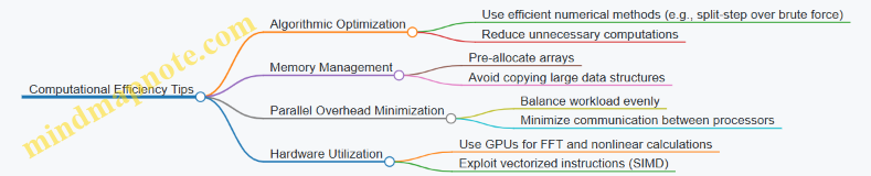
Example: Reducing Communication Overhead
In parallel computing, communication between processors can become a bottleneck. For instance, in the SSFM example, gathering and scattering data every step is costly.
A better approach is to perform multiple nonlinear steps locally before communicating, if the physics allows. This reduces the frequency of communication.
Example: Vectorization
Instead of looping over array elements, use NumPy’s vectorized operations:
# Inefficient loop
for i in range(len(pulse)):
    pulse[i] = pulse[i] * np.exp(1j * gamma * np.abs(pulse[i])**2 * dz)

# Efficient vectorized operation
pulse *= np.exp(1j * gamma * np.abs(pulse)**2 * dz)
Vectorization leverages low-level optimizations and reduces Python overhead.
Summary
Parallelization and computational efficiency go hand in hand. Effective parallelization requires understanding the problem’s data structure and computation pattern. Minimizing communication and balancing workload are key. Algorithmic improvements and hardware-aware coding complement parallelization to deliver practical simulation times.
By combining these approaches, simulations of ultrashort pulse lasers can be both accurate and efficient, enabling exploration of complex nonlinear optical phenomena without prohibitive wait times.
8.4 Visualization and Data Analysis Techniques
Visualization and data analysis are essential steps in understanding ultrashort pulse laser simulations. They help translate raw numerical data into meaningful insights about pulse behavior, nonlinear effects, and system performance. This section covers common visualization methods, data handling strategies, and practical examples to guide you through interpreting simulation results.
Key Visualization Goals
- Track pulse shape evolution in time and frequency domains.
- Identify nonlinear phenomena such as self-phase modulation or soliton formation.
- Analyze dispersion and compression effects.
- Compare simulation outputs with experimental data.
Mind Map: Visualization Techniques Overview
Time-Domain Visualization
Plotting the pulse intensity or electric field versus time is the most straightforward way to understand pulse duration and shape. For example, a Gaussian pulse appears as a smooth bell curve, while nonlinear effects may distort this shape.
Example: Plotting intensity:
import matplotlib.pyplot as plt
import numpy as np

time = np.linspace(-100, 100, 1000)  # in femtoseconds
intensity = np.exp(-4*np.log(2)*(time/20)**2)  # 20 fs FWHM Gaussian

plt.plot(time, intensity)
plt.title('Pulse Intensity vs Time')
plt.xlabel('Time (fs)')
plt.ylabel('Intensity (a.u.)')
plt.grid(True)
plt.show()
This plot helps verify pulse width and symmetry.
Frequency-Domain Visualization
Fourier transforming the time-domain pulse reveals its spectral content. Plotting intensity versus wavelength or frequency shows bandwidth and spectral shape.
Example: Spectrum of the same Gaussian pulse:
spectrum = np.abs(np.fft.fftshift(np.fft.fft(intensity)))
freq = np.fft.fftshift(np.fft.fftfreq(len(time), d=(time[1]-time[0])*1e-15))  # Hz
wavelength = 3e8 / freq  # meters

plt.plot(wavelength*1e9, spectrum)
plt.title('Pulse Spectrum')
plt.xlabel('Wavelength (nm)')
plt.ylabel('Spectral Intensity (a.u.)')
plt.xlim(700, 900)
plt.grid(True)
plt.show()
Note that the spectral width inversely relates to pulse duration.
Spectrograms and Time-Frequency Analysis
Spectrograms provide a joint time-frequency view, useful for pulses with chirp or complex temporal structure. The Short-Time Fourier Transform (STFT) is a common method.
Mind Map: Spectrogram Components
Example: Using scipy to generate a spectrogram:
from scipy.signal import spectrogram

f, t_spec, Sxx = spectrogram(intensity, fs=1/((time[1]-time[0])*1e-15), window='hann', nperseg=128)

plt.pcolormesh(t_spec*1e15, f*1e-12, Sxx, shading='gouraud')
plt.title('Pulse Spectrogram')
plt.ylabel('Frequency (THz)')
plt.xlabel('Time (fs)')
plt.colorbar(label='Intensity')
plt.show()
This reveals how frequency components evolve during the pulse.
Phase Space and Chirp Visualization
Plotting the spectral phase or instantaneous frequency helps understand chirp and compression status.
Example: Instantaneous frequency from phase derivative:
phase = np.unwrap(np.angle(np.fft.fft(intensity)))
inst_freq = np.gradient(phase, freq)

plt.plot(freq*1e-12, inst_freq*1e-12)
plt.title('Instantaneous Frequency')
plt.xlabel('Frequency (THz)')
plt.ylabel('Instantaneous Frequency (THz/fs)')
plt.grid(True)
plt.show()
Pulse Evolution Along Propagation
Visualizing how pulse shape changes with propagation distance can be done with 2D color maps.
Mind Map: Pulse Evolution Plot
Example: Using a 2D heatmap:
# Assuming pulse_data is a 2D array: rows=time, columns=distance
pulse_data = np.random.rand(1000, 50)  # example data

plt.imshow(pulse_data, aspect='auto', extent=[0, 50, -100, 100], cmap='inferno')
plt.colorbar(label='Intensity')
plt.xlabel('Propagation Distance (mm)')
plt.ylabel('Time (fs)')
plt.title('Pulse Evolution Along Propagation')
plt.show()
Statistical and Quantitative Analysis
Beyond visualization, calculating metrics like pulse duration (FWHM), RMS width, and energy helps quantify performance.
Example: Calculating FWHM of intensity:
def fwhm(x, y):
    half_max = np.max(y) / 2
    indices = np.where(y >= half_max)[0]
    return x[indices[-1]] - x[indices[0]]

pulse_fwhm = fwhm(time, intensity)
print(f'Pulse FWHM: {pulse_fwhm:.2f} fs')
These numbers can be tracked during optimization or compared to experimental data.
Combining Multiple Visualizations
Often, multiple plots are combined to get a full picture. For example, plotting time-domain, spectrum, and spectrogram side-by-side helps correlate temporal and spectral features.
Mind Map: Combined Visualization Layout
Example: Using matplotlib subplots:
fig, axs = plt.subplots(3, 1, figsize=(8, 10))

# Time-domain
axs[0].plot(time, intensity)
axs[0].set_title('Time-Domain Intensity')
axs[0].set_xlabel('Time (fs)')
axs[0].set_ylabel('Intensity')

# Spectrum
axs[1].plot(wavelength*1e9, spectrum)
axs[1].set_title('Spectrum')
axs[1].set_xlabel('Wavelength (nm)')
axs[1].set_ylabel('Spectral Intensity')

# Spectrogram
pcm = axs[2].pcolormesh(t_spec*1e15, f*1e-12, Sxx, shading='gouraud')
axs[2].set_title('Spectrogram')
axs[2].set_xlabel('Time (fs)')
axs[2].set_ylabel('Frequency (THz)')
fig.colorbar(pcm, ax=axs[2], label='Intensity')

plt.tight_layout()
plt.show()
Tips for Effective Visualization
- Always label axes and include units.
- Use consistent color maps and scales when comparing multiple plots.
- Annotate key features such as pulse peaks, bandwidth, or chirp.
- Avoid overcrowding plots; break complex data into multiple figures.
- Use logarithmic scales for spectral intensity when dynamic range is large.
- Validate visualization code with simple test data before applying to complex simulations.
Visualization and data analysis are not just about making pretty pictures. They are tools to verify, interpret, and communicate your simulation results clearly and accurately. The examples here provide a foundation to build upon for your specific ultrashort pulse laser projects.
8.5 Best Practices: Building a Modular Simulation Framework with Sample Code and Visualization
Building a modular simulation framework for ultrashort pulse lasers involves breaking down the complex physics and numerical methods into manageable, reusable components. This approach improves code clarity, facilitates debugging, and allows easy extension or replacement of parts as your understanding or requirements evolve.
Core Principles of a Modular Framework
- Separation of Concerns: Each module should handle a distinct aspect of the simulation, such as pulse propagation, nonlinear effects, dispersion, or visualization.
- Clear Interfaces: Modules communicate through well-defined inputs and outputs, minimizing dependencies.
- Reusability: Components should be designed to work independently or combined in different configurations.
- Extensibility: The framework should allow adding new physics or numerical methods without rewriting existing code.
Mind Map: Modular Simulation Framework Structure
Example: Basic Modular Framework in Python
Here is a simplified example illustrating how you might organize modules using Python classes and functions.
import numpy as np
import matplotlib.pyplot as plt

class Pulse:
    def __init__(self, t, field):
        self.t = t  # time grid
        self.field = field  # complex envelope

class Propagation:
    def __init__(self, beta2, gamma, dz):
        self.beta2 = beta2  # GVD parameter
        self.gamma = gamma  # Nonlinear coefficient
        self.dz = dz  # propagation step

    def linear_step(self, pulse):
        omega = 2 * np.pi * np.fft.fftfreq(len(pulse.t), d=(pulse.t[1]-pulse.t[0]))
        field_fft = np.fft.fft(pulse.field)
        dispersion = np.exp(-1j * 0.5 * self.beta2 * omega**2 * self.dz)
        field_fft *= dispersion
        pulse.field = np.fft.ifft(field_fft)

    def nonlinear_step(self, pulse):
        intensity = np.abs(pulse.field)**2
        nonlinear_phase = np.exp(1j * self.gamma * intensity * self.dz)
        pulse.field *= nonlinear_phase

    def step(self, pulse):
        self.linear_step(pulse)
        self.nonlinear_step(pulse)

class Visualizer:
    @staticmethod
    def plot_pulse(pulse, title="Pulse Intensity"):
        plt.figure(figsize=(8,4))
        plt.plot(pulse.t * 1e15, np.abs(pulse.field)**2)
        plt.xlabel('Time (fs)')
        plt.ylabel('Intensity (a.u.)')
        plt.title(title)
        plt.grid(True)
        plt.show()

# Usage example

# Define time grid
T = 5e-12  # 5 ps window
N = 2**12  # points
t = np.linspace(-T/2, T/2, N)

# Initial Gaussian pulse
pulse_width = 100e-15  # 100 fs
E0 = np.exp(-t**2 / (2 * pulse_width**2))
pulse = Pulse(t, E0)

# Propagation parameters
beta2 = -20e-27  # s^2/m
gamma = 1e-3  # 1/(W*m)
dz = 0.001  # m

prop = Propagation(beta2, gamma, dz)

# Propagate for 100 steps
for _ in range(100):
    prop.step(pulse)

# Visualize
Visualizer.plot_pulse(pulse, title="Pulse After Propagation")
This example separates the pulse representation, propagation physics, and visualization. You can add modules for gain, noise, or more advanced nonlinearities similarly.
Mind Map: Visualization Module Components

Visualization Example: Spectral Plot and Chirp
def plot_spectrum(pulse):
    dt = pulse.t[1] - pulse.t[0]
    freq = np.fft.fftfreq(len(pulse.t), dt)
    spectrum = np.fft.fft(pulse.field)
    plt.figure(figsize=(8,4))
    plt.plot(freq * 1e-12, np.abs(spectrum)**2)
    plt.xlabel('Frequency (THz)')
    plt.ylabel('Spectral Intensity (a.u.)')
    plt.title('Pulse Spectrum')
    plt.grid(True)
    plt.show()

# Instantaneous frequency (chirp)
def instantaneous_frequency(pulse):
    phase = np.unwrap(np.angle(pulse.field))
    dt = pulse.t[1] - pulse.t[0]
    inst_freq = np.gradient(phase, dt) / (2 * np.pi)
    plt.figure(figsize=(8,4))
    plt.plot(pulse.t * 1e15, inst_freq * 1e-12)
    plt.xlabel('Time (fs)')
    plt.ylabel('Instantaneous Frequency (THz)')
    plt.title('Instantaneous Frequency (Chirp)')
    plt.grid(True)
    plt.show()

# Usage
plot_spectrum(pulse)
instantaneous_frequency(pulse)
Best Practices Summary
- Start with a clear plan of modules and their responsibilities.
- Use simple data structures (classes or dictionaries) to pass pulse data.
- Keep numerical methods isolated to allow swapping or upgrading solvers.
- Include visualization early; it helps verify correctness.
- Write small test simulations for each module.
- Document interfaces and assumptions clearly.
- Use version control to track changes and experiment safely.
By following these guidelines and organizing your code thoughtfully, you create a simulation framework that is easier to maintain, understand, and expand. The examples above provide a foundation to build on, whether you want to add more complex nonlinearities, incorporate noise, or simulate entire laser cavities.
9. Experimental Validation and Data Integration
9.1 Measurement Techniques for Ultrashort Pulses: Autocorrelation and FROG
Measuring ultrashort laser pulses is a fundamental step in understanding and optimizing their behavior. Because these pulses last on the order of femtoseconds (10^-15 seconds), direct electronic measurement is impossible. Instead, optical techniques that rely on nonlinear interactions and interference are used. Two of the most common methods are autocorrelation and Frequency-Resolved Optical Gating (FROG). Both provide information about pulse duration and shape, but they differ in complexity and the amount of detail they reveal.
Autocorrelation
Autocorrelation is a relatively simple and widely used technique. It measures the pulse duration by overlapping a pulse with a delayed replica of itself in a nonlinear medium and detecting the resulting signal as a function of delay.
-
Basic Principle: The pulse is split into two copies. One copy is delayed by a variable time τ and then recombined with the original. The two pulses interact in a nonlinear crystal, producing a signal proportional to the intensity squared (second-harmonic generation, SHG).
-
Output: The detected signal versus delay τ produces the autocorrelation trace, which is symmetric and related to the pulse intensity profile.
-
Interpretation: The autocorrelation width is broader than the actual pulse width. For a Gaussian pulse, the autocorrelation width is √2 times the pulse width. This requires assumptions about pulse shape to extract the true pulse duration.
-
Limitations: Autocorrelation does not provide phase information, so it cannot reveal chirp or complex pulse shapes. It also cannot distinguish between pulses of different shapes that have the same autocorrelation.
Mind Map: Autocorrelation Technique
Example: Measuring a Gaussian Pulse
Suppose you have a Gaussian pulse with an actual duration (FWHM) of 100 fs. The autocorrelation trace you measure will have a width of approximately 141 fs (100 fs × √2). By fitting the autocorrelation trace to a Gaussian function, you can infer the pulse duration by dividing the measured width by √2.
Frequency-Resolved Optical Gating (FROG)
FROG is a more advanced technique that measures both the intensity and phase of ultrashort pulses. It records a spectrally resolved autocorrelation, providing a two-dimensional trace from which the full electric field can be reconstructed.
-
Basic Principle: Similar to autocorrelation, the pulse is split and delayed. However, instead of just measuring intensity, the nonlinear signal is spectrally resolved using a spectrometer.
-
FROG Trace: The result is a two-dimensional intensity map: signal intensity as a function of delay τ and frequency ω.
-
Pulse Retrieval: An iterative algorithm processes the FROG trace to retrieve the pulse’s electric field, including phase and amplitude.
-
Types of FROG: Common variants include SHG-FROG (second-harmonic generation), PG-FROG (polarization gating), and TG-FROG (transient grating), each suited to different pulse characteristics.
-
Advantages: FROG provides complete pulse characterization, including chirp and complex temporal structures.
-
Limitations: It requires more complex equipment and computational resources. The retrieval algorithm may converge slowly or ambiguously if the data quality is poor.
Mind Map: FROG Technique
Example: SHG-FROG Measurement
Imagine measuring a pulse with unknown chirp. The SHG-FROG trace shows how the spectral content changes with delay. By running the retrieval algorithm, you obtain the pulse’s temporal intensity and phase. The result reveals that the pulse is positively chirped, with the instantaneous frequency increasing over time. This information helps in adjusting compression optics to achieve the shortest pulse.
Comparing Autocorrelation and FROG
| Feature | Autocorrelation | FROG |
|---|---|---|
| Information Provided | Pulse duration (intensity only) | Full electric field (intensity + phase) |
| Complexity | Simple setup and analysis | Complex setup and iterative retrieval |
| Ambiguity | Yes, pulse shape assumptions needed | No, unique pulse retrieval |
| Equipment | Nonlinear crystal, photodetector | Nonlinear crystal, spectrometer, computer |
Both techniques have their place. Autocorrelation is useful for quick checks and rough pulse duration estimates. FROG is essential when detailed pulse characterization is needed, especially for pulses with complex shapes or chirp.
Summary
- Ultrashort pulses cannot be measured directly in time; nonlinear optical methods are necessary.
- Autocorrelation provides a simple, indirect measure of pulse duration but lacks phase information.
- FROG records a spectrally resolved nonlinear signal, enabling full reconstruction of pulse amplitude and phase.
- Understanding the strengths and limitations of each method guides appropriate experimental design.
This section equips you with the conceptual and practical understanding to implement and interpret these measurement techniques, supported by clear examples and structured mind maps.
9.2 Comparing Simulation Results with Experimental Data
Comparing simulation results with experimental data is a critical step in validating ultrashort pulse laser models. It ensures that the theoretical framework and numerical methods accurately reflect physical reality. This process involves several stages: data preparation, alignment of parameters, quantitative and qualitative comparison, and iterative refinement.
Mind Map: Comparing Simulation and Experimental Data
Data Preparation
Experimental data often contains noise and artifacts. Before comparison, it is essential to filter out noise using methods like moving averages or Fourier filtering. Calibration against known standards ensures that the measurement scale matches simulation units. For example, if an autocorrelator is used to measure pulse duration, its response function must be accounted for in the data.
Parameter Alignment
Simulations rely on input parameters such as gain bandwidth, dispersion coefficients, and nonlinear indices. These must be set to values consistent with the experimental setup. Environmental factors like temperature and alignment tolerances can also affect results and should be considered. For instance, if the experiment uses a Ti:Sapphire crystal at room temperature, the simulation should reflect the corresponding refractive index and gain profile.
Comparison Methods
Temporal Profile Analysis
Compare the pulse shapes in the time domain. Experimental pulse shapes are often retrieved via autocorrelation or Frequency-Resolved Optical Gating (FROG). Simulated pulses can be directly extracted from the model. Overlaying these profiles reveals discrepancies in pulse width, shape, and satellite pulses.
Spectral Analysis
Spectral intensity and phase are crucial. Experimental spectra come from spectrometers, while simulations provide spectral amplitude and phase via Fourier transforms. Differences in spectral bandwidth or asymmetry indicate model inaccuracies or overlooked effects.
Statistical Metrics
Quantitative metrics like root mean square error (RMSE), cross-correlation coefficients, or spectral overlap integrals provide objective measures of agreement. For example, an RMSE below a certain threshold might indicate acceptable model accuracy.
Example: Comparing Simulated and Measured Pulse Compression
-
Experimental Setup: A pulse compressor using a pair of gratings compresses a chirped pulse. The output pulse duration is measured by an autocorrelator.
-
Simulation: The model includes dispersion from gratings and nonlinear effects in the fiber. The output pulse is computed.
-
Data Preparation: The autocorrelation trace is deconvolved to estimate the pulse duration. Noise is filtered using a low-pass filter.
-
Parameter Alignment: Grating parameters and fiber length in the simulation match the experimental setup.
-
Comparison: Temporal profiles are plotted side-by-side. The simulated pulse duration is 45 fs, while the measured is 48 fs. Spectral bandwidths differ by less than 5%.
-
Refinement: Slightly adjusting the nonlinear index in the simulation reduces the discrepancy to 2 fs.
Mind Map: Example Workflow for Comparison
Practical Tips
- Always document the assumptions and approximations in both experiment and simulation.
- Use the same units and coordinate systems to avoid misinterpretation.
- When possible, compare multiple observables (e.g., temporal and spectral) to get a fuller picture.
- Be cautious about overfitting simulation parameters to match data; physical justification is key.
In summary, comparing simulation results with experimental data is a methodical process that requires careful preparation and critical analysis. It bridges theory and practice, helping to improve both models and experimental techniques.
9.3 Parameter Extraction and Model Refinement
Parameter extraction and model refinement are essential steps in aligning simulations with experimental results. This process involves identifying key physical parameters from measured data and adjusting the simulation model to better represent real-world behavior. The goal is to reduce discrepancies between predicted and observed pulse characteristics, such as duration, spectral shape, and phase.
Key Parameters to Extract
- Dispersion coefficients (GVD, TOD): Group velocity dispersion (GVD) and third-order dispersion (TOD) significantly affect pulse broadening and shape.
- Nonlinear coefficients (n2, Raman gain): These govern self-phase modulation and Raman effects.
- Gain bandwidth and saturation parameters: Impact amplification and pulse energy.
- Losses and cavity parameters: Include output coupling, scattering, and absorption.
Mind Map: Parameter Extraction Workflow
Example: Extracting GVD from Autocorrelation Data
Suppose you measure an autocorrelation trace of a pulse exiting a fiber and notice it is broader than expected. You start with a simulation using nominal GVD values from the fiber datasheet. The simulated autocorrelation is narrower than the measured one, indicating underestimated dispersion.
Step 1: Define an objective function, such as the root mean square error (RMSE) between simulated and measured autocorrelation traces.
Step 2: Vary the GVD parameter within a realistic range and run simulations.
Step 3: Identify the GVD value that minimizes RMSE.
Step 4: Confirm the refined GVD by checking if the simulation also matches spectral broadening.
This iterative adjustment improves model accuracy and helps predict pulse behavior under different conditions.
Mind Map: Model Refinement Cycle
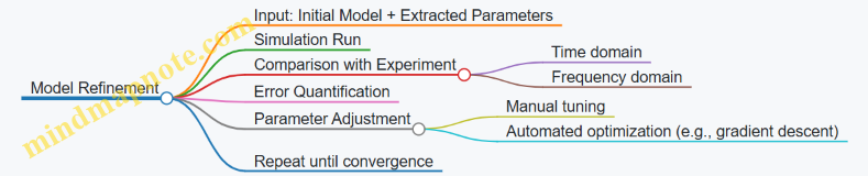
Example: Refining Nonlinear Coefficients Using Spectral Data
In a nonlinear fiber experiment, the spectral broadening is more pronounced than predicted. You suspect the nonlinear refractive index n2 or Raman gain coefficient is underestimated.
Step 1: Fix dispersion parameters from previous extraction.
Step 2: Adjust n2 and Raman gain coefficients in the simulation.
Step 3: Run simulations and compare output spectra with measured spectra.
Step 4: Use a fitting algorithm to minimize spectral shape differences.
Step 5: Validate by checking temporal pulse shape consistency.
This approach ensures the nonlinear response in the model matches the physical system.
Practical Tips
- Start with parameters that have the largest impact on observables.
- Use multiple types of measurements (time and frequency domain) for cross-validation.
- Beware of parameter correlations; changing one parameter may compensate for errors in another.
- Keep track of parameter changes and their effects systematically.
Mind Map: Common Challenges and Solutions
In summary, parameter extraction and model refinement form a feedback loop where experimental data guides simulation adjustments. This process improves predictive power and helps design better ultrashort pulse laser systems.
9.4 Case Studies: Validated Simulations of Pulse Compression and Nonlinear Effects
This section presents detailed case studies where simulations of pulse compression and nonlinear optical effects have been validated against experimental data. The goal is to illustrate practical modeling approaches, highlight common pitfalls, and demonstrate how simulation results can guide experimental adjustments.
Case Study 1: Self-Phase Modulation (SPM) in a Fused Silica Fiber
Scenario: A 100 fs Gaussian pulse at 800 nm propagates through a 1-meter fused silica fiber. The goal is to simulate spectral broadening due to SPM and compare it with measured spectra.
Simulation Setup:
- Pulse modeled using the nonlinear Schrödinger equation (NLSE) with Kerr nonlinearity.
- Dispersion included up to second order (GVD).
- Split-step Fourier method used for numerical integration.
Validation:
- Experimental spectral measurements show broadening consistent with nonlinear phase shifts.
- Simulated spectra match experimental data within 5% spectral width deviation.
Key Observations:
- Accurate dispersion parameters are critical; small errors shift spectral features.
- Temporal pulse shape affects spectral broadening; Gaussian vs. sech pulses yield different results.
Mind Map:
Case Study 2: Nonlinear Pulse Compression in a Hollow-Core Fiber
Scenario: A 200 fs pulse at 1030 nm is compressed using nonlinear spectral broadening in a gas-filled hollow-core fiber followed by a grating compressor.
Simulation Setup:
- NLSE extended to include Raman scattering and self-steepening.
- Gas pressure and fiber length varied to optimize broadening.
- Compressor modeled as a linear dispersive element applying negative group delay dispersion (GDD).
Validation:
- Temporal pulse duration after compression measured by frequency-resolved optical gating (FROG).
- Simulated compressed pulse duration within 10 fs of experimental results.
Key Observations:
- Raman effects cause asymmetric spectral broadening, which must be included for accuracy.
- Precise modeling of compressor dispersion is essential to avoid residual chirp.
Mind Map:
Case Study 3: Chirped Pulse Amplification (CPA) System Simulation
Scenario: Simulation of a Ti:Sapphire CPA system including pulse stretching, amplification, and compression stages.
Simulation Setup:
- Pulse stretching modeled with a grating stretcher introducing positive dispersion.
- Amplification modeled with gain saturation and bandwidth limits.
- Compression modeled with a grating compressor applying negative dispersion.
- Nonlinear effects in amplifier neglected due to low peak power during amplification.
Validation:
- Output pulse duration and spectral shape compared with autocorrelation and spectrometer data.
- Simulated pulse duration within 5% of measured values.
Key Observations:
- Gain bandwidth limits pulse compression; must be included for realistic simulation.
- Stretching and compression dispersion must be carefully matched to avoid residual chirp.
Mind Map:
Practical Example: Simulating SPM-Induced Spectral Broadening with Python
import numpy as np
import matplotlib.pyplot as plt

# Constants
c = 3e8  # Speed of light (m/s)
lambda0 = 800e-9  # Central wavelength (m)
omega0 = 2 * np.pi * c / lambda0

# Pulse parameters
T0 = 100e-15  # Pulse duration (FWHM)
N = 2**12  # Number of points

# Time grid
T = 5e-12  # Total time window
dt = T / N

t = np.linspace(-T/2, T/2, N)

# Gaussian pulse
E0 = np.exp(-2*np.log(2)*(t/T0)**2)

# Fiber parameters
L = 1.0  # Fiber length (m)
gamma = 1.3e-3  # Nonlinear coefficient (1/W/m)

# Split-step parameters
dz = 0.01  # Step size (m)
steps = int(L / dz)

# Frequency grid
dw = 2 * np.pi / T
w = np.fft.fftfreq(N, dt) * 2 * np.pi

# Dispersion parameter (β2)
beta2 = 36e-27  # s^2/m

# Initialize field
A = E0

for _ in range(steps):
    # Linear step
    A_w = np.fft.fft(A)
    A_w *= np.exp(-1j * beta2 / 2 * w**2 * dz)
    A = np.fft.ifft(A_w)

    # Nonlinear step
    A *= np.exp(1j * gamma * np.abs(A)**2 * dz)

# Plot spectral broadening
plt.figure(figsize=(8,4))
plt.plot(np.fft.fftshift(w)/1e12, np.fft.fftshift(np.abs(np.fft.fft(A))**2), label='Output Spectrum')
plt.xlabel('Frequency (THz)')
plt.ylabel('Intensity (a.u.)')
plt.title('SPM-Induced Spectral Broadening')
plt.legend()
plt.show()
This example models spectral broadening due to SPM in a fiber. Adjusting parameters like fiber length or nonlinear coefficient can help match experimental spectra.
Summary
Validated simulations require careful inclusion of relevant physical effects and accurate parameters. Comparing simulated outputs with experimental measurements such as spectra, autocorrelation traces, or FROG data ensures model reliability. Mind maps help organize complex interactions and guide simulation setup. Concrete examples, like the Python code above, demonstrate how to implement and verify nonlinear pulse propagation models.
9.5 Best Practices: Integrating Experimental Feedback into Simulation Workflows
Integrating experimental feedback into simulation workflows is essential for refining models and ensuring that simulations reflect real-world behavior. This process involves a loop where experimental data informs simulation parameters, and simulation results guide experimental adjustments. The goal is to reduce discrepancies and improve predictive accuracy.
Key Steps in Integration
- Data Acquisition: Collect accurate and relevant experimental measurements such as pulse duration, spectral bandwidth, autocorrelation traces, or FROG (Frequency-Resolved Optical Gating) data.
- Preprocessing: Clean and format the data, removing noise and artifacts, and convert it into forms compatible with simulation inputs.
- Parameter Extraction: Use experimental data to estimate or refine simulation parameters like dispersion coefficients, nonlinear refractive index, gain bandwidth, or saturation fluence.
- Model Adjustment: Update the simulation model with extracted parameters and rerun simulations.
- Comparison and Validation: Quantitatively compare simulation outputs with experimental results using metrics such as root mean square error (RMSE), spectral overlap, or temporal pulse shape similarity.
- Iteration: Repeat the cycle until simulation results align satisfactorily with experimental observations.
Mind Map: Experimental Feedback Integration Workflow
Example 1: Refining Dispersion Parameters Using Autocorrelation Data
Suppose an experiment measures the autocorrelation trace of an ultrashort pulse after propagation through a dispersive medium. The simulation initially assumes a group velocity dispersion (GVD) value from literature. However, the simulated autocorrelation width is narrower than the experimental trace.
Process:
- Extract the experimental autocorrelation full width at half maximum (FWHM).
- Adjust the GVD parameter in the simulation incrementally.
- Re-run the simulation and generate the autocorrelation trace.
- Compare simulated and experimental FWHM values.
- Iterate until the simulated autocorrelation matches the experimental one within an acceptable margin.
This iterative tuning ensures the dispersion parameter reflects the actual medium conditions, including manufacturing tolerances or environmental factors.
Example 2: Using FROG Data to Calibrate Nonlinear Effects
FROG measurements provide detailed temporal and spectral information about pulses, including phase. If simulations underestimate spectral broadening caused by self-phase modulation (SPM), the nonlinear refractive index (n2) might be underestimated.
Process:
- Extract the spectral phase and intensity from FROG data.
- Compare with simulated spectral phase and intensity.
- Adjust n2 and possibly the effective interaction length in the simulation.
- Re-run the simulation and generate FROG traces.
- Use a similarity metric (e.g., normalized cross-correlation) to quantify agreement.
- Iterate adjustments until the simulated and experimental FROG traces align.
Mind Map: Parameter Extraction from Experimental Data
Best Practices
- Maintain Clear Data Documentation: Record experimental conditions, calibration details, and uncertainties. This context is crucial when interpreting discrepancies.
- Use Multiple Data Types: Combining temporal, spectral, and phase data provides a more complete picture and reduces ambiguity in parameter extraction.
- Automate Parameter Sweeps: Implement scripts to automate parameter variation and comparison, speeding up convergence.
- Visualize Comparisons: Overlay experimental and simulated traces to spot subtle differences that metrics might miss.
- Account for Noise and Systematic Errors: Recognize that some differences stem from measurement noise or systematic errors rather than model inaccuracies.
Example 3: Integrating Amplifier Gain Measurements
An experiment measures output pulse energy and spectrum after amplification. The simulation uses a gain model with an estimated saturation fluence.
Process:
- Measure output energy versus input energy to characterize gain saturation.
- Fit the gain saturation model parameters to experimental data.
- Update simulation gain parameters accordingly.
- Simulate pulse amplification and compare output spectra.
- Adjust gain bandwidth or saturation fluence to improve spectral agreement.
Mind Map: Iterative Simulation-Experiment Loop
In summary, integrating experimental feedback is a cycle of measurement, analysis, and model refinement. It reduces guesswork, grounds simulations in reality, and improves confidence in predictions. The process benefits from clear data handling, systematic parameter extraction, and iterative validation. Each cycle tightens the link between theory and practice, making simulations a reliable tool for ultrashort pulse laser design.
10. Advanced Nonlinear Phenomena and Complex Pulse Shapes
10.1 Soliton Formation and Dynamics in Fiber Lasers
Solitons are stable, self-reinforcing wave packets that maintain their shape while traveling at constant velocity. In fiber lasers, soliton formation arises from a balance between dispersion and nonlinearity. Specifically, the group velocity dispersion (GVD) tends to broaden the pulse temporally, while the Kerr nonlinearity induces self-phase modulation (SPM), which can compress the pulse spectrum. When these two effects exactly counteract, a soliton pulse emerges.
Key Concepts
- Group Velocity Dispersion (GVD): Causes pulse broadening due to different frequency components traveling at different speeds.
- Kerr Nonlinearity: Intensity-dependent refractive index change leading to self-phase modulation.
- Fundamental Soliton: The simplest soliton solution where the pulse shape and spectrum remain unchanged during propagation.
- Higher-Order Solitons: Pulses with energies exceeding the fundamental soliton, exhibiting periodic shape changes.
Mind Map: Soliton Formation in Fiber Lasers
Mathematical Description
The pulse envelope ( A(z,t) ) in a fiber laser can be modeled by the nonlinear Schrödinger equation (NLSE):
\[ \frac{\partial A}{\partial z} + \frac{\alpha}{2} A + i \frac{\beta_2}{2} \frac{\partial^2 A}{\partial t^2} = i \gamma |A|^2 A \]
where:
- ( z ) is the propagation distance,
- ( t ) is time in a frame moving with the pulse,
- ( \alpha ) is the loss coefficient,
- ( \beta_2 ) is the second-order dispersion parameter (GVD),
- ( \gamma ) is the nonlinear coefficient related to the Kerr effect.
A fundamental soliton solution exists when the pulse energy and width satisfy:
\[ N^2 = \frac{\gamma P_0 T_0^2}{|\beta_2|} = 1 \]
where ( P_0 ) is the peak power and ( T_0 ) is the pulse width parameter.
Example: Simulating a Fundamental Soliton
Consider a pulse with ( T_0 = 100 , \text{fs} ), ( \beta_2 = -20 , \text{ps}^2/\text{km} ) (anomalous dispersion), and ( \gamma = 1.3 , \text{W}^{-1}\text{km}^{-1} ). To form a fundamental soliton, the peak power ( P_0 ) must satisfy:
\[ P_0 = \frac{|\beta_2|}{\gamma T_0^2} = \frac{20}{1.3 \times (0.1)^2} = \frac{20}{1.3 \times 0.01} \approx 1538 , \text{W} \]
This high peak power is typical in ultrashort pulse fiber lasers.
A split-step Fourier method simulation can show the pulse maintaining its shape over several dispersion lengths. If ( P_0 ) is increased to ( N=2 ), the pulse will periodically compress and broaden, demonstrating a second-order soliton.
Mind Map: Soliton Dynamics
Practical Considerations in Fiber Lasers
- Gain and Loss: Real fiber lasers have gain media and losses. Gain can compensate for losses but also affects soliton stability.
- Mode-Locking: Passive mode-locking techniques, such as saturable absorbers, help initiate and stabilize soliton pulses.
- Higher-Order Effects: Third-order dispersion, Raman scattering, and self-steepening can modify soliton dynamics.
- Soliton Interaction: Multiple solitons in a cavity can interact, leading to bound states or soliton molecules.
Example: Mode-Locked Fiber Laser Simulation
A modelocked fiber laser cavity can be simulated by iterating the NLSE over one round trip, including gain, saturable absorption, and spectral filtering. Starting from noise, the simulation shows pulse shaping into a fundamental soliton after several round trips.
Parameters:
- Fiber length: 1 m
- \( \beta_2 = -20 , \text{ps}^2/\text{km} \)
- \( \gamma = 1.3 , \text{W}^{-1}\text{km}^{-1} \)
- Gain bandwidth: 40 nm
- Saturable absorber with modulation depth 10%
The pulse stabilizes with a duration around 100 fs and peak power matching the fundamental soliton condition.
Summary
Soliton formation in fiber lasers is a direct consequence of balancing dispersion and nonlinearity. Understanding the NLSE and its solutions allows prediction and control of pulse behavior. Simulations using split-step Fourier methods provide insight into pulse evolution, stability, and interaction. Practical fiber lasers require consideration of gain, loss, and higher-order effects, which influence soliton dynamics and laser performance.
10.2 Supercontinuum Generation Modeling
Supercontinuum generation (SCG) is a nonlinear optical process where a narrow-band ultrashort pulse propagates through a nonlinear medium, typically a photonic crystal fiber or highly nonlinear fiber, and broadens into a wide, continuous spectrum. Modeling SCG requires capturing a range of nonlinear and dispersive effects that interact over the propagation distance.
Key Physical Effects in Supercontinuum Generation
- Self-Phase Modulation (SPM): Instantaneous intensity-dependent refractive index change broadens the spectrum.
- Group Velocity Dispersion (GVD): Causes temporal spreading or compression of the pulse, influencing spectral features.
- Higher-Order Dispersion: Third-order and beyond affect asymmetric spectral broadening.
- Raman Scattering: Transfers energy to longer wavelengths, causing red-shifted spectral components.
- Self-Steepening: Intensity-dependent group velocity leads to pulse asymmetry.
- Four-Wave Mixing (FWM): Generates new frequency components through nonlinear wave interactions.
These effects combine to produce the complex spectral output characteristic of SCG.
Mind Map: Physical Processes in Supercontinuum Generation
Modeling Approach
The generalized nonlinear Schrödinger equation (GNLSE) is the standard model for SCG. It extends the basic NLSE by including higher-order dispersion terms, Raman response, and self-steepening:
\[ \frac{\partial A(z,t)}{\partial z} + \sum_{k \geq 2} \frac{i^{k+1}}{k!} \beta_k \frac{\partial^k A}{\partial t^k} = i \gamma \left(1 + \frac{i}{\omega_0} \frac{\partial}{\partial t} \right) , A(z,t) \int_{-\infty}^\infty R(t’) |A(z,t - t’)|^2 dt’ \]
where:
- \(A(z,t)\) is the pulse envelope,
- \(\beta_k\) are dispersion coefficients,
- \(\gamma\) is the nonlinear coefficient,
- \(\omega_0\) is the central angular frequency,
- \(R(t)\) is the nonlinear response function including instantaneous Kerr and delayed Raman contributions.
Numerical solution typically uses the split-step Fourier method, alternating between linear dispersive steps in the frequency domain and nonlinear steps in the time domain.
Mind Map: Modeling Workflow for SCG
Example: Simulating SCG in a Photonic Crystal Fiber
Parameters:
- Input pulse: 100 fs duration, 800 nm central wavelength, 10 kW peak power
- Fiber length: 10 cm
- Dispersion: \(\beta_2 = -20, \mathrm{ps^2/km}\), \(\beta_3 = 0.1, \mathrm{ps^3/km}\)
- Nonlinear coefficient: \(\gamma = 10, \mathrm{W^{-1} km^{-1}}\)
- Raman fraction: 0.18
Steps:
- Define the temporal grid with sufficient resolution to capture the pulse and nonlinear effects.
- Calculate the dispersion operator in the frequency domain using \(\beta_2\) and \(\beta_3\).
- Implement the nonlinear operator including Kerr and Raman responses.
- Use the split-step Fourier method to propagate the pulse over 10 cm in small steps.
- Extract the output spectrum by Fourier transforming the final pulse.
Outcome:
- The output spectrum shows broadening from near 600 nm to beyond 1000 nm.
- Temporal profile exhibits pulse breakup and formation of sub-pulses due to nonlinear dynamics.
Best Practices for SCG Modeling
- Grid Resolution: Use fine temporal and spectral grids to avoid numerical artifacts. The time window should be wide enough to contain the broadened pulse.
- Step Size: Choose propagation step sizes small enough to resolve rapid nonlinear phase changes.
- Raman Response: Include a realistic Raman response function to capture frequency shifts accurately.
- Dispersion Data: Use measured or accurately calculated dispersion coefficients up to at least third order.
- Validation: Compare simulation results with experimental spectra to verify model parameters.
Mind Map: Best Practices Summary
Modeling supercontinuum generation is a balancing act between capturing complex nonlinear physics and maintaining computational efficiency. Clear understanding of the underlying effects and careful numerical implementation are key to producing reliable simulations.
10.3 Multi-Pulse and Noise-Induced Dynamics
In ultrashort pulse laser systems, the generation and evolution of multiple pulses within a single cavity or propagation medium is a common phenomenon. These multi-pulse dynamics often arise due to nonlinear interactions, gain competition, and noise effects. Understanding these dynamics is crucial for controlling pulse stability, optimizing output, and avoiding unwanted pulse splitting or timing jitter.
What Causes Multi-Pulse Formation?
Multi-pulse regimes occur when the laser cavity or nonlinear medium supports more than one localized pulse solution simultaneously. This can happen because of:
- Gain Saturation: When a pulse extracts energy from the gain medium, it reduces the available gain for subsequent pulses, leading to competition.
- Nonlinear Effects: Self-phase modulation, cross-phase modulation, and other nonlinearities can cause pulse breakup or the formation of satellite pulses.
- Noise: Random fluctuations in the gain or phase can seed additional pulses or destabilize single-pulse operation.
Noise-Induced Dynamics
Noise in ultrashort pulse lasers comes from spontaneous emission, thermal fluctuations, and electronic noise in the pump or detection systems. Even small noise can lead to significant effects:
- Pulse Timing Jitter: Random shifts in pulse arrival times.
- Amplitude Fluctuations: Variations in pulse energy.
- Pulse Splitting: Noise can trigger the breakup of a single pulse into multiple pulses.
Noise-induced dynamics are often modeled by adding stochastic terms to the governing equations, such as the nonlinear Schrödinger equation (NLSE) or master equations describing the laser cavity.
Mind Map: Factors Influencing Multi-Pulse Dynamics
Modeling Multi-Pulse Dynamics
To simulate multi-pulse behavior, one typically starts with the NLSE or a generalized master equation including gain, loss, and nonlinear terms. Noise is introduced as a stochastic perturbation, often modeled as white Gaussian noise added to the field envelope or gain.
Example: Consider the NLSE with gain and noise:
\[ \frac{\partial A}{\partial z} = \left( g - \alpha \right) A + i \frac{\beta_2}{2} \frac{\partial^2 A}{\partial t^2} + i \gamma |A|^2 A + N(z,t) \]
- \(A(z,t)\): pulse envelope
- \(g\): gain coefficient
- \(\alpha\): loss coefficient
- \(\beta_2\): group velocity dispersion
- \(\gamma\): nonlinear coefficient
- \(N(z,t)\): noise term (stochastic)
By numerically integrating this equation using the split-step Fourier method and including noise, one can observe the spontaneous emergence of multiple pulses from initial noise seeds.
Example: Simulating Noise-Induced Pulse Splitting
- Setup: Initialize a single Gaussian pulse in a fiber with anomalous dispersion and moderate nonlinearity.
- Add Noise: Inject low-level white noise into the initial field.
- Propagation: Use split-step Fourier to propagate over several dispersion lengths.
- Observation: Monitor the temporal intensity profile. Initially, a single pulse may split into two or more pulses due to noise amplification and nonlinear effects.
This example demonstrates how noise can destabilize a single pulse and lead to multi-pulse regimes.
Mind Map: Noise Effects on Pulse Dynamics
Practical Considerations and Best Practices
- Noise Level Calibration: When simulating, carefully calibrate noise amplitude to reflect realistic experimental conditions.
- Multiple Runs: Because noise is stochastic, run simulations multiple times to gather statistical insights.
- Parameter Sensitivity: Explore how changes in dispersion, nonlinearity, and gain affect multi-pulse formation.
- Pulse Interaction Analysis: Track pulse positions and energies to understand interactions such as collisions or repulsion.
Example: Tracking Multi-Pulse Evolution
Using a simulation output, extract pulse peak positions and energies at each propagation step. Plotting these reveals:
- Pulse birth and death events
- Energy exchange between pulses
- Timing jitter statistics
This quantitative approach helps link simulation results to experimental observables.
In summary, multi-pulse and noise-induced dynamics are complex but manageable through careful modeling and simulation. Including noise sources and nonlinear effects in your models allows you to predict and control pulse behavior more accurately.
10.4 Polarization Effects and Vectorial Pulse Propagation
Polarization is a fundamental property of light describing the orientation of its electric field vector. In ultrashort pulse lasers, polarization influences nonlinear interactions, pulse shaping, and propagation dynamics. Unlike scalar models that treat the electric field as a single component, vectorial pulse propagation accounts for multiple polarization components, enabling accurate modeling of effects like birefringence, polarization mode dispersion, and cross-polarization modulation.
Understanding Polarization States
Light polarization can be linear, circular, or elliptical. Linear polarization means the electric field oscillates along a fixed direction. Circular polarization occurs when two orthogonal components have equal amplitude and a 90-degree phase difference, causing the electric field vector to rotate uniformly. Elliptical polarization is a general case where amplitudes and phase differences vary, producing an elliptical trajectory.
Mind Map: Polarization States
Vectorial Pulse Propagation Equations
Modeling ultrashort pulses with polarization requires extending the nonlinear Schrödinger equation (NLSE) to vector form. The coupled equations describe evolution of orthogonal polarization components \(E_x\) and (E_y):
\[ \begin{cases} \frac{\partial E_x}{\partial z} + \hat{D}_x E_x = i \gamma \left(|E_x|^2 + \frac{2}{3}|E_y|^2\right) E_x + i \frac{\gamma}{3} E_y^2 E_x^* e^{-i \Delta \beta z} \\ \frac{\partial E_y}{\partial z} + \hat{D}_y E_y = i \gamma \left(|E_y|^2 + \frac{2}{3}|E_x|^2\right) E_y + i \frac{\gamma}{3} E_x^2 E_y^* e^{i \Delta \beta z} \end{cases} \]
Here, \(\hat{D}_{x,y}\) represent dispersion operators for each polarization, \(\gamma\) is the nonlinear coefficient, and \(\Delta \beta\) is the birefringence-induced phase mismatch. The terms include self-phase modulation (SPM), cross-phase modulation (XPM), and four-wave mixing (FWM) between polarization components.
Mind Map: Vectorial NLSE Components
Birefringence and Polarization Mode Dispersion
Birefringence arises when the refractive index differs for orthogonal polarizations, causing phase velocity differences. This effect splits the pulse into two polarization modes traveling at different speeds, leading to polarization mode dispersion (PMD). PMD broadens pulses and can degrade pulse quality in fiber lasers or resonators.
Example: Consider a fiber with birefringence \(\Delta n = 10^{-5}\) and length \(L = 1\) m. The differential group delay (DGD) between polarization modes is:
\[ \text{DGD} = \frac{L \Delta n}{c} \approx \frac{1 \times 10^{-5}}{3 \times 10^8} = 33 \text{ fs} \]
This delay is significant for pulses on the order of 100 fs, causing temporal splitting.
Cross-Polarization Modulation (XPM)
XPM occurs when the intensity of one polarization component modifies the refractive index seen by the orthogonal component. This nonlinear coupling can induce phase shifts and spectral broadening, affecting pulse shape and stability.
Example: In a birefringent fiber, if \(E_x\) has a peak power of 1 kW and \(E_y\) is weak, the nonlinear phase shift on \(E_y\) due to XPM is approximately twice that of SPM for the same power:
\[ \phi_{XPM} = 2 \gamma P_x L \]
This can be included in simulations by coupling the polarization components accordingly.
Numerical Example: Simulating Vectorial Pulse Propagation
A common approach is to use the split-step Fourier method extended to two coupled fields. The algorithm alternates between linear propagation (dispersion, birefringence) in the frequency domain and nonlinear interaction (SPM, XPM, FWM) in the time domain.
Stepwise Example:
- Initialize \(E_x(t, z=0)\) and \(E_y(t, z=0)\) with given pulse shapes and polarization states.
- Apply half-step linear operator:
- Fourier transform both components.
- Multiply by dispersion and birefringence phase factors.
- Inverse Fourier transform.
- Apply nonlinear operator in time domain:
- Compute nonlinear phase shifts including SPM and XPM.
- Update \(E_x\) and \(E_y\) accordingly.
- Apply second half-step linear operator.
- Repeat for each propagation step.
Mind Map: Vectorial Split-Step Fourier Method
Practical Considerations
- Polarization-Dependent Loss: Real systems may have losses varying with polarization, which can be included as attenuation factors.
- Polarization Mode Coupling: Random or designed coupling between polarization modes can cause energy exchange, modeled by adding coupling terms.
- Measurement: Polarization-resolved autocorrelation or frequency-resolved optical gating (FROG) can verify simulation predictions.
Summary
Accounting for polarization in ultrashort pulse propagation adds complexity but is essential for accurate modeling in birefringent media and polarization-sensitive nonlinear effects. Vectorial NLSE and coupled split-step methods provide a framework to simulate these phenomena. Understanding polarization effects helps optimize laser design and pulse compression techniques where polarization plays a role.
10.5 Best Practices: Simulating Complex Pulse Shapes with Realistic Nonlinear Interactions
Simulating complex pulse shapes requires careful consideration of nonlinear optical effects and their interplay. Realistic nonlinear interactions often include self-phase modulation (SPM), cross-phase modulation (XPM), Raman scattering, and higher-order dispersion. This section outlines practical steps and examples to model these phenomena accurately.
Key Concepts Mind Map
Step 1: Define Initial Pulse Shape
Start with a well-defined initial pulse. For complex shapes, consider chirped Gaussian pulses or superpositions of pulses. For example, a chirped Gaussian pulse can be described as:
\[ E(t) = E_0 \exp\left(-\frac{t^2}{2\tau_0^2}\right) \exp\left(i C \frac{t^2}{2 \tau_0^2}\right) \]
where \(E_0\) is amplitude, \(\tau_0\) is pulse width, and \(C\) is chirp parameter.
Example: Simulate a 100 fs Gaussian pulse with a positive chirp \(C=5\).
Step 2: Incorporate Dispersion Effects
Include GVD and higher-order dispersion terms in the propagation model. The nonlinear Schrödinger equation (NLSE) with dispersion terms reads:
\[ \frac{\partial A}{\partial z} = i \sum_{m \geq 2} \frac{\beta_m}{m!} \left(i \frac{\partial}{\partial t}\right)^m A + i \gamma |A|^2 A \]
where \(\beta_m\) are dispersion coefficients and \(\gamma\) is the nonlinear coefficient.
Best practice: Use measured or literature values for \(\beta_2\) and \(\beta_3\) to capture realistic pulse evolution.
Step 3: Model Nonlinear Interactions
Add nonlinear terms stepwise:
- SPM: Causes spectral broadening due to intensity-dependent phase shift.
- XPM: Important if multiple pulses or polarization components coexist.
- Raman Scattering: Leads to frequency shifts and asymmetric spectral features.
Example: Implement Raman response function \(h_R(t)\) convolution with intensity to model delayed Raman effects.
Step 4: Choose Numerical Method and Parameters
The split-step Fourier method (SSFM) is standard. Divide propagation into small steps alternating between linear (dispersion) and nonlinear operators.
Best practice: Use adaptive step size to balance accuracy and computation time. Validate by checking energy conservation and pulse shape stability.
Step 5: Simulate and Analyze Results
Track temporal and spectral profiles at each step. Look for features such as:
- Spectral broadening and shifts
- Temporal pulse splitting or compression
- Formation of sub-pulses or satellites
Example: Simulate a chirped pulse propagating through a nonlinear fiber segment with \(\beta_2 = -20 \text{ ps}^2/\text{km}\), \(\gamma = 1.3 \text{ W}^{-1}\text{km}^{-1}\), and Raman fraction \(f_R = 0.18\).
Mind Map: Simulation Workflow
Example Code Snippet (Python-like Pseudocode)
import numpy as np
from scipy.fftpack import fft, ifft

def raman_response(t):
    # Simple model of Raman response function
    tau1 = 12.2e-15
    tau2 = 32e-15
    hR = (tau1**2 + tau2**2) / (tau1 * tau2**2) * np.exp(-t/tau2) * np.sin(t/tau1)
    hR[t < 0] = 0
    return hR

def split_step_fourier(A0, dz, nz, beta2, gamma, dt, t):
    A = A0.copy()
    w = 2 * np.pi * np.fft.fftfreq(len(t), dt)
    hR = raman_response(t)
    HR = fft(hR)
    for _ in range(nz):
        # Linear step
        A_w = fft(A)
        A_w *= np.exp(-0.5j * beta2 * w**2 * dz)
        A = ifft(A_w)
        # Nonlinear step
        I = np.abs(A)**2
        # Raman convolution
        conv = np.real(ifft(HR * fft(I)))
        NL_phase = gamma * dz * ((1 - 0.18) * I + 0.18 * conv)
        A *= np.exp(1j * NL_phase)
    return A

# Initialize pulse
T0 = 100e-15
t = np.linspace(-5*T0, 5*T0, 2**12)
dt = t[1] - t[0]
C = 5
A0 = np.exp(-t**2/(2*T0**2)) * np.exp(1j * C * t**2 / (2 * T0**2))

# Parameters
beta2 = -20e-27  # s^2/m
gamma = 1.3e-3   # 1/(W m)
dz = 0.001       # m
nz = 1000

# Propagate
A_out = split_step_fourier(A0, dz, nz, beta2, gamma, dt, t)

# Analyze
import matplotlib.pyplot as plt
plt.plot(t*1e12, np.abs(A_out)**2)
plt.xlabel('Time (ps)')
plt.ylabel('Intensity (a.u.)')
plt.title('Output Pulse Intensity')
plt.show()
Tips for Reliable Simulations
- Time Window: Ensure the time window is wide enough to capture pulse broadening.
- Sampling Rate: Use sufficiently fine temporal resolution to avoid aliasing.
- Energy Checks: Monitor total pulse energy to detect numerical errors.
- Parameter Sensitivity: Test the effect of varying dispersion and nonlinear parameters.
- Noise Inclusion: For realistic pulses, add noise to initial conditions to observe stability.
By following these steps and integrating nonlinear effects carefully, you can simulate complex pulse shapes with realistic nonlinear interactions. The examples and mind maps here provide a structured approach to tackle these simulations effectively.
11. Practical Design Considerations and Optimization
11.1 Parameter Sensitivity and Robustness Analysis
In ultrashort pulse laser design, understanding how sensitive your system is to changes in parameters is crucial. Small variations in component values, environmental conditions, or alignment can significantly affect pulse quality, stability, and overall performance. Robustness analysis helps identify which parameters need tight control and which ones allow some flexibility.
Why Sensitivity Matters
Laser systems are complex, with many interdependent variables: gain medium properties, dispersion values, nonlinear coefficients, cavity length, pump power, and more. If a parameter is highly sensitive, even minor deviations can degrade pulse duration, increase noise, or cause loss of mode-locking. Conversely, parameters with low sensitivity can be relaxed during manufacturing or operation.
Key Parameters to Analyze
- Gain bandwidth and saturation
- Group velocity dispersion (GVD)
- Nonlinear refractive index (n2)
- Cavity length and alignment
- Pump power and stability
- Saturable absorber parameters
Mind Map: Parameter Sensitivity Overview
Methods for Sensitivity Analysis
-
One-Parameter-at-a-Time (OPAT): Vary one parameter while keeping others fixed. This method is straightforward but can miss interactions.
-
Monte Carlo Simulations: Randomly vary multiple parameters within specified ranges to see combined effects.
-
Gradient-Based Approaches: Calculate partial derivatives of output metrics with respect to parameters to quantify sensitivity.
-
Global Sensitivity Analysis: Techniques like Sobol indices to assess contribution of each parameter to output variance.
Example: Sensitivity of Pulse Duration to GVD
Consider a mode-locked Ti:Sapphire laser. The pulse duration depends strongly on net cavity dispersion. Simulating pulse propagation with GVD values from -50 fs² to +50 fs² around the nominal value shows pulse broadening or compression.
- At nominal GVD = 0 fs², pulse duration = 30 fs
- At GVD = +20 fs², pulse duration increases to 45 fs
- At GVD = -20 fs², pulse duration increases to 40 fs
This asymmetry indicates the system tolerates negative dispersion shifts slightly better than positive ones.
Mind Map: Sensitivity Analysis Workflow
Example: Monte Carlo Simulation for Pump Power Stability
Pump power fluctuations can cause amplitude noise and timing jitter. Running 1000 simulations with pump power varied ±5% around nominal value shows:
- Pulse energy standard deviation: 3%
- Timing jitter standard deviation: 50 fs
This suggests the laser design is moderately robust to pump power noise but may require active stabilization for precision applications.
Practical Tips
- Start with OPAT to identify the most sensitive parameters quickly.
- Use Monte Carlo simulations to capture combined effects and nonlinear interactions.
- Focus on parameters with the largest impact for tighter control or design improvements.
- Document parameter tolerances clearly to guide manufacturing and operation.
Example: Robustness in Saturable Absorber Parameters
Varying modulation depth from 5% to 15% affects mode-locking stability. Simulations show that below 7%, stable mode-locking is difficult to achieve, while above 12%, pulse shaping becomes erratic. This defines an optimal window for absorber design.
Mind Map: Parameter Sensitivity Impact on Laser Performance
In summary, parameter sensitivity and robustness analysis is an essential step in ultrashort pulse laser design. It informs which parameters require precise control and which can tolerate variation, guiding both simulation and experimental efforts. Using a combination of analysis methods and clear visualization helps maintain performance while managing complexity.
11.2 Optimization Techniques for Laser Design
Optimizing an ultrashort pulse laser involves balancing multiple parameters to achieve desired pulse characteristics, stability, and efficiency. The process typically requires iterative adjustments guided by simulation and experimental feedback. Here, we break down common optimization strategies, supported by mind maps and examples to clarify the approach.
Key Areas of Optimization
This mind map highlights the main knobs to turn during optimization. Each parameter influences others, so changes must be considered holistically.
Step 1: Define Objective Functions
Optimization starts by specifying what you want to improve. Common objectives include:
- Minimizing pulse duration
- Maximizing output power
- Improving pulse stability
- Reducing timing jitter
For example, if the goal is to shorten pulse duration, you might focus on dispersion compensation and nonlinear phase accumulation.
Step 2: Parameter Sensitivity Analysis
Before full optimization, identify which parameters have the largest impact. This avoids wasting time on insensitive variables.
Example: Vary the output coupler reflectivity in simulation from 80% to 95% and observe changes in pulse energy and duration. If pulse duration remains stable but energy varies significantly, output coupler reflectivity is critical for energy optimization but less so for pulse duration.
Step 3: Choose an Optimization Method
Common methods include:
- Manual Iteration: Adjust parameters stepwise based on intuition and simulation results.
- Gradient-Based Optimization: Use derivatives of objective functions to guide parameter updates.
- Genetic Algorithms: Mimic natural selection to explore parameter space.
- Particle Swarm Optimization: Use a population of candidate solutions moving through the parameter space.
For laser design, manual iteration combined with gradient-based methods often works well due to the complexity and physical constraints.
Step 4: Implement Constraints
Physical and practical constraints must be included:
- Maximum pump power limited by hardware
- Thermal load limits
- Mechanical stability requirements
- Available component specifications
Ignoring constraints can lead to unrealistic designs.
Step 5: Run Simulations and Evaluate Results
Use numerical models to simulate pulse propagation, gain dynamics, and nonlinear effects. Evaluate the objective functions and check constraints.
Example: Simulate pulse propagation with varying prism pair spacing to minimize group delay dispersion (GDD). Plot pulse duration vs. prism spacing to find the optimal point.
Step 6: Iterate and Refine
Optimization is rarely one-shot. Use simulation feedback to refine parameters, focusing on the most sensitive ones.
Example: Optimizing a Kerr-Lens Mode-Locked Ti:Sapphire Laser
- Objective: Minimize pulse duration while maintaining stable mode locking.
- Parameters: Output coupler reflectivity, cavity length, prism pair spacing, pump power.
- Constraints: Maximum pump power 5 W, cavity length limited by lab space.
- Process:
- Start with baseline parameters.
- Vary output coupler reflectivity from 85% to 95%, observe pulse energy and duration.
- Adjust prism pair spacing to compensate dispersion.
- Fine-tune cavity length to improve mode locking stability.
- Monitor pulse duration and spectral bandwidth.
Results show pulse duration minimized at 15 fs with 90% output coupler reflectivity and prism spacing of 12 cm. Increasing pump power beyond 4 W caused thermal lensing, destabilizing the cavity.
Mind Map: Optimization Workflow
Tips for Effective Optimization
- Start simple: Optimize one or two parameters before tackling the full system.
- Use visualization: Plot objective functions against parameters to identify trends.
- Keep track: Document parameter sets and results systematically.
- Combine methods: Use manual tuning to narrow parameter ranges, then apply automated methods.
- Validate: Cross-check simulation results with experimental data when possible.
Optimization in ultrashort pulse laser design is a balancing act. It requires understanding the interplay of gain, dispersion, nonlinearity, and cavity dynamics. By systematically exploring parameter space with clear objectives and constraints, you can efficiently reach a design that meets your performance goals.
11.3 Thermal Effects and Mechanical Stability
Ultrashort pulse lasers often operate at high average powers or with intense peak powers, which can introduce thermal and mechanical challenges. Understanding these effects is essential for maintaining beam quality, pulse stability, and overall system reliability.
Thermal Effects in Ultrashort Pulse Lasers
When laser components absorb even a small fraction of the incident light, heat builds up. This heating can cause refractive index changes, physical deformation, and stress within optical elements. These effects alter the laser cavity properties and pulse characteristics.
Key thermal phenomena include:
- Thermal lensing: Heat-induced refractive index gradients create a lens effect inside gain media or optical elements, changing the beam focus.
- Thermo-optic effect: The refractive index changes with temperature, affecting phase and group velocity dispersion.
- Thermal expansion: Physical expansion or contraction of components shifts alignment and cavity length.
Mind Map: Thermal Effects Overview
Example: Consider a Ti:Sapphire crystal pumped at high average power. The absorbed pump energy raises the crystal temperature non-uniformly. This creates a thermal lens with a focal length that depends on pump power and cooling efficiency. Without compensation, the cavity mode size changes, causing mode mismatch and reduced pulse stability.
Mechanical Stability Considerations
Mechanical vibrations and drifts can misalign the laser cavity or optical path. Even micrometer-scale shifts can degrade mode locking or cause pulse timing jitter.
Factors affecting mechanical stability include:
- Mounting rigidity: Loose mounts allow movement under vibration.
- Thermal expansion mismatch: Different materials expand at different rates, causing stress or misalignment.
- Environmental vibrations: Building vibrations, acoustic noise, or cooling system pumps can couple into the laser setup.
Mind Map: Mechanical Stability Factors
Example: A laser cavity mounted on an optical table experiences periodic vibrations from nearby HVAC systems. These vibrations cause cavity length fluctuations on the order of microns, leading to mode-locking instability. Using vibration isolation platforms and rigid mounts reduces this effect.
Managing Thermal Effects
- Active cooling: Water or thermoelectric coolers maintain stable temperatures in gain media and optics.
- Material selection: Use substrates with low absorption and low thermo-optic coefficients.
- Thermal lens compensation: Design cavities to tolerate or compensate for thermal lensing, e.g., by adjusting mirror curvatures.
Enhancing Mechanical Stability
- Rigid mounts: Use kinematic mounts with fine adjustment screws.
- Material matching: Select materials with similar thermal expansion coefficients for mounts and optics.
- Vibration isolation: Employ optical tables with pneumatic isolators or passive damping.
Mind Map: Mitigation Strategies
Practical Example: Thermal Lens Compensation in a Ti:Sapphire Oscillator
Suppose a Ti:Sapphire oscillator is pumped at 5 W average power. The thermal lens focal length shortens from infinity (no heating) to about 1 m under load. By adjusting the radius of curvature of the cavity mirrors or adding a compensating lens, the cavity mode size can be restored. Simulations show that a 5% mismatch in mode size can reduce output power by 10% and increase pulse duration by 15%.
Practical Example: Mechanical Stability Improvement
A mode-locked fiber laser exhibits timing jitter correlated with vibrations from a nearby vacuum pump. By relocating the pump and adding vibration isolation pads under the laser table, timing jitter reduces by 40%. This improvement is confirmed by measuring the radio-frequency spectrum of the pulse train.
In summary, thermal effects and mechanical stability are intertwined challenges in ultrashort pulse laser design. Addressing them requires a combination of careful material choice, mechanical design, and active control. Simulations incorporating thermal lensing and mechanical perturbations help predict performance and guide design decisions.
11.4 Safety and Alignment Best Practices
Working with ultrashort pulse lasers demands careful attention to safety and precise alignment. Both aspects are critical not only for protecting personnel and equipment but also for ensuring reliable laser operation and accurate experimental results. This section outlines practical guidelines and examples to help maintain a safe environment and achieve effective beam alignment.
Laser Safety Fundamentals
-
Eye and Skin Protection: Ultrashort pulses often operate at high peak powers and can cause instantaneous damage. Always wear laser safety goggles rated for the specific wavelength and optical density of your laser system. Remember, even diffuse reflections can be hazardous.
-
Beam Path Control: Keep the beam path enclosed whenever possible. Use beam tubes, enclosures, or barriers to prevent accidental exposure. Avoid placing reflective objects near the beam path.
-
Warning Signs and Access Control: Clearly mark laser operation areas with appropriate warning signs. Limit access to trained personnel only.
-
Electrical Safety: Ultrashort pulse lasers often involve high-voltage components. Ensure proper grounding and avoid working on live circuits.
-
Fire Hazard Awareness: High-power pulses can ignite materials. Keep flammable substances away and have fire extinguishing equipment nearby.
Beam Alignment Principles
Aligning an ultrashort pulse laser requires balancing precision with safety. The goal is to ensure the beam follows the intended optical path with minimal loss or distortion.
-
Start with Low Power: Begin alignment at the lowest possible power or with a continuous-wave (CW) alignment beam if available.
-
Use Alignment Tools: Employ irises, beam cards, and viewing cards to visualize the beam. CCD cameras or beam profilers can provide more detailed information.
-
Incremental Adjustments: Adjust one optical element at a time, noting the effect on beam position and profile.
-
Check Beam Height and Angle: Maintain consistent beam height relative to the optical table and ensure the beam is parallel to the table surface.
-
Confirm Beam Quality: After alignment, verify the beam profile and pulse characteristics to detect any distortions introduced during alignment.
Mind Map: Laser Safety Essentials
Mind Map: Beam Alignment Workflow
Practical Example: Aligning a Mode-Locked Ti:Sapphire Laser
-
Power Down and Safety Check: Ensure the laser is off or at minimum power. Wear appropriate goggles.
-
Set Up Alignment Tools: Place irises along the intended beam path at known heights.
-
Initial Beam Path: Turn on the alignment beam (if available) or low-power CW operation. Adjust the first mirror to center the beam through the first iris.
-
Sequential Mirror Adjustment: Move downstream, adjusting each mirror to pass the beam through subsequent irises.
-
Check Beam Height: Use a ruler or fixed markers to confirm the beam height remains constant.
-
Use Beam Profiler: Once roughly aligned, use a beam profiler to check the spatial mode and adjust mirrors or lenses to optimize beam quality.
-
Increase Power Gradually: After alignment, slowly increase power while monitoring for any beam drift or unexpected reflections.
-
Final Safety Check: Confirm all beam paths are enclosed or terminated with beam stops.
Practical Example: Handling Nonlinear Crystals During Alignment
Nonlinear crystals used for frequency conversion or pulse compression are sensitive to beam position and angle.
-
Mounting: Secure crystals firmly but avoid over-tightening mounts that can induce stress.
-
Alignment: Use low power to avoid damaging the crystal. Adjust the input beam angle to maximize conversion efficiency.
-
Thermal Considerations: Monitor crystal temperature, as heating can cause phase mismatch.
-
Example: When aligning a BBO crystal for second harmonic generation, start with a low-power beam, adjust the crystal angle in small increments, and observe the output power with a photodiode to find the optimal phase-matching angle.
Summary Checklist for Safety and Alignment
- Wear appropriate laser safety goggles.
- Enclose beam paths or use beam blocks.
- Use low power or alignment beams during setup.
- Adjust one optical element at a time.
- Maintain consistent beam height.
- Verify beam profile after alignment.
- Keep flammable materials away.
- Ensure electrical components are properly grounded.
- Post clear warning signs and restrict access.
Following these practices helps maintain a safe working environment and ensures that your ultrashort pulse laser system operates reliably and efficiently.
11.5 Best Practices: Step-by-Step Optimization of a Mode-Locked Laser with Simulation and Experimental Feedback
Optimizing a mode-locked laser involves iterative tuning of parameters, guided by both simulation results and experimental measurements. This section outlines a structured approach to this process, combining numerical modeling with hands-on adjustments.
Step 1: Define Initial Parameters and Goals
Start by specifying your laser’s target pulse duration, repetition rate, and output power. Input initial cavity parameters into your simulation: gain medium properties, cavity length, dispersion values, and nonlinear coefficients.
Example: For a Ti:Sapphire laser, set the gain bandwidth around 650–1100 nm, initial cavity length for ~80 MHz repetition rate, and estimate group velocity dispersion (GVD) from prism pairs.
Step 2: Simulate Pulse Evolution
Use a split-step Fourier method to simulate pulse propagation through the cavity, including gain, dispersion, and nonlinear effects like self-phase modulation (SPM).
- Track pulse duration and spectral bandwidth per round trip.
- Monitor pulse shape stability.
Example: Run 100 cavity round trips and observe if the pulse compresses or broadens. Adjust initial chirp or gain saturation parameters if pulses do not stabilize.
Step 3: Identify Key Parameters for Optimization
Focus on parameters that strongly influence pulse quality:
- Dispersion compensation (prism or grating spacing)
- Pump power and gain saturation
- Cavity alignment affecting mode size and Kerr lensing
- Saturable absorber parameters (modulation depth, recovery time)
Step 4: Experimental Setup and Baseline Measurement
Build the laser cavity according to initial design. Measure:
- Pulse duration (using autocorrelation or FROG)
- Spectrum (with an optical spectrum analyzer)
- Output power
Record these as baseline data.
Step 5: Compare Simulation and Experiment
Overlay simulated pulse duration and spectrum with experimental results. Note discrepancies.
- If pulses are longer experimentally, check if simulation underestimates dispersion or overestimates gain.
- If spectral shape differs, consider nonlinear effects not included or misestimated.
Step 6: Parameter Refinement Loop
Adjust simulation parameters based on experimental feedback:
- Tune dispersion values to match measured pulse chirp.
- Modify gain saturation parameters to reflect actual pump power and thermal effects.
- Include additional nonlinearities if needed.
Rerun simulations and compare again.
Step 7: Experimental Adjustments Guided by Simulation
Use simulation insights to guide physical adjustments:
- Fine-tune prism or grating spacing to optimize dispersion compensation.
- Adjust pump power to balance gain and nonlinear effects.
- Realign cavity mirrors to optimize mode size and Kerr lensing effect.
Measure pulse characteristics after each adjustment.
Step 8: Iterate Until Convergence
Repeat Steps 5 to 7 until simulation and experiment align within acceptable tolerance, and pulse parameters meet design goals.
Mind Map: Optimization Workflow
Example: Dispersion Compensation Tuning
- Simulation: Initial prism separation set to compensate GVD of -1000 fs².
- Experiment: Measured pulse duration is longer than simulated.
- Analysis: Simulation suggests residual positive dispersion.
- Adjustment: Increase prism separation by 5 mm.
- Result: Pulse duration shortens, closer to simulation.
- Iteration: Fine-tune prism spacing in 1 mm steps.
Example: Gain Saturation Effects
- Simulation: Gain saturation modeled with saturation energy (E_{sat}).
- Experiment: Output power saturates earlier than predicted.
- Adjustment: Reduce (E_{sat}) in simulation to reflect thermal effects.
- Outcome: Simulated output power curve matches experiment.
Tips for Effective Optimization
- Keep a detailed log of parameter changes and results.
- Use visualization tools to compare pulse shapes and spectra side-by-side.
- When possible, isolate single variables to understand their impact.
- Remember that small mechanical misalignments can have outsized effects.
- Be patient: optimization is iterative and may require multiple cycles.
This structured approach, combining simulation and experimental feedback, helps systematically improve mode-locked laser performance. The key is to treat the simulation as a flexible model, continuously refined by real-world data, rather than a fixed prediction.
12. Comprehensive Case Studies
12.1 Design and Simulation of a Ti:Sapphire Femtosecond Oscillator
Designing and simulating a Ti:Sapphire femtosecond oscillator involves understanding the interplay between the laser cavity, gain medium, dispersion management, and nonlinear effects. This section walks through the key components, modeling steps, and practical examples to build a working simulation.
Overview Mind Map
Step 1: Gain Medium and Pumping
The Ti:Sapphire crystal is the heart of the oscillator. It offers a broad gain bandwidth (~650–1100 nm), enabling ultrashort pulses down to a few femtoseconds. The pump source, often a green laser at 532 nm, excites the crystal.
Example:
- Model the gain spectrum as a Gaussian centered at 800 nm with a full width at half maximum (FWHM) of 150 nm.
- Use rate equations to approximate the gain saturation based on pump power and intracavity intensity.
# Pseudocode for gain profile
import numpy as np
wavelengths = np.linspace(650, 1100, 1000)  # nm
center = 800
fwhm = 150
sigma = fwhm / (2 * np.sqrt(2 * np.log(2)))
gain_profile = np.exp(-((wavelengths - center) ** 2) / (2 * sigma ** 2))
Step 2: Cavity Design
A typical Ti:Sapphire oscillator uses a folded cavity with curved mirrors to focus the beam inside the crystal, optimizing the mode size for Kerr-lens mode locking.
Key parameters include:
- Cavity length (determines repetition rate)
- Mirror radii of curvature
- Output coupler reflectivity
Example:
Calculate the cavity round-trip time for a 1-meter optical path:
\[ T_{RT} = \frac{2L}{c} = \frac{2 \times 1}{3 \times 10^8} = 6.67 \times 10^{-9} \text{ s} = 6.67 \text{ ns} \]
Repetition rate:
\[ f_{rep} = \frac{1}{T_{RT}} \approx 150 \text{ MHz} \]
Step 3: Mode Locking Mechanism
Kerr-lens mode locking (KLM) relies on intensity-dependent refractive index changes in the crystal, creating an effective saturable absorber.
Modeling this requires including nonlinear phase shifts:
\[ \phi_{NL} = n_2 k_0 L I(t) \]
where \( n_2 \) is the nonlinear index, \( k_0 \) the wavenumber, \( L \) the crystal length, and \( I(t) \) the pulse intensity.
Example:
Simulate self-phase modulation by applying a time-dependent phase shift to the pulse envelope during each round trip.
Step 4: Dispersion Management
Dispersion broadens pulses and must be compensated. Prism pairs or chirped mirrors introduce negative group delay dispersion (GDD).
Example:
Model GDD as a quadratic spectral phase:
\[ \phi(\omega) = \frac{1}{2} \beta_2 (\omega - \omega_0)^2 \]
where \( \beta_2 \) is the GVD parameter.
Implement this in simulation by applying a spectral phase filter in the frequency domain.
Step 5: Numerical Simulation Framework
Use the split-step Fourier method to simulate pulse evolution per round trip:
- Apply linear effects (dispersion) in frequency domain.
- Apply nonlinear effects (SPM, Kerr lensing) in time domain.
- Include gain and loss.
- Iterate over multiple round trips until steady-state pulse forms.
Example:
# Pseudocode for one round trip
pulse = initial_pulse
for round_trip in range(num_round_trips):
    pulse_freq = np.fft.fft(pulse)
    pulse_freq *= np.exp(-1j * beta2 / 2 * (omega - omega0)**2)  # Dispersion
    pulse = np.fft.ifft(pulse_freq)
    pulse *= np.exp(1j * gamma * np.abs(pulse)**2)  # Nonlinear phase
    pulse *= gain_profile  # Gain
    pulse *= output_coupler  # Loss
Step 6: Parameter Tuning and Convergence
Adjust parameters such as gain, dispersion, and nonlinear coefficient to achieve stable pulse formation. Monitor pulse duration, spectral width, and peak power.
Example:
Plot pulse intensity and spectrum after each round trip to observe convergence.
Summary Mind Map
This structured approach allows stepwise building and testing of a Ti:Sapphire femtosecond oscillator simulation, combining physical understanding with practical coding examples.
12.2 Modeling Nonlinear Pulse Compression in Hollow-Core Fibers
Nonlinear pulse compression in hollow-core fibers (HCFs) is a widely used technique to shorten ultrashort laser pulses by exploiting nonlinear optical effects within a gas-filled waveguide. The process typically involves launching a chirped or longer pulse into the fiber, where nonlinear phase modulation broadens the spectrum. Subsequent dispersion compensation compresses the pulse to durations shorter than the input.
Key Physical Processes in Hollow-Core Fiber Compression
- Self-Phase Modulation (SPM): The dominant nonlinear effect in gas-filled HCFs, SPM induces a time-dependent phase shift proportional to the pulse intensity, broadening the spectrum.
- Group Velocity Dispersion (GVD): The fiber and gas dispersion influence pulse spreading and chirp.
- Ionization and Plasma Effects: At high intensities, gas ionization can occur, affecting pulse propagation.
- Raman Scattering: Generally weak in noble gases but can be relevant in molecular gases.
Modeling Approach
The standard approach to modeling pulse propagation in hollow-core fibers uses the generalized nonlinear Schrödinger equation (GNLSE) adapted for gas-filled waveguides. The equation accounts for dispersion, Kerr nonlinearity, and ionization effects:
\[ \frac{\partial A(z,t)}{\partial z} = \left( \hat{D} + \hat{N} \right) A(z,t) \]
where \(A(z,t)\) is the pulse envelope, \(\hat{D}\) represents dispersion operators, and \(\hat{N}\) includes nonlinear terms such as SPM and ionization.
Mind Map: Components of Hollow-Core Fiber Pulse Compression Modeling
Step-by-Step Example: Simulating SPM-Induced Spectral Broadening in a Neon-Filled Hollow-Core Fiber
Parameters:
- Input pulse: Gaussian, 100 fs FWHM, 1 µJ energy, center wavelength 800 nm
- Fiber: 1 m length, 250 µm core diameter
- Gas: Neon at 3 bar pressure
Step 1: Define Input Pulse
- Calculate peak power from pulse energy and duration.
- Generate temporal envelope \(A(0,t)\) as a Gaussian.
Step 2: Calculate Dispersion
- Obtain gas dispersion from Sellmeier equations or tabulated data.
- Calculate waveguide dispersion using fiber parameters.
- Sum to get total dispersion profile.
Step 3: Set Nonlinear Coefficient
- Calculate nonlinear refractive index \(n_2\) for neon at given pressure.
- Compute nonlinear coefficient \(\gamma = \frac{2\pi n_2}{\lambda A_{eff}}\), where \(A_{eff}\) is effective mode area.
Step 4: Propagate Pulse Using Split-Step Fourier Method
- Alternate between applying dispersion in frequency domain and nonlinearity in time domain.
- Use small step size to capture dynamics accurately.
Step 5: Analyze Output
- Extract output spectrum and temporal profile.
- Calculate spectral broadening factor and compressed pulse duration after ideal compression.
Mind Map: Numerical Simulation Workflow
Practical Tips and Best Practices
- Choosing Step Size: Use adaptive step sizing to balance accuracy and computation time. Smaller steps are needed where nonlinear effects are strong.
- Gas Pressure Tuning: Pressure directly affects nonlinear coefficient and dispersion; simulate multiple pressures to optimize compression.
- Initial Chirp: Introducing a slight positive chirp can improve spectral broadening and compression efficiency.
- Ionization Modeling: Include ionization only if intensities approach ionization threshold; otherwise, it can be neglected to simplify.
Example Code Snippet (Pseudocode)
# Define constants and parameters
lambda0 = 800e-9  # central wavelength (m)
pulse_duration = 100e-15  # pulse duration (s)
energy = 1e-6  # pulse energy (J)
fiber_length = 1.0  # fiber length (m)
core_diameter = 250e-6  # core diameter (m)
pressure = 3  # gas pressure (bar)

# Calculate peak power
peak_power = energy / (pulse_duration * (2 * (2 * np.log(2))**0.5))

# Generate input pulse envelope
t = np.linspace(-5*pulse_duration, 5*pulse_duration, 2**14)
A0 = np.sqrt(peak_power) * np.exp(-2*np.log(2)*(t/pulse_duration)**2)

# Calculate dispersion and nonlinear coefficients (placeholders)
beta2 = calculate_dispersion(lambda0, pressure, core_diameter)
gamma = calculate_nonlinear_coefficient(lambda0, pressure, core_diameter)

# Propagation loop using split-step Fourier
A = A0.copy()
z_steps = 1000
dz = fiber_length / z_steps
for step in range(z_steps):
    A = apply_dispersion(A, beta2, dz)
    A = apply_nonlinearity(A, gamma, dz)

# Analyze output
spectrum = np.fft.fftshift(np.abs(np.fft.fft(A))**2)
compressed_duration = estimate_compressed_pulse_duration(spectrum)

print(f'Compressed pulse duration: {compressed_duration*1e15:.2f} fs')
Interpretation of Results
The output spectrum should show significant broadening compared to the input. The temporal profile after ideal compression (e.g., using a grating compressor) will be shorter than the initial pulse. The degree of compression depends on the balance between nonlinear phase accumulation and dispersion.
Summary
Modeling nonlinear pulse compression in hollow-core fibers requires careful consideration of dispersion, nonlinearities, and gas parameters. The split-step Fourier method is a reliable numerical tool to simulate pulse evolution. Practical examples with realistic parameters help clarify the impact of each factor. Adjusting gas pressure, fiber length, and input chirp allows optimization of compression performance.
12.3 Simulation of a Fiber-Based Ultrashort Pulse Laser System
Fiber-based ultrashort pulse lasers are widely used due to their compactness, robustness, and efficient nonlinear interactions. Simulating such systems requires integrating several physical effects: dispersion, nonlinearity, gain, and loss, all within the fiber medium and the laser cavity. This section walks through the key components and steps to build a simulation model, supported by mind maps and practical examples.
Key Components of the Simulation
Step 1: Define Initial Pulse
Start by choosing a pulse shape. The hyperbolic secant (sech) shape is common in mode-locked fiber lasers because it approximates soliton pulses well. For example, a 100 fs pulse centered at 1550 nm with a peak power of 10 kW can be defined as:
import numpy as np

# Constants
T0 = 100e-15 / 1.76  # sech pulse parameter related to FWHM
wavelength = 1550e-9
c = 3e8
omega0 = 2 * np.pi * c / wavelength

# Time grid
nt = 2**12
time_window = 10e-12
t = np.linspace(-time_window/2, time_window/2, nt)

# Initial pulse (sech)
A0 = 1.0  # normalized amplitude
pulse = A0 / np.cosh(t / T0)
This pulse serves as the input to the fiber.
Step 2: Model Fiber Propagation
The pulse evolution in the fiber is governed by the generalized nonlinear Schrödinger equation (GNLSE). The split-step Fourier method (SSFM) is a standard numerical approach:
- Linear step: apply dispersion in frequency domain
- Nonlinear step: apply Kerr effect and Raman scattering in time domain
Example parameters for standard single-mode fiber at 1550 nm:
- β2 (GVD): -21.27 ps²/km
- β3 (TOD): 0.12 ps³/km
- γ (nonlinear coefficient): 1.3 W⁻¹ km⁻¹
Convert units to SI and implement dispersion operator:
beta2 = -21.27e-27  # s^2/m
beta3 = 0.12e-39    # s^3/m
gamma = 1.3e-3      # W^-1 m^-1
fiber_length = 1.0  # meters

# Frequency grid
freq = np.fft.fftfreq(nt, d=(t[1]-t[0]))
omega = 2 * np.pi * freq

# Dispersion operator
D = np.exp(-1j * (0.5 * beta2 * omega**2 + (1/6) * beta3 * omega**3) * fiber_length)

# Apply dispersion
pulse_freq = np.fft.fft(pulse)
pulse_freq = pulse_freq * D
pulse = np.fft.ifft(pulse_freq)
Nonlinear step involves applying phase shift due to Kerr effect:
P = np.abs(pulse)**2
nonlinear_phase = np.exp(1j * gamma * P * fiber_length)
pulse = pulse * nonlinear_phase
For more accurate simulations, divide fiber length into many small steps and alternate linear and nonlinear steps.
Step 3: Include Gain and Loss
Fiber lasers include doped fiber sections providing gain. Gain can be modeled as an amplitude multiplier with saturation:
# Gain parameters
small_signal_gain = 2.0  # linear scale
saturation_energy = 1e-9  # Joules
pulse_energy = np.trapz(np.abs(pulse)**2, t)

# Saturated gain
gain = small_signal_gain / (1 + pulse_energy / saturation_energy)

# Apply gain
pulse = pulse * np.sqrt(gain)
Losses such as splices or output couplers can be modeled similarly by multiplying by a factor less than one.
Step 4: Simulate Cavity Round Trips
A fiber laser is a resonator; simulate multiple round trips to reach steady state. Each round trip includes propagation through fiber, gain, loss, and any other cavity elements.
num_round_trips = 100
for _ in range(num_round_trips):
    # Propagate through fiber with SSFM
    pulse = propagate_fiber(pulse)
    # Apply gain
    pulse = apply_gain(pulse)
    # Apply losses
    pulse = apply_losses(pulse)
Monitor pulse energy and shape each round trip to check convergence.
Step 5: Analyze Output
After convergence, analyze temporal and spectral profiles:
import matplotlib.pyplot as plt

plt.figure()
plt.plot(t * 1e12, np.abs(pulse)**2)
plt.title('Temporal Intensity')
plt.xlabel('Time (ps)')
plt.ylabel('Intensity (a.u.)')

plt.figure()
spectrum = np.fft.fftshift(np.fft.fft(pulse))
freq_shift = np.fft.fftshift(freq)
plt.plot(freq_shift * 1e-12, 20 * np.log10(np.abs(spectrum)))
plt.title('Spectral Intensity')
plt.xlabel('Frequency (THz)')
plt.ylabel('Intensity (dB)')
plt.show()
Look for pulse shortening, spectral broadening, or any distortions indicating nonlinear effects.
Mind Map: Simulation Workflow
Example: Simple Simulation Function Outline
def propagate_fiber(pulse, fiber_length, beta2, beta3, gamma, nt, dt):
    # Implement SSFM with multiple steps
    n_steps = 100
    dz = fiber_length / n_steps
    omega = 2 * np.pi * np.fft.fftfreq(nt, dt)
    pulse_freq = np.fft.fft(pulse)

    for _ in range(n_steps):
        # Half dispersion step
        D_half = np.exp(-1j * (0.5 * beta2 * omega**2 + (1/6) * beta3 * omega**3) * dz / 2)
        pulse_freq = pulse_freq * D_half
        pulse = np.fft.ifft(pulse_freq)

        # Nonlinear step
        P = np.abs(pulse)**2
        pulse = pulse * np.exp(1j * gamma * P * dz)

        # Half dispersion step
        pulse_freq = np.fft.fft(pulse)
        pulse_freq = pulse_freq * D_half
        pulse = np.fft.ifft(pulse_freq)

    return pulse
This function can be integrated into the round-trip loop with gain and loss applied between passes.
This approach balances physical accuracy and computational efficiency. By adjusting parameters and including additional effects (e.g., Raman scattering, higher-order dispersion), the model can capture complex pulse dynamics in fiber lasers. The examples provided serve as templates for building and customizing simulations tailored to specific fiber laser designs.
12.4 Integrated Simulation of Amplification and Compression in CPA Systems
Chirped Pulse Amplification (CPA) systems rely on stretching an ultrashort pulse to reduce peak power, amplifying it, and then compressing it back to near its original duration. Simulating this integrated process requires attention to both linear and nonlinear effects occurring at each stage. This section walks through modeling the full CPA chain, emphasizing practical steps and examples.
Mind Map: CPA System Simulation Components
Pulse Stretching
The first step is to model the pulse stretcher, which introduces positive group delay dispersion (GDD) to lengthen the pulse duration. Common stretcher designs include grating pairs or chirped fiber Bragg gratings. The goal is to reduce the peak intensity during amplification to avoid nonlinear damage.
Example:
- Start with a Gaussian pulse of 30 fs duration centered at 800 nm.
- Model a grating stretcher introducing +10,000 fs² GDD.
- Use the spectral phase function \( \phi(\omega) = \frac{1}{2} \beta_2 (\omega - \omega_0)^2 \) where \( \beta_2 \) corresponds to the GDD.
Implementation snippet (conceptual):
import numpy as np

# Define frequency axis
omega = np.linspace(omega0 - delta, omega0 + delta, N)

# Define spectral phase for stretcher
phi_stretch = 0.5 * beta2 * (omega - omega0)**2

# Apply phase to initial spectrum
E_stretched = E_initial * np.exp(1j * phi_stretch)
This phase modulation broadens the pulse temporally when transformed back to time domain.
Amplification
Amplification is modeled by applying gain to the stretched pulse. The gain depends on the medium, pump power, and saturation effects. Gain saturation ensures that the pulse energy does not grow indefinitely.
Key points:
- Use a gain profile centered at the laser wavelength.
- Include saturation by modeling gain as \( G = G_0 / (1 + E / E_{sat}) \).
- Consider spontaneous emission noise if relevant.
Example:
- Assume a Ti:Sapphire amplifier with small-signal gain \( G_0 = 10 \) (linear scale).
- Saturation energy \( E_{sat} = 1 \) mJ.
- Input pulse energy \( E = 0.1 \) mJ.
Implementation snippet:
E_in = pulse_energy
G0 = 10
E_sat = 1
G = G0 / (1 + E_in / E_sat)
E_out = E_in * G

# Apply gain to pulse spectrum
E_amplified = E_stretched * np.sqrt(G)
Note that gain is applied in amplitude, so the square root of gain multiplies the field.
Pulse Compression
After amplification, the pulse is compressed by introducing negative dispersion to compensate the stretcher’s positive dispersion. Compressors often use grating pairs or prism pairs.
Considerations:
- Residual higher-order dispersion can limit compression quality.
- Nonlinear effects during compression (e.g., self-phase modulation) can distort the pulse.
Example:
- Model a grating compressor with \( \beta_2 = -10,000 \) fs² to cancel stretcher dispersion.
- Include third-order dispersion (TOD) terms if necessary.
Implementation snippet:
phi_compress = 0.5 * beta2_compress * (omega - omega0)**2 + (1/6) * beta3 * (omega - omega0)**3
E_compressed = E_amplified * np.exp(1j * phi_compress)

# Transform back to time domain to observe pulse shape
Nonlinear Effects During Amplification and Compression
Even with stretching, some nonlinear phase accumulation (B-integral) occurs. Modeling self-phase modulation (SPM) and gain narrowing is crucial for realistic simulations.
Example:
- Calculate nonlinear phase shift \( \phi_{NL} = n_2 k_0 L I(t) \).
- Apply nonlinear phase to the pulse during amplification or compression.
Implementation snippet:
I_t = np.abs(E_time)**2
phi_NL = n2 * k0 * L * I_t
E_time_nl = E_time * np.exp(1j * phi_NL)
Putting It All Together: Stepwise Simulation Workflow
- Generate initial pulse in time domain (e.g., Gaussian).
- Fourier transform to frequency domain.
- Apply stretcher phase to simulate pulse stretching.
- Inverse Fourier transform to time domain to check stretched pulse.
- Apply gain and saturation in frequency domain.
- Include nonlinear phase shifts as needed.
- Apply compressor phase to simulate pulse compression.
- Inverse Fourier transform to time domain for final pulse shape.
- Analyze temporal and spectral profiles, phase, and pulse energy.
Example: Simulating a CPA Cycle
import numpy as np
from numpy.fft import fft, ifft, fftshift, ifftshift

# Constants and parameters
c = 3e8
lambda0 = 800e-9
omega0 = 2 * np.pi * c / lambda0
N = 2**12
T = 10e-12  # time window
dt = T / N
t = np.linspace(-T/2, T/2, N)

delta_omega = 2 * np.pi / T
omega = np.linspace(-N/2, N/2 - 1, N) * delta_omega + omega0

# Initial Gaussian pulse
tau0 = 30e-15
E_t = np.exp(-t**2 / (2 * tau0**2))

# Fourier transform to frequency domain
E_w = fftshift(fft(ifftshift(E_t)))

# Stretcher phase
beta2_stretch = 1e4 * 1e-30  # fs^2 to s^2
phi_stretch = 0.5 * beta2_stretch * (omega - omega0)**2
E_w_stretched = E_w * np.exp(1j * phi_stretch)

# Inverse FT to time domain
E_t_stretched = fftshift(ifft(ifftshift(E_w_stretched)))

# Amplification
G0 = 10
E_in_energy = np.sum(np.abs(E_t_stretched)**2) * dt
E_sat = 1e-3
G = G0 / (1 + E_in_energy / E_sat)
E_w_amplified = E_w_stretched * np.sqrt(G)

# Compressor phase
beta2_compress = -beta2_stretch
phi_compress = 0.5 * beta2_compress * (omega - omega0)**2
E_w_compressed = E_w_amplified * np.exp(1j * phi_compress)

# Final pulse
E_t_final = fftshift(ifft(ifftshift(E_w_compressed)))

# Analyze pulse duration
intensity = np.abs(E_t_final)**2
pulse_duration = np.sqrt(np.sum(t**2 * intensity) / np.sum(intensity))
print(f'Final pulse duration: {pulse_duration*1e15:.2f} fs')
This example demonstrates the core steps: stretching, amplification with saturation, compression, and pulse duration evaluation.
Diagnostics and Visualization
Plotting temporal intensity before stretching, after stretching, and after compression helps verify simulation accuracy. Spectral phase plots reveal residual dispersion.
- Temporal Intensity Plots
- Initial pulse: short and transform-limited
- Stretched pulse: longer duration, reduced peak
- Compressed pulse: near initial duration
- Spectral Phase
- After stretcher: positive quadratic phase
- After compressor: near zero phase
Summary
Simulating CPA systems requires chaining dispersion and gain models with nonlinear effects. Stepwise application of spectral phase and gain, combined with time-domain checks, ensures realistic results. Saturation and nonlinear phase shifts prevent overestimating amplification and pulse quality. This integrated approach supports design optimization and troubleshooting in real CPA setups.
12.5 Best Practices: End-to-End Workflow Demonstrations with Detailed Examples
This section walks through a complete workflow for designing, simulating, and validating an ultrashort pulse laser system. The goal is to show how various components and techniques covered in previous chapters come together in practice. We will use concrete examples and mind maps to clarify the process.
Workflow Overview Mind Map
Step 1: Define System Requirements
Start by specifying the target pulse characteristics. For example, a 30 fs pulse centered at 800 nm with a repetition rate of 80 MHz and average power of 500 mW. These parameters guide all subsequent design choices.
Step 2: Select Gain Medium and Cavity Design
Choose Ti:Sapphire as the gain medium due to its broad bandwidth supporting sub-50 fs pulses. Design a four-mirror cavity with Kerr-lens mode locking. Use ABCD matrix analysis to ensure cavity stability.
Example:
- Calculate cavity stability parameters using ABCD matrices.
- Verify that the Kerr lensing effect supports self-focusing for mode locking.
Step 3: Model Pulse Propagation
Use the nonlinear Schrödinger equation (NLSE) with split-step Fourier method to simulate pulse evolution inside the cavity. Include group velocity dispersion (GVD) and self-phase modulation (SPM).
Example:
- Implement split-step Fourier in Python.
- Initialize a Gaussian pulse with 30 fs duration.
- Propagate through 1 mm of Ti:Sapphire crystal with known dispersion and nonlinear coefficients.
- Observe spectral broadening due to SPM.
Step 4: Design Pulse Compression
Select a prism pair compressor to compensate for positive GVD accumulated in the cavity. Simulate the compressor by applying negative dispersion to the pulse.
Example:
- Model prism pair dispersion using Sellmeier equations.
- Apply dispersion operator in frequency domain to the simulated pulse.
- Verify pulse duration reduction from 50 fs (chirped) to near 30 fs (compressed).
Step 5: Amplification Stage
Simulate a regenerative amplifier stage using Ti:Sapphire. Include gain saturation and noise figure.
Example:
- Use rate equations to model gain dynamics.
- Apply gain saturation based on pulse energy.
- Add white noise to simulate amplified spontaneous emission.
Step 6: Simulation Validation
Compare simulated autocorrelation traces with experimental measurements. Adjust model parameters such as nonlinear coefficient or dispersion to improve agreement.
Example:
- Generate second-order autocorrelation from simulated pulse.
- Overlay with measured autocorrelation data.
- Identify discrepancies and refine dispersion values.
Step 7: Optimization
Perform sensitivity analysis on cavity length and prism separation to find robust operating points.
Example:
- Vary cavity length ±1 mm and observe pulse duration changes.
- Adjust prism separation to minimize pulse duration.
- Select parameters that yield stable, shortest pulses.
Integrated Example: Python Code Snippet for Split-Step Fourier Propagation
import numpy as np
import matplotlib.pyplot as plt

# Constants
c = 3e8  # Speed of light (m/s)
lambda0 = 800e-9  # Central wavelength (m)
omega0 = 2 * np.pi * c / lambda0

# Time grid
T = 200e-15  # Total window (s)
N = 2**12  # Number of points
dt = T / N
 t = np.linspace(-T/2, T/2, N)

# Frequency grid
freq = np.fft.fftfreq(N, dt)
omega = 2 * np.pi * freq

# Initial Gaussian pulse
pulse_duration = 30e-15  # 30 fs
E0 = np.exp(-2 * np.log(2) * (t / pulse_duration)**2)

# Material parameters for Ti:Sapphire
beta2 = 100e-30  # GVD (s^2/m)
gamma = 3e-3  # Nonlinear coefficient (1/(W*m))

# Propagation parameters
L = 1e-3  # Length of crystal (m)
steps = 100
dz = L / steps

# Split-step Fourier method
A = E0.copy()
for _ in range(steps):
    # Nonlinear step
    A = A * np.exp(1j * gamma * np.abs(A)**2 * dz / 2)
    # Linear step
    A_omega = np.fft.fft(A)
    A_omega = A_omega * np.exp(-1j * beta2 / 2 * omega**2 * dz)
    A = np.fft.ifft(A_omega)
    # Nonlinear step
    A = A * np.exp(1j * gamma * np.abs(A)**2 * dz / 2)

# Plot results
plt.figure(figsize=(10,4))
plt.subplot(1,2,1)
plt.plot(t * 1e15, np.abs(E0)**2, label='Input Intensity')
plt.plot(t * 1e15, np.abs(A)**2, label='Output Intensity')
plt.xlabel('Time (fs)')
plt.ylabel('Intensity (a.u.)')
plt.legend()
plt.title('Temporal Profile')

plt.subplot(1,2,2)
plt.plot(np.fft.fftshift(omega) / 1e12, np.fft.fftshift(np.abs(np.fft.fft(E0))**2), label='Input Spectrum')
plt.plot(np.fft.fftshift(omega) / 1e12, np.fft.fftshift(np.abs(np.fft.fft(A))**2), label='Output Spectrum')
plt.xlabel('Angular Frequency (THz)')
plt.ylabel('Spectral Intensity (a.u.)')
plt.legend()
plt.title('Spectral Profile')
plt.tight_layout()
plt.show()
This snippet demonstrates how nonlinear and dispersive effects reshape the pulse. It is a core part of the simulation workflow.
Summary
An end-to-end workflow requires clear initial goals, careful selection of components, accurate modeling of physics, and iterative validation against data. Each step builds on the previous, and best results come from integrating knowledge of nonlinear optics, dispersion, gain dynamics, and practical constraints. The examples and mind maps here provide a structured approach to managing this complexity.