Wireless Charging Roads
1. Scope and System Requirements for Dynamic Inductive Charging
1.1 Defining Dynamic Wireless Charging for Road Vehicles
Dynamic wireless charging is the ability for a vehicle to receive electrical power while it is moving through a roadway equipped with inductive power transfer infrastructure. The key difference from static charging is that the system must tolerate changing alignment, varying speed, and continuous entry and exit from energized zones without asking the driver to stop. For autonomous fleets, it also has to fit into the vehicle’s control and safety logic so charging becomes a normal part of motion, not a special mode.
A practical definition starts with boundaries. The roadway is divided into energized segments, each with its own power electronics and control. The vehicle carries a receiver coil and power conditioning hardware. When the vehicle is within a segment’s effective coverage, the system establishes a controlled power transfer link. When it leaves, the system reduces power smoothly and stops energization in a way that avoids abrupt electrical or thermal stress.
Core Functional Requirements
Dynamic charging needs four things to work together: power transfer, regulation, communication, and safety.
Power transfer means the inductive coupling between roadway and vehicle coils is strong enough to deliver usable power across realistic misalignment. Regulation means the delivered power stays within limits even as coupling changes with lateral offset and speed. Communication means the vehicle and roadway can exchange enough information to authorize charging and tune operating parameters. Safety means the system prevents unsafe energization when conditions are not met, such as foreign objects in the field or unexpected vehicle behavior.
A simple way to picture it is a “three-loop” system. The electrical loop regulates current and voltage so the receiver can charge a battery or power a traction load. The magnetic loop accounts for coupling changes by adjusting resonant conditions and power levels. The operational loop coordinates segment activation, handover, and fault handling.
Coverage and Handover Logic
Coverage is not just “where the coil is.” It is the region where the system can maintain acceptable efficiency and stable control. Designers typically specify coverage in terms of lateral offset tolerance and longitudinal position tolerance at different speeds.
Handover is the moment the vehicle transitions from one energized segment to the next. A robust definition of dynamic charging includes a handover strategy that avoids a power dip or a control instability. One common approach is overlap: adjacent segments are activated with a controlled timing window so the vehicle is never fully outside both effective couplings at once. Another approach is predictive activation using vehicle position estimates so the next segment ramps up before the current one ramps down.
System Roles and Interfaces
On the roadway side, each segment includes a transmitter coil, compensation components, power converters, sensing, and a segment controller. The segment controller decides when to energize, at what power level, and how to respond to faults.
On the vehicle side, the receiver includes a coil, rectification and filtering, and a power management stage that interfaces with the battery management system or traction power electronics. The vehicle also needs sensors and diagnostics to report alignment quality, receiver temperature, and electrical measurements used for regulation.
The interface between roadway and vehicle is typically a low-power communication channel used for authorization and parameter exchange. Even when communication is intermittent, the system must still behave safely, usually by limiting power and de-energizing when confidence is low.
Operational Modes
Dynamic charging is easiest to define by its modes.
- Standby: segments are de-energized; the system monitors for vehicle presence.
- Approach and Authorization: the system verifies that a valid vehicle is present and that conditions allow energization.
- Active Transfer: the system regulates power while the vehicle is within coverage.
- Handover: the system transitions between segments with controlled ramping.
- Exit and De-energization: the system reduces power and stops energization after the vehicle leaves.
Each mode has clear entry and exit criteria. For example, active transfer should not start until the receiver reports it is ready and electrical measurements indicate stable coupling.
Mind Map: Defining Dynamic Wireless Charging
Example: What “Dynamic” Means in Numbers
Consider a corridor with 4 m long energized segments and an overlap region of 0.5 m between neighbors. If a vehicle travels at 60 km/h, it spends about 0.24 s within a 4 m segment. That short dwell time forces the control system to establish stable transfer quickly and to ramp power without overshoot. The overlap ensures that even if the vehicle’s position estimate is off by a few tens of centimeters, there is still a period where coupling to at least one segment remains strong.
Now add lateral offset. If the design requires acceptable efficiency up to 0.3 m offset, the transmitter and receiver tuning must be robust enough that the receiver can maintain charging current without hitting thermal or voltage limits. In practice, this means the system defines allowable operating windows based on measured electrical quantities, not only geometric assumptions.
Example: Mode Transitions Without Surprises
A clean transition sequence looks like this. As the vehicle approaches, the roadway remains in standby while sensors detect a likely vehicle presence. When authorization is confirmed, the segment ramps power from a low level to a target level. During active transfer, the controller continuously adjusts power to keep receiver current within limits. At handover, the next segment ramps up while the current segment ramps down, keeping delivered power within a narrow band. After exit, the segment de-energizes and remains in standby until the next authorization event.
This is what “defining dynamic wireless charging” comes down to: precise boundaries, measurable criteria, and coordinated behavior that stays stable while the vehicle is in motion.
1.2 Translating Vehicle Energy Needs into Roadside Power Requirements
Dynamic inductive charging is easiest to design when you start from a vehicle’s energy demand and work backward to what the road must deliver. The key is to separate three layers: energy (how much), power (how fast), and delivery constraints (where and when).
Step 1: Convert Driving Behavior into Energy Demand
Begin with a vehicle energy budget for the charging zone. For a corridor segment, define the required traction energy per distance, plus any auxiliary loads that must be supported during charging.
A practical approach is to compute energy per meter for the vehicle’s target speed profile, then multiply by the length of the electrified zone. For example, if a vehicle needs 0.18 kWh per km for traction at a given speed and has 0.02 kWh per km of auxiliary load, then total demand is 0.20 kWh per km. Over a 300 m zone, energy demand is:
- 0.20 kWh/km × 0.300 km = 0.060 kWh = 60 Wh
This number is the energy the vehicle must receive while it is within the charging region, not the energy the road must generate in every instant.
Step 2: Translate Energy into Average Power over Passage Time
Next, convert the energy requirement into average power using the time the vehicle spends in the zone. If the vehicle travels through the 300 m zone at 72 km/h (20 m/s), passage time is 300 m ÷ 20 m/s = 15 s.
Average required power is:
- 60 Wh ÷ 15 s = 240 W
That’s the baseline. Real systems need headroom for conversion losses, control margins, and the fact that charging is not perfectly efficient at the edges of the zone.
Step 3: Add Losses and Control Margins
Roadside power must cover losses on both sides of the inductive link. Include:
- Receiver-side power electronics losses
- Road-side inverter and transformer losses
- Inductive coupling efficiency variation with misalignment
- Battery charging efficiency and control overhead
A simple first-pass method is to apply an overall efficiency factor η. If you assume η = 0.80 for the end-to-end path under typical alignment, then required delivered electrical power from the road is:
- 240 W ÷ 0.80 = 300 W average
Then add a control margin, for example 10–20%, to avoid under-delivery when the vehicle enters late, alignment is slightly off, or the vehicle requests less predictable charging current. Using 15% margin gives:
- 300 W × 1.15 = 345 W average
Step 4: Convert Average Power into Road Segment Ratings
Road infrastructure is built from segments, each with its own power electronics and control. The road must be rated for the worst-case number of vehicles simultaneously present in overlapping coverage.
If a segment length is 100 m and the vehicle’s effective charging footprint overlaps 150 m, then at any moment a vehicle may draw from multiple segments. To keep it concrete, suppose you plan for up to two vehicles whose footprints overlap a given segment. If each vehicle needs 345 W average from the road, then segment average demand could be about 2 × 345 W = 690 W.
Now apply a design factor for transient behavior during entry and exit. A common practice is to size for peak power capability above average, because the control system often ramps power quickly once coupling is established.
Step 5: Account for Spatial Delivery and Edge Effects
Energy is delivered over position, not time alone. The coupling strength typically peaks near the lane center and falls off toward the edges. That means the vehicle may require higher instantaneous power near the center to compensate for lower efficiency at the boundaries.
A systematic way to handle this is to define an effective power transfer profile along the zone length. For each position x, estimate coupling efficiency and compute the power the road must supply so that the integral of received energy matches the vehicle’s demand.
Mind Map: From Vehicle Energy to Road Segment Power

Example: Sizing a Two-Segment Zone for One Vehicle
Assume a 200 m charging zone split into two 100 m segments. Vehicle demand is 0.22 kWh/km total. For 200 m:
- Energy = 0.22 × 0.200 = 0.044 kWh = 44 Wh
At 60 km/h (16.7 m/s), passage time is 200/16.7 ≈ 12 s.
- Average road-side electrical power = (44 Wh / 12 s) ÷ 0.82 ≈ 273 W
- With 15% margin: 273 × 1.15 ≈ 314 W average
If the vehicle’s effective footprint overlaps both segments roughly equally, each segment should be able to supply about half of that on average, around 157 W, with additional headroom for ramping. If you target a peak capability of 2× average for safe entry and exit behavior, each segment might be rated near 300 W per vehicle footprint contribution.
Example: Handling Two Vehicles with Overlap
If two vehicles are present and their footprints overlap the same segment, multiply the per-vehicle segment peak contribution by two. If one vehicle requires about 300 W peak capability per segment contribution, then the segment peak rating should be around 600 W, plus protection headroom and any scheduling constraints your control system enforces.
The result of this translation step is a set of segment power targets: average delivery capability, peak capability for ramping, and overlap-aware ratings. Those targets then drive inverter sizing, thermal design, and control limits in later sections.
1.3 Establishing Operating Constraints for Lane Geometry and Vehicle Motion
Dynamic inductive charging only works when the electromagnetic coupling stays within a predictable envelope. That envelope is shaped by lane geometry, vehicle motion, and the timing of segment energization. The goal of this section is to turn “vehicles will move” into measurable constraints you can design, test, and operate.
Core Constraint: Coupling Stability Across Motion
Inductive power transfer depends on the effective coupling between the road coil and the vehicle receiver. As lateral offset, longitudinal position, and speed change, coupling changes, which changes transferred power and efficiency. A practical operating constraint therefore specifies acceptable ranges for:
- Lateral offset from lane center
- Longitudinal position relative to coil segment boundaries
- Vehicle speed and acceleration during entry, steady travel, and exit
- Yaw angle and pitch/roll effects that alter coil alignment
A useful mental model is to treat the road as a sequence of “coverage windows.” Inside a window, the system can maintain charging targets; outside it, the system must reduce power or stop charging to avoid under-delivery or unsafe conditions.
Lane Geometry Constraints That Matter
Lane geometry determines the maximum misalignment you must tolerate.
-
Lane width and coil placement tolerance
- If the lane is 3.5 m wide and the coil centerline is installed with ±20 mm placement error, the lateral offset budget is not just lane half-width; it includes installation error plus vehicle tracking error.
- Example: If the vehicle guidance system keeps the vehicle within ±0.25 m of lane center, and installation error adds ±0.02 m, then the worst-case lateral offset is 0.27 m. Your coil and shielding design must keep coupling adequate at that offset.
-
Curvature and banking
- Curves introduce yaw and lateral velocity components. Banking changes the effective vertical separation and receiver tilt.
- Example: On a curve, a vehicle may track the lane center but still experience yaw relative to the road coil axis. Your operating constraint should include a yaw range derived from the vehicle’s path curvature and typical control behavior.
-
Segment boundaries and overlap strategy
- If coil segments are separated by gaps, coupling can drop sharply at boundaries. Overlap reduces the “cliff” effect.
- Example: Two 2.0 m segments with a 0.2 m gap create a region where coupling may be too low. If you instead overlap by 0.3 m, the handover can be smoother, allowing the control system to ramp power rather than abruptly switch.
Vehicle Motion Constraints That Matter
Motion constraints translate road geometry into time-based requirements.
-
Speed range and dwell time in coverage windows
- Charging requires a minimum dwell time to reach stable resonant conditions and battery charging targets.
- Example: If the effective coverage window is 1.2 m and the minimum speed is 10 m/s, dwell time is 0.12 s. If your control needs 0.15 s to settle, you must either enlarge the window, adjust control timing, or set a minimum speed for charging authorization.
-
Acceleration and jerk during entry and exit
- Rapid changes in speed shift the coupling trajectory quickly, stressing closed-loop control.
- Example: If a vehicle accelerates from 8 m/s to 12 m/s over 2 m, the time spent near peak coupling decreases. Your constraints should include worst-case acceleration profiles used in testing.
-
Yaw rate and lateral dynamics
- Even with good lane centering, yaw rate can change alignment faster than lateral position alone.
- Example: A vehicle negotiating a lane change may keep lateral position within bounds but still produce a yaw transient. Include yaw rate limits in the constraint set used for control tuning.
Operational Modes and Guardrails
Constraints should be enforced through operating modes rather than hope.
- Charging Authorization Mode: Enable charging only when predicted position and alignment fall inside the coverage window.
- Ramp Mode: Gradually increase power when entering and decrease when exiting to avoid sudden power drops.
- Hold-Off Mode: If alignment is outside limits, keep power at a safe low level or de-energize.
Example: A vehicle approaches a segment. The control unit predicts entry based on vehicle-reported motion. If the predicted lateral offset is within limits but speed is below the minimum dwell-time threshold, the system can authorize a “low-power diagnostic” mode instead of full charging.
Mind Map: Lane Geometry and Vehicle Motion Constraints
Constraint Documentation That Prevents Surprises
To make constraints actionable, document them as a table of ranges and derived quantities.
- Input ranges: lane width, coil placement tolerance, expected vehicle tracking error, curvature radius, speed/acceleration bounds.
- Derived ranges: maximum lateral offset, minimum dwell time, maximum yaw angle, worst-case coupling margin.
- Control implications: ramp durations, minimum authorization time, thresholds for hold-off.
Example: If the derived minimum dwell time is 0.10 s and your controller requires 0.08 s to reach target regulation, you can set authorization to require at least 0.09 s of predicted coverage. That single number becomes a clear, testable rule.
Example Constraint Set for a Straight Lane Segment
Assume a straight lane with a 3.5 m width, coil centerline installed within ±0.02 m, and vehicle tracking within ±0.25 m. The maximum lateral offset is 0.27 m. If the effective coverage window along the travel direction is 1.2 m, then at 12 m/s dwell time is 0.10 s. If the controller settles in 0.08 s, you can authorize full charging only when predicted dwell time exceeds 0.09 s, and use ramp mode over the first and last 0.2 m of the window.
This is the essence of operating constraints: geometry and motion become numbers, numbers become rules, and rules become predictable behavior for both power delivery and safety.
1.4 Defining Electrical Interfaces Between Grid Power and Road Segments
Dynamic inductive charging needs a clean electrical boundary between the utility grid and the embedded charging segments. This section defines that boundary so power electronics, protection devices, and control systems can be designed and tested without guessing.
Electrical Interface Goals
Start by stating what the interface must achieve:
- Deliver power reliably to each road segment under real traffic loading.
- Limit electrical stress on converters, coils, and vehicle receivers.
- Provide safe isolation paths for maintenance and fault handling.
- Enable predictable control by exposing the right measurements and status signals.
A useful mental model is “power in, power conditioned, power controlled, power monitored.” Each layer has its own interface requirements.
Grid Connection and Power Quality Requirements
The interface begins at the point where grid power enters the road system, typically through a dedicated feeder and switchgear.
Define these items explicitly:
- Voltage and frequency at the service point.
- Short-circuit capability (so breakers and converters can survive worst-case fault currents).
- Voltage dips and harmonics (so the converter control and protection remain stable).
- Grounding scheme (TN, TT, or IT) because it affects leakage current behavior and fault detection.
Example: If the grid experiences a brief voltage dip, the converter may momentarily lose regulation. The interface should specify whether the system must ride through the dip, trip immediately, or enter a controlled low-power mode.
Road Segment Power Architecture
Road segments are usually powered by one of two patterns:
- Centralized feeding where one upstream unit supplies multiple segments via downstream switching.
- Distributed feeding where each segment has its own local converter and protection.
Both patterns require a defined interface between upstream and downstream equipment:
- Bus type (AC bus, DC link, or segmented DC distribution).
- Switching granularity (how quickly a segment can be isolated).
- Current rating and cable impedance (so voltage drop and fault energy are known).
Best practice: Treat each segment as a “replaceable electrical module.” That means the interface includes clear limits for voltage, current, and allowable interruption time.
Power Conversion Interface
Between grid and coil drive, power conversion typically includes rectification, DC-link filtering, and an inverter stage.
Define interface parameters so protection and control can coordinate:
- DC-link voltage range and ripple limits.
- Inverter output voltage/current limits and switching frequency bounds.
- Allowed operating envelope for temperature and cooling state.
- Start-up and shut-down behavior including pre-charge timing.
Example: If pre-charge is too slow, the interface may cause nuisance trips in upstream breakers. If it is too fast, it can stress components. Specify the timing and the maximum inrush current at the interface.
Protection Interface and Coordination
Protection is not just “add breakers.” It is a coordinated system that decides what happens during abnormal conditions.
At minimum, define:
- Overcurrent protection for cables and converters.
- Ground-fault/leakage detection strategy, aligned with the grounding scheme.
- Overvoltage and undervoltage thresholds for safe converter operation.
- Emergency stop and safe de-energization path that removes energy from the coil drive.
Coordination rules should state which device acts first, and what the expected outcome is for each fault class.
Example: For a cable insulation fault, the interface should specify whether the system trips the segment only or isolates the entire feeder. This decision affects both safety and uptime.
Control and Measurement Interface
Electrical interfaces also include signals. Without them, protection may act but control cannot respond intelligently.
Define:
- Measurements: DC-link voltage, inverter current, output current/voltage, temperature sensors, and leakage/ground-fault indicators.
- Status signals: segment enabled, converter ready, fault active, interlock open/closed.
- Control commands: charge authorization, power setpoint, and ramp rate.
- Timing: sampling rates and control loop update periods.
Best practice: Specify signal semantics. For instance, “fault active” should mean the same thing across firmware, cabinet wiring, and test procedures.
Physical Interface and Cabling Constraints
The electrical interface must include physical realities:
- Connector and termination ratings for moisture and temperature.
- Cable routing rules to reduce noise coupling into sensor lines.
- Shielding and grounding of signal cables separate from power grounding.
- Service access requirements so isolation can be verified during maintenance.
Example: If sensor cables share a conduit with high-current inverter output, measurement noise can trigger false faults. The interface should prohibit or mitigate that routing.
Mind Map: Electrical Interface Between Grid Power and Road Segments
Integrated Example: From Grid Feed to Segment Enable
A practical interface specification can follow a simple sequence:
- Grid feeder energizes the cabinet switchgear.
- Converter pre-charge brings the DC link up within the defined voltage range.
- Protection checks confirm no active ground fault, leakage above threshold, or overtemperature.
- Control handshake sets segment enabled and provides a power setpoint with a ramp rate.
- Inverter output drives the segment within current and voltage limits.
- Fault handling isolates only the affected segment when possible, while maintaining safe de-energization.
This sequence turns “electrical interface” into something testable: each step has defined inputs, outputs, and limits.
1.5 Documenting Acceptance Criteria for Performance and Safety
Acceptance criteria are the measurable statements that decide whether a dynamic inductive charging system is “good enough” to operate. For road embedded charging, the tricky part is that performance and safety are coupled: a configuration that transfers power efficiently can also increase electromagnetic exposure, heat, or fault energy. Good documentation makes those tradeoffs explicit and testable.
Start with What “Pass” Means
Define acceptance criteria at three levels so teams do not argue about the same requirement in different places.
- System-level outcomes: what the driver and the grid experience.
- Example: “During steady-state charging, the vehicle receives at least X kW for at least Y seconds while the roadside segment remains within thermal limits.”
- Component-level constraints: what each subsystem must not violate.
- Example: “Roadside power electronics shall limit surface temperature of encapsulated coil regions to T_max under specified traffic duty cycle.”
- Test evidence rules: how you prove it.
- Example: “Efficiency is computed from measured DC input to the vehicle receiver and measured DC output to the battery interface, using calibration traceable to a specified standard.”
A practical best practice is to write each criterion as: condition → measurement → threshold → method. That format prevents “interpretation drift” between engineering, test, and compliance.
Define Performance Criteria with Clear Boundaries
Performance criteria should cover both normal operation and the common ways reality deviates from the lab.
-
Power transfer and regulation
- Example: “For lateral misalignment up to L_max and speed up to V_max, the system shall maintain receiver power within ±P_tol of the commanded value for at least Z seconds.”
- Measurement: log receiver DC power and roadside commanded setpoints at a fixed sampling rate.
-
Efficiency
- Example: “End-to-end efficiency from grid-side AC to vehicle battery-side DC shall be at least η_min averaged over the defined misalignment and speed profile.”
- Method: specify whether efficiency is averaged over time, over segments, or over test runs.
-
Dynamic behavior and handover
- Example: “During transition between adjacent energized segments, the receiver shall not experience a power drop greater than ΔP for more than t_drop, and shall recover within t_recover.”
- Method: define the handover trigger (communication event, position estimate, or current threshold).
-
Thermal performance
- Example: “After N minutes of operation at duty cycle D, the maximum encapsulated coil temperature shall remain below T_max with no thermal runaway indicators.”
- Method: specify sensor placement and whether you use steady-state or peak temperature.
Define Safety Criteria That Map to Failure Modes
Safety acceptance criteria should be traceable to hazards and fault conditions. A good rule is: every safety criterion must correspond to a specific fault mechanism and a specific safe response.
-
Electromagnetic exposure limits
- Example: “For specified operating states, measured or modeled magnetic field strength at defined locations shall not exceed H_limit.”
- Method: define measurement points, vehicle positions, and whether the criterion is worst-case or statistical.
-
Electrical safety
- Example: “Touch voltage and insulation resistance shall meet thresholds after environmental conditioning, and protective devices shall operate within specified clearing times under fault injection.”
- Method: include test setup details like grounding configuration and allowable measurement uncertainty.
-
Foreign object detection and safe de-energization
- Example: “When a foreign object is detected in the field region, the system shall reduce power to below P_safe within t_safe and remain in a safe state until authorization is re-established.”
- Method: specify the detection trigger and the power reduction verification window.
-
Protection of power electronics and cabling
- Example: “Overcurrent and overvoltage protections shall prevent component stress beyond rated limits, verified by logged currents/voltages and post-test inspection.”
-
Functional safety of control and communication
- Example: “If communication is lost or inconsistent, the system shall enter a defined safe mode within t_comm and shall not resume charging without a valid authorization handshake.”
Specify Test Conditions and Evidence Requirements
Acceptance criteria without test conditions are just opinions with units.
- Operating envelope: speed range, alignment range, lane geometry, and vehicle types.
- Environmental conditions: temperature, moisture, and road surface conditions.
- Repeatability: number of runs, acceptable variance, and calibration checks.
- Data integrity: sampling rates, timestamp synchronization, and how missing data is handled.
Include a “measurement uncertainty” statement so thresholds are not accidentally impossible. For example, if the limit is H_limit and measurement uncertainty is U, document whether the effective threshold is H_limit − U or whether you use a guard band.
Mind Map of Acceptance Criteria Documentation
Mind Map: Acceptance Criteria for Performance and Safety
Example Acceptance Criteria Set
Performance
- Condition: vehicle speed 0–V_max, lateral misalignment within ±L_max, roadside segment energized.
- Measurement: receiver DC power and roadside current.
- Threshold: receiver power ≥ P_min and regulation error ≤ ±P_tol for ≥ Z seconds.
- Method: log at ≥100 Hz, compute average over the central 80% of the dwell window.
Safety
- Condition: worst-case operating state with maximum commanded power.
- Measurement: magnetic field at defined public access points.
- Threshold: H_measured ≤ H_limit with documented uncertainty handling.
- Method: repeat for each relevant vehicle position and report the maximum observed value.
Fault Response
- Condition: foreign object introduced in the field region.
- Measurement: receiver power and roadside output state.
- Threshold: power reduced to ≤ P_safe within t_safe and remains disabled until authorization is re-established.
- Method: verify timing using synchronized timestamps from roadside controller and vehicle receiver.
When acceptance criteria are written this way, the system’s “pass” is not a vibe. It is a chain of conditions, measurements, thresholds, and evidence that can be checked by different teams without re-litigating the meaning of the words.
2. Inductive Power Transfer Fundamentals for Roadway Applications
2.1 Coupling Mechanisms and Magnetic Field Behavior
Dynamic inductive charging relies on controlled magnetic coupling between a road-embedded transmitter coil and a vehicle receiver coil. The key idea is simple: alternating current in the transmitter creates a time-varying magnetic field, and the receiver converts the changing flux into voltage. The details that matter are how coupling changes with position, how much of the field actually links both coils, and how the field spreads through the road materials.
Mutual Inductance as the Bridge Between Coils
Mutual inductance, M, quantifies how effectively the transmitter’s field links the receiver. In an idealized view, the receiver voltage is proportional to the time derivative of the linked flux, which is proportional to M. In practice, M depends on geometry and alignment: lane centerline placement, coil dimensions, and the air gap created by the pavement and vehicle underbody clearance.
A useful mental model is “linkage fraction.” Two coils can be close in distance yet couple poorly if their effective overlap is small. For embedded systems, the transmitter coil is fixed, while the receiver moves laterally and longitudinally. That motion changes the overlap region and therefore M.
Field Components and Why They Matter
The magnetic field near a coil is not a single neat blob. It has spatial structure: strong regions near the coil windings, weaker regions farther away, and non-uniform distribution across the receiver area. The receiver “sees” the part of the field that threads its turns. Shielding and magnetic back iron reshape the field so more flux travels through the intended path rather than spreading into the surrounding pavement and air.
Road materials introduce additional effects. Asphalt and concrete are generally non-magnetic, so they don’t provide a strong magnetic return path. However, they can still affect performance through eddy currents in nearby conductive elements (for example, reinforcement bars or embedded metallic hardware). Those currents oppose changes in flux, reducing effective coupling and adding loss.
Coupling Variation with Misalignment
Coupling changes with two main kinds of misalignment:
- Lateral misalignment: the receiver shifts sideways relative to the transmitter. This reduces overlap of the receiver’s effective area with the transmitter’s field.
- Longitudinal misalignment: the receiver shifts along the direction of travel. This changes the overlap along the coil length.
A practical best practice is to design for a coupling “window” rather than a single peak point. For example, if the system must charge reliably while the vehicle is within ±0.3 m of lane center, the coil geometry and shielding should be chosen so that M stays high enough across that range. Then the power electronics can regulate power without demanding unrealistic operating conditions.
Resonant Behavior and Field-Current Relationship
In inductive power transfer, coils are typically part of resonant circuits. Resonance makes the system more sensitive to coupling because the effective load seen by the transmitter depends on how strongly the receiver is linked. When coupling decreases, the receiver draws less power for the same transmitter drive, and the resonant conditions shift.
This is why control and tuning matter. A transmitter operating at a fixed frequency might see reduced efficiency when coupling drops. A system that measures electrical quantities (such as transmitter current and voltage) can adjust operating conditions to maintain stable power transfer.
Practical Example with Numbers
Assume a transmitter-receiver pair where the mutual inductance at perfect alignment is M0. If lateral misalignment reduces coupling by 25%, then M becomes 0.75·M0. Since induced receiver voltage scales with M, the open-circuit receiver voltage drops similarly. With a resonant receiver and power conditioning, the delivered charging power will drop more than linearly because the system must also maintain resonance and manage losses. This is why “good enough” coupling across the expected alignment range is a design requirement, not a nice-to-have.
Mind Map: Coupling and Magnetic Field Behavior
Example: Interpreting a Coupling Map
A coupling map is a grid of M values over lateral and longitudinal offsets. A practical way to use it is to overlay the vehicle’s expected trajectory envelope. If the envelope passes through regions where M falls below the minimum required for stable charging, the system either needs wider coil coverage, stronger field shaping, or a control strategy that reduces power demand when coupling is low. The map turns “alignment tolerance” into a concrete engineering constraint.
Summary of What to Watch
Effective coupling is not just about distance. It is about how much of the transmitter’s field actually links the receiver, how the road environment modifies losses, and how resonance and control respond when coupling varies during motion.
2.2 Resonant Compensation Topologies for High Efficiency Operation
Dynamic inductive charging works best when the power transfer stage behaves predictably as the vehicle moves. Resonant compensation is the tool that makes “predictable” achievable: it shapes the impedance seen by the inverter so that power transfer stays efficient even when coupling varies with lateral and longitudinal misalignment.
Foundational Concepts for Resonant Operation
Start with the basic two-coil model: a transmitter coil with inductance \(L_1\) and a receiver coil with inductance \(L_2\), coupled by \(M\). The coupling coefficient \(k = M/\sqrt{L_1L_2}\) changes with position, so the reflected load at the transmitter changes too. Without compensation, the inverter sees a load that can swing widely, forcing it to operate away from its intended switching conditions.
Resonant compensation adds capacitors so the transmitter and receiver form resonant tanks. At resonance, the reactive components cancel and the impedance becomes more resistive, which improves efficiency and reduces circulating reactive power. The key design goal is to keep the system near resonance across the expected range of \(k\) and vehicle speed.
Series Compensation for Simple, Robust Behavior
In a series-series (SS) topology, both sides use series capacitors to resonate with their coil inductances. The transmitter inverter drives a series resonant circuit, and the receiver presents a resonant load to the rectifier.
Why it works: the current tends to be shaped by the series resonance, so the system can tolerate moderate coupling changes without the inverter losing control of current amplitude.
Easy example: Suppose \(L_1 = 200,\mu H\) and you choose a series capacitor \(C_1\) so that \(f_0 = \frac{1}{2\pi\sqrt{L_1C_1}}\) lands near the operating frequency. If the vehicle shifts and \(k\) drops, the resonant condition is not perfectly maintained, but the current waveform remains relatively stable compared to an uncompensated link.
Tradeoff: SS can be sensitive to load changes on the receiver side because the receiver resonance interacts with the rectifier and battery charging behavior.
Parallel Compensation for Voltage-Friendly Operation
In a series-parallel (SP) topology, the transmitter uses series compensation while the receiver uses parallel compensation. The receiver parallel capacitor resonates with \(L_2\), creating a high impedance at resonance for reactive components while allowing the rectifier to draw real power.
Why it works: parallel resonance can make the receiver voltage less sensitive to load, which is helpful when the rectifier and battery charging current vary.
Easy example: If the receiver tank is tuned so that the receiver coil voltage stays near a target level, the rectifier can operate with a steadier input, reducing stress on semiconductor devices.
Tradeoff: parallel tanks can support larger circulating currents, so component current ratings and thermal design must be treated as first-class requirements.
Series-Parallel and Parallel-Series Variants
The series-parallel family includes SP and PS arrangements, where one side is series-tuned and the other is parallel-tuned. These topologies are often chosen to balance two needs: stable inverter current on the transmitter side and manageable voltage/current stress on the receiver side.
A practical way to decide is to ask which side is more constrained by packaging and thermal limits. If the receiver is constrained, parallel compensation can help keep receiver voltage controlled. If the transmitter is constrained, series compensation can help keep inverter current predictable.
Coupling Variation and Detuning Management
Resonant tuning is never perfect because \(k\) changes continuously. Detuning shifts the effective resonant frequency and changes the impedance match.
A systematic approach:
- Choose a nominal tuning point at a representative coupling value (often near the lane center).
- Estimate the coupling range for expected lateral and longitudinal offsets.
- Select compensation values so the system remains acceptably close to resonance across that range.
- Use control to correct the remaining mismatch by adjusting inverter frequency or phase so the inverter “tracks” the effective resonance.
Easy example: If tuning is exact at \(k=0.25\) but drops to \(k=0.15\), the resonant peak typically shifts. Frequency tracking can keep the inverter near the peak power transfer condition, improving efficiency without changing hardware.
Efficiency Mechanisms and Loss Accounting
Efficiency is not only about resonance; it is about where losses land.
- Conductor and skin-effect losses rise with current magnitude, so topologies that create large circulating currents can lose efficiency even if resonance is perfect.
- Switching losses depend on inverter current and voltage waveforms, which resonance shapes.
- Core losses depend on flux density and frequency; resonance can indirectly affect these by changing current.
A good practice is to compute efficiency as a function of coupling \(k\) and load power, not just at one operating point. That makes the topology choice feel less like a guess and more like an engineering decision.
Mind Map: Resonant Compensation Topologies
Example: Choosing Between SS and SP for a Road Segment
Assume a road segment where the vehicle spends most time near lane center but can drift laterally by a few tens of centimeters. The receiver electronics must handle varying battery charge acceptance, which changes effective load.
- If you prioritize inverter current stability and can tolerate receiver-side load sensitivity, SS is a straightforward starting point.
- If you prioritize receiver voltage steadiness to keep rectifier and battery charging behavior consistent, SP is often the better fit, provided you design for the extra circulating current.
Either way, the best practice is to tune and test using the same coupling range you expect in operation, then confirm that efficiency remains high where vehicles actually spend time.
2.3 Modeling Power Transfer Under Lateral and Longitudinal Misalignment
Dynamic inductive charging lives and dies by alignment. When a vehicle shifts sideways (lateral misalignment) or changes its position along the lane (longitudinal misalignment), the coupling between the road transmitter coil and the vehicle receiver coil changes. That coupling change alters transferred power, efficiency, and the receiver’s ability to maintain stable charging current.
Core Modeling Quantities
Start with a compact set of quantities that connect geometry to electrical behavior:
- Coupling coefficient (k): captures how much magnetic flux links the receiver. It depends on coil shapes, separation, and relative position.
- Mutual inductance (M): relates to k via M = k·√(L1·L2), where L1 and L2 are self-inductances.
- Resonant detuning: misalignment can change effective coupling and sometimes the effective load seen by the resonant network, shifting the operating point.
- Transferred power (P): in resonant inductive systems, P is strongly influenced by k and by how well both sides remain near resonance under load.
A practical modeling approach is to compute k as a function of position, then map k into electrical power using the chosen circuit model (often a resonant two-coil equivalent).
Geometry to Coupling
Treat the road and vehicle coils as planar or quasi-planar structures embedded in layered media. The simplest modeling pipeline is:
- Define coordinate system: x for lateral offset, y for longitudinal offset, z for vertical separation.
- Compute or approximate k(x, y, z): use analytical approximations for simple coil shapes, or precomputed field maps for more realistic geometries.
- Convert k to M: M(x, y, z) = k(x, y, z)·√(L1·L2).
- Insert M into the circuit equations: solve for currents and power at the operating frequency.
If you’re building a design spreadsheet, the key is to keep k(x, y) smooth and physically plausible. A model that jumps abruptly with position will create control problems later, because the controller will “chase” discontinuities.
Lateral Misalignment Effects
Lateral offset changes the overlap region between the transmitter and receiver coil. For many lane-centered designs, k decreases as |x| increases, often in a roughly bell-shaped manner for moderate offsets.
Modeling best practice: represent lateral behavior with a separable approximation when feasible:
- k(x, y, z) ≈ k_lat(x) · k_long(y) · k_vert(z)
This is not exact, but it is useful for early sizing and for control design. You can validate the approximation by comparing it to a few measured or simulated points across the lane.
Example: Suppose the system is tuned so that at x = 0 and y = 0 the coupling is k0. If lateral misalignment reduces coupling by 25% at x = 0.2 m, then mutual inductance M drops by 25% as well (since M scales linearly with k). In many resonant power transfer models, transferred power scales approximately with k^2 near the operating point, so a 25% drop in k can produce roughly a 44% drop in power. That’s why lateral centering matters even when the vehicle speed is perfect.
Longitudinal Misalignment Effects
Longitudinal offset changes how much of the receiver coil sits over the effective energized region of the road segment. If the road uses segmented transmitters, longitudinal misalignment also determines whether the receiver is coupled to one segment strongly or shared across two.
Modeling best practice: treat longitudinal position as a weighted sum of segment couplings.
If segment i has coupling k_i(y), then the effective coupling can be modeled as:
- M_eff(y) = Σ_i k_i(y)·√(L1_i·L2)
This approach naturally captures handover regions where power transfers gradually from one segment to the next.
Example: Consider two adjacent road segments with overlapping coverage. At the center of segment A, k_A is high and k_B is low. Midway between them, both couplings are moderate. The receiver sees a combined effect, which can keep power from dropping sharply—provided the control system does not assume a single dominant segment.
Combined Misalignment and Interaction
When both x and y shift, k(x, y) is not always the product of independent effects. Coil geometry, shielding, and the magnetic field distribution can create interaction terms.
A systematic way to include interaction without exploding complexity is to use a correction factor:
- k(x, y) = k_lat(x)·k_long(y)·(1 + Δ(x, y))
where Δ(x, y) is small near the design region. You can estimate Δ using a grid of simulation points and then fit a low-order surface (for instance, bilinear or quadratic) that stays bounded and smooth.
From Coupling to Power and Efficiency
Once M(x, y, z) is known, compute currents in the resonant equivalent circuit. Key modeling steps:
- Include resistive losses in both coils and in the compensation network.
- Include load dependence on the receiver side (battery charging current and power electronics input).
- Evaluate efficiency as P_out/P_in using the computed input power.
Example: If misalignment reduces k, the receiver current may drop, which reduces output power. But losses also change because current distribution changes. Efficiency can therefore degrade faster than power alone, especially if the system is tuned for a narrow coupling range.
Mind Map: Misalignment Modeling Workflow
Mind Map: Lateral Versus Longitudinal Behavior

Practical Modeling Checks
Before trusting the model, run three sanity checks:
- Monotonicity near the design point: as |x| increases from zero, k should not increase unexpectedly.
- Smooth handover: as y moves across segment boundaries, predicted power should transition without discontinuities.
- Load-consistent behavior: if the receiver load changes, the model should show corresponding changes in current and power without violating energy balance.
These checks keep the model useful for both engineering decisions and controller tuning, because misalignment is where “it works on the bench” usually meets “it works on the road.”
2.4 Designing for Efficiency Across Realistic Vehicle Speeds
Efficiency in dynamic inductive charging is not a single number; it’s a moving target. As vehicle speed changes, the time spent over an energized road segment changes, which shifts how much energy is transferred, how much reactive power circulates, and how much heat accumulates in both coils. The goal of this section is to design the system so that efficiency stays high across the speed range you actually expect, not just at the “happy alignment” test point.
Start with the Speed-to-Interaction Window
A vehicle traveling at speed \(v\) over a charged zone of effective length \(L\) experiences an interaction time \(t = L / v\). If you double speed, you halve the time available for power transfer. That means your control strategy and electrical design must be able to deliver the required charging power within a shorter window.
Easy example: Suppose \(L = 2.0,m\). At \(v = 10,m/s\) (36 km/h), \(t = 0.2,s\). At \(v = 20,m/s\) (72 km/h), \(t = 0.1,s\). If your system assumes 0.2 s to reach a target battery charging current, it will under-deliver at 0.1 s unless power is increased or the effective energized length is adjusted.
Use a Transfer Model That Includes Time, Not Just Coupling
Inductive transfer efficiency depends strongly on coupling \(k\), which varies with lateral offset and longitudinal position. At speed, the coupling becomes a function of time: \(k(t)\). A practical design workflow treats the vehicle path as a trajectory and computes expected power over that trajectory.
Best practice: Build a “speed sweep” simulation where you keep the same lane geometry and vary only speed. For each speed, integrate transferred energy over the pass. This prevents the common mistake of optimizing for peak power at one speed while ignoring the energy under the curve.
Design for the Worst-Case Energy Shortfall
Efficiency is often highest near the center of the energized zone, but speed reduces the time spent near that peak. The most useful metric is energy delivered per pass, not instantaneous efficiency.
Easy example: If at low speed you deliver 1.0 kWh per pass with 85% efficiency, at high speed you might deliver only 0.6 kWh even if instantaneous efficiency remains 80% during the brief overlap. Your design should target the energy requirement per pass across the speed range.
Choose Compensation So Power Doesn’t Collapse at Short Windows
Resonant compensation controls how the system behaves when coupling changes. With dynamic charging, coupling varies quickly as the vehicle enters and exits. If compensation is tuned too narrowly, the system can become detuned at the edges, causing current spikes or reduced power.
Best practice: Select compensation and tuning ranges so that the system maintains stable operating points across expected coupling values. Then verify stability using time-domain behavior, not only steady-state phasors.
Control Strategy Must Track Speed-Induced Dynamics
A fixed setpoint can work at one speed and fail at another because the system has less time to settle. Control loops need to regulate power while respecting limits on current, voltage, and thermal rise.
Easy example: If your road-side controller updates every 10 ms and your effective overlap time at high speed is 80 ms, you only get about 8 updates. If the controller requires 20 updates to reach the target, it will consistently underperform at that speed.
Best practice: Use control update rates and ramp profiles that assume the shortest interaction window. Add guardrails so that when the vehicle is leaving, the controller doesn’t keep trying to “catch up” and overshoot.
Manage Thermal Constraints Across Speed
Heat accumulation depends on both power level and dwell time. Lower speed increases dwell time and can raise average temperature; higher speed reduces dwell time but may increase peak power demands if you try to meet energy targets.
Easy example: If you increase power at high speed to compensate for shorter overlap, coil losses (roughly proportional to current squared) can rise even though the pass is shorter. Meanwhile, at low speed, losses may be lower per instant but higher in total due to longer exposure.
Best practice: Evaluate thermal rise using duty cycles derived from expected traffic speed distributions. Then set power limits that satisfy both “hot from long dwell” and “hot from high peaks.”
Mind Map: Efficiency Across Realistic Vehicle Speeds
Example: Speed Sweep with Acceptance Criteria
Define acceptance criteria that match how the system will be used.
- Pick a speed range (e.g., 30–70 km/h) and a representative lane trajectory.
- For each speed, compute energy delivered per pass and the maximum coil temperature rise.
- Require that energy delivered stays within a target band and that temperatures remain below limits.
Easy example: If the requirement is “at least 0.8 kWh per pass” and “coil temperature rise below 25°C,” then a design that looks efficient at one speed but fails the energy band at another is not acceptable.
Practical Takeaways
Design for the shortest interaction window, model coupling over time, and evaluate efficiency using energy per pass under realistic speed distributions. When you do that, the system stops being a one-speed wonder and starts behaving like an actual road system—predictable, controllable, and thermally sane.
2.5 Selecting Materials and Insulation for Road Embedded Coils
Dynamic inductive charging lives or dies by what sits between the coil and the world. The coil must transfer power efficiently, survive heat and moisture, and keep electromagnetic fields where they belong. Material selection is the practical bridge between electromagnetic design and real pavement.
Core Material Goals
Start with four targets that drive nearly every choice.
- Low loss in the coil environment: Insulation and encapsulants should not add significant dielectric loss at the operating frequency, and they must resist aging that raises loss over time.
- Thermal stability: Roadside coils see continuous or near-continuous duty during traffic peaks. Materials must maintain mechanical integrity and electrical insulation strength as temperature cycles.
- Moisture and chemical resistance: Water ingress is the classic “slow failure” mechanism. Road salts, oils, and cleaning agents add chemical stress.
- Mechanical robustness: Pavement loads create vibration, shear, and thermal expansion mismatch. Materials must tolerate strain without cracking or delaminating.
A useful mental model is a layered stack: conductor and magnetic structure, then electrical insulation, then encapsulation and environmental barriers, then mechanical support and pavement bonding.
Insulation Types and Where They Fit
Electrical Insulation Around Conductors
Common approaches include polymer films, molded insulation, and varnish systems. For embedded coils, the insulation must withstand partial discharge risk. A practical best practice is to specify insulation with a clear dielectric strength margin and to validate it with withstand and partial discharge testing on representative coil assemblies.
Example: If your design assumes a 2 kV insulation withstand, do not build to the minimum. Choose an insulation system that can pass a higher withstand level after thermal cycling, because moisture and microvoids reduce effective strength.
Encapsulation and Potting Materials
Encapsulation serves two jobs: it protects against water ingress and it mechanically locks the coil against movement. Look for low water absorption, stable dielectric properties, and good adhesion to the coil housing or magnetic back iron.
Example: A potting compound with low water absorption helps prevent conductivity paths that can increase losses and trigger insulation failure. During qualification, compare samples aged in salt fog against unaged samples using dielectric loss measurements, not just visual inspection.
Barrier Layers and Moisture Management
Even with good potting, seams exist: cable entries, segment joints, and access covers. Use barrier strategies such as gaskets, conformal sealing at penetrations, and controlled drainage paths so water does not sit against the coil assembly.
Example: If cable conduits enter from the side, route them with a drip loop and seal the entry with a system rated for both pressure and chemical exposure. This reduces the chance that water migrates along the cable jacket.
Magnetic Backing and Stray Field Control
Materials near the coil also affect field distribution and heating.
- Magnetic back iron improves coupling efficiency by steering flux toward the vehicle receiver.
- Nonmagnetic structural layers prevent eddy current losses where they are not wanted.
Example: If you use a conductive metal plate as part of the mechanical structure, it can create eddy currents that waste power as heat. Replace it with a nonconductive spacer or a material with controlled conductivity, and verify temperature rise under load.
Thermal Design Through Material Properties
Thermal performance depends on more than peak power. You need thermal conductivity, heat capacity, and how the material behaves after cycling.
A practical workflow:
- Estimate heat generation from coil resistance and dielectric losses.
- Model heat flow through encapsulation and into the surrounding pavement.
- Validate with thermal tests on assembled segments.
Example: Two encapsulants may have similar initial dielectric loss, but one may soften at operating temperature, allowing micro-movement. That movement can increase frictional heating and create voids that later worsen insulation.
Mechanical Compatibility and Failure Modes
Road embedded systems experience repeated expansion and contraction. Mismatched coefficients of thermal expansion can crack encapsulation.
Key failure modes to design against:
- Cracking in encapsulant due to strain concentration.
- Delamination at interfaces from poor adhesion or moisture pressure.
- Void formation during curing or thermal cycling.
Best practice: specify interface preparation (surface roughness, cleaning, primers) and require adhesion testing on coupon samples, not only on finished coils.
Mind Map: Materials and Insulation Selection
Integrated Selection Checklist
When you choose materials, treat it like a qualification plan, not a shopping list.
- Specify performance metrics: dielectric strength, dielectric loss, water absorption, thermal conductivity, and adhesion.
- Require representative testing: test assembled coil segments with cable entries and sealing details.
- Validate under combined stress: thermal cycling plus moisture exposure, then electrical insulation checks.
- Confirm field-relevant temperatures: measure temperature rise in the encapsulation region, not only at the coil terminals.
Example: A coil that passes insulation tests in a dry lab can fail after salt exposure if water migrates through a cable entry. Including the entry seal in qualification catches that early.
Practical Example: Choosing a Layered Stack
Imagine a segmented lane where each coil sits in a potting cavity with a magnetic back iron.
- Use a conductor insulation system rated for the required withstand margin.
- Encapsulate the coil with a low-water-absorption potting compound that maintains dielectric properties after thermal cycling.
- Add a sealing strategy at the cable entry and segment joint, plus drainage so water does not pool.
- Ensure structural layers near the coil do not create eddy-current losses.
The “win condition” is simple: stable electrical insulation and controlled heating over repeated traffic-like duty cycles, with moisture managed at the seams where it actually enters.
3. Roadway Infrastructure Architecture and Power Electronics
3.1 Segmenting The Road Into Electrified Zones And Control Blocks
Dynamic inductive charging works best when the road is treated like a set of cooperating “power cells,” not one giant energized slab. Segmenting the roadway into electrified zones and control blocks reduces electrical stress, simplifies commissioning, and makes vehicle handover predictable. The goal is to ensure that at any moment, only the segments that should be charging are actively controlled, while neighboring segments remain in a safe, low-activity state.
Foundational Concepts for Segmentation
Start with three definitions.
- Electrified Zone: A contiguous stretch of lane where charging is intended to occur as the vehicle passes. A zone may contain multiple control blocks.
- Control Block: A smaller unit of roadside hardware with its own power electronics and control logic. Control blocks are the granularity at which you regulate power and manage faults.
- Handover Boundary: The location where control responsibility shifts from one block to the next. Boundaries should be placed where vehicles experience consistent alignment behavior.
A practical rule: choose control blocks small enough to limit the impact of a fault, but large enough to avoid excessive switching and communication overhead.
Designing Zone Layout from Vehicle Motion
Segment boundaries should align with how vehicles move relative to embedded coils.
- Longitudinal segmentation: Place boundaries so that a vehicle spends enough time in each block for stable resonance and charging control. If a block is too short, the receiver may enter, stabilize, and exit before the control loop reaches steady behavior.
- Lateral segmentation: If lanes have different alignment tolerances (for example, due to lane width changes or markings), treat each lane as its own zone or use separate lateral coil groups within a zone.
- Overlap strategy: Use a controlled overlap region between adjacent blocks. In the overlap, both blocks may be softly prepared, but only one should actively deliver charging power at a time. This reduces the “cliff” effect at handover.
Example: A two-lane corridor is divided into 40 m electrified zones. Each zone contains two 20 m control blocks. The handover boundary is placed at the midpoint of a straight section where lane geometry is stable. A 2 m overlap region is used so the outgoing block can ramp down while the incoming block ramps up.
Control Block Boundaries and Electrical Behavior
Control blocks must be defined so that electrical coupling and interference are manageable.
- Isolation by design: Ensure that coil groups in different blocks are separated or shielded enough that “off” blocks do not unintentionally draw significant power.
- Power ramp profiles: Define ramp-up and ramp-down curves for each block. The ramp should be slow enough to avoid large current transients, but fast enough to keep charging continuous.
- Resonant tuning consistency: If blocks use similar compensation components, keep tuning ranges aligned. Otherwise, a handover can cause a receiver to see a sudden change in effective load.
Example: Block A and Block B use the same compensation topology and target resonant frequency. During handover, Block A reduces its commanded current over 500 ms while Block B increases over the same interval, keeping the receiver’s operating point within its acceptable window.
Communication and Authorization per Segment
Segmentation only helps if the control system knows which vehicle is in which zone.
A robust approach is to use a two-step authorization:
- Zone presence: Roadside detects or infers that a vehicle is within a zone (for example, via vehicle-to-infrastructure handshake plus timing from entry detection).
- Block activation: The controller grants permission to a specific control block based on vehicle position and alignment estimates.
To keep behavior deterministic, define a simple state machine for each block: Idle, Prepared, Charging, Ramping Down, Faulted.
Example: When a vehicle enters a zone, the controller sets the first block to Prepared. Once the vehicle reports receiver readiness and the estimated alignment is within limits, the block transitions to Charging. At the handover boundary, the next block transitions to Charging only after the first block enters Ramping Down.
Safety Coupling Between Neighboring Blocks
Neighboring blocks must fail safely without cascading.
- If a block faults, it should de-energize quickly and report the fault state. Adjacent blocks should remain in Idle or Prepared, not Charging.
- Overlap regions should not create a scenario where two blocks simultaneously drive full power.
- Foreign object detection should be scoped to the block that senses it, with clear rules for how neighboring blocks respond.
Example: A foreign object triggers Block B to Faulted. Block A continues charging only if the overlap policy allows it; otherwise, Block A ramps down to avoid charging through an area where the field pattern may be disturbed.
Mind Map: Segmentation Decisions
Practical Checklist for Implementation
- Choose zone lengths based on vehicle dwell time and control loop settling.
- Define control block boundaries where lane geometry and alignment are consistent.
- Implement overlap with explicit ramp coordination and power exclusivity.
- Use a per-block state machine and deterministic activation rules.
- Scope faults to the affected block and define neighbor behavior to prevent unintended charging.
Example: During commissioning, you verify that a vehicle at the handover boundary experiences continuous charging power within a specified tolerance, while the off-going block’s current decays and the on-coming block’s current rises according to the agreed ramp curves.
3.2 Power Converter Selection and Switching Strategy
Dynamic inductive charging behaves like a moving transformer with a temperamental handshake: the road segment, the vehicle receiver, and the control system must agree quickly enough to keep efficiency high and temperatures sane. The power converter is the “translator” between the grid and the resonant inductive link, so selection starts with electrical requirements and ends with switching behavior.
Start with Electrical Targets
Begin by writing the converter requirements as numbers, not vibes. You need: (1) the DC-link voltage range after rectification, (2) the maximum charging power per lane segment, (3) the allowable ripple on the resonant supply, and (4) the efficiency target at partial load. For example, if a lane segment must deliver 60 kW peak to a vehicle and you expect frequent partial operation at 20–40 kW, design for stable operation across that range rather than only at the maximum.
Next, map those targets to the resonant link. Inductive road systems typically use resonant compensation so the current and voltage waveforms are more predictable under misalignment. That means the converter must supply a controllable AC excitation whose frequency and amplitude can be adjusted without pushing the resonant components into unsafe stress.
Choose Converter Topology by What It Must Control
A practical way to choose topology is to ask what the system needs to regulate: frequency, voltage, or current.
- Frequency control emphasis fits resonant links where efficiency peaks near resonance. A converter that can vary switching frequency helps track the effective resonant point as coupling changes.
- Voltage or current control emphasis fits cases where resonance tracking is limited by hardware constraints or where safety requires tighter current limiting.
Common choices include:
- Full-bridge inverter with phase-shift control: good for bidirectional energy flow in some designs and for robust control of resonant excitation.
- Half-bridge inverter: simpler and often efficient, but it may require careful DC-link management.
- LLC-like resonant converters: sometimes used when the resonant tank is integrated into the converter behavior, but road systems often separate the “power stage” from the “magnetic link” for maintainability.
Best practice: pick a topology that makes the required control variable the easiest one to measure and regulate. If you can reliably measure resonant current, current-mode limiting is straightforward. If current sensing is difficult, frequency control plus conservative amplitude limits can be safer.
Build the Switching Strategy Around Resonant Behavior
Switching strategy is where efficiency and component stress are won or lost. The goal is to switch when the device conditions are favorable.
Core idea: synchronize switching to the resonant waveforms. If the inverter switches at times that align with near-zero voltage or near-zero current conditions, switching losses drop and electromagnetic noise becomes easier to manage.
A systematic approach:
- Define a switching window relative to the measured resonant current or voltage zero crossings.
- Use a frequency sweep or step approach during segment activation to find a stable operating point.
- Lock to the operating point using closed-loop control that adjusts frequency and/or phase shift.
- Enforce hard limits on current, device voltage, and temperature-related derating.
Concrete example: during vehicle entry, coupling is uncertain. The controller can start with a conservative frequency near the nominal resonance and a reduced excitation amplitude. As the receiver handshake confirms alignment and the measured resonant current stabilizes, the controller increases excitation and tightens the switching window to maintain low switching loss.
Control Loops That Don’t Fight Each Other
A converter in this application usually needs at least two layers of control:
- Fast loop: regulates resonant current or resonant voltage to keep the link within safe bounds.
- Slow loop: regulates delivered power to the vehicle battery or load.
If both loops try to correct the same variable with similar bandwidth, you get oscillations that look like “mystery instability.” Best practice is to assign bandwidth separation: the fast loop handles waveform shape and protection, while the slow loop handles power tracking.
Also, include a mode manager with clear states: idle, pre-charge/soft-start, handshake, active charging, and fault/hold. Each state defines which control variables are allowed to move.
Switching Harmonics and EMI as Design Constraints
Even when the power is correct, switching can create unwanted effects: interference with vehicle electronics, coupling into nearby conductors, and stress on insulation. Switching strategy should therefore include:
- Dead-time selection to avoid shoot-through while not overly increasing voltage overshoot.
- Spread of switching events or controlled phase behavior to reduce narrowband peaks.
- Snubbers and filters sized for the expected switching frequency range, not only the nominal point.
A practical rule: validate EMI-related waveforms at the extremes of the operating range—high coupling and low coupling—because the resonant current shape changes, and so does the spectral content.
Mind Map of Converter Selection and Switching Strategy
Mind Map: Power Converter Selection and Switching Strategy
Example: Segment Activation with Conservative Then Optimized Operation
Suppose a road segment must charge up to 50 kW. The controller starts in pre-charge/soft-start with limited excitation amplitude to avoid large resonant currents before coupling is known. It then enters handshake, where it performs a short frequency step sequence around the nominal resonance while monitoring resonant current magnitude and device voltage. Once the receiver confirms authorization and the resonant current stabilizes within limits, the controller transitions to active charging and narrows the switching window to reduce switching loss. If current rises beyond the configured threshold, it immediately returns to a safe excitation level while keeping the vehicle link alive long enough for a controlled retry.
This example shows the practical philosophy: choose a converter topology that supports the needed control variable, then design switching and control so the system behaves predictably during the messy parts—entry, misalignment, and partial coupling.
3.3 Communication Paths Between Road Control Units and Vehicles
Dynamic inductive charging only works when the road and the vehicle agree on timing, power level, and safety state. Communication is the glue that turns “a lane has coils” into “this specific vehicle is charging right now, safely, with the right parameters.” The goal is not maximum data rate; it is predictable, low-latency coordination with clear failure behavior.
Foundational Model of Road-to-Vehicle Messaging
Start with a simple split: (1) road control units (RCUs) manage power electronics and segment control, and (2) vehicles manage the receiver, battery charging logic, and safety interlocks. Communication messages should therefore be grouped by purpose:
- Authorization: whether charging is permitted for this vehicle and segment.
- Setpoints: target power, allowable current, and tuning parameters.
- Status: what the vehicle is actually doing and whether it is safe to continue.
- Faults: what went wrong and what the safe next action is.
A practical best practice is to treat each message as a contract with a validity window. For example, a “setpoint” message should expire quickly if it is not refreshed, so the vehicle does not keep charging under stale assumptions.
Physical Communication Options and Their Roles
RCUs need a path to vehicles that works reliably under motion and in real road conditions. Common approaches map naturally to roles:
- Short-range vehicle-to-road links for handshake and parameter exchange when the vehicle is near a segment.
- Roadside-to-vehicle broadcast for coarse guidance like “segment is active” or “charging is disabled due to a fault.”
- Backhaul from RCU to central systems for logging, configuration, and maintenance actions.
Even if the vehicle uses a short-range link for the handshake, the system still benefits from a broadcast “state of the segment” so the vehicle can decide quickly whether to attempt charging.
Message Flow from Entry to Steady Charging
A systematic flow reduces ambiguity. One workable sequence is:
- Approach detection: the vehicle determines it is entering a charging zone using lane-level sensing or map-based localization.
- Segment presence: the vehicle listens for a segment state broadcast and confirms the segment ID and operational mode.
- Handshake: the vehicle sends an authorization request containing its identity token, receiver capability class, and current safety status.
- Setpoint negotiation: the RCU responds with allowed power range and tuning targets, plus a validity time.
- Start transfer: both sides begin resonant operation and ramp power using measured electrical quantities.
- Steady regulation: the vehicle reports measured receiver conditions; the RCU adjusts setpoints within the agreed limits.
- Handover: as the vehicle nears the end of the segment, the RCU coordinates a transition to the next segment.
- Exit and stop: the vehicle confirms it has stopped charging and the RCU de-energizes the segment.
A key best practice is to make the ramp rules explicit. For instance, if the vehicle reports a receiver temperature rise above a threshold, the RCU should reduce setpoints rather than abruptly stopping, unless safety interlocks require immediate shutdown.
Data Content and Validation Rules
Messages should be compact and structured. Typical fields include:
- Segment ID and timing: identifies which coils are intended and when the setpoints are valid.
- Vehicle capability class: receiver power range and tuning limits.
- Safety state flags: interlock status, foreign object detection result, and insulation monitoring status.
- Measured electrical values: receiver voltage/current estimates and resonance indicators.
- Control parameters: target power, current limits, and ramp rate.
Validation rules prevent “garbage in, charging out.” Examples:
- Reject setpoints if the segment ID does not match the vehicle’s current zone.
- Reject any message with an expired validity window.
- Require monotonic sequence numbers so the vehicle can ignore out-of-order updates.
Reliability Under Motion and Loss
Communication will occasionally fail due to shielding, multipath, or brief link dropouts. The system should define safe behavior for each failure mode:
- Loss of handshake: vehicle does not start charging.
- Loss during steady charging: vehicle continues for a short grace period while monitoring electrical and safety conditions; then it stops if updates do not arrive.
- RCU fault broadcast received: vehicle stops charging promptly and reports the stop reason.
A practical example: if the vehicle stops receiving updates for 200 ms, it can hold the last safe current limit for that window while checking receiver resonance stability. If resonance indicators drift beyond tolerance, it stops immediately.
Mind Map: Communication Paths and Message Responsibilities
Example: Coordinating Handover Between Adjacent Segments
Imagine two adjacent segments, A and B, each controlled by its own RCU. The vehicle enters A and reaches steady charging. As it approaches the boundary, it must not “double charge” or fall into a gap.
A clean approach is to require a handover message that includes:
- the next segment ID (B),
- a handover start time relative to the vehicle’s local clock reference,
- and a power ramp plan.
During handover, the vehicle ramps down in A while ramping up in B, using the setpoints received for each segment. If the handover message is missing, the vehicle should ramp down to zero in A rather than guessing, because the safest assumption is “no confirmed segment.”
Example: Minimal Message Set for a First Working Prototype
For an initial integrated implementation, you can keep the message set small:
- Segment Broadcast: segment ID, active/inactive, fault flag.
- Vehicle Request: vehicle token, capability class, safety flags.
- RCU Setpoint Response: allowed power range, validity time, ramp rate.
- Vehicle Status: measured receiver current and resonance indicator.
- Fault Stop: stop reason code.
Even with this minimal set, the system can follow the full operational phases by using broadcasts for quick decisions and targeted messages for control authority.
3.4 Synchronization and Timing for Multi Segment Operation
Dynamic inductive charging typically spans multiple road segments, each with its own power electronics and coil set. Synchronization and timing ensure that only the intended segment(s) energize at the right moment, with stable power transfer despite vehicle motion and electrical delays. The goal is simple: prevent overlap surprises, avoid gaps in charging, and keep control loops calm.
Segment Timing Fundamentals
Start with a timeline model. Treat each segment as having three phases: approach, active transfer, and handover. Approach begins when the vehicle enters the segment’s lateral and longitudinal acceptance window. Active transfer continues while coupling is sufficient for regulated power. Handover begins before the vehicle leaves the segment, so the next segment can ramp up while the current one ramps down.
A practical timing rule is to define a handover overlap window that covers the worst-case combination of vehicle speed variation, sensor/communication latency, and power converter response time. For example, if the vehicle can vary by ±10% speed and your control update arrives with up to 50 ms delay, you size overlap so that the next segment reaches target regulation before the current segment falls below it.
Clocking and Reference Alignment
Multi-segment systems need a shared notion of time. You can do this with a road-side controller that timestamps events and issues commands, or with synchronized segment controllers that follow a common timing reference. In either case, the key is consistent event ordering: “vehicle enters segment A” must be processed before “vehicle leaves segment A,” and “segment B enable” must be scheduled relative to those events.
A robust approach is to use time-stamped state transitions rather than immediate “turn on now” commands. Each segment receives a command like “enter active transfer at T0 + Δ,” where Δ accounts for known propagation and converter ramp characteristics. That way, jitter in message arrival does not directly translate into power jitter.
Control Loop Coordination During Handover
During handover, both segments may be partially energized. Coordination prevents the system from fighting itself. Use a power budget handoff: segment A reduces its commanded power according to a ramp function, while segment B increases according to a complementary ramp. The combined commanded power should remain near the vehicle’s requested level, subject to efficiency limits.
To keep the ramps stable, define three timing parameters per segment pair:
- Ramp-up duration: time for converter and receiver coupling to reach regulation.
- Ramp-down duration: time to safely reduce power without abrupt changes.
- Deadband: a short interval where neither segment is allowed to exceed a conservative limit, used when sensor confidence is low.
A concrete example: if ramp-up is 120 ms and ramp-down is 100 ms, you might set a 150 ms overlap window. Segment A starts ramp-down at entry to the overlap window, while segment B starts ramp-up at the point where coupling is expected to be sufficient.
Communication Latency and Decision Latency
Latency has two flavors. Decision latency is how long it takes to determine that a vehicle is in a segment window. Actuation latency is how long it takes for the power electronics to respond after receiving a command.
You can reduce sensitivity to both by using predictive scheduling. When the vehicle’s speed estimate is available, compute the expected time of segment boundary crossing and schedule commands for that predicted time. If speed estimate uncertainty is large, widen the overlap window and increase the deadband to avoid oscillation.
Failure Modes and Safe Timing Behavior
Timing errors show up as either overlap too long (unwanted double energization) or overlap too short (charging gaps). Safe behavior means the system should fail toward conservative output. If communication is delayed beyond a threshold, segments should default to a safe state: either hold the current segment at a reduced power limit or stop energization until timing confidence returns.
Mind Map: Synchronization and Timing for Multi Segment Operation
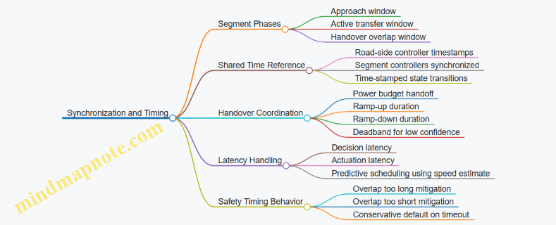
Example: Two-Segment Handover with Measured Delays
Assume a vehicle travels at 20 m/s through adjacent segments A and B. Segment boundary detection has a worst-case decision latency of 60 ms, and the converter reaches regulation in 110 ms. If the overlap window is 200 ms, you can schedule:
- Segment A ramp-down start at boundary prediction time minus 100 ms.
- Segment B ramp-up start at boundary prediction time minus 90 ms.
The overlap ensures that by the time A’s power falls below the regulation threshold, B has already reached regulation. If the measured communication delay spikes to 120 ms, the system should enter deadband: cap both segments at a conservative power until timing confidence is restored.
Example: Timing Parameters from a Simple Ramp Model
Use a linear ramp as a first approximation to set timing parameters. Let commanded power be P(t). For a ramp-up of duration Tru, segment B uses:
- P_B(t) increases from 0 to P_target over Tru.
For a ramp-down of duration Trd, segment A uses:
- P_A(t) decreases from P_target to 0 over Trd.
Choose overlap To such that Trd + safety_margin ≤ To and Trd and Tru are consistent with converter response. Then verify with measured coupling behavior: if coupling rises slower than expected, extend overlap rather than forcing abrupt ramps.
Practical Checklist for Implementation
- Define acceptance windows and a measurable overlap window.
- Use time-stamped commands, not “immediate” toggles.
- Coordinate ramps with a power budget handoff.
- Quantify decision and actuation latency separately.
- Implement deadband and conservative behavior on timing timeouts.
- Validate with a handover test that includes speed variation and message jitter.
3.5 Protection Engineering for Overcurrent Overvoltage and Ground Faults
Protection Engineering for Overcurrent Overvoltage and Ground Faults
Dynamic inductive charging couples power electronics, embedded coils, vehicle receivers, and the grid. Protection has to stop faults fast enough to prevent damage, but also avoid nuisance trips that would interrupt charging every time a vehicle enters or leaves a segment. The goal is simple: detect abnormal electrical conditions, isolate the affected part, and leave the rest of the system available.
Foundational Protection Concepts for Roadside Inductive Systems
Protection starts with three decisions: what to measure, what thresholds mean “fault,” and what action follows. For overcurrent and overvoltage, the key measured quantities are phase currents, DC-link voltage, inverter output voltage/current, and resonant tank variables. For ground faults, the key is how the system references earth: whether the power stage is floating, how shielding is bonded, and where insulation is expected to hold.
A practical best practice is to define protection layers by time scale. Fast layers handle electrical stress (milliseconds to tens of milliseconds). Slower layers handle thermal or insulation degradation (seconds to minutes). This prevents a slow thermal limit from being the only line of defense against a hard short.
Overcurrent Protection Strategy
Overcurrent can come from a shorted coil segment, a miswired connection, a receiver fault, or a resonant mismatch that drives excessive current. Use a combination of current sensing and energy-based limits.
-
Instantaneous current limit: trip when current exceeds a hard maximum for a short window. Example: if inverter output current rises above the design limit for 20 ms, disable the inverter and command the segment to “standby.”
-
I²t or energy-limited protection: trip based on the integral of current squared over time. Example: a partially shorted coil may not spike instantly, but it increases heating; I²t catches it before insulation life is consumed.
-
Resonant tank current supervision: monitor resonant current or equivalent tank current. Example: if the vehicle receiver detunes the system and the tank current climbs while DC-link voltage stays normal, you can classify it as a coupling fault rather than a grid fault.
To reduce nuisance trips, thresholds should be derived from worst-case operating envelopes that include misalignment and speed. A common mistake is setting limits from “nominal” coupling only, then discovering that real traffic alignment is never nominal.
Overvoltage Protection Strategy
Overvoltage can appear at the DC link, across inverter switches, or in the resonant network due to open-circuit conditions, sudden load removal, or switching transients.
-
DC-link overvoltage: use a hardware comparator or fast digital protection that trips the inverter when DC-link exceeds a hard limit. Example: if the DC link rises above the maximum rated voltage, gate signals are removed immediately.
-
Resonant overvoltage supervision: monitor resonant voltage peaks. Example: if the resonant capacitor voltage exceeds its rating during entry/exit, the controller can reduce power command and then stop if it persists.
-
Snubber and clamp coordination: protection thresholds must align with the energy the clamp components can absorb. Example: if the clamp is designed to handle a brief spike, the overvoltage trip should occur before the clamp reaches its thermal limit.
A useful integrated practice is to define “graceful stop” behavior: first reduce power command and wait for voltage/current to settle; if it does not, then isolate the segment.
Ground Fault Protection Strategy
Ground faults are tricky because they depend on bonding, insulation, and where the system is intentionally referenced. For embedded coils and their cabling, insulation failure can create leakage paths that may not trip overcurrent immediately.
-
Insulation monitoring: measure insulation resistance or leakage current to earth. Example: if leakage current exceeds a set limit while coupling current is low, classify it as an insulation or moisture ingress fault.
-
Residual current detection: use a residual current device or equivalent measurement to detect imbalance between outgoing and returning conductors. Example: if the inverter output current returns through an unexpected path, residual current rises even if total current looks “reasonable.”
-
Bonding and shielding checks: ensure the coil shield and metallic parts have a defined bonding scheme so that faults drive protective action rather than floating hazards. Example: if the shield is bonded to protective earth at the correct point, a leakage fault produces a detectable residual current.
When a ground fault is detected, the action should be conservative: disable the affected segment and keep the rest of the corridor available only if the architecture supports selective isolation.
Integrated Protection Mind Map
Mind Map: Protection Engineering for Overcurrent, Overvoltage, and Ground Faults
Example Fault Scenarios with Protection Actions
Example: Receiver Detunes During Entry
- Observation: resonant current increases, DC-link remains stable, resonant voltage rises moderately.
- Protection: resonant overvoltage supervision triggers a “graceful stop” by reducing power command.
- Outcome: if values settle within the grace window, charging resumes; if not, the segment hard-stops.
Example: Coil Segment Cable Insulation Degrades
- Observation: residual current rises and insulation monitoring shows reduced resistance; coupling current may be normal.
- Protection: ground fault classification disables the segment and logs the event.
- Outcome: the corridor continues only if selective isolation is available; otherwise, the system stops charging for safety.
Example: Hard Short in Power Stage
- Observation: instantaneous current exceeds the hard limit within milliseconds.
- Protection: hardware-level current limit removes inverter gating immediately.
- Outcome: energy storage is discharged to safe levels; reset requires explicit operator or system confirmation.
Validation Checklist for Protection Correctness
Protection is only “real” after testing. Validate thresholds under realistic coupling conditions, including misalignment and speed, and verify that each fault scenario produces the intended action without cascading failures. Finally, confirm that logs and reset conditions are deterministic: a fault should not clear itself due to transient measurements, and a cleared fault should not be able to re-enable charging without meeting the defined reset criteria.
4. Coil Design and Electromagnetic Layout for Embedded Systems
4.1 Coil Geometry Selection for Lane Centering and Vehicle Coverage
Dynamic inductive charging works only if the magnetic coupling stays strong enough while the vehicle moves and shifts within the lane. Coil geometry is the lever that shapes that coupling: it determines where the field is strongest, how quickly it falls off with lateral offset, and how much coverage you get along the travel direction.
Start with the Coupling Map You Actually Need
Begin by translating “lane centering and vehicle coverage” into measurable geometry targets.
- Lateral coverage: the maximum expected offset from lane center (including steering error, tire wear effects, and sensor uncertainty). Example: if the vehicle can drift ±0.35 m, design the coil so coupling remains within an acceptable band from -0.35 m to +0.35 m.
- Longitudinal coverage: the distance over which the vehicle should charge reliably during entry, steady travel, and exit. Example: if you want stable charging over 6 m, your coil layout must provide sufficient overlap across that window.
- Vehicle envelope: where the receiver coil sits relative to the vehicle centerline and ground clearance. Example: if the receiver is 0.2 m forward of the axle, the roadside coil must account for that offset when defining “entry” and “exit” positions.
A practical way to proceed is to sketch a coordinate system: x is lateral offset, y is travel direction, and z is height. Then you decide the coupling “sweet spot” region in (x, y) that should meet charging power requirements.
Choose a Geometry That Matches the Field Shape
Embedded coils can be arranged in several geometries, but lane centering usually benefits from designs that create a relatively flat coupling profile near the lane center and a controlled roll-off toward the edges.
-
Single Longitudinal Coil
- Best when you want simple installation and can tolerate stronger dependence on lateral alignment.
- Example: a single rectangular coil per lane segment can work for low lateral uncertainty, but coupling may drop quickly near the lane edge.
-
Dual Or Multi-Coil Arrays
- Best when you need a wider lateral “plateau” of acceptable coupling.
- Example: two coils spaced symmetrically about the lane center can be driven with coordinated power so that the combined field stays strong even when the receiver shifts laterally.
-
Segmented Coils With Overlap
- Best when you need both longitudinal coverage and smooth handover.
- Example: overlapping segments along the lane allow the system to maintain charging as the vehicle transitions from one segment to the next.
A useful rule of thumb is to treat geometry like a filter: single coils are narrowband in lateral tolerance, while arrays and overlaps broaden the passband.
Use Geometry Parameters with Clear Physical Meaning
Instead of picking dimensions by intuition, tie each parameter to an effect.
- Coil width (lateral): wider coils generally increase lateral tolerance, but they also spread flux and can raise coupling to unintended areas.
- Coil length (longitudinal): longer coils improve longitudinal coverage but can increase stray coupling and thermal load.
- Gap and spacing in arrays: the spacing between multiple coils controls how the combined field sums at different lateral offsets.
- Turns and conductor layout: more turns can increase induced voltage, but it also affects resistance, heating, and tuning requirements.
- Shielding and back iron: these don’t change the coil’s “placement logic,” but they reshape the field so the geometry’s intended coupling actually reaches the receiver.
Example: if your receiver is sensitive to lateral offset, you can widen the effective coupling region by increasing coil width or by using a dual-coil array with appropriate spacing, then verify that shielding keeps the field from leaking into adjacent lanes.
Validate with a Coverage Metric, Not Just Peak Coupling
Peak coupling at perfect alignment is easy to achieve and often misleading. Use a coverage metric that reflects the worst-case alignment.
- Coverage band: define the minimum acceptable coupling (or minimum received power) and compute the fraction of the (x, y) region where the requirement is met.
- Worst-case lateral slice: for each y position in the charging window, evaluate coupling at x = ±x_max.
- Handover margin: ensure that at the boundary between adjacent segments, the coupling doesn’t dip below the requirement for typical offsets.
Example: if you require at least 80% of nominal received power, you can compare a single-coil design versus a dual-array design by plotting received power across x at multiple y positions. The better geometry is the one that keeps the 80% contour wide and continuous.
Mind Map: Coil Geometry Decisions for Lane Centering
Example: Designing a Dual-Coil Lane-Center Array
Assume a lane where the vehicle can drift ±0.35 m. You want a 6 m longitudinal charging window.
- Start with a baseline: choose a single coil length that covers 6 m plus an overlap allowance for entry and exit, then estimate lateral roll-off.
- Add lateral robustness: split the coil into two symmetric sub-coils centered about the lane center. Drive them so that their combined field peaks near x = 0 and remains sufficiently high near x = ±0.35 m.
- Control stray coupling: include shielding/back iron so the field concentrates downward rather than sideways into adjacent lanes.
- Check the handover: if you segment the lane into 3 m blocks, ensure overlap between blocks so that at y boundaries the coupling remains above the minimum for typical offsets.
If the dual-coil array produces a coupling profile that is too peaked at x = 0, reduce the effective lateral “sharpness” by adjusting sub-coil spacing or increasing lateral width. If it’s too flat but weak, increase effective coupling by revisiting turns, tuning, or shielding effectiveness.
Geometry Selection Output You Should Expect
A good coil geometry selection ends with concrete artifacts:
- A defined charging window in (x, y) with a minimum coupling threshold.
- A dimension set for coil width, length, spacing, and segment overlap.
- Coverage plots showing worst-case lateral performance and boundary handover margin.
When those are in place, lane centering stops being a hope and becomes a measured property of the design.
4.2 Managing Stray Flux With Shielding And Magnetic Back Iron
Stray flux is the magnetic field that leaks outside the intended coupling region between the road-side transmitter coil and the vehicle receiver. In dynamic inductive charging, it matters because leakage can (1) reduce delivered power by “wasting” field lines, (2) increase electromagnetic exposure in nearby areas, (3) couple into nearby metal and electronics, and (4) create extra losses that show up as heat in places you did not plan to heat.
Start with Field Direction and Where Leakage Comes From
Begin by separating leakage into two practical categories. The first is lateral leakage, which spreads sideways beyond the lane centerline. The second is vertical leakage, which escapes upward toward the vehicle underbody and downward into the pavement layers and any embedded metallic infrastructure.
A useful mental model is that the transmitter coil produces a magnetic field that prefers the path of least reluctance. If the road construction provides no low-reluctance return path, the field takes detours through air and surrounding materials. Those detours are where stray flux is born.
Best practice: treat the road segment as a magnetic circuit, not just an electrical component. When you map the magnetic circuit, you can predict where leakage will go before you build a prototype.
Shielding Versus Magnetic Back Iron
Shielding and back iron often get lumped together, but they do different jobs.
- Shielding primarily reduces external field strength by providing a path for induced currents or by shaping the field distribution. In practice, it is usually implemented with conductive or high-permeability layers depending on the frequency and design constraints.
- Magnetic back iron provides a low-reluctance return path behind the transmitter, steering flux toward the receiver and away from the ground and nearby structures.
Easy example: imagine a flashlight beam aimed at a target. A back iron is like adding a reflective surface behind the light so more photons go forward. Shielding is like adding a curtain around the beam so fewer photons escape sideways.
Magnetic Back Iron Design Logic
Magnetic back iron is typically a high-permeability material placed behind the transmitter coil. Its job is to “close the loop” for magnetic flux. The closer and more continuous the back iron, the more the field lines are forced to travel through the intended region.
Key design variables:
- Distance from the coil: smaller spacing increases coupling to the back iron and improves flux steering, but it can raise losses if the back iron is too close.
- Coverage area: partial coverage can create edge leakage where flux lines bend around the back iron boundary.
- Material selection: high permeability helps, but saturation limits how much flux it can carry. Saturation shows up as reduced efficiency and increased stray field.
Best practice: size the back iron so it does not saturate at the maximum operating current. Then verify with a field map that the leakage outside the lane is actually reduced, not just “expected to be.”
Shielding Approaches That Actually Work
Shielding choices depend on whether you want to reduce field magnitude, reduce coupling into nearby conductors, or both.
- Conductive shielding layers can reduce external magnetic fields by inducing currents that oppose the changing flux. The tradeoff is added eddy-current loss and heating.
- Permeable shielding can redirect flux by offering an alternate magnetic path. The tradeoff is again saturation and possible increased losses if the material is not thermally managed.
Easy example: if you place a thin metal sheet near the coil, it may reduce measured field strength, but the sheet can become a heater. If your thermal budget is tight, you may need a different thickness, material, or placement.
Best practice: treat shielding as a coupled electromagnetic-thermal design. A shielding layer that “meets field limits” on paper can still fail in the real world if it overheats.
Managing Edge Effects and Segmentation
In real roadways, coils are segmented. Edge effects occur at segment boundaries because the magnetic circuit is interrupted. Flux can leak around the ends of the back iron and across the gaps between segments.
Mitigation tactics:
- Extend back iron beyond the coil footprint to reduce end leakage.
- Use consistent segmentation geometry so the magnetic circuit breaks in predictable locations.
- Ensure the shielding continuity across segments where feasible.
Best practice: measure leakage at segment edges during commissioning, not only at the centerline. Edge leakage is often the limiting case.
Verification with Measurements and Acceptance Criteria
Field mapping is the practical way to confirm stray flux control. You want both a spatial view and a link to system performance.
Recommended checks:
- Leakage field map at representative vehicle positions and speeds.
- Temperature rise of back iron and any shielding layers under sustained operation.
- Coupling into nearby metallic structures such as fasteners, conduits, or embedded frames.
Acceptance criteria example: require that leakage field strength outside the lane stays below the compliance threshold while maintaining target efficiency and keeping shielding temperatures within the design limits.
Mind Map: Stray Flux Control Workflow
Example: From Concept to Layout Decisions
Suppose a lane segment uses a transmitter coil embedded in asphalt with a metallic conduit running nearby. A first layout includes only the coil and insulation. Field mapping shows elevated leakage toward the conduit and a noticeable temperature rise in the conduit region.
A revised design adds magnetic back iron behind the coil to steer flux upward toward the receiver and away from the ground plane. Field mapping improves, but leakage near the segment ends remains high. The final step adds a shielding layer that wraps the coil region and extends slightly past the back iron edges, reducing end leakage while keeping temperatures within limits.
The key point is that each change addresses a specific failure mode: back iron reduces the main leakage path, while shielding handles the leakage that escapes at boundaries and through nearby conductors.
4.3 Thermal Design for Continuous Operation Under Traffic Loads
Continuous charging means the road segment is not a “hit it once and cool down” system. Thermal design has to treat traffic as a repeating heat input, with realistic pauses, partial loads, and occasional misalignment that changes power transfer efficiency. The goal is simple: keep coil insulation, encapsulant, and nearby materials within their allowable temperatures while maintaining stable electrical tuning.
Start with Heat Sources and Temperature Limits
Begin by listing the heat sources that actually scale with operation:
- Copper loss in the embedded coil: rises with current and increases as resistance grows with temperature.
- Core and shielding losses: depend on magnetic flux density and switching frequency.
- Eddy currents in nearby conductive parts: can be triggered by stray flux and poor shielding.
- Power electronics dissipation: if converters are near the road segment, their heat can raise local ambient temperature.
Then define temperature limits for each material class. Use manufacturer ratings for insulation and encapsulants, and set conservative operating targets below those limits to account for measurement uncertainty and aging. A practical approach is to define:
- Maximum hot-spot temperature for the coil conductor region.
- Maximum encapsulant temperature at the interface where heat spreads.
- Maximum allowable temperature rise relative to the worst-case ambient.
Example: If the encapsulant rating is 90°C and the worst-case ambient is 40°C, you might target a steady-state encapsulant temperature of 70–80°C to preserve margin for hot spots and sensor placement error.
Convert Traffic into a Thermal Load Profile
Traffic loads are not uniform. Build a load profile that maps vehicle presence to charging power and duty cycle. For each time step, estimate:
- Transferred power based on expected alignment and operating mode.
- Efficiency to determine how much becomes heat in the coil and nearby structures.
- On-time fraction for each road segment.
A simple method is to create a time series with three states: idle, partial charging, and full charging. Even if you later refine it, this structure prevents thermal design from being based on a fantasy “average” that hides peaks.
Use a Layered Thermal Model That Matches the Build
A road-embedded system is layered: conductor, insulation, encapsulant, pavement, and surrounding soil or air. Use a thermal model that mirrors that stack. Common modeling choices include:
- Thermal resistance network for steady-state and quasi-steady behavior.
- Lumped thermal capacitances for transient rise during vehicle passes.
- Finite element analysis when you need hot-spot localization around coil edges or cable penetrations.
The key is to ensure the model can reproduce measured temperatures from commissioning tests. If the model predicts a smooth temperature rise but the field shows sharp hot spots near coil ends, you need to refine contact resistances and geometry.
Design for Steady-State and Transient Peaks
Thermal failure is usually about hot spots, not average temperature. Design around both steady-state and transient conditions:
- Steady-state: worst-case duty cycle where heat input balances heat removal.
- Transient: short periods where heat accumulates faster than it can dissipate.
Example: A segment might be idle most of the time, but during a convoy it experiences back-to-back full charging. The transient hot spot can exceed the steady-state value because the system hasn’t reached equilibrium.
Manage Heat Paths with Materials and Geometry
Heat removal depends on conduction into pavement and soil, plus any convection at exposed surfaces. Practical levers include:
- Encapsulant selection: higher thermal conductivity reduces temperature rise but must still meet electrical insulation and moisture resistance.
- Coil placement depth: deeper placement can reduce surface temperature but may increase thermal resistance to soil depending on soil properties.
- Thermal contact quality: voids and imperfect bonding increase thermal resistance dramatically.
- Shielding strategy: good magnetic shielding can reduce eddy-current heating in unintended conductors.
A small but important detail: cable conduits and drainage channels can create localized thermal bridges or insulation gaps. Treat them as part of the thermal stack, not as “electrical-only” features.
Instrumentation and Verification That Actually Helps
Thermal design without measurement is just a guess with better formatting. Use instrumentation to validate both model and design margins:
- Place temperature sensors where hot spots are expected: near coil ends, beneath the encapsulant interface, and close to any conductive shielding.
- Record temperatures alongside charging power and vehicle alignment indicators so you can correlate heat generation with operating conditions.
- Verify that sensor readings are stable under wetting and temperature cycling.
Example: If coil resistance-based loss estimates disagree with measured temperature rise, you may be missing an eddy-current path or underestimating contact thermal resistance.
Mind Map for Thermal Design Under Traffic Loads
Example Workflow from Requirements to Hot-Spot Acceptance
- Define allowable temperatures for conductor and encapsulant with margin.
- Build a traffic-based duty cycle with explicit peak states.
- Estimate losses using expected efficiency versus alignment.
- Run a layered thermal model to compute hot-spot temperature for both transient and steady-state cases.
- Adjust encapsulant conductivity, coil placement, shielding, or thermal contact assumptions until hot spots meet acceptance criteria.
- Commission with sensors and compare measured temperatures to the model; update the model parameters if the mismatch is systematic.
This workflow keeps thermal design grounded in what the system actually experiences: repeating power pulses, alignment variability, and heat paths through real materials.
4.4 Encapsulation Materials and Mechanical Integration Into Pavement
Dynamic inductive charging lives or dies by the boring stuff: keeping embedded coils electrically safe, mechanically stable, and thermally manageable while the road does what roads do—freeze, thaw, flex, and get driven on. Encapsulation is the layer system that sits between the coil assembly and the pavement environment. It must protect against water ingress, limit corrosion, control thermal expansion mismatch, and survive repeated mechanical loading without cracking or debonding.
Core Encapsulation Functions
Start with four non-negotiable functions. First, moisture and chemical protection: water plus salts is a corrosion accelerator, especially around copper windings and any exposed conductors. Second, electrical insulation: encapsulant must provide adequate dielectric strength and resist tracking when exposed to contaminants. Third, mechanical support: it should damp vibration and distribute stresses so the coil doesn’t become a stress concentrator. Fourth, thermal conduction and heat spreading: encapsulation should not trap heat in a way that drives coil temperatures beyond design limits.
A practical way to reason about materials is to map each requirement to a failure mode. If water ingress is the concern, the failure mode is corrosion at conductor terminations. If insulation is the concern, the failure mode is partial discharge or surface tracking under contamination. If mechanical support is the concern, the failure mode is cracking from cyclic traffic loads. If thermal management is the concern, the failure mode is excessive temperature rise that shifts resonant tuning and reduces efficiency.
Material Selection Logic
Encapsulants are typically polymer-based systems, sometimes combined with fillers and protective coatings. The selection process should be systematic rather than “pick what’s available.” Begin with thermal range and glass transition behavior, because a material that softens under operating temperatures will lose stiffness and allow micro-movement. Next, check moisture absorption and permeability; even a “water-resistant” material can slowly transport water if the barrier is thin or contains microvoids.
Mechanical properties matter in two directions. Tensile and shear strength help prevent delamination at the coil edges and terminations. Elastic modulus matters too: too stiff can transfer stress into the coil; too soft can allow coil motion that fatigues solder joints and wire bonds.
Fillers and additives are used to tune performance. Thermally conductive fillers can reduce hotspot temperatures, but they can also increase brittleness if overused. Surface treatments for adhesion—on coil laminations, ferrite shields, and cable jackets—often determine whether the encapsulant stays bonded after years of thermal cycling.
Mechanical Integration into Pavement
Mechanical integration is more than “embed it and pour.” The coil assembly must be positioned with repeatable geometry so the magnetic field pattern aligns with lane center and the vehicle receiver. That means controlling embedment depth, lateral offset, and the thickness of encapsulant above and below the coil.
A common best practice is to design a mechanical “frame” or support structure that holds the coil during installation, then relies on encapsulant to fill gaps and lock the assembly in place. This reduces the risk of voids, which are trouble because voids can concentrate stress and create pathways for water.
Terminations deserve special attention. Cable exits and connector regions should be strain-relieved so traffic-induced pavement movement doesn’t pull on the conductors. Where cables cross expansion joints or saw cuts, route them with slack and protective conduits so the encapsulant isn’t forced to take bending loads.
Testing and Acceptance Criteria
Encapsulation should be verified with tests that mirror the actual stressors. Moisture exposure tests should be paired with electrical insulation checks to confirm that dielectric strength remains adequate after conditioning. Mechanical tests should include cyclic loading and thermal cycling, looking for crack initiation and debonding.
A useful acceptance approach is to define measurable thresholds: maximum allowable void fraction, minimum bond strength after conditioning, and limits on insulation resistance or dielectric breakdown parameters. If you can’t measure it, you can’t accept it—especially when the encapsulant is buried under asphalt where repairs are expensive.
Mind Map: Encapsulation and Integration
Example: Encapsulant Stack-Up for a Lane Segment
Imagine a coil assembly with a ferrite shield and a cable exit on one side. A robust stack-up approach is to use a thin, well-adhered base layer to bond to the coil shield, then apply encapsulant to achieve a controlled thickness over the coil windings. The goal is to keep the encapsulant thickness consistent so thermal gradients and mechanical stiffness are predictable.
For the cable exit, add a strain-relief feature before encapsulation. Instead of letting the cable jacket transition directly into rigid encapsulant, route the cable through a flexible section or a bend radius control so movement is absorbed by geometry, not by tearing the encapsulant. After curing, inspect for voids around the exit region, because that’s where water ingress and stress concentration tend to start.
Example: Avoiding Voids and Debonding
Voids often appear when encapsulant is poured into complex shapes or when air is trapped near corners. A practical mitigation is to design the encapsulation mold or formwork with vent paths and to use controlled mixing and placement procedures that reduce bubbles. After installation, verify voids using appropriate inspection methods and reject assemblies that exceed the defined void fraction threshold.
Debonding can be prevented by ensuring surface cleanliness and by using adhesion-promoting layers where needed. If the coil shield surface is contaminated with oils or oxidation, the encapsulant may cure but still fail under thermal cycling. Treat the bonding interface as a first-class design element, not a side note.
Example: Mechanical Compatibility with Pavement
Asphalt and encapsulants expand differently with temperature. If the encapsulant is much stiffer than the surrounding pavement, it can experience high interfacial shear stress during thermal cycling. A mechanical compatibility strategy is to choose an encapsulant modulus that reduces stress transfer and to include a controlled transition layer at the interface. The result is fewer crack initiation points and a longer period of stable electrical performance.
Encapsulation and mechanical integration are the “system glue” between electrical design and real-world durability. When material properties, geometry control, and termination mechanics are treated as one package, the embedded coil behaves like an engineered component rather than a buried experiment.
4.5 Field Uniformity and Coverage Verification Using Measurement Plans
Dynamic inductive charging only works if the power transfer stays predictable where vehicles actually travel. “Uniformity” does not mean every point gets identical power; it means the variation stays within defined bounds across the lane area, speed range, and alignment tolerances. A measurement plan turns that idea into evidence you can compare against acceptance criteria.
Start with Coverage Geometry and Test Grid
Begin by translating lane layout into a testable coordinate system. Define the lane centerline as the reference, then specify lateral offsets (e.g., −0.3 m, −0.15 m, 0, +0.15 m, +0.3 m) and longitudinal positions relative to segment boundaries (e.g., −0.5 m before entry, 0 m at coil center, +0.5 m after exit). Use the same grid for both field mapping and power-transfer measurements so you can correlate “what the field looks like” with “what the vehicle gets.”
Best practice: include at least one “edge case” point per side of the lane where alignment is worst but still plausible for autonomous control. If you only test the centerline, you will learn something—just not the thing you need.
Define Metrics That Match Real Charging Behavior
Field uniformity should be measured using metrics tied to receiver performance. Common metrics include:
- Coupling proxy: magnitude of the relevant magnetic field component at receiver height, or an equivalent coupling estimate derived from measurements.
- Power transfer proxy: measured transferred power or regulated output power at the receiver under controlled load.
- Variation bounds: maximum deviation from the target metric across the grid.
To avoid confusion, specify whether bounds apply to absolute power, efficiency, or regulated receiver voltage/current. For example, a system can show a fairly uniform field but still produce uneven charging if the receiver tuning or control loop saturates.
Build a Measurement Plan with Three Layers
A solid plan usually has three layers, each with a clear purpose.
- Static field mapping: measure magnetic field strength at fixed positions to characterize spatial coverage.
- Quasi-static power transfer: repeat measurements while stepping the receiver through the grid with realistic receiver load and tuning.
- Dynamic verification: run a controlled motion test across the segment at representative speeds and alignment errors.
Best practice: use the static map to locate “hot” and “weak” regions, then focus dynamic tests on the worst-case regions. This reduces test time without sacrificing coverage.
Instrumentation and Setup That Won’t Lie
Measurement accuracy depends on setup discipline.
- Sensor placement: define receiver height above pavement and keep it constant during mapping. If you must vary height, treat it as a separate dimension in the grid.
- Orientation: magnetic sensors and receiver coils must be aligned to the expected field direction. A small rotation can look like a big uniformity failure.
- Calibration and repeatability: verify sensor calibration and perform repeat passes at a few grid points to quantify measurement drift.
Example: If your sensor is mounted on a rigid arm, include a quick “return-to-origin” check at the start and end of each session. It catches mechanical slop that otherwise becomes mysterious data scatter.
Acceptance Criteria and Pass-Fail Logic
Turn metrics into explicit rules. For instance:
- Coverage requirement: at least X% of grid points must meet a minimum coupling proxy threshold.
- Uniformity requirement: the regulated receiver output power must stay within ±Y% across the defined lane area.
- Boundary behavior: power must not drop below a minimum during entry and exit windows.
Keep the logic simple. If you define multiple overlapping criteria, document how they interact. Otherwise, you may pass one test and fail another for reasons that are actually the same underlying issue.
Mind Map of the Measurement Plan
Field Uniformity and Coverage Verification Mind Map
Example Measurement Workflow for One Segment
Assume a single electrified segment with a defined lane width and a receiver height of 120 mm above the pavement.
- Static map: measure the magnetic field component at the receiver height on the grid. Produce a heatmap and compute the worst-case and best-case values.
- Quasi-static power: place a receiver emulator at each grid point, apply the same load model used in design, and record regulated output power.
- Dynamic run: drive the receiver emulator through the segment at the representative speed. Repeat at the worst-case lateral offset found in step 1.
If the static map shows a weak region but quasi-static power looks acceptable, the receiver control may be compensating. That’s useful information, but you still need dynamic verification because control limits and transient behavior can change the outcome during motion.
Reporting Outputs That Engineers Can Use
Deliver results in formats that support decisions:
- Heatmaps for coupling proxy and regulated output power.
- Grid point tables listing measured values and pass-fail status.
- Anomaly notes tied to specific grid locations and likely causes (alignment error, sensor orientation, tuning mismatch).
A measurement plan is only as good as its traceability. When someone later asks, “Why did this segment underperform at the lane edge?”, your grid-based evidence should answer it without guesswork.
5. Vehicle Side Receiver Design and Energy Management
5.1 Receiver Coil Design for Vehicle Packaging and Alignment Tolerance
A vehicle receiver coil has two jobs that must coexist: it must fit inside the vehicle without causing structural or clearance problems, and it must still transfer useful power when the vehicle is not perfectly centered over the road coil. The design process starts with packaging constraints, then moves to electromagnetic performance, and finally turns into alignment-tolerance engineering.
Packaging Constraints That Drive Coil Geometry
Begin with the physical envelope. Typical constraints include underbody clearance, suspension travel, crash-structure requirements, and the need to keep the receiver away from exhaust heat and moving linkages. A practical rule is to treat the receiver as a “stiff mechanical object” even though it is electrically resonant; that means you plan for vibration, road impacts, and long-term fatigue.
Next, decide the receiver coil placement relative to the vehicle’s reference point. If the vehicle uses lane-level guidance, you can align the receiver to the vehicle’s centerline. If guidance is less precise, you may intentionally offset the coil to bias coverage toward the most likely lateral position. Either way, the receiver must be mechanically repeatable: mounts should locate the coil with tight tolerances so that electrical tuning does not drift with time.
A simple example: if the receiver is mounted on a removable skid plate, the plate’s locating pins should control coil position within a few millimeters. Otherwise, every service visit becomes a tuning change.
Alignment Tolerance as a Design Requirement
Dynamic inductive charging is sensitive to lateral misalignment and air-gap variation. Lateral misalignment reduces mutual coupling because the overlap between the receiver and road magnetic fields shrinks. Air-gap variation changes coupling and detunes the resonant system.
Instead of treating alignment as a “nice-to-have,” define it as a requirement with ranges. For instance:
- Lateral offset: ±X cm
- Longitudinal offset: ±Y cm
- Air-gap: Z mm (including suspension travel)
Then translate those ranges into coil geometry choices. A larger receiver coil can tolerate more lateral offset, but it may increase size, weight, and stray fields. A segmented receiver can improve tolerance by allowing effective overlap to remain high across a wider lateral range.
Resonant Tuning and Mechanical Repeatability
The receiver coil typically operates in a resonant mode with a compensation capacitor network. The tuning must remain stable despite temperature and mechanical stress. Encapsulation materials and potting thickness affect thermal expansion and dielectric properties, which in turn shift resonance.
A systematic approach is to tune the receiver at the expected operating temperature, not at room temperature. For example, if the receiver electronics sit near a heat source, measure resonance after the system reaches steady thermal conditions, then set the capacitor values or control tuning accordingly.
Mechanical repeatability matters because even small changes in coil-to-shield spacing can alter the effective inductance. Use consistent mounting interfaces and include a calibration procedure during commissioning.
Shielding and Backing for Packaging-Friendly Performance
Packaging often forces compromises: you may have limited room for magnetic back iron or shielding. Still, shielding is not optional if you want predictable coupling and reduced interference.
A common layout is:
- Receiver coil
- Magnetic backing or back iron to redirect flux
- Shielding layer to control stray fields
- Encapsulation and mechanical support
The goal is to keep the magnetic field concentrated toward the road while reducing coupling to nearby vehicle structures. If you cannot add full back iron, you can use partial shielding plus careful placement away from sensitive components.
Mind Map: Receiver Coil Packaging and Alignment Tolerance
Example: Designing for Lateral Offset Without Oversizing
Suppose the vehicle can be laterally offset by up to 8 cm while still being considered “in the charging zone.” A single large receiver coil might meet the coupling target, but it could exceed underbody space.
A practical alternative is a segmented receiver with two coil sections separated by a small gap. When the vehicle is centered, both segments contribute. When the vehicle shifts laterally, one segment aligns better with the road coil and still provides enough coupling for charging. The power electronics then select or blend the effective contribution by controlling the resonant network.
To make this work, you must ensure the segments share a consistent reference for tuning and that the segmentation does not create strong hotspots in the encapsulation. Verification should include tests at multiple lateral offsets, not just the nominal centerline.
Example: Air-Gap Tolerance Through Suspension-Aware Design
If suspension travel can change the air-gap by 6 mm, the receiver design should account for the worst-case gap. One approach is to design the resonant system so that it remains within an acceptable detuning range across the gap variation. Another approach is to use mechanical features that limit air-gap extremes, such as compliant mounts that maintain a minimum clearance.
During acceptance testing, measure power transfer at the minimum and maximum air-gap positions while also applying a representative lateral offset. This prevents the common mistake of optimizing for one variable while ignoring the other.
Summary of the Systematic Flow
Package the receiver first with mechanical repeatability as a requirement. Then define alignment and air-gap ranges, and choose coil geometry and shielding to meet coupling targets within those ranges. Finally, tune for expected thermal conditions and verify performance across offset combinations so the system behaves consistently when the vehicle is not perfectly centered.
5.2 Resonant Tuning and Adaptive Control for Stable Transfer
Dynamic inductive charging lives or dies by resonance. The road segment and the vehicle receiver form a coupled resonant system whose effective behavior changes with distance, lateral offset, and alignment. Stable transfer means two things: (1) the power delivered stays within a usable charging window, and (2) the system avoids runaway conditions where small changes in coupling cause large changes in current.
Foundational Model of the Resonant Pair
Start with the practical view: each side has an inductor and a compensation network, tuned so that the combined system draws current at a predictable frequency. When coupling is strong, the resonant frequency of the coupled system shifts slightly; when coupling is weak, the shift changes direction and magnitude. That shift is why “set it once” tuning is not enough for roads.
A useful mental model is to treat the system as having two resonant behaviors: the road-side resonance and the receiver-side resonance. The coupling between them creates a third behavior that depends on mutual inductance. Your control goal is to keep the operating frequency near the coupled resonance peak while limiting current and voltage stress.
Tuning Strategy That Survives Misalignment
Resonant tuning is usually implemented in two layers.
-
Fixed baseline tuning: Choose component values so that, at nominal alignment, the system resonates at the target frequency. This is the “happy path” that makes commissioning straightforward.
-
Adaptive fine tuning: Adjust either the switching frequency, the effective capacitance (via switched capacitor banks), or the phase relationship in the inverter control. The adaptation responds to measured electrical quantities rather than relying on geometry alone.
A simple example: suppose the vehicle enters a charged lane with good centering, then drifts laterally by 0.3 m. The coupling drops, the coupled resonance shifts, and the same fixed frequency produces lower transfer efficiency and higher circulating currents. Adaptive fine tuning corrects the frequency to re-center the resonance peak.
What to Measure and Why
Adaptive control needs signals that correlate with resonance without requiring perfect sensing of position.
- Road-side inverter current and voltage: Resonance shows up as predictable relationships between current magnitude and reactive power. If the system is off-resonance, current rises for the same delivered power.
- Receiver-side rectifier DC voltage and charging current: These reflect how much AC power is actually reaching the battery/load.
- Phase angle or impedance estimate: If you estimate input impedance, you can infer whether the system looks inductive or capacitive at the current frequency.
A practical rule: use road-side measurements for fast inner-loop stabilization, and use receiver-side measurements for slower outer-loop power regulation.
Control Architecture for Stable Transfer
A robust architecture is layered control with clear responsibilities.
Inner loop keeps the inverter operating safely and near resonance.
- Adjust switching frequency (or equivalent tuning) to minimize a resonance error metric.
- Enforce hard limits on current and voltage.
Outer loop regulates delivered power to the receiver.
- Use receiver-reported charging current or DC voltage to set a target power.
- Modify the inner-loop setpoints so the system stays within the charging window.
This separation prevents a common failure mode: if power regulation directly manipulates frequency without current limiting, the controller can chase a moving target and excite oscillations.
Resonance Error Metrics That Work in Practice
You need a scalar “error” that indicates how far you are from the coupled resonance. Common choices include:
- Reactive power sign and magnitude: At resonance, reactive power is near zero (or near the designed compensation point). Off-resonance, it becomes clearly positive or negative.
- Impedance magnitude slope: If you sweep slightly around the operating frequency, the direction of change in impedance magnitude indicates whether you are left or right of resonance.
- Current-to-voltage ratio: For a given inverter voltage command, resonance tends to minimize current for a given delivered power level.
Example: if reactive power estimate flips sign as the vehicle moves, the controller can use that sign change to bracket resonance and then converge with smaller adjustments.
Adaptive Tuning Without Getting Lost
Adaptive control must converge quickly but not thrash.
- Convergence step size: Use larger steps when the resonance error is large (entry into a zone), then reduce step size as the error shrinks.
- Rate limiting: Limit how fast frequency can change to avoid exciting mechanical or electrical transients.
- Hysteresis around the setpoint: If the resonance error hovers near zero, hysteresis prevents constant toggling.
A concrete scenario: the vehicle enters and the system starts with a conservative frequency near baseline tuning. The controller detects high reactive power magnitude, increases frequency adjustment step size, and quickly reduces the error. Once the error is within a small band, it switches to fine adjustments and relies on outer-loop power regulation.
Mind Map: Resonant Tuning and Adaptive Control
Example: From Entry to Steady Charging
Assume the road segment has baseline tuning at 85 kHz. When the vehicle first couples, the controller sees reactive power magnitude higher than expected, indicating off-resonance. The inner loop increases frequency adjustment step size until the reactive power estimate approaches zero and current drops to the expected range. Then the outer loop uses receiver-reported charging current to raise or lower the power target while keeping the inner loop within the resonance band.
If lateral misalignment increases, the reactive power estimate drifts again. The inner loop corrects frequency to re-center resonance, while the outer loop prevents charging current from exceeding the receiver’s allowable limit. The result is stable transfer even as coupling changes—without requiring the controller to know the vehicle’s exact position.
5.3 Power Conditioning for Battery Charging and Load Support
Power conditioning is the part of the system that turns whatever the road and vehicle coils can safely deliver into the exact electrical behavior the battery and vehicle loads need. In dynamic inductive charging, the input power can change quickly as alignment shifts, so the conditioning stage must regulate both voltage and current without making the battery or the vehicle electronics unhappy.
What “Conditioning” Means in This System
Start with the energy path: grid power → roadside inverter → inductive link → vehicle receiver → conditioning → battery and loads. The receiver typically produces an AC or rectified waveform whose amplitude depends on coupling and resonance. Conditioning therefore has three jobs:
- Rectify and filter the receiver output into a controlled DC bus.
- Regulate battery charging current and/or battery voltage.
- Support loads that may run while charging, such as compute, steering, lighting, and traction auxiliaries.
A practical way to think about it: the battery wants a controlled “push,” while the inductive link provides a “floating” source that varies with geometry. Conditioning is the translator.
Receiver Output to DC Bus
Most designs begin with a rectifier and DC-link capacitor. The rectifier converts the receiver AC to DC, while the capacitor smooths ripple so downstream converters can operate predictably.
Best practice: size the DC-link capacitor based on the expected ripple current and the minimum coupling case. If coupling drops, the receiver voltage and current change, and ripple can rise. A quick example: if your converter control assumes a bus ripple under 5%, but the capacitor is undersized, the control loop will chase noise and cause current oscillations into the battery.
Load support detail: if vehicle loads draw from the same DC bus, the conditioning stage must prevent bus sag when loads step. That usually means either enough capacitance for short transients or a converter topology that can source current quickly.
Battery Charging Control Objectives
Battery charging is not just “set a current and hope.” The conditioning stage typically follows a charging profile with constraints:
- Current limit to protect battery chemistry and wiring.
- Voltage limit to avoid overcharge.
- Temperature-aware behavior using battery management system inputs.
- Efficiency targets so charging doesn’t waste energy as heat.
A common approach is a two-loop structure:
- An outer loop regulates battery voltage or state-of-charge target behavior.
- An inner loop regulates charging current tightly.
Easy example: Suppose the vehicle enters a charged lane segment and coupling is strong. The inner current loop ramps to the requested charging current. As the vehicle exits and coupling weakens, the outer loop may reduce the current request to keep battery voltage within limits, while the inner loop still tracks the updated current command.
Converter Topologies and Their Tradeoffs
The conditioning stage often uses a DC-DC converter between the DC bus and the battery. Two common categories are:
- Buck-type behavior when the bus is typically higher than the battery voltage.
- Buck-boost or full-bridge behavior when the bus can be lower than the battery across alignment and speed.
Best practice: choose topology based on the worst-case receiver voltage range, not the nominal case. If the bus can dip below the battery voltage during misalignment, a buck-only design may force the system into “no charge” periods or require aggressive control that increases ripple.
Handling Dynamic Input Variations
Dynamic inductive charging changes input power as coupling varies. Conditioning must therefore tolerate:
- Input voltage droop when coupling decreases.
- Input ripple from the resonant link.
- Fast transitions at segment entry and exit.
A robust method is to regulate the DC bus with a control loop that reacts faster than the battery charging loop. Then the battery loop can focus on battery limits.
Concrete example: If the DC bus drops by 10% over 50 ms due to reduced coupling, a bus regulation loop with a bandwidth around a few hundred Hz can correct the bus quickly enough that the battery current loop sees a stable input. If the bus loop is too slow, the battery loop will reduce current because it cannot maintain its voltage/current targets.
Load Sharing and Power Budgeting
When charging and vehicle loads share the same power source, conditioning must allocate power. A simple power budget can be implemented as:
- Measure available DC bus power.
- Subtract estimated load power.
- Send the remainder as the charging current command.
Easy example: If the bus can supply 3.5 kW, and vehicle loads consume 1.2 kW, the conditioning stage requests charging power up to 2.3 kW. If loads increase (for example, a high-power actuator cycle), the charging current command reduces smoothly rather than causing abrupt bus dips.
Protection and Safe Operating Behavior
Protection is part of conditioning, not an afterthought. Typical protections include:
- Overcurrent detection on both bus and battery side.
- Overvoltage clamps if the receiver output spikes.
- Undervoltage lockout to prevent unstable operation during weak coupling.
- Thermal monitoring of power semiconductors and inductors.
Best practice: define protection thresholds so they coordinate with the charging controller. For instance, if undervoltage lockout triggers too aggressively, the system may repeatedly start and stop charging during normal alignment changes.
Mind Map: Power Conditioning Responsibilities
Example: Coordinated Charging During Segment Entry and Exit
Imagine a vehicle approaching a charged lane segment. The vehicle requests charging authorization and the conditioning stage begins regulating the DC bus. As coupling improves, the bus becomes stable and the battery current loop ramps toward the requested value while the outer loop checks voltage limits.
Near the segment exit, coupling drops. The bus regulation loop reacts first, keeping the bus within its allowed ripple and voltage window. The battery loop then reduces current command to maintain battery voltage constraints. If vehicle loads increase at the same time, the power budget logic reduces charging current smoothly rather than forcing a hard stop.
The result is a controlled handover: the battery sees a predictable current profile, the loads see a stable bus, and the conditioning stage avoids oscillations caused by the inductive link’s changing behavior.
5.4 Handling Transient Events During Entry and Exit from Charged Zones
Dynamic inductive charging behaves like a power handshake with a moving target. The “transient” part is what happens when the vehicle receiver first overlaps the roadside transmit field, and again when it leaves. During those moments, coupling changes quickly, resonance conditions drift, and control loops can momentarily chase the wrong target. Good handling is mostly about sequencing: detect, authorize, ramp, regulate, then ramp down—without letting the system overshoot or oscillate.
Entry Transient Fundamentals
Start with what changes at entry: the mutual coupling coefficient rises from near zero to a useful value as lateral alignment improves and the receiver coil approaches the effective lane region. That coupling increase raises transferred power for the same transmitter drive, which can cause a brief surge in receiver current and battery charging power.
A practical entry sequence uses three layers of gating:
- Geometric readiness: the vehicle reports approximate position or alignment quality (from onboard sensors or receiver-side signal strength). The roadside controller uses this to decide whether the vehicle is likely within the effective coupling window.
- Electrical readiness: the receiver performs a quick measurement of reflected impedance or resonant response and reports a compact status. If the receiver indicates it is not tuned or is saturated, the roadside holds a low-power state.
- Power ramp authorization: once both readiness checks pass, the transmitter begins a controlled ramp rather than jumping to the requested power.
Easy example: A vehicle approaches a 2-meter charging segment. At the first overlap, the receiver reports “alignment uncertain” and “resonance not yet stable.” The roadside controller starts at 10% power for 200 ms, watches receiver current and resonant phase, then increases to the target charging level only after stability is confirmed.
Exit Transient Fundamentals
Exit is the mirror image: coupling collapses as the receiver leaves the coil’s effective region. If the transmitter keeps driving at the previous power level, the receiver current drops, the resonant network can detune, and the control loop may react late. The safe response is to treat exit as a controlled ramp-down triggered by coupling loss.
A robust exit strategy uses two triggers:
- Receiver-side trigger: the receiver detects falling induced voltage or reflected impedance and immediately requests a reduced power state.
- Roadside-side trigger: the roadside controller monitors transmitter current, voltage, and phase margin. If the coupling estimate drops or the control loop approaches instability, it initiates ramp-down even if the receiver request is delayed.
Easy example: As the vehicle’s front wheels cross the segment boundary, the receiver’s induced voltage drops below a threshold. The receiver sends “reduce power” within tens of milliseconds. The roadside controller simultaneously ramps down over a fixed time window, preventing a sudden drop that could cause a control overshoot.
Control Sequencing and Ramp Profiles
Transient handling is easiest when the system uses explicit states. A common state set is:
- Standby: transmitter is off or at a minimal diagnostic level.
- Precharge: low-power drive to verify resonance and communication.
- Ramp Up: increase power with a bounded slope.
- Regulate: closed-loop power control at the requested setpoint.
- Ramp Down: reduce power with the same bounded slope.
Ramp profiles should be rate-limited and coupling-aware. If coupling is uncertain, use a conservative slope and longer dwell time. If coupling is stable, you can ramp faster without risking overshoot.
Mind Map: Transient Handling Logic
Concrete Example: A Full Entry-to-Exit Timeline
Assume a vehicle requests 20 kW charging power for a 30-meter corridor with multiple energized segments.
- t = 0 ms: Vehicle enters the corridor boundary. Roadside remains in Standby.
- t = 50 ms: Receiver reports “near field present” but alignment uncertain. Roadside enters Precharge at 2 kW.
- t = 250 ms: Receiver confirms stable resonant response and current is within limits. Roadside transitions to Ramp Up, increasing power by 1 kW every 50 ms.
- t = 1050 ms: Power reaches 20 kW and control enters Regulate. The loop maintains setpoint by adjusting drive frequency or phase within allowed bounds.
- t = 1800 ms: Vehicle approaches the end of the segment. Receiver induced voltage drops; it requests reduction.
- t = 1850 ms: Roadside detects coupling estimate drop and initiates Ramp Down, decreasing power by 2 kW every 50 ms.
- t = 1950 ms: Power reaches a safe low level. Roadside returns to Standby and clears the charging authorization for that segment.
The key detail is that the system never “free-runs” during the transition. Every change in coupling is met with a bounded, state-driven response.
Practical Checks That Prevent Common Failures
- No abrupt setpoint jumps: even if the vehicle requests a new power level, the transmitter applies it through the ramp state.
- Timeouts on readiness: if electrical readiness never stabilizes, the system stays in Precharge and refuses full charging.
- Fail-safe on control margin: if phase margin or current limits indicate instability, ramp-down starts immediately.
- Consistent thresholds: entry and exit thresholds should be coordinated so the system doesn’t “chatter” when the vehicle hovers near the boundary.
Handled this way, entry and exit transients become predictable events rather than surprises—like stepping onto a moving walkway where the system already knows how fast you’re allowed to move.
5.5 Implementing Vehicle Safety Interlocks and Diagnostic Reporting
Dynamic inductive charging needs two things at the same time: a fast way to stop charging when conditions are unsafe, and a clear record of what happened so the system can be repaired without guesswork. The interlock design should start with simple, physical truths—power transfer depends on alignment, temperature, and electrical isolation—and then add layered checks that fail safe.
Safety Interlock Foundations
Begin by defining the “charging permission” signal as a single boolean outcome derived from multiple checks. If any check fails, permission becomes false and the power electronics must reduce output to a safe state within a bounded time.
Core interlocks typically include:
- Foreign Object Detection: If a conductive or ferromagnetic object is present near the road coil, the vehicle should refuse charging. A practical approach is to monitor receiver-side current and estimate coupling; abnormal coupling patterns indicate likely foreign objects.
- Isolation and Leakage Monitoring: The system should verify that insulation integrity is acceptable. On the vehicle side, leakage current sensors or insulation resistance checks can be used to prevent energization when isolation degrades.
- Temperature Limits: Receiver coil temperature and power electronics temperature must be tracked. Interlocks should use both absolute thresholds and rate-of-rise behavior to catch sudden problems.
- Alignment and Coupling Window: Charging should only occur when coupling is within a range that supports stable regulation. If coupling drops below a threshold, the system should ramp down rather than abruptly cut.
- Communication Authorization: The vehicle should only accept charging parameters that match the road segment identity and charging mode. If the handshake is missing or inconsistent, permission is denied.
A good best practice is to separate fast electrical shutdown from slower diagnostic logging. Shutdown should happen on the shortest control path available; logging can be handled by a supervisory controller.
Interlock Logic and Timing
Interlocks should be organized into two tiers:
- Tier 1: Immediate Actions. These are triggered by hard limits such as overtemperature, isolation fault, or unsafe coupling. The vehicle must command the power stage to stop within a strict time budget.
- Tier 2: Controlled Transitions. These handle conditions like marginal alignment or temporary communication loss. The vehicle should ramp down, maintain safe monitoring, and only re-enable charging after conditions recover and a new authorization is confirmed.
Example: If receiver temperature exceeds the limit, Tier 1 disables charging permission and commands a power stage stop. The system then logs the event with the measured temperature, the time since charging start, and the last known coupling estimate.
Diagnostic Reporting That Engineers Can Use
Diagnostic reporting should answer three questions: What failed? Where did it fail? How often and how bad was it? To do that, define a compact set of diagnostic codes with consistent severity levels.
Recommended diagnostic fields:
- Fault Code: A stable identifier for the failure mode.
- Severity: Warning, fault, or lockout.
- Measured Values: Key sensor readings at the time of detection, such as temperature, leakage current, receiver current, and coupling estimate.
- State Context: Whether the vehicle was in entry, steady charge, or exit.
- Timing: Timestamp relative to charging session start, plus duration of the fault.
- Action Taken: Whether the system ramped down, stopped immediately, or refused to start.
A practical example: If coupling is too low, the system should log “Marginal Coupling” with the coupling estimate and the vehicle speed at detection. That lets maintenance teams distinguish between a lane alignment issue and a receiver tuning issue.
Mind Map: Safety Interlocks and Diagnostics
Example Interlock Set with Clear Outcomes
Use explicit outcomes so the behavior is predictable:
- Refuse to Start: If authorization fails, if isolation is out of range, or if coupling is below the minimum.
- Ramp Down: If coupling becomes marginal or communication drops briefly.
- Stop Immediately and Lockout: If isolation fault persists, if temperature exceeds a hard limit, or if foreign object indicators remain abnormal for longer than a debounce window.
Example: During a lane change, coupling may dip for a moment. The system should ramp down (not lock out), keep monitoring, and re-enable only after coupling returns to the stable window and a valid authorization is confirmed.
Implementation Notes for Robustness
To avoid “interlock chatter,” apply debounce and hysteresis: require a condition to persist for a minimum duration before triggering Tier 1, and require recovery to exceed a higher threshold before re-enabling. Also ensure that diagnostic logging is triggered by state transitions, not by every control-cycle sample, so logs remain readable.
Finally, define lockout reset rules. A lockout should clear only after the underlying condition is resolved and a new authorization handshake succeeds, preventing the system from restarting into the same unsafe situation.
6. Control Systems and Communication for Dynamic Charging
6.1 Control Objectives for Power Regulation and Efficiency Maximization
Dynamic inductive charging is a moving target: the vehicle changes position, the coupling changes, and the power electronics must stay within safe limits. Control objectives therefore start with what must be true at every moment, then expand into how to achieve it efficiently.
Core Objectives That Must Always Hold
1) Regulate Delivered Power to the Vehicle The controller should track a target power setpoint (or battery charging current) despite variations in coupling and speed. A practical way to think about this is: the road side controls how much electrical “push” is sent, while the vehicle side controls how that push becomes battery charging. If the road side over-delivers, the vehicle must absorb it safely; if it under-delivers, the vehicle may not meet energy goals.
Example: A vehicle enters a charged lane segment. The coupling is initially weak, so the controller ramps the inverter drive gradually until the measured receiver-side power matches the target. When the vehicle reaches the lane center, coupling increases; the controller reduces drive so power stays near the setpoint.
2) Maintain Stable Resonant Operation Inductive systems often use resonant compensation to improve efficiency. Stability means the system does not drift into a mode where current spikes or voltage stress rises. Control should keep the effective resonant condition near the designed operating point, even as temperature and alignment shift.
Example: As the road coils warm up, their resistance increases. The controller compensates by adjusting frequency or phase so that the measured current and voltage remain within expected resonant envelopes.
3) Maximize Efficiency Without Violating Constraints Efficiency maximization is not a single knob; it is the outcome of meeting power targets while minimizing losses in coils, switching devices, and rectification. The controller should treat efficiency as a constrained optimization problem: “deliver required power, but don’t waste energy as heat.”
Example: Two drive settings can both deliver 50 kW. One produces higher coil current and higher copper loss. The controller prefers the setting with lower measured or estimated losses, as long as thermal and electromagnetic exposure limits remain satisfied.
Control Architecture from Measurements to Actions
A robust control loop typically uses three layers:
- Measurement Layer collects electrical quantities such as inverter current, inverter voltage, and (if available) receiver-side power or rectified current.
- Regulation Layer computes control actions to meet power and stability objectives.
- Constraint Layer clamps or modifies actions when limits are approached.
Example: If inverter current approaches a limit, the constraint layer reduces drive amplitude or shifts frequency, even if the regulation layer still “wants” more power.
Mind Map: Objectives and How They Connect
Practical Control Strategy: A Systematic Sequence
Step 1: Define Setpoints and Operating Modes Choose whether the primary setpoint is vehicle-side power, charging current, or DC bus voltage. Then define modes such as “approach,” “tracking,” and “exit,” each with different ramp rates and allowable control ranges.
Step 2: Use a Two-Variable Control Approach A common pattern is to use one variable to regulate power and another to maintain resonant behavior. For instance, frequency can be used to steer resonance, while drive amplitude (or duty/phase) sets power level.
Example: During approach, frequency is adjusted to reduce reactive mismatch, while amplitude is increased slowly to reach the power target.
Step 3: Add Loss-Aware Decision Logic Instead of always maximizing power transfer efficiency blindly, the controller can compare candidate operating points using measured proxies. Proxies include inverter input power versus estimated transferred power, or coil current squared as a proxy for copper loss.
Example: If two settings meet the power target, the controller selects the one with lower inverter input current for the same delivered power, indicating reduced losses.
Step 4: Enforce Constraints With Priority Rules Constraints must override regulation. A simple priority rule is: safety and hardware limits first, then resonant stability, then efficiency.
Example: If the system detects rising coil temperature or current stress, it reduces drive even if the vehicle requests the same power.
Step 5: Ensure Smooth Handover Between Road Segments When the vehicle transitions from one electrified segment to the next, coupling changes abruptly. The controller should coordinate ramp-down in the outgoing segment and ramp-up in the incoming segment so the vehicle sees a continuous power profile.
Example: The outgoing segment reduces power as the incoming segment begins tracking, using a short overlap window where both segments contribute within their limits.
Acceptance Criteria for This Section
A control design that meets these objectives should demonstrate: (1) power tracking within a defined tolerance across alignment and speed changes, (2) bounded inverter current and voltage under worst-case coupling, (3) stable resonant behavior without oscillation or excessive corrective action, and (4) efficiency improvements that correlate with reduced loss proxies while still meeting power targets.
If you can explain these outcomes in terms of measured signals and explicit constraints, the control objectives are doing their job.
6.2 Handshake Protocols for Charging Authorization and Parameter Exchange
Dynamic inductive charging only works if both sides agree on three things before power ramps: who is allowed to charge, what parameters are safe to use, and when to start and stop. The handshake is that agreement. It should be short enough to fit real driving behavior, strict enough to prevent “almost compatible” states, and boring enough that it can be tested with repeatable scenarios.
Core Handshake Goals
First, the road segment must verify authorization. A simple example is a fleet vehicle presenting a credential that the roadside controller recognizes; if the credential is missing, the controller keeps the segment in a low-energy “standby” state.
Second, the vehicle must confirm it can safely receive power. For instance, the receiver electronics report battery temperature and allowable charge current. If the battery is near a thermal limit, the vehicle requests a reduced power profile rather than accepting full power and then throttling later.
Third, both sides must exchange the electrical parameters needed for stable resonance and regulation. A practical example is exchanging the receiver’s tuned resonant frequency range and the road’s available compensation settings so the system can pick a matching operating point.
Message Sequence from Entry to Power Ramp
A reliable sequence is: discovery, authorization, parameter exchange, readiness confirmation, and controlled ramp.
Example: single segment, normal entry
- Discovery: Vehicle broadcasts a “charging capability” identifier when it enters the lane zone. Road responds with segment ID and supported charging modes.
- Authorization: Vehicle sends credential and vehicle safety status. Road checks access rules and verifies that the segment is not in a faulted state.
- Parameter Exchange: Vehicle provides receiver tuning data and maximum allowable input power. Road provides its compensation mode options and target operating frequency candidates.
- Readiness Confirmation: Both sides confirm the chosen operating point and the ramp schedule.
- Power Ramp: Road increases power in steps while monitoring current and voltage. Vehicle acknowledges each step by reporting measured input current and any protection flags.
If any step fails, the road returns to standby and logs the reason. A good test case is a vehicle that enters with a valid credential but reports an out-of-range receiver tuning value; the handshake should fail before any meaningful power transfer.
Authorization Details That Prevent Accidental Charging
Authorization should combine identity and context. Identity is the credential; context is whether the vehicle is actually in the charging zone and whether the segment is safe to energize.
A concrete best practice is to require both: (1) a valid credential and (2) a “zone presence” signal derived from vehicle position or lane detection. If the credential is valid but the vehicle is not present, the road refuses to energize.
Another best practice is time-bounding. Credentials should be accepted only for a short handshake window. For example, if the vehicle pauses at the edge of the zone and the handshake times out, the road should not keep the segment ready indefinitely.
Parameter Exchange for Stable Resonant Operation
Parameter exchange must be explicit about what is being negotiated. At minimum, exchange should cover:
- Operating frequency range: Vehicle reports its receiver resonant frequency tolerance; road reports available compensation settings.
- Power limits: Vehicle reports maximum allowable input power and any current limits; road reports its maximum deliverable power for that segment.
- Control mode: Vehicle indicates whether it can accept constant-current, constant-power, or constant-voltage behavior.
A practical example: if the vehicle can only accept constant-current charging, the road selects a control mode that regulates current while keeping the resonant point within tolerance.
Readiness Confirmation and Stepwise Ramp
Readiness confirmation should include both electrical and safety checks. Electrical checks include verifying that measured current and reflected voltage are within expected bounds after each ramp step. Safety checks include foreign object detection status and insulation monitoring state.
A simple ramp strategy is stepwise increase with acknowledgment. For instance, ramp to 10% power, verify current and temperature constraints, then ramp to 30%, then to the negotiated target. If the vehicle reports a protection flag at 30%, the road stops ramping and transitions to a safe low-power state.
Mind Map: Handshake Components and Flow
Example: Minimal Message Set for a Single Segment
Below is a compact message set that keeps the handshake testable. Field names are illustrative.
Vehicle -> Road: DISCOVER
  - vehicle_id
  - receiver_tuning_range
  - max_input_power
  - control_mode_support

Road -> Vehicle: AUTHORIZE_REQUEST
  - segment_id
  - supported_modes
  - handshake_deadline

Vehicle -> Road: AUTHORIZATION
  - credential
  - zone_presence_proof
  - safety_status

Road -> Vehicle: PARAMETER_OFFER
  - chosen_compensation_mode
  - candidate_frequency
  - max_segment_power

Vehicle -> Road: PARAMETER_ACCEPT
  - selected_frequency
  - accepted_power_limit
  - readiness_flags

Road -> Vehicle: RAMP_COMMAND
  - ramp_steps
  - step_dwell_time

Vehicle -> Road: STEP_ACK
  - measured_input_current
  - protection_flags
Integrated Best Practices for Real-World Robustness
Use explicit deadlines so the road never waits forever for a response. Validate parameters before energization so mismatches fail early, not during power transfer. Require acknowledgments during ramp so the system can stop quickly if conditions change. Finally, log the handshake outcome with enough detail to reproduce the scenario, such as which parameter field caused the rejection and at what stage the timeout occurred.
6.3 Closed Loop Control Using Measured Electrical Quantities
Dynamic inductive charging works only when the power electronics and the vehicle receiver agree on what “good” looks like right now. Closed-loop control uses measured electrical quantities—currents, voltages, and sometimes phase—to keep the system inside safe and efficient operating boundaries as alignment and speed change.
Core Idea and Control Variables
Start with what you can measure reliably on the roadside and on the vehicle. On the roadside, typical measured quantities include inverter output voltage, inverter current, DC-link voltage, and resonant tank current (or a proxy derived from current sensors). On the vehicle, measurements often include receiver coil current, rectifier input voltage, battery pack voltage, and battery charge current.
The controller’s job is to regulate one or more objectives:
- Power delivery to match the vehicle’s charging request.
- Resonant behavior so the inductive link stays near the intended operating point.
- Safety limits so currents and voltages do not exceed design thresholds.
A practical approach is to treat power regulation as the outer loop and resonance or current limiting as inner loops. This keeps the system stable even when the coupling coefficient changes quickly.
Signal Conditioning and Measurement Integrity
Measured quantities are only useful if they are consistent. Roadside sensors need calibration for gain and offset, plus filtering to remove switching ripple. A common mistake is to filter too aggressively and introduce delay; delay turns a feedback loop into a slow-motion oscillation.
Use a measurement pipeline like this:
- Sample synchronized with the inverter switching cycle or use averaging windows.
- Apply band-limited filtering that preserves the dynamics relevant to control.
- Convert sensor readings to physical units using calibration constants.
- Validate plausibility with simple checks, such as “current magnitude must be within sensor range.”
When plausibility checks fail, the controller should fall back to a conservative mode that reduces power and increases safety margins.
Inner Loop Resonance and Current Shaping
The resonant tank determines how much of the inverter energy couples into the receiver. As lateral misalignment changes, the effective load seen by the roadside changes, shifting the resonance.
An inner loop can regulate resonant current magnitude or regulate frequency to maintain a target phase relationship. Two common strategies:
- Current magnitude control: keep tank current near a setpoint that corresponds to safe power transfer.
- Frequency trimming: adjust inverter frequency to keep the tank near resonance, using measured phase or impedance estimates.
Easy-to-understand example: imagine the vehicle drifts slightly off lane center. Coupling drops, so for the same inverter settings the tank current tends to change. The inner loop detects the deviation and either increases frequency slightly (to restore resonance) or reduces drive amplitude (to keep current within limits). Either way, it prevents the system from “trying harder” in the wrong direction.
Outer Loop Power Regulation Using Receiver Feedback
The outer loop decides how much power to deliver. It uses measured electrical quantities that reflect the receiver’s state. The vehicle can report charging current request and measured battery-side current, while the roadside can measure delivered power proxies such as DC-link power or inverter output power.
A straightforward outer-loop structure:
- Compute power error between requested charging power and measured delivered power.
- Adjust a command that the inner loop can realize, such as tank current setpoint or inverter frequency offset.
To avoid fighting between loops, the outer loop should change more slowly than the inner loop. If the outer loop reacts as fast as the inner loop, the system can chase its own tail.
Handover Between Road Segments
When a vehicle moves from one electrified segment to the next, the coupling changes abruptly. Closed-loop control handles this by using measured quantities during the transition.
A robust handover sequence:
- Pre-charge: start the next segment at a low power setpoint.
- Measure: confirm tank current and voltage behavior are within expected ranges.
- Ramp: gradually increase power while the vehicle is still overlapping both segments.
- Transfer authority: once the overlap ends, reduce the old segment to zero using current-limited ramps.
Easy-to-understand example: during overlap, the vehicle receiver “sees” two sources. If both segments ramp aggressively, the receiver current can spike. Current-limited ramps prevent that by keeping the receiver within its safe operating envelope.
Mind Map: Closed Loop Control Using Measured Electrical Quantities
Example: A Two-Loop Controller with Concrete Signals
Assume the vehicle requests 6 kW charging. The roadside measures inverter output power as 5.4 kW, so the power error is +0.6 kW. The outer loop converts this into a new tank current setpoint, for example increasing the target tank current by 3%. The inner loop then drives the inverter so the measured tank current tracks the setpoint.
Now suppose misalignment reduces coupling, and the tank current begins to rise faster than expected. The inner loop detects the deviation and either reduces drive amplitude or shifts frequency to restore resonance. The outer loop continues to adjust slowly, so it does not command large changes while the inner loop is still stabilizing.
The result is behavior that is easy to reason about: the inner loop handles fast electrical dynamics, and the outer loop handles slower energy goals. Both loops use measured electrical quantities, so the controller responds to what is happening rather than what the system hoped would happen.
6.4 Managing Handover Between Adjacent Road Segments
Dynamic inductive charging is segmented so each road section can be controlled, protected, and tuned. The handover problem is simple to state: as a vehicle moves from Segment A to Segment B, the delivered power must stay within limits while the system avoids overlap-induced overcurrent, unstable resonance, and confusing authorization states.
Foundational Concepts for Safe Handover
A handover is not just a position change; it is a coordinated transition across three layers.
-
Electrical layer: both segments may be resonant at the same time, so the system must prevent unintended power sharing that can shift operating points.
-
Control layer: the vehicle-side receiver and the road-side controllers must agree on who is “in charge” of regulation during the overlap window.
-
Operational layer: the system needs deterministic behavior when communication is delayed, sensors disagree, or a segment is temporarily unavailable.
A practical rule is to define a handover window where both segments are allowed to participate, but only in a controlled manner. Outside that window, only one segment is permitted to actively regulate power.
Handover State Machine That Engineers Can Implement
Use a small, explicit state machine on the road side and mirror it with a vehicle-side expectation.
- Idle: segment is energized only if authorized by a vehicle handshake.
- Approach: vehicle is within the pre-charge region; segment prepares parameters but limits output.
- Active: segment regulates power for the vehicle.
- Overlap: both segments may be energized; regulation authority is split by a deterministic rule.
- Release: Segment A stops regulating and transitions to a safe low-output mode.
- Inhibit: segment refuses activation due to fault, foreign object detection, or inconsistent alignment.
A concrete authority split is: during overlap, Segment A regulates current while Segment B regulates voltage setpoints to avoid fighting. If your topology does not support that split, use a simpler rule: Segment B ramps up while Segment A ramps down with a shared ramp profile.
Overlap Management with Power Ramps
The most common failure mode is a “power bump” when both segments briefly deliver more than the receiver can absorb. Avoid this by using coordinated ramps.
- Define a ramp duration based on vehicle speed and the physical length of the overlap zone.
- Use a monotonic ramp: Segment A power command decreases linearly or with a smooth curve; Segment B increases with the same curve but complementary slope.
- Enforce a receiver-side ceiling so even if commands overlap, the receiver clamps charging power.
Example: if the overlap zone is 2.0 m and the minimum speed is 10 m/s, the vehicle spends 0.2 s in overlap. Choose a 0.15 s ramp to leave margin for sensor latency, then keep the remaining 0.05 s for stabilization and fault checks.
Communication Timing and Fallback Behavior
Handover depends on timely messages, but the system must behave correctly when they arrive late.
- Primary trigger: vehicle position estimate based on onboard sensors and road beacons.
- Secondary trigger: received signal quality and handshake confirmation.
- Fallback: if Segment B authorization is not confirmed before the vehicle reaches the overlap end, Segment A continues regulation until the vehicle exits Segment A’s safe region.
This fallback prevents a “dead zone” where neither segment is regulating. It also keeps the system conservative: the vehicle gets power rather than silence.
Mind Map: Handover Between Adjacent Road Segments
Case Example: Two-Lane Corridor with Overlap
Consider a corridor where each segment is 10 m long with a 1.5 m overlap zone. The vehicle travels at 12 m/s, so overlap time is 0.125 s. The system sets a 0.10 s complementary ramp.
- At 0.20 m before overlap entry, Segment A enters Approach and limits power to 60% of target.
- When overlap begins, Segment B enters Overlap but does not regulate at full power yet.
- During the 0.10 s ramp, Segment A command decreases from 60% to 0%, while Segment B increases from 0% to 60%.
- After the ramp, Segment A transitions to Release and drops to safe low-output. Segment B transitions to Active and raises to the full target if the receiver reports stable tuning.
If the handshake from Segment B is delayed beyond 0.125 s, Segment A stays Active until the vehicle exits its safe region, then both segments return to Idle. The vehicle never experiences a sudden drop to zero power, and the system never allows both segments to fully regulate at the same time.
Practical Acceptance Checks for Handover
To verify handover behavior, test three scenarios with the same vehicle speed and alignment profile.
- Nominal overlap: confirm power command is smooth and receiver reports stable tuning.
- Late authorization: confirm Segment A fallback prevents a dead zone.
- Segment B fault: confirm Segment B inhibits activation and Segment A continues until exit.
These checks ensure handover is not just “working,” but working for the reasons you can explain to the next person who has to maintain it.
6.5 Logging Telemetry for Maintenance and Operational Auditing
Dynamic inductive charging only looks simple from the driver’s seat. Under the pavement and in the vehicle, it’s a coordinated dance of power electronics, resonant tuning, alignment sensing, and safety interlocks. Telemetry logging is how you keep that dance on time—so maintenance can diagnose what happened, and operators can prove what the system did.
What Telemetry Logs Must Capture
Start with three categories of evidence, each with a clear purpose.
- Operational context: which road segment was active, vehicle identity or session token, lane position estimate, and charging mode (e.g., entry ramp, steady transfer, exit). This answers “where and under what conditions.”
- Electrical behavior: key measurements such as primary inverter current, resonant capacitor voltage, reflected load indicators, receiver-side DC output, and efficiency proxies. This answers “how the power transfer behaved.”
- Safety and health events: interlock states, foreign object detection results, insulation monitoring flags, thermal warnings, and fault codes with latched status. This answers “what safety logic decided.”
A practical best practice is to log both raw samples (for analysis) and derived summaries (for quick triage). For example, store 100 ms samples of inverter current during a session, but also compute and log the session’s peak current, minimum efficiency proxy, and total time in each interlock state.
Designing a Logging Model That Stays Useful
Telemetry becomes noise if it lacks structure. Use a consistent event schema across road segments and vehicles.
- Session identifiers: a unique charging session ID created at authorization and propagated to both roadside and vehicle logs.
- Time base: synchronize clocks using a shared time reference so events can be correlated. If full synchronization isn’t possible, log both local time and an offset estimate.
- Severity levels: classify entries as info, warning, fault, or safety-critical. Maintenance dashboards should filter by severity without hiding the underlying measurements.
- Retention policy: keep high-resolution data for a short window and low-resolution summaries longer. This prevents storage from becoming the system’s main failure mode.
Example: if a vehicle experiences a “power transfer inhibited” event, the log should show the exact interlock state transition, the associated measurement thresholds, and the active segment ID. Without that chain, the event is just a label.
Event Triggers and Sampling Strategy
Not every system variable needs the same sampling rate.
- High-rate sampling for fast-changing electrical quantities that affect control stability, such as inverter current and resonant component voltages.
- Medium-rate sampling for thermal trends and alignment estimates.
- Event-driven logging for state changes: authorization granted, segment handover, interlock asserted/deasserted, fault latched, and recovery actions.
A simple rule: if a variable can explain a fault, log it at a rate that captures the lead-up to the fault. For instance, if foreign object detection trips, you want enough samples to see the approach in reflected impedance trends, not just the final trip.
Correlating Roadside and Vehicle Logs
Maintenance is usually a cross-system question: “Was the roadside behaving oddly, or did the vehicle receiver do something unexpected?” Correlation makes that answer deterministic.
Use the session ID plus a small set of anchors:
- Entry trigger: first moment charging becomes active.
- Steady-state anchor: when efficiency proxy stabilizes for a defined duration.
- Exit trigger: last moment charging is active.
Then compare timelines. If the roadside shows stable inverter current but the vehicle shows repeated receiver-side tuning resets, the issue likely sits in receiver control or vehicle-side sensing. If both show instability at the same time, the roadside segment’s power electronics or coil environment is the prime suspect.
Mind Map: Logging Telemetry for Maintenance and Operational Auditing
Example Logging Workflow for a Fault
Assume a session on Segment A where charging is inhibited.
- Authorization event: log “authorized” with session ID, vehicle token, and segment ID.
- Entry phase: log alignment estimate and initial resonant tuning parameters.
- Fault trigger: when foreign object detection asserts, log the exact threshold values and the measured signals that caused the decision.
- Latch and recovery: log whether the system de-energized immediately, how long it stayed inhibited, and whether a manual reset was required.
- Summary record: write a compact session summary including peak currents, total inhibited duration, and final safety state.
For auditing, the key is that the log provides a complete chain: authorization → active attempt → safety decision → outcome. For maintenance, the key is that the log includes enough measurements to reproduce the conditions offline.
Operational Auditing Without Guesswork
Auditing should answer questions with evidence, not interpretation.
- Who/what initiated charging: session authorization records.
- Where charging occurred: segment IDs and lane mapping.
- What the system did: state transitions and de-energization actions.
- Why it did it: fault codes, interlock states, and threshold comparisons.
A small but effective best practice is to include a human-readable “reason string” derived from the structured fault fields. It should be deterministic, like “Inhibited due to foreign object detection threshold exceeded,” not a free-text narrative.
Finally, ensure every log entry includes a generation timestamp and a source (roadside controller, power converter module, vehicle receiver controller). If you can’t tell where a record came from, you can’t trust it—especially when you’re trying to fix the next one.
7. Safety Engineering for People Vehicles and Grid Interactions
7.1 Electromagnetic Exposure Limits and Compliance Testing Methods
Dynamic inductive charging exposes people and animals to time-varying electromagnetic fields. Compliance is about proving that exposure stays below regulatory limits under realistic operating conditions, not about achieving a single “best case” measurement. The workflow below moves from the basics of what is limited, to how to test, to how to document results so an assessor can reproduce the logic.
What Limits Actually Mean
Most regulations express limits in terms of field quantities and derived metrics. For inductive systems, the key practical quantities are magnetic flux density (B), electric field strength (E), and induced current density in the body. Because the fields vary with frequency and geometry, limits are typically frequency-dependent and may be expressed as:
- Basic restrictions on internal body quantities (like induced current density).
- Reference levels on external fields (like B and E) that are easier to measure.
A common best practice is to treat reference levels as a screening step. If measured external fields are comfortably below reference levels, internal quantities are very likely compliant. If measurements are near the boundary, you tighten the analysis using conservative modeling and targeted measurements.
System Boundaries for Testing
Compliance testing must define the “worst credible” exposure scenario. For road embedded charging, that usually means:
- A vehicle receiver is present and aligned within the operational tolerance.
- The system is operating at the power level that produces maximum field strength at the relevant location.
- The vehicle is positioned so the magnetic field couples most strongly to the roadside region.
A practical way to avoid gaps is to create an exposure map of the roadway cross-section: lane centerline, lane edges, sidewalk/shoulder zones, and any accessible areas near maintenance walkways. Then you test at the points that are most likely to exceed limits.
Mind Map: Compliance Logic for Dynamic Inductive Charging
Measurement Method That Does Not Lie
Start with calibration and traceability. Instruments used for B and E measurements must have valid calibration certificates, and you should record probe model, serial number, and calibration date. Next, define probe orientation. For magnetic fields, the probe axis matters; you either measure along the principal direction or rotate and record the maximum component, depending on the regulation’s method.
For dynamic charging, the field is not constant. You need a time-handling rule that matches the regulatory definition of exposure. If the system modulates power or uses burst operation, measure over representative intervals and compute the metric required by the standard (often involving time averaging). A simple example: if the system charges in 0.5 s bursts separated by 0.5 s idle, you measure during multiple bursts and average according to the standard’s time window.
Example: Roadside Point Selection and Grid Testing
Imagine a lane with embedded coils and a typical accessible shoulder 1.5 m from the lane edge. You create a grid across the shoulder width: points at 0.0 m, 0.5 m, 1.0 m, and 1.5 m from the lane edge, plus the lane edge itself. At each point, you measure B at the height corresponding to the torso of a standing person (commonly around 1.0–1.7 m depending on the standard’s definition). You then repeat for the vehicle positions that maximize coupling: centered over the segment and slightly offset laterally within the operational tolerance.
If the highest B occurs at the lane edge when the receiver is laterally offset, you do not stop there. You refine by using smaller lateral steps around that offset region to confirm the true maximum. This avoids the classic mistake of “testing the obvious point” and missing the actual peak.
Example: Comparing Measurements to Limits
Suppose your measured peak magnetic flux density at a roadside point is 18 µT, and the applicable reference level at that frequency band is 25 µT. You also include an uncertainty budget, say ±10% for probe placement and ±5% for instrument accuracy. A conservative compliance check uses the upper bound of uncertainty: 18 µT × 1.10 × 1.05 ≈ 20.8 µT. Since 20.8 µT is still below 25 µT, you can justify compliance at the reference level screening stage.
If the upper-bound estimate crosses the reference level, you either (1) perform measurements with tighter control of alignment and probe placement, or (2) proceed to a more detailed assessment using internal quantity evaluation as required by the applicable framework.
Documentation That Makes Compliance Auditable
A compliance report should include:
- Roadway segment configuration: coil layout, operating frequency, compensation type, and power level.
- Vehicle/receiver state: presence, alignment tolerance used, and charging mode.
- Measurement setup: probe type, calibration details, coordinate system, and point list.
- Results: raw readings, processed metrics, uncertainty calculations, and the explicit comparison to limits.
When these items are complete, the assessor can rerun the logic with the same assumptions. That’s the real point of compliance testing: not just passing, but being able to explain why the numbers mean what they mean.
7.2 Electrical Safety Design for Touch Voltage and Insulation Integrity
Touch voltage is what a person might feel if they bridge two points with their body while standing on or near the roadway surface. In dynamic inductive charging, the risk is shaped by three things: how the system is grounded, how insulation is built and monitored, and how quickly faults are detected and cleared. The goal is not just “no shock,” but predictable behavior under single faults, moisture, and imperfect installation.
Core Concepts That Drive the Design
Start with the simplest model: a fault creates a conductive path from energized conductors to accessible metal parts. The resulting touch voltage depends on fault current, the impedance of the path through soil and surfaces, and the grounding arrangement. Insulation integrity matters because it prevents faults from forming in the first place; when insulation degrades, monitoring and protective clearing limit the time and magnitude of any touch voltage.
A practical design treats insulation and protection as a team:
- Insulation reduces the probability of a fault.
- Protective devices limit the fault duration and current.
- Bonding and grounding reduce the voltage difference a person can bridge.
- Monitoring detects insulation loss early enough to act before a hazardous condition persists.
System Boundaries and What Counts as Accessible
Define accessible parts early: lane-side metallic housings, cable armor, mounting frames, handholes, and any conductive surface that a maintenance worker could touch. Then define “simultaneous access” scenarios, such as a person touching a bonded metal part while standing on wet pavement. This matters because the worst touch voltage often occurs when the person’s body completes a path between two points that are not at the same potential.
A good best practice is to map each conductive item to one of three categories:
- Bonded and expected to be at protective earth potential.
- Insulated from energized parts with monitored integrity.
- Floating or indirectly coupled, requiring extra analysis for potential rise.
Insulation Integrity Strategy
Insulation integrity is usually implemented as layered barriers plus verification. For road embedded equipment, layers typically include:
- Functional insulation around energized conductors.
- Protective insulation for accessible parts.
- Environmental sealing that prevents moisture ingress that can turn insulation into a leaky resistor.
To keep the design systematic, specify insulation in terms of measurable parameters:
- Dielectric withstand for short-duration tests.
- Insulation resistance targets under wet and dry conditions.
- Creepage and clearance distances that account for contamination and water films.
A concrete example: if a roadside coil lead exits the encapsulation into a junction box, the encapsulation may be excellent, but the termination region can become the weak link. The design should therefore include insulation and sealing requirements specifically for terminations, not just for the coil body.
Touch Voltage Control Through Bonding and Grounding
Touch voltage is reduced when accessible metal parts are bonded to a common protective earth reference with low impedance. The design should ensure that a fault current returns through a predictable path so protective devices operate quickly.
Key practices:
- Use equipotential bonding for all accessible conductive parts within a segment.
- Ensure cable armor and metallic conduits are bonded where required, not left to float.
- Avoid relying on pavement conductivity as the primary return path; treat it as an uncertain variable.
Example scenario: a fault from an inverter output to a coil housing. If the housing is bonded with a low-impedance path, the fault current rises enough to trip the protective device within the allowed clearing time. If the housing is poorly bonded, the fault current may be limited, causing a longer duration of elevated potential on the housing.
Fault Detection and Protective Clearing Coordination
Insulation monitoring complements protective clearing. For insulation loss, the system should detect reduced insulation resistance and trigger a safe state before a hazardous touch voltage can persist.
A systematic approach is to define three time windows:
- Detection time: how quickly monitoring identifies insulation degradation.
- Clearing time: how quickly protective devices disconnect.
- Residual exposure time: the remaining time until touch voltage falls below the design threshold.
Example: if monitoring triggers at a conservative insulation resistance level, the system can shut down the affected segment before a moisture-driven leakage path grows into a sustained fault.
Mind Map: Touch Voltage and Insulation Integrity
Validation That Proves the Design Works
Validation should connect design assumptions to measured outcomes. Use representative installation details, including terminations, seals, and the actual bonding method.
A practical test sequence:
- Insulation tests under controlled wetting to verify resistance and dielectric withstand.
- Bond continuity checks to confirm equipotential behavior.
- Fault simulations that verify protective clearing time and confirm that accessible parts do not remain at hazardous potential.
- Touch voltage measurements using representative body contact models and surface conditions.
Example: if the design passes insulation resistance tests on a bench but fails touch voltage limits after installation, the likely cause is a bonding or termination issue rather than the coil insulation itself. Treat the measurement results as a map back to the specific barrier or connection that failed.
Acceptance Criteria That Stay Usable in the Field
Finally, acceptance criteria should be written so they can be checked without interpretation gymnastics. Include:
- Minimum insulation resistance thresholds for monitored states.
- Maximum allowable touch voltage under defined fault and surface conditions.
- Maximum clearing time for specified fault types.
- Required bonding continuity and acceptable conductor resistance.
When these criteria are paired with clear test setups and pass/fail rules, the safety case becomes something engineers can execute, not just something they can describe.
7.3 Interlocks for Foreign Object Detection and Safe De-Energization
Dynamic inductive charging needs a simple promise: if something unsafe is present, power transfer stops quickly and predictably. Interlocks are the mechanism that turns that promise into hardware behavior, not just software intent.
Foundational Concepts for Safe De-Energization
Start by separating three ideas that often get mixed together:
- Detection: deciding whether a foreign object is present and whether it is likely to heat.
- Authorization: deciding whether charging is allowed to proceed for the current vehicle and lane segment.
- De-Energization: removing or reducing power in a controlled way so the system reaches a safe state without creating new hazards.
A practical interlock design uses a layered approach. The vehicle handshake confirms the vehicle is eligible, while the roadside system independently checks for conditions that could cause unsafe heating or electrical stress. If any layer disagrees, the system transitions to a de-energized state.
Interlock Architecture and Signal Flow
A robust architecture typically includes:
- Roadside sensing: measurements from the inverter and compensation network, such as input current, inverter voltage, resonant tank behavior, and temperature proxies.
- Foreign object detection logic: rules that interpret those measurements as “object present” or “object uncertain.”
- Safety controller: a dedicated path that can command de-energization even if the main controller is busy.
- Actuation: inverter gating control that disables switching, plus optional discharge paths for the resonant capacitor network.
A key best practice is to define interlock states explicitly: Charge Enabled, Charge Suspended, and Safe De-Energized. “Suspended” is for temporary uncertainty; “Safe De-Energized” is for confirmed unsafe conditions.
Foreign Object Detection Logic That Engineers Can Explain
Foreign object detection is easiest when you treat it as a classification problem based on measurable electrical signatures.
Common indicators include:
- Detuning: a foreign object changes the effective coupling and resonance, shifting the resonant frequency and tank impedance.
- Loss signature: heating-prone objects increase effective losses, which often shows up as higher-than-expected current for a given commanded power.
- Mismatch persistence: a real vehicle receiver typically produces a stable signature while it remains in the zone; a transient object often produces a different pattern.
A simple, easy-to-understand rule set:
- If the system is commanded to a target power and the measured tank response indicates detuning beyond a threshold, mark Object Suspected.
- If, in addition, the measured current or inferred loss exceeds a second threshold, mark Object Confirmed.
- If thresholds are not met but the signature is inconsistent, mark Object Uncertain and suspend charging.
Safe De-Energization Modes and Timing
De-energization should be fast enough to prevent meaningful heating, but controlled enough to avoid electrical stress.
Use two modes:
- Mode A Safe Ramp Down: reduce commanded power to near zero while maintaining stable inverter operation. This is used for “uncertain” conditions.
- Mode B Hard Stop With Discharge: disable inverter switching and actively discharge the resonant capacitors through a defined path. This is used for “confirmed” conditions.
Best practice: specify timing budgets in terms of system states, not just milliseconds. For example, define the maximum time from “Object Confirmed” to “Switching Disabled,” and separately define the maximum time for resonant energy to decay to a safe level.
Mind Map: Interlocks and De-Energization
Integrated Example Scenarios
Example 1: Metal Debris Under the Lane
A small steel plate lies on the road surface. The vehicle enters the zone and the controller attempts to start charging. The tank detunes more than expected, and the measured current rises for the same commanded power. On the first control cycle, the system marks Object Suspected; on the next cycle, the loss proxy confirms Object Confirmed. The safety controller commands Mode B Hard Stop With Discharge, disabling inverter switching and discharging the resonant capacitors. The system remains in Safe De-Energized until the signature returns to normal and a new authorization handshake is completed.
Example 2: Receiver Misalignment During Handover
A vehicle receiver is partially over the lane boundary during a segment handover. The signature looks “off,” but the loss proxy stays within expected bounds. The system transitions to Charge Suspended and uses Mode A Safe Ramp Down to avoid oscillating between enable and disable. Once the receiver alignment stabilizes and the signature matches expected behavior, charging resumes without requiring a full system reset.
Example 3: Sensor Disagreement and Conservative Choice
Suppose one measurement channel is noisy and produces an inconsistent detuning estimate. The logic classifies the condition as Object Uncertain rather than confirmed. The system suspends charging and keeps the inverter in a low-power state. This prevents a single bad measurement from causing either unsafe operation or unnecessary hard stops.
Practical Implementation Details That Prevent Surprises
- Use independent safety paths so de-energization does not depend on the main control loop completing its cycle.
- Define thresholds with hysteresis to avoid rapid toggling when the vehicle is near the edge of the zone.
- Log the triggering evidence (detuning estimate, loss proxy, and state transitions) so maintenance teams can reproduce why the system stopped.
The end result is straightforward: detection logic decides whether the situation is safe to continue, and interlocks enforce the correct de-energization mode with clearly defined timing and electrical end states.
7.4 Safe Operating Modes for Faults and Partial System Degradation
Dynamic inductive charging has a simple promise: deliver power when conditions are safe and stop when they are not. The tricky part is that “not safe” can mean many things—an electrical fault, a misalignment, a sensor disagreement, or a roadside segment that can’t deliver its share. Safe operating modes define what the system does in each case, so vehicles and infrastructure behave predictably rather than improvising.
Foundational Principles for Mode Design
Start with three rules.
- Fail to stop, not to guess. If the system cannot verify charging authorization, it must reduce power to a defined safe level or de-energize.
- Degrade gracefully. If only part of the infrastructure is impaired, the system should continue charging using remaining healthy segments when possible.
- Make transitions observable. Mode changes must be communicated to the vehicle and logged, so the control loop doesn’t bounce between states.
A practical way to implement this is to classify faults by impact: power path faults (converter, resonant components), communication faults (missing authorization or inconsistent parameters), electromagnetic safety faults (foreign object detection, exposure limit risk), and mechanical alignment faults (vehicle position uncertainty).
Mode Set and Entry Conditions
A typical mode set includes:
-
Mode A: Normal Charging
- Entry: vehicle authorization confirmed, measured transfer within limits, communication consistent.
- Behavior: regulate power to the requested charging current while monitoring thermal and exposure constraints.
-
Mode B: Reduced Charging
- Entry: alignment uncertainty increases, efficiency drops below a threshold, or one safety margin tightens.
- Behavior: cap delivered power and tighten control gains to prevent oscillation. The vehicle may continue charging at a lower rate.
-
Mode C: Segment-Limited Charging
- Entry: one roadside segment is degraded (e.g., higher losses, elevated temperature, or a protection counter reached).
- Behavior: only energize healthy segments that can meet exposure and power transfer requirements for the vehicle’s current position.
-
Mode D: Controlled De-Energization
- Entry: a safety condition is detected but the system can safely ramp down without exceeding current or voltage stress.
- Behavior: ramp power down using the converter’s safe trajectory, then keep the segment off until the fault clears and a re-check passes.
-
Mode E: Safe Idle
- Entry: communication loss, inconsistent authorization, or repeated fault events within a short window.
- Behavior: keep all segments off, allow only non-energized diagnostics, and require a fresh authorization handshake before returning to charging.
To avoid “mode chatter,” transitions should use hysteresis: for example, require stable measurements for a minimum dwell time before moving from Reduced Charging back to Normal Charging.
Mind Map: Faults to Modes
Example: Partial Segment Degradation on a Corridor
Assume a two-segment corridor where Segment 1 is healthy and Segment 2 has elevated coil temperature. The roadside controller detects that Segment 2’s thermal model predicts it will exceed its limit if energized again.
- Detection: temperature sensor and converter loss counters agree that Segment 2 is degraded.
- Mode decision: switch from Normal Charging to Segment-Limited Charging.
- Vehicle behavior: the vehicle continues charging only while it remains within the effective coupling window of Segment 1.
- Handover handling: when the vehicle approaches Segment 2, the controller keeps Segment 2 off and either (a) maintains Reduced Charging using Segment 1 if coupling remains adequate, or (b) transitions to Controlled De-Energization if power transfer can’t meet the minimum safe charging threshold.
This avoids a sudden stop at the exact boundary and prevents energizing a segment that can’t meet thermal safety.
Example: Communication Loss During Charging
If the vehicle stops receiving authorization updates while still physically over the energized region, the system should not keep charging “because it looks fine.”
- Detection: link timeout triggers a communication fault.
- Mode decision: transition to Safe Idle.
- Behavior: ramp down to zero using the controlled de-energization path, then keep segments off.
- Recovery: return to Normal Charging only after a fresh authorization handshake and a safety re-check.
The key detail is that the system requires re-validation, not just a timer expiry.
Verification and Logging Requirements
Each mode should have explicit checks:
- Safety margin verification: confirm exposure and foreign object constraints before energizing.
- Segment health verification: confirm thermal and electrical protection status.
- Control stability verification: ensure the power regulation loop is stable under reduced coupling.
Logging should record the fault category, the triggering measurement, the selected mode, and the reason for transition. That record is what turns “it stopped” into “it stopped for a specific, traceable reason.”
7.5 Documentation of Safety Cases and Test Evidence
A safety case is a structured argument that the system is acceptably safe for its intended use. Documentation of that argument matters because it lets someone else verify the logic, not just the conclusions. For dynamic inductive charging roads, the safety case must connect hazards to requirements, requirements to design decisions, and design decisions to test evidence.
Safety Case Structure That Stays Traceable
Start with a clear claim: what is safe, for whom, and under which operating modes. Then list hazards in a way that matches how the system behaves in the real world—vehicles enter, align, charge, and exit while roadside segments energize and de-energize. Each hazard should map to one or more safety requirements, and each requirement should map to design controls and verification activities.
A practical documentation pattern is:
- System context: road segments, vehicle receiver, communications, power electronics, and protection functions.
- Hazard identification: electromagnetic exposure, electrical shock/insulation, foreign object detection, unintended energization, and fault handling.
- Safety requirements: measurable constraints such as maximum field levels, safe de-energization timing, and allowable fault recovery behavior.
- Evidence: test results, inspection records, calibration certificates, and analysis summaries.
- Assumptions and limitations: what the evidence covers and what it does not.
To keep the argument from becoming a pile of documents, every requirement should have a unique identifier and a trace link to evidence. If a requirement is not tested, it should be justified by analysis with clear boundaries.
Evidence Types and What They Prove
Use multiple evidence types because each one answers different questions.
- Verification tests prove performance under controlled conditions: efficiency targets, regulation stability, and de-energization behavior.
- Validation tests prove the system meets safety intent in realistic scenarios: vehicles at expected speeds and alignment tolerances, plus representative traffic patterns.
- Inspection and workmanship evidence proves the physical build matches the design: encapsulation integrity, cable terminations, and shielding continuity.
- Calibration and measurement evidence proves the instruments and procedures are trustworthy: sensor calibration dates, uncertainty budgets, and acceptance thresholds.
- Analysis evidence supports cases that are hard to test directly: worst-case electromagnetic exposure calculations using conservative assumptions.
A useful rule of thumb: if the safety requirement is about a physical limit, evidence should include measurement or a measurement-backed model. If the requirement is about timing or logic, evidence should include recorded traces from the control system.
Mind Map: Safety Case Documentation
Safety Case Documentation Mind Map
Example Evidence Package for a Single Requirement
Consider a safety requirement: the system must de-energize a road segment within a specified maximum time after a foreign object is detected.
Document it like this:
- Requirement statement: include the exact time limit, the detection condition, and the safe state definition.
- Control description: identify which sensor or diagnostic triggers the interlock, and which power stage action achieves de-energization.
- Test procedure: specify the setup, the representative foreign object characteristics, and the measurement method for timing.
- Pass/fail criteria: define how timing is measured (e.g., from trigger timestamp to measured current decay below threshold).
- Results: include multiple runs across relevant operating points, not just one convenient case.
- Uncertainty: state measurement uncertainty so the reader can see margin versus the requirement.
- Trace links: connect the test report to the requirement ID and the hazard it mitigates.
A small but important detail: record the software and firmware version used during the test. If the control logic changes, the evidence may need revalidation even if the hardware is unchanged.
Review Workflow and Audit-Ready Records
Safety case documentation should be reviewed by people who were not the original authors. The reviewer checks three things: completeness (every hazard has requirements and evidence), correctness (evidence actually supports the claim), and consistency (terminology and thresholds match across documents).
For audit readiness, keep an evidence index that lists each requirement, the evidence documents, and the test dates. If a date is needed for a record, use a stable historical reference such as 2026-03-01 for example templates and version stamps.
Finally, ensure the safety case is not “one big PDF.” Use a modular structure so a reader can jump from a hazard to the exact requirement and then to the exact test report without hunting through unrelated material. This is how the argument stays understandable even when the system evolves.
8. Installation Methods Pavement Integration and Quality Assurance
8.1 Site Survey and Lane Layout Planning for Coil Placement
A good coil placement starts before you touch a pavement saw. The site survey turns “we want charging here” into measurable constraints: lane geometry, vehicle trajectories, utilities, drainage, and the electrical room’s practical limits. Lane layout planning then converts those constraints into a repeatable coil map that can be built, tested, and maintained.
Define the Charging Use Case and Vehicle Motion Envelope
Start with the operational intent: continuous charging through a corridor, charging at specific approach zones, or charging at intersections. Then define the motion envelope the infrastructure must support—typical speeds, expected lateral drift, and the maximum misalignment you will tolerate.
Example: If autonomous vehicles follow a lane centerline with occasional corrections, you might plan for ±0.3 m lateral offset during steady motion and a larger offset during lane changes. That offset directly informs coil width, shielding strategy, and how aggressively you can rely on alignment for efficiency.
Collect Site Geometry and Build a Lane-Centered Coordinate System
Survey lane width, lane centerline, curvature, grade, and any markings that affect guidance. Convert everything into a consistent coordinate system tied to the lane centerline and stationing (for example, distance along the road). This prevents the classic mistake of designing coils in one coordinate frame and installing them in another.
Best practice: Mark reference points that survive construction—benchmarks, fixed poles, or utility manholes—and use them to verify stationing after paving.
Identify Physical Constraints That Affect Coil Placement
Create a constraint map for anything that blocks or complicates embedding coils: existing conduits, expansion joints, drainage channels, manholes, cable routes, and future maintenance access. Also account for minimum cover depth and mechanical protection requirements.
Example: If a drainage inlet sits near the planned coil line, you may shift the coil laterally within the lane or split the charging zone into two shorter segments to avoid the inlet while keeping the vehicle coverage acceptable.
Determine Coil Coverage Targets Along the Vehicle Path
Coverage is not just “the coil is under the lane.” It is the overlap between vehicle receiver position and roadside transmitter field region across the motion envelope.
A practical way to set targets:
- Choose the receiver’s effective lateral and longitudinal tolerance.
- Decide the minimum overlap percentage needed to meet charging power goals.
- Translate overlap into coil length and spacing between adjacent segments.
Example: If the receiver’s effective coupling region is about 0.6 m long and you want at least 70% overlap at the edge of the tolerance band, you can compute a minimum coil length and then add margin for construction tolerances.
Plan Segment Boundaries for Electrical and Control Practicality
Segment boundaries should align with both electrical design and control handover. Place boundaries where vehicles naturally slow, where lane guidance is stable, or where you can tolerate brief power ramping.
Best practice: Avoid boundaries near sharp curvature transitions or near areas with frequent lane changes. If you must place a boundary there, plan for more conservative power regulation and stricter alignment checks.
Map Utilities and Cable Routes with Installation Reality in Mind
Cable routing affects coil placement because power electronics and communication equipment need space and safe separation from high-voltage and signal lines. Survey the electrical room location, trench routes, and access points.
Example: If the only feasible cable route crosses the lane at a specific location, you may place coil segment gaps so the crossing occurs in a non-energized zone, reducing rework during commissioning.
Validate Alignment Assumptions with Field Measurements
Before finalizing the coil map, verify that the assumed vehicle trajectories match reality. Use lane geometry measurements and, where available, vehicle path data from test runs.
Best practice: Measure the as-built lane centerline after any resurfacing. Even small shifts can change lateral overlap enough to affect charging performance.
Produce a Buildable Coil Placement Drawing Set
Your deliverables should include:
- A station-based coil layout drawing with segment boundaries.
- A coordinate reference table for each coil edge and cable route.
- Tolerance notes for construction and acceptance testing.
- A utility clearance diagram showing “no-go” regions.
Example: A coil placement table that lists station start/end, lateral offset from lane centerline, and required cover depth lets installers and inspectors work from the same numbers.
Mind Map: Site Survey to Coil Placement Workflow
Example: Converting Survey Data into a Coil Map
Assume a straight lane section 120 m long with a planned charging corridor. The receiver tolerance is ±0.25 m laterally and ±0.15 m longitudinally relative to the lane centerline stationing. You choose coil segments of 6 m length with 1 m non-energized gaps for cable routing and control handover. The coil lateral offset is set to center the transmitter field under the expected receiver mean position, then adjusted away from a drainage inlet “no-go” region by 0.1 m for the affected segment.
The result is a station-based coil schedule: each segment lists start station, end station, lateral offset, and the associated cable route. During installation, the reference benchmarks ensure the stationing matches the drawing, and the tolerance notes define what “close enough” means for acceptance testing.
8.2 Construction Sequencing for Embedded Components and Cabling
Dynamic inductive charging only works if the embedded hardware is installed in the right order, with the right checks at the right time. Construction sequencing is the practical bridge between design drawings and reliable operation, especially because embedded coils, shielding, conduits, and power cables are hard to access once the pavement is closed.
Foundations Before You Touch Concrete
Start with a “buildable” plan that ties electrical requirements to construction realities. Confirm lane geometry, coil centerlines, and segment boundaries against the latest as-built survey. Then lock the cable routing concept early: where the feeder cables enter the road, how they transition to roadside cabinets, and how slack is managed so installers are not forced to stretch or kink cable during placement.
A useful baseline is a three-layer checklist:
- Geometry readiness: templates, reference points, and tolerances for coil placement.
- Electrical readiness: cable types, conductor sizes, shielding continuity expectations, and termination locations.
- Environmental readiness: waterproofing approach, drainage paths, and sealing materials compatible with the encapsulation system.
Stepwise Installation Flow
A typical sequence moves from “place and protect” to “connect and verify” to “seal and document.” Each step should include a short verification so errors are caught before they become expensive.
- Site marking and templates: Install reference stakes and coil placement templates. Verify coil centerlines and segment edges using the same measurement method that will later be used for commissioning.
- Subbase preparation: Ensure the subbase is level and compacted to the specified profile. Embedded systems hate unevenness because it changes coil-to-vehicle coupling and can stress encapsulation.
- Conduit and duct installation: Lay conduits for feeder cables and any sensor wiring. Keep bends gentle and use sweep elbows where possible. Label ducts by segment and direction so later pulling does not become a scavenger hunt.
- Coil and shielding placement: Position coils and magnetic back structures using the templates. Confirm shielding continuity and grounding points before encapsulation. If you wait, you may trap a wiring mistake under hardened material.
- Mechanical fixation and spacing control: Secure coils so they cannot float during encapsulation. Maintain designed spacing between coil, shield, and any thermal barriers.
- Encapsulation and curing: Apply encapsulation according to the specified mix, thickness, and curing window. Avoid rushing; curing affects dielectric properties and long-term stability.
- Cable pulling and termination: After curing, pull cables through conduits. Terminate at designated junction points with strain relief. Verify shielding continuity and insulation resistance before energization.
- Waterproofing and surface restoration: Apply sealing layers and restore the pavement profile. Ensure drainage paths remain unobstructed.
- Pre-energization verification: Perform insulation tests, continuity checks, and basic functional checks of segment wiring.
- As-built documentation: Record actual coil locations, cable routes, and termination IDs. This is what makes future troubleshooting sane.
Mind Map: Sequencing Decisions
Integrated Example for a Two-Segment Lane
Assume a lane with two adjacent charging segments, each with its own feeder and control interface. The sequencing goal is to prevent cross-wiring and to keep access for testing.
- Conduit routing: Install two separate duct groups, one per segment, with labeled pull strings. Leave a service loop near the roadside cabinet entry so termination can be redone without re-pulling.
- Coil placement: Place Segment A coils first, then Segment B, using the same template datum. Measure coil centerlines after each placement and record deviations.
- Encapsulation: Encapsulate Segment A and allow full curing before pulling cables for Segment B. This reduces the chance of disturbing Segment A during later cable work.
- Termination: Terminate Segment A cables first and run continuity and insulation checks. Only then proceed to Segment B termination. This creates a clean “verification boundary” between segments.
Verification Gates That Prevent Rework
Treat verification as a set of gates, not a single end-of-project event.
- Gate 1: after conduits: Confirm duct IDs, pull path continuity, and bend integrity.
- Gate 2: after coils and shielding: Confirm coil resistance, shielding continuity, and grounding points.
- Gate 3: after encapsulation: Confirm no trapped moisture pathways and that encapsulation thickness meets spec.
- Gate 4: after termination: Confirm insulation resistance, conductor mapping, and strain relief.
A practical habit is to attach a “segment card” to each segment during construction. It lists the next gate to complete, the responsible crew, and the required test results. When the pavement closes, the segment card becomes the construction-to-commissioning handshake.
Common Sequencing Pitfalls and How to Avoid Them
- Cables pulled too early: Pulling before encapsulation can damage insulation or shift conduits.
- Skipping shielding continuity checks: A missing bond under encapsulation can turn into a safety and performance issue.
- No slack management: Tight cable runs force installers to bend beyond minimum radius during termination.
- Documentation left for the end: If you record coil IDs and cable routes only after restoration, you will eventually “lose” the details that matter.
A good sequence is not just a schedule. It is a chain of custody for geometry, wiring, and test evidence—so the system that gets commissioned is the same one that was built.
8.3 Waterproofing Drainage and Environmental Sealing Requirements
Dynamic inductive charging lives in a place that is both wet and busy: rain, wash water, de-icing salts, tire splash, and repeated thermal cycling. Waterproofing and drainage are therefore not “cover it and forget it” tasks; they are a system that keeps water out where it must stay out, gives water a controlled path where it can’t be fully prevented, and ensures seals survive vibration, heat, and mechanical loads.
Foundational Principles for Water Management
Start with a simple rule: manage water at the lowest practical level of the assembly. Roadside coils, encapsulation layers, conduits, and cable entries should be treated as a stack of barriers with defined failure behavior. The goal is to prevent water from reaching energized conductors and to limit moisture migration into insulation systems.
A practical way to set requirements is to define three zones:
- Zone A, Electrical Critical: areas where moisture must not reach conductors or terminations.
- Zone B, Sealing and Transition: interfaces such as cable glands, splice compartments, and coil-to-duct transitions.
- Zone C, Drainage and Environmental Exposure: the outer encapsulation and surrounding pavement environment.
Each zone gets different design intent. Zone A emphasizes impermeability and controlled ingress paths. Zone B emphasizes robust sealing interfaces and strain relief. Zone C emphasizes drainage, pressure relief, and compatibility with pavement materials.
Waterproofing Requirements for Embedded Components
Waterproofing is usually achieved through encapsulation plus sealing at interfaces. Encapsulation materials must be chemically compatible with road salts and oils, and they must maintain adhesion under thermal cycling. Interface sealing is where most real-world failures occur, so requirements should specify:
- Cable entry sealing method: use glands or potting systems rated for the expected cable diameter range and installation tolerances.
- Strain relief: prevent cable motion from “working” the seal over time.
- Surface preparation: require cleaning and priming steps that match the encapsulant and membrane system.
- Void control: specify acceptable void fractions and inspection methods for encapsulation around coil edges.
A useful acceptance test mindset is to treat waterproofing as a measurable barrier. Define pass/fail criteria for water ingress testing at the assembly level, not only at material coupon level.
Drainage Requirements for Controlled Water Paths
Even with good seals, water can enter through micro-paths, construction imperfections, or condensation. Drainage requirements ensure that any ingress does not accumulate.
Key drainage design choices include:
- Slope and channeling: design the ducting and bedding so water flows away from cable terminations.
- Weep paths with filters: provide controlled outlets that prevent sediment from clogging.
- Pressure relief: avoid trapping water behind impermeable layers where freeze-thaw could expand it.
A concrete example: if a coil duct runs under a lane marking, the duct should not be a flat “bathtub.” Provide a gentle longitudinal slope and a low-point drain location where a filtered weep path can discharge water without carrying debris into the electrical compartment.
Environmental Sealing for Roadside Interfaces
Environmental sealing includes more than water. It covers de-icing salts, oils, and mechanical abrasion from maintenance activities.
Requirements should address:
- Chemical resistance: specify exposure to salt solutions and typical road contaminants.
- Mechanical protection: protect membranes and encapsulants at edges where plow blades or milling equipment may contact the surface.
- Thermal cycling durability: require that seals tolerate expansion mismatch between embedded components and pavement.
To keep this systematic, map each interface to its dominant stressor: water pressure, chemical attack, thermal strain, or mechanical shear. Then choose materials and installation steps that address that stressor directly.
Mind Map: Waterproofing and Drainage System Logic
Example: Cable Entry and Weep Path Design
Consider a cable entering the roadside power segment through a duct. A robust approach is to combine a sealed gland (Zone B) with a drainage strategy in the duct (Zone C). The duct should include a low-point weep outlet located away from the gland. The weep outlet should use a filter element sized to stop sediment while allowing water to pass. This arrangement means that if any water migrates along the duct wall, it exits through the weep path rather than reaching the gland.
Example: Acceptance Criteria That Engineers Can Actually Use
Instead of “waterproof,” define criteria such as:
- Water ingress test: no detectable moisture at Zone A after the specified exposure duration and conditions.
- Seal integrity check: verification of gland torque, potting fill, and absence of voids at interface regions.
- Drainage verification: confirm that water introduced during commissioning flows to the weep outlet without pooling near terminations.
These criteria connect design intent to measurable outcomes, which keeps installation teams focused on what matters.
Summary of What Must Be Specified
A complete specification for 8.3 should cover barrier zones, interface sealing methods, drainage paths, environmental compatibility, and verification tests. When those elements are written as requirements with clear acceptance criteria, waterproofing and drainage stop being a hope-based activity and become a controllable part of the road’s electrical reliability.
8.4 Quality Assurance Procedures for Continuity Insulation and Alignment
Quality assurance for embedded inductive charging is mostly about preventing two kinds of surprises: electrical surprises (unexpected resistance, insulation breakdown, intermittent connections) and mechanical surprises (misalignment that quietly reduces power transfer). The goal is to prove, with repeatable evidence, that every electrified segment is safe and performs as designed.
Continuity Insulation Foundations
Continuity and insulation are related but tested differently. Continuity checks whether the intended conductor path is continuous end-to-end. Insulation checks whether the conductor is electrically isolated from the surrounding conductive structures and from adjacent conductors.
A practical QA mindset is to treat each embedded coil segment as a “mini system” with three boundaries: conductor-to-conductor, conductor-to-ground/structure, and conductor-to-insulation system. If you can verify all three boundaries before paving is fully closed, you avoid expensive rework.
Test Planning and Traceability
Start with a segment-level test plan that maps each coil, lead, splice, and cable run to a unique identifier. QA results should be traceable to that identifier, the installation location, and the test equipment settings. A simple rule helps: if a test result cannot be tied to a specific physical item, it cannot be used for acceptance.
Example: For a lane segment with four embedded coil zones, label each zone and each lead pair. Record the insulation test voltage, dwell time, and measured values for each zone. Later, if one zone fails, you know whether the issue is localized to a splice, a cable jacket, or the coil encapsulation.
Continuity Verification Procedures
Continuity testing should be performed after mechanical installation and before final encapsulation closure where access is still possible.
- Visual and mechanical checks: Verify lead routing, strain relief, and that no conductor is pinched under the encapsulation. A continuity meter cannot fix a crushed cable.
- Low-resistance continuity: Measure resistance across the intended conductor path. Compare to an installation baseline or manufacturer expectation. Look for outliers rather than chasing a single “perfect” number.
- End-to-end continuity across splices: If splices exist, test each splice individually and then test the full path. This isolates whether a failure is at the splice or elsewhere.
Example: If a full-path resistance is high but each individual splice reads normal, the problem likely sits in the cable run between splices, such as a partially disconnected connector.
Insulation Integrity Verification Procedures
Insulation testing is about confirming that leakage paths remain below acceptable limits.
- Pre-test conditioning: Ensure the system is dry and free of conductive debris. Moisture can cause leakage that looks like insulation failure.
- Insulation resistance measurement: Apply the specified test voltage and measure insulation resistance after the required dwell time. Use consistent dwell time across all segments.
- Polarization checks when specified: Some QA plans require additional measurements to confirm stability of insulation resistance over time.
- Post-test inspection: After testing, re-check for any signs of damage at terminations.
Example: A segment that fails insulation resistance only at one lead suggests a localized jacket breach or a termination issue rather than a systemic encapsulation problem.
Alignment Assurance Procedures
Alignment is tested because inductive transfer depends on relative position and orientation. QA should confirm both geometry and electrical alignment proxies.
- Physical placement checks: Measure coil centerline position, depth, and orientation relative to lane markings and reference datums.
- Lead routing alignment: Confirm that lead exits and cable paths do not introduce torsion or pull that shifts the coil during final pour.
- Electrical proxy checks: Where feasible, perform a commissioning-friendly electrical check that correlates with alignment, such as verifying resonant behavior at a controlled test condition.
Example: If physical measurements show the coil is offset laterally by a small amount, you may still pass insulation and continuity, but power transfer efficiency will drop. QA should treat alignment as a separate acceptance gate.
Acceptance Criteria and Decision Rules
Define acceptance criteria before testing begins. Use clear pass/fail thresholds for continuity resistance and insulation resistance, plus tolerance bands for alignment.
Decision rules should specify what happens next:
- Fail continuity: Inspect splice, termination, and cable run; retest after correction.
- Fail insulation: Identify the affected boundary (conductor-to-structure vs conductor-to-conductor) and inspect terminations and encapsulation integrity; retest.
- Fail alignment: Correct mechanical placement before final closure; retest alignment and then re-run electrical checks.
Mind Map: QA Workflow for Continuity Insulation and Alignment
Example: Segment QA Sequence with Concrete Evidence
A typical sequence that avoids rework looks like this:
- Before encapsulation closure: Perform visual checks, then continuity end-to-end and per splice. Record resistance values for each segment ID.
- Same access window: Perform insulation resistance tests for conductor-to-structure and conductor-to-conductor as defined by the design. Record voltage and dwell time.
- Alignment measurement: Measure coil centerline offset, depth, and orientation against the lane datum. Photograph reference points.
- After encapsulation closure: Re-run a limited set of electrical checks that are safe and accessible, focusing on continuity at terminations and any accessible insulation points.
If a segment fails at step 2, you do not “hope it improves” after closure. You locate the boundary that failed, correct the physical cause, and then repeat both insulation and continuity checks to confirm the fix did not introduce a new issue.
Documentation That Makes Retesting Meaningful
QA records should include: segment ID, location, test date, equipment identifiers, calibration status, settings (test voltage and dwell time), measured values, and the acceptance decision. A good record also notes the corrective action taken, so a retest is not just another number—it is a verification of the specific fix.
8.5 Commissioning Checklists for Electrical and Functional Verification
Commissioning is where theory meets asphalt. The goal is simple: prove that each electrified segment behaves correctly on its own, then prove that the whole corridor behaves correctly together. Use the checklist in order, because later checks assume earlier ones are already true.
Pre-Commissioning Electrical Readiness
Start by confirming the installation is safe to energize.
- As-built verification: Confirm coil positions, segment boundaries, and cable routing match the approved drawings. A 10 cm placement error can shift coupling enough to change power transfer behavior.
- Insulation and continuity: Measure insulation resistance for power cables and verify continuity for protective earth conductors. Record values per cable run and per termination.
- Grounding and bonding: Verify bonding between embedded metallic structures and the protective earth system. If bonding is inconsistent, fault currents may take the scenic route.
- Surge protection and fusing: Check that surge arresters, fuses, and disconnects are installed and correctly rated for the segment power electronics.
- Interlock wiring continuity: Verify that foreign object detection circuits, door/cover switches, and emergency stop circuits are wired to the expected inputs.
Example: If insulation resistance is low on one feeder, stop. Do not attempt to “see if it works.” Low insulation can become a fault under operating voltage.
Segment-Level Functional Verification
Now energize one segment at a time, using controlled conditions.
- No-load power electronics check: Power up the converter with the receiver absent. Confirm startup sequence, fan/heatsink behavior, and that measured currents remain within expected limits.
- Resonant tuning confirmation: Verify compensation components are correctly connected and that measured resonant behavior matches the design window.
- Controlled power transfer test: Use a test receiver or calibrated dummy load to verify power transfer across a small alignment range. Record input power, delivered power, and efficiency.
- Handover readiness: With adjacent segments de-energized, confirm the segment can accept a charging authorization command and respond to stop commands within the required time.
- Thermal sanity check: Run a short duty-cycle test and confirm temperatures rise within expected margins. If temperatures spike early, you want to know before traffic does.
Example: If delivered power is consistently low at the same test alignment, suspect coil wiring polarity, tuning mismatch, or a shielding gap that changes field distribution.
Corridor-Level Verification with Vehicle-Like Scenarios
After each segment passes, verify coordinated behavior.
- Multi-segment energization logic: Confirm that only the intended segments energize for a given vehicle position window.
- Handover timing: Run a vehicle-like pass through overlapping zones. Verify that power ramps down in the outgoing segment while ramping up in the incoming segment without abrupt discontinuities.
- Communication and control loop stability: Validate that control commands are received with acceptable latency and that regulation remains stable under changing coupling.
- Fault injection tests: Trigger representative faults one at a time, such as a simulated receiver absence, interlock open, or overcurrent condition. Confirm correct safe-state behavior and fault reporting.
Example: If a handover causes a brief power drop, check whether the outgoing segment stop threshold is too conservative or whether the incoming segment authorization arrives late.
Electromagnetic Exposure and Field Behavior Checks
Functional correctness includes electromagnetic behavior.
- Field mapping at representative positions: Measure magnetic field strength at defined points for typical alignment states.
- Stray flux verification: Confirm shielding and magnetic back iron perform as installed by comparing measured patterns to the acceptance envelope.
- Adjacent infrastructure checks: Verify that nearby metallic structures and sensors do not experience unexpected coupling that could affect safety systems.
Documentation and Acceptance Evidence
Commissioning is only complete when evidence is complete.
- Test records: For each segment, store measurement values, instrument identifiers, calibration dates, and environmental conditions.
- Pass/fail criteria mapping: Link each test to the acceptance criteria defined earlier, including thresholds for efficiency, regulation stability, thermal rise, and safety interlock response.
- As-built corrections: If any discrepancy is found, document the change, re-test the affected checks, and update the as-built record.
- Sign-off package: Include a summary table of results and a list of any deviations with their disposition.
Example: If a cable routing change was made to avoid a conduit conflict, re-check insulation, continuity, and the specific segment’s functional transfer test.
Mind Map: Commissioning Checklists
Example Commissioning Checklist Table
| Checkpoint | What To Measure | Typical Acceptance Signal | Evidence To Record |
|---|---|---|---|
| Insulation resistance | MΩ per cable run | Above defined threshold | Meter ID, value, temperature |
| Protective earth continuity | Ω | Near-zero continuity | Terminal IDs, readings |
| No-load startup | Converter currents | Within expected limits | Waveforms or logged currents |
| Controlled transfer | Input vs delivered power | Efficiency within window | Alignment state, power logs |
| Handover timing | Ramp overlap behavior | No unsafe discontinuity | Position trigger timestamps |
| Interlock response | Time to safe state | Within required time | Fault log, stop command time |
| Field mapping | Magnetic field at points | Within exposure envelope | Coordinates, instrument ID |
Use this table as a template, but keep the real thresholds and limits in your project-specific acceptance criteria so the checklist remains unambiguous.
9. Performance Verification and Test Protocols
9.1 Defining Test Scenarios for Speed Range and Alignment States
Dynamic inductive charging lives or dies by two variables: how fast the vehicle moves and how well the receiver stays aligned with the roadway transmitter. A good test plan treats speed and alignment as a controlled grid, then adds a few “messy reality” cases so you don’t only prove the system works when everything is perfect.
Start with What You Must Prove
Define measurable outcomes before you pick scenarios. Typical acceptance targets include:
- Power delivery: delivered DC power within a tolerance band over the charging window.
- Efficiency: end-to-end efficiency above a minimum threshold for each scenario.
- Stability: no oscillation or repeated charge enable/disable events during steady travel.
- Safety behavior: correct foreign-object response, safe de-energization, and no unsafe exposure conditions.
A practical rule: if a scenario cannot be tied to at least one measurable outcome, it’s probably not worth the test time.
Define Speed Range as Discrete Bands
Instead of testing every speed, choose bands that match how the control system behaves. For example:
- Low band: near crawl speeds where dwell time is long.
- Mid band: typical operational speed where control loop timing matters.
- High band: shortest dwell time where coupling drops fastest.
Within each band, pick at least three speeds: one at the band center and two near the edges. This catches nonlinear behavior without exploding the scenario count.
Example: If the corridor is intended for 40–90 km/h, you might test 45, 65, and 85 km/h as representative points, then add one boundary case at the maximum allowed speed.
Define Alignment States as a Coverage Matrix
Alignment includes lateral offset, longitudinal offset, and angular misalignment. Build a matrix that covers both “typical” and “worst-case but plausible” conditions.
Use these state definitions:
- Lateral offset: receiver center shifted left/right from lane center.
- Longitudinal offset: receiver ahead/behind the transmitter segment center.
- Yaw angle: receiver rotated relative to lane direction.
Choose discrete levels for each dimension. Keep the levels few but meaningful:
- Nominal: near lane center and correct timing.
- Moderate: within expected control and guidance error.
- Edge: near the operational limit where coupling is still expected to be safe and controllable.
Example: Lateral offset at 0 cm, 10 cm, and 20 cm; longitudinal offset at 0 cm, 30 cm, and 60 cm; yaw at 0°, 2°, and 4°.
Combine Speed and Alignment into Scenarios
Now create scenarios by pairing each speed band with a subset of alignment states. A full Cartesian product can be huge, so use a structured approach:
- Test all speeds with nominal alignment to confirm baseline control.
- Test all speeds with edge lateral to stress coupling loss.
- Test mid and high speeds with longitudinal offset to stress handover timing.
- Test high speed with yaw misalignment to stress resonance and regulation.
This ensures you cover the dominant failure modes without wasting time on combinations that are unlikely to occur.
Add Real-World Variations Without Guessing
Real roads introduce variation: entry/exit timing jitter, slight lane drift, and receiver bounce. Add a small set of deterministic variations:
- Entry ramp: receiver alignment changes over a short distance rather than stepping instantly.
- Handover jitter: boundary between adjacent segments occurs slightly earlier or later.
- Speed perturbation: one scenario includes a brief speed change within the band.
These are not “future predictions”; they are controlled perturbations that mimic measurement noise and vehicle dynamics.
Mind Map of Scenario Design Logic
Mind Map: Speed and Alignment Test Scenarios
Example Scenario Table for a Corridor Segment
Example: Corridor intended for 40–90 km/h with a single transmitter segment and controlled handover.
| Scenario ID | Speed (km/h) | Lateral (cm) | Longitudinal (cm) | Yaw (deg) | Variation | Primary Outcome |
|---|---|---|---|---|---|---|
| S1 | 45 | 0 | 0 | 0 | None | Baseline power and efficiency |
| S2 | 65 | 20 | 0 | 0 | None | Regulation under reduced coupling |
| S3 | 85 | 20 | 60 | 0 | None | Handover timing stress |
| S4 | 85 | 10 | 30 | 4 | None | Stability under combined misalignment |
| S5 | 65 | 10 | 30 | 0 | Entry ramp | Smooth enable and no oscillation |
| S6 | 85 | 0 | 60 | 0 | Handover jitter | Correct segment handover behavior |
What to Log During Each Scenario
To interpret results, log synchronized signals:
- Vehicle position estimate vs time (or measured alignment proxies)
- Receiver voltage/current and delivered power
- Roadside transmitter current and switching state
- Control loop variables used for regulation
- Fault flags and de-energization timestamps
If you only log power, you’ll struggle to explain why it dipped. If you log everything above, you can trace the dip to alignment, control behavior, or safety logic.
Practical Scenario Count Guidance
A typical starting set might be 12–24 scenarios for one segment configuration. If you exceed that, you likely duplicated coverage. If you go below 10, you probably missed a meaningful edge case. The goal is a scenario set that is small enough to execute well, yet broad enough to make failures diagnosable.
9.2 Measuring Efficiency Power Transfer and Thermal Rise
Efficiency in dynamic inductive road charging is not a single number you can measure once and forget. It depends on alignment, speed, operating power level, and how much of the system is allowed to run hot. Thermal rise, meanwhile, is the system’s way of saying “I can keep doing this… within limits.” This section gives a systematic measurement approach that ties electrical efficiency to temperature behavior.
Efficiency Measurement Foundations
Start by defining what “efficiency” means for your acceptance criteria. For road charging, a practical split is:
- Power transfer efficiency: power delivered to the vehicle-side DC bus divided by power drawn from the road-side AC supply (or grid interface).
- Coupling efficiency: how effectively the magnetic coupling converts into useful electrical power, excluding conversion losses.
- Converter efficiency: losses in rectifiers, inverters, and resonant components.
A simple measurement plan uses three power points:
- Road input power at the grid interface or road-side AC input.
- Road-to-vehicle delivered power at the vehicle-side DC input to the battery charger.
- Vehicle-side output power at the battery terminals or charger DC output.
If you can only instrument two points, measure road input and vehicle DC input first; then infer converter losses by comparing with bench characterization.
Instrumentation and Measurement Setup
Use instrumentation that matches the waveform reality. Resonant inductive systems often produce non-sinusoidal currents and voltages, so rely on true-RMS power measurement with appropriate bandwidth and current probe ratings.
Best practice: synchronize measurement timestamps across road and vehicle logs. Even a small timing mismatch can make “efficiency vs. speed” plots misleading because the vehicle may be in a different alignment state at each measurement.
Concrete example: during a lane pass at a fixed speed, record road input power every 10 ms, vehicle DC input power every 10 ms, and alignment estimate every 50 ms. Then compute efficiency per time window where alignment is stable.
Efficiency Under Misalignment and Motion
Dynamic charging changes coupling continuously. Instead of averaging over the entire pass, compute efficiency over defined alignment windows:
- Centered window: vehicle receiver near lane centerline.
- Edge window: lateral offset near the worst-case tolerance.
- Handover window: transition between adjacent road segments.
For each window, report:
- Mean efficiency
- Minimum efficiency
- Standard deviation
This avoids the classic trap where the average looks fine but the minimum violates thermal or safety constraints.
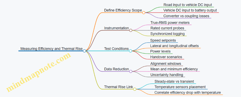
Thermal Rise Measurement Foundations
Thermal rise is measured as temperature increase over baseline under a defined electrical loading profile. Use baseline readings taken after a consistent preconditioning period.
Sensor placement matters more than people expect. Place temperature sensors where losses actually heat:
- Road embedded coil region near the conductor and insulation boundary.
- Road power electronics on heatsinks or module surfaces.
- Vehicle receiver coil region if available.
Use contact sensors rated for the expected temperature range, and ensure consistent mounting pressure or encapsulation conditions.
Concrete example: if you only measure heatsink temperature on the road inverter, you may miss coil hot spots that drive insulation aging. Measure at least one embedded coil-adjacent point to capture the “real” thermal constraint.
Thermal Rise Test Profiles
Thermal behavior depends on whether you test for steady-state or transient response.
- Transient test: apply a step in power (or start charging at a fixed power) and record temperature vs. time.
- Steady-state test: run repeated passes until temperature change per cycle falls below a small threshold.
A systematic approach is to do one transient test to estimate time constants, then use that to design a steady-state schedule.
Correlating Efficiency and Thermal Rise
Efficiency often drops as temperature rises because resistance increases and component characteristics shift. To connect the dots:
- Plot efficiency vs. time during the test.
- Plot coil temperature rise vs. time using the embedded sensor.
- Identify the time region where efficiency begins to trend downward.
Then compute a simple correlation metric within that region. You are not trying to prove causality; you are verifying that the thermal model and loss mechanisms are consistent with measured behavior.
Example: if efficiency minimum occurs after coil temperature reaches a repeatable threshold, you can use that threshold to set operational limits for future acceptance tests.
Reporting Results Clearly
For each test condition, report a compact set of values:
- Efficiency (mean and minimum) per alignment window
- Road input power level
- Vehicle DC input power level
- Temperature rise at each sensor location
- Time to reach near-steady behavior
Keep units explicit and avoid mixing “temperature” and “temperature rise” in the same table. If you must summarize in one line, use temperature rise and minimum efficiency together; that combination is usually what drives pass/fail decisions.
Practical Data Reduction Example
Suppose a pass at 60 km/h at a mid power level yields:
- Centered window: mean efficiency 88%, minimum 84%
- Edge window: mean efficiency 83%, minimum 78%
- Handover window: minimum 75% for 0.5 s
If the embedded coil temperature rise reaches the acceptance limit during the edge window, you have a clear link between electrical performance and thermal constraint. The next step is not “try harder,” it’s to adjust the operating strategy or design parameters so the minimum efficiency window no longer coincides with the hottest thermal region.
9.3 Validating Communication Latency and Control Loop Stability
Dynamic inductive charging depends on two timing realities: the vehicle must receive power only when the electrical conditions are safe, and the control system must react quickly enough to keep those electrical conditions within limits. Communication latency matters because it turns a feedback controller into a delayed one; delayed feedback can oscillate, overshoot, or chatter between safe and unsafe states. The goal of this section is to validate that end-to-end delays stay within a budget and that the closed-loop behavior remains stable across realistic operating conditions.
Foundational Timing Model
Start by separating three delays that often get lumped together:
- Sensing and measurement delay: time from electrical change to the moment the controller has a usable measurement (ADC sampling, filtering, and scaling).
- Communication delay: time for messages to travel between road segment controller and vehicle controller, including serialization and network scheduling.
- Actuation delay: time from controller output to the electrical system response (power stage switching latency, resonant settling, and any current/voltage loop bandwidth limits).
A practical validation approach treats the total delay as an effective delay in the outer control loop. If the outer loop commands a target power or resonant operating point, the controller must not “chase” stale measurements.
Communication Latency Budget
Define a latency budget before testing. For example, if the vehicle controller updates its charging setpoint every 20 ms, you can require that the road-to-vehicle authorization and parameter messages arrive within 10 ms worst-case, leaving the remaining 10 ms for measurement processing and actuation scheduling. The exact numbers depend on your control update period, but the method stays the same.
Best practice: specify both worst-case and typical latency. Typical latency helps performance, while worst-case latency prevents rare timing spikes from causing instability.
Stability Mechanisms Affected by Delay
Delay impacts stability through two common failure modes:
- Phase lag: the controller reacts after the system has already moved, reducing damping and increasing oscillation risk.
- Mode switching chatter: if safety thresholds depend on communicated states (for example, “charging allowed” or “alignment quality”), delayed updates can repeatedly cross thresholds.
To validate stability, you need to test not only steady operation but also transitions: entering a charged zone, moving between segments, and recovering from a faulted state.
Test Strategy from Simple to Realistic
Use a staged plan so you can attribute problems.
- Loopback tests: run the vehicle and road controllers in a hardware-in-the-loop setup where communication is emulated. Sweep delay values while keeping electrical conditions constant.
- Static coupling tests: fix vehicle position and alignment so the inductive coupling coefficient stays constant. Validate that the control loop converges without oscillation for each delay setting.
- Dynamic coupling tests: introduce controlled lateral and longitudinal motion so coupling varies. Confirm stability while the system naturally experiences changing power transfer conditions.
- Fault and recovery tests: inject a communication drop or a delayed “charging allowed” message. Verify that the system transitions to a safe mode without oscillatory recovery.
Example: If your controller uses a power regulation loop that updates every 20 ms, emulate delays of 0 ms, 5 ms, 10 ms, and 15 ms. For each case, record overshoot, settling time, and whether the controller hits safety limits repeatedly.
Mind Map: Latency and Stability Validation
Metrics and Acceptance Criteria
Record metrics that directly reflect stability and safety:
- Overshoot: how far power or current exceeds the target after a setpoint change.
- Settling time: time until the system stays within a tolerance band.
- Oscillation indicators: repeated crossings of the target band or sustained oscillations in current.
- Safety limit crossings: count and duration of any excursions beyond configured thresholds.
- Mode transition count: number of times the system flips between charging and non-charging due to delayed states.
Best practice: define acceptance criteria in terms of these metrics, not just “it looks stable.” For instance, require convergence within a maximum settling time and limit the number of safety threshold crossings during a delay sweep.
Example Control Loop Validation Procedure
Assume the vehicle controller regulates resonant power using a discrete-time controller updated every 20 ms. Perform a delay sweep in the communication emulator while holding coupling constant.
- Setpoint step: change target power by a fixed amount.
- Delay sweep: 0 ms to 15 ms in 5 ms increments.
- For each run: log measurement timestamps, received message timestamps, controller outputs, and electrical responses.
If stability degrades sharply at a particular delay, you can compute the effective phase margin loss and adjust either the communication budget or the controller update strategy (for example, reducing reliance on delayed messages for immediate actuation).
Example: Handling Delayed Authorization
Consider a scenario where the road controller sends “charging allowed” plus a recommended operating parameter. If authorization arrives late, the vehicle might already be ramping power. A stable design ensures that the vehicle either:
- ramps using a conservative default until authorization arrives, or
- gates the ramp so that actuation depends on fresh authorization.
Validation should confirm that delayed authorization does not cause repeated ramp-up/ramp-down cycles. The acceptance criterion can be “no more than one mode transition per entry event” and “safe mode reached within a defined time window.”
Putting It Together
A communication latency test is successful when it proves two things: the system stays stable under the measured worst-case delay, and transitions remain well-behaved when messages arrive late or not at all. When you can trace each instability symptom back to a specific delay component and reproduce it in a controlled test, you have something more useful than a vague feeling of “it probably works.”
9.4 Conducting Electromagnetic Field Mapping and Shielding Verification
Dynamic inductive charging lives or dies by what the fields do in the real world: under misalignment, during entry and exit, and in the presence of nearby metallic structures. Field mapping turns “it should be fine” into measured evidence, while shielding verification confirms that the system stays within electromagnetic exposure and interference limits.
Define What You Will Measure
Start with a measurement plan tied to acceptance criteria. Identify the operating states you must cover: nominal lane center, worst-case lateral offset, partial overlap during handover, and the maximum power mode used for charging. For each state, specify the measurement grid resolution and the height above the road where limits apply. A practical approach is to map at two heights: one near the typical human exposure plane and one closer to the vehicle undercarriage plane.
Example: If your corridor uses 2 m segments, use a grid that captures segment boundaries. Place measurement points every 0.25 m across the lane and every 0.5 m along the travel direction, then densify near the segment edges where coupling changes fastest.
Establish Baseline and Reference Conditions
Before energizing the system, record the ambient electromagnetic background. Then perform a reference run with a known configuration: a single segment at a defined power level and a fixed vehicle-receiver state or a calibrated test load. This baseline prevents you from “verifying” shielding against noise you never measured.
Best practice: Use the same coil drive waveform and control mode for every run. If the road controller changes frequency or compensation during operation, log those parameters so the mapping can be reproduced.
Map the Field Distribution Systematically
Use a consistent coordinate system tied to lane markings. For each operating state, capture field magnitude and phase where possible, or at least magnitude at each grid point. If your instrumentation supports it, measure both magnetic field strength and induced electric field proxies relevant to exposure and interference.
A systematic workflow looks like this:
- Sweep along the lane direction while holding lateral position fixed.
- Sweep laterally at the segment center and at the segment boundary.
- Repeat for the worst-case misalignment state.
Verify Shielding with Controlled Comparisons
Shielding verification is not a single measurement; it is a comparison. Create two configurations: shielding installed and shielding bypassed or replaced with a non-shielding equivalent. Keep everything else identical: coil drive settings, segment selection, vehicle test load, and environmental conditions.
Example: If you use magnetic back iron under the coil, compare field levels at the roadside edge points for both configurations. You should see a consistent reduction pattern, not just a lower average. If the average drops but the edge points do not, the shielding may be redirecting flux rather than blocking it.
Identify Hot Spots and Explain Them
After mapping, compute worst-case points and plot heat maps. Hot spots usually occur near:
- Segment boundaries where coupling changes rapidly.
- Edges of shielding where flux can “leak” around the barrier.
- Areas with nearby metallic infrastructure that alters current paths.
To explain a hot spot, correlate it with geometry. If the hot spot sits near a cable trench, check whether the trench contains metallic conduits that can act like unintended conductors.
Validate Against Limits and Uncertainty
Field limits are not just numbers; they come with measurement uncertainty. Record instrument calibration status, probe orientation, and repeatability. For each operating state, report the measured value, the uncertainty band, and whether the worst-case point stays within the limit.
Best practice: Repeat the measurement at the top three worst-case grid points at least twice. If results vary beyond expected uncertainty, you likely have probe placement or alignment issues.
Produce Evidence That Survives Real Audits
Your final deliverable should include:
- A table listing each operating state, grid definition, and drive parameters.
- Heat maps for each state.
- A worst-case summary table with measured values and uncertainty.
- A shielding comparison summary that shows reduction at the critical points.
Example output structure:
- State A: Lane center, nominal power
- State B: Worst lateral offset, nominal power
- State C: Entry overlap, max power
- State D: Boundary overlap, max power
For reproducibility, include the exact test date used for the run, such as 2026-03-07, and the firmware or control configuration identifier used during energization.
9.5 Acceptance Testing for Grid Power Quality and Harmonics
Grid power quality acceptance for dynamic inductive charging is about proving two things: (1) the charging system draws power in a way the grid can tolerate, and (2) the system’s switching behavior does not create unacceptable voltage distortion or flicker at the point of common coupling (PCC). The test plan should start with definitions and measurement points, then move into harmonic limits, flicker, and verification under realistic operating states.
Define the Test Boundaries and Measurement Points
Acceptance testing begins by locking down where measurements happen and what “good” means.
- PCC selection: Use the PCC at the facility side feeding the road power converters. If multiple feeders exist, document the exact breaker and cable segment.
- Operating states: Include at least these states: idle, pre-charge, active charging with nominal power, partial power, and a controlled fault recovery sequence. Each state changes current shape and control behavior.
- Time window: Harmonics require steady-state windows long enough to capture stable switching patterns. Flicker and transients require shorter windows with event capture.
Easy example: If the road segment controller ramps power in 200 ms steps, then a “steady-state” harmonic window must start after the ramp completes, not during it.
Establish Baseline Instrumentation and Data Integrity
You need measurement tools that agree with each other and with the standards.
- Meter class and bandwidth: Use power quality analyzers that support harmonic analysis and flicker metrics with appropriate bandwidth.
- Synchronization: Ensure time alignment between voltage and current channels so phase-based harmonic calculations are consistent.
- Calibration checks: Perform a quick verification using a known reference or internal calibration mode before and after the test run.
Easy example: If voltage and current channels are misaligned by even a few degrees, the computed harmonic power factor can look “worse” than reality.
Verify Harmonic Emissions at the PCC
Harmonic acceptance typically focuses on current harmonics and their resulting voltage distortion at the PCC.
- Current harmonic spectrum: Measure THD of current and individual harmonic orders relevant to the converter switching and control loops.
- Voltage distortion: Measure voltage THD and harmonic components at the PCC to confirm the grid sees acceptable distortion.
- Operating dependence: Repeat measurements at nominal and reduced charging power, because control modes can change the effective switching pattern.
Easy example: A converter that uses different modulation at 30% power may shift dominant harmonics from, say, the 5th/7th region to higher orders.
Check Flicker and Short-Term Voltage Variations
Dynamic inductive charging can cause short-term voltage changes due to power ramping and control actions.
- Flicker metrics: Measure flicker severity during active charging ramps and handover events between road segments.
- Event capture: Record voltage dips or spikes around transitions like entry into a charged zone and exit from it.
- Correlation to control actions: Tag events with controller logs so you can link a voltage variation to a specific ramp or protection action.
Easy example: If a handover causes a brief power interruption, the voltage variation may be visible even when average power looks stable.
Validate Power Factor and Reactive Power Behavior
Even when harmonic limits are met, poor reactive behavior can stress the feeder.
- Displacement and non-linear components: Separate reactive power behavior from harmonic-driven effects by analyzing both fundamental power factor and harmonic reactive contributions.
- Regulation behavior: Confirm that the converter’s grid interface control maintains the intended power factor target across operating states.
Easy example: A system that maintains unity displacement power factor at nominal power might still show elevated reactive current at partial power due to control mode changes.
Acceptance Criteria and Pass-Fail Logic
Acceptance criteria should be explicit and testable.
- Harmonics: Define limits for current THD, individual harmonic magnitudes, and voltage THD at the PCC.
- Flicker: Define maximum flicker severity over the relevant measurement intervals.
- Consistency: Require that results remain within limits across repeated runs and across the defined operating states.
Easy example: If one run exceeds a harmonic limit during a ramp, the pass condition can require that the steady-state window meets limits, while the ramp window is documented as “transient allowed” only if the standard permits it.
Reporting and Traceability That Engineers Actually Use
A useful acceptance report ties measurements to configuration.
- Test setup diagram: Show PCC location, feeder rating, and where the analyzer connects.
- Configuration snapshot: Record converter settings, filter configuration, and any active compensation modes.
- Results table: Provide harmonic and flicker metrics per operating state, with measurement window details.
- Raw data retention: Store raw waveforms for voltage and current so reviewers can reproduce calculations.
Mind Map: Grid Power Quality and Harmonics Acceptance
Example: A Practical Acceptance Run
A test run targets a single road segment power converter feeding a defined PCC. The procedure measures idle, pre-charge, active charging at nominal power, active charging at 30% power, and a controlled handover event. For each state, the analyzer captures a steady-state harmonic window and a separate event window for voltage variation. The report then lists current THD, dominant harmonic orders, voltage THD, and flicker severity, each tied to the controller log timestamps. If a dominant harmonic spikes only during the ramp window, the pass decision is based on the steady-state window meeting limits, while the ramp behavior is documented with the exact controller action that caused it.
10. Reliability Maintenance and Lifecycle Operations
10.1 Failure Modes for Embedded Coils Power Electronics and Cabling
Dynamic inductive charging lives or dies by what happens when things go wrong. Embedded coils, power electronics, and cabling share a common reality: they operate in heat, moisture, vibration, and electrical stress at the same time. This section maps the most common failure modes to their root causes, what you can observe, and what best practices prevent.
Foundational Failure Drivers
Failure modes usually start with one of four drivers: thermal stress, mechanical stress, insulation degradation, or electrical overstress. Thermal stress accelerates aging of insulation and potting compounds. Mechanical stress comes from traffic loads, thermal expansion, and installation tolerances. Insulation degradation can be slow and invisible until leakage currents rise. Electrical overstress includes overvoltage, overcurrent, and repeated high-frequency stress that damages dielectric layers.
A practical way to think about it is to separate “where the energy goes” from “where the heat goes.” If a coil is transferring power efficiently, most losses become predictable heat. If losses suddenly increase, the failure is often already underway.
Embedded Coil Failure Modes
Coil conductor fatigue and open circuits. Repeated thermal cycling and vibration can crack fine strands or solder joints. You may see a gradual rise in equivalent series resistance or a sudden drop in transferred power.
Insulation breakdown and shorted turns. Moisture ingress or voids in encapsulation can create partial discharge paths. Shorted turns reduce effective inductance and detune resonance, causing the power electronics to work harder to maintain output.
Ferrite or magnetic material degradation. Corrosion or cracking in magnetic components can change permeability and increase stray flux. The symptom is often higher electromagnetic coupling variability across the lane.
Encapsulation cracking and water pathways. Even hairline cracks can become water highways. The electrical symptom is leakage current growth; the physical symptom is elevated moisture content near the segment.
Power Electronics Failure Modes
Switching device overstress. IGBTs/MOSFETs can fail from overcurrent, insufficient gate drive, or thermal runaway. The observable pattern is a sharp increase in device temperature and fault trips during normal charging.
Capacitor aging in resonant networks. Film capacitors can lose capacitance or increase dissipation factor. Detuning shows up as reduced efficiency and unstable regulation.
Control and sensing faults. Bad current/voltage sensing, loose connectors, or drift in measurement circuits can cause the controller to command unsafe operating points. The symptom is “wrong behavior with correct-looking voltages,” where measured quantities don’t match expected relationships.
Cooling path failures. Blocked thermal interfaces or degraded thermal grease can create hot spots. The symptom is consistent overheating at the same component location.
Cabling Failure Modes
Connector corrosion and contact resistance growth. Moisture and road salts can raise contact resistance, producing localized heating. Expect intermittent faults that correlate with humidity or temperature.
Cable insulation breakdown. Repeated voltage stress and mechanical abrasion can thin insulation. The symptom is increased leakage current and insulation resistance trending down.
Strain and pull damage. Installation shortcuts can leave cable sections under tension. Over time, micro-movements fatigue conductors.
EMI-induced nuisance faults. Poor shielding or grounding can inject noise into sensing lines. The symptom is faults that appear during specific operating modes, even when electrical stress is unchanged.
Mind Map: Failure Modes and What to Look For
Integrated Best Practices with Concrete Examples
Example: Detecting shorted turns early. During commissioning, record baseline resonance frequency and efficiency versus vehicle position. Later, if resonance frequency shifts by a small but repeatable amount while transferred power drops, treat it as a coil-side detuning issue rather than immediately blaming the vehicle receiver.
Example: Preventing connector corrosion. Use sealed connector designs with strain relief and verify torque and sealing during installation. A common field pattern is “works in the lab, fails in rain,” which often traces back to water ingress at connectors rather than the coil itself.
Example: Avoiding capacitor aging surprises. Select resonant capacitors with appropriate voltage and temperature derating, then monitor dissipation factor proxies through efficiency trends. If efficiency declines faster than expected with stable operating conditions, investigate the resonant network before the switching devices.
Example: Reducing sensing-driven faults. Route current-sense leads away from high dv/dt nodes and validate sensor scaling with a known test load. When the controller’s commanded power and measured power diverge, you want to know whether the measurement chain is lying.
Practical Diagnostic Flow for Embedded Segments
Start with the simplest discriminators: does the fault correlate with moisture, temperature, or a specific lane position? Then compare electrical signatures to baseline: resonance shift, leakage current trend, and efficiency change. If resonance shifts, focus on coil and resonant components. If leakage rises without resonance shift, focus on insulation and cabling. If faults occur with correct electrical signatures, focus on sensing, control, and grounding.
This approach keeps troubleshooting grounded: you’re not guessing which part is “bad,” you’re using consistent symptoms to narrow the failure driver.
10.2 Maintenance Strategies for Roadside Components and Connectors
Dynamic inductive charging depends on embedded coils, power electronics, and the connectors that tie them together. Maintenance is not just “fix when broken”; it is a planned routine that keeps electrical performance stable while preventing water ingress, insulation breakdown, and connector overheating.
Foundational Maintenance Goals
Start with three measurable goals. First, preserve electrical characteristics such as coupling efficiency and resonant behavior by preventing coil damage and detuning. Second, preserve safety by ensuring insulation integrity and reliable protective shutdown. Third, preserve uptime by reducing unplanned outages through early detection.
A practical way to translate goals into work is to define what “healthy” looks like for each asset. For a roadside coil segment, healthy typically means stable insulation resistance, no abnormal temperature rise, and consistent electrical signatures during commissioning and periodic checks. For connectors, healthy means low contact resistance, no corrosion at interfaces, and secure strain relief.
Asset Breakdown and Maintenance Ownership
Treat the roadside system as layers with different failure modes. Embedded coils and encapsulation are slow-to-fail but hard to access. Power electronics are faster to fail and easier to replace. Connectors sit in the middle: they are accessible, but they fail in ways that can cascade into larger problems.
Assign ownership by layer. Roadside civil teams handle sealing, drainage, and pavement restoration. Electrical teams handle insulation testing, thermal checks, and connector replacement. Control and communications teams verify that segment enable/disable commands match the physical state.
Preventive Maintenance That Actually Prevents
Preventive maintenance should be scheduled around stress cycles: traffic load, thermal cycling, and moisture exposure. A useful baseline routine is:
- Visual inspection of accessible junction boxes and cable routes.
- Electrical insulation resistance testing between coil conductors and ground.
- Contact resistance checks for connectors using a safe measurement method.
- Thermal verification during controlled charging sessions, focusing on hotspots near terminations.
- Verification of protective devices such as fuses and surge protection.
Example: If insulation resistance drops faster than the historical trend, you do not just “retest.” You correlate the drop with recent construction activity, nearby drainage issues, or connector work. The maintenance action becomes targeted rather than repetitive.
Corrective Maintenance with Controlled Scope
Corrective maintenance should be structured to avoid turning one fault into several. When a connector shows high contact resistance or signs of corrosion, replace it as a set with the mating interface and any damaged cable end terminations. After replacement, re-verify insulation resistance and perform a short controlled electrical test to confirm that resonant tuning and protective thresholds behave as expected.
Example: A connector that overheats during a test run often indicates either poor crimp quality, insufficient torque, or moisture intrusion. Replacing only the connector body without addressing strain relief can recreate the same failure under vibration.
Connector-Centric Practices
Connectors deserve special attention because they combine electrical stress with environmental exposure.
- Use strain relief so cable motion does not load the contact interface.
- Ensure sealing compounds and gaskets are compatible with the encapsulation materials.
- Maintain correct mating alignment to prevent partial contact and arcing.
- Keep connector surfaces clean and dry during installation; contamination can raise contact resistance.
Example: During commissioning, a connector may pass initial resistance checks but fail later if the seal was installed with a small void. A void can wick moisture over time, so periodic thermal checks during charging are a strong complement to purely electrical measurements.
Mind Map: Maintenance Strategy
Documentation and Feedback Loops
Maintenance becomes effective when measurements are comparable over time. Establish baselines during commissioning for each segment: insulation resistance values, connector resistance ranges, and thermal behavior under a defined charging profile. Store results with location identifiers so you can spot patterns such as “all segments in one drainage basin show faster insulation decline.”
Work orders should include root-cause tags tied to evidence: moisture ingress indicators, connector torque issues, insulation degradation rate, or protective device nuisance trips. This prevents the same fix from being repeated without learning.
Practical Example Workflow
A connector alarm triggers a maintenance ticket after a thermal check shows a termination hotspot. The team:
- Confirms the hotspot location and checks for visible seal damage.
- Performs insulation resistance testing to rule out broader insulation failure.
- Measures contact resistance at the connector interface.
- Replaces the connector and mating interface, including any compromised cable end terminations.
- Restores sealing and strain relief, then verifies mechanical integrity.
- Runs a controlled charging test and records thermal and electrical results.
If insulation resistance remains stable and thermal rise returns to baseline, the corrective work is considered complete. If not, the team expands scope to adjacent cable runs or encapsulation areas, because connector faults can be symptoms rather than the only cause.
10.3 Condition Monitoring Using Electrical Signatures and Sensors
Dynamic inductive roads live a double life: electrically, they behave like a power-transfer system; mechanically, they behave like embedded infrastructure under heat, moisture, and vibration. Condition monitoring should therefore treat “electrical weirdness” as a first-class signal, not a late surprise.
Foundational Idea: What You Can Measure Without Guessing
Start by separating monitoring signals into three groups:
- Roadside electrical signatures: currents, voltages, resonant tank behavior, switching waveforms.
- Thermal and environmental sensors: temperatures at coil and power electronics, moisture indicators, surface conditions.
- System-level observables: communication health, charge authorization outcomes, segment-to-segment handover behavior.
A practical best practice is to define a baseline for each electrified segment under normal operation. For example, during a morning commissioning window, record resonant frequency, input current ripple, and coil temperature rise at a fixed vehicle speed and alignment band. Later, monitoring compares live measurements to that baseline using thresholds and trend rules.
Electrical Signatures That Reveal Real Problems
Electrical signatures are powerful because many failures change impedance before they change temperature.
- Resonant frequency drift: A loose connection, aging insulation, or altered coil geometry shifts the effective inductance and capacitance. You can estimate resonant behavior from measured current and voltage phase relationships or from the frequency response of the control’s tuning routine.
- Quality factor degradation: Increased losses show up as higher current for the same transferred power. Watch for rising RMS current at constant delivered energy.
- Switching waveform changes: Gate drive timing errors, device degradation, or snubber issues can alter voltage overshoot and ringing amplitude.
- Grid-side harmonics and power factor: A failing converter stage often changes how the system draws current from the grid, even when the vehicle-side load looks similar.
A concrete example: if a segment’s coil insulation absorbs moisture, the effective loss increases. In monitoring, you may see higher converter input current ripple and a slower decay of resonant oscillations after the switching transitions, even before coil temperature rises noticeably.
Sensor Strategy That Complements Electrical Data
Electrical measurements tell you “something changed.” Sensors help you answer “what changed and where.” Use a layered approach:
- Coil temperature sensing: Place sensors near the embedded coil region and, if feasible, near the highest-loss path. The goal is not perfect absolute temperature, but consistent relative rise.
- Power electronics temperature sensing: Track heatsink or module temperatures and correlate them with electrical load.
- Moisture and ingress indicators: Even simple conductivity or dielectric-loss indicators can flag water presence that accelerates insulation aging.
- Mechanical integrity checks: Where available, monitor vibration or strain indirectly via electrical effects like contact resistance changes.
Best practice example: when coil temperature rises but resonant frequency stays stable, suspect thermal coupling issues or airflow changes around the electronics. When resonant frequency shifts first, suspect electromagnetic or connection changes.
Monitoring Architecture and Data Flow
A robust monitoring loop typically follows this sequence:
- Acquire: sample currents, voltages, and switching-related signals at a consistent rate.
- Condition: filter noise and normalize measurements by operating point (vehicle speed band, segment power level).
- Extract features: resonant estimate, RMS current, ripple metrics, overshoot amplitude, phase error.
- Detect: apply rule-based thresholds and trend checks.
- Diagnose: map detected feature patterns to likely fault categories.
- Act: log events, adjust operating limits, and trigger maintenance when thresholds persist.
To keep this manageable, define a small set of features that are stable and repeatable. For instance, “resonant frequency estimate” and “current ripple at a fixed power level” are usually more actionable than raw waveforms.
Detection Rules That Avoid False Alarms
Use two layers of decision-making:
- Hard limits for safety-critical conditions, such as overcurrent, insulation resistance indicators, or converter fault codes.
- Soft limits with persistence for condition trends, such as resonant drift exceeding a band for N consecutive charging events.
Example rule set for a segment:
- If resonant frequency estimate shifts by more than a defined percentage for 10 consecutive vehicle passes, flag “electromagnetic parameter drift.”
- If RMS input current increases by a defined percentage while delivered energy remains within tolerance, flag “efficiency loss.”
- If coil temperature rise exceeds expected rise at constant electrical features, flag “thermal path degradation.”
Mind Map: Electrical Signatures and Sensor Correlation
Example: From Measurement to Maintenance Ticket
Imagine a segment that begins showing a gradual resonant frequency shift. Over several days, the system logs: resonant estimate drift beyond the soft threshold, while delivered energy remains acceptable and coil temperature rise is still within expected bounds. That pattern suggests an electromagnetic parameter change rather than immediate thermal failure.
The maintenance ticket should therefore request inspection of embedded coil terminations and encapsulation integrity in that segment, along with verification of converter tuning and connection torque. The key is that the ticket is driven by correlated evidence: electrical drift first, thermal confirmation later.
Practical Checklist for Implementation
- Define baselines per segment and per operating band.
- Choose a small set of stable electrical features.
- Correlate electrical anomalies with temperature and moisture signals.
- Use persistence rules to reduce false alarms.
- Log raw measurements only when an event triggers; store features routinely.
- Ensure maintenance actions map to fault categories with clear inspection targets.
10.4 Repair Procedures for Pavement Sections and Recommissioning
Dynamic inductive charging depends on embedded coils, insulation, and power electronics that must survive water, traffic loads, and repeated thermal cycling. When a pavement section is repaired, the goal is not just to restore appearance—it is to re-establish the electrical, mechanical, and electromagnetic conditions that the system was accepted for.
Repair Foundations and Decision Triggers
Start with a clear trigger list so crews do not guess. Typical triggers include repeated vehicle-side receiver faults in one zone, abnormal roadside temperatures, insulation resistance trending down, or a post-incident inspection showing cracked encapsulation or disturbed conduit.
A practical best practice is to classify the repair scope before opening the pavement:
- Electrical-only: a connector, splice, or roadside power module issue with intact encapsulation.
- Embedded coil disturbance: coil leads, ferrite/shielding, or encapsulation damage.
- Civil-only: surface damage with no evidence of coil or conduit movement.
Each scope maps to different test requirements and different risk controls.
Site Preparation and Safe Isolation
Before any work, isolate the affected road segment electrically and verify absence of hazardous voltage. Then control the mechanical environment: mark lane geometry references, protect exposed edges, and prevent debris from entering conduits.
A simple but effective workflow is a three-step checklist:
- Confirm the exact segment ID and boundaries.
- Lock out and tag out the roadside power feeding that segment.
- Photograph the pre-open condition from fixed angles so later comparisons are objective.
Pavement Opening and Component Handling
Remove pavement in a way that preserves surrounding encapsulation. Avoid cutting near coil lead paths unless the repair plan explicitly includes lead replacement. If the repair requires lifting a coil assembly, treat it like a precision part: keep it supported, avoid twisting, and prevent contamination of encapsulation surfaces.
When replacing materials, match the original encapsulation class and thickness. If the repair uses a different encapsulant, plan additional verification because dielectric properties and thermal conductivity affect both safety margins and transfer efficiency.
Electrical Verification During Repair
After exposing the embedded system, perform staged electrical checks:
- Continuity of coil conductors and shields.
- Insulation resistance between conductors and any grounded structures.
- Connector integrity: verify seating, strain relief, and corrosion protection.
If insulation resistance is below the acceptance threshold, stop and identify the failure location before proceeding. A common mistake is to “patch and hope” when the insulation problem is actually deeper than the visible damage.
Reassembly, Encapsulation, and Mechanical Integrity
Reassembly is where many repairs drift from the original design. Ensure coil alignment relative to lane references, restore spacing to the intended geometry, and confirm that shielding and back iron are seated without gaps.
Encapsulation should be applied to eliminate voids around leads and to restore the intended cover thickness. Voids can trap moisture and create localized heating under load. After curing, verify that the surface profile meets the mechanical tolerances used during commissioning.
Recommissioning Plan and Acceptance Tests
Recommissioning should mirror commissioning, but focused on what changed. Use a test sequence that reduces risk and saves time.
Mind Map: Repair to Recommissioning Flow
Example: Electrical-Only Repair
A connector replacement in a roadside segment typically requires:
- Continuity and insulation resistance checks after reconnecting.
- A functional charging test at a controlled vehicle speed and alignment band.
- Verification that the segment control unit reports expected status codes and that handover to adjacent segments remains stable.
If the segment previously showed stable efficiency, you still re-check efficiency because connector changes can alter effective coupling and resonant behavior.
Example: Embedded Coil Disturbance
If a coil assembly was lifted or encapsulation was cut out, treat it as a higher-risk repair:
- Electrical checks as above.
- Alignment verification against lane references.
- Electromagnetic field mapping or equivalent coverage verification to confirm the effective coupling region.
- Thermal rise checks during a representative charging cycle.
If field coverage is off, do not proceed to full traffic operation. The system might still “work,” but it may violate exposure limits or cause uneven charging.
Documentation and Sign-Off
Close the loop with repair records that link cause to outcome. Include:
- Segment ID and exact boundaries.
- Scope classification and materials used.
- Pre- and post-repair electrical test results.
- Recommissioning test logs and pass/fail criteria.
- Photos of key stages: exposed components, encapsulation, and final surface.
A repair without traceable evidence is like a charging zone without a handshake—technically possible, operationally unreliable.
10.5 Spare Parts Planning and Operational Downtime Management
Spare parts planning starts with a simple question: what must be available to keep charging segments operating safely and predictably. Downtime management then turns that availability into procedures, roles, and measurable targets.
Foundational Inputs That Drive Spares
Begin by listing the assets that can fail and the consequences of each failure mode. For dynamic inductive roads, the practical list usually includes embedded coil assemblies, resonant compensation components, power electronics modules, roadside power converters, cooling elements, connectors and cable runs, sensors, and the segment controller.
Next, translate failures into operational impact categories. A useful approach is to define three tiers:
- Tier 1: prevents any charging in a segment (for example, a power stage fault that trips protection).
- Tier 2: allows reduced charging or limited lanes (for example, degraded thermal performance or partial sensor availability).
- Tier 3: affects diagnostics or convenience but not charging (for example, a non-critical indicator).
Finally, map each asset to a maintenance action type: replace-in-place, swap-and-recalibrate, or repair-and-verify. This mapping determines both the spare quantity and the time required to restore service.
Spare Parts Strategy That Matches Maintenance Reality
A good spares plan balances three constraints: probability of failure, lead time, and the time to restore service. Probability comes from historical maintenance logs, commissioning test results, and early-life reliability checks. Lead time comes from procurement and logistics. Restore time depends on how quickly a crew can access the component and complete electrical verification.
Use a tiered stocking model:
- Critical spares for Tier 1 assets that require immediate replacement.
- Buffer spares for Tier 2 assets that can tolerate short service degradation.
- Consumables and repair spares for items used during every intervention, such as sealing materials, connector hardware, and test adapters.
Example: if a roadside power converter module is a Tier 1 asset and typical replacement takes 6 hours including verification, then the spares plan should ensure at least one module is available per maintenance region so that a single failure does not cascade into multi-day downtime.
Quantities Using Service Level Targets
Quantities should be expressed as service level targets, not just “one extra.” Define a maximum acceptable downtime per segment per month and a maximum acceptable number of consecutive days with reduced charging. Then compute spares based on expected failure frequency and restoration time.
A practical method is to maintain a rolling window of failure counts and compute an average daily failure rate for each Tier. Multiply by the restoration time to estimate the expected number of simultaneous replacements. Round up to the next whole unit and add a small safety buffer for logistics delays.
Operational Downtime Management Workflow
Downtime management is a sequence, not a reaction. The workflow below keeps decisions consistent across crews.
- Detect: alarms from segment controllers and vehicle-reported charging anomalies are correlated to identify the affected segment and asset class.
- Isolate: protection states are checked to confirm whether the segment is safe to energize. Isolation prevents repeated trips that waste time and components.
- Dispatch: maintenance teams are assigned based on access constraints and required tools. If the fault is likely Tier 1, dispatch is prioritized.
- Replace or Repair: the crew performs the planned action type. For swap-and-recalibrate items, the procedure includes the minimum verification set.
- Verify: electrical checks confirm resonance tuning behavior, insulation integrity where applicable, and communication health.
- Close the Loop: the maintenance record updates the failure mode taxonomy so future spares calculations improve.
Example: if a connector shows intermittent faults, the workflow should avoid repeated energization attempts. Instead, isolate the segment, replace connector hardware, and run the same verification steps used during commissioning.
Mind Map: Spares and Downtime
Example Metrics and How They Guide Decisions
Track four metrics per segment family. Mean time to restore measures how fast you return to service. Tier 1 resolution within target window shows whether spares are sufficient. Repeat fault rate highlights weak points in procedures or component quality. Verification pass rate indicates whether the verification set is complete and whether crews are following it.
A small operational detail matters: after a replacement, the segment should be returned to service only after verification passes and the maintenance record is updated with the specific failure mode. That single step prevents the same component class from being misclassified later, which is how downtime quietly multiplies.
Documentation That Keeps Everyone Aligned
Maintain a spares catalog with part identifiers, compatible alternates, and the verification steps required after installation. Pair it with a downtime playbook that lists who can authorize energization, what constitutes a safe isolation state, and which tests must be logged.
For example, a playbook entry for a resonant compensation component should specify the minimum post-install checks and the exact data fields to record, such as measured tuning behavior and communication status. This makes handoffs between shifts straightforward and reduces “we think it’s fine” outcomes.
11. Deployment Planning and System Integration for Autonomous Fleets
11.1 Integrating Charging Zones into Vehicle Routing and Mission Planning
Dynamic inductive charging only helps if the route plan actually lines up with where power is available. This section treats charging zones as constraints and resources inside the mission planner, so the vehicle can decide when to enter, how long to stay, and how to hand off between segments without guessing.
Foundational Concepts for Routing with Charging Zones
Start by modeling each charging zone as a spatial interval along the road and as an operational capability. A practical model includes: (1) entry and exit boundaries, (2) lane or corridor geometry, (3) maximum supported power per segment, (4) expected efficiency versus speed and alignment, and (5) safety limits that force de-energization when conditions are not met.
Routing then becomes a constrained optimization problem. The planner chooses a path that satisfies navigation constraints while also meeting energy needs. The key is that charging is not a “nice-to-have stop”; it is a power transfer window with electrical and timing requirements.
Easy example: A delivery vehicle must arrive with 20% battery. The mission planner estimates consumption for the route and then schedules one charging zone whose interval overlaps the vehicle’s predicted trajectory. If the vehicle is expected to arrive 30 seconds late, the planner either selects a different zone or adjusts speed to re-align with the charging window.
Mission Planning Inputs and Data Flow
A mission plan typically has three layers of information: vehicle energy state, route geometry, and infrastructure capability.
- Vehicle energy state includes battery state of charge, estimated usable capacity, and a conservative power demand profile for propulsion and auxiliary loads.
- Route geometry includes lane-level alignment expectations and speed limits that affect coupling efficiency.
- Infrastructure capability includes per-segment power limits, communication availability, and fault behavior such as “no charge if foreign object detection is active.”
The planner uses these inputs to compute an energy budget and a feasible charging schedule. The schedule is feasible only if the vehicle can meet the zone’s entry conditions and if the infrastructure can allocate power at the required time.
Easy example: If a zone supports 150 kW but only when communication is established, the planner must treat “communication handshake success” as a gating condition. If the vehicle cannot reliably connect at that location, the plan should not assume full power.
Zone Selection and Scheduling Logic
Zone selection should balance energy gain, time cost, and risk of missing the window. A simple scoring approach works well in practice:
- Energy gain estimate: expected charged energy over the overlap between predicted trajectory and zone interval.
- Time penalty: extra time due to speed adjustments or detours.
- Feasibility penalty: likelihood of violating entry/exit constraints or encountering infrastructure faults.
The planner then chooses the set of zones that satisfies the energy requirement with minimal total penalty.
Easy example: Two zones are available. Zone A is closer but has lower efficiency at higher speeds. Zone B is farther but supports stable power at the vehicle’s expected speed. If the vehicle can’t slow down safely, Zone B may yield more net energy despite the longer path.
Handling Handover Between Adjacent Segments
Dynamic charging often uses multiple adjacent segments. The mission planner should avoid plans that rely on perfect timing at boundaries. Instead, it should include a buffer so the vehicle can transition while maintaining acceptable charging quality.
A robust handover rule is to require that the vehicle enters the next segment before the previous segment’s effective charging window ends, based on worst-case speed and alignment error.
Easy example: If the vehicle’s speed estimate can be off by ±5%, and the effective charging window shrinks with misalignment, the planner can target an overlap margin of a few seconds so the vehicle does not experience a sudden power drop.
Multi Vehicle Capacity and Fair Allocation
When multiple vehicles share the same charging corridor, the planner must coordinate capacity. The infrastructure can expose per-segment power availability, and the fleet controller can allocate it.
A practical approach is to treat power as a limited resource and schedule vehicles in a way that prevents overcommitment. Vehicles with urgent energy needs can be prioritized, while others may be routed to alternative zones or charged at reduced power.
Easy example: Two autonomous shuttles arrive at the same segment. If both request full power, the segment can only deliver enough for one at a time. The fleet controller assigns full power to the vehicle with the lower remaining range and routes the other to a nearby segment with spare capacity.
Mind Map: Routing and Mission Planning Integration
Example Workflow from Plan to Execution
- Compute energy demand for the candidate route using a conservative consumption model.
- Identify charging zones whose intervals intersect the predicted trajectory.
- Estimate net charged energy for each zone using expected efficiency at the planned speed.
- Apply feasibility checks for communication and safety gating.
- Select zones and schedule entry times with overlap buffers for handover.
- If multiple vehicles are present, apply capacity allocation and re-route any vehicle that cannot meet its energy requirement.
Easy example: A route initially includes one zone, but capacity is already reserved by another vehicle. The planner re-runs the schedule, keeps the same entry buffer logic, and swaps in a second zone that still satisfies the energy requirement without violating handover overlap.
This integrated approach turns charging from a roadside feature into a predictable part of mission planning, which is exactly what autonomous systems need: fewer surprises, more measurable constraints, and decisions that can be explained with numbers.
11.2 Data Requirements for Fleet Level Energy Accounting
Fleet level energy accounting answers one practical question: “How much electrical energy did we spend to move vehicles, and where did it go?” For dynamic inductive charging, the answer depends on what you measure, when you measure it, and how you reconcile vehicle events with roadside operation.
Foundational Data Categories
Start with four data categories that map cleanly to the physical system.
-
Grid and Roadside Energy
- Measure feeder-side energy (kWh) per charging segment and per time window.
- Record converter electrical quantities needed to compute delivered power and losses (input voltage/current, DC link voltage, switching state if available).
- Example: If Segment A runs from 10:00:00 to 10:10:00, store energy for that exact window, not just “during traffic.”
-
Vehicle Charging Events
- Log vehicle identifiers, entry and exit timestamps for each charging zone, and the charging mode (authorized, charging, paused, fault).
- Store receiver-side telemetry such as received power estimate, battery charge current/voltage, and state of charge at entry and exit.
- Example: A vehicle enters at 10:03:12, leaves at 10:03:28. Even if it briefly pauses due to misalignment, the event record must preserve those sub-intervals.
-
Alignment and Coupling Context
- Capture alignment indicators used by control logic, such as lateral offset estimate, coil-to-coil coupling index, or resonant frequency tracking values.
- Record environmental context that affects performance, like pavement temperature sensor readings near the segment.
- Example: If efficiency drops on a cold morning, you want the data that explains whether it was thermal, alignment, or control tuning.
-
Accounting Metadata and Provenance
- Define time synchronization method, measurement source, units, and calibration version.
- Keep a “data lineage” field that tells you whether a value is raw, filtered, or computed.
- Example: If received power is computed from receiver current and voltage, mark it as computed so audits can reproduce it.
Event Model That Prevents Double Counting
A fleet account must avoid counting the same energy twice across overlapping segments and handovers.
- Define a charging zone as a set of one or more segments that operate together.
- Define a vehicle charging session as the interval from first authorization to final exit for that vehicle in that zone.
- Within a session, define sub-intervals where power transfer is active, paused, or faulted.
Best practice: store energy at the roadside segment level, then allocate to vehicle sessions using the sub-interval timeline. Allocation should be deterministic, documented, and reproducible.
Allocation Rules That Match Real Operation
Use rules that reflect how power is actually delivered.
-
Roadside Energy Attribution
- Attribute converter input energy to the segment’s active sub-intervals.
- Exclude energy during “standby enabled but no vehicle coupled” if the system can detect coupling absence.
-
Vehicle Energy Attribution
- Attribute delivered energy to the vehicle using receiver-side measured or computed received power integrated over active sub-intervals.
- When receiver telemetry is missing, use a controlled fallback such as segment-level power transfer estimate multiplied by a coupling index.
Example: If Segment B consumed 12.0 kWh during a 10-minute window but only 3 minutes had confirmed coupling, allocate 12.0 kWh across those 3 minutes, then split among vehicles by their active sub-interval durations.
Data Schema Mind Map
Mind Map: Fleet Energy Accounting Data
Concrete Example Data Flow
Consider a two-segment zone where a vehicle crosses from Segment 1 to Segment 2.
- Roadside logs Segment 1 active from 09:41:10 to 09:41:22 and Segment 2 active from 09:41:22 to 09:41:35.
- Vehicle session spans 09:41:10 to 09:41:35, with a single session record containing two sub-intervals.
- Allocation integrates receiver received power over each sub-interval and sums to a session delivered energy.
- Fleet report then compares total delivered energy across vehicles to total segment input energy, with the difference tracked as losses and non-attributed energy.
Quality Checks That Keep Reports Honest
- Timestamp Consistency: verify monotonic event times and that vehicle sub-intervals fall within roadside active windows.
- Energy Balance: compute residual energy per segment window and store it as a named category (losses, non-coupling, missing data).
- Calibration Version Tracking: if tuning changes, keep separate calibration versions so historical reports remain comparable.
Example: If a segment’s residual energy spikes after a firmware update, the accounting system should flag the change because the calibration version and control parameters changed at the same time.
11.3 Managing Multi Vehicle Charging Capacity on Shared Infrastructure
Shared inductive lanes rarely serve one vehicle at a time. Capacity management means deciding who gets power, how much, and for how long—while keeping electrical limits, thermal limits, and vehicle charging requirements all satisfied. The trick is to treat the road like a power system with a schedule, not like a passive charger.
Foundational Capacity Model
Start with a simple accounting model for each electrified segment: available grid power, conversion efficiency, and the power actually delivered to vehicles. For segment s, define:
- Grid power limit: \( P_{grid,max,s} \)
- Converter efficiency: \(\eta_s\) (use measured values, not nameplate guesses)
- Delivered power per vehicle: \(P_{deliv,i}\)
- Segment load constraint: \(\sum_i P_{deliv,i} \le P_{grid,max,s} \cdot \eta_s\)
A practical best practice is to include a headroom factor (for example 10–20%) to cover measurement error and transient behavior during entry and exit. If you skip headroom, the system will “work” until it doesn’t—usually during the busiest moment.
Scheduling and Allocation Logic
Vehicles request charging power when they are within the effective coupling region. The road controller responds with an allowed power setpoint. Allocation can be handled in layers:
- Admission control: decide whether a vehicle is allowed to charge in this segment.
- Power budgeting: compute each vehicle’s permitted power.
- Rate limiting: prevent abrupt changes that stress converters and receivers.
A straightforward policy that works well in practice is time-sliced fairness with minimum service. Each vehicle gets a minimum power floor if it is present long enough to benefit, and any remaining capacity is distributed proportionally to requested power.
Example: A segment has a budget of 300 kW delivered. Three vehicles are present:
- Vehicle A requests 160 kW and will stay 40 s
- Vehicle B requests 120 kW and will stay 25 s
- Vehicle C requests 90 kW and will stay 15 s
If you allocate purely by request, you may starve C or force oscillations. With time-sliced fairness, you can grant A 120 kW, B 110 kW, and C 70 kW initially, then re-evaluate at each control interval based on measured coupling quality and remaining dwell time.
Handling Overlap Across Adjacent Segments
Dynamic charging corridors often use multiple segments with handover. Capacity must be managed across overlaps so that a vehicle does not cause a sudden jump in load when it transitions. Use a handover window where both segments briefly coordinate:
- The upstream segment reduces its power allowance as the vehicle’s coupling indicator drops.
- The downstream segment increases allowance as coupling indicator rises.
This prevents “double billing” of power during the handover moment. A good operational rule is to base the handover on electrical measurements (coupling strength or receiver-reported status) rather than only on position.
Thermal and Electrical Constraints as First-Class Limits
Power budgeting is not only about grid power. Roadside components have thermal limits, and converters have current limits. Treat these as additional constraints in the allocation step:
- If converter temperature approaches its limit, reduce the segment’s effective delivered budget.
- If current limit is reached, cap the sum of vehicle power even if grid power remains available.
Example: Two vehicles request high power, but one segment’s coil temperature sensor indicates reduced thermal headroom. The controller lowers the segment budget, and vehicles receive lower setpoints without needing to renegotiate the entire charging session.
Mind Map: Multi Vehicle Capacity Management
Case Example: Shared Lane with Four Vehicles
Consider one segment with a delivered budget of 250 kW and a control interval of 1 s. Four vehicles arrive in sequence with different coupling quality:
- V1: strong coupling, requests 90 kW
- V2: moderate coupling, requests 80 kW
- V3: weak coupling, requests 70 kW
- V4: strong coupling, requests 120 kW
The controller grants power based on both request and expected transfer efficiency. Weak coupling vehicles receive lower setpoints because the same delivered target would require higher currents and would waste capacity. Meanwhile, strong coupling vehicles get the capacity that actually converts into battery charging. If V3’s coupling improves later, it can be re-admitted to a higher share without restarting the session.
Implementation Checklist for Capacity Control
- Use measured efficiency and include headroom.
- Enforce thermal derating as part of the same budget calculation.
- Allocate with fairness plus minimum service to avoid starvation.
- Coordinate adjacent segments using electrical coupling indicators.
- Rate-limit power setpoint changes to protect hardware.
- Log allocation decisions with the measured quantities that justified them.
11.4 Operational Procedures for Mixed Traffic and Charging Authorization
Dynamic inductive charging has one job during mixed traffic: decide who may draw power, when they may draw it, and how to stop safely when conditions change. The procedures below assume a roadway divided into charging segments, each with its own power electronics, sensing, and local controller.
Operational Goals and Roles
Start with clear responsibilities. The Roadside Controller authorizes charging per segment; the Vehicle Charging Controller requests authorization and reports receiver readiness; the Segment Power Unit executes power setpoints and enforces safety limits. Mixed traffic adds a fourth actor: non-charging vehicles that must pass through without being treated as charging candidates.
A practical best practice is to define three states for each segment: Idle (ready but not charging), Authorized (vehicle is eligible and power is permitted), and Charging (power transfer is actively regulated). Every procedure should map to one of these states.
Authorization Flow for Mixed Traffic
Authorization should be conservative: it should only grant permission when the vehicle is likely aligned and the system can maintain safe electromagnetic and electrical conditions.
- Vehicle approach detection: Roadside sensors detect a vehicle entering a segment’s detection window. The controller creates a short-lived “candidate session” tied to that vehicle’s identity token.
- Charging capability check: The vehicle responds with receiver capability data and a request for charging. Non-charging vehicles either do not respond or respond with “not capable,” which keeps the segment in Idle.
- Pre-charge eligibility: The roadside controller checks lane rules, segment availability, and whether the vehicle’s requested power is within the segment’s current capacity.
- Safety gating: Before any power is applied, the controller verifies foreign object conditions and confirms that electromagnetic exposure constraints can be met for the current operating mode.
- Handover readiness: For vehicles near segment boundaries, the controller ensures the next segment can accept the vehicle without a gap that would cause repeated start-stop cycles.
- Authorization grant: The controller sends an authorization token with allowed power limits and timing windows.
- Power ramp and regulation: The vehicle begins a controlled ramp. The roadside controller monitors electrical quantities and receiver feedback to keep transfer stable.
- Stop conditions: If alignment degrades, communication fails, or a safety condition triggers, the controller transitions to Idle by commanding a safe power reduction and de-energization.
A simple example: a passenger car without a receiver passes through. It triggers detection, but it never completes capability exchange, so the segment remains Idle and no power is applied.
Mixed Traffic Rules That Prevent Unnecessary Starts
Authorization should avoid “thrashing,” where the system repeatedly starts and stops due to borderline eligibility.
- Minimum dwell time: Once Charging begins, require a minimum time window before allowing a stop unless a safety fault occurs.
- Hysteresis on eligibility: Use separate thresholds for “eligible to start” and “eligible to continue.” This reduces oscillation when a vehicle is near the edge of the alignment envelope.
- Capacity-aware admission: If multiple vehicles are present, prioritize based on segment load and charging requests. The system should not grant authorization to a vehicle that would force immediate throttling.
- Communication timeout policy: Define a strict timeout after which the segment must stop charging if the vehicle cannot confirm receiver readiness.
Mind Map: Operational Procedures and Authorization Logic
Example: Passenger Car and Autonomous Truck in the Same Segment
Assume a segment supports up to 60 kW and has two vehicles arriving within the detection window.
- Passenger car: It is detected, but capability exchange returns “no receiver.” The controller keeps the segment in Idle and logs the candidate session as non-capable.
- Autonomous truck: It requests 45 kW and reports receiver readiness. The roadside controller confirms foreign object status is clear, checks that 45 kW fits within remaining capacity, and grants authorization with a timing window that overlaps the truck’s expected passage.
- Boundary crossing: As the truck approaches the segment end, the controller verifies the next segment is available and that its authorization window will overlap. If the next segment is not ready, the controller reduces power smoothly rather than forcing a hard stop mid-transition.
Example: Communication Drop During Charging
If the vehicle’s controller stops sending periodic readiness confirmations, the roadside controller does not guess. It follows the timeout policy: it commands a controlled power reduction to a safe level, then de-energizes the segment and returns to Idle. The vehicle can later re-request authorization when communication is restored and eligibility checks pass again.
Operational Logging and Auditability
Every candidate session should produce a compact record: detection time, capability outcome, eligibility checks passed or failed, authorization grant parameters, start and stop timestamps, and the reason for any stop. This makes troubleshooting straightforward because the system’s decisions are traceable to specific inputs rather than vague “fault” labels.
11.5 Training Documentation for Operators Maintenance Teams and Inspectors
Dynamic inductive charging works only when people follow the same rules the hardware was designed for. This section turns those rules into training documentation that operators, maintenance teams, and inspectors can use without guessing.
Training Goals and Audience Split
Operators need safe, repeatable procedures for starting and stopping charging, handling exceptions, and recording events. Maintenance teams need step-by-step work instructions for replacing components, verifying electrical health, and restoring alignment assumptions. Inspectors need evidence-based checklists that confirm installations meet requirements and that records match what is physically present.
A practical approach is to train each group on what they touch, then cross-train them on the interfaces they affect. For example, operators should understand what “foreign object detected” means in terms of system behavior, while inspectors should understand what a maintenance action changes in the documentation trail.
Documentation Set and How It Stays Coherent
Use a small set of documents with clear ownership:
- Operator Runbook: what to do during normal operation and common faults.
- Maintenance Work Instructions: how to perform tasks, including tool lists and verification steps.
- Inspection Checklist: what to verify visually and with measurements.
- Configuration Record: the current segment map, tuning parameters, and firmware versions used for charging authorization.
- Incident and Change Log: what happened, what was changed, and what tests were repeated.
Keep the documents linked by shared identifiers: road segment ID, lane ID, coil set ID, vehicle charging zone ID, and the commissioning batch number. If a technician replaces a component, the change log must reference the exact identifiers used by the control system.
Mind Map: Training Documentation Workflow
Operator Training Content That Prevents Common Mistakes
Operators should practice a “three-check” routine before allowing charging to proceed: (1) the zone is authorized by the control system, (2) the vehicle handshake is successful, and (3) the system reports stable power regulation rather than repeated retries. A simple example scenario: a vehicle enters the zone but the system repeatedly requests re-handshake; the operator should not override the behavior. Instead, they should follow the runbook’s exception steps, which include verifying that the correct lane segment is active and that no maintenance lockout is set.
For stopping, operators should learn the difference between a normal exit and a fault stop. Normal exit expects the system to ramp down as the vehicle leaves. Fault stop expects immediate de-energization and a recordable reason code. Training should include what to write in the event log so maintenance can reproduce the conditions.
Maintenance Training Content with Verification Steps
Maintenance work instructions must include verification, not just replacement. Example: when replacing an embedded coil module, the instruction should specify de-energization and lockout verification, then require insulation resistance measurement before energization. After installation, the team should confirm resonant tuning parameters match the configuration record for that coil set ID.
Include a “minimum test set” that is repeated after any work that could affect coupling or safety. For instance, after connector replacement, the team should run a controlled functional test that checks stable transfer behavior at a representative coupling level, then update the configuration record and change log.
Inspector Training Content That Produces Usable Evidence
Inspectors should be trained to treat the checklist as a data collection tool, not a memory test. Each checklist item should state: what to look for, how to measure or photograph it, and what evidence to attach.
Example checklist item: encapsulation integrity. The inspector should document visible cracking, measure any exposed edges if applicable, and photograph the area with a consistent framing reference. Then the inspector should cross-check that the segment’s commissioning batch and any subsequent change log entries align with what is physically present.
Training Schedule and Competency Checks
Use a structured sequence:
- Foundations: system roles, identifiers, and safety states.
- Role Procedures: operator runbook scenarios, maintenance task walkthroughs, inspection checklist walkthroughs.
- Integrated Exercises: a simulated fault where operators initiate the correct stop, maintenance performs a targeted fix, and inspectors verify closure.
- Competency Sign-off: pass/fail criteria tied to evidence quality and correct use of identifiers.
A sample training record date can be recorded as 2026-03-01 to demonstrate how documents should capture when competency was assessed.
Example: One Page Training Snapshot
- Operator: three-check start routine; correct fault stop behavior; event log completeness.
- Maintenance: lockout verification; insulation resistance before energization; resonant tuning confirmation; update configuration record.
- Inspector: evidence-first checklist; photo and measurement consistency; cross-check with change log and segment IDs.
This structure keeps the documentation consistent across roles, so the system’s safety and performance assumptions survive contact with real roads and real schedules.
12. Practical Design Examples from Requirements to Commissioning
12.1 Example System Sizing for a Two Lane Dynamic Charging Corridor
This example sizes a two-lane dynamic inductive charging corridor using practical assumptions, then shows how those assumptions turn into segment power, electrical ratings, and control targets. The goal is not to guess the “best” design, but to demonstrate a repeatable sizing workflow.
Corridor Assumptions
- Lane layout: Two lanes, each with a charging lane segmented into equal-length power blocks.
- Vehicle behavior: Vehicles travel at 90 km/h with typical lateral offset within ±0.3 m.
- Charging requirement: Target 120 kW peak charging power at the vehicle battery interface during the time the vehicle is over the energized region.
- Power transfer efficiency: Assume 90% end-to-end from road-side AC input to vehicle DC output under nominal alignment.
- Availability margin: Design for 80% utilization of the corridor at any moment (not every vehicle is present over every segment).
- Segment length: Choose 10 m energized length per power block to balance coil coverage and manageable thermal zones.
Step 1: Convert Vehicle Power to Road-Side Power
Vehicle peak DC charging power is 120 kW. With 90% efficiency, required road-side delivered power is:
- Road-side delivered power = 120 kW / 0.90 = 133.3 kW per vehicle.
If a single segment can serve one vehicle at a time in the same lane, then the segment must be capable of ≥ 133.3 kW delivered to the vehicle under nominal conditions.
Sizing practice: Add a small headroom for control and tuning losses. Use +10% road-side capability:
- Segment rated power ≈ 133.3 kW × 1.10 = 146.7 kW.
Step 2: Determine How Many Segments Are Energized Simultaneously
At 90 km/h, speed is 25 m/s. With 10 m energized length, a vehicle is over a given segment for:
- Dwell time = 10 m / 25 m/s = 0.4 s.
Dynamic charging typically energizes a short window ahead and behind to smooth handover. For sizing, assume two adjacent segments per lane are energized during a vehicle’s passage.
So, per lane, simultaneous energized segments ≈ 2.
With two lanes, total simultaneous energized segments ≈ 4.
Step 3: Apply Utilization and Compute Corridor Power
If utilization is 80%, the average number of simultaneously active segments is:
- Active segments = 4 × 0.80 = 3.2.
Average corridor road-side power ≈ 3.2 × 146.7 kW = 469.4 kW.
For electrical design, also consider peak demand when multiple vehicles overlap. Use a peak factor of 1.25 on average for sizing transformers and feeders:
- Peak corridor road-side power ≈ 469.4 kW × 1.25 = 586.8 kW.
A practical design target is ~600 kW road-side peak capability for the corridor.
Step 4: Split Power into Converter and Grid Ratings
Assume each power block uses a dedicated converter module. Then each converter must support one segment rated output:
- Converter output per segment ≈ 150 kW.
If each lane has N segments, the corridor total installed converter capacity is N × 150 kW per lane. For a 1 km corridor:
- Segments per lane = 1000 m / 10 m = 100
- Installed capacity per lane = 100 × 150 kW = 15 MW
- Installed capacity both lanes = 30 MW
Important nuance: Installed capacity is not the same as demand. The grid and thermal systems must handle the peak demand (~600 kW), while the installed hardware is sized for local segment operation and redundancy.
Step 5: Set Control Targets for Stable Handover
Sizing only works if control can keep power stable during entry, overlap, and exit.
Key control targets:
- Power regulation bandwidth: Keep vehicle-side delivered power within ±5% during the 0.4 s dwell.
- Handover overlap: Ensure the overlap region maintains transfer without a noticeable dip. With two segments energized, the controller should smoothly shift the power split.
- Thermal headroom: Limit road-side coil temperature rise so that the next vehicle sees consistent coupling. A simple practice is to reserve 15% thermal margin beyond nominal continuous operation.
Mind Map: System Sizing Workflow
Worked Summary Table
| Item | Value | Why it matters |
|---|---|---|
| Vehicle peak charging | 120 kW | Defines the service level |
| Road-side delivered power | 133.3 kW | Converts through efficiency |
| Segment rated power | 146.7 kW | Adds control headroom |
| Dwell time per segment | 0.4 s | Sets control timing constraints |
| Energized segments at once | 4 total | Drives instantaneous demand |
| Active segments with utilization | 3.2 | Converts to average demand |
| Peak corridor road-side power | ~600 kW | Feeder and transformer sizing |
Practical Check Before Finalizing
Before locking the design, verify that the assumed overlap (two segments per lane) matches the real handover strategy and that the thermal model can support repeated 0.4 s energization bursts without excessive coil temperature drift. If either assumption changes, the segment rating and corridor demand scale directly and predictably.
12.2 Example Coil and Shielding Layout With Measured Field Constraints
A practical coil-and-shielding layout starts with a measured field constraint, then works backward to geometry, materials, and placement tolerances. The goal is not just to “meet limits,” but to meet them while still transferring usable power across the expected vehicle path.
Step 1: Translate Field Constraints into Design Targets
Begin with the measured quantity your compliance test uses, such as magnetic flux density at specified locations and heights. Convert that into a design target per lane segment.
Example target for one corridor segment:
- Measurement grid: 0.2 m above pavement at pedestrian-relevant points and 1.0 m at vehicle-relevant points.
- Constraint: peak B-field must stay below a specified limit across the full speed and alignment envelope.
- Design margin: keep the predicted peak at 70–80% of the limit to absorb manufacturing variation and installation tolerances.
A useful habit: record the constraint as a function of position along the lane, not just a single number. That lets you see whether the worst case happens near segment edges, where misalignment is most likely.
Step 2: Choose a Baseline Coil Geometry That Matches the Vehicle Path
For dynamic charging, a common baseline is a segmented primary coil pattern aligned with the lane centerline. The coil pitch and active length should cover the receiver’s effective coupling region.
Example baseline choices:
- Active coil length per segment: 2.0–3.0 m, sized so a vehicle receiver stays within strong coupling for a meaningful portion of the pass.
- Coil width: slightly narrower than the lane width to reduce stray flux toward the shoulder.
- Turn count and conductor cross-section: selected to reach the required power at the expected coupling, while keeping current density within thermal limits.
At this stage, you do not “optimize” shielding yet. You establish a baseline electromagnetic behavior so later changes can be attributed to specific design decisions.
Step 3: Add Shielding to Control Stray Flux and Create a Predictable Field Profile
Shielding works best when it is treated like a magnetic circuit, not just a barrier. The layout should reduce flux leakage into sensitive directions while preserving coupling toward the receiver.
A typical approach uses:
- Magnetic back iron under the coil to redirect flux downward and toward the lane center.
- Lateral side shielding near the coil edges to limit sideways leakage.
- Non-magnetic encapsulation and structural layers chosen to avoid unintended eddy-current losses.
Example shielding dimensions and placement logic:
- Back iron thickness: enough to provide a low-reluctance path under the coil, sized from measured field reduction rather than only simulation.
- Side shield height: tall enough to intercept fringing fields at the measurement height, but not so tall that it forces the field to “bulge” elsewhere.
- Gap control: keep a consistent spacing between coil and shielding to avoid local hotspots that show up as narrow peaks in measured B-field.
Step 4: Use Measured Field Constraints to Drive Iterative Layout Adjustments
Instead of changing everything at once, adjust one variable per iteration.
Example iteration plan:
- Measure baseline B-field with the coil installed but shielding at a conservative default.
- Identify the worst-case location on the grid, often near segment boundaries.
- Adjust side shield width by a small increment (e.g., 5–10 cm) and re-measure.
- If the peak shifts upward or sideways, adjust back iron thickness or the coil-to-iron gap.
A good rule: if the peak location moves, you are changing the field distribution; if the peak magnitude changes without moving, you are mostly changing attenuation.
Step 5: Verify Coverage Across Misalignment and Speed
Measured constraints must hold across the alignment envelope. For dynamic charging, misalignment includes lateral offset and longitudinal position relative to the segment.
Example verification matrix:
- Lateral offsets: centerline, ±0.2 m, ±0.4 m.
- Longitudinal positions: receiver aligned to segment center, and at 0.5 m before/after the center.
- Speeds: test at representative values used in acceptance testing.
You should see the worst-case B-field occur at a consistent combination of offset and position. If it does not, the shielding may be creating multiple local maxima, which complicates acceptance.
Mind Map: Coil and Shielding Layout with Measured Constraints
Example: Interpreting a Measured Peak and Fixing It
Suppose the measured peak B-field occurs at the shoulder-side grid point when the receiver is longitudinally near the segment boundary. That pattern usually indicates fringing fields are not being redirected effectively at the coil edge.
A targeted fix:
- Increase side shield coverage near the segment boundary by adding a tapered extension that follows the fringing field direction.
- Reduce the coil’s effective edge turn contribution by trimming the active conductor end region, keeping the main coupling area unchanged.
Re-measure after each change. If the peak magnitude drops but the peak shifts toward the lane center, you may have over-redirected flux; in that case, slightly reduce side shield height while keeping the extension.
Step 6: Lock the Layout with Tolerance Budgets
Finally, convert the measured success into tolerance budgets so the installed system behaves like the tested system.
Example tolerance items:
- Coil-to-shield gap: ±2 mm, because small gaps can create noticeable local peaks.
- Shield positioning: ±5 mm laterally to keep the field profile aligned with the measurement grid.
- Encapsulation thickness: controlled to avoid changing the effective distance to the measurement plane.
When these tolerances are documented, acceptance testing becomes a check of known behavior rather than a surprise scavenger hunt.
12.3 Example Control Parameter Selection for Stable Power Regulation
Stable power regulation in dynamic inductive charging is mostly about choosing parameters that make the closed-loop system behave well across the range of real conditions: entry and exit, speed changes, lateral offset, and component tolerances. The goal is simple: keep the delivered DC power near a target while avoiding oscillation, excessive current stress, and long recovery times after disturbances.
Foundational Control Variables
Start by defining what you regulate and what you can measure.
- Regulated quantity: typically receiver DC power (or battery charge current), because it maps directly to energy delivery.
- Primary measurable electrical signals: transmitter-side current, receiver-side current, resonant tank voltage/current, and DC-link voltage.
- Actuators: usually inverter switching frequency (or phase), resonant compensation selection via fixed hardware, and power-stage duty or amplitude commands.
A practical best practice is to choose a control target that is measurable with low latency. For example, if DC-link voltage is sampled quickly and reliably, regulating power through a power estimate derived from DC-link measurements can reduce control delay.
Step 1: Build a Small-Signal Mental Model
Before tuning numbers, identify the dominant dynamics.
- The resonant tank sets the fast electrical time constant.
- The power electronics and rectifier add switching and filtering dynamics.
- The DC-link and load add slower energy storage dynamics.
A stable design keeps the controller bandwidth below the frequency where unmodeled phase lag becomes significant. If you tune too aggressively, the loop will “fight” the tank and you’ll see power ripple and current spikes.
Step 2: Select Controller Structure
A common structure is a two-loop system:
- Inner loop: regulates resonant current or tank voltage to maintain resonance conditions.
- Outer loop: regulates delivered power by adjusting the inner-loop setpoint.
This separation is not just neat engineering; it prevents the outer loop from reacting to fast electrical fluctuations. A simple example: when a vehicle enters the zone, coupling changes quickly. The inner loop reacts within milliseconds to keep current controlled, while the outer loop slowly nudges power toward the target.
Step 3: Choose Initial Gains Using Time-Scale Ratios
Use a time-scale ratio approach rather than random gain hunting.
- Let the inner loop settling time be roughly 5–10× faster than the outer loop.
- Choose the outer loop sampling period so it averages out switching ripple.
Example parameter set for a typical implementation:
- Inner loop update: 1–2 ms
- Outer loop update: 10–20 ms
- Inner loop bandwidth: high enough to track resonance changes during entry
- Outer loop bandwidth: low enough to avoid reacting to short coupling glitches
Then set gains so the closed-loop response is critically damped or slightly underdamped. If you observe oscillation in power, reduce outer-loop proportional gain first, then increase derivative or add integral anti-windup limits.
Step 4: Add Saturation, Anti-Windup, and Rate Limits
Real actuators saturate. Without protection, the integrator will wind up during saturation and cause overshoot when the system recovers.
- Saturation limits: clamp commanded inverter amplitude/frequency deviation to safe bounds.
- Anti-windup: freeze or back-calculate the integrator when saturation occurs.
- Rate limits: limit how quickly the power command changes.
Concrete example: during handover between adjacent road segments, coupling can drop abruptly. If the outer loop power command is allowed to jump instantly, the inner loop may saturate and the integrator may wind up. Rate limiting makes the transition look like a controlled ramp instead of a cliff.
Step 5: Tune for Coupling Variations and Misalignment
Coupling varies with lateral offset and speed. Instead of tuning for a single operating point, tune using a worst-case envelope.
- Identify expected coupling range, e.g., 0.6× to 1.0× of nominal.
- Simulate or test at low coupling and high coupling.
- Ensure stability margins remain acceptable when phase shifts change.
A practical method is to tune gains at the “hard” condition (often low coupling), then verify at nominal and high coupling. If high coupling becomes oscillatory, reduce inner-loop bandwidth or add damping via controller terms.
Step 6: Validate with Disturbance Scenarios
Use repeatable scenarios that mirror road operation.
- Entry: coupling ramps up over a short distance.
- Steady: constant coupling with small noise.
- Exit: coupling ramps down.
- Handover: sudden change in effective coupling due to segment boundary.
Success criteria should be measurable: power error within a tolerance band, no sustained oscillation, and current staying below thermal and protection limits.
Mind Map: Control Parameter Selection Flow
Worked Example Parameter Set
Assume a target receiver power of 8 kW with a safe current limit and a two-loop controller.
- Outer loop: PI controller
- Proportional gain chosen to reduce steady-state error without overshoot
- Integral gain limited to avoid windup during saturation
- Output rate limit: restrict power command slope
- Inner loop: current regulation
- PI or resonant-current controller with higher bandwidth
- Saturation limits tied to inverter current capability
During entry, the inner loop keeps tank current within bounds while the outer loop gradually brings power to 8 kW. During handover, rate limiting prevents a sudden command jump, and anti-windup prevents integrator carryover from causing overshoot after coupling recovers.
A final sanity check is to ensure controller behavior remains consistent when sampling jitter or measurement noise increases. If power regulation becomes noisy, reduce outer-loop bandwidth or increase filtering on the power estimate so the controller reacts to the average, not the ripple.
12.4 Example Safety Test Plan for Interlocks and Fault Conditions
Example Safety Test Plan for Interlocks and Fault Conditions
A good safety test plan starts with a simple promise: every interlock must be provable, and every fault must lead to a safe, repeatable outcome. For dynamic inductive road charging, that outcome is usually “stop power transfer fast enough, keep the system in a known safe state, and record what happened.” The plan below moves from foundational definitions to concrete test steps, using a consistent vocabulary so the results are comparable across sites and vehicle types.
Safety Goals and Pass Fail Criteria
Define measurable goals before you touch hardware.
- Interlock response time: Maximum time from fault detection to commanded de-energization.
- Safe state definition: For example, inverter output disabled and vehicle-side receiver not drawing charging current.
- Fault classification: Each fault maps to a specific safe action (stop transfer, limit power, or require manual reset).
- Evidence requirements: Log timestamps, measured currents/voltages, and interlock status bits.
Example pass criteria for a “foreign object” interlock:
- Transfer is inhibited within the specified response time.
- No sustained heating signature is observed during the test window.
- The system flags the correct fault code and requires a reset condition.
Mind Map: Safety Test Plan Logic
Test Scope and Instrumentation Setup
Before injecting faults, verify measurement integrity.
- Roadside instrumentation: Measure inverter output current, DC bus voltage, and interlock status signals.
- Vehicle-side instrumentation: Record receiver current, rectifier output, and receiver controller state.
- Timing reference: Use a shared timebase or a synchronized trigger so response times are not “best effort.”
- Load emulation: For receiver-side tests, use a controlled electronic load or a test receiver mode to avoid charging a real battery during safety validation.
A practical rule: if you cannot prove timing with your instrumentation, you cannot claim compliance with response-time requirements. Yes, it’s boring. It’s also correct.
Interlock Test Cases and Stepwise Procedures
Use a consistent structure for each interlock: setup, trigger, observe, verify reset.
-
Authorization Handshake Interlock
- Setup: Vehicle enters the charging zone with valid alignment but no authorization.
- Trigger: Block the authorization message or corrupt the parameter exchange.
- Observe: Roadside should inhibit power transfer and log a “no authorization” fault.
- Verify reset: Restore authorization and confirm transfer resumes only after the system returns to the ready state.
-
Foreign Object Detection Interlock
- Setup: Use a calibrated test object positioned to create a detectable coupling change.
- Trigger: Introduce the object during an active transfer attempt.
- Observe: System transitions to safe state and stops sustained power.
- Verify reset: Remove the object and confirm the system does not automatically restart without a new authorization cycle.
-
Misalignment and Coverage Limits Interlock
- Setup: Start with stable transfer at nominal lane position.
- Trigger: Apply controlled lateral offset beyond the configured threshold.
- Observe: Power should reduce or stop according to the configured action.
- Verify reset: Return alignment to within limits and confirm the system’s restart logic matches the safety specification.
-
Overcurrent and Overtemperature Interlocks
- Setup: Run at a controlled power level with thermal monitoring.
- Trigger: Induce an overcurrent condition via load increase or controlled impedance change; for temperature, use a thermal stimulus consistent with the design’s thermal model.
- Observe: Immediate reduction/stop and correct fault code.
- Verify reset: Confirm that reset requires the defined cooling or manual action, not just a momentary fault clearance.
Fault Injection Matrix and Boundary Tests
Create a matrix that pairs fault type with expected safe action.
- Power stage faults: Overvoltage, inverter current limit, gate driver fault.
- Communication faults: Lost link, corrupted messages, stale parameters.
- Sensor faults: Stuck-at readings for temperature or leakage.
- Environmental faults: Water ingress detection signal, insulation monitoring threshold breach.
Boundary tests matter because real systems fail at edges. For each fault, test:
- Nominal threshold (just enough to trigger)
- Worst-case threshold (clearly beyond limits)
- Recovery behavior (fault clears and system returns to ready only when allowed)
Example Evidence Capture and Result Recording
For each test run, record:
- Fault code and interlock identifier
- Trigger timestamp and first detection timestamp
- Commanded de-energization timestamp
- Measured current/voltage waveforms summary
- Final safe state confirmation
- Reset outcome and time to ready
Example result table fields:
Test IDFault TypeExpected Safe ActionMeasured Response Time (ms)State Transition VerifiedLogging Integrity VerifiedReset Behavior Verified
Repeatability and Date-Stamped Run Sets
Run each critical interlock test at least three times under the same configuration to catch timing jitter and sensor noise. Use a consistent run set label such as “Run Set 2026-03-05” for traceability across teams and equipment lots.
A final sanity check: after every fault test, confirm the system remains in the defined safe state until the specified reset condition occurs. If it “kind of recovers,” it’s not a safety test; it’s a guessing game with extra steps.
12.5 Example Commissioning Workflow with Acceptance Test Results
Commissioning is where design intent meets pavement reality. The workflow below assumes a dynamic inductive corridor split into multiple energized segments, each with its own power electronics and control authority. The goal is to prove that (1) the system behaves safely, (2) it transfers power efficiently within the specified operating window, and (3) it hands over between segments without surprises.
Commissioning Workflow Overview
-
Pre-energization verification
- Confirm mechanical installation: coil encapsulation integrity, cable routing, strain relief, and correct lane alignment marks.
- Verify electrical continuity for each embedded coil and insulation resistance to ground.
- Check protective devices: fuses, breakers, surge protection, and ground bonding.
- Example acceptance result: insulation resistance readings exceed the project minimum at commissioning temperature, and continuity tests match the coil map within the defined tolerance.
-
Bench bring-up of each segment
- Power up a single segment with a dummy load or calibrated test receiver to validate resonant tuning and converter control.
- Confirm current and voltage waveforms stay within limits under commanded power levels.
- Example acceptance result: resonant frequency stays within the tuning band after temperature stabilization, and converter current ripple remains under the specified threshold.
-
Static field tests with a calibrated receiver
- Place a receiver at defined lateral offsets and longitudinal positions while keeping vehicle motion disabled.
- Measure transferred power, efficiency, and electromagnetic field levels at each point.
- Example acceptance result: at the worst-case offset, transferred power remains above the minimum required for charging authorization, and field measurements remain below exposure limits with margin.
-
Dynamic tests with controlled motion
- Run a test vehicle or rail-guided platform through the corridor at the specified speed range.
- Validate handover logic between adjacent segments: authorization, power ramping, and de-energization timing.
- Example acceptance result: power ramps are monotonic (no oscillation) and handover occurs within the allowed time window, with no fault trips.
-
Safety and fault injection tests
- Trigger representative faults: receiver misalignment beyond limits, foreign object detection, open/short conditions, communication loss, and ground fault simulation.
- Confirm the system transitions to the correct safe operating mode and logs the event.
- Example acceptance result: when communication is lost, the segment reduces power to a defined safe level and then fully de-energizes after the configured timeout.
-
Final acceptance and documentation
- Compile test evidence: calibration certificates, measurement settings, raw data summaries, and pass/fail criteria.
- Confirm traceability from requirements to test cases.
- Example acceptance result: all segments pass the same acceptance thresholds, and the measured performance map matches the design model within the allowed uncertainty.
Acceptance Test Results Example
Assume a corridor with three energized segments (S1, S2, S3). The acceptance criteria include minimum transferred power at worst-case alignment, efficiency floor at nominal speed, and strict safety limits for electromagnetic exposure.
-
Transferred Power
- Worst-case alignment point: receiver offset at the edge of coverage.
- Result: each segment delivers at least the minimum required charging power during static tests.
- Reasoning: this proves the resonant system and control loop can sustain power transfer even when coupling is weak.
-
Efficiency
- Nominal speed run: vehicle passes through each segment at the target speed.
- Result: efficiency stays above the project floor across the corridor, not just at the centerline.
- Reasoning: this confirms the system is not tuned only for ideal alignment.
-
Handover Performance
- Boundary between S1 and S2, and between S2 and S3.
- Result: power ramps down on the outgoing segment and ramps up on the incoming segment with no gap longer than the allowed window.
- Reasoning: this demonstrates that timing, authorization, and control setpoints are coordinated.
-
Safety Response
- Communication loss and misalignment beyond limit.
- Result: the system enters the configured safe mode, de-energizes within the specified time, and records the correct fault code.
- Reasoning: correct behavior under abnormal conditions is what keeps “it works on the test track” from turning into “it fails on the road.”
Mind Map: Commissioning and Acceptance Flow
Example Test Case Template for Results Reporting
Use a consistent structure so reviewers can compare segments quickly.
- Test ID: DYN-S2-HO-01
- Purpose: Validate handover from S2 to S3 at nominal speed.
- Setup: Calibrated receiver, defined lane position, logging enabled.
- Procedure: Run three passes; record power and fault logs.
- Acceptance Criteria: No fault; handover gap ≤ allowed window; power ramps monotonic.
- Result Summary: Pass on all passes; measured gap within limit; no fault codes.
- Notes: Any deviation must include measurement context and corrective action taken.
A good commissioning package reads like a map: it shows where the system was tested, what was measured, and why the measured values count as proof.