Advanced Petroleum Reservoir and Drilling Engineering
1. Reservoir Characterization Foundations for Drilling Decisions
1.1 Reservoir Rock Properties and Their Impact on Wellbore Design
Reservoir rock properties determine what the wellbore must survive and what it must deliver. If you treat the rock as “just a target,” you end up designing around surprises: unstable hole, poor cement bonding, lost circulation, or disappointing production because the well never connected to the right rock quality. The goal here is to connect rock properties to specific wellbore design choices, step by step.
Rock Texture and Pore Structure
Rock texture controls pore size distribution, which then controls permeability and how fluids move.
- Grain size and sorting affect pore throat sizes. Coarse, well-sorted sandstones often have larger, more connected throats, which can tolerate higher flow rates before severe near-wellbore damage.
- Cement type and amount reduce effective pore space. Carbonate cementation can make a formation harder but less permeable, changing both drilling response and completion strategy.
Example: Two reservoirs both report 20% porosity. The first has mostly large pores with wide throats; the second has many small pores with narrow throats. The second formation typically shows stronger sensitivity to mud filtrate invasion and more pronounced permeability reduction near the wellbore.
Mineralogy and Chemical Reactivity
Mineralogy affects drilling fluid compatibility, scale risk, and cement performance.
- Clay content and type influence swelling and dispersion. Reactive clays can cause hole enlargement or stuck pipe risk if the mud chemistry encourages clay migration.
- Carbonates and evaporites react with acidic components and can dissolve under certain conditions, altering hole geometry and damaging zonal isolation.
- Iron-bearing minerals can contribute to corrosion and influence cement chemistry requirements.
Example: A sandstone with reactive smectite clays may require tighter control of salinity and polymer type to prevent clay swelling. If you ignore this, you may see increasing torque and drag as the wellbore diameter grows and the hole becomes less stable.
Mechanical Strength and Geomechanical Response
Even before you run logs, rock strength sets the rules for drilling and casing.
- Unconfined compressive strength and brittleness influence cutting behavior and the tendency for breakouts.
- Young’s modulus and Poisson’s ratio relate to how the formation deforms under stress, which affects wellbore stress concentration.
- Natural fractures and bedding planes change the failure mode. A layered rock can fail along interfaces even if the bulk strength looks acceptable.
Example: In a laminated reservoir, you may observe frequent ledges or directional drilling “wandering” that correlates with bedding. Designing a mud window purely from bulk properties can miss the real failure planes.
Porosity, Permeability, and Flow Sensitivity
Porosity and permeability determine how easily the reservoir accepts fluids and how quickly pressure changes propagate.
- Permeability magnitude affects how much pressure drop occurs near the wellbore for a given rate.
- Permeability anisotropy from layering or aligned grains can cause directional productivity differences, making trajectory placement and perforation orientation more important.
- Relative permeability and wettability influence how easily injected or produced fluids move through pore throats.
Example: A reservoir with high permeability but strong water-wet behavior may produce water early if the completion exposes zones with unfavorable wettability. Rock properties then push you toward better zonal selection and completion design, not just “more perforations.”
Capillary Pressure and Entry Pressure
Capillary pressure governs what fluids invade first and how far invasion can travel.
- High entry pressure can limit filtrate invasion depth, but it can also make gas entry into the wellbore harder during underbalanced drilling.
- Low entry pressure increases the risk that mud filtrate invades deeply, reducing effective permeability.
Example: If capillary entry pressure is low, a slightly aggressive mud system can create a thick damaged zone. The well may still drill successfully, but production can lag because the near-wellbore region no longer conducts flow as well.
Rock Properties to Wellbore Design Mapping
Use rock properties to set constraints for mud, trajectory, casing, and completion.
| Rock Property | What It Affects | Typical Wellbore Design Implication |
|---|---|---|
| Clay reactivity | Hole stability and invasion | Mud chemistry targets; solids control emphasis |
| Cementation and grain structure | Permeability and damage sensitivity | Filtrate control; completion interval selection |
| Strength and layering | Failure mode | Mud window width; casing setting depth; trajectory smoothness |
| Fractures | Losses and connectivity | Loss management; geosteering caution; isolation strategy |
| Capillary entry pressure | Invasion depth and fluid entry | Filtrate and pressure control; under/overbalanced choice |
Mind Map: Reservoir Rock Properties to Wellbore Design
Integrated Example Workflow
- Start with lithology and mineralogy from cuttings and logs to identify clay reactivity and cement type.
- Estimate pore structure and permeability sensitivity to decide how strict filtrate control must be.
- Use mechanical properties and layering to define a stability-focused mud window and casing strategy.
- Incorporate capillary behavior to predict invasion depth under the planned pressure regime.
- Translate results into design constraints: mud chemistry targets, ECD limits, casing setting depth, and which intervals are worth exposing.
When these steps are connected, the wellbore design stops being a list of separate engineering tasks and becomes a single response to the rock’s actual behavior. That’s the practical payoff: fewer surprises, and better odds that the wellbore delivers the reservoir you modeled.
1.2 Reservoir Fluid Properties and Phase Behavior for Operational Planning
Operational planning starts with a simple question: what phases will be present where, and how will they move when pressure, temperature, and composition change? Reservoir fluid properties answer that question in a way that drilling, completion, and production teams can use without guessing.
Fluid Types and What They Imply
Reservoir fluids are commonly categorized by how many phases they form at reservoir conditions. A single-phase liquid system behaves like a predictable “one-lane highway” for pressure propagation. Two-phase systems (oil–gas or gas–liquid) introduce interfaces, which affect flow resistance and measurement interpretation. Three-phase systems add water, which changes wettability, relative permeability, and scale risk.
A practical planning habit is to treat each fluid property as an operational lever:
- Viscosity influences pressure drop and required draw or injection pressure.
- Density influences hydrostatic pressure and buoyancy effects.
- Gas solubility and formation volume factor control how much gas appears or disappears as pressure changes.
- Interfacial tension affects capillary entry pressure and residual saturation.
Key Properties and Their Operational Roles
Composition and molecular weight determine how strongly the fluid responds to pressure changes. Heavier components tend to condense more readily as pressure drops.
Phase equilibrium behavior is captured by bubble point and dew point concepts. Bubble point is the pressure where dissolved gas begins to form in oil. Dew point is where vapor begins to condense in gas. In planning terms, these points define “safe operating zones” for avoiding unexpected gas liberation or condensation.
Viscosity and density as functions of pressure and temperature matter because drilling and completion operations change both. For example, mud weight and bottomhole pressure determine whether the reservoir fluid stays in a single phase during early production drawdown.
Relative permeability and capillary pressure translate phase behavior into flow behavior. If gas forms, relative permeability to oil can drop sharply, reducing effective mobility. If capillary pressure is high, gas may be trapped near entry points, delaying production response.
Phase Behavior Under Pressure and Temperature Changes
Phase behavior is not static; it evolves along the wellbore and across the reservoir. Operational planning must account for:
- Pressure depletion during production: As bottomhole pressure decreases, oil may cross the bubble point and release gas. That changes flowing gas fraction and can alter choke settings and sand control risk.
- Pressure increase during injection: Injection can push the system toward condensation or dissolution depending on whether the injected fluid is gas-rich or oil-rich.
- Temperature gradients: Temperature affects equilibrium and viscosity. Even modest temperature changes can shift phase boundaries, especially for volatile fluids.
A concrete example: suppose an oil reservoir is slightly above its bubble point at initial conditions. During drawdown, the bottomhole pressure crosses the bubble point. The immediate consequence is an increase in gas volume fraction, which lowers liquid density and can reduce hydrostatic support. That can change the effective pressure profile used for wellbore stability and for interpreting pressure gauges.
Building an Operational Phase Map
A phase map is a planning tool that links conditions to expected phases. Start with reservoir temperature and pressure, then add the expected pressure range along the wellbore and near the perforations.
Example: Using Phase Behavior to Avoid a Planning Mistake
Assume a well plan uses a single-phase liquid assumption for early production calculations. If the reservoir fluid is near the bubble point, the drawdown may trigger gas release. The planning mistake is subtle: the model may underpredict gas fraction, leading to an overly optimistic estimate of liquid rate and an incorrect bottomhole pressure requirement.
A better workflow is to:
- Determine bubble/dew points at reservoir temperature.
- Estimate bottomhole pressure during the planned rate ramp.
- Identify whether the operating point crosses a phase boundary.
- Adjust expected densities, viscosities, and mobility using the appropriate phase regime.
This is not about being conservative for its own sake. It’s about matching the physics that control pressure, flow, and measurement interpretation.
Example: Quick Decision Checklist for Operational Planning
- Is the expected bottomhole pressure above or below the bubble point for the oil phase?
- If producing gas, is the bottomhole pressure above or below the dew point?
- Does temperature along the wellbore shift the equilibrium enough to change the phase regime?
- Are relative permeability and capillary pressure inputs consistent with the expected phases?
- Do density changes affect hydrostatic support and pressure gauge interpretation?
When these checks are answered consistently, the rest of the operational plan—mud program choices, completion strategy, and production rate targets—has a solid foundation instead of a guess.
1.3 Static and Dynamic Reservoir Models for Target Selection
Target selection is where reservoir understanding meets drilling reality. A static model answers, “What is where?” A dynamic model answers, “What will happen if we produce or inject?” Using both prevents the classic mismatch: a well that lands in the right rock but performs like it landed in the wrong one.
Static Models for Target Selection
A static reservoir model is a geometry and property map built from interpreted data. It typically includes a structural framework (faults and horizons), a grid, and petrophysical properties such as porosity, net-to-gross, permeability, and fluid contacts. For target selection, the static model is most useful for:
- Choosing the target interval by mapping net pay thickness and reservoir quality.
- Defining contact positions using interpreted fluid levels and log-derived saturation trends.
- Estimating heterogeneity by identifying high-permeability streaks and baffles.
A practical way to keep the static model honest is to run “sanity checks” before using it for well planning. For example, if a porosity trend suggests a thick reservoir but core-derived porosity is consistently lower, the model may be smoothing away important barriers. In that case, target selection should rely more heavily on the zones supported by both logs and core, not just the most continuous log trend.
Dynamic Models for Target Selection
A dynamic model uses the same reservoir geometry but adds time-dependent physics: pressure depletion, fluid flow, and well responses. It requires relative permeability, capillary pressure (if relevant), PVT behavior, and well and boundary conditions. For target selection, dynamic modeling helps you answer:
- Which interval produces earlier and more strongly under the planned rate and constraints.
- How sweep and conformance behave for injection patterns.
- How sensitive performance is to uncertainty in permeability distribution and contacts.
A simple example: two candidate landing zones have similar net pay thickness in the static model. The dynamic model may show that the higher-permeability zone is connected to the producer via a channelized pathway, while the other zone is separated by lower-permeability streaks. The static model alone cannot see that connectivity; the dynamic model can.
Model Coupling Workflow
The most reliable workflow couples static and dynamic models in a controlled sequence:
- Build a static framework with horizons, faults, and a grid suitable for both interpretation and simulation.
- Populate properties using a consistent petrophysical workflow and uncertainty ranges.
- Create an initial dynamic model by translating static properties into simulation-ready inputs.
- Calibrate using history data from existing wells or pressure tests, adjusting only what the data can justify.
- Run scenario comparisons for candidate target intervals and landing strategies.
This coupling is not about making the model “perfect.” It is about making it “useful for decisions.” If calibration requires changing permeability by an order of magnitude without supporting evidence, the model is likely compensating for an interpretation problem rather than representing reservoir behavior.
Mind Map: Static and Dynamic Models for Target Selection
Example: Choosing Between Two Landing Zones
Assume two candidate landing zones, A and B, each with 20 m of net pay in the static model. Zone A has higher average permeability but sits closer to an interpreted oil-water contact. Zone B has slightly lower permeability but is farther from the contact.
- Static interpretation step: You map contact uncertainty as a vertical band rather than a single line. If the contact band overlaps Zone A’s lower portion, you flag higher water risk.
- Dynamic scenario step: You run two cases with the same well trajectory but different landing zones. The results show that Zone A produces higher early rates but reaches a water-cut threshold sooner when the contact is at the unfavorable end of its uncertainty band. Zone B produces a steadier profile with later water breakthrough.
The decision becomes clear: if the development plan values early rate and can tolerate water management, Zone A may be acceptable. If the plan prioritizes longer stable production, Zone B wins. Either way, the choice is grounded in both geometry and time-dependent behavior.
Example: Using Uncertainty to Avoid Overconfident Targets
A common failure mode is selecting a target based on a single “best” permeability realization. Instead, you can use a small set of realizations that span plausible permeability and contact positions. If all realizations agree that one interval yields better pressure support at the producer, the target is robust. If performance flips depending on realization, you should tighten the data acquisition strategy or adjust the landing plan to reduce sensitivity, such as targeting a thicker interval where heterogeneity averages out.
In short: static models guide where to land; dynamic models guide how the reservoir will respond once you land there. Together, they turn target selection from a map exercise into an engineering decision.
1.4 Core and Cuttings Based Petrophysical Workflows for Parameter Estimation
Core and cuttings are the two “ground truth” lanes of petrophysics: core gives you clean, measurable rock behavior; cuttings give you coverage across depth where core is scarce. The workflow below keeps both lanes consistent so porosity, saturation, and permeability estimates don’t drift just because the sample type changed.
Core First, Then Calibrate the Cuttings
Start with core measurements that directly constrain the parameters you need.
-
Define the parameter list and measurement targets Decide what you must estimate for drilling and completion decisions: typically porosity, water saturation (or resistivity-based saturation), permeability, and rock type indicators. Write down which measurements support each parameter so you can trace every number back to a method.
-
Measure core properties with a consistent lab plan Common core measurements include grain density, bulk density, porosity (often multiple methods), permeability (steady-state or pulse-decay), and wettability or capillary pressure when available. Use the same sample handling rules for all plugs so differences reflect rock, not lab procedure.
-
Convert measurements into petrophysical relationships Core porosity becomes the anchor for log-derived porosity. Core permeability becomes the anchor for permeability models. If you have capillary pressure or relative permeability data, they anchor saturation and flow-unit style interpretations.
-
Build a “core-to-log” calibration dataset For each core plug, record depth, lithology, and the corresponding log responses at the same depth window. Depth matching is not optional; a 0.5–1.0 m mismatch can create a fake correlation that later looks like rock physics.
Cuttings Workflow That Respects Sample Bias
Cuttings are convenient, but they are not the same rock as core. They can be contaminated by drilling fluid, altered by temperature and pressure changes, and mixed by cuttings transport.
-
Establish cuttings quality gates Use simple checks before trusting cuttings-derived properties: lithology consistency, presence of drilling-fluid indicators, and reasonable grain density ranges. If cuttings show strong contamination, treat them as qualitative for lithology and avoid using them for quantitative porosity or saturation.
-
Correct for drilling-fluid invasion when possible When cuttings are used for saturation-related calibration, you must account for invasion effects. A practical approach is to use invasion indicators from logs (such as resistivity separation) to define which depths likely represent flushed versus partially invaded zones.
-
Use cuttings to extend the depth coverage of core-derived models Rather than forcing cuttings to reproduce every lab measurement, use them to support the relationships you built from core. For example, cuttings can refine lithology-dependent porosity trends or help classify rock types for later permeability modeling.
Parameter Estimation Logic That Doesn’t Skip Steps
A systematic estimation chain keeps uncertainty under control.
-
Porosity estimation
- Start with core porosity to set the expected porosity range by lithology.
- Calibrate log porosity using the core-to-log dataset.
- Apply environmental corrections to logs so the calibrated porosity reflects formation rock, not measurement artifacts.
-
Volume of Shale and Lithology Partitioning
- Use cuttings and core lithology to define shale indicators.
- Calibrate log-based shale volume using core descriptions.
- Partition porosity into matrix and shale components so later saturation models don’t treat shale as clean sand.
-
Water Saturation estimation
- Choose a saturation model consistent with rock type and wettability assumptions.
- Calibrate model parameters using core measurements or core-derived saturation proxies.
- Validate against log response patterns across depth intervals with similar lithology.
-
Permeability estimation
- Build permeability models using core permeability versus porosity, grain size proxies, or flow-unit style descriptors.
- Use cuttings to extend lithology classification so the permeability model is applied to the right rock type.
-
Uncertainty handling Track uncertainty by stage: lab measurement uncertainty, depth matching uncertainty, log calibration uncertainty, and model parameter uncertainty. Reporting a single “final error bar” hides where the problem actually lives.
Mind Map: Core and Cuttings Workflow
Example: One Depth Interval, Two Sample Types
Imagine a reservoir interval where core plugs show a strong porosity–permeability trend for a specific facies. Core plugs at 2140.6–2141.2 m yield porosity from 18% to 24% and permeability from 50 to 250 mD.
-
Build the permeability model from core Fit a permeability relationship using only plugs from that facies. Record the facies label and the depth window.
-
Use cuttings to extend the facies across depth Cuttings at 2139.8–2142.0 m show the same lithology pattern as the facies, but cuttings-derived porosity is noisier due to contamination checks. Treat cuttings porosity as a lithology support signal, not as the final porosity number.
-
Apply log-calibrated porosity to the permeability model Use the calibrated log porosity for the entire interval, then apply the facies-gated permeability model. This keeps permeability consistent even when cuttings quality varies.
-
Validate with log response patterns Confirm that the permeability estimate aligns with resistivity and porosity trends expected for that facies. If permeability spikes where logs suggest shale influence, revisit shale volume partitioning rather than forcing the permeability model.
Practical Checklist for Parameter Estimation
- Depth matching is verified before any correlation is trusted.
- Core anchors porosity, permeability, and model calibration; cuttings extend lithology and coverage.
- Saturation modeling respects invasion and shale partitioning.
- Uncertainty is tracked by stage so you know which step to fix.
- Every final parameter has a traceable path back to a measurement and a calibration decision.
1.5 Uncertainty Management in Reservoir Inputs for Engineering Calculations
Engineering calculations are only as trustworthy as the inputs they start with. Uncertainty management is the disciplined process of (1) identifying which inputs are uncertain, (2) quantifying that uncertainty in a usable form, and (3) propagating it through calculations so decisions reflect risk rather than false precision. The goal is not to eliminate uncertainty; it’s to make it measurable and manageable.
Identify Uncertain Inputs and Their Roles
Start by listing the reservoir inputs that feed your workflow. Typical categories include:
- Rock properties: porosity, permeability, net-to-gross, relative permeability endpoints.
- Fluid properties: viscosity, formation volume factor, solution gas ratio, compressibility.
- Geometry and connectivity: net pay thickness, fault offsets, well-to-well connectivity assumptions.
- Boundary and operational assumptions: well deliverability parameters, injection rates, pressure constraints.
A practical way to avoid missing something is to trace the calculation chain backward from the output you care about, such as expected rate, recovery factor, or pressure drawdown. Every intermediate variable becomes a candidate for uncertainty.
Classify Uncertainty Types
Not all uncertainty behaves the same way.
- Measurement uncertainty comes from tool resolution, calibration, and sampling error. Example: log-derived porosity has a repeatability limit.
- Model uncertainty comes from how you translate measurements into properties. Example: permeability estimation from porosity and capillary pressure.
- Spatial uncertainty comes from heterogeneity and limited sampling. Example: permeability variations between wells.
- Conceptual uncertainty comes from assumptions about flow behavior. Example: whether a reservoir interval is laterally continuous.
Treating all uncertainty as one blob leads to misleading confidence. Measurement uncertainty might be reduced with better QC, while conceptual uncertainty often requires different data or a different modeling approach.
Quantify Uncertainty with Distributions and Ranges
Once you know what’s uncertain, you need a representation.
- Use ranges when you only know bounds, such as “porosity is between 0.18 and 0.22.”
- Use probability distributions when you have evidence for shape, such as a normal distribution around a log-derived mean.
- Use correlations when variables move together. Example: higher porosity often aligns with higher permeability in the same facies.
Concrete example: Suppose permeability (k) is estimated from a cross-plot. You might represent (k) as lognormal because permeability is positive and often spans orders of magnitude. Then you assign parameters based on residuals from the cross-plot fit.
Propagate Uncertainty Through Calculations
Two common propagation strategies are:
- Sensitivity analysis: vary one input at a time (or a few at once) to see which uncertainties matter most.
- Monte Carlo simulation: sample inputs from their distributions and compute outputs repeatedly.
A quick sensitivity example: If predicted rate depends strongly on permeability but weakly on viscosity within your expected range, then effort should focus on permeability characterization rather than over-tuning viscosity.
For Monte Carlo, the workflow is straightforward:
- Sample uncertain inputs respecting correlations.
- Run the reservoir calculation.
- Record outputs and compute statistics like P10/P50/P90.
Use Decision-Relevant Metrics Instead of Raw Outputs
Uncertainty should be expressed in terms that match decisions.
- If you need to decide whether a completion will meet a minimum rate, use the probability of exceeding that threshold.
- If you need to plan pressure management, use the distribution of maximum drawdown or bottomhole pressure.
Example: If the target is 800 STB/d and your simulation outputs show that only 60% of realizations exceed it, then the risk is explicit. You can then compare mitigation options, such as adjusting perforation strategy or revisiting the permeability model.
Validate Uncertainty Models with Evidence
A common failure mode is “confidently wrong” uncertainty. Validation means checking whether your uncertainty representation is consistent with observed data.
- Compare simulated property distributions to log statistics at sampled locations.
- Check whether predicted pressures or rates match historical well tests within uncertainty bounds.
- Ensure that uncertainty does not contradict basic physical constraints, such as porosity limits or phase behavior consistency.
Mind Map of the Uncertainty Management Workflow
Worked Example with Clear Steps
Assume you estimate net pay thickness (h) and permeability (k) for a reservoir interval.
- From logs, (h) has a mean of 12 m with a plausible range of 10–14 m.
- From a cross-plot, (k) is lognormal with a median of 50 mD and a factor-of-2 spread.
- You observe that thicker intervals tend to be more permeable, so you impose a positive correlation between (h) and (k).
You run 1,000 realizations of a deliverability calculation. The output rate distribution might show:
- P10: 650 STB/d
- P50: 820 STB/d
- P90: 980 STB/d
If the operational requirement is 800 STB/d, you compute the exceedance probability: about half the realizations meet it. That result is actionable because it quantifies risk and points directly to the inputs that drive the spread.
Practical Checklist for Engineering Calculations
- Trace outputs back to inputs and intermediate variables.
- Separate measurement, model, spatial, and conceptual uncertainty.
- Use distributions and correlations, not just single-point values.
- Propagate uncertainty with sensitivity first, then Monte Carlo when needed.
- Report uncertainty in decision metrics, not only in raw statistics.
- Validate uncertainty models against logs and well tests.
When uncertainty is handled this way, your calculations stop pretending they are exact and start behaving like engineering tools: transparent about risk, consistent with evidence, and useful for choosing what to do next.
2. Wellbore Geomechanics and Rock Strength Modeling
2.1 In Situ Stress Tensors and Stress Regime Identification
In situ stress describes the forces acting inside the rock before drilling. For wellbore design, the key question is not just “how big are the stresses,” but “how do they act relative to the borehole and the direction of drilling.” The stress tensor provides that direction-aware answer.
Stress Tensor Basics
A stress tensor is a 3D description of normal stresses and shear stresses on mutually perpendicular planes. In the simplest engineering view, you can think of three principal stresses that act without shear on their corresponding planes. These are commonly labeled \(\sigma_1\), \(\sigma_2\), and \(\sigma_3\), ordered from largest to smallest magnitude.
- Normal stress acts perpendicular to a plane.
- Shear stress acts along a plane.
- Principal stresses are the directions where shear becomes zero.
In many reservoir and drilling problems, the principal stresses are assumed to align with the local geologic fabric well enough that a “principal stress model” is useful. That assumption is not magic; it is a practical simplification that must be checked against data.
From Principal Stresses to a Stress Regime
A stress regime is the pattern of which stress is vertical and which are horizontal. The regime classification is based on the relative magnitudes of vertical stress \(\sigma_v\) and the two horizontal stresses \(\sigma_H\) and \(\sigma_h\).
Common regimes:
- Normal faulting: \(\sigma_v\) is the largest, so \(\sigma_v > \sigma_H \ge \sigma_h\).
- Strike-slip faulting: one horizontal stress is largest, and the vertical is intermediate, so \(\sigma_H > \sigma_v > \sigma_h\).
- Reverse faulting: vertical stress is smallest, so \(\sigma_H \ge \sigma_h > \sigma_v\).
Why this matters: wellbore failure modes depend on which direction is “easiest” for the rock to deform. For example, the tendency for tensile fracturing or shear failure changes with the stress ordering and with the orientation of the borehole relative to \(\sigma_H\).
Building the Stress Tensor Model
A practical workflow starts with estimating magnitudes and orientations, then converting them into a form usable for wellbore stability calculations.
Step 1: Estimate Vertical Stress
Vertical stress is usually approximated from overburden density and depth. The result is \(\sigma_v\), often adjusted for pore pressure effects depending on the method used.
Step 2: Estimate Horizontal Stresses
Horizontal stresses are harder because they depend on tectonics and rock properties. Typical inputs include:
- Leak-off tests and breakdown pressures from drilling.
- Borehole breakouts and drilling-induced fractures observed in image logs.
- Hydraulic fracturing results when available.
- Geomechanical inversion combining multiple measurements.
Each measurement constrains a different aspect of the stress state. Leak-off tests relate to the minimum horizontal stress near the borehole wall. Breakouts relate to the maximum horizontal stress direction and relative magnitude.
Step 3: Determine Orientation of Horizontal Stresses
The orientation of \(\sigma_H\) and \(\sigma_h\) is usually inferred from image log features. Breakouts tend to align with the direction of minimum horizontal stress, because the borehole wall experiences the lowest effective confinement there.
Step 4: Convert to Effective Stresses
For failure and fracture predictions, use effective stress: \(\sigma’ = \sigma - \alpha p_p\) where \(p_p\) is pore pressure and \(\alpha\) is Biot’s coefficient (often near 1 for many rocks). This step is crucial because pore pressure changes the rock’s ability to resist deformation.
Stress Regime Identification Using Field Evidence
Stress regime identification is strongest when multiple evidence types agree. A common “sanity check” approach is:
- Use \(\sigma_v\) from overburden.
- Use minimum horizontal stress constraints from leak-off or fracture behavior.
- Use breakout orientation from image logs to infer which horizontal stress is larger.
- Confirm the ordering by comparing magnitudes after converting to effective stress.
If the inferred regime contradicts the observed failure pattern, the likely culprit is usually depth mismatch, poor pore pressure estimation, or an incorrect assumption about stress symmetry.
Mind Map: Stress Tensor and Regime Identification
Example: Classifying the Regime from Measured Constraints
Assume at a target depth you estimate:
- \(\sigma_v = 55\) MPa
- Minimum horizontal stress from leak-off: \(\sigma_h = 40\) MPa
- Maximum horizontal stress from breakout interpretation: \(\sigma_H = 60\) MPa
The ordering is \(\sigma_H (60) > \sigma_v (55) > \sigma_h (40)\), which corresponds to a strike-slip faulting regime.
Now include pore pressure. If pore pressure is \(p_p = 30\) MPa and \(\alpha = 1\), then effective stresses become:
- \(\sigma’_v = 25\) MPa
- \(\sigma’_h = 10\) MPa
- \(\sigma’_H = 30\) MPa
The ordering remains strike-slip, but the margin between stresses shrinks. That shrinkage directly affects how tight the mud window must be to avoid failure.
Example: When Evidence Conflicts
Suppose leak-off suggests \(\sigma_h\) is very low, but image logs show breakouts consistent with a much higher \(\sigma_h\). The most common non-dramatic explanations are:
- The leak-off test depth was not well matched to the image log depth.
- Pore pressure used in converting pressures to stresses was inconsistent.
- The breakout interpretation assumed the wrong borehole azimuth relative to the stress orientation.
Resolving these issues usually restores a coherent stress regime classification without changing the underlying physics.
2.2 Pore Pressure Estimation Methods for Safe Mud Window Definition
Pore pressure estimation is the step that turns “we think the formation is pressurized” into numbers you can use to define a safe mud window. The mud window is bounded by two practical limits: too low mud weight risks influx, and too high risks lost circulation or excessive fracture pressure. Pore pressure sits near the influx side, so getting it wrong usually shows up as either kicks or stability problems.
Foundational Concepts You Need First
Pore pressure is the pressure of fluids trapped in the rock’s pore space. In drilling, the relevant quantity is the effective pressure that resists fluid movement. When the bottomhole pressure from the mud (plus hydrostatic and friction effects) drops below pore pressure, formation fluids can enter the wellbore.
A useful mental model is to compare pressures at the same depth reference. Use a consistent datum for depth, and keep your units consistent. Then compute a bottomhole pressure estimate for a candidate mud weight and compare it to pore pressure. If you do not do this comparison explicitly, you will end up “feeling” your way through mud weight selection, which is a great way to spend time on avoidable incidents.
Method 1: Offset Well Data and Pressure Trend Building
The most reliable estimates often come from nearby wells drilled in similar geology. The workflow is straightforward:
- Collect measured pore pressure indicators from offset wells, such as shut-in drillpipe pressure, formation test results, or interpreted pore pressure from logs.
- Convert reported values to a common reference and depth basis.
- Build a pore pressure gradient trend versus depth.
Easy example: Suppose Well A shows a pore pressure gradient of 0.95 psi/ft at 8,000 ft and 1.02 psi/ft at 10,000 ft. You can interpolate between these points to estimate the pore pressure gradient at 9,000 ft as about 0.985 psi/ft. Multiply by depth increment from the chosen datum to get pore pressure at 9,000 ft.
Strength: grounded in real measurements. Weakness: assumes lateral continuity of pressure mechanisms.
Method 2: Compaction Trend and Abnormal Pressure Detection
When pore pressure deviates from normal compaction, it often indicates undercompaction due to reduced fluid expulsion. The method uses a baseline “normal” trend and flags where the measured response departs.
Common inputs include:
- Sonic velocity trends
- Density or resistivity trends
- Shale compaction indicators
Systematic workflow:
- Establish a normal compaction trend from the shallow, normally pressured interval.
- Choose a measurable log curve that correlates with compaction.
- Identify the depth where the curve departs from the normal trend.
- Convert the departure into an estimated pore pressure gradient using a calibrated relationship.
Easy example: If the normal sonic velocity trend predicts expected velocity at 9,500 ft, but the observed velocity is lower, that suggests undercompaction. You then map that deviation to a pore pressure gradient using the calibration derived from offset wells or known pressure points.
Strength: works where offset data are sparse. Weakness: calibration matters; the same log deviation can mean different mechanisms.
Method 3: Shale Resistivity and Fluid Resistivity Relationships
Resistivity-based methods use the idea that shale resistivity changes with pore fluid conductivity. As pore pressure rises, pore fluids often become more conductive, reducing resistivity.
Workflow:
- Select a shale interval with minimal lithologic variation.
- Correct resistivity for borehole effects and ensure good depth matching.
- Use a relationship between resistivity, formation water resistivity, and pore pressure gradient.
- Validate the result against any known pressure points.
Easy example: If corrected shale resistivity drops sharply at a certain depth while nearby wells show a pressure increase at the same stratigraphic level, you can infer that the pore pressure gradient increases there too. The key is to use consistent shale selection so you are not mistaking a lithology change for a pressure change.
Strength: can be effective in conductive systems. Weakness: sensitive to water salinity and shale quality.
Method 4: Seismic Velocity and Geomechanical Constraints
Seismic methods estimate pressure indirectly through velocity and rock property relationships. Geomechanical constraints can also bound pore pressure using observed stress behavior.
Workflow:
- Use seismic velocity to infer overburden and compaction state.
- Apply a rock physics or empirical mapping to pore pressure.
- Cross-check with drilling observations such as equivalent circulating density behavior and stability indicators.
Easy example: If seismic-derived velocity suggests undercompaction begins at a depth consistent with drilling cuttings changes and increased torque or drag, that supports the pore pressure estimate. If the drilling data contradict it, you should revisit the mapping assumptions.
Strength: useful for regional coverage. Weakness: indirect; requires careful calibration.
Building a Safe Mud Window from Pore Pressure
Once pore pressure is estimated, define the mud window using bottomhole pressure comparisons.
- Influx limit: ensure mud bottomhole pressure stays above pore pressure by a margin that accounts for uncertainty and friction.
- Fracture or loss limit: ensure mud pressure stays below fracture pressure or formation breakdown pressure.
- Include operational effects: friction, temperature, and casing shoe effects where relevant.
Easy example: If pore pressure at TD is 9,800 psi and your modeled fracture pressure is 11,200 psi, then the safe window is between these bounds after applying your chosen safety margin and accounting for friction. If your pore pressure estimate is too low, the “influx limit” shifts downward and you may unknowingly select a mud weight that is close to the kick threshold.
Mind Map: Pore Pressure Estimation to Mud Window
Practical Example Workflow for One Well Section
Assume you have an offset well with a measured pore pressure point at 8,500 ft and a log suite that shows a compaction deviation starting near 8,600 ft.
- Use the offset point to anchor the pore pressure gradient at 8,500 ft.
- Use the compaction deviation to shape the gradient curve below 8,600 ft.
- Use shale resistivity in the same interval to confirm the direction and magnitude of the gradient change.
- Convert the final pore pressure curve into an influx limit at the planned casing shoe and at TD, then compute the mud window after including friction.
If the three methods disagree, treat it as a data-quality or calibration issue first: check depth matching, verify shale selection, and confirm that the offset point is on the same reference basis. Only then adjust the pore pressure curve.
2.3 Rock Failure Mechanisms Including Breakouts and Tensile Fracturing
Rock failure around a wellbore happens when the stresses acting on the rock exceed its strength in the relevant failure mode. In practice, you see this as borehole enlargement, drilling rate changes, mud losses, or fractures that later complicate cementing and production. The key is to connect three things: the in-situ stress state, the wellbore stress redistribution, and the rock strength criteria.
Stress Redistribution Around a Wellbore
A vertical well in an elastic formation experiences a change in stress as the borehole removes material. Far from the hole, the rock carries the regional stresses. Near the hole, the radial stress must match the wellbore pressure boundary condition, while tangential stresses rise or fall depending on the direction of the maximum horizontal stress.
A useful mental model is: tangential stress controls failure more than radial stress because tangential stress is what drives shear and tensile cracking around the circumference. If the mud pressure is too low, tangential stress can exceed the rock’s compressive strength in certain azimuths, producing breakouts. If the mud pressure is too high or the stress regime favors it, tangential stress can drop enough to exceed tensile strength, producing tensile fracturing.
Breakouts: Compressive Failure Around the Hole
Breakouts are zones where the rock fails in compression, typically aligned with the direction of the least horizontal stress. The borehole becomes oval because the failed region enlarges, and the enlargement tends to be repeatable in azimuth if the stress field is stable.
Mechanism in steps
- Mud pressure sets the radial stress at the borehole wall.
- Tangential stress becomes highest in specific azimuths due to the far-field stress anisotropy.
- When tangential compressive stress exceeds the rock’s compressive strength, the rock yields and spalls.
- The hole enlarges, which can increase drag and change cuttings size distribution.
Easy example Assume the maximum horizontal stress is higher than the minimum horizontal stress. If mud pressure is reduced, tangential compressive stress increases in the azimuth where the least horizontal stress influence dominates. Once it crosses the compressive strength threshold, the borehole wall yields in that sector. You then observe a consistent breakout pattern and often a higher rate of penetration at the start of failure, followed by worsening stability as the hole ovalizes.
Tensile Fracturing: When the Wall Cannot Hold Tension
Tensile fracturing occurs when the effective tangential stress becomes tensile beyond the rock’s tensile strength. This can happen if mud pressure is high enough to reduce compressive tangential stress or even reverse it.
Mechanism in steps
- Mud pressure increases radial stress at the wall.
- Tangential stress decreases relative to far-field conditions.
- Effective tangential stress reaches a tensile state.
- The rock cracks, creating a fracture network that can propagate away from the wellbore.
Easy example Suppose you are trying to stay within a narrow mud window. If you raise mud weight to stop losses but overshoot the safe limit, the tangential stress near the wall can drop below zero effective stress. The borehole then develops tensile fractures, which may show up as sudden loss of circulation control, rapid changes in pressure response, or later cement channeling if fractures remain open.
Distinguishing Failure Modes in Real Operations
Field observations rarely label failure modes neatly, so you infer them from patterns.
- Breakouts often correlate with borehole enlargement, consistent azimuthal features on imaging tools, and stability issues that worsen as mud pressure decreases.
- Tensile fracturing often correlates with high-pressure events, loss of circulation behavior, and fractures that can be detected by microseismic or inferred from pressure falloff behavior.
A practical workflow is to compare the observed drilling response with the expected direction of stress change when mud weight is adjusted. If increasing mud weight worsens losses, tensile fracturing becomes more likely. If decreasing mud weight worsens enlargement and imaging shows consistent azimuthal sectors, breakouts become more likely.
Mind Map: Failure Modes and What to Look For
Integrated Example: Building a Practical Mud Window
Consider a section where you have estimates of pore pressure, in-situ stresses, compressive strength, and tensile strength. You compute two limits: a lower limit to prevent compressive failure and an upper limit to prevent tensile fracturing.
- Lower limit concept: mud pressure must be high enough that tangential compressive stress does not exceed compressive strength in the breakout azimuth.
- Upper limit concept: mud pressure must be low enough that effective tangential stress does not drop below tensile strength.
Now add a real-world constraint: if you already see early signs of breakout, you raise mud pressure slightly and watch for improvement in hole condition and imaging azimuth stability. If instead you see pressure spikes and circulation losses after increasing mud pressure, you step back toward the lower side of the window to avoid tensile fracturing.
The point is not to chase a single number. It is to keep the mud pressure within the range where the dominant failure mode stays suppressed, while using operational signals to confirm which mechanism you are actually approaching.
2.4 Wellbore Stability Analysis Using Practical Geomechanical Inputs
Wellbore stability is the art of keeping the hole from turning into a rock-sculpting project. In practice, you start with a few geomechanical inputs that are usually available, then you run stability checks that translate stresses and rock strength into failure likelihood. The goal is not to predict a single perfect outcome; it is to define an operational mud window and the actions that keep you inside it.
Core Stability Mechanisms and What They Mean
Most drilling failures trace back to two families of mechanisms:
- Shear failure: the rock fails along a plane when the effective stresses and shear strength line up. This often shows up as breakouts, drilling-induced fractures, or persistent hole enlargement.
- Tensile failure: the rock splits when the minimum effective stress drops below the tensile strength. This is associated with lost circulation and fracture-driven fluid losses.
A practical workflow treats these as separate checks because the controlling parameters differ. Mud weight affects both through effective stress, but the rock strength terms enter differently.
Practical Inputs You Actually Need
A workable analysis typically uses:
- In situ stresses: at least vertical stress (Sv) and horizontal stresses (Sh) or their difference (often expressed via a stress ratio or stress regime). If you have a full tensor, great; if not, you can still proceed with a calibrated approximation.
- Pore pressure (Pp): from pressure tests, logs, or pore pressure models.
- Rock strength parameters: cohesion (c) and friction angle (φ) for shear failure, and tensile strength (T0) for tensile failure. When direct measurements are missing, you use correlations tied to lithology and depth, then you apply conservative bounds.
- Mud pressure profile: mud hydrostatic plus frictional pressure losses to compute bottomhole pressure (BHP).
- Wellbore geometry and trajectory: inclination and azimuth matter because they change the orientation of principal stresses relative to the borehole.
Step 1: Compute Effective Stresses at the Wellbore
Stability is driven by effective stress, not just absolute stress. For a given depth:
- Effective vertical stress: \(\sigma’_v = S_v - P_p\)
- Effective horizontal stresses: \(\sigma’_h = S_h - P_p\)
Then you relate mud pressure to effective stress around the hole. A practical way to proceed is to compute BHP and treat it as the pore pressure acting at the borehole wall, so the effective stress near the wall becomes \(\sigma’*{wall} = S - P*{mud}\).
Step 2: Apply Shear Failure Check Using Mohr Coulomb
For shear failure, you can use a Mohr-Coulomb style criterion. The practical idea is to compare the shear stress available on the borehole wall to the shear strength provided by \(c\) and \(\phi\).
A common operational output is a minimum mud weight needed to avoid shear failure in the direction that is most critical for the current stress orientation. If your well is deviated, the critical direction can shift, so you do not reuse a vertical-well result blindly.
Example:
- At a depth where \(S_v = 60\) MPa and \(P_p = 30\) MPa, you estimate \(S_H = 52\) MPa and \(S_h = 45\) MPa.
- Using \(c = 5\) MPa and \(\phi = 30^\circ\), you compute the mud pressure that keeps the shear failure criterion from being exceeded.
- If the resulting mud weight is higher than your current plan, you either increase mud weight or reduce friction losses (for example, by adjusting flow rate and hydraulics) to keep BHP from dropping.
Step 3: Apply Tensile Failure Check Using Minimum Effective Stress
Tensile failure is controlled by the minimum effective stress around the borehole. A practical check compares the minimum effective hoop stress to tensile strength.
Example:
- Suppose your tensile strength estimate is \(T_0 = 2\) MPa.
- If your computed minimum effective stress near the wall becomes \(-1\) MPa, then the rock is effectively in tension beyond its capacity, and you should expect fracture-driven losses.
- The operational response is to increase mud weight (within mechanical limits) or reduce BHP by adjusting hydraulics only if it does not violate the shear constraint.
Step 4: Build a Mud Window and Identify the Tight Spot
Once you have:
- Upper bound from tensile failure risk (too low BHP can fracture the rock), and
- Lower bound from shear failure risk (too high BHP can crush or enlarge the hole),
you define a mud window. The “tight spot” is where the two constraints nearly meet. That is where small errors in pore pressure, stress estimates, or strength parameters can flip the outcome.
Example:
- Tensile constraint suggests BHP must be above 38 MPa.
- Shear constraint suggests BHP must be below 42 MPa.
- Your window is 38–42 MPa. If pore pressure is uncertain by ±3 MPa, your window can shrink quickly, so you plan tighter monitoring and conservative parameter choices.
Step 5: Validate with Drilling Observations
A stability model is only useful if it matches what the rig is seeing. You validate using:
- ROP changes and torque trends: persistent torque increases can indicate hole enlargement from shear failure.
- Mud losses or gain: sudden losses suggest tensile or fracture opening.
- Cuttings and cavings: cavings can indicate active failure and transport issues.
- Borehole imaging or caliper: enlargement patterns help confirm whether shear or tensile mechanisms dominate.
When observations disagree, you do not just “tune until it fits.” You identify which input is most likely wrong: pore pressure, stress orientation, or strength parameters.
Mind Map: Practical Workflow for Wellbore Stability
Practical Example: Turning Inputs into Decisions
Assume you plan a deviated section and you compute a mud window of 1.18–1.26 SG. During drilling, you observe increasing torque and intermittent cavings while losses remain low. That pattern aligns more with shear failure than tensile failure. The practical response is to raise mud weight toward the upper end of the shear-safe range, then re-check the BHP against the tensile constraint. If you cannot increase mud weight due to equipment or formation limits, you adjust hydraulics to reduce frictional pressure losses and improve hole cleaning, because the effective stress at the wall depends on BHP, not just surface mud weight.
Summary of the Practical Logic
A practical stability analysis is systematic: compute effective stresses, run separate shear and tensile checks using reasonable strength parameters, convert results into a mud window, and validate with drilling observations. When the window is tight, you treat uncertainty as part of the design, not an afterthought.
2.5 Cement Sheath Integrity and Zonal Isolation Risk Controls
A cement sheath is the barrier that keeps fluids from migrating behind casing. When it fails, the well can lose pressure integrity, crossflow can occur between zones, and remedial work becomes expensive and time-consuming. The goal of zonal isolation risk controls is simple: detect weak points early, prevent them from forming, and verify that the barrier is actually behaving as designed.
Barrier Basics That Drive Risk
Start with what “integrity” means in practice. A cement sheath must provide (1) mechanical support, (2) chemical resistance to formation fluids, and (3) hydraulic isolation. Each requirement maps to a failure mode:
- Hydraulic isolation failures come from channels, microannuli, or poor cement placement.
- Mechanical failures come from shrinkage, debonding, or casing deformation.
- Chemical failures come from cement degradation due to aggressive brines or gases.
A useful mental model is to treat the sheath as a set of interfaces: formation-to-cement, cement-to-casing, and cement-to-cement. Most real problems begin at an interface, not in the middle of the cement.
Common Failure Mechanisms and How They Show Up
- Poor centralization and eccentric annuli lead to uneven cement thickness. Thin regions are where channels form first.
- Inadequate displacement efficiency leaves mud or spacer residue, creating weak, permeable paths.
- Gas migration during cement setting creates voids and reduces effective barrier thickness.
- Debonding from shrinkage or thermal cycling can open a microannulus even if cement was initially well placed.
- Cement sheath cracking can occur if stresses exceed cement tensile capacity.
Field symptoms are not always dramatic. A subtle pressure response during testing, a recurring temperature anomaly, or a bond-quality pattern that tracks with casing eccentricity can all be early indicators.
Risk Controls Before Cementing
Risk control begins long before the slurry hits the annulus.
- Casing and hole geometry checks: Verify hole size, washouts, and ovality. If the annulus is irregular, cement placement design must account for it.
- Centralization plan: Use centralizer spacing and bow-spring selection to target a near-uniform annulus. A practical rule is to treat every restriction or deviation change as a place where eccentricity can increase.
- Mud and spacer compatibility: Confirm that spacer chemistry and viscosity are compatible with both the drilling mud and the cement. The objective is clean displacement, not just “good enough” flow.
- Cement slurry design: Choose additives for fluid loss control, rheology, and setting behavior. Also ensure the slurry can tolerate expected temperature and pressure during the job.
- Placement strategy: Plan for adequate displacement volume and flow rates to minimize segregation and ensure turbulent or sufficiently mixed conditions where required.
Risk Controls During Cementing
During execution, the controls focus on maintaining the designed cement placement window.
- Real-time monitoring: Track pump rates, returns, and pressures to detect under-displacement, unexpected influx, or loss of circulation.
- Gas handling: If gas is expected, design for it explicitly through slurry selection and placement parameters. Gas migration is a barrier killer.
- Displacement verification: Use return volumes and density trends to confirm that mud and spacer were actually displaced.
- Cement top and bottom verification: Ensure the cement reaches the planned heights. A correct top but a short column below can still create a pathway.
A good practice is to define “stop and fix” thresholds before the job. For example, if returns density deviates beyond a set band, pause and investigate rather than assuming the trend will correct itself.
Verification After Cementing
Verification is where many wells either earn confidence or quietly accumulate risk.
- Cement bond evaluation: Interpret cement bond logs with attention to tool limitations and borehole conditions. A low bond reading in a washed-out section is different from a low bond reading in a stable, centered interval.
- Annulus integrity testing: Pressure tests and integrity checks help confirm that the sheath behaves as a seal under load.
- Zonal isolation confirmation: Compare log-based bond quality with the planned isolation intervals. If the bond quality is inconsistent across the interval, treat the weakest segment as the effective barrier.
When interpreting results, avoid a single-number mindset. Instead, look for patterns that correlate with known risk drivers like casing eccentricity, hole enlargement, or cement top uncertainty.
Mind Map: Zonal Isolation Risk Controls
Example: Turning Log Signals into Action
Assume a cement bond log shows consistently lower bond quality in the lower part of an isolation interval, while the upper part looks stronger. If the wellbore survey indicates a dogleg increase near that depth and the hole size record suggests a washout, the most likely cause is cement placement inefficiency in an eccentric annulus.
A systematic response is:
- Confirm cement top and bottom using job records to ensure the interval is fully covered.
- Re-check displacement efficiency by reviewing pump schedule, returns, and density trends.
- Assess whether the low-bond segment aligns with known hole enlargement rather than treating it as random.
- Choose the remediation method based on the failure mechanism. If the issue is likely microannulus or channeling, the remediation plan should target sealing the interface rather than only adding more cement volume.
Example: Microannulus Risk from Thermal Cycling
Consider a well where cement was placed successfully, but later temperature changes during production could induce debonding. If integrity testing indicates pressure communication at a specific depth band, the risk control response is to focus on that band’s interface behavior.
The workflow is:
- Use bond evaluation to identify the depth band with weaker cement-to-casing contact.
- Compare casing stress expectations with cement tensile capacity assumptions from the slurry design.
- Verify whether the casing is experiencing deformation that could open a microannulus.
This approach keeps the remediation targeted: you are not treating the whole well as if every interface failed equally.
3. Directional Drilling Planning for Reservoir Contact Optimization
3.1 Survey Design Principles for Targeting Reservoir Zones
Survey design is the part of directional drilling that turns “hit the reservoir” into a measurable plan. The goal is simple: choose a trajectory and a measurement strategy that keep the wellbore close to the target zone while respecting mechanical limits and uncertainty.
Start with Target Geometry and Tolerances
A reservoir zone is not a point; it has thickness, dip, and lateral variability. Convert the geologic target into engineering inputs: top and base depths (or time/depth surfaces), expected dip, and a lateral footprint. Then define tolerances that reflect what “good” means. For example, if the reservoir thickness is 10 m and the pay is only the middle 6 m, you might set a vertical tolerance of ±2 m around the desired centerline. If the dip is steep, lateral tolerance must be tighter because small horizontal errors move the well out of zone.
A practical way to set tolerances is to translate them into allowable miss distance at the reservoir depth. If you know the planned inclination and azimuth near target, you can approximate how a north/east error maps into vertical error. This prevents the common mistake of using one tolerance everywhere.
Choose the Coordinate Frame and Reference Surfaces
Survey calculations depend on how you define position. Decide on the earth model (spherical vs ellipsoidal), the projection method, and the datum for coordinates. Use consistent reference surfaces for depth: measured depth (MD), true vertical depth (TVD), and sometimes subsea or formation top datums. If your geologic model is in TVD and your drilling plan is in MD, you must ensure the conversion is consistent with the well path definition.
Example: If the reservoir top is given as TVDsubsea and your plan uses TVDss, confirm the datum alignment before you compute kickoff and landing depths. A mismatch of even 5–10 m can force unnecessary trajectory changes.
Build a Trajectory That Matches the Well’s Constraints
A survey plan is only as good as the trajectory it supports. Define the build, hold, and drop sections (or other planned shapes) based on constraints such as maximum dogleg severity, toolface stability, and casing/liner limitations. Then check that the planned path can physically reach the target window with the expected survey uncertainty.
A useful mindset is to treat the trajectory as a “control problem.” If you have limited ability to change azimuth later, you must aim correctly earlier. That’s why kickoff point placement and early azimuth control matter even when the reservoir is far away.
Define the Survey Measurement Strategy
Directional drilling uses discrete measurements. The survey strategy specifies where you take readings and how you interpolate between them. Key choices include:
- Survey frequency: more frequent measurements reduce uncertainty growth.
- Tool type and calibration: measurement quality affects the error model.
- Interpolation method: affects how you estimate the path between survey stations.
Example: Suppose your target window is narrow and the reservoir is reached after a long tangent. If you take sparse surveys during the tangent, the uncertainty ellipse grows, and you may end up “technically in zone” on paper while actually missing the pay thickness.
Quantify Uncertainty and Use It to Set Decision Thresholds
Uncertainty is not an afterthought; it drives operational decisions. Use an error model that includes tool measurement error and wellbore tortuosity effects. Then compute the position uncertainty at the reservoir depth, often represented as an uncertainty ellipse or confidence region.
Decision thresholds should be tied to tolerances. For instance, if the vertical tolerance is ±2 m, you might set a steering action threshold when the predicted TVD error approaches 1.5–2 m. This ensures you act before the uncertainty region overlaps the “out of zone” portion.
Plan Geosteering Updates with a Clear Feedback Loop
Geosteering refines the plan using real-time formation and trajectory information. Even if you are not using LWD, the principle holds: define what data will be used, when it will be available, and how it changes the steering decision.
A simple feedback loop looks like this:
- Predict position at the next decision point.
- Compare predicted position to target window and uncertainty.
- Apply steering adjustments within mechanical limits.
- Recompute the path and update the next decision point.
Example: If the reservoir dip causes the target centerline to shift with depth, your “in zone” criterion should be depth-dependent. That means your steering target is not a fixed TVD; it moves as you progress.
Mind Map of Survey Design Logic
Worked Example for a Narrow Pay Window
Assume a reservoir thickness of 10 m with pay centered in the middle 6 m. Set vertical tolerance to ±2 m around the centerline. The reservoir is reached after a long tangent where uncertainty grows. If your planned survey spacing during the tangent would likely produce a predicted TVD uncertainty of ±3 m at target, you must either reduce survey spacing, improve measurement quality, or adjust the trajectory so the reservoir is reached sooner with fewer interpolation intervals. The “best” survey plan is the one that keeps the uncertainty region mostly inside the pay thickness, not one that merely reaches the reservoir top.
In practice, the survey design is successful when every decision point has a clear answer: where you are predicted to be, how uncertain that prediction is, and what steering action you will take if the uncertainty threatens the target window.
3.2 Trajectory Constraints Including Dogleg Severity and Build Rate Limits
A directional well plan is not just a line on a map. It is a sequence of mechanical actions that must stay within limits set by the drillstring, the formation, and the steering system. Two of the most important constraints are dogleg severity (DLS) and build rate. They control how sharply the wellbore changes direction, which in turn affects tool wear, torque and drag, hole cleaning, and the risk of losing steering effectiveness.
Foundational Concepts That Drive the Limits
Dogleg severity measures how quickly the wellbore curvature changes along the measured depth. In practice, higher DLS means tighter turns. Build rate is the rate of change of inclination with depth; it is a specific way of expressing curvature during a build section. Both are linked to curvature, so if you exceed either limit, you are effectively asking the system to bend more than it can reliably do.
A useful mental model is to treat the trajectory as a “staircase” of direction changes. If each step is too steep, the drillstring experiences higher bending stress and the bit may not follow the intended path. If steps are too small, you may fail to reach the target zone in the available depth window.
How Constraints Show Up in the Drilling Program
Trajectory constraints are applied at the planning stage and then enforced during execution through survey design and steering decisions.
- Survey interval and stationing: If you survey too infrequently, you may not detect that the well is curving faster than planned. That can lead to late corrections, which often require even more aggressive steering.
- Section transitions: Kicks, builds, holds, and drops each have different curvature demands. The tightest constraint usually occurs at transitions, where the plan changes from one curvature regime to another.
- Mechanical feasibility: Even if the geology allows it, the drillstring may not. Higher DLS increases bending and can raise frictional drag, especially in long laterals.
- Operational controllability: Steering tools have response limits. If the plan demands a build rate that the tool cannot achieve consistently, the well will “lag” behind the plan.
Practical Limits and Their Engineering Meaning
Instead of memorizing a single universal number, treat DLS and build rate limits as a set of “guardrails” derived from your system.
- DLS limit: A cap on curvature change per unit length. When DLS is high, expect higher bending stress and potentially poorer hole cleaning.
- Build rate limit: A cap on inclination change per unit length. When build rate is high, expect more aggressive steering commands and greater sensitivity to tool response.
A simple example: Suppose you need to go from 0° inclination to 20° inclination over 500 ft. The average build rate is 20° / 500 ft = 0.04°/ft, which is 2.0° per 50 ft. If your tool and BHA can only sustain, say, 1.5° per 50 ft reliably, you must either increase the build length, reduce the required inclination change, or adjust the overall trajectory geometry.
Mind Map: Trajectory Constraints
Example Workflow from Plan to Execution
Consider a well that must reach a reservoir at a target inclination and azimuth. The plan includes a build section followed by a hold.
- Define the required inclination change: If the target inclination is 30° and you start at 0°, you need 30° of build.
- Allocate build length using build rate: Choose a build length that keeps the average build rate within your operational capability. If you only have 600 ft, the average build rate is 30°/600 ft = 0.05°/ft = 2.5° per 50 ft. If your feasible limit is 2.0° per 50 ft, you must extend the build length or redesign the trajectory.
- Check DLS consistency: Even if the build rate seems acceptable on average, the curvature distribution matters. A plan that concentrates curvature into a short interval can spike DLS beyond the limit.
- Set steering decision thresholds: During drilling, compare measured curvature to planned curvature. If the well is trending toward higher curvature, reduce steering aggressiveness rather than waiting for a large correction.
Common Failure Modes and How to Avoid Them
- Late corrections: Waiting until the well is far off plan forces larger curvature changes, which can exceed DLS or build rate limits.
- Overly optimistic tool response: Assuming the tool will always achieve the commanded build rate ignores real variability from formation and friction.
- Ignoring survey spacing effects: Sparse surveys can hide curvature excursions until they are difficult to correct.
A good rule of thumb is to treat DLS and build rate limits as constraints on curvature behavior, not just on the final inclination. When you design the trajectory with enough “room” for controlled curvature, steering becomes a series of manageable adjustments rather than a scramble to fix geometry after the fact.
3.3 Kickoff Point Selection and Geosteering Readiness Checks
Kickoff point selection is where the well stops being a straight-line idea and becomes a controlled trajectory. The goal is simple: start the build early enough to reach the target zone, but not so early that you spend the reservoir interval fighting avoidable doglegs, stability issues, or poor log quality.
Foundational Inputs That Decide Where You Kick Off
Start with three coordinate systems that must agree: (1) the geological target depth and thickness, (2) the planned well path geometry, and (3) the operational depth reference used by the rig and tools. If these are off by even a small amount, geosteering decisions can look consistent while actually steering toward the wrong rock.
Next, confirm the “reachability” envelope. Use the planned build rate, maximum dogleg severity, and available measured depth window to check that the well can land inside the reservoir window with margin for survey uncertainty. A practical way to think about it: if your kickoff is too late, you will either miss the top of pay or exceed dogleg limits while trying to catch up.
Finally, define the stability and logging constraints for the kickoff interval. Kickoff is often drilled through a transition where pore pressure, lithology, and stress change. If the mud window is narrow or cuttings are likely to be sticky, you may need to adjust the kickoff depth so that the first high-curvature segment occurs where the wellbore is most stable.
Kickoff Point Selection Workflow with Easy Checks
- Build geometry sanity check: Compute the measured depth required to build from the tangent angle to the target inclination and azimuth. Compare it to the available interval between kickoff and the reservoir top.
- Dogleg and survey spacing check: Ensure the planned survey frequency captures curvature changes. If you will steer with LWD, confirm the tool’s depth of investigation and update rate align with the decision cadence.
- Geology contact timing: If the target is a thin bed, treat the kickoff-to-landing segment as a “landing approach.” You want the well to reach the bed before you start making fine adjustments.
- Operational readiness check: Verify the BHA can achieve the planned build rate with the expected weight on bit and rotary speed. If the BHA is likely to underperform, kickoff must be earlier or the build plan must be revised.
Geosteering Readiness Checks Before You Commit
Geosteering is not just “turning on the steering mode.” It is a readiness checklist that prevents confident steering based on unreliable signals.
Data Quality Readiness
- Depth matching: Confirm time-to-depth conversion and tool face reference are consistent with the rig’s depth system. A common failure mode is a systematic offset that makes the formation response appear shifted.
- Signal strength and tool health: Check that gamma resistivity and density/neutron (as applicable) are within expected ranges and not saturated or noisy. If the tool is struggling, decisions should be based on fewer, higher-confidence indicators.
- Environmental corrections: Ensure corrections for borehole size, mud properties, and tool-specific effects are available for the interval you will steer through.
Decision Readiness
- Steering targets and thresholds: Define what “on target” means in measurable terms, such as staying within a depth band relative to the interpreted bed boundary.
- Action rules: Specify what you will do when the well is early, late, or laterally off. For example, if the bed boundary is consistently above the predicted position, you may reduce build rate or adjust tool face to correct inclination before changing azimuth.
- Uncertainty budget: Include survey error, depth conversion error, and formation interpretation uncertainty. If the uncertainty band is wider than the pay thickness, geosteering should focus on reaching the correct vicinity rather than chasing small deviations.
Mind Map: Kickoff and Geosteering Readiness
Example: Choosing Kickoff for a Thin Reservoir Bed
Assume the reservoir top is at 2,450 m measured depth and the pay thickness is 6 m. The planned build rate is 2.0°/30 m, and the target inclination is 35°. If you kickoff at 2,420 m, you have 30 m to build, which gives about 2° of inclination change—far too little to reach 35° by the top. You would land shallow and then try to correct inside the pay, which is risky because the bed is thin and uncertainty dominates.
If you move kickoff to 2,360 m, you gain 90 m of build interval. That provides roughly 6° of inclination change at the same build rate. You still need to verify the full geometry to reach 35° by the landing point, but the key improvement is that you can reach the vicinity before the bed boundary becomes a high-stakes contact.
Now add readiness checks: if depth matching shows a consistent 3 m offset during the approach segment, you should correct the depth model before interpreting bed position. If the corrected uncertainty band remains larger than 6 m, you should avoid “fine steering” and instead prioritize stable landing and reliable logging.
Example: Readiness Failure and the Correct Response
During the kickoff-to-landing segment, gamma and resistivity signals show intermittent noise spikes, and the interpreted bed boundary jumps between updates. Rather than steering aggressively, apply the decision framework: reduce the steering aggressiveness, increase reliance on the most stable indicator, and confirm depth matching and tool health. Once signal quality stabilizes and the bed boundary interpretation stops oscillating, resume normal steering actions.
Kickoff selection and readiness checks work best when they are treated as one system: geometry determines where you can go, and readiness determines whether you can trust what you see while you get there.
3.4 Drilling Program Development for Multi Section Wells
A multi section well is built like a sequence of “smaller problems” that get solved as the well gets deeper. Each section has its own casing size, mud program, and operational priorities, and the drilling program must show how you transition between them without losing control of pressure, stability, or hole quality.
Section Objectives and Boundaries
Start by writing down what each section must accomplish before you touch a rig schedule. Typical objectives include: maintaining wellbore stability in the target interval, setting casing before the hole becomes too risky or too narrow for the next plan, and ensuring the cemented annulus can isolate pressure zones.
Define boundaries using three practical limits:
- Geomechanical limit: maximum allowable equivalent circulating density (ECD) and maximum dogleg severity before stability degrades.
- Hydraulic limit: maximum annular pressure loss that keeps the mud window safe.
- Operational limit: maximum time or complexity you can tolerate before you must run casing (for example, because of hole cleaning or tool availability).
A good drilling program makes these limits visible at the section level, not buried in a spreadsheet.
Trajectory and Casing Seat Planning
For each section, specify the planned trajectory shape and the casing seat depth. The casing seat is not just a depth marker; it is the point where you must stop drilling, condition the hole, run casing, and cement with a predictable geometry.
A systematic approach is:
- Choose the kickoff and build strategy to reach the next target window.
- Identify the landing zone where you will hold inclination and azimuth.
- Select a casing seat that avoids sharp lithology changes and minimizes the chance of poor hole cleaning.
Example: If the reservoir top is at 2,800 m MD and you need a 9 5/8" casing to protect the upper unstable shale, you might set the seat at 2,650 m MD where logs show a more competent interval. Then the 8 1/2" section can focus on geosteering through the reservoir approach without repeatedly reworking the upper hole.
Hole Quality Criteria Before Casing
Before you commit to running casing, define hole quality acceptance criteria that match the casing design. Common criteria include:
- Hole diameter and gauge: avoid tight spots that prevent casing centralization.
- Roughness and washouts: reduce cement channeling risk.
- Cleaning effectiveness: confirm cuttings removal using circulation and trip practices.
- Stability indicators: monitor torque/drag trends and rate of penetration changes.
Example: If you see increasing torque/drag during the last 50 m before the seat, you can schedule an extra circulation period and adjust flow rate to improve cleaning. The program should state the decision rule: “If torque/drag increases by X% over baseline for Y meters, perform Z hours of circulation and re-run caliper.”
Mud Program Integration Across Sections
Each section typically uses a different mud system or chemistry because the wellbore environment changes with depth and casing diameter. The drilling program should connect mud choices to operational needs:
- Stability: mud weight and inhibition strategy.
- Hydraulics: target annular velocity for cuttings transport.
- Compatibility: how the next section’s mud will behave with residual mud left in the annulus.
Example: Suppose the 12 1/4" section uses a potassium-based system for shale inhibition, while the 8 1/2" section shifts to a lower-solids formulation to support LWD tool performance. The program should include a planned spacer and mixing volumes so the transition does not leave incompatible solids that later degrade log quality.
Casing Running and Cementing Windows
The drilling program must include the “casing day” plan: when you stop drilling, how you condition the hole, and what cementing parameters you will hold constant. Cementing is where many multi section wells lose time, so the program should reduce surprises.
Include:
- Pre-run conditioning steps: circulation rate, spotting plan, and expected returns.
- Centralization plan: where centralizers go and how you verify spacing.
- Cement slurry placement: spacer design, lead/lag volumes, and minimum displacement.
- Acceptance criteria: what bond quality or pressure test results must meet before moving on.
Example: If you anticipate a narrow mud window near the seat, you can schedule a tighter ECD control plan during the final drilling interval and specify maximum allowable pump rates during cement displacement.
Operational Sequencing and Contingencies
Multi section wells need a sequence that respects both physics and logistics. A practical program lists the order of operations and the “if-then” actions.
Example: During the 12 1/4" section, you might set a contingency trigger for partial losses. If losses exceed a defined rate for a defined duration, the program specifies immediate actions: reduce flow rate, adjust mud properties, and decide whether to continue to seat or pause for remediation. The key is that the program defines the decision logic before the rig crew faces the problem.
Deliverables That Make the Program Usable
A drilling program is only helpful if it can be executed. For each section, produce a compact set of deliverables:
- Section summary table: casing size, seat depth, target interval, mud system, ECD limit.
- Trajectory plan: kickoff, build rates, hold points, and survey frequency.
- Hole quality checklist: caliper and cleaning acceptance criteria.
- Casing and cementing run sheet: conditioning steps, spacer volumes, displacement targets.
- Contingency decision rules: thresholds and actions.
When these pieces are consistent, the well transitions between sections smoothly, and the team spends less time arguing about what “good enough” means and more time drilling the next interval.
3.5 Practical Example Workflow From Geological Target to Well Plan
A practical workflow starts with a target that is defined in geology, then repeatedly translated into drilling and logging constraints until it becomes a buildable well plan. The goal is not to “get a trajectory,” but to ensure the planned well can actually land in the right rock, measure it reliably, and complete it in a way that supports production.
Step 1: Define the Geological Target in Measurable Terms
Begin with a target window that includes depth range, thickness, and reservoir quality expectations. For example, suppose the target is a 12 m thick sandstone between two shale markers. Convert this into a drilling-relevant description:
- Top and base depths in TVD (true vertical depth) with uncertainty bands.
- Expected net-to-gross range (e.g., 0.65–0.80).
- Facies expectation (sandstone vs. siltstone) that will later be checked with logs.
- A “do-not-enter” zone such as a tight interval that risks poor productivity.
A simple sanity check prevents a common failure mode: if the uncertainty band is wider than the reservoir thickness, geosteering will be forced to guess. In that case, tighten the geological interpretation using additional well control before proceeding.
Step 2: Translate Target Geometry into a Trajectory Problem
Directional drilling planning needs a path that respects mechanical limits and still intersects the target window. Choose a reference frame and define key points:
- Surface location and planned kickoff point (KOP).
- Target point(s) in TVD and horizontal displacement.
- Allowed dogleg severity (DLS) and build/drop rates.
- Maximum inclination and azimuth constraints based on wellbore stability and casing plan.
Example: If the reservoir is shallow enough that you want to reach it quickly, you may select an earlier KOP. If the wellbore stability model is sensitive at higher inclination, you might delay KOP and accept a longer lateral. The “best” option is the one that keeps the well inside the mechanical envelope while still landing in the target.
Step 3: Build an Initial Trajectory and Identify Landing Risk
Create an initial trajectory using the chosen build and hold strategy. Then compute the expected wellbore position uncertainty at the reservoir depth. Use a practical approach:
- Combine survey error, toolface uncertainty, and formation dip uncertainty.
- Compare the resulting position uncertainty ellipse to the target thickness.
If the uncertainty ellipse is, say, ±6 m in TVD and the reservoir is 12 m thick, you have a 50% chance of landing near the wrong marker. That doesn’t mean “stop”; it means you must plan for steering decisions using real-time measurements.
Step 4: Select Logging While Drilling Measurements That Can Confirm the Rock
A well plan is only as good as its ability to verify it is in the intended rock. For geosteering, pick measurements that respond quickly to lithology and reservoir quality changes. A typical integrated set might include:
- Gamma ray or spectral gamma for shale vs. sand discrimination.
- Resistivity for hydrocarbon vs. water sensitivity and for marker recognition.
- Optional porosity proxy or density-related measurement if available, to reduce ambiguity.
Define decision thresholds before drilling. Example thresholds:
- If gamma ray drops below a set value for a sustained interval, treat it as entering the sand package.
- If resistivity rises while gamma ray remains low, treat it as moving toward the better-quality portion.
The key is to translate log behavior into actions: “If measurement A crosses threshold B for N feet, then adjust toolface to reduce TVD error.”
Step 5: Define a Steering Plan with Clear Decision Rules
Steering is a loop: measure, compare to expected response, adjust, and re-check. A workable steering plan includes:
- Steering interval length (how often you update).
- Minimum confidence requirement (avoid overreacting to noisy data).
- Action table mapping measurement trends to trajectory corrections.
Example action table logic:
- If gamma ray indicates sand entry but resistivity is lower than expected, prioritize staying within the sand thickness rather than chasing resistivity.
- If both gamma and resistivity indicate you are exiting the sand, prioritize returning to the sand marker even if it temporarily reduces lateral quality.
This prevents a common trap: optimizing for one log while accidentally leaving the reservoir window.
Step 6: Integrate Well Construction Constraints into the Plan
Now bring in drilling fluids, casing points, and wellbore stability considerations. The trajectory that works on paper can fail in practice if ECD or hole cleaning is mismanaged.
- Confirm mud weight and hydraulics support the pore pressure and stability window.
- Ensure casing setting depths align with the planned trajectory and geologic markers.
- Plan for cementing and isolation where the “do-not-enter” zones are located.
Example: If the target sits close to a reactive shale, you may need tighter mud property control and earlier casing to reduce risk of hole collapse or poor cement bond.
Step 7: Produce the Well Plan Outputs That Teams Can Execute
The final well plan should include:
- Survey strategy and update frequency.
- Trajectory parameters and constraints.
- Geosteering decision rules tied to specific measurements.
- Contingency actions for poor data quality or unexpected lithology.
- A checklist for pre-spud readiness: tool calibration status, depth reference method, and marker correlation approach.
Mind Map: Geological Target to Well Plan Workflow
Example: One Pass Through the Workflow
Assume the reservoir is 12 m thick with top at 2,450 m TVD and base at 2,462 m TVD. You plan a trajectory that reaches the reservoir at 2,452 m TVD at the expected lateral start, but your landing uncertainty is ±5 m. That means you could land anywhere from 2,447 to 2,457 m TVD, so you must steer.
You select gamma ray and resistivity for real-time marker recognition. Before drilling, you set a gamma threshold for sand entry and a resistivity trend rule for staying in the better-quality portion. During drilling, if gamma indicates sand entry but resistivity is muted, you correct primarily to keep within the sand thickness. If gamma indicates you are leaving the sand, you switch priority to returning to the sand marker even if resistivity temporarily worsens.
Finally, you verify that the planned casing point sits above the reactive shale marker and that the mud program supports stability at the measured inclination. The result is a well plan that is coherent: geology defines the window, trajectory respects mechanics, logging confirms rock, and drilling operations support the plan rather than fight it.
4. Measurement While Drilling and Logging While Drilling Integration
4.1 Tool String Selection and Operational Constraints for MWD and LWD
Selecting an MWD/LWD tool string is mostly an exercise in matching measurements to the job while respecting physics, hydraulics, and downhole realities. The goal is simple: get usable data at the right depth, with enough reliability to make decisions during drilling.
Core Concepts for Tool String Selection
Start with what you must measure. MWD typically provides directional data (inclination, azimuth) and drilling parameters (depth, toolface, sometimes gamma). LWD adds formation evaluation measurements such as resistivity, density, neutron, sonic, and gamma ray—often while drilling.
Then define the operational constraints that will govern the final configuration:
- Borehole environment: hole size, inclination, temperature, pressure, and expected mud properties.
- Hydraulics and ECD: flow rate, annular velocity, and pressure losses affect both stability and tool performance.
- Power and telemetry: tool electronics and mud-pulse telemetry have limits that depend on mud type and flow.
- Mechanical limits: maximum weight on bit, torque, vibration sensitivity, and allowable stand-off.
A practical way to avoid surprises is to treat the tool string as a system: each tool’s measurement needs (standoff, borehole conditions, logging speed) must be compatible with the drilling plan.
Measurement Requirements to Tool Capabilities
Map your objectives to tool families:
- Trajectory control: MWD survey quality depends on magnetics, accelerometers, and toolface computation. If you need tight geosteering, prioritize high-quality directional sensors and stable toolface.
- Formation boundaries: LWD gamma and resistivity are commonly used to correlate with reservoir tops and sand/shale contrasts. If the reservoir is thin, you need sufficient vertical resolution and consistent depth control.
- Zonal isolation planning: density/neutron and resistivity help estimate porosity and hydrocarbon indicators, which influence casing and perforation decisions.
A useful rule of thumb: if the reservoir thickness is comparable to your effective vertical resolution, you must tighten operational control (standoff, drilling speed, and depth matching) rather than relying on “more data.”
Operational Constraints That Actually Matter
Mud System and Telemetry Compatibility
Mud type affects mud-pulse telemetry strength and noise. For example, high solids or highly variable rheology can degrade pulse detection. Before finalizing the string, confirm that your planned mud properties support stable pulse transmission and that the surface system can interpret the expected signal.
Temperature and Electronics Limits
Tool electronics have temperature ratings and may require derating at high bottomhole temperatures. If you expect high temperature, plan for conservative operating windows: lower drilling speed, controlled flow, or reduced power modes if available.
Depth Control and Synchronization
Depth is not just “measured”—it must be synchronized across systems. MWD depth references (often based on encoder and bit position) must align with LWD logging depth. Depth matching errors can be small in meters but large in decision impact when you are steering to a narrow target.
Standoff and Borehole Quality
Many LWD measurements depend on tool standoff from the borehole wall. If the hole is rugose or enlarging, standoff changes and so does the measurement response. That means your drilling fluid and hydraulics are not separate from logging—they directly influence data quality.
Mechanical Loading and Vibration
Downhole tools are sensitive to lateral vibration and shock. If the bit is aggressive or the formation is hard, the tool string may experience higher cyclic loads. Operationally, you manage this with WOB and RPM limits, bit selection, and careful control of drilling parameters.
Building the Tool String Step by Step
- Define the steering and formation objectives: what boundaries and properties must be identified in real time.
- Set the acceptable decision error: translate target thickness and tolerance into required vertical resolution and depth accuracy.
- Check environmental limits: temperature, pressure, expected hole size, and mud compatibility.
- Choose measurement tools: include only what you can operate reliably under the constraints.
- Plan for integration: ensure MWD directional data and LWD formation data share a consistent depth framework.
- Define operating windows: specify allowable ranges for flow rate, RPM, WOB, and drilling rate that keep both drilling performance and logging quality within limits.
Mind Map: Tool String Selection Logic
Example: Selecting Tools for a Thin Sand Target
Assume a reservoir sand is 6 m thick and you need to land within the middle 2 m. If your effective vertical resolution is about 1.5–2.5 m under current drilling speed and standoff, you can still succeed, but only if depth matching is tight and borehole quality is stable.
A sensible approach is:
- Use MWD for high-quality inclination/azimuth and reliable toolface.
- Use LWD gamma and resistivity to track sand/shale contrast while geosteering.
- Add density/neutron only if you can maintain acceptable standoff; otherwise, prioritize the measurements that remain stable in your expected hole condition.
Operationally, you would set a conservative drilling rate to improve logging resolution, keep flow steady to reduce pulse noise, and monitor depth alignment so that the “top” you interpret corresponds to the same depth reference used for steering.
Example: When Borehole Quality Forces a Simpler String
Suppose the well is drilled in a section prone to hole enlargement. If standoff varies widely, density and resistivity responses can shift even when the formation does not. In that case, you may reduce the tool string complexity to focus on measurements less sensitive to standoff variation (for example, gamma-based correlations) and rely on MWD directional data for the trajectory.
The key is not to “collect everything,” but to choose tools whose measurement assumptions match the borehole you can actually maintain.
Practical QC Triggers During Run-In and On-Bottom
Before trusting the data, define checks that can be acted on immediately:
- Directional sanity checks: inclination/azimuth trends consistent with expected trajectory changes.
- Telemetry stability: no prolonged data dropouts or obvious depth jumps.
- Logging consistency: formation signatures appear coherent over short intervals rather than fluctuating with drilling parameter changes.
- Depth alignment: confirm that MWD and LWD depth references remain synchronized.
When a trigger fails, the response is operational: adjust drilling parameters, mud properties, or standoff conditions, then re-evaluate data quality before making steering or completion decisions.
4.2 Real Time Data Quality Control for Survey and Formation Measurements
Real-time quality control (QC) is the difference between “we think we’re in the target” and “we can prove it while drilling.” In MWD/LWD operations, QC must cover two streams at once: survey measurements that define where the well is, and formation measurements that describe what the well is seeing. The goal is to detect problems early, explain why they happened, and apply corrections that keep decisions consistent.
Establishing a QC Baseline Before the First Decision
Start with what “good” looks like for your specific tool and environment. Define acceptable ranges for:
- Sensor health: battery/telemetry status, internal temperatures, and tool diagnostics.
- Geometry: expected toolface behavior and minimum signal strength.
- Sampling behavior: expected update rate and depth increment.
A practical baseline check is to compare the first 20–50 m of data against known drilling conditions. If the rig is running a steady build rate and the toolface is stable, survey outputs should also be stable. If formation curves show sudden step changes while drilling parameters remain constant, suspect tool response or depth alignment rather than geology.
Survey QC Logic for Position Integrity
Survey QC focuses on whether the measured trajectory is internally consistent.
1) Depth and time alignment
- Confirm the depth reference used by the survey system matches the depth used by LWD logging.
- If the rig records are in time, ensure the downhole depth conversion uses the correct speed model.
2) Magnetic and inertial consistency
- Compare inclination and azimuth trends across short intervals. Erratic azimuth jumps with smooth inclination often indicate magnetic interference or tool calibration drift.
- Use toolface stability as a sanity check: if toolface swings wildly while the motor settings are steady, the survey solution is likely compromised.
3) Dogleg and curvature plausibility
- Compute dogleg severity from consecutive survey points. If dogleg spikes exceed what the motor and bit program could produce, flag the interval.
Example: During a 1.5°/30 m build section, azimuth should change gradually. If azimuth changes by 20° over 5 m while pump rate and RPM remain steady, treat that interval as suspect and hold geosteering decisions until corrected.
Formation Measurement QC Logic for Interpretability
Formation QC ensures the curves represent rock properties rather than measurement artifacts.
1) Signal quality and environmental corrections
- Verify that raw resistivity, gamma, density, or neutron signals meet minimum quality thresholds.
- Check whether environmental corrections are being applied with reasonable inputs such as mud resistivity, salinity, and borehole size.
2) Borehole condition checks
- Track borehole size or caliper-like proxies when available. A sudden increase in borehole size can mimic a porosity or resistivity change.
- Watch for washouts: if borehole size increases while drilling parameters indicate reduced WOB effectiveness, interpret formation changes cautiously.
3) Depth repeatability
- In static or slow-drilling intervals, formation curves should be smoother. If curves “buzz” at high frequency, suspect tool noise, insufficient averaging, or depth mismatch.
Example: If gamma ray shows a sharp spike exactly at a depth where survey depth is corrected by 2 m, the spike may be a depth-mapping artifact. Re-run depth matching before concluding a lithology boundary.
Real-Time QC Workflow That Supports Decisions
A workable workflow is a loop with clear outputs: flag, explain, correct, and proceed.
- Ingest: bring survey and formation data into the same depth frame.
- Validate: run sensor health and signal quality checks.
- Cross-check: compare survey plausibility with drilling program and formation curve behavior with borehole condition.
- Correct: apply depth alignment fixes and environmental parameter updates.
- Decide: update geosteering and zoning only after QC passes.
Mind Map: Real-Time QC for Survey and Formation Measurements
Mini Case Example with Integrated QC
On 2026-03-01 (example date), a well transitions from a stable tangent to a build section. Survey QC shows inclination trending smoothly, but azimuth becomes noisy for 12 m. Formation QC simultaneously shows resistivity dropping sharply while caliper-like indicators suggest borehole enlargement.
The integrated response is:
- Flag the azimuth interval due to inconsistency with toolface stability.
- Treat resistivity drop as potentially borehole-driven because borehole condition changed.
- Apply depth alignment correction first, then re-evaluate resistivity after environmental parameters are updated.
- Resume geosteering only after survey QC passes and formation curves are requalified.
This approach keeps the well plan coherent: you don’t mix a questionable position with a questionable rock interpretation, because that’s how “confident wrong” happens.
4.3 Depth Matching and Time Depth Conversion for Consistent Interpretation
Depth matching is the process of aligning what the wellbore tools report (measured depth, time, and tool-specific references) with what the reservoir model expects (true stratigraphic depth). Time depth conversion (TDC) then translates seismic-style time to depth using well control, so the same formation boundaries line up across drilling, logging, and interpretation.
Foundational Concepts That Prevent Confusion
Measured depth (MD) is the along-hole distance from the reference point. True vertical depth (TVD) is the vertical component. Tools report data in their own depth reference, often based on encoder position, while some systems also provide time-stamped measurements. If you interpret a formation boundary using one depth basis and later compare it to another boundary using a different basis, you get “phantom offsets” that look like geology but are really bookkeeping.
A practical rule: pick a single depth basis for each interpretation step. For example, use MD for wellbore trajectory decisions, TVD for geologic correlation, and TDC depth for tying to seismic horizons.
Depth Matching Workflow from Tool Data to Formation Tops
- Establish a reference depth track: choose the depth curve that will anchor the well (commonly a corrected MD or a TVD derived from the survey). Ensure the reference is consistent across logs and drilling reports.
- Identify tie markers: select events that should coincide across datasets, such as casing setting depths, bit trips, mud log shows, or LWD/LWD-derived formation changes.
- Compute a depth shift function: depth matching is rarely a single constant shift. Tool response delays, encoder drift, and processing filters can create depth-dependent offsets. Use a piecewise approach: fit shifts between tie markers, then interpolate between them.
- Validate with independent checks: after shifting, verify that multiple markers align simultaneously. If one marker aligns but another diverges, the shift model is missing a systematic effect.
Example: A casing shoe is reported at 3120 m MD in drilling records. Your gamma ray log shows a sharp change at 3114 m MD after initial processing. You also see a mud log lithology boundary at 3116 m MD. A constant -6 m shift would align the gamma ray, but the mud log boundary would still be 2 m off. A two-segment shift—-6 m between 3100–3120 m and -4 m between 3080–3100 m—may better reflect a depth-dependent tool delay.
Time Depth Conversion Using Well Control
TDC converts seismic two-way time (TWT) to depth by estimating an interval velocity model. The well provides the calibration: you correlate well markers to seismic reflectors, then fit a velocity function so the reflector times map to the correct depths.
Key steps:
- Pick seismic tie horizons: select reflectors that correspond to well markers (e.g., top of a reservoir sand, base of a shale). Use consistent polarity and avoid ambiguous events.
- Convert marker depths to TWT: for each marker, compute its expected time using an initial velocity model (often derived from checkshot or a regional model).
- Fit the velocity model: adjust interval velocities so predicted TWT matches picked seismic times at the tie points.
- Apply the TDC curve: once the model fits the ties, use it to convert any seismic time to depth at the same well location.
Example: Suppose top reservoir is at 2850 m TVD. Seismic picks it at 0.860 s TWT. If your initial model predicts 0.900 s, the interval velocities are too slow in that zone. After fitting, you might increase velocities between 2700–2900 m TVD, bringing the predicted time down to 0.860 s while keeping other ties within tolerance.
Integrating Depth Matching and TDC for Consistent Interpretation
Consistency means the same geologic boundary has the same depth everywhere you use it.
- Well-to-well consistency: depth matching ensures logs and drilling events agree on the chosen depth basis.
- Well-to-seismic consistency: TDC ensures seismic horizons map to the same depths as the well markers.
- Interpretation consistency: when you define perforation intervals or geosteering targets, you should reference the depth basis used by the reservoir model and the completion design.
Example: You geosteer using LWD formation boundaries in TVD. Later, you overlay a seismic horizon interpreted in TWT. Without TDC, the horizon might appear 8 m shallower than the LWD boundary, leading to a “correction” that is actually a conversion mismatch. After applying TDC, the horizon and LWD boundary align, and the geologic interpretation becomes stable.
Mind Map: Depth Matching and Time Depth Conversion
Practical Quality Checks That Catch Real Problems
- Marker spread check: if tie markers disagree after matching, investigate tool delay, depth reference mismatch, or processing resampling.
- Residual pattern check: random residuals suggest noise; systematic residual trends suggest a missing depth-dependent correction.
- Unit and reference sanity: confirm whether depths are TVDSS, TVDMSL, or TVD relative to a datum, and confirm whether seismic times are TWT or depth-converted already.
When depth matching and TDC are handled as two linked calibration steps—first aligning well data to a depth basis, then aligning seismic time to that same depth basis—interpretation stops “moving” when you switch tracks. The geology stays put; only the coordinate system changes.
4.4 Geosteering Using Real Time Signals and Decision Thresholds
Geosteering is the practice of adjusting the well trajectory while drilling so the borehole stays inside the target interval. In real time, you rarely have perfect knowledge of the rock ahead of the bit, so the job becomes managing uncertainty with disciplined signals and explicit decision thresholds.
Foundational Signals and What They Actually Mean
Start with the three signal families that typically drive geosteering decisions:
- Trajectory and depth control: inclination, azimuth, toolface, and measured depth. These tell you where the well is pointing, not what the formation is doing.
- Formation response from LWD/MWD: resistivity, gamma ray, density/neutron where available, and sometimes seismic-derived depth-to-formation. These indicate lithology and fluid-related contrasts.
- Operational context: rate of penetration, torque/drag trends, cuttings behavior, and drilling fluid changes. These help you detect when the formation signal might be biased by hole conditions.
A practical rule: treat each signal as a measurement with a known failure mode. For example, resistivity can be distorted by mud filtrate invasion or tool standoff changes; gamma ray can shift with borehole size and tool calibration; trajectory can be wrong if survey quality degrades. Good geosteering doesn’t “trust everything”; it cross-checks.
Building a Decision Framework Before You Need It
Decision thresholds convert measurements into actions. Without thresholds, teams end up debating opinions during the most expensive minutes of the well.
A systematic framework uses four layers:
- Target definition: top and base of the reservoir, plus acceptable lateral deviation from the planned path.
- Signal-to-formation mapping: which log response corresponds to “in target” versus “out of target.”
- Confidence weighting: how reliable each signal is at the current hole conditions.
- Action rules: what trajectory change is allowed and when to apply it.
Example decision rule set:
- If resistivity indicates target entry with high confidence for at least 10 m of continuous depth, allow normal drilling parameters.
- If resistivity drops below the “leave target” threshold for 5 m while gamma ray simultaneously indicates non-reservoir lithology, trigger a steering correction.
- If only one signal crosses a threshold, require confirmation from the next depth window before changing course.
This avoids overreacting to single-sample noise. It also makes the steering log defensible after the fact.
Mind Map: Real Time Geosteering Logic
Depth Alignment and the “Wrong Depth, Right Idea” Problem
Real-time signals are only useful if they are placed at the correct depth relative to the bit and the reservoir model. A common failure mode is a depth mismatch caused by tool delay, time-depth conversion errors, or survey timing. The result is a well that appears to be steering correctly on the screen while actually drifting relative to the formation.
To prevent this, teams typically:
- Calibrate tool delay using known markers (for example, a casing collar or a distinctive gamma event).
- Use consistent depth conversion parameters during the run.
- Apply a short smoothing window only after depth alignment, not before.
Example: Threshold-Based Steering with Confirmation Windows
Assume the reservoir is bounded by two markers: a gamma-ray increase at the top and a resistivity drop at the base. You define:
- In-target resistivity threshold: R target_min
- Leave-target resistivity threshold: R leave
- Gamma threshold: GR nonres
During drilling, you evaluate every depth window of 2 m. You also compute a confidence score based on standoff quality.
Decision logic:
- Hold course if resistivity is above R target_min and confidence score is acceptable.
- Correct trajectory if resistivity falls below R leave for two consecutive windows (total 4 m) and gamma exceeds GR nonres.
- Pause and re-evaluate if resistivity crosses R leave but gamma does not, or if confidence score is low.
Concrete steering action example:
- If correction is triggered, apply a controlled build or turn toward the direction that reduces the predicted distance to the target boundary. The magnitude should be consistent with your survey constraints (dogleg severity limits) and the expected response time of the formation signal.
The key detail is the confirmation window. It prevents a single noisy measurement from causing a course change that you then have to undo.
Managing Signal Quality Without Ignoring It
Confidence scoring should influence thresholds, not just color the dashboard. A simple approach:
- When confidence is high, use the primary thresholds.
- When confidence is medium, require longer confirmation windows.
- When confidence is low, avoid steering changes and focus on stabilizing hole conditions.
This keeps the geosteering process consistent: you don’t “steer blind,” and you don’t freeze forever either.
Documenting Decisions So They Survive the Debrief
Every steering action should be recorded with three items:
- The measurements that crossed thresholds.
- The confidence score and the reason it was assigned.
- The action rule that mapped the decision to a trajectory change.
A good debrief is mostly arithmetic: what happened, which rule fired, and whether the well ended up where the rule expected. That’s how geosteering becomes engineering rather than guesswork.
4.5 Practical Example Workflow for Updating Trajectory Using LWD Logs
Directional drilling only looks “set and forget” from a distance. In practice, you update the plan as new LWD measurements arrive, and you do it with a clear chain of cause and effect: measurement quality → formation interpretation → steering decision → updated well path constraints.
Foundational Setup for the Example
Assume a horizontal well targeting a thin, laterally continuous reservoir sand. The well is already in the build-to-horizontal transition, and the operator wants to stay inside a 6 m-thick pay window while minimizing dogleg severity.
You have:
- A geologic target window defined by top and base surfaces with uncertainty.
- A reference trajectory (planned inclination and azimuth versus measured depth).
- LWD tools providing gamma ray (GR), resistivity (deep and shallow), and density-neutron or porosity proxy.
- A real-time survey stream (MWD) and a depth reference method (time-to-depth conversion with an updated velocity model).
The workflow below shows one update cycle. Repeat it every time the LWD signal stabilizes over a depth interval.
Step 1: Validate Depth and Tool Data Quality
Start by aligning the LWD curves to the same depth basis as the survey. If your time-to-depth conversion is off by even 1%, the “pay window” contact can shift by meters.
Practical checks:
- Confirm the LWD depth is synchronized with the MWD survey depth using the same reference clock.
- Apply a simple sanity filter: if GR spikes for only one sample and resistivity simultaneously drops to noise levels, treat it as a tool artifact until the next interval.
- Compute a rolling stability score over the last 5–10 m: stable means the curves are not rapidly oscillating beyond expected formation variability.
Example: Over 8 m, GR stays within ±3 API and deep resistivity stays within ±5% of its running mean. That interval is “interpretable,” so you proceed.
Step 2: Interpret the Formation Using LWD Signals
Next, translate logs into a formation position relative to the pay window. Use a consistent decision rule so the steering team is not arguing about vibes.
A common rule set for this example:
- Pay is indicated by lower GR and higher resistivity compared with the surrounding shale.
- Porosity proxy supports the interpretation when resistivity alone is ambiguous.
Example: At 2450–2458 m measured depth, GR trends downward while deep resistivity rises. The porosity proxy increases slightly, matching the expected reservoir signature. You label this interval as “in pay” with moderate confidence.
Step 3: Convert Log Interpretation into a Position Error
Now you need a number you can steer with: how far you are from the desired trajectory within the reservoir window.
Method:
- Determine the interpreted reservoir top contact depth and base contact depth from the LWD curves using your decision thresholds.
- Compare the interpreted contact position to the planned contact position at the same along-well location.
- Convert the vertical separation into a target correction direction using the current wellbore inclination and azimuth.
Example: Planned top contact is at 2452 m, but LWD indicates the top at 2447 m. That means you are 5 m high relative to plan. With a near-horizontal inclination, “high” corresponds mainly to a north-south correction component (depending on azimuth). You record a position error vector rather than a single scalar.
Step 4: Choose a Steering Action Under Constraints
Steering is not just “move toward the target.” You must respect mechanical and operational constraints: maximum build/drop rate, toolface stability, and the need to avoid excessive dogleg.
A practical decision framework:
- If you are high: choose a controlled drop (or reduce build) to move downward toward the window.
- If you are low: choose a controlled build (or increase build) to move upward.
- If confidence is low: hold course and wait for the next stable LWD interval.
Example decision:
- Confidence is moderate because porosity proxy supports the interpretation.
- You are 5 m high.
- You select a drop rate that would correct the position error over the next 20–30 m while keeping dogleg below the limit.
You also set a “recheck interval”: the next steering decision will be based on LWD stability over a new 8–12 m window.
Step 5: Update the Trajectory Model and Recompute the Next Plan
After selecting the steering action, update the trajectory model so the next plan uses the best estimate of where the well actually is.
Update inputs:
- Latest survey (inclination/azimuth) and dogleg history.
- Updated depth reference and any velocity model adjustments.
- Updated formation contact depths from the latest LWD interpretation.
Then recompute:
- The expected well path versus measured depth.
- The predicted distance to pay window at the next recheck interval.
- The toolface and steering parameters needed to maintain the correction.
Example: After applying the drop action, the recalculated model predicts the well will cross the pay window center at 2480 m, with a 2–3 m margin on either side given uncertainty.
Step 6: Close the Loop with the Next LWD Interval
The final step is verification. You do not declare victory when the plan looks good; you confirm when the logs agree.
Verification rule:
- If the next stable interval shows the expected GR/resistivity pattern and the interpreted contact depth shifts toward the planned position, keep the current steering mode.
- If the logs contradict the expected shift, revisit depth alignment first, then revisit interpretation thresholds.
Example: In the next 10 m, GR remains low and resistivity stays high, and the interpreted top-to-center distance matches the updated model. You continue the same steering mode until you reach the desired lateral placement.
Mind Map: LWD-Based Trajectory Update Cycle
Worked Mini-Scenario Summary
At 2450–2458 m, stable LWD indicates you entered pay early by 5 m. You choose a constrained drop to correct the position over the next 20–30 m, update the trajectory model with the interpreted contact depths, and set a recheck interval. In the next stable interval, the log pattern and interpreted contact shift toward the planned position, so you continue the steering mode until you center the well in the pay window.
5. Well Logging for Reservoir Evaluation and Completion Zoning
5.1 Logging Tool Types and Their Measurement Principles
Well logging is basically measurement plus interpretation discipline. The measurement principle tells you what the tool “sees,” while the interpretation workflow tells you how to turn that signal into rock and fluid properties. This section organizes the main tool families by physics, then ties each family to the practical decisions you make during drilling and completion.
Core Logging Families by Physics
- Electrical and electrochemical tools measure how fluids and rock conduct electricity.
- Nuclear tools measure how the formation responds to radiation.
- Acoustic and mechanical tools measure how the formation transmits stress waves or resists deformation.
- Magnetic and electromagnetic tools measure how conductive materials respond to changing fields.
A useful mental model is that each tool has a “sensing volume” and a “sensitivity target.” For example, a shallow resistivity tool is sensitive to near-wellbore fluids, while a deeper one averages over a larger radius. If you match tool depth of investigation to the reservoir question, you avoid a lot of avoidable confusion.
Electrical Resistivity Tools
Principle. A transmitter applies current to the formation and receivers measure resulting voltage. Because current paths depend on conductivity, resistivity relates to fluid type, saturation, and salinity.
Key variants.
- Laterolog and induction styles differ in how they drive current and how they behave in conductive mud.
- Microresistivity focuses on very near-wellbore zones, which helps with invasion interpretation.
Practical example. Suppose you see a resistivity increase across a shale-to-sand transition. If the mud is fresh and invasion is moderate, the near-wellbore resistivity rise often indicates higher hydrocarbon presence or lower water salinity. If the mud is salty, the same resistivity pattern may be muted, so you rely more on environmental corrections and multi-depth resistivity trends.
Nuclear Tools
Principle. Formation atoms interact with neutrons and gamma rays. The measured count rates depend on lithology and hydrogen content.
Common measurements.
- Gamma ray reflects natural radioactivity, useful for shale volume estimation.
- Neutron porosity responds strongly to hydrogen, so it tracks porosity and fluid type effects.
- Density and photoelectric effect respond to electron density and atomic composition, supporting porosity and lithology discrimination.
Practical example. In a carbonate reservoir, density logs may indicate porosity changes that neutron logs interpret differently because hydrogen distribution and matrix composition differ. You reduce ambiguity by using both density and neutron together, plus lithology context from gamma ray and cuttings.
Acoustic and Sonic Tools
Principle. A transmitter generates acoustic energy and receivers measure travel time through the formation. Travel time relates to elastic properties, which correlate with porosity and rock fabric.
Key variants.
- Sonic tools provide compressional travel time.
- Formation micro-imager and borehole imaging are not sonic, but they complement sonic by showing bedding and fractures.
Practical example. If a sand shows increasing sonic travel time while resistivity also increases, you likely have a porosity increase with better hydrocarbon presence. If travel time increases but resistivity stays flat, you may be looking at porosity that is filled with conductive water or at a lithology change that affects elastic response.
Magnetic and Electromagnetic Tools
Principle. Electromagnetic fields induce currents in conductive formations. The tool measures the resulting field response, which depends on conductivity and geometry.
Practical example. In deviated wells, tool response can be affected by borehole shape and proximity to conductive beds. Using multiple frequencies or depth responses helps separate invasion effects from true formation conductivity changes.
Imaging Tools for Structure and Fractures
Principle. Imaging tools measure reflected or resistive patterns around the borehole, producing a map of bedding planes, fractures, and tool-induced features.
Practical example. When geosteering depends on staying within a thin reservoir, imaging can confirm whether the wellbore is cutting bedding at the expected angle. If the image shows frequent breakouts or washouts, you treat nearby petrophysical logs with extra caution because the sensing volume may no longer be representative.
Mind Map: Tool Types and What They Measure
Measurement Principles to Interpretation Workflow
- Choose the tool family that matches the reservoir question. If the question is shale content, gamma ray and imaging are primary. If it is hydrocarbon presence, resistivity and density-neutron cross-checks matter.
- Account for borehole and mud effects. Deviated holes, washouts, and mud salinity change the signal path, so you apply environmental corrections and use multiple depths.
- Use cross-plots and consistency checks. When density porosity and sonic porosity disagree sharply, you investigate lithology mismatch, cement effects, or tool calibration.
- Tie measurements to depth and trajectory. In geosteering, the same tool can behave differently as the well crosses bedding, so you interpret in the context of the well path and image quality.
Example: Building a Coherent Log Story
Imagine a well section where gamma ray drops, resistivity increases, and imaging shows cleaner borehole walls. The gamma ray suggests reduced shale volume, resistivity supports higher formation resistivity consistent with hydrocarbons, and imaging reduces the risk that washout is inflating resistivity. If neutron porosity is higher than density porosity, you check for fluid effects or lithology differences rather than forcing a single porosity value. The result is a consistent narrative: cleaner sand, higher hydrocarbon likelihood, and porosity interpretation that respects the measurement physics.
5.2 Environmental Corrections and Calibration for Reliable Petrophysics
Petrophysics lives and dies by measurement integrity. Environmental corrections and calibration are the steps that turn raw log responses—affected by borehole conditions, tool physics, and mud chemistry—into formation properties you can actually use for zoning and saturation estimates.
Core Idea: Separate Tool Behavior from Formation Behavior
A log tool measures an electrical, acoustic, or nuclear response. That response is influenced by the environment around the tool: borehole diameter, mud type, invasion depth, temperature, pressure, and tool drift. Calibration aims to quantify tool behavior under known conditions, while environmental corrections remove the predictable influence of the borehole and mud.
A practical way to keep the workflow sane is to treat the process as three layers:
- Tool calibration converts instrument outputs into physical units.
- Environmental correction adjusts for borehole and mud effects.
- Formation interpretation uses corrected curves in petrophysical models.
Step 1: Establish Depth, Units, and Reference Conditions
Before any correction, ensure the curves share a consistent depth basis and units.
- Depth alignment: MWD/LWD and wireline tools can have different depth references. Misalignment creates false correlations between porosity and resistivity.
- Reference temperature and pressure: Many tools assume nominal conditions. If the well has significant thermal gradients, you need temperature-aware correction factors.
Example: If resistivity is plotted against depth but the temperature curve is offset by 2 m, the corrected resistivity will show a “formation change” that is really a depth mismatch.
Step 2: Correct for Borehole Geometry and Tool Position
Borehole diameter and tool standoff change the measured response, especially for resistivity and density.
- Diameter effects: Enlarged holes increase the fraction of signal traveling through mud.
- Standoff effects: If the tool is not centered, the near-wall region dominates the measurement.
Common practice: use caliper (and standoff when available) to apply diameter-dependent corrections.
Example: In a washout zone, density porosity appears artificially low because the tool “sees” more mud than rock. After diameter correction, the porosity curve typically returns toward the expected trend.
Step 3: Correct for Mud Properties and Chemical Environment
Mud affects both electrical and nuclear measurements.
- Resistivity and salinity: Mud resistivity and ionic content determine how much the formation is invaded and how the invasion zone conductivity behaves.
- Filtrate invasion: The tool senses a composite of invaded zone and deeper formation. If mud filtrate differs from formation water, saturation calculations shift.
- Nuclear tool moderation: Neutron and gamma responses depend on hydrogen index and matrix effects, which mud can alter.
Example: A mud with higher salinity than formation water reduces the contrast between invaded zone and formation, making resistivity gradients flatter. If you ignore this, you may under-estimate water saturation.
Step 4: Handle Invasion and Bed Boundary Effects
Environmental correction is incomplete without invasion modeling.
- Invasion profile: Determine invasion depth and shape (often approximated) using resistivity measurements at multiple depths of investigation.
- Bed boundary effects: Thin beds cause signal averaging across layers. Corrections require bed thickness estimates and tool response characteristics.
Example: In a 2 m shale-sand alternation, a resistivity tool with a 3–4 m investigation depth will smear the sand and shale. Bed boundary correction prevents the sand from inheriting shale conductivity.
Step 5: Apply Tool Calibration and Quality Checks
Calibration ensures the tool output matches known behavior.
- Gamma calibration: Verify energy window settings and check for systematic offsets.
- Density-neutron calibration: Confirm matrix and fluid references used in the interpretation workflow.
- Resistivity calibration: Validate that the tool’s scaling matches the expected response in known intervals.
Quality checks that catch problems early:
- Cross-plot sanity: Corrected porosity should not systematically violate expected lithology trends.
- Consistency across tools: If density porosity and neutron porosity diverge sharply only in one interval, suspect mud effects, tool standoff, or invasion assumptions.
Mind Map: Environmental Corrections and Calibration Workflow
Example: A Systematic Correction Sequence for Resistivity and Porosity
- Align depth and confirm caliper coverage.
- Correct density for borehole diameter and standoff.
- Use mud resistivity and filtrate salinity to constrain invasion behavior.
- Fit invasion depth using multi-depth resistivity curves.
- Apply bed boundary correction where bed thickness is comparable to tool investigation.
- Re-check porosity-resistivity consistency: corrected curves should show coherent lithology and fluid response.
If any step produces a curve that contradicts the lithology you already trust, stop and identify the mismatch source—depth, geometry, mud chemistry, or invasion assumptions—before moving to saturation modeling.
5.3 Lithology Identification and Facies Mapping From Log Suites
Lithology identification is the step where you translate log responses into rock types, and facies mapping is where you arrange those rock types into laterally consistent depositional patterns. The workflow works best when you treat logs as measurements of properties, not as direct labels. A sandstone peak on one curve might mean “sand,” but it could also mean “sand with a lot of clay,” or “sand with a thin shale streak,” depending on the rest of the suite.
Foundations You Need Before Naming Rocks
Start by grouping the log suite into three roles:
- Volume indicators: curves that respond strongly to mineral or grain content (commonly gamma ray, resistivity, sometimes density-neutron).
- Porosity and fluid proxies: curves that help separate pore space from matrix effects (density-neutron, sonic, resistivity with proper corrections).
- Structure and bedding hints: curves that help detect layering and tool-related artifacts (caliper, borehole size, imaging if available).
A practical habit is to build a “behavior table” for each candidate lithology using typical curve shapes. For example, a clean sandstone often shows lower gamma ray, higher resistivity, and a density-neutron separation consistent with porosity. A shaly sandstone tends to keep gamma ray elevated and resistivity lower, even if porosity is present.
Stepwise Workflow from Logs to Lithology
Establish a Clean Baseline Using Shale and Sand Reference Points
Pick two depth intervals that are confidently end-members: a shale-dominated interval and a relatively clean sand interval. Use them to anchor your expectations for gamma ray level, resistivity contrast, and density-neutron behavior. This prevents you from forcing every interval into the same mold.
Example: If your shale baseline has gamma ray around 120 API and your sand baseline around 35 API, then intervals hovering near 80 API are likely mixed lithology rather than pure sand. You can still map them, but you should label them as “interbedded” or “silty” rather than pretending they are uniform.
Use Cross-Plot Logic to Separate Lithology from Fluid Effects
Resistivity is influenced by both rock texture and fluids. To reduce ambiguity, combine resistivity with porosity proxies. A common approach is to use density-neutron separation and resistivity together:
- If resistivity is high but gamma ray is also high, the interval may be clay-rich but still resistive due to fluid effects or cementation.
- If gamma ray is low and resistivity is moderate, the interval might be sand with partial clay content or lower hydrocarbon saturation.
Example: Suppose you see a low gamma ray interval with a resistivity drop. If density-neutron indicates similar porosity to nearby sands, the resistivity change is more likely fluid-related than a major lithology shift.
Apply Environmental Corrections and Check for Borehole Effects
Before declaring lithology, verify that the curves are not lying to you. Track caliper and borehole conditions. Enlarged holes can distort density-neutron and resistivity measurements. If you see systematic curve “wiggles” aligned with caliper spikes, treat those depths as lower confidence.
Convert Lithology Picks into Facies Using Bedding-Scale Patterns
Facies are not just rock types; they include how those rocks stack. Use vertical trends and repeating motifs:
- Coarsening-upward sequences often suggest increasing sand fraction.
- Fining-upward sequences often suggest decreasing sand fraction.
- Thin interbeds with frequent alternations suggest heterolithic deposition.
Example: A zone where gamma ray oscillates between low and moderate values with frequent density-neutron changes can represent heterolithic facies such as interbedded sand and silt. If the oscillations are rhythmic and laterally persistent, you can map it as a distinct facies rather than isolated beds.
Mind Map: the Integrated Approach
Example: Turning a Log Suite into a Facies Panel
Imagine a 60 m interval where gamma ray shows three repeating motifs, each about 15–20 m thick. In motif 1, gamma ray trends downward while resistivity trends upward, and density-neutron separation increases slightly. This supports a coarsening-upward pattern consistent with a sandier facies. Motif 2 shows higher gamma ray with resistivity that remains moderate; density-neutron suggests porosity is present but clay content likely increases, supporting a shaly sand or silty facies. Motif 3 has frequent gamma ray spikes and alternating resistivity, indicating heterolithic interbeds.
You can map three facies vertically within the interval:
- Facies A: Coarsening-Up Sandier Interval
- Facies B: Mixed Sand and Clay Interval
- Facies C: Heterolithic Interbedded Interval
Then you correlate these facies to adjacent wells using the motif thickness and stacking style, not just the absolute gamma ray level. That last detail is what keeps facies mapping from becoming a curve-labeling exercise.
5.4 Saturation and Porosity Estimation with Practical Validation Steps
Porosity and saturation estimates are only useful if they survive contact with reality. The workflow below starts with what the logs measure, then turns those measurements into porosity and fluid saturation, and finally checks whether the results are consistent with rock physics and with what the well actually produced or flowed.
Foundational Measurements and Why They Matter
Most porosity work begins with neutron and density logs, because they respond to hydrogen content and electron density. In clean, water-wet formations, these tools track effective porosity reasonably well. In shaly or gas-bearing intervals, each tool can be biased: neutron can read higher in gas zones, density can be biased by lithology and cementation, and both can be affected by borehole conditions.
A practical habit is to treat each log as a measurement with known failure modes. For example, if the gamma ray is high and the resistivity is low, you should expect shale effects to contaminate porosity and saturation unless you apply shale corrections.
Porosity Estimation Workflow
- Pick the porosity basis: decide whether you will use density porosity, neutron porosity, or a combined approach. In many reservoirs, a density-neutron cross-check is more reliable than trusting a single curve.
- Apply environmental and borehole corrections: correct for tool standoff, mudcake, and depth shifts. Even small depth mismatches can create “false” porosity changes across thin beds.
- Handle lithology and shale: use a shale indicator (often gamma ray) to adjust the porosity response. If you ignore shale, you may interpret clay-bound water as pore space.
- Validate porosity with cutoffs and consistency checks: porosity should not jump wildly between adjacent beds unless lithology changes. A good sanity check is to compare porosity trends with cuttings descriptions or core-derived porosity if available.
Saturation Estimation Workflow
Saturation is usually computed from resistivity measurements using Archie-type relationships or their shaly equivalents. The key inputs are formation resistivity, porosity, and water resistivity.
- Compute or select formation resistivity: use deep resistivity for invasion-affected zones and ensure the curve is in the correct depth reference.
- Estimate water resistivity: derive it from water-bearing intervals or from a salinity model. If you have no clean water zone, you must be explicit about the assumption and test sensitivity.
- Choose the saturation model: Archie works best in relatively clean, laminated sands. If shale is present, use a model that accounts for clay conductivity and bound water.
- Use porosity consistently: saturation calculations are sensitive to porosity. If porosity was derived with shale correction, the saturation model must match that corrected porosity basis.
Mind Map: Porosity and Saturation with Validation
Practical Validation Steps That Actually Catch Errors
Validation step 1: Cross-plot resistivity versus porosity. If the reservoir is reasonably consistent, points should follow a trend rather than forming a cloud. A cluster of outliers often indicates either shale contamination (porosity too high) or incorrect resistivity selection (still invaded or affected by tool issues).
Validation step 2: Check saturation against lithology and gamma ray. In a typical clastic reservoir, higher shale content should correlate with higher bound-water fraction and lower effective hydrocarbon saturation. If your computed hydrocarbon saturation increases with gamma ray, something is inconsistent—either the porosity correction is wrong, or the saturation model is not appropriate.
Validation step 3: Validate water resistivity using a water-bearing interval. Pick an interval that is confidently water-bearing from log character and, if available, from pressure or production behavior. Compute saturation there; it should be close to 1.0 (within your model tolerance). If it is far from 1.0, adjust water resistivity or revisit the model choice.
Validation step 4: Sensitivity testing with controlled changes. Change porosity within its plausible uncertainty range and observe how saturation responds. If saturation swings dramatically for small porosity changes, your porosity estimate is the dominant uncertainty. That tells you where to focus: improve corrections, refine shale handling, or tighten depth alignment.
Validation step 5: Interval-level consistency with well performance. Use production logs or well tests to compare expected fluid behavior. For example, if a perforated interval shows low resistivity and computed low hydrocarbon saturation, you should expect higher water contribution. If the interval produces mostly oil despite low computed saturation, the saturation model inputs likely need revision.
Example: A Clean Sand Versus a Shaly Sand
Consider two adjacent intervals.
-
Interval A has low gamma ray, stable deep resistivity, and density-neutron porosity that agree within a few porosity units. You compute saturation using an Archie-type model. Validation: the cross-plot trend is coherent, and water-bearing checks give saturation near 1.0.
-
Interval B has higher gamma ray and density-neutron porosity disagreement. If you apply shale correction to porosity and use a shaly saturation model, computed hydrocarbon saturation decreases relative to Interval A, and the saturation trend aligns with increasing shale. Validation: saturation no longer increases with gamma ray, and sensitivity shows smaller swings after corrections.
The lesson is simple: porosity and saturation are a coupled system. When you correct porosity for shale, you must use a saturation model that respects that same physical interpretation, then validate with cross-plots, water checks, and interval behavior.
5.5 Practical Example Workflow for Selecting Perforation Intervals
Selecting perforation intervals is mostly a disciplined matching exercise: align what the logs say with what the completion can physically deliver, then sanity-check the result against flow and integrity constraints. The workflow below uses a realistic, step-by-step approach that you can repeat on any well.
Step 1: Define the Goal in Measurable Terms
Start by writing down what “good” means for this well. For example:
- Target zone: Upper and Middle reservoir members.
- Primary objective: maximize net pay contacted by perforations.
- Constraints: avoid water-bearing streaks, keep perforations away from shale barriers, and maintain casing integrity.
A practical trick is to translate the objective into log-driven thresholds. For instance, you might require minimum effective thickness and minimum hydrocarbon saturation proxy before a depth is eligible.
Step 2: Build a Depth-Consistent Log Basis
Perforation selection fails when depth references don’t agree. Use a single depth framework across:
- Gamma ray and resistivity curves (from wireline or LWD)
- Porosity and volume of shale indicators
- Any formation pressure or fluid indicator tracks
Then apply depth matching so that key markers—like top reservoir, shale breaks, and any marker beds—line up within the stated depth uncertainty.
Step 3: Identify Candidate Intervals Using Log Logic
Create a “candidate window” by applying straightforward rules. Example rules for a clastic reservoir:
- Net pay indicator: volume of shale below a set limit.
- Hydrocarbon indicator: resistivity above a set limit or saturation proxy above a set limit.
- Quality filter: porosity above a set limit and permeability proxy consistent with expected flow.
Instead of treating these as absolute truths, treat them as gates. A depth that fails one gate is usually excluded; a depth that barely passes is flagged for review.
Step 4: Segment the Reservoir into Flow-Relevant Layers
Within the candidate window, split the reservoir into layers based on log changes. A common segmentation method:
- Use shale breaks or sharp GR/resistivity transitions as boundaries.
- Merge thin layers only if they are too thin to justify separate perforation clusters.
- Keep layer thicknesses compatible with your perforation strategy and expected pressure communication.
This step prevents the classic mistake of perforating “the whole zone” when the reservoir is actually a stack of different flow units.
Step 5: Apply Completion Geometry Constraints
Now convert depth layers into perforation design constraints:
- Perforation clusters per interval based on expected contact and stimulation plan.
- Cluster spacing to avoid excessive overlap with low-quality streaks.
- Shot density and perforation type consistent with casing and cement condition.
Example: If the Middle member contains two thin high-quality layers separated by a low-quality streak, you may perforate each high-quality layer but skip the streak even if it lies inside the broader candidate window.
Step 6: Check for Water Risk and Communication Barriers
Use log patterns to avoid perforating likely water-bearing streaks. Practical checks:
- Look for persistent low resistivity or high shale volume within the candidate window.
- Confirm that barriers (shales or tight streaks) are thick enough to reduce crossflow.
If barriers are uncertain, bias toward fewer perforations in the questionable depths and rely on production logging later to confirm zonal contribution.
Step 7: Validate with Simple Flow and Pressure Reasoning
You don’t need a full simulator to catch obvious issues. Use basic reasoning:
- If the selected interval has low effective thickness, expect limited deliverability.
- If perforations span multiple layers with very different quality, expect uneven inflow and potential early water breakthrough.
A quick sanity check is to compute an “interval quality score” by combining effective thickness and hydrocarbon indicator strength, then compare scores across alternative interval choices.
Step 8: Finalize Interval Selection and Document the Decision
Choose the final perforation intervals and record:
- Depths and layer boundaries used
- The log thresholds applied
- Any exclusions and why they were excluded
- The perforation geometry plan tied to those depths
This documentation matters because later troubleshooting often depends on knowing what you believed at the time.
Mind Map: Perforation Interval Selection Workflow
Example: Two Candidate Zones with a Thin Low-Quality Streak
Assume the Middle member has:
- Layer A: 6 m thick, high resistivity, low shale volume
- Layer B: 1 m thick, lower resistivity, higher shale volume
- Layer C: 4 m thick, high resistivity, low shale volume
Option 1 perforates A+B+C as one continuous interval. Option 2 perforates A and C separately, skipping B.
Using the gates from Step 3, Layer B fails the hydrocarbon gate. Using the geometry constraints from Step 5, you can place two clusters sets for A and C without violating spacing limits. The validation reasoning from Step 7 then favors Option 2 because the skipped streak reduces the chance of early water contribution while preserving most of the effective thickness.
The final design therefore selects two perforation intervals aligned to A and C, with cluster placement mapped to the layer boundaries and documented with the specific log thresholds used.
6. Petrophysical Modeling for Permeability and Flow Unit Identification
6.1 From Porosity and Saturation to Permeability Using Established Models
Permeability is the bridge between pore structure and flow. Porosity tells you how much space exists; saturation tells you what portion of that space is filled with fluids. Permeability models translate those two inputs into an estimate of how easily fluids move—usually with some assumptions about pore geometry and fluid distribution. The goal in this section is to make that translation explicit, so you can see where the estimate is strong and where it is fragile.
Core Inputs and What They Mean
Start with porosity, typically effective porosity (φe), because permeability is controlled by the connected pore space rather than the total pore volume. Next use phase saturations, usually water saturation (Sw) and hydrocarbon saturation (1 − Sw) in a two-phase view. If you have three phases, you still reduce the problem to an effective flow geometry by using an effective saturation concept for the phase you care about.
A practical reminder: porosity and saturation are not independent in real rocks. If your saturation model changes, your effective pore connectivity for each phase changes too, which then changes the permeability you infer.
Step 1: Choose a Permeability Model Family
Most established approaches fall into two groups:
- Empirical correlations that relate permeability to porosity and sometimes to saturation through a power law or log-linear form.
- Capillary-driven or pore-structure models that incorporate saturation effects via relative permeability or pore-throat concepts.
A common workflow is to compute a baseline permeability from porosity, then apply saturation-dependent reduction using a relative permeability or effective saturation factor.
Step 2: Compute Baseline Permeability from Porosity
A widely used starting point is a porosity-permeability relationship such as:
- Power law: \(k = a · φ^b\)
Here, k is permeability, φ is porosity, and a and b are fitted constants for your rock type. The constants are usually calibrated using core measurements from the same formation or a geologically similar interval.
Example: Suppose core data for a sandstone show that a = 0.5 and b = 4.0 (with consistent units). If φe = 0.18, then k ≈ 0.5 · (0.18)^4 ≈ 0.5 · 0.00105 ≈ 0.00053 (in the model’s permeability units). The number is small because permeability rises quickly with porosity in many sandstones; a small porosity error can matter.
Step 3: Add Saturation Effects Using an Effective Connectivity Concept
Even if the rock has the same pore volume, permeability to a given phase drops when that phase does not occupy the connected pore network. A standard way to represent this is to use a saturation-dependent factor, often tied to relative permeability.
A simple integrated approach is:
- Phase permeability: k_phase = k_intrinsic · kr_phase
Where k_intrinsic comes from porosity (Step 2), and kr_phase is the relative permeability for the phase at the measured saturation.
For water-wet systems, water saturation reduces hydrocarbon relative permeability. If you have a relative permeability curve (from core or a calibrated model), you can compute kr_hc at the current Sw and then estimate hydrocarbon permeability.
Example: Using the baseline k_intrinsic from above, assume Sw = 0.35 and a calibrated relative permeability model gives kr_hc = 0.25. Then k_hc ≈ k_intrinsic · 0.25 ≈ 0.00053 · 0.25 ≈ 0.00013.
If you do not have relative permeability curves, you can still use a saturation-dependent permeability reduction factor, but you must treat it as a proxy and validate it against core where possible.
Step 4: Validate with Cross-Checks That Catch Common Errors
- Unit consistency: Porosity is dimensionless; permeability units must match the fitted constants.
- Effective vs total porosity: Using total porosity in a model calibrated to effective porosity shifts results systematically.
- Rock type consistency: A single porosity-permeability fit across very different lithofacies can produce misleading averages.
- Saturation model sanity: If Sw is derived from logs with uncertain shale volume or wettability assumptions, the saturation-dependent permeability will inherit that uncertainty.
Mind Map: Porosity and Saturation to Permeability
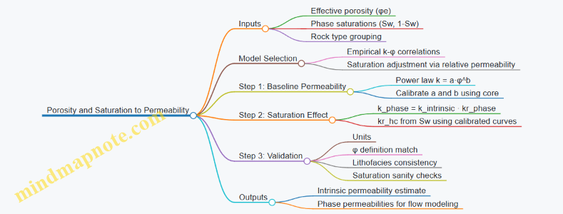
A Compact Worked Example from Logs to Flow Inputs
Assume you have log-derived φe = 0.20 and Sw = 0.30 for a sandstone interval. From core calibration, use k = 0.5·φ^4.0, giving k_intrinsic ≈ 0.5·(0.20)^4 = 0.5·0.0016 = 0.0008. If the relative permeability model at Sw = 0.30 yields kr_hc = 0.35, then k_hc ≈ 0.0008·0.35 = 0.00028. This pair (k_intrinsic, k_hc) can then feed reservoir simulation or completion productivity calculations, with the understanding that the saturation step is only as reliable as the saturation and relative permeability calibration.
The practical takeaway is simple: porosity gives you the “how much pore space,” saturation tells you “how much of that space actually carries the phase,” and the model decides how those two statements become permeability.
6.2 Capillary Pressure and Relative Permeability Inputs for Flow Modeling
Flow modeling needs two linked ideas: how pressure drives fluids through pore space (capillary pressure) and how easily each phase moves at a given saturation (relative permeability). Treat them as a pair, not separate ingredients—if your capillary pressure curve implies a certain saturation distribution, your relative permeability curves must be consistent with that same saturation scale.
Foundational Definitions and Why They Matter
Capillary pressure, \(P_c\), is the pressure difference between non-wetting and wetting phases: \(P_c = P_{nw} - P_w\). In most reservoir rocks, \(P_c\) decreases as wetting-phase saturation increases. That shape matters because it controls how fluids partition between phases during drainage or imbibition.
Relative permeability, \(k_{rw}\) and \(k_{r,nw}\), scales each phase’s mobility relative to single-phase flow. In practice, you use \(k_r(S_w)\) curves to compute phase flow rates in a multiphase simulator.
A common modeling pitfall is mixing saturation conventions. Some datasets use \(S_w\) measured from cores directly; others use effective saturation after irreducible and residual endpoints are applied. Decide which saturation variable your simulator expects, then map every curve to that same definition.
Building Capillary Pressure Curves Systematically
Start with a drainage/imbibition context. Drainage typically corresponds to displacing wetting by non-wetting (e.g., water displaced by oil or gas). Imbibition corresponds to the reverse. Capillary pressure curves differ between these paths because pore filling and trapping are hysteretic.
- Choose endpoints: \(S_{w,i}\) (initial wetting saturation), \(S_{w,ir}\) (irreducible wetting), and \(S_{w,res}\) (residual wetting). These endpoints anchor the saturation axis.
- Convert to effective saturation: \(S_{we} = (S_w - S_{w,ir})/(1 - S_{w,ir} - S_{w,res})\). This makes curves comparable across rocks and reduces sensitivity to endpoint uncertainty.
- Fit a functional form: Use a smooth model that respects monotonic behavior and endpoint limits. The goal is not artistic curve fitting; it is stable numerical behavior and correct saturation mapping.
- Apply hysteresis rules: If your reservoir experiences both drainage and imbibition, include a hysteresis model so trapped non-wetting saturation is represented. Without it, you can get the right average saturations and the wrong production response.
Relative Permeability Curves That Match the Capillary Story
Relative permeability depends on saturation and often on the same endpoints used in capillary pressure. A consistent workflow looks like this:
- Select saturation variable: Use the same \(S_w\) or \(S_{we}\) definition as the capillary pressure curve.
- Ensure endpoint consistency: \(k_{rw}=1\) at full wetting saturation (or at the simulator’s reference), and \(k_{r,nw}=1\) at full non-wetting saturation. At irreducible endpoints, the corresponding phase mobility should approach zero.
- Match curvature to expected flow regime: Steeper rises in \(k_r\) with saturation imply faster mobility gain and can increase early production rates. Flatter curves can delay breakthrough.
- Check against fractional flow behavior: Fractional flow \(f_w = \frac{\lambda_w}{\lambda_w+\lambda_{nw}}\) uses mobilities \(\lambda = k_r/\mu\). If your \(k_r\) curves produce unrealistic fractional flow at key saturations, the simulator will compensate elsewhere, often by creating odd pressure gradients.
Integrated Example Workflow
Assume you have core data for drainage capillary pressure and relative permeability for oil-water flow.
- Measured endpoints: \(S_{w,ir}=0.25\), \(S_{w,res}=0.05\).
- Simulator expects effective saturation \(S_{we}\).
- You convert each measured point using \(S_{we}\) and fit \(P_c(S_{we})\) for drainage.
- For relative permeability, you fit \(k_{rw}(S_{we})\) and \(k_{ro}(S_{we})\) so that \(k_{rw}\to 0\) near \(S_{we}=0\) and \(k_{ro}\to 0\) near \(S_{we}=1\) (with the correct phase mapping).
Now do a quick sanity check using a representative viscosity ratio. If water viscosity is half oil viscosity, then at mid saturations the water fractional flow should not exceed what your \(k_r\) curves allow. If it does, you likely mis-assigned which endpoint corresponds to irreducible water versus residual water.
Mind Map: Capillary Pressure and Relative Permeability Inputs
Practical Consistency Checks Before Running the Model
- Saturation axis audit: Confirm that capillary pressure and both relative permeability curves use the same \(S_w\) or \(S_{we}\) definition.
- Phase labeling audit: Verify which phase is wetting in your simulator and in your lab data.
- Endpoint audit: Ensure irreducible and residual saturations match across all curves.
- Numerical stability audit: Smooth fits should avoid sharp kinks that can cause oscillations in multiphase solvers.
When these checks pass, capillary pressure and relative permeability stop being “two curves” and start acting like a coherent description of how fluids share pore space and how that sharing translates into flow.
6.3 Flow Unit Concepts and How to Delineate Them Using Logs
A flow unit is a repeatable package of reservoir rock that tends to behave similarly during flow. The key idea is not just “good porosity” or “good permeability,” but a consistent combination of pore geometry, pore throat size, and wettability-related behavior that controls how fluids move. When you delineate flow units from logs, you’re building a practical map from measurable log responses to the flow behavior you care about.
What Controls Flow Unit Behavior
Flow behavior is dominated by how easily fluids pass through pore throats and how that ease changes with saturation. In practice, three log-linked themes show up repeatedly:
- Pore size distribution proxy: Grain size, sorting, and cementation influence pore throat sizes. Logs that respond to lithology and texture help here.
- Connectivity proxy: Permeability depends on whether pores connect across the rock. Net-to-gross, facies, and effective porosity trends often track this.
- Capillary entry proxy: The pressure needed to move non-wetting fluids relates to pore throat size. Even when you don’t compute capillary pressure directly, log-derived facies and saturation patterns can guide the interpretation.
A useful mental model: two intervals can have the same porosity, but different pore throat distributions. The one with larger and more connected throats usually shows better flow under the same conditions. Your job is to separate those intervals using log signals that correlate with pore throat and connectivity.
Stepwise Workflow from Logs to Flow Units
Step 1: Build a log-driven facies framework. Start with lithology and depositional layering because flow units often align with rock type. Use a consistent suite such as gamma ray, resistivity, density-neutron, and sonic. Convert raw curves into interpretable attributes: shale volume proxy, effective porosity proxy, and a cleaned resistivity trend.
Step 2: Define “effective” reservoir intervals. Exclude intervals that are too shaly or too tight to contribute meaningfully. A simple rule is to apply cutoffs to shale volume and effective porosity, then check that the remaining intervals show coherent resistivity behavior.
Step 3: Create log-derived permeability and flow-relevant proxies. Instead of trying to predict absolute permeability perfectly, build relative indicators that separate pore throat and connectivity effects. Common choices include:
- Effective porosity trends from density-neutron with shale correction.
- Resistivity-based saturation indicators to infer how easily fluids move through pore throats at the current saturation.
- Sonic or density texture proxies that often track cementation and grain packing.
Step 4: Use cross-plot logic to cluster intervals. Take your log-derived proxies and group intervals that behave similarly. A typical approach is to cross-plot effective porosity versus a resistivity-derived saturation proxy, then color points by lithofacies or by a texture proxy. Clusters in this space often correspond to distinct flow units.
Step 5: Tie clusters to vertical layering. Flow units are usually layered. After clustering, map the cluster labels back onto the stratigraphic sequence. If a cluster appears in multiple separated layers with similar log signatures, it’s a strong candidate for a repeatable flow unit.
Step 6: Validate with available measurements. Use core-derived permeability, pressure tests, or production logs if available. Validation doesn’t require perfect agreement; it requires that the ranking of flow quality matches the measurements. If the ranking is reversed, revisit cutoffs, corrections, or the proxies used for clustering.
Mind Map: Log-Based Flow Unit Delineation
Example: Turning Log Curves into Flow Unit Labels
Assume you have a cored interval and a consistent log suite. You compute an effective porosity proxy and a saturation proxy from resistivity. On a cross-plot of effective porosity versus saturation proxy, you observe three point clouds:
- Cluster A: Moderate porosity, relatively higher saturation proxy values, and lower sonic quality. These intervals likely have smaller pore throats and more cementation, so they flow less easily.
- Cluster B: Higher porosity, intermediate saturation proxy, and relatively stable sonic. This cluster tends to represent better connectivity.
- Cluster C: High porosity and the most favorable saturation proxy, with texture consistent with cleaner rock. This is your best candidate for the highest flow quality.
Next, you map A, B, and C back onto the well log. If the clusters align with distinct stratigraphic layers and repeat laterally across nearby wells, you can define three flow units. For completion planning, you then prioritize perforations in the best-flow unit while still using the other units for pressure support or staged development, depending on the reservoir’s fluid distribution.
Practical Checks That Prevent Common Mistakes
- Don’t cluster on one curve. A single log can reflect multiple rock properties. Using at least one lithology/texture proxy plus one fluid or saturation proxy reduces ambiguity.
- Watch for shale correction artifacts. If your effective porosity proxy swings sharply where shale volume changes, you may be clustering correction behavior rather than rock behavior.
- Confirm vertical consistency. If a flow unit label appears as scattered single-thickness spikes, it may be a noise artifact. Flow units should show stratigraphic coherence.
When done carefully, log-based flow unit delineation becomes a disciplined translation: from measured curves to pore-throat-and-connectivity groupings that you can use to choose perforation intervals and interpret production behavior interval by interval.
6.4 Cross Plot Diagnostics and Quality Screening of Petrophysical Results
Cross plots are where petrophysical numbers stop being a neat spreadsheet and start behaving like measurements. The goal is simple: check whether porosity, saturation, and lithology indicators agree with each other and with the rock physics assumptions used to compute them. When they don’t, you want to know why—before the completion design pays the price.
Foundations for Cross Plot Logic
Start with the variables you expect to correlate. For example, in a clean carbonate or sandstone, effective porosity often trends with resistivity and with density-neutron separation. If your computed water saturation is reasonable, it should show a consistent relationship with resistivity and with porosity quality.
A practical screening mindset helps:
- First check units and depth alignment: cross plots are only as good as the depth matching between logs, calibrations, and any derived curves.
- Then check environmental corrections: bad borehole corrections can create “perfect” correlations that are actually artifacts.
- Finally check physical plausibility: the trends should match the rock type you think you have.
Core Cross Plots and What They Diagnose
Use cross plots as diagnostic tests rather than as decoration.
Porosity Versus Resistivity
Plot effective porosity (φe) on one axis and formation resistivity (Rt or Rxo) on the other. In hydrocarbon-bearing zones, resistivity typically increases as water saturation decreases, and porosity quality often influences the slope.
Example: Suppose φe is computed from density and neutron after shale volume correction. If the cross plot shows two distinct resistivity bands at similar φe, that often indicates either (1) different fluid saturations, (2) different lithology or cementation, or (3) a systematic correction problem that differs by interval.
Porosity Versus Water Saturation
Plot φe versus Sw from your saturation model. A physically consistent dataset should show Sw decreasing as resistivity increases, but the relationship should not be random.
Example: If Sw clusters around a narrow range across a wide resistivity spread, the saturation model may be dominated by an assumed parameter (like cementation exponent or saturation exponent) rather than by the measured resistivity.
Density-Neutron Separation Versus Shale Volume
Plot ΔρN (density-neutron separation) versus Vsh. This helps confirm whether your shale indicator is behaving as expected.
Example: If ΔρN increases while Vsh decreases, you may be seeing gas effects, tool response issues, or an incorrect lithology classification. The point is not to guess immediately; it’s to identify which assumption is inconsistent.
Quality Screening Rules That Catch Common Failures
Apply screening rules in a consistent order.
- Trend coherence: does the main trend look monotonic where you expect it to be?
- Cluster separation: do points form meaningful groups by facies or by identified intervals?
- Outlier behavior: are outliers isolated spikes or systematic bands?
- Parameter sensitivity: do small changes in inputs move points across the expected trend?
Example: If outliers occur only where borehole rugosity is high, the likely culprit is imperfect borehole correction. If outliers occur only where Vsh is high, the saturation model may be using a shale parameter that doesn’t match the actual shale behavior.
Mind Map: Cross Plot Workflow
Systematic Example Workflow
Assume you have three log-derived curves: φe, Sw, and Vsh, plus Rt. You suspect the saturation model may be misbehaving in a particular interval.
- Segment by lithology: split the cross plots into at least two facies groups using your existing classification.
- Plot φe vs Rt: confirm that each facies group has a coherent trend.
- Plot φe vs Sw: check whether Sw decreases with increasing Rt within each facies group.
- Plot ΔρN vs Vsh: verify that shale behavior matches the classification.
- Interpret the mismatch:
- If φe vs Rt is coherent but φe vs Sw is not, the saturation model parameters or exponents likely need adjustment.
- If φe vs Rt is incoherent, focus on corrections or porosity computation.
- If ΔρN vs Vsh contradicts the facies split, the lithology classification is likely mixing responses.
Practical Decision Criteria
Quality screening is complete when cross plots agree with each other in a way that supports your modeling assumptions. If you can’t get coherence across the key plots without changing assumptions, treat the derived petrophysical results as conditional and revisit the specific step that breaks consistency. In other words: don’t just “accept” the curves because they look smooth; accept them only when the relationships between variables behave like the rock you measured.
6.5 Practical Example Workflow for Building a Flow Unit Based Completion Map
A flow unit based completion map is a practical way to translate petrophysical results into where you perforate, how you group perforations, and what you expect each interval to contribute. The core idea is simple: instead of treating the reservoir as one uniform target, you partition it into flow units that behave similarly under flow.
Step 1: Define the Flow Unit Inputs
Start with the log-derived properties that control flow behavior. A typical minimum set is porosity, water saturation, and a permeability proxy (from a model or cross-plot). Add capillary pressure or relative permeability inputs only if you have them reliably; otherwise, focus on the log-based partitioning.
Example workflow inputs:
- Porosity from a calibrated density-neutron combination.
- Water saturation from a validated resistivity model with environmental corrections.
- Permeability proxy from a permeability model or a log cross-plot using core or well tests.
Quality gate: if porosity and saturation disagree strongly with core or production trends, fix the petrophysics before building flow units. A completion map built on shaky inputs will look neat and still perform poorly.
Step 2: Build Flow Unit Classes Using Cross Plots
Flow units are commonly separated using combinations of permeability proxy and saturation or permeability proxy and porosity. Use cross plots to see natural clusters.
Example classification approach:
- X-axis: permeability proxy (log scale).
- Y-axis: effective water saturation or net-to-gross proxy.
- Identify clusters that correspond to distinct flow behavior.
Then assign each cluster a flow unit label, such as FU-A, FU-B, FU-C. Keep the number of classes manageable; three to five is usually enough to drive completion decisions without turning the map into a taxonomy project.
Step 3: Convert Interval Picks into a Spatial Map
A completion map needs geometry. Convert each well’s flow unit picks into a consistent stratigraphic framework.
Practical steps:
- Pick top and base of the reservoir interval in each well.
- Tie picks to a common datum using time or depth conversion consistent with your interpretation.
- Interpolate flow unit properties between wells using a method aligned with your reservoir layering.
Example: If the reservoir is layered, use a stratigraphic interpolation that honors layering rather than a purely distance-based interpolation. This prevents mixing flow units across boundaries that are geologically meaningful.
Step 4: Create a Completion-Relevant Metric
Perforation decisions should not be based on flow unit labels alone. Build a completion metric that combines:
- Net pay thickness within each flow unit.
- Expected productivity contribution using permeability proxy and saturation.
- Practical constraints such as minimum perforation interval length and mechanical limits.
Example metric definition:
- Score = (Net pay thickness) × (normalized permeability proxy) × (1 − normalized water saturation).
Normalize each component within the reservoir so one term does not dominate purely due to units or scale.
Step 5: Translate the Metric into Perforation Zoning
Now convert the map into zones that can be executed.
Example zoning logic:
- Zone 1: Highest score flow unit areas with consistent thickness.
- Zone 2: Moderate score areas where thickness is adequate but saturation is higher.
- Zone 3: Low score areas where you either avoid perforating or perforate minimally for pressure support.
Keep zoning consistent with wellbore trajectory. If a well crosses multiple flow units, define how many clusters per well and how to distribute them along the trajectory.
Step 6: Validate with Well-Level Checks
Before finalizing, run checks that catch common mistakes.
Validation checks:
- Thickness check: does the mapped flow unit thickness match log-derived thickness at each well?
- Continuity check: do adjacent wells show consistent flow unit transitions?
- Production check: if you have offset wells, does the best-performing interval align with the highest-score flow unit?
If validation fails, adjust the stratigraphic tie or revisit the flow unit classification thresholds.
Mind Map: Flow Unit Based Completion Map Workflow
Example: From Logs to a Two-Zone Completion Decision
Assume two flow units appear in the reservoir: FU-A and FU-B.
- FU-A: higher permeability proxy and lower effective water saturation.
- FU-B: moderate permeability proxy and higher effective water saturation.
At Well 1, FU-A thickness is 18 m and FU-B thickness is 6 m. At Well 2, FU-A thickness is 10 m and FU-B thickness is 14 m.
Completion decision:
- Well 1: perforate primarily in FU-A with a small FU-B contribution only if mechanical constraints require coverage.
- Well 2: perforate mostly in FU-A but include a controlled FU-B segment to maintain reservoir contact where FU-A is thinner.
The map supports this by showing that FU-A is laterally continuous in the area of Well 1 but becomes compartmentalized near Well 2. The zoning is therefore not just “best everywhere,” it is “best where it exists.”
Step 7: Document Assumptions and Lock the Map
A completion map should be reproducible. Record:
- Flow unit classification thresholds.
- Interpolation method and stratigraphic datum.
- Metric formula and normalization approach.
- Zoning rules that convert score to perforation intervals.
This documentation matters because the next well will reuse the workflow, and the team will need to know exactly why FU-A became the main target in one area and a supporting target in another.
7. Drilling Fluids and Hydraulic Design for Wellbore Performance
7.1 Fluid Selection Criteria Including Compatibility and Rheology Requirements
Fluid selection is where drilling plans meet reality: the wrong fluid can cause stuck pipe, poor cuttings transport, unstable wellbore walls, or cement placement problems. A good selection starts with compatibility—chemical and physical—and then locks in rheology so the fluid behaves correctly across the actual pressure, temperature, and shear conditions downhole.
Start with Compatibility Requirements
Compatibility means the fluid does not create new problems when it contacts formation rock, existing fluids, and cement. Treat it like a checklist with measurable outcomes.
- Formation interaction: If the formation contains clays, the fluid must limit clay swelling and dispersion. A practical sign is whether the mud maintains viscosity and solids behavior after exposure to representative cuttings.
- Hydrocarbon and water compatibility: If the well will later encounter oil or gas-bearing zones, the fluid should avoid excessive emulsion formation that can complicate logging and completion operations.
- Cement compatibility: Cement needs predictable rheology and placement. If the drilling fluid chemistry interferes with cement hydration or increases contamination risk, you will see poor bond quality or delayed set.
- Scale and corrosion control: Brines and produced-fluid chemistry can drive scale. Corrosion inhibitors must be compatible with the mud system so they don’t get “spent” early.
Example: Suppose you’re drilling through a shale interval known for swelling. You choose a base fluid and additives, then run a simple jar test: mix representative shale with the candidate fluid at downhole temperature, agitate, and observe dispersion and viscosity change. If the shale sloughs quickly or the fluid thickens unpredictably, the chemistry is not compatible.
Define Rheology in Operational Terms
Rheology is not just a lab number; it’s how the fluid transports cuttings, controls ECD, and maintains stability under changing shear rates.
Key rheology targets:
- Viscosity at low shear: Helps suspend cuttings when circulation slows or stops.
- Shear-thinning behavior: Many drilling fluids are designed to reduce viscosity under high shear near the bit and increase it when shear drops in the annulus.
- Yield stress: Prevents settling of solids during static periods.
- Gel strengths: Controls how quickly the fluid rebuilds structure after pumps stop, which affects surge and swab behavior.
Example: During a connection, pumps stop for 10–20 minutes. If gel strength is too high, you may get excessive pressure surges when circulation resumes. If it’s too low, cuttings can settle, increasing the risk of differential sticking and poor hole cleaning.
Match Rheology to the Well’s Hydraulic Reality
Rheology must be consistent with the planned hydraulics: annular geometry, flow rate, pipe rotation, and expected solids loading.
A systematic approach:
- Set the circulation regime: Determine target flow rates for hole cleaning and ECD limits.
- Estimate shear rates: Use annular velocity and pipe rotation to understand where the fluid experiences high shear.
- Plan for solids increase: As cuttings and barite concentration change, rheology shifts. Build a “mud aging” expectation into the design.
- Check ECD sensitivity: Confirm that rheology changes do not push ECD outside the safe mud window.
Example: If you plan to reduce flow rate to manage ECD, you must verify that the fluid still meets hole-cleaning needs at the lower shear conditions. A fluid that performs well at high flow can fail when flow drops because yield stress and gel behavior dominate.
Use Compatibility and Rheology Together in a Single Decision Loop
Compatibility affects rheology, and rheology affects compatibility outcomes. For instance, clay inhibition can change viscosity response, and solids control can change chemical effectiveness.
A practical decision loop:
- Screen chemistry with compatibility tests (jar tests, contamination sensitivity, cement contact checks).
- Measure rheology at representative temperature and shear conditions.
- Stress test under contamination: simulate dilution, formation water entry, or lost circulation materials.
- Validate with hydraulics: confirm hole cleaning, pressure losses, and ECD behavior.
Example: A fluid passes a clay inhibition jar test but fails hydraulics because it becomes too viscous after solids loading. The fix might be adjusting weighting strategy, selecting a different viscosifier, or improving solids control—not abandoning the chemistry outright.
Mind Map: Fluid Selection Criteria
Example: Comparing Two Candidate Mud Systems
- System A: Strong clay inhibition but high gel strengths after contamination.
- System B: Moderate inhibition but stable rheology under solids loading.
If the well has frequent connections and tight ECD limits, System B may be safer operationally because it reduces pressure transients and maintains predictable hole cleaning. If the formation is highly reactive and the interval is short, System A might still win because it prevents rapid wall damage. The selection is therefore a trade study anchored to both compatibility outcomes and rheology behavior under the actual operating cycle.
Practical Acceptance Checks Before Spudding
Before drilling, confirm that the fluid meets measurable criteria:
- Rheology targets at planned temperature and flow rates.
- Gel strength and restart behavior consistent with connection procedures.
- Compatibility tests showing controlled clay response and acceptable contamination sensitivity.
- Cement contact checks indicating no unacceptable interference.
- Solids control expectations that keep rheology within the designed range.
When these checks align, the drilling fluid stops being a “recipe” and becomes a controlled system—one that keeps the wellbore stable and the cuttings moving, even when the day-to-day details get messy.
7.2 Solids Control and Cuttings Transport Management
Solids control is the part of drilling operations that keeps the wellbore stable, the hydraulics predictable, and the rig’s “mud system” from turning into a slow-motion sediment project. The goal is simple: remove drilled solids at the right rate, keep the remaining solids within the mud’s design limits, and transport cuttings so they don’t settle in the annulus.
Foundations: What Solids Do to the Mud System
Drilled solids enter the mud as cuttings and formation particles. Their size distribution matters because it controls viscosity, filtration behavior, and the effectiveness of the solids-removal equipment. Coarse particles settle quickly, increasing risk of stuck pipe and poor hole cleaning. Fine particles can raise viscosity and gel strength, making pumps work harder and increasing equivalent circulating density.
A practical way to think about solids control is by three outcomes:
- Hydraulics: Annular pressure loss and ECD rise when solids increase.
- Stability: Excess reactive fines can worsen shale swelling or weaken cement bonding.
- Operational reliability: Poor hole cleaning increases torque and drag, and can trigger differential sticking.
Solids Control Train: From Coarse Removal to Polishing
Most systems use a staged approach so each device handles the particle sizes it can remove efficiently.
- Primary separation removes large cuttings early.
- Secondary separation reduces the mid-size fraction.
- Polishing targets fines that slip through earlier stages.
A common rig flow is: shaker(s) → desander → desilter → degasser and/or centrifuge polishing (depending on mud type and solids loading). Each stage should be sized for the expected flow rate and solids concentration, not for an optimistic “average day.”
Shakers and Screen Selection
Shakers are the first line of defense. Screen type and mesh size determine what fraction is rejected. If the screen is too fine, it blinds and reduces throughput; if it’s too coarse, solids pass downstream and accumulate.
Example: If cuttings are mostly 200–600 microns, using a screen that rejects that range while maintaining flow prevents the desander from being overloaded. The rig may still run the same pump rate, but the mud’s viscosity stays closer to target because fines don’t build up.
Desanders and Desilters
Desanders handle larger sand than desilters. Their performance depends on feed rate, inlet geometry, and the density of the slurry. Overfeeding a desander reduces separation efficiency and sends more sand to the next stage.
Example: During a section change, if drilling rate increases and the mud system’s solids loading spikes, the desander may need a temporary feed adjustment or additional capacity to keep the sand fraction from climbing.
Centrifuges and Final Polishing
Centrifuges can remove fine solids that are hard to manage with cyclones alone. They are especially useful when the mud design is sensitive to fine particles.
Example: In a water-based mud where filtration control is critical, fine solids can raise filter cake thickness. A centrifuge polishing step can reduce the fine fraction so the filtration behavior returns toward baseline.
Cuttings Transport: Keeping the Annulus Clean
Solids control equipment removes solids at the surface, but hole cleaning determines whether solids stay suspended downhole. Transport is governed by flow rate, rheology, and annular geometry.
Key practices:
- Maintain target pump rates for the hole size and drillstring configuration.
- Control rheology so the mud carries cuttings without excessive pressure.
- Watch for changes in torque, drag, and standpipe pressure that can indicate settling.
Example: If the drillstring is pulled into a larger hole section, the annular velocity drops. Even with the same pump rate, cuttings may settle more easily. Adjusting pump rate or operating parameters helps restore transport.
Monitoring and Control: Turning Measurements into Actions
Solids management is not a “set it and forget it” task. It’s a feedback loop.
What to Track
- Mud density and solids content (to detect accumulation).
- Viscosity and gel strengths (to see how solids affect flow).
- Sand content and particle size distribution (to match removal stage performance).
- Shaker performance metrics like feed rate and screen blinding.
Simple Decision Rules
- If sand content rises, check shaker efficiency first, then desander feed and cyclone performance.
- If viscosity rises without a density jump, suspect fine solids or inadequate polishing.
- If hole cleaning symptoms appear, verify annular velocity and rheology before blaming the surface equipment.
Mind Map: Solids Control and Cuttings Transport Management
Example Workflow: From Rising Solids to Corrective Action
- Observe: Sand content trends upward over several hours.
- Check surface performance: Confirm shaker feed rate matches screen capacity and screens are not blinding.
- Inspect separation stages: Verify desander/desilter inlet conditions and that flow splits are correct.
- Confirm downhole transport: Review pump rate and rheology during the same interval to rule out settling.
- Correct: Adjust screen selection or feed rate, then re-balance mud properties using the measured solids response.
The best solids control systems behave like well-tuned plumbing: they remove what the mud system can’t carry, and they keep the rest moving so the wellbore stays clean and the drilling plan stays on track.
7.3 Hydraulic Calculations for Annular Pressure Loss and ECD Control
Hydraulic calculations translate pump rate and fluid properties into pressure losses along the wellbore. Those losses matter because they raise the effective pressure at the bit, which is what you manage when you control ECD. A good workflow starts simple, then adds realism: first compute annular pressure loss, then convert it into ECD, then check it against the mud window.
Foundational Quantities for Annular Pressure Loss
Annular pressure loss is the sum of frictional loss and any additional terms you include for fittings, cuttings loading, and elevation changes. For most drilling design work, the core pieces are:
- Flow rate: usually given as surface rate, then converted to downhole volumetric flow using formation temperature and pressure.
- Fluid properties: density (for hydrostatic), viscosity and rheology model (for friction), and solids concentration (for effective viscosity and density).
- Geometry: hole diameter, casing/liner ID, tool OD, and the annular clearance that controls velocity.
- Flow regime: laminar vs turbulent affects friction factor and pressure gradient.
A practical habit: keep a single “reference depth” for your calculations (often the bit depth) and compute everything consistently at that depth, including temperature and pressure assumptions.
Stepwise Calculation Workflow
-
Convert surface rate to downhole rate Use a volumetric correction for compressibility and thermal expansion. If you use a constant density approximation, document it and keep it consistent across the well plan.
-
Compute annular cross-sectional area and hydraulic diameter For a simple annulus, area is based on hole ID minus tool/casing OD. Hydraulic diameter helps when you use correlations that depend on characteristic length.
-
Compute average annular velocity Velocity is downhole flow divided by annular area. This is the driver for friction.
-
Select a friction model
- For Newtonian fluids, friction factor can be based on Reynolds number.
- For drilling muds, use an appropriate rheology model (commonly power-law or Bingham plastic) and compute an effective Reynolds number.
-
Compute frictional pressure gradient Multiply frictional gradient by measured depth increment or integrate along the interval. If you have multiple sections with different annulus geometry, treat each section separately.
-
Add hydrostatic pressure Hydrostatic pressure at depth is fluid density times true vertical depth (or measured depth with inclination correction, depending on your convention). The key is that ECD uses the effective pressure at the bit.
-
Compute ECD A common form is:
- ECD = (Hydrostatic pressure + frictional pressure) / TVD expressed as an equivalent mud weight.
-
Check against the mud window Compare ECD to the fracture pressure limit and ensure you have margin for uncertainties in temperature, rheology, and solids.
Mind Map: Hydraulic Pressure Loss and ECD Control
Example: Quick Annular Pressure Loss and ECD Estimate
Assume a vertical well section at TVD = 3000 m. Hole diameter is 12.25 in, tool OD is 6.75 in, and casing is not present in this interval. Mud density is 1.20 sg (≈ 1200 kg/m³). Pump rate at surface is 600 gal/min, and you approximate downhole volumetric flow as 600 gal/min for a first estimate. Use a friction model that yields an average frictional pressure gradient of 0.35 bar/m over the interval.
-
Hydrostatic pressure Convert density to pressure gradient: 1.20 sg corresponds to about 11.8 kPa/m (since ρg ≈ 1200×9.81 ≈ 11.8 kPa/m). Hydrostatic at 3000 m is:
- 11.8 kPa/m × 3000 m = 35.4 MPa.
-
Frictional pressure
- 0.35 bar/m × 3000 m = 1050 bar = 105 MPa.
-
Total effective pressure at bit
- 35.4 MPa + 105 MPa = 140.4 MPa.
-
Convert to ECD Equivalent density is total pressure divided by (g×TVD):
- 140.4×10^6 Pa / (9.81×3000 m) ≈ 4770 kg/m³. That is ~4.8 sg, which is clearly unrealistic for typical drilling fluids—so the friction gradient assumption is too high for this quick example. The point of the exercise is not the number; it’s the sanity check.
A more realistic friction gradient for many cases might be closer to 0.01–0.05 bar/m depending on rate and annulus. If we use 0.02 bar/m instead:
- Friction = 0.02×3000 = 60 bar = 6 MPa.
- Total = 35.4 + 6 = 41.4 MPa.
- ECD density ≈ 41.4×10^6 /(9.81×3000) ≈ 1410 kg/m³ → ~1.41 sg.
Now the result is in the realm of plausible ECD increases. This is why you always run a “does this look sane?” check before trusting the calculation.
Example: Sensitivity to Pump Rate and Viscosity
If you double pump rate while geometry and fluid density stay constant, annular velocity roughly doubles. In turbulent conditions, frictional pressure loss often increases more than linearly with velocity because friction factor changes with Reynolds number. In laminar or near-laminar regimes, friction can scale more directly with viscosity and velocity.
A practical control strategy follows from that:
- If ECD is too high, first check whether viscosity or solids are elevated (which increases friction even at the same rate).
- If viscosity is normal, reducing pump rate usually provides the most immediate ECD reduction.
Common Pitfalls and How to Avoid Them
- Mixing measured depth and true vertical depth in the ECD conversion. Pick one convention and apply it consistently.
- Using surface rheology without temperature correction. Mud viscosity often changes with temperature, especially deeper in the well.
- Ignoring annulus changes across tool joints, stabilizers, or casing transitions. Treat each interval with its own geometry.
- Assuming friction gradient is constant when it isn’t. Integrate or segment the well where geometry and flow conditions change.
When these steps are done carefully, annular pressure loss becomes a controlled engineering input rather than a mysterious number that shows up in the ECD plot and ruins your day.
7.4 Lubrication and Friction Reduction for Directional Drilling Efficiency
Directional drilling efficiency is often limited by friction between the drillstring and the wellbore. That friction shows up as higher hook loads, slower penetration, stuck-pipe risk, and extra wear on tools. Lubrication is the practical lever you control to reduce that friction while keeping wellbore stability and hydraulics in balance.
Foundations of Friction in Directional Wells
Friction is not one single effect; it is the sum of contact mechanics and fluid effects. In a curved well, the drillstring presses against the high side, creating normal force. Higher normal force increases friction, which then increases required torque and can worsen stick-slip. A useful mental model is: normal force comes from geometry and weight-on-bit, while the coefficient of friction depends on contact conditions and the lubricating film.
A simple field example: if you keep WOB constant but increase dogleg severity, the contact normal force rises because the string must follow a tighter curve. Even with the same mud, friction typically increases because the contact area and local shear conditions change.
Lubrication Mechanisms That Actually Matter
Lubrication reduces friction by changing what the drillstring “sees” at the contact point.
- Boundary lubrication forms a thin film that prevents metal-to-rock contact. This is most important when the film is thin or when contact pressure is high.
- Viscosity and hydrodynamic effects help when there is enough fluid separation between surfaces. In many directional wells, the separation is limited, so boundary lubrication often dominates.
- Surface conditioning reduces adhesion and helps the film stay intact. In practice, this means controlling solids and managing how additives interact with the rock and cuttings.
A practical example: if you switch from a clean, low-solids system to one with higher barite/formation solids, you may lose lubricity even if the same lubricant concentration is maintained. The solids can disrupt the film and increase abrasive contact.
Selecting Lubrication Strategy by Well Conditions
Choose a lubrication approach based on the dominant friction driver.
- High curvature and tight build sections: prioritize boundary lubrication and friction modifiers that remain effective under high contact pressure.
- Long horizontal sections: focus on maintaining film stability over time, which depends on solids control and consistent additive dosing.
- Reactive formations and cuttings beds: emphasize surface conditioning and solids management to prevent abrasive contact.
A straightforward example workflow: start with baseline mud properties and a known lubricity additive. During the first survey interval, compare torque trends and differential pressure behavior. If torque rises while flow and RPM remain stable, friction is likely increasing due to contact conditions, not hydraulics.
Operational Controls That Prevent Friction from Winning
Lubrication additives help, but operational choices determine whether they work.
- Maintain consistent additive concentration: dosing errors and mixing delays can create “lubrication gaps.” Verify mixing order and monitor treating rates.
- Control solids and cuttings transport: poor hole cleaning increases the cuttings bed, which increases abrasive contact and can trap the string.
- Manage ECD and annular pressure: excessive ECD can worsen stability and increase contact, indirectly raising friction.
- Avoid unnecessary RPM and torque spikes: stick-slip can increase wear and momentary friction coefficients.
Example: if you observe repeated torque spikes during a slide, check whether hole cleaning is adequate before increasing lubricant concentration. If the cuttings bed is the root cause, extra lubricant may not fix the mechanical contact.
Measuring Lubrication Effectiveness in the Field
You need evidence, not just good intentions.
- Trend torque and drag: compare torque at similar RPM and WOB across comparable intervals.
- Monitor differential pressure and flow regime: sudden changes can indicate hole cleaning issues.
- Use lab lubricity tests when available: confirm that the additive performs with your specific mud formulation and solids level.
A practical example: if torque decreases after a treating change but differential pressure rises, you may have improved boundary lubrication while also increasing solids or viscosity. The net effect could still be positive for drag, but you should understand the trade.
Mind Map: Lubrication and Friction Reduction
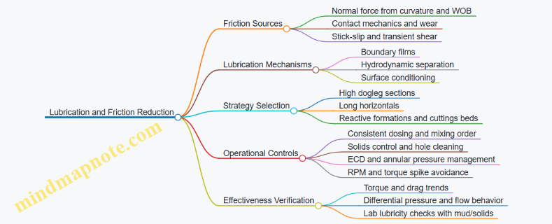
Example: A Systematic Lubrication Adjustment
Assume a directional well shows rising torque during a build section while penetration rate slows.
- Confirm operating comparability: ensure RPM, WOB, and flow rate are comparable to prior intervals.
- Check hole cleaning indicators: look for rising annular pressure or signs of cuttings accumulation.
- Evaluate solids trend: if solids increased, address solids control first.
- Apply targeted lubrication: adjust lubricity additive concentration and verify mixing order and treating rate.
- Reassess within the next interval: if torque stabilizes or drops without adverse pressure behavior, the lubrication change is likely effective.
The key is sequencing: fix mechanical contributors like hole cleaning and solids, then tune lubrication to reduce the remaining friction coefficient.
Practical Checklist for Directional Efficiency
- Verify mud lubricity additive concentration and mixing order.
- Keep solids low enough to avoid abrasive contact and film disruption.
- Maintain hole cleaning with appropriate flow and circulation strategy.
- Track torque, drag, and differential pressure trends interval by interval.
- Adjust lubrication based on observed friction behavior, not only on mud recipe.
When lubrication and operations are aligned, friction becomes a controllable constraint rather than a surprise bill you pay in torque, wear, and time.
7.5 Practical Example Workflow for Designing a Mud Program for Stability
A stable wellbore is mostly a math problem with a few practical constraints. The goal is to keep the effective mud pressure inside the “safe window” where the formation neither collapses nor fractures. In practice, you build that window from pore pressure, fracture pressure, and rock strength, then choose mud properties and operating limits that keep you inside it while accounting for hydraulics and temperature.
Step 1: Define the Stability Window from Formation Inputs
Start with three pressures at each depth interval: pore pressure (Pp), minimum horizontal stress (Shmin), and fracture pressure (Pf). If you have a log-derived Shmin, use it; if not, estimate Shmin from regional stress and calibrate with any observed breakouts or drilling-induced fractures.
Example: At 2,400 m, assume Pp = 28.0 MPa and Shmin = 34.0 MPa. A common stability target is to keep effective mud pressure (Pm,eff = Pm − Pp) below the rock’s failure threshold for shear failure, while staying above the threshold for preventing collapse. A practical “safe window” might be 1.0 to 4.0 MPa effective overbalance for that interval.
Step 2: Convert Window into Mud Weight Limits with Hydraulics
Mud weight alone is not the whole story because annular pressure loss increases bottomhole pressure. Use a hydraulic model to compute equivalent circulating density (ECD):
- ECD = static mud weight pressure + annular friction + any additional effects from cuttings loading
- Bottomhole pressure during circulation = hydrostatic + friction
Example: If the static mud weight corresponding to the upper safe limit is 1.20 SG, but your friction adds 0.10 SG equivalent, then the allowable surface mud weight must be reduced so that ECD stays within the window.
Step 3: Choose Base Fluid and Solids Strategy
Pick a base fluid that matches formation sensitivity and operational needs. Then decide solids content and particle size distribution so the filter cake is thin, strong, and not overly permeable.
Example workflow:
- If the formation is shale-prone, favor inhibition (e.g., KCl-based systems or polymer-inhibited brines) and keep solids low.
- If the formation is sandstone with reactive clays, use a controlled polymer system and avoid excessive reactive fines.
- For directional drilling, prioritize lubricity and friction control without letting solids rise.
A good rule of thumb is to target a filter cake that forms quickly during circulation and is resilient during pressure fluctuations. That means you control both chemistry and solids.
Step 4: Build the Mud Property Set and Check Compatibility
A mud program is a set of coupled properties: density, viscosity, gel strengths, filtration behavior, and inhibition level. You also need compatibility with cementing plans and any planned casing setting depths.
Example property targets for the 2,400 m interval:
- Density: choose a surface value that keeps ECD within the safe window at planned flow rate
- Plastic viscosity: enough to suspend cuttings during low flow, not so high that friction spikes
- Gel strengths: strong enough to prevent settling when pumps stop, not so strong that you create large pressure surges
- Filtration: aim for low, stable filtrate volume and a thin cake
Compatibility check: verify that the chosen inhibition and polymer system does not destabilize cement or interfere with planned displacement efficiency.
Step 5: Plan for Transients and Operational Limits
Stability failures often happen during changes: pump start/stop, rate changes, trips, and changes in ROP. Define operational limits tied to the stability window.
Example limits:
- Maximum flow rate so ECD does not exceed the upper bound
- Maximum allowable pump-off time so cuttings do not settle and create localized overbalance
- Trip speed limits to reduce pressure surges and avoid differential sticking
If you expect a narrow window, you may also reduce ROP to keep cuttings size and solids loading under control.
Step 6: Run a “What If” Calculation for the Most Likely Failure Modes
Use simple scenarios to test robustness.
- Scenario A: Pump rate increases by 20% → friction increases → ECD rises
- Scenario B: Solids increase due to higher ROP → filtration and cake quality degrade
- Scenario C: Temperature increases → viscosity and inhibition behavior shift
Example: If a 20% flow increase raises ECD by 0.05 SG equivalent, confirm that the resulting bottomhole pressure still stays below the fracture-related limit.
Step 7: Field Execution with Monitoring and Feedback Loops
Design the program so you can verify it while drilling. Monitoring should connect measurements to decisions.
Track:
- Density and rheology trends (to detect solids loading)
- Filtration proxy tests and inhibitor concentration checks
- ECD proxy indicators from pump data and standpipe pressure
- Shale response indicators such as torque/drag changes, cuttings condition, and cavings
Example feedback loop:
- If density rises faster than expected, reduce ROP and improve solids control rather than simply diluting
- If filtration increases, adjust bridging/filtration additives and verify solids size distribution
- If torque/drag rises, check lubricity and consider viscosity reduction within the stability constraints
Step 8: Document the Program as a Decision Table
A stability mud program should be actionable under time pressure. Use a decision table that links measurements to corrective actions.
| Observation | Likely Cause | Immediate Action | Stability Impact Check |
|---|---|---|---|
| Density rising | Solids loading | Reduce ROP, improve solids control | Recompute ECD |
| Standpipe pressure rising at same flow | Increased friction | Check hole condition, cuttings, viscosity | Verify ECD window |
| Cavings or torque spikes | Shale instability | Increase inhibition/filtration control | Confirm effective overbalance |
| Pump-off settling | Gel too weak | Raise gels or adjust sweep plan | Avoid localized collapse |
Mind Map: Mud Program Workflow for Stability
Example: Putting It Together for a 200 m Interval
Assume you drill from 2,350 m to 2,550 m with a planned flow rate that yields an ECD of 1.22 SG at the start. After 60 m, density rises and ECD proxy indicates 1.26 SG. You recompute bottomhole pressure and find you are approaching the upper effective overbalance limit. Corrective actions are: reduce ROP, tighten solids control, and adjust viscosity downward within the suspension requirement. After stabilization, ECD returns to 1.22–1.23 SG and cuttings condition improves, indicating the filter cake and inhibition are back in the intended operating range.
This workflow keeps the mud program grounded in measurable inputs, ties hydraulics to stability, and turns “stability” from a vague goal into a set of constraints you can actually operate within.
8. Casing Cementing and Well Integrity Verification
8.1 Casing Design Including Collapse Burst and Tensile Considerations
Casing design is the part of the well plan where “it should work” becomes “it will work under specific loads.” Collapse, burst, and tensile are the three load families that most directly govern whether a casing survives drilling, cementing, production, and any pressure or temperature swings. The trick is to treat them as interacting constraints rather than separate checkboxes.
Foundational Load Cases and What They Mean
Collapse is external pressure crushing the casing. Burst is internal pressure expanding it. Tensile is axial stretching from weight, temperature changes, and applied forces during running, cementing, and production.
A practical way to structure the design workflow is to list the governing phases:
- Running and landing: axial tension from casing weight and friction.
- Cementing: internal pressure from pumps and possible temperature rise.
- Production and shut-in: internal pressure plus thermal cycling.
- Depressurization or well control events: external pressure changes that can drive collapse.
Each phase has its own pressure and temperature profile, and each profile changes effective stresses through fluid densities, hydrostatic gradients, and frictional effects.
Collapse Design Including External Pressure and Buckling
Collapse resistance depends on casing geometry, material strength, and how the casing is supported. The basic inputs are:
- Outside diameter and wall thickness
- Steel grade and yield strength
- External pressure profile along depth
- Support conditions such as cement sheath quality and centralization
A common pitfall is using a single “worst” external pressure without checking where the casing is least supported. If cement coverage is poor or the casing is poorly centralized, the casing can behave like it is more freely supported, increasing the risk of collapse or buckling-like behavior.
Example: Suppose a casing section experiences a higher external pressure at a depth where cement bond is expected to be weak. Even if the average external pressure is within limits, the local effective support can be lower, so the collapse check should be performed with the appropriate support assumption for that interval.
Burst Design Including Internal Pressure and Safety Margins
Burst checks ensure the casing wall can withstand internal pressure without exceeding allowable hoop stress. Inputs include:
- Internal pressure during cementing or production
- Temperature effects on pressure and fluid properties
- Casing grade and wall thickness
Burst is often governed by short-duration events like cementing, where pump rates and surface pressures can create a transient internal pressure peak. The design should therefore consider the maximum credible internal pressure at the depth of interest, not just the steady-state production pressure.
Example: During cementing, if the planned pump schedule includes a high-rate stage to improve placement, the internal pressure peak may occur before the cement sets. A burst check that only uses final shut-in pressure can miss the peak hoop stress.
Tensile Design Including Weight, Temperature, and Running Loads
Tensile capacity must cover axial forces that try to pull the casing apart or exceed allowable axial stress. Major contributors are:
- Casing weight in the hole
- Friction during running, which can increase required hook load
- Temperature change between running conditions and operating conditions
- Any applied axial loads from packers, hangers, or wellhead systems
Temperature effects matter because steel expands or contracts. If the casing is constrained at the top by a hanger or packer, thermal strain turns into axial stress.
Example: If the casing is run at a cooler temperature and later heats up during production, the casing wants to expand. If the expansion is restrained, axial tensile stress increases. The tensile check should therefore use the correct temperature differential and the correct constraint condition.
Integrated Design Logic for Governing Checks
Collapse, burst, and tensile are not independent. For instance, a thicker wall improves collapse and burst resistance but increases weight, which raises tensile demand. A systematic approach is to:
- Define load cases for each well phase.
- Build pressure and temperature profiles.
- Apply casing support assumptions consistent with cementing and centralization.
- Run collapse, burst, and tensile checks.
- Identify the governing constraint and iterate on wall thickness, grade, or design geometry.
Mind Map: Casing Design Load Paths and Inputs
Example: Choosing the Governing Constraint Across Phases
Imagine three candidate casing designs for the same interval: Design A (thin wall), Design B (medium wall), and Design C (thick wall). During running, Design A may pass tensile but fail collapse in the interval with weaker cement support. Design C may pass collapse and burst comfortably but increases axial weight enough that tensile becomes the governing constraint during landing. Design B often ends up governing because it balances collapse resistance with manageable tensile demand.
The point is not that one design is always best; it is that the governing constraint can shift by phase and by depth. A correct design documents which phase and which interval controls each limit, so the final casing choice is defensible under the actual operating sequence.
8.2 Cement Slurry Design Including Additives and Placement Strategy
A cement job is a controlled chemical and mechanical process: you mix a slurry that can be pumped, place it so it contacts the right rock and casing surfaces, and then harden it into a seal that survives pressure and temperature. The design starts with what the cement must do, then works backward to what the slurry must be.
Cement Function Requirements
First define the performance targets in plain terms. Zonal isolation means the cement must develop sufficient compressive strength and low permeability. Wellbore integrity also depends on resisting fluid migration during the time cement is setting and after it sets. For directional wells, placement quality matters because deviations and ledges increase the risk of poor displacement and channeling.
A practical way to translate requirements into slurry parameters is to list: (1) target thickening time window, (2) pumpability limits for surface and downhole equipment, (3) expected bottomhole temperature and pressure, (4) maximum allowable ECD increase, and (5) strength and bonding needs at the casing shoe and across the interval.
Slurry Composition and Additive Roles
Cement slurry is typically built from base cement plus water and a set of additives. Each additive has a job description, and the best designs keep those descriptions from stepping on each other.
- Fluid loss control: Reduces filtrate invasion into the formation, helping maintain a stable slurry and reducing early permeability near the wellbore.
- Retarders: Slow hydration to keep the slurry workable long enough to reach the end of the interval and displace properly.
- Accelerators: Speed setting when the temperature is low or when a shorter waiting time is needed.
- Viscosity modifiers and dispersants: Improve pumpability and reduce flocculation so the slurry can carry cuttings and maintain uniformity.
- Density control: Achieved with weighting materials to match formation pressure needs and reduce influx risk.
- Gas migration control: Often uses anti-foaming and gas-handling strategies, especially where gas-cut mud is expected.
- Fluid loss and bonding aids: Some systems include components that support bonding and reduce shrinkage effects.
A useful mental model is to treat the slurry as three coupled systems: rheology (how it flows), filtration (how it interacts with rock), and hydration (how it hardens). Additives tune all three, so changing one often changes the others.
Thickening Time and Temperature Profile
Thickening time is not a single number pulled from a datasheet; it depends on the downhole temperature history and the slurry formulation. Use a temperature profile along the well path and compute thickening behavior at relevant depths. Then set the design window so that cement remains pumpable through displacement and reaches a minimum strength before the next operational step.
Example: If the interval requires 90 minutes of pumping and displacement time, and the bottomhole temperature is high enough to shorten hydration, you may need a retarder to keep thickening time comfortably beyond the operational window. If you overshoot, you risk delayed strength gain and extended waiting-on-cement.
Density, Rheology, and Pumpability Checks
Density is chosen to balance pressure safety and mechanical needs. Too light can underbalance formation pressure; too heavy can increase fracture risk and complicate placement. Rheology must support effective displacement without excessive friction or risk of settling.
A simple check is to ensure the slurry can be pumped at planned rates while maintaining stable viscosity and preventing excessive gel strength buildup before placement. In practice, engineers also verify that the slurry can suspend weighting material and any contaminants from the preceding mud.
Placement Strategy for Reliable Displacement
Placement is where good chemistry meets real hydraulics. The goal is to remove mud from the casing exterior and replace it with cement without leaving channels.
Key elements include:
- Casing centralization: Better centralization reduces eccentricity and improves annular flow paths. Even a well-designed slurry can underperform if the annulus is poorly swept.
- Preflush selection: Preflushes help condition the annulus by removing mud cake and improving cement contact. The choice depends on mud type and formation characteristics.
- Displacement fluid design: The spacer and displacement fluids must be compatible with both mud and cement to avoid contamination that changes thickening time and strength.
- Pumping rate and turbulence: Rates should be high enough to maintain effective annular cleaning but not so high that they cause excessive ECD or erosion.
- Cement volume and yield: Overestimating volume wastes material; underestimating risks underfilling and poor coverage. Yield calculations should include temperature effects and mixing tolerances.
Example: In a deviated section, a lower-than-planned displacement rate can reduce turbulence and allow mud remnants to persist. Those remnants become weak spots where cement bonding is reduced, even if the slurry itself would have been strong.
Contamination Control and Mixing Discipline
Cement is sensitive to contamination from drilling mud, spacer carryover, and improper mixing. Mixing discipline includes correct water-to-cement ratio, adequate mixing time, and consistent additive dosing.
A straightforward operational practice is to run a batch-by-batch verification: confirm slurry density, measure rheology, and check thickening behavior against the planned window. If results drift, the job plan should be adjusted before pumping continues.
Mind Map: Cement Slurry Design and Placement Strategy
Example: Integrated Design-to-Placement Workflow
Start with the interval and operational timeline. Compute a temperature profile and determine a thickening time target that exceeds the total pumping plus displacement time with a safety margin. Choose density to maintain pressure safety and select additives to achieve the required rheology and fluid loss control. Then design the preflush, spacer, and displacement fluids for compatibility with the specific mud system.
Finally, plan centralization and pumping rates to maintain annular cleaning in the worst-case deviation. Verify each batch before pumping by checking density, rheology, and thickening behavior. This closes the loop: the slurry chemistry is tuned for the placement hydraulics, and the placement plan is built to preserve the slurry’s intended performance.
8.3 Centralization and Annular Geometry Effects on Bond Quality
Cement bond quality is not just about slurry chemistry and placement volume. It is also about geometry: how the casing sits in the borehole and how the annulus behaves as cement flows, expands, and sets. Centralization controls that geometry, and annular shape controls how evenly cement contacts the casing and the formation.
Foundational Geometry Concepts That Drive Bond Quality
A casing string rarely sits perfectly centered. Even in a “good” hole, tool joints, stabilizers, and hole irregularities create eccentricity. When the casing is off-center, the annulus thickness varies around the circumference. Cement must fill the thinnest path first, but it can leave channels in the thicker regions if flow and displacement are not balanced.
Bond quality is typically judged by how continuous the cement sheath is and how well it adheres to both surfaces. Poor centralization often produces three repeatable bond problems:
- Thin annulus starvation: cement reaches the thin side quickly, then flow paths bypass the thick side.
- Debonded streaks: localized gaps form where cement did not fully displace mud.
- Uneven sheath thickness: even if cement volume is correct, distribution can be uneven.
A simple mental model helps: imagine pushing toothpaste into a ring-shaped gap. If the ring is thicker on one side, the paste will not magically spread uniformly unless the push and mixing conditions force it to.
Centralization Mechanisms and What They Change
Centralizers reduce eccentricity by forcing the casing toward the borehole centerline. Their effect depends on three practical variables: spacing, stiffness, and placement relative to key intervals.
- Spacing controls how long the casing can remain unsupported. Too wide a spacing allows the casing to “hang” against the low side.
- Stiffness controls how effectively the centralizer resists collapse under weight and mud buoyancy.
- Placement matters because bond risk is highest where hole conditions change: near casing shoes, in deviated sections, and across formations with variable hardness.
Centralizers also influence flow resistance. More centralizers can increase drag and alter displacement hydraulics, so the goal is not maximum hardware. The goal is controlled geometry that supports uniform cement placement.
Annular Geometry Effects During Placement
Annular geometry affects cement placement through hydraulics, displacement efficiency, and settling behavior.
- Hydraulics and flow regime: In eccentric annuli, the cement slurry and spacer can preferentially travel along the path of least resistance. This can reduce mud removal effectiveness in the thick side.
- Displacement efficiency: Mud removal depends on shear and contact. If the casing is pressed to one side, the opposite side may experience insufficient shear to clear mud.
- Settling and segregation: If cement is not well mixed or if the annulus is highly non-uniform, heavier solids can concentrate in thicker regions, leaving thinner regions with different effective properties.
A practical example: consider a 12.25 in hole with a 9.625 in casing. If eccentricity increases the thick-side annulus from 1.0 in to 2.0 in, the cement must cover twice the cross-sectional area while still displacing mud. Even with correct total cement volume, the thick side can remain under-displaced.
How Centralization Choices Show Up in Cement Bond Logs
When centralization is inadequate, cement bond logs often show patterns rather than random noise. Common indicators include:
- Circumferential variability: stronger bond where cement contact was better, weaker bond where channels formed.
- Depth-localized poor bond: intervals near where the casing likely de-centered due to hole shape changes.
- Streaky signatures: alternating good and poor bond around the circumference, consistent with uneven annular filling.
These patterns help distinguish geometry-driven issues from slurry chemistry issues. Chemistry problems tend to affect bond more uniformly, while geometry problems often create repeatable circumferential and depth patterns.
Mind Map of Centralization and Annular Geometry to Bond Quality
Mind Map: Centralization and Annular Geometry Effects on Bond Quality
Example: Diagnosing a Geometry-Driven Bond Problem
Assume a cement job where the total cement volume and slurry design were accepted, but bond logs show weak bond concentrated across a 200 ft interval in a deviated section.
- Check casing position indicators: if the casing is likely to have been pressed to one side due to hole enlargement or keyseat effects, eccentricity would be high.
- Compare interval location to centralizer coverage: if centralizers were sparse near the interval, the casing could have de-centered during placement.
- Relate to annular thickness change: if the thick-side annulus was significantly larger, mud displacement would be less effective there, producing streaky bond.
A corrective action in similar future wells is to adjust centralizer spacing and ensure coverage across the interval where hole geometry changes, rather than only optimizing near the shoe. That targets the root cause: cement distribution under non-uniform annular conditions.
8.4 Cement Evaluation Using Logging and Integrity Tests
Cement evaluation is the quality-control bridge between what was designed on paper and what actually sits in the annulus. The goal is simple: confirm that cement was placed where intended, that it provides zonal isolation, and that it can withstand mechanical and chemical stresses during the life of the well. A good workflow starts with the basics of what to measure, then moves to how to interpret it, and ends with how to decide whether remedial action is warranted.
What Cement Must Achieve
- Coverage: Cement should contact the casing and the formation across the targeted interval.
- Bond Quality: The cement should form a competent sheath rather than a channeling or debonded layer.
- Integrity Over Time: The sheath should resist pressure communication and mechanical deformation.
- Isolation of Fluids: The cement should limit crossflow between zones with different pressures or fluid properties.
A practical way to think about this is to treat the annulus as a system of “paths.” If cement leaves gaps, micro-annuli, or channels, those paths can carry fluids even when the well looks fine at the surface.
Logging Tools and What They Measure
Cement bond evaluation typically uses a combination of acoustic and electromagnetic measurements.
- Sonic or Ultrasonic Cement Bond Logs: Measure how acoustic energy travels from the tool to the casing and back. Strong coupling between casing and cement reduces signal amplitude and changes travel time.
- Cement Evaluation Logs with Attenuation and Travel Time: Provide a more quantitative view of bond strength and cement thickness.
- Temperature and Caliper Context: Help interpret whether tool position, borehole size, or thermal effects could bias the cement response.
A useful mental model: if the casing is “ringing” freely, the cement is likely not well coupled. If the casing is “damped,” the cement is likely well bonded.
Interpreting Cement Bond Logs Systematically
Interpretation should be structured so that decisions are reproducible.
-
Depth Alignment and Quality Checks
- Confirm depth reference consistency with the well trajectory and casing setting depth.
- Check for tool speed issues, poor contact, or noisy traces.
-
Identify Cemented Intervals
- Use amplitude and travel-time trends to mark where cement coupling is strong.
- Separate “cement present” from “cement competent.” A cement-filled annulus can still be poorly bonded.
-
Assess Cement Thickness and Channeling Risk
- Compare bond response with borehole size and centralization expectations.
- Look for localized low-bond zones that may indicate channels or incomplete displacement.
-
Cross-Check With Operational Records
- Compare log results with cement job parameters such as spacer effectiveness, displacement rate, and slurry design.
- If the log shows a consistent pattern that matches known operational deviations, the interpretation becomes more confident.
Integrity Tests That Complement Logging
Logging is excellent for spatial mapping, while integrity tests validate pressure behavior.
- Pressure Tests: Evaluate whether the well can hold pressure without sustained leakage across the cemented interval.
- Annulus Pressure Monitoring: Detect communication between annulus compartments or between zones.
- Mechanical Integrity Checks: Confirm that casing and connections behave as expected under applied loads.
A key nuance: a cement bond log can look “okay” while still allowing slow leakage through micro-paths. Integrity tests catch those cases by measuring system behavior under pressure.
Mind Map: Cement Evaluation Workflow
Example: Turning Log Patterns into Decisions
Assume a casing cemented across three zones: A (overpressure risk), B (target reservoir), and C (water-bearing). The bond log shows:
- Strong bond across most of B.
- A narrow low-bond band at the top of B.
- Moderate bond across C.
Interpretation steps:
- The narrow low-bond band suggests a localized channel or incomplete displacement rather than a full-job failure.
- If the cement job records show a spacer rate reduction near the top of B, the low-bond band becomes a likely consequence.
- A pressure test that holds stable pressure with no sustained leakage supports the conclusion that the channel is not yet providing a significant flow path.
Decision: accept the cement for now but schedule annulus monitoring because the geometry indicates a potential micro-path.
Example: When Logging and Tests Disagree
In another well, the bond log indicates moderate-to-good coupling across the interval, but the pressure test shows pressure decline consistent with communication.
A systematic resolution approach:
- Re-check depth alignment and casing collar locations to ensure the test interval matches the logged interval.
- Review tool contact quality; poor contact can make bond logs overestimate coupling.
- Consider that micro-annuli can exist even when acoustic coupling appears acceptable.
Decision: remediate the isolation problem using a targeted approach aligned to the suspected leakage path, then re-test to confirm the system behavior.
Decision Criteria for Accept, Monitor, or Remediate
Use a combined evidence rule rather than a single metric.
- Accept when bond logs show consistent coupling and integrity tests show stable pressure behavior.
- Monitor when logs show localized defects that do not produce measurable leakage under test conditions.
- Remediate when integrity tests indicate communication, especially if the defect location is consistent with a known operational deviation.
A cement job is not just a placement event; it’s a performance requirement. Logging maps the sheath, integrity tests confirm the isolation function, and the best decisions come from treating both as measurements of the same system from different angles.
8.5 Practical Example Workflow for Mitigating Zonal Isolation Failures
Zonal isolation failures usually show up as unwanted fluid communication between intervals: gas migrating into a water leg, water entering a hydrocarbon zone, or cement microannulus growth that quietly ruins production. The workflow below treats the problem like a chain: identify the weak link, verify the failure mode, fix the barrier, and prevent recurrence with design and execution checks.
Step 1: Define the Failure Signature and Suspect Zone Boundaries
Start with what you can measure. Gather pressure and rate history, annulus pressures, temperature logs if available, and any cement bond or integrity results. Then map the likely communication path.
Example: A producer shows stable rates for 30 days, then water cut rises sharply. Annulus pressure between casing strings increases while tubing pressure drops slightly. That pattern often points to a barrier breach near the interval where annulus pressure responds first.
Practical checks:
- Compare changes in tubing pressure and annulus pressure at the same time.
- Confirm whether the water-cut increase aligns with a workover, stimulation, or drilling event.
- Use formation tops and casing depths to define candidate isolation boundaries.
Step 2: Confirm the Failure Mode Using Multiple Evidence Types
Do not assume cement failure just because cement exists. Use at least two independent evidence sources.
Common failure modes:
- Channeling: a continuous path through poor cement placement.
- Microannulus: debonding or shrinkage gaps that grow under pressure/temperature cycling.
- Mechanical damage: casing deformation, perforation-induced leaks, or tool-related defects.
Example evidence set:
- Cement bond log indicates poor bond quality across a short depth window.
- Pressure falloff suggests a leak path with relatively low resistance.
- Temperature log shows a localized anomaly consistent with fluid movement.
Decision rule: If bond quality is poor and leak timing matches the interval, prioritize cement placement and sheath integrity. If bond quality is acceptable but leak persists, investigate mechanical deformation or perforation-related pathways.
Step 3: Diagnose Root Causes with a Structured Checklist
Isolation failures are rarely one thing. Use a checklist that ties design to execution.
Root-cause categories:
- Casing and centralization: poor standoff leads to thin cement.
- Mud and contamination: inadequate displacement or incompatible mud-cement contact.
- Cement slurry design: incorrect density, viscosity, or thickening time.
- Placement execution: insufficient spacer volume, pump rate issues, or gas migration.
- Thermal and pressure cycling: cement sheath debonding under load.
Example: During cementing, pump rate was reduced late in the job to manage ECD. Later logs show a narrow depth interval with poor bond. That combination points to placement and displacement effectiveness rather than a purely mechanical issue.
Step 4: Choose a Remediation Strategy Based on Barrier Location
Remediation options depend on where the barrier is failing.
- If the leak is near the cemented casing shoe or a short poor-bond window: consider squeeze cementing or targeted cement repair.
- If the leak is associated with perforations or stimulation damage: consider selective isolation using mechanical plugs, packers, or cement behind casing where feasible.
- If mechanical deformation is suspected: prioritize zonal isolation that bypasses the damaged section, and verify casing integrity before attempting cement-only fixes.
Example: The suspected communication window is 12 m thick, centered at a known poor-bond depth. A squeeze job is selected with a packer set above and below the window to avoid spreading repair into clean intervals.
Step 5: Plan the Repair Job with Clear Acceptance Criteria
Define what “success” means before pumping anything.
Acceptance criteria examples:
- Annulus pressure stabilizes within a defined band for a set monitoring period.
- Tubing pressure response to shut-in matches the expected barrier behavior.
- No further increase in water cut after the repair.
Job planning items:
- Packer setting depths and tolerances.
- Maximum allowable pressures to protect casing and formation.
- Cement volume and placement rate to ensure coverage without fracturing the target.
- Contingency steps if pressure rises too quickly (possible plugging) or too slowly (possible bypass).
Step 6: Execute with Process Controls and Documented Deviations
During the job, control the variables that most often cause repeat failures.
Controls:
- Verify spacer and cement volumes against the planned displacement efficiency.
- Monitor pressure and rate continuously; interpret trends, not just final values.
- Record any deviations such as pump interruptions, temperature changes, or unexpected pressure behavior.
Example: If pressure rises faster than expected during squeeze, stop and evaluate. Continuing blindly can force cement into unintended pathways or create new microchannels.
Step 7: Post-Repair Verification and Operational Confirmation
Verification should be staged.
- Immediate: pressure hold test and annulus stabilization.
- Short term: compare shut-in tubing and annulus pressures to pre-repair baselines.
- Operational: track water cut and rate behavior over the next production cycle.
Example: After repair, annulus pressure declines to baseline and remains steady during a controlled shut-in. Water cut stops increasing, and interval-specific production stabilizes.
Mind Map: Zonal Isolation Failure Mitigation Workflow
Step 8: Mini Case Example with a Complete Decision Chain
A well with two producing intervals shows water breakthrough after a stimulation. Annulus pressure rises first in the upper interval annulus. Cement bond logs show poor bond quality across a narrow depth window that overlaps the upper interval top.
Workflow outcome:
- Failure signature points to upper interval communication.
- Failure mode confirmation supports cement sheath debonding or channeling.
- Root cause checklist highlights spacer effectiveness concerns during cementing.
- Remediation selects targeted squeeze cementing with packers bracketing the poor-bond window.
- Acceptance criteria require annulus pressure stabilization and cessation of water-cut growth.
Result: After the repair, annulus pressure returns to baseline during shut-in, and water cut stops increasing during the next production cycle.
9. Completion Engineering for Maximizing Reservoir Contact
9.1 Completion Architecture Selection Including Open Hole and Cased Hole Options
A completion architecture is the physical plan that connects the reservoir interval to the production tubing while controlling sand, fluids, and pressure communication. The “open hole vs cased hole” choice is not a style preference; it follows from wellbore stability, formation strength, drilling fluid compatibility, and how precisely you need to isolate zones.
Foundational Decision Inputs
Start with four practical inputs:
- Formation mechanical behavior: If the interval is prone to sloughing or sand production, you need either a liner-based sand control approach or a completion that can tolerate fines without losing flow area.
- Zonal isolation requirements: If you must prevent crossflow between layers, cased-hole isolation with cemented casing is often the cleanest path.
- Reservoir contact precision: If you need to perforate a narrow target window, cased-hole perforation gives repeatable placement after cementing.
- Operational constraints: Rig time, available casing sizes, and whether you can run and cement casing through the planned trajectory affect what is feasible.
Open Hole Completion Architecture
Open hole completions keep the reservoir interval uncased, typically using a liner or leaving the wellbore wall exposed with a sand control or gravel pack strategy.
When open hole makes sense
- The interval is mechanically competent enough to remain stable during drilling and completion.
- You want to maximize contact area without perforation tunnels.
- You can deploy sand control reliably across the target interval.
Common open hole variants
- Liner with sand control: A slotted liner or screens are run to manage sand while maintaining a large inflow area.
- Gravel pack: A controlled pack is placed around a screen to create a filtration system.
Integrated best practice Treat the wellbore as part of the completion. If the drilling fluid leaves a filter cake that is hard to remove, your “open hole advantage” can disappear because near-wellbore permeability is reduced. A practical workflow is to plan a cleaning step that matches the fluid chemistry and the sand control design, then verify inflow potential using the expected skin behavior.
Cased Hole Completion Architecture
Cased hole completions place casing through the reservoir section and then perforate the casing to create flow paths.
When cased hole makes sense
- You need strong zonal isolation, especially where multiple pay zones exist.
- The formation is weak or unstable, making open hole exposure risky.
- You want consistent perforation placement and easier remediation options.
Common cased hole variants
- Perforated casing with selective isolation: Cement behind casing supports isolation, and packers can isolate segments.
- Liner or casing with zonal isolation packers: Useful when you need compartmentalization within a long horizontal.
Integrated best practice Perforation design is only half the story; the other half is cement quality and placement. A simple example: if cement coverage is patchy near the target, you may get unintended communication pathways even if perforations are correctly placed. Therefore, cement evaluation and placement checks should be treated as completion inputs, not post-job paperwork.
Mind Map: Completion Architecture Tradeoffs
Example: Choosing Between Open Hole and Cased Hole
Assume a horizontal well targeting a 20 m thick reservoir with two adjacent layers separated by a thin shale streak.
-
Option A: Open hole with sand control
- You plan a screen or gravel pack across the 20 m interval.
- If the shale streak is mechanically weak, it may erode during drilling, and the completion may end up filtering sand from more than just the intended layer.
- The upside is large inflow area and fewer perforation tunnels.
-
Option B: Cased hole with selective isolation
- You set casing through the interval and cement it.
- You perforate only the desired layer and use packers to limit crossflow.
- The downside is reduced inflow area due to perforation tunnels and the need to manage perforation-related damage.
A practical rule of thumb from engineering logic: if the cost of unintended communication between layers is high, cased hole isolation usually wins; if the cost of damaging the near-wellbore region is high and the formation is stable, open hole can be the better match.
Example: Architecture Selection Checklist
- Confirm whether the interval can remain stable without casing support.
- Estimate sand production likelihood and choose a sand control mechanism accordingly.
- Determine whether isolation between adjacent layers is required and how precisely the target must be perforated.
- Verify cement placement quality expectations if using cased hole.
- Plan how drilling fluid damage will be addressed before finalizing inflow design.
Practical Integration with Completion Zoning
Once the architecture is chosen, it directly shapes zoning strategy. Open hole tends to favor longer continuous inflow intervals because the inflow surface is distributed. Cased hole often supports tighter zoning because perforation placement and packer segmentation can be controlled. Either way, the completion plan should align with the reservoir model’s assumptions about which intervals actually contribute to production and which intervals must be isolated.
9.2 Perforation Design Including Cluster Spacing and Shot Density
Perforation design is where reservoir intent meets mechanical reality. Cluster spacing and shot density control how much reservoir rock is exposed, how evenly that exposure is distributed, and how much damage or pressure drop you create during production and stimulation. A good design starts with the reservoir target and ends with a completion plan that can be executed consistently.
Foundational Concepts That Drive Spacing and Density
Cluster spacing is the distance between centers of perforation clusters along the wellbore. Shot density is the number of shots per cluster (and, indirectly, the total number of perforations per interval). Together they determine:
- Effective drainage area: Larger spacing reduces overlap between clusters, which can be fine if the reservoir is highly conductive. Smaller spacing increases overlap, which helps when conductivity is limited.
- Stimulation coverage: If you plan to stimulate, spacing and density influence how uniformly the created flow paths connect to the wellbore.
- Near-wellbore pressure behavior: Too few perforations can raise drawdown and slow cleanup. Too many can increase frictional losses during stimulation and complicate fluid distribution.
A practical way to think about it: cluster spacing sets the “map grid,” while shot density sets the “number of doors” in each grid cell.
Step 1: Define the Perforation Interval Geometry
Start by selecting the perforation interval boundaries from the log-based completion zoning. Then decide whether you are perforating in open hole or cased hole, and whether you expect sand production. These choices affect how much you can rely on perforation tunnels alone versus needing sand control.
Example: Suppose the target net pay is 20 m thick, and you plan to perforate 16 m after excluding intervals with poor net-to-gross. If you choose 4 clusters per 10 m, you will place 6–7 clusters total depending on how you distribute them along the 16 m.
Step 2: Choose Cluster Spacing Using Drainage Logic
Cluster spacing should reflect expected reservoir conductivity and the degree of stimulation you can deliver. A common workflow is to compare two designs using a simple drainage-area check:
- Estimate an effective drainage radius per cluster based on reservoir thickness, expected permeability, and whether stimulation is planned.
- Convert that radius into a spacing that avoids large gaps.
If the reservoir is relatively tight and you rely on stimulation to create conductivity, you typically reduce spacing so clusters are close enough to benefit from the stimulated region. If the reservoir is already conductive, you can increase spacing to reduce unnecessary perforation volume.
Example: If you estimate an effective drainage radius of 3 m per cluster, a spacing around 6 m keeps clusters from leaving wide “dry” zones. If you later find that stimulation effectiveness was lower than expected, you would revisit spacing or density in the next well.
Step 3: Select Shot Density Based on Flow Demand and Tunnel Coverage
Shot density determines how much perforation area you provide. Higher density can reduce wellbore friction and improve initial production rates, but it also increases the number of entry points that must be cleaned and can increase the risk of uneven flow if some shots contribute less than others.
A systematic approach is to set a target perforation count per interval from:
- Expected production rate and allowable pressure drop.
- Perforation diameter and expected tunnel efficiency.
- Whether you are using staged stimulation or a single treatment.
Example: If you design for a target rate that requires a certain total effective perforation area, you may find that 12 shots per cluster meets the pressure-drop requirement. If you then reduce cluster spacing, you might keep shot density constant to avoid overexposure.
Step 4: Balance Spacing and Density with Execution Constraints
Even a mathematically neat design can fail if it cannot be executed. Consider:
- Tool and gun limitations: Shot counts per cluster must match the available gun configuration.
- Depth control and repeatability: If depth accuracy is limited, very tight spacing can cause clusters to miss the intended stratigraphic positions.
- Stimulation fluid distribution: High density in a short interval can increase local pressure and change how fluid enters the perforations.
A useful rule of thumb is to design for a spacing that tolerates depth uncertainty while still meeting drainage logic.
Mind Map: Cluster Spacing and Shot Density Design Drivers
Example: Two Designs for the Same 16 m Interval
Assume a 16 m perforation interval.
Design A: Wider spacing, moderate density
- Cluster spacing: 6 m
- Number of clusters: 3
- Shot density: 12 shots per cluster
- Total shots: 36
This design assumes the reservoir will become conductive enough that each cluster drains a larger region.
Design B: Narrower spacing, same density
- Cluster spacing: 4 m
- Number of clusters: 4
- Shot density: 12 shots per cluster
- Total shots: 48
This increases coverage and reduces the chance of under-drained zones if stimulation effectiveness is uneven.
The decision between A and B is not about “more is better.” It is about matching expected drainage and stimulation coverage to the reservoir’s actual behavior, while keeping the completion plan executable.
Practical Checklist for Finalizing Spacing and Density
- Confirm interval boundaries and stratigraphic placement.
- Verify cluster spacing against depth uncertainty and desired drainage overlap.
- Compute total effective perforation area and check pressure-drop reasonableness.
- Ensure shot density matches gun configuration and planned stimulation sequence.
- Re-check that the final cluster count fits the interval thickness without forcing awkward spacing at the ends.
When these checks agree, the design is not just plausible on paper; it is likely to behave predictably once the well is producing and the perforations are doing their job.
9.3 Stimulation Readiness for Sand Control and Productivity Enhancement
Stimulation readiness means you can predict, with reasonable confidence, what the well will do during and after a treatment. For sand control and productivity enhancement, that prediction depends on three linked systems: (1) reservoir deliverability and flow units, (2) wellbore and completion mechanics, and (3) operational execution limits. If any one system is treated as an afterthought, the job tends to “work” on paper while underperforming in the field.
Foundational Checks That Prevent Avoidable Failures
Start with sand risk. Use log-derived sand indicators (porosity, shale volume, grain size proxies) plus any available production history such as sand rate, pressure drawdown, and choke performance. A practical rule is to translate sand risk into a target drawdown range for the completion. If the completion will be asked to produce at a drawdown that exceeds the reservoir’s sand-control capability, no stimulation design can compensate.
Next, confirm flow unit compatibility. Sand control hardware and stimulation fluids must match the pore structure. If the reservoir contains multiple flow units, perforation placement should isolate the intended unit rather than averaging everything together. A simple example: if one interval is tighter but more oil-wet while another is more conductive but water-wet, a single stimulation recipe can create uneven cleanup and uneven sand exposure.
Then verify completion integrity. Check that casing/tubing, packers, and any sand-control screens are rated for the planned pressures and temperatures. Cement bond quality and isolation effectiveness matter because stimulation often increases the chance of crossflow through imperfect zonal isolation. A good readiness step is to define the maximum allowable treating pressure and the maximum allowable differential across packers, then compare them to the mechanical limits of the completion design.
Sand Control Strategy Selection with Clear Decision Logic
Sand control typically uses either gravel packing, frac-pack style approaches, or standalone screens depending on reservoir sand behavior and well geometry. Readiness requires choosing the strategy that matches the expected sand production mechanism.
- If sand production is primarily from drawdown-driven grain movement, screens or gravel packs are the primary defense, and stimulation should focus on near-wellbore damage removal.
- If sand production is triggered by poor cleanup or fluid invasion, the stimulation plan must include a cleanup and displacement sequence that reduces residual damage and minimizes continued invasion.
A concrete example: consider a horizontal well with a long perforated interval. If the plan assumes uniform cleanup but the fluid distribution is likely to be uneven, you can end up with sand risk concentrated in the sections that receive less effective cleanup. Readiness should therefore include a distribution check using perforation cluster design, expected pressure drops, and planned injection rates.
Designing Stimulation for Productivity Without Creating New Sand Problems
Stimulation design should be built around three measurable outcomes: effective damage removal, controlled fluid invasion, and stable post-treatment flow. Damage removal depends on fluid chemistry and treatment sequence. Controlled invasion depends on viscosity, leakoff behavior, and the rate at which the near-wellbore region is stressed.
For sand control, the key is to avoid conditions that mobilize fines after the treatment. That means readiness should include a plan for post-treatment drawdown management: the well should not be asked to immediately produce at the maximum planned rate if the near-wellbore region is still settling from the treatment fluids.
A practical workflow is to define a “ramp-up” production plan tied to monitoring. For instance, start with a conservative choke setting, track sand rate and produced water, and only increase drawdown once sand rate is stable and pressure behavior indicates cleanup.
Operational Readiness and Quality Gates
Operational execution is where good designs go to die, so readiness uses quality gates.
- Fluid system verification: confirm compatibility with formation fluids and completion materials, and verify that solids content and friction characteristics match the pumping plan.
- Proppant or gravel handling readiness: if using gravel or proppant, verify gradation, concentration control, and transport capability for the well’s inclination and length.
- Perforation and access readiness: confirm perforation diameter, shot density, and phasing relative to the intended flow units.
- Isolation and diversion readiness: if diversion is planned, validate that it can operate within the expected pressure window without exceeding mechanical limits.
- Post-job monitoring plan: define what data will be collected immediately after flowback and how it will be used to adjust production.
Mind Map: Stimulation Readiness for Sand Control and Productivity Enhancement
Example: Readiness Checklist Applied to a Horizontal Well
A horizontal well targets two adjacent flow units. The sand risk is higher in the lower unit based on log-derived shale volume and historical sand rate from an offset. Readiness actions:
- Perforate primarily in the lower-risk upper unit, and limit lower-unit exposure to the portion with the best log quality.
- Set a maximum initial drawdown based on the sand-control target, then plan a choke ramp-up tied to sand rate stability.
- Confirm that treating pressure stays within packer differential limits and that cement bond quality supports zonal isolation.
- Plan flowback monitoring to detect delayed cleanup, then adjust production rate before sand rate rises.
This approach keeps the stimulation focused on productivity enhancement while treating sand control as a design constraint, not a hope.
9.4 Flow Assurance Considerations Including Scale and Wettability Effects
Flow assurance is the practical art of keeping fluids moving the way the reservoir and completion were designed to. In this section, the focus is on two common causes of performance loss: scale deposition and wettability-driven changes in relative permeability. Both are strongly influenced by temperature, pressure, fluid chemistry, and how the wellbore and completion surfaces were built.
Scale Formation Mechanisms and Where They Show Up
Scale forms when ions in produced water exceed solubility under the local conditions. The key is that solubility is not a single number; it depends on temperature, pressure, pH, and the presence of other ions. In practice, scale tends to appear where conditions change quickly: near the wellbore where pressure drops, across perforations where velocity spikes, and in tubing where temperature may differ from the reservoir.
A useful way to reason about risk is to separate formation into three steps: ion availability, precipitation trigger, and transport to a surface. Ion availability comes from produced brine composition. The precipitation trigger is often a pressure or temperature change that shifts equilibrium. Transport is governed by flow regime and whether the scale-forming species can reach the wall without being carried away.
Example: A producer brings up formation water with high calcium and sulfate. During production, pressure drops across perforations and the local temperature near the tubing wall is slightly lower than in the reservoir. The solubility limit is crossed, and calcium sulfate begins to precipitate. Early deposits may be thin and patchy, but as roughness increases, local turbulence and residence time change, which can accelerate further deposition.
Scale Types and Practical Implications
Not all scales behave the same. Carbonate scales (like calcium carbonate) are sensitive to pH and CO2. Sulfate scales (like barium sulfate and calcium sulfate) can be extremely stubborn because their solubility can be low even when other conditions vary. Iron sulfide can form when iron and sulfide meet under reducing conditions, often linked to corrosion products.
The operational implication is straightforward: a chemical treatment that targets one mechanism may not address another. For instance, a carbonate-focused approach may not prevent sulfate precipitation if the sulfate ion concentration is high and the temperature-pressure path still crosses the sulfate solubility boundary.
Wettability Effects on Flow Paths
Wettability describes which phase prefers the rock surface: oil-wet, water-wet, or mixed. It matters because wettability changes how fluids share pore space, which directly affects relative permeability and capillary pressure. In completions, wettability is influenced by crude composition, brine chemistry, and the history of contact with drilling fluids, completion fluids, and produced fluids.
When wettability shifts toward water-wet, water can spread more easily and may reduce oil mobility in pore throats. When wettability shifts toward oil-wet, water may become less mobile, which can trap water and reduce sweep efficiency. Either way, the result is often a mismatch between expected and observed production rates.
Example: A sandstone interval is perforated after exposure to an oil-based drilling fluid. If the produced brine later has a different salinity and contains ions that promote wettability alteration, the near-well region can change from oil-wet to more water-wet. The immediate symptom might be a decline in oil rate at nearly constant drawdown, while water cut rises because water finds easier pathways.
Integrated View of Scale and Wettability
Scale and wettability can interact. Deposits can change surface chemistry and roughness, which alters contact angles and can shift wettability behavior. Conversely, wettability affects how water and oil wet the surface, which changes where scale is likely to form. If water preferentially wets the surface, scale-forming ions carried in water are more likely to deposit on the wetted areas.
A practical workflow is to treat the near-well region as a coupled system: chemistry determines what can precipitate, flow determines where it deposits, and surface state determines how fluids distribute.
Mind Map: Scale and Wettability in Flow Assurance
Operational Controls That Connect Design to Outcomes
Start with chemistry and hydraulics together. If scale risk is high, the design should avoid unnecessary local extremes such as very low flow areas that increase residence time. If wettability risk is high, the completion and stimulation fluids should be chosen to minimize unfavorable surface exposure and to support stable contact between produced fluids and rock.
Example: A well shows rising pressure drop across the tubing while water cut increases. Scale is a candidate because pressure drop suggests reduced flow area. Wettability alteration is also plausible because water cut changes indicate altered fluid distribution. The integrated response is to check produced water chemistry against scale solubility under measured temperature-pressure conditions, then compare observed rate behavior with expected relative permeability changes from wettability shifts.
Practical Checklist for Engineers
- Identify where temperature and pressure change most sharply along the flow path.
- Compare produced brine composition to likely scale-forming ion pairs under those conditions.
- Map completion and stimulation fluid exposure to the reservoir rock and consider how produced brine chemistry will interact.
- Use production signatures together: pressure drop trends for scale, and rate or water-cut changes for wettability-driven mobility shifts.
- Treat scale and wettability as coupled when interpreting symptoms, not as separate checkboxes.
9.5 Practical Example Workflow for Designing a Completion Based on Flow Units
Foundational Goal
Designing a completion around flow units means you choose perforation intervals and completion hardware that match the reservoir’s dominant flow pathways. The workflow below starts with flow unit identification from logs, then turns that into a practical perforation and stimulation plan, and ends with a validation checklist you can use before spudding and after first production.
Step 1: Define the Flow Unit Target Using Log-Derived Evidence
Start with a log suite that can separate lithology, porosity, and fluid content. Use a consistent depth reference (same datum and depth matching) so your flow unit boundaries line up with where you will perforate.
Example workflow (one well, one reservoir interval):
- Pick a working interval from the gamma-ray and resistivity trends.
- Compute effective porosity and water saturation using your standard petrophysical workflow.
- Build cross-plots of porosity vs. permeability proxy (or porosity vs. Sw with a permeability model).
- Identify clusters that represent distinct flow behavior. Typical separators include different pore-throat sizes and different connectivity.
Practical rule: If your “good” cluster is only present in a thin band, treat it as a completion driver, not a statistical curiosity. Thin bands often control sweep and production.
Step 2: Translate Flow Units into Completion-Relevant Metrics
Flow units are not just labels; they should map to decisions.
Create a small table for each flow unit you plan to target:
- Net thickness within the wellbore
- Estimated effective permeability (or a proxy)
- Expected fluid type (oil vs. water-prone)
- Mechanical risk indicators (shale content, brittleness proxy)
- Uncertainty range from log and model sensitivity
Example:
- Flow Unit A: 6 m net, high permeability proxy, moderate shale content
- Flow Unit B: 2 m net, lower permeability proxy, higher shale content
If Flow Unit A dominates net thickness and permeability, it should receive the majority of perforated exposure.
Step 3: Build a Perforation Zoning Plan
Now convert flow unit boundaries into perforation intervals.
Workflow:
- Set a minimum perforation interval length that your stimulation design can treat effectively.
- Place perforations to maximize exposure to the best flow unit while avoiding sharp transitions where log uncertainty is high.
- Decide whether to use commingling or isolate zones based on expected fluid contrast and mechanical risk.
Example decision:
- Perforate Flow Unit A in two sub-intervals (to manage stage length) and keep Flow Unit B isolated in a separate stage if it has higher water risk.
- If the well is cased and you have limited stage control, prioritize the best flow unit and reduce exposure to the weaker one.
Step 4: Choose Stage Geometry and Cluster Strategy
Stage design should reflect flow unit thickness and expected fracture behavior.
Example:
- Flow Unit A sub-intervals: 2.5 m each
- Choose stage length that fits the interval while leaving room for operational tolerances.
- Use cluster spacing that supports uniform coverage across the target band.
Practical check: If the flow unit thickness is smaller than your effective stimulation coverage, you risk treating adjacent rock that belongs to a different flow unit. That dilutes the benefit of the zoning.
Step 5: Select Sand Control and Stimulation Approach by Flow Unit
Different flow units often require different sand control and stimulation intensity.
Example mapping:
- Flow Unit A: higher permeability proxy, moderate sand risk → consider a stimulation-first approach with careful proppant sizing and monitoring.
- Flow Unit B: lower permeability proxy, higher shale content → either reduce intensity or avoid it by isolating it behind a barrier.
Use mechanical and petrophysical indicators together. A flow unit with good permeability but poor mechanical response may still underperform if it cannot create effective conductivity.
Step 6: Validate with a Simple Coverage and Risk Checklist
Before finalizing, run a short checklist that catches common failure modes.
Checklist items:
- Depth alignment: are flow unit boundaries within your perforation placement tolerance?
- Exposure balance: does the perforated length proportionally match the permeability ranking?
- Isolation logic: will commingling mix fluid types you intended to separate?
- Stage fit: does each stage cover a single flow unit or a controlled combination?
- Uncertainty handling: if Sw or porosity has a known error band, does your plan still target the best cluster?
Mind Map: Flow Unit Completion Design Workflow
Example: One Well Completion Plan from Flow Units
Given: Flow Unit A (6 m net) and Flow Unit B (2 m net). Flow Unit A has higher permeability proxy and lower water-prone indicators.
Plan:
- Use two stages for Flow Unit A, each covering ~2.5 m net with perforations centered on the most stable log-defined portion.
- Isolate Flow Unit B in a separate stage with reduced intensity, or skip it if mechanical risk is high and the well’s objective is oil rate.
- Confirm that the total perforated length is weighted toward Flow Unit A rather than split evenly.
Expected outcome (operationally measurable): early production should show interval-specific contribution consistent with the permeability ranking, and water production should not spike immediately from the weaker, water-prone band.
Step 7: Post-Installation Verification Using Early Production Diagnostics
After completion, verify that the well behaved as designed.
What to check:
- Production logging or interval tests to confirm which stages contribute.
- Pressure response across stages to see whether conductivity matches the intended flow unit ranking.
- Water cut timing relative to stage activation to validate isolation decisions.
If stage contribution contradicts the flow unit ranking, the most common causes are depth misalignment, perforation placement outside the intended cluster, or stimulation coverage that extended beyond the flow unit boundary.
10. Enhanced Recovery Technology Selection and Implementation
10.1 Screening Criteria for Waterflood and Miscible Gas Processes
A waterflood or miscible gas project starts with a simple question: can the reservoir accept injection and can the injected fluid move through the rock in a way that improves recovery? Screening turns that question into measurable checks across reservoir, fluid, injectivity, mobility control, and operational constraints.
Core Screening Logic
-
Confirm the target interval and sweep opportunity
- Use net pay, thickness, and vertical communication to judge whether injected fluids can contact the pay. A thin interval with strong layering may need tighter well spacing or selective completion.
- Example: If the net pay is 6 m but effective permeability is concentrated in two 1.5 m streaks, a wide spacing waterflood may mostly sweep the streaks near injectors.
-
Verify fluid compatibility and displacement feasibility
- For waterflood, check whether injected water can reduce oil saturation without causing severe emulsion or scaling.
- For miscible gas, check whether the gas can achieve miscibility with the reservoir oil under expected pressure and temperature.
- Example: If produced water shows high hardness and the reservoir has high sulfate, scaling risk can dominate the project economics even when displacement is otherwise favorable.
-
Assess injectivity and pressure limits
- Estimate injectivity using permeability, skin, wellbore conditions, and expected injection rates. Then compare required injection pressure to fracture pressure and mechanical limits.
- Example: A reservoir with moderate permeability may still fail screening if the required rate pushes bottomhole pressure close to fracture pressure.
-
Evaluate mobility ratio and sweep efficiency
- Waterflood screening focuses on mobility ratio (injectant mobility relative to oil mobility). If the injected phase is too mobile, fingers form and bypass oil.
- Miscible gas screening focuses on gas-oil relative mobility and how quickly the gas bank forms and propagates.
- Example: If oil viscosity is 5 cP and injected water viscosity is 0.5 cP, the mobility ratio is unfavorable unless permeability contrast is managed or mobility control is added.
-
Check reservoir heterogeneity and well pattern practicality
- Use permeability variation, faulting, and channeling indicators to decide whether a standard pattern will sweep uniformly.
- Example: In a reservoir with strong permeability streaks, a line-drive pattern may outperform a five-spot because it aligns injectors with the dominant flow paths.
Waterflood Screening Criteria
A. Water Quality and Scaling Control
- Screen injection water for compatibility with formation water: scaling potential (carbonates, sulfates), corrosion risk, and clay swelling tendency.
- Example: If formation water is high in Ca2+ and injection water is high in SO4^2-, sulfate scale can precipitate near the injector, reducing injectivity.
B. Mobility Control Options
- If mobility ratio is unfavorable, screening should identify whether mobility control is feasible through polymer, foam, or selective water chemistry.
- Example: A simple first check is whether polymer concentration needed for target viscosity would be stable at reservoir temperature and salinity.
C. Residual Oil and Capillary Effects
- Consider capillary pressure and wettability. Even when displacement is thermodynamically possible, capillary forces can trap oil.
- Example: In strongly water-wet systems with high capillary entry pressure, early breakthrough may occur but incremental recovery can still be limited.
D. Injection Rate and Breakthrough Timing
- Estimate breakthrough time using effective permeability and pattern geometry. Early breakthrough usually signals poor sweep or high mobility.
- Example: If modeled breakthrough occurs before significant oil production from the far field, the project may need tighter spacing or mobility control.
Miscible Gas Screening Criteria
A. Minimum Miscibility Pressure and Operating Window
- Determine whether the reservoir pressure can reach minimum miscibility pressure (MMP) near injectors at planned rates.
- Example: If MMP is 3,500 psi but injector bottomhole pressure is capped at 3,000 psi, miscibility may not be achieved, pushing the project toward immiscible gas behavior.
B. Gas Composition and Contact Efficiency
- Check whether the injected gas composition can generate the required solvent strength. Also evaluate how quickly the gas contacts oil through relative permeability and dispersion.
- Example: A lean gas may require higher pressures to achieve the same displacement effect as a richer gas.
C. Relative Permeability and Mobility
- Gas mobility can be high, so screening must test whether gas will channel through high-permeability paths.
- Example: If permeability contrast is extreme, the gas may bypass oil even when miscibility is achieved locally.
D. Condensation and Phase Behavior Risks
- For gas processes, phase behavior can change as pressure declines, affecting solvent effectiveness.
- Example: If solvent strength drops quickly as the gas bank moves away from injectors, the displacement may become less efficient in the outer sweep region.
Mind Map: Screening Criteria Structure
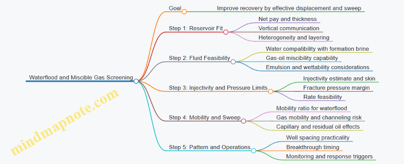
Example: Side-by-Side Screening Decision
Assume a reservoir with moderate permeability, strong layering, and high salinity formation water.
- Waterflood check: Injection water compatibility fails scaling risk unless treated; mobility ratio is unfavorable because oil is viscous. Screening outcome: waterflood is only viable if scaling control and mobility management are included.
- Miscible gas check: MMP is slightly above achievable injector pressure, but near-injector miscibility might still occur. Screening outcome: miscible gas is not a clean yes; it becomes a conditional case requiring careful rate and pressure planning, plus a pattern that reduces channeling.
Practical Screening Outputs
A good screening produces clear go/no-go or conditional decisions:
- Required injection pressure versus fracture margin
- Expected mobility ratio and whether control is needed
- Compatibility constraints and mitigation requirements
- Pattern spacing implications based on heterogeneity
- Breakthrough timing estimates tied to operational rate targets
When these outputs align, the project moves forward with confidence that the physics and constraints are at least in the same neighborhood. When they don’t, the screening has done its job: it prevents spending time and money on a plan that cannot meet basic reservoir and fluid realities.
10.2 Pattern Design and Injection Allocation Using Reservoir Constraints
Pattern design is the part where reservoir reality meets operational math. The goal is to place injectors and producers so that pressure support and sweep are effective, while mechanical and operational limits are respected. The “reservoir constraints” piece means you do not design from a blank grid; you design from permeability structure, heterogeneity, fault or barrier behavior, and fluid properties.
Foundational Inputs That Actually Control Allocation
Start with a few reservoir facts that determine where injected fluid can go.
- Flow capacity map: Use permeability and flow-unit style layering to identify high-connectivity corridors and low-connectivity barriers.
- Vertical communication: Determine whether the reservoir behaves like one connected layer or multiple stacked flow units with limited crossflow.
- Pressure response: Estimate how pressure propagates with distance and time using a simple pressure transient model or calibrated simulation history.
- Fluid compatibility: Confirm that injected water or gas does not cause immediate plugging through scale or emulsion behavior.
A practical way to keep this grounded is to translate each reservoir fact into an engineering constraint: “Where can injection move?” becomes a connectivity constraint; “How fast does pressure reach producers?” becomes an injection rate constraint.
Pattern Geometry from Connectivity, Not Symmetry
Common pattern shapes are useful starting points, but the reservoir should decide the final geometry.
- Define connectivity zones: Partition the reservoir into regions that share effective flow paths. Faults, shale streaks, and tight streaks often create boundaries.
- Choose injector-producer pairing: Pair injectors to producers that lie within the same connectivity zone. If you pair across a barrier, allocation math will look fine on paper and fail in production.
- Set spacing using sweep logic: Use effective distance rather than map distance. If vertical communication is weak, horizontal sweep may be good while vertical sweep remains poor.
A simple example: Suppose a reservoir has two stacked flow units. If injectors are placed to sweep the upper unit well but the lower unit has poor vertical communication, producers completed only in the lower unit will underperform even if overall pattern injection looks adequate.
Injection Allocation as a Constraint-Satisfaction Problem
Allocation answers: “Given limited injection capacity, how do we distribute rates among injectors and possibly among intervals?”
Treat allocation with three constraint sets.
- Reservoir constraints: connectivity, pressure support needs by producer group, and sweep effectiveness by interval.
- Well and surface constraints: maximum injection rate per well, tubing or casing pressure limits, and available injection water or gas.
- Operational constraints: minimum stable rates to avoid severe cycling, and limits on pressure drawdown or injection pressure.
A workable workflow is:
- Group producers by response: Producers that share the same connectivity zone should be grouped.
- Assign target pressure support: For each producer group, define a minimum pressure maintenance level or a rate support requirement.
- Allocate injector rates: Start with a proportional allocation based on connectivity strength, then adjust to satisfy pressure and mechanical limits.
- Check interval allocation: If commingled injection is used, verify that the intended interval receives the majority of injected flow.
Mind Map: Pattern Design and Injection Allocation
Concrete Example with Numbers
Assume a pattern with two injectors (I1, I2) and two producer groups (P1, P2).
- Connectivity strength: I1 connects strongly to P1 and weakly to P2; I2 connects strongly to P2 and weakly to P1.
- Maximum injection rates: I1 ≤ 6,000 bbl/d; I2 ≤ 4,500 bbl/d.
- Total available injection: 9,000 bbl/d.
- Pressure support targets: P1 needs 5,000 bbl/d equivalent support; P2 needs 4,000 bbl/d equivalent support.
A proportional starting allocation might set I1 = 5,000 and I2 = 4,000 bbl/d. Now apply the constraint logic: because I1’s connection to P2 is weak, much of I1’s injection will not help P2. If the predicted support to P2 falls short, shift rate toward I2 while staying within its maximum. One feasible allocation is I1 = 4,500 bbl/d and I2 = 4,500 bbl/d, which respects both well limits and increases support to P2.
The key nuance is that allocation is not just “meet total injection.” It is “meet the right support in the right connectivity zone.”
Interval Allocation Example for Commingled Injection
If injectors feed two intervals, U (upper) and L (lower), and vertical communication is limited, commingled injection can bias flow toward U. Suppose interval acceptance factors are AU = 0.7 and AL = 0.3. If you inject 9,000 bbl/d total, the expected split is roughly 6,300 bbl/d to U and 2,700 bbl/d to L.
If producers in L require pressure support equivalent to 4,000 bbl/d but you only deliver 2,700 bbl/d, you must either increase total injection (if allowed), change injection interval isolation, or adjust completion and injection strategy so that L receives more of the injected volume.
Validation Checks That Prevent Silent Failure
After allocation, verify with measurable signals.
- Pressure response by injector: confirm that pressure increases align with expected propagation into each connectivity zone.
- Rate response by producer group: ensure producer groups tied to each injector show the intended improvement.
- Interval contribution evidence: use production logging, tracer behavior, or pressure falloff signatures to confirm where injected fluid actually went.
When these checks disagree with the allocation model, the fix is usually not “try a different pattern shape.” It is to correct the connectivity assumptions, interval acceptance, or pressure response parameters that the allocation depends on.
10.3 Injection Well Design Including Pressure Limits and Mechanical Integrity
Injection Well Design Goals
An injection well must deliver a target rate while keeping pressures inside safe mechanical and operational limits. The design starts with three numbers that govern almost everything: maximum allowable wellhead pressure, maximum bottomhole injection pressure, and the pressure at which the formation or the wellbore fails. A practical way to keep the design grounded is to treat each limit as a “stop sign” and then check that the planned operating envelope stays comfortably behind it.
Pressure Limits That Actually Matter
Pressure limits come from multiple failure modes, so the governing limit is the lowest one.
- Formation fracture pressure: If bottomhole pressure exceeds fracture pressure, injected fluid can create unintended pathways. A common best practice is to compute fracture pressure using effective stress and then apply a safety margin for uncertainty in pore pressure and stress.
- Caprock and fault reactivation risk: Even if the target reservoir can fracture, the overburden may not tolerate the same pressure. The design should evaluate pressure at relevant stratigraphic intervals and treat the caprock as a separate constraint.
- Wellbore integrity limits: Casing and tubing have burst and collapse limits, plus tensile limits during pressure changes. These limits depend on pressure, temperature, and axial loads from weight and thermal expansion.
- Surface and flowline limits: Wellhead, valves, and surface piping must handle the maximum expected pressure with margin for transient events like pump start-up.
Example: If fracture pressure at the target interval is 42 MPa and the design bottomhole injection pressure is 35 MPa, you have a 7 MPa buffer. But if casing burst capacity at the same depth corresponds to an allowable 33 MPa, the casing becomes the governing limit and the operating plan must be reduced accordingly.
Mechanical Integrity Design Workflow
Mechanical integrity is not a single calculation; it is a chain of barriers that must remain functional.
-
Set casing program to survive the worst load case
- Determine maximum internal pressure (burst) and external pressure (collapse) for each casing string.
- Include temperature effects that change fluid density and induce axial stress.
- Check cement sheath integrity indirectly through bond quality expectations and directly through planned cement placement quality controls.
-
Design cementing for zonal isolation under injection conditions
- Cement must withstand pressure differentials across the annulus and resist micro-annulus formation.
- Centralization and slurry design reduce channeling risk, especially in deviated sections.
-
Select tubing and packer strategy for pressure containment
- Tubing must handle internal pressure and potential external pressure from annulus fluids.
- Packers must seal against pressure while tolerating temperature and chemical exposure from injected fluids.
-
Plan for pressure management during operations
- Rate changes should be controlled to avoid pressure spikes.
- Surface pressure monitoring should be tied to bottomhole pressure estimates so operators can react before limits are crossed.
Mind Map: Pressure Limits and Mechanical Integrity
Integrated Example: Turning Limits into an Operating Envelope
Assume a well is planned to inject at 2,500 bpd. The hydraulic model predicts that at this rate the bottomhole pressure would be 34 MPa. Next, compute allowable pressures from constraints:
- Fracture pressure at target: 42 MPa
- Casing burst allowable at injection depth: 33 MPa
- Surface wellhead allowable: 36 MPa
The governing limit is 33 MPa, so the operating envelope must keep bottomhole pressure at or below 33 MPa. If the hydraulic model shows bottomhole pressure scales roughly with rate, you can reduce the rate to achieve 33 MPa. Then verify that the reduced rate still meets injection objectives for the planned time window.
Mechanical Integrity Verification During Execution
Mechanical integrity is verified through execution checks that prevent “design on paper” from becoming “surprise in the field.” Cement placement quality should be confirmed with logs or tests appropriate to the well design. After completion, pressure tests and baseline measurements establish reference points for later monitoring. During injection, pressure and temperature trends should be compared to baseline behavior to detect abnormal changes in friction, fluid properties, or sealing performance.
Practical Checklist for the Injection Well Design Stage
- Identify governing pressure limit from formation, wellbore, and surface constraints.
- Build a casing and tubing load-case envelope including temperature and axial effects.
- Design cement and centralization to support zonal isolation under expected ΔP.
- Define operational ramp rates and monitoring thresholds tied to bottomhole pressure estimates.
- Establish baseline integrity measurements for later comparison during injection.
10.4 Produced Fluid Handling and Surface Constraints for Reliable Operations
Produced fluid handling starts at the wellhead and ends at the point where fluids are measured, separated, treated, and disposed or exported. The goal is simple: keep the process stable so the reservoir data you worked hard to obtain doesn’t get scrambled by surface bottlenecks. A reliable system also protects people and equipment by controlling pressure, temperature, solids, and corrosive components.
Foundational Flow Paths and What They Must Preserve
A typical surface chain includes: wellhead throttling, gathering lines, separators, gas handling, produced water treatment, and storage or export. Each step must preserve three things: (1) phase separation quality, (2) measurement integrity, and (3) pressure control. If any step causes slugging, foaming, or measurement bias, downstream decisions become guesswork.
A practical example: suppose two wells feed a common header. If one well intermittently produces gas-rich fluid, the header pressure can oscillate. That oscillation changes separator performance, which then changes oil carryover into the gas line. The result is not just “messier separation”; it’s also biased oil rate measurement and higher chemical usage.
Separator Performance and Phase Management
Separators are the workhorses for separating gas, oil, and water. Their effectiveness depends on residence time, pressure, temperature, and internals. Key operational constraints include:
- Pressure control: maintains vapor-liquid equilibrium and prevents gas breakthrough into liquid streams.
- Temperature control: affects viscosity and gas solubility, which changes how much gas stays dissolved.
- Liquid level control: prevents oil-water mixing and reduces carryover.
A concrete check: if gas carryover into the oil outlet rises, you may see unstable differential pressure across downstream filters and a sudden increase in emulsion stability. That often traces back to separator level settings or inlet flow pattern changes.
Gas Handling Constraints and Measurement Integrity
Gas handling typically includes dehydration, compression or pressure regulation, and metering. The surface constraints that matter most are:
- Hydrate and free-water control: dehydration units must match the actual water content.
- Backpressure management: excessive backpressure can reduce well deliverability and increase liquid loading.
- Metering stability: metering devices need steady flow; otherwise, the “rate” becomes a moving target.
Example: if a dehydration unit cycles due to poor inlet separation, the outlet water content swings. That can shift corrosion rates in downstream piping and change the calibration behavior of some gas meters.
Produced Water Treatment and Solids Control
Produced water often contains dissolved salts, suspended solids, and emulsified oil. Treatment commonly uses chemical conditioning, gravity separation, flotation, filtration, and sometimes dissolved gas removal. The constraints are mechanical and chemical:
- Solids loading: filters clog faster when upstream separation is poor.
- Emulsion stability: if oil droplets remain small and stable, gravity separation becomes ineffective.
- Chemical dosing accuracy: overdosing can increase sludge; underdosing increases oil in water.
A practical example: after a workover, a well may produce more fine solids. Even if total water rate is unchanged, filter differential pressure rises and treatment skims become oilier. The fix is not only “more filtration”; it’s verifying upstream solids capture and adjusting chemical conditioning based on measured water quality.
Oil Quality, Emulsion Control, and Export Readiness
Oil export systems care about water cut, sediment, and viscosity. Surface constraints include heater settings (if used), emulsion breakers (if applied), and storage tank mixing. Tanks can hide problems: oil may look acceptable while water stratifies and later returns during drawdown.
Example: if tank draw schedules change, the water cut at the export pump can jump even though separator performance is steady. That points to tank stratification and draw control rather than a reservoir change.
Pressure, Temperature, and Corrosion Management
Reliable operations require consistent pressure and temperature control to limit corrosion and scaling. Corrosion is influenced by CO₂, H₂S, oxygen ingress, water chemistry, and flow regime. Scaling depends on ion concentrations and temperature changes.
A concrete operational rule: avoid unnecessary temperature drops across choke and lines when you can. Cooling can reduce solubility and increase scale risk, especially when brine composition is near saturation.
Measurement Points and Data Consistency
Surface constraints directly affect measurement points: inlet header meters, separator outlet meters, water skids, and gas metering. To keep data consistent:
- Use mass balance checks between separator outlets and header inputs.
- Track quality parameters (water cut, BS&W, gas-oil ratio) alongside rates.
- Monitor differential pressures across filters and separators as early warning.
Example: if oil rate from separator outlet stays steady but water rate increases while total header flow is unchanged, you likely have measurement bias or a routing/valve configuration issue.
Mind Map: Produced Fluid Handling and Surface Constraints
Example Workflow: Diagnosing a Surface Instability
- Observe the symptom: gas rate meter shows oscillations and separator oil carryover increases.
- Check pressure stability: verify header and separator pressure control loops are not hunting.
- Inspect separator level control: confirm level setpoints and sensor health.
- Review inlet flow pattern: check whether a well changed contribution (liquid loading or gas fraction).
- Validate measurement consistency: compare header flow with separator outlet mass balance.
- Correct upstream routing or throttling: stabilize phase behavior before changing chemical programs.
This sequence keeps the investigation grounded: you start with the surface variables that directly control phase separation and measurement, then move to treatment adjustments only after the flow physics are stable.
10.5 Practical Example Workflow for Building an EOR Implementation Plan
An EOR implementation plan is easiest to manage when it reads like a sequence of decisions. Each decision should be backed by a measurable input: reservoir properties, well constraints, surface limits, and risk controls. Below is a systematic workflow using a single, consistent example so the logic stays connected.
Step 1: Define the EOR Objective and Boundaries
Start by writing the objective in operational terms, not in process terms. Example objective: increase incremental oil rate by improving sweep efficiency in a waterflooded reservoir.
Set boundaries:
- Time window for pilot operations (example: 12 months)
- Target pattern size (example: 5-spot)
- Maximum injection pressure at the wellhead and at the formation (example: 10% below fracture pressure)
- Mechanical constraints for injection wells (example: tubing pressure rating, packer setting depth)
Practical check: if the objective cannot be translated into rate, pressure, and interval targets, the plan will stall later.
Step 2: Select the Candidate EOR Process Using Screening Logic
Use a short screening table to avoid “process shopping.” For each candidate process, score only what you can verify.
Example screening inputs:
- Reservoir temperature and salinity range
- Oil viscosity and mobility ratio
- Remaining oil distribution from production logs and tracer data
- Rock mineralogy relevant to wettability or scaling
Outcome example:
- Water-alternating-gas is rejected due to insufficient gas availability and poor injectivity risk.
- Polymer is rejected due to high residual resistance factor from prior scale events.
- Chemical flooding is rejected due to uncertain adsorption from limited core data.
- Miscible gas is selected because minimum miscibility pressure is achievable with available gas composition and reservoir pressure decline is not yet too severe.
Step 3: Build the Injection Strategy from Reservoir Geometry
Injection strategy should specify where, how much, and how to sequence.
Example pattern:
- 1 injector per 4 producers (5-spot)
- Injector perforations in the best connected flow units identified from log-based permeability and production logging
- Injection starting rate chosen to keep bottomhole pressure below the limit
Sequencing example:
- Stage 1: gas injection at a lower rate to establish injectivity and pressure response
- Stage 2: ramp to target injection rate once injectivity stabilizes
- Stage 3: maintain pressure while monitoring breakthrough indicators
Step 4: Translate Reservoir Targets into Well and Completion Design
Convert reservoir needs into well constraints.
Completion design example:
- Perforate only intervals with net pay thickness above a cutoff (example: 2 m)
- Use a completion type that minimizes plugging risk (example: sand control where grain size warrants it)
- Ensure injection wells have sufficient tubing and packer integrity margin for the planned pressure range
Operational example:
- If injectivity declines during Stage 1, reduce rate and adjust perforation contribution rather than forcing the pressure limit.
Step 5: Define Monitoring, Measurement, and Control Rules
Monitoring must be tied to actions. Otherwise it becomes expensive paperwork.
Example monitoring suite:
- Monthly pressure and rate histories for injector and producers
- Periodic production logging to confirm interval contribution changes
- Tracer or composition sampling where feasible to detect sweep and early communication
Control rules example:
- If injector bottomhole pressure rises faster than a defined threshold over 2 consecutive weeks, pause rate ramp and investigate injectivity impairment.
- If producer gas-oil ratio increases in a specific interval, adjust injection rate or timing to manage breakthrough.
Step 6: Create a Material Balance and Performance Forecast Using Measured Inputs
Use a simple, defensible model that matches the data you trust.
Example modeling workflow:
- Calibrate base production decline and water cut using historical rates
- Use log-derived flow unit volumes to distribute injected gas effectiveness
- Run sensitivity on injection rate and well spacing using the same uncertainty bounds you already have
Deliverable: a forecast table with base case and two bounded cases (low and high injectivity).
Step 7: Plan Surface Facilities and Operational Readiness
Facilities must support the injection plan without creating new bottlenecks.
Example readiness items:
- Gas supply pressure and metering accuracy for ramp control
- Compression capacity and power limits
- Produced fluid handling capacity for increased gas production
Operational example:
- If compression limits cap injection rate, revise the injection ramp schedule rather than exceeding facility constraints.
Step 8: Identify Risks and Write Mitigation Actions
Risk controls should be specific and testable.
Example risk register:
- Injectivity impairment from fines migration: mitigation includes rate ramp control and interval selection
- Cement or mechanical integrity concerns under pressure cycling: mitigation includes integrity checks and conservative pressure limits
- Early breakthrough: mitigation includes sequencing changes and producer interval management
Step 9: Assemble the Implementation Schedule and Acceptance Criteria
Turn the plan into a timeline with go/no-go gates.
Example gates:
- Gate A after Stage 1: injectivity within an acceptable range and stable pressure response
- Gate B after Stage 2 ramp: no sustained pressure exceedance and stable well integrity indicators
- Gate C after pilot end: incremental oil response meets the minimum threshold defined at the start
Mind Map: EOR Implementation Plan Workflow
Example: Putting It Together in a One-Page Pilot Plan
A practical pilot plan can be summarized as:
- Objective: incremental oil via miscible gas sweep in a 5-spot pattern
- Injection: Stage 1 low-rate to stabilize injectivity, Stage 2 ramp to target while staying below pressure limits
- Wells: perforate best-connected flow units, use conservative integrity margins
- Monitoring: monthly pressure/rate, periodic interval contribution checks, composition sampling where available
- Control: pause ramp if pressure rise trend exceeds threshold; adjust injection timing if breakthrough indicators appear
- Acceptance: injectivity stable by Gate A, no sustained pressure exceedance, and minimum incremental oil response by pilot end
This structure keeps the plan coherent: reservoir logic drives well design, well design drives operational limits, and operational limits drive monitoring and control actions.
11. Reservoir Performance Optimization with Integrated Surveillance
11.1 Production Logging and Well Testing for Rate and Interval Diagnostics
Production logging (PL) and well testing (WT) answer two related questions: where fluids are entering or leaving the wellbore, and how much is happening at each interval. When you combine them, you can separate “the well is producing less” from “the well is producing from the wrong place.”
Core Concepts for Rate and Interval Diagnostics
Start with the measurement logic. A well test gives you a time-averaged rate and pressure response for the whole well or a major segment. Production logging breaks the well into depth intervals and estimates contributions from each interval using downhole measurements.
A practical diagnostic workflow treats the well as a system with three layers:
- Surface layer: total rate, choke settings, separator conditions, and test duration.
- Wellbore layer: flow paths, crossflow, and depth-specific inflow/outflow.
- Reservoir layer: interval properties and pressure support.
If surface rate drops, you first check whether the change is operational (choke, pump, downtime) or physical (interval loss, water rise, coning, plugging). PL and WT help confirm which layer is responsible.
Production Logging for Interval Contributions
Production logging tools typically estimate phase rates versus depth. The key is interpreting tool outputs with correct reference frames: depth matching, tool calibration, and fluid property assumptions.
Example: A well historically produced 600 bpd oil with 20% water. After a workover, surface oil rate falls to 420 bpd while water rises to 35%. A PL run shows oil inflow shifting from the upper perforated interval to the lower one, while the upper interval now shows reduced inflow and increased water contribution. The diagnostic conclusion is not “the reservoir got worse everywhere,” but “the flow distribution changed,” which points to altered near-wellbore conditions, partial plugging, or mechanical issues affecting zonal isolation.
To make PL results actionable, compare:
- Pre- and post-event PL profiles aligned to the same depth datum.
- PL inflow/outflow pattern against perforation and completion geometry.
- Water cut and phase split against expected fluid behavior from logs and PVT.
Well Testing for Rate and Pressure Response
Well tests provide pressure and rate history that can be interpreted to estimate effective productivity and flow behavior. The goal is interval diagnostics through pressure transient interpretation and rate normalization.
A clean test requires consistent operating conditions. Normalize rates to a stable reference by accounting for choke position, gas lift or pump changes, and separator constraints. Then interpret pressure response with a model that matches the well’s flow regime and boundary conditions.
Example: Two wells show the same surface rate decline after a similar completion. WT on Well A shows a productivity index drop with a similar skin signature, while Well B shows a delayed pressure response consistent with a flow restriction near the wellbore. PL on Well A indicates reduced inflow across multiple depths, suggesting reservoir damage or reduced pressure support. PL on Well B shows a strong inflow from a single interval with reduced contribution from others, suggesting a mechanical or zonal flow-path issue.
Integrated Diagnostic Logic
Use PL to locate where the change is happening, and WT to quantify whether the change is primarily mechanical, reservoir-related, or operational.
Mind the common pitfall: PL can be run at a single operating point, while WT captures dynamic behavior. If PL shows interval shifts but WT shows no meaningful productivity change, the issue may be flow redistribution rather than total deliverability loss.
Mind Map: Rate and Interval Diagnostics Workflow
Example: Diagnosing Water Rise After Workover
Assume a multilayer completion with two main perforated intervals. After a workover, surface water cut increases from 15% to 45% while total liquid rate stays nearly constant.
- WT result: total productivity for liquid remains similar, but the pressure response suggests increased effective water mobility.
- PL result: water inflow increases sharply in the lower interval, while oil inflow in the upper interval decreases.
- Integrated conclusion: the workover likely altered flow distribution or zonal isolation, allowing more water to enter from the lower interval rather than a uniform reservoir decline.
This combination matters because it changes the remediation target. If WT indicated a major productivity loss, you would prioritize near-wellbore damage assessment. If WT indicates stable deliverability but PL shows redistribution, you focus on zonal flow paths and mechanical integrity.
Practical Quality Checks That Prevent Bad Decisions
- Depth alignment: a shifted datum can make a correct tool look wrong.
- Operating point consistency: PL and WT should be compared under comparable rates and fluid conditions when possible.
- Phase property assumptions: incorrect fluid properties can bias phase-rate estimates.
- Cross-check with completion records: perforation intervals and packer positions must match the interpretation framework.
When these checks are done, PL and WT together provide a coherent story: the well’s total behavior (WT) and the depth-by-depth contributions (PL) agree on what changed and where it changed.
11.2 Tracer and Pressure Data Use for Connectivity and Sweep Assessment
Connectivity answers a practical question: do injectors and producers actually communicate through the reservoir rock, or are they just sharing the same map? Sweep assessment asks a second question: even if they communicate, does the injected fluid move through the intended intervals and volumes, or does it shortcut along higher-permeability paths and bypass oil?
Foundational Concepts for Interpreting Tracer and Pressure Signals
Start by separating three layers of evidence.
- Timing evidence comes from tracer arrival times at producers relative to injection start and shut-in events. A tracer that appears quickly suggests shorter flow paths or higher effective permeability connections.
- Magnitude evidence comes from tracer concentration levels and mass balance consistency. If concentrations are low despite sustained injection, either connectivity is weak or dilution and dispersion are dominating.
- Pressure evidence comes from pressure responses at wells. Pressure changes propagate through connected flow paths; the shape of the response helps distinguish distributed communication from localized channeling.
A simple mental model is to treat the reservoir as a network of flow paths. Tracer rides the same paths as the injected fluid, while pressure responds to changes in flow resistance and storage along those paths.
Mind Map: What to Measure and Why
Tracer Data Workflow for Connectivity
Step 1: Align time and rates. Build a consistent timeline using injection start, any rate changes, and any tracer concentration changes. If injection rate varies, convert tracer mass injected per day rather than relying on concentration alone.
Step 2: Identify arrival and peak windows. For each producer, plot tracer concentration versus time and mark the first statistically meaningful rise above baseline. The first rise is your connectivity flag; the peak time and peak width help characterize path length and dispersion.
Step 3: Check mass balance sanity. Compute the fraction of injected tracer recovered at each producer over the observation window. If the sum recovered is far below expectations while pressure indicates strong communication, suspect sampling gaps, adsorption or retention effects, or tracer loss in equipment.
Step 4: Use cross-well correlation. Compare tracer curves between multiple producers. The producer with the earliest and highest tracer response is typically the best-connected path, but confirm with pressure behavior so you don’t confuse dilution with weak connectivity.
Example: An injector runs at 2,000 bpd for 30 days with a tracer concentration step from 50 to 100 ppm on day 15. Producer A shows a baseline-to-rise transition on day 22 and a peak shortly after the step, while Producer B shows only a small, delayed bump. The step-following behavior at A suggests the connection is not only present but responsive to injection changes.
Pressure Data Workflow for Sweep Assessment
Pressure data is especially useful when tracer is sparse, delayed, or affected by retention. Use pressure to evaluate whether injected fluid is moving through the reservoir volume you care about.
Step 1: Normalize pressure response to rate history. Pressure changes depend on how much fluid was injected or produced. Use rate-normalized plots or apply a consistent correction so that a larger pressure response isn’t mistaken for better sweep.
Step 2: Look at response timing and curvature. Early pressure response at a producer indicates faster communication. A gradual, broad response can indicate distributed sweep, while a sharp response can indicate a more localized high-permeability path.
Step 3: Combine with zonal information. If you have multi-zone completions, use interval production rates and interval pressure measurements (or inferred interval contributions) to attribute pressure response to specific layers. Sweep is about where the injected fluid goes, not just whether it goes somewhere.
Example: In a layered reservoir, an injector targets the upper interval. Producer C has two producing intervals. Tracer is only detected in the upper interval sample stream, while pressure at the lower interval shows a delayed, smaller change. This pattern supports the idea that the injected fluid sweeps the upper interval and only weakly communicates with the lower one.
Integrated Interpretation: Connectivity Strength Meets Sweep Quality
To avoid contradictory conclusions, treat tracer and pressure as complementary constraints.
- If tracer arrives early and pressure responds early, connectivity is strong and the flow path is likely efficient.
- If pressure responds but tracer is weak or absent, consider tracer retention, sampling issues, or bypass flow that dilutes tracer below detection.
- If tracer arrives but pressure response is muted, the connection may be narrow or dominated by mixing and dispersion rather than large-scale pressure communication.
Practical Checks That Prevent Common Misreads
- Baseline drift check: Verify producer baseline tracer levels before injection. A rising baseline can mimic tracer arrival.
- Sampling cadence check: Sparse sampling can shift apparent arrival time. Use the first sample above threshold, but record the uncertainty window.
- Rate-change alignment check: If injection rates changed, ensure tracer and pressure plots reflect those exact changes.
- Interval attribution check: For commingled production, confirm that interval rate estimates are consistent with completion logs and operational records.
Output Formats for Engineering Use
Deliver results in forms that can be acted on.
- Connectivity matrix: injector-to-producer pair scores based on arrival time, peak magnitude, and recovered tracer fraction.
- Sweep by interval: effective sweep fraction or qualitative ranking (good, partial, poor) derived from tracer presence and pressure response attribution.
- Uncertainty notes: a short list of the main reasons a conclusion might be less certain, such as sampling gaps or commingling.
When these outputs are consistent with both tracer timing and pressure response shape, you can confidently distinguish “they communicate” from “they sweep the right places.”
11.3 Material Balance and Decline Analysis Using Measured Field Data
Material balance connects what you put into a reservoir and what you get out, using measured production and injection data. Decline analysis describes how rates fall over time. Used together, they help you separate “the reservoir is changing” from “the data handling is changing.”
Core Idea and Data Inputs
Start with a consistent accounting basis: time intervals, fluids tracked, and reference conditions. For each period, compile:
- Production rates and cumulative volumes for oil, gas, and water.
- Injection volumes by fluid type and injection well.
- Pressure measurements at a defined reference location or averaged wellhead-to-reservoir mapping.
- Any operational adjustments such as shut-ins, recompletions, and measurement method changes.
A practical habit: build a single table where every row is a time step and every column is a measured quantity. If you cannot make that table without manual edits, the material balance will be messy too.
Material Balance Equations in Practice
Material balance is often written in terms of a “driving mechanism” such as solution gas drive, gas cap drive, water drive, or combinations. In field work, the exact form depends on the reservoir fluid behavior and the pressure range. The workflow is more important than memorizing the algebra.
- Choose the fluid model inputs: formation volume factors, gas-oil ratio behavior, and compressibility terms.
- Convert measured surface volumes to reservoir volumes using the correct conditions.
- Compute cumulative produced and injected reservoir volumes for each time step.
- Use measured pressure to evaluate the balance at each step.
If you see the computed balance “drift” systematically with time even when pressure is stable, suspect one of these: wrong reference pressure, inconsistent unit conversions, or a fluid property set that doesn’t match the pressure range.
Decline Analysis as a Consistency Check
Decline analysis uses production rate history to estimate parameters that describe decline behavior. For oil, a common approach is to fit a decline model to rate versus time (or cumulative). The key is to fit the model to the same intervals used in material balance.
A useful comparison:
- If material balance indicates increasing effective drive support, decline should flatten relative to a simple decline expectation.
- If material balance indicates worsening drive support, decline should steepen.
When they disagree, it’s usually not because the reservoir is being mysterious. It’s because the accounting basis differs: one method may include shut-in time, recompletions, or allocation changes.
Step-by-Step Workflow with Measured Data
- Define time steps aligned with reporting periods and operational events.
- Normalize volumes to reservoir conditions using the same fluid property set across all steps.
- Compute cumulative production and injection for each step.
- Select a pressure series that matches the material balance reference. If you average pressures, document the averaging method and keep it consistent.
- Evaluate material balance residuals at each step: the difference between left and right sides of the balance equation.
- Fit decline parameters using the same oil rate series and the same time steps.
- Reconcile by checking whether residual patterns correlate with pressure changes, injection changes, or measurement changes.
Mind Map: How the Pieces Connect
Example: Water Drive with Injection Changes
Assume a waterflood where oil rate declines from 800 to 500 STB/d over 18 months. Injection is increased in month 7 to maintain pressure.
- Material balance: when you compute reservoir volumes, you find that the “effective water influx” term increases after month 7, and the balance residuals shrink during the same period.
- Decline analysis: the oil decline curve shows a noticeable flattening after month 7 compared with the earlier segment.
Now suppose the opposite happens: injection increases, but material balance residuals worsen and decline steepens. The most common causes are not exotic physics; they are accounting problems such as using injection volumes that exclude certain wells, or using a pressure reference that doesn’t represent the swept region.
Example: Decline Fit Looks Good, Balance Says Otherwise
You fit an oil decline model and get a tight match to the rate history. Yet material balance residuals oscillate with time steps.
That pattern often indicates a mismatch in the pressure series or in the conversion factors. For instance, if formation volume factors are updated using a different pressure basis than the one used in the balance, the decline fit can still look fine because it only needs rates, not full reservoir-volume accounting.
Practical Diagnostics for Measured-Data Integrity
Use these checks before changing reservoir parameters:
- Unit audit: surface-to-reservoir conversions must use the same units everywhere.
- Time alignment: production and injection must be summed over identical intervals.
- Event handling: recompletions and workovers must be reflected consistently in both methods.
- Pressure representativeness: if pressure is measured in a different compartment than the producing interval, the balance will show systematic residuals.
When material balance residuals and decline behavior both improve after a data-handling fix, you’ve learned something valuable: the reservoir may be doing what it always did, and the analysis just needed better bookkeeping.
11.4 Updating Reservoir Models With Well and Logging Evidence
A reservoir model is only as good as the evidence that shaped it. Updating it with well and logging data means replacing assumptions with measurements, and then checking whether the updated model still honors the physics of flow and the geometry of the reservoir. The goal is not to “fit the numbers,” but to reduce uncertainty in a controlled way.
Start with Model–Data Alignment
Before changing properties, align the model’s coordinate system and depth reference to the well data. Depth mismatches can masquerade as formation changes, especially when time-depth conversion differs between drilling and logging workflows. A practical check is to compare key stratigraphic markers—such as gamma-ray peaks or sand tops—between the well log and the model’s interpreted horizons. If the markers don’t line up, fix the mapping first; otherwise, every subsequent update will be “accurate in the wrong place.”
Classify Evidence by What It Constrains
Not all logging outputs constrain the same model parameters. A useful way to organize updates is to map each evidence type to the model layer it affects:
- Lithology and facies constrain where properties should change laterally.
- Porosity and saturation constrain storage and flow potential.
- Net-to-gross and thickness constrain volumetrics and connectivity.
- Well test and production logging constrain effective permeability and flow behavior, often at a larger scale than logs.
This classification prevents a common failure mode: using a high-resolution log to “correct” a low-resolution flow model without accounting for scale.
Update Static Properties with Logging-Derived Constraints
A systematic update typically follows a sequence: facies → porosity → saturation → permeability. For example, if logs show a shift from cleaner sand to silty sand across a lateral boundary, you first update the facies model so that porosity trends are applied to the right rock type. Then you update porosity using calibrated log responses (after environmental and borehole corrections). Finally, you update saturation using the appropriate fluid model and cutoffs, and you propagate those changes into permeability using the selected petrophysical relationship.
A concrete example: suppose the original model assumed uniform porosity of 0.22 in a channelized interval. New logs show porosity averaging 0.18 in the upper part and 0.24 in the lower part, with a clear facies boundary. The update should introduce that vertical heterogeneity first, then adjust permeability accordingly. If you jump straight to permeability without updating facies, you risk creating permeability contrasts that contradict the observed lithology.
Honor Uncertainty Instead of Forcing a Single Answer
Logging data are informative but not perfect. Treat updated properties as distributions or scenarios rather than one deterministic set. A practical approach is to define a small set of realizations that reflect plausible ranges for porosity, saturation, and permeability. Then you test each realization against both the well logs and the larger-scale behavior implied by production data.
This is where “evidence” becomes more than a spreadsheet: you check whether the updated model still reproduces observed net pay thickness, interval averages, and stratigraphic continuity.
Use Well Tests to Calibrate the Flow-Relevant Scale
Logs describe rock properties at the scale of measurement, while well tests respond to flow paths and effective properties. When you update the model with well test data, you should focus on parameters that represent flow-relevant behavior, such as effective permeability, skin, and completion-related effects. A good check is to compare predicted and measured pressure transient responses for the same wellbore and completion configuration. If the mismatch is consistent across multiple wells, it points to a reservoir-scale property issue rather than a single-well operational artifact.
Validate with Cross-Well Consistency
After updating one well, validate across neighbors. For instance, if a channel boundary is moved to match one well’s facies log, the same boundary should not create impossible discontinuities at adjacent wells. Cross-well validation is a sanity filter: it catches updates that are locally correct but globally inconsistent.
Document the Update Logic
Model updates should be traceable: what evidence changed, what parameter was updated, and what constraints were applied. This documentation prevents “mystery tuning” and makes it easier to reproduce the update when new logs arrive.
Mind Map: Updating Reservoir Models with Well and Logging Evidence
Example: From Log Evidence to Model Property Changes
A reservoir model initially treats a target interval as a single facies with porosity 0.21 and permeability derived from a single correlation. After drilling a new well, gamma-ray and resistivity logs show two distinct sand bodies separated by a thin silty streak. The update process:
- Re-interpret the facies boundary using the log markers.
- Recompute porosity trends separately for the upper and lower sand bodies.
- Recompute saturation using the same fluid model but apply facies-specific cutoffs.
- Re-derive permeability for each facies using the correlation appropriate to that rock type.
- Validate that the updated net pay thickness matches the log-derived interval thickness.
- Calibrate effective permeability against well test behavior, adjusting only flow-relevant parameters if needed.
The result is a model that reflects the observed stratigraphy and still behaves correctly under flow constraints—no magic, just disciplined bookkeeping between measurements and physics.
11.5 Practical Example Workflow for Diagnosing Underperformance in a Pattern
A pattern underperforms when measured production is lower than expected, or when the decline is faster than the forecast. The workflow below starts with what you can trust, then narrows to where the mismatch likely comes from, and ends with a decision-ready set of actions.
Step 1: Confirm the Gap with Interval-Level Evidence
Start by separating “less oil” from “less reservoir contact.” Use production allocation by interval (from well tests, production logging, or proxy allocations) and compare:
- Rate vs. time: oil, water, gas, and total liquid.
- Interval contribution: which zones are producing less than modeled.
- Pressure and temperature: verify that the well is flowing under similar conditions to the forecast.
Example: In a 6-well pattern, the forecast assumed Zone B contributes 60% of oil. After 90 days, Zone B contributes 35%, while Zone A contributes 50% (up from 30%). That shift is a clue: either Zone B is not delivering, or Zone A is delivering more than expected.
Step 2: Check Measurement and Accounting Errors First
Before blaming the reservoir, verify the boring stuff:
- Allocation method consistency: same interval boundaries and calibration.
- Metering and sampling: confirm that oil/water separation and gas measurement are stable.
- Well status: downtime, choke changes, and workovers.
Example: One well had a choke setting change that reduced drawdown on Zone B perforations. The pattern gap shrank after normalizing for choke and shut-in time.
Step 3: Build a “Most Likely” Cause Tree
Use a structured list of causes grouped by system:
- Reservoir deliverability: permeability, skin, relative permeability effects.
- Wellbore and completion: perforation damage, cement issues, casing leaks, sand control restriction.
- Flow assurance and operating constraints: scale, emulsion, gas handling, water loading.
- Model inputs: wrong net pay, wrong saturation, incorrect flow unit assignment.
Step 4: Use Targeted Evidence Tests to Eliminate Branches
Pick tests that match the suspected branch.
- If interval contribution shifted: run production logging (or review existing PL) to confirm where fluids enter.
- If deliverability is low across the pattern: compare wellhead pressures and flowing bottomhole pressures to identify drawdown shortfalls.
- If water cut rose quickly: check whether water is entering earlier zones or via unintended pathways.
- If pressure response is inconsistent: use pressure transient analysis or well test sequences to estimate skin and connectivity.
Example: Production logging shows Zone B has low entry despite normal tubing pressure. That points away from simple operating constraints and toward completion restriction or damage.
Step 5: Translate Evidence into Parameter Updates
Update only what the evidence supports. Common parameter adjustments include:
- Net pay and effective thickness: revise based on log-derived cutoffs and corrected depth matching.
- Permeability or skin: if PL shows reduced entry, estimate skin increase or near-wellbore damage.
- Relative permeability endpoints: if water rises faster than expected, revisit water saturation and mobility.
- Zonal isolation: if water appears in zones that should be oil-dominant, investigate cement bond and casing integrity.
Example: Zone B effective thickness was overestimated because the log interpretation used an uncorrected shale volume cut. After recalculating net pay, modeled oil contribution drops closer to measured values.
Step 6: Decide Actions Using a Simple Scoring Rule
For each candidate action, score three items: expected impact, confidence from evidence, and operational risk.
- High impact + high confidence: proceed.
- High impact + low confidence: run one more diagnostic before acting.
- Low impact: document and move on.
Example actions in this pattern:
- If Zone B restriction is confirmed: consider a targeted intervention plan (e.g., stimulation or mechanical cleanup) focused on Zone B.
- If cement/zonal isolation is suspect: prioritize integrity verification before any aggressive stimulation.
- If the model inputs are wrong: update the reservoir model and re-run forecasts to prevent repeating the same mismatch.
Step 7: Close the Loop and Prevent Repeat Mismatches
After actions, compare post-intervention interval rates and pressure behavior to the updated model. The goal is not just to raise production, but to make the next forecast match reality better.
Example: After correcting net pay and applying a Zone B-focused treatment, Zone B contribution returns to 55% and water cut stabilizes. The revised forecast now tracks the observed decline rate within an acceptable margin, indicating the root cause was primarily input error plus localized restriction rather than a systemic operating failure.
12. Integrated Case Studies from Geology to Production Outcomes
12.1 Case Study: Directional Drilling With LWD Geosteering and Log Based Zoning
A field operator planned a 3,200 m horizontal well to drain a thin, laterally continuous reservoir sand. The geological model showed a net pay thickness of 6–10 m, but the top and base picks varied by up to 3 m between wells. The drilling team used LWD geosteering to stay inside the pay while the logging team built a log-based zoning scheme to define where perforations should go.
Mind Map: End-to-End Workflow
Step 1: Define the Pay Window from Logs
The team started with offset well data to translate “sand presence” into “drillable and productive.” They created three zones along the reservoir interval: Zone A (high-quality sand), Zone B (mixed quality), and Zone C (shaly or tight). The zoning used a simple rule set derived from log behavior: gamma ray low indicates sand, resistivity higher indicates better hydrocarbon saturation, and density-neutron separation helps confirm porosity trends.
Example: In one offset well, Zone A corresponded to gamma ray below 65 API and resistivity above 8 ohm·m, while Zone B used gamma ray 65–85 API with resistivity 4–8 ohm·m. Zone C was everything else. The operator then converted these log-based boundaries into depth boundaries for the target well using a consistent depth reference and a measured depth-to-time conversion.
Step 2: Build a Steering Reference Model
Geosteering needs more than a top and base surface. The team built a “reference corridor” around the pay window using the log-based zones. They set a centerline trajectory target and two guardrails: an upper guardrail near the top of Zone B and a lower guardrail near the base of Zone B. This approach prevents the well from oscillating between zones when the reservoir thickness changes.
Example: If the pay window was 8 m thick, the corridor might be 10 m wide to allow for uncertainty, with the perforation plan later restricted to the inner 8 m where Zone A and B dominate.
Step 3: Configure LWD for Reliable Real-Time Decisions
The LWD tool string included gamma ray and resistivity measurements suitable for bed boundary detection. Before geosteering began, the team ran a short calibration check: they compared early LWD curves to the expected log shapes from the reference model. Any systematic depth shift was corrected using a depth matching procedure tied to a nearby marker interval.
Example: If the LWD gamma peak arrived 0.6 m shallower than expected, the team applied a correction so that subsequent steering decisions used consistent depth. Without this, the well could “correct” in the wrong direction and spend more time in the guardrails than the pay.
Step 4: Use Threshold-Based Steering Actions
During drilling, the team evaluated the well position every survey update using two signals: proximity to the upper/lower guardrails and the likelihood of being in Zone A vs Zone B based on resistivity trends. They used a simple decision table to avoid subjective steering.
Example decision rule:
- If the well is above the upper guardrail and resistivity trend indicates Zone C, build angle to move down.
- If the well is within the corridor but resistivity indicates Zone B, hold inclination and adjust azimuth only if gamma suggests approaching the top.
- If the well is below the lower guardrail, drop angle to move up.
This kept steering actions consistent even when drilling conditions changed.
Step 5: Validate Zone Contact While Drilling
The operator tracked “zone contact length” in real time: how much measured depth fell into Zone A and Zone B. The team also monitored tool quality indicators to ensure the curves were trustworthy. When data quality degraded, they temporarily reduced steering aggressiveness and relied more on the most stable measurement.
Example: If resistivity became noisy due to mud property changes, the team weighted gamma more heavily for boundary proximity until resistivity stabilized.
Step 6: Convert the Final Trajectory into a Perforation Plan
After reaching the target section, the logging team ran wireline logs for higher-resolution confirmation. They updated the zoning boundaries using the actual well’s log response, then overlaid the final trajectory to compute where Zone A and Zone B truly occurred.
Example: Suppose the well spent 120 m in Zone B and 45 m in Zone A. The operator perforated primarily across Zone A with limited Zone B coverage where resistivity indicated better saturation. They avoided Zone C even if it was within the corridor, because the corridor was for steering safety, not completion quality.
Mind Map: Steering to Zoning Link
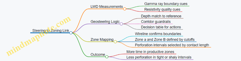
Results and Practical Takeaways
The well maintained contact within the corridor for the majority of the horizontal section, and the final log-based zoning showed a higher proportion of Zone A than the pre-drill model suggested. The key reason was not a single clever tool setting; it was the consistent chain from log-derived zone definitions to a corridor used for steering, then back to confirmed zoning for perforation selection. When the team treated steering as a controlled positioning problem and zoning as a completion-quality problem, the workflow stayed coherent from first marker to final interval choice.
12.2 Case Study: Wellbore Stability and Cement Integrity With Remediation Steps
Problem Setup and Initial Observations
A directional well in a moderately overpressured, interbedded sandstone–shale sequence showed early signs of trouble after casing was run. During cementing, returns were slow and the cement bond log later indicated poor bonding in the upper portion of the target interval. In parallel, the wellbore stability indicators during drilling had been mixed: torque and drag rose near a shale-rich section, and the rate of penetration dropped without a clear lithology change.
The engineering team treated this as two linked issues. Poor cement bonding can allow fluid movement behind casing, which then changes effective stresses and can worsen wellbore stability. Meanwhile, instability during drilling can create irregular borehole geometry, making cement placement harder and bond quality lower.
Foundational Concepts That Drive the Remediation Plan
Wellbore stability is governed by the balance between in situ stresses, pore pressure, and the mud system’s ability to control pressure and support the rock. Cement integrity depends on slurry design, placement efficiency, and the mechanical and chemical environment during and after setting.
A practical rule guided the workflow: if the borehole was already compromised, the cement job must be evaluated for placement failure modes, not just for “cement quality” in isolation. That means checking whether the cement was placed where it was intended, whether it displaced mud effectively, and whether the casing–formation interface was prepared.
Data Review and Root Cause Screening
The team assembled a short list of evidence and mapped each item to a likely failure mechanism.
- Cement bond log shows low bond quality near the top of the interval.
- Cement evaluation indicates possible channeling consistent with incomplete mud displacement.
- Drilling records show higher torque and drag in the same depth range.
- Mud properties were within spec, but the solids content and viscosity trend were elevated during the problematic section.
From these, the leading hypotheses were: (1) borehole enlargement or washouts created an irregular annulus, (2) solids and cuttings reduced displacement efficiency, and (3) cement placement did not achieve full annular coverage before setting.
Mind Map: Stability and Cement Integrity Remediation Logic
Remediation Steps with Concrete Actions
Step 1: Confirm the Depth Window and Failure Mode
Before any intervention, the team narrowed the suspect zone using cement evaluation curves and depth matching to drilling logs. They aligned the interval of poor bond with the time window of elevated torque and drag. This avoided the common mistake of treating the entire casing length as equally suspect.
Example: If the bond log showed poor bonding from 2,340–2,380 m, but drilling indicators spiked only from 2,350–2,370 m, the remediation focus shifted to the narrower window to reduce risk and cost.
Step 2: Improve Annulus Condition Before Cement Repair
Because instability likely created irregular geometry and retained solids, the remediation plan began with annulus conditioning.
- Circulate to restore mud properties and reduce solids concentration.
- Use a cleaning sweep to remove loose cuttings and minimize filter cake thickness.
- Maintain pressure control to avoid further destabilization.
Example: If the mud viscosity had drifted upward during the problematic section, the team corrected rheology before any squeeze operation so the injected cement could displace mud rather than get trapped in a thickened filter cake.
Step 3: Select a Squeeze Cement Strategy
A squeeze job was chosen to target the suspected flow path behind casing. The key design variables were pump rate, pressure limits, and slurry rheology.
- Use a slurry with controlled fluid loss to reduce migration into the formation.
- Choose a placement rate that fills micro-annuli without exceeding fracture pressure.
- Plan for staged pressure application to avoid sudden channel opening.
Example: If fracture pressure was estimated at 48 MPa and the operational limit was set at 42 MPa, the squeeze schedule used pressure steps that stayed below 42 MPa while still achieving the required injection volume.
Step 4: Execute with Monitoring and Stop Criteria
During the squeeze, the team monitored injection volume versus pressure response. A stable pressure rise with increasing volume suggested effective filling. A rapid pressure spike with little volume suggested plugging or poor communication.
Example: When pressure rose quickly but volume stalled, they paused, circulated lightly to recondition the interface, and then resumed with adjusted pump rate rather than forcing the job.
Step 5: Verify Zonal Isolation and Stability Improvement
After the squeeze, verification used pressure testing and a targeted cement evaluation pass where feasible. The goal was not just “better bond,” but reduced communication across the suspect interval.
Example: If pressure testing showed a significant reduction in leak rate across the interval compared with pre-job baseline, the remediation was considered successful even if bond quality improved only partially on the log.
Integrated Lessons Learned
- Stability and cement integrity are coupled through borehole geometry. If washouts or shale-related damage occurred, cement placement must account for it.
- Remediation should be interval-specific. Correlating drilling indicators with cement evaluation prevents over-treatment.
- Annulus conditioning is not optional. Cement repair works better when solids and filter cake are controlled before injection.
- Verification must include both mechanical and hydraulic evidence. Logs help, but pressure response confirms whether isolation actually improved.
12.3 Case Study: Petrophysical Modeling for Flow Unit Completion Targeting
A field operator wants to maximize production from a heterogeneous sandstone reservoir. The target interval is 40 m thick, but logs show repeating changes in grain size, clay content, and cementation. Instead of perforating the entire interval, the team uses petrophysical modeling to identify flow units and then designs perforation clusters to preferentially contact the best-connected rock.
Step 1: Build a Consistent Petrophysical Input Set
The workflow starts with a log suite that can support porosity, water saturation, and lithology. The team uses gamma ray and resistivity to separate shale-prone and sand-prone sections, then applies environmental and calibration corrections so porosity and resistivity are on the same depth basis.
A practical check prevents silent errors: the team compares porosity from density-neutron logs with porosity from core or sidewall samples where available. If the mismatch is systematic, they adjust the model inputs rather than forcing a perfect fit. This matters because flow unit classification is sensitive to relative differences, not just absolute values.
Step 2: Estimate Saturation with Quality Controls
Water saturation is computed using a resistivity-based approach with capillary pressure support. The team does not treat the saturation curve as a single truth. They run two saturation scenarios: one using a conservative cementation exponent and one using a more conductive rock assumption. The goal is not to pick a winner immediately, but to see whether the best-connected zones remain best-connected across reasonable parameter variation.
A simple example: if a 6 m interval stays high in effective permeability proxy under both scenarios, it is likely a robust flow unit candidate. If the ranking flips, the interval needs more scrutiny or additional constraints.
Step 3: Convert Petrophysics into Permeability Proxies
Direct permeability measurements are sparse, so the team uses permeability models calibrated to available data. They choose a model that respects the physics of pore structure: permeability should respond strongly to changes in effective porosity and less to changes that mainly affect bound water.
To keep the model honest, they apply cross-plot diagnostics. For instance, they plot porosity versus permeability proxy and look for two clusters: one representing cleaner, better-connected sand and another representing clay-rich rock. If the points smear into one cloud, the log corrections or saturation inputs are likely too noisy for flow unit work.
Step 4: Identify Flow Units Using Cross-Plot Patterns
Flow units are defined by combinations of pore throat size, connectivity, and wettability-related behavior. The team uses a set of cross-plots that separate pore structure from fluid effects. A common approach is to use effective porosity against a permeability proxy, then overlay saturation-related indicators.
Concrete example: suppose the team observes three bands on a porosity–permeability cross-plot.
- Band A has high effective porosity and high permeability proxy.
- Band B has moderate effective porosity but lower permeability proxy.
- Band C has similar porosity to B but much lower permeability proxy.
Band C often corresponds to clay-cemented rock where pore throats are constricted. Even if total porosity looks acceptable, the flow unit classification flags it as less productive.
Step 5: Build a Flow Unit Stratigraphic Map Along the Well
The team converts the flow unit classification into a depth-based zonation. They then correlate across nearby wells using consistent log normalization so that a “Band A” in one well matches the same rock type in another.
A systematic rule prevents overfitting: each flow unit boundary must be supported by at least two independent log behaviors, such as a resistivity shift plus a porosity-permeability proxy change. If only one log suggests a boundary, the team treats it as a tentative marker.
Step 6: Translate Flow Units into Completion Targeting
Now the modeling becomes operational. The team selects perforation intervals that maximize contact with the best flow unit while minimizing exposure to flow unit C.
Example completion logic:
- Perforate 70% of clusters in Band A.
- Place the remaining 30% in Band B to maintain drainage coverage.
- Avoid Band C except where it is the only way to reach the reservoir thickness.
They also adjust cluster spacing so that each cluster samples a similar flow unit mix. If the wellbore crosses a thin Band A streak, the team reduces cluster spacing locally to avoid “averaging out” the good rock.
Step 7: Validate with Production Logging and Interval Tests
After completion, the team compares measured interval contributions against the predicted flow unit ranking. If Band B produces more than expected, they revisit saturation assumptions and check whether the reservoir is more oil-wet than the base model assumed. If Band A underperforms, they check for mechanical issues such as near-wellbore damage or incomplete perforation effectiveness.
This validation loop is not a victory lap; it is a calibration step. The next well’s flow unit model uses the updated constraints so the classification becomes sharper.
Mind Map: Petrophysical Modeling for Flow Unit Targeting
Example: From Logs to Perforation Plan in One Pass
The team summarizes the workflow in a single internal checklist: (1) corrected logs, (2) two saturation scenarios, (3) permeability proxy cross-plot with cluster separation, (4) flow unit bands with boundary rules, (5) perforation allocation by band fractions, and (6) validation against interval tests.
In this case, the final plan concentrates clusters in Band A and reduces exposure to Band C. The result is a clearer production profile across intervals, with less contribution from rock that looked porous but behaved like it had narrow throats and weak connectivity.
12.4 Case Study: Enhanced Recovery Implementation With Injection And Surveillance Controls
A mature sandstone reservoir produced below plan because sweep was uneven: some injectors pushed water early into high-permeability streaks, while other compartments stayed underutilized. The operator chose a waterflood pattern with tight injection control and interval-level surveillance to prevent “fast paths” from dominating recovery.
Starting Point and Constraints
The team began with three inputs that must agree before field changes:
- Reservoir compartment map from well logs and core-derived flow units, identifying likely high-permeability streaks.
- Pressure and fracture risk from geomechanics and historical shut-in behavior, defining a maximum allowable injection pressure.
- Well integrity status from cement bond logs and casing pressure tests, ensuring injection could be applied without crossflow surprises.
A practical rule was used: if a well’s mechanical integrity was uncertain, it was treated as a “monitor-only” candidate until integrity was verified. This avoided spending injection effort on a pathway that might leak behind casing.
Injection Design with Control Logic
The pattern used five-spot geometry with injector–producer spacing selected to balance pressure support and sweep time. Each injector was completed with zonal isolation so injection could be allocated to compartments rather than averaged across the whole interval.
Injection allocation followed a simple control logic:
- Start with a conservative rate split based on estimated injectivity per compartment.
- Adjust monthly using two signals: injector bottomhole pressure trend and producer response lag.
- Apply rate throttling before pressure increases, because pressure escalation is the faster route to unwanted fractures or conformance loss.
Example: Injector I-3 had two perforated zones, Z1 and Z2. Initial allocation was 60% to Z1 and 40% to Z2. After three weeks, Z1 showed a faster pressure rise at the injector and an early water rise at the nearest producer. The team reduced Z1 allocation to 45% and increased Z2 to 55%, keeping total rate constant. The next producer response shifted later, indicating improved sweep distribution.
Surveillance Plan with Interval-Level Evidence
Surveillance was built around “prove it, then adjust it” rather than relying on one measurement type.
-
Pressure surveillance
- Continuous injection pressure and temperature at each injector.
- Periodic shut-in tests to estimate reservoir pressure response and detect communication changes.
-
Production surveillance
- Daily rates and water cut at producers.
- Periodic well tests to separate oil rate decline from water breakthrough timing.
-
Interval diagnostics
- Production logging on selected wells to confirm which compartments were actually producing.
- Tracer tests in a subset of injectors to validate flow connectivity between compartments.
Example: A producer P-7 showed rising water cut but stable oil rate for two months. Production logging indicated the water increase was concentrated in the upper compartment only. The injection team responded by reducing injection to the upper zone while maintaining total injection rate, preventing further pressure build-up in the wrong compartment.
Control Metrics and Decision Thresholds
To avoid endless tuning, the team defined thresholds tied to operational actions.
- Pressure trend threshold: if injector bottomhole pressure increased faster than the baseline slope for two consecutive weeks, reduce rate by 10–15% and re-check allocation.
- Water breakthrough timing threshold: if producer water cut rose earlier than predicted by compartment connectivity, shift injection away from the likely fast path.
- Integrity trigger: if casing pressure or annulus pressure changed beyond established limits, pause allocation changes and investigate mechanical causes.
These thresholds were applied consistently across the pattern, so decisions were explainable rather than subjective.
Mind Map: Enhanced Recovery Controls
Implementation Sequence and Results
The rollout followed a deliberate order:
- Verify integrity and zonal isolation performance on each injector.
- Establish baseline pressure and production response during conservative injection.
- Apply allocation adjustments using pressure trend and producer response lag.
- Confirm compartment behavior with interval diagnostics on a rotating schedule.
Within the first operating cycle, the pattern showed delayed water breakthrough in the majority of producers and reduced early water dominance near the highest-permeability streaks. Importantly, the team could explain each adjustment using measured signals: pressure slope changes led to rate throttling, and interval production evidence led to zone reallocation. That closed the loop between engineering intent and reservoir behavior, with fewer “mystery” decisions and more controlled learning.
Example: One Month of Allocation Tuning
- Week 1: Maintain total injection rate; observe pressure slope.
- Week 2: If pressure slope exceeds threshold, reduce rate 10% and keep allocation constant.
- Week 3: If producer water response indicates fast-path dominance, shift 5–10% injection from the fast zone to the slower compartment.
- Week 4: Run interval diagnostics on one key producer to confirm compartment-level impact, then lock the allocation for the next cycle unless thresholds are breached.
12.5 Case Study: End-to-End Optimization Using Measured Data and Engineering Constraints
A field operator planned a multizone horizontal well to maximize reservoir contact while staying inside mechanical and operational limits. The workflow below shows how measured data and engineering constraints were used together, step by step, to avoid “model-only” decisions.
Case Setup and Constraints
The target reservoir had three stacked pay intervals separated by thin shales. The well plan required:
- Trajectory limits: maximum dogleg severity and a build rate that matched the motor capability.
- Wellbore stability: a mud weight window defined by pore pressure and fracture pressure.
- Cement and isolation: zonal isolation risk controlled by centralization and cement placement quality.
- Completion practicality: perforation clusters sized for the expected inflow and sand control approach.
A baseline geologic model provided interval depths and expected net-to-gross, but the operator treated it as a hypothesis until logs confirmed it.
Mind Map: End-to-End Optimization Loop
Step 1: Lock the Depth Story Before Optimizing Anything
During drilling, the operator used LWD curves to guide geosteering, but the real optimization began after wireline logging. Depth matching was performed by aligning marker beds and correcting for time-depth conversion errors. A practical example: a shale marker that appeared 6 m shallower in LWD than in wireline was traced to a tool speed assumption. After correction, the pay intervals aligned consistently across the wellbore, preventing the common mistake of “optimizing” the wrong depth slice.
Step 2: Use Real-Time Indicators to Stay Inside the Mud Window
The drilling team defined an ECD limit that kept the effective mud pressure above pore pressure while remaining below the fracture gradient. When LWD indicated a faster-than-expected transition into a higher-pressure segment, the operator adjusted mud properties rather than simply increasing weight. Example: instead of raising mud weight by 0.3 ppg, they reduced flow rate and optimized viscosity to lower frictional losses, keeping ECD within the window while maintaining cuttings transport.
Step 3: Re-Zone the Target Using Calibrated Logs
After wireline logs, the operator recalibrated porosity and saturation using core or cuttings-based checks available from the field. The key was to treat each interval separately rather than averaging across the stacked pays. Example: interval A showed higher porosity but also higher clay volume, which reduced effective permeability. Interval B had slightly lower porosity but cleaner rock and better connectivity. The completion plan shifted toward interval B for perforation density, while interval A received fewer clusters to avoid spending shots where inflow would be limited.
Step 4: Validate Cement and Isolation Before Assuming Production Will Behave
Cement evaluation logs were reviewed with a simple decision rule: if bond quality fell below a threshold near a shale boundary, the operator flagged that zone for additional isolation attention. Example: a localized poor bond segment was detected near the top of interval C. Rather than changing the reservoir plan, the team adjusted the completion execution sequence and verified pressure integrity before stimulation, preventing a later “mystery” where injected fluids bypassed the intended interval.
Step 5: Match Completion Design to Flow Units, Not Just Net Pay
The operator used cross-plots and facies mapping to identify flow units, then tied perforation placement to those units. Example: two sections with similar net pay thickness had different flow unit quality. The final perforation plan increased cluster density where the flow unit quality index was higher, and it reduced density where the rock was likely to produce more sanding risk.
Step 6: Surveillance-Driven Interval Diagnostics After First Production
Once the well produced, production logging and pressure data were used to compare actual inflow distribution to the planned one. The operator looked for three measurable mismatches:
- Rate imbalance across intervals.
- Pressure drop anomalies suggesting restricted flow paths.
- Time-dependent changes indicating fluid entry into unintended zones.
Example: interval B underperformed relative to interval A during early flow. The team checked whether the underperformance aligned with any cement integrity concerns or with a depth mismatch discovered earlier. After confirming depth alignment and cement quality, they concluded the issue was inflow distribution tied to flow unit heterogeneity, not mechanical failure. They then adjusted choke settings and performed targeted workover only if pressure diagnostics continued to show interval-specific restriction.
Step 7: Update the Reservoir Model with Measured Evidence
The final optimization output was an updated reservoir model that reflected the measured inflow distribution and the recalibrated petrophysical parameters. The operator recorded which assumptions changed and which stayed stable. Example: the initial model overestimated connectivity in interval A; after log calibration and inflow diagnostics, the model reduced interval A’s effective permeability while preserving interval B’s connectivity. This prevented the next well from repeating the same “good-looking on paper” mistake.
Diagram: Constraint-Guided Integration Flow
    flowchart TD
  A[Pre-Drill Model and Limits] --> B[Drilling with MWD/LWD Indicators]
  B --> C[Maintain Mud Window and Trajectory Constraints]
  C --> D[Wireline Logging and Depth Matching]
  D --> E[Petrophysical Recalibration and Re-Zoning]
  E --> F[Cement Evaluation and Integrity Checks]
  F --> G[Completion Design by Flow Units]
  G --> H[First Production and Surveillance]
  H --> I[Interval Diagnostics from Measured Data]
  I --> J[Model Update and Final Lessons]
Outcome Summary
By treating depth, mud window behavior, cement quality, and interval zoning as one connected system, the operator reduced the gap between planned and actual performance. The most important habit was simple: every major decision was tied to a measurable input and a constraint check, so the well’s story stayed consistent from drilling to production.