Advanced Welding and Friction Stir Processing Technologies
1. Scope, Materials, and Joint Design Foundations
1.1 Defining Process Scope for Friction Stir Processing and Hybrid Welding
Process scope is the boundary that tells you what you will control, what you will measure, and what you will accept as “good enough” for the joint or treated zone. For friction stir processing (FSP) and hybrid welding, scope is not just paperwork; it determines which parameters matter, which defects are realistic, and which tests prove the process works.
What You Are Actually Doing
Start by naming the primary outcome:
- Friction Stir Processing aims to modify a region’s microstructure and properties without melting the base metal.
- Friction Stir Welding aims to join two parts by creating a bonded stir zone.
- Hybrid Welding combines friction stir with a fusion source such as laser, so you must define how the two energy inputs share the job.
A practical rule: if the design requires a continuous bond across the interface, you are in welding scope. If the design requires property tailoring in a surface or subsurface band, you are in processing scope. Hybrid scope is both, but with extra constraints because you now have two heat sources and two sets of defect risks.
Where the Process Applies
Define the geometry and location of the treated or welded region:
- Joint type: butt, lap, T-joint, edge-to-edge.
- Thickness range: thin sheets behave differently from thick plates because tool penetration and heat dissipation change.
- Material pairing: single alloy, dissimilar alloys, or alloy-to-coating stacks.
- Access and fixturing: whether the tool can maintain tilt and whether the laser beam has a clear line of sight.
Example: For a lap joint on an aluminum structure, scope might specify a stir zone that fully mixes through the faying interface while leaving the outer surface finish within a defined roughness window. That single sentence immediately tells you to control tool plunge depth, traverse speed, and surface condition.
What “Success” Means
Scope must include measurable acceptance criteria. Typical categories are:
- Geometry: stir zone width, underfill/overfill, surface flash limits, and alignment tolerances.
- Metallurgy: minimum hardness range, acceptable grain refinement extent, and limits on unmixed regions.
- Bond quality: absence of kissing bonds, lack of penetration, and through-thickness defects.
- Performance: tensile shear strength, fatigue-relevant behavior, and fracture mode expectations.
Example: If the joint is expected to fail in a predictable location during qualification, scope should state the allowed fracture path. Otherwise, you risk “passing” by strength while failing the intended failure mechanism.
Parameter Ownership and Control
Hybrid scope requires explicit ownership of parameters. Treat the process as a set of coupled levers:
- FSP/Friction Stir levers: rotation speed, traverse speed, axial force or plunge depth, tool tilt, dwell time, and tool wear state.
- Laser levers: power, spot size, focal position, beam offset relative to the tool, travel speed synchronization, and shielding gas.
- Synchronization rules: define whether the laser leads, trails, or overlaps the stir zone in time and space.
A simple example workflow: choose a baseline stir condition that produces a stable stir zone without surface tearing. Then add laser power in small steps while keeping tool rotation and traverse fixed. If you change everything at once, you cannot tell whether improved bonding came from better mixing, better wetting, or both.
Defect Map and Risk Boundaries
Scope should list the defects you will actively prevent and the ones you will monitor:
- FSP/Friction Stir: tunneling, voids, incomplete mixing, surface tearing, and excessive flash.
- Hybrid laser-assisted: porosity from keyhole instability, spatter-related inclusions, and misalignment that causes uneven fusion.
- Interface-specific: lack of bond at the faying interface, reaction layers that become too thick, and compositional gradients that affect hardness.
Example: If the design allows only a narrow hardness band, scope must include a plan to detect over-softened regions caused by excessive heat input or insufficient mixing.
Mind Map: Process Scope for FSP and Hybrid Welding
Example: Scope Statement That Actually Guides Work
A scope statement should be specific enough to prevent “parameter drift.” For instance:
- “For a lap joint in aluminum alloy, the hybrid process shall produce a continuous bonded stir zone across the faying interface with no through-thickness voids. The laser shall be synchronized to overlap the stir zone region while maintaining a defined beam offset. Acceptance requires hardness within a specified band and fracture behavior consistent with the intended failure mode.”
That level of detail forces the team to define tool wear checks, laser alignment verification, and inspection methods before production starts.
Example: Scope for a Dissimilar Interface
For dissimilar materials, scope must include how you will manage the interface reaction:
- Define whether you will rely on mixing alone (FSP-dominant) or on partial fusion (hybrid-dominant).
- Set limits on intermetallic thickness or hardness spikes.
- Specify inspection locations that correspond to the expected reaction zone.
If you skip this, you may end up with a joint that looks fine on the surface but fails because the interface chemistry produced a brittle layer where the load concentrates.
1.2 Aerospace and Industrial Materials Selection Criteria for Joining
Choosing materials for friction stir processing (FSP) and friction stir welding (FSW), or for hybrid laser and electron beam joining, is mostly a question of “what will move, what will bond, and what will survive.” The trick is to treat material selection as a system: chemistry, microstructure, geometry, and the joining physics all have to agree.
Start with the Joining Physics You Need
Begin by matching the process to the material’s dominant behavior.
- FSP/FSW relies on plastic flow and solid-state bonding. It prefers materials that can soften without cracking and that can form a continuous bond under stirring.
- Laser welding relies on melting and solidification. It is sensitive to absorptivity, melt pool stability, and keyhole or conduction regime control.
- Electron beam welding also melts, but with vacuum constraints and deep penetration behavior.
A practical rule: if the joint must avoid melting for distortion or metallurgical reasons, start with FSP/FSW or hybrid strategies that limit fusion. If full penetration and strong fusion bonding are required, laser or electron beam become the primary candidates.
Map Material Families to Expected Metallurgy
Materials selection should predict what happens in the joint region.
- Aluminum alloys often benefit from FSW/FSP due to grain refinement and reduced porosity risk compared with some fusion routes. However, oxide films and magnesium content can complicate bonding and defect tolerance.
- Titanium alloys can be excellent for solid-state joining, but tool wear and heat input control matter because titanium’s high reactivity and thermal sensitivity can drive defects if conditions are off.
- Steels are possible for FSW in many cases, but the process window can be narrower due to higher flow stress and heat requirements. For fusion methods, carbon and alloying elements influence solidification cracking susceptibility.
- Nickel alloys often demand careful control for both solid-state and fusion routes because microsegregation and cracking mechanisms can be unforgiving.
Selection is not just “which alloy,” but “which microstructure state.” A solution-treated and aged condition can change softening behavior, precipitate dissolution, and hardness in the stir zone.
Use a Compatibility Checklist for Chemistry and Microstructure
Before you pick a process, check compatibility items that directly affect bonding.
- Oxide and surface films: FSW/FSP must disrupt and transport films; laser and electron beam must manage melt pool cleanliness and gas entrapment.
- Thermal conductivity and heat capacity: These affect temperature rise and cooling rate, which in turn control grain size and residual stresses.
- Melting range and solidification behavior: For fusion methods, melting range, latent heat, and solidification mode influence porosity and cracking.
- Alloying element sensitivity: Elements like Mg in aluminum, S and P in steels, and reactive elements in titanium can shift defect risk.
- Precipitate stability: Aging state affects hardness drop or recovery after processing.
A simple example: two aluminum plates with the same nominal alloy can behave differently if one is overaged. In FSW, the overaged condition may soften more easily, widening the defect-free window for bonding but reducing peak hardness in the stir zone.
Consider Joint Geometry as a Material Decision
Geometry changes the local thermal and mechanical environment.
- Thickness: Thin sections amplify heat loss and distortion; thick sections demand stable heat generation and tool engagement.
- Joint type: Butt, lap, and T joints alter contact area and how material is transported or melted.
- Edge distance and restraint: Aerospace parts often have limited fixturing freedom, so material selection must account for distortion tolerance and residual stress sensitivity.
Example: for a lap joint where one adherend is a thin sheet, FSW can be attractive because it can bond without fully melting the thin sheet. But if the thin sheet is a hard-to-flow alloy, you may need a different tool design or a hybrid approach that adds controlled heat.
Define Acceptance Targets Before Choosing Materials
Materials selection should be anchored to performance requirements.
- Strength and hardness: Decide whether you need stir-zone hardness retention, base-metal match, or a controlled gradient.
- Fatigue behavior: Fatigue is often governed by surface condition, internal defects, and residual stress distribution.
- Corrosion performance: Dissimilar joints and stir-zone chemistry can create galvanic or localized corrosion risks.
A concrete workflow: if the requirement is high fatigue life, prioritize materials and processes that minimize internal voids and ensure consistent surface finish. If the requirement is corrosion resistance, pay attention to how dissimilar materials mix and whether intermetallic layers form.
Mind Map: Materials Selection Logic for Joining
Integrated Example: Choosing Between FSW and Laser Hybrid
Suppose you need to join a high-strength aluminum alloy to a dissimilar metal for an aerospace bracket. If distortion must be tightly controlled and you want to avoid a fully melted interface, start with FSW/FSP concepts for the aluminum side and consider a laser hybrid only where bonding at the interface is insufficient. If the interface requires full fusion for strength, laser hybrid or electron beam becomes the primary route, and material selection shifts toward alloys with manageable cracking and predictable solidification.
In both paths, the “best” material choice is the one that gives you a process window where defects are controllable and the resulting microstructure supports the required strength, fatigue, and corrosion behavior.
1.3 Joint Geometry Selection for Butt Lap and T Joint Configurations
Choosing joint geometry is less about picking a shape and more about controlling how heat, material flow, and load paths behave during friction stir processing and welding. For butt lap and T joints, the geometry you choose determines where bonding happens, how defects show up, and how easy it is to qualify the joint repeatedly.
Foundational Goals for Geometry
Start with three practical goals.
- Ensure full contact under load. Lap joints can open slightly if clamping is weak or if thermal expansion differs between plates. That gap becomes a defect magnet.
- Create a predictable bonding region. In butt joints, the bond line is central and continuous. In lap and T joints, the bond line is offset and may be partially shielded by overlap or flange geometry.
- Support defect-friendly processing. Many defects are geometry-sensitive: lack of penetration in butt joints, kissing bonds in lap joints, and incomplete sidewall bonding in T joints.
A good geometry makes the “bad case” easier to detect during inspection and easier to prevent during setup.
Butt Lap Geometry Selection
A butt lap joint uses overlap to increase effective throat while keeping a near-butt alignment. The overlap also gives you a place to manage tool access and backing support.
Key geometry variables
- Overlap length. Too little overlap reduces effective bonding area; too much overlap can trap heat and increase the chance of insufficient mixing at the overlap edge.
- Plate thickness ratio. If one plate is much thicker, the tool may preferentially stir one side, leaving the thinner side under-processed.
- Edge preparation and land. A small land or controlled edge gap can help maintain contact, but excessive gaps force the process to “bridge,” which is rarely consistent.
- Back support and clearance. Lap joints are sensitive to backing stiffness. A soft backing plate allows local deflection, which can reduce contact pressure at the bond line.
Easy example
Two aluminum plates, 3 mm and 3 mm thick, overlap by 8 mm. If you reduce overlap to 3 mm, the bonded area shrinks and the overlap edge becomes a common location for incomplete bonding. If you increase overlap to 15 mm, you may see more variability near the far edge because the tool has to work through a longer thermal path.
T Joint Geometry Selection
T joints place one plate against the face of another, creating a flange-like load path. Geometry here is about controlling sidewall access and ensuring the stir or weld action reaches the root.
Key geometry variables
- Flange thickness and height. A thick flange can block tool access to the root region, especially when the tool shoulder must ride on a limited surface.
- Root gap or contact condition. A small controlled gap can help avoid trapped oxides, but a large gap forces the process to bridge without reliable contact.
- Corner radius and chamfer. A sharp internal corner concentrates stress and can also concentrate defect initiation. A modest radius or chamfer improves both bonding and inspection visibility.
- Side access and fixturing. T joints often require careful clamping to prevent flange lift. Even a small lift can create a thin unbonded region along the root.
Easy example
A 2 mm flange on a 5 mm web. If the flange is perfectly flush and clamped, bonding tends to be consistent along the root. If clamping is relaxed, the flange can lift by fractions of a millimeter, and the unbonded region typically forms at the root first because that is where contact pressure is lowest.
Geometry-to-Process Mapping
Geometry influences where the process “works hardest.” Use this mapping to choose dimensions that match your process capability.
- Butt lap: Bond quality is most sensitive near the overlap edge and near the farthest region from tool access.
- T joint: Bond quality is most sensitive at the root line and along the internal corner where access and contact pressure are worst.
When you change geometry, treat it like a parameter change: update your trial plan and re-check the specific region that geometry makes vulnerable.
Mind Map: Geometry Drivers and Outcomes
Practical Selection Workflow
- Define the load path. Butt lap joints typically carry load through a more continuous bond line; T joints rely heavily on root and sidewall bonding.
- Set thickness ratio targets. If one plate is much thicker, plan geometry so the tool can reach the thinner side without starving it of mixing.
- Choose overlap or root contact intentionally. Use overlap length and root gap to maintain contact pressure where bonding must occur.
- Design for inspection. Pick geometry that makes the likely defect locations easy to section, scan, and measure.
- Run a focused trial. Evaluate the region your geometry makes most vulnerable, not just the average weld.
This approach keeps geometry selection grounded in what the process can reliably do, rather than hoping the setup will compensate for a shape that fights you.
1.4 Surface Preparation Requirements for Cleanliness and Fit Up
Surface preparation is the boring part that makes the rest of the process behave. For friction stir processing and friction stir welding, the tool needs intimate contact with the workpieces to drive plastic flow. For laser and electron beam hybrids, surface condition controls how energy couples into the joint. In both cases, cleanliness and fit-up are not separate tasks; they are the same job viewed from two angles: chemistry and geometry.
Cleanliness Foundations for Reliable Bonding
Start by removing anything that can interfere with contact or introduce gases. Common offenders include cutting oils, fingerprints, oxide films, paint residues, and moisture trapped in seams or surface scratches.
A practical way to think about cleanliness is to separate it into three categories:
- Loose contamination: dust, chips, and grit. These act like ball bearings and prevent full contact.
- Film contamination: oils, greases, and some coatings. These can vaporize and form pores or weak interfaces.
- Reactive contamination: oxides and corrosion products. These change wetting and can reduce bonding quality.
For aluminum alloys, oxide films are persistent and thin, but they still matter because they can become entrained into the stir zone or interfere with fusion in hybrid welding. For steels, corrosion products and mill scale can be thicker and more stubborn, so mechanical cleaning often needs to be paired with solvent cleaning.
Fit Up Geometry That Prevents Gaps and Misalignment
Fit-up is the mechanical version of cleanliness: if the parts don’t sit correctly, the process can’t compensate. Typical issues include:
- Gap between plates: promotes lack of contact and can lead to tunnel-like voids.
- Step mismatch: forces the tool or beam to “work around” geometry, increasing defect risk.
- Edge waviness: creates local variations in penetration and mixing.
A good fit-up target is consistent contact along the joint line before any thermal or mechanical action begins. For friction stir processes, even small gaps can cause the tool to stir air rather than material, which is about as helpful as stirring an empty bowl.
Integrated Cleaning and Fit Up Workflow
Use a workflow that prevents recontamination after cleaning. A simple sequence that works in shop conditions:
- Dry removal: vacuum or brush away loose debris.
- Mechanical cleaning: remove oxides and surface films where required, using methods appropriate to the material.
- Degreasing: solvent wipe or wash to remove oils and residues.
- Final handling: use clean gloves and avoid touching joint faces.
- Immediate fit-up: assemble and clamp promptly so the cleaned surfaces don’t pick up new contamination.
If you must pause between cleaning and assembly, cover the parts or store them in a controlled way to limit dust and moisture pickup.
Surface Condition Checks Before Processing
Before you run the first trial, verify the two things that most often cause surprises: surface cleanliness and joint geometry.
- Visual inspection: look for oil sheen, discoloration, and residue at the joint line.
- Touch test with clean gloves: a squeaky-clean surface should not feel slick or tacky.
- Straightedge and feeler gauge: confirm gap and step limits along the full joint length.
- Dimensional check after clamping: clamps can introduce distortion; re-check the joint line after the parts are secured.
For friction stir, also confirm that the joint line is aligned with the tool path so the shoulder and pin engage the intended material volume.
Mind Map: Cleanliness and Fit Up Requirements
Example: Aluminum Lap Joint with Oil Residue
Two identical aluminum lap joints are prepared for friction stir welding. In Joint A, the faying surfaces are solvent wiped and assembled immediately. In Joint B, the surfaces are cleaned but left on a bench for an hour, during which fingerprints and light dust accumulate.
During processing, Joint A produces a consistent stir zone with stable surface appearance. Joint B shows localized discontinuities near the overlap edge, where contamination was most likely to collect. The difference is not the tool settings; it’s the contact quality and the amount of volatile material available at the interface.
Example: Steel Butt Joint with Edge Waviness
A steel butt joint is clamped with a small but uneven edge gap caused by waviness. The first trial run shows inconsistent penetration along the weld line. After inspection, the team finds that the gap is larger at the wave crest, so the process spends more energy on bridging empty space rather than mixing base metal.
Correcting the fit-up by re-machining the edges and re-clamping to restore uniform contact eliminates the penetration variation. The lesson is straightforward: energy and force can compensate for material flow limits, but they cannot compensate for missing material.
Practical Acceptance Criteria for Shop Use
Define acceptance criteria that match your process sensitivity. At minimum, require:
- No visible oil or residue on faying surfaces.
- Joint gap and step within your specified limits along the full length.
- Alignment of joint line with tool path or beam target.
- Re-check of geometry after clamping.
When these are met, the process parameters you choose have a chance to do their job instead of correcting for preventable preparation errors.
1.5 Mechanical and Thermal Loading Considerations for Welded Structures
Welded and friction-stirred structures experience two coupled realities: heat creates a changing temperature field, and that field creates strains, stresses, and property gradients. If you treat mechanical loading and thermal loading as separate problems, you usually end up chasing defects with the wrong lever.
Core Thermal Loading Concepts
Start with the heat source and its time history. For friction stir processing, the heat input is largely driven by friction at the tool-work interface and by plastic deformation; for laser and electron beam welding, it is dominated by energy deposition and beam-material interaction. In both cases, the temperature rise is not uniform, so different regions expand and contract by different amounts.
A practical way to think about it is to track three zones: the hottest region where microstructure changes most, the transition region where properties shift but less dramatically, and the cooler base metal. The hottest region tends to soften for many alloys, which affects how loads redistribute during and after cooling.
Thermal Strain and Residual Stress Formation
As the structure heats, it expands. When it cools, it contracts, but it cannot fully contract because surrounding material constrains it. That constraint creates residual stress and often distortion. The direction and magnitude depend on joint geometry, clamping, and heat flow paths.
A simple example: imagine a lap joint clamped at the edges. The weld line heats and expands upward and inward. During cooling, the weld region wants to contract, but the clamped edges restrain it, so the weld region ends up in tension while adjacent regions carry compression. If the clamping is removed too early, the stress state relaxes differently and distortion increases.
Mechanical Loading During Service
Service loads interact with residual stresses. If the residual stress is tensile at a critical location, the same external load can push the local stress above yield sooner, accelerating fatigue crack initiation. If the residual stress is compressive, it can slow crack growth, but only if the compressive region remains in compression under service loading.
For aerospace joints, cyclic bending and vibration are common. For industrial structures, steady loads plus occasional overloads are typical. Either way, the key is to identify where the combined stress is highest: near the weld toe, along the stir zone boundary, or at a fusion boundary depending on the process.
Distortion Mechanisms and Control
Distortion is the visible symptom of internal strain. Common contributors include:
- Through-thickness shrinkage that pulls the joint together.
- In-plane shrinkage that pulls edges toward the weld path.
- Bending from asymmetric heating when one side receives more heat or when tool/beam access differs.
Control starts with fixturing strategy. Rigid clamping reduces movement during heating but can increase residual stress if the structure is forced into an unnatural shape. Flexible restraint can reduce stress but may allow more distortion. The best approach is to match restraint stiffness to the expected thermal contraction so the structure ends up close to its final geometry while still allowing controlled stress relaxation.
Property Gradients and Load Redistribution
Heat does not just create stress; it changes material behavior. In friction stir processing, the stir zone often shows refined microstructure, while the heat-affected region may show different hardness and ductility. In fusion welding, the fusion zone and heat-affected zone can have distinct microstructures.
When a joint has a softened region, it deforms more under load. That can be good if it spreads strain away from brittle features, or bad if it concentrates strain at an interface. For design, you want to know whether the joint behaves more like a uniform member or like a composite of regions with different stiffness.
Mind Map: Mechanical and Thermal Coupling
Example: Clamping Strategy for a Thin Panel
Consider a thin aluminum panel with a butt joint. If you clamp only at the ends and release immediately after welding, the panel can spring back and warp because the residual stress relaxes while the panel is still warm and compliant. If you keep moderate restraint until the panel reaches near-ambient temperature, contraction is guided into the final geometry, and the residual stress distribution becomes more repeatable.
Example: Load Path Awareness for Fatigue
Suppose a bracket experiences cyclic bending about an axis that loads the weld toe in tension. Even if the average stress is below yield, tensile residual stress at the toe reduces the margin. A process that shifts the tensile region deeper into the joint or increases compressive residual stress near the surface can improve fatigue performance, but only if the toe region remains the controlling location. The point is not to chase a single “better” residual stress value; it is to align the stress state with the actual load path.
Practical Takeaway for Qualification
During procedure qualification, treat thermal history and mechanical response as a combined outcome. Record the restraint conditions, joint geometry, and parameter set that define the temperature field. Then verify distortion and mechanical performance using test coupons that represent the same constraint and load direction as the real structure. That is how you avoid a qualification that looks great on paper and behaves differently on the shop floor.
2. Metallurgy of Friction Stir Processing and Welding
2.1 Heat Generation Mechanisms and Material Flow During Friction Stir Processing
Friction stir processing (FSP) is best understood as a coupled system: the tool converts mechanical work into heat, and that heat drives plastic flow that mixes and refines the material. The “magic” is not mysterious; it is the predictable consequence of friction at the tool surfaces plus plastic deformation in the stirred volume.
Core Heat Sources
Friction at the Tool–Work Interfaces
Heat is generated where the tool contacts the workpiece. Two regions matter most:
- Shoulder contact: The shoulder typically contributes the majority of heat because it has the largest contact area and experiences strong sliding and sticking behavior.
- Pin contact: The pin adds heat through localized friction and deformation as it travels through the material.
A useful mental model is to treat the tool as a moving brake. Higher rotation speed increases the relative surface speed, raising frictional heat. Higher axial force increases real contact area and pressure, also raising frictional heat.
Plastic Deformation in the Stir Zone
Even if friction were absent, the material would still heat because it is forced to deform plastically. The pin and shoulder impose shear strains that raise the internal energy of the material. This deformation heating depends on:
- Material flow resistance (stronger alloys generally require more work)
- Strain rate (faster tool motion tends to increase heating)
- How fully the material is stirred (insufficient penetration can reduce effective deformation volume)
Heat Partition and Temperature Rise
Not all generated heat stays in the stir zone. Some conducts into the surrounding base metal and tooling. Temperature rise therefore depends on both heat generation and heat removal. In practice, you can see this as a balance: increasing rotation speed raises heat faster than conduction can remove it, while increasing travel speed reduces the time the tool spends over a given location.
Material Flow Patterns
The Stirring Volume and Flow Front
The stirred region forms around the pin and under the shoulder. Material ahead of the tool experiences compression and then is redirected into a circulating flow. Behind the tool, the material cools and solidifies into the processed microstructure.
A key detail: flow is not uniform. The material near the shoulder experiences stronger shear and mixing than material near the lower boundary, which is why the top portion of the stir zone often shows different grain refinement than the bottom portion.
Rotation-Driven Circulation
The tool rotation imposes a tangential motion on the plasticized material. Combined with the tool’s forward travel, this creates a characteristic circulation pattern. In simplified terms:
- Material is swept from the leading side toward the pin region.
- It circulates around the pin due to rotation.
- It exits toward the trailing side as the tool advances.
Shear Layers and Mixing Efficiency
Mixing quality depends on how strongly material elements are sheared and how long they remain in the plasticized state. Higher heat generally increases plasticity and can improve mixing, but excessive heat can also enlarge softened regions and reduce the sharpness of microstructural gradients. The goal is a stable “plastic window” where the material flows readily without turning the process into a slow, mushy smear.
Integrated Example: Aluminum Plate Pass
Consider a 6 mm thick aluminum plate processed with a shoulder diameter that fully covers the surface and a pin length that provides slight penetration into the backing support.
- If rotation speed is increased while travel speed stays constant, the stir zone typically becomes hotter and more plastic, which can improve bonding and reduce tunnel-like voids caused by insufficient flow.
- If travel speed is increased while rotation stays constant, the tool spends less time over each location. The stir zone may become cooler and less plastic, increasing the risk of incomplete mixing and surface defects.
A practical check is to compare the processed cross-section: a well-developed stir zone shows continuous material flow around the pin with no obvious unfilled regions. A poorly developed one shows weak bonding features and sharp, poorly mixed boundaries.
Mind Map: Heat and Flow Coupling
Quick Reasoning Summary
Heat generation sets the plasticity level, and plasticity controls how completely material can circulate and mix. Material flow then determines whether the stir zone forms a continuous, defect-resistant bond. In other words: heat makes flow possible, and flow makes the microstructure.
2.2 Microstructure Evolution for Aluminum Alloys and Titanium Alloys
Friction stir processing (FSP) and friction stir welding (FSW) change microstructure by combining plastic deformation with a controlled thermal cycle. The result is not just “heating plus stirring”; it is a sequence of material states that depend on alloy chemistry, heat capacity, and how the tool drives flow. Aluminum and titanium respond differently, so the microstructure story is parallel in logic but different in details.
Foundational Mechanisms That Drive Microstructure Changes
Start with the three coupled drivers:
- Thermal input raises temperature enough to soften the alloy and enable dynamic recovery or recrystallization.
- Plastic strain breaks up existing microstructural features and provides nucleation sites.
- Material flow mixes stirred material, so the final microstructure reflects both local temperature/strain and how long material spends in the stir zone.
In FSP/FSW, the stir zone typically experiences the highest strain and a temperature high enough to transform microstructure, while the heat-affected zone (HAZ) sees lower peak temperature and less strain.
Aluminum Alloys Microstructure Evolution
Aluminum alloys often show a strong link between precipitates and mechanical properties. During processing, the thermal cycle can dissolve precipitates, while deformation promotes new grain structures.
1. Stir zone grain refinement
- In many aluminum alloys, the stir zone forms fine equiaxed grains due to dynamic recrystallization.
- The key idea: deformation increases dislocation density, and at elevated temperature those dislocations rearrange and form new grains.
2. Precipitate dissolution and re-precipitation
- Strengthening precipitates may dissolve when peak temperature is high enough.
- As the material cools, some precipitates may re-form, but their size and distribution depend on how fast cooling occurs and how much solute remains.
3. HAZ behavior
- The HAZ often shows partial dissolution and recovery rather than full recrystallization.
- Grain growth can occur if peak temperature is sufficient, which can reduce strength compared with the stir zone.
Easy example: Consider a precipitation-strengthened 6xxx-series aluminum. If the stir zone temperature is high enough to dissolve Mg-Si precipitates, the stir zone may become softer immediately after processing. If the joint is then naturally aged, new precipitates can form, partially restoring strength. The HAZ, having experienced less deformation, may retain a coarser precipitate state and show a different hardness profile.
Titanium Alloys Microstructure Evolution
Titanium alloys are sensitive to temperature because phase stability and diffusion are slower than in aluminum. The microstructure evolution often emphasizes grain morphology changes and alpha/beta transformations rather than precipitate dissolution alone.
1. Grain refinement through dynamic recrystallization
- Titanium can develop refined grains in the stir zone due to dynamic recrystallization driven by strain.
- The refined grains improve toughness by reducing the size of microstructural features that concentrate stress.
2. Alpha and beta phase response
- Many titanium alloys contain alpha (hcp) and beta (bcc) phases. Processing can shift the balance by heating into regions where transformation is thermodynamically favorable.
- Cooling then “freezes” a microstructure that may include transformed beta and retained alpha morphologies.
3. HAZ transformation gradients
- The HAZ experiences a lower peak temperature than the stir zone, so phase transformation may be partial.
- This creates a gradient: stir zone with more refined structure, HAZ with less transformation and potentially coarser features.
Easy example: For a Ti-6Al-4V joint, the stir zone may show a finer alpha morphology and transformed beta features compared with the base metal. If the thermal cycle is not high enough to fully transform, the HAZ may retain more of the original lamellar or colony structure, leading to a hardness transition across the joint.
How Tool-Driven Thermal-Mechanical History Shapes the Outcome
Microstructure is not uniform across the joint. A practical way to reason is to track how material parcels experience:
- Peak temperature: controls dissolution/phase transformation extent.
- Strain magnitude: controls recrystallization and grain refinement.
- Residence time at elevated temperature: controls how much transformation and coarsening can occur.
This is why two welds with the same nominal parameters can differ if tool wear changes frictional heating or if fit-up affects heat conduction.
Mind Map: Microstructure Evolution in Aluminum and Titanium
Practical Integration: Reading Microstructure Like a Map
When you examine a cross-section, use a simple checklist:
- Stir zone: expect the strongest grain refinement and the most complete transformation consistent with peak temperature.
- HAZ: expect partial changes and gradients.
- Base metal: retains original precipitate/phase morphology.
If hardness is lowest in the stir zone for an aluminum alloy, it often points to precipitate dissolution without sufficient re-precipitation during the thermal cycle. If hardness drops mainly in the HAZ for a titanium alloy, it often indicates partial phase transformation and less recrystallization there. The microstructure and the hardness profile should tell the same story—just in different dialects.
2.3 Grain Refinement and Precipitate Behavior in Stir Zone Regions
Friction stir processing (FSP) refines grains by combining severe plastic deformation with controlled thermal exposure. In the stir zone, the material experiences a moving “mixing” volume where strain is high, temperature is sufficient for recovery and partial recrystallization, and the tool shoulder and pin shape the flow pattern. The result is usually a finer grain structure than the base metal, but the exact outcome depends on how strain and temperature overlap in time.
Core Mechanisms That Create Fine Grains
Grain refinement starts with deformation-driven microstructural changes. First, dislocation density rises rapidly as the material is sheared and rotated around the tool. Second, recovery reduces dislocation tangles into lower-energy configurations. Third, recrystallization can occur when stored energy becomes high enough and the local temperature supports nucleation and growth. In many aluminum alloys, the stir zone often shows a banded or onion-like flow pattern, and grain size tends to be smallest where deformation and heat are both strong.
A useful way to picture it is as a balance between two clocks: the deformation clock (how quickly strain accumulates) and the thermal clock (how long the material stays hot). If deformation is strong but temperature is too low, recrystallization is limited and grains remain elongated. If temperature is high but deformation is weak, grains can grow during exposure, reducing refinement.
Precipitate Evolution During Stir Processing
Precipitates control strength in many precipitation-hardened alloys, so their behavior is not a side quest. During FSP, precipitates can dissolve, coarsen, or re-precipitate depending on alloy chemistry and the local thermal cycle.
At moderate temperatures, precipitates may coarsen: diffusion lets atoms migrate, and the precipitate population shifts toward fewer, larger particles. At higher temperatures, precipitates can dissolve into the matrix, reducing strengthening immediately after processing. If the temperature is high enough and time is sufficient, new precipitates may form upon cooling, but their size and distribution can differ from the original condition.
The stir zone often contains a gradient: the hottest region near the shoulder can show more dissolution or coarsening, while cooler regions near the advancing side or retreating side can preserve more of the original precipitate state. This is why hardness profiles across the weld or processed track frequently mirror microstructural changes.
Linking Grain Size to Strength and Hardness
Fine grains typically increase strength through grain boundary strengthening. However, the strengthening contribution from precipitates can be reduced if precipitates dissolve or coarsen. So the stir zone strength is a combined outcome of grain refinement and precipitate state.
A practical example helps: consider a precipitation-hardened aluminum alloy processed with a higher rotation speed. Higher rotation speed increases heat input and plastic work. You may get smaller grains, but you also risk dissolving strengthening precipitates. The net hardness could rise or fall depending on which effect dominates. If the hardness drops, it usually means precipitate loss outweighs grain refinement.
Typical Spatial Patterns in the Stir Zone
The stir zone is not uniform. Tool shoulder contact creates a hotter, more strongly mixed region near the top surface. The pin generates intense deformation around its swept volume, often leading to a refined central region. Below the shoulder, temperature drops and strain distribution changes, so grain size and precipitate state can vary with depth.
In many cases, the advancing side and retreating side show different thermal histories because material flow and friction conditions differ. This can produce asymmetry in grain size and precipitate retention, which is why sampling locations matter when you compare micrographs to hardness.
Mind Map: Grain Refinement and Precipitate Behavior
Example: Reading a Microstructure Like a Map
Suppose you process a precipitation-hardened aluminum plate and measure hardness across the track. You observe a central hardness peak with a softened band near the shoulder edge. Metallography shows fine equiaxed grains in the center, but the shoulder-edge region has fewer, larger precipitates or partial dissolution. The reasoning is straightforward: the center likely reached conditions favorable for recrystallization without fully destroying strengthening particles, while the shoulder-edge region stayed hot long enough for precipitate coarsening or dissolution.
If you repeat the process at lower rotation speed, the hardness peak may shift or shrink. Micrographs then show less recrystallization and a coarser grain structure, but better precipitate retention. That tradeoff—grain refinement versus precipitate preservation—is the core logic behind parameter selection for stir zone performance.
Example: Why “More Heat” Is Not Automatically Better
Imagine increasing travel speed while keeping rotation constant. Heat input per unit length drops, and the thermal clock shortens. You might see less precipitate dissolution, but grains may be larger because recrystallization has less time to proceed. The stir zone can become stronger if precipitates are preserved, even if grains are not as fine. Conversely, if the alloy is sensitive to precipitate loss, excessive heat can reduce strength despite excellent grain refinement.
In short, grain refinement and precipitate evolution are coupled through the local strain–temperature history. Treat the stir zone as a controlled microstructural “budget”: deformation spends energy to create nucleation sites, temperature decides how much of the existing precipitation structure survives, and the final properties are the arithmetic result.
2.4 Defect Formation Mechanisms Including Tunneling and Lack of Bond
Friction stir processing (FSP) and friction stir welding (FSW) defects often start as “process geometry problems” before they become “metallurgy problems.” In other words, the material flow path and the thermal-mechanical mixing decide whether bonding is continuous. Two common outcomes are tunneling and lack of bond, both tied to incomplete consolidation and insufficient intimate contact.
Foundational Flow and Consolidation Concepts
During FSP/FSW, the rotating tool shoulder and pin push plasticized material around and under the pin. A stable defect-free zone requires three things to happen together:
- Plasticization is adequate so the material can deform rather than fracture.
- Contact is intimate so adjacent surfaces meet under pressure.
- Consolidation occurs as the material cools and solidifies without leaving voids.
If any one of these fails, voids can form and persist. The “void” may be a true cavity (tunneling) or a thin unbonded interface (lack of bond).
Tunneling Mechanism
Tunneling is typically a void channel that runs along the weld line, often near the advancing side or around the pin region depending on tool and parameter balance. The simplest way to picture it: the tool creates a flow field, but part of the material fails to fill the space created by the pin’s displacement.
Key causes include:
- Insufficient axial force or plunge depth: the material is not pressed together strongly enough, so a gap survives.
- Excessive travel speed: the tool moves faster than the material can flow into the wake.
- Low rotation speed: plasticization is incomplete, so the material behaves more like a solid and cannot fill.
- Tool wear or pin geometry changes: the effective stirring volume shrinks, leaving an unfilled region.
A practical example: imagine joining two plates with a tool that is slightly worn down. The first few centimeters may look fine, but as the pin no longer reaches the same effective mixing depth, a narrow void channel can appear and grow along the weld. The defect often looks worse after sectioning because the void is continuous even if the surface appears acceptable.
Lack of Bond Mechanism
Lack of bond is an unbonded or poorly bonded region, frequently appearing as an interface defect rather than a full void channel. It can be thought of as “contact without consolidation.” The material may be softened, but the pressure and mixing are not sufficient to break up oxide films, disrupt surface asperities, and forge the interface.
Common causes include:
- Inadequate heat input: too low rotation speed or too high travel speed reduces plastic flow and mixing.
- Poor surface preparation: oxide layers, paint, or contamination act like a stubborn separator.
- Incorrect joint fit-up: a small gap can remain unclosed, especially if axial force is marginal.
- Tool tilt and alignment issues: the pressure distribution shifts, leaving an under-pressed region.
Concrete example: two aluminum plates are cleaned quickly but not thoroughly. During welding, the tool may stir the bulk material, yet a thin oxide-rich layer can persist at the interface. After cooling, the interface can separate under tensile shear, even though the stir zone looks “mostly mixed.”
How Tunneling and Lack of Bond Relate
Both defects can share root causes—especially insufficient axial pressure and insufficient plastic flow—but they differ in geometry:
- Tunneling is dominated by void formation and filling failure in the wake of the pin.
- Lack of bond is dominated by insufficient interface consolidation and incomplete disruption of barriers.
A useful diagnostic approach is to ask: “Is there a cavity, or is there an interface?” Sectioning and macroetching usually answer that quickly.
Mind Map: Defect Drivers and Observable Signatures
Systematic Troubleshooting Workflow
Start with the simplest checks, because many defects are “parameter-meets-setup” rather than mysterious metallurgy.
- Verify tool condition: measure pin length and shoulder wear. If the effective stirring volume changed, tunneling becomes likely.
- Check axial force and depth: confirm consistent contact pressure across the weld path.
- Review parameter balance: if travel speed is high relative to rotation, both tunneling and lack of bond can appear, but tunneling is more sensitive to filling.
- Confirm surface cleanliness and fit-up: if lack of bond dominates, contamination and gaps are prime suspects.
- Correlate defect geometry to mechanism: void-like channels suggest tunneling; planar interfaces suggest lack of bond.
When you treat defects as outcomes of flow and consolidation, the “fix” becomes straightforward: restore plastic flow, restore pressure, and remove barriers between surfaces. That’s the whole game—just with more metal and fewer surprises.
2.5 Property Mapping Between Microstructure and Mechanical Performance
Property mapping is the disciplined translation from what you see in the microstructure to what you measure in mechanical tests. In friction stir processing (FSP) and friction stir welding (FSW), the mapping is especially direct because the stir zone experiences a controlled thermal-mechanical history. The goal is not just correlation, but a usable chain of cause and effect: processing parameters → thermal-mechanical conditions → microstructure features → mechanical response.
Foundations: What Changes First
Start with the microstructural features that most strongly govern strength and ductility.
- Grain size and grain boundary character: FSP commonly refines grains, and finer grains raise yield strength through grain boundary strengthening. A simple example is an aluminum alloy where the stir zone hardness increases as the stir zone grain size decreases.
- Precipitate state and distribution: In precipitation-hardened alloys, the stir zone can dissolve, coarsen, or partially re-precipitate strengthening phases depending on peak temperature and time at temperature. If precipitates coarsen, strength drops even if grains are refined.
- Texture and local orientation: Texture affects anisotropy. Two regions with similar grain size can show different tensile behavior if their crystallographic texture differs.
- Defects and interfaces: Lack of bonding, tunneling, voids, or oxide films can dominate failure. In that case, microstructure “strength” is irrelevant because the joint fails at the defect.
A practical mapping starts by separating metallurgical strengthening from defect-driven weakening.
Building the Mapping Chain
Use a structured approach that keeps the logic tight.
- Define the property target: tensile strength, yield strength, elongation, fatigue life, fracture toughness, or hardness profile.
- Define the sampling path: for example, hardness and microstructure measured from advancing side to retreating side across the stir zone and heat-affected zone.
- Quantify microstructure features: grain size (e.g., equivalent circle diameter), precipitate size and number density, second-phase volume fraction, and defect metrics.
- Link features to mechanisms:
- Grain refinement → yield strength trend.
- Precipitate coarsening or dissolution → strength and work hardening trend.
- Texture → anisotropy in tensile response.
- Defects → reduced ductility and early fracture.
- Validate with mechanical tests: ensure the failure mode matches the dominant microstructural mechanism.
A good sanity check: if hardness increases but tensile elongation collapses, defects or brittle fracture mechanisms are likely taking over.
Mind Map: Microstructure to Mechanical Response
Example: Aluminum Stir Zone with Competing Effects
Consider an aluminum alloy where FSP increases stir zone hardness but tensile strength shows only a modest gain.
- Microstructure observation: grain size is refined, but precipitates are partially coarsened.
- Mapping interpretation:
- Grain refinement raises yield strength.
- Precipitate coarsening reduces precipitation strengthening.
- The net tensile strength becomes limited by the weaker of the two strengthening contributions.
- Mechanical evidence: fracture surfaces show mixed dimples and occasional cleavage-like facets near regions with coarser precipitates.
This is a classic “two levers, one outcome” situation. Mapping prevents you from blaming only grain size when precipitates are doing their own thing.
Example: Defect-Dominated Failure in Hybrid Joints
In laser hybrid joining combined with friction stir, a region may show acceptable hardness yet fail early in tensile tests.
- Microstructure observation: an oxide film or lack-of-bond feature exists at a specific interface.
- Mapping interpretation: the dominant mechanism is crack initiation at the defect, not microstructural strengthening.
- Mechanical evidence: fracture initiates at the interface and propagates along it, producing low elongation.
Here, property mapping correctly flags that improving microstructure alone will not fix the joint; the defect must be eliminated.
Practical Output: Turning Mapping into Process Rules
A mapping becomes useful when it yields repeatable adjustment rules.
- If hardness correlates with refined grains but ductility drops, check for defects and oxide entrainment.
- If strength improves but fatigue life worsens, inspect near-surface regions for micro-voids and local precipitate coarsening that can accelerate crack growth.
- If properties vary strongly across advancing and retreating sides, include texture and local thermal asymmetry in the mapping rather than assuming uniform mixing.
Property mapping is essentially disciplined bookkeeping: you record the microstructural features that matter, you connect them to the mechanism that controls the test, and you verify the mechanism using the fracture mode and spatial property trends.
3. Tooling, Machine Systems, and Process Parameterization
3.1 Tool Geometry Selection Including Shoulder Pin and Threaded Features
Tool geometry is the part of the process you can’t “average out” with good intentions. In friction stir processing (FSP) and friction stir welding (FSW), the shoulder and pin control where heat goes, how material flows, and whether the joint ends up bonded or merely persuaded. Geometry selection starts with the physics you can observe: contact area, penetration depth, and the way the pin stirs the softened material.
Shoulder Role and Geometry Choices
The shoulder is the primary heat source and the main “seal” against flash or voids. A larger shoulder contact area generally increases heat input and improves surface consolidation, but it also increases frictional drag and can raise the risk of excessive flash on thin sections. A smaller shoulder can reduce heat and flash, but it may not provide enough confinement to close defects.
Practical example: when processing a 3 mm aluminum plate, a shoulder that is too large can push material out of the joint line, leaving a rough top surface. A slightly smaller shoulder, combined with a modest increase in axial force, often restores consolidation without turning the plate into modern art.
Key geometry variables include shoulder diameter, shoulder profile (flat vs. concave), and surface features. A concave shoulder can increase effective contact pressure near the pin region, improving stirring efficiency. However, concavity also changes how the tool “seats,” so the same axial force may not produce the same penetration.
Pin Role and Geometry Choices
The pin creates the stirring volume. Its length sets the minimum penetration into the workpiece, and its shape controls flow patterns and defect tolerance. If the pin is too short, the bottom region may not mix enough to achieve bonding. If it is too long, it can overmix, increase tool wear, and sometimes trap voids.
Pin shapes commonly include cylindrical, tapered, threaded, and stepped profiles. Cylindrical pins are straightforward and often forgiving for baseline trials. Tapered pins can improve material flow toward the trailing side, which helps when you need consistent bonding across a joint path.
Practical example: for a butt joint in 6 mm thick aluminum, a cylindrical pin that barely reaches the backing plate can leave a weak bonding line at the root. Increasing pin length by a small increment that ensures full stirring of the root region typically improves tensile performance.
Threaded Features and Their Effects
Threaded pins add axial pumping and enhanced shear. The thread pitch and helix angle determine whether the pin primarily drags material upward, circulates it around the pin, or pushes it along the travel direction. In general, threaded features can improve mixing and reduce tunnel-like defects, but they also increase tool load and can raise the chance of excessive flash if the shoulder confinement is insufficient.
A useful way to think about threaded pins is to separate two outcomes: (1) how well the pin fills the stirred cavity behind it, and (2) how stable the flow remains as the tool advances. If the thread geometry is aggressive relative to travel speed, the material can be displaced faster than it can consolidate, creating surface irregularities.
Practical example: in a lap joint where the faying surfaces must bond without trapping voids, a threaded pin with moderate pitch can help pull softened material into the interface. If you see voids aligned with the tool path, the thread may be pumping material too strongly, so reducing thread aggressiveness or adjusting axial force can restore closure.
Geometry Selection Workflow
Start with thickness and joint type, then map geometry to the defect you’re trying to prevent.
- Set penetration targets: choose pin length so the stirred volume covers the interface and root region. For thin sections, prioritize minimal flash and stable seating.
- Choose shoulder size for confinement: ensure the shoulder provides enough contact area to close the surface and contain flow, without overdriving flash.
- Select pin shape for flow stability: use cylindrical or gently tapered pins for baseline robustness; move to threaded features when you need stronger pumping or improved defect tolerance.
- Match thread aggressiveness to travel speed and axial force: if the process is moving fast or axial force is limited, overly aggressive threads can outrun consolidation.
- Verify with simple observables: top surface flash, root appearance after sectioning, and hardness uniformity across the stir zone. These are faster than waiting for full mechanical testing.
Mind Map: Tool Geometry Drivers and Outcomes
Example: Choosing Geometry for a 5 mm Aluminum Butt Joint
Assume you need consistent bonding across the full thickness with minimal flash. Begin with a shoulder sized to provide stable confinement at the chosen axial force, then select a pin length that ensures the stirred volume reaches the root region. If baseline trials show a weak root line, increase pin length slightly or switch from cylindrical to a gently tapered pin to improve flow toward the trailing side. If you still see interface voids, introduce a threaded pin with moderate pitch to enhance pumping, then reduce thread aggressiveness or adjust axial force if flash increases.
This approach keeps geometry decisions tied to what you can see in the weld cross-section, rather than treating the tool as a mysterious variable that “should work.”
3.2 Tool Materials and Coatings for Wear Resistance and Thermal Stability
A friction stir tool is a moving heat source and a mechanical load path. Tool material and coating choices determine how long the tool keeps its shape, how steadily it transfers heat, and how reliably it avoids surface damage that can seed defects in the weld or stir zone. The goal is simple: maintain shoulder and pin geometry while controlling surface chemistry and thermal expansion.
Core Requirements for Tool Materials
Start with three baseline requirements. First, high hot strength so the pin does not plastically deform under axial force. Second, adequate thermal conductivity to reduce steep temperature gradients that promote cracking and uneven wear. Third, resistance to abrasive and adhesive wear, because the tool surface repeatedly contacts softened metal and hard particles.
A practical way to think about it is to separate bulk properties from surface behavior. Bulk properties govern stiffness, creep resistance, and fatigue under cyclic loading. Surface behavior governs friction, galling, and oxidation products that can contaminate the joint.
Bulk Material Families and Where They Fit
Common tool bulk materials include tool steels, refractory alloys, and nickel-based alloys. Tool steels are often chosen for cost and ease of machining, but their hot strength and oxidation resistance can limit long runs at higher temperatures. Refractory alloys and nickel-based alloys typically handle higher temperatures better, though they may be more expensive and require more careful handling to avoid brittle behavior.
For example, consider a production run on aluminum alloys where the tool experiences moderate peak temperatures but high sliding contact. A tool steel may be sufficient if the process parameters keep peak temperatures under control and if the coating system is robust. For titanium or high-strength alloys where temperatures and chemical reactivity are more punishing, a higher-temperature-capable bulk material becomes the safer bet.
Coating Functions and Failure Modes
Coatings are not just “extra hardness.” They serve multiple functions: reducing friction, acting as a diffusion barrier, improving oxidation resistance, and protecting against adhesive wear. A coating that is too soft will wear quickly and expose the substrate. A coating that is too brittle may crack under thermal cycling, creating pathways for oxidation and accelerated wear.
Two failure modes show up repeatedly. Adhesive wear occurs when softened work material bonds to the tool surface, then tears away during motion. Oxidation wear occurs when the tool surface forms a scale that spalls or changes friction behavior, which can shift heat input and alter material flow.
Coating Types and Selection Logic
Coating systems often include hard ceramic layers, metallic diffusion barriers, or composite stacks. Ceramic coatings can provide low friction and high hardness, which helps with abrasive wear. Diffusion barriers aim to slow chemical interaction between tool and workpiece, especially where reactive metals are involved.
Selection logic should be tied to the workpiece. For aluminum-heavy processes, the main concern is galling and adhesive transfer. A coating that reduces friction and resists adhesion helps maintain consistent heat generation. For titanium and other reactive alloys, oxidation and interdiffusion become more important, so barrier layers and oxidation-resistant top layers matter.
Thermal Stability and Geometry Retention
Thermal stability is about more than average temperature. The tool experiences rapid heating during engagement and cooling during dwell or path changes. Materials with lower thermal expansion reduce dimensional drift, which helps keep pin diameter and shoulder contact conditions consistent.
Geometry retention can be monitored with simple checks. Measure pin diameter at set intervals and compare against a wear allowance curve. If diameter loss is faster than expected, the issue is often coating wear or inadequate lubrication of the tool-work interface by process conditions.
Mind Map: Tool Materials and Coatings
Example: Choosing a Coating for Aluminum Versus Titanium
Imagine two jobs. Job A is friction stir welding of an aluminum alloy with a stable parameter window and moderate peak temperatures. The tool sees frequent sliding contact, so adhesive wear is the dominant risk. A low-friction, hard surface layer that resists galling helps keep shoulder contact consistent and reduces the chance of surface tearing that can translate into voids.
Job B is friction stir processing of a titanium alloy where oxidation and chemical interaction are more severe. Even if friction is controlled, the tool surface can form oxide scales and interdiffuse with the workpiece. A coating stack that includes a diffusion barrier plus an oxidation-resistant top layer is more likely to maintain stable friction and prevent scale spallation.
Example: Diagnosing Wear from Simple Observations
If the shoulder shows a smooth, shiny patch with localized scoring, adhesive wear is likely. If the tool surface looks rough with visible scale-like regions and the weld shows inconsistent heat-affected behavior, oxidation wear is likely. If cracks appear in the coating after a few thermal cycles, the coating may be too brittle for the thermal expansion mismatch.
In each case, the fix should match the diagnosis: adjust process parameters to reduce peak temperature for oxidation issues, refine coating selection for adhesion versus diffusion control, and review thermal cycling severity through tool engagement and path planning.
Practical Integration with Parameter Control
Tool materials and coatings work best when paired with parameter control. Higher rotation and axial force can increase tool temperature and contact stress, which shortens coating life even if the coating is “strong.” Conversely, overly conservative settings can increase rubbing time and also accelerate wear. The best practice is to treat coating life as part of the process window, not an afterthought: when tool wear changes, re-check the parameter window because heat input and material flow can shift with geometry.
3.3 Machine Kinematics Including Spindle Feed and Tilt Control
Machine kinematics is the part of the process that turns “good parameters on paper” into a consistent tool path in real material. In friction stir welding and friction stir processing, the tool’s motion and orientation determine how much material is stirred, where the peak temperature occurs, and whether the stirred zone stays defect-free.
Core Motion Model
Start with the simplest kinematic picture: the tool rotates about its axis while the machine translates the tool along the weld line. The spindle feed rate sets the travel speed, and the axial force (or plunge depth) sets how firmly the tool engages the workpieces. Tilt control adds a third degree of freedom by angling the tool relative to the travel direction.
A practical way to think about it: rotation governs stirring intensity, feed governs residence time, and tilt governs how the material is “captured” and transported behind the tool.
Spindle Feed Control
Spindle feed is usually implemented as a controlled linear motion synchronized with spindle rotation. Two details matter most.
First, feed rate affects residence time. If you keep rotation and plunge depth constant, increasing feed reduces the time each material point spends under the shoulder and pin. That can lead to incomplete mixing and a higher chance of tunnel-like voids. Decreasing feed increases mixing time but can over-soften the material, increasing the risk of excessive flash or surface thinning.
Second, feed rate must be stable through corners and start-stop regions. A common shop-floor example is a weld that begins with a ramp-up and ends with a ramp-down. If the ramp is too aggressive, the first few millimeters may see insufficient effective stirring, even though the “average” feed looks correct. A simple mitigation is to include a short lead-in/lead-out length where the tool is already at target rotation and depth before full-speed travel begins.
Tilt Control and Its Effects
Tilt is typically a small angle that leans the tool so the leading edge penetrates slightly more and the trailing edge helps consolidate the stirred material. Tilt changes the effective contact area between shoulder and workpiece, which changes heat input distribution and material flow.
Too little tilt can reduce the ability of the trailing shoulder to forge the stirred material, increasing the likelihood of internal voids or weak bonding. Too much tilt can overload one side of the shoulder, promoting asymmetric flow, surface defects, and uneven hardness across the weld.
A concrete example: when processing a thin plate, excessive tilt can cause the tool to “dig” more on the advancing side, thinning the surface and creating a lopsided stir zone. For thicker sections, moderate tilt can improve consolidation without causing surface damage, but the optimum depends on pin length and shoulder diameter.
Synchronization and Path Geometry
Kinematics is not only about individual settings; it is about synchronization. The control system must coordinate rotation speed, feed, and depth so that the tool engagement is consistent along the path.
Path geometry introduces additional constraints. For straight welds, the kinematic model is straightforward. For curved paths, the controller must maintain feed while the tool orientation relative to the local tangent changes. If the machine uses a fixed tilt direction in machine coordinates rather than path coordinates, the effective tilt relative to the travel direction can drift on curves.
A simple check is to mark a test coupon with a short curved segment and measure the stir zone width and surface profile at multiple points along the curve. If the stir zone systematically widens or narrows, the tilt-to-tangent relationship is likely not being maintained.
Parameter Interactions You Can Actually Feel
Feed, rotation, and tilt interact through material flow. For example, if you increase feed to improve throughput, you may need to adjust rotation or tilt to keep the stirred zone consolidated. If you increase rotation without changing feed, you raise heat and can soften the material more, which may require a slightly different tilt to maintain forging action.
Think of tilt as a “flow direction lever” and feed as a “time lever.” Rotation sets the stirring intensity. Together they decide whether the material behind the tool is compacted or left with voids.
Mind Map: Machine Kinematics
Example: Setting Up a Repeatable Tool Path
Suppose you are joining a 6 mm aluminum plate with a shoulder diameter that leaves a small margin to the plate edges. You choose a baseline rotation and plunge depth, then focus on feed and tilt.
- Use a lead-in where rotation reaches target speed before full feed starts. Keep the lead-in length long enough that the first full-speed segment begins after the tool has already established steady stirring.
- Start with a conservative tilt and verify symmetry by sectioning a short test weld. If hardness is higher on one side and lower on the other, adjust tilt toward reducing asymmetry.
- If you must increase feed for productivity, run a short matrix: keep rotation constant and test two feed rates with the same tilt. Select the feed that preserves stir zone continuity and avoids surface thinning.
This workflow treats kinematics as a measurable system: you set motion, you verify the resulting stir zone, and you adjust feed and tilt based on observed bonding and uniformity rather than guesswork.
3.4 Parameter Sets for Traverse Speed Rotation Speed and Axial Force
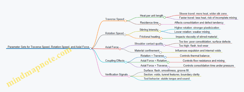
Traverse speed, rotation speed, and axial force form the “three knobs” that control heat input, material flow, and consolidation in friction stir processing and friction stir welding. Treat them as a coupled system: changing one knob usually forces you to re-check the other two, because the tool’s ability to stir depends on both thermal conditions and mechanical pressure.
Foundational Relationships That Guide Parameter Sets
Start with the idea that heat comes mainly from friction and plastic deformation. Rotation speed increases the rate of stirring and frictional heating. Traverse speed changes how long the tool spends at a location: slower travel increases heat per unit length, while faster travel reduces it.
Axial force (or plunge depth in some setups) governs how well the shoulder contacts the workpiece and how strongly the pin drives plasticized material. Too little axial force can lead to poor contact, insufficient consolidation, and surface defects. Too much axial force can over-plasticize the material, increase flash, and accelerate tool wear.
A practical way to think about parameter sets is to target a stable “stir regime” where the stirred zone is fully consolidated and the tool maintains consistent contact. You don’t need a perfect equation; you need repeatable behavior.
Building a Parameter Set Step by Step
- Choose a baseline rotation speed based on material and tool size. Higher rotation generally improves mixing but also raises heat and can widen the stir zone.
- Select a traverse speed that matches the desired heat per unit length. If you see incomplete consolidation or lack of mixing, reduce traverse speed or increase rotation slightly. If you see excessive flash or overly softened material, increase traverse speed or reduce rotation.
- Set axial force to achieve full shoulder contact and stable material flow. If the surface shows void-like features or tunnel-like indications, increase axial force modestly. If you see heavy flash, reduce axial force or increase traverse speed.
Use small, controlled changes. A good rule is to adjust only one parameter at a time by a small step, then verify with surface appearance and a quick section check.
Mind Map: How the Three Knobs Interact
Example Parameter Sets for Common Scenarios
Example 1: Aluminum Alloy Butt Joint With Stable Surface and Clean Cross-Section
- Goal: consistent consolidation without excessive flash.
- Start point: medium rotation, moderate traverse, sufficient axial force.
- If the first trial shows a slightly dry-looking surface and a faint internal lack-of-bond region, reduce traverse speed by a small step (more heat and time) before changing rotation.
- If the stir zone becomes too wide and flash increases, increase traverse speed slightly or reduce axial force rather than dropping rotation aggressively.
Example 2: Thick Section With Risk of Internal Voids
- Goal: ensure the pin and shoulder fully consolidate the volume.
- Use a parameter set that increases mechanical confinement: increase axial force modestly and verify shoulder contact.
- If voids persist, reduce traverse speed slightly to increase residence time under pressure.
- Avoid compensating solely with rotation speed; higher rotation can soften material but may not provide enough confinement to close internal gaps.
Example 3: Dissimilar Joint Where Mixing Must Be Controlled
- Goal: promote bonding while limiting excessive intermixing that can create brittle regions.
- Use a balanced thermal-mechanical set: moderate rotation to stir, slightly higher traverse than you would use for a single-material joint, and axial force set to ensure full contact.
- If bonding is incomplete, increase axial force first, then adjust traverse speed. If the joint looks overly smeared or the stir zone is too large, reduce rotation slightly.
Practical Verification Checklist for Each Trial
After each parameter set, check three things in order: surface condition, cross-section features, and tool stability indicators (such as consistent torque or power draw). Surface flash is not automatically bad, but sudden changes usually mean you moved out of the stable contact regime. Cross-section checks tell you whether the thermal balance and confinement were sufficient to eliminate internal voids.
Finally, record the parameter set as a unit: rotation speed, traverse speed, axial force, tool geometry, and any plunge depth or dwell used. The “best” set is the one that reproduces the same defect pattern with the same tool condition—because friction stir is less about magic numbers and more about controlled cause-and-effect.
3.5 Tool Condition Monitoring Using Dimensional Checks and Surface Wear Indicators
Tool condition monitoring is the practical bridge between “parameters on paper” and “quality on the part.” The goal is to detect drift early enough that you can correct it before defects show up in the weld or stir zone.
Foundational Concepts for What Changes First
A friction stir tool mainly changes in three ways: geometry, surface condition, and alignment. Geometry drift includes shoulder face wear, pin length reduction, and thread or flute rounding. Surface condition changes include polishing, galling, and buildup of workpiece material. Alignment drift includes tilt or runout that alters effective contact pressure.
Start with a simple rule: if the tool’s effective contact area changes, the heat input and material flow change. That’s why dimensional checks and wear indicators are not “nice to have”; they are the fastest way to explain why a stable parameter set suddenly produces different results.
Dimensional Checks That Catch Geometry Drift
Use a repeatable measurement routine at defined intervals, such as after a set number of welds or after a fixed run time. Measure the features that control contact and penetration.
- Pin length and shoulder-to-pin relationship: Compare current pin length to the qualified baseline. A shorter pin can reduce mixing volume and increase the risk of incomplete bonding.
- Shoulder face diameter and flatness: Shoulder wear changes the effective heat generation area. Even a small reduction can shift the stir zone size.
- Pin profile and thread sharpness: Rounding of threads reduces grip and can increase defect sensitivity.
- Tool concentricity and runout: Measure spindle/tool runout with a dial indicator. Excess runout can create uneven material flow and surface defects.
A practical example: if pin length decreases by 0.3 mm and you keep the same axial force, the tool may still “feel” similar during setup, but the stir volume shrinks. The first symptom is often a narrower stir zone in sectioning, followed by lower joint strength.
Surface Wear Indicators That Explain the “Why”
Dimensional checks tell you what changed; surface indicators tell you how it changed.
- Shoulder face polishing: A smooth, mirror-like shoulder often indicates stable sliding contact. If polishing becomes uneven, it can signal misalignment or debris interference.
- Galling and smeared workpiece transfer: Look for dark smears or adhered material on the pin. This can alter friction behavior and promote inconsistent mixing.
- Edge chipping on the pin: Chips create local stress concentrations and can seed surface defects.
- Debris in grooves or threads: Packed debris can act like a thermal insulator or change the effective tool profile.
A practical example: after several runs on a magnesium-containing alloy, you notice increased dark buildup on the pin flanks. The next weld shows more surface flash and a slightly higher torque. Cleaning the tool and verifying pin profile often restores the previous defect-free window.
Measurement Workflow That Stays Consistent
Use a workflow that minimizes measurement variability.
- Before production: Verify tool baseline dimensions and record spindle runout.
- During production: Perform quick checks at set intervals, focusing on pin length and shoulder condition.
- After abnormal events: If you hit a fixture mismatch, tool chatter, or an unexpected torque spike, measure immediately.
Keep a simple log with: tool ID, run count, measured dimensions, observed wear type, and the last two weld outcomes (for example, visual surface quality and one quick NDT metric if available). This turns monitoring into a cause-and-effect trail.
Mind Map: Tool Condition Monitoring Signals and Actions
Example: Turning Measurements into a Decision
Assume a tool baseline pin length is 9.50 mm. After 12 welds, you measure 9.20 mm and observe mild shoulder polishing with no galling. You also see slightly increased flash and a small reduction in stir zone width on a routine section.
A structured decision looks like this:
- Confirm measurement repeatability with a second check.
- Compare wear pattern to prior logs for similar run counts.
- If the stir zone reduction matches the expected mixing volume loss from pin shortening, treat it as geometry-driven.
- Correct by either replacing the tool or requalifying the process with the new effective geometry, depending on your quality system.
The key is that you do not “guess” based on one weld. You connect the dimensional change to the observed quality shift, then act on that link.
Practical Limits and Acceptance Mindset
Set clear acceptance thresholds for each measured feature, tied to your qualified process window. For example, a pin length reduction threshold should be linked to the minimum stir volume needed for defect-free bonding. Surface indicators should trigger cleaning or replacement when they suggest friction behavior has changed, not merely when the tool looks “worn.”
Monitoring works best when it is boringly consistent: measure the same way, log the same fields, and make decisions based on recorded cause-and-effect rather than memory.
4. Friction Stir Welding Process Development and Qualification
4.1 Establishing Baseline Trials Using Design of Experiments Methods
Baseline trials are the first “reality check” before you spend time chasing optimization. The goal is simple: map how key inputs affect measurable outputs, using a plan that avoids wasting runs and avoids fooling yourself with accidental correlations.
Step 1: Define the Trial Objective and Success Metrics
Start by writing one sentence that states what you want the baseline to tell you. For friction stir processing and friction stir welding, typical objectives include stable defect-free bonding, consistent penetration, and repeatable hardness or tensile performance. For laser hybrid and electron beam hybrid concepts, baseline objectives often include defect suppression (porosity, lack of fusion, keyhole instability) and stable joint geometry.
Then define measurable outputs. Examples:
- Defect indicators: tunnel presence, kissing bond, porosity count, lack of fusion length.
- Geometry indicators: penetration depth, surface flash height, undercut, bead width.
- Property indicators: hardness profile across the processed zone, tensile shear strength, fatigue crack initiation location.
- Process stability indicators: torque or spindle load trend, temperature proxy signals, beam power stability.
A good baseline includes at least one output you can measure quickly (geometry or hardness) and one that represents performance (tensile or fatigue-relevant proxy).
Step 2: Choose Factors and Set Practical Ranges
Design of experiments (DoE) works best when factors are controllable and ranges are realistic. Pick a small set of “likely drivers” first.
For friction stir processing, common factors include:
- rotation speed (RPM)
- traverse speed (mm/min)
- axial force or plunge depth
- tool tilt angle
- tool pin profile and shoulder diameter (often fixed during baseline)
For laser hybrid, add:
- laser power
- spot size or beam diameter
- standoff distance
- laser travel synchronization relative to tool motion
For electron beam welding, add:
- acceleration voltage
- beam current
- focus setting
- beam dwell or travel speed
Set ranges using prior shop knowledge, vendor data, and a few “safe” scouting runs. If you don’t know the range, start narrow enough to avoid catastrophic defects, then widen after you see trends.
Step 3: Select an Experimental Design That Matches Your Constraints
Baseline trials usually need efficiency and robustness. Common choices:
- Fractional factorial when you expect interactions but can’t run full combinations.
- Response surface designs (like central composite) when you want curvature and a likely optimum region.
- Taguchi-style orthogonal arrays when you need a quick ranking of factors with limited runs.
A practical rule: if you mainly want to identify which factors matter, use a screening design. If you want to model the relationship and later tune parameters, use a response surface design.
Step 4: Plan Replication, Randomization, and Blocking
Replication estimates experimental noise. Randomization prevents systematic bias from creeping in (for example, tool wear increasing over time). Blocking handles known nuisance variables.
Examples of blocking:
- different plate lots or heat treatments
- different tool conditions (new vs. lightly worn)
- different fixture setups or operator shifts
If you can only afford a few runs, prioritize randomization and at least one replicated center point. Center points are useful because they reveal whether your response is linear in the region or already curving.
Step 5: Build a Baseline Run Sheet with Clear Acceptance Checks
Each run should include:
- factor settings
- specimen ID and block ID
- planned measurement sequence
- immediate go/no-go checks (fit-up, tool contact, laser alignment, vacuum stability)
A baseline run sheet should also specify what happens if a run fails early. For instance, if friction stir processing shows severe surface tearing, you record it as a defect outcome and stop further machining on that specimen.
Mind Map: Baseline DoE Workflow
Example: Screening DoE for Friction Stir Processing on Aluminum
Assume you want to find which factors most affect tunnel formation and hardness uniformity. You choose three factors for a screening design:
- rotation speed: 900, 1100, 1300 RPM
- traverse speed: 60, 90, 120 mm/min
- axial force: 6, 9, 12 kN
You include center points at 1100 RPM, 90 mm/min, 9 kN to estimate noise and curvature. You randomize run order across the day and block by tool condition (new tool for half the runs, lightly worn tool for the other half).
After testing, you measure hardness at fixed offsets from the stir zone centerline and inspect cross-sections for tunnel presence. If the model shows that traverse speed has the strongest effect on tunnel probability, you narrow the range around the “safe” traverse region for the next response surface study.
Example: Baseline DoE for Laser Hybrid Alignment Sensitivity
For a laser-assisted friction stir concept, you keep mechanical parameters fixed at a known good baseline and vary only laser power and standoff distance. Outputs include porosity count and surface flash height.
If higher power reduces lack of bonding but increases porosity, the baseline model will show a tradeoff. You don’t need to “solve” it yet; you only need to identify the region where defects are minimized without causing new failure modes.
Step 6: Analyze with Models That Match the Data Quality
Use the DoE results to compute main effects and interactions first. Then check whether curvature is present by comparing center point behavior to the model’s linear prediction. If the model fits poorly, it usually means either ranges are too wide, measurement noise is high, or an important factor was omitted.
A baseline is successful when you can state, with evidence, which factors matter most, which interactions are real, and what parameter region produces consistent, measurable outcomes.
4.2 Parameter Windows for Defect Free Stir Zones and Consistent Penetration
A “parameter window” is the range of tool rotation, travel speed, and axial force that produces a stable stir zone with full bonding and predictable penetration. Think of it as a three-dimensional envelope: move one knob too far and the process compensates poorly, so defects show up where the material flow stops behaving.
Foundational Relationships That Define the Window
Start with the material state at the tool. Rotation supplies heat and drives plasticized material circulation; travel speed controls how long the material stays under the tool; axial force governs contact pressure, frictional heating, and the ability to forge the stirred material into the joint.
A practical baseline rule is: if you increase travel speed without changing rotation and force, the stir zone tends to become underdeveloped because the material has less time to soften and mix. If you increase rotation without increasing axial force, you may generate heat but not enough forging pressure to close voids. If you increase axial force too much, you can overfill the stir zone, raise flash, and disturb the interface.
Defect Signatures and What They Usually Mean
Defects are not random; they are usually consistent with a specific imbalance.
- Lack of bond at the advancing side often points to insufficient heat input or inadequate contact pressure during that portion of the pass.
- Tunneling or voids near the tool axis often indicate that the material is not being fully consolidated as it flows downward and then back up.
- Surface flash or excessive material extrusion often indicates over-pressurization or too much material being stirred relative to the available consolidation.
- Inconsistent penetration along the weld line often indicates unstable tool condition, inconsistent fit-up, or parameter drift that changes the effective contact.
Use these signatures to map your observations back to the likely parameter imbalance.
Building the Window Systematically
- Lock the joint and tooling baseline. Confirm consistent fit-up, correct tool shoulder contact, and stable tool length. Even perfect parameters fail if the tool is effectively “floating” due to poor fixturing.
- Choose one parameter to sweep first. Typically sweep rotation while holding travel speed and axial force constant. Record stir zone appearance, interface bonding quality, and penetration depth.
- Identify the “minimum viable heat” boundary. Reduce rotation until you start seeing incomplete bonding or a measurable drop in penetration. That boundary is your lower limit for rotation under current travel speed and force.
- Identify the “overheating and overfilling” boundary. Increase rotation until you see flash, excessive thinning, or signs of unstable flow. That boundary is your upper limit.
- Repeat the process for travel speed. With rotation fixed near the middle of the rotation window, vary travel speed to find the range that maintains full bonding without creating under-stirred regions.
- Repeat for axial force. With rotation and travel speed fixed near the center of the earlier windows, vary axial force to find the range that consolidates the stirred material without producing excessive flash.
The center of the window is not where defects are absent in a single cross-section; it is where defects are least sensitive to small variations in tool condition and fit-up.
A Simple Example Parameter Map
Assume an aluminum alloy butt joint. You start with a conservative baseline: rotation 900 rpm, travel speed 80 mm/min, axial force 6 kN.
-
Sweep rotation from 800 to 1000 rpm at 80 mm/min and 6 kN.
- At 800 rpm you observe intermittent lack of bond near the advancing side.
- At 950 rpm bonding is consistent and penetration is full.
- At 1000 rpm you see increased surface flash and slightly rougher interface.
- Result: rotation window roughly 850–980 rpm.
-
Fix rotation at 950 rpm and sweep travel speed from 60 to 100 mm/min at 6 kN.
- At 100 mm/min penetration becomes shallow.
- At 80–90 mm/min results are consistent.
- At 60 mm/min you see more flash and wider stir zone.
- Result: travel speed window roughly 70–95 mm/min.
-
Fix rotation at 950 rpm and travel speed at 85 mm/min and sweep axial force from 4 to 8 kN.
- At 4 kN you get voids near the axis.
- At 6–7 kN voids close and interface bonding improves.
- At 8 kN you get overfill and flash.
- Result: axial force window roughly 5–7.5 kN.
Now choose a “working point” near the middle: 950 rpm, 85 mm/min, 6.5 kN.
Mind Map: Parameter Window Logic
Validation Checks That Confirm the Window
After selecting a working point, validate with at least a small matrix around it, not just one trial. For example, test rotation ±5%, travel speed ±5%, and axial force ±0.5 kN. If penetration and bonding remain consistent across that neighborhood, you likely found a robust window rather than a lucky one.
Finally, confirm that the tool shoulder actually maintains contact along the weld path. If penetration changes when the tool is moved to a new section of the part, the issue is often fixturing or surface height variation, not the “wrong” rotation or force.
4.3 Multi Pass Strategies for Thick Sections and Complex Weld Paths
Thick-section friction stir welding and friction stir processing are less forgiving than thin plates because the tool must move enough heat and plasticized material through a larger volume. Multi-pass strategies address this by controlling how much material is stirred, where the mixing happens, and how defects get “worked out” rather than simply averaged away. The key idea is simple: each pass has a job, and the next pass either builds on that job or corrects what the previous pass could not fully accomplish.
Foundational Pass Roles
A practical multi-pass plan usually combines three roles:
- Penetration establishment: early passes ensure the tool reaches the intended bottom of the stir zone (or the intended depth for processing). If the first pass is too shallow, later passes may only remix the top portion.
- Mixing and bonding improvement: intermediate passes increase the chance of full contact and reduce unbonded regions by re-stirring previously processed material.
- Surface and edge finishing: final passes smooth the top surface, reduce surface voids, and help align the stir zone with the final joint line.
A useful rule of thumb is to treat the first pass as the “depth setter,” the middle passes as “quality builders,” and the last pass as “geometry corrector.”
Thick-Section Strategy: Overlap and Step-Down Logic
For thick sections, the tool’s effective stirring volume is limited by shoulder contact, pin length, and thermal conditions. Multi-pass approaches typically use either overlap in the travel direction or step-down in depth (when the process allows). In both cases, the goal is to avoid leaving a persistent band that never gets fully stirred.
A systematic approach looks like this:
- Choose a target stir-zone envelope based on joint requirements and allowable defect size.
- Select a pass spacing so that the stir zones overlap enough to eliminate “cold seams.” If overlap is too small, you get a layered structure of partially mixed bands.
- Set the axial force and tool tilt consistently across passes so the overlap is repeatable.
Easy example: Suppose you are joining a 12 mm plate and your single-pass stir zone reliably reaches only about 7–8 mm depth. You can run two passes with controlled overlap so the second pass re-stirs the lower portion that the first pass under-processed. The second pass should not be a copy-paste; it must be positioned so its stirred volume intersects the first pass’s lower boundary.
Complex Weld Paths: Managing Heat and Material Flow
Complex paths include curved seams, branching joints, and multi-segment tool trajectories. The risk is that the tool may repeatedly stir the same region while leaving other regions under-processed, especially near corners and direction changes.
A robust method is to design the path as a sequence of straight segments plus controlled transitions:
- Straight segments: maintain stable kinematics and consistent contact.
- Transitions: slow down slightly or adjust dwell at corners so the material flow has time to reorganize.
- Segment overlap: ensure the transition zones are not “dead ends” where the tool exits before bonding is established.
Easy example: For a T-joint with a branch, run the main seam first to establish a continuous stir track. Then run the branch pass so it overlaps the end region of the main seam. If you start the branch exactly at the main seam end without overlap, the corner can trap an unbonded pocket because the material flow from the main seam has already cooled and settled.
Pass Sequencing and Direction Control
Pass direction matters because material flow is not perfectly symmetric. When you reverse direction between passes, you can change how the stirred material fills gaps and how surface flash forms.
A practical sequencing method:
- Keep the same direction for passes that are meant to build a continuous stir envelope.
- Reverse direction only when you need a specific correction, such as re-stirring a surface defect band.
- Avoid abrupt direction changes without a transition plan.
Easy example: If the first pass leaves a thin surface groove along the joint line, a second pass in the same direction may not fully cover it. A corrective pass that slightly offsets and re-stirs that groove can be more effective than simply increasing speed.
Mind Map: Multi-Pass Strategy Framework
Verification Checks That Actually Tell You Something
After you run a multi-pass trial, you want evidence that the overlap and transitions did what you intended. Three checks are especially informative:
- Cross-section inspection: look for continuous bonding across pass boundaries rather than isolated “islands” of good material.
- Hardness mapping: hardness often reveals whether a band was under-processed, even when the surface looks fine.
- Surface defect review: surface voids and lack of fill can indicate that the final pass did not correct the earlier flow pattern.
Easy example: If hardness drops sharply at the boundary between pass 1 and pass 2, the overlap is likely insufficient or the second pass did not re-stir the boundary region. Increasing overlap or adjusting tool position by a small, controlled offset usually fixes the pattern more reliably than changing multiple parameters at once.
A good multi-pass strategy is not just “more passes.” It is a planned sequence where each pass has a defined job, the overlap is intentional, and the path transitions are treated as part of the process rather than an afterthought.
4.4 Qualification Testing Plans for Tensile Shear and Fatigue Relevant Metrics
A qualification plan turns “it seems strong” into measurable evidence. For friction stir welding (FSW) and friction stir processing (FSP) joints, the tensile shear and fatigue metrics should be tied to the failure modes you actually expect: interface separation, reduced load transfer through the stir zone, and crack initiation near the weld toe or processed boundary.
Foundational Metrics and What They Prove
Start by defining the metrics that map to performance requirements.
- Tensile shear strength verifies load transfer across the joint under near-uniform stress. It is sensitive to incomplete bonding, weak stir-zone regions, and poor penetration.
- Fatigue life and crack growth behavior verify how microstructure and residual stress distributions affect cyclic damage. It is sensitive to surface condition, internal defects, and local hardness gradients.
- Fracture location and fracture mode confirm whether failure is in the stir zone, heat-affected region (for hybrid or fusion welds), or base material. This is where many qualification plans quietly win or lose.
A practical rule: if tensile shear fails by consistently pulling apart at the interface, fatigue results will be dominated by the same weakness. If tensile shear breaks in base material, fatigue scatter typically narrows.
Test Article Selection and Baseline Control
Qualification is only as good as the test articles.
- Replicate production geometry: use the same joint type, thickness, edge distance, and fixturing strategy as production. A “lab coupon” with different restraint can change residual stress and distortion.
- Control the process window: pick at least three parameter sets—low, nominal, and high within the intended window. Include one set that is intentionally near the edge of acceptable quality to prove robustness.
- Standardize tool condition and surface prep: tool wear and oxide contamination can shift both tensile shear and fatigue scatter. Record tool wear indicators and cleaning steps for every batch.
Tensile Shear Testing Plan
Tensile shear tests should be designed to reveal joint integrity rather than just peak load.
- Specimen geometry: choose a configuration that produces shear-dominant loading at the joint. Ensure the gauge region includes the full stir zone length and any transition regions.
- Strain rate and temperature: keep them consistent across all parameter sets. Even when the material is ductile, changing strain rate can change failure mode.
- Measurements: record load-displacement curves, calculate shear strength, and document fracture location with a simple coordinate system (e.g., “0% at advancing side toe, 50% at mid-length”).
- Acceptance logic: set minimum strength and require that a defined fraction of specimens fail outside the interface. For example, require that at least 80% of specimens show fracture through the stir zone or base material rather than along the bond line.
Example: If nominal parameters yield 95% stir-zone fracture and the low-parameter set yields 40% interface fracture, you have evidence that penetration or bonding quality is the limiting factor. That same limiting factor should be reflected in fatigue expectations.
Fatigue Testing Plan for Cyclic Relevance
Fatigue qualification needs a loading definition that matches service.
- Select a stress metric: use stress ratio (R), mean stress control method, and a consistent definition of nominal stress at the critical section.
- Choose a frequency range: keep it within a range that does not introduce heating or rate effects that change crack initiation.
- Define runout criteria: specify the maximum cycles for runout and the allowable stiffness change. Runout without stiffness tracking can hide slow crack growth.
- Surface and notch control: fatigue cracks often start at the weld toe or processed boundary. Keep surface finishing consistent and document any grinding or machining steps.
Example: Two parameter sets can have similar tensile shear strength, yet one shows earlier fatigue crack initiation because it produces a sharper hardness gradient at the toe. Your plan should therefore include crack initiation location mapping and hardness profiling at the same coordinates.
Mind Map: Qualification Testing Workflow
Data Integration and Decision Rules
Qualification is not just collecting results; it is deciding what they mean.
- Correlate tensile shear fracture mode to fatigue scatter: if interface fracture appears in tensile tests, expect larger fatigue scatter and earlier initiation.
- Use defect and NDE outcomes as gating criteria: if internal defects exceed a defined threshold, fatigue results should not be used to “prove” acceptability. Treat them as disqualifying for the qualified process window.
- Set parameter window boundaries: use the low and high sets to define where tensile shear and fatigue remain within acceptance. The nominal set should sit comfortably inside those boundaries.
Example: Suppose nominal parameters meet tensile shear strength and show stir-zone fracture, while the low set meets strength but shows mixed fracture locations. In that case, you can qualify nominal parameters for fatigue while requiring additional controls or tighter limits for the low boundary.
Practical Documentation Checklist
Keep the plan auditable and repeatable.
- Specimen batch IDs tied to tool condition and surface prep.
- Parameter set definitions with recorded spindle speed, traverse speed, axial force, and tilt.
- Test conditions for tensile shear and fatigue including temperature, strain rate, stress ratio, frequency, and runout.
- Fracture location method and coordinate reference.
- Fatigue crack initiation tracking method and inspection intervals.
A good qualification plan makes it hard to argue with the data. It also makes it easy to reproduce the results without guessing which detail mattered.
4.5 Documentation Requirements for Procedure Qualification Records
Procedure qualification records (PQRs) are the paper trail that turns “it worked in trials” into “it will work on the shop floor.” The goal is simple: a qualified procedure must be reproducible by someone who was not in the room during qualification.
Foundations of What Must Be Documented
Start by capturing the identity of the procedure and the scope of qualification. Record the process family (friction stir processing, friction stir welding, laser hybrid, electron beam welding), the joint type, and the material system. Then document the exact variables that control heat input, material flow, and fusion behavior. If a variable is not recorded, it cannot be controlled later, and the qualification becomes more of a story than a procedure.
A practical way to think about PQR content is to separate it into four layers:
- Who and where: organization, equipment, and calibration status.
- What: base materials, thickness, joint geometry, and consumables.
- How: parameter set, tool or beam settings, and process controls.
- What happened: test results, defect observations, and acceptance decisions.
Core Record Elements and Their Purpose
Procedure Identification and Qualification Basis
Include a unique procedure identifier, revision level, and the qualification date (for example, 2026-03-11). State the standard or internal acceptance framework used for qualification. List the test coupons and the locations where they were extracted so the mechanical results can be traced back to the weld or processed zone.
Materials, Consumables, and Condition Control
Record alloy designations, temper condition, and batch or heat numbers where available. For friction stir, note tool material and any coating or surface treatment. For laser and electron beam, record shielding gas type and flow settings, and for electron beam, record vacuum conditions and beam alignment method.
A small but important habit: document the as-received surface condition and cleaning method. For example, if aluminum coupons were degreased with acetone and brushed with stainless wire, write it down. If you only say “cleaned,” you lose the ability to explain why porosity or surface oxide inclusion behaved differently.
Process Parameters and Controls
List the parameter set exactly as used, including rotation speed, traverse speed, axial force (or equivalent), tool tilt, plunge depth, dwell time, and pass strategy. For hybrid laser systems, include laser power, spot size or beam diameter, focal position, and standoff distance, plus the alignment offset relative to the tool.
For electron beam, record acceleration voltage, beam current, focus setting, and scan pattern. Also record fixturing constraints and any preheating or post-weld handling steps.
Test Results and Evidence of Acceptance
Document macro and micro examination methods, including sectioning orientation and etchant or polishing approach. Record hardness mapping locations and grid spacing. For mechanical tests, specify specimen geometry, test temperature, strain rate or loading method, and failure location.
When defects are found, record them with their location and severity assessment. If a trial coupon fails acceptance, keep the record and note which parameter change corrected it. That turns “failure” into useful engineering information rather than a dead end.
Mind Map: Procedure Qualification Record Content
Example: A Traceable PQR Entry Set
Example scenario: qualifying a friction stir weld on 6 mm AA6061-T6 butt joints.
- Materials: AA6061-T6, thickness 6.0 mm, coupon batch ID recorded.
- Joint geometry: butt joint with 0.5 mm root gap, edges milled and cleaned.
- Surface prep: degreased with solvent, brushed, then assembled within a defined time window.
- Tooling: tool diameter, pin profile, tool material, and measured wear state.
- Parameters: rotation speed, traverse speed, axial force, tool tilt, plunge depth, and dwell time.
- Evidence: macro section showing continuous bonding, hardness map with grid coordinates, tensile results with fracture location.
- Acceptance: pass decision tied to the stated criteria, with any observed minor surface flash documented.
If the next production run uses the same procedure ID but a different tool wear state, the PQR should already explain how tool condition is handled. For instance, it may specify a maximum allowable shoulder wear or a re-measurement step before production.
Practical Documentation Habits That Prevent Rework
Write parameter values in the same units used on the machine interface. Record tolerances where they matter, such as axial force limits or alignment offsets. Keep calibration identifiers for key sensors so measurements are not treated as “trust me, it was calibrated.” Finally, ensure the record links test results to the exact coupon and extraction location, so a reviewer can follow the chain without guessing.
5. Friction Stir Processing for Property Tailoring
5.1 Friction Stir Processing Fundamentals for Surface and Subsurface Modification
Friction Stir Processing (FSP) is friction stir welding’s more focused cousin: instead of joining two parts, it locally stirs and thermomechanically modifies a region of a single workpiece. The goal is usually to change surface condition, refine microstructure beneath the surface, or reduce defects left by casting, forming, or prior processing. Think of it as controlled mixing with a heat source that comes from mechanical work rather than a flame.
Core Mechanism and What Actually Moves
FSP uses a rotating tool with a shoulder and a pin. The shoulder rubs near the surface, generating most of the heat and constraining material flow. The pin penetrates into the workpiece, forcing plasticized material to circulate around it. Material motion is not random: it follows a pattern tied to tool rotation direction, pin geometry, and the tool’s traverse direction.
A useful mental model is a “stirring loop.” As the tool advances, material ahead of the pin is heated and softened, then swept around the pin, and finally deposited behind the tool in a refined, mixed state. This loop is why FSP can improve subsurface regions even when the surface looks only moderately changed.
Heat Input and Plasticization Without Melting
In most FSP conditions, the material is heated into a plastic state without fully melting. That matters because solid-state processing tends to limit some fusion-weld issues such as large solidification shrinkage porosity. The temperature rise depends mainly on rotation speed, traverse speed, axial force, and tool geometry. Higher rotation speed generally increases heat generation, while faster traverse reduces time for heating.
A practical example: if you see a surface that is too rough and hardness drops sharply, you likely ran too “hot” or too long at a given location. If you see incomplete mixing and a patchy microstructure, you likely ran too “cool” or too fast, so the material never fully plasticized.
Microstructural Zones and Their Roles
Even though FSP is a single operation, the processed region is not uniform. Typical zones include:
- Stir Zone: where intense mixing and grain refinement occur.
- Thermo-Mechanically Affected Zone: where deformation and moderate heating alter microstructure.
- Heat-Affected Zone: where temperature changes occur with less deformation.
Surface modification often targets the stir zone depth. Subsurface modification requires enough pin penetration and sufficient heat to drive mixing below the surface. If the pin barely reaches the target depth, you may get a refined surface layer with a less improved core.
Tool Geometry and Process Parameters as Coupled Knobs
Tool design and process parameters work together, not independently.
- Pin length and shape control the depth and pattern of material circulation.
- Shoulder diameter influences heat generation and surface confinement.
- Axial force affects contact pressure, heat generation, and how well the tool “grips” the softened material.
- Rotation speed and traverse speed set the balance between heat input and residence time.
Example workflow for a shallow surface improvement: choose a pin length that covers the desired depth plus a small margin, then start with moderate rotation speed and a traverse speed that produces a continuous, defect-free surface. If you need deeper subsurface refinement, increase pin penetration first, then adjust rotation and traverse to maintain adequate mixing rather than simply raising temperature.
Defect Control and Surface Integrity
FSP can introduce defects if material flow is unstable or if the tool does not maintain consistent contact.
Common issues include:
- Surface tearing or voids from insufficient plasticization or poor contact.
- Tunnel-like features when the tool does not fully consolidate the stirred material.
- Overheating-related softening that reduces hardness and strength.
A simple diagnostic approach is to compare surface appearance with cross-section observations. If the surface looks fine but the subsurface shows poor mixing, the issue is often insufficient penetration or inadequate heat-time balance. If both surface and subsurface look degraded, the issue is often excessive heat input or axial force mismatch.
Mind Map: Fundamentals for Surface and Subsurface Modification
Integrated Example: From Surface to Subsurface in One Plan
Suppose you need to refine a 2 mm surface layer and improve the microstructure down to 4 mm in an aluminum plate. Start by selecting a pin length that reaches slightly beyond 4 mm while ensuring the tool can maintain stable contact. Use a moderate rotation speed and a traverse speed that yields a continuous stir zone without surface tearing. After the first trial, cut a cross-section: if the stir zone depth is short, increase pin penetration or reduce traverse speed slightly; if the stir zone is deep but hardness is too low, reduce heat input by lowering rotation speed or increasing traverse speed. This keeps the reasoning anchored to what you observe rather than chasing numbers blindly.
5.2 Pass Layout Design Including Overlap and Overlap Direction Effects
Pass layout design is where “the process” becomes “the part.” In friction stir processing, each pass leaves behind a stirred region with a characteristic stir zone shape, thermal history, and material flow pattern. Overlap determines whether adjacent stirred regions fuse into a continuous, defect-resistant processed volume—or whether you end up with seams, soft bands, or inconsistent properties.
Foundational Concepts of Overlap
Overlap is the intentional sharing of material between neighboring passes. If overlap is too small, the processed regions remain separated by partially processed material that may not reach the intended temperature or strain state. If overlap is too large, you can overwork the material, increase heat input, and promote excessive softening or defect sensitivity depending on alloy and tool condition.
A practical way to think about overlap is to treat the stir zone as having a “core” that is fully mixed and a “periphery” that is only partially mixed. Your goal is to cover the periphery of one pass with the core of the next pass.
Overlap Direction Effects and Why They Matter
Overlap direction refers to how the second pass is positioned relative to the first in the direction of travel and the tool’s rotation-driven material flow. Even when the overlap percentage is the same, changing direction can alter whether the advancing side of one pass meets the retreating side of the next.
In many setups, material flow is not symmetric across the tool. That means the interface between passes can become either a well-bonded, well-mixed transition or a boundary where mixing is weaker. A simple rule of thumb for layout trials: keep the overlap direction consistent while you establish a parameter window, then vary direction only after you know the baseline defect behavior.
Systematic Pass Layout Workflow
- Define the target processed volume: For a plate, this is usually a strip or a rectangle of stirred material. Mark the edges and any required coverage margins.
- Choose a starting overlap: Begin with a moderate overlap that is known to produce continuity in your material class. Use it to validate defect-free continuity before optimizing.
- Plan the first row and subsequent rows: For multi-pass coverage, decide whether each new pass will be aligned directly beside the previous pass or offset to manage interface quality.
- Control the overlap direction: Decide whether the second pass will “chase” the first pass interface in the same relative flow sense or oppose it. Lock this choice for the first qualification run.
- Verify continuity with sectioning: Cut cross-sections perpendicular to travel and inspect the interface region for lack of mixing, voids, or tunnel-like features.
Mind Map: Pass Layout Design Logic
Concrete Example: Single Row Overlap Optimization
Imagine processing a 10 mm thick aluminum plate to create a continuous stirred strip. You run three adjacent passes in a single row. Pass 1 and Pass 2 overlap by a chosen amount, and Pass 2 and Pass 3 overlap by the same amount.
- If overlap is small: the cross-section shows a faint boundary line where mixing is weaker. Hardness across the strip varies, and tensile specimens taken across the boundary show reduced performance.
- If overlap is moderate: the interface becomes indistinct, and hardness becomes flatter across the strip.
- If overlap is large: the interface may still look continuous, but hardness drops overall, indicating excessive thermal exposure or overstraining.
The key is that the “best” overlap is the one that makes the interface disappear without shifting the entire stir zone into a softer state.
Concrete Example: Two-Row Layout and Direction Choice
Now process a wider area using two rows of passes. Row 1 is laid first, then Row 2 is added beside it.
- Consistent overlap direction: the interface between rows forms a smooth transition. Microstructure shows continuous grain refinement across the row boundary.
- Reversed overlap direction: even with identical overlap percentage, the interface can show a thin band with less uniform mixing. This often appears as a localized change in hardness or a subtle defect-like feature.
To manage this, treat direction as a controlled variable. If you must change direction for geometric reasons, compensate by adjusting overlap magnitude slightly and re-check the interface region.
Practical Checks for Interface Quality
When you section the processed area, focus on three observations: (1) whether the interface line is visible, (2) whether hardness changes abruptly at the interface, and (3) whether microstructure indicates continuous mixing rather than a partially stirred seam. If any of these fail, adjust overlap magnitude first, then revisit overlap direction.
A good layout is the one that makes the part behave like it was processed as a single continuous volume, not like it was assembled from separate strips. Overlap is how you get that illusion to become reality.
5.3 Thickness and Substrate Constraints for Controlled Material Mixing
Controlled material mixing in friction stir processing (FSP) depends on whether the tool can “stir through” the full thickness without starving the stir zone or overheating the interface. Thickness and substrate constraints are not just geometric limits; they determine how much material is available to shear, how the plasticized volume flows, and whether the interface stays bonded.
Foundational Mixing Logic
Start with the idea of a stir zone volume: the tool shoulder and pin displace material, then frictional heating softens it enough for plastic flow. If the workpiece is too thin, the pin may break through or create an unstable bottom surface condition, leading to flash, thinning, or weak bonding at the exit side. If the workpiece is too thick, the pin may not generate sufficient through-thickness mixing, leaving a “cold” core that shows poor homogenization and a sharp property gradient.
A practical way to think about constraints is to compare three thickness-related quantities: workpiece thickness (T), effective pin penetration (P), and the region influenced by shoulder contact (S). For stable mixing, P should be close to but not exceed T, and shoulder contact should consistently engage the top surface to maintain heat and forging pressure.
Thickness Constraints That Control Flow
-
Too Thin: When T is close to pin length, the bottom boundary becomes a hard stop. Material has nowhere to go except sideways, which can increase surface turbulence and trap voids near the exit. A simple example is processing a 2 mm sheet with a 2.5 mm pin: the pin tip contacts the backing plate, and the bottom layer experiences severe disruption rather than controlled plastic flow.
-
Too Thick: When T is much larger than pin length, the pin may only mix the upper fraction. The lower portion can remain comparatively unmixed, so hardness and microstructure vary strongly with depth. A common symptom is a stir zone that looks uniform on a cross-section near the top but shows a distinct transition band toward the bottom.
-
Borderline Thickness: The most troublesome cases are where P is “almost” right. Small changes in tool wear, stick-out, or part height can shift the effective penetration enough to change bonding quality. That’s why thickness constraints must be treated as tolerance constraints, not just nominal dimensions.
Substrate Constraints That Control Bonding
Substrate constraints include backing support, surface condition, and any interlayer or coating present at the interface.
-
Backing and Support: The backing plate must provide consistent support so the tool doesn’t lose effective forging pressure. If the backing is compliant or uneven, the tool can deflect, reducing penetration where you need it most.
-
Surface Condition: Oxide films and contamination affect heat transfer and plastic flow. In thin sections, a small surface defect can become a through-thickness flaw because the stir zone spans a larger fraction of the thickness.
-
Interface Layers: If the substrate includes an interlayer (for example, a thin coating or dissimilar interface), mixing must be sufficient to distribute it without creating a continuous brittle reaction band. Controlled mixing means the interface is disrupted enough to avoid planar defects, but not so aggressively that it forms a thick, segregated band.
Parameter Coupling with Thickness
Thickness constraints interact with rotation speed, traverse speed, and axial force.
-
Axial Force and Penetration Stability: Higher axial force increases forging pressure and helps close voids, but it can also increase flash in thin parts. For thin sheets, reduce axial force and ensure pin length is matched to T with tight setup control.
-
Traverse Speed and Heat Balance: Faster traverse reduces heat input per unit length, which can leave the lower region insufficiently softened in thick parts. Slower traverse can improve mixing but risks excessive grain growth or surface over-softening.
-
Rotation Speed and Plasticization: Higher rotation increases frictional heating and plasticization. In thick parts, this can help reach deeper mixing; in thin parts, it can overheat the interface and promote defects.
Mind Map: Thickness and Substrate Constraints
Example: Choosing Tool Length for a 6 mm Plate
Assume a 6 mm aluminum plate and a pin length of 5.8 mm. The goal is to mix through the thickness while avoiding bottom gouging. If the setup height varies by ±0.2 mm, the effective penetration could range from 5.6 to 6.0 mm. That range is acceptable if the backing plate is flat and the axial force is controlled, because the shoulder still provides forging pressure and the pin tip does not repeatedly impact the backing. If instead the pin length were 6.5 mm, even small height errors would cause bottom disruption, increasing the chance of a weak exit-side region.
Example: Thin Sheet with a Backing Plate Gap
Consider a 1.5 mm sheet processed with a pin length matched to thickness. If the backing plate has a small gap or is not clamped flat, the tool can deflect and reduce shoulder contact. The result is a stir zone that may look fine at the top surface but shows poor bonding near the bottom because the forging pressure dropped exactly where the interface closure is most sensitive.
Practical Constraint Checklist
- Verify pin length relative to T with tolerance, not just nominal values.
- Ensure backing plate flatness and stiffness to prevent deflection.
- Confirm shoulder contact consistency across the weld path.
- Match traverse and rotation to thickness so the lower region reaches adequate plasticization.
- Treat surface cleanliness as a thickness multiplier: thin parts magnify small defects.
When thickness and substrate constraints are handled this way, mixing becomes predictable: the stir zone spans the intended depth, interface bonding is maintained, and properties change smoothly rather than abruptly.
5.4 Hardness and Strength Optimization Using Process Parameter Adjustments
Hardness and strength in friction stir processing (FSP) are not “set and forget” outcomes. They come from controlling how much heat is introduced, how long the material spends in that heat-affected range, and how effectively the stirred zone mixes and breaks up microstructural features. A practical way to think about it is: parameters control thermal history, thermal history controls microstructure, and microstructure controls hardness and strength.
Foundations: What Parameters Actually Change
Start with the three knobs that most directly shape the stir zone thermal history.
-
Rotation speed (ω) controls frictional heating rate. Higher ω generally increases peak temperature and can enlarge the stirred zone’s softened region if other settings do not compensate.
-
Traverse speed (v) controls time at temperature. Faster v reduces heat input per unit length and shortens the time available for grain growth and precipitate coarsening.
-
Axial force or plunge depth (F) influences contact conditions and material flow. Too little force can reduce bonding quality and leave weak regions; too much can overheat or cause excessive flash and mixing.
A useful rule of thumb for optimization is to adjust one knob at a time while holding the others constant, then map the hardness response across the stir zone. If you change two knobs simultaneously, you may get a nice hardness number but you won’t know which lever caused it.
Microstructure Targets That Drive Hardness
For many aluminum alloys, hardness is strongly tied to precipitate state and grain size. FSP can refine grains, but it can also dissolve or coarsen strengthening precipitates depending on peak temperature and time.
- Grain refinement tends to increase hardness by increasing grain boundary area.
- Precipitate dissolution or coarsening tends to reduce hardness if strengthening precipitates are lost or grow too large.
- Defect-related soft spots such as voids or tunnel-like features can lower local hardness and reduce strength even if the average microstructure looks fine.
So the optimization goal is usually not “more heat” or “less heat,” but “heat enough to refine and mix, not so much that strengthening features disappear.”
Parameter Adjustment Logic from Simple to Advanced
Step 1: Establish a Baseline Hardness Profile
Measure hardness across the processed width (for example, from advancing side to retreating side and through the stir zone centerline). Record the peak hardness location and the minimum hardness location.
- If hardness is uniformly low, you likely over-softened the alloy or created insufficient consolidation.
- If hardness peaks near the center but drops sharply at edges, you may have inadequate overlap, insufficient mixing at the periphery, or local under-processing.
Step 2: Tune Heat Input Using Rotation and Traverse
A common optimization pattern is:
- If hardness is low due to over-aging or precipitate coarsening, reduce ω or increase v to lower peak temperature or reduce time at temperature.
- If hardness is low due to insufficient mixing or incomplete consolidation, increase ω slightly or reduce v to improve material flow and bonding.
Because these effects can oppose each other, the best practice is to run a small matrix around the baseline, such as three ω values and three v values, then choose the combination that maximizes hardness while keeping the minimum hardness above your acceptance threshold.
Step 3: Adjust Axial Force for Consolidation Without Overheating
Axial force affects contact and material flow. If you see weak bonding or hardness dips near the stir zone boundary, increase force in small increments.
If you see excessive softening or surface issues, reduce force. The key is to treat force as a consolidation lever, not just a “more is better” lever.
Step 4: Use Tool Geometry and Tilt as Secondary Controls
Tool shoulder diameter, pin profile, and tool tilt influence how much material is stirred and how the strain is distributed.
- A pin that does not adequately penetrate the target depth can reduce mixing and leave a weaker band.
- Excessive tilt can change the effective contact area and alter heat generation distribution.
For optimization, change tool geometry only after you have a stable parameter window for ω, v, and F, because geometry changes can shift the whole thermal and flow regime.
Mind Map: Hardness and Strength Optimization Path
Example: Aluminum Alloy with a Hardness Dip at the Stir Zone Edge
You process a 6 mm thick plate and measure hardness. The centerline hardness is acceptable, but the edge hardness drops by 15–20 HV.
-
Check consolidation first. If you also see surface flashes or slight under-processing at the boundary, increase axial force by a small step and repeat.
-
Then tune heat input. If the edge hardness remains low, reduce ω slightly or increase v to prevent excessive softening at the periphery while keeping mixing adequate.
-
Validate with a hardness map. The best outcome is not only higher average hardness, but a reduced hardness gradient from center to edge.
This example highlights a common trap: optimizing only the peak hardness can hide a weak boundary that controls strength under load.
Example: Strength Loss After Increasing Rotation Speed
In a trial, you increase ω to improve mixing. Hardness drops across the entire stir zone.
A likely explanation is that higher ω raised peak temperature and promoted precipitate coarsening or dissolution throughout the processed region. The fix is to compensate with traverse speed: increase v to shorten time at temperature, or reduce ω back toward the baseline and adjust force to maintain consolidation.
Practical Selection Rule for Final Settings
When choosing final parameters, prioritize the minimum hardness within the stir zone and the hardness gradient across the width. A process that produces a single high hardness peak but leaves a low-hardness band is usually a process that will disappoint in mechanical testing.
Finally, repeat the chosen parameter set at least once. If hardness shifts noticeably between runs, the issue is often tool condition, fixturing consistency, or variation in plunge depth rather than the nominal ω, v, and F values.
5.5 Case Study: Methods for Repairing Localized Degradation Zones
Localized degradation zones show up as soft spots, surface pitting, or reduced bonding length after service or initial processing. The goal of repair is not to “make it look good,” but to restore the load path by re-establishing sound material flow and a defect-free bond region. This case study walks through a practical workflow for an aluminum aerospace panel with a small region of reduced hardness and suspected lack of consolidation after friction stir processing.
Problem Framing and Evidence Collection
Start by mapping the zone before touching it. Use a simple grid and record three signals at each point: surface hardness, visual condition, and NDT response (ultrasonic or thermography). In this case, hardness dropped by about 20% over a 40 mm diameter area, while ultrasonic scans showed weaker reflectivity consistent with poor consolidation.
Next, confirm whether the degradation is limited to the stir zone or extends into the backing material interface. A shallow section cut is often enough to verify depth. Here, the softened region extended to roughly 3 mm below the processed surface, with no obvious through-thickness defect.
Repair Strategy Selection
Choose a repair method based on depth, geometry, and whether you can rework without changing the surrounding joint integrity.
- Localized material removal and re-stir when the degraded depth is shallow and the surrounding material is sound.
- Hybrid laser-assisted rework when surface access is limited or you need faster thermal stabilization to reduce rework defects.
- Fusion-based patching when the degraded region is deeper than practical for re-stir alone, or when the joint design requires a fusion bond.
For this case, re-stir is the most direct option because the defect depth is limited and the panel is aluminum.
Step-by-Step Repair Workflow
Controlled Removal
Machine out the degraded region into a defined pocket. Use a geometry that supports tool engagement: a flat-bottom pocket with smooth transitions is better than a sharp-edged cavity. Leave a small “machining allowance” so the final stir pass can fully consolidate the pocket bottom.
Example: remove a 45 mm diameter pocket to a depth of 3.2 mm, leaving 0.2 mm for final cleanup.
Surface Preparation and Fit
Clean the pocket walls and bottom thoroughly. Any oxide film or machining residue can become a defect starter during re-stir. Dry wipe, solvent clean, and immediate fixturing help keep the pocket condition consistent.
Example: after cleaning, start the process within the same shift to reduce oxide growth.
Toolpath Planning for Re-Stir
Plan the re-stir so the tool shoulder and pin overlap the pocket edges without over-processing the surrounding sound material.
A practical approach is a spiral or concentric pass that begins near the pocket edge and ends toward the center, ensuring material is pushed inward and upward into the pocket volume.
Example parameter logic for aluminum: keep rotation and travel within the original process window, then adjust axial force slightly upward to compensate for the pocket’s reduced constraint.
Defect Avoidance Checks
Re-stir repairs can introduce tunnel-like voids if the pocket is too deep, if axial force is too low, or if the tool exits the pocket too abruptly.
Use two checks:
- Exit behavior: slow the tool ramp-out or perform a short dwell at the end of the pass to reduce sudden flow release.
- Overlap coverage: ensure the shoulder fully sweeps the pocket bottom; partial shoulder contact is a common reason repairs “look bonded” but test weak.
Post-Repair Verification
Verify in the same way you diagnosed the original issue, plus one additional check: confirm that the repaired zone hardness returns to the target band and that NDT reflectivity matches the surrounding stir zone.
Example acceptance criteria: hardness within ±10% of the adjacent sound region, and ultrasonic indications consistent with a continuous bond across the pocket area.
Mind Map: Repairing Localized Degradation Zones
Integrated Example: A Pocket Re-Stir Repair in Practice
A 40 mm diameter degraded area is identified. The pocket is machined to 3.2 mm depth with a flat bottom and smooth radius transitions. After cleaning, a concentric re-stir pass is executed with shoulder coverage over the entire pocket bottom. The tool ramp-out includes a short dwell to reduce flow release. Post-repair hardness returns to within 8% of the adjacent sound region, and ultrasonic scans show reflectivity consistent with the original stir zone.
The key lesson is that repair success depends on matching the repair geometry to the tool’s flow behavior. If the pocket shape or shoulder coverage prevents full material consolidation, the repair will fail inspection even if the surface appears intact.
6. Hybrid Laser and Friction Stir Joining Methods
6.1 Hybrid Process Architectures for Laser Assisted Friction Stir Welding
Laser assisted friction stir welding (LAFSW) combines a friction stir tool with a laser heat source so the laser supports the stir process rather than replacing it. The core idea is simple: the tool still drives material flow and bonding, while the laser adjusts the thermal field to reduce defects, stabilize penetration, and tune microstructure.
Foundational Architecture Choices
A hybrid architecture is defined by three decisions: where the laser energy lands relative to the tool, how the laser is controlled during travel, and how the two heat inputs are balanced.
- Laser placement relative to the tool
- Ahead-of-tool placement: the laser heats the incoming material so the tool meets a softer, more workable region. This often helps when penetration is sensitive to base metal hardness.
- Centered placement: the laser targets the stir zone region to support mixing and reduce the risk of insufficient bonding.
- Behind-tool placement: the laser primarily affects the cooling and post-stir thermal history, which can be useful when you need to manage hardness gradients.
- Laser control strategy
- Constant power with synchronized travel: simplest to implement; you tune power to match a target thermal input at a given travel speed.
- Power modulation tied to tool position: improves repeatability across joint features like start/stop ramps and thickness transitions.
- Heat balance logic The laser must be “helpful,” not dominant. If the laser contributes too much energy, you can shift the process toward partial melting behavior that undermines the friction stir flow pattern. If it contributes too little, you get the same defects you would see in conventional friction stir welding.
Mind Map: Hybrid Process Architecture
Integrated Process Flow
A practical development workflow starts with a conventional friction stir baseline, then adds the laser in a controlled way.
-
Set the friction stir baseline Choose a tool rotation speed, traverse speed, and axial force that produce a sound weld without the laser. Record the typical defect signatures and the sensitivity to fit-up gaps.
-
Define the laser objective Decide whether you want to improve penetration, reduce lack of bond, or manage hardness. Each objective points to a different placement and power range.
-
Select placement and focal height Align the laser so the spot overlaps the intended thermal region relative to the tool. For ahead-of-tool placement, the focal point is typically set to maximize absorption in the pre-stir region. For centered placement, you aim the spot to support the mixing zone while keeping the tool shoulder in control.
-
Balance energy with travel speed If you increase traverse speed, the laser must deliver comparable energy per unit length. A common starting rule is to scale laser power with travel speed so the energy density stays in a workable range.
-
Validate with targeted checks Use sectioning to confirm bonding continuity and measure hardness across the stir zone. If you see excessive softening or irregular flow marks, reduce laser contribution or shift placement.
Example: Choosing Between Ahead and Centered Placement
Consider a 6 mm thick aluminum alloy butt joint where conventional friction stir welding shows occasional lack of bond near the advancing side.
- Ahead-of-tool architecture: You place the laser slightly ahead so the advancing side enters a warmer, more plastic state. The tool then achieves more consistent material flow, which reduces the chance of incomplete bonding.
- Centered architecture: You place the laser so it supports the stir zone directly. This can help when the defect correlates with insufficient mixing rather than entering conditions.
In both cases, you keep the tool parameters near the baseline and adjust only the laser power and placement offset during early trials. That way, you can attribute improvements to the hybrid change rather than to unrelated shifts in tool-driven flow.
Example: Position-Synchronized Power for Start and Stop
Start/stop regions often behave differently because the tool shoulder and pin engage material gradually. A constant-power laser can overheat the start region or underheat the stop region depending on how the tool ramps.
A position-synchronized approach uses a simple rule: during the first few millimeters of travel, reduce laser power to match the ramp-up of tool contact; after full engagement, return to the target power. During the final millimeters, taper power down so the thermal field does not linger after the tool exits. The result is fewer start/stop defects without changing the mechanical engagement strategy.
Practical Constraints That Shape Architecture
- Surface condition and absorption: oxide layers and coatings change how much of the laser energy actually becomes heat in the target region.
- Shielding and spatter control: even when the laser is not intended to melt, shielding helps keep the surface stable and reduces contamination that can interfere with bonding.
- Tool wear and thermal coupling: higher laser support can reduce tool load variability, but it also changes shoulder temperature, so you monitor wear patterns and adjust maintenance intervals accordingly.
Summary of Architecture Selection
Pick a placement that matches the defect mechanism you observe, then tune laser power to support tool-driven mixing without pushing the system into partial melting behavior. Treat the tool parameters as the anchor, and let the laser be the controlled variable. This keeps the hybrid process understandable, repeatable, and easier to qualify.
6.2 Laser Beam Delivery and Alignment With Tool Motion Paths
Laser hybrid joining works only if the laser energy lands where the friction stir process creates the right thermal and flow conditions. Beam delivery and alignment are therefore not separate tasks; they are part of one geometry problem: the laser spot must track the same material region the tool is actively stirring, with predictable offsets across the weld path.
Beam Delivery Fundamentals That Control Spot Location
Start with the optical chain as a coordinate system. The laser source defines the beam axis; the delivery optics define where that axis becomes a spot; the machine defines where the tool tip and shoulder contact the workpiece. Alignment succeeds when you can map these systems into a single reference frame.
Key practical controls include:
- Focal position and standoff: A small standoff error changes spot size and intensity distribution. For example, if the focal plane is set 2 mm above the surface but the workpiece height varies by 1 mm, the spot may shift from a tight, high-intensity profile to a wider, lower peak profile.
- Beam diameter and clipping: If the beam is slightly miscentered in a lens mount, the effective spot can become asymmetric. In a hybrid weld, that asymmetry can bias melting to one side of the stir zone.
- Window cleanliness and thermal drift: A smudged protective window adds attenuation and can slightly distort the beam. Even when power is regulated, the spatial energy distribution can still change.
Coordinate Alignment Strategy from Tool to Laser
Treat the tool motion path as the primary reference. Then define the laser aim point relative to the tool features that matter for hybrid coupling: typically the stir pin tip region and the leading edge of the shoulder contact area.
A systematic approach:
- Define the tool contact reference: Use a known datum on the workpiece and record the tool centerline position at a representative weld location.
- Define the laser spot reference: With the laser at low power, project the spot onto the surface and record its coordinates relative to the same datum.
- Compute the offset vector: Determine the lateral and longitudinal offsets between spot center and the chosen tool reference point.
- Validate under motion: Perform a short run with the laser at safe power while tracking the spot position relative to the tool path.
A simple example: suppose the desired coupling is to place the laser spot 1.5 mm ahead of the stir pin in the travel direction and 0.5 mm toward the advancing side. If the machine coordinate system is rotated or the tool is tilted, those offsets must be applied in the correct axes, not assumed from a drawing.
Alignment Under Tool Tilt, Curvature, and Multi-Pass Paths
Hybrid joints often involve tool tilt and non-straight weld paths. Alignment must therefore include orientation changes.
- Tool tilt: When the tool axis tilts, the stir pin tip traces a different surface footprint than the tool centerline. Align the laser to the pin tip region, not to a generic tool center reference.
- Curved paths: On a curved seam, “ahead of the pin” changes direction continuously. Use a path-based coordinate system where the laser offset is defined in tangential and normal directions to the weld trajectory.
- Multi-pass overlap: If you re-stir or re-weld with overlap, the laser offset may need to be adjusted to avoid repeatedly heating the same narrow band. For instance, when overlap is 30%, a fixed laser offset can concentrate energy in the overlap ridge, increasing the risk of excessive melting.
Practical Verification Using Controlled Test Patterns
Before running production, verify alignment with a controlled surface pattern.
Example procedure
- Mark a straight 100 mm line on a scrap coupon.
- Run the tool along the line at the intended travel speed.
- Project the laser spot at low power with the same motion program.
- After the run, measure the spot track relative to the tool track.
If the measured spot track is consistently offset by 0.8 mm instead of the intended 1.5 mm, check whether the laser head calibration uses the same reference point as the tool program. Mis-registration often comes from mixing “machine coordinates” with “workpiece coordinates.”
Mind Map: Beam Delivery and Alignment with Tool Motion Paths
Common Alignment Failure Modes and How to Fix Them
- Spot tracks correctly on paper but not on the part: The likely cause is a reference mismatch between the laser calibration datum and the workpiece datum. Re-record both using the same physical datum.
- Power seems correct but coupling is weak: Focus or standoff drift can widen the spot. Confirm the focal plane relative to the actual surface height at the weld location.
- Coupling varies along the weld: Lens contamination or thermal drift can change beam quality during longer runs. Use short verification runs to isolate whether the issue is time-dependent.
When beam delivery and alignment are treated as a geometry-and-reference problem, the hybrid process becomes repeatable: the laser energy consistently arrives at the region the tool is actively mixing, and the joint quality stops depending on guesswork.
6.3 Thermal Coupling Strategies for Reduced Defects and Improved Wetting
Thermal coupling is the deliberate way you coordinate heat from the laser and the friction stir tool so the joint reaches the right temperature range at the right time. In hybrid laser–friction stir welding, the goal is simple: promote stable plastic flow and surface wetting without giving the material enough time to form pores, excessive keyhole activity, or brittle intermetallic layers.
Foundations: What “Coupling” Actually Means
Thermal coupling has three practical targets. First, the laser should raise the local surface temperature enough to lower flow resistance, so the stirred material can spread and wet the faying surfaces. Second, the combined heat input must avoid overheating that thickens reaction layers or enlarges void-prone regions. Third, the thermal field should be steady along the travel direction so the tool does not chase a moving “hot spot” that changes penetration and mixing behavior.
A useful mental model is a heat timeline. The laser heats the surface ahead of the tool, while the tool mixes and consolidates behind it. If the laser peak arrives too early, the surface can form a thin, unstable molten film that later gets disrupted. If it arrives too late, the tool encounters a colder interface, increasing the chance of lack of bond and poor wetting.
Coupling Strategy 1: Align Heat Source with Tool Mixing Zone
Start with geometry and motion. The laser spot should be positioned so its hottest region overlaps the leading edge of the stir zone, not the trailing edge. That overlap encourages the stirred material to carry heat and fluidity into the interface as the tool consolidates.
Easy example: for a lap joint, place the laser slightly toward the advancing side of the tool path so the top sheet surface is warmed just before the pin reaches it. If you instead aim the laser at the trailing side, you often see a “wetting lag” where the interface remains dry until after consolidation, which shows up as low shear strength.
Coupling Strategy 2: Control Energy Density to Avoid Unhelpful Melting
Laser energy density governs whether you get a helpful softened layer or a troublesome molten pocket. Too little energy yields insufficient wetting; too much energy can increase spatter and create a keyhole-like instability that later collapses into porosity.
A practical approach is to tune in small steps while monitoring two signals: surface behavior and interface quality. Surface behavior includes spatter rate and the appearance of a smooth, continuous wetting track. Interface quality includes cross-section void fraction and lack-of-bond indications.
Easy example: if you increase laser power and see more spatter while voids increase, reduce power or shift the spot slightly away from the exact interface line. You are usually correcting the “molten too long” problem, not the “too cold” problem.
Coupling Strategy 3: Match Travel Speed to Tool Consolidation Time
Travel speed sets the residence time of both heat sources. In hybrid welding, the tool needs enough time to consolidate the softened material before it cools below the effective plastic range.
If travel speed is too high, the laser may still create a molten or semi-molten surface, but the tool cannot fully mix and press it into intimate contact. If travel speed is too low, the interface can spend too long at elevated temperature, promoting excessive reaction-layer growth.
Easy example: keep rotation and axial force constant, then reduce travel speed in increments. If you see improved wetting up to a point but then porosity rises, you have crossed from “helpful heating” into “too much time at temperature.”
Coupling Strategy 4: Use Axial Force and Tilt to Shape the Thermal-Mechanical Interface
Axial force and tool tilt influence how much material is squeezed into the interface and how effectively the softened layer is disrupted and reformed. Thermal coupling is not only about heat; it is about how heat-enabled plasticity is converted into contact.
Easy example: when wetting is poor, first check whether the interface is under-consolidated. A small increase in axial force can improve contact and reduce lack-of-bond even if laser power is unchanged. Conversely, if you see excessive thinning or surface flash, reduce axial force or adjust tilt to avoid overdriving the softened material.
Coupling Strategy 5: Manage Shielding Gas and Surface Cleanliness for Stable Wetting
Wetting depends on surface chemistry and oxide behavior. Shielding gas affects oxidation rate and spatter deposition, both of which can trap gas at the interface.
Easy example: if you observe intermittent void clusters near the start of a weld, check whether the shielding flow is stable at ignition and whether the surface has consistent oxide removal. A stable gas environment helps the laser-heated surface remain wettable long enough for the tool to consolidate it.
Mind Map: Thermal Coupling Levers and Their Effects
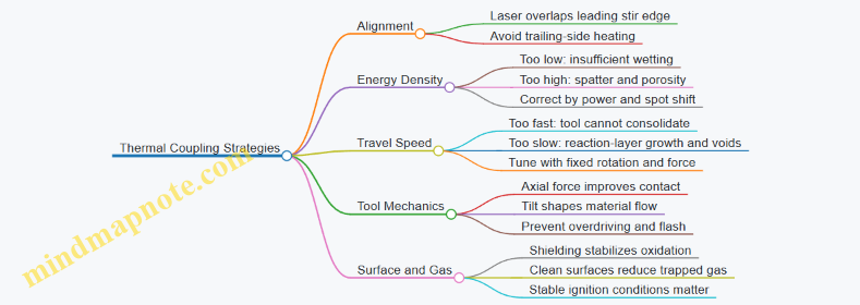
Integrated Example Workflow: From Setup to Cross-Section
- Set tool rotation, traverse speed, and axial force to a known stable friction stir baseline.
- Position the laser so its peak is slightly ahead of the pin’s leading edge.
- Start with a conservative laser power and verify surface wetting continuity.
- Increase laser power in small steps until wetting improves without a spatter/void jump.
- If lack-of-bond persists, adjust axial force before increasing power.
- If porosity increases, reduce energy density or shift the spot away from the exact interface line.
- Confirm with cross-sections at multiple locations along the weld to ensure coupling stability, not just local success.
This systematic tuning treats thermal coupling as a controlled relationship between heat timing, heat intensity, and mechanical consolidation. When those three align, the interface behaves like it was meant to be joined rather than merely heated and hoped for.
6.4 Process Parameter Integration for Laser Power Spot Size and Travel Speed
Laser-assisted friction stir joining behaves like a controlled heat input system wrapped around a mechanical stirring process. The laser parameters—power, spot size, and travel speed—must be integrated so the laser supplies enough energy to assist wetting and bonding without overheating the stir zone or creating excessive melt that the tool cannot manage.
Foundational Relationships That Tie the Parameters Together
Start with the idea that the laser delivers energy per unit length along the travel path. A practical first pass uses linear energy density:
- Linear energy density \(E_L\) ≈ \(\frac{P}{v}\)
- Power density depends on spot size \(d\): higher power and smaller spot raise peak intensity.
Because spot size affects how quickly energy is spread, two setups can share the same \(E_L\) but still behave differently if one uses a tighter spot (higher peak intensity, steeper thermal gradients). Travel speed changes both the time the beam dwells on a point and the degree of heat accumulation ahead of the tool.
A useful mental model is: travel speed sets exposure time, spot size sets intensity distribution, and power sets total energy. In practice, you tune them together to hit a target thermal window for improved bonding.
Stepwise Integration Method for Parameter Selection
- Choose a baseline travel speed based on mechanical constraints and desired tool-workpiece interaction. If the tool path is fixed, speed also affects how long the laser can assist each segment.
- Select a spot size that matches the joint scale. For narrow gaps or tight edge distances, a smaller spot can concentrate energy where it matters. For wider faying surfaces, a larger spot can reduce local overheating.
- Set laser power to reach the required energy density for the chosen speed and spot. If you increase speed, you typically need more power to maintain similar energy per length.
- Check thermal balance with the friction stir process. The tool’s stirring action redistributes heat and material. If the laser creates too much melt, the tool may trap fluid and increase porosity risk. If it creates too little, you get poor wetting and inconsistent bonding.
- Validate with a short parameter sweep around the baseline, changing one variable at a time while keeping the others fixed, then refine using the observed defect and microstructure trends.
What Changes When You Adjust Each Parameter
- Increasing power at constant speed and spot raises peak temperature and melt fraction. Expect improved wetting up to a point, then a higher chance of excessive melt and unstable flow.
- Increasing travel speed at constant power and spot reduces exposure time. Bonding may become inconsistent because the laser no longer supplies enough energy to assist oxide disruption and surface wetting.
- Reducing spot size at constant power and speed increases intensity and steepens gradients. This can improve local activation but also increases the risk of localized overheating and keyhole-like behavior in fusion-dominant regions.
Mind Map: Parameter Integration Logic
Example: Aluminum Lap Joint Parameter Sweep
Assume a lap joint where the laser assists the faying surface just ahead of the tool. You start with a travel speed that matches the tool traverse plan, then test two spot sizes.
- Baseline: \(v = 200\ \text{mm/min}\), spot diameter \(d = 1.2\ \text{mm}\)
- Power sweep: 1.5 kW, 1.8 kW, 2.1 kW
Expected outcomes:
- At 1.5 kW, bonding may improve slightly, but you still see occasional lack of fusion at the interface.
- At 1.8 kW, interface wetting becomes consistent and the stir zone shows more uniform mixing.
- At 2.1 kW, you may observe increased porosity or a wider region of softened material that the tool struggles to homogenize.
Then repeat with a smaller spot \(d = 0.8\ \text{mm}\) at the same speed. If you keep power the same, peak intensity rises, so you often reduce power (for example, 1.8 kW down to ~1.6 kW) to avoid localized overheating while preserving the improved wetting.
Example: Speed Change with Energy Compensation
If you must increase travel speed from 200 to 250 mm/min to meet throughput, keep the linear energy density approximately constant by scaling power:
- \(E_L \propto P / v\)
- \(P_2 \approx P_1 \times (v_2 / v_1)\)
So if \(P_1 = 1.8\ \text{kW}\) at 200 mm/min, then \(P_2 \approx 1.8 \times (250/200) = 2.25\ \text{kW}\). In practice, you still verify because spot size and absorption can shift the effective thermal input, but this calculation gives a grounded starting point rather than a blind guess.
Practical Integration Checks During Trials
During early trials, evaluate three things in order: (1) interface wetting and continuity, (2) defect presence such as porosity or lack of bond, and (3) stir zone microstructure uniformity. If wetting is poor, raise power or reduce speed first. If porosity increases, reduce power or increase speed slightly, and consider enlarging the spot to spread intensity.
When the parameters are integrated correctly, the laser stops being a separate heat source and becomes a predictable assistant to the tool’s mixing and bonding role.
6.5 Practical Example Workflows for Aluminum and Dissimilar Joint Trials
Goal and Setup Logic
Start with aluminum-on-aluminum trials to establish a stable friction stir window, then move to dissimilar joints once you can reproduce defect-free stir zones repeatedly. This order matters because dissimilar joints add extra variables: different thermal conductivity, different melting behavior, and different intermetallic formation tendencies. A practical workflow uses short, measurable experiments that narrow the parameter space quickly.
Mind Map: Trial Workflow for Aluminum and Dissimilar Joints
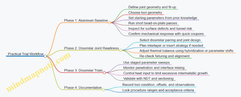
Phase 1: Aluminum Baseline Trials
Pick a common aerospace aluminum alloy pair such as 6xxx to 2xxx or 6xxx to 6xxx, but keep the first phase simple: same alloy on both sides. Use a butt joint with consistent root gap and a clean faying surface. If you are unsure about fit-up, measure it—friction stir is forgiving, but only within limits.
-
Establish a stable stir zone: Run a series of short welds (for example, 50–100 mm) at a fixed rotation speed and axial force, then vary traverse speed in steps. The easy-to-understand rule is: slower traverse increases heat and mixing; faster traverse reduces heat and can increase lack of bond risk.
-
Check for surface indicators: Look for excessive flash, surface tearing, and obvious voids at the exit. A practical trick is to mark the start and end of each run and compare them; many issues show up at the start due to tool plunge and at the end due to exit conditions.
-
Section one coupon per parameter set: Cut a cross-section at mid-length and at least one near the start. Confirm that the stir zone shows continuous material flow without a persistent tunnel. If you see a tunnel, increase axial force slightly or reduce traverse speed—either change increases contact and helps close the interface.
-
Lock a baseline window: Choose a parameter range that produces consistent bonding across multiple coupons. Record tool wear state too; a worn shoulder changes heat input and can shift your window without any other changes.
Phase 2: Dissimilar Joint Readiness
For dissimilar trials, define the interface strategy before touching parameters. If you are joining aluminum to steel or aluminum to titanium, the main practical concern is not just bonding—it is controlling the reaction layer thickness and the distribution of brittle phases.
- Joint design choice: Use a butt joint with controlled land or a lap joint with overlap that supports material flow. Ensure the interface is accessible to the tool shoulder and pin without forcing the pin to “hunt” for contact.
- Interlayer strategy: If your process uses an insert (for example, a thin aluminum-compatible interlayer), treat it as part of the thermal balance. Place it consistently; thickness variation at the interface is a direct cause of uneven reaction.
- Fixturing: Dissimilar stacks distort differently. Use rigid clamping and confirm flatness before each run.
Phase 3: Dissimilar Trials
Use a staged sweep that changes one “heat-and-mixing lever” at a time.
-
Start from the aluminum baseline: Use the same rotation speed as your best aluminum window, then adjust traverse speed first. This keeps tool behavior familiar while you learn how the dissimilar interface responds.
-
Add a second sweep for penetration control: If bonding is incomplete, adjust axial force before you make large rotation changes. Axial force is the most direct way to improve contact and reduce lack-of-bond defects.
-
Watch the interface, not just the surface: Sectioning is essential for dissimilar joints. You want a continuous bond line and a reaction layer that is present but not excessively thick. If the interface shows a wide, uneven reaction zone, reduce heat input by increasing traverse speed or lowering axial force slightly.
-
Use NDT to avoid blind iteration: Run ultrasonic testing or radiography where applicable before you cut too many coupons. Even a simple scan plan helps you decide which runs deserve destructive sectioning.
Example Workflow: Aluminum-to-Aluminum Then Aluminum-to-Steel
- Run A–C (Aluminum baseline): Keep rotation constant, vary traverse speed in three steps. Section one coupon from each run. Select the set with continuous bonding and minimal tunnel risk.
- Run D–F (Dissimilar): Use the selected rotation speed. Vary traverse speed around the baseline while keeping axial force fixed. Section the best two and one worst case. If the worst case shows lack of bond, increase axial force in Run G–H while returning traverse speed to the best value.
Practical Acceptance Checks
For each trial set, record four items: tool condition, measured fit-up, surface defect notes, and one cross-section observation. A workflow is “done” when you can repeat defect-free bonding in aluminum and then reproduce acceptable interface bonding in the dissimilar case using a defined parameter range.
7. Laser Welding and Laser Hybrid Joining for Aerospace Structures
7.1 Laser Welding Modes Including Conduction and Keyhole Regimes
Laser welding quality is strongly tied to how the material absorbs energy and how the molten pool behaves. Two practical regimes explain most outcomes: conduction welding, where heat spreads mainly through the solid and shallow melt, and keyhole welding, where a vapor cavity forms and the laser couples into it. The regime is not a personality trait of the laser; it is mostly a consequence of power density, beam focus, travel speed, and how the surface state changes during melting.
Conduction Regime Fundamentals
In conduction welding, the laser energy raises the surface temperature above melting but does not sustain a deep vapor cavity. Heat flows from the melt into the surrounding material by conduction, so penetration is limited and the weld pool is relatively shallow and wide.
A simple way to picture it: imagine heating a metal plate with a hot spot that is just strong enough to melt a shallow “dish.” The dish spreads laterally because the dominant transport is conduction, not cavity-driven recoil pressure.
What you typically see
- Penetration depth increases gradually with higher power or slower travel speed.
- The weld bead is usually broader with smoother sidewalls.
- Porosity is less likely to be driven by keyhole instability, though gas entrapment can still occur if shielding and surface cleanliness are poor.
Easy example Take a 2 mm aluminum plate. If you start with a moderate laser power, a reasonably small spot, and a travel speed that keeps the surface from overheating, you often get a consistent shallow fusion zone. If you then reduce travel speed slightly, penetration increases without suddenly changing the bead shape.
Keyhole Regime Fundamentals
In keyhole welding, the laser intensity is high enough to create a vapor cavity. The cavity deepens because the laser energy couples into the cavity walls, and recoil pressure from vapor generation helps keep the cavity open. This creates a narrow, deep penetration channel.
A simple way to picture it: the beam “bores” a tunnel, and the tunnel walls absorb more energy than the flat surface would. When the beam moves forward, the cavity collapses behind it, leaving a deep weld.
What you typically see
- Penetration increases sharply once the keyhole forms.
- The bead becomes narrower with deeper fusion.
- Defects can include porosity from trapped gas, and irregularities when the keyhole surface becomes unstable.
Easy example Using the same 2 mm aluminum plate, increase power or reduce travel speed until the bead suddenly transitions from broad shallow fusion to a deeper, narrower weld. If you overshoot, you may notice more sensitivity to small changes in alignment or surface condition.
Regime Transition Logic
The conduction-to-keyhole transition is governed by whether the local power density and absorbed energy can sustain vaporization. In practice, three factors often decide the outcome:
- Power density at the workpiece: Higher intensity makes vapor generation easier to sustain.
- Beam focus and spot size: A tighter focus raises intensity but also increases sensitivity to standoff and surface curvature.
- Interaction time: Slower travel speed increases the time the beam dwells on a location, raising the chance of keyhole formation.
Surface condition matters too. Oxide layers, coatings, and contamination change absorption and can shift the effective threshold. That is why “same settings, different surface” can behave like a different process.
Mind Map: Laser Welding Modes
Practical Identification Without Guesswork
You can identify the regime by combining bead appearance with a cross-section check.
- If penetration increases smoothly and the bead looks broad with gentle sidewalls, you are likely in conduction.
- If penetration jumps and the bead narrows with a deep fusion channel, you are likely in keyhole.
For process development, it helps to change one variable at a time. For instance, adjust travel speed first while keeping focus and power stable. If the weld transitions abruptly, you have likely crossed the keyhole threshold. Then you can refine by small changes in speed or focus to regain stability.
Example: Choosing a Regime for a Joint
Suppose you are joining a lap joint where you want reliable fusion without excessive risk of deep cavity defects.
- Start in conduction: use settings that produce full wetting and consistent fusion at the faying surfaces.
- If penetration is insufficient, increase energy in small steps, watching for a sudden narrowing and deeper channel formation.
- If you reach keyhole unintentionally, back off slightly and prioritize stable bead geometry over maximum depth.
This approach keeps the process understandable: you are not chasing numbers, you are managing the physical interaction between the beam and the melt.
7.2 Shielding Gas Selection and Flow Management for Weld Quality
Shielding gas does two jobs at once: it keeps oxygen and moisture away from the molten pool, and it shapes how heat and metal vapor move across the surface. In laser welding and laser-assisted friction stir welding, the second job matters because the keyhole or partially fused region is sensitive to surface contamination and flow disturbances. A good gas choice with poor flow control can still produce porosity; a mediocre gas with disciplined flow can sometimes hold quality together.
Foundational Principles of Shielding
Start with what the gas must protect. In aluminum laser welding, the molten pool surface can oxidize quickly, and oxide films can become nucleation sites for pores. In titanium and steel, the risk is more severe because reactive elements form stable oxides and nitrides that degrade wetting and joint strength.
Next, consider how gas reaches the pool. Shielding is not just “covering the weld.” It is delivering a stable, laminar-enough flow over the critical area while avoiding turbulence that entrains air. The gas must also clear the plume region where metal vapor and spatter travel.
Finally, remember that gas flow interacts with the process. Higher flow can improve coverage but may increase turbulence, disturb the keyhole, and cool the surface enough to change penetration behavior. Lower flow can reduce disturbance but may allow air ingress at edges and undercuts.
Gas Selection Logic for Common Materials
For aluminum alloys, argon is the usual baseline because it is inert and provides consistent wetting. Helium can be used when higher thermal conductivity is desired to support stable penetration, but it often requires higher flow rates to maintain coverage.
For stainless steels and nickel alloys, argon is common, sometimes with small additions depending on the welding method and surface condition. The goal is still inert protection; additions are used to manage arc or plasma behavior in fusion welding, but in laser welding the main effect is coverage stability and plume handling.
For titanium, argon is typically preferred, with careful attention to coverage continuity because titanium reacts readily with air. Any gap in shielding coverage can show up as discoloration and reduced corrosion resistance.
Flow Management That Actually Works
Flow management is about three measurable targets: coverage, stability, and plume clearance.
Coverage means the gas envelope reaches the weld edges before air can mix in. Practically, this depends on nozzle-to-work distance, nozzle geometry, and travel speed. A nozzle that is too far away creates a wide mixing zone where air can be entrained.
Stability means the flow remains coherent over the weld length. If the gas jet hits the workpiece at an angle or is blocked by fixturing, it can create recirculation pockets that pull air into the shielding region.
Plume clearance means the gas helps carry vapor and spatter away without blowing them into the keyhole or re-depositing them on the trailing edge. This is where many “it looked fine on the first pass” problems begin.
Nozzle Geometry and Placement Practices
Use a nozzle that matches the weld width and the expected plume footprint. For narrow seams, a focused nozzle reduces edge air ingress. For wider seams, a broader nozzle or dual-stream approach can maintain coverage without excessive jet velocity.
Keep nozzle distance consistent along the weld path. If the workpiece height varies or the joint includes steps, the shielding can thin out at the lowest points. A simple check is to mark the nozzle position relative to the fixture and verify it after any tool or head adjustment.
Flow Rate Tuning with Simple Experiments
A practical tuning method is to run short weld segments while holding laser parameters constant and varying only shielding flow and nozzle distance. Inspect for porosity trends and surface discoloration. If porosity increases when flow is reduced, you likely have edge air ingress. If porosity increases when flow is increased, you may be disturbing the keyhole or increasing turbulence.
Also watch for spatter behavior. If spatter lands inside the shielding envelope and then re-enters the pool, you can get localized porosity even when overall coverage seems adequate.
Mind Map: Shielding Gas Selection and Flow Management
Example: Aluminum Lap Joint with Laser Hybrid Assistance
A shop welding 6 mm aluminum lap joints noticed occasional porosity near the trailing edge. They kept laser power and travel speed fixed and tested three shielding setups: (1) argon at moderate flow with a standard nozzle distance, (2) argon at higher flow with the same distance, and (3) argon at moderate flow with a reduced nozzle distance.
The higher flow case showed more spatter disturbance and slightly reduced penetration stability, with porosity appearing in a narrow band behind the keyhole. The reduced nozzle distance case improved edge coverage and reduced trailing-edge porosity, while the moderate flow baseline remained inconsistent. The final setup used the reduced distance and a moderate flow rate, prioritizing stable coverage over maximum flow.
Example: Titanium Joint with Fixturing-Induced Air Ingress
In a titanium weld, discoloration appeared only where the fixture blocked the gas jet. The team corrected the nozzle angle and added a small clearance relief in the fixture so the shielding envelope could reach the joint edges. After the change, the discoloration disappeared and porosity dropped without altering laser parameters.
Practical Checklist for Consistent Shielding
- Confirm nozzle-to-work distance is consistent along the weld path.
- Choose argon for inert protection unless material or setup requires helium.
- Tune flow using short trials while keeping laser parameters constant.
- Watch spatter landing and trailing-edge behavior as a porosity clue.
- Ensure fixturing does not block the shielding envelope at any point.
7.3 Beam Oscillation And Path Strategies For Uniform Penetration
Uniform penetration in laser welding depends on keeping the keyhole stable and centered in the joint. Beam oscillation and path strategy are the two main levers: oscillation shapes the energy distribution over time, while the path controls how that distribution moves through the workpiece. The goal is simple—avoid long periods where the keyhole drifts off the joint line or collapses, because those moments show up as lack of fusion, undercut, or inconsistent bead width.
Foundational Concepts for Penetration Uniformity
Start with what “uniform penetration” means in practice. In a typical butt joint, penetration depth varies along the weld length when the effective heat input per unit length changes or when the keyhole experiences repeated destabilization. Two mechanisms dominate:
- Energy concentration drift: the beam is not consistently centered relative to the joint gap and fit-up.
- Keyhole instability: the keyhole forms, then intermittently collapses due to insufficient local energy or excessive lateral energy spread.
Oscillation helps by averaging out small misalignments and by smoothing the thermal field, but only if the oscillation frequency and amplitude match the material’s ability to maintain a molten pool and keyhole.
Beam Oscillation Fundamentals
Beam oscillation is usually implemented as a controlled lateral motion (often along a line perpendicular to travel) or a combined lateral and longitudinal pattern. The most useful way to think about it is as a “time-averaged footprint” of the beam.
- Amplitude controls how far the beam sweeps across the joint line. Too small: the process behaves like a fixed beam and is sensitive to fit-up. Too large: the keyhole spends too much time away from the joint, reducing penetration.
- Frequency controls how quickly the beam cycles. Too low: the keyhole responds to each sweep, causing depth fluctuations. Too high: the molten pool averages the motion, but the keyhole may not track the motion effectively, leading to shallow or irregular penetration.
- Waveform matters because it changes dwell time. A sinusoidal motion gives smoother dwell near extremes than a sharp triangular motion, which can reduce abrupt changes in keyhole behavior.
A practical rule of thumb is to tune oscillation so that the beam does not “outrun” the keyhole. If you observe a weld where penetration is deepest at one side of the joint and shallow at the other, the oscillation is likely biased or too wide for the current power and travel speed.
Path Strategies for Joint Line Tracking
Even with oscillation, the path must keep the beam aligned with the joint. Path strategy includes how you handle the joint start, the joint end, and any changes in gap or thickness.
- Straight-line travel with oscillation: simplest baseline for flat butt joints. Use it to establish a stable penetration window.
- Lead-in and lead-out shaping: start with a controlled ramp in power or motion so the keyhole forms gradually. End the weld with a controlled taper to avoid a crater that can trap gas and create porosity.
- Gap-following and seam tracking: when fit-up varies, the path should compensate. If seam tracking is unavailable, you can still reduce sensitivity by using a slightly wider oscillation pattern early in the weld while the joint is most uncertain.
A common failure pattern is “good penetration in the middle, poor at the ends.” That usually points to start/stop dynamics rather than steady-state oscillation settings.
Systematic Tuning Workflow with Examples
Use a structured approach so changes are interpretable.
Step 1: Establish a steady-state baseline. Weld a short straight segment with fixed beam (no oscillation). Confirm penetration depth and bead shape.
Step 2: Introduce oscillation at small amplitude. Increase amplitude gradually while keeping travel speed and power constant. Example: if fixed-beam weld shows shallow penetration near the edges of the joint, try a modest lateral sweep that increases time-averaged energy at the joint line.
Step 3: Adjust frequency to reduce depth fluctuation. If cross-sections show alternating deep and shallow bands, increase frequency or switch to a smoother waveform.
Step 4: Add path shaping at start and end. Example: for a crater-prone end, extend the lead-out with a reduced travel speed and a controlled power taper so the keyhole closes before the beam stops.
Step 5: Validate with cross-sections at multiple locations. Check at least three positions: start, mid, and end. Uniformity is about consistency, not just maximum depth.
Mind Map: Beam Oscillation and Path Strategies
Concrete Example: Butt Joint with Variable Gap
Consider a butt joint where the gap is slightly larger at the start due to fixturing. A fixed-beam weld may show shallow penetration at the beginning and deeper penetration later. A workable strategy is to use a short lead-in with a modest oscillation amplitude to average out the initial gap uncertainty, then transition to a narrower oscillation during steady travel. Finish with a longer lead-out taper at reduced travel speed to close the keyhole gradually. After welding, compare cross-sections at start, mid, and end; the target is not identical penetration everywhere, but a controlled variation that stays within the joint’s acceptance criteria.
Concrete Example: Thick Section with Consistent Fit-Up
For a thick section with good fit-up, start with a straight-line path and oscillation only after confirming stable penetration with fixed beam. Use smaller amplitude than you would for variable gap, because the keyhole already stays centered. If you see depth fluctuations, increase frequency before changing amplitude; that preserves the lateral footprint while smoothing the time-averaged energy delivery.
The practical takeaway is that oscillation and path are not independent knobs. Oscillation shapes the energy over time, while the path ensures the beam stays where the keyhole needs to be. When both are tuned together, penetration becomes repeatable rather than lucky.
7.4 Defect Control Including Porosity Spatter and Cracking Mechanisms
Defect control starts with a simple idea: most welding defects are not random; they are the visible result of a few controllable physical causes. In laser welding and laser-hybrid friction stir joining, those causes usually fall into three buckets—gas-related porosity, melt instability that produces spatter, and cracking driven by thermal gradients and restraint. The goal is to prevent the cause, not just chase the symptom.
Porosity Control from Gas Sources to Stable Keyhole Behavior
Porosity forms when gas is trapped in the solidifying weld pool. In laser welding, the most common gas sources are surface contamination, trapped air in joint gaps, and decomposition of coatings or oxides. In hybrid joining, additional gas can come from friction stir mixing that redistributes oxides and moisture into the fusion region.
A practical control sequence is: (1) reduce gas generation, (2) reduce gas entry, (3) ensure the pool can vent before freezing. For example, consider a lap joint of aluminum sheet. If the faying surfaces have a thin oxide film and the overlap has a slight gap, the first laser passes can heat the oxide and any adsorbed moisture, producing gas. You can often see the effect as scattered small pores near the start of the weld. Fixing it is usually not a single knob: clean both faying surfaces, clamp to minimize the gap, and use shielding gas coverage that actually reaches the weld zone rather than just “being present.”
Keyhole porosity is linked to keyhole stability. When the keyhole collapses intermittently, vapor bubbles can form and be trapped. Stabilizing the keyhole means matching laser power and travel speed so the keyhole maintains a consistent shape. If you increase power without adjusting speed, the keyhole can grow and become unstable; if you increase speed without enough power, the keyhole may not form consistently, leaving lack-of-fusion-like voids. A useful shop-floor check is to correlate pore distribution with weld start and end. Pores concentrated at the start often point to insufficient initial stabilization; pores at the end often point to end-of-weld solidification and shielding coverage.
Spatter Control from Melt Dynamics to Surface Wetting
Spatter is ejected molten material that lands outside the intended fusion zone. It is usually caused by excessive vapor pressure, unstable keyhole behavior, or poor wetting that allows droplets to detach. Spatter also increases defect risk because it can create local surface roughness and act as initiation sites for cracks or porosity.
Control begins with energy balance. If the laser input is too high for the travel speed, the vapor recoil pressure can blow the melt outward. If the input is too low, the pool may be shallow and less able to wet the joint faces, which can also promote droplet ejection. In a laser-hybrid setup, the friction stir action can change surface condition and local heat distribution, so spatter can shift location when you change stir parameters even if laser settings stay constant.
A concrete example: welding a 2 mm aluminum lap joint with a narrow beam. If you observe spatter concentrated along the leading edge, the keyhole may be unstable at the front due to insufficient shielding gas flow uniformity or a mismatch between laser focus position and joint thickness. Adjusting focus to center the keyhole in the thickness and improving shielding gas flow straightness often reduces leading-edge spatter more effectively than lowering power alone.
Cracking Mechanisms from Metallurgy to Restraint
Cracking can be hot cracking (during solidification) or cold cracking (after cooling). In aluminum and titanium systems, hot cracking is often tied to solidification range behavior, segregation, and the presence of brittle intermetallics in dissimilar joints. In restrained structures, thermal contraction adds tensile stress while the material is still weak.
Hot cracking control is therefore a combination of metallurgy and mechanics. Metallurgy controls include managing heat input to avoid excessive segregation and ensuring adequate mixing in hybrid processes so brittle phases do not concentrate at critical locations. Mechanics controls include reducing restraint and managing joint fit so the weld does not have to “stretch” to close gaps.
A useful example is a dissimilar joint between aluminum and steel using an interlayer or insert. Cracking often initiates near the interface where intermetallic layers form and where shrinkage stress concentrates. If you see cracks that follow the interface line, the first checks are interlayer thickness consistency, surface cleanliness, and whether the process produces a continuous, well-bonded interface rather than a patchy one. If the cracks appear after full cooling and are associated with high hardness regions, you should also check whether the thermal cycle created an overly hard, brittle microstructure in the vicinity of the crack path.
Integrated Mind Map for Defect Control
Mind Map: Defect Control in Laser and Laser-Hybrid Joining
Practical Diagnostic Workflow That Stays Grounded
- Map where defects appear: start, middle, end, and whether they align with the interface or weld centerline.
- Identify the dominant mechanism: pores that cluster near start suggest stabilization; pores spread throughout can indicate gas entry; spatter-heavy leading edges suggest keyhole or shielding issues; cracks following interfaces point to brittle-phase or restraint effects.
- Change one variable at a time with a reason: for example, if pores concentrate at the start, adjust initial stabilization (power ramp or travel speed) and confirm shielding coverage before changing joint prep.
- Confirm with simple checks: weld cross-sections for pore location and crack path, and surface inspection for spatter distribution. If the defect pattern shifts predictably after a controlled change, you are learning the mechanism—not just hoping.
When you treat porosity, spatter, and cracking as linked outcomes of gas behavior, melt stability, and stress-metallurgy interactions, defect control becomes systematic. The process stops being a guessing game and becomes a chain of cause-and-effect decisions you can repeat.
7.5 Qualification Testing Including Sectioning Nondestructive Evaluation and Mechanical Checks
Qualification testing proves that a qualified process produces joints that meet requirements, not that a single trial looked good. A practical workflow starts with what you can measure without cutting, then confirms what you cut, and finally verifies performance with mechanical tests.
Qualification Testing Strategy
Begin with a qualification plan that ties each requirement to a test method. For example, if the joint must be free of internal voids above a certain size, you need an NDE method with known sensitivity for the joint thickness and geometry. If the joint must meet shear strength and fatigue performance, you need mechanical tests that match the expected loading mode.
A simple rule: use NDE to screen and locate, sectioning to confirm, and mechanical tests to validate properties. When these three agree, you can trust the process window.
Sectioning Plan and Sampling Logic
Sectioning is not just “cut and look.” It is controlled sampling that answers specific questions: Did the stir or fusion create a continuous bond? Where are defects located? How consistent is the microstructure across the weld path?
- Define cut locations based on the weld path and expected stress regions. For a lap joint, include at least one section near the start, one near the middle, and one near the end of the weld path.
- Choose section orientations that reveal the critical interface. For friction stir, cross-sections should show the stir zone, thermo-mechanically affected zone, and the advancing and retreating sides.
- Control sectioning quality so you do not create artifacts. Use low-speed cutting, proper mounting, and careful grinding/polishing to avoid smearing or pulling out soft phases.
- Record geometry such as penetration depth, underfill, and flash or surface features. These measurements help interpret NDE signals.
Example: Sampling for a Hybrid Laser Assisted Friction Stir Joint
If the laser is intended to improve wetting and reduce lack of bond, sectioning should focus on the interface region where lack of bond would appear. Take one section at the weld start where heat input is often less stable, and one at the middle where parameters are steady. Compare interface continuity and any unmixed regions.
Nondestructive Evaluation Workflow
NDE should be planned around defect types. For friction stir and fusion hybrids, typical concerns include lack of bond, voids, porosity, and planar defects near interfaces.
Mind Map: Qualification Testing Logic
NDE Method Selection and Correlation
Use a defect-to-method mapping mindset. Ultrasonic testing is often effective for internal discontinuities, while radiography can reveal volumetric porosity. The key is correlation: sectioning confirms what the NDE signal actually represents.
A workable correlation approach:
- Run NDE on the as-welded specimens.
- Mark suspected regions on the specimen.
- Section through those regions.
- Update interpretation rules, such as which signal amplitudes correspond to acceptable versus unacceptable features.
Example: Correlating Ultrasonic Indications with Sectioned Findings
Suppose ultrasonic inspection flags a linear indication near the interface. Sectioning shows a narrow lack-of-bond region aligned with the tool path. If the indication size consistently matches the lack-of-bond dimensions, you can set an acceptance threshold tied to that geometry rather than relying on raw signal amplitude alone.
Mechanical Checks and Acceptance Criteria
Mechanical checks confirm that the joint performs under load, including the effects of microstructure and any remaining defects.
- Select the test type to match the joint behavior. Lap joints often emphasize shear and peel-like components, while butt joints may emphasize tension and bending response.
- Use consistent specimen geometry and orientation. Misalignment can change failure mode, which makes qualification results hard to interpret.
- Define acceptance criteria before testing. Criteria should include minimum strength and allowable failure locations. If failure must occur in the base material rather than the joint, specify that.
- Review fracture surfaces systematically. A fracture that crosses the stir zone differently from one that stays at an interface tells you whether the process created a robust bond.
Example: Interpreting Failure Mode
If a shear specimen fails along the interface, sectioning and NDE should be revisited to determine whether lack of bond or a weak interfacial microstructure is responsible. If failure occurs through the stir zone with ductile features, it supports the conclusion that the process window produces a sound bond.
Integrated Qualification Evidence Package
A qualification file should connect the dots:
- Process parameters used for the qualified trials.
- NDE results with scan maps and interpretation rules.
- Sectioning evidence showing interface continuity and defect morphology.
- Mechanical test results with failure mode documentation.
When these elements agree, qualification becomes more than paperwork. It becomes a repeatable story: the process produces the microstructure you expect, NDE finds what matters, sectioning confirms it, and mechanical tests prove the joint meets requirements.
8. Electron Beam Welding for High Integrity Joints
8.1 Electron Beam Welding Fundamentals Including Vacuum Requirements
Electron beam welding uses a focused stream of electrons to deliver energy to a joint. The electrons gain kinetic energy from a high voltage power supply, then transfer that energy to the workpiece when they slow down in the metal. Because the electrons travel through a vacuum, the process can concentrate heat into a narrow region and achieve deep penetration with relatively low surface melting.
Core Physics and What the Vacuum Enables
In air, electrons collide with gas molecules and lose energy before reaching the joint. A vacuum reduces collisions, letting electrons maintain their path from the gun to the workpiece. The vacuum level also affects beam stability: at insufficient vacuum, the beam can spread, wander, or produce inconsistent penetration.
A practical way to think about it is like aiming a flashlight beam through fog. In air, the “fog” scatters energy; in vacuum, the beam travels more like a straight line. The result is a controllable energy deposition profile that supports keyhole formation.
Electron Beam Gun and Beam Formation
An electron gun typically includes a cathode that emits electrons, an anode region that accelerates them, and electromagnetic lenses that focus the beam. Beam current largely controls the total energy delivered, while beam focus controls how tightly that energy concentrates.
A simple mental model for setup is:
- Higher beam current increases penetration potential.
- Better focus reduces the molten pool width and helps maintain a stable keyhole.
- Proper alignment ensures the beam hits the intended joint line.
Keyhole Welding Mechanism
At sufficient power density, the workpiece surface forms a vapor-filled keyhole. The keyhole acts like a moving cavity: the beam follows the joint, the cavity stays open long enough to allow deep fusion, and the metal behind the beam solidifies to form the weld.
If the keyhole collapses prematurely, penetration drops and fusion defects become more likely. If the keyhole becomes unstable, you can see irregular bead shape or internal porosity. Vacuum quality and beam stability are central because they influence how consistently the beam energy reaches the keyhole.
Vacuum System Requirements and Practical Targets
Electron beam welding is commonly performed in either high vacuum or ultra-high vacuum depending on the application and equipment design. The key requirement is that the mean free path of electrons is long enough to prevent significant scattering.
In production terms, operators manage vacuum in three stages:
- Pump down the chamber from atmospheric pressure.
- Stabilize vacuum before welding so beam conditions remain repeatable.
- Maintain vacuum during welding to avoid energy loss and beam distortion.
Common contributors to vacuum problems include contaminated chamber surfaces, moisture, and outgassing from fixtures or workpiece coatings. A “boring” but effective practice is to keep fixtures clean and dry, because outgassing can raise pressure during the weld cycle.
Joint Preparation and Fixturing Under Vacuum Constraints
Because the chamber is sealed, fixturing must do two jobs: hold alignment and avoid introducing contaminants that outgas. Surface cleanliness matters because oxides and residues can interfere with keyhole behavior and weld chemistry.
A useful example is a butt joint on a thick plate. If the root gap is inconsistent, the keyhole can form at different depths along the seam. Under vacuum, the beam may still be stable, but the joint geometry changes the local thermal boundary conditions. The fix is to control fit-up with consistent spacers or machined land features.
Process Parameter Relationships That Matter
Even without memorizing numbers, you can connect parameters to outcomes:
- Beam current and accelerating voltage set energy delivery and penetration tendency.
- Beam focus affects weld width and keyhole stability.
- Travel speed controls how long the beam dwells at each point.
- Vacuum level influences beam transport and energy deposition consistency.
If penetration is shallow, check energy delivery first, then verify focus and alignment. If penetration is erratic, vacuum stability and joint fit-up are often the culprits.
Mind Map: Electron Beam Welding Fundamentals with Vacuum
Example: Diagnosing a Penetration Drop
A shop reports that a previously reliable butt weld now shows reduced penetration and occasional lack of fusion at the root. The first check is vacuum stability during the weld cycle: if pressure rises, electrons scatter and deliver less energy to the keyhole. Next, verify beam focus and alignment using the machine’s standard calibration routine. Finally, re-check root gap consistency; a slightly larger gap can cause the keyhole to open differently and solidify before full fusion.
Example: Preventing Vacuum-Related Instability
For a fixture that holds multiple parts, technicians notice longer pump-down times and more variability between runs. They clean the fixture surfaces, bake out components that retain moisture, and ensure no oils or cutting residues remain on contact areas. After these steps, vacuum reaches the target more consistently, and weld penetration returns to the expected repeatable range.
8.2 Beam Parameters for Acceleration Voltage Beam Current and Focus Settings
Electron beam welding quality is mostly decided by how energy is delivered into the workpiece: acceleration voltage sets the electron energy, beam current sets the electron quantity per unit time, and focus settings determine how tightly that energy is concentrated. Treat these three as a coupled system—change one and the others usually need a sanity check.
Acceleration Voltage: What It Controls and Why It Matters
Acceleration voltage (often written as kV) determines electron penetration depth and how energy is deposited with depth. Higher voltage generally increases penetration because electrons carry more energy before they slow down. In practice, you choose voltage to match joint thickness and desired keyhole behavior.
A simple way to reason about it: if you see a shallow weld with incomplete fusion, you may need more penetration capability, which can point toward higher voltage. If you see excessive undercut or a keyhole that seems too aggressive, voltage may be too high for the thickness and fit-up.
Example: For a 6 mm butt joint in a vacuum-compatible alloy, start with a mid-range voltage that produces a stable keyhole. If the root shows lack of fusion after sectioning, increase voltage in small steps while keeping current and focus constant, then re-check penetration.
Beam Current: Energy Rate and Weld Pool Size
Beam current (mA) sets the beam power together with voltage. Higher current increases heat input and typically enlarges the weld pool and keyhole size. Too little current can produce a narrow, shallow weld that fails mechanical requirements; too much current can widen the pool, increase spatter-like surface activity, and worsen dimensional control.
A practical workflow is to lock voltage first based on penetration needs, then adjust current to hit the required weld width and penetration depth. Because current also affects keyhole stability, you should watch for changes in surface appearance and bead geometry, not just final penetration.
Example: If a joint shows correct penetration but excessive bead width, reduce current slightly and keep voltage and focus unchanged. If bead width is too narrow and fusion is incomplete, increase current.
Focus Settings: Where the Energy Goes
Focus settings control beam spot size at the workpiece. A tighter focus concentrates energy, raising peak power density and promoting deeper penetration for the same overall power. A defocused beam spreads energy, which can widen the weld but reduce penetration.
Think of focus as the “where” parameter and voltage/current as the “how much” parameters. If penetration is inconsistent across the joint, focus drift or misalignment is a common culprit. If penetration is consistently too deep or too shallow, voltage and current are more likely the primary causes.
Example: Suppose two trials use the same voltage and current, but one produces a narrow, deep weld with a rougher root. Tighten focus slightly less (or increase defocus) to broaden the effective spot and improve root shape.
Coupling Rules for Systematic Parameter Selection
Use these rules to avoid chasing your tail:
- Set voltage for depth capability: choose a voltage range that can physically reach the required fusion depth.
- Set current for weld width and heat input: adjust current to meet bead width and penetration without destabilizing the keyhole.
- Set focus for energy concentration: fine-tune focus to correct root shape and consistency.
- Change one knob at a time: when you alter voltage, re-check current and focus assumptions because keyhole behavior changes.
- Verify with geometry and cross-sections: surface bead alone can mislead; sectioning confirms fusion and keyhole remnants.
Mind Map: Beam Parameter Logic
Example: Parameter Tuning for a 10 mm Butt Joint
Start with a voltage that supports deep penetration for 10 mm. Then set current to achieve full penetration without excessive bead width. Finally, adjust focus to smooth the root and reduce variability.
A concrete sequence:
- Trial A: mid voltage, mid current, nominal focus. If root shows lack of fusion, increase voltage slightly.
- Trial B: updated voltage, keep current and focus. If penetration is now sufficient but bead is too wide, reduce current.
- Trial C: keep voltage and current, adjust focus to refine root shape. If the root is too narrow and irregular, reduce tightness of focus.
Practical Checks That Prevent “Good Numbers, Bad Weld”
Before concluding that parameters are wrong, confirm the basics that distort the beam’s effective delivery. Check beam alignment relative to the joint line, verify vacuum level stability, and ensure the workpiece surface condition is consistent along the travel path. Even perfect kV and mA settings can produce inconsistent fusion if the beam is effectively landing in different conditions along the seam.
8.3 Joint Preparation and Fixturing for Vacuum Compatibility and Alignment
Vacuum electron beam welding demands more than “good fit-up.” The joint must survive vacuum pumping, maintain alignment under thermal and mechanical loads, and avoid anything that turns into gas inside the chamber. The goal is simple: keep the joint geometry stable from the moment parts are loaded until the beam finishes the pass.
Joint Preparation Foundations
Start with joint design intent and translate it into measurable preparation steps. For butt and lap joints, confirm that the gap and land widths match the welding plan, because the beam cannot “forgive” a wandering interface the way some arc processes can. A practical workflow is to create a joint acceptance checklist with three items: gap range, surface flatness, and edge condition.
Surface cleanliness is not optional. Remove oils, cutting fluids, oxide scale, and paint from both faying surfaces and adjacent regions that will sit near the beam path. A useful rule of thumb is to clean beyond the expected beam footprint by enough margin to cover minor part movement during clamping. After cleaning, avoid touching faying surfaces with bare gloves; skin oils are small, but vacuum is not impressed.
Edge preparation should be consistent. If you machine bevels, keep the tool marks uniform and avoid burrs that can trap contaminants. For dissimilar joints, pay extra attention to the interface region because thin reaction layers can form if residues remain.
Fixturing Principles for Vacuum Compatibility
Fixturing must do three jobs at once: hold alignment, tolerate vacuum conditions, and avoid introducing outgassing. Choose materials and finishes that are compatible with vacuum service. Avoid coatings that can shed under heat or that contain volatile binders.
Clamping strategy matters. Use a kinematic approach when possible: constrain the part in a repeatable way with minimal overconstraint. Overconstraint can lock in stress that relaxes during heating, causing the joint to open or shift mid-weld.
Thermal behavior is the silent alignment killer. Place clamps and supports so they conduct heat away in a controlled manner, and keep them away from areas that will experience the highest temperature gradients. If the fixturing is too close to the weld zone, it can pull the joint out of alignment as it heats.
Vacuum compatibility also includes mechanical cleanliness. Chips, dust, and loose fasteners are not “small.” They can migrate and contaminate surfaces or interfere with pumping. Before loading, blow off debris and verify that no loose items can rattle in transit.
Alignment Control and Verification
Alignment is best treated as a measurement problem, not a hope problem. Establish a reference datum scheme on the parts and fixturing. Then verify alignment at two stages: before vacuum loading and after final clamping.
Use a method that matches your tolerance needs. For many electron beam setups, you can combine visual checks with feeler gauges for gap verification and dial indicators or laser measurement for straightness. Record the measured values so you can correlate them with weld outcomes later.
A practical technique is to define a “no-surprises” sequence. First, dry-fit the parts in the fixturing to confirm contact points. Second, apply final clamping force and re-measure the joint gap and offset. Third, perform a vacuum loading check if your process allows it, or at least ensure the fixturing cannot shift during transfer.
Managing Outgassing and Contamination Risk
Vacuum welding is sensitive to trapped gases. Design the joint so that the interface does not create sealed pockets where contaminants can vaporize. For lap joints, ensure that any overlap region has a path for gases to escape rather than becoming a sealed cavity.
If you use any temporary tack features, confirm they are vacuum-safe and that they do not leave residues. Even small amounts of adhesive or marking ink can produce gas loads.
Consider pre-bake steps when your parts have a history of moisture uptake. The purpose is to reduce water and volatile contaminants before they see vacuum and heat.
Example: Butt Joint on Aluminum Alloy
You are preparing a butt joint for an aluminum alloy component. The plan specifies a controlled gap and a narrow land.
- Machine the edges with a consistent bevel and remove burrs.
- Clean both faying surfaces with a solvent appropriate for aluminum, then dry fully.
- Assemble in a fixturing block that uses three-point kinematic constraints and a separate clamp that sets the gap.
- Measure gap and edge offset after final clamping using feeler gauges and a straightedge.
- Confirm that no chips remain in the chamber loading path and that clamp surfaces are free of loose debris.
- Load into vacuum, ensuring the fixturing cannot shift during transfer.
If the measured gap drifts beyond the acceptance range after clamping, stop and adjust the fixturing contact points. Chasing the issue during welding is expensive and usually ends with a defect that looks “mysteriously” like misalignment.
Mind Map: Vacuum Compatibility and Alignment
Example: Lap Joint with Overlap Escape Path
For a lap joint, the overlap region can trap contaminants if it forms a sealed pocket. Prepare the overlap so there is a controlled escape path, such as a designed edge relief or a gap strategy that prevents full sealing. During fixturing, clamp in a way that maintains overlap contact without squeezing out residues into a closed cavity. Measure overlap alignment after clamping, because lap joints are especially sensitive to small lateral offsets that change how the beam interacts with the interface.
8.4 Defect Types Including Porosity Keyhole Instabilities and Undercut
Even when the process parameters look “in family,” welds can still develop defects. In laser and electron beam welding, three defect families show up often because they share the same root problem: the molten pool is not behaving like a stable, well-fed container. Porosity, keyhole instabilities, and undercut are the most common ways that instability shows itself.
Porosity
Porosity is trapped gas bubbles or voids formed during solidification. In fusion welding, the molten pool can dissolve gases up to a limit; when the pool cools quickly, the solubility drops and gas must leave. If it cannot escape before the metal freezes, it becomes a void.
Common causes
- Surface contamination and moisture: Oil, oxide films, paint residues, and absorbed moisture generate gas at the beam spot. A simple example is a lap joint where the faying surfaces were wiped on the outside but not cleaned inside the overlap; the overlap traps volatiles and porosity appears near the interface.
- Inadequate shielding or shielding turbulence: For laser welding, poor gas coverage lets air enter the pool. A practical check is to observe whether the shielding gas plume is disturbed by drafts or part geometry; porosity often clusters where the shielding line-of-sight is blocked.
- Keyhole-driven gas entrapment: When the keyhole is unstable, vapor recoil can form cavities that later collapse into pores.
How to recognize it
- Distributed fine pores often correlate with widespread contamination or unstable shielding.
- Larger, more localized pores often correlate with a specific region of keyhole instability or a local gap in fit-up.
Best-practice controls
- Clean and degrease both faying surfaces for lap joints, not just the top surface.
- Use consistent fit-up and avoid tight “pinch points” that trap gas.
- Verify shielding coverage with a simple smoke-free visual check of gas flow and part geometry clearance.
Keyhole Instabilities
A keyhole is the deep cavity formed by intense beam energy. It is useful because it increases penetration, but it is also sensitive: the keyhole wall is constantly shaped by surface tension, recoil pressure from vapor, and fluid flow in the molten pool.
Instability modes
- Keyhole collapse: The cavity necks down and closes before the surrounding metal can refill it, leaving voids or lack of fusion-like regions.
- Spiking and oscillation: The keyhole tip moves irregularly, which changes penetration depth and can create a “wavy” bead with internal voids.
- Recoil-driven turbulence: Excess vapor recoil can destabilize the cavity wall, increasing the chance of pore formation.
Why it happens
- Energy too high for the available conduction and flow: If the beam power is high relative to travel speed and joint thermal conditions, the keyhole becomes more aggressive and less controllable.
- Beam alignment and focus drift: A small focus offset can change the balance between vaporization and melting. For example, if the focus is consistently above the intended surface, the keyhole may be shallow and prone to collapse.
- Material and thickness mismatch: A parameter set that works on one thickness can produce unstable keyholes on another because the melt pool volume and heat extraction differ.
Best-practice controls
- Establish a stable parameter window using short test coupons and inspect cross-sections for internal voids.
- Confirm focus position and standoff consistently across the part, especially on curved or stepped geometries.
- Maintain stable travel speed; sudden speed changes often show up as localized keyhole instability.
Undercut
Undercut is a groove melted into the edge of the joint that does not fully fill during solidification. It reduces effective throat thickness and can concentrate stress at the weld toe.
Common causes
- Excessive heat at the edges: When the beam energy distribution or travel path over-melts the sidewalls, the molten metal runs away instead of building reinforcement.
- Incorrect joint preparation or edge condition: A sharp edge with poor fit-up can encourage edge melting. In a butt joint with a small root gap, undercut may appear on one side if the beam is slightly biased toward that edge.
- Insufficient filler or pool support: In processes without filler, the pool must be supported by controlled wetting; if wetting is weak, the edge can erode.
How to recognize it
- Undercut appears as a surface notch along the weld toe, often visible without sectioning.
- It may correlate with a bead profile that is too narrow or too “thin” at the edges.
Best-practice controls
- Adjust beam offset and aim to balance energy between the groove and the sidewalls.
- Use consistent edge preparation and fit-up so the beam sees the same geometry along the weld.
- Reduce edge over-melting by tuning energy input relative to travel speed.
Mind Map: Defect Pathways and Controls
Example: Diagnosing Three Defects in One Trial
A lap joint trial shows three issues in different regions: fine porosity near the overlap start, a cluster of larger voids mid-weld, and undercut on the trailing edge.
- Fine porosity at the overlap start points to trapped volatiles. The overlap area was cleaned on the outside but not between faying surfaces; the first centimeters see the most trapped gas release.
- Larger voids mid-weld suggest keyhole instability. Cross-sections show irregular penetration and voids aligned with the keyhole path. The travel speed was slightly reduced mid-run, changing the energy balance and destabilizing the cavity.
- Undercut on the trailing edge indicates edge over-melting. The beam offset was biased toward that side to compensate for a perceived gap, but the fit-up was actually consistent; the compensation created toe erosion.
The fix is systematic: clean the overlap interface, restore stable travel speed, and re-center beam aim to the intended groove geometry. The result is not just fewer defects; it is a weld whose internal behavior matches the process intent.
8.5 Practical Example Workflows for Thick Section Butt and Lap Joints
Thick-section joining is where “it should work” meets “it must work every time.” The workflow below uses friction stir welding (FSW) and friction stir processing logic to build a repeatable plan for thick butt and lap joints, then adds practical checks that catch the usual troublemakers: insufficient mixing, poor root contact, and tool wear effects.
Mind Map: Thick Section Butt and Lap Joints Workflow
Step 1: Define the Joint and Targets
Start by writing down the joint type and what “good” means in measurable terms. For a thick butt joint, the key risk is incomplete root bonding; for a thick lap joint, the key risk is lack of intermixing at the faying interface.
Example targets:
- Butt joint: full penetration at the root, minimal tunnel-like voids, consistent stir zone width.
- Lap joint: continuous bonding line across the overlap, controlled thinning, and stable interface mixing.
Step 2: Choose a Starting Parameter Window
Use a baseline that matches the material class and thickness, then narrow it with short trials.
Practical starting logic:
- Rotation speed: set high enough to maintain plasticized material flow without excessive flash.
- Traverse speed: set slow enough to avoid under-mixing, then increase only after root quality is proven.
- Axial force: set to ensure shoulder contact and stable plunge, then adjust after observing surface flash and cross-section bonding.
Example workflow for thick butt joints:
- Run a short 100–150 mm trial weld.
- Section one location near the middle.
- If the root is not bonded, reduce traverse speed slightly and/or increase axial force.
- If you see excessive flash and surface thinning, reduce axial force and/or increase traverse speed slightly.
Step 3: Prepare the Workpieces
Thick joints punish sloppy fit-up. Keep the gap consistent and ensure backing support where the root needs help.
Example preparation checklist:
- Butt joint: ensure edge alignment and backing plate flatness to support the root during plastic flow.
- Lap joint: ensure overlap surfaces are flat and free of oxide scale; clamp stiffness matters because the interface is where bonding must survive.
Step 4: Plan Tool Path and Pass Strategy
For thick sections, a single pass often cannot deliver uniform through-thickness mixing. Multi-pass strategies are the norm.
Butt joint multi-pass example:
- Use a primary pass to establish penetration.
- Add a second pass with controlled overlap to widen and homogenize the stir zone.
- Plan run-on and run-off so the start/stop region does not become the weakest spot.
Lap joint multi-pass example:
- Use a first pass to initiate bonding at the interface.
- Use a second pass to improve interface mixing without over-thinning the top sheet.
- Keep overlap direction consistent so the material flow pattern does not alternate between passes.
Step 5: Execute with In-Process Checks
In-process checks should be simple and repeatable.
Use these checks during each trial:
- Torque and spindle load stability: sudden changes often indicate tool wear, poor contact, or a fit-up issue.
- Shoulder contact consistency: confirm plunge depth and maintain stable axial force.
- Surface flash behavior: steady flash usually correlates with steady material flow.
Step 6: Inspect and Diagnose
Sectioning is the fastest truth for thick joints. Pair it with NDT when production constraints matter.
Cross-section diagnosis guide:
- Root lack of bonding: typically insufficient heat input, inadequate axial force, or poor backing support.
- Tunnel-like voids: often linked to unstable material flow, start/stop defects, or excessive traverse speed.
- Interface discontinuity in lap joints: often linked to insufficient mixing at the faying surfaces or poor clamping.
Step 7: Iterate Parameters Systematically
Change one factor at a time, and keep the tool condition in mind.
Example iteration sequence for a thick butt joint that shows weak root:
- Reduce traverse speed by a small step.
- If root improves but flash increases, reduce axial force slightly.
- If defects persist, verify tool wear and shoulder cleanliness.
Step 8: Lock the Procedure
Once the trial welds meet acceptance criteria, convert the workflow into a procedure with explicit rules.
Procedure lock items:
- Document the parameter set used for both passes.
- Define tool change limits based on wear observations.
- Specify run-on/run-off lengths and start/stop handling.
- Set acceptance criteria for root bonding and interface continuity.
Example final acceptance statement for thick butt and lap trials:
- Butt: bonded root across the sectioned length with no continuous void path.
- Lap: continuous bonding line at the interface with no unbonded regions larger than the defined tolerance.
This workflow keeps the logic tight: establish a parameter window, prove penetration or interface bonding with sections, then iterate with one-variable changes until the joint quality is stable enough to write down and repeat.
9. Dissimilar and Multi Material Joining Strategies
9.1 Dissimilar Pairing Selection Criteria for Aluminum Titanium and Steel Combinations
Choosing aluminum–titanium–steel pairings is mostly about controlling what happens at the interface: how fast atoms mix, which phases form, and whether the joint can tolerate the thermal and mechanical loads of the service. A good selection starts with a few practical questions, then narrows to chemistry, thickness, and process compatibility.
Foundational Constraints and What They Mean
First, identify the joining method you will actually use. Friction stir processing (FSP) and friction stir welding (FSW) rely on plastic flow and solid-state bonding, while laser and electron beam welding rely on melting and solidification. That single difference changes what “good pairing” means.
Second, define the allowable defect types. Solid-state routes tend to be sensitive to insufficient mixing or lack of intimate contact, while fusion routes tend to be sensitive to porosity, cracking, and brittle intermetallic layers. If you select a pairing that forms thick brittle intermetallics, you may still get a bond, but you’ll spend your qualification budget explaining why it fails.
Third, check thermal mismatch and stiffness. Aluminum expands more than titanium and steel; during cooling, that mismatch can drive residual stresses and distortions. In practice, the joint design and fixturing matter as much as the alloy selection.
Chemistry and Intermetallic Control
For aluminum–titanium, the main risk is formation of hard, brittle intermetallic compounds at the interface. The selection goal is not “no intermetallics,” because some interfacial reaction is hard to avoid; the goal is to limit thickness and create a more gradual transition.
For aluminum–steel, the risk shifts toward Fe-rich reaction layers and possible oxide-driven defects if surface preparation is poor. For titanium–steel, the reaction layers can also be brittle, but the bigger practical issue is often wetting and mixing quality in fusion processes.
A systematic selection approach is to compare alloy families by their dominant alloying elements. For example, aluminum alloys with higher Si or Mg can change reaction kinetics and local melting behavior, which matters for laser or electron beam routes. Titanium grade choice affects oxygen and alloying content, which influences interfacial reaction and hardness.
Mechanical Compatibility and Service Loading
Next, match the joint’s expected failure mode to the material pair. If the design is load-bearing in shear, you want the interface region to resist crack initiation. If the design cycles thermally or mechanically, you need a pairing that does not create a sharp hardness jump across the interface.
A simple screening test is to estimate hardness contrast. If the interface region is predicted to be much harder than the surrounding stirred or welded material, cracks often start at the hardness gradient. That doesn’t mean the pairing is impossible; it means you must plan for controlled mixing and careful parameter selection.
Thickness, Heat Input, and Process Fit
Thickness drives whether you can achieve full penetration and adequate mixing. In FSW/FSP, tool geometry and traverse speed control how much material is stirred across the interface. In laser hybrid approaches, the laser heat can help improve contact and reduce voids, but it can also increase interfacial reaction if overdone.
For electron beam welding, the deep penetration and high energy density can produce strong mixing but also demands strict vacuum fixturing and alignment. Pairings that are marginal in reaction control may still fail even if penetration is perfect.
Practical Selection Workflow
- Choose the process first based on joint geometry and thickness.
- Select aluminum alloy family to control Mg/Si effects on reaction and hardness.
- Select titanium grade to manage oxygen sensitivity and interfacial reaction behavior.
- Select steel grade to control Fe-rich layer formation and carbon-related effects.
- Define an interface strategy: direct contact, interlayer, or insert, based on whether you can tolerate reaction layer thickness.
- Plan parameter windows that target intimate contact for solid-state bonding or controlled melting for fusion.
- Validate with representative coupons and measure hardness and sectioned interface morphology.
Mind Map: Aluminum Titanium Steel Pairing Criteria
Example: Choosing an Aluminum–Titanium–Steel Stack
Suppose you need a lap joint for a structure that sees shear loads and moderate thermal cycling. You decide to use a friction stir based route with a hybrid laser assist only if voids appear.
- Pick an aluminum alloy with stable behavior under stirring and avoid extreme Mg/Si combinations that can create large hardness spikes.
- Pick a titanium grade that is consistent in oxygen content and does not create overly aggressive interfacial reaction.
- Pick a steel grade with controlled carbon and alloying so the Fe-rich layer does not become excessively brittle.
If sectioning shows a thick, continuous brittle intermetallic band, you do not “turn up the speed and hope.” Instead, you adjust the interface strategy: add an interlayer or insert to grade composition, then re-run parameter development to restore a smoother transition.
Example: When Direct Contact Fails Fast
In a direct-contact fusion attempt, you observe a sharp hardness jump right at the interface and microcracks near the reaction layer. That pattern points to an interface that formed too aggressively for the chosen pairing. The fix is not only parameter tuning; it is pairing strategy. You either change the aluminum family to reduce reaction intensity, or you introduce a controlled interlayer so the interface forms thinner, less continuous brittle phases.
Case Selection Checklist
A pairing is “good enough to test” when it satisfies all of the following: (1) process fit for penetration and mixing, (2) manageable interfacial reaction thickness, (3) limited hardness contrast across the interface, and (4) a joint design that controls distortion and residual stress. If any one item is missing, the qualification plan becomes a guessing game rather than a measurement-driven process.
9.2 Interlayer and Insert Approaches for Controlled Reaction and Bonding
Interlayer and insert approaches manage what happens at the interface by adding a deliberate “third body” between the base metals. In friction stir processing and friction stir welding, the interface is stirred and mechanically mixed; in fusion welding, it is melted and solidified. Either way, uncontrolled reactions can form brittle intermetallics, trap oxides, or leave composition gradients that weaken the joint. Interlayers and inserts give you a knob to steer chemistry, wetting, and bonding without changing the entire process.
Core Idea: Control the Interface Chemistry
An interlayer is a thin coating or foil placed between faying surfaces before joining. An insert is a thicker piece or localized filler placed to shape the reaction zone. The practical goal is to reduce the driving force for unwanted phases while still enabling metallurgical bonding.
A simple way to think about it: the interlayer changes the “path” from base metal A to base metal B. Without it, the path may jump straight into a brittle phase. With it, the path can pass through a more ductile intermediate or limit the maximum concentration of reactive species.
Interlayer Materials and Their Roles
- Diffusion Barriers: These slow down element transport that would otherwise create thick, brittle intermetallic layers. A barrier works best when it is continuous and stable under the thermal cycle.
- Reaction Modifiers: These encourage formation of a thinner, more uniform intermetallic layer by shifting local composition.
- Wetting and Oxide Management Layers: These help the molten or plasticized material spread and reduce oxide entrapment. In practice, they must be compatible with the surface condition you start with.
- Mechanical Compliance Layers: These can reduce stress concentration by providing a more gradual stiffness transition across the interface.
Foundational Selection Steps
Start with three questions, in order.
First: What reaction is the problem? Identify which intermetallics or brittle phases are forming and where. If the joint fails near the interface, the interface chemistry is usually the culprit.
Second: What is the thermal exposure? Friction stir processing typically creates a plasticized stirred zone with a peak temperature that depends on tool parameters; fusion welding creates a melt pool with rapid solidification. Interlayers must survive the relevant temperature window.
Third: How will the interlayer be delivered? Foils, coatings, or machined inserts behave differently under clamping, tool pressure, and material flow. A foil that wrinkles under load may do more harm than good.
Interlayer Geometry and Placement
Even a good material can fail if it is placed poorly.
- Continuity: Aim for full coverage across the joint line. Gaps become local reaction hotspots.
- Thickness Control: Too thin may not influence chemistry; too thick can dilute strength or create a weak layer.
- Alignment: Misalignment increases edge effects and can concentrate mixing at one side.
A practical example: when joining aluminum to steel, a thin interlayer placed exactly at the interface can reduce the thickness of the Fe–Al intermetallic region. If the foil is offset by even a small amount, the reaction zone becomes asymmetric, and tensile specimens often show the fracture path biased toward the thicker intermetallic side.
Insert Approaches for Shaping the Bond Zone
Inserts are useful when you need more than chemistry control.
- Localized Inserts: Place inserts only where the load path is critical, such as near a fastener hole or high-stress corner.
- Tapered Inserts: Use a thickness gradient to promote a smoother transition in composition and stiffness.
- Multi-Insert Stacks: Combine a barrier layer with a reaction modifier layer to balance diffusion control and bonding.
A concrete workflow for a lap joint: machine a stepped insert so that its top surface sits flush with the faying surface. During joining, the insert provides a controlled reservoir of elements, limiting abrupt composition jumps. After processing, sectioning typically reveals a narrower intermetallic band and a more uniform hardness profile across the interface.
Mind Map: Interlayer and Insert Design Logic
Example: Aluminum–Titanium Interface with a Reaction-Managed Insert
Suppose you are joining aluminum to titanium and you observe a brittle interfacial layer after initial trials. A reaction-managed insert can be used to reduce the maximum interfacial concentration of the most reactive elements.
- Prepare the interface: remove oxides and ensure flatness so the insert contacts fully.
- Choose an insert role: use a thin reaction modifier layer to promote bonding while limiting the growth of the brittle intermetallic.
- Set thickness conservatively: start with a thickness that is large enough to influence chemistry but small enough to avoid creating a distinct weak plane.
- Validate with sectioning: check whether the intermetallic layer becomes thinner and more uniform rather than simply disappearing.
If the intermetallic layer becomes patchy, that usually indicates incomplete contact or local oxide entrapment. In that case, the fix is often mechanical—improving fit-up and clamping—before changing materials again.
Practical Integration with Process Parameters
Interlayers and inserts do not replace process control; they amplify it.
- In friction stir processing, tool pressure and traverse speed affect how well the interface is stirred and how thoroughly the interlayer is dispersed.
- In fusion welding, heat input and shielding affect how the insert melts, wets, and mixes before solidification.
A useful rule: treat the interlayer as part of the joint design, not as an afterthought. When you change tool parameters or heat input, re-check the intermetallic morphology and hardness gradient, because the interlayer’s intended effect depends on the thermal history.
9.3 Managing Intermetallic Formation and Composition Gradients
When friction stir processing (FSP) or friction stir welding (FSW) meets dissimilar metals, the joint is rarely a clean “two-materials meet and stay put” situation. Intermetallic compounds (IMCs) form where atoms mix and react, and composition gradients form because mixing is not perfectly uniform across the stir zone. Managing both is mostly about controlling how much mixing happens, how long reactive contact persists, and how the thermal cycle is shaped.
Foundational Idea: Where IMCs Come From
IMCs require (1) intimate contact between unlike elements, (2) sufficient temperature to activate diffusion and reaction, and (3) time for diffusion to move atoms across the interface. In practice, the interface starts as a sharp line, but stirring stretches it into a band. That band becomes a reaction zone: it has a higher interfacial area than the original interface, so reactions can proceed faster even if the peak temperature is not extreme.
A simple mental model helps: the interface area grows with mixing, while the “reaction time” is governed by the thermal cycle. If you increase mixing without controlling heat input, you often increase IMC thickness. If you reduce peak temperature but still allow long dwell near the reaction temperature, IMCs can still grow—just more slowly.
Controlling Composition Gradients with Process Logic
Composition gradients are not a defect by themselves; they are a map of how mixing and diffusion occurred. The goal is to keep gradients within ranges that avoid brittle IMC networks and to prevent localized spikes that become crack initiation sites.
Key levers:
- Thermal input: Higher heat generally increases diffusion, broadening gradients and thickening IMCs.
- Material flow pattern: Tool geometry and tilt influence how the interface band is transported and folded.
- Contact time at reactive temperatures: Travel speed and dwell at ends of weld paths change how long reactive mixing persists.
- Surface condition and oxide state: Oxides can hinder wetting and bonding, but they can also change local chemistry by trapping or releasing elements during stirring.
Practical Strategies for IMC Management
-
Use a controlled mixing “sweet spot.” Too little mixing leaves lack of bonding; too much mixing can create a thick reaction band. For example, in an aluminum-to-steel joint, moderate stirring can break up the interface and distribute reaction products as a thinner layer rather than a continuous, brittle band.
-
Shape the thermal cycle instead of chasing a single peak temperature. Two processes can share a similar peak temperature but differ in how long the joint stays above the IMC-forming threshold. Increasing travel speed often reduces time-at-temperature. In contrast, reducing travel speed can increase IMC thickness even if peak temperature barely changes.
-
Control tool condition and wear. Tool wear changes frictional heating and flow. A worn shoulder can raise heat input and widen the reaction zone. A practical check is to compare hardness and cross-section IMC thickness across runs made with the same nominal parameters but different tool wear states.
-
Manage end-of-weld effects. Many joints show thicker reaction layers near start/stop regions because the tool dwells while establishing or releasing contact. A simple mitigation is to design a run-in and run-out strategy so the tool does not linger at the interface band.
-
Consider interlayers or inserts when chemistry is unforgiving. When dissimilar pairs form IMCs that are inherently brittle, a thin interlayer can act as a diffusion barrier or a controlled reaction medium. The aim is to shift the reaction from “direct, thick IMC growth” to “limited, more uniform reaction products.”
Example: Aluminum-To-Steel Interface Band Control
Imagine a lap joint where the steel surface is exposed to aluminum during stirring. If the interface band is folded repeatedly into the stir zone, it experiences repeated thermal exposure and high interfacial area, which can produce a continuous IMC layer.
A systematic approach:
- Start with parameters that produce full bonding without excessive heat input.
- Adjust travel speed upward to shorten time-at-temperature.
- Verify cross-sections at multiple locations: mid-weld, run-in, and run-out.
- If IMCs are thickest at run-in, reduce dwell time there rather than changing the entire parameter set.
The “win” is not eliminating IMCs entirely; it is preventing a thick, continuous IMC network and avoiding sharp composition jumps that concentrate stress.
Mind Map: Intermetallic Formation and Composition Gradients
Example: Interpreting a Gradient Map Without Guesswork
Suppose hardness is highest near the interface band and drops into the stir zone. That pattern often indicates a reaction product region plus a gradient in aluminum-rich and steel-rich phases. If the hardness spike is narrow and IMCs appear discontinuous, the joint may tolerate load better than a case with a wide, continuous brittle layer. The interpretation becomes actionable when you pair it with where the thickest IMCs sit: if they cluster at start/stop, you fix dwell; if they spread across the full weld, you adjust heat input and mixing intensity.
Summary of the Integrated Approach
Managing IMCs and composition gradients is a balancing act between mixing and time-at-temperature. Treat the interface band as the “reaction stage,” then tune process parameters and tooling so the stage is active enough for bonding but not so aggressive that it builds a thick, continuous brittle layer.
9.4 Process Selection Logic for Friction Stir and Fusion Based Methods
Choosing between friction stir and fusion welding is less about “which is better” and more about matching a process to constraints: joint geometry, material behavior, allowable heat input, defect tolerance, and inspection expectations. A practical selection starts with what must not go wrong, then works backward to the process that makes those failures least likely.
Step 1: Start with Joint and Material Reality
Begin by listing the joint type (butt, lap, T, corner), thickness range, and access for tooling. Friction stir generally prefers solid-state joining with good access for the tool path and enough thickness to support shoulder contact. Fusion methods can handle many geometries, including those where a tool cannot reach, but they introduce a melting pool and therefore more sensitivity to heat input and shielding.
Material pairing is the next gate. For aluminum alloys, friction stir often produces a refined stir zone and avoids fusion-related porosity when surface cleanliness and tool condition are controlled. For titanium, steel, and dissimilar combinations, both families can work, but the dominant risk shifts: friction stir may face limited intermixing and bonding at the interface, while fusion may form brittle intermetallics or porosity depending on surface oxides and thermal cycles.
Step 2: Define the “Must-Have” Performance Targets
Write down the required properties and where they matter. If the joint must survive fatigue with minimal crack initiation sites, the process should minimize surface defects and internal voids. If corrosion resistance is critical, the selection should consider how the process affects oxide disruption, intermetallic distribution, and heat-affected zone width.
A useful rule of thumb: if the design allows a narrow, controlled heat-affected region, friction stir often fits well. If the design requires full penetration or a specific fusion geometry, fusion welding may be the safer path.
Step 3: Map Constraints to Failure Modes
Selection becomes systematic when you connect constraints to likely defects.
- Low allowable distortion and narrow thermal footprint push toward friction stir or hybrid approaches.
- Tight fit-up tolerance favors friction stir when surfaces can be cleaned and clamped consistently; fusion can tolerate some gaps but may increase lack-of-fusion risk.
- Surface contamination and oxide layers are usually more forgiving in friction stir if the tool can disrupt and mix at the interface, but severe contamination can still create kissing bonds. Fusion is more sensitive to oxides and moisture because they can feed porosity.
- Thick sections often require multi-pass fusion strategies; friction stir can work but may demand multiple passes or larger tools to ensure full bonding.
Step 4: Choose the Process Family, Then the Variant
Once the process family is chosen, pick the variant that matches the thermal and mechanical delivery.
- Friction Stir Welding: choose when solid-state bonding and refined microstructure are beneficial, and when tool access and thickness support are available.
- Friction Stir Processing: choose when the goal is property tailoring in a region rather than a full joint, then use that processed region as part of the joining strategy.
- Laser Hybrid with Friction Stir: choose when you need extra thermal assistance to improve wetting or bonding at challenging interfaces while keeping heat input lower than pure fusion.
- Fusion Welding: choose when full penetration, complex joint access, or specific fusion bead geometry is required.
Step 5: Validate with a Small, Structured Trial Plan
Before committing to production, run a trial matrix that targets the known failure modes. Keep the number of variables small: hold fit-up and tooling consistent, then vary only the parameters most tied to bonding and defect formation.
A simple trial logic is to bracket the parameter window: for friction stir, test rotation and traverse combinations that cover under-mixing to over-heating; for fusion, test heat input and travel speed combinations that cover lack-of-fusion to excessive penetration and keyhole instability.
Mind Map: Process Selection Logic
Process Selection Logic Mind Map
Example: Aluminum Lap Joint with Tight Distortion Limits
Suppose you need an aluminum lap joint for an aerospace bracket and distortion must be minimal. The joint is accessible for a tool, thickness is moderate, and surfaces can be cleaned and clamped. The failure mode to avoid is porosity and excessive heat-affected zone softening. Friction stir becomes the first choice because it avoids melting and can produce a refined stir zone under controlled axial force and tool condition. A trial plan would bracket rotation and traverse to ensure full interfacial mixing without overheating that would broaden the softened region.
Example: Dissimilar Aluminum to Steel with Interface Control Needs
For an aluminum-to-steel lap joint, the key risk is brittle intermetallic formation and weak bonding at the interface. Pure friction stir may struggle if intermixing is insufficient for a continuous bond, while pure fusion may create a thicker intermetallic layer due to higher thermal cycles. A hybrid laser-assisted friction stir approach can be selected when you need additional thermal energy to promote bonding while limiting the extent of melting and the resulting intermetallic thickness. The trial focus should be on achieving consistent interface bonding without generating excessive reaction layers.
Example: Thick Section Butt Joint Requiring Full Penetration
If you must join a thick section with full penetration and the geometry prevents reliable tool support for friction stir, fusion welding is the practical choice. The selection logic then shifts to controlling heat input, shielding, and bead shape to avoid lack of fusion and porosity. A structured trial would bracket travel speed and power to find the penetration window that meets acceptance criteria while keeping the heat-affected zone within allowable limits.
Step 6: Lock the Selection to Evidence, Not Preference
The final selection should be documented as a chain: requirement → constraint → expected failure mode → process family and variant → trial evidence. This keeps the decision grounded when the project team inevitably meets the real world: slightly imperfect fit-up, tool wear, and the occasional “why is this one joint different?” moment.
9.5 Practical Example Workflows for Multi Material Assembly Integration
Multi material assemblies usually fail for boring reasons: the parts don’t fit, the interfaces aren’t clean, or the process parameters were chosen for one material and hoped to work for the other. A practical workflow prevents that by treating the joint like a system—geometry, surface state, thermal budget, and inspection plan all move together.
Foundational Setup for a Dissimilar Stack
Start with a clear stack definition: which side is aluminum, which is steel or titanium, and whether you are using friction stir welding, friction stir processing, laser hybrid assistance, or electron beam fusion. Then lock three constraints before any parameter trials:
- Interface strategy: direct bonding, interlayer foil, or insert geometry. For example, an aluminum-to-steel lap joint often benefits from an interlayer to manage reaction products and wetting.
- Thermal budget: decide the maximum allowable heat exposure for the most sensitive material. A simple rule of thumb is to treat the lower melting or precipitation-sensitive alloy as the “timekeeper.”
- Fit-up tolerance: choose a target gap and clamp method. If the gap varies along the joint, the process will too.
Mind Map: Multi Material Integration Workflow
Stepwise Example Workflow for Aluminum to Steel Lap Assembly
Assume a lap joint where aluminum is 3 mm thick and steel is 2 mm thick. The goal is a sound interface without excessive brittle reaction layers.
Step 1: Baseline trials on each material side. Run friction stir welding or friction stir processing on aluminum coupons and on steel coupons using the same tooling and travel direction you plan for the assembly. Record tool wear, surface finish, and any obvious defects. This step prevents you from mistaking “material mismatch” for “process instability.”
Step 2: Choose an interface strategy and verify it mechanically. If you use an interlayer foil, place it with consistent overlap and tack it so it cannot shift during clamping. A practical check is to measure the foil position at three points along the intended weld length; if it drifts, the interface chemistry will drift too.
Step 3: Fit-up and alignment verification. Clamp the stack and measure the gap at the start, middle, and end. If the gap changes by more than your chosen tolerance, correct the fixturing before parameter work. In multi material joints, geometry errors often dominate over parameter tweaks.
Step 4: Parameter window mapping focused on the interface. Instead of a large factorial experiment, use a small matrix that varies one or two parameters that strongly affect interface mixing and heat input. For instance, vary traverse speed and axial force while holding rotation or beam settings constant. After each trial, section the joint and evaluate:
- interface continuity
- presence of voids or kissing bonds
- thickness and morphology of reaction products
Step 5: Integrate hybrid assistance only after interface trends are clear. If you add laser hybrid assistance, align the laser spot relative to the tool path so the added energy supports wetting rather than simply increasing heat. A concrete way to do this is to mark the tool shoulder contact line on a sacrificial sample and verify laser incidence with a simple alignment procedure before welding production coupons.
Step 6: Lock acceptance criteria that match the failure modes. For aluminum-steel lap joints, typical concerns are lack of bonding at the interface and excessive brittle intermetallic thickness. Define measurable criteria from your sectioning results, then tie them to nondestructive evaluation targets. For example, if voids correlate with a specific ultrasonic signal pattern in your coupons, use that pattern as a production screening rule.
Example: Decision Points During Trials
When a trial shows weak interface bonding, don’t immediately increase heat. First check whether the interlayer shifted or whether the gap increased locally. When reaction layers become too thick, reduce the effective thermal input by adjusting traverse speed or beam/laser power while keeping mechanical mixing adequate. The point is to change one lever at a time and confirm the mechanism with a section.
Case Study: From Coupon Success to Assembly Repeatability
A small production run can be derailed by tool wear. Track tool condition by measuring shoulder/pin dimensions at set intervals and compare microstructure at the interface across early and late coupons. If the interface quality degrades as the tool wears, update the tool change schedule and re-qualify the acceptance criteria using the new tool state.
Practical Checklist for Multi Material Integration
- Confirm interface strategy and placement before parameter work.
- Verify fit-up at multiple locations along the joint.
- Map parameters using interface-focused sectioning, not just surface appearance.
- Add hybrid energy only after you understand the baseline interface behavior.
- Convert coupon observations into measurable acceptance criteria and inspection rules.
- Control tool and alignment state so the process stays the same from first coupon to production assembly.
10. Nondestructive Evaluation and in Process Monitoring
10.1 Nondestructive Evaluation Planning for Welded and Processed Zones
Nondestructive evaluation (NDE) planning is where you decide what you will measure, how you will measure it, and what “good” looks like before you start scanning. For welded and friction stir processed zones, this matters because the defects you care about are tied to specific mechanisms: lack of bonding, voids, tunnel-like features, porosity, incomplete penetration, and surface-breaking flaws. A plan that starts with mechanisms ends with acceptance criteria that actually match the physics.
Foundations for Planning
Begin with a zone map that separates the weld or stir region into functional sub-areas. For friction stir processing, treat the stir zone, thermo-mechanically affected zone, and base material as distinct inspection targets because microstructure and defect risk differ across them. For fusion welds, separate the fusion zone, heat-affected zone, and any keyhole-related volume where porosity may cluster.
Next, define the inspection objective in plain terms: detect, size, locate, or verify. “Detect” is not the same as “size,” and “locate” is not the same as “characterize.” If you only need to flag unacceptable indications, a faster approach may work. If you must correlate defect size to mechanical performance, you need measurement-grade capability.
Then choose the NDE methods based on defect geometry and material state. Ultrasonic testing is often effective for planar lack of fusion and volumetric discontinuities, provided coupling and geometry are controlled. Radiography and computed tomography are strong for internal voids and porosity distributions, especially when the defect is roughly spherical or irregularly distributed. Surface methods like dye penetrant or eddy current can catch surface-breaking issues and near-surface cracks, but they do not see what is buried.
Method Selection and Coverage Logic
A good plan uses a coverage matrix that links each defect type to one or more methods. Use redundancy only where it reduces risk. For example, porosity in fusion welds may be best confirmed by radiography or CT, while ultrasonic can screen larger volumes for lack of fusion. For friction stir processed joints, ultrasonic can help find internal lack of bonding, while surface checks verify tool-related surface conditions that often correlate with internal quality.
Define scan strategy early. For ultrasonic, specify probe type, frequency, angle, focal settings, and scanning step size. For radiography, specify exposure geometry, thickness limits, and how you will interpret image contrast. For CT, specify voxel size targets so that the smallest defect you must size is represented by enough voxels to measure reliably.
Calibration, Reference Standards, and Repeatability
Calibration is not paperwork; it is how you ensure the instrument response matches the defect you are trying to find. Use reference blocks that mimic the joint thickness and material condition. For friction stir processed zones, include representative stir-zone-like features when possible, because attenuation and scattering differ from base metal.
Set repeatability checks into the plan. If the same operator scans the same area twice, the indication location and amplitude should be consistent within defined tolerances. If not, fix the cause—couplant consistency, surface preparation, probe wear, or fixturing—before you trust results.
Acceptance Criteria and Decision Rules
Acceptance criteria should be tied to what the method can measure. If your ultrasonic sizing uncertainty is ±X, do not set a threshold tighter than that uncertainty. For radiography, base acceptance on detectable equivalent thickness or image-based sizing rules that match your system resolution.
Use decision rules that separate “reject,” “repair,” and “monitor” outcomes. For example, a surface-breaking indication found by penetrant may trigger immediate repair, while a small internal indication found by screening ultrasonic may require confirmatory radiography or CT before final disposition.
Mind Map: NDE Planning Workflow
Example: Planning for a Mixed Joint Inspection
A hybrid aluminum joint is inspected after welding and friction stir processing of a lap region. The plan starts with a zone map: stir-processed overlap area, adjacent heat-affected band, and the outer edges where fit-up gaps are most likely. The defect model prioritizes lack of bonding in the stir zone and porosity near the fusion interface.
The coverage matrix assigns ultrasonic scanning for volumetric screening across the overlap, with tighter step size near the interface band. Radiography is reserved for confirmatory sizing of any ultrasonic indications that exceed the screening threshold. A penetrant check covers the outer edges and any accessible surface where tool marks or underfill could correlate with surface-breaking flaws.
Finally, the decision rule is explicit: if penetrant shows a linear surface indication, disposition is repair; if ultrasonic shows a volumetric indication above threshold, radiography confirms and sizing determines acceptance. This keeps the workflow efficient without pretending one method can do everything.
Example: Planning for Thick Section Fusion Welds
For a thick butt weld, the plan emphasizes internal porosity and incomplete penetration. Radiography or CT is used to establish a baseline porosity distribution and to validate that the ultrasonic scan settings can detect the relevant defect sizes. Ultrasonic then becomes the production screening tool, with calibration verified against reference standards that match the weld thickness and expected attenuation.
Acceptance criteria are set using the measured sizing capability. If the smallest defect size that matters is near the system’s resolution limit, the plan requires confirmatory CT for that size class rather than forcing ultrasonic to “guess” under uncertainty.
10.2 Ultrasonic Testing Setup for Stir Zones and Fusion Welds
Ultrasonic testing (UT) finds internal discontinuities by sending sound into the material and analyzing echoes. For friction stir processing (FSP) stir zones and fusion welds, the setup must account for different microstructures, anisotropy, and geometry-driven attenuation. A good setup is less about “maximum sensitivity” and more about repeatable coupling, correct probe selection, and calibration that matches the part.
Core Setup Workflow
-
Define the inspection target and access Start with the joint type and expected defect modes. For stir zones, look for lack of bonding, tunneling, and hook-like features near the advancing side. For fusion welds, focus on lack of fusion, porosity clusters, and planar cracks near the fusion boundary.
-
Choose probe type and frequency
- Angle-beam probes are typical for locating planar reflectors such as lack of fusion.
- Straight-beam probes help screen for volumetric indications like porosity.
- Frequency selection balances resolution and penetration. Higher frequency improves detail but attenuates faster, which can be limiting in thick sections or heavily attenuating alloys.
-
Establish coupling and sound path Use a consistent couplant and ensure the probe face is clean and flat. On curved surfaces, use appropriate wedges or contour-matched fixtures so the sound path stays stable. If the sound path shifts, your “defect size” estimate becomes a guess with confidence.
-
Calibrate using reference reflectors Calibrate time base, gain, and distance using a block with known features. For welds, use reflectors that mimic the expected orientation and depth range. Confirm that the reference echo amplitude is stable across the inspection area.
-
Set gates and evaluation rules Define time gates for the stir zone or weld metal and adjacent heat-affected zones. Use consistent gate widths and document them. Then apply acceptance logic based on indication type, location, and amplitude relative to the reference.
Mind Map: UT Setup Logic
Practical Example: Stir Zone Inspection Setup
Assume a butt joint in an aluminum alloy where the stir zone is expected to be roughly centered through thickness, with potential tunneling near the advancing side. Use a straight-beam probe to screen for volumetric anomalies across the stir zone depth range. Then add an angle-beam probe to catch planar lack-of-bond reflectors that may not produce strong straight-beam echoes.
Calibration steps should include verifying that the sound path intersects the stir zone region at the expected depth. During scanning, keep the probe travel speed consistent and avoid “hovering” that changes coupling. If you see a repeating echo at the same distance on multiple locations, treat it as a structural reflector and adjust gates so it does not masquerade as a defect.
Practical Example: Fusion Weld Inspection Setup
For a fusion weld, lack of fusion often forms planar surfaces aligned with weld geometry. Start with an angle-beam probe whose refracted angle matches the expected reflector orientation. Calibrate using a reference reflector at a similar depth and apply gain so that the reference echo sits in a stable region of the instrument’s response.
Porosity can be more volumetric, so supplement with straight-beam scanning or a second angle that improves sensitivity to near-surface and weld-metal volumes. When you set gates, separate weld metal from the fusion boundary region so that a strong reflector in one region does not inflate evaluation in another.
Advanced Details That Prevent Setup Errors
-
Sound Path Verification on Real Surfaces: Before scanning the full area, run a short verification scan on a representative section. If the echo pattern changes abruptly when you move a few millimeters, the issue is usually probe seating or wedge contact, not the weld.
-
Attenuation and Microstructure Effects: Stir zones can attenuate differently than base metal due to grain refinement and altered precipitate distributions. If your sensitivity drops across the stir zone, re-check gain calibration and consider frequency adjustments rather than increasing gain blindly.
-
Gate Placement Discipline: Gates should be tied to physical regions of interest, not just instrument time windows. Use consistent gate boundaries and record them so the same settings can be reproduced.
-
Coverage Mapping: Define a scanning pattern that ensures overlap between adjacent scan positions. Missed coverage is a defect you didn’t detect, not a defect that isn’t there.
Setup Checklist for Repeatable Results
- Probe type and frequency selected for target defect mode
- Couplant and probe face condition verified
- Calibration block and reference reflector matched to depth range
- Time base, distance, and gain set and documented
- Sound path confirmed on representative area
- Gates placed for stir zone or weld metal and adjacent regions
- Scanning pattern defined with overlap
- Indication evaluation rules applied consistently
A well-built UT setup turns echoes into measurements you can defend. The trick is to make the instrument behave like a tool, not a mood.
10.3 Radiography and Computed Tomography for Porosity and Internal Defects
Radiography and computed tomography (CT) are the go-to tools when surface checks can’t see what matters: internal voids, lack of fusion, and clustered defects that can quietly govern fatigue life. Radiography gives a fast, projection-based view of thickness variations, while CT reconstructs a 3D volume so you can measure defect shape, location, and orientation relative to the weld or stir zone.
Foundational Concepts That Drive Good Interpretation
Radiography relies on differential attenuation of X-rays through material. A pore or lack-of-fusion region attenuates less than surrounding metal, so it appears as a darker feature on the radiograph. The catch is geometry: defect size, distance from the detector, and beam angle all affect apparent size and contrast. CT reduces this ambiguity by reconstructing the internal volume from multiple views, but it introduces its own constraints such as voxel size, beam hardening, and reconstruction artifacts.
A practical mindset helps: radiography answers “Is there something internal?” CT answers “Where is it, how big is it, and what is its 3D character?”
Radiography Workflow for Porosity and Internal Defects
Start with a defect-relevant setup rather than a generic one. Choose source energy to penetrate the full thickness with adequate contrast; too low energy yields poor penetration, too high energy reduces contrast between sound metal and pores. Collimation and source-to-object distance influence sharpness and magnification, which in turn affect how small pores appear.
Next, control image quality indicators. Use a standard penetrameter appropriate to the material and thickness so you can confirm that the system can resolve the defect sizes you care about. Then define acceptance criteria in terms of measurable radiographic features: equivalent diameter, defect length on the projection, and defect distribution across the joint.
Interpretation should be systematic. First, separate true defect indications from artifacts such as weld reinforcement geometry, edge effects, and surface-connected porosity that may cast differently. Second, correlate indication density with process variables you already track, such as heat input, travel speed, and shielding quality for fusion welds, or tool plunge depth and dwell for friction stir processing. Third, confirm whether indications align with expected defect mechanisms, like keyhole-related porosity in laser welding or tunnel-like voids in friction stir processing.
Computed Tomography Workflow for 3D Defect Characterization
CT begins with voxel planning. Voxel size should be small enough to resolve the smallest defect that could affect performance. If you only resolve large pores, you may still pass radiography but fail CT-based dimensional checks.
Then manage reconstruction quality. Beam hardening can make thicker regions appear artificially different, so calibrate using reference materials or correction routines consistent with your system. Ring artifacts and misalignment can create false circular features, so verify stability using reference scans.
Once reconstructed, segment defects using a thresholding strategy tied to measured intensity histograms. Use a two-step approach: apply an initial threshold to isolate candidate voids, then refine with morphological filters that remove isolated noise while preserving pore boundaries. Always validate segmentation by checking slices in multiple orientations, not just a single view.
Finally, quantify defects. Measure equivalent diameter, volume, sphericity, and centroid location relative to the weld or stir zone. For fatigue-relevant assessment, record orientation: pores elongated along the thermal or material flow direction can behave differently than near-spherical pores.
Mind Map: Radiography and CT Decision Logic
Integrated Example: Aluminum Hybrid Joint with Suspect Porosity
Assume a hybrid laser-assisted friction stir joint shows scattered darker indications on radiography. The first step is to check whether the indications cluster near the expected thermal coupling region. If they do, radiography suggests internal voids but can’t reliably separate a small pore from a larger defect partially aligned with the beam.
Proceed to CT on representative coupons chosen by indication severity and location. In CT, you confirm whether the features are true pores or projection artifacts. You then measure whether voids are isolated or form a connected chain, and whether they sit near the interface where lack of fusion would be most harmful. If CT shows elongated voids aligned with material flow, you can link the defect morphology to parameter choices such as tool force balance or laser power distribution, and you can adjust the process while keeping the acceptance framework consistent.
Practical Acceptance Checks That Prevent “Looks Fine” Mistakes
Use radiography for screening and CT for verification, but keep the metrics aligned. If radiography acceptance is based on projected equivalent diameter, ensure CT-derived equivalent diameter uses the same definition so you don’t compare apples to shadows. Also, document the measurement method: segmentation threshold, minimum pore size included, and how you treat pores touching the boundary of the scan volume.
A final sanity check is location consistency. If CT shows pores concentrated in a region that radiography indicated as uniform, revisit segmentation and reconstruction parameters before changing the process. Internal defect inspection is only as good as the chain from imaging physics to measurement rules.
10.4 Thermography and Signal Based Monitoring for Process Stability
Process stability is easiest to define as “the part you expect to make is the part you actually make,” even when conditions drift. Thermography and signal-based monitoring help by turning invisible process behavior—surface temperature, heat input, and dynamic response—into measurable signals you can compare against a baseline.
Foundations of Thermal Signals in Welding and Friction Stir Processing
Thermography measures surface temperature patterns, not internal metallurgy directly. Still, surface temperature is tightly linked to heat generation and heat flow, which strongly influence defect risk such as lack of bonding, excessive flash, porosity, or tool wear.
A practical monitoring mindset uses three layers:
- Reference: a baseline thermal signature and signal set from qualified runs.
- Detection: thresholds and statistical limits that flag deviations.
- Action: operator guidance or automated interlocks that correct the process.
For friction stir processing, the thermal signature is shaped by rotation speed, traverse speed, axial force, and tool condition. For laser and electron beam welding, it is shaped by beam power, focus position, shielding gas behavior, and joint fit-up. In both cases, the goal is not to “see temperature everywhere,” but to track repeatable features tied to stable heat input.
Thermography Setup That Actually Works
Start with emissivity. If emissivity is wrong, the camera will produce a confident lie. A common approach is to calibrate emissivity using a known reference condition on the same material surface finish and coating state.
Next, control geometry. Keep camera distance, angle, and focus consistent so the same pixel region corresponds to the same physical location on every run. Use a fixed region of interest (ROI) that covers the hottest zone and the leading edge of the thermal footprint.
Finally, synchronize. If your thermal frames are not time-aligned with tool position or beam travel, you will end up comparing apples to slightly different fruit. Use a shared trigger from the machine controller or a reliable time-stamp mapping.
Signal Features for Stability Monitoring
Thermography becomes useful when you extract stable features rather than staring at heat maps.
Key features include:
- Peak temperature in the ROI.
- Time-to-peak as a proxy for heat build-up rate.
- Thermal rise slope during approach and early dwell.
- Cooling rate after the heat source passes.
- Spatial centroid shift of the hottest region, which can indicate misalignment or changing contact conditions.
For signal-based monitoring, pair thermal features with machine signals such as spindle torque, axial force, motor current, vibration, laser power feedback, and shielding gas flow. The combination reduces false alarms because temperature alone can shift due to ambient conditions or surface emissivity drift.
Mind Map: Thermography and Signal Based Monitoring
Integrated Example: Friction Stir Processing Stability Check
Assume you qualified a friction stir processed lap joint on 2024-T3 using a specific tool condition. During production, you notice occasional softening in the stir zone.
- Baseline: From qualified runs, record peak ROI temperature and time-to-peak for each weld segment.
- During production: A run flags because peak temperature is 6% lower and cooling rate is slower than baseline.
- Interpretation: Lower peak suggests reduced heat generation, while slower cooling suggests altered heat flow, often consistent with tool wear or reduced effective contact.
- Action: Check tool shoulder wear and measure pin diameter. If wear exceeds your limit, replace the tool and re-run a short verification segment.
This example works because the decision uses both thermography (heat signature) and a likely physical cause (tool wear) rather than treating temperature as a standalone truth.
Integrated Example: Laser Hybrid Joining Drift Detection
For a laser-assisted friction stir hybrid process, the thermal footprint can shift when laser alignment drifts or when joint gap changes.
- Baseline: Track hot-spot centroid location relative to the tool path and monitor laser power feedback.
- During production: The thermal centroid moves laterally while laser power feedback remains within tolerance.
- Interpretation: Power is stable, so the shift likely comes from alignment or joint fit-up rather than energy output.
- Action: Pause, verify beam/tool alignment using your standard calibration marks, and inspect joint gap at the flagged segment.
The key is that the system distinguishes “energy changed” from “where the energy goes changed.”
Practical Decision Rules Without Overcomplication
Use a two-stage logic:
- Stage 1: flag any run where one primary feature exceeds limits (for example, peak temperature or time-to-peak).
- Stage 2: confirm with at least one supporting signal feature (for example, axial force trend or laser alignment proxy).
This reduces nuisance alarms and keeps the monitoring system from becoming a full-time job for the operator.
Validation and Acceptance of Monitoring Performance
Before relying on monitoring for production, validate it against outcomes from a set of known-good and known-problem runs. Record how often flags occur on good parts (false alarms) and how often defects occur without flags (misses). Your monitoring is only as good as its correlation with real quality, not its ability to produce dramatic color maps.
10.5 Acceptance Criteria Development Using Measured Defect Distributions
Acceptance criteria are easiest to defend when they are tied to measurable defect distributions and to the way those defects affect performance. The goal is not to “pass or fail” by a single number, but to set limits that match the joint’s risk profile and the inspection method’s real capability.
Start with What You Can Measure Reliably
Before setting limits, define the defect list and the measurement rules. For friction stir processing and friction stir welding, common targets include lack of bond, tunnel defects, voids, and surface-connected flaws. For fusion methods, common targets include porosity, keyhole-related voids, and lack of fusion.
Example: If your ultrasonic testing (UT) can reliably size planar lack-of-bond indications but struggles with small spherical porosity, then acceptance criteria should use UT-relevant metrics for lack of bond and a different metric for porosity (or require a complementary method).
Convert Inspection Results into Defect Distributions
Measured defect distributions turn scattered inspection outcomes into a shape you can compare against limits. Use consistent binning for size and location.
A practical approach:
- Define defect size metric: equivalent diameter for porosity, projected area for planar indications, or length/height for surface-connected flaws.
- Define spatial metric: distance from weld centerline, through-thickness position, and along-weld coordinate.
- Build distributions from a qualification dataset: histograms for size bins and heat maps for location bins.
Example: For a butt joint, you might find that porosity size peaks at the mid-thickness region while the near-surface region shows mostly small indications. Acceptance criteria should reflect that asymmetry rather than treating the weld as uniform.
Choose Metrics That Map to Performance
Not every defect is equally harmful. Link each acceptance metric to a performance-relevant mechanism.
- Planar lack of bond and tunnel-like defects often drive fatigue crack initiation because they create effective discontinuities.
- Isolated small pores may be less critical if they are far from high-stress regions and if their size distribution stays below a threshold.
- Clustered defects can matter more than single defects because they increase local stress concentration and reduce effective load-bearing area.
Example: If fatigue tests show cracks initiating near the weld toe and your inspection indicates that the largest planar indications cluster within 5 mm of the toe, then your acceptance criteria should tighten limits in that toe region.
Set Limits Using Statistical Guardrails
Acceptance criteria should include both a maximum limit and a distribution-based limit. A maximum limit prevents rare but severe defects from slipping through. A distribution-based limit controls the overall defect population.
A simple, defensible structure:
- Maximum defect size: no indication larger than X in any inspected region.
- Population limit: no more than Y indications in a defined area or length.
- Tail control: require that the 95th percentile of defect size stays below Z.
Example: Suppose your dataset for friction stir welds shows a 95th percentile of tunnel defect length at 2.1 mm. If fatigue qualification indicates that lengths above 2.5 mm correlate with unacceptable crack initiation, you can set Z at 2.5 mm and keep X slightly lower to account for measurement uncertainty.
Account for Measurement Uncertainty and Coverage
Inspection uncertainty is not a nuisance; it is part of the acceptance logic. Include:
- sizing uncertainty for each defect type
- false negative risk (coverage gaps)
- false positive behavior (how often benign features are misclassified)
Example: If UT sizing uncertainty is ±0.3 mm for planar indications, then a measured 2.0 mm indication should be treated as potentially up to 2.3 mm when applying the acceptance limit.
Define Region-Based Criteria and Inspection Coverage Rules
Welds are not uniform, so acceptance criteria should be region-based. Common regions include:
- weld centerline vs. weld toe
- mid-thickness vs. near-surface
- advancing side vs. retreating side in friction stir processes
Example: For a hybrid laser-assisted friction stir joint, you may observe that laser influence changes the defect distribution near the top surface. Region-based limits prevent a top-surface defect population from being masked by a more benign mid-thickness distribution.
Validate the Criteria Against Qualification Data
After setting limits, verify that the criteria separate qualified from nonconforming conditions. Use the same dataset used to build distributions, plus any additional qualification runs.
Example: If a set of trials with slightly reduced rotation speed produces a shift toward larger lack-of-bond indications, your criteria should reject those trials consistently. If they do not, the limits likely do not match the defect mechanism you care about.
Mind Map: Acceptance Criteria from Defect Distributions
Example Workflow with Concrete Numbers
Assume you inspect a friction stir weld with UT and measure planar lack-of-bond projected area.
- Build distributions from 30 qualified runs.
- 95th percentile projected area: 6.0 mm²
- Maximum observed in qualified runs: 8.0 mm²
- Incorporate uncertainty.
- UT projected-area uncertainty: treat measured values as up to +15%
- Set criteria.
- Maximum: no indication above 7.5 mm² measured in any region
- Tail: 95th percentile must be ≤ 6.5 mm² measured
- Population: no more than 3 indications per 100 mm weld length
- Validate.
- Trials with reduced axial force shift the distribution to a 95th percentile of 8.2 mm² and are rejected.
- Trials with stable parameters remain below both the tail and maximum limits.
This structure keeps the criteria tied to what you actually measured, how you measured it, and why the defects matter.
11. Mechanical Testing, Fracture Behavior, and Performance Verification
11.1 Tensile Shear and Tension Testing Methods for Joint Strength Assessment
Joint strength is usually judged by how the material and the joint region carry load under controlled geometry and loading mode. For friction stir processing (FSP) and friction stir welding (FSW), the joint is not a single “weld metal” but a set of regions with different microstructures, so test selection must match the failure mode you want to measure. For aerospace and industrial structures, tensile and shear tests are the workhorses because they are repeatable, easy to compare across procedures, and directly tied to design allowables.
Core Concepts for Choosing the Right Test
Start with the load path. A tension test measures resistance to separation along the gauge length, while a tensile shear test measures resistance to sliding and separation along a bonded interface. If your joint is expected to fail by interfacial fracture or weak bonding, a shear-dominated specimen is more revealing than a simple tension coupon. If your joint is expected to fail by tearing through the stir zone or heat-affected region, a tension coupon captures that behavior.
Next, match specimen geometry to the joint type. Butt joints often use tension specimens with the joint centered in the gauge section. Lap joints and many hybrid joints are commonly assessed with tensile shear specimens that load the overlap in a way that concentrates stress near the interface.
Finally, control alignment. Misalignment adds bending and can shift failure location away from the intended region. A practical rule is to verify that the specimen’s joint line is centered and that grips do not introduce visible twist.
Specimen Types and What They Measure
Tension specimens: Use a standard dog-bone or reduced-section geometry. Place the joint in the gauge length so the maximum stress occurs where you want to evaluate strength. Record whether fracture occurs in the stir zone, in the heat-affected region, or in the base metal. If fracture consistently occurs outside the joint, the joint may be stronger than the surrounding material, and the test is still useful because it tells you the limiting region.
Tensile shear specimens: For lap joints, load the overlap so shear stress dominates. The goal is to make the interface experience the highest driving force for debonding or interfacial cracking. Failure can be cohesive (within the joint region) or adhesive-like (near the interface). The failure mode is often more informative than the peak load alone.
Notched tension and shear variants: A notch can force initiation at a controlled location, which helps compare procedures when natural failure locations vary. Use notches carefully because they can change the stress state and may not represent service conditions.
Test Setup and Measurement Practices
Use strain measurement that matches the specimen. For tension, extensometers or digital image correlation can capture strain localization, which is common near the stir zone boundary. For shear specimens, ensure the strain measurement does not slip or get obscured by grip rotation.
Control crosshead speed or strain rate. Too fast can raise apparent strength by limiting time for microstructural relaxation; too slow can allow different deformation mechanisms. The key is consistency across specimens so comparisons are meaningful.
Record load and displacement with sufficient resolution. A small change in peak load can correspond to a meaningful change in joint quality, especially when comparing parameter sets.
After testing, document fracture surfaces. A simple workflow is: photograph the fracture, mark the approximate origin point, and note whether the fracture surface shows features consistent with ductile tearing or interfacial separation.
Mind Map: Tensile Shear and Tension Testing Workflow
Example: Comparing Two FSW Parameter Sets
Imagine two FSW parameter sets for an aluminum butt joint. You prepare tension specimens with the joint centered in the reduced section. Set A produces higher peak load, but fractures occur in the base metal away from the stir zone. Set B shows slightly lower peak load, and fracture initiates at the stir zone boundary. The correct interpretation is not “Set A is better because it has higher load” but “Set A likely exceeds the strength of the surrounding base material, while Set B has a weaker region at or near the stir zone boundary.”
Now consider a lap joint assessed with tensile shear. Set A fails cohesively within the stir-processed region, while Set B fails near the interface with a more separation-like surface. Even if peak loads are close, the failure mode difference indicates that Set B has a bonding or mixing deficiency that tension coupons might not reveal.
Example: Avoiding Alignment-Induced Misleading Results
If a tensile specimen is slightly twisted in the grips, the joint may experience bending stress that shifts fracture location. You might see fracture consistently near one side of the stir zone, even though microstructure should be symmetric. A quick check is to compare fracture location across multiple specimens from the same batch. If the location clusters on one side, treat alignment as a suspect before concluding that the process created an asymmetric defect.
What to Report for Joint Strength Assessment
Report peak load, failure location, and failure mode for each specimen. Include the specimen geometry used to compute stress, the loading rate, and the method of strain measurement. When comparing procedures, present results as distributions rather than single values, because joint strength scatter is normal and often contains the information you need to understand process consistency.
11.2 Fracture Toughness Testing for Crack Initiation and Propagation Analysis
Fracture toughness testing answers two practical questions: when a crack starts to grow, and how it grows under a controlled stress state. For friction stir processed (FSP) and friction stir welded (FSW) regions, the answer depends strongly on the stir zone microstructure, the presence of any tunnel-like voids, and the local hardness gradient. For hybrid laser and electron beam welds, it also depends on fusion zone geometry, porosity distribution, and residual stress. A good test plan keeps these variables from turning into a guessing game.
Core Concepts for Crack Initiation and Propagation
Crack initiation is usually treated as the transition from stable crack growth to a measurable increase in crack length or a load drop. Crack propagation is treated as stable growth up to a defined condition, often tied to a critical stress intensity factor. In practice, you choose a specimen geometry and a loading method that produce a known relationship between load, crack length, and stress intensity factor.
For most engineering fracture toughness work, the stress intensity factor K is the central quantity. You compute K from the measured load and crack size using geometry functions. You then define a critical value such as K_IC for initiation under plane strain conditions, or K_JC using J-integral concepts when the specimen is not thick enough for plane strain.
Specimen Selection and Test Readiness
Start with specimen geometry that matches the expected fracture mode. Compact tension (CT) specimens are common for controlled crack growth studies because they provide a clear crack path and straightforward compliance measurement. Single edge notch bend (SENB) specimens are also widely used and can be convenient for thicker plates.
For FSP/FSW, specimen orientation matters. If you want to study crack initiation in the stir zone, place the notch so the crack front intersects the stir zone at a known location. If you want to study propagation across the stir zone boundary, position the notch to force the crack to traverse the interface between stir zone and base material. A simple check is to mark the expected crack path on the drawing and confirm it still fits the specimen after machining.
Before testing, verify notch quality. A sharp, well-defined notch reduces ambiguity in initiation. If you use fatigue pre-cracking, ensure the pre-crack grows to a consistent length and that the crack front is straight enough for your measurement method.
Instrumentation and Measurement Strategy
Use a load frame with stable control and a measurement system that can track crack growth. Compliance-based methods work well when you have a reliable relationship between displacement and crack length. Clip gauges or extensometers should be mounted consistently across specimens.
For initiation analysis, you need a criterion that is repeatable. One practical approach is to define initiation at a specific offset in the load-displacement curve, then confirm with crack length measurements. For propagation analysis, you record crack length versus load and compute K or J at each step.
Residual stress can shift the apparent toughness. If residual stress is significant, consider using a method that reduces its influence, such as careful specimen machining and consistent heat history. At minimum, document the specimen extraction location and orientation relative to the weld or stir tool path.
Data Reduction for K and J Metrics
For K-based analysis, you compute K at each crack length using the appropriate geometry function. You then identify the critical value corresponding to the initiation or a defined crack growth criterion.
For J-based analysis, you compute J from load-displacement data and specimen geometry, then relate it to crack growth using a tearing resistance curve. This is especially useful when the material shows significant plasticity or when plane strain requirements are hard to satisfy.
A useful sanity check is to compare fracture surface features with the computed initiation site. If the crack clearly initiates in a different region than the one assumed in your crack length measurement, the math is telling the truth about the crack size, but the experiment may be telling a different story about where the crack actually started.
Mind Map: Crack Initiation and Propagation Workflow
Example: Comparing Initiation in Stir Zone and Base Material
Consider two CT specimens extracted from an FSW joint in aluminum. Specimen A has the notch such that the crack front intersects the stir zone center. Specimen B has the notch placed so the crack front intersects the base material first, then crosses into the stir zone.
During testing, Specimen A shows initiation at a lower load than Specimen B, and the fracture surface reveals initiation near a region with a local hardness drop and a fine void population. Specimen B initiates at a higher load, and the crack then propagates into the stir zone with a more gradual resistance curve.
In analysis, you compute K at each measured crack length. You report K at initiation for both specimens and also plot K versus crack growth or J versus tearing distance. The key integrated conclusion is not just “one is tougher,” but “initiation is controlled by the stir zone microstructural condition, while propagation is controlled by how the crack interacts with the stir zone boundary and any internal defects.”
Example: Using Fracture Surface Evidence to Confirm Initiation Criteria
Suppose two SENB specimens produce similar load-displacement curves, but one shows a slightly earlier initiation criterion based on compliance. After fracture, the specimen with earlier initiation shows a clear initiation site at a small internal defect cluster, while the other shows initiation at a different location consistent with the later criterion. You keep both results, but you tighten your initiation definition by tying it to crack length confirmation rather than displacement alone.
This is how you prevent the test from becoming a curve-fitting exercise. The fracture surface is not decoration; it is the physical check that your initiation criterion corresponds to the actual crack start location.
Practical Reporting for Crack Initiation and Propagation
Report the specimen geometry, thickness, notch and pre-crack details, orientation relative to the processed region, loading method, and measurement setup. Include the initiation criterion used, the computed K or J values, and the crack growth behavior up to the critical condition. Finally, state where the crack initiated and how it propagated relative to stir zone boundaries, fusion lines, or defect populations. That combination makes the results usable for both design decisions and process qualification.
11.3 Fatigue Relevant Testing Methods for Welded Aerospace Components
Fatigue testing for welded aerospace components aims to answer one question: how do the joint and its heat-affected or stir-processed regions behave under repeated loading. The key is to test the right geometry, with the right stress state, at the right location in the joint, using a method that can separate material behavior from joint-specific defects.
Foundations for Fatigue Relevant Testing
Load Type and Stress State
Aerospace joints see tension, bending, shear, and mixed-mode loading. Choose a test that matches the dominant stress component at the critical location. For example, a lap joint in service often experiences bending plus shear, so a specimen design that reproduces that mix is more informative than a simple axial tension coupon.
Critical Location Selection
Fatigue cracks usually start at stress concentrators: weld toes, lack-of-fusion boundaries, stir-zone tunnel defects, or surface-connected porosity. Before testing, map likely crack initiation sites using joint inspection results and stress analysis. Then design the specimen so the initiation site is present and accessible for measurement.
Specimen Geometry and Scale
Small coupons are useful for parameter screening, but fatigue is sensitive to notch radius, thickness, and constraint. Use representative thickness and joint configuration when the goal is qualification. If you must scale down, keep the ratio of weld size to thickness and the notch geometry consistent.
Test Methods That Cover Realistic Failure Modes
Constant Amplitude Tests
Constant amplitude fatigue tests apply a repeating load waveform with fixed peak and minimum values. They are ideal for generating S–N curves and comparing process variants. A practical approach is to run a small matrix: pick three stress levels that bracket failure and keep the waveform and frequency consistent across specimens.
Variable Amplitude Tests
Variable amplitude tests use load histories that better represent service spectra. They are more work, but they reduce the risk of “passing” under a simplified load case while failing under realistic sequences. Use damage-relevant scaling so the specimen experiences the same effective loading intensity at the crack initiation site.
Crack Growth Focused Tests
When you need to understand how fast a crack propagates through the joint region, use fracture mechanics style crack growth tests. This is especially helpful when the initiation life is dominated by a small defect population and the propagation behavior differs between base metal and processed zones.
Specimen Preparation and Instrumentation
Surface Condition Control
Fatigue is extremely sensitive to surface condition. Keep weld toe finish, grinding direction, and surface roughness consistent. If you change surface preparation between process variants, you may accidentally measure surface effects instead of joint effects.
Residual Stress Considerations
Welding and friction stir processing leave residual stresses that can shift effective mean stress and crack driving forces. Decide whether your goal is “as-welded” behavior or stress-relieved behavior. If you include stress relief, verify it with residual stress measurements or at least hardness mapping and sectioning evidence.
Instrumentation for Crack Initiation Tracking
Use optical methods for surface crack initiation and, when needed, compliance-based crack length estimation. Mark the expected initiation site and record crack length versus cycles. Even a simple repeatable imaging schedule improves the interpretability of scatter.
Data Reduction and Acceptance Logic
S–N Curve Construction
For constant amplitude tests, convert applied load to a stress measure that reflects the joint geometry. Use a consistent stress definition across specimens so scatter can be attributed to material and joint variability rather than calculation differences.
Mean Stress and Effective Stress Treatment
Many welded joints show sensitivity to mean stress. Apply an effective stress method consistently across the dataset. The goal is not perfection; it is comparability so that process A and process B are judged under the same rule.
Scatter Management and Statistical Reporting
Fatigue lives often scatter due to defect distributions and local microstructure variations. Plan enough specimens per condition to estimate variability. Report both central tendency and dispersion so the acceptance decision is not based on a single lucky specimen.
Practical Example Workflows
Example: Comparing Two Friction Stir Welding Parameter Sets
- Select a representative butt joint thickness and tool path.
- Inspect each weld for surface-connected defects and internal indications.
- Prepare specimens with identical surface finishing at the weld toe.
- Run constant amplitude fatigue at three stress levels using the same waveform.
- Record initiation location and crack growth rate; compare whether differences come from initiation life, propagation rate, or both.
Example: Mixed Mode Fatigue on a Laser Hybrid Weld
- Use a specimen geometry that reproduces the dominant bending-plus-shear stress at the joint.
- Confirm that the critical region contains the intended fusion and processed overlap.
- Apply variable amplitude loading scaled to the same effective intensity at the critical location.
- Use post-test fracture surface inspection to confirm whether cracks initiated at the same type of feature across specimens.
Mind Map: Fatigue Relevant Testing Methods
Common Failure Points to Watch
If fatigue results look inconsistent, check whether the initiation site changed between specimens, whether surface finishing differed, or whether residual stress conditions were not controlled. When those basics are aligned, the remaining scatter is usually tied to microstructural variability and defect populations, which the test plan should be designed to quantify rather than ignore.
11.4 Corrosion and Environmental Exposure Testing for Processed Materials
Corrosion testing for friction stir processed (FSP) and friction stir welded (FSW) regions starts with a simple question: what environment will attack the joint, and which microstructural features are most likely to feed that attack. In practice, the answer is usually a mix of chemistry (chlorides, acids, sulfates), exposure mode (immersion, salt spray, cyclic humidity), and heat history (stir zone mixing, heat-affected zones, and any post-weld treatments). The goal is to reproduce the attack mechanism you care about, not just to measure mass loss.
Foundational Concepts for Choosing Tests
Start by mapping the likely corrosion mode to the joint’s microstructure. For aluminum alloys, common concerns include pitting and crevice corrosion driven by chloride ions, plus galvanic effects when dissimilar materials are present. For titanium and nickel-based systems, the focus often shifts toward crevice corrosion, oxide film stability, and localized attack at weld interfaces.
Then decide what “processed materials” means for your specimen. FSP/FSW can create a stir zone with refined grains, altered precipitate distributions, and sometimes subtle compositional gradients. Those features can change corrosion potential and passive film behavior. A practical way to avoid blind testing is to define three specimen locations up front: base metal, stir zone, and any heat-affected or transition region. If you only test one location, you’re guessing which microstructure controls the failure.
Environmental Exposure Test Matrix
A useful test matrix ties environment to measurable outcomes.
- Salt spray or cyclic salt fog: good for screening surface-driven corrosion and coating integrity. Measure blistering, underfilm corrosion, and mass change after defined cycles.
- Immersion tests: good for comparing corrosion rates and pitting susceptibility. Use controlled temperature and agitation so results are comparable across batches.
- Cyclic humidity with condensation: good for capturing crevice behavior around lap joints, fasteners, and shielded interfaces.
- Electrochemical tests: good for ranking susceptibility quickly. Potentiodynamic polarization and open-circuit potential help identify passivation breakdown, while electrochemical impedance spectroscopy can track film resistance.
A key best practice is to keep the specimen surface condition consistent. If one sample has different oxide thickness or machining marks, you can accidentally test surface prep rather than corrosion resistance.
Specimen Preparation and Location Strategy
Prepare specimens so the corrosion path is controlled. For lap joints, ensure crevice geometry is repeatable; for butt joints, expose the weld face and sidewall consistently. Use the same cleaning steps for all samples and document them. If you plan to compare FSP/FSW to base metal, include at least one base-metal control that has undergone the same cleaning and handling.
When you cut specimens, avoid introducing new corrosion sites. For example, grinding can leave micro-scratches that become initiation points. A simple mitigation is to standardize final finishing grit and rinse protocol, then verify surface roughness across groups.
Electrochemical Testing That Actually Helps
Electrochemical measurements are powerful when paired with microstructural context. A typical workflow is:
- Record open-circuit potential until it stabilizes.
- Run polarization to identify passivation behavior and breakdown potential.
- Use impedance to compare film resistance across base metal and stir zone.
Interpretation should be tied to what you see later in microscopy. If the stir zone shows earlier breakdown, check whether grain refinement increased defect density, altered precipitates, or changed local chemistry. If the heat-affected region behaves differently, that often points to precipitate coarsening or segregation effects.
Post-Exposure Characterization and Failure Mapping
After exposure, use a consistent inspection sequence:
- Visual and stereomicroscopy for pit density and crevice initiation sites.
- Metallography cross-sections through the most attacked areas.
- Surface chemistry checks such as energy-dispersive spectroscopy to confirm whether corrosion products concentrate at specific microstructural features.
A practical rule: quantify what you can measure. For pitting, count pits per unit area and measure maximum pit depth. For crevice corrosion, measure underfilm penetration length and correlate it with crevice geometry.
Mind Map: Corrosion Testing Workflow
Example: Comparing Stir Zone and Base Metal in Chloride Exposure
Consider an aluminum alloy joint exposed to a chloride immersion solution at controlled temperature. Prepare three specimen sets: base metal, stir zone, and a transition region. Run immersion for a fixed duration, then quantify pit density and maximum pit depth on each location. If the stir zone shows higher pit density but similar average mass loss, that suggests more initiation sites with limited growth, which can happen when grain refinement changes passive film stability. Follow with cross-sections through representative pits to confirm whether attack concentrates along specific microstructural features such as precipitate-depleted bands.
Example: Crevice Corrosion in Lap Joints
For a lap joint, cyclic humidity with condensation is more informative than simple salt spray because the crevice traps moisture and ions. Use a spacer or controlled overlap to keep crevice thickness consistent across samples. After cycling, open the joint and measure underfilm penetration length from the crevice mouth inward. If the heat-affected region shows deeper penetration than the stir zone, the difference likely reflects how each region supports passive film repair under wet-dry cycling.
Practical Reporting Checklist
Report the environment composition, temperature, exposure duration, specimen orientation, surface preparation steps, and the exact locations tested. Include quantified corrosion metrics and representative images tied to those metrics. When results differ between base metal and processed zones, state the microstructural features you believe are responsible based on the observed corrosion morphology, not just on general expectations.
11.5 Failure Analysis Workflows Linking Fractography to Microstructure
A good failure analysis workflow connects three things in a chain: what broke, how it broke, and what the material and process did to make that break possible. The goal is not to guess faster; it is to reduce uncertainty step by step until the fracture surface and the microstructure tell the same story.
Start with Failure Context and Evidence Integrity
Begin by capturing the “failure context” before touching the fracture surface. Record component geometry, joint type, process route (friction stir, laser hybrid, electron beam), and any known deviations such as tool wear, misalignment, or shielding issues. Photograph the part in situ, then label fracture surfaces so you can track orientation relative to weld or stir direction.
A practical habit: treat the fracture surface like a map. If you grind or clean too aggressively early on, you can erase the very features you need later.
Triage the Fracture Mode Using Macroscopic Clues
Use low-magnification inspection to classify the failure mode. Look for:
- Fracture location relative to the weld or stir zone.
- Surface texture: smooth, dimpled, faceted, or mixed.
- Symmetry: uniform fracture across the section or localized initiation.
- Secondary features: oxidation films, corrosion products, or trapped debris.
Example: A failure that initiates near the advancing side of a friction stir weld often points to local microstructural heterogeneity or defect remnants. A failure that shows widespread porosity-related initiation suggests gas entrapment or keyhole instability in fusion processes.
Map Fractography Features to Mechanisms
Fractography is where the “how” becomes visible. Common feature-to-mechanism links include:
- Ductile dimples: microvoid coalescence from plastic deformation.
- Cleavage facets: brittle fracture with limited plasticity.
- River patterns: fatigue crack growth with characteristic directionality.
- Quasi-cleavage: intermediate behavior often tied to limited ductility and local chemistry or microstructure.
- Flat facets around pores: fracture initiated at voids or lack-of-bond regions.
The key is to connect feature location to the joint’s thermal and deformation history. For instance, a stir zone typically experiences intense plastic flow and thermal cycling, so ductile features near the stir center can coexist with brittle or mixed features near interfaces if mixing was incomplete.
Build a Microstructure Hypothesis from the Fracture Map
Once you know where fracture initiated and what it looks like, form a microstructure hypothesis. This step should be specific enough to test. Examples:
- “Crack initiation at a flat region suggests lack of bonding or a tunneling defect.”
- “Mixed ductile and brittle features near the fusion boundary suggests a narrow region with reduced toughness due to microstructural coarsening or segregation.”
- “Fatigue striations aligned with a particular direction suggest a persistent slip or crack growth path through a heterogeneous grain structure.”
Plan Sectioning and Sampling to Preserve the Link
Sectioning must preserve the fracture-to-microstructure relationship. Choose cut planes that include:
- The fracture origin and at least one adjacent region.
- The full joint thickness or stir depth.
- Interfaces such as fusion boundaries, retreating/advancing sides, or interlayer locations.
Then prepare metallographic samples with care. Over-etching can smear grain boundary contrast, and aggressive polishing can round sharp defect edges, making defect identification harder.
Characterize Microstructure with Targeted Methods
Use a staged characterization approach:
- Optical microscopy for general zone identification and defect presence.
- SEM for defect morphology and fracture surface comparison.
- EBSD when grain orientation gradients matter for fatigue or anisotropy.
- EDS or similar for local chemistry changes near interfaces or defects.
Example workflow: If fractography shows pore-linked initiation, prioritize SEM imaging of the suspected pore population in the same region of the joint. If fractography shows cleavage-like facets, prioritize grain size, second-phase distribution, and boundary character in that region.
Correlate Fractography and Microstructure Using a “Feature Ledger”
Create a simple ledger that lists each observed fractography feature, its likely mechanism, the expected microstructural signature, and the evidence you found. This prevents the classic failure analysis trap: collecting data without forcing agreement.
Validate the Explanation with Mechanical and Process Evidence
Microstructure alone rarely closes the case. Validate with mechanical context and process records:
- Compare measured hardness or strength gradients to the fracture location.
- Check whether tool wear, parameter drift, or alignment issues match the defect type.
- For fatigue, compare crack initiation site with the region most likely to experience stress concentration from geometry or residual stress patterns.
If the fracture surface suggests ductile tearing but microstructure shows a brittle phase network, re-check both the fracture classification and the microstructure sampling plane. Mismatches are information, not failure.
Mind Map: Fractography to Microstructure Workflow
Failure Analysis Workflow Mind Map
Case Example: Mixed Fracture in a Hybrid Laser Assisted Joint
A joint fails with a fracture surface that shows both dimples and flat regions. Macroscopic inspection places initiation near the interface between the laser-influenced region and the mechanically stirred region. Fractography reveals flat facets surrounding small voids, while adjacent areas show ductile dimples.
Microstructure sampling across the same interface shows a narrow band with reduced mixing quality and a higher density of small voids. SEM confirms that voids align with the flat regions on the fracture surface. Hardness mapping shows a local drop consistent with a less favorable microstructure in that band. The final explanation becomes coherent: voids and incomplete bonding provided initiation sites, and the remaining material deformed plastically during propagation, producing the mixed fracture appearance.
Output Format for the Final Report
Close the workflow with a report structure that mirrors the chain of evidence:
- Failure context and fracture orientation.
- Fractography observations and feature-to-mechanism mapping.
- Sampling plan and microstructure findings.
- Correlation ledger linking each feature to evidence.
- Validation against process and mechanical data.
When the fracture surface and microstructure point to the same local cause, the analysis is complete. When they don’t, the workflow tells you exactly where to look again.
12. Manufacturing Implementation, Procedure Control, and Costed Production Planning
12.1 Procedure Development for Welding and Friction Stir Processing Operations
Procedure development is where “it worked in trials” becomes “it will work on the production floor.” The goal is not to write a document that sounds confident; it is to capture the process logic so another trained operator can reproduce the same weld or stir zone quality under controlled conditions.
Foundations That Prevent Rework
Start with a clear scope: joint type, material grades, thickness range, and target performance (strength, fatigue life, leak tightness, or corrosion resistance). Then define the acceptance basis: what defects are allowed, where they may occur, and how they will be measured. A procedure without an inspection plan is like a map without roads.
Next, translate the process physics into controllable variables. For friction stir processing and friction stir welding, the key levers are tool rotation, traverse speed, axial force, tool tilt, plunge and dwell strategy, and tool condition. For laser and electron beam welding, the levers include beam power, spot size or focus position, travel speed, shielding or vacuum conditions, and joint preparation tolerances. The procedure should state not only the settings but also the reasoning for why those settings control heat input, material flow, and defect risk.
Stepwise Procedure Build
- Baseline trials with a controlled matrix: Use a small design-of-experiments plan to find a stable window rather than a single “best” point. Record tool wear state, fixture stiffness, and any deviations in fit-up.
- Define a parameter window: Convert trial results into ranges with boundaries tied to defect mechanisms. Example: if lack of bonding appears when axial force drops below a threshold, the procedure should set a minimum axial force and specify what to do if the machine cannot reach it.
- Lock the joint preparation rules: Specify surface cleanliness, gap limits, edge alignment, and any backing or interlayer requirements. For aluminum, even a thin oxide film can change wetting and bonding behavior; the procedure should state the cleaning method and the time limit before welding.
- Specify fixturing and handling: Distortion control is a process variable. State clamping strategy, support spacing, and how parts are positioned to maintain alignment through thermal cycles.
- Write the work instructions: Include step-by-step actions for setup, start-up, run, and shut-down. Operators need the “what to do when X happens,” not just the “what to set.”
- Qualify and document: Perform qualification tests aligned to the acceptance basis. Record the exact configuration used so the procedure is traceable.
Integrated Mind Map
Procedure Development Mind Map
Concrete Examples That Belong in the Procedure
Example 1: Friction Stir Welding axial force control If trials show tunneling when axial force is low, the procedure should state: minimum axial force, how to verify it before the first pass, and what to do if the machine reports a force limit. A practical rule is to require a short “dry run” at the start to confirm tool engagement depth and force stability.
Example 2: Joint gap limits for laser hybrid joining If porosity or incomplete fusion correlates with excessive gap, the procedure should specify a measurable gap limit and the inspection method used at incoming inspection. It should also state whether the laser assist is intended to compensate for fit-up errors; if it is not, the procedure must say so plainly.
Example 3: Tool condition and replacement triggers Tool wear changes heat generation and material flow. The procedure should define a measurable trigger such as shoulder diameter loss, pin wear length, or surface roughness threshold. It should also specify how worn tools are tagged so operators do not “finish the job” with a tool that no longer matches the qualified condition.
Deviation Handling That Keeps Quality Consistent
Include a deviation section that is specific and non-negotiable. For instance: if shielding gas pressure drops below a defined minimum, stop and correct before continuing; if vacuum cannot reach the required level for electron beam welding, the procedure should define whether the part is rejected or reworked and under what conditions.
Procedure Document Structure
A strong procedure is easy to navigate. Use a consistent order: scope, responsibilities, equipment and tooling, joint preparation, parameter tables with ranges, step-by-step instructions, inspection plan, records, and deviation actions. The document should be written so a new operator can follow it without guessing, and so a quality reviewer can verify that each requirement is measurable.
12.2 Tooling Management and Change Control for Repeatability
Repeatability starts with the tool, not the operator. In friction stir processing and hybrid welding, small tooling differences—shoulder wear, pin length drift, surface finish, or thread damage—change heat input and material flow. Change control is the system that keeps those differences from silently accumulating.
Tooling Baselines and Traceability
Create a tooling baseline before production. Assign each tool a unique ID and record: material, geometry drawing revision, pin length and shoulder diameter at new condition, thread or retention method, and any coating batch. Capture the first-run measurements as the “golden” reference, including tool runout and surface roughness where feasible.
A practical rule: if two tools cannot be measured and compared, they cannot be treated as interchangeable. For example, when switching from Tool A to Tool B, compare pin length at three points and shoulder diameter at two points. If the pin is 0.2 mm shorter than expected, expect reduced penetration and a higher chance of lack of bonding in the lower region.
Inspection Cadence and Wear Models
Tool wear is not random; it follows usage and contact conditions. Set an inspection cadence tied to production cycles and measurable indicators. Typical indicators include:
- Shoulder wear land width and edge rounding
- Pin tip rounding or chipping
- Thread wear or galling on retention features
- Surface finish change that affects frictional heating
Use a simple wear model to decide when to refurbish or retire. For instance, if shoulder wear land increases by 0.05 mm per 100 parts, and your process window tolerates only 0.10 mm drift, schedule refurbishment at 200 parts. The model does not need to be perfect; it needs to be consistent and tied to measurements.
Tool Change Control Workflow
Treat any tooling change like a controlled process change, even if the replacement is “the same part number.” The workflow should include four gates: request, verify, qualify, and release.
Request
Document why the tool is changing: scheduled refurbishment, damage, coating replacement, supplier batch change, or geometry revision.
Verify
Confirm that the replacement matches the baseline measurements within defined tolerances. Include a check for runout and pin length. If the tool uses a threaded retention system, inspect thread condition and mating surfaces.
Qualify
Run a short qualification set that is targeted to the failure modes most sensitive to tooling. For friction stir, that often means verifying penetration and internal bonding quality. For hybrid welding, include checks that reflect thermal coupling stability.
Release
Update the procedure record with the new tool ID, measurement results, and qualification outcomes. Release should be explicit, not implied.
Parameter Coupling and Controlled Offsets
Tooling changes often require parameter offsets to maintain the same effective heat input and material flow. Instead of changing everything at once, apply controlled offsets tied to measured tooling differences.
Example: if pin length is reduced by 0.15 mm due to wear, increase axial force slightly and reduce traverse speed modestly to compensate for reduced penetration. Keep rotation speed constant during the first adjustment so you can attribute changes to the tooling effect rather than to multiple variables.
Data Management for Repeatability
Repeatability fails when records are incomplete. Maintain a “tool history” that links each tool ID to:
- Inspection measurements and dates
- Refurbishment events and what was changed
- Production batches processed
- Any observed defect trends correlated to tool condition
When a defect appears, you should be able to answer: which tool was used, what its measured condition was, and whether it was within the expected wear stage.
Mind Map: Tooling Management and Change Control
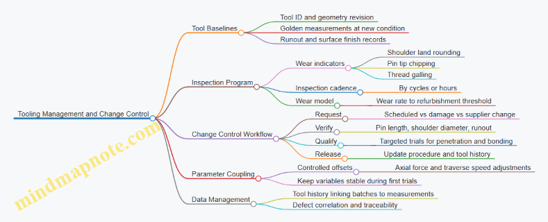
Example: Controlled Tool Replacement Without Surprise Defects
A production line uses a threaded retention tool. After 180 parts, inspection shows shoulder wear land increased from 0.30 mm to 0.38 mm, still within the allowed limit but close. The team schedules refurbishment and replaces the tool with a refurbished unit.
They verify pin length at three points and confirm runout is within the same tolerance band as the baseline. They run a short qualification weld path on representative coupons, then section and check for consistent bonding at the lower region. Only after the qualification passes do they release the tool for production and record the tool ID, measurements, and results in the procedure log.
The key is that the team does not assume “refurbished means identical.” They measure, qualify, and release with evidence. That discipline keeps repeatability from depending on memory, luck, or the last person’s notes.
12.3 Fixturing and Handling Practices for Distortion Control
Distortion control starts before any welding or friction stir processing begins. The goal is simple: keep parts where they belong, let heat do its job, and prevent the part from “deciding” to move on its own. In practice, that means combining rigid restraint, smart compliance, and handling routines that avoid accidental stress.
Foundational Principles of Distortion Control
Heat input creates a thermal gradient, which expands material unevenly. When the heat source moves away, the hotter region cools and contracts, pulling the joint toward the last heated area. Fixturing counters this by controlling three things: (1) where the part can move, (2) how forces are introduced, and (3) when restraint is applied.
A useful mental model is to treat the assembly like a spring system. Too much restraint too early can trap residual stress and increase cracking risk. Too little restraint can allow warpage and misalignment, which then forces the process to compensate with parameters, often with mixed results.
Fixturing Strategy from Geometry to Restraint
Datum Selection and Contact Planning
Choose datums that reflect functional requirements, not just what is easiest to clamp. For aerospace panels, datums often align with mating surfaces or critical holes. Plan contact points so they support the part without rocking. A common mistake is clamping on thin edges that bend under load; the part then “springs” after the clamp is removed.
A practical approach is to define:
- Primary datum for location in one direction.
- Secondary datum for location in the perpendicular direction.
- Tertiary datum for preventing lift or twist.
Clamp Placement and Load Paths
Clamps should create a clear load path into the fixture base. If the load path is indirect, the part flexes locally and distortion increases. For long seams, use multiple restraint points spaced to avoid concentrating force at one spot.
For friction stir processing, remember that tool forces and heat both act through the joint region. If the fixture allows the panel to lift, you can see surface waviness and inconsistent penetration. If the fixture is overly rigid at the wrong locations, you can see excessive residual stress near the clamped edges.
Handling Practices That Prevent Accidental Stress
Handling is not a side task; it is part of the distortion budget. Avoid dragging parts across fixture surfaces, which can introduce micro-scratches and local stress raisers. Use lifting points that match the part’s stiffness. Thin panels should be supported close to their natural bending stiffness; otherwise, they arrive at the machine already biased.
Before processing, verify:
- Fit-up gap and alignment at multiple points along the joint.
- Surface cleanliness at contact zones so clamps seat consistently.
- Fixture cleanliness so chips or debris do not create false gaps.
Advanced Restraint Techniques for Complex Assemblies
Backing Support and Thermal Isolation
Backing plates reduce sag and help maintain joint line straightness. Use backing materials that support the part without acting like a heat sink that changes the thermal gradient unexpectedly. If the backing is too conductive, the joint cools faster near the support, which can shift microstructure and residual stress distribution.
Thermal isolation pads can reduce unwanted heat flow into the fixture, but they must be stable under clamp load. A pad that compresses unevenly can tilt the part by fractions of a millimeter—enough to matter for tight aerospace tolerances.
Controlled Compliance and Sequencing
Controlled compliance means allowing small, predictable movement while preventing gross warpage. One method is to use slotted clamp features or spring-backed supports that maintain contact but reduce peak stress.
Sequencing matters: apply restraint in a way that matches the process path. For example, if you clamp both ends rigidly and then process from one end, the part may bow toward the free side. A better approach is to restrain in stages or use intermediate stops that maintain alignment as the heat source advances.
Mind Map: Distortion Control Through Fixturing and Handling
Integrated Example Workflow
Consider a lap joint on a stiffened aluminum panel. Start by selecting datums on the stiffener base and the panel edge that interfaces with the next assembly. Place backing support under the lap region to prevent sag, but keep the backing contact area consistent along the seam.
Clamp at three zones: near the start, mid-length, and near the end. Use firm seating at the start and end to prevent drift, and a slightly compliant support at mid-length to reduce peak stress concentration. Before processing, confirm the overlap gap is within tolerance at multiple points and that clamp faces are free of chips.
During handling, lift the panel using supports near the stiffener locations, not at the thinnest sheet edges. After the first trial run, measure straightness and joint line alignment. If the panel bows toward the last heated region, adjust sequencing by adding an intermediate stop or increasing compliance on the side that is moving.
Practical Checks That Catch Problems Early
- Clamp witness marks: consistent marks indicate stable seating.
- Pre-run alignment survey: measure before heat, not after.
- Post-run edge lift inspection: look for lift at clamp release zones.
- Repeatability test: run the same fixturing setup twice and compare alignment.
Distortion control is a chain. When each link—datum choice, contact design, handling, and verification—does its job, the process parameters can focus on welding quality rather than compensating for movement.
12.4 Production Line Integration Including Cycle Time Throughput and Scrap Reduction
Production line integration starts with a simple question: what is the slowest step, and why is it slow? For friction stir processing and hybrid laser/electron beam welding, the bottleneck is often not the “welding time” itself, but the handoffs around it—tool changes, fixturing, inspection sampling, and rework loops.
Foundational Flow Design
Begin by mapping the end-to-end route from incoming material to final acceptance. For each operation, record: setup time, active processing time, cooling/handling time, and inspection time. A practical example: if a friction stir weld takes 2 minutes of tool travel but requires 6 minutes of fixturing adjustment and 4 minutes of cooling before handling, the effective cycle time is dominated by the non-active steps.
Next, define station boundaries so that each station has a clear input and output. A common mistake is letting one station “own” both fixturing and inspection. Instead, keep fixturing and loading at one station, processing at another, and inspection at a third. This reduces waiting and makes scrap containment easier.
Cycle Time Accounting That Actually Matches Reality
Use a cycle time model with three layers:
- Planned cycle time: active processing plus required handling and safety delays.
- Observed cycle time: what operators experience, including micro-stoppages.
- Effective cycle time: observed cycle time multiplied by yield (the fraction of parts that pass without rework).
Example workflow for a mixed aluminum structure: Station A loads and clamps the panel, Station B performs friction stir processing, Station C performs a quick dimensional check, and Station D performs NDT sampling. If dimensional checks catch misalignment early, you avoid sending bad parts into NDT and mechanical testing, which lowers effective cycle time.
Throughput Planning with Constraint Awareness
Throughput is limited by the station with the highest effective cycle time per part. To avoid surprises, compute capacity per shift using the station’s effective cycle time and the number of parallel fixtures.
Example: Suppose the processing station can run 30 parts per shift, but the inspection station only clears 20 per shift. Adding more processing capacity won’t increase output until inspection capacity rises or inspection sampling is adjusted to match risk.
For friction stir and hybrid welding, also account for consumables and tool wear. Tool wear can shift the process window, increasing defect rates and therefore rework time. A simple control practice is to schedule tool condition checks at fixed production intervals and after a defined number of welds, then treat out-of-tolerance tools as a planned stop rather than an emergency.
Scrap Reduction Through Early Containment
Scrap reduction works best when you prevent defects from traveling downstream. Organize containment around defect types:
- Fit-up and alignment issues: catch with pre-process checks such as gap measurement and clamp verification.
- Process window violations: catch with in-process monitoring signals and immediate parameter logging.
- Metallurgical and internal defects: catch with NDT sampling tuned to the joint geometry and critical zones.
Example: If lack of penetration or tunnel-like features correlate with low axial force or incorrect plunge depth, then a station-level “go/no-go” check on axial force and plunge depth before full travel can prevent a whole batch from becoming scrap.
Rework should be treated as a separate route with its own time and acceptance criteria. If rework shares the same inspection queue as first-pass parts, it quietly increases cycle time for everyone.
Integrated Mind Map
Mind Map: Production Line Integration
Concrete Example: One Line, Two Processes
Consider a line that builds mixed joints: friction stir for stiffener-to-skin, and laser hybrid for a localized seam. The line design uses a shared material staging area and separate fixturing pallets.
- For friction stir, the processing station includes a quick pre-check of clamp torque and a tool wear indicator readout. If the indicator is out of range, the part is held and the tool is swapped before processing.
- For laser hybrid, the processing station includes a beam alignment verification step tied to the fixture ID. If alignment drifts, the part is re-queued for re-alignment rather than processed with incorrect conditions.
Inspection sampling is aligned to where defects are most likely: dimensional checks for alignment-sensitive friction stir joints, and porosity-focused NDT sampling for laser hybrid seams. This keeps scrap from spreading across the line and makes throughput predictable.
The result is a production system where cycle time is measured honestly, throughput is limited by known constraints, and scrap is reduced by stopping defects early—before they become expensive problems.
12.5 Practical Example Workflows for Building and Verifying Production Procedures
A production procedure is not a recipe card; it’s a controlled chain of decisions that turns material, equipment, and inspection results into a repeatable joint. The workflow below uses one practical scenario—an aluminum friction stir weld (FSW) with a laser-assisted hybrid pass on a lap joint—then shows how the same logic applies to friction stir processing (FSP) and to fusion methods.
Workflow Overview
- Start with the qualified intent: define the joint type, target properties, and allowable defect types. If you already have a qualified procedure, treat it as the “physics baseline.”
- Translate intent into controllables: list the parameters that actually move the outcome (tool rotation, traverse speed, axial force, laser power, gas flow, stand-off, travel path, dwell, and start/stop behavior).
- Build a parameter-to-measurement map: for each controllable, define what you will measure and what “in family” looks like.
- Create a stepwise work instruction: include setup, run, and verification steps in the order operators will execute them.
- Verify with a production-style trial: run a small batch under realistic constraints (tool wear state, fixturing, operator, and inspection timing).
- Lock down changes: define what triggers a revision (tool replacement, new batch of material, different fixturing, or inspection results outside control).
Mind Map: Procedure Build and Verify
Example Workflow: Building a Production Procedure
Step 1: Define the “What Good Looks Like”
For a lap joint, specify the target failure mode and where you expect it to occur. Example: tensile shear specimens should fail in the stir zone with no interface separation. Acceptance criteria should include defect types you will reject (for instance, lack of bonding or excessive porosity) and measurement methods (ultrasonic settings, sectioning locations, and sampling frequency).
Step 2: Convert Qualified Parameters into Operator Actions
Operators need actions, not just numbers. Example work instruction fragments:
- Tool and machine checks: confirm tool length against a reference, verify shoulder contact condition, and record spindle runout if your system supports it.
- Fixturing: set clamp pressure so the joint stays closed during thermal expansion; a simple check is to measure gap at the start and end of the intended weld path.
- Start sequence: ramp rotation to setpoint before first contact; begin traverse only after axial force reaches the target band.
- Hybrid coordination: start laser emission at a defined offset relative to tool position so the laser energy arrives when the material is in the correct mixing state.
Step 3: Parameter-to-measurement map
Example mapping for hybrid FSW:
- Rotation setpoint → verify with machine logs; control band is typically tighter than the traverse band because rotation fluctuations strongly affect heat input.
- Axial force → verify with force sensor traces; reject runs with sustained force drift.
- Laser power → verify with interlock status and power readback; also record stand-off distance.
- Gas flow → verify flow meter reading; document any nozzle changes.
This mapping prevents a common failure mode: you measure the wrong thing, then argue about why the weld looks different.
Example Workflow: Verifying the Procedure in Production Style
Step 4: Run a Trial That Resembles Production
Use the same operator, the same fixturing approach, and the same inspection timing you will use later. Example trial plan:
- Produce three joints using the current tool condition.
- Inspect all joints for surface continuity and internal defects using your chosen NDE method.
- Section one joint at the defined locations for microstructure and bonding verification.
- Test two specimens for tensile shear if your qualification plan allows it; otherwise, test one and keep the other as a reserve.
Step 5: Decide Release vs. Revision
Release when results fall within control limits and the defect distribution matches expectations. If you see a consistent defect pattern, revise the procedure in the smallest way that addresses the root cause.
Example revision logic:
- If lack of bonding appears near the start region, adjust start sequence timing or ramp behavior.
- If defects cluster near the end, add dwell or refine end ramp-down so the material doesn’t cool too quickly.
- If porosity increases in the hybrid zone, review laser stand-off and gas flow consistency, then re-check alignment between tool and laser.
Step 6: Lock the Change Control
Write explicit triggers for procedure revision. Example triggers:
- Tool replacement or measurable wear beyond your threshold.
- Switch to a different material heat or thickness tolerance band.
- Change in fixturing hardware or clamp strategy.
- NDE results outside the established acceptance envelope.
Case-Style Checklist for Operators and Engineers
- Setup complete and recorded
- Tool condition verified
- Fixturing gap check performed
- Start, main, and end sequences executed as written
- Hybrid laser interlocks confirmed
- Machine logs archived for every run
- NDE performed on every joint
- Sectioning and mechanical sampling executed per plan
- Results compared to control limits and acceptance criteria
This workflow keeps the procedure grounded: it ties each step to a measurable outcome, so verification is evidence-based rather than hope-based.