Industrial Photonics Manufacturing
1. Scope and Manufacturing Foundations for Industrial Photonics
1.1 Defining Laser Optical Systems in Manufacturing Terms
A laser optical system is not just a beam and a lens. In manufacturing terms, it is a set of components and interfaces that must reliably produce a specified optical output while surviving handling, assembly, test, and use. The key is to define it using measurable inputs and outputs so production decisions have something solid to stand on.
What to Define First
Start with the optical output you must deliver. Typical outputs include beam diameter at a reference plane, divergence, wavefront quality, spectral bandwidth, polarization state, and transmitted or reflected power at defined wavelengths. Then define the operating conditions that affect those outputs: drive current or pulse energy, duty cycle, ambient temperature, and any required cooling method.
Next define the system boundaries. Manufacturing needs to know what is inside the optical system and what is treated as an external interface. For example, a laser module might include the laser source, collimation optics, beam shaping elements, and protective windows, while the fiber coupling or motion stage is external. Clear boundaries prevent “mystery failures” where test results look fine but integration fails.
Translate Optical Intent into Manufacturing Requirements
Optical design intent becomes manufacturing requirements through a chain of measurable characteristics.
- Surface quality: roughness and figure errors that affect scattering and wavefront.
- Geometry: diameters, thicknesses, wedge angles, and centering that affect alignment and focus.
- Coatings: reflectance/transmittance versus wavelength and angle, plus durability under the expected laser exposure.
- Mechanical stability: mount stiffness, thermal expansion behavior, and datum references for repeatable alignment.
- Assembly relationships: bond line thickness, adhesive cure constraints, and torque or clamp force limits.
A practical way to keep this systematic is to define each requirement with a unit, a tolerance, and a test method. If a requirement cannot be tested on the shop floor, it will be managed by hope, and hope is not a process.
System Architecture as a Production Map
Manufacturing benefits from describing the system as a hierarchy: source → beam conditioning → beam shaping → protection → interfaces. Each block has distinct production steps and failure modes.
For instance, the source block is sensitive to electrical integration and thermal control. The beam conditioning block is sensitive to lens figure and coating performance. The protection block is sensitive to contamination control and coating durability. The interfaces block is sensitive to mechanical datums and alignment repeatability.
Mind Map: Laser Optical System in Manufacturing Terms
Example: Turning a Beam Spec into Shop-Floor Checks
Suppose the requirement is: “At 200 mm from the output window, beam diameter must be 1.0 ± 0.1 mm, divergence must be below 2 mrad, and polarization must be linear with extinction ratio above 20 dB.”
A manufacturing-friendly definition would specify:
- Test setup: reference plane distance, measurement method (e.g., beam profiler), and acceptance criteria.
- Optics contributors: lens focal length tolerance, lens centering tolerance, and coating transmission at the operating wavelength.
- Alignment contributors: allowable angular misalignment and how it is measured during assembly.
- Thermal contributors: allowable drift in beam diameter across the specified temperature range.
If the team only writes the first line, they can measure the result but cannot reliably explain why it passed or failed. If they write the full chain, they can connect outcomes to controllable steps.
Example: Defining Boundaries to Avoid Integration Confusion
A common manufacturing mistake is treating the “optical system” as a single blob. Instead, define what the test fixture includes. For example, if the final test uses a temporary coupling lens that is removed during field integration, then the test must either replicate the real coupling or explicitly account for the difference. Otherwise, the system can pass final test and still miss the real optical output once the external lens is installed.
The Manufacturing Definition in One Sentence
A laser optical system is the configured set of optical and mechanical elements, with defined interfaces and operating conditions, that must meet specified optical outputs verified by repeatable measurement methods and supported by traceable production controls.
1.2 Mapping Product Requirements to Process Capabilities
Mapping product requirements to process capabilities is the step where “what we need” becomes “what we can reliably make.” For industrial photonics, the trap is assuming that meeting a spec at the end of the line is enough. In reality, most optical performance is the sum of many small process outcomes: surface figure, coating uniformity, alignment repeatability, and even how parts are handled between steps.
Start with Requirements That Can Be Measured
Write requirements in terms that can be verified on the shop floor. For each requirement, define:
- Measurement method (what instrument and procedure)
- Acceptance limits (numerical thresholds)
- Sampling plan (100% test, statistical sampling, or end-of-lot)
- Timing (in-process, post-process, or final)
Example: If the product requirement says “high transmission,” convert it into something measurable like “Transmission ≥ 98% at 1064 nm, measured at 0° incidence, with defined aperture.” If the requirement is “stable alignment,” define what “stable” means, such as “beam pointing drift ≤ X over Y hours after thermal soak.”
Break Requirements into Physical Drivers
Next, translate each requirement into the physical drivers that manufacturing controls. A simple way is to ask, “Which process outputs change this measurement?”
- Optical transmission is driven by substrate cleanliness, coating stack design, deposition uniformity, and post-coating handling.
- Wavefront error is driven by substrate figure, polishing process control, and mounting stress.
- Beam pointing is driven by alignment strategy, mechanical datum scheme, adhesive/bond line thickness, and thermal behavior of mounts.
This is where you prevent gaps: if a requirement depends on multiple drivers, you must map it to multiple process steps, not just the final assembly.
Build a Requirements-to-Process Matrix
Create a matrix that links each requirement to candidate process steps and their controllable outputs. Keep it practical: list the process steps you actually run, not every theoretical operation.
A good matrix includes:
- Requirement ID
- Process step (e.g., substrate prep, polishing, coating, bonding, alignment)
- Process output (e.g., Ra, PV/figure, coating thickness uniformity, bond line thickness)
- Key control parameters (e.g., polish pressure, deposition rate, cure profile)
- Measurement/verification
Example: For a transmission requirement, the matrix might connect it to coating thickness uniformity and substrate contamination. Then you ensure you have an inspection method for those outputs, not just the final transmission.
Convert Process Outputs into Capability Targets
Process capability is not a vibe; it’s a measurable spread. For each mapped process output, define capability targets that support the requirement limits.
Use a structured approach:
- Define allowable variation for the process output based on how it affects the final requirement.
- Measure current process performance using historical data or pilot runs.
- Set control limits and acceptance criteria aligned to the allowable variation.
Example: If coating thickness uniformity affects transmission, and the final transmission limit is tight, then the thickness uniformity target must be tighter than you might guess. If you only set a broad coating acceptance limit, you’ll discover the mismatch at final test—usually after you’ve spent time and money.
Mind Map: Requirements to Capabilities
Example: A Tight Optical Spec with Multiple Drivers
Suppose the requirement is “Wavefront error ≤ 0.05 waves RMS at 633 nm.” A realistic mapping might look like this:
- Substrate figure from polishing process output (mapped to metrology after polishing)
- Surface roughness affecting scattering (mapped to roughness measurement)
- Mounting stress from assembly torque and adhesive cure profile (mapped to assembly parameters and post-bond metrology)
- Alignment-induced optical path effects (mapped to alignment procedure and verification)
If you only control substrate figure and ignore mounting stress, you can pass polishing and still fail final wavefront. The matrix forces you to control every driver that can move the measurement.
Validation: Confirm the Mapping Works Before Scale
Before full production, validate the mapping with a controlled trial. The goal is not perfection; it’s confirming that the mapped process outputs explain the final results.
A practical validation checklist:
- You can reproduce the final measurement using the mapped process outputs.
- You have in-process checks for the outputs that matter most.
- You know which process step is the dominant contributor when failures occur.
When the mapping is correct, nonconformance investigations become straightforward: you don’t start by guessing which step “probably went wrong.” You start by checking the mapped outputs in the order that matches their influence.
1.3 Cleanliness, Contamination Control, and Handling Practices
Cleanliness in industrial photonics is not a moral virtue; it’s a measurable input that protects optical performance, yield, and safety. Contamination shows up as haze, scattering, coating defects, bond failures, and intermittent test results that vanish when you re-run the same part. The goal is to prevent particles, films, and residues from entering sensitive steps, and to keep them from migrating later.
Foundations of Contamination in Photonics
Start by separating contamination into three practical categories:
- Particles: dust, grit, and fibers that land on surfaces and create scattering or coating pinholes.
- Films: thin residues from handling, cleaning agents, lubricants, adhesives, or outgassing.
- Chemistry: reactive residues such as chlorides or sulfur compounds that attack coatings or metals.
A useful rule is that particles are usually a surface problem, while films and chemistry are surface + time problems. A part can look fine immediately after assembly and still fail after thermal cycling because residues slowly redistribute or react.
Cleanliness Levels and Where They Matter
Not every step needs the same cleanliness. Define cleanliness by risk, then assign controls to the risk.
- Optical surface exposure (before coating, before bonding, during alignment): highest sensitivity.
- Coating chamber interfaces (substrate loading, handling between cleaning and deposition): high sensitivity.
- Mechanical interfaces (mounting faces, dowel seats): medium sensitivity, but still important for repeatability.
For example, a mirror blank can tolerate minor handling marks on the back side, but a single fingerprint on the reflective area can seed scattering sites that survive polishing and show up as a “mystery” loss in transmission.
Handling Practices That Prevent Contamination
Handling is where most contamination enters, because it combines human touch, air exposure, and tool contact.
Gloves, Tools, and Contact Rules
Use gloves appropriate to the task and keep them clean. Nitrile gloves are common for general handling, but for optics work you often need a glove strategy that avoids lint shedding and reduces skin oils transfer.
Tool contact rules should be explicit:
- Only touch non-critical edges or defined grip zones.
- Use dedicated tweezers or vacuum wands for optics, with tips maintained and cleaned.
- Avoid metal-to-optic contact unless the process explicitly allows it.
A simple example: if you routinely pick up lenses by the rim, mark the rim region on the work instruction and require that the rim is the only allowed contact zone. This turns “be careful” into a repeatable behavior.
Packaging and Time Control
Contamination control is also about time. Define maximum exposure windows between cleaning and the next process step.
- Store cleaned optics in sealed containers or controlled environments.
- Use desiccant or humidity control where relevant to coating and bonding.
- Label containers with lot, cleaning step, and expiration time.
If you clean a substrate and leave it on an open bench for an hour, you’ve effectively replaced “cleaning” with “waiting for dust.” The process should prevent that.
Cleaning Workflow with Verification
Cleaning should be systematic: remove particles first, then remove residues, then verify.
Stepwise Cleaning Logic
- Dry removal: remove loose particles using controlled methods (for example, filtered air or gentle wipe protocols that match the surface).
- Wet cleaning: remove oils and residues using compatible chemistry and controlled agitation.
- Rinse and drying: prevent redeposition by using clean rinse water and drying that doesn’t leave droplets.
- Final inspection: verify cleanliness before the next sensitive step.
A practical example is cleaning a substrate before thin-film deposition. If you skip the final inspection, you may coat over a residue film, which later causes adhesion loss or haze. Verification is what turns cleaning from “hope” into “evidence.”
Verification Methods
Choose verification that matches the contamination type:
- Visual inspection under appropriate lighting for gross defects.
- Surface inspection tools for particles and haze.
- Contact angle or residue checks where the process demands it.
Even a basic practice helps: inspect immediately after drying and again right before coating. If the second inspection finds new contamination, the issue is handling or storage time, not the cleaning chemistry.
Advanced Controls for Coating and Bonding Steps
Coating and bonding are where contamination becomes expensive.
Coating Readiness Checks
Before loading into a deposition tool, confirm:
- Substrate is within the defined time window after cleaning.
- Handling tools are clean and compatible.
- Containers and transfer paths are controlled.
If you see recurring coating defects on specific lots, check whether those lots share the same transfer container or staging area. Contamination often travels with the logistics.
Bond Line Cleanliness
For optical bonding, residues can interfere with wetting and cure.
- Control adhesive storage and dispense cleanliness.
- Ensure mating surfaces are cleaned and dried per the bond procedure.
- Limit open time between cleaning and adhesive application.
A concrete example: if bond strength varies, compare the time between cleaning and bonding across lots. A longer open time can allow a thin film to form, reducing adhesion even when the adhesive is correct.
Mind Map: Cleanliness and Contamination Control
Practical Standard Work for Daily Use
A good standard work set is short enough to follow and strict enough to matter. For example:
- Inspect optics after drying.
- Use defined grip zones only.
- Transfer in sealed containers with lot and time labels.
- Enforce a maximum time window between cleaning and the next step.
- Verify cleanliness again right before coating or bonding.
When these steps are consistent, most “random” optical defects stop being random. They become traceable, and traceable problems are fixable.
1.4 Quality Management Systems for Optical and Laser Products
Quality management for optical and laser products is less about slogans and more about making the right thing the easiest thing. A practical system connects requirements to measurable characteristics, then ties those characteristics to controlled processes, evidence, and decisions.
Quality Goals That Match Optical Reality
Start with what “quality” means for the product. For optical and laser systems, quality usually includes optical performance (transmission, wavefront, beam quality), physical integrity (surface figure, coating adhesion), and operational behavior (power stability, thermal response). A useful first step is to translate customer and design requirements into Critical to Quality characteristics, then define how each characteristic is measured and at what point in the workflow it is verified.
Example: If a lens must maintain a specific transmission band after coating, the system should specify the coating acceptance test (spectral measurement method, sampling plan, and pass/fail limits) rather than only stating “good coating.”
Process Control from Incoming to Final Test
A quality management system works when it controls variation at every stage where variation can enter.
- Incoming control: Verify that substrates, mounts, and electrical components meet specifications. For optics, this often means checking surface damage risk, dimensional stability, and documentation consistency.
- In-process control: Monitor steps that strongly affect final performance, such as polishing parameters, cleaning steps before coating, and coating thickness uniformity.
- Final acceptance: Confirm that the assembled product meets performance and safety requirements using calibrated measurement equipment.
Example: If coating yield drops, the system should let you trace which lot of cleaned substrates was used, which tool recipe ran, and which in-process readings were recorded. That turns “something changed” into “here is what changed.”
Documented Procedures That People Actually Follow
Documentation should be specific enough to reduce ambiguity and simple enough to be used on the floor.
- Work instructions: Define the exact sequence, key parameters, and required checks. For optical cleaning, include acceptable residue criteria and drying method constraints.
- Inspection plans: Specify what is measured, how often, and what to do when results are borderline.
- Configuration control: Ensure that a change in coating recipe, mount material, or firmware version is tracked and approved.
Example: A polishing instruction that only says “polish until good” is not a procedure. A procedure that states target roughness range, measurement interval, and rework rules is.
Measurement System Integrity
If measurement is unreliable, quality decisions become guesswork.
A robust system includes:
- Calibration of gauges and optical measurement instruments.
- Uncertainty awareness so pass/fail limits account for measurement variability.
- Repeatability and reproducibility checks for operators and setups.
Example: Two operators measure the same wavefront sample. If their results differ beyond expected uncertainty, the system should address fixture alignment, measurement settings, or training before using those measurements to release product.
Nonconformance Handling That Prevents Repeat Issues
Nonconformance is not just a form; it is a structured decision.
- Containment: Stop further processing of affected lots.
- Disposition: Decide whether to scrap, rework, or use-as-is based on defined criteria.
- Root cause analysis: Use evidence, not blame. For optical failures, common root causes include contamination before coating, incorrect substrate handling, or misapplied assembly torque.
- Corrective and preventive actions: Update procedures, training, or controls so the same failure mode does not return.
Example: If coating adhesion fails, the system should check cleaning logs, storage conditions, and time between cleaning and coating. If the failure correlates with a specific handling step, the corrective action should modify that step and verify improvement with a controlled retest.
Mind Map: Quality Management System for Optical and Laser Products
Records and Traceability That Support Real Decisions
Traceability is valuable when it helps you answer questions quickly and accurately.
A workable approach is to record the minimum set of data needed to connect a finished unit to:
- the substrate lot,
- the coating tool and recipe,
- the assembly configuration,
- the test results and measurement settings.
Example: During a customer return investigation, traceability should let you identify whether the unit used a specific coating recipe revision and whether its spectral curve shows the same deviation pattern as other affected units.
Internal Audits and Management Review with Clear Outputs
Audits should check both compliance and effectiveness. A procedure can be followed and still fail to produce good outcomes.
- Internal audits: Verify that records exist, procedures are current, and results match expectations.
- Management review: Use trends from yield, rework rates, measurement capability, and nonconformance themes to decide what to fix.
Example: If rework is concentrated in one assembly station, the system should examine fixture wear, torque calibration, and operator technique consistency, then verify improvement with a measurable reduction in rework.
Integrated Example: From Requirement to Release
A lens requirement specifies a transmission band and surface figure limit. The system defines incoming substrate checks, in-process polishing metrology, and coating spectral acceptance. During assembly, it records mount configuration and bonding parameters. Final test uses calibrated optics to verify wavefront and transmission. If a unit fails, the nonconformance process identifies the likely step via recorded lot and tool data, applies containment, and updates the relevant work instruction. The result is not just a decision for one unit, but a controlled reduction in the same failure mode across future lots.
1.5 Documentation Standards for Traceability and Configuration Control
Industrial photonics manufacturing lives and dies by repeatability. Documentation standards are the system that makes “the same part” mean the same thing across operators, shifts, suppliers, and time. Traceability answers “what was made,” while configuration control answers “what design and process choices were used to make it.” Together, they prevent the classic failure mode: a part that passes today’s test but can’t be explained tomorrow.
Foundational Concepts and What They Prevent
Start with three definitions that should appear in your controlled procedures.
- Traceability: the ability to link a finished unit back to the specific materials, components, process lots, and test records used.
- Configuration control: the ability to ensure the exact intended design and manufacturing instructions are used, and that changes are reviewed, approved, and recorded.
- Controlled records: documents and data that are versioned, authorized, and retained according to policy.
A simple example: a coated optic fails a laser-induced damage test. Traceability lets you identify the coating run and substrate lot. Configuration control lets you confirm whether the coating recipe, substrate cleaning step, and mounting procedure matched the approved build instruction.
Traceability Model from Materials to Finished Units
Use a consistent “unit genealogy” structure. For each finished laser optical assembly, capture identifiers at these levels:
- Material and component identifiers: substrate lot, coating batch, adhesive lot, fastener grade, lens element serial.
- Process identifiers: tool ID, recipe ID, operator or workstation ID, run start/end timestamps, and in-process inspection results.
- Test identifiers: test procedure version, calibration state, measurement system ID, and pass/fail outcomes.
- Nonconformance identifiers: NCR number, disposition, rework instructions used, and final verification results.
Keep the identifiers short but unambiguous. If your substrate lot is “S-1042,” your coating batch is “CB-77,” and your assembly serial is “A90321,” you should be able to reconstruct the chain without opening five spreadsheets and guessing which column matters.
Configuration Control Model for Design and Process Instructions
Configuration control should cover both “what” and “how.”
- Design configuration: drawings, optical layouts, bill of materials, and any interface specifications.
- Process configuration: work instructions, coating recipes, cleaning steps, curing profiles, alignment procedures, and acceptance criteria.
Each controlled document should have:
- A unique document ID
- A version number
- An approval authority
- Effective dates or release status
- A clear mapping to the records it generates
When a change happens, you want to know whether it affects existing inventory, whether it requires rework, and whether it changes acceptance criteria. Configuration control is not just paperwork; it’s the decision trail.
Mind Map: Traceability and Configuration Control
Practical Example: Coated Optic with a Laser Test Failure
Assume optic serial O-55109 fails a laser-induced damage test.
- Traceability record shows:
- Substrate lot S-1042
- Coating batch CB-77
- Coating tool TC-3 and recipe RCP-COAT-12
- Cleaning step CLN-05 performed on line L2
- Configuration control record shows:
- Approved coating work instruction version WI-COAT-4.1
- Acceptance criteria version AC-LIDT-2.0
- Any later revision status for WI-COAT-4.2 marked “not effective for this lot”
With that, the investigation can focus on the coating batch and cleaning step rather than debating which instruction was used.
Advanced Details That Keep the System Honest
- Audit trail requirements: record who changed what, when, and why. If a value is corrected, store the original value and the reason.
- Version locking for test procedures: test results should always reference the exact procedure version and calibration state used at the time.
- Linking rules: define how identifiers connect across systems. For example, coating batch ID must map to the substrate lot and tool run record.
- Retention and access: specify retention duration and who can view or edit controlled records.
Example: Minimal Record Set for an Assembly Traveler
Assembly Traveler Record Set
- Assembly serial: A90321
- Design reference: Drawing D-2201 Rev B
- BOM snapshot: BOM-2201 Rev 3
- Optic serials: O-55109, O-55110
- Coating batch IDs: CB-77, CB-78
- Process run IDs: TC-3 Run 2026-03-18-014
- In-process checks: surface roughness, centering
- Final test: procedure TP-LAS-1 Rev 2
- Calibration state: MS-FTIR-04 Cal 2026-03-01
- NCR linkage: NCR-1184 if applicable
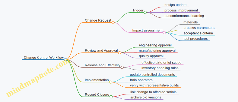
Mind Map: Change Control Workflow
Summary of What “Good” Looks Like
Good documentation standards let you answer three questions quickly: which design and instructions were used, which materials and process runs were involved, and which tests were performed under which calibrated conditions. When those answers are consistent, investigations become precise, and production becomes calmer—even when something goes wrong.
2. Materials, Components, and Optical Design Inputs for Production
2.1 Optical Materials Selection for Glass, Crystals, and Polymers
Choosing an optical material is mostly a matching exercise: you align the material’s optical behavior with the laser’s wavelength, power, and environment, then confirm the mechanical and manufacturing realities won’t sabotage the design. A good selection starts with a few measurable properties, not a gut feeling.
Core Requirements from the Laser and the Optics
Start by listing the constraints that directly affect performance.
- Wavelength compatibility: Verify transmission at the operating wavelength and check for absorption bands that can heat the optic.
- Example: A glass that transmits well at 1064 nm may absorb strongly at 532 nm, turning a “works on paper” optic into a thermal problem.
- Power handling and thermal behavior: Use absorption to estimate temperature rise, then check thermal conductivity, expansion, and stress sensitivity.
- Example: Two materials with similar transmission can behave very differently under high average power because one conducts heat better.
- Surface and figure stability: Consider how the material responds to polishing, coating stress, and mounting forces.
- Example: If your mount clamps near the edge, a brittle material with low fracture toughness can fail during assembly even when optical quality is excellent.
- Environmental exposure: Account for humidity, solvents, and temperature cycling.
- Example: Polymers can fog or craze under certain cleaning chemicals, even if they look fine initially.
Material Families and What They’re Good At
Think of the three families as different toolkits.
Glass
Glasses are widely used because they balance optical quality, availability, and manufacturability.
- Strengths: Good optical homogeneity, mature polishing processes, and predictable thermal expansion.
- Watch-outs: Some glasses are sensitive to thermal shock; others have limited transmission windows.
- Example: For a compact laser module with rapid on-off cycling, you may prefer a glass with better thermal shock resistance to reduce microcracking risk.
Crystals
Crystals can offer excellent transmission and tailored optical properties, especially for specific wavelengths.
- Strengths: Often superior transmission in narrow bands and strong performance for certain nonlinear or high-precision applications.
- Watch-outs: Growth defects, birefringence, and cost; also more demanding machining and mounting.
- Example: If polarization purity matters, you must check birefringence and orientation tolerances, not just average transmission.
Polymers
Polymers are attractive for weight, cost, and sometimes for large optics where glass would be heavy.
- Strengths: Easy shaping, low density, and potentially good performance at longer wavelengths.
- Watch-outs: Lower thermal stability, higher creep, and chemical sensitivity.
- Example: A polymer lens in a sealed housing may survive, but the same material exposed to repeated solvent wipes can develop surface haze.
Selection Workflow That Doesn’t Skip Steps
Use a repeatable sequence so the decision is defensible.
- Define the optical job: wavelength, beam size, incidence angle, and required wavefront quality.
- Screen by transmission and absorption: reject materials that absorb at the laser wavelength.
- Check thermal and mechanical compatibility: compare thermal expansion with mount design and coating stress.
- Confirm manufacturability: can you polish, edge, and coat to the required surface roughness and figure?
- Validate with a small build: test one optic in the real mounting and cleaning process.
Mind Map: Optical Material Selection
Practical Examples That Tie the Logic Together
Example: Choosing for 1064 nm with high average power
- Start with transmission at 1064 nm and quantify absorption.
- Then compare thermal conductivity and expansion to your mount design.
- If the optic must be clamped tightly, prioritize mechanical robustness and stress tolerance over “best-case” optical transmission.
Example: Choosing for 532 nm with strict polarization requirements
- Confirm transmission at 532 nm and check for absorption-driven heating.
- If polarization purity matters, evaluate birefringence for crystals and ensure glass selection doesn’t introduce unwanted stress birefringence from mounting.
Example: Choosing for a low-cost, lightweight lens at 1550 nm
- Verify polymer transmission at 1550 nm and confirm cleaning compatibility.
- Design the mount to reduce creep: avoid long-term stress at the lens edge.
- Run a cleaning trial using the same wipes and solvents your operators will use.
Decision Notes for Coatings and Mounting
Even perfect bulk material can fail at the interfaces.
- Coating stress: A coating can warp a substrate if thermal expansion mismatch is large.
- Mounting pressure: Point loads can create birefringence in glass or microcracks in brittle optics.
- Cleaning process: The “best” material is the one that survives the actual maintenance routine without surface degradation.
A disciplined selection treats material choice as a system decision: optical performance, thermal behavior, mechanical handling, and manufacturing steps all have to agree, or the final assembly will tell you where the mismatch lives.
2.2 Coatings and Substrate Compatibility With Laser Environments
Laser optics rarely fail because the coating is “bad” in isolation. More often, the coating is doing its job while the substrate, mounting, cleaning, or thermal behavior quietly makes the job harder. Compatibility means the coating and substrate agree on thermal expansion, adhesion, moisture tolerance, and how they respond to the laser’s power density.
Foundational Compatibility Concepts
Start with two basic questions: What is the coating trying to achieve, and what is the substrate likely to do under load? A coating’s job is usually spectral control (reflectance or transmission) plus durability against the specific laser wavelength and intensity. The substrate’s job is to stay dimensionally stable, keep its surface chemistry predictable, and avoid introducing stress that cracks or peels the coating.
A practical way to think about it is a “stress chain.” Laser heating creates a temperature gradient. That gradient produces thermal stress because the coating and substrate expand differently. If the stress exceeds the coating’s adhesion strength or fracture toughness, you get blistering, edge lift, or microcracking. Even when the coating survives, repeated cycling can still degrade performance by changing surface roughness or causing subtle delamination.
Substrate Properties That Control Coating Behavior
Thermal expansion match. If the coating’s coefficient of thermal expansion differs strongly from the substrate’s, the interface sees cyclic shear stress. For example, a coating on a low-expansion glass can be stable at moderate power, while the same stack on a higher-expansion glass may show faster degradation at the same irradiance.
Thermal conductivity and heat spreading. A substrate that spreads heat well reduces peak temperatures at the coating surface. In practice, two optics with identical coatings can behave differently because one substrate runs hotter under the same beam size.
Surface chemistry and cleanliness. Coatings bond best to surfaces that are chemically consistent. If cleaning leaves residues or alters the surface layer, adhesion can drop even if the coating thickness and design are correct. A simple example: an optic that was “cleaned enough” for visible inspection may still carry a thin film that interferes with adhesion.
Mechanical stiffness and mounting stress. Coatings are sensitive to bending and point loads. A lens clamped too tightly can warp slightly; the coating then experiences tensile stress during thermal cycling. The fix is often mechanical: use proper seat geometry, avoid over-torque, and ensure the optic is supported where it is designed to be supported.
Coating Stack Compatibility with Laser Environments
A coating stack is not one material; it is a sequence of layers with different refractive indices and thicknesses. Compatibility depends on how those layers respond to the laser’s wavelength, polarization, and intensity.
Absorption and local heating. Even “high-reflectance” coatings absorb a small fraction. At high power, that absorption becomes heat at the surface. If the stack has layers that absorb more at the operating wavelength, the temperature rise increases stress and accelerates damage.
Moisture and environmental exposure. Some coating materials are more sensitive to humidity. If the environment allows moisture ingress, you can see performance drift or adhesion loss. This is why storage and handling matter: a coating that is fine in a controlled assembly area can degrade after repeated exposure to humid air.
Laser-induced damage mechanisms. Common failure modes include coating cracking, delamination, and surface pitting. The key compatibility point is that the substrate can influence which mechanism dominates by changing thermal gradients and stress distribution.
Handling and Cleaning Practices That Preserve Compatibility
Treat cleaning as part of the coating system. Aggressive wipes, abrasive residues, or solvent choices that leave films can reduce adhesion or create micro-defects that later become damage initiation sites.
A simple workflow example for coated optics:
- Remove loose particles with a controlled method that minimizes contact.
- Use a cleaning approach that leaves no residue and avoids re-depositing contaminants.
- Dry using a method that does not leave droplets or streaks.
- Inspect under appropriate lighting to catch haze or residue that might not be obvious.
If you must rework a coating, remember that “re-cleaning” is not always equivalent to “re-coating.” A surface that has been damaged or chemically altered may not bond well the second time.
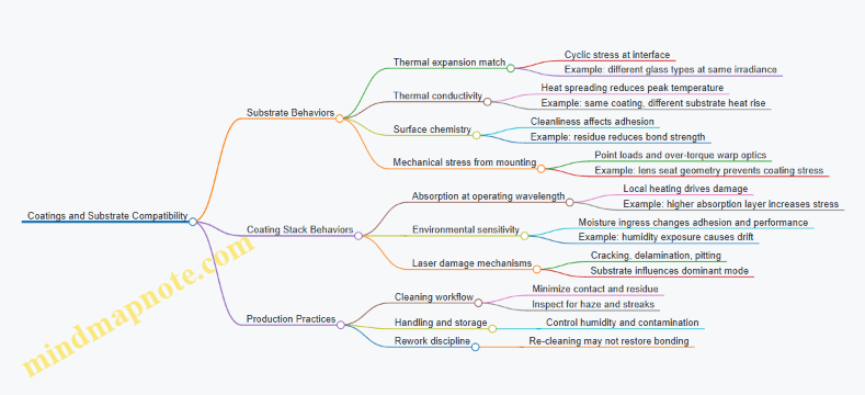
Mind Map: Coatings and Substrate Compatibility
Example: Choosing a Coated Optic for a High-Power Laser
Assume you need a high-reflectance optic at a specific wavelength. Two candidate substrates look similar on paper, but one has lower thermal conductivity and higher expansion. Even if the coating design is identical, the lower-conductivity substrate will run hotter at the coating surface, increasing thermal stress and accelerating damage. The compatibility check is therefore not just spectral performance; it includes thermal and mechanical fit. In production, you confirm this by using the same mounting approach, the same cleaning method, and the same acceptance test conditions for both candidates.
Example: Preventing Edge Lift During Assembly
Edge lift often starts where stress concentrates. If an optic is clamped with uneven pressure, the coating near the rim sees tensile stress during thermal cycling. A compatibility-focused assembly practice is to use a seat that supports the optic uniformly and to control torque so the optic is held without bending. The result is fewer coating failures that look mysterious until you notice the mechanical cause.
2.3 Mechanical Interfaces for Optics Alignment and Stability
Mechanical interfaces decide whether optical alignment survives handling, vibration, thermal cycling, and assembly variability. The goal is simple: make the optical element land in the same place, with the same orientation, every time, and keep it there while the system experiences real-world forces.
Core Principles of Optical Mechanical Interfaces
Start with three foundational ideas.
First, define datums that match how the optics are actually positioned. If the optical axis is set by a reference surface on the mount, then that surface must be treated as a datum in drawings and inspection. A common mistake is to reference a cosmetic face while the real alignment is controlled by a different feature.
Second, separate location from retention. Location features (pins, shoulders, reference bores) establish where the optic sits. Retention features (clips, rings, screws, adhesives) hold it without pulling it off the location. When retention features also act as location, small torque or adhesive shrinkage can shift the optic.
Third, manage stiffness and compliance intentionally. A mount that is too flexible will “average out” alignment errors during assembly, but it will also move under load. A mount that is too stiff can transmit stress into the optic, causing figure distortion or birefringence in stress-sensitive materials.
Interface Geometry That Supports Repeatable Alignment
Use geometry that constrains all degrees of freedom in a controlled order.
A typical approach is a kinematic-style constraint: three points define a plane, two points define a line, and one point defines a remaining rotation. For optics, this often becomes:
- A precision seat for axial position (a shoulder or reference surface).
- A centering feature for radial location (a bore, spigot, or V-groove).
- A rotational reference for angular orientation (a key, flat, or index mark).
Example: A lens mount with a ground shoulder sets axial position. A close-fit spigot centers the lens. A keyed slot prevents rotation. The retaining ring applies uniform pressure near the lens edge, avoiding direct clamping on the optical surface.
Material and Thermal Compatibility
Thermal stability is mostly about differential expansion and how stress is introduced.
Choose materials so that the interface does not force the optic to follow the mount’s expansion. If the optic and mount expand differently, the interface must allow controlled compliance. Options include:
- Clearance fits with spring retention.
- Flexures that maintain position while accommodating expansion.
- Adhesive layers designed for low shrink and appropriate modulus.
Example: For a glass optic in an aluminum mount, a thin compliant ring can maintain contact without over-constraining the optic. If the design instead uses a rigid clamp directly on the optic edge, temperature changes can create stress that shows up as wavefront error.
Stress Control and Contact Mechanics
Mechanical stability is not only about position; it is also about avoiding unwanted forces.
Key practices:
- Clamp near the optic edge or on designated mechanical zones, not on the optical surface.
- Use contact pads or rings with controlled hardness to reduce point loading.
- Control torque and preload so the optic is not “pinched”.
Example: A mirror held by three screws can warp if the screw tips create localized pressure. Switching to a continuous ring with a defined preload path reduces stress concentration and improves repeatability.
Assembly Procedures That Preserve Alignment
Even a perfect interface fails if assembly introduces variability.
Treat assembly like a measurement system.
- Use controlled torque tools or calibrated tightening sequences.
- Clean interface surfaces to prevent particulate-induced tilt.
- Apply consistent adhesive volumes and cure conditions when bonding is used.
- Verify that the optic seats fully before final retention.
Example: During assembly of a multi-optic module, a technician seats each optic against its shoulder, then tightens the retaining ring in a star pattern. This prevents one side from pulling the optic off-axis.
Inspection and Verification of Interfaces
Mechanical interfaces should be verified at two levels: geometry and functional fit.
Geometry checks include flatness of seats, concentricity of centering features, and perpendicularity of reference faces. Functional checks include:
- Dry fit with witness marks to confirm full seating.
- Repeat assembly cycles to measure alignment drift.
- Load tests to confirm that retention does not introduce tilt under expected forces.
Example: If a lens mount uses a spigot for centering, inspect the spigot diameter and also confirm that the lens sits without rocking. A small rocking condition can be invisible in dimensional inspection but obvious in alignment results.
Mind Map: Mechanical Interface Stability
Practical Example Workflow
- Start with the optical drawing and identify which features define the optical axis and rotation.
- Translate those into mechanical datums on the mount and specify inspection targets.
- Choose a constraint scheme that locates without over-constraining.
- Select materials and retention method to manage thermal expansion and stress.
- Define assembly steps with torque, sequence, and seating checks.
- Validate with repeat assembly cycles and functional fit checks.
This workflow keeps the interface from becoming a “mystery box” where alignment depends on who assembled it and how hard they tightened the screws.
2.4 Tolerancing Inputs From Optical Design to Manufacturing
Optical tolerancing is the bridge between “what the lens should do” and “what the shop can reliably make.” The goal is not to make every dimension perfect; it is to make the performance predictable by translating optical sensitivity into manufacturing-friendly limits.
Foundational Concepts That Drive Tolerances
Start with the optical design outputs: nominal geometry, material indices, surface figures, and alignment assumptions. Then define performance metrics that matter in production, such as wavefront error, modulation transfer function, spot size, or coupling efficiency. A tolerance stack is only useful if it connects those metrics to specific physical variations.
Next, identify variation sources that manufacturing actually controls. For optics, these include surface figure, surface roughness, thickness, curvature, decenter, and tilt. For assemblies, include mount machining, bond line thickness, and alignment repeatability. If a design assumes “perfect centering,” but the assembly process can only hold centering within a few tens of micrometers, the tolerance model must reflect reality.
A practical rule: every tolerance should have a measurable counterpart. If the drawing calls for “good alignment,” the metrology plan must say how alignment is measured, with what instrument, and with what uncertainty.
Translating Sensitivity into Manufacturing Limits
Optical sensitivity analysis tells you which parameters most affect performance. A common workflow is to run a tolerance sensitivity study where one parameter is perturbed at a time, then combined. The output is a ranking: for example, tilt might dominate wavefront error while thickness has a smaller effect.
From that ranking, convert sensitivity into allowable variation. The conversion depends on how the performance metric responds to parameter changes. If the metric is approximately linear over the expected range, you can use straightforward root-sum-square budgeting. If it is nonlinear, you need a more careful model or a conservative linear approximation.
To keep the model grounded, use realistic distributions. Manufacturing variation is often closer to normal for some processes and closer to bounded for others. Using a uniform distribution when the process is actually normal can understate risk.
Building a Tolerance Stack That Matches the Build
A tolerance stack is only as good as its assumptions. Begin by separating “part tolerances” from “assembly tolerances.” Part tolerances cover optics fabrication and coating effects; assembly tolerances cover mounting, bonding, and alignment.
Then decide how to combine them. Root-sum-square works well when variations are independent and approximately random. Worst-case stacking is appropriate when correlations are likely or when a single parameter can cause a hard failure mode, such as exceeding a clear aperture.
Finally, include correlations where they exist. For instance, if a polishing process tends to change figure and roughness together, treating them as independent can misrepresent yield. Even a simple correlation assumption can improve the usefulness of the tolerance budget.
Making Tolerances Actionable on Drawings
A tolerance that cannot be inspected becomes a wish. Convert optical requirements into drawing callouts that manufacturing teams can execute and verify.
Use coordinate frames consistently. If the optical design uses a lens coordinate system, the drawing must define datums that match how the part is measured and mounted. Otherwise, the same physical error can be reported as different values.
Prefer tolerances that align with process control. If the assembly process controls tilt via a fixture, specify tilt in the same reference frame and with a measurement method that mirrors the fixture.
Also separate functional and cosmetic requirements. A surface figure requirement that affects performance should be tied to a measurement method and acceptance criteria. A cosmetic scratch tolerance that does not affect performance should not be mixed into the optical stack.
Example: From Sensitivity to a Practical Drawing Callout
Suppose the design sensitivity study shows that decenter of a lens relative to the optical axis contributes strongly to coupling loss. The model might indicate that a decenter of ±10 µm increases coupling loss beyond the allowed budget.
If the assembly process can place the lens within ±6 µm (1σ) and the remaining error comes from part-to-part variability, you can budget the total allowable decenter. For instance, if the optical model requires total decenter within ±10 µm (3σ), you can allocate 1σ budgets such that the combined result stays within the 3σ limit.
Then the drawing callout should specify decenter relative to the assembly datum, not just relative to the lens mechanical edge. The acceptance test should measure decenter in the same datum scheme, using a fixture that reproduces the mounting condition.
Mind Map: Tolerancing Inputs from Optical Design to Manufacturing
Quick Checklist for a Clean Handoff
- Every tolerance in the optical model maps to a controllable parameter in manufacturing.
- Every drawing callout has a defined measurement method and acceptance criterion.
- Datums and coordinate frames match between design, drawing, and metrology.
- The tolerance stack uses combination rules consistent with how errors behave in the process.
- Part and assembly contributions are budgeted separately so teams can improve the right step.
2.5 Component Procurement Specifications and Incoming Inspection
Industrial photonics manufacturing starts long before the first optic touches a polishing pad. It starts when you write procurement specifications that are precise enough to prevent surprises, and when incoming inspection is structured enough to catch issues early—before they become expensive alignment problems.
Procurement Specifications That Engineers Can Actually Use
A component procurement specification should translate optical and manufacturing needs into measurable requirements. For laser optical systems, that usually means performance, physical fit, cleanliness, and documentation.
Define Requirements in Three Layers
First, state the functional requirement. Example: “AR-coated lens must transmit at 1064 nm with minimum transmission of 99% at 0° incidence.”
Second, state the measurable acceptance criteria. Example: “Transmission measured by spectrophotometer from 1050–1080 nm; acceptance ≥99%.”
Third, state the evidence required from the supplier. Example: “Provide certificate of analysis with measurement method, instrument model, and uncertainty statement.”
This three-layer structure prevents the common failure mode where a spec reads like a wish list and inspection reads like a guessing game.
Specify Optical Coatings with Conditions
Coatings are not just “good” or “bad”; they are good under specific conditions. Include:
- Wavelength band and tolerance (e.g., 1064 nm ± 2 nm).
- Angle of incidence range (e.g., 0° to 10°).
- Polarization handling if relevant (s and p).
- Damage-relevant limits when applicable (e.g., laser-induced damage threshold test method and test parameters).
Example: If your system uses a beam at 8° incidence, a supplier’s 0° data sheet is not enough. Your spec should require data at the operating angle range.
Specify Mechanical Interfaces for Assembly Reality
Optics rarely fail because the glass is wrong; they fail because the mount is wrong. Include:
- Datum scheme and critical dimensions (e.g., reference surfaces for centering).
- Surface finish and flatness requirements for mating faces.
- Thread standards, concentricity, and allowable runout.
Example: If a lens must seat against a shoulder, require the shoulder flatness and the lens edge chamfer geometry. Otherwise, you will “fix” it with adhesive thickness, and that thickness will vary across lots.
Specify Cleanliness and Handling Requirements
Incoming inspection should not be the first time you learn that a component arrived dusty. Add cleanliness requirements such as:
- Maximum allowable particulate contamination level.
- Required packaging type (sealed bags, desiccant, foam supports).
- Handling rules during shipment and receipt.
Example: For optics that will be coated or bonded, require sealed packaging and include a cleaning/handling instruction sheet that matches your shop practice.
Incoming Inspection That Finds the Right Problems
Incoming inspection should be risk-based. Not every part needs the same level of scrutiny, but every part needs a defined check.
Build an Inspection Plan by Risk
Use a simple risk matrix:
- Criticality: how much the part affects optical performance, safety, or yield.
- Variability: how often the supplier shows drift.
- Detectability: how easily the defect is found at incoming.
Example: A coated optic with tight transmission and damage requirements is high criticality and low detectability until you test it, so it deserves spectrophotometer verification and coating documentation review.
Perform Documentation Review First
Before measuring anything, verify that the paperwork matches the part identity:
- Lot number and revision level.
- Coating data sheet matches the specified wavelength band and angle.
- Material certificates for glass or crystal type.
Example: If the supplier provides transmission data for 532 nm but your spec is 1064 nm, stop there. Measuring the part won’t fix a mismatch in the first place.
Use Sampling Rules That Protect Throughput
Full inspection is rarely practical. Define sampling by lot size and risk.
Example: For low-risk mechanical spacers, inspect dimensions on a statistical sample. For high-risk optics, inspect every unit for key attributes like coating transmission at the operating wavelength.
Measure What Matters, Not What’s Convenient
A good incoming inspection set includes:
- Optical checks: transmission, reflectance, surface figure proxy measurements when feasible.
- Mechanical checks: critical dimensions, centering features, and mating surface flatness.
- Cleanliness checks: visual inspection under controlled lighting and, when required, particulate checks.
Example: If your assembly depends on lens centering, measure centering features and runout rather than only surface roughness.
Mind Map: Procurement and Inspection Flow
Example: Spec and Inspection in One Coherent Loop
A coated lens for a 1064 nm system arrives with a transmission certificate. Your procurement spec requires transmission ≥99% from 1050–1080 nm at 0°–10° incidence, plus packaging in a sealed bag with desiccant.
Incoming inspection does three steps: (1) verify lot number and coating revision match the purchase order, (2) measure transmission at 1064 nm for every unit, and (3) check mechanical seating features for runout and shoulder flatness on a statistical sample.
If transmission fails, you quarantine the lot and stop assembly. If mechanical seating fails but transmission is fine, you still quarantine because assembly yield will suffer. If paperwork is inconsistent, you reject without measuring, because the measurement would be answering the wrong question.
This is the core idea: procurement specifications define what “good” means, and incoming inspection confirms that the received parts are actually the ones you asked for.
3. Laser System Architecture and Production Requirements
3.1 Laser Types and Their Manufacturing Implications
Laser systems in manufacturing are not just “light sources.” They are tightly coupled assemblies where the laser type determines optical cleanliness needs, alignment strategy, thermal behavior, safety interlocks, and test methods. Picking the laser type early prevents expensive rework later, because the downstream optics and electronics are built around its electrical and optical characteristics.
Foundational Classification by Gain Medium and Output Mode
Start with two questions: What creates the light (gain medium), and how stable is the output (mode and power behavior)? In production terms, these answers map to three manufacturing implications: (1) what optics must survive, (2) how the system must be aligned and sealed, and (3) what measurements prove it works.
Common manufacturing-relevant laser types include:
- Solid-state lasers: Light generated in a solid gain medium, often pumped by diodes. They typically require careful thermal management and stable optical mounts.
- Fiber lasers: Light guided in an optical fiber gain medium. They often simplify beam delivery but introduce fiber handling and connector cleanliness requirements.
- Gas lasers: Light generated in a gas discharge. They require enclosure integrity, gas handling considerations, and strict safety procedures.
- Semiconductor lasers: Light generated in a semiconductor junction. They are compact but sensitive to drive current stability and thermal gradients.
Output mode matters because it changes how optics are designed and tested. A single-mode beam is forgiving for some alignment tasks but demands tight wavefront and mode-matching checks. A multimode beam can tolerate some alignment variation while still stressing coatings and apertures due to higher local intensity.
Manufacturing Implications by Laser Type
Solid-State Lasers
- Thermal coupling: Pump diodes and the gain medium create heat that shifts alignment. Best practice is to design mounts with defined thermal paths and to include temperature stabilization during test. Example: when verifying focus position, measure at the same stabilized temperature used in production acceptance.
- Optics survivability: High peak power can damage coatings. Best practice is to translate optical design damage thresholds into practical acceptance tests, such as post-test transmission checks and surface inspection.
Fiber Lasers
- Connector and endface cleanliness: Fiber output depends on endface quality. Best practice is to standardize cleaning steps and inspection lighting for endfaces. Example: treat a fiber connector like a “mini optical window” and require endface inspection before mating.
- Back-reflection control: Reflections can destabilize output. Best practice is to include optical isolators or angled interfaces and to verify return loss during system test.
Gas Lasers
- Enclosure integrity: Manufacturing must ensure leak-tight containment and correct airflow or gas flow paths. Best practice is to test enclosure performance as part of the build, not only at final assembly.
- Electrical safety: Discharge systems require robust interlocks and controlled start-up sequences. Example: production acceptance should include interlock verification and safe fault handling, not just “laser turns on.”
Semiconductor Lasers
- Drive current stability: Small current variations can change output power and wavelength. Best practice is to calibrate driver behavior and to test with representative drive profiles. Example: if the product uses pulsed operation, acceptance should include pulse energy consistency, not only average power.
- Thermal gradients: Uneven cooling can warp optics or shift alignment. Best practice is to use repeatable thermal interface materials and torque procedures for mounts.
Mapping Laser Characteristics to Optical and Assembly Requirements
A practical way to connect laser type to manufacturing is to map key characteristics to build steps:
- Wavelength affects coating selection, contamination sensitivity, and inspection methods.
- Power and pulse format affect damage testing, heatsinking, and test duration.
- Beam quality and mode affect alignment tolerance and wavefront or mode-matching verification.
- Stability requirements affect how long the system must run before measurements are valid.
Example workflow: if a design specifies a narrowband single-mode output, the manufacturing plan should include (1) coating verification at the operating wavelength, (2) alignment verification using a mode or wavefront metric, and (3) a stabilization period before final acceptance readings.
Mind Map of Laser Types and Manufacturing Implications
Mind Map: Laser Types and Their Manufacturing Implications
Example: Choosing a Laser Type for a Precision Optical Module
Suppose a module must deliver a stable beam through a coated optical train.
- If you choose fiber, you prioritize endface cleanliness and connector inspection, because the optical train starts at the fiber output.
- If you choose solid-state, you prioritize thermal stability of the gain medium and mounts, because alignment drift shows up as focus and coupling changes.
- If you choose semiconductor, you prioritize driver calibration and thermal gradient control, because output power and wavelength shift with current and cooling.
In all cases, the manufacturing plan should specify which measurements prove the laser type’s risks are controlled, and those measurements should be repeated with the same stabilization and handling conditions used in production.
3.2 Optical Layout Translation From Drawings to Build Kits
Optical layout translation turns a design drawing into a build kit that technicians can assemble without guessing. The goal is simple: every part in the kit must map to a specific function in the optical path, and every critical dimension must be measurable, verifiable, and traceable.
From Requirements to Assembly Reality
Start with the optical requirements that drive the physical build: wavelength band, beam diameter, working distance, alignment tolerances, and allowable wavefront or transmission limits. Then translate those into manufacturing constraints: which surfaces must be within figure/roughness limits, which interfaces must be flat or concentric, and which features must be datum-referenced.
A practical way to prevent “drawing drift” is to maintain a requirements-to-build checklist. For example, if the design specifies a lens-to-mirror spacing tolerance of ±25 µm, that tolerance must reappear as a measurable stack-up item in the kit plan (spacers, shims, or machined shoulders), not as a vague “set spacing during assembly.”
Establishing Datums and Coordinate Frames
Optical assemblies live or die by consistent datums. Define a primary datum for each optical element (often the optical axis or a mechanical reference surface) and a secondary datum for rotational orientation. Next, define the assembly coordinate frame: where the beam enters, where it exits, and which axis is considered “zero” for alignment.
Example: A mirror mount may reference the mirror’s optical face to a mechanical seat using a kinematic feature set. If the drawing uses “A” for the seat and “B” for a dowel, the build kit must include a fixture datum scheme that reproduces A and B during assembly and test.
Converting Optical Layouts into Physical Part Lists
Drawings typically show optical elements as idealized shapes with nominal positions. Build kits require concrete items: lens part numbers, coating lots, mount hardware, spacers, and any shims or adjustment ranges.
Use a translation table that links each optical element to:
- Part number and revision
- Coating or material grade
- Surface quality class
- Mounting interface type
- Required orientation features
- Verification method and acceptance criteria
Example: If the layout calls for a beam splitter with a specific reflectance at 1064 nm, the kit must specify the coating lot acceptance and the inspection measurement method (e.g., spectral reflectance) so the assembly doesn’t rely on “looks right” judgment.
Building the Stack-Up Plan
Spacing in optical systems is rarely a single dimension; it’s a stack-up of seats, thicknesses, and adjustment ranges. Create a stack-up plan that lists each contributor and its tolerance. Then decide how the build will control it.
Common control methods include:
- Machined shoulders that set a baseline distance
- Precision spacers with defined thickness grades
- Shims selected from a controlled set
- Adjustable mounts with a known repeatability range
Example: For a lens positioned relative to a reference flange, the kit might include a set of 10 µm step shims. The stack-up plan should state which shim range covers the worst-case tolerance stack, and the assembly procedure should specify how to measure and select the shim.
Defining Kit Contents and Handling Constraints
A build kit is not just parts; it includes constraints that protect optical performance. Each kit line item should carry handling requirements such as cleaning steps, allowable exposure time, and packaging orientation.
Example: If a coated optic is sensitive to fingerprints, the kit should include gloves guidance and a packaging method that prevents contact with the coated surface. If the assembly requires a specific adhesive, the kit should include cure-time constraints and batch traceability.
Translating Alignment Features into Work Instructions
Optical layouts often imply alignment by geometry, but technicians need explicit actions. Convert alignment features into measurable steps: where to place the part, what to torque, what to lock, and what to measure.
Example: If the design expects angular alignment within 50 µrad, the kit plan should specify the measurement approach (e.g., autocollimation) and the adjustment mechanism travel. The build instruction should also state the order of operations so that tightening doesn’t shift alignment.
Mind Map: Drawing to Build Kit Translation
Example Workflow from One Optic to a Complete Kit
Consider a single lens element in the layout:
- Identify the lens part number, coating grade, and surface quality class.
- Confirm the mounting interface and orientation feature (e.g., keyed ring or reference notch).
- Add the lens thickness and mount seat geometry into the stack-up plan.
- Choose the spacer/shim method that guarantees the required spacing tolerance.
- Specify how alignment will be measured and adjusted, including the order of tightening.
- Package the lens with orientation marks and cleaning constraints.
Repeat this for every optical element, then verify that the kit outputs match the test plan. If the test plan measures wavefront error, the kit must ensure the optical elements and their mounting interfaces are controlled tightly enough to make that measurement meaningful.
Verification That the Kit Matches the Drawing
Before assembly begins, run a “kit-to-drawing sanity check.” Confirm that:
- Every drawing revision is reflected in the kit revision
- Every critical dimension has a measurable counterpart in the kit plan
- Every optic has an inspection method and acceptance criteria
- Every alignment step has a defined measurement and adjustment mechanism
This is the unglamorous part that prevents most rework: when the kit is correct, assembly becomes a controlled sequence rather than a negotiation with tolerances.
3.3 Electrical Subsystems Integration for Laser Safety and Performance
Laser performance depends on more than optics. Electrical subsystems decide how stable the beam is, how repeatable the output power is, and whether the system behaves safely when something goes wrong. Integration means you treat safety and performance as one design problem: the same signals that protect people also protect the laser from operating outside its intended envelope.
Foundational Concepts That Drive Integration
Start with three requirements that must be translated into electrical design constraints.
- Operating envelope: Define allowable ranges for current, voltage, temperature, and timing. Example: if a diode laser is rated for a maximum drive current, the controller must prevent overshoot during startup and fault recovery.
- Failure modes: Identify what happens when a sensor fails or a cable is disconnected. Example: a broken thermistor should not be interpreted as “cold and safe”; it should trigger a fault state.
- Energy control: Decide how the system limits exposure energy. Example: if the beam is shuttered, the electrical logic must ensure the shutter command and the laser enable command cannot contradict each other.
A practical integration rule follows: every safety-relevant measurement must be wired, read, and acted on in a way that is testable during production.
Signal Architecture and Control Loop Boundaries
Electrical integration is easiest when you draw clear boundaries between subsystems.
- Power stage: Converts supply power into laser drive current or voltage.
- Control stage: Generates setpoints, reads sensors, and enforces interlocks.
- Protection stage: Implements fast shutdown paths that do not rely on software timing.
Example: a typical diode laser module uses a power stage for current regulation, a control stage for ramping and setpoint control, and a protection stage that trips when photodiode feedback indicates loss of regulation.
To keep boundaries clean, define which signals are “slow” and which are “fast.” Slow signals include temperature readings and status flags. Fast signals include overcurrent detection, shutter position feedback, and emergency stop chain state. Fast signals should cut power or disable the driver within a defined response time.
Interlocks That Protect People and Hardware
Interlocks are not just switches; they are logic with defined states.
- Shutter interlock: Laser enable is permitted only when the shutter is confirmed open. If the shutter feedback is ambiguous, the system must default to laser-off.
- Door and enclosure interlock: When an enclosure door opens, the system must stop emission and remain stopped until a deliberate reset.
- Emergency stop: E-stop should override everything else and force a safe state, typically by disabling the driver and commanding the shutter closed.
- Thermal interlock: Over-temperature should inhibit drive and log the event.
Concrete example: if the enclosure door switch is wired to the controller input but the driver enable is controlled by a separate protection circuit, then a door opening triggers both a software fault and an immediate hardware disable. That redundancy reduces the chance that a software hang becomes a safety issue.
Feedback for Performance Stability
Performance integration uses feedback to keep output consistent.
- Optical feedback: A photodiode or power monitor measures output power. The controller compares measured power to the setpoint and adjusts drive current.
- Current and voltage sensing: These detect driver faults and help diagnose regulation problems.
- Thermal feedback: Temperature sensors guide TEC control and prevent thermal drift from shifting wavelength or efficiency.
Example: during warm-up, the controller can ramp current slowly while TEC stabilizes temperature. If optical power feedback drops suddenly while current remains within range, the system can flag a likely optical path issue rather than continuing to drive blindly.
Wiring, Grounding, and Noise Control
Electrical integration often fails due to grounding and noise, not because the logic is wrong.
- Use a star grounding approach for high-current returns so sensor grounds are not contaminated by driver currents.
- Route sense lines away from switching nodes and keep them twisted or shielded when needed.
- Add filtering where it helps: for example, low-pass filtering on temperature signals can prevent TEC control chatter.
Example: if the photodiode signal shows periodic spikes synchronized with PWM switching, you can reduce coupling by changing cable routing and adding proper shielding rather than “tuning harder” in software.
Production Test and Verification Strategy
Integration must be verifiable. Build a test plan around measurable outcomes.
- Interlock tests: Confirm each interlock forces laser-off and that the system requires a reset sequence.
- Fault injection: Simulate sensor open/short conditions and verify the system enters a safe state.
- Timing checks: Measure shutdown response time using a scope trigger from the interlock input.
- Calibration checks: Verify power monitor scaling and TEC sensor readings.
Example: during final test, you can command shutter open, verify laser enable occurs, then command shutter close and confirm emission stops within the specified response window.
Mind Map: Electrical Integration for Safety and Performance
Example: Integrated Enable Logic with Safe Defaults
A simple enable rule can be stated as: the laser driver is allowed only when all required conditions are true, and any missing or invalid signal forces laser-off.
Example conditions:
- Shutter feedback indicates open
- Enclosure door interlock indicates closed
- E-stop chain indicates normal
- Temperature is below threshold
- Driver current sense indicates no overcurrent latch
If any condition fails, the protection stage disables the driver immediately, while the control stage records the reason and blocks re-enable until a deliberate reset sequence is performed.
3.4 Thermal Management Design for Assembly and Test
Thermal management in laser optical systems is the quiet workhorse that keeps alignment stable, coatings within limits, and electronics operating where they were designed to. The goal is simple to state and tricky to execute: move heat from where it is generated to where it can be safely rejected, while controlling temperature gradients that would otherwise bend optics, shift mounts, or change refractive behavior.
Start with Heat Sources and Temperature Targets
Begin by listing heat sources by subsystem: laser diode electrical dissipation, driver losses, absorption in optics, and any heat from beam dumps or housings. Then set temperature targets that reflect both performance and reliability. A practical approach is to define three numbers per critical location: maximum steady-state temperature, maximum allowable temperature rise above ambient, and a gradient limit across any optical mount. For example, if a lens mount spans 20 mm, a gradient of 5 °C can cause measurable focus shift even when the average temperature looks fine.
A useful mental model is to treat thermal design as a chain of resistances: junction to case, case to mount, mount to heat spreader, spreader to chassis, and chassis to ambient. Each resistance has a “knob” you can turn during assembly and test.
Choose the Heat-Flow Path Before Choosing Materials
Thermal performance depends more on the path than on the material alone. If heat must cross an interface with poor contact, the interface dominates the total resistance. Design the path so that the lowest-resistance routes are also the ones you can reproduce during assembly.
For instance, a common failure mode is relying on a thin adhesive layer for heat transfer while also using it as a structural bond. If the adhesive thickness varies by 50%, thermal resistance varies too, and test results become inconsistent. Instead, separate roles: use a controlled bond line for optical positioning and a dedicated thermal interface for heat flow.
Mechanical Interfaces That Actually Conduct Heat
Thermal interfaces include mating surfaces, fasteners, springs, and any thermal compound or pad. The best interface is the one that achieves stable contact pressure over time.
Key practices:
- Surface preparation: Clean mating faces to remove oils and polishing residues. Even a thin film can reduce contact conductance.
- Contact pressure control: Use torque specs and controlled fastener stacks. If you use springs, verify their force range across the operating temperature.
- Thermal interface material selection: Choose compound or pad based on expected compression and allowable pump-out. For example, a pad that is too thick may never reach full compression, while a compound that is too viscous may squeeze out unevenly.
Example: A laser module mounted to an aluminum baseplate uses a thin thermal pad. During assembly, technicians vary clamp force. The result is a 10 °C spread in steady-state temperature across units. After switching to a defined spring preload and adding a simple go/no-go thickness check for the pad, the spread drops to 2 °C.
Heat Spreading and Mount Geometry
Heat spreading reduces temperature gradients that cause optical misalignment. Spreading can be achieved with a heat spreader, a larger baseplate, or a finned structure. Geometry matters: a thick block can spread heat but may increase thermal mass and slow test stabilization.
A systematic way to design is to identify where gradients are most harmful: near optical mounts, around flexure features, and at interfaces between dissimilar materials. Then shape the heat path to minimize gradient across those regions.
Example: If a mirror mount sits near a laser diode, a direct heat path through the baseplate can keep the mirror region cooler than the diode region. Adding a localized copper spreader under the diode area can reduce the gradient across the mirror mount without making the entire chassis heavier.
Thermal Modeling That Matches Assembly Reality
Thermal models are only useful if they represent the actual assembly stack. Use measured or characterized interface resistances rather than idealized “perfect contact” assumptions.
Minimum modeling inputs:
- interface thermal resistance values for the chosen thermal interface material and compression state
- estimated heat loads per subsystem at the operating point
- boundary conditions for ambient convection and any airflow used in test
When you can’t measure everything, validate the model with a thermal test coupon that mimics the same stack-up and torque conditions.
Assembly and Test Workflow for Thermal Stability
Thermal design is incomplete without a test method that reaches repeatable thermal equilibrium.
Recommended workflow:
- Precondition: Allow the assembly to reach a defined ambient state before powering the laser.
- Instrument: Place sensors where gradients matter: near the laser source, at the optical mount, and on the chassis.
- Stabilize: Run to steady-state using a consistent dwell time rule, such as “temperature change below a threshold for a fixed interval.”
- Measure performance: Only after stabilization, record optical alignment metrics and electrical performance.
- Record thermal data: Store sensor readings with serial traceability so you can correlate failures to thermal behavior.
Example: During acceptance testing, alignment is measured 2 minutes after power-up. Units show inconsistent results because the mount is still warming. After changing the test to wait until the optical mount sensor changes less than 0.2 °C over 60 seconds, the alignment repeatability improves and the test no longer flags healthy units.
Mind Map for Thermal Management Design
Quick Checklist for Assembly and Test
- Thermal interface stack-up is defined with torque or spring preload.
- Interface cleanliness and thickness checks are part of standard work.
- Sensors cover both heat source and optical mount locations.
- Test waits for thermal equilibrium using a measurable stabilization rule.
- Acceptance criteria include thermal data correlation, not just optical results.
3.5 Safety Interlocks, Enclosures, and Production Verification
Industrial laser systems fail in predictable ways: a door opens, a beam path shifts, a cover is removed, or a controller forgets what state it is in. Safety interlocks and enclosures turn those predictable events into controlled outcomes, and production verification proves the controls work on every unit, not just the first one.
Foundations of Interlock Logic
Start with a simple principle: the laser must not deliver hazardous energy unless the system is in a verified safe state. That safe state is defined by conditions such as enclosure closed, interlock circuit healthy, required covers installed, and beam path components present.
A practical way to design interlocks is to separate them into two layers:
- Access control interlocks stop operation when a person can reach the hazard.
- State control interlocks stop operation when the system configuration is not what the software and hardware expect.
Example: a service panel on the optical bench can be removed for alignment. The access interlock should prevent emission while the panel is open, while the state control interlock should also confirm that the correct optical module is installed before enabling emission.
Interlock Hardware and Wiring Practices
Use interlock circuits that fail safe. In practice, that means the default state when a wire breaks or a connector loosens must be “do not enable.” Many teams implement this with normally closed contacts or monitored safety circuits that detect shorts and opens.
Key wiring practices that reduce surprises:
- Single-point bypass prevention: design so no one can defeat the interlock by swapping a connector or moving a jumper.
- Positive opening devices: use components that physically separate contacts when actuated, rather than relying on friction or alignment.
- Cable strain relief: route and secure cables so door motion cannot fatigue conductors.
Example: if a door switch is mounted so the cable flexes each time the door opens, the first failure may appear as an intermittent “door closed” signal. The system might then enable emission briefly. Strain relief and proper routing prevent that failure mode.
Enclosure Design That Matches the Hazard
Enclosures are not just boxes; they are part of the safety argument. Design them around the beam path and the likely failure modes.
Consider these enclosure elements:
- Physical barriers sized to prevent direct line-of-sight to the beam and to reduce access to reflective surfaces.
- Viewing windows with appropriate optical filtering and mechanical retention so they cannot be removed without triggering an interlock.
- Cable and service penetrations sealed or baffled to prevent reaching internal optics.
- Interlock-actuated covers for removable modules.
Example: a removable beam expander cover can be a hazard if it exposes a reflective surface. Treat it like a door: the cover should trigger an interlock and the system should verify the cover state before enabling emission.
Production Verification That Proves the Safety
Safety verification should be systematic and repeatable. Treat it like a test plan with measurable outcomes.
A good production verification flow includes:
- Continuity and fault detection checks for interlock circuits.
- Door and cover motion tests to confirm the laser cannot enable while open.
- State transition tests to confirm the system shuts down promptly when an interlock changes.
- Configuration checks to confirm the correct module is present.
- Documentation checks to ensure the unit’s safety configuration matches the approved build.
Example: during final test, run a scripted sequence: attempt enable with the door open, confirm no emission; then close the door and confirm emission is allowed; then open the door during emission and confirm the laser output stops within the specified time window.
Mind Map: Safety Interlocks, Enclosures, and Production Verification
Example: Interlock Test Sequence for a Door and Service Panel
Use a single test script that covers both access and configuration.
- Step 1: Door open, service panel installed. Command enable. Expected result: no emission.
- Step 2: Door closed, service panel installed. Command enable. Expected result: emission allowed.
- Step 3: During emission, open door. Expected result: emission stops within the defined shutdown window.
- Step 4: Door closed, remove service panel. Command enable. Expected result: no emission.
- Step 5: Reinstall service panel, command enable. Expected result: emission allowed.
This sequence catches common wiring and logic errors, including “door switch wired to the wrong input,” “panel interlock not included in the enable condition,” and “shutdown path only works when software is in a particular mode.”
Nonconformance Handling That Keeps Safety Honest
When a unit fails interlock verification, do not treat it as a cosmetic issue. Record the failing condition, isolate whether the fault is in the hardware, wiring, or control logic, and re-test after correction.
Example: if the door open test sometimes allows emission, the likely causes include intermittent switch actuation, connector looseness, or timing logic that depends on a software state. Replacing the switch without checking wiring and timing can lead to repeat failures on the next unit.
Safety interlocks, enclosures, and production verification form one chain. If any link is vague, the chain breaks in the field; if every link is measurable, the system behaves predictably in the factory and the lab.
4. Precision Optics Fabrication Processes
4.1 Wafer and Substrate Preparation for Optical Surfaces
Optical surface quality starts long before polishing. If the starting wafer or substrate arrives with chips, haze, residue, or stress, later steps can only reduce the damage, not erase it. Preparation is therefore a controlled sequence: inspect, clean, condition, and verify—each step leaving the surface in a state that the next step can work with.
Foundational Goals and Success Criteria
A prepared optical surface should meet four practical goals: (1) no loose particles that can scratch during grinding or polishing, (2) no chemical residues that interfere with slurry wetting or coating adhesion, (3) stable surface chemistry so cleaning is repeatable, and (4) a surface condition that matches the intended removal process (for example, grinding needs a robust surface; polishing needs a surface that won’t shed contaminants).
A simple way to define “ready” is to tie it to what you will measure next. If you will do figure polishing, you need low particle counts and consistent wettability. If you will coat, you need a surface that is clean enough to avoid pinholes and poor adhesion.
Incoming Inspection and Surface Triage
Start with a visual and dimensional check under appropriate lighting. Look for edge chips, scratches, digs, coating remnants, and stains. Then perform a quick particle assessment using a swab or wipe test on a sacrificial area, especially for parts that came from wet processing or storage.
Triage matters because not all defects are equal. A minor scratch on the center may be acceptable for a later removal process, while an edge chip can propagate during handling and create a new scratch source. Mark regions for removal or rework so you don’t treat the whole wafer as equally salvageable.
Cleaning Fundamentals That Actually Matter
Cleaning is not one thing; it is a sequence that targets different contamination types.
- Remove loose particles first. Use gentle rinsing and controlled agitation to avoid embedding particles into surface micro-roughness.
- Remove organics next. Many residues are thin films from handling, packaging, or prior processing. Use a cleaning chemistry compatible with the substrate material and any existing coatings.
- Remove ionic contamination last. Ionic residues can cause haze, corrosion, or coating defects. Final rinses and drying steps should minimize re-deposition.
- Dry without leaving marks. Drying is where many surfaces get ruined. Choose a method that avoids water spots and minimizes particle reattachment.
A concrete example: if you are preparing fused silica for polishing, you might see fingerprints as faint streaks after drying. Those streaks often correlate with organic residue that later causes poor slurry contact. Cleaning should therefore be verified by a post-clean wettability check or a residue-sensitive inspection.
Conditioning for the Intended Removal Process
After cleaning, the surface may still be “too good” or “not good enough” for the next step.
- For grinding and rough removal: you want a surface that can tolerate contact without shedding particles. If the surface is too contaminated, the first abrasive contact becomes a scratch generator.
- For polishing and figure work: you want a surface that is chemically stable and free of films that change friction and slurry behavior.
If you switch processes midstream, re-cleaning is often required. A surface that looked clean after a rinse can pick up residue during transfer, especially if it sits exposed.
Handling and Environmental Controls
Even a perfect clean can be undone by handling. Use clean gloves or vacuum tools designed for optical parts, and avoid touching the active area. Control airflow to reduce airborne particle fallout, and keep transfer times short.
A practical rule: treat every movement as a contamination event. If you must move parts between stations, use sealed carriers or covers, and standardize the time between cleaning and the first contact step.
Verification at Each Stage
Verification prevents “hope-based manufacturing.” Use stage-appropriate checks:
- After incoming inspection: confirm defect mapping and decide rework vs. scrap.
- After cleaning: inspect for water break patterns, haze, or streaking; confirm particle cleanliness with a defined wipe or inspection method.
- Before polishing or coating: perform a final check that the surface is consistent with the process requirements.
When verification fails, don’t just repeat the last step blindly. Identify whether the failure is particle-related, residue-related, or handling-related, then correct the upstream cause.
Mind Map: Wafer and Substrate Preparation Flow
Example: Preparing a Wafer for Polishing After Storage
A wafer stored in a standard cassette may develop faint haze after cleaning, even if it looks fine visually. The likely issue is residue or micro-particles re-deposited during storage and handling. The preparation sequence should therefore include: (1) incoming inspection to locate edge chips that can seed scratches, (2) a cleaning sequence that removes organics before final ionic cleanup, (3) a drying method that avoids water spots, and (4) a pre-polish inspection that checks for streaking or altered wettability.
If the pre-polish check shows streaks, repeating only the final rinse often fails because the residue film remains. The fix is to adjust the earlier organic removal step and tighten handling controls between cleaning and polishing.
Example: Preparing a Substrate for Coating
For coating readiness, the surface must be clean enough to avoid adhesion problems and pinhole formation. After cleaning, inspect for haze and streaking, then ensure the substrate is transferred to coating without long exposure. If coating adhesion is inconsistent across the batch, the cause is frequently not the coating process itself but variability in cleaning effectiveness or drying residue.
A consistent preparation workflow reduces that variability: standardize cleaning chemistry, rinse volume, drying method, and the maximum time between cleaning and coating.
4.2 Grinding and Polishing Workflows for Surface Quality
Surface quality is the sum of many small decisions: how you remove material, how you avoid introducing new damage, and how you confirm the result before the next step makes it harder to fix. A good workflow treats grinding as controlled damage removal and polishing as controlled smoothing, with measurement checkpoints that prevent “polish until it looks right” from becoming a production strategy.
Foundations of Surface Quality
Start by separating three surface attributes that often get mixed together:
- Roughness: the short-wavelength texture that affects scattering and contact behavior.
- Figure: the long-wavelength shape error that affects focus and alignment.
- Subsurface damage: microcracks and deformation that can reappear as haze or pits after later steps.
A practical rule: grinding sets the figure and removes bulk material; polishing refines roughness and reduces subsurface damage. If subsurface damage is left too deep, polishing can only “hide” it for a while—until it shows up in coating adhesion or optical performance.
Workflow Overview from Coarse Removal to Final Finish
A systematic workflow usually follows this order:
- Incoming inspection and datum definition
2. Grinding with controlled stock removal
3. Intermediate cleaning and inspection
4. Polishing with decreasing abrasive aggressiveness
5. Final cleaning, inspection, and release
Each step should have a clear stop condition tied to measurement, not time.
Grinding Step with Controlled Damage Removal
Grinding aims to reduce form error and remove material efficiently while limiting subsurface damage. Key practices:
- Use the right wheel and binder for the substrate hardness and thermal sensitivity. Softer binders can cut faster but may increase edge chipping.
- Control contact pressure and dwell. High pressure increases deformation and can create a “burned” layer that later polishing struggles to remove.
- Maintain consistent kinematics. If the tool path changes mid-run, you can get directional texture that polishing may not fully erase.
Example: A fused silica lens shows a roughness spike after coarse grinding. Instead of jumping directly to fine polishing, reduce grinding pressure and verify wheel condition. Then re-check roughness after the intermediate cleaning step; you’re looking for a trend, not a single number.
Intermediate Cleaning and Inspection Checkpoints
Between grinding and polishing, cleaning is not optional—it’s part of the process. Abrasive residue can act like a contaminant abrasive during polishing, creating scratches that look like they came from nowhere.
Inspection checkpoints should include:
- Surface inspection for visible defects (chips, digs, embedded grit)
- Roughness trend using a consistent method
- Figure check at a frequency that matches your process risk
Example: If you see recurring micro-scratches after polishing, inspect the grinding stage for wheel shedding and verify that cleaning removes abrasive particles from edges and bevels.
Polishing Step with Controlled Smoothing
Polishing reduces roughness and removes the damaged layer left by grinding. The workflow should manage three variables:
- Abrasive size and type: smaller abrasives reduce roughness but can be slower.
- Slurry chemistry and pH: chemistry affects how abrasives break down and how surfaces interact.
- Pad condition and compliance: worn pads can change pressure distribution and create waviness.
A common mistake is treating polishing as a single step. In practice, you often need a sequence of polishing passes with decreasing aggressiveness.
Example: For a mirror substrate, use a medium abrasive polish to remove the majority of grinding damage, then switch to a finer abrasive only after the intermediate roughness and haze checks confirm the damaged layer is shrinking.
Edge Management and Defect Prevention
Edges are where many defects start: chips from handling, stress concentration during grinding, and slurry trapping during polishing.
Best practices:
- Protect edges during handling with appropriate fixtures and gloves.
- Use bevel or edge treatment that matches the optical design and mounting method.
- Avoid slurry pooling by ensuring proper flow and pad loading.
Example: If edge digs appear after polishing, check whether slurry is accumulating at the rim due to pad saturation or uneven contact.
Mind Map: Grinding and Polishing Workflow for Surface Quality
Practical Release Criteria and Documentation
Release criteria should be measurable and consistent with the optical requirement. For example, if the design is sensitive to scatter, roughness and subsurface damage matter more than if the part is used in a low-coherence system.
Document:
- Tooling identifiers (wheel, pad, slurry batch)
- Process parameters (pressure range, kinematics settings)
- Inspection results at each checkpoint
Example: If two lots meet final roughness but one shows higher subsurface damage indicators, you can trace it back to a grinding pressure deviation and correct the workflow without guessing.
Common Failure Modes and How the Workflow Prevents Them
- Scratches after polishing: usually grinding residue or wheel shedding; fixed by cleaning verification and wheel maintenance.
- Waviness or figure drift: often inconsistent kinematics or pad wear; fixed by tool path control and pad condition checks.
- Edge chipping: handling or edge treatment mismatch; fixed by fixture protection and edge process alignment.
A workflow that includes intermediate cleaning and inspection turns these from mysteries into controllable variables. The goal is simple: each step should reduce the problem it created, and the measurements should prove it.
4.3 Edge Treatment, Centering, and Surface Figure Control
Edge treatment, centering, and surface figure control are the three levers that keep an optical surface from “looking fine” on a metrology screen while behaving badly in the real world. The workflow below moves from what the edge actually does, to how you measure centering, to how you control figure without accidentally trading one error for another.
Edge Treatment Fundamentals for Optical Performance
Edges influence stress, chipping risk, and how the optic seats in its mount. A sharp, untreated edge can concentrate stress during handling or bonding, which later shows up as figure change after thermal cycling.
Start with a clear edge goal: reduce edge damage, remove micro-chips, and create a consistent seating land. For example, when producing a lens for a laser module, you may specify a small chamfer or radius that prevents the optic from contacting the mount at a single point. That reduces stress-induced astigmatism.
Common edge operations include:
- Deburring to remove loose material that can scratch coatings or interfere with seating.
- Chamfering or radiusing to control contact geometry.
- Edge polishing or lapping when the edge must be cosmetically clean or when the mount design is sensitive to edge roughness.
A practical best practice is to treat edge operations as part of the surface figure budget. If you remove material aggressively, you can warp the optic during the process, then “fix” it later with polishing—only to find the edge region still drives stress.
Centering Concepts and How They Show Up in Metrology
Centering is not just “optical axis alignment.” It is the relationship between the optic’s functional surface geometry and its mechanical reference features. If your mechanical reference is off, every downstream alignment step becomes a compensating act.
Define three references early:
- Mechanical reference such as a datum face, bore, or mounting land.
- Optical reference such as the vertex of the surface or the best-fit sphere/cylinder center.
- Process reference used during grinding and polishing fixtures.
A simple example: a plano-convex lens with a specified center thickness and curvature. If the fixture centers on the wrong datum, the lens may still meet surface roughness, but the curvature center shifts. In a beam expander, that shift can translate into uneven beam waist placement across the aperture.
Measure centering using methods that match the tolerance intent. If the tolerance is about optical performance, measure the optical center relative to the mechanical datum using a coordinate metrology approach or a repeatable optical test setup. If the tolerance is about assembly repeatability, measure the mechanical datum runout and seating repeatability.
Surface Figure Control Through Edge-Aware Processes
Surface figure control is where edge treatment and centering either cooperate or fight. The key idea: figure errors can be introduced by stress, fixture contact, and removal patterns, not just by the polishing tool.
Use a staged approach:
- Stabilize the optic before fine figuring. If the optic is still relaxing from edge machining, your figure measurements will lie.
- Control fixture contact so the tool pressure does not create bending moments. For instance, if the optic is supported at two points near the edge, a small chamfer difference can change the contact area and induce a different bending profile.
- Iterate with feedback using metrology that can separate figure from form errors.
A concrete workflow example for a spherical mirror blank:
- Perform edge deburr and radius to the specified seating geometry.
- Mount the blank using a support scheme that contacts the same edge land each time.
- Rough grind to near form, then measure figure.
- During fine polishing, adjust removal based on the measured error map while monitoring for stress signatures such as changing astigmatism after each iteration.
If astigmatism grows after edge operations, treat it as a process interaction. Often the fix is not “polish more,” but to revise edge radius, support location, or clamp force.
Mind Map: Edge Treatment, Centering, and Figure Control
Example: Diagnosing a Centering-Induced Figure Drift
Suppose a lens passes surface roughness and average figure, but fails a final wavefront test after assembly. Start with a hypothesis that centering and edge seating are interacting.
- Compare figure maps before and after edge rework. If the figure changes, the edge operation likely altered stress.
- Verify that the mechanical datum used for centering matches the datum used in assembly fixtures.
- Check support contact during polishing. If the support points are near the chamfer, a small change in chamfer radius can alter contact area and bending.
A corrective action that often works: standardize the edge radius and update the fixture support geometry so it references the same seating land every time.
Practical Acceptance Checks That Keep the Process Honest
Use acceptance checks that reflect the real error mechanisms:
- Edge inspection for chips, burrs, and radius consistency.
- Centering verification against the specified mechanical datum.
- Figure measurement after the final edge and after the final mounting simulation.
When these checks are aligned to the same references, you reduce the chance of “passing the test” while still building an optic that behaves differently once it meets the real mount and real thermal conditions.
4.4 Metrology During Fabrication for Figure and Roughness
Metrology during fabrication is the difference between “we measured it at the end” and “we corrected it while it was still cheap.” For figure and roughness, the goal is to measure often enough to catch drift, but not so often that you turn every process step into a lab vacation.
Foundational Concepts for Figure and Roughness
Figure describes the low- and mid-spatial shape errors of an optical surface. Roughness describes the high-spatial texture that scatters light and can accelerate damage in high-power use. These two error families behave differently in manufacturing: figure tends to change with tool geometry, contact mechanics, and material removal balance; roughness tends to change with slurry or pad condition, pressure, speed, and cleaning discipline.
A practical rule: measure figure when you can still adjust the removal strategy, and measure roughness when you can still adjust the finishing chemistry and pad state. If you only measure roughness after polishing is “done,” you can end up doing more polishing than you planned—because the surface doesn’t care about your schedule.
Measurement Planning That Matches the Process
Start by mapping each fabrication step to the error it most influences.
- Grinding and early shaping: expect figure to move significantly; roughness will also evolve but is less diagnostic until later.
- Polishing: expect both figure and roughness to respond; figure corrections are often limited by how much material you can remove.
- Post-cleaning and handling: expect roughness and contamination to change; figure usually stays stable unless you introduce mechanical stress.
Define a measurement cadence per step. For example, after a major shaping pass, measure figure. During finishing, measure roughness at intervals that correspond to pad or slurry changes.
Figure Metrology Methods and How to Use Them
Common figure measurement tools include interferometers and profilometers. Interferometry is powerful because it measures wavefront differences directly, but it is sensitive to setup stability and surface reflectivity.
To get useful figure data:
- Control the measurement environment. Temperature drift changes optical path length and can masquerade as figure error.
- Use consistent alignment and reference optics. If you change reference placement between measurements, you can confuse repeatability with process improvement.
- Choose the right spatial filtering. Many systems can separate low-frequency figure from higher-frequency components. Use that separation to decide whether you need more shaping or only finishing.
A concrete example: suppose your interferometer shows a dominant low-frequency astigmatism after grinding. If you proceed directly to polishing without confirming that the astigmatism persists, you may spend polishing time trying to fix a shape error that should have been corrected earlier.
Roughness Metrology Methods and How to Interpret Them
Roughness is often measured with stylus profilometers or optical scatter methods. Stylus tools can be accurate but may be slow and can risk surface damage on very soft coatings or delicate finishes. Optical scatter methods can be faster but require careful calibration and consistent illumination geometry.
To interpret roughness measurements correctly:
- Ensure the sampling area matches your spec intent. A roughness value from a tiny patch may not represent the whole optic.
- Confirm the measurement bandwidth or filtering settings. Roughness parameters depend on how the instrument separates trends from texture.
- Treat cleaning as part of the measurement. A surface that looks “fine” under one lighting condition can still have residue that increases scatter.
Example: after a polishing run, you measure roughness and find it slightly worse than the previous lot. Before you blame the pad, inspect for cleaning residue. If the residue is present, the roughness number may be reflecting contamination texture rather than true surface micro-topography.
Linking Measurements to Corrective Actions
Metrology is only useful if it drives decisions. Use a simple decision logic:
- If figure error is trending upward across successive lots, review tool wear, contact mechanics, and removal balance.
- If figure is stable but roughness is drifting, review finishing parameters such as pad condition, slurry concentration, and pressure.
- If both figure and roughness shift after a handling change, review fixturing and cleaning steps.
A good practice is to record the measurement context: tool ID, pad batch, slurry lot, pressure setting, and cleaning method. When you later compare two “similar” optics, you’ll discover that the only real difference was the pad batch number. That’s not a mystery; it’s just data doing its job.
Mind Map: Figure and Roughness Metrology During Fabrication
Example Workflow from Shaping to Finishing
- After grinding, measure figure on a representative sample. If low-frequency error dominates, adjust the shaping strategy before polishing.
- During polishing, measure roughness after each pad or slurry change. If roughness worsens, stop and check pad glazing, slurry concentration, and pressure consistency.
- After final cleaning, re-check roughness on the same measurement area. If roughness improves or worsens sharply, treat cleaning as the variable rather than the polishing step.
This workflow keeps the measurement effort proportional to the decision it enables. You measure enough to steer the process, and you measure in the places where the surface is still willing to change.
4.5 Process Documentation and Lot Traceability for Optics
Process documentation turns “we did it” into “we can prove we did it the same way next time.” For optics, that proof matters because small deviations—cleaning time, polishing pressure, coating bake temperature—can shift surface figure, roughness, or spectral performance. Lot traceability connects those deviations to the exact parts they affected, so investigations stay factual instead of guessy.
Foundational Concepts for Optical Traceability
Start with three building blocks: a lot definition, a process record, and a trace link.
- Lot definition: Decide what “one lot” means for each step. For example, a “coating lot” might be all substrates loaded into one vacuum run, while a “polishing lot” might be all blanks processed on the same machine under the same recipe window.
- Process record: Capture the inputs and the evidence of execution. For optics, that includes machine settings, operator ID, timestamps, and measurement results.
- Trace link: Ensure every measurement and decision ties back to the lot and the specific part identifier.
A practical rule: if a record cannot be tied to a part or lot ID, it cannot help you later.
Documentation Structure That Scales
Use a consistent hierarchy so operators and quality teams can find the right detail quickly.
- Work Instructions: Step-by-step actions with acceptance checks. Example: “Rinse with DI water for 30–45 s, then spin dry at 1500 rpm for 60 s.”
- Process Recipes: Parameter sets for equipment. Example: polishing pressure, platen speed, slurry type, and target dwell time.
- Batch/Lot Travelers: The running sheet that records what actually happened. Example: “Lot P-2403-17 polished on machine #2; slurry lot S-88; operator A; start 09:12; end 11:05.”
- Quality Records: Inspection results and decisions. Example: surface roughness Ra measured at three locations; pass/fail; rework if allowed.
To keep documentation usable, write instructions so they can be followed without interpreting intent. If a step requires judgment, define the judgment criteria and the measurement method.
Lot Traceability Workflow for Optics
A clean workflow prevents “orphan parts,” where an optic exists but its history does not.
- Assign identifiers early: Label substrates before any surface-altering step. Use durable marking that won’t contaminate optics.
- Track custody: Record transfers between areas (grind/polish, cleaning, coating, assembly). Example: a part moved from polishing to cleaning must carry its traveler or electronic equivalent.
- Record consumables: Track slurry, polishing pads, cleaning chemicals, and coating targets by lot number.
- Capture equipment context: Record tool ID, chamber ID, and maintenance status relevant to the step.
- Link measurements: Every inspection result should reference the part ID and the lot ID of the process that produced it.
When a nonconformance occurs, you should be able to answer three questions quickly: Which parts were processed with the suspect parameters? What measurements show the impact? What evidence supports the containment decision?
Mind Map: Process Documentation and Traceability
Example: Traveler Entries That Actually Help
Consider a polishing step for a lens blank.
- Traveler header: Lens lot L-2403-17, blank IDs 17A–17F, polishing recipe PR-02.
- Execution block: Machine M-2, platen speed 60 rpm, pressure 1.2 N/cm², slurry lot SL-14, pad lot PD-07, operator J.
- Evidence block: Start 09:12, end 11:05, coolant temperature range 18–22°C.
- In-process check: Surface roughness Ra after step 3 measured at three points; values recorded.
- Decision: If Ra exceeds limit, traveler triggers rework step R-03 with updated measurements.
This structure prevents a common failure mode: recording settings but not the consumables and not the measurement outcomes.
Example: Traceability During Coating
For thin film coatings, the “lot” often maps to a vacuum run. A coating lot traveler should include:
- Chamber ID and pump-down start/end times
- Substrate cleaning completion timestamp
- Masking configuration ID
- Target material batch numbers
- In-process monitoring data (as applicable)
- Post-coating spectral measurements tied to each part ID
If a spectral band shifts, you can compare across parts in the same coating lot and separate chamber-related causes from substrate-related causes.
Advanced Details Without Making It Complicated
- Version control: When a recipe changes, record the revision and effective date. For example, “PR-02 Rev C effective 2026-03-20.”
- Change impact notes: If a change affects surface prep, note which downstream inspections become stricter.
- Measurement traceability: Ensure gauges and instruments used for acceptance checks have calibration status recorded.
- Data integrity: Use controlled fields for IDs and numeric ranges so entries cannot silently drift into nonsense.
A good documentation system feels boring on purpose: it should make the next investigation faster, not harder.
5. Thin Film Coatings for Laser Optical Systems
5.1 Coating Stack Design Inputs for Laser Performance
A coating stack is not just “a few layers that look shiny.” It is a controlled optical filter whose layer thicknesses, materials, and interfaces must match the laser’s wavelength, angle, polarization, and power density. Good design starts with inputs that come from the laser system and the optical layout, then flows into manufacturable layer stacks with clear acceptance criteria.
Foundational Inputs from the Laser and Optics
Wavelength and Bandwidth
Start with the center wavelength and the spectral width. A narrowband laser can tolerate tighter design assumptions, while a broader source requires the stack to maintain performance across a wavelength range. For example, if a 1064 nm laser has ±0.5 nm drift, the stack should be designed for that band so the reflectance or transmission does not swing sharply at the edges.
Angle of Incidence and Beam Geometry
Most coatings are specified at a nominal angle. Real systems rarely hold a perfect angle, especially after assembly tolerances. If the beam hits at 0° in the drawing but ends up at 5° due to mounting, the effective optical thickness changes and the spectral response shifts. A practical input is the expected angle range, such as 0° to 7°, plus whether the beam is collimated or slightly converging.
Polarization State
Polarization matters because s- and p-polarized light experience different phase shifts in multilayers. If the system uses a fixed polarization (for instance, after a polarizer), you can design for that state. If polarization can vary, you either design for worst-case polarization or choose a stack that is less sensitive. A simple example: a coating that looks fine for s-polarization at 45° may underperform for p-polarization at the same angle.
Desired Optical Function
Define what the coating must do: high transmission, high reflection, bandpass, notch, or edge filtering. Also specify whether the goal is maximum throughput, maximum rejection, or a balance. A common manufacturing-friendly approach is to translate “performance” into measurable targets like reflectance at specific wavelengths, transmission minimums, and ripple limits.
Laser Power Density and Thermal Constraints
Coatings must survive the optical intensity they see. Inputs include average power, pulse energy, pulse duration, repetition rate, and beam diameter at the coating. Even when the coating is designed for the right spectrum, it can fail due to heating, absorption, or damage at hot spots. For instance, a small beam diameter increases power density dramatically, so the same coating that survives at 10 mm beam diameter may not survive at 2 mm.
Material and Stack Design Inputs
Substrate Material and Surface Quality
The substrate refractive index and thermal expansion affect layer stress and optical behavior. Surface roughness and figure also influence scattering and effective performance. If the substrate has micro-scratches, the coating can amplify scatter and reduce contrast in filtering applications.
Coating Materials Selection
Choose materials based on refractive index range, absorption at the laser wavelength, and compatibility with deposition processes. Inputs should include allowed material set and any restrictions from procurement or tool capability. A coating stack that requires a material your deposition system struggles to deposit uniformly will create yield problems.
Layer Count, Thickness Quantization, and Tolerances
Layer thicknesses are not infinitely adjustable in manufacturing. Inputs should include the deposition tool’s thickness control capability and the expected thickness error distribution. This determines whether the design can be realized with acceptable performance spread. A useful practice is to specify tolerances early, then run sensitivity analysis so you know which parameters matter most.
Interface Quality and Stress Budget
Interfaces affect optical loss and durability. Inputs include acceptable stress limits to avoid cracking or delamination, plus any known adhesion constraints between substrate and first layer. If the design uses alternating high- and low-index materials with large index contrast, stress can rise, so the stack must be stress-aware.
System-Level Performance Inputs
Spectral Targets at Multiple Wavelength Points
Instead of designing to a single wavelength, define targets at several points: center wavelength, band edges, and any rejection wavelengths. Example: for a bandpass filter around 532 nm, you might specify transmission ≥ 90% at 532 nm, ≥ 80% at 531 nm and 533 nm, and transmission ≤ 1% at 520 nm and 545 nm.
Environmental and Handling Conditions
Inputs include operating temperature range, humidity exposure during assembly, and cleaning method constraints. If the coating must tolerate repeated cleaning, the stack should be designed with robust outer layers and an adhesion strategy that matches the cleaning chemistry.
Mind Map: Coating Stack Design Inputs for Laser Performance
Example: Turning Inputs into a Coating Specification
Suppose you need a 1064 nm high-reflection coating for a CW laser at 20 W average power. You specify: center wavelength 1064 nm, bandwidth ±0.5 nm, angle 0° to 5°, polarization unknown, and beam diameter 4 mm at the optic. You then set spectral targets: reflectance ≥ 99.5% from 1063.0 to 1065.0 nm, reflectance ≤ 98% outside that band, and ripple limits that keep transmission through any unintended paths low. Finally, you align damage testing conditions to the actual beam diameter and power density, so the acceptance test checks the same risk the coating will see in production.
Practical Design Workflow for Inputs
- Collect laser and geometry inputs: wavelength, angle range, polarization, and power density.
- Translate optical intent into measurable spectral targets at multiple wavelengths.
- Add substrate and surface quality constraints that affect scattering and stress.
- Constrain materials and deposition feasibility using tool capability and allowed material set.
- Apply tolerance and sensitivity analysis so the stack can be manufactured repeatedly.
- Define acceptance measurements that match the operating conditions, not just the lab setup.
5.2 Vacuum Deposition Methods and Tooling Considerations
Vacuum deposition builds optical coatings by moving atoms or molecules from a source to a substrate, then letting them condense into thin layers. In production, the method you choose is inseparable from the tooling: the chamber geometry, pumping speed, fixturing, and monitoring hardware all shape film density, uniformity, and repeatability.
Core Deposition Methods and What They Imply
Thermal evaporation heats a source material until it evaporates, then the vapor travels to the optics. It’s straightforward and often used for materials that evaporate cleanly. The tooling implication is that the chamber must manage outgassing from the source and maintain stable source temperature; otherwise, deposition rate drifts and thickness control becomes noisy.
Electron-beam evaporation uses a focused beam to melt or vaporize the source. It can handle higher melting point materials and can reduce contamination from crucible interactions. Tooling needs include beam stability, shielding to protect sensors, and careful control of deposition angle because the vapor plume is not perfectly isotropic.
Sputtering ejects atoms from a target using an ionized gas. It can produce dense films at lower substrate temperatures than many evaporation processes. The tooling implication is that you must control plasma uniformity and target erosion patterns; otherwise, the film composition and stress can vary across the optic.
Reactive deposition combines a deposition method with a reactive gas to form oxides or nitrides. Here, the chamber’s gas delivery, pumping balance, and residual gas composition matter as much as the source. If the gas flow and pumping are mismatched, you’ll see composition swings that thickness monitors alone cannot catch.
Vacuum System Design for Stable Film Growth
A coating chamber is a system, not just a box. Pumping strategy determines base pressure, pump-down time, and how quickly the chamber recovers after venting.
Start with materials and cleanliness: chamber walls, shields, and fixtures should be compatible with the gases used. A practical example is using dedicated shields for reactive processes; otherwise, leftover nitrides or oxides can contaminate later runs.
Next, consider pressure measurement placement. A gauge near the pumping port may read “fine” while the region near the substrate is still contaminated by slow outgassing. For repeatability, place at least one measurement that reflects the substrate region, or use a calibrated approach that ties gauge readings to deposition conditions.
Finally, manage leaks and virtual leaks. A small leak can be tolerable for pump-down but harmful during deposition because it changes the reactive gas partial pressure. Virtual leaks from trapped volumes in fittings can also cause slow pressure rise; tooling should include purgeable lines and well-designed vent paths.
Tooling Components That Control Uniformity
Fixturing and rotation are the quiet heroes of uniform coatings. If you coat a lens or window, the substrate sees a changing vapor angle as it rotates and translates. The chamber must support repeatable motion: consistent rotation speed, stable bearings, and a repeatable center of rotation.
A concrete example: for a rectangular optic, a simple rotation about its geometric center can still produce thickness gradients if the vapor source is off-axis. The fix is often mechanical—adjusting the rotation axis or using a mask—rather than changing the recipe.
Shields and masks shape the deposition footprint. They reduce edge effects and can protect sensitive areas like mounting surfaces. Tooling should include a way to verify mask alignment after maintenance, because a millimeter shift can translate into measurable coating nonuniformity.
Substrate heating and temperature sensing affect film density and stress. Even when the recipe specifies a temperature, the real substrate temperature depends on emissivity, contact, and airflow. Use temperature sensing that matches the heating method, and verify with a calibration run using a dummy optic.
Monitoring and Control Hardware
Most production coatings rely on in situ optical monitoring. A thickness monitor measures optical thickness by tracking reflected or transmitted light at one or more wavelengths. The tooling must keep the monitor optics clean and aligned, and it must account for the optical path changes caused by chamber geometry.
A practical example: if you swap a shield set between runs, the monitor signal can change because the monitor beam sees a different stray-light environment. The correct response is to include a verification step that confirms monitor behavior before starting a full production run.
For reactive processes, add process control beyond thickness. Composition can shift with reactive gas partial pressure, so you need a stable gas delivery system and a control loop that responds to pressure changes without overshoot.
Mind Map: Vacuum Deposition Methods and Tooling Considerations
Example Workflow for a Production Coating Run
- Prepare the chamber by cleaning shields and fixtures used for the specific material set, then confirm mask alignment marks.
- Pump down to the target base pressure, watching for slow pressure rise that indicates virtual leaks or trapped volumes.
- Verify heating and temperature using a dummy substrate or a previously characterized reference optic.
- Run a short monitor verification to confirm thickness monitor behavior after any tooling changes.
- Execute the deposition with stable source conditions and controlled reactive gas partial pressure when applicable.
- Record tooling state such as shield set ID, rotation parameters, and monitor calibration status so the next run can reproduce the same geometry.
This approach keeps the coating outcome tied to controllable physical variables rather than hoping the chamber “behaves” the same way every time.
5.3 Substrate Preparation and Cleaning for Coating Yield
Coating yield starts before the vacuum pump ever turns on. If the substrate surface carries particles, residues, or the wrong surface chemistry, the coating process can only “faithfully reproduce” the problem—usually with lower adhesion, pinholes, haze, or rapid performance drift. The goal of substrate preparation is simple: create a surface that is clean, chemically compatible, and mechanically stable, then keep it that way until coating.
Surface State Basics That Control Yield
A coating system is sensitive to three surface conditions: contamination, surface energy, and surface topography. Contamination includes dust, polishing debris, fingerprints, and organic films from handling. Surface energy affects how the first monolayer of coating material wets and bonds. Topography matters because microscopic scratches and pits can become nucleation sites for defects.
A practical way to think about it is to separate “what you can see” from “what you can’t.” You might see no dust on a glass blank, yet still have a thin organic film that survives a quick rinse. Conversely, a surface that looks slightly matte may still be chemically clean but mechanically rough, which can reduce coating uniformity.
Cleaning Workflow with Clear Decision Points
Use a staged workflow so each step has a purpose and a measurable outcome. A common sequence is: pre-clean to remove loose debris, solvent cleaning to remove organics, aqueous cleaning for ionic residues, final rinse, and controlled drying.
- Pre-clean and inspection: Blow off loose particles with clean filtered air or nitrogen. Inspect under bright, angled light and, when available, with a low-power microscope. If you see embedded debris, don’t “polish it out” with cleaning—remove it mechanically or repeat the appropriate earlier step.
- Solvent cleaning: Use a solvent that dissolves organics without leaving residues. Agitate gently to avoid re-depositing loosened particles. Keep contact time consistent so you don’t turn cleaning into a guessing game.
- Aqueous cleaning: Remove ionic contaminants that can cause haze or adhesion problems. Use deionized water with controlled resistivity and avoid tap water “for convenience.”
- Final rinse: A thorough rinse reduces carryover of dissolved salts and surfactants. The rinse is not optional; it’s where many subtle defects are prevented.
- Drying: Drying is where water spots are born. Use filtered air/nitrogen and a technique that avoids touching the surface. For some substrates, spin drying or controlled bake steps are appropriate, but only if they don’t alter surface chemistry.
Mind Map: Cleaning Inputs, Mechanisms, and Checks
Examples That Make the Steps Concrete
Example: Fingerprints on a lens blank
A technician touches the edge of a lens blank with a gloved hand. The center looks fine, but the coating shows scattered haze after deposition. The likely cause is an organic film that survives a quick wipe. The fix is to run the full solvent + aqueous + final rinse sequence, then verify with a water break test before coating.
Example: Polishing debris that cleaning can’t “wash away” A substrate has microscopic polishing debris trapped in shallow scratches. Solvent cleaning removes oils, but the coating still develops pinholes. The correct response is not to increase solvent time indefinitely; it’s to address the mechanical surface state earlier (better polishing, improved edge treatment) and then repeat cleaning.
Example: Water spots from rushed drying
A part is rinsed and then dried with a non-filtered air source. The coating later shows localized defects that correlate with the drying pattern. The fix is to use filtered nitrogen/air and a drying method that prevents droplet residue from drying in place.
Verification Checks That Prevent “Clean Enough” Guessing
After cleaning, use checks that match the failure mode you’re trying to avoid. Visual inspection catches obvious particles. A water break test can indicate whether the surface is contaminated or has poor wetting behavior. If your process supports it, contact angle or a surface energy proxy provides a more quantitative indicator.
Finally, connect cleaning to coating outcomes. Track defect density, adhesion test results, and any recurring failure signatures by substrate lot and cleaning batch. When the same defect pattern appears, you’ll know whether the issue is chemistry, particles, or surface roughness—without rewriting the entire process every time.
Process Controls That Keep Yield Stable
Define hold times between final cleaning and coating. Store cleaned substrates in clean, sealed containers and handle them with dedicated tools. Even a perfect cleaning step can lose effectiveness if the part sits exposed to airborne dust or handling aerosols. In practice, the best yield improvements often come from boring consistency: repeatable steps, controlled environment, and verification that confirms the surface state rather than assuming it.
5.4 In Process Monitoring and Post Coating Characterization
In-process monitoring answers one question: “Is the coating behaving like the recipe, right now?” Post-coating characterization answers the second question: “Does the finished coating meet the optical and durability requirements, and where did it drift?” Treat them as a feedback loop rather than two separate checklists.
Foundational Concepts for Monitoring
Start with three measurable coating behaviors:
- Thickness growth rate: how fast the film builds.
- Optical constants stability: whether the film’s refractive index and extinction behavior stay consistent.
- Uniformity across the optic: whether the film matches the target across diameter and along the beam-relevant zone.
A practical mental model is “recipe → tool state → film outcome.” The tool state includes source power, shutter timing, substrate temperature, and chamber pressure. The film outcome is what you measure: thickness, spectral response, and surface quality.
In Process Monitoring Methods
Quartz Crystal Microbalance and Thickness Control
A quartz crystal monitor converts deposition rate into thickness. Use it to control timing and to catch obvious tool problems (like a source that is underperforming). The key practice is to calibrate monitor-to-substrate transfer for your specific geometry and tooling.
Example: If your monitor reads 0.10 nm/s but your witness coupon shows 0.085 nm/s, you can correct the deposition time or apply a scaling factor. Without that calibration, you’ll “hit” the monitor target while missing the optical design.
Optical Monitoring for Real-Time Spectral Response
When available, optical monitoring tracks the evolving reflectance or transmittance during deposition. This is especially useful for multilayer stacks where thickness errors compound.
Example: During a high-index layer deposition, the monitored reflectance may lag if the substrate temperature is too low, causing different film density. If you see a consistent lag across runs, adjust temperature control and re-verify with a witness sample.
Vacuum, Pressure, and Source Stability
Pressure excursions change mean free path and can alter film microstructure. Track chamber pressure trends and correlate them with coating outcomes.
Example: A recurring pressure spike during the first 10% of a run can create a slightly different first layer. That often shows up as a systematic shift in the stopband edge rather than random noise.
Substrate Temperature and Rotation
Temperature affects densification and stress. Rotation affects uniformity. Monitor both and treat them as “process variables with consequences,” not housekeeping.
Example: If rotation speed drifts lower, edge regions may become thicker, shifting the spectral response. You’ll often see a consistent spectral tilt rather than a localized defect.
Post Coating Characterization Workflow
Post-coating characterization should be systematic: verify optical performance first, then surface and durability, then trace back to the likely cause.
Spectral Verification for Optical Performance
Measure reflectance/transmittance over the specified wavelength range and compare to the design tolerance.
Example: If the measured peak reflectance is correct but the band edges are shifted, suspect thickness scaling or layer timing. If both peak and edges shift, suspect refractive index deviation or substrate temperature issues.
Thickness and Layer Structure Checks
Use methods such as ellipsometry, profilometry on step features, or witness-coupon analysis. The goal is to confirm whether the stack built as intended.
Example: If total thickness matches but the layer-by-layer distribution is off, the issue may be shutter timing or tooling calibration rather than overall deposition rate.
Surface Quality and Defect Inspection
Inspect for haze, scratches, pinholes, and particulate contamination. Optical coatings can be optically “on target” yet fail reliability due to surface defects.
Example: A small number of pinholes may not strongly affect spectral curves, but they can reduce laser-induced damage threshold. Pair defect inspection with the acceptance criteria that matter for your application.
Adhesion and Environmental Resistance Tests
Use adhesion checks and relevant environmental exposure tests aligned to your product requirements.
Example: If adhesion is marginal, you may see coating peeling after thermal cycling even when spectral performance looks fine. That points to cleaning quality, interlayer issues, or contamination trapped at the interface.
Mind Map: Monitoring and Characterization Flow
Integrated Example: From Drift Detection to Root Cause
Suppose a batch shows a consistent shift of the spectral edge toward shorter wavelengths. First, confirm whether the shift correlates with monitor thickness readings. If monitor thickness matches but spectral edges shift, check witness-coupon structure: a refractive index deviation often comes from substrate temperature or source stability. Then inspect surface and defects; if the spectral shift is accompanied by increased haze, contamination or cleaning variability may be involved. Finally, record the tool state parameters for the affected runs and update the calibration or standard work that governs temperature and shutter timing.
The practical point is that monitoring tells you where to look, and characterization tells you what to change. When both are tied to clear acceptance criteria and traceable measurements, you get fewer surprises and faster, calmer troubleshooting.
5.5 Coating Acceptance Criteria and Rework Boundaries
Acceptance criteria turn coating work from “looks fine” into measurable outcomes that can be compared across lots, tools, and operators. Rework boundaries define when you can fix a problem without wasting time, and when you should stop and scrap to protect downstream assembly and safety.
Foundational Inputs for Acceptance
Start with the coating requirements that already exist in the optical design: wavelength band, incidence angle range, polarization assumptions, and allowable transmission or reflection targets. Convert those into measurable test plans so the acceptance checks match what the optics actually need.
A practical baseline is to define three layers of criteria:
- Optical performance: spectral reflectance/transmittance at specified wavelengths and angles.
- Physical integrity: adhesion, scratch/abrasion resistance proxies, pinhole or haze screening, and edge coverage.
- Process traceability: tool, run parameters, substrate batch, and metrology results tied to the part serial or lot.
Example: If the design calls for high reflectance at 1064 nm for a near-normal incidence mirror, acceptance should include reflectance at 1064 nm plus a tolerance band around it, rather than only a single-point measurement.
Building Acceptance Criteria That Match Reality
Optical tests should be specified with enough detail to avoid “measurement arguments.” Include:
- Test geometry: incidence angle, spot size, polarization state.
- Spectral resolution: step size and bandwidth so thin-film fringes are not missed.
- Reference standards: calibration source and how often the instrument is verified.
- Pass/fail logic: whether you use absolute limits, deviation from target, or weighted scoring across wavelengths.
Physical integrity criteria should reflect the failure modes that show up in production. For many laser optics, the most common issues are edge defects, contamination-driven haze, and coating adhesion problems. That means acceptance should include:
- Visual and low-magnification inspection for stains, digs, and edge chips.
- Surface haze or scatter screening using a consistent method.
- Adhesion checks appropriate to the coating system, such as tape pull tests or controlled scratch screening where permitted.
Example: A coating that meets spectral reflectance but has poor edge coverage can still fail in assembly because the edge becomes the first place for moisture ingress or mechanical stress concentration.
Defining Rework Boundaries Without Guesswork
Rework boundaries should be written as decision rules, not as vibes. The key is to separate problems into categories based on whether the coating can be corrected without changing the optical design.
Use a three-tier approach:
- Tier A rework: issues that can be corrected with a defined process step and are unlikely to shift spectral behavior beyond tolerance.
- Tier B rework: issues that might be correctable but require additional testing and may consume more time.
- Tier C nonconformance: issues that indicate fundamental coating failure modes or substrate damage where rework is likely to be ineffective.
Example decision rule: If spectral reflectance at the key wavelength is within limits but edge inspection shows minor cosmetic defects, you may allow Tier A rework that includes localized cleaning and re-inspection. If adhesion screening fails, treat it as Tier C because re-coating on a compromised interface often repeats the failure.
A Systematic Acceptance Workflow
- Incoming substrate screening: verify surface quality and cleanliness before coating.
- In-process checks: confirm deposition rate stability, thickness monitoring, and tooling conditions.
- Post-coating optical test: measure spectral response at the required angles and polarizations.
- Post-coating physical screening: inspect edges, check for haze/scatter, and run adhesion or scratch proxies.
- Final decision: apply pass/fail logic, then route to rework or scrap.
To keep the workflow consistent, define a single “acceptance packet” per part that includes the test results, the coating run identifier, and the criteria version used.
Mind Map: Acceptance and Rework Decision Logic
Example: Applying Criteria to a Realistic Scenario
Scenario: A batch of dielectric mirrors is produced for a 1064 nm system. Optical testing shows reflectance at 1064 nm is 99.2% with a tolerance of 99.0% minimum, but the 0.5–1.0° angle sweep shows a dip that exceeds the allowed deviation.
- Acceptance: fail, because the acceptance logic includes angle sweep behavior, not only a single normal-incidence point.
- Rework boundary: Tier B, because the issue likely relates to thickness control or angle-dependent behavior. Rework may involve stripping and re-depositing, but only after reviewing deposition monitoring data and running expanded verification.
Scenario 2: Another batch meets spectral limits, but edge inspection finds micro-chips and a faint haze band near the perimeter.
- Acceptance: fail physical integrity criteria.
- Rework boundary: Tier A if the haze is consistent with removable contamination and the substrate edge is not damaged; otherwise Tier C if the chips indicate substrate damage that will undermine adhesion.
Documentation That Prevents Repeat Failures
Record the criteria version, the exact measurement settings, and the routing decision. When a part fails, capture the reason code tied to the criteria category (optical performance, physical integrity, or traceability). That makes it possible to spot whether the problem is tool-related, substrate-related, or measurement-related—without turning every failure into a new mystery.
6. Precision Alignment, Assembly, and Bonding Techniques
6.1 Alignment Strategies for Mirrors Lenses and Beam Paths
Alignment is the art of making geometry behave like a promise: the beam goes where the design says it should, and it stays there after tightening, cooling, and shipping. In production, the goal is not “perfect” in a lab sense; it is repeatable, measurable, and robust against the small surprises that always show up.
Foundational Concepts That Drive Every Alignment Plan
Start with three ideas.
-
Degrees of freedom: A mirror typically needs tip and tilt; a lens needs tip, tilt, and often axial position; a beam path needs angular and lateral placement. If you cannot name the degrees of freedom, you cannot control them.
-
Reference frames: Decide what is fixed. Common choices are the mechanical datum on the mount, the optical axis of a housing bore, or a tooling kinematic interface. Every measurement must be tied to a reference frame, or you will “correct” the wrong thing.
-
Error propagation: Misalignment at one optic changes where the beam hits the next optic. A practical strategy is to align in an order that reduces compounding error—usually from the most stable reference outward.
A Systematic Alignment Workflow
A reliable workflow keeps the team from chasing ghosts.
-
Pre-checks: Verify mount cleanliness, fastener condition, and that optical elements are seated without rocking. Example: if a mirror sits on a burr, your tip/tilt adjustments will look consistent but will drift after torque.
-
Coarse placement: Use mechanical features to bring the beam near the target. Example: set mirror position using dowel pins and a witness mark, then confirm beam entry height on the first screen.
-
Fine angular alignment: Adjust tip/tilt while monitoring a beam spot shift. For a mirror, a small angular change produces roughly twice the beam angle change, so the spot moves faster than you might expect.
-
Axial and lateral refinement: For lenses, adjust axial position to optimize focus or coupling, then correct lateral offset to center the beam on the next optic.
-
Locking and verification: Tighten in a controlled sequence, then re-check the key metrics. Example: after tightening three screws, re-measure spot position; if it moved, you need a different tightening pattern or a better interface.
Mind Map: Alignment Strategy for Mirrors, Lenses, and Beam Paths
Alignment Strategy Mind Map
Concrete Examples That Show the Logic
Example: Two-Mirror Beam Steering
Goal: send a beam from mirror A to mirror B so it exits at a fixed angle and position.
- Align mirror A first using a screen at the approximate location of mirror B. Adjust tip/tilt until the beam hits the center of a target mark.
- Without changing mirror A, align mirror B by adjusting its tip/tilt until the outgoing beam lands on the final screen.
- Verification: loosen and re-tighten mirror B once, then confirm the outgoing spot returns. If it doesn’t, the mount interface is not repeatable.
Why this works: mirror A defines the incoming beam direction to mirror B, so aligning A first prevents you from “fixing” B to compensate for A’s error.
Example: Lens Alignment for Coupling into a Fiber
Goal: maximize coupling while keeping the beam centered.
- Coarse: set lens height and lateral position using mechanical alignment features.
- Fine axial: adjust lens position along the optical axis while monitoring coupling signal. You should see a clear peak; if the peak is broad and flat, suspect focus measurement noise or lens seating variation.
- Fine lateral: once axial is optimized, adjust lateral position to maximize coupling without significantly moving the focus peak.
- Locking: tighten the lens mount, then repeat the axial check. If the peak shifts, the mount is applying stress or the lens is not seated consistently.
Why this works: axial position primarily controls focus; lateral position primarily controls overlap with the fiber mode. Mixing them too early makes the optimization look chaotic.
Advanced Details Without the Guesswork
-
Tightening sequence matters: If a mount uses multiple screws, tighten in a star pattern or in measured increments. Uneven clamping can create tilt.
-
Use “one knob at a time”: During fine alignment, change only one degree of freedom per iteration. Example: adjust lens axial position while keeping lateral locked; otherwise you can’t tell whether the coupling change came from focus or centering.
-
Control measurement geometry: Keep screen distance consistent and ensure the camera or reticle is perpendicular to the beam path. A small perspective error can masquerade as a real alignment shift.
-
Plan for re-checks: After locking, expect a small movement. The strategy is to quantify it and reduce it, not to pretend it will be zero.
Practical Acceptance Metrics
Define what “aligned” means before you start. Typical metrics include outgoing beam spot position within a tolerance at a specified distance, coupling efficiency above a threshold, and repeatability after tightening. When these metrics are tied to a reference frame and measured with a consistent setup, alignment becomes a controlled process rather than a series of hopeful adjustments.
6.2 Adhesives, Optical Cements, and Bond Line Control
Bonding optics is less about “gluing” and more about controlling a tiny, measurable region between parts. In laser optical assemblies, that region must manage mechanical stability, optical transmission, thermal behavior, and long-term reliability—often while staying thin enough to avoid introducing optical path errors.
Core Concepts for Optical Bonding
Start with the three things you can control consistently: surface condition, bond line thickness, and cure process.
- Surface condition determines wetting and adhesion. A clean surface lets the adhesive spread to the designed bond area instead of forming voids or edge gaps.
- Bond line thickness controls both mechanical stiffness and optical effects. Even when the adhesive is optically clear, thickness variations can change beam steering through refractive index differences.
- Cure process sets final properties. Temperature ramps, dwell times, and UV exposure (for some systems) affect shrinkage, residual stress, and cure completeness.
A practical rule of thumb: if you cannot measure the bond line thickness and verify cure conditions, you are guessing. Guessing is fine for recipes; it is not fine for optics.
Adhesives and Optical Cements Selection Logic
Choose by matching the adhesive’s properties to the assembly’s demands.
- Optical clarity and refractive index: For transmissive optics, select materials with low absorption at the laser wavelength and a refractive index compatible with the optical design tolerance.
- Thermal expansion compatibility: If the optic and mount expand differently, the bond line becomes a stress concentrator. Pick an adhesive whose coefficient of thermal expansion and modulus reduce stress transfer.
- Modulus and creep behavior: A stiff adhesive can lock alignment but may crack under thermal cycling. A more compliant system can survive motion but may allow slow alignment drift.
- Outgassing and contamination risk: In sealed optical systems, volatiles can deposit on nearby surfaces. Control storage, handling, and cure completeness.
Mind Map: Bond Line Control
Bond Line Thickness Control Methods
Bond line thickness is usually the difference between “works in the lab” and “works on the line.” Common methods include:
- Spacers and controlled gap features: Use precision shims, patterned dots, or machined stops to define thickness. For example, when bonding a lens to a metal mount, three equally spaced polymer dots can set thickness while leaving a clear optical aperture.
- Dispense volume control: For repeatability, dispense a measured volume and rely on wetting to spread. Example: a metered syringe dispense for an optical cement can reduce thickness variation compared with manual squeeze-out.
- Pressure during cure: Applying a gentle, consistent clamping force can flatten the bond line and improve contact. Too much pressure can squeeze adhesive into unwanted regions and starve the edges.
To keep thickness from wandering, treat bond line control as a process parameter set, not a one-time trick.
Surface Preparation and Wetting Practices
Surface preparation should be consistent and compatible with both parts and adhesive.
- Cleaning: Remove oils and particulates using a validated sequence. For instance, after solvent cleaning, handle parts with gloves and avoid touching optical surfaces.
- Drying: Residual moisture can interfere with adhesion and cure. Drying time should be standardized.
- Wetting check: Before committing to the full assembly, perform a small-scale wetting trial on representative surfaces. If the adhesive beads up, the surface energy is not right.
Cure Control and Shrinkage Management
Cure affects both optical and mechanical outcomes.
- Temperature profile: A slow ramp can reduce thermal gradients and shrinkage stress. Example: cure a cement at a controlled ramp rather than a single step to reduce microcracking risk in brittle optics.
- UV cure considerations: For UV-curable systems, ensure the optical path to the adhesive is not blocked and that exposure time matches the adhesive’s thickness.
- Post-cure steps: Some systems benefit from a controlled post-cure to stabilize properties. Use the manufacturer’s cure schedule as a baseline and verify with your acceptance tests.
Example: Bonding a Lens to a Mount
A typical workflow:
- Clean lens and mount surfaces using a validated method, then handle with gloves.
- Apply adhesive using a metered dispense. Place three thickness-setting dots near the periphery.
- Align the lens using the mechanical datum features, then apply a light, consistent clamp force.
- Cure using the specified temperature or UV schedule while maintaining the clamp.
- Verify alignment and optical transmission after cure.
If you see edge squeeze-out, the clamp force or dispense volume is likely too high. If you see bubbles, the dispense method or viscosity may be causing entrapment, and the cure schedule may be too fast.
Verification and Acceptance Checks
Bonding is not complete until you verify.
- Bond line thickness measurement: Use cross-section sampling on qualification lots, and use non-destructive checks where possible for production.
- Optical performance: Confirm transmission and beam alignment after cure.
- Environmental robustness: Perform stress screening appropriate to the product’s thermal and mechanical environment.
- Traceability: Record adhesive lot, cure profile, and assembly parameters so you can isolate causes when something drifts.
Bond line control is a chain: surface → thickness → cure → verification. Break any link, and the assembly will eventually tell you—usually at the least convenient time.
6.3 Mechanical Mounting Methods for Repeatability
Repeatability in optical assemblies starts with a simple question: when you remove and reinstall a part, what stops it from “helpfully” changing its position? Mechanical mounting methods answer that question by controlling datums, stiffness, thermal behavior, and how forces are introduced during tightening.
Foundations of Repeatable Mounting
A repeatable mount uses three ideas together: defined datums, controlled force paths, and stable materials.
Defined datums means the part touches the fixture at specific surfaces that are treated as reference. For example, a lens barrel can be seated against a shoulder and located by a cylindrical pilot. The shoulder sets axial position; the pilot sets lateral position.
Controlled force paths means tightening loads go where the design expects them. If a clamp squeezes a lens cell unevenly, the lens can tilt or shift. A repeatable design routes clamping forces through rigid rings and uses compliant elements only where they are meant to absorb minor mismatch.
Stable materials means the mount does not “walk” as temperature changes. If the optic and mount have very different thermal expansion, the optic can shift relative to the optical axis. A practical approach is to choose materials with compatible coefficients and to design for the expected temperature range of the process and test.
Mounting Interfaces That Behave
The interface is where repeatability is won or lost. Three interface patterns show up often.
-
Shoulder and pilot locating: A shoulder provides axial stop; a pilot provides radial centering. This is common in lens and mirror mounts because it tolerates small manufacturing variation while still constraining position.
-
Kinematic-style constraints: Using three points for one plane and three for another can reduce over-constraint. In practice, this can be implemented with precision balls or flexure features that control where contact occurs.
-
Reference surfaces with controlled preload: When you must clamp, use a defined preload and a consistent tightening sequence. The goal is to keep the optic from moving during tightening, not just to hold it after tightening.
A useful rule of thumb: if the optic can move during tightening, repeatability will be inconsistent even if the final torque looks correct.
Fasteners and Preload Control
Repeatability depends on how preload is created. Torque alone is an imperfect proxy because friction varies with lubricant, surface finish, and thread condition.
A better method is to control preload indirectly through consistent friction conditions and a tightening procedure. For example, use the same lubricant specification (or none), clean threads the same way, and tighten in a cross pattern for multi-fastener rings. If you have four screws around a mount, tighten them in two stages: bring all screws to a low torque first, then to final torque. This reduces tilt caused by uneven initial contact.
If the design allows, use shouldered screws or spacers so the fastener bottoms out at a repeatable point. That turns “how far the screw goes” into a controlled geometry rather than a friction-dependent outcome.
Threaded vs. Clamped Mounting
Threaded mounting can be repeatable when the thread engagement is controlled and the seating surface is clean and consistent. A common practice is to specify a seating torque and to ensure the optic cell has a defined stop surface.
Clamped mounting is repeatable when the clamp geometry prevents rocking. For instance, a ring clamp with a flat, continuous contact surface and a compliant gasket can maintain contact without point loading. The gasket thickness should be controlled because it affects the axial position of the optic.
Handling and Seating Practices
Even a perfect mount fails if the part is seated inconsistently.
- Clean contact surfaces: A single particle can create a tilt. Wipe and inspect seating surfaces before assembly.
- Consistent orientation: Mark or key parts so the same face always contacts the same datum.
- Controlled seating steps: If the optic is inserted into a cell, use a consistent insertion depth and avoid “forcing” it past a stop.
A concrete example: when reinstalling a mirror, seat the mirror against the shoulder first, then tighten the retaining ring gradually. If you tighten first and seat later, the mirror will “find” a different equilibrium position each time.
Verification for Repeatability
Mechanical repeatability should be measured, not assumed.
A practical verification flow is:
- Assemble the optic.
- Measure a position-sensitive output such as beam pointing or optical axis alignment.
- Disassemble.
- Reassemble using the same procedure.
- Compare results.
If the repeatability is poor, the likely causes are contact variability (dirty or inconsistent surfaces), preload variability (fastener friction or sequence), or thermal mismatch between mount and optic.
Mind Map: Mechanical Mounting Methods for Repeatability
Example: Repeatable Lens Reinstallation
Suppose a lens is mounted in a barrel that seats against a shoulder and a cylindrical pilot. The assembly procedure is:
- Clean the shoulder and pilot surfaces.
- Insert the lens barrel until it contacts the shoulder stop.
- Tighten the retaining ring with four screws in a cross pattern.
- Use two-stage tightening: low torque to seat, then final torque.
After disassembly and reinstallation, you measure beam pointing at a fixed distance. If the pointing shifts, you check whether the shoulder stop is truly contacting every time and whether the retaining ring preload is consistent. In many cases, the fix is not “more torque,” but a cleaner seating surface and a more controlled tightening sequence.
6.4 Active Alignment Procedures for Performance Build Up
Active alignment is the step where you adjust optics while measuring the actual performance you care about. Instead of trusting drawings and passive tolerances, you “steer” the beam or wavefront until the system meets acceptance criteria. The trick is to make the steering repeatable, measurable, and safe for production.
Foundational Concepts and What You Measure
Start by defining the performance metric that will drive alignment. For a laser optical assembly, common metrics include transmitted power through an aperture, beam position at a target plane, focus spot size, coupling efficiency into a fiber, and wavefront error. Pick one primary metric and one or two supporting metrics.
Example: If you’re aligning a lens to couple into a fiber, the primary metric might be coupled optical power. A supporting metric could be beam centering on a reference card before fiber insertion, which helps you avoid chasing the wrong knob.
Next, map the adjustable degrees of freedom. Typical adjustments are tip/tilt of a mirror, lateral translation of a lens, axial translation of a lens or fiber, and rotation about the optical axis. Write down which fasteners or actuators correspond to each degree of freedom. If you can’t name the knob, you can’t control the process.
Build a Measurement Setup That Won’t Lie
Active alignment depends on measurement stability. Use a measurement chain with known behavior: calibrated power meter or detector, stable reference target, and consistent illumination conditions. Lock down the test geometry: same distance, same target plane, same polarization state if relevant.
Practical practice: Warm up the laser and any thermal components long enough to reach steady output before you start adjusting. If you skip this, you’ll “align” to a moving target.
Also control measurement repeatability. Use the same detector placement each time, and avoid touching mounts after initial placement. If you use a camera, ensure consistent exposure settings and disable auto adjustments.
Choose an Alignment Sequence That Reduces Coupling
A good sequence minimizes how one adjustment ruins another. A common approach is coarse-to-fine with staged constraints.
- Coarse alignment: Get the beam roughly centered and within the capture range of the next stage.
- Intermediate alignment: Optimize the primary metric while keeping secondary constraints within limits.
- Fine alignment: Tighten to acceptance criteria using the smallest, most linear adjustments.
Example: For a mirror that steers a beam into a downstream aperture, first center the beam on the aperture plane using mirror tip/tilt. Only after the beam is inside the aperture do you refine for maximum transmitted power.
Active Alignment Mind Map
Execution Loop with Concrete Examples
Use a controlled loop: adjust, measure, record, and only then decide. Avoid “random walking” around the optimum.
Example: Coupling into a fiber
- Start with lens position near the design focal distance.
- Adjust lateral translation to maximize coupled power while keeping axial position fixed.
- Then adjust axial position to maximize power again.
- Finally, refine tip/tilt to maximize power and minimize sensitivity.
To keep the loop efficient, change only one degree of freedom at a time during each pass. If you change two knobs simultaneously, you lose the cause-and-effect relationship.
Example: Mirror steering into a target
- Place a target at the specified plane.
- Adjust mirror tip/tilt to center the beam on the target.
- If you have a second mirror, align the first to center, then align the second to maximize power at the target.
If you see the beam “walk” when you tighten a screw, you’ve discovered a mechanical coupling. Fix it by tightening with a consistent torque and using a locking method that minimizes shift.
Locking the Alignment Without Breaking It
Active alignment ends when the optics are locked in place. Locking can shift alignment due to friction, adhesive shrinkage, or mount deformation.
Best practice: After you reach the optimum, perform a final measurement sweep before locking. Then lock using a controlled method—torque-limited fasteners, calibrated adhesive application, or a mechanical clamp designed for repeatable preload. Immediately re-check the primary metric.
Example: If you use a small amount of optical adhesive, apply it consistently and allow the specified cure time before final verification. If you verify too early, you’ll accept a temporary alignment.
Production-Ready Standard Work
Turn the procedure into standard work with clear stop conditions. Include:
- initial setup checklist
- adjustment order
- metric thresholds for coarse, intermediate, and fine steps
- torque or adhesive process parameters
- required re-check after locking
Record the final metric and the key adjustment states. If a unit fails acceptance, you need to know whether it failed because the optimum was unreachable or because locking shifted it.
A simple decision rule helps: if the metric is good before locking but poor after locking, treat it as a locking/process issue. If it’s poor before locking, treat it as an alignment reach or component/interface issue.
6.5 Assembly Verification Fixtures and Datum Schemes
Assembly verification fixtures do two jobs at once: they hold parts in the same way every time, and they provide a repeatable reference frame so measurements mean something. Without a datum scheme, you can measure “correct,” “close,” and “not sure,” but you cannot reliably connect those results to a specific alignment error.
Foundational Concepts for Repeatable Verification
Start with the part’s functional intent. If the optics must deliver a beam to a target, then the fixture must reproduce the optical axis and the mechanical reference surfaces that define that axis. A good datum scheme begins with three decisions:
- Primary reference: the surface or feature that best represents the optical axis location. For example, a machined bore that carries the optic mount often becomes the primary datum because it is stable and easy to inspect.
- Secondary reference: the feature that controls rotation about the primary datum. A planar face on the mount can serve as a secondary datum because it constrains “clocking.”
- Tertiary reference: the feature that removes remaining degrees of freedom, often a third surface or a locating pin.
A practical example: when assembling a mirror into a kinematic-style mount, use the mount’s reference bore as the primary datum, the mount’s base plane as the secondary datum, and a dowel pin location as the tertiary datum. Then every verification measurement is tied to the same geometric story.
Fixture Design Principles That Prevent False Passes
A verification fixture should be treated like a measurement instrument, not a helpful clamp. Three principles keep it honest:
- Stiffness where it matters: place support near the datum features, not near decorative edges. If the fixture flexes, the part moves relative to the sensor.
- Controlled interfaces: use defined contact points (e.g., hardened pads or V-blocks) and avoid “whatever touches” contact. If you must use compliant elements, specify their behavior and keep them consistent.
- Repeatable loading: define how the part is seated and how fasteners are tightened. A common mistake is to “snug by feel,” which changes preload and shifts alignment.
A simple check: assemble the same unit twice, remove it, and re-seat it. If the measured alignment changes more than your tolerance budget, the fixture is contributing error.
Datum Schemes for Optical and Mechanical Interfaces
Optics often introduce two coordinate worlds: the mechanical mount datums and the optical axis. Your scheme should explicitly connect them.
- Mechanical-to-optical mapping: define how the optical axis relates to the mount datums. For instance, if the optic’s clear aperture is centered relative to a reference edge, then the fixture should locate that edge consistently.
- Feature selection: prefer features that are stable through manufacturing. If the optic’s edge is used as a datum, ensure it is produced with predictable geometry and surface finish.
When bonding or cementing is involved, verify before and after cure. Before cure, you validate placement; after cure, you validate that shrinkage and handling did not move the optic relative to the datums.
Measurement Workflow Using the Fixture
Use a staged verification flow so you can pinpoint where error enters.
- Seat verification: confirm the part is fully seated against the datums. A quick dial indicator sweep across the mount face can catch partial seating.
- Coarse alignment check: verify gross position and orientation using low-cost sensors or templates. For example, check mirror tilt against a reference plate before fine wavefront testing.
- Fine optical verification: run the alignment procedure that produces the final performance metric, such as beam pointing or transmission.
- Post-process verification: repeat the same measurements after any thermal cycle, bonding cure, or protective coating step.
This workflow prevents the classic “it passed the final test, so everything must be fine” trap. If coarse alignment fails, you know where to look.
Mind Map: Fixture and Datum Thinking
Example: Mirror Assembly Verification Fixture
Imagine a mirror module where final beam pointing depends on mirror tilt and position. The fixture uses three locating features matching the mount datums: a precision bore for the primary datum, a base plane for the secondary datum, and a dowel pin for the tertiary datum. The mirror is placed into the mount, then the mount is seated into the fixture with a defined clamp force.
Verification proceeds in two passes. First, a mechanical check confirms the mirror mount’s orientation relative to the fixture datums using a reference plate and a dial indicator. Second, the fixture is connected to the optical test setup, where the beam pointing is measured. If beam pointing is off but the mechanical check is within spec, the error likely sits in the mirror-to-mount relationship during bonding or adjustment.
Example: Bonded Lens with Pre and Post Cure Checks
For a bonded lens, the fixture locates the mount using the datum scheme and includes a stop that defines lens insertion depth. Pre-cure verification measures lens position relative to the datums using a coordinate measurement probe. After cure, the same fixture is used to repeat the measurement. If the lens shifts after cure, the root cause is bond line behavior or handling during cure, not the initial placement.
Acceptance Criteria and Nonconformance Triggers
Tie acceptance to the datum scheme. If the fixture repeatability is, say, 2 µm at the measurement point, then your acceptance criteria must account for that baseline. A nonconformance trigger should be specific: for example, “seat verification out of tolerance” versus “optical performance out of tolerance.” That distinction keeps corrective actions targeted and prevents guesswork.
7. Metrology, Inspection, and Measurement Systems
7.1 Optical Inspection Methods for Surface and Figure
Optical inspection for surface and figure is about separating three things: what the surface looks like, how it deviates from the intended shape, and whether those deviations will matter for the laser system’s performance. A good workflow starts with the easiest measurement that answers the biggest question, then escalates to more sensitive methods only when needed.
What You Measure and Why It Matters
Surface inspection typically targets roughness and defects such as scratches, digs, pits, and contamination. Figure inspection targets low- and mid-spatial errors that change the optical wavefront, such as spherical aberration-like shape errors or astigmatism. The key is matching measurement scale to the optical effect: roughness can scatter light and reduce contrast, while figure errors can shift focus, distort wavefront, or increase coupling loss.
A practical example: if a lens is used for high-power laser focusing, a small scratch may be visually obvious but still harmless; meanwhile, a subtle figure error can raise spot size and lower peak intensity. Conversely, for imaging optics, a faint haze or micro-roughness can degrade modulation transfer even if the figure looks “close enough.”
Baseline Visual and Low-Magnification Checks
Begin with controlled illumination and consistent viewing angles. Use a bright, diffuse light source and a dark background to reveal surface defects and coating damage. For uncoated or lightly coated optics, check for edge chips and handling marks first; these often correlate with later failures in polishing or coating.
A simple best practice: photograph every inspected optic under the same lighting setup and store images with the part ID. When a later metrology step flags an issue, you can quickly confirm whether the defect was present from the start or introduced during processing.
Surface Roughness and Scattering-Oriented Methods
For roughness, common approaches include stylus profilometry for larger scales and optical scatter measurements for functional relevance. Stylus tools can be useful for quick screening, but they may miss fine features and can damage very delicate surfaces if used incorrectly.
Optical scatter methods measure how much light leaves the surface at angles rather than measuring height directly. This is often more directly connected to performance for laser systems because scatter contributes to stray light and reduces contrast.
Example: if two optics have similar RMS roughness but different scatter signatures, the difference may come from defect-driven scattering rather than uniform roughness. In that case, you should investigate localized defects with higher-resolution imaging.
Figure Measurement with Interferometry
Interferometry is the workhorse for figure because it measures wavefront deviation. The method compares the test beam to a reference, producing fringes that map optical path differences. From those fringes, you compute surface figure and often separate errors by spatial frequency.
Two common setups are Fizeau interferometry and phase-shifting interferometry. Fizeau is often used for flat or near-flat optics and can be efficient for production. Phase-shifting improves robustness by reducing sensitivity to vibration and fringe interpretation.
Best practice: control environmental conditions. Temperature gradients and air turbulence can create fringe patterns that look like figure errors. A practical check is to repeat the measurement after allowing the optic and instrument to reach thermal equilibrium; if the result changes significantly, you are measuring the room as much as the optic.
Spatial Frequency Thinking for Real Decisions
Figure errors are not all equal. Low-spatial errors typically dominate focus and wavefront shape, while higher-spatial errors can contribute to scatter and local aberrations. Many inspection systems allow you to filter or analyze by spatial frequency.
Example: if a mirror shows a low-order astigmatism component, you can often correct it by adjusting mounting or alignment. If the problem is high-frequency micro-figure, alignment won’t fix it; you need process changes in polishing or figuring.
Defect Imaging and Localized Metrology
When interferometry indicates a problem but doesn’t identify its cause, switch to localized imaging. Techniques include white-light interferometric microscopy, confocal microscopy, and scanning methods that reveal pits, digs, and scratch morphology.
A useful workflow is to correlate: take an interferometric map, identify the region with the largest deviation, then image that region at higher magnification. This prevents “measure everything everywhere” from turning into a time sink.
Acceptance Criteria and Measurement Uncertainty
Acceptance criteria should be tied to the optical function. For figure, specify wavefront error limits and whether they are measured over a clear aperture. For surface, specify roughness and defect size thresholds, including whether defects are allowed only outside critical zones.
Measurement uncertainty matters because it defines how close you can measure to the limit without false rejects. A simple rule: if a part is within the uncertainty band of the acceptance limit, treat it as a borderline case and confirm with a repeat measurement or an alternate method.
Integrated Mind Map
Mind Map: Optical Inspection Methods for Surface and Figure
Worked Example Workflow
Suppose a production lot of laser lenses shows increased stray light in system testing. Start with visual inspection for coating damage and edge chips. Next, run a scatter-based surface check to confirm whether the issue is surface-driven. If scatter is elevated, use localized imaging to find pits or scratches. Finally, run interferometry to ensure figure is within limits; if figure is fine but scatter is not, you focus on surface defects rather than reworking the figuring process.
This approach keeps the investigation grounded: each step either narrows the cause or rules out a category of failure, so the final corrective action targets the actual problem rather than the loudest symptom.
7.2 Coating Inspection and Spectral Verification
Coating inspection answers two practical questions: did we deposit what the design specified, and will it behave the same way when the part is used? For laser optical systems, “same” means the spectrum, angle behavior, and durability under the expected power and environment. The inspection plan should therefore connect coating process controls to measurement methods, then to acceptance criteria.
Foundational Concepts for Spectral Verification
Thin-film coatings are stacks of layers with thicknesses that determine interference. A small thickness error shifts the reflectance or transmission features, and a surface or interface defect can add scatter that shows up as haze or reduced contrast. Spectral verification typically measures reflectance (R) and/or transmission (T) across a wavelength band, then compares the measured curve to a target model.
A key detail is that the “target” is not a single number. It is a curve defined by wavelength, polarization, and angle of incidence. If your product uses a fixed angle and polarization, measure under those conditions. If the system tolerates angle variation, verify at representative angles rather than pretending everything is normal incidence.
Measurement Setup and Calibration
Start with a stable optical path and a measurement geometry that matches the coating spec. Use a reference standard appropriate to the wavelength range: for reflectance, a calibrated mirror or reflectance standard; for transmission, a calibrated throughput reference. Verify instrument calibration before running production lots, and record the calibration state with the lot traveler.
Polarization matters for many coatings. If the coating is designed for a specific polarization state, measure both s and p when feasible. If the design assumes unpolarized light, measure at least two polarization states and confirm the worst-case behavior.
Inspection Workflow from Quick Checks to Full Spectra
A systematic workflow prevents wasted time. First, perform fast checks that catch obvious issues: visual inspection for coating uniformity, edge coverage, and gross defects. Next, verify basic optical performance with a limited set of wavelengths near critical design points. Only then run full spectral scans for the final confirmation.
For example, suppose a bandpass filter targets high transmission between 1060–1080 nm with steep rejection outside the band. A quick check might measure transmission at 1065 nm (in-band) and at 1040 nm and 1100 nm (out-of-band). If those points fail, the full scan is less about “finding the truth” and more about documenting the failure mode.
Spectral Data Handling and Acceptance Logic
Raw spectra must be processed consistently. Ensure wavelength axis alignment, correct for baseline offsets, and apply the same smoothing rules across lots. Avoid aggressive smoothing that can hide narrow features or shift apparent edge steepness.
Acceptance criteria should be defined in terms of performance metrics that map to system needs. Common metrics include:
- Peak transmission or minimum reflection at specified wavelengths
- Band edge positions where transmission crosses defined thresholds
- Average performance over a band
- Out-of-band rejection level
When comparing measured curves to the model, use a tolerance strategy. For instance, allow small wavelength shifts due to measurement geometry, but tighten tolerances on rejection depth where scatter and thickness errors are most damaging.
Mind Map: Coating Inspection and Spectral Verification
Example: Verifying a High-Reflector for a Laser Line
Imagine a high-reflector coating intended to reflect 532 nm with high rejection elsewhere. The acceptance plan might require:
- Reflectance at 532 nm above a threshold.
- Reflectance below a maximum at a nearby diagnostic wavelength used in the system.
- A minimum rejection level across a small band around 532 nm to account for laser wavelength drift.
During inspection, measure reflectance at 532 nm and at two off-nominal points. If the 532 nm value is low, check whether the issue resembles a thickness shift (edges moved) or a scatter problem (baseline elevated). A thickness shift often moves the curve laterally; scatter tends to raise the entire curve floor. That distinction helps decide whether the coating run needs parameter adjustment or whether the substrate preparation likely introduced defects.
Example: Diagnosing Angle Sensitivity
Some coatings show stronger polarization and angle dependence than others. If your system uses a non-normal incidence, verify at the actual angle. For instance, if the design assumes 10° incidence, measure at 10° and at a nearby tolerance angle such as 8° or 12°. If performance degrades sharply, the coating may still pass at normal incidence but fail the real optical path. In that case, acceptance should be tied to the operational geometry, not convenience.
Linking Inspection Back to Process Controls
Spectral results should feed back into the coating process records. If a lot shows consistent wavelength shifts, review deposition rate calibration and tooling rotation stability. If scatter-related degradation appears, review substrate cleaning, handling, and masking quality. The goal is not to “blame” a step; it is to connect measurement signatures to likely process causes so that the next lot is less of a guessing game.
Documentation That Makes Results Usable
Record the measurement geometry, polarization, calibration state, and the exact acceptance metrics used. Store the full spectral trace alongside the pass/fail decision. When a part fails, the trace should make it clear whether the failure is primarily spectral position, rejection depth, or baseline behavior. That clarity keeps corrective actions targeted and prevents repeating the same troubleshooting loop on the next traveler.
7.3 Dimensional Metrology for Mechanical Interfaces
Dimensional metrology for mechanical interfaces is the part of the process that keeps optics and laser modules from “almost fitting.” Mechanical interfaces include datums, mounting faces, bores, threads, dowel features, and any surface that controls position, orientation, or clamping force. The goal is not just measuring size; it is measuring the geometry that drives alignment repeatability.
Interface Metrology Goals and Failure Modes
Start by translating interface intent into measurable geometry. If a mount face is meant to establish Z position, you measure flatness and thickness-related effects. If a bore locates a pin, you measure diameter, roundness, and coaxiality relative to the datum scheme. Common failure modes are straightforward: a part that passes diameter but fails concentricity, a face that meets flatness but has a waviness pattern that changes under clamping, or a thread that gauges “OK” but creates tilt due to burrs.
A practical best practice is to define a datum hierarchy early and keep it consistent across drawings, inspection plans, and fixtures. For example, a typical optical module might use a primary datum on the mounting face, a secondary datum on a cylindrical feature, and a tertiary datum on a reference edge. When the datum scheme is stable, measurement results become comparable across lots.
Measurement Strategy from Geometry to Instruments
Choose instruments based on the geometry you must control and the tolerance sensitivity. For planar features, use optical or contact profilometry for flatness and surface texture. For cylindrical features, use bore gauges, CMM probing, or roundness instruments depending on required uncertainty. For relative positioning, use CMMs with probing strategies that capture runout, coaxiality, and perpendicularity.
A simple rule: measure the relationship, not just the parts. If the interface controls angular alignment, measure perpendicularity between the mounting face and the locating axis. If the interface controls repeatable assembly, measure the stack-up contributors that change with clamping.
Datum Schemes and Measurement Planning
Before touching a probe, plan the measurement sequence. Establish which features are primary datums and which are derived. Then decide how you will probe: number of points, probing direction, and whether you need temperature compensation. A good inspection plan also specifies how you handle orientation during measurement so that the same physical face is always treated as the same datum.
Example: Suppose a lens holder uses three equally spaced dowel pins to locate a ring. Measuring each dowel diameter alone is insufficient. You also need the pattern geometry: pitch circle diameter, angular spacing, and the plane of the dowel tips relative to the mounting face. If you skip the pattern geometry, you can accept parts that assemble with a consistent but wrong angular offset.
Uncertainty, Calibration, and Repeatability
Metrology is only as good as its uncertainty budget. Include contributions from instrument calibration, probe repeatability, measurement strategy, and environmental variation. Temperature matters because metals expand and optics are unforgiving. Even when you cannot control temperature tightly, you can control measurement timing and compensate using measured part temperature.
Repeatability is often the first place to look. If a CMM reports tight scatter but the assembly still varies, the issue may be fixture-induced deformation during measurement or probing forces that change the surface contact.
Practical Examples for Mechanical Interfaces
Example: Flatness and clamping
- Measure flatness of a mounting face using a method that matches the intended contact area. If the interface uses a kinematic clamp, measure over the same effective contact region rather than the entire part.
- Check surface texture because a “flat” face with deep tool marks can create micro-tilt when clamped.
Example: Coaxiality and bore alignment
- For a bore that locates a shaft, measure coaxiality between the bore axis and a reference axis tied to the mounting face.
- Use a probing strategy that avoids burrs and edge effects by probing slightly inside the functional diameter.
Example: Threaded interfaces
- Threads are tricky because gauge contact can distort the part or mask burr-related tilt. Inspect thread condition visually and measure functional diameter where possible.
- For critical alignment, consider measuring the axis of the threaded feature with a probing method that averages multiple points.
Mind Map: Dimensional Metrology for Mechanical Interfaces
Closing Checklist for Inspection Readiness
Use a short checklist to keep the inspection plan honest: datum scheme defined, geometry-to-instrument mapping documented, probing strategy specified, uncertainty budget reviewed, and measurement orientation standardized. If any item is missing, the results may look precise while still being wrong for the assembly that matters.
7.4 Calibration, Uncertainty, and Measurement System Analysis
Measurement quality is a chain: the instrument, the method, the environment, and the person running the test. Calibration and uncertainty analysis tell you how strong each link is, and Measurement System Analysis (MSA) tells you whether the whole chain is stable enough for production decisions.
Calibration Foundations for Optical and Laser Measurements
Calibration means establishing the relationship between an instrument reading and a known reference. For photonics manufacturing, that reference might be a traceable power standard, a calibrated interferometer, or a certified gauge block for mechanical datums.
A practical starting point is to separate two tasks:
- Zero and span checks: confirm the instrument responds correctly at known low and high points.
- Scale verification: confirm the slope and offset match the calibration certificate.
Example: A power meter used for laser output verification is checked at two power levels. If the meter reads 0.2% high at both points, the error is mostly a scale offset. If the error grows with power, you likely have a nonlinearity issue or a sensor heating effect.
Uncertainty Basics That Actually Matter
Uncertainty is not a single number pulled from thin air. It is the combined effect of multiple sources, each with its own distribution and magnitude.
Common uncertainty contributors in optical manufacturing include:
- Reference uncertainty from the calibration standard.
- Instrument resolution and repeatability from the measurement device.
- Method uncertainty from alignment, spot size, coupling, or fixture repeatability.
- Environmental effects such as temperature drift in optics mounts or electronics.
A useful habit is to write uncertainty as a list of “what could move the result” and then quantify each item. If you cannot quantify it, you either improve the process so it becomes negligible or you treat it as a larger conservative term.
Measurement System Analysis for Production Decisions
MSA evaluates whether measurement results are reliable and repeatable enough for the job. In manufacturing, the job is usually one of these:
- Sorting parts into pass/fail bins.
- Monitoring a process trend.
- Comparing lots or tools.
MSA typically focuses on repeatability (same operator, same conditions) and reproducibility (different operators or setups). For optical systems, reproducibility often hides in alignment and fixture loading.
Example: When measuring lens focal length, two technicians may mount the optic in slightly different orientations. Even if the instrument is calibrated, the measurement system can still show spread because the method is not fully constrained.
Mind Map: Calibration, Uncertainty, and MSA
Systematic Workflow from Calibration to Decision Limits
- Define the measurement goal: what characteristic is being measured and what tolerance matters.
- Calibrate the instrument: apply correction factors if appropriate, and record calibration conditions.
- Quantify uncertainty: list contributors, estimate each, and combine them into total uncertainty.
- Run an MSA study: measure a set of parts across the expected range using multiple operators or setups.
- Compare measurement variation to tolerance: if measurement uncertainty is too large, pass/fail results become unreliable.
Example: Suppose a coated optic must meet a transmission requirement with a tolerance of ±0.5%. If the combined uncertainty is ±0.3% and the MSA shows additional reproducibility spread of ±0.2%, the effective measurement variation can approach the tolerance. In that case, you either tighten the method (better fixture repeatability, more stable alignment) or adjust the acceptance strategy so you are not rejecting good parts due to measurement noise.
Advanced Details Without the Headaches
Coverage and decision rules: Total uncertainty is often converted into an expanded uncertainty using a coverage factor. The key is consistency: the same decision rule must be used for every lot, or you will create hidden bias.
Correlations: Some uncertainty sources are not independent. For instance, if temperature affects both the reference and the device under test in the same direction, treating them as independent can overstate uncertainty. When you suspect correlation, document the assumption and verify it with targeted checks.
Method repeatability improvements: If MSA shows large reproducibility, fix the method before chasing instrument specs. Common fixes include hard datums in fixtures, consistent optical coupling procedures, and controlled warm-up times for laser sources.
Practical Example: MSA for Laser Power Verification
A production line measures laser output power at a fixed distance using a beam dump and a power meter.
- Calibration: the power meter is calibrated against a traceable standard.
- Uncertainty: contributors include reference uncertainty, meter repeatability, and alignment sensitivity.
- MSA: three operators measure ten parts across the expected power range, using the same fixture.
If repeatability is small but reproducibility is large, the method is the culprit. A typical root cause is inconsistent beam centering on the sensor. The fix is to add a centering feature or a guided alignment procedure so operator skill stops being a variable.
Summary of What “Good” Looks Like
A measurement system is fit for purpose when:
- Calibration establishes traceable correctness.
- Uncertainty is quantified and small enough relative to tolerance.
- MSA confirms repeatability and reproducibility under real production conditions.
When these three align, measurement results stop being a debate and start being a reliable input to manufacturing decisions.
7.5 Statistical Process Control for Optical Manufacturing
Statistical Process Control (SPC) helps you answer one question: are the optics and assemblies coming out because the process is behaving, or because something changed? In optical manufacturing, “something changed” can be as small as a cleaning step that left residue, a polishing pad that aged unevenly, or an alignment fixture that shifted by a fraction of a millimeter. SPC turns those possibilities into measurable signals.
Core Ideas That Make SPC Work
SPC starts with three foundations.
- A stable baseline: You first confirm the process is in statistical control. If the process is already wandering, control charts will mostly report the obvious.
- A measurable characteristic: For optics, that might be surface roughness, figure error, coating transmission at a wavelength band, or bond-line thickness.
- A decision rule: You need a consistent way to flag special-cause variation and a consistent response when it happens.
A practical example: suppose you measure coating thickness at the same location on every optic. If thickness drifts slowly, the process may still look “fine” by averages. Control charts reveal the drift before it becomes a batch of rejects.
Choosing the Right Data and Chart
Optical manufacturing produces different data types, and SPC tools should match.
- Variables data (continuous): roughness (Ra), figure error (PV), thickness (nm). Use charts like X-bar and R or Individuals and Moving Range when sample sizes are small.
- Attributes data (pass/fail): coating acceptance yes/no, scratch detection pass/fail. Use p-charts or u-charts.
A common pitfall is forcing pass/fail data into a variables chart. If you only record “accept/reject,” you lose information that could explain why the process changed.
Mind Map: SPC for Optical Manufacturing
Building Control Limits Without Guessing
Control limits are not the same as specification limits. Specification limits are about customer requirements; control limits are about process behavior.
A straightforward approach for variables data:
- Collect an initial dataset from a period you believe is stable.
- Compute the center line (mean or median) and the control limits.
- Confirm measurement stability so the chart reflects the process, not the metrology.
If your measurement system is noisy, control limits become wide and you miss real changes. If your measurement system is biased, the chart may look stable while you drift toward failure.
Sampling Plans That Match Production Reality
Sampling is a trade-off between statistical confidence and operational burden.
- If you can measure every part, you can use Individuals charts and detect changes quickly.
- If you measure a subset, choose a sampling frequency that catches drift before it crosses acceptance thresholds.
Example: for coating thickness, measuring every optic might be too slow. A workable plan is to measure a fixed number per run and ensure the sampling covers the full deposition time window, not just the beginning.
Interpreting Signals with Clear Rules
Control charts typically use rules such as:
- One point beyond a control limit: strong evidence of special cause.
- A run of points on one side of the center line: suggests a mean shift.
- A trend of steadily increasing or decreasing values: suggests a gradual change.
Example: you track figure error after polishing. If you see a downward trend in roughness but PV figure error rises at the same time, the process may be trading one surface attribute for another. That’s not “random noise”; it’s a clue to adjust the polishing recipe or pad conditioning.
Response Plan When the Chart Flags
A chart is only useful if the response is defined.
- Containment: stop the line or segregate product from the affected window.
- Check measurement first: verify calibration status and recent tool maintenance.
- Inspect process inputs: cleaning chemistry age, pad wear pattern, coating tooling temperature stability, or assembly adhesive lot.
- Confirm with additional data: measure nearby lots or earlier/later time windows to locate when the shift began.
- Document and close the loop: record what changed, what evidence supported it, and whether the process returned to control.
A small but effective habit: when you investigate a special-cause signal, record the time and the likely process step. Later, you can map signals to specific operations without relying on memory.
Example: SPC in Coating Thickness Control
Assume you measure thickness (nm) for a batch of optics. You plot an Individuals chart.
- The center line is 120.0 nm.
- Control limits are 118.5 to 121.5 nm.
If a point appears at 122.2 nm, it exceeds the upper control limit. You contain the run segment, then check deposition parameters: shutter timing, source power stability, and substrate temperature sensor readings. If the sensor was drifting, you correct it and resume production, then verify that subsequent points return within control limits.
Example: SPC for Assembly Bond-Line Thickness
Bond-line thickness might be measured on a subset of assemblies using a cross-section method.
If you use an X-bar and R chart, you can detect changes in the bonding process such as adhesive viscosity variation or clamp force drift. If the chart shows a shift, you don’t just reject parts; you identify which input changed and whether the measurement method is still consistent.
Governance That Keeps SPC Honest
SPC fails when it becomes paperwork. Make it operational:
- Define sampling and charting frequency in standard work.
- Maintain measurement system checks so charts reflect process behavior.
- Review charts at a cadence tied to production rhythm.
- Keep a clear record of special-cause events and outcomes.
When SPC is run this way, it becomes a practical feedback loop: not a judge, not a guesser—just a disciplined way to notice when the process stops behaving like itself.
8. Laser System Testing and Acceptance Verification
8.1 Test Planning From Requirements to Test Procedures
Test planning turns “it must work” into a set of measurable checks that production can run consistently. The goal is simple: every requirement gets at least one test method, and every test method has a clear pass/fail rule, setup, and record.
From Requirements to Testable Statements
Start with the requirements document and rewrite each item into a testable statement. A good testable statement names the stimulus, the measurement, and the acceptance boundary.
Example: “The laser module shall produce stable output power.”
- Stimulus: specified drive current and warm-up time.
- Measurement: optical power at a defined wavelength and aperture.
- Boundary: power variation within a stated percent over a stated time window.
If a requirement lacks a boundary, the test plan must flag it as incomplete. Otherwise, the procedure will end up guessing, and the factory will pay for that later.
Mind Map: Test Planning Flow
Test Strategy Choices That Prevent Rework
A single test is rarely enough. Use a layered approach:
- Screening catches obvious defects quickly (for example, continuity checks, basic alignment sanity checks, or quick power measurement after warm-up).
- Acceptance confirms performance against the final criteria (for example, wavefront or transmission checks at defined conditions).
- In-process checks reduce scrap by stopping early when a step drifts (for example, verifying coating thickness uniformity on representative parts before running the full lot).
A practical rule: if a failure is likely to be caused by a specific manufacturing step, place the earliest reliable test right after that step.
Designing the Test Sequence
Order matters because earlier steps can change later measurements. A typical laser optical module flow might look like this:
- Visual and mechanical inspection to catch missing parts, damage, or incorrect orientation.
- Electrical safety checks to confirm interlocks and insulation resistance before optical power is applied.
- Initial optical power check after a defined warm-up to stabilize output.
- Alignment-sensitive measurements such as beam profile or coupling efficiency.
- Optical performance verification such as transmission, spectral characteristics, or wavefront metrics.
- Environmental or reliability screening only if required, because it can consume parts and time.
Each step should list dependencies. If a fixture alignment is required for a later measurement, the procedure should verify that alignment before proceeding.
Defining Stimulus, Measurement, and Acceptance Criteria
For each test, specify three things in plain language:
- Stimulus: drive current, exposure time, temperature setpoint, and any duty cycle.
- Measurement: instrument model or measurement method, measurement location, aperture size, and averaging time.
- Acceptance criteria: numeric limits and decision rules.
Example acceptance rule for power stability:
- Measure power at time T1 and T2 after warm-up.
- Compute percent change: (P2 − P1) / P1 × 100.
- Pass if absolute value is within the specified percent.
This avoids the common failure mode where operators interpret “stable” differently.
Procedure Authoring with Operator-Ready Detail
A test procedure should read like a checklist that also explains why each step exists.
Include:
- Setup: fixture installation, cable routing, and environmental conditions.
- Calibration and verification: what must be calibrated, what must be checked before the run, and how to document it.
- Step-by-step actions: exact order of instrument settings and part handling.
- Data capture: which fields are mandatory in the record.
- Pass/fail logic: what to do when a reading is near the boundary.
Use consistent naming for instruments and fixtures. If the procedure says “beam profiler,” the test plan should define the exact device and its configuration.
Traceability and Records That Survive Audits
Create a traceability matrix mapping each requirement to one or more tests. Then ensure the test record includes:
- part identifier and lot number
- software version or test configuration ID
- calibration status of key instruments
- raw measurements and computed results
- operator ID and timestamp
For example, if the acceptance criteria depend on warm-up time, the record must show the warm-up duration used, not just the final reading.
Example: Turning One Requirement into a Procedure Skeleton
Requirement: “Optical output power shall be within ±10% of nominal after warm-up.”
Procedure skeleton:
- Set ambient temperature to the specified range.
- Install the part in the optical fixture using the defined datum.
- Verify interlock status.
- Apply drive current and wait the specified warm-up time.
- Measure optical power at the defined aperture and wavelength.
- Compute percent deviation from nominal.
- Pass if deviation is within ±10%.
- Record raw power, nominal value used, and warm-up duration.
Mind Map: Test Procedure Content
Closing the Loop
A test plan is complete when every requirement has a test method, every test method has a procedure with acceptance criteria, and every procedure produces records that can be traced back to the requirement. When that chain is tight, production stops arguing about definitions and starts making consistent decisions.
8.2 Optical Performance Testing for Beam Quality and Power
Optical performance testing for beam quality and power is where “it looks right” becomes “it measures right.” The goal is to verify that the laser output meets optical requirements at the levels that matter for downstream optics, alignment, and process stability.
Beam Quality Foundations
Beam quality is usually treated as a combination of spatial mode behavior and how the beam spreads across the working distance. In manufacturing, you typically test beam shape, divergence, and stability rather than trying to infer every internal mode detail.
A practical starting point is to define what “good” means in your product requirements. For example, if a laser module must couple into a fiber, the test should focus on spot size at the coupling plane and alignment sensitivity. If the laser is used for material processing, the test should focus on power density uniformity and how divergence affects the delivered energy profile.
Key Metrics You Will Actually Measure
- Beam diameter at defined planes (often using 1/e² or equivalent conventions).
- Divergence from diameter versus distance.
- Beam profile shape using intensity maps.
- Power at the output under specified conditions.
- Stability over time, usually as relative fluctuations.
A useful rule: measure the same physical quantity in the same way every time. If you change the definition of “beam diameter” between lots, you will create false process variation.
Test Setup That Does Not Lie
Testing is only as trustworthy as the geometry and calibration. Start by locking down three things: plane locations, sensor calibration, and alignment repeatability.
- Define measurement planes using mechanical datums. For instance, place a target plane at a known distance from the laser output window using a fixed spacer and a reference surface.
- Calibrate power sensors for the laser wavelength and operating range. A power meter that is calibrated at one wavelength but used at another can shift readings enough to fail acceptance.
- Control polarization and reflections. If your optics include polarizers or reflective surfaces, verify that the test configuration matches the production configuration.
Example: Divergence from Two Planes
If you measure beam diameter at two distances, you can estimate divergence. Suppose you measure a 1/e² diameter of 1.2 mm at 200 mm and 1.5 mm at 300 mm. The divergence estimate depends on the beam model you assume, but the manufacturing action is the same: compare the measured divergence to the allowed range and check whether the change is systematic (alignment) or random (instability).
Measuring Beam Profile and Spot Size
Beam profile measurement typically uses a camera, a scanning profiler, or a beam analyzer. Each has tradeoffs in dynamic range, sensitivity, and how it handles saturation.
Camera-Based Profiles
- Use a diffuser or appropriate optics only if your acceptance criteria are defined for that measurement method.
- Avoid saturation; it flattens peaks and makes the beam look more uniform than it is.
- Ensure the camera is focused at the measurement plane, not “close enough.”
Scanning or Analyzer-Based Profiles
Scanning systems can provide more direct intensity sampling but require careful motion calibration. If the scan grid spacing is too coarse, the measured beam diameter can be biased.
Practical Acceptance Logic
Acceptance should separate “beam shape issues” from “power issues.” For example:
- If power is low but the profile shape is normal, the likely cause is output power drift or attenuation.
- If power is normal but the profile is distorted, the likely cause is alignment, aberration, or mode mismatch.
This separation prevents you from chasing the wrong root cause.
Power Measurement and Delivered Energy
Power testing should reflect how the beam is used. If the laser output is delivered through an optical train, measure power at the same plane where the process expects it.
Example: Power at the Work Plane
If production uses a focusing lens and the process depends on delivered power at focus, measure power at the work plane after the same lens and protective window used in production. Measuring only at the laser head can hide losses or window contamination effects.
Stability over Time
Stability is often tested by recording power over a fixed window and computing relative fluctuation. A simple approach is to sample continuously for a defined duration and compute percent variation relative to the mean.
If your stability requirement is tight, ensure the test environment does not introduce artificial variation, such as airflow-induced thermal drift near the sensor.
Integrated Test Flow for Manufacturing
A cohesive flow reduces rework and makes failures interpretable.
- Warm-up to reach the operating condition used in production.
- Power check at the defined plane.
- Beam profile capture at the defined plane.
- Second-plane measurement for divergence if required.
- Stability recording during the same operating window.
- Pass/fail decision using acceptance criteria tied to the measured quantities.
Mind Map: Optical Performance Testing
Common Failure Patterns and How to Confirm Them
- Beam diameter too large at both planes: often indicates misfocus or a lens position error.
- Beam diameter changes with distance more than expected: often indicates divergence mismatch from alignment or optical aberration.
- Profile distortion with normal power: often indicates aberration or misalignment in the beam shaping optics.
- Power low with normal profile: often indicates attenuation, window contamination, or output power drift.
The confirmation step should use one additional measurement that targets the suspected cause, such as repeating the profile after adjusting focus or checking power at an intermediate plane in the optical train.
Example: A Complete Acceptance Snapshot
For a module that must meet both beam quality and power requirements, a typical acceptance record includes:
- Mean power at the work plane and percent stability over the test window.
- Beam diameter at the first plane and the estimated divergence from the second plane.
- A captured intensity profile image used to verify shape consistency.
If the module passes power but fails divergence, you focus corrective action on alignment and optical geometry rather than on power supply behavior.
8.3 Alignment, Wavefront, and Transmission Verification
Alignment, wavefront, and transmission verification are three views of the same reality: the beam must go where the design expects, the optical phase must be consistent with the wavefront budget, and the optics must pass the required fraction of power. Treat them as a sequence so you don’t “fix” alignment while the real issue is coating damage, or “fix” transmission while the beam is simply missing the aperture.
Alignment Verification Foundations
Start with a coordinate system and a plan. Define datums on the mechanical assembly so the test setup can reference the same physical features every time. Then verify alignment in the order that reduces rework: coarse pointing first, then fine angular alignment, then lateral centering.
A practical example: you mount a collimator and a focusing lens in a laser module. First, place the module on a fixture that constrains the same three points each build. Use a low-power beam and a target card at a known distance to check gross pointing. If the beam lands off-target, stop and correct mechanical seating before touching optical screws.
Next, measure angular alignment using a two-screen method or a position-sensitive detector. Record the beam spot coordinates at two distances, compute the angle, and compare to the allowable angular error derived from the optical design. Finally, check lateral centering by scanning the beam across the lens clear aperture and confirming symmetry in transmitted power.
Wavefront Verification Concepts
Wavefront verification answers a different question than alignment: even if the beam points correctly, the phase can be wrong due to surface figure errors, coating stress, or mis-seated optics. Choose a wavefront method that matches the beam size and wavelength.
Common approaches include interferometry for high-precision phase measurement and wavefront sensing for faster production checks. In production, you often use a reference optic or a stable interferometer configuration so the measurement is repeatable across lots.
A concrete workflow: measure wavefront at the operating wavelength with the same polarization state used in the system. If the setup requires a reference arm, ensure the reference optic is clean and stable, and verify fringe contrast before trusting the phase map. Convert the measured wavefront into the metric your design uses, such as RMS wavefront error or peak-to-valley, then compare to the budget.
If the wavefront fails, don’t guess. Correlate the failure with alignment and transmission results. A beam clipping event can distort the wavefront measurement; a low transmission reading can indicate contamination or coating defects that also affect phase.
Transmission Verification Practices
Transmission verification confirms that the optics pass the required power and that the beam doesn’t lose energy due to absorption, scattering, or coating issues. Measure transmission at the same wavelength and power level used in acceptance, and control polarization if the coatings are polarization-sensitive.
Use a reference measurement path: measure incident power, then measure transmitted power through the assembled optics. Normalize the result to the reference so day-to-day laser power drift doesn’t masquerade as a product defect. For assemblies, also check for stray reflections by monitoring a beam dump channel; unexpected reflection patterns often point to misalignment or a mounting-induced wedge.
A simple example: if transmission is low but alignment is within tolerance, inspect for coating scratches, fingerprints, or adhesive residue at the clear aperture. If transmission is low and alignment is off, the beam may be missing the optical clear aperture, producing both reduced power and a misleading wavefront.
Integrated Verification Flow
Run the three checks in a loop that narrows the cause of failure.
- Coarse alignment to ensure the beam reaches the optics.
- Fine alignment to satisfy pointing and centering tolerances.
- Transmission to confirm power passage and detect clipping or contamination.
- Wavefront to verify phase quality after the beam is correctly placed.
- Re-check alignment if wavefront correction requires mechanical changes.
This order prevents the classic “fix alignment, then discover the coating is the problem” scenario.
Mind Map: Alignment, Wavefront, and Transmission Verification
Example: Diagnosing a Failed Wavefront
Suppose wavefront error exceeds the budget while alignment is within tolerance and transmission is slightly low.
- First, confirm the beam isn’t clipping by reviewing the transmitted power versus expected aperture throughput.
- Next, inspect the optic surfaces for residue or micro-scratches that can increase scatter and alter phase.
- Then, repeat the wavefront measurement after cleaning and re-seating the optic using the same fixture datums.
If the wavefront improves but transmission remains low, the issue is likely absorption or coating damage rather than pure alignment. If both improve together, the original failure was probably caused by a seating or contamination condition that affected both phase and throughput.
Example: Acceptance Test Recording
Record results in a structured way so operators can interpret failures without guessing. Capture alignment angles, centering offsets, incident and transmitted power, and the wavefront metric used for pass/fail. Include the measurement conditions such as wavelength and polarization state, and note any observed clipping or reflection anomalies. This makes it possible to distinguish “beam missed the optic” from “optic phase is wrong” without turning the test station into a detective novel.
8.4 Environmental and Reliability Testing for Production Lots
Environmental and reliability testing answers one practical question: will the product still meet optical and safety requirements after it has lived through the conditions your manufacturing line and customers actually impose? For production lots, the goal is not to “prove forever.” It is to detect process drift, material sensitivity, and assembly issues early enough that you can correct them before they become expensive.
Foundational Concepts for Production Lot Testing
Start by separating three ideas that often get mixed together:
- Environmental testing stresses the product with temperature, humidity, vibration, shock, or other conditions to reveal weaknesses.
- Reliability testing uses time, cycling, or repeated operation to observe degradation patterns.
- Acceptance testing decides pass or fail for a specific lot based on defined criteria.
A production lot test plan should map each stress to a suspected failure mode. For example, if you see intermittent optical power drops in field returns, you might test for connector fretting, adhesive creep, or coating damage under thermal cycling. If your concern is beam pointing stability, you might emphasize vibration and thermal gradients.
Test Planning That Connects Requirements to Evidence
Build the plan in four steps.
- Define the critical characteristics: optical transmission, wavefront error, beam pointing, output power stability, alignment retention, and safety interlock behavior.
- Define the stress envelope: the ranges and durations that represent real handling and operating conditions. Use your product’s operating temperature limits, storage conditions, and shipping assumptions.
- Define the measurement checkpoints: what you measure before stress, during stress (if applicable), and after stress. For optics, pre- and post-stress measurements should use the same alignment reference and similar setup settings.
- Define the acceptance criteria: specify numeric limits and tolerances. A common mistake is to test without clear thresholds, which turns results into opinions.
A simple example: if transmission must remain above 98% and beam pointing must stay within a specified angular window, you measure those before and after thermal cycling. If either limit is missed, the lot fails or triggers containment.
Environmental Stress Selection and Execution
Use a staged approach so you can interpret results.
- Thermal cycling: exposes differential expansion between mounts, substrates, and coatings. Example: cycle between a low and high temperature with controlled ramp rates, then re-check alignment and optical performance.
- Humidity exposure: targets corrosion, moisture ingress, and coating or adhesive sensitivity. Example: after humidity exposure, inspect for haze, check connector integrity, and repeat optical transmission measurements.
- Vibration and shock: targets mechanical loosening, mount stress, and connector wear. Example: apply vibration profiles that match handling; then verify alignment retention and electrical continuity under load.
- Operational stress: runs the laser under representative duty cycles to reveal thermal management issues. Example: perform a burn-in style run at the upper end of normal operating conditions, then re-check output power stability.
Keep the test sequence consistent across lots. If you change the order, you may change the failure mode you observe.
Reliability Logic for Lot-Level Decisions
Reliability testing for production lots usually uses time-compressed evidence rather than long-term observation. The key is to choose a method that produces measurable degradation within a practical window.
A common pattern is:
- Pre-stress baseline: record optical and electrical measurements.
- Stress exposure: apply environmental conditions and/or repeated operation.
- Post-stress verification: repeat the same measurements.
- Trend tracking: compare results across lots to catch drift.
If you only test pass/fail, you can miss gradual movement toward the limit. Tracking the measured values helps you spot a slow slide caused by a cleaning change, a coating process adjustment, or a supplier variation.
Mind Map: Environmental and Reliability Testing Flow
Example: Thermal Cycling with Alignment Retention Checks
Suppose your optical system uses a bonded lens assembly inside a metal housing. You suspect that temperature cycling could shift the lens position due to adhesive creep or mount stress.
A practical test sequence:
- Measure baseline transmission and beam pointing.
- Perform thermal cycling between two defined temperatures with controlled dwell times.
- Allow the unit to equilibrate at measurement temperature.
- Re-measure transmission and beam pointing using the same fixture datums.
- Inspect the bond line region for visible changes and verify connector seating.
Acceptance criteria might be: transmission drop no more than a specified percentage and beam pointing shift no more than a specified angular limit. If the lot fails, you contain and investigate the assembly step that controls bond line thickness and cure conditions.
Example: Humidity Exposure with Connector and Coating Focus
If you see field issues that correlate with damp environments, humidity testing should include both optical and electrical checks.
A practical approach:
- Expose units to a controlled humidity level for a defined duration.
- After exposure, dry under controlled conditions.
- Inspect for corrosion at connectors and check insulation resistance.
- Repeat optical transmission and any wavefront or beam quality metrics.
This structure prevents a common failure mode of its own: passing optical checks while missing electrical degradation that could later affect safety interlocks.
Documentation and Traceability for Test Results
For production lots, test records should connect each unit’s results to manufacturing history. At minimum, capture:
- Unit identifier and configuration state.
- Test conditions and equipment calibration identifiers.
- Pre- and post-stress measurement values.
- Any deviations from the test procedure.
- Final disposition and nonconformance details.
A good record makes it possible to answer, quickly and calmly, why a lot passed or failed—without relying on memory or guesswork.
Practical Sampling and Containment Mindset
Sampling rules should reflect risk and process stability. If the process is stable, you can use smaller samples to reduce cost. If you recently changed a critical step—like cleaning chemistry, coating parameters, or adhesive cure profiles—use a larger sample or add targeted checks.
When a unit fails, treat it as a signal, not a surprise. Containment should start with the units most similar to the failing one in configuration and manufacturing steps, so you can narrow the search without turning the investigation into a scavenger hunt.
Summary of What “Good” Looks Like
Good environmental and reliability testing for production lots is systematic: it ties stresses to failure modes, measures the right characteristics before and after stress, uses clear acceptance criteria, and records results with traceability. It also keeps the sequence consistent so that results remain interpretable from lot to lot.
8.5 Acceptance Documentation and Nonconformance Handling
Acceptance documentation is the bridge between “we built it” and “we can ship it.” It ties test results to requirements, records what was measured, and explains what happens when something doesn’t meet the plan. Nonconformance handling then turns that bridge into a controlled path, so exceptions don’t become surprises.
Acceptance Documentation Foundations
Start with a single acceptance package per unit or per lot, depending on your process. The package should include:
- Requirement mapping: a table that links each acceptance criterion to the exact test method, instrument, and acceptance threshold.
- Test records: raw readings where useful, plus calculated results with units and tolerances.
- Configuration evidence: part numbers, revision levels, and any serialized identifiers that affect optical or safety performance.
- Instrument traceability: calibration status, calibration due date, and the measurement uncertainty approach if required.
- Operator and environment: who ran the test, when it ran, and key conditions such as temperature or purge status.
A practical example: if your acceptance criterion is “transmission at 1064 nm ≥ 98%,” the record should show the spectrometer model, wavelength calibration status, the sample ID, the measured spectrum or summary, and the computed transmission band average. If the record only shows “pass,” it’s not acceptance documentation; it’s a shrug.
Standard Work for Acceptance Records
Use a consistent workflow so the package is complete every time:
- Pre-test verification: confirm the unit configuration matches the build record, and confirm the test setup is within its own limits.
- Run the test: capture data in the same format every time, including units and timestamps.
- Review results: check for out-of-pattern behavior such as swapped channels, saturation, or missing metadata.
- Release decision: document pass, conditional release, or hold with the reason and the controlling document.
- Close the loop: if a nonconformance is raised, link the acceptance record to the nonconformance record.
Conditional release is not a loophole; it’s a controlled exception. If you use it, define the exact conditions under which it is allowed and how the unit is tracked until closure.
Nonconformance Handling Logic
Nonconformance handling should be systematic: identify, contain, evaluate, and decide. The goal is to prevent unreviewed product from moving forward while still keeping production moving.
- Containment: place affected units on hold and prevent mixing with conforming inventory. Labeling must be unambiguous.
- Evaluation: determine whether the issue is isolated or systemic. For example, a coating adhesion failure on one optic might be a cleaning step error, while repeated failures across a batch suggest a vacuum process drift.
- Disposition: choose one of the defined outcomes such as rework, repair, use-as-is with documented justification, or scrap.
- Root cause and corrective action: record what changed in the process, not just what was fixed on the unit.
A useful rule of thumb: if the same failure mode appears in multiple acceptance tests, treat it as a process problem until proven otherwise.
Mind Map: Acceptance and Nonconformance Flow
Example: Coating Acceptance Failure with Controlled Rework
Suppose a batch of coated optics fails the spectral acceptance criterion for a narrow band. The acceptance record shows the measured band average is below the threshold, and the instrument metadata is complete.
- Raise nonconformance: reference the exact acceptance criterion and the measured data.
- Contain: hold all optics from the same coating run lot, not just the failing units.
- Evaluate: check whether the failure correlates with substrate cleaning logs, batch assignment, or deposition parameters.
- Disposition: if the coating thickness is low but the surface figure is acceptable, rework may be allowed by your defined recoat procedure.
- Corrective action: if the root cause is a cleaning step timing deviation, update the standard work and verify by running a controlled retest on a representative sample.
The key detail is that rework is not “try again.” It’s a documented path with defined criteria for when rework is permitted and how the unit is re-accepted.
Example: Measurement Setup Error Caught During Review
Sometimes the unit is fine, but the measurement setup isn’t. If a review finds that the reference wavelength calibration was out of tolerance, you can invalidate the test result rather than forcing a failure disposition. The nonconformance record should then capture the test-system issue, the corrective action for the setup, and the requirement to rerun acceptance with valid calibration.
Verification of Effectiveness and Closure
Closure should confirm that the corrective action prevented recurrence. That means you verify with evidence tied to the original failure mode, such as improved pass rate for the same criterion or elimination of the specific error pattern. When closure is done, the acceptance package should reflect the final disposition and include the linked nonconformance references so the story is complete from measurement to decision.
9. Process Engineering for Yield, Throughput, and Cost
9.1 Defining Critical to Quality Characteristics for Photonics
Critical to Quality (CTQ) characteristics are the measurable aspects of a photonics product that most directly determine whether it meets performance, safety, and reliability requirements. In manufacturing, CTQs are useful because they turn “good optics” into specific targets you can inspect, control, and improve. The trick is to define CTQs from requirements first, then trace them down to processes and measurements.
Start with Requirements That Can Be Measured
CTQs begin as customer and engineering requirements: beam quality, transmission, reflectance, alignment stability, power handling, and environmental robustness. Convert each requirement into a measurable attribute with a unit and a test method. For example, “high transmission” becomes “center wavelength transmission ≥ 98% at 1064 nm measured with a calibrated spectrophotometer.” If a requirement cannot be measured directly, define a proxy that is measurable and strongly linked to the requirement.
A simple practice: write each requirement as a statement with three fields—what matters, where it is measured, and how it is verified. If you cannot fill all three, the CTQ definition is not ready.
Translate Performance into Optical, Mechanical, and Thermal CTQs
Photonics failures often show up as optical performance drift, mechanical misalignment, or thermal stress. Organize CTQs into three buckets so you don’t mix causes and effects.
- Optical CTQs: surface figure/roughness, coating spectral response, wavefront error, stray light, and polarization behavior.
- Mechanical CTQs: concentricity, tilt, runout, bond line thickness, and mount interface flatness.
- Thermal CTQs: thermal resistance paths, stress-induced birefringence risk, and temperature rise under rated power.
Example: If the system requirement is “stable focus during operation,” the CTQs might include mount flatness (mechanical), wavefront error after thermal soak (optical), and temperature rise at the optic (thermal). Each CTQ is testable, and together they explain the stability outcome.
Mind Map: CTQ Definition Flow
Choose CTQs by Correlation and Controllability
Not every measurable attribute deserves CTQ status. A good CTQ is both correlated to end performance and controllable through manufacturing. Correlation answers “if this changes, does performance change?” Controllability answers “can we influence it reliably with process settings or inspection gates?”
Practical example: coating thickness uniformity is often CTQ because it strongly affects spectral transmission and is influenced by deposition parameters. In contrast, a general cleanliness metric might be important, but only becomes CTQ if it correlates with coating defects or laser-induced damage outcomes.
Define CTQ Specifications with Testability in Mind
A CTQ specification should include:
- Target: the nominal value.
- Tolerance: the allowable range.
- Measurement method: instrument, procedure, and conditions.
- Uncertainty budget: enough detail to avoid “passing by luck.”
- Sampling plan: 100% inspection or statistical sampling based on risk.
Example: For surface roughness, define whether you measure Ra, RMS, or a specific scattering metric, and state the scan area and filter settings. If the method changes, the CTQ definition changes too.
Map CTQs to Processes and Failure Modes
Once CTQs are defined, connect them to the process steps that create them. This prevents the common failure mode where inspection happens late, after the process has already drifted.
Example mapping for a coated optic:
- Optical CTQ: spectral transmission at 1064 nm.
- Process steps: substrate cleaning, deposition parameters, and post-deposition handling.
- In-process checks: thickness monitor readings and witness sample characterization.
- Final verification: spectral scan with defined acceptance limits.
Use a Concrete CTQ Set Example
Consider a laser module that must deliver stable output power and beam quality.
- Optical CTQ: wavefront error after assembly and thermal soak, measured with interferometry.
- Optical CTQ: coating reflectance at the operating wavelength, measured with calibrated spectrometry.
- Mechanical CTQ: optic tilt relative to the mount datum, measured with a coordinate measurement system.
- Thermal CTQ: temperature rise at the optic under rated power, measured with embedded or surface sensors using a defined thermal test procedure.
Each CTQ has a direct measurement path and a clear manufacturing lever. That is the point: CTQs are not just “important numbers.” They are the numbers that let the factory run consistently.
Keep CTQs Lean and Update Them Carefully
A CTQ list should be short enough to manage and broad enough to cover the main failure mechanisms. When new defects appear, resist the urge to add CTQs for everything that seems suspicious. Instead, check whether the new issue already shows up through an existing CTQ measurement. Add or refine CTQs only when you can justify a measurable link to end performance and a controllable process driver.
9.2 Process Capability Studies for Optical and Assembly Steps
Process capability studies answer a practical question: “If we run this step repeatedly under stable conditions, how often will we hit the optical and assembly requirements?” In optical manufacturing, “stable” is not a slogan; it’s a measurable state. A capability study is only as useful as the data quality behind it.
Foundations for Capability in Optical Manufacturing
Start by separating requirements into two groups. First are specifications like surface roughness, transmission, or alignment repeatability. Second are process drivers like polishing pressure, coating thickness uniformity, adhesive cure profile, or fixture repeatability. A capability study links drivers to outcomes through measurement.
A common mistake is to compute capability on the wrong scale. For example, if you measure wavefront error as a single number but the spec is based on a spatially weighted metric, you can get a “good” capability number while still failing acceptance. Use the same measurement method and acceptance criterion used at final test.
Stability comes next. Collect data over time and check whether the process mean drifts. In optical steps, drift often comes from consumable wear, temperature changes, or tool conditioning. If the process is not stable, capability indices can look deceptively optimistic or pessimistic.
Choosing the Right Capability Model
For many optical and assembly steps, the output is approximately continuous and near-normal after proper transformation. When that holds, you can use standard capability metrics. When it doesn’t, you still can study capability, but you must be honest about the distribution.
Use these rules of thumb:
- If the measurement is continuous and the histogram looks roughly symmetric, start with a normal-based approach.
- If the data is skewed, bounded, or shows mixture behavior, consider a transformation or a non-normal approach.
- If you have discrete outcomes like pass/fail at a threshold, capability can be expressed through yield and defect rates rather than only indices.
A slightly playful reminder: capability indices are not magic numbers. They are summaries of assumptions. Your job is to verify the assumptions with the data you actually collected.
Mind Map: What to Study and Why
Measurement System First, Capability Second
Before you compute capability, confirm the measurement system can resolve the variation you care about. In optics, metrology uncertainty can be large enough to mask real process variation. A simple example: if alignment repeatability of the measurement rig is ±2 µrad and your spec band is ±5 µrad, then most of your observed spread might be measurement noise.
A practical workflow is to run a measurement system check on the exact instrument and procedure used for production acceptance. Then, when you compute capability, you can separate “process variability” from “measurement variability.”
Example: Capability Study for Active Alignment Assembly
Suppose an assembly step uses active alignment to set mirror tilt. The spec is ±10 µrad on tilt error at final test. You collect 30 parts across multiple shifts, using the same fixture and the same operator training.
- Define the output metric: tilt error measured at the same wavelength and test geometry as acceptance.
- Verify stability: plot tilt error over time. If you see a step change after a fixture cleaning, split the data into before/after segments.
- Check measurement system: run repeated measurements on a reference assembly. If repeatability is small compared to the spread of parts, proceed.
- Compute capability: estimate how much of the distribution lies within ±10 µrad. Report both the capability summary and the observed fraction meeting spec.
- Interpret margin: if the process mean is centered but variability is high, focus on reducing variability sources like adhesive cure uniformity or fixture seating force.
A useful detail: active alignment can hide variability if the adjustment step compensates for upstream variation. That means the capability you compute is real for final performance, but you still need to understand which upstream drivers are causing the adjustment to work harder.
Example: Capability Study for Coated Optics Roughness
For coated optics, roughness and haze can be correlated with coating thickness and substrate preparation. Imagine a roughness spec of Ra ≤ 1.0 nm. You run a study on 40 substrates from two lots, keeping the same coating recipe.
- If the two lots show different means, you do not have one stable process. You have two processes or two material states.
- If the means match but spread differs, the driver is likely variability in substrate cleaning or fixturing pressure during rotation.
- If the distribution is skewed, check for outliers tied to specific cleaning batches or handling events.
In each case, the capability study tells you where to look next, but it does not replace root-cause analysis.
Advanced Interpretation for Optical and Assembly Steps
Once you have capability results, interpret them in terms of risk to production. A process can be “capable” yet still fail if the spec is tight and the process mean is near a boundary. Also watch for capability that improves only after rework. If rework is common, the capability of the as-built step is not the capability you should report.
Finally, document assumptions clearly: measurement method, stability checks, data segmentation rules, and how you handled outliers. In optical manufacturing, clarity prevents the next study from re-litigating the same arguments with different spreadsheets.
9.3 Design of Experiments for Manufacturing Optimization
Design of Experiments (DoE) is a structured way to learn how process inputs affect outcomes, using fewer runs than changing one factor at a time. In industrial photonics manufacturing, that matters because each run can include long cleaning steps, coating cycles, alignment time, and test fixtures that do not magically appear.
Foundational Concepts That Make DoE Work
Start with three definitions that keep teams from arguing about the same thing in different words:
- Factors are controllable inputs, like polishing pressure, coating thickness target, adhesive cure temperature, or alignment torque.
- Levels are the specific settings you test, such as 0.5 N and 1.0 N polishing pressure.
- Responses are measurable outputs, such as surface roughness Ra, coating transmission at a wavelength, bond line thickness, or pass/fail on optical performance.
A useful rule: if you cannot measure the response consistently, DoE will mostly measure measurement noise. So before planning runs, confirm that the metrology system can repeat results on a stable reference part.
Choosing What to Study Without Studying Everything
DoE is not a permission slip to test every knob. Begin with a process map and a risk list:
- List steps that touch the optical surface or beam path.
- Identify where variation is likely: consumables, tool wear, operator technique, environmental conditions.
- Pick a small set of factors that plausibly drive the responses.
Example: For coated optics, you might choose factors like substrate cleaning method (two levels), deposition rate (two levels), and substrate temperature (two levels), while holding chamber pressure and target power constant.
Selecting an Experimental Design
For early optimization, you usually want designs that reveal main effects and some interactions without requiring dozens of runs.
- Two-level factorial designs are efficient for screening. They test each factor at a low and high level.
- Fractional factorial designs reduce runs by assuming some higher-order interactions are negligible.
- Response surface designs (like central composite) are used after screening to model curvature and find better settings.
A practical workflow is: screen first, then refine.
Building a DoE Plan That Matches Manufacturing Reality
A DoE plan must respect constraints like tool availability, lot sizes, and the fact that coatings and assemblies often happen in batches.
Key planning elements:
- Randomization reduces bias from time-based drift. If you cannot randomize fully, randomize within each batch.
- Blocking accounts for known sources of variation, like different coating days, different polishing machines, or different adhesive prep stations.
- Replication estimates experimental error. Even two replicates per condition can help you avoid overconfident conclusions.
Example: If you run coatings over two days, treat “day” as a block. Then compare factor effects within each day rather than mixing day-to-day shifts into the factor estimates.
Modeling and Interpreting Results
After collecting data, fit a model that matches the design.
- For two-level factorial screening, start with a model that includes main effects and selected two-factor interactions.
- For response surface work, include quadratic terms to capture curvature.
Interpretation should be grounded in effect size and uncertainty, not just p-values. A factor with a statistically significant effect that is smaller than your measurement repeatability is not operationally useful.
Example: Suppose coating transmission at 1064 nm improves with higher substrate temperature, but the improvement is only 0.2% while your test repeatability is ±0.5%. The model may be “right,” but the process change may not be worth the operational cost.
Turning Findings into Standard Work
Optimization is not complete when the model is printed. It is complete when the chosen settings can be executed reliably.
Translate results into:
- Control factors: the settings you will standardize.
- Guardrails: limits for variables you did not study but that could still affect outcomes.
- Verification steps: a small confirmation test after changing the process.
Example: If DoE shows that deposition rate and substrate temperature interact, you standardize both together as a pair. Then you add a quick in-process check that confirms the deposition rate stays within the guardrail.
Mind Map: DoE for Manufacturing Optimization
Example: Screening Coating Yield with a Two-Level Design
Imagine you want to reduce the fraction of coated optics that fail a transmission threshold.
- Factors (two levels each):
- Substrate cleaning method: A vs B
- Deposition rate: low vs high
- Substrate temperature: low vs high
- Response: transmission at 1064 nm, measured as percent.
- Blocking: coating day.
You run a fractional factorial so you can estimate main effects and a few interactions. After analysis, you might find that cleaning method has the largest main effect, while deposition rate and temperature show a meaningful interaction. You then standardize cleaning method and set deposition rate and temperature as a matched pair, followed by a confirmation run on a small lot.
The result is not just a better number; it is a process that explains itself in terms of controllable inputs and measurable outputs, which is exactly what manufacturing needs.
9.4 Bottleneck Analysis and Line Balancing for Optical Workflows
Bottleneck analysis starts with a simple question: where does work wait the most, and why? In optical manufacturing, “waiting” can be time on a polishing machine, time waiting for a coating run slot, or time waiting for an alignment fixture to be freed. Line balancing then aims to reduce that waiting by matching work content to available capacity, while keeping optical quality steps intact.
Foundational Concepts for Optical Flow
A bottleneck is the resource with the lowest effective capacity relative to demand. In practice, the bottleneck may not be the slowest tool; it can be the step with the longest queue due to limited setups, long cure times, or scarce metrology bandwidth.
Start by separating time into three buckets:
- Process time: the hands-on or tool-on time.
- Queue time: waiting for a tool, fixture, inspection slot, or material.
- Move and wait time: transport, staging, and “ready/not ready” mismatches.
A useful rule: if queue time dominates, you balance capacity and scheduling; if process time dominates, you improve the process.
Data Collection That Actually Helps
Collect data at the operation level for at least one full production cycle. For each optical workflow step, record:
- Throughput per shift (units completed)
- Average and maximum queue time
- Setup time and changeover frequency
- Yield and rework rate by step
- Inspection capacity and pass/fail timing
Example: In a coated optics line, deposition might run 8 hours/day, but inspection might only be staffed for 4 hours/day. The “inspection” step becomes the effective bottleneck even if deposition is fast.
Bottleneck Identification Method
Use a capacity view first, then validate with flow observations.
- Capacity check: compute effective capacity per step as (available time − planned downtime) / average cycle time.
- Flow check: measure where WIP accumulates and where parts pause.
- Constraint check: confirm whether the constraint is physical (tool count), procedural (approval gates), or logistical (fixture availability).
When you find a bottleneck, do not stop at “add another machine.” Optical workflows often fail to scale because fixtures, metrology, or acceptance testing become the new constraint.
Line Balancing for Optical Workflows
Line balancing aims to distribute work so that each step has enough demand coverage without creating excessive WIP. For optics, you must respect step dependencies, such as cleaning before coating, or metrology after figure correction.
Key tactics:
- Split work into parallel lanes where quality-critical steps can run independently, such as separate polishing recipes for different substrate grades.
- Reduce setup frequency by batching similar optics parameters, but cap batch size to avoid long queue times before coating.
- Stabilize handoffs using clear “ready” criteria, like minimum cleanliness verification before coating scheduling.
- Balance inspection load by aligning test scheduling with production completion windows.
Example: If active alignment requires a specific fixture, you can balance by assigning fixtures to product families and scheduling alignment windows so that polishing output arrives in consistent waves.
Mind Map: Bottleneck Analysis and Line Balancing
Practical Example: From Diagnosis to Balanced Flow
Consider an optical workflow: substrate prep → polishing → cleaning → coating → spectral inspection → assembly alignment.
Observed symptoms:
- Coating tool is idle 20% of the time.
- WIP piles up between cleaning and coating.
- Spectral inspection has long waits after coating.
Diagnosis:
- Cleaning releases parts in small lots, but coating scheduling expects larger batches.
- Inspection staffing is not aligned with coating completion.
Line balancing actions:
- Standardize cleaning lot sizes to match coating run planning.
- Create a daily “inspection window” that starts immediately after coating completes, with a fixed number of testers.
- Add a simple staging rule: parts cannot enter coating queue unless cleanliness verification is recorded.
Verification:
- Queue time between cleaning and coating drops.
- Coating idle time decreases because parts arrive in predictable batches.
- Inspection wait time drops because staffing aligns with completion waves.
Advanced Details Without the Guesswork
Two details matter in optical lines:
- Rework loops create hidden constraints. If polishing rework is 8% and rework uses the same metrology slot, the effective bottleneck can shift to inspection even when tools look balanced.
- Acceptance gates can throttle flow. If a step requires manual approval, treat it as capacity-limited. Balance by defining objective criteria and ensuring the gate is staffed when upstream work completes.
When you rebalance, always re-run the bottleneck identification steps. The constraint often moves, and your job is to keep it from moving into a quality step where it would cause more than just delays.
9.5 Scrap, Rework, and Recovery Planning with Traceability
Scrap, rework, and recovery planning starts with one question: what exactly counts as “not meeting requirements” for this product? In industrial photonics, the answer is usually a mix of optical performance, surface quality, coating behavior, mechanical fit, and test results. The planning goal is to prevent the same failure from escaping, while also preventing unnecessary destruction of parts that can be safely corrected.
Foundational Definitions and Decision Boundaries
Create three explicit buckets with written criteria:
- Scrap: the part cannot be brought back to acceptance limits without violating safety, reliability, or process constraints.
- Rework: the part can be corrected using defined steps and will be re-tested to the same acceptance criteria.
- Recovery: the part is not fully acceptable as-is, but can be routed to a lower-spec configuration, a different product variant, or a controlled use case that still meets defined requirements.
A practical example: a coated optic fails spectral transmission at one wavelength band. If the coating stack is intact but the spectrum is off due to a tool drift, rework might be “strip and recoat” only if substrate damage limits are not exceeded. If the optic shows microcracks or coating delamination, recovery is usually not allowed because the failure mode can reappear under laser stress.
Traceability That Actually Helps
Traceability is not just a label; it is the chain of evidence that connects each decision to data. For each part, record:
- Identity: unique serial or lot identifier tied to the physical part.
- Process history: key parameters and timestamps for critical steps (cleaning, polishing, coating deposition, bonding cure).
- Inspection results: measurements with units, uncertainty where applicable, and the acceptance limits used.
- Disposition actions: who approved the route, what was done, and what was re-tested.
A simple rule keeps traceability useful: every disposition must cite the specific measurement that triggered it. If a part is scrapped, the record should point to the failing criterion, not just “quality issue.”
Mind Map: Scrap, Rework, and Recovery Planning
Systematic Workflow from Containment to Closure
- Containment: When a part fails, stop the flow for the affected batch or process window. Containment should be based on traceable commonality, such as the same coating run or the same polishing recipe.
- Failure Mode Classification: Use a consistent taxonomy so decisions are repeatable. For example, “coating spectral deviation” is different from “coating delamination,” even if both show up as a test failure.
- Disposition Proposal: The proposal should include the intended route (scrap, rework, recovery), the specific evidence, and the re-test plan.
- Feasibility Check: Confirm that rework does not exceed substrate or component limits. A common mistake is reworking beyond what the material can tolerate, leading to repeated failures.
- Execution With Process Control: Rework steps must use the same level of control as original production. If you recoat, you must re-clean and re-verify surface readiness.
- Post-Action Verification: Re-test to the same acceptance criteria unless recovery explicitly changes the configuration and limits.
- Closure and Learning: Record the root cause at the level that can change the process. If the cause is “operator error,” the corrective action should be training plus a control change, not just a reminder.
Example: Coated Optic with Spectral Deviation
- Observed failure: transmission is low by 3% in the target band.
- Traceability check: the part shares the same coating run identifier as three other failures.
- Classification: spectral deviation with no delamination signs.
- Rework feasibility: strip-and-recoat is allowed because substrate roughness remains within limits.
- Action: rework recipe includes a controlled strip step, re-cleaning, and a recoat with the corrected deposition parameters.
- Verification: re-test includes the same spectral measurement method and acceptance limits.
- Disposition: if it passes, close the nonconformance with the corrected parameter set linked to the coating run.
Example: Mechanical Fit Failure After Assembly
A lens mount fails a torque-and-seat check. Traceability shows the same fixture was used for multiple parts, and the fixture calibration date is missing in the record. The disposition might be rework by re-mounting with a verified fixture, but the corrective action must also address the missing calibration record so the next batch does not repeat the same assembly drift.
Practical Guardrails
- No “silent” rework: every rework must create a new record entry tied to the original identity.
- One measurement, one decision: disposition must reference the failing criterion and the measured value.
- Segregate physically and digitally: prevent mixed lots from re-entering production without a disposition.
- Limit rework loops: define maximum attempts to avoid endless cycles that consume time and hide process problems.
    flowchart TD
A[Failure detected in test] --> B[Containment based on shared traceability]
B --> C[Classify failure mode]
C --> D{Feasible rework?}
D -->|Yes| E[Execute defined rework steps]
E --> F[Post-action verification]
D -->|No| G{Eligible recovery?}
G -->|Yes| H[Route to controlled configuration]
H --> I[Verification to recovery limits]
G -->|No| J[Scrap with documented reason]
F --> K[Close nonconformance with root-cause action]
I --> K
J --> K
Scrap, rework, and recovery planning works best when it is boringly consistent: clear boundaries, traceability that points to evidence, and actions that end with verification and closure.
10. Automation, Tooling, and Fixturing for Precision Production
10.1 Automation Use Cases for Optics Handling and Placement
Automation in optics manufacturing is less about “moving parts faster” and more about reducing the number of times a fragile surface is touched, reoriented, or exposed to contamination. The best use cases start with a clear job definition: what must be positioned, what must be protected, and what must be verified before the next step begins.
Foundational Use Cases for Optics Handling
Pick-and-place for uncoated and coated optics is the most common entry point. The automation goal is consistent orientation and minimal contact force. A practical example is moving a lens blank from a foam carrier to a polishing fixture: the gripper uses a compliant interface (for instance, a ring contact) and the motion path avoids crossing over the optical face. The process is paired with a “no-contact zone” in the robot program so the tool never approaches the surface during acceleration.
Orientation control for asymmetric optics prevents silent build failures. Many optics have a mark for wedge direction, a keyed edge, or a coating side. Automation handles this by combining part singulation with vision-based verification of the mark before placement. For example, a wedge window can be placed with the wedge up or down; the system reads the mark, then chooses the correct end-effector pose.
Buffering and staging between stations reduces downtime and protects quality. Instead of waiting for a coating tool to finish, a handler can stage incoming optics in a controlled environment. In practice, a small carousel or cassette system holds parts while maintaining a defined orientation and cleanliness level, so the next station starts with predictable inputs.
Placement Use Cases for Precision Assembly
Datum-based placement into mounts is where automation earns its keep. Optical assemblies often require repeatable seating against a mechanical datum, not against the optical surface. A typical workflow places a mirror into a kinematic mount: the robot brings the optic to a reference plane, then a fixture clamps it using controlled force. The key practice is to separate “positioning” from “clamping,” so the gripper never becomes the alignment tool.
Active alignment support uses automation to reduce operator variability. The robot can position components to a coarse location, while the final fine alignment is performed by a metrology-guided stage. For instance, during laser module assembly, the system places a lens and then the alignment stage adjusts tip, tilt, and translation while the controller monitors transmitted power. Automation ensures the lens starts close enough that the fine stage stays within its adjustment range.
Adhesive dispensing and placement synchronization improves bond-line consistency. When optics are bonded, the timing between dispensing and placement matters. A common approach is to have the robot place the optic immediately after dispensing while maintaining a fixed gap using spacers or a controlled standoff. The assembly then cures under a defined thermal profile, with the robot ensuring the optic does not drift during initial contact.
Verification and Feedback Loops
Automation without verification is just faster mistakes. Use cases should include at least one of the following checks:
- Vision confirmation of part identity and orientation before placement.
- Force or torque monitoring during seating to detect chips, debris, or misalignment.
- Post-placement metrology such as quick optical checks or dimensional verification of mount features.
A concrete example is placing a coated window into a laser housing: the system reads the coating side mark, seats the window against a mechanical shoulder, and logs the seating force. If the force profile deviates, the part is diverted to inspection before it reaches the expensive test step.
Mind Map: Automation Use Cases for Optics Handling and Placement
Example Workflow: From Incoming Optics to Seated Assembly
- Incoming optics are loaded into a cassette with a defined orientation. The cassette barcode links to the build configuration.
- A robot singulates the optic and uses vision to confirm the coating side or wedge direction.
- The robot approaches using a no-contact path and places the optic near the mount reference plane without clamping.
- A fixture clamps using controlled force while the robot retracts, so alignment is not dependent on the gripper.
- Force data is recorded; if it falls outside limits, the part is routed to inspection.
- A quick check verifies seating geometry, and only then does the process proceed to bonding or final test.
This structure keeps each automation step accountable: handling protects surfaces, placement respects datums, and verification catches problems early—before they become expensive, time-consuming surprises.
10.2 Fixturing Design Principles for Repeatable Alignment
Repeatable alignment starts with a simple promise: the part goes in the same way every time, and the fixturing constrains the same degrees of freedom every time. If that promise is broken, your alignment procedure becomes a guessing game with better paperwork.
Core Goal and Constraint Strategy
Design the fixture around the alignment-critical interfaces: optical datum surfaces, mechanical mounting faces, and any features that define beam path geometry. Begin by listing the degrees of freedom that must be controlled for alignment to land within tolerance. Then constrain only those degrees of freedom using stable datums.
A practical rule: use a primary datum to control translation, a secondary datum to control rotation about the primary, and a tertiary datum to prevent the remaining in-plane motion. For example, when mounting a lens in a barrel, the barrel bore can be the primary datum for centering, the shoulder face can be the secondary datum for axial position, and a keyed feature can be the tertiary datum for angular orientation.
Datum Scheme That Survives Real Life
Datums should be defined by features that are measurable, stable, and not easily damaged during handling. Avoid relying on surfaces that get cleaned aggressively, coated, or touched by operators. If you must use a functional surface, add a sacrificial interface layer such as a removable ring or soft contact pad.
When parts arrive with variation, design the fixture to accommodate it without losing the controlled datums. A common approach is to use clearance fits for non-critical features and controlled fits only where alignment matters. For instance, allow clearance on fastener holes so the part can seat on optical datums rather than being pulled into position by bolt tightening.
Locating Features and Contact Mechanics
Repeatability depends on contact mechanics: where the part touches, how hard it is pressed, and whether the contact points change over time. Use kinematic principles when possible: three points define a plane, two define a line, and one defines a point. For a mirror mount, three precision pads on a base can define the mirror plane, while a V-groove or cylindrical pin can define lateral location.
Control contact force with springs or controlled clamping torque. Too little force invites micro-movement; too much force can deform thin optics or shift coatings. A simple check is to run a short repeatability study: load and unload the same part ten times, measure the alignment-critical output, and confirm the spread is consistent with your tolerance budget.
Compliance and Thermal Behavior
Fixturing materials and geometry must handle the temperature range of the production area. If the fixture and the part expand differently, the alignment point drifts. Choose materials with predictable coefficients and keep the fixture near the part’s operating temperature before alignment.
Add compliance where it prevents stress without changing datums. For example, use flexures or compliant pads to accommodate minor thickness variation in spacers, but keep the primary datum contacts rigid. This prevents the fixture from “helping” the part into a new position each time.
Alignment Reference Transfer and Verification
A fixture should not only hold the part; it should also provide a stable reference for the alignment instrument. Align using the same reference frame each time by tying the fixture to machine datums or metrology tooling.
Include built-in verification features: reference holes for camera alignment, gauge surfaces for height checks, or fiducials for quick inspection. For a laser module, you can add a removable alignment plate that references the optical axis and provides a consistent target for wavefront or transmission checks.
Mind Map: Fixturing Design Principles for Repeatable Alignment
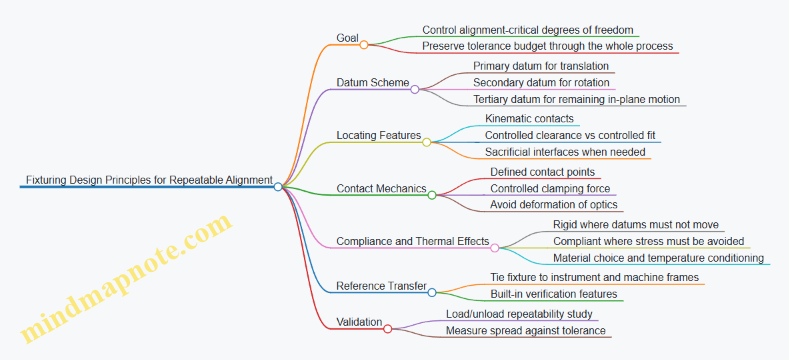
Example: Repeatable Lens-to-Base Alignment
Suppose a lens must be centered and seated at a fixed axial height before bonding.
- Primary datum: the lens seating ring bore centers the lens.
- Secondary datum: a shoulder face sets axial height.
- Tertiary datum: a notch and matching key set angular orientation.
- Contact control: a spring clamp applies consistent force to the lens edge, not the coated surface.
- Thermal control: fixture and lens are conditioned to the same shop temperature before alignment.
- Verification: a gauge pin checks that the lens is seated against the shoulder before bonding.
If you later change the lens supplier and thickness shifts by a small amount, the fixture should still seat on the shoulder and keep centering defined by the bore, so the alignment procedure remains the same and the output stays predictable.
10.3 Robotics and Motion Control for Optical Assembly
Robotic assembly for optical systems is mostly about repeatability: placing parts in the same pose, at the same time, with the same force limits, and then verifying the result. Motion control is the part that makes “same” measurable. A good workflow starts with the mechanical reality of optics—small tolerances, fragile surfaces, and alignment features that hate being treated like generic hardware.
Foundations of Motion for Optical Assembly
Kinematics and Coordinate Frames
Optical assembly typically uses multiple frames: robot base, cell datum, fixture datum, and part features. Motion planning becomes reliable when every pose is expressed relative to a known datum chain. A practical rule: define one “assembly datum” on the fixture, then transform robot coordinates into that frame for every pick, place, and alignment move.
Example: A lens barrel has a keyed feature. Instead of commanding the robot to rotate to a guessed angle, measure the key orientation once per lot (or per fixture load), then compute the commanded rotation relative to the fixture datum.
Motion Profiles and Settling
Optical parts don’t just move; they settle. Use motion profiles that limit jerk and control acceleration so the part doesn’t bounce into a mount. After each move, include a settling delay or a sensor-based confirmation before applying final seating force.
Example: When placing a mirror into a flexure mount, the robot can arrive quickly but must wait for vibration to decay before the final press. If you skip the wait, you’ll see random tilt variations that look like “mystery alignment drift.”
End Effector Design for Optical Safety
Grippers and Vacuum Handling
Optics handling needs contact control. Soft jaws, compliant pads, and vacuum cups with controlled suction area reduce stress concentrations. Avoid gripping on optical surfaces unless the design explicitly supports it.
Example: For a coated window, use a vacuum cup on the perimeter land and add a mechanical stop so the robot cannot overtravel and crush the edge.
Force and Compliance
Motion control and end effector compliance work together. If the robot can’t guarantee perfect alignment, the end effector should tolerate small misplacements without damaging coatings.
Example: During insertion of a lens into a barrel, command a low-force approach, then switch to a higher-force seating only after the part is guided into the lead-in chamfer.
Programming the Assembly Sequence
Approach, Align, Seat, Verify
A robust sequence separates tasks:
- Approach: move near the target with conservative speed.
- Align: perform fine motion using either passive guidance (dowels, chamfers) or active alignment (measured offsets).
- Seat: apply controlled force or torque to reach the mechanical stop.
- Verify: check pose, height, or optical alignment metrics before releasing.
Example: For a mirror mount, use passive guidance for coarse placement, then use active alignment to correct tip/tilt based on a measured reference before final seating.
Teach Points and Calibration
Teach points are only as good as calibration. Calibrate robot-to-fixture transforms using fiducials or metrology targets. Recalibrate after tool changes, fixture redesigns, or any event that can shift datums.
Example: If a vacuum gripper is swapped, its effective center changes. Treat gripper swaps like a calibration event, not a “minor maintenance.”
Closed-Loop Motion Control for Alignment
Sensor Inputs
Common sensor inputs include vision for pose, displacement sensors for height, and force/torque sensors for seating. Optical assembly often benefits from combining vision (for lateral pose) with height measurement (for axial seating).
Example: Use vision to align a lens to a reference mark, then use a height sensor to stop at the correct axial position so the coating doesn’t get dragged across a surface.
Error Budget and Control Limits
Define acceptable error ranges per axis and per step. Motion control should enforce limits so the system refuses to seat when alignment is outside tolerance.
Example: If lateral misalignment exceeds a threshold, the robot retracts and reattempts with updated offsets rather than forcing the part into place.
Mind Map: Robotics and Motion Control for Optical Assembly
Example: Active Alignment with Controlled Seating
A common pattern is “measure, move, seat, confirm.”
- Measure: capture the part pose with vision relative to fixture datum.
- Compute offsets: calculate required lateral and rotational corrections.
- Move with constraints: command fine motion with reduced speed and bounded acceleration.
- Seat with force limit: apply seating force only after the part is within a small alignment window.
- Confirm: re-check height and, if required, tip/tilt before releasing.
Example: During assembly of a laser optical module, the robot places a lens into a kinematic mount. Vision corrects lateral position, a height sensor confirms axial seating, and a force limit prevents coating edge damage. If height is out of range, the robot retracts and the operator receives a clear nonconformance code tied to the step that failed.
Practical Integration Notes
Motion control is not just the robot’s job; it’s the whole cell’s behavior. Keep the fixture rigid, ensure repeatable part presentation, and treat calibration as part of the process, not an occasional chore. When the sequence is structured and the limits are enforced, the system stops “trying harder” and starts producing consistent assemblies—quietly, reliably, and with fewer surprises than a human handoff.
10.4 Vision Systems for Part Identification and Positioning
Vision systems in precision photonics manufacturing do two jobs: they tell you what you have (identification) and where it is (positioning). When both are reliable, downstream alignment and bonding steps stop compensating for avoidable mistakes. The goal is not “see everything,” but “measure the few things that matter” with repeatable results.
Foundations for Reliable Identification and Positioning
Start with a clear part model. A vision system needs stable features: etched marks, molded geometry, fiducials, coating edge contrast, or distinctive screw patterns. If the feature changes with cleaning, coating, or batch variation, identification becomes a guessing game.
Next, define the coordinate story. Your machine has a work coordinate system; your camera has an image coordinate system; your part has its own local coordinate system. Positioning is correct only when you consistently transform between these frames. A practical approach is to calibrate once per fixture family and verify each shift with a known reference target.
Finally, decide what “good” means. For identification, good might be “correct part number and orientation within 90 degrees.” For positioning, good might be “center within ±10 µm and rotation within ±0.02°.” These tolerances should match the sensitivity of the next process step, such as active alignment or adhesive curing.
Lighting, Optics, and Image Quality
Most vision failures are lighting failures wearing a different hat. Use illumination that makes the target features stand out while suppressing glare from optics surfaces.
- For matte features, diffuse ring lighting often works well.
- For shiny edges, coaxial or angled illumination can reveal boundaries without washing them out.
- For transparent or reflective optics, add polarization or use background contrast so edges appear as intensity transitions.
A simple rule: if you can’t describe how the image changes when the part moves, you don’t yet understand the measurement.
Identification Workflow with Practical Examples
Identification typically uses one of three strategies:
- Template matching for fixed shapes like housings or connector faces.
- Feature-based matching for fiducials or etched marks.
- Code reading for labels, Data Matrix, or laser-etched identifiers.
Example: A laser module housing has two alignment notches and a laser-etched serial code. The system first checks the code for part identity. Then it verifies orientation by locating the notches. If the code is readable but the notches are rotated, the system flags the part for reorientation before it reaches the bonding station.
Example: Coated optics often have low-contrast markings. Instead of relying on the coating surface, use a mechanical reference such as a chamfer or a dedicated fiducial on the mount. The camera reads the mount geometry, not the optic’s reflective face.
Positioning Workflow with Coordinate Transformations
Positioning can be done with:
- 2D pose estimation using detected fiducials and a planar transform.
- 3D pose estimation using stereo vision or structured light when height variation matters.
For most fixtured photonics assembly, 2D is enough if the part seats repeatably. The key is to measure the part relative to the fixture datum, not relative to the camera.
Example: A lens is placed into a kinematic mount. The system detects two fiducial marks on the mount, computes the mount’s rotation and center offset, and then commands the robot to correct placement. If the mount is slightly tilted, the computed rotation captures it, and the downstream alignment step starts closer to nominal.
Error Handling and Verification
A robust system includes checks that prevent silent failures.
- Confidence thresholds: if the match score drops, stop and request a regrip.
- Outlier detection: reject measurements that imply impossible geometry, like a rotation jump inconsistent with robot motion.
- Redundant cues: use both identification and pose checks so a wrong part can’t “fit” by accident.
Example: If a code read succeeds but the pose is inconsistent with the expected part geometry, the system reports “identity/pose mismatch” rather than “pose failure.” That distinction speeds up troubleshooting.
Mind Map: Vision Systems for Part Identification and Positioning
Example: End-to-End Station Logic
A practical station sequence looks like this:
- Place part into a known staging area.
- Capture image under the configured lighting mode.
- Identify part using code or shape features.
- Compute pose from fiducials and compare to expected geometry.
- If within tolerance, send corrected placement coordinates to the robot.
- If not, trigger reorientation, regrip, or operator intervention.
- Log the measurement outcome with the part identity for traceability.
This structure keeps the system deterministic: every decision is tied to a measurable condition, and every failure mode points to a specific cause rather than a vague “vision error.”
10.5 Tool Maintenance, Calibration, and Change Control
Tooling in precision photonics is less like “equipment” and more like a quiet part of the measurement chain. A worn fixture, a drifted gauge, or a swapped tool with a slightly different datum can turn a good process into a slow leak of yield. This section lays out a practical system that keeps tools stable, measurements trustworthy, and changes controlled.
Tool Maintenance Foundations
Start with a clear inventory: every tool that touches optics, substrates, coatings, alignment, or measurement gets a unique ID and a defined role. Then classify tools by impact. A vacuum chuck used for coating adhesion is higher impact than a general-purpose wipe station. For each tool, define:
- Maintenance tasks: what to do, how often, and what “good” looks like.
- Consumables: what gets replaced on a schedule (pads, seals, filters, wipers).
- Cleaning rules: what chemicals and methods are allowed, and what surfaces must never be exposed.
- Failure symptoms: examples like “repeatability drops” or “surface contamination increases.”
Example: If a polishing fixture uses a compliant pad, record pad replacement intervals based on measured roughness outcomes, not calendar time alone. When roughness trends upward, you have a maintenance signal that is tied to product behavior.
Calibration That Matches How Tools Are Used
Calibration is not just “set it to spec.” It must match the tool’s operating conditions. A gauge calibrated at room temperature but used near a thermal soak can be off in the exact direction that matters.
Define calibration scope in three layers:
- Measurement tools: interferometers, profilometers, thickness monitors, torque tools.
- Alignment tools: autocollimators, reference mirrors, dial indicators, optical benches.
- Process tools: vacuum gauges, deposition rate monitors, thermal stages.
For each layer, specify:
- Calibration method and reference standard.
- Acceptance criteria and allowable drift.
- Uncertainty handling so you know whether a deviation is real or just measurement noise.
Example: If a thickness monitor’s reading is used to stop a coating run, calibrate it against a reference that matches the same material stack and measurement geometry. A mismatch can create systematic error that looks like “process instability.”
Change Control That Prevents Silent Variations
Change control is about preventing untracked differences. The goal is not to slow work; it is to make differences visible.
Use a structured change workflow:
- Change request: what is changing, why, and where it affects the process.
- Risk screening: does it touch critical dimensions, optical datums, or measurement references.
- Qualification plan: what tests prove the tool still produces acceptable results.
- Documentation update: drawings, work instructions, calibration records, and software settings.
- Release and verification: run a defined set of checks before full production.
Example: Replacing a fixture plate with a “drop-in” equivalent is risky if the datum scheme changes by even a few microns. Require a verification run that compares alignment repeatability and key dimensions against the previous tool.
Traceability and Record Keeping That Actually Helps
Records should answer three questions quickly: What was used? What was its condition? What did it produce? Maintain:
- Tool maintenance logs with dates, tasks, and parts replaced.
- Calibration certificates with reference IDs, results, and uncertainty.
- Change control records linking tool changes to affected lots.
When a nonconformance occurs, traceability should let you isolate whether the cause is upstream process variation or a tool condition shift.
Mind Map: Tool Maintenance, Calibration, and Change Control
Practical Example Workflow for a Fixture Replacement
Assume a precision alignment fixture needs replacement due to wear on a locating feature. The workflow:
- Request: document the exact feature that changed and the supplier part number.
- Screen: mark it as high impact because it defines optical datums.
- Qualify: run a repeatability study comparing old and new fixtures using the same reference optics and measurement method.
- Update: revise the work instruction to reference the new fixture ID and its calibration status.
- Verify: before production, complete a short acceptance checklist and confirm the measured alignment metrics fall within the established limits.
If the new fixture passes, you can release it with confidence. If it fails, you stop before the issue spreads into production lots.
Implementation Notes for Daily Discipline
A system works only if it is used consistently. Keep standard work short and specific: where tools are stored, how they are labeled, who can approve changes, and what triggers a maintenance or calibration event. A good rule of thumb is simple: if a tool’s condition can change the product, it must have a record trail and a verification step.
11. Cleanroom Operations, Safety, and Laser Compliance in Manufacturing
11.1 Cleanroom Class Selection and Operational Controls
Cleanroom class selection is the part where you decide how “clean” is clean enough for the job, then you build controls that keep it that way. For industrial photonics manufacturing, the goal is not to chase the lowest possible class; it’s to prevent particles and molecular contamination from turning into coating defects, surface scratches, or optical performance drift.
Foundations for Choosing a Cleanroom Class
Start with the failure modes that matter. For optics and laser systems, the most common are particulate contamination on optical surfaces, residue on lens edges, and coating defects that originate from substrate contamination or airborne particles during deposition.
A practical way to choose a class is to map each process step to its sensitivity:
- Substrate cleaning and handling: sensitive to particles that can re-deposit during transfer.
- Optics fabrication steps: sensitive to scratches and debris introduced by handling.
- Thin film coating: sensitive to both particles and outgassing residues that can create haze or pinholes.
- Assembly and bonding: sensitive to particles that can interfere with bond lines or alignment surfaces.
Then set a baseline by considering the cleanroom’s intended use. If the room supports multiple steps, you typically design for the most sensitive step and use local controls elsewhere to avoid over-classing the entire facility.
Operational Controls That Make the Class Meaningful
A cleanroom class is only a snapshot. Operational controls are what keep the snapshot from becoming a lie.
Airflow and Pressure Strategy
Maintain pressure relationships so air flows from cleaner to less clean areas. Use a cascade that matches your process flow: cleanroom to antechamber to support spaces. This reduces the chance that opening doors or moving carts pulls contamination into the room.
Example: When a technician enters for a coating substrate change, the antechamber should stabilize before the main door opens. If the main door opens early, the pressure cascade can reverse and pull particles from the corridor.
Particle Control Through Behavior and Workflow
People are the largest variable. Controls should focus on predictable behaviors:
- gowning sequence and fit checks
- controlled movement speed
- minimized door-open time
- scheduled cleaning that matches production rhythms
Example: If operators rush between stations, they generate turbulence and shed particles from garments. A simple rule like “walk at a measured pace and pause before entering the work zone” can reduce variability more than adding extra fans.
Cleaning and Decontamination Practices
Cleaning must be compatible with optics materials and coatings. Use cleaning methods that remove residues without leaving films. Define what “clean” means for each step: visible cleanliness for handling, and residue limits where coatings are involved.
Example: A wipe procedure that works for metal parts may leave lint or residues on glass edges. For optics, specify lint-free materials, solvent compatibility, and a drying method that prevents water spots.
Equipment and Tooling Controls
Tools can be contamination sources. Treat fixtures, carts, and transfer containers as part of the cleanroom system.
- keep tools dedicated or controlled by cleaning schedules
- avoid porous materials that trap residues
- verify that vacuum lines and air jets are filtered
Example: A polishing fixture stored in a general warehouse can carry dust into the cleanroom. Even if it is wiped, trapped debris can re-release during handling.
Monitoring, Sampling, and Response
Monitoring should be tied to actions. Particle counters, pressure gauges, and periodic surface checks are useful only if you define thresholds and response steps.
Example: If particle counts spike during a door-open event, the response might be to review door discipline and confirm pressure recovery time, not to stop production for every minor excursion.
Mind Map: Cleanroom Class Selection and Controls
Integrated Example Workflow for a Photonics Line
A typical approach is to run a single cleanroom class for coating and high-sensitivity handling, then use controlled staging for less sensitive steps.
Example:
- Substrates are cleaned in a controlled area and transferred in sealed containers.
- The cleanroom supports coating substrate loading and optical handling.
- Assembly steps that tolerate slightly higher particulate levels occur in a local enclosure or controlled zone within the same room.
- Monitoring verifies pressure stability during door openings and confirms particle levels during active work.
- When a deviation occurs, the investigation starts with door discipline, transfer container condition, and tool cleanliness before changing the cleanroom class.
This structure keeps the cleanroom class selection grounded in actual process needs, while operational controls prevent contamination from sneaking in through the usual suspects: doors, tools, and people.
11.2 Contamination Sources and Mitigation in Optical Workflows
Optical contamination is rarely one big villain. It’s usually a chain of small events: a particle lands, a film forms, a residue transfers, or a surface gets reworked without realizing it. The goal of mitigation is to stop the chain at multiple points so one failure doesn’t ruin the lot.
Foundational Contamination Concepts
Start by separating contamination into three practical categories. Particles are discrete debris that scatter light or scratch surfaces. Films are thin layers that absorb, reflect, or change wettability, often invisible until testing. Residues are leftover chemicals from cleaning, adhesives, or handling that can outgas or react under heat.
A useful mental model is “source → transport → deposition → effect.” For example, a gloved finger sheds skin oils (source), those oils spread during contact or wiping (transport), they leave a thin layer on glass (deposition), and the coating adhesion or transmission shifts (effect). When you map the chain, mitigation becomes specific rather than generic.
Common Contamination Sources in Optical Workflows
1. Human handling and clothing. Skin oils, lint, and microfibers are frequent culprits. Even “clean” gloves can shed particles if they’re reused too long or stored improperly.
2. Airborne particles and airflow patterns. Turbulence near workstations, open doors, and fans can move particles toward optics. A common pattern is higher contamination near the edges of a bench where airflow is less controlled.
3. Tools and fixtures. Worn tweezers, dirty vacuum wands, and reusable wipes can transfer debris. If a fixture contacts an optical surface, it must be treated like an optical component.
4. Cleaning chemistry and process. Over-aggressive cleaning can leave residues or generate new contamination through poor rinsing. Using the wrong solvent for a specific residue can smear it into a film.
5. Coating and thermal steps. Outgassing from mounts, adhesives, or packaging can deposit films on optics. Even small trapped volumes can release contaminants during bake.
6. Packaging, storage, and transport. Dusty containers, reused foam, and loose caps allow deposition during downtime. A part that “sat overnight” is often the part that fails.
Mitigation Strategy from Source Control to Deposition Control
Mitigation works best when it’s layered.
Layer A: Source control. Define who touches what and when. Use dedicated gloves per task, replace gloves on a schedule tied to observed contamination, and keep hair and sleeves out of the work zone. For tools, assign optics-only tools and label them by station.
Layer B: Transport control. Reduce airflow turbulence by keeping doors closed and avoiding unnecessary movements over open optics. Use localized covers or staging trays so parts are exposed only during the exact step.
Layer C: Deposition control. Prevent contact deposition by using proper handling aids: vacuum wands with clean tips, edge-grip methods, and caps that protect optical faces. When wiping is required, use controlled wipe direction and minimal pressure to avoid grinding particles into the surface.
Layer D: Effect control through verification. Don’t rely on “looks clean.” Use inspection steps appropriate to the risk: visual checks for gross debris, surface inspection for haze, and post-cleaning verification before coating or bonding.
Practical Examples That Tie Cause to Action
Example: Fingerprints before coating. If a part shows a faint oily sheen after handling, the likely source is skin oils transferred during edge handling. The fix is to handle only edges with clean gloves, avoid touching the rim with the same glove that touched other parts, and stage the optic in a covered tray between steps.
Example: Wipe-induced haze. If haze appears after cleaning, the residue may be from the wipe or incomplete rinsing. The mitigation is to switch to wipes compatible with the solvent system, ensure a full rinse step, and verify with a post-cleaning inspection before moving to coating.
Example: Tool transfer. If multiple parts show similar scratch patterns, the source may be a worn tweezer tip or a contaminated fixture. The mitigation is to inspect and replace tool contact surfaces, then clean fixtures using the same rigor as optics.
Mind Map: Contamination Sources and Mitigation
Operational Rules That Prevent “Accidental Recontamination”
Treat the cleanest step as the most fragile. If a part is cleaned, it should not be placed on a surface that also hosts dirty tools. Keep a clear separation between “dirty” and “clean” zones on the bench, and use distinct trays for each. When a glove is dropped, it’s not “probably fine”; it’s a contamination event, and the workflow should reflect that.
Finally, document the step-level checks that matter. If you record only final inspection results, you lose the trail. If you record what was done right before the defect, you can fix the process instead of arguing about what “must have happened.”
11.3 Laser Safety Program for Production Environments
A production laser safety program is not a binder of rules; it’s a set of controls that make unsafe exposure unlikely and make mistakes easier to catch. The goal is simple: prevent access to hazardous beams, limit exposure when access happens, and ensure the system behaves predictably during normal work and maintenance.
Program Scope and Roles
Start by defining what “production environment” covers: laser workstations, test stands, alignment benches, rework areas, and any shared optics rooms. Assign responsibilities so safety doesn’t depend on who is on shift.
- Safety lead: owns hazard analysis, training requirements, and audits.
- Line supervisor: ensures standard work is followed and stop-work authority is respected.
- Operator: performs daily checks, uses correct PPE, and reports anomalies.
- Maintenance and engineering: controls modifications, verifies interlocks, and updates procedures.
A practical example: if a technician swaps a power supply, engineering updates the configuration record and the safety lead verifies that interlock logic and labeling still match the new setup.
Hazard Identification and Risk Controls
Begin with a hazard inventory for each laser product and workstation. Capture wavelength, class, maximum output, beam path geometry, accessible apertures, and failure modes relevant to manufacturing.
Risk controls should follow a hierarchy:
- Engineering controls: interlocks, beam enclosures, shutters, beam stops, and protective housings.
- Administrative controls: access restrictions, signage, work instructions, and permit-to-work for maintenance.
- PPE: last line of defense, selected to the wavelength and expected exposure.
Example: for a fiber-coupled laser used in alignment, the enclosure prevents direct viewing, a shutter closes during cover removal, and PPE is used during troubleshooting when the enclosure must be opened.
Interlocks, Enclosures, and Safe Access
Interlocks must be designed for production reality, not lab ideal conditions. Verify that:
- Interlocks are fail-safe or fail-secure according to the safety analysis.
- Covers and doors cannot be bypassed without deliberate tools.
- Reset behavior is defined after trips so operators don’t “hunt” for a working state.
A useful check: after an interlock trip, the system should require a deliberate restart sequence and should not resume emission automatically when a cover is closed.
Standard Work for Operators
Standard work should be short enough to follow and specific enough to prevent improvisation. Include:
- Pre-start checks: enclosure closed, interlock status verified, beam path unobstructed, and labels visible.
- During-operation rules: no reflective items near the beam path, no “quick peek” through openings, and no overriding interlocks.
- Shutdown and lockout: defined steps for power down, discharge verification where applicable, and safe storage of keys or access codes.
Example: if a test fixture requires temporary access to an optical port, the procedure should specify the exact sequence: shutter open only after the workstation is in a controlled mode, and shutter closed immediately after alignment.
Training and Competency
Training must match job tasks. A good program distinguishes between:
- General laser awareness for all staff in the area.
- Task-specific training for operators and technicians.
- Maintenance training for those who can open housings or modify components.
Competency checks should be practical. For instance, trainees demonstrate correct use of interlock status indicators, identify the correct PPE for the workstation wavelength, and perform a mock shutdown and restart.
PPE Selection and Use
PPE selection is based on wavelength and expected exposure conditions, not on generic “laser goggles.” The program should define:
- Which PPE is required at each workstation and when it is required.
- How PPE is inspected for damage and replaced.
- How PPE is stored to prevent contamination and mix-ups.
Example: if multiple wavelengths are present across lines, PPE bins should be labeled by wavelength and workstation ID, not by color alone.
Maintenance, Change Control, and Nonconformance
Maintenance is where safety programs often get quietly ignored. Require a controlled process for:
- Any change to beam path components, optical mounts, enclosures, or interlock wiring.
- Repairs that could alter alignment, output power, or accessible apertures.
When something goes wrong, nonconformance handling should include safety impact assessment. If an interlock fails during a test, treat it as a safety event: stop the line, isolate the affected workstation, and verify that the interlock and labeling are correct before returning to service.
Audits, Records, and Continuous Verification
Keep records that prove controls are working. Typical items:
- Inspection logs for interlocks, enclosures, and signage.
- Training completion and competency verification.
- Maintenance and change records tied to workstation configuration.
- Incident and near-miss reports with corrective actions.
A simple audit cadence works well: daily checks by operators, weekly verification of key indicators, and periodic deeper checks by safety and engineering.
Mind Map: Laser Safety Program for Production Environments
Example: Daily Start-Up Checklist for a Laser Workstation
- Verify enclosure is closed and interlock indicator shows “safe.”
- Confirm correct labels for wavelength and workstation ID.
- Check beam path for obstructions and ensure beam stops are in place.
- Confirm shutter behavior during cover open and cover close.
- Put on required PPE before enabling emission.
- Start the test using the approved procedure and monitor for abnormal indicators.
This checklist is short on purpose: it targets the few failures that most often turn “routine” into “surprise.”
11.4 Chemical Handling for Cleaning and Coating Support
Chemical handling in optical manufacturing is mostly about controlling three things: what touches the part, how long it touches, and what residues are left behind. In laser and optics work, “clean” is not a vibe; it’s a measurable state that supports coating adhesion, reduces scatter, and prevents surface defects.
Foundational Principles for Chemical Safety and Process Control
Start with a simple rule: never treat cleaning chemicals as interchangeable. Each chemical has a specific role—removing organics, dissolving salts, lifting particulates, or activating surfaces—and each leaves behind something if rinsing and drying are not done correctly.
A practical workflow begins with a written chemical compatibility check for the materials you handle: substrates (fused silica, BK7, sapphire), coatings (if you’re cleaning between coating steps), and bonding materials (optical cements, adhesives). For example, a solvent that’s fine for polymer handling can attack certain adhesives or soften edge coatings, changing alignment surfaces.
Next, control exposure time and concentration. If a cleaning step is specified for 5 minutes at a given dilution, extending it “just to be safe” can increase surface roughness or create a film that later coating steps struggle to wet.
Finally, treat rinse water quality as part of the process. A common failure mode is leaving ionic residue after cleaning, which later shows up as haze, pinholes, or poor coating adhesion. If you can’t measure it, you can’t reliably control it.
Chemical Handling System and Standard Work
Build standard work around segregation and traceability.
- Segregate by function: separate containers and tools for solvent cleaning, aqueous cleaning, and final rinsing. Label them clearly and keep them physically apart.
- Use dedicated PPE and ventilation: choose gloves and eye protection based on the chemical’s hazard class, not on what’s available. Ensure fume extraction is active before opening chemical containers.
- Prevent cross-contamination: use clean baskets or holders for each step. If you reuse a holder across steps, you must clean it with the same rigor.
- Record batch parameters: log chemical lot, dilution, make date, and operator. A simple example is a coating-support cleaning bath: when adhesion drops, you need to know whether the bath was refreshed or drifted.
A useful mental model is “chemical custody.” Once a part enters a chemical step, it should not be moved into another step without completing the required rinse and drying sequence.
Cleaning Step Logic for Optical Surfaces
Optical cleaning typically follows a sequence that reduces the risk of redeposition.
- Dry removal first: blow-off or gentle wipe with lint-free materials to remove loose particles. This prevents grinding debris into the surface.
- Solvent step for organics: use a solvent appropriate for oils and fingerprints. Example: if operators touch edges during handling, a solvent step can remove residues before aqueous steps.
- Aqueous step for salts and residues: use an aqueous chemistry designed for ionic removal. Example: if parts come from packaging with desiccant dust, aqueous cleaning helps remove soluble contaminants.
- Final rinse and controlled drying: rinse with high-purity water and dry using filtered air or spin-drying where appropriate. Drying matters because water spots can become nucleation sites for coating defects.
If you’re supporting coating, include a “surface readiness check” before coating begins. A simple example is inspecting under appropriate lighting for streaking or residue patterns after drying.
Advanced Details That Prevent Common Failures
Residue management: Many cleaning problems are actually rinse problems. If you see streaks, re-check rinse flow, immersion depth, and whether parts drain consistently. Uneven drainage can leave thicker residue trails.
Temperature control: Some chemistries perform differently at room temperature versus elevated temperatures. If your procedure specifies temperature, keep it stable; otherwise, adhesion and surface cleanliness can vary across lots.
Material compatibility: Edge chips and microcracks can trap cleaning solutions. Example: a small chip in a lens edge can hold residue that later releases during coating, causing localized defects.
Tooling and agitation: Gentle agitation can improve cleaning uniformity, but aggressive agitation can increase micro-scratches. Use fixtures that support consistent immersion and avoid contact with optical surfaces.
Mind Map: Chemical Handling for Cleaning and Coating Support
Example: Cleaning-to-Coating Support for a Coated Optic
A coated-optic support flow can look like this: the optic is first handled with gloves and held by a clean fixture. Loose particles are removed with filtered air. The optic then receives a solvent step to remove fingerprints from the edge region. After that, it goes through an aqueous cleaning step sized for the optic geometry, followed by a high-purity final rinse. The optic is dried with filtered air in a controlled area, then inspected for streaking before coating begins. If streaking appears, the first corrective action is to review rinse quality and drainage behavior, not to increase chemical strength.
Example: Batch Logging for Troubleshooting Adhesion Drops
When coating adhesion declines on a specific lot, the log helps pinpoint whether the cleaning bath was refreshed, whether dilution matched the specification, and whether the final rinse conductivity was within the expected range. If the bath was not refreshed on schedule or if dilution was adjusted informally, you can correct the process without guessing. If the bath parameters were correct, the next check is tooling segregation and holder cleanliness, since cross-contamination often shows up as “mystery residue.”
11.5 Training, PPE, and Standard Work for Operators
Industrial photonics manufacturing is a “small mistakes, big consequences” environment. Operators handle optics, lasers, vacuum-coated parts, and chemicals, so training must connect cause to effect: what you do, what it changes, and how you prove it worked.
Training Foundations for Safe and Repeatable Work
Start with a short baseline: operators must demonstrate they can identify hazards and follow the same steps every time. A practical training flow looks like this:
- Hazard recognition: laser beam paths, reflected beams, interlocks, high-voltage areas, sharp edges, and chemical exposure. Example: during a walkthrough, trainees point out where a reflection could reach an eye even when the beam is “off” at the source.
- Process understanding: what each step is trying to achieve. Example: when cleaning optics, the goal is removing particulates and residues without scratching; trainees learn why wiping direction and lint-free materials matter.
- Skill demonstration: operators perform tasks under observation until they meet defined criteria. Example: they assemble a mount using the specified torque range and verify seating with a go/no-go gauge.
- Documentation discipline: operators record what they did, not what they hope happened. Example: they log cleaning lot numbers and inspection results immediately after each step.
Training should include “stop points” where the operator pauses to confirm the right setup before proceeding. Example: before energizing a laser for alignment, the operator verifies enclosure status, interlock indicators, and correct test fixture selection.
PPE Selection and Use That Matches the Task
PPE is not a single outfit; it’s a set of controls chosen for the specific risk at that station.
- Eye and face protection: select laser-rated eyewear matched to the wavelength and optical density required by the work instruction. Example: an operator uses eyewear rated for the alignment wavelength, not a generic “laser glasses” pair.
- Gloves and hand protection: choose based on chemical compatibility and grip needs. Example: nitrile gloves for many cleaning steps, but switch to a different material if a solvent attacks the glove.
- Lab coat or gown: protect optics from skin oils and protect skin from splashes. Example: a clean-room gown is worn during handling of uncoated substrates to reduce contamination.
- Respiratory protection: used only when required by the chemical risk assessment and the station procedure. Example: if a station uses a specific solvent with known inhalation risk, the procedure specifies the respirator type and fit-check.
- Footwear and hair control: required by the cleanroom and chemical handling rules. Example: hair covers prevent stray fibers from landing on optical surfaces.
Operators must also know the “PPE failure modes.” Example: eyewear that is scratched or dirty can reduce visibility and increase risk; the standard work should require inspection and replacement criteria.
Standard Work for Operators That Prevents Drift
Standard work is written so an operator can follow it without improvising. It should include the sequence, acceptance checks, and what to do when something is off.
Core elements to include in every work instruction
- Preconditions: station state, correct tools, correct part identifiers, and required PPE.
- Step-by-step actions: short, unambiguous verbs.
- In-process checks: what to measure or inspect before moving on.
- Escalation rules: when to stop, who to notify, and what to record.
- Clean handoff: how to transfer parts to the next step without mixing lots.
Example standard work for optics handling includes: verify part ID, wear clean gloves, use approved wipes, inspect under the specified lighting, and record inspection outcome before packaging.
Mind Map: Training, PPE, and Standard Work
Example Operator Workflow for a Typical Station
An operator begins by donning the PPE specified for the station and verifying it meets the acceptance criteria (for example, eyewear is clean and unbroken). They confirm the part ID and lot number, then follow the work instruction steps in order. After each critical action, they perform the in-process check and record the result. If a check fails, the operator stops, isolates the part, and documents the reason using the required fields so the next person can act without guessing.
This approach keeps training practical: operators learn what to do, why it matters, and how to prove it was done correctly—every shift, every lot, no improvisation.
12. Case Studies for End-to-End Laser Optical Manufacturing
12.1 Case Study: Laser Module Assembly With Active Alignment
This case study follows one production lot of a compact laser module: a laser source, a collimating lens, and a steering mirror that must hit a fixed beam spot at the module output. The goal is repeatable optical performance without turning every assembly into a one-off art project.
Product Requirements That Drive Assembly Choices
The module drawing specifies three measurable outcomes: output beam pointing within a tight angular window, optical power at the output aperture, and beam quality that stays stable after thermal soak. Those requirements translate into assembly decisions:
- The mirror mount must allow controlled angular adjustment.
- The lens seat must constrain position while tolerating small part-to-part variations.
- The bonding method must preserve alignment during cure.
A practical habit is to write a “measurement-first” plan before touching hardware. For example, the team defines the exact test fixture datum surfaces and the order of measurements: coarse pointing check, fine pointing adjustment, then power and beam quality verification.
Bill of Materials Control and Incoming Checks
Active alignment is only as good as the parts you start with. Incoming inspection focuses on the features that directly affect alignment:
- Lens: clear aperture diameter and surface quality class.
- Mirror: substrate thickness and coating transmission band.
- Mounting hardware: thread pitch, flatness of reference faces, and coating compatibility.
A simple example: if mirror coating transmission is low at the laser wavelength, the team can still align pointing, but the module fails the power acceptance test. That wastes time, so the inspection gates prevent it.
Work Instructions for Clean Handling and Datum Discipline
Optics handling is standardized to avoid “mystery contamination.” Operators wear gloves, use lint-free wipes, and keep optics capped until the moment of placement. More importantly, the work instruction defines datums for every part:
- Lens seat datum A: controls lateral position.
- Mirror mount datum B: controls angular adjustment reference.
- Fixture datum F: controls the module-to-test relationship.
When datums are consistent, the same adjustment procedure produces similar results across the lot.
Active Alignment Workflow with Clear Stop Points
The assembly uses a two-stage approach: mechanical pre-positioning, then active adjustment.
- Mechanical pre-positioning: The lens and mirror are seated without final bonding. The steering mirror is set to a baseline angle using a calibrated adjustment tool.
- Coarse optical check: The module is placed in the test fixture. The team measures beam pointing at a defined distance.
- Fine active alignment: The mirror is adjusted in small increments while monitoring pointing error. The procedure includes a maximum adjustment step size to prevent overshoot.
- Locking step: Once pointing is within tolerance, the mirror is bonded or mechanically locked.
- Post-lock verification: Pointing is re-measured immediately after the lock step.
- Final performance tests: Power and beam quality are checked, followed by a thermal soak and re-test.
A key best practice is the stop point after fine alignment but before locking. If the module is out of tolerance at that stage, the team can correct the mechanical seating or part selection rather than curing a misaligned assembly.
Bonding and Cure Control That Protects Alignment
Alignment can drift during cure due to shrinkage, thermal gradients, or bond-line thickness variation. The work instruction therefore controls:
- Bond-line thickness using spacers or controlled dispense volume.
- Cure schedule with a defined ramp rate.
- Fixture support that holds the mirror at the aligned angle during cure.
Example: if the dispense volume varies, the bond-line thickness changes, and the mirror can tilt by a small but measurable amount. The team reduces this by using a calibrated dispense routine and verifying dispense mass per lot.
Measurement System and Uncertainty Handling
The test fixture and sensors are treated as part of the process, not just a “readout.” The team performs calibration checks and tracks uncertainty so acceptance decisions are defensible.
A practical example: if the pointing measurement uncertainty is ±0.5 mrad and the tolerance is ±2 mrad, the team ensures the alignment target is centered with enough margin that normal measurement noise does not cause avoidable rejects.
Nonconformance Handling with Root-Cause Structure
When a unit fails after locking, the team separates optical causes from process causes:
- If pointing shifts right after cure, suspect bond-line or fixture support.
- If pointing was correct before locking but fails after thermal soak, suspect thermal mismatch or bond cure completeness.
- If power is low across tests, suspect incoming optics or laser drive configuration.
Corrective actions are tied to the specific step that introduced the deviation.
Mind Map: Active Alignment Laser Module Assembly
Example: One Lot’s Decision Logic
During the lot, the team aligns 10 modules. Two fail after locking. Both passed the pre-lock pointing check, so the team focuses on cure-related causes. They measure dispense mass and find one batch of adhesive dispenses trending high, increasing bond-line thickness. After correcting the dispense calibration and re-running the cure schedule, the next set shows post-lock pointing within tolerance.
The result is not just better yield; it is a process that explains itself. Each step has a measurable purpose, and each failure points to a specific stage rather than a vague “assembly issue.”
12.2 Case Study: Coated Optics Production With Acceptance Testing
A mid-volume manufacturer builds coated optics for a laser system used in industrial metrology. The optics are small, the coatings are expensive, and the customer acceptance test is strict enough that “close” is not a strategy. The goal of this case study is to show how a coating process becomes a controlled production step, and how acceptance testing turns into a repeatable decision.
Foundational Setup
The team starts by translating optical requirements into coating-specific characteristics. They define what must be true after coating: transmission at key wavelengths, reflectance band edges, and surface quality that does not drift during deposition. They also define what must be true before coating: substrate cleanliness, surface figure stability, and mechanical datum integrity.
A practical habit is to treat the substrate as a “measurement instrument.” If the substrate is contaminated, the coating can look fine under one inspection method and fail under another. So they standardize handling: gloves, sealed storage, and a fixed cleaning recipe with documented dwell times. For example, if a batch of substrates is cleaned for 5 minutes instead of 10, the team expects a measurable change in coating adhesion and uses that expectation to prevent silent drift.
Coating Process Control
The coating step uses a vacuum deposition tool with a defined pump-down and bake sequence. The team controls three categories of variables: chamber state, material delivery, and substrate conditions.
-
Chamber state: they track base pressure and residual gas indicators. If base pressure rises, the coating can shift in optical constants.
-
Material delivery: they control evaporation rates and shutter timing. A simple example is a calibration run where the same recipe is executed twice; if the optical thickness differs beyond tolerance, the recipe is not “good,” it is “unverified.”
-
Substrate conditions: they control temperature and rotation speed. Rotation matters because it affects thickness uniformity; the team checks uniformity by mapping a witness coupon across the same holder geometry.
To keep the process systematic, they define in-process checkpoints. After deposition, they perform a quick spectral scan on a witness sample and a visual inspection for defects such as haze, striations, or peeling edges. They do not treat these as final proof; they are early signals that prevent wasting full sets of optics.
Acceptance Testing Plan
Acceptance testing is built around a clear rule: every optic must meet optical performance criteria, and every optic must be traceable to the process conditions that produced it.
They use three layers of evidence:
- Optical performance: spectral reflectance and/or transmission measured at the customer-relevant wavelengths.
- Surface and defect screening: inspection for scratches, digs, coating defects, and edge integrity.
- Process traceability: linking each optic to its coating run, witness results, and key tool parameters.
A concrete example: the customer requires reflectance within a band around 1064 nm. The manufacturer measures reflectance on each optic using the same instrument settings and calibration procedure. If the measured curve is slightly off, they check whether the witness coupon from the same run shows a similar shift. If both shift together, the issue is likely recipe or tool state; if only one optic shifts, the issue is likely handling, mounting, or substrate-specific contamination.
Decision Logic for Pass, Rework, and Reject
The team defines decision thresholds before production begins.
- Pass: meets spectral criteria and defect screening.
- Rework: allowed only for specific failure modes where the coating can be stripped and recoated without damaging the substrate.
- Reject: when defects indicate substrate damage, coating delamination risk, or when spectral deviation suggests a systemic run problem.
They also define a “no-surprises” rule for rework. If rework is performed, the optic must be re-measured with the same acceptance method, and the run must be flagged for investigation. This prevents the classic trap where reworked parts pass once and fail later because the underlying cause was never corrected.
Mind Map: Coated Optics Acceptance Flow
Example: One Batch, Two Failure Modes
In one production lot, two different issues appear.
First failure mode: multiple optics show reflectance shifted in the same direction, and the witness coupon matches the shift. The team concludes the run recipe or tool state is off. They stop the line, verify evaporation rate calibration, and confirm base pressure stability.
Second failure mode: only one optic shows a defect pattern near the edge, while the witness coupon is within tolerance. The team traces the optic’s handling history and mounting fixture contact points. They adjust the fixture contact surface and add a pre-coating edge inspection step.
The key is that acceptance testing does not just label parts; it guides where to look. When optic behavior matches the witness, the process is suspect. When it diverges, the handling or substrate-specific path is suspect.
Summary of Integrated Best Practices
This case study shows a coherent loop: define optical requirements, control coating variables, screen early with witness evidence, and decide acceptance using both performance and defect criteria tied to traceability. The result is not just compliance; it is a production system where each test outcome has a clear, actionable interpretation.
12.3 Case Study: Precision Optics Fabrication With Metrology Feedback
A mid-volume optics supplier builds precision substrates for a laser system that requires tight surface figure and low roughness. The team’s goal is not just to hit specs once, but to keep yield stable across lots. They start by treating metrology as part of the process, not a final verdict.
Foundations That Make Feedback Work
The first step is defining what “good” means in measurable terms. For each optical surface, the engineering team maps requirements to metrology outputs: surface figure error, mid-spatial roughness, and scatter-relevant cleanliness. They also define measurement uncertainty and acceptance thresholds so operators know when a result is meaningful.
Next, they standardize datums. Every substrate gets a consistent reference for rotation and centering. A simple example: if the polishing tool assumes the part’s “A” edge is up, then the metrology setup must also treat that edge as up. Otherwise, the feedback loop corrects the wrong error.
Finally, they establish a baseline process run. One lot is processed without midstream corrections to capture typical drift. This baseline becomes the reference for deciding when feedback is warranted.
Mind Map: Metrology Feedback Loop
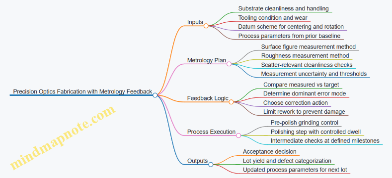
The Feedback Loop in Practice
The team uses a milestone approach. After grinding, they measure figure and identify whether the error is dominated by low-frequency shape (figure) or higher-frequency texture (roughness). If figure error is large but roughness is still acceptable, they prioritize shape correction before polishing time increases.
A concrete example: a batch shows a consistent astigmatism pattern after grinding. The metrology map indicates the error rotates with the part, not with the tool. That points to a datum or fixturing repeatability issue. The corrective action is not “polish more,” but to tighten centering repeatability and verify the part’s rotational reference. After the change, the same measurement method shows the astigmatism amplitude dropping, while roughness remains stable.
During polishing, they use short dwell increments with intermediate checks. Instead of polishing until the surface “looks right,” they polish for a controlled time slice, measure, and decide. This prevents overshoot, which is common when the process is tuned to a single historical lot.
Error Mode Identification Without Guesswork
Metrology results are only useful if they are interpreted consistently. The team uses a simple decision rule: if the figure error changes significantly between milestones while roughness changes only slightly, the dominant lever is shape removal. If roughness changes quickly but figure barely moves, the dominant lever is surface texture control.
They also track tool wear. A practical example: when the same polishing pad shows increasing removal rate, the figure error may shift faster than expected. The feedback loop catches this because the measured-to-target gap closes too quickly. The team then updates dwell time limits and schedules pad conditioning earlier.
Acceptance Criteria That Prevent “Measurement Theater”
To avoid chasing noise, they incorporate uncertainty. Suppose the measured figure error is 0.20 µm and the uncertainty band is ±0.08 µm. The team treats results within the overlap region as “not actionable.” Operators then follow standard next-step parameters rather than making micro-adjustments that don’t improve outcomes.
They also define rework boundaries. If intermediate measurements indicate the surface is approaching a thickness or edge constraint, the process shifts to a conservative path. This keeps rework from trading one failure mode for another.
What Changed After Feedback Was Integrated
After several lots, the team’s yield improves because corrections become targeted. Early in the program, many parts were reworked due to late discovery of figure issues. With feedback, the majority of figure correction happens before polishing time becomes expensive.
They also reduce variability. The baseline run plus uncertainty-aware decisions means the process doesn’t “hunt” for the target. Instead, it converges predictably.
Finally, they close the loop operationally. Each lot’s metrology outcomes update the next lot’s parameter windows, including fixturing checks and milestone timing. The feedback system becomes routine: measure, interpret, act, and document—without turning every measurement into a new debate.
12.4 Case Study: Integrated Test Flow for Optical Performance and Safety
This case study follows a production lot of laser optical modules through an integrated test flow that checks performance and safety in one pass. The goal is simple: catch optical defects early, prove the laser system behaves safely under realistic conditions, and record results in a way that makes later troubleshooting efficient.
Starting Point and Test Philosophy
The module under test includes a laser source, beam-shaping optics, and a protective enclosure with interlocks. The integrated flow is built around three principles:
- Sequence by risk and information value: start with checks that reveal gross issues quickly (wrong parts, misalignment, missing interlock signals), then move to deeper optical measurements.
- Use the same fixture for multiple steps: alignment and safety checks share mechanical datums so you don’t “test different parts” of the assembly.
- Record evidence, not just pass/fail: capture key measurement values so nonconformance analysis has something to work with.
Test Flow Overview
The flow is executed in four stages.
Stage A: Pre-Power Verification
- Confirm serial-number mapping to the correct optical stack and enclosure hardware.
- Verify interlock continuity and correct actuator engagement.
- Inspect connector seating and cable strain relief.
Example: If the interlock actuator is slightly mispositioned, the system may still power up in a bench setup but will fail in the production enclosure. Catching it before power prevents wasted time and avoids confusing “optical” failures that are actually safety logic failures.
Stage B: Low-Power Optical Checks
- Power the laser at a reduced level using a controlled current limit.
- Measure beam position at a reference plane and verify transmission through the optical train.
- Confirm that optical alignment is within a defined window before full-power testing.
Example: A coated optic with a scratch can pass a visual inspection yet scatter light enough to shift beam position. Low-power beam position measurement flags this without stressing the component.
Stage C: Full-Power Performance Verification
- Measure output power stability over a fixed warm-up interval.
- Verify beam quality metrics relevant to the application (for instance, spot size or wavefront-derived indicators).
- Check optical throughput against acceptance criteria.
Example: If power is high but beam quality is poor, the likely causes differ from a low-power module. Capturing both power and beam quality prevents “one-number thinking.”
Stage D: Safety and Functional Proof
- Exercise interlocks under controlled conditions and confirm the system transitions to a safe state.
- Validate enclosure behavior by simulating access conditions while monitoring laser output.
- Confirm fault handling behavior when sensors report out-of-range values.
Example: A module may meet optical performance yet fail safety if a sensor signal is inverted or if the fault logic masks a specific error. Safety proof is therefore not optional even when optics look perfect.
Mind Map: Integrated Test Flow
Integrated Test Flow Mind Map
Integrated Data Handling and Decision Rules
Each stage writes results into a single record keyed by module serial number. The record includes:
- Calibration identifiers for measurement instruments.
- The exact test settings used (current limit, warm-up time, reference plane geometry).
- Raw or minimally processed measurement values.
Decision rules prevent contradictory outcomes. For example:
- If interlock verification fails, the module is rejected before any optical measurements are considered valid.
- If low-power beam position is out of range, full-power testing is either blocked or limited to a diagnostic mode that does not overwrite the alignment history.
- If full-power performance fails but safety passes, the module is routed to optical rework rather than safety rework.
Example: One Lot, Three Outcomes
In a typical lot, you might see:
- Outcome 1: All stages pass. The module ships with a complete measurement trail.
- Outcome 2: Low-power beam position fails due to misalignment. Safety passes, so rework focuses on alignment and mounting, not enclosure logic.
- Outcome 3: Full-power performance passes, but interlock actuation fails during enclosure access simulation. The module is rejected for safety correction even though optics are fine.
Diagram: Stage-Gated Logic
    flowchart TD
  A[Stage a Pre-Power Verification] --> B[Interlock Continuity Pass?]
  B -- No --> R1[Reject Before Power]
  B -- Yes --> C[Stage B Low-Power Optical Checks]
  C --> D[Beam Position Within Window?]
  D -- No --> R2[Route to Alignment Rework]
  D -- Yes --> E[Stage C Full-Power Performance Verification]
  E --> F[Performance Meets Criteria?]
  F -- No --> R3[Route to Optical Rework]
  F -- Yes --> G[Stage D Safety and Functional Proof]
  G --> H[Safe-State Verified Under Access and Faults?]
  H -- No --> R4[Route to Safety Logic or Enclosure Rework]
  H -- Yes --> S[Release with Full Traceability]
Execution Notes That Prevent Common Test Failures
- Use the same fixture datums for beam position and enclosure access simulation so mechanical shifts don’t masquerade as optical changes.
- Keep warm-up timing consistent; power stability measurements are sensitive to timing drift.
- Store the interlock test results even when the module fails earlier stages, because safety failures often explain “mysterious” optical anomalies.
The integrated flow ends with a single, coherent decision: performance and safety are proven together, and the record points directly to the most likely corrective action.
12.5 Case Study: Nonconformance Investigation and Corrective Action
A production lot of laser optical modules fails final acceptance at the same step: transmission drops and beam quality shifts. The first move is to stop guessing and start sorting. The team records the exact failing measurements, the test station ID, operator, and the serial range. They also pull the last known-good batch for comparison, using the same test procedure and same calibration state.
Step 1: Containment That Actually Helps
Containment prevents more bad units from reaching customers, but it must also preserve evidence. The team quarantines only units built with the same optical coating lot and the same assembly fixture revision. They keep the rest of the lot available for analysis rather than scrapping everything. For example, if only the coated optics are suspect, uncoated mechanical parts can still be reused after inspection.
They then verify whether the failure is real or a measurement artifact. The test station performs a quick check using a reference optic. If the reference passes, the problem likely lives in the product, not the instrument.
Step 2: Nonconformance Definition with Clear Boundaries
The nonconformance report states what is wrong in measurable terms: wavelength band transmission below spec, and wavefront metric outside tolerance. It also states what is not wrong: no visible coating defects under standard inspection, and no gross misalignment in the mechanical datum check.
This boundary matters because it guides the investigation. If the optics look fine visually, the cause may be subtle: cleaning residue, coating thickness shift, or bonding stress.
Step 3: Root Cause Investigation Using Evidence
The team uses a structured approach that links process steps to the observed symptoms.
Step 4: Evidence Collection with Narrow Tests
They start with the coating process because the failure clusters by coating lot. Coating records show a parameter change during the same production window: a minor adjustment to substrate rotation speed after a maintenance event. The team does not assume this is the cause; they test it.
They pull witness samples from the same run and measure thickness and spectral response. The data shows the high-reflectance band is shifted, consistent with thickness variation rather than a catastrophic coating failure.
Next, they inspect substrates from the same incoming inspection lot. Under higher magnification, a few show faint residue patterns that were not visible at the standard inspection level. The cleaning log also reveals a rinse water conductivity excursion during that shift.
Finally, they check assembly bonding. Adhesive cure logs match the approved profile, and bond line thickness measurements fall within range. Torque checks show no systematic over-tightening. That reduces the likelihood of assembly stress as the primary cause.
Step 5: Root Cause Statement and Confirmation
The root cause is documented as: cleaning rinse water conductivity excursion led to residue on substrates, which affected coating uniformity and produced spectral shift. The confirmation step is practical: they re-clean a small set of substrates using the corrected rinse control, re-coat them using the same deposition recipe, and run the same final test. The reworked sample returns to spec.
Step 6: Corrective Action That Changes the Process, Not Just the Paper
Corrective actions include both process fixes and control upgrades:
- Cleaning Control Update: Add a hard stop tied to rinse conductivity limits, with automatic operator notification.
- Coating Run Guardband: Require witness sample spectral verification before releasing a run after any maintenance affecting rotation speed.
- Inspection Enhancement: Upgrade the inspection method for residue detection when rinse excursions occur, even if standard checks pass.
- Traceability Reinforcement: Ensure coating lot-to-module serial mapping is complete so containment can be targeted.
Step 7: Effectiveness Review with Measurable Outcomes
Two weeks after the corrective actions are implemented, the team builds and tests two subsequent lots. They track the same transmission and beam quality metrics and confirm that reference optics still pass on the same station.
They also review the nonconformance trend for the last 90 days, focusing on whether similar spectral shifts appeared earlier under different lot labels. If the corrective actions work, the failure mode should disappear without new failure modes appearing.
Example: A Good Nonconformance Report Snippet
- Nonconformance: Transmission below spec at the final acceptance test wavelength band; wavefront metric outside tolerance.
- Affected Scope: Modules using coating lot C-1842 and fixture revision F3.
- Containment: Quarantine by coating lot and fixture revision; preserve witness samples.
- Root Cause: Rinse water conductivity excursion caused residue, impacting coating uniformity.
- Confirmation: Re-clean and re-coat witness substrates; final test returns to spec.
- Corrective Actions: Hard stop on conductivity; witness spectral verification after rotation maintenance; enhanced residue inspection after excursions.
- Effectiveness: Two subsequent lots meet spec; reference optic checks remain stable.