Biochar and Soil Microbe Engineering
1. Foundations of Living Soil and Carbon Microbial Ecology
1.1 Soil Microbial Communities and Their Functional Roles in Nutrient Cycling
Soil microbes are the main workforce that turns raw inputs into plant-usable nutrients. They do this through coordinated chemistry: breaking down organic matter, transforming nitrogen and phosphorus, and cycling sulfur and micronutrients. A useful way to think about soil microbial communities is as overlapping teams that specialize in different steps of nutrient processing, while sharing resources and competing for space.
Core Community Components
Most nutrient cycling is driven by a mix of bacteria, fungi, archaea, and protists. Bacteria often dominate fast reactions like short-term decomposition and nitrogen transformations. Fungi tend to contribute to breakdown of more complex organic compounds and can physically explore soil pores with hyphae. Archaea are important for nitrogen and carbon transformations under specific conditions, especially where oxygen is limited. Protists and other microfauna regulate bacterial populations and release nutrients by grazing, which can speed up nutrient availability.
Functional Guilds Behind Nutrient Cycling
Microbes can be grouped by what they do rather than what they look like. For nutrient cycling, the most relevant guilds are decomposers, nitrifiers, denitrifiers, nitrogen fixers, phosphate solubilizers, and sulfur oxidizers or reducers. These guilds do not operate in isolation; they rely on each other’s byproducts.
Nitrogen Cycling as a Stepwise System
Nitrogen cycles through several transformations:
- Mineralization: Decomposers convert organic nitrogen into ammonium (NH4+). This is often the first step after adding compost or crop residues.
- Nitrification: Nitrifiers convert ammonium into nitrate (NO3−) under oxygenated conditions. Nitrate is mobile, so it can move beyond the root zone if not taken up.
- Denitrification: In low-oxygen microsites, denitrifiers reduce nitrate to nitrogen gases, removing nitrogen from the soil system.
- Assimilation: Plants and microbes incorporate inorganic nitrogen into biomass.
- Nitrogen fixation: Nitrogen-fixing microbes convert atmospheric N2 into ammonium, usually supported by carbon sources and often associated with plant roots.
A practical implication: if a soil has frequent waterlogging, nitrification may slow while denitrification increases, lowering nitrogen retention.
Phosphorus Cycling as a Chemistry Problem
Phosphorus availability depends on how strongly it binds to minerals and how quickly microbes change that chemistry. Phosphate solubilizers produce organic acids that can help release phosphate from mineral surfaces. Other microbes contribute by mineralizing organic phosphorus compounds. Even when total phosphorus is high, plants can struggle if phosphate is locked in forms that are hard to access.
Carbon Cycling Sets the Pace
Carbon availability controls microbial activity and the balance between nutrient transformations. When fresh residues with a low carbon-to-nitrogen ratio are added, decomposers can mineralize nitrogen quickly. When residues are carbon-rich, microbes may immobilize nitrogen to build biomass, temporarily reducing plant-available nitrogen.
Microhabitats and Why “Same Soil” Behaves Differently
Soil is patchy at small scales. Oxygen, moisture, and substrate availability vary across aggregates and pore spaces. This creates microsites where different processes dominate. For example, an aggregate interior can be oxygen-limited, favoring denitrification, while the aggregate surface supports nitrification.
Example: After Irrigation
Consider a field that receives irrigation after a dry period. The first wetting can stimulate microbial activity, increasing mineralization. If the soil then stays saturated, oxygen drops and denitrification rises. The net nitrogen outcome depends on how long low-oxygen conditions persist.
Mind Map: Nutrient Cycling Functions
Integrated Example: Residue Addition and Nutrient Timing
Suppose you incorporate a crop residue with a moderate carbon-to-nitrogen ratio. In the first weeks, decomposers increase mineralization, raising ammonium levels. As the residue continues to break down, microbial demand for nitrogen may rise, especially if the residue is carbon-rich, leading to temporary immobilization. If the soil experiences drying and rewetting, microbial activity often spikes again, which can shift the balance between mineralization and immobilization.
Practical Takeaways for Biochar-Related Trials
Even before adding any amendment, it helps to predict how microbial communities will respond to changes in habitat and substrate. If an amendment changes moisture retention, it can alter oxygen exposure and therefore shift nitrification versus denitrification. If it changes available carbon forms, it can change whether microbes mineralize or immobilize nitrogen. If it changes surface chemistry, it can influence how microbes access nutrients and attach to particles.
In other words, nutrient cycling is not just about “more microbes.” It is about which microbial functions dominate under the specific microhabitats created by soil conditions and amendments.
1.2 Carbon Pathways in Soil Including Decomposition, Stabilization, and Microbial Metabolism
Soil carbon does not sit still. It moves through a set of linked pathways that start with fresh plant and microbial inputs, pass through microbial processing, and end in more persistent forms. Thinking in pathways helps you predict what changes when you add biochar, compost, or engineered microbes.
The Carbon Flow from Inputs to Outputs
Fresh carbon enters soil mainly as litter, root exudates, and microbial biomass turnover. Microbes break down some of it quickly to gain energy and nutrients, while other fractions are transformed into compounds that resist further breakdown. The balance between fast loss as CO₂ and slower retention as soil organic matter determines whether soil carbon builds or declines.
A useful mental model is a three-box system:
- Active carbon: recently added, easily metabolized compounds.
- Transitional carbon: partially processed material that can still be decomposed.
- Stable carbon: carbon protected from enzymes or chemically altered into resistant forms.
Microbial metabolism connects these boxes. Enzymes convert complex carbon into smaller molecules, microbes take up those molecules, and the carbon ends up either as biomass, CO₂, or transformed residues.
Decomposition as Enzyme-Guided Chemistry
Decomposition is not just “microbes eating.” It is enzyme-guided chemistry that depends on substrate availability, enzyme production costs, and environmental constraints like moisture and oxygen.
- Enzyme production: microbes invest in enzymes such as cellulases, phenol oxidases, and proteases. Enzyme activity rises when substrates are present and when conditions support microbial growth.
- Substrate depolymerization: polymers like cellulose are cut into monomers or small oligomers.
- Uptake and metabolism: microbes metabolize the smaller molecules through pathways that generate ATP and reducing power.
- Respiration and incorporation: carbon is either respired as CO₂ or incorporated into biomass and later released as microbial residues.
A practical example: if you add a high-sugar amendment to soil, you often see a quick CO₂ pulse because microbes can process simple carbohydrates rapidly. If you add lignin-rich material, decomposition is slower because the relevant enzymes are more specialized and often limited by oxygen or nutrient availability.
Stabilization Through Physical Protection and Chemical Transformation
Stabilization means carbon persists longer than the active pool. Two major mechanisms dominate.
Physical protection happens when carbon is shielded from enzymes by aggregates and mineral surfaces. Fine particles and microaggregates can trap organic matter, reducing contact between enzymes and substrates.
Chemical stabilization happens when carbon is transformed into forms less accessible to enzymes. This includes oxidation-reduction changes, formation of organo-mineral complexes, and condensation reactions that reduce chemical reactivity.
Biochar can contribute to both mechanisms. Its aromatic structure is often more resistant to decomposition, and its surfaces can promote organo-mineral associations. But stabilization is not automatic; it depends on how biochar mixes, how aggregates form, and whether nutrients and moisture support microbial processing of surrounding organic matter.
Microbial Metabolism as the Engine of Carbon Routing
Microbial metabolism routes carbon into different fates. When microbes have enough nitrogen and phosphorus, they can build biomass efficiently and may respire less per unit of carbon processed. When nutrients are limiting, microbes may respire more to meet energy needs while slowing biomass formation.
Oxygen status also matters. Aerobic conditions generally favor faster decomposition of many substrates. Under low oxygen, microbes shift toward anaerobic pathways, producing different end products and often slowing some decomposition routes.
A concrete example: in a well-aerated topsoil, adding compost may increase both CO₂ and microbial biomass. In waterlogged microsites, the same addition can yield less CO₂ and more reduced compounds because oxygen-limited microbes follow different metabolic routes.
Mind Map: Carbon Pathways in Soil
Putting It Together with a Simple Example
Imagine two treatments applied to the same soil: one receives a sugar-rich amendment, the other receives a lignin-rich amendment plus biochar. The sugar-rich treatment feeds active microbes, increasing enzyme-driven decomposition and CO₂ quickly. The lignin-rich treatment slows decomposition because the needed enzymes and conditions are more restrictive. Adding biochar can further shift outcomes by providing resistant carbon and surfaces that influence aggregation and organo-mineral associations. The net result is often a slower carbon turnover rate, not because microbes stop working, but because the pathway bottlenecks move from “substrate availability” toward “accessibility and chemistry.”
Key Takeaways for Interpreting Carbon Changes
Carbon retention depends on three linked levers: how easily microbes can access substrates, how efficiently they convert carbon into biomass versus CO₂, and how much of the resulting material becomes physically or chemically protected. When you observe changes after adding amendments, you are usually seeing shifts in one or more of these levers rather than a single magic effect.
1.3 Biochar Interactions with Microbial Habitats Including Pore Structure and Surface Chemistry
Biochar becomes a habitat when microbes can access water, nutrients, and safe attachment sites. Two features do most of the work: pore structure (where microbes and solutes can go) and surface chemistry (what the surface does once they arrive). Together, they shape whether biochar acts like a quiet apartment building for microbes or like a locked storage unit.
Pore Structure as a Microbial Access Map
Biochar pores range from large channels that act like hallways to tiny micropores that behave more like storage lockers for dissolved molecules. Microbes themselves are usually larger than the smallest pores, so the key idea is size matching: microbes colonize pore entrances and larger pores, while micropores mainly influence chemistry by holding water and dissolved organics.
Water-filled pores matter because microbial enzymes need an aqueous phase. If pores are mostly dry during early establishment, microbes may attach to external surfaces but struggle to access internal carbon and nutrient hotspots.
A practical way to think about pore structure is to separate three roles:
- Transport role: larger pores and connected pathways reduce diffusion limits for oxygen and soluble nutrients.
- Retention role: smaller pores can retain water and dissolved organics, extending the time nutrients remain available.
- Protection role: pore interiors can buffer microbes from rapid salt or pH swings by slowing ion and solute movement.
Example: In a sandy soil with fast drainage, a biochar with more connected mesopores can keep a thin water film around particle surfaces longer after irrigation. Microbes then have time to produce extracellular enzymes instead of being forced to “pause and wait.”
Surface Chemistry as a Set of Attachment Rules
Biochar surfaces carry functional groups formed during pyrolysis and modified during post-processing. Common groups include oxygen-containing moieties that can participate in hydrogen bonding and electrostatic interactions. These groups influence:
- Wettability: surfaces that wet well spread water films, improving enzyme contact.
- Charge interactions: surfaces with net negative charge can attract cations like Ca²⁺, which can bridge to negatively charged microbial cell surfaces.
- Adsorption: phosphate, ammonium, organic acids, and other solutes can bind to surfaces, changing both availability and residence time.
Surface chemistry also affects whether microbes form stable biofilms. Biofilms are not just “more microbes”; they are structured communities that produce sticky extracellular polymeric substances (EPS). Biochar can either support EPS attachment through compatible surface chemistry or hinder it if the surface is too hydrophobic or chemically hostile.
Example: If a biochar is strongly hydrophobic, water beads on the surface. Microbes may still attach, but enzyme activity drops because substrates cannot reach the cell-bound enzymes efficiently.
How Pores and Surface Chemistry Work Together
Pores determine access; surface chemistry determines what happens after access. A connected pore network with favorable surface groups tends to create stable microenvironments where:
- Water remains present long enough for microbial metabolism.
- Nutrients adsorb near microbial attachment sites.
- Enzymes operate in close proximity to their substrates.
A useful mental model is “local concentration.” Even if bulk soil nutrient levels are modest, adsorption and water retention can raise local concentrations around biochar particles, which can shift microbial activity.
Example: In alkaline soils, phosphate can precipitate or become less available. Biochar surfaces that adsorb phosphate and maintain a hydrated microfilm can keep phosphate closer to microbial enzymes that release or transform it.
Practical Checks for Habitat Quality
Before assuming biochar will help microbes, evaluate habitat-relevant properties.
- Wettability test: place a small amount of biochar in water and observe spreading versus beading. Better wetting usually supports faster colonization.
- Salt sensitivity check: mix biochar with saline water and monitor whether water films collapse or whether particles flocculate strongly. Habitat stability matters in saline-alkali settings.
- Nutrient adsorption sanity check: perform a simple batch test for phosphate or ammonium to see whether the biochar binds too strongly for early microbial use.
These checks are not about chasing perfect numbers; they help you avoid mismatches between biochar chemistry and the soil’s constraints.
Mind Map: Biochar Habitat Drivers
Example Workflow for Interpreting a Biochar Trial
Suppose you apply biochar and see improved plant growth but only modest changes in bulk soil respiration. One explanation is that microbial activity is concentrated near biochar particles rather than evenly distributed. If the biochar has good wettability and mesopore connectivity, microbes can build microcolonies and run enzymes locally, while bulk measurements remain muted.
To test this interpretation, sample near particles (or use particle-associated fractionation if available) and compare enzyme activity or microbial biomass associated with biochar versus the surrounding soil. If the “near-biochar” fraction shows stronger signals, the pore-and-surface habitat mechanism is doing its job.
In short: pore structure controls who can reach the habitat and how long water and solutes stay available; surface chemistry controls whether microbes can attach, form biofilms, and access substrates at the right time.
1.4 Defining Soil Health Indicators That Are Measurable and Actionable for Biochar Trials
Soil health indicators should answer three practical questions: What is changing? How fast can we detect it? And does the change matter for plants and soil function? For biochar trials, the trick is to choose indicators that are sensitive to carbon amendments and microbial shifts, yet stable enough to compare treatments without getting fooled by weather, irrigation, or fertilizer timing.
Step 1: Start with Function, Not Just Numbers
Begin by listing the soil functions you expect biochar to influence. Typical targets include nutrient availability, organic matter stabilization, water retention, and stress tolerance. Then map each function to indicators that can be measured repeatedly.
A useful rule: every indicator should have a clear “mechanism story.” For example, if you expect improved phosphorus availability in alkaline soil, you need indicators that reflect both chemical availability and biological processes that mobilize or mineralize phosphorus.
Step 2: Choose a Balanced Indicator Set
Use a small set that covers chemistry, biology, and physical behavior. Too many indicators create noise; too few miss key mechanisms.
Chemistry Indicators
- Soil pH and electrical conductivity (EC): Biochar can shift pH and salts, which strongly affects nutrient solubility and microbial activity.
- Plant-available nutrients: Use consistent extraction methods for nitrate-N, ammonium-N, available phosphorus, and exchangeable potassium.
Biology Indicators
- Microbial activity: Enzyme assays (for example, phosphatase or β-glucosidase) and short-term respiration provide functional signals.
- Microbial biomass or active fraction: Methods like microbial biomass carbon or substrate-induced respiration help distinguish “more life” from “more activity.”
Physical Indicators
- Aggregate stability: Measures how well soil resists breakdown, which affects aeration and root growth.
- Water retention or infiltration proxies: Even simple infiltration tests can show whether biochar is improving water movement.
Step 3: Make Indicators Actionable with Decision Thresholds
Actionability means you can decide what to do next. Set thresholds based on baseline variability and agronomic relevance.
Example decision logic for a 90-day trial:
- If pH shifts but available phosphorus does not, you may be seeing chemical changes without biological mobilization.
- If enzyme activity increases but plant uptake does not, the limitation may be water, nitrogen, or root access rather than microbial function.
- If aggregate stability improves but infiltration worsens, the amendment may be altering pore structure in a way that needs adjustment in particle size or application rate.
Step 4: Design Measurement Timing to Avoid False Signals
Biochar effects often show up in phases.
- Early phase (days to weeks): Expect changes in pH, EC, and immediate nutrient adsorption or release.
- Middle phase (weeks to months): Enzyme activity and nutrient availability often become clearer as microbial communities respond.
- Later phase (months): Physical structure and carbon stabilization signals become more reliable.
To keep comparisons fair, sample at the same growth stage and use consistent moisture conditions. If irrigation differs, EC and enzyme activity can change even when biochar is identical.
Step 5: Control Confounders and Track Them Like Grown-Ups
Record the variables that commonly masquerade as “biochar effects”:
- Fertilizer rate and timing
- Irrigation volume and frequency
- Soil moisture at sampling
- Temperature and exposure
- Biochar batch properties (feedstock, pyrolysis conditions, particle size)
Then include controls that separate effects:
- No-biochar control
- Carbon-only control if you use nutrient-loaded biochar
- Nutrient-only control if you pre-load biochar with amendments
Mind Map: Indicator Framework for Biochar Trials
Example: A Minimal Yet Strong Indicator Set
Suppose you test two biochars in an alkaline field soil with a nutrient program kept constant.
A practical set for a 90-day trial:
- Weekly: soil moisture, EC (quick check for salt shifts)
- Day 0 and Day 45: pH, nitrate-N, available phosphorus
- Day 45: phosphatase activity and respiration (functional signal)
- Day 90: aggregate stability and plant tissue phosphorus
Interpretation example:
- Biochar A raises pH and EC slightly but also increases phosphatase activity and plant tissue phosphorus. That combination supports a mechanism: microbial mobilization plus improved nutrient access.
- Biochar B changes pH but shows no phosphatase increase and no tissue phosphorus gain. That suggests the chemical shift alone is not enough, so you would adjust nutrient loading, particle size, or application timing.
Example: Turning Indicators into a Simple Decision Rule
Use a three-part rule for each treatment:
- Chemistry moved in the expected direction (pH/EC/nutrients).
- Biology responded with a functional indicator (enzyme activity or respiration).
- Plant outcome matched with a measurable response (tissue nutrient or biomass).
If any one part fails, you don’t declare the treatment useless; you identify the limiting step and refine the next trial design.
1.5 Designing Experiments to Separate Biochar Effects from Moisture Fertility and Plant Effects
Biochar trials often fail for a simple reason: biochar changes more than one variable at once. It can alter water retention, nutrient availability, pH, and microbial habitat. If you don’t design around those overlaps, you end up measuring “something happened” rather than “biochar did this.” The goal is to create comparisons where moisture, fertility, and plant growth conditions are as equal as possible, while biochar treatments differ in a controlled way.
Mind Map: Experimental Separation Strategy
Step 1: Define Endpoints Before You Choose Treatments
Start with two or three primary endpoints. For example: (1) mineral nitrogen after 30 days, (2) soil respiration or a relevant enzyme activity, and (3) plant biomass at harvest. If you also measure many secondary variables, that’s fine, but the primary endpoints determine which controls matter most.
A practical example: if your main claim is “biochar improves nitrogen cycling,” then plant biomass alone is not enough. Plants respond to many things, including water and nutrient timing. Include at least one soil-side activity or pool measurement.
Step 2: Separate Moisture Effects Using Moisture-Matched Controls
Biochar can hold water, so a “no-biochar” control may simply dry out faster. To prevent that, use one of these approaches:
-
Gravimetric moisture matching: Weigh pots daily (or every other day) and add water to reach the same target mass across treatments. This keeps plant water supply comparable even if biochar changes retention.
-
Soil water potential control: If you have tensiometers, maintain a similar target range. This is more equipment-heavy but reduces bias from different evaporation rates.
-
Pre-equilibrated moisture: For short incubations, pre-adjust all soils to the same water content, then seal or cover to limit evaporation differences. This works best when the trial is brief and evaporation is controlled.
Example setup: four treatments in a randomized block design—(A) no biochar, (B) biochar at dose X, (C) inert carbon carrier with similar bulk density, (D) biochar at dose X but moisture matched by gravimetric control. If (B) differs from (D) on soil nitrogen pools, that difference is less likely to be moisture-driven.
Step 3: Separate Fertility Effects with Nutrient-Matched Inputs
Biochar can adsorb nutrients or release them depending on feedstock and pre-treatment. If you apply the same fertilizer rate to every pot, the effective nutrient availability may still differ.
Use nutrient-matching in one of two ways:
-
Equal fertilizer addition plus monitoring: Apply the same nutrient solution to all treatments, then measure mineral N and available P over time. If biochar changes the soil pools, that’s evidence of a biochar effect on nutrient dynamics.
-
Equalize nutrient availability: For some designs, you can adjust fertilizer additions so that initial mineral N and available P are the same at the start of the main phase. This is more work, but it directly targets the confounder.
Example: If you’re testing a biochar pre-loaded with phosphate, include a “phosphate-only” control where phosphate is added to the no-biochar soil at the same starting available P level. Then any remaining difference is more likely due to biochar’s habitat effects rather than just extra phosphate.
Step 4: Reduce Plant-Driven Confounding with Plant Controls and Timing
Plants change soils through root exudates, oxygenation, and nutrient uptake. To separate plant effects from biochar effects:
- Include a plant-free incubation using the same soil and biochar treatments. This isolates microbial and chemical processes.
- If you must use plants, standardize plant size at transplant, use the same cultivar, and keep planting density identical.
- Consider a two-phase design: incubate soils with biochar under controlled moisture and fertility for a fixed period, then plant. This reduces the chance that early plant establishment differences dominate the results.
Example: Run a 21-day soil incubation with moisture and nutrient controls, then plant for 28 days. If soil nitrogen pools shift during incubation in the biochar treatment, you have a mechanistic foothold before plant growth begins.
Step 5: Use Contrasts That Match Your Claim
Predefine comparisons that map to your hypothesis.
- If your claim is “biochar improves microbial nitrogen cycling,” compare biochar vs no-biochar under moisture-matching and nutrient-matching, and interpret soil enzyme or respiration changes alongside mineral N trends.
- If your claim is “biochar improves plant performance,” compare plant biomass across treatments but ensure moisture and nutrient availability were held constant or measured and used in interpretation.
A simple contrast logic:
- Biochar effect = (biochar treatment) − (no-biochar control) under matched moisture and fertility.
- Moisture effect = (no-biochar under matched moisture) − (no-biochar under un-matched moisture), if you include that extra condition.
Step 6: Check for Hidden Shifts in pH and EC
Even when you match moisture and fertilizer, biochar can shift pH and electrical conductivity. These shifts can directly affect microbial activity and nutrient forms.
Therefore, measure pH and EC at the start and at key time points. If biochar changes pH substantially, report it and treat it as part of the causal chain rather than pretending it didn’t happen.
Step 7: Keep the Design Honest with Replication and Randomization
Use enough replicates to detect realistic differences, and randomize pot positions within blocks to reduce light and temperature gradients. If you run multiple biochar batches, include batch as a factor or at least test two batches so your results aren’t tied to one production run.
Example: three replicates per treatment can be enough for a pilot, but for claims about nutrient pools and microbial activity, more replication is usually needed to avoid “one pot was weird” outcomes.
When you combine moisture-matched controls, nutrient-matched inputs, and plant-free or two-phase designs, you stop guessing which variable caused the effect. You measure biochar’s contribution with fewer loopholes—and fewer surprises when you look at the data.
2. Biochar Production Pathways and Feedstock Selection for Microbial Compatibility
2.1 Feedstock Chemistry and Its Influence on Biochar Composition and Reactivity
Biochar starts as a feedstock, and the feedstock’s chemistry largely decides what ends up in the char. Two biochars made from the same pyrolysis settings can still behave differently if their starting materials differ in minerals, nitrogen forms, oxygen-containing compounds, and ash chemistry. Think of feedstock as the “recipe,” while pyrolysis is the “cooking method.”
Core Feedstock Chemistry That Shapes Biochar
Biomass polymers and their breakdown products. Lignocellulosic materials (straw, wood residues) contain cellulose, hemicellulose, and lignin. During heating, these components dehydrate and crack into smaller organics that recombine into aromatic carbon structures. Feedstocks richer in lignin often yield chars with higher aromaticity and more stable carbon, while feedstocks richer in easily degradable carbohydrates can produce more oxygenated functional groups at comparable conditions.
Ash content and mineral composition. Mineral matter is not “burned off.” It concentrates as the organic fraction is converted to char, and it catalyzes secondary reactions. High-ash feedstocks (manures, some crop residues) can increase char reactivity by promoting oxidation and by forming mineral-carbon interfaces. The specific minerals matter: carbonates can buffer pH, while silicates and aluminosilicates can physically shield carbon surfaces.
Nitrogen and sulfur forms. Feedstocks with more protein or manure-derived nitrogen can introduce nitrogen into the char matrix. The form of nitrogen in the feedstock influences whether nitrogen ends up as pyridinic, pyrrolic, or graphitic-like structures after pyrolysis. Sulfur-containing feedstocks can contribute to surface functional groups and to the chemistry of mineral phases, which can affect adsorption of nutrients and tolerance to saline conditions.
Oxygenated compounds and extractives. Oils, resins, and phenolic extractives can increase the fraction of condensed aromatic structures and alter surface polarity. Feedstocks with more extractives often produce chars that wet differently and adsorb different solutes, even when the same particle size and application rate are used.
How Feedstock Chemistry Translates into Reactivity
Reactivity is not one property; it’s a bundle of behaviors. Feedstock chemistry influences at least four practical outcomes.
- Surface functional groups. Oxygen- and nitrogen-containing precursors tend to leave behind functional groups after pyrolysis. These groups affect nutrient adsorption, microbial attachment, and wettability.
- Mineral catalysis and ash-driven surfaces. Minerals can catalyze oxidation of carbon during aging, changing how fast biochar loses labile carbon and how quickly surfaces evolve.
- Pore development and accessibility. Feedstock structure influences how volatiles escape. More volatile-rich feedstocks can create more pathways, but excessive ash can block pores.
- Electrical and chemical interactions. Ionic composition from ash affects conductivity and local microenvironments, which matters for saline-alkali soils where ion competition can dominate.
Practical Examples with Clear Cause-and-Effect
Example: Straw vs. manure. Straw is typically low in ash and rich in lignocellulose. A straw biochar often has higher aromatic character and fewer mineral phases, which can mean slower oxidation and more predictable nutrient adsorption behavior. Manure biochar usually has higher ash and more mineral-carbon interactions, which can increase short-term reactivity and change pH buffering, but it can also introduce variability if manure composition changes.
Example: Rice husk vs. wood chips. Rice husk is mineral-rich, especially in silica. That can create a more mineral-dominated surface that may reduce some types of oxidation while also affecting wettability. Wood chips, with lower ash, more directly reflect the organic breakdown pathway, often producing chars with more pronounced surface functional group patterns.
Example: High-protein residues. Feedstocks with higher protein content can increase nitrogen incorporation into the char. In soil, that can influence ammonium retention and microbial nitrogen cycling, but the effect depends on how nitrogen is stabilized during pyrolysis.
Mind Map: Feedstock Chemistry to Biochar Outcomes
A Simple Decision Checklist for Feedstock Choice
Before pyrolysis, record three things: ash content expectation, nitrogen and sulfur likelihood, and whether the feedstock is lignocellulosic or extractive-rich. After pyrolysis, verify with basic measurements such as ash percentage and pH, and confirm that the char’s surface behavior matches the intended soil function. If you’re aiming for predictable microbial attachment, prioritize feedstocks with consistent chemistry and avoid large swings in mineral or manure-derived inputs.
Example Workflow for Comparing Two Feedstocks
Step 1: Choose two candidate feedstocks with different chemistry (e.g., straw and manure). Step 2: Use the same pyrolysis temperature and residence time for both. Step 3: Measure ash content and pH for each char. Step 4: Compare how each char wets in water and how it adsorbs a simple nutrient surrogate (for instance, phosphate solution) under the same mixing time. Step 5: Use the results to decide which char better matches the soil goal, rather than assuming that “more carbon” automatically means “more useful.”
This approach keeps the logic tight: feedstock chemistry sets the starting chemistry, pyrolysis sets the transformation, and the measured properties tell you what you actually produced.
2.2 Pyrolysis Temperature Residence Time and Heating Rate for Targeting Stability and Surface Area
Pyrolysis Temperature, Residence Time, And Heating Rate for Targeting Stability and Surface Area
Biochar properties are mostly set by three knobs: temperature, how long the feedstock stays hot, and how fast it ramps up. Think of it like baking: higher heat and longer time drive more carbonization, while the ramp rate changes how quickly volatiles escape and how much structure gets preserved. The goal is not “more carbon” in general; it’s the right balance between stability (resisting decomposition) and surface area (offering space for water, nutrients, and microbial attachment).
Temperature: Carbonization Level and Surface Chemistry
As temperature rises, biomass components break down more completely. At lower temperatures, biochar retains more oxygen-containing groups and often shows higher apparent surface area, but it can also be more reactive and easier for microbes to use. At higher temperatures, many labile functional groups are removed, aromatic carbon structures increase, and the char becomes more chemically stable.
A practical way to connect temperature to outcomes is to track two competing effects:
- Stability increases because more carbon becomes condensed and less easily oxidized.
- Surface area can decrease because pores may collapse or merge during intense heating, even if the material becomes more graphitic.
Example: If you’re targeting a biochar meant to persist in soil for years while still supporting microbial habitat, you’d typically avoid the extremes. A moderate-to-high range often gives enough aromatic structure for stability without fully sacrificing pore accessibility.
Residence Time: How Much the Char Has Time to Rearrange
Residence time is the duration the material remains at the target temperature. Longer residence time allows secondary reactions: cracking of larger fragments, continued devolatilization, and further condensation of carbon structures. This usually increases stability but can reduce the fraction of accessible pores.
Short residence time can preserve more original biomass structure and may yield higher pore accessibility, but it risks leaving more partially carbonized material that can oxidize or dissolve faster in soil.
Example: Two batches produced at the same temperature but with different hold times can show different behavior in water. The longer-held char often wets more slowly and can show lower “fast sorption” of soluble nutrients, while the shorter-held char may show quicker initial uptake but less persistence.
Heating Rate: Volatile Escape and Pore Development
Heating rate controls how quickly the feedstock reaches pyrolysis conditions. A fast ramp can cause volatiles to rush out, which may create pores through rapid gas release. However, if the ramp is too aggressive, it can also lead to pore blockage from tar deposition or uneven heating, producing a wider variability between particles.
A slower ramp gives time for volatiles to escape more gradually and for the developing char matrix to reorganize. This can improve uniformity, but it may reduce the number of newly formed pores because the structure has time to collapse or densify.
Example: In a lab reactor, a slow ramp often yields more consistent particle-to-particle properties. In a field-scale system, the same principle matters because mixing and heat transfer determine whether the “average” temperature is actually experienced by most of the feedstock.
Putting the Knobs Together: A Systematic Targeting Logic
Use temperature to set the carbonization level, residence time to control secondary reactions, and heating rate to shape pore formation and uniformity. A useful workflow is to define a target function first, then map it to process settings.
- For higher stability: increase temperature and/or residence time, but watch for pore loss.
- For higher accessible surface area: moderate temperature, shorter residence time, and a heating rate that promotes pore creation without tar clogging.
- For consistent performance: prioritize uniform heating and controlled ramping to reduce batch variability.
Mind Map: Process Knobs and Expected Outcomes
Example: Choosing Settings for Two Different Soil Needs
Need A: Long-lasting carbon amendment with steady nutrient buffering. Choose a moderate-to-high temperature, a mid-to-long residence time, and a heating rate that avoids tar clogging. The expected result is a char that resists decomposition and maintains sorption capacity over time.
Need B: Biochar that supports rapid early microbial colonization and nutrient exchange. Choose a moderate temperature, shorter residence time, and a heating rate that encourages pore formation while maintaining uniform heating. The expected result is higher accessibility and faster initial interactions, with less emphasis on extreme persistence.
Practical Checks That Keep the Process Honest
Even with good planning, you need verification. After production, compare batches using simple indicators: water wetting behavior, particle size distribution, and basic ash content consistency. If you have access to more detailed measurements, pore structure and surface chemistry confirm whether the chosen temperature-time-ramp combination actually produced the intended balance.
A good rule of thumb: if your biochar is extremely stable but seems “inactive” in the first weeks, pore accessibility may be too low. If it seems active but disappears quickly, the carbonization level or residence time may be too low. Adjust one knob at a time so you can explain the change without guessing.
2.3 Activation and Post Processing Methods That Modify Surface Functional Groups
Biochar surfaces are not just “sticky spots.” They are chemical neighborhoods where microbes decide whether to attach, whether enzymes can work, and whether nutrients stay available. Activation and post processing change those neighborhoods by adding, removing, or rearranging functional groups such as hydroxyl (-OH), carboxyl (-COOH), carbonyl (>C=O), and phenolic groups. The goal is usually not maximum reactivity, but the right balance between adsorption capacity, wettability, and microbial compatibility.
Foundational Concepts for Surface Chemistry Changes
Start with two linked ideas. First, pyrolysis creates a carbon matrix with pores and a mix of oxygen-containing groups. Second, post processing can shift both the chemistry and the accessibility of those pores. Treatments that increase oxygen functional groups often improve wettability and can increase nutrient binding, but they may also raise the risk of releasing soluble compounds that temporarily stress microbes. Treatments that increase porosity can improve habitat space, yet very aggressive activation can collapse pore walls or create surfaces that adsorb nutrients too strongly.
A practical way to think about it: functional groups influence “what sticks,” while pore structure influences “where it sticks.” Good activation improves both, but in measured steps.
Oxidative Activation to Add Oxygen Functional Groups
Oxidative activation uses oxidants to introduce oxygen-containing groups and open some pore pathways. Common approaches include air oxidation at controlled temperatures, steam oxidation, and chemical oxidation.
Air or steam oxidation is usually gentler. It can increase surface oxygen and improve wettability without adding large amounts of salts. A simple example is treating biochar at a moderate temperature in a controlled airflow or steam environment until mass loss reaches a target range. You then cool and store it sealed to prevent uncontrolled re-oxidation.
Chemical oxidation can be stronger and faster. For instance, treating biochar with dilute oxidizing solutions can increase carboxyl and carbonyl groups, which often improves phosphate interaction in alkaline soils. The tradeoff is that washing becomes essential to remove residual salts and soluble byproducts. A good operational check is to measure conductivity of wash water; when it drops near the starting water level, you have likely removed most soluble residues.
Physical Activation to Increase Pore Accessibility
Physical activation focuses on creating or enlarging pores rather than directly adding functional groups. Steam activation and CO2 activation are typical routes. Higher surface area can improve adsorption of dissolved organics and nutrients, which can indirectly support microbial growth by stabilizing organic substrates.
A concrete example: if a biochar has low water uptake, physical activation may increase pore volume and improve infiltration. However, if the activation is too intense, pores can become so small or so numerous that nutrients are held tightly, reducing their availability to microbes. That’s why activation should be paired with a quick “availability test,” such as monitoring phosphate release or mineralization of a simple added organic substrate in a short lab incubation.
Chemical Functionalization to Tailor Specific Interactions
Chemical functionalization adds or modifies groups using reagents that attach to the carbon surface. The most common practical outcomes are increased hydrophilicity and altered binding strength for nutrients.
For example, introducing carboxyl-rich surfaces can increase cation exchange capacity, which helps buffer nutrient losses in sandy or low-organic-matter soils. In saline-alkali contexts, functionalization that increases wettability can also improve how water spreads through the biochar-soil interface, which matters for microbial activity.
The key best practice is to treat functionalization as a controlled chemistry step, not a “soak and hope” step. Use consistent reagent concentration, contact time, temperature, and thorough washing. Then verify with simple indicators: water contact angle or water uptake rate, plus a nutrient adsorption/desorption test relevant to your soil.
Post Processing to Stabilize and Reduce Unwanted Solubles
Activation can create two kinds of problems: residual chemicals and unstable soluble fractions. Post processing addresses both.
Washing and neutralization remove salts and oxidant residues. A systematic approach is to wash until wash water conductivity stabilizes and pH returns toward the wash water baseline. If you are working with chemical oxidants, this step is non-negotiable.
Thermal conditioning can reduce overly labile surface groups that would otherwise react quickly in soil. A mild heat treatment after activation can also drive off volatile residues. Keep it moderate to avoid undoing the functional group gains.
Aging or equilibration in water or dilute nutrient solutions can help the surface reach a steady state before field use. For example, equilibrating activated biochar in a dilute calcium solution can reduce immediate ion shock when applied to saline-alkali soils. The point is to reduce the “first-week surprises” that come from highly reactive surfaces.
Mind Map: Activation and Post Processing Logic
Example Workflow for a Measured Activation Trial
- Choose the target soil issue. If the soil is alkaline and phosphate is limiting, prioritize oxygen functional groups that support phosphate interactions.
- Select an activation type. Use mild oxidative activation first, then compare to a physical activation-only batch.
- Apply consistent processing parameters. Keep temperature, time, and oxidant/steam conditions fixed across batches.
- Wash to a measurable endpoint. Stop when wash water conductivity stabilizes.
- Condition and verify. Equilibrate in water, then run a quick water uptake check and a short incubation with a simple carbon source to see whether microbial activity is supported rather than suppressed.
This workflow keeps the chemistry changes tied to outcomes you can actually observe, instead of treating activation as a black box.
2.4 Safety and Quality Controls Including Contaminant Screening and Batch Consistency
Biochar can be a soil helper or a soil problem, depending on what went into the kiln and what came out. This section turns “it seems fine” into a repeatable quality system by covering contaminant screening, batch consistency, and practical acceptance criteria.
Core Principles for Safe Biochar Use
Start with the idea that safety is not a single test; it is a chain. Feedstock selection reduces risk before pyrolysis. Process controls reduce variability during pyrolysis. Post-processing and storage reduce contamination after production. Finally, batch testing confirms that the chain held.
A useful mental model is: risk sources → measurable indicators → decision rules. If you can’t measure an indicator, you can’t reliably make a decision.
Contaminant Screening That Actually Matters
Screening focuses on contaminants that either persist in soil or move into plants and water. The exact panel depends on local regulations and intended use, but a typical risk-based set includes:
- Heavy metals: cadmium, lead, mercury, arsenic, chromium, nickel, copper, zinc. These can accumulate and are not “burned away” by pyrolysis.
- Polycyclic aromatic hydrocarbons and related organics: incomplete combustion can leave residues that are undesirable.
- Pathogens and biological hazards: relevant when feedstock includes manure, sewage sludge, or mixed organic waste.
- Salts and excessive ash: not always “toxic,” but high electrical conductivity or sodium can worsen saline-alkali conditions.
- Chlorine and sulfur compounds: can influence corrosion and may contribute to unwanted emissions and residues.
A practical workflow is to test representative samples from each batch and to keep a chain-of-custody record from feedstock to finished biochar.
Batch Consistency Controls for Predictable Soil Effects
Soil outcomes depend on biochar properties that vary with feedstock and pyrolysis conditions. Consistency controls aim to keep those properties within a narrow band.
Track these batch-level parameters:
- Feedstock identity and blend ratio: document source, season, and any mixing.
- Pyrolysis temperature and residence time: record kiln settings and actual run logs.
- Heating rate and oxygen exposure: affects carbonization and residual organics.
- Particle size distribution: influences surface area and nutrient adsorption.
- Ash content and pH: affects alkalinity, salt load, and microbial response.
- Electrical conductivity: helps prevent salt shock in sensitive soils.
- Surface area and porosity proxies: even simple measures like BET when available, or standardized sieving and water retention tests when not.
If you can’t measure everything, measure the most influential variables consistently and set acceptance thresholds.
Acceptance Criteria and Decision Rules
Quality control becomes useful when it produces clear go/no-go decisions. A decision rule should specify:
- Which tests are required.
- What thresholds trigger rejection or reprocessing.
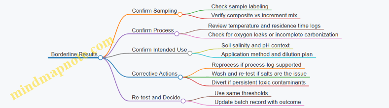
- What happens next when results are borderline.
Example decision rules for a small production run:
- If heavy metals exceed internal action limits, the batch is rejected for soil application.
- If PAH indicators are high, the batch is reprocessed only if process logs suggest incomplete carbonization; otherwise it is diverted.
- If electrical conductivity is above the target range for the intended soil type, the batch is either washed and re-tested or reserved for low-salinity sites.
- If pH and ash are far from prior batches, investigate feedstock changes or kiln performance before releasing.
Mind Map: Safety and Batch Consistency Workflow
Example: Contaminant Screening with a Simple Sampling Plan
Suppose you produce 1,000 kg of biochar in a single kiln run. You don’t sample once and hope. Instead:
- Take multiple increments from different locations in the cooled biochar pile.
- Combine increments into a composite sample for lab testing.
- Keep retained samples from the same batch for re-testing if results are borderline.
This reduces the chance that a localized contamination event hides in the average.
Example: Batch Consistency When Feedstock Changes
A common failure mode is “same kiln, different feed.” For instance, switching from crop residues to a mixed agricultural waste stream can raise ash and salts. If your batch shows higher electrical conductivity and ash than prior runs, treat it as a signal to:
- verify feedstock blend documentation,
- check kiln run logs for temperature and residence time,
- and re-test after any corrective action.
The goal is not perfection; it is controlled variation with evidence.
Practical Documentation That Makes Testing Credible
Quality control records should include:
- batch ID and production date,
- feedstock source and blend ratio,
- kiln settings and run logs,
- sampling method and sample weights,
- lab test results with units,
- acceptance decision and any reprocessing steps.
Use a consistent format so that later comparisons are meaningful. If you can’t match a test result to a production run, the test result is just a number.
Mind Map: What to Do When Results Are Borderline
Summary Decision Checklist
Before biochar leaves your control, ensure you have: (1) a contaminant screening result appropriate to the feedstock, (2) batch consistency measurements that explain expected soil behavior, and (3) a clear go/no-go decision recorded under the batch ID.
2.5 Practical Biochar Characterization Methods Including Proximate Analysis and Surface Properties
Characterization is the fastest way to stop guessing. For biochar, “what it is” matters because it controls how microbes and nutrients behave on and around the particles. A practical workflow starts with bulk composition and stability, then moves to surface features that govern adsorption, wettability, and microbial attachment.
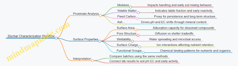
Proximate Analysis for Bulk Composition and Stability
Proximate analysis is a set of measurements that describe how much of the material is volatile, fixed carbon, and ash. It’s not a full chemical fingerprint, but it’s extremely useful for comparing batches and predicting persistence.
Moisture and Volatile Matter
Moisture is measured by drying a known mass at a controlled temperature until mass stabilizes. Volatile matter is then estimated by heating under conditions that drive off gases without fully burning the carbon skeleton.
Example: If two biochar batches have similar ash but one has higher volatile matter, the higher-volatiles batch often shows faster early changes in soil because it can release more labile compounds. In trials, that difference can look like “better performance,” even when the long-term stability is lower.
Fixed Carbon and Ash
Fixed carbon is the fraction that remains after volatiles are removed and before complete combustion. Ash is what remains after complete oxidation.
Example: A biochar with high ash can raise soil pH and electrical conductivity more strongly than a low-ash biochar, which can matter in saline-alkali soils. When you compare treatments, record ash content so you can interpret pH and EC shifts without blaming microbes for chemistry.
Practical Quality Checks
- Use the same sample mass and drying/heating schedule for every batch.
- Run at least duplicates; biochar is heterogeneous, so one-off numbers are rarely trustworthy.
- Keep a batch log that includes feedstock source, pyrolysis settings, and measured proximate values.
Surface Properties That Control Microbial Habitat
Microbes don’t colonize “biochar” in general; they colonize surfaces with specific chemistry and geometry. Surface properties also influence how nutrients move from soil solution to the biochar surface.
Surface Area and Pore Structure
Surface area and pore size distribution determine how much internal space is available for adsorption and microbial shelter.
- BET surface area estimates accessible surface from gas adsorption.
- Pore size distribution distinguishes micropores from mesopores and macropores.
Example: Two biochars can have the same BET area but different pore sizes. Mesopores often support faster mass transfer of nutrients and oxygen, while micropores can increase adsorption capacity but may slow diffusion.
Wettability and Surface Charge
Wettability affects whether water spreads across particles or beads up. Surface charge affects electrostatic interactions with ions and organic molecules.
- Contact angle or surrogate wettability tests indicate how easily water wets the surface.
- Zeta potential (measured in a controlled suspension) helps interpret ion interactions.
Example: A more hydrophobic biochar can reduce immediate wetting, which may delay microbial colonization until soil moisture and organic films accumulate.
Functional Groups and Reactivity
Functional groups on biochar surfaces influence adsorption of phosphate, ammonium, and organic acids.
- FTIR identifies broad functional group classes.
- Elemental analysis supports interpretation of oxygen and nitrogen content.
Example: Biochars with more oxygen-containing groups often show stronger interactions with polar nutrients and can buffer pH changes differently than highly carbonized, low-oxygen chars.
A Systematic Workflow from Sample to Interpretation
Use a tiered approach so you don’t spend advanced effort on samples that are clearly out of spec.
Stepwise Plan
- Record batch identity and sample representativeness.
- Run proximate analysis to classify stability and ash-driven chemistry.
- Measure surface area and pores to estimate adsorption capacity and diffusion constraints.
- Assess wettability and charge to predict water and ion behavior.
- Confirm functional groups to interpret nutrient interactions.
- Link results to soil observations using a simple decision logic.
Mind Map: What Each Measurement Tells You
Concrete Example: Interpreting Two Biochars
Imagine Biochar A and Biochar B are produced from similar feedstocks but with different pyrolysis conditions.
- Biochar A: lower ash, higher fixed carbon, moderate surface area.
- Biochar B: higher ash, higher volatile matter, higher surface area.
Reasoned interpretation: Biochar B is likely to cause stronger early chemical shifts because of higher ash and volatiles, and it may adsorb more nutrients initially due to higher surface area. Biochar A may show slower early effects but greater persistence because fixed carbon is higher. In a microbial trial, you’d expect early enzyme activity to rise faster with Biochar B, while longer-term carbon retention and habitat stability may favor Biochar A.
Reporting Results in a Way That Helps Decision-Making
A useful report includes both numbers and what they mean for soil behavior.
- Proximate values with units and method conditions.
- Surface area and pore distribution summary.
- Wettability and charge measurements under consistent suspension conditions.
- Functional group summary with the specific spectra features you used.
Example: Instead of writing “high surface area,” report the measured BET value and the dominant pore range. That level of detail makes it possible to compare batches and interpret why a treatment worked or didn’t.
3. Biochar Surface Chemistry and Microbial Attachment Mechanisms
3.1 Functional Groups on Biochar Surfaces and Their Relevance to Microbial Colonization
Biochar is not just “carbon.” Its surface contains chemical groups left behind by the feedstock and shaped by pyrolysis conditions. Microbes colonize biochar when the surface chemistry makes attachment easier and when the local microenvironment supports metabolism. Think of functional groups as the biochar’s “contact points” and “small-scale weather system” rolled into one particle.
Core Surface Chemistry Concepts
Functional groups fall into a few practical categories. Oxygen-containing groups (like hydroxyl and carboxyl) tend to increase wettability and provide sites for hydrogen bonding. Aromatic and graphitic domains contribute stability and a relatively hydrophobic character. Quinoid and phenolic-like structures can participate in redox reactions, which matters for microbes that rely on electron transfer. Mineral-associated surfaces (from ash) add additional reactive sites, including metal oxides and carbonates.
Microbial colonization is usually a sequence: approach → attachment → biofilm formation → sustained activity. Functional groups influence each step by changing how water and ions arrange near the particle, how nutrients adsorb, and how microbes interpret chemical cues.
How Functional Groups Influence Attachment
Attachment begins with cell-surface interactions. Many bacterial and fungal cell walls carry charged groups such as carboxylates and phosphates. If the biochar surface has complementary charge or hydrogen-bonding capacity, cells can stick long enough to start secreting extracellular polymeric substances (EPS).
Hydroxyl and carboxyl groups often improve initial wetting. Better wetting means cells are not trapped in dry pockets and can contact the surface during irrigation cycles. Carboxyl groups also interact with cations (like Ca²⁺ or Mg²⁺), which can act as bridges between cell surfaces and biochar.
Phenolic-like and quinone-like groups can affect attachment indirectly by altering redox conditions. Some microbes prefer microzones where electron acceptors or donors are available, and redox-active sites can shift those microzones.
How Functional Groups Shape Microbial Microhabitats
Once attached, microbes live in a thin boundary layer where chemistry differs from bulk soil water. Functional groups influence that boundary layer by controlling:
- Water retention and diffusion: Oxygen groups increase hydrophilicity, slowing water loss and improving diffusion of small solutes.
- Ion behavior: Carboxyls and other oxygen groups can bind ions, changing local electrical charge and osmotic conditions.
- Nutrient availability: Adsorption sites can capture phosphate, ammonium, and organic acids. This can be helpful when nutrients are released gradually, but harmful if adsorption is too strong and nutrients become unavailable.
A useful rule of thumb: functional groups that increase wettability and provide moderate binding often support colonization, while overly strong binding to key nutrients can reduce microbial growth.
Functional Groups and Biofilm Development
Biofilms are not just “more microbes.” EPS is a matrix of polysaccharides, proteins, and nucleic-acid-like substances. EPS formation depends on whether the surface chemistry supports secretion and whether the microenvironment remains stable.
Biochar surfaces with mixed oxygenated groups can support EPS anchoring through hydrogen bonding and electrostatic interactions. Redox-active groups can also influence biofilm stability by affecting oxidative stress around the particle.
Practical Examples You Can Visualize
Example: Carboxyl-rich biochar in a dry spell. A biochar produced at conditions that preserve more oxygen-containing groups tends to stay better wetted. After irrigation, cells can reach the surface and form early attachment points. In contrast, a more hydrophobic biochar may repel water, leaving cells stranded in the surrounding soil rather than on the particle.
Example: Phosphate availability in alkaline soil. In high pH conditions, phosphate can precipitate or become less available. Biochar surfaces with oxygen groups and mineral ash can adsorb phosphate near the particle. If the adsorption is not excessive, microbes that solubilize phosphate can access it locally, improving plant-available phosphorus indirectly.
Example: Salt stress and ion bridging. In saline conditions, high ionic strength can compress electrical double layers and weaken attachment. Biochar functional groups that bind specific cations can create localized ion environments that help cells maintain contact and reduce immediate osmotic shock.
Mind Map: Functional Groups and Colonization Pathways
What to Measure to Connect Chemistry to Biology
To connect functional groups to colonization, pair surface chemistry indicators with microbial outcomes. A practical workflow is: characterize biochar surface features, then test microbial attachment and activity in controlled soil-like moisture.
For surface chemistry, common indicators include oxygen content trends and functional group signatures. For biology, use measures that reflect early attachment (short incubations) and sustained activity (longer incubations). If a biochar shows improved wettability and moderate nutrient adsorption, you typically see stronger early attachment and more stable activity over time.
In short, functional groups matter because they control the interface where microbes decide whether to stay. The surface chemistry sets the rules for water, ions, nutrients, and EPS anchoring—so colonization is less random than it looks.
3.2 Hydrophobicity, Wettability, and Water Retention Effects on Microbial Activity
Soil microbes live in thin water films. Whether biochar helps or hinders them often comes down to how the biochar surface handles water: it can encourage wetting and stable films, or repel water and leave microbes stranded in dry pockets.
Core Concepts That Link Surface Water to Microbial Work
Hydrophobicity is the tendency of a surface to resist wetting. On biochar, it commonly arises from aromatic carbon domains, waxy residues, and certain surface functional groups that do not interact strongly with water.
Wettability describes how easily water spreads across a surface. A surface that wets quickly forms continuous films; a poorly wetting surface creates droplets and discontinuous contact.
Water retention is the ability of a material to hold water against gravity and evaporation. In soil, this is shaped by pore size distribution, pore connectivity, and surface energy.
Microbial activity depends on all three because enzymes diffuse through water, nutrients dissolve into water films, and cells need hydration to maintain membrane transport.
How Biochar Surface Chemistry Changes Water Behavior
Biochar surfaces are not uniform. They contain a mix of polar groups (like oxygen-containing functionalities) and nonpolar carbon domains. When polar groups are more abundant and accessible, water molecules form stronger interactions, improving wetting. When nonpolar domains dominate, water forms beads.
A practical way to think about it: microbes do not “care” about hydrophobicity directly; they care whether water stays where they are and whether dissolved substrates can reach them.
How Pores and Particle Geometry Control Water Availability
Biochar pores create microhabitats. Small pores can retain water by capillary forces, while larger pores can act as channels that supply water during wetting events.
- Micropores often increase water retention but can slow diffusion if they trap water too tightly.
- Mesopores can balance retention and transport, supporting enzyme diffusion and nutrient movement.
- Macropores improve drainage and aeration, but may dry out quickly.
Particle size matters too. Finer biochar increases surface area and contact points, but it can also increase hydrophobic patchiness if the surface is uneven. Coarser particles may create fewer contact points but can maintain more stable pore networks.
The Water Film Mechanism for Microbial Activity
When soil wets, water spreads across biochar and soil aggregates. If biochar is well-wetting, it helps form a continuous film that supports:
- Enzyme function: enzymes work best when substrates are dissolved and can diffuse.
- Nutrient transport: dissolved nitrogen, phosphorus, and organic acids move through the film.
- Cell survival: hydration reduces membrane stress and slows dormancy.
If biochar is hydrophobic, water may bead and run off, leaving nearby regions drier. Microbes can still function in the brief wetting window, but repeated drying cycles reduce overall activity and can shift communities toward drought-tolerant strategies.
Easy-to-Understand Examples You Can Visualize
Example: Hydrophobic biochar in a sandy soil Imagine a sandy soil with large pores and fast drainage. If the biochar surface beads water, the water drains before a stable film forms. Microbes experience short hydration periods, so respiration and enzyme activity drop even if nutrients are present.
Example: Moderately wetting biochar in a clay loam Clay loam holds water longer. If biochar is moderately wetting, it can extend the duration of thin water films inside aggregates. That supports steady enzyme activity and reduces the “on-off” pattern of microbial metabolism.
Example: Biochar with nutrient loading improving wettability When biochar is preloaded with soluble nutrients or organic amendments, the surface often becomes more polar and more wettable. Water spreads more evenly, and microbes gain access to dissolved substrates sooner after irrigation.
Practical Best Practices to Manage Wettability and Water Retention
-
Choose biochar with appropriate surface polarity If your goal is microbial activity, prefer biochar that wets reasonably well in soil moisture conditions. Very hydrophobic batches are more likely to create dry microzones.
-
Match biochar pore structure to your soil’s water regime
- For fast-draining soils, prioritize water retention without creating overly tight water trapping.
- For waterlogged soils, ensure pores do not overly restrict oxygen diffusion.
-
Use preconditioning when needed Pre-wetting biochar with water or mild nutrient solutions can reduce contact-angle effects and help establish early microbial access to water films.
-
Avoid overloading with salts High electrical conductivity can change water behavior and stress microbes. Better to use nutrient additions that support wetting and dissolution without pushing osmotic stress too far.
Mind Map: Water Behavior to Microbial Outcomes
A Simple Field-Ready Check That Connects to the Mechanism
Before committing to a large application, do a small jar test with your target soil and realistic moisture. Observe whether water spreads and whether the mixture stays evenly moist after gentle wetting. If water forms persistent droplets on biochar-rich spots, expect reduced and more variable microbial activity because the water film will be patchy.
When wettability and retention are aligned with your soil’s moisture cycle, biochar becomes more than a carbon store; it becomes a stable microhabitat where microbes can keep doing the chemistry that builds soil function.
3.3 Adsorption of Nutrients and Organic Compounds Including Phosphate and Organic Acids
Adsorption is the moment a dissolved nutrient or organic molecule meets a biochar surface and sticks long enough to matter. In soil, “sticking” can mean several things: it may be a weak attraction that releases quickly, a stronger binding that persists through wetting cycles, or a surface reaction that changes the molecule’s form. Biochar influences all three because its surfaces carry minerals, pores, and functional groups that differ by feedstock and pyrolysis conditions.
Core Concepts of Adsorption on Biochar Surfaces
Biochar surfaces provide three main adsorption routes. First, mineral-associated sites can bind ions directly, especially in ash-rich biochars. Second, functional groups on the carbon matrix can attract or bind molecules through electrostatic interactions and hydrogen bonding. Third, pore spaces create “microenvironments” where molecules concentrate near surfaces, increasing the chance of binding.
Phosphate is a good example because it exists in multiple charged forms depending on pH. At many soil pH values, phosphate anions can be attracted to positively charged sites on mineral surfaces or can form inner-sphere complexes with metal ions such as Ca, Fe, and Al. Organic acids behave differently: they can chelate metals, compete for binding sites, and also adsorb through carboxyl groups and hydrophobic interactions.
Phosphate Adsorption Mechanisms and What They Mean
Phosphate adsorption on biochar often follows a sequence. When phosphate enters the biochar pore network, it encounters charged sites. If the surface has cations or reactive mineral phases, phosphate can form stronger complexes that resist immediate leaching. If the surface is mostly neutral and lacks reactive minerals, phosphate may adsorb more weakly and desorb faster.
A practical way to reason about this is to separate “holding” from “availability.” Strong binding can reduce immediate loss, but it can also slow plant uptake if phosphate becomes too tightly held. The goal is not maximum adsorption; it is adsorption that slows leaching while still allowing gradual release as soil chemistry shifts.
Organic Acid Adsorption and Competition Effects
Organic acids such as acetate, citrate, and oxalate can adsorb to biochar and also compete with phosphate. Competition happens because both phosphate and organic acids seek similar surface regions, especially where functional groups and metal ions are present. Organic acids can also change phosphate behavior indirectly by complexing metal ions. If a metal ion that would bind phosphate is tied up by an organic acid, phosphate may desorb or remain in solution longer.
This is why organic amendments often change the “shape” of nutrient retention. A biochar that initially adsorbs phosphate strongly may show reduced phosphate retention after organic acids accumulate, not because adsorption disappears, but because the chemistry of the binding sites changes.
Mind Map: Adsorption Pathways and Soil Outcomes
Example: Phosphate Retention in Alkaline Soil
Consider an alkaline soil where phosphate tends to precipitate with calcium and becomes less available. A Ca- and ash-rich biochar can add additional reactive surfaces. After application, phosphate in soil water contacts biochar surfaces and can form complexes that reduce immediate loss. Over time, repeated wetting and drying can allow partial release as the local solution chemistry changes.
A simple way to test whether the biochar is “holding too hard” is to compare plant-available phosphate in treated versus untreated soil using the same irrigation and fertilization schedule. If plant uptake improves while leaching decreases, adsorption is likely contributing to availability rather than blocking it.
Example: Organic Acids Shifting Phosphate Release
Now add a compost extract or a small amount of readily degradable organic matter that produces organic acids during early decomposition. Those acids can adsorb to biochar and also chelate metal ions. If the biochar’s phosphate binding relies heavily on those metals, phosphate may desorb more readily into soil solution.
In practice, this can be beneficial when the soil is prone to phosphate lock-up. It can also be risky if the organic acids are strong and abundant enough to keep phosphate in solution and increase leaching. The integrated best practice is to match organic input timing with the period when plants can take up phosphate, so the “extra mobility” becomes uptake rather than loss.
Example: Pore Diffusion and Contact Time
Biochar pores can trap molecules long enough to increase adsorption, but diffusion into fine pores can be slow. If phosphate is applied in a single irrigation event, some phosphate may not reach interior surfaces before conditions change. That means adsorption capacity may be underused even when the biochar has high total surface area.
A practical approach is to ensure adequate contact time through incorporation or repeated wetting. If you top-dress biochar and rely on a single rainfall, you may see weaker retention than expected because transport into pores is limited.
Practical Checks for Adsorption Function
To keep adsorption effects grounded in reality, evaluate three linked outcomes: (1) phosphate remaining in soil solution after a controlled wetting event, (2) phosphate uptake by plants under the same nutrient supply, and (3) changes in soil pH and dissolved organic carbon that could indicate organic acid competition.
When these align—lower leaching, improved uptake, and chemistry consistent with the expected mechanisms—you can treat adsorption as a useful mediator rather than a mysterious black box.
3.4 Biofilm Formation on Biochar Particles and How It Alters Local Microenvironments
Biofilm formation is the moment when a biochar particle stops being “just a surface” and becomes a small, structured habitat. Microbes attach, produce sticky extracellular polymeric substances (EPS), and build a community that changes how water, nutrients, and oxygen move around the particle. The result is a microenvironment that can be more stable than the surrounding soil, especially during wet-dry cycles.
From Attachment to Architecture
Attachment usually starts with weak interactions: van der Waals forces, electrostatic attraction, and hydrophobic effects. Biochar surface chemistry matters here. If the surface is moderately wettable, cells can spread and make contact; if it is too hydrophobic, cells may touch but fail to stay. Once cells are close enough, they begin producing EPS, which acts like both glue and infrastructure.
EPS is not one thing. It includes polysaccharides, proteins, lipids, and nucleic-acid-like materials. Different microbes contribute different EPS compositions, so biofilm structure varies across soils. A practical way to think about it: EPS determines whether the biofilm behaves like a thin film that lets solutes pass quickly, or like a thicker matrix that slows diffusion.
How Biofilms Change Water Movement
Biochar particles often have internal pores and external roughness. When a biofilm forms, it can partially block pores, which reduces the rate at which water and solutes enter and leave. That sounds bad until you remember the tradeoff: slower exchange can protect microbes from sudden changes in salinity, pH, or nutrient availability.
A simple example: imagine a biochar particle in a saline-alkali soil. After irrigation, salt concentration near the particle can spike as water evaporates. A biofilm with thicker EPS can buffer the immediate salt shock by limiting how fast ions reach the cells. At the same time, the same barrier can slow oxygen diffusion, which shifts the local chemistry toward more reduced conditions.
How Biofilms Shift Oxygen and Redox Conditions
Oxygen availability controls which metabolic pathways dominate. In a biofilm, oxygen diffuses from the soil pores toward the biofilm interior. If the biofilm is thick or the surrounding soil is waterlogged, oxygen can be depleted near the center. That creates gradients: aerobic activity near the outer surface and anaerobic processes deeper in.
This matters for nutrient cycling. For instance, nitrate reduction is favored under low-oxygen conditions, while nitrification requires oxygen and is typically stronger where oxygen can reach cells. Biochar can also adsorb oxygen-related compounds, but the biofilm often determines whether those compounds are actually accessible to microbes.
How Biofilms Alter Nutrient Availability
Biofilms change nutrient dynamics in three main ways.
- Adsorption and retention: EPS contains functional groups that bind cations and organic molecules. This can concentrate nutrients near the cells.
- Consumption and recycling: Cells inside the biofilm consume nutrients, but they also release metabolites that other members can use. That creates internal “handoffs.”
- Diffusion control: Thick EPS slows diffusion, so nutrients may be depleted near the biofilm surface while remaining available deeper, depending on uptake rates.
Example: phosphate. In alkaline soils, phosphate can precipitate or bind strongly to mineral surfaces. A biofilm can locally increase the concentration of organic acids and enzymes that mobilize phosphate. Even if bulk soil phosphate remains unchanged, the biofilm can create a micro-zone where phosphate is more available to attached microbes and their plant partners.
Microbial Community Effects and Division of Labor
Biofilms promote spatial organization. Different species occupy different niches along gradients of oxygen, pH, and carbon availability. One group may specialize in breaking down complex organic matter into smaller compounds, while another group uses those products for growth or for producing EPS.
A useful mental model is “roles by location.” Near the biofilm edge, microbes experience more oxygen and fresh substrates. Deeper inside, microbes experience less oxygen and more accumulated metabolites. This division of labor can improve overall stability of the community on biochar.
Mind Map: Biofilm Formation and Microenvironment Shifts
Example: A Practical Biochar Trial Setup
To observe biofilm-driven microenvironment effects without getting lost in jargon, pair a biochar treatment with a simple gradient-sensitive readout.
- Setup: Mix a nutrient-amended biochar into soil at a consistent moisture level. Include a control biochar that is not nutrient preloaded.
- Observation: After a short incubation, measure oxygen-related indicators (for example, redox potential) near the particle scale if you have the tools, or use bulk proxies alongside microscopy.
- Interpretation: If the nutrient-preloaded biochar shows stronger redox shifts and higher EPS presence, that supports the idea that biofilm thickness and diffusion control are changing local chemistry.
The key is to connect structure to function: attachment and EPS determine transport, transport determines gradients, and gradients determine which microbial processes dominate.
Example: What “Good” Biofilm Looks Like for Soil Function
A biofilm that improves soil function is not necessarily the thickest one. If EPS is too dense, it can trap nutrients and limit exchange, reducing overall activity. If EPS is too thin, microbes may detach during drying or salt spikes.
A balanced outcome often looks like this: stable attachment during wet-dry cycles, measurable changes in local redox behavior, and improved nutrient availability in the micro-zone around the particle. That combination usually indicates that the biofilm is thick enough to buffer stress but porous enough to allow key substrates to reach cells.
3.5 Practical Approaches to Assessing Biochar Microbial Compatibility in Laboratory Assays
Biochar compatibility means more than “microbes survive.” In a lab assay, you want evidence that biochar supports microbial activity, does not block key functions, and does not create toxic microenvironments. A good workflow starts with simple screening, then moves to function-based tests, and finally checks whether any observed effects come from chemistry rather than handling artifacts.
Compatibility Questions You Can Test
- Does biochar change microbial growth or viability? If growth drops sharply, the biochar may be too reactive, too nutrient-poor, or chemically stressful.
- Does biochar change activity rates? Even if cells survive, enzyme activity and respiration can reveal functional suppression.
- Does biochar adsorb nutrients or substrates? Some biochars bind phosphate, ammonium, or organics, which can make “less available” look like “less compatible.”
- Does biochar create oxygen or moisture microgradients? Fine particles and high surface area can shift diffusion and local redox conditions.
Mind Map: Compatibility Testing Logic
Step 1: Build Controls That Prevent False Conclusions
Use at least four treatments: (A) inoculum + medium only, (B) inoculum + medium + biochar, (C) biochar + medium without inoculum (checks abiotic changes), and (D) inoculum + medium + inert particle matched for particle size (checks physical effects). If you test nutrient-loaded biochar, include (E) nutrient-only at the same added concentration without biochar.
Easy example: If your biochar treatment shows lower respiration, treatment C tells you whether the biochar itself consumes oxygen or produces CO2 abiotically. Treatment D helps separate “surface effects” from “chemical effects.”
Step 2: Measure Viability and Growth with a Clear Sampling Plan
For bacteria, you can use CFU counts or flow cytometry with viability dyes. For fungi, use colony counts on selective media or microscopy-based hyphal growth scoring. Keep biochar concentration consistent and mix gently to avoid settling differences.
Practical detail: Biochar particles can trap cells and interfere with plating. To reduce bias, include a biochar wash step before plating: centrifuge gently, remove supernatant, and resuspend cells in fresh buffer. Then plate equal volumes.
Easy example: If CFU drops but enzyme activity stays similar, the biochar may be stressing cells without fully shutting down metabolism, or the plating recovery may be lower due to cell adsorption.
Step 3: Add Function-Based Readouts Instead of Only Growth
Growth is slow and sometimes misleading. Pair it with respiration and enzyme assays.
- Respiration: Monitor CO2 production in sealed vials using an infrared CO2 sensor or colorimetric traps. Normalize to biomass or initial cell counts.
- Enzymes: Choose assays aligned with your target functions. For nitrogen cycling, use urease or nitrification-related proxies. For phosphorus mobilization, use phosphatase activity.
Easy example: In an alkaline soil context, a biochar might not increase CFU, but phosphatase activity could rise, indicating improved access to organic phosphorus substrates or altered microenvironments.
Step 4: Detect Adsorption Artifacts with “Availability Controls”
Biochar can bind substrates, making the assay medium effectively different. To test this, run substrate availability checks.
- Measure residual phosphate or ammonium in the supernatant after mixing biochar with medium, before adding microbes.
- For enzyme assays, confirm that the substrate remains detectable in the presence of biochar.
Easy example: If phosphatase activity appears lower in the biochar treatment, but residual phosphate is also lower, the result may reflect substrate depletion rather than enzyme inhibition.
Step 5: Use a Time Course to Separate Immediate Stress from Adaptation
Take measurements at 0, early (e.g., 4–6 hours), and later (e.g., 24–72 hours) depending on organism and assay. Immediate drops suggest toxicity or adsorption shock. Later recovery suggests adaptation, biofilm formation, or gradual nutrient release.
Easy example: A biochar that suppresses respiration at 6 hours but matches controls at 48 hours may be initially adsorbing substrates, then becoming less limiting as the system equilibrates.
Step 6: Interpret Results Using a Simple Decision Matrix
- If CFU decreases and respiration decreases
- Likely toxicity or severe nutrient limitation
- If CFU decreases but respiration or enzyme activity stays similar
- Possible plating recovery issues or mild stress
- If respiration decreases but substrate availability also decreases
- Likely adsorption artifact
- If enzyme activity decreases but CFU is stable
- Possible enzyme inhibition or unfavorable microenvironment
- If abiotic control shows CO2 or oxygen effects
- Correct for non-biological background
Example Workflow: Screening Two Biochars for Phosphatase Compatibility
- Prepare medium with a known concentration of an organic phosphate substrate.
- Mix biochar at a fixed dose with medium, sample supernatant to confirm substrate availability.
- Add a standardized inoculum and incubate under the same temperature and mixing.
- Measure phosphatase activity at early and late time points.
- Compare to nutrient-only and inert-particle controls.
If Biochar 1 increases phosphatase activity without reducing substrate availability, it is compatible for phosphorus-related functions. If Biochar 2 reduces activity and also lowers substrate in the supernatant, it is likely binding the substrate rather than harming microbes.
Reporting That Makes Results Usable
Record biochar dose, particle size distribution, pH and EC of the assay mixture, incubation conditions, and the exact timing of sampling. Report both raw measurements and normalized values (e.g., per unit biomass or per initial cell count). Compatibility is a pattern, not a single number, so include at least two readout types: one viability-related and one function-related.
4. Engineering Biochar with Nutrient Amendments and Microbial Consortia
4.1 Biochar Pre Treatment With Nutrients Including Nitrogen Phosphorus And Potassium Sources
Biochar often arrives as a mostly “dry” surface: pores may be present, but nutrients are not automatically waiting inside them. Pre treatment is the step where you load nutrients onto or into biochar so that, once mixed into soil, microbes and plant roots encounter a ready supply rather than a slow, uneven scavenger hunt.
Foundational Idea: What Pre Treatment Changes
Pre treatment mainly affects three things. First, it increases the immediate availability of N, P, and K near the biochar particle. Second, it can reduce nutrient losses by pairing nutrients with adsorption sites and pore spaces. Third, it shapes the microenvironment around the particle, which influences microbial attachment and enzyme activity.
A practical way to think about it: biochar is the “address,” nutrients are the “mail,” and soil moisture is the “delivery truck.” If the mail arrives already placed in the right compartments, delivery is faster and more uniform.
Choosing Nutrient Forms That Match the Soil Problem
Nitrogen can be supplied as ammonium (NH4+) or nitrate (NO3−), but their behavior differs. Ammonium tends to adsorb more readily and can be held near the particle, while nitrate is more mobile and can wash away if moisture is high. Phosphorus is often the trickiest: many soils bind phosphate strongly, so pre treatment should aim for forms that can persist long enough to be used. Potassium is generally more mobile than ammonium but less strongly sorbed than phosphate, so loading helps mainly with short-term availability.
Pre Treatment Workflow Overview
- Select biochar with low ash contaminants and a particle size that will mix well.
- Decide nutrient targets based on soil test results and crop needs.
- Prepare nutrient solution at a concentration that avoids leaving excess salts.
- Load biochar by soaking, mixing, or tumbling.
- Dry or slurry store depending on your application timing.
- Check basic quality like pH and electrical conductivity (EC) of the final slurry or dried product.
Step by Step: Nitrogen Loading
Start with ammonium-based sources when your goal is short-term retention. Dissolve the nitrogen source in water to make a uniform solution, then mix biochar thoroughly so liquid contacts internal pores. A simple “kitchen test” for uniformity is to stir for long enough that the biochar darkens evenly; dry clumps usually mean incomplete wetting.
Example: For a small batch, soak 1 kg biochar in a measured volume of ammonium solution until fully wetted, then mix for 30–60 minutes. After loading, drain excess liquid and keep the biochar covered to prevent evaporation-driven salt concentration.
Step by Step: Phosphorus Loading
Phosphorus loading works best when you avoid creating a thick layer of precipitated salts that microbes cannot access. Use phosphate solutions at moderate strength and mix long enough for adsorption. If your biochar is very alkaline, phosphate may precipitate quickly, so you may need to adjust solution pH slightly toward neutral to keep phosphate in a usable form.
Example: In an alkaline soil trial, pre treat biochar with a phosphate solution, then apply soon after loading. The goal is to place phosphate where it can be accessed before it fully converts into less available mineral forms.
Step by Step: Potassium Loading
Potassium loading is straightforward but easy to overdo. Because K can be present in soil already, start with a conservative dose and focus on improving early availability rather than trying to “fertilize the whole season” in one step.
Example: Mix biochar with a potassium solution, then apply as a banded amendment near the root zone. This reduces the chance that excess K moves away before plants can use it.
Integrated Mind Map
Mind Map: Nutrient Pre Treatment with Biochar
Practical Batch Design Using a Simple Ratio Logic
Instead of guessing, use a ratio approach: decide the nutrient mass you want per kg biochar, then calculate the solution volume needed to dissolve and distribute it. Keep the solution not too concentrated so that, after loading, you do not end up with a salty residue that can stress seedlings or suppress sensitive microbes.
Example: Balanced N-P-K Pre Treatment for a Pot Trial
- Biochar: 1 kg
- Nutrient targets: modest N, limited P, supportive K
- Method: prepare a mixed nutrient solution, soak biochar with agitation for 45 minutes, drain excess, then apply immediately.
Reasoning: modest N reduces nitrate loss risk, limited P avoids heavy precipitation, and supportive K improves early uptake without creating a high-salt zone.
Quality Control That Prevents Common Failures
- Salt management: If the slurry EC is very high, reduce concentration or shorten loading time.
- pH awareness: Very alkaline nutrient solutions can drive phosphate precipitation.
- Uniform wetting: Dry pockets lead to uneven nutrient loading.
- Batch consistency: Record solution volumes, mixing time, and drainage method so results are repeatable.
When pre treatment is done carefully, biochar becomes less of a “carbon-only” amendment and more of a structured nutrient carrier that microbes and roots can actually use.
4.2 Biochar Loading With Organic Matter Including Compost Extracts and Fermentation Liquors
Biochar loading with organic matter is the step where you turn a mostly inert carbon surface into a usable habitat and nutrient buffer. The goal is not to “feed the biochar,” but to pre-assemble a functional microenvironment: a thin layer of dissolved organics, microbial-compatible surfaces, and a nutrient release pattern that matches soil conditions.
Core Concept: What Organic Loading Actually Does
Organic matter in solution or suspension can attach to biochar pores and surfaces, then act as:
- A carbon source that microbes can access quickly at first, then more slowly as compounds degrade.
- A nutrient carrier that reduces nutrient shock by releasing gradually.
- A habitat conditioner that improves wettability and supports biofilm formation.
- A buffering layer that can moderate local pH and osmotic stress near the particle.
A practical way to think about it: biochar is the “seat,” and the organic loading is the “cushion” that makes the seat comfortable for microbes and plants.
Choosing the Right Organic Input
Compost extracts and fermentation liquors differ in composition and behavior.
Compost Extracts
Compost extracts are typically more balanced and less extreme in salt content. They often contain soluble humic-like substances, small organic acids, and microbial metabolites.
Easy example: If you have a mature compost, steep it in clean water, filter out solids, and use the filtrate to load biochar. This gives you dissolved organics without large particles that can clog pores.
Fermentation Liquors
Fermentation liquors can be more concentrated and more variable. They may include sugars, amino compounds, organic acids, and sometimes higher salts depending on the feedstock.
Easy example: If you ferment crop residues with a controlled recipe, you can load biochar with the filtered liquor to provide a quick carbon pulse. Use lower loading rates first because strong liquors can increase electrical conductivity.
Stepwise Loading Workflow
Step 1: Start with Biochar That Can Accept Organics
Before loading, confirm the biochar is not excessively hydrophobic. If water beads strongly, pre-wet it with clean water and mix thoroughly. Better wetting improves contact and reduces uneven coating.
Step 2: Prepare the Organic Solution
- For compost extracts, steep compost in water, then filter to remove solids.
- For fermentation liquors, filter to remove biomass and check conductivity if you can.
Aim for a solution that is usable without being harsh. If the liquor is very salty, dilute it so the final mixture does not spike soil salinity.
Step 3: Load by Mixing and Soaking
Combine biochar with the organic solution at a consistent ratio, then mix for a set time. Soaking helps organics diffuse into pores; mixing helps distribute the solution across particle surfaces.
Easy example: Mix biochar with extract at a ratio that keeps the slurry pourable, then stir for 1–2 hours. Let it sit briefly so organics can enter pores, then drain excess liquid.
Step 4: Control the Drying Stage
Drying too fast can crack coatings and reduce microbial-friendly films. Drying too slowly can encourage unwanted microbial blooms in the loader.
A common compromise is to dry to a workable moisture level for handling, not to bone-dry. The loaded biochar should remain stable enough to store without turning into a smelly science project.
Step 5: Verify Loading Quality with Simple Checks
You do not need a lab to catch obvious problems.
- Wettability: Does water spread more easily than on raw biochar?
- Odor and appearance: Strong off-odors can indicate poor control.
- Conductivity trend: If you have a meter, compare raw and loaded slurry.
Mind Map: Biochar Loading with Organic Matter
Example: Two Loading Recipes for Different Soil Needs
Example: Gentle Loading for Neutral to Mildly Stressed Soil
Use compost extract as the organic phase.
- Filter extract to remove solids.
- Mix with biochar until evenly coated.
- Drain and dry to handling moisture.
- Apply during soil moisture conditions that support microbial activity.
This approach favors steady microbial colonization without large osmotic swings.
Example: Stronger Loading for Carbon-Limited Patches
Use a diluted fermentation liquor.
- Filter liquor.
- Dilute to reduce salt and acidity extremes.
- Load biochar with shorter mixing time and moderate soaking.
- Apply at a conservative rate first.
This approach provides a faster carbon pulse while limiting the chance of nutrient or salt shock.
Practical Integration with Soil Application
Organic-loaded biochar works best when soil moisture and nutrient availability do not fight it. If soil is very dry, microbes cannot use the coating. If soil is already high in readily available nutrients, the coating may mainly act as a habitat conditioner rather than a nutrient source. Matching the loading intensity to the site condition keeps the process coherent and measurable.
4.3 Inoculation Strategies for Establishing Beneficial Microbes on Biochar Carriers
Biochar can act like a small apartment building for microbes: pores provide space, surfaces provide attachment points, and co-loaded nutrients provide a first meal. Inoculation is the process of getting the right tenants to arrive, stick, and start working before conditions turn hostile. The goal is not just survival; it is early establishment of function.
Core Principles for Successful Establishment
Start with three constraints. First, biochar can adsorb microbes or their nutrients, which may help attachment but can also strip away the inoculum’s immediate resources. Second, biochar’s surface chemistry and particle size influence whether cells can physically anchor and whether they can access water. Third, soil conditions—especially moisture, salinity, and pH—determine whether the inoculated microbes can keep growing long enough to matter.
A practical way to plan inoculation is to match the microbe’s needs to the carrier’s features. For example, if the target is phosphate solubilization, choose a biochar that retains moisture and has functional groups that do not strongly bind the solubilizing acids. If the target is nitrogen cycling, ensure the carrier is not so nutrient-poor that the microbes spend the first days starving.
Mind Map: Inoculation Workflow
Conditioning the Biochar Before Inoculation
Biochar often benefits from a brief conditioning step. Wetting it to a workable moisture level reduces dust loss and improves contact between cells and surfaces. If the biochar is very alkaline or highly adsorptive, a mild pre-wash with clean water can reduce extreme pH shocks and remove loosely bound ash components that interfere with early attachment.
Nutrient preloading should be deliberate. A simple approach is to co-load a small, readily available carbon source (for example, a dilute molasses solution) plus the nutrient most likely to limit the inoculated microbe (for example, a low phosphate dose for phosphate solubilizers). The point is to support the first 24–72 hours, not to turn the carrier into a fertilizer bag.
Inoculum Handling and Concentration
Use a standardized inoculum concentration so results are comparable across batches. Viability matters more than total volume: a thick suspension with low live cells is still a weak inoculation. If you cannot directly measure viability, use consistent culturing conditions and record growth phase timing.
Mixing method affects attachment. Gentle mixing helps distribute cells across particles without causing excessive shear stress. If the inoculum is in a liquid, allow the biochar to absorb the suspension rather than leaving cells floating on top.
Attachment and Establishment Tactics
A short incubation after mixing can improve attachment. Keep the mixture at a temperature and moisture level that supports the microbe’s early metabolism but does not trigger rapid die-off. For many beneficial bacteria, a few hours to a day of controlled incubation is enough to start biofilm formation on particle surfaces.
Oxygen and moisture balance should be treated as a knob, not a mystery. Too wet can limit oxygen diffusion and encourage unwanted anaerobes. Too dry prevents cell activity. A workable target is a damp, non-dripping consistency that allows diffusion through pores.
Compatibility Testing Before You Commit
Do not assume “it grew in culture” means “it will function on biochar in soil.” Run a small microcosm test using the same soil type or a close proxy. Include a salt and pH stress check if the target field has saline-alkali conditions.
Function assays should be aligned with the microbe’s role. For phosphate solubilizers, measure soluble phosphate or acidification proxies. For nitrogen-related functions, track ammonium or nitrate dynamics over time. For stress-tolerant consortia, monitor survival and respiration as a basic activity check.
Example: Inoculating Biochar for Phosphate Solubilization
A practical workflow for a phosphate-solubilizing bacterial inoculum:
- Condition biochar by wetting to a damp consistency and letting it equilibrate for a short period.
- Preload with a low dose of phosphate and a small carbon source to support early metabolism.
- Mix inoculum into the biochar suspension at a standardized cell concentration.
- Incubate briefly under controlled moisture to encourage attachment.
- Test in a small soil microcosm for soluble phosphate increase compared with biochar-only and inoculum-only controls.
If soluble phosphate does not increase, the issue is often one of three things: the biochar binds the acids too strongly, the inoculum is too low in viable cells, or the soil pH is outside the microbe’s effective range.
Example: Inoculating Biochar for Salt Stress Support
For saline-alkali soils, focus on survival plus function. Use a biochar that improves water retention without creating extreme osmotic conditions. Preload with nutrients that support stress response rather than heavy fertilization. After mixing, keep moisture stable during the short incubation so cells do not experience repeated drying and rewetting.
In microcosms, compare inoculated biochar against the same biochar without inoculum under the target electrical conductivity and pH range. The best inoculation is the one that shows both higher microbial activity and the intended soil function signal.
Quality Control That Prevents Silent Failures
Track batch IDs for biochar and inoculum, record moisture targets, and keep mixing times consistent. Include contamination checks when working with mixed consortia. Replicate the inoculation step at least twice so you can distinguish real effects from one-off handling differences.
A good inoculation strategy is systematic: condition the carrier, standardize the inoculum, encourage early attachment, verify compatibility, and apply with consistent placement and moisture management. When those steps line up, beneficial microbes are more likely to do their job instead of just hitchhiking.
4.4 Building Consortia for Specific Functions Such as N Fixation and Phosphate Solubilization
Consortia are not just “more microbes.” They are small teams where each member does a job that the others cannot do as well. When you build a consortium for biochar carriers, you want three things: (1) functional complementarity, (2) stable coexistence on the biochar surface, and (3) measurable outcomes in soil conditions that actually exist (moisture swings, salt, pH, and competition).
Core Design Logic for Function-Targeted Consortia
Start with a function map. For nitrogen fixation, the consortium must support nitrogenase activity, protect it from oxygen stress, and provide carbon and micronutrients. For phosphate solubilization, it must produce organic acids or phosphatases and keep phosphate in a form plants can access.
Then translate the function map into “roles” rather than species names. A practical role set for N fixation includes a nitrogen fixer, a carbon-providing or fermentative partner, and a microhabitat helper that reduces stress. For phosphate solubilization, roles often include a solubilizer, a mineral weathering helper, and a biofilm-former that improves contact between microbes, biochar, and soil minerals.
Finally, choose compatibility constraints. Many failures come from mismatched growth rates or antagonism. Use simple pre-tests: pairwise growth on the same nutrient medium, and a short biochar attachment test under the soil moisture level you plan to use.
Consortium Blueprint for Nitrogen Fixation
A common design is a two- or three-member consortium. Member A is the nitrogen-fixing bacterium. Member B is a partner that supplies readily available carbon and helps maintain low-oxygen microzones near biochar pores. Member C, if used, is a biofilm-former or stress-tolerant helper that improves survival during drying and rewetting.
Easy-to-understand example: imagine a biochar particle as a small apartment building. The nitrogen fixer is the tenant who does the heavy work, but it needs a quieter hallway and a steady supply of food. The partner provides food and helps create that calmer microenvironment. The biofilm-former keeps the building’s doors from slamming shut when conditions change.
To make this work on biochar, load the carrier with a modest carbon source before inoculation. Too much carbon can cause fast microbial blooms that consume oxygen and shift pH. A practical approach is to use a dilute organic loading solution and then let the biochar equilibrate briefly so microbes attach before the carbon is fully consumed.
Consortium Blueprint for Phosphate Solubilization
Phosphate solubilization often depends on acidification and enzymatic release. Member A is the solubilizer that produces organic acids or phosphatases. Member B can be a mineral-weathering helper that increases access to bound phosphate by altering microenvironments at the mineral surface. Member C is a biofilm-former that stabilizes the consortium on biochar and improves contact with soil particles.
Easy-to-understand example: consider phosphate as a locked cabinet. The solubilizer brings the right “key chemistry,” while the weathering helper makes sure the cabinet is reachable by loosening the surrounding material. The biofilm-former is the person who keeps the cabinet area clean enough for repeated access.
On biochar, phosphate solubilizers benefit from surface chemistry that supports attachment. If your biochar is very hydrophobic, microbes may not colonize well. A simple compatibility check is to observe whether inoculated biochar becomes uniformly wetted and whether cells remain attached after gentle mixing.
Mind Map: Role-Based Consortium Construction
Practical Assembly Workflow That Avoids Common Traps
-
Start with a small consortium. Two members often outperform five if compatibility is unknown.
-
Pre-test attachment. Mix inoculum with biochar at your intended moisture level and check whether cells remain associated after gentle agitation.
-
Use role-appropriate loading. For N fixation, provide a limited carbon source to support early attachment and metabolism. For phosphate solubilization, avoid overloading with phosphate that can suppress solubilization behavior.
-
Co-inoculate in the right order. If one member forms biofilm quickly, inoculate it first so it can establish surface coverage. Then add the functional partner.
-
Verify function in a soil-relevant microcosm. Use a short incubation with the same pH and salinity range as your target soil, and measure the functional proxy rather than only counting cells.
Example: Two-Member N Fixation Consortium on Biochar
Choose nitrogen fixer A and carbon partner B. Load biochar with a dilute carbon solution, inoculate with B first, allow attachment, then add A. In a soil microcosm, compare four treatments: biochar only, biochar plus A, biochar plus B, and biochar plus A+B. The best consortium is the one where the A+B treatment shows higher nitrogen fixation proxy than A alone, without a large drop in survival.
Example: Three-Member Phosphate Consortium on Alkaline Soil
Select solubilizer A, weathering helper B, and biofilm-former C. Inoculate C first, then A and B together. In alkaline soil microcosms, track soluble phosphate and plant-available indicators. If soluble P rises but plant uptake does not, the consortium may be producing phosphate in forms that plants cannot access, or it may be failing to persist on biochar after mixing.
A good consortium is built to be tested. When you measure function and persistence together, you stop guessing whether “more microbes” means “more useful soil chemistry.”
4.5 Field Ready Preparation Protocols Including Storage Handling and Application Timing
Field success usually fails for boring reasons: biochar batches vary, inoculum dies quietly, and application timing ignores soil moisture. This section turns those failure points into a repeatable workflow.
Define Your Target Use Case Before You Touch a Bag
Start by writing three numbers and one constraint on a sheet: (1) application rate target (kg biochar per hectare or per bed), (2) target soil moisture at application (for example, “field capacity range” or a practical proxy like “soil forms a weak ball but crumbles when pressed”), (3) target crop establishment stage, and (4) whether you need nutrient loading, microbial inoculation, or both. This prevents mixing incompatible goals, such as applying a nutrient-loaded carrier when the soil is already saturated and oxygen-limited.
Example: If you are using biochar as a microbial carrier for early root establishment, you plan for application right before irrigation or the first post-plant watering. If you are using biochar mainly for salt stress buffering, you plan around leaching events so the soil solution chemistry stabilizes after salts are moved.
Standardize Biochar Handling from Batch to Bed
Biochar is porous and likes to absorb water and soluble compounds from the air. Store it covered, dry, and off the ground. Use a batch ID on every container so you can trace outcomes back to production conditions.
Before field use, do a quick “fit check”:
- Particle size: confirm it matches your mixing method (fine dust disperses easily but can clog spreaders).
- Moisture: if it is clumping, it will not mix uniformly.
- Salt and pH basics: if your biochar is unusually alkaline or saline, adjust co-amendments and application timing.
Example: Two biochar batches with the same label can behave differently. Batch A mixes smoothly and shows uniform soil coverage; Batch B forms lumps and creates patchy microbial survival.
Prepare Nutrient Loading and Inoculation Without Killing the Plan
Use separate preparation steps for nutrient loading and microbial inoculation. Nutrient loading can be done first, then the loaded carrier is cooled and held briefly before inoculation.
For inoculation, keep three rules:
- Temperature control: keep inoculum cool and out of direct sun.
- Oxygen and mixing: avoid long stagnant holds; mix gently to distribute cells.
- Time window: inoculated biochar should be applied soon after preparation.
Example: If you inoculate in the morning and the field is accessible only after midday heat, prepare in smaller batches so the last batch is not sitting for hours.
Storage Handling That Preserves Viability and Uniformity
If you must store loaded or inoculated material, store it in sealed containers to reduce moisture swings and contamination. Use breathable options only when you are certain oxygen needs are met; otherwise, sealed storage is safer for short holding times.
Track these fields in your log:
- preparation start and end time
- container type and fill level
- ambient temperature
- estimated moisture of the carrier
Mind Map: Field Ready Workflow
Application Timing That Matches Soil Physics
Timing is about moisture and oxygen, not calendar dates. Apply when the soil surface is workable and the root zone will receive water soon after application.
Use a simple decision rule:
- If the soil is too dry, biochar and inoculum may not contact soil solution well.
- If the soil is too wet, mixing becomes uneven and oxygen drops, which can reduce microbial performance.
Plan application around irrigation or rainfall so that the first wetting event occurs within a short window after spreading. Avoid applying right before heavy rain that can cause runoff and uneven deposition.
Example: For drip-irrigated beds, apply loaded biochar immediately before the first irrigation cycle after transplanting. For furrow systems, apply before irrigation so the first water movement distributes the carrier into the active root zone.
Application Methods and Uniformity Checks
Choose a method that matches particle size and carrier moisture.
- Top dressing: good for established plants, but requires prompt watering.
- Band incorporation: improves contact near roots, but needs careful depth control.
- Mixing into planting media: best for inoculated carriers, but requires consistent mixing.
Before treating the whole area, do a small “coverage test” by spreading a measured amount over a marked strip and checking for visible streaking or bare patches. Adjust spreader settings or mixing water content accordingly.
Minimal Verification After Application
Within the first few days, verify two things: (1) the carrier is present where you intended, and (2) the soil moisture regime stayed within your target range. A practical approach is to take small samples from treated and untreated micro-zones and compare basic indicators like moisture and simple microbial activity proxies.
Example: If you see strong differences in moisture between treated strips, you can attribute inconsistent plant response to uneven wetting rather than to biochar chemistry.
Field Checklist for the Day of Work
- Biochar batch IDs labeled on containers
- Inoculum prepared last and kept cool
- Application planned around irrigation timing
- Coverage test completed on a marked strip
- Sampling points marked before spreading
- Log sheet filled with times, temperatures, and any deviations
Mind Map: Timing Decision Rule

Integrated Example with Realistic Steps
On 2026-03-05, a team prepares nutrient-loaded biochar and inoculated carrier for a saline-alkali plot. They store biochar covered and dry, run a quick clumping check, and label Batch A and Batch B. They load nutrients the day before, cool the loaded material, and inoculate in the morning in two smaller batches to avoid heat exposure. They spread the inoculated carrier right before the first irrigation cycle after transplanting, then take samples from treated and untreated micro-zones to confirm moisture uniformity. The log records preparation times, ambient temperature, and any deviations, so later results can be interpreted without guessing.
5. Microbial Engineering Approaches for Soil Functions Without Uncontrolled Release
5.1 Selecting Target Functions Such as Nitrogen Cycling Phosphorus Mobilization and Stress Tolerance
Choosing target functions is the part where you stop collecting “interesting soil effects” and start collecting evidence for specific outcomes. A good target function is measurable, tied to a soil constraint, and compatible with how biochar and microbes actually behave in soil water films.
Start with Soil Constraints and Crop Demands
Begin by listing the limiting factors you can observe or measure: low available nitrogen, phosphorus fixation in alkaline soils, salinity stress, poor aggregation, or slow organic matter turnover. Then translate each constraint into a function that microbes can influence.
- If nitrogen is limiting, the function might be ammonification, nitrification, or nitrogen fixation.
- If phosphorus is limiting, the function might be phosphate solubilization, mineral dissolution, or reducing phosphorus sorption.
- If plants struggle under salt or sodicity, the function might be osmoprotection, ion homeostasis support, or improved aggregation that reduces salt movement.
A practical rule: pick one primary function and one secondary function. Two primaries often turn into two half-measures.
Map Functions to Microbial Processes
Each target function should connect to a process chain you can reason about.
- Substrate availability: Does the system have the carbon and micronutrients microbes need to run the process?
- Enzyme activity: Which enzymes or metabolic steps are required?
- Environmental conditions: What pH, oxygen level, and moisture range support the process?
- Transport and access: Can microbes reach the substrate on biochar surfaces or in pore spaces?
For example, phosphate solubilization depends on organic acid production and on whether those acids can access mineral surfaces. If the biochar is too hydrophobic or the soil is too dry, the acids never reach the minerals, and the function fails quietly.
Define Measurable Outcomes and Acceptance Thresholds
A target function needs a measurable output. Use outcomes that match the process.
- Nitrogen cycling: changes in nitrate and ammonium pools, net nitrification rate, or plant-available nitrogen after a defined incubation.
- Phosphorus mobilization: changes in soluble phosphate, resin-extractable phosphorus, or phosphate uptake by plants.
- Stress tolerance support: reduced salt stress indicators such as improved plant growth under the same irrigation salinity, or microbial osmolyte activity proxies.
Set acceptance thresholds based on your baseline variability. If your control treatment already swings widely, you need a higher bar for “success” than if your baseline is stable.
Choose Functions That Fit Biochar and Soil Microhabitats
Biochar is not just “carbon.” Its surface chemistry, porosity, and ash content shape which microbes can attach and which reactions are favored.
- For nitrogen cycling, you want biochar that supports microbial colonization and provides a stable carbon source without locking nutrients too tightly.
- For phosphorus mobilization, you want surfaces that can adsorb and later release relevant ions, and you want conditions that allow organic acids to persist long enough to act.
- For stress tolerance, you want improved water retention and aggregation so microbes and roots experience less ionic shock.
A simple check: if your target function requires microbial activity in the soil water film, then your application must maintain moisture and avoid extreme pH shifts that stop enzyme work.
Mind Map: Target Function Selection Logic
Example: Nitrogen Cycling Target with Clear Logic
Suppose a field has low nitrate after spring thaw and frequent waterlogging. A reasonable nitrogen-cycling target is controlled nitrification plus reduced nitrogen loss.
- Process logic: waterlogging lowers oxygen, which slows nitrification; when oxygen returns, nitrification can surge.
- Function design: choose a primary function of “faster recovery of nitrification after re-aeration,” not “maximum nitrification at all times.”
- Evidence: measure ammonium and nitrate at multiple time points after drainage, and track net change rather than single-point concentrations.
If you only measure nitrate once, you might miss the recovery pattern and mislabel the treatment.
Example: Phosphorus Mobilization Target in Alkaline Soil
In alkaline soil, phosphate often binds strongly to calcium minerals. A target function could be phosphate solubilization via organic acids.
- Process logic: organic acids must reach mineral surfaces and persist long enough to shift local chemistry.
- Biochar fit: select biochar that supports microbial attachment and does not overly adsorb the acids or block water access.
- Evidence: track soluble phosphate over a short incubation and confirm with plant uptake or resin-extractable phosphorus.
If soluble phosphate rises briefly but plant uptake does not, the mobilized phosphorus may be re-sorbed quickly or not accessible to roots.
Example: Stress Tolerance Target for Saline-Alkali Land
For saline-alkali conditions, a practical target function is improved root-zone stability through aggregation and microbial osmoprotection support.
- Process logic: salt stress harms enzymes and disrupts aggregation; aggregation reduces salt movement and improves water availability.
- Evidence: compare plant growth and root-zone moisture retention under the same salinity, and pair that with microbial activity proxies.
This target avoids the trap of measuring only “microbes survived” without linking it to soil structure and plant outcomes.
A Simple Selection Checklist
- The function matches a real constraint you can measure.
- The function has a process chain you can explain.
- The function has measurable outcomes with a defined success threshold.
- The function fits the biochar’s likely microhabitat effects.
- You choose one primary and one secondary function to keep the experiment interpretable.
5.2 Strain Selection Criteria Including Survival Traits and Compatibility with Soil Conditions
Selecting strains for biochar carriers is less about finding the “best” microbe and more about matching traits to the soil’s constraints. A strain that performs well in a lab tube can fail in the field if it cannot tolerate the local pH, salt level, oxygen pattern, moisture regime, and available carbon forms. The goal is to choose strains that can survive the first weeks, then maintain useful activity long enough to affect nutrient cycling.
Step 1: Translate Soil Conditions into Selection Filters
Start by turning soil measurements into practical filters. Use baseline data such as pH, electrical conductivity, texture, moisture history, and organic matter level. Then add operational details: irrigation frequency, typical temperature range, and whether the site is frequently tilled.
- pH filter: Many bacteria prefer near-neutral conditions, while fungi often tolerate broader ranges. If your soil is alkaline, prioritize strains with stable enzyme activity at higher pH.
- Salt and sodicity filter: High electrical conductivity and sodium stress can reduce membrane integrity and enzyme function. Choose strains with salt tolerance and good osmoregulation.
- Moisture and aeration filter: Waterlogging shifts oxygen availability. Choose strains that match the expected oxygen profile: aerobic for well-drained soils, microaerophilic or facultative for fluctuating conditions.
- Carbon availability filter: Biochar can be a slow carbon source and a habitat. Strains should either use available root exudates or tolerate low readily degradable carbon.
Step 2: Survival Traits That Matter in the First Weeks
Early survival is often the limiting step. Biochar helps, but it does not magically fix every stress.
Key survival traits to screen for:
- Desiccation tolerance: Strains should maintain viability during drying-rewetting cycles. A simple test is to expose cultures to the site’s typical dry-down moisture range and measure viable counts after rehydration.
- Osmotic stress tolerance: For saline or sodic soils, evaluate growth or survival across a gradient of salt concentrations that bracket field values.
- pH stability: Measure enzyme activity or growth across the soil pH range rather than only at one point.
- Biofilm formation ability: Strains that form biofilms can persist on biochar surfaces and resist wash-off during irrigation.
- Stress response capacity: Look for robust recovery after exposure to heat or oxidative conditions that occur during mixing and application.
A practical rule: if a strain cannot survive the application handling and the first drying event, it is not a good candidate, even if it shows strong nutrient cycling in ideal conditions.
Step 3: Compatibility with Biochar Carriers and Soil Chemistry
Compatibility is about how the strain interacts with the carrier and the surrounding chemistry.
- Surface attachment: Biochar pore size and surface functional groups influence attachment. Strains with strong adhesion traits are more likely to establish microhabitats.
- Nutrient adsorption effects: Biochar can adsorb phosphate and some organics. Select strains that can access nutrients under reduced availability, or pair them with biochar preloading strategies.
- Toxicity screening: Some biochars contain residual compounds that inhibit microbes. Screen biochar batches using a short viability assay with the candidate strains.
- Competition and predation: Soil already has microbes. Choose strains that can coexist without being outcompeted immediately. A co-incubation test with native soil slurry can reveal whether the strain persists.
Step 4: Functional Fit Without Overpromising
A strain should match the intended function, but function must be measured under realistic conditions.
- If the target is nitrogen cycling, screen for survival plus measurable activity such as ammonia oxidation or nitrogen fixation under the soil’s pH and moisture constraints.
- If the target is phosphate mobilization, test for organic acid production or phosphatase activity in the presence of biochar and at the soil’s pH.
- If the target is salt stress mitigation, prioritize strains that maintain growth and produce extracellular polymeric substances under saline conditions.
Step 5: A Simple Screening Workflow
Use a staged approach to avoid wasting time on strains that fail basic constraints.
- Trait screening in vitro: pH, salt, moisture stress survival assays.
- Biochar compatibility: viability on the specific biochar batch.
- Soil co-incubation: persistence in native soil slurry or microcosms.
- Function assay: activity measurement under the same conditions.
- Carrier readiness: check that the strain remains viable after mixing with the carrier and during storage conditions typical for your workflow.
Mind Map: Strain Selection Criteria
Example: Choosing Strains for an Alkaline, Saline Field
Assume a site with pH 8.3, electrical conductivity around 6 mS/cm, and irrigation that creates wet-dry cycles.
- Filter: prioritize strains with stable growth near pH 8 and salt tolerance near the site’s conductivity.
- Survival test: expose candidates to a salt gradient and a drying-rewetting cycle matching the irrigation interval.
- Compatibility test: mix each candidate with the intended biochar batch and measure viable counts after 24–72 hours.
- Function test: run a phosphate mobilization assay at pH 8.3 with biochar present, then confirm activity is not just a lab artifact.
- Decision: select strains that show both survival and measurable function, not only one.
Example: Avoiding a Common Failure Mode
A strain may survive salt stress but fail after mixing because it is sensitive to oxygen exposure during aeration steps. If your workflow includes vigorous mixing or aeration, include a handling stress test that mimics the mixing duration and intensity. This prevents selecting a strain that is “field-suitable” in theory but not in practice.
5.3 Containment and Risk Management Practices for Engineered Microbes in Soil Systems
Engineered microbes can be useful in soil, but soil is not a sealed lab. Containment is therefore less about “never leaving the jar” and more about managing where the engineered trait can persist, spread, and express. The goal is to reduce unintended establishment while still allowing the intended function to occur long enough to be measured.
Core Risk Questions
Start by answering four practical questions before any release.
- Can the engineered microbe survive and reproduce in the target soil? Survival depends on moisture, temperature, nutrient availability, and competition.
- Can the engineered trait move to other microbes? Horizontal gene transfer is a key pathway to consider.
- Can the engineered microbe disperse beyond the application zone? Movement can occur via water flow, tillage, wind-blown dust, or animal transport.
- Can the engineered trait express under unintended conditions? Expression control matters when soil chemistry varies across depth and time.
These questions drive the design choices that follow.
Containment by Design
Containment begins with the organism’s biology.
Use genetic safeguards that limit persistence. Common strategies include making the engineered strain dependent on a condition not expected in the field, or using genetic “off switches” that reduce viability when specific signals are absent. For example, a strain can be engineered to require a nutrient supplement for stable growth during establishment; once that supplement is depleted, the population declines.
Reduce gene transfer opportunities. If the engineered trait is carried on mobile elements, the risk of transfer increases. Prefer chromosomal integration over plasmids when possible, and avoid designs that increase transfer likelihood.
Control expression tightly. Even if the microbe survives, you want the engineered function to run only when the soil environment matches the intended trigger. A simple example is using a promoter that responds to a substrate supplied in the treatment plan, so the engineered enzyme is produced mainly near the amendment.
Containment by Physical and Operational Controls
Biology needs help from logistics.
Define a treatment boundary and keep it consistent. Use buffer zones around waterways, field edges, and drainage outlets. A buffer is not just a “nice-to-have”; it reduces the chance that engineered cells move with runoff.
Minimize disturbance after application. Excess tillage can spread particles and cells. If banding is used, keep the application depth and equipment settings consistent to avoid smearing engineered material across layers.
Manage runoff and irrigation. Plan irrigation so it does not create heavy surface flow. For example, use smaller, more frequent applications that infiltrate rather than pond.
Prevent cross-contamination. Clean equipment between plots, especially when moving from treated to untreated areas. If you use shared hoses or spreaders, treat cleaning as part of the protocol, not as a cleanup chore.
Monitoring That Actually Tests Containment
Monitoring should measure both presence and function.
Track engineered cells with a specific marker. Use a detection method that distinguishes engineered strains from native relatives. Sampling should include the application zone and buffer zones, plus multiple depths.
Measure persistence over time. A single time point is not enough. Sampling at early, mid, and late intervals shows whether populations decline as intended.
Check for unintended gene presence. If the trait could transfer, test for the trait marker in surrounding microbial DNA, not only in cultured isolates.
Verify that function is localized. For instance, if the engineered microbe produces an enzyme to mobilize phosphate, measure enzyme activity or the relevant chemical change in the treated zone and compare it to buffers.
Example: Practical Containment Workflow
A field team applies a biochar carrier loaded with an engineered strain.
- Before application: They confirm the strain’s survival limits under the expected soil moisture and nutrient conditions, and they verify the trait marker is stable in the carrier.
- During application: They band the carrier at a defined depth, keep equipment dedicated to the treated plot, and record batch IDs.
- After application: They sample the band zone and a buffer zone at two depths. They also sample after the first irrigation event and again after several weeks to see whether engineered cells decline.
If engineered markers appear in buffers at early time points but drop quickly, that suggests limited dispersal. If markers persist in buffers, the operational controls likely need tightening.
Mind Map: Containment and Risk Management Practices
Decision Rules for Tightening the System
Use monitoring results to adjust only what the data supports.
- If engineered cells persist outside the boundary, reduce dispersal pathways by improving runoff control and limiting disturbance.
- If engineered function appears outside the intended zone, revisit expression control and carrier placement depth.
- If engineered cells decline too quickly in the target zone, adjust establishment conditions that support the intended short-term activity without increasing long-term persistence.
Containment is a system, not a single feature. When design, operations, and monitoring agree, you get both measurable soil function and controlled risk.
5.4 Genetic and Phenotypic Characterization Methods for Confirming Function Before Application
Before any engineered trait touches soil, you want evidence that the microbe does what you claim under conditions it will actually face. The goal is not to prove perfection; it is to prove the trait is present, measurable, and stable enough for the intended use window.
Core Principle: Function Must Be Measurable in Soil-Like Conditions
Start with a simple logic chain: genotype implies expression, expression implies activity, and activity implies a measurable soil-relevant output. If any link is missing, you redesign the construct, the expression conditions, or the delivery method.
Step 1: Confirm the Genetic Construct and Its Integrity
Use a two-layer check: sequence-level confirmation and structural confirmation.
- Sequence-level confirmation: verify the engineered region matches the intended design. For example, if your nitrogen-cycling circuit includes a promoter, a regulator, and an enzyme gene, confirm the junctions and reading frames. A single base change near a promoter can shift expression timing enough to fail in soil.
- Structural confirmation: confirm the engineered element is present in the expected genomic location or plasmid form. For plasmids, check copy number stability under non-selective conditions. For chromosomal integration, confirm the insertion site does not disrupt nearby essential genes.
Easy example: You engineer a phosphate-solubilizing enzyme under an inducible promoter. After assembly, you run a junction check and confirm the promoter-enzyme boundary is correct. Then you grow the strain without selection for several passages and re-check presence of the engineered region.
Step 2: Verify Expression Under Relevant Environmental Cues
Soil is not a lab incubator. Expression checks should include cues that resemble the target field conditions.
- Induction or repression conditions: test the circuit at the expected ranges of pH, salinity, oxygen, and carbon availability. If the circuit is inducible, confirm it turns on when the cue is present and stays low when it is absent.
- Time course: measure expression at multiple time points, not just one. Many circuits show a short early peak followed by decline due to resource limits.
Easy example: For a salt-stress enzyme, measure expression at low and high electrical conductivity. If expression only rises after long lag times, the trait may not help during early establishment.
Step 3: Measure Phenotype with Direct Functional Readouts
Genetic expression is not the same as functional output. Choose assays that map to the soil function.
- Enzyme activity assays: quantify activity using substrates that reflect the target nutrient pool. For phosphate solubilization, measure soluble phosphate increase in a buffered medium that mimics soil ionic strength.
- Metabolite or product formation: for nitrogen cycling, track ammonium or nitrate changes over time under controlled carbon and oxygen conditions.
- Stress tolerance phenotypes: for saline-alkali contexts, measure growth and survival across salt and pH gradients, then connect survival to functional output.
Easy example: If the trait is organic acid production to mobilize nutrients, measure acid concentration and the corresponding nutrient solubilization in the same experiment. If acids rise but solubilization does not, the downstream chemistry is missing or the strain cannot access the substrate.
Step 4: Confirm Stability and Consistency Across Passages
A trait that works once but disappears after handling is a practical failure.
- Genetic stability: test after serial passaging without selection. Track whether the engineered region remains intact.
- Phenotypic stability: repeat the functional assay after passaging. A construct can remain present while expression drifts due to regulatory changes.
Easy example: Run three rounds of growth and assay the same enzyme activity each time. If activity drops sharply after the second round, you adjust the construct design or delivery formulation.
Step 5: Rule Out Confounding Traits and Unintended Effects
Engineered strains can carry side effects that look like the intended function.
- Growth-rate confounding: a strain that simply grows faster can change nutrient levels without performing the targeted pathway. Include a non-engineered control with similar growth.
- Non-specific chemistry: some engineered metabolites can chelate ions or shift pH. Measure pH and ionic changes alongside the target output.
- Contamination checks: confirm culture purity before assays, since mixed populations can produce misleading results.
Step 6: Use Decision Criteria for “Go” Versus “No-Go”
Define thresholds before testing. Examples:
- Expression must exceed a minimum level under the target cue.
- Functional output must increase relative to controls by a set margin.
- Stability must hold across the planned handling steps.
Mind Map: Characterization Workflow
Example: A Practical Pre-Application Test Set
- Genotype check: confirm engineered junctions and presence after handling.
- Expression test: grow in two media that mimic low and high salinity; sample at early and mid time points.
- Functional test: run the nutrient-relevant assay in the same media and track both product and pH.
- Stability test: passage the strain without selection, then repeat the functional assay.
- Controls: include the parental strain and a non-functional engineered control.
If the strain meets the thresholds in these steps, you have evidence that the trait is present, expressed when it should be, and producing the intended soil-relevant effect under conditions that resemble the application environment.
5.5 Practical Documentation for Regulatory Ready Workflows and Traceability
Regulatory-ready documentation is less about paperwork theater and more about making your work reproducible by someone who was not in the room. The goal is simple: every claim about what happened in the lab or field must be traceable to a specific batch, instrument reading, sampling event, and decision.
Core Traceability Principles
Start with a traceability chain that answers four questions: What was used, who used it, where and when it was used, and what evidence shows it worked. Build your workflow around unique identifiers so nothing relies on memory.
Use a consistent ID scheme:
- Biochar Batch ID: produced date, feedstock lot, pyrolysis run number.
- Amendment Lot ID: nutrients, compost extract, salts, buffers.
- Microbial Inoculum ID: strain name, culture date, viability check result.
- Field Plot ID: site code, block, row, treatment code.
- Sample ID: plot ID + depth + sampling date + replicate number.
Every record should link back to these IDs. If a record cannot be linked, it is not evidence.
Documentation Package Structure
A regulatory-ready package typically includes four layers.
- Protocol layer: the planned method, acceptance criteria, and deviations policy.
- Execution layer: what actually happened, with timestamps and operator initials.
- Evidence layer: instrument outputs, raw data files, calibration logs, and QC results.
- Interpretation layer: how results were processed and how decisions were made.
Keep raw data immutable. If you must transform data, save a processing script and record the exact version used.
Workflow for Biochar and Microbial Trials
A practical workflow can be documented as a sequence of controlled steps.
Step 1: Pre-use verification
- Confirm biochar meets basic quality thresholds you define in advance, such as moisture range, ash content window, and contaminant screening results.
- Record storage conditions and any pre-application handling (drying, sieving, rehydration).
Step 2: Preparation records
- For nutrient loading or co-amendment, record target ratios, actual measured concentrations, mixing time, and temperature.
- For inoculation, record culture conditions, harvest time, and viability counts.
Step 3: Application records
- Record application date, weather notes relevant to soil moisture, equipment settings, and application rate calculations.
- Document mixing uniformity checks, such as a simple subsampling mass balance from the prepared carrier.
Step 4: Sampling and chain of custody
- Use a sampling plan that specifies depth, number of replicates, and timing relative to application.
- Record who collected samples, how they were labeled, storage temperature, and transport time.
Step 5: Laboratory analysis records
- For each assay, record reagent lot IDs, instrument model and serial number, calibration status, and acceptance criteria.
- Store raw chromatograms, plate reader files, and sequencing run metadata with the sample IDs.
Acceptance Criteria and Deviations
Define acceptance criteria before you start. Examples that work well in soil microbe studies:
- Viability must be above your minimum threshold before inoculation.
- Biochar batch must pass contaminant screening and basic physical checks.
- Replicate variability must be within a pre-set range for key measurements.
When deviations occur, document them immediately with three fields: what changed, why it changed, and what impact it might have. Then record the corrective action. If you do not assess impact, you cannot justify the data.
Mind Map: Documentation and Traceability
Example: One Biochar Trial Record Set
A complete record set for a single treatment should let a reviewer reconstruct the trial without guessing.
- Biochar Batch ID: BC-2026-03-R17
- Amendment Lot ID: NPK-LOT-044, CompostExtract-LOT-019
- Inoculum ID: CONS-NFIX-2026-03-12, viability 8.2×10^7 CFU/mL
- Plot ID: SITE-A / BLK-2 / TRMT-B3
- Sample IDs: SITE-A-BLK2-B3-D0-2026-03-28-R1, R2, R3
- Evidence links: enzyme assay raw files, respiration readings, and sequencing run metadata all stored under the sample IDs.
If a reviewer asks why a replicate looks unusual, you can point to the chain of custody record (transport time), the assay QC flag, and the deviation log for that sampling event.
Example: Deviation Log Entry
Use a short, consistent format.
- Deviation ID: DEV-BC-2026-03-07
- Step: Inoculum preparation
- What changed: incubation time increased by 30 minutes due to equipment delay
- Why: centrifuge maintenance
- Impact assessment: viability measured after incubation remained above minimum threshold; proceed with note in analysis
- Corrective action: adjust next batch timing and record centrifuge maintenance completion
Mind Map: Data Integrity and Storage

Practical Tips That Prevent Common Failures
- Label containers at the moment of preparation, not later.
- Record instrument calibration status in the same row as the measurement.
- Keep a single master index that maps IDs to file paths.
- Treat “notes” as evidence only when they include IDs and timestamps.
A good documentation system makes the science easier to defend because it reduces the number of places where interpretation can drift away from what was actually done.
6. Synthetic Biology Tools for Soil Microbe Engineering with Measurable Outputs
6.1 Choosing Genetic Circuit Designs That Produce Detectable Metabolic Outputs
A genetic circuit is only useful if you can measure what it does in soil conditions. “Detectable metabolic outputs” means the engineered microbe produces a signal that survives sampling and can be tied back to activity rather than background noise. The design process starts with three questions: What metabolic function do you want? What output can you measure reliably? What environmental conditions will turn the circuit on at the right time?
Step 1: Define the Function and the Output Type
Pick a target function that maps cleanly to a measurable product. For example, if the goal is phosphate mobilization, the output could be an organic acid that shifts pH locally and releases phosphate from mineral surfaces. If the goal is nitrogen cycling, the output might be a specific enzyme activity (such as phosphatase or urease) or a metabolite that correlates with that pathway.
Outputs fall into four practical categories:
- Small molecules: acids, sugars, amino acids, or volatile compounds. These are measurable by chromatography or colorimetric assays, but they can diffuse.
- Enzyme activities: measurable in extracts using substrate conversion. These are often easier to interpret because they link directly to catalytic function.
- Redox or electron-transfer signals: measurable via colorimetric redox dyes or electrochemical methods, but they require careful controls.
- Reporter proteins: fluorescent or luminescent readouts. They are convenient in lab microcosms, but soil autofluorescence and light attenuation can complicate interpretation.
A good rule: choose an output that is both chemically stable enough to detect and specific enough to distinguish from native soil metabolism.
Step 2: Choose Circuit Architecture for Soil Reality
Soil is not a petri dish. Oxygen, moisture, and nutrient gradients change over hours. Circuit architecture should reflect that.
- Constitutive expression is simple but often wastes energy and can create background signals that are hard to attribute.
- Inducible expression uses an environmental trigger, such as a nutrient availability signal or pH-responsive promoter. This improves interpretability because you can compare induced versus uninduced treatments.
- Logic-gated expression uses two inputs, for example “nutrient present AND stress present,” to reduce expression when conditions are not relevant.
- Feedback-controlled expression limits runaway production. For metabolic outputs, feedback can be as simple as repressing the circuit when the product accumulates beyond a threshold.
For detectable outputs, inducible or logic-gated designs usually produce cleaner contrasts in soil assays.
Step 3: Map Inputs to Induction Conditions
Select an inducer that is likely to vary in your experimental setup. If you plan to test biochar-amended plots, you can often create predictable differences in available carbon, pH, or ionic strength. Then choose promoters that respond to those differences.
A practical workflow is to run a small matrix in soil-like media before any soil trial:
- Test the circuit under a range of pH, salinity, and carbon availability.
- Measure the output using the assay you will use later in soil.
- Identify the induction window where output changes are large relative to background.
This step prevents the classic failure mode: a circuit that works in lab media but never reaches the induction threshold in soil.
Step 4: Ensure Output Detectability and Attribution
Detectability is not just “can we measure it,” but “can we measure it with controls.” Use at least these controls:
- No-engineer control to capture native soil background.
- Engineered without inducer to capture leakiness.
- Engineered with inducer to capture the induced response.
- Nonfunctional circuit control where the output gene is disrupted, to separate expression from output chemistry.
If your output is a small molecule, include a blank that contains the same biochar and nutrients but no cells. Biochar can adsorb molecules and skew apparent concentrations.
Step 5: Balance Metabolic Load with Signal Strength
Strong expression can reduce survival and slow growth, which can reduce total output. You want enough activity to detect, but not so much that the microbe collapses.
A systematic approach is to tune expression strength by promoter variants or ribosome binding site changes, then select the lowest expression level that still yields a measurable output above background.
Mind Map: Circuit Design to Measurable Metabolic Output
Example: Inducible Phosphate Mobilization Output
Goal: increase phosphate availability in alkaline soil.
Design choice:
- Architecture: inducible expression triggered by a carbon source that is more available after biochar amendment.
- Output type: an enzyme activity that produces organic acids or directly participates in organic phosphate breakdown.
Assay plan:
- Measure enzyme activity in soil extracts using a substrate that yields a color change.
- Include a biochar-only blank to account for adsorption.
- Compare induced versus uninduced engineered strains, plus a no-engineer control.
Interpretation logic:
- If enzyme activity rises only in the induced engineered treatment and not in controls, the signal is attributable to circuit function.
- If activity rises in biochar-only blanks, the assay is being confounded and the output choice or extraction method needs adjustment.
Example: Logic-Gated Nitrogen Cycling Output
Goal: enhance nitrogen transformation when both carbon and moisture conditions are favorable.
Design choice:
- Architecture: AND-like logic where expression requires a carbon-responsive promoter and a second condition such as low oxygen or a stress-responsive promoter.
- Output type: a measurable enzyme activity tied to the nitrogen pathway.
Why it helps:
- Soil often has carbon but not the right redox state, or vice versa. Logic gating reduces expression during mismatched conditions, improving the signal-to-background ratio.
In both examples, the circuit design is judged by measurable contrast under realistic soil-like conditions, not by expression level alone.
6.2 Promoter Selection for Soil Relevant Induction Conditions and Controlled Expression
Promoters decide when an engineered microbe makes a useful product and how hard it works while it does. In soil, “when” is rarely the same as in a lab incubator, because oxygen, moisture, salts, and available carbon shift over centimeters and days. A good promoter choice therefore starts with mapping soil signals to the biological output you need.
Step 1: Define the Output and Its Timing
First, write down the job you want the engineered microbe to do and when you want it done.
- If the output is an enzyme that helps mobilize phosphorus, you usually want expression to rise when plants and microbes are actively metabolizing, not when the soil is dry and quiet.
- If the output is a stress response protein for saline-alkali conditions, you want expression to increase when salt or pH stress is present.
- If the output is a signaling molecule that helps establish a niche, you want expression to be strong early after inoculation, then taper to avoid wasting energy.
A simple planning rule: match promoter induction to the limiting factor that controls the microbe’s success in that soil.
Step 2: Identify Soil Signals That Are Actually Inducers
Soil offers many variables, but not all are reliable triggers for promoter control. Choose signals that are measurable, spatially consistent enough, and biologically meaningful.
Common induction candidates include:
- Oxygen availability: micro-sites can be aerobic or anaerobic depending on water content and aggregation.
- Carbon availability: added organic substrates and root exudates change local carbon levels.
- Nitrogen status: nitrate, ammonium, and nitrogen limitation can regulate expression.
- pH and ionic strength: saline-alkali soils can shift enzyme stability and regulatory pathways.
- Osmotic stress: high salt can act as a direct stress cue.
The practical move is to pick one primary inducer and one secondary constraint. For example, a promoter that responds to carbon can be paired with a design that reduces expression under extreme salt, so you don’t get “on” when the cell can’t afford it.
Step 3: Choose Promoter Logic That Fits Soil Constraints
Promoters come in different “logic styles,” and soil tends to punish the wrong logic.
- Constitutive promoters run all the time. They are simple, but in soil they often waste energy and can reduce survival when conditions are harsh.
- Inducible promoters turn on when a specific signal appears. This is usually better for energy budgeting, but you must ensure the inducer is present at meaningful levels.
- Conditional promoters respond to multiple cues through native regulatory networks. They can be more robust in fluctuating soil, but they require careful characterization.
A controlled expression strategy often uses a promoter that is inducible by a common soil signal, plus a genetic design that limits expression strength.
Step 4: Control Expression Strength, Not Just On/Off
Even when a promoter is “on,” the amount matters. Too much product can burden cells or alter soil chemistry in unintended ways.
Control knobs include:
- Promoter strength: select variants with different baseline and induced activity.
- Ribosome binding site tuning: adjust translation efficiency so protein output matches the cell’s capacity.
- Protein degradation tags: shorten protein half-life so expression responds faster to changing soil conditions.
- Copy number and genomic placement: chromosomal integration typically reduces variability compared with high-copy plasmids.
In soil, variability is not a bug; it’s the environment. Your design should tolerate it without turning expression into a constant drain.
Step 5: Validate Induction Using Soil-Mimicking Assays
Before field use, test promoter behavior under conditions that resemble the target soil.
A minimal validation set includes:
- Inducer gradient tests: measure expression across a range of the chosen inducer.
- Moisture and oxygen variation: compare aerobic and low-oxygen microcosms at different water contents.
- Salt and pH stress overlays: confirm that induction still works when the soil is saline-alkali.
- Biochar presence checks: biochar can adsorb small molecules and change local availability, so induction should be measured with and without biochar.
Use a reporter that matches the output’s context. If the real output is an enzyme, a reporter that reports enzyme activity is more informative than a fluorescent signal that depends on oxygen and light.
Mind Map: Promoter Selection Workflow for Soil Induction
Example: Carbon-Responsive Promoter for Alkaline Soil Phosphorus Mobilization
Suppose you want expression of a phosphatase that helps release phosphate. You choose a carbon-responsive promoter because root exudates and added organic amendments increase carbon availability in the rhizosphere.
- Inducer gradient: test expression with increasing carbon sources in microcosms.
- Alkaline overlay: repeat at the target pH range to confirm the promoter still induces.
- Salt overlay: include saline-alkali conditions to ensure induction doesn’t collapse when osmotic stress rises.
- Biochar check: run the same induction tests with biochar added at the intended rate, because adsorption can reduce effective inducer concentration.
Success looks like a high induction ratio with low baseline leakiness, plus maintained viability during induction. If induction is weak only in the presence of biochar, the promoter may be fine but the inducer availability is not.
Example: Stress-Inducible Promoter for Saline-Alkali Survival
If the goal is survival and activity under salt stress, pick a promoter that responds to osmotic or ionic stress cues. Validate that induction begins at the salt levels where cells actually experience stress, not at extreme levels that only occur in dry, highly concentrated pockets.
Then add a strength limiter so the stress response doesn’t become a permanent energy sink. A common pattern is: strong induction under stress, but a controlled return to baseline when conditions ease.
Example: Two-Stage Control Using Primary Induction and Secondary Constraint
For early establishment, you can use a promoter induced by a common early signal such as carbon availability, but constrain expression under severe salt so the microbe doesn’t overproduce when it can’t function.
Operationally, you implement this by selecting promoter variants with appropriate baseline activity and by tuning translation or protein stability so that even when induction occurs, output stays within a survivable range.
Controlled expression in soil is less about finding a perfect switch and more about designing a system that behaves sensibly across changing microenvironments. When promoter choice, strength tuning, and soil-mimicking validation are aligned, the engineered microbe spends its energy where it matters.
6.3 Chromosomal Integration Versus Plasmid Based Systems for Stability of Engineered Traits
Engineered soil microbes need traits that keep working long enough to matter. In practice, “stability” means two things: the trait stays present across generations, and the trait keeps producing the intended function at useful levels. The choice between chromosomal integration and plasmid-based systems controls both.
Core Concepts of Genetic Stability
Chromosomal integration inserts the engineered DNA into the genome. Because the genome is copied during cell division, the inserted trait is inherited with high regularity.
Plasmid-based systems carry the engineered DNA on an extra-chromosomal element. Plasmids replicate independently, and their inheritance depends on plasmid copy number, partitioning systems, and whether cells keep the plasmid under the local conditions.
A useful mental model is “inheritance reliability” versus “expression flexibility.” Chromosomal systems favor inheritance reliability. Plasmids often favor expression flexibility and faster construction, but they can lose the trait when cells experience stress or when plasmid maintenance costs outweigh benefits.
How Chromosomal Integration Works
Integration typically uses a recombination method to place the engineered cassette into a defined genomic locus. That locus choice matters. A neutral site reduces disruption of essential genes. If the locus is near native regulatory elements, expression can become unpredictable.
Expression control is usually handled by placing a promoter and regulatory elements inside the inserted cassette. For soil use, promoters are often chosen to respond to conditions that correlate with activity, such as available carbon sources or oxygen gradients. The goal is not maximum expression at all times, but enough expression when the microbe is metabolically active.
Practical Example
Suppose you want a microbe to produce an enzyme that helps mobilize phosphate. With chromosomal integration, you can place the enzyme gene under a promoter that turns on when simple organic acids are present. In a microcosm, you would expect the engineered population to remain largely positive for the trait across repeated transfers, even if expression levels fluctuate with substrate availability.
How Plasmid Systems Work
Plasmids can be designed with a promoter driving the gene of interest and with replication and partitioning features that improve inheritance. High-copy plasmids can yield strong expression, but they also increase metabolic burden and can trigger stress responses that reduce survival.
Low-copy plasmids reduce burden but can lead to fewer gene copies per cell, which can lower expression below functional thresholds. Partitioning systems help distribute plasmids during cell division, but they are not perfect.
Practical Example
Imagine the same phosphate-mobilizing enzyme gene on a plasmid. In early growth, expression might be strong because plasmids are abundant. After several growth cycles in soil-like conditions with limited substrate, plasmid-bearing cells may decline if the plasmid is costly. The result is a population that initially performs well and then gradually loses the trait.
Stability Tradeoffs You Can Measure
Stability is not a vibe; it is a set of measurable outcomes.
- Trait retention across generations: Track the fraction of cells carrying the engineered DNA after serial passaging.
- Functional output over time: Measure enzyme activity or a proxy readout in soil microcosms at multiple time points.
- Fitness impact: Compare growth rates and survival between engineered and non-engineered strains under relevant stressors like salinity or nutrient limitation.
Chromosomal integration tends to score better on trait retention. Plasmids can score better on early output, especially when expression is needed quickly.
Designing for Soil Conditions
Soil conditions are variable: moisture changes, salts can spike, and nutrient availability shifts. That variability affects both systems.
For chromosomal integration, the main risk is that expression control is mismatched to when the microbe is active. If the promoter is too tightly repressed under soil conditions, the trait may be present but functionally quiet.
For plasmids, the main risk is loss of the plasmid under stress or competition. Even if the promoter is well chosen, the gene may disappear from the population.
A practical approach is to align the expression strategy with the expected microbe activity window. For example, if the microbe’s activity peaks shortly after amendment mixing, a plasmid might be acceptable for short-term effects. If the goal is sustained function during longer establishment, chromosomal integration is usually the safer baseline.
Mind Map: Stability Drivers and Design Choices
Example: Choosing Between Systems for a Specific Trait
If the engineered trait is meant to support a process that requires persistence—like maintaining enzyme activity during establishment—chromosomal integration is typically chosen first. If the trait is meant to provide a short burst—like producing a protective factor during early colonization—plasmids can be considered, but you would validate retention under soil-like stress and competition.
In both cases, the “best” system is the one that meets the measured stability threshold for your target function, not the one that looks strongest in a single lab snapshot.
6.4 Verification Assays Including Reporter Readouts Enzyme Activity and Substrate Utilization
Verification is where “it should work” becomes “it did work,” using assays that match the function you engineered. A good workflow starts with simple readouts, then confirms mechanism with enzyme activity, and finally checks ecological relevance through substrate utilization.
Reporter Readouts That Map Gene Expression to Soil Conditions
Reporter systems translate gene activity into measurable signals. Choose reporters that respond under realistic soil conditions, not just in rich lab media.
Step 1: Pick the signal type.
- Fluorescence or luminescence works well for microcosms with controlled moisture.
- Colorimetric reporters are easier for routine sampling but can be slower to develop.
Step 2: Define induction logic. If your circuit is meant to respond to phosphate limitation or nitrogen availability, include an induction series that spans the expected soil range. For example, prepare microcosms with three levels of available phosphate (low, medium, high) while keeping moisture constant.
Step 3: Use controls that prevent false positives.
- No-engineered strain control to capture background signal.
- No-inducer control to detect leaky expression.
- Killed-cell control to check whether the reporter signal is coming from soil chemistry rather than living cells.
Example: In a phosphate-solubilization circuit, you might measure reporter output after 24 and 48 hours. If reporter signal rises only in low-phosphate treatments and stays flat in high-phosphate treatments, you have evidence that the regulatory part behaves as intended.
Enzyme Activity Assays That Confirm Mechanism
Reporter output tells you expression happened; enzyme assays tell you the functional chemistry occurred. Enzyme activity assays should be designed around the substrate your engineered pathway acts on.
Step 1: Decide whether you measure potential or actual activity.
- Potential activity uses added substrate in a standardized assay buffer.
- Actual activity measures activity in soil extracts with minimal manipulation.
Step 2: Normalize properly. Activity should be normalized to either:
- Biomass proxy such as engineered cell counts, or
- Soil organic matter proxy to reduce variability across samples.
Step 3: Include matrix blanks. Soil can contain enzymes from native microbes. Run blanks with the same soil but without the engineered strain.
Example: For a phosphatase enzyme, you can quantify released phosphate from a soil extract after adding a defined substrate. If engineered treatments show higher phosphate release than both the native control and the no-substrate blank, you have mechanism-level confirmation.
Substrate Utilization Tests That Check Ecological Relevance
Substrate utilization tests connect engineered function to real resource use. They also reveal whether engineered microbes can access substrates in the presence of biochar and soil particles.
Step 1: Choose a substrate that is both relevant and measurable. Examples include simple carbon sources for respiration-based readouts or specific organic acids for solubilization pathways.
Step 2: Track utilization with at least two signals.
- Substrate depletion using chemical quantification.
- Metabolic response using respiration or product formation.
Step 3: Control for adsorption. Biochar can bind substrates and skew depletion measurements. Include a “no-microbe” adsorption control where the substrate is incubated with biochar and soil but without cells.
Example: If your engineered strain is designed to use an organic acid, measure both the decrease in that acid and the increase in a downstream product. If the acid decreases in the no-microbe control, you know adsorption is contributing; if the acid decreases only in the presence of engineered cells, you have utilization evidence.
Mind Map: Verification Assays Logic Chain
Practical Decision Rules That Keep Results Coherent
Use a simple consistency check across assays.
- All three agree: reporter signal increases, enzyme activity rises, and substrate utilization shifts in the engineered treatment. This is the cleanest outcome.
- Reporter on, enzyme flat: expression may be uncoupled from catalysis, or the enzyme may be inhibited by soil chemistry.
- Enzyme up, utilization absent: the enzyme may be active on accessible substrates in extracts, but the substrate may be inaccessible in intact soil due to adsorption or diffusion limits.
Example Workflow for One Engineered Function
- Run a phosphate induction series and measure reporter output at 24 hours.
- Extract soil and measure phosphatase activity using a standardized substrate.
- Incubate with a defined organic phosphate source, then quantify substrate depletion and released phosphate.
- Interpret with adsorption and native-soil blanks so you can separate biology from chemistry.
This sequence turns verification into a chain of evidence: regulation, mechanism, and ecological function. Each assay answers a different question, and the controls ensure you are not answering the wrong one.
6.5 Practical Bench to Soil Translation Including Scaling Inoculum Preparation and Viability Checks
Moving from a lab flask to a field plot is mostly about one thing: keeping the microbes alive, active, and in the right place at the right time. The bench-to-soil step is where many good ideas quietly fail—usually due to handling stress, mismatched moisture, or inoculum that looks fine under a microscope but behaves poorly in soil.
Scaling Inoculum Preparation
Start with a clear target: how many viable cells (or colony-forming units) per gram of soil or per gram of biochar carrier you want at application. Then work backward from your application rate.
A practical workflow:
- Choose a scaling unit: either “per gram of biochar” or “per hectare at a given soil mass.” Biochar-based delivery is easier to standardize because the carrier mass is known.
- Prepare a starter culture: grow the microbes under conditions that match the inoculation medium used in your bench assays. If your bench assay used a specific carbon source, keep it consistent during scaling.
- Use stepwise scale-up: increase volume gradually (for example, 1 L to 5 L to 20 L) rather than jumping straight to the final batch size. This reduces oxygen limitation and keeps growth in a predictable phase.
- Time inoculum harvest: harvest when cells are metabolically ready, not just when they are most numerous. For many soil bacteria, this is near late exponential phase; for spore-formers, it can be earlier depending on the strain.
- Standardize mixing: when loading onto biochar, mix long enough to wet the particles uniformly, but avoid prolonged agitation that can shear cells or strip protective polymers.
- Control moisture during storage: keep inoculum-biochar mixtures at a moisture level that prevents drying stress but avoids anaerobic conditions. A simple check is whether the mixture clumps slightly and releases a small amount of liquid when pressed.
Easy example: If you want 10^8 CFU per gram of biochar and you plan to apply 500 kg biochar per hectare, you can compute the total CFU needed and then calculate the required culture volume based on your measured CFU/mL. The key is that the calculation uses your actual CFU counts from the batch you will apply, not a textbook number.
Viability Checks That Actually Predict Soil Performance
Viability is not just “alive.” You want cells that can resume activity after exposure to soil moisture, salts, and the biochar microenvironment.
Use a two-layer approach: quick viability plus functional viability.
-
Quick viability
- CFU counts on a selective or non-selective medium appropriate for the strain.
- Microscopy with a viability stain if you have it, mainly to catch obvious failures like massive cell death.
- Clumping check: if cells form large aggregates, they may survive but fail to disperse in soil.
-
Functional viability
- Substrate response assay: expose the inoculum to the substrate that your microbe uses for the target function (for example, a phosphate-solubilizing carbon source or a nitrogen-relevant carbon source). Measure a simple output such as acidification, enzyme activity, or substrate disappearance.
- Biochar microhabitat test: mix a small amount of your actual biochar batch with soil-like moisture, then measure whether the inoculum maintains activity over a short time window (often 24–72 hours).
Easy example: A culture might show 90% viability by staining, but if it cannot solubilize phosphate in a short substrate response test, it likely entered a stress state during scaling or storage. That’s the difference between “cells present” and “cells doing the job.”
Handling Steps That Reduce Stress
Microbes get stressed by heat, oxygen swings, osmotic shock, and drying.
- Temperature control: keep inoculum at a stable, strain-appropriate temperature during transport and mixing.
- Osmotic matching: if your inoculum medium is low-salt but your field soil is saline, avoid sudden salt jumps during loading. If needed, gradually adjust the ionic strength during the final conditioning step.
- Avoid drying: if you must store inoculum-biochar, use sealed containers and monitor moisture. Drying is a common cause of “looks fine, performs poorly.”
- Minimize time between harvest and application: the longer the delay, the more you should rely on functional viability checks.
Mind Map: Bench to Soil Translation Workflow
Example: A Simple Acceptance Gate
Set thresholds before you start. For instance:
- CFU gate: inoculum-biochar must meet a minimum CFU per gram based on your target application.
- Functional gate: in a short substrate response test, the inoculum must produce at least a defined fraction of the bench output.
- Practical gate: the mixture must be workable (no extreme clumping) and must remain stable during the planned transport window.
If any gate fails, adjust the process (harvest timing, loading mixing, storage moisture, or conditioning). The goal is not to “hope it works,” but to make the bench-to-soil step measurable and repeatable.
7. Biochar as a Delivery Platform for Engineered and Non Engineered Microbes
7.1 Carrier Design Principles Including Particle Size Distribution and Surface Accessibility
Biochar works as a carrier when microbes can reach its surfaces, attach, and keep working long enough to matter. Two design levers drive that outcome: particle size distribution (how far microbes must travel and how much surface they can access) and surface accessibility (whether water, nutrients, and cells can actually get to the places on the biochar that do the chemistry).
Particle Size Distribution That Matches Microbial Scale
Start with a simple physical picture: smaller particles offer more surface area per unit mass, but they also move more easily with water and can be harder to keep in place. Larger particles are slower to colonize but can act like stable “islands” in the soil matrix.
A practical approach is to blend sizes rather than chase a single number. For example, a mix of coarse (for stability), medium (for colonization), and fine (for reactive surface) often performs better than an all-fine or all-coarse batch.
- Coarse fraction (roughly millimeter to sub-millimeter): improves retention in the application zone and reduces dust-like movement.
- Medium fraction (hundreds of micrometers): balances manageable handling with good contact opportunities.
- Fine fraction (tens to a few hundred micrometers): increases accessible surface but can increase transport losses.
Easy-to-understand example: if you apply only fine biochar to a sandy soil with fast infiltration, a portion may wash downward before microbes establish attachment. If you apply only coarse biochar, the surface area may be too low for rapid colonization. A mixed distribution reduces both problems.
To design the mix, measure your biochar’s particle size distribution (sieving is enough for many field planning steps). Then choose a target distribution based on soil texture and application method. Banding and incorporation favor coarser stability, while surface mulching may benefit from a larger fine fraction to increase early contact.
Surface Accessibility That Controls “Can They Get There”
Surface accessibility is not the same as total surface area. A biochar can have lots of pores on paper, yet still be difficult for microbes to access if pores are blocked, too hydrophobic, or filled with air during early wetting.
Think in three layers:
- Wetting behavior: If water beads up, microbes and dissolved nutrients cannot reach internal surfaces.
- Pore accessibility: Even when wetting is good, pores may be too narrow, too tortuous, or partially occluded by tarry residues.
- Surface chemistry: Functional groups influence adhesion and the formation of biofilms, which are the microbial “staging areas” for sustained activity.
Easy-to-understand example: two biochars can have similar pore volume. The one that wets quickly after mixing with soil moisture will usually show faster colonization because cells can enter the pore network while nutrients are still available.
Designing for Attachment Without Overloading
Microbial attachment depends on both physical proximity and chemical compatibility. If the surface is overly reactive in the wrong way, it can adsorb nutrients too strongly and starve the very microbes you want to keep active.
A balanced design uses accessibility to support attachment while maintaining a reasonable nutrient release window. In practice, that means you should avoid extreme surface modifications that create strong adsorption of key ions without providing a replenishing nutrient source.
A Simple Workflow to Choose a Carrier Profile
- Match size to placement: decide whether you want the carrier to stay put (more coarse) or spread contact (more fine).
- Check wetting: do a quick water contact or slurry wetting test to compare batches.
- Confirm accessibility: observe how quickly a biochar slurry becomes uniformly dispersed and how readily it re-wets after drying.
- Run a short colonization screen: compare attachment and early activity using a consistent inoculum and moisture regime.
Mind Map: Carrier Design Principles
Example: Two Biochar Batches with Different Outcomes
- Batch A: mostly fine particles with strong wetting. In a loamy soil, microbes attach quickly, but after heavy irrigation the fine fraction disperses and activity becomes patchy.
- Batch B: mostly coarse particles with slower wetting. Attachment is slower, yet the carrier stays localized and supports steadier activity over time.
A mixed-size carrier profile often gives the best compromise: early colonization from the fine fraction and localized persistence from the coarse fraction.
Example: Surface Accessibility Fix Without Changing the Whole Biochar
If wetting is poor, you can improve accessibility by adjusting how the biochar is prepared for use. For instance, pre-wetting and mixing biochar into a nutrient-containing slurry before application can reduce air entrapment and improve early contact. The key is to keep the process consistent across batches so you can attribute results to carrier properties rather than handling differences.
Design Checks That Keep Results Interpretable
When you compare treatments, record the carrier profile details: particle size distribution, wetting behavior, and how the biochar was hydrated before mixing. Without those notes, two “same dose” applications can behave like different materials, because accessibility and contact time are doing the heavy lifting.
7.2 Co Loading with Nutrients and Signaling Molecules for Establishing Activity After Application
Co loading means you prepare the biochar so it delivers both (1) resources microbes need right away and (2) chemical cues that help them start the right metabolic work after mixing into soil. The key is timing: soil is a harsh place for microbes, so the first 1–7 days after application often determine whether activity ramps up or stalls.
Core Idea: Match Delivery to Microbial “First Week” Needs
Start with three practical questions. What nutrient is limiting in the target soil? What stress is most likely to block activity (dryness, salinity, low nitrogen, high pH)? Which microbial function matters most (nitrogen cycling, phosphate solubilization, organic matter breakdown)? Then choose a co loading bundle that addresses those constraints.
A simple way to think about it:
- Nutrients provide immediate building blocks and energy.
- Signaling molecules act like “permission slips” that shift microbial metabolism toward the desired pathway.
- Biochar provides a protected microhabitat and adsorption sites that slow nutrient loss.
Nutrient Co Loading: Choose Forms That Survive the Trip
Not all nutrients behave the same on biochar. Highly soluble forms can leach quickly, while less soluble forms may require microbial processing.
Best-practice nutrient choices
- Nitrogen: use low-risk, microbially usable forms such as ammonium salts or amino-acid rich extracts. Avoid heavy, single-dose urea loads that can spike ammonia and inhibit sensitive microbes.
- Phosphorus: use phosphate sources that are not instantly locked up. In alkaline soils, co loading with organic acids (see below) can help keep phosphate available.
- Carbon for “starter energy”: add small amounts of readily metabolizable carbon such as acetate, simple sugars, or compost-derived soluble fractions. Keep it modest so you don’t feed unwanted fast growers.
Easy example If you’re treating a field with low available phosphorus and high pH, co load biochar with a small phosphate dose plus a mild organic acid fraction from a compost extract. After application, microbes that can produce phosphatases and organic acids get both the substrate and the chemical environment to act.
Signaling Molecules: Use Them as Metabolic Switches
Signaling molecules are not magic; they’re chemistry that changes gene expression and enzyme production. In soil, the most useful signals are often those already common in microbial communication.
Common categories that work well in co loading designs:
- Organic acids that shift pH microzones and support phosphate release.
- Quorum-like signals or signal analogs that encourage biofilm formation and coordinated metabolism.
- Amino acid derivatives that can prime uptake systems and enzyme expression.
Easy example For phosphate mobilization, co load with phosphate plus a small amount of organic acid. The acid creates a local microenvironment where phosphate is less tightly bound, and microbes can more effectively express enzymes that further liberate phosphorus.
How to Co Load Without Creating a Leaching Party
Co loading works best when nutrients and signals are held near the biochar surface and released gradually.
Practical preparation workflow
- Pre-wet biochar to reduce uneven adsorption.
- Prepare a nutrient-signal solution at a concentration that won’t oversaturate pores.
- Mix gently for a set contact time so adsorption reaches equilibrium.
- Dry to a workable moisture that supports handling but doesn’t fully desiccate microbes if you include live inoculants.
- Store briefly and apply promptly.
If you’re co loading without live microbes, drying is mainly about preventing clumping. If you include live microbes, drying must be gentle and consistent, because viability is your limiting factor.
Mind Map: Co Loading Design Logic
Example: Two Co Loading Recipes You Can Actually Use
Example: Alkaline, low-phosphorus soil
- Biochar: choose a batch with moderate surface oxygen groups.
- Co load: phosphate plus a mild organic acid fraction from compost extract.
- Expected early outcome: higher phosphatase activity and more measurable available phosphorus within the first week.
Example: Saline-alkali patch with weak microbial turnover
- Biochar: select a material that improves water retention and reduces salt shock.
- Co load: small starter carbon plus a signal mix rich in organic acids.
- Expected early outcome: faster reactivation of decomposition enzymes and improved nutrient cycling without a large salt-driven inhibition spike.
Verification: Confirm Activity, Not Just Chemistry
After co loading and application, verify with simple, direct checks.
- Enzyme activity assays for the target function (phosphatase for phosphorus, protease for nitrogen turnover).
- Soil respiration trend as a proxy for overall metabolic reactivation.
- Available nutrient measurements to confirm that nutrients are not immediately immobilized or leached.
- Moisture and EC tracking to ensure the release environment matches the design.
The goal is a coherent chain: chosen nutrients and signals should plausibly lead to measurable enzyme activity and nutrient availability, not just a change in soil chemistry.
7.3 Protecting Microbes From Desiccation and Salt Stress Using Biochar Mediated Microhabitats
Microbes applied to soil face two common stressors: drying cycles and salt-driven osmotic pressure. Biochar helps by creating small, stable “microhabitats” around particles, where water, nutrients, and protective organic films can persist longer than in the surrounding soil solution.
Start with the basics of what stresses do. Desiccation reduces water activity, concentrates salts in thin water films, and slows enzyme activity. Salt stress adds osmotic pressure and can disrupt ion balance inside cells. In practice, the same mechanism often links both problems: when soil dries, salts become more concentrated in the remaining water, so osmotic stress spikes right when water is scarce.
Biochar microhabitats mitigate this by three linked effects: water retention, ion moderation, and physical shelter. First, biochar’s pore structure and surface functional groups increase water holding capacity. Second, biochar can adsorb some ions and provide exchange sites that reduce the immediate ionic shock near cells. Third, biochar surfaces encourage biofilm formation, which thickens the boundary layer around microbes and slows the rate at which salts and water change.
Microhabitat Design Principles
- Match biochar pore scale to the stress pattern
- In drying-prone soils, favor biochar with a mix of mesopores and micropores so water is held at multiple scales. Mesopores buffer short dry spells; micropores retain water more tightly.
- Easy example: if you’re applying to a sandy loam that dries quickly, use a biochar known to have higher water retention than a very low-surface-area char. You don’t need lab numbers to start; you can compare batches by simple water uptake and wetting behavior.
- Use surface chemistry to support attachment and film formation
- Biochar with more oxygen-containing functional groups tends to improve wettability and can support stronger microbial attachment.
- Easy example: if your biochar is very hydrophobic and beads of water roll off, pre-wet it and consider a mild organic pre-treatment (for example, compost extract) before inoculation so microbes land in a wet microenvironment.
- Reduce salt shock at the moment of application
- Salt stress is worst when cells are newly exposed. A practical approach is to co-apply a low-salt nutrient carrier so microbes are not placed directly into a high-EC solution.
- Easy example: instead of mixing inoculum into concentrated saline water, prepare inoculum in a dilute buffer or clean water, then apply with biochar that has been pre-equilibrated with the target soil moisture level.
Practical Workflow for Microhabitat Protection
Step 1: Prepare biochar for wetting and microbial landing
- Pre-wet biochar to near field capacity so pores are not empty when microbes arrive.
- If using co-amendments, keep them moderately concentrated to avoid immediate osmotic stress.
Step 2: Load microbes in a way that favors retention
- Mix inoculum with biochar slowly while maintaining gentle moisture. The goal is uniform coating without creating free liquid pools.
- Easy example: aim for a “crumbly damp” consistency. If it looks like slurry, you’ll likely get uneven distribution and faster salt concentration in the free water.
Step 3: Encourage protective biofilms without suffocating cells
- Provide a small amount of readily available carbon or organic extract so microbes can form extracellular polymeric substances (EPS) that slow ion movement.
- Keep the dose modest. Too much labile carbon can trigger rapid oxygen demand and shift conditions away from what the inoculant tolerates.
Step 4: Apply at a moisture window
- Apply before irrigation or rainfall so the first 24–72 hours include stable moisture. This is when microhabitats are being established.
- Easy example: schedule application right before a planned watering event rather than on a dry, hot day.
How Salt and Drying Interact in the Microhabitat
Biochar microhabitats work best when they prevent “rapid concentration.” When soil dries, water retreats into pores and thin films. If biochar retains water, the retreat is slower and salts concentrate less aggressively around the cells. Biofilm EPS further slows diffusion, so ions change more gradually inside the boundary layer.
A useful way to think about it is a simple sequence: water retention buys time, attachment buys stability, and EPS buys buffering. If any one of these is missing, protection drops sharply.
Mind Map: Biochar Mediated Microhabitats
Example: Salt-Impacted Orchard Block
A saline-alkali orchard shows high EC in the top 10 cm after irrigation cycles. The goal is to protect a salt-tolerant inoculant during establishment.
- Choose a biochar batch with good water uptake and reasonable wettability.
- Pre-wet biochar to field capacity and load inoculum into a damp, non-slurry mix.
- Add only a small amount of compost extract to support EPS formation, avoiding heavy nutrient overloading.
- Apply right after irrigation so the first drying phase is gradual.
Within a few weeks, the treated rows typically show better early root-zone microbial activity than untreated rows, because the inoculant experienced fewer “instant shock” events and had time to form stable microhabitats.
Example: Dryland Vegetable Beds with Uneven Moisture
In a bed that alternates between irrigation and hot dry spells, the inoculant fails when it lands on nearly dry biochar or on dry soil clods.
- Pre-wet biochar and incorporate it into the top layer where moisture will be replenished.
- Keep inoculum loading damp and uniform.
- Apply before irrigation and avoid midday application.
The key difference is timing and moisture state at contact: microbes survive better when they start inside a hydrated pore network rather than on a dry surface.
7.4 Compatibility Testing for Survival and Function After Mixing with Soil Moisture Regimes
Biochar can help microbes persist, but only if the microbes still survive and still do the job after the biochar meets real soil water conditions. Compatibility testing answers two questions: (1) do cells remain alive and attached long enough, and (2) do they keep expressing the intended functions under the moisture regime you actually plan to use.
Step 1: Define Moisture Regimes That Match Your Use Case
Start with three moisture levels that reflect field reality rather than lab convenience. For example, choose a low level near plant stress, a mid level typical of managed irrigation, and a high level near saturation but not waterlogging.
Use a simple target metric for each regime, such as gravimetric water content (g water per g dry soil) or soil water-filled pore space. Then set a consistent duration for exposure, like 1, 7, and 21 days, so you can see both short-term survival and longer-term function.
Example: If your crop is irrigated every 10–14 days, test a mid moisture regime for 7 days and a low moisture regime for 14 days. If you expect heavy rainfall events, include a high moisture regime for 3–5 days.
Step 2: Prepare Biochar-Microbe Test Carriers
Make carriers the same way you will apply them. If you plan to co-load nutrients, do it before testing. If you plan to inoculate after activation or washing, follow that exact order.
Keep carrier particle size consistent, because smaller particles increase surface contact but can also change oxygen diffusion. Record batch ID, biochar mass, inoculum concentration, and mixing method.
Example: For a 1% biochar rate test, mix biochar into soil at the same moisture level you will use for incubation, then add inoculum to reach a defined starting cell count.
Step 3: Use Soil Microcosms with Realistic Mixing and Aeration
Moisture regimes change oxygen availability, not just water. Set up microcosms that control both moisture and aeration as much as possible.
A practical approach is to use sealed but breathable containers for moisture control, while maintaining a consistent headspace volume. Mix thoroughly at the start, then avoid re-mixing so you measure stability rather than re-attachment.
Example: Use identical soil mass, container type, and headspace volume across moisture treatments. Only change water content.
Step 4: Measure Survival and Attachment Separately
Survival tells you whether cells are alive; attachment tells you whether they remain near the biochar surface where gradients of nutrients and oxygen are shaped.
Use two complementary measurements:
- Viable counts after extracting cells from soil-biochar mixtures.
- Attachment proxies such as the fraction of cells recovered from biochar-rich fractions versus bulk soil.
Example: If viable counts drop sharply but attachment fraction stays high, cells may be stressed by chemistry. If viable counts stay stable but attachment fraction drops, the problem is physical detachment.
Step 5: Measure Function Under Each Moisture Regime
Function depends on the pathway you engineered or selected for. Choose assays that reflect the actual mechanism.
For nutrient cycling functions, common options include:
- Nitrogen cycling: measure potential nitrification or denitrification activity using substrate-amended microcosms.
- Phosphate solubilization: track soluble phosphate increase after a defined incubation.
- Stress tolerance traits: measure enzyme activity linked to osmotic or salt stress.
Keep the assay timing consistent across moisture treatments. If you measure at day 7, measure day 7 for all regimes.
Example: For a phosphate-solubilizing consortium, run a short extraction-based phosphate measurement at day 7 and compare it to a no-biochar inoculated control and a biochar-only control.
Step 6: Include Controls That Prevent False Conclusions
At minimum, include:
- Soil only (no biochar, no inoculum)
- Soil + biochar (no inoculum)
- Soil + inoculum (no biochar)
- Soil + biochar + inoculum
If you test engineered microbes, also include a nonfunctional strain or a no-induction condition if your system requires induction.
Example: If function improves in “soil + inoculum” but not in “soil + biochar + inoculum,” the biochar may be adsorbing substrates or creating oxygen conditions that reduce activity.
Step 7: Interpret Results with a Simple Decision Framework
A useful compatibility outcome is not “best survival” but “survival plus function.” Create a scoring rule:
- Survival score: viable fraction relative to day-0
- Function score: activity relative to the inoculum-only control
- Compatibility score: survival score × function score
Then decide whether the carrier is acceptable for your moisture regime.
Example decision: If survival is 70% of day-0 but function is 20% of inoculum-only, the carrier is not compatible for that moisture level even though cells remain alive.
Mind Map: Compatibility Testing Logic
Example: Interpreting a Moisture-Dependent Failure
Suppose viable counts remain high at low moisture, but phosphate solubilization drops compared to inoculum-only. That pattern suggests biochar is not killing cells; instead, it likely changes the chemical environment that phosphate-solubilizing pathways need, such as substrate availability or pH microgradients.
To diagnose, repeat the test with the same moisture regime but adjust only one variable: co-load a small amount of easily metabolized carbon, or change biochar pre-washing status. If function recovers without harming survival, you have identified a compatibility gap you can fix in carrier design.
Example: Interpreting a Detachment-Driven Failure
If attachment fraction falls quickly at high moisture while viable counts stay moderate, the issue is physical retention. In that case, test a narrower particle size distribution or modify application mixing intensity so microbes remain in contact with biochar surfaces during the critical early days.
Compatibility testing is successful when you can explain the outcome with measurements, not guesses: survival, attachment, and function each tell a different part of the story, and moisture regimes reveal which part breaks first.
7.5 Practical Application Methods Including Banding Incorporation and Top Dressing Considerations
Biochar can help microbes only if it lands in the right soil zone, at the right moisture, with enough contact time to form stable microhabitats. Application method controls those three variables, so treat “how you place it” as part of the engineering design—not an afterthought.
Banding Incorporation for Targeted Root Zone Contact
Banding places biochar in narrow strips near where roots will grow, creating a concentrated “microbe neighborhood” without flooding the whole field with carbon. This is especially useful when you are co-loading biochar with nutrients or when you are carrying microbes that need proximity to root exudates.
Core idea: keep biochar close enough to roots for exchange of dissolved organics, but far enough to avoid salt or nutrient hotspots.
Practical setup:
- Choose a band depth that matches your crop rooting pattern. For many annuals, bands placed a few centimeters below the seed zone reduce direct contact stress while still capturing early root exudates.
- Use consistent spacing so every plant has access to a band. Uneven placement creates uneven microbial function.
- Apply biochar at a rate that your soil can buffer. If you are using nutrient-loaded biochar, start lower than you would for plain biochar.
Easy example: For a vegetable bed with shallow roots, place biochar bands 5–8 cm below the seed line. If you co-load with a compost extract, keep the band rate modest and rely on irrigation to distribute dissolved compounds.
Moisture timing: banding works best when soil is already moist enough to dissolve the first wave of soluble nutrients and allow microbes to move from biochar surfaces into surrounding pores.
Top Dressing for Building Soil Surface Microhabitats
Top dressing spreads biochar on the surface and relies on rainfall, irrigation, and biological activity to move it downward. This method is simple, but it changes the “delivery timeline”: microbes get habitat first at the surface, then gradually deeper.
Core idea: use top dressing when you want gradual carbon input and when your system already has active surface biology.
Practical setup:
- Apply on a day with predictable moisture. If the surface dries quickly, microbes and nutrient carriers may stall.
- Lightly incorporate only if your tillage system allows it. Too much mixing can disrupt soil structure and reduce the benefit of surface microhabitats.
- If you are using microbe carriers, consider that surface exposure can increase desiccation risk. Pair with irrigation or mulch to stabilize moisture.
Easy example: In a no-till orchard row, top dress a thin layer of biochar between tree rows and irrigate soon after. The surface layer supports microbial activity that gradually improves infiltration and aggregation.
Choosing Between Banding and Top Dressing
Use banding when you need early, localized microbial function near roots. Use top dressing when you need broad, gradual carbon support and you can manage moisture.
A simple decision rule:
- If your goal is nutrient cycling that should start immediately with crop establishment, band.
- If your goal is improving surface structure, infiltration, and ongoing microbial activity, top dress.
Co-Loaded Biochar Placement Considerations
When biochar carries nutrients or microbes, placement becomes more sensitive.
- Salt and pH effects: nutrient-loaded biochar can raise electrical conductivity locally. Banding concentrates that effect, so keep loading moderate and ensure irrigation after application.
- Microbe survival: microbes need moisture and protection from temperature swings. Top dressing may require more careful moisture management than banding.
- Contact time: banding creates immediate contact with root exudates; top dressing requires time for downward movement.
Integrated Application Workflow for a Field Trial
- Prepare biochar correctly: confirm it is post-processed and stable, and that co-loading is complete and mixed uniformly.
- Set placement geometry: decide band depth and spacing, or top dressing thickness and row coverage.
- Plan moisture support: schedule irrigation or rely on rainfall windows so biochar is not left dry.
- Apply with uniformity: calibrate spreaders and plan for consistent travel speed and overlap.
- Record batch and placement: note biochar batch ID, rate, and exact placement method so you can interpret results later.
Mind Map: Application Methods and Placement Logic
Example Pairing for a Mixed Objective System
If you want both early nutrient cycling and longer-term soil improvement, combine methods in one season: band a smaller portion at planting for immediate root-zone function, then top dress the remainder after establishment to extend microbial habitat across the surface. Keep the total annual rate the same as your single-method plan, and adjust loading so you do not concentrate salts in one place.
Quick Checklist Before You Apply
- Band depth matches crop rooting zone.
- Top dressing layer is thin and evenly spread.
- Biochar is co-loaded uniformly and not clumped.
- Irrigation or rainfall timing supports moisture within 24–48 hours.
- Application equipment is calibrated for consistent rate and placement.
- You record batch ID, rate, and method so results are interpretable.
8. Saline Alkali Land Regeneration Using Carbon Amendments and Microbial Function
8.1 Soil Salinity and Sodicity Mechanisms Including Ion Effects on Aggregation and Enzymes
Salinity and sodicity are different problems with overlapping symptoms. Salinity is mainly about high soluble salts, often measured as electrical conductivity. Sodicity is mainly about excess sodium on soil exchange sites, often reflected by high sodium adsorption ratio or high exchangeable sodium percentage. Both conditions can reduce plant growth, but they do it through different pathways—one through osmotic stress and ion toxicity, the other through soil structure breakdown.
Core Ion Players and What They Do
In saline soils, dissolved ions move with soil water. Sodium (Na⁺) competes with calcium (Ca²⁺) and magnesium (Mg²⁺) for binding sites. Chloride (Cl⁻) and sulfate (SO₄²⁻) contribute to total salt load and can accumulate in the root zone as water evaporates. In sodic soils, the key issue is that Na⁺ dominates exchange sites. When Na⁺ replaces Ca²⁺ on clay and organic surfaces, the soil loses the “glue” effect that helps particles stay together.
A simple way to picture it: Ca²⁺ and Mg²⁺ are like small, positively charged connectors that help surfaces attract each other. Na⁺ is also positive, but it hydrates strongly and keeps surfaces separated by a thicker water layer.
Aggregation Breakdown from Sodium Dominance
Soil aggregation depends on forces that hold particles together: cation bridging (especially Ca²⁺), organic matter binding, and microbial exudates that help form stable microaggregates. Under sodicity, Na⁺ hydration increases the repulsion between clay particles. This leads to dispersion, where aggregates break apart into smaller particles.
Dispersion has knock-on effects. Smaller particles clog pore spaces, reducing infiltration and increasing surface crusting. Water then moves more slowly into the profile, so salts concentrate near the surface and around roots. The result is a feedback loop: poor infiltration increases salt accumulation, and salt accumulation further stresses soil biology.
Enzyme Activity Under Salt and Sodium Stress
Soil enzymes drive nutrient cycling, such as decomposition and nitrogen transformations. Their activity depends on water availability, pH, and the ionic environment. High salt can inhibit enzymes by changing water structure around proteins and by competing with substrates. Sodium can also affect enzymes indirectly by altering aggregation and oxygen diffusion.
When aggregates disperse, enzyme-rich organic matter becomes more exposed and can be washed away or become less protected from microbial degradation. At the same time, reduced pore connectivity can create microzones with low oxygen, shifting microbial metabolism toward pathways that may not support the same enzyme suite.
Mechanistic Mind Map
Mind Map: Soil Salinity and Sodicity Mechanisms
Integrated Example: Two Soils, Two Failure Modes
Consider two fields with similar plant symptoms: stunting and patchy emergence.
Field A is saline. EC is high, but exchangeable sodium is moderate. Water enters the soil, but roots struggle because the soil solution is “too salty to drink.” Enzyme assays for decomposition show reduced activity, and respiration drops because microbes face osmotic stress.
Field B is sodic. EC is moderate, but exchangeable sodium is high. Water infiltration is poor, and the surface crusts after irrigation. Aggregates break down after wetting-drying cycles, and enzyme activity declines mainly because the physical habitat for microbes collapses and diffusion becomes limiting.
In both cases, adding carbon amendments can help, but the mechanism matters. If the main issue is sodicity, improving structure and promoting calcium-mediated flocculation is central. If the main issue is salinity, managing salt concentration and supporting microbial function under osmotic stress is central.
Practical Implications for Carbon Amendment Design
When you evaluate a carbon amendment for saline-alkali land, interpret outcomes through these mechanisms. If infiltration improves and aggregate stability rises, you are likely addressing sodicity-driven dispersion. If enzyme activity improves without major structural change, you may be mainly supporting microbial function under saline conditions. If both improve, the amendment is likely helping on multiple fronts: structure, water retention, and enzyme microhabitats.
A good field workflow is to measure EC and a sodicity metric first, then pair them with aggregate stability and at least one enzyme activity indicator tied to the dominant nutrient limitation. That way, you can connect what changed in the soil to why it changed.
8.2 Selecting Biochar Properties for Salt Tolerance and Improved Water Infiltration
Salt-alkali soils tend to do two things at once: they raise the electrical conductivity (more dissolved salts) and they often push pH upward while stressing plant roots and soil microbes. Biochar helps when its physical structure and surface chemistry work together—so water can enter and stay long enough for roots to use it, while salt effects are moderated at the particle scale.
Start with the Two Problems Biochar Must Solve
First, infiltration slows when aggregates disperse. Dispersed clay seals pores, so water runs off instead of soaking in. Second, salt stress increases osmotic pressure and can disrupt enzymes and membranes. A useful biochar for saline-alkali land therefore needs: (1) pore structure that supports infiltration and (2) surface behavior that reduces harmful ion impacts.
Choose Biochar with Pore Structure That Promotes Infiltration
Look for biochars with a mix of micropores and mesopores. Micropores contribute to water retention, while mesopores help create connected pathways for flow. In practice, you can screen candidates by simple handling tests: a biochar that quickly wets and does not repel water is usually more helpful than one that floats or beads strongly.
Particle size matters. Finer particles increase surface area but can clog pores if applied too heavily or if they are very dusty. Coarser particles create more stable macropores but offer less surface for ion interactions. A practical approach is to aim for a blend where most particles pass a coarse sieve but not the finest fraction—enough to coat soil pores without turning the surface into a fine filter.
Match Surface Chemistry to Salt and Sodicity Mechanisms
In saline-alkali soils, sodium (Na⁺) is often the main troublemaker because it weakens aggregation. Biochar can help by providing surfaces that favor cation exchange in a way that supports flocculation rather than dispersion. Properties that support this include a moderate density of oxygen-containing functional groups and a surface that is not overly hydrophobic.
Wettability is a practical proxy for surface behavior. If water spreads easily on biochar, the surface is more likely to interact with soil water films and ions rather than staying separated. Conversely, very hydrophobic biochars can reduce infiltration even if they have high surface area.
Use Ash Content and Mineral Content Carefully
Biochar ash can be beneficial because it may supply exchangeable cations and buffering capacity. However, high ash can also raise electrical conductivity if the biochar carries soluble salts from feedstock or incomplete washing. For saline-alkali land, the goal is not “more salts,” it is “better structure and moderated ion effects.”
A simple quality step is to measure biochar water extract conductivity and pH before field use. If the extract is already very saline, the biochar can worsen the initial salt shock. Washing or selecting cleaner feedstock can reduce this risk.
Control pH Effects Without Creating Another Problem
Many biochars are alkaline. In saline-alkali soils, that can be helpful for certain chemical pathways but harmful if it pushes pH too high for nutrient availability. The key is to select biochar whose pH and alkalinity align with the target soil condition and with the rest of the amendment plan.
A practical rule: if the soil is already extremely alkaline, prioritize biochars with strong infiltration benefits and moderate buffering rather than the most caustic options.
Balance Stability with Immediate Function
Salt tolerance and infiltration improvements often depend on early physical effects and surface interactions. Biochar stability affects how long those effects last, but stability alone is not enough. A very stable biochar with poor wettability may still underperform.
Choose a biochar that is stable enough to persist through wetting-drying cycles, yet not so “locked up” that it cannot wet and interact with soil water. This is where production conditions and post-processing matter: post-treatment that improves wettability can be as important as the original carbon structure.
Mind Map: Property Selection Logic for Saline-Alkali Infiltration
Example: Choosing Between Two Biochars for a Sodic Field
Biochar A has high surface area but beads water and shows high extract conductivity. Biochar B wets readily, has moderate ash, and its water extract conductivity is low to moderate. Even if Biochar A has impressive lab surface area, it can reduce infiltration because water cannot form continuous films on the particle surface. Biochar B is more likely to improve infiltration while not adding extra soluble salts at the start.
Example: A Simple Infiltration-Oriented Application Plan
If your biochar is slightly dusty, apply it as a mixed blend with a coarser carrier fraction to reduce surface clogging. Incorporate it into the top soil layer where infiltration is measured, and avoid overloading a single fine fraction. Pair the biochar with a water management step that allows initial leaching of salts through the profile; biochar improves the pathway, but it cannot replace the need to move salts out of the root zone.
Practical Checklist Before You Commit
- Biochar wets quickly and does not strongly repel water.
- Water extract conductivity is not excessively high.
- Particle size distribution avoids extreme fines.
- Ash and pH are compatible with the soil’s current salinity and alkalinity.
- The biochar’s pore structure supports both retention and flow.
When these properties line up, infiltration improves because pores stay open and water can move through connected pathways. Salt stress is reduced because the soil-water film and ion interactions become less disruptive at the micro-scale, giving roots and microbes a more stable environment to work with.
8.3 Managing pH and Electrical Conductivity with Biochar and Co Amendments
Saline-alkali soils often fail for two linked reasons: pH pushes nutrients into unavailable forms, and electrical conductivity (EC) reflects dissolved salts that stress roots and microbes. Biochar helps, but only when you match its chemistry to the soil’s limiting problem and when you manage co amendments so they don’t accidentally raise EC or swing pH the wrong way.
Core Concepts That Drive pH and EC Changes
pH in soil is influenced by acid-base reactions at mineral surfaces, dissolution of salts, and the balance between nitrification and ammonium uptake. EC is mainly a measure of total dissolved ions in the soil solution, so any amendment that adds soluble salts can raise EC even if it improves structure.
Biochar affects both through three pathways:
- Surface reactions: Functional groups and ash minerals can adsorb ions and neutralize acidity.
- Carbon-driven microbial activity: As microbes decompose labile fractions, they can produce organic acids that locally shift pH.
- Water and ion transport: Pore structure and wettability influence how quickly salts move and how long they remain in the root zone.
Co amendments add their own chemistry. Compost, manure, and mineral amendments can supply nutrients, but they also bring salts and buffering capacity. The goal is to use them to steer pH and reduce harmful ion effects rather than simply add more ions.
Stepwise Workflow for Practical Control
Start with Soil Targets and Baselines
Measure pH (in water or CaCl2 consistently), EC, and if possible sodium adsorption ratio (SAR) or exchangeable sodium percentage. Treat EC as a root-stress indicator: if EC is already high, prioritize salt management before adding nutrient-rich materials.
A simple rule of thumb for planning: if EC is high, use biochar and low-salt organic inputs first, and delay soluble fertilizer until EC drops or plants establish.
Choose Biochar Properties That Match the Problem
For alkaline soils, biochar with higher ash content can raise pH further, which is not what you want. Instead, select biochar that has moderate ash and meaningful surface functional groups, and consider pre-treatment to reduce readily soluble components.
For saline soils, focus on biochar that has low initial leachate EC and good water retention. If your biochar is “salty out of the bag,” it can worsen EC immediately after application.
Use Co Amendments with Salt Budgeting
Before mixing, estimate whether your co amendment is salt-heavy. Manure and some composts can have high EC. A practical approach is to use compost that has been well matured and to apply it in smaller doses paired with biochar, rather than one large application.
If you need mineral nutrients, prefer forms that don’t spike EC quickly. Split applications reduce the chance of a short-term salt surge.
Manage Timing and Placement
pH and EC effects are strongest near where amendments contact soil moisture. Incorporate biochar where it can influence the root zone, but avoid concentrating soluble amendments in the same narrow band if EC is already high.
A common integrated practice is biochar incorporation plus separate, smaller nutrient placement. This lets biochar moderate local chemistry while nutrients are delivered without overwhelming the soil solution.
Mechanisms You Can Observe in the Field
Biochar can reduce the effective impact of salts even when total EC doesn’t drop dramatically, because it can:
- Increase aggregation and reduce salt movement into micro-pores where roots are most sensitive.
- Promote microbial production of organic acids that can temporarily shift pH near particles.
- Improve infiltration so salts are less concentrated at the surface.
However, if biochar raises pH too much, phosphate can precipitate and micronutrients can become less available. If EC rises, plants may show leaf burn or poor establishment even when pH looks “fine.” The two metrics must be managed together.
Mind Map: pH and EC Control Logic
Example: Alkaline Soil with Moderate EC
A field test soil has pH 8.6 and EC 2.0 dS/m. You want better phosphorus availability and stable early growth.
- Choose a biochar with moderate ash and test its leachate EC; if it’s high, rinse or soak and drain.
- Apply biochar incorporated into the top 15–20 cm at a moderate rate.
- Add compost in a smaller dose rather than a heavy single application, and keep mineral phosphorus placement separate from the densest compost zone.
- Monitor pH and EC at two depths after irrigation events. If pH climbs further, reduce ash-heavy biochar and rely more on functional-group-rich material.
Expected result: pH may stabilize or shift slightly downward in the micro-zone around biochar, while EC stays controlled because you avoided salt-heavy inputs.
Example: Saline-alkali Soil with High EC
A saline-alkali plot has pH 8.9 and EC 5.5 dS/m. Roots struggle even before nutrient deficiencies show up.
- Prioritize biochar with low initial leachate EC and strong water retention.
- Use low-salt organic amendments first, and avoid manure-heavy additions.
- If sodium is a major driver, pair amendments that supply calcium and support aggregation, and apply them in a way that doesn’t concentrate soluble salts in one band.
- Use irrigation to manage salt distribution and consider leaching only when it can move salts out of the root zone.
Expected result: EC in the root zone declines over time, and pH becomes less disruptive because sodium-driven dispersion is reduced.
Practical Checks That Prevent Common Mistakes
- Don’t assume biochar always lowers pH. Ash-rich biochar can raise pH in alkaline soils.
- Don’t assume EC will improve automatically. Soluble components from biochar or co amendments can spike EC right after application.
- Measure after irrigation, not just once. EC and pH shifts depend on wetting and drying cycles.
- Track both metrics with plant establishment. A “good” pH with rising EC is still a bad day for roots.
Diagram: Decision Flow for Amendment Choices
    flowchart TD
A[Measure pH and EC] --> B{EC high?}
B -->|Yes| C[Use low-leachate-EC biochar]
C --> D[Use low-salt organics first]
D --> E[Split nutrients and separate placement]
B -->|No| F{pH too high?}
F -->|Yes| G[Choose functional-group-rich biochar]
F -->|No| H[Proceed with balanced biochar + compost]
E --> I[Monitor root-zone pH and EC after irrigation]
G --> I
H --> I
I --> J{EC or pH moving the wrong way?}
J -->|Yes| K[Adjust biochar type rate or co amendment dose]
J -->|No| L[Continue with consistent management]
8.4 Microbial Functions That Support Reclamation Including Organic Matter Decomposition and EPS Production
Saline-alkali soils often have two linked problems: organic matter is scarce, and the microbial processes that turn residues into stable soil structure slow down. Reclamation needs both. You want microbes to (1) break down organic inputs into usable nutrients and (2) build protective extracellular polymeric substances, or EPS, that help soil particles clump and resist salt stress.
Organic Matter Decomposition Under Salt and High pH
Decomposition starts with enzymes that microbes release into the soil solution. In saline-alkali conditions, enzyme activity can drop because salts change water availability and high pH shifts enzyme chemistry. The practical implication is simple: decomposition improves when you provide both a carbon source and a microenvironment where enzymes can work.
A useful way to think about the process is in steps. First, microbes colonize fresh residues and produce enzymes for the “easy” fractions such as sugars and small organic acids. Second, they shift toward more resistant compounds like cellulose and hemicellulose. Third, they convert breakdown products into microbial biomass and then into new organic matter.
Biochar can support this sequence by acting like a habitat. Its pores can retain moisture and small molecules, which keeps enzymes from being diluted too quickly. Its surface can also adsorb some organic compounds, slowing their release so microbes can use them over time rather than all at once.
Example: If you apply a small amount of compost or crop residue together with biochar, you can observe faster early decomposition (more CO₂ release and more soluble organic carbon) than with residue alone. In saline-alkali plots, the improvement is often strongest when residue is chopped and mixed shallowly so microbes can access it without long diffusion distances.
EPS Production and Why It Matters for Soil Structure
EPS are sticky polymers secreted by bacteria and fungi. They glue cells to surfaces, trap water, and bind mineral particles. In saline-alkali soils, EPS play an extra role: they help counteract the dispersing effect of sodium by promoting aggregation.
EPS can be grouped by function. Some EPS form a coating around microbes, reducing direct salt exposure. Other EPS act like a soil “mortar,” binding clay and silt particles into aggregates. When aggregates form, pore spaces reopen, infiltration improves, and oxygen diffusion becomes less limited.
EPS production depends on carbon availability and on stress level. When salts are high, microbes may divert energy toward protection rather than growth. That is why reclamation strategies often combine carbon amendments with conditions that keep microbes from being overwhelmed.
Example: In a jar test, mix saline-alkali soil with either (a) residue only or (b) residue plus biochar. After a few days, the residue-only mix often shows faster settling and more crusting, while the residue-plus-biochar mix tends to form more stable clumps. If you gently wash the clumps, you usually find more EPS-associated material in the biochar treatment, consistent with better aggregation.
Linking Decomposition to EPS Production
EPS production is not separate from decomposition; it is downstream of it. As microbes break down residues, they generate both energy and precursor molecules for polymer synthesis. When decomposition is efficient, microbes have the carbon and metabolic capacity to produce EPS.
This link can be managed. If residues are too low, microbes lack substrate for both enzyme production and EPS synthesis. If residues are too high, you can get oxygen depletion and a shift toward less stable organic pathways. The goal is a steady supply of degradable carbon that supports microbial activity without creating anaerobic pockets.
Biochar helps by buffering the carbon supply. It can adsorb soluble organics and release them gradually, which smooths the microbial workload. That smoother workload often corresponds to more consistent EPS formation rather than short bursts followed by collapse.
Practical Microbial Function Targets for Reclamation
- Early enzyme activity: Aim for a quick start on labile carbon so microbes can build biomass.
- Sustained decomposition: Maintain activity long enough to process more resistant fractions.
- EPS-driven aggregation: Promote stable clumps that resist dispersion during wetting.
- Moisture retention: Support microhabitats so enzymes and polymers remain in the active zone.
Example: A simple workflow for a saline-alkali plot is to apply a modest carbon input (chopped residue or compost) and incorporate it with biochar at shallow depth. Keep irrigation consistent for the first weeks so microbes can cycle through wetting and drying without extreme desiccation. Then evaluate aggregation and infiltration rather than only nutrient levels.
Mind Map: Microbial Functions for Saline-Alkali Reclamation
A Small, Concrete Measurement Logic
To keep the work grounded, choose indicators that reflect the two functions directly. For decomposition, track CO₂ evolution or soluble organic carbon shortly after amendment. For EPS and aggregation, assess aggregate stability in water and observe crust formation after wetting. When decomposition improves but aggregation does not, the limiting factor is often EPS synthesis or sodium-driven dispersion overpowering polymer binding. When aggregation improves without decomposition, the carbon input may be insufficient for sustained microbial activity.
Example: If aggregate stability rises after treatment but CO₂ evolution drops quickly, you may be seeing short-term binding rather than ongoing EPS production. Adjusting the carbon input rate or mixing depth can restore a longer window of microbial processing and polymer formation.
8.5 Practical Regeneration Protocols Including Leaching Requirements and Application Rates
Saline-alkali land regeneration works best when you treat water movement as the main engineering problem. Biochar helps, but it cannot replace leaching when salts and exchangeable sodium are the limiting factors. The protocol below is designed to be systematic: start with soil targets, choose a leaching plan, apply carbon amendments at workable rates, and verify progress with simple measurements.
Step 1: Set Targets Before You Touch the Soil
Measure baseline electrical conductivity (ECe), sodium adsorption ratio (SAR) or exchangeable sodium percentage (ESP), soil pH, and texture. If you only have time for two numbers, use EC and pH; they still guide the leaching intensity and amendment choice.
Practical targets for decision-making
- If EC is high and salts are mobile, prioritize leaching first, then carbon amendments.
- If pH is high and ESP is elevated, plan for sodium displacement using calcium sources and leaching water.
- If infiltration is poor, apply amendments in a way that improves structure before expecting fast salt removal.
Step 2: Choose a Leaching Strategy That Matches Drainage
Leaching without drainage is like rinsing a sponge in a puddle and expecting it to dry. You need an exit path for dissolved salts.
Leaching options
- Surface irrigation leaching: workable where you can control runoff and have drainage.
- Furrow or basin leaching: reduces lateral spreading and helps keep salt movement predictable.
- Subsurface drainage: used where water tables are high or salts accumulate at depth.
Leaching water management
- Use water with lower salinity than the soil when possible.
- Apply in pulses rather than one heavy soak to avoid crusting and channel flow.
- Stop when EC in the drainage water drops and soil EC begins to stabilize.
Step 3: Apply Carbon Amendments at Rates That Don’t Create New Problems
Biochar rates depend on salinity, soil structure, and whether you are correcting sodium or mainly improving organic matter. Over-application can raise EC locally or worsen dispersion if the amendment is poorly prepared.
Working application rate ranges
- Soil conditioning and structure support: 5–15 t/ha biochar (dry basis) in one season.
- Sodium-affected soils with strong leaching: 10–20 t/ha split into two applications to reduce salt shock.
- Very saline surface layers: start lower (5–10 t/ha), then adjust after the first leaching cycle.
Split application rule If you expect strong salt movement, split the dose: apply half before the first leaching pulse and half after infiltration improves. This reduces the chance that salts concentrate around fresh particles.
Step 4: Pair Biochar with Calcium and Organic Inputs When ESP Is the Issue
Biochar can support aggregation and microbial activity, but sodium exchange is fundamentally a chemistry problem. Where ESP is high, include a calcium source (for example, gypsum) and ensure leaching water carries displaced sodium away.
Integrated amendment logic
- Calcium source provides the exchange mechanism.
- Biochar improves aggregation and water infiltration.
- Leaching removes the displaced sodium and dissolved salts.
Step 5: Leaching Schedule with a Simple, Repeatable Pattern
Use a cycle that you can repeat across plots.
Cycle template
- Pre-wetting: irrigate lightly to avoid crusting.
- Amendment incorporation: mix biochar into the top 10–20 cm where feasible.
- Leaching pulse: apply enough water to move salts below the root zone.
- Rest and infiltration check: wait until infiltration rate returns to a workable level.
- Drainage confirmation: confirm that EC in drainage water is decreasing or that soil EC in the next sampling depth is reduced.
A practical rule is to sample after each cycle at two depths: 0–15 cm and 30–45 cm. If the deeper layer EC drops while the surface stays high, you likely need more infiltration improvement rather than more biochar.
Step 6: Monitoring and Stop Conditions
Track three indicators each cycle: soil EC, pH, and infiltration rate (or a proxy like time-to-ponding). Stop increasing leaching intensity when deeper EC is decreasing and surface EC is no longer rising.
Decision checkpoints
- EC decreases at depth but pH remains high: focus on calcium pairing and aggregation support.
- EC decreases slowly at both depths: improve drainage or reduce application intensity.
- Infiltration worsens after amendment: reassess biochar quality and mixing depth.
Mind Map: Regeneration Protocol Flow
Example: Two-Plot Protocol for a Saline-Alkali Field
Site conditions: surface EC is high, pH is alkaline, infiltration is slow.
- Plot A (structure-first): apply 8 t/ha biochar mixed into 10–15 cm. Run one leaching pulse after pre-wetting. Sample 0–15 cm and 30–45 cm.
- Plot B (sodium-correction): apply 15 t/ha biochar split into two 7.5 t/ha doses. Pair with a calcium source before the first leaching pulse. Run the same leaching schedule.
Adjustment rule
- If Plot A shows deeper EC reduction but surface EC remains high, increase infiltration support (better mixing depth or a second split dose) rather than doubling biochar immediately.
- If Plot B shows both surface and depth EC reduction with improved infiltration, keep the same rate and focus on maintaining calcium availability through the cycle.
Example: Leaching Pulse Sizing Without Fancy Equipment
If you cannot measure drainage EC, use a practical proxy: apply water until the soil profile shows wetting beyond the top 30–45 cm and then stop before runoff becomes persistent. Afterward, check infiltration time-to-ponding and compare it to baseline. If infiltration improves, salts are likely moving downward; if infiltration worsens, you may be creating surface sealing or dispersion and should reduce intensity or improve amendment mixing.
9. Monitoring Soil Microbial Response to Biochar and Engineered Inputs
9.1 Sampling Design Including Depth Stratification Replication and Timing
A good sampling plan answers three questions before you touch a shovel: where in the soil, how many places, and when to measure. Biochar and engineered microbe effects can be patchy, so the design must capture spatial variability and time-dependent microbial responses.
Depth Stratification That Matches Soil Processes
Microbes and carbon amendments do not behave uniformly with depth. Near the surface, fresh residues and oxygen drive faster decomposition and nutrient cycling. Deeper layers often show slower turnover, different moisture regimes, and stronger protection of carbon.
Use a depth scheme that reflects your amendment placement. If you incorporate biochar into the top 10–15 cm, sample at least three layers: 0–5 cm, 5–10 cm, and 10–15 cm. If you apply as a surface dressing, include 0–2 cm and 2–5 cm as separate layers, because the amendment may stay near the surface longer than you expect.
For saline-alkali soils, also consider that salts can concentrate with evaporation. Include a deeper layer that is likely to show salt movement, such as 15–25 cm, especially if irrigation or leaching is part of the management.
Replication That Separates Real Effects from Random Noise
Replication is not a formality; it is how you avoid fooling yourself. A single core per plot can miss hotspots where biochar particles cluster or where inoculum survives better.
A practical approach is to use multiple cores per plot and treat the plot as the experimental unit. For example, take 5–8 cores within each plot, spaced to cover the plot area rather than clustered in one corner. Combine them into a composite sample for chemical and microbial assays, or keep them separate if you expect strong micro-variability and have budget for extra analyses.
Then replicate plots across the field. If you have 4 treatments, aim for at least 3 replicate plots per treatment. Randomize plot positions to reduce bias from gradients in soil texture, slope, or drainage.
Timing That Tracks Microbial Phases
Microbial responses often follow a sequence: immediate changes in moisture and available substrates, then shifts in community activity, and later changes in carbon stabilization and nutrient availability.
A systematic timing schedule helps you see that sequence instead of averaging it away.
Use at least four time points:
- Baseline before amendment to capture starting conditions.
- Early after application, such as 1–2 weeks, to detect short-term enzyme activity and nutrient release/adsorption.
- Mid around 4–8 weeks, when microbial communities and functional activity often show clearer treatment differences.
- Late after a longer period, such as 3–6 months, to observe persistence signals like carbon pool changes and slower nutrient dynamics.
If you are monitoring engineered microbe function, include an additional sampling point shortly after inoculation, such as 24–72 hours, but only for assays that can handle that early window.
A Concrete Field Sampling Workflow
- Pre-map the plot with a simple grid. Mark core locations using a consistent spacing rule.
- Collect cores by depth using the same corer and depth stops each time.
- Label immediately with plot ID, depth, and time point.
- Handle samples differently by assay: keep material for DNA/RNA cold and process promptly; keep material for respiration/enzyme assays at appropriate temperatures and moisture conditions.
- Record soil conditions at sampling time, including gravimetric moisture or at least field moisture notes, because microbial activity is moisture-sensitive.
Example: In a 20 m × 20 m plot, take 6 cores per plot. Place them at grid intersections, then split each core into the depth layers 0–5 cm, 5–10 cm, and 10–15 cm. Combine the 6 samples per depth into one composite per plot per time point. If you measure multiple assays, split the composite into subsamples right away.
Mind Map: Sampling Design Logic
Example: Choosing Depths for Different Application Methods
If biochar is incorporated to 10 cm, use 0–3 cm, 3–7 cm, and 7–10 cm. If it is surface-applied and not tilled, use 0–2 cm, 2–5 cm, and 5–10 cm. This choice prevents a common mistake: sampling deeper layers that never received the amendment, then wondering why you see weak effects.
Example: Timing Around Irrigation and Leaching
If the field receives irrigation shortly before the early sampling point, microbial activity may spike due to moisture rather than amendment chemistry. Record irrigation dates and, when possible, sample at consistent intervals after irrigation across treatments. For instance, if irrigation occurred on 2026-03-05, schedule the early sampling at the same number of days after that event for every plot.
A sampling design that is consistent in depth, replicated across space, and timed to microbial phases will produce results that are interpretable. It also makes troubleshooting easier when something looks off, because the plan already tells you where and when to expect change.
9.2 Measuring Microbial Activity With Enzyme Assays Respiration and Substrate Induced Methods
Measuring microbial activity is about choosing the right “signal” for the question you’re asking. Enzyme assays estimate potential or actual biochemical work. Respiration tracks total microbial energy use through CO₂ release. Substrate-induced methods test how quickly communities respond when you add a defined carbon source. Used together, they help you separate “microbes are present” from “microbes are doing something useful.”
Core Concepts and What Each Method Actually Measures
Enzyme assays quantify the rate at which specific enzymes convert a substrate into a measurable product. This is useful when you care about functions like phosphorus mineralization (phosphatase) or nitrogen cycling (β-glucosidase as a proxy for carbon processing; protease for protein breakdown).
Respiration measures CO₂ production, which reflects microbial metabolism across many pathways. It’s sensitive to moisture, temperature, and readily available carbon, so it’s best interpreted alongside soil conditions and treatment history.
Substrate-induced methods add a known substrate and measure the immediate change in respiration or activity. The logic is simple: if a community has the capacity and access to process that substrate, the response is faster and larger.
Enzyme Assays Step by Step
- Pick enzymes that match your hypothesis. For biochar trials, common targets include phosphatase (P availability), β-glucosidase (cellulose-derived carbon processing), and urease (urea to ammonium). Choose a small set so you can interpret patterns.
- Decide between potential and actual activity. Potential activity is measured under standardized lab conditions, giving a function capacity signal. Actual activity is closer to in-soil conditions but requires careful handling to avoid artifacts.
- Control extraction and soil-to-buffer ratio. Too much soil can inhibit extraction efficiency and trap enzymes. Too little can dilute the signal. Use consistent ratios across treatments.
- Use blanks and standards. Include reagent blanks (no soil) and substrate blanks (no substrate) to correct for background. Run a calibration curve for the product when applicable.
- Normalize results. Report activity per gram of dry soil and, when possible, alongside soil organic carbon or microbial biomass so you can tell whether changes are due to more enzyme or more substrate.
Easy example: If alkaline soil shows low phosphatase activity, you might test whether biochar with nutrient pre-loading increases phosphatase potential. If activity rises without a major change in total carbon, the effect is more likely functional than just “more food.”
Respiration Measurements with Practical Controls
Respiration is usually measured as CO₂ flux from soil incubations. The key is consistency.
- Standardize incubation conditions. Fix temperature and moisture using a target water-filled pore space or gravimetric water content.
- Use sealed or semi-sealed setups with CO₂ capture. Ensure mixing and avoid leaks. If you use CO₂ traps, verify trap recovery and replace solutions on schedule.
- Include a baseline and a reference. Baseline respiration comes from the soil as-is. A reference can be a control soil or a treatment with known carbon content.
- Track time course, not just one point. Early rates reflect readily available carbon use; later rates reflect slower processing.
- Interpret carefully with biochar. Biochar can adsorb CO₂ or alter diffusion, so compare treatments using the same headspace and correction approach.
Easy example: Suppose biochar-treated soil has higher CO₂ in the first 24 hours but similar later rates. That pattern often points to improved access to labile carbon rather than a long-term boost in total microbial metabolism.
Substrate-Induced Methods for Response Capacity
Substrate-induced respiration tests how quickly microbes respond to a specific carbon source.
- Choose a substrate that matches the function you want to test. For carbon processing capacity, glucose or acetate are common. For cellulose-like processing, you might use a more complex substrate, but interpret cautiously.
- Use a consistent dose. Too much substrate can overwhelm differences and create a “everyone runs at full speed” situation.
- Measure the response curve. The initial slope indicates how fast microbes activate metabolism. The peak and decline show whether the added substrate is rapidly consumed or whether diffusion and adsorption limit access.
- Pair with enzyme assays when possible. If respiration responds strongly to glucose but β-glucosidase activity doesn’t change, the community may be using existing enzymes rather than producing new ones.
Easy example: In a saline-alkali soil, you might add acetate and compare induced respiration across biochar doses. A moderate dose that increases the initial response without causing a large increase in baseline respiration suggests improved microbial access rather than just added labile carbon.
Mind Map: Choosing and Interpreting Microbial Activity Signals
Quality Checks That Prevent Misleading Results
- Replicate and randomize. Microbial assays are variable; technical and biological replicates reduce noise.
- Track soil moisture and pH. Small shifts can change enzyme kinetics and respiration rates.
- Record handling time. Delays between sampling and incubation can change the “starting line.”
- Report units clearly. CO₂ as mg C-CO₂ per kg dry soil per day, enzyme activity as product per time per mass, and induced response as change relative to baseline.
Integrated Example Workflow for a Biochar Trial
Start with baseline respiration to capture existing metabolic activity. Run enzyme assays for the functions you care about, using consistent extraction and normalization. Then perform substrate-induced respiration with a defined carbon source to test response capacity. If biochar increases enzyme potential but not induced respiration, the limitation may be substrate access or moisture. If induced respiration rises but enzyme activity stays flat, the community may be using existing enzyme pools rather than changing functional capacity. Together, these outcomes point to the most likely bottleneck without guessing.
9.3 Community Profiling Using Amplicon Sequencing and Interpreting Functional Signals
Community profiling answers a practical question: “Which microbes are present, and which functions are likely happening?” Amplicon sequencing doesn’t measure function directly, but it can infer functional signals when you connect marker genes to known metabolic roles.
From Sampling Design to Sequencing Outputs
Start with sampling that won’t sabotage interpretation. Use consistent depth, replicate counts, and timing across biochar and control plots. For biochar studies, keep moisture and fertilizer history aligned, because community composition shifts quickly when salt, nitrate, or labile carbon changes.
After DNA extraction and PCR amplification, you receive a table of sequence variants (often ASVs) with read counts per sample. Read counts are not absolute abundance, so treat them as relative signals unless you normalize carefully and include extraction and PCR controls.
Interpreting Community Composition Without Overclaiming
Taxonomic profiles show who is there. Functional signals require extra steps. A common workflow is:
- Assign ASVs to taxonomy using a curated database.
- Predict functional potential using marker-to-function mappings (for example, genes linked to nitrogen cycling).
- Compare treatment effects using consistent normalization and statistical testing.
A useful mental model is “presence of capability,” not “rate of activity.” If a marker associated with phosphate solubilization increases, that suggests more organisms with that capability, but it doesn’t guarantee more phosphate release in the same sampling window.
Mind Map: Amplicon Sequencing Interpretation Path
Functional Signals from Marker Genes and Pathway Inference
Functional inference depends on what you sequenced.
- 16S rRNA or ITS markers: good for community structure, weaker for direct function. Functional predictions rely on broad associations between taxa and metabolic roles.
- Targeted amplicons: stronger for specific processes. For example, sequencing a gene marker tied to nitrogen transformations can provide clearer functional signals.
When interpreting functional signals, check whether the marker is actually present in your dataset and whether its taxonomic assignments are confident. Low-confidence assignments can create “function” that is really just taxonomy noise.
Practical Example: Biochar in Alkaline Soil
Imagine two treatments: alkaline soil with biochar and alkaline soil without biochar. After sequencing, you see a shift in community composition and a predicted increase in taxa associated with organic matter decomposition.
To interpret this systematically:
- Confirm the direction of change: does the functional marker signal increase consistently across replicates?
- Check for confounders: did biochar also change electrical conductivity or available nitrogen? If yes, the functional shift may reflect altered substrate availability.
- Link to soil chemistry: if biochar increased dissolved organic carbon, decomposition-associated taxa may rise because the substrate became easier to use.
- Use diversity metrics correctly: beta diversity can show community separation, but it doesn’t tell you which functions changed.
A simple decision rule helps: only treat a functional signal as meaningful if it aligns with both (a) consistent differential abundance and (b) a plausible substrate or pH mechanism supported by your soil measurements.
Practical Example: Saline-Alkali Stress and Community Shifts
In saline-alkali plots, you often see reduced diversity and enrichment of salt-tolerant groups. If you also observe functional signals related to osmoprotection or stress response markers, interpret them as “capability to persist under stress.”
Then connect it to biochar properties. Biochar that improves aggregation and water retention can reduce salt exposure duration around roots. That can select for microbes that tolerate fluctuating osmotic conditions, even if total carbon input is unchanged.
Mind Map: From Differential Abundance to Functional Claims
Reporting Functional Signals Clearly
Write results in a way that matches the evidence. Use phrasing like “predicted functional potential increased” when based on marker-to-function inference. If you also measured enzyme activity or respiration, you can connect community signals to process measurements without claiming direct causality.
Finally, include the practical caveat that PCR biases can distort relative abundances. Controls and consistent protocols reduce this risk, but interpretation should still treat sequencing as a structured proxy rather than a direct meter for soil function.
9.4 Quantifying Biochar Persistence Including Carbon Pools and Mineral Association Indicators
Biochar persistence is about where the carbon goes after application and how long it stays in forms that matter for soil function. Because “stable” can mean several different things, persistence is best quantified using a set of complementary indicators: carbon pools (how much carbon is present in operational fractions) and mineral association (how strongly carbon is held to soil minerals).
Carbon Pools That Represent Different Stability Levels
Start with a practical idea: soil carbon is not one substance. It is a mixture of fast-cycling plant residues, microbial biomass, and more resistant material. Biochar carbon typically appears in the more resistant fractions, but the exact fraction depends on the fractionation method.
A common workflow uses sequential fractionation or density-based separation to estimate operational pools:
- Total soil carbon: the sum of all carbon forms. Useful for mass balance, but it does not tell you which fraction is biochar-derived.
- Particulate organic carbon: often includes partially decomposed residues and some biochar fragments. It can decline quickly if the biochar is physically fragile.
- Mineral-associated organic carbon: carbon bound to clays and oxides. This pool often changes more slowly and is where biochar carbon can contribute after aging.
- Light fraction versus heavy fraction: density separation can separate more labile material from mineral-associated material. Biochar tends to concentrate in heavier fractions after aging, but not always.
To make these pools interpretable, pair them with a biochar-specific tracer when possible. If you have access to ^13C-labeled feedstock or a distinct stable isotope signature, you can estimate the proportion of each pool that is biochar-derived rather than just “carbon that happens to be there.” If no tracer is available, you can still track persistence by comparing treatments with different biochar doses and using carbon balance plus fraction changes.
Mineral Association Indicators That Explain Why Carbon Lasts
Mineral association is the “physical reason” behind many persistence outcomes. Biochar can persist because carbon becomes occluded in pores, adsorbed to mineral surfaces, or coated by organo-mineral complexes that slow access by microbes.
Use mineral association indicators that map onto these mechanisms:
- Carbon-to-clay and carbon-to-oxide ratios: higher ratios can indicate more carbon held per unit mineral surface, but interpret alongside soil texture and iron/aluminum content.
- Selective extraction of organo-mineral complexes: operationally separates carbon associated with specific mineral phases (for example, iron-oxide associated carbon). This helps distinguish whether biochar carbon is merely present or actually bound.
- Thermal oxidation or chemical oxidation of fractions: by oxidizing specific fractions under controlled conditions, you can estimate how much carbon is resistant within each pool.
- Microscale imaging with elemental mapping: if available, microscopy can show whether biochar particles are still identifiable or whether carbon is now dispersed as coatings.
A key nuance: mineral association can increase over time even if total biochar carbon decreases. That means persistence is not only “how much remains,” but also “how the remaining carbon is organized.”
Mind Map: Carbon Pools and Mineral Association Indicators
Example: A Simple Persistence Budget with Fraction Data
Imagine a loam soil treated with biochar at two rates: low (L) and high (H). After 0, 3, and 12 months, you measure total soil carbon and mineral-associated organic carbon (MAOC) using a density separation method.
- Check total carbon change: If total carbon increases from L to H at 0 months but converges by 12 months, that suggests some biochar carbon is lost or transformed into CO2 or labile pools.
- Track MAOC proportion: If MAOC increases more strongly in H than in L at 12 months, that indicates biochar carbon is being retained in the mineral-associated pool.
- Add a mineral association indicator: Measure iron-oxide content or use a selective extraction to estimate carbon in organo-iron complexes. If the organo-iron carbon fraction increases with time, it supports the idea that aging promotes stronger binding.
Even without isotopes, the pattern “total carbon flattens while MAOC and organo-mineral carbon rise” is informative. It means persistence is shifting from particle-level presence toward mineral-bound organization.
Example: Distinguishing Physical Fragmentation from Chemical Stabilization
Two biochars are applied at equal carbon dose. Both show similar total carbon at 3 months, but one has a higher fraction of particulate organic carbon and lower mineral-associated carbon.
- The biochar with more particulate carbon likely fragmented faster, increasing surface area but also making it more accessible to microbes.
- The biochar with more mineral-associated carbon likely formed stronger organo-mineral associations or coatings, reducing microbial access.
This distinction matters because it changes how you interpret “persistence.” A biochar can lose identifiable particles while still contributing to mineral-associated carbon.
Practical Measurement Logic That Keeps Results Coherent
To avoid contradictory conclusions, use a consistent sampling plan and reporting structure:
- Report pool sizes (for example, MAOC concentration) and pool proportions (for example, MAOC as a fraction of total carbon).
- Pair pool data with at least one mineral association indicator so you can connect changes to mechanisms.
- Include controls without biochar so you can separate natural carbon turnover from biochar-driven effects.
When these pieces agree, persistence estimates become more than a number. They become a story about carbon organization in soil—less guesswork, more evidence.
9.5 Data Management and Quality Assurance for Comparing Treatments Across Sites
Comparing biochar and microbe treatments across sites is mostly a data problem: if the measurements are inconsistent, the conclusions will be too. The goal of this section is to make your comparisons fair, traceable, and easy to audit—by organizing data, standardizing quality checks, and using analysis rules that match the experimental design.
Core Data Model for Cross-Site Comparisons
Start by defining a single structure that every site follows. Use the same identifiers for the same things.
- Site: unique ID, coordinates, climate summary, soil class, baseline salinity and pH.
- Block or Field Unit: where randomization happens.
- Treatment: biochar type, dose, pre-treatment, inoculation details, and application method.
- Sampling Event: date, crop stage, and sampling depth.
- Sample: lab subsample IDs, storage conditions, and extraction batch.
- Measurement: method, instrument, units, and detection limits.
A practical rule: if two columns would have different meanings in different sites, they should not share a column name.
Quality Assurance Workflow That Actually Scales
A good workflow has checkpoints from the field to the spreadsheet.
- Field recording discipline: record treatment IDs before sampling, not after. Photograph labels on bags and sample containers.
- Chain of custody: log who handled each sample, when it moved, and where it was stored.
- Lab batch tracking: every extraction and assay run gets a batch ID. If you rerun, you keep the original.
- Method consistency: if a method changes between sites, you document it and treat it as a known source of variation.
- Blanks and controls: include field blanks for contamination checks, extraction blanks for reagents, and positive controls for assay performance.
Quality checks should be automatic where possible. For example, flag any measurement that falls below the assay’s detection limit and store it as censored data rather than forcing zeros.
Harmonizing Units, Depths, and Timing
Cross-site comparisons fail when “the same” measurement isn’t truly the same.
- Units: convert everything to a canonical unit set (e.g., EC in dS/m, pH in pH units, enzyme activity in µmol/g/h).
- Depth: if one site samples 0–10 cm and another samples 0–15 cm, you either compute an equivalent layer using bulk density and mass, or you treat them as different depth strata.
- Timing: align sampling to crop stage or days after application. If you only use calendar dates, you’ll mix different growth phases.
Example: Site A measures urease at 30 days after application, Site B at 45 days. If crop stage differs, you should compare within stage windows or include stage as a covariate.
Data Cleaning Rules with Clear Decision Logic
Cleaning is not “make it look nice.” It is applying consistent rules.
- Outlier handling: use pre-defined criteria (e.g., instrument error flags, impossible values, or replicate disagreement beyond a threshold). Do not remove points because they weaken a hypothesis.
- Replicate agreement: compute replicate variance per sample. If replicates disagree, revisit the batch log before discarding.
- Missingness tracking: record why data are missing (sample lost, assay failed, below detection). Missingness is information.
A simple decision table helps teams stay consistent.
| Condition | Action | Stored Value |
|---|---|---|
| Below detection limit | Mark as censored | “<LOD” with LOD value |
| Instrument flagged | Exclude from summary | Keep raw, add reason |
| Replicates disagree | Recheck batch and method | Keep both, note variance |
| Unit mismatch | Convert using documented factor | Converted value + factor |
Mind Map: Cross-Site Data Management and Quality Assurance
Analysis Readiness and Audit Trail
Before analysis, verify that treatment mapping is consistent. A common failure mode is that “Biochar-N” at one site corresponds to a different dose at another due to naming drift.
Maintain an audit trail: every transformation (unit conversion, censoring, depth adjustment) is logged with the rule used, the date, and the person who applied it. If you later revise a rule, you keep the old version so results can be reproduced.
Example: You convert EC from mS/cm to dS/m using a factor of 0.1. Store the factor and the original column name, so the conversion can be repeated exactly.
Concrete Example: One Treatment Compared Across Three Sites
Suppose you test three treatments: Control, Biochar-only, and Biochar+Inoculant. Across Site 1, 2, and 3, you measure enzyme activity and microbial biomass at two depths and two sampling events.
- You first filter to the same sampling windows by crop stage.
- You harmonize units and apply detection-limit censoring.
- You compute replicate variance per sample and flag any sample with high variance for batch review.
- You then summarize per field unit (not per replicate) to respect randomization.
Finally, you compare treatments using baseline soil properties as covariates, because salinity and pH differences can shift microbial activity even when treatments are identical. The comparison becomes about treatment effects, not about who had the better starting soil.
A small but important habit: keep a “data exceptions” sheet that lists every flagged sample and why. It turns quality assurance from a vague promise into something you can point to when results need to be trusted.
10. Practical Field Implementation Plans for Biochar Microbe Engineering Systems
10.1 Site Characterization Including Baseline Soil Chemistry Texture and Hydrology
A good field plan starts with a baseline that explains what the soil is doing before any amendments show up. Think of site characterization as building a “starting map” for interpreting results, because biochar and microbes rarely act in isolation; they respond to chemistry, structure, and water movement.
Define the Sampling Frame and Baseline Goals
Start by clarifying what decisions the baseline must support: choosing biochar properties, setting application rates, and selecting irrigation or leaching needs. Then define the sampling frame using field boundaries, slope positions, and management history. If the site has obvious zones—low spots, ridges, saline patches—sample them separately so you do not average away the problem.
A practical baseline goal is to capture three layers of variability: within-zone differences, between-zone differences, and depth gradients. Depth matters because microbes and carbon amendments interact differently near the surface than deeper down.
Measure Baseline Soil Chemistry That Controls Biochar and Microbes
Collect soil for chemistry from the same depths you will later sample for response. Common baseline targets include pH, electrical conductivity, cation exchange capacity, exchangeable sodium percentage, available phosphorus, total nitrogen, and organic carbon. For saline-alkali land, include sodium and chloride explicitly, because salinity is not just “high EC,” it is specific ion chemistry.
Interpretation should be tied to mechanisms. For example, high pH can reduce nutrient availability and shift microbial community composition, while high EC can limit microbial activity through osmotic stress. Cation exchange capacity helps predict how strongly the soil will buffer nutrient additions and how biochar’s surface charge may influence retention.
Example: If a field shows pH 8.6, EC 6 dS/m, and high exchangeable sodium, you should expect dispersion risk and reduced infiltration. That means hydrology measurements and amendment strategy must be aligned, not treated as separate tasks.
Determine Texture and Structure for Water Movement Predictions
Texture is the proportion of sand, silt, and clay, but structure is how those particles assemble into aggregates. Both affect infiltration, aeration, and how biochar particles distribute after application.
Use a simple texture test in the field for rapid screening, then confirm with lab analysis. Structure can be assessed by observing aggregate stability and how soil behaves when wetted. If aggregates slake easily, water movement will likely be slow and uneven, which can create patchy amendment effects.
Example: Two fields may both be “clay loam,” yet one forms stable aggregates and drains well while the other crusts and seals. The first can benefit from biochar’s pore effects, while the second may require stronger attention to infiltration improvement and surface management.
Characterize Hydrology Including Infiltration and Moisture Regimes
Hydrology answers two questions: how water enters the soil and how long it stays available. Measure infiltration or infiltration proxy tests, and record drainage behavior after irrigation or rainfall. Track moisture at multiple depths using soil moisture probes or gravimetric sampling.
For saline-alkali sites, also note groundwater influence and salt movement. If salts rise with evaporation, surface amendments may experience repeated salt stress cycles.
Example: If moisture drops quickly in the top 10 cm after irrigation while deeper layers remain moist, microbes near the surface may face repeated drying and rewetting. That pattern affects how you time application and how you interpret enzyme activity measurements.
Map Spatial Variability and Choose Replication That Makes Sense
Use a grid or zone-based approach. A grid works when variability is gradual; zone-based sampling works when you can see distinct conditions. Record GPS coordinates, slope, and visible indicators such as crusting, bare patches, or vegetation differences.
Replication should reflect variability. If chemistry and EC vary sharply across the field, increase replication within each zone rather than relying on one composite sample.
Quality Control for Baseline Data Integrity
Baseline data must be consistent across samples. Use the same sampling depths, tools, and handling procedures. Avoid contamination by cleaning tools between samples. For lab tests, follow holding time and storage requirements, and keep batch IDs so you can trace results back to sample handling.
Mind Map: Site Characterization Workflow
Example: Turning Measurements into a Baseline Summary
After sampling, write a short baseline profile per zone: “chemistry snapshot,” “structure snapshot,” and “water behavior snapshot.” Then link them to amendment implications. For instance, a zone with high pH and low infiltration needs both nutrient availability support and water movement improvement, while a zone with moderate pH and stable aggregates may respond more directly to carbon amendment effects.
A baseline summary should end with a checklist of what you will measure later to confirm response. That checklist keeps the trial coherent, so later results are not just numbers, but answers to the questions the site characterization raised.
10.2 Treatment Design Including Controls Randomization and Replication Requirements
A good treatment design answers one question at a time: “Does this change cause the measured outcome?” Controls, randomization, and replication are the three tools that keep the answer from being a coincidence.
Start with a Clear Unit of Comparison
Define the experimental unit before you pick numbers. In field work, the unit is often a plot (e.g., 10 m × 10 m) rather than an individual plant, because soil and water move across space. If you plan to apply biochar and inoculants uniformly across a plot, treat the plot as the unit and analyze plot-level averages.
Choose Controls That Match Real Life
Use controls that isolate the effect you care about.
- Negative control: no biochar, no inoculant, and the same baseline fertility and irrigation management.
- Carrier control: if you apply a liquid inoculant or nutrient solution, apply the same volume without live microbes to separate “water and nutrients” from “microbial action.”
- Biochar-only control: biochar at the target rate but without engineered or enriched microbes.
- Nutrient-only control: the nutrient loading used to pre-treat biochar, but without biochar, to separate adsorption effects from nutrient effects.
- Process control: if biochar is pre-treated, include a control that receives the same pre-treatment liquid and drying steps but without biochar (useful when the pre-treatment liquid itself changes soil chemistry).
A simple example: if your treatment is “biochar pre-loaded with phosphate and inoculated with phosphate-solubilizing bacteria,” then your control set should include “phosphate pre-load only” and “biochar only” at the same rates.
Build a Treatment Matrix Without Overcrowding
List each factor and decide whether you are testing it.
- If you test biochar rate (low vs high) and microbial addition (none vs added), you have a 2×2 factorial design.
- If you also test salinity level (normal vs saline-alkali), you may need a split-plot or blocked design to keep logistics manageable.
Keep the number of treatments consistent with your replication budget. Too many treatments with too few replicates turns “statistically significant” into “statistically confusing.”
Randomize to Reduce Spatial Bias
Soil properties vary across a site: texture, baseline salinity, and drainage can change within tens of meters. Randomization spreads these gradients across treatments.
- Randomize treatment assignment within blocks rather than across the entire field when you expect gradients.
- Use a random number generator or a simple randomization table to assign treatments to plots.
- Maintain consistent application order across treatments to avoid systematic differences from equipment warm-up or operator fatigue.
Block to Handle Gradients You Can’t Randomize Away
Blocking groups plots that are more similar to each other. Common blocks are based on slope position, irrigation zone, or baseline EC/pH bands.
Example: if EC is higher on the down-slope side, create blocks that each include both higher and lower EC zones, then randomize treatments within each block.
Replicate Enough to See Real Differences
Replication estimates natural variability. A practical rule is to use at least three replicates per treatment per block for field soil work, and more when variability is high (saline-alkali soils often are).
- More replicates beat “more measurements” when the experimental unit is noisy.
- If you expect strong spatial heterogeneity, increase blocks before increasing treatment complexity.
Use a Consistent Sampling Plan That Matches the Design
Replication and sampling must align.
- Take multiple soil cores per plot and combine them into a composite for each depth, so the plot remains the unit.
- Keep sampling timing identical across treatments (same day window after irrigation or rainfall).
- Record any deviations, because missing one plot’s application can break the logic of the comparison.
Mind Map: Controls Randomization Replication Logic
Example: A 2×2 Biochar and Microbe Factor with Blocks
Suppose you test biochar rate (0 vs 10 t/ha) and microbial addition (none vs inoculated). You also know the site has an EC gradient, so you use four blocks.
- Treatments: 4 combinations (0/none, 0/inoculated, biochar/none, biochar/inoculated).
- Plots per block: 4.
- Total plots: 4 blocks × 4 plots = 16.
Within each block, assign the four treatments randomly to the four plots. Apply the same nutrient solution volume to both inoculated and non-inoculated treatments if you use a carrier liquid. Sample each plot with the same composite-core method at the same times.
Example: What to Avoid
Avoid designs where only one control is present. If you compare “biochar + inoculated” to “biochar only” but ignore “inoculated without biochar,” you can’t tell whether the microbes help because of the carrier effect, the biochar habitat, or both. Controls are not paperwork; they are the difference between a clean answer and a guess.
10.3 Application Logistics Including Equipment Calibration and Mixing Uniformity Checks
Application logistics is where good lab intentions meet real soil. If biochar, nutrients, and microbes are unevenly distributed, you can end up measuring “where the pile was” instead of “what the treatment did.” The goal is repeatable delivery: correct dose, correct placement, and consistent mixing across the whole field.
Equipment Calibration for Consistent Dose
Start with a calibration mindset: every machine has a personality. Calibrate the spreader or applicator using the exact material form you will use in the field—dry biochar, pre-wetted biochar, biochar–compost blends, or biochar carriers with inoculant.
- Define the target mass per area using your planned application rate (for example, 10 t/ha biochar equivalent). Convert to the machine’s working width and travel speed so the target becomes a measurable setting.
- Calibrate at the intended travel speed rather than a convenient speed. Flow behavior changes with speed because material has less time to settle into the discharge stream.
- Use a catch-and-weigh method: place collection trays or tarps under the discharge zone for a fixed travel distance, then weigh the collected material. Repeat at least three times to capture variability.
- Adjust feed controls and verify: change gate opening, auger speed, or spinner settings in small steps, then re-run the catch test until the mean dose is within your tolerance.
- Check moisture and flow stability: if biochar is pre-wetted to protect microbes, flow can slow and clump. Record moisture conditions and keep them consistent; if you must change moisture, re-calibrate.
A simple example: if your target is 500 kg per hectare and your working width is 3 m at 8 km/h, you can compute the required mass per minute. Then you calibrate until the catch test matches that mass per minute within tolerance.
Mixing Uniformity Checks for Real-World Soil
Uniformity is not just “good mixing.” It is spatial consistency in the applied layer. For banded or incorporated applications, uniformity depends on how material is distributed across the width and how it mixes with soil after contact.
Pre-Application Mixing Controls
- Batch size discipline: mix in batches that match the applicator’s consumption rate. If you mix a huge batch and the material segregates while waiting, uniformity drops.
- Segregation prevention: biochar particles differ in size and density from compost or carrier materials. Use a mixing sequence that reduces stratification, such as pre-blending dry components before adding any liquid.
- Time limits: set a maximum time between mixing and application. If inoculated carriers are involved, keep the time short enough to maintain viability while still allowing practical workflow.
In-Field Uniformity Verification
Use a practical sampling plan that matches the application method.
- For broadcast/top-dress: place sampling points across the swath width and along the travel direction. Collect material from a consistent depth or surface area, then compare mass per area.
- For banding/incorporation: sample within and between bands. Compare band center versus band edge to detect lateral spread issues.
- For incorporated treatments: if you can, sample after incorporation at the target depth. Surface-only sampling can miss mixing failures caused by tillage patterns.
A concrete example: after applying a biochar–nutrient blend, collect samples at 0.5 m intervals across the width and at two positions along the travel path. If the coefficient of variation is high, you likely have uneven discharge, inconsistent travel speed, or clumping.
Workflow That Connects Calibration to Uniformity
Calibration tells you what the machine delivers; uniformity checks tell you what the field receives. Tie them together with a repeatable workflow.
- Calibrate once per material condition (dry vs pre-wetted, different blend ratios).
- Run a short verification strip before the full field. Use the same route and speed as the main application.
- Sample the strip using the plan above.
- Adjust and re-check if uniformity fails. Fix the likely cause first: clumping, worn parts, inconsistent feed, or travel speed drift.
Mind Map: Application Logistics Checks
Practical Example: Diagnosing Uneven Distribution
Suppose your samples show higher biochar mass on the left side of the swath. The first checks are mechanical and operational: confirm spinner or gate alignment, verify that the tractor speed is steady, and inspect for partial blockage or uneven discharge. If the blend contains pre-wetted carrier material, check for clumping near the feed inlet. After adjustments, run another short strip and re-sample.
Documentation That Makes Results Trustworthy
Record the following for each application run: material batch ID, moisture condition, machine settings, travel speed, working width, calibration catch-test weights, and uniformity sampling results. This turns “the field looked different” into a traceable chain of evidence, so later interpretation focuses on treatment effects rather than logistics noise.
10.4 Crop Management Integration Including Irrigation Fertility and Plant Establishment Support
Crop management is where biochar and soil microbe engineering either meet reality or get stuck in the lab. The goal is simple: match irrigation and fertility practices to how biochar changes water, nutrients, and microbial activity, so plants establish quickly and then keep benefiting.
Start with Plant Establishment Targets
Before choosing irrigation timing or fertilizer rates, define establishment targets for your crop: days to emergence, early root depth, and acceptable early leaf color range. Biochar can improve water retention and nutrient buffering, but it can also temporarily adsorb nutrients if the soil is dry or if the biochar is not pre-conditioned. Treat establishment as a phase with its own rules, not just “the same management, but with biochar.”
Example: In a cereal field, you might aim for uniform emergence within a 5–7 day window. If biochar is applied pre-plant, ensure the seedbed stays consistently moist during germination, because uneven moisture will create uneven emergence even if the biochar is excellent.
Irrigation Scheduling That Respects Biochar Water Behavior
Biochar often increases water holding and changes infiltration. That means the soil may stay wet longer after irrigation, but it may also dry differently in different microzones around particles.
Best practice: Use shorter irrigation cycles with monitoring rather than long “soak” events. Check soil moisture at two depths relevant to the crop’s early roots (for many crops, roughly 5–10 cm and 10–20 cm). Adjust the next irrigation based on the deeper reading, not only the surface.
Example: If you normally irrigate every 7 days, switch to every 4–5 days at lower volumes for the first few weeks, then re-evaluate. The point is to avoid letting the deeper layer swing from too dry to too wet, which can disrupt microbial activity and plant root growth.
Fertility Integration with Nutrient Availability and Microbial Demand
Biochar can adsorb ammonium, phosphate, and organic compounds. That can be helpful when it reduces nutrient losses, but it can slow early availability if the crop needs nutrients immediately.
Best practice: Split fertility into establishment and maintenance portions. Apply a modest establishment dose that meets crop demand, then let biochar and microbes contribute to the later supply.
Example: For a vegetable transplant system, you might use a starter fertilizer at transplanting and then follow with fertigation that gradually increases. If you loaded biochar with nutrients or used compost extracts during biochar preparation, you can often reduce the establishment dose slightly while keeping the same total seasonal nitrogen.
Also manage pH and salinity. In saline-alkali soils, biochar may lower sodium stress and improve aggregation, but irrigation water quality still matters. If electrical conductivity is high, avoid over-fertilizing early; salt stress can suppress root uptake even when nutrients are present.
Placement and Timing That Match Root Access
Where biochar sits relative to roots determines whether plants benefit during establishment.
Best practice: Prefer incorporation methods that keep biochar within the active rooting zone. For banded placement, ensure bands are not too far from seed rows or transplant holes. For top dressing, delay application until roots can access the amended layer.
Example: If you broadcast biochar on the surface before planting, it may remain near the top during early growth. If your crop roots are shallow at first, that can still work, but if the soil crusts or infiltration is poor, roots may struggle to reach the amended zone.
Microbe Support Through Moisture and Organic Substrate Management
Engineered or inoculated microbes need conditions to survive and function. Irrigation and fertility practices should avoid extremes that reduce viability.
Best practice: Maintain moderate moisture and avoid sudden fertilizer spikes. If you use organic co-amendments (like compost extract or low-rate organic matter), coordinate them with irrigation so microbes receive a usable carbon and nutrient pulse without creating anaerobic conditions.
Example: If you apply a nutrient-rich liquid to activate microbes, irrigate immediately afterward to move it into the soil matrix and reduce volatilization or surface runoff.
Simple Decision Rules for Ongoing Adjustment
Use a small set of observations to guide adjustments rather than changing everything at once.
- If emergence is uneven, prioritize moisture uniformity before changing fertilizer.
- If early leaf color is pale, check whether the soil is too dry (slows mineralization) or too salty (reduces uptake).
- If growth is slow but moisture is stable, verify that fertilizer rates match the biochar’s adsorption capacity and that placement is within the rooting zone.
Mind Map: Crop Management Integration
Example: Coordinated Plan for a Saline-Alkali Field
A practical sequence for the first month might look like this: incorporate biochar into the top rooting layer at planting, use frequent low-volume irrigations to keep deeper soil from drying, apply a starter fertilizer that covers crop demand without relying on biochar for immediate supply, and irrigate immediately after any nutrient-supporting liquid amendment. Then adjust only one variable at a time based on moisture at depth and early plant appearance.
This integration keeps the plant in the driver’s seat while letting biochar and soil microbes do their jobs in the background—quietly, consistently, and in the same direction.
10.5 Documentation Templates for Field Records Including Batch IDs and Sampling Logs
Field work is mostly careful repetition: the same inputs, the same timing, the same measurements. Documentation makes that repetition auditable. The goal is simple: if someone asks later “What exactly went where, when, and with what material?”, the answer should come from your records without guessing.
Batch ID System That Survives Real Life
A Batch ID ties together biochar (or amendment) production, any pre-treatments, and the final field application. Use a consistent structure so you can sort and filter records.
Batch ID template
- BC = biochar
- Feedstock = short code (e.g., RICE, MANURE, WOOD)
- Pyro = temperature band (e.g., 450C, 550C)
- Lot = sequential number
- Prep = treatment code (e.g., NONE, NLOAD, COMPOSTEX)
Example Batch ID
BC-WOOD-550C-L03-NLOAD
Batch record fields to capture
- Producer and site
- Feedstock source and any blending ratio notes
- Pyrolysis settings and post-processing steps
- Moisture content and storage conditions
- QC results relevant to microbes and soil chemistry (e.g., EC, pH, ash, contaminant screening status)
- Pre-treatment details (nutrient type, concentration, soak time, drying or curing method)
- Final mass prepared for field and container count
Application Record Template That Links Inputs to Plots
Each application event should reference the Batch ID(s) used and the exact plots treated.
Application record fields
- Date and time window (start–end)
- Operator(s)
- Weather notes that affect mixing and infiltration (e.g., wind, rainfall in prior 24 hours)
- Equipment used and calibration check (e.g., spreader setting)
- Target rate and actual delivered mass
- Incorporation depth and method (banding, top dressing, tillage depth)
- Plot list with treatment code and replication
- Any deviations (e.g., missed plot, equipment jam, re-mix time)
Example application note
- “Applied
BC-WOOD-550C-L03-NLOADat 10 t/ha equivalent to plots A2, A3, B2, B3 using banding; incorporation depth 5–7 cm; spreader calibrated to deliver 18.2 kg per 10 m band; mixing stopped for 12 minutes due to hose clog, then resumed with same batch.”
Sampling Log Template That Prevents “Which Bag Was It?”
Sampling logs should be written at the moment of collection. If you wait, you will forget which sample corresponds to which plot.
Sampling log fields
- Sampling date (use a fixed format, e.g., 2026-03-01)
- Sampling time window
- Team member initials
- Plot ID and treatment code
- Sampling depth (e.g., 0–10 cm, 10–20 cm)
- Replicate number and subsample count
- Sample type (soil bulk, rhizosphere, biochar particle fraction if separated)
- Storage method (cooling, freezing, preservative used)
- Container ID and labeling scheme
- Field observations (soil moisture feel, visible crusting, plant stage)
- Chain-of-custody handoff to lab (time, receiver initials)
Container ID example
S-2026-03-01-A2-10-20-R1-C01
Mind Map: Documentation Flow from Batch to Lab
Deviation Log That Keeps Data Usable
Not every field day goes perfectly. Record deviations in a way that helps interpretation later.
Deviation log fields
- Deviation ID
- Date and plot(s)
- What happened (one sentence)
- Likely impact category (mixing uniformity, moisture difference, sampling disturbance)
- Corrective action taken
- Whether the sample or plot is flagged for exclusion
Example deviation entry
- “Deviation D07: Plot B3 sampling depth drifted to 0–12 cm due to hardpan; corrected by using consistent corer length for remaining replicates; B3 sample flagged as depth variance.”
Minimal Spreadsheet Layout That Works in the Field
Use three linked tables. Keep column names short and consistent.
Table 1: Batch Registry
- BatchID, FeedstockCode, PyroBand, PrepCode, QC_Status, PreparedMass_kg
Table 2: Application Events
- EventID, Date, BatchID, PlotID, Rate_t_ha, Method, Depth_cm, DeliveredMass_kg
Table 3: Sampling Logs
- SampleID, Date, PlotID, EventID, Depth_cm, Replicate, ContainerID, Storage, Receiver
Example linking rule
- Every SampleID must reference an EventID, and every EventID must reference a BatchID. That single rule prevents orphan samples.
Quick Field Checklist for the Last 10 Minutes
- Batch ID on the application sheet matches the container label.
- Plot IDs on the sampling sheet match the plot markers.
- Container IDs are written before leaving the plot.
- Chain-of-custody handoff is signed with time.
- Deviations are recorded immediately, not “later.”
When these templates are used consistently, your soil and microbe measurements become traceable facts rather than a story you have to remember.
11. Case Studies of Biochar and Microbial Engineering Workflows
11.1 Case Study: Biochar Loaded with Nutrients for Improved Phosphate Availability in Alkaline Soil
Setting the Problem in Alkaline Soil
Alkaline soils often lock phosphorus into forms that plants cannot access. The main culprits are calcium-bound phosphates and precipitation reactions that happen as pH rises. In practice, you can see the symptom as low plant P uptake even when total soil P looks “okay” on paper.
This case study uses a simple goal: raise plant-available phosphate without creating a salt or nutrient imbalance. The approach is to load biochar with a small, targeted nutrient package and apply it in a way that improves contact between soil solution, biochar surfaces, and roots.
Foundational Concepts Used Here
Biochar helps in three connected ways. First, its porous structure increases the residence time of water around particles, so phosphate has more chances to interact with reactive surfaces. Second, surface functional groups and mineral ash can adsorb or buffer ions, which can reduce the intensity of precipitation reactions. Third, loaded nutrients provide an initial “starter” environment that supports microbial activity and organic acid production, which can help keep phosphate in more available forms.
Materials and Treatment Design
A single batch of biochar is produced from a consistent feedstock and kept dry to avoid batch-to-batch variability. The biochar is then loaded with a nutrient solution designed to be modest rather than aggressive.
Nutrient loading target: a low dose of soluble P plus a complementary carbon source (as a short-chain organic) and a small amount of nitrogen to support microbial activity. The loading is done by soaking the biochar, draining, and drying to a workable moisture level.
Field layout: three treatments with replicated plots: (1) untreated control, (2) biochar without loading, (3) nutrient-loaded biochar. All plots receive the same baseline mineral fertilization except for the P component being tested, so the comparison stays interpretable.
Mind Map: Case Study Logic
Step-by-Step Implementation
- Baseline sampling. Before application, measure soil pH, electrical conductivity (EC), and a phosphate fractionation proxy if available. Record texture and moisture conditions because they control diffusion.
- Biochar loading. Mix biochar with the nutrient solution at a controlled ratio. After draining, dry until the material can be handled without clumping. This matters because overly wet biochar can cause uneven distribution.
- Application timing. Apply before planting so that early root growth encounters biochar surfaces. Incorporate lightly into the topsoil where feeder roots develop.
- Uniform mixing. Use the same equipment and mixing time for each plot. Uneven mixing is a common reason trials “fail” even when the chemistry is sound.
Monitoring and What to Expect
Soil chemistry checks: pH and EC are measured soon after application and again at a later sampling point. The goal is not to chase pH changes at all costs; the goal is to avoid creating a high-salt microenvironment.
Phosphate availability checks: measure plant-available P using a consistent extraction method. In parallel, track soil P fractions if you have access, because total P can mislead.
Plant response checks: sample plant tissue P at a growth stage tied to early nutrient demand. Also note early vigor and root density, since improved P availability often shows up as stronger early root growth.
Concrete Example of Interpreting Results
Suppose the control plots show low tissue P and modest plant growth. Biochar-only plots improve tissue P slightly, suggesting that surface area and water retention help but are not enough to overcome alkaline fixation. Nutrient-loaded biochar plots show a larger tissue P increase while EC remains within a safe range.
That pattern supports the integrated mechanism: biochar provides the physical and chemical contact, while the loaded nutrients support microbial processes that reduce phosphate fixation intensity. If instead EC rises sharply and plant growth stalls, the loading concentration was too high or distribution was uneven.
Practical Best Practices Embedded in the Case
- Keep loading modest. A small nutrient package is easier to control than a heavy one.
- Control batch variability. Store biochar dry and use the same production batch for the trial.
- Measure EC, not just pH. Salinity stress can mask phosphate benefits.
- Use consistent incorporation. Root-zone contact is the difference between “biochar on the field” and “biochar in the root neighborhood.”
Outcome Summary for This Case Study
Nutrient-loaded biochar improves phosphate availability in alkaline soil when three conditions are met: the biochar batch is consistent, the nutrient loading avoids salt stress, and application places biochar where roots can access it early. The strongest evidence is the combination of higher plant tissue P with stable EC and improved early root performance.
11.2 Case Study: Biochar Carrier Inoculation for Enhanced Nitrogen Cycling in Temperate Cropping Systems
Case Setup and Goals
A temperate farm with a loam soil runs a wheat–cover crop rotation. The baseline issue is modest nitrogen availability after cover crop termination, shown by pale lower leaves and inconsistent early growth. The goal is not to “add nitrogen,” but to improve the soil’s ability to convert organic nitrogen into plant-available forms while keeping losses low.
The intervention uses biochar as a microbial carrier. The carrier is paired with a targeted inoculum for nitrogen cycling: one group supports ammonification and organic matter breakdown, and another supports nitrification under moderate oxygen conditions. The biochar is selected to avoid extreme pH shifts and to provide stable microhabitats.
Foundational Concepts Applied Here
Biochar helps mainly through three mechanisms that matter for nitrogen cycling:
- Microhabitats: pores and surface roughness protect microbes from desiccation and grazing.
- Surface chemistry: functional groups can improve attachment and local retention of dissolved nutrients.
- Local resource gradients: biochar can concentrate small amounts of dissolved carbon and nitrogenous compounds near microbial cells, speeding up turnover.
A key constraint is that nitrogen cycling depends on oxygen and moisture. Inoculation that ignores soil aeration and water timing often fails even when the microbes are viable.
Materials and Preparation
Biochar selection
- Feedstock: hardwood or crop residue biochar with low ash variability.
- Target properties: moderate surface area, stable pH near neutral after equilibration, and low salt content.
- Particle size: mostly 0.5–2 mm to balance handling and pore accessibility.
Inoculum Selection
- Ammonification support: bacteria that tolerate the soil’s temperature range and can use amino compounds.
- Nitrification support: organisms that perform best when oxygen is available and ammonium is present.
Carrier Loading Method
The biochar is pre-wetted and loaded with a nutrient solution that is mild enough to avoid osmotic stress. A practical approach is to mix biochar with the inoculum in a slurry, then allow short contact time so cells attach before field application.
Mind Map: Nitrogen Cycling Through Biochar Carrier Inoculation
Field Implementation Plan
The trial uses four treatments in replicated plots:
- Control: standard fertility only.
- Biochar only: same biochar dose without inoculum.
- Inoculum only: inoculum applied without biochar.
- Biochar + inoculum: carrier-loaded inoculum.
Application timing is aligned with cover crop termination. The field is irrigated lightly after application to keep the top 5–10 cm from drying. This matters because nitrifiers are slow growers and need stable moisture to establish.
Sampling and Measurements
Soil samples are taken at consistent depths and intervals: baseline, early establishment (about one week), and key growth stages (two to three additional points). Measurements focus on:
- Mineral nitrogen: NH4+ and NO3- concentrations.
- Soil moisture and temperature: to interpret microbial activity.
- Plant response: early biomass and leaf greenness as a practical proxy.
A simple decision rule is used: if NH4+ rises without a corresponding NO3- increase, the system may be stuck at ammonification. If NO3- rises quickly but plant uptake lags, nitrogen may be moving faster than roots can use it.
Results Pattern and Interpretation
A typical outcome for successful carrier inoculation is:
- Biochar + inoculum shows a faster early increase in NH4+ than inoculum-only.
- NO3- increases more steadily than in biochar-only, indicating nitrification support rather than just organic matter effects.
- Plant early growth improves in the biochar + inoculum plots, while control and inoculum-only show more variability.
If the inoculum-only treatment performs similarly to the combined treatment, the carrier may be unnecessary for that site. If both inoculated treatments underperform, the limiting factor is likely moisture, oxygen, or inoculum compatibility with the soil pH and EC.
Practical Example: What “Success” Looks Like
In one wheat season, the combined treatment increased early-season NO3- enough to reduce the need for a split nitrogen top-up. The farmer still applied the standard final fertility dose, but the early correction was smaller. The key operational lesson was timing: applying the carrier-loaded inoculum right before a light irrigation window improved establishment compared with applying before a dry spell.
Quality Checks That Prevent Common Failures
- Biochar batch consistency: high-ash or high-salt batches can suppress attachment.
- Inoculum viability: inoculum that sits too long after preparation loses function.
- Mixing uniformity: uneven distribution creates “hot spots” and “dead zones.”
When these checks are in place, biochar carrier inoculation becomes a controlled way to support nitrogen cycling rather than a gamble with microbes and luck.
11.3 Case Study: Biochar Based Microhabitats for Salt Stress Mitigation in Saline Alkali Plots
Problem Setup and Baseline Observations
The plots sit on saline-alkali soil where two issues show up together: high soluble salts (raising osmotic stress) and elevated exchangeable sodium (dispersing aggregates and reducing infiltration). In a typical baseline check, you measure soil electrical conductivity (EC), sodium adsorption ratio or exchangeable sodium percentage, pH, bulk density, and infiltration rate. You also record plant establishment counts and early leaf chlorophyll or SPAD values.
A practical starting point is to treat the problem as a microclimate mismatch. Salt stress is not only about bulk soil chemistry; it also depends on what the root zone experiences right after irrigation. The case study therefore targets the root zone interface using biochar microhabitats that buffer moisture, moderate ion contact, and host microbial processes that improve aggregation.
Core Concept: Microhabitats Instead of “More Carbon”
Biochar is not treated as a magic sponge. The goal is to create particle-scale zones where water stays longer and where microbial activity can proceed despite salt. This requires three linked design choices:
- Biochar pore and surface accessibility to hold water and provide attachment sites.
- Surface chemistry that reduces immediate salt-driven osmotic shock near roots.
- Co-amendments that supply carbon and nutrients for microbes to produce extracellular polymeric substances (EPS) and aggregation-supporting compounds.
Materials and Treatment Design
The trial compares four treatments with replicated plots:
- Control: saline-alkali soil with standard irrigation and no biochar.
- Biochar Only: biochar applied at a fixed rate.
- Biochar + Nutrient Loading: biochar pre-loaded with a dilute nutrient solution and a simple organic feedstock.
- Biochar + Nutrient Loading + Microbial Inoculation: the same as above plus a salt-tolerant microbial consortium.
Biochar is selected for moderate surface area and stable structure, then pre-treated to reduce dust and to improve wetting. Nutrient loading uses a low-concentration approach so the first irrigation does not create a concentrated salt pulse. The organic feedstock is added in a way that microbes can use quickly, but not so fast that it drives oxygen depletion.
Mind Map: Treatment Logic and Mechanisms
Implementation Steps with Concrete Examples
Step 1: Biochar preparation. The biochar is sieved to a consistent particle range and pre-wetted. In practice, you mix biochar with clean water until it stops floating and then let it equilibrate briefly. This reduces uneven wetting that can create dry pockets.
Step 2: Nutrient loading. A dilute nutrient solution is applied to biochar in a way that coats surfaces rather than flooding pores. For example, you can prepare a solution with modest nitrogen and phosphorus levels and mix until the biochar looks uniformly damp. After loading, the material is allowed to rest so microbes later find usable substrates.
Step 3: Inoculation. The inoculum is mixed with the loaded biochar shortly before application. Viability matters: if the inoculum is stored too long or dries out, attachment fails. A simple check is to confirm that the inoculum suspension remains active before mixing.
Step 4: Field mixing and placement. Biochar is incorporated into the top root-active layer rather than left on the surface. Uniform mixing prevents “hot spots” where salts and nutrients concentrate.
Step 5: Irrigation scheduling. Irrigation is timed to keep the root zone moist but not waterlogged. Salt stress is worst when plants experience repeated cycles of drying and salt concentration.
Results Pattern and Interpretation
Across the season, the Biochar Only treatment typically shows improved infiltration and modest plant gains, because water retention and physical structure help. The Biochar + Nutrient Loading treatment usually performs better because microbes have immediate substrate access, leading to more EPS formation and stronger aggregation. The Biochar + Nutrient Loading + Microbial Inoculation treatment tends to show the most consistent early establishment when inoculum viability and mixing uniformity are good.
A key interpretation point is to connect measurements to mechanisms. If EC in the root zone drops faster than in the control, you can attribute part of the improvement to reduced dispersion and better infiltration rather than assuming salts are “removed.” If infiltration improves but plant establishment does not, the limiting factor may be nutrient availability timing or inoculum survival.
Practical Troubleshooting Within the Case
- If EC spikes right after application: reduce loading concentration and improve pre-wetting so the first irrigation does not mobilize concentrated salts.
- If soil crusting persists: adjust incorporation depth and ensure particle size distribution includes enough fine fraction to bridge aggregates.
- If inoculated plots underperform: verify inoculum viability and avoid long delays between inoculation and application.
Summary of What Worked and Why
This case study treats biochar as a microhabitat builder. The best-performing treatment combines stable pore structure, careful low-salt nutrient loading, and inoculation with salt-tolerant microbes that support EPS-driven aggregation. The outcome is not just lower bulk EC; it is a root zone that experiences less harsh salt concentration swings and better physical conditions for early growth.
11.4 Case Study: Engineered Microbe Verification Workflow for Controlled Enzyme Production in Soil Microcosms
This case study shows how to verify that an engineered microbe produces a target enzyme at the right time and at a measurable level inside soil microcosms. The workflow is built to answer three questions: Does the strain survive and attach? Does it express the enzyme under the intended conditions? Does the enzyme activity translate into the expected soil function without obvious side effects.
Core Setup and Controls
Start with a microcosm that mimics the soil environment you care about while keeping variables manageable. Use sterilized soil for baseline expression checks and non-sterile soil for realistic competition and background activity.
Include four treatments:
- Engineered strain with inducer: tests expression under the intended trigger.
- Engineered strain without inducer: tests leakiness.
- Non-engineered parental strain with inducer: measures background enzyme activity from the host.
- No-inoculation control: captures native soil enzymes.
A simple example target is phosphatase activity for phosphate mobilization. The same logic applies to cellulases, proteases, or nitrogen-cycle enzymes, as long as you choose an assay that matches the enzyme’s chemistry.
Step 1: Soil Microcosm Conditioning
Condition soil moisture to a consistent water-filled pore space target so enzyme assays aren’t dominated by drying effects. Pre-equilibrate for 24–48 hours at the incubation temperature you will use.
If the soil is saline-alkali, record electrical conductivity and pH at the start and end. Engineered expression can be sensitive to ionic strength, so you want to know whether the microbe is stressed or simply uninduced.
Step 2: Inoculum Preparation and Viability Check
Prepare inoculum in a way that preserves viability. A practical approach is to harvest cells at a consistent growth stage, wash gently, and resuspend in a buffer compatible with the soil pH.
Before adding to soil, run a quick viability check such as plate counts or a viability dye method. Then, after inoculation, sample a small subsample to estimate initial cell recovery. If recovery is low, later “no expression” results might actually be “no cells.”
Step 3: Induction Strategy and Sampling Schedule
Choose an inducer that is stable under your incubation conditions and has a clear on/off behavior. Add inducer at a defined time point after inoculation, then sample at multiple time points to separate early attachment from later expression.
A typical schedule is:
- T0: immediately after inoculation.
- T1: shortly after inducer addition.
- T2: mid-incubation.
- T3: end of incubation.
For enzyme verification, you want both gene expression readouts and enzyme activity readouts. If you only measure activity at the end, you can miss transient expression or delayed induction.
Step 4: Verification Assays That Match the Claim
Use a layered verification approach.
- Presence and persistence: quantify engineered cells over time using a marker such as qPCR for a unique genetic element.
- Expression: measure transcript levels for the enzyme gene or a reporter linked to the same promoter.
- Function: measure enzyme activity in soil extracts using a substrate that releases a measurable product.
Concrete example for phosphatase: use a colorimetric substrate that produces a detectable signal after hydrolysis. Run the same assay on sterile soil extracts spiked with known enzyme standards to confirm the assay responds linearly.
Step 5: Interpreting Results Without Guessing
A clean outcome looks like this:
- Engineered strain persists in both induced and uninduced treatments.
- Transcript and reporter signals are high only with inducer.
- Enzyme activity increases in induced engineered microcosms compared with all controls.
If enzyme activity rises in the uninduced engineered treatment, you likely have promoter leakiness, inducer carryover, or stress-triggered expression. If cells persist but activity stays flat, the issue may be enzyme folding, substrate accessibility in soil, or extraction inefficiency.
Step 6: Mind Map for the Workflow
Mind Map: Engineered Microbe Verification Workflow
Step 7: Example Decision Tree for Next Actions
If induced engineered microcosms show higher activity but only in sterile soil, the engineered cells may be outcompeted or inhibited in non-sterile soil. If both sterile and non-sterile show induction but activity is low, extraction or substrate accessibility is the likely bottleneck. If expression is induced but activity is unchanged, the enzyme may be produced but not functional under soil conditions, which can happen when pH or ionic strength disrupts activity.
This workflow keeps the logic tight: every measurement is tied to a specific claim, and every claim has a control that can falsify it. That’s the difference between “we saw a signal” and “we verified controlled enzyme production in soil.”
11.5 Case Study: Monitoring and Decision Rules for Adjusting Biochar Dose Based on Measured Soil Responses
Case Study: Monitoring and Decision Rules for Adjusting Biochar Dose Based on Measured Soil Responses
A practical dose adjustment plan starts before the first bag is opened. In this case study, a team is working with alkaline soil where phosphate availability is limited and salinity can spike after irrigation. They use a nutrient-loaded biochar as the carbon amendment and track soil responses that matter for both microbes and plants.
Baseline Measurements That Prevent Guesswork
Before treatment, they measure soil pH, electrical conductivity (EC), exchangeable sodium percentage (ESP) or sodium adsorption ratio (SAR) where available, bulk density, and water infiltration rate. They also record a simple biological baseline: soil respiration over a short incubation and one enzyme activity proxy such as phosphatase. The point is not to predict outcomes perfectly; it is to know what “normal” looks like for that field block.
Example: If baseline EC is already high, the team expects microbial activity to be constrained by osmotic stress. That changes the dose logic: they prioritize smaller increments and faster feedback rather than a single heavy application.
Dose Ladder Design and Sampling Timing
They apply three biochar doses plus a control: 0, low, medium, and high. The doses are chosen so that each step is large enough to detect differences but small enough to avoid wasting the whole season if something goes wrong. They also include a consistent application method across plots to reduce noise.
Sampling happens at two decision points: early (for microbial activity and short-term chemistry) and later (for plant-relevant outcomes). Early sampling focuses on respiration and phosphatase, plus soil moisture and EC. Later sampling focuses on available phosphorus, aggregate stability or infiltration, and plant growth metrics.
Decision Rules That Convert Measurements into Actions
The team uses a rule set with thresholds tied to measurable changes relative to the control.
- If EC rises sharply without a compensating improvement in phosphatase, reduce dose.
- Reasoning: salt stress can suppress microbial functions that release or mobilize nutrients.
- If phosphatase increases but plant growth does not, check nutrient balance and water regime.
- Reasoning: microbial enzyme activity can improve nutrient availability, but plants still need accessible nitrogen and adequate moisture.
- If respiration increases strongly but infiltration worsens, reassess biochar particle size and application rate.
- Reasoning: rapid microbial turnover can coincide with structural changes that affect water movement.
- If pH shifts upward with no biological gain, stop increasing dose.
- Reasoning: higher pH can further limit phosphorus availability in alkaline soils.
- If low dose performs similarly to medium dose, cap the dose at the lower level.
- Reasoning: more is not automatically better; efficiency matters.
Example: Suppose medium dose increases phosphatase by 35% but EC is up by 25% and respiration is only slightly higher than control. The rule triggers a dose reduction for the next cycle and prompts a check of irrigation scheduling and biochar loading level.
Mind Map: Monitoring Signals and Dose Actions
A Worked Example with Conflicting Signals
In one block, low dose shows modest EC increase and a clear phosphatase boost. Medium dose shows a larger phosphatase boost but also a noticeable EC rise and a small drop in infiltration. The team applies the conflict rule: when biological gains come with structural or salt penalties, they do not jump to the highest dose.
They choose the low dose as the operating dose for the next round and adjust two operational variables: they refine irrigation timing to reduce salt accumulation and they verify that the biochar was applied evenly (patchy application can create local hotspots of EC and nutrient adsorption).
Quality Checks That Keep the Rules Honest
Dose decisions fail when measurements are inconsistent. The team standardizes sampling depth, uses the same extraction method each time, and records soil moisture at sampling so that enzyme and respiration comparisons are interpretable. They also track biochar batch ID and application date so that if a batch underperforms, the cause can be traced to material differences rather than soil randomness.
Example: If respiration is unexpectedly low across all treated plots, the team checks whether sampling occurred after a drying event. If so, they treat the respiration result as a moisture artifact and rely more on phosphatase and EC for the dose decision.
Mind Map: Minimal Data Set for Dose Decisions
The final outcome of the case study is not a single “best dose” number. It is a repeatable decision workflow: measure early, compare to control, apply conflict-aware rules, and only then adjust dose. That keeps the experiment grounded in what the soil actually does, not what the team hopes it will do.
12. Troubleshooting and Quality Assurance for Reliable Carbon Amendment Outcomes
12.1 Biochar Batch Variability and How to Detect It Before Field Use
Biochar is not a single product; it’s a family of materials whose properties shift with feedstock, pyrolysis conditions, and post-processing. Batch variability matters because microbial attachment, nutrient adsorption, and salt/pH behavior depend on surface chemistry and pore structure. If two batches differ, the same application rate can produce different soil responses—sometimes quietly, sometimes not.
What Causes Batch Variability
Start with the inputs. Feedstock moisture, ash content, and mineral composition influence how much char forms and what minerals remain on the surface. Even “similar” residues can differ: a switch from crop straw to pruning wood changes ash minerals and the ratio of volatile compounds to fixed carbon.
Next are process parameters. Temperature controls aromatic condensation and the fraction of stable carbon. Residence time affects whether volatiles fully crack or re-condense. Heating rate and oxygen leakage change the balance between micropores and larger pores.
Finally, post-processing adds its own variability. Cooling conditions can alter surface oxidation. Sieving creates different particle size distributions, which changes water contact time and microbial colonization. Washing or activation can remove soluble ash and shift surface functional groups.
Why Variability Shows Up in Soil
A batch with higher ash can raise electrical conductivity and alter pH buffering. A batch with more labile carbon can stimulate short-term respiration, which may be useful or may temporarily “steal” oxygen and nitrogen from plants. A batch with fewer accessible pores can reduce microbial habitat space even if the total surface area looks similar.
The practical takeaway: you want to detect differences that affect (1) chemistry, (2) physical structure, and (3) impurity load before you mix anything into field soil.
A Pre-Field Detection Workflow
Step 1: Create a Batch Identity Record
For each batch, record feedstock source, pyrolysis temperature range, residence time, oxygen control method, cooling method, and any washing/activation steps. Also record sieve range used for packaging. This record won’t predict performance by itself, but it makes troubleshooting possible when results don’t match.
Step 2: Run Fast, Low-Cost Screening Tests
Use a consistent set of measurements on every batch.
- Moisture and bulk density: helps compare handling and application uniformity.
- pH and electrical conductivity (EC): flags high-salt or high-alkalinity batches.
- Ash content: indicates mineral load and often correlates with EC.
- Particle size distribution: ensures you’re not accidentally changing the “dose form.”
- Total carbon and volatile matter: gives a quick sense of stability and labile fraction.
If a batch is out of your internal acceptance ranges, treat it as “needs review,” not “probably fine.”
Step 3: Check Surface and Adsorption Behavior
Two simple tests can catch meaningful chemistry shifts.
- Water extract test: measure pH and EC of a standardized water slurry (same ratio and time). This estimates what soluble components will hit the soil first.
- Phosphate adsorption or nutrient binding proxy: run a small standardized adsorption test with a known phosphate solution. If adsorption is dramatically different, expect different nutrient availability outcomes.
Step 4: Confirm Microbial Compatibility Indirectly
Instead of trying to culture everything, use functional proxies.
- Short incubation respiration: compare CO₂ evolution over a short window under the same moisture and substrate conditions. Large deviations suggest different labile carbon fractions.
- Enzyme activity snapshot: measure one or two enzymes relevant to your goal (for example, phosphatase for phosphorus mobilization). Consistent activity patterns across batches are a good sign.
Step 5: Decide with a Simple Acceptance Rule
Create a rule that combines the tests above. Example: accept batches that meet EC and pH limits, fall within a target ash range, and show respiration within a defined band relative to a reference batch. If one metric fails, require a second test run or a small pilot application.
Mind Map: Batch Variability Detection
Example: Two Batches, One Field Plan
A team plans to apply biochar at the same rate to an alkaline soil. Batch A shows EC of 1.2 mS/cm in the water extract and ash of 18%. Batch B shows EC of 3.8 mS/cm and ash of 30%. Even if total carbon is similar, Batch B likely delivers more soluble ions and mineral surfaces.
They run a short respiration test under identical moisture. Batch B produces higher CO₂ in the first few days, consistent with a higher labile fraction or more readily metabolizable compounds from ash-associated organics. Based on the acceptance rule, they either reduce the application rate for Batch B or require washing to lower soluble components before field use.
Example: Particle Size Surprise
A batch is packaged after sieving to a narrower range. The lab reports similar pH and EC, but particle size shifts toward finer material. In soil, finer particles increase contact area and can change adsorption speed and early nutrient availability. The team detects this in the particle size distribution test and adjusts the application method to maintain comparable mixing behavior.
Practical Checklist Before You Mix
- Batch identity record completed
- pH and EC measured on both dry material and water extract
- Ash and total carbon/volatiles screened
- Particle size distribution confirmed
- Adsorption proxy run for the target nutrient
- Short respiration and one enzyme snapshot compared to a reference batch
- Acceptance rule applied, with a pilot step for borderline cases
When you treat batch variability as a measurable input rather than a nuisance, you reduce the number of “mystery outcomes” and make the rest of the biochar-microbe work far easier to interpret.
12.2 Inoculation Failure Modes Including Low Viability Poor Attachment and Competition Effects
Inoculation aims to place the right microbes in the right microhabitats at the right time. When it fails, the failure usually comes from one of three bottlenecks: the cells are not alive enough to matter, they do not stay where they need to be, or they get outcompeted by the existing soil community. These bottlenecks often overlap, so the best troubleshooting starts with separating them.
Low Viability After Preparation and Storage
Low viability means the inoculum arrives at the soil already weakened. Common causes include drying during handling, oxygen stress for anaerobes, nutrient starvation before application, and temperature swings during transport.
Easy example: A lab-prepared inoculum is mixed with a carrier and left at room temperature for several hours before field application. The next day, soil respiration is unchanged and the target function (for example, ammonium oxidation or phosphate solubilization) does not increase. The likely culprit is cell stress and death rather than lack of nutrients.
What to check systematically:
- Viable counts before and after mixing with biochar or slurry water.
- Viability after a short “soak” period that mimics the real workflow time.
- Moisture and temperature exposure during storage and transport.
Best-practice fix: Prepare inoculum closer to application time, keep temperature within the organism’s comfort zone, and avoid long holds in nutrient-poor water. If you must store, store in conditions that preserve viability and record the time-temperature history.
Poor Attachment and Retention on Biochar
Even if cells are alive, they may not attach to biochar surfaces or may detach quickly after wetting. Attachment depends on surface chemistry, particle size, ionic strength, and the presence of extracellular polymeric substances (EPS) from either the inoculum or co-amended organic matter.
Easy example: Biochar is applied as a dry powder, then irrigated lightly. The soil stays relatively dry for a day, and the inoculated microbes never establish contact with water films on the biochar. Later, when moisture increases, the cells are already gone.
What to check systematically:
- Wetting behavior of the biochar in your soil water regime.
- Ionic strength and pH of the inoculation suspension, since salts can reduce attachment.
- Particle size distribution, because very fine particles can be hard to handle uniformly and may lead to uneven contact.
Best-practice fix: Use a biochar pre-wetting step that matches field moisture conditions, and co-load with a small amount of compatible organic matter that supports EPS formation. Mix thoroughly so each biochar particle gets a similar inoculum dose.
Competition Effects from Native Soil Microbes
Soil is already busy. Native microbes can consume the same substrates, occupy the same niches, or produce inhibitory compounds. Competition is especially strong when the inoculum arrives without a resource advantage or when the soil environment strongly favors resident taxa.
Easy example: You inoculate a nitrogen-cycling strain into a soil that already has high ammonium and active nitrifiers. The inoculated strain survives briefly but contributes little to net nitrogen transformation because the resident community dominates the flux.
What to check systematically:
- Substrate availability after inoculation, including whether the target function has a limiting input.
- Community response using functional enzyme activity or targeted gene markers rather than relying on survival alone.
- Spatial uniformity of application, since clumps create microzones where competition differs.
Best-practice fix: Align inoculation with the limiting step. If phosphate is limiting, ensure phosphate availability and consider co-amendments that support solubilization. If nitrogen cycling is limited by carbon quality, pair inoculation with a carbon amendment that matches the target pathway.
Mind Map: Inoculation Failure Modes
Integrated Troubleshooting Workflow
Start with viability, then attachment, then competition. If viability is low, no attachment strategy will help. If viability is fine but attachment is poor, adjust wetting and suspension chemistry. If both viability and attachment look reasonable, focus on resource alignment and uniformity.
Mini example workflow: You observe no functional improvement after inoculation.
- Viable counts drop by 90% during mixing: fix handling time and temperature.
- Viable counts remain stable, but wash-off tests show weak retention: pre-wet biochar and reduce salt shock.
- Viable counts and retention are acceptable, but enzyme activity stays flat: adjust co-amendment to address the limiting substrate and improve spatial uniformity.
This sequence prevents “fixing the wrong thing with confidence,” which is a surprisingly common way to waste both inoculum and biochar.
12.3 Nutrient Imbalance Problems Including Overloading and Unintended Adsorption
Nutrient imbalance is what happens when the nutrient you intended to deliver ends up in the wrong place, at the wrong concentration, or in a form microbes and plants cannot use. With biochar, this often shows up as “too much of a good thing” (overloading) or “it got stuck” (unintended adsorption). Both can reduce plant growth even when soil tests look busy.
Foundational Mechanisms That Create Imbalance
Biochar can change nutrient availability through three main pathways. First, it can adsorb ions and organics onto surfaces, especially when the biochar has many charged functional groups. Second, it can raise pH and alter mineral solubility, which changes whether nutrients stay dissolved or precipitate. Third, it can shift microbial activity by changing local carbon supply and microhabitats, which affects nutrient transformations like ammonification, nitrification, and phosphate solubilization.
Overloading occurs when the added nutrient mass exceeds what the soil-biochar system can buffer. For example, loading biochar with high phosphate can saturate adsorption sites quickly, then create local high-phosphate zones that favor precipitation with calcium or iron. Unintended adsorption occurs when the nutrient you want to keep mobile gets captured by biochar surfaces or by newly formed mineral coatings on biochar.
Overloading: What It Looks Like and Why It Happens
A practical way to spot overloading is to compare early growth and tissue nutrient patterns. If plants show stunted growth while leaf phosphorus or nitrogen is high, you may be dealing with availability problems rather than total nutrient scarcity.
Common overloading patterns include:
- Phosphate overloading: High P loading can lead to rapid fixation and reduced uptake of other nutrients like zinc.
- Nitrogen overloading: Excess ammonium or urea can increase salt stress and suppress nitrification if oxygen is limited, causing uneven nitrogen forms.
- Potassium overloading: High K can compete with magnesium and calcium uptake, especially in sandy soils with low cation exchange capacity.
Easy-to-understand example: Suppose you pre-load biochar with a phosphate-rich solution for a trial. In a pot with limited mixing, the biochar particles create tiny “hot spots.” In those hot spots, phosphate concentration spikes, and precipitation happens before plants can access it. The result is a soil test that may show elevated P, but plant P uptake stays modest.
Unintended Adsorption: The “Stuck Nutrient” Problem
Unintended adsorption is most likely when biochar is used as a carrier without considering what else is present in the soil solution. Biochar can bind phosphate strongly, and it can also bind organic acids that microbes use to mobilize nutrients. If you add a nutrient solution to biochar and then apply it to soil that already contains competing ions, adsorption can shift from “helpful retention” to “blocking availability.”
A simple example: You load biochar with an organic nitrogen source to support microbial activity. In alkaline soil, the biochar surface may bind phosphate and also adsorb some organic acids. Microbes then have less access to the carbon-linked compounds they need to mobilize nutrients, so plant growth lags even though you added “food.”
Mind Map: Nutrient Imbalance Pathways
Systematic Prevention and Correction Steps
- Match loading rate to soil buffering capacity. If the soil already has moderate nutrients, reduce pre-loading and rely more on post-application fertigation or split applications.
- Use small pilot batches with consistent mixing. Overloading effects often appear only when biochar is unevenly distributed. Mix biochar thoroughly with soil in a test strip or pot before scaling.
- Control the nutrient form. For phosphate, consider whether your loading solution will likely precipitate under the soil’s pH and calcium/iron conditions. For nitrogen, avoid forms that create strong salt or oxygen stress in the establishment window.
- Split applications instead of one heavy dose. Multiple smaller additions reduce local concentration spikes and give microbes time to process nutrients.
- Track both soil chemistry and plant response. Soil tests alone can mislead. Pair them with tissue nutrient ratios and early growth measurements.
Example: Fixing a Phosphate Overload Trial
Imagine a trial where biochar pre-loaded with phosphate is applied at a single rate. After two weeks, plants look chlorotic and small. Soil P is high, but leaf P is not proportionally higher.
A corrective workflow is straightforward: reduce the biochar phosphate loading rate by half, apply it in two splits, and increase mixing uniformity. In parallel, measure soil pH and EC right after application and again after one week. If pH rises sharply, precipitation is likely contributing to the “stuck” effect. If EC rises, salt stress may be limiting root function and nutrient uptake.
The key idea is to treat nutrient imbalance as a system behavior, not a single-number failure. Overloading and unintended adsorption both come from concentration, chemistry, and mixing—so your fixes should target those three first.
12.4 Misinterpretation Risks Including Confounding From Moisture and Fertility Management
Biochar and microbe results can look inconsistent for reasons that have nothing to do with the carbon amendment itself. The most common culprit is confounding: moisture and fertility management change at the same time as biochar, so the measured response can’t be cleanly attributed. The goal here is not to “control everything,” but to design and interpret trials so that alternative explanations are either measured or made unlikely.
Foundational Concept: What Confounding Looks Like in Soil Trials
Confounding happens when two factors move together and both plausibly affect the outcome. In practice, biochar trials often change water retention, infiltration, nutrient availability, and microbial activity all at once. If irrigation schedules, fertilizer rates, or compost additions are adjusted during the experiment, the treatment effect becomes a blend of biochar chemistry plus management choices.
A simple example: suppose biochar improves plant growth. If the biochar plots also receive slightly more irrigation because the soil “looks drier,” the growth gain could be moisture-driven rather than carbon-driven. Another example: if nitrogen fertilizer is reduced in biochar plots to avoid “overfeeding,” microbial nitrogen cycling may shift due to fertilizer rate, not biochar.
Moisture Confounding: How Water Management Masks or Mimics Biochar Effects
Biochar changes water holding capacity and pore structure, which can alter soil moisture even when irrigation is nominally identical. Moisture confounding shows up as differences in:
- Soil water content at sampling time
- Drying-rewetting cycles
- Oxygen availability in waterlogged microzones
- Salt redistribution in saline-alkali soils
Easy-to-understand example: Two plots receive the same irrigation volume. Biochar increases infiltration and reduces surface runoff, so more water stays in the root zone. If sampling is done after a dry spell, the biochar plot may still be wetter, and microbial respiration and enzyme activity will be higher simply because conditions are less limiting.
Best-practice interpretation rule: treat soil moisture as a measured covariate. If you only record irrigation events, you’ll miss the real exposure the microbes experienced.
Fertility Confounding: Nutrient Management Changes the Microbial “Starting Line”
Fertility confounding occurs when nutrient inputs differ across treatments or when nutrient timing differs. Biochar can adsorb ammonium, phosphate, and organic compounds, so the same fertilizer dose can produce different effective availability.
Common confounding patterns include:
- Different fertilizer rates to “balance” plant performance
- Different application timing relative to sampling
- Unequal compost or manure additions across plots
- Using foliar feeding in one treatment group
Easy-to-understand example: Biochar adsorbs phosphate. If you apply a higher phosphate fertilizer rate to biochar plots because early plant growth looks slow, later measurements may show “no phosphate limitation,” but that outcome reflects the higher fertilizer dose rather than biochar’s adsorption behavior.
Best-practice interpretation rule: keep nutrient inputs fixed across treatments during the measurement window, or measure nutrient availability directly (for example, extractable phosphate and ammonium) so you can separate “input” from “effective availability.”
Interaction Confounding: Moisture and Fertility Together
Moisture and fertility interact. Fertilizer salts dissolve and move with water, and biochar can change both retention and transport. In saline-alkali soils, this becomes especially important because ion movement affects aggregation, pH microenvironments, and enzyme performance.
Easy-to-understand example: If irrigation is increased in biochar plots to compensate for perceived salinity stress, salts may leach differently. The improved microbial activity could be due to reduced salt exposure rather than carbon-driven habitat effects.
Mind Map: Confounding Pathways in Biochar Trials
Practical Safeguards That Prevent Misattribution
- Match management across treatments. If irrigation differs, record it and measure soil moisture anyway. If fertilizer differs, record it and measure extractable nutrient pools.
- Sample at consistent moisture states. If you can’t, include moisture as a factor in analysis rather than assuming equal conditions.
- Use “management controls.” For example, if biochar plots receive a different fertilizer schedule, include a control that receives the same fertilizer schedule without biochar.
- Check early divergence. If plant performance diverges before the first sampling, management adjustments may already have occurred. Document and treat those adjustments as part of the experimental pathway.
- Interpret enzyme and respiration data with context. Enzymes respond quickly to water and substrate availability, so a spike can reflect moisture timing rather than microbial adaptation.
A Concrete Interpretation Checklist for the Lab Notebook
Before concluding “biochar worked,” verify:
- Were soil moisture readings similar at each sampling time?
- Were fertilizer rates and timings identical across treatments during the measurement window?
- Did any management change after early plant observations?
- Do nutrient pool measurements align with the claimed mechanism?
- Are treatment differences still present after accounting for moisture and nutrient availability?
When these checks fail, the correct response is not to discard the data, but to reframe the conclusion: the result may be a combined effect of carbon amendment plus management-driven exposure. That’s still useful information; it just shouldn’t be credited to the wrong lever.
12.5 Standard Operating Procedures for Reproducible Results From Lab Screening to Field Trials
Reproducibility starts with controlling what you can control: materials, measurements, timing, and documentation. The goal is not to make every site identical; it is to make every comparison fair.
Define the Test Question and Lock the Variables
Write a one-sentence question before any bench work, such as “Does biochar preloaded with phosphate increase plant-available P in alkaline soil without raising EC beyond a threshold?” Then list variables in three buckets:
- Fixed: soil type, target application rate basis, incubation temperature range, sampling depths, and measurement methods.
- Controlled: moisture target, mixing intensity, and equilibration time.
- Measured: pH, EC, mineral N, available P, respiration, and microbial activity indicators.
Example: If you compare biochar doses, keep the same biochar batch, same preloading recipe, and same soil moisture target across all doses. If you change any of those, treat it as a new experiment.
Standardize Materials and Create Batch Traceability
For each biochar batch, record feedstock source, pyrolysis conditions, and post-processing steps. Assign a Batch ID and attach it to every subsample, container, and field bag.
Minimum batch checks before use:
- Moisture content and particle size distribution.
- EC and pH of a standardized water extract.
- Contaminant screening results relevant to your feedstock.
Example: If Batch A has higher ash and Batch B has lower ash, your “dose by mass” may deliver different mineral loads. Either normalize by ash-corrected mass or treat ash differences as a measured covariate.
Use a Two-Stage Screening Funnel
Stage 1 is about compatibility and basic function; Stage 2 is about performance under realistic soil conditions.
- Stage 1: microcosms: short incubation, controlled moisture, and quick functional assays.
- Stage 2: mesocosms or greenhouse: longer duration, plant presence if relevant, and tighter monitoring of EC and pH.
Example: For phosphate mobilization, Stage 1 can measure phosphate release in soil slurries or enzyme-linked indicators, while Stage 2 confirms whether plant-available P actually increases without EC spikes.
Standardize Soil Handling and Moisture Targets
Soil handling is where “mystery variation” hides. Use the same sieving method, same storage duration, and same equilibration time before treatment.
Moisture SOP:
- Choose a moisture target (e.g., field capacity fraction or gravimetric water content).
- Adjust with the same water source.
- Re-check moisture at a fixed interval.
Example: If you adjust moisture only at the start, microbial activity can drift as evaporation changes. If you re-adjust too often, you may disturb aggregates. Pick an interval that matches your incubation vessel and record it.
Apply Treatments with a Defined Mixing Protocol
Mixing intensity changes contact between biochar and soil. Define:
- Mixing device type.
- Mixing time.
- Soil-to-biochar ratio basis.
- Order of addition.
Example: Add biochar to dry soil first, then add water to reach the target moisture. If you add biochar after wetting, you may create different wetting patterns and different microbial colonization.
Sampling, Replication, and Randomization Rules
Use replication that matches expected effect size. Randomize treatment placement to avoid gradients in temperature, light, or airflow.
Sampling SOP:
- Sample at consistent times relative to application.
- Use consistent depth increments.
- Homogenize subsamples within each replicate before analysis.
Example: For field trials, take composite samples within each plot using the same number of cores and the same core spacing. If you change core count, you change the effective sampling variance.
Measurement SOPs That Prevent “Method Drift”
Lock measurement methods and calibrations:
- Calibrate instruments before each batch of measurements.
- Use the same extraction ratios and incubation times for chemical assays.
- Run blanks and standards with every analytical batch.
Example: If you measure available P using an extraction method, do not switch extractant concentration mid-study. If you must, treat it as a new method and re-run controls.
Decision Criteria for Moving from Lab to Field
Define pass/fail thresholds before starting field work.
Common criteria:
- No unacceptable EC or pH shift relative to your tolerance range.
- Measurable functional response in Stage 1.
- No evidence of nutrient immobilization that contradicts your goal.
Example: If a biochar dose increases EC above your plant tolerance in greenhouse tests, you either reduce dose or change preloading strategy rather than “hoping the field will be different.”
Field Implementation SOP for Consistent Dose Delivery
Field variability is real, so focus on delivery consistency:
- Calibrate spreaders or applicators using the same settings for all plots.
- Apply at the same soil moisture window.
- Incorporate uniformly if your protocol requires incorporation.
Example: If you top-dress in one trial and incorporate in another, you are changing exposure time and transport. Keep the method consistent within a study.
Documentation That Makes Results Auditable
Maintain a single record system with:
- Batch IDs for all materials.
- Treatment recipes and mixing parameters.
- Sampling times, depths, and sample IDs.
- Instrument calibration logs.
- Deviations and corrective actions.
A good SOP record answers: “If someone repeats this tomorrow, what exact choices would they make?”
Mind Map: Lab to Field Reproducibility Workflow
Example: A Reproducible Biochar Dose Trial Timeline
Week 0: Verify biochar batch checks and assign Batch IDs. Equilibrate soil to the moisture target.
Week 1: Stage 1 microcosms run with locked mixing and sampling times. Analyze pH, EC, and functional indicators.
Week 2: Select doses that meet decision criteria. Prepare greenhouse/mesocosms using the same Batch IDs.
Week 3: Field readiness review confirms EC and pH behavior and confirms that the recipe matches the lab batch.
Field day: Calibrate applicator, apply within the same soil moisture window, and record plot-level application logs.
Post-application: Sample at fixed intervals using the same depth increments and composite rules.