Carbon-to-Product Industrial Technologies
1. Scope, Definitions, and Carbon Accounting for Industrial Conversion
1.1 Defining Carbon Inputs and Product Outputs Across Fuel, Materials, and Chemical Value Chains
Carbon-to-product projects start with a boring question that saves a lot of trouble later: what exactly counts as the carbon input, and what exactly counts as the product output? The answer must be consistent across accounting, process design, and commercial terms, even when the plant makes multiple products or recycles streams.
Carbon Inputs: What You Measure and Where It Enters
Carbon inputs come in two practical forms: captured carbon streams and supplemental carbon sources. Captured carbon is usually a CO₂-containing stream from a capture unit, but it may also include CO or other carbon species depending on the upstream process. Supplemental carbon sources can include purchased CO₂, biomass-derived carbon, or carbon-containing feedstocks used for hydrogenation, synthesis, or polymerization.
A useful way to define inputs is by location and form:
- Location: the boundary where the plant receives carbon (tank farm, pipeline header, or reactor feed manifold).
- Form: the chemical species and phase (gas CO₂, dissolved carbonates, syngas carbon, or solid carbonate precursors).
- Quality: impurities that change performance, such as sulfur compounds, oxygenated species, nitrogen species, and water content.
Example
If your captured stream is 98 mol% CO₂ with 200 ppm H₂S and 1% water, then your “carbon input” is not just CO₂ mass. Your carbon input definition should explicitly state that the plant receives a CO₂-rich gas stream at a specified temperature, pressure, and impurity envelope, because those impurities affect catalyst life and downstream cleanup requirements.
Product Outputs: What You Sell and What Counts as Carbon in the Product
Product outputs should be defined at the point of sale or handoff, not at the point of first separation. For fuels, the sold product might be a fuel cut with a defined boiling range and sulfur limit. For materials, it might be polymer pellets with a target molecular weight distribution and moisture spec. For chemicals, it might be a purified chemical with defined assay and impurity limits.
To connect carbon inputs to product outputs, you need a consistent carbon accounting basis:
- Carbon in product: the fraction of carbon atoms in the sold product that originated from the captured carbon input.
- Carbon in by-products: carbon that leaves the system as offgas, purge, waste streams, or co-products.
- Carbon in internal recycles: carbon that circulates within the plant and should not be double-counted.
Example
A methanol-to-fuels unit may produce light olefins and aromatics. If you define product output only as “methanol converted,” you lose clarity on how much captured carbon ends up in each sold fraction. A better definition ties each sold stream to a carbon-in-product calculation using measured composition and flow rates.
Value Chain Mapping: Fuel, Materials, and Chemicals
Different value chains translate carbon atoms into different product structures.
- Fuel value chains typically end with hydrocarbons or oxygenates. Carbon ends up in molecules that are later distributed across distillation cuts.
- Materials value chains often convert carbon into polymer backbones, carbonate structures, or mineralized solids. Carbon may be locked into a solid matrix, which changes how you treat moisture and residual solvents.
- Chemical value chains produce discrete molecules where assay and impurity profiles are central. Carbon accounting must handle side reactions that form trace by-products.
Example
In carbonate-based materials, the same captured CO₂ can become a solid carbonate intermediate and then a polymer feed. Your product output definition should specify whether the sold product is the carbonate, the polymer, or both, because each has different carbon accounting boundaries.
System Boundary Rules: Avoiding Double Counting and Accounting Drift
A clean boundary definition prevents “accounting drift” where the carbon balance slowly stops matching reality.
- Choose the plant boundary: include all units that transform carbon from the defined input header to the defined output handoff.
- Choose the carbon basis: carbon atoms, CO₂-equivalent mass, or molar carbon. Pick one and use it consistently.
- Define stream treatment: recycles are counted once; purges and offgas are counted as leaving the system.
- Define co-products: if multiple products are sold, specify allocation rules based on mass, carbon content, or economic value, and apply them consistently.
Example
If a unit produces both a fuel cut and a waxy by-product, allocation based on carbon content is often more stable than allocation based on mass alone, because wax and fuel can have different carbon densities.
Mind Map: Carbon Inputs and Product Outputs
Practical Checklist for Writing the Definitions
A definition is complete when it answers these questions without hand-waving:
- What stream enters the boundary, and what species does it contain?
- What stream leaves the boundary, and what composition defines it?
- How do you treat recycles, purges, and offgas?
- How do you allocate carbon when multiple products are sold?
If you can answer those four questions in one page, your later mass balance, yield calculations, and commercial terms will line up instead of arguing with each other.
1.2 Distinguishing Capture Streams from Purified Feedstocks and Product Specifications
A carbon-to-product project runs on three different “truths,” and mixing them causes most avoidable trouble. First is the capture stream: what the capture unit delivers, with its real variability and impurities. Second is the purified feedstock: what the conversion unit is willing to accept, after conditioning and cleanup. Third is the product specification: what customers and downstream steps require, measured in finished-product terms.
Capture Streams: What You Actually Receive
A capture stream is defined by its origin and operating context. Even when the capture technology is stable, the stream composition can shift with upstream conditions, solvent behavior, flue-gas composition, and cycling. Typical characteristics include:
- Gas-phase composition: CO₂ concentration plus residual O₂, N₂, CO, SOx, NOx, and water vapor.
- Physical state: pressure, temperature, flow rate, and moisture content.
- Trace contaminants: species at ppm or ppb levels that still matter to catalysts, compressors, and corrosion allowance.
A practical way to think about it: the capture stream is “what arrives at the fence line,” not “what the reaction chemistry wants.”
Purified Feedstocks: What Conversion Units Can Tolerate
A purified feedstock is the output of conditioning and purification steps designed around conversion constraints. The conversion unit has a tolerance envelope: acceptable ranges for impurities, dew point, oxygen level, sulfur level, and sometimes even particle carryover.
Purification is not just about removing contaminants; it also standardizes the stream so the conversion unit can run at steady conditions. Common conditioning goals include:
- Moisture control to prevent condensation in downstream lines and to protect catalysts.
- Oxygen and reactive impurity control to reduce side reactions and catalyst poisoning.
- Sulfur and nitrogen species control because small amounts can cause disproportionate deactivation.
- Pressure and flow stabilization so mass flow controllers and recycle loops behave predictably.
A useful operational example: if the capture stream contains 1–2% O₂, the hydrogenation reactor may still run, but the catalyst lifetime and selectivity can suffer. A polishing step that reduces O₂ to a low target turns “possible operation” into “repeatable operation.”
Product Specifications: What Downstream Steps Need
Product specifications are written in customer-facing or process-facing terms, not in terms of what the capture unit produced. Specifications typically include:
- Main component purity (e.g., methanol wt% or CO purity).
- Impurity limits that affect storage, blending, or further processing (e.g., water, sulfur, halides, oxygenates).
- Physical properties such as density, viscosity, freezing point, or distillation cut points.
- Form and packaging requirements like liquid grade, gas pressure, or allowable solids.
Here’s the key distinction: a stream can meet a conversion-unit feed tolerance yet still fail product specs due to separation performance, recycle purge strategy, or measurement basis.
Mind Map: Three Layers of Truth
Example: One CO₂ Line, Three Different Documents
Assume a plant captures CO₂ from a flue gas and plans to hydrogenate it to an oxygenate.
- Capture stream document might state: CO₂ 85–92 mol%, H₂O variable, O₂ present at low percent, and sulfur species at trace levels. It also lists temperature and pressure at the capture outlet.
- Purified feedstock document might state: CO₂ at ≥98 mol%, H₂O below a dew point target, O₂ below a ppm limit, and sulfur below a catalyst-kill threshold. It also includes pressure and flow stability requirements.
- Product specification document might state: methanol purity ≥99.85 wt%, water ≤0.05 wt%, and sulfur below a storage-blending limit, along with distillation cut requirements.
Notice how each layer uses different measurement priorities. The capture stream is about what you can’t control yet; the purified feedstock is about what you must control to keep the reactor happy; the product specification is about what the buyer will measure.
Practical Acceptance Criteria Without Guesswork
To keep the layers aligned, define acceptance criteria at each handoff:
- Capture-to-conditioning: sampling frequency, representative sampling method, and a short list of critical impurities.
- Conditioning-to-conversion: guaranteed feed envelope with measurement methods and turnaround time.
- Conversion-to-product: separation performance indicators tied to final specs.
A simple rule of thumb: if a number appears only in the product spec but not in the feed envelope, the plant will discover the mismatch during commissioning—usually at the least convenient time.
1.3 Mass Balance and Carbon Balance Methods for Plant and Unit Operations
Mass balance answers a simple question: where did the matter go? Carbon balance answers a slightly narrower one: where did the carbon atoms go? In carbon-to-product plants, both are needed because yields depend on mass flows, while product carbon content depends on carbon flows.
Foundational Definitions That Keep You Sane
A unit operation (compressor, reactor, separator) is modeled with an inlet stream set and an outlet stream set. For each stream, you track at least:
- Total mass flow (e.g., kg/h)
- Component composition (e.g., mol% or mass%)
- For carbon balance: carbon content per component (e.g., kg C per kg component)
A practical rule: if you can’t explain how you would measure each stream, you probably can’t balance it reliably.
Core Equations for Unit Operations
For a unit with steady operation, the mass balance is:
- Sum of inlet mass flows = sum of outlet mass flows + accumulation
For steady state, accumulation is zero. If you’re doing a campaign or start-up, accumulation matters and you must use a time window.
For carbon balance, treat carbon as a “pseudo-component.” For each stream, compute carbon mass flow:
- Carbon flow = Σ (mass flow of component × mass fraction of carbon in that component)
Then apply:
- Sum of inlet carbon flows = sum of outlet carbon flows + carbon accumulation
This catches errors that mass balance alone won’t, such as carbon leaving as trace CO, dissolving into a solvent, or ending up in purge gas.
Stream Accounting Choices That Affect Results
You must decide what “carbon” means in your accounting boundary:
- Elemental carbon in all carbon-containing species (CO₂, CO, CH₄, methanol, organics, carbonates)
- Carbon in dissolved phases (important for scrubbers and absorbers)
- Carbon in solids (catalyst coke, salts, filter cake)
A common best practice is to define a carbon accounting boundary that matches your measurement plan. If you measure only gas-phase carbon, don’t pretend your balance includes solids carbon.
Mind Map: What You Track and How You Balance It
Example: Reactor with Purge and Recycle
Assume a CO₂-to-methanol loop where a reactor feed is a mixture of CO₂ and H₂, and the system has a purge to prevent inert buildup. Let’s do a unit-level carbon balance on the reactor.
Given (reactor inlets):
- CO₂ feed: 1000 kg/h (assume pure CO₂)
- H₂ feed: 200 kg/h (no carbon)
Reactor outlets (measured):
- Methanol: 600 kg/h
- CO₂ slip: 350 kg/h
- Offgas (CO₂ + CO): 50 kg/h total, with 90% CO₂ and 10% CO by mass
- Ignore hydrogen-only species for carbon balance
Step 1: Convert to carbon mass flow.
- Carbon in CO₂ is (12/44) of CO₂ mass.
- Carbon in methanol CH₃OH is (12/32) of methanol mass.
- Carbon in CO is (12/28) of CO mass.
Step 2: Inlet carbon.
- Inlet carbon = 1000 × (12/44) = 272.7 kg C/h
Step 3: Outlet carbon.
- Methanol carbon = 600 × (12/32) = 225.0 kg C/h
- CO₂ slip carbon = 350 × (12/44) = 95.5 kg C/h
- Offgas carbon = 50 × [0.9×(12/44) + 0.1×(12/28)]
- = 50 × [0.9×0.2727 + 0.1×0.4286]
- = 50 × (0.2455 + 0.0429) = 14.2 kg C/h
- Total outlet carbon = 225.0 + 95.5 + 14.2 = 334.7 kg C/h
You now have a closure problem: outlet carbon exceeds inlet carbon by 62.0 kg C/h. That’s not “math being dramatic”; it’s a signal.
Step 4: Reconcile systematically. Check these typical causes in order:
- Composition basis mismatch: methanol flow may be on a different purity basis than assumed.
- Offgas accounting: offgas may include additional carbon species (e.g., formate, light hydrocarbons) not included in the assumed 90/10 split.
- Sampling bias: CO₂ slip and offgas may be measured with different sampling locations or time alignment.
- Untracked solids: catalyst coking would reduce outlet carbon, not increase it, so it’s less likely here.
A good practice is to compute a carbon closure ratio:
- Closure = (Outlet carbon − Inlet carbon) / Inlet carbon
Then you can compare closure across units and spot where the accounting breaks.
Advanced Detail Without the Headaches
For plants with multiple units, do unit-by-unit closure first, then enforce inter-unit stream consistency. If Unit A outputs a stream that Unit B treats as an inlet, the stream should match within measurement uncertainty. When it doesn’t, you either have:
- a measurement timing mismatch,
- a phase split issue (gas vs liquid carryover), or
- a missing transfer stream (e.g., drain, purge header, vent).
Finally, when you compute yields, always state whether yield is based on mass, moles, or carbon atoms. Carbon-based yield is often the most robust for comparing routes that produce different molecular weights.
1.4 Allocation Rules for Co-Products and By-Products in Revenue and Reporting
When a carbon-to-product plant makes more than one saleable output, the accounting question is simple to ask and annoyingly easy to get wrong: how do you assign costs, carbon, and revenue when the outputs share upstream steps? Allocation rules prevent “everything goes to the biggest product” thinking and keep reporting consistent across units, sites, and time.
Core Concepts for Allocation
Start with three definitions that drive the math.
- Co-products are multiple outputs that are both intended for sale (or internal use) and are not merely incidental.
- By-products are outputs that are not the primary target but still have measurable value or disposal cost.
- Allocation basis is the measurable property used to split shared inputs, such as mass, energy content, market value, or net realizable value.
A practical rule of thumb: if the plant would redesign the process to increase one output even when the other output is unchanged, that output behaves like a co-product.
Stepwise Allocation Logic
- Identify the shared process boundary. Draw a line around the steps where outputs diverge. Everything upstream of that line is “shared.” Downstream steps are product-specific.
- Classify outputs. Decide which streams are co-products versus by-products based on intent and commercial treatment.
- Choose an allocation method that matches the decision being reported. Revenue reporting and carbon reporting often use different bases.
- Apply the method consistently. Use the same basis for the same boundary across reporting periods.
- Document assumptions and measurement points. Allocation fails quietly when sampling or product accounting changes.
Allocation Methods and When They Fit
Mass-Based Allocation
Use when products have comparable value per unit mass or when chemistry is similar.
Example: A captured CO₂ hydrogenation unit produces methanol and a small amount of dimethyl ether (DME). If both are tracked by mass and the plant uses similar purification effort per kilogram, mass allocation is straightforward.
Energy Content Allocation
Use when products are fuels or have comparable heating value relevance.
Example: A syngas route yields a fuel blend and a lighter fuel fraction. If the market and performance are tied to energy content, allocate shared costs by lower heating value (LHV).
Market Value Allocation
Use when products are sold at distinct prices and the shared steps primarily create economic value.
Example: A carbonate route yields a polymer-grade carbonate intermediate and a solvent-grade carbonate stream. If both are actively sold and prices are stable enough, allocate by net realizable value (NRV) using average selling prices over the period.
Net Realizable Value with Treatment of By-Products
By-products can be handled in two common ways:
- Revenue netting: subtract by-product revenue from shared costs, then allocate the remaining costs to co-products.
- Full allocation: allocate shared costs across all outputs using NRV, including by-products.
Revenue netting often produces cleaner “cost per main product” reporting, but it must be applied consistently and with clear rules for what counts as a by-product.
Mind Map: Allocation Rules in Practice
Carbon Reporting Nuance
Carbon allocation often mirrors cost allocation, but not always. Carbon accounting may allocate by the same basis as cost to keep narratives aligned, or it may allocate by a physical causality basis (like carbon atoms ending in each product) when that is measurable.
Example: If a portion of carbon is vented as CO₂ during purification, that carbon is not “allocated” to products; it is accounted as a loss stream. Only the carbon that ends up in saleable products is eligible for product-level allocation.
Worked Example: Two Co-Products and One By-Product
Assume shared upstream costs of $10,000,000 for a period. Outputs are:
- Co-product A: 10,000 tonnes at $400/tonne
- Co-product B: 5,000 tonnes at $300/tonne
- By-product C: 1,000 tonnes at $50/tonne
NRV values:
- A = $4,000,000
- B = $1,500,000
- C = $50,000
Full allocation approach: allocate shared costs by total NRV ($5,550,000). A receives 4,000,000/5,550,000 of costs; B receives 1,500,000/5,550,000; C receives 50,000/5,550,000.
Revenue netting approach: subtract by-product revenue ($50,000) from shared costs, leaving $9,950,000 to allocate only to A and B by their NRV share (4,000,000 and 1,500,000). This yields a higher “cost per tonne” for A and B than full allocation would, because C is treated as reducing shared burden rather than consuming it.
Practical Controls That Prevent Allocation Drift
- Lock the allocation basis to a boundary definition so process changes trigger a review.
- Use period-consistent pricing inputs (for example, a rolling average) so month-to-month swings don’t masquerade as allocation changes.
- Verify product accounting with assays so mass or composition used in allocation matches what is actually shipped.
Done well, allocation rules turn a messy shared-process reality into numbers that can be compared across units, sites, and reporting periods without turning every spreadsheet into a debate.
1.5 Practical Data Requirements for Feedstock Assays, Utilities, and Product Quality
A carbon-to-product plant lives or dies by data that is consistent, traceable, and tied to the chemistry. Feedstock assays, utility measurements, and product quality specs should be designed together so that every number has a job: predicting performance, preventing damage, and proving compliance.
Foundational Data Categories
Start with three data buckets and keep them synchronized across the plant:
- Feedstock assays: what enters the conversion section.
- Utility conditions: what supports the conversion section.
- Product quality: what leaves the conversion section.
A practical rule is simple: if a variable can change reaction rates, catalyst life, separation difficulty, or safety behavior, it belongs in at least one bucket.
Feedstock Assays That Actually Matter
CO₂ and Carbonaceous Stream Composition
For captured CO₂ streams, measure not only CO₂ mole fraction but also the “small stuff” that causes big headaches.
- Water content: affects compression, drying load, and catalyst poisoning risk.
- Oxygen and reactive impurities: can change corrosion behavior and catalyst stability.
- Sulfur and nitrogen species: often drive catalyst deactivation and downstream odor or emissions issues.
- Chlorides and halides: can accelerate corrosion and foul equipment.
- Particulates and aerosols: can plug filters and damage valves.
Example: If sulfur in the CO₂ feed rises from 0.1 ppm to 1 ppm, you may see a slower conversion rate and earlier catalyst regeneration needs. The assay should be frequent enough to catch that shift before it becomes a maintenance event.
Hydrogen and Co-Reactant Quality
When hydrogen is supplied or generated, assay it for:
- Moisture and oxygen: impacts catalyst and reactor safety.
- Inert diluents: changes partial pressures and affects selectivity.
- Trace poisons: sulfur compounds and halides are common culprits.
Sampling and Acceptance Criteria
Data quality depends on sampling design.
- Use representative sampling points with stable flow and minimal dead zones.
- Define acceptance criteria that map to operational limits, not just lab capabilities.
- Record sampling time, method, and uncertainty so later troubleshooting can separate “real change” from “measurement noise.”
Utility Data Requirements for Stable Operation
Utilities are not background noise; they are part of the process model.
Steam, Cooling, and Power
Track:
- Steam pressure and quality: affects reactor heat transfer and temperature control.
- Cooling water temperature and fouling indicators: influences heat removal and condensation behavior.
- Power quality: voltage stability and frequency can matter for compressors and control valves.
Example: A gradual rise in cooling water inlet temperature can shift reactor temperature profiles, changing product distribution even if feed assays look unchanged.
Instrument Air and Nitrogen Blanketing
For systems that require inerting or purging, measure:
- Dew point for instrument air and nitrogen.
- Oxygen content where relevant.
- Flow rates that confirm purge effectiveness.
Product Quality Specs That Close the Loop
Product quality requirements should be written so they can be checked quickly and used for control.
Fuels and Oxygenates
Typical spec families include:
- Composition: key hydrocarbons or oxygenates by GC or equivalent.
- Water content: affects storage stability and downstream blending.
- Acidity and corrosives: prevent tank and pipeline issues.
- Trace contaminants: sulfur, nitrogen, and halides where applicable.
Example: If methanol contains elevated water, distillation energy rises and downstream blending may fail spec. The product spec should include a water target and a measurement method with known turnaround time.
Chemicals and Materials Intermediates
For chemical intermediates and materials precursors, specs often include:
- Molecular weight distribution or relevant property proxies.
- Impurity limits that affect polymerization, crystallization, or reactivity.
- Color and appearance when they correlate with impurity levels.
Lot Traceability and Release Testing
Define:
- Lot boundaries based on time and operating conditions.
- Release tests that are sufficient for compliance and sufficient for process learning.
- Hold points when a feed assay is outside acceptance criteria.
Mind Map: Data Flow from Assay to Release
Integrated Example Workflow
- Before production: confirm feed assay method and acceptance criteria for CO₂ impurities and hydrogen moisture.
- During production: log utility conditions at the same cadence as key feed measurements.
- After production: release product only when product specs are met, and attach the relevant feed and utility history to each lot.
This workflow prevents the classic problem where the plant “meets spec” while the data trail cannot explain why it did. The goal is not more data; it is data that can answer the next operational question quickly and correctly.
2. Captured Carbon Feedstock Conditioning and Impurity Management
2.1 CO₂ Stream Characterization Including Moisture, Oxygen, Sulfur, and Nitrogen Species
Carbon Dioxide Stream Characterization Foundations
A captured CO₂ stream is rarely “just CO₂.” Before you choose a conversion pathway, you need a characterization plan that turns messy reality into numbers you can design around. The goal is simple: identify which impurities will affect reaction rates, catalyst life, corrosion, separation performance, and safety.
Start with a clear sampling basis. Define where the sample is taken (after capture, after compression, after drying, before the conversion unit), what phase it is in (gas, liquid, or two-phase), and how long the sample represents. A good rule is to match the sampling location to the unit boundary where the stream first meets sensitive equipment.
Moisture Measurement and Control
Moisture matters because it changes phase behavior and can form corrosive species when combined with oxygen and sulfur compounds. In hydrogenation and syngas routes, water also affects equilibrium and can shift selectivity.
Measure moisture as water content (e.g., ppmv or wt%) and confirm whether it is truly vapor-phase or present as condensed droplets. For example, if a CO₂ stream is cooled for compression or purification, a “dry” specification can be violated by condensation downstream. A practical check is to compare dew point temperature against the lowest expected equipment temperature.
Example: Suppose your CO₂ dew point is 10°C and your reactor inlet line runs at 5°C. Even if the average moisture reading looks acceptable, you can still get condensation that plugs filters and accelerates corrosion.
Oxygen Species and Reactivity
Oxygen in CO₂ streams can be small in concentration but big in consequences. It can oxidize catalysts, promote unwanted side reactions, and increase corrosion risk in the presence of moisture.
Characterize oxygen as O₂ concentration and also consider whether oxygen is present as part of other oxidants (depending on upstream capture and compression). Use oxygen analyzers designed for low levels, and verify calibration with appropriate span gases.
Example: A catalyst bed that tolerates trace oxygen during startup may still degrade faster if oxygen spikes occur during maintenance venting. That’s why you characterize not only steady-state but also transient behavior during normal operating events.
Sulfur Species and Catalyst Poisoning
Sulfur compounds are often the most operationally painful impurities. Even at low ppm levels, they can poison catalysts and foul downstream separation equipment.
Characterize sulfur as total sulfur and, where possible, speciate into likely forms such as H₂S, COS, and mercaptans (the exact list depends on the capture source and upstream cleanup). If speciation isn’t available, total sulfur plus a conservative assumption can still support safe design choices.
Example: If total sulfur is measured at 0.5 ppmv but speciation shows a meaningful fraction as H₂S, you may need a different guard bed design than if sulfur were mostly in a less reactive form.
Nitrogen Species and Dilution Effects
Nitrogen typically enters with air ingress or from upstream process streams. Its main impacts are dilution, changes in partial pressures, and effects on separation trains.
Characterize nitrogen as N₂ concentration and check for related species such as NOx or NH₃ if the capture system or upstream utilities introduce them. Even if nitrogen is “inert” for the reaction chemistry, it changes the gas-phase composition you use for equilibrium calculations and compressor sizing.
Example: If your syngas synthesis target assumes a certain CO₂ partial pressure, a higher N₂ fraction reduces reactant partial pressure and can shift conversion per pass.
Integrated Characterization Workflow
Treat characterization as a chain of custody from sample to specification. The workflow below keeps the logic tight.
- Define unit boundary requirements: list which impurities affect which equipment.
- Select measurement methods: choose analyzers and sampling methods that match expected concentration ranges.
- Verify phase and temperature conditions: confirm dew point margin and avoid two-phase surprises.
- Speciate when it changes decisions: sulfur speciation often changes guard bed design.
- Set acceptance criteria: translate measurements into operational limits.
- Plan for variability: include startup, shutdown, and maintenance vent conditions.
Mind Map: CO₂ Stream Impurity Characterization
Practical Acceptance Criteria and Monitoring
Acceptance criteria should be tied to the consequences above. For instance, moisture limits can be expressed as dew point margin rather than a single ppm number. Oxygen limits can be expressed as maximum O₂ concentration with an allowance for short transients if the catalyst tolerates them.
Monitoring should mirror the risk. If sulfur is the limiting factor, prioritize continuous or frequent sulfur checks at the inlet to the conversion unit and ensure the sampling system avoids adsorption or condensation artifacts.
Example: A sampling line that cools the gas can create water condensation, which then traps sulfur species and biases measurements low. The fix is to control sampling temperature and use materials compatible with the impurity chemistry.
Summary of What You Should Know Before Conversion
By the end of characterization, you should be able to answer four questions with numbers: How much water can condense where it matters? How much oxygen can oxidize sensitive surfaces? How much sulfur can poison catalysts or foul equipment? How much nitrogen dilutes reactants and shifts partial pressures? When those answers are grounded in measurement and sampling logic, downstream design choices stop being guesswork and start being engineering.
2.2 Compression, Drying, and Conditioning Steps for Stable Downstream Operation
Captured CO₂ streams rarely arrive as a perfect feedstock. They typically contain water, oxygen, nitrogen, trace sulfur compounds, and particulates that can foul compressors, degrade catalysts, and shift reactor performance. The goal of this section is simple: make the stream stable enough that downstream units behave like the design basis.
Foundational Principles for Stable Downstream Operation
Start with three constraints that drive the sequence of steps.
- Compression changes composition and phase behavior. As pressure rises, water can condense, and impurities can concentrate in the gas phase or dissolve into condensed water.
- Drying prevents corrosion and catalyst poisoning. Water plus oxygen can accelerate corrosion, while sulfur species can poison active sites or form sticky deposits.
- Conditioning protects equipment and controls variability. Downstream units often have narrow tolerances for moisture, oxygen, and particulates, so conditioning is about meeting those tolerances consistently.
A practical way to think about the train is: remove bulk water and solids early, compress with protection, then dry and polish to meet spec.
Step 1: Upstream Pretreatment Before Compression
Before any compression, separate what can be separated cheaply.
- Particulate removal: Use filtration or coalescing elements to reduce dust and aerosol droplets. Example: if the capture system entrains fine mist, filtration prevents compressor blade erosion and reduces downstream fouling.
- Bulk water knock-out: Install knock-out drums or separators upstream of the compressor. Example: a high-moisture inlet might carry liquid water; removing it prevents compressor wetting and reduces corrosion risk.
- Oxygen and reactive impurities awareness: If oxygen is present, plan for materials compatibility and consider downstream oxygen limits. Example: oxygen can react with trace hydrocarbons to form deposits in cooler sections.
Step 2: Compression Strategy with Water and Impurity Control
Compression is not just about pressure; it’s about managing what happens during compression.
- Intercooling between stages: Multi-stage compression with intercooling reduces temperature, which helps limit water carryover and reduces thermal stress. Example: if the gas heats up significantly, moisture can remain in vapor form until later cooling, where it condenses unexpectedly.
- Aftercooling and knock-out after compression: Aftercoolers bring the stream closer to the dew point so condensed water can be removed. Example: a knock-out after the final stage prevents water from entering dryers.
- Seal and lubrication considerations: Compressors can leak oil mist into the gas. Example: oil carryover can foul adsorbents and create sticky residues in heat exchangers.
Step 3: Drying Methods Matched to Moisture Targets
Drying is chosen based on how low the moisture must be and how the stream behaves.
- Refrigeration drying for moderate targets: Cooling to condense water works when the required dew point is not extremely low. Example: if downstream equipment tolerates a dew point of -20°C, refrigeration drying plus knock-out can be sufficient.
- Adsorption drying for deep moisture removal: Molecular sieves or similar adsorbents achieve very low moisture levels. Example: if the downstream catalyst is sensitive to trace water, adsorption drying provides tighter control.
- Regeneration and switching logic: Adsorbent systems typically use two beds so one can regenerate while the other dries. Example: a simple two-bed swing system avoids production interruptions and keeps moisture stable.
Key operating discipline: drying performance depends on inlet temperature and oxygen compatibility. If the inlet is too warm, adsorbents load faster; if oxygen reacts with contaminants, adsorbent life can shorten.
Step 4: Conditioning for Impurity Tolerance
After drying, polish the stream so downstream units see consistent chemistry.
- Trace sulfur control: If sulfur species are present, include a guard bed or appropriate polishing step before sensitive catalysts. Example: even ppm-level sulfur can reduce catalyst activity over time.
- Oxygen management: If oxygen must be limited, use materials and design features that prevent oxygen-driven corrosion and deposits. Example: oxygen in combination with moisture can increase corrosion rates in stainless and carbon steel components.
- Particulate polishing: A final filter after drying prevents desiccant dust or remaining aerosols from reaching reactors.
Step 5: Instrumentation and Acceptance Criteria
Stable operation requires measurement that matches the spec.
- Moisture monitoring: Use dew point or moisture analyzers at dryer outlet and critical heat exchanger inlets.
- Pressure drop tracking: Rising pressure drop across filters or beds indicates loading or fouling.
- Temperature control: Track inlet and outlet temperatures across dryers and aftercoolers to detect drift.
Example acceptance criteria logic: if the downstream unit requires a maximum dew point, then the dryer outlet analyzer becomes the gatekeeper; if it exceeds the limit, the batch is held or the dryer is switched.
Mind Map: Compression, Drying, and Conditioning Train
Example: From Inlet Variability to Stable Reactor Feed
Assume the inlet CO₂ has fluctuating moisture and occasional aerosol carryover.
- Pretreatment removes bulk water and particulates so the compressor sees fewer wet droplets.
- Compression with intercooling and aftercooling reduces temperature swings and enables water knock-out.
- Adsorption drying enforces a tight dew point limit using a two-bed swing system.
- Polishing with a guard bed and final filter ensures trace impurities and desiccant dust do not reach the reactor.
- Instrumentation holds the line: if moisture exceeds the dew point spec, the system switches beds or pauses feed to protect downstream performance.
This sequence turns a messy capture stream into a controlled feed without relying on heroic maintenance or guesswork.
2.3 Impurity Removal Technologies Including Adsorption, Scrubbing, and Membrane Separation
Captured CO₂ streams rarely arrive as “clean CO₂.” They often carry water, oxygen, nitrogen, sulfur species, and trace organics that can foul catalysts, corrode equipment, or poison downstream reactions. Impurity removal is therefore not a single unit operation; it is a sequence of targeted steps matched to the impurity list and the sensitivity of the next process block.
Foundational Concepts for Choosing Removal Steps
Start with three inputs: (1) impurity identity and concentration, (2) allowable impurity limits at the conversion unit, and (3) the physical state of the stream (dry gas, wet gas, liquid, or mixed). Then map each impurity to a removal mechanism.
- Adsorption works best for trace components that can be captured on a solid surface, especially when you can regenerate or replace the media.
- Scrubbing is a liquid–gas contact method that transfers impurities into a solvent or reactive liquid, which is useful for soluble gases and for removing particulates that hitchhike in the gas.
- Membrane separation uses selective permeability to separate components based on molecular size and interactions, which is useful when you want compact equipment and steady operation.
A practical rule: if the impurity is present at ppm levels and is strongly adsorbed, adsorption is often efficient; if the impurity is reactive or highly soluble, scrubbing is often efficient; if the impurity is a major component you need to reduce without large solvent handling, membranes can be efficient.
Adsorption Systems Including Bed Design and Breakthrough Control
Adsorption typically uses fixed beds packed with activated carbon, molecular sieves, alumina, or specialized sorbents. The bed must be designed around breakthrough behavior, because the outlet concentration rises gradually as the mass transfer zone moves through the bed.
Key design elements:
- Media selection: water and light polar molecules often require molecular sieves; sulfur species may require impregnated sorbents; organics may require activated carbon.
- Bed sizing: determine the required bed volume from expected loading and target outlet limits.
- Moisture management: adsorption media can lose capacity if the stream is too wet, so upstream drying may be required.
- Regeneration strategy: thermal regeneration, purge regeneration, or media replacement depends on impurity type and economics.
Example:
A CO₂ stream going to a hydrogenation reactor has a sulfur limit of 0.1 ppmv. The stream contains 5 ppmv H₂S and 50 ppmv water. The process first dries the gas to protect the sorbent capacity, then passes it through a sulfur-selective bed. Operators monitor outlet H₂S continuously and switch beds before breakthrough reaches the 0.1 ppmv criterion. The “easy to understand” part is that the bed is like a sponge with a front edge: once the front reaches the outlet, the cleanup stops.
Scrubbing Systems Including Solvent Choice and Mass Transfer
Scrubbers use packed columns, trays, or venturi systems to contact gas with liquid. Removal occurs via absorption and, when appropriate, chemical reaction.
Key design elements:
- Solvent choice: water, amine solutions, carbonate solutions, or specialized solvents depending on impurity chemistry.
- pH and alkalinity control: reactive scrubbing depends on maintaining the right chemical form.
- Liquid-to-gas ratio: higher ratios increase removal but also increase solvent circulation and waste handling.
- Mist elimination: scrubbers can generate aerosols; demisters prevent solvent carryover into downstream units.
Example:
A CO₂ stream contains acidic impurities such as SO₂ and HCl at low ppmv levels. A packed scrubber uses an alkaline solution to convert these into salts. The outlet gas is then dried to avoid carrying solvent moisture into the next step. The reasoning is straightforward: the gas impurity dissolves into the liquid, and the chemistry “locks it up” as a nonvolatile species.
Membrane Separation Systems Including Selectivity and Operating Window
Membranes separate based on permeability and selectivity. For impurity removal, membranes are most useful when you need to reduce a specific component without consuming large amounts of solvent.
Key design elements:
- Feed pressure: many gas membranes require elevated pressure to achieve useful flux.
- Temperature: affects permeation rates and can influence selectivity.
- Fouling control: water, heavy organics, and particulates can reduce performance; pre-filtration and drying may be required.
- Permeate handling: the separated impurity stream must be safely vented, treated, or recycled.
Example:
A CO₂ stream has elevated nitrogen that dilutes downstream conversion. A membrane module reduces N₂ in the retentate sent to the conversion unit. The permeate, enriched in nitrogen, is routed to a treatment or vent system. The “gotcha” is that membranes dislike dirty feeds, so a small upstream filter and dryer can prevent months of performance drift.
Integrated Train Logic Including Sequencing and Verification
In real plants, these technologies are sequenced to protect each other.
- First, remove particulates and heavy condensables to protect membranes and reduce fouling.
- Next, manage water because it affects adsorption capacity and membrane performance.
- Then, remove the most catalyst-sensitive impurities using adsorption or reactive scrubbing.
- Finally, polish with a small guard bed or final membrane stage to hit tight specs.
Verification is done with a measurement plan: inlet impurity profiling, outlet continuous monitoring for key species, and periodic media health checks.
Mind Map: Impurity Removal Train Logic
Mind Map: Matching Impurities to Technologies
Example: Building a Removal Train for a Mixed Impurity Stream
Assume a CO₂ feed with 200 ppmv water, 10 ppmv H₂S, 5 ppmv SO₂, and 1 ppmv hydrocarbons, targeting a conversion unit that requires H₂S below 0.1 ppmv and SO₂ below 0.5 ppmv.
A coherent sequence is:
- Coalescing filter and knock-out to remove aerosols and condensables.
- Drying step to protect adsorption capacity and membrane stability.
- Reactive scrubbing for SO₂ using an alkaline solution with demisting.
- Sulfur-selective adsorption bed for H₂S polishing and tight control.
- Activated carbon guard bed for hydrocarbons.
This train is systematic because each step addresses a specific failure mode: water causes capacity loss, SO₂ is handled chemically, sulfur is handled selectively, and hydrocarbons are handled by adsorption.
2.4 Handling Trace Contaminants That Affect Catalysts and Corrosion
Trace contaminants are the small guests that ruin the party: they may be present at ppm or ppb levels, yet they can poison catalysts, accelerate corrosion, and foul separation equipment. The goal is not to chase every molecule, but to build a defensible control strategy that links contaminant sources to measurable impacts and then to practical limits.
Foundational Concepts for Trace Control
Start with three definitions that keep teams aligned. First, a contaminant is any species that is not part of the intended feed specification. Second, “trace” means low concentration but high consequence, often because the contaminant is reactive or strongly adsorbs. Third, “impact” is the measurable change in performance, such as catalyst activity loss, selectivity shift, pressure drop increase, or corrosion rate rise.
A useful mental model is the chain: source → transport → phase behavior → surface interaction → operational consequence. For example, sulfur compounds can travel with the gas stream, dissolve into condensed water films, adsorb on metal sites, and then reduce catalytic activity. Corrosion follows a similar chain: contaminants change water chemistry and deposit composition, which then changes metal surface reactions.
Contaminant Classes and Their Typical Failure Modes
Not all contaminants behave the same way, so group them by mechanism.
- Sulfur species: often poison hydrogenation and reforming catalysts by forming strongly bound sulfides. They also promote corrosion in wet systems by generating acidic species.
- Chlorine and halides: can form volatile metal chlorides at elevated temperatures, leading to corrosion and catalyst deactivation. They also increase the risk of salt deposition.
- Nitrogen and oxygenated organics: can form coke precursors or alter catalyst acidity, shifting selectivity. In some systems they also increase fouling propensity.
- Metals and particulates: can physically block pores, erode equipment, and catalyze unwanted reactions. Even tiny dust loads can matter when they accumulate.
- Water and condensables: while not always classified as “contaminants,” they control whether reactive species dissolve and whether corrosion cells form.
Measurement Strategy That Matches the Risk
A good measurement plan has two layers: screening and confirmation. Screening identifies what is present; confirmation verifies what is actually reaching the catalyst or metal surfaces.
Use upstream sampling to characterize the capture stream and downstream sampling near the conversion unit inlet. If the upstream and downstream results disagree, the difference is often due to condensation, adsorption in guard beds, or leaks in sampling lines.
Practical acceptance criteria should be tied to outcomes. For instance, if sulfur correlates with catalyst activity loss, set a limit based on the maximum sulfur level that still meets a defined activity retention target over a run length.
Control Methods That Work in Real Plants
Control is usually a combination of prevention, capture, and operational discipline.
- Guard beds and polishing media: Use adsorbents or reactive media sized for breakthrough time. The key is to match media chemistry to the contaminant mechanism, not just to the contaminant name.
- Drying and condensation management: Remove water early to prevent dissolution and corrosion. Keep temperature profiles steady enough to avoid unexpected condensation in lines.
- Material and design choices: Select alloys and coatings based on the expected contaminant chemistry in the presence of water. A corrosion-resistant material that never sees water may not need the same grade as one that repeatedly wets.
- Filtration and particulate control: Install appropriate filtration upstream of sensitive equipment. Pressure drop trends are often the earliest warning signal.
Mind Map: Contaminant Control Logic
Example: Sulfur and Chlorine in a CO₂ Hydrogenation Train
Assume a CO₂ hydrogenation unit uses a catalyst that is sensitive to sulfur and halides. The capture stream shows sulfur at 5 ppmv and chlorine at 0.2 ppmv, but the inlet to the reactor after conditioning is measured at 0.05 ppmv sulfur and below detection for chlorine.
A systematic response looks like this:
- Confirm that the conditioning step includes a guard bed designed for sulfur capture and a drying step that prevents water-assisted transport.
- Verify that the guard bed is not bypassed and that its pressure drop is within expected bounds.
- Correlate catalyst performance with guard bed run time. If activity declines faster than expected, check for media saturation, channeling, or unexpected sources such as make-up gas.
For corrosion, if the system has intermittent wetting, chlorine can drive localized corrosion even when average concentrations are low. Drainage checks and controlled start-up/shutdown procedures reduce the time metals spend in a wet, reactive state.
Example: Metals and Particulates Causing Pressure Drop
In a polishing section upstream of a separation column, a gradual pressure drop increase suggests fouling. If metals analysis of deposits shows elevated Fe and Ni, the likely sources include upstream corrosion products or wear debris. The fix is not only to clean the column; it is to identify the upstream wear mechanism, improve filtration, and ensure that the guard media is capturing particulates before they reach the column.
Operational Discipline That Prevents “Invisible” Failures
Finally, treat trace control as a living system. Maintain sampling lines to avoid adsorption losses, calibrate instruments used for breakthrough monitoring, and review trends rather than single-point readings. When the plant behaves, trace contaminants are usually quiet; when it doesn’t, they become loud through pressure drop, corrosion coupons, and performance drift.
2.5 Sampling, Monitoring, and Acceptance Criteria for Continuous Production
Continuous production lives or dies by what you measure, how you measure it, and what you do when the numbers drift. This section lays out a practical chain: define what “good” means, design sampling so it represents the process, monitor the right variables with the right frequency, and set acceptance criteria that protect product quality without stopping the plant for every minor wiggle.
Foundations for What “Acceptance” Means
Start by translating product requirements into measurable process targets. For a conditioned CO₂ feed, “acceptance” might mean moisture below a threshold, oxygen below a threshold, and no catalyst-poisoning sulfur species above a limit. For a hydrogenation product, acceptance might mean composition within a spec window, water content below a limit, and impurity levels that would otherwise foul downstream separation.
A useful rule: acceptance criteria should be tied to a failure mode. If a contaminant causes catalyst deactivation, the criterion belongs on the contaminant level and the sampling method that detects it. If a temperature excursion causes selectivity loss, the criterion belongs on temperature history and the control system’s ability to prevent excursions.
Sampling Strategy That Represents the Stream
Sampling is not just collecting a sample; it’s proving that the sample is representative. For continuous systems, representation depends on phase, mixing, and residence time.
- Choose the sampling point by hydraulics: take samples where the stream is well mixed and away from dead zones. For gas lines, avoid locations with condensation pockets unless you also control for them.
- Use sampling lines that preserve composition: minimize dead volume, avoid reactive materials, and keep temperature controlled when condensation or adsorption is possible.
- Decide between grab and composite sampling: grab samples are fast snapshots; composite samples average variability. Composite sampling is often better for slow-changing impurities, while grab sampling is better for intermittent upsets.
- Control sampling frequency with process dynamics: if a variable changes quickly, sampling must keep up. If it changes slowly, frequent sampling wastes effort and can create noise.
Example: Suppose trace sulfur in a CO₂ feed spikes when an upstream sorbent bed regenerates. A grab sample taken only once per shift might miss the spike entirely. A composite sample over the same shift could dilute the spike below the detection limit. The acceptance strategy should instead align sampling windows with the regeneration schedule and use a faster indicator measurement (like an online sulfur monitor) to trigger targeted lab confirmation.
Monitoring Plan from Online Indicators to Lab Confirmation
A robust monitoring plan uses layers:
- Online indicators catch deviations immediately. Examples include moisture analyzers, oxygen analyzers, pressure drop trends, and temperature profiles.
- Automated sampling and rapid tests confirm key variables without waiting for full lab workflows. Examples include quick GC methods for major components or fast ion chromatography for specific ions.
- Laboratory analysis verifies compliance with the full spec set, especially for impurities that require specialized methods.
To avoid “measurement whack-a-mole,” define which measurements are control variables and which are verification variables. Control variables drive the process (for example, adjusting conditioning steps). Verification variables confirm that the control strategy worked.
Acceptance Criteria Design with Clear Triggers
Acceptance criteria should include three elements: a numeric limit, a sampling basis, and an action rule.
- Numeric limits: derived from product quality requirements and process sensitivity. Keep limits consistent with measurement uncertainty.
- Sampling basis: specify whether the limit applies to grab samples, composite samples, or time-weighted averages.
- Action rules: define what happens when limits are exceeded.
Action rules should be graded:
- Informational: deviation detected, no immediate hold, but increased sampling frequency.
- Corrective: deviation confirmed, adjust conditioning or operating parameters.
- Disposition: deviation confirmed and persistent, hold product, rework if possible, or divert to a defined disposition stream.
Example: For continuous CO₂ conditioning, set an informational trigger when moisture rises above 80% of the spec limit. If it stays elevated for a defined duration, corrective action starts (for example, adjusting dryer regeneration). If moisture exceeds the spec limit on confirmed samples, disposition rules apply to any product made during the affected window.
Mind Map: Sampling, Monitoring, and Acceptance
Practical Acceptance Workflow for Continuous Runs
A clean workflow prevents ambiguity during steady operation and during upsets.
- Pre-run setup: confirm sampling hardware readiness, analyzer calibration status, and defined sampling windows.
- During run: online indicators track trends; automated sampling triggers when thresholds are approached.
- Post-run reconciliation: map confirmed lab results to production time windows using timestamps and flow rates.
- Disposition decision: apply action rules to each affected time window, not the entire run.
Example: If an oxygen analyzer shows a brief spike, but lab confirmation shows oxygen stayed below spec for the relevant time-weighted window, you can release product for that window. If lab confirmation shows exceedance, you hold only the product produced during the confirmed exceedance period.
Common Failure Points and How to Prevent Them
- Non-representative sampling: caused by poor sampling point selection or condensation in sampling lines. Fix by validating representativeness during commissioning and by controlling sampling line conditions.
- Mismatch between sampling and dynamics: caused by sampling too slowly or averaging away short spikes. Fix by aligning sampling windows with known operational events.
- Unclear action rules: caused by acceptance criteria that state limits but not responses. Fix by defining graded triggers and disposition steps before steady operation begins.
When sampling, monitoring, and acceptance criteria are designed as one system, continuous production becomes measurable and manageable. The plant still runs; the data just tells you what to trust and what to correct.
3. Process Integration from Capture to Conversion Units
3.1 Selecting Conversion Pathways Based on Carbon Form and Required Hydrogen Supply
Choosing a carbon-to-product pathway is mostly a matching exercise: you start with the carbon form you actually have, then you match it to the chemistry and process constraints of the product you want. The “hydrogen supply” part is the steering wheel—because many conversion routes are hydrogen-hungry, and the hydrogen availability often determines what is practical.
Step 1: Classify Carbon Form and What It Implies
Captured carbon can arrive as CO₂-rich gas, CO₂ with impurities, or as a purified CO₂ stream. The carbon form matters because it sets the minimum reaction steps and the separation burden.
- CO₂-rich feed typically supports routes that either reduce CO₂ to CO (then to syngas) or directly hydrogenate CO₂ to oxygenates and fuels.
- CO-containing feed (if present from upstream processing) can reduce the number of conversion steps for syngas-based routes.
- Impurity profile affects catalyst life, corrosion risk, and whether you need aggressive conditioning before conversion.
A practical way to avoid surprises is to translate the feed assay into three buckets: reactive components (that change chemistry), poisoning components (that shorten catalyst life), and process disruptors (that foul separators or create corrosion).
Step 2: Translate Product Targets into Chemistry Needs
Each product family implies a hydrogen requirement and a carbon utilization pattern.
- Fuels and oxygenates (e.g., methanol, higher alcohols) generally require hydrogenation chemistry, so hydrogen demand is central.
- Syngas and CO production routes shift the problem toward CO₂-to-CO conversion, followed by downstream synthesis that may or may not be hydrogen-intensive depending on the target.
- Materials and chemicals may require either hydrogen directly (for reduced products) or hydrogen indirectly (through upstream syngas composition).
A useful check is to write the overall stoichiometry in “carbon atoms in, product carbon atoms out” terms, then separately track hydrogen atoms needed for the reduced functional groups in the product.
Step 3: Quantify Hydrogen Supply in a Way That Can Be Compared
Hydrogen supply is not just “available or not.” You need a comparable metric across pathways.
- Convert hydrogen availability into moles of H₂ per mole of CO₂ (or per unit carbon feed).
- Include realistic constraints: hydrogen purity, compression energy, and whether hydrogen must be produced onsite or imported.
- Track hydrogen losses in purge/recycle systems; a pathway with excellent theoretical stoichiometry can still be hydrogen-inefficient if purge rates are high.
A simple example: if your hydrogen supply supports only a limited fraction of the stoichiometric requirement for direct CO₂ hydrogenation, you may still proceed via a syngas route where hydrogen is used more selectively in downstream steps.
Step 4: Match Pathways Using a Decision Logic
Use a structured decision tree that starts with carbon form, then checks hydrogen sufficiency, then verifies operability.
Mind Map: Carbon Form to Pathway Selection
Step 5: Work Through Two Concrete Examples
Example 1: CO₂-Rich Feed with Limited Hydrogen
- Carbon form: CO₂-rich, well-conditioned.
- Hydrogen supply: insufficient for full direct hydrogenation to methanol at your desired throughput.
- Decision: prioritize a pathway that uses hydrogen in later steps rather than immediately saturating the carbon.
- Implementation logic: convert part of CO₂ to CO (or syngas) using the available energy and process conditions, then use hydrogen where it is required to reach the target synthesis stoichiometry.
- Key operability check: ensure the syngas composition control strategy can tolerate fluctuations in CO₂ feed and impurity levels.
Example 2: CO₂-Rich Feed with Abundant Hydrogen
- Carbon form: CO₂-rich, conditioned to protect catalysts.
- Hydrogen supply: supports stoichiometric hydrogenation with room for purge losses.
- Decision: direct hydrogenation routes become attractive because they reduce intermediate handling.
- Implementation logic: focus on reactor and separation design to manage heat release, equilibrium limits, and product specification (e.g., removing unreacted gases efficiently).
- Key operability check: verify that impurity levels won’t shorten catalyst life faster than your maintenance schedule allows.
Step 6: Validate the Choice with a Constraint Checklist
Before committing, confirm that the selected pathway satisfies the practical constraints that usually decide the winner:
- Hydrogen sufficiency at the required production rate, including recycle and purge.
- Carbon utilization meaningfully captures carbon into product rather than into low-value offgas.
- Impurity tolerance matches your conditioning capability and maintenance plan.
- Separation feasibility supports product purity without excessive energy or solvent losses.
- Integration compatibility aligns heat and utilities so the plant can run steadily.
When these checks line up, the pathway selection stops being a chemistry-only decision and becomes an engineering match: the carbon you have, the hydrogen you can supply, and the product you can actually specify.
3.2 Heat Integration Using Pinch Analysis for Endothermic and Exothermic Steps
Heat integration is the art of moving heat from where it is available to where it is needed, without violating temperature constraints. Pinch analysis gives a structured way to find the minimum external heating and cooling required for a network of endothermic and exothermic process steps. The “pinch” is the tightest temperature approach that limits how much heat can be internally transferred.
Foundations: Temperatures, Streams, and Heat Loads
Start by listing every heat-relevant unit operation as a heat stream. For each stream, define:
- Source or sink: exothermic (source) or endothermic (sink)
- Temperature range: inlet and outlet temperatures
- Heat duty: the amount of heat transferred across that range
A key practical detail is the minimum temperature difference, ΔTmin. It represents the smallest temperature approach allowed between hot and cold streams in heat exchangers. If you set ΔTmin too small, you may find an unrealistically low utility demand that your exchanger design cannot achieve. If you set it too large, you may overpay for utilities.
To handle ΔTmin consistently, shift temperatures:
- Shift hot stream temperatures down by ΔTmin/2
- Shift cold stream temperatures up by ΔTmin/2
This makes the pinch analysis work with “effective” temperature levels while preserving the real temperature driving forces.
Step-by-Step Pinch Construction
- Create temperature intervals: Sort all shifted temperatures and form intervals between consecutive unique levels.
- Compute net heat in each interval: For each interval, sum heat duties of hot streams minus cold streams.
- Build the heat cascade: Starting from the highest temperature interval, accumulate net heat. The lowest point of the cascade indicates the minimum external cooling requirement; the final level indicates the minimum external heating requirement.
- Identify the pinch: The interval where the cascade hits its minimum is the pinch location. Heat transfer across the pinch is limited by ΔTmin.
- Split the network into above- and below-pinch regions: Above the pinch, you should not use external heating; below the pinch, you should not use external cooling. This is the rule that prevents “cheating” the cascade.
A simple example: suppose you have one hot stream releasing 50 MW between 200→120°C and one cold stream requiring 40 MW between 140→220°C. With ΔTmin = 10°C, you shift hot down and cold up, then build intervals. If the cascade shows a deficit at mid-temperatures, that deficit becomes the minimum heating utility. The pinch will appear where the deficit is tightest.
Mind Map: Pinch Analysis Workflow
Practical Details That Prevent Common Mistakes
1) Use consistent heat duties. If duties come from different bases (mass flow, conversion basis, or steady-state assumptions), the cascade will lie. A quick check is to verify that the sum of all hot duties minus cold duties equals the net utility requirement implied by the cascade.
2) Treat phase change carefully. Condensing and boiling streams often have nearly constant temperature. In pinch analysis, they still occupy temperature intervals, but the effective driving force is sensitive to ΔTmin. When a condensing stream overlaps multiple cold intervals, it can create multiple feasible matches.
3) Don’t ignore approach temperature in exchanger design. Pinch analysis is a targeting tool. After you propose matches, you must verify that each exchanger can meet the required temperature profile with realistic heat transfer coefficients and pressure drops.
From Targeting to Network Design
Once you know the pinch and the utility targets, you can design the exchanger network. A common systematic approach is:
- Generate feasible matches: hot streams can only match cold streams within the shifted temperature constraints.
- Prioritize matches near the pinch: these are the most constrained and often determine feasibility.
- Balance duties: each exchanger match should transfer a duty consistent with stream heat capacities and required outlet temperatures.
A concrete mini-case: imagine two hot streams, H1 (300→200°C, 60 MW) and H2 (220→140°C, 30 MW), and one cold stream C1 (160→260°C, 70 MW). If ΔTmin = 10°C forces the cascade to hit its minimum around the 200°C region, you will find that only limited heat can cross that pinch. The network above pinch will use H1 to supply the highest-temperature portion of C1, while the lower-temperature portion will rely on H2, with utilities only where the cascade demands them.
Mind Map: Above-Pinch and Below-Pinch Rules
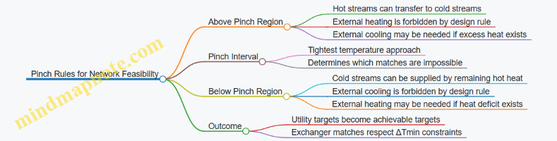
Summary of the Logic Chain
Pinch analysis starts with stream temperatures and duties, applies ΔTmin through temperature shifting, and uses a heat cascade to compute minimum utilities. The pinch marks the boundary where internal heat transfer becomes constrained. Then above- and below-pinch rules guide exchanger matching so the network can meet the targets without relying on “forbidden” utility shortcuts.
3.3 Utility System Design Including Steam, Cooling Water, and Power Distribution
A carbon-to-product plant lives or dies by utilities that behave predictably. Steam, cooling water, and power distribution are the three pillars that keep reactors, separators, compressors, and heat exchangers within their operating envelopes. The goal is not just “enough capacity,” but the right quality, the right pressure/temperature, and the right redundancy so the process can run through normal upsets without turning every trip into a full plant event.
Foundations for Utility Design
Start by mapping each major unit’s utility demand into three buckets: heat duty, mechanical duty, and control/auxiliary duty. Heat duty includes reboilers, condensers, fired heaters, and steam tracing. Mechanical duty includes compressor drives, pumps, and any rotating equipment requiring variable speed control. Control and auxiliary duty includes instrument air, boiler feedwater treatment, cooling tower fans, and motorized valves.
Then convert that demand into utility “quality” requirements. Steam is not just steam; it is pressure level, dryness, and condensate return quality. Cooling water is not just cold water; it is temperature approach, flow stability, and fouling allowance. Power is not just kW; it is voltage level, harmonic tolerance, and protection coordination.
Steam System Design
Steam systems typically use multiple pressure levels to match process needs efficiently. A common pattern is high-pressure steam for major reboilers and medium/low-pressure steam for tracing and smaller heaters. Condensate return is a quiet hero: returning condensate reduces boiler load and improves water chemistry stability.
Key design steps:
- Define steam headers and pressure drops using the maximum simultaneous demand scenario, not the average.
- Specify steam quality by controlling dryness fraction and limiting carryover. If steam contains droplets, downstream heat exchangers can suffer uneven condensation and corrosion.
- Design condensate recovery with separate lines for clean and potentially contaminated condensate. For example, condensate from product-contact services may need additional handling before return.
- Add steam pressure control at major users so a header fluctuation does not force every valve to chase the same error.
Easy example: If a methanol-to-olefins section needs reboiler steam at 3 barg and the hydrogenation section needs 20 barg, you can run a 20 barg boiler and step down through pressure reducing stations. The step-down stations prevent the 3 barg users from “stealing” pressure from the 20 barg header during peak demand.
Cooling Water System Design
Cooling water must remove heat reliably across varying loads. The design should include both normal operation and the “hot day” case where ambient conditions push cooling tower performance toward its limits.
Key design steps:
- Choose a cooling strategy: once-through, recirculating with cooling towers, or chilled water for specific duties. Many plants use recirculating cooling water for bulk duties and a separate chilled loop for sensitive equipment.
- Set temperature targets and approach so heat exchangers can meet outlet temperature requirements. A small approach margin can become a big operational headache when fouling increases.
- Include fouling and scaling allowances in heat transfer area sizing. If you ignore fouling, you end up compensating with higher flow, which can stress pumps and increase power draw.
- Provide flow control using bypasses or variable speed pumps where process heat loads vary widely.
Easy example: Suppose a compressor intercooler requires 35°C outlet cooling water. If the cooling tower can only deliver 40°C during peak conditions, you either increase heat exchanger area or add a dedicated chilled loop. The decision should be made from the heat exchanger pinch and approach, not from hope.
Power Distribution and Electrical Reliability
Power distribution connects utility generation to rotating equipment and controls. The design must consider starting currents, motor loading, harmonics from drives, and the consequences of losing power to specific subsystems.
Key design steps:
- Select voltage levels to reduce current and losses while keeping equipment costs reasonable.
- Coordinate protection so a fault in one branch does not trip critical loads like control systems or essential pumps.
- Plan for motor starting using soft starters, VFDs, or staged starts. For instance, multiple large pumps starting simultaneously can cause a voltage dip that trips sensitive instruments.
- Define emergency power scope for safe shutdown and critical instrumentation. Even if the plant is not designed to keep producing during an outage, it must be able to reach a safe state.
Easy example: If three large boiler feedwater pumps are on the same bus, a coordinated start sequence prevents the bus voltage from sagging below the VFD minimum DC-link voltage. That turns “mysterious trips” into a controlled, predictable start.
Integrated Utility Mind Maps
Mind Map: Utility System Inputs and Outputs
Mind Map: Design Workflow for Steam, Cooling Water, Power
Practical Integrated Example
Consider a unit train where a CO₂ hydrogenation reactor uses steam for a feed heater, cooling water for a product cooler, and power for a recycle compressor. During a normal production shift, the plant runs at steady loads. During a scheduled changeover, the compressor recycle flow may drop while the feed heater duty rises because of a different feed composition.
A good utility design handles this without chaos:
- Steam pressure control at the feed heater user prevents header swings from disturbing reactor temperature.
- Cooling water flow control maintains product cooler outlet temperature even as overall heat load shifts.
- Power distribution uses coordinated starts and protection settings so the compressor’s VFD ramp does not trip other motor branches.
The result is boring in the best way: stable temperatures, stable flows, and stable electrical behavior—so the process can focus on chemistry rather than fighting utilities.
3.4 Offgas Management and Recycle Strategies for Carbon Utilization
Offgas management is where carbon utilization either stays efficient or quietly leaks away. In carbon-to-product plants, “offgas” usually means any gas leaving a unit that still contains usable carbon species (CO₂, CO, light hydrocarbons, or synthesis gas components) plus inert gases, purge-worthy impurities, and sometimes oxygenated traces. The goal is systematic: measure what leaves, separate what can be reused, purge what must be removed, and route the rest to the next best destination.
Foundational Concepts for Offgas Loops
Start by classifying offgas streams by role:
- Recycle candidates: streams with carbon species that match the inlet requirements of a downstream step (after conditioning).
- Purge streams: streams needed to control inert buildup or impurity accumulation.
- Disposal or conversion streams: streams that cannot be reused economically or safely, but can be converted (for example, to heat, power, or secondary products).
A practical rule: if a stream’s carbon can be reused without breaking downstream specs, it belongs in a recycle loop; otherwise it belongs in a purge or conversion path.
Mass Balance Thinking That Prevents “Hidden Losses”
Every offgas decision should be anchored to a carbon balance around the conversion train. Build a simple accounting table for each unit boundary:
- Carbon in (mol C/h) from feed and make-up gases
- Carbon out in product
- Carbon out in offgas
- Carbon out in purge
- Carbon out in any vent or flare
Then compute carbon recovery for the train and inert slip for the recycle loop. Inert slip is the fraction of inert components (often N₂, Ar, CH₄, or other non-reactive gases) that keep circulating. High inert slip increases compression and reduces reactor partial pressures, which lowers conversion.
Offgas Conditioning Before Recycle
Recycle is not just “send it back.” Offgas often needs conditioning so it doesn’t poison catalysts, foul equipment, or violate safety limits.
Common conditioning steps include:
- Compression and pressure matching: recycle compressors must overcome pressure drops and maintain stable flow to the receiving unit.
- Moisture control: water can cause corrosion and shift phase behavior in separators.
- Impurity removal: sulfur compounds, oxygenates, and halides can damage catalysts or materials.
- Particulate removal: fine solids can plug lines and degrade heat exchangers.
Example: If a hydrogenation unit produces offgas containing CO₂ and light hydrocarbons, but the downstream methanol synthesis step requires low hydrocarbons to avoid coking, you separate the recycle into a “CO₂-rich” stream and a “hydrocarbon-rich” stream. The CO₂-rich portion goes to the receiving synthesis loop after polishing; the hydrocarbon-rich portion is purged or routed to a secondary oxidation/heat recovery step.
Mind Map: Offgas Management and Recycle Strategies
Recycle Loop Design That Balances Conversion and Control
A recycle loop typically includes: (1) collection and pressure equalization, (2) conditioning, (3) mixing with fresh feed, and (4) return to the receiving unit. The design challenge is controlling accumulation.
Two accumulation mechanisms matter most:
- Inert buildup: increases total flow without increasing reactive carbon, reducing residence time per mole of reactant.
- Impurity buildup: gradually shifts catalyst performance and increases corrosion risk.
To manage both, plants use a purge fraction. The purge fraction is chosen so that inert and impurity concentrations remain below limits while maintaining acceptable carbon recovery.
Example: Suppose a recycle loop contains 5% inert by volume and the receiving reactor tolerates no more than 8% inert. If the loop would otherwise rise to 12% inert due to upstream variations, you add a purge stream sized to remove enough inert each cycle. The purge is then treated to recover any remaining carbon species (for example, by sending it to a CO₂ capture unit used elsewhere in the plant, or to a secondary conversion step if the carbon form is suitable).
Purge Handling Without Throwing Away Carbon
Purge handling should be “useful by default.” Options depend on what the purge contains:
- Purge to carbon recovery: route purge to a unit that can capture CO₂ or convert CO to a usable intermediate.
- Purge to energy recovery: if carbon is mostly in combustibles, controlled oxidation can generate heat for steam or reboilers.
- Purge to treatment: if carbon is low-value or impurities dominate, treat for emissions compliance while minimizing vent losses.
Example: If purge gas contains CO₂ plus small amounts of CO from a syngas recycle, you can send it to a shift/conversion step that reduces CO to CO₂, then route the CO₂ to a capture/recycle system feeding the main conversion pathway. This turns “purge” into “managed carbon routing.”
Measurement and Control for Stable Offgas Routing
Stable offgas management depends on measurement that matches the decision points. Minimum instrumentation typically includes:
- Flow measurement on offgas and purge lines
- Online composition for CO₂, CO, H₂, CH₄, and key inerts
- Temperature and pressure for compressor and separator performance
- Periodic sampling for trace impurities that don’t show up in routine analyzers
Control logic should tie directly to specs. For instance, if sulfur in offgas exceeds a threshold, the system should reduce recycle fraction and increase purge until conditioning performance returns to normal. That prevents a slow catalyst decline that would otherwise be blamed on “mysterious deactivation.”
Integrated Example Workflow for Offgas Routing
- Measure offgas composition after a conversion unit.
- Compare carbon species and impurity levels to downstream inlet requirements.
- Condition the recycle candidate (drying, polishing, filtration).
- Mix with fresh feed and return to the receiving unit.
- Set purge fraction based on inert and impurity accumulation targets.
- Route purge to carbon recovery or controlled conversion.
- Recalculate carbon recovery and inert slip using updated mass balances.
This workflow keeps carbon utilization measurable, not hopeful, and it makes recycle decisions consistent across operating conditions.
3.5 Plant Layout Considerations for Safety, Materials Compatibility, and Maintenance
A good layout is a safety device you can walk through. It reduces the distance between hazards and people, keeps incompatible materials from meeting in the wrong way, and makes routine work possible without turning maintenance into a scavenger hunt.
Foundational Layout Rules That Prevent Most Problems
Start with the process boundary: define where each major system begins and ends (feed conditioning, compression, purification, conversion, separation, recycle, utilities). Then apply three layout rules.
-
Keep energy and inventory separated. Place high-pressure equipment and large holdup volumes away from common access routes. For example, if a compressor discharge line feeds a purification skid, route the line overhead or in a dedicated pipe rack so a leak does not spray an operator walkway.
-
Design for controlled flow of people and materials. Use one-way or clearly marked traffic lanes for normal operations, and separate routes for maintenance staging. If you need to swap catalyst cartridges, provide a straight pull path from a laydown area to the reactor module.
-
Plan drainage and containment as part of layout, not an afterthought. Put sumps and drains where they can capture the likely leak direction. For instance, locate acid-resistant floor drains downhill from formic acid or carbonate handling areas, and keep them isolated from general drains.
Materials Compatibility Through Spatial Separation
Materials compatibility is mostly about preventing the wrong contact: the wrong chemical with the wrong surface, or the right chemical at the wrong concentration and temperature.
-
Separate by chemical family. Group equipment by what they see: dry CO₂, wet CO₂, hydrogen-rich streams, syngas, oxygenates, acids, and salts. A practical example: keep “wet CO₂” purification equipment (where water and impurities concentrate) in a zone with corrosion-resistant internals, and keep “dry CO₂” compression nearby but not inside the same containment bay.
-
Control mixing points. Layout should minimize uncontrolled cross-connections. If you have purge gas and recycle gas manifolds, place valves and sample points so that line breaks cannot send purge into recycle. A simple check is to ensure that any manual valve change requires a visible confirmation step and a labeled isolation location.
-
Match utilities to materials exposure. Cooling water quality and steam condensate can be corrosive. Route condensate return lines away from carbon steel structures in areas where leaks would wet sensitive equipment. If you use stainless for process lines but carbon steel for supports, ensure supports are protected from direct chemical impingement.
Safety Layout Patterns That Reduce Consequence
Safety is not only about detectors; it is about where people stand when something goes wrong.
-
Use zoning and buffer distances. Place control rooms, electrical rooms, and offices outside the likely blast or jet impact zones. For high-pressure hydrogen service, keep ignition sources and electrical panels out of the immediate leak plume path.
-
Orient vents and relief discharge. Relief valves should discharge to safe locations with predictable dispersion. Layout should provide a clear path for vent stacks that avoids recirculation into air intakes. Example: if a vent stack rises near a building wall, place it so prevailing winds carry it away from doors and HVAC intakes.
-
Make emergency access straightforward. Provide unobstructed routes for fire trucks and for personnel to reach isolation valves. If a reactor is in a fenced module, ensure there is at least one emergency egress route that does not pass through the same containment boundary as the main access.
Maintenance-First Layout That Keeps Throughput Real
Maintenance needs space, access, and predictable removal paths.
-
Plan for component removal. Heavy or awkward items need overhead lifting clearance and a stable staging area. For a reactor with catalyst replacement, align the crane hook directly above the module lifting points and keep the laydown area free of pipe racks that force awkward angles.
-
Provide service corridors and isolation access. Include narrow “service aisles” next to critical valves, filters, and sampling skids. Example: if you expect frequent filter changes in a CO₂ purification train, place the filter housings at consistent heights and ensure the change-out does not require removing adjacent piping.
-
Design for sampling without contamination. Sample points should be reachable and safe to operate. Put sampling valves on pipe spools that are accessible from a platform, not from a ladder that sits over a chemical drain.
Mind Map: Layout Priorities for Safety, Compatibility, and Maintenance
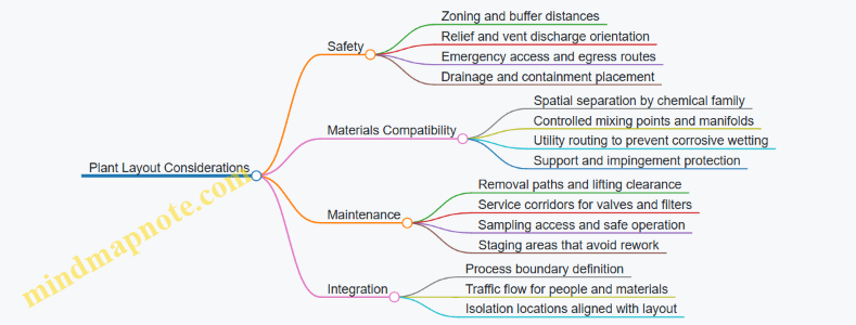
Example: Layout Walkthrough for a CO₂ Hydrogenation Skid
Imagine a skid that converts conditioned CO₂ with hydrogen to an oxygenate.
- Place CO₂ conditioning (drying/impurity removal) upstream in a corrosion-controlled zone with dedicated drains.
- Route hydrogen piping through a dedicated rack segment that keeps it away from general walkways.
- Put the reactor module inside a containment boundary with emergency egress on the opposite side from the main access.
- Locate relief discharge stacks so they do not align with HVAC intakes or doorways.
- Provide a service corridor along the reactor feed valves and filter housings, and ensure the catalyst replacement path is straight from the crane staging point to the module.
The result is a layout where safety, materials compatibility, and maintenance are not separate checklists; they are the same geometry viewed from different angles.
4. CO₂ Hydrogenation to Fuels and Oxygenates
4.1 Reaction Pathways Including CO₂ to CO and CO₂ to Methanol and Higher Alcohols
Captured CO₂ becomes useful only after it is converted into a more reactive form. Two common pathway families start from CO₂: (1) routes that produce CO or syngas-like intermediates, and (2) routes that directly build oxygenates such as methanol and higher alcohols. Both families rely on the same core idea: CO₂ is thermodynamically stable, so the process must supply energy and, usually, hydrogen.
Foundational Chemistry and What “Pathway” Means
A pathway is the chain of reactions plus the separation steps that keep the system running at steady composition. For CO₂ conversion, the key reactions are:
- CO₂ to CO via reverse water-gas shift (RWGS): CO₂ + H₂ ⇌ CO + H₂O
- CO₂ to methanol via hydrogenation: CO₂ + 3H₂ ⇌ CH₃OH + H₂O
- CO₂ to higher alcohols via extended hydrogenation and carbon–carbon growth, typically through CO/CO-derived intermediates and then alcohol synthesis.
A practical way to think about selectivity is to track where carbon goes. In RWGS, carbon ends up as CO. In methanol synthesis, carbon ends up as CH₃OH. In higher alcohol synthesis, carbon can end up as a distribution of alcohols, with chain length influenced by catalyst and operating conditions.
CO₂ to CO Pathway
RWGS is the workhorse for making CO from CO₂ when you want a carbon monoxide feed for downstream synthesis.
Reaction control levers
- Hydrogen-to-CO₂ ratio: More H₂ pushes conversion forward, but it also changes downstream recycle and purge requirements.
- Temperature: RWGS is endothermic, so higher temperature generally increases conversion. The tradeoff is that side reactions and equilibrium constraints can shift selectivity.
- Water removal: Because H₂O is a product, removing it (or designing the system to reduce its partial pressure) helps drive the equilibrium.
Easy example Suppose you have a CO₂ stream and you add enough H₂ to target a moderate conversion, then you separate water from the reactor effluent. If the reactor outlet contains 10% CO₂ and 90% converted carbon as CO plus water, the downstream CO yield improves because the separation reduces the water that would otherwise push the reaction backward.
CO₂ to Methanol Pathway
Methanol synthesis can be approached through two conceptual routes: (1) CO₂ is converted to CO first (RWGS-like behavior) and then hydrogenated to methanol, or (2) the catalyst network effectively couples CO₂ activation with hydrogenation steps. In both cases, the net stoichiometry is CO₂ + 3H₂ → CH₃OH + H₂O.
Why methanol synthesis is “system-level” Methanol synthesis is sensitive to how you manage water and how you keep the catalyst free from poisons. Water is not just a by-product; it affects catalyst surface chemistry and equilibrium.
Operating logic
- Moderate temperature and pressure are chosen to balance conversion and equilibrium.
- Gas purification upstream reduces catalyst deactivation risks from sulfur- and nitrogen-containing contaminants.
- Condensation and separation of methanol from the reactor effluent provides a continuous sink for methanol, which supports overall conversion.
Easy example Imagine a reactor effluent where methanol is partially condensed in a separator. If you remove methanol efficiently, the gas leaving the separator has a lower methanol partial pressure, which reduces the tendency for reverse reactions. The result is higher net methanol production per pass, even if single-pass conversion is not extremely high.
CO₂ to Higher Alcohols Pathway
Higher alcohols are harder because they require not only hydrogenation but also carbon–carbon coupling. Many industrial concepts route through CO or CO-derived intermediates, then extend to alcohols.
Key mechanistic stages
- CO₂ activation and reduction to CO (directly or indirectly).
- Hydrogenation to oxygenates such as methanol-like species.
- Chain growth through surface reactions that form C–C bonds.
- Hydrogenation to saturate the growing carbon skeleton into alcohols.
Selectivity drivers
- Catalyst choice governs whether the system favors methanol or shifts toward longer-chain alcohols.
- Residence time and temperature influence how long intermediates remain on the catalyst surface, which affects chain growth probability.
- Water management influences surface coverage and reaction rates.
Easy example If you run conditions that strongly favor methanol formation, most carbon leaves as CH₃OH. If you adjust conditions to increase the fraction of carbon–carbon forming intermediates (often by changing temperature, pressure, and catalyst formulation), the product slate shifts toward ethanol and beyond. The “easy” part is the accounting: you can measure carbon distribution across products to see whether your operating changes moved carbon into longer alcohols.
Mind Map: Pathway Map from CO₂ to CO and Oxygenates
Integrated Takeaway for Process Design
Choose the pathway based on where you want the carbon to land. If CO is the target intermediate, RWGS-style conversion plus water-aware separation is the center of gravity. If methanol is the target, the process becomes a coupled equilibrium-and-separation problem where removing methanol and managing water are decisive. If higher alcohols are the target, you must also manage carbon–carbon formation, which makes catalyst selection and operating window tighter. In all cases, the most useful “best practice” is the same: measure carbon distribution and water behavior, then adjust the system levers that directly control those outcomes.
4.2 Reactor Selection Including Fixed Bed, Slurry, and Membrane Reactor Concepts
Choosing a reactor is mostly choosing a way to manage three things: heat, mass transfer, and how the system behaves when the feed is not perfectly behaved. For CO₂ hydrogenation and related routes, the “not perfectly behaved” part often shows up as impurities, catalyst deactivation, and gas–liquid or gas–solid transport limits. The right reactor concept makes those issues easier to control, not magically disappear.
Foundations for Selecting a Reactor
Start with the reaction phase and the limiting step.
- Phase and mixing: Fixed beds excel when the reaction is gas–solid and the heat can be removed through the bed or surrounding medium. Slurry reactors excel when you can stir well and keep solids suspended, which helps when mass transfer is the bottleneck.
- Heat management: Many CO₂ conversion reactions are sensitive to temperature. If heat removal is slow, you get hot spots, faster deactivation, and selectivity drift.
- Catalyst life and fouling: If the catalyst is prone to coking, sintering, or poisoning, the reactor must either tolerate gradual loss or provide a practical way to regenerate or replace catalyst.
- Pressure and safety: Hydrogenation routes often run at elevated pressure. Reactor geometry and containment strategy matter for both normal operation and upset conditions.
A practical way to frame the decision is to ask: “What is the hardest transport step in my process?” If it’s gas contacting catalyst, fixed bed can work well. If it’s diffusion through a liquid film or within a particle, slurry often helps. If it’s selective permeation of reactants, a membrane reactor can reduce the distance reactants travel inside the system.
Fixed Bed Reactor Concepts
A fixed bed places catalyst particles in a stationary arrangement, typically with gas flowing through. Heat is handled via external jackets, internal cooling, or heat exchange surfaces depending on design.
Where fixed beds fit best
- Gas-phase feeds with manageable impurity levels.
- Reactions where maintaining a stable temperature profile is feasible.
- Systems where pressure drop is acceptable and catalyst replacement is operationally straightforward.
Key design knobs
- Bed temperature profile: Use staged cooling or multiple beds with interstage heat removal to prevent hot spots.
- Space velocity and conversion per pass: Higher flow reduces residence time and can limit conversion; lower flow increases conversion but raises the risk of temperature gradients.
- Pressure drop: Catalyst particle size and packing quality affect pressure drop and can influence compressor load.
Easy example Imagine a CO₂/CO feed with hydrogen passing over a catalyst. If your measured selectivity drops when temperature rises locally, that’s a sign you need better heat removal. A common fix is to split the catalyst into two beds with cooling between them, so the gas cools before entering the next section.
Slurry Reactor Concepts
A slurry reactor suspends catalyst particles in a liquid phase, with agitation to improve contact. Heat removal is often done through cooling coils, jackets, or internal heat exchange surfaces.
Where slurry reactors fit best
- When the reaction involves gas–liquid contact and mass transfer is limiting.
- When you want strong mixing to reduce concentration gradients.
- When you can tolerate catalyst handling complexity.
Key design knobs
- Agitation intensity: Too little mixing increases film resistance; too much can increase attrition and fines.
- Gas dispersion: Bubble size and gas holdup affect how quickly hydrogen reaches catalyst surfaces.
- Solid management: Settling, filtration, and recycle of catalyst fines must be designed so you don’t gradually change the effective catalyst inventory.
Easy example Suppose hydrogenation produces a liquid-phase product and the reaction rate is limited by hydrogen transfer from bubbles to liquid. If conversion is lower than expected at constant temperature, check whether gas dispersion is poor. Increasing agitation or adjusting sparger design can raise effective mass transfer without changing chemistry.
Membrane Reactor Concepts
A membrane reactor uses selective transport through a membrane to control where reactants meet. In many designs, one species permeates while another is retained, shifting the reaction environment along the reactor length.
Where membrane reactors fit best
- When you can identify a species that should be selectively removed or supplied to drive conversion or selectivity.
- When you want to reduce the impact of equilibrium limitations by changing local composition.
- When you can manage membrane fouling and maintain permeance.
Key design knobs
- Permeance stability: Membranes can lose performance due to coking, wetting, or chemical attack.
- Module pressure and temperature gradients: These affect both flux and selectivity.
- Integration with separation: Sometimes the membrane replaces a downstream separation step; other times it reduces the load on it.
Easy example If the reaction consumes hydrogen and equilibrium limits conversion, a membrane that supplies hydrogen locally can increase conversion per pass. The practical question becomes: can the membrane maintain flux long enough that the overall yield and downtime economics make sense.
Mind Map: Reactor Selection Logic
Integrated Selection Example
Consider three candidate designs for the same overall reaction target.
- Fixed bed is chosen first if your data show stable selectivity at uniform temperature and impurities are controlled. You then design staged cooling to keep the temperature profile flat.
- Slurry becomes attractive if conversion is sensitive to hydrogen availability and you observe strong dependence on agitation or gas dispersion.
- Membrane is considered when equilibrium or local composition is the dominant constraint and you can protect the membrane from fouling while maintaining flux.
The selection is not a quiz of “which is best.” It’s a match between what limits your rate and what your plant can reliably control day after day.
4.3 Catalyst and Operating Parameter Selection Including Temperature, Pressure, and Space Velocity
Selecting a catalyst and setting temperature, pressure, and space velocity are tightly linked decisions. The catalyst controls how fast reactions occur and what side reactions are favored, while temperature, pressure, and space velocity determine how often reactants meet the catalyst in the right chemical environment. A practical approach is to start with reaction targets and constraints, then narrow to operating windows that match both kinetics and transport limits.
Foundational Inputs That Drive Parameter Choices
Begin with the reaction system and feed quality. For CO₂ hydrogenation, you typically care about CO₂ conversion, selectivity to the desired oxygenate (for example, methanol), and tolerance to impurities that can poison active sites. For syngas-based routes, you also care about water management and the balance between chain growth and termination.
Next, define constraints that are not optional. Maximum allowable reactor temperature limits catalyst stability and materials stress. Minimum pressure limits gas-phase residence time and can affect equilibrium. Space velocity is constrained by achievable conversion per pass and by pressure drop limits.
Finally, decide what “success” means operationally. A catalyst that gives high selectivity at low conversion can still be a poor choice if it forces excessive recycle or creates downstream purification burdens.
Catalyst Selection Tied to Temperature and Pressure
Catalyst families differ in the temperature range where they are both active and selective. A common pattern is that increasing temperature accelerates desired kinetics but can also increase undesired pathways such as methanation, reverse reactions, or carbon deposition. Catalyst formulation and support influence heat capacity, thermal conductivity, and resistance to deactivation.
Pressure selection is often about equilibrium and phase behavior. Higher pressure can increase the partial pressures of reactants, shifting equilibrium toward products for reactions where gas-phase product formation reduces moles. It also changes adsorption strength on the catalyst surface, which can improve selectivity up to a point.
A simple way to connect catalyst choice to operating conditions is to map expected activity and selectivity trends versus temperature, then check whether the required conversion can be achieved without pushing the catalyst beyond its stable regime.
Temperature Selection with Kinetics and Heat Transfer in Mind
Temperature affects three things at once: reaction rate, equilibrium position, and catalyst stability. If the reactor is adiabatic or has limited heat removal, temperature rise from reaction can create hot spots that accelerate deactivation. If the reactor is well-cooled, you can often run closer to the kinetic optimum.
A systematic method is to set a target temperature based on kinetics for the desired conversion, then verify that heat transfer can maintain that temperature across the catalyst bed. For gas-phase systems, mass transfer limitations can appear at high rates; for liquid-phase systems, viscosity and diffusion through boundary layers matter.
Concrete example: suppose you want a fixed CO₂ conversion per pass. If you raise temperature to increase rate, you may reduce selectivity to methanol because side reactions become more competitive. The “best” temperature is the one that meets conversion while keeping the selectivity-weighted yield acceptable.
Pressure Selection Using Equilibrium and Practical Limits
Pressure influences equilibrium and also affects how much reactant is available at the catalyst surface. Higher pressure generally increases gas density, which can improve mass transfer to the surface but also increases pressure drop and mechanical requirements.
Practical selection steps:
- Check equilibrium constraints for the reaction and the expected feed composition.
- Estimate how much conversion per pass is needed to hit overall yield targets.
- Confirm that pressure drop and compressor power remain within design limits.
Concrete example: if your process includes recycle, you may tolerate lower per-pass conversion because recycle increases overall conversion. In that case, you can choose a pressure that supports selectivity rather than maximizing conversion per pass.
Space Velocity Selection Balancing Conversion, Selectivity, and Deactivation
Space velocity (often expressed as GHSV for gas or LHSV for liquid) controls contact time between reactants and catalyst. Lower space velocity increases conversion by giving more time for reaction, but it can also increase residence time for side reactions and can worsen deactivation mechanisms that depend on exposure.
A useful rule is to treat space velocity as a lever for conversion while temperature and pressure are levers for selectivity and equilibrium. Then verify that the chosen space velocity does not push the system into transport-limited behavior.
Concrete example: if you increase space velocity to boost throughput, you may maintain conversion by raising temperature. That can work, but it may also increase by-product formation. If by-product formation increases faster than the desired product, the net yield drops even though conversion is unchanged.
Integrated Selection Workflow
Use an iterative workflow that keeps the decisions connected:
- Choose catalyst candidates based on chemistry and known stability.
- Identify a temperature range where the catalyst is active and not prone to rapid deactivation.
- Choose pressure to satisfy equilibrium and adsorption behavior while respecting mechanical limits.
- Select space velocity to meet conversion targets without creating transport limitations.
- Validate with mass and energy balances, then check that downstream purification loads remain manageable.
Mind Map: Catalyst and Operating Parameter Selection
Example: Parameter Tuning for CO₂ Hydrogenation
Assume you have a catalyst that shows strong methanol selectivity at moderate temperature but loses selectivity at higher temperature. You also know that higher pressure improves equilibrium favorability. Start by selecting pressure near the point where equilibrium supports the target conversion without excessive compression burden. Then choose a temperature at the lower edge of the catalyst’s active window that still achieves the required conversion at a reasonable space velocity. Finally, adjust space velocity to hit conversion while monitoring whether selectivity degrades due to increased side reaction contribution at the chosen residence time.
The key is that each adjustment has a trade: temperature changes both rate and selectivity, pressure changes equilibrium and adsorption, and space velocity changes contact time and side reaction exposure. When you tune them together, you avoid the common failure mode of “fixing conversion” while accidentally worsening the product slate.
4.4 Product Separation and Purification Including Distillation and Gas Cleanup
Why Separation Comes After Reaction
After CO₂ hydrogenation, methanol synthesis, or related steps, the outlet stream is rarely “product-only.” It typically contains unreacted gases (H₂, CO₂, CO), inert diluents, light by-products, catalyst fines, and trace impurities that can poison downstream units or violate product specs. Separation is therefore a spec-driven exercise: you decide what must be removed to meet purity, then you choose the simplest train that achieves it reliably.
Foundational Stream Splits and What They Solve
Start by classifying what you have:
- Gas phase components: unreacted reactants, purge candidates, and light by-products.
- Condensable organics: methanol, higher alcohols, oxygenates, or intermediates.
- Solids and aerosols: catalyst dust, corrosion products, and entrained liquids.
A practical rule: remove solids and aerosols first, because they foul heat exchangers and distillation internals. Then separate by volatility (distillation) and finally polish with gas cleanup steps sized for trace contaminants.
Distillation Fundamentals for Oxygenate Products
Distillation works because components differ in boiling point and vapor–liquid equilibrium. For oxygenates, you often face a mix of:
- Light ends (dissolved gases and very volatile impurities)
- Main product (e.g., methanol)
- Heavies (water, higher alcohols, and trace organics)
Key design choices:
- Column pressure selection: lower pressure reduces boiling temperatures but can increase relative volatility challenges and require vacuum equipment.
- Reflux ratio: higher reflux improves separation but increases energy use and can increase entrainment if not controlled.
- Tray or packing selection: packing can handle lower pressure drops; trays can be easier to inspect and troubleshoot.
A simple example: if your methanol product spec requires low dissolved gases, you typically use a flash drum or top condenser to knock out volatiles before the main column. Otherwise, those gases ride through the column and complicate condenser load and overhead composition.
Condensers, Reboilers, and Heat Integration That Actually Matters
Distillation is energy-intensive, so you design around heat recovery:
- Overhead condensation removes latent heat and sets overhead purity.
- Reboiler duty drives separation; it is often the largest utility cost.
A common integrated approach is to use condensers and reboilers to exchange heat with other process streams, such as cooling reactor effluent before a separator, or using hot bottoms to preheat feed to the column. The goal is not maximum heat recovery; it is stable operation with manageable temperatures and no cross-contamination.
Gas Cleanup Steps After Condensation
Even after condensation and distillation, gas streams can contain trace contaminants that matter for recycle compressors, downstream synthesis, or product stability. Typical cleanup targets include:
- Water: affects corrosion and can shift equilibrium in some systems.
- Sulfur compounds: can poison catalysts and foul equipment.
- Oxygenates and heavy organics: can condense in recycle lines and create deposits.
- Acid gases: can corrode and degrade materials.
Cleanup options are chosen by contaminant form and concentration:
- Adsorption beds for low-level organics or acid gases.
- Scrubbers when contaminants are soluble and you can manage wash effluent.
- Membranes for selective removal when you need a compact polishing step.
- Knockout drums and demisters for aerosol control.
A concrete example: suppose overhead gas from a methanol column still contains ppm-level methanol. If you send it directly to a recycle compressor, you risk condensation in the compressor suction and loss of control. A small polishing condenser or adsorption guard bed can prevent that without redesigning the whole column.
Managing Recycle Loops Without Creating a “Purity Spiral”
Recycle streams concentrate impurities if purge is too small or cleanup is insufficient. The separation train should therefore include:
- A purge strategy tied to impurity buildup
- A measurement plan for key contaminants (not just total composition)
- A control scheme that keeps column operation stable under feed variability
Example workflow: if water is the impurity that accumulates, you monitor water in the recycle gas and adjust purge rate or cleanup bed changeout based on a mass-balance target. This keeps the system from gradually drifting into corrosion or spec failure.
Mind Map: Separation Train Logic
Example: Integrated Train for an Oxygenate Product
Consider a reactor effluent that enters a knockout drum to remove aerosols and condensed water. The gas then goes to a top condenser that reduces light organics in the overhead. The condensed liquid feeds a main distillation column that separates the product from heavier oxygenates. Overhead gas is routed to gas cleanup where a small adsorption bed removes residual acid gases and trace organics. Finally, the cleaned gas returns to recycle, with a purge controlled by a water and impurity balance.
Advanced Details That Prevent Common Failure Modes
- Fouling control: solids removal upstream reduces column pressure drop growth.
- Material compatibility: acid gases and water require correct metallurgy and gasket selection.
- Control interactions: condenser duty and reflux ratio must be tuned together to avoid oscillations.
- Sampling realism: take samples where phases are representative; a “perfect” analyzer is still wrong if the sample line condenses.
Summary of the Separation Strategy
You separate in layers: remove solids and aerosols, condense what you can, distill to meet bulk purity, then polish gas streams to protect recycle and downstream units. When each step is tied to a specific spec and a specific failure mode, the train stays understandable and operable—no mystery, just controlled separation.
4.5 Practical Example Workflow From Feed Assay to Product Specification and Yield Calculation
This workflow turns a real CO₂ feed assay into a defensible product yield number and a specification check. The trick is to keep the chain of custody tight: every assumption should have a place in the mass balance, and every measurement should map to a decision.
Step 1: Start with Feed Assay and Convert It into a Usable Basis
Assume a captured CO₂ stream with the following dry-gas composition (mole %): CO₂ 93.2, CO 1.1, O₂ 0.2, N₂ 5.0, and H₂ 0.5. Also assume water is 200 ppmv and the stream is at 30 bar, 35°C.
Convert to a consistent basis. A practical choice is “per 1 kmol of dry feed.” Then compute the dry component kmol:
- CO₂: 0.932 kmol
- CO: 0.011 kmol
- O₂: 0.002 kmol
- N₂: 0.050 kmol
- H₂: 0.005 kmol
Water is handled separately because many downstream steps specify it as ppmv or mass ppm. If water is 200 ppmv on a wet basis, convert it to kmol water per kmol dry feed using the wet-to-dry relation; the exact conversion depends on the definition of ppmv used by the analyzer, so record the analyzer basis in your calculation sheet.
Step 2: Apply Conditioning and Define What “Goes In” to the Reactor
Suppose conditioning removes oxygen via polishing adsorption and reduces O₂ from 0.2% to 0.01% (99.95% removal). Also assume a dryer reduces water from 200 ppmv to 20 ppmv.
Now define the reactor feed composition after conditioning. For the dry components, the simplest approach is to apply removal efficiencies and renormalize to the same dry basis if your mass balance is dry-basis. For example, O₂ becomes 0.0001 kmol per 1 kmol dry feed before renormalization; after renormalization, CO₂ and N₂ slightly increase in mole fraction.
Step 3: Choose the Conversion Reaction Basis and Track Carbon
For hydrogenation to methanol, a common stoichiometric reference is:
- CO₂ + 3 H₂ → CH₃OH + H₂O
In reality, side reactions occur, but yield calculations often start with a “carbon accounting” layer. Carbon in is carbon out plus carbon lost to purge or by-products.
Define a carbon balance frame:
- Carbon in = kmol(CO₂ in) + kmol(CO in)
- Carbon out = kmol(C in methanol) + kmol(C in by-products) + carbon in offgas/purge
If CO is present, decide whether it is treated as fully convertible to methanol carbon or whether it is partially routed to CO₂ formation or other products. A clean way is to introduce a CO conversion fraction, X_CO.
Step 4: Use Performance Metrics to Convert Stoichiometry into Yield
Assume the reactor performance metrics are:
- CO₂ single-pass conversion: X_CO2 = 0.60
- CO conversion fraction: X_CO = 0.80
- Methanol selectivity on converted carbon: S_MeOH = 0.92
- Remaining converted carbon forms by-products that do not end up in methanol (lumped).
Compute converted carbon:
- CO₂ converted carbon = 0.932 × 0.60 = 0.5592 kmol C
- CO converted carbon = 0.011 × 0.80 = 0.0088 kmol C
- Total converted carbon = 0.5680 kmol C
Methanol carbon produced = 0.5680 × 0.92 = 0.5226 kmol C
Since methanol has 1 carbon per molecule, methanol produced = 0.5226 kmol CH₃OH per kmol dry feed.
Define yield in a way that matches your commercial contract. Two common choices:
- Carbon yield to methanol = 0.5226 / (0.932 + 0.011) = 0.5226 / 0.943 = 0.554
- Molar yield to methanol = 0.5226 kmol per kmol dry feed
Step 5: Translate Reactor Output into Product Specification Checks
Product specs usually include purity and water content, not just “how much methanol.” Suppose downstream separation achieves:
- Methanol recovery: R_MeOH = 0.98
- Water removal: residual water in methanol product = 0.05 wt%
- CO and CO₂ in product are limited to 50 ppmw each.
Then methanol in product per kmol dry feed is:
- CH₃OH product = 0.5226 × 0.98 = 0.5121 kmol
Off-spec risk comes from components that slip through separation. Use a simple “spec mass fraction” check by estimating how much CO₂/CO remains in the methanol-rich stream after cleanup. If your separation model predicts CO in product above the ppm limit, you either adjust the cleanup duty or treat the excess as nonconforming product and reduce effective yield.
Step 6: Close the Loop with a Consistency Check
A good yield number survives sanity checks:
- Hydrogen demand: verify that H₂ available (including recycle) matches stoichiometric demand for the methanol formed plus any hydrogen consumed in by-products.
- Oxygen balance: confirm that residual O₂ after conditioning is low enough to avoid catalyst deactivation assumptions.
- Carbon closure: ensure carbon in equals carbon out within rounding.
If carbon closure is off by more than your tolerance, the issue is usually basis mismatch (wet vs dry, renormalization, or ppm conversion).
Mind Map: Feed Assay to Yield and Specification
Example: One-Line Summary of the Calculation Chain
Given 1 kmol dry feed, apply conditioning to get reactor feed, compute converted carbon using X_CO2 and X_CO, multiply by methanol selectivity S_MeOH, then multiply by recovery R_MeOH, and finally verify that separation-predicted impurities meet ppm and water specs.
5. CO₂ to Carbon Monoxide and Syngas Production
5.1 CO₂ Conversion Methods Including Reverse Water Gas Shift and Electrochemical Routes
Foundations for CO₂ Conversion
CO₂ conversion starts with a simple constraint: CO₂ is stable, so turning it into useful carbon monoxide (CO), syngas, or reduced products requires either a chemical driving force (heat and catalysts) or an electrical driving force (electrochemistry). In industrial practice, the “conversion method” is also a “system method,” because feed conditioning, heat removal, product separation, and recycle loops determine whether the chemistry can run continuously.
A useful way to compare routes is to track three items through the process: (1) what carbon oxidation state you end up with, (2) what energy form supplies the driving force, and (3) what impurities tend to poison performance. CO₂ to CO is the most direct step because it changes carbon from +4 to +2, and it can feed downstream synthesis units.
Reverse Water Gas Shift Method
Reverse water gas shift (RWGS) converts CO₂ and hydrogen into carbon monoxide and water:
- CO₂ + H₂ → CO + H₂O
RWGS is typically run at elevated temperature because reaction rates increase and equilibrium limitations become less restrictive. The practical challenge is that the equilibrium favors reactants at lower temperatures, so operators often choose a temperature high enough to get acceptable CO formation while still managing materials and heat integration.
Catalyst role and why it matters. RWGS catalysts commonly use metals (such as supported nickel, iron, or noble metals) that activate H₂ and facilitate CO₂ adsorption and reduction. Catalyst performance is strongly affected by water presence, because water can influence surface coverage and shift effective kinetics. A good design therefore treats steam as part of the reaction environment, not as a nuisance.
Feed and impurity management. RWGS is sensitive to sulfur and other poisons that bind strongly to metal sites. That means the upstream conditioning step for the CO₂ stream and the hydrogen stream is not optional paperwork; it directly protects active sites.
Separation logic. Because water is produced, the downstream separation train often includes condensation or selective removal of H₂O to reduce back-reaction and to deliver a CO-rich gas to syngas conditioning.
Easy example. Suppose you have a CO₂ stream at 95% purity and hydrogen at 80% purity. After conditioning to meet sulfur limits, you run RWGS at a temperature where equilibrium and kinetics give you, say, 20–40% single-pass CO formation. You then remove condensed water and recycle unreacted CO₂ and H₂. The overall conversion becomes much higher than the single-pass number, but only if the recycle loop is designed to avoid accumulating inerts.
Electrochemical CO₂ Reduction Routes
Electrochemical conversion uses electrical energy to drive CO₂ reduction at an electrode surface. Instead of relying on high-temperature equilibrium, the process uses controlled potential to steer reaction pathways.
A common target is CO production:
- CO₂ → CO
Why electrochemistry is different. Electrochemical systems separate the driving force from the reaction temperature. That can reduce thermal stress on materials, but it introduces new constraints: mass transport to the electrode, local pH effects, and catalyst selectivity under operating current.
Key components. The system typically includes a cathode catalyst, an anode reaction (often oxygen evolution or related reactions depending on electrolyte), an electrolyte that supports ion transport, and a membrane or separator that prevents mixing of products.
Selectivity and competing reactions. CO₂ reduction competes with hydrogen evolution when hydrogen is available at the cathode surface. That competition is why current density, catalyst choice, and electrolyte conditions matter. A design that ignores these will produce a gas stream with more H₂ than CO, which then forces extra separation and reduces carbon efficiency.
Mass transport as the hidden bottleneck. CO₂ must reach the catalyst surface faster than it is consumed. If gas-liquid transport is slow, the local CO₂ concentration drops and selectivity shifts. Engineers often address this with gas diffusion layers, flow field design, and controlled pressure.
Easy example. Consider a cell where the cathode produces a mixture of CO and H₂. If you operate at a current that is too high for the CO₂ supply rate, the cell compensates by producing more H₂. If you instead lower current density or improve CO₂ delivery, the fraction of CO in the product gas increases, and the downstream separation duty decreases.
Mind Map: Comparing CO₂ Conversion Routes
Integrated Decision Logic for Plant Design
Choosing between RWGS and electrochemical CO₂ conversion is less about “which chemistry is better” and more about which system constraints you can manage. RWGS tends to fit well when you already have high-temperature integration and reliable hydrogen supply, and when you can keep sulfur and other poisons low. Electrochemical routes fit when you want to avoid high-temperature equilibrium limits and can engineer mass transport and selectivity to keep hydrogen evolution under control.
In both cases, the conversion method must be evaluated with the same accounting mindset: single-pass conversion is not the whole story, because recycle and purge determine overall carbon utilization. Product separation is also part of conversion, because the “effective conversion” depends on how much CO you actually deliver to the next unit rather than how much forms inside the reactor or cell.
5.2 Syngas Composition Targets and Their Impact on Downstream Synthesis
Syngas is a “recipe gas”: downstream synthesis performance depends less on the total amount of carbon and more on the ratios among CO, CO₂, H₂, and sometimes CH₄ and N₂. Setting syngas composition targets means choosing values that match the stoichiometry, catalyst selectivity, and separation constraints of the next unit.
Foundational Composition Metrics
Start with the four numbers that usually drive everything:
- H₂/CO ratio: Controls whether reactions are carbon-favoring (lower ratio) or hydrogen-favoring (higher ratio). For many synthesis routes, the ratio shifts product distribution and conversion efficiency.
- CO₂/CO ratio: CO₂ can be a diluent, a reactant in the presence of catalysts, or a driver of water-gas shift behavior. It also affects equilibrium and purge needs.
- Inert fraction (often N₂ and Ar): Inerts reduce partial pressures and can lower space-time yield. They also increase recycle loop volume.
- Methane and higher hydrocarbons: CH₄ can be inert or can participate depending on conditions. It also changes downstream hydrogen balance and can foul catalysts.
A practical way to think about targets is to treat syngas as a set of constraints: downstream units want certain partial pressures and ratios, while upstream units want stable operation and manageable purification loads.
How Targets Map to Downstream Reactions
Downstream synthesis typically falls into two families: carbonylation and oxygenate synthesis (often CO-based chemistry) and hydrocarbon synthesis (often syngas-to-hydrocarbons via chain growth). Even when the chemistry differs, the same logic applies: composition determines equilibrium position, catalyst surface coverage, and the amount of recycle required to reach net conversion.
For example, in hydrocarbon synthesis based on CO and H₂, the chain-growth mechanism depends strongly on the availability of CO and surface hydrogen. If H₂/CO is too low, you can see incomplete hydrogenation steps and lower selectivity toward desired fractions. If it is too high, you may increase methane formation and reduce carbon efficiency.
For routes where CO₂ participates through water-gas shift, CO₂/CO influences how much of the “effective CO” is produced in situ. Too much CO₂ can increase water formation and shift equilibrium in ways that require additional separation or more aggressive recycle.
Practical Target Setting Workflow
A systematic workflow keeps targets grounded in plant reality:
- Define product slate and operating basis: Choose the downstream product distribution you need (for instance, a fuel cut versus a chemical intermediate). This sets the acceptable ranges for conversion and selectivity.
- Write stoichiometric relationships: Convert desired net reaction requirements into required feed ratios. For instance, if a unit consumes CO and H₂ in a fixed stoometric relationship, the H₂/CO target follows directly.
- Include equilibrium and catalyst behavior: Adjust targets for the fact that real reactors operate at finite temperature and pressure, and catalysts do not behave like ideal stoichiometric mixers.
- Account for purification and recycle: If you plan to remove CO₂ or purge inerts, the “as-fed” syngas target may differ from the “net reacted” composition.
- Set tolerances, not just point values: A target of H₂/CO = 2.0 is less useful than a range that reflects analyzer accuracy, control valve resolution, and acceptable selectivity drift.
A concrete example: suppose downstream synthesis needs H₂/CO near 2.0 and low inerts. If upstream purification leaves a small but variable N₂ fraction, you might keep the H₂/CO target tight while allowing a wider CO₂ tolerance, because CO₂ can be partially managed by shift and recycle, while inerts cannot.
Control Levers and Their Composition Effects
Syngas composition is rarely “set once and forgotten.” The plant uses control levers that change ratios in predictable ways:
- Water-gas shift adjustment: Shifting changes CO and H₂ while often converting CO₂ indirectly. This is a common lever for tuning H₂/CO.
- CO₂ removal intensity: More CO₂ removal increases CO fraction and reduces diluent load, but it can raise energy and solvent duty.
- Purge rate and recycle ratio: Purge removes inerts and sometimes methane. Higher purge reduces inerts but lowers overall carbon utilization.
- Hydrogen addition or reforming severity: Changing hydrogen availability alters H₂/CO directly and can also affect methane slip.
The key is to link each control action to the downstream sensitivity. If selectivity is most sensitive to H₂/CO, prioritize levers that adjust that ratio with minimal collateral changes.
Mind Map: Syngas Targets and Downstream Impact
Example: Turning Analyzer Readings into Action
Assume a syngas analyzer reports: H₂/CO is drifting high, CO₂/CO is stable, and inert fraction is rising slowly. A typical response is to avoid changing CO₂ removal first, because CO₂/CO is already stable and the downstream unit is likely more sensitive to H₂/CO than to CO₂ in this operating window. Instead, you would adjust the shift conditions or hydrogen supply to bring H₂/CO back into range, while using purge control to arrest inert accumulation.
This example highlights the core discipline: composition targets are not just numbers; they are a map from measurement to the specific lever that corrects the ratio the downstream unit actually cares about.
5.3 Reactor And Separation Train Design Including Water Management And Gas Purification
A CO₂-to-syngas train lives or dies by two things: how well you keep water under control, and how clean you keep the gas before it meets the next catalyst or membrane. The design goal is simple to state and annoyingly detailed to execute—make the reactor effluent predictable, then make the downstream units forgiving.
Start with the Reactor Effluent You Actually Have
Begin with a reactor outlet envelope: temperature, pressure, total flow, CO₂ conversion, CO selectivity, and the expected water content. Even if the chemistry is steady, the effluent composition can shift with feed humidity, purge rate, and recycle loop performance. Treat the effluent as a mixture that must be conditioned, not as a clean “product gas” waiting politely for separation.
Key streams to quantify:
- Gas phase: CO, CO₂, H₂, N₂ or Ar (if present), residual O-containing species, and light inerts.
- Condensables: water and any oxygenates formed in trace amounts.
- Solids or aerosols: catalyst fines, corrosion products, and any entrained liquids.
Water Management as a Design Constraint
Water affects both equilibrium and equipment. In many CO₂ conversion routes, water participates directly in reaction steps or indirectly by changing partial pressures and heat removal.
Practical water-control sequence:
- Quench or cool the reactor effluent to a controlled temperature where condensation is thermodynamically expected.
- Separate condensed water using a knock-out drum sized for droplet capture and residence time.
- Prevent re-entrainment by using demisters and maintaining appropriate gas velocities.
- Control water in recycle so the reactor sees a stable steam-to-carbon ratio.
Easy example: if your reactor effluent contains 5 mol% water and you cool to a point where most water condenses, the gas leaving the knock-out drum may drop to 0.2 mol% water. That change can shift downstream membrane performance and alter purge requirements. The separation train must therefore be designed around the post-drain gas, not the raw reactor outlet.
Gas Purification Train from Coarse to Fine
A separation train usually follows a “coarse-first” logic: remove what can foul first, then remove what can poison next.
Typical order:
- Cyclone or filter to remove catalyst fines and aerosols.
- Knock-out drum for bulk water removal.
- Acid gas removal if CO₂ slip or other acid gases must be reduced for downstream synthesis.
- Drying to meet dew point targets for compressors, membranes, and catalysts.
- Final polishing to protect sensitive units.
Design targets should be explicit: dew point at the compressor inlet, allowable CO₂ in syngas, maximum sulfur or nitrogen species, and maximum particulate concentration.
Reactor Effluent Cooling and Heat Integration
Cooling is not just a utility choice; it sets condensation behavior and drives separation duty. Use heat integration to reduce steam consumption, but keep temperature profiles compatible with condensation and corrosion limits.
A common approach:
- Recover heat in a waste-heat boiler or feed preheater.
- Use a controlled cooler to reach the knock-out drum operating temperature.
- Ensure materials and insulation prevent cold spots that create localized corrosion.
Separation Unit Sizing Logic
Sizing should reflect mass transfer and residence time, not just flow rate.
- Knock-out drum sizing: based on gas velocity, droplet size distribution assumptions, and demister efficiency.
- Filter sizing: based on expected particulate loading, pressure drop limits, and regeneration or changeout intervals.
- Absorber or adsorber sizing: based on breakthrough curves and target outlet purity.
- Dryer sizing: based on water loading and allowable outlet dew point.
Integrated Control Strategy for Stability
A separation train needs control loops that match the physics.
- Water control: maintain knock-out drum level and vent strategy so water removal doesn’t oscillate.
- Drying control: regulate dryer inlet temperature and monitor outlet dew point.
- Recycle control: adjust purge and recycle ratio to keep syngas composition within spec.
- Pressure control: keep downstream units within their operating pressure windows to avoid performance drift.
Mind Map: Reactor Effluent Conditioning and Purification
Example: From Reactor Outlet to Syngas Spec
Assume a reactor effluent at 30 bar and 320°C containing CO, CO₂, H₂, and water. The downstream synthesis requires syngas with a dew point below the compressor inlet limit and CO₂ reduced to a defined level.
A practical sequence:
- Cool effluent to 60°C using integrated heat recovery plus a controlled cooler.
- Send to a knock-out drum with demister; drain water continuously.
- Filter to remove fines before acid gas removal.
- Use an acid gas removal step to reduce CO₂ slip.
- Dry the gas to meet dew point, then compress to synthesis pressure.
The “gotcha” is water carryover: if the knock-out drum is undersized, water droplets bypass the demister, raising dryer load and causing dew point excursions. That failure shows up later as catalyst deactivation risk or compressor corrosion, so the design must treat knock-out performance as a primary requirement, not a housekeeping step.
Design Checklist for No-Gaps Execution
- Reactor outlet envelope defined with water and particulate assumptions.
- Cooling profile supports condensation without creating corrosion-prone cold spots.
- Knock-out drum and demister sized for droplet capture and stable level control.
- Filtration protects downstream purification and compressors.
- Purification steps ordered coarse-to-fine with explicit outlet specs.
- Dryer meets dew point at the actual compressor inlet condition.
- Control loops align with separation physics and recycle composition stability.
- Materials and pressure ratings verified for every phase change and drain condition.
5.4 Carbon Utilization Strategies Including Recycle Loops and Purge Minimization
Core Idea and Why Purges Exist
Recycle loops aim to reuse unreacted carbon species and hydrogen, improving overall carbon efficiency. Purges exist because some components accumulate in the loop: inert gases, light by-products, or impurities that slip through conditioning. If you never purge, the loop composition drifts until separation becomes harder, catalysts see worse conditions, or compressors start working against a rising “junk” fraction.
A practical way to think about it: recycle controls how much of the stream returns, while purge controls what fraction of the loop inventory you remove to keep composition within operating limits.
Foundational Building Blocks
- Define the loop boundary: Decide what counts as “inside” the recycle system (reactor effluent, separator, compressor, and return line) and what counts as “outside” (fresh feed, product draw, vent).
- Choose the controlled variable: Typical targets are loop inert fraction, CO/CO2 ratio, water content, or sulfur/nitrogen levels. Pick one variable to control first; controlling five at once is how you get five different alarms.
- Set a purge basis: Purge can be a fixed fraction of recycle, a flow controlled by inert concentration, or a purge triggered by impurity breakthrough.
Purge Minimization Logic
Purge minimization is not “minimize purge flow at all costs.” It is “minimize purge while meeting composition and operability constraints.” The constraints usually come from:
- Separator performance: Higher inert or heavier by-products can reduce recovery in gas-liquid or gas-solid separations.
- Reactor stability: Accumulated species can change partial pressures and shift reaction equilibrium.
- Materials and corrosion: Trace impurities can concentrate in the loop, especially if they partition into the same phase repeatedly.
A simple mass-balance framing helps. Let the loop contain a component that is not consumed (an inert). Each pass adds a small amount from fresh feed and losses; purge removes a fraction. At steady state, purge rate must match the net accumulation rate. If you reduce purge, you must reduce the net accumulation source (better feed conditioning, tighter product draw, or improved separation).
Recycle Loop Design Patterns
Pattern A: Single-pass conversion with recycle
- Reactor converts part of the feed.
- Separator returns unreacted gas to the reactor.
- Purge removes inerts and light by-products.
Pattern B: Two-stage separation with targeted purge
- First separator recovers condensables.
- Second separator polishes the gas.
- Purge is taken from the stream with the highest inert concentration to reduce the amount of “good” carbon leaving the system.
Pattern C: Purge with heat recovery
- Purge gas is used to preheat incoming streams or generate steam in a controlled way.
- This does not change the purge requirement, but it reduces the energy penalty.
Example: Syngas Loop with Inert Accumulation
Assume a CO2-to-CO process where fresh feed contains a small inert fraction (for example, nitrogen from upstream sources). The reactor converts CO2 to CO and produces an offgas. A separator returns unreacted gas to the reactor.
- Without purge: nitrogen accumulates each recycle pass. Over time, the partial pressures of CO2 and CO shift, conversion per pass drops, and the separator may require higher temperatures or pressures to maintain recovery.
- With purge: a purge stream removes a fraction of the recycle gas. If you control purge based on measured nitrogen mole fraction, you can keep conversion stable while limiting carbon loss.
A concrete operating strategy is to set a nitrogen limit that preserves conversion and separation performance. Then purge flow is adjusted to hold the loop nitrogen at that limit. If nitrogen rises faster than expected, the first troubleshooting step is not “increase purge”; it is checking fresh feed conditioning and product draw rates, because those determine the net accumulation.
Example: Targeted Purge from a Polishing Stream
In a two-stage separation train, the first stage may remove condensables while leaving most inerts in the gas. The second stage may polish the gas and concentrate remaining inerts in a smaller slip stream. Taking purge from the polishing stage can reduce the amount of unreacted carbon species lost, because the purge is drawn where “junk” is most concentrated.
Practical Control and Monitoring Checklist
- Monitor loop composition at a frequency that captures drift, not just startup.
- Tie purge control to a composition measurement that correlates with the constraint you care about.
- Verify that purge changes do not silently upset downstream product specifications by checking product draw composition and flow.
- Confirm that purge routing preserves safety and avoids unintended accumulation in low-flow dead zones.
Recycle loops and purge minimization work as a pair: recycle improves utilization, purge prevents accumulation from turning utilization into a slow-motion composition problem. When the purge is controlled by the right variable and the recycle boundary is clearly defined, the system behaves predictably—like a well-tuned instrument, not a guessing game.
5.5 Practical Example Workflow for Converting CO₂ Stream Data into Syngas Specs
Goal and Inputs
You start with a captured CO₂ stream and a chosen conversion route to syngas. The workflow below turns measured CO₂ data into target syngas specifications that downstream synthesis can actually use.
Assumed route: CO₂ dry reforming of methane (DRM) to syngas, followed by cleanup to meet synthesis requirements.
Given CO₂ stream measurements (example):
- CO₂ mole fraction: 0.94
- H₂O: 2,000 ppmv
- O₂: 10 ppmv
- N₂: 4,000 ppmv
- Total sulfur: 2 ppbv (as H₂S/SO₂ equivalents)
- Total chlorine: 0.5 ppbv (as HCl/Cl₂ equivalents)
- Pressure: 3.5 bar(g)
- Temperature: 35°C
Step 1: Convert Stream Data into a Feed Basis
Pick a basis so calculations don’t wobble. Use 1 kmol of “as-received” CO₂ stream.
From the mole fraction:
- CO₂ = 0.94 kmol
- Inerts (N₂) = 0.004 kmol
- H₂O = 0.002 kmol
- O₂ = 0.00001 kmol
- Remaining balance = 0.05399 kmol (lumped minor species)
Why this matters: syngas specs are usually reported on a dry basis, but your reactor sees wet gas unless you condition it. So you decide whether to model conditioning explicitly.
Step 2: Define the Reaction Stoichiometry and Target Syngas
For DRM:
- CO₂ + CH₄ → 2 CO + 2 H₂
You must decide the syngas ratio for downstream use. A common practical target is a H₂:CO ratio near 1.0 for many synthesis trains, but the exact value depends on the next unit.
Example target syngas specs (dry basis):
- CO: 35 mol%
- H₂: 35 mol%
- CO₂: ≤ 2 mol%
- CH₄: ≤ 1 mol%
- H₂O: ≤ 0.5 mol%
- N₂: as low as feasible, but accept up to 5 mol%
- Sulfur: ≤ 0.1 ppbv
- Chlorine: ≤ 0.05 ppbv
Step 3: Choose Conversion and Determine Required Methane Feed
Let X be the CO₂ conversion in the reformer. CO₂ leaving is (1 − X) times the CO₂ fed.
If you feed CH₄ in stoichiometric proportion, the ideal syngas from reacted CO₂ is:
- CO produced = 2X·n(CO₂)
- H₂ produced = 2X·n(CO₂)
Example: choose X = 0.85 to keep CO₂ slip manageable.
- CO produced = 2·0.85·0.94 = 1.598 kmol
- H₂ produced = 1.598 kmol
- CO₂ remaining = (1 − 0.85)·0.94 = 0.141 kmol
Now account for excess methane or methane slip. If you want CH₄ ≤ 1 mol% in dry syngas, you typically run with slight excess or adjust with recycle and purge; for this example, assume CH₄ feed is set so that CH₄ slip is 0.01 kmol on the dry basis.
Step 4: Build a Dry Syngas Composition from Material Balance
Compute dry moles after reaction and before cleanup, using a consistent dry basis.
Dry components before cleanup (example):
- CO = 1.598 kmol
- H₂ = 1.598 kmol
- CO₂ = 0.141 kmol
- CH₄ slip = 0.010 kmol
- N₂ = 0.004 kmol
- O₂ assumed fully consumed or removed upstream (for this example, treat as negligible)
Total dry moles = 1.598 + 1.598 + 0.141 + 0.010 + 0.004 = 3.351 kmol
Dry mole fractions:
- CO = 1.598/3.351 = 47.7%
- H₂ = 47.7%
- CO₂ = 4.2%
- CH₄ = 0.3%
- N₂ = 0.1%
This doesn’t meet the earlier CO₂ ≤ 2 mol% target, so you adjust either conversion (higher X), add a shift step, or include CO₂ removal.
Step 5: Apply Cleanup and Conditioning Constraints
Cleanup units change composition and trace contaminants.
Example cleanup train:
- Water removal (condensation or adsorption) to meet H₂O ≤ 0.5 mol%.
- Sulfur guard bed to meet sulfur ≤ 0.1 ppbv.
- Chlorine guard bed to meet chlorine ≤ 0.05 ppbv.
- CO₂ polishing (amine or physical solvent) or a shift + separation strategy.
Integrated practice: treat trace contaminants as capacity-limited. If sulfur is 2 ppbv in CO₂ feed, the reformer effluent concentration depends on how much sulfur partitions into gas versus deposits. For a practical spec workflow, you set a conservative capture efficiency in the guard bed and verify it against bed capacity using the gas flow.
Step 6: Iterate to Meet Syngas Specs
To reduce CO₂ from 4.2% to ≤ 2%, you can:
- Increase conversion X from 0.85 to ~0.92 (quick check: CO₂ remaining scales with (1 − X)).
- Or remove CO₂ downstream.
Example iteration: keep X = 0.85 but remove CO₂ in a polishing step.
- CO₂ to remove = 0.141 kmol
- If you remove 50% of CO₂, dry total becomes 3.351 − 0.0705 = 3.2805 kmol
- New CO₂ fraction = 0.0705/3.2805 = 2.15% (still slightly high)
- Remove ~52% CO₂ to land at 2.0%
You also verify that removing CO₂ doesn’t break H₂:CO ratio. Since CO₂ removal doesn’t change CO and H₂ moles, the ratio stays ~1.0 in this example.
Step 7: Produce the Final Syngas Spec Sheet
Your output should be a clear, unit-ready spec set.
Example final syngas specs (dry basis, after cleanup):
- CO: 47.7 mol%
- H₂: 47.7 mol%
- CO₂: 2.0 mol%
- CH₄: 0.3 mol%
- N₂: 0.1 mol%
- H₂O: ≤ 0.5 mol%
- Sulfur: ≤ 0.1 ppbv
- Chlorine: ≤ 0.05 ppbv
Mind Map: CO₂ Data to Syngas Specs Workflow
Example: Quick Sanity Checks You Should Always Do
- Dry basis consistency: if you remove water, recompute dry totals before comparing to dry specs.
- CO₂ slip control: CO₂ often dominates downstream catalyst poisoning and shift equilibrium behavior, so treat it as a first-class constraint.
- Trace impurity handling: sulfur and chlorine should be checked against guard bed capacity using gas flow, not just inlet concentration.
- Ratio preservation: if you remove CO₂ without shifting, H₂:CO stays constant; if you shift, recompute both components.
6. Fischer Tropsch and Related Synthesis for Hydrocarbon Fuels
6.1 Feed Preparation Including Syngas Conditioning and Sulfur Control
Syngas feed preparation is where “chemistry on paper” becomes “chemistry that runs.” In Fischer–Tropsch and related syngas routes, the conversion catalysts are sensitive to sulfur compounds, and the downstream synthesis is sensitive to water, oxygenates, and particulates. Feed preparation therefore aims to (1) remove sulfur to a target level, (2) condition the gas for stable reactor operation, and (3) protect compressors, heat exchangers, and catalyst beds from fouling.
Core Inputs and Why Conditioning Matters
Syngas typically contains CO, H2, CO2, N2, and water vapor, plus trace impurities such as H2S, COS, mercaptans, and thiophenes. Sulfur species can poison catalysts by binding strongly to active sites, reducing activity and selectivity. Water can promote corrosion and shift reaction equilibria in ways that change the effective H2/CO ratio. Particles and aerosols can plug filters and create hot spots in fixed beds.
A practical way to think about conditioning is to separate “bulk composition” from “trace hazards.” Bulk composition is handled by upstream synthesis and reforming controls. Trace hazards are handled here with targeted cleanup steps.
Sulfur Control Strategy from Measurement to Targets
Start with a sulfur spec that matches the catalyst and operating mode. A common approach is to set a maximum total sulfur (often in the low-ppm range) at the reactor inlet, then work backward to determine allowable slip through each cleanup stage.
-
Measure sulfur forms, not just total sulfur. Total sulfur can hide the difference between H2S and COS, which respond differently to removal chemistry. If COS is present, hydrolysis to H2S may be required before the main cleanup.
-
Use a staged removal train. A typical sequence is guard filtration and dehydration, then sulfur removal, then polishing cleanup. The guard steps protect the sulfur media from poisoning by particulates and water.
-
Control temperature and space velocity. Sulfur adsorbents and guard catalysts have operating windows. Too cold can reduce reaction rates; too hot can reduce capacity or cause unwanted side reactions.
Example: If inlet gas contains 5 ppmv H2S and 2 ppmv COS, a sulfur train might first hydrolyze COS to H2S (using a small catalyst bed under controlled steam), then pass the gas through a zinc oxide or similar sorbent bed for bulk removal, followed by a polishing bed to catch residual sulfur.
Syngas Conditioning Steps in Logical Order
A reliable conditioning sequence is usually:
-
Particulate and aerosol removal
- Use inlet filtration or cyclones to remove dust and condensed droplets.
- This prevents plugging and reduces carryover into sulfur media.
-
Dehydration
- Remove water to reduce corrosion and to stabilize downstream heat exchange.
- Methods include glycol dehydration or molecular sieves depending on operating pressure and required dew point.
-
CO2 and oxygen management
- CO2 is not a “poison” in the same way sulfur is, but it affects the effective syngas ratio and heat release.
- Oxygen traces can cause unwanted oxidation of sensitive materials; oxygen is typically controlled upstream, but conditioning includes monitoring and safe handling.
-
Sulfur removal and polishing
- Main removal bed captures sulfur species.
- Polishing bed ensures the reactor inlet meets the sulfur spec.
-
Final conditioning for reactor inlet stability
- Adjust temperature and pressure to match reactor requirements.
- Ensure stable H2/CO ratio by managing recycle purge and any residual water effects.
Example: Suppose dehydration reduces water from a dew point of 30°C to below 0°C. That change can reduce corrosion risk in downstream exchangers and keep sulfur media from losing capacity due to water-assisted deactivation.
Advanced Details That Prevent “Small” Failures
Bed protection and breakthrough control. Sulfur beds should be monitored for breakthrough using online analyzers or periodic sampling. When breakthrough approaches the limit, switching to a fresh bed avoids catalyst exposure.
Hydrolysis of COS. COS removal often requires hydrolysis because some sorbents capture H2S more effectively than COS. Hydrolysis performance depends on steam availability and temperature.
Material compatibility. Conditioning equipment must handle acidic species. Even after cleanup, trace sulfur can remain, so metallurgy and gasket selection matter.
Heat management. Sulfur removal is often exothermic or endothermic depending on chemistry. Temperature control prevents hot spots that can accelerate sorbent degradation.
Mind Map: Syngas Conditioning and Sulfur Control
Worked Example: From Inlet Sulfur to Reactor Spec
Assume a reactor inlet sulfur limit of 0.1 ppmv total sulfur. If the main sulfur bed is expected to remove 99.5% of sulfur and the polishing bed removes 90% of the residual, the combined removal is 0.5% × 10% = 0.05% slip. For an inlet of 7 ppmv total sulfur, expected reactor inlet sulfur is 7 × 0.0005 = 0.0035 ppmv, which meets the 0.1 ppmv limit with margin.
The key operational lesson is that the calculation is only as good as the sulfur speciation and the actual bed performance under real temperature, steam, and space velocity. That’s why the train is designed as a sequence with guard steps and a polishing stage, not as a single “one-and-done” cleanup.
6.2 Catalyst Systems and Operating Windows for Chain Growth and Selectivity
Chain growth in Fischer–Tropsch and related syngas-to-hydrocarbon routes depends on a handful of coupled variables: catalyst chemistry, active-site environment, and operating conditions that control residence time, hydrogen availability, and heat removal. Selectivity is not a single knob; it’s the outcome of how fast chains grow versus how fast they terminate, crack, or desorb.
Foundational Concepts for Selectivity
Start with three competing pathways on the catalyst surface:
- Chain growth: surface carbon species insert into growing chains.
- Termination by hydrogenation: adsorbed carbon species get hydrogenated into saturated products.
- Side reactions: readsorption, water-gas shift, and—if conditions allow—secondary cracking or oxygenate formation.
A useful mental model is that selectivity is governed by the balance between surface carbon coverage and hydrogen coverage. Too much hydrogen coverage pushes the surface toward termination (more methane, fewer longer chains). Too little hydrogen coverage can increase unsaturated species and promote undesired reactions.
Catalyst Systems and What They Change
Different catalyst families tune the balance above by changing active-site structure and how strongly they bind key intermediates.
Iron catalysts
- Often favor higher hydrocarbon yields under conditions that can tolerate some water formation.
- Their activity and selectivity are sensitive to promoters and to how the catalyst is reduced and stabilized.
- Typical operating windows emphasize robust heat management because reaction enthalpy is strongly exothermic.
Cobalt catalysts
- Commonly used when the goal is higher selectivity toward long-chain hydrocarbons and lower water-gas shift activity.
- Their reduced form and dispersion strongly influence chain-growth probability.
- They tend to be less forgiving to sulfur and certain poisons, so feed cleanup matters.
Promoters and supports
- Promoters can adjust electron density and modify adsorption strengths, shifting the hydrogen-to-carbon balance.
- Supports influence heat transfer and dispersion. Better dispersion increases the number of active sites but can also increase sensitivity to sintering if temperature control is poor.
Operating Windows That Control Chain Growth
Think of the operating window as a region where three constraints are satisfied simultaneously: temperature for kinetics, pressure for adsorption and residence time, and gas composition for surface coverage.
Temperature
- Higher temperature generally increases reaction rates but also increases the likelihood of secondary reactions and catalyst deactivation mechanisms.
- Lower temperature can improve selectivity toward heavier products but may reduce overall conversion, forcing longer residence time and increasing the chance of mass-transfer limitations.
A practical rule: choose a temperature that achieves target conversion without pushing the catalyst into regimes where methane selectivity rises sharply or where hot spots accelerate deactivation.
Pressure
- Higher pressure increases partial pressures of reactants, which can raise surface coverage and affect chain-growth probability.
- It also changes the balance between adsorption and desorption, often shifting product distribution toward heavier fractions when other variables are controlled.
Syngas Composition and Hydrogen Availability
- The H2/CO ratio is the most direct lever for hydrogen coverage.
- If H2/CO is too high, termination dominates and methane rises.
- If H2/CO is too low, carbon coverage increases, which can increase unsaturated products and promote side reactions.
In practice, operators tune H2/CO to match the catalyst’s preferred surface chemistry, then verify using product distribution trends rather than relying only on inlet composition.
Space Velocity and Residence Time
- Gas hourly space velocity (GHSV) controls how long reactants spend in the reactor.
- Longer residence time can increase conversion and favor heavier products, but it can also amplify secondary reactions if temperature is not tightly managed.
Coupled Effects and How to Avoid “One-Knob” Thinking
A change in one variable often forces compensating shifts in others. For example:
- Increasing temperature may require lowering GHSV to keep conversion stable, but that can change selectivity because residence time increases.
- Raising pressure can increase conversion; if conversion rises too quickly, heat release can create local hot spots that alter selectivity.
The goal is to keep the catalyst experiencing a stable local environment, not just a stable inlet condition.
Mind Map: Catalyst Systems and Operating Windows
Example: Tuning for Heavier Hydrocarbons Without Losing Conversion
Assume a syngas feed with a fixed CO concentration and a target to increase C5+ selectivity while keeping conversion near a set value.
- Start with a baseline H2/CO appropriate to the catalyst family.
- Adjust temperature slightly downward to reduce termination and secondary cracking, then compensate conversion by reducing GHSV rather than increasing temperature back.
- Check methane trend: if methane rises, hydrogen coverage is likely too high or residence time is too long at the current temperature.
- Verify heat management: if heavier selectivity improves but conversion becomes unstable, local hot spots may be driving inconsistent surface chemistry.
This workflow works because it respects the coupling: temperature affects kinetics and secondary reactions, while GHSV changes residence time and therefore the probability of chain growth before termination.
Example: Diagnosing Selectivity Drift During Steady Operation
If selectivity shifts toward lighter products over time, consider three common causes:
- Catalyst deactivation that reduces active-site availability, often changing the effective residence time on the surface.
- Feed impurity breakthrough (especially for cobalt systems), which can preferentially poison sites responsible for chain growth.
- Heat transfer degradation that increases local temperature, pushing the system toward termination and secondary reactions.
A practical diagnostic approach is to compare inlet composition, measured temperature profiles, and product distribution changes together. When only one variable changes, the selectivity shift usually points to a specific mechanism; when multiple signals move together, the issue is often heat or mass transfer rather than chemistry alone.
6.3 Reactor Configurations Including Fixed Bed and Slurry Reactors
Reactor configuration is where chemistry meets plumbing. The same overall reaction can behave very differently depending on how gas, liquid, and solids share space, how heat is removed, and how the catalyst is kept in its happy place. This section compares fixed bed and slurry reactors for carbon-to-product synthesis routes that commonly use hydrogenation, syngas conversion, or CO₂-derived intermediates.
Foundational Concepts That Drive Configuration Choice
Start with three questions.
-
What phases are present? Fixed beds suit gas–solid reactions and gas-phase operation with minimal bulk liquid. Slurry reactors handle gas–liquid–solid systems where mixing and heat transfer benefit from liquid circulation.
-
How is heat managed? Many carbon conversion reactions release or absorb significant heat. Fixed beds remove heat through reactor walls and internal cooling surfaces; slurry reactors remove heat via heat exchange in the liquid loop.
-
How does the catalyst behave over time? Fixed beds can suffer from hot spots and pressure drop growth from fouling or coking. Slurry systems can tolerate catalyst attrition and require solids separation and recycle.
A quick mental model: fixed beds are like a stationary “catalyst road,” while slurry reactors are like a “catalyst river” where particles move with the flow.
Fixed Bed Reactors
Fixed bed reactors pack catalyst into tubes or a shell-and-tube arrangement. Reactants flow through the bed, and heat is controlled by conduction to the wall and, in many designs, by an external coolant circuit.
Key design features
- Pressure drop control: As particles age or foul, pressure drop rises. Designers size the bed and select particle geometry to keep pressure drop within compressor and pumping limits.
- Temperature profile management: In exothermic reactions, the center of the bed can run hotter than the inlet region. Cooling strategy and inlet distribution are used to flatten the profile.
- Mass transfer considerations: If diffusion through catalyst pores is slow, the observed rate drops even when bulk conditions look favorable. Particle size and catalyst formulation matter.
Operational strengths
- Simple solids handling because the catalyst stays put.
- Straightforward sampling of gas-phase composition along the reactor, depending on instrumentation.
Operational watch-outs
- Hot spots: A small fraction of maldistribution can create large temperature differences.
- Coking or fouling: Carbonaceous deposits can block pores and reduce activity.
Easy example
Imagine a gas-phase hydrogenation step where CO and H₂ enter a packed bed. If the reaction is exothermic, a fixed bed with good inlet distribution and adequate coolant flow can keep the bed temperature within a narrow band. If the inlet distributor is poorly designed, some channels run hotter, accelerating catalyst deactivation in those channels first.
Slurry Reactors
Slurry reactors suspend catalyst particles in a circulating liquid phase. Gas bubbles disperse through the liquid, and the catalyst moves with the slurry, improving contact and mixing.
Key design features
- Gas–liquid mass transfer: The rate depends on how effectively gas dissolves or contacts the catalyst. Agitation, sparger design, and liquid properties influence this.
- Heat removal through the liquid loop: Heat exchangers in the circulation path can control temperature more uniformly than wall-only cooling.
- Solids separation and recycle: After reaction, the slurry must be separated into product liquid and catalyst solids, then returned to the reactor.
Operational strengths
- Better mixing reduces temperature gradients.
- Catalyst can be replaced or regenerated more flexibly because solids are handled as a stream.
Operational watch-outs
- Attrition: Catalyst particles can break down, changing activity and separation behavior.
- Separation performance: If separation is inefficient, product purity suffers and catalyst losses increase.
Easy example
Consider a syngas-to-oxygenate step where a liquid solvent carries dissolved gases to catalyst particles. If the slurry circulation rate is too low, gas bubbles coalesce and mass transfer drops, lowering conversion. Increasing agitation improves contact, but it also raises power demand and can increase attrition.
Comparing Fixed Bed and Slurry Reactors Systematically
Use this checklist to connect configuration to performance.
- Phase compatibility: Gas–solid favors fixed beds; gas–liquid–solid favors slurry.
- Temperature control: Fixed beds rely on wall and coolant heat transfer; slurry reactors rely on liquid circulation and internal heat exchange.
- Catalyst management: Fixed beds minimize solids handling; slurry reactors require separation and recycle loops.
- Deactivation mode: Fixed beds often face pore blockage and channeling effects; slurries face attrition and separation-related losses.
- Scale-up behavior: Fixed beds scale by adding parallel tubes or larger shells; slurry scale-up emphasizes mixing power, gas dispersion, and separation capacity.
Mind Map: Reactor Configuration Logic
Practical Selection Example for CO₂-Derived Synthesis
Suppose you are converting a CO₂-derived syngas stream into a liquid-phase product using a catalyst that performs best with dissolved gases in a solvent. A fixed bed would require the reaction to occur with minimal bulk liquid, which can limit gas dissolution and create strong temperature gradients. A slurry reactor, by contrast, can maintain better contact between gas and catalyst through agitation and can remove heat via the liquid loop. The trade is that you must design a reliable separation system so catalyst does not contaminate the product stream.
Summary of the Configuration Trade
Fixed bed reactors emphasize stable catalyst placement and wall-based heat control, making them attractive when the reaction can be run with predominantly gas flow and manageable fouling. Slurry reactors emphasize mixing and liquid-mediated heat and mass transfer, making them attractive when gas dissolution and uniform contact are essential. The “right” choice is the one that matches phase behavior, heat removal needs, and the way your catalyst naturally ages.
6.4 Product Fractionation Including Wax Handling and Distillate Upgrading
Fractionation turns a reacted hydrocarbon stream into cuts that match product specs. In CO₂-to-syngas-to-Fischer–Tropsch (FT) systems, the feed to fractionation is typically a mixture of straight-chain hydrocarbons, waxy paraffins, dissolved light gases, and heavier oxygenates or contaminants depending on upstream cleanup. The goal is to separate by volatility first, then upgrade the heavier fractions into saleable distillates.
Foundational Concepts for Fractionation
Start with the separation logic: light components leave overhead, mid-boiling components form side draws, and heavy waxes accumulate as bottoms. Two practical constraints shape the design. First, waxes can precipitate when temperatures drop, fouling trays, packing, and heat exchangers. Second, dissolved gases and light ends can cause pressure swings and foaming in condensers and reflux drums.
A useful mental model is “temperature ladder plus phase behavior.” As the column cools down the height, the mixture crosses dew and bubble points. If waxes cross their crystallization temperature inside the column internals, you get wax deposition. That’s why fractionation is as much about thermal control as it is about distillation theory.
Column Train Layout and Cut Strategy
A typical FT fractionation train uses multiple columns rather than one giant column. One common approach is:
- A high-pressure flash to remove dissolved gases and very light hydrocarbons.
- A main fractionator to split into naphtha-range, middle distillate-range, and heavy bottoms.
- A wax separation step to split heavy bottoms into wax and residual oil.
Cut points should be tied to downstream upgrading needs. For example, hydrocracking catalysts prefer feeds with limited wax content and controlled nitrogen and sulfur levels. If you send too much wax into hydrocracking, you increase reactor fouling and raise hydrogen consumption.
Wax Handling Principles That Prevent Fouling
Waxes are long-chain paraffins that solidify near ambient temperatures. Handling them requires keeping them above their pour or crystallization behavior until they are intentionally separated.
Key practices:
- Maintain controlled temperatures in heat exchangers and transfer lines. A waxy stream that cools in a line can form a plug. Operators often use tracing and insulation, but the real win is designing for minimal residence time in cold zones.
- Use staged cooling only where separation is intended. If you cool early “just to see,” you may create deposits that later require mechanical cleaning.
- Choose separation equipment that tolerates solids. When wax is intentionally crystallized, you may use filtration or centrifugation rather than relying solely on distillation.
A concrete example: suppose the main fractionator bottoms contain 40 wt% wax. If you route that stream directly to a hydrocracker, you might see rapid catalyst deactivation due to wax deposition. Instead, you cool the bottoms in a controlled crystallizer, separate wax solids, and send the remaining oil to hydrocracking. The wax can be sold as a product or further processed depending on spec.
Distillate Upgrading Logic
Distillate upgrading typically targets properties like cetane number (diesel), smoke point, aromatic content, and stability. FT distillates are often paraffinic and low in sulfur, which is helpful. However, they can still require upgrading for cold flow and combustion performance.
Common upgrading steps include:
- Hydrotreating to remove trace heteroatoms and stabilize the feed.
- Hydrocracking for converting heavier fractions into lighter distillates.
- Isomerization for improving cold flow by adjusting branching.
A practical example workflow:
- Take the middle distillate cut from the fractionator.
- If wax content is high, reduce it via wax separation first.
- Hydrotreat to meet sulfur and nitrogen targets.
- If the cut is too heavy, hydrocrack a portion to restore the desired boiling range.
This sequencing matters because hydrocracking is expensive hydrogen and catalyst time. You want the feed to be “upgradeable,” not “solid-forming.”
Mind Map: Fractionation and Upgrading Flow
Operational Checks and Troubleshooting
Fractionation performance is best monitored with a few high-signal indicators. Track temperature profiles across column sections; a drifting profile can indicate early wax deposition. Monitor pressure drop across packing or trays; rising ΔP often precedes visible fouling. In wax separation, watch for changes in filter differential pressure or centrifuge torque, which signal crystal size and slurry behavior changes.
A simple diagnostic example: if distillate yield drops while bottoms yield rises, and ΔP increases in the main column, the likely cause is wax deposition reducing effective separation efficiency. The corrective action is usually thermal: adjust tracing setpoints, reduce cold spots, and verify insulation coverage before changing cut points.
Example: From Column Cuts to Upgraded Products
Assume the main fractionator produces three streams: a naphtha cut, a middle distillate cut, and heavy bottoms. The heavy bottoms contain significant wax.
- Step 1: Send naphtha and middle distillate cuts to their respective product or blending tanks after hydrotreating.
- Step 2: Route heavy bottoms to a wax separation unit.
- Step 3: Send separated residual oil to hydrocracking to correct boiling range.
- Step 4: Blend upgraded distillate with the hydrotreat-treated middle cut to meet final boiling and stability specs.
This approach keeps wax out of the hydrocracking feed, reduces catalyst fouling risk, and preserves separation quality where it matters: in the fractionator and the wax separation step.
6.5 Practical Example Workflow for Converting Syngas Specs into Fuel Cuts and Yields
A practical workflow starts with syngas specifications and ends with a fuel slate expressed as “cuts” (boiling ranges) and yields (mass or carbon basis). The key is to keep the chain of assumptions visible: what you know from the syngas, what you infer through synthesis, and what you compute during fractionation.
Step 1: Translate Syngas Specs into Synthesis Inputs
Assume you receive syngas specs from the upstream section:
- Composition: H2 55 mol%, CO 40 mol%, CO2 5 mol% (trace N2 and CH4 ignored for now)
- Pressure: 30 bar
- Temperature: 220°C
- Water content: 2 mol% (after conditioning)
First, compute the effective synthesis gas ratio. For Fischer–Tropsch, CO is the primary carbon source, while H2 controls hydrogen availability. A simple starting point is the H2/CO molar ratio:
- H2/CO = 55/40 = 1.375
Next, decide how to treat CO2. In many plants, CO2 is either removed earlier or allowed to participate indirectly via water-gas shift. For a workflow example, assume CO2 is inert for carbon accounting but contributes to steam balance. That means carbon in CO2 does not enter the hydrocarbon product slate.
Step 2: Set Carbon Basis and Throughput Basis
Choose a basis so yields are not floating. A clean choice is 1,000 kg/h of dry syngas or 1 kmol/h of CO. Here, use 1,000 kmol/h total syngas with the given composition.
- CO in syngas = 0.40 × 1000 = 400 kmol/h
- H2 in syngas = 0.55 × 1000 = 550 kmol/h
Carbon basis for hydrocarbons is then tied to CO consumption. If you later estimate CO conversion, you can compute carbon entering products.
Step 3: Apply Conversion and Selectivity Models
You need two numbers to move from “reactor feed” to “product distribution”:
- CO conversion, X_CO
- Hydrocarbon selectivity, S_HC (fraction of converted CO that becomes hydrocarbons rather than CO2, water, or light gases)
For an example, assume:
- X_CO = 0.70
- S_HC = 0.85
Converted CO = 400 × 0.70 = 280 kmol/h
Hydrocarbon-forming carbon equivalents = 280 × 0.85 = 238 kmol/h (as CO equivalents).
Now split hydrocarbon carbon equivalents into chain-length regions. A common practical approach is to use an empirical distribution (often summarized as an alpha value or Anderson–Schulz–Flory-like behavior). For a workflow example, assume the resulting carbon fraction by product region is:
- C5–C9 gasoline range: 0.30
- C10–C20 diesel range: 0.45
- C21+ wax and heavy: 0.25
Convert these fractions into carbon equivalents:
- Gasoline carbon equivalents = 238 × 0.30 = 71.4 kmol/h
- Diesel carbon equivalents = 238 × 0.45 = 107.1 kmol/h
- Heavy carbon equivalents = 238 × 0.25 = 59.5 kmol/h
Step 4: Convert Carbon Equivalents into Mass Cuts
Fuel cuts require boiling-range mapping, not just carbon ranges. Use average molecular weights per region as a practical approximation.
Assume average carbon numbers:
- Gasoline region average C8.0
- Diesel region average C14.0
- Heavy region average C25.0
Mass flow from carbon equivalents uses the idea that each carbon atom corresponds to one carbon in the hydrocarbon molecule. For hydrocarbons, a rough mass estimate is:
- mass ≈ (kmol carbon equivalents) × (molecular weight per kmol of molecules) But since we have carbon equivalents, we convert to kmol of molecules by dividing by average carbon number.
Gasoline molecules kmol/h = 71.4 / 8.0 = 8.925 kmol/h
Diesel molecules kmol/h = 107.1 / 14.0 = 7.65 kmol/h
Heavy molecules kmol/h = 59.5 / 25.0 = 2.38 kmol/h
Then multiply by approximate molecular weights (use 12×C + 2×(C) + 2×(C) for typical paraffins is too detailed; instead use a simple hydrocarbon MW ≈ 14×C for paraffin-like behavior):
- Gasoline MW ≈ 14×8.0 = 112 kg/kmol
- Diesel MW ≈ 14×14.0 = 196 kg/kmol
- Heavy MW ≈ 14×25.0 = 350 kg/kmol
Mass flows:
- Gasoline ≈ 8.925 × 112 = 1000 kg/h
- Diesel ≈ 7.65 × 196 = 1499 kg/h
- Heavy ≈ 2.38 × 350 = 833 kg/h
These are “as-synthesized” cuts. If heavy is hydrocracked or hydroisomerized, you must reallocate carbon into lighter cuts.
Step 5: Allocate Heavy into Final Fuel Cuts
Assume a downstream upgrading step converts 60% of heavy carbon into diesel-range and 40% into gasoline-range (the rest becomes offcuts or losses).
- Diesel from heavy = 0.60 × 833 = 500 kg/h
- Gasoline from heavy = 0.40 × 833 = 333 kg/h
- Losses = 0 kg/h in this simplified example (you can add a loss term later)
Final fuel cuts:
- Gasoline total = 1000 + 333 = 1333 kg/h
- Diesel total = 1499 + 500 = 1999 kg/h
Step 6: Compute Yields and Check Consistency
Yields are typically reported per mass of syngas or per mass of CO. Here, compute per kmol of CO fed.
- CO fed = 400 kmol/h
- Convert gasoline and diesel back to CO-equivalent carbon usage if needed, but a quick check is mass-based yield:
- Gasoline yield (kg per kmol CO) = 1333 / 400 = 3.33 kg/kmol CO
- Diesel yield (kg per kmol CO) = 1999 / 400 = 5.00 kg/kmol CO
Consistency checks prevent silent mistakes:
- Sum of product carbon should not exceed carbon from converted CO.
- If you add light gases (C1–C4) or CO2 formation, the hydrocarbon selectivity must be reduced accordingly.
- If fractionation losses are included, they must be subtracted from the cut masses.
Mind Map: From Syngas Specs to Fuel Cuts and Yields
Example Workflow Summary in One Page
Start with syngas composition and compute H2/CO. Choose a carbon basis (CO-fed or syngas-fed). Apply CO conversion and hydrocarbon selectivity to get hydrocarbon carbon equivalents. Split carbon equivalents into chain-length regions, convert to mass cuts using average molecular weights, then reallocate heavy into final gasoline and diesel cuts based on upgrading conversion. Finish by calculating yields per CO fed and running mass-balance checks so the numbers agree with the assumptions rather than just looking plausible.
7. Methanol to Fuels and Chemicals via MTO and Related Routes
7.1 Methanol Production Integration and Quality Requirements for Downstream Use
Methanol is often treated like a commodity, but downstream units care about details: water level, dissolved gases, trace sulfur, and even how the product was handled between the methanol loop and the receiving tank. Integration starts with a simple question: what does the downstream process need to see at its inlet, and what does the methanol plant actually produce under normal operating swings?
Methanol Integration Fundamentals
A practical integration view uses three layers. First, define the methanol “product boundary” at the methanol plant battery limits: what stream is transferred (vapor, liquid, or stabilized liquid), at what pressure and temperature, and with what guaranteed composition. Second, map the receiving system: storage tanks, transfer lines, pumps, and any polishing steps. Third, connect to the downstream unit’s feed system: metering, filtration, vapor removal, and any catalyst-protecting guard beds.
A common best practice is to align the methanol plant control strategy with downstream sensitivity. For example, if the downstream unit is sensitive to water, the methanol plant should control dehydration upstream rather than relying on downstream drying. This reduces “mystery variability,” where the downstream sees the same average water content but different transient spikes.
Quality Requirements That Actually Matter
Downstream methanol conversion routes—such as methanol-to-olefins and methanol-to-chemicals—typically require tight control of impurities that poison catalysts or cause corrosion and fouling. The key quality categories are:
- Water content: Water affects catalyst performance and can shift reaction selectivity. In practice, water control is usually achieved through distillation and dehydration, then verified with frequent sampling.
- Sulfur compounds: Even low ppm levels can deactivate catalysts and increase corrosion risk. Sulfur control depends on feedstock cleanup and on preventing contamination from upstream equipment.
- Halides and nitrogen species: These can form corrosive by-products or interfere with downstream separations. They are often managed through feed purification and careful materials selection.
- Dissolved gases and light ends: Non-condensables can change metering behavior and create vapor pockets in feed lines. Light ends can also alter heat balance in downstream reactors.
- Particulates and corrosion products: Fine solids can plug filters and foul heat exchangers. This is where “boring” housekeeping pays off: strainers, filtration, and clean transfer lines.
A useful way to set requirements is to translate them into downstream failure modes. If a catalyst guard bed is used, the methanol spec should be consistent with the guard bed’s capacity and regeneration schedule.
Integration Design Choices
Storage and transfer deserve special attention because quality can drift after production. Methanol is hygroscopic, so tank breathing and temperature cycling can raise water content. A simple mitigation is to use dry inert gas blanketing and minimize warm, humid air ingress during transfers.
Line design matters too. Dead legs and low-flow sections can accumulate water and solids, then release them during startup or grade changes. Keeping transfer lines short, sloped, and flushed reduces these “surprise slugs.”
Sampling strategy should match the integration reality. A single grab sample once per day is rarely enough when the receiving tank is large and transfer events are frequent. Composite sampling during transfers often gives a more representative picture of what the downstream unit actually receives.
Example: From Plant Output to Downstream Feed Spec
Assume the downstream unit requires methanol with water below 200 ppm, total sulfur below 1 ppm, and no visible particulates. The methanol plant produces a stabilized liquid after dehydration, but the receiving tank is blanketed with nitrogen at a pressure slightly above atmospheric.
During a transfer, the receiving tank temperature rises, and tank breathing increases. If the nitrogen supply is not dry, water can creep upward even though the plant spec was met. The integration response is straightforward: verify nitrogen dryness, tighten transfer temperature limits, and sample during the transfer to confirm the delivered profile. If the delivered water occasionally exceeds the limit, the fix is applied where it belongs—either improve dehydration performance at the plant boundary or add a controlled polishing step at the receiving system.
Example: Guard Bed Consistency
If a downstream catalyst guard bed is designed to capture sulfur species until a defined breakthrough time, the methanol spec should be set so that normal operating sulfur levels do not consume guard bed capacity too quickly. This prevents a situation where the methanol meets a generic “low sulfur” number but still causes frequent guard bed changes because the spec was not tied to actual guard bed performance.
Practical Checklist for Integration Readiness
- Define the transfer stream state and guaranteed composition at plant boundary.
- Set downstream specs by failure mode, not by convenience.
- Control water upstream when possible; manage tank breathing and blanketing.
- Use filtration and clean transfer lines to prevent solids carryover.
- Sample during transfers and verify delivered profiles, not just production averages.
- Ensure impurity specs align with any guard bed capacity and maintenance cadence.
7.2 MTO Process Fundamentals Including Catalyst Behavior and Deactivation Management
MTO, or methanol-to-olefins, turns methanol into a mixture of light hydrocarbons dominated by ethylene and propylene. The core of the process is a solid acid catalyst, typically a zeolite, that converts methanol through a network of surface reactions. The chemistry is fast, but the catalyst is not immortal—its activity changes as it accumulates carbonaceous deposits. Good MTO design treats catalyst behavior as a first-class engineering variable, not an afterthought.
Core Reaction Network and What the Catalyst Actually Does
Methanol adsorbs on acid sites and forms surface intermediates that can rearrange into hydrocarbon pool species. Those species then grow into olefins and aromatics, which can either leave the catalyst as products or further react on the surface. A practical way to think about the reactor is as a moving balance:
- Formation of reactive intermediates from methanol
- Conversion of intermediates into olefins
- Side formation of heavier species that eventually become deposits
A useful mental model is that the catalyst is both a chemical reactor and a “filter” for carbon. The filter clogs with time, and the process must include a regeneration strategy.
Zeolite Acid Sites and Why Shape Matters
Zeolites provide a cage-like pore structure. Acid strength and pore dimensions influence which intermediates can form and how they can grow. When pores are well matched to the relevant intermediates, the catalyst favors olefin formation. When conditions push intermediates toward larger polyaromatics, the catalyst deactivates faster.
In operation, temperature and partial pressures steer the balance between olefin-forming pathways and deposit-forming pathways. That’s why MTO reactors often run at conditions that are “hot enough to keep reactions moving” but not so harsh that deposits form rapidly.
Deactivation Mechanisms and How They Show Up
The dominant deactivation mechanism is coke deposition—carbonaceous material that blocks pores and covers active sites. Deactivation is not uniform; it often starts in regions where diffusion is slower or where heavier intermediates linger.
Common operational symptoms include:
- Rising methanol slip as conversion drops
- Lower olefin selectivity as pathways shift toward heavier products
- Higher pressure drop if deposits also affect flow resistance
Coke is not just “bad carbon.” Its structure and location determine how fast activity falls and how completely regeneration restores performance.
Regeneration Strategy and Catalyst Cycle Logic
Because MTO is typically run in a continuous mode with catalyst circulation, regeneration is integrated into the process. The basic cycle is:
- Reaction: catalyst contacts methanol-rich feed and produces olefins
- Coke build-up: activity declines over time
- Regeneration: controlled oxidation removes coke
- Return to reaction: catalyst resumes activity
Regeneration must be controlled. Over-oxidation can damage the zeolite framework or sinter particles, which reduces lifetime even if coke is removed. Under-oxidation leaves residual coke, causing incomplete recovery.
A practical control approach is to regenerate based on measured activity proxies (such as conversion trends) and temperature limits that protect catalyst integrity.
Reactor Modes and Their Implications for Deactivation
MTO commonly uses fixed-bed or fluidized-bed concepts. Fluidized-bed operation can handle heat and mass transfer more uniformly, which helps manage hot spots and reduces gradients that accelerate local coking. Fixed-bed designs can still work well, but they require careful attention to heat removal and feed distribution.
Regardless of mode, the key is to ensure that methanol contacts the catalyst in a way that supports olefin-forming pathways rather than promoting deep condensation into heavy deposits.
Advanced Details That Matter in Real Units
Temperature and Partial Pressure Effects
Higher temperature can increase reaction rates but also changes the residence time of intermediates on the catalyst surface. If intermediates spend too long in the pore network, they can polymerize into coke precursors. Lower temperature may reduce coke formation but can also slow olefin-forming steps, increasing the fraction of unconverted methanol and shifting selectivity.
Water and Impurities
Water can influence adsorption and intermediate lifetimes. Some impurities can poison acid sites or alter coke formation chemistry. Even when impurities are present at low levels, their effect can be amplified because the catalyst is the bottleneck.
Heat Management and Hot Spots
MTO reactions are exothermic overall. If heat removal is insufficient, local temperature spikes can accelerate coke formation. That’s why reactor internals, catalyst circulation rates, and heat exchange design are tightly linked to deactivation performance.
Example: Translating Catalyst Behavior into Operating Actions
Suppose an MTO unit shows declining methanol conversion over a catalyst cycle. You also observe increased methanol in the product gas and a drop in propylene selectivity.
A systematic response is:
- Check feed quality for water and trace contaminants that could alter adsorption behavior.
- Review reactor temperature profile for evidence of hot spots or insufficient heat removal.
- Confirm regeneration effectiveness by comparing expected activity recovery after regeneration.
- Adjust operating conditions to reduce residence time of heavy intermediates, such as tuning temperature and feed partial pressure within safe bounds.
If conversion rebounds after regeneration but declines faster in the next cycle, the issue is likely related to regeneration severity or catalyst damage. If conversion declines similarly across cycles, the issue may be feed-related or heat-transfer related.
Mind Map: MTO Catalyst Behavior and Deactivation Management
7.3 Separation Trains for Light Olefins and Aromatics Production
Light olefins (ethylene, propylene, butenes) and aromatics (benzene, toluene, xylenes) are usually produced from syngas-derived intermediates or from methanol-derived feeds. In both cases, the separation train is where chemistry meets reality: you must remove water, CO/CO2 traces, sulfur and nitrogen poisons, and then split close-boiling hydrocarbons without turning the plant into a steam-eating contest.
Foundational Separation Goals
A separation train typically has four jobs, in order:
- Condition the feed so downstream catalysts and adsorbents are not harmed. For olefins, that means low sulfur, low oxygenates, and controlled water. For aromatics, it means removing light gases and polar contaminants that foul adsorbents.
- Concentrate the target hydrocarbon family using phase behavior and volatility differences.
- Refine composition with fractionation or selective adsorption to meet product specs.
- Recover value from side streams by recycling purge gas, condensing heavies, and routing off-spec material to reprocessing.
A useful mental model is to treat each unit as a “filter with a reason”: condensers remove what condenses, absorbers remove what dissolves, adsorbers remove what sticks, and distillation removes what boils at a different temperature. If you can state the reason for each unit, the train usually makes sense.
Train Architecture for Light Olefins
Most light olefin trains start with a reactor effluent cleanup step. Even when the upstream reaction is selective, the effluent contains water, unreacted light gases, and sometimes oxygenates.
Step A: Knockout and condensation. Cool the effluent to condense water and heavier hydrocarbons. This reduces load on compressors and downstream fractionators.
Step B: Gas purification. Remove acid gases and trace poisons. A common approach is amine-based scrubbing for CO2 and H2S removal where applicable, followed by polishing using guard beds.
Step C: Primary fractionation. Use a debutanizer or similar column to separate C4 and lighter from C5+ depending on the product slate. For ethylene/propylene systems, the key is to prevent polymer-forming species from reaching the final purification.
Step D: Olefin purification. Ethylene and propylene are close enough in boiling behavior that you often need a combination of fractionation and selective adsorption or distillation sequences. If the train includes a metathesis or oligomerization loop upstream, the separation must also manage isomer distributions.
Step E: Product finishing. Final polishing columns remove residual methane/ethane or propane/butane, and ensure water content is low enough for storage and downstream polymerization.
Integrated best practice: set acceptance criteria for each separator outlet, not just the final product. For example, if water is allowed to slip into an adsorption step, the adsorbent capacity drops and the cycle time becomes unpredictable.
Train Architecture for Aromatics
Aromatics separations often rely on selective adsorption or extractive distillation, because aromatics are not always the most volatile components.
Step A: Feed pre-treatment. Remove light gases and polar contaminants. Water and sulfur compounds can reduce adsorption performance and increase corrosion risk.
Step B: Bulk separation. Split the feed into a light fraction (mostly C6 and lighter) and a heavier fraction (C8+ depending on the source). This reduces the load on the most selective units.
Step C: Aromatics enrichment. Use adsorption beds or extractive steps to separate benzene, toluene, and xylene isomers. For xylene isomers, the separation is typically staged because the boiling points are close and the spec may require para-selectivity.
Step D: Isomer finishing and solvent recovery. If extractive distillation is used, recover and recycle the solvent. If adsorption is used, regenerate with controlled conditions and route the desorbate to fractionation.
Integrated best practice: design regeneration gas handling so that the desorbate does not overload the downstream fractionator. A small mismatch in vapor load can turn a clean separation into a recurring operational headache.
Mind Map: Separation Train Logic
Example: Turning Effluent Data into a Train
Suppose a reactor effluent contains: 5 mol% water, 0.5 ppm H2S, and a hydrocarbon mix of C2–C4 with minor C5+. A practical train decision sequence looks like this:
- Water removal first: add a knockout/condensation stage so the fractionator doesn’t carry water into trays where it can cause corrosion and tray flooding.
- Poison control next: use a guard bed sized for the expected sulfur breakthrough time, then verify outlet sulfur is below the catalyst sensitivity threshold.
- Primary split: choose a column cut that removes C5+ early so polymer-formers don’t accumulate in the final purification.
- Final polishing: set ethylene or propylene purity targets and compute the required number of theoretical stages or adsorption cycles based on the measured light-gas composition.
For aromatics, the same logic applies, but the “why” shifts: you pre-treat to protect adsorption/extraction performance, then you stage the separation so that each selective unit sees a feed within its operating window.
Integrated Control and Quality Checks
A separation train is only as good as its control strategy. Use consistent measurement points: feed composition to each major unit, key temperatures and pressures for column stability, and outlet impurity checks for sulfur, water, and oxygenates. When these are monitored, you can adjust reflux, reboil duty, and regeneration conditions without guessing.
In short: cleanup units prevent damage, bulk fractionation reduces complexity, selective steps handle close-boiling targets, and recycling routes keep the train from throwing away carbon that you already paid to make.
7.4 Converting Olefins into Fuel Components Using Established Refining Steps
Olefins from CO₂-derived synthesis routes—often light olefins like ethylene and propylene, plus some C4–C6 streams—rarely drop straight into a finished fuel pool. Refineries convert olefins into gasoline-range and diesel-range components by combining three ideas: (1) control carbon number and branching, (2) manage hydrogen balance, and (3) meet volatility, octane, cetane, and stability specifications. The steps below follow the same logic refineries use, just with a different olefin origin.
Start with Olefin Stream Reality
Before choosing a conversion train, treat the olefin feed like a spec sheet, not a single number. Key inputs include:
- Carbon number distribution (C2, C3, C4+, and any heavier fractions)
- Olefin type (terminal vs internal; 1-olefin vs 2-olefin)
- Impurity levels that affect catalysts (sulfur, nitrogen, oxygenates)
- Water and oxygen content that can poison or deactivate downstream units
A practical example: if your C3 stream is mostly propylene with low sulfur, you can route it to gasoline-range components via oligomerization and/or alkylation. If it contains significant diolefins or oxygenates, you may need a guard step (adsorption or selective hydrogenation) to prevent rapid catalyst fouling.
Convert Olefins into Gasoline Components
Gasoline blending values depend strongly on octane and volatility. Common refining steps map well to olefin conversion.
Oligomerization and Polymerization to Gasoline-Range
Oligomerization links smaller olefins into larger molecules. For example, propylene can form C6–C9 hydrocarbons that blend into gasoline after fractionation.
- Foundational control: temperature and catalyst acidity determine whether you get more linear vs branched products.
- Operational guardrails: keep water low and remove catalyst poisons early.
Example: A propylene-rich stream is contacted over an acid catalyst at conditions that favor C6–C8 formation. The effluent is separated into light gases, gasoline-range cuts, and heavier bottoms. The gasoline cut is then stabilized to remove dissolved light ends.
Alkylation to High-Octane Components
Alkylation combines an olefin with an isoparaffin to form branched molecules with high octane. In classic refineries, isobutane is the paraffin partner.
- Why it works: branching increases octane without requiring large hydrogen addition.
- What to watch: olefin purity and isoparaffin availability; too much olefin can increase heavies.
Example: If you have an isobutane recycle and a C4 olefin stream, you can produce an alkylate cut. Fractionation separates alkylate from unreacted isobutane, which is recycled to maintain conversion.
Hydroprocessing for Stability and Spec Compliance
Even after oligomerization or alkylation, gasoline components may need hydrogenation and cleanup.
- Hydrotreating: reduces residual olefins and removes sulfur/nitrogen.
- Hydroisomerization: adjusts structure to improve octane and meet distillation curves.
Example: A gasoline-range cut with elevated bromine number (residual olefins) is hydrotreated to improve oxidation stability, then blended to meet volatility targets.
Convert Olefins into Diesel Components
Diesel blending focuses on cetane, cold flow, and sulfur/nitrogen limits. Olefins can be converted into diesel-range molecules through chain growth and then hydrogenation.
Oligomerization to Middle Distillates Followed by Hydrogenation
Heavier olefins (C4–C6) can be oligomerized to C10–C16 range, then hydrogenated to saturate double bonds.
- Foundational control: catalyst selectivity and residence time limit overgrowth into lube-range material.
- Hydrogenation role: saturation improves stability and cetane.
Example: A C5–C6 olefin stream is oligomerized to a middle-distillate range. The product is then hydrogenated under conditions that reduce unsaturation while avoiding excessive cracking.
Isomerization and Fractionation for Cold Flow
Diesel cold flow depends on branching and wax content. After hydrogenation, fractionation and isomerization steps tune the cut.
- Fractionation: removes light ends and heavy tails.
- Isomerization: improves flow properties without changing carbon number.
Example: A hydrogenated middle cut is separated into a diesel-range fraction and a heavier fraction. The diesel-range fraction is isomerized to reduce pour point.
Integrate with Refinery-Style Recycle and Product Blending
Conversion units rarely operate in isolation. Recycle streams reduce losses and stabilize unit operation.
- Isoparaffin recycle in alkylation maintains catalyst performance.
- Hydrogen recycle in hydroprocessing balances consumption and purge.
- Light gas handling prevents buildup of inerts and keeps fractionation stable.
Example: Unreacted olefins from a fractionation column are returned to the conversion reactor. Purge rates are set to control nitrogen and other nonreactive impurities.
Mind Map of Olefin-to-Fuel Conversion Logic
Mind Map: Olefins into Fuel Components Using Established Refining Steps
A Coherent Example Train from Olefins to Finished Cuts
- Guard and condition the olefin stream to reduce catalyst poisons and remove problematic oxygenates.
- Choose conversion based on carbon number: propylene-rich feeds lean toward oligomerization and/or alkylation; C4–C6 feeds lean toward middle-distillate oligomerization.
- Separate by fractionation into gasoline-range, diesel-range, and heavy tails.
- Hydroprocess the cuts to meet stability and heteroatom limits.
- Blend to specs using distillation curves, octane/cetane targets, and stability indicators.
This approach keeps the refinery logic intact: you start with olefin composition, convert with the right chemistry for carbon number and branching, then finish with hydrogenation and fractionation so the final blends behave like real fuels, not just real molecules.
7.5 Practical Example Workflow for Mass Balance From Methanol to Product Slate
A mass balance for methanol-to-products starts with a simple question: “What leaves the plant as saleable products, and what stays inside as recycle or purge?” The workflow below uses one consistent basis so every number has a home.
Step 1: Choose a Basis and Define Streams
Pick a basis that matches how you’ll report production. A common choice is 1,000 kg/h methanol feed to the conversion section.
Define stream types:
- Fresh feed: methanol entering the unit.
- Reactant makeup: any added hydrogen, steam, or diluent.
- Recycles: gases or liquids returned to the reactor.
- Purge: small bleed to prevent inert buildup.
- Products: separated streams that meet specs.
- By-products: non-saleable or lower-value streams (still counted).
Example basis (illustrative):
- Methanol feed: 1,000 kg/h
- Assume no external carbon besides methanol
- Assume hydrogen is supplied separately only if required by the chosen route
Step 2: Convert Methanol to Carbon Atoms and Track Carbon First
Carbon accounting is the backbone because most methanol-derived products share the same carbon skeleton.
Compute carbon in methanol:
- Methanol formula: CH3OH → 1 carbon per molecule
- Molecular weight: 32.04 kg/kmol
- Carbon mass fraction in methanol: (12.01 / 32.04) ≈ 0.3747
So carbon in 1,000 kg/h methanol:
- Carbon mass ≈ 374.7 kg/h
Now decide how that carbon splits among the product slate. For a methanol-to-olefins and onward fuel/chemical slate, a typical split might be represented as:
- Light olefins (C2–C4): 45%
- Aromatics and gasoline-range components: 35%
- Heavier liquids and waxy fractions: 10%
- Coke and losses: 5%
- Offgas and purge components: 5%
These percentages are placeholders for the example; in practice they come from reactor selectivity and downstream yields.
Step 3: Build a Stoichiometric Skeleton for Each Conversion Step
You don’t need perfect chemistry to start; you need consistent bookkeeping.
Use a skeleton like this:
- Methanol conversion to an intermediate hydrocarbon pool (olefins/aromatics precursors) plus by-products.
- Separation into product cuts.
- Upgrading or blending steps that may change composition but not total carbon.
For each step, write a conservation statement:
- Carbon in = carbon out + carbon in coke/losses
- Hydrogen and oxygen balance if you track them explicitly
A practical approach is to track carbon mass through every cut, then optionally refine with hydrogen/oxygen if specs require it.
Step 4: Allocate Product Slate Using Yield Fractions
Translate carbon split into mass of each product stream.
Example product slate (illustrative, based on carbon allocation):
- Product A: Light olefins (assume average formula C3H6)
- Product B: Gasoline-range aromatics and aliphatics (assume average formula C7H8)
- Product C: Diesel-range components (assume average formula C12H24)
- Product D: Offgas (assume mostly CO, CO2, and light hydrocarbons)
- Product E: Coke
Compute carbon mass assigned to each product:
- Carbon to A: 0.45 × 374.7 = 168.6 kg/h
- Carbon to B: 0.35 × 374.7 = 131.1 kg/h
- Carbon to C: 0.10 × 374.7 = 37.5 kg/h
- Carbon to D: 0.05 × 374.7 = 18.7 kg/h
- Carbon to E: 0.05 × 374.7 = 18.7 kg/h
Convert carbon mass to total product mass using carbon mass fraction in the assumed average formula.
- For C3H6: carbon fraction = 36.03 / 42.08 ≈ 0.856
- Mass of A ≈ 168.6 / 0.856 = 197.0 kg/h
- For C7H8: carbon fraction = 84.07 / 92.14 ≈ 0.912
- Mass of B ≈ 131.1 / 0.912 = 143.7 kg/h
- For C12H24: carbon fraction = 144.12 / 168.20 ≈ 0.857
- Mass of C ≈ 37.5 / 0.857 = 43.7 kg/h
- For offgas and coke, you may keep carbon as a tracked component and compute mass from measured composition.
Check the carbon closure first; then check total mass closure.
Step 5: Include Separation and Purge Losses Explicitly
Separation rarely sends everything cleanly to product. Account for:
- Non-condensables leaving with offgas
- Solvent or water in condensate streams
- Purge that removes inerts (often nitrogen, argon, or light gases)
A clean way to do this is to treat offgas as a sink that receives:
- Reactor offgas
- Any purge bleed
- Any vented gases from downstream equipment
Then verify:
- Carbon in methanol = carbon in A + B + C + offgas carbon + coke carbon
Step 6: Validate Against Practical Constraints
Before you call the balance “done,” test it against constraints:
- No negative stream rates
- Reasonable product cut totals (sum of cuts equals separated stream)
- Coke rate consistent with catalyst regeneration frequency (even if you don’t model regeneration, the magnitude should not be absurd)
- Hydrogen availability if hydrogenation or hydrotreating is included
Mind Map: Mass Balance Workflow from Methanol to Product Slate
Example: One-Page Closure Summary
Using the illustrative carbon split above:
- Carbon in methanol: 374.7 kg/h
- Carbon out to A, B, C, D, E: 168.6 + 131.1 + 37.5 + 18.7 + 18.7 = 374.6 kg/h (rounding)
That carbon closure is the green light. Next, you refine offgas and coke using measured compositions, then adjust product masses so total separated stream rates match the plant’s measured condensate and gas volumes.
When the balance closes on carbon and the stream rates are physically consistent, you can confidently compute yields, unit efficiencies, and the product slate distribution that drives revenue reporting.
8. CO₂ to Formic Acid and Derivatives
8.1 Reaction Chemistry and Industrial Operating Considerations for Formate and Formic Acid
Core Chemistry and What Actually Reacts
Formate and formic acid are two faces of the same carbon-oxygen-hydrogen system. In water, formic acid (HCOOH) partially dissociates to formate (HCOO⁻) and H⁺, so industrial chemistry often tracks both as a single equilibrium pool. The key carbon step is converting carbon dioxide into a formyl species, then stabilizing it as formate or acid.
A practical way to think about the chemistry is as a sequence of transformations:
- CO₂ becomes activated at a reactive site (often via a catalyst or an electrochemical environment).
- A hydrogen source supplies the needed hydrogen atoms.
- The product leaves as formate in solution or as formic acid after acidification.
Two common industrial routes are:
- Hydrogenation route: CO₂ + H₂ → HCOOH (directly or via CO/CO₂ intermediates depending on catalyst and conditions).
- Electrochemical route: CO₂ is reduced at a cathode to formate, typically with an aqueous electrolyte and a proton source.
Industrial Operating Considerations That Control Yield
Industrial performance is usually dominated by three controllable variables: hydrogen availability, mass transfer, and catalyst or electrode selectivity.
Hydrogen availability and speciation Hydrogen can be supplied as H₂ gas, or generated in situ depending on the process. In aqueous systems, the effective hydrogen concentration near the reactive interface matters more than the bulk pressure. A simple example: if you run the same total H₂ pressure but reduce agitation, the reaction can stall because the interface never sees enough dissolved hydrogen.
Mass transfer and CO₂ solubility CO₂ dissolves in water only to a limited extent, and its solubility drops with temperature. That means higher temperature can improve kinetics but worsen CO₂ availability. A common operating compromise is to keep temperatures high enough for reasonable reaction rates while using gas-liquid contactors (spargers, structured packing, or membrane contactors) to maintain CO₂ flux.
Selectivity and side reactions Selectivity is the difference between “we made formate” and “we made something else.” Side pathways can include:
- Hydrogenation to other oxygenates or hydrocarbons (route-dependent).
- Decomposition reactions that consume formate under harsh conditions.
- In electrochemical systems, competing reductions that produce CO or hydrocarbons.
A concrete example: if formate decomposition is significant at your chosen pH and temperature, you may see high initial formation rates but falling net yield over time. Operators then adjust residence time, temperature, and acid/base balance to keep formate stable.
Equilibrium and pH Control for Formate Versus Formic Acid
Because formic acid and formate interconvert, pH is not just a “downstream” detail; it changes the chemistry you measure.
- Higher pH favors formate (HCOO⁻), which is often easier to keep in solution.
- Lower pH shifts equilibrium toward formic acid, which can be recovered by downstream separation.
A practical operating pattern is to run the reaction in a pH window that supports selectivity and stability, then acidify in a controlled step to convert formate to formic acid for purification.
Catalyst and Electrode Environment
For catalytic hydrogenation, the catalyst’s surface chemistry determines whether CO₂ activation and hydrogen transfer happen efficiently. For electrochemical routes, the electrode surface and electrolyte composition govern adsorption, proton availability, and product desorption.
In both cases, impurities can matter. Trace sulfur or nitrogen species can poison active sites or foul electrodes. A simple example: if you switch feed gas sources and notice a selectivity drop, check whether the CO₂ stream changed in moisture, oxygen, or trace contaminants—even if the bulk CO₂ purity looks the same.
Separation and Purification Logic
Industrial separation usually follows the chemistry logic:
- Keep formate in solution during reaction.
- Convert to formic acid when you want a recoverable acid phase.
- Remove water and residual salts or gases.
If you acidify too aggressively, you can increase corrosion and create emulsions that slow phase separation. If you acidify too gently, you may leave too much formate in solution, forcing extra downstream steps.
Mind Map: Reaction Chemistry and Operating Levers
Example: Turning Operating Data into Decisions
Suppose you observe: increasing temperature raises initial formate formation rate, but net yield declines after a few hours. The systematic interpretation is:
- Higher temperature improves kinetics but reduces CO₂ solubility, lowering CO₂ flux.
- The same temperature may also accelerate formate decomposition.
A typical response is to reduce temperature slightly, increase gas-liquid contact intensity, and shorten effective residence time. Then you verify by checking both formation rate and stability over time, not just the first-hour performance.
Example: pH Shift and Downstream Recovery
If your downstream unit struggles to concentrate formic acid, the upstream pH control may be off. Running too high pH can leave formate unconverted, increasing the load on acidification and salt handling. Running too low pH can increase corrosion and promote unwanted decomposition. The fix is to target a reaction pH that maintains selectivity and stability, then acidify in a controlled step sized for the actual formate concentration.
8.2 Solvent and Electrolyte Selection for Stable Operation and Product Purity
Solvent and electrolyte choice is where “chemistry on paper” becomes “chemistry that behaves in a plant.” In CO₂-to-formic acid and related electrochemical or catalytic routes, the solvent/electrolyte system controls three practical outcomes: (1) how fast reactants move and react, (2) how cleanly products separate, and (3) how long the system tolerates impurities without drifting.
Foundations for Selection
Start with the product target and the separation reality. If the product is ionic (e.g., formate salts) or forms an ionic intermediate, the medium must support stable speciation so the product stays in the desired form during reaction and workup. If the product is neutral (e.g., formic acid), the medium must allow controlled acidification or phase behavior so you can reach a predictable pH window before final purification.
Next, map the solvent/electrolyte to the operating environment. Temperature affects viscosity, gas solubility, and equilibrium between acid and formate. Pressure affects CO₂ availability and mass transfer. Impurities from the captured CO₂ stream—water, oxygenated species, sulfur compounds, and trace nitrogen—can shift conductivity, promote corrosion, or poison catalysts and electrodes.
Finally, treat compatibility as a first-class requirement. Materials of construction, seals, and gaskets must survive both the solvent and the electrolyte’s electrochemical conditions. A solvent that is “chemically fine” can still fail if it swells elastomers or extracts protective layers from metals.
Mind Map: Solvent and Electrolyte Decision Logic
Practical Criteria That Actually Move the Needle
1) Speciation and pH stability. In formate-forming systems, the electrolyte must maintain a workable balance between CO₂-derived species and the conjugate base. A simple example: if you run with a weakly buffered medium, a small impurity load that consumes base can shift equilibrium, lowering formate concentration and increasing neutral by-products that separate poorly. The fix is not “more base,” but choosing an electrolyte system with enough buffering capacity to resist pH drift during steady operation.
2) Conductivity and current efficiency. For electrochemical routes, conductivity affects ohmic drop, which changes the effective potential at the electrode surface. Lower conductivity can reduce current efficiency and increase heat generation, which then accelerates solvent degradation. A practical check is to measure conductivity at operating temperature and after impurity exposure, then confirm that the cell voltage trend remains stable over time.
3) Solvent volatility and downstream cleanup. If the solvent is volatile, it can contaminate the product stream and force additional polishing steps. For instance, a solvent that co-distills with water during acidification can raise product color or residual solvent content. Choosing a less volatile solvent (or designing a separation step that removes it early) often reduces the number of purification stages.
4) Scaling and salt management. Electrolytes can form sparingly soluble salts when CO₂-derived species react with cations or when water content changes. Example: if your electrolyte contains a cation that forms low-solubility carbonate or formate under certain pH conditions, you may see gradual loss of heat transfer and higher pressure drop. Mitigation includes selecting cations with better solubility profiles, controlling water balance, and specifying a cleaning protocol that targets the likely scale chemistry.
5) Corrosion and electrode wetting. Even when corrosion rates look acceptable in static tests, electrochemical conditions can change surface chemistry. A solvent that improves wetting can reduce local hot spots and stabilize electrode behavior. Conversely, a solvent that forms films can increase resistance and reduce purity by promoting side reactions.
Example: Choosing Between Two Electrolyte Systems
Suppose you are targeting high-purity formic acid from a formate intermediate. You compare two electrolyte options:
- Option A: Strongly dissociated inorganic electrolyte. It gives high conductivity, which reduces ohmic losses. However, it can increase scaling risk if sparingly soluble salts form during acidification.
- Option B: Organic or mixed electrolyte. It may reduce scaling and improve separation because fewer inorganic residues carry through. But it can lower conductivity and require tighter temperature control to maintain mass transfer.
A systematic way to decide is to run a small matrix: keep temperature and feed composition constant, then measure (1) pH drift over a fixed time, (2) conductivity change, (3) impurity partitioning into the product phase, and (4) residual electrolyte in the final product after your planned separation sequence.
Validation Tests for Stable Operation
Use a short, structured test plan that mirrors plant failure modes:
- Impurity tolerance screening: introduce representative impurity levels into the solvent/electrolyte and observe pH, conductivity, and product purity.
- Stability under operating temperature: hold at temperature for a period long enough to reveal slow degradation, then check for changes in viscosity, color, or residual solvent.
- Separation feasibility check: perform a mini workup that matches the intended purification route and quantify residual electrolyte and solvent.
- Materials compatibility confirmation: run coupons or gasket/seal exposure tests in the actual solvent/electrolyte at operating temperature.
When these tests agree, you get something valuable: a solvent/electrolyte system that doesn’t just produce the right compound once, but keeps producing it with predictable purity while the plant runs long enough to matter.
8.3 Separation and Purification Including Distillation and Crystallization Options
Separation and purification turn a reaction effluent into a product that meets spec, while protecting downstream equipment and meeting carbon balance expectations. The starting point is always the same: define what “product” means in measurable terms (purity, water content, sulfur limits, particle size, color, and allowable trace impurities). Then map those requirements backward to the separation train.
Foundational Concepts for Designing a Separation Train
A separation train is a sequence of unit operations chosen to remove impurities by exploiting differences in volatility, solubility, or phase behavior. Distillation targets volatility differences; crystallization targets solubility differences; gas cleanup targets trace species that are too small to matter in a mass balance but too big to matter in a catalyst bed or a polymerization reactor.
Start with three practical inputs:
- Effluent composition and phase: gas, vapor-liquid mixture, or liquid with dissolved gases.
- Impurity list with consequences: for example, water may hydrolyze esters, sulfur may poison catalysts, and oxygenates may affect downstream stability.
- Heat and utilities constraints: available steam levels, cooling water temperature, and whether you can tolerate large pressure drops.
A useful rule of thumb is to remove “hard” impurities early when they cause equipment fouling or corrosion, and remove “easy” impurities later when they can be polished with lower energy.
Distillation Options and How to Choose Them
Distillation works best when components have different boiling points or relative volatilities. In carbon-to-chemicals systems, distillation often handles light ends, removes water, and separates product from unreacted feed.
Common distillation tasks
- Light ends removal: strip dissolved gases and low-boiling contaminants.
- Water removal: reduce moisture to prevent corrosion or spec failures.
- Product fractionation: separate methanol from higher alcohols, or isolate a narrow boiling range for downstream conversion.
Column configuration choices
- Simple column: when you need one main split and impurities are minor.
- Multi-effect or divided wall concepts: when you must reduce reboiler duty or handle temperature-sensitive components.
- Reactive distillation: only when reaction and separation are tightly coupled and kinetics support it.
Example: Suppose a CO₂-derived alcohol stream contains methanol, water, and a small fraction of heavier oxygenates. A first column can strip methanol and water overhead to meet a “dry alcohol” spec for the heavier fraction. A second polishing column can then narrow the heavier fraction’s boiling range, reducing variability in a downstream reactor feed.
Crystallization Options and How to Choose Them
Crystallization separates by driving a solution to supersaturation and forming a solid phase. It is especially effective when the product can crystallize cleanly and impurities either remain in the mother liquor or form different crystal habits.
Crystallization modes
- Cooling crystallization: lower temperature reduces solubility.
- Evaporative crystallization: remove solvent to increase concentration.
- Anti-solvent crystallization: add a solvent that reduces solubility without excessive temperature change.
Key design levers
- Solubility curve: determines achievable supersaturation.
- Nucleation and growth rates: control crystal size distribution.
- Impurity partitioning: determines whether impurities concentrate in crystals or mother liquor.
Example: For a carbonate or salt product, you may crystallize from an aqueous solution. If a trace impurity co-crystallizes, you can adjust cooling rate and residence time to favor larger crystals with lower impurity inclusion, then wash crystals with a controlled solvent composition to remove mother liquor.
Integrated Separation Train Logic
A systematic train typically follows this logic:
- Phase conditioning: remove entrained gases, knock out aerosols, and ensure stable feed to separation equipment.
- Bulk separation: use distillation to remove major light components and recover unreacted feed.
- Polishing: apply a second distillation stage or a crystallization step for spec-critical impurities.
- Solid handling: wash, filter, and dry solids to meet moisture and particle size requirements.
Mind the “hidden” interactions: distillation can change solvent composition and affect crystallization behavior, while crystallization can leave residual solvent that later impacts catalyst performance.
Mind Map: Separation and Purification Decision Flow
Practical Example Workflow for Distillation Plus Crystallization
Consider a formate-derived liquid stream that must be purified into a solid product with low water content.
- Distillation step: remove the bulk of volatile impurities and reduce water to a level that prevents excessive solubility during crystallization.
- Concentration step: adjust composition to reach the supersaturation target without creating excessive nucleation.
- Crystallization step: cool under controlled rate to form crystals with acceptable size distribution.
- Washing and drying: wash crystals to reduce mother liquor carryover, then dry to meet moisture spec.
- Recycle management: send mother liquor to a controlled recycle loop only if its impurity profile does not exceed the allowable limits for the next crystallization cycle.
Verification and Control Points That Prevent Surprises
Separation design is only as good as its verification plan. Use mass balance closure to confirm you are not “losing” carbon into unmeasured streams. Track key quality indicators at each stage: overhead composition for distillation, mother liquor composition for crystallization, and crystal moisture for final product acceptance. When these indicators drift, the separation train usually reveals the cause quickly—often a feed composition shift, a temperature control offset, or a change in impurity partitioning.
8.4 Derivative Pathways Including Formate Salts and Downstream Chemical Uses
Formic acid and formate salts are often treated as “derivative” products of CO₂ conversion because they can be produced in multiple ways and then routed into different chemical functions. The key is to keep the chain of custody clear: CO₂ and hydrogen go into formate/formic acid, then the salt form (or ester form) determines which downstream reactions are practical.
Foundational Concepts for Formate Salt Derivatives
Formate salts are typically made by neutralizing formic acid with a base (for example, sodium hydroxide, potassium hydroxide, or ammonia). The resulting salt changes handling and reactivity:
- Solubility and phase behavior: Sodium formate is usually water-soluble and can be pumped and metered like other aqueous salts.
- Reactivity profile: Formate ions act as mild reducing agents and as carbon sources in reactions that need a one-carbon unit.
- Impurity sensitivity: Trace metals and residual acids can affect downstream catalysts, so salt purification is not optional when the next step is catalytic.
A simple way to think about it: formic acid is the “reactive liquid,” while formate salts are the “transportable chemical form” that can be tailored to downstream needs.
Salt Formation and Conditioning for Downstream Use
Downstream chemical uses usually require one of three conditioning outcomes: correct concentration, controlled pH, and low levels of catalyst poisons.
- Concentration control: If you plan to use the salt in a solution-phase reaction, you want a predictable molarity. For example, a formate salt solution used as a reducing agent should have a stable concentration so the stoichiometry matches the oxidant feed.
- pH and residual acid control: Residual free acid can shift reaction kinetics and corrosion rates. In a plant setting, this shows up as changing heat release and altered separation behavior.
- Impurity removal: If the next step uses a metal catalyst, remove ions that bind strongly to active sites. A practical example is reducing sulfur-containing impurities before sending the salt to a catalytic hydrogenation or carbonylation step.
Derivative Pathways for Formate Salts
Formate Salts as Reducing Agents
Formate can reduce oxidized species in aqueous or mixed solvents. A common industrial pattern is using formate to convert an oxidant to a less reactive form while avoiding harsher reductants.
Example: Suppose a wastewater stream contains dissolved oxidizing agents that interfere with downstream biological treatment. Adding sodium formate solution can reduce the oxidant under controlled dosing, after which the stream can be neutralized and sent onward. The operational detail that matters is dosing control: too little leaves residual oxidant; too much can increase oxygen demand later.
Formate Salts as One-Carbon Building Blocks
Formate can participate in reactions that install a one-carbon unit into a product. This is where salt purity and stoichiometric accuracy matter.
Example: If a downstream synthesis requires a controlled supply of formate equivalents to generate an intermediate, the salt concentration and water content determine the effective feed rate. A plant can avoid “mystery yield loss” by measuring salt concentration and water content continuously and adjusting feed accordingly.
Formate Salts as Precursors to Esters and Other Derivatives
Formate salts can be converted into formate esters (for example, methyl formate) or used to generate reactive intermediates depending on the process chemistry.
Example: A chemical unit that needs methyl formate can take sodium formate solution and convert it via esterification chemistry in a controlled reactor. The practical constraint is that esterification often requires removal of water or driving equilibrium, so the upstream salt solution must be compatible with the reactor’s separation strategy.
Downstream Chemical Uses and How They Connect
Formate derivatives show up in several industrial roles. The connection to upstream formate quality is consistent: downstream units care about concentration, impurities, and physical form.
- Chemical intermediate production: Formate provides a one-carbon input that can be incorporated into larger molecules. The downstream unit typically specifies formate equivalents per kilogram of solution.
- Reducing and quenching steps: Formate can neutralize oxidants or quench reactive species. Here, the downstream unit specifies allowable residual oxidant and total organic load.
- Catalyst-adjacent operations: When formate is used near metal catalysts, impurities such as sulfur or heavy metals can reduce catalyst life. That makes salt purification a reliability issue, not just a quality issue.
Mind Map: Derivative Pathways and Downstream Uses
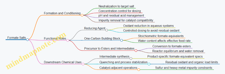
Integrated Example Workflow
A practical integrated workflow looks like this: produce formic acid, neutralize to the chosen salt, condition to a target concentration and pH, polish to meet impurity limits, then route to the downstream function.
Example: If the salt is destined for an aqueous reducing step, prioritize concentration stability and residual oxidant control. If it is destined for a catalytic intermediate synthesis, prioritize impurity polishing and consistent formate equivalents. In both cases, the “handoff specification” should be explicit: concentration, pH, and impurity thresholds are the three numbers that prevent downstream surprises.
8.5 Practical Example Workflow for Converting CO₂ and Hydrogen Inputs into Acid Product Specs
This workflow turns two messy realities—CO₂ feed variability and hydrogen quality—into a predictable formic acid product specification. The goal is not to “get close,” but to produce a measurable acid stream that passes acceptance criteria every time.
Step 1: Start with Inputs and Define the Target Specs
Assume you receive a captured CO₂ stream and a hydrogen stream for formic acid production. Before any calculations, write down the product specs you must meet, such as:
- Formic acid concentration (mass %)
- Water content (mass %)
- Total impurities (e.g., CO, methanol, sulfur compounds) with maximum limits
- Color and odor thresholds if required by downstream users
- Physical properties needed for storage and shipping (e.g., density at a reference temperature)
Then list input specs you can actually measure at the plant boundary:
- CO₂ purity and moisture
- Oxygen and nitrogen species that can affect catalysts
- Hydrogen purity and trace sulfur or oxygen
A practical trick: define “must-meet” specs and “monitor-only” specs. Must-meet items drive control loops; monitor-only items help you diagnose drift without stopping production.
Step 2: Convert Feed Data into a Mass Balance That Matches the Real Process
Use a basis such as 1,000 kg/h CO₂ entering the conditioning section. Include hydrogen consumption and any recycle purge. A simplified stoichiometric relationship is:
- CO₂ + H₂ → HCOOH In reality, you also account for:
- Losses in purification and vent streams
- Water formed or removed depending on the reaction and separation scheme
- Recycle streams that change impurity concentrations
Example basis (illustrative):
- CO₂ feed: 95 mol% CO₂, 3 mol% N₂, 2 mol% O₂, with 200 ppmv moisture
- Hydrogen feed: 99.9 mol% H₂ with 1 ppmv O₂ and 0.5 ppmv sulfur species
From this, compute the effective CO₂ available to reaction and the impurity load entering the reactor system.
Step 3: Condition CO₂ and Hydrogen to Protect the Reactor and Downstream Separation
Impurities rarely “stay put.” They either poison catalysts, foul heat exchangers, or carry through separations.
For CO₂ conditioning, typical control actions include:
- Drying to reduce water that can shift equilibrium and increase corrosion risk
- Oxygen removal or mitigation to avoid catalyst deactivation
- Nitrogen management so it doesn’t dilute partial pressures beyond operating windows
For hydrogen conditioning:
- Remove sulfur compounds because they can bind active sites
- Control oxygen because it can promote side reactions or degrade performance
Concrete acceptance criteria should be tied to the reactor’s needs. For example, if catalyst performance drops sharply above a certain oxygen level, set an oxygen acceptance limit at the conditioning outlet, not at the inlet of the reactor.
Step 4: Set Reactor Operating Targets Using a Spec-Driven Approach
Instead of selecting reactor conditions first, select them to hit product specs.
Key reactor-related variables:
- Temperature and pressure that determine conversion and selectivity
- Space velocity that affects residence time and impurity breakthrough
- Hydrogen-to-CO₂ ratio that controls conversion and limits side products
Example logic:
- If water content in the product is too high, adjust separation duty or operating conditions that influence water formation.
- If CO impurity in the acid is high, tighten CO₂ conditioning and reduce oxygen ingress, then verify with reactor outlet gas analysis.
Step 5: Purify and Finish the Acid to Meet Concentration and Impurity Limits
Formic acid purification typically involves separation steps that remove light gases, water, and trace organics. The workflow should map each impurity to its likely removal mechanism:
- Light gases: removed by gas-liquid separation and vent handling
- Water: adjusted by distillation or polishing steps
- Trace organics: reduced by controlling upstream selectivity and using polishing separation
Use a “spec-to-unit” mapping so operators know what to change when a spec fails.
Step 6: Build a Verification Loop with Sampling, Balances, and Acceptance Tests
Verification is where many workflows fail. Make it systematic:
- Sample CO₂ and hydrogen at conditioning outlets
- Sample reactor outlet gas and liquid phases
- Sample intermediate streams feeding purification columns
- Sample final acid product for concentration and impurity suite
Acceptance tests should be linked to control actions. If formic acid concentration is low, confirm whether the issue is conversion (reactor) or separation (purification). If impurities spike, check conditioning first, then reactor selectivity.
Mind Map: Spec-Driven Workflow from Inputs to Acid Output
Step 7: Worked Example Workflow with Decision Points
Assume final product must meet:
- Formic acid concentration: 85–90 wt%
- Water: ≤ 10 wt%
- CO impurity: ≤ 50 ppmw
- Start with measured feeds and compute effective CO₂ and impurity loads.
- Confirm conditioning outlet specs: oxygen and sulfur below thresholds.
- Run reactor at setpoints chosen to maintain selectivity; verify reactor outlet gas composition.
- Operate purification with column reflux and reboiler duty targets that match the water and concentration requirements.
- Sample final product.
Decision point A: If concentration is low but water is on target, conversion is likely low. Adjust hydrogen-to-CO₂ ratio or residence time, then re-check reactor outlet gas.
Decision point B: If water is high, separation duty is likely insufficient. Increase distillation separation effectiveness and confirm column overhead composition.
Decision point C: If CO impurity is high, treat it as a selectivity or conditioning failure. Re-check oxygen ingress and catalyst performance indicators, then verify CO in reactor outlet gas before changing purification.
This workflow keeps every adjustment tied to a measurable cause, so the plant doesn’t “chase numbers” blindly. The result is a repeatable path from CO₂ and hydrogen inputs to acid product specs that can be defended with mass balance and unit-level evidence.
9. CO₂ to Carbonates and Polymers for Materials Revenue
9.1 CO₂ Mineralization and Carbonate Formation Using Industrially Relevant Feedstocks
Foundations of Mineralization
CO₂ mineralization converts carbon dioxide into stable carbonate minerals by reacting it with divalent cations such as Ca²⁺, Mg²⁺, or Fe²⁺. In practice, the process is usually split into two steps: (1) dissolve or mobilize cations from a solid feedstock, and (2) precipitate carbonates from the resulting aqueous solution. The “industrial relevance” part matters because the best-performing chemistry is useless if the feedstock is too scarce, too expensive, or too contaminated to handle at scale.
A useful way to think about the system is as a set of equilibria competing with each other. Dissolution controls how much cation you can supply. Carbonate precipitation controls how much CO₂ you can lock up. Meanwhile, side reactions can consume alkalinity, form unwanted solids, or foul equipment.
Industrially Relevant Feedstocks
Most industrial feedstocks fall into three buckets.
-
Calcium-rich solids: limestone, quicklime, and industrial slags with high CaO content. These are common because calcium carbonates are relatively easy to form and the feedstocks are widely available.
-
Magnesium-rich solids: serpentine, olivine, and some brines or tailings streams. Magnesium mineralization can be slower because Mg²⁺ is less readily released, but it can be attractive where Mg sources are abundant.
-
Iron-bearing solids: steel slags and certain mine wastes. Iron can participate in carbonate formation, but it often introduces extra complexity through redox behavior and impurity-driven solids.
Feedstock quality is not a footnote. If a solid contains silica, alumina, or organics, it can change dissolution kinetics and create scale layers that slow mass transfer. If it contains chlorides or sulfides, it can increase corrosion risk and alter precipitation pathways.
Core Reaction Logic and Carbonate Types
Carbonate formation typically targets one of these mineral families:
- Calcite and aragonite from calcium-rich systems.
- Magnesite from magnesium-rich systems.
- Mixed carbonates when multiple cations are present.
The practical lever is alkalinity and ion availability. In calcium systems, increasing dissolved Ca²⁺ and maintaining conditions that favor CO₃²⁻ formation drives calcite precipitation. In magnesium systems, the same idea holds, but the dissolution step often limits the overall rate.
Process Pathways from Feedstock to Carbonate
Mineralization can be implemented in several operational styles, but they share the same logic.
-
Pre-treatment and dissolution: grind the solid to increase surface area, then contact it with water and sometimes an acid or CO₂-derived solution to mobilize cations.
-
CO₂ contact and precipitation: introduce CO₂ (often as a pressurized gas or dissolved CO₂) to the cation-bearing liquor, then control pH, temperature, and mixing so carbonate precipitates rather than remaining dissolved.
-
Solid-liquid separation and curing: separate precipitated solids, wash to remove soluble impurities, and optionally cure to improve mineral stability.
A concrete example: a calcium-rich slag slurry can be leached with water under controlled pH to generate Ca²⁺ in solution. Then CO₂ is bubbled or injected to raise carbonate ion availability, leading to calcite precipitation. The “easy-to-understand” part is that the solid feedstock provides the cations, while CO₂ provides the carbonate building blocks.
Mind Map: Mineralization Design
Practical Example with Decision Points
Consider a calcium-rich industrial solid with moderate silica content. If you simply slurry it in water and inject CO₂, you may get carbonate precipitation, but silica can form a gel-like layer that slows further dissolution. A systematic approach starts with bench tests that measure: (1) how quickly Ca²⁺ appears in solution, (2) how fast carbonate solids form at different pH levels, and (3) what solids appear besides carbonates.
If silica-driven scale is significant, you can adjust the sequence: increase dissolution time before CO₂ contact, improve mixing to reduce local supersaturation, or modify leach conditions to keep silica in solution longer. The goal is not to “force” precipitation; it is to align dissolution and precipitation so the system spends less time stuck in the wrong equilibrium.
Advanced Details That Prevent Common Failures
- pH management: carbonate precipitation is sensitive to pH because CO₃²⁻ availability changes strongly with acidity. Poor control can lead to bicarbonate-dominant solutions that later precipitate unpredictably.
- Mass transfer limits: CO₂ dissolution and gas-liquid transfer can be rate-limiting. Increasing interfacial area and controlling slurry rheology often matters as much as reaction kinetics.
- Impurity handling: soluble impurities can co-precipitate or form separate salts. Washing and liquor recycle strategies should be designed around measured impurity concentrations, not assumptions.
- Solid properties: particle size and morphology affect filtration and downstream use. Even when carbon is mineralized, poor solids can raise operating costs through slow separation.
Summary of the Section’s Logic
Industrial CO₂ mineralization works when three pieces align: a feedstock that can release cations at a practical rate, operating conditions that favor carbonate precipitation over competing solids, and separation steps that produce stable carbonate while controlling impurities and scale. When those pieces are treated as a connected system rather than isolated unit operations, the chemistry becomes predictable enough to engineer.
9.2 CO₂ to Cyclic Carbonates and Their Use in Polymer and Solvent Applications
Cyclic carbonates are five- or six-membered ring compounds that contain a carbonate group inside the ring. They matter in carbon-to-product systems because they can be made by reacting captured CO₂ with an epoxide, then used as monomers, intermediates, or high-value solvents. A useful way to think about the value chain is: CO₂ becomes a ring-forming carbon source, the epoxide provides the carbon skeleton, and the product’s ring stability controls how it behaves in polymers and solvents.
Foundational Chemistry and Reaction Logic
The core transformation is cycloaddition of CO₂ to an epoxide to form a cyclic carbonate. In practice, the reaction is usually performed with a catalyst and a base or activator that helps generate a reactive species from the epoxide. The stoichiometry is straightforward: one mole of CO₂ and one mole of epoxide form one mole of cyclic carbonate. That simplicity is helpful for mass balance, but real plants still need to manage side reactions such as epoxide polymerization, carbonate hydrolysis, and formation of oligomers when water or impurities are present.
A practical example: if you target propylene carbonate (a common cyclic carbonate), you start with propylene oxide. If the feed contains water, you may see extra by-products from hydrolysis and a drop in selectivity. That’s why feed drying and impurity control are not “nice to have”; they directly affect yield.
Catalyst and Process Choices
Catalysts are typically either nucleophilic/ionic systems or metal-based systems that activate the epoxide and facilitate CO₂ insertion. The most important operational knobs are temperature, pressure (to maintain sufficient CO₂ availability), and the ratio of CO₂ to epoxide. Higher CO₂ pressure often improves conversion, while temperature affects both kinetics and side reactions.
A systematic operating approach looks like this:
- Dry the epoxide and remove water from CO₂ feed.
- Choose a catalyst system aligned with the epoxide type.
- Set CO₂ pressure to avoid CO₂ starvation.
- Run at a temperature that balances reaction rate and selectivity.
- Separate product from unreacted epoxide and catalyst residues.
Product Families and Where They Fit
Cyclic carbonates are not one product; they are a family. Common examples include:
- Propylene carbonate from propylene oxide, widely used as a solvent and electrolyte component.
- Ethylene carbonate from ethylene oxide, often used where higher polarity and melting behavior are important.
- Butylene carbonate variants from substituted epoxides, used as intermediates and specialty solvents.
In polymer applications, cyclic carbonates can serve as monomers or as building blocks that introduce carbonate functionality into polymer backbones or side chains. In solvent applications, their polarity and ability to dissolve salts or organics make them useful in formulations where conventional solvents struggle.
Mind Map: CO₂ to Cyclic Carbonates and Uses
Polymer and Solvent Application Pathways
Cyclic carbonates influence polymers through carbonate functionality. That functionality can affect glass transition, thermal stability, and chemical resistance. In solvent use, the ring structure provides strong polarity and good solvating power. The same chemical traits that make cyclic carbonates useful in solvents also make them effective intermediates for downstream chemistry.
A concrete example for polymer integration: suppose a polymer route requires a cyclic carbonate-derived intermediate with low water content. If the cyclic carbonate feed to the polymer step contains significant moisture, you can get unwanted chain termination or altered reaction kinetics. The fix is not “try harder”; it’s to set purification specs for water and to verify them with consistent sampling.
Quality Control That Actually Matters
Downstream performance is sensitive to a few measurable properties:
- Water content: drives hydrolysis and side reactions.
- Unreacted epoxide: can react further and change product behavior.
- Color and stability: reflect impurity levels and catalyst carryover.
- Impurity profile: certain impurities can poison catalysts in later steps.
A simple plant-level example: if you observe rising by-product levels during a solvent campaign, check whether the epoxide drying step drifted. Even small changes in drying performance can show up as selectivity loss within days.
Example: From Feed Specs to Product Use
Imagine you produce cyclic carbonate for solvent use. Your target spec might include low water and low epoxide carryover to ensure consistent solvating performance. You can translate feed assumptions into expected outcomes: higher CO₂ pressure improves conversion, but if temperature is too high you may increase decomposition products that affect color. Separation then becomes a balancing act between recovering unreacted epoxide and achieving the impurity limits required by the solvent specification.
The result is a coherent chain: CO₂ and epoxide conditioning enables high selectivity; reaction control sets the impurity baseline; purification sets the final quality; and that quality determines whether the cyclic carbonate performs reliably as a solvent or as a polymer building block.
9.3 Polymerization Routes Including Polycarbonates and Copolymer Feed Preparation
Polymerization routes for carbonate-based materials start with a simple question: what chemical “handle” will the carbon dioxide-derived carbonate provide, and how will you control molecular weight and composition? In practice, you prepare feeds so the polymerization step sees the right functional groups, at the right purity, with the right stoichiometry—because most quality problems are feed problems wearing a polymer disguise.
Polycarbonate Route Foundations
Polycarbonates are typically made by reacting a diol with a carbonate precursor (often a diaryl carbonate) or by transesterification routes that generate the carbonate linkage in the melt or in a solvent. The key functional requirement is that the diol must be able to form carbonate bonds without being poisoned by water or acids. Water is the usual troublemaker: it can shift reactions toward low-molecular-weight species and increase chain termination.
A practical way to think about the polymerization chemistry is to track three “control knobs”:
- Stoichiometry: diol-to-carbonate ratio sets the average chain length.
- Catalyst and base strength: determines reaction rate and side reactions.
- Water and acid control: prevents premature termination and discoloration.
Copolymer Feed Preparation Logic
Copolymerization adds a second monomer or comonomer stream, which means you must control not only molecular weight but also composition distribution. For carbonate-containing copolymers, feed preparation often focuses on ensuring comonomer reactivity matches the carbonate-forming chemistry. If one comonomer is less reactive, you get composition drift along the reactor, which later shows up as broad property variation.
A systematic feed-prep approach uses a “spec ladder”:
- Chemical identity: confirm functional group presence and absence of unwanted reactive impurities.
- Physical state: ensure viscosity and solubility are compatible with mixing and heat transfer.
- Impurity budget: set limits for water, peroxides, acids, and metal residues.
- Stoichiometric balance: calculate required mass flows using target composition and expected conversion.
Polycarbonate Feed Preparation Steps
Start with the carbonate precursor and diol. Then treat feed preparation as a sequence of conditioning operations rather than a single “purify everything” step.
- Drying and dehydration: remove water from diol and carbonate precursor. A simple example is drying a diol to reduce hydrolysis; if you skip this, you may see lower viscosity and higher fraction of low-molecular-weight material.
- Impurity removal: filter solids, strip volatile contaminants, and manage residual catalysts from upstream carbonate formation.
- Stoichiometry verification: weigh and blend to match target number-average molecular weight. Example: if your target is higher molecular weight, you reduce the effective chain terminator fraction by tightening water and monofunctional impurity limits.
- Pre-reaction blending: combine feeds under controlled temperature to avoid premature reaction or gel formation.
Copolymer Feed Preparation Steps
For copolymers, you add one more layer: composition control.
- Comonomer purity and reactivity: comonomers often have higher sensitivity to impurities that affect radical or ionic pathways. Even small peroxide levels can change the reaction mechanism.
- Composition targeting: compute feed ratios based on desired copolymer composition, not just nominal monomer ratios. Example: if comonomer A reacts faster than B, you must feed less A than the naive stoichiometry suggests to hit the target composition.
- Mixing and residence time control: ensure uniform distribution before polymerization begins. Poor mixing can create local composition gradients that persist after polymerization.
Mind Map: Feed Preparation to Polymer Properties
Example: Translating Feed Specs into Polymer Targets
Suppose you target a polycarbonate with higher viscosity. You start by setting a tighter water spec for the diol and carbonate precursor. Then you verify stoichiometry using a mass-balance calculation that accounts for expected conversion and any chain terminators. During blending, you ensure the feeds reach reaction temperature uniformly before the catalyst is fully active. The result is not just “higher molecular weight,” but a narrower molecular weight distribution, which improves melt stability and reduces batch-to-batch variation.
For a copolymer, imagine you want a specific carbonate-to-comonomer ratio that yields a target glass transition range. You calculate feed ratios using the relative reactivity of the comonomers, then enforce impurity limits that could change the reaction pathway. Finally, you confirm mixing performance so the reactor sees the intended composition from the first moment, preventing composition drift that would otherwise broaden thermal and mechanical properties.
Practical Integration with Upstream Carbonate Production
Polymerization feed preparation must match the upstream carbonate output. If upstream carbonate formation leaves residual salts, acids, or metal traces, they can catalyze unwanted side reactions or promote discoloration. A clean interface is therefore part of the polymerization design: specify what “acceptable residue” means in terms of polymer impact, not only chemical purity. When feed preparation is treated as a controlled bridge between carbonate production and polymerization, the polymer step becomes predictable rather than mysterious—like a recipe where the oven temperature actually matches the instructions.
9.4 Quality Control for Materials Including Moisture, Molecular Weight, and Impurities
Quality control for carbonate-derived materials and polycarbonate-like products starts with a simple idea: customers pay for consistent performance, and performance depends on measurable properties. Moisture, molecular weight, and impurities are the three levers that most directly shift viscosity, mechanical strength, processing behavior, and long-term stability.
Moisture Control as a Process and Product Variable
Moisture affects materials in two ways. First, water can participate in side reactions or hydrolysis, lowering molecular weight and changing end-group chemistry. Second, water changes processing conditions by altering melt behavior and promoting foaming or unstable extrusion.
A practical QC workflow begins with defining where moisture matters. For example, if you are producing a cyclic carbonate intermediate that will be polymerized, moisture tolerance is often tighter at the polymerization feed stage than at the final pellet stage. Then you set acceptance criteria based on a measurable link to performance.
Example: Suppose a polymer grade requires stable melt viscosity. You measure moisture in incoming cyclic carbonate feed using Karl Fischer titration. If moisture rises from 200 ppm to 800 ppm, you observe a consistent drop in intrinsic viscosity and a shift toward lower molecular weight. The acceptance criterion becomes a number tied to that relationship, not a guess.
Sampling must be designed, not improvised. Moisture is uneven in bags and bulk solids, so you use composite sampling and specify sample handling to prevent re-adsorption. Store samples in sealed containers and run tests promptly.
Molecular Weight Measurement and Interpretation
Molecular weight controls chain length distribution, which governs strength and processing. For polymers, you typically care about number-average and weight-average molecular weight, plus dispersity. For carbonate-based materials, you may also track end-group functionality because it influences reactivity and stability.
A systematic approach is to measure molecular weight with a method that matches the material state. Size-exclusion chromatography is common for soluble polymers, while melt flow index can serve as a fast screening tool for pellets. Screening is useful, but it should be calibrated against a primary method.
Example: You run SEC on a weekly basis and use melt flow index daily. When SEC shows a shift toward lower weight-average molecular weight, melt flow index trends upward the same week. That correlation lets you catch drift earlier while keeping the SEC results as the anchor.
Interpretation should include distribution shape, not only averages. A broader distribution can sometimes preserve impact strength while changing tensile behavior. QC reports should therefore include dispersity and any repeatable shifts in chromatogram profile.
Impurity Identification and Control Strategy
Impurities are everything that is not the target species. In practice, they fall into categories: reactive impurities that change chemistry, catalyst residues that affect stability, and physical contaminants that cause defects.
Start by mapping impurity sources to unit operations. For carbonate and polymer routes, common contributors include residual solvents, unreacted monomers, inorganic salts from purification steps, and trace catalyst components. Each source suggests a measurement method: gas chromatography for volatile organics, ICP-OES for metals, ion chromatography for salts, and spectroscopy for functional group shifts.
Example: If you see brittle fracture in molded parts, you check whether the impurity is a residual monomer that plasticizes early processing but evaporates later, or a metal residue that accelerates degradation. A simple QC sequence can prevent guesswork: measure residual monomer first, then metals, then inorganic ions.
Set impurity limits using a risk-based logic. Reactive impurities get tighter limits because they can change molecular weight during storage or processing. Physical contaminants get limits tied to defect formation, such as gels or haze.
Integrated QC Plan for Materials
A strong QC plan links inputs to outputs. You define critical control points, choose test frequency, and specify actions when results drift.
- Moisture: test feed and intermediate before polymerization; test final pellets for storage stability.
- Molecular Weight: primary measurement on a schedule; fast screening for every lot.
- Impurities: targeted tests for known risk species; broader checks when process conditions change.
When a result fails, the response should be pre-written. For instance, if moisture exceeds the limit, you may re-dry and re-test. If molecular weight is low, you may quarantine the lot and investigate upstream hydrolysis or residence time issues. If impurities spike, you trace back to the purification step and verify reagent and filter performance.
Mind Map: Quality Control Variables and Actions
Example: From Test Results to Release Decision
Imagine a lot of carbonate-derived polymer pellets. Moisture is 350 ppm, within the 500 ppm limit. Melt flow index matches the calibrated range, and SEC confirms weight-average molecular weight is on target with dispersity unchanged. Impurity testing shows metals at 0.8 ppm, below the limit, and residual monomer is at 0.2%, also within spec.
Because each measurement supports the same story—no moisture-driven chain loss, no chemistry-altering impurities, and no distribution shift—the lot is released. If any one measurement contradicts the others, the lot is quarantined and the investigation focuses on the unit operation most likely to create that specific mismatch.
9.5 Practical Example Workflow for Translating Carbonate Production Into Polymer Grade Requirements
Start with a simple goal: you have a carbonate product stream leaving the carbonate unit, and you need it to meet polymer-grade specifications for downstream polycarbonate or copolymer synthesis. The workflow below turns “we made carbonates” into “we made the right carbonate for polymer performance,” using measurable checks at each step.
Step 1: Define Polymer Grade Requirements in Measurable Terms
Polymer grade requirements should be written as numbers and test methods, not vibes. For cyclic carbonates and carbonate intermediates, typical categories include:
- Purity: mass fraction of target carbonate, plus limits on isomers and non-carbonate organics.
- Water content: affects hydrolysis and downstream catalyst behavior.
- Acid number or acidity: drives corrosion and side reactions.
- Residual salts or metals: can poison catalysts or create discoloration.
- Color and odor: proxies for trace organics and degradation.
Example requirement set for a carbonate intermediate used in polycarbonate synthesis:
- Water: ≤ 200 ppm
- Acidity: ≤ 0.05 mg KOH/g
- Total metals (Na+K+Fe): ≤ 5 ppm
- Target carbonate purity: ≥ 99.5 wt%
- Color: ≤ 20 APHA
Step 2: Map Carbonate Unit Outputs to Polymer Failure Modes
Next, connect each impurity category to how it harms polymer quality. This prevents “test everything” and focuses on what matters.
- Water → hydrolysis, lower conversion, higher oligomer fraction
- Acidity → catalyst deactivation, corrosion, off-spec color
- Metals → catalyst poisoning, unstable reaction kinetics
- Non-carbonate organics → viscosity changes, gel formation risk
A practical way to do this is a one-page matrix: impurity → mechanism → polymer symptom → acceptable limit. If a symptom is not linked to a measurable impurity, the limit is usually not enforceable.
Step 3: Build a Sampling Plan That Matches the Process Reality
Carbonate streams can stratify in tanks and change during transfer. Sampling must represent the polymer feed, not the first bucket.
- Where to sample: after final polishing step, before storage
- How often: during steady operation, plus at transitions (start-up, grade change)
- Composite vs grab: use composites for stable streams; use grabs for transient events
Example: if polishing is a drying column followed by filtration, sample at the outlet of filtration and after the transfer line stabilizes for 10–15 minutes.
Step 4: Translate Polymer Limits Back into Carbonate Unit Control Targets
Now reverse the logic. If polymer needs water ≤ 200 ppm, the carbonate unit must deliver a stream that stays below that limit through storage and transfer.
- Add a safety margin for handling losses and measurement uncertainty.
- Convert polymer limits into unit-level targets for each control step.
Example targets:
- Water at unit outlet: ≤ 120 ppm (to allow for storage pickup)
- Acidity at unit outlet: ≤ 0.03 mg KOH/g
- Metals at unit outlet: ≤ 2 ppm
This is where “best practice” becomes operational: drying and polishing steps are not optional extras; they are the mechanism that makes polymer-grade limits achievable.
Step 5: Create a Mass Balance and Yield Accounting for Grade Compliance
Grade compliance affects yield because polishing removes material. Track both chemical yield and purification yield.
- Define a basis, such as 1,000 kg of carbonate feed to the polishing train.
- Track losses to vents, purge, filter cake, and off-spec recycle.
Example accounting:
- Carbonate produced: 980 kg
- Polishing losses: 20 kg (filter cake + purge)
- Polymer-grade compliant output: 960 kg
Then compute a “compliance yield” metric: compliant output divided by total carbonate produced. This number belongs in the same spreadsheet as economics.
Step 6: Run a Trial Batch or Continuous Campaign with Acceptance Criteria
A campaign should include steady-state operation and at least one controlled disturbance (like a small change in feed impurity) to prove robustness.
- Predefine acceptance criteria for each test.
- Include hold-time checks if the polymer feed is stored.
Example acceptance criteria for a 24-hour campaign:
- Water: mean ≤ 120 ppm, no sample > 160 ppm
- Acidity: mean ≤ 0.03 mg KOH/g, no sample > 0.04 mg KOH/g
- Metals: ≤ 2 ppm average
Step 7: Close the Loop with Downstream Reaction Verification
Even perfect-looking carbonate specs can fail if the downstream process is sensitive to a specific impurity form. Verification should be minimal but decisive.
- Use a small-scale polymerization run with the carbonate feed.
- Confirm key polymer properties tied to the earlier failure modes: conversion, molecular weight distribution, and color.
Example verification outcomes:
- If conversion is low, re-check water and acidity first.
- If color is high, re-check trace organics and metals.
Mind Map: Carbonate to Polymer Grade Translation Workflow
Example: One Impurity Path from Spec to Action
Suppose polymer-grade requires water ≤ 200 ppm, and a campaign shows water at 180–220 ppm in the polymer feed. The workflow points to likely causes: drying column breakthrough, filter bypass, or storage pickup.
- If water spikes right after transfer, improve transfer line drying and add a stabilization hold.
- If water rises gradually over the day, adjust drying column regeneration timing.
- If water correlates with higher acidity, check for carryover from upstream neutralization.
The key is that each action is tied to a measurable link in the chain, so the next campaign can confirm whether the fix worked.
10. CO₂ to Urea and Ammonia Derivatives for Fertilizer and Chemicals
10.1 Nitrogen Feedstock Options and Integration With Carbon Conversion Steps
Nitrogen is the “other half” of many carbon-to-urea and carbon-to-ammonia derivative routes. It can enter the process as pure N₂, as nitrogen-containing off-gases, or as ammonia that already carries both nitrogen and hydrogen. The key integration question is simple: what form of nitrogen do you have, and what form do you need at the point where carbon chemistry starts?
Foundations: Where Nitrogen Meets Carbon Chemistry
Most urea-family production ultimately requires ammonia (NH₃) as the nitrogen carrier. Carbon dioxide (CO₂) then reacts with ammonia to form urea, typically via carbamate intermediates. That means nitrogen feedstock selection is really selection of the ammonia-making step and its coupling to CO₂ handling.
A practical way to think about the plant is to separate three blocks:
- Nitrogen-to-ammonia block: converts N₂ to NH₃ using hydrogen.
- Ammonia-to-urea block: converts NH₃ and CO₂ into urea.
- Utilities and recycle block: manages steam, condensate, purge, and recovery of unreacted gases.
If your nitrogen source changes, the nitrogen-to-ammonia block changes first; the ammonia-to-urea block changes only if ammonia purity or contaminants change.
Nitrogen Feedstock Options
Pipeline Nitrogen or On-Site N₂ Separation
Using high-purity N₂ is the cleanest starting point. It minimizes nitrogen-related impurities in the ammonia synthesis loop, which reduces catalyst fouling risk and simplifies gas cleanup. A typical integration pattern is:
- N₂ compression and drying
- mixing with hydrogen in the synthesis loop
- ammonia condensation and purification
- sending purified NH₃ to the urea section
Easy example: If you already have a reliable N₂ supply at ~99.9% purity, you can often keep the synthesis gas cleanup focused on hydrogen-side contaminants rather than nitrogen-side ones.
Air Separation Unit Nitrogen
An air separation unit (ASU) can provide N₂ as a product stream. This option is common when oxygen is also needed elsewhere in the plant. The integration advantage is shared infrastructure: cryogenic equipment, nitrogen compression, and sometimes shared utilities.
The integration constraint is impurity control. Even when N₂ is high purity, trace oxygen or argon can affect downstream gas handling and purge strategy. You also need to ensure that any oxygen slip does not create unwanted side reactions in the ammonia synthesis loop.
Easy example: If the ASU produces N₂ with trace O₂, you may add a polishing step or adjust loop purge to prevent oxygen accumulation.
Nitrogen-Rich Off-Gases
Some industrial sites have nitrogen-containing off-gases from furnaces, boilers, or process vents. These streams can reduce the need for new nitrogen production, but they bring variability: oxygen content, CO₂ content, water vapor, and trace sulfur or hydrocarbons.
Integration here is mostly about cleanup and control. You typically need:
- particulate removal
- moisture removal
- oxygen management (often via blending or controlled venting)
- removal of catalyst poisons if ammonia synthesis is sensitive to them
Easy example: If an off-gas contains 2–5% O₂, you can blend it with fresh N₂ to keep oxygen below a setpoint, rather than trying to run ammonia synthesis directly on the raw stream.
Ammonia as a Nitrogen Carrier
If ammonia is purchased or generated elsewhere, you can treat it as the nitrogen input and skip the nitrogen-to-ammonia block. This changes integration priorities:
- urea section feed conditioning becomes the main task
- ammonia storage and handling dominate the nitrogen logistics
- you still need CO₂ conditioning and recycle management
Easy example: If you receive ammonia at a stable spec, you can focus on carbamate formation control and urea crystallization conditions rather than on synthesis gas cleanup.
Integration with Carbon Conversion Steps
Once ammonia is available, CO₂ integration becomes the next constraint. CO₂ purity affects carbamate formation and downstream separation. Nitrogen feedstock choice influences CO₂ integration indirectly through loop purge composition and how much inert gas accumulates.
A systematic integration approach is:
- Set ammonia spec requirements for the urea section (purity, water content, and inert levels).
- Define purge and recycle targets in the ammonia synthesis loop so inert accumulation stays within limits.
- Condition CO₂ to match urea section needs, including removal of contaminants that would interfere with separation or crystallization.
- Balance mass and energy so that ammonia condensation, CO₂ compression, and urea synthesis heat duties align.
Mind Map: Nitrogen Feedstock Choices and Integration Points
Example: Choosing Between Pure N₂ and Off-Gas
Assume you have two options for nitrogen: (A) pure N₂ at high purity, or (B) an off-gas stream with variable composition. If option A is used, the ammonia synthesis loop can run with a straightforward gas cleanup train and stable purge targets.
If option B is used, the plant needs an additional conditioning step to control oxygen and moisture, plus a monitoring strategy that updates blending ratios. The urea section still expects ammonia at a consistent spec, so the ammonia purification system becomes the “buffer” that absorbs nitrogen-feed variability.
The decision is not just about nitrogen cost. It’s about where variability is easiest to manage: in gas conditioning upstream, or in purification and control downstream.
10.2 Urea Synthesis Process Steps Including Ammonia and CO₂ Reaction Integration
Foundational Chemistry and What Must Be True
Urea forms from ammonia and carbon dioxide through a sequence that can be summarized as: ammonia reacts with CO₂ to form ammonium carbamate, and carbamate dehydrates to urea while releasing water. In practice, the plant does not run “one reaction and done.” It runs a controlled loop where carbamate is formed, converted, and recycled so that overall conversion stays high even when equilibrium limits single-pass performance.
A useful mental model is to treat the process as three coupled tasks: (1) create carbamate efficiently, (2) drive dehydration toward urea without overheating, and (3) separate urea from water and unreacted species so the loop can return what is still valuable.
Ammonia Preparation and Conditioning
Ammonia is typically available as a purified feed, but the synthesis section still needs conditioning. The key operational needs are stable flow, controlled temperature, and removal of contaminants that can foul heat transfer surfaces or interfere with downstream separation. A practical example: if ammonia enters colder than design, the carbamate formation zone may run below its intended temperature, lowering carbamate formation rate and forcing higher recycle loads to compensate.
CO₂ Handling and Integration Strategy
CO₂ is introduced in a way that matches the carbamate formation kinetics. The synthesis section usually uses a CO₂-to-ammonia ratio that supports carbamate formation while leaving enough ammonia to sustain urea formation. A concrete example: if CO₂ is fed too lean relative to ammonia, carbamate formation can be incomplete and the loop returns more unreacted ammonia; if CO₂ is fed too rich, more carbamate can form than the system can dehydrate efficiently, increasing water and complicating separation.
Carbamate Formation Zone
In the carbamate formation step, ammonia and CO₂ react to form ammonium carbamate, typically under elevated pressure and controlled temperature. The plant design aims to maximize carbamate formation while keeping conditions compatible with corrosion control and heat transfer.
Operationally, this zone is where “good mixing” matters. If gas-liquid contact is poor, local composition swings can occur: some regions form carbamate rapidly while others remain ammonia-rich. That imbalance shows up later as uneven recycle behavior and separation load.
Urea Formation and Dehydration Zone
Carbamate dehydrates to urea and water. This step is sensitive to temperature because higher temperatures can increase conversion but also raise the risk of side reactions that reduce yield and increase impurities. The integration challenge is to provide enough driving force for dehydration while keeping the residence time and thermal profile within the intended window.
A practical example: if the dehydration zone runs too hot, more by-products can form, and the downstream evaporator and crystallizer will have to handle a more complex impurity profile. That increases recycle of mother liquor and can reduce overall urea recovery.
Reactor Effluent Cooling and Concentration
After reaction, the effluent contains urea, water, unreacted ammonia, and carbamate species. Cooling and concentration are not just “cool it down.” They are timed to support phase behavior that enables separation. The goal is to move the system into a regime where urea can be recovered efficiently while volatile components can be returned to the loop.
Separation and Recycle Loop Closure
Separation typically includes stripping and recovery steps that return ammonia and carbamate-related species to the formation zone. This is the heart of integration: the plant uses recycle to overcome equilibrium limits.
A simple example of loop logic: if the separation section removes urea but leaves too much ammonia in the product stream, you lose product purity and increase off-gas handling. If it removes too little ammonia, the formation zone receives less reactive inventory and conversion drops, forcing higher CO₂ feed and increasing water load.
Mass Balance Checkpoints That Prevent Surprises
Three checkpoints keep the integration honest:
- Ammonia balance across the synthesis loop: compare ammonia in to ammonia recovered and returned.
- CO₂ balance across the synthesis loop: confirm that CO₂ consumption matches expected carbamate formation and dehydration.
- Water balance tied to dehydration: track water generation and removal because it strongly affects concentration and crystallization behavior.
When these balances drift, the cause is usually not “mystery chemistry.” It is typically a shift in temperature profile, a change in feed ratio, or a separation inefficiency that changes recycle composition.
Mind Map: Ammonia and CO₂ Reaction Integration
Example: How Integration Choices Show Up in Operating Data
Suppose the plant operator observes that urea crystallizer throughput drops while mother liquor recycle increases. A systematic diagnosis ties it back to integration: if the dehydration zone ran cooler than intended, carbamate conversion to urea would be lower, leaving more reactive species that later increase impurity load and hinder crystallization. Alternatively, if the CO₂-to-ammonia ratio drifted, carbamate formation could shift the effluent composition, changing viscosity and separation performance. In both cases, the fix is not random tweaking; it is adjusting feed ratio and temperature profile to restore the expected loop composition and mass balances.
10.3 Purification and Crystallization Including Product Moisture and Granulation Targets
Purification and crystallization turn a chemically correct product into a product that can be handled, stored, and sold without turning into a sticky science experiment. For urea and related nitrogen products, the key control variables are impurity levels, water content, crystal size distribution, and the mechanical behavior of the solid during drying and granulation.
Foundational Purity Targets and Why Moisture Is Not Just “Water”
Start by defining purity targets in the same units used for acceptance testing: mass fraction for impurities, and weight percent for moisture. Moisture affects more than mass balance; it changes dissolution rate, caking tendency, and how easily the product can be screened and bagged.
A practical way to set targets is to map each impurity to its likely failure mode:
- Biuret and related nitrogenous impurities can reduce performance in downstream use.
- Residual ammonia or carbonate species can shift pH and promote corrosion in storage.
- Inorganic salts can seed unwanted crystal forms and increase filter fouling.
Then translate those into process controls: where the impurity enters, which unit removes it, and what measurement confirms removal.
Purification Train Logic from Liquid to Solid
Most purification trains follow a consistent logic: remove volatile components first, then separate dissolved non-volatiles, then polish to meet final spec.
-
Volatile Removal
- Strip or flash to reduce free ammonia and other light components.
- Example: If ammonia in the melt is high, the crystallizer can produce crystals with higher surface moisture because the system stays closer to a hydrated equilibrium.
-
Dissolved Impurity Separation
- Use filtration, centrifugation, or controlled crystallization to reject impurities into mother liquor.
- Example: If an inorganic impurity is poorly soluble, it will concentrate in mother liquor; increasing recycle of mother liquor can improve overall yield but also raises impurity levels unless purged.
-
Polishing Steps
- Apply a final wash or controlled re-crystallization to reduce trace impurities.
- Example: A short wash with conditioned condensate can remove adhering mother liquor without over-dissolving the product crystals.
Crystallization Fundamentals That Control Crystal Quality
Crystallization is where you “choose” the solid form. The main levers are supersaturation, residence time, temperature profile, and agitation.
- Supersaturation determines nucleation rate. Too low gives large crystals and poor filtration; too high gives excessive fines.
- Temperature Profile affects solubility and the stability of the desired crystal form.
- Residence Time and Mixing influence whether crystals grow uniformly or break into smaller particles.
A useful operational check is to compare expected crystal size distribution from mass balance with measured sieve results. If the measured fines fraction is high, you typically see one or more of: excessive supersaturation, aggressive agitation, or insufficient separation time.
Moisture Targets and Drying Strategy
Moisture targets should be tied to handling requirements. For granulated products, moisture is often set to balance two competing needs: low enough to prevent caking, high enough to avoid dusting and excessive brittleness.
Drying strategy should be staged:
- Stage 1 removes bulk free water with minimal thermal stress.
- Stage 2 removes bound water to reach final moisture.
Example: If a dryer is run too hot early, you can drive rapid surface drying that creates a crust. That crust can trap moisture inside, leading to uneven moisture and higher re-wetting during storage.
Granulation Targets and How They Link to Crystallization
Granulation is not a separate world; it is a continuation of crystallization quality. Granules form when fines and partially dried crystals are agglomerated under controlled moisture and mechanical energy.
Set granulation targets in terms of:
- Sieve distribution (what fraction is too small, acceptable, or too large)
- Moisture at granulator outlet (enough for bonding, not so much that it smears)
- Attrition resistance (how much breaks during handling)
Example: If the crystallizer produces too many fines, the granulator may consume extra binder moisture and produce oversized lumps. If the crystallizer produces too few nuclei, granulation may stall and yield a narrow size range with poor flowability.
Mind Map: Purification and Crystallization Controls
Example: Turning Spec Sheets into Unit Operations
Assume the product spec requires low biuret, moisture at a defined weight percent, and a granule size distribution that supports consistent bagging.
- If biuret is high, prioritize mother liquor management: increase purge fraction to prevent impurity build-up, then verify with mother liquor assays.
- If moisture is high after drying, check dryer staging and residence time; uneven drying often points to crust formation or insufficient mixing.
- If granules are too fine, reduce supersaturation or agitation intensity in crystallization, then confirm by comparing sieve results to the expected nucleation behavior.
The integrated approach is simple: each spec maps to a unit operation lever, and each lever has a measurement that tells you whether you moved in the right direction.
10.4 Handling By-Products and Recycle Streams for Carbon Efficiency
Carbon efficiency is often decided in the “in-between” spaces: purge lines, offgas headers, condensate drains, and recycle compressors. In a CO₂-to-urea or CO₂-to-fuels plant, by-products are not just waste streams; they are signals about where carbon is leaving the intended product path. The goal of this section is to keep carbon in play by (1) identifying by-product formation mechanisms, (2) routing each stream to the right recovery or disposal option, and (3) designing recycle loops so they stabilize composition without creating new bottlenecks.
Foundational Concepts for By-Products and Recycles
A by-product is any carbon-containing material that is not the target product but still carries value or at least carbon accounting impact. A recycle stream is any stream returned to a reactor feed or upstream unit to improve overall conversion and reduce net carbon loss.
Two practical rules guide the design:
- Track carbon at decision points. If you only measure carbon at the product tank, you will miss carbon lost in purge, vent, or condensate.
- Control build-up. Recycles improve conversion, but they also concentrate inerts, water, salts, sulfur species, or nitrogen compounds depending on the chemistry.
Stream Taxonomy and What It Means for Carbon
Start by classifying streams by phase and function:
- Recycle gas: typically contains CO₂, CO, H₂, and inerts; it needs impurity management and purge strategy.
- Recycle liquid: may include dissolved salts, amines, or oxygenates; it needs corrosion control and solids handling.
- Condensate and wash water: often carries dissolved organics or salts; it can be a hidden carbon sink if not routed.
- Purge and vent: the safety valve of the process; it prevents runaway impurity accumulation.
- Offgas from separations: can be rich in CO₂ or light hydrocarbons; it is a candidate for recovery.
A simple example: in a urea synthesis train, ammonia and CO₂ react, but side reactions and decomposition can create small amounts of biuret and other nitrogenous species. If the downstream scrubbers send nitrogen-rich condensate to drain without recovery, carbon and nitrogen efficiency both suffer.
By-Product Formation Mechanisms and Targeted Control
By-products form for predictable reasons:
- Thermodynamic limits: some reactions favor equilibrium mixtures; conversion caps are real.
- Kinetic side reactions: catalysts or residence time can promote undesired pathways.
- Impurity-driven chemistry: sulfur, oxygen, or trace metals can shift selectivity.
- Operating extremes: temperature and pressure swings can increase decomposition or polymerization.
Control is most effective when it is targeted. For instance, if a recycle gas gradually accumulates water, it can shift catalyst performance and increase by-product formation. The fix is usually not “more catalyst”; it is water management via dehydration, better knockout design, and a purge that removes water-carrying components.
Purge Strategy as a Carbon Efficiency Lever
A purge is required when inerts or reactive contaminants build up beyond acceptable limits. The trick is to purge the right fraction, at the right location, with the right recovery.
A systematic approach:
- Define impurity limits for each unit: reactor catalyst tolerance, corrosion limits, and separation constraints.
- Identify the dominant impurity carrier: water, nitrogen species, sulfur compounds, or heavy hydrocarbons.
- Choose purge location where the impurity concentration is highest relative to valuable components.
- Recover purge value using a flash, absorber, or membrane step before disposal.
Example: suppose a CO₂-to-syngas loop includes a purge to prevent inert buildup. If the purge is taken upstream of a condenser, it may contain more CO₂ and less condensable heavies. Routing that purge through a recovery absorber can capture CO₂ back to feed, while the remaining tail gas goes to controlled vent after meeting emissions limits.
Recycle Loop Design for Stability
Recycle loops must be designed like living systems: they need composition control, pressure control, and instrumentation that catches drift early.
Key design elements:
- Knockout drums and demisters to prevent liquid carryover into compressors.
- Dehydration or drying when water accumulation affects catalysts or equilibrium.
- Salt and solids management for liquid recycles, including filtration and periodic purge.
- Instrumentation and control logic based on composition indicators, not just flow.
A concrete example from urea systems: liquid recycle streams can accumulate biuret and other higher-order nitrogen species. If the recycle is not periodically purged or if solids are not removed, the reactor can see a shift in effective feed composition, increasing viscosity and complicating heat transfer. A controlled purge from the recycle loop, combined with a recovery step for dissolved urea, keeps both carbon and nitrogen efficiency stable.
Recovery Routing for Condensates and Wash Streams
Condensates and wash waters are frequent carbon “leak points” because they look like utilities rather than process streams.
A practical routing hierarchy:
- Return condensates that contain recoverable product or feed components to the nearest upstream separator or recycle header.
- Send wash streams to a dedicated recovery unit if they contain dissolved organics or significant CO₂.
- Only then treat remaining aqueous streams in a way that preserves carbon accounting and prevents uncontrolled emissions.
Example: in a hydrogenation section, a separator may produce a condensate rich in oxygenates. If that condensate is routed to wastewater, carbon is lost as treatment load. If instead it is routed to a product polishing step or back to the separation train, the plant recovers carbon as product rather than as chemical oxygen demand.
Mind Map: By-Products and Recycle Streams
Integrated Example Workflow for Carbon Efficiency
Consider a CO₂-to-urea plant section where a recycle loop returns unreacted CO₂ and ammonia while a purge prevents inert and higher-order nitrogen build-up.
- First, set impurity limits for the reactor feed based on viscosity, corrosion risk, and acceptable by-product levels.
- Next, identify which stream carries the impurity: if it concentrates in the liquid recycle, place the purge on the liquid side and include a recovery step to reclaim dissolved urea.
- Then, route condensate from separators back to the recovery unit rather than to drain.
- Finally, verify carbon efficiency by closing the mass balance at the purge, condensate, and product boundaries, not only at the final product tank.
When these steps are done together, the plant reduces net carbon loss while keeping the recycle loop within safe and stable operating envelopes. The by-products still exist, but they stop being silent carbon sinks.
10.5 Practical Example Workflow for Mass Balance from CO₂ and Nitrogen Inputs to Urea Output
A practical mass balance for urea starts with a clear boundary: what enters the battery limits and what leaves as product, purge, vent, and wastewater. In this example, the plant converts captured CO₂ and a nitrogen source into urea solution, then crystallizes urea to a solid product.
Step 1: Define the Basis and Species
Use a basis that matches how operators think. For instance: 1,000 kg/h of CO₂ feed to the plant battery limits. Assume nitrogen is supplied as ammonia (NH₃) from upstream synthesis, and urea is the only desired carbon-containing product.
Key reactions used for stoichiometry:
- CO₂ + 2 NH₃ → NH₂COONH₄ (ammonium carbamate)
- NH₂COONH₄ → (NH₂)₂CO + H₂O (urea + water)
Overall stoichiometry:
- CO₂ + 2 NH₃ → (NH₂)₂CO + H₂O
This tells you carbon and nitrogen bookkeeping immediately: 1 mol CO₂ becomes 1 mol urea, and 2 mol NH₃ becomes 1 mol urea.
Step 2: Convert Feed Masses to Moles
Molar masses: CO₂ = 44.01 kg/kmol, NH₃ = 17.03 kg/kmol, urea (CH₄N₂O) = 60.06 kg/kmol, water = 18.02 kg/kmol.
CO₂ feed: 1,000 kg/h = 22.72 kmol/h CO₂.
Stoichiometric NH₃ requirement for complete conversion: 2 × 22.72 = 45.44 kmol/h NH₃.
Step 3: Apply Conversion and Account for Losses
Real plants do not hit 100% single-pass conversion. Introduce a single-pass conversion for CO₂ in the urea synthesis section, plus a purge fraction for unreacted nitrogen species.
Assume:
- CO₂ single-pass conversion = 92%
- Unreacted NH₃ is mostly recycled, with a purge that removes 1.5% of the NH₃ entering the synthesis loop
CO₂ reacted: 0.92 × 22.72 = 20.90 kmol/h.
CO₂ leaving as unreacted (to recycle/vent): 22.72 − 20.90 = 1.82 kmol/h.
Urea formed on stoichiometry: 20.90 kmol/h urea.
Water formed: 20.90 kmol/h water.
Step 4: Determine Required NH₃ Feed to the Loop
Because NH₃ is recycled, the fresh NH₃ feed must cover both reaction demand and purge losses.
NH₃ consumed by reaction: 2 × 20.90 = 41.80 kmol/h.
Let the NH₃ purge be 1.5% of NH₃ entering the synthesis loop. If NH₃ entering the loop is L kmol/h, then purge = 0.015L.
Fresh NH₃ feed equals consumption plus purge, so:
Fresh NH₃ = 41.80 + 0.015L.
Also, NH₃ entering the loop equals consumed plus unreacted leaving the loop. Unreacted NH₃ leaving corresponds to CO₂ unreacted only if the process is tightly coupled; in practice, NH₃ is in excess. For a workable example, assume NH₃ is maintained at 10% excess relative to stoichiometric for the reacted CO₂. Then NH₃ entering loop ≈ 1.10 × (2 × reacted CO₂) = 1.10 × 41.80 = 45.98 kmol/h.
Purge NH₃ = 0.015 × 45.98 = 0.6897 kmol/h.
Fresh NH₃ feed = 41.80 + 0.6897 = 42.49 kmol/h.
Fresh NH₃ mass = 42.49 × 17.03 = 723.0 kg/h.
Step 5: Convert Urea Moles to Product Mass and Include Crystallizer Losses
Urea produced from reacted CO₂: 20.90 kmol/h.
Urea mass = 20.90 × 60.06 = 1,255 kg/h.
Now include crystallizer yield. Assume 98.5% of urea leaving the synthesis section ends up as solid product; the rest leaves with mother liquor.
Solid urea product = 1,255 × 0.985 = 1,236 kg/h.
Mother liquor urea loss = 1,255 − 1,236 = 19 kg/h.
Step 6: Close the Carbon and Nitrogen Balances
Carbon check:
- CO₂ in: 1,000 kg/h
- CO₂ to urea: 20.90 kmol/h × 44.01 = 920 kg/h
- CO₂ remaining unreacted: 1.82 kmol/h × 44.01 = 80 kg/h
Total carbon accounted: 920 + 80 = 1,000 kg/h.
Nitrogen check:
- NH₃ fresh: 723 kg/h = 42.49 kmol/h
- NH₃ consumed: 41.80 kmol/h
- NH₃ purged: 0.6897 kmol/h
Total nitrogen accounted: 41.80 + 0.6897 = 42.49 kmol/h.
This is the key habit: every “extra” number must land somewhere physical—purge, recycle, or product mother liquor.
Mind Map: Mass Balance Workflow for CO₂ and Nitrogen to Urea
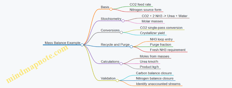
Example: Quick Spreadsheet-Style Calculation Flow
- Choose basis: 1,000 kg/h CO₂.
- Convert to kmol/h: 1,000/44.01 = 22.72.
- Reacted CO₂: 22.72 × 0.92 = 20.90.
- Urea kmol/h: 20.90.
- Urea kg/h: 20.90 × 60.06 = 1,255.
- Solid urea: 1,255 × 0.985 = 1,236.
- Fresh NH₃: compute loop NH₃ entry from excess assumption, then add consumption + purge.
- Close carbon and nitrogen balances to confirm no missing streams.
The workflow is systematic because it separates what is fixed by chemistry (stoichiometry) from what is fixed by operations (conversion, excess, purge, yield). Once those are set, the rest is arithmetic with accountability.
11. Circular Manufacturing Revenue Using Carbon-Based Inputs
11.1 Defining Circular Manufacturing Boundaries for Carbon-Based Materials and Products
Circular manufacturing boundaries answer one practical question: which flows count as “in” and which count as “out” for the carbon-based product you are selling. If you draw the boundary loosely, your numbers will look tidy and meaningless. If you draw it too tightly, you will spend months arguing about whether a valve is inside the system.
Start with the product definition. Pick a specific sellable item, such as “polycarbonate resin pellets,” “methanol,” or “formic acid.” Then define the functional unit you will use consistently across the boundary, such as 1 metric ton of product at specified purity and moisture. This prevents the classic mismatch where one team counts mass leaving the plant and another counts mass meeting a spec.
Next, define the system type. For carbon-to-product plants, boundaries usually include:
- The conversion process that turns captured carbon into intermediates and final products.
- The purification and separation steps that bring product quality to spec.
- The internal recycle loops that return unreacted carbon or solvents.
- The handling of co-products and by-products that leave the plant.
Then decide what to include for upstream and downstream. A boundary can be “gate-to-gate” (inside the plant fence) or “cradle-to-gate” (including upstream feed preparation and utilities sourcing). For circular revenue accounting, gate-to-gate is often the cleanest starting point because it ties directly to operational control. If you later extend the boundary, keep the original gate-to-gate definitions unchanged so you can compare results.
Now specify the carbon flow categories. Use three buckets and stick to them:
- Carbon input: captured CO₂ (and any additional carbon sources, such as purchased CO, biomass carbon, or purchased methanol used as a feed).
- Carbon retained: carbon that ends up in the product or in co-products you allocate to the product.
- Carbon released: carbon leaving as vented emissions, purge streams, waste streams, or off-spec material that is not recovered within the boundary.
Allocation is where boundaries become real. If your process produces multiple products, you must allocate carbon retained and energy use. A workable approach is to allocate by mass for physical co-products and by stoichiometric carbon content when products are chemically linked. For example, if a syngas-based unit produces both Fischer–Tropsch wax and light hydrocarbons, allocate carbon retained based on carbon atoms in each product fraction, not on revenue share.
Finally, define recovery rules for circularity. Circular manufacturing is not just “we recycle something.” It is “we recover a defined stream and reintroduce it within the boundary under defined quality constraints.” For instance, a solvent recycle loop counts as circular only if the recycled solvent meets the same impurity limits required for stable catalyst performance. If impurities accumulate and force a purge, that purge becomes a boundary loss unless you can demonstrate recovery of the purged carbon into another product stream.
Mind Map: Circular Manufacturing Boundaries
Example: Boundary Choice for Polycarbonate Resin
Suppose a plant converts captured CO₂ into a cyclic carbonate intermediate, then polymerizes it into polycarbonate pellets.
- Product boundary: 1 metric ton of polycarbonate pellets at a defined melt flow index and moisture limit.
- Included steps: carbonate synthesis, purification of carbonate feed, polymerization, pellet drying, and internal solvent recovery.
- Excluded steps: pellet packaging and customer use.
- Circularity rule: recycled solvent counts only if it meets impurity limits that prevent polymer discoloration.
- Carbon accounting: carbon retained includes carbon incorporated into polymer chains and any allocated co-products; carbon released includes vented CO₂ and carbon in waste streams that are not recovered within the boundary.
Example: Boundary Choice for Methanol-to-Fuels
For a methanol-to-fuels unit, boundaries must handle a common confusion: methanol can be both a product and a feed. If methanol is purchased and used as feed, it is an external carbon input. If methanol is produced on-site from captured CO₂ and then converted, it is internal and should not be double-counted as an input. The boundary should therefore be defined around the final sellable fuels or chemicals, with internal intermediates tracked as internal transfers.
A good boundary ends with measurable outputs. You should be able to compute carbon retained and carbon released per ton of product using plant data: stream compositions, measured purge rates, and product assay results. When those calculations are repeatable, circular manufacturing boundaries stop being a diagram and start being a working system.
11.2 Designing Product Portfolios Including Fuels, Chemicals, and Material Intermediates
A carbon-to-product plant rarely sells a single product. It sells a portfolio: fuels for volume, chemicals for margin, and material intermediates for stability and customer lock-in. Designing that portfolio is mostly about matching three things: (1) what your carbon and hydrogen streams can reliably become, (2) what your customers can reliably buy, and (3) what your plant can reliably produce across feed variability.
Start with Product Roles and Constraints
Treat each product as serving a role in the portfolio.
- Fuels provide throughput and straightforward specification targets (e.g., distillation cuts, oxygen content, sulfur limits). They tolerate some variability but punish off-spec batches.
- Chemicals often require tighter purity and consistent impurity profiles because downstream customers use them as inputs.
- Material intermediates can be more forgiving on volatility but strict on molecular weight distribution, residual catalysts, and color or ash.
A practical constraint check comes early: list the required specs, the tolerable impurity bands, and the required form (gas, liquid, solid, solution). Then map each spec to the unit operations you already plan: purification, drying, filtration, crystallization, and finishing steps.
Build a Portfolio Map from Conversion Pathways
Portfolio design should follow the conversion logic of the process, not the sales logic of the market. Start from your carbon conversion “spine” and then branch into product families.
- If your spine is CO₂ hydrogenation, you naturally get oxygenates and alcohol derivatives.
- If your spine is CO₂-to-syngas, you can reach hydrocarbons and a broader chemical slate.
- If your spine is carbonates or polymerizable intermediates, you focus on solid handling, impurity control, and consistent material properties.
A useful rule: every branch adds purification complexity. The portfolio that looks best on paper often loses money in the last 10% of specs.
Mind Map: Portfolio Design Logic
Choose a Base-Load, Flex, and Specialty Mix
A portfolio works when it can absorb variability without constant reconfiguration.
- Base-load product runs most hours and sets the plant’s steady-state operating window. Pick the product whose specs are easiest to maintain given your purification train.
- Flex product uses the same upstream conversion but different downstream finishing. It helps when feed composition shifts or when one customer’s demand pauses.
- Specialty product is smaller volume but higher value, and it justifies the extra purification steps. It should not require frequent catalyst changes or frequent shutdowns.
Example: Suppose your CO₂ stream sometimes carries trace sulfur. A fuel slate might tolerate minor sulfur after standard cleanup, while a chemical intermediate might require tighter sulfur control and additional polishing. In that case, the fuel becomes base-load, and the chemical becomes specialty with stricter acceptance criteria.
Translate Specs into a “Gate” Checklist
For each product, define the gates that must be passed.
- Upstream gate: feed conditioning and impurity removal performance.
- Conversion gate: reactor selectivity and conversion stability.
- Separation gate: fractionation or purification capability to meet composition.
- Finishing gate: drying, filtration, crystallization, and packaging requirements.
Example: For a carbonate intermediate, the upstream gate might focus on removing water and reactive impurities that cause foaming or side reactions. The finishing gate might focus on residual salts and moisture content because they affect downstream polymerization behavior.
Example Portfolio Design Using One Spine
Assume a CO₂-to-syngas spine feeding downstream synthesis.
- Base-load: a hydrocarbon fuel blend with defined distillation cuts and sulfur limits.
- Flex: a lighter chemical intermediate that shares the same syngas conditioning and separation train but uses a different downstream fractionation cut.
- Specialty: a higher-purity chemical feedstock requiring additional cleanup and tighter impurity control.
The integrated logic is simple: the syngas conditioning and major synthesis units run continuously, while the downstream finishing steps determine which product is produced that day.
Keep the Portfolio Honest with Operational Reality
Portfolio design must include operational rules that prevent “spec whiplash.” Define:
- sampling frequency and hold points,
- what triggers a switch between products,
- how off-spec material is reworked or blended,
- and which unit operations are allowed to vary without upsetting the rest of the plant.
If you cannot describe these rules clearly, the portfolio is not yet a portfolio—it’s a wish list with a process flow diagram.
11.3 Procurement and Contracting Requirements for Feedstock and Product Quality Assurance
Procurement for carbon-to-product plants is not just buying inputs; it is buying predictable chemistry. Contracts should therefore translate quality requirements into measurable acceptance criteria, define who owns sampling and analysis, and specify what happens when results drift. The goal is simple: the plant should know, before shipment, whether the feedstock will behave and whether the product will sell.
Foundational Quality Concepts for Contracts
Start with three definitions that prevent most disputes.
- Specification is the target limits for composition, impurities, and physical properties.
- Acceptance criteria are the test methods and thresholds used at receipt or at shipment.
- Quality assurance is the system that proves the specification is met, including sampling plans and traceability.
A practical example: if a CO₂ stream must meet a maximum sulfur level to protect catalysts, the contract should state both the sulfur limit and the method used to measure it, because different methods can yield different numbers even when the real sulfur content is the same.
Feedstock Procurement Requirements
Feedstock contracts should cover the full chain from delivery conditions to analytical proof.
1. Stream identity and continuity
- Require the supplier to declare the source and process history of the captured carbon stream.
- Specify allowable variability ranges for key components such as moisture, oxygen, nitrogen species, and trace contaminants.
Example: If the plant uses a drying step, the contract can still require a maximum inlet moisture, but it should also define the drying system’s design basis so the supplier’s variability does not force the plant into constant off-spec operation.
2. Sampling plan and custody
- Define who takes samples, how many, where they are taken, and how they are sealed.
- Require chain-of-custody documentation and retention samples for dispute resolution.
3. Test methods and calibration
- List the analytical methods, instrument requirements, and calibration frequency.
- Allow an agreed alternative method only if it is demonstrated to be equivalent.
4. Delivery conditions
- Specify pressure, temperature, and phase expectations for gases and liquids.
- For compressed CO₂, include limits on water content and oxygen to reduce corrosion and unwanted side reactions.
5. Nonconformance handling
- Define what constitutes nonconformance at receipt.
- Include remedies such as rework, blending allowances, price adjustments, or rejection.
A useful rule of thumb: if the plant can tolerate a deviation only after blending, the contract should state the blending rules and the resulting acceptance criteria for the blended feed.
Product Procurement Requirements for Sales and Offtake
Product contracts should ensure the buyer receives material that fits their process and regulatory needs.
1. Product specification by use case
- For fuels, specify distillation cuts, water content, sulfur, and density.
- For chemical intermediates, specify purity, reactive impurities, and inhibitor content.
Example: A carbonate-grade product may require tight limits on moisture and residual monomers because those affect polymerization behavior downstream. The contract should therefore treat moisture as a first-class specification, not a “nice to have.”
2. Measurement timing
- Define whether acceptance is based on shipment analysis, receipt analysis, or both.
- For products that change during storage, require stability testing and define maximum hold times.
3. Packaging, labeling, and traceability
- Require batch/lot traceability, labeling standards, and documentation that links production conditions to test results.
4. Dispute resolution
- Use a tiered approach: supplier analysis, then independent referee testing.
- Define who pays for referee testing and how results are averaged or treated.
Integrated Mind Map for Contracting and Quality Assurance
Mind Map: Procurement and Contracting Requirements
Example Contract Workflow for One Feedstock and One Product
Feedstock example: A supplier delivers compressed CO₂. The contract requires moisture below a defined limit, sulfur below a defined threshold, and oxygen below a defined ceiling. At receipt, the plant QA team samples using the agreed method, retains a sealed sample, and compares results to acceptance criteria. If sulfur is slightly high but within a defined blending allowance, the plant can blend with a compliant cylinder lot and then re-test the blended feed before starting the run.
Product example: The plant ships a chemical intermediate. The contract specifies purity and inhibitor limits, plus a maximum water content. Acceptance is based on shipment analysis and receipt analysis, with a defined maximum hold time before receipt testing. If the buyer’s receipt test fails, the contract triggers referee testing using the agreed method, and the remedy is either replacement or a price adjustment based on the measured deviation.
Practical Checklist for Procurement Teams
- Specifications are written as measurable limits, not descriptions.
- Every critical parameter has an agreed test method.
- Sampling plans are explicit and include custody and retention.
- Delivery conditions are stated for the physical form of the stream.
- Nonconformance actions are defined before the first shipment.
- Product acceptance timing matches how the material changes in storage.
- Traceability ties each lot to production conditions and test results.
When these elements are present, procurement becomes a controlled interface between chemistry and commerce—less guesswork, fewer surprises, and a lot more “we knew this would work” at commissioning.
11.4 Manufacturing Execution Including Batch Versus Continuous Operations and Traceability
Manufacturing execution is where plans become reality: recipes turn into batch records, control strategies turn into operating actions, and “we think it will work” turns into “here is what actually happened.” For carbon-to-product plants, execution also has a second job—making carbon flows auditable—so traceability can connect captured carbon inputs to product outputs without hand-waving.
Foundational Concepts for Execution
Execution starts with a clean separation of responsibilities:
- Production planning defines what to make, when, and in what quantities.
- Manufacturing execution records how it was made, including deviations.
- Quality management decides whether the output meets specifications and what to do with nonconforming material.
A practical way to keep this straight is to treat every run as a “story” with three anchors: inputs, process conditions, and outputs. If any anchor is missing, traceability becomes a scavenger hunt.
Batch Versus Continuous Operations
Batch and continuous execution differ in what you must record and how you structure traceability.
Batch execution is organized around discrete lots. You typically track:
- Batch identity: batch number, start/stop times, equipment used.
- Recipe and charges: amounts of purified feedstock, hydrogen, catalysts, solvents, and utilities where relevant.
- In-process checks: temperature profiles, pressure holds, sampling results.
- End-of-batch outcomes: yields, intermediate assay results, and final product test results.
Easy example: a methanol-to-olefins run. You charge methanol and run a defined contact time. If catalyst activity drops, the batch record shows the temperature adjustments and the resulting product distribution shift.
Continuous execution is organized around steady operation with time-based windows. You typically track:
- Line identity and operating mode: normal, reduced rate, start-up, shutdown.
- Time windows: for example, 15-minute or hourly reporting blocks.
- Online measurements: flow rates, temperatures, pressures, and key analyzer readings.
- Material attribution: which time window’s output belongs to which downstream lot.
Easy example: a CO₂ hydrogenation loop feeding a separation train. If the CO₂ purity dips for 30 minutes, the time-window record ties that dip to the downstream lot that was produced during the same interval.
A useful rule of thumb: batch execution emphasizes what was charged, while continuous execution emphasizes when conditions applied.
Traceability Design That Works in Real Plants
Traceability should be designed around the plant’s carbon-to-product logic, not around paperwork. A robust approach uses three layers.
- Physical traceability: equipment, lines, tanks, and transfer events.
- Analytical traceability: feedstock assays, intermediate specs, and final release tests.
- Process traceability: critical parameters and deviations.
To keep it systematic, define critical-to-quality attributes and map them to critical-to-process parameters. For instance, catalyst poisoning by sulfur compounds is a quality issue, so the execution system must record sulfur-relevant measurements and any impurity removal performance indicators.
Execution Data Model and Event Recording
Execution systems work best when they treat events as first-class objects. Common event types include:
- Start-up event with initial conditions and acceptance checks.
- Charge or transfer event with quantities and identities.
- Sampling event with sample ID, time, and method.
- Deviation event with cause category, impact assessment, and disposition.
- Release event linking test results to a product lot.
Integrated Example Workflow
Consider a carbonate production line that receives purified CO₂ and a mineral feed, then sends carbonate slurry to a packaging step.
- Batch mode: the carbonate reactor run is recorded as a lot. The execution record includes CO₂ assay at charge time, reactor temperature and residence time profile, and slurry viscosity checks.
- Continuous mode downstream: slurry is metered continuously into a dryer. The execution system attributes dryer output to time windows, then consolidates those windows into a packaged lot.
- Traceability outcome: if a packaged lot fails moisture spec, the deviation record points to the exact reactor lot and the exact dryer time windows, along with the relevant parameter trends.
This is the difference between “we think it happened” and “we can show what happened.”
Practical Controls That Prevent Traceability Gaps
Execution should include guardrails that catch missing or inconsistent data before release:
- Completeness checks: required assays and critical parameter coverage must exist for the lot.
- Consistency checks: transfer quantities must reconcile with tank level changes and mass balance inputs used for reporting.
- Deviation rules: define which deviations trigger hold-and-review versus which are within predefined operating envelopes.
A small but effective habit: require every deviation to state the affected lot(s) or time window(s). Without that, traceability becomes a maze with no exit.
Summary of Execution Choices
Batch execution is best when discrete recipes and discrete lots matter. Continuous execution is best when steady operation dominates and time-window attribution is reliable. Either way, traceability succeeds when execution records are structured around carbon-relevant inputs, critical process conditions, and unambiguous links from events to lots.
11.5 Practical Example Workflow for Building a Revenue Stack from Product Specs and Market Requirements
A revenue stack is a structured way to translate product specifications into monetizable value, then into a unit-level revenue number you can use in costing and decision-making. The workflow below starts with what the customer actually buys, then works backward to what your plant must deliver.
Step 1: Lock the Product Definition and Spec Sheet
Start with a single product “SKU” per revenue line item. Write down the measurable specs that control acceptance and price. For a circular carbon product, typical specs include purity, water content, impurity limits, physical form, and performance-related properties.
Example: You sell a carbonate intermediate as a liquid feedstock. Your spec sheet includes: moisture ≤ 0.10 wt%, total impurities ≤ 0.5 wt%, and viscosity range at 25°C. If your plant produces a solid, you either change the process or you add a conversion step; otherwise the revenue stack is built on the wrong product.
Step 2: Convert Market Requirements into Price Drivers
Market requirements usually map to price drivers. Create a “spec-to-value” table that links each spec to a customer impact.
Example mapping:
- Moisture: affects downstream drying energy and defect rate; tighter moisture earns a premium.
- Impurity: affects catalyst poisoning and batch rejection; higher impurity triggers discounts.
- Physical form: determines whether the customer needs additional handling; wrong form can eliminate the premium.
Keep the mapping grounded: if a spec is only a compliance threshold with no premium, treat it as a gate, not a driver.
Step 3: Build a Revenue Stack Template
A revenue stack typically has layers: base price, quality premiums/discounts, contract terms, and deductions. Use a consistent structure so different products can be compared.
Example template for one SKU:
- Base price for meeting the minimum grade
- Premium for each spec that beats the target band
- Discount for specs that miss the target band
- Deductions for off-spec frequency, rework, or freight/handling terms
- Net realized price after contract adjustments
Step 4: Create a Yield-to-Realization Bridge
Your plant produces distributions, not perfect points. Convert expected production quality into expected realized price.
Practical method:
- Define quality bands (e.g., Moisture: A ≤0.05%, B 0.05–0.10%, C >0.10%).
- Estimate probability of each band from historical data or pilot results.
- Multiply each band by its corresponding premium/discount.
Example: Moisture band probabilities are A 60%, B 35%, C 5%. If premium/discount is +$40/t for A, 0 for B, and -$120/t for C, then moisture contribution to net price is:
0.60×40 + 0.35×0 + 0.05×(-120) = +$12/t.
Step 5: Add Mass Balance and Accounting Boundaries
Revenue should align with how you measure product mass and carbon accounting boundaries. Decide whether you sell on net product mass, on dry basis, or after removal of entrained water.
Example: If the contract pays on “dry product,” then wet-basis production must be converted to dry mass using measured moisture. This conversion affects both revenue and unit economics.
Step 6: Assemble the Full Mind Map for the Workflow
Mind Map: Revenue Stack from Specs to Realized Price
Step 7: Run a Worked Example for One Revenue Line
Assume you sell a carbonate intermediate at 1,000 t/month.
- Base price: $650/t for minimum grade
- Moisture contribution: +$12/t (from Step 4)
- Impurity contribution: -$8/t (because 10% of batches fall into a discount band)
- Contract deduction: -$15/t for handling and documentation
Net realized price = 650 + 12 - 8 - 15 = $639/t.
Monthly revenue = 1,000 t × $639/t = $639,000.
Then convert to a carbon basis using your measured carbon content and accounting boundary. If the product contains 0.85 t CO2 equivalent per tonne product on the contract basis, revenue per tonne CO2 equivalent is $639 / 0.85 = $752/t CO2e.
Step 8: Validate with a “Spec Failure” Check
Before finalizing, test the stack against extreme but plausible outcomes: what happens if moisture drifts one band worse, or if impurity control improves but physical form is off? This check prevents building a revenue stack that assumes the plant can ignore the hardest spec.
Step 9: Produce Decision-Ready Outputs
Finish by generating three outputs for each SKU:
- Net realized price ($/t)
- Revenue per carbon unit ($/t CO2e)
- Sensitivity ranking showing which spec bands move revenue the most
That ranking becomes the bridge from market requirements back to process control priorities, so the revenue stack is not just a spreadsheet exercise—it’s a map of what the plant must reliably do.
12. Project Engineering and Commercialization for Carbon-to-Product Plants
12.1 Process Design Package Contents Including PFDs, P&IDs, and Material Compatibility
A solid process design package is the bridge between chemistry and hardware. It answers three questions in a consistent way: what the plant does (flows and reactions), how it does it (equipment and controls), and what it can survive (materials, corrosion, and cleaning).
Core Deliverables and Their Roles
A typical package starts with a Process Flow Diagram (PFD) that shows major equipment, stream directions, and the overall logic of conversion, separation, recycle, and purge. The PFD is where you confirm that the carbon ends up in the right place and that the hydrogen and utilities are balanced with reality.
Next comes the Piping and Instrumentation Diagram (P&ID), which turns the PFD into an operable system. It identifies line numbers, valves, pumps, compressors, instruments, control loops, interlocks, relief devices, and sampling points. If the PFD is the map, the P&ID is the route you can drive without guessing.
Finally, material compatibility documentation ensures the plant does not fail quietly. It ties together expected compositions, temperatures, pressures, water content, contaminants, and cleaning chemicals. For carbon-to-product systems, this matters because trace impurities in captured CO₂ streams can accelerate corrosion and catalyst poisoning.
Mind Map: Process Design Package
PFD Contents That Prevent Design Drift
A good PFD includes stream numbers that match the P&ID and a clear labeling convention for carbon-bearing streams. For example, CO₂ feed might be stream 101, conditioned CO₂ stream 201, reactor feed stream 301, and product-separated streams 401+.
Include at least one explicit recycle loop on the PFD with a purge point. In practice, recycle without purge is like reusing a coffee filter until it becomes a coffee filter-shaped problem. The purge rate should be shown as a function of inert buildup or water management.
Also show the utility tie-ins at a high level: steam generation or steam consumption, cooling duty, and power requirements for compression. Even if final utility sizing comes later, the PFD should already indicate where heat is gained or removed so the energy balance does not surprise you during commissioning.
P&ID Contents That Make Operations Possible
On the P&ID, every major line should have a line number and service description. A useful discipline is to group lines by phase and chemistry: dry CO₂ gas lines, wet gas lines, hydrogen-rich lines, solvent lines, and product lines. This makes it easier to apply correct insulation, tracing, and material rules.
Control loops should be visible and consistent with the PFD. For instance, if a reactor feed compressor is used to maintain reactor pressure, the P&ID should show the pressure controller, the control valve or speed control element, and the interlock logic that prevents operation outside safe limits.
Sampling points deserve special attention. If you need to verify CO₂ purity or impurity levels that affect catalysts, place sampling taps where mixing is representative and where the sample can be cooled and filtered without plugging. Label sample lines and show whether they are grab or online.
Safety devices must be mapped to credible scenarios. Relief valves and rupture disks should be connected to the correct disposal system, and the P&ID should show the basis for isolation valves so that emergency shutdown does not trap pressure in the wrong place.
Material Compatibility Documentation That Connects to Reality
Material compatibility is not a list of alloys; it is a set of service definitions. Start by defining each service on the P&ID: temperature range, pressure range, phase, and expected composition. Then add corrosion drivers such as water content, oxygen ingress risk, sulfur species, chlorides, and any solvent carryover.
A practical example: if a CO₂ conditioning section includes drying, the downstream “dry CO₂” service should be treated differently from “wet CO₂” service. If a dryer fails or regenerates imperfectly, water can reappear and change corrosion behavior. Your documentation should reflect that by specifying acceptance criteria for dryness and by identifying which lines are sensitive to water-driven corrosion.
Weld and fabrication details matter too. Many failures start at interfaces: dissimilar metal welds, crevices, and areas with poor drainage. Include notes on weld procedures, inspection requirements, and whether passivation or coating systems are required after fabrication.
Example: Minimal Package Traceability
To keep the package coherent, ensure each PFD stream has a corresponding P&ID line set, and each equipment tag on the PFD has a matching tag on the P&ID. Then link each equipment tag to a material service definition.
Example mapping:
- PFD stream 201 “Conditioned CO₂” → P&ID line 201A “Dry CO₂ to Reactor Feed Header”
- Reactor tag R-301 on PFD → P&ID tag R-301 with instrument loops for inlet temperature and pressure
- Reactor internals material note → material compatibility entry “R-301 service: hydrogenated gas, trace sulfur, controlled water content”
This traceability prevents the classic problem where the PFD says “dry,” the P&ID says “wet,” and the material spec says “should be fine.”
12.2 Safety and Risk Controls Including Pressure Systems and Reactive Chemical Handling
Carbon-to-product plants often run with high-pressure equipment and reactive chemistries, even when the “headline” reaction looks straightforward. Safety controls must therefore start with how pressure and reactivity actually behave in hardware, not just how the chemistry behaves on paper.
Foundational Risk Logic for Pressure and Reactivity
Begin with two linked questions: (1) what energy is stored, and (2) what can release it unexpectedly. Pressure systems store mechanical energy in compressed gases and pressurized liquids; reactive chemical handling stores chemical potential energy in unstable mixtures, reactive intermediates, or incompatible combinations.
A practical way to structure the hazard review is to map each unit operation to three layers of control:
- Prevent abnormal conditions (good design, correct operating envelopes, reliable utilities).
- Detect deviations early (alarms, interlocks, sampling discipline).
- Mitigate consequences (relief devices, containment, safe venting, emergency shutdown).
This layering keeps the team from relying on any single “hero” control.
Pressure Systems Controls That Actually Matter
Pressure safety is not only about relief valves; it is about ensuring the system can’t be driven beyond safe limits.
1. Design basis and operating envelope. Define maximum allowable working pressure (MAWP), setpoints, and credible blocked-in scenarios. For example, if a line can be isolated between two valves and heated by steam tracing, the “blocked-in” case must be included even if the normal flow path is open.
2. Relief system sizing and discharge routing. Relief devices must be sized for the credible worst case, not the average case. Discharge routing should prevent backpressure from defeating the relief function. A common example is routing relief to a header without checking that the header pressure can rise during simultaneous events.
3. Isolation and venting strategy. Use valve arrangements that avoid trapping pressure in dead legs. Where trapping is unavoidable, provide engineered venting or thermal relief paths. For instance, a condensate trap upstream of a heat exchanger can create a “pocket” if downstream valves close during a trip.
4. Materials compatibility and corrosion allowance. Carbon-to-product service can include wet CO₂, oxygenated species, sulfur traces, and amines. Corrosion can reduce thickness and change relief performance. A simple example: if a relief valve is installed in a line that corrodes faster than expected, the valve may still open, but the piping may not survive the event.
5. Instrumentation and interlocks. Pressure transmitters should be placed where they represent the actual risk point. Interlocks must be tied to safe states, such as stopping feed pumps, closing isolation valves, and depressurizing to a controlled system.
Reactive Chemical Handling Controls with Clear Boundaries
Reactive hazards often come from mixing, temperature rise, and contamination.
1. Incompatibility management. Maintain strict segregation of oxidizers, reducing agents, acids, bases, and reactive solvents. Example: if a CO₂ hydrogenation loop uses a catalyst bed that is sensitive to oxygen, oxygen ingress during maintenance can create an exotherm. The control is not just “be careful”; it is procedural isolation plus verified purge and oxygen monitoring.
2. Temperature control and heat removal assurance. Many reactions have strong temperature sensitivity. Controls should include redundant temperature measurement and a defined heat removal path. Example: if a reactor relies on cooling water, the safety case should address what happens when cooling water flow drops—do you trip feeds, open a quench path, or route to a safe hold tank?
3. Mixing and addition sequencing. Addition order can determine whether a reaction stays controlled or runs away. Example: when preparing a reactive solution, adding reagent A into reagent B can be safe, while adding B into A can create local high concentration zones that trigger rapid heat generation.
4. Purge, inerting, and ignition control. For systems that must be oxygen-free or moisture-controlled, define purge targets and verification steps. Example: before introducing hydrogen, verify inert gas oxygen levels and confirm purge effectiveness using sampling points that represent the reactor volume, not just the inlet.
5. Sampling and maintenance safety. Sampling ports and maintenance blinds can become hazard points. Example: opening a sample valve on a pressurized line without confirming pressure relief status can expose personnel to jetting or flash release.
Mind Map: Safety Controls for Pressure and Reactivity
Integrated Example: Hydrogenation Loop Trip and Relief Behavior
Consider a CO₂ hydrogenation loop with a catalyst bed, high-pressure feed lines, and a heat exchanger for temperature control. A credible scenario is a trip that closes feed isolation valves while the line between valves remains heated by hot recycle.
A coherent safety response includes:
- Prevention: design the line so it cannot trap pressure when valves close, or provide a controlled vent path.
- Detection: pressure and temperature alarms tied to the reactor inlet and bed outlet.
- Mitigation: relief devices sized for blocked-in heating, with discharge to a flare or closed recovery system that can handle the expected composition.
- Reactive handling: ensure hydrogen introduction is blocked unless inerting verification is complete, and ensure oxygen ingress is prevented during maintenance by procedural isolation and monitoring.
When these elements are consistent, the plant behaves predictably: the trip stops the energy input, the relief system handles the stored energy, and the reactive chemistry stays within controlled boundaries.
12.3 Commissioning and Performance Testing Including Acceptance Criteria and Data Capture
Commissioning turns a design into a behaving plant. The goal is not just to “run,” but to prove that each system performs within defined limits under realistic operating conditions. A good commissioning plan starts with what must be true at handover, then works backward to test steps, instrumentation, and data capture.
Commissioning Foundations and Readiness Checks
Begin with readiness criteria that are measurable. Typical readiness items include mechanical completion, instrument calibration status, loop checks, safety system functional tests, and clean utility supply. For example, if a hydrogenation unit depends on stable hydrogen pressure, verify the hydrogen header pressure control loop is tuned and that relief devices are verified.
Next, define the commissioning boundary: which systems are tested together and which are tested in isolation. A common mistake is testing a reactor while the downstream separation train is still in “construction mode,” which makes it impossible to interpret yields.
Acceptance Criteria That Match Real Operations
Acceptance criteria should be tied to product and process outcomes, not only to equipment status. Use three layers:
- Functional acceptance: equipment responds correctly. Example: a valve reaches commanded position within a specified time and without oscillation.
- Performance acceptance: process variables stay within limits. Example: during a steady run, reactor inlet temperature remains within ±2 °C and pressure within ±1%.
- Quality acceptance: product meets specification. Example: methanol product purity meets a defined impurity threshold, and offgas composition stays within limits that protect downstream catalysts.
A practical approach is to define acceptance windows for each critical parameter and link them to the control strategy. If the control strategy uses cascade control, acceptance should include both primary and secondary loop behavior.
Test Phasing from Cold Checks to Integrated Runs
Commissioning is easiest to manage when it is phased. A systematic sequence reduces rework and makes troubleshooting faster.
- Phase 1: Static verification. Confirm drawings match installed equipment: tag mapping, line numbers, insulation coverage, and material compatibility. Example: verify that CO₂ service lines use the intended gasket material before any pressure test.
- Phase 2: Dynamic loop checks. Validate sensors and actuators. Example: run a flow loop through a range and confirm linearity and deadband.
- Phase 3: System energization and utilities. Confirm steam, cooling water, power quality, and instrument air. Example: check that steam condensate return is functioning so heat exchangers do not drift.
- Phase 4: Single-train operation. Operate one process train end-to-end at low severity. Example: run a syngas cleanup train with inert gas first, then with controlled reactive gas.
- Phase 5: Integrated steady-state performance. Run at target operating conditions long enough to reach stable behavior. Example: define a minimum duration based on residence time and catalyst stabilization needs.
Data Capture That Enables Decisions
Data capture is not “logging everything.” It is capturing the minimum set that proves performance and supports root-cause analysis.
Define a data dictionary before testing: tag name, units, sampling interval, scaling method, and data validation rules. Ensure timestamps are synchronized across systems so mass balance calculations are meaningful.
Include both process and context data:
- Process: flows, pressures, temperatures, compositions, and control outputs.
- Context: setpoints, mode changes, alarms, maintenance actions, and any deviations.
For example, if a catalyst bed shows lower conversion during a run, you need to know whether a temperature controller was in manual for 12 minutes.
Mind Map: Commissioning and Performance Testing
Example: Acceptance Criteria and Evidence Package
Suppose the plant must demonstrate carbon-to-fuel conversion in a hydrogenation unit. Define acceptance evidence as follows:
- Reactor performance: conversion target achieved within a specified range, with inlet temperature and pressure within windows.
- Selectivity: product distribution meets defined cutoffs for undesired by-products.
- Operational stability: no sustained oscillations in key control loops; alarm count below a defined threshold.
- Quality: final product meets purity and impurity limits.
Evidence should include run sheets, trend exports, calibration certificates, and a mass balance summary that uses the captured data. If the mass balance does not close, the acceptance decision should explicitly state whether the discrepancy is due to measurement uncertainty, sampling error, or process deviation.
Example: Data Capture Rules That Prevent Confusion
During a steady-state run, record compositions at a fixed cadence and tie them to sampling events. If a gas analyzer requires warm-up, capture the warm-up period as a separate segment so it does not contaminate the steady-state averages. Also record any purge or recycle valve position changes; otherwise, the plant may look “stable” while the carbon routing quietly changes.
Diagram: Commissioning Flow with Acceptance Gates
    flowchart TD
  A[Readiness Checks] --> B[Static Verification]
  B --> C[Dynamic Loop Checks]
  C --> D[Utilities Energization]
  D --> E[Single-Train Low Severity Run]
  E --> F{Acceptance Gate}
  F -- Pass --> G[Integrated Steady-State Run]
  F -- Fail --> H[Troubleshoot and Re-test]
  G --> I{Final Acceptance Gate}
  H --> C
  I -- Pass --> J[Handover Package]
  I -- Fail --> H
A commissioning program succeeds when acceptance criteria, test phasing, and data capture are designed together. When they are aligned, the evidence package answers the only question that matters at handover: did the plant do what it was built to do, under defined conditions, with traceable measurements?
12.4 Costing and Economic Modeling Using Bottom Up Unit Operations and Yield Assumptions
Bottom-up costing starts with unit operations, not with a single “plant cost number.” You estimate each equipment block, compute mass and energy flows using yield assumptions, then roll everything up into a costed product slate. The trick is to keep the accounting consistent: the same assumptions that drive yields must also drive utilities, consumables, waste handling, and credits.
Mind Map: Bottom Up Costing Flow
Step 1: Define the Modeling Boundary and Reporting Basis
Start by writing down what “one unit of product” means. For example, choose a basis such as “1 metric ton of finished methanol meeting spec” or “1 metric ton of polymer-grade polycarbonate pellets.” Then list battery limits: where the captured CO₂ enters, where hydrogen enters, where utilities connect, and where product exits. This prevents the classic mismatch where yields are calculated on a different basis than costs.
A practical rule: if a loss affects product mass, it must also affect cost. If it only affects composition, it may affect purification energy and waste volumes.
Step 2: Translate Yield Assumptions into Flow Rates
Bottom-up economics depends on yield assumptions that are explicit and measurable. Use four categories.
-
Conversion and selectivity: In CO₂ hydrogenation, conversion might be 70% per pass and selectivity to methanol might be 95% of converted carbon. That means 0.70 × 0.95 = 0.665 of carbon ends up as methanol carbon per pass, before considering separation.
-
Separation recoveries: If distillation recovers 99.5% of methanol from the overhead and bottoms, the remaining 0.5% becomes off-spec losses or goes to a recycle stream with its own purge.
-
Purge and vent losses: Gas loops often require purge to control inerts. If purge is 2% of loop gas flow, it becomes a direct carbon loss unless the purge is routed to a utilization step.
-
Catalyst life and regeneration: Catalyst replacement is a cost, but also a yield factor if regeneration causes temporary downtime or activity loss. Model catalyst activity as an effective reduction in conversion over time, then convert that into additional feed and utilities.
Example: Suppose you need 1,000 kg/day of finished product. If overall carbon yield to product is 0.80, you must feed 1,250 kg/day of carbon-equivalent reactant (after accounting for stoichiometric differences). That higher feed rate automatically increases compression, conditioning, and reactor throughput sizing.
Step 3: Estimate Capital Cost by Unit Operation
For each unit operation, estimate equipment purchase cost, then apply installation factors for piping, structural steel, electrical, and instrumentation. Keep the level of detail consistent: if you model a reactor with detailed internals, do the same for separators that dominate pressure drop and energy use.
A useful accounting habit is to separate process equipment from utilities equipment. Utilities often scale with duty (kW, MW, steam ton/hr), while process equipment scales with throughput and pressure. Mixing these can hide the real drivers.
Step 4: Estimate Operating Cost with Yield-Driven Consumptions
Operating cost should be computed from the same flow model used for yields.
- Feedstock: Multiply required feed rate by unit price. If product quality requires additional conditioning, include reagent and disposal.
- Utilities: Use heat duties from the unit model. A small yield loss can increase recycle flow, which increases compression power and cooling duty.
- Waste treatment: Off-spec streams and purge streams create disposal costs. If a purge contains valuable carbon, include a credit only if it is actually recovered.
- Maintenance and catalyst: Maintenance can be approximated as a fraction of installed equipment cost, but catalyst replacement should be tied to modeled activity loss and replacement interval.
Example: If separation recovery drops from 99.5% to 99.0%, the 0.5% extra loss might look small on paper, but it increases both product rework and waste. In a tight spec product, that can dominate operating cost.
Step 5: Roll Up to Economics and Do Sensitivity Without Guessing
Compute annualized capital using a chosen basis (e.g., straight-line depreciation or capital charge rate) and add operating costs. Revenue comes from product quantity times price, adjusted for quality penalties.
Then run sensitivity on the few parameters that actually move the numbers: overall yield, separation recovery, purge fraction, and catalyst life. Keep the rest fixed so you can attribute changes.
A sanity check: if a sensitivity changes product mass but your cost model doesn’t change feed and utilities accordingly, the model is inconsistent. Fix the flow-to-cost linkage before interpreting results.
Step 6: Reconcile Mass Balance with Cost Balance
Before finalizing, verify three reconciliations.
- Carbon balance: captured carbon in equals carbon in products plus carbon in purge/vent plus carbon in waste plus carbon in inventories.
- Energy balance: reactor and separation duties match utility consumption.
- Cost balance: every stream that appears in the mass balance must have a cost or credit pathway.
When these three agree, the bottom-up model becomes a tool rather than a spreadsheet with opinions. It will still be wrong sometimes, but it will be wrong in a traceable way—usually the best kind of wrong.
12.5 Practical Example Workflow for From-Design-Basis to Unit Economics and Production Readiness
This workflow shows how a carbon-to-product project moves from design basis assumptions to a unit economics model that is actually usable during commissioning. The example uses a CO₂ hydrogenation-to-oxygenates plant concept, but the steps apply to fuels, syngas, and materials.
Step 1: Lock the Design Basis Inputs
Start by writing a one-page design basis that includes:
- Feedstock specs: CO₂ purity, moisture, oxygen, sulfur, and inert fraction.
- Hydrogen spec: purity and allowable contaminants that poison catalysts.
- Product specs: purity target, water content, and any impurity limits that affect downstream blending.
- Operating mode: continuous vs. batch, target on-stream factor, and planned turnaround window.
- Utilities assumptions: steam pressure levels, cooling water temperature range, and power demand basis.
Example: If CO₂ moisture is specified as 50 ppmv max but your capture system occasionally spikes to 200 ppmv, you must decide whether to add extra drying capacity or treat spikes as a yield loss event. Either choice must be reflected in the economics.
Step 2: Convert Assumptions into Unit Operation Material and Energy Balances
Build a simple mass balance first, then add energy and separation duties.
- Create a “carbon ledger” that tracks CO₂ in, carbon in intermediates, and carbon in final products.
- Create a “hydrogen ledger” that tracks H₂ consumption and purge losses.
- Add separation efficiencies as explicit numbers, not vague statements.
Example: Suppose the reactor conversion is 20% per pass with a recycle loop. If purge is 2% of recycle flow to prevent inert buildup, your net conversion and hydrogen efficiency depend on purge rate. Put those numbers in the balance so the economics model doesn’t guess.
Step 3: Translate Balances into a Costed Process Model
Unit economics needs three layers:
- Variable costs tied to throughput: feedstock, hydrogen, utilities, catalysts makeup, and consumables.
- Semi-variable costs tied to operating time: maintenance labor, planned inspection, and waste handling.
- Fixed costs tied to capacity: staffing, overhead, property-related costs, and insurance.
Example: If catalyst life is estimated as 18 months at design conditions, convert that into an annual catalyst replacement mass and a downtime allowance. If the plant runs at 85% on-stream factor, the effective catalyst replacement schedule changes.
Step 4: Build the Revenue Model from Product Slate and Quality
Revenue should be computed from product quantities that meet specs.
- Define product slate: primary product plus any credits for co-products.
- Apply quality-based yield: if off-spec material is downgraded, model the downgrade explicitly.
- Include packaging or blending losses if they affect net saleable volume.
Example: If methanol-like oxygenates are sold with a 0.1 wt% water limit, and your separation train achieves 99.2% water removal at steady state but drops to 98.5% during startup, you must decide whether startup losses are treated as normal operating losses or as a separate startup event.
Step 5: Create a Commissioning-Ready Performance Map
Production readiness means the model can be tested against measured data.
- Define acceptance criteria for key performance indicators: conversion, selectivity, recycle purge rate, compressor efficiency, and separation recoveries.
- Define measurement points and sampling frequency.
- Define how you will update the model after each commissioning milestone.
Example: Set an acceptance criterion for CO₂ conversion based on measured inlet composition and outlet product composition. If the measured conversion is 2 percentage points lower than design, the model should immediately show the impact on hydrogen consumption and net product rate.
Step 6: Run a “From-Basis to Economics” Consistency Check
Before finalizing unit economics, verify internal consistency:
- Carbon balance closure within a defined tolerance.
- Energy balance closure within a defined tolerance.
- Throughput basis matches the capacity basis used in fixed cost allocation.
- Purge and recycle assumptions match the compressor and flare duty assumptions.
Example: A common failure mode is using a purge rate from the process simulation but forgetting to update flare duty and waste gas handling costs. The consistency check catches this.
Step 7: Document the Decision Trail for Readiness
Write down what is “locked” and what is “tunable” during commissioning.
- Locked: feed specs, product specs, major equipment sizing basis.
- Tunable: setpoints, recycle ratios, catalyst activation procedure, and control tuning.
- Define who approves changes and how changes flow into the economics model.
Mind Map: From Design Basis to Unit Economics and Readiness
- Design Basis
- Feed specs
- Hydrogen specs
- Product specs
- Operating mode
- Utilities basis
- Process Modeling
- Mass balance
- Carbon ledger
- Hydrogen ledger
- Energy balance
- Separation efficiencies
- Recycle and purge
- Mass balance
- Economics Model
- Variable costs
- CO2
- H2
- Utilities
- Catalyst makeup
- Semi-variable costs
- Maintenance
- Waste handling
- Fixed costs
- Staffing and overhead
- Variable costs
- Revenue Model
- Product slate
- Quality-based yield
- Co-product credits
- Commissioning Readiness
- KPI acceptance criteria
- Sampling and measurement plan
- Model update rules
- Consistency Checks
- Balance closure
- Duty and cost alignment
- Throughput basis alignment
- Documentation
- Locked vs tunable parameters
- Approval and change control
Mini Example Workflow in One Pass
- CO₂ purity: 95 mol% with 0.5 mol% O₂ max; decide on impurity removal duty.
- Reactor: conversion and selectivity at design temperature; include recycle purge.
- Separations: water removal and product recovery efficiencies.
- Costs: compute net product rate, then multiply by variable costs per unit.
- Revenue: apply spec-based yield and saleable volume.
- Readiness: define KPIs and acceptance criteria tied to the same calculations used in economics.
Step 8: Finalize Unit Economics with a Commissioning Adjustment Factor
Use a commissioning adjustment factor that reflects measured performance uncertainty without inventing new physics.
- Start with a conservative factor for startup and early operation.
- Replace it with measured values once acceptance criteria are met.
Example: If early operation typically shows 1–3% lower selectivity due to control tuning, model that as a temporary adjustment tied to selectivity KPI results, not as a permanent assumption.
By the end of this workflow, the unit economics model is not just a spreadsheet with numbers; it is a set of traceable calculations that can be verified during commissioning and updated using the same KPIs that define production readiness.