Counter-Drone Microwave Defense
1. Mission Requirements for Counter-Drone Microwave Systems
1.1 Defining Protected Assets and Operational Constraints
Start by naming what you are protecting in plain terms. For critical infrastructure, “protected asset” usually means a physical location, a function, or both: a substation that must stay energized, a control center that must remain reachable, or a communications tower that must keep links stable. Your first job is to translate that into measurable boundaries and acceptable outcomes.
Protected Asset Definition
A good protected-asset statement has three parts.
- Asset scope: what exactly is included. Example: “Transformer yard and associated switchgear at Site A,” not “the whole site.”
- Required function: what must continue to work. Example: “Maintain power delivery to feeder circuits within normal operating limits.”
- Acceptable disruption: what can change without unacceptable impact. Example: “Temporary loss of non-critical auxiliary loads is acceptable for up to 30 minutes; loss of feeder delivery is not.”
To keep the scope from drifting during design, record a short “asset boundary rule.” Example: if the microwave system’s beam can reach beyond the fence line, then the protected boundary is not the fence; it is the region where effects are permitted.
Operational Constraints
Operational constraints are the guardrails that determine when and how the system may operate. They come from safety, legal requirements, engineering limits, and day-to-day operations.
Safety and Exposure Limits
You need a constraint set that ties electromagnetic exposure to operational states. A practical approach is to define three states:
- Standby: sensors active, transmitters inhibited.
- Armed: transmitters enabled only when interlocks confirm safe conditions.
- Engaged: transmitters active under a specific waveform and aiming plan.
Example: if a maintenance crew is working near a mast, the system must remain in Standby even if a drone is detected. That means your interlocks must be able to override detection cues.
Environmental and Site Constraints
Microwave performance depends on the site. Obstacles, ground reflectivity, and weather can change where energy goes. Operational constraints should therefore include:
- Weather gating: define conditions where operation is allowed, such as wind limits that affect antenna pointing stability.
- Obstacle gating: define “no-go” aiming sectors where reflections could violate exposure boundaries.
- Power and cooling limits: define maximum duty cycle and thermal thresholds.
Example: if the cooling system can sustain only a 10-minute continuous run, then the operational constraint is not “engage whenever needed,” but “engage with a duty cycle that keeps junction temperatures below the configured limit.”
Engagement Constraints
Engagement constraints connect the protected asset to the engagement method.
- Target eligibility: what counts as a valid threat for engagement. Example: only drones within a defined range and altitude band.
- Aim constraints: where the beam may point. Example: exclude angles that would direct energy toward occupied buildings.
- Timing constraints: how long the system may transmit per engagement. Example: cap per-burst duration and enforce a minimum cool-down.
Example: if the system requires stable tracking for 0.5 seconds before firing, then the operational constraint is “no engagement until tracking confidence is met,” not “fire immediately on detection.”
Mind Map: Protected Assets and Constraints
Constraint Matrix Example
A constraint matrix turns the narrative into something engineers and operators can use.
- Zone A (inside fence line): Engaged allowed when interlocks confirm no personnel present; burst duration up to 2 seconds; cool-down 10 seconds.
- Zone B (near control building): Engaged prohibited if any access sensor indicates occupancy; aiming restricted to a sector that avoids direct line-of-sight toward windows.
- Zone C (public-facing perimeter): Engaged allowed only in Standby-to-Armed transitions with verified boundary conditions; if tracking confidence drops below threshold, system returns to Standby.
This matrix becomes the reference point for later chapters on hardware limits, waveform choices, and testing. If a requirement cannot be expressed as a condition and an outcome, it is not yet a constraint—it is a wish.
Practical Example: From Asset to Rules
Suppose the protected asset is a communications tower that must keep service. The required function is “maintain link availability.” Acceptable disruption might be “brief outages under 60 seconds are tolerable.” From there, you set operational constraints: transmit only when the beam can be aimed away from the tower’s service equipment area, enforce a maximum duty cycle that prevents thermal stress, and require interlocks that keep the system in Standby during scheduled maintenance. The result is a system that can respond to threats without turning the site into its own casualty.
1.2 Threat Characterization Using Measurable Drone Parameters
Threat characterization starts with measurable drone parameters, because “it’s a drone” is not actionable. The goal is to translate observable facts into engineering inputs: what frequencies matter, how much time you have to react, and what level of RF energy is likely to disrupt the target’s electronics.
Core Measurable Parameters
Begin with a short list of parameters you can measure repeatedly, not just once. A practical set includes:
- Airframe and size class: approximate rotor diameter, wingspan, or overall length. This influences radar cross-section and how the drone moves through the beam.
- Motion profile: typical speed, turn rate, and altitude band. These determine tracking stability requirements and dwell time.
- Navigation and control behavior: hovering tendency, loiter patterns, and response latency to operator commands.
- RF emissions: presence and strength of telemetry, control links, and any onboard radios that leak energy.
- Operating frequency bands: which bands show activity during the mission phase.
- Modulation and bandwidth: how wide the signal is and how it changes with distance or data rate.
- Duty cycle: how often transmissions occur and whether they are bursty.
- Antenna orientation effects: whether the drone’s antenna pattern changes noticeably as it yaws.
A useful mindset is to treat each parameter as a knob in your system model. If you can’t map it to a knob, you probably can’t use it for design or test.
Measurement Workflow That Stays Grounded
- Collect time-aligned observations: record sensor outputs with timestamps so you can correlate motion with RF activity.
- Segment the mission into phases: approach, loiter, and retreat often have different RF behavior.
- Estimate kinematics from tracking: compute speed and turn rate from successive position estimates.
- Extract RF features from spectra: identify active bands, estimate bandwidth, and measure burst timing.
- Quantify uncertainty: report ranges, not single values, because real measurements wobble.
A small example: if a drone loiters at 30–40 m altitude and shows bursty transmissions every 120–180 ms, your system timing and waveform selection should respect that cadence rather than assuming continuous emissions.
Mapping Parameters to Defense-Relevant Requirements
Once you have parameters, convert them into requirements your microwave system can use.
- Range and dwell time: motion profile and altitude determine how long the target stays within effective beam coverage.
- Beam pointing tolerance: fast turn rate and yaw changes increase pointing error, so you need a tracking-to-aim stability budget.
- Frequency planning: RF emissions and bandwidth tell you which frequencies are likely to couple into the drone’s receiver or control electronics.
- Waveform duty cycle constraints: burst timing and transmission duty cycle affect how often the drone is “listening,” which matters for repeatable disruption.
- Exposure boundary planning: size class and typical altitude help estimate where the target can be located relative to safety limits.
Mind Map: Threat Characterization Inputs and Outputs
Example: Turning Observations into a Parameter Set
Assume a site sensor suite reports the following during a loiter phase on 2026-03-07:
- Speed: 3–6 m/s with occasional 90° turns
- Altitude: 25–35 m
- RF activity: two bands centered at 2.4 GHz and 5.2 GHz
- Bandwidth: ~20 MHz around each center
- Duty cycle: bursts lasting 10–30 ms, repeating every 150 ms
- Orientation effect: signal strength varies by up to 8 dB as the drone yaws
From this, you can set a tracking stability target that accounts for the turn rate, plan frequency coverage across both bands, and choose a waveform timing strategy that aligns with the burst cadence. The 8 dB orientation swing becomes a coupling uncertainty term in your test acceptance criteria.
Quality Checks That Prevent Bad Inputs
Before using parameters in system design, verify three things:
- Consistency across phases: if frequency activity appears only during approach, don’t treat it as universal.
- Sensor agreement: compare RF measurements from different antennas or positions to catch local artifacts.
- Plausibility with motion: if RF bursts are “steady” while the drone is clearly maneuvering, re-check timestamps and tracking association.
When threat characterization is done this way, the rest of the book has solid ground to stand on: detection cueing, waveform selection, and safety engineering all start from the same measurable facts.
1.3 Performance Metrics for Detection Tracking and Neutralization
Performance metrics should answer three practical questions: “Can we see it?”, “Can we aim at it?”, and “Can we stop it safely and reliably?”. Good metrics also separate what the system does well from what the site conditions do to it, so you can improve the right thing.
Detection Metrics That Reflect Real Operating Conditions
Start with detection metrics that measure probability and timing, not just raw sensor range.
- Probability of Detection (Pd): Pd is the fraction of drone events correctly detected under defined conditions. Example: at a fixed range and altitude, run 100 controlled passes and count detections that exceed your detection threshold.
- False Alarm Rate (FAR): FAR is how often you trigger on non-drone events. Example: log detections during “no-drone” windows and compute alarms per hour.
- Detection Latency: latency is the time from the first observable cue to the first trackable detection. Example: if the sensor reports a detection at t=0.35 s after the drone enters the gate, that latency must fit your tracking and engagement timing.
- Track Initiation Time: track initiation is when the system transitions from detections to a stable track. Example: require three consistent detections within a time window; measure how long it takes.
A useful best practice is to report Pd and FAR together as an operating point. If you tune thresholds to raise Pd but FAR doubles, your cueing logic will spend time chasing ghosts.
Tracking Metrics That Measure Aim-Point Quality
Tracking metrics should focus on the error that matters for beam pointing and timing.
- Position Error (RMS and Percentiles): compute RMS error in azimuth/elevation or cross-range/along-range coordinates. Example: if RMS pointing error is 0.3° but the 95th percentile is 1.2°, your worst-case beam commands will be off more often than you expect.
- Track Stability: stability measures how often the track jumps between hypotheses. Example: count “track breaks” when the filter’s innovation exceeds a threshold for N consecutive updates.
- Update Rate and Jitter: tracking needs consistent timing. Example: if your control loop expects 50 Hz updates but you sometimes deliver 20 Hz bursts, the filter will appear “accurate” in logs yet fail in the field.
- Latency From Track To Command: measure end-to-end time from the moment the track is declared to the moment the beam steering command is issued.
A practical integration rule: track metrics must be expressed in the same coordinate system used by the beam steering controller. If one team reports meters at 200 m and another reports degrees at boresight, you’ll argue about numbers instead of fixing them.
Neutralization Metrics That Tie RF Output to Effect
Neutralization metrics should connect RF parameters to the observed effect on the drone’s relevant electronics.
- Effect Probability (Pe): Pe is the fraction of engagements that produce the intended effect, such as loss of command link or loss of navigation stability, within a defined observation window. Example: for each engagement, label success when the drone’s telemetry indicates link loss for at least 2 seconds.
- Time To Effect: time from transmit start to the first measurable effect. Example: if your system takes 0.8 s to reach the required field conditions, your engagement window must be long enough.
- Minimum Effective Range: the shortest range where Pe meets your threshold. Example: at 150 m you get 90% success; at 120 m you might still succeed but with different thermal and safety constraints.
- Energy Delivered Per Attempt: track delivered energy (integrated power over time) rather than only peak power. Example: two waveforms with the same peak can differ in delivered energy due to duty cycle and ramping.
- Safety Margin Metrics: include maximum allowed exposure compliance margin and interlock response time. Example: if the interlock trips in 30 ms but your waveform is 200 ms, your “effective” neutralization may be limited by safety behavior.
Metrics That Support Decision Logic
Neutralization is only as good as the decision logic that chooses when to transmit.
- Engagement Readiness Rate: fraction of time the system is in a state where it can safely and correctly engage. Example: log how often cooling, interlocks, and beam calibration status permit transmission.
- Cue-to-Engage Success Rate: fraction of cue events that lead to a successful neutralization. Example: if cueing is accurate but engagement readiness is low, the system will look “bad” even with good sensing.
- Reacquisition Rate: fraction of times the system regains a stable track after a temporary loss. Example: if the drone crosses behind a structure, measure how quickly the track returns.
Mind Map: Performance Metrics
Example Metric Set for a Single Site Trial
Assume you define an operating gate: drone enters at 200 m slant range, altitude 60 m, speed 8 m/s.
- Detection: Pd = 0.92, FAR = 0.03 alarms/hour, detection latency median 0.25 s.
- Tracking: RMS pointing error 0.35°, 95th percentile 1.1°, track-to-command latency 0.18 s with <5 ms jitter.
- Neutralization: Pe = 0.85 within a 3 s observation window, time to effect median 1.1 s, minimum effective range 170 m.
- Safety: interlock response time 25 ms, and measured exposure compliance margin stays above the configured limit for all successful engagements.
This set is coherent because each metric feeds the next: detection latency constrains track initiation, track error constrains beam pointing, and beam pointing plus waveform timing constrains time to effect. When a metric fails, you can usually point to the specific link in the chain rather than blaming the whole system.
1.4 Engagement Rules for Safety and Operational Continuity
Engagement rules are the written “do not surprise anyone” layer between sensing and high-power RF action. Their job is simple: prevent unsafe exposure, avoid unintended interference, and keep operations predictable even when the target picture is messy.
Foundational Principles
Start with three non-negotiables.
-
Safety boundaries come first. Define spatial zones where transmission is allowed, limited, or forbidden. For example, a facility might allow engagement only within a fenced perimeter and only when the beam is steered away from public walkways.
-
Interlocks must be deterministic. If an interlock fails, the system should move to a safe state without relying on operator judgment. Think of it like a seatbelt: you do not want it to “work better if you remember.”
-
Operational continuity is part of safety. A system that repeatedly trips faults and restarts can create new risks. Engagement rules should include fault handling that preserves stable behavior and logs enough detail to diagnose issues.
Engagement State Machine
A practical way to structure rules is a state machine with explicit transitions.
- Standby: No transmission. Sensors and health monitoring run.
- Arming: Preconditions are checked, including safety zones, system health, and waveform availability.
- Track Confirmation: Target is verified with minimum confidence and stable tracking for a required dwell time.
- Engagement: Transmission occurs only while all conditions remain true.
- Hold or Abort: If any condition breaks, transmission stops and the system returns to a safe state.
Below is a mind map that ties these states to the rule checks.
Mind Map: Engagement Rules
Safety Boundary Rules
Safety boundaries should be expressed in terms the system can enforce: beam steering limits, geofenced zones, and interlock conditions.
Example: If the antenna array can steer only within a sector, encode that sector as a hard limit. Even if the tracker suggests a target outside the sector, the engagement logic should refuse arming.
For “limited zones,” use reduced-power or shorter pulse rules. For instance, a near-field area might require a lower duty cycle because thermal rise could exceed local limits.
Preconditions and Interlocks
Preconditions prevent the system from transmitting when hardware or environment is not ready.
Common preconditions include:
- Thermal readiness: cooling flow and temperature within limits.
- RF path integrity: reflected power and switch position verified.
- Control authorization: correct operator mode and a valid permit-to-engage token.
Example: If reflected power exceeds a threshold, engagement rules should immediately block arming and require a manual or timed reset after the fault clears. This avoids repeated “try again” behavior that can stress components.
Target Verification and Cueing Discipline
Engagement should not be triggered by a single sensor blip. Require verification steps that reduce false starts.
Rules often include:
- Sensor agreement: radar track and RF signature align within tolerances.
- Tracking stability: position variance stays under a threshold for a dwell time.
- Aim-point sanity: predicted beam direction remains inside allowed steering limits.
Example: If the tracker jumps because of clutter, the system should remain in Track Confirmation and not enter Engagement until stability returns.
Real-Time Guards During Transmission
Even after arming, conditions can change. Engagement rules should continuously monitor:
- Beam pointing: steering angles remain within bounds.
- Output envelope: power and duty cycle stay within the configured range.
- Conflicts: no simultaneous RF activity that would violate EMI/compatibility rules.
Example: If a door opens to a maintenance bay and a safety interlock trips, transmission must stop immediately, not “finish the pulse.”
Failure Handling and Operational Continuity
Define what happens after an abort.
- Immediate stop: transmission ceases at the next control cycle.
- Fault logging: record the exact guard that failed, sensor states, and beam parameters.
- Reset policy: require cooldown or a verified return to safe health.
- Rate limiting: prevent rapid re-engagement attempts.
Example: If three consecutive aborts occur due to thermal limits, the system should lock out engagement until temperatures return to a safe band and the operator acknowledges the fault.
Example: A Complete Engagement Rule Set
Rule set for a perimeter site:
- Arming allowed only when cooling OK, RF switch position verified, and operator mode is “authorized.”
- Track Confirmation requires stable target for 2 seconds with radar-RF agreement.
- Engagement allowed only when beam steering is inside the allowed sector and the target remains within the permitted geofence.
- During Engagement, if any guard fails, stop transmission within one control cycle and enter Hold.
- Hold requires fault logging and a cooldown timer before re-arming.
These rules keep the system predictable: it either transmits under clearly stated conditions or it does not. That predictability is what lets operators and engineers trust the behavior under real-world messiness.
1.5 System Integration Requirements With Existing Security Operations
A counter-drone microwave system only works well when it behaves like a good neighbor to the rest of the security stack. Integration requirements start with shared definitions, then move to timing, interfaces, safety boundaries, and finally operational workflows that people can actually follow.
Shared Objectives and Authority Boundaries
Define what “success” means in the context of the site’s security mission. For example, a perimeter site might prioritize stopping a drone from crossing a gate line, while a facility inside a campus might prioritize preventing approach within a specific standoff zone.
Next, specify who has authority to request, approve, and cancel an engagement. A practical pattern is:
- Detection systems request engagement readiness.
- The microwave system confirms safety interlocks and coverage.
- A security operator or automated policy grants permission.
- The microwave system executes only within the approved time window.
Example: If a fire alarm triggers, the system should automatically suspend engagements and log the reason, even if a drone is still present.
Interface Requirements for Sensors and Command
Integration depends on clean data contracts. Your detection sources may include radar, EO/IR, and RF monitoring. Each source should provide at least:
- Target identifier and confidence
- Position estimate and uncertainty
- Timestamp and update rate
- Track quality status
Your command interface should support:
- Engage request with target track reference
- Beam or coverage selection parameters
- Abort command and immediate inhibit
- Status feedback including interlock state and transmit state
Example: If the radar track quality drops, the system should either hold aim using the last stable estimate or refuse to transmit, based on a configured policy.
Timing and Latency Budgeting
Microwave defense is sensitive to timing because beam steering and target motion must align. Build a latency budget that accounts for:
- Sensor update interval
- Track filtering and stabilization time
- Cue-to-command processing time
- Beam steering settle time
- Transmit pulse timing and duty cycle constraints
A simple way to validate timing is to run a “timing echo” test: send a cue from the security system, capture the exact moment the microwave system begins transmit, and compare it to the expected timeline.
Example: If the system expects transmit within 120 ms of cue approval but real measurements show 180 ms, you adjust either processing steps or the cueing logic.
Safety Interlocks and Operational Inhibit Logic
Safety integration is not just hardware interlocks; it is also policy logic. Interlocks should cover:
- Door and access states for maintenance enclosures
- Emergency stop conditions
- RF transmit enable/disable states
- Environmental conditions that affect safe operation
- Coverage boundary checks tied to site geometry
Operational inhibit logic should define precedence. For instance, an emergency stop should override all other commands, while a maintenance mode should block transmit but still allow diagnostics.
Example: During a scheduled test, the system may allow low-power calibration pulses only when the site is in a “test mode” and the safety boundary sensors confirm conditions.
Logging, Auditability, and Evidence for Operators
Security operations need traceability. Log events with consistent fields:
- Who or what requested engagement
- Which track and which parameters were used
- Interlock states and safety boundary results
- Transmit start/stop timestamps
- Abort reasons and operator actions
Keep logs readable by humans during incident response. A good rule is that an operator should be able to answer “What happened?” without opening five different dashboards.
Example: If an engagement was denied, the log should state the specific interlock or boundary condition rather than a generic failure code.
Training Workflows and Runbooks
Integration fails when procedures don’t match system behavior. Provide runbooks that map directly to interface states:
- What operators see when the system is armed, inhibited, or faulted
- How to request engagement and how to cancel it
- What to do when sensor confidence is low
- How to interpret boundary warnings
Example: If the system reports “coverage mismatch,” the runbook should instruct the operator to verify antenna orientation settings and confirm the site layout configuration, not to repeatedly press engage.
Data Flow and Control Loop Mind Map
Mind Map: Integration Requirements with Existing Security Operations
Example Integration Scenario
A gate perimeter uses radar for track detection and a security control room for approvals. When a drone enters the approach zone, the radar track is stabilized and a cue is sent to the microwave system. The microwave system checks safety interlocks and boundary coverage, then requests approval from the security operator. If approval is granted, the system transmits using parameters tied to the track reference and logs the exact interlock states and timestamps. If the track quality drops below the configured threshold, the system automatically aborts transmission and records the reason, leaving the operator with a clear next action: wait for track recovery or switch to a different sensor cue.
2. Electromagnetic Fundamentals for High-Power Microwave Defense
2.1 Propagation Mechanisms in Air for Microwave Frequencies
Microwave propagation in air is mostly about how electromagnetic energy moves through a medium that is not perfectly uniform. The “medium” is the atmosphere: air molecules, humidity, temperature gradients, and occasional clutter like rain, dust, or the drone’s own body. At microwave frequencies, small changes in path conditions can noticeably change received power and the effectiveness of coupling into a target.
Core Mechanisms That Shape Microwave Paths
Microwave energy typically reaches a receiver through one or more of these mechanisms:
- Free-space propagation: In ideal, uniform air, power spreads with distance. This is the baseline for link budgets.
- Reflection and scattering: Surfaces and objects redirect energy. Even when the direct path exists, reflected paths can add or cancel at the receiver.
- Absorption: Atmospheric constituents convert some electromagnetic energy into heat. This reduces range and can distort pulse shapes.
- Refraction and bending: Temperature and humidity gradients change the effective refractive index, bending rays slightly.
- Multipath: Multiple paths with different delays create constructive and destructive interference.
A practical way to remember the hierarchy: free-space sets the distance trend, absorption sets the “overall loss floor,” and multipath sets the “wiggles” you see in measurements.
Free-Space Loss and Why It Matters for Defense Geometry
In free space, received power decreases roughly with the square of distance. For microwave systems, this means that doubling range costs about 6 dB of received power. That’s not just a math detail: it drives antenna placement, beamwidth choice, and how much power you can afford to spend per engagement.
Example: If a system is designed so that a target at 500 m sits near the minimum effective field level, moving the target to 1000 m without changing anything typically drops the received level by about 6 dB. In many real setups, that drop is compounded by additional losses from clutter and imperfect pointing.
Multipath and Polarization Effects in Real Air
Multipath occurs when the direct path is joined by reflected or scattered components from terrain, buildings, vehicles, or even the ground near the antenna. The receiver sees a sum of fields, not just power. That means phase matters.
Polarization adds another layer. If the transmitted polarization is not aligned with the target’s effective receiving polarization, coupling drops. In practice, polarization can rotate due to reflections and scattering, so “wrong polarization” is not always a total loss—but it is often a measurable penalty.
Example: A horizontally polarized transmit beam reflects off a flat surface and returns with a different polarization mix. A receiver that expects a mostly horizontal component may see reduced coupling even though the signal is still present.
Atmospheric Absorption and Humidity Dependence
Atmospheric absorption is frequency dependent. Water vapor contributes to absorption lines in the microwave region, so humidity changes can alter attenuation across frequency bands. Temperature also affects molecular absorption strength.
Example: Two test days with the same range and antenna settings but different humidity can show different received levels. If you measure only power without tracking environmental conditions, you may misattribute the difference to hardware variation.
Refraction, Beam Spreading, and Effective Range
Refraction is usually subtle for short-to-moderate ranges, but it can still shift where the beam “lands,” especially when using narrow beams or when the path crosses layers with different humidity or temperature.
Beam spreading is also influenced by antenna pattern and pointing stability. A narrow beam gives higher gain, but it is less forgiving of pointing errors and platform motion.
Example: If the beam is narrow enough that a small pointing error moves the target from the main lobe toward a sidelobe, the received level can drop sharply even though the range is unchanged.
From Mechanisms to System Behavior
These mechanisms combine into what you observe at the receiver:
- Average received power follows free-space loss plus absorption.
- Short-term fluctuations come from multipath and motion.
- Frequency-dependent changes often trace back to absorption and antenna matching.
- Angle-dependent changes reflect antenna patterns, polarization mismatch, and scattering.
Mind Map: Propagation Mechanisms in Air
Example: Interpreting a Measurement Session
Suppose you measure received field strength at several ranges while keeping the antennas fixed. If the curve follows the expected distance trend but shows extra loss at higher humidity, absorption is a likely contributor. If the curve has irregular dips at the same range across repeated runs, multipath and motion are likely contributors. If the received level changes strongly with small aim adjustments, antenna pattern and pointing stability are likely contributors.
The key best practice is to treat propagation as a set of interacting mechanisms, not a single “loss number.” When you separate average trends from fluctuations and track environmental conditions, the system behavior becomes explainable rather than mysterious.
2.2 Antenna Concepts for Gain Beamwidth and Polarization
A counter-drone microwave system lives or dies by how well its antenna converts transmitter power into useful field strength at the target, while keeping interference and safety limits under control. Three concepts do most of the heavy lifting: gain, beamwidth, and polarization.
Gain and Beamwidth Tradeoffs
Antenna gain describes how strongly the antenna concentrates energy in a particular direction compared with an ideal isotropic radiator. In practice, higher gain usually means a narrower main lobe, because the aperture (or effective area) is being used more efficiently. The simplest mental model is: if you squeeze the beam, you get more intensity per unit area near the boresight, but you also become more sensitive to pointing errors.
Beamwidth is commonly expressed as half-power beamwidth (HPBW), the angular width where the radiated power drops by 3 dB from the peak. A useful rule-of-thumb for planning is to compare HPBW to expected pointing uncertainty and target motion. If your beam is much wider than the uncertainty, you waste energy. If it is much narrower, you may miss the target even when the tracking is “good.”
Example: Suppose a site uses a directional antenna with HPBW of 5°. If the combined pointing error is about 1°, the target stays within the main lobe most of the time. If the pointing error grows to 3°, the target spends more time near the edges where gain is lower, reducing effective power density at the drone.
Polarization Matching and Polarization Loss
Polarization is the orientation of the electric field vector. For many microwave links, polarization mismatch causes polarization loss: the receiver “sees” less of the transmitted field when the antenna polarizations are not aligned.
For linear polarization, the received power scales roughly with the square of the cosine of the polarization angle difference. That means a 45° mismatch can reduce received power to about half (−3 dB). A 90° mismatch can be catastrophic (near the null), though real systems rarely achieve perfect orthogonality due to reflections and multipath.
Example: If your transmit antenna is vertically polarized and the drone’s onboard antenna effectively responds more to horizontal polarization, you may observe a consistent reduction in disruption effectiveness. Rotating the antenna polarization (or using dual-polarized antennas) can restore link margin.
Aperture, Array, and Effective Area
Gain is tied to effective aperture. For a given frequency, a larger physical aperture can produce higher gain. Arrays achieve similar behavior by combining many radiating elements with controlled phase. Beamwidth narrows as the array aperture grows, and sidelobes depend on element spacing and weighting.
A practical design workflow is to start with required coverage and safety constraints, then choose an antenna type:
- Single-aperture horns or reflectors: straightforward gain, fixed beam shape.
- Phased arrays: beam steering and tracking-friendly, but more complex calibration and control.
- Dual-polarized elements: improved robustness to orientation and multipath.
Polarization in Real Environments
Even if you transmit a clean polarization, the environment can rotate or mix polarization through reflections from buildings, ground, and structures. This is why polarization mismatch loss is often worse in open line-of-sight than in cluttered areas (where multipath can “fill in” polarization components). The key operational point is to design for the worst case you can reasonably bound: the drone orientation may change, and the dominant path may switch as it moves.
Mind Map: Gain, Beamwidth, Polarization
Practical Design Checks
- Pointing budget vs HPBW: Estimate combined pointing error from sensor latency, mechanical tolerances, and control loop behavior. Ensure the target remains within the main lobe for the majority of dwell time.
- Polarization strategy: If the drone may rotate unpredictably, prefer dual-polarized transmission or a polarization scheme that maintains coupling across orientations.
- Sidelobe awareness: Narrow beams can still leak energy through sidelobes. Use antenna patterns and beam steering limits to avoid unintentionally illuminating unintended areas.
Example: If you steer a phased array off boresight by several beamwidths, the main-lobe gain drops and sidelobes can rise. That combination can reduce effective field strength at the drone while increasing exposure elsewhere, so steering limits should be treated as a safety and performance constraint, not just a control convenience.
2.3 Power Density Field Quantities and Exposure Relevance
Power density describes how much electromagnetic power flows through space per unit area. In counter-drone microwave defense, it matters because the same transmitter can produce very different effects depending on distance, beam shape, polarization alignment, and the target’s orientation. The key is to connect field quantities you can compute or measure to exposure quantities you can compare against safety and operational limits.
Foundational Quantities You Will Actually Use
Start with the electric field magnitude, \(E\) (V/m). For a plane wave in free space, the time-averaged power density \(\langle S \rangle\) (W/m\(^2\)) relates to \(E\) by:
\[\langle S \rangle = \frac{E^2}{\eta}\]
where \(\eta\) is the intrinsic impedance of free space (about 377 \(\Omega\)). This is the simplest bridge between “field strength” and “power flow.” In real systems, the wave is not perfectly plane, but the relationship still provides a useful baseline for sanity checks.
Next, consider the magnetic field magnitude \(H\) (A/m). For a plane wave, \(\langle S \rangle = E H\). In practice, you may measure or model one of these and infer the other, but exposure assessments typically rely on \(E\) because it is directly tied to many safety metrics.
From Power Density to Exposure Metrics
Power density is a spatial quantity; exposure metrics often integrate it over time and space. Two common pathways are:
- Time averaging: safety limits frequently use time-averaged values over a specified interval. If your system transmits in pulses, the duty cycle changes the effective exposure even if peak power stays the same.
- Spatial averaging: safety limits may be defined over a small volume or effective area, reflecting that the body is not a point sensor.
A practical way to think about pulses: if you have peak power density \(S_{\text{peak}}\) during a pulse of duration \(\tau\) repeating every period \(T\), then the time-averaged power density is approximately \(S_{\text{avg}} = S_{\text{peak}},(\tau/T)\) when the field shape is consistent. This approximation is often good enough for early planning and becomes more precise once you include measured waveforms.
Why Geometry Changes Everything
Power density falls with distance in a way that depends on whether the system behaves like a point source, a focused beam, or an array with steering. For far-field behavior, you can use a link-budget style relationship to estimate received power density at range. For near-field or tightly focused beams, the spatial pattern can be more complex, and the “same W/m\(^2\) everywhere” assumption fails.
Beam steering adds another layer: as the main lobe moves, the local power density at a given location changes. That means exposure relevance is not just “maximum at the target,” but “maximum anywhere within the controlled area during the scan pattern.”
Polarization and Coupling Effects
Even if the power density in space is the same, how much energy couples into a drone’s electronics or into a nearby body depends on polarization and orientation. For a receiving structure, the effective coupling often scales with the projection of the incident field onto the structure’s sensitive axis. A quick example: if a drone’s antenna responds strongly to one polarization and your beam is rotated by 90 degrees, the coupled energy can drop dramatically even though the field magnitude remains unchanged.
Mind Map: Field Quantities and Exposure Relevance
Concrete Example: Converting Field Strength to Power Density
Suppose a measurement or simulation gives \(E = 200,\text{V/m}\) at a location of interest. Using \(\eta \approx 377,\Omega\):
\[\langle S \rangle \approx \frac{(200)^2}{377} \approx 106,\text{W/m}^2\]
Now imagine the system transmits pulses with duty cycle \(\tau/T = 0.01\). The time-averaged power density becomes roughly \(1.06,\text{W/m}^2\). This single calculation shows why pulse parameters are not “just timing details”—they directly scale exposure-relevant quantities.
Practical Example: Exposure Maxima During Scanning
Consider a beam that scans across a perimeter zone. The target might sit near the center of the scan, but the highest power density at a fixed location could occur when the beam passes closest to that point. Therefore, exposure checks should evaluate the maximum \(\langle S \rangle\) over the full scan trajectory, not only at the intended aim point.
Summary of What to Keep Straight
Power density connects field strength to energy flow, while exposure relevance depends on how that power density is averaged over time, distributed over space, and shaped by geometry and polarization. If you can compute or measure \(E\), convert to \(\langle S \rangle\), apply the correct averaging for your pulse pattern, and then search for spatial maxima across the controlled area, you have a coherent, defensible chain from physics to exposure.
2.4 Modulation Effects on Coupling and Energy Deposition
Microwave modulation changes how much energy actually reaches the drone electronics, and how that energy is distributed in time. Two systems can have the same average power, yet produce different disruption because modulation alters peak field strength, spectral content, and the way the drone’s circuits respond.
From Field Coupling to Circuit Response
Coupling starts with the incident field at the drone: antenna geometry, polarization alignment, and range determine the received power. Modulation then determines whether that received power arrives as steady energy or as bursts with higher peaks.
A useful mental model is “received power × time structure.” If the drone front-end includes nonlinearities (common in RF receivers), peak power matters because nonlinear devices generate mixing products and can drive subsequent stages into different operating regions. Even when the average power is unchanged, a bursty waveform can produce stronger instantaneous effects.
Time Structure and Peak-to-Average Ratio
Most high-power systems use pulsed operation. Modulation can be as simple as turning the transmit on and off, or as complex as varying amplitude or phase within a pulse.
Peak-to-average ratio (PAR) is the knob that often explains the difference between “it should work” and “it works reliably.” For example, compare two waveforms with the same average power over one second:
- Continuous wave: constant field, constant received power.
- Pulsed with 10% duty cycle: the peak field is about 10× higher during the on-time.
If the drone’s receiver front-end has a threshold-like behavior (e.g., gain compression or desensitization onset), the pulsed case can cross that threshold during the on-time even if the average energy matches the continuous case.
Spectral Spreading and Unintended Coupling Paths
Modulation also changes the spectrum. Amplitude modulation, frequency modulation, and phase modulation spread energy around a center frequency. That matters because the drone’s coupling is not purely “at one frequency.” Real antennas and cables have frequency-dependent impedance, and the drone’s internal resonances may favor certain bands.
A practical example: suppose the defense system targets 5.8 GHz. If the waveform uses a wideband modulation that spreads energy ±100 MHz, the drone may couple more strongly at a nearby resonance, increasing delivered power without increasing the transmitter’s average power. Conversely, if the modulation spreads energy into frequencies where the drone couples poorly, the same average power yields less disruption.
Duty Cycle, Burst Length, and Receiver Recovery
Many drone receivers include automatic gain control, limiting, or filtering. These systems recover after the interference stops. Modulation therefore affects not only peak stress but also recovery timing.
Consider three burst patterns with equal average power:
- Short bursts with long gaps: high peaks, but the receiver may recover fully between bursts.
- Medium bursts with moderate gaps: partial recovery, leading to cumulative desensitization.
- Long bursts: sustained stress, but higher thermal and safety constraints on the transmitter.
A good engineering practice is to align burst timing with the observed recovery behavior of the target class. In testing, you can measure “disruption duration” after each burst and choose a duty cycle that keeps the receiver in a degraded state.
Pulse Shaping and Energy Deposition Uniformity
Pulse shaping changes how energy is deposited across time. A rectangular pulse has abrupt edges; those edges create higher-frequency components and can increase coupling into unintended paths (including reflections and near-field effects around the drone body).
Using smoother envelopes (e.g., raised-cosine-like amplitude ramps) can reduce edge-driven spectral artifacts. The tradeoff is that smoother pulses may require slightly different peak power to achieve the same peak field at the drone.
Polarization and Modulation Interaction
Polarization mismatch reduces coupling, but modulation can still influence effective disruption. If the waveform is narrowband and the drone’s polarization response is frequency-selective, spectral spreading from modulation can partially “average out” mismatch by exciting multiple frequency-dependent coupling modes.
This is not a license to ignore polarization alignment. It’s a reminder that modulation can change the effective coupling factor, especially when the drone’s internal structures behave differently across the modulated spectrum.
Mind Map: Modulation Effects on Coupling and Energy Deposition
Example: Same Average Power, Different Disruption
Assume both waveforms deliver 100 W average at the transmitter output, and assume the drone coupling factor is constant for simplicity.
- Continuous wave delivers 100 W steadily.
- A 10% duty pulsed waveform delivers 1000 W peak during on-time.
If the drone front-end begins gain compression at a received peak power level that the CW never reaches, the pulsed waveform can still cause desensitization during each on-time. If the receiver recovers quickly, you then adjust burst spacing so the next burst arrives before full recovery.
Example: Modulation Bandwidth and Resonance Matching
Target a center frequency where the drone’s coupling is moderate. If you apply amplitude modulation that spreads energy into a nearby resonance, the effective received power increases even without changing average transmitter power. In testing, you can verify this by sweeping modulation bandwidth while keeping average power fixed and observing changes in disruption onset and duration.
2.5 Link Budget Methods for Range and Coverage Planning
A link budget is a structured way to answer two practical questions: how much power reaches the target region, and how much of that power is “useful” given antenna patterns, losses, and safety constraints. For counter-drone microwave systems, the goal is not a clean “connectivity” story; it is a predictable field level at the intended location while keeping exposure and equipment stress within limits.
Core Quantities and What They Mean
Start with transmit power and work outward.
- Transmit power (Pt): RF power delivered to the antenna input.
- Antenna gain (Gt, Gr): directional amplification relative to an isotropic radiator. For a microwave defense transmitter, the “receiver” is often the drone’s electronics or a notional coupling point, so Gr may be modeled as an effective coupling gain.
- Path loss (Lfs): free-space spreading loss, plus additional losses from atmosphere, radomes, and cabling.
- Received power (Pr): power available at the target reference point.
- Power density (S): power per unit area at the target plane, often more relevant than Pr because the drone may not behave like a simple matched receiver.
A useful planning shortcut is to compute both Pr (for sanity checks) and S (for exposure and coupling reasoning). If you only compute one, you’ll eventually need the other.
Step-by-Step Link Budget for Range
-
Choose the operating frequency and polarization Frequency sets wavelength and antenna beamwidth; polarization affects how much field aligns with the drone’s effective coupling. If your antenna polarization is vertical but the drone’s sensitive structures behave more like horizontal, you should expect a polarization mismatch penalty.
-
Compute free-space path loss Use the standard form:
- Lfs(dB) = 20 log10(4πR/λ) where R is range and λ is wavelength.
-
Subtract gains and subtract losses A common planning equation is:
- Pr(dBm) = Pt(dBm) + Gt(dBi) + Gr(dBi) − Lfs(dB) − Lmisc(dB) Here, Lmisc includes cable loss, RF switching loss, radome loss, and any mismatch losses you model as additional dB.
-
Convert received power to power density when needed For a target region, approximate:
- S(W/m²) ≈ Pr(W) / Aeff where Aeff is an effective area representing how the drone “samples” the field. In practice, you estimate Aeff from test data or conservative assumptions tied to coupling geometry.
-
Apply safety and system constraints Even if the math says you can reach farther, you may be limited by maximum permissible exposure, duty cycle, and thermal limits. Treat these as hard caps on Pt and waveform parameters.
Coverage Planning Beyond One Range
Coverage is about where the field stays above a threshold across angles and obstacles. The link budget becomes a map-making tool.
- Antenna pattern loss with angle: Replace Gt with Gt(θ,φ) from measured or simulated patterns. A 3 dB drop at a certain off-axis angle is not a small detail; it halves power density.
- Scan loss and pointing error: If you steer beams, include the reduction from imperfect pointing and scan-related gain degradation.
- Obstacle and clutter attenuation: Model additional loss for walls, trees, and terrain. Use conservative attenuation values for planning, then verify with field measurements.
A practical workflow is to compute a grid of points (range and bearing), apply pattern gain and losses, and then mark regions where S exceeds your operational threshold while staying within exposure limits.
Mind Map: Link Budget Inputs and Outputs
Worked Example: Planning a Threshold Range
Assume:
- Pt = 60 dBm (1 kW peak, planning with duty cycle handled separately)
- Gt = 30 dBi at boresight
- Gr = 0 dBi effective coupling reference
- Lmisc = 3 dB total cabling and switching loss
- Threshold power density corresponds to a target Pr requirement of −20 dBm at the reference point (from prior test calibration)
At range R, set Pr = −20 dBm:
- −20 = 60 + 30 + 0 − Lfs − 3
- Lfs = 109 dB
Solve for R using Lfs = 20 log10(4πR/λ). Once R is computed, repeat the same calculation at off-axis angles using Gt(θ,φ) and add obstacle losses for non-line-of-sight points. The “range” becomes a set of ranges by direction, not a single number.
Worked Example: Turning a Range Budget into a Coverage Map
- Build a grid of points around the site.
- For each point, compute Lfs from its distance.
- Apply antenna pattern gain at that bearing and elevation.
- Add obstacle loss if a line-of-sight path is blocked.
- Convert to S and compare to the operational threshold.
- Reject points that violate exposure constraints given the waveform duty cycle.
The result is a coverage boundary that is consistent with both RF physics and the realities of hardware and safety limits. It’s less glamorous than a single “effective range” figure, but it’s the one that survives site conditions.
3. System Architectures for Microwave Counter-Drone Solutions
3.1 Functional Block Diagrams for Detection Cueing and Firing
A counter-drone microwave system is easiest to reason about when you treat it like a pipeline with strict handoffs. Detection produces a target hypothesis, cueing turns that hypothesis into a stable aim command, and firing applies RF energy only when safety and timing conditions are satisfied. The functional block diagram makes those handoffs explicit, which reduces “mystery behavior” during testing.
Core Pipeline Blocks
-
Detection and Classification
- Inputs: radar returns, RF monitoring, and optional EO/IR tracks.
- Outputs: target tracks with confidence, estimated position, and a “track quality” score.
- Best practice: keep classification separate from tracking. A track can be high quality even if the label is uncertain.
-
Track Management and Cue Generation
- Inputs: track updates and sensor timestamps.
- Outputs: a cue message containing aim point, predicted motion, and a validity window.
- Best practice: define a cue validity window shorter than the system’s worst-case latency. If the cue expires, the firing chain must stop.
-
Engagement Decision and Safety Gating
- Inputs: cue message, operator mode, geofencing boundaries, and interlock states.
- Outputs: “permit fire” boolean plus reason codes for logging.
- Best practice: treat safety gating as a hard requirement, not a suggestion. If any gate fails, the RF path remains inhibited.
-
Beam Control and Pointing
- Inputs: aim point and beam steering parameters.
- Outputs: actuator commands and a “beam ready” signal when pointing error is within tolerance.
- Best practice: include a pointing settle time in the logic, not as an operator habit.
-
RF Generation and Transmit Control
- Inputs: permit fire, waveform selection, and timing triggers.
- Outputs: gated transmit pulses with measured forward/reflected power telemetry.
- Best practice: require “RF chain healthy” before enabling the final switch. A healthy chain is not the same as “power is on.”
-
Telemetry, Logging, and Post-Event Review
- Inputs: all intermediate signals and timestamps.
- Outputs: event records for each engagement attempt, including failures.
- Best practice: log the reason for inhibition so troubleshooting doesn’t become interpretive dance.
Mind Map: Functional Blocks and Data Flow
Integrated Block Diagram in Visualization
    flowchart TD
  A[Sensor Inputs] --> B[Detection and Classification]
  B --> C[Track Management]
  C --> D[Cue Generation]
  D --> E[Engagement Decision]
  E -->|permit_fire true| F[Beam Control]
  E -->|permit_fire false| Z[Inhibit RF]
  F --> G[Beam Ready Check]
  G -->|within tolerance| H[RF Transmit Control]
  G -->|not ready| Z
  H --> I[RF Pulse Output]
  H --> J[RF Telemetry]
  I --> K[Event Outcome Logging]
  J --> K
  Z --> K
Example: One Engagement Attempt from Start to Finish
Assume a radar track is updated at time t0. Track management predicts an aim point at t0 + 120 ms and sets a cue validity window of 80 ms. The engagement decision checks three gates: (1) operator mode is armed, (2) the predicted aim point stays inside the configured safety boundary, and (3) all interlocks report safe states. If any gate fails, the system records the reason and never enables beam steering.
If gates pass, beam control receives the aim point and begins steering. When pointing error drops below tolerance and the settle timer expires, it asserts beam_ready. RF transmit control then performs a final health check using forward/reflected power sensors and amplifier fault flags. Only then does it issue a short pulse train aligned to the cue’s remaining validity time. After the attempt, telemetry logs include the cue timestamp, beam-ready timestamp, pulse timing, and any inhibition reason.
Practical Design Rules for the Diagram
- Separate “cue validity” from “beam ready.” A system can be pointed correctly but still have an expired cue.
- Make inhibition explicit. The diagram should show an inhibit path that still produces logs.
- Use reason codes everywhere. A boolean is useful for control, but reason codes are what make test results actionable.
- Keep timestamps visible. Every block that consumes time should label what it expects (sensor time, system time, or predicted time).
3.2 Radar and RF Sensing Inputs for Target Localization
Target localization is the step where “something is out there” becomes “aim here, now.” In a counter-drone microwave defense system, radar and RF sensing inputs must agree on a target’s position well enough to drive beam steering and safety interlocks. The key is to treat localization as a pipeline: measure, estimate, fuse, and validate.
Foundational Measurements and What They Really Mean
Radar provides geometry through range and angle. Range comes from time-of-flight or frequency techniques; angle comes from antenna patterns, phase differences, or scanning. RF sensing can provide complementary cues: emissions from the drone’s control link, telemetry bursts, or onboard oscillators. These emissions rarely give direct “range” by themselves, but they can support bearing, identify likely operating bands, and help confirm that the radar track corresponds to a real target rather than clutter.
A practical best practice is to define measurement outputs in consistent units and coordinate frames early. For example, represent radar detections as
- range (meters),
- azimuth and elevation (degrees),
- timestamp (milliseconds),
- confidence (0–1). Then represent RF detections as
- bearing (degrees) if available,
- frequency band and signal strength (dBm),
- timestamp,
- confidence. This prevents the common failure mode where fusion logic becomes a patchwork of conversions.
Localization from Radar: Range, Angle, and Track Quality
Single-scan localization is noisy. Track quality improves when you model motion and update estimates over time. A simple approach is to use a constant-velocity model for short intervals: assume the target’s velocity doesn’t change much between updates. Each radar detection updates the track state, and the system computes a predicted position for the next beam command time.
Two details matter for reliable pointing:
- Latency accounting: beam steering and transmitter gating have delays. The track must be propagated forward by the known latency so the aim point matches when energy would be emitted.
- Clutter handling: ground reflections and moving foliage can create false detections. Use gating based on expected kinematics and require a minimum number of consistent detections before promoting a track.
RF Sensing as a Localization Helper
RF sensing typically contributes in three ways.
- Band confirmation: if the radar track claims a target but RF energy appears in a matching control/telemetry band, confidence increases. If RF energy is absent, the system can lower confidence or require more radar consistency.
- Bearing support: with directional RF antennas or an RF array, you can estimate bearing from relative signal strength across elements. This is not as geometrically direct as radar, but it helps when radar angle estimates are unstable.
- Target discrimination: drones often have periodic transmissions. Detecting those timing patterns can help distinguish a drone-like emitter from random noise or non-target interference.
A concrete example: suppose radar reports a track at 300 m with azimuth 40°. RF sensing detects strong emissions near 2.4 GHz with a bearing estimate around 42° at nearly the same timestamp. The fusion layer can treat this as corroboration and reduce the uncertainty ellipse used for beam steering.
Sensor Fusion Logic That Doesn’t Fight Itself
Fusion should be deterministic and explainable. A clean method is to fuse at the measurement level when possible: convert radar detections and RF bearing estimates into a common target state update. If RF provides only bearing, treat it as a partial observation that constrains azimuth while leaving range to radar.
Mind the gating rules:
- Time gating: only fuse measurements within a tolerance window.
- Spatial gating: only fuse if the implied bearing/range is consistent with the current track.
- Confidence weighting: scale measurement influence by confidence and estimated sensor noise.
Validation with Simple Consistency Checks
Before localization drives any high-power action, run consistency checks that catch mismatches early.
- Track plausibility: does the implied speed and turn rate fit the system’s engagement envelope?
- Cross-sensor agreement: is RF bearing aligned with radar azimuth within a tolerance?
- Stability requirement: require localization to remain within bounds for a short dwell time before declaring “aim-ready.”
These checks are boring in the best way: they prevent the system from chasing a single lucky detection.
Mind Map: Radar and RF Inputs for Target Localization
Example: End-To-End Localization Update
At time T, radar produces two detections: (range 280 m, azimuth 38°) and (range 285 m, azimuth 39°). The system updates a track using a constant-velocity model and propagates it forward by the known beam command latency. At time T+Δ, RF sensing reports strong emissions in a matching band with a bearing estimate of 40° and high confidence. Fusion applies a partial azimuth constraint from RF, tightening the uncertainty in azimuth while leaving range dominated by radar. Finally, the system checks that predicted speed and turn rate remain plausible and that the aim point stays within the stability bounds for the required dwell time.
3.3 Beam Steering Approaches for Coverage and Tracking
Beam steering is the art of pointing energy where it matters, while keeping the system predictable under motion, clutter, and hardware limits. In counter-drone microwave defense, you typically need two behaviors at once: broad coverage to catch a target and tighter tracking to keep the beam aligned long enough to disrupt the drone’s electronics.
Foundational Concepts for Steering
Start with three quantities: pointing direction, beam shape, and timing. Pointing direction is controlled by either mechanical motion or electronic phase control. Beam shape is determined by antenna aperture and array geometry, which sets main-lobe width and sidelobe levels. Timing matters because the target moves and the control loop has latency; if you steer too slowly, you “aim behind” the target.
A useful mental model is a moving target inside a moving uncertainty box. The uncertainty box comes from sensor latency, tracking filter error, and actuator response time. Your steering approach must keep the beam main lobe overlapping that box often enough to achieve the desired effect.
Mechanical Steering for Simple Coverage
Mechanical steering rotates the antenna or the whole radiator. It is straightforward: you map desired azimuth and elevation to actuator angles, then command the position controller.
Best practice: treat mechanical steering like a slow but accurate pointer. Use it when the coverage pattern can be coarse and when targets are not expected to move rapidly across the beam. For example, a perimeter site might sweep a sector every few seconds to ensure no blind gaps, then switch to a narrower mode once a track is confirmed.
Tradeoff example: if your actuator settles in 200 ms and your target can cross the beamwidth in 150 ms, mechanical steering will lag. In that case, mechanical motion can still help with initial acquisition, but tracking should hand off to electronic steering.
Electronic Steering for Fast Tracking
Electronic steering uses phased arrays to change the beam direction without moving parts. The core idea is that different antenna elements transmit with different phases so the wavefront adds in the desired direction.
Best practice: design for a known scan range and accept that gain drops as you steer away from boresight. For instance, if the array is optimized for 0° to 20° scan, steering to 35° may reduce effective gain enough that your link budget no longer supports the required power density.
A practical example: during tracking, you can command phase shifts at each update cycle from the current target angle estimate. If your control loop runs at 50 Hz, you get a 20 ms update interval, which is often fast enough to keep the beam within the uncertainty box for moderate target speeds.
Hybrid Steering for Coverage and Lock
Hybrid approaches combine mechanical scanning for wide-area coverage with electronic steering for fine tracking. The mechanical axis sets a coarse pointing region, while the electronic array performs rapid adjustments within that region.
Best practice: define a “handoff boundary” based on angle and confidence. For example, when the tracker’s covariance shrinks below a threshold and the target angle is within the array’s efficient scan region, you lock the mechanical position and let electronic steering handle the rest.
Concrete example: a site controller sweeps 60° of azimuth using mechanical steps, then when a track is stable it centers the array electronically on the target while keeping mechanical motion minimal. This reduces actuator wear and avoids the lag that would otherwise degrade tracking.
Steering Patterns for Coverage Planning
Coverage is not just “point somewhere.” It is a schedule: which directions you visit, how long you dwell, and how you prioritize.
A common pattern is sector scanning with dwell time proportional to expected target probability. If you have a known approach corridor, you can spend more dwell time there. Another pattern is raster scanning, where you step through a grid of angles.
Best practice: ensure the scan period is shorter than the time it takes a target to move through your beamwidth plus uncertainty. If your beamwidth is 3° and the target can change angle by 10° per second, then a scan revisit time much longer than 300 ms risks missing the overlap window.
Beam Steering Control Loop and Calibration
Steering control needs calibration because real hardware has phase offsets, element-to-element gain differences, and temperature drift.
Best practice: calibrate two layers. First, calibrate the array’s phase-to-angle mapping so commanded steering angles match actual beam direction. Second, calibrate gain versus scan angle so your power planning remains consistent.
Example: if calibration shows that steering to 15° reduces gain by 2 dB compared to boresight, you can compensate by adjusting transmit duty cycle or selecting a waveform mode that maintains the required effective coupling.
Mind Map: Beam Steering Approaches for Coverage and Tracking
Example: Choosing a Steering Mode in Operation
Suppose a system has a 3° beamwidth and a tracking update interval of 20 ms. During acquisition, you run a sector scan that revisits the likely approach corridor within 200–300 ms. Once a track is stable and the target angle lies within the array’s efficient scan region, you switch to electronic tracking and stop mechanical movement. If the track confidence drops, you return to scanning, but you bias the scan toward the last known direction to reduce time-to-lock.
This mode switching is the practical glue between coverage and tracking: scanning finds candidates, tracking keeps the beam aligned, and calibration ensures the commanded angles actually mean what the system thinks they mean.
3.4 Power Amplifier Chains and RF Distribution Networks
A microwave counter-drone system lives or dies by how reliably it turns electrical power into controlled RF energy. The power amplifier chain is the part that does the turning; the RF distribution network is the part that decides where that energy goes and how consistently it arrives. Good design treats both as one system: the amplifier’s behavior shapes the distribution requirements, and the distribution network’s losses and phase shifts shape amplifier stress and performance.
Chain Roles and Signal Flow
Start with a simple mental model: a stable RF source feeds a chain that (1) conditions the signal, (2) amplifies it to the required peak power, (3) protects itself from faults, and (4) delivers the result to the antenna with predictable timing and phase.
A typical chain includes:
- Driver stage to set gain and linearity.
- Power amplifier stage(s) to reach target power.
- RF switching and gating to control when energy is emitted.
- Directional couplers and detectors to measure forward and reflected power.
- RF distribution to split/route energy to one or more antennas or beamforming elements.
A practical best practice is to define “what must be measured” before “what must be built.” For example, if you need to know whether a fault is happening at the amplifier output or somewhere in the distribution network, you place couplers so you can localize the problem.
Gain Budget and Headroom
Power amplifiers rarely behave like ideal blocks. Gain varies with temperature, supply voltage, and drive level. That’s why you plan a gain budget with headroom.
Example: Suppose the antenna system requires 10 kW peak at the feed, but the distribution network has 1.5 dB insertion loss and the switching path has 0.5 dB loss. Total loss is 2.0 dB, which is about 1.58× power reduction. If you want 10 kW at the feed, you need roughly 15.8 kW at the amplifier output. Then you add margin for amplifier gain droop under duty cycle and for component tolerances.
Headroom also protects against reflected power. If the antenna load changes due to alignment or environmental effects, the amplifier should not be pushed beyond its safe operating region.
Impedance Control and Reflected Power
Reflected power is the amplifier’s way of saying “the load isn’t what you thought.” Mismatches can come from antenna feed variations, waveguide transitions, or switching states.
Best practices:
- Use well-characterized matching networks and verify them at the operating frequency range.
- Place directional couplers close enough to the amplifier output to detect problems before they propagate.
- Implement fast RF shutdown when reflected power exceeds a threshold.
Example: If your coupler reads forward power and reflected power, you can compute VSWR-like behavior and trigger a shutdown. The key is setting thresholds based on amplifier protection curves, not on guesswork.
RF Distribution Network Topologies
Distribution networks come in a few common forms, each with tradeoffs.
- Single-path distribution: one amplifier output to one antenna feed. Simplest and easiest to calibrate.
- Star distribution: one source splits to multiple feeds. Requires careful equalization of amplitude and phase.
- Bus distribution: feeds tap along a transmission line. Useful when physical layout is constrained.
- Matrix switching: routes signals among multiple antennas or channels. Adds complexity but supports flexible operation.
For counter-drone defense, consistency matters. If two antenna elements receive different phases, the effective radiated field changes, which can reduce coupling to the target or create uneven coverage.
Phase and Amplitude Equalization
Equalization is not just about matching power; it’s about matching timing. A 1° phase error at 3 GHz corresponds to about 0.93 ps of time shift. That’s small, but it can matter when you’re steering or combining.
Best practices:
- Use fixed-length waveguide or phase-stable coax where possible.
- Add trim elements (e.g., adjustable attenuators or phase shifters) only where calibration needs them.
- Calibrate at the same temperature range you expect in operation.
Example: In a two-antenna setup, you can measure relative phase at the antenna feeds using a low-power test mode, then adjust distribution trims until the measured phase difference matches the design target.
Switching, Gating, and Isolation
Switching controls emission windows, but it also introduces insertion loss, leakage, and transient behavior.
Best practices:
- Ensure switch isolation is high enough that “off” channels don’t leak power into the antenna.
- Account for turn-on/turn-off transients in timing-sensitive workflows.
- Use interlocks so the amplifier cannot drive an unintended path.
Example: If a transmit switch fails in a partially conductive state, your forward power might look normal while the distribution delivers energy to the wrong feed. That’s why you pair switching with monitoring at the right points.
Monitoring and Fault Localization
A robust chain includes measurements that let you answer three questions quickly:
- Is the amplifier producing power?
- Is the load reflecting it?
- Is the distribution delivering it to the intended path?
Mind map below shows a practical monitoring layout.
Mind Map: Power Amplifier Chain and Distribution
Worked Example for a Two-Feed Star Distribution
Assume one amplifier must feed two antenna feeds with equal power.
- Amplifier output power needed: Pout.
- Star splitter loss: Ls = 3.0 dB (power halves ideally).
- Additional path loss per branch: Lb = 0.5 dB.
If each antenna feed must receive Pfeed, then:
- Total loss from amplifier to each feed is Ls + Lb = 3.5 dB.
- 3.5 dB corresponds to a factor of about 2.24 reduction.
So Pout ≈ 2.24 × Pfeed.
Then you equalize phase by trimming one branch until the measured phase at both feed points matches. Finally, you set reflected power thresholds using the worst-case mismatch you can tolerate, because the star split means each branch can see different effective load conditions.
Example: Minimal Monitoring That Still Helps
If you want a lean but effective setup, monitor forward and reflected power at the amplifier output and monitor switch state transitions. This combination can distinguish “no drive,” “amplifier fault,” and “load mismatch” more reliably than relying on antenna-side measurements alone.
3.5 Control Software Interfaces for Scheduling and Interlocks
A microwave counter-drone system lives or dies by timing discipline. The control software must coordinate sensors, compute aim cues, command RF subsystems, and enforce safety interlocks with predictable behavior. This section focuses on the interface layer—the “plumbing” between modules—so scheduling and safety constraints are enforced consistently.
Core Interface Concepts
Start with a simple rule: every module publishes its state, and every module consumes only the states it needs. That prevents hidden dependencies like “the beam controller assumes the tracker is fresh.”
Use three interface types:
- Commands: intent messages such as “arm,” “set beam parameters,” or “transmit pulse.”
- Telemetry: measured values such as temperature, reflected power, and sensor timestamps.
- Status and Health: discrete states like “ready,” “faulted,” “interlock open,” or “cooling active.”
Scheduling becomes easier when each command has a clear lifecycle: request, validation, execution, and completion. Interlocks become easier when they are evaluated in one place, using a single “safety verdict” derived from all relevant inputs.
Scheduling Model That Doesn’t Drift
A practical approach is a time-triggered loop for control decisions plus event-driven updates for sensor changes. The time-triggered loop runs at a fixed cadence (for example, 50–200 ms) and produces a deterministic “next action plan.” Event-driven handlers update internal buffers when new sensor data arrives.
Key practices:
- Timestamp everything: each sensor measurement carries its acquisition time; the scheduler rejects stale data.
- Bound latency: define maximum allowed delay from detection to beam command; if exceeded, the system transitions to “hold” rather than “guess.”
- Separate planning from actuation: the scheduler computes parameters, then the RF layer executes only after safety verdict and hardware readiness are confirmed.
Example: If the tracker updates at 30 Hz but the scheduler runs at 100 ms, the scheduler selects the most recent track whose timestamp is within the allowed freshness window. If none qualify, it keeps the last safe aim state or stays idle.
Interlock Architecture and Safety Verdict
Interlocks should be treated like a gate with a single output: SAFE_TO_TRANSMIT. The software evaluates multiple conditions and produces one verdict that downstream modules can trust.
Typical interlock inputs:
- Access and enclosure: door closed, cabinet locked, maintenance mode off.
- RF hardware health: amplifier temperature within limits, reflected power below threshold, cooling flow confirmed.
- Beam boundary compliance: computed safety boundary check based on current pointing and site geometry.
- Operational mode: only allow transmit in authorized mode with operator confirmation.
Best practices:
- Fail closed: any missing or invalid interlock input forces SAFE_TO_TRANSMIT false.
- Debounce transitions: require stable interlock states for a short interval to avoid chatter.
- Log every verdict: store the interlock inputs and the resulting verdict for traceability.
Example: During a brief cooling sensor dropout, the interlock input becomes “invalid.” The safety verdict flips to false, preventing transmission even if other conditions look good.
Interface Contracts Between Modules
Define explicit contracts so modules agree on data meaning.
- Tracker to Scheduler: provides target pose, velocity estimate, confidence score, and timestamp.
- Scheduler to Beam Controller: provides beam pointing angles, frequency plan identifier, waveform selection, and a transmit window.
- Beam Controller to RF Hardware: provides validated RF settings and requests execution.
- RF Hardware to Interlock Evaluator: provides reflected power, forward power, amplifier status, and fault codes.
A contract should specify units, valid ranges, and what happens on “unknown.” For instance, confidence below a threshold can be treated as “no valid aim,” not as “aim anyway with low confidence.”
Mind Map: Scheduling and Interlocks Interfaces
Example: End-to-End Command Lifecycle
- Detection arrives: sensor module publishes target update with timestamp.
- Scheduler validates freshness: if stale, it issues no transmit plan.
- Scheduler computes aim: generates beam parameters for the next transmit window.
- Interlock evaluator computes verdict: combines access state, RF health, and boundary check.
- Beam controller requests execution: only if SAFE_TO_TRANSMIT is true.
- RF hardware executes and reports: returns completion status and any fault codes.
- System logs the lifecycle: command request, verdict inputs, and completion outcome.
This structure keeps the system predictable: scheduling decides what to do, interlocks decide whether it is allowed, and the RF layer does the physical work without improvising.
Practical Implementation Notes
To keep interfaces robust under real-world faults:
- Use versioned message schemas so field meanings don’t silently change.
- Apply input validation at boundaries: reject NaNs, out-of-range angles, and impossible timestamps.
- Ensure atomic state transitions for mode changes like “maintenance” or “armed,” so interlocks never evaluate a half-updated configuration.
When these interface rules are followed, the system behaves like a well-run relay race: each runner hands off cleanly, and the baton never gets dropped into the wrong lane.
4. High-Power RF Hardware Design and Implementation
4.1 Transmitters Using Solid State Amplifiers and Their Constraints
Solid state transmitters are popular because they scale in power with modular design and avoid the operational quirks of older tube-based approaches. In a counter-drone microwave system, the transmitter’s job is simple to state and hard to execute: generate the required RF power at the required frequency, with the required pulse shape, while staying within thermal, electrical, and safety limits.
Core Building Blocks
A practical solid state transmitter chain usually includes a reference source, frequency generation, an exciter, driver amplification, a final power stage, RF distribution, and protection/interlock hardware. The exciter sets frequency and waveform timing; the final stage delivers power; the protection system decides when “power” is allowed to happen.
A useful mental model is to treat the transmitter as a set of constraints that must all be satisfied simultaneously. If any constraint is violated, the protection system should reduce power or shut down rather than “fight through it.”
Solid State Amplifier Types and What They Imply
Two common device families show up in high-power microwave work: GaN HEMTs and GaAs pHEMTs. GaN devices often support higher power density and can be efficient in pulsed operation, but they still require careful thermal design and bias control. GaAs devices can be excellent for certain frequency ranges and linearity needs, yet they also demand strict handling of load mismatch and thermal stress.
Regardless of device family, the amplifier behaves like a system with three main sensitivities:
- Load mismatch sensitivity: reflected power can stress the output stage.
- Thermal sensitivity: junction temperature limits determine duty cycle.
- Bias and drive sensitivity: incorrect biasing can cause gain collapse or device damage.
Power, Efficiency, and Duty Cycle Constraints
Solid state efficiency matters because it determines how much heat you must remove. A transmitter that looks fine on a bench at short pulses can fail in the field if the cooling path is slower than the pulse schedule.
A concrete example: suppose your waveform uses 10 microsecond pulses at a 10% duty cycle. If the amplifier dissipates 40% of RF output power as heat, then average heat load is roughly 0.4 times the average RF output. If the cooling system can only remove a fixed average heat load, the same peak power may be safe while the same duty cycle becomes unsafe.
This is why transmitter specifications should be read as a set of operating envelopes, not single numbers. Pay attention to:
- maximum junction temperature
- maximum average power dissipation
- maximum peak power and pulse width
- maximum duty cycle
Gain Flatness and Frequency Planning
Even when the amplifier can reach the target power, it may not do so uniformly across the intended frequency range. Gain flatness affects how consistent the delivered field is when the system retunes for different drone behaviors or different engagement windows.
A best practice is to define an “operating frequency window” and verify power and phase behavior across that window, not just at the center frequency. For example, if the system must cover a 200 MHz band, you want to know how output power droops near the edges and whether the phase shift changes enough to affect beamforming or waveform timing.
Load Mismatch and Protection Behavior
Output stages are designed for a particular impedance environment. In real systems, the load can vary due to antenna mismatch, switching transients, or cable changes.
A solid state transmitter should include:
- RF directional couplers to measure forward and reflected power
- fast RF switches or attenuators under protection control
- VSWR or reflected-power thresholds
- bias shutdown logic
- interlocks tied to cooling status and door/access states
Example: if reflected power exceeds a threshold during a pulse, the protection logic can reduce drive for the next pulse or inhibit the next transmit cycle. The key is to make the response fast enough to protect the device while slow enough to avoid nuisance trips from brief transients.
Thermal Management and Mechanical Realities
Thermal design is not just about heatsinks; it’s about thermal resistance from junction to case, case to heatsink, and heatsink to ambient or liquid loop. Interfaces matter: thermal paste quality, mounting pressure, and surface flatness can change effective thermal resistance.
A practical workflow is to instrument the system with temperature sensors near the amplifier module and to correlate those readings with delivered power and duty cycle. If the amplifier reaches a safe temperature limit earlier than expected, the fix is usually mechanical (contact quality, airflow, coolant flow) or scheduling (reduce duty cycle), not “turn up the drive.”
Biasing, Drive Levels, and Linearity
Bias control sets the operating point of the amplifier. In pulsed systems, bias must settle quickly enough to support the pulse timing without overshoot.
Drive levels also matter. Overdriving can increase output power briefly but can push the device into regions where gain compresses and spectral regrowth increases. Even if the system only cares about coupling into a target receiver, spectral regrowth can raise EMI risk and reduce predictability.
A good practice is to define a drive-to-output calibration curve under representative pulse conditions. Then enforce that the control system uses calibrated drive values rather than assuming “more drive equals more power.”
Mind Map: Transmitter Constraints for Solid State Amplifiers
Example: Turning Bench Settings into Safe Field Operation
Imagine a transmitter that reaches the required peak power on the bench using a 1% duty cycle. In field use, the engagement schedule increases to 8% duty cycle. The correct response is not to assume the same peak power is safe; instead, you verify average dissipation and thermal rise under the new schedule.
A systematic approach is:
- Confirm the amplifier’s maximum average dissipation and duty cycle limits.
- Measure temperature rise at the module during representative pulse trains.
- Adjust either duty cycle, pulse width, or output power so the measured temperatures remain within limits.
- Re-check reflected-power behavior during switching and retuning.
When these steps are followed, the transmitter becomes predictable: it delivers the needed RF output when conditions are within its envelope, and it refuses unsafe operation when they are not.
4.2 Waveguides Coaxial Lines and RF Switching Components
A high-power microwave defense system lives or dies by how reliably it moves RF energy from the transmitter to the antenna while keeping losses, reflections, and safety hazards under control. This section treats waveguides, coaxial lines, and RF switching as one continuous chain: geometry and materials set the electrical behavior, the switching element sets the timing and protection behavior, and the interconnects determine whether the chain behaves the same in the lab and in the field.
Foundational Concepts for Transmission Paths
Start with three practical ideas.
First, transmission lines convert “what you intend” into “what arrives” through attenuation and phase delay. Attenuation reduces delivered power; phase delay matters when beam steering or timing alignment is used.
Second, impedance mismatches create reflections. A reflection is not just a nuisance; it can send power back into the amplifier, raising stress and causing faults. The goal is to keep the system close to the designed impedance across the operating band.
Third, power handling is not only about average power. Peak power, pulse width, duty cycle, and breakdown risk all matter. A line that survives continuous operation can fail under short, high-peak pulses if the electric field at a junction is too high.
Waveguides for High Power and Controlled Fields
Waveguides guide energy using field patterns constrained by metal boundaries. Compared with coaxial lines, they often handle higher power more comfortably because the fields are distributed over a larger cross-section and the geometry can reduce localized hotspots.
Key design choices include:
- Mode selection: You design for the intended dominant mode and avoid higher-order modes that can appear at higher frequencies or with poor transitions.
- Transitions: The interface between coax and waveguide, or between different waveguide sizes, must be engineered to minimize reflections. A “good enough” transition in a low-power demo can become a fault generator at high power.
- Surface finish and joints: Microscopic roughness and imperfect flange contacts increase loss and can concentrate fields at seams.
Example: Choosing a Waveguide Transition
Suppose the transmitter output is coaxial and the antenna feed is waveguide. A practical approach is to use a matched coax-to-waveguide adapter with a specified return loss over the band. During commissioning, verify performance with a vector network analyzer by measuring S-parameters at the adapter and again after installation. If the return loss worsens after tightening flanges, the issue is usually contact quality or alignment, not “mystery RF.”
Coaxial Lines for Flexibility and Short Runs
Coaxial lines are convenient for routing, especially when space is tight or when you need manageable bends. They can be efficient at microwave frequencies, but at high power they demand careful attention to dielectric choice, connector quality, and bend radius.
Important considerations:
- Dielectric stability: Dielectrics can change loss with temperature and humidity. In outdoor sites, this can shift effective performance.
- Connector repeatability: Many field failures trace to connectors that were fine once and then degraded after vibration or repeated mating.
- Bend radius: Tight bends can increase loss and create local impedance changes.
Example: Diagnosing Loss After Installation
If delivered power drops after routing changes, measure insertion loss end-to-end and compare it to pre-installation values. If the loss increase is concentrated near a connector or a bend, replace or re-terminate that section. Treat “it worked on the bench” as a clue that the bench setup hid a routing-induced mismatch.
RF Switching Components for Timing and Protection
Switching components decide when RF power is allowed to reach the antenna and when it must be blocked. In a counter-drone microwave system, switching is also part of the protection strategy: it can prevent reflected power from reaching the amplifier during faults or during transitions.
Common switching types include:
- Mechanical switches: High power capability and good isolation, but slower actuation and wear over time.
- Solid-state switches: Faster switching and easier control, but power handling and thermal design are more demanding.
- Waveguide switches: Often used with waveguide systems; they can offer robust power handling and good isolation when properly designed.
Example: Using Switching to Reduce Amplifier Stress
Consider a scenario where the system must remain “armed” but not transmit until tracking is stable. A properly controlled switch keeps the amplifier output from seeing antenna mismatch during aim acquisition. The control logic should also enforce a minimum settling time after switching to allow the RF path to reach steady conditions.
Mind Map: Transmission and Switching Chain
Advanced Details That Prevent “It Works Until It Doesn’t”
-
Switch placement matters: Put switching where it protects the most sensitive element. If the amplifier is sensitive to reflections, the switch should isolate it from the antenna path during fault conditions.
-
Isolation and leakage are not the same: Isolation describes how much power is blocked in the off state; leakage describes what still makes it through. For systems with sensitive receivers or strict safety boundaries, both must be characterized.
-
Control timing must match RF physics: Switching edges can excite transient behavior in the line. Use measured timing and include settling delays in the control sequence.
-
Thermal behavior changes electrical behavior: Line loss and switch performance can shift with temperature. Plan measurements at operating temperature, not only at room temperature.
Example: Building a Simple Acceptance Checklist
A practical checklist for this subsystem includes:
- Measure S-parameters for each transmission segment.
- Measure end-to-end insertion loss with the final routing.
- Verify return loss at the switch ports in both switch states.
- Confirm isolation and leakage levels under representative control timing.
- Inspect connectors and flange joints after installation and after any maintenance.
When these checks are done consistently, the transmission chain becomes predictable rather than hopeful, and the switching behavior becomes a controlled part of the system rather than a source of surprises.
4.3 Thermal Management for Continuous and Pulsed Operation
High-power microwave systems turn electrical power into heat whether you like it or not. Thermal management is the discipline of deciding where that heat goes, how fast it moves, and what the hardware is allowed to tolerate while it does its job. The goal is not just “keep it cool,” but to keep temperatures inside safe limits across both continuous and pulsed operation, while maintaining stable RF performance.
Core Thermal Concepts That Drive Design
Start with the power balance. If a transmitter delivers 10 kW of RF and the efficiency is 60%, then 6.7 kW becomes heat in the amplifier chain. Even if the RF output is pulsed, the heat still accumulates according to the thermal time constants of the package, heat spreader, and heatsink.
Next, separate temperature into three layers of concern:
- Junction temperature: the semiconductor’s internal limit. Exceeding it reduces reliability and can trigger protection.
- Case or baseplate temperature: a measurable proxy that correlates with junction temperature.
- Ambient and coolant temperature: boundary conditions that determine how much heat can be removed.
Finally, remember that thermal resistance is not a single number. A realistic path looks like: junction → package → interface material → heatsink → airflow or coolant. Each segment has its own resistance and capacitance, which is why a system can survive a short pulse but fail during a long burst.
Continuous Operation: Steady-State Control
For continuous operation, you design for steady-state equilibrium. The amplifier dissipates a near-constant heat load, so the system settles at a stable temperature rise above ambient.
A practical best practice is to treat the thermal design like a budget:
- Estimate worst-case dissipation for each stage.
- Allocate allowable temperature rise from baseplate to ambient.
- Choose heatsink and cooling method that meet the required thermal resistance.
- Add margin for dust, fan degradation, and higher-than-expected ambient.
Example: Suppose the amplifier baseplate limit is 70°C, ambient is 35°C, and you can tolerate a 25°C rise. If the required total thermal resistance from baseplate to ambient is 25°C / 6.7 kW ≈ 0.0037 °C/W, that is far too low for passive cooling. You would then move to forced air with a larger heatsink, or liquid cooling, or both.
Pulsed Operation: Transient Heat and Duty Cycle
Pulsed operation changes the problem from “how hot does it get” to “how fast does it get hot.” During a pulse, the device temperature rises; between pulses, it cools. Whether it stays safe depends on the relationship between pulse width, repetition rate, and the thermal time constants.
A useful mental model is to compare the pulse period to the thermal RC network:
- If pulses are much shorter than the relevant thermal time constants, heat accumulates mainly in the device and nearby layers.
- If the off-time is long enough, the temperature can partially reset toward ambient.
Example: If your thermal system has a dominant time constant of 10 seconds and you run 1-second pulses with 1-second gaps, the device never fully cools. The average temperature can approach the continuous-operation value even though the duty cycle looks modest.
Cooling Methods and When They Make Sense
Air cooling works when heat loads are moderate and airflow can be controlled. It is sensitive to inlet temperature, filter clogging, and installation orientation.
Liquid cooling is effective for higher heat flux and tighter temperature control. It introduces new failure modes: pump loss, flow blockage, and coolant leaks. That means you must monitor flow and pressure, not just temperature.
Heat pipes and vapor chambers can spread heat laterally, reducing hotspots. They help when the mechanical mounting creates uneven contact pressure or when the heatsink geometry is constrained.
Interface Materials and Mounting Practices
Thermal interface resistance often decides whether the math works in real life. A thin, consistent layer of thermal compound or a properly compressed pad reduces contact resistance. Uneven torque or misalignment can create microscopic gaps that behave like thermal insulation.
Best practices:
- Use torque-controlled mounting and document the value.
- Clean mating surfaces consistently.
- Verify contact pressure distribution, especially on large baseplates.
- Re-check after any service that removes and remounts components.
Instrumentation and Protection Logic
Thermal management is only as good as its measurements. Place sensors where they represent the limiting temperatures: near the amplifier baseplate, on coolant inlet/outlet, and where airflow temperature matters.
Then connect sensors to protection logic:
- Rate limiting: prevent repeated pulses from pushing temperature upward faster than cooling can respond.
- Soft derating: reduce duty cycle or RF power when temperatures approach thresholds.
- Hard shutdown: stop transmission when a hard limit is exceeded.
Example: If baseplate temperature rises 5°C after each burst and your threshold is 80°C, you can compute a safe maximum burst count per minute by combining measured rise rate with the cooling curve.
Mind Map: Thermal Management Workflow
Validation That Closes the Loop
Thermal design must be verified with tests that match the operating pattern. For continuous mode, run a thermal soak until temperatures stabilize and confirm that baseplate and coolant temperatures remain within limits. For pulsed mode, test the exact pulse width and repetition rate, then verify that the temperature peak stays below the protection threshold.
A simple but effective acceptance check is to compare measured temperature rise against the predicted rise. If the measured rise is consistently higher, the usual culprits are interface resistance, insufficient airflow or flow, or underestimated dissipation.
Practical Checklist for Engineers
- Confirm dissipation estimates include worst-case efficiency.
- Model both steady-state and transient thermal behavior.
- Choose cooling hardware sized for worst-case ambient.
- Instrument baseplate and coolant/air conditions.
- Implement derating and rate limiting tied to temperature trends.
- Mount with torque control and validated interface materials.
- Test with real duty cycles, not just single pulses.
4.4 Protection Circuits for VSWR Reflected Power and Faults
High-power microwave transmitters behave like disciplined bullies: they push hard, but they also punish sloppy connections. Protection circuits exist to prevent damage when the antenna, transmission line, or switching path turns a planned load into a reflective mess. The core idea is simple: measure what the RF is doing, compare it to safe limits, and take fast, deterministic action.
Foundational Measurements and Why They Matter
VSWR is a ratio that describes how much of the forward power returns toward the source. In practice, you don’t need to compute VSWR every microsecond; you need to know whether reflected power is rising beyond what your amplifier chain can tolerate.
A typical protection chain measures forward power and reflected power using directional couplers. From those signals, the controller derives either reflected power directly or an equivalent VSWR estimate. The controller then applies thresholds with time behavior: a short transient might be allowed, but sustained reflection triggers shutdown.
Example: During a site setup, an operator connects a waveguide flange incorrectly. Forward power ramps normally, but reflected power spikes immediately. A fast reflected-power trip prevents the amplifier from repeatedly dumping energy into a mismatch.
Protection Architecture from Sensor to Action
A robust design separates sensing, decision logic, and actuation. That separation makes behavior predictable and easier to test.
-
Sensing layer
- Directional couplers for forward and reflected power.
- Optional temperature sensors near power devices and in the RF switch module.
- Optional current/voltage sensing for bias and supply health.
-
Decision layer
- Comparator thresholds for reflected power and VSWR-equivalent.
- Timing filters that distinguish brief events from sustained faults.
- Latching logic so a fault remains recorded until a deliberate reset.
-
Actuation layer
- RF inhibit or transmitter enable line deassertion.
- RF switch state forcing to a safe position.
- Bias ramp-down to avoid abrupt stress.
Example: If reflected power exceeds the limit for 5 ms, the system inhibits RF output and ramps bias down over 20 ms. If reflected power returns below threshold quickly, the system may allow a retry only if other conditions are healthy.
Thresholds and Time Behavior That Don’t Surprise Anyone
Protection thresholds should be grounded in amplifier and switch survivability. Two common patterns are:
- Instantaneous trip for severe faults (e.g., open-circuit or hard short) where reflected power rises too fast to tolerate.
- Integrating trip for moderate mismatches where heating accumulates.
Time constants should match the thermal and electrical stress mechanisms. A mismatch that causes a brief reflection might be safe, while the same mismatch held for seconds can overheat components.
Example: A directional coupler indicates reflected power at 30% of forward power. If that level persists beyond the integrating window, the controller trips. If it appears only during a switching transition, the controller ignores it because it falls inside a defined blanking interval.
Fault Taxonomy and Interlocks
VSWR-related faults are only one category. Protection circuits typically include interlocks for:
- RF path faults: switch position mismatch, coupler saturation, missing enable.
- Thermal faults: heatsink temperature too high, cooling flow failure.
- Bias and power supply faults: overcurrent, undervoltage, bias supply out of range.
- Control faults: loss of control signal, watchdog timeout.
Interlocks should be consistent: a single “RF enable” condition should represent the conjunction of all safe states. That prevents the classic failure mode where one subsystem thinks it’s safe while another is not.
Example: If cooling flow fails, the thermal interlock removes RF enable even if reflected power is low. That avoids a slow thermal death-by-a-thousand-cuts.
Mind Map: Protection Circuit Logic
Practical Example: Designing a Reflected-Power Trip
Assume the amplifier chain tolerates reflected power up to a limit corresponding to a VSWR-equivalent of 2.0 for short bursts, but not for long durations.
- Forward power: measured and used to normalize reflected power.
- Reflected power: compared to a threshold expressed as a fraction of forward power.
- Timing:
- Trip immediately if reflected power exceeds a “hard limit” fraction.
- Otherwise, integrate reflected power over a window; trip if the integrated value exceeds a safe energy budget.
Example: If reflected power fraction exceeds the hard limit for 1 ms, inhibit RF immediately. If it stays at a lower but still elevated fraction for 200 ms, inhibit RF after the integrating window.
Verification and Calibration Without Guesswork
Protection circuits should be tested with controlled fault injection so you can confirm both detection and response timing.
- Coupler calibration: verify that forward and reflected readings scale correctly across expected power levels.
- Threshold calibration: confirm that the trip point matches the intended VSWR-equivalent.
- Timing verification: measure the time from fault onset to RF inhibit and bias ramp-down.
Example: During a bench test, apply a known mismatch using a calibrated load. Confirm that reflected-power rises as expected, and that the system trips within the specified time window.
Summary of the System Behavior
A well-designed protection circuit turns RF uncertainty into deterministic outcomes: it measures forward and reflected power, applies thresholds with sensible timing, uses interlocks to cover non-VSWR faults, and forces the transmitter into a safe state with latching fault records. The result is less guesswork during setup and fewer surprises when something is connected incorrectly.
4.5 Component Selection and Verification Using Bench Testing
Bench testing is where good intentions meet reality. The goal is to confirm that each RF component behaves correctly under the same stress patterns your system will use: power level, duty cycle, temperature, switching speed, and timing. Start with selection criteria, then verify with measurements that directly map to those criteria.
Define Requirements Before You Touch a Soldering Iron
Write down the component requirements in measurable terms. For a power amplifier chain, typical items include forward power, reflected power tolerance, allowable insertion loss, switching time, phase stability, and thermal limits. For example, if your transmit duty cycle is 10% with 100 µs pulses, you must test at that duty cycle rather than at a convenient continuous-wave setting.
A practical checklist:
- Electrical: gain, noise figure (if relevant), linearity behavior, VSWR tolerance, isolation.
- Mechanical: connector type, mounting method, vibration tolerance.
- Thermal: junction-to-case assumptions, heatsink requirements, airflow needs.
- Control: enable/disable timing, interlock behavior, fault reporting.
Select Components Using a “Worst Case First” Mindset
Choose parts that survive the highest likely stress, not the average day. If your system can see antenna mismatch due to alignment errors, select RF switches, couplers, and amplifiers with reflected-power handling that exceeds your maximum credible mismatch.
Example: If your link budget suggests 1 kW peak but your beam steering can briefly place the antenna off-axis, your bench plan should include a mismatch condition that produces a higher VSWR at the amplifier input. You are not trying to “break it,” you are trying to prove the protection circuits and the amplifier’s survivability margin.
Build a Bench Setup That Mirrors System Behavior
A bench test fixture should reproduce the signal path and control path. At minimum, include:
- A controllable RF source with the intended frequency range.
- A power measurement chain with calibration status you can trust.
- A directional coupler or power sensor arrangement that can measure forward and reflected power.
- A thermal measurement method: thermocouples on heatsink surfaces and, when possible, device case temperature.
- The same interlock signals and enable logic used in the field.
Run Verification Tests in the Right Order
Order matters because early failures can mask later issues.
-
Small-Signal Characterization
Measure gain, insertion loss, and phase response at low power first. This catches wiring errors, wrong connector types, and unexpected impedance mismatches. Example: If a coupler shows the wrong coupling factor, your later reflected-power readings will be misleading. -
Power Ramp With Reflected Power Monitoring
Increase power gradually while recording forward and reflected power. Watch for sudden gain compression, oscillation signs, or protection triggers. Example: If reflected power rises sharply at a specific power level, it may indicate a switch timing overlap problem or a bias condition that changes the effective impedance. -
Duty Cycle and Thermal Verification
Repeat the test at the intended pulse width and repetition rate. Confirm that temperatures stabilize within your operational envelope. Example: A component might pass a short pulse test but fail during a 30-minute duty-cycle run because the heatsink thermal resistance is higher than assumed. -
Switching and Timing Checks
For RF switches, verify switching time, isolation during transitions, and control signal timing. Example: If enable timing is off by a few microseconds, you can create a brief condition where the amplifier sees an unsafe mismatch or the coupler measurement window is wrong.
Define Acceptance Criteria That Are Actually Testable
Acceptance criteria should be specific enough to avoid arguments later. Use thresholds tied to system needs.
Example acceptance criteria for a power amplifier module:
- Forward power reaches the target peak within ±1 dB.
- Reflected power remains below the protection trigger threshold for the specified mismatch condition.
- Gain drop after thermal stabilization is within a defined limit.
- No fault interlock events occur during the test window.
For an RF switch:
- Isolation meets the minimum during steady transmit.
- Switching time stays within the specified tolerance.
- No measurable spurious emissions during transitions as observed by your bench spectrum measurement.
Document Results So They Can Be Reproduced
Create a test record that ties each measurement to a component serial number and fixture configuration. Include:
- Calibration status of sensors and instruments.
- Exact waveform settings and repetition rate.
- Temperature readings and ambient conditions.
- Control signal timing captures.
Example Mind Map:
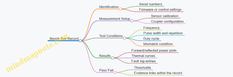
A good bench test ends with clarity: you know what passed, what failed, and why the data supports the decision. That’s the whole point—no mystery, no guesswork, just evidence that the component will behave when the system is under real operating stress.
5. Antenna and Beamforming Engineering for Effective Coverage
5.1 Array Design for Beamwidth Sidelobes and Scan Loss
A beamforming array is a trade machine: you choose how narrow the main beam gets (beamwidth), how much energy leaks into other angles (sidelobes), and how much performance you lose when you steer away from broadside (scan loss). The trick is to design these together, not one at a time.
Beamwidth Basics and Why It Is Not Just “More Elements”
For a uniform linear array, the approximate main-beam width shrinks as the physical aperture grows. A larger aperture can come from more elements or a wider spacing, but spacing is limited by grating lobes. A practical rule is to keep element spacing at or below about half the wavelength for predictable sidelobe behavior.
Easy example: If you double the number of elements while keeping spacing fixed, the aperture doubles, and the main beam becomes about half as wide. That helps tracking accuracy, but it also makes pointing errors more noticeable because the beam is narrower.
Sidelobes: Where the “Unwanted” Energy Goes
Sidelobes are not random; they are a direct consequence of the amplitude and phase distribution across the array. Uniform amplitude tends to produce higher sidelobes, while tapering the amplitude reduces sidelobes at the cost of a wider main beam.
A common approach is to apply a taper such as a Taylor or Chebyshev-like distribution. The design target is usually expressed as a sidelobe level relative to the main beam peak, for example “sidelobes at least 20 dB below the main beam.”
Easy example: If your array has sidelobes only 10 dB down, a target near the edge of the main beam can still receive significant energy from sidelobe illumination. If you push sidelobes to 20–30 dB down, that leakage drops by 10–100×, which can materially improve boundary control.
Scan Loss: The Cost of Steering
When you steer a beam, the array factor changes. Even if the beam points correctly, the effective aperture in the steering direction shrinks, and the gain drops. Scan loss depends on array geometry, element pattern, and how you implement the phase progression.
Two practical contributors are:
- Array-factor scan loss: finite aperture effects reduce peak gain as scan angle increases.
- Element-pattern scan loss: if each element has its own directional pattern, steering can move the beam toward angles where the element gain is lower.
Easy example: Suppose your broadside gain is 20 dB. If you steer to a moderate angle and your system loses 3 dB, the peak power density halves. If your neutralization effectiveness depends on exceeding a threshold field level, that 3 dB can be the difference between “works” and “works inconsistently.”
The Integrated Design Workflow
- Set the scan sector and safety boundary goals. Decide the maximum steering angle you must cover and how much energy you can tolerate outside the protected zone.
- Choose spacing to control grating lobes. Start with ≤ 0.5λ spacing for predictable sidelobe structure.
- Pick a taper to meet sidelobe targets. Use tapering to reduce sidelobe levels until boundary leakage is acceptable.
- Estimate scan loss early. Compute or simulate array gain versus scan angle for your chosen taper and element pattern.
- Verify beamwidth versus tracking needs. Ensure the main beam width at the worst scan angle still supports the tracking accuracy you need.
- Check implementation limits. Phase quantization, amplitude errors, and RF switch losses can add extra sidelobes and additional scan loss.
This workflow matters because sidelobe reduction often widens the main beam, and wider beams can increase the energy delivered to nearby angles. Meanwhile, aggressive tapering can reduce peak gain, which interacts directly with scan loss.
Mind Map: Beamwidth Sidelobes and Scan Loss
Example: Choosing Taper and Spacing for a Perimeter Sector
Assume a perimeter system must scan ±20° and you want sidelobes low enough that energy outside the fence line stays below a boundary threshold. You start with half-wavelength spacing to avoid grating lobes. Next, you compare two tapers:
- Uniform amplitude: narrowest beam, but sidelobes are higher, so off-axis leakage is harder to control.
- Tapered amplitude: wider beam, but sidelobes drop, making boundary control more reliable.
Then you compute gain versus scan angle for both cases. If the tapered case loses an extra 2 dB of peak gain at ±20°, you check whether the remaining margin still exceeds your required field level at the target range. If it does not, you compensate by increasing aperture (more elements) rather than simply relaxing sidelobe requirements.
Design Rules of Thumb That Actually Help
- If you see unexpected energy near boundary angles, suspect sidelobes first, then phase/amplitude calibration.
- If performance drops mainly at scan extremes, suspect scan loss and element-pattern effects.
- If the beam is too wide for tracking, increase aperture rather than removing taper entirely.
The best array designs treat beamwidth, sidelobes, and scan loss as one coupled problem: you pick a spacing strategy, choose a taper that meets sidelobe limits, and confirm that the scan gain and beamwidth still satisfy the operational geometry.
5.2 Polarization Matching and Orientation Effects
Polarization is the direction of the electric field component of a radio wave. For microwave counter-drone systems, polarization matching matters because antennas do not “see” energy equally in every direction; they respond most strongly when the incoming field aligns with the antenna’s polarization.
Core Concepts That Drive Polarization Matching
Start with two practical facts. First, a linearly polarized transmit antenna launches an electric field that points in a specific plane. Second, a receiving or coupling path inside the drone is sensitive to the field orientation it encounters. If the drone’s relevant electronics present an effective receiving polarization that differs from the transmitted polarization, coupling drops and the same transmitter power produces less effect.
Orientation effects come from geometry. A drone rotates, tilts, and yaws while moving. Even if the drone’s body-mounted antennas are fixed relative to the airframe, their orientation relative to your site changes continuously. That means the polarization mismatch is not a constant; it varies with time.
Polarization Types and What They Mean in Practice
Most counter-drone microwave designs use linear polarization, because it simplifies antenna design and beam steering. Circular polarization can reduce sensitivity to rotation, but it requires specific antenna and waveform choices to maintain the intended sense of rotation.
For linear polarization, you can think in terms of a “projection.” If the transmitted electric field is aligned with the drone’s effective receiving polarization, coupling is near maximum. If it is orthogonal, coupling is near minimum. The relationship is often approximated by the cosine of the angle between polarization vectors, so a 45° mismatch can reduce coupling substantially.
System-Level Polarization Matching Strategy
A good strategy begins with defining what you are matching to. In many cases, you are not matching to a single known antenna on the drone; you are matching to the dominant coupling path into the drone’s electronics, which may involve cables, apertures, or PCB traces. That coupling path tends to behave like an effective polarization that depends on the drone’s orientation and the frequency.
Next, choose an antenna polarization that matches the most likely drone orientations at your site. For a perimeter defense, drones often approach with varying yaw but a relatively consistent pitch and roll profile depending on flight control behavior and wind. You can treat this as a probability distribution rather than a single angle.
Finally, design for robustness. Instead of relying on perfect alignment, you can use antenna polarization diversity or dual-polarized elements so that at least one polarization remains reasonably aligned during motion.
Mind Map: Polarization Matching and Orientation Effects
Engineering Details That Prevent “Looks Right, Performs Wrong”
Polarization purity is the first check. Real antennas leak energy into the orthogonal polarization due to imperfect feed alignment, manufacturing tolerances, and reflector or array symmetry. That leakage is not always bad; it can provide some robustness. But if the leakage is uncontrolled, it can also complicate safety boundary calculations and reduce predictability.
Orientation calibration is the second check. If the antenna is mounted with a small tilt error, the polarization plane rotates by the same amount. A 10° mounting error might sound minor, but it changes the projection and therefore the coupling. Calibration should include verifying the mechanical alignment relative to the site coordinate system.
Field mapping is the third check. You do not need to map every possible drone attitude, but you should map representative orientations that cover the expected range of yaw, pitch, and roll. For each orientation, measure or simulate the received field component aligned with your intended polarization and compare it to the orthogonal component.
Concrete Examples for Intuition
Example: Single Linear Polarization Perimeter Assume your transmit polarization is horizontal. A drone approaches with yaw changes but mostly stable pitch. When the drone’s effective receiving polarization is also mostly horizontal, coupling stays strong. If the drone rolls 90° during a maneuver, the effective receiving polarization rotates toward vertical, and coupling can drop sharply. In practice, this shows up as reduced effectiveness during aggressive maneuvers.
Example: Dual-Polarized Antenna Elements Use two co-located linear polarizations, one horizontal and one vertical, with independent control. When the drone rolls, one polarization becomes less aligned while the other becomes more aligned. If your control logic can select or combine the polarization that yields higher coupling, you reduce sensitivity to attitude changes.
Example: Circular Polarization for Rotation Tolerance If the drone rotates rapidly, the instantaneous polarization mismatch averages out. Circular polarization can maintain a more consistent coupling level over time because the electric field rotates in a way that does not depend as strongly on the drone’s yaw. The tradeoff is that you must maintain the intended polarization sense and axial ratio across the operating band.
Practical Takeaway
Polarization matching is not a one-time setting; it is a relationship between your antenna’s electric field direction and the drone’s effective receiving polarization as it moves. Treat orientation as a variable, measure or model the aligned and cross-polar components, and design so that the system remains effective even when the drone does not cooperate.
5.3 Beam Steering Control Using Phase and Time Alignment
Beam steering is the art of making the transmitted energy arrive where you want it, not where the geometry happens to point. For microwave counter-drone defense, phase and time alignment are the two levers that turn a set of antennas into a controllable beam.
Core Idea Phase Alignment
A phased array steers by adjusting the relative phase of the signal feeding each element. If element i is driven with phase \(\phi_i\), the array factor produces constructive interference in the desired direction and destructive interference elsewhere. A practical way to think about it: phase alignment is “where the wavefront lines up” across the aperture.
Easy example: a 4-element linear array with spacing d. If you want the beam at angle \(\theta\), the required phase progression is approximately \(\Delta\phi = -k d \sin\theta\), where \(k=2\pi/\lambda\). You apply phases \(0, \Delta\phi, 2\Delta\phi, 3\Delta\phi\) (modulo 2\(\pi\)). The negative sign just matches a chosen coordinate convention.
Core Idea Time Alignment
Time alignment is phase alignment expressed in the time domain. A delay of \(\tau\) at carrier frequency f produces phase shift \(\phi = 2\pi f\tau\). Time alignment matters when you steer across bandwidth, when you use pulsed waveforms, or when you need repeatable timing for gating and interlocks.
Easy example: if your system uses a 10 ns pulse and you apply a 1 ns relative delay between two elements, the phase difference at 3 GHz is \(2\pi\cdot 3\text{GHz}\cdot 1\text{ns}=2\pi\cdot 3\), which is effectively 0 modulo 2\(\pi\). So the beam might look “fine” at that carrier, but the pulse shape across elements will not match, which can reduce peak gain and increase sidelobes.
From Geometry to Steering Commands
Start with the target direction. For a planar array, you map the desired look direction into a steering vector that tells each element what phase (or delay) to apply.
- Choose a reference element (often the array center).
- Compute the path difference from each element to the far-field point.
- Convert path difference to delay \(\tau_i\) and then to phase \(\phi_i\) at the operating frequency.
- Apply the commands through your RF distribution and beamforming control.
Easy example: if element i is physically farther along the look direction by \(\Delta r_i\), then the needed delay is \(\tau_i = \Delta r_i / c\). The beamforming controller can store \(\tau_i\) for each steering angle and update them at the rate your tracking system provides.
Phase Quantization and Why It Matters
Real systems use finite-resolution phase shifters or digitally controlled attenuators with phase control. Quantization introduces phase error, which broadens the main lobe and raises sidelobes.
Easy example: if you only have 6-bit phase control (64 steps), the maximum phase error is about \(\pm\pi/64\) (about 2.8 degrees). That error is small, but it accumulates across the aperture, so you validate it with a beam pattern measurement rather than assuming it’s negligible.
Time Delay Implementation Choices
You can implement time alignment with true time delay (TTD) or with phase-only control.
- Phase-only steering is simpler and often sufficient for narrowband continuous-wave operation.
- True time delay better preserves alignment across bandwidth and for pulsed waveforms.
Easy example: if your waveform occupies a wide frequency span, phase-only steering will steer differently at different frequencies, causing beam squint. TTD keeps the delay consistent, so the beam direction stays stable across the band.
Calibration and Alignment Verification
Phase and time alignment are only as good as your calibration. Hardware introduces fixed offsets: cable lengths, connector tolerances, amplifier group delay, and switch paths.
A systematic calibration workflow:
- Measure per-element relative phase at the operating frequency using a network analyzer or a dedicated calibration mode.
- Measure per-element relative delay for pulsed operation using time-domain instrumentation.
- Store correction terms \(\phi_{corr,i}\) and \(\tau_{corr,i}\) in the controller.
- Re-check after maintenance or when temperature changes exceed your defined threshold.
Easy example: if element 3 consistently leads by 12 degrees compared to the reference, you apply a correction of -12 degrees in software so the commanded steering vector lands on the calibrated baseline.
Practical Control Loop with Tracking Cueing
Beam steering is usually driven by a tracking cue. The control loop converts the estimated target direction into steering commands, then schedules transmit gating.
A robust approach:
- Use a stabilized direction estimate (filtering reduces jitter).
- Update steering commands at a rate that matches your beamformer settling time.
- Gate transmission only when interlocks confirm the system is in a safe state and the beamformer has reached the commanded settings.
Easy example: if the beamformer needs 2 ms to settle after a phase update, but your tracker outputs new angles every 0.5 ms, you should either hold the last steering command until settling completes or interpolate carefully to avoid transmitting during transient misalignment.
Mind Map: Phase and Time Alignment for Beam Steering
Worked Example: Two Angles with Corrections
Assume a 6-element array at 3 GHz with spacing d = 0.5\(\lambda\). You want \(\theta_1=10^\circ\) and \(\theta_2=20^\circ\).
- Compute \(\Delta\phi\) for each angle using \(\Delta\phi=-k d\sin\theta\).
- Build the phase list \(\phi_i = i\Delta\phi\) relative to the reference.
- Apply calibration corrections: \(\phi_i^{cmd} = \phi_i + \phi_{corr,i}\).
- If using TTD, convert the same geometry into \(\tau_i\) and add \(\tau_{corr,i}\).
Easy example: if calibration shows element 0 has +5 degrees offset and element 5 has -7 degrees offset, your commanded phases shift accordingly. The beam pattern measurement should then show the main lobe near the intended angles rather than consistently drifting.
Key Takeaways for Reliable Steering
Phase alignment sets the beam direction at a given frequency, while time alignment preserves that direction across pulses and bandwidth. Calibration turns theoretical steering vectors into real-world beam pointing, and the control loop ensures you transmit only when the beamformer has settled into the commanded alignment.
5.4 Calibration Procedures for Pointing Accuracy and Gain
Pointing accuracy and gain are linked: if the beam is aimed a few tenths of a degree off target, the gain you thought you had is no longer the gain you deliver. Calibration turns that “it should be right” into measured, repeatable behavior.
Calibration Goals and What to Measure
Start by defining what “correct” means in your system’s terms.
- Pointing accuracy: the angular error between commanded aim and measured beam direction at the operating frequency.
- Gain accuracy: the realized gain (or equivalent EIRP) in the direction of interest, including losses and scan effects.
- Repeatability: how much the answer changes when you repeat the same command after power cycles, temperature changes, and mechanical settling.
A practical rule: calibrate what you can measure directly (angles, phase, power), then compute what you need (gain, effective EIRP, coverage boundaries).
Foundational Setup and Reference Frames
Calibration depends on a stable reference frame.
- Define coordinate conventions: azimuth/elevation relative to the mount, plus any mechanical offsets (for example, a known tilt of the pedestal).
- Lock the mechanical reference: ensure the antenna mount is level and the same bolt pattern is used each time.
- Use a consistent test geometry: place a reference receiver at a known location and height, with line-of-sight where possible.
Example: if your receiver is 30 m away and you mis-measure its height by 10 cm, the implied elevation angle error is about 0.19°. That can be enough to move you off the main lobe for narrow beams.
Instrumentation and Measurement Strategy
You typically need three measurement channels:
- Angle verification: either by measuring beam direction directly (rotary mount with a power sensor) or by using interferometric/phase-based methods.
- Power measurement: a calibrated RF power meter or spectrum analyzer with appropriate attenuation and correction factors.
- System telemetry: logs of commanded angles, scan state, amplifier mode, and protection interlock status.
Best practice: record raw readings with timestamps and include the commanded parameters. When something looks off, you want to know whether it was a control issue, a hardware fault, or a measurement artifact.
Stepwise Calibration Flow
Baseline Electrical Checks
Before touching pointing, confirm the RF chain behaves.
- Verify forward/reflected power behavior at low power.
- Confirm phase and amplitude stability across the intended frequency range.
- Check that the RF switching network selects the expected path.
Example: if a switch state is mis-mapped, you can “calibrate” pointing forever while the beam is actually coming from a different subarray.
Mechanical Zero and Alignment
Set the mechanical zero so commanded angles correspond to the mount frame.
- Use a sighting method or a reference mark to align the antenna boresight.
- Command a known angle pair and verify the beam peaks at the expected direction.
If you have a scan mechanism, do this at the same scan limits you will use operationally, not at a convenient middle position.
Beam Peak Finding for Each Scan State
For each relevant scan state (for example, each steering step or each calibration grid point):
- Sweep a small azimuth/elevation neighborhood around the commanded aim.
- Record the power (or field proxy) and fit a peak location.
- Store the offset between commanded and measured peak.
Example: if the commanded elevation is 15.0° but the measured peak is at 14.7°, store an elevation correction of +0.3° for that scan state.
Gain Realization and Loss Budget Corrections
Measured gain depends on more than the antenna.
- Measure received power at the reference receiver.
- Apply known path loss and any antenna pattern corrections you already trust.
- Correct for system losses: cables, waveguides, switching, and amplifier efficiency.
A simple consistency check: if gain drops sharply at certain scan angles, verify whether it’s due to scan loss (pattern/beamforming) or due to reduced amplifier output from thermal or protection behavior.
Build Correction Maps and Interpolation Rules
Create a mapping from commanded angles to corrected angles and gain adjustments.
- Use a grid that matches how the system will steer.
- Interpolate smoothly between grid points.
- Keep the correction model separate from waveform and power settings.
Example: store two tables—angle correction and gain correction—so you can update one without disturbing the other.
Validate with Independent Points
Don’t just re-measure the same grid points.
- Choose intermediate angles and random points within the operational region.
- Confirm that pointing error stays within your acceptance threshold.
- Confirm that gain matches within your gain tolerance.
Error Sources and How to Reduce Them
- Receiver placement error: verify distance and height with a tape and level; re-check after any site movement.
- Polarization mismatch: align polarization axes; even a small mismatch can reduce received power and distort peak finding.
- Thermal drift: allow warm-up time and repeat a subset of measurements at the end of the session.
- Timing and control latency: ensure the measurement is taken after the beam settles, not during transient steering.
Mind Map: Calibration Procedures for Pointing Accuracy and Gain
Example: Small-Angle Peak Fit and Correction Storage
Assume you sweep ±0.5° around a commanded aim and record power versus angle. You fit a peak location and compute the correction.
- Commanded elevation: 15.0°
- Measured peak elevation: 14.7°
- Stored elevation correction for that scan state: +0.3°
Then you validate at an intermediate elevation, say 15.3° commanded. If the measured peak is 15.31° after applying the correction, your correction model is doing its job.
Example: Gain Correction Sanity Check
If measured received power at the reference point is lower than expected by 3 dB at one scan angle, check:
- Did amplifier output reduce due to thermal/protection?
- Did switching select the intended subarray?
- Is the polarization aligned?
- Is the beam actually centered on the receiver?
Only after those checks should you attribute the loss to pattern scan effects and store a gain correction.
Calibration Records and Acceptance Criteria
A calibration is only useful if it can be repeated and audited.
- Store the date of calibration (for example, 2026-03-07), instrument IDs, and calibration constants.
- Record environmental conditions and warm-up duration.
- Save correction tables and the validation results.
Acceptance criteria should be explicit: maximum pointing error and maximum gain deviation across the validated region. If a point fails, treat it as a data quality issue first, not a “close enough” issue.
5.5 Practical Examples of Coverage Mapping for Site Layouts
Coverage mapping turns “we can aim a beam” into “we can aim it safely and effectively where it matters.” The goal is to produce a site-specific map of where the system can deliver sufficient field strength to the target zone while keeping exposure and interference constraints satisfied in all other areas.
Step 1: Start with a Site Grid and a Target Zone
Begin by choosing a coordinate frame tied to the site: a northing/easting grid, a known reference point, and a consistent height model (ground level plus typical antenna height). Then define:
- Target zone: the region where drones are expected to appear, including likely approach paths.
- Exclusion zones: areas where exposure limits or operational restrictions apply.
- No-go surfaces: buildings, vehicles, and permanent structures that block or reflect energy.
Example: A utility substation has a fence line on the north side. You define the target zone as a 60 m by 40 m rectangle inside the perimeter, and exclusion zones as public access areas outside the fence.
Step 2: Convert Geometry into a Propagation-Friendly Model
Coverage mapping needs a model that respects line-of-sight and obstruction. Use a simplified 3D representation:
- Terrain and major structures as polygons or height fields.
- Antenna locations as fixed points.
- Heights for key surfaces (roof edges, walls).
Keep the model consistent with your later calculations. If you assume flat ground for propagation but later measure with a sloped site, your map will be “accurate” in the wrong universe.
Example: A warehouse roof creates a partial line-of-sight shadow. You model the roof edge explicitly so the map shows reduced coverage behind it.
Step 3: Define Beam States and Map Them to Field Metrics
A practical mapping workflow uses discrete beam states rather than a continuous sweep. For each state, record:
- Pointing direction and steering angles.
- Frequency and waveform parameters.
- Duty cycle or pulse schedule.
- Expected field metric at each grid cell (often power density or an exposure-relevant proxy).
Example: You choose 9 steering directions covering the target zone in a 3×3 pattern. Each direction becomes a beam state with its own predicted field footprint.
Step 4: Apply Safety Boundaries as Hard Constraints
Safety mapping is not a “nice-to-have overlay.” Treat constraints as hard rules:
- For each grid cell outside the target zone, mark whether the predicted field exceeds the allowable threshold.
- For cells near sensitive areas, include measurement uncertainty margins.
Example: Near a control building, the predicted field at certain grid cells is close to the limit. You mark those cells as “restricted” even if the target zone looks fine, because the system must remain safe under realistic aiming errors.
Step 5: Produce a Coverage Map with Decision Layers
A useful output is layered so operators can reason quickly:
- Coverage layer: cells meeting the minimum field metric for disruption.
- Safety layer: cells violating exposure constraints.
- Feasibility layer: cells that are covered and safe simultaneously.
- Confidence layer: cells where the model is supported by measurements.
Example: The map shows that the center of the target zone is feasible for all beam states, while the corners are feasible only for certain steering angles.
Step 6: Validate the Map with Targeted Measurements
Modeling alone is never the final word. Validate using a small set of measurement points that stress the assumptions:
- Points near obstacles.
- Points near safety boundaries.
- Points at the far edge of the target zone.
Use the same beam states and the same operational parameters you used in the model.
Example: You measure at three points: one behind the warehouse roof edge, one near the fence line, and one at maximum range. If the measured field is consistently lower than predicted, you adjust the coverage threshold or apply a conservative correction factor.
Mind Map: Coverage Mapping Workflow for Site Layouts
Example: Turning a Map into Beam Selection Rules
Suppose the feasibility layer shows that only beam states 2, 5, and 8 keep the safety layer clear while covering the target zone edge. You then implement a simple rule set:
- If the target is within the edge band, select among the feasible beam states.
- If the target moves into a region where safety constraints tighten, switch to a different steering set.
This is how a map becomes a working procedure rather than a pretty picture.
Example: Multi-Antenna Layout with Overlap Management
With two antennas, overlap can improve coverage but also complicates safety. Map each antenna’s feasible footprint separately, then compute the combined feasibility:
- A cell is feasible only if both the coverage requirement is met and the combined safety constraint remains satisfied.
- If overlap causes constraint violations, reduce simultaneous beam states or adjust steering schedules.
The result is a site-specific “who points where, when” plan that stays grounded in measured and modeled behavior.
6. Waveform Selection and Coupling to Drone Electronics
6.1 Understanding Coupling Paths into Drone Receivers
High-power microwave systems don’t “hit the drone” in one magical step. They couple energy into specific parts of the drone’s receiver chain, and that coupling depends on geometry, frequency, polarization, and how the drone’s electronics are packaged. A useful way to reason about it is to track energy from the transmit antenna to the drone, then from the drone’s exposed surfaces to the receiver inputs.
Coupling Path Basics
Start with the simplest path: free-space propagation to an antenna or wire on the drone. The receiver is usually sensitive at a particular frequency band, so coupling is strongest when the incident field can induce a voltage or current at that band. In practice, coupling happens through three common mechanisms:
- Direct antenna coupling: incident RF couples into the drone’s own receive antenna (or into a nearby resonant structure).
- Cable and feed coupling: energy couples into wiring harnesses, coax runs, or PCB traces that act like unintended antennas.
- Enclosure and chassis coupling: fields penetrate or couple through openings, seams, and mounting points, then redistribute inside the enclosure.
A key best practice is to treat the drone as an RF system with multiple “entry points,” not a single target. If you can identify likely entry points, you can predict which receiver stage is most affected.
From Field to Receiver Input
Once energy reaches the drone, it must be converted into something the receiver can’t ignore. The receiver typically includes an RF front end, filtering, low-noise amplification, mixing, and baseband processing. Coupling can disrupt any of these, but the most common failure modes are:
- Front-end overload: induced voltage drives the LNA or mixer beyond its linear range.
- Desensitization: strong interference raises the noise floor at the receiver input.
- Intermodulation: multiple coupled components create spurious products that corrupt demodulation.
- AGC saturation: automatic gain control clamps the signal so the desired packets become unreadable.
A practical example: if a drone’s control link uses a narrowband channel, coupling that produces a strong narrowband component at the same center frequency is more likely to cause desensitization than coupling that is broadband and mostly filtered out.
Geometry and Polarization Effects
Coupling strength changes dramatically with orientation. Polarization mismatch reduces the induced current on the receive antenna, while aspect angle changes which surfaces are most exposed. For a concrete example, imagine a dipole-like receive antenna mounted vertically on the drone. A horizontally polarized incident field couples poorly when the drone is level, but coupling increases when the drone pitches or rolls, because the effective electric field component aligns with the antenna.
This is why beam steering and polarization selection matter even when the system is “on frequency.” If you can’t control drone orientation, you plan for worst-case coupling by covering multiple polarizations or by selecting an antenna polarization that maintains a reasonable projection across likely attitudes.
Frequency Selectivity and Resonances
At some frequencies, the drone’s structures behave like resonators: a PCB trace, a cable loop, or a housing seam can support currents that concentrate energy at the receiver input. That means two frequencies can produce very different coupling even if both are “near” the receiver band.
Best practice: when you test, don’t only sweep the center frequency. Include a small band around it and observe receiver disruption thresholds. If disruption peaks at an offset, you likely found a structural resonance or a coupling path that aligns with the receiver’s input impedance.
Mind Map: Coupling Paths to Receiver Disruption
Example: Predicting the Dominant Path
Suppose a drone’s control receiver uses a small patch antenna on the top shell. If your transmit beam is aimed at the top and your polarization matches the patch’s expected orientation, direct antenna coupling dominates, and you should see rapid desensitization at relatively lower power. If instead the beam is aimed from the side, direct coupling drops, and the dominant path may shift to enclosure/chassis coupling, which often requires higher field strength to induce enough voltage on internal wiring.
A simple operational best practice follows: during system setup, vary aim angle and polarization while monitoring receiver metrics (RSSI, link quality, or packet error rate). The pattern of disruption versus angle tells you which coupling path is doing the heavy lifting.
Practical Measurement Mindset
When you interpret test results, separate “radiated power” from “coupled power.” Radiated power is what you set; coupled power is what the receiver experiences. Even with the same transmit settings, changes in drone attitude, distance, and orientation can shift coupling by orders of magnitude. Treat those variables as part of the coupling model, not as annoying noise.
6.2 Pulse Shaping and Duty Cycle Constraints for Hardware
Pulse shaping is how you decide what the transmitter “hands over” to the target: not just frequency, but time structure, rise and fall behavior, and how much energy you can afford to spend per unit time. Duty cycle constraints are the guardrails that keep the RF chain, cooling system, and protection circuits inside safe operating limits.
Foundational Concepts for Timing and Energy
A pulse train can be described by three numbers: pulse width (how long each burst lasts), repetition rate (how often bursts occur), and duty cycle (the fraction of time the transmitter is actually on). Duty cycle is often written as:
- Duty cycle = pulse width × repetition rate
Energy delivered per second scales with duty cycle and with the average power level. That matters because many hardware limits are thermal or protection-based, not instantaneous. For example, a power amplifier might tolerate a high peak power for a short time, but its average heating over seconds can still exceed safe temperatures.
A practical way to think about constraints is to separate “peak stress” from “average stress.” Peak stress is driven by pulse width and peak power. Average stress is driven by duty cycle and cooling capacity.
Pulse Shaping Choices That Affect Hardware Stress
Pulse shaping is not only about target coupling; it also changes how the RF chain behaves.
- Rise and fall time: A fast edge can increase spectral splatter and stress switching elements. A slower edge can reduce ringing in some RF paths but may reduce effective coupling if the waveform spends more time ramping than dwelling.
- Flat-top stability: If the pulse has a drooping envelope, the amplifier is likely operating near a region where gain compression or control loops cannot hold the requested power. Flat-top stability improves repeatability of test results.
- Pulse-to-pulse consistency: Small timing jitter or amplitude variation can cause inconsistent receiver disruption during bench tests, which then leads to confusing field outcomes.
A simple engineering habit helps: treat pulse shaping parameters as part of the “system calibration,” not as a one-time waveform tweak.
Duty Cycle Constraints and Where They Come From
Duty cycle limits arise from several places, and each has a different time constant.
- Thermal limits: Heat accumulates over milliseconds to minutes depending on package and heatsink. If you exceed the thermal time constant, the amplifier temperature rises until protection triggers or long-term reliability is affected.
- Protection circuits: Many systems monitor reflected power, over-temperature, and supply current. If your pulse train causes repeated excursions, you may see intermittent shutdowns that look like “random failures.”
- Power supply capability: Even if the amplifier can handle the peak, the supply must deliver current during pulses and recover between them.
- Cooling and airflow: Fans and liquid loops have recovery time. A duty cycle that is fine in a lab with strong airflow may fail in a sealed enclosure.
The key is to match your pulse train to the slowest limiting mechanism. If thermal recovery is slow, you can’t “fix” it by shortening pulses while keeping the same duty cycle.
Systematic Method for Selecting Pulse Width and Repetition Rate
Start with a target waveform requirement, then translate it into hardware-safe timing.
- Choose a peak power level that meets the coupling goal in your test setup.
- Select pulse width to achieve the desired on-target effect while keeping peak stress within amplifier linearity and switching limits.
- Set repetition rate to satisfy thermal recovery. Use measured temperature or protection event thresholds rather than assumptions.
- Verify average power against the amplifier’s rated continuous or duty-cycled operation.
- Add guard bands so that worst-case conditions (higher ambient temperature, slightly worse cooling, cable losses) still remain safe.
A good example: if your amplifier’s datasheet allows 10% duty cycle at a given pulse width, don’t immediately run at 10%. If your field enclosure runs 8–12°C hotter than the bench, you might reduce duty cycle to keep the same temperature margin.
Mind Map: Pulse Shaping and Duty Cycle Constraints
Example: Duty Cycle Tuning Using Temperature and Protection Logs
Suppose you test two pulse trains at the same peak power and pulse width.
- Train A: 2 microseconds pulses at 1 kHz (duty cycle 0.2%)
- Train B: 2 microseconds pulses at 10 kHz (duty cycle 2%)
If Train B causes the amplifier temperature to climb steadily and triggers over-temperature protection after 90 seconds, while Train A remains stable for 30 minutes, you’ve learned that thermal recovery is the binding constraint. The next step is not to guess a “safe” repetition rate; it’s to run a short series of repetition rates (for example 2 kHz, 4 kHz, 6 kHz) while logging temperature and protection counters. Then choose the highest repetition rate that stays below thresholds with margin.
Practical Guardrails That Prevent Confusing Failures
- Monitor supply current during pulses to catch cases where the amplifier is “working” but the supply is sagging.
- Log reflected power because a duty cycle that is safe into a good load can become unsafe when coupling changes.
- Keep waveform parameters consistent during tests so you can attribute outcomes to duty cycle rather than to accidental changes in rise time or flat-top.
Pulse shaping and duty cycle constraints are ultimately about controlling energy delivery while respecting the RF chain’s time-dependent limits. When you treat timing as a measurable, testable variable, the hardware stops behaving like a mystery box and starts behaving like a system.
6.3 Frequency Planning Across Common Drone Communication Bands
Frequency planning is the step where you translate “we will disrupt drone electronics” into “we will put energy where it matters, while staying inside safety and hardware limits.” For microwave counter-drone systems, the practical goal is not to cover every possible frequency; it is to cover the likely operating bands with enough margin for real-world drift, modulation differences, and antenna pointing errors.
Foundational Inputs That Drive the Plan
Start with four inputs, because every later decision depends on them.
- Target behavior assumptions: Many drones use common control and telemetry bands, plus separate links for video or navigation assistance. Even when exact frequencies vary, the band families tend to cluster.
- System RF constraints: Your transmitter tuning range, amplifier efficiency curve, and available waveforms determine which center frequencies are feasible and how much power you can deliver at each.
- Coupling and exposure limits: Higher frequencies can couple differently into electronics and can change propagation through obstacles. Your exposure assessment may also vary with frequency.
- Operational geometry: Range, altitude, and line-of-sight quality affect link budget and how much effective field strength you can deliver at the target.
A simple way to keep the plan grounded is to write a one-page “frequency requirements” sheet: each candidate band gets a required effective coverage level, an estimated duty cycle, and a maximum allowed transmit time per engagement.
Band Families and What They Imply
Common drone communication uses a mix of ISM and licensed-ish behaviors depending on region and manufacturer. For planning, treat them as band families rather than exact channels.
- 2.4 GHz family: Often used for control and telemetry in hobby and some commercial systems. Expect wide channel spacing and frequent coexistence with other devices.
- 5.8 GHz family: Common for video links and sometimes control. Propagation can be more line-of-sight sensitive than 2.4 GHz.
- Sub-GHz family: Used by some long-range control links. Lower frequency can diffract more, but your microwave system may not be able to operate there.
- Licensed microwave links: Some drones use higher bands that can be narrow and stable. If your system cannot tune there, you plan around what you can reach.
The key is mapping each band family to your system’s tuning and waveform capability. If you can only operate, say, in a narrow microwave range, you should plan to disrupt the electronics that are most likely to be present in that range, rather than pretending you can “hit everything.”
Coverage Strategy That Avoids Waste
A frequent mistake is to schedule many center frequencies with equal dwell time. That spreads energy thin and reduces the chance of reaching the disruption threshold.
Instead, use a band-weighted schedule:
- Allocate more dwell time to the bands most likely to be active at your site.
- Use shorter dwell time for less likely bands, just enough to test whether the target is operating there.
- Keep a minimum dwell time per frequency that matches your waveform repetition and measurement cadence.
Example: If your sensing indicates a drone is likely using 2.4 GHz control and 5.8 GHz video, you might spend 60% of engagement time on the 2.4 GHz family and 40% on the 5.8 GHz family, while still using a small “probe” portion for any unexpected tuning shifts.
Handling Frequency Drift and Channel Offsets
Real drones rarely sit exactly on a nominal center frequency. Drift can come from oscillator tolerances, temperature changes, and adaptive channel selection.
Use a channel offset margin approach:
- Define an offset window around each planned center frequency.
- Choose a set of discrete transmit frequencies that cover that window with overlap.
- Ensure the overlap is large enough that a target shifted toward the edge still receives effective field strength.
Concrete example: If you plan around a 2.4 GHz center and assume ±10 MHz drift, you might transmit at three frequencies spaced so that the target cannot land in a “dead zone” between them. The exact spacing depends on your antenna beamwidth and the waveform’s effective bandwidth.
Measurement-Driven Refinement During System Setup
Before field operations, you can refine the frequency plan using controlled tests.
- Spectrum survey at the site: Identify which band families are already busy. Busy does not mean “ignore it,” but it helps you set expectations for coexistence and sensing confidence.
- System tuning verification: Confirm output power and phase stability at each planned frequency. If power drops sharply at one edge, you reduce dwell time there.
- Coupling checks: Use instrumentation to verify that the delivered field strength at representative ranges matches your model assumptions.
A practical workflow is to generate a frequency plan, run bench and range checks for each planned frequency, then adjust dwell weights based on measured delivered performance rather than assumptions.
Mind Map: Frequency Planning Workflow
Example: Building a Two-Band Plan
Assume your system can tune across 2.3–2.5 GHz and 5.7–5.9 GHz, and your sensors suggest the drone is likely using 2.4 GHz control and 5.8 GHz video.
- Choose one center frequency in each family.
- Add two offset frequencies per family to cover drift.
- Set dwell weights to 60% for the 2.4 GHz family and 40% for the 5.8 GHz family.
- Keep a short probe window for any unexpected activity by briefly stepping to the nearest available alternative frequency within each family.
The result is a plan that is specific enough to execute, but robust enough to handle the messy reality of real radios. It also keeps your transmitter from spending most of its time on frequencies that your system cannot use effectively or that your site evidence suggests are unlikely.
6.4 Signal Quality Requirements for Repeatable Test Results
Repeatable tests start with a simple idea: the signal you think you are transmitting is the signal the device under test actually receives. For counter-drone microwave defense, “signal quality” is not just about peak power. It includes frequency accuracy, modulation consistency, pulse timing, spectral purity, and how the test setup couples energy into the target electronics. If any of these drift, results can look like the drone changed behavior when it was really the measurement that changed.
Core Signal Quality Targets
Frequency accuracy matters because many drone receivers and front ends have frequency-dependent gain and filtering. A practical target is to keep the center frequency within the same tolerance across all runs, and to log the actual measured frequency at the transmitter output (not just the setpoint).
Power stability matters because disruption thresholds often behave like “more is more” only within a narrow region. Use a power meter or directional coupler with a calibrated detector to confirm that each pulse train stays within a defined range. For example, if you allow ±1 dB variation, you should expect noticeably different outcomes when comparing runs.
Pulse timing consistency matters because coupling into nonlinear receiver stages can depend on instantaneous envelope shape. Keep rise time, pulse width, inter-pulse spacing, and duty cycle fixed. If you use an external trigger, verify that the trigger-to-RF latency is constant by measuring it with a fast detector or sampling scope.
Spectral purity matters because spurs and harmonics can change how energy lands in the drone’s band of interest. Measure the spectrum at the output and ensure that spurious emissions remain below a set limit relative to the carrier. This also helps interpret results when you see partial disruption.
Polarization and pointing consistency matters because the received field depends on antenna alignment. Even if the RF source is perfect, a small change in antenna orientation can reduce coupling enough to mimic “no effect.” Treat alignment as part of the signal quality, not as a separate setup detail.
Measurement Chain Integrity
Signal quality is only as good as the measurement chain. A common failure mode is calibrating one instrument and then using it in a different configuration. Keep the chain stable: same cables, same attenuators, same coupler orientation, and same measurement bandwidth. If you must change anything, record it and rerun a baseline.
Use a two-level verification approach:
- Source verification at the transmitter output: frequency, power, pulse shape, and spectrum.
- Delivered verification at the antenna input or at a calibrated field probe location: confirm that what leaves the source is what reaches the coupling point.
Repeatability Workflow
A repeatable test run follows a tight loop. First, perform a baseline check with a known load or reference probe. Second, run the same waveform settings and confirm measured parameters match the baseline within tolerance. Third, execute the test sequence while logging all relevant telemetry: transmitter settings, measured output, timing markers, and any interlock events.
To make this concrete, consider a test that compares two waveform settings. Before comparing, run three “identical” trials of waveform A. If the disruption metric varies more than your allowed test uncertainty, you do not yet have a signal quality problem solved—you have a measurement problem.
Mind Map: Signal Quality Requirements
Example: Defining Tolerances and Gating Trials
Suppose your test metric is “receiver link loss duration” measured over a fixed observation window. You can define gating rules so you only accept trials where the RF signal quality is within bounds.
- Center frequency: within ±X MHz of measured baseline
- Peak power: within ±Y dB of measured baseline
- Pulse width: within ±Z ns
- Duty cycle: within ±W%
- Spectrum: spurs at least N dB below carrier
- Antenna alignment: within a fixed mechanical tolerance
If any gating rule fails, you stop and correct the setup before collecting more data. This prevents mixing “bad signal” trials with “real behavior” trials, which is how you end up with results that look statistically interesting but are operationally meaningless.
Example: Diagnosing a Repeatability Failure
You run waveform A three times and see inconsistent disruption. Start with the simplest checks: compare logged measured frequency and power for each run. If frequency is stable but power varies, inspect the amplifier bias control and thermal state. If power is stable but pulse width shifts, check the timing generator configuration and any firmware or trigger path changes. If both are stable, examine coupling: antenna polarization, distance, and any mechanical drift in mounts. In practice, the fastest path to clarity is to map each observed inconsistency to the specific signal quality parameter that most directly affects coupling into the drone receiver.
6.5 Practical Test Setups for Verifying Receiver Disruption
Receiver disruption is easiest to verify when you treat it like a measurement problem, not a “did it work?” question. The goal is to show that a target receiver’s performance degrades in a repeatable way when exposed to your planned microwave energy, while staying within safety and hardware limits.
Core Test Principle
Start with a controlled link between three elements: (1) a known transmit signal that represents what the drone receiver expects, (2) a receiver-under-test (RUT) that you can measure, and (3) a controlled exposure path that delivers the microwave energy at the intended frequency, polarization, and power density.
A practical setup uses a “reference link” for baseline performance and a “disruption link” for stressed performance. If the baseline is stable and the stressed case shows consistent degradation, you have evidence rather than vibes.
Test Setup Categories
Use one of these categories depending on what you can access and measure.
-
Over-the-Air Link With Real Receiver
- You transmit a modulated signal toward the RUT using a calibrated antenna.
- You measure receiver output metrics such as demodulated bit error rate, packet loss, or decoded frame validity.
- You then introduce your microwave exposure and repeat the same measurements.
-
Coupling-Path Emulation
- You keep the receiver and its antenna environment fixed.
- You inject energy through a controlled coupling method (for example, near-field probe placement or a defined coupling fixture) to mimic how the drone’s front end is affected.
- This is useful when full over-the-air geometry is hard to reproduce.
-
Intermediate Receiver Proxy
- If you cannot test the exact drone receiver, you use a proxy receiver that matches the relevant RF front-end characteristics.
- You still verify disruption using the same metrics and exposure controls.
Mind Map: Verification Workflow
Baseline Setup Details
A baseline prevents you from mistaking normal link fragility for disruption. Use a fixed geometry: mount the RUT antenna on a rigid stand, mark alignment positions, and keep cable routing unchanged.
For the reference link, generate the expected modulation with a signal generator or RF modem emulator. Measure at least one receiver-side metric that correlates with link quality. For example, if the receiver outputs decoded frames, log frame validity rate; if it provides RSSI and SNR estimates, record those alongside packet loss.
Before any exposure, run a short stability check: repeat the baseline measurement at the same settings three times. If the metric wanders significantly, fix that first. A receiver that randomly drops packets will make your disruption results look like a coin toss.
Exposure Configuration Details
Treat exposure control as part of the measurement chain.
- Frequency and polarization: Set the exposure frequency to the planned value and match polarization to the RUT antenna orientation. A 90-degree polarization mismatch can reduce coupling enough to hide disruption.
- Power calibration: Calibrate the delivered power at the transmit aperture or coupling point using a power meter and directional coupler. Log forward power and reflected power during every run.
- Pulse parameters: If your system uses pulsed energy, keep pulse width and duty cycle identical between runs. Record the trigger timing so you can correlate exposure windows with receiver logs.
A simple but effective practice is to include a “no exposure” run between exposure runs. If the receiver metric drifts over time, you can separate drift from disruption.
Example Test Matrix and Execution
Use a matrix that isolates variables.
- Keep distance fixed (or keep coupling fixture position fixed).
- Sweep exposure power across a small set of steps, such as low, mid, and high.
- Repeat each step at least three times.
- Optionally repeat for two modulation formats that represent different receiver sensitivities.
During each run, log: exposure settings, forward/reflected power, receiver metrics, and timestamps. If your receiver supports a lock indicator, capture it; lock loss often appears before complete packet failure.
Instrumentation Sanity Checks
Before trusting results, verify that the exposure signal is actually what you think it is.
- Use a spectrum analyzer to confirm center frequency and bandwidth.
- Confirm that the exposure waveform remains within the expected envelope during the test.
- Check that your trigger timing aligns with the receiver logging start.
If the spectrum shows frequency drift or unexpected harmonics, you may be disrupting for the wrong reason.
Failure Modes to Watch
Common reasons disruption tests mislead:
- Thermal effects: Receiver gain can change with temperature. Keep the RUT in a stable thermal state or allow warm-up time.
- Mechanical misalignment: Small antenna shifts can change coupling. Use fixed mounts and repeatable alignment marks.
- Measurement saturation: If the receiver output saturates or the logging system clips, you may see “flatlined” metrics that look like disruption.
Practical Acceptance Criteria
Define acceptance before testing. For example: disruption is verified when packet validity drops below a chosen threshold at or above a specified exposure power, with consistent results across repeats and no comparable drop in the no-exposure baseline.
A good rule of thumb is to require both a clear threshold behavior and repeatability. If you only get one-off bad runs, you don’t have a verification result—you have a mystery.
7. Safety Engineering and Electromagnetic Compatibility Controls
7.1 Exposure Assessment Using Measured and Modeled Fields
Exposure assessment is the step where you stop guessing and start quantifying. For counter-drone microwave defense, the goal is to determine whether transmitted fields could exceed applicable exposure limits in areas where people or sensitive equipment may be present. A good workflow combines modeling for coverage and planning with measurements for reality checks, then ties both to safety boundaries and operational controls.
Define the Assessment Scope and Boundaries
Start by stating what “exposure” means for your use case: typically time-averaged and peak quantities over relevant durations, plus spatial regions where bystanders could stand. Convert operational intent into a geometry you can compute: antenna locations, beam steering limits, mounting height, and the maximum duty cycle you will allow. A practical best practice is to define three zones before any RF work begins: a controlled zone where engagement is permitted, a restricted zone where access is limited, and an exclusion zone where no one should be present during operation.
Example: If the system can steer ±20° in azimuth and tilt, you should assess exposure across the full steering envelope, not only the “center” pointing direction.
Choose Quantities That Map to Limits
Exposure limits are expressed in terms of field quantities that depend on frequency and polarization. Your assessment should use the same quantities the standard requires, such as electric field strength, magnetic field strength, power density, or derived metrics. The key is consistency: if your model outputs E-field magnitude, your measurement plan must measure E-field (or a quantity that can be converted reliably).
Best practice: keep a one-page “quantity mapping” sheet that lists each required metric, the unit, the measurement method, and the conversion formula you will use.
Build a Modeling Baseline with Realistic Assumptions
Modeling answers “where could it be high?” and “how does it change with steering?” Use a propagation approach that matches the environment: free-space for quick sanity checks, then add ground effects, reflections, and obstacle attenuation where needed. Include antenna patterns, not just boresight gain, because sidelobes often dominate exposure near the edges of coverage.
A systematic modeling baseline includes:
- Antenna pattern and polarization orientation
- Beam steering angles and scan loss
- Transmit power, duty cycle, and waveform assumptions
- Height above ground and local ground properties
- Receiver point grid resolution for boundary finding
Example: If your antenna has a -20 dB sidelobe level, a point near the edge of the main beam can still receive meaningful exposure when the system steers toward it. Modeling prevents you from underestimating that edge case.
Plan Measurements That Validate the Model Where It Matters
Measurements should target the same quantities and the same spatial regions used for boundary decisions. Use a measurement grid that is dense near predicted boundary crossings and coarser elsewhere. Instrumentation must support the frequency range and dynamic range of interest, and the probe orientation must match the polarization you are assessing.
Best practice: measure at multiple steering angles that represent worst-case exposure, such as the extreme steering positions and the angle that produces the highest predicted field at the boundary.
Example: If the model predicts the maximum exposure occurs when the beam points slightly downward, you should include that steering angle in the measurement set even if it is not the most visually “direct” pointing.
Convert Measurements into Exposure Metrics
Raw measurements often come as field strength at a point for a specific duty cycle. Convert them into the exposure metric used by your limits by applying the correct time averaging and accounting for pulse structure. If your system uses pulsed operation, ensure the measurement setup captures peak values and that the averaging method matches the standard’s definition.
A practical check: verify that the conversion from measured peak to averaged metric is consistent with your duty cycle settings and any gating used by the control system.
Reconcile Measured and Modeled Results Without Hand-Waving
You will rarely get perfect agreement. The reconciliation step is where you quantify the discrepancy and decide how it affects boundaries.
- Compare measured and modeled values at identical points
- Compute error factors or offsets in dB
- Identify whether the mismatch is systematic (e.g., antenna pattern) or localized (e.g., an obstacle not modeled)
Best practice: use the measured results to adjust the model confidence. For safety boundaries, apply a conservative margin that reflects both measurement uncertainty and modeling uncertainty.
Determine Safety Boundaries and Operational Controls
Once you have exposure metrics across the region, determine the boundary surfaces where the metric equals the limit (or the internal threshold you choose). Then translate boundaries into controls: interlocks that prevent operation when people could be inside the restricted region, and beam steering limits that keep the boundary within the controlled perimeter.
Example: If the boundary shifts outward at extreme steering, you can restrict steering angles when the system is in a mode that allows human presence nearby.
Document Assumptions, Uncertainty, and Evidence
Documentation should be audit-friendly and traceable. Record:
- Modeling inputs and software settings
- Antenna calibration data used in the model
- Measurement equipment calibration dates and settings
- Grid definition and steering angles tested
- Uncertainty budget and how margins were applied
This is not paperwork for its own sake; it is how you explain why a boundary is credible.
Mind Map: Exposure Assessment Workflow
Example: Boundary Determination with One Steering Envelope
Assume the model predicts a boundary at 25 m for a specific steering angle. You measure E-field at points along a line perpendicular to the antenna and find the averaged metric is 3 dB higher than predicted at the two points closest to 25 m. You then apply a conservative margin that covers measurement uncertainty and modeling uncertainty, shifting the operational boundary inward so that the internal threshold is met even under the higher observed level. The result is a boundary that is not just “modeled,” not just “measured,” but reconciled into a single safety decision.
7.2 Interlock Design for Access Control and Safe Operation
An interlock is the system’s “no-go gate”: it prevents high-power microwave operation unless a defined set of conditions is true. Good interlocks are not just safety checkboxes; they are engineered control points that fail safely, are testable, and are hard to bypass without leaving evidence.
Foundational Principles for Interlock Behavior
Start by defining what “safe” means in your operating context. For counter-drone microwave defense, safe operation typically includes: correct access authorization, verified enclosure or exclusion zone status, confirmed RF path readiness, and absence of fault states that could cause unintended emissions.
Interlocks should follow three rules. First, default to inhibit: if a signal is missing, ambiguous, or stale, the system must not transmit. Second, make interlocks independent where possible: a single software bug should not be able to defeat all safety gates. Third, ensure interlocks are observable: the system should record which condition blocked operation and why.
Interlock Categories and Where They Sit
A practical design groups interlocks into layers so that each layer covers a different failure mode.
- Access Control Interlocks gate who can command operation.
- Zone and Physical State Interlocks gate whether people and equipment are in safe positions.
- RF Safety Interlocks gate whether the transmit chain is healthy and configured.
- System Health Interlocks gate thermal, power, and fault conditions.
Place these gates so that the final transmit enable is computed only after all layers agree. The final enable should be a hardware-level signal or a tightly constrained safety controller output, not a general-purpose software flag.
Mind Map: Interlock Design Logic
Access Control Interlocks That Don’t Rely on Trust
Access control should treat every command as untrusted until proven otherwise. A common pattern is: authentication grants permission to request an “arm” state, but only a separate safety controller can grant “transmit enable.”
Use role-based permissions so that routine tasks like diagnostics cannot directly trigger transmission. For example, an operator might be allowed to run a self-test that checks sensors and RF switches, but not allowed to bypass zone checks.
Audit logging matters because it turns “who did what” into a concrete record. When a transmit request is blocked, store the reason code (for example, “exclusion zone sensor fault” or “RF switch not in transmit position”). This reduces troubleshooting time and prevents repeated guesswork.
Zone and Physical State Interlocks with Clear Evidence
Zone interlocks should be tied to physical or measurable states. If you use door switches, they must be wired so that the safety controller sees an open circuit or a defined logic level when the door is not secured. If you use occupancy detection, define what sensor states mean “safe” versus “unknown,” and treat unknown as inhibit.
Emergency stop should cut transmit enable immediately and require a deliberate reset sequence. A good reset sequence includes verifying that the emergency condition is cleared and that critical sensors return to valid states.
Beam direction constraints can be part of zone safety. If the system can steer beams, interlocks should prevent steering into regions that violate exposure boundaries. A simple example is a software-configured “allowed steering sector” enforced by the safety controller before any transmit enable is asserted.
RF Safety Interlocks That Prevent Unintended Emissions
RF safety interlocks protect against misconfiguration and component failures. Verify RF switch positions before enabling transmit. Confirm frequency and waveform selection are locked to the intended configuration.
Reflected power limits are especially important. If the antenna path is mismatched or a connector is loose, reflected power can rise quickly. Interlock logic should inhibit transmission when reflected power exceeds a threshold for a defined time window, and it should latch the fault until a manual reset after inspection.
A practical example: during commissioning, you might intentionally disconnect a dummy load and observe that the system inhibits transmission within the specified response time, logs “reflected power high,” and refuses to re-enable until the RF path is restored and reset.
System Health Interlocks and Sensor Plausibility
Thermal and power interlocks prevent damage and reduce the chance of abnormal emission behavior. Cooling flow confirmation should be treated as mandatory; if the flow sensor is missing or out of range, inhibit.
Sensor plausibility checks add robustness. For instance, if temperature rises but cooling flow reads normal, the system should flag a sensor inconsistency and inhibit rather than assuming the most convenient interpretation.
Example: End-to-End Interlock Sequence
A typical sequence for a safe transmit attempt:
- Operator authenticates and requests “arm.”
- Safety controller checks access role and logs the request.
- Safety controller verifies zone state is “safe” and not “unknown.”
- Safety controller verifies RF switch positions and confirms waveform lock.
- Safety controller checks reflected power is within limits and cooling is active.
- Only then does it assert transmit enable to the RF chain.
- If any condition changes during operation, transmit enable drops and the system logs the first failing condition.
This structure keeps the logic systematic: each gate answers a specific question, and the final decision is made only when all answers are acceptable.
7.3 EMI and EMC Risk Management for Nearby Systems
High-power microwave defense can be effective, but the same energy that disrupts a target can also interfere with nearby electronics. EMI (electromagnetic interference) is the unwanted coupling that causes malfunctions; EMC (electromagnetic compatibility) is the discipline that ensures equipment works correctly in its electromagnetic environment. Risk management means you treat coupling paths, not just the transmitter.
EMI Coupling Basics That Drive Risk
Start with the three coupling families that show up in real installations:
- Conducted coupling through power lines, control cables, and grounding conductors. Example: a faulted RF switch draws a transient current that rides on the facility’s 24 V control wiring, causing a nearby access-control controller to reset.
- Radiated coupling through space to antennas, enclosures, and cable runs. Example: a long unshielded sensor cable acts like a receiving antenna, picking up stray fields and producing false alarms.
- Near-field effects around antennas and waveguides, where field strength changes quickly with distance. Example: a maintenance laptop placed too close to an active aperture shows corrupted readings because its internal wiring picks up local fields.
A practical rule: if you can’t name the coupling path, you can’t reliably mitigate it.
System Inventory and “Susceptibility Mapping”
Before mitigation, build a local inventory of nearby systems within the site’s operational area: radios, PLCs, SCADA gateways, cameras, telemetry links, metering, and any safety controllers. For each, record:
- Susceptibility clues: known sensitivity (e.g., analog front ends, high-impedance sensors), cable length, and enclosure type.
- Operational criticality: whether a glitch is tolerable or triggers a safety state.
- Interface points: power entry, data ports, and external antennas.
Then map them to physical zones: “near” (close to apertures and waveguides), “mid” (within typical cable routing influence), and “far” (beyond meaningful coupling). This zoning is not guesswork; it’s based on where cables run and where antennas point.
Mitigation Stack That Works in Layers
Mitigation is most reliable when it’s layered. Think of it as stacking barriers so that if one fails, another still blocks the coupling.
-
Control the source
- Use RF interlocks and timing logic so the transmitter is active only when required.
- Keep spurious emissions low by maintaining proper matching and filtering in the RF chain.
- Example: if a harmonic spur is detected during bench checks, fix the amplifier biasing or filtering before field deployment rather than adding “band-aids” later.
-
Control the path
- Route cables away from likely field regions and avoid long parallel runs with RF cables.
- Use shielded cables with correct termination at the entry point.
- Example: a camera coax run that crosses near the waveguide is rerouted to cross at right angles and to shorten the parallel segment.
-
Control the receiver
- Add input filtering and surge/EMI protection where appropriate.
- Use proper grounding practices so shields drain current instead of injecting it into signal references.
- Example: a telemetry receiver gains a common-mode choke and a well-defined reference ground, reducing false packet errors.
-
Control the environment
- Use RF shielding enclosures or barriers for sensitive cabinets.
- Maintain separation distances and define “no-cable” corridors.
- Example: a PLC cabinet is placed behind a conductive barrier and its cable entry uses filtered feedthroughs.
Verification Through Measurement and Acceptance Criteria
Risk management isn’t complete until you verify. Use a measurement plan that matches the coupling type:
- Pre-install bench checks: verify RF output purity, spurious levels, and switching transients.
- Site measurements: measure conducted noise on power/control lines and radiated effects at representative equipment locations.
- Functional tests: confirm that nearby systems maintain correct operation during controlled transmitter activity.
Acceptance criteria should be explicit. Example criteria: “No resets of control units during a defined pulse schedule,” “No loss of video sync beyond a specified threshold,” and “No false triggers from safety sensors.”
Mind Map: EMI and EMC Risk Management Workflow
Example: A Practical EMI Incident and Its Fix
A perimeter site reports intermittent resets of a nearby controller cabinet during microwave operation. The cabinet shares a power feed with other equipment, and its control wiring runs in a long bundle near the RF cable tray.
The fix follows the stack:
- Source control: the RF chain is rechecked for switching transients; a misconfigured RF switch timing is corrected.
- Path control: the control cable bundle is rerouted to increase separation and reduce parallel run length; shield terminations are tightened at the cabinet entry.
- Receiver control: a common-mode choke and input filtering are added to the controller’s external interface.
- Verification: functional tests confirm no resets under the defined pulse schedule.
The key lesson is that the “reset” symptom was real, but the root cause was coupling through both timing transients and cable routing. When you manage both, the problem stops showing up like an uninvited guest.
7.4 Shielding Grounding and Cable Routing Practices
High-power microwave defense systems only work as intended when the RF energy stays where it belongs and the control electronics stay sane. Shielding, grounding, and cable routing are the three levers that make that happen, and they interact: a “good” ground with sloppy routing can still create unwanted coupling, while perfect routing can’t fix a missing shield bond.
Foundational Concepts That Drive Every Design Choice
Start with two practical goals. First, reduce unintended RF coupling into cables that carry control, sensing, or timing signals. Second, control return currents so they flow along planned paths instead of wandering through chassis panels and signal grounds.
A useful mental model is “where the current wants to go.” RF currents follow the lowest-impedance path at the operating frequency, which is rarely the same as the lowest DC resistance. That’s why grounding is not just a single wire to a stake in the dirt; it’s a network of low-impedance bonds, short connections, and controlled interfaces.
Shielding Practices That Actually Reduce Coupling
Shielding works best when it is continuous, bonded correctly, and terminated with predictable impedance. Treat the shield like a conductor that must be electrically connected at both ends when the system requires it.
Key practices:
- Use continuous metallic shielding for runs that pass near the transmitter, waveguide transitions, or high-field areas. Avoid relying on paint or thin coatings as the “shield.”
- Bond shield to chassis with wide, low-inductance connections. A braided strap or a properly designed gland is usually more effective than a single small screw that pinches the shield.
- Prevent shield breaks at connectors. If you must use a connector, choose one with a 360-degree shield termination or add a clamp that maintains contact around the circumference.
- Separate shield roles. Use shield for RF containment, and use a dedicated reference scheme for signal ground. Mixing them casually can create ground loops that look like antennas.
Example: If a control cable runs parallel to the RF feed for 3 meters, even a “good” cable shield can lose effectiveness if the shield is only bonded at one end. Bonding at both ends with a controlled strategy reduces the chance that the cable becomes a secondary radiator.
Grounding Practices That Control Return Currents
Grounding should be designed as a return-current path, not a catch-all reference. The chassis, shield, and power supply returns should form a coherent structure.
Key practices:
- Create a star-like reference only where it makes sense. For high-frequency systems, a strict star can increase inductance. Prefer a distributed low-impedance bonding grid for the chassis, then connect subsystems to that grid with short, wide paths.
- Use short connections for high-frequency bonds. If a bond is long, it behaves like an inductor. Keep bonding leads as short as the mechanical layout allows.
- Separate power return from sensitive signal reference where required. Route high-current returns so they don’t share the same impedance with low-level measurement returns.
- Bond enclosures and doors. If you have access panels, ensure the RF shield continuity survives opening and closing. Use conductive gaskets or dedicated bonding straps.
Example: A common failure mode is a control PCB ground that “returns” through a chassis screw. Under RF stress, the screw’s impedance can shift the local ground reference, causing comparator thresholds to drift and timing to jitter.
Cable Routing Practices That Reduce Unwanted Antenna Behavior
Routing is the quiet workhorse. The goal is to minimize parallel runs, avoid loops, and keep sensitive cables away from strong fields.
Key practices:
- Route by function. Separate RF-adjacent cables (power, interlocks near the transmitter) from low-level sensing and control cables.
- Minimize parallelism. If two cables must cross, cross at right angles rather than running side-by-side.
- Avoid large loops. Loop area turns into pickup area. Bundle and dress cables so they follow the chassis contours.
- Use proper strain relief and bend radius. Damaged insulation or sharp bends can degrade shielding and create intermittent faults.
- Plan cable entry points. Bring cables into the enclosure through shielded entry structures so the shield can be bonded immediately.
Mind Map: Shielding, Grounding, and Routing
Verification Steps That Catch Problems Early
Before powering the RF section, verify the physical assumptions. Perform continuity checks on shield bonds and chassis bonding points, and confirm that connector shields terminate as designed. Then run functional tests while monitoring control signal stability and interlock behavior.
Example: If interlock status changes when the transmitter ramps, treat it as a coupling symptom first. Check shield terminations, bonding straps, and whether the interlock cable shares a return path with a high-current circuit.
Practical Example Layout for a Typical Enclosure
A common integrated approach is to treat the enclosure as a bonding “box” and to keep cable shields bonded at the entry. The transmitter area uses short, shielded runs to the waveguide interface, while control and sensing cables enter through separate gland plates. Inside, sensitive cables stay on one side of the chassis bonding grid, and power returns stay on the other, meeting at the planned reference structure rather than through random screws and brackets.
This is less about rules and more about repeatability: when you can point to the exact bond point and the exact return path, troubleshooting becomes a checklist instead of a guessing game.
7.5 Documentation for Safety Reviews and Operational Readiness
A safety review is only as good as its paperwork. For counter-drone microwave defense, the goal of documentation is simple: anyone trained on your system should be able to understand what it does, what it must never do, and how you prove it stays within limits.
Safety Documentation Package Overview
Start with a single index page that points to every required artifact. A practical package typically includes:
- System description and operating modes
- RF safety analysis summary and exposure basis
- Hardware safety functions and interlock logic
- Test and verification records
- Operating procedures and checklists
- Incident and fault handling documentation
- Change control records
Keep the index consistent with the system’s physical layout. If the site has multiple emitters, name them the same way in drawings, software logs, and procedures.
Foundational Content That Reviewers Expect
Your first pages should answer five questions without forcing the reader to hunt:
- What is the system intended to do in each mode?
- What are the maximum allowed operating parameters?
- What prevents unsafe operation when something goes wrong?
- How do operators verify readiness before energizing?
- How do you demonstrate compliance through test evidence?
A good trick is to include a one-page “Mode Sheet” that lists each mode, its purpose, and its safety constraints. Example: “Standby” might require interlocks satisfied but no transmit; “Engage” might require verified target cueing, beam steering within a defined sector, and thermal headroom.
Interlock and Safety Function Documentation
Document each safety function as a small, testable unit. For every interlock, include:
- Trigger condition and what it measures
- Required state to allow transmit
- Fail-safe behavior when the condition is violated
- Reset rules and who can authorize reset
- Proof test method and pass/fail criteria
Example: If an enclosure door sensor disables transmit, specify whether the system blocks all modes or only engagement. Then document the proof test: open the door, confirm transmit inhibit, verify logs record the reason code, and confirm the system cannot resume until the reset procedure is followed.
Evidence and Traceability Records
Safety reviews rely on evidence, not memory. Organize test records so a reviewer can trace from requirement to result:
- Requirement statement
- Test procedure reference
- Instrumentation used and calibration status
- Test conditions and measured outcomes
- Deviations and corrective actions
Use a consistent naming scheme for test reports. For instance, include the emitter ID, waveform family, and date in the filename. If you need a date, use a fixed example such as “2026-03-01” in templates so teams don’t invent formats.
Operational Readiness Procedures
Operational readiness documentation should be written for the moment before energizing. It should not read like a manual for a lab experiment.
Include:
- Pre-start inspection steps
- Interlock status verification steps
- Thermal and power system checks
- Beam steering calibration verification steps
- Communications and logging verification steps
- A final “go/no-go” checklist signed by the duty supervisor
Example checklist item: “Confirm cooling system reports stable flow and temperature within limits for at least 10 minutes.” This prevents the common failure mode where transmit is enabled before the thermal system reaches steady behavior.
Incident, Fault, and Post-Event Documentation
Define what counts as an incident versus a routine fault. Then document the response workflow:
- Immediate actions to place the system in a safe state
- How to capture logs and fault codes
- How to preserve relevant measurements
- Who can authorize restart
- How to perform a structured post-event review
Keep the workflow short and deterministic. If the system disables transmit due to reflected power, the procedure should specify whether operators can clear the fault after inspection or must escalate to technical staff.
Mind Map: Documentation for Safety Reviews and Operational Readiness
Integrated Example of a Review-Ready Workflow
A reviewer should be able to follow one scenario end-to-end. Example scenario: “Operator initiates Engage mode.”
- The Mode Sheet states Engage requires interlocks satisfied, thermal headroom, and beam sector constraints.
- Interlock documentation lists the exact sensors and fail-safe behavior.
- The readiness checklist instructs the operator to verify interlock status and confirm thermal stability.
- The evidence folder contains proof tests showing the interlocks inhibit transmit under fault conditions.
- If a fault occurs, the incident procedure specifies safe-state actions and log capture.
When these pieces align, the documentation stops being a pile of documents and becomes a working safety system on paper.
8. Detection Tracking and Cueing Workflows
8.1 Sensor Fusion with Radar EO IR and RF Monitoring
Sensor fusion for counter-drone microwave defense is about one thing: getting a stable, actionable target track with enough confidence to aim and enough safety margin to avoid firing at the wrong object. Radar, EO/IR, and RF monitoring each see different parts of the problem. Fusion combines them into a single track state, a confidence score, and a set of cues for beam steering.
Core Concepts and Data Roles
Radar provides geometry: range, bearing, and often velocity. EO/IR provides confirmation: shape cues, motion consistency, and sometimes altitude estimates via stereo or known camera geometry. RF monitoring provides identity hints: transmitter presence, frequency, modulation characteristics, and timing patterns that help distinguish a drone-like emitter from background noise.
A practical fusion design treats each sensor as a contributor with a known reliability profile. Reliability changes with conditions: rain and clutter affect radar; glare and low light affect EO/IR; spectrum congestion affects RF. The fusion layer should therefore accept measurements with timestamps, sensor health flags, and estimated measurement uncertainty.
Stepwise Fusion Pipeline
- Time alignment and normalization: Convert all measurements into a common coordinate frame (site coordinates) and common time base. If radar reports in polar coordinates, convert to Cartesian before fusion.
- Track initiation: Start a track only when at least one sensor produces a measurement that passes gating rules. For example, radar detections that persist across consecutive sweeps are stronger candidates than single-frame camera detections.
- Prediction: Use a motion model (often constant velocity with acceleration limits) to predict where the target should be at the next sensor timestamp.
- Association: Match incoming measurements to existing tracks using gating based on predicted position and uncertainty. If multiple tracks compete, prefer the association with the smallest normalized innovation.
- Update: Fuse measurements using a filter such as an Extended Kalman Filter or Unscented Kalman Filter, depending on nonlinearity. Update the track state and covariance.
- Confidence scoring: Compute a confidence value from covariance size, sensor agreement, and sensor health. Confidence should be monotonic with evidence quality, not just number of sensors.
- Cue generation: Produce a beam aim point and timing cue only when confidence and safety constraints are satisfied.
Mind Map: Fusion Inputs, Logic, and Outputs
Sensor Fusion Mind Map
Integrated Example: One Target, Three Sensors
Assume a perimeter site with a radar unit, a gimbaled EO/IR camera, and an RF receiver covering the drone communication bands. At time T0, radar detects a small moving object at 450 m with bearing 12.3°. The radar system reports a clutter metric, and the detection passes gating because the velocity is consistent with a drone-like profile.
At T0 + 80 ms, the camera produces a tracklet centroid near the projected bearing line. The fusion layer predicts the target position at the camera timestamp and checks whether the centroid lies within the predicted uncertainty ellipse. If it does, the camera measurement updates the track state.
At T0 + 120 ms, RF monitoring detects an emitter with a frequency and bandwidth pattern that matches the site’s known drone-like signature set. RF does not directly provide range, but it improves confidence by confirming that the track is likely associated with an active transmitter. The fusion layer increases confidence without forcing a range update.
The result is a single track with a tighter covariance than any sensor alone. Beam steering uses the fused position and velocity, while engagement readiness depends on confidence thresholds and safety interlocks.
Practical Best Practices That Prevent Common Failure Modes
- Use uncertainty, not vibes: If radar covariance is large due to clutter, don’t let camera confirmation alone drive confidence to maximum. Confidence should reflect combined uncertainty.
- Gate aggressively early, then relax: Tight gating during track initiation reduces false tracks. Once a track is established, allow slightly larger gates to accommodate maneuvering.
- Handle sensor dropout explicitly: If EO/IR drops due to glare, keep the track alive using radar prediction and reduce confidence based on missing confirmation.
- Avoid “RF-only” tracks: RF can confirm presence, but without geometry it should not create a full track by itself. Use RF to support association with radar or EO/IR tracks.
- Track agreement matters: If radar and camera disagree beyond uncertainty, treat it as a conflict and lower confidence rather than averaging blindly.
Output Contract for the Engagement Layer
The fusion module should output: (1) a fused track state in site coordinates, (2) a confidence score derived from covariance and sensor agreement, (3) an aim point for beam steering with a timestamp, and (4) a readiness flag that is false when safety constraints are not satisfied. This keeps the engagement layer simple: it consumes a clean, time-stamped target estimate and refuses to act when the estimate is not trustworthy.
8.2 Target Tracking Filters for Stabilized Aim Points
Stabilized aim points matter because a microwave beam that “walks” across the target wastes energy and increases safety risk. Target tracking filters turn noisy measurements—range, bearing, and sometimes elevation—into a smooth estimate that your pointing controller can trust. The goal is not perfect truth; it is consistent, bounded error with predictable latency.
What the Filter Must Deliver
A tracking filter should output four practical items: an estimated target state (position and velocity), an uncertainty measure (so you can decide whether to aim or pause), a predicted future position at the command time (to compensate for system delay), and a track quality score (so you can reject clutter). For example, if your sensor reports a bearing that jitters by ±1° at 200 m, a simple “last measurement” aim point will swing by several meters. A filter should reduce that swing while keeping the predicted aim aligned with the target’s motion.
Measurement Model and Coordinate Choices
Start by defining what the sensor actually measures. Radar might provide range and angles; EO/IR might provide pixel coordinates that you convert to angles; RF sensing might provide coarse direction. Convert everything into a common coordinate frame used by the gimbal or antenna array. A common best practice is to represent the target state in Cartesian coordinates (x, y, z) with a constant-velocity motion model, then map sensor measurements into that space. This avoids mixing units and reduces the chance of “it looks right but it isn’t” bugs.
Foundational Motion Model
A constant-velocity model is often enough for short engagement windows. The filter assumes the target’s velocity changes slowly, but it allows uncertainty to grow when motion becomes less predictable. If you use a constant-velocity model and the target accelerates sharply, the filter will lag. That lag is manageable if you tune process noise to match typical drone maneuvering and if you cap how aggressively you update the aim point.
Kalman Filter Structure for Stabilized Aim Points
A standard approach is a Kalman filter with two steps repeated each cycle: prediction and update. Prediction advances the state using the motion model and your measured time step. Update corrects the prediction using the latest measurement and the measurement noise model.
A practical tuning method: begin with measurement noise derived from sensor testing (for instance, bearing standard deviation when the target is stationary). Then set process noise so that the filter’s innovation—the difference between predicted and measured observations—stays within a reasonable band. If innovations are consistently large, the filter is overconfident; if they are consistently tiny, the filter may be too sluggish.
Handling Latency with Predictive Aim
Your pointing command is not applied instantly. If the total delay from filter update to beam arrival is τ, you should aim at the predicted state at time t+τ. With a constant-velocity model, prediction is straightforward: position_pred = position + velocity * τ. Example: if your filter estimates velocity as 6 m/s and τ is 0.25 s, the aim point should shift by about 1.5 m ahead of the current estimate. Without this, the beam trails the target even if the filter is otherwise well tuned.
Gating and Track Management
Gating prevents a filter from “snapping” to unrelated detections. Use an innovation gate based on the predicted measurement uncertainty. If a new measurement falls outside the gate, you either ignore it or treat it as a missed detection. Track management also includes handling dropouts: if measurements disappear for a short period, the filter should continue predicting while uncertainty grows. Once uncertainty exceeds a threshold, you should stop aiming and wait for a reliable track.
Practical Example of Filter Behavior
Imagine a target at 150 m with bearing noise that produces ±0.5° jitter. That jitter corresponds to roughly ±1.3 m lateral error. A well-tuned filter might reduce lateral aim jitter to ±0.3 m while keeping predicted aim within a few tenths of a meter during moderate motion. If you see aim jitter remain large, increase measurement smoothing by raising measurement noise or reducing update rate. If you see aim lag behind turns, increase process noise or shorten the prediction horizon.
Mind Map: Target Tracking Filter Responsibilities
Mind Map: Tuning Knobs That Actually Matter
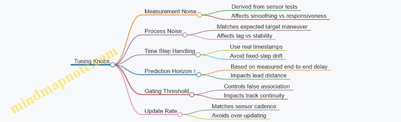
Example: A Simple Decision Rule for Aim Enable
Use a confidence threshold tied to uncertainty and gating status. For instance: enable aiming only when (1) the track has been updated within the last N milliseconds, (2) the predicted position uncertainty projected onto the pointing axis is below a limit, and (3) the last innovation was within the gate. This keeps the beam from “chasing” uncertain estimates when the sensor is confused, like when the target is partially occluded or the background produces spurious detections.
8.3 Latency Budgeting From Detection To Beam Command
Latency budgeting is the practice of turning “we need it fast” into a measurable chain of time allowances. In a counter-drone microwave system, the chain runs from the moment a sensor declares a target to the moment the beam command reaches the RF control hardware. If any stage is too slow, the beam points late; if any stage is too variable, the system becomes inconsistent even when the average latency looks fine.
Foundational Timing Model
Start with a simple timeline:
- Detection time: sensor processing until a track is declared.
- Tracking time: filter update and track state stabilization.
- Decision time: engagement readiness checks and aim selection.
- Command time: message formatting, transport, and handoff to beam controller.
- Actuation time: beam steering settling and RF gating readiness.
- On-target time: when the beam is actually radiating toward the computed aim.
A useful budget separates fixed latency (deterministic delays like buffering) from variable latency (jitter from scheduling, network contention, or sensor mode switching). Variable latency is usually the bigger enemy because it breaks repeatability.
Stepwise Budget Construction
Build the budget top-down, then verify bottom-up.
Step 1: Define the “on-target” requirement. For example, if the drone can move enough that a 50 ms pointing error becomes unacceptable, then your total detection-to-on-target latency must stay below that threshold with margin.
Step 2: Allocate time per stage. A practical approach is to assign conservative maxima to each stage, then sum them. If the sum exceeds the requirement, reduce the largest contributors first.
Step 3: Add safety margin for jitter. Use a rule of thumb: keep variable stages to a small fraction of the total budget. If you cannot, you must compensate elsewhere (for example, by predicting track motion, or by tightening sensor update rates).
Step 4: Validate with instrumentation. Every stage needs a timestamp source. Without timestamps, you’re guessing.
Mind Map: Latency Budgeting Chain
Measurement That Actually Helps
Instrument the system with event markers that correspond to the stage boundaries. For instance:
T_detect: sensor track declared.T_track: track state published to the engagement controller.T_decide: engagement decision and aim computed.T_cmd_rx: beam controller received command.T_beam_on: RF gating enabled.
Then compute:
Latency_total = T_beam_on - T_detectLatency_jitterfrom the distribution, not just the mean.
A histogram of Latency_total often reveals a pattern: one stage occasionally spikes when the system switches sensor modes, or when a safety interlock check runs longer than usual.
Decision Time and Interlocks
Decision time is not only “math time.” It includes checks that prevent unsafe or ineffective operation. For example, if the system requires a minimum confidence score and a safety boundary clearance check, those checks must be included in the budget. A common best practice is to structure decision logic so that fast checks happen first, and expensive checks happen only when earlier conditions pass.
Concrete example: if a confidence threshold fails, you should stop early and avoid spending time on aim computation and command formatting. That keeps the latency distribution tighter for the cases that matter.
Command Time and Transport
Command time includes message creation, transport, and controller handoff. Even when the network is “fast,” buffering can add fixed delays. Best practice is to avoid variable-length payloads in the critical path and to keep command processing single-threaded or deterministically scheduled.
Concrete example: if the command message includes optional diagnostic fields, ensure they are either preallocated or sent on a separate channel so the critical command path stays consistent.
Actuation Time and Beam Settling
Actuation time is where physical reality shows up. Beam steering may require a settling interval before RF gating. If you gate immediately, you get energy during the transient, which can reduce effectiveness and complicate safety boundary behavior.
Best practice: gate RF only after the steering controller reports “settled” or after a fixed settling delay validated by testing. If you use a fixed delay, confirm it across temperature and load conditions.
Example Latency Budget and Interpretation
Assume a requirement of 60 ms from T_detect to T_beam_on.
- Detection time: 18 ms (fixed)
- Tracking time: 10 ms (variable ±2 ms)
- Decision time: 8 ms (fixed)
- Command time: 6 ms (variable ±1 ms)
- Actuation time: 14 ms (fixed settling)
Total nominal: 18 + 10 + 8 + 6 + 14 = 56 ms.
Now check worst-case jitter: add the variable margins (2 + 1 ms) to get 59 ms worst-case, leaving only 1 ms of slack. That’s tight. The systematic fix is to reduce the largest variable stage (tracking) by tightening update cadence or optimizing filter computation, or to reduce detection processing time by selecting a faster sensor mode when appropriate.
Practical Checklist for System Integration
- Every stage boundary has a timestamp.
- Latency is evaluated as a distribution, including worst-case.
- Interlocks are included in the budget, not treated as “rare events.”
- RF gating is tied to beam settling, not just command receipt.
- The budget is validated on the actual hardware and operating conditions, not only in a lab simulation.
Latency budgeting is ultimately about making timing predictable. Once you can point to the exact stage that eats your milliseconds, you can fix it without guessing—and your beam command stops arriving late in the only way that matters: to the wrong place.
8.4 Cueing Logic for Prioritization and Engagement Readiness
Cueing logic is the part of the system that decides what to aim at, when to aim, and when to refuse to aim. It sits between detection and the RF control chain, so it must be both conservative and fast. A good cueing design treats every engagement as a short checklist: confirm the target is real, confirm the aim point is stable enough, confirm the safety gates are satisfied, and confirm the transmitter is ready.
Core Inputs and State Model
Start by naming the inputs the cueing logic will consume. Typical sources include radar tracks, RF sensing hits, and operator or EO/IR confirmations. Each input should come with a confidence score and a timestamp. The cueing system then maintains a small internal state machine:
- Idle: no valid track, or safety gates not satisfied.
- Candidate: at least one track is plausible, but stability or safety gates are not yet met.
- Ready: a track is stable, aim is within limits, and safety gates are satisfied.
- Engaging: transmitter is active for the current dwell.
- Cooldown: transmitter is inhibited until thermal and safety timers expire.
A practical rule: never let a single sensor flip the state. Require either consistent evidence across sensors or consistent evidence over time from one sensor.
Prioritization Rules That Actually Work
Prioritization answers: if multiple tracks exist, which one gets the next dwell? Use a scoring function that is easy to explain and easy to tune. A simple approach is a weighted score:
- Track quality: number of hits, track age, and estimated uncertainty.
- Threat relevance: size or speed class if available, plus whether the track is moving toward the protected zone.
- Engagement feasibility: predicted dwell time inside the safe aim window and expected coupling conditions.
- Operational constraints: whether another engagement is in cooldown or whether the system is already committed to a different beam schedule.
Example: if Track A has higher confidence but will exit the safe aim window in 0.3 seconds, while Track B has slightly lower confidence but stays for 1.2 seconds, the scoring should favor Track B because it yields a more reliable dwell.
Engagement Readiness Gates
Readiness gates prevent wasted transmissions and reduce safety risk. Treat them as boolean checks with clear failure reasons.
- Safety gates: access interlocks, enclosure status, and any required “no transmit” conditions.
- Aim gates: predicted pointing within mechanical limits and within the precomputed exposure boundary.
- Stability gates: target angular rate and aim-point variance must be below thresholds for a minimum dwell pre-roll.
- RF readiness gates: amplifier temperature and protection status indicate the chain can deliver the planned pulse train.
- Timing gates: latency from cue to beam command must be within the tracking window so the aim does not “chase late.”
Example: if the target is moving fast enough that the predicted aim error exceeds the allowed margin, the system should remain in Candidate and wait for a brief stability window rather than firing and missing.
Cueing Logic Flow
The flow below is systematic: it filters, scores, stabilizes, and only then commands RF.
    flowchart TD
  A[Receive Sensor Tracks] --> B[Normalize Timestamps and Coordinates]
  B --> C[Validate Track Plausibility]
  C --> D[Compute Priority Score per Track]
  D --> E[Select Highest Score Track]
  E --> F[Check Safety Gates]
  F -->|Fail| A
  F -->|Pass| G[Check Aim Gates]
  G -->|Fail| A
  G -->|Pass| H[Check Stability Gates]
  H -->|Fail| A
  H -->|Pass| I[Check RF Readiness Gates]
  I -->|Fail| A
  I -->|Pass| J[Enter Engaging for One Dwell]
  J --> K[Log Event and Update State]
  K --> L[Enter Cooldown Timers]
  L --> A
Stability and Hysteresis
Stability gates should include hysteresis so the system does not oscillate between Candidate and Ready. Use two thresholds: one to enter Ready and a slightly looser one to remain Ready. Also require a minimum number of consecutive samples meeting the stability criteria.
Example: require 3 consecutive updates where angular-rate is below the “enter” threshold, then allow remaining Ready until angular-rate exceeds the “exit” threshold for 2 consecutive updates.
Practical Example with Numbers
Assume two tracks are present. Track A has uncertainty radius 0.8 mrad and stays in the safe aim window for 0.4 seconds. Track B has uncertainty radius 1.1 mrad but stays for 1.0 seconds. The dwell requires 0.6 seconds of continuous aim feasibility.
- Track A fails engagement feasibility because it cannot sustain the dwell.
- Track B passes feasibility and, despite higher uncertainty, still meets stability thresholds for the first 0.7 seconds.
The cueing logic selects Track B, waits for the stability gate to be satisfied for the pre-roll interval, then commands one dwell. If the target exits early, the system transitions to Candidate rather than attempting a second dwell immediately.
Mind Map: Cueing Logic
Integrated Logging for Operator Trust
Every decision should produce a compact “why” record: selected track ID, gate pass/fail results, and the reason for refusal when it refuses. This turns cueing logic from a black box into a checklist with receipts, which helps operators verify that the system is being consistent rather than random.
8.5 Practical Example of End-to-End Timing Verification
A timing verification exercise answers one question: when the system decides to transmit, do all components act in the right order, with tolerances that keep the beam aimed and the safety interlocks satisfied? The easiest way to prove this is to build a repeatable timing test that measures real delays, not assumptions.
Foundational Timing Model
Start with a simple chain of events. In a typical workflow, a detection system produces a target cue, the tracking module computes aim commands, the beam controller schedules steering and transmit, and the RF chain fires a waveform only if safety conditions are true.
Define these timestamps for each engagement attempt:
- T0: detection cue time-stamped at the sensor output.
- T1: track update time-stamped after filtering.
- T2: aim command time-stamped when the controller issues beam parameters.
- T3: steering achieved time-stamped by encoder or beamformer status.
- T4: transmit start time-stamped by RF controller.
- T5: safety interlock satisfied time-stamped by the safety PLC.
A practical rule of thumb is to require T5 ≤ T4 and T3 ≤ T4, with margins that reflect worst-case jitter. If you can’t measure jitter yet, measure it during this verification.
Mind Map: Timing Verification Workflow
Example Setup with Concrete Instrumentation
Use a controlled test where the target cue is generated by a simulator or a recorded cue stream. The goal is repeatability, not realism.
- Time synchronization: Ensure all devices share a common time base (for example, a PTP-capable clock). Then verify by comparing timestamp streams during idle operation.
- Instrumentation points: Capture timestamps at each stage using the system’s native logs, plus one external reference for transmit start. A simple external reference is a trigger output from the RF controller captured by a scope or logic analyzer.
- Event tagging: For each trial, force a known cue at T0, then let the system run to transmit. Record T1, T2, T3, T4, and T5.
To keep the test grounded, run three categories of trials:
- Nominal: no faults, typical target motion.
- Steering stress: command a larger aim change to exercise steering latency.
- Interlock stress: temporarily toggle a non-critical safety condition to confirm the inhibit behavior and re-enable timing.
Extracting Latency and Jitter
For each trial, compute:
- Detection-to-Track Latency: Δ01 = T1 − T0
- Track-to-Aim Latency: Δ12 = T2 − T1
- Aim-to-Steering Latency: Δ23 = T3 − T2
- Steering-to-Transmit Latency: Δ34 = T4 − T3
- Interlock Lead/Lag: Δ54 = T4 − T5
Then compute jitter as the spread across trials, such as max(Δ) − min(Δ) for each segment. The acceptance criteria should be based on the measured worst-case, not a guess.
Acceptance Checks That Actually Catch Mistakes
Use ordering constraints and margin checks:
- Safety ordering: Require T5 ≤ T4 for every trial. If any trial violates this, the RF controller is not correctly gated.
- Steering ordering: Require T3 ≤ T4. If transmit begins before steering settles, you may still get energy, but it won’t be where you think it is.
- Margin sanity: Require Δ34 to be comfortably below the time window in which the beam remains within acceptable pointing error.
A common failure mode is “it works on average.” That’s why you should also check the worst 10% of trials for each segment, not only the mean.
Example Trial Timeline with Numbers
Assume a single trial produces these timestamps (in microseconds relative to T0):
- T0 = 0
- T1 = 420
- T2 = 610
- T3 = 980
- T5 = 960
- T4 = 1010
Compute:
- Δ01 = 420
- Δ12 = 190
- Δ23 = 370
- Δ34 = 30
- Δ54 = 50 (meaning interlock satisfied 50 µs before transmit)
If you repeat this for 30 trials, you might find Δ34 ranges from 20 to 45 µs. If your pointing tolerance window is, say, 60 µs after steering completion, then the measured worst-case Δ34 fits with margin.
Mind Map: What to Record for Each Trial

Practical Reporting Format
For each trial, present a compact timeline table, then a summary of worst-case latencies and jitters. The evidence package should include the raw timestamp logs and the external RF trigger capture so a reviewer can reconcile internal controller time with actual transmit timing.
A good verification ends with a simple statement: the system consistently satisfies T5 ≤ T4 and T3 ≤ T4, and the measured worst-case segment delays remain within the pointing and safety margins across nominal and stress trials.
9. Field Deployment Planning for Critical Infrastructure Sites
9.1 Site Surveys for RF Propagation and Obstacle Effects
A good site survey turns “we think it will work” into “we can explain why it should work.” For counter-drone microwave defense, the survey’s job is to map how RF energy moves through the real environment: terrain, buildings, vehicles, trees, and even temporary clutter like scaffolding. The output should be a practical coverage and safety picture, not a pile of plots.
Foundations of RF Propagation on Real Sites
Start with the propagation model you will actually use. For microwave defense, you typically care about line-of-sight behavior, diffraction around edges, and reflections that create hot spots or coverage holes. Begin by classifying the site into zones: open perimeter, semi-obstructed areas, and dense obstruction pockets. Then record the dominant geometry features—building faces, rooflines, berms, and fences—because these control diffraction and reflection paths.
A simple field rule helps: if an obstacle blocks direct line-of-sight, you should expect reduced coupling and more sensitivity to small placement changes. That sensitivity is not a theoretical inconvenience; it shows up as inconsistent performance when the drone’s height or yaw changes.
Survey Inputs and What to Measure
Collect inputs in three categories.
-
Geometry: antenna mounting heights, mast sway limits, roof setbacks, and the exact locations of potential reflectors. Use measurements tied to a consistent coordinate system so later beam aiming and safety boundaries align.
-
Environment: surface materials and roughness. Concrete, metal mesh, and glass behave differently under reflection. Vegetation matters too; wet leaves can change attenuation enough to shift effective range.
-
Operational constraints: where the system can point, where it must not point, and where personnel access could intersect safety boundaries.
For each candidate antenna location, note the “first obstruction” along likely engagement directions. If the first obstruction is a fence with metal elements, reflections may increase local fields near the fence while reducing energy beyond it.
Obstacle Effects and How They Show Up
Obstacles create three common survey findings.
- Shadowing: the direct path is blocked, so received field strength drops sharply. You’ll see this as a coverage gap that tracks obstacle edges.
- Diffraction: energy bends around edges, but the effect depends on edge shape and height. A rounded berm can diffract differently than a sharp concrete corner.
- Multipath: reflections from buildings and metal surfaces can form constructive and destructive interference. This can produce “good spots” and “bad spots” that are not obvious from a simple line-of-sight check.
To keep this grounded, run a quick on-site sanity test: place a low-power RF source or use a calibrated survey transmitter at representative drone heights, then measure field strength at multiple points behind obstacles. Even if you later use a formal model, this step reveals whether multipath is dominating.
Measurement Plan and Data Quality
Plan measurements to cover the range of drone heights and lateral positions you expect. Use a grid that is denser near obstacles and safety boundaries, because that’s where gradients are steep. Record antenna orientation, polarization, and any radome or protective cover effects.
Data quality is mostly about repeatability. Keep the same measurement height reference, avoid moving tripods during sweeps, and log weather conditions that affect propagation, such as rain or heavy fog. If you must survey on a day with unusual conditions, document it so later interpretation remains consistent.
Translating Survey Results into Coverage and Safety Boundaries
Convert measurements into actionable outputs.
- Coverage map: identify regions where field strength meets your operational threshold with margin. Mark areas where performance is highly sensitive to small geometry changes.
- Safety boundary: define exclusion zones based on worst-case field behavior, including reflections that could extend fields beyond the direct path.
- Beam placement guidance: recommend antenna locations and aiming angles that reduce shadowing and minimize problematic multipath.
A practical approach is to create two overlays: one for expected engagement coverage and one for safety limits. If they overlap too tightly, you may need to adjust placement or orientation rather than relying on “tighter aiming” alone.
Mind Map: Site Survey Workflow for RF Propagation
Example: Perimeter with Buildings and a Metal Fence
Imagine a perimeter where the direct path from an antenna to the far side is blocked by a building corner, and a metal fence runs along the near side.
- In the survey, you mark the building corner as the first obstruction for the far engagement direction.
- You measure behind the corner at multiple lateral points and at two representative heights. You find a coverage gap that aligns with the corner’s shadow.
- You then measure near the fence and observe stronger fields close to the fence line, with reduced fields beyond it. That pattern suggests reflection-driven hot spots and multipath cancellation.
- In the coverage map, you avoid relying on the far-side region near the shadow edge. In the safety boundary, you expand the exclusion zone near the fence because reflected fields are not confined to the direct line.
The key lesson is that obstacle effects are not uniform. A single obstacle can create both a coverage gap and a localized field increase, so the survey must treat geometry and safety as one connected problem.
9.2 Placement of Antennas for Coverage and Safety Boundaries
Antenna placement is where theory meets the real world: buildings block line-of-sight, ground reflections change field strength, and safety boundaries must hold even when the system is operating at its most demanding settings. The goal is simple to state and harder to execute: provide sufficient field strength over the intended engagement region while keeping exposure outside that region within limits.
Coverage First, Then Boundaries
Start with the engagement geometry. Mark the expected target volume (for example, a perimeter corridor or a gate approach lane) and note the worst-case positions: closest approach, lowest elevation, and the most obstructed path. Coverage is not just “can it reach”; it is “can it reach with enough margin after losses and steering limits.”
Next define safety boundaries as a set of surfaces in space, not a vague perimeter line on a map. A practical way is to create three zones: an inner engagement zone, a transition zone where performance may degrade, and an outer exclusion zone where operation must be safe. Then translate those zones into measurable constraints for antenna pointing, beam steering range, and maximum effective radiated output.
Site Survey Inputs That Actually Matter
Use a site survey that captures the parameters that placement decisions depend on:
- Obstacles and clutter: building faces, fences, poles, trees, and roof overhangs. Even a low wall can create a shadow that forces higher steering angles.
- Elevation and mounting options: mast height, roof load limits, and cable routing paths.
- Ground conditions: hard surfaces increase reflections; soft ground reduces them but can also increase variability.
- Access and maintenance routes: antennas must be reachable without crossing exclusion boundaries.
A useful rule: if you cannot measure it on site, you cannot confidently place it. For example, if you cannot estimate the effective height of a target drone relative to the antenna, you will end up “tuning” placement by trial and error.
Antenna Geometry Choices
Placement usually falls into one of three geometry patterns.
- Fixed facing arrays: One or more antennas point toward the engagement region. This is simplest for safety because the pointing is stable, but it can underperform when targets move laterally.
- Single-axis or dual-axis steering: Steering covers a wider area and can reduce the need for multiple sites. The tradeoff is that safety boundaries must be enforced across the full steering envelope, not just the nominal aim.
- Distributed multi-antenna layouts: Several smaller antennas cover different segments. This can improve uniformity and reduce peak exposure at any one location, but it increases coordination complexity.
In all cases, aim to minimize the number of times the system must operate near the edge of its steering limits. Edge operation often correlates with higher uncertainty in field distribution.
Safety Boundary Engineering Through Placement
Safety boundaries depend on both field strength and where the beam can point. Placement should therefore be treated as a constraint satisfaction problem:
- Line-of-sight planning: avoid pointing directions that allow the beam to “see” public areas through gaps.
- Steering envelope restriction: physically limit or logically constrain steering so the beam cannot reach sensitive directions.
- Elevation control: mounting height affects how quickly the field drops with distance and how reflections behave.
A concrete example: if a road runs parallel to a fence, place antennas so that the main lobe and sidelobes do not align with the road direction at the maximum steering angle. If you cannot avoid alignment, reduce the maximum effective output for those steering states and verify with measured field mapping.
Integrated Mind Map
Mind Map: Antenna Placement for Coverage and Safety Boundaries
Example Workflow for a Perimeter Site
- Draw the engagement corridor along the fence line and include the closest approach point.
- Mark the outer exclusion zone using the locations of people-accessible areas, building entrances, and vehicle lanes.
- Choose geometry: for a narrow corridor, a fixed facing array may be enough; for a wider gate approach, steering or distributed antennas are usually more reliable.
- Constrain steering: set mechanical or software limits so the beam cannot point toward the exclusion zone even during tracking.
- Validate with mapping: perform field measurements at representative steering angles and compare against the boundary model. If the transition zone is too wide, adjust placement height or lateral offset rather than relying on “hope and calibration.”
Done well, placement turns safety from a paperwork exercise into a physical property of the system. The antennas should be positioned so that the safest operating states are also the most natural operating states.
9.3 Power Distribution and Environmental Protection Planning
A microwave counter-drone system lives or dies by power quality and survivability. Power distribution planning is where you prevent avoidable downtime, protect high-power RF hardware, and keep safety interlocks reliable even when the site is messy—because sites are always messy.
Start with Load Reality and Power Quality
Begin by listing every electrical load with its electrical “personality”: steady-state draw, pulsed draw, inrush behavior, and sensitivity to voltage dips. For example, a cooling pump may draw a stable current, while the RF power amplifier may pull large current during short pulses. If the site supply sags when the amplifier fires, the control computer might keep running but the RF chain may misbehave.
Best practice: separate loads into at least three groups—control and sensing, cooling and fans, and RF transmit chain. Then plan distribution so the RF chain has its own protection and switching path. A simple example is using a dedicated feeder from the main panel to an RF distribution cabinet, while the control rack stays on a separate feeder with tighter voltage regulation.
Power quality checks should include voltage tolerance, frequency stability, and harmonic impact. If you have long cable runs, the voltage drop can be the silent saboteur. Measure or estimate worst-case drop at maximum load, not average load.
Design the Distribution Topology
A practical topology for field systems is: utility or generator input → main disconnect and surge protection → distribution board → branch breakers for each subsystem → local UPS or regulated supply for control electronics.
Key planning details:
- Branch protection: Use appropriately rated breakers or fuses per subsystem, not one oversized device for everything.
- Selective coordination: Ensure a fault clears locally without knocking out the entire site. If a fan motor shorts, you want the RF chain to remain inhibited but the rest of the system to stay alive.
- Grounding and bonding: Bond all metallic enclosures and cable shields to a common grounding scheme. Avoid “ground loops” by following a single-point or controlled bonding strategy.
Example: If the cooling cabinet trips a breaker due to a motor fault, the system should detect the cooling loss and inhibit RF transmission via interlocks, rather than continuing to transmit and overheating the amplifier.
Plan for Inrush, Starting Currents, and Generator Behavior
Many field sites use generators. Generators dislike sudden large current draws, especially at startup. Cooling motors, battery chargers, and power supplies can create inrush that causes voltage dips.
Best practice: stagger starts. For instance, start cooling pumps first, confirm flow and temperature sensors are within limits, then enable the RF chain. If you use a UPS for control, size it to ride through short dips so the controller doesn’t reboot mid-event.
A concrete example: a 3-phase motor starter can draw several times its running current for a brief period. If the RF chain is enabled simultaneously, the amplifier power supply may see a dip and fail its “ready” thresholds.
Environmental Protection for Electrical Enclosures
Environmental protection is not just about rain. It’s about condensation, dust ingress, corrosion, and temperature cycling.
Use enclosure ratings that match the site. For outdoor equipment, plan for water ingress control with proper cable glands, conduit seals, and drip loops. For condensation, include space heaters or desiccant where appropriate, and ensure airflow paths are designed so warm air doesn’t short-circuit into cold surfaces.
Cable routing matters. Keep power cables separated from sensitive signal cables to reduce conducted and radiated interference. Where they must cross, cross at right angles and use proper shielding.
Example: If a cable gland is installed without a drip loop, water can wick along the cable jacket into the enclosure. That can corrode terminals and create intermittent faults that are hard to reproduce.
Interlocks, Monitoring, and Fault Containment
Power planning must connect to safety logic. Interlocks should monitor conditions that indicate unsafe operation: cooling status, amplifier temperature, reflected power protection status, and emergency stop state.
Best practice: implement “fail safe” behavior. If a breaker trips or a phase is lost, the RF transmit chain should remain inhibited. Monitoring should also log the reason for inhibition so maintenance can act without guesswork.
Worked Example for a Perimeter Site Cabinet
Assume a perimeter cabinet with: a control rack, a cooling unit, and an RF transmit module.
- Feeder split: Run two feeders from the site panel: one for control and cooling, one for RF transmit. Add surge protection on both.
- Local protection: Place a dedicated breaker for the RF transmit module and a separate breaker for the cooling unit.
- UPS for control: Provide UPS coverage for the control rack long enough to ride through generator dips and brief switching transients.
- Start sequence: Enable cooling first, verify flow and temperature, then allow RF enable. If cooling fails, the interlock keeps RF inhibited.
- Environmental details: Use outdoor-rated enclosures, sealed cable glands, and drip loops. Add condensation control appropriate to the enclosure volume.
The result is a system that fails in a controlled way: faults in motors or water ingress don’t silently turn into RF overheating, and power disturbances don’t cause random reboots or half-enabled states.
9.4 Network Connectivity for Control Telemetry and Logging
A counter-drone microwave system lives or dies by timing, and timing depends on network behavior. This section treats connectivity as a control problem: the network must deliver commands and telemetry with predictable latency, reliable delivery where it matters, and safe failure modes where it doesn’t.
Foundational Requirements for Control and Telemetry
Start by separating traffic into three classes.
- Safety-critical commands: interlock status, transmit enable, and shutdown. These must be deterministic and immediately actionable.
- Control-plane messages: mode selection, beam steering setpoints, waveform selection, and sensor cue requests. These need reliability but can tolerate small jitter.
- Telemetry and logging: temperatures, reflected power, fault codes, target tracks, and operator actions. These can tolerate delay as long as records are complete and ordered.
A practical best practice is to define a “network contract” per class: expected latency range, acceptable loss rate, and required ordering. For example, transmit enable might require sub-50 ms end-to-end delivery, while telemetry can arrive seconds later without breaking safety.
Network Topology and Segmentation
Use segmentation to prevent one noisy subsystem from affecting another. A common layout is:
- Control segment: interlocks, transmit enable, beam steering control.
- Sensing segment: radar/EO/IR cueing feeds.
- Operations segment: operator UI, configuration tools, and log viewers.
- Logging segment: a write-once or append-only collector path.
Keep routing simple. If you must traverse multiple switches, document the path and verify it with packet captures during commissioning.
Time Synchronization and Ordering
Telemetry without time alignment is like a map with no north. Use a single time source across controllers and collectors. Then enforce ordering rules:
- Include a monotonic sequence number in every command and telemetry packet.
- Include a system timestamp from the synchronized clock.
- On the collector, store both raw arrival time and event time.
Example: if a reflected-power fault occurs at event time T, the log should show T even if the packet arrives later due to network congestion.
Transport Choices and Reliability Strategy
Not every message needs the same transport behavior.
- For safety-critical commands, prefer a transport that supports low-latency delivery and immediate failover. Add application-level acknowledgments and a “command valid window” so stale commands are ignored.
- For control-plane messages, use reliable delivery with bounded retries. If a retry would exceed the valid window, drop it and request a fresh state.
- For telemetry, allow buffering at the edge. If the network blips, the system should continue collecting locally and then upload when connectivity returns.
A simple rule helps engineers avoid surprises: never let logging backpressure control loops. Logging should be best-effort in terms of delivery, but complete in terms of local capture.
Logging Design That Stays Useful Under Stress
Design logs for forensics and operational review, not just dashboards.
Each log event should include:
- Event type (fault, interlock change, transmit start/stop, beam update)
- Device identifier (controller ID, RF unit ID)
- Sequence number and event timestamp
- Key parameters (e.g., forward/reflected power, temperature, VSWR state)
- Operator context when applicable (who/what initiated the action)
Use structured records so filtering is reliable. A good example is a JSON line per event stored locally, then streamed to the collector.
Example Mind Map: Connectivity and Logging
Example: Commissioning Checklist for a Real Site
On a test day, verify the system behaves correctly when the network is imperfect.
- Latency test: measure command-to-action time for transmit enable under normal load.
- Loss test: introduce packet loss on a non-safety segment and confirm telemetry still uploads later.
- Outage test: disconnect the logging path and confirm the edge device continues writing local logs.
- Recovery test: reconnect and verify the collector reconstructs event order using sequence numbers.
Use a commissioning log entry dated 2026-03-01 to record measured latency, packet loss conditions, and the exact configuration used. That date anchors the evidence trail without forcing anyone to guess which settings were active.
Practical Integration Notes
Finally, treat the network as part of the safety case. Document the network contract per traffic class, the segmentation boundaries, the time synchronization method, and the logging schema. When something goes wrong, these details turn “the network was weird” into a concrete explanation with timestamps, sequence numbers, and device identifiers.
9.5 Practical Example of a Deployment Plan for a Perimeter
This example shows how to turn requirements into a perimeter deployment plan for a site with a controlled access gate, a main building, and a service road. The goal is to cover the likely approach corridor while keeping safe boundaries clear for people, vehicles, and nearby RF-sensitive systems.
Step 1: Start with a Site Map That Actually Drives Decisions
Begin with a working perimeter drawing that includes: fence line, gate locations, building footprints, parking areas, service road width, and any permanent structures that block or reflect RF energy. Add “no-go” zones where people may be present, such as the gate queue area and maintenance bays.
Example: If the service road runs parallel to the fence for 120 m, treat it as a primary approach path. If the gate is the only entry point for vehicles, prioritize coverage angles that intersect the gate approach rather than trying to light up the entire perimeter.
Step 2: Define Operational Modes and Engagement Rules
Create two modes that map to real operations:
- Standby mode: sensors active, transmitters inhibited.
- Engagement mode: transmitters enabled only when cueing and safety checks pass.
Example: If staff sometimes walk near the fence during shift changes, require a “guarded window” where engagement is disabled unless the interlock chain confirms the area is clear.
Step 3: Choose Locations Using Coverage Geometry and Safety Boundaries
Place emitters so the main beams intersect the approach corridor at useful angles, not just at maximum range. Use the antenna’s beamwidth and steering limits to ensure coverage overlaps where targets are expected.
Example placement logic:
- Put two emitter sites on opposite sides of the approach corridor to reduce single-point failure.
- Keep the steering envelope away from the gate queue and away from reflective surfaces that could create unexpected sidelobe paths.
- If one side has more obstructions, compensate by slightly increasing overlap from the other side rather than pushing beams harder.
Step 4: Build a Cueing Chain That Matches Real Latency
A practical plan includes a timing budget from detection to transmit authorization. Record sensor update rates, tracking update intervals, and the time needed for beam steering commands.
Example: If the tracking loop updates every 50 ms and beam steering settles in 100 ms, then your authorization logic should tolerate a target position that changes between updates. In practice, this means using stabilized aim points and requiring a minimum dwell time before enabling transmit.
Step 5: Define Power and Exposure Controls as Measurable Constraints
Translate safety requirements into measurable system constraints: maximum allowable transmit duty cycle, interlock behavior, and boundary verification method.
Example: Set a conservative duty cycle for initial acceptance testing, then only increase within the allowed envelope after field measurements confirm boundary compliance. Treat reflected energy as part of the boundary verification, not as an afterthought.
Step 6: Plan Instrumentation for Verification, Not Just Curiosity
For acceptance and commissioning, include measurement points at:
- the closest public access area,
- the nearest vehicle path,
- the fence line segments with the highest reflection risk,
- and the sensor-to-emitter line where cueing accuracy matters.
Example: If the service road has a metal guardrail, place a measurement point where reflections are most likely to raise field levels. Use the same points during commissioning so results are comparable.
Step 7: Create a Deployment Checklist That Prevents Common Mistakes
Use a checklist that covers RF, mechanical, and operational items:
- antenna orientation and polarization alignment,
- cable routing and connector torque verification,
- cooling and airflow checks for the transmitter enclosure,
- interlock wiring continuity tests,
- logging enabled for every authorization decision.
Example: Require a “dry run” where the system processes detections and tracking but never transmits. This catches cueing logic errors without risking boundary compliance.
Mind Map: Perimeter Deployment Plan Flow
Example: A Concrete Perimeter Layout Summary
Assume a 250 m perimeter segment with one gate and one service road. Deploy two emitter sites 80 m apart along the fence, both aimed so their main beams intersect the service road approach corridor. Place sensor units to provide early cueing from both sides of the approach, then fuse detections into a single track used for authorization. During commissioning, run with a reduced duty cycle and verify boundary points at the gate queue and along the service road. Only after boundary measurements pass do you enable the full operational duty cycle within the predefined constraints.
The result is a plan that is easy to execute: it starts from a map, turns requirements into modes and constraints, places hardware using geometry, and proves safety with repeatable measurements.
10. Testing Verification and Acceptance for Microwave Defense Systems
10.1 Test Objectives and Acceptance Criteria Definition
A good acceptance plan starts with one question: what must be true for the system to be considered safe and effective in the specific environment where it will operate? For counter-drone microwave defense, “effective” is not a single number; it is a chain of measurable behaviors from sensing to RF output to safety interlocks.
Test Objectives from System Behavior
Safety First, Measurable Second
Define objectives that can be verified without relying on operator judgment. Typical safety objectives include:
- Interlock integrity: the system must refuse transmit when access panels are open, cooling is out of range, or commanded enable is missing.
- Exposure boundary compliance: measured field levels at defined locations must remain below configured limits during authorized test modes.
- Fault handling: on over-temperature, VSWR excursions, or RF chain faults, the system must inhibit output and log the event.
Example: During a bench test, force a cooling fault and confirm that the transmit command is rejected within a defined time window and that the log records the fault code.
RF Output Performance
Objectives should specify what the transmitter must deliver and what it must avoid:
- Frequency accuracy and stability during the pulse train.
- Peak power and duty cycle within tolerance.
- Pulse shape repeatability so coupling behavior stays consistent.
- Protection response when reflected power rises.
Example: Run a pulse train at the planned duty cycle and verify that peak power stays within tolerance for the full duration, not just the first pulse.
Beam and Coverage Behavior
For beam-steered systems, acceptance must include both pointing and coverage:
- Pointing accuracy across scan angles.
- Gain and sidelobe behavior sufficient to meet safety boundaries.
- Calibration validity after installation and after environmental changes relevant to the site.
Example: At several azimuth/elevation points, measure EIRP or equivalent field strength at a set of verification points and compare to the predicted map.
End-to-End Timing and Cueing
Microwave defense is often limited by timing more than by raw RF capability. Objectives should cover:
- Latency from detection cue to beam command.
- Stabilization time for the beam to settle before transmit.
- Synchronization between sensing timestamps and RF firing windows.
Example: Use a test trigger that simulates a target cue and confirm that the system fires only after the beam is within the pointing tolerance.
Acceptance Criteria That Are Testable
Acceptance criteria should be written as thresholds with measurement methods. A practical structure is:
- Condition (what state the system is in)
- Metric (what you measure)
- Threshold (pass/fail number)
- Method (instrumentation and setup)
- Timing (how quickly the behavior must occur)
- Data requirement (how many trials)
Example acceptance statement:
- Interlock response time: When cooling flow drops below the configured minimum, transmit must be inhibited within 50 ms, measured using a synchronized RF power detector and system event log, over 10 trials.
Mind Map: Test Objectives and Acceptance Criteria
Example Test Matrix for Definition
Use a matrix to ensure coverage without duplicating work. Each row should map to one objective and one acceptance criterion.
| Test Case | Objective | Metric | Threshold | Trials |
|---|---|---|---|---|
| Cooling Fault Inhibit | Safety | Inhibit time | ≤ 50 ms | 10 |
| Reflected Power Protection | Safety | Output reduction | Within 1 pulse | 10 |
| Frequency Stability | RF Performance | Δf over pulse train | ≤ configured limit | 5 |
| Pointing Accuracy | Beam Behavior | Angular error | ≤ configured tolerance | 9 |
| Cue to Fire Timing | Timing | Latency + settle | Within window | 10 |
Evidence and Traceability
Acceptance criteria are only as strong as the evidence behind them. Require:
- Instrument calibration status before tests.
- A repeatable setup description so another team can reproduce the measurement.
- Raw data retention for the pass/fail metrics, not just summary results.
Example: Store the RF detector waveform and the event log for each trial so the inhibit time can be computed from the same reference points.
Practical Start Point
Begin by drafting acceptance criteria for safety interlocks and RF output first, because they define safe operating envelopes for later beam and end-to-end tests. Then add beam and timing criteria once the system can reliably produce the intended RF behavior in a controlled way.
A useful kickoff date for documentation is 2026-03-01, which can anchor the versioning of the test plan and acceptance thresholds for the build under test.
10.2 Bench Testing for RF Performance and Protection Behavior
Bench testing is where you prove two things at once: the RF chain can deliver the intended field behavior, and the protection system can stop the chain safely when conditions drift. Treat it like a checklist with measurements, not like a “try it and hope” session.
Test Objectives and Pass-Fail Boundaries
Start by writing measurable objectives before powering anything. Separate RF performance from protection behavior so failures point to the right subsystem.
- RF performance objectives: forward power accuracy, frequency stability, pulse width and rise time, beam-forming or antenna-port matching, and repeatability across temperature.
- Protection behavior objectives: trip thresholds for reflected power, over-temperature, over-current, and interlock violations; response time from fault detection to RF inhibit; and safe state verification.
Example: If your protection is specified to inhibit within 50 ms of a VSWR fault, set a bench test that intentionally introduces mismatch and logs the inhibit timestamp. Your pass condition is “inhibit occurs within 50 ms and no sustained power is delivered after inhibit.”
Instrumentation Setup That Prevents False Conclusions
Bench results are only as trustworthy as the measurement chain.
- Use directional couplers and power meters appropriate to your frequency range; verify calibration dates and connector integrity.
- Measure reflected power at the same point the protection system “sees,” or include a documented mapping if the sensors are elsewhere.
- For pulsed systems, use an oscilloscope with a suitable RF detector or sampling method so you can see pulse shape, not just average power.
- Log everything with timestamps: commanded state, interlock status, sensor readings, inhibit command, and measured forward/reflected power.
Example: If you only watch average forward power, a protection trip that shortens pulses might look like “slightly low output” rather than “correct fault response.” Pulse-shape logging prevents that confusion.
Baseline RF Chain Characterization
Before fault testing, establish a clean baseline.
- Frequency sweep at low power to confirm tuning range and identify any resonant anomalies.
- Power sweep at fixed frequency to verify linearity and gain compression onset.
- Pulse parameter verification: confirm pulse width, duty cycle limits, and rise/fall times match the waveform generator settings.
- Matching verification: measure S-parameters or at least forward/reflected behavior across the expected operating band.
Example: If reflected power rises sharply at one frequency, note whether it correlates with a known component tolerance or a connector mismatch. Fixing that now saves you from “faults that are really just bad setup.”
Protection Behavior Tests with Controlled Fault Injection
Fault injection should be deliberate and reversible.
- Reflected power fault: introduce a calibrated mismatch (e.g., a precision attenuator or load network) while monitoring both the protection sensor and the RF output.
- Over-temperature fault: use controlled heating or a thermal chamber approach if available; otherwise, use a repeatable thermal soak method and verify sensor placement.
- Over-current fault: confirm current sensor scaling and trip logic by stepping load conditions while staying within safe bench limits.
- Interlock fault: simulate open/short interlock states using a test harness that mirrors the real wiring logic.
Example: For interlock testing, command “RF enable,” then toggle the interlock input low for a single pulse window. Your pass condition is that RF is inhibited immediately and the system remains in a safe state until the interlock is restored and a valid re-enable sequence occurs.
Response Time and Safe-State Verification
Protection is not just “it trips,” it’s “it trips correctly and stays tripped.”
Measure:
- Detection-to-inhibit latency.
- Residual RF output after inhibit.
- Recovery behavior after fault clearance.
Example: If the system inhibits but then resumes RF automatically without an explicit re-enable, that violates many safety philosophies. Your bench test should confirm the required recovery sequence.
Thermal and Duty-Cycle Stress Testing
Protection thresholds often depend on thermal dynamics.
- Run representative duty cycles that match operational patterns, not just maximum power.
- Track temperature rise versus time and compare it to the protection model assumptions.
- Confirm that the system can sustain the intended operating envelope without nuisance trips.
Example: A system that trips only after 12 minutes at a specific duty cycle might still pass short bench checks. Include at least one time-based run that matches the longest realistic bench scenario.
Data Logging, Traceability, and Repeatability
Make the results auditable.
- Record firmware or control software version, waveform settings, and all calibration identifiers.
- Repeat key tests at least twice to confirm repeatability.
- Store raw traces for pulse shape and sensor logs for fault timing.
Example: If forward power matches but pulse rise time varies between runs, you may be seeing amplifier bias settling or switching jitter. Repeatability checks reveal that quickly.
Mind Map: Bench Testing Workflow
Example: A Minimal Bench Test Matrix
- Test A: Baseline at nominal frequency
- Low power, verify pulse width and forward/reflected behavior.
- Test B: VSWR fault injection
- Introduce mismatch, confirm inhibit within the specified latency.
- Test C: Interlock violation
- Toggle interlock during a commanded pulse window, confirm safe state.
- Test D: Thermal duty-cycle run
- Apply representative duty cycle, confirm no nuisance trips and correct threshold behavior.
Use the same logging format across all tests so you can compare traces without reinterpreting them each time.
10.3 Range Testing for Coverage Mapping and Beam Accuracy
Range testing turns “it should cover the area” into measured coverage and aim accuracy. The goal is to produce a map you can trust for both performance and safety boundaries.
Define Test Objectives and Acceptance Thresholds
Start by writing down what “good” means before you touch hardware. Coverage mapping typically needs: (1) spatial grid resolution, (2) acceptable variation in received field or disruption proxy, and (3) confidence level based on repeats. Beam accuracy needs: (1) pointing error tolerance at the maximum range, (2) allowable scan-to-scan drift, and (3) acceptable sidelobe behavior if you track it.
A practical approach is to set two thresholds: a “meets” threshold for the intended effect region and a “no-go” threshold for safety boundary exceedance. For example, you might require that the measured proxy stays above a chosen level across the target grid while remaining below a separate limit outside the boundary.
Build a Measurement Plan That Matches the System
Coverage mapping depends on how the system radiates. If the system uses beam steering, you must test multiple steering angles, not just boresight. If it uses multiple frequencies or waveforms, you must test the worst-case combination for coupling and pointing.
Create a grid plan with these rules:
- Use finer spacing near the expected edge of coverage where the gradient is steep.
- Include at least one row and one column that align with the antenna’s principal scan axes.
- Repeat a subset of points to quantify measurement repeatability.
Example: For a 60 m perimeter, you might use 5 m spacing in the center region and 2.5 m spacing near the boundary line, then repeat every third point on two additional runs.
Instrumentation and Calibration Workflow
You need a measurement chain that is stable, traceable, and documented. Typical elements include a calibrated RF power or field probe, a position reference (total station or GNSS with known accuracy), and a data logger synchronized with the beam control system.
Calibration should be done in two layers:
- Instrument calibration: verify probe response and cable losses using a known source.
- System calibration: verify that the beam command corresponds to actual pointing by measuring at a near reference distance.
A simple but effective check is to run a short “ping” sequence at a fixed point and confirm that the measured level and pointing-derived geometry agree with the expected command.
Execute Range Runs with Controlled Variables
Keep variables controlled so differences are meaningful.
- Hold waveform parameters constant during a coverage run.
- Keep environmental conditions recorded, including wind and temperature, because they affect propagation and mechanical stability.
- Ensure the target receiver position is not disturbed between repeats.
Use a run structure like: warm-up, reference checks, grid sweep, repeat subset, then end reference checks. If the end reference differs from the start, you know you have drift and can flag the run.
Coverage Mapping Method from Raw Measurements
Convert raw measurements into a coverage map using consistent processing.
- Assign each measurement to a grid cell based on position.
- Compute summary statistics per cell, such as mean and spread.
- Apply a threshold to classify cells as “effective” or “not effective” using your acceptance criteria.
- Generate boundary contours from the threshold-crossing points.
Example: If your effective proxy threshold is 0.8 of a reference level, then any cell with mean above 0.8 is effective. For boundary contouring, interpolate between neighboring cells so the contour isn’t jagged.
Beam Accuracy Evaluation and Error Budget
Beam accuracy is more than “it points roughly there.” Evaluate it in two dimensions:
- Pointing error: difference between commanded aim direction and measured peak location.
- Consistency: how much the peak location shifts across repeats.
Build an error budget that separates contributions:
- Mechanical alignment error
- Control command quantization or latency
- Beamforming/phase calibration error
- Measurement positioning error
Example: If positioning uncertainty is ±0.5 m at range and measured peak spread is ±0.8 m, your combined uncertainty is not just the larger number; you combine them appropriately so you don’t over-claim precision.
Data Products That Make Decisions Easy
Deliverables should be decision-ready, not just pretty plots.
- Coverage heatmap with effective/not-effective classification
- Boundary contour with safety margin annotation
- Beam pointing scatter plot at maximum range
- A table of worst-case cells and worst-case pointing errors
Example Test Matrix for One Site Section
Example: A single sector test covering 40 m by 40 m.
- Steering angles: 0°, ±10° in azimuth
- Frequencies: two representative bands used in operations
- Grid: 4 m spacing in the center, 2 m spacing near the boundary
- Repeats: 20% of points repeated twice
Acceptance checks:
- Effective classification must include all intended cells with mean above threshold.
- Boundary contour must remain at least the safety margin away from the no-go line.
- Beam pointing scatter at max range must stay within the pointing tolerance.
    flowchart TD
  A[Set objectives and thresholds] --> B[Design grid and steering angles]
  B --> C[Calibrate instruments and system reference]
  C --> D[Warm-up and start reference check]
  D --> E[Perform grid sweep]
  E --> F[Repeat subset for repeatability]
  F --> G[End reference check and drift flag]
  G --> H[Process into heatmap and boundary contour]
  H --> I[Compute beam pointing error and error budget]
  I --> J[Produce decision-ready outputs]
10.4 Live System Trials With Instrumentation And Logging
Live trials prove the system behaves correctly in real air, real clutter, and real operator workflows. The goal is not to “see if it works,” but to measure whether each safety, timing, and RF behavior requirement is satisfied while producing repeatable results.
Trial Readiness Foundations
Start with a checklist that ties directly to measurable outcomes. Confirm the interlock chain is testable end to end, the beam control interface is reachable from the control station, and the RF protection sensors report to the logging system. A practical example: run a “no-transmit” dry run where the cueing logic issues commands but the transmit enable remains blocked; verify that logs show the command sequence and that the transmit state never flips.
Define a trial matrix before you step outside. Include at least three target geometries (e.g., approaching, crossing, and hovering), two aim points (centerline and offset), and two environmental conditions (clear line-of-sight and partially obstructed). For each combination, specify expected instrumentation traces: tracking timestamps, beam steering commands, transmit enable windows, and protection events.
Instrumentation Plan
Use instrumentation that answers four questions: what was detected, where the system aimed, when it transmitted, and what the RF hardware experienced.
- Detection and tracking logs: sensor timestamps, track IDs, estimated position, and confidence metrics.
- Beam and control logs: commanded azimuth/elevation, steering mode, dwell time, and any inhibit reasons.
- RF output measurements: forward/reflected power, VSWR alarms, PA current/voltage, and temperature or coolant flow.
- Exposure and safety monitoring: field probes or surrogate measurement points, plus interlock state transitions.
A concrete approach is to timestamp everything with a common clock source. If you cannot synchronize perfectly, record the offset and keep it consistent across the trial day; otherwise, you will “discover” timing bugs that are really clock drift.
Trial Execution Workflow
Run trials in short, repeatable runs. Each run should follow the same sequence: arm system, verify interlocks, acquire track, issue cue, command beam, transmit for a bounded window, then safe down.
During execution, treat operator actions as part of the system. For example, log the exact moment the operator confirms “engagement ready,” because that confirmation often gates the transmit enable. If the system refuses to transmit, the log should explain why: missing track confidence, safety boundary inhibit, protection fault, or steering out of tolerance.
Data Logging Standards
Logs must be structured so you can compare runs without manual spreadsheet archaeology. Use consistent event names and include key fields on every record: run ID, trial scenario ID, target type, sensor track ID, commanded aim angles, transmit window start/stop, and protection status.
For RF traces, store both raw samples and derived summaries. Raw samples help diagnose anomalies like intermittent reflected power spikes; derived summaries make acceptance checks fast. A simple example: compute “peak reflected power during each transmit window” and “time above VSWR threshold,” then record them as per-window metrics.
Acceptance Checks During Live Trials
Perform checks immediately after each run so you can correct issues without repeating the whole day.
- Timing integrity: verify transmit windows align with the intended cue-to-fire latency budget.
- Aim correctness: confirm commanded steering stays within tolerance for the duration of the transmit window.
- Protection behavior: ensure protection circuits either remain quiet during normal operation or trigger expected inhibit actions during fault injection.
- Safety boundary compliance: confirm field monitoring indicates no exceedance at designated points.
A useful “small win” example: if reflected power rises slightly but protection does not trigger, record it and compare against baseline runs. If it crosses the threshold, you should see both the reflected power trace and the inhibit reason in the same time slice.
Mind Map: Live Trials Instrumentation and Logging
Example: One Run with Trace-Based Verification
Run ID TR-042 on 2026-03-07 with a crossing target. Expected sequence: track acquired at T0, cue issued at T0+Δ, transmit window from T1 to T2, then safe down. After the run, confirm that (1) transmit enable occurred only during T1–T2, (2) commanded aim angles remained within tolerance for the full window, (3) peak reflected power stayed below the inhibit threshold, and (4) any interlock transitions are recorded with timestamps and reasons.
If any check fails, stop and classify the failure using the log: timing mismatch, steering error, protection fault, or safety inhibit. The log should make the classification obvious; if it doesn’t, the instrumentation plan needs adjustment before the next run.
10.5 Practical Example of a Test Matrix for System Acceptance
A system acceptance test matrix turns “it seems to work” into “it meets defined behavior under defined conditions.” The goal is to cover the full chain: sensing cue, tracking stability, beam command timing, RF output behavior, safety interlocks, and post-test verification. Below is a practical matrix you can adapt for a critical-infrastructure microwave counter-drone system.
Acceptance Mind Map
Test Matrix Mind Map
Test Matrix Structure
Use a consistent row format so results are comparable across sites and hardware revisions.
- Test ID: Unique label for traceability.
- Objective: What requirement is being verified.
- Setup: Sensors, antenna mode, waveform profile, and test target.
- Procedure: Step-by-step actions that produce repeatable conditions.
- Pass Criteria: Numeric or boolean outcomes.
- Evidence: What logs, screenshots, or instrument readings must be saved.
Example Matrix Rows
Functional Performance
T-01 Cueing Latency End To End
- Setup: Simulated drone track input or controlled target motion; tracking filter enabled.
- Procedure: Start timing at sensor detection timestamp; stop at beam “transmit enable” command.
- Pass Criteria: Latency within the system budget; no missed cue events during a 30-minute run.
- Evidence: Timestamp logs from sensor interface and beam controller.
T-02 Tracking Stability Under Motion
- Setup: Target moving laterally at a fixed speed across the coverage sector.
- Procedure: Run tracking for multiple dwell cycles; record aim-point corrections.
- Pass Criteria: Aim-point error stays within the configured tolerance; beam steering does not saturate.
- Evidence: Tracking telemetry and steering command history.
RF Performance
T-03 Output Power Flatness Across Duty Cycle
- Setup: Calibrated RF power measurement at the system output; waveform duty cycle set to the operational profile.
- Procedure: Execute repeated transmit bursts; measure peak and average power.
- Pass Criteria: Power remains within tolerance band; no protection trips.
- Evidence: Power meter traces and protection event logs.
T-04 Frequency Accuracy and Spectral Cleanliness
- Setup: Spectrum analyzer connected per approved test method.
- Procedure: Measure center frequency and spurious levels during steady bursts.
- Pass Criteria: Frequency within spec; spurious emissions below limits.
- Evidence: Analyzer screenshots with instrument settings recorded.
T-05 Beam Steering Pointing Accuracy
- Setup: Known reference angles using a calibration target or positioner.
- Procedure: Command a set of steering angles; verify pointing by measuring received power at the target.
- Pass Criteria: Pointing error within tolerance for each angle; no systematic bias beyond calibration allowance.
- Evidence: Received power vs commanded angle plots.
Safety and Compliance
T-06 Interlock Enforcement During Unauthorized Access
- Setup: Access panel opened or interlock chain broken; system otherwise configured.
- Procedure: Attempt transmit commands.
- Pass Criteria: Transmit is inhibited; no RF output; fault state is latched and visible.
- Evidence: Interlock status logs and RF monitor readings showing zero output.
T-07 Exposure Boundary Behavior With Boundary Sensors
- Setup: Boundary monitoring instrumentation placed at defined locations.
- Procedure: Run transmit bursts while monitoring boundary readings.
- Pass Criteria: Boundary indicators remain within allowed thresholds; if exceeded, system transitions to safe state.
- Evidence: Boundary sensor logs and controller state transitions.
T-08 EMI/EMC Sanity Check for Nearby Equipment
- Setup: Representative nearby electronics powered and operating normally.
- Procedure: Run transmit bursts while monitoring for resets, lock loss, or error spikes.
- Pass Criteria: No functional disruption beyond defined limits.
- Evidence: System health logs from nearby equipment and controller logs.
Reliability and Recoverability
T-09 Thermal Stability and Protection Trip Behavior
- Setup: Ambient conditions representative of the site; cooling system operating.
- Procedure: Execute a sustained burst pattern that matches worst-case duty cycle.
- Pass Criteria: Temperature rises stay within limits; protection trips only when expected; recovery time is within spec.
- Evidence: Temperature telemetry, fan/pump status, and protection event timestamps.
T-10 Fault Detection and Safe Shutdown
- Setup: Induce a controlled fault such as a simulated reflected-power condition.
- Procedure: Trigger the fault; verify shutdown and inhibit behavior.
- Pass Criteria: Correct fault code; RF output stops; system requires explicit reset.
- Evidence: Fault logs and RF monitor confirmation.
Practical Acceptance Run Sheet Example
For a typical acceptance day, group tests into three blocks to reduce setup churn.
- Block A: T-01, T-02, T-05 (timing and aiming)
- Block B: T-03, T-04 (RF output quality)
- Block C: T-06, T-07, T-08, T-09, T-10 (safety and recoverability)
Record the configuration at the start of Block A and again before Block C. A simple configuration drift check prevents “we tested the right thing” from turning into a debate.
Evidence Checklist
A test matrix is only as good as its evidence. For each test row, require:
- Controller state logs with timestamps
- RF monitor or instrument readings
- Any protection or fault event records
- Operator sign-off for setup correctness
If you want one date to anchor the acceptance package, use 2026-03-07 as the document revision date for the test matrix template and evidence naming convention.
11. Operations Training Maintenance and Reliability Practices
11.1 Operator Procedures for Safe Setup and Controlled Engagement
Operators run microwave defense systems like they run any safety-critical equipment: step-by-step, with checks that catch mistakes early and with interlocks that prevent “oops” from becoming “oops plus RF.” The goal is controlled engagement only when the system is configured, the site is safe, and the target is within the planned operating envelope.
Operator Mindset and Roles
Before touching controls, confirm who is responsible for what. One person owns the system state (arming, inhibit, firing commands). Another monitors safety boundaries and communications. A third person, if available, verifies logs and telemetry. If you only have one operator, you still need a “pause point” routine: stop after each major phase and verify the system state matches the checklist.
Phase 1: Pre-Shift Safety and Readiness Checks
- Inspect the physical setup: verify antenna mounts are secure, cables are strain-relieved, and connectors are seated. If a connector looks slightly misaligned, fix it now rather than after power-up.
- Verify cooling readiness: confirm fans/pumps are running and that airflow paths are unobstructed. For systems with liquid cooling, check for leaks and correct coolant level per the site procedure.
- Confirm protective interlocks are enabled: access doors, covers, and safety key switches should be in the “safe” configuration until the operator explicitly transitions to “ready.”
- Check RF chain health: run built-in self-tests for forward/reflected power sensors, temperature sensors, and fault flags. If any sensor reports “unknown” or “out of range,” treat it as a fault.
- Review the engagement plan: confirm the planned operating area, the allowed engagement window, and the current inhibit zones.
Mind Map: Operator Readiness Flow
Phase 2: System Setup and Configuration
- Select the correct configuration profile: choose the waveform and beam settings intended for the site’s antenna orientation and coverage plan. Do not “wing it” by changing parameters mid-session.
- Set and verify safety boundaries: confirm that the system’s geofenced or operator-defined inhibit regions match the current site layout. If personnel are moving, update the boundary state before arming.
- Run alignment and calibration checks: if the system supports quick pointing verification, perform it. A small pointing error can shift where energy lands, even if the system thinks it is aiming correctly.
- Confirm communications and logging: verify that control telemetry is connected and that event logs will record arming, inhibit changes, and engagement commands.
Example: Boundary Update Before Arming
If a maintenance crew enters the perimeter gate area, the operator should switch the system to an inhibited boundary state for that sector, verify the inhibit indicator changes on the control panel, and only then proceed to arming checks. This prevents “the system is ready” from being true while “the site is safe” is false.
Phase 3: Controlled Engagement Workflow
Controlled engagement is a sequence of gates. Each gate must pass before the next one can proceed.
Gate A: Target cue validity
- Confirm the detection cue is current and consistent with the tracking solution.
- Verify the target is within the planned engagement envelope (range, azimuth/elevation, and dwell time limits).
Gate B: Safety state confirmation
- Confirm interlocks are closed and no safety inhibit is active.
- Verify that the active beam direction lies within the approved coverage region.
Gate C: RF readiness
- Confirm temperatures are within limits.
- Confirm forward power control is stable and protection circuits report nominal status.
Gate D: Engagement command
- Use the system’s standard engagement command method (single-shot or scheduled dwell) rather than manual overrides.
- Monitor immediate post-shot telemetry: forward/reflected power behavior and any fault flags.
Gate E: Post-engagement stabilization
- Return to a safe state if the target is cleared or if any fault is detected.
- Record the engagement event with the relevant parameters for traceability.
Mind Map: Engagement Gates
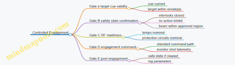
Phase 4: Operator Actions During Abnormal Conditions
If any abnormal condition occurs, the procedure should be boring and consistent:
- Fault flags appear: stop engagement attempts immediately and keep the system in inhibited/safe state.
- Cooling fault or temperature rise: do not attempt repeated firings; troubleshoot cooling first.
- Sensor disagreement: if forward/reflected power sensors or temperature sensors disagree beyond tolerance, treat it as a fault and follow the system fault response.
- Boundary mismatch: if the beam direction or inhibit region does not match the approved plan, inhibit and re-check configuration.
Example: What “Stop” Means
“Stop” should mean more than “don’t press the fire button.” It should include switching to a safe state, confirming interlocks remain enabled, and ensuring the control system is not still armed in a way that could allow an unintended command.
Phase 5: End-of-Shift Shutdown and Handover
- Disarm in the correct order: follow the system’s shutdown sequence so RF stages cool down safely.
- Verify no lingering faults: note any persistent warnings and whether they were resolved.
- Secure the site: confirm covers and access points are returned to safe configuration.
- Handover with specifics: provide the next operator with the last known system state, any faults encountered, and the current inhibit/boundary configuration.
11.2 Maintenance Schedules for RF Components and Cooling Systems
Maintenance Schedules for RF Components and Cooling Systems
A good maintenance schedule does two things: it prevents failures that are expensive to diagnose, and it keeps the system’s RF output and thermal limits inside the envelope you validated during acceptance. For counter-drone microwave defense, the schedule should be tied to operating mode (pulsed vs continuous), duty cycle, and the specific hardware path from RF source to antenna.
Foundational Concepts for Scheduling
Start by separating maintenance into three layers.
- Preventive checks catch drift: connector looseness, filter aging, fan clogging, and thermal interface degradation.
- Condition-based actions respond to measured symptoms: reflected power trends, amplifier temperature rise, coolant flow reduction.
- Corrective maintenance replaces parts after a fault or a measured parameter crosses a threshold.
A practical rule: if a component’s failure mode is sudden and dangerous (for example, a protection circuit that stops reacting), schedule it more frequently than a component that degrades gradually (for example, a cable whose loss slowly increases).
RF Component Maintenance Cadence
Use a tiered cadence that matches how often the system is likely to run.
-
Daily or per-shift (when the system is used)
- Verify system self-test results and confirm no protection faults latched during the last run.
- Inspect exterior RF connectors and waveguide interfaces for signs of looseness, corrosion, or moisture ingress.
- Confirm that the RF interlock status indicates “ready” only when cooling is within limits.
-
Monthly
- Measure forward and reflected power under a controlled low-power test condition. Track baseline values and look for slow changes.
- Inspect RF switching devices for contact wear indicators such as increased insertion loss or repeated switching errors.
- Check filter passband health indirectly by comparing measured output power at a fixed test frequency.
-
Quarterly
- Perform a deeper thermal and electrical check: verify amplifier bias stability, confirm that temperature sensors report consistent values across channels.
- Inspect waveguide runs and gaskets. Replace gaskets that show compression set or uneven sealing.
-
Semiannual or annual
- Recalibrate any measurement paths used for protection logic and output verification.
- Conduct a full connector torque verification using the manufacturer’s torque guidance, because “tight enough” is not a measurement.
Cooling System Maintenance Cadence
Cooling maintenance should be scheduled more like plumbing than like electronics: flow, cleanliness, and heat transfer surfaces matter.
-
Daily or per-shift
- Confirm coolant flow rate and temperature differential are within the allowed range.
- Check pump status indicators and alarms. If the system reports “flow low,” treat it as a real problem, not a nuisance.
-
Monthly
- Inspect strainers and filters for debris. Even small particulate loads can reduce heat transfer.
- Verify fan operation if air-cooling is used for heat exchangers.
-
Quarterly
- Inspect thermal interface materials on amplifier modules during safe access. Replace if the surface shows drying, cracking, or uneven contact.
- Check for leaks at fittings and seals. Look for residue patterns, not just active drips.
-
Semiannual or annual
- Perform coolant quality checks appropriate to the coolant type: conductivity, pH, or other parameters specified for corrosion control.
- Flush and renew coolant if required by the system’s documented maintenance procedure.
Mind Map for Integrated Maintenance Planning
Integrated Example Schedule for a Typical Site
Assume the system runs a few hours per day in pulsed mode.
- Every shift: run self-test, confirm cooling interlocks are satisfied, and record flow rate and amplifier temperatures during the first short test pulse.
- Monthly: perform a low-power RF check at a fixed frequency, compare reflected power to the last baseline, and inspect cooling strainers.
- Quarterly: open the amplifier module access path, inspect thermal interfaces, and verify waveguide gasket condition.
- Semiannually: recalibrate protection-related measurement paths and verify connector torque on the highest-loss RF runs.
The key integration point is that RF checks and cooling checks share the same timeline. If reflected power rises while coolant temperature delta also rises, you troubleshoot thermal transfer and flow first; if reflected power rises without thermal symptoms, you focus on RF interfaces and matching.
Thresholds and What to Do When They Trigger
Define “stop and troubleshoot” triggers before you need them. Examples include:
- Reflected power increases beyond a set percentage compared to baseline during the same test condition.
- Cooling flow drops below the minimum allowed value for the current operating mode.
- Temperature sensor disagreement exceeds a small tolerance between redundant sensors.
When a trigger occurs, record the exact test conditions, then isolate the likely subsystem using the most direct evidence: RF interface inspection for matching issues, and strainer/filter plus pump checks for flow issues. This keeps maintenance systematic instead of guessy, and it prevents the classic problem of fixing the wrong thing twice.
11.3 Fault Diagnosis Using Telemetry and Event Logs
Fault diagnosis starts with a simple rule: treat telemetry as measurements and event logs as a timeline of decisions. When you combine them, you can separate “the system is failing” from “the system is protecting itself,” which is usually the difference between a fix and a shutdown.
Foundations for Reading Telemetry and Logs
Telemetry answers: What is happening right now? Typical signals include forward and reflected power, amplifier temperature, cooling flow status, interlock states, phase/attenuator commands, and RF switch positions. Event logs answer: What did the controller decide to do? Examples include “interlock opened,” “VSWR threshold exceeded,” “beam inhibit asserted,” and “waveform change requested.”
A practical workflow is to align both streams on a common time base. If your controller timestamps events at the moment of state change, and your telemetry samples at a fixed rate, you can still correlate by using the nearest sample before and after each event. That correlation prevents a common mistake: blaming the amplifier for a fault that was actually triggered by a safety boundary check.
Mind Map: Diagnosis Inputs and Reasoning
Step 1: Find the First Causal Event
Start at the earliest event that changes system behavior. If the log shows “beam inhibit asserted” at 14:02:11.3, do not begin by inspecting temperatures at 14:02:11.3. Instead, look for the event that occurred just before it, such as “reflected power exceeded threshold” or “cooling flow below minimum.” The first causal event is often the one that explains the rest.
Example: A site operator reports intermittent beam stops. The event log shows repeated sequences:
- 14:02:10.8 “Cooling flow below minimum”
- 14:02:11.3 “Beam inhibit asserted”
- 14:02:12.0 “Waveform stop acknowledged”
Telemetry around 14:02:10.8 should show a cooling flow pressure drop and a rising amplifier temperature trend. If temperatures remain stable while flow dips, the issue may be a flow sensor calibration or a valve control timing mismatch.
Step 2: Use Telemetry Windows, Not Single Samples
Telemetry is noisy in the way real hardware is noisy. Use a window, such as 2–5 seconds before and after the first causal event. For RF power, check whether reflected power rises sharply at the same time as the event. For thermal faults, check whether temperature slope changes, not just absolute values.
Example: “VSWR threshold exceeded” appears in the log. Telemetry shows reflected power spiking for 200 ms, then returning to normal, while forward power stays steady. That pattern suggests a transient mismatch, such as a brief RF switch transition or a momentary antenna alignment change, rather than a permanent connector issue.
Step 3: Classify Faults by Signature
Use consistent categories so diagnosis doesn’t become guesswork.
- Protection Triggered
- Signature: event log shows a protective action, and telemetry crosses a threshold.
- Example: “Interlock opened” follows “door switch state invalid.” Telemetry should show the interlock input changing state, not a sudden thermal collapse.
- Hardware Degradation
- Signature: repeated faults with similar telemetry trends, often with slower drift.
- Example: reflected power gradually increases over weeks, and the log shows frequent “VSWR threshold exceeded” even during stable operation.
- Configuration Mismatch
- Signature: faults occur right after a mode change or waveform update.
- Example: after “waveform change requested,” telemetry shows unexpected frequency-dependent behavior, and the log records “beam inhibit asserted” shortly afterward.
- Sensor or Logging Fault
- Signature: telemetry contradicts other evidence.
- Example: the log claims “cooling flow below minimum,” but the cooling pump status remains normal and amplifier temperature does not rise.
Step 4: Confirm with Cross-Channel Consistency
A good diagnosis checks more than one channel. If reflected power spikes, verify whether RF switch state changed, whether beam steering commands updated, and whether any interlock input toggled. If a thermal fault occurs, verify cooling metrics and amplifier temperature slope.
Step 5: Record Evidence for the Next Diagnosis
When you resolve a fault, capture the minimal evidence package: the first causal event timestamp, the telemetry window summary (threshold crossings and slopes), the system mode at the time, and the corrective action taken. This turns future “it happened again” reports into a repeatable investigation.
Example evidence entry:
- First causal event: 14:02:10.8 “Cooling flow below minimum”
- Telemetry window: flow pressure dropped 18% within 0.5 s; PA temperature slope increased after 1.2 s
- Mode: perimeter tracking, waveform A
- Corrective action: restarted cooling controller; verified stable flow and cleared fault latch
Step 6: Decide Between Reset and Service
Use the log’s fault latch behavior. If the same fault reappears immediately after reset, treat it as a real condition rather than a transient. If it clears and stays clear while telemetry remains within normal bounds, you likely addressed a temporary cause such as a control timing hiccup.
A slightly playful but useful rule: if the system keeps telling you the same story, don’t keep asking it to retell the story—fix the plot point.
11.4 Configuration Management for Waveforms and Beam Parameters
Configuration management keeps waveform settings and beam parameters consistent across design, testing, and operations. In a microwave counter-drone system, “consistent” means more than saving a file name; it means every parameter change is traceable, validated, and tied to a specific intent and safety envelope.
Foundational Concepts and What Must Be Controlled
Start with a clear inventory of what can change. Treat each item as a configuration parameter with an owner, a valid range, and a reason for change.
- Waveform parameters: center frequency, bandwidth, pulse width, repetition rate, duty cycle, modulation type, and ramping behavior.
- Beam parameters: pointing angles, scan pattern, dwell time, beam steering mode, polarization selection, and any gain/attenuation settings.
- Coupling and safety parameters: interlock thresholds, maximum allowed output power, thermal limits, and RF switching states.
A practical rule: if a parameter affects either emitted energy distribution or safety boundaries, it belongs in configuration control.
Configuration Items and Naming That Prevents Confusion
Use a naming scheme that encodes intent and constraints. For example, “WFM-3.2GHz-10us-1kHz-Duty0.01” is more useful than “test7.” Pair it with a beam profile name like “BEAM-Perimeter-ScanA-PolV.”
Each configuration item should include:
- Version: immutable identifier for the exact parameter set.
- Scope: which hardware variant and site profile it applies to.
- Constraints: allowed ranges and required interlocks.
- Validation evidence: what tests proved it works.
Change Control Workflow from Request to Release
A good workflow is boring on purpose.
- Request: describe the problem the change solves, not just the parameter edits.
- Impact assessment: identify which waveform and beam parameters shift, and whether safety limits are affected.
- Approval: require sign-off from RF engineering and safety engineering.
- Test plan selection: choose the minimum set of tests that covers the changed parameters.
- Verification: confirm timing, output power behavior, and beam pointing accuracy.
- Release: publish a versioned configuration bundle that operators can select.
- Audit trail: record who changed what, when, and why.
A small example: if you change pulse width from 10 µs to 12 µs, you must re-check duty cycle compliance, thermal headroom, and any beam dwell assumptions tied to repetition rate.
Parameter Bundles and Coupling Between Waveform and Beam
Waveform and beam settings are not independent. A beam dwell time that is safe for one duty cycle might be too aggressive for another.
Use a bundle concept: a waveform version plus one or more beam profiles plus the safety configuration that governs them. Operators then select a bundle, not a random mix.
Example Bundle
- Bundle ID: BNDL-2024-09-PerimA-v5
- Waveform: WFM-3.2GHz-10us-1kHz-Duty0.01
- Beam: BEAM-Perimeter-ScanA-PolV
- Safety: MAX-PWR-Allowed=defined, ThermalLimit=defined, Interlock thresholds=defined
When the waveform changes, the bundle version changes even if the beam profile name stays the same.
Validation Rules That Catch Mistakes Early
Before any field use, enforce rules that prevent invalid combinations.
- Range checks: every parameter must fall within allowed limits.
- Consistency checks: pulse width and repetition rate must produce the configured duty cycle.
- Timing checks: beam steering commands must align with waveform start and stop windows.
- Thermal checks: predicted average power must remain under thermal limits for the intended dwell pattern.
If a check fails, the system should refuse to load the configuration bundle rather than “best-effort” it.
Mind Map: Configuration Management
Operator-Facing Controls and Auditability
Operators need a small set of bundle choices with clear descriptions and visible status. The system should display the active bundle ID, waveform version, beam profile, and safety state.
A useful operational habit: log the bundle ID at the start of each run and record any interlock events with the exact configuration version. That way, troubleshooting becomes a lookup exercise instead of a memory contest.
Example Change Scenario with Correct Handling
Suppose a site test shows reduced effectiveness at a particular approach angle. The fix is to adjust the beam scan pattern dwell distribution, not to tweak waveform parameters randomly.
- Create a new beam profile version: BEAM-Perimeter-ScanA-v3
- Build a new bundle: BNDL-2024-09-PerimA-v6 using the same waveform version
- Run verification focused on beam pointing, dwell timing, and safety interlock behavior
- Release the new bundle while keeping the prior bundle available for comparison
This keeps the system explainable: the waveform stayed constant, the beam changed, and the evidence matches the change.
11.5 Practical Example of a Maintenance and Readiness Checklist
A good readiness checklist does two things: it prevents “looks fine” failures, and it makes troubleshooting faster when something is off. Below is a practical, end-to-end example you can adapt for a microwave counter-drone system with transmitters, beam steering, sensing inputs, and safety interlocks.
Readiness Checklist Overview
Start with a simple rule: every item either (1) verifies a measurable state, (2) confirms a safety constraint, or (3) records evidence for later review. If an item can’t be measured or evidenced, it usually becomes a “maybe” and should be rewritten.
Mind Map: Maintenance and Readiness Checklist
Pre-Shift Checks
1) Visual and mechanical integrity
- Inspect antenna radomes, mounts, and cable strain reliefs. Example: if a radome shows a hairline crack, treat it as a potential moisture ingress path and schedule replacement before the next shift.
- Verify connectors are seated and labeled. Example: mismatched labels on RF coax can cause “wrong path” faults that look like electronics failures.
2) Cooling and power system status
- Confirm coolant level/flow indicators and that fans or pumps are running within expected ranges. Example: a pump that starts but cavitates may still show “running,” so check flow rate or temperature rise.
- Check power distribution health: breaker positions, fuses, and any monitored voltages. Example: a slightly low DC rail can reduce output power without triggering a hard fault.
3) RF path integrity
- Verify RF switch positions and that any attenuators or directional couplers report plausible states. Example: if a directional coupler reports reflected power spikes during a no-transmit test, investigate switch contacts before attempting engagement.
- Confirm waveguide/coax routing is unchanged from the last documented configuration.
4) Safety interlocks and access control
- Test door/guard interlocks by attempting a transmit command with guards open. The expected result is refusal to transmit and a clear fault code.
- Validate emergency stop behavior: pressing E-stop should force the system into a safe state and require a deliberate reset.
Operational Readiness
5) Sensor health and data quality
- Run a sensor self-check for radar/EO/IR/RF monitoring modules. Example: if tracking confidence drops, the system may still “work” but aim commands will be unstable.
- Confirm time synchronization between sensors and the beam control computer. Example: a small clock offset can create consistent aim lag that looks like calibration drift.
6) Timing and cueing workflow
- Perform a dry-run cueing test that exercises the pipeline without transmitting. Example: the system should accept a simulated target track, produce beam commands, and log the intended aim point.
- Verify latency logging is enabled and that timestamps are monotonic.
7) Beam control calibration sanity checks
- Confirm beam steering limits and that the current calibration set matches the site configuration. Example: after a maintenance visit, a wrong calibration profile can cause the beam to “work” but miss the intended coverage sector.
- Run a low-power alignment check if your design supports it, using a known reference target or internal test mode.
8) Waveform configuration verification
- Confirm frequency, pulse width, repetition rate, and duty cycle settings match the approved engagement profile for the site. Example: a duty cycle mismatch can overheat amplifiers even if peak power is within limits.
- Ensure any inhibit conditions are present and active (for example, “no transmit when safety boundary is violated”).
Fault Handling and Recovery
9) Fault taxonomy and safe-state verification
- Categorize faults into: RF hardware faults, interlock faults, sensor faults, and configuration faults.
- For each category, define the expected safe state. Example: RF hardware faults should inhibit transmit but may allow sensing; interlock faults should inhibit both transmit and any beam command outputs.
10) Reset and re-test procedure
- After a fault, reset only the affected subsystem when the design allows it, then re-run the smallest test that proves the fix. Example: if reflected power fault triggers, re-check RF switch state and directional coupler readings before attempting any higher-level workflow.
Evidence and Logging
11) Configuration snapshot and operator sign-off
- Record waveform parameters, calibration profile ID, and interlock test results. Example: include the exact waveform ID used during the shift so later investigations aren’t guesswork.
- Sign off with a timestamp and operator ID. If you need a reference date for a maintenance record, use 2026-03-07.
12) Example checklist form fields
- Date: 2026-03-07
- System ID and site sector
- Cooling status: OK / measured values
- Interlock test: Pass / fail with fault code
- Sensor self-check: OK / degraded modules
- Cueing dry-run: Pass / fail
- Beam alignment sanity: Pass / fail
- Waveform profile: Approved ID
- Faults during shift: none / list with resolution
This checklist works because it moves from physical integrity to safety constraints, then to operational correctness, and finally to evidence. When something fails, you can trace it to a category quickly—without turning every shift into a mystery novel.
12. Case Studies of Microwave Defense System Integration
12.1 Case Study of a Perimeter System With Beam Steering Arrays
This case study describes a perimeter microwave defense system designed to cover a fenced critical site while keeping safety boundaries predictable. The system uses beam steering arrays to aim high-power microwave energy only when a tracked drone is inside an approved engagement volume.
System Goals and Constraints
The perimeter had three practical goals: (1) detect small drones early enough to aim, (2) steer beams accurately across the fence line without excessive scan loss, and (3) enforce safety interlocks so the transmitter cannot fire outside the engagement volume.
Constraints were equally concrete. The site had uneven terrain and partial line-of-sight from some angles. Nearby infrastructure required strict electromagnetic compatibility controls. Operators needed a workflow that could be checked quickly during drills.
Architecture Overview
The system was built around four coordinated subsystems:
- Sensing and tracking: A radar/EO cueing layer produced a target track with a timestamp and uncertainty.
- Beam steering: A phased array (or mechanically steered array with electronic fine steering) produced a commanded pointing direction.
- High-power transmit chain: RF generation, amplification, and distribution delivered pulses only when permitted.
- Safety and control: Interlocks verified geometry, exposure limits, and system health before firing.
A key design choice was treating the beam as a controlled resource. The beam controller accepted only “approved aim commands” derived from the safety volume and the current track uncertainty.
Engagement Geometry and Safety Volume
The engagement volume was defined as a 3D region aligned to the perimeter. It included a buffer for tracking error and a margin for beam pointing uncertainty.
A simple way to reason about this is to separate three boundaries:
- Detection boundary: where the system can reliably track.
- Aim boundary: where the array can point with acceptable gain and sidelobe behavior.
- Fire boundary: where safety limits are satisfied for the worst-case pointing error.
In this deployment, the fire boundary was the smallest region. If the target track wandered near the edge, the system either reduced duty cycle or refused to fire, depending on the configured mode.
Beam Steering Array Design Choices
The array design balanced coverage and controllability.
- Array layout: The array was mounted to minimize blind spots caused by nearby structures. The mounting height was chosen so the beam path cleared the fence line at typical engagement ranges.
- Scan strategy: The controller used a scan pattern that prioritized the fence-facing sector first, then expanded outward. This reduced time spent at extreme steering angles where gain drops.
- Calibration: A calibration routine mapped commanded angles to measured pointing error. The system stored a correction table so the safety volume could be computed using real performance, not optimistic assumptions.
Example: Edge-of-Perimeter Handling
If a drone hovered near the fire boundary, the track uncertainty grew because the target’s aspect angle changed. The controller responded by tightening the acceptance gate: it required a smaller uncertainty ellipse before allowing a fire pulse. Operators saw this as “tracking stable” versus “tracking uncertain,” rather than a confusing on/off flicker.
Control Workflow with Timing Discipline
The firing workflow used a strict sequence:
- Track update: The tracker produced position and uncertainty at time T.
- Predictive aim: The beam controller predicted where the target would be at the transmit time, accounting for system latency.
- Safety check: The predicted aim was tested against the fire boundary and exposure model.
- Hardware readiness: The transmit chain confirmed amplifier temperature, reflected power limits, and RF switch state.
- Pulse command: Only then did the system issue a transmit pulse with the selected waveform parameters.
This sequencing prevented a common failure mode: aiming correctly but firing at the wrong time. The system treated latency as a first-class input, not an afterthought.
Mind Map: Perimeter Beam Steering System
Hardware and Operational Integration
The transmit chain included protection behavior that operators could understand. For instance, if reflected power exceeded a threshold, the system entered a safe state and logged the event. During drills, the team practiced interpreting logs as “what happened” and “what to do next,” not as mystery codes.
A practical integration detail was the separation of responsibilities: the safety controller owned the decision to permit firing, while the beam controller owned pointing commands. This reduced the chance that a software bug in one module could bypass the other.
Example: Acceptance Testing for Array Pointing
Acceptance testing focused on verifying that the safety volume calculations matched reality.
- The team measured pointing error across the steering sector.
- They compared measured gain and sidelobe behavior against the assumptions used to define the fire boundary.
- They repeated the workflow test by simulating tracks near the boundary and confirming the system refused to fire when uncertainty exceeded the configured gate.
The result was a perimeter system where “beam steering” and “safety” were not separate topics. The array could steer, but it only steered into a region where firing was permitted, and the permission depended on measured performance and timing discipline.
12.2 Case Study of a Multi Sensor Cueing Workflow with Timing Controls
A perimeter site uses three sensors to cue a microwave defense unit: a long-range radar for coarse detection, an EO/IR camera for confirmation and bearing refinement, and an RF monitor for band identification and signal stability. The goal is simple: produce a beam command that is timely, repeatable, and safe, even when the target is moving and sensors disagree.
Foundations of the Cueing Chain
The workflow is built around four timing checkpoints.
- Detection timestamp: the radar produces a track with a timestamp tied to its own clock.
- Confirmation timestamp: the EO/IR system confirms the target and refines bearing and elevation.
- Cue generation timestamp: the fusion layer converts sensor estimates into a single aim point and a transmit window.
- Actuation timestamp: the microwave controller starts transmit only when interlocks are satisfied and the aim point is still valid.
A practical best practice is to treat timestamps as first-class data. Each sensor message carries a time tag, and the fusion layer refuses to use stale inputs. In this case study, any sensor update older than 150 ms is ignored for aim computation, while older data may still be used for track continuity.
System Setup and Timing Controls
The site controller runs a fixed-rate loop at 50 Hz (20 ms per cycle). Sensor messages arrive asynchronously, so the fusion layer maintains a small buffer per sensor and interpolates to the current fusion time.
Timing Rules That Prevent “Aim Drift”
- Fusion time selection: the fusion layer chooses a target time equal to “now minus actuation latency.” This compensates for the time between cue computation and beam start.
- Latency budgeting: the system measures end-to-end latency during commissioning and stores it as a parameter. If measured latency changes beyond a tolerance, the system reduces transmit duty or pauses.
- Transmit window gating: each cue includes a start time and an end time. The beam fires only within that window.
A concrete example: if actuation latency is 80 ms and the beam steering settles in 10 ms, the fusion layer computes aim for now + (10 ms) but schedules transmit for now + 90 ms. That way, the beam is already settled when energy is applied.
Multi Sensor Fusion Logic
The fusion layer outputs an aim point and confidence score. Confidence is not a vibe; it is computed from measurable factors.
- Radar confidence increases with track stability and consistent velocity estimates.
- EO/IR confidence increases when the target is visible with consistent edges and minimal motion blur.
- RF confidence increases when the RF monitor reports a stable signal in the expected band and the signal strength is above a threshold.
If EO/IR is unavailable, the system can still cue using radar plus RF band stability, but it widens the transmit window and reduces power density targets to maintain safety margins.
Example Workflow with Realistic Numbers
Assume a drone enters detection range at time T0.
- At T0 + 0 ms, radar creates a track and sends an update stamped at T0.
- At T0 + 60 ms, EO/IR confirms and sends a bearing refinement stamped at T0 + 60 ms.
- At T0 + 95 ms, fusion computes an aim point for the actuation schedule and emits a cue.
- At T0 + 180 ms, the microwave controller receives the cue, verifies interlocks, checks that the aim point is not stale, and starts transmit.
The system also checks for disagreement. If EO/IR bearing differs from radar bearing by more than a configured threshold, the fusion layer either blends estimates with lower weight on the outlier or waits for the next EO/IR frame. This avoids firing based on a single questionable measurement.
Mind Map: the Cueing Workflow
Operational Example: What Gets Logged
After each engagement attempt, the system records:
- sensor timestamps used for the cue,
- the fusion time chosen,
- the computed aim point and confidence,
- the transmit window boundaries,
- interlock status at actuation time,
- whether the cue was fired or suppressed due to staleness or disagreement.
This logging is what makes timing issues diagnosable. If a cue is consistently suppressed, you can see whether the cause is sensor staleness, latency drift, or steering readiness.
Integrated Takeaway
A multi sensor cueing workflow works when timing is treated as a control variable, not an afterthought. By buffering sensor data, compensating for measured latency, gating transmit windows, and handling disagreement explicitly, the system produces beam commands that are both timely and defensible—without relying on guesswork or heroic operator timing.
12.3 Case Study of Safety Boundary Engineering and Interlock Validation
A perimeter microwave defense unit was integrated into an active critical-infrastructure site with three constraints: keep personnel exposure within limits, avoid interference with nearby communications, and ensure the system cannot transmit unless the site is in a known safe state. The engineering team treated safety boundaries as a measurable geometry problem, then enforced that geometry through interlocks that fail safe.
Foundational Safety Boundary Concepts
Safety boundaries start with a defined “transmit allowed” volume. The boundary is not a vague fence line; it is a surface derived from field modeling and verified by measurement. The workflow begins with three inputs: antenna pointing limits, maximum credible transmit parameters, and the exposure criterion used by the organization.
A practical example: if the array can steer within a 30° sector and the maximum effective radiated power occurs at the center of that sector, the boundary is computed for the worst-case pointing angle. If the system later changes steering limits, the boundary must be recomputed or constrained to remain inside the original safe envelope.
Boundary Engineering Workflow
- Model the field and exposure metric for the maximum transmit configuration. Use conservative assumptions for losses, alignment, and duty cycle. The goal is to ensure the modeled boundary is at or outside the true boundary.
- Convert the boundary into operational constraints. The boundary becomes a set of allowed aim angles, allowed transmit modes, and allowed times when personnel are expected to be outside the boundary.
- Define physical and procedural controls. Physical controls include signage, barriers, and access points. Procedural controls include operator checklists and authorization steps.
- Validate with measurement at representative points. Measurement is used to confirm that the boundary is not accidentally smaller than predicted.
A concrete example of step 2: the system’s control software can map “beam command” to a safe/unsafe flag using a precomputed lookup table. If the operator attempts a beam command that would aim toward a location where the boundary would be violated, the software refuses the command and logs the attempt.
Interlock Validation Strategy
Interlocks are the enforcement layer. Each interlock must be testable, independently monitored, and designed so that any failure results in “no transmit.” The case study used a layered approach:
- Access interlock tied to gate switches and door sensors. If any access point is open, transmit is inhibited.
- Aim interlock tied to encoder feedback and software-verified pointing. If pointing is out of tolerance, transmit is inhibited.
- RF chain interlock tied to amplifier readiness signals and reflected-power protection. If the RF chain is not in a known-good state, transmit is inhibited.
- Mode interlock tied to waveform selection and duty-cycle limits. If an operator selects a mode outside the validated set, transmit is inhibited.
Validation focused on three questions: Does the interlock prevent transmit when it should? Does it remain effective under realistic timing delays? Does it fail safe when sensors disagree?
Mind Map: Safety Boundary and Interlock Validation
Example Validation Tests and Results
Test A: Access Interlock Timing The team simulated a gate opening during an attempted transmit. The expected behavior was immediate inhibition, but the system also had to handle the reality of control-loop latency. The test measured the time from gate-open signal to RF inhibit command and confirmed it stayed within the design allowance. The key detail was verifying that the RF chain did not “finish” a pulse after the inhibit signal; the transmit controller was configured to stop at the next pulse boundary.
Test B: Aim Interlock Under Encoder Drift They introduced controlled encoder offsets to mimic drift. The aim interlock used both encoder readings and a software tolerance band. When the commanded aim exceeded the safe envelope, transmit was blocked even if the operator interface still displayed a plausible direction. This prevented “human-visible correctness” from masking “system-actual incorrectness.”
Test C: Sensor Disagreement Fail-Safe Access sensors were intentionally forced into conflicting states. The system required consensus within a short window; otherwise it entered a locked transmit-disabled mode. The validation confirmed that disagreement never resulted in transmit enablement, even if one sensor reported “closed.”
Evidence and Operational Readiness
The final evidence package tied everything together: the boundary computation assumptions, the measurement points used to verify the boundary, and the interlock logic that enforced the operational constraints. A simple but effective practice was a test matrix that listed each interlock, the unsafe condition that triggers it, the expected system state, and the measured response time.
In this case study, safety boundary engineering and interlock validation were treated as one system: geometry defined the rules, and interlocks ensured the rules were actually followed. The result was not just “it seems safe,” but “it is safe because the system cannot transmit outside the validated envelope, even when operators make mistakes or sensors misbehave.”
12.4 Case Study of RF Hardware Thermal Management in Field Conditions
A fielded counter-drone microwave system has to survive the boring parts: sun, dust, wind, and long duty cycles. Thermal management is the difference between “it worked on the bench” and “it works when the site is busy.” This case study follows one deployment cycle for a compact high-power RF unit with a beam-steering antenna and a pulsed solid-state transmitter.
Field Setup and Thermal Baseline
The unit was installed in an outdoor enclosure with forced-air cooling and a heat exchanger. Before any high-power trials, the team established a baseline thermal map at low power: surface temperatures at the enclosure wall, airflow temperature rise across the heat exchanger, and device temperatures at the amplifier module. They used a simple rule: if the amplifier case temperature rose faster than the airflow temperature rise, the airflow path was not matching the design intent.
A practical example: during the first site check, the inlet filter was installed with partial blockage. The amplifier case temperature climbed quickly even though the measured airflow temperature rise looked “reasonable.” The fix was to correct filter seating and add a visual indicator for filter misalignment.
Cooling Architecture and Why It Matters
The cooling system had three layers.
- Airflow delivery: fans and ducting that enforce where air goes.
- Heat transfer: heat exchanger surfaces sized for the expected duty cycle.
- Device protection: temperature sensors and power derating logic.
The key best practice was to treat airflow as a controlled variable, not a hope. Ducting reduced recirculation, and the heat exchanger was instrumented so the team could compare expected versus actual temperature rise.
Instrumentation and Control Loop Design
Thermal control worked in two stages.
- Monitoring: multiple sensors on amplifier modules, power supplies, and the heat exchanger outlet.
- Action: when a sensor exceeded a threshold, the controller reduced duty cycle or limited peak power.
A systematic approach prevented “sensor theater.” The team validated each sensor by running a controlled load step and checking that the sensor response time matched the physical location. If a sensor lagged too much, it could trigger protection late, which is how you end up with repeated trips and degraded reliability.
Duty Cycle Testing with Realistic Loads
Field conditions rarely match lab conditions, so the test plan used staged duty cycles.
- Stage 1: short pulses to verify RF performance while keeping temperatures low.
- Stage 2: longer pulse trains to reach steady-state.
- Stage 3: worst-case sequence based on expected operational patterns.
Example: the system was scheduled to fire in bursts while tracking targets. The team measured the cooling recovery time between bursts. They found that recovery was slower than expected when the enclosure internal air temperature approached ambient plus solar heating. The operational mitigation was straightforward: adjust burst spacing so the amplifier case temperature stayed below the derating threshold.
Failure Modes and Field Fixes
The most common thermal issues were not exotic.
- Dust loading: filters clogged, reducing airflow. The fix was a maintenance interval tied to measured airflow pressure drop rather than calendar time.
- Fan degradation: one fan slowed due to bearing wear. The controller detected reduced airflow indirectly via heat exchanger outlet temperature behavior and triggered a maintenance flag.
- Hot spots from airflow bypass: gaps in duct seals let air take shortcuts. The fix was mechanical sealing and re-checking airflow paths after any enclosure service.
Mind Map: Thermal Management Logic
Thermal Management Mind Map
Acceptance Criteria and What “Good” Looked Like
The acceptance criteria were measurable and tied to operational behavior.
- Steady-state: during the worst-case duty cycle, amplifier case temperature stayed below the derating threshold with margin.
- Recovery: after a burst sequence, temperatures returned to the normal operating band within a defined time window.
- Stability: repeated burst sequences did not cause oscillation between full power and derating.
A final example: once the filter-based maintenance trigger was adopted, the system stopped showing late-day thermal trips. The improvement wasn’t magic; it was simply aligning the cooling system’s real-world constraints with the controller’s expectations.
Practical Checklist for Field Thermal Readiness
- Confirm airflow path integrity after installation and any service.
- Validate sensor timing with a controlled load step.
- Test duty cycles that match the operational burst pattern.
- Use pressure-drop-based filter maintenance criteria.
- Verify recovery time, not just peak temperature.
- Ensure protection thresholds lead to controlled derating, not repeated hard trips.
12.5 Case Study of Acceptance Testing and Documentation Package
Acceptance testing for a counter-drone microwave defense system is less about proving it can transmit power and more about proving it behaves correctly under real operational constraints. This case study uses a perimeter deployment with a steerable microwave array, a multi-sensor cueing chain, and a safety interlock cabinet. The acceptance package is organized so an auditor can trace any outcome back to a requirement, a test method, and a recorded result.
Acceptance Scope and Entry Criteria
The scope covers RF performance, safety behavior, control software timing, and documentation completeness. Entry criteria include calibrated measurement equipment, verified firmware build identifiers, and a locked configuration baseline for waveforms, beam limits, and interlock thresholds. A practical rule: if the system cannot reproduce the same beam command sequence twice in a row during bench tests, it does not earn field testing.
Test Matrix from Requirements to Evidence
The matrix maps each requirement to a test category, method, acceptance threshold, and evidence artifact. For example, “beam steering accuracy” is tested with a known target position and verified against measured pointing error. “Interlock response time” is tested by forcing a controlled fault and timing the shutdown sequence.
A compact way to keep the matrix readable is to group tests into four layers:
- Bench RF and Protection: forward/reflected power behavior, fault handling, thermal limits.
- Control and Timing: cue-to-command latency, beam command stability, logging integrity.
- Safety and EMI: exposure boundary enforcement, interlock chain integrity, immunity checks.
- Site Integration: placement verification, network connectivity, environmental operation.
Mind Map: Acceptance Testing Evidence Flow
Bench RF and Protection Verification
The bench phase confirms that the transmitter chain and protection circuits behave predictably. A typical sequence starts with a low-power sweep to validate frequency response, then steps to rated pulse settings while monitoring forward power, reflected power, and amplifier temperature. Protection behavior is verified using a controlled mismatch: the system should detect abnormal reflected power and transition to a safe state within the specified time window.
Repeatability is tested by running the same waveform and beam command sequence five times and comparing key outputs. If the measured peak power varies beyond the allowed tolerance, the acceptance report records the spread and the likely cause category (calibration drift, thermal state, or control timing jitter).
Control and Timing Acceptance
Control timing is validated end-to-end: sensor cue arrives, tracking computes aim, beam command is issued, and the transmitter enable follows the correct gating logic. The acceptance threshold is not just “fast enough,” but “consistent enough.” For instance, the system may be allowed a maximum latency while also requiring that the standard deviation across runs stays below a set value.
Logging integrity is part of acceptance. Each run must produce a complete event record: cue timestamp, computed aim, beam steering command, interlock status, and transmit enable state. If any field is missing, the run is marked incomplete even if the RF output looks correct.
Safety and EMI Behavior Checks
Safety acceptance focuses on interlock correctness and exposure boundary enforcement. The interlock chain is tested by simulating cabinet door open, emergency stop activation, and sensor fault states. The system must refuse transmission when any required condition is not satisfied, and it must return to a safe idle state after a fault.
EMI checks in acceptance are practical: verify that the system does not cause unintended resets or loss of control in nearby subsystems during representative operation. The goal is stable behavior, not absolute silence.
Site Integration and Configuration Lock
Site integration acceptance verifies that the as-installed configuration matches the tested baseline. This includes antenna orientation checks, beam limit enforcement, and network connectivity for control telemetry. A configuration lock procedure is documented so that any later change triggers a controlled re-test of the affected items.
Documentation Package Contents
The documentation package is organized into four folders with consistent naming:
- Test Reports: each report includes purpose, setup, instrumentation list with calibration dates, procedure steps, raw data references, pass-fail results, and deviations.
- As-Built Configuration: waveform settings, beam steering parameters, interlock thresholds, firmware build identifiers, and wiring diagrams.
- Safety Case Artifacts: interlock logic descriptions, exposure boundary calculation summaries, and evidence of safe-state behavior.
- Operator Procedures: setup checklist, fault response steps, and shutdown/restart rules.
Example: Acceptance Report Entry Template
Test ID: RF-PROT-03
Requirement: Reflected power protection triggers safe state
Setup: 10% mismatch using calibrated attenuator
Instruments: Directional coupler, oscilloscope, thermal sensor
Procedure: Apply rated pulse sequence for 30 s, then induce mismatch
Acceptance Threshold: Safe-state transition within 200 ms
Results: Triggered in 143–176 ms across 5 runs
Uncertainty: ±10 ms timing resolution noted
Deviations: None
Evidence: Data file references and screenshots attached
Mind Map: Documentation Package Structure
Acceptance Decision and Closeout
Closeout requires a traceability check: every requirement has at least one evidence artifact, and every deviation has a documented corrective action or a formally accepted risk statement tied to the requirement. The final sign-off is based on completeness, repeatability, and safety behavior—not on a single impressive run. For this case study, the system passed after two corrective actions: tightening thermal preconditioning time and correcting a logging field mapping that initially omitted interlock state during one fault scenario.