Radar Systems and Countermeasure Technologies Essentials
1. Radar Fundamentals for Detection and Tracking
1.1 Radar Purpose and System Building Blocks
Radar exists to answer a simple operational question: what is out there, where is it, and how is it moving? The “how” is a chain of physical and computational steps that turn transmitted energy into measurements. Each step has constraints, so good radar design is mostly careful bookkeeping—timing, geometry, signal quality, and processing resources.
Radar Purpose in Practical Terms
A radar system performs three core functions:
- Detection: decide whether a target-related return is present in the received signal. This is a statistical decision, not a guess.
- Tracking: estimate target position and velocity over time by combining new measurements with past estimates.
- Management: choose what to illuminate, when to illuminate it, and how to allocate limited processing to competing tasks.
A useful way to remember this is: detection answers “is there something,” tracking answers “what is it doing,” and management answers “what can we afford to do right now.”
System Building Blocks Overview
A radar is easiest to understand as a set of blocks that pass information forward and sometimes feed control signals backward.
- Antenna and RF Front End: radiates energy and collects echoes. It also conditions the received signal for the rest of the chain.
- Transmitter: generates the waveform with the required power, frequency stability, and timing.
- Receiver: amplifies, filters, and downconverts the echo to a form suitable for digitization.
- Timing and Synchronization: aligns transmit and receive timing so range and Doppler estimates are meaningful.
- Signal Processing: performs matched filtering or other coherent processing, then detection and measurement extraction.
- Tracking and Data Association: converts measurements into tracks and resolves which measurements belong to which target.
- Control and Resource Management: schedules modes, waveforms, beam pointing, and processing budgets.
- Human or System Interface: presents tracks, alerts, and diagnostics in a usable way.
From Transmit to Track Without Gaps
A coherent radar measurement depends on knowing three things precisely: when the pulse was sent, where the beam was pointing, and how the waveform relates to the received echo.
- Waveform generation sets the “template” for processing. If the receiver processing assumes the wrong waveform parameters, detection and range estimates degrade.
- Propagation and reflection determine the echo strength and delay. Range is inferred from time-of-flight, so timing errors map directly into range errors.
- Downconversion and digitization preserve phase and amplitude relationships needed for coherent processing. Poor filtering or sampling choices can smear Doppler information.
- Coherent processing compresses energy and improves signal-to-noise ratio. Detection thresholds are then applied to the processed outputs.
- Measurement extraction converts detections into range, angle, and Doppler (or velocity) estimates with associated uncertainties.
- Tracking uses those uncertainties to update state estimates. If uncertainties are wrong, the filter either overreacts or becomes sluggish.
- Management ensures the radar spends its limited time and compute where it matters, such as searching broadly versus focusing on a few tracks.
Mind Map: Radar Purpose and Building Blocks
Example: A Simple Search-to-Track Flow
Imagine a radar that alternates between scanning for new targets and updating existing tracks.
- In search mode, the controller points the antenna across a sector and uses a waveform optimized for detection. The processing chain emphasizes sensitivity and reliable detection.
- When detections appear, the system initiates tracks by collecting enough measurements to estimate motion. The tracking block now becomes active.
- In track mode, the controller allocates more dwell time and uses waveform/beam settings that improve measurement precision for the tracked targets. The signal processing chain shifts emphasis from “find something” to “measure precisely.”
This example highlights why building blocks must be designed together: the transmitter waveform choice affects processing, which affects measurement quality, which affects tracking stability.
Key Design Inputs You Must Know Early
Even at the fundamentals level, radar design starts with inputs that propagate through the entire chain:
- Geometry: antenna location, beam pointing, and target-relative motion.
- Waveform parameters: bandwidth, pulse width or modulation, and repetition timing.
- Timing accuracy: determines range fidelity.
- Receiver noise and dynamic range: determines detection limits and susceptibility to interference.
- Processing constraints: compute and memory budgets limit how many beams, pulses, or tracks can be handled.
When these inputs are consistent, the radar can produce measurements that are not just “present,” but also trustworthy enough to track.
A Useful Mental Model
Think of radar as a measurement instrument with a built-in conversation between physics and computation. Physics sets what echoes look like; computation decides what those echoes mean. The building blocks are the translators between the two, and the timing is the grammar that keeps the translation from turning into nonsense.
1.2 Radar Waveforms and Their Practical Tradeoffs
Radar waveforms are the “voice” of the sensor: they determine how energy is transmitted, how echoes are compressed or filtered, and how well the system can separate targets from clutter and interference. The practical tradeoffs come from a few constraints that keep showing up: time on target, bandwidth, coherence, peak power limits, and how much processing you can afford.
Waveform Building Blocks
A waveform is usually described by its modulation (how frequency or phase changes), its duration (pulse length or coherent processing interval), and its bandwidth (how much frequency spread it occupies). Those parameters drive four key outcomes.
First, bandwidth controls range resolution. Roughly, wider bandwidth means finer separation in range, because the matched filter can distinguish echoes that arrive at slightly different times.
Second, waveform duration controls Doppler sensitivity. Longer coherent observation improves velocity discrimination, because Doppler estimation needs phase history.
Third, peak power and average power shape detection range. A narrow pulse can require high peak power to deliver enough energy, while long or coded waveforms can trade peak power for processing gain.
Fourth, coherence requirements affect implementation. Some waveforms rely on stable phase relationships across the coherent interval; if the oscillator or platform motion breaks coherence, the theoretical gains shrink.
Pulse Radar Versus Pulse Compression
Pulse radar transmits relatively short pulses and listens for echoes. Its range resolution is tied to pulse width: shorter pulses give better resolution but demand higher peak power for the same energy.
Pulse compression keeps the energy advantage while improving resolution. The transmitter sends a longer coded pulse, then the receiver applies a matched filter to compress it in time. The result is a narrow effective response without requiring the same peak power at the transmitter.
A practical way to remember the trade: pulse compression shifts difficulty from hardware peak power to receiver processing and waveform accuracy. If the code is distorted by phase errors or timing jitter, compression sidelobes rise and false alarms become more likely.
Example: Choosing Pulse Width for a Warehouse Scan
Suppose you need to separate two reflectors 5 meters apart. In free space, 5 meters corresponds to about 33 ns round-trip time. A pulse width on the order of 30–35 ns supports that separation. If peak power is limited, you can use a longer coded pulse and compress it, but you must ensure the code timing and phase are consistent across the receive chain.
Continuous Wave and Frequency Modulated Waveforms
Continuous wave (CW) radar transmits continuously and often measures Doppler directly. It can be excellent for velocity measurement because it avoids the “listen” gaps of pulsed systems. The catch is that range information is not inherent unless you add modulation or use a scanning geometry.
Frequency modulated continuous wave (FMCW) radar solves this by sweeping frequency over time and estimating range from the beat frequency between transmitted and received signals. The sweep slope sets the range resolution, while the sweep duration sets velocity sensitivity.
The practical trade is that FMCW ties performance to sweep linearity and timing. If the frequency sweep is not linear, range estimates bias and sidelobes increase.
Example: FMCW Sweep Linearity Check
If you observe a target at a known fixed range and the estimated range drifts with sweep rate, the sweep may be non-linear. A simple operational check is to compare beat-frequency-derived range across multiple sweep rates while keeping antenna pointing constant.
Scan Strategies and Waveform Scheduling
Waveforms rarely operate alone; they are scheduled across search, track, and surveillance modes. A system might use a wideband waveform for search to get fine range bins, then switch to a waveform optimized for track stability.
Scheduling involves two competing goals: maximize detection probability and maintain track quality. If you spend too much time on high-resolution search, you may starve the track update rate. If you spend too much time on track-optimized waveforms, you may miss new targets entering the scene.
A good best practice is to treat waveform selection as a resource allocation problem: bandwidth, coherent processing interval, and compute time are the “budget.”
Mind Map: Waveform Tradeoffs
Advanced Details That Actually Matter
Matched filtering is the heart of pulse compression. It provides processing gain, but it also shapes sidelobes. High sidelobes can masquerade as weak targets, especially when clutter is structured (for example, strong reflections from edges).
Doppler processing depends on coherent integration. If the platform or target motion causes phase to change faster than expected, Doppler estimates smear. That smearing can be reduced by choosing an appropriate coherent interval and by using motion-compensated processing when available.
Finally, waveform switching can create discontinuities. If you change bandwidth or coding between modes, you must ensure the receiver’s calibration and timing references remain consistent, or measurement biases will appear as track jitter.
Example: Mode Switching Without Track Jitter
Imagine a radar that uses a wideband coded waveform for search and a narrower waveform for track. If the receiver timing reference is updated incorrectly during the switch, the compressed pulse peak shifts slightly. The track filter then interprets that shift as motion. A practical mitigation is to validate timing alignment by injecting known calibration signals or by using stable reference targets during integration testing.
Summary of Tradeoffs in One Line Each
- Wider bandwidth improves range resolution but increases sensitivity to timing and waveform fidelity.
- Longer coherent intervals improve Doppler discrimination but increase vulnerability to phase instability and motion mismatch.
- Pulse compression reduces peak power needs but demands accurate coding and sidelobe management.
- FMCW offers strong range-Doppler measurement in one sweep but depends on sweep linearity and timing discipline.
- Waveform scheduling balances detection coverage against track refresh so measurement quality stays consistent.
1.3 Propagation Effects and Link Budget Inputs
A radar link budget is just bookkeeping with physics. You start with transmitted power and end with the smallest echo you can reliably detect, while accounting for how the signal spreads, loses strength, and gets distorted by the environment.
Core Propagation Effects
Free-space path loss is the baseline reduction from spreading in space. For a monostatic radar, the round-trip loss matters because the wave travels out and comes back. A useful mental model: if the one-way loss is 1/L, the echo suffers roughly 1/L².
Atmospheric attenuation adds extra loss from gases and humidity. It is usually small at many radar bands over short ranges, but it can become noticeable at higher frequencies or long ranges. Treat it as an additional multiplicative factor in the link budget.
Ground and clutter interactions are not “just noise.” Surface reflections can create multipath that changes the apparent phase and amplitude of the echo, affecting coherent processing gain. Clutter also raises the effective noise floor, which changes the detection threshold.
Weather and refractivity influence propagation speed and bending. Even when you still get a return, the bending can shift where the target appears in angle and range, which then stresses tracking filters.
Link Budget Inputs
A practical link budget lists inputs in four groups: radar transmit, propagation, target, and receiver.
Radar transmit inputs
- Transmit power (peak and average). Peak power matters for range in pulsed systems; average power matters for thermal limits and duty cycle.
- Antenna gain or effective aperture. Gain converts power into directional intensity.
- Waveform parameters such as pulse width and bandwidth, which influence matched-filter gain and noise bandwidth.
Propagation inputs
- Range to target.
- Frequency and polarization, which affect attenuation and scattering.
- Path loss terms: free-space loss plus any atmospheric loss.
Target inputs
- Radar cross section (RCS) or an RCS model. RCS is the “how much it reflects” knob, but it depends on aspect angle and polarization.
- Aspect angle and elevation, which determine whether the target behaves like a smooth reflector, a corner-like reflector, or something in between.
Receiver inputs
- Receiver noise figure and system losses (cables, duplexers, radomes).
- Detection threshold expressed via probability of detection and false alarm, which ties into the effective noise bandwidth.
- Processing gain from coherent integration, which depends on whether the target motion and environment allow phase stability.
Systematic Computation Flow
- Compute one-way path loss from range and frequency.
- Square it for monostatic round-trip loss.
- Multiply by atmospheric attenuation and any additional propagation losses.
- Convert antenna gain into effective received power using the radar equation.
- Apply target RCS and include system losses.
- Convert receiver noise figure into noise power over the relevant bandwidth.
- Use the detection criterion to determine the minimum detectable signal.
- Compare predicted echo power to the minimum detectable signal to infer maximum range or required integration.
Mind Map: Propagation Effects and Link Budget Inputs
Example: Quick Link Budget Sanity Check
Assume a monostatic pulsed radar at 10 GHz, target range 50 km, and a target with RCS of 1 m². Suppose antenna gain is 35 dBi, system losses total 3 dB, and receiver noise figure is 5 dB. Start with free-space path loss for one-way propagation, then apply it twice for round trip. The received power scales with antenna gain squared and inversely with range to the fourth power (because of the squared one-way loss). If you double range to 100 km, the echo power drops by about 24 dB, which is why long-range performance is so sensitive to propagation assumptions.
Example: Propagation vs. Detection Threshold
Two radars with identical transmit power can still differ in detection range if one experiences stronger clutter. Even if the propagation loss is the same, clutter increases the effective noise floor, raising the threshold for a given false alarm rate. In practice, you can treat clutter as an additional noise term in the detection calculation, but you must ensure the threshold logic matches the processing chain used to form detections.
Example: Coherent Integration Limits
If the environment or target motion causes phase decorrelation, coherent integration gain shrinks. A link budget that assumes full coherent gain will overestimate range. A simple check is to compare expected phase stability over the integration interval against the radar’s motion model and the likely multipath variability from the ground and weather.
1.4 Signal Processing Chain From Echo to Track
A radar “track” is not a raw echo; it is a structured estimate of target state built by a chain of processing steps. Each step shapes the data so later stages can make decisions with predictable behavior. Think of the chain as a conveyor belt: if one station is sloppy, the next station has to guess, and guesses tend to multiply.
Echo Conditioning and Sampling
The received signal is first mixed down to an intermediate frequency or baseband, then sampled. Sampling rate must cover the signal bandwidth after downconversion, or you get aliasing that looks like real targets. Practical systems also apply automatic gain control so weak and strong returns fit within the analog-to-digital converter range.
Example: If a target return is 20 dB weaker than clutter, but the receiver gain is set for strong clutter, the target may fall below quantization noise. The “echo” exists, but the digital data never becomes useful.
Range Compression and Coherent Processing
For pulse-like waveforms, range compression converts time delay into a sharper range profile. Matched filtering (or an equivalent implementation) maximizes signal-to-noise ratio for known waveform structure. Coherent processing then combines multiple pulses to improve detectability and estimate Doppler.
Example: A chirped pulse spreads in time at the receiver but compresses back into a narrow peak after matched filtering. Without compression, the peak is broad and harder to separate from nearby clutter.
Detection in Range-Doppler or Range-Angle Cells
After compression, the processor forms a representation such as range bins, Doppler bins, or angle bins. Detection compares cell energy against a threshold. Thresholding is not arbitrary: it is set to control false alarms under assumed noise statistics.
Best practice: Use a constant false alarm rate approach when noise level varies across time or frequency. If you keep a fixed threshold, a quiet period and a noisy period will produce different false alarm rates.
Example: In a range-Doppler map, a small moving target may be visible only in a specific Doppler bin. If you detect only in range bins, you may miss it.
Measurement Extraction and Parameter Estimation
Detections become measurements. Instead of storing “a blob exists,” the system estimates parameters like range, Doppler (or radial velocity), and angle. Estimation uses local peak fitting, centroiding, or phase-based methods depending on the waveform and antenna configuration.
Example: For angle, a multi-element array can estimate direction by comparing phase across elements. If the array is calibrated, the same target produces consistent angle estimates across scans.
Gating and Data Association
A track is built from measurements over time, so the processor must decide which measurement belongs to which existing track. Gating uses predicted state uncertainty to limit candidate measurements. This prevents a track from “jumping” to a nearby false alarm.
Example: If a track’s predicted range at the next scan is 10,000 m with a 200 m uncertainty, a measurement at 10,600 m is outside a tight gate and is less likely to be associated.
Track Initiation and Maintenance Logic
Tracks are not created from a single detection. Initiation typically requires multiple consistent measurements across consecutive scans. Maintenance updates the state estimate when associations are made and manages track deletion when detections are missed.
Best practice: Use separate counters for initiation and deletion so a brief glitch doesn’t create a permanent track, and a short dropout doesn’t erase a real one.
Example: A two-scan initiation rule reduces false tracks from random noise spikes, while a three-scan deletion rule allows for occasional missed detections due to scan scheduling.
State Estimation and Filtering
Filtering combines the motion model with measurement updates. A common approach is a Kalman filter for linear motion with Gaussian noise, or an extended/unscented variant when the measurement relationship is nonlinear. The filter outputs a smoothed state and an uncertainty estimate.
Example: With a constant-velocity model, the filter predicts where the target should be next. When a measurement arrives, it corrects the prediction proportionally to measurement reliability.
Quality Checks and Output Packaging
Before output, the system validates track quality using residuals, innovation statistics, and consistency checks. It also packages track data with metadata such as time stamps, covariance, and source measurements.
Example: If residuals are consistently large, the system may flag the track as low confidence, even if it remains associated.
Mind Map: Signal Processing Chain from Echo to Track
Example: One Scan Cycle End to End
- The receiver samples baseband returns and applies gain control.
- The processor matched-filters each pulse to form compressed range profiles.
- It performs Doppler processing to build a range-Doppler map.
- CFAR thresholds identify candidate cells.
- The processor estimates range and radial velocity from the strongest local peaks.
- It predicts existing track states and gates candidate measurements.
- It updates matched tracks using a filter and initiates new tracks only after consistency.
- It outputs updated track states with uncertainty and residual-based quality flags.
1.5 Radar Performance Metrics for Operational Use
Radar performance metrics are only useful if they connect directly to what operators and planners need: detect the right targets, track them reliably, and do it with limited time, power, and processing. This section turns common radar metrics into an operational checklist, then shows how to interpret them together.
Detection Metrics That Drive Search Decisions
Probability of Detection (Pd) answers: “How often do we see a target when it’s there?” It depends on signal-to-noise ratio, waveform properties, and processing choices. A practical way to think about Pd is to imagine repeated passes over the same scenario: if Pd is 0.9, you should expect roughly 9 detections out of 10 similar attempts, assuming the same conditions.
Probability of False Alarm (Pfa) answers: “How often do we cry wolf?” In clutter, Pfa is not just a receiver setting; it reflects how thresholds interact with noise and clutter statistics. A common operational practice is to set Pfa to a value that keeps operator workload manageable, then verify Pd with realistic data.
Detection Threshold and CFAR Behavior connect Pd and Pfa to implementation. For example, in a simple cell-averaging CFAR, the radar estimates local background from neighboring range cells and sets a threshold relative to that estimate. If the background rises due to clutter, the threshold rises too, which can reduce Pd unless the waveform or processing compensates.
Tracking Metrics That Matter After Detection
Detection is the start; tracking is the job. Tracking metrics quantify how well the radar maintains target state estimates over time.
Track Update Rate is how often you produce a new track estimate. Higher update rates can improve responsiveness, but they also increase data association pressure and processing load.
Track Accuracy is typically summarized by errors in range, azimuth/elevation, and velocity. A useful operational view is to compare these errors to the tolerances of downstream tasks, such as weapon cueing or airspace deconfliction.
Track Stability measures how often a track jumps, splits, or loses continuity. Even if average accuracy is good, frequent instability can break mission logic. A simple example: if a track alternates between two close targets, the mean error might look acceptable while the operational outcome is poor.
Resolution Metrics That Explain “Why We Can’t Separate Them”
Resolution tells you what the radar can distinguish, not how well it can estimate.
Range Resolution is tied to waveform bandwidth. If two targets are separated by less than the range resolution, their returns overlap and can bias detection and tracking.
Angular Resolution depends on antenna aperture and beamwidth. If two targets are within the same beam footprint, the radar may detect them as one or produce ambiguous angle measurements.
Operational best practice is to treat resolution as a constraint on data association: when resolution is poor, gating windows must be larger, which increases the chance of associating measurements to the wrong track.
Coverage and Performance Under Constraints
Maximum Detection Range is often quoted, but operationally it’s conditional: it assumes a target radar cross section, aspect angle, propagation conditions, and a required Pd at a chosen Pfa.
Minimum Detectable Signal is the receiver-and-processing equivalent of “how weak can we go.” It’s useful because it lets you compare different radar modes on a common basis.
Coverage Volume combines range and angle limits with scan strategy. A radar that can detect far away may still underperform if its dwell time per beam is too small to achieve the needed Pd.
A Unified View Through Tradeoffs
Most radar metrics are coupled. Increasing dwell time improves SNR and Pd, but it reduces revisit rate. Widening gates improves association probability, but it increases false associations. The operational goal is not to maximize every metric; it’s to meet mission thresholds simultaneously.
A practical workflow:
- Choose mission requirements for Pd, Pfa, and track quality.
- Select waveform and scan mode to meet those requirements under expected clutter and noise.
- Validate with representative scenarios, then check stability and workload impacts.
Mind Map: Operational Radar Metrics
Example: Reading Metrics Together in a Cluttered Scenario
Suppose a radar uses CFAR in a harbor environment. You set Pfa to keep false alarms at a tolerable rate. After testing, you find Pd is acceptable for isolated targets but drops when targets are near strong clutter returns. The likely cause is that the CFAR threshold rises with local background, reducing effective SNR.
To fix it without breaking everything else, you might adjust the scan mode to increase dwell time on likely target sectors, or refine the processing to better separate target-like signatures from clutter. Then you re-check tracking stability: improved Pd can increase the number of measurements, which can stress data association if gates are unchanged.
Example: When Resolution Limits Masquerade as Tracking Failure
Two aircraft pass close in angle. Range separation is sufficient, but angular resolution is marginal. The radar produces angle measurements that alternate between two plausible values. Average track accuracy might look okay, but track stability is poor due to repeated association swaps. The operational fix is not just “tune the tracker”; it’s to use a scan strategy that improves angular sampling, or to adjust gating and track management logic to reflect the resolution limit.
Operational Metric Checklist
When you evaluate a radar mode, confirm that these are simultaneously satisfied:
- Pd meets the mission need at the chosen Pfa.
- Track accuracy errors are within downstream tolerances.
- Track stability avoids frequent splits, jumps, or losses.
- Resolution supports the separation assumptions used by data association.
- Coverage volume matches the scan strategy, not just the headline range.
If any one item fails, the radar can still be “working” technically while the mission outcome quietly degrades. That’s why operational metrics must be read as a system, not as a set of independent numbers.
2. Radar Waveforms, Antennas, and Scan Strategies
2.1 Pulse Radar and Pulse Compression Basics
Pulse radar sends short bursts of radio energy and listens for echoes. The basic idea is simple: a target reflects some of the transmitted energy back toward the radar, and the time delay tells you range. The “short burst” part gives range resolution, but it also spreads energy across time, which can hurt detection at long range. Pulse compression fixes that by using coded or shaped pulses that occupy a longer time on the air while still producing a narrow effective pulse after matched processing.
Core Timing and Range Logic
If the radar transmits a pulse at time \(t_0\) and receives an echo at \(t_r\), the slant range \(R\) is
\[ R = \frac{c,(t_r - t_0)}{2} \]
The factor of 2 accounts for the round trip. A practical best practice is to keep the timing reference consistent across modes: if the radar switches waveforms or processing chains, the system must still map measured delay to the same range coordinate.
Pulse Width and Range Resolution
Range resolution is tied to how quickly the radar can distinguish two nearby targets. For an ideal rectangular pulse, the approximate resolution is
\[ \Delta R \approx \frac{c,\tau}{2} \]
where \(\tau\) is pulse duration. Shorter \(\tau\) improves resolution but reduces energy in the pulse, which can lower signal-to-noise ratio (SNR). This is the trade you keep seeing: resolution wants short pulses; detection wants more energy.
Pulse Compression Concept
Pulse compression uses a longer transmitted waveform that carries more energy, then applies processing that effectively “compresses” it into a narrow peak in time. The result is a waveform that behaves like a short pulse for resolution, while benefiting from the energy of a longer pulse.
A key term is processing gain. If the matched filter coherently combines energy across \(N\) samples of the code, the output SNR improves by roughly \(N\) (in linear terms), which corresponds to \(10\log_{10}(N)\) dB. The radar must maintain phase coherence between transmit and receive processing; otherwise, the gain evaporates.
Matched Filtering in Plain Language
Matched filtering correlates the received signal with a replica of the transmitted waveform. For a simple example, imagine you transmit a chirp whose frequency increases linearly over time. When the echo returns, the chirp is delayed. The matched filter aligns the frequency sweep so that energy adds at the correct delay, producing a sharp peak.
This is why pulse compression is often described as “trading bandwidth for time resolution.” The chirp uses a wide bandwidth \(B\), which supports fine delay discrimination after compression.
Example: Chirp Pulse Compression Workflow
- Choose a chirp duration \(\tau\) and bandwidth \(B\).
- Transmit the chirp with known phase law.
- Receive echoes and sample them coherently.
- Apply a matched filter (often implemented efficiently with FFT-based convolution).
- Detect peaks in the compressed output to estimate delay, then convert to range.
A concrete check: if two targets differ in range by less than \(c\tau/2\), they may blur in the raw received waveform. After compression, the effective resolution becomes closer to \(c/(2B)\), so the same targets can separate if \(B\) is large enough.
Mind Map: Pulse Radar and Pulse Compression
Practical Design Constraints That Matter
Pulse compression is not just “add a filter.” The radar must control sidelobes in the compressed response because sidelobes can mask weaker targets near stronger ones. It must also manage Doppler effects: if the target moves significantly during the pulse duration, the echo’s phase evolution deviates from the transmit replica, reducing compression gain and broadening the peak. In system terms, that means waveform duration and processing assumptions must match the expected motion and the radar’s coherent processing interval.
Finally, the radar’s detection threshold should be set using the statistics of the compressed output, not the raw waveform. After matched filtering, noise is shaped by the filter, so a threshold chosen in the wrong domain can either miss targets or flood the display with false alarms.
2.2 Continuous Wave and Frequency Modulated Waveforms
Continuous wave (CW) and frequency modulated (FM) waveforms are the two workhorses behind many modern radar behaviors: CW is great at measuring Doppler, while FM—usually implemented as chirps—helps with range resolution. The key idea is simple: CW trades range information for clean velocity information, and FM trades some complexity for the ability to resolve range.
Continuous Wave Waveforms
A CW radar transmits a steady tone at a carrier frequency. The receiver mixes the incoming echo with a local oscillator, producing an intermediate frequency (IF) signal whose frequency is proportional to the target’s radial velocity. If a target moves toward the radar, the echo’s frequency shifts upward; if it moves away, it shifts downward. This is the Doppler effect doing the heavy lifting.
Doppler Measurement Chain
- Transmit a constant-frequency tone.
- Receive the echo and mix with the same-frequency local oscillator.
- The IF output contains a Doppler frequency component.
- Estimate velocity from the IF frequency using a frequency estimator (often an FFT over coherent processing intervals).
A practical example: suppose the radar carrier is 10 GHz. A target moving at 30 m/s has a Doppler shift of approximately
\[ f_d \approx \frac{2 v}{\lambda} \]
where \(\lambda \approx 0.03,m\). That gives \(f_d \approx 2000,Hz\). If your coherent processing interval is 0.5 s, the FFT bin width is 2 Hz, so velocity bins are fine enough to separate nearby speeds.
What CW Cannot Do by Itself
CW has no inherent time-of-flight measurement, so it does not directly provide range. If you try to infer range from amplitude alone, you quickly run into ambiguities because many different ranges can produce similar received power. CW radars therefore rely on additional techniques (such as using multiple frequencies or pairing with other modes) when range is needed.
Practical Best Practices
- Use coherent processing intervals long enough to resolve Doppler, but short enough to avoid excessive phase smearing from acceleration.
- Control oscillator stability, because phase noise in the local oscillator can blur Doppler estimates.
- Manage interference: CW receivers can be sensitive to strong continuous emitters, so front-end filtering and dynamic range planning matter.
Frequency Modulated Waveforms
Frequency modulated waveforms change the transmitted frequency over time. The most common radar implementation is the linear frequency modulated chirp: the instantaneous frequency sweeps at a constant rate. After reception, the radar performs matched filtering (or an equivalent processing step) to compress the chirp, turning time delay into a peak in the output.
Chirp Basics and Range Mapping
A linear chirp can be written conceptually as a signal whose frequency increases (or decreases) linearly across the pulse duration. When the echo returns after a delay \(\tau\), the receiver’s matched filter produces a strong response at a time corresponding to that delay.
Range resolution is tied to bandwidth \(B\):
\[ \Delta R \approx \frac{c}{2B} \]
Example: with \(B = 100,MHz\), \(\Delta R \approx 1.5,m\). That is why bandwidth is the lever for range detail.
Doppler and Chirp Interaction
Targets moving during the chirp cause Doppler shifts that slightly distort the matched-filter peak. The effect depends on chirp duration, sweep rate, and target velocity. In practice, radars mitigate this by choosing waveform parameters so that the Doppler-induced mismatch stays within acceptable limits, and by using processing that accounts for Doppler (for example, performing Doppler processing after range compression).
Pulse Compression and SNR
Matched filtering coherently combines energy across the chirp, improving detectability. The “compression gain” is roughly proportional to time-bandwidth product. A useful mental model: you transmit a longer, lower-peak-power chirp, then compress it to a narrow effective pulse at the receiver.
Practical Best Practices
- Choose bandwidth to meet the required range resolution, then verify that the chirp duration and sweep rate do not create unacceptable Doppler distortion.
- Ensure sampling and processing support the full chirp bandwidth without aliasing.
- Calibrate timing and frequency: small errors in chirp slope can shift peaks and degrade range accuracy.
Integrated Comparison
CW and FM chirps often appear in the same radar system because they answer different questions. CW focuses on velocity; FM chirps focus on range. When both are available, the system can build richer track estimates by combining range and Doppler information rather than forcing one waveform to do everything.
Mind Map: Continuous Wave and Frequency Modulated Waveforms
Example: Choosing Parameters for a Simple Mission
Assume you need to detect a moving vehicle and estimate its speed and approximate range. You can:
- Use a CW-like processing path to get a stable Doppler estimate from the IF frequency.
- Use an FM chirp path with bandwidth chosen for the desired \(\Delta R\). For instance, if you want \(\Delta R \le 2,m\), pick \(B \ge 75,MHz\).
- After range compression, apply Doppler processing across the compressed range bins to refine velocity while keeping the chirp duration short enough that Doppler distortion stays manageable.
This parameter logic keeps each waveform doing what it does best, instead of forcing one waveform to compensate for the other’s missing information.
2.3 Antenna Types and Beamforming Fundamentals
A radar antenna is more than a “dish that looks around.” It shapes how energy is transmitted, how echoes are collected, and how the system turns spatial information into range-angle tracks. Beamforming is the control knob that decides where the radar listens and transmits, and antenna type decides what hardware can do that efficiently.
Antenna Types and What They Trade
Parabolic Reflector Antennas concentrate energy into a narrow beam using a shaped reflector. They are mechanically simple for a fixed pointing direction, but scanning requires moving the reflector or using additional techniques. A practical example: a ground-based radar that must cover a sector can rotate the reflector in azimuth while keeping elevation fixed for a limited time window.
Phased Array Antennas use many radiating elements with phase control to steer the beam electronically. This enables fast beam switching between search and track without moving parts. The trade is complexity: calibration, element failures, and sidelobe control become part of the job.
Aperture Arrays and Active Arrays push the same idea further by integrating more electronics near the elements. They can support multiple simultaneous beams more naturally, but they demand careful thermal and power management.
Horn and Waveguide Feeds often appear in reflector systems or as element-level feeds for arrays. They affect polarization purity and impedance matching, which matters because mismatch can reduce effective gain and increase sidelobes.
Beamforming Basics from Geometry to Weights
Beamforming starts with a simple idea: if you want the array to radiate strongest in direction \(\theta\), you choose element phases so their contributions add in that direction and cancel elsewhere.
For a uniform linear array with element spacing \(d\), the phase progression for steering to angle \(\theta\) is tied to the path difference across elements. A key constraint is grating lobes: if \(d\) is too large relative to wavelength \(\lambda\), extra lobes appear at other angles, creating false angular responses.
Beamwidth depends on aperture size. Roughly, larger physical aperture gives a narrower main lobe, which improves angular resolution but can reduce tolerance to pointing errors and calibration drift.
Sidelobes depend on the amplitude and phase weights. Uniform weighting gives narrower beams but higher sidelobes; tapered weighting lowers sidelobes at the cost of wider beams.
Weighting Strategies That Matter in Practice
Uniform Weighting: equal amplitudes across elements. Example: when you need maximum angular resolution for a small number of targets in low clutter, uniform weighting can be attractive.
Taylor and Chebyshev Tapering: designed to control sidelobe levels. Example: when clutter or strong reflectors create unwanted angular energy, you may accept a slightly wider beam to suppress sidelobes that would otherwise “see” the wrong direction.
Adaptive Weighting: uses received data to reduce interference. Example: if a jammer or strong clutter patch dominates one direction, adaptive methods can place nulls there while maintaining gain toward the expected target region.
Scan Strategies and Beam Management
Beam steering can be done in different ways:
Mechanical Scanning: rotate or tilt the antenna. It is straightforward but slower. Example: a surveillance radar that updates a sector every few seconds can tolerate mechanical scan rates.
Electronic Scanning: steer by changing phases. It is fast and supports rapid mode switching. Example: in a search-track loop, the radar can spend most time on search beams and briefly switch to track beams for updates.
Hybrid Scanning: combine mechanical coarse pointing with electronic fine steering. Example: a large array mounted on a platform can cover a wide azimuth sector mechanically, while electronic steering handles elevation and fine angle adjustments.
Mind Map: Antenna Types and Beamforming Fundamentals
Example: From Weights to a Usable Beam
Suppose a phased array has 16 elements with spacing set to about half a wavelength to avoid grating lobes. If you use uniform weights, you get a tight main lobe but sidelobes that can pick up strong reflections from nearby clutter. Switching to a tapered weight set widens the main lobe slightly, but the reduced sidelobes lower the chance that the radar “locks onto” an angular artifact. In a tracking mode, that difference shows up as steadier angle estimates and fewer track-to-track swaps during clutter-rich passes.
Practical Checks Before You Trust the Beam
A beamforming design is only as good as its calibration. Element phase and amplitude errors distort the intended pattern, typically raising sidelobes and shifting the main lobe. A simple operational check is to verify that a known reference target produces the expected peak angle and consistent beamwidth across the scan region; if the peak drifts with steering angle, you likely have calibration or mutual coupling effects that need correction.
2.4 Mechanical and Electronic Scanning Methods
Radar scanning is the choreography that turns a single antenna into a map of detections. The core idea is simple: you steer the beam across space, collect returns, and then decide which directions deserve more attention. The difference between mechanical and electronic scanning is how the steering happens and what that implies for timing, accuracy, and system complexity.
Mechanical Scanning Methods
Mechanical scanning moves the antenna or the reflector to point the beam. Because the hardware has inertia, the scan rate is limited, but the beam quality can be excellent and the design can be straightforward.
Common mechanical approaches
- Azimuth-elevation gimbals: The antenna rotates in two axes, covering a volume like a slow-moving lighthouse. This is common for long-range surveillance where update rates are moderate.
- Parabolic reflector rotation: A rotating feed or subreflector can steer the beam with fewer moving parts than full gimbals, but alignment tolerances become critical.
- Conical scanning: The beam traces a cone around a boresight direction. This is often used for tracking-like behavior because the geometry naturally produces an error signal.
Practical best practices
- Account for settling time: After a step move, the beam takes time to stabilize. If you ignore settling, you effectively smear measurements across adjacent angles.
- Use consistent dwell windows: If dwell time varies with scan speed, your detection threshold and track quality will vary too. Keep dwell and processing aligned.
- Model mechanical backlash: Small reversals can shift the pointing. A simple calibration routine that maps commanded angle to actual angle prevents “mystery” track jumps.
Easy example
Imagine a surveillance radar that steps 1° in azimuth. If the antenna needs 30 ms to settle but you only dwell for 20 ms, the first part of each dwell is mispointed. The result is weaker detections near the edges of each step and noisier angle estimates.
Electronic Scanning Methods
Electronic scanning steers the beam by changing the phase (and sometimes amplitude) of signals across an antenna array. The beam can move quickly without physically moving the antenna, which helps when targets maneuver or when you need frequent updates.
Two main electronic categories
- Phased-array beam steering: A fixed array forms a beam whose direction changes by applying phase shifts to each element.
- Active electronically scanned arrays: Each element has its own transmit/receive chain, enabling tighter control of waveform and calibration.
Key concepts that matter operationally
- Beam pointing vs. beam shape: Steering changes the effective aperture and can alter sidelobe levels. If you only look at pointing accuracy, you may miss increased false alarms from sidelobes.
- Quantized phase control: If phase steps are coarse, the beam can “wobble” between discrete angles. This shows up as angle jitter in tracks.
- Calibration and drift: Temperature changes alter phase responses. A calibration schedule that matches the environment keeps angle errors from accumulating.
Easy example
Suppose a phased array updates beam direction every 1 ms. If phase calibration is off by a small amount, the beam might be consistently biased by, say, 0.2°. For tracking, that bias can look like a systematic angular error that the filter keeps correcting, increasing track covariance.
Comparing Mechanical and Electronic Scanning
Mechanical scanning trades speed for simplicity and often yields stable beam patterns. Electronic scanning trades complexity for agility.
- Update rate: Electronic scanning supports faster revisit times, which improves tracking continuity during maneuvers.
- Angle accuracy: Both can be accurate, but electronic systems depend heavily on calibration, while mechanical systems depend on backlash and settling.
- Sidelobe behavior: Mechanical systems generally preserve a fixed reflector geometry; electronic arrays can vary sidelobes with steering angle and weighting.
Scan Strategy Integration with Search and Track
Scanning is not just steering; it is resource management. A useful way to think about it is to separate where you look from how long you look.
- Search mode: Cover space broadly with a scan pattern that balances revisit time and angular resolution.
- Track mode: Concentrate dwell on predicted target directions, using tighter gating and more consistent dwell.
A practical integration rule is: when switching from search to track, preserve measurement timing. If the track dwell starts at a different phase of the scan cycle, you can introduce discontinuities in angle measurements.
Mind Map: Mechanical and Electronic Scanning Methods
Example: Choosing a Scan Pattern for a Mixed Task
Consider a radar tasked with both area surveillance and tracking a small number of contacts. A mechanical scan can sweep the volume at a steady cadence, but when a contact appears, the system may need to wait for the next pass to update it. An electronic scan can shift the beam immediately to the predicted direction, improving track smoothness.
To keep the comparison fair, define two metrics before implementation: revisit time for new detections and measurement continuity for existing tracks. Then select the scanning method and scan pattern that best satisfies those metrics under realistic dwell and processing limits.
2.5 Beam Management for Search and Track Modes
Beam management is the art of deciding where the radar looks, how long it looks there, and how the beam pattern and processing change when the radar switches from finding targets to following them. In practice, the radar has limited time, limited processing, and a finite number of beam positions per scan. Good beam management keeps those limits from turning into missed detections or unstable tracks.
Core Idea: Search vs Track
Search mode prioritizes coverage. The beam sweeps across a region to maximize the probability of detection for unknown targets. Track mode prioritizes consistency. The beam revisits the same angular region often enough to keep the track alive and to refine estimates.
A simple way to think about it: search asks, “Is anything here?” track asks, “Where is it now, and where is it going?” That difference drives dwell time, scan geometry, and how aggressively the radar changes beam pointing.
Beam Pointing and Scan Geometry
Beam pointing is defined by azimuth and elevation (or by azimuth plus elevation-equivalent coordinates). Scan geometry determines the order of beam positions and the spacing between them.
- Search scan uses wider angular coverage and typically smaller revisit requirements per direction.
- Track scan uses narrower coverage around predicted target angles and higher revisit requirements.
A practical best practice is to align scan spacing with the beamwidth. If the angular step is much larger than the beamwidth, you create “holes” where targets can slip through. If the step is much smaller, you waste time revisiting nearly the same angles.
Dwell Time Allocation
Dwell time is how long the beam stays at one pointing direction. Longer dwell time improves measurement quality for that direction because it gathers more returns, which helps detection and angle estimation. The tradeoff is that longer dwell time reduces the number of directions you can cover per scan.
A systematic approach is to allocate dwell time based on mode and confidence:
- In search, dwell time is set to meet a target detection probability across the scan volume.
- In track, dwell time is set to meet a target update rate and angle accuracy for stable tracking.
A concrete example: suppose a radar can visit 200 beam positions per second. If you double dwell time per position, you halve the number of positions per second. In search, that reduces coverage. In track, it can improve angle estimates but may cause the radar to fall behind on other tracks.
Beam Switching and Revisit Rate
Revisit rate is how often a given angular region is revisited. Track management depends heavily on revisit rate because targets move. If revisit is too slow, the target’s angle can drift outside the beam, causing missed updates and track breaks.
A useful rule of thumb is to tie revisit rate to the expected angular change during the time between updates. For a target at range R with transverse velocity V, the angular rate is roughly proportional to V/R. That means close targets need faster revisit than distant ones.
In integrated systems, beam switching is often scheduled as a priority queue:
- Continue servicing existing tracks.
- Insert search beams to maintain coverage and to catch new targets.
- Use a “grace” policy that temporarily relaxes search coverage when track demands spike.
Mode Transition Logic
Switching from search to track should be deliberate. If the radar jumps to track immediately on a weak detection, it may waste time on false alarms. If it waits too long, it may miss the chance to establish a stable track.
A common integrated logic is:
- Detection confirmation: require consistent measurements across multiple beam revisits or multiple pulses.
- Track initiation: once confirmed, allocate a dedicated track beam budget.
- Track maintenance: keep revisiting the predicted angle using gating so the beam stays near where the target should be.
This logic prevents the radar from “thrashing” between modes, where it repeatedly starts and abandons tracks.
Gating and Beam Budgeting
Gating is the process of limiting where the radar looks for a measurement based on the current track estimate. It reduces wasted time by focusing the beam on likely angles.
Beam budgeting is the accounting system that ensures the radar does not over-commit. Each track consumes time for pointing, dwell, and processing. When there are many tracks, the radar must decide which tracks get full attention and which get reduced updates.
A practical example: if you have 10 tracks but only enough beam time for 6 full updates per scan, you can still maintain the other 4 by updating them less frequently while keeping their gates wide enough to avoid immediate track loss.
Mind Map: Beam Management for Search and Track Modes
Example: A Simple Beam Schedule
Consider a radar with a scan cycle of 100 ms and a beam budget of 120 beam positions per cycle. You have 3 active tracks and a search region.
- Allocate 60 positions to track beams, split as 20 positions per track.
- Allocate 50 positions to search beams across the region.
- Reserve 10 positions for confirmation beams when a new detection candidate appears.
If one track’s gate widens due to increased uncertainty, you can shift 5 positions from search to that track for the next cycle. The key is that the schedule changes in response to measurable uncertainty, not just a fixed pattern.
Example: Preventing Track Loss with Gate-Aware Pointing
Suppose a track estimate predicts azimuth 30.0° with uncertainty ±0.3°. If the beamwidth is 1.0°, you can point at 30.0° and use gating in processing to accept returns within the uncertainty window. If the uncertainty grows to ±0.8°, you either widen the gate or increase dwell time for that track. Widening the gate alone may increase false associations; increasing dwell time alone may reduce coverage. Beam management chooses the combination that preserves stable track updates without starving search.
3. Target Detection in Clutter and Noise Environments
3.1 Clutter Sources and Their Modeling Assumptions
Clutter is everything in the radar return that is not the target you care about. In practice, clutter is not a single thing; it is a collection of mechanisms that produce echoes with different time behavior, Doppler behavior, spatial structure, and statistical properties. Modeling clutter well matters because detection thresholds, false alarm rates, and track quality all depend on the assumed statistics.
Clutter Categories That Drive Modeling Choices
-
Ground and Surface Clutter
Ground clutter comes from reflections off terrain, roads, sea states, and man-made surfaces. A key modeling assumption is that the clutter power varies with range and aspect angle due to geometry and surface roughness. For example, a radar looking toward a flat field at low grazing angles often sees stronger returns than when looking more steeply, because the illuminated patch is larger and the effective reflectivity is higher. -
Volume Clutter
Volume clutter is produced by scattering from distributed particles in a region, such as rain, snow, insects, or chaff clouds. The modeling assumption is that returns are spread across range and angle, and their Doppler spectrum can be broad. A simple example is light rain: individual drops move with wind and gravity, so the clutter Doppler is not a single line but a spread. -
Weather and Propagation-Linked Clutter
Weather can create both volume scattering and propagation effects like attenuation and multipath. Modeling assumptions often separate “direct scattering” from “propagation distortion.” For instance, heavy rain can reduce target amplitude while also increasing clutter power, so the net effect on detection is not just a threshold shift. -
Chaff, Decoys, and Other Friendly-Environment Returns
Even when you are not trying to jam or deceive, the environment may contain radar-reflective materials. Modeling assumptions treat these as discrete or semi-discrete scatterers that can mimic targets in range-angle space. A practical example is a training scenario where deployed reflectors create localized peaks in the clutter map.
Statistical Assumptions and Why They Matter
Most radar detection processing starts by assuming a statistical distribution for clutter-plus-noise. The common modeling assumption is that, after matched filtering and coherent integration, the complex clutter samples can be approximated as Gaussian in the complex plane when many independent scatterers contribute. That leads to a Rayleigh or exponential magnitude distribution for power.
However, the “many scatterers” condition is not always true. If the radar resolution cell contains only a few dominant reflectors—like a shoreline edge, a large building corner, or a sparse tree canopy—the clutter can become non-Gaussian with heavier tails. That changes detection behavior: thresholds tuned for Gaussian clutter can produce more false alarms than expected.
A systematic way to handle this is to model clutter in layers:
- Deterministic structure for predictable components (terrain-dependent mean power, known sidelobe patterns).
- Stochastic residual for the remaining variability (random scatterers, micro-motion, turbulence).
Range, Angle, and Doppler Structure
Clutter is rarely uniform across the radar’s measurement space.
- Range dependence: Surface clutter often decreases with range due to spreading loss and antenna pattern effects, but it can also show irregularities from multipath. Modeling assumption: clutter power is a smooth function of range with occasional outliers.
- Angle dependence: Clutter can be stronger near boresight sidelobes or when the beam intersects highly reflective features. Modeling assumption: the clutter map is tied to antenna pattern and platform geometry.
- Doppler dependence: Moving scatterers create Doppler spectra. Ground clutter often concentrates near zero Doppler with some spread from platform motion and surface micro-velocity. Volume clutter can have a wider Doppler spread.
These structures feed directly into processing choices like CFAR window sizing, Doppler filtering, and gating for track initiation.
Practical Example Assumptions for a Detection Processor
Suppose a radar uses a CFAR detector in search mode. A reasonable modeling workflow is:
- Estimate a clutter mean per range bin using training cells that exclude the target gate.
- Choose a CFAR type that matches expected clutter statistics (cell-averaging when clutter is relatively homogeneous; ordered-statistics when clutter has outliers).
- Apply Doppler gating if the clutter Doppler is known to be concentrated while targets have a different expected Doppler.
Example: In a coastal scenario, the shoreline can create strong, localized clutter peaks. If you average training cells blindly, those peaks inflate the threshold and reduce sensitivity. Ordered-statistics CFAR can reduce that effect by being less sensitive to a few high-return training samples.
Mind Map: Clutter Sources and Modeling Assumptions
Modeling Assumptions Checklist for Coherent Processing
Before you pick a detection threshold strategy, verify these assumptions against your scenario:
- Is clutter dominated by many small scatterers or a few strong ones?
- Does clutter power vary smoothly with range and angle, or does it have localized peaks?
- Is clutter Doppler concentrated or spread?
- Are you separating deterministic structure from stochastic residuals?
When these answers are consistent, detection and tracking behave predictably. When they are not, the radar can still work, but the “expected false alarm rate” becomes a polite suggestion rather than a guarantee.
3.2 Noise Statistics and Detection Threshold Setting
Noise statistics decide whether a radar return is “real” or just the universe tapping the glass. In practice, you set a detection threshold using a noise model, then verify it with measured data so the threshold behaves the way your math claims.
Start with the Detection Decision
A common starting point is a binary decision at each range-Doppler cell:
- Hypothesis H0: only noise is present.
- Hypothesis H1: signal plus noise is present.
You compute a test statistic T from the received samples. A simple example is energy detection: T is the sum of squared magnitudes over N coherent samples. The detector declares a target when T exceeds a threshold γ.
Model the Noise You Actually Have
Noise models depend on how you process the data.
- Complex baseband samples: If I and Q are independent zero-mean Gaussians with equal variance, then the magnitude-squared of a single sample follows an exponential distribution.
- Integrated energy over N samples: Summing N independent magnitude-squared terms yields a gamma distribution. In many radar chains, after matched filtering and coherent integration, this approximation is accurate enough to set thresholds.
Key parameters:
- σ²: noise power per complex sample (or per dimension, depending on your definition).
- N: number of independent degrees of freedom after processing.
If your processing introduces correlation (for example, windowing without accounting for it), the effective N shrinks. Treating correlated noise as independent makes thresholds too low and false alarms too high.
Choose the Operating Point Using False Alarm Rate
Most radars use a target-independent metric: the probability of false alarm Pfa. You set γ so that under H0, the chance that T > γ equals Pfa.
For energy detection with exponential noise (N = 1), the relationship is straightforward:
- If T is exponential with mean σ², then Pfa = exp(-γ/σ²).
- Solving gives γ = -σ² ln(Pfa).
For integrated energy with N > 1, the gamma distribution gives a similar “solve for γ” step, usually implemented via a lookup table or a small numerical routine. The important idea is consistent: threshold scales with the noise level and the chosen Pfa.
Account for Processing Losses and Non-Idealities
Matched filtering, coherent integration, and windowing change both the statistic and the noise variance.
- Matched filter gain: increases signal amplitude relative to noise, but also changes the effective noise variance at the output.
- Coherent integration: improves SNR by roughly N, but only if phase is aligned.
- Windowing: reduces sidelobes but spreads energy, altering the noise statistics.
A practical best practice is to measure σ² from “noise-only” cells near the expected target region. Then compute γ from that measured σ² rather than trusting a nominal receiver noise figure.
Work Through a Concrete Example
Assume complex baseband samples after processing yield an energy statistic T with N = 1 behavior. You want Pfa = 1e-6. From noise calibration, the mean noise power is σ² = 2.5 (in your T units).
Compute:
- γ = -σ² ln(Pfa) = -2.5 ln(1e-6)
- ln(1e-6) = -13.815
- γ ≈ 2.5 × 13.815 ≈ 34.54
Interpretation: any cell with T above about 34.5 triggers a detection. If you later observe false alarms higher than 1e-6, the usual culprits are underestimated σ², correlation reducing effective N, or interference that violates the “noise-only” assumption.
Mind the Difference Between Thresholding and CFAR
A fixed threshold is simple but brittle across range due to propagation and receiver gain changes. CFAR adapts γ locally by estimating noise from neighboring cells.
- In a CFAR window, you estimate σ² from surrounding “training” cells.
- Then you set γ to meet a desired Pfa for that local estimate.
This is still threshold setting, just with σ² replaced by an on-the-fly estimate. The same statistical logic applies; the difference is where σ² comes from.
Mind Map
Mind Map: Noise Statistics and Detection Threshold Setting
Quick Validation Checklist
- Confirm the statistic T matches the assumed distribution (single-sample energy vs integrated energy).
- Estimate σ² from noise-only cells using the same processing chain.
- Verify Pfa empirically by counting detections in known empty regions.
- If Pfa is off, check correlation and effective N before changing the math.
When these steps line up, threshold setting becomes a controlled lever rather than a guess with a calculator.
3.3 Matched Filtering and Detection Loss Accounting
Matched filtering is the radar receiver’s way of saying: “If the echo looks like what I expected, I’ll believe it more.” Detection loss accounting then quantifies how far real performance falls from the ideal matched-filter case due to mismatches, processing limits, and practical thresholds.
Matched Filter Foundations
A matched filter maximizes the signal-to-noise ratio (SNR) at its output when the received signal is known and the noise is additive and white. For a known transmitted waveform \(s(t)\), the matched filter uses a time-reversed, conjugated version \(s^*(T-t)\). In discrete time, the filter is the conjugate of the reference samples aligned to the expected delay.
A key practical detail: matched filtering is not just “correlate and peak.” It also includes coherent processing gain, which depends on how well the receiver’s reference waveform matches the transmitted one in time, frequency, and phase.
Mind Map: Matched Filtering and Where Loss Comes From
From Correlation Peak to Detection Statistic
After matched filtering, the receiver forms a detection statistic at each hypothesized delay (and often each Doppler bin). In the simplest case, the statistic is the magnitude-squared of the correlation output.
If the noise is white and the filter is matched, the noise-only statistic follows a known distribution. That matters because the threshold for a target false alarm rate is set using that distribution. If the noise model is wrong, the threshold is wrong, and “detection loss” shows up as either too many false alarms or missed detections.
Coherent Processing Gain
For a pulse compression waveform, coherent integration across the waveform duration yields processing gain. A useful way to think about it: if you compress \(N\) effectively independent samples into one decision variable, the SNR at the decision variable improves by roughly \(N\) in linear terms (\(10\log_{10}N\) in dB), assuming perfect coherence.
Detection Loss Accounting: What You Measure and Why
Detection loss accounting expresses performance as an equivalent SNR reduction relative to the matched-filter ideal. The goal is to translate real-world imperfections into a single number you can use when setting thresholds and predicting detection probability.
A systematic approach separates losses into categories:
- Waveform mismatch loss: the reference used in the matched filter differs from the actual echo.
- Coherence loss: phase alignment degrades due to Doppler, oscillator offsets, or phase noise.
- Processing loss: finite quantization, windowing, limited sidelobe suppression, or imperfect normalization.
- Thresholding loss: using a threshold derived from an incorrect noise statistic.
Mind Map: Loss Accounting Pipeline

Computing Correlation Loss Factors
A common practical metric is the correlation loss factor \(\eta\), defined as the ratio of the matched-filter output SNR with mismatch to the ideal SNR. For many mismatches, \(\eta\) can be computed from the normalized ambiguity function or from the expected correlation magnitude under the mismatch.
Then the equivalent detection loss in dB is:
\[ L_{dB} = -10\log_{10}(\eta) \]
If \(\eta = 0.5\), the loss is \(3,\text{dB}\). That’s a handy rule: halving effective SNR is a 3 dB hit.
Example: Timing Error in a Pulse Compression Receiver
Assume a pulse compression waveform where the ideal matched filter produces a correlation peak of magnitude \(A\). If the receiver’s reference is delayed by a small timing error, the correlation peak magnitude drops to \(A’\). Because the detection statistic is often proportional to magnitude-squared, the effective SNR scales like \((A’/A)^2\).
Let \(A’/A = 0.8\). Then \(\eta = 0.8^2 = 0.64\), and:
\[ L_{dB} = -10\log_{10}(0.64) \approx 1.94,\text{dB} \]
This number is what you carry forward into detection probability calculations and threshold planning.
Example: Doppler Mismatch and Coherent Loss
For a moving target, the received waveform experiences Doppler shift. If the matched filter assumes zero Doppler, the correlation peak reduces because the phase evolution across the pulse no longer matches the reference.
In accounting terms, Doppler mismatch produces a coherence loss factor \(\eta_{D}\). You can treat it like any other correlation loss: compute \(\eta_{D}\), convert to dB, and combine with other losses.
Combining Losses Without Double-Counting
If multiple independent mismatch effects each reduce the effective SNR by factors \(\eta_1, \eta_2, …\), a common approximation is:
\[ \eta_{total} \approx \prod_i \eta_i \]
This works when each effect acts like a multiplicative reduction in coherent gain. If two effects are strongly coupled (for example, Doppler and timing errors interacting through the ambiguity function), you should compute \(\eta\) from the combined mismatch rather than multiplying separate terms.
Practical Accounting Checklist
- Use a normalized correlation metric so \(\eta\) is dimensionless.
- Ensure the detection statistic matches the assumed distribution when setting thresholds.
- Separate “SNR loss” from “threshold mismatch” so you know whether the receiver is underperforming due to coherence or due to decision rules.
- Validate \(\eta\) with measured correlation peaks on representative data, not only with ideal simulations.
Matched filtering gives you the best possible decision variable; detection loss accounting tells you how much reality steals from that ideal, in a form you can use consistently across modes and waveforms.
3.4 Constant False Alarm Rate Processing
Constant False Alarm Rate (CFAR) processing sets a detection threshold that adapts to local interference and noise so the probability of false alarm stays approximately constant. The core idea is simple: estimate the “background” level around each cell under test (CUT), then compare the CUT to a threshold derived from that estimate.
Foundational Setup and Notation
A typical radar range-Doppler map is processed cell-by-cell. For each CUT at index \(i\), you form a neighborhood of reference cells that represent clutter and noise but exclude the CUT itself. You then compute a statistic \(Z_i\) from the reference cells and set a threshold \(T_i\) such that \[ \text{Detect if } X_i > T_i \] where \(X_i\) is the CUT magnitude (often power). The threshold is usually \[ T_i = \alpha \cdot Z_i \] The scale factor \(\alpha\) is chosen to target a desired false alarm probability \(P_{fa}\) under an assumed noise model.
A practical example: suppose you want \(P_{fa}=10^{-6}\) in a range profile. In a quiet region, \(Z_i\) is small, so \(T_i\) is tight. Near a strong clutter ridge, \(Z_i\) grows, so \(T_i\) rises to avoid triggering on background fluctuations.
Mind Map: CFAR Processing Flow
Guard Cells and Why They Matter
Reference cells must not include the target energy you are trying to detect. Guard cells create a buffer between the CUT and the reference window. Without them, a strong target can “pollute” the background estimate, inflating \(Z_i\) and making the target harder to detect—an annoying self-inflicted wound.
Concrete example: in a 1D range profile, use 2 guard cells on each side of the CUT and 8 reference cells per side. If a target peak spreads into the reference window due to sidelobes or pulse compression artifacts, the estimated background rises and the threshold follows it upward.
Common CFAR Variants and Their Behavior
Different CFAR variants trade robustness and sensitivity based on how they treat the reference cells.
Cell-Averaging CFAR (CA-CFAR) uses the average of all reference cells: \[ Z_i = \frac{1}{N} \sum_{k \in \text{ref}} X_k \] It performs well when the background is fairly uniform. In a clutter edge, averaging can be too optimistic because one side may be much stronger.
Greatest-Of CFAR (GO-CFAR) estimates background using the larger of the two side averages: \[ Z_i = \max(\bar{X}_{left}, \bar{X}_{right}) \] This is conservative at edges, reducing false alarms when one side contains stronger clutter.
Smallest-Of CFAR (SO-CFAR) uses the smaller side average: \[ Z_i = \min(\bar{X}_{left}, \bar{X}_{right}) \] It can be more sensitive in uniform regions but risks false alarms near strong clutter transitions.
Ordered-Statistic CFAR (OS-CFAR) selects a particular order statistic from sorted reference cells. If you pick the \(k\)-th largest value, you get a threshold that is less sensitive to outliers than CA-CFAR and less brittle than SO-CFAR.
A concrete rule-of-thumb example: if you expect occasional interferers inside the reference window, OS-CFAR with a median-like order statistic can prevent those outliers from dominating \(Z_i\).
Choosing \(\alpha\) from \(P_{fa}\)
The scale factor \(\alpha\) depends on the assumed distribution of the reference statistic. A common assumption is that noise-only power samples follow an exponential distribution (or a gamma distribution after averaging). Under that model, \(\alpha\) can be computed so that \[ P(X_i > \alpha Z_i) = P_{fa} \] In practice, \(\alpha\) is often derived analytically for the chosen CFAR type and reference configuration, then validated with recorded data.
Example with intuition: if you increase \(P_{fa}\) from \(10^{-6}\) to \(10^{-4}\), \(\alpha\) decreases, so the threshold drops and you detect more targets—but you also accept more false alarms.
Advanced Details Without the Usual Hand-Waving
1) Window Geometry and Adaptation Speed
A larger reference window stabilizes \(Z_i\) but adapts more slowly when the background changes with range or Doppler. A smaller window adapts quickly but yields a noisier estimate, which can cause threshold jitter.
2) Model Mismatch
If the reference cells include residual clutter structure not captured by the assumed distribution, the achieved \(P_{fa}\) can drift. This is why guard cells, window placement, and CFAR choice matter as much as the math.
3) Two-Dimensional CFAR Considerations
In range-Doppler processing, you can apply CFAR in 2D by using a rectangular or cross-shaped neighborhood. The reference set must exclude the target neighborhood in both dimensions; otherwise, sidelobes and Doppler spread can corrupt \(Z_i\).
Example: Designing a CFAR Decision for a Range Profile
Assume a 1D range profile with a CUT at bin \(i\). Use 2 guard cells on each side and 8 reference cells on each side. Choose CA-CFAR for a mostly uniform noise floor.
- Compute left reference mean \(\bar{X}*{left}\) and right reference mean \(\bar{X}*{right}\).
- For CA-CFAR, average all 16 reference cells to get \(Z_i\).
- Set \(T_i = \alpha Z_i\) using the \(P_{fa}\) target and the assumed reference distribution.
- Declare detection if \(X_i > T_i\).
If you observe false alarms near clutter edges, switch to GO-CFAR so the threshold follows the stronger side background. If you observe missed detections due to occasional interferers in the reference window, switch to OS-CFAR with an order statistic that ignores extreme outliers.
Mind Map: CFAR Design Choices
Summary of the Processing Logic
CFAR processing is a disciplined way to turn a local background estimate into a threshold that aims for a constant false alarm rate. The practical success of CFAR comes from three levers: correct neighborhood selection (including guard cells), appropriate CFAR variant for the background behavior, and a threshold scaling factor consistent with the assumed statistics. When those align, the detector behaves predictably—quiet regions stay quiet, clutter edges stop causing surprise alarms, and targets stand out without needing a different threshold for every situation.
3.5 Detection Performance Validation With Test Data
Detection performance validation answers one question: when the radar says “target present,” how often is it right, and how often is it fooled? The key is to use test data that exercises the same signal chain assumptions used in your detection processor, from waveform timing to clutter statistics.
Define What “Good” Means Using Measurable Outcomes
Start by choosing metrics that map directly to operational decisions.
- Probability of Detection (Pd): fraction of true target trials where the detector fires.
- Probability of False Alarm (Pfa): fraction of noise-only trials where the detector fires.
- ROC Curves: Pd versus Pfa across thresholds.
- Detection Loss: Pd drop relative to an ideal reference for the same SNR.
A practical rule: validate at multiple operating points, not just one threshold. If you only test at a single Pfa, you may hide threshold sensitivity that later shows up in the field.
Build a Test Dataset That Separates “Signal” from “Everything Else”
Use three trial categories.
- Noise-only: no target returns, only thermal noise and modeled or measured clutter.
- Target-present: target returns embedded at known amplitudes and kinematics.
- Edge cases: partial illumination, range sidelobe contamination, or imperfect calibration.
Example: If your detector uses a matched filter, ensure the test data includes the same pulse shape, timing jitter, and coherent integration length assumptions. If the test data uses a slightly different waveform, you will validate the mismatch, not the detector.
Ensure Ground Truth Labels Are Consistent with the Detector’s Time and Gate Logic
Detectors often operate on gated windows in range and Doppler. Your labels must align with those windows.
- Define the truth window where a target return is considered present.
- Apply the same range-Doppler gating to both truth labeling and detection outputs.
- Record any trials where the target crosses a gate boundary; treat them explicitly rather than letting them blur results.
A small but common mistake: using a truth label tied to a different coherent processing interval than the detector uses. The result looks like “random performance,” but it is actually bookkeeping.
Calibrate the Test Data So Thresholds Mean What You Think They Mean
Threshold setting depends on the assumed distribution of the detector statistic.
- For CFAR-like processing, verify the statistic’s empirical distribution under noise-only trials.
- Confirm that training cells are representative of the test cell environment.
- If you use a reference SNR-to-statistic mapping, validate it with a controlled amplitude sweep.
Example: Sweep target amplitude in steps that are fine enough to see the Pd transition region. If your step size is too coarse, you will only observe “always detect” and “never detect,” which is not enough to tune thresholds.
Compute Pd and Pfa Correctly from Trial Counts
For each threshold value:
- Pfa = false alarms / noise-only trials.
- Pd = detections / target-present trials.
Use enough trials to stabilize estimates. If you have very few target-present trials at low SNR, your Pd estimate will jump around. That jump is not physics; it is statistics.
Validate the Whole Pipeline, Not Just the Detector Core
A detector can be mathematically correct and still fail because upstream processing changes the statistic.
- Verify preprocessing: range compression, Doppler processing, clutter suppression, and normalization.
- Confirm that the detector’s input scaling matches training and threshold derivation.
- Check for quantization effects if the test data is digitized or compressed.
Example: If normalization uses an estimated noise power, test with the same estimator settings used in production. Otherwise, your ROC curve will be “too optimistic” in the lab.
Use Mind Maps to Keep the Validation Logic Straight
Example Workflow with a Concrete Test Plan
Assume you test at 10 thresholds spanning the expected Pfa range.
- Collect noise-only trials across the same clutter conditions as the target trials.
- Collect target-present trials with an amplitude sweep that covers the transition region.
- For each threshold, compute Pd and Pfa from the corresponding trial sets.
- Plot ROC and identify the threshold region where Pd rises sharply.
- Re-run the same thresholds on edge cases to see whether performance degrades due to gate boundary effects or mismatch.
If the ROC looks smooth but edge cases collapse, the detector is fine; the integration assumptions are not. If the ROC is jagged even for noise-only, the statistic calibration or trial counting is off.
Practical Quality Checks That Catch Common Failure Modes
- Noise-only sanity: Pfa should track the intended threshold behavior across thresholds.
- Monotonicity: Pd should generally increase as threshold decreases.
- Consistency across batches: repeat the same test in separate batches and compare ROC shapes.
- Gate boundary audit: quantify how many “near-miss” trials are being counted as present or absent.
A good validation is boring in the best way: it produces results that are stable, explainable, and consistent with the detector’s assumptions.
4. Tracking Algorithms and Track Management
4.1 Measurement Extraction From Radar Returns
Measurement extraction turns raw radar echoes into usable numbers like range, angle, Doppler, and sometimes polarization features. The key idea is simple: every measurement is a parameter estimate with an uncertainty, and every uncertainty matters later when you gate and associate tracks.
From Echo Samples to Measurement Candidates
A radar receiver produces complex samples over time (fast time) and, depending on the antenna system, across channels or pulses (slow time). Extraction typically follows this pipeline:
- Preprocessing: remove DC offsets, apply windowing, correct known phase/gain errors, and optionally compensate for motion of the platform.
- Range processing: convert time samples into range bins using matched filtering or FFT-based processing.
- Doppler processing: across pulses, estimate Doppler via coherent integration (FFT or bank processing).
- Angle processing: use array data to estimate direction, often via beamforming or subspace methods.
- Detection and candidate selection: find peaks or clusters that likely correspond to targets.
- Parameter refinement: estimate continuous-valued parameters around the coarse bin estimates.
A practical way to think about it: coarse processing gives you a “where to look” grid; refinement gives you “how exactly” for the final measurement.
Range Measurement Extraction
For pulsed radar, range comes from the time delay of the echo. In an FFT range processor, each bin corresponds to a specific delay. The simplest measurement is the bin index converted to range. Better practice refines the peak location using interpolation.
Example: Suppose a target peak lands at range bin 37. If you use parabolic interpolation on the log-magnitude spectrum around bins 36–38, you might estimate a fractional offset of +0.3 bins. If the bin spacing is 150 m, the refined range becomes
- coarse: 37 × 150 m = 5550 m
- refined: (37 + 0.3) × 150 m = 5595 m
That 45 m difference is not cosmetic; it changes gating radius and can prevent track swaps.
Doppler Measurement Extraction
Doppler estimation relies on coherent processing across pulses. After range gating (or selecting the relevant range bins), you form a Doppler spectrum for each candidate. The peak bin gives a coarse Doppler; refinement uses interpolation or phase-based estimators.
Best practice: keep the processing coherent with the radar’s timing model. If the platform motion or oscillator phase is not properly compensated, Doppler estimates broaden and bias, which later increases track uncertainty.
Example: A target with true Doppler of 120 Hz appears at bin 8 in an FFT grid where bin spacing is 20 Hz. Coarse Doppler is 160 Hz. After interpolation, you estimate 122 Hz. That improvement directly reduces velocity residuals in the tracker.
Angle Measurement Extraction
Angle estimation depends on the antenna type.
- Beamforming: compute beam power across steering angles; pick the maximum and refine.
- Monopulse: use sum and difference channels to estimate angle from the ratio, often with better accuracy.
- Array processing: use MUSIC/ESPRIT-like methods when you have enough snapshots and can manage computational cost.
Example: With a uniform linear array, you might estimate azimuth by finding the strongest beam among discrete look angles. If the peak is at 10° but the adjacent beams show a symmetric roll-off, interpolation can yield 9.4°. Again, the tracker benefits because angle uncertainty shrinks.
Candidate Formation and Measurement Quality
Extraction is not just “find the peak.” You must decide what becomes a measurement.
- Thresholding: use CFAR-like logic to control false alarms.
- Clustering: group neighboring bins in range-Doppler space into a single target candidate.
- Multi-channel consistency: reject candidates that disagree strongly across channels.
Example: A clutter patch might create several small peaks across adjacent Doppler bins. Clustering can merge them into one candidate with lower confidence, or discard them if the cluster shape doesn’t match expected target signatures.
Uncertainty Modeling and Output Format
Trackers need not only values but also uncertainties. A good extraction stage outputs:
- measurement vector (e.g., range, azimuth, Doppler)
- covariance or per-parameter standard deviations
- quality indicators like SNR, peak-to-sidelobe ratio, or detection confidence
Example: If SNR is low, range interpolation becomes unreliable and the range standard deviation should increase. If you ignore this, the tracker may over-trust noisy measurements and create unstable track updates.
Mind Map: Measurement Extraction from Radar Returns
Integrated Mini-Example from Raw Returns to One Measurement
Consider a radar with range FFT bins and a 16-pulse coherent processing interval. After range processing, you gate around the strongest bin and compute a Doppler spectrum. The peak occurs at bin 8, but interpolation yields a Doppler estimate of 122 Hz. For angle, you apply monopulse using sum and difference channels at that range-Doppler candidate, producing an azimuth of 9.4°.
Finally, you compute uncertainties from SNR and local curvature of the spectral peak. The output measurement might be:
- range: 5595 m with σ = 60 m
- azimuth: 9.4° with σ = 0.6°
- Doppler: 122 Hz with σ = 8 Hz
- quality: detection confidence score
That package is what the tracker uses to decide whether the measurement belongs to an existing track or starts a new one. In other words, extraction is where “raw echoes” become “trackable facts,” with uncertainty attached so the rest of the system can behave sensibly.
4.2 Data Association and Gating Techniques
Data association answers a simple question with messy reality: which measurement belongs to which track? Gating makes that question tractable by rejecting implausible pairings before the algorithm spends effort on them.
Foundational Idea of Association
A radar track is a hypothesis about a target’s state, typically position and velocity. A measurement is what the sensor reports after processing: range, azimuth, Doppler, or derived Cartesian coordinates. Because multiple targets and clutter exist, the same measurement can be consistent with several tracks, and the same track can generate multiple candidate measurements.
A practical association pipeline has three steps: predict where each track should be, generate candidate measurements near that prediction, and choose the best pairing under constraints.
Prediction and Innovation
For each track, you compute a predicted measurement using the track state and the sensor model. The difference between the actual measurement and the predicted one is the innovation (also called residual). If the innovation is small relative to expected uncertainty, the measurement is a candidate; if it’s large, it’s likely wrong.
A key detail: uncertainty is not a single number. It comes from track covariance, sensor noise, and any model mismatch. Good gating uses the innovation covariance, not just a fixed distance threshold.
Gating as a Statistical Filter
Gating defines an acceptance region in measurement space. A common choice is an ellipsoidal gate based on the Mahalanobis distance:
- Compute innovation: \(\nu = z - \hat{z}\)
- Compute innovation covariance: \(S = HPH^T + R\)
- Compute distance: \(d^2 = \nu^T S^{-1} \nu\)
If \(d^2\) is below a threshold derived from a chi-square distribution for the measurement dimension, the measurement is inside the gate.
Why this matters: a gate that is too tight drops true measurements and causes track fragmentation; a gate that is too loose admits clutter and causes track swapping.
Measurement Space Choices
Gating can be done in different spaces:
- Cartesian gating: easier geometry, but measurement noise may be non-uniform.
- Polar gating: matches radar outputs directly, but angle wrap-around and range-dependent noise require care.
A best practice is to gate in the space where your measurement noise model is closest to Gaussian. If you must convert, do it consistently with the covariance transformation.
Candidate Generation and Complexity Control
Once gates are defined, each track has a set of candidate measurements. The number of candidates drives computational cost and association ambiguity.
A simple rule of thumb: if a track has dozens of candidates, either the gate is too wide, the uncertainty model is too pessimistic, or the measurement processing is too permissive.
One-to-One Association and Assignment
Many tracking systems enforce that each measurement is assigned to at most one track per update cycle. This prevents two tracks from “sharing” the same return.
A typical approach is:
- Build a cost matrix where each entry is the innovation distance (or a monotonic function of it) between track i and measurement j.
- Set costs for out-of-gate pairs to a large value.
- Solve a global assignment problem.
Common solvers include greedy selection for small problems and the Hungarian algorithm for larger ones. Greedy is fast but can lock in a bad early choice; global assignment reduces that risk.
Handling Missed Detections and Track Continuity
Not every track will get a measurement every cycle. Gating alone can’t decide that; the association logic must allow for missed detections.
A standard mechanism is to include a “no assignment” option for each track. If a track repeatedly misses measurements beyond a configured limit, it is deleted; if it receives measurements again, it continues.
This is where gating and track management meet: a gate that’s slightly too tight can increase missed detections even when the target is present.
Mind Map: Data Association and Gating Techniques
Example: Two Tracks and One Clutter Return
Assume two existing tracks, A and B, and three measurements in the same scan: \(z_1\) near A, \(z_2\) near B, and \(z_3\) is clutter.
- Track A predicts \(\hat{z}_A\) with innovation covariance \(S_A\).
- Track B predicts \(\hat{z}_B\) with innovation covariance \(S_B\).
Compute \(d^2\) for each track-measurement pair.
- \(d^2(A,z_1)\) is small, so \(z_1\) is in A’s gate.
- \(d^2(B,z_2)\) is small, so \(z_2\) is in B’s gate.
- \(d^2(A,z_3)\) and \(d^2(B,z_3)\) are large, so \(z_3\) is out of both gates.
Result: candidate sets are \({z_1}\) for A and \({z_2}\) for B, so assignment is unambiguous.
Now consider a failure mode: if \(S\) is underestimated (too confident), the gates shrink. Suppose \(z_1\) falls just outside A’s gate due to normal noise. Then A gets no candidates, and the system records a missed detection, even though the target was present.
Example: Gate Overlap and Track Swap Risk
If two targets are close in measurement space, their gates can overlap. Suppose \(z_2\) lies inside both A and B gates.
A local greedy rule might assign \(z_2\) to A because it has slightly smaller cost, leaving B with no measurement. If B’s true measurement is \(z_3\) but \(z_3\) was excluded by a too-tight gate, B will miss and may later be reinitialized.
A robust practice is to use global assignment when gates overlap and to tune gate thresholds using realistic noise statistics so that true measurements remain inside while clutter remains outside.
Summary of Best Practices for This Section
- Gate using Mahalanobis distance with innovation covariance, not a fixed pixel or meter radius.
- Choose the gating space that matches your measurement noise model.
- Enforce one-to-one assignment per update to reduce track swapping.
- Include a no-assignment option so missed detections are handled explicitly.
- Tune gate thresholds and noise models together; changing one without the other often just moves the failure from one mode to another.
4.3 Kalman Filtering for Linear Motion Models
Radar tracking often starts with a simple story: a target moves with roughly constant velocity for short intervals, and the radar provides noisy measurements of position (or range/angle that we convert into position). Kalman filtering turns that story into a repeatable procedure: predict where the target should be, compare with what the radar reports, then adjust the estimate using a mathematically consistent weighting.
Linear Motion Model Setup
Assume a 2D constant-velocity model with state
- State vector \(x = [p_x, p_y, v_x, v_y]^T\)
- State transition over time \(\Delta t\): \[ x_{k|k-1} = F x_{k-1|k-1} \] where \[ F = \begin{bmatrix} 1&0&\Delta t&0 \\ 0&1&0&\Delta t \\ 0&0&1&0 \\ 0&0&0&1 \end{bmatrix} \]
The radar measurement model depends on what you measure. If you measure Cartesian position directly, then
- Measurement \(z = [p_x, p_y]^T\)
- Measurement matrix: \[ H = \begin{bmatrix} 1&0&0&0 \\ 0&1&0&0 \end{bmatrix} \]
- Measurement equation \(z_k = Hx_k + v_k\)
Here, \(v_k\) is measurement noise with covariance \(R\). Motion uncertainty is captured by process noise \(w_k\) with covariance \(Q\). A common practical choice is to model unmodeled acceleration as process noise; you don’t need perfect physics, just a reasonable \(Q\).
Mind Map: Kalman Filtering Flow for Linear Motion
Prediction Step and What It Means
At time step \(k\), you start with the previous filtered estimate \(x_{k-1|k-1}\) and covariance \(P_{k-1|k-1}\). The prediction computes:
- Predicted state \(x_{k|k-1} = F x_{k-1|k-1}\)
- Predicted covariance \(P_{k|k-1} = F P_{k-1|k-1} F^T + Q\)
The covariance update is the key idea: even if the state transition is deterministic, uncertainty grows because the model is only an approximation. If \(Q\) is too small, the filter becomes overconfident and will “fight” new measurements. If \(Q\) is too large, the filter will chase noise.
Update Step and the Innovation
When a measurement \(z_k\) arrives, you compute the innovation:
- \(y_k = z_k - H x_{k|k-1}\)
This is the residual in measurement space. If the innovation is consistently large, either the model is wrong for that target segment or the measurement noise assumptions are off.
Then compute:
- \(S_k = H P_{k|k-1} H^T + R\)
- \(K_k = P_{k|k-1} H^T S_k^{-1}\)
The Kalman gain \(K_k\) decides how much to trust the measurement versus the prediction. Intuition: if \(R\) is small (clean measurements), \(K_k\) increases; if \(P_{k|k-1}\) is small (you’re already confident), \(K_k\) decreases.
Finally:
- \(x_{k|k} = x_{k|k-1} + K_k y_k\)
- \(P_{k|k} = (I - K_k H) P_{k|k-1}\)
Worked Example with Numbers
Let \(\Delta t = 1\) s. Suppose at \(k-1\) you have
- \(x_{k-1|k-1} = [0, 0, 10, 0]^T\) meters and meters/second
- \(P_{k-1|k-1}\) is diagonal with position variance \(25\) and velocity variance \(4\)
- Choose \(Q\) so that position uncertainty grows moderately; take \(Q\) diagonal with \([1, 1, 0.5, 0.5]\)
- Measurement provides position with \(R = \text{diag}(9, 9)\)
Prediction gives \(x_{k|k-1} = [10, 0, 10, 0]^T\). Imagine the radar reports \(z_k = [12, 1]^T\). Then
- \(y_k = [12, 1]^T - [10, 0]^T = [2, 1]^T\)
Because measurement noise variance is \(9\) and predicted position variance is larger than that (from \(P_{k|k-1}\)), the filter will move the estimate toward \([12, 1]\) but not all the way. After the update, you should see position shift by a fraction of the innovation, and velocity adjust slightly to remain consistent with the new position.
Practical Details That Prevent Common Tracking Bugs
- Use the correct \(H\): If your radar measures range and bearing, you must convert to Cartesian or use a nonlinear filter. Using the wrong \(H\) makes the innovation meaningless.
- Tune \(Q\) to maneuver expectations: A target that turns sharply will produce innovations that the filter cannot absorb if \(Q\) is too small.
- Handle missed detections cleanly: If no measurement is available at step \(k\), skip the update and keep \(x_{k|k} = x_{k|k-1}\), \(P_{k|k} = P_{k|k-1}\). Uncertainty grows naturally.
- Respect time step changes: If \(\Delta t\) varies, recompute \(F\) each time. Otherwise, the model quietly becomes inconsistent.
Mind Map: Tuning Knobs and Their Effects

Kalman filtering for linear motion is less about memorizing formulas and more about maintaining consistency between your motion model, your measurement model, and your uncertainty assumptions. When those three agree, the innovation becomes a reliable signal and the track behaves predictably—even when the radar is imperfect.
4.4 Track Initiation Maintenance and Deletion Logic
Track initiation, maintenance, and deletion logic is the part of a radar tracker that decides whether a set of measurements deserves a persistent identity. Done well, it prevents “ghost tracks” from clutter and interference, and it keeps real targets from dropping out when measurements are temporarily missing.
Core Concepts That Drive Decisions
A track is a hypothesis that a target exists and follows a motion model. Each scan produces measurements (range-angle or range-Doppler, depending on the radar mode). The tracker must answer three questions every scan:
- Initiate: Which measurement clusters could be the first reliable evidence of a new target?
- Maintain: For existing tracks, which measurements belong to them, and how confident should the track remain?
- Delete: Which tracks have become too inconsistent to keep?
A practical system uses a state estimate (position and velocity), a covariance (uncertainty), and a track score (confidence). The score is updated using association outcomes and measurement residuals.
Measurement Association as the Gatekeeper
Before initiation or deletion, the tracker performs association. A common approach is gating: for each predicted track state, compute the expected measurement and compare it to candidate measurements using a distance metric (often based on residual normalized by predicted covariance). Measurements outside the gate are not considered for that track.
Best practice: keep gates tight enough to reject clutter, but not so tight that normal maneuvering or model mismatch causes frequent misses. If you see repeated “almost fits” residuals, widen the gate or improve the motion model.
Track Initiation Logic
Initiation typically uses a two-stage confirmation process:
- Tentative tracks are created from measurements that pass basic quality checks and association rules.
- A tentative track is promoted to a confirmed track only after it receives consistent associations over multiple scans.
A simple and effective rule set:
- Create a tentative track when a measurement cluster cannot be explained by existing tracks.
- Require N hits within M scans to confirm. Example: N=3 hits in M=5 scans.
- If a tentative track misses too many times before confirmation, delete it immediately.
Example: Suppose scan 1 has a single strong measurement near the predicted clutter level but no existing track matches it. You create a tentative track. Scan 2 produces a measurement that falls inside the gate and yields a small residual; score increases. Scan 3 matches again; score increases. If scan 4 has no matching measurement, the tentative track can still be promoted if the miss budget allows it.
Track Maintenance Logic
Once confirmed, a track persists through imperfect measurement conditions. Maintenance has two main tasks: update the state estimate and manage the score.
State Update
When an associated measurement exists, update the filter (e.g., Kalman update) using the residual. When no measurement is associated, perform a predict-only step and increase uncertainty.
Score Update
A track score can be updated using:
- Hit reward: increase score when a measurement is associated and residual is reasonable.
- Miss penalty: decrease score when no measurement is associated.
- Quality penalty: optionally reduce score when residuals are large but still inside the gate.
Best practice: tie score changes to residual magnitude, not just hit/miss. Two tracks can both “hit,” but one might hit with a residual that barely clears the gate.
Track Deletion Logic
Deletion prevents clutter from accumulating as tracks. Most systems use a combination of time-based and score-based rules.
Common deletion triggers:
- Excessive consecutive misses: delete after K misses in a row (e.g., K=3).
- Score below threshold: delete when the track score drops under a minimum.
- Inconsistent motion: delete when residuals repeatedly exceed expected bounds, even if occasional associations occur.
Example: A confirmed track receives associations for two scans, then misses three consecutive scans due to a temporary radar coverage gap. With K=3, it is deleted at the end of the third miss. This avoids keeping a track that is likely no longer present.
Integrated Example Walkthrough
Consider a tracker with these parameters: tentative confirmation requires 3 hits in 5 scans, confirmed deletion allows 3 consecutive misses, and score drops faster when residuals are large.
- Scan 1: A measurement cluster is unassigned. Create tentative track T1 with low initial score.
- Scan 2: T1 associates with a measurement inside the gate and with a moderate residual. Score increases.
- Scan 3: Another association occurs with a small residual. T1 is promoted to confirmed.
- Scan 4: No association. Predict-only update increases covariance; score decreases slightly.
- Scan 5: Association occurs but residual is near the gate edge. Score decreases more than a typical hit.
- Scan 6: No association. Miss count becomes 2.
- Scan 7: No association again. Miss count reaches 3, so the track is deleted.
This sequence shows how the logic balances persistence with skepticism: it tolerates short gaps, but it does not keep a track alive when evidence stops matching the predicted behavior.
4.5 Multi Target Tracking With Resource Constraints
Multi target tracking is where “good math” meets “limited compute.” The radar can only process so many detections per scan, maintain only so many tracks, and update only so many states. Resource constraints force you to decide what to track well, what to track poorly, and what to ignore.
Core Idea and Resource Budget
A practical tracker starts with a fixed budget per scan: maximum detections to consider, maximum tracks to update, and maximum association hypotheses to evaluate. If you exceed the budget, you must prune. Pruning should be guided by track quality and measurement likelihood, not by who shouted the loudest in the data.
A simple budget model:
- Detection cap: keep the top N detections by detection score or CFAR strength.
- Track cap: update the top M tracks by estimated covariance quality or predicted relevance.
- Association cap: limit candidate measurement-to-track pairs using gating and a cost threshold.
Measurement Gating Before Association
Gating prevents wasted work. For each track, predict the measurement (range, azimuth, Doppler) and compute an innovation. Only measurements within a gate become candidates.
Easy example: Suppose a track predicts azimuth 10° with a 3σ gate of ±2°. A detection at 13.5° is outside and never enters association, even if it has a high detection score. This keeps compute proportional to what is physically plausible.
Candidate Pair Scoring and Pruning
Once you have candidate pairs, you need a cost. Common choices include Mahalanobis distance between predicted and measured values, sometimes with penalties for track age or mode mismatch.
Then you prune:
- Keep only the best K pairs per track.
- Or keep only pairs with cost below a threshold.
Why it matters: If you allow every candidate pair, association complexity grows quickly. If you prune too aggressively, you increase missed updates and track fragmentation.
Association Under Constraints
With limited compute, you often use greedy or limited-hypothesis assignment rather than full global optimization.
Greedy approach: Sort candidate pairs by increasing cost, assign the best pair first, then remove the used track and measurement from further consideration.
Constraint-aware approach: If you can only evaluate H hypotheses, generate hypotheses in order of best cost first and stop when the budget is used.
Easy example: You have 6 tracks and 8 detections. After gating, only 10 pairs remain. A greedy assignment will likely work well because gating already removed most nonsense pairs. If gating is loose, greedy can mis-assign early and cause later conflicts.
Track Management with Limited Updates
Resource constraints also affect track lifecycle.
A robust policy uses three track classes:
- Tentative tracks: newly initiated, require confirmation.
- Confirmed tracks: stable enough to keep updating.
- Stale tracks: not updated for several scans, eligible for deletion.
When you cannot update all confirmed tracks, prioritize by:
- Predicted uncertainty: larger covariance gets earlier attention.
- Time since last update: older tracks are more likely to drift.
- Operational relevance: if you have a mission-driven priority, apply it consistently.
Easy example: Two confirmed tracks both have candidates, but one has not been updated for 3 scans and its covariance is large. Updating it first reduces the chance of losing it due to prediction error.
Mind Map: Multi Target Tracking Under Constraints
Worked Example: 12 Detections, 5 Tracks, Tight Budget
Assume per scan limits: update at most 3 tracks, consider at most 10 detections, and allow at most 12 candidate pairs.
- Select detections: keep the top 10 by detection score.
- Gate: for each of 5 tracks, compute predicted measurements and keep only detections within gate.
- Count candidate pairs: if you exceed 12, prune by keeping the lowest-cost pairs first.
- Prioritize tracks: choose the 3 tracks with highest predicted uncertainty or longest time since last update.
- Associate: run greedy assignment only for those 3 tracks.
- Update lifecycle: tentative tracks get confirmation only if assigned; stale tracks increment age and may be deleted.
Result: you may leave two tracks unupdated this scan, but you avoid the bigger problem of corrupting assignments across all tracks. In tracking, “not updating” is often less harmful than “updating with the wrong measurement.”
5. Radar Modes, Waveform Scheduling, and System Integration
5.1 Search Track and Surveillance Mode Definitions
Radar modes are not just labels; they define what the radar is trying to measure, how it spends time and energy, and what quality you can expect from the resulting tracks. A clean way to think about it is: search finds candidates, track refines estimates, and surveillance manages coverage across time, space, and resources.
Search Mode Definitions
A search mode is optimized for discovering targets that are not yet in a stable track. The radar typically uses a waveform and scan pattern that maximize detection probability over a wide region.
Key characteristics:
- Coverage-first scheduling: The antenna dwells across azimuth/elevation sectors to ensure you don’t “stare” too long at empty space.
- Detection-oriented processing: Thresholds, clutter handling, and detection logic are tuned to produce candidate detections rather than precise kinematics.
- Lower update rate per candidate: Because time is shared across many cells, each potential target gets fewer revisits until it is declared track-worthy.
Easy example: A radar scans a 60° sector with a repeating pattern. In each scan, it forms range-angle cells and flags returns that exceed a detection threshold. A small aircraft appears only briefly as it crosses a beam edge; search logic still catches it because the scan revisits the region frequently enough.
Track Mode Definitions
A track mode is optimized for maintaining and improving estimates of a target’s state, such as position and velocity. Once a candidate is promoted, the radar allocates resources to keep measurements consistent.
Key characteristics:
- Measurement extraction focus: The radar emphasizes coherent processing and accurate parameter estimation (range, angle, Doppler when available).
- Gating and association: Track logic predicts where the target should appear next, then gates measurements to reduce false associations.
- Higher revisit rate for the tracked target: The antenna and processing spend more time on the target’s expected location.
Easy example: After two detections suggest a consistent motion, the radar initiates a track. On subsequent scans, it narrows the beam to the predicted angle and uses tighter gating. Even if clutter spikes in the background, the track is less likely to “jump” because association is constrained by the predicted state.
Surveillance Mode Definitions
A surveillance mode is the umbrella that describes how the radar maintains awareness of a broader area over time. It often includes both search and track behavior, with mode switching and resource management.
Key characteristics:
- Area management: Surveillance defines the overall scan volume, revisit goals, and how often the radar must refresh coverage.
- Mode blending: The radar may run search in some sectors while simultaneously supporting track updates for already-known targets.
- Operational stability: Surveillance aims to keep the system responsive without letting track maintenance starve coverage.
Easy example: In a busy airspace, the radar must keep updating tracks for three aircraft while still discovering new ones. Surveillance scheduling assigns beam time so that each sector is revisited often enough for detection, while track updates occur at a rate that preserves track quality.
Mode Relationships and Promotion Logic
Search and track are connected by a promotion pipeline: detections become candidates, candidates become tentative tracks, and tentative tracks become confirmed tracks. Surveillance then decides how many resources to allocate at each stage.
A practical rule of thumb: search tolerates uncertainty, track reduces uncertainty, and surveillance balances both.
Mind Map: Mode Definitions and Responsibilities
Practical Example: Defining a Simple Mode Set
Assume a radar must cover a 90° azimuth sector. You can define a straightforward mode set:
- Search: Scan the full 90° with a pattern that revisits each sub-sector every few seconds. Use detection thresholds and clutter suppression tuned for candidate generation.
- Track: For confirmed targets, allocate a narrower beam and higher update rate. Use gating based on predicted position and velocity.
- Surveillance: Run search continuously, but when a track is confirmed, reserve time slices for track updates so the antenna doesn’t abandon the target.
The integrated outcome is measurable: new targets are likely to be found because search coverage is maintained, and existing tracks remain stable because track mode gets consistent revisit time.
Mode Definition Checklist
When you define modes for a system, verify these points:
- Search mode specifies scan volume, dwell strategy, and detection logic.
- Track mode specifies update rate, gating/association approach, and measurement precision priorities.
- Surveillance mode specifies how mode switching happens and how resources are partitioned.
If any one of these is missing, the system often compensates implicitly, and the result is usually inconsistent behavior that’s hard to explain during integration and test.
5.2 Waveform Scheduling for Overlapping Missions
Waveform scheduling is the art of deciding which radar waveform runs when, where, and for how long—especially when multiple missions want attention at the same time. The core problem is simple: radar resources are finite, but the battlespace is busy. A good schedule prevents one mission from starving another, while keeping detection and tracking quality consistent.
Foundational Concepts for Scheduling
A radar waveform is more than a “transmit pattern.” It bundles bandwidth, pulse width, repetition rate, scan dwell, processing assumptions, and expected measurement quality. When missions overlap, the scheduler must translate mission goals into waveform requirements.
Start with three practical building blocks:
- Time budget: how many milliseconds per scan cycle are available for transmit and receive.
- Resource budget: how much compute and memory the signal processing chain can handle per cycle.
- Measurement budget: how many high-quality detections and track updates each mission needs to maintain its required track quality.
A useful mental model is that each waveform “spends” time and compute to buy measurement quality. If you spend too much on one mission, the others get fewer updates and their tracks drift.
Mission Requirements to Waveform Choices
Convert each mission into measurable needs:
- Search missions prioritize coverage. They can tolerate lower per-pulse sensitivity if they maintain revisit rate.
- Track missions prioritize consistent measurement quality. They need stable update timing and predictable waveform characteristics.
- Surveillance and classification missions often need particular bandwidth or dwell patterns to support discrimination.
A scheduler should avoid mixing incompatible expectations. For example, if a track filter assumes a certain range resolution and Doppler estimation quality, swapping to a waveform that changes those properties without updating the filter logic can degrade association.
Overlap Management with Scheduling Policies
When two missions overlap, the scheduler chooses a policy. Common policies map cleanly to operational intent:
- Priority with minimum service: each mission has a guaranteed minimum share; higher priority can take extra time when available.
- Round-robin with quality weighting: missions take turns, but track-critical missions get more frequent slots.
- Event-driven preemption: if a track enters a “needs attention” state (for example, high maneuver uncertainty), it can interrupt lower-priority search.
The best policy is the one that matches how track quality actually fails. If track quality collapses when updates are delayed beyond a threshold, then “minimum service” is not optional—it’s a requirement.
Practical Scheduling Workflow
A systematic workflow keeps the schedule from becoming a pile of ad-hoc rules:
- Define scan cycle and revisit targets for each mission.
- Assign waveform candidates to each mission based on required resolution and Doppler performance.
- Estimate measurement throughput: how many waveform firings fit in the time budget and how many can be processed.
- Plan mode transitions: include guard time for switching waveforms and updating processing parameters.
- Run a schedule simulation using representative target scenarios to check revisit rates and track update regularity.
- Add runtime safeguards: if compute load spikes, degrade gracefully by reducing non-critical slots rather than breaking track timing.
A small but important detail: guard time and processing latency are real. If you ignore them, the schedule looks feasible on paper but produces stale measurements in practice.
Mind Map: Waveform Scheduling
Example: Building a Schedule for Search and Track Overlap
Assume a single antenna system with a scan cycle of 120 ms. Two missions share the cycle:
- Mission A: Search wants a revisit every 80 ms over a broad sector.
- Mission B: Track has 6 active tracks and needs updates at least every 20 ms for stable association.
A workable schedule might allocate:
- 60 ms total to search, split into three 20 ms bursts across the sector.
- 60 ms total to tracking, split into six 10 ms bursts, each burst dedicated to a subset of tracks.
If a track enters a higher uncertainty state, the scheduler can preempt the next search burst and use that 20 ms slot to run an extra tracking burst. The key is that the schedule still preserves search’s minimum revisit requirement; otherwise, you fix one track and lose the next detection opportunity.
Example: Guard Time and Parameter Consistency
Suppose waveform X is used for search with a certain pulse repetition frequency, while waveform Y is used for tracking with a different Doppler processing setup. If the scheduler switches from X to Y, it must also switch the processing parameters and allow for any latency in the receiver chain. A common best practice is to reserve a small guard interval between slots and to tag each measurement with the waveform identity so downstream tracking knows what assumptions were used.
When this is done, association gating becomes reliable because the scheduler’s timeline and the tracking filter’s expectations stay aligned. When it isn’t done, you get “mystery misses” that look like target maneuvers but are really waveform bookkeeping errors.
5.3 Resource Allocation for Antenna and Processing
Resource allocation is the practical art of deciding where radar time, antenna dwell, and compute cycles go—so detection and tracking stay consistent when the environment and mission demands change. Think of it as scheduling: every scan, waveform, and processing step competes for limited resources.
Core Constraints That Drive Allocation
Antenna Time and Beam Dwell
A mechanically scanned antenna can only point one direction at a time, so dwell time per beam is directly limited. With electronically scanned arrays, you can steer faster, but you still trade dwell time against beam coverage and update rate. A simple rule: if you shorten dwell too much, you reduce coherent integration and the signal-to-noise ratio drops, which raises false alarms or causes missed detections.
Processing Throughput and Latency
The processing chain typically includes detection, measurement extraction, track management, and sometimes track fusion. Each step consumes compute and memory bandwidth. If latency grows, the system may process returns later than the next scan’s timing expects, which can break gating assumptions and cause track fragmentation.
Waveform and Mode Mix
Search, track, and surveillance modes often require different waveforms and different processing settings. Allocating resources means deciding how many pulses or chirps belong to each mode and how often each mode runs.
Allocation Framework from Basics to Decisions
Step 1: Define What “Good” Means
Start with measurable objectives tied to the mission. Examples include minimum probability of detection for a given range and aspect, maximum track update interval, and acceptable false alarm rate. These objectives translate into required dwell time, coherent integration length, and gating thresholds.
Step 2: Convert Objectives Into Resource Demands
For each mode, estimate resource demand:
- Antenna demand: number of beams and dwell per beam.
- Waveform demand: pulses or chirps per dwell and required bandwidth.
- Processing demand: number of candidate detections and tracks to update.
A practical example: if you tighten detection thresholds to reduce false alarms, you may increase missed detections and reduce candidate counts, which can lower processing load. That’s a trade you can exploit, but only if it doesn’t violate detection objectives.
Step 3: Allocate Resources with a Priority Policy
A common policy is priority-based scheduling with guardrails:
- Priority: track maintenance for existing tracks, then detection for new contacts.
- Guardrails: ensure search coverage doesn’t starve, and ensure track update rates don’t exceed latency limits.
When resources are tight, you can reduce search dwell while keeping track dwell stable, because track quality often depends more on consistent updates than on broad coverage.
Step 4: Add Feedback from Real-Time Conditions
Clutter level, interference, and target density change the number of detections and the difficulty of association. Allocation should respond by adjusting thresholds, gating sizes, or mode proportions. For instance, if clutter spikes, detection processing may produce more candidates; you can compensate by tightening thresholds or reducing the number of beams in the next search cycle.
Mind Map: Resource Allocation for Antenna and Processing
Concrete Example: One Scan Cycle with Limited Compute
Assume a radar cycle must cover 60° azimuth using 12 beams. The system can spend either:
- Option A: 10 ms dwell per beam (120 ms total antenna time), but compute budget allows only 400 detection candidates to be processed.
- Option B: 7 ms dwell per beam (84 ms total antenna time), leaving more compute headroom, but coherent integration is shorter.
If the environment is clean and target density is low, Option A may be best because longer dwell improves detection probability and reduces the need for aggressive thresholding. If clutter is high, Option A can overwhelm candidate processing, forcing you to cap candidates and potentially drop true targets. In that case, Option B’s shorter dwell may reduce candidate volume enough to keep association stable.
A good allocation practice is to precompute candidate growth expectations from clutter and threshold settings, then choose the option that keeps candidate processing within budget while meeting detection objectives.
Practical Best Practices That Keep Allocation Stable
- Separate antenna time from processing time budgets so you can see which bottleneck is actually limiting performance.
- Use track priority tiers such as “must-update” for tracks with recent measurements and “best-effort” for older tracks.
- Cap candidate processing deterministically rather than randomly, so behavior is repeatable during test and evaluation.
- Keep gating consistent with the expected update interval so association doesn’t silently degrade when the schedule changes.
Mini Checklist for Implementation
- Are search beams guaranteed a minimum fraction of the cycle?
- Does track update latency stay within the gating assumptions?
- Are detection thresholds and candidate caps coordinated with expected clutter?
- Does the mode mix keep waveform resources within availability?
A well-allocated radar doesn’t just “run more processing.” It spends the right amount of antenna dwell and compute on the right tasks at the right time—so detection and tracking remain coherent even when the inputs get messy.
5.4 Mode Switching and Its Effects on Track Quality
Mode switching is what turns a radar from “find something” into “keep up with it.” The catch is that every switch changes what the radar is optimizing for: detection sensitivity, measurement accuracy, update rate, or interference resilience. Track quality is the scoreboard, and mode switching is the referee that sometimes changes the rules mid-play.
Foundational Concepts of Modes and Measurements
A radar mode typically defines three things that directly affect tracking:
- Waveform and processing determine range resolution, Doppler sensitivity, and detection thresholds.
- Antenna scan strategy determines how often the target is illuminated and how much angular information is collected per update.
- Tracking logic determines how measurements are fused, how long tracks survive missed updates, and how association gates are sized.
A simple way to think about it: a track is a chain of measurements. Mode switching changes the links—sometimes strengthening them, sometimes making them weaker or delayed.
How Switching Changes Track Quality
Measurement Quality Changes
- Search mode often prioritizes coverage. It may use wider beams, longer dwell per scan, or waveforms that trade precision for detection range. The result is measurements that are noisier or less frequent.
- Track mode prioritizes accuracy. It may narrow the beam, increase coherent processing, and allocate more resources to the target. The result is tighter measurement distributions.
When the radar switches from search to track, the first track update can look “jumpy” because the measurement noise characteristics change. Good tracking systems account for this by adapting measurement covariance rather than assuming all updates are equally reliable.
Update Rate Changes
Track quality depends heavily on how often you get new measurements. If the radar alternates between multiple targets or between search and track, the effective revisit time grows. Larger revisit time increases the uncertainty of predicted position, which can cause missed associations or track breaks.
A practical example: suppose a target is moving laterally at a rate that produces noticeable angle change between scans. If the radar spends two scans in search while the target is already detected, the next track update may arrive after the target has moved beyond the association gate.
Data Association and Gating Effects
Track management usually uses gating to decide which detections could belong to an existing track. Gate size depends on predicted uncertainty. Mode switching affects that uncertainty through:
- different measurement noise (search vs track)
- different time gaps between updates
- different biases from waveform or scan geometry
If gating is not adjusted when mode changes, the system either:
- rejects correct detections (track drop), or
- accepts wrong detections (track corruption).
Track Initiation and Deletion Effects
Mode switching also changes how quickly a track can be initiated and how long it can survive gaps.
- In search-heavy operation, initiation may be slower because detections are less frequent or less precise.
- In track-heavy operation, deletion may be delayed because the radar is more likely to keep measuring the same target.
A common best practice is to tie initiation and deletion thresholds to the expected revisit time and measurement quality of the current mode schedule.
Systematic Mode Switching Strategy
A robust strategy is to treat mode switching as a controlled change in measurement statistics.
-
Define mode-dependent measurement models
- Use different covariance estimates for search and track measurements.
- Update these models when waveform or scan parameters change.
-
Plan the schedule with resource awareness
- If you must alternate between search and track, ensure the revisit time stays within what the gating and filter can tolerate.
-
Use transition handling
- On the first update after switching, down-weight the measurement if its noise model is different.
- Avoid “hard resets” of the filter state unless the geometry or waveform change is extreme.
-
Validate with a track-quality metric
- Track quality should be evaluated using metrics that reflect both continuity and correctness, such as track continuity rate and association error rate.
Example: Alternating Search and Track for One Target
Assume a radar alternates:
- Search for 1 scan (wide beam, lower precision)
- Track for 1 scan (narrow beam, higher precision)
During the search scan, the measurement noise is larger, so the filter prediction uncertainty grows. When the radar switches to track, the next measurement is more precise, but the filter must reconcile it with the larger predicted uncertainty from the previous scan.
Best practice: set the measurement covariance for the track update to the track-mode value, and ensure the gating uses the predicted covariance that includes the longer time gap. If you instead use a single covariance for both modes, you’ll either over-trust noisy search measurements or under-trust precise track measurements.
Mind Map: Mode Switching and Track Quality
Practical Checklist for Transition Moments
- Does the tracker use different measurement covariance for search vs track?
- Does gating account for the actual time since the last update?
- On the first post-switch measurement, is the filter allowed to reconcile without overconfidence?
- Are initiation and deletion thresholds consistent with the expected revisit time?
Mode switching is not inherently harmful; it’s harmful when the tracking system assumes the measurement world stayed the same. When the measurement statistics and timing are handled explicitly, track quality improves instead of wobbling.
5.5 Practical Example: Building a Mode Timeline
A radar mode timeline is a schedule that decides what the radar does at each moment: search, surveillance, track, and any special actions like calibration or waveform changes. The key idea is simple: every mode consumes resources (time, coherent processing intervals, antenna dwell, processing budget), and those resources directly shape detection probability and track quality.
Step 1: Define the Mission and Constraints
Start with three inputs: (1) what you must detect and track, (2) the environment, and (3) the radar’s limits. Example inputs for a practical timeline:
- Mission: detect up to 20 targets, track the closest 6 with stable tracks.
- Environment: moderate clutter, intermittent rain, and a mix of aspect angles.
- Constraints: one antenna, limited processing for multi-target tracking, and a coherent processing interval (CPI) length that must remain consistent within a track update.
Best practice: write down the “hard” limits first. If your track update needs a CPI of 20 ms, you cannot casually swap waveforms mid-update without accounting for phase and measurement consistency.
Step 2: Choose Waveform and Measurement Cadence
Pick a waveform for search and a waveform for track. Search often prioritizes coverage and detection, while track prioritizes measurement accuracy and stable tracking.
- Search waveform: shorter CPI for faster revisit, wider beam or broader scan.
- Track waveform: longer CPI or better matched filtering for tighter range and Doppler estimates.
Example cadence targets:
- Search revisit: every 0.5 s for the full sector.
- Track update: every 50 ms per maintained track.
If you have 6 maintained tracks and each track update needs 10 ms of antenna dwell plus processing, you already know you cannot update all 6 continuously without interleaving.
Step 3: Allocate Antenna Dwell and Processing Budget
Assume the antenna can dwell on a beam position for 10 ms per track update. With 6 tracks, raw dwell is 60 ms. If the track update period is 50 ms, you must either:
- reduce dwell per track,
- reduce the number of simultaneously maintained tracks,
- or accept that some tracks update every other cycle.
A practical compromise is “staggered updates”: update all 6 tracks over two cycles.
Step 4: Build the Timeline with Interleaving
Use a repeating frame. Example frame length: 100 ms. Within each 100 ms frame:
- 40 ms for search coverage (sector scan)
- 60 ms for track updates (staggered)
A concrete schedule for one 100 ms frame:
- 0–40 ms: Search scan in 8 steps of 5 ms each
- 40–90 ms: Track updates for tracks 1–3 in 3 blocks of 10 ms
- 90–100 ms: Track updates for tracks 4–6 in 3 blocks of ~3.3 ms each, or combine with a shorter track measurement mode
To keep it systematic, define two track measurement modes:
- Track Mode A: full measurement CPI, used for tracks 1–3
- Track Mode B: reduced CPI, used for tracks 4–6
This avoids breaking coherence requirements while still keeping every track from going stale.
Step 5: Mind Map of the Mode Timeline Logic
Mode Timeline Mind Map
Step 6: Add Mode Switching Rules That Prevent Surprises
Mode switching should be rule-based, not “whenever we feel like it.” Example rules:
- If a track’s age exceeds 100 ms, promote it to Track Mode A next time it is scheduled.
- If clutter spikes (detected via CFAR statistics), temporarily increase search dwell per step by 1–2 ms and reduce Track Mode B usage.
- If a new detection is confirmed, initiate track with a short Track Mode B update first, then promote after two consistent measurements.
These rules connect directly to the timeline: they specify what changes, when it changes, and which resources are reallocated.
Step 7: Verify with a Simple Timeline-to-Performance Check
After building the schedule, do a quick sanity check:
- Track age: ensure every maintained track gets an update at least once per 100 ms frame.
- Search revisit: ensure the full sector is covered within the 0.5 s target.
- Measurement consistency: ensure Track Mode A updates use the same CPI length and processing chain across consecutive updates for promoted tracks.
Example outcome: tracks 1–3 get full updates every 100 ms, tracks 4–6 get reduced updates every 100 ms but are promoted if they miss consistency checks.
That’s the whole point of a mode timeline: it turns abstract radar modes into a concrete, repeatable schedule where detection and tracking quality are consequences of resource allocation, not luck.
6. Electronic Protection Fundamentals for Survivability
6.1 Threat Emitter Characteristics and Emitter Libraries
Threat emitters are the radar and electronic warfare sources you model when you want electronic protection to be more than guesswork. An emitter library is the structured “memory” of those sources: what they radiate, how they radiate, and how their emissions behave across time and operating conditions. Good libraries let you predict receiver exposure, choose protection settings, and evaluate countermeasure effectiveness using the same assumptions everywhere.
Foundational Concepts for Emitter Modeling
Start with three layers of description.
-
Identity: what the emitter is. In practice this means a label (e.g., “search radar type A”), plus a threat class that groups similar behaviors.
-
Waveform and modulation: what the emitter transmits. You capture pulse timing, frequency behavior, bandwidth, polarization, and any modulation that affects detectability.
-
Emission behavior over time: how it operates. This includes scan patterns, dwell times, burst structure, and how often it changes parameters.
A simple mental model is: identity tells you what to expect, waveform tells you what the receiver will measure, and time behavior tells you when and how often those measurements occur.
Core Characteristics to Capture
An emitter library entry should be consistent enough that two engineers can use it and get similar results.
-
Frequency coverage: center frequency, tuning range, and hop or drift rules. Example: a radar that sweeps 8.9–9.1 GHz with a fixed step size produces different receiver exposure than one that hops pseudo-randomly.
-
Power and EIRP assumptions: include nominal power and variability. Example: if power varies by ±6 dB, your protection thresholds should be tested against both typical and high-power cases.
-
Polarization: linear, circular, or mixed. Example: a receiver optimized for horizontal polarization will see reduced coupling for vertical emissions.
-
Waveform structure: pulse width, repetition interval, chirp parameters (if applicable), and duty cycle. Example: narrow pulses with low duty cycle can be harder to detect in noise, but they may still be track-relevant if repetition is stable.
-
Angle behavior: scan type, beamwidth, and pointing update rate. Example: a mechanically scanned antenna with slow updates yields longer coherent intervals than a fast electronically scanned beam.
-
Coherency and phase stability: whether phase is stable pulse-to-pulse. Example: coherent bursts support Doppler-based processing; incoherent bursts reduce Doppler discrimination.
-
Side-lobe and spectral shape: how energy spreads beyond the main lobe or nominal bandwidth. Example: strong side-lobes can increase false detections in adjacent frequency bins.
Building an Emitter Library Entry
Treat each entry like a recipe with measurable ingredients.
-
Parameter ranges: store min, max, and nominal values. This prevents “single-number” overconfidence.
-
Distributions: when variability is known, represent it (uniform, Gaussian, empirical histogram). Example: if pulse repetition interval jitters, model the jitter distribution rather than using an average.
-
Scenario hooks: include how the emitter is used in a threat system. Example: a search radar may alternate between sector scans and full-volume scans, changing dwell time.
-
Versioning: keep changes traceable. Example: if you update chirp bandwidth from 20 MHz to 25 MHz, you should be able to reproduce prior results.
Mind Map: Emitter Library Content
Practical Example: Two Emitters with Similar Frequencies
Consider two emitters that both radiate near 9 GHz.
- Emitter A: stable repetition interval, narrow pulse width, coherent bursts during a sector scan.
- Emitter B: wider pulse width, significant repetition jitter, and intermittent bursts.
Even if their center frequencies match, a receiver’s exposure and detection likelihood differ. Emitter A supports consistent timing features that improve detection and tracking stability. Emitter B produces less repeatable structure, so detection may rely more on energy integration and less on timing regularity. If your library collapses both into one “average” pulse description, you will mis-predict both detection probability and the effectiveness of protection settings.
Advanced Details Without the Usual Hand-Waving
-
Receiver-relevant representations: store parameters in forms that map directly to measurement outputs. Example: if your receiver estimates pulse width and PRI, include those directly rather than only describing the transmitter in abstract terms.
-
Uncertainty propagation: when you know a parameter is uncertain, represent it and carry it through. Example: if beam pointing error is ±1°, test how that uncertainty changes the predicted received power and detection thresholds.
-
Library consistency checks: validate that waveform parameters align with time behavior. Example: if duty cycle implies continuous transmission but scan logic implies short bursts, the entry should be flagged.
Mind Map: From Emitter Characteristics to Receiver Measurements
Summary of What a Good Library Enables
A well-constructed emitter library turns “threat presence” into concrete, testable expectations: what the receiver sees, how often it sees it, and how uncertainty affects outcomes. That is what makes later sections on electronic protection and countermeasures behave like engineering rather than storytelling.
6.2 Electronic Protection Concepts and Design Constraints
Electronic protection is the set of design choices that help a radar receiver and its associated processing keep working when the electromagnetic environment is trying to make it misbehave. Think of it as building habits into the system: how it listens, how it decides, and how it survives when the signal it wants is buried.
Core Protection Goals
Electronic protection usually targets four outcomes. First, maintain detection and tracking quality by reducing the probability of missed detections and track jumps. Second, preserve measurement integrity so range, angle, and Doppler estimates stay consistent. Third, avoid receiver damage or saturation when strong interference arrives. Fourth, limit exploitable behavior so the system does not reveal useful details about its processing to an adversary.
A practical way to connect these goals to design constraints is to map each goal to a failure mode. For example, if jamming causes the receiver to saturate, you lose both detection and measurement integrity at once. If clutter dominates and thresholds are set too high, detection quality drops while the receiver remains safe.
Receiver Front-End Constraints
The front-end is where many constraints become physical. Dynamic range determines how much interference the receiver can tolerate before gain compression or ADC clipping. Linearity matters because nonlinear behavior creates distortion products that can look like real targets. Noise figure sets the baseline sensitivity, which then interacts with protection measures like filtering and blanking.
A common design trade is between selectivity and sensitivity. Narrow filtering improves rejection of out-of-band interference, but it can reduce usable bandwidth and distort waveform-dependent processing if not matched carefully.
Processing Constraints and Decision Logic
Protection does not stop at the antenna. The processing chain must handle interference without turning it into false tracks. Key constraints include coherent processing integrity and threshold stability.
Coherent integrity means the system must preserve phase and timing relationships required for matched filtering and Doppler estimation. If interference disrupts local oscillator stability or introduces time-varying phase errors, the processing gain collapses.
Threshold stability means the detection threshold should adapt to changing noise and interference statistics without becoming so reactive that it chases the jammer. A good rule of thumb is to adapt slowly enough to avoid “learning the jammer” while still tracking legitimate environment changes.
Frequency Management and Agility Limits
Frequency agility can reduce exposure to a narrowband interferer, but it is not free. Constraints include tuning speed, calibration validity, and waveform compatibility. If the system hops frequencies faster than it can recalibrate phase offsets, coherent processing suffers. If the waveform set is limited, agility may not cover the interferer’s entire band.
Design constraints also include spectral masks for emissions and spurious responses. A receiver that is too permissive in its local oscillator leakage can create self-interference that looks like an external threat.
Antenna and Beamforming Constraints
Spatial filtering is a powerful protection lever, but it depends on array calibration and beam control. Constraints include side-lobe levels, beam pointing accuracy, and array element phase/amplitude errors.
If side lobes are high, interference arriving from off-boresight can leak into the main processing beam. If pointing errors exist, the system may not place nulls where they are needed. Beamforming also interacts with tracking: aggressive null steering can distort the target’s apparent amplitude or angle if the target and jammer are close in direction.
Protection Techniques as Design Building Blocks
Electronic protection techniques are most effective when treated as building blocks with explicit constraints.
- Front-end limiting and blanking: Protects against saturation, but can create data gaps that complicate track continuity.
- Filtering and channelization: Improves rejection, but must preserve the waveform features used by detection and estimation.
- Adaptive interference suppression: Reduces interference energy, but can bias measurements if the suppression model is wrong.
- Robust estimation and outlier handling: Helps when interference produces occasional bad measurements, but must avoid over-rejecting legitimate returns.
A systematic design approach is to define which stage is responsible for which failure mode. For instance, saturation is primarily a front-end problem; false alarms are primarily a decision logic problem; track bias is primarily an estimation problem.
Mind Map: Electronic Protection Concepts and Design Constraints
Example: Constraint-Driven Protection Choice
Suppose a radar receiver must operate in a band where a strong narrowband interferer appears intermittently. A design that only raises detection thresholds will reduce false alarms, but it may also miss weak targets during the interferer’s presence. A design that only relies on blanking may protect the ADC, but it creates measurement gaps that can break track continuity.
A more systematic approach is to combine front-end limiting to prevent saturation, narrow filtering aligned to the interferer’s band to reduce energy entering the processing chain, and robust track management that tolerates occasional missing measurements. The constraints are explicit: blanking duration must be short enough to keep track initiation and update logic stable, and filtering must not distort the waveform features used for Doppler estimation.
Example: Beamforming Tradeoff Near a Jammer
If a jammer is close in angle to a target, aggressive null steering can suppress the jammer but also attenuate the target return. The constraint is that the array’s null depth and width depend on calibration quality and beam pattern. A practical mitigation is to limit how quickly the beamformer changes weights during track updates, so the system does not “chase” the jammer direction and accidentally bias the target angle estimate.
In other words, protection is not just about rejecting interference; it is about rejecting it in a way that keeps the measurements usable.
6.3 Frequency Agility and Its Implementation Considerations
Frequency agility means changing the radar’s operating frequency (or frequency set) in a controlled way so the receiver and the environment can’t rely on a single, predictable spectral signature. In practice, agility is not just “pick another frequency”; it is a system-level behavior that touches waveform generation, timing, calibration, and countermeasure resistance.
Core Concepts That Drive Implementation
A radar waveform has a center frequency, bandwidth, and time structure. Changing frequency shifts the entire waveform in the spectrum, which affects propagation loss, antenna matching, and clutter statistics. The first implementation step is to define what must remain stable across hops: coherent processing intervals, timing references, and calibration assumptions. If you hop too aggressively without compensating, you can trade countermeasure resilience for self-inflicted track jitter.
Frequency agility typically comes in two forms. In “step” agility, the radar jumps between discrete frequencies. In “sweep” agility, the radar moves continuously or in short segments across a band. Step agility is easier to synchronize with mode scheduling and measurement gating; sweep agility can reduce spectral gaps but requires careful handling of Doppler processing and receiver bandwidth.
Choosing Hop Sets and Constraints
A hop set is the list of frequencies the radar can use in a given mode. Good hop sets respect hardware limits (synthesizer step size, PA linearity, filter passbands), regulatory constraints, and antenna performance. A practical rule is to avoid frequencies where the antenna pattern or feed impedance changes sharply, because that creates amplitude and phase biases that look like target motion.
Bandwidth matters too. If the waveform bandwidth is a large fraction of the carrier frequency, then “same bandwidth, different center” changes the effective fractional bandwidth and can alter range sidelobes and detection thresholds. Implementation should therefore treat hop selection and waveform parameters as a coupled decision.
Timing, Coherency, and Signal Processing
Agility interacts with coherent processing. If the radar uses coherent integration across multiple pulses, then phase relationships across hops must be handled. Two common approaches are:
- Coherent within a hop: integrate only over pulses at the same frequency, then reinitialize phase when hopping.
- Coherent across hops: maintain phase continuity by tracking the oscillator and synthesizer phase, then compensate in processing.
The first approach is simpler and often sufficient for detection and track initiation. The second can preserve sensitivity but requires tighter phase calibration and more bookkeeping in the signal chain.
A concrete example: suppose a radar uses a 10 ms coherent integration window for detection. If it hops every 2 ms, coherent integration across five hops would require cross-hop phase compensation. If that compensation is not reliable, the radar should instead integrate within each 2 ms hop and combine detections noncoherently across hops.
Receiver and Transmitter Hardware Considerations
Frequency agility stresses the RF front end. The synthesizer must settle quickly and repeatably after each hop. Filters must provide adequate out-of-band rejection at each hop frequency, or the receiver will see extra interference that changes the noise floor.
On the transmit side, power amplifier behavior can vary with frequency. If output power droops at certain hop points, detection thresholds must adapt or the radar will show inconsistent sensitivity. A best practice is to maintain a calibration table indexed by hop frequency that corrects gain and phase biases.
Antenna matching is another practical issue. Even if the antenna “works” across the band, the phase center can shift with frequency. That shift can bias angle estimates and degrade track quality, especially when the radar relies on precise monopulse or beamforming phase relationships.
Calibration and Operational Guardrails
Calibration should be hop-aware. At minimum, the system needs:
- Frequency-to-gain correction for consistent detection thresholds.
- Frequency-to-phase correction for stable angle and track updates.
- Timing alignment checks so range measurements don’t drift due to different group delays in filters.
Guardrails prevent agility from breaking tracking. For example, if a mode switch changes both frequency and waveform timing, you should verify that the track manager’s gating tolerances account for the expected measurement variance. Otherwise, the tracker may interpret hop-induced bias as a maneuver.
Mind Map: Frequency Agility Implementation
Example: A Mode with Step Agility
Consider a surveillance mode that uses step agility across four frequencies: f1, f2, f3, f4. The radar schedules 1 ms dwell per frequency and performs detection within each dwell. It then produces a combined detection list for the track manager.
Implementation details that keep it sane:
- The system applies gain correction per frequency so the CFAR threshold uses a consistent effective noise level.
- The tracker gating uses measurement variance derived from per-hop calibration, not a single averaged value.
- If the radar cannot guarantee phase continuity across hops, it avoids coherent integration across frequencies and instead merges detections noncoherently.
The result is predictable performance: agility changes the spectral signature without turning the tracker into a guessing game.
Example: Coherency Failure and How to Contain It
If cross-hop phase compensation is imperfect, coherent integration across hops can smear target returns and reduce detection probability. A containment strategy is to detect the mismatch by monitoring a known reference (for example, a stable internal calibration tone or a fixed clutter patch) and then automatically switch to within-hop coherent integration for that mode. This keeps sensitivity from collapsing while preserving the agility benefit.
Summary of Implementation Considerations
Frequency agility is effective when hop selection is constrained by RF and antenna behavior, coherency strategy matches the processing chain, and calibration is hop-aware. When these pieces align, the radar gains resilience against spectral predictability without sacrificing measurement stability.
6.4 Low Probability of Intercept Techniques for Radar Receivers
Low Probability of Intercept (LPI) techniques aim to make a radar transmitter hard to detect by an adversary’s radar warning receiver. The core idea is simple: if the receiver’s probability of noticing the radar energy is low, the adversary’s ability to react early drops. The trick is doing that without ruining your own detection and tracking.
Foundations of Intercept Risk
Intercept risk depends on three things: how much energy is radiated, how it is distributed in time and frequency, and how well the adversary’s receiver can integrate weak signals. A warning receiver typically performs energy detection or matched filtering over limited time-frequency windows. If your radar energy is spread so that it rarely lands inside those windows with enough coherent structure, the receiver’s decision statistic stays below threshold.
A practical way to think about it is “visibility per opportunity.” If the warning receiver gets many chances to observe you, even low power can add up. If you reduce the number of meaningful chances—by using short bursts, hopping, or low duty cycle—you reduce the total chance of detection.
Time Domain Techniques
Time control is the first lever. Many LPI approaches reduce duty cycle so the transmitter is silent most of the time. For example, instead of continuous illumination, a radar might transmit short bursts during scheduled scan instants. A warning receiver that expects longer dwell times sees fewer samples above its detection threshold.
However, short bursts can hurt your own processing if you need coherent integration for range resolution or Doppler estimation. A best practice is to pair low duty cycle with waveforms that preserve processing gain, such as pulse compression, so you still get strong range discrimination from brief transmissions.
Frequency Domain Techniques
Frequency agility reduces interceptability by preventing the warning receiver from locking onto a stable carrier. If the radar hops among many frequencies, the warning receiver must either cover a wide band quickly or accept that it will miss most hops.
A concrete example: suppose a warning receiver can effectively monitor only a 20 MHz slice at a time. If the radar hops across 200 MHz with dwell times shorter than the receiver’s retuning time, the receiver may observe only a fraction of the radar’s transmissions. Even if the radar’s peak power is unchanged, the receiver’s accumulated evidence is smaller.
This is where receiver bandwidth and scan strategy matter. If the warning receiver uses a fast swept front end, it can still catch some hops. Your mitigation is to choose hop patterns and dwell times that align poorly with the warning receiver’s effective observation windows.
Waveform Structure and Coherency
LPI is not only about being “quiet.” It also concerns how the signal looks to a receiver that does not know your waveform parameters. If the warning receiver cannot perform matched filtering, it must rely on generic energy detection, which is less efficient.
Pulse compression is a useful bridge: you can transmit a waveform that is easy to process for your own receiver (which knows the code or chirp parameters) while being harder for an unknown receiver to exploit. The warning receiver sees a short, low-duty burst with a spectral shape that may not be coherently combinable.
A key nuance: if your waveform parameters repeat too predictably, an adversary can build a library and improve detection. Good practice is to vary parameters within constraints that preserve your own tracking needs, such as maintaining consistent timing relationships for coherent processing.
Spatial and Polarization Considerations
Even though this section focuses on receivers, spatial factors influence intercept probability. If the radar uses narrow beams and only illuminates a target region briefly, the warning receiver may receive less energy due to antenna pattern mismatch. Polarization diversity can also reduce the effective coupling into the warning receiver’s antenna.
A simple example: if the radar alternates polarization states between bursts, a warning receiver with a fixed polarization response may see reduced amplitude on half the transmissions. That reduction can be enough to keep it below threshold when combined with low duty cycle.
Practical Design Tradeoffs
LPI techniques trade intercept resistance against performance and complexity.
- Duty cycle vs. detection probability: Lower duty cycle reduces intercept chances but can reduce your own detection probability unless you maintain processing gain.
- Frequency agility vs. coherence: Hop patterns must still support your coherent processing needs for Doppler and track continuity.
- Parameter variability vs. operational constraints: More variability can improve LPI, but it must remain compatible with calibration, timing, and waveform generation.
A useful checklist for system engineers is to evaluate intercept probability alongside track quality metrics. If LPI changes cause track breaks or large estimation errors, the operational cost can outweigh the intercept benefit.
Mind Map: LPI Techniques for Radar Receivers
Example: Putting It Together in a Receiver Model
Imagine a radar that uses short pulse bursts (low duty cycle), hops across a wide band, and uses pulse compression with a code known to its own receiver. A warning receiver that performs energy detection over fixed time-frequency windows will often see only partial bursts and fragmented frequency coverage. Its decision statistic grows slowly because it cannot coherently combine the radar’s structure.
If you then compare two configurations—fixed frequency versus hopping—you’ll typically find that hopping reduces the number of windows where the radar energy is both present and concentrated enough to cross threshold. The radar still achieves range resolution through pulse compression, so your tracking remains stable while the warning receiver’s detection probability drops.
Summary of the Section
LPI for radar receivers is achieved by controlling time occupancy, distributing energy across frequency, and shaping waveform structure so that an unknown receiver gains little from integration. The best results come from combining these levers while preserving your own coherent processing and track quality.
6.5 Receiver Hardening Against Interference
Receiver hardening is the set of design and operating choices that keep a radar receiver useful when unwanted signals try to steal attention. The goal is not to “ignore” interference; it is to prevent interference from dominating the noise floor, corrupting detection thresholds, or breaking tracking continuity.
Core Concepts and Failure Modes
Start with what interference actually does inside a receiver chain.
- Front-end overload: Strong jamming or nearby transmit leakage drives the LNA, mixer, or ADC into nonlinearity. The result is distortion products that look like real echoes.
- Gain compression: Even if the receiver does not fully saturate, reduced gain makes amplitude-based processing unreliable.
- Phase noise and timing errors: Interference can expose weaknesses in local oscillator stability and sampling alignment, degrading coherent processing.
- Dynamic range collapse: When the receiver cannot represent both weak targets and strong interferers, weaker signals vanish.
- Threshold and false alarm inflation: Interference changes the statistics that CFAR-like logic assumes, raising false alarms or masking targets.
A practical way to reason about hardening is to ask: which stage is most sensitive to the interference you expect, and what observable symptom would you see if that stage failed?
Mind Map: Receiver Hardening Logic
Front-End Protection That Actually Helps
Hardening begins where the receiver is most easily damaged: the RF front end.
-
Preselection filtering: Use bandpass or SAW/ceramic filters to reduce out-of-band energy before it reaches the LNA. Example: if a jammer sits 30 MHz away from the radar band, a preselector with steep skirts can cut its power by tens of dB, preventing overload.
-
Limiting and attenuation: Add controlled attenuation or limiter stages so strong interferers do not drive the LNA into compression. Example: a fixed attenuator might cost a few dB of sensitivity, but it can preserve linearity so the receiver still behaves predictably under jamming.
-
Isolation from transmit leakage: In monostatic systems, leakage can be stronger than the target echo. Use circulators, duplexers, and careful grounding and shielding. Example: if leakage creates a strong DC or near-DC component after downconversion, you can mitigate it with improved isolation and DC offset handling rather than pretending it is “just noise.”
Mixer, LO, and Coherent Processing Stability
Even a well-protected RF chain can fail coherently.
-
LO phase noise control: Coherent processing depends on stable phase. Interference can raise the effective noise in ways that make phase errors more damaging. Example: if you use narrowband coherent integration, phase noise that is tolerable in quiet conditions can smear energy and reduce coherent gain.
-
Image and spurious rejection: Ensure the mixer and IF chain suppress images that interference might excite. Example: a jammer at an image frequency can bypass preselection if the IF filtering is weak.
-
Calibration discipline: Receiver gain and phase calibration must remain valid when interference changes operating conditions. Example: if automatic gain control (AGC) shifts gain during jamming, but calibration assumes a fixed gain, amplitude and phase-based processing can drift.
Dynamic Range Management and AGC Strategy
Dynamic range is the receiver’s ability to represent weak and strong signals simultaneously.
-
AGC with guardrails: AGC should prevent saturation while avoiding unnecessary gain pumping. Example: if AGC reacts too quickly to a burst jammer, it can cause target amplitude to fluctuate even after the jammer ends.
-
Stepwise gain control: Use discrete gain steps with hysteresis so small interference variations do not cause constant gain changes.
-
Digital headroom: Ensure the ADC and subsequent scaling leave enough headroom for interference peaks. Example: if the ADC clips, distortion products can create false detections that persist even when the jammer is gone.
Detection Logic That Survives Interference Statistics
Many detection schemes assume noise-like behavior. Interference breaks that assumption.
-
Interference-aware thresholding: When interference is present, estimate local noise-plus-interference rather than using a fixed threshold. Example: in a range gate where a jammer dominates, CFAR reference cells that include jammer energy will raise the threshold appropriately.
-
Reference cell selection: Exclude cells likely contaminated by strong interferers. Example: if interference is localized in angle, using reference cells from the same angle sector can inflate thresholds; using neighboring angles may better represent the interference-free background.
-
Use of additional features: Incorporate measures like spectral occupancy or temporal stability to distinguish target-like returns from structured jamming. Example: a jammer that produces narrow spectral lines can be separated from a target whose return spreads across expected Doppler bins.
Track Continuity Under Interference
Even if detection survives, tracking can still break.
-
Gating tuned to expected measurement quality: When interference increases measurement variance, gates should widen accordingly. Example: if Doppler estimates become noisy during jamming, a tight gate causes track drops.
-
Track quality scoring: Maintain a score that reflects both detection confidence and measurement consistency. Example: a track that keeps producing consistent position updates despite reduced amplitude is more trustworthy than one that alternates between detections and gaps.
-
Graceful degradation: When interference overwhelms the receiver, it is better to reduce update rate than to inject wildly inconsistent measurements. Example: if the receiver flags a gate as interference-dominated, you can hold the last good state and wait for recovery.
Practical Example: Hardening Checklist for a Jammed Mode
Assume a radar mode with coherent integration and narrowband processing.
- Before the LNA: add preselection filtering and a limiter/attenuator sized to prevent gain compression.
- After downconversion: verify DC offset and spurious behavior under transmit leakage.
- During jamming bursts: configure AGC with hysteresis and ensure ADC headroom to avoid clipping.
- In detection: adjust thresholding using reference cells that reflect noise-plus-interference.
- In tracking: widen gates when measurement variance rises and suppress interference-dominated updates.
If each step is validated with the same interference scenario, you can pinpoint which stage is responsible for performance loss instead of treating the receiver as a black box.
7. Electronic Countermeasures for Radar Deception
7.1 Deception Goals and Common Countermeasure Categories
Deception in radar contexts aims to change what the receiver believes is happening, not just to reduce signal strength. A useful way to think about it is to separate goals by the radar function they disrupt: detection (finding something), tracking (keeping a consistent story over time), and classification or identification (assigning a type). Each goal maps cleanly to countermeasure categories, which then map to practical implementation constraints like timing, coherence, and resource limits.
Detection Disruption Goals
The first goal is to prevent a real target from being declared present. This can be done by raising the effective detection threshold or by making the target’s return look statistically inconsistent with what the radar expects.
Common category: Noise and masking deception. In practice, this often overlaps with jamming, but the deception angle is that the radar’s decision logic sees “something else” rather than a clean target-like echo. A simple example is a receiver that uses a fixed detection threshold: if the environment’s apparent noise floor rises, the same target echo may fall below threshold.
Best-practice example: a training scenario where a radar operator compares detection probability with and without an added broadband interferer. The key observation is not “the target disappears,” but that the radar’s decision rate changes in a predictable way.
Tracking Disruption Goals
The second goal is to break the continuity of a track. Tracking systems typically rely on data association, gating, and motion models. If the radar receives measurements that don’t fit the predicted state, it may drop the track, spawn a new one, or merge it with another.
Common category: False target generation. This includes creating returns that appear at different ranges, angles, or Doppler values than the real target. The receiver then associates those returns to a track hypothesis.
Best-practice example: a scenario where a target at constant bearing produces consistent angle measurements. A deception system introduces a second return that alternates between two adjacent angle bins. The tracker’s gating rejects one measurement as an outlier, then accepts the other, producing a jittery track that may fail maintenance rules.
Classification and Identification Disruption Goals
The third goal is to steer the radar toward the wrong interpretation. Classification can depend on waveform features, micro-Doppler-like signatures, or consistency across multiple looks.
Common category: Signature shaping. Instead of only spoofing geometry, the deception tries to make the return’s feature set resemble a different type. This is harder than range-angle spoofing because it requires more than “where”; it needs “how it looks.”
Best-practice example: a simplified classifier that uses two features—estimated Doppler stability and amplitude variation across scans. A deception sequence that changes Doppler consistency can cause the classifier to label a target as “non-maneuvering” even when the real target is maneuvering.
Coherency and Timing Constraints
Many deception techniques depend on whether the radar uses coherent processing. If the radar is coherent, the deception must respect phase relationships across time and frequency; if it is non-coherent, the deception can be more forgiving but may still need correct timing to align with scan moments.
A practical rule: if the radar’s processing integrates energy over a dwell, deception must place energy into the same integration window. If it misses by even a fraction of the dwell, the receiver may average it away or treat it as clutter.
Common Countermeasure Categories and What They Target
The categories below are organized by the radar belief they try to change.
- Masking and noise-like interference: targets detection decisions by altering the apparent noise or clutter statistics.
- Range-angle spoofing: targets tracking by creating measurement points at wrong geometry.
- Doppler and velocity spoofing: targets tracking by shifting predicted motion consistency.
- Timing and coherency spoofing: targets tracking stability by aligning or misaligning measurement timing with the radar’s processing.
- Decoy-like physical or semi-physical returns: targets tracking by generating additional persistent measurement sources.
Mind Map: Goals and Categories
Integrated Example: From Goal to Category
Consider a radar that performs search-to-track promotion using a two-step logic: it first detects candidates, then confirms tracks over several scans. If the goal is tracking disruption, a deception system can choose a category that still allows initial detection but prevents confirmation. For instance, it can generate a false return that appears plausible for one scan, then shifts range or Doppler slightly on the next scan so the tracker’s motion model rejects the measurement. The result is a “near miss” that wastes radar resources without needing to fully erase the real target.
This goal-to-category mapping is the core discipline: start with what radar function you want to break, then select the smallest countermeasure category that breaks it reliably under the radar’s timing and processing constraints.
7.2 False Target Generation and Range Angle Spoofing
False target generation aims to create returns that look like real targets at specific ranges and angles. Range-angle spoofing focuses on manipulating the radar’s measurement chain so that the radar’s computed geometry—range from time delay and angle from phase or beam position—points to a “target” that is not actually there. The practical challenge is that modern radars often use coherent processing, gating, and track management, so spoofing must match the radar’s expectations closely enough to survive those filters.
Core Measurement Chain
Range is typically estimated from time-of-flight: the receiver measures when energy arrives relative to a reference transmit time. Angle is estimated from antenna geometry using phase differences across elements or from which beam the energy appears strongest in. A useful way to think about spoofing is to treat it as “lying to two meters at once”: one meter for delay, one meter for direction.
A simple example: if a radar uses a pulse with a 10 µs unambiguous range window, then a false target at 3 km must produce an apparent delay consistent with 3 km. If the spoofed delay is off by even a fraction of the radar’s range resolution, the target will smear across range bins and may fail detection thresholds.
Foundational Spoofing Primitives
There are two common primitives for range-angle spoofing.
-
Delay-controlled retransmission: a device receives radar energy and retransmits it with a controlled time delay. This can place energy into the receiver’s range bins.
-
Angle-controlled retransmission: a device shapes the retransmitted wavefront so that the radar’s angle estimator interprets the energy as coming from a chosen direction.
In practice, systems combine both. If you only control delay, the radar may see a “blob” at the right range but with inconsistent angle estimates. If you only control angle, the radar may see directionally consistent energy but at the wrong range.
Range Spoofing Mechanics
To spoof range, the retransmitted signal must arrive at the receiver at the correct time. The delay control must also respect the radar’s processing.
-
Coherent processing: if the radar uses coherent integration across pulses, the spoofed delay must remain stable across those pulses. A delay that jitters by a small fraction of the radar’s phase reference can reduce coherent gain and make the false target weaker.
-
Gating and blanking: many radars blank the receiver near transmit time to protect the receiver. A spoofing delay that falls inside blanking will not be observed.
-
Range resolution: if the radar has 1 m range resolution, then the spoofed delay must be accurate within roughly the corresponding time bin. Otherwise the energy spreads and may not meet detection thresholds.
Concrete example: suppose a radar’s range bin corresponds to 5 m. If the spoofed delay is consistently 2 bins late, the false target appears at the wrong range and may be rejected by track logic that expects continuity.
Angle Spoofing Mechanics
Angle estimation depends on how the radar compares signals across its antenna. Two broad approaches exist.
-
Beam-position spoofing: the spoofed energy is made to appear strongest in a particular beam or scan sector. This is easiest when the radar uses discrete beams or sector processing.
-
Phase-front spoofing: the retransmitted wavefront is shaped so that the phase differences across the antenna elements match the steering direction you want.
Angle spoofing must also handle side lobes. If the spoofed direction is near a side lobe, the radar may report inconsistent angles across pulses or show a wider angular spread. That angular spread can trigger track management logic to label the return as clutter.
Concrete example: if the radar’s main beam is narrow and the spoofed direction is placed just outside it, the radar may still detect energy, but the estimated angle may wander as the scan changes. A stable spoof requires matching the scan timing and the radar’s angle estimator behavior.
Integrated Range-Angle Spoofing Workflow
A systematic workflow for range-angle spoofing is:
- Measure radar timing: identify transmit timing and the radar’s reference used for range calculation.
- Compute required delay: convert desired false range into the corresponding time delay.
- Shape the wavefront: set the retransmission phase relationships to match the desired angle.
- Maintain coherence: keep delay and phase consistent across the radar’s integration interval.
- Respect processing gates: ensure the retransmission lands in unblanked, detectable intervals.
- Validate against detection logic: ensure the false target’s apparent strength and consistency survive thresholding and gating.
Mind Map: False Target Generation and Range Angle Spoofing
Example: Two Failure Modes That Teach the Most
Failure mode 1: Correct range, wrong angle. The spoofed delay is accurate, so energy lands in the expected range bin. However, the phase relationships across the antenna are inconsistent, so the angle estimator reports a spread of angles. Track logic may interpret this as clutter or as multiple weak returns rather than a single target.
Failure mode 2: Correct angle, wrong range. The wavefront points where you want, but the delay is off by one or more range bins. The radar may detect energy, but it appears at an implausible range relative to other measurements, so the track may fail association or be deleted.
In both cases, the radar is not “fooled” by a single trick. It is convinced only when the spoofed return matches the radar’s combined expectations for delay and direction at the level required by its processing chain.
7.3 Velocity and Doppler Deception Mechanisms
Velocity deception aims to make a radar system report the wrong target radial speed, wrong direction of motion, or both. The key idea is simple: most Doppler processing converts time-varying phase into a frequency shift, so countermeasures try to manipulate that phase history seen by the receiver. In practice, deception works best when it aligns with the radar’s coherent processing assumptions and the target’s expected motion model.
Doppler Basics That Deception Must Respect
A monostatic radar measures Doppler from the change in path length. If the target’s radial velocity is \( v_r \), the Doppler frequency shift is approximately \(f_d = 2v_r/\lambda\), where \(\lambda\) is wavelength. Coherent processing then groups returns over a dwell time to estimate Doppler bins. Deception therefore has two constraints: (1) the countermeasure must produce a return whose phase evolves like a different velocity, and (2) it must do so consistently across the radar’s integration interval.
A helpful mental model is “phase choreography.” If the radar expects a steady phase ramp across pulses for a given velocity, the deception must create a phase ramp that matches the wrong velocity. If the phase is inconsistent, the radar’s Doppler energy spreads across bins and the track quality drops.
Mechanism 1: Coherent Repeater with Velocity Bias
One common approach is to retransmit a received radar signal after a controlled delay and frequency shift. The delay affects range alignment, while the frequency shift biases Doppler. For velocity deception, the frequency shift is chosen so that the retransmitted signal’s Doppler appears offset by \(\Delta f_d\), corresponding to an apparent velocity \(\Delta v_r = (\lambda/2)\Delta f_d\).
Best-practice implementation detail is matching the radar’s coherent processing. If the radar uses a known pulse repetition interval (PRI) and coherent integration length, the repeater must preserve phase relationships relative to those pulses. A simple example: suppose a radar at 10 GHz (\(\lambda\approx 3\) cm) estimates Doppler with a bin spacing of 100 Hz. To bias the apparent velocity by 5 m/s, the required Doppler shift is \(\Delta f_d = 2\Delta v_r/\lambda \approx 333\) Hz, which spans about 3–4 Doppler bins. The deception should target a consistent bin region rather than a single instant.
Mechanism 2: False Doppler via Modulated Re-Transmission
Instead of a fixed frequency shift, the countermeasure can modulate the retransmitted signal so the apparent Doppler changes over time. This can support track disruption by causing the radar’s track filter to “chase” a moving estimate. The radar’s tracking logic often assumes smooth motion; if the Doppler-derived velocity measurements jump in a way that violates the motion model, gating may reject them or the track may split.
A concrete example: a radar track uses a constant-velocity model with a gating threshold that allows velocity changes up to 2 m/s per update. If the countermeasure alternates between two apparent Doppler values corresponding to velocities 0 m/s and 4 m/s every update, the measurements will frequently fall outside the gate. The result is not just a wrong velocity report; it is degraded track continuity.
Mechanism 3: Range–Doppler Coupled Deception
Many radars process in a way that couples range and Doppler estimation, especially when using windowing, sidelobe control, or multiple processing channels. Deception that only targets Doppler can still fail if the return’s apparent range is inconsistent with the Doppler phase history.
To keep the coupling favorable, the countermeasure must align the retransmission delay so the energy lands in the intended range cell while the phase ramp matches the intended Doppler bin. A practical way to think about it: Doppler estimation assumes a consistent time reference for each pulse. If the countermeasure’s effective delay drifts, the phase ramp becomes distorted, and the Doppler energy smears.
Mechanism 4: Noise-Like and Noncoherent Approaches That Still Affect Velocity
Not all deception is coherent. Some techniques aim to reduce the confidence of Doppler estimates by raising noise floor or creating returns that do not maintain stable phase. While this may not “fake” a specific velocity, it can still cause the radar to report stale or biased velocity due to measurement selection logic.
Example: if a radar selects the strongest return within a range gate and then estimates Doppler, a countermeasure that increases clutter-like energy can cause the strongest return to come from a different apparent scatterer geometry. The Doppler estimate then reflects that geometry, which may differ from the true target motion.
Mind Map: Velocity and Doppler Deception Mechanisms
Practical Example: From Apparent Doppler to Track Impact
Consider a radar tracking a vehicle with update interval \(T\). The filter expects velocity changes consistent with acceleration limits. A deception that produces an apparent Doppler corresponding to a velocity offset \(\Delta v\) yields a measurement residual roughly proportional to \(\Delta v\) after conversion. If \(\Delta v\) is small, the track may simply converge to the wrong velocity. If \(\Delta v\) is large enough to exceed gating, the radar may reject the measurement, leading to missed updates and increased uncertainty.
A simple numeric illustration: if the gate allows \(\pm 3\) m/s velocity residual and the deception biases the apparent velocity by 4 m/s, many updates will be rejected. The track either degrades in quality or breaks, depending on how many consecutive rejections are tolerated.
Summary of Mechanism Selection Logic
Choose the mechanism based on what you want to break: Doppler estimation itself (coherent bias), measurement consistency over time (modulated Doppler), or the radar’s ability to associate returns correctly (range–Doppler coupling and noncoherent effects). In all cases, the “win condition” is not just a wrong number once; it is a wrong pattern that survives the radar’s coherent processing and tracking logic long enough to matter.
7.4 Timing and Coherency Requirements for Effective Spoofing
Spoofing works only when the receiver’s processing chain treats the counterfeit signal as if it were the real one. That means timing and phase relationships must line up with what the radar expects during search, detection, and tracking. If the counterfeit is even slightly “out of step,” the radar’s gating, coherent integration, and track filters will quietly reject it.
Foundational Timing Concepts
A radar measures range from time-of-flight: the receiver correlates echoes against expected delays. For spoofing, the jammer or decoy must place energy into the receiver at the correct delay bins. A practical way to think about it: if the radar uses a pulse repetition interval (PRI) and forms range bins, the spoofed return must land in the same bin the real target would occupy.
Coherency is the phase relationship across time and frequency. Many radars use coherent processing—such as coherent integration across multiple pulses or matched filtering across waveform samples. If the spoofed signal’s phase drifts relative to the radar’s reference, the coherent sum shrinks, and the detection threshold becomes harder to meet.
Timing Requirements Across Processing Stages
Search and Detection
In search mode, the radar typically performs detection on range-Doppler or range-angle data. Spoofing must satisfy two timing constraints:
- Delay alignment: energy must appear at the correct range gate. Example: if the radar’s range bin width is 150 m, a delay error of 1 bin moves the counterfeit return by 150 m, often outside the gate used for confirmation.
- Pulse-to-pulse alignment: if the radar integrates across N pulses, the spoofed return must maintain the correct timing relative to each PRI so it stays in the same coherent processing window.
Track Initiation and Maintenance
Tracking adds stricter timing behavior because the radar associates measurements over time. Track initiation often requires consistent measurements across multiple scans. That means the spoofed range and Doppler must remain stable enough that the extracted measurements fall within gating limits.
Example: suppose a tracker uses a gate that allows ±0.5 m/s Doppler variation between updates. If the spoofed Doppler estimate jitters beyond that, the radar may drop the measurement or create a new track that fails confirmation.
Coherency Requirements and Why They Matter
Coherency is not just “phase is correct.” It is “phase is correct relative to the radar’s reference signals and processing assumptions.” Key coherency aspects include:
- Within-pulse coherency: matched filtering expects the waveform to have the right time-frequency structure. If the spoofed waveform is stretched or compressed, the correlation peak shifts.
- Across-pulse coherency: coherent integration expects stable phase progression across pulses. If phase changes randomly, the radar’s coherent gain collapses.
- Doppler-consistent phase evolution: Doppler corresponds to phase change from pulse to pulse. If the spoofed Doppler implies a different phase slope than what the radar observes, the energy spreads in Doppler bins.
A useful mental model: range comes from delay alignment; Doppler comes from phase slope over time. Spoofing must satisfy both simultaneously, or the radar’s 2D processing (range-Doppler) will smear the counterfeit into neighboring bins.
Practical Timing and Coherency Checks
Before a spoofing attempt can be effective, the system must ensure it can reproduce the radar’s timing references closely enough. Even without deep hardware details, the operational checks are straightforward:
- PRI estimation accuracy: the spoofed signal must repeat at the same effective PRI used by the radar’s processing.
- Stable delay generation: the delay from the radar’s reference to the spoofed return must be repeatable within a fraction of the range bin.
- Phase reference stability: the phase used to generate the spoofed waveform must not wander faster than the radar’s coherent integration window.
If any of these drift, the radar’s detection may still trigger occasionally, but tracking will be inconsistent.
Mind Map: Timing and Coherency Requirements for Effective Spoofing
Example: Coherency Failure and Its Observable Consequences
Consider a radar that coherently integrates over 8 pulses. If the spoofed signal’s phase reference drifts so that the phase error grows by roughly π/2 across the integration window, the coherent sum drops significantly. The radar may still see energy in the correct range bin, but the detection statistic falls below threshold. If the radar does detect, the extracted Doppler may appear inconsistent because the phase slope is effectively corrupted, causing track gating misses.
Example: Timing Error That Breaks Track Association
Assume the radar updates tracks every T seconds and uses a gate that tolerates small range-rate changes. If the spoofed delay is off by half a range bin and fluctuates between updates, the extracted range will jump. Even if each individual measurement is plausible, the sequence will not match the motion model used by the tracker, leading to track deletion or track swapping.
Summary of the Core Requirement
Effective spoofing requires the counterfeit return to be placed at the right delay and to evolve in phase in a way that matches the radar’s coherent processing assumptions. Timing errors mainly cause range-bin and gate failures; coherency errors mainly cause reduced coherent gain and Doppler smearing. Together, they determine whether the radar treats the signal as a stable measurement or as something that never quite belongs.
7.5 Practical Example: Designing a Deception Sequence
A deception sequence is a planned set of emissions and timing choices intended to mislead a radar’s detection and tracking logic. The key idea is simple: you don’t just “make a signal,” you shape how the receiver’s processing interprets measurements over time. This example builds a sequence for a ground-based pulse radar that alternates between search and track, using range-angle measurements and Doppler-derived velocity.
Step 1: Define the Radar Processing Targets
Start by identifying what the radar likely cares about in your scenario.
- Detection target: keep the radar from confirming the real target or force it to confirm a false one.
- Tracking target: cause track initiation on the wrong return, then maintain that wrong track long enough to waste resources.
- Resource target: trigger mode switching or measurement gating failures so the radar spends time re-acquiring.
Example: The radar uses a CFAR detector in search, then a track gate in track mode. If your deception produces returns that fall inside the gate but correspond to a different plausible motion, the tracker may prefer the false track.
Step 2: Choose Deception Type by Measurement Channel
Deception works best when it targets the measurement dimensions the radar uses.
- Range deception: manipulate apparent time-of-flight using timing offsets or retransmission.
- Angle deception: manipulate phase across an antenna aperture using a directional emitter or re-radiation.
- Velocity deception: manipulate Doppler by choosing a waveform that shifts frequency or by moving the effective scattering center.
Example: If the tracker uses range and Doppler primarily, you prioritize range and velocity deception, while angle deception can be coarse as long as it stays within the angular gate.
Step 3: Build a Measurement-Consistent Timeline
Track logic is temporal. Your sequence should respect the radar’s update cadence.
Assume:
- Search dwell produces detections every Tsearch.
- Track updates occur every Ttrack.
- The tracker uses a gate window of ±ΔR in range and ±Δv in velocity.
Example: If Ttrack is 1 second and the gate allows ±30 m in range and ±2 m/s in velocity, you design false returns that move smoothly within those bounds rather than jumping.
Step 4: Ensure Coherency Where It Matters
Many radars rely on phase or Doppler consistency across pulses.
- For coherent processing, your deception must preserve phase relationships over the relevant pulse train.
- For noncoherent processing, you can be less strict, but you still must avoid abrupt changes that break gating.
Example: If the radar estimates Doppler from a short burst, you keep the effective Doppler shift constant across that burst, then step it only between bursts.
Step 5: Design the Deception Sequence Blocks
Use a three-block structure: Acquire, Hold, Release.
Acquire Block
Goal: create a false measurement that passes CFAR and enters the track gate.
- Emit a deception return at a chosen false range Rf.
- Match the radar’s expected waveform characteristics so the detector sees it as a legitimate echo.
Example: Start with Rf = real range + 200 m, chosen so it is outside the real target’s immediate gate but still plausible for the tracker’s motion model.
Hold Block
Goal: maintain the false track by keeping measurements inside the gate.
- Update Rf and v_f gradually so predicted motion stays consistent.
- If the radar alternates modes, keep deception active during track updates and reduce emissions during search to avoid confusing the detector.
Example: Over 5 track updates, ramp v_f by +1 m/s per update so the tracker’s predicted state remains aligned.
Release Block
Goal: break the association so the radar discards the false track.
- Stop coherency-preserving emissions abruptly or shift measurements outside the gate.
- Time the release so the radar is busy re-acquiring.
Example: After the radar commits to the false track for 3 updates, shift Rf by +60 m in one step, exceeding ΔR.
Mind Map: Deception Sequence Design Logic
Example: A Concrete Sequence with Numbers
Assume a radar track gate of ±30 m in range and ±2 m/s in velocity, with Ttrack = 1 s.
- Acquire (t = 0 to 1 s): emit false returns at Rf = Rreal + 200 m with Doppler corresponding to v_f = v_real + 0.5 m/s.
- Hold (t = 1 to 4 s): update every second:
- t=1: Rf = Rreal + 200 m, v_f = v_real + 0.5
- t=2: Rf = Rreal + 210 m, v_f = v_real + 1.5
- t=3: Rf = Rreal + 220 m, v_f = v_real + 2.0
- t=4: Rf = Rreal + 225 m, v_f = v_real + 2.0
- Release (t = 5 s): shift to Rf = Rreal + 285 m in one step, which breaks the ±30 m gate.
The tracker typically prefers the track whose measurements yield smaller residuals. By keeping the false measurements smooth during Hold, you reduce residual growth and increase the chance of association.
Step 6: Validate with a Simple Consistency Check
Before committing, run a quick logic check: can the false measurements remain inside the gate for the intended number of updates?
- Compute the maximum allowed change per update in each dimension.
- Ensure your planned steps do not exceed those limits during Hold.
Example: If ΔR is 30 m and you update once per second, then any planned range step during Hold should be ≤30 m to stay associated.
Step 7: Integrate with the Larger Countermeasure Plan
A deception sequence is rarely standalone. It should align with electronic protection and other countermeasure choices.
- If the radar uses frequency agility, your deception must track the active frequency.
- If the radar employs receiver protection, your deception must still produce detectable returns.
- If physical countermeasures are used, coordinate timing so the tracker’s measurement stream is dominated by the intended false track.
Example: If you expect the radar to switch waveforms, schedule Acquire to coincide with the waveform that your deception can best match, then keep Hold consistent with that channel until Release.
8. Electronic Countermeasures for Radar Jamming
8.1 Jammer Types and Their Signal Characteristics
Jamming works by changing what a radar receiver “sees” in its signal processing chain. The receiver typically expects echoes with a particular relationship between frequency, time, and phase. A jammer changes one or more of those relationships, so detection thresholds, Doppler processing, and track filters all pay a price.
Jammer Types by How They Distort Radar Processing
Noise jamming raises the receiver’s effective noise floor. If the radar uses a fixed detection threshold, more noise means fewer detections. If it uses adaptive thresholds, the jammer still forces the radar to become more conservative.
Spot jamming concentrates energy in a narrow frequency region. It is effective when the radar’s waveform occupies a limited band at a given moment, such as during a specific pulse or dwell.
Swept jamming moves the jammer’s energy across a frequency range. This targets radars that hop frequencies or use wideband processing by “chasing” the radar’s occupied frequencies.
Deceptive jamming aims to create false measurements rather than just hide targets. It can mimic certain timing or Doppler characteristics so the radar’s tracking logic forms the wrong track.
Signal Characteristics That Matter in Practice
A jammer’s impact depends on several signal parameters. Think of these as knobs that map to receiver behavior.
- Center frequency and bandwidth: Determines overlap with the radar’s instantaneous occupied band and the receiver’s filter shapes.
- Power and power distribution: Determines how much the jammer raises noise or saturates front-end stages.
- Modulation and spectral shape: Determines whether energy looks like noise, a tone, or structured interference.
- Time structure: Determines whether interference aligns with radar pulses or spreads across many pulses.
- Coherency and phase stability: Determines whether the jammer can maintain a consistent relationship that survives coherent processing.
- Polarization and antenna pattern: Determines coupling efficiency into the radar receiver.
Noise Jamming Signal Model and Receiver Effects
Noise jamming is often modeled as additive interference with a certain power spectral density. If the radar uses matched filtering, the jammer’s energy within the matched filter bandwidth increases the output noise variance. A simple operational takeaway: noise jamming is most effective when the jammer power is high enough to dominate thermal noise and when the radar cannot easily estimate and subtract interference.
Example: A radar uses a pulse-compression waveform with a known matched filter bandwidth. A jammer emits broadband noise covering that bandwidth. Even if the jammer is not synchronized to the radar pulses, the matched filter integrates energy over its processing window, boosting the probability of false alarms and forcing higher detection thresholds.
Spot Jamming Signal Model and Receiver Effects
Spot jamming concentrates energy near a frequency where the radar receiver is most sensitive at that moment. If the radar uses narrowband filtering or strong frequency selectivity, a spot jammer can create a localized interference peak.
Example: During a short dwell, the radar’s receiver front-end has a bandpass response. A jammer transmits a narrowband tone centered inside that response. The radar’s Doppler processing may still work, but the detection stage sees a strong interference component, reducing the effective dynamic range for weak echoes.
Swept Jamming Signal Model and Receiver Effects
Swept jamming changes its center frequency over time. The key is the sweep rate relative to the radar’s dwell time and frequency agility.
- If the sweep is slow, the jammer behaves like a sequence of spot jammers.
- If the sweep is fast, energy smears across frequencies, which can reduce peak interference but still raise overall effective noise.
Example: A radar hops among several frequency channels. A swept jammer covers the full hop span during the radar’s dwell, so at least one hop experiences strong interference. Even when the jammer misses some hops, the radar’s overall detection probability drops because the track may not be updated consistently.
Deceptive Jamming Signal Characteristics
Deceptive jamming tries to feed the radar’s measurement extraction with signals that look like plausible target returns. The receiver often estimates range from timing and velocity from Doppler. If the jammer can produce energy that aligns with those estimates, it can cause track confusion.
Example: A jammer generates a delayed replica-like signal with a delay corresponding to a false range and a Doppler shift corresponding to a false velocity. The radar’s tracker may initiate or maintain a track at the wrong location if gating thresholds accept the measurements.
Practical Integration Checklist
When analyzing a jammer’s likely effect, start with overlap (frequency and bandwidth), then strength (power and distribution), then structure (time and coherency), and finally measurement alignment (whether it attacks detection only or also range/Doppler extraction). This order matches how radar receivers fail in real systems: first they lose sensitivity, then they lose confidence, and only then do they lose the correct track.
8.2 Noise Jamming and Power Spectral Density Effects
Noise jamming aims to raise the receiver’s effective noise floor so that real radar echoes become harder to detect. The key bridge between “what the jammer transmits” and “what the radar measures” is power spectral density (PSD): how jammer power is distributed across frequency. If the jammer spreads energy broadly, it tends to increase noise-like components across the radar’s processing bandwidth. If it concentrates energy, the receiver may see a stronger interference line in a narrower region, which can still degrade detection but interacts differently with filtering and detection thresholds.
From Transmitted Power to Receiver Noise Floor
Start with a simple chain. The jammer has a transmit power, a waveform shape, and an antenna gain pattern. The radar has a receiver bandwidth, filtering, and a detection processor. The practical question is: what portion of the jammer’s PSD overlaps the radar’s effective bandwidth at the receiver?
A useful mental model is “power in the bucket.” The radar’s front-end and intermediate-frequency filters define a bucket of bandwidth B. The jammer’s PSD, S(f), tells you how much power per hertz lands in that bucket. The jammer power that matters is approximately the integral of S(f) over the bucket. If the jammer is flat across the bucket, then doubling the jammer power roughly doubles the jammer contribution to the noise floor.
PSD Shapes and Why They Matter
Noise jamming is often treated as “white” noise, but real systems are not perfectly flat. Common PSD shapes include:
- Flat across the radar bandwidth: the receiver sees a near-constant increase in noise across the processing band.
- Swept or partially covered PSD: the receiver sees strong interference only during certain frequency regions, which can be mitigated by radar frequency agility or by how the receiver integrates energy.
- Notches or spectral holes: if the jammer avoids certain frequencies, the radar’s filters may pass more of the echo relative to interference.
Even when the jammer is “noise-like,” its PSD relative to the radar’s filter response determines whether the interference behaves like added noise or like structured interference that can be partially suppressed by processing.
Receiver Bandwidth, Filtering, and Integration
Radar receivers rarely treat all frequencies equally. Filters shape the effective PSD seen by the detector. Two effects are especially important:
- Bandwidth matching: A jammer with the same total power but narrower PSD overlap can be less effective than one whose PSD covers the radar’s processing bandwidth.
- Coherent vs noncoherent integration: Detection processors may integrate energy over time and frequency. If the jammer’s noise is uncorrelated across the integration interval, its contribution grows more slowly than coherent signal energy. If the jammer is correlated or structured, it can grow more like a deterministic interferer.
A concrete example: suppose a radar integrates over N pulses. A target echo adds coherently (assuming correct motion compensation), while noise-like jammer energy tends to average out statistically. However, the detection threshold is often set to maintain a constant false alarm rate, so the radar may raise the threshold when the measured noise statistics increase.
Constant False Alarm Rate and Threshold Shifts
In many radars, the detector threshold is adjusted so that the probability of false alarm stays roughly constant. When noise jamming increases the measured variance, the threshold rises. That means the jammer’s impact is not only “more noise,” but also “harder decision boundary.”
Example: if the radar’s detector uses an energy statistic, the statistic’s distribution under interference shifts upward. To keep the false alarm rate fixed, the threshold increases. The target must then produce a larger post-processing statistic to be declared a detection.
Practical Example: PSD Overlap with a Receiver Filter
Assume the radar receiver has an effective bandwidth of 2 MHz. The jammer produces noise with a PSD that is approximately constant over its own 10 MHz span. If the jammer’s PSD is flat, then the jammer power in the radar bucket is proportional to 2 MHz out of 10 MHz, i.e., about 20% of the jammer’s total noise power (ignoring roll-off). If instead the jammer’s PSD is concentrated so that it is flat only over 2 MHz, then nearly all its noise power falls into the bucket, making it more effective for the same total jammer power.
This is why “total jammer power” alone is not enough. What matters is how the jammer’s PSD aligns with the radar’s effective processing bandwidth and filter shape.
Mind Map: Noise Jamming PSD Effects
Summary of the Mechanism
Noise jamming degrades radar detection by increasing the receiver’s effective noise statistics. PSD determines how much jammer power lands inside the radar’s effective processing bandwidth after filtering. Once the receiver’s noise statistics rise, constant false alarm rate processing typically raises the detection threshold, so the target must exceed a higher decision boundary. In short: PSD overlap and receiver bandwidth are the main levers, and integration plus threshold control decide how much that lever actually hurts detection.
8.3 Spot and Swept Jamming Strategies
Spot and swept jamming are two practical ways to interfere with radar receivers. Spot jamming targets a limited region of the radar’s scan at a time, while swept jamming moves the interference across angles and/or frequencies to keep the radar’s attention “busy.” Both strategies work best when you understand what the radar is doing in search versus track modes, because the radar’s dwell time and processing shape determine how long your interference must be effective.
Foundational Idea: Match the Radar’s Time and Frequency
A radar receiver typically forms decisions from a chain of steps: it samples returns, applies filtering, then compares results to a threshold. Jamming helps when it raises the jammer energy inside the receiver’s effective processing window. That window is shaped by waveform bandwidth, pulse repetition, coherent processing interval, and any angle processing in the antenna.
Spot jamming assumes the radar will look at one place long enough for the jammer to dominate that look. Swept jamming assumes the radar will revisit multiple places, so the jammer “chases” the radar’s scan or the receiver’s frequency agility.
Spot Jamming Strategy
Spot jamming concentrates power to create a strong interference region in angle and often in frequency. The receiver then sees a higher apparent return level, which can reduce detection probability or corrupt track measurements.
Core Design Choices
- Angular coverage versus gain: Narrower angular coverage increases effective interference density. The trade is that you must point accurately and keep up with scan motion.
- Temporal alignment: If the radar dwells for 2 ms in a direction, your spot jammer must be strong during those 2 ms (not just nearby). A simple way to think about it is “overlap time,” the fraction of dwell time where jammer energy sits in the receiver’s main lobe.
- Frequency placement: If the radar uses a known or guessable frequency, place jammer energy where the receiver’s matched filtering is most sensitive. If the radar hops, spot jamming becomes less reliable unless you can follow the hop pattern.
Practical Example: Spot Jamming a Search Sweep
Assume a radar scans in azimuth with a repeating pattern. You estimate the scan rate and predict when the radar main beam points near your target direction. You then gate the jammer so it turns on only during those predicted dwell intervals. If the radar’s scan rate changes slightly, you can widen the jammer’s angular beam to tolerate pointing error, but that reduces peak interference density.
Swept Jamming Strategy
Swept jamming spreads interference across a larger set of angles and/or frequencies by moving the interference “spot” over time. The goal is to keep the radar from finding a clean look long enough to form a stable detection or track.
Two Common Sweep Modes
- Angle sweep: The jammer steers its interference across the radar’s scan sector. This is useful when you know the radar is scanning and you cannot reliably predict exact dwell timing.
- Frequency sweep: The jammer moves across frequencies to counter frequency agility. This is useful when the radar changes operating frequency faster than you can lock onto a single band.
Key Constraint: Sweep Rate versus Receiver Integration
A receiver integrates energy over a processing interval. If your sweep moves too quickly, the receiver may average the jammer energy down across bins, reducing its impact. If your sweep is too slow, the radar may complete a dwell with insufficient interference.
A useful rule of thumb is to choose a sweep step size that is comparable to the receiver’s effective resolution in angle or frequency. Then choose a step dwell time that is comparable to the radar’s dwell or coherent integration window.
Practical Example: Swept Jamming During Track Updates
In track mode, the radar often revisits the same target region more frequently and with tighter measurement processing. A swept jammer can reduce the chance that the radar gets a clean measurement by sweeping across the expected angle error region around the target. If the radar uses a narrow angle gate for tracking, your sweep should cover that gate with enough overlap so that each revisit includes significant interference.
Mind Map: Spot and Swept Jamming Strategies
Integration with Operational Use
Spot and swept jamming are often combined. For example, you can use a coarse swept pattern to ensure coverage across the radar’s likely scan sector, then tighten into spot-like behavior when you detect a stable dwell pattern. The practical metric is not “how much jamming exists,” but “how much jamming overlaps the receiver’s decision windows.” If your overlap is high, the radar sees interference where it matters; if overlap is low, the jammer energy may be present but ineffective.
Quick Checklist for Implementation
- Estimate scan rate and dwell timing for spot gating.
- Choose angular coverage to balance pointing error tolerance and peak interference density.
- If frequency agility exists, decide whether you can follow hops or must sweep.
- Set sweep step size to match receiver resolution bins.
- Verify overlap time with the radar’s processing interval, not just with the scan period.
8.4 Adaptive Jamming and Control Loop Requirements
Adaptive jamming is not just “turning up power.” It is a closed-loop process that measures what the radar is doing, decides what to transmit, and updates the transmit plan quickly enough to matter. The control loop must be designed around three realities: the radar’s time-varying behavior, the jammer’s own constraints, and the fact that the radar receiver is actively trying to reject interference.
Control Loop Foundations
A practical adaptive jammer loop has four stages.
- Sense: estimate the radar’s operating parameters from intercepted signals. At minimum, you need frequency, approximate modulation type, and timing cues such as pulse repetition interval.
- Decide: choose a jamming strategy that targets the radar mode currently in use, such as search versus track. The decision should include expected effectiveness and risk of counter-countermeasures.
- Act: generate the waveform with the chosen parameters, including power, bandwidth, sweep rate, and timing alignment.
- Update: revise the strategy using new measurements and performance feedback.
A useful mental model is a “budget ledger.” Every action spends something: transmit power, spectrum occupancy, processing time, and coherence resources. If you spend too much on one dimension, you lose elsewhere and the radar’s processing wins.
Timing and Latency Requirements
The loop must update faster than the radar changes modes in a way that affects detectability. If the radar switches from a wide-area search waveform to a narrower track waveform, the jammer must reconfigure before the radar’s receiver integrates enough energy to regain confidence.
Key timing elements include:
- Measurement latency: time from signal interception to parameter estimates.
- Computation latency: time to run the decision logic.
- Reconfiguration latency: time to retune frequency, change waveform settings, and stabilize the transmit chain.
A concrete example: suppose the radar’s track waveform repeats every few milliseconds, and the jammer’s measurement-to-decision pipeline takes longer than that. The jammer may keep transmitting a jamming pattern tuned to the previous mode, which the radar can partially filter out. The fix is not “more compute,” but reducing the measurement set to what is needed for the current decision and using faster estimation methods.
Feedback Signals and Effectiveness Metrics
Adaptive control needs feedback. In electronic warfare, feedback is often indirect because the jammer does not “see” the radar’s internal detection probability. Still, you can define operationally meaningful metrics.
Common feedback sources:
- Interception quality: how stable the intercepted radar parameters remain while jamming is active.
- Spectral impact: whether the jammer’s energy is actually present where intended at the receiver input.
- Receiver response proxies: changes in the radar’s emissions that suggest it is adjusting to interference.
Effectiveness metrics should be tied to the radar’s likely processing. For example, if the radar uses coherent integration, then maintaining the correct timing and phase relationships (or deliberately breaking them) becomes a metric, not an afterthought.
Decision Logic and Strategy Selection
The decision stage should map estimated radar mode and parameters to a jamming action. A robust approach is to use a small set of candidate strategies rather than trying to continuously optimize everything.
Example strategy set:
- Broad noise coverage for uncertain mode identification.
- Spot jamming when the radar frequency is stable and narrowband processing dominates.
- Swept or range-dependent patterns when timing cues indicate a waveform structure that can be exploited.
The decision logic also needs guardrails. If the jammer cannot confidently estimate the radar’s parameters, it should avoid aggressive fine-tuning that wastes time and power. A “confidence-weighted” decision prevents thrashing, where the jammer rapidly changes settings and ends up being ineffective.
Actuation Constraints and Safety Margins
Even a perfect decision fails if the actuator cannot deliver it. Constraints include:
- Power amplifier limits and thermal behavior.
- Frequency agility limits and tuning settling time.
- Waveform generation limits such as maximum sweep rate or modulation fidelity.
- Spectral masks that restrict how wide or how spiky the transmitted energy can be.
A practical requirement is to include safety margins in the control loop. If the computed action sits at the edge of amplifier capability, the loop may oscillate: transmit slightly too hard, hit a limiter, then back off, then repeat. Adding margin reduces this control instability.
Stability, Thrashing, and Update Scheduling
Adaptive loops can become unstable when the decision changes faster than the system can respond, or when feedback is noisy. Thrashing is the jammer’s version of “nervous finger syndrome”: constant switching that prevents any strategy from lasting long enough to matter.
Mitigations:
- Hysteresis in mode selection so small estimation changes do not trigger a new action.
- Hold times that keep a strategy active for a minimum duration.
- Rate limits on parameter changes such as sweep rate and center frequency.
A concrete example: if the jammer estimates pulse repetition interval with high variance, then switching between two sweep patterns every few pulses will smear the intended effect. Holding the chosen pattern until the estimate variance drops below a threshold improves consistency.
Mind Map: Adaptive Jamming Control Loop Requirements
Example: A Minimal Yet Effective Loop
Consider a jammer that intercepts a radar and must decide between two actions: broad noise coverage and spot jamming. The loop runs in short frames.
- During each frame, it estimates center frequency and a coarse timing indicator.
- If confidence is low, it transmits broad noise to avoid missing the target mode.
- If confidence is high and the timing indicator suggests narrow processing, it switches to spot jamming.
- It holds the selected action for a minimum frame count to avoid thrashing.
- It updates confidence using feedback from interception quality and whether the radar’s emission pattern remains consistent.
This design works because it respects latency, limits unnecessary switching, and ties decisions to measurable signals rather than wishful thinking.
8.5 Practical Example: Evaluating Jamming Impact on Detection
This example walks through a repeatable way to measure how a jammer changes radar detection performance. The goal is simple: quantify the detection probability and false alarm behavior under specific jamming conditions, then interpret which signal-processing assumptions break first.
Step 1: Define the Baseline Detection Problem
Start with a single radar channel and a clear detection rule. Assume the radar uses coherent processing with a matched filter and a threshold set to achieve a target false alarm rate.
- Baseline inputs: target range, aspect, expected radar cross section, antenna gain, system noise figure, waveform bandwidth, coherent processing interval length, and clutter level.
- Detection metric: probability of detection \( P_d \) at a fixed probability of false alarm \(P_{fa}\).
Easy example: If the radar is tuned so that \(P_{fa}=10^{-6}\) in noise-only conditions, then any change in \(P_d\) under jamming is attributable to the jammer’s effect on the post-processed signal-to-interference-plus-noise ratio.
Step 2: Model Jamming as Interference in the Receiver Chain
Jamming impact depends on where it lands in the processing chain.
- Noise jamming raises the effective noise floor after filtering.
- Spot or swept jamming can concentrate energy into specific time-frequency bins, creating localized interference spikes.
- Coherent deception is not the focus here; we treat the jammer as interference that does not perfectly align with the matched filter.
Practical modeling choice: represent jammer power spectral density and its overlap with the radar waveform and receiver bandwidth. Then compute the interference contribution to the post-detection statistics.
Step 3: Compute Post-Processing SNR and Interference-to-Noise Ratio
For a matched filter with coherent integration, the key quantity is the ratio of expected target energy to the combined interference and noise energy at the detector input.
- Let \(S\) be expected matched-filter output from the target.
- Let \(I\) be expected matched-filter output contribution from the jammer.
- Let \(N\) be expected matched-filter output noise variance.
Then the effective detection statistic behaves like a signal in Gaussian (or approximately Gaussian) disturbance, with \(S/(I+N)\) driving \(P_d\).
Easy example: If baseline \(S/N=15,\text{dB}\) and jamming increases \(I/N\) to \(10,\text{dB}\), the combined term drops by roughly the difference between those ratios, and \(P_d\) typically falls sharply once the statistic crosses the threshold margin.
Step 4: Run a Monte Carlo Detection Evaluation
Use Monte Carlo trials to capture the randomness of noise, clutter, and jammer amplitude. Keep the detection threshold fixed to preserve the meaning of \(P_{fa}\).
- Generate complex samples for noise and clutter.
- Add jammer samples consistent with the chosen jamming type.
- Apply the same matched filter and coherent integration length as the baseline.
- Apply the fixed threshold and record detections.
Concrete example: Run 50,000 trials for each jamming scenario. Count detections and estimate \( P_d \). Separately verify that \(P_{fa}\) remains near the design value in noise-only trials.
Step 5: Evaluate Multiple Jamming Scenarios Systematically
Create a small matrix of scenarios so you can attribute changes to specific mechanisms.
- Scenario A: noise jamming at jammer-to-noise ratio \( J/N = 0,\text{dB} \)
- Scenario B: noise jamming at \(J/N = 10,\text{dB}\)
- Scenario C: spot jamming with the same total power as Scenario B but narrower time-frequency occupancy
- Scenario D: swept jamming with partial overlap across the coherent processing interval
For each scenario, report \( P_d \) at the same \(P_{fa}\) target.
Step 6: Interpret Results by Looking at Where the Statistics Change
Detection degradation usually comes from one of three effects.
- Threshold margin collapse: interference raises the mean or variance of the detector statistic, so fewer target trials exceed the threshold.
- Integration mismatch: if the jammer energy does not align with the matched filter, it may increase variance more than mean, still hurting \( P_d \).
- Clutter interaction: in cluttered environments, jamming can mask the target by increasing the effective disturbance level beyond what clutter alone causes.
Easy example: If Scenario C (spot) produces a larger \(P_d\) drop than Scenario A even at equal total jammer power, the jammer likely overlaps the matched-filter passband more effectively.
Mind Map: Jamming Impact Evaluation Flow
Example Results Template and How to Use It
Use a compact table to keep decisions grounded.
| Scenario | Jamming Type | Overlap Assumption | Expected Change | Measured Pd Trend |
|---|---|---|---|---|
| A | Noise | Broad | Noise floor rises | Moderate drop |
| B | Noise | Broad | Variance increases | Large drop |
| C | Spot | High overlap | Statistic variance spikes | Strong drop |
| D | Swept | Partial overlap | Mixed effect | Smaller than C |
When you see a mismatch between expected and measured trends, check the overlap model first, then confirm the threshold was held constant and the same processing chain was used.
9. Chaff, Decoys, and Physical Countermeasure Integration
9.1 Chaff Mechanisms and Radar Cross Section Behavior
Chaff is a physical countermeasure that trades a controlled, compact target signature for a cloud of many small scatterers. The radar sees the result as a changing pattern of returns across range, angle, and Doppler, with the details determined by particle size, length, material, and how the cloud expands after release.
What Chaff Is Doing to Radar Returns
A monostatic radar measures echoes that depend on the target’s radar cross section (RCS) and the geometry between radar, target, and scatterers. Chaff replaces one coherent object with many independent scatterers. Each particle contributes a small echo; the radar’s receiver sums them according to phase relationships and the radar’s resolution cells.
A useful mental model is “RCS per particle times number of particles that fall inside a radar resolution cell.” If the cloud spreads so that fewer particles occupy the same cell, the apparent RCS per cell drops even if the total number of particles is unchanged.
Particle Geometry and Resonant Scattering
Chaff strips are typically thin metal fibers. Their length is chosen so that the strip behaves like a resonant scatterer at radar wavelengths. When the strip length is near a fraction of the wavelength, induced currents along the strip create stronger reradiation. If the strip is much shorter than the wavelength, the echo weakens because the induced current distribution cannot form the same effective pattern.
Polarization matters too. A strip oriented roughly along the electric field direction couples more strongly than one oriented orthogonally. Since chaff tumbles and spreads, the radar effectively averages over many orientations, which is why chaff performance is often described statistically rather than as a single deterministic RCS.
Expansion, Dispersion, and Time-Dependent RCS
Right after release, the cloud is dense and the radar sees a stronger return. As the cloud expands, the same total mass occupies a larger volume, reducing the number of scatterers per resolution cell. That creates a time-varying apparent RCS.
Two practical consequences follow:
- Timing the release relative to the radar’s scan and track update rate changes whether the radar samples the densest part of the cloud.
- Dispersion affects whether the radar forms one “blob” return or several separated clusters that can confuse tracking logic.
Range and Angle Behavior
In range, the radar maps echoes to time-of-flight. Chaff particles at different positions within the cloud have slightly different ranges, so the return can smear across multiple range bins. In angle, the radar’s beamwidth and the cloud’s lateral spread determine whether the energy stays within one angular resolution cell or spreads out.
If the cloud is wider than the beam, the radar may see a lower peak amplitude but a broader angular footprint. That can be useful against detection thresholds, but it can also reduce the ability to spoof a tight track if the tracker expects a compact target.
Doppler and Velocity Effects
Doppler comes from relative motion along the radar line of sight. Chaff particles drift and tumble, so their radial velocities vary across the cloud. A coherent target produces a narrow Doppler signature; a cloud produces a Doppler spread.
This Doppler spread can help against systems that rely on narrowband coherent integration, because energy is distributed across Doppler bins. It can also hurt if the radar’s processing searches for energy in a specific Doppler neighborhood; the chaff may then appear as lower-confidence detections.
How Trackers Interpret Chaff
Trackers typically use gating and data association to decide which measurements belong to which track. Chaff can generate multiple measurement candidates in the same region, causing track splitting, track swapping, or increased track uncertainty.
The key is that chaff does not need to “look like” the original target perfectly. It only needs to produce measurement points that are plausible under the tracker’s motion model and gating thresholds.
Mind Map: Chaff Mechanisms and Radar Cross Section Behavior
Example: Choosing Chaff Parameters for a Specific Radar Band
Assume a radar operates at 10 GHz, so the wavelength is 3 cm. If the chaff strip length is chosen near a resonant fraction of the wavelength (for instance, on the order of a few centimeters), the induced currents are stronger than for much shorter strips. If the strip length is doubled while keeping the same radar frequency, the resonance behavior shifts and the effective scattering can change, often reducing performance at that band.
Now consider cloud expansion. If the radar’s dwell time on a sector is short, releasing chaff earlier may cause the cloud to be too dilute when the radar samples it. Releasing too late may miss the scan window. The best practice is to align release timing with the radar’s search-to-track transition so the densest portion of the cloud overlaps the moments when detections are formed.
Example: Why “More Chaff” Does Not Always Mean “Better Spoofing”
Doubling the mass increases the total number of particles, but if the cloud expands to twice the volume, the number of particles per resolution cell may not increase proportionally. The radar then sees a smaller peak return, which can fail to raise detections above threshold or fail to create strong measurement candidates for track disruption.
In practice, effectiveness depends on the combined outcome of particle count, expansion rate, and the radar’s range-angle-Doppler resolution, not on mass alone.
9.2 Decoy Types and Their Operational Use Cases
Decoys are physical or electronic stand-ins meant to change what a radar system thinks it is seeing. In practice, “decoy” is not one thing; it’s a set of types that exploit different weaknesses in detection and tracking. A useful way to organize them is by what they try to control: apparent range, apparent angle, apparent velocity, or the track’s persistence.
Foundational Concepts for Choosing a Decoy Type
A radar track is built from repeated measurements over time. If a decoy can produce measurements that are plausible for the tracker, the system may keep the wrong track alive. If it can break measurement consistency, the tracker may drop or split tracks. The best choice depends on the radar mode (search vs track), the tracking logic (gating and association), and the environment (clutter and multipath).
A simple operational rule: pick the decoy type that matches the most “expensive” part of the enemy’s process. If the enemy relies heavily on angle stability, angle-focused decoys matter more. If it relies on Doppler consistency, velocity-focused decoys matter more.
Decoy Type Map for Operational Use
- Chaff-like dipoles: emphasize range and angle confusion by creating many weak scatterers.
- Corner-reflector decoys: emphasize a strong, stable return that can anchor a false track.
- Active radio-frequency decoys: emphasize controllable range, angle, or Doppler by retransmitting or generating signals.
- Decoy platforms and expendables: emphasize timing and geometry by placing the decoy where it will be measured.
Mind Map: Decoy Types and What They Target
Passive Decoys That Create Many Plausible Returns
Dipole clouds (often grouped with chaff in broader discussions) are useful when you want to flood the radar with returns that look like legitimate scatterers. The operational use case is straightforward: dispense a cloud so that, during the radar’s revisit time, the tracker sees multiple measurements in the same general region. This increases the chance of mis-association, especially when the environment already contains clutter.
Concrete example: if a radar uses a narrow gate around predicted range and angle, a cloud that produces a cluster of returns can cause the tracker to associate some measurements to the wrong target. Even if the decoy is not “strong,” the sheer number of candidate points can be enough to keep the wrong track alive.
Passive Decoys That Provide a Strong Anchor Return
Corner-reflector decoys aim for a different effect: a strong, repeatable radar cross-section that behaves like a consistent target. This is valuable when the radar’s tracking logic favors stable measurements. A strong anchor can be especially effective against systems that use smooth motion models and expect measurement continuity.
Concrete example: imagine a tracker that assumes near-constant velocity and uses tight gating. A corner reflector placed so that its apparent angle and range remain consistent over several scans can “fit” the model better than the real target, leading to track swapping.
Active Decoys That Control Measurement Consistency
Active radio-frequency decoys attempt to shape what the radar receiver measures. Instead of relying on passive scattering, they can retransmit or generate signals so that the radar sees returns aligned with desired range/angle/Doppler characteristics.
Operational use case: active decoys are most relevant when the radar uses coherent processing and when the enemy’s tracking depends on Doppler consistency. By controlling the apparent Doppler and timing of returns, an active decoy can produce measurements that remain inside the tracker’s gating for longer.
Concrete example: if a radar track is maintained by Doppler-based discrimination, an active decoy that produces a stable Doppler signature can reduce the chance of track deletion. The key is not just “being visible,” but being visible in a way that stays consistent with the tracker’s expectations.
Platform Timing and Geometry That Make the Decoy Work
Even the best decoy type fails if it is in the wrong place at the wrong time. Dispense timing and geometry determine whether the radar sees the decoy during the intervals that matter for track initiation, update, or handoff.
Concrete example: if the radar alternates between search and track modes, a decoy released during search may create detections but not sustain a track. Releasing it to coincide with track updates increases the odds that the tracker will associate measurements to the decoy rather than the real target.
Practical Selection Checklist
- If you need to overwhelm association: prefer passive scatterer clouds.
- If you need stable false continuity: prefer corner-reflector decoys.
- If you need controlled Doppler or measurement shaping: prefer active decoys.
- If you need the tracker to commit: focus on timing and geometry so the decoy is present during track updates.
Operational Mindset for Decoy Use
A decoy is successful when it changes the measurement-to-track mapping. That mapping is governed by gating, revisit rate, and the measurement features the tracker trusts most. Choose the decoy type that manipulates those features directly, then place it so the radar sees the manipulated measurements at the moments the tracker is most likely to believe them.
9.3 Dispensing Timing and Dispersion Pattern Considerations
Dispensing timing and dispersion pattern are the two knobs that decide whether chaff or decoys help tracking or accidentally make it worse. Timing controls when the countermeasure enters the radar’s processing window, while dispersion controls where the energy goes relative to the radar’s range, angle, and Doppler estimation.
Foundational Timing Concepts for Effective Spoofing
Start with the radar’s measurement loop: search or track mode alternates between illumination, return processing, and track updates. A practical way to reason about timing is to align the countermeasure’s “effective start” with the radar’s next few coherent processing intervals.
-
Coherent processing interval awareness: If the radar uses coherent integration, the countermeasure must present a consistent apparent target during that interval. For example, if a chaff bundle begins dispersing halfway through the interval, the return can smear in angle and range, reducing spoofing effectiveness.
-
Track update cadence: Many radars update tracks at a slower rate than they process individual pulses. If you dispense too early, the track may already have committed to a solution; too late, and the radar may have moved on to the next scan sector.
-
Latency budgeting: Real systems have delays: command-to-dispense, actuator response, and initial motion. Treat these as fixed offsets. A simple best practice is to measure the system’s effective dispense time using a test range and then reference all timing decisions to that measured offset.
A concrete example: Suppose a radar track update occurs every 200 ms, and the chaff release mechanism has a 40 ms latency. If you want the chaff to appear during the next update, you command release about 160 ms after the last known track update time, then verify with recorded range-angle plots.
Dispersion Pattern Fundamentals for Range Angle and Doppler
Dispersion pattern determines the spatial distribution of radar-reflecting material over time. For chaff, the pattern is shaped by aerodynamic drag, gravity, and initial velocity. For decoys, it’s shaped by motion control and separation mechanics.
-
Range spread: Dispersion that increases apparent range spread can cause the tracker to see multiple candidate measurements. This can be helpful for track splitting, but harmful if it overwhelms the tracker’s gating logic.
-
Angle spread: Angle spread is often the most visible effect. If the pattern is too tight, it may fall inside the tracker’s gate and simply reinforce the original track. If it’s too wide, it may produce measurements that are rejected as outliers.
-
Doppler spread: Doppler deception depends on whether the countermeasure’s motion creates an apparent velocity consistent with the intended false target. A chaff cloud that quickly slows relative to the aircraft can shift Doppler away from the spoofed value, reducing the chance of maintaining a coherent false track.
A concrete example: If you aim to spoof a target moving at 150 m/s closing speed, but the chaff rapidly decelerates to 80 m/s within the first second, the radar may initially accept the false measurements and then drop them on subsequent updates. The fix is not “more chaff,” but better matching of the countermeasure’s motion profile to the radar’s update cadence.
Coupling Timing and Dispersion into a Single Decision
Timing and dispersion are not independent. Dispersion evolves after release, so the pattern at the radar’s measurement time is what matters.
A systematic workflow:
- Estimate the radar’s relevant measurement times: identify when the radar will likely form or update the track solution.
- Model or measure countermeasure evolution: determine how the cloud size and velocity change over the first few hundred milliseconds.
- Choose a dispense command time: so that the cloud’s geometry at measurement time matches the intended range-angle-Doppler footprint.
- Validate with gating behavior: ensure the resulting measurement cluster sits where the tracker is likely to associate it.
Mind Map: Timing and Dispersion Considerations
Example: Chaff Release for Track Splitting
Assume a radar track gate that accepts measurements within a certain range-angle window and uses a constant-velocity model. You want the tracker to associate some returns with a false branch.
- Timing choice: Release so the chaff cloud is compact during the first update after command, then expands enough to create a second measurement cluster by the next update.
- Dispersion choice: Use a configuration that produces moderate angle spread rather than extreme spread. Extreme spread increases rejection as outliers; moderate spread increases the chance of association.
- Operational check: If recorded data shows the tracker keeps the original track and rejects the chaff cluster, shorten the time-to-expansion or reduce angle spread. If the tracker jumps unpredictably, widen the timing window slightly or reduce range spread.
A practical rule of thumb: aim for a countermeasure footprint that is “just large enough” to create competing measurements at the tracker’s update times, not so large that it becomes a scatter plot the tracker refuses to believe.
9.4 Interaction With Tracking and Track Splitting Effects
Tracking is where radar returns stop being “blips” and start becoming “stories.” Track splitting happens when the tracker decides that one physical target is better explained by multiple motion hypotheses, or when multiple targets get temporarily merged and then separated. Both outcomes can be triggered by the same underlying mechanics: how measurements are gated, how association scores are computed, and how the filter handles conflicting kinematics.
Foundational Mechanics of Track Splitting
A tracker typically works in a loop: predict each existing track state, extract measurements for the current scan, associate measurements to tracks using gating and scoring, then update or manage tracks. Track splitting appears when two different measurement sets both look plausible for the same track prediction.
The most common triggers are:
- Ambiguous gating: The gate is wide enough that two distinct measurement clusters both fall within the acceptable region.
- Coherent or semi-coherent artifacts: Side lobes, multipath, or processing artifacts create “ghost” measurements that move in a way that still fits the motion model.
- Mismatched motion model: A target that accelerates, turns sharply, or changes aspect can produce measurements that don’t match the predicted trajectory, causing the tracker to spawn alternate hypotheses.
- Resource limits: When the tracker can only maintain a limited number of hypotheses, it may commit early to one branch and later create a second branch when new evidence arrives.
How Splitting Manifests in Practice
Track splitting often shows up as one of these patterns:
- Two tracks with similar kinematics: The tracker creates a second track that is close in position and velocity, then alternates updates between them.
- Track fragmentation: One track stops being updated and is deleted, while a new track starts from later measurements.
- Track swapping: Two nearby targets exchange identities, which can look like splitting when the system tries to reconcile inconsistent associations.
A simple example: two aircraft pass near each other in range-angle space. At the closest approach, the measurement clusters overlap. If the gate for each track is large relative to the separation, both tracks can accept both measurements. The tracker may then create two hypotheses: one where each track continues with its original measurement, and another where the assignments swap. If the evidence later supports both explanations at different times, you get splitting-like behavior.
Gating and Association: The First Domino
Gating defines which measurements are even eligible. A gate that is too permissive increases the chance of multiple eligible measurements per track, which raises the likelihood of splitting. A gate that is too tight increases missed updates, which can also cause splitting indirectly by forcing track initiation and deletion.
Association scoring adds nuance. If scoring uses only distance-to-prediction, then measurements that are physically different but kinematically similar can be treated as interchangeable. If scoring includes additional features—such as Doppler consistency, track history smoothness, or measurement quality—then ambiguous measurements are less likely to spawn competing hypotheses.
Interaction with Countermeasure-Induced Measurement Sets
Countermeasures can create measurement patterns that are “plausible enough” to satisfy gating. For deception, false range-angle points may appear consistent with the motion model for a short time. For jamming, the measurement extractor may produce spurious peaks that drift slowly due to processing artifacts.
This matters because splitting is not just a tracking problem; it is a decision problem. If the tracker sees two measurement clusters that both satisfy gating, it may create multiple tracks or multiple hypotheses. Later, when the countermeasure effect changes (for example, the false target’s apparent Doppler shifts), one branch becomes less consistent and the tracker may either collapse back to a single track or keep both tracks alive for a while.
Mind Map: Track Splitting Pathways
Example: Overlapping Returns During a Mode Switch
Consider a radar that alternates between search and track modes. During the transition, the measurement update rate and waveform characteristics can change, which affects measurement uncertainty. Suppose the uncertainty temporarily increases, widening the effective gate. Two targets separated by a small angle now both fall within each other’s gates.
At scan N, the tracker predicts Track A and Track B. The measurement extractor returns two clusters, but each cluster is broad enough that both tracks accept both clusters. The tracker creates two hypotheses: A→cluster1 and B→cluster2, and A→cluster2 and B→cluster1. At scan N+1, the uncertainty returns to normal, and Doppler consistency favors one assignment. The other hypothesis loses support, but depending on hypothesis lifetime settings, the system may still keep a second track alive briefly, producing a visible split.
Practical Mitigation Logic
Mitigation is about reducing “plausible ambiguity” rather than chasing perfection.
- Gate sizing tied to measurement quality: If uncertainty grows, gates should grow carefully, not automatically. Use quality metrics so that low-confidence measurements don’t dominate association.
- Association features beyond geometry: Doppler consistency and track history smoothness reduce the chance that two different physical targets look identical to the tracker.
- Hypothesis lifetime management: Allow short-term ambiguity, but cap how long competing branches can survive without consistent updates.
- Track confidence and deletion rules: If one branch repeatedly updates with lower-quality measurements, it should lose confidence faster than a branch that updates consistently.
Track splitting is often the tracker doing its job: representing uncertainty. The goal is to ensure that uncertainty is represented in a controlled way, so that downstream decisions—like classification, fusion, or countermeasure response—don’t treat temporary ambiguity as stable truth.
9.5 Practical Example: Planning a Chaff Employment Profile
A chaff employment profile is a plan for when to dispense, how much to dispense, and what physical pattern to create so that radar returns are misleading at the times and angles that matter. The goal is not to “hide everything,” but to degrade detection and tracking quality for specific radar modes and engagement timelines.
Step 1: Start with the Radar Mode Timeline
Assume a simple engagement timeline: search mode first, then track mode as the target is selected. Example inputs:
- Search mode: wide scan, lower dwell, longer revisit time.
- Track mode: narrow beam, higher dwell, tighter gating.
- Threat radar rotates at a known rate, so the target’s aspect angle changes predictably.
Best practice: align chaff release to the radar’s transition into track mode. If you release too early, the chaff cloud may be outside the beam when the radar tightens gates.
Step 2: Choose the Chaff Quantity Using a Coverage Target
Define a coverage target in operational terms: “create enough false return energy within the track gate volume for at least N dwells.” A practical way to estimate N is to count how many track updates occur before the next maneuver or before the radar reverts to search.
Easy example: if track mode updates every 0.5 s and you need to disrupt for 2 s, then N = 4 updates. You then size the chaff mass so that, during those updates, the cloud maintains sufficient reflectivity in the relevant range-angle cells.
Step 3: Set Release Timing with Geometry and Dispersion
Chaff dispersion is driven by initial velocity, gravity settling, and wind shear. A systematic approach:
- Compute the target-to-radar line-of-sight range at release time.
- Estimate cloud center position at each track update time.
- Ensure the cloud overlaps the expected radar beam footprint and track gate.
Concrete example: if the radar beam sweeps past the target every 1.2 s and track mode begins 0.3 s after the first illumination, release at t = (0.3 s) minus the time it takes the cloud to reach the beam footprint center. If your dispersion model says the cloud center lags by 0.2 s, then release 0.1 s before track begins.
Step 4: Select a Dispense Pattern That Matches the Tracking Behavior
Tracking systems often use gating and data association. Chaff can help by creating multiple ambiguous returns or by broadening the apparent angular extent.
- For range ambiguity: use a pattern that produces a sustained return across the expected range gate.
- For angle ambiguity: use a dispersion that broadens the apparent angle so the tracker’s association becomes less stable.
Easy example: if the tracker is angle-tight but range-loose, prioritize angular dispersion by using a release profile that maximizes lateral spread early, then lets the cloud settle through later updates.
Step 5: Plan for Coherency and Receiver Processing Realities
Many radars use processing that can reduce the impact of simple “one-shot” clutter. Your profile should therefore avoid relying on a single instant of maximum reflectivity.
Best practice: create a time-extended cloud rather than a single peak. Practically, that means using multiple smaller releases spaced across the track window so that at least one release aligns with each track update.
Step 6: Build a Release Schedule and Verify Gate Overlap
Create a schedule with release times relative to the predicted track start. Example schedule for a 2.0 s disruption window:
- Release A at 0.0 s (track start)
- Release B at 0.6 s
- Release C at 1.2 s
Verification rule: for each release, check that the predicted cloud center remains within the radar’s effective gate region for the duration of each update. If any update has poor overlap, shift the schedule earlier or increase spacing density.
Step 7: Mind the Operational Constraints
Constraints include maximum dispenser capacity, platform attitude limits, and safety margins. If you cannot increase total mass, you can trade mass for timing density: more frequent smaller releases can maintain coverage even when each individual release is weaker.
Mind Map: Chaff Employment Profile Planning
Example: Putting It Together with Numbers
Assume track updates occur every 0.5 s. You need disruption for 2.0 s, so four updates matter. You plan three releases at 0.0 s, 0.6 s, and 1.2 s. Using a dispersion estimate, you predict that the cloud center will overlap the effective angle gate during updates 1–4, with the strongest overlap at updates 2 and 3. If your predicted overlap at update 1 is marginal, shift Release A earlier by 0.2 s rather than adding a fourth release, because the tracker’s first association attempt is the most sensitive to timing.
The final profile is therefore a schedule plus a validation checklist: every track update in the disruption window must have acceptable gate overlap, and the pattern must match the tracker’s tightest dimension. When those two conditions hold, chaff becomes a controlled tool rather than a hopeful cloud.
10. Stealth and Low Observable Design for Radar Reduction
10.1 Radar Cross Section Fundamentals and Measurement Concepts
Radar Cross Section (RCS) is a single number that describes how strongly a target reflects radar energy back toward the radar. It is not a material property by itself; it depends on geometry, aspect angle, polarization, frequency, and even how the target is illuminated. A useful mental model is: RCS converts a complicated scattering problem into an equivalent “reflector area” that produces the same received power.
What RCS Means in Link Budget Terms
RCS enters the radar equation through the received power term. If two targets have the same RCS at the same aspect and polarization, they produce the same received power under identical propagation and waveform conditions. That equivalence is why RCS is measured and tabulated: it lets system designers compare targets without re-running full electromagnetic simulations.
A practical example: imagine a small drone and a similarly sized metal sphere. The sphere often has a larger RCS over many angles because its curvature and symmetry reflect energy more consistently. The drone’s RCS can vary dramatically with aspect because edges, cavities, and surface orientations change the scattering behavior.
Scattering Mechanisms and Why Geometry Wins
RCS is shaped by several mechanisms that trade off with frequency and viewing angle:
- Specular reflection from smooth surfaces can create strong returns when the radar line of sight aligns with a surface normal.
- Edge diffraction from sharp features can produce returns even when surfaces are not directly facing the radar.
- Resonance effects occur when the target dimensions relate to the wavelength, causing energy to build up and re-radiate.
- Multiple scattering happens when energy bounces between parts of the target, altering both magnitude and phase.
This is why “stealth” is often less about hiding everything and more about managing which mechanisms dominate at the radar’s frequencies and angles.
Aspect Dependence and Polarization
RCS is typically measured as a function of aspect angle (where the target is rotated relative to the radar) and polarization (how the radar transmits and receives electric field orientation). Two targets with identical shapes can show different RCS if their surface orientations differ relative to the radar’s polarization.
Concrete example: a flat plate can look nearly invisible in one polarization and highly reflective in another, depending on whether the induced currents align with the radar’s field.
Frequency Dependence and Measurement Bandwidth
RCS changes with frequency because scattering mechanisms scale with wavelength. A feature that is “large” at one frequency may be “electrically small” at another, shifting the dominant mechanism. Measurement systems therefore specify a frequency range and often a step size.
A measurement that is too narrow can mislead you: a target might have low RCS at the center frequency but higher RCS at nearby frequencies where resonances or diffraction peaks occur.
Measurement Setups and What They Control
Common measurement concepts include:
- Anechoic chamber environments to reduce reflections from walls and equipment.
- Range geometry that approximates far-field conditions so the radar behaves like a plane-wave illumination.
- Polarization control using defined transmit and receive antennas.
- Target mounting and rotation to sweep aspect angles accurately.
Even small setup details matter. If the target is not centered correctly or the rotation axis is misaligned, the measured RCS pattern can shift, making later comparisons unreliable.
From Raw Returns to RCS Values
A measurement typically compares the target return to a reference so the system can convert received power into RCS. The workflow is:
- Calibrate the system using a known reference reflector.
- Measure the complex received signal (magnitude and phase) or magnitude alone.
- Apply corrections for system gain, antenna patterns, and geometry.
- Convert to RCS using the chosen radar equation form.
If phase is measured, you can also analyze coherent effects that explain sharp peaks and nulls in the RCS pattern.
Practical Example of Interpreting an RCS Pattern
Suppose a rotating target shows a deep null at a particular aspect angle. That null often indicates destructive interference between dominant scattering paths. If you then change polarization and the null disappears, it suggests the interference depends on induced current orientation rather than purely geometric blocking.
A second check: if the null shifts with frequency, resonance or electrically sized features are likely involved. If it stays fixed across frequency, specular or diffraction geometry may be the primary cause.
Mind Map: RCS Fundamentals and Measurement Concepts
Measurement Best Practices That Prevent Common Mistakes
- Verify far-field assumptions for the chosen range geometry; otherwise, the measured RCS can include near-field artifacts.
- Track alignment of the rotation axis and antenna boresight; small angular errors can smear sharp features.
- Record polarization explicitly so later comparisons do not mix transmit/receive states.
- Use consistent frequency stepping so you can distinguish smooth trends from narrowband resonances.
- Document correction methods for antenna patterns and system calibration so the RCS values remain reproducible.
A simple checklist before trusting a dataset: if the RCS pattern is smooth where you expect sharp interference features, or if polarization swaps do not change the pattern at all, the measurement setup or reduction steps likely need attention.
10.2 Shaping and Edge Effects for Reduced Returns
Radar reduction starts with a simple idea: the radar doesn’t “see” the target directly; it sees the energy that gets reflected back toward the radar. Shaping changes where that energy goes, and edge effects explain why some shapes still produce strong returns even when the main surfaces look well-behaved.
Core Reflection Pathways
A monostatic radar (transmit and receive in the same direction) is most sensitive to specular reflections—cases where the incident wave reflects like a mirror and returns near the source direction. If a surface normal points roughly toward the radar for a given aspect angle, the return tends to be stronger. If the geometry steers the dominant specular directions away from the radar, the return drops.
A practical way to reason about this is to treat each major surface as a “reflection steering element.” For a flat plate, the strongest return occurs when the radar line of sight aligns with the plate’s specular reflection direction. For a corner-like feature, the geometry can force energy back toward the source over a wider range of angles.
Shaping Strategies That Work in Practice
Shaping is not just about making things pointy or angled. It’s about controlling surface normals, avoiding strong return geometries, and managing how waves interact with multiple surfaces.
-
Facet alignment for specular avoidance: Use angled facets so that for the expected engagement aspects, the specular reflection directions miss the radar. Example: a wedge on a vehicle front can be oriented so that the most common radar viewing angles reflect energy upward or sideways rather than back.
-
Surface continuity and smooth transitions: Sudden changes in surface slope can create local specular “hot spots.” Example: if a curved panel meets a flat panel with a sharp step, the step can act like a small flat that reflects strongly for certain angles.
-
Avoidance of trihedral and near-trihedral corners: True trihedral corners (three mutually perpendicular surfaces) are famous for returning energy back to the source. Even partial corner-like features can behave similarly. Example: a recessed bay with three orthogonal walls can produce a strong return even if the outer shape looks angled.
-
Controlled cavity behavior: Cavities can trap energy and re-radiate it. The goal is to prevent energy from bouncing into a direction that lines up with the radar. Example: a vent opening can be shaped with internal baffles so that the direct line of sight to reflective interior surfaces is broken.
Edge Effects and Why They Matter
Edges are where the physics gets stubborn. Even if you steer specular reflections away, edges can still scatter energy back through diffraction. Diffraction is the spreading of wave energy around obstacles and discontinuities, and edges provide many such discontinuities.
A useful mental model: shaping reduces “mirror-like” returns, while edges create “leaky” returns that don’t care as much about perfect alignment.
Key edge behaviors include:
- Diffraction from sharp discontinuities: Sharp corners and thin edges can produce stronger backscatter because the wave has to bend around a well-defined boundary.
- Multiple-edge interactions: Waves can diffract from one edge and then strike another surface, producing secondary returns.
- Polarization sensitivity: Some edges and surface orientations scatter differently depending on polarization, which can change the apparent effectiveness of a shape.
Systematic Design Workflow
A systematic approach keeps shaping grounded in measurable outcomes.
-
Define the aspect envelope: Identify the angles where the radar is likely to view the target. Shaping that works at one aspect can fail at another.
-
Partition the geometry into dominant reflectors: Mark the surfaces that contribute most to specular returns for those aspects.
-
Identify edge and corner risk points: Look for sharp edges, orthogonal junctions, and cavity entrances that can act like diffraction sources.
-
Apply facet steering first, then edge mitigation: If you only soften edges without steering, you may still have strong specular returns. If you only steer without addressing edges, diffraction can keep the return higher than expected.
-
Validate with aspect-based checks: Compare predicted return behavior across the aspect envelope, not just at a single “best” angle.
Example: Angled Panel with a Problem Edge
Consider an angled panel intended to steer specular reflections away from a radar at a common viewing angle. If the panel has a sharp outer edge, diffraction from that edge can still send energy back toward the radar. A mitigation is to add a small chamfer or a controlled radius at the edge, reducing the abrupt discontinuity and smoothing the way the wave bends around the boundary.
The key is that the edge fix is not a substitute for steering. If the panel’s main facets still reflect specularly toward the radar, smoothing the edge only reduces part of the return.
Mind Map: Shaping and Edge Effects for Reduced Returns
Practical Takeaway
Shaping reduces the “mirror return” by steering specular reflections away, while edge effects add a “diffraction return” that can survive even good steering. Effective designs treat both as first-class contributors: steer the big surfaces, then tame the edges that leak energy back.
10.3 Materials and Coatings for Attenuation and Absorption
Radar reduction via materials and coatings is mostly about controlling how electromagnetic energy moves through surfaces and how much of it turns into heat or is redirected away from the radar receiver. The key idea is simple: attenuation is not just “how lossy” a material is; it’s how loss interacts with thickness, incidence angle, polarization, and the radar band.
Attenuation and Absorption Fundamentals
Absorption happens when the material’s electromagnetic fields induce currents and polarization changes that dissipate energy. In practice, you’ll see two linked effects:
- Bulk loss: energy decays as it propagates through the material. This is governed by the material’s complex permittivity and permeability.
- Surface reflection: some energy never enters the material because the surface impedance doesn’t match free space.
A coating can be “very lossy” and still underperform if it reflects most of the incident wave. That’s why good designs manage both reflection and bulk attenuation.
Material Properties That Matter in Radar Bands
For radar, the most useful properties are:
- Complex permittivity (ε = ε′ − jε″): ε″ relates to dielectric loss. Higher ε″ generally increases absorption, but it can also shift impedance and change reflection.
- Conductivity and percolation: conductive fillers can create pathways that raise loss. Too much connectivity can turn a coating into a near-metal reflector.
- Magnetic response (μ): magnetic loss materials can add absorption without requiring extreme dielectric loss, but they’re often harder to integrate mechanically.
- Thickness relative to wavelength: a coating that’s too thin may not provide enough path length for attenuation; too thick can add weight and cost and may introduce unwanted resonances.
A practical rule of thumb: start with the target frequency band, estimate wavelength, then choose thickness that supports meaningful decay while avoiding quarter-wave “reflection peaks” that can accidentally boost returns.
Coating Architectures and Their Roles
Coatings are rarely a single uniform layer. Common architectures include:
- Single-layer absorber: simplest, but impedance matching is harder.
- Multi-layer impedance matching: an outer layer reduces reflection, while inner layers provide bulk loss.
- Salisbury-style resistive layers: a resistive sheet or graded layer over a backing structure can create a controlled input impedance.
- Conductive-dielectric composites: tuned filler concentration provides loss while keeping surface impedance closer to free space.
The best architecture depends on whether you’re optimizing for normal incidence, grazing angles, or a mix of polarizations.
Impedance Matching and Reflection Control
Reflection is determined by the mismatch between the coating’s effective impedance and free space. If the match is poor, the radar sees a strong return even if the material would absorb well.
Two practical techniques:
- Graded compositions: gradually change filler concentration from air-facing to interior. This smooths the impedance transition and reduces abrupt reflection.
- Layered stacks: choose an outer layer with properties that bring the effective impedance closer to free space, then rely on deeper layers for absorption.
A concrete example: if a coating is formulated with high conductive filler at the surface, it may behave like a thin conductor and reflect strongly. Moving the highest-loss region inward can improve net absorption.
Thickness, Incidence Angle, and Polarization Effects
Radar waves arrive at different angles and polarizations. Absorbers can perform well at one incidence condition and degrade at others.
- Angle dependence: at grazing angles, the effective path length through the coating changes, and the boundary conditions shift. Some designs that look great at normal incidence underperform in real geometries.
- Polarization dependence: TE and TM polarizations interact differently with anisotropic or layered structures.
A practical check: measure or simulate at multiple incidence angles and both polarizations across the band, then verify that the worst-case still meets the attenuation target.
Manufacturing and Environmental Constraints
Materials that absorb well in a lab can fail in the field due to processing and aging.
- Curing and voids: trapped air pockets reduce effective permittivity and can create scattering sites.
- Surface roughness: roughness can increase diffuse scattering, which may raise returns even if absorption is good.
- Moisture uptake: many dielectric systems change ε′ and ε″ when they absorb water, altering both reflection and loss.
- Thermal cycling: expansion mismatch between layers can crack coatings, breaking impedance control.
A good practice is to treat coating qualification like a system test: confirm electromagnetic performance after the same environmental steps used for the platform.
Example: Designing a Coating for a Narrow Radar Band
Suppose you need reduced returns around a 10 GHz band (wavelength ≈ 3 cm). A workable approach is:
- Choose a thickness that provides meaningful bulk attenuation, often on the order of a fraction of a wavelength to a wavelength depending on loss level.
- Use an outer layer with lower effective conductivity to reduce reflection, then place higher-loss material beneath.
- Validate with angle and polarization sweeps to ensure the coating doesn’t “flip” into a reflective behavior at grazing angles.
If measurements show strong returns at a specific frequency, it often indicates an impedance resonance or a thickness-related reflection peak. Adjusting layer thickness or grading profile usually fixes it without changing the entire material system.
Mind Map: Materials and Coatings for Attenuation and Absorption
Summary of Best Practices
Treat coatings as impedance-and-loss systems, not just “absorbers.” Start with band and wavelength, manage reflection with matching layers or grading, verify across angles and polarizations, and qualify the coating after realistic environmental processing so the electromagnetic behavior survives contact with reality.
10.4 Signature Management for Antennas and Openings
Signature management for antennas and openings is about controlling what a radar “sees” when energy leaks through, reflects off, or gets reradiated by structures. The key idea is simple: antennas and apertures are not just hardware; they are part of the electromagnetic boundary conditions that shape radar returns. Good practice starts with identifying the dominant scattering paths, then managing them with geometry, materials, and installation details.
Foundations of Antenna and Opening Signatures
An antenna signature is driven by three coupled effects: (1) direct radiation and reradiation from the antenna structure, (2) reflections from nearby conductive surfaces, and (3) leakage through gaps, seams, and radome features. Openings add a fourth effect: cavity and edge scattering. Even when the antenna is “off,” the structure can still scatter incident energy.
A practical way to reason about this is to separate the return into components:
- Main-beam contribution when the antenna pattern aligns with the radar look direction.
- Side-lobe and spillover contribution from imperfect tapering, feed support scattering, and housing reflections.
- Edge and seam contribution from discontinuities that behave like small reflectors.
- Cavity contribution from openings that form resonant or quasi-resonant paths.
Geometry and Boundary Conditions
Start with the physical layout. Sharp edges and right-angle corners tend to create strong localized reflections. Rounded transitions reduce the strength of specular returns and spread energy into less coherent components.
For openings, treat the aperture boundary like a waveguide termination. A flat plate with a sudden cutout can reflect strongly; a recessed opening with controlled depth and slope can reduce the effective coupling. If the opening must exist, manage its “view” by using baffles or labyrinth paths so that the radar energy encounters multiple surfaces before it can re-radiate toward the sensor.
Example: A rectangular vent near an antenna housing produces a strong return at certain aspect angles. Adding a shallow chamfer around the vent and installing a simple internal baffle shifts the dominant scattering from a single edge reflection to multiple weaker interactions.
Materials and Coatings for Controlled Attenuation
Materials influence signature through reflection coefficient and absorption. Conductive surfaces reflect; resistive or lossy layers can absorb, but only if the thickness and placement match the frequency band and incidence angles.
For radomes and covers, the goal is not “maximum loss everywhere,” but predictable transmission and controlled reflection. Coatings should be evaluated for:
- Frequency-dependent permittivity and loss tangent
- Moisture and temperature sensitivity
- Surface roughness that can increase scattering
Example: A thin lossy coating applied to a cover reduces return at normal incidence but worsens it at grazing angles because the coating’s effective thickness becomes too small relative to the wavelength. Adjusting thickness or changing the cover geometry restores the intended behavior.
Aperture and Cavity Effects
Openings can act like cavities that store energy and reradiate it. The cavity response depends on depth, shape, and boundary conditions. A cavity that is “too resonant” can create narrowband spikes in radar cross section.
Mitigation options include:
- Depth tuning so resonant conditions shift away from the operational band.
- Internal absorber placement that reduces cavity Q.
- Surface shaping to break up coherent reflections.
Example: A recessed maintenance hatch shows periodic peaks in measured return versus frequency. Adding absorber panels on the cavity floor and slightly changing the hatch depth reduces the peak amplitude and broadens the response.
Installation Details That Matter More Than They Should
Seams, fasteners, and mounting interfaces often dominate real-world signatures. A seam can behave like a thin slot reflector, especially if it is continuous and aligned with the radar polarization.
Best practices:
- Use EM gaskets designed for the frequency range and compression conditions.
- Ensure overlap joints rather than end-to-end seams when possible.
- Treat mounting brackets as potential scatterers; their edges can create strong returns.
Example: Two panels meet with a narrow gap that looks harmless mechanically. In RF testing, the gap produces a pronounced return at a specific aspect angle. Adding a conductive gasket and tightening the overlap joint reduces the gap’s effective slot behavior.
Mind Map: Antenna and Opening Signature Management
Verification Workflow That Keeps You Honest
A systematic check prevents “fixing the wrong thing.” Use measurements that separate variables:
- Aspect-angle sweeps to identify where edges, seams, or cavity coupling dominate.
- Frequency sweeps to detect resonant cavity behavior.
- Polarization checks to confirm whether a seam or slot-like feature is the culprit.
Example: After adding a baffle, the return drops broadly at most angles, but a narrow spike remains at one polarization. That pattern suggests a remaining seam or fastener edge aligned with the polarization, so the next change targets the interface rather than the baffle.
Practical Checklist for Antenna and Opening Design
- Identify likely scattering paths: edges, seams, feed supports, and cavity boundaries.
- Reduce specular reflections with geometry shaping.
- Use materials and coatings with band-appropriate thickness and stable properties.
- Control cavity resonance with depth tuning and internal absorption.
- Treat interfaces as RF components: gaskets, overlaps, and fasteners.
- Verify with aspect, frequency, and polarization measurements tied to the suspected mechanism.
10.5 Practical Example: Mapping Design Features to RCS Reduction
Start with a simple goal: reduce the radar return at the frequencies and aspect angles that matter for the mission. In practice, you map each design feature to a specific RCS mechanism—then you check whether the mechanism actually applies to your geometry, materials, and radar illumination.
Step 1: Define the “RCS Problem” in Plain Terms
Pick a representative set of radar conditions: frequency band(s), polarization, look angles, and whether the radar is monostatic or bistatic. For a concrete example, assume a vehicle with a front-facing sensor threat at 10–12 GHz (X-band), horizontal polarization, and look angles from 0° to 30° off boresight.
Now translate that into measurable targets. Example targets might be: reduce peak RCS at near-normal incidence by 6 dB, and reduce average RCS across 0°–30° by 3 dB. These targets guide which features are worth the effort.
Step 2: Identify Dominant Scattering Paths
Most “big” returns come from a few repeatable paths: specular reflections from flat facets, edge diffraction from sharp corners, and cavity resonances from openings. A quick way to find candidates is to sketch the geometry and mark likely line-of-sight reflectors and edges.
Example geometry: a flat-ish nose panel, two side panels meeting at a corner, and a rectangular sensor bay opening. The likely culprits are the nose panel’s specular reflection, the side-panel corner edge, and the bay opening acting like a resonant scatterer.
Step 3: Map Features to RCS Mechanisms
Create a feature-to-mechanism table in your notes. Each row should state what the feature changes and why that reduces scattering.
- Shaping nose surfaces: Change the facet normals so specular reflection points away from the radar look direction.
- Corner treatments: Add fillets or chamfers so the radar sees a smoother transition, reducing edge diffraction intensity.
- Cavity and opening control: Use internal baffles or depth/geometry changes so energy entering the opening is attenuated before it can reflect back.
- Material and coating choices: Add resistive or absorptive layers to reduce the amplitude of reflected fields, especially for angles where shaping alone is insufficient.
Step 4: Build a Mind Map of the Cause-and-Effect Chain
Use the mind map to keep the logic tight: feature → electromagnetic effect → expected RCS change → validation metric.
Mind Map: Mapping Design Features to RCS Reduction
Step 5: Work Through a Concrete Feature Mapping Example
Assume the baseline has a strong peak at 8° off boresight due to a nose panel specular reflection.
-
Shaping change: Adjust the nose panel angle so its specular direction moves beyond 30°. If the radar look is 8°, the specular reflection no longer points back, so the peak drops. You should see the peak shift or shrink, not just a uniform reduction.
-
Corner change: The next noticeable bump occurs around 15° where the side-panel corner edge dominates. Replace a sharp corner with a chamfer or fillet. This reduces edge diffraction, so the bump should flatten and the RCS should become less sensitive to small aspect changes.
-
Opening control: A third contributor appears near 0° because the sensor bay opening returns energy. Add an internal baffle or adjust the opening depth so the round-trip phase and attenuation reduce coherent return. The expected outcome is a reduction localized to the aspect angles where the opening is “seen” directly.
-
Material support: If residual RCS remains after shaping and corner control, apply an absorptive coating to the most illuminated surfaces. This is not a substitute for geometry; it mainly reduces the remaining reflected amplitude.
Step 6: Validate with a “One Change at a Time” Discipline
To avoid confusing cause and effect, compare baseline vs modified designs while changing only one feature per iteration. Record three things each time: the RCS curve shape (peak locations), the magnitude change (dB level), and the aspect-angle region affected.
If shaping reduces the peak but increases return elsewhere, that’s still useful information. It means the specular path moved rather than disappeared, and you can refine the surface angles or add localized treatments at the new dominant path.
Step 7: Turn the Mapping into an Actionable Checklist
- For each feature, state the scattering mechanism it targets.
- Tie each mechanism to an expected RCS behavior change (peak shift, peak flattening, localized reduction).
- Validate using aspect-angle plots and polarization-consistent comparisons.
- Iterate with single-feature changes so the mapping stays honest.
That’s the practical point of mapping design features to RCS reduction: you’re not just “adding stealth,” you’re controlling which electromagnetic paths survive long enough to get back to the radar.
11. Sensor Fusion and Countermeasure Effectiveness Assessment
11.1 Multi Sensor Data Fusion for Detection and Tracking
Multi-sensor fusion combines measurements from different radars, electro-optical sensors, and passive receivers to produce tracks that are more stable, more complete, and less sensitive to any single sensor’s blind spots. The key idea is simple: each sensor provides partial information with its own noise, latency, and detection gaps, so the fusion layer must manage uncertainty and timing rather than just averaging numbers.
Core Inputs and Measurement Models
Start with what each sensor actually outputs. A radar may provide range, azimuth, and radial velocity; an EO/IR system may provide bearing and sometimes angular rate; a passive system may provide bearing and coarse frequency-dependent cues. Fusion works best when every measurement is expressed in a consistent coordinate frame and mapped to a common state model, typically position and velocity in 2D or 3D.
A practical best practice is to standardize measurement representation early:
- Convert all angles to a common convention and wrap consistently (e.g., azimuth in radians within a fixed interval).
- Express velocities in the same sign convention.
- Attach a measurement covariance matrix that reflects the sensor’s real uncertainty, not a “typical” value.
Example: If Sensor A’s azimuth error grows at low elevation while Sensor B’s does not, the fusion covariance for A must reflect that geometry. Otherwise, the fusion filter will trust A too much exactly when it is least reliable.
Timing, Synchronization, and Track Latency
Fusion must decide whether measurements are “simultaneous.” In reality, sensors report at different rates and with different processing delays. A robust approach is to time-stamp every measurement at the sensor output time, then propagate tracks to the measurement time before updating.
Best practice: maintain a small measurement buffer and perform out-of-sequence handling when late data arrives. If you ignore latency, you can get track jitter that looks like bad filtering but is actually a timing mismatch.
Example: A target turns slightly between Sensor 1 and Sensor 2 updates. If Sensor 2’s measurement is applied as if it arrived at Sensor 1’s time, the filter will “fight” the motion model and may repeatedly reassign the target.
Data Association Before State Estimation
Before you update a track, you must decide which measurement belongs to which track. This is the difference between “fusion” and “confidently mixing the wrong things.”
A systematic pipeline uses:
- Gating: discard measurements too far from the predicted track state using an innovation metric.
- Assignment: choose the best measurement-to-track pairing when multiple candidates exist.
- Track Management: initiate new tracks from unassigned measurements and delete stale tracks.
Example: Two targets cross. Without gating, a measurement from Target B can fall within the acceptance region of Target A, causing a track swap. With gating plus assignment, the filter prefers the pairing that yields the smallest innovation across both tracks.
Fusion Architectures That Actually Work
There are two common architectures:
- Centralized fusion: all raw or preprocessed measurements go to one fusion engine that performs association and filtering.
- Distributed fusion: each sensor or local node maintains tracks, then shares track summaries for higher-level fusion.
Centralized fusion is easier to reason about because association happens in one place. Distributed fusion can reduce bandwidth but requires careful handling of correlated errors, since two nodes may share the same underlying uncertainty source.
How the Filter Uses Multiple Sensors
Once association selects a measurement set, the estimator updates the track state. A typical approach is a Kalman filter variant:
- Prediction: propagate state and covariance forward using a motion model.
- Update: incorporate each sensor measurement using its measurement matrix and covariance.
When multiple sensors update the same track at the same time step, you can apply updates sequentially in any order as long as you use consistent covariances. If you fuse correlated measurements without accounting for correlation, you can become overconfident.
Best practice: if two sensors share a common reference clock or calibration chain, treat their errors as potentially correlated and inflate covariance or use a correlation-aware method.
Mind Map: the Fusion Workflow
Integrated Example with Concrete Steps
Assume a fusion engine tracks a single aircraft using Radar R and EO E.
- Receive measurements: R reports at time t=0.0 with covariance σR; E reports at t=0.1 with covariance σE.
- Propagate: predict the track from t=0.0 to t=0.1 using the motion model.
- Gate: compute the innovation for each candidate measurement at t=0.1; keep only those within the gate.
- Associate: if only one measurement passes, assign it to the track; if multiple pass, choose the pairing that minimizes total innovation.
- Update: apply the EO update using its covariance, then optionally apply a radar update if a second radar measurement exists at t=0.1.
- Manage track confidence: if EO is missing for several cycles, rely on radar updates and let covariance grow rather than forcing a measurement.
The result is a track that stays smooth when one sensor drops out, but still responds quickly when the other sensor provides new information. That behavior comes from timing discipline, association discipline, and covariance honesty—not from averaging.
Practical Diagnostics That Prevent Silent Failures
Fusion systems fail quietly when assumptions break. Useful internal checks include:
- Innovation statistics: if residuals are consistently larger than predicted, covariance is wrong or association is drifting.
- Track swap indicators: sudden changes in assigned measurement identity during crossings.
- Covariance growth patterns: if covariance shrinks without new measurements, you likely mishandled correlation or applied updates twice.
These checks keep the fusion layer grounded in what the data is actually doing, which is the whole point of combining sensors in the first place.
11.2 Countermeasure Effect Metrics for Operational Evaluation
Operational evaluation needs metrics that answer three questions: Did the countermeasure reduce detection? Did it break tracking quality? Did it change mission-relevant outcomes? The trick is to measure those effects in the same units your operators care about, while still keeping the math honest.
Core Metric Categories
-
Detection Impact
- Detection Probability Change (ΔPd): Compare Pd with and without countermeasures under the same radar mode and environment.
- False Alarm Rate Change (ΔPfa): Track whether countermeasures cause the radar to “see ghosts,” which can waste resources.
- Detection Latency Change (ΔTdet): Measure time-to-first-detection shift, especially important when countermeasures aim to delay rather than fully defeat.
-
Tracking Impact
- Track Continuity (Tc): Fraction of time the track remains unbroken across a scenario window.
- Track Quality (Q): A composite of position/velocity error and covariance consistency, computed per update.
- Track Gate Stress (G): How often measurements fall outside association gates, causing drops or swaps.
-
Mission Impact
- Engagement Effectiveness (Ee): Change in probability of successful engagement or classification, using the system’s own decision logic.
- Resource Consumption (Rc): CPU/antenna time spent on extra track management, re-acquisition, or operator workload proxies.
- Survivability Proxy (Sp): A scenario-level score tied to whether the threat reaches protected zones or completes its task.
A practical best practice is to compute metrics per radar mode and per countermeasure type, then aggregate with weights that reflect operational priorities.
Metric Definitions That Don’t Lie
Use paired comparisons. For each scenario run, keep geometry, environment, and radar scheduling identical, changing only the countermeasure configuration. That isolates causal effect.
Separate detection from tracking. A countermeasure can reduce Pd but still allow stable tracks from sidelobes or residual returns. Conversely, it can keep Pd similar while degrading track quality through Doppler or angle confusion.
Normalize by update rate. Track metrics should be computed over a fixed time window or a fixed number of radar updates; otherwise, different scheduling makes results look better or worse for the wrong reasons.
Mind Map: Countermeasure Effect Metrics
Example: Computing Detection and Tracking Effects
Assume a surveillance radar runs 60 seconds per scenario. You run 200 Monte Carlo trials for two configurations: baseline and baseline plus a deception technique.
-
Detection metric: For each trial, record whether the threat is detected at any time. Compute Pd as detections divided by trials. Then compute ΔPd = Pd(countermeasure) − Pd(baseline).
-
Latency metric: For detected trials, compute Tdet as time of first detection. Use the median Tdet to reduce sensitivity to outliers, then report ΔTdet as the median difference.
-
Tracking metric: Define Tc as the fraction of updates where a track exists and remains associated to the same target identity. Compute Q using root-mean-square position error over time, but also check consistency by comparing normalized innovation statistics against expected distributions. If the filter is “confident but wrong,” you’ll see it here.
This example yields a clean operational story: “Detection probability dropped by 0.18, latency increased by 6.2 seconds, and track continuity fell from 0.74 to 0.41.” Each number maps to a decision lever.
Example: Countermeasure Tradeoffs You Should Expect
A common pattern is detection suppression with tracking side effects. Suppose a jammer increases noise floor, reducing Pd. However, it may also increase measurement clutter, causing more false alarms and more track management. That shows up as ΔPfa > 0 and Rc rising, even if Tc improves or worsens depending on gate tuning.
So evaluation should report metrics together, not in isolation. If only ΔPd improves, but Tc collapses and Rc spikes, the system may still struggle operationally.
Statistical Confidence and Reporting
Use confidence intervals for each metric, not just point estimates. For probability metrics like Pd and Pfa, report binomial confidence intervals. For continuous metrics like Q and Tdet, report mean and median plus an interval (or a robust bootstrap interval). This prevents overreacting to random trial variation.
Finally, present results per radar mode and per countermeasure configuration, then provide a single aggregated score only after the mode-wise breakdown is reviewed. Operators trust the summary more when the details explain it.
11.3 Track Quality Degradation and Mission Impact Measures
Track quality degradation is what happens when the radar’s measurements stop matching the track model well enough to keep the track stable. The key is to measure degradation in ways that connect directly to mission outcomes, not just to signal processing internals.
Foundational Concepts for Measuring Degradation
Start with three layers:
- Measurement health: Are detections accurate, timely, and consistent with expected target motion?
- Track health: Do the filters and track management logic keep the track coherent over time?
- Mission impact: Does the degraded track cause wrong decisions, delayed actions, or wasted resources?
A practical rule: if you can’t explain how a metric would change an operator’s decision, it’s probably not a mission-impact metric.
Core Track Quality Metrics
Use metrics that reflect both estimation accuracy and stability.
- Innovation statistics: The innovation is the difference between the predicted measurement and the actual measurement. Track degradation often shows up as larger innovations and more frequent innovation outliers.
- Covariance growth: When measurements are missing or inconsistent, the filter uncertainty grows. This is a direct indicator that the track is becoming less reliable.
- Track continuity: Count how often a track is lost, reinitiated, or split/merged. Continuity failures are often more operationally harmful than small increases in error.
- Update regularity: Track quality depends on measurement timing. Irregular updates can cause filter mismatch even when individual measurements look fine.
Easy example: Suppose a target is moving at constant velocity. If the radar’s scan revisits the target every 2 seconds, the filter stays steady. If the radar switches modes and revisits every 5 seconds, the covariance grows between updates, and the same measurement noise now produces larger innovations.
Translating Degradation Into Mission Impact Measures
Mission impact measures should be tied to the decision chain: detection-to-track-to-action.
- Gating failure rate: Track management uses gating to decide whether a measurement belongs to a track. A higher gating failure rate means more missed updates and more track fragmentation.
- Track-to-action latency: Measure the time from first reliable track to the moment the system can support the required action (for example, cueing another sensor or providing a firing solution). Degradation increases latency.
- Decision error rate: If the mission requires classifying or prioritizing tracks, degradation can raise misclassification or wrong-priority rates. Track quality affects the inputs to those decisions.
- Resource waste: When tracks are unstable, the system may spend more processing on re-association, re-initiation, or additional sensor requests.
Easy example: If a weapon cue requires a track with uncertainty below a threshold, then covariance growth directly increases the fraction of time the track is “not good enough,” extending cueing time.
A Systematic Measurement Workflow
- Define the mission requirement: What does “good” mean operationally? Uncertainty bounds, update rate, or continuity thresholds.
- Log track internals: Record innovations, covariance traces, gating outcomes, and association decisions at each update.
- Compute degradation indicators: Summarize per-track and per-scenario statistics, such as outlier frequency and continuity breaks.
- Map to mission measures: Convert indicators into latency, decision error, and resource waste.
- Validate with controlled perturbations: Change one factor at a time—like increased clutter or reduced revisit rate—to confirm the metric behaves as expected.
Easy example: Run the same scenario with three clutter levels. If innovations rise and gating failures increase together, you’ve found a consistent degradation chain. If latency rises but innovations don’t, the issue is likely timing or mode scheduling rather than measurement noise.
Mind Map: Track Quality to Mission Impact
Example: Clutter Increase and Its Measured Consequences
Assume a scenario where clutter increases due to environmental conditions. You observe:
- Innovations become more spread out, with more outliers.
- Covariance grows faster between updates.
- Gating failure rate rises, causing more missed associations.
- Track continuity drops: more tracks are reinitiated after brief losses.
Mission impact follows logically:
- Track-to-action latency increases because the system spends more time waiting for uncertainty to fall below the action threshold.
- Decision error rate increases if prioritization depends on stable track estimates.
- Resource waste increases because the system repeatedly tries to re-associate measurements.
The important detail is that each step is measurable and causally connected, so you can tell whether the degradation is primarily measurement quality, timing, or track management behavior.
11.4 Test and Evaluation Methodology with Recorded Data
Recorded data turns “it worked in the lab” into “it works under the same conditions again.” The core idea is simple: you replay real sensor outputs through your detection and countermeasure evaluation pipeline, then measure outcomes with repeatable metrics.
Foundations of Recorded Data Evaluation
Start by separating three layers that often get mixed together:
- Raw measurements: digitized radar returns, intermediate-frequency samples, or already-formed range-Doppler maps.
- Derived products: detections, track files, track quality flags, and measurement lists.
- System actions: countermeasure timing, waveform changes, receiver protection states, and any operator or algorithm decisions.
A good methodology locks down which layer is replayed. If you replay only derived products, you can evaluate tracking and countermeasure logic, but you cannot re-test detection sensitivity changes caused by different processing settings.
Data Curation and Ground Truth Alignment
Recorded data must be curated so that every trial is comparable.
- Time alignment: ensure sensor timestamps, platform motion, and any external reference clocks share a consistent time base.
- Calibration metadata: store receiver gain settings, antenna pointing logs, waveform parameters, and any known calibration pulses.
- Ground truth: use truth tracks or target truth markers that match the sensor time base. If truth is sparse, document the interpolation method and its expected error.
A practical example: if your truth track is sampled at 10 Hz but your radar processing produces measurements at 30 Hz, you should resample truth to the measurement times and record the resampling error so later metrics don’t quietly inherit it.
Test Design and Scenario Coverage
You want coverage across the dimensions that actually move the needle.
- Environment: clutter intensity, weather proxies, and multipath conditions.
- Geometry: aspect angle, slant range, and relative motion.
- Threat behavior: emitter characteristics for electronic protection tests, and target maneuver patterns for tracking tests.
- Countermeasure conditions: chaff/decoy timing relative to radar modes, and jamming power or spectral placement relative to the receiver.
Use a matrix so you can see gaps. For instance, if you only test one aspect angle, you may overestimate performance because Doppler and sidelobe behavior change with geometry.
Processing Reproducibility and Configuration Control
Recorded data evaluation fails when configurations drift.
- Version everything: processing code version, parameter files, and configuration for detection thresholds, gating sizes, and track initiation rules.
- Deterministic replay: if the pipeline uses randomness (e.g., hypothesis selection), fix seeds and log them.
- Parameter sweeps with guardrails: vary one parameter at a time when diagnosing, but use factorial sweeps when estimating sensitivity.
A simple best practice: store a “run manifest” per trial containing hashes of input files and the exact parameter set used.
Metrics That Connect Detection to Mission Impact
Use metrics that map to the chain of events.
- Detection metrics: probability of detection vs. false alarm rate, detection latency, and detection confidence.
- Tracking metrics: track continuity, mean time to lose track, track fragmentation rate, and position/velocity error distributions.
- Countermeasure effectiveness metrics: reduction in correct detections, increase in track errors, and changes in track-to-target association stability.
- Operational metrics: time spent in search vs. track modes, resource usage, and any decision-level outcomes tied to tracks.
Concrete example: if countermeasures increase false alarms but do not reduce correct detections, your tracking may still degrade due to data association confusion. That’s why you measure both detection and association outcomes.
Mind Map: Recorded Data Test Flow
Example: End-to-End Evaluation Using a Recorded Jamming Trial
Assume you have a recorded scenario where a receiver faces swept jamming while a target performs a mild turn.
- Replay baseline: run detection and tracking with protection disabled. Record detection probability vs. range bins and track continuity.
- Replay with protection: enable the receiver protection configuration used in the trial. Compare detection confidence and measurement extraction quality.
- Replay with countermeasure logic: apply the countermeasure timing exactly as logged, then evaluate how track initiation and gating behave.
- Attribute failures: classify outcomes into categories such as “no detections,” “detections but wrong association,” and “track fragmentation.”
If you see track fragmentation spikes at specific times, inspect whether the measurement noise increased, whether gating thresholds were too tight, or whether countermeasure timing overlapped with a radar mode transition.
Failure Mode Taxonomy and Diagnostic Loop
A systematic evaluation includes a diagnostic loop that prevents endless metric staring.
- Data issues: dropouts, timestamp drift, or calibration mismatch.
- Detection issues: threshold too high, filter mismatch, or clutter model mismatch.
- Tracking issues: gating too narrow, track initiation too strict, or model mismatch for maneuvers.
- Countermeasure interaction issues: countermeasure timing mis-modeled, receiver state not synchronized, or waveform scheduling mismatch.
Reporting Structure for Repeatable Results
Report results in a consistent order:
- Trial description and configuration manifest.
- Detection outcomes by range and aspect bins.
- Tracking outcomes by maneuver segments.
- Countermeasure impact summary with the failure mode breakdown.
- A short list of the top three configuration sensitivities observed.
This structure makes it easy to compare trials without re-deriving what changed, which is the whole point of using recorded data.
11.5 Practical Example: Building an Effectiveness Scorecard
A good effectiveness scorecard turns “countermeasures worked” into a repeatable, auditable decision. The trick is to score outcomes that matter to the mission, not just signal-level effects. This example builds a scorecard for a radar engagement where the goal is to degrade track quality enough to prevent a reliable intercept solution.
Step 1: Define the Decision and the Scoring Horizon
Start with a clear decision statement: “Given a threat radar mode and a countermeasure plan, how likely is the defender to lose track quality below an operational threshold during the engagement window?” Use a fixed scoring horizon so runs are comparable. For instance, score from T0 = 2026-04-01 00:00:00 to T0 + 60 s.
Step 2: Choose measurable outcomes
Pick metrics that map to detection and tracking performance. A practical set:
- Detection success rate: fraction of time the radar maintains detection above threshold.
- Track stability: fraction of updates where the track remains associated and does not fragment.
- Parameter accuracy: error in range/angle (or derived position error) relative to truth.
- Update latency: time until the track re-stabilizes after a disruption.
- Operational cost: countermeasure energy budget, time-on-air, or resource usage.
Each metric should have a direction: higher is better for detection success and accuracy, lower is better for latency and cost.
Step 3: Normalize Metrics Into Comparable Scores
Convert each metric into a 0–100 score using thresholds.
- For a “good” metric (higher is better): score = clamp(0..100, 100 * (x - xmin)/(xmax - xmin)).
- For a “bad” metric (lower is better): score = clamp(0..100, 100 * (xmax - x)/(xmax - xmin)).
Example thresholds for a single run:
- Detection success rate: xmin = 0.2, xmax = 0.95
- Track stability: xmin = 0.1, xmax = 0.9
- Parameter accuracy error: xmin = 0.5°, xmax = 3.0° (error in degrees; lower is better)
- Update latency: xmin = 0 s, xmax = 10 s (lower is better)
- Cost: xmin = 0, xmax = 1.0 (normalized cost; lower is better)
Step 4: Weight Metrics to Reflect Mission Priorities
Weights should reflect what the engagement needs. A common pattern for track-focused missions:
- Detection success rate: 20%
- Track stability: 30%
- Parameter accuracy: 30%
- Update latency: 10%
- Operational cost: 10%
This makes the score sensitive to track disruption rather than just momentary detection loss.
Step 5: Compute the Composite Score
For each run, compute weighted sum:
- Effectiveness Score = Σ \( weight_i * metricScore_i \)
Then define decision bands:
- 80–100: effective (track quality largely maintained)
- 50–79: partially effective (degradation but not enough for mission impact)
- 0–49: ineffective (countermeasure fails to disrupt track quality)
To avoid confusion, label the score as “Defender Track Degradation Effectiveness” so higher means more degradation.
Step 6: Validate with Scenario-Consistent Test Cases
Run at least three cases to ensure the score behaves sensibly:
- Baseline: no countermeasure.
- Low intensity: reduced power or shorter time-on-air.
- Planned intensity: the intended countermeasure plan.
If the scorecard is correct, baseline should score low, planned intensity should score higher, and low intensity should land in between.
Mind Map: Scorecard Inputs and Flow
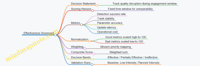
Example: One Run with Concrete Numbers
Assume the planned intensity run yields:
- Detection success rate = 0.70 → metricScore = 62
- Track stability = 0.55 → metricScore = 56
- Parameter accuracy error = 1.6° → metricScore = 63
- Update latency = 6 s → metricScore = 40
- Cost = 0.35 → metricScore = 65
Composite effectiveness score:
- 0.2062 + 0.3056 + 0.3063 + 0.1040 + 0.10*65
- = 12.4 + 16.8 + 18.9 + 4.0 + 6.5
- = 58.6 → partially effective
That result is actionable: the score is held back mainly by update latency. If the plan can’t change latency, then the mission should rely on other tactics; if it can, adjust timing or coherency constraints so the track re-stabilizes later.
Mind Map: Interpreting the Score
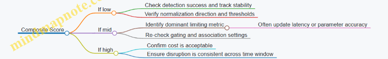
Step 7: Turn Scores Into Operational Guidance
Finally, record not only the composite score but also the metricScore breakdown. In reviews, you want to answer two questions quickly: “Did it work?” and “Why did it work or not?” The breakdown prevents the classic trap of optimizing the wrong knob—like improving detection loss while leaving track association intact.
12. Integrated Battlespace Scenarios for Detection Tracking and Countermeasures
12.1 Scenario Setup With Geometry And Environmental Inputs
A solid scenario setup turns “radar and countermeasures” into a repeatable experiment. Start by defining the geometry, then lock in environmental effects, then verify that the resulting measurements make physical sense.
Scenario Geometry Inputs
-
Coordinate frame and units: Choose a right-handed frame, define axes (e.g., east-north-up), and stick to one unit system. A common mistake is mixing meters for position with kilometers for range in later calculations.
-
Platform states: For each radar and target, specify initial position, velocity, and heading. If the radar rotates or scans, include its scan center and boresight pointing law.
-
Antenna and beam geometry: Define antenna phase center location, beamwidth (or pattern), and scan limits. If you use a simplified beam model, document whether gain is constant within the mainlobe and zero outside, or whether you use a taper.
-
Line-of-sight and occlusion: Compute slant range and aspect angle from radar to target at each time step. If terrain or structures matter, define simple blockers (e.g., a hill plane) and apply an occlusion rule to reduce received power.
-
Target motion model: Pick a motion model that matches the scenario goal. For tracking exercises, constant-velocity with occasional maneuver is often enough; for clutter studies, include micro-motion or aspect changes if relevant.
Example: Place a radar at (0, 0, 50 m) and a target at (8,000 m, 2,000 m, 100 m) moving at 120 m/s with a slight turn. Use a 1-second time step for track-level outputs, but keep a finer internal step for waveform timing if you model scan dwell.
Environmental Inputs
-
Propagation model selection: Choose a propagation approach consistent with the range scale. For short ranges, free-space loss may suffice; for longer ranges, include atmospheric attenuation and horizon effects.
-
Clutter definition: Specify clutter type (ground, sea, foliage) and clutter intensity as a function of range and aspect. Even a simple range-dependent clutter-to-noise ratio helps you test detection thresholds realistically.
-
Noise model: Define receiver noise figure, system temperature, and bandwidth. Convert these into an equivalent noise power at the detector input so your detection thresholds are grounded.
-
Weather and refractivity: If you include it, represent it through an attenuation term and a refractivity-driven bending or range bias. Keep it simple: one parameter set for the whole run is easier to debug than a time-varying field.
-
Interference and background emitters: If you model electronic countermeasures, include baseline interference levels. This prevents the “everything works until we add jamming” surprise.
Example: Set sea clutter higher at low elevation angles and reduce it above a certain height. Then verify that the radar’s detection probability drops when the target dips toward the clutter ridge.
Time Management and Data Products
-
Scenario timeline: Define start/stop times, scan period, and mode schedule (search vs track). Use a mode timeline that matches how the radar actually allocates dwell time.
-
Measurement outputs: Decide what the radar produces each update: detections (range/angle bins), measurements with noise, or full complex returns. Countermeasure evaluation depends on this choice.
-
Countermeasure timing hooks: Add event times for chaff release, decoy activation, or jammer start/stop. Tie these to platform states so the geometry at the moment of effect is correct.
Example: If chaff is released at t=120 s, compute its initial position from the dispenser location and then apply a simple fall-rate model to update its altitude each second.
Mind Map: Scenario Setup with Geometry and Environmental Inputs
Validation Checklist with Concrete Sanity Checks
-
Range sanity: Confirm that computed slant range matches the Euclidean distance from geometry at each time step.
-
Aspect sanity: Ensure aspect angle changes smoothly with target motion; sudden jumps usually mean a sign convention error.
-
SNR sanity: Compute expected received power using your link budget and verify that it sits in a plausible band relative to your clutter and noise assumptions.
-
Update consistency: Verify that measurement timestamps align with scan dwell and mode switching. If track updates occur when the radar is “not looking,” you’ll get mysterious performance.
Example: After setting noise and clutter, run a short 10-second baseline with no countermeasures. If detections appear even when the target is behind an occluder, the occlusion rule is not being applied to the measurement chain.
12.2 Building a Radar Employment and Track Timeline
A radar timeline is the schedule that turns “we can detect and track” into “we actually do it” under limited time, processing, and antenna dwell. The goal is to map each radar mode to a time window, then show how track quality evolves as the system alternates between search, track, and any supporting tasks like calibration or special waveform bursts.
Foundational Inputs That Drive the Timeline
Start with a few concrete numbers, because the timeline is just arithmetic with consequences.
- Antenna dwell and scan rate: how long the beam stays on a region per revisit.
- Waveform set: which waveforms support search, which support track, and which support measurement refinement.
- Processing budget: how many detections and tracks can be handled per update cycle.
- Update interval: how often a track filter expects new measurements.
- Environment and clutter: which thresholds and processing choices are stable across the mode.
A practical rule: if the track update interval is 1.0 s, then your timeline should deliver track measurements at roughly that cadence, not in a lopsided pattern where some tracks get updates and others wait.
Timeline Mind Map
Mind Map: Radar Employment and Track Timeline
Stepwise Construction Method
Step 1: Define the Time Grid
Pick a base time step that matches your track update cycle. For example, use Δt = 0.5 s so you can represent both frequent updates and occasional mode changes cleanly.
Step 2: Allocate Search Time for Coverage
Choose a search window that ensures revisit before tracks degrade. If the antenna revisit time is 2.0 s, then a timeline that spends long stretches in track-only mode may starve new targets of initial detection.
A simple balancing approach is to keep search active enough to seed new tracks while still dedicating most dwell to established tracks.
Step 3: Allocate Track Time for Measurement Quality
Track mode should emphasize waveforms and processing that improve measurement stability. If your track filter relies on consistent range and angle measurements, then track mode should avoid waveform changes that cause systematic shifts unless you also model them.
Step 4: Add Support Tasks Without Breaking Cadence
Calibration or health checks should be placed where they minimally disrupt track updates. If a support task consumes 0.5 s and your update interval is 1.0 s, you can often absorb it by alternating which tracks get the “full” update versus a reduced update.
Step 5: Apply Mode Switching Logic
Switching should be driven by track state, not by a fixed schedule alone. For instance:
- If a track is newly initiated, prioritize consistent measurements.
- If a track is stable, you can reduce measurement richness slightly.
- If a track is fading due to missed detections, you may temporarily increase dwell or adjust gating.
Example Timeline with Concrete Numbers
Assume:
- Track update interval: 1.0 s
- Base time step: 0.5 s
- Modes: Search (S), Track (T), Calibration burst (C)
- Two established tracks: A and B
- One new target appears at t = 1.0 s
Timeline (0.0 s to 3.0 s):
- t = 0.0–0.5: S (scan wide area, detect candidates)
- t = 0.5–1.0: T (measure A and B, update filters)
- t = 1.0–1.5: S (new target likely detected; keep search active for latency control)
- t = 1.5–2.0: T (initiate track for new target if detection meets threshold; update A and B)
- t = 2.0–2.5: C (short calibration burst; keep gating permissive for one track to avoid deletion)
- t = 2.5–3.0: T (resume full measurement set; tighten gating)
What to watch in this example:
- Detection-to-track latency: the new target is detected during 1.0–1.5 s and can be initiated by 1.5–2.0 s.
- Cadence integrity: A and B still receive updates at 0.5–1.0 s and 1.5–2.0 s, then a reduced-impact period during calibration.
- Resource fairness: calibration doesn’t cause immediate deletion because the timeline includes a gating adjustment during the disrupted interval.
Track Quality Checks That Close the Loop
After you draft the timeline, verify it with simple counters:
- Update count per track over the window
- Missed update count and whether it crosses deletion thresholds
- Measurement quality distribution by mode (e.g., range error higher during search)
- Latency distribution from first detection to first track update
If any metric fails, adjust the timeline by moving time between S and T or by changing waveform assignment within a mode. The timeline is not a one-time plan; it’s a constraint system you tune until the track lifecycle behaves as intended.
12.3 Selecting Countermeasure Options by Threat and Mode
Countermeasure selection is easiest when you treat it like a decision chain: identify what the radar is trying to do (mode), identify what the threat is likely to be (emitter and geometry), then choose the countermeasure that best attacks the radar’s weakest link in that mode. The goal is not to “win” against radar in general; it is to degrade the specific detection or tracking function currently being used.
Threat and Mode Inputs That Actually Matter
Start with three inputs that drive almost every choice.
- Radar mode intent: search, surveillance, track, or terminal guidance. Search modes often tolerate more false alarms; track modes demand stable measurements.
- Waveform and processing assumptions: pulse, pulse-compressed, continuous-wave, or frequency-modulated. Processing determines whether deception needs timing coherency or whether it can be “good enough.”
- Measurement type: range only, range-rate (Doppler), angle, or combinations. A countermeasure that spoofs range may not help if the tracker is dominated by angle-rate.
A practical way to keep this grounded is to map each countermeasure to the measurement it targets. For example, chaff mainly changes apparent range and angle statistics; velocity deception targets Doppler-derived motion; jamming attacks detection thresholds and sometimes track update rates.
Selection Logic from Foundational Rules to Operational Choices
Use a layered approach: first decide whether you are trying to deny detection, break tracking, or mislead association, then pick the mechanism.
- Deny detection: raise the radar’s effective noise floor or clutter so the detector stops declaring targets.
- Break tracking: force measurement updates to become inconsistent so the filter gates out returns.
- Mislead association: create returns that look plausible enough to be assigned to the wrong track, causing track swaps or track splitting.
Now connect those goals to countermeasure families.
- Electronic protection first: if your platform is receiving emissions, frequency agility and receiver hardening reduce the effectiveness of jamming and deception. This is “counter-countermeasure” work, and it changes what the attacker can do.
- Jamming for denial: when the radar is in a search-like mode with threshold-based detection, noise or spot jamming can reduce detection probability. If the radar uses narrow beams or adaptive sidelobe processing, the jammer’s placement and spectral shape matter.
- Deception for misassociation: when the radar is tracking and expects coherent measurements, deception must match the radar’s measurement model closely enough to pass gating. If the tracker uses tight gates, sloppy deception becomes self-defeating.
- Chaff and decoys for physical disruption: when you need a fast, mode-agnostic way to change the radar return environment, chaff can increase clutter-like false returns. Its timing and dispersion determine whether it behaves like a persistent cloud or a short-lived burst.
Mind Map: Countermeasure Choice by Mode and Measurement
Example: Choosing Between Jamming and Deception in Track Mode
Assume a threat radar is in track mode and the tracker relies heavily on Doppler plus angle updates. Your countermeasure options include noise jamming and a deception waveform.
- Check the gating behavior: track filters typically reject measurements that jump too far in range-rate or angle. If your deception cannot maintain consistent Doppler across successive updates, it will be gated out.
- Compare mechanisms against measurement dominance:
- Noise jamming mainly increases uncertainty and can reduce update rate, but if the radar can still extract stable measurements from sidelobes or alternate channels, tracking may persist.
- Doppler deception targets the measurement the tracker trusts most. However, it must remain coherent with the radar’s expectations over the update interval.
- Select based on which failure mode is more likely:
- If you can generate Doppler-consistent deception for multiple updates, deception is the better choice for breaking track.
- If you cannot maintain that consistency, jamming becomes the safer option because it attacks the detector and reduces the chance of valid updates.
A simple operational rule of thumb follows: track mode selection favors measurement-consistent effects; search mode selection favors threshold disruption. That rule won’t replace analysis, but it prevents common mistakes like using a “range-only” tactic against a tracker that is mostly angle-rate driven.
Example: Chaff Timing for Search Versus Surveillance
In a search mode, the radar may revisit the same sector frequently, so a short chaff burst can still produce intermittent false returns that inflate false alarms. In surveillance, the radar may integrate over longer dwell times, so a chaff cloud that persists and spreads in angle can better degrade track initiation by making the return environment statistically messy.
To apply this systematically, decide whether you want chaff to behave like:
- a burst that creates momentary confusion during scan passes, or
- a cloud that increases clutter-like returns during longer dwells.
The selection is then mostly about timing and dispersion, not just the amount of material.
Practical Output Format for the Decision
When you finalize the selection, record three items so the team can execute consistently:
- Mechanism: jamming, deception, chaff/decoys, or a combination.
- Targeted measurement: range, Doppler, angle, or association behavior.
- Mode-specific constraint: coherency requirement for track, dwell timing for surveillance, or threshold disruption for search.
This keeps countermeasure selection tied to what the radar is doing right now, not what it might do later.
12.4 Interpreting Results for Detection and Track Outcomes
When you run an end-to-end detection and tracking experiment, you don’t just want “did it detect?” You want to understand why the outcome happened and what it implies for the next decision in the chain: thresholding, association, track maintenance, and countermeasure response. The most useful workflow is to interpret results in layers, from raw measurements to track-level consequences.
Measurement-Level Outcomes
Start by classifying each radar return into one of three buckets: true detection of a real target, false alarm from clutter/noise, or missed detection. A practical way to interpret this is to compare the measured detections against the known truth in your scenario.
- Detection present but track fails later usually means the measurements are too inconsistent for the tracker’s motion model or gating rules.
- Track exists but is wrong often points to data association errors, such as confusing two nearby targets or letting a spurious measurement steal the track.
- No track forms frequently comes from thresholds that are too strict, insufficient dwell time, or scan scheduling that doesn’t provide enough geometry diversity.
A simple example: suppose a target is visible in search mode, but the track never initiates. If you plot detection times, you may find that the target is detected only once per scan cycle, and the tracker requires two consistent hits within a gating window. The “missing” track is not a radar failure; it’s a track-management requirement not being met.
Track-Level Outcomes
Once tracks are formed, interpret them by how they behave over time. Track outcomes typically include correct tracks, track fragmentation, track swaps, and track loss.
- Correct track: the track’s estimated position and velocity remain close to truth, and the track’s uncertainty shrinks as more measurements arrive.
- Fragmentation: the track breaks into multiple segments because association fails during a difficult interval, such as a clutter spike or a maneuver.
- Track swap: two targets exchange identities, often when their predicted positions overlap within the gating region.
- Track loss: the track is deleted after consecutive missed updates, which can happen when countermeasure effects reduce measurement quality.
To interpret these, examine three plots together: (1) measurement-to-track residuals, (2) gating pass/fail history, and (3) track confidence or covariance growth. If residuals spike but gating still passes, you may be accepting low-quality measurements. If gating fails repeatedly, you may be too conservative for the scenario’s maneuver or countermeasure-induced distortion.
Countermeasure Interaction Interpretation
Countermeasures change the measurement stream. Your job is to map that change to the track outcome.
- Deception that creates consistent false measurements can produce a stable but incorrect track. The residuals may look “good” because the tracker is happily fitting the wrong story.
- Jamming that increases noise often increases missed detections and causes track loss or fragmentation rather than a clean wrong track.
- Chaff or decoys that generate multiple returns can increase association ambiguity, raising the probability of track swaps.
A concrete example: if a decoy produces returns at similar angles but inconsistent ranges, you may see residuals that alternate between “near” and “far” values. The tracker might keep updating with the wrong measurement early, then later reject it as the residual grows, causing fragmentation.
Mind Map: Detection and Track Outcome Interpretation
A Systematic Diagnostic Checklist
Use this sequence to avoid guesswork:
- Count detections vs truth to separate radar sensitivity issues from tracking issues.
- Check detection timing to see whether scan scheduling provides enough measurement opportunities.
- Inspect residuals to determine whether errors are systematic (model mismatch or deception) or random (noise/jamming).
- Review gating history to confirm whether the tracker is rejecting good measurements or accepting bad ones.
- Correlate track events with countermeasure timing so you can attribute fragmentation, swaps, or loss to specific effects.
- Summarize outcomes in track terms (correct, fragmented, swapped, lost) because that’s what downstream decision logic consumes.
Example: From Residuals to Outcome Label
Assume two targets cross paths. Early in the crossing, both tracks show small residuals. Midway through the crossing, one track’s residuals grow but still pass gating, and the association alternates between the two targets. Later, the track that accumulated larger residuals becomes the one that survives, while the other is deleted after missed updates. The correct interpretation is a track swap followed by track loss, not a pure radar failure. That distinction matters because the fix is likely association and gating tuning (and possibly mode scheduling), not simply lowering detection thresholds.
Practical Output Format for Interpretation
End the section by reporting results in a compact, decision-ready form:
- Detection metrics: true detections, false alarms, misses.
- Track metrics: correct tracks, fragmentation count, swap count, loss count.
- Root-cause tags: thresholding, gating, association ambiguity, countermeasure-induced measurement degradation.
This structure keeps the interpretation grounded in evidence and ensures the next system adjustment targets the actual failure mode.
12.5 Practical End-to-End Example From Detection to Countermeasure Response
Assume a coastal surveillance radar must detect and track a small fast craft in a harbor clutter environment. The radar runs two modes: a search waveform for wide-area detection and a track waveform for stable tracking. The countermeasure system has three options available: electronic protection measures (receiver settings and waveform scheduling), deception (false range/angle), and chaff (range-angle obscuration). The goal is not to “win” instantly; it is to keep the track usable long enough to cue the correct response.
Scenario Setup and Inputs
- Geometry: The target is at 18 km, moving tangentially at 22 m/s. The radar is at 0 m altitude; sea clutter is strong near the horizon.
- Environment: Clutter is modeled as non-homogeneous with higher variance near the shoreline. Wind-driven surface returns create intermittent spikes.
- Radar configuration: Search uses a pulse-compressed waveform with moderate bandwidth; track uses a narrower, higher-coherence waveform for better Doppler stability.
- Processing constraints: The tracker can maintain up to 20 tracks, but only 6 can be updated at the highest rate.
Step 1: Detection in Clutter and Noise
The search mode produces detections using a threshold tuned to a constant false alarm rate. In practice, the threshold is adjusted using recent noise estimates and clutter statistics from the same range bins. A useful best practice is to log the threshold value and the estimated clutter variance each scan; when the threshold rises, you can explain missed detections without guessing.
Example: At scan time T0, the radar sees three candidate hits in the target’s expected bearing sector. Two are likely clutter spikes because their Doppler estimates are inconsistent with the craft’s tangential motion. The third candidate has a Doppler centroid that matches the track waveform’s expected sign and is therefore promoted to a tentative track.
Step 2: Track Initiation and Quality Control
Track initiation uses gating to limit which detections can belong to the same track. A simple gating rule is based on predicted range and angle uncertainty from the last state estimate. The tracker also checks whether the measurement residuals are plausible for the assumed motion model.
Example: At T1, the tentative track receives a second measurement. The residual in angle is within the gate, but the residual in range is slightly high. Instead of immediately deleting the track, the system increases process noise for one update cycle, allowing for small model mismatch while still preventing clutter from hijacking the track.
Step 3: Mode Switching and Waveform Scheduling
Once the track is confirmed, the radar schedules the track waveform more frequently for that track’s region while still performing periodic search to catch maneuvers. A practical scheduling rule is to allocate track updates based on predicted uncertainty growth: the more uncertainty grows, the more update time the track earns.
Example: Between T2 and T3, the craft’s speed causes Doppler centroid drift. The scheduler increases track waveform dwell time for the track, improving Doppler stability and reducing the chance of track splitting.
Step 4: Countermeasure Selection Logic
The countermeasure system receives track quality metrics: detection confidence, track stability, and predicted future position uncertainty. It also considers which countermeasure is effective against the current radar mode.
- If track stability is high: deception is more likely to create a coherent false track.
- If track stability is low: chaff can reduce measurement quality by increasing clutter-like returns.
- If receiver is saturated or interference is present: electronic protection settings take priority.
Example: At T4, the track residuals spike due to a brief clutter surge. The system chooses chaff rather than deception because deception requires consistent measurement structure to be convincing.
Step 5: Countermeasure Execution and Feedback
Chaff is dispensed with a timing offset so that it enters the radar’s main beam when the next track update is expected. The system also adapts receiver processing to avoid being fooled by the chaff returns.
Example: At T4+0.3 s, chaff is released. At T5, the radar sees increased returns in the target’s range-angle neighborhood. The tracker’s gating tightens only after the measurement statistics settle; otherwise, it risks discarding the true target track due to transient measurement distortion.
Step 6: Track Recovery or Reassignment
After the chaff cloud disperses, the tracker either recovers the original track or reassigns measurements to a new track. A robust practice is to keep a short “track memory” so that a temporarily degraded track can be re-linked when measurement quality improves.
Example: At T6, the residuals decrease and the Doppler centroid returns to the craft’s expected sign. The tracker re-associates the measurements to the original track ID, preventing unnecessary re-initiation.
Mind Map: End-to-End Flow from Detection to Countermeasure Response
Example: Compact Timeline with Decisions
- T0: Search detects candidates; one promoted to tentative track.
- T1: Second measurement confirms plausibility; residuals handled with increased process noise.
- T2–T3: Scheduler increases track dwell as Doppler drift grows.
- T4: Track residuals spike; system selects chaff over deception.
- T5: Chaff increases returns; tracker tightens gating only after statistics settle.
- T6: Doppler and residuals normalize; track re-linked and stabilized.
The key integration point is that countermeasure choice is driven by track quality and radar mode context, while radar processing adapts to countermeasure-induced measurement changes. That feedback loop is what keeps the system from chasing clutter, overreacting to transient spikes, or discarding the correct track at the worst possible moment.