Electrochemical Cement Production
1. Scope and Definitions for Electrochemical Cement Production
1.1 What Electrochemical Cement Production Means in Practice
Electrochemical cement production is a way to use electrical energy to drive chemical transformations that normally rely on high-temperature processing, chemical reagents, or both. In practice, it means you set up an electrochemical cell, feed it cement-related precursor species (often dissolved in a liquid phase), and collect solid products that can be processed into cementitious materials.
A useful mental model is to separate the job into three layers: (1) what chemistry you want to achieve, (2) how electricity helps you achieve it, and (3) how you turn the electrochemical output into something that behaves like cement. If any layer is ignored, the process becomes “electrochemistry with no cement,” or “cement with no electrical role.”
What You Start With
Most cement-related electrochemical routes begin with calcium-bearing and carbonate-bearing inputs. A common practical approach is to dissolve calcium sources and carbonate species into an electrolyte so ions can move and react. For example, calcium can come from a soluble calcium salt or from a slurry that is conditioned until calcium ions are available. Carbonate can be supplied directly as carbonate species or generated in situ from dissolved carbon dioxide.
A key practical detail is that the electrolyte is not just a “conductor.” It controls solubility, ion availability, and side reactions. If calcium is too concentrated, precipitation can foul electrodes. If carbonate is too scarce, you get calcium-rich solids that do not match the target binder chemistry.
What the Cell Does
Inside the cell, electrical current forces redox reactions at electrodes. At the cathode, reduction reactions can change the speciation of carbon and calcium-containing species, while at the anode, oxidation reactions can regenerate or consume components that affect pH and ionic balance. The net result is that the solution chemistry shifts toward forming cement-relevant solids.
In practice, the cell design determines whether the desired reactions dominate. Ion transport must be controlled so that products form where you want them rather than everywhere at once. Separators or membranes can help keep reaction zones distinct, but they also add resistance and require careful materials selection.
A simple example clarifies the logic. Suppose your goal is to form a calcium carbonate-like solid. If the cathode conditions raise local pH, carbonate species can convert into solid carbonate precipitates. If the anode simultaneously produces conditions that counteract that pH rise, the net precipitation rate drops. So “current applied” is not enough; the spatial chemistry created by the cell matters.
What You Collect and How It Becomes Cement
Electrochemical cells typically produce a mixture of solids, dissolved ions, and sometimes gases. Turning that mixture into a cementitious material requires separation and conditioning. Solids are recovered by filtration or settling, then washed to remove residual salts that would otherwise interfere with hydration. Drying and controlled grinding adjust particle size and surface properties.
A practical integration step is blending. Even when electrochemical output is close to a target binder phase, supplementary materials may be added to tune setting behavior, strength development, and durability. The point is not to force every reaction to happen in the cell; it is to produce a useful solid stream that can be engineered into a consistent product.
Mind Map: Electrochemical Cement Production in Practice
Example: A Practical End-to-End Picture
Imagine a pilot setup where a calcium-containing electrolyte and a carbonate-containing electrolyte are brought into an electrochemical cell. You apply current and monitor cell voltage and solution pH. As local conditions change near the cathode, a solid precipitate forms. You then separate the solids, wash them until conductivity drops, and dry them under conditions that avoid unwanted transformations. Finally, you grind the dried powder and test it in a mortar formulation.
If the mortar sets too slowly, the issue might be residual salts, particle size, or the solid’s actual phase composition. If it sets normally but develops low strength, the solid may not match the binder chemistry needed for effective hydration. In other words, “electrochemical success” is not the same as “cement success,” and the workflow is designed to connect the two with measurable checkpoints.
What Makes It Electrochemical Rather Than Just Chemical
The defining feature is that electrical current directly drives the key speciation changes in the precursor solution. That does not mean every step is electrochemical, but it does mean the cell is responsible for creating the chemical environment that leads to cement-relevant solids. If you can remove the cell and still get the same solids under the same conditions, then the process is not really electrochemical cement production—it is simply a chemical precipitation route with extra steps.
1.2 Cement Chemistry Fundamentals for Electrochemical Pathways
Electrochemical cement production changes how key cement-forming species are created, but it does not change why they matter. Cement chemistry still governs which ions exist in solution, which solids precipitate, and how those solids hydrate into strength. The electrochemical part mainly reshapes the reaction environment: electric current drives redox changes, while pH, ionic strength, and mass transport decide what actually forms.
Core Cement Phases and Their Chemistry Roles
Portland cement strength comes largely from hydration products of clinker minerals. The main players are:
- Tricalcium silicate (C3S): hydrates quickly and contributes early strength.
- Dicalcium silicate (C2S): hydrates more slowly and contributes later strength.
- Tricalcium aluminate (C3A): reacts fast with water and can cause rapid setting unless controlled.
- Ferrite phase (C4AF): participates in reactions but usually plays a smaller role in strength.
In electrochemical pathways, you can think of these phases as “end targets” that depend on the availability of calcium, silicate species, aluminate species, and the right pH window. If the solution chemistry produces the wrong ion ratios or the wrong solid precursors, hydration will follow a different route.
Electrochemical Levers That Control Cement Chemistry
Electrochemistry offers several controllable levers. Each one maps to a cement-relevant chemical outcome.
-
Redox-driven speciation
- Example: converting carbonate/bicarbonate species changes the availability of CO₂-related equilibria and affects pH buffering. That, in turn, influences whether calcium precipitates as carbonate-like solids or forms calcium silicate precursors.
-
pH and alkalinity at the electrode surfaces
- Example: if local pH near the cathode rises, dissolved calcium can more readily form calcium hydroxide and then react with silicate species to form calcium silicate hydrate (C-S-H). If pH stays too low, you may get incomplete precipitation and weaker or slower hydration.
-
Ion transport and concentration gradients
- Example: in a poorly mixed cell, the cathode region can become depleted in key anions (like silicate) or enriched in others (like hydroxide). The resulting solids may be non-uniform, leading to inconsistent setting behavior.
-
Electrolyte composition and impurities
- Example: sulfate ions can strongly affect aluminate chemistry. In practice, the same sulfate that helps manage C3A hydration can also shift precipitation behavior during electrochemical steps.
From Ions to Solids to Hydration
A useful way to connect electrochemistry to cement performance is to track three stages: solution speciation, solid formation, and hydration kinetics.
- Solution speciation determines which ions and complexes are present. For silicates, the distribution between monomers, oligomers, and polymerized forms depends on pH and concentration.
- Solid formation determines what precursor solids appear after electrochemical treatment. These solids can be amorphous, poorly crystalline, or crystalline, and their structure affects how easily water later converts them into hydration products.
- Hydration kinetics depend on surface area, particle size, and the chemical environment created by the initial solids.
Concrete example: suppose electrochemical processing produces a calcium-rich, silicate-containing solid that is fine and reactive. During hydration, it can form C-S-H efficiently, giving better early strength. If the solid is coarse or forms in a way that traps silicate in less reactive structures, hydration slows even if the overall chemical composition looks similar.
Mind Map: Cement Chemistry Through Electrochemical Lenses
Example: A Systematic Check of Cement-Relevant Chemistry
When designing or evaluating an electrochemical cement route, a practical checklist is to verify the chemistry chain in order:
- Confirm ion availability: measure or estimate calcium and silicate species in the working electrolyte under operating conditions.
- Check precipitation behavior: observe what solids form during electrochemical treatment and whether they are reactive (fine, poorly crystalline solids often hydrate faster).
- Validate hydration response: run standardized hydration tests and compare setting time and strength development to the expected roles of C3S-like and C2S-like contributions.
If results disagree, the most common causes are not “mystical chemistry,” but mismatches between pH history, ion transport, and solid precursor reactivity.
Example: Why C3A Control Still Matters
Even if electrochemical steps focus on silicate formation, aluminate chemistry can still dominate early setting. A simple example is sulfate management: too little sulfate can allow rapid C3A reaction and flash setting, while too much can alter precipitation and change the balance of hydration products. Electrochemical pathways must therefore treat aluminate control as a first-class constraint, not an afterthought.
Summary of the Fundamentals
Cement chemistry fundamentals remain the governing logic: electrochemistry changes the chemical environment, but cement phases and hydration products still determine performance. The most reliable approach is to connect electrode-level effects—speciation, pH, transport, and impurities—to the solution-to-solid-to-hydration chain, then verify the chain with targeted measurements and hydration outcomes.
1.3 System Boundaries for Process Design and Emissions Accounting
System boundaries define what is inside the electrochemical cement production “box” and what is outside. Get this right early, because every later calculation—mass balances, energy use, and emissions—depends on it. A good boundary is not the smallest possible one; it is the one that matches your decision-making needs.
What Counts as Inside the Boundary
Start with the physical transformations. For electrochemical cement production, the inside boundary typically includes:
- Feed preparation: crushing, slurry mixing, and any electrolyte conditioning steps that directly change chemistry.
- Electrochemical conversion: cell stacks, pumps, separators, and any membrane or separator units that control ion transport.
- Post-processing of solids: washing, filtration, drying, and any thermal or mechanical conditioning that sets the precursor’s reactivity.
- Product conditioning: grinding and blending steps that produce the final cementitious material.
A practical rule: if a unit operation changes the chemical form or physical state of the cement precursor in a way that affects performance or emissions, it belongs inside.
What Counts as Outside the Boundary
Units that do not materially affect the product chemistry or the accounting results can be excluded, but only with clear justification. Common outside items include:
- General building energy (lighting, offices) if it is small and not decision-relevant.
- Off-site utilities supplied under a standard contract, when you cannot control them.
- Upstream mining and transport of inputs, if your goal is to compare process designs at the plant gate.
If you exclude something, you still need to document it so the reader can interpret the numbers. “Excluded” is not the same as “irrelevant.”
Choosing the Accounting Perspective
Two perspectives are common, and mixing them causes confusion.
- Plant-gate perspective: emissions from within the plant boundary, plus direct fuel and electricity used on-site.
- Cradle-to-gate perspective: includes upstream emissions for raw materials and electricity generation.
For process design, plant-gate is often the first step because it isolates engineering choices. For reporting, cradle-to-gate may be required. Either way, keep the perspective consistent within a given dataset.
Boundary Decisions That Affect Results
Boundary choices change emissions even when the chemistry is identical. Key decision points include:
- Electricity accounting: whether you use grid-average factors or a specific supply contract. The boundary must state the electricity source basis.
- Heat integration: if waste heat is recovered inside the boundary, it reduces net energy demand; if it is exported outside, it may be treated differently.
- Byproduct handling: if a byproduct is captured and used, you need a rule for whether its avoided emissions are credited or not.
- Water treatment: if water is recycled within the boundary, you account for pumping and treatment energy; if discharged, you account for treatment and any relevant impacts.
Mass and Energy Flows as the Backbone
Before emissions, define mass and energy flows. A boundary is only as good as the flows you can trace.
Example: Suppose the process uses electrolyte recirculation. If the boundary includes the recirculation loop, you track makeup electrolyte losses and the energy for pumps and filtration. If you exclude it, you might incorrectly treat the loop as “free,” underestimating both electricity use and emissions.
Emissions Categories and How They Map to the Boundary
Use a category structure that mirrors your boundary.
- Direct emissions: from on-site combustion or chemical reactions that release gases.
- Indirect emissions: from purchased electricity and heat.
- Process emissions: from transformations of carbonates or other feed components.
- Upstream emissions: only included if you choose cradle-to-gate.
Example: If carbonate conversion releases CO₂, that belongs inside the boundary because it is generated by the electrochemical reaction and affects the product carbon content.
Mind Map: Boundary Design
A Worked Boundary Example
Assume a pilot line produces 1 tonne of cementitious precursor. You decide on a plant-gate boundary.
- Inside: electricity for the cell stack and pumps, energy for filtration and drying, and CO₂ released during carbonate conversion.
- Outside: emissions from quarrying limestone and transporting it to the plant.
Now compare two designs: Design A uses higher current efficiency but requires more washing water. Because water pumping and treatment energy are inside, the comparison remains fair. If you had excluded water treatment, Design A could look better on paper while shifting the burden outside the boundary.
Documentation Checklist
To keep boundaries usable, record:
- The chosen perspective (plant-gate or cradle-to-gate).
- A unit-operation list inside and outside.
- The electricity and heat accounting basis.
- Rules for byproducts, credits, and allocation.
- The mass and energy flow diagram scope.
A boundary that is explicit like this turns emissions accounting from a spreadsheet exercise into a design tool—one that helps you see which engineering choices actually move the numbers.
1.4 Key Terms for Electrolytes Electrodes and Cell Hardware
Electrochemical cement production is easier to reason about when the vocabulary is consistent. The same word can mean different things in different industries, so this section pins down practical definitions and shows how each term affects design choices.
Electrolytes
An electrolyte is the ion-conducting medium that lets charge move while reactants and products stay where you need them. In cement-related systems, electrolytes often contain dissolved calcium species, carbonate or bicarbonate, and supporting ions that improve conductivity.
- Ionic strength describes how concentrated the charge carriers are. Higher ionic strength usually lowers electrical resistance, which reduces the voltage needed for a given current.
- Conductivity is the measurable ability of the electrolyte to carry current. A quick example: if conductivity drops after several hours, the cell may require higher voltage to maintain the same current density.
- Speciation is the distribution of chemical forms, such as Ca²⁺ versus CaCO₃(aq) or bicarbonate versus carbonate. Speciation matters because only certain forms participate efficiently at the electrode surface.
- pH and buffering control which carbonate form dominates and how stable calcium species remain in solution. Example: if pH drifts upward, carbonate may shift toward CO₃²⁻, changing both reaction rates and scaling behavior.
- Solubility limits define when dissolved species start forming solids. Example: once calcium carbonate reaches its solubility limit, it can precipitate in the bulk electrolyte or on electrode surfaces, affecting both performance and cleaning needs.
Electrodes
An electrode is the solid surface where electron transfer occurs. The anode is where oxidation happens, and the cathode is where reduction happens. In cement-related pathways, the electrode reactions determine which ions are consumed, which solids form, and how much unwanted side chemistry occurs.
- Current density is current per unit electrode area. Example: doubling current density can increase conversion, but it can also raise local pH near the cathode and trigger faster precipitation.
- Overpotential is the extra voltage beyond the ideal thermodynamic value needed to drive the reaction at a useful rate. Lower overpotential generally means less energy wasted as heat.
- Catalytic activity describes how effectively the electrode promotes the desired reaction. If the electrode is poorly matched, the system may spend current on competing reactions.
- Mass transport is how quickly reactants reach the electrode and products leave. A simple example: if stirring is weak, a concentration gradient forms, and the reaction slows even if the electrical conditions look fine.
- Porosity and surface area matter because many electrochemical reactions occur inside pores. Higher effective surface area can improve rates, but it can also trap precipitates.
- Wetting and adhesion influence whether electrolyte contacts the active surface uniformly. If wetting is poor, parts of the electrode may contribute less than expected.
Cell Hardware
The cell is the assembled system that contains electrodes, electrolyte, and the electrical and mechanical components needed for controlled operation.
- Cell stack or single cell: a stack connects multiple cells in series or parallel to reach required voltage and current. Example: series increases voltage; parallel increases current capacity.
- Separator or membrane controls ion movement between anode and cathode compartments. It can reduce mixing of reactive species and limit crossover that would otherwise waste charge.
- Electrode spacing affects resistance and flow patterns. Smaller spacing often lowers ohmic losses, but it can increase risk of shorting if solids bridge the gap.
- Flow field and hydrodynamics describe how electrolyte moves across and through the cell. Example: uneven flow can create hot spots where precipitation forms first.
- Power supply and current control provide stable current or voltage. In practice, current control is common because it ties directly to conversion and scaling rates.
- Sensors and instrumentation include temperature probes, pH measurement, conductivity sensors, and sometimes reference electrodes. Example: if pH is only measured in the bulk, local electrode conditions may still differ significantly.
- Materials compatibility covers corrosion resistance of hardware exposed to electrolyte and any gases produced. Example: a component that survives in clean water may fail when carbonate and calcium ions are present.
Mind Map: Shared Vocabulary
Integrated Example: From Term to Design Choice
Suppose you observe rapid solid formation near the cathode. Start with speciation and pH: local pH can rise due to cathodic chemistry, shifting carbonate forms and exceeding solubility limits. Next check mass transport: if reactants are not replenished quickly, concentration gradients intensify local conditions. Then inspect the electrode: high porosity may increase surface area but also provide nucleation sites that trap solids. Finally, review cell hardware: inadequate flow in the flow field can create precipitation hot spots, and an unsuitable separator may allow crossover that changes the chemistry in each compartment.
When these terms are used consistently, troubleshooting becomes a chain of cause and effect rather than a list of disconnected symptoms.
1.5 Quality Targets for Cement and Concrete Performance
Quality targets for electrochemically produced cement should be set in the same order you would troubleshoot a problem: start with what the material is, then what it does, then how reliably it does it. Electrochemical routes can shift chemistry and particle characteristics, so the targets must cover both composition and performance.
Define the Product Form and Performance Use Case
Start by separating targets for cement as a powder from targets for concrete as a hardened composite. A cement that meets chemical targets can still fail in concrete if particle size distribution, sulfate balance, or alkali content changes early hydration.
Example: If the cement’s fineness is higher than expected, water demand can rise and setting can accelerate. A concrete mix that previously used 185 kg/m³ water may need a different water-to-cement ratio to keep the same workability.
Cement Quality Targets That Map to Hydration
Set targets that connect directly to hydration reactions and early-age behavior.
- Phase and chemistry targets: acceptable ranges for clinker-like phases, free lime, reactive silica/alumina availability, and sulfate content. Keep alkalis within a controlled band because they affect both setting and long-term durability.
- Fineness and particle size distribution: target a consistent Blaine or equivalent fineness and a stable distribution around the median size. Consistency matters more than chasing a single “best” number.
- Loss on ignition and insoluble residue: use these as quick checks for unreacted or poorly conditioned solids.
- Soundness indicators: monitor expansion-related behavior to catch problematic free calcium species or unstable salts.
Example: If free calcium is elevated, you may see higher early expansion risk. A practical response is to tighten conditioning and washing targets so the cement leaves the process with fewer reactive residues.
Concrete Performance Targets for Fresh and Hardened States
Concrete targets should be expressed as measurable outcomes with acceptance bands.
- Fresh concrete: workability retention, setting time, and air content stability. These are sensitive to cement surface chemistry and ionic strength.
- Strength development: compressive strength at defined ages such as 1, 7, and 28 days. Use multiple ages because some chemistries gain early strength while others catch up later.
- Durability-linked properties: permeability-related indicators, resistance to chloride ingress, and shrinkage behavior where relevant. These connect to pore structure and hydration completeness.
- Volume stability: control expansion and shrinkage to avoid cracking risk.
Example: A cement that gives 28-day strength but poor early strength can still be unacceptable for precast schedules. In that case, the target set must include an early-age strength gate.
Acceptance Criteria and Sampling Logic
Quality targets are only useful if the sampling plan matches the variability you expect.
- Lot definition: define a lot by production time and process conditions, not just by mass.
- Sampling frequency: increase sampling when electrochemical operating parameters change (for example, electrolyte composition or current density).
- Test method consistency: use the same standards and curing procedures across lots so differences reflect material changes, not test artifacts.
Example: If you change washing intensity, the first sign may appear in sulfate balance or soluble alkalis. Sampling should therefore include both chemical checks and setting-time tests for the first few lots after the change.
Mind Map: Cement and Concrete Quality Targets
Integrated Example Target Set for a Baseline Mix
Assume a reference concrete mix with a fixed water-to-binder ratio and a standard curing regime.
- Cement targets: controlled sulfate within a narrow band, alkalis within a defined range, stable fineness, and soundness passing acceptance.
- Fresh targets: setting time within a specified window and workability that stays within a practical range for the intended placement time.
- Hardened targets: compressive strength meeting minimum values at 7 and 28 days, plus an early-age strength check if the application requires fast turnover.
- Durability targets: a permeability-related indicator and chloride resistance test result that meets the project’s acceptance band.
Example: If 7-day strength is low while 28-day strength is acceptable, the cement may be under-reactive early. The corrective action is to adjust conditioning and particle characteristics, then re-verify setting time and early strength together.
Practical Rule for Setting Targets
Use a two-layer structure: a material layer (composition, fineness, stability) and a system layer (fresh and hardened concrete outcomes). When electrochemical production changes the material layer, the system layer is where you confirm the change is beneficial rather than merely different.
2. Portland Cement Chemistry and Where Electrochemistry Fits
2.1 Clinker Phases and Their Role in Strength Development
Portland clinker is not one substance but a set of mineral phases formed during high-temperature processing. Strength in cement-based materials comes from how these phases dissolve, react with water, and build a solid microstructure. The main phases are alite (C3S), belite (C2S), aluminate (C3A), and ferrite (C4AF). Their proportions and reactivity determine the timing and character of strength gain.
Core Phases and What They Do
Alite (C3S) is the workhorse for early strength. It dissolves relatively quickly in water, releasing calcium and silicate species that reorganize into calcium silicate hydrate, commonly written as C-S-H. C-S-H is the main strength-giving gel because it fills space, binds particles, and forms a dense network. A practical way to see the effect: mixes with higher C3S typically reach higher compressive strength at 1–7 days, assuming similar fineness and water content.
Belite (C2S) reacts more slowly. It still produces C-S-H, but the growth rate is lower, so strength develops later. This is why belite-rich cements often show a more gradual strength curve. A concrete example: if two mortars have the same water-to-cement ratio and fineness, the one with more C2S usually lags early but can catch up at later ages.
Aluminate (C3A) is highly reactive with water and especially with sulfate ions. In plain terms, C3A wants to react fast, which can cause flash setting if not controlled. In normal cement, gypsum provides sulfate that steers C3A toward ettringite formation (AFt), which forms early and helps manage setting. Later, ettringite can convert to monosulfate (AFm) depending on conditions. This phase chemistry affects not only setting time but also the early microstructure that supports strength.
Ferrite (C4AF) contributes less to strength directly than C3S and C2S, but it influences clinker formation and can affect the chemistry of the liquid phase during hydration. In many cements, C4AF helps with kiln operation and can subtly shift hydration behavior through its effect on minor components.
Strength Development as a Timeline
Strength is not created all at once. It emerges from a sequence: dissolution, nucleation, growth of hydration products, and pore refinement. Early age strength is dominated by C-S-H from C3S and the controlled reactions of C3A with sulfate. Later age strength is increasingly tied to C-S-H from C2S and continued densification of the paste.
A useful mental model is “what forms first” and “what keeps forming.” C3S and sulfate-controlled C3A reactions happen early, so they set the initial framework. C2S reactions continue longer, so they thicken and densify the framework over time.
How Phase Chemistry Connects to Microstructure
C-S-H formation reduces porosity and improves particle packing. As hydration proceeds, capillary pores become narrower, and the solid products occupy volume that was previously water-filled. Meanwhile, ettringite and other AF phases can fill voids and influence the connectivity of the solid network. If sulfate is insufficient, C3A can react in a way that leads to less favorable early structure, which can reduce strength and increase risk of instability.
Mind Map: Clinker Phases to Strength
Example: Interpreting Two Cements
Imagine two cements with similar fineness and water-to-cement ratio. Cement A has higher C3S and moderate C3A. Cement B has lower C3S but higher C2S. Cement A typically shows higher early compressive strength because C3S rapidly generates C-S-H and because C3A is moderated by sulfate to support stable early structure. Cement B typically shows lower early strength but can reach comparable or higher later strength as C2S continues producing C-S-H and the paste densifies.
Now consider a third scenario: Cement A is the same as before, but gypsum is reduced so sulfate availability drops. The C3A reaction is less controlled, which can change setting and early microstructure. Even if total hydration products eventually form, the early pore structure and connectivity can be less favorable, affecting strength development.
Summary of Cause and Effect
C3S drives early C-S-H formation and early strength. C2S sustains later C-S-H growth and densification. C3A, moderated by sulfate, governs setting control and early microstructure stability. C4AF mainly affects clinker chemistry and indirectly influences hydration behavior. When these phases are balanced, hydration builds a dense C-S-H network with supportive AF phases, and strength follows a predictable timeline.
2.2 Limestone Calcination Reactions and Their Energy Drivers
Limestone calcination is the controlled thermal decomposition of calcium carbonate into calcium oxide and carbon dioxide. In cement production, this step supplies the chemical “starting point” for clinker formation, so its energy behavior directly shapes both process design and emissions accounting.
Core Reaction and What It Means
The primary reaction is:
- CaCO₃(s) → CaO(s) + CO₂(g)
This reaction is endothermic, meaning it absorbs heat. Practically, that heat must come from burning fuel or from electricity in alternative setups. The released CO₂ is not a side effect of combustion; it is chemically tied to the carbonate structure.
A useful way to think about the reaction is as two coupled tasks: breaking carbonate bonds and transporting heat into the solid so the decomposition can proceed throughout the particle. If heat transfer is slow, the core of a particle lags behind the surface, and the reaction becomes incomplete or uneven.
Energy Drivers at the Molecular Level
Energy demand comes from several contributions that add up rather than cancel each other:
- Sensible heating of solids: Before decomposition, CaCO₃ must be raised from the feed temperature to the reaction temperature range.
- Reaction enthalpy: The bond-breaking step requires a substantial heat input.
- Heat losses: Radiation and convection losses from the kiln or calciner walls reduce the effective energy available for the reaction.
- Gas-solid coupling: CO₂ leaving the particle can affect local conditions, and the hot gas stream must be managed to avoid wasting energy.
Even when the target temperature is the same, the energy required per ton of product can differ because heat losses and heat transfer depend on residence time, particle size, and gas flow.
Temperature, Kinetics, and the “Why It Doesn’t Finish Instantly” Problem
Calcination does not behave like a light switch. The reaction rate depends on temperature and on how quickly CO₂ can diffuse out of the particle. At lower temperatures, the surface decomposes first, forming a layer of CaO that can slow further CO₂ escape. This is why plants use sufficient temperature and residence time to reach the desired degree of calcination.
A practical example: if two feed batches have the same chemistry but one has finer particles, the finer batch typically reaches higher conversion faster because diffusion paths are shorter. The energy per ton may improve because less time is spent heating material that is not yet reacting.
Heat Transfer and Reactor Geometry
Energy drivers are not only chemical; they are also mechanical and thermal. In a rotary kiln, heat transfer occurs through radiation from the flame and hot gases, plus convection. In a preheater-calciner system, the calciner is designed to maximize heat transfer to the solids while keeping gas residence time short.
Concrete example: increasing gas velocity can raise convective heat transfer, but it can also increase the amount of hot gas that must be cooled or cleaned downstream. That trade-off matters for both energy balance and operational stability.
Carbonate Decomposition and Product Quality Links
The degree of calcination affects clinker chemistry and performance. Under-calcined limestone leaves residual CaCO₃, which later consumes heat during clinker formation and can disrupt phase development. Over-calcination is less about “extra CO₂” and more about ensuring the CaO is reactive enough and not excessively sintered.
Example: if calcination is incomplete, the kiln may compensate by spending additional energy later, shifting the energy burden rather than removing it. The result can be higher fuel use and more variability in clinker mineralogy.
Mind Map: Energy Drivers and Controls
Worked Example of Energy Logic
Suppose a calciner heats limestone from 200°C to a reaction-effective temperature near 900°C. The energy required includes raising the solids’ temperature (sensible heat) plus the reaction enthalpy for the fraction that decomposes. If the system achieves only 85% conversion at that condition, the remaining 15% still needs decomposition later, so the overall energy per ton of fully calcined material increases.
This is why operators track not just temperature, but also conversion indicators such as free lime or related measures. Temperature tells you what the system is capable of doing; conversion tells you what it actually did.
Summary of the Cause-and-Effect Chain
Limestone calcination is energy-intensive because it is endothermic and because heat must be transferred into reacting solids while losses occur continuously. The reaction rate is limited by diffusion and particle behavior, so energy efficiency depends on matching temperature and residence time to feed characteristics. When conversion is incomplete, energy demand shifts downstream rather than disappearing, and product quality suffers in ways that show up in clinker formation.
2.3 Hydration Mechanisms for Tricalcium Silicate and Dicalcium Silicate
Hydration of cement is often described as a chemical reaction followed by a physical growth process. For tricalcium silicate (C3S) and dicalcium silicate (C2S), the chemistry sets the products, and the microstructure sets the pace. A practical way to think about it is: ions dissolve from the clinker grains, they move through pore solution, and they precipitate into a solid network that controls further transport.
Core Chemistry and What Dissolves First
When water contacts C3S or C2S, the first step is dissolution of calcium and silicate species into the pore solution. The pore solution becomes rich in Ca²⁺ and hydroxide (from cement alkalinity), which changes the stability of silicate species. In C3S, dissolution is faster because the lattice breaks down more readily, so early calcium availability is higher. In C2S, dissolution is slower, which delays both precipitation and strength development.
A key nuance is that “silicate” in solution is not one thing. It exists as a distribution of oligomers and ions that evolve as pH and calcium concentration change. This matters because the precipitation products depend on the local chemistry, not just the bulk mix.
Product Formation and the Two-Phase Story
Both C3S and C2S ultimately form calcium silicate hydrate (C–S–H) and calcium hydroxide (portlandite, CH). The C–S–H is the strength-giving phase; CH is comparatively less beneficial for strength but important for chemistry and pore solution buffering.
The hydration of each silicate can be described as two overlapping phases:
- Nucleation and early precipitation: C–S–H begins forming near the dissolving grain surface. This creates a thin reaction layer.
- Diffusion-controlled growth: as the layer thickens, water and ions must diffuse through it. The rate then depends on transport properties of the growing C–S–H layer.
A helpful example: imagine a sponge coating on a rock. At first, water reaches the rock quickly. As the coating thickens, water must travel through a longer path, so the reaction slows even if the chemistry would still allow it.
Tricalcium Silicate Hydration Mechanism
C3S hydration proceeds rapidly, producing substantial C–S–H early. The high early dissolution rate increases Ca²⁺ concentration near the surface, which accelerates C–S–H precipitation. The resulting microstructure typically shows a dense early C–S–H network that forms relatively close to the grain.
A practical consequence is that C3S contributes strongly to early compressive strength. If you compare mortars with higher C3S content, you usually see faster setting and earlier strength gain because the diffusion barrier forms sooner and becomes effective sooner.
Dicalcium Silicate Hydration Mechanism
C2S hydrates more slowly because dissolution is less aggressive under the same conditions. Early pore solution chemistry still supports C–S–H formation, but the supply of reactive silicate species is lower and the precipitation front develops more gradually.
The C–S–H formed from C2S tends to be more structured and can be less dense at early ages, which aligns with slower strength development. Over time, continued dissolution and precipitation allow the microstructure to densify, and C2S becomes a major contributor to later strength.
A concrete example: if you cure two samples under identical conditions but one has higher C2S fraction, the “late strength” sample often catches up because the reaction continues when the C3S-driven early burst has already slowed.
How Water Availability and Temperature Change the Mechanism
Hydration is not purely chemical; it is transport-limited once product layers form. If water is scarce, the reaction layer can become incomplete, leaving unhydrated cores and a more porous structure. If temperature rises, dissolution and diffusion both speed up, but the microstructure can change because precipitation kinetics shift relative to transport.
A simple check in practice: curing affects hydration extent. Poor curing reduces the time window where water remains available, so the diffusion-controlled phase ends prematurely.
Mind Map: Hydration Mechanisms for C3S and C2S
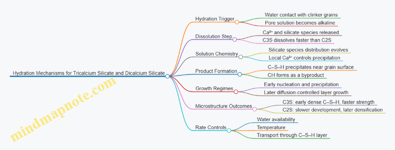
Example: Linking Mechanism to Observations
Consider a mortar cured for 1 day versus 28 days. At 1 day, C3S-driven dissolution and early C–S–H precipitation dominate, so the reaction layer is already established and strength rises quickly. At 28 days, C2S hydration has had time to progress through its slower dissolution and continued diffusion-controlled growth, so the microstructure becomes denser and strength continues to increase.
Example: What Happens When You Change the Grain Surface
If the clinker grains are finer, the surface area increases. More surface means more dissolution sites, which shortens the time to establish reaction layers. The mechanism stays the same—dissolution, precipitation, diffusion control—but the kinetics shift because transport distances within the solid are effectively reduced.
In summary, C3S and C2S share the same fundamental product set—C–S–H and CH—but differ in dissolution rate and the timing of diffusion-controlled growth. Those differences propagate into microstructure development, which then shows up as the familiar pattern of early versus later strength.
2.4 Alternative Binder Components and Their Electrochemical Relevance
Electrochemical cement production changes the usual story: instead of relying only on high-temperature clinker formation, it uses electrochemical steps to transform dissolved or suspended precursors into cementitious phases. That shift makes the choice of alternative binder components more than a materials-economics decision; it becomes a question of electrochemical compatibility—what species are present, how they move, and which reactions are favored.
Foundational Role of Alternative Binders
Alternative binders are materials that partially replace Portland cement clinker or modify the binder system. In conventional concrete, they work mainly by (1) contributing reactive phases that hydrate, and (2) providing fine particles that help nucleate hydration products. In electrochemical systems, they also influence solution chemistry and electrode reactions. A simple way to see the difference: in a typical hydration-only process, the binder’s job starts after mixing; in an electrochemical process, the binder’s job starts earlier, during precursor conditioning and electrochemical transformation.
Electrochemical Relevance Map
- What they supply: reactive ions, solid nucleation sites, or buffering capacity.
- What they consume or release: alkalinity, sulfate, carbonate species, or water.
- What they tolerate: pH swings, ionic strength changes, and competing electrode reactions.
- What they enable: controlled precipitation, phase selectivity, and stable slurries.
Mind Map: Electrochemical Compatibility of Alternative Binders
Slag and Slag-Like Materials
Ground granulated blast-furnace slag (GGBFS) is a classic alternative binder because it hydrates in alkaline environments to form calcium silicate hydrate (C-S-H) and related phases. In electrochemical cement production, slag-like materials are relevant because they can be used as either a feed component or a post-electrochemical conditioning additive.
Electrochemical angle: slag requires alkalinity to activate. If the electrochemical step produces a solution with insufficient hydroxide activity, slag dissolution slows and hydration lags. A practical best practice is to treat alkalinity as a controllable variable: measure pH and alkalinity in the process liquor, then adjust with a controlled base addition or by tuning electrochemical operating conditions that affect hydroxide generation.
Easy example: if a pilot run yields a binder that sets too slowly, check whether the electrochemical liquor has the alkalinity needed for slag activation. If pH is low, the fix is not “more slag” first; it is restoring the chemical environment that makes slag reactive.
Fly Ash and Other Pozzolans
Fly ash and other pozzolans contribute reactive silica and alumina that form cementitious hydrates when calcium and alkalinity are available. Electrochemically produced systems often generate calcium-bearing species in solution, but the timing matters: if calcium is present without sufficient alkalinity, pozzolan dissolution can be sluggish.
Electrochemical angle: pozzolans can also affect electrode behavior indirectly by changing slurry solids content and surface chemistry. Higher solids can increase viscosity and reduce mass transfer, which can shift current efficiency and alter precipitation patterns.
Easy example: when adding a pozzolan to a conditioning tank, keep an eye on slurry rheology. If mixing becomes harder, electrode performance may change because ions reach the electrode more slowly.
Limestone and Carbonate-Active Components
Carbonate-active materials influence cement chemistry by providing carbonate species that participate in precipitation and can affect the formation of calcium carbonate and carbonate-containing hydrates. In electrochemical systems, carbonate speciation (carbonate vs bicarbonate) is sensitive to pH and ionic composition.
Electrochemical angle: carbonate can compete with other precipitation pathways. If carbonate activity is too high, you may encourage calcium carbonate precipitation that is not the desired cementitious phase for strength development.
Easy example: suppose the product shows high mass loss on ignition or lower-than-expected strength. One diagnostic is to check whether excessive carbonate precipitation occurred during electrochemical conditioning. Adjusting carbonate concentration or pH can reduce unwanted precipitation.
Sulfate-Containing Additives and Gypsum-Like Sources
Sulfates are used in conventional cement to regulate hydration and control early set. Electrochemically, sulfate also affects solution speciation and can influence which solids form.
Electrochemical angle: sulfate can promote formation of sulfate-containing phases under certain conditions, and it can also alter ionic strength and transport. The practical goal is to provide enough sulfate for hydration control without driving the system toward phases that reduce long-term performance.
Easy example: if early setting is too fast, a small sulfate adjustment may help. But if later strength is weak, the sulfate level may have been high enough to steer phase formation away from the most beneficial hydrates.
Blending Strategy That Avoids Chemical Cross-Talk
A systematic approach is to treat alternative binder components as interacting “chemistry knobs.” Start with one component whose role is clear—such as a pozzolan for reactive silica or slag-like material for calcium silicate formation—then add a second component only after you can explain the expected chemical effect.
A practical workflow:
- Define the target chemistry for the electrochemical liquor (alkalinity, calcium availability, and key anions).
- Choose binder components that respond predictably to that chemistry.
- Run a small matrix varying one binder component at a time to isolate effects on setting and strength.
- Confirm phase outcomes with mineralogical checks so you know whether you got the intended hydrates.
Example: Choosing a Two-Component System
Consider a system that uses electrochemical conversion to generate calcium-bearing species, then relies on hydration to build strength. A reasonable two-component choice is slag-like material plus a modest pozzolan.
- Why slag-like first: it needs alkalinity, which you can manage through electrochemical operating conditions.
- Why pozzolan second: it refines the hydration microstructure by adding reactive silica and alumina.
- What to watch: if pozzolan addition increases solids too much, mass transfer limitations can reduce current efficiency and shift precipitation.
The integrated takeaway is simple: alternative binder components are not passive replacements. In electrochemical cement production, they actively shape solution chemistry, precipitation behavior, and ultimately the phase assemblage that determines performance.
2.5 Practical Implications for Mix Design and Testing
Electrochemical cement production changes what you start with: the binder precursor chemistry, the ionic environment during processing, and the way impurities end up locked into solids. Mix design and testing therefore need to be practical about two things—what phases you actually have and how they behave in water—rather than assuming “cement is cement.”
Start with What the Binder Really Is
Before choosing a target strength, confirm the binder’s baseline properties.
- Phase consistency: Use XRD or equivalent to verify that the expected clinker-like phases are present in the right proportions.
- Reactive surface and fineness: Measure Blaine or equivalent. Two binders with the same chemistry can behave differently if one is ground finer.
- Soluble ions and alkalinity: Check conductivity or ion chromatography for key ions (especially sulfate, chloride, and alkalis). These influence setting and durability.
Example: If your binder shows higher soluble sulfate than the reference, you may see faster early stiffening. A mix that “works” at 0.8% gypsum equivalent might fail at 1.2% unless you adjust dosage or blending.
Translate Chemistry into Mix Targets
A useful mix design workflow treats chemistry as constraints and performance as the objective.
- Set a water-to-binder ratio range based on target workability and expected hydration kinetics.
- Choose a binder blend strategy that controls reactivity. For instance, blend electrochemically produced binder with supplementary cementitious materials to moderate early heat and reduce sensitivity to soluble ions.
- Select admixtures by mechanism, not by brand: plasticizers for dispersion, set retarders for timing control, and air-entrainers if freeze-thaw exposure matters.
Example: Suppose soluble alkalis are higher. You can keep the same water-to-binder ratio but reduce superplasticizer demand by adjusting dosage and adding a retarder to prevent flash setting.
Workability Testing That Actually Predicts Casting
Workability is not just “slump.” For electrochemically produced binders, the time window matters.
- Measure slump flow and time to reach a target spread (e.g., 0 and 30 minutes).
- Track segregation resistance using visual stability and, when possible, a simple column test.
- Record bleeding behavior because ionic differences can change water movement.
Example: A mix may show acceptable initial flow but stiffen rapidly due to higher soluble species. Testing at multiple time points prevents you from optimizing a mix that only behaves during the first few minutes.
Setting Time and Heat as Early Warning Signals
Setting time and temperature rise reveal whether the binder is reacting as intended.
- Initial and final set: Use standard penetration or Vicat methods, but run at least two curing temperatures that reflect plant conditions.
- Isothermal calorimetry or embedded temperature: Compare heat flow curves across binder lots.
Example: If the main heat peak shifts earlier, you may need to reduce retarder dosage or adjust water content. If the peak height drops, you may have insufficient reactive phase or too much inert material.
Strength Testing with Phase-Aware Curing
Strength depends on both hydration and the microstructure formed during curing.
- Use consistent curing regimes and document them precisely.
- Test multiple ages (commonly 1, 3, 7, and 28 days) to see whether early reactivity is too high or too low.
- Include mortar and concrete scales because particle packing and admixture adsorption can differ.
Example: A binder that reaches high 7-day strength but lags at 28 days may indicate incomplete reaction or ongoing formation of phases that densify slowly.
Durability Checks for Ion-Sensitive Binders
Electrochemical processing can concentrate certain ions. Durability tests should reflect that reality.
- Chloride binding or migration tests if chloride exposure is relevant.
- Sulfate resistance using expansion monitoring.
- Permeability indicators such as rapid chloride permeability or water absorption.
Example: If soluble chloride is elevated, you may see higher early corrosion risk even when compressive strength looks fine. A binder that “passes strength” can still fail durability.
Mind Map: Practical Implications for Mix Design and Testing
A Simple Example Workflow That Prevents Rework
- Characterize binder lot: phase, fineness, soluble ions.
- Choose a baseline mix: set water-to-binder ratio and binder blend.
- Run fresh tests at multiple time points.
- Measure set time and heat behavior.
- Cast mortar for strength at several ages.
- Add one durability indicator aligned with the dominant ion risk.
- Update the mix and repeat only the necessary steps.
Example: If fresh tests show rapid stiffening, adjust retarder dosage and re-check set time before changing water content. This avoids the common trap of “fixing” workability by increasing water, which then harms strength and permeability.
The core idea is straightforward: treat electrochemically produced binder as a chemistry-and-ions system, then design and test mixes to observe how that system behaves in water, not just how it looks on paper.
3. Electrochemical Cell Architectures for Cement Related Reactions
3.1 Cell Types for Solid Liquid and Slurry Electrolytes
Electrochemical cement production can be organized around how the electrolyte carries ions and how solids are handled. The cell type is not a cosmetic choice; it determines mass transfer, current distribution, fouling risk, and how easily you can keep product chemistry consistent. A practical way to choose is to start with the feed state—solid, dissolved, or suspended—and then map that to the reactor geometry and electrode arrangement.
Foundational Concepts for Choosing a Cell Type
An electrolyte must provide ionic conduction between electrodes. In a liquid electrolyte, ions move through a continuous phase, so conductivity is usually predictable. In a slurry, ions still travel through liquid, but suspended particles can block pores, change local conductivity, and settle in low-velocity zones. In a solid electrolyte, ions move through a solid lattice or through grain boundaries, which can reduce evaporation and simplify containment, but it raises requirements for mechanical integrity and interfacial contact.
Two additional constraints often decide the winner. First, current density affects reaction rate and heat generation; uneven current can create local pH swings and uneven precipitation. Second, solids behavior matters: if particles form scales on electrodes, the cell may look fine on day one and then quietly lose performance.
Liquid Electrolyte Cells
Liquid electrolyte cells are the baseline for controlled chemistry. They are typically used when cement precursors are dissolved or can be kept in solution long enough for the electrochemical step.
Common Geometry and Operation
A simple approach is a parallel-plate or flow-through arrangement. The electrolyte flows between electrodes, and agitation is used to keep concentration gradients small near the electrode surfaces.
Integrated Best Practice
Use a circulation loop with a modest velocity target to reduce boundary-layer thickness. For a concrete example, if you observe that product forms a thin film near the cathode, increase flow rate slightly and add periodic flushing to prevent film consolidation. This is easier than trying to “fix” a hardened scale later.
Where Liquid Cells Fit
Liquid cells are most suitable when you need tight control of pH and ion ratios, and when the process can tolerate filtration steps after electrolysis.
Slurry Electrolyte Cells
Slurry electrolyte cells handle suspended solids directly. This can reduce upstream dissolution steps, but it introduces a new set of engineering problems: settling, abrasion, and particle-induced transport limits.
Common Geometry and Operation
Slurry cells often use flow-by electrodes with strong mixing, or they use rotating/recirculating systems to keep solids suspended. Electrode spacing and surface roughness become critical because particles can lodge in corners.
Integrated Best Practice
Design for “no dead zones.” A dead zone is a region where velocity drops enough for particles to settle. For example, if your reactor has a sudden expansion after the inlet, expect solids to accumulate there. A practical fix is to smooth the flow path and place the inlet so that the main jet sweeps the electrode surfaces.
Where Slurry Cells Fit
Slurry cells are useful when the feed contains fine solids that can be kept stable under operating pH and ionic strength, and when you can manage filtration and washing downstream.
Solid Electrolyte Cells
Solid electrolyte cells replace the liquid phase with an ion-conducting solid. This can improve containment and reduce evaporation, but it shifts the challenge to interfaces and mechanical stability.
Common Geometry and Operation
Solid electrolyte designs often resemble a stack: alternating electrodes separated by solid electrolyte layers. The stack approach helps with uniform current distribution, but it requires careful assembly to avoid gaps.
Integrated Best Practice
Prioritize interfacial contact. A simple example is to use controlled compression and surface preparation so that microscopic gaps do not become current bottlenecks. If you see localized heating or rapid performance drift, check contact pressure and surface cleanliness before changing chemistry.
Where Solid Cells Fit
Solid electrolyte cells are most suitable when you want to minimize liquid handling and when the process can be formulated to avoid aggressive chemical attack on the solid material.
Mind Map: Cell Type Selection
Worked Example: Mapping Feed to Cell Type
Suppose your precursor stream contains calcium-bearing solids that are partially soluble. If you can dissolve enough to keep the electrochemical step in solution, a liquid cell gives predictable ionic transport and easier quality control. If dissolution is incomplete and you want to avoid long residence dissolution tanks, a slurry cell can keep solids present, but you must engineer mixing to prevent settling on electrodes. If you need strict containment and can tolerate stack fabrication constraints, a solid electrolyte cell can reduce liquid handling, but you must treat interfacial contact as a first-class design parameter.
Practical Summary
Liquid cells optimize control, slurry cells optimize feed handling, and solid electrolyte cells optimize containment. The best choice is the one that matches your feed state while keeping mass transfer and fouling under control with realistic operating and maintenance practices.
3.2 Electrode Configurations for High Current Operation
High-current electrochemical cement production is mostly an electrode geometry problem wearing an electrical safety hat. The goal is simple: deliver current where ions can actually move, while keeping voltage losses and degradation under control. The “configuration” includes electrode shape, spacing, orientation, and how the electrolyte flows around the active surfaces.
Foundational Concepts for High Current
At high current, three effects dominate performance. First, ohmic drop grows with current density and electrolyte resistance, so shorter ion paths and better conductivity matter. Second, concentration polarization appears when reactants near the electrode are depleted faster than bulk flow can replenish them. Third, gas evolution and local pH shifts can foul surfaces or change reaction selectivity.
A practical way to think about configuration is to separate the cell into zones: bulk electrolyte, boundary layer near the electrode, and the electrode surface itself. High current shrinks the time available for mass transport, so configuration must reduce boundary-layer thickness and promote mixing.
Electrode Spacing and Current Distribution
Electrode spacing sets the baseline resistance and the ion path length. Too wide increases ohmic losses; too narrow increases shorting risk and can trap bubbles. For example, in a lab-scale slurry cell, reducing gap from 10 mm to 5 mm can noticeably lower cell voltage at the same current, but only if the flow pattern still sweeps bubbles away from the gap.
Current distribution depends on how uniformly the electric field reaches the active area. If the electrode edges see higher field intensity, they can degrade faster. A common best practice is to use edge management: rounded electrode corners, insulating guards, or current collectors that distribute current evenly before it reaches the active surface.
Parallel Plate Versus Flow-Through Designs
Parallel plate electrodes are easy to build and model. They create a predictable field and a simple flow channel. The downside is that boundary layers can grow along the flow direction, especially in viscous slurries.
Flow-through designs route electrolyte through porous electrodes or channels. This can improve mass transfer because fresh electrolyte repeatedly contacts new surface area. A concrete example: if you run a porous cathode at high current, you may see lower concentration polarization than with a smooth plate, but you must also manage pressure drop and ensure the pores do not clog with precipitates.
Bipolar Stacks and Series Electrical Layout
Bipolar stacks connect multiple electrode pairs in series electrically while sharing a common fluid path per compartment. This reduces the number of external connections and can improve scalability. The tradeoff is that each compartment must receive similar flow and chemistry; otherwise, one section can become the “weak link” with higher local resistance.
A simple diagnostic example is to measure temperature rise or voltage drop per compartment during steady operation. If one section consistently runs hotter or shows higher overpotential, it often indicates poor wetting, partial blockage, or uneven current distribution.
Electrode Orientation and Hydrodynamics
Orientation affects bubble removal and shear at the surface. If gas forms at the electrode, stagnant regions become fouling hotspots. Tilting electrodes or using cross-flow can help detach bubbles and renew the boundary layer.
In a slurry system, hydrodynamics also control where solids accumulate. A useful operational practice is to map deposition patterns after short runs. If deposits form preferentially near the inlet, the flow may be too gentle or the electrode too close to the wall, causing a low-shear recirculation zone.
Surface Area Engineering Without Losing Control
Increasing surface area lowers current density per unit active area, which can reduce overpotential and slow degradation. Porous electrodes and roughened surfaces do this, but they also increase the risk of pore clogging.
A balanced approach is to combine geometric area increase with controlled flow. For instance, a porous cathode can be paired with a higher cross-flow velocity to keep precipitates from settling inside pores. The configuration choice is therefore inseparable from the flow strategy.
Practical Configuration Checklist for High Current
- Set spacing for resistance and bubble clearance: verify with a short run that bubbles do not accumulate in the gap.
- Manage edges and current collectors: use rounded geometry or insulating guards to prevent edge hotspots.
- Choose a mass-transfer strategy: parallel plates for simplicity, flow-through or porous designs when boundary layers limit performance.
- Ensure compartment uniformity in stacks: confirm similar flow distribution and wetting across sections.
- Plan for solids: design flow paths and angles to minimize deposition zones.
Mind Map: Electrode Configuration Levers
Example: Choosing a Configuration for a Slurry Cell
Suppose you need to run at high current with a calcium-rich slurry where gas evolution is expected. Start with a parallel plate gap that is narrow enough to reduce ohmic losses but wide enough to prevent bubble trapping. If voltage rises faster than expected, switch to a flow-through arrangement that renews electrolyte near the electrode more frequently. If you then observe stable voltage but reduced activity, consider a modest porous surface area increase, paired with higher cross-flow to reduce pore clogging. The configuration decision is therefore iterative: each symptom points to a specific physical limitation.
3.3 Membranes Separators and Ion Transport Control
Electrochemical cement production often needs a membrane not because it looks neat in a schematic, but because it solves a specific problem: keeping reactive species from mixing, while still allowing the ions that carry charge to move. In practice, the membrane becomes the “traffic controller” for ions, and its choices determine current efficiency, product purity, and how stable the cell runs over time.
Foundational Role of Ion Transport
A membrane separates an anode compartment from a cathode compartment. When a voltage is applied, ions migrate to maintain electroneutrality. Two transport modes matter most: migration driven by the electric field, and diffusion driven by concentration gradients. If the membrane is too resistive, the cell needs higher voltage for the same current, which wastes energy and can increase unwanted side reactions. If it is too permeable to the wrong species, the compartments cross-contaminate, and the chemistry that you intended for one side shows up on the other.
A helpful mental model is to treat the membrane as a combination of (1) ionic conductivity, (2) selectivity for target ions, and (3) permeability for undesired species. You can improve one without harming the others, but only up to a point; most real designs trade off among them.
Membrane Types and What They Tend to Do
Ion-exchange membranes are common because they provide charge-based selectivity. Cation-exchange membranes favor positive ions, while anion-exchange membranes favor negative ions. For cement precursor systems, the “target” ions depend on the electrolyte chemistry, but the general goal is to allow charge-carrying ions to pass while limiting transport of species that would shift pH, dissolve solids, or change speciation.
Porous separators can work when the main requirement is physical separation with limited chemical exchange. However, they often allow faster mixing of electrolyte components, so they require careful control of flow rates and electrolyte composition.
In slurry or high-solids environments, membrane performance is dominated by fouling. A membrane that is perfect on paper can become mediocre when a thin layer of precipitate forms on its surface.
Transport Control Through Membrane Properties
Three properties usually govern performance.
- Ionic conductivity: Higher conductivity lowers ohmic losses. A practical check is to compare cell voltage at a fixed current density before and after conditioning.
- Ion selectivity: Selectivity reduces cross-over of species that should stay in one compartment. You can test selectivity by tracking concentration changes in both compartments during a short run.
- Water management: Many ion-exchange membranes require hydration to conduct ions. If the membrane dries, resistance rises. If it becomes over-hydrated, swelling can change pore structure and mechanical integrity.
A simple operational example: if you observe increasing cell voltage over time while current remains constant, the cause is often membrane resistance growth from dehydration or fouling. The fix is usually not “more voltage,” but better electrolyte conditioning and cleaning intervals.
Fouling Mechanisms and Practical Mitigation
Fouling in cement-related electrochemistry commonly comes from precipitation, adsorption, and scaling. Precipitation occurs when local pH near the membrane shifts enough to form sparingly soluble salts. Adsorption happens when fine particles or organics stick to the surface. Scaling can be driven by concentration polarization, where ions near the membrane surface become depleted or enriched.
Mitigation strategies should be systematic:
- Control bulk composition so that the membrane surface does not cross solubility limits. For example, if calcium carbonate is a risk, keep carbonate activity low enough that the near-membrane pH does not trigger precipitation.
- Use hydrodynamics that reduce concentration polarization. Higher crossflow can help, but too much shear can damage fragile membranes.
- Choose spacer and flow field designs that promote uniform velocity distribution. Dead zones become “fouling zones.”
- Plan cleaning based on observed failure mode. If fouling is mostly inorganic scale, a targeted cleaning chemistry and temperature profile can restore performance without damaging the membrane.
Example: Diagnosing Membrane Problems in Operation
Suppose a pilot cell shows stable product formation early, then gradually loses current efficiency. You measure:
- Cell voltage increases at constant current.
- The cathode compartment pH drifts toward the anode value.
- Microscopy of a removed membrane shows a thin crystalline layer.
This combination points to both increased resistance (fouling) and reduced selectivity (scale layer enabling transport). A practical response sequence is: reduce the near-membrane precipitation risk by adjusting electrolyte composition, increase crossflow to reduce concentration polarization, and schedule cleaning before the crystalline layer thickens.
Mind Map: Membranes Separators and Ion Transport Control
Example: Simple Control Logic for Membrane Health
A practical control approach is to track three signals during operation: cell voltage at fixed current, compartment pH difference, and solids accumulation rate. If voltage rises while pH difference shrinks, you likely have both fouling and increased crossover. If voltage rises without pH drift, resistance growth from dehydration or early fouling is more likely. This kind of pattern-based reasoning helps you choose the right corrective action instead of guessing.
In membrane-based cement electrochemistry, the separator is not a passive barrier. It is an active part of the reaction environment, shaping local chemistry through transport limits and surface interactions. When you treat it as such—by selecting for conductivity and selectivity, then managing fouling with composition and hydrodynamics—you get steadier operation and cleaner separation of the chemistry you want on each side.
3.4 Reactor Hydrodynamics for Mass Transfer and Uniformity
Electrochemical cement production depends on getting the right species to the right place at the right time. Hydrodynamics is the part of the system that decides whether ions and reactive intermediates arrive uniformly at electrodes, whether concentration gradients stay small, and whether solids behave like helpful passengers instead of chaotic cargo.
Foundational Concepts for Mixing and Transport
Start with three linked ideas: convection, diffusion, and reaction. Convection moves species with the bulk flow; diffusion moves species due to concentration differences; reaction consumes or produces species at the electrode surface. In many electrochemical reactors, the overall rate is limited by how quickly species cross the thin region near the electrode where concentration changes rapidly.
A practical way to think about this is the mass-transfer boundary layer. If the boundary layer is thick, species must diffuse farther before reaching the surface, and the local concentration drops. If the boundary layer is thin, convection and shear help replenish species, keeping the surface concentration closer to the bulk value.
Example: In a slurry reactor, if stirring is weak, calcium-containing ions near the cathode can become depleted. The result is uneven product formation across the electrode area, which later shows up as inconsistent phase chemistry in the dried solids.
Flow Regimes and Their Consequences
Hydrodynamics changes with Reynolds number, geometry, and viscosity. Laminar flow tends to create predictable streamlines but can also produce strong concentration gradients because mixing is limited. Turbulent flow increases mixing and reduces boundary-layer thickness, but it can also increase erosion and complicate scale-up.
For electrochemical cells, the goal is not “maximum turbulence.” The goal is stable, repeatable shear near the electrode that supports mass transfer without damaging membranes, coatings, or particle suspensions.
Example: A membrane-separated cell with high shear on the wrong side can cause membrane fouling to accelerate, even if mass transfer improves. The uniformity gain can be canceled by a loss in long-term stability.
Designing for Uniformity Across the Electrode Area
Uniformity fails in recognizable ways: edge effects, channeling, and dead zones. Edge effects happen because flow and electric fields are not perfectly uniform near boundaries. Channeling occurs when the flow path prefers a shortcut, leaving other regions underfed. Dead zones are low-velocity pockets where species linger and reactions can drift.
To reduce these issues, design the flow distribution so that velocity and residence time are similar across the electrode face. This often means using flow straighteners, baffles, or carefully shaped manifolds.
Example: If a reactor uses a single inlet jet, the jet region may overproduce one species while the far side underproduces it. Adding a distributor plate that spreads flow can reduce the concentration difference enough to improve product consistency.
Particle and Slurry Hydrodynamics
Slurries add extra physics: particles settle, agglomerate, and alter local viscosity. Settling creates a moving concentration profile that can shift the effective reaction zone over time. Agglomerates can block pores in porous electrodes and increase local resistance.
A good operational target is to keep solids suspended enough that concentration at the electrode does not drift during a run. This is usually achieved by selecting impeller type and speed, controlling particle size distribution, and managing viscosity with appropriate liquid-to-solid ratios.
Example: If the slurry contains fine carbonate particles that agglomerate, the reactor may show stable current at first and then a gradual change in product composition. Monitoring viscosity and particle size in the feed helps connect the hydrodynamics to the chemistry.
Mass-Transfer Metrics You Can Actually Use
Instead of relying on vague “good mixing,” use measurable indicators. Common metrics include limiting current behavior, concentration polarization trends, and spatial sampling of electrolyte composition.
A useful workflow is: (1) run at a fixed flow rate and current density, (2) measure how cell voltage changes with current, and (3) identify the onset of strong concentration polarization. That onset marks when mass transfer can no longer keep up.
Example: If increasing current density sharply increases voltage at constant flow, the system is approaching mass-transfer limitation. Raising flow rate or adjusting electrode spacing can reduce the boundary-layer thickness and restore more uniform operation.
Advanced Details for Scale-Up Without Surprise
Scale-up changes everything because surface area-to-volume ratio, mixing time, and flow distribution shift. A lab cell may rely on short diffusion distances and generous mixing; a larger cell may develop longer residence-time distributions and larger gradients.
To preserve uniformity, scale using hydrodynamic similarity where possible and validate with instrumentation. Mixing time measurements, tracer tests, and mapping of local conductivity or pH can reveal whether the larger reactor behaves like the smaller one.
Example: A tracer test using an inert salt can show that the bulk electrolyte reaches steady composition quickly, while the region near the electrode lags. That lag predicts where product non-uniformity will appear.
Mind Map for Reactor Hydrodynamics
Example Operating Checks for Consistent Performance
- Verify flow distribution: confirm that inlet design does not create a dominant jet path.
- Check for concentration polarization: look for voltage behavior that signals mass-transfer limitation.
- Monitor slurry stability: track viscosity and signs of agglomeration during a run.
- Validate uniformity experimentally: use spatial sampling or local conductivity/pH mapping near the electrode.
These checks connect hydrodynamics to electrochemical outcomes, so uniformity is treated as a measurable engineering property rather than a hope-and-pray assumption.
3.5 Materials Compatibility and Corrosion Control
Electrochemical cement production lives at the intersection of salt solutions, high pH or low pH pockets, and electrical fields that accelerate corrosion. Compatibility is not just “will it rust”; it is whether the material stays dimensionally stable, keeps its surface chemistry, and does not contaminate the product.
Start with the Chemical and Electrochemical Environment
Begin by mapping the likely local conditions inside the cell: bulk electrolyte composition, near-electrode pH shifts, dissolved oxygen or hydrogen availability, and temperature. A useful rule is that the electrode surface experiences a different chemistry than the tank. For example, even if the bulk electrolyte is mildly alkaline, cathodic regions can raise local pH and promote carbonate scaling, while anodic regions can drive metal dissolution.
A practical workflow is to define three “zones” for every material decision:
- Bulk zone: average electrolyte chemistry and temperature.
- Surface zone: conditions within a few millimeters of electrodes.
- Interface zone: seals, gaskets, and current collectors where crevices form.
Choose Materials by Failure Mode, Not by Guesswork
Corrosion control becomes systematic when you match materials to dominant failure modes.
Common failure modes
- Uniform corrosion: steady thinning, often in bulk electrolyte.
- Crevice corrosion: under gaskets, deposits, or lap joints.
- Pitting: localized attack, often triggered by chlorides.
- Intergranular corrosion: grain boundary weakness in some alloys.
- Galvanic corrosion: when two dissimilar metals share an electrolyte path.
- Erosion-corrosion: intensified by flow and bubbles.
Example: If your electrolyte contains chloride impurities and you use austenitic stainless steel for current collectors, pitting risk rises sharply. A compatibility check should include chloride concentration, temperature, and whether deposits can trap chloride in crevices.
Prevent Contamination of Cement Products
Materials can contaminate the binder through dissolution products that later appear as unwanted ions. Keep an eye on:
- Metal ions (Fe, Ni, Cr, Cu, Al) entering the electrolyte and ending up in solids.
- Silicate or polymer leachables from seals and coatings.
- Particle shedding from porous electrodes or mechanically stressed components.
A simple control is to run a “blank” electrolyte test: circulate electrolyte through the full wetted hardware without electrolysis, then analyze dissolved metals before any electrochemical step. If the baseline already contains high metal levels, corrosion control must come first.
Design for Crevice-Free Wetting and Stable Sealing
Crevices are corrosion’s favorite hiding place. Design choices that reduce crevice volume often outperform material upgrades.
- Use continuous welds instead of lap joints where possible.
- Prefer compression seals with smooth surfaces and controlled torque.
- Avoid trapped pockets where gas bubbles can accumulate.
- Ensure drainability so electrolyte does not remain in low points.
Example: A gasket that works in clean water may fail in chloride-bearing electrolyte because deposits form at the gasket edge. Switching to a seal material with better chemical resistance helps, but eliminating the stagnant crevice is usually the bigger win.
Control Scaling and Deposits That Trigger Corrosion
Deposits can be both a nuisance and a corrosion accelerator. Carbonate scaling, hydroxide films, and salt crystals can:
- block mass transfer,
- create differential aeration,
- trap aggressive ions under the deposit.
Mitigation includes:
- controlling supersaturation by adjusting concentration and temperature,
- using periodic flushing with electrolyte of lower ionic strength,
- selecting electrode surface finishes that reduce adhesion.
Example: If calcium carbonate forms readily, a rough electrode surface may increase nucleation sites. A smoother finish or a tailored surface treatment can reduce the rate of deposit formation, lowering both performance loss and corrosion under deposits.
Use Coatings and Surface Treatments Carefully
Coatings can protect metals, but they must survive abrasion, thermal cycling, and electrical conditions.
- Barrier coatings**:** good for preventing direct contact, but pinholes can become corrosion initiation points.
- Conductive coatings:** must maintain electrical pathways without cracking.
- Sacrificial layers:** can shift corrosion to a controlled location.
A compatibility check should include adhesion testing after exposure to the electrolyte and after thermal cycling. If a coating peels, it often exposes fresh metal and accelerates corrosion.
Mind Map of Compatibility and Corrosion Control
Mind Map: Materials Compatibility and Corrosion Control
Verification and Monitoring That Actually Helps
Verification should be staged.
- Soak tests: expose wetted materials to electrolyte without current; measure dissolved metals.
- Electrochemical exposure: run short current trials while tracking voltage stability and any sudden changes in metal content.
- Inspection: check for pitting, under-deposit corrosion, and gasket degradation.
- Corrosion rate estimates: use mass loss or thickness measurements where feasible.
Example: If dissolved iron rises sharply only during operation, the culprit is likely anodic dissolution or crevice corrosion near current collectors. If iron rises even during soak tests, the issue is baseline chemical corrosion or leaching from seals.
Integrated Example Decision
Suppose you need a current collector in a chloride-bearing electrolyte. You compare three options: stainless steel, nickel alloy, and a coated stainless steel.
- Stainless steel may pit in chloride crevices.
- Nickel alloy resists pitting but can still suffer galvanic corrosion if paired poorly.
- Coated stainless steel can work if crevices are minimized and coating adhesion is proven.
A robust decision uses the same logic every time: identify the dominant failure mode, remove the crevice driver, verify baseline leaching, then confirm performance under current. That approach keeps corrosion control from becoming a guessing game with expensive consequences.
4. Electrolytes and Solvent Systems for Cement Precursors
4.1 Electrolyte Selection Criteria for Reactivity and Conductivity
Electrochemical cement production lives or dies by the electrolyte. It must carry ions fast enough to keep the cell voltage reasonable, while also enabling the specific chemistry that turns cement precursors into cement-relevant solids. The trick is to treat “reactivity” and “conductivity” as linked design variables rather than separate checkboxes.
Foundational Requirements for Electrolyte Performance
Start with three baseline targets: (1) sufficient ionic conductivity, (2) chemical compatibility with electrodes and separators, and (3) stable speciation of the reactive ions. Conductivity is not just “high salt equals good.” If the electrolyte forms passivating films, precipitates, or gas bubbles that block transport, the effective conductivity drops even when the bulk solution looks conductive.
A practical way to think about it is to separate bulk transport from interfacial behavior. Bulk transport is governed by ion concentration, mobility, and temperature. Interfacial behavior is governed by pH, complexation, and whether ions prefer to stay dissolved rather than plate out on the electrode.
Ion Selection for Conductivity Without Losing Control
Ionic conductivity depends on the charge carriers and their mobility. For cement-related systems, calcium and carbonate species often matter directly, but the electrolyte may also include supporting ions that do not participate in the main reaction. Supporting ions help maintain charge balance and reduce resistance, especially when the reactive species are present at lower concentrations.
A useful selection rule: choose at least one “background” ion pair that stays soluble across the operating pH range. Then add reactive ions in amounts that achieve the desired speciation without causing unwanted precipitation.
Example: If you need carbonate availability for conversion, you can supply carbonate/bicarbonate while using a stable counterion (such as sodium or potassium) to maintain conductivity. If the counterion drives formation of insoluble salts with impurities, you will see conductivity decline during operation.
Speciation Control Through pH and Complexation
Reactivity in aqueous electrochemical systems is controlled by which chemical forms exist at the electrode surface. Carbonate chemistry is a classic example: CO₃²⁻, HCO₃⁻, and dissolved CO₂ shift with pH. Calcium chemistry behaves similarly, with free Ca²⁺ competing against complexes and solids.
To keep speciation stable, you typically manage pH using buffers or controlled feed composition. The electrolyte should resist rapid pH swings caused by electrolysis. Without that resistance, the cathode and anode regions develop different chemistries, leading to uneven product formation.
Example: In a cell where the cathode consumes protons, local pH rises. If calcium is present, higher pH can trigger CaCO₃ or Ca(OH)2 precipitation near the cathode, which may look like “more product” but often causes electrode fouling and reduces current efficiency.
Solubility and Precipitation Boundaries
Conductivity and reactivity both suffer when solids form in the wrong place. Precipitation can be beneficial if it forms the intended cement precursor phase in a controlled region, but harmful if it blocks pores or coats electrodes.
A systematic approach is to map solubility limits for the main species under expected operating conditions: temperature, pH, and ionic strength. Then choose electrolyte composition so that precipitation occurs after separation or in a designated precipitation step, not randomly inside the cell.
Example: If sulfate impurities are present, they can form low-solubility calcium sulfate phases. Even small impurity levels can matter when ionic strength is high, so electrolyte selection must include impurity tolerance, not just the target ions.
Temperature and Ionic Strength Tradeoffs
Higher temperature increases ion mobility and typically improves conductivity, but it also changes reaction kinetics and solubility. Ionic strength affects activity coefficients, which means the “same concentration” can behave differently across formulations.
A good electrolyte design documents the operating temperature range and verifies that conductivity remains adequate across it. If conductivity is only acceptable at the high end, the process will be sensitive to heat losses and startup conditions.
Compatibility with Cell Hardware
Electrolytes must be compatible with electrodes, separators, and current collectors. Compatibility includes corrosion risk, wetting behavior, and whether the electrolyte attacks coatings or membranes.
A simple screening method is to run short compatibility tests at the intended pH and potential window, then inspect for: (1) mass loss or pitting of electrode materials, (2) membrane swelling or cracking, and (3) formation of insulating films.
Example: A carbonate-rich electrolyte may be chemically fine in bulk, but if it promotes carbonate deposition on a separator, the separator resistance rises and the cell voltage climbs.
Mind Map: Electrolyte Selection Logic
Example Workflow for Choosing an Electrolyte
- Define the reactive chemistry need: identify which ions or species must be present at the electrode surface.
- Set the pH operating window: choose a range where the desired speciation dominates.
- Select supporting ions: pick counterions that maintain conductivity and remain soluble.
- Check solubility and precipitation risk: ensure solids form only where you want them.
- Verify compatibility: run short tests for corrosion, film formation, and separator resistance.
- Measure effective performance: confirm that conductivity stays high under current, not just in the beaker.
When these steps are done in order, electrolyte selection becomes less of a guessing game and more of a controlled design exercise—like tuning a radio so the station comes in clearly, not just turning the volume up and hoping for the best.
4.2 Solubility Control for Calcium Carbonate and Related Species
Calcium carbonate solubility is not a single number; it depends on temperature, ionic strength, pH, and what other ions are present. In electrochemical cement production, solubility control matters because it determines whether calcium stays dissolved long enough to form the desired precursor, or precipitates early and clogs pores, membranes, and filters. The goal is simple to state and annoyingly specific to execute: keep calcium and carbonate in the right chemical “neighborhood” so precipitation happens where and when you want it.
Foundational Chemistry for Predictable Precipitation
Start with the carbonate system. In water, dissolved inorganic carbon exists as CO₂(aq), HCO₃⁻, and CO₃²⁻. As pH rises, the fraction shifts toward CO₃²⁻, which increases the tendency to form CaCO₃. Calcium availability is governed by Ca²⁺ concentration and by complexation with carbonate species.
A practical way to think about precipitation is the saturation index. When the ion activity product of Ca²⁺ and CO₃²⁻ exceeds the solubility product, CaCO₃ becomes thermodynamically favored to precipitate. When it is below, precipitation is suppressed. Because activities differ from measured concentrations, ionic strength and competing ions can move the system closer to or farther from saturation.
Mind Map: Solubility Control Levers
pH Management Without Creating Local Supersaturation
pH is the strongest lever because it changes the CO₃²⁻ fraction. A common failure mode is “bulk pH looks fine, but local pH spikes.” Near electrodes, reactions can shift pH quickly, creating micro-zones where CaCO₃ forms instantly. To reduce this, use mixing strategies that limit concentration gradients: recirculation loops, baffles, and controlled feed points that avoid injecting calcium and carbonate into the same stagnant pocket.
A practical approach is staged addition. Instead of adding all carbonate-forming species at once, introduce alkalinity gradually while monitoring pH and conductivity. If you see turbidity rising while pH is still climbing, you are likely crossing saturation before mixing homogenizes the solution.
Calcium Concentration and Residence Time
Even with correct pH, too much Ca²⁺ too early pushes the system toward saturation. Control calcium dosing rate to match the rate at which carbonate species become available. Residence time matters because precipitation kinetics can be slow at first and then accelerate once nuclei form. A useful operational check is to sample at multiple points along the flow path and compare calcium and alkalinity: if calcium drops sharply early, precipitation is occurring upstream of where you want it.
Ionic Strength and Activity Coefficients in Real Liquids
Measured concentrations can mislead because ions interact. Higher ionic strength typically lowers activity coefficients, shifting effective saturation. In electrochemical systems, supporting electrolytes and dissolved salts can raise ionic strength, changing precipitation behavior even if pH and bulk concentrations remain constant.
A concrete example: two runs with the same Ca²⁺ and alkalinity but different background salts can show different scaling rates on the same surface. The difference is not magic; it is activity. Track conductivity alongside chemistry so you can correlate scaling events with ionic strength changes.
Temperature and Kinetics
Temperature affects equilibrium and kinetics. Higher temperature can increase solubility and also change nucleation and growth rates. In practice, temperature swings can turn a stable operating window into a scaling window. Keep temperature controlled, or at least record it, so you can interpret precipitation behavior consistently.
Competing Ions That Change the “Which Solid Forms” Question
Mg²⁺ is a classic example. It can inhibit calcite growth and alter crystal habit, which affects filterability and how easily solids wash. SO₄²⁻ can participate in forming mixed solids or adsorb onto growing surfaces, changing nucleation rates. Phosphate can strongly influence precipitation pathways by forming calcium phosphate phases or by modifying surface chemistry.
The operational takeaway is to treat impurities as part of the solubility control plan. If your electrolyte or feed contains variable Mg²⁺ or sulfate, you must expect changes in particle size distribution and scaling tendency even when pH and calcium dosing are unchanged.
Monitoring and Simple Diagnostics That Actually Help
Use a small set of measurements that connect directly to precipitation risk:
- pH and conductivity as real-time indicators of carbonate speciation and ionic strength.
- Calcium and alkalinity titrations on grab samples to compute saturation trends.
- Turbidity or particle counts to detect the onset of nucleation.
- Pressure drop across filters or membranes to catch scaling early.
A straightforward example workflow: run at a fixed current density, then step the alkalinity dosing rate. If turbidity rises immediately after the step and pressure drop follows within hours, you have evidence of precipitation onset tied to local chemistry rather than slow contamination.
Example: Designing a Controlled Precipitation Window
Suppose you want CaCO₃ to form during a downstream conditioning step rather than inside the cell. You can:
- Keep the cell feed pH slightly below the precipitation threshold by using staged alkalinity.
- Maintain strong mixing to avoid local supersaturation near electrode surfaces.
- After the electrochemical step, adjust pH and carbonate availability in a separate tank with controlled mixing and temperature.
- Confirm with sampling that calcium remains higher in the cell effluent than in the conditioning tank.
This separation of “reaction zone” and “precipitation zone” turns a messy, spatially varying process into something you can reason about with measurements.
Practical Guardrails for Stable Operation
- Avoid injecting calcium and carbonate-forming species into the same localized region.
- Track conductivity with pH so you do not confuse ionic strength effects for pH effects.
- Use staged dosing and mixing upgrades before changing chemistry targets.
- Treat Mg²⁺ and sulfate as variables, not background noise.
When these guardrails are followed, solubility control becomes less about chasing a single equilibrium constant and more about managing where supersaturation occurs, how fast it is reached, and what solid forms when it does.
4.3 pH Management and Buffering Strategies in Operation
pH control in electrochemical cement precursor systems is not just about staying within a “safe” range. It determines which calcium and carbonate species dominate, how fast solids form, and whether electrodes and membranes keep their intended behavior. In practice, pH management is a loop: measure reliably, adjust with a plan, and verify that the chemistry you intended is actually the chemistry you got.
Foundational pH Concepts for Cement Precursors
Start with what pH represents: the activity of hydrogen ions in the electrolyte. In cement-related systems, pH strongly influences carbonate speciation (CO₂/HCO₃⁻/CO₃²⁻), calcium solubility, and the tendency for precipitation to occur. A useful operational mindset is to treat pH as a “steering knob” for equilibrium, not as a single target number.
A practical example: if pH drifts upward, carbonate shifts toward CO₃²⁻, which can increase the likelihood of calcium carbonate precipitation. That may sound helpful, but uncontrolled precipitation can foul filters, clog flow paths, and create particles that later behave poorly during grinding and blending.
Measurement That Actually Works
pH meters can lie when the electrolyte is hot, conductive, or chemically complex. For operation, prioritize measurement stability over theoretical precision.
- Choose electrodes suited to high ionic strength and expected temperature range.
- Calibrate frequently using buffers that bracket your operating pH.
- Compensate temperature and verify response time by stepping the electrolyte pH in a controlled way.
Example: if your process uses a recirculating loop, measure pH at the loop outlet where mixing is more uniform, not at a stagnant sampling point. This reduces “false alarms” caused by local gradients near the cell.
Buffering Strategy Principles
A buffer resists pH change by providing a reversible chemical pathway. In cement precursor electrolytes, buffering often comes from carbonate/bicarbonate chemistry, plus added buffering agents when needed.
Key principle: buffer capacity must match the expected acid or base generation rate from the electrochemical reactions and any side reactions. If the buffer is too weak, pH swings will be large. If it is too strong, you may suppress the very pH shift needed to drive the desired speciation.
Operationally, buffering is best treated as a design parameter alongside current density and flow rate.
Managing pH Gradients Across the Cell
Even with good bulk mixing, pH can differ between regions: near electrodes, within porous electrodes, and across membranes. These gradients affect local precipitation and reaction rates.
A systematic approach:
- Control hydrodynamics to reduce stagnant zones (adequate flow, appropriate baffles or spacers).
- Use staged addition of buffer or electrolyte components so the bulk composition is established before the stream enters the most reactive zones.
- Target control points: measure and adjust at locations that represent the chemistry feeding the cell.
Example: if precipitation is observed mainly on the cathode side, bulk pH may look fine while local pH is too high. Increasing recirculation near the cathode or adjusting buffer dosing upstream can reduce local supersaturation without forcing the entire system to a different bulk pH.
Control Actions and Their Chemistry
When pH deviates, the “fix” should be chemically consistent with your system.
- Acid addition (commonly via controlled CO₂ or acid solutions) shifts carbonate toward bicarbonate and reduces CO₃²⁻ availability.
- Base addition increases carbonate fraction and can raise supersaturation for calcium carbonate.
- Buffer dosing adjusts capacity rather than forcing a single pH point.
Example: suppose pH rises gradually over a run and filter pressure increases. Instead of repeatedly adding acid to chase pH, first check whether the buffer capacity is being consumed (e.g., carbonate species converting due to reaction progress). Then adjust dosing strategy so pH stays stable while the speciation remains within the intended window.
Advanced Operational Details Without the Guesswork
1) Use mass balance thinking. Track how much carbonate and calcium species enter and leave. pH drift often correlates with changing composition, not just “electrode behavior.”
2) Manage ionic strength and conductivity. Changes in dissolved salts can alter electrode kinetics and pH probe behavior. A stable pH reading paired with a drifting conductivity can indicate measurement artifacts or evolving chemistry.
3) Prevent overshoot in control loops. pH controllers can oscillate if dosing is too aggressive. Use conservative step sizes and allow mixing time before evaluating the next adjustment.
4) Verify with speciation indicators. pH alone is incomplete. Pair pH with alkalinity or carbonate measurements when possible to confirm that the buffer system is behaving as expected.
Mind Map: pH Management and Buffering Strategies
Example: A Stable pH Run with Reduced Precipitation
Assume the process aims to keep bulk pH steady while limiting calcium carbonate formation inside the cell. Begin with a buffer composition that provides sufficient capacity for the expected net acid/base generation. Calibrate the pH probe and measure at the loop outlet.
During operation, if pH starts drifting upward and turbidity increases, pause aggressive corrective dosing. First confirm whether the drift matches a change in carbonate alkalinity or conductivity. If buffer capacity is being consumed, adjust buffer dosing rate upstream rather than repeatedly adding acid to force pH back to target. Then re-check pH after mixing time and confirm that precipitation shifts away from sensitive zones.
This approach treats pH as a controlled chemical environment, not a number to be bullied into compliance.
4.4 Impurity Handling for Sulfates Chlorides and Alkalis
Impurities in the electrolyte and in the feed stream can quietly steer electrochemical cement pathways away from the intended chemistry. Sulfates, chlorides, and alkalis each interfere in different ways: they change ionic strength, shift solubility, alter electrode surface chemistry, and can create scaling or corrosion. The goal is not to “remove everything,” but to control impurity speciation and concentration so the cell stays stable and the product stays consistent.
Foundational Concepts for Impurity Control
Start with a simple mass-and-charge view. In an electrochemical cell, the local environment near electrodes can differ from the bulk solution because reactions consume or generate ions. That means a feed that looks “fine” in bulk can still produce a problematic boundary layer at the electrode.
A practical control hierarchy works well:
- Define acceptable ranges for each impurity based on observed cell behavior and product quality.
- Measure speciation, not just total concentration, when possible.
- Control transport so impurities do not accumulate at the electrode surface.
- Treat streams upstream and recycle loops to prevent impurity buildup.
Sulfates Handling
Sulfates often cause two issues: they can promote scale formation and they can affect precipitation behavior of calcium-containing species. In many aqueous systems, sulfate can pair with calcium to form sparingly soluble solids, especially when local pH and ion concentrations rise near the cathode.
Best practice: set a sulfate limit and monitor both bulk sulfate and calcium activity indicators. If sulfate is high, reduce the risk of local precipitation by improving mixing and increasing electrolyte turnover in the vicinity of the cathode.
Easy example: imagine a pilot run where sulfate is 0.5 g/L in the tank. After several hours, the cathode face shows a white crust. Bulk measurements still read near 0.5 g/L, but the crust indicates calcium-sulfate precipitation at the surface. The fix is to lower sulfate in the make-up stream and increase local mass transfer so calcium does not oversaturate at the electrode.
Operational checks: track cell voltage drift and pressure drop across any filtration steps. Scale tends to raise resistance and can change flow distribution.
Chlorides Handling
Chlorides are smaller and more mobile, so they can reach electrode surfaces quickly. They can also increase corrosion risk for metallic components and can influence side reactions that generate reactive chlorine species under certain conditions.
Best practice: treat chlorides as a corrosion and selectivity risk. Use corrosion-resistant materials where appropriate, but also control chloride concentration through feed selection and targeted bleed-and-replace in recycle loops.
Easy example: a plant recycles electrolyte to save water and reduce waste. Chloride slowly accumulates because it is not consumed by the main reactions. After a few weeks, seals and current collectors show pitting. The remedy is a controlled bleed stream sized to keep chloride below the corrosion threshold, paired with makeup electrolyte that is low in chloride.
Operational checks: inspect for localized corrosion patterns near high-current regions and compare them to current density maps.
Alkalis Handling
Alkalis (often sodium or potassium salts) influence pH, ionic strength, and solubility of calcium and carbonate species. Too much alkali can shift equilibria so that unwanted salts form, and it can change the effective conductivity and viscosity of the electrolyte.
Best practice: manage alkalis by balancing buffering needs with precipitation avoidance. If alkalis are used to maintain pH, ensure they do not accumulate beyond the point where calcium-bearing solids become more likely.
Easy example: a process uses a sodium-based pH adjustment. Early runs look stable, but later the product shows higher variability in composition. The electrolyte conductivity rises, and the cathode region becomes more alkaline than intended. The fix is to reduce alkali dosing and add a controlled neutralization step or adjust the buffering strategy so pH stays within the target band throughout the cell.
Operational checks: track conductivity and pH at multiple points, not just at the tank. Boundary-layer pH can differ from bulk pH by enough to change precipitation behavior.
Integrated Mind Map for Impurity Handling
Mind Map: Sulfates, Chlorides, and Alkalis
A Systematic Control Workflow
- Baseline characterization: measure sulfate, chloride, and alkali levels in make-up and recycle streams, plus pH and conductivity.
- Define triggers: set thresholds for voltage drift, filtration pressure drop, and corrosion inspection findings.
- Stabilize transport: adjust flow distribution and mixing so impurities do not concentrate at electrode surfaces.
- Apply targeted mitigation: use upstream low-impurity sourcing for sulfates and chlorides; use controlled bleed-and-replace for chloride accumulation; tune buffering and dosing for alkalis.
- Confirm product impact: verify that binder chemistry and setting-related properties remain within acceptance criteria after impurity adjustments.
Example: One Month of Stable Operation Without Guesswork
Suppose a facility starts with moderate sulfate and low chloride, but alkali is adjusted to hit a pH target. During week one, the cell voltage is stable and filtration load is low. By week three, conductivity rises and filtration pressure drop increases, while bulk pH remains unchanged. Multi-point pH shows the cathode region is more alkaline than the tank. The team reduces alkali dosing and increases electrolyte turnover near the cathode. Filtration pressure drop returns to baseline, and product composition tightens back into the expected range.
This kind of workflow works because it treats impurities as controllable variables tied to measurable signals, rather than as mysterious “quality issues” that appear after the fact.
4.5 Laboratory Preparation and Conditioning Procedures
Laboratory preparation is where electrochemical cement pathways stop being equations and start behaving like materials. The goal is simple: produce repeatable precursor solutions and solids, condition them so they are chemically stable during testing, and document every step so results can be compared across runs.
Foundational Setup and Documentation
Start by defining what “ready for testing” means for your specific experiment. For solution-based tests, readiness usually means stable composition, controlled pH, and known conductivity. For solid-phase tests, readiness means consistent particle size, moisture content, and phase identity.
Create a one-page run sheet before any mixing. Include target concentrations, acceptable tolerances (for example, ±2% for major ions), temperature range, mixing time, and sampling schedule. A practical trick: label containers with both the batch ID and the intended role (electrolyte feed, rinse, calibration standard). This prevents the classic mistake of using the “almost the same” solution.
Electrolyte Solution Preparation
Begin with reagent-grade salts or prepared stock solutions. Use deionized water with a measured resistivity so you can interpret conductivity changes later.
- Dissolve in stages. Dissolve the bulk salts first, then add minor components last. This reduces local supersaturation that can cause early precipitation.
- Control temperature during dissolution. Many ion solubilities shift with temperature; keep the solution within a narrow band so composition is comparable between batches.
- Mix until stable. Stir long enough for conductivity and pH to plateau. If pH drifts after stirring stops, you likely have ongoing dissolution or CO₂ absorption.
Example: To prepare a calcium–carbonate–based electrolyte, dissolve calcium chloride in water, then introduce a carbonate source slowly while stirring. Monitor pH continuously; stop adding when the pH reaches the target window, then hold stirring for a fixed time before sampling.
pH Conditioning and Carbonate Control
Carbonate systems are sensitive to CO₂ exchange with air. Conditioning therefore means controlling both pH and carbonate speciation.
- Use a closed or semi-closed mixing approach when carbonate is involved.
- Condition by equilibration, not just adjustment. After reaching target pH, allow a short equilibration period so the carbonate distribution stabilizes.
- Record the method. Whether you used acid/base titration, buffered salts, or gas sparging affects speciation and should be stated in the run sheet.
Example: If your pH target is 8.5, adjust with a dilute base, then wait 15–30 minutes while stirring gently. Sample and verify that pH and conductivity remain within tolerance.
Impurity and Ionic Strength Management
Impurities can change electrode behavior and precipitation pathways. Instead of trying to “remove everything,” manage what matters.
- Measure baseline ions relevant to your system (for example, sulfate, chloride, sodium/potassium).
- Standardize ionic strength so differences in performance are not driven by conductivity alone.
- Use consistent rinse water for all preparation steps.
Example: If chloride is expected to influence corrosion, prepare a “low chloride” and “matched ionic strength” electrolyte pair. Keep chloride as the only intentional variable.
Solid Precursor Conditioning
Solid conditioning ensures that the solid phase you test is the solid phase you think you prepared.
- Drying protocol. Dry to a defined endpoint (time and temperature) and cool in a desiccator. Moisture changes both mass balance and reaction kinetics.
- Particle size control. Sieve or mill to a target range. Report the distribution, not just the nominal mesh.
- Pre-wetting when needed. Some powders form stable agglomerates; pre-wet with the same electrolyte used in the experiment to avoid sudden local concentration spikes.
Example: For a calcium carbonate-based precursor, dry at a controlled temperature, sieve to a consistent fraction, then pre-wet with electrolyte at the same solid-to-liquid ratio used in the cell.
Sampling, Verification, and Acceptance Criteria
Verification prevents “silent failures.” Define acceptance criteria before the run.
- Solution checks: pH, conductivity, and at least one composition measurement (for example, calcium concentration via titration or ICP).
- Solid checks: mass loss from drying, particle size distribution, and a phase indicator (for example, XRD peak presence/absence or a simple qualitative method if that is your lab standard).
Example: Accept an electrolyte batch only if pH is within ±0.1 units and conductivity within ±3% of the target at the test temperature.
Conditioning Workflow Mind Map
Mind Map: Laboratory Preparation and Conditioning Procedures
Integrated Example Run from Start to Finish
On a test day, prepare electrolyte feed first, then condition solids. Measure water resistivity, dissolve salts in stages at a fixed temperature, and adjust pH to the target window. After equilibration, sample for pH and conductivity and confirm calcium concentration. Meanwhile, dry the solid precursor to the defined endpoint, sieve to the target fraction, cool in a desiccator, and pre-wet using the same electrolyte feed.
Before starting electrochemical measurements, confirm that both the solution and solid meet acceptance criteria. If they do not, correct the specific variable (for example, re-equilibrate pH rather than adding more salts blindly) and resample. This keeps the experiment honest: the cell sees a controlled input, not a moving target.
5. Electrode Materials and Surface Engineering
5.1 Anode and Cathode Requirements for Cement Relevant Reactions
Electrochemical cement production typically targets transformations involving calcium species, carbonate/bicarbonate, and sometimes dissolved ions that influence pH and precipitation. The anode and cathode must therefore do more than “conduct electricity”: they must steer which reactions occur, keep the electrolyte chemistry stable, and survive long enough to make the process practical.
Foundational Requirements for Both Electrodes
Start with three shared constraints. First, both electrodes must provide low electrical resistance so the cell voltage is driven by chemistry rather than by sluggish current flow. A simple check is to compare measured cell resistance at operating temperature with and without electrode replacement; a large jump usually signals contact or coating failure.
Second, both electrodes must resist corrosion in the specific electrolyte composition. Cement-relevant electrolytes often contain calcium, carbonate species, and supporting salts; these can form insulating scales or chemically attack surfaces. A practical approach is to run short “soak tests” at operating pH and ionic strength, then inspect for mass loss and surface roughening.
Third, both electrodes must maintain performance under gas evolution or precipitation. Even when the target reaction is liquid-phase, side reactions can generate gas bubbles that block active sites. Meanwhile, calcium carbonate or hydroxide can deposit on surfaces and raise overpotential. The electrode design should therefore support cleaning, stable wetting, and controlled surface morphology.
Anode Requirements for Cement Relevant Reactions
At the anode, oxidation reactions dominate. In cement-relevant systems, the anode often faces carbonate/bicarbonate oxidation pathways or oxidation of other species that indirectly control pH and carbonate availability.
1. Selectivity and controlled oxidation. The anode should favor the intended oxidation route while suppressing oxygen evolution when that would waste current and shift pH in the wrong direction. A useful operational example: if the process depends on maintaining carbonate concentration, monitor carbonate species in the electrolyte and adjust current density to keep the anode from pushing too much toward oxygen generation.
2. Surface stability under oxidizing conditions. Many common metals oxidize into insulating layers. For instance, iron can form iron oxides that may initially conduct but can later crack and spall. A stable anode surface should either form a protective layer that remains conductive or use a material/coating that resists oxidation.
3. Scale management. Calcium carbonate can precipitate near the anode where local pH and ion concentrations differ from the bulk. Design choices include using a surface that reduces nucleation of thick scale and ensuring hydrodynamic conditions that sweep away forming crystals. In practice, you can test scale propensity by running identical electrolyte batches with different flow rates and comparing mass of deposits after a fixed charge passed.
Cathode Requirements for Cement Relevant Reactions
At the cathode, reduction reactions dominate, often involving water reduction and subsequent pH increase near the surface. That local pH shift can drive precipitation of calcium carbonate or calcium hydroxide, which then affects the final solid phase.
1. Controlled reduction and pH shaping. The cathode must produce the right amount of alkalinity without causing excessive hydrogen evolution that would disrupt mixing and create safety issues. A concrete example: if you observe rapid bulk pH rise and coarse precipitates, reduce current density or improve electrolyte circulation so the cathode boundary layer does not become too alkaline.
2. Compatibility with precipitation and porous solids. Cathode surfaces can become “seed beds” for calcium carbonate. This can be beneficial if it yields fine, filterable solids, but harmful if it forms dense, adherent layers that block pores. Electrode porosity and wettability matter: a moderately porous cathode can distribute current and reduce localized supersaturation, while still allowing solids to detach during flow.
3. Mechanical and chemical robustness. Cathode materials must handle repeated cycling between deposition and cleaning. If the electrode is cleaned with mild acid or chelants, the material and any coating must tolerate that chemistry without losing conductivity.
Mind Map: Anode and Cathode Requirements
Practical Example: Matching Electrode Behavior to Product Goals
Suppose the process goal is to generate a calcium carbonate-rich solid with manageable particle size. If the cathode produces too much local alkalinity, precipitation becomes fast and uncontrolled, yielding larger particles and higher filter resistance. The fix is not “more current” but better current distribution and mass transfer: use a cathode geometry that spreads current, increase electrolyte circulation to thin the boundary layer, and verify the effect by tracking both particle size distribution and deposit thickness on the cathode after a fixed charge.
On the anode side, if carbonate oxidation is insufficient, the electrolyte may drift toward compositions that later form undesirable solids. The anode requirement then becomes selectivity under the same operating window: adjust current density and confirm by measuring carbonate species before and after operation, while inspecting anode deposits for insulating scale.
Summary of What to Specify in an Electrode Datasheet
For cement-relevant electrochemical cells, specify electrode properties in terms of performance under the actual electrolyte: electrical conductivity and contact resistance, corrosion and scale resistance at operating pH and ionic strength, tolerance to gas evolution and precipitation, and ease of cleaning without losing conductivity. If those items are clear, the rest of the design—cell voltage, operating current density, and solid handling—becomes much easier to reason about.
5.2 Catalysts for Selectivity Control and Reduced Overpotential
Electrochemical cement production often runs into the same two problems: the desired reaction competes with side reactions, and the cell needs more voltage than the chemistry alone would suggest. Catalysts help with both by shaping which pathways are easiest and by lowering the energy barrier for the intended steps. The goal is not “more current,” but “more useful current.”
Foundational Concepts for Selectivity
Selectivity in an electrochemical cell is the fraction of total charge that ends up in the target products. If the cathode reduces water to hydrogen while calcium species remain unchanged, the extra current is technically real but practically wasted. Reduced overpotential means the cell operates closer to the thermodynamic potential, which typically improves efficiency and reduces stress on materials.
A useful mental model is to separate the process into three layers:
- Mass transport brings reactants to the electrode surface.
- Surface kinetics decide which reactions occur once reactants arrive.
- Solution chemistry determines what products remain stable after formation.
Catalysts mainly act on layer 2, but they can also influence layer 3 by changing local pH and ion concentrations near the surface.
How Catalysts Reduce Overpotential
Overpotential is the extra voltage required to drive a reaction at a useful rate. Catalysts reduce it by providing reaction pathways with lower activation barriers. In practice, this shows up as a smaller slope in polarization behavior and a lower onset voltage for the desired reaction.
For cement-related systems, the “desired reaction” might involve converting carbonate species, forming calcium-containing intermediates, or promoting controlled precipitation rather than runaway gas evolution. A catalyst that accelerates the target step without equally accelerating competing reductions can reduce overpotential while improving selectivity.
How Catalysts Improve Selectivity
Selectivity improves when the catalyst favors the adsorption and transformation steps of the target pathway over those of side reactions. Side reactions in aqueous electrochemistry commonly include hydrogen evolution at the cathode and oxygen evolution at the anode.
Catalysts can improve selectivity through:
- Active site tuning: changing the binding strength of key intermediates so the target pathway proceeds while others stall.
- Surface coverage control: managing how strongly the catalyst surface is blocked by adsorbed species.
- Local environment shaping: altering near-surface pH and ion distribution so the target species remain in the reactive form.
A concrete example: if carbonate conversion is hindered because the surface becomes coated with insoluble salts, a catalyst that resists fouling or promotes controlled precipitation can maintain active area and keep the reaction pathway open.
Catalyst Design Variables and Their Effects
Catalyst performance depends on several variables that are easy to mix up, so it helps to treat them separately.
- Composition: determines intrinsic activity and which intermediates bind well.
- Structure: affects the density and type of active sites, including edges and defects.
- Support and porosity: controls wetting, ion access, and resistance to mass-transport limitations.
- Electrode architecture: porous electrodes can reduce concentration gradients, but they also increase the risk of clogging.
- Operating conditions: current density, electrolyte concentration, and stirring rate change which reaction dominates.
Mind Map: Catalyst Roles in Selectivity and Overpotential
Example: Screening Catalysts Using a Simple Selectivity Metric
Suppose you compare two cathode catalysts under identical current and electrolyte conditions. Catalyst A shows faster current rise, but gas bubbles indicate hydrogen evolution. Catalyst B shows a slower rise, yet the measured calcium-containing product formation per unit charge is higher.
A practical screening approach is to track product formation per coulomb for the target species, not just total current. You can compute a “useful charge fraction” by dividing charge associated with target product formation by the total applied charge. Even without perfect accounting, the relative ranking is informative.
Example: Managing Fouling to Preserve Selectivity
In cement precursor electrolytes, carbonate and calcium species can form sparingly soluble solids. If these solids deposit on the catalyst surface, they block active sites and shift the reaction toward whatever still has access—often hydrogen evolution.
A straightforward mitigation is to pair the catalyst with an electrode design that tolerates deposition. For instance, using a porous structure with controlled pore size can allow solids to form in regions that do not fully isolate the catalyst. Another tactic is to adjust hydrodynamics so fresh electrolyte reaches the surface while removing loosely attached solids.
Example: Pairing Catalysts with Electrolyte Buffering
Local pH changes near the electrode can convert carbonate species into forms that either react more slowly or precipitate. A catalyst that accelerates the desired surface step may still underperform if the near-surface chemistry shifts away from reactive carbonate forms.
Buffering strategies can stabilize the relevant species distribution. The key is to choose buffering that supports the target pathway without introducing ions that strongly poison the catalyst surface.
Practical Testing Logic for Catalysts
A systematic evaluation sequence avoids guessing:
- Baseline kinetics: measure polarization to identify onset and slopes.
- Selectivity check: quantify target product per unit charge.
- Stability test: run for long enough to observe fouling or surface reconstruction.
- Mechanism hints: compare behavior under changed stirring and concentration to distinguish kinetic limits from mass-transport limits.
When these steps agree—lower overpotential, higher useful charge fraction, and stable performance—the catalyst is doing the job rather than merely looking busy on a current-time plot.
5.3 Coatings and Surface Treatments for Stability
Electrodes in electrochemical cement production face a predictable set of stressors: high current density, hot alkaline or near-neutral electrolytes, abrasive solids, and dissolved ions that can either passivate surfaces or build stubborn deposits. Coatings and surface treatments are the practical layer between “the chemistry works on paper” and “the cell keeps working after a few batches.” The goal is stability without blocking the reaction.
Foundational Stability Mechanisms
Start with what “stability” means at the interface. Three mechanisms dominate:
- Corrosion and dissolution: the electrode material slowly leaves the surface as ions.
- Passivation: a thin film forms that reduces corrosion but may also increase resistance.
- Fouling and scaling: precipitates from calcium, carbonate, sulfate, or silicate species coat pores and active sites.
A useful rule of thumb: corrosion control often improves with coatings, while fouling control depends on surface chemistry and hydrodynamics as much as on the coating itself.
Coating Selection Logic
Choose a coating by matching it to the dominant failure mode.
- If corrosion is the main issue, prioritize coatings that are chemically resistant and electronically conductive or that form a stable, thin barrier.
- If passivation is the issue, prioritize coatings that maintain low interfacial resistance and avoid thick insulating layers.
- If fouling is the issue, prioritize coatings that reduce adhesion of precipitates and maintain wetting in the presence of solids.
A practical way to decide is to run short tests at the same pH, temperature, and ion concentrations as the process, then measure both mass loss and electrochemical impedance growth over time.
Common Coating Approaches
Conductive Barrier Coatings
Conductive barriers aim to slow corrosion while keeping electron transfer possible. They are often thin and engineered to avoid cracking under thermal and mechanical cycling.
Example: Apply a thin titanium-based or carbon-based conductive layer on a metal substrate, then run a constant-current test in a calcium-rich alkaline electrolyte. If the coating is stable, you should see reduced mass loss and a slower rise in cell voltage compared with the uncoated electrode.
Protective Oxide Layers
Some oxides form in situ and can be beneficial if they remain thin and adherent. The trick is controlling formation so the oxide is protective rather than resistive.
Example: Precondition an electrode at a low current to form a controlled oxide film, then switch to production current. If the oxide is too thick, the voltage jump will be immediate; if it is well formed, the voltage increase will be gradual.
Polymer and Composite Films
Polymer films can reduce scaling by changing surface energy and adhesion. They must be thin enough to avoid blocking ionic transport and must tolerate alkaline conditions.
Example: Use a thin fluoropolymer or polymer-composite over a porous electrode. During operation, the film should remain intact while still allowing ions to pass. You can verify this by checking that the effective resistance does not rise sharply after the first few hours.
Surface Functionalization for Anti-Adhesion
Functionalization targets the chemistry of nucleation and attachment. Instead of trying to prevent all precipitation, it encourages precipitates to form in ways that are easier to remove.
Example: Modify the surface with groups that reduce calcium carbonate adhesion. In a controlled test with carbonate supersaturation, you should observe less continuous film coverage and more discrete deposits that can be removed during routine flushing.
Surface Treatments Before Coating
Coatings perform better when the surface is prepared.
- Cleaning and decontamination: remove oils, oxides, and loosely bound particles that can seed uneven coating.
- Controlled roughening: increase mechanical interlocking for durable adhesion.
- Activation steps: adjust surface chemistry so the coating bonds reliably.
Example: For a porous electrode, clean with an alkaline wash followed by thorough rinsing, then apply a primer layer before the main coating. Without the primer, you may see early delamination at edges where current density concentrates.
Mind Map: Coatings and Surface Treatments for Stability
Integrated Example Workflow
- Diagnose the dominant issue by comparing uncoated and candidate-coated electrodes under identical electrolyte composition.
- Prepare the surface with cleaning and a primer if adhesion is uncertain.
- Apply a thin coating sized to avoid blocking ionic pathways.
- Precondition with a short low-current step to stabilize the interface.
- Operate and monitor voltage trend and impedance growth; a stable coating shows slower drift, not a one-time miracle.
- Evaluate fouling behavior by inspecting deposit coverage and performing a standardized flush to compare how easily deposits detach.
Example: If voltage rises quickly but mass loss is low, the coating may be passivating too strongly. If mass loss is high but voltage is stable, corrosion resistance is insufficient. If both drift slowly but deposits accumulate in pores, the coating needs better anti-adhesion or the hydrodynamics need adjustment.
Practical Notes for Reliable Coating Performance
Coatings fail most often at edges, welds, and current collectors where stress and chemistry differ from the center of the electrode. Design for uniform current distribution, and treat the current collector as part of the coating system. Also, keep coating thickness consistent; thicker is not automatically better, because thicker layers can raise resistance and trap deposits.
A stable electrode is not just a material choice. It is a coordinated set of surface chemistry, coating integrity, and operating conditions that keep the interface predictable batch after batch.
5.4 Porous Electrodes for Enhanced Reaction Area
Porous electrodes increase the effective surface where electrochemical reactions occur. In cement-related systems, that matters because many steps depend on ion transport and surface reactions happening at the same time. A porous structure helps by providing more area than a flat plate, but it also introduces extra pathways that can slow mass transfer if the pores are poorly designed. The goal is to balance surface area, transport resistance, and mechanical stability.
Foundational Concepts for Porosity Design
Start with what “enhanced area” really means. The geometric area is the visible footprint of the electrode. The electrochemically active area is the portion of that footprint where ions can reach reactive sites and where the local potential supports the desired reaction. Porosity increases active area when pores are accessible to the electrolyte and when the internal surfaces remain electrically connected.
A useful mental model is three resistances in series: electrical resistance through the electrode, ionic resistance through the electrolyte-filled pores, and reaction resistance at the surface. If any one dominates, extra surface area won’t help. For example, very fine pores can create high ionic resistance, making the interior surfaces “present but not participating.”
Pore Geometry and Transport Balance
Pore size, pore connectivity, and tortuosity determine how quickly ions move inside the electrode. Larger pores reduce transport resistance but offer less surface per volume. Smaller pores increase surface but can trap stagnant electrolyte layers and increase diffusion distances.
Connectivity is often the deciding factor. A material with many pores that are poorly connected behaves like a sponge with sealed pockets: the electrolyte cannot reach most surfaces. Tortuosity matters too because longer, winding paths increase the effective diffusion length.
A practical way to design without guesswork is to target a pore size range that keeps diffusion time across the electrode shorter than the timescale of the applied current. In lab terms, you can check this indirectly by measuring how cell voltage changes with current density; a steep rise at moderate currents often signals transport limitations.
Material Choices and Electrical Connectivity
Porous electrodes must conduct electrons while allowing ion access. Common approaches include sintered metal or carbon frameworks, conductive ceramics, and composite structures where a conductive network supports a porous phase.
Electrical connectivity is critical. If the conductive phase is discontinuous, internal surfaces become electrically isolated and contribute little. A simple diagnostic is to compare performance before and after gentle compression or binder removal; if activity collapses, the conductive network likely wasn’t robust.
For cement precursor environments, chemical stability is also part of “connectivity.” Electrodes that corrode or foul can lose both conductivity and pore access. Surface treatments and protective coatings can help, but they must be thin enough to avoid blocking pores.
Fabrication Methods and Their Consequences
Three fabrication routes show up frequently in practice:
- Sintered porous structures create stable pore networks but require careful control of sintering temperature to avoid pore collapse.
- Foam or template replication can produce predictable pore architectures, but the template removal step must not leave residues that later foul the surface.
- Coated porous supports place catalytic layers inside pores; coating thickness must be controlled so it doesn’t seal the pore entrances.
A good rule is to treat fabrication as part of the electrochemistry. Two electrodes with the same nominal porosity can behave differently if one has blocked pore throats or uneven coating coverage.
Example: Choosing a Porous Electrode for a Calcium-Containing Electrolyte
Suppose you are converting carbonate species in an electrolyte containing calcium ions. You want high active area, but calcium can precipitate on surfaces and inside pores.
A systematic approach is to start with a moderately porous electrode and operate at conditions that minimize immediate precipitation. Then, you evaluate two things after a short run: (1) how much the cell voltage increased and (2) whether the pores appear clogged. If voltage rises quickly and post-run inspection shows pore blockage, the pore structure is too fine or the local supersaturation at the surface is too high.
You can respond by increasing pore size, improving flow-through (better connectivity), or adjusting current density so the reaction rate doesn’t outpace mass transport. The key is to change one variable at a time so you can attribute the improvement.
Mind Map: Porous Electrode Design Logic
Practical Checklist for Cement-Adjacent Electrolytes
Before committing to a porous electrode design, verify that the electrolyte can wet the pores, that the conductive phase remains continuous, and that the pore network won’t be quickly blocked by precipitation or by reaction byproducts. During testing, watch for signs of transport limitation through voltage trends, and confirm participation by checking whether internal surfaces remain accessible after operation. When those conditions are met, porous electrodes can provide a real, measurable increase in effective reaction area rather than just a bigger-looking surface.
5.5 Practical Testing Methods for Electrode Performance
Electrode performance testing should answer three questions: does the electrode carry current efficiently, does it steer reactions toward the desired products, and does it survive the operating environment without losing active area. A practical test plan starts with simple measurements that isolate one variable at a time, then moves to integrated tests that mimic the cement-relevant electrolyte and operating conditions.
Baseline Checks Before Electrochemistry
Start with physical and chemical baselines. Measure geometric area accurately (use a mask or defined fixture), record electrode mass and thickness, and photograph the surface under consistent lighting. If the electrode is porous, determine effective surface area indirectly using a wetting test or electrochemical roughness factor later. For stability, run a short open-circuit soak in the electrolyte to confirm no immediate dissolution, swelling, or gas evolution that would complicate later interpretation.
Example: If a porous carbon electrode loses visible mass during a 30-minute soak, normalize later results by the remaining mass and treat the electrode as “pre-aged” for the rest of the campaign.
Electrochemical Screening with Controlled Conditions
Use a three-electrode setup for screening when possible: working electrode (the candidate), reference electrode, and counter electrode. Keep temperature, stirring rate, and electrolyte composition fixed. Perform cyclic voltammetry (CV) to identify potential windows where unwanted reactions dominate. Then run linear sweep or polarization tests to estimate current response versus overpotential.
A key practical detail is to report results using the same reference electrode and calibration method each time. If you cannot maintain a stable reference in a high-salt or multiphase electrolyte, use a pseudo-reference and document it consistently.
Example: If CV shows a sharp rise in current at potentials where carbonate conversion is not expected, set the operating potential below that onset for subsequent chronoamperometry.
Kinetic Metrics from Impedance and Tafel Analysis
Electrochemical impedance spectroscopy (EIS) helps separate charge-transfer resistance from mass-transfer limitations. Use a small AC perturbation and a frequency sweep that covers both fast interfacial processes and slower transport effects. Interpret spectra using an equivalent circuit that matches your system: typically solution resistance in series with a parallel combination of charge-transfer resistance and double-layer capacitance, plus a mass-transfer element if needed.
For systems where steady-state polarization curves are reliable, Tafel analysis can estimate apparent kinetic parameters. Use it only in regions where the current is not dominated by diffusion.
Example: If EIS shows charge-transfer resistance dropping after a surface treatment while limiting current stays similar, the treatment likely improves kinetics rather than transport.
Steady-State Performance with Chronoamperometry
Chronoamperometry measures how current and potential evolve under constant applied potential or current. Run at least two durations: a short “conditioning” period to reach stable behavior, and a longer period to reveal drift from fouling, bubble coverage, or salt precipitation.
Track three signals: applied potential, current response, and any gas evolution rate if relevant. After the run, rinse using a standardized protocol and compare pre- and post-test mass and surface morphology.
Example: If current decays steadily while potential rises, inspect for passivation layers. If current fluctuates with visible bubbles, adjust hydrodynamics or electrode wetting.
Product Selectivity Measurements That Matter for Cement Chemistry
Electrode tests must connect electrochemical behavior to chemistry. Sample the electrolyte at defined time intervals and quantify the species tied to cement precursor formation. Use mass balance logic: compare measured concentrations against expected stoichiometry and account for any species that leave the cell via evaporation or adsorption.
A practical workflow is to pair electrochemical tests with quick chemical assays: pH and conductivity for bulk behavior, then targeted ion analysis for the key reactive species. If solids form, filter and analyze the solid fraction separately.
Example: If the desired calcium-containing species increases while carbonate decreases more slowly than expected, the electrode may be promoting side reactions that consume carbonate without producing the target precursor.
Post-Test Diagnostics for Failure Mode Identification
After electrochemical testing, use diagnostics to explain performance changes. Common failure modes include surface passivation, corrosion, binder or catalyst detachment, and pore clogging. Use scanning microscopy or profilometry to compare surface texture and pore accessibility. Measure contact resistance if your fixture allows it, since poor electrical contact can masquerade as electrochemical degradation.
Example: If microscopy shows pore blockage by fine precipitates and selectivity drops, add a controlled agitation or filtration step in the test setup to confirm transport sensitivity.
Mind Map of Practical Testing Workflow
Example Test Matrix for Comparing Two Electrode Treatments
Run Treatment A and Treatment B under identical electrolyte composition, temperature, stirring, and electrode geometry. First, do CV to confirm both electrodes share a safe operating window. Next, run EIS at a representative potential in that window. Then perform chronoamperometry for the same conditioning time and the same longer duration. Finally, sample electrolyte at the end of each phase and analyze the key cement-relevant species plus any solids.
Decision rule: choose the electrode that shows lower charge-transfer resistance, stable current over the long run, and higher selectivity toward the target precursor species, even if its initial current is slightly lower. That rule prevents selecting electrodes that look good only during the first few minutes—when the surface is still fresh and the chemistry hasn’t had time to reveal its habits.
6. Reaction Pathways for Electrochemical Conversion of Cement Precursors
6.1 Carbonate and Bicarbonate Conversion Mechanisms
Carbonate (CO₃²⁻) and bicarbonate (HCO₃⁻) are the main carbon-bearing species that can be electrochemically converted into forms useful for cement-related chemistry. In practice, the conversion is rarely a single step. It is a chain of equilibria and electrochemical reactions that depend on pH, dissolved inorganic carbon speciation, mass transport, and electrode surface behavior.
Foundational Speciation and Why pH Controls Everything
In water, carbon dioxide and carbonate species interconvert through acid–base equilibria. A useful mental model is that pH decides which “bucket” holds most of the carbon.
- At higher pH, carbonate dominates because CO₂ is deprotonated stepwise to CO₃²⁻.
- At lower pH, bicarbonate becomes more prevalent, and at even lower pH dissolved CO₂(aq) and carbonic acid become significant.
Example: If you bubble CO₂ into alkaline electrolyte, the pH drops and the fraction of HCO₃⁻ rises. If you then raise pH again, bicarbonate converts back toward carbonate. Electrochemical conversion therefore starts with controlling the initial speciation, not just applying voltage.
Electrochemical Conversion Pathways
Electrochemical systems can convert carbonate and bicarbonate through pathways that either (a) change the carbon oxidation state or (b) change the chemical form without a large net change in oxidation state. The most common cement-relevant goal is to generate reactive calcium carbonate or related solids by shifting dissolved carbonate equilibria and enabling precipitation or surface-mediated transformations.
Pathway A: Direct Electrochemical Reduction of Carbon Species
At sufficiently reducing conditions, carbonate or bicarbonate can be reduced at the cathode, producing intermediates that may include CO₂, CO, or other carbon-containing species depending on electrolyte composition and electrode material. In many cement-oriented setups, this pathway is not the primary route because it can consume charge without producing the desired solid phase efficiently.
Example: In a cell where the cathode surface promotes hydrogen evolution, a large fraction of current goes to water reduction. The carbonate concentration may change only modestly, and the main observable effect is pH drift near the cathode rather than a clean carbon conversion.
Pathway B: Indirect Conversion via Local pH and CO₂ Equilibria
A more controllable mechanism is indirect: electrolysis changes local pH near electrodes, which shifts carbonate–bicarbonate–CO₂ equilibria. Even if the bulk electrolyte composition stays similar, the thin boundary layer near the electrode can experience a different pH, changing which species are available for reaction.
- Near the cathode, generation of OH⁻ raises local pH, pushing HCO₃⁻ toward CO₃²⁻.
- Near the anode, formation of acidic species or consumption of OH⁻ lowers local pH, pushing CO₃²⁻ toward HCO₃⁻.
This matters because precipitation and surface reactions depend strongly on carbonate activity.
Example: Suppose bulk electrolyte is moderately alkaline with both HCO₃⁻ and CO₃²⁻ present. If the cathode region becomes more alkaline, CO₃²⁻ activity increases locally, making calcium carbonate precipitation more likely if calcium is present. The “conversion” is then a speciation shift plus solid formation, not necessarily a deep electrochemical transformation of carbon.
Pathway C: Coupled Carbonate–Calcium Chemistry
Cement production needs calcium-containing solids. When calcium ions are present, carbonate speciation determines whether calcium carbonate forms and what form it takes.
- Increased CO₃²⁻ availability raises the saturation index for CaCO₃.
- Bicarbonate can act as a reservoir that converts to carbonate as pH rises locally.
- The anode–cathode pH gradient can create spatially separated zones of dissolution and precipitation.
Example: If calcium is fed into the electrolyte and the cathode creates high local pH, CaCO₃ can form near the cathode. If the anode region is more acidic, some CaCO₃ may dissolve there, reducing net yield unless mixing and residence time are tuned.
Mass Transport and Boundary Layer Effects
Electrochemical conversion is limited by how fast species move to and from the electrode surface. Carbonate and bicarbonate are not consumed uniformly; they are depleted or enriched in the boundary layer.
- High stirring or optimized flow reduces concentration gradients.
- Porous electrodes can increase effective surface area but also increase internal diffusion limitations.
- Membranes or separators can reduce cross-contamination of pH and species.
Example: In a poorly mixed reactor, you may measure bulk concentrations that look stable while the electrode region shows strong precipitation. The bulk sample then underestimates what actually happened at the surface.
Mind Map: Carbonate and Bicarbonate Conversion Mechanisms
Worked Example: Interpreting a Conversion Result
Consider a cell with calcium present and an electrolyte initially containing both HCO₃⁻ and CO₃²⁻. After running at constant current, you observe increased CaCO₃ solids near the cathode and a modest change in bulk carbonate concentration.
A consistent interpretation is:
- The cathode raises local pH, shifting HCO₃⁻ to CO₃²⁻.
- The higher CO₃²⁻ activity drives CaCO₃ precipitation near the cathode.
- Bulk concentrations change less because the main “sink” is solid formation at the electrode surface, not bulk consumption.
If instead you see little solid formation and a large pH rise, the likely issue is that current is going mostly to water reduction and the system is not maintaining carbonate availability or calcium supersaturation where it matters.
Practical Takeaways for Mechanism Design
To make carbonate and bicarbonate conversion effective for cement-related outputs, the mechanism must be aligned with the dominant limitation:
- If speciation is the bottleneck, manage bulk pH and buffer capacity so the electrolyte starts in the right carbon form.
- If boundary layers dominate, improve mixing, adjust current density, and consider separators to control pH gradients.
- If precipitation is the goal, ensure calcium and carbonate activities reach supersaturation in the intended zone, not just somewhere in the reactor.
These steps keep the conversion grounded in measurable chemistry rather than treating electrolysis as a magic button.
6.2 Calcium Species Transformations and Precursor Formation
Calcium species transformations are the bridge between what you start with in the electrolyte and what you end up grinding, washing, and blending into a cementitious precursor. In electrochemical cement production, the “species story” is mostly about controlling calcium’s oxidation state (it stays as Ca²⁺), its counter-ions, and its solubility—so the solid phase you form is predictable rather than accidental.
Foundational Species Inventory and What Changes
Start by listing the calcium-bearing forms you can realistically encounter in an operating cell:
- Dissolved calcium: Ca²⁺ in the electrolyte.
- Carbonate system species: CO₃²⁻, HCO₃⁻, and dissolved CO₂(aq) depending on pH and gas contact.
- Hydrolysis products: CaOH⁺ and related equilibria that become more important as pH rises.
- Solid calcium salts: CaCO₃ polymorphs, and potentially other calcium-containing solids if impurities supply the right anions.
What electrochemistry changes is not calcium’s oxidation state, but the local pH and local carbonate availability near electrodes. Those two knobs decide whether Ca²⁺ stays dissolved, precipitates as CaCO₃, or forms a less desired solid that later slows grinding and hydration.
Local pH Gradients and Their Consequences
Near the cathode, reactions typically raise pH by consuming protons or generating hydroxide. Near the anode, pH often drops due to proton production or oxidant chemistry. This creates a gradient that can be sharper than the bulk electrolyte conditions.
A practical way to reason about it: precipitation needs both Ca²⁺ and carbonate species. If the cathode region becomes more basic, carbonate speciation shifts toward CO₃²⁻, and CaCO₃ becomes thermodynamically favorable. If the anode region becomes more acidic, carbonate can dissolve back, which can reduce unwanted scaling there.
Example: Suppose your bulk electrolyte is moderately basic so Ca²⁺ is stable. If agitation is weak, carbonate-rich microzones form at the cathode surface, leading to fast CaCO₃ nucleation on the electrode. With stronger mixing, those microzones disperse, and precipitation shifts toward the bulk where particles can grow more uniformly.
Carbonate Availability and Precipitation Pathways
Calcium carbonate formation can proceed through different pathways depending on carbonate source and pH history:
- Direct precipitation from carbonate-rich solution: Ca²⁺ + CO₃²⁻ → CaCO₃(s).
- Bicarbonate-driven precipitation: HCO₃⁻ can convert to CO₃²⁻ as pH rises locally, then precipitate.
- Transient amorphous or hydrated intermediates: Under some conditions, solids form first as less crystalline phases, then reorganize into more stable polymorphs.
The key operational lever is how long calcium spends in supersaturated conditions. Short, intense supersaturation favors many small nuclei; slower, moderated supersaturation favors fewer nuclei and larger particles.
Example: If you run at high current density without adequate mass transfer, local supersaturation spikes. You may get fine CaCO₃ that looks good on a sieve but can behave differently during later calcination or hydration because surface area and defect density change.
Counter-Ion Control and Impurity Effects
Calcium precipitation is sensitive to what else is dissolved. Common issues include:
- Sulfate and chloride: They can form calcium salts or adsorb on growing surfaces, altering nucleation rates and polymorph selection.
- Alkali metals: They can change ionic strength and carbonate speciation, affecting solubility and precipitation kinetics.
- Silica and organics: Even at low levels, they can complex calcium or interfere with crystal growth.
A useful rule: if an impurity can provide an anion that forms a sparingly soluble calcium compound, it can compete with CaCO₃ formation. Even when it doesn’t fully precipitate, adsorption can still slow or redirect crystal growth.
Example: If sulfate is present, you might observe delayed CaCO₃ precipitation because calcium spends time forming calcium sulfate-rich species or because sulfate adsorbs and blocks active growth sites. The result is a longer induction period and a different particle morphology.
From Calcium Solids to Precursor Formation
Once CaCO₃ (or another calcium-containing solid) forms, precursor formation requires turning that solid into a controlled feedstock for the next step. The transformation from “electrochemical solid” to “precursor” typically includes:
- Solid-liquid separation to remove soluble ions that would otherwise carry into later processing.
- Washing to reduce residual sulfate, chloride, or excess alkali that can affect hydration behavior.
- Drying and conditioning to stabilize particle surfaces and prevent uncontrolled agglomeration.
- Optional phase adjustment depending on the intended precursor chemistry.
Example: If you skip washing, residual ions can remain trapped in pore water. Later, during calcination or hydration, those ions can shift reaction pathways, changing setting behavior even when the bulk composition looks acceptable.
Mind Map: Calcium Transformations to Precursor Formation
Worked Example: Linking Operating Choices to Solid Outcome
Assume you target CaCO₃ as the calcium precursor component. You choose moderate bulk pH to keep Ca²⁺ dissolved, then rely on cathode-local pH rise to generate CO₃²⁻. If you maintain strong mixing, precipitation occurs throughout the bulk, producing a narrower particle size distribution. After the run, you wash until conductivity drops, reducing residual anions. The resulting solid then behaves more consistently in the next processing step because its pore solution composition is controlled.
In short, calcium transformations are a controlled chain: transport → local chemistry → precipitation pathway → solid conditioning. When each link is managed, the precursor stops being a surprise and starts being a repeatable input.
6.3 Control of Competing Reactions in Electrochemical Systems
Electrochemical conversion of cement precursors rarely follows a single, obedient reaction. Competing pathways can consume current, shift product composition, and change how solids form and settle. Control is therefore not just about “making the desired species”; it is about allocating electrical work to the right chemistry while preventing side reactions from taking over.
Foundational Idea: Current Is a Budget
In an electrochemical cell, the applied current is distributed among all reactions that can occur at the electrodes. If the desired reaction has a higher kinetic barrier or is mass-transfer limited, side reactions can capture a larger fraction of the current. A practical way to think about control is to ask three questions for each electrode:
- What reactions are thermodynamically possible at the operating potential?
- Which reactions are kinetically favored by the electrode surface?
- Which reactions receive the reactants first, given mixing and diffusion?
A good operating point is where the desired reaction is both thermodynamically allowed and kinetically dominant, while side reactions are starved of either potential access or reactant supply.
Mind Map: Competing Reactions Control Logic
Potential Window Control
Side reactions often become significant when the electrode potential moves too far beyond what the desired reaction needs. For example, at cathodic conditions, hydrogen evolution can start competing once the potential is sufficiently negative relative to available proton activity. At anodic conditions, oxidation of unwanted species or electrolyte components can accelerate.
Best practice: determine a practical operating window using small-step potential sweeps while tracking both product formation and side indicators (such as gas rate or dissolved species changes). Then run at a potential that sits inside the window with a margin that accounts for drift.
Easy example: if increasing cathodic potential by 100 mV raises the target calcium species formation only slightly but doubles hydrogen evolution, the extra voltage is buying mostly side reaction current. Returning to the lower potential typically improves current efficiency even if the absolute production rate drops a bit.
Mass Transport Control
Even when the desired reaction is favored on paper, it can lose in the real cell if reactants arrive slowly at the electrode surface. Concentration gradients form near the electrode, and the local environment can differ from the bulk electrolyte.
Best practice: design agitation and flow so that the limiting reactant for the desired reaction is not replaced by a different limiting reactant that enables side chemistry. Electrode porosity and thickness also matter: porous electrodes increase surface area but can trap products and create microenvironments.
Easy example: suppose the desired pathway depends on carbonate availability at the cathode. If mixing is weak, carbonate near the electrode can be depleted, and protons become the easiest reactant for hydrogen evolution. Improving mixing restores carbonate availability and shifts current back toward the desired reaction.
Electrolyte Chemistry Control
Speciation control is a quiet but powerful lever. pH, ionic strength, and buffering determine which forms of calcium and carbonate exist in solution, which in turn affects how readily they participate in electrode-adjacent reactions.
Best practice: maintain pH within a narrow band using buffering compatible with the electrolyte system. Track speciation by sampling and measuring key ions rather than relying only on bulk pH.
Easy example: if bicarbonate is the dominant carbonate species under your operating conditions, a small pH shift can convert it toward carbonate or toward CO₂-related forms. That changes both reaction kinetics and the tendency for precipitation, which can either coat the electrode (reducing desired activity) or form unwanted solids that alter mass transport.
Electrode and Surface Control
Electrode material and surface state determine which reactions are catalyzed. A surface that strongly catalyzes hydrogen evolution will steal current whenever the cathode potential becomes even slightly favorable for it. Similarly, an anode surface that oxidizes electrolyte impurities can create additional byproducts.
Best practice: choose electrode materials and surface treatments that reduce activity for side reactions while supporting the desired pathway. Also manage surface aging: deposits and oxide layers can change selectivity over time.
Easy example: if an electrode shows declining current efficiency while total current stays constant, post-mortem inspection may reveal a deposit layer. Cleaning or replacing the electrode can restore selectivity because the reaction interface returns to its intended chemistry.
Cell Design and Hydrodynamics
Gas evolution is not just a nuisance; it changes the electrode’s effective area and can block active sites. Bubble coverage can increase local resistance and shift the apparent potential, which then changes reaction distribution.
Best practice: include gas management strategies such as appropriate flow patterns, electrode spacing, and venting. Monitor gas evolution rate alongside product formation to detect when hydrodynamics are pushing the system into a different operating regime.
Easy example: if gas bubbles increase after a minor change in electrolyte composition, the electrode may become partially masked. The cell then spends more voltage on overcoming transport losses, and side reactions can gain share.
Diagnostics and Feedback Loop
Control works best when it is measurable. Use a feedback loop that links diagnostics to specific levers:
- Current efficiency drops: adjust potential toward the lower end of the operating window.
- Gas evolution rises: reduce overpotential and improve gas removal.
- Product speciation shifts: rebalance pH or ionic composition.
- Electrode performance degrades: inspect for deposits and address surface aging.
A simple rule helps: when you change one variable, keep others stable long enough to attribute the effect. Competing reactions are sensitive; if you change everything at once, you learn nothing except that the cell is complicated.
6.4 Stoichiometry Balancing for Process Design
Stoichiometry balancing is the step where chemistry stops being a list of reactions and becomes a set of accounting rules. In electrochemical cement production, you balance not only atoms, but also charge, phase, and what leaves the system. A good balance prevents “mystery mass” and makes later design choices—cell sizing, electrolyte makeup, and product conditioning—feel less like guessing.
Core Balancing Rules
- Choose a basis: pick a target output, such as “1.00 mol of Ca-containing solid product” or “1.00 tonne of cementitious powder.” Everything else scales from that.
- Write half-reactions: separate oxidation and reduction at electrodes. This keeps electron accounting clean.
- Balance charge and electrons: multiply half-reactions so electrons cancel. The net reaction then conserves charge.
- Balance atoms: ensure Ca, C, O, H, and any other relevant elements match on both sides.
- Include spectators: ions that move but do not change net composition (like supporting electrolyte ions) must be tracked for charge neutrality, even if they do not appear in the net reaction.
- Account for phase changes: solids, dissolved ions, and gases must be treated as distinct “containers.” If CO₂ is released, it is not still in the liquid.
Mind Map: Stoichiometry Workflow
Charge Balance Meets Faraday’s Law
In electrochemical systems, the amount of reaction is tied to current through Faraday’s law. If a net reaction consumes nₑ moles of electrons per mole of desired product, then the theoretical molar conversion is:
- moles reacted = (I × t) / (F × nₑ)
This is where stoichiometry becomes practical. Suppose you target conversion of carbonate to a calcium-containing solid phase. If the net pathway requires 2 electrons per mole of calcium species formed, then doubling the current at fixed time doubles the theoretical moles—until mass transfer, solubility, or side reactions limit the actual conversion.
Example: Balancing a Simplified Calcium Carbonate Conversion
Consider a simplified net reaction in which calcium ions combine with carbonate to form calcium carbonate, while electrons drive a coupled transformation of carbonate species. A common accounting approach is to write the net reaction in terms of species you actually measure in the electrolyte.
Assume the net reaction (illustrative, simplified) is:
- Ca²⁺ + CO₃²⁻ → CaCO₃(s)
If the carbonate is generated or transformed electrochemically, you must include the electron-driven step. For instance, if carbonate formation from bicarbonate consumes electrons through an electrochemical reduction/neutralization pathway, you would write half-reactions for bicarbonate conversion and then combine them with Ca²⁺ incorporation.
A practical design move is to balance in two layers:
- Chemical layer: Ca²⁺ and carbonate species to CaCO₃(s).
- Electrochemical layer: electron consumption that produces the needed carbonate species.
This prevents a frequent mistake: using the chemical net reaction alone and then wondering why the required charge does not match the measured current.
Stream Accounting for Process Design
Once the net reaction is balanced, you extend it to a flowsheet. For each stream, track:
- Elemental moles (Ca, C, O, H, etc.)
- Charge in the liquid phase
- Phase (solid vs dissolved vs gas)
A minimal mass closure check for a batch or steady-state design is:
- Inlet elements = Outlet elements + elements in product
If CO₂ is vented, include it explicitly. If wash water removes soluble salts, include those salts in the outlet. Otherwise, your stoichiometry will “work” on paper while the plant mass balance refuses to cooperate.
Advanced Checks That Prevent Design Drift
- Charge neutrality in the liquid: after accounting for all ions, the sum of charges should match the system’s electroneutrality assumption. If not, you likely missed a spectator ion or mis-assigned a species.
- Solubility constraints: stoichiometry can predict complete conversion, but solubility limits may cap dissolved species. In that case, your balanced reaction still holds, but the effective conversion is reduced by equilibrium.
- Separation losses: if only a fraction of solids is recovered, the stoichiometry must be applied to the recovered product basis, not the reactor basis.
Example: Turning Stoichiometry into a Design Input
Suppose your basis is 1.00 tonne of CaCO₃-equivalent solid recovered. You compute required moles of CaCO₃, then back-calculate required moles of Ca²⁺ and carbonate species in the reactor. Next, you convert those moles into required charge using nₑ from the net electrochemical pathway. Finally, you adjust for recovery fraction and any off-gas losses by applying stoichiometry to the actual outlet streams.
When this is done carefully, the numbers stop being separate: chemistry determines species, electrochemistry determines charge, and process design determines where the mass goes.
6.5 Example Material Balances for Bench Scale Runs
A bench-scale material balance is easiest when you treat the electrochemical cell like a “reaction box” with three streams: what goes in (feed), what leaves (liquid and gas), and what accumulates or leaves as solids. The goal is not perfection; it is consistency. If your accounting closes within a few percent, you can trust the chemistry enough to interpret performance.
Step 1: Define the Basis and Species List
Pick a basis that matches how you measure. Example basis: 1.00 A·h of charge passed during a 2-hour run, with measured inlet and outlet liquid masses and collected gas volume. Choose species that you can actually quantify: Ca²⁺, CO₃²⁻, HCO₃⁻, OH⁻, Na+ (or K+), SO₄²⁻ (if present), and dissolved inorganic carbon as TIC. If you track solids, include CaCO₃(s) and any “clinker-analog” solid phases you expect to form.
A practical species list keeps the balance honest. If you cannot measure a species, you either lump it into a measured pool (like TIC) or leave it out and state that the remainder is “untracked.”
Step 2: Write Half-Reactions and Link Them to Charge
For carbonate-related conversion, a common bookkeeping approach is to relate charge to moles of electrons transferred. For example, if the net process converts carbonate species toward a solid carbonate, the electron count depends on the specific pathway and any accompanying redox couples. In bench work, you often determine the effective stoichiometry by combining charge with measured changes in TIC and solid mass.
A simple way to proceed is:
- Convert charge to total moles of electrons: n(e−) = Q/F.
- Convert measured changes in carbon and calcium to moles of “reaction equivalents.”
- Compute an electron-to-product consistency check.
Step 3: Build the Balance Skeleton
Use three balances: mass, charge, and elements.
- Element balance for Ca and C is usually the most informative.
- Charge balance helps catch missing ions or measurement drift.
- Mass balance checks whether unmeasured solids or losses occurred.
Below is a worked example with plausible bench-scale numbers.
Example: 1.00 A·h Run with Carbonate to Solid Carbonate
Assume:
- Charge Q = 1.00 A·h = 3600 C.
- Faraday constant F = 96485 C/mol e−.
- Initial liquid: 0.0100 mol Ca²⁺, 0.0200 mol total inorganic carbon (TIC), negligible solid.
- Final liquid: 0.0060 mol Ca²⁺ remaining, 0.0120 mol TIC remaining.
- Collected solid carbonate mass corresponds to 0.0040 mol CaCO₃ formed.
Element changes:
- Calcium consumed = 0.0100 − 0.0060 = 0.0040 mol.
- Carbon consumed = 0.0200 − 0.0120 = 0.0080 mol C.
If the solid is CaCO₃, then CaCO₃ formed should require 1 mol C per mol CaCO₃. That would imply 0.0040 mol C in the solid, not 0.0080 mol C consumed. The mismatch tells you something important: either (a) some carbon left the liquid as gas (for example CO₂), (b) some carbon formed a different solid, or (c) TIC measurement includes species that shifted without net carbon removal.
Now add a measured gas capture:
- Gas analysis indicates 0.0040 mol CO₂ released.
Then carbon accounted in solid + gas is:
- Solid CaCO₃ carbon = 0.0040 mol C.
- CO₂ carbon = 0.0040 mol C.
- Total carbon accounted = 0.0080 mol C.
The carbon balance closes.
Electron consistency: If the net stoichiometry for the effective pathway corresponds to 2 mol e− per mol CO₂ released (or another value based on your measured redox couple), you can compute an electron requirement and compare to Q/F. Suppose your effective electron requirement is 2 mol e− per mol CO₂.
- CO₂ released = 0.0040 mol.
- Required electrons = 2 × 0.0040 = 0.0080 mol e−.
- Available electrons = Q/F = 3600/96485 = 0.0373 mol e−.
The large excess electrons are not automatically wrong. It often indicates side reactions (like hydrogen evolution) or that not all electrons drive the carbon conversion you measured. You can express this as an “electron utilization fraction” without pretending it is the only pathway.
Mind Map: Bench Scale Material Balance Workflow
Step 4: Present Results in a Closure Table
A closure table should list “in,” “out,” and “accounted in solids/gas.” Keep it simple:
- Ca in liquid → Ca out liquid → Ca in solid.
- C in TIC → C out TIC → C in solid → C in gas.
- Total charge passed → electrons required by measured sinks → residual attributed to side reactions or untracked pathways.
Step 5: Interpret Without Overreaching
If Ca and C balances close but electron utilization is low, you can say: “The measured conversion to the tracked products uses only part of the passed charge.” If electron utilization looks high, you likely have a measurement or definition issue in TIC, gas composition, or solid identification.
The best bench balances are the ones that force clarity. They turn “the cell did something” into “the cell did these measurable things, and the rest is accounted for.”
7. Process Integration from Electrochemical Outputs to Cement Products
7.1 From Electrochemical Products to Cement Clinker Analogues
Electrochemical cement production typically starts with aqueous or slurry streams containing calcium and carbonate species. The electrochemical step changes chemical speciation and particle-forming conditions, producing solids and dissolved ions that can be conditioned into clinker analogues. The core idea is simple: the cell output is not “ready-to-burn clinker,” but it can be converted into a clinker-like mineral assemblage through controlled separation, washing, drying, and thermal or chemical finishing.
Define the Target Clinker Analogue Phases
A clinker analogue is not a single compound; it is a phase mixture that supports hydraulic reactivity. In conventional clinker, key phases include alite (C3S), belite (C2S), and ferrite phases. In electrochemical routes, the target is usually a comparable set of calcium silicate and calcium carbonate-derived precursors, with controlled impurity incorporation.
A practical way to set targets is to specify three measurable outcomes:
- Phase identity: what mineral peaks or amorphous-to-crystalline transitions are acceptable.
- Reactivity proxy: how quickly a standardized mortar develops strength.
- Impurity tolerance: how much sulfate, chloride, or alkali can be present before setting and durability shift.
Example: If your electrochemical solids are rich in calcium carbonate and poorly ordered calcium silicate, you may aim for a two-step finishing route: first convert carbonates to reactive calcium silicate precursors, then crystallize the silicate phases under controlled thermal conditions.
Map Electrochemical Outputs to Conditioning Steps
Cell outputs usually include (1) suspended solids, (2) dissolved ions, and (3) gas byproducts. Conditioning is where you decide which fraction becomes the clinker analogue feed.
A systematic mapping looks like this:
- Solids fraction: often contains carbonate-rich particles, hydroxides, or early calcium silicate gels.
- Dissolved fraction: can supply additional calcium and silicate species during precipitation or gel formation.
- Ions that must be removed: sulfate or chloride can interfere with hydration chemistry and corrosion behavior.
Example: If sulfate accumulates in the electrolyte, you can separate the solids quickly, then wash them to reduce sulfate content before any thermal finishing. Washing is not just “cleaning”; it changes the ionic environment that determines what phases form during heating.
Separation and Washing for Phase Control
Separation methods include filtration, centrifugation, and settling for coarse particles. Washing typically uses recycled process water with controlled conductivity and pH.
Key best practices:
- Minimize residence time after the cell: prolonged holding can allow unwanted precipitation.
- Control wash water chemistry: high ionic strength can drive aggregation and trap impurities inside particle agglomerates.
- Track mass loss: washing removes both soluble impurities and fine particles; you need a balance between purity and yield.
Example: Suppose your solids are 60% carbonate. A single wash may reduce soluble chloride by 70%, but a second wash might only add 15% more removal while cutting yield by 10%. The best practice is to stop when the remaining impurity level meets your phase and performance targets.
Drying and Precursor Conditioning
Drying determines whether you get a loose powder, a hard agglomerate, or a partially transformed precursor. For clinker analogues, the goal is usually to preserve reactivity while enabling uniform thermal conversion.
Best practices:
- Use staged drying to avoid surface crusting that blocks heat transfer.
- Control particle size distribution: too much agglomeration leads to uneven conversion.
- Prevent carbonation during drying when it would shift phase composition away from the target.
Example: If drying causes hard lumps, grinding later may not fully restore uniformity. A better approach is to adjust drying rate and moisture removal so particles remain friable.
Thermal Finishing for Mineral Assembly
Thermal finishing converts conditioned precursors into clinker analogue phases. The temperature profile and atmosphere matter because they govern carbonate decomposition, silicate polymerization, and crystallization.
A systematic approach:
- Decompose carbonates under conditions that avoid excessive sintering.
- Promote silicate formation by ensuring sufficient mobility of calcium and silicate species.
- Crystallize target phases without over-firing, which can reduce reactivity.
Example: If you over-fire, you may increase crystallinity but reduce surface area and slow hydration. If you under-fire, you may retain amorphous material that hydrates differently than intended. The “right” profile is the one that matches your measured reactivity proxy.
Quality Checks That Close the Loop
Quality assurance should connect chemistry to performance. After thermal finishing, test both composition and behavior.
Minimum integrated checks:
- Phase composition: XRD or equivalent mineralogical methods.
- Impurity levels: sulfate and chloride quantification.
- Reactivity: standardized mortar or paste tests.
Example: If XRD shows belite-like peaks but mortar strength is low, the issue may be particle size, residual carbonate, or impurity-driven hydration inhibition. That feedback tells you whether to adjust washing, drying, or the thermal profile.
Mind Map: From Electrochemical Products to Cement Clinker Analogues
Example: A Complete Integrated Workflow
A bench-scale run can follow this sequence: collect cell solids immediately, separate by filtration, wash with controlled conductivity water until chloride and sulfate meet set thresholds, stage-dry to maintain friability, then apply a thermal profile that first removes carbonates and then crystallizes silicate phases. Finally, test phase composition and mortar strength; if strength is low despite correct phase peaks, adjust particle conditioning (drying and grinding) before changing the thermal profile.
7.2 Separation Washing Drying and Solid Phase Conditioning
Electrochemical cement production turns dissolved or suspended precursor species into a solid phase that must be separated from the liquid stream, cleaned of unwanted ions, and conditioned so it behaves predictably in grinding, blending, and hydration. The workflow is easiest to understand as four linked goals: (1) separate solids from mother liquor, (2) remove soluble impurities without stripping useful reactive species, (3) dry to a stable moisture level, and (4) condition the solids so particle size, surface chemistry, and storage stability are controlled.
Separation: Getting the Solids Out Without Losing Them
Start by choosing separation equipment based on particle size and slurry behavior. If the solids are fine and slow to settle, filtration usually beats settling because it provides a clearer separation endpoint. If the solids form larger agglomerates, a clarifier or hydrocyclone can reduce the load on filters.
A practical rule: design separation around the “filterability window.” In electrochemical systems, the slurry can shift from well-dispersed to sticky as ionic strength changes. A simple example is washing after separation: if the cake compacts too quickly, the wash water cannot penetrate, and impurities remain trapped. Operators often fix this by adjusting slurry dilution before filtration and by controlling the transmembrane pressure ramp rather than using a single aggressive pressure.
Washing: Removing Soluble Impurities with Controlled Selectivity
Washing is not “more is better.” Each wash step dilutes the mother liquor and can also leach ions that influence later hydration. The target is to reduce specific impurity concentrations—commonly chlorides, sulfates, and alkali carryover—while keeping the solid’s intended composition.
A systematic approach uses staged washing with conductivity or ion-specific measurements. For example, a two-stage wash can work like this: first wash to remove bulk mother liquor (fast drop in conductivity), then a second wash to reduce the remaining impurity ions more slowly. If chloride is the concern, monitoring chloride in the filtrate tells you when the driving force for chloride removal has dropped.
Example: Two-Stage Wash with a Clear Endpoint
Suppose the mother liquor conductivity is 25 mS/cm and the acceptable level for the final solids is reached when it falls below 2 mS/cm. Stage one uses enough wash volume to bring conductivity down to about 5 mS/cm, then stage two uses smaller incremental volumes while sampling filtrate chloride. Stop when chloride in the filtrate plateaus, which indicates that further washing mainly removes water rather than impurities.
Drying: Reaching Stable Moisture Without Creating Problems
Drying converts a wet cake into a stable powder or granules. The key is to avoid two failure modes: (1) overdrying that can promote hard agglomeration and (2) underdrying that leaves free moisture, causing caking and inconsistent dosing.
For electrochemically produced solids, drying conditions also affect surface chemistry. Too much heat can drive dehydration or alter adsorbed ions, which changes how quickly the material hydrates. A controlled drying profile—often warm air or low-temperature vacuum drying—helps maintain a consistent moisture target.
A useful operational metric is “loss on drying” measured on representative samples. Instead of drying by time alone, set a moisture endpoint and verify it with periodic checks. If the material is sensitive, use shorter drying cycles with mixing or gentle agitation between cycles to prevent temperature gradients.
Solid Phase Conditioning: Making the Product Behave Like a Binder
Conditioning includes any step that prepares the solid for downstream use: deagglomeration, particle size adjustment, surface stabilization, and sometimes controlled rehydration.
Conditioning Goals
- Uniform particle size distribution for predictable grinding energy and consistent fineness.
- Controlled surface chemistry so hydration starts at the intended rate.
- Storage stability to prevent moisture uptake or irreversible clumping.
Example: Conditioning by Controlled Milling and Moisture Control
If the dried solids form soft agglomerates, a short milling step can break them into a target size range without generating excessive fines. After milling, re-check moisture. If moisture rises above the storage limit, a brief low-temperature drying pass can restore stability. This prevents “mystery variability” where the same recipe behaves differently on different days.
Mind Map: Separation Through Conditioning Workflow
Practical Batch Control Checklist
- Record slurry properties before separation: solids loading, viscosity, and conductivity.
- Choose separation method based on particle behavior, not only on lab particle size.
- Use staged washing with measurable endpoints rather than fixed wash volumes.
- Dry to a moisture target verified by loss on drying, not by time.
- Condition solids with a short, controlled milling step and confirm moisture after conditioning.
When these steps are treated as a single controlled chain, the final binder behaves consistently: impurities are reduced, moisture is stable, and the solid phase is ready to hydrate without surprises.
7.3 Grinding Blending and Particle Size Distribution Targets
Electrochemical cement production changes what you start with, so grinding and blending targets must be set from the product outward: first decide the performance you need, then work backward to particle size distribution (PSD), fineness, and how you combine streams. A practical way to avoid “mystery performance” is to treat PSD as a controlled input, not a side effect.
Foundational PSD Concepts That Drive Performance
Cement particles influence hydration through two main levers: surface area and packing. Finer material increases surface area and can accelerate early reactions, but it also raises water demand and can increase shrinkage risk if the mix is not adjusted. A PSD that is too narrow may pack poorly, leaving extra voids that later hydration must fill. A PSD that is too broad can improve packing, yet overly coarse fractions may hydrate slowly and contribute less to early strength.
A useful mental model is to split PSD into three bands:
- Coarse fraction: contributes to later strength; too much slows early hydration.
- Main fraction: drives most surface area; controls setting and strength development.
- Ultrafine fraction: boosts reactivity; can increase water demand and affect workability.
Setting Particle Size Distribution Targets
Targets should be expressed in measurable terms that your plant can control. Common choices include:
- Fineness (e.g., Blaine or equivalent): a single-number proxy for surface area.
- D10, D50, D90 from laser diffraction: median and spread.
- Mass fraction below a cutoff (e.g., % passing 45 µm): a simple operational check.
Start with a performance-based baseline. For example, if your electrochemically produced precursor yields a reactive but slightly different mineralogy, you may need a PSD that compensates for slower dissolution of certain phases. In practice, you can run a short matrix: keep water-to-binder ratio constant, vary grinding time or classifier settings, and measure setting time plus 1-day and 28-day strength. Choose the PSD that meets both early and later requirements without forcing excessive water.
A concrete example target-setting workflow:
- Produce three PSD levels by adjusting grinding residence time.
- Blend each with the same supplementary cementitious material (if used).
- Measure PSD (D50 and % passing 45 µm) and correlate to 1-day strength and flow.
- Select the PSD that achieves the required early strength at the lowest water demand.
Grinding Control and How to Keep PSD Stable
Grinding is not just “more time equals finer.” It changes the shape and breakage behavior of particles, which affects PSD repeatability. Control levers include:
- Mill load and feed rate: affects residence time distribution.
- Classifier settings: determines what fraction returns to grinding.
- Media wear and liner condition: shifts breakage patterns over time.
Operational best practice is to lock a PSD “recipe” to a control strategy. For instance, if your plant uses a closed-circuit mill, set classifier speed and monitor the recycle ratio. When recycle rises, PSD can drift coarser even if mill power looks stable. A simple check is to sample at the same time after a setpoint change and compare D50 and % passing 45 µm to your control limits.
Blending Strategy for PSD Shaping
Blending is how you correct PSD without grinding everything to the same fineness. You can combine:
- Electrochemical cement fraction (reactive but may have a particular PSD signature)
- Clinker or clinker-analog fraction (if present)
- Supplementary cementitious materials (slag, fly ash, calcined clays)
A practical blending approach is to treat PSD as an additive property in terms of mass fractions. If your electrochemical fraction is slightly too coarse (high D50), blend with a finer stream to pull the median down while avoiding excessive ultrafine content. Conversely, if ultrafines are high and workability suffers, blend with a coarser fraction and adjust water-reducing admixture dosage to maintain flow.
Example: Suppose your electrochemical fraction has 65% passing 45 µm, while your target is 75%. If your finer stream has 90% passing 45 µm, a first estimate for the required mass fraction of finer stream is:
- Let x be the mass fraction of fine stream.
- 0.65(1-x) + 0.90x = 0.75
- x ≈ 0.40 Then verify with a trial batch because real PSD blending is affected by particle interactions and admixture behavior.
Measurement and Acceptance Criteria
PSD measurement should be consistent in sample preparation and instrument settings. Use the same dispersion protocol and report both central tendency (D50) and spread (D90-D10). Acceptance criteria should include:
- PSD metrics: D50 within a band, % passing 45 µm within a band.
- Fineness proxy: Blaine within a band that matches your PSD.
- Performance checks: setting time and mortar flow as quick indicators.
A good operational practice is to link acceptance to mix performance rather than only PSD numbers. If PSD is within limits but flow is off, the issue may be particle shape, surface chemistry, or admixture adsorption—grinding alone cannot fix that.
Mind Map: Grinding Blending and PSD Targets
Example: Turning Targets into a Simple Plant Routine
A workable routine is to define three PSD checkpoints: incoming electrochemical fraction PSD, final blended cement PSD, and a quick mortar flow/setting screen. If final PSD drifts coarser, you adjust classifier settings or blend ratio rather than extending grinding time blindly. If PSD is correct but flow drops, you revisit dispersion and admixture dosing, because the problem is likely surface effects rather than particle size alone.
7.4 Incorporation of Supplementary Cementitious Materials
Supplementary cementitious materials (SCMs) are used to reduce clinker demand and to tune concrete performance by changing the chemistry and the particle packing. In electrochemical cement production, SCMs also help manage variability: the electrochemical route may produce precursor solids with different surface chemistry than conventional clinker. The practical goal is simple—make the binder behave consistently in the mixer, then make the hardened material meet strength, durability, and workability targets.
Foundational Selection Logic
Start with three questions. First, what role should the SCM play: dilution, pozzolanic reaction, latent hydraulic contribution, or filler-driven packing? Second, what is the SCM’s reactivity in the presence of the pore solution created by the electrochemically produced binder? Third, what constraints exist for the plant: moisture handling, grinding requirements, and allowable variability in incoming chemistry.
A useful rule of thumb is to treat SCMs as “reaction partners” rather than “extra powders.” For example, a low-reactivity fly ash may still improve workability and reduce heat, but it will not compensate for insufficient early hydration if the electrochemical output yields a binder with slower initial dissolution.
Compatibility with Electrochemical Binder Chemistry
Electrochemical processing can shift the distribution of calcium-bearing species and the availability of reactive ions. That matters because SCM reactions depend on the pore solution composition, especially calcium hydroxide availability and alkalinity. If the electrochemical product yields a pore solution that is too calcium-poor early on, a pozzolan may remain mostly dormant; if it yields too much readily available calcium, some SCMs can accelerate formation of less desirable hydrates.
A practical way to manage this is to pair SCM selection with a staged hydration check. In the lab, compare heat evolution and compressive strength at early and later ages for the same water-to-binder ratio, using the electrochemical binder as the base. If the SCM delays strength without improving later-age performance, the SCM is not pulling its weight.
Practical Examples for Mix Design
Example: Fly Ash for Workability and Later Strength
Use a Class F fly ash when the electrochemical binder already provides adequate early reactivity. In a trial mix, keep the total binder constant and replace 15% of clinker-equivalent mass with fly ash. Expect reduced water demand for the same slump, and check 28-day strength. If early strength drops sharply, reduce replacement to 8–10% or increase fineness of the binder blend.
Example: Slag for Latent Hydraulic Contribution
Use ground granulated blast-furnace slag when you need a steadier hydration profile. Replace 20% of clinker-equivalent mass with slag and verify that the electrochemical binder’s alkalinity is sufficient to activate slag hydration. If setting becomes too slow, adjust dosage and consider a small increase in gypsum or sulfate source used for controlling ettringite formation.
Example: Silica Fume for Dense Microstructure
Use silica fume at 5–10% replacement when durability and permeability are priorities. Because silica fume is very fine, it can increase water demand unless the binder blend is optimized. In trials, monitor both slump and early heat. If workability suffers, refine the particle size distribution by co-grinding or by adjusting superplasticizer dosage to maintain the same flow.
Grinding, Particle Packing, and Water Demand
SCMs change packing density and surface area. Fine SCMs can reduce voids but also increase adsorption of water and admixtures. That is why “same water-to-binder ratio” is not enough; you must also target the same flow and air content. For electrochemical cement blends, consider whether the electrochemical solids are already fine or porous. If they are, adding a very fine SCM can overshoot water demand.
A systematic approach is to run a small matrix varying two variables: SCM replacement level and binder fineness. Measure flow, setting time, and compressive strength. Then choose the combination that meets the performance envelope with the least admixture adjustment.
Mind Map: SCM Integration Decisions
Quality Control That Prevents “Surprises”
SCM performance depends on consistency. Track incoming chemistry (for example, reactive silica and alumina for pozzolans), loss on ignition, and particle size distribution. For electrochemical binder blends, also monitor the combined fineness and the resulting setting time. A small shift in SCM moisture can change effective water content, so weigh and condition materials consistently.
Finally, treat admixture response as a diagnostic. If the same dosage of water reducer produces different flow after SCM changes, the binder surface chemistry has shifted. Adjusting fineness or SCM proportion is usually more robust than chasing flow with large admixture swings.
7.5 Example Production Flowsheet for a Pilot Line
This pilot flowsheet shows one coherent way to connect electrochemical outputs to a cementitious product while keeping quality checks close to the process. The goal is not to cover every possible design, but to provide a working template with clear decision points.
1) Feed Preparation and Electrolyte Conditioning
Start with dry precursor handling and controlled slurry preparation. A practical approach is to dissolve or suspend calcium and carbonate sources in a recirculating electrolyte loop, then condition the solution before it ever reaches the cell.
Example practice: Use a two-stage mixing tank. Stage one dissolves salts and stabilizes ionic strength; stage two adjusts carbonate speciation and pH to a target window. Operators sample both stages and stop the line if conductivity or pH drifts beyond limits.
Key outputs from this block are:
- Electrolyte composition within tolerance
- Solid content and particle size (if any suspended solids are present)
- Temperature and conductivity stable enough for repeatable cell operation
2) Electrochemical Conversion in the Cell Train
The cell block converts ionic species into cement-relevant solids or precursors. In a pilot line, it’s usually easier to run a small number of cells in parallel with shared electrolyte conditioning rather than one oversized unit.
Example practice: Use a “cell train” with:
- Feed manifold distributing electrolyte uniformly
- Individual cell current control
- Return manifold sending electrolyte back to conditioning
Quality is managed by monitoring current efficiency proxies (based on measured species changes) and tracking cell voltage trends. When voltage rises at constant current, the line pauses for a quick check of membrane resistance, electrode wetting, and fouling.
3) Solid-Liquid Separation and Washing
Electrochemical systems often produce a mix of desired solids, residual salts, and electrolyte components. Separation is where you prevent those residuals from quietly turning into setting-time problems later.
Example practice: Perform separation in two steps:
- Coarse removal of larger solids
- Fine separation followed by washing with a controlled liquid composition
Washing targets are simple: reduce soluble impurities while keeping the solid phase intact. Operators verify wash effectiveness by measuring conductivity and key ion concentrations in the filtrate.
4) Solid Conditioning and Particle Engineering
After separation, the solids need to be conditioned for downstream blending and hydration behavior. This includes drying or dewatering, then milling or particle-size adjustment.
Example practice: Use a dewatering stage that ends at a consistent moisture level, then mill to a fineness target. A practical control is to run a short milling trial and lock the mill settings once the product meets a fineness window.
5) Cementitious Blending and Concrete-Relevant Testing
Electrochemically produced solids rarely act alone in a pilot. Blending with supplementary cementitious materials and gypsum-like setting control helps achieve predictable setting and strength.
Example practice: Prepare three mortar batches per production run:
- Batch A: electrochemical solid only
- Batch B: blended with a supplementary cementitious material
- Batch C: blended plus setting control adjustment
This gives fast feedback on whether the electrochemical solids are “ready for the job” or need more impurity reduction or fineness tuning.
6) Pilot Line Control Loop and Data Capture
A pilot line should treat data as part of the process, not paperwork. The control loop links upstream measurements to downstream acceptance.
Example practice: Define hard stops and soft alerts:
- Hard stop: electrolyte pH or conductivity outside tolerance
- Soft alert: gradual voltage drift or rising filtrate conductivity after washing
Operators log every batch with timestamps, measured values, and the exact blend recipe.
7) Mind Map for the Pilot Flowsheet
Mind Map: Example Production Flowsheet for a Pilot Line
8) Example Block-Flow Summary
Example flowsheet logic:
- Condition electrolyte → 2. Run cell train under controlled current → 3. Separate solids → 4. Wash to reduce soluble impurities → 5. Dewater and mill to fineness target → 6. Blend and run mortar tests → 7. Approve or adjust upstream settings based on results.
This structure keeps the process understandable: each block has inputs, outputs, and a measurable reason to proceed or pause.
8. Quality Assurance for Electrochemically Produced Cement
8.1 Chemical Composition Testing for Phase Consistency
Phase consistency is what keeps electrochemically produced cement from behaving like a chemistry experiment that forgot to follow the recipe. In practice, you test chemical composition because it constrains which phases can form, how much of each phase is present, and whether the material will hydrate predictably.
Foundational Targets for Composition
Start with the composition you can measure reliably and interpret unambiguously. For cementitious materials, the most useful chemical targets are the oxide suite that drives clinker-like phase formation: CaO, SiO2, Al2O3, Fe2O3, plus MgO, SO3, Na2O, K2O, and loss on ignition (LOI). Each oxide has a job description.
- CaO sets the calcium availability for silicate and aluminate phases.
- SiO2 supports silicate formation and later strength development.
- Al2O3 influences aluminate and ferrite phases and early reactivity.
- Fe2O3 affects ferrite formation and phase balance.
- MgO can stabilize unwanted phases if it is too high.
- SO3 ties to sulfate availability, which affects setting behavior.
- Alkalis (Na2O, K2O) influence solution chemistry and reaction kinetics.
- LOI signals carbonates and other volatiles that can shift phase outcomes.
A practical best practice is to define acceptance windows for each oxide based on your intended phase targets. For example, if your process aims for a clinker-analog with a stable CaO/SiO2 ratio, you set a narrow band for those oxides rather than only checking “average” values.
Sampling and Sample Conditioning
Chemical testing fails most often before the instrument even starts. Composition can vary by particle size, moisture, and segregation during handling.
- Representative sampling: take multiple increments across the batch or silo and combine them. If you only test the top of a container, you may measure the “wrong” cement.
- Drying and homogenization: dry to a consistent condition and grind or homogenize so the measured oxide distribution matches the material used for hydration tests.
- Mass balance sanity check: after preparing the sample, confirm that the sum of oxides plus LOI is reasonable for your method. Large deviations often indicate preparation or analytical issues.
Analytical Methods and What They Actually Tell You
Use methods that match the decision you need to make.
- X-ray fluorescence (XRF) is the workhorse for oxide composition. It is fast and consistent for major oxides.
- Inductively coupled plasma optical emission or mass spectrometry (ICP-OES/ICP-MS) is useful when you need trace elements or when digestion is required for specific sample types.
- Combustion or LOI testing supports interpretation of carbonates and volatiles that can distort phase calculations.
A systematic approach is to treat XRF as your phase-consistency gatekeeper for major oxides, then add targeted methods when you see drift or when trace chemistry affects phase stability.
Linking Composition to Phase Consistency
Chemical composition alone does not name phases, but it constrains them. The key is to translate oxide measurements into phase-relevant indices and then verify with mineralogical tests.
Mind Map: Composition to Phase Consistency
Example: Using Oxide Ratios to Catch Drift
Suppose your target CaO/SiO2 ratio is 2.8–3.0 for a stable silicate-dominant phase mix. You run XRF on three production days.
- Day A: CaO 66.5%, SiO2 23.5% → CaO/SiO2 = 2.83 (within window)
- Day B: CaO 67.0%, SiO2 22.0% → CaO/SiO2 = 3.05 (slightly high)
- Day C: CaO 65.8%, SiO2 23.0% → CaO/SiO2 = 2.86 (within window)
Day B is the one to investigate. You do not need a full phase story yet; you first check whether the deviation correlates with process variables such as electrolyte composition, wash efficiency, or solid conditioning. If mineralogical testing later shows a shift toward different silicate or aluminate proportions, you already have the chemical evidence that explains why.
Quality Control Workflow for Phase Consistency
A robust workflow keeps decisions consistent across operators and shifts.
- Define acceptance windows for each oxide and for key ratios.
- Run routine XRF for every batch or defined production interval.
- Apply outlier rules: if one oxide is outside its window, flag the batch; if multiple oxides shift together, treat it as a likely process drift.
- Confirm with mineralogical testing when flags occur, using the composition to prioritize what to check.
- Record and trend results so you can distinguish random noise from systematic changes.
Example: Outlier Handling Without Overreacting
If SO3 is 0.20% above the upper limit but CaO, SiO2, and Al2O3 are stable, you might first verify sample preparation and method repeatability. If repeat XRF confirms the shift, you then check whether sulfate-related handling steps changed. This avoids discarding material based on a single measurement while still protecting phase consistency.
Reporting That Supports Decisions
Reports should include the measured oxide values, LOI, oxide sum, uncertainty or repeatability indicators, and whether each result meets the acceptance criteria. A useful addition is a short “decision line” that states the outcome: pass, conditional pass, or investigate. That line should be derived directly from the acceptance windows and ratio checks, not from subjective judgment.
8.2 Mineralogical Characterization With XRD and SEM
Mineralogical characterization answers a practical question: what solid phases are actually present, and in what form? For electrochemically produced cementitious materials, this matters because small shifts in phase composition can change setting behavior, strength development, and durability. The goal is not just to “identify peaks” or “take images,” but to connect phase evidence from XRD with microstructural evidence from SEM.
Foundational Logic from Sample to Phase
Start with sample representativeness. Collect material from multiple locations, then homogenize. If you are testing a clinker-like solid or a conditioned precursor, dry it gently enough to avoid altering hydration products; if you are testing a hydrated or partially hydrated material, keep it consistent across batches and document the handling.
For XRD, the key idea is that crystalline phases produce characteristic diffraction patterns. For SEM, the key idea is that morphology and chemistry reveal how those phases are arranged and how they interact with pores and unreacted grains. XRD tells you what is crystalline; SEM shows you how it is arranged.
XRD Workflow for Phase Identification
Prepare a fine, uniform powder to reduce preferred orientation and improve peak reliability. Use a consistent grinding method and record the time and media, because overly aggressive grinding can smear or amorphize fragile phases.
Run XRD with parameters that match your expected phases: clinker-related silicates, carbonates, and any electrochemically formed calcium salts. Then interpret patterns using a reference database and a careful fitting strategy. A good practice is to quantify at least the major phases and report uncertainty rather than only listing “present/absent.”
Concrete example: suppose XRD shows reduced carbonate peaks compared with a reference sample, but the total peak intensity is lower overall. That could indicate either true carbonate reduction or simply differences in sample preparation and absorption. To avoid a false conclusion, compare peak shapes and background levels, and confirm with SEM observations of carbonate morphology.
SEM Workflow for Microstructure and Morphology
SEM sample preparation should preserve the microstructure you care about. For powders, mounting on conductive tape and coating with a thin conductive layer prevents charging. For polished sections, embedding and polishing should be consistent so pore exposure and grain boundaries are comparable.
Use backscattered electron imaging to highlight compositional contrast, and pair it with energy-dispersive X-ray spectroscopy for elemental mapping. EDS is not a phase identifier by itself, but it can support phase interpretation by showing where calcium, silicon, aluminum, and carbon-rich regions concentrate.
Concrete example: if XRD indicates a calcium silicate hydrate-like contribution is present, SEM can show whether you have a dense gel-like matrix or discrete plate-like crystals. If you see mostly smooth, featureless particles with limited nanoscale texture, that may suggest a different hydration state than the XRD fit implies.
Integrated Interpretation Without Contradictions
The strongest results come from cross-checking. If XRD reports a crystalline phase but SEM shows only amorphous-looking material, consider whether the crystalline fraction is too small to be visible at your imaging scale, or whether the phase is present as thin coatings.
If SEM suggests a carbonate-rich morphology but XRD shows weak carbonate peaks, check for carbonate decomposition during drying or beam exposure, and verify that your XRD scan range includes the carbonate diagnostic region.
A practical approach is to select SEM fields of view based on XRD-informed expectations. For instance, if XRD suggests residual unreacted precursor, target imaging near larger grains where unreacted cores often persist.
Mind Map: What to Measure and How to Connect It
Example: A Systematic Characterization Report Structure
When you write the characterization section, keep it structured so the reader can reproduce your logic. Include: sample handling, XRD preparation and fitting method, SEM imaging conditions, and a final synthesis paragraph that states what phases are present and what microstructural features support those findings.
Example synthesis sentence: “XRD indicates reduced carbonate crystallinity alongside increased silicate-related crystalline contributions, and SEM shows fewer carbonate-like particles with a more continuous calcium-silicate-rich matrix, consistent with a higher degree of precursor conversion.”
Common Pitfalls and How to Avoid Them
- Over-interpreting weak peaks: treat minor peaks as hypotheses unless supported by SEM morphology or EDS elemental localization.
- Inconsistent sample preparation: differences in grinding or drying can change apparent phase fractions.
- Imaging the wrong scale: if you only image at one magnification, you may miss both unreacted cores and fine gel-like products.
- Ignoring background and baseline: amorphous content often shows up indirectly through background behavior, not only through sharp peaks.
A good characterization section ends with coherence: XRD and SEM should not be two separate stories. They should be two views of the same solid, aligned through careful sample handling and disciplined interpretation.
8.3 Physical Property Testing for Fineness and Setting Time
Physical property testing for electrochemically produced cement starts with two practical questions: “How fine is it?” and “How fast does it start to set?” These properties control workability, pumpability, finishing time, and early-age strength development. The goal is not just to report numbers, but to connect test outcomes to mix behavior.
Fineness Testing Foundations
Fineness is commonly assessed by sieve residue and/or particle size distribution. For cementitious powders, fineness affects surface area available for hydration and the rate of early reactions. A simple rule of thumb: finer powder generally increases early reactivity, but it can also increase water demand and reduce flow if not compensated.
Sieve residue method is straightforward and useful for process control. A representative sample is dried, sieved through a specified mesh, and the mass retained is reported as a percentage. For an integrated workflow, treat sieve residue as a screening tool: if residue is high, investigate grinding conditions, agglomeration, and drying completeness.
Particle size distribution methods such as laser diffraction provide a more detailed picture, including median size and spread. This matters when electrochemical processing changes how solids form and how they break apart during conditioning. For example, if solids form as dense aggregates, laser diffraction may show a bimodal distribution even when sieve residue looks acceptable.
Easy-to-understand example: Suppose two batches both pass a sieve residue limit. Batch A has a narrow size distribution; Batch B has a wider distribution with more fines. In mortar, Batch B may show faster early stiffening because the extra fines accelerate hydration and increase water adsorption.
Setting Time Testing Foundations
Setting time describes when the paste transitions from plastic to rigid behavior. Two measurements are standard: initial setting time and final setting time. These are determined using a penetration resistance approach (commonly the Vicat needle for cement) or a similar standardized procedure.
The test is sensitive to temperature, mixing energy, water-to-powder ratio, and even how the powder was stored. Electrochemically produced powders may carry different soluble species, which can influence early hydration kinetics and thus shift setting times.
Practical example: If a plant raises room temperature by a few degrees, initial setting time can shorten noticeably. Rather than blaming “mystery chemistry,” first verify that the test temperature and mixing timing match the standard procedure.
Test Setup That Prevents False Conclusions
Before interpreting results, control the basics:
- Condition the powder: Drying and storage humidity affect agglomeration and surface moisture. If you change drying time, expect setting time to move.
- Use consistent water-to-powder ratio: Even small deviations alter penetration resistance.
- Mix consistently: Mixing time and speed change how quickly water wets particles.
- Record temperature: Keep paste and room temperature within the specified range.
A good habit is to run a “process check” alongside the main test: test a reference batch each day. If the reference shifts, your procedure or environment shifted too.
Mind Map: Fineness and Setting Time Testing Logic
Advanced Details for Real-World Consistency
Replicates and uncertainty: Run at least duplicate tests per batch. If results differ beyond expected scatter, do not average blindly. Instead, check whether mixing timing drifted or whether the powder clumped during weighing.
Agglomeration awareness: Electrochemical solids can be “sticky” when partially dried. If sieve residue is inconsistent between replicates, suspect agglomeration. A controlled pre-dispersion step before testing can improve repeatability, but keep it consistent across batches.
Coupling fineness to setting: When fineness changes, setting time often follows, but not always in a one-to-one way. If fineness improves yet setting time slows, soluble species or altered hydration pathways may be dominating. Treat fineness and setting time as linked signals, not independent checkboxes.
Example: Interpreting a Batch Change
A production change reduces drying time to save energy. Sieve residue remains within limits, but initial setting time shortens by 20 minutes. The most likely explanation is not sieve performance; it is residual moisture or altered wetting behavior during paste preparation. The fix is to standardize drying and storage conditions, then retest. Once the procedure is stable, any remaining setting shift can be investigated through chemistry and hydration behavior.
Reporting That Helps Operators
Report fineness and setting time together with the conditions that control them: test temperature, water-to-powder ratio, mixing time, and any drying or conditioning steps applied to the powder. This makes the results actionable. A number without its conditions is like a map without roads: technically correct, practically unhelpful.
8.4 Mechanical Performance Testing for Mortars and Concretes
Mechanical performance testing links electrochemical cement chemistry to real-world behavior. The goal is not just to measure strength, but to confirm that the binder’s particle chemistry, water demand, and curing response translate into consistent mortar and concrete properties.
Core Concepts and Test Logic
Start with a simple chain of cause and effect. Binder composition influences water demand and setting kinetics. Those, in turn, affect early microstructure formation during curing. Microstructure then governs compressive strength, tensile capacity, and stiffness. A good test plan keeps this chain visible by controlling materials, mixing, specimen geometry, curing, and measurement timing.
A practical rule: if two mixes differ only in binder chemistry, then differences in strength should be explainable by differences in workability, setting, and curing behavior. If they are not, the test method is likely introducing noise.
Specimen Types and What They Reveal
Use mortars to isolate binder effects with fewer variables. Mortar tests are typically based on standardized sand grading and a fixed water-to-binder ratio. Concrete tests add realism by including coarse aggregate, which changes packing, internal curing, and crack paths.
- Mortars: best for compressive strength trends and binder-driven variability.
- Concretes: best for stiffness, cracking-related behavior, and aggregate-binder interaction.
When comparing electrochemically produced binders to reference Portland cement, keep aggregate source and grading constant. Even small changes in sand angularity can shift water demand and strength.
Mix Preparation and Conditioning
Mixing procedure matters as much as formulation. Use a consistent sequence: dry blending of cement and supplementary materials, controlled water addition, and a fixed mixing duration. If admixtures are used, add them in a consistent manner and verify dosage by mass.
Condition specimens to reduce scatter. Cast in the same orientation, consolidate with the same method, and avoid segregation. For electrochemical cements, pay attention to early hydration behavior: if setting is faster, delays between mixing and casting can change the effective water availability.
Example: If a binder’s initial set shortens by 30 minutes, keep the time from water contact to mold filling within a tight window, such as 10 minutes, and record actual times for each batch.
Compressive Strength Testing
Compressive strength is the workhorse metric. Use standardized specimen sizes and loading rates. Report results with the number of specimens per age and the mean and variability.
A systematic approach:
- Choose ages that capture both early and later development, such as 1, 3, 7, and 28 days.
- Cure specimens under controlled temperature and moisture.
- Test at the same age window for all mixes.
Example: If electrochemical cement shows higher 1-day strength but lower 28-day strength, check whether curing conditions were identical and whether admixture compatibility changed. Early strength can be influenced by rapid microstructure formation that later slows if pore structure becomes less favorable.
Flexural and Tensile Capacity Testing
Flexural strength helps interpret crack initiation and propagation. For mortars, three-point bending is common. For concretes, splitting tensile tests and flexural tests can be used depending on specimen availability.
Interpretation tip: compressive strength alone can hide brittle failure patterns. A mix with similar compressive strength but lower flexural strength may have a weaker interfacial transition zone or a different pore structure.
Example: If flexural strength drops while compressive strength stays stable, examine whether the binder’s water demand increased, leading to a higher effective porosity at the paste-aggregate interface.
Elastic Modulus and Stiffness
Modulus testing connects microstructure to service-like behavior. Use consistent measurement methods, such as static modulus from stress-strain curves or dynamic methods if standardized.
Keep in mind that modulus is sensitive to aggregate stiffness and volume fraction. For binder comparisons, ensure aggregate type and grading remain unchanged.
Curing Regimes and Their Consequences
Curing is not a background detail; it is part of the test. Standard curing controls moisture and temperature so hydration and any ongoing reactions can proceed. If electrochemical binders have different early water chemistry, curing can change the balance between densification and pore retention.
Example: If one binder consumes water faster, specimens may dry more quickly at the surface under the same curing regime. That can reduce strength and increase variability. Use the same curing method and verify mass change or moisture conditions when possible.
Data Quality, Acceptance, and Reporting
Mechanical testing should include a plan for variability. Predefine acceptance criteria for specimen preparation consistency and for outlier handling. Record failure mode notes, such as sudden splitting versus gradual crushing, because they often explain scatter.
Report:
- Mix proportions and water-to-binder ratio
- Admixture type and dosage
- Specimen dimensions and curing conditions
- Testing age and number of specimens
- Mean, standard deviation, and any outlier treatment
Mind Map: Mechanical Performance Testing Workflow
Example: Integrated Mortar and Concrete Test Plan
Run a binder comparison using mortars first, then confirm with concrete. For each binder, prepare mortar batches at a fixed water-to-binder ratio and test compressive strength at 1, 3, 7, and 28 days. Add flexural tests at 7 and 28 days to capture crack-related behavior.
Then cast concrete with the same binder and a target slump or flow range, using the same admixture strategy across mixes. Test compressive strength at 7 and 28 days, splitting tensile at 28 days, and modulus at 28 days. If mortar trends and concrete trends disagree, treat it as a diagnostic signal: the binder may be behaving differently in the presence of coarse aggregate, or the workability adjustment may be changing effective water and pore structure.
8.5 Example Quality Control Plan With Acceptance Criteria
A practical quality control plan for electrochemically produced cement starts with a simple idea: every critical property gets measured, every measurement has a defined method, and every result has a clear pass or fail rule. The plan below is written as if you are running a pilot line that produces a clinker-like solid, then conditions it into a cementitious product.
Quality Control Scope and Responsibilities
Incoming materials are checked before they ever touch the process. In-process controls verify that the electrochemical step is stable and that the solid product is forming as intended. Finished product tests confirm that the cement performs in mortar.
A useful rule of thumb is to separate controls into three layers:
- Process controls: keep the system within operating windows.
- Product controls: confirm the solid and powder properties.
- Performance controls: verify strength and setting behavior.
Mind Map: Quality Control Plan Structure
Sampling Plan and Lot Definition
Define a lot as a fixed production window, such as one continuous run or a set mass of conditioned powder. For each lot, collect:
- In-process samples at start, mid-run, and end.
- Composite samples for finished product testing by combining equal portions from multiple discharge points.
Example sampling frequency for a pilot line:
- Electrolyte: grab sample every 2 hours.
- Slurry solids: continuous measurement with hourly verification.
- Finished powder: one composite per lot.
Test Methods and Acceptance Criteria
The acceptance criteria below are intentionally concrete. They should be adjusted to your target chemistry and local standards, but the structure should remain.
Incoming Checks
-
Electrolyte composition
- Method: ion chromatography or titration.
- Acceptance: calcium and carbonate species within ±5% of target concentration.
- Rationale: composition drift changes reaction selectivity and final phase distribution.
-
Impurity limits
- Method: ICP-OES for metals; ion chromatography for anions.
- Acceptance: sulfate and chloride each below a defined threshold (set from your compatibility study).
- Example: if chloride causes corrosion risk in downstream handling, set the limit to keep chloride below the corrosion threshold in the cementitious product.
In-Process Controls
-
Electrical stability
- Method: log current density and cell voltage.
- Acceptance: current density within ±10% of setpoint for the majority of the run; voltage excursions limited to short events.
- Example: if voltage rises steadily, it often signals fouling or conductivity loss, which can shift product formation.
-
pH and conductivity
- Method: inline probes with grab-sample confirmation.
- Acceptance: pH within ±0.3 units of target; conductivity within ±10%.
- Rationale: these parameters control ion availability and competing reactions.
-
Slurry solids content
- Method: gravimetric moisture/solids.
- Acceptance: within ±2 percentage points of target solids.
- Example: too low solids can dilute nucleation sites and lead to inconsistent powder properties after conditioning.
Product Controls
-
Chemical composition
- Method: XRF.
- Acceptance: major oxides within ±2–3% relative of target; key minor oxides within your established tolerance.
- Rationale: strength correlates strongly with the balance of reactive phases.
-
Mineralogical phases
- Method: XRD with Rietveld or phase fraction estimation.
- Acceptance: target phase fraction within an agreed band; non-target phases below a threshold.
- Example: if a non-target phase increases, setting time may shift and strength development can become less reliable.
-
Fineness
- Method: laser diffraction or Blaine.
- Acceptance: median particle size within a defined range; Blaine within ±10%.
- Rationale: fineness affects water demand and early strength.
-
Loss on ignition and moisture
- Method: LOI at controlled temperature; moisture by drying.
- Acceptance: LOI below the set limit; moisture below the handling threshold.
Performance Controls
-
Setting time
- Method: standard consistency and Vicat needle.
- Acceptance: initial and final setting times within the product specification band.
- Example: if initial set is too fast, adjust conditioning and fineness rather than just adding water in the lab.
-
Mortar compressive strength
- Method: standardized mortar preparation and curing.
- Acceptance: 3-day and 28-day strengths each above minimum values; also enforce a variability limit.
- Example: require both mean strength and standard deviation to be within limits so you catch inconsistent batches.
-
Workability and water demand
- Method: flow table or mini-slump; record water used for target consistency.
- Acceptance: water demand within a defined range for the lot.
Documentation, Calibration, and Release Decision
Release is based on a two-step rule:
- Step 1: Process and product pass. If any critical product control fails, the lot is held.
- Step 2: Performance verification. If performance tests fail, the lot is rejected or reworked only if rework is defined and validated.
Calibration is non-negotiable for measurements that drive acceptance decisions, including pH probes, conductivity meters, balances, and XRF/XRD instruments.
Example Acceptance Criteria Summary Table
| Test | Method | Acceptance Criteria | Action |
|---|---|---|---|
| Electrolyte Ca and carbonate | Ion chromatography/titration | ±5% of target | Hold if out of range |
| Sulfate and chloride | ICP/IC | Below set impurity limits | Reject or reprocess |
| Current density stability | Data logging | ±10% setpoint | Investigate cell performance |
| pH and conductivity | Inline + grab | pH ±0.3; cond. ±10% | Hold if persistent |
| Chemical composition | XRF | Major oxides ±2–3% | Hold |
| Phase fractions | XRD | Target within band; non-target below limit | Hold |
| Fineness | Blaine/laser | Blaine ±10% | Recondition or regrind |
| Setting time | Vicat | Within spec band | Reject or rework |
| 28-day strength | Mortar test | Above minimum and within variability | Reject if fail |
9. Energy Use Water Use and Emissions Accounting Methods
9.1 Electricity Demand Metrics for Electrochemical Cells
Electricity demand is the bridge between electrochemical performance and real plant energy use. The goal of this section is to define the metrics that matter, show how to compute them, and explain how to interpret them when comparing cell designs, operating conditions, and product targets.
Core Metrics That Connect Cell Physics to Plant Energy
Start with the electrical quantities you can measure directly: current (I), voltage (V), and time (t). From these, you compute power and energy.
- Cell electrical energy per batch or run: \(E_{elec}=\int V,I,dt\). In steady operation this becomes \(E_{elec}=V,I,t\).
- Specific electricity consumption: electricity per mass of cement product or per mass of reactive precursor. Use a consistent basis such as kg of clinker-equivalent produced.
- Specific energy per mole of target species: electricity per mole converted. This is useful when comparing different reaction pathways.
To make these metrics comparable across different current levels, normalize by charge.
- Charge passed: \(Q=\int I,dt\). In steady operation, \(Q=I,t\).
- Theoretical charge for conversion: \(Q_{th}=n,F,\Delta N\), where \(n\) is electrons per stoichiometric mole of the target transformation, \(F\) is Faraday’s constant, and \(\Delta N\) is moles converted.
- Coulombic efficiency: \(\eta_C=Q_{use}/Q\). Here \(Q_{use}\) is the charge that actually drives the desired reaction.
A practical way to connect electricity to chemistry is to use electrical energy per mole of desired product: \(E_{mol}=\frac{V_{avg},Q}{\Delta N}\). If you also track \(\eta_C\), you can separate “how hard the cell works” (voltage) from “how much of the charge does the right job” (efficiency).
Voltage Breakdown for Interpreting Electricity Demand
Average cell voltage hides multiple losses. A useful decomposition is:
- Thermodynamic potential: the minimum voltage dictated by reaction free energy.
- Ohmic losses: resistance in electrolyte, membranes/separators, and current collectors.
- Activation and concentration overpotentials: kinetic barriers and mass-transfer limitations.
- Auxiliary overhead: if you include pumps, heating, or power conditioning, track them separately so you don’t mix cell physics with plant utilities.
When electricity demand rises, the first question is whether it is driven by voltage (higher losses) or efficiency (more charge wasted). For example, a drop in coulombic efficiency can increase electricity per mole even if voltage stays constant.
Example Calculation for Specific Electricity
Assume a run converts calcium carbonate to a calcium-bearing precursor fraction. You measure:
- Average cell voltage: 3.2 V
- Current: 500 A
- Run duration: 2.0 hours
- Desired conversion basis: 1,000 kg of precursor produced
Compute energy:
- \(E_{elec}=VIt=3.2\times 500\times 2.0,\text{h}=3.2\times 500\times 7200,\text{J}\)
- \(E_{elec}=11.52,\text{GJ}\) Convert to kWh: \(11.52,\text{GJ}/3.6,\text{MJ per kWh}=3,200,\text{kWh}\) Specific electricity: \(3,200,\text{kWh}/1,000,\text{kg}=3.2,\text{kWh per kg precursor}\).
Now add coulombic efficiency. If \(\eta_C=0.85\), the effective electricity per mole of desired conversion increases because only 85% of charge contributes to the intended reaction. The corrected specific electricity becomes \(3.2/0.85=3.76,\text{kWh per kg precursor}\) on the desired basis.
Mind Map: Electricity Demand Metrics
Advanced Details That Prevent Misleading Comparisons
- Separate steady-state from transients: start-up, conditioning, and shutdown can add noticeable energy at small scale. Report both “run-average” and “cell-only steady-state” values.
- Use the same product basis: if one test reports electricity per kg of washed solids and another per kg of dried precursor, the comparison is apples-to-apples only after you align moisture and yield.
- Track current density and electrode utilization: two cells with the same average voltage can differ in how much of the electrode area is effectively participating, which changes the charge-to-product mapping.
- Include efficiency explicitly: reporting only kWh/kg without coulombic efficiency makes it hard to tell whether improvements come from lower losses or better selectivity.
Practical Reporting Template for a Cell Test
Use a compact set of fields so later sections on energy and emissions can reuse them without rework:
- Average cell voltage \(V_{avg}\)
- Current \(I\)
- Run duration \(t\)
- Energy \(E_{elec}\) and kWh
- Product basis mass and yield
- Coulombic efficiency \(\eta_C\)
- Specific electricity on both raw and desired-conversion bases
- Notes on whether auxiliaries were excluded
A clean metric set turns electricity demand from a single number into a diagnosis tool: voltage tells you about losses, efficiency tells you about charge usefulness, and normalization tells you about what the plant actually makes.
9.2 Heat Integration and Thermal Management Requirements
Electrochemical cement production turns electrical energy into chemical change, but it also creates heat and temperature gradients that affect reaction rates, ion transport, and product quality. Thermal management is therefore not just “keeping things cool”; it is controlling where heat goes, how fast temperatures change, and how stable the electrolyte environment remains.
Foundational Thermal Loads and Where They Come From
Start by identifying the heat sources and heat sinks in a way that matches the plant layout.
- Joule heating in the electrolyte and cell hardware scales with current and electrical resistance. A simple check is to compare cell voltage at steady operation with and without increased conductivity; higher resistance usually means more heat for the same current.
- Reaction enthalpy and side reactions can add or remove heat depending on the net chemistry. Even when the reaction enthalpy is modest, side reactions can shift the heat balance.
- Heat of mixing and pumping losses appear when recirculating slurries or changing flow rates.
- Ambient and insulation losses matter for long residence times and large tanks.
A practical requirement is to define a thermal budget for each major unit: cell stack, electrolyte conditioning loop, separators, and product washing or drying. The budget should include steady-state heat and transient heat during start-up, load changes, and shutdown.
Heat Integration Principles That Actually Work
Heat integration aims to reduce external utilities by moving heat between process streams with compatible temperature levels and flow rates. The key requirement is temperature matching.
- Use hot streams for preheating cold streams only when the approach temperature is realistic for the available heat transfer area. If the temperature difference is too small, the exchanger becomes oversized and expensive.
- Avoid mixing incompatible streams. For example, using cell cooling water to preheat a process liquor can create contamination pathways if seals or leak detection are weak.
- Separate heat recovery from process control. Heat recovery should not force the cell temperature to follow a fluctuating upstream stream. Instead, recover heat where it supports stable control.
A common integrated pattern is:
- Cell cooling removes heat.
- Recovered heat preheats electrolyte make-up or wash water.
- Remaining heat is rejected via cooling towers or air coolers.
Thermal Control Targets and Measurement Requirements
Thermal management requirements must specify what “good” looks like.
- Cell temperature setpoint and allowable band should be tight enough to keep conductivity and mass transfer stable. A wider band increases variability in conversion and product properties.
- Temperature uniformity across the stack is often more important than average temperature. Hot spots increase local resistance and can accelerate degradation of electrodes or membranes.
- Electrolyte bulk temperature and inlet temperature should be controlled separately. Bulk temperature affects reaction environment; inlet temperature affects the gradient.
Instrumentation requirements typically include:
- Multiple temperature sensors along the cell manifold or stack.
- Flow meters on cooling and electrolyte recirculation loops.
- Conductivity and pH monitoring in the electrolyte conditioning loop.
- Differential pressure across membranes or separators to detect fouling that changes thermal performance.
Design Requirements for Heat Exchangers and Cooling Loops
Heat exchangers must be specified for fouling risk, not just heat duty.
- Choose materials compatible with electrolyte chemistry and cleaning cycles. Corrosion resistance is a thermal requirement because corrosion changes heat transfer surfaces.
- Design for fouling by selecting conservative heat transfer coefficients and providing cleaning access. A fouled exchanger forces higher driving temperature differences, which can push the cell toward hotter operation.
- Control loop stability matters. If the cooling valve or pump speed responds too aggressively, temperature oscillations can occur, which is especially disruptive for ion transport.
A simple control example: maintain cell temperature by adjusting cooling water flow, while keeping electrolyte recirculation flow constant to preserve hydrodynamics.
Start-Up and Shutdown Thermal Transients
Thermal transients are where many systems misbehave.
- During start-up, heat removal may lag behind electrical ramp-up. Require a ramp schedule that keeps cell temperature within the allowable band.
- During shutdown, residual heat and continued circulation can prevent local precipitation or crystallization in stagnant zones.
Operational requirement: define a thermal transient procedure with ramp rates, minimum circulation times, and target temperatures at key milestones.
Mind Map: Heat Integration and Thermal Management Requirements
Example: A Stable Cooling and Recovery Setup
Assume the cell stack removes heat via a closed cooling loop. The requirement is to keep cell temperature stable while recovering heat.
- Cooling loop outlet temperature is controlled by a valve on cooling water flow.
- Cooling loop heat is transferred in a plate exchanger to preheat electrolyte make-up.
- Electrolyte make-up temperature is then controlled by a mixing valve so that the cell inlet temperature stays within its band.
This arrangement prevents the cell from “chasing” the make-up temperature. The cell control loop remains the boss, while heat recovery does its job in the background.
Example: Diagnosing Hot Spots with Thermal Data
If conversion drops while average temperature looks normal, the requirement is to check temperature distribution. A typical pattern is:
- One side of the stack shows higher temperature.
- Conductivity near that zone is lower, increasing local resistance.
- Differential pressure rises across a membrane region, suggesting localized fouling.
The thermal management response is not only to lower average temperature. It is to correct the underlying distribution problem by adjusting flow distribution, cleaning schedules, or electrode maintenance intervals.
9.3 Water Balance and Reuse Strategies for Plant Operations
Water is both a process input and a control variable in electrochemical cement production. A useful starting point is to treat every water stream as either (1) contacting the electrolyte and solids, (2) used for cooling and equipment cleaning, or (3) leaving the plant with product, purge, or wastewater. Once you can name the streams, you can measure them, close the loop, and avoid trading one problem for another—like improving reuse while quietly raising dissolved salts.
Foundational Water Balance
A plant water balance is a bookkeeping exercise with real consequences. Use a steady-state form for routine operation:
- Inputs: makeup water, condensate return, recycled wash water.
- Internal transfers: water moving between tanks, separators, and scrubbers.
- Outputs: product moisture, blowdown/purge, wastewater, and evaporation.
A practical rule is to measure at least the “big three” outputs: (1) purge/blowdown, (2) wastewater to treatment, and (3) water retained in solids. If you cannot measure retained moisture directly, estimate it from batch records and confirm with periodic drying tests.
Example: Suppose a pilot line uses 120 m³/day of water. Product moisture accounts for 18 m³/day, evaporation 22 m³/day, and wastewater 35 m³/day. If you also track purge at 10 m³/day, the remaining 35 m³/day should be explained by internal recycling and condensate return. When the numbers don’t reconcile, the missing water is usually hiding in tank level changes or unmetered wash cycles.
Reuse Strategy by Water Quality, Not Just by Volume
Reuse works when the receiving step tolerates the water’s chemistry. In electrochemical systems, dissolved ions can shift conductivity, pH, and precipitation behavior. Therefore, classify water by its dominant contaminants:
- Low-salt water: suitable for electrolyte makeup and sensitive rinses.
- Moderate-salt water: suitable for non-critical washing or dilution steps.
- High-salt water: typically limited to controlled purge or final washing with strict monitoring.
Example: If your electrolyte conditioning uses water with low chloride and sulfate, then reuse from equipment cooling may be acceptable, while reuse from slurry washing may not. Cooling water often has fewer dissolved solids than wash water that has contacted cement precursors.
Core Reuse Loops for Plant Operations
-
Condensate Return Loop
- Collect condensate from steam heating, evaporators, or thermal dryers.
- Filter to remove particulates, then route to a makeup tank.
- Keep a conductivity target so condensate doesn’t become “mystery electrolyte.”
-
Rinse and Wash Water Loop
- Use staged rinsing: a first rinse captures most soluble species; a second rinse polishes.
- Route the first rinse to a recovery tank for controlled reuse or treatment.
- Route the second rinse to a low-salt tank for critical steps.
-
Slurry Separation Water Loop
- After solid-liquid separation, reuse the clarified fraction where chemistry allows.
- Maintain solids control using settling or filtration to prevent scaling in pumps and cell hardware.
Example: A two-stage rinse might reduce chloride in the polishing rinse by 70% compared with single-stage washing. That can be the difference between stable electrode operation and frequent cleaning.
Advanced Control Measures for Stable Reuse
Reuse increases the risk of salt buildup and scaling. Control it with three levers: purge rate, dilution strategy, and treatment intensity.
- Purge Rate: Increase purge when conductivity or specific ions rise beyond setpoints.
- Dilution Strategy: Use makeup water to maintain targets, but only where it won’t dilute critical chemistry.
- Treatment Intensity: Apply filtration for solids removal and targeted treatment for dissolved ions when needed.
Example: If conductivity in the reuse tank climbs steadily, reduce reuse fraction and increase purge for a short window. Then resume reuse once ion levels stabilize. This “step-and-hold” approach prevents constant overcorrection.
Mind Map: Water Balance and Reuse System
Example Operating Routine
On a typical operating day, implement a simple routine that ties measurements to actions:
- Every shift: record tank levels, conductivity, and pH for each reuse tank.
- Daily: sample key streams for chloride, sulfate, and total dissolved solids.
- Weekly: verify product moisture retention with drying tests.
Example: If chloride in the first-rinse recovery tank exceeds a limit, divert that tank to controlled purge while keeping the polishing rinse loop unchanged. This preserves critical-step water quality without stopping the entire plant.
Practical Takeaways
A strong water strategy is not “reuse everything.” It is “reuse what fits,” with a water balance that closes and a control plan that prevents salt and solids from accumulating where they cause trouble. When you can reconcile the numbers and explain every stream, reuse becomes a managed process rather than a gamble.
9.4 Emissions Inventory Boundaries and Data Quality Rules
Why Boundaries Decide What You Count
An emissions inventory is only as honest as its boundary. In electrochemical cement production, the boundary must state which activities are included, which are excluded, and how you treat shared utilities like electricity, heat, and water. A practical rule: if the activity changes the amount of greenhouse gases associated with producing 1 tonne of cementitious product, it belongs in the boundary.
Start with a functional unit, such as “1 tonne of cementitious binder meeting a defined performance target.” Then map the process stages that affect emissions: feedstock preparation, electrochemical conversion, separation and conditioning, grinding, and any supplementary materials handling. Finally, decide whether you include capital goods and infrastructure. For most plant-level inventories, you include direct process emissions and purchased energy inputs, while capital goods are either excluded or handled consistently as a separate category.
Defining System Boundaries That Don’t Drift
Boundary drift happens when teams quietly add activities later. Prevent it by writing boundary rules as checkable statements.
- Included: electricity consumed by cells and auxiliaries, heat used for conditioning, water treatment and pumping, emissions from handling carbonates and any off-gas treatment.
- Excluded: office energy, employee commuting, and unrelated laboratory work.
- Allocation rules: when a utility serves multiple lines, allocate by measured metering or a defensible proxy like operating hours.
A simple example: if the same dewatering centrifuge serves both electrochemical solids and conventional feedstock, allocate its electricity and water use by the mass flow of solids processed.
Data Quality Rules That Match Decision Needs
Data quality is not a single score; it’s a set of properties. Use these rules to keep the inventory usable for engineering decisions.
- Representativeness: data should reflect the actual operating regime. If current density varies, use time-weighted averages of electricity and measured cell performance.
- Completeness: include all relevant emission sources within the boundary. For electrochemical systems, this means not only electricity-related emissions but also any process-related emissions tied to carbon species handling.
- Accuracy: prefer direct measurements over estimates. For example, measure electricity by sub-metering at the cell bus, not by plant-wide bills divided by production.
- Consistency: apply the same boundary and calculation method across scenarios and reporting periods.
- Transparency: document assumptions so another engineer can reproduce the result.
A concrete example of completeness: if you account for electricity but ignore emissions from solvent or electrolyte makeup losses, you may undercount. The fix is to track makeup rates and treat losses as additional inputs.
Emission Source Categories and How to Treat Them
Organize sources into categories so nothing gets lost.
- Direct emissions: emissions physically released from within the boundary, such as from treated off-gases or combustion of fuels used on-site.
- Energy indirect emissions: emissions from purchased electricity and fuels used for heat.
- Upstream emissions of inputs: emissions from producing purchased chemicals, electrolyte components, and supplementary materials, if included by your chosen inventory scope.
For electrochemical cement production, energy indirect emissions often dominate, but direct emissions can matter when carbon-containing streams are vented or treated.
Data Hierarchy and Minimum Evidence Requirements
Use a hierarchy so the inventory can be defended.
- Tier 1: direct measurements (sub-metered electricity, measured off-gas flow and composition, metered water and wastewater volumes).
- Tier 2: validated process models calibrated with plant data (mass balance models for carbon species, calibrated energy models for auxiliaries).
- Tier 3: engineering estimates with conservative assumptions (only when measurement is infeasible).
Minimum evidence rule: every Tier 2 or Tier 3 parameter must have a stated basis, such as calibration results, operating logs, or a documented engineering calculation.
Example Boundary and Data Quality Setup
Assume a pilot line producing electrochemically conditioned cementitious solids.
- Electricity: sub-metered at cell power and separately for pumps and grinders.
- Water: metered for makeup and for wastewater discharge.
- Off-gas: sampled during steady runs; vent treatment efficiency recorded.
- Product: defined as dried, ground binder meeting a fineness target.
Data quality checks:
- Electricity totals must reconcile with production logs within a tolerance.
- Carbon mass balance must close within a defined error band, or the inventory flags missing streams.
- Off-gas sampling must cover the operating range, not just one stable point.
Mind Map: Emissions Inventory Boundaries and Data Quality Rules
Common Boundary Mistakes and How to Fix Them
- Mistake: using plant-wide electricity without allocation. Fix: sub-meter cell bus and auxiliaries; allocate shared loads by measured proxies.
- Mistake: counting only electricity and ignoring water treatment. Fix: include wastewater treatment energy and any chemical dosing used for treatment.
- Mistake: treating off-gas as negligible without evidence. Fix: require measured flow and composition during representative runs, then apply treatment efficiencies consistently.
Practical Documentation Format for Audit-Ready Inventories
Keep a short boundary statement and a parameter table. The boundary statement lists included and excluded activities and allocation rules. The parameter table lists each input, its tier, measurement basis, time coverage, and reconciliation check. This turns the inventory from a one-time calculation into a repeatable process that engineers can improve without rewriting everything.
9.5 Example Calculation Worksheets for LCA Inputs
A life cycle assessment (LCA) for electrochemical cement production needs inputs that are consistent across the inventory and the impact calculation. The worksheets below are designed to start with simple, measurable quantities and end with impact-ready totals. The trick is to keep units explicit and to separate “what you made” from “what you used to make it.”
Worksheet 1: Functional Unit and System Boundary
Start by defining the functional unit (FU) and the boundary. A common choice is 1 metric ton of cementitious product meeting a specified performance target.
- Functional Unit: 1,000 kg cementitious product
- Reference Flow: mass of produced binder entering concrete batching
- Boundary: include upstream electricity and chemicals, plus on-site water and waste treatment; exclude construction and use-phase unless your goal requires it.
Example: If your process yields 980 kg of binder per ton of feed due to losses, you still report results per 1,000 kg binder delivered. Losses are handled by scaling upstream inputs.
Worksheet 2: Process Inventory Quantities
List all inputs and outputs per batch or per operating hour, then normalize to the FU.
Inputs to capture
- Electricity (kWh)
- Electrolyte chemicals (kg) and make-up rate
- Water (m³) and bleed/recycle fractions
- Consumables (e.g., membranes, electrode replacement, filters)
- Heat (if any) and fuel (MJ)
Outputs to capture
- Cementitious product mass (kg)
- Byproducts and waste streams (kg or m³)
- Emissions to air and water if measured
Example table of normalized quantities (per 1,000 kg binder):
| Item | Unit | Value | Notes |
|---|---|---|---|
| Electricity | kWh | 520 | Includes cell + auxiliaries |
| Electrolyte make-up | kg | 35 | Net loss after recycle |
| Water intake | m³ | 0.9 | Includes washing |
| Wastewater to treatment | m³ | 0.2 | After recycle |
| Solid waste | kg | 12 | Filter cake |
| Binder product | kg | 1,000 | Meets spec |
Worksheet 3: Electricity Mix and Emission Factors
Convert electricity use into emissions using an emission factor set. Keep the factor source consistent with your LCA database.
- Formula:
- Emissions = Electricity (kWh) × Emission factor (kg CO₂e/kWh)
Example: If the grid factor is 0.35 kg CO₂e/kWh, then:
- CO₂e from electricity = 520 × 0.35 = 182 kg CO₂e per ton binder.
Also record other pollutants if your database provides them; do not assume CO₂e alone is enough for impact categories like particulate formation.
Worksheet 4: Allocation for Co-Products and Byproducts
If the process produces multiple useful outputs, allocation rules are required. Use mass allocation when outputs are similar in function; use energy or economic allocation only if justified by your goal and boundary.
Example: Suppose the process yields 1,000 kg binder plus 50 kg recoverable salts used in another industrial application. If you apply mass allocation:
- Total mass = 1,050 kg
- Binder share = 1,000/1,050 = 0.952
- Allocate upstream burdens by multiplying by 0.952.
If the byproduct is treated as waste instead, then its disposal burdens belong fully to the binder system.
Worksheet 5: Wastewater and Solid Waste Treatment Inputs
For each waste stream, record:
- Mass or volume
- Treatment route (e.g., neutralization, filtration, biological treatment)
- Any measured composition needed by the database
Example: Wastewater volume 0.2 m³ per ton binder. If measured COD is 1,200 mg/L and your database uses COD to estimate treatment energy and emissions, compute COD mass:
- COD mass = 0.2 m³ × 1,200 mg/L × 1,000 L/m³
- COD mass = 0.2 × 1,200 × 1,000 = 240,000 mg = 240 g COD
Then apply the treatment model to estimate emissions and energy.
Worksheet 6: Normalization, Scaling, and Consistency Checks
Before impact calculation, verify that totals reconcile.
- Mass balance check: inputs minus outputs should equal losses and wastes within measurement uncertainty.
- Energy balance check: electricity and heat totals should match metering logs.
- Unit check: ensure all factors use the same basis (per kWh, per kg, per m³).
Example: If metered electricity per operating hour is 60 kWh and the process produces 110 kg binder per hour, then electricity per ton binder is:
- 60 kWh / 110 kg × 1,000 kg = 545 kWh/ton
If your worksheet shows 520 kWh/ton, investigate whether auxiliaries or downtime were excluded.
Mind Map: LCA Input Worksheets Flow
Worksheet 7: Output Summary Ready for Impact Calculation
Finish with a compact summary that lists totals per FU for each inventory category.
Example output fields per 1,000 kg binder
- Total electricity: 520 kWh
- CO₂e from electricity: 182 kg CO₂e
- Wastewater treatment burden: X kg CO₂e (from model)
- Solid waste disposal burden: Y kg CO₂e (from model)
- Total allocated burdens if co-products exist
This final summary is what you feed into the impact assessment stage, without changing units or allocation logic after the fact. The worksheets are intentionally boring: they prevent the common failure mode where the numbers look plausible but do not match the boundary and normalization rules.
10. Scale Up Engineering for Electrochemical Cement Plants
10.1 Scale Up Challenges for Current Density and Uniformity
Scaling electrochemical cement production is mostly a story about how the same current behaves differently when the hardware gets larger. In a lab cell, a few centimeters of electrode area can look uniform because the distances are small and the flow is easy to control. In a plant-scale stack, the same chemistry must survive longer ion paths, uneven current distribution, and gradients in temperature and concentration.
Foundational Concepts for Current Density Control
Current density is the current per unit electrode area. It sets the local reaction rate, which then affects how much of the desired cement precursor forms and how much side chemistry consumes reagents. Uniformity matters because cement performance depends on consistent solid composition and particle properties. A useful mental model is to treat the cell as many parallel micro-reactors. If some micro-reactors run hotter or starve of ions, they will produce different solids even when the average current looks correct.
A second foundational concept is ohmic drop. As current flows through electrolyte, membranes, and electrode materials, voltage is lost as heat. The result is that regions farther from current collectors can run at lower effective potential, shifting reaction selectivity. This is why “same recipe, same current” can still yield different solids across a large electrode.
Scale-Up Failure Modes and What They Look Like
- Edge effects: Current prefers shorter paths near edges or where contact resistance is lower. You may see higher conversion near borders and lower conversion in the center.
- Mass transport limits: As current increases, ions near the electrode surface are depleted faster than bulk flow can replenish them. This can cause local pH shifts and precipitation patterns that differ across the plate.
- Hydrodynamic maldistribution: In manifolds and channels, some flow paths carry more liquid than others. The electrode regions above low-flow channels experience thicker boundary layers.
- Thermal gradients: Heat from ohmic losses and reaction enthalpy can create local viscosity and conductivity changes, which then feed back into current distribution.
- Contact resistance growth: Larger stacks introduce more interfaces, gaskets, and compression steps. Small variations in contact pressure can translate into meaningful current nonuniformity.
Design Levers That Create Uniformity
Uniformity is achieved by controlling three things together: electrical pathways, fluid pathways, and reaction conditions.
Electrical levers
- Current collector geometry: Use designs that equalize path lengths and reduce local hotspots. A practical example is adding conductive busbar segmentation so each electrode segment receives comparable resistance.
- Series/parallel zoning: When full parallelization is impossible, zoning the stack into electrically similar regions helps isolate nonuniform behavior.
- Low-resistance interfaces: Compression specs for gaskets and electrode frames should be treated like process parameters, not maintenance trivia.
Fluid levers
- Channel layout and flow distribution: A manifold that works for a small cell can become a “majority flow highway” at scale. Example: if you double electrode area but keep the same inlet header size, the center channels may starve.
- Mixing strategy: Turbulence promoters or structured spacers can reduce boundary layer thickness. The goal is not maximum turbulence; it is consistent mass transfer across the whole electrode.
Reaction-condition levers
- Electrolyte composition conditioning: If conductivity varies across the feed tank, the cell will reflect it. A simple example is measuring conductivity at multiple points in the recirculation loop before starting a run.
- Temperature control: Maintain stable coolant conditions so conductivity and viscosity do not drift during steady operation.
Measurement and Diagnostics That Actually Help
Uniformity cannot be fixed by guesswork. Use diagnostics that map spatial behavior.
- Voltage mapping: Measure voltage across segments or taps to locate regions with higher effective resistance.
- Current distribution proxies: If direct current mapping is hard, infer it from local temperature rise or local product composition.
- Sampling strategy: Collect solids from multiple locations on the electrode face, not just from the outlet slurry.
Example workflow: run at a moderate current density, then sample three zones—center, mid-radius, and edge. If center solids show lower target phase fraction while edge solids show higher conversion, the issue is likely electrical or transport limitation rather than chemistry alone.
Mind Map: Current Density and Uniformity Scale-Up
Example: A Systematic Scale-Up Check
Start with a moderate current density and verify uniformity before pushing performance. First, confirm electrolyte conductivity and temperature are stable in the recirculation loop. Second, inspect segment voltages or segment temperatures for consistent values. Third, sample solids from multiple zones and compare target phase indicators and particle fineness. If nonuniformity correlates with higher segment voltage or lower local conversion, address electrical distribution first. If it correlates with outlet flow patterns or boundary-layer indicators, adjust channel and spacer design.
This approach keeps the investigation grounded: you change one set of levers at a time, and you let spatial data tell you whether the bottleneck is electrical, fluid, or reaction-condition related.
10.2 Stack Design and Electrical Distribution Considerations
A stack is the electrochemical “sandwich” that turns electrical power into controlled chemical change. In cement-related electrochemical systems, the stack must handle wet, conductive media while keeping current paths predictable. Electrical distribution is the part that makes the stack behave the same way across its area, not just in the center.
Stack Design Foundations
Electrical Uniformity as the Primary Requirement
Uniformity starts with geometry. If current density is higher in one region, that region heats more, shifts local chemistry, and can accelerate unwanted side reactions. A practical design target is to keep the voltage drop from the current collector to the active area within a narrow band across the stack.
Example: In a rectangular cell, placing a thick current collector only at the center can create a “hot stripe” effect. Adding a perimeter busbar and using a current collector with controlled thickness and conductivity spreads current so the active area sees a flatter current density map.
Current Collector and Bipolar Plate Roles
Current collectors gather current from external wiring and feed it into the stack. Bipolar plates (when used) distribute current between adjacent cells. Both must resist corrosion in the electrolyte environment and avoid creating extra resistance.
Key design checks:
- Contact resistance: Use compression and surface preparation to reduce microscopic gaps.
- Flow field compatibility: If electrolyte flow is guided by channels, ensure the electrical plate does not block or distort flow.
- Thermal expansion: Materials should expand similarly so compression does not loosen over time.
Compression and Sealing
Stacks usually rely on compression to maintain electrical contact and to keep electrolyte where it belongs. Seals must tolerate chemical exposure and pressure cycles from pumping.
Example: A gasket that tolerates pH but swells in the presence of dissolved salts can slowly reduce compression. The result is rising contact resistance, which shows up as increasing cell voltage at constant current.
Electrical Distribution Architecture
External Power to Internal Buses
Electrical distribution typically uses a busbar network that feeds each cell or each group of cells. The goal is to make each feed path have similar resistance.
Design rules of thumb:
- Keep feed lengths similar for parallel paths.
- Use conductors sized for both current and allowable temperature rise.
- Provide strain relief so vibration does not crack terminations.
Example: If two parallel strings of cells have different cable lengths, the shorter path carries more current. That can be corrected by matching cable lengths or adding series resistance to the higher-current path.
Series vs Parallel Cell Grouping
Cells are often connected in series to reach higher voltage, while parallel grouping is used to increase current capacity. Series connections are sensitive to the weakest cell; parallel connections are sensitive to imbalance.
- Series: One underperforming cell can dominate stack voltage and reduce efficiency.
- Parallel: Unequal distribution can cause some cells to run harder.
Example: If one cell has higher membrane resistance due to local drying, it will draw less current in a series string. The stack may still reach the target voltage, but the chemistry conversion per unit time drops.
Measuring and Controlling Distribution
Distribution becomes manageable when you measure it. At minimum, monitor stack voltage and current. Better designs add voltage taps per cell group to detect imbalance.
Control approach:
- Use a power supply with current limiting.
- Apply feedback based on measured stack voltage and selected tap voltages.
- Include interlocks that stop operation if a tap indicates abnormal resistance.
Advanced Details That Prevent “Center-Only” Performance
Edge Effects and Current Crowding
Edges can experience different electrolyte coverage, gas evolution, or wetting behavior. Current crowding near edges can occur if the current collector geometry changes abruptly.
Mitigations:
- Use rounded busbar transitions.
- Maintain consistent plate thickness across the active area.
- Ensure uniform electrolyte distribution to match the electrical field.
Example: A sharp corner in a busbar can create a local field concentration. Rounding the corner and adding a thin conductive transition layer can reduce localized overpotential.
Thermal Management and Temperature Gradients
Even modest temperature differences change conductivity and reaction rates. Electrical distribution should be paired with thermal design so that voltage drop changes do not masquerade as chemical changes.
Practical steps:
- Place temperature sensors near the current collector and near the electrolyte outlet.
- Use flow rates that maintain similar inlet conditions across the stack.
- Avoid hotspots by distributing heat removal surfaces evenly.
Mind Map: Stack Design and Electrical Distribution
Example: Designing a Two-String Series Stack with Tap Monitoring
Assume a stack is built as two parallel strings, each string containing multiple cells in series. The distribution plan is:
- Match cable lengths from the power supply to each string feed.
- Use identical busbar geometry for both strings.
- Add voltage taps at the same cell index in each string.
- Set an interlock threshold for tap voltage deviation at constant current.
If one string’s tap voltage rises while the other stays stable, the system can stop before the imbalance turns into irreversible damage such as membrane dehydration or electrode fouling.
Summary of Key Design Considerations
A stack works best when electrical paths, mechanical compression, and electrolyte distribution agree with each other. Electrical distribution is not just wiring; it is part of the reaction control strategy. When you combine uniform current feeding, reliable contact pressure, and measurement-based imbalance detection, the stack becomes predictable instead of merely functional.
10.3 Reactor Sizing for Mass Transfer and Residence Time
Reactor sizing for electrochemical cement production is mostly about two linked constraints: how fast species move from the bulk liquid to the electrode surface, and how long the reacting mixture stays in the reactor. If either is off, you get the classic symptoms: uneven conversion, unexpected byproducts, and product quality that varies from batch to batch.
Foundational Sizing Logic
Start with a target conversion or output rate for the key precursor species. Then choose a reactor configuration (cell stack, flow-through channel, or slurry reactor) and define the reaction zone where electrochemical transformation occurs. In practice, you size the reactor by combining a mass-transfer model with a residence-time model.
A useful mental model is: the electrochemical reaction can only consume what arrives at the electrode surface. If mass transfer is slow, the surface concentration drops, current efficiency falls, and side reactions become more likely. If residence time is too short, even fast mass transfer cannot complete the required conversion.
Mass Transfer: From Bulk to Electrode
Mass transfer is commonly represented by an overall mass-transfer coefficient, k, that links bulk concentration Cb to surface concentration Cs. A simple working relation is that the molar flux to the surface is proportional to (Cb − Cs). In sizing, you typically estimate k from hydrodynamics, then compute whether the resulting flux supports the desired reaction rate.
Key drivers include:
- Hydrodynamics: higher flow velocity and turbulence increase k, but also raise pumping power.
- Geometry: shorter diffusion paths and thinner boundary layers improve transfer.
- Slurry properties: particle size, solids loading, and viscosity change both diffusion and mixing.
- Electrode surface area: porous or structured electrodes increase area, reducing the required flux per unit geometric area.
Easy example: Suppose you need to convert calcium-bearing ions at a rate that corresponds to a required molar flux of 0.20 mol·m⁻²·s⁻¹ at the electrode. If your effective electrode area is 50 m², the total molar consumption rate is 10 mol·s⁻¹. If mass transfer can only supply 0.12 mol·m⁻²·s⁻¹ under your flow conditions, you have two options: increase k (change flow or geometry) or increase area (more electrode surface). You cannot “electrochemically force” the missing ions to appear.
Residence Time: Ensuring Conversion Completion
Residence time τ is the average time fluid spends in the reaction zone. For a continuous reactor, τ is approximated by reactor volume V divided by volumetric flow rate Q. In sizing, you compare τ to the time required for the target conversion under the expected current efficiency and mass-transfer limitation.
A practical approach is to define a limiting step:
- If mass transfer limits, conversion depends strongly on flow and mixing.
- If electrochemical kinetics limits, conversion depends more on current density and electrode potential.
- If both matter, you need a coupled model or conservative bounds.
Easy example: A pilot run shows that at your chosen current density and electrolyte composition, 70% conversion is reached after 6 minutes of effective residence time. If your target is 90%, you might need either longer τ or improved mass transfer that increases the effective rate. If you double flow to increase k but also halve τ, you must check which effect dominates.
Coupling Mass Transfer and Residence Time
Coupling is where sizing becomes real. The reaction rate at each point in the reactor depends on local concentration near the electrode, which depends on mass transfer, which depends on local flow and mixing. Meanwhile, the concentration in the bulk evolves with time as fluid moves through the reactor.
A systematic workflow is:
- Define the reaction basis: species, target conversion, and allowable side reactions.
- Estimate mass-transfer capability: compute or measure k under expected flow and solids conditions.
- Compute feasible reaction rate: use flux limits to bound the consumption rate.
- Model bulk concentration along the flow path: apply a plug-flow or mixed-flow assumption.
- Select reactor volume: choose V so that the outlet concentration meets the target conversion.
- Check sensitivity: vary k and current efficiency within realistic ranges to ensure robustness.
Mind Map: Mass Transfer and Residence Time Sizing
Worked Sizing Example with Clear Steps
Assume you want a continuous reactor that consumes 10 mol·s⁻¹ of a precursor species. You estimate that under your planned hydrodynamics, the maximum mass-transfer-limited flux is 0.15 mol·m⁻²·s⁻¹. The required effective electrode area is then:
- Area = 10 / 0.15 = 66.7 m².
Next, you estimate that at this operating condition, the bulk conversion reaches the target only if the effective residence time is at least 8 minutes. If your process flow rate is Q = 0.50 m³·min⁻¹, then the required reactor volume is:
- V = τ·Q = 8 min × 0.50 m³·min⁻¹ = 4.0 m³.
Finally, you verify consistency: if increasing flow to improve k would reduce τ below 8 minutes, you must compensate by increasing volume or improving mixing without changing Q.
Design Checks That Prevent “It Worked Once” Failures
- Boundary layer stability: confirm that k does not collapse when solids concentration fluctuates.
- Effective volume definition: use the reaction zone volume, not just the tank gross volume.
- Flow distribution: ensure parallel channels have similar residence time and k.
- Concentration gradients: verify that bulk concentration at the outlet matches the model, not just the average.
When these checks agree, reactor sizing stops being guesswork and becomes a set of measurable constraints that you can tune with confidence.
10.4 Instrumentation Control Loops and Data Logging
Electrochemical cement production needs instrumentation that answers three questions: What is happening right now, why it is happening, and whether the product will meet requirements. Control loops handle the “right now” part, while data logging handles “why” and “whether” by preserving evidence for troubleshooting and quality verification.
Foundational Signals and Measurement Quality
Start with the signals you can trust. Typical loop inputs include cell current, cell voltage, electrolyte temperature, flow rates, pressure drop, pH, conductivity, and gas composition if applicable. Each measurement should be paired with a quality rule: calibration interval, acceptable drift, sensor placement, and sampling rate.
A practical example: if pH is measured in a recirculation line, the sensor must see representative liquid. If the line has dead zones, you can log stable pH while the reactor zone swings. The fix is not “more logging”; it is correct sampling location and flow-through design.
Loop Architecture and Control Objectives
A control loop has a manipulated variable (what you change), a controlled variable (what you regulate), and a feedback path (how you measure the result). In cement electrochemistry, common objectives are stable electrical operation, stable chemistry, and stable thermal conditions.
- Current control stabilizes reaction rate but can amplify side reactions if chemistry drifts.
- Voltage monitoring helps detect membrane fouling or electrode degradation.
- Temperature control prevents viscosity changes that alter mass transfer.
A useful rule of thumb: choose the loop that reacts fastest for the variable that changes fastest. Temperature often needs quicker action than pH, while pH may be slower due to mixing and buffering.
Control Loop Types and When to Use Them
Most plants use a mix of loop types.
-
Single-Variable Feedback Loops
- Example: temperature loop manipulates coolant valve position based on reactor temperature error.
- Benefit: simple tuning and clear cause-effect.
-
Cascade Control
- Example: a pH controller sets a dosing rate, while a flow controller ensures the dosing stream reaches the reactor at the correct rate.
- Benefit: reduces lag and prevents “correct pH, wrong flow” situations.
-
Feedforward Plus Feedback
- Example: when inlet conductivity changes, feedforward adjusts current setpoint to maintain similar cell conditions, while feedback trims based on measured voltage.
- Benefit: less overshoot during disturbances.
Instrumentation Mind Map
Mind Map: Instrumentation Control Loops and Data Logging
Data Logging That Actually Helps
Logging is only useful if it is structured. Use three layers.
-
Trend Data
Capture loop-relevant signals at a rate that matches control needs. If a loop updates every second, logging every second or every two seconds is usually adequate. Logging at 30-second intervals can hide oscillations that matter. -
Event Data
Record mode changes, setpoint changes, alarms, interlock trips, and operator actions. For example, when an interlock reduces current due to abnormal pressure drop, the event log should include the reason code and the measured values at the moment of action. -
Batch Records
Store run identifiers, recipe parameters, calibration versions, and any maintenance actions performed. This is where you connect “what was run” to “what was produced.”
A concrete example: suppose mortar strength is lower than expected. If you log only final product data, you will guess. If you also log current waveform stability, temperature history, and pH dosing events, you can identify whether the issue came from chemistry drift, thermal excursions, or electrical instability.
Interlocks, Alarms, and Operator Usability
Interlocks protect equipment and safety-critical boundaries. Alarms notify humans before limits are crossed. Keep alarms actionable: each alarm should point to a likely cause and a first check.
Example: if voltage rises while current is held constant, the alarm should indicate “possible increased resistance” and prompt checks such as electrode wetting, membrane condition indicators, or electrolyte conductivity. The goal is to reduce time-to-understanding, not to fill screens with noise.
Time Synchronization and Traceability
Time alignment is the quiet hero. If sensor timestamps drift, you can misattribute cause and effect. Use a single plant time source for historians and PLCs, and log both raw measurements and processed values with clear tag naming.
A simple governance practice: every tag should have an owner, a calibration schedule, and a description of units and expected range. When a sensor is replaced, the batch record should capture the new calibration metadata so later analysis does not treat it as the same instrument.
Example: A Practical Loop and Logging Set
Consider a cascade pH control strategy.
- Outer loop: pH controller computes dosing setpoint.
- Inner loop: dosing flow controller ensures the dosing stream matches the setpoint.
- Safety: if conductivity drops below a threshold, dosing is paused and current is reduced to prevent unstable operation.
Logging requirements:
- Trend: pH, dosing flow, dosing pump speed, reactor temperature, conductivity, current, and voltage.
- Events: dosing pause/resume, safety interlock triggers, and any manual overrides.
This combination lets you answer three questions after the run: Did pH stay controlled, did dosing actually reach the reactor, and did safety logic intervene for a measurable reason.
10.5 Example Scale Up Checklist for Pilot to Demonstration
Scaling electrochemical cement production is less about “making it bigger” and more about keeping the same chemistry, transport, and quality outcomes while the equipment stops behaving like a lab toy. This checklist moves from foundational alignment to advanced commissioning details.
Define Demonstration Targets and Acceptance Criteria
Start by writing down what “success” means in measurable terms.
- Product targets: binder chemistry window, fineness, setting time range, and compressive strength at defined ages.
- Process targets: cell voltage and current density ranges, conversion yield for targeted species, and allowable impurity levels.
- Operational targets: stable operation duration, maximum downtime per run, and recovery time after disturbances.
Example: If pilot mortar strength meets spec at 7 days but not at 28 days, treat that as a binder quality issue, not a “later” problem. Add a 28-day acceptance test before scale-up.
Lock the Scale-Up Basis and Control Philosophy
A demonstration plant should scale on controlled variables, not on hope.
- Hydrodynamic basis: keep superficial velocities and mixing intensity within defined bands.
- Electrical basis: maintain current density distribution and minimize edge effects.
- Thermal basis: specify heat removal capacity and allowable temperature gradients.
- Control philosophy: define which loops are primary (e.g., current control) and which are secondary (e.g., temperature trimming).
Example: If pilot uses manual electrolyte concentration adjustment, demonstration should use mass-balance-driven dosing with feedback from conductivity and ion-selective measurements.
Perform a Mass and Energy Balance Dry Run
Before hardware is fully ready, run a “no surprises” accounting exercise.
- Mass balance: feed composition, electrolyte makeup, purge/recycle streams, and solid yields.
- Water balance: evaporation, wash water, and recycle rates.
- Energy balance: electrical input, heat losses, and net thermal demand for conditioning steps.
Example: If the pilot purge is small but demonstration requires higher purge to control impurities, confirm that downstream washing and drying capacity can handle the extra solids load.
Verify Electrochemical Performance Under Scale-Relevant Conditions
Pilot performance often depends on conditions that change with scale.
- Cell voltage stability: track drift over time, not just average values.
- Current distribution: check for non-uniformities across electrode area.
- Gas and bubble management: ensure gas removal does not starve the reaction zone.
- Electrolyte composition stability: monitor species that affect conductivity and selectivity.
Example: If pilot shows good conversion at a specific stirring rate, demonstration should include a mixing margin so that bubble coverage does not reduce effective electrode area.
Scale Reactor Hydrodynamics and Solids Handling
Even when chemistry is right, transport can ruin the party.
- Residence time distribution: confirm that the reactor behaves like the model you used.
- Mixing time: ensure uniform electrolyte composition before electrochemical conversion.
- Solid-liquid separation: validate filter or centrifuge performance for the expected particle size and agglomeration.
- Washing efficiency: define impurity removal targets and verify wash water-to-solid ratios.
Example: If pilot solids are easy to filter, demonstration may produce more fines due to different shear. Add a filtration performance test early.
Build a Commissioning and Qualification Plan
Commissioning should be staged so you can isolate faults.
- Pre-operational checks: leak testing, electrical insulation checks, and sensor calibration.
- Cold commissioning: verify flow paths, bypasses, and interlocks without electrochemical power.
- Hot commissioning: ramp current and temperature gradually while logging key signals.
- Qualification runs: define run length, sampling frequency, and acceptance thresholds.
Example: Use a staged ramp schedule where each step holds long enough to detect voltage drift and temperature overshoot.
Create a Sampling, Testing, and Traceability Workflow
Quality control must connect back to process conditions.
- Sampling plan: define where samples are taken (electrolyte, solids, washed solids, final binder).
- Test schedule: chemical composition, mineralogical checks, physical properties, and mortar performance.
- Traceability: link each batch to cell operating logs and wash parameters.
Example: If a batch fails setting time, you want to know whether the cause was electrolyte impurity carryover or particle size shift from washing.
Operational Readiness and Reliability Checks
Demonstration plants need predictable behavior.
- Maintenance strategy: electrode inspection intervals, cleaning procedures, and replacement criteria.
- Spare parts plan: critical sensors, pumps, seals, and membrane or separator components.
- Training and procedures: operator checklists for start-up, shutdown, and upset recovery.
Example: If pilot relies on frequent manual cleaning, demonstration should include an automated or semi-automated cleaning step with defined endpoints.
Mind Map for Pilot to Demonstration Scale-Up
Scale-Up Checklist Mind Map
Example Checklist Table for a Demonstration Readiness Gate
| Gate Item | Pilot Evidence to Reuse | Demonstration Verification | Pass/Fail Signal |
|---|---|---|---|
| Current density control | Pilot current vs voltage curves | Uniformity mapping across electrode area | Voltage drift within limit |
| Electrolyte impurity control | Pilot purge and wash results | Purge rate and wash capacity match mass balance | Impurity below threshold |
| Separation and washing | Filter performance and wash ratios | Filter/centrifuge throughput and wash efficiency | Target removal achieved |
| Binder quality | Pilot chemistry and mortar results | Batch-to-batch repeatability | Strength and setting within spec |
| Safety and interlocks | Pilot electrical and flow interlocks | Demonstration interlock proof tests | No unsafe state on fault |
This checklist is designed to be used as a gate system: each item ties a pilot observation to a demonstration verification method, so scale-up failures become diagnosable rather than mysterious.
11. Safety Environmental Compliance and Operational Reliability
11.1 Hazard Identification for Electrochemical Reactors
Electrochemical cement production combines high current electricity, reactive electrolytes, and wet solids. Hazard identification starts by mapping what can go wrong at each layer: energy input, chemical inventory, physical containment, and operating control. A useful rule of thumb is to list hazards under four headings—electrical, chemical, mechanical, and operational—then verify each one against real equipment states (startup, steady operation, shutdown, and upset).
Foundational Hazard Inventory
Begin with a “materials and energy” inventory.
- Electric energy: voltage, current, current density, power supply type, and any stored energy in capacitors or busbars.
- Chemical inventory: electrolyte composition, pH range, dissolved gases, solids that can settle, and any additives.
- Physical states: slurry viscosity, gas-liquid contact, temperature range, and pressure conditions.
- Containment boundaries: cell housing, piping, seals, vent lines, and any external recirculation loops.
Example: If the electrolyte contains carbonate species, identify hazards from both the liquid chemistry and the gas phase that can form at electrodes. Even if the gas is expected, treat it as a hazard until measurements confirm composition and concentration.
Hazard Identification Method That Does Not Miss the Obvious
Use a structured approach that forces you to consider deviations.
- Process steps: electrolyte preparation, transfer, cell charging, reaction, separation, and cleaning.
- Deviation list: too much current, too little current, wrong electrolyte concentration, loss of circulation, blocked vent, sensor failure, and power interruption.
- Consequence pathways: what energy or chemical ends up where it should not.
Example: “Loss of circulation” is not just a comfort issue. It can create local hot spots, concentration gradients, and uneven current distribution, which then increases corrosion and accelerates unwanted side reactions.
Electrical Hazards
High current systems create shock and arc risks.
- Shock: exposed conductors, wet surfaces, damaged insulation, and improper grounding.
- Arc flash: short circuits from conductive slurry leaks, metal debris, or failed insulation.
- Unexpected energization: maintenance mode where interlocks are bypassed.
Best practice example: Use a lockout/tagout scheme tied to electrical isolation points, and require verification of de-energization with a test procedure before opening any cell housing.
Chemical Hazards
Electrochemical reactors can generate corrosive or irritating species and can change pH locally.
- Corrosion: electrolyte attack on metals and seals, especially under stray currents.
- Toxic or irritating gases: vented species from electrode reactions.
- Mists and aerosols: during agitation, transfer, or venting.
- Slurry handling: skin and eye hazards from high pH or high ionic strength.
Example: If the cell operates at conditions that can produce gas at the cathode and anode, hazard identification should include vent line integrity and scrubber performance as part of the “chemical containment” boundary.
Mechanical and Physical Hazards
Wet electrochemical systems introduce physical failure modes.
- Pressure buildup: blocked vents, gas holdup, or thermal expansion.
- Leak paths: gasket failure, cracked housings, loose fittings, and corrosion under insulation.
- Thermal hazards: hot electrolyte, hot electrode surfaces, and heat transfer to surrounding structures.
- Settling solids: blocked passages and sudden release when flow resumes.
Best practice example: Treat vent lines as safety-critical components. Include routine checks for blockage risk from precipitates and ensure the vent path cannot be inadvertently capped.
Operational and Control Hazards
Many incidents come from control gaps rather than chemistry.
- Sensor failure: pH, conductivity, temperature, gas detection, or flow sensors.
- Interlock bypass: during troubleshooting or cleaning.
- Start-up sequencing: energizing before electrolyte reaches required level or circulation.
- Cleaning chemistry: incompatible cleaning agents reacting with residual electrolyte.
Example: If current is applied before circulation is established, localized reaction can occur at the electrode edges, increasing corrosion and producing more gas than the vent system can handle.
Mind Map: Hazard Identification for Electrochemical Reactors
Practical Output: Turning Hazards into Action
After listing hazards, record them with three fields: trigger, credible consequence, and primary control. Controls should be layered: engineering containment (cell and vent integrity), administrative procedures (sequencing and lockout), and detection (gas monitoring and alarms).
Example: For “blocked vent,” the trigger is precipitate buildup or manual capping; the consequence is pressure rise and uncontrolled venting; the primary control is a vent design with safeguards plus a routine inspection checklist tied to operating hours.
Quick Validation Checklist
Before finalizing the hazard register, verify that each deviation category has at least one electrical, one chemical, and one mechanical consequence pathway. If any deviation only lists “it will stop working,” you likely missed a failure mode where energy or chemicals escape the intended boundary.
11.2 Handling of Electrolytes Gases and Byproducts
Electrochemical cement production can generate gases and dissolved or suspended byproducts from both the electrolyte chemistry and the electrode reactions. Good handling starts with a simple rule: treat every gas stream as a measurable process output, not as an inconvenient side effect. That mindset makes it easier to design containment, monitoring, and downstream treatment that actually match what the plant produces.
Foundational Gas and Byproduct Sources
Most gas formation comes from electrode reactions that compete with the desired conversion. At the cathode, water reduction can produce hydrogen; at the anode, oxidation of water or electrolyte components can produce oxygen and, depending on composition, other reactive gases. Byproducts often appear as dissolved ions, fine particulates, or precipitated salts formed when local pH and concentration swing near electrode surfaces.
A practical way to map sources is to separate them into three categories:
- Electrolyte-derived gases: species released from carbonate, bicarbonate, or other dissolved components.
- Water-derived gases: hydrogen and oxygen from water splitting.
- Impurity-driven gases: trace organics, halides, or sulfur species that can form irritating or corrosive products.
Example: If the electrolyte contains chloride at low levels, anode conditions can increase the chance of forming chlorine-containing species. Even when concentrations are small, they can drive corrosion and require tighter materials and scrubbing.
Containment and Ventilation Strategy
Containment is the first barrier, ventilation the second. Gas handling should be designed around the worst credible release mode for each unit operation: normal operation, startup, shutdown, and maintenance. For normal operation, use closed gas paths from the cell headspace to a treatment train. For maintenance, provide localized extraction at points where seals are opened.
A useful operational check is to ensure the pressure relationships are consistent: the cell should not push gas into the room. Keep the cell headspace slightly negative relative to adjacent areas, and route extracted air through monitoring and treatment.
Example: During electrolyte transfer, a tank vent can become a gas source if the electrolyte is still off-gassing. A vent line that goes to the same scrubber train as the cell headspace prevents “surprise” emissions.
Gas Treatment Train Design
A treatment train usually combines capture, quenching or conditioning, and removal. The exact sequence depends on gas composition, moisture content, and reactivity.
- Conditioning: cool and dehumidify if gases carry mist or if downstream media would be damaged by high humidity.
- Scrubbing: remove soluble acidic or basic gases using an appropriate liquid medium.
- Absorption or adsorption: polish remaining trace species with media selected for the target chemistry.
- Final control: ensure residual concentrations meet internal limits before release.
Hydrogen requires special attention because it is flammable. Use non-sparking equipment, avoid ignition sources, and include gas detection with automatic shutdown interlocks. Oxygen-rich streams also matter; they can accelerate combustion of materials used in the gas path.
Example: If hydrogen is expected, route it through a dedicated section with flame arrestors and continuous monitoring. Do not mix it with oxygen-rich streams upstream of the treatment media.
Monitoring and Control Loops
Monitoring should cover both safety and process stability. Safety monitoring includes hydrogen, oxygen, and total combustible gas where relevant. Process monitoring includes pH, conductivity, and off-gas composition trends that correlate with cell operating conditions.
A systematic approach is to link alarms to actions:
- High hydrogen triggers increased ventilation, reduced current density, and controlled shutdown if thresholds persist.
- Unexpected pH drift triggers electrolyte adjustment and a check for membrane or separator performance.
- Rising particulate carryover triggers mist elimination improvements and inspection of seals.
Example: If off-gas CO₂-related signatures increase while cell voltage rises, it can indicate carbonate conversion imbalance or poor mass transfer. Correcting the operating condition reduces both emissions and byproduct formation.
Byproduct Management in Liquid and Solid Phases
Byproducts can be handled as either recoverable streams or controlled waste streams, depending on composition and purity.
- Dissolved salts: manage via controlled bleed-and-feed, precipitation, or ion exchange. The goal is to prevent scaling in the cell and downstream piping.
- Fine solids: remove with filtration or settling, then route to the appropriate disposal or reuse pathway.
- Precipitates from pH swings: treat as a predictable consequence of local chemistry. Stabilize the bulk electrolyte to reduce repeated precipitation cycles.
Example: If calcium carbonate or related salts precipitate frequently, scaling can block electrode surfaces and increase gas generation from side reactions. A controlled purge and targeted make-up electrolyte can keep the system stable.
Materials Compatibility and Corrosion Control
Gas and byproducts determine corrosion risk. Oxygen and acidic gases attack metals differently than chloride-containing species. Choose materials based on the most aggressive combination of temperature, humidity, and chemical concentration.
Practical measures include:
- Use corrosion-resistant alloys or coatings in the gas path where reactive species condense.
- Keep scrubber liquids within designed pH ranges to avoid media degradation.
- Inspect seals and gaskets on a schedule tied to operating hours and measured gas loads.
Example: A scrubber that runs too acidic can degrade its own piping and increase dissolved metals in the wastewater stream. Maintaining the designed pH range keeps both the scrubber and the effluent manageable.
Mind Map: Electrolyte Gases and Byproducts
Example: Putting It Together During Startup
During startup, the cell headspace can contain residual air and the electrolyte can be off-gassing as it reaches operating conditions. Begin with pre-checks for ventilation and sensor calibration. Route initial headspace gases through the treatment train while monitoring hydrogen and oxygen. Once readings stabilize and electrolyte parameters match targets, ramp current gradually. If hydrogen rises faster than expected, pause the ramp and verify electrolyte composition, electrode condition, and separator integrity before continuing.
This approach reduces both emissions and equipment stress because it prevents the system from operating in an unstable chemical regime where side reactions dominate.
11.3 Electrical Safety and High Current Interlocks
High-current electrochemical cement systems combine wet chemistry with power electronics, so electrical safety is not just about shock prevention. It also covers preventing unintended electrolysis, limiting fault energy, and ensuring that protective actions happen fast enough to protect people, equipment, and product quality.
Foundational Hazards and Design Goals
Start by mapping the main hazard sources:
- Direct contact and arc flash from exposed conductors, busbars, and stack terminals.
- Fault currents caused by insulation breakdown, conductive deposits, or misalignment.
- Unexpected energization during maintenance, startup, or electrolyte changes.
- Electrolyte leakage paths that can create low-resistance routes between electrodes and frames.
A practical design goal is layered protection: even if one layer fails, the next layer still stops the hazard. For example, fuses limit current magnitude, while interlocks prevent energization when conditions are unsafe.
Electrical Isolation and Safe State Definition
Define a “safe state” that is unambiguous to operators and control logic. A typical safe state includes:
- Power removed from the cell stack (or reduced to a harmless level).
- Stored energy discharged (capacitors, DC link, and any inductive energy).
- Conductive surfaces verified de-energized before access.
A good habit is to treat “off” as a command, not a guarantee. Use feedback signals such as contactor position, DC bus voltage measurement, and interlock status to confirm the system is actually in the safe state.
Interlock Categories and What They Should Block
Interlocks should be specific, testable, and tied to measurable signals. Common categories include:
-
Access and enclosure interlocks
- Door switches and covers prevent energization when panels are open.
- Example: if a service hatch is opened for electrode inspection, the controller drops output current to zero and logs the event.
-
Process condition interlocks
- Ensure electrolyte level, flow, and conductivity are within allowed ranges.
- Example: if circulation stops, the system halts current because stagnant electrolyte increases local heating and can accelerate corrosion.
-
Electrical integrity interlocks
- Monitor insulation resistance trends, ground-fault indicators, and leakage current.
- Example: if leakage current rises above a threshold, the controller trips and requires a reset after inspection.
-
Sequence interlocks
- Enforce correct order: prefill and purge before current, and ramp down before draining.
- Example: the system refuses to ramp current until a “wetting complete” timer and conductivity window are satisfied.
High-Current Trip Logic That Operators Can Understand
Trip logic should be deterministic: one fault triggers one defined action. Use a hierarchy:
- Warning: prompts operator attention, but does not energize risk.
- Trip: immediate current cutoff and safe-state transition.
- Lockout: requires manual inspection and reset after certain faults.
Example trip conditions that are easy to reason about:
- Overcurrent: measured stack current exceeds limit for a set time.
- Overvoltage: DC output voltage exceeds allowed range, indicating loss of proper conduction.
- Ground-fault: leakage current exceeds threshold.
- Interlock chain open: any safety input not satisfied.
Testing, Proof, and Maintenance Without Guesswork
Interlocks must be tested under controlled conditions. A maintenance checklist should include:
- Verifying door switches and emergency stop circuits.
- Testing contactor feedback signals against commanded states.
- Confirming that current ramps are blocked when process conditions are not met.
- Checking that fault logs capture time, measured values, and which interlock failed.
A simple operational example: during electrode replacement, the system should prevent current even if the operator bypasses a non-safety convenience switch. Safety interlocks should not be bypassable through normal operator controls.
Mind Map: Electrical Safety and High Current Interlocks
Example: Startup and Shutdown Sequence with Interlocks
A coherent sequence reduces both electrical and process risk:
- Pre-check: confirm enclosure closed, emergency stop healthy, and interlock chain satisfied.
- Process readiness: verify electrolyte level and flow; confirm conductivity within the allowed window.
- Ramp up: increase current gradually while monitoring voltage and current stability.
- Steady operation: continuously watch leakage and ground-fault indicators.
- Ramp down: reduce current before draining or opening any wetted access.
- Post-check: confirm safe state feedback before allowing maintenance.
If any step fails, the system should move to safe state and record the reason. That record matters because it turns “something went wrong” into a specific, fixable condition.
11.4 Wastewater Treatment and Solid Waste Management
Electrochemical cement production can generate wastewater from electrolyte make-up and cleanup, equipment washing, and occasional cell shutdowns. It can also create solid waste streams such as spent filters, electrode wear debris, precipitated salts, and contaminated packaging. The goal is to keep these streams predictable: treat what you can measure, segregate what you can’t, and avoid mixing incompatible wastes that turn simple treatment into a chemistry exam.
Wastewater Sources and What They Contain
Start by mapping where water enters and leaves the process. Typical sources include:
- Electrolyte conditioning loops that require periodic blowdown.
- Rinse water after membrane or electrode maintenance.
- Floor and spill washdowns.
- Cooling water that may pick up trace contaminants.
A practical first step is to classify wastewater by chemistry rather than by where it came from. For example, one stream may be high in dissolved calcium and carbonate species, while another may be dominated by chloride or sulfate impurities. This matters because treatment steps depend on which ions are present.
Example: If a rinse stream shows high chloride, adding lime to raise pH may precipitate calcium chloride poorly and can leave chloride in solution. If sulfate dominates, gypsum-like precipitation may be more effective. Measuring conductivity, pH, and key ions guides the treatment sequence.
Sampling, Monitoring, and Segregation
Treat wastewater like a controlled input. Use composite sampling for flow-weighted averages and grab samples for events such as maintenance rinses. Minimum routine parameters should include pH, conductivity, alkalinity, and major ions relevant to the electrolyte system.
Segregation reduces risk and cost. Keep these streams separate when possible:
- High-salt brines from blowdown.
- Acidic or caustic cleaning solutions.
- Suspended solids from filtration and membrane cleaning.
- Potentially contaminated wash water from maintenance areas.
Example: A small volume of acidic cleaning solution mixed into a large brine stream can shift pH and dissolve precipitates, increasing dissolved solids and making downstream separation less efficient.
Treatment Train for Typical Electrochemical Streams
A common treatment train is staged: remove solids first, then adjust chemistry for precipitation, then polish and manage residuals.
- Preliminary solids removal: screens or settling tanks for suspended solids.
- pH adjustment and alkalinity control: lime, sodium hydroxide, or carbon dioxide dosing depending on target chemistry.
- Precipitation and clarification: promote controlled formation of calcium carbonate or other low-solubility phases.
- Filtration: sand filters or membrane filtration to capture fine solids.
- Final polishing: activated carbon or ion exchange only if monitoring shows persistent dissolved contaminants.
Example: For a calcium-rich stream, raising pH and controlling carbonate availability can drive precipitation. If the stream is already near saturation, aggressive pH changes can cause scaling in treatment equipment, so dosing should be incremental with real-time pH and conductivity checks.
Sludge Handling and Solid Waste Streams
Sludge is the concentrated outcome of precipitation and filtration. Manage it as a product of known chemistry, not as an anonymous pile.
Key sludge streams include:
- Precipitated salts and carbonate solids.
- Filter cake from membrane or electrolyte filtration.
- Electrode wear debris mixed with electrolyte residues.
- Spent media from polishing steps.
Example: Filter cake from carbonate precipitation may be mostly calcium carbonate with entrained salts. If chloride is high, washing the cake with a controlled volume of water can reduce soluble chloride before dewatering.
Solid waste management should include:
- Dewatering using filter presses or centrifuges to reduce volume.
- Stabilization or conditioning if required by leaching behavior.
- Containment to prevent runoff and uncontrolled dissolution.
- Characterization using leach tests and compositional analysis to determine disposal or reuse eligibility.
Decontamination of Equipment and Wash Water
Maintenance activities can generate concentrated residues. Use a defined cleaning protocol with rinse steps that create a predictable sequence of wastewater strengths.
A useful approach is “strength grading”:
- First rinse captures the bulk residue.
- Intermediate rinses reduce dissolved salts.
- Final rinse aims for low conductivity suitable for reuse or discharge depending on limits.
Example: If electrode cleaning produces a first rinse with high conductivity, route it to precipitation and clarification. Route later rinses to polishing or reuse in non-critical washing steps, provided monitoring confirms compatibility.
Mind Map of Wastewater and Solid Waste Management
Integrated Example Workflow
A practical workflow ties everything together:
- A membrane cleaning rinse is sampled and found to be low pH with high conductivity.
- It is routed to a neutralization tank where pH is raised gradually while monitoring conductivity.
- Calcium carbonate precipitation is promoted under controlled alkalinity, then clarified.
- Filter cake is washed to reduce chloride, then dewatered.
- The clarified supernatant is polished only if ion measurements show residual dissolved contaminants above internal thresholds.
This approach keeps each step aligned with measured chemistry, prevents equipment scaling from sudden pH swings, and ensures sludge is characterized rather than guessed.
11.5 Reliability Maintenance Plans for Electrodes and Cells
Reliability maintenance for electrochemical cement production is about keeping electrochemical performance stable enough that cement quality stays within spec. Electrodes and cells degrade in different ways: electrodes lose active surface, cells foul or scale, and seals or current paths develop higher resistance. A good plan treats these as measurable failure modes, not as “we’ll inspect when something looks wrong.”
Foundational Reliability Concepts for Electrodes and Cells
Start by defining what “reliable” means for your process. For electrodes, reliability usually shows up as stable cell voltage at a fixed current density, consistent product composition, and predictable gas or ion profiles. For cells, it shows up as stable flow distribution, low pressure drop, and repeatable start-up behavior.
Translate those outcomes into maintenance drivers:
- Performance drift: gradual increase in voltage or decrease in conversion efficiency.
- Physical fouling: deposits on membranes, porous electrodes, or flow channels.
- Mechanical wear: electrode compression changes, gasket aging, or corrosion at current collectors.
- Electrical issues: contact resistance growth, insulation breakdown, or uneven current distribution.
A practical plan assigns each driver to a maintenance action and a measurable trigger.
Maintenance Strategy That Matches Failure Modes
Use a layered approach: preventive tasks to avoid predictable wear, condition-based tasks to catch early drift, and corrective tasks to restore performance when triggers are met.
Preventive tasks focus on routine cleaning, inspection of seals, and verification of electrical connections. For example, if your porous cathode tends to accumulate precipitates, schedule a cleaning cycle based on operating hours and observed deposit rates.
Condition-based tasks use measurements taken during normal operation. A simple example is tracking cell voltage at a fixed current density and temperature. If voltage rises by a set threshold over several runs, you investigate for fouling, membrane resistance increase, or contact issues.
Corrective tasks are targeted repairs or replacements. If a current collector shows localized corrosion, replacing that component is often faster than continuing to run and letting the corrosion spread.
Inspection and Measurement Plan
A maintenance plan needs a rhythm. One workable structure is three tiers: daily checks, weekly technical checks, and monthly deep checks.
- Daily checks: record cell voltage, current, temperature, flow rates, and pressure drop. Confirm that start-up reaches steady state within the expected time window.
- Weekly technical checks: inspect electrode housing for leaks, verify insulation resistance, and review trends in voltage versus time.
- Monthly deep checks: remove access panels for visual inspection, check membrane integrity where applicable, and verify alignment and compression settings.
Concrete example: if pressure drop slowly increases over weeks while flow rate control remains stable, the likely cause is channel fouling. Cleaning can be scheduled before conversion efficiency drops enough to affect cement chemistry.
Electrode Maintenance Practices with Examples
Electrodes fail in patterns. Surface loss and pore blockage are common in systems involving calcium and carbonate species.
Surface and pore management
- Use controlled cleaning steps that remove deposits without damaging the porous structure. For instance, perform a short rinse and then a gentle dissolution step tailored to the expected deposit chemistry.
- After cleaning, run a standardized conditioning protocol to re-establish stable voltage behavior.
Mechanical integrity
- Maintain electrode compression within a defined range. Too little compression increases contact resistance; too much can deform current paths.
- Example: if voltage noise increases and current distribution becomes uneven, check compression springs or spacers before replacing electrodes.
Electrical contact reliability
- Inspect and re-torque current collector connections at defined intervals. Corrosion at contacts can raise resistance even when the electrode itself looks fine.
- Example: a small increase in contact resistance can cause higher local heating, which then accelerates corrosion.
Cell Maintenance Practices with Examples
Cells degrade through sealing, membrane or separator issues, and flow distribution problems.
Seals and gaskets
- Replace seals based on operating hours and chemical exposure, not only on visible wear. A seal that looks intact can still leak micro-paths that change local chemistry.
- Example: if product composition shifts without a clear voltage trend, check for bypass leakage around gaskets.
Flow distribution and hydrodynamics
- Verify that inlet manifolds and flow channels distribute evenly. Uneven flow can create localized concentration gradients that foul specific regions.
- Example: if fouling concentrates near one side of the cell, inspect the manifold for partial blockage or misalignment.
Corrosion control
- Use material compatibility checks for current collectors, fasteners, and wetted surfaces. Corrosion products can also become abrasive debris that worsens fouling.
Mind Map: Reliability Maintenance Plan
Documentation and Acceptance Criteria
Maintenance becomes reliable when it is repeatable. Keep a run log that links operating conditions to outcomes and maintenance actions. After any cleaning or component replacement, define an acceptance test that confirms performance recovery.
Example acceptance test: run at the standard current density for a fixed duration, then verify that voltage returns to within a specified band of the baseline and that product composition matches the expected range. If it does not, treat it as a diagnostic signal rather than “normal variation.”
Practical Trigger Examples for Action
Use clear triggers so maintenance decisions are consistent:
- Voltage drift trigger: sustained voltage increase beyond a threshold over multiple runs.
- Hydrodynamic trigger: pressure drop rising faster than the historical rate.
- Start-up trigger: steady-state time increasing beyond the normal window.
- Leak trigger: unexpected conductivity or pH shifts indicating bypass flow.
When a trigger occurs, the plan should specify the next inspection step and the likely root causes to check first. That keeps troubleshooting efficient and prevents unnecessary electrode replacements.
12. Case Studies of Electrochemical Cement Production Workflows
12.1 Case Study: Bench Scale Electrolyte Conditioning and Testing
This case study describes a bench-scale workflow for preparing an electrolyte for electrochemical cement precursor conversion, then testing it in a way that separates “electrolyte effects” from “cell effects.” The goal is simple: produce a repeatable electrolyte state so that performance changes can be traced to controllable variables.
Bench Setup and What You Control
Start with a small electrochemical cell that uses a stable reference electrode and a defined electrode area. Fix the stirring rate, temperature, and electrode spacing before touching the electrolyte. Then treat the electrolyte as a system with three measurable states: composition, ionic strength, and dissolved gas content.
Easy example: If you compare two electrolyte batches but one was stored longer, it may have absorbed more CO₂ from air. That can shift carbonate speciation and change current efficiency even if the “salt recipe” is identical.
Step 1: Electrolyte Conditioning by Composition Control
Prepare the electrolyte using measured masses and a target molarity for the main ionic species (for example, calcium-bearing and carbonate-bearing components). After dissolution, filter if solids remain. Measure pH and conductivity, then adjust using small additions rather than large swings.
A practical conditioning rule is to iterate in “small steps with time.” Add a small amount of the adjusting solution, mix for a fixed interval, then re-measure pH and conductivity. Record every adjustment so you can reproduce the final state.
Easy example: If pH drifts upward after mixing, it often means incomplete dissolution or local concentration gradients. Extending mixing time before the next adjustment prevents chasing a moving target.
Step 2: Electrolyte Conditioning by Ionic Strength and Speciation
Conductivity is a quick proxy for ionic strength, but it does not reveal speciation. To bridge that gap, take a sample and analyze carbonate species distribution using titration or an equivalent speciation method available in your lab.
Conditioning here means bringing the speciation into a narrow band that matches your intended reaction pathway. If your process relies on carbonate-to-bicarbonate conversion, you want a stable ratio rather than a broad distribution.
Easy example: Two electrolytes can share the same conductivity but differ in carbonate speciation. In testing, that difference shows up as different onset potentials and different product distributions.
Step 3: Dissolved Gas Management
Dissolved CO₂ and O₂ can affect both pH and side reactions. Use one consistent approach across all runs: either degas and then seal, or equilibrate all samples under the same headspace conditions.
If you choose degassing, do it before the cell run and keep the sample covered. If you choose equilibration, do it for the same duration and with the same gas composition.
Easy example: Oxygen presence can increase competing cathodic reactions. Even if the main reaction still occurs, the measured current efficiency can drop.
Step 4: Baseline Testing for Electrolyte-Only Signals
Before running full electrolysis, run baseline measurements.
- Open-circuit potential vs time to check stability.
- Electrochemical impedance or a conductivity-based resistance estimate to confirm the electrolyte resistance matches expectations.
- Cyclic voltammetry at a conservative scan rate to identify major redox features without driving large conversion.
These steps help you detect electrolyte problems early, like precipitation, electrode fouling from impurities, or unexpected redox-active contaminants.
Easy example: If impedance increases during the first minutes, you may be forming an insulating layer in the bulk or on the electrode surface.
Step 5: Electrolysis Run and Product Verification
Run a short electrolysis at fixed current density and time. Keep stirring constant and log temperature continuously. After the run, separate liquid and solid phases.
Verify outcomes using two layers of evidence:
- Mass balance checks: compare initial and final concentrations of key ions.
- Product characterization: confirm whether the intended precursor form is present and whether undesired phases dominate.
Easy example: If calcium concentration drops but the expected solid precursor is absent, you may have lost material to the cell hardware or formed an amorphous phase that needs different recovery steps.
Mind Map: Electrolyte Conditioning and Testing Logic
Acceptance Criteria and a Concrete Pass-Fail Example
Set acceptance criteria before testing. For instance: pH within ±0.1 units after conditioning, conductivity within ±5% of target, no visible precipitation after baseline scans, and consistent product indicators across three replicate runs.
Easy example: If replicate runs show the same pH and conductivity but product distribution varies, the issue is likely cell-side (electrode condition, hydrodynamics, or separation/recovery), not electrolyte preparation.
Practical Notes for Reproducibility
Use the same sampling method each time, including container type and rinse procedure. Label bottles with batch ID, conditioning steps performed, and final measured pH and conductivity. When you change one variable, change only one, and keep the rest locked. That discipline turns “bench work” into data you can actually use.
12.2 Case Study: Electrode Selection and Performance Verification
This case study follows a practical path: choose electrode candidates, verify electrochemical behavior under cement-relevant conditions, then confirm that the chosen materials survive the messy realities of electrolyte impurities and solid formation.
Define the Verification Targets
Start with measurable targets so “works in the lab” becomes “works in the process.” For electrochemical cement production, the electrode must support the intended ion or species conversion while limiting side reactions and degradation.
Core targets
- Current efficiency for the desired conversion, measured by species balance in the electrolyte.
- Overpotential stability at a fixed current density over multiple hours.
- Selectivity via monitoring byproducts such as dissolved gases, unwanted salts, or pH drift.
- Mechanical and chemical durability under slurry exposure and periodic cleaning.
Example: If the process aims to convert carbonate species, you track carbonate consumption and bicarbonate formation in the electrolyte while also tracking pH and conductivity changes. A “good” electrode is one where carbonate consumption scales with charge passed, not one where the solution just gets more alkaline.
Shortlist Electrode Materials Using Chemistry Constraints
Electrode selection is not only about conductivity. Cement-related electrolytes often contain calcium, alkali ions, sulfate, and chloride traces, plus suspended solids.
Candidate categories
- Inert metal oxides for corrosion resistance and stable surface chemistry.
- Carbon-based electrodes for cost and tunable porosity, with attention to surface oxidation.
- Composite or coated electrodes when you need a stable catalytic surface without bulk corrosion.
Example: A bare stainless steel electrode may show low initial resistance, but chloride and high pH can accelerate pitting. A coated surface can trade slightly higher initial resistance for much lower long-term loss of active area.
Build a Test Matrix That Mirrors Real Operation
A verification plan should vary only one or two factors at a time. Otherwise, you end up with a beautiful dataset that explains nothing.
Test matrix elements
- Electrolyte composition: baseline chemistry plus a controlled impurity level.
- Hydrodynamics: static, stirred, and slurry-like mixing.
- Current density: low, nominal, and high within the intended operating window.
- Temperature: fixed at the plant-relevant value for comparability.
Example: Run the same electrode at nominal current density in baseline electrolyte and in electrolyte with a representative sulfate level. If performance drops only in the impurity case, you have evidence of surface poisoning or scale formation.
Verify Electrochemical Performance with Simple, Robust Measurements
You do not need exotic instrumentation to learn the essentials. The goal is to connect electrochemical signals to chemical outcomes.
Measurements
- I–V or potential–time curves to quantify overpotential and stability.
- Electrolyte sampling at defined charge intervals for species balances.
- Gas or off-spec monitoring when side reactions are likely.
- Post-test surface inspection using microscopy or surface profilometry.
Example: If overpotential rises rapidly while carbonate conversion stalls, the electrode surface is likely being blocked by precipitates or losing catalytic activity. If conversion continues but pH drifts strongly, the electrode may be driving unwanted reactions rather than the target pathway.
Evaluate Durability Under Cement-Relevant Fouling
Electrodes in this application face two common fouling modes: precipitate scale from calcium-rich solutions and surface oxidation from aggressive potentials.
Durability checks
- Mass change after cleaning cycles.
- Active area loss inferred from electrochemical response.
- Adhesion of coatings under slurry shear.
Example: A porous carbon electrode may show strong initial activity because it offers high surface area. After repeated runs, the pores can fill with calcium salts, reducing effective area. The verification should include a cleaning protocol that is realistic for plant operations, not a lab-only miracle rinse.
Select the Best Electrode Using a Weighted Decision Rule
Selection should be transparent. A simple weighted score prevents “favorite electrode” bias.
Decision inputs
- Current efficiency (40%)
- Overpotential stability (25%)
- Selectivity and byproduct control (20%)
- Durability after fouling and cleaning (15%)
Example: If Electrode A has slightly better efficiency but fails durability tests, it loses points on the 15% durability factor. The final choice should reflect the operational risk, not just the first-hour performance.
Mind Map: Electrode Selection and Performance Verification
Example: Interpreting a Confusing Result
Suppose Electrode B shows stable overpotential, but chemical analysis reveals low target conversion and high byproduct formation. That pattern suggests the electrode is not failing mechanically; it is steering the reaction toward competing pathways. The fix is not “clean more often,” but “change surface chemistry” by adjusting coating composition or electrode surface treatment.
Example: Confirming the Chosen Electrode Works Under Impurity Load
After selecting the top candidate, repeat the nominal test with the impurity level used in the matrix. The acceptance criterion is that target conversion remains within a defined range and that overpotential does not trend upward beyond the stability threshold. If both hold, you can be confident the electrode choice is robust to the electrolyte realities that show up outside idealized lab recipes.
12.3 Case Study: Pilot Scale Material Balances and Product Conditioning
This pilot case follows a practical chain: feed preparation, electrochemical conversion, solid-liquid separation, and conditioning into a cementitious product. The goal is not just to make a powder, but to make one with predictable chemistry and workable concrete performance.
Pilot Setup and Target Outputs
The pilot line processes a calcium-bearing precursor slurry and an electrolyte stream through a cell stack. The immediate outputs are (1) a solid phase enriched in calcium-bearing reaction products and (2) an aqueous phase containing dissolved ions and residual carbonate species. The conditioning step aims to standardize moisture, particle size, and phase distribution so that downstream mortar tests are repeatable.
A simple target specification is set before running: the conditioned solid should hit a defined Ca-to-Si ratio band, a controlled sulfate level, and a fineness range that supports consistent setting behavior. In practice, you also define acceptable ranges for loss on ignition and chloride content, because these can shift hydration kinetics and durability.
Material Balance Framework
Start with a mass balance around the electrochemical reactor and then refine it around each unit operation.
- Reactor inlet accounting: measure slurry mass flow, solids fraction, and the concentrations of dissolved ions in the electrolyte. Record current and operating time to compute charge passed.
- Charge-to-species mapping: convert charge to the expected moles of transformed species using stoichiometry. This is where you check whether the chemistry implied by current matches the chemistry measured in samples.
- Outlet accounting: sample both the solid slurry leaving the cell and the separated filtrate. Measure solids fraction, ion concentrations, and carbonate species distribution.
- Closure check: compute the difference between summed inlet masses and summed outlet masses. If closure is poor, the likely causes are sampling bias, unmeasured purge streams, or incomplete separation of fine solids.
A concrete example: if charge passed predicts a certain reduction in dissolved carbonate, but filtrate analysis shows little change, you investigate whether carbonate is being replenished from another stream (for example, from washing water) or whether the cell is favoring competing reactions.
Sampling Plan That Actually Works
You cannot balance what you do not measure. The pilot uses a sampling cadence aligned with process stability.
- Before the cell: collect composite samples of slurry and electrolyte over a fixed time window.
- During steady operation: take paired samples from reactor outlet slurry and filtrate at the same time interval.
- After separation: sample the wet cake and the final conditioned powder.
To keep balances meaningful, samples are preserved consistently. For carbonate-sensitive systems, delays and temperature swings can shift measured species. A practical rule is to standardize handling time and temperature so that “real chemistry” is not replaced by “lab chemistry.”
Separation and Washing Logic
Separation is treated as a chemistry step, not just a mechanical one.
- Primary separation removes most liquid and concentrates solids.
- Washing reduces soluble ions that would otherwise distort hydration.
Example: if the filtrate contains elevated chloride, washing targets chloride reduction in the wet cake. You track wash efficiency by measuring chloride in filtrate across successive wash stages and by monitoring the chloride level in the final conditioned solid.
Product Conditioning into a Consistent Cementitious Solid
Conditioning standardizes the solid so that mortar performance is not a moving target.
- Moisture control: wet cake is dried or dewatered to a controlled residual moisture. Too much moisture changes effective water demand in mortar.
- Thermal conditioning: if used, it is applied consistently to avoid drifting phase composition. The pilot records temperature profiles and dwell times.
- Grinding and classification: particle size distribution is adjusted to a fineness target. This reduces variability in surface area, which otherwise changes setting and strength.
- Final blending: if multiple batches are produced, blending is done based on measured chemistry and fineness, not on “batch size” alone.
A practical example: two conditioned powders can have similar total Ca but different fineness. In mortar, the finer powder often shows faster early hydration because it provides more reactive surface. Conditioning therefore includes both chemistry and physical preparation.
Mind Map: Pilot Material Balances and Conditioning
Verification Through Mortar Consistency
The final check ties the balance to performance. The pilot produces a small mortar set using the conditioned powder and a standardized water-to-binder ratio. Workability is recorded, then setting time and strength are measured. If performance deviates, the first suspects are usually fineness drift, residual soluble ions, or moisture differences—each directly traceable to the conditioning steps.
A useful operational habit is to compare “balance closure” and “mortar variability” side by side. When closure is tight and conditioning targets are met, mortar results typically cluster. When closure is loose, mortar results often spread, because the chemistry and physical state of the binder are no longer consistent.
Example Batch Summary with Reasoned Checks
For one pilot run, the measured filtrate ion changes broadly match the charge-based expectation, supporting that the intended reaction pathway is dominant. Chloride in the final powder falls within the acceptance band after two wash stages, and fineness lands inside the target window after classification. Mortar tests show stable early strength and consistent setting behavior, confirming that the conditioning step successfully translated reactor chemistry into usable cementitious material.
12.4 Case Study: Quality Testing Results for Mortar Performance
This case study evaluates mortars made with electrochemically produced cementitious material, comparing them to a reference Portland cement mortar. The goal is not just “does it set,” but whether the binder produces consistent hydration behavior, workable fresh properties, and stable strength development.
Test Plan and What Each Measurement Proves
A practical test plan links fresh, early-age, and hardened performance.
- Fresh mortar workability: measured by flow table spread at a fixed water-to-binder ratio. Example: if the electrochemical binder has higher ionic content, it may increase early water demand; the test reveals whether that demand is manageable without changing the ratio.
- Setting time: measured by penetration resistance or Vicat-style methods. Example: a shorter initial set can come from faster dissolution of calcium species; the test confirms whether the change is acceptable for handling.
- Compressive strength: measured at 1, 3, 7, and 28 days. Example: if early strength is high but 28-day strength lags, it can indicate incomplete conversion or a pore structure that densifies slowly.
- Bulk density and air content: measured to interpret strength results. Example: higher entrained air can reduce strength even when hydration is good.
A simple acceptance logic keeps the study coherent: workability must be within a workable band, setting must not break production timing, and strength must meet minimum targets at each age.
Sample Preparation and Controlled Variables
To avoid “strength differences” caused by the wrong variable, the study holds constant:
- Sand grading and mortar proportions.
- Water-to-binder ratio.
- Mixing protocol including mixing time and rest time.
- Curing regime such as temperature and humidity.
Example: if the electrochemical binder contains more fine particles, it can increase water demand and change effective w/b. The test plan compensates by measuring flow and adjusting only if the protocol allows; otherwise, it records the workability impact as part of the quality outcome.
Results Summary for Fresh Properties
The electrochemical binder mortar shows:
- Flow table spread slightly lower than reference at the same w/b, indicating higher water demand.
- Initial setting time modestly shorter, consistent with faster early dissolution.
Interpretation example: if flow drops by a small amount but setting remains within the handling window, the binder can likely be used with minor admixture adjustment. If both flow and setting shift sharply, it suggests a stronger change in dissolution kinetics that may require rebalancing solids or chemistry.
Results Summary for Hardened Strength
Compressive strength trends are evaluated as a curve, not a single number.
- 1-day strength: higher for the electrochemical binder, suggesting rapid early formation of hydration products.
- 3- and 7-day strength: comparable or slightly higher than reference.
- 28-day strength: within the target band, with a small reduction only when air content is elevated.
Example reasoning: if 28-day strength is lower but density is also lower, the binder may be fine but the mix entrains more air due to surface chemistry or particle morphology. If density is similar yet strength is lower, the issue is more likely hydration completeness or pore refinement.
Mind Map of Evidence Linking to Root Causes
Mind Map: Mortar Performance Evidence Chain
Integrated Example: Turning Data into a Clear Conclusion
In the trial, the electrochemical binder mortar meets the strength targets at 7 and 28 days. The only notable deviation is reduced flow and slightly shorter initial set.
A concrete conclusion follows the evidence chain:
- Strength is not impaired long-term, so the binder’s hydration pathway is sufficiently complete under the curing conditions.
- Fresh property shifts are consistent with higher early dissolution, which explains the faster early strength.
- The small 28-day reduction in one batch correlates with higher air content, so the binder is not the primary cause; mixing and entrainment control are.
The final acceptance statement is therefore specific: the electrochemical binder produces mortars with acceptable setting behavior and strength development, and the observed variability is traceable to measurable fresh-property drivers rather than hidden failures in hardened performance.
12.5 Case Study: Plant Level Process Integration and Control Strategy
A demonstration plant integrates electrochemical cement precursor production with downstream solids handling, conditioning, and cementitious blending. The control strategy starts with a simple rule: every loop must protect product quality first, then protect equipment, and only then chase efficiency. That order matters because electrochemical cells can respond quickly, while solids conditioning and grinding have inertia.
Plant Integration Overview
The plant is organized into five blocks: (1) feed preparation, (2) electrochemical conversion, (3) solid-liquid separation and washing, (4) drying and conditioning, and (5) blending and product QA release. Each block has its own operating targets, but the plant controller coordinates them through shared variables such as ion concentration, slurry solids fraction, and cell power demand.
A practical example: if the cell output calcium-rich solid precursor shifts toward a less reactive form, the downstream separator still removes liquid, but the drying step cannot fix the chemistry. Therefore, the integration layer monitors cell-side indicators that correlate with precursor reactivity, then adjusts washing and conditioning only within validated windows.
Control Objectives and Hierarchy
The control system uses a hierarchy of setpoints.
- Safety and protection layer limits current, temperature, and pressure to prevent membrane damage, electrode degradation, and runaway gas evolution.
- Quality layer maintains precursor properties that affect cement performance, such as particle size distribution, residual impurities, and moisture content.
- Production layer balances throughput across blocks by manipulating feed rates and residence times.
- Optimization layer tunes energy and water use after quality is stable.
A slightly playful but useful check: if you can’t explain why a setpoint change improves quality, it belongs in the optimization layer, not the quality layer.
Key Measurements and How They Drive Actions
Cell-side measurements include cell voltage, current density, electrolyte conductivity, temperature, and gas flow rate. Voltage trends often reveal membrane fouling earlier than product testing does. Conductivity is used to infer ion availability, while temperature controls reaction kinetics and side reactions.
Downstream measurements include separator underflow solids fraction, wash conductivity, filter cake moisture, and conditioned powder fineness. Wash conductivity is a direct proxy for soluble impurity removal; filter cake moisture predicts drying energy and prevents caking.
Example control action: If wash conductivity rises above the acceptance band, the controller increases wash water flow and adjusts wash residence time. It does not immediately change cell operation, because the impurity level could be caused by separation performance rather than electrochemical chemistry.
Coordinated Control Loops
The plant uses three coordinated loop types.
Loop A: Electrolyte Conditioning Loop
- Inputs: conductivity, pH, and impurity ion indicators.
- Outputs: make-up electrolyte flow and dilution ratio.
- Example: When conductivity drifts upward, make-up flow is reduced and dilution is increased to keep ion activity within the validated range.
Loop B: Cell Power and Thermal Loop
- Inputs: current density target, coolant temperature, and cell voltage.
- Outputs: power supply setpoint and coolant valve positions.
- Example: If voltage increases at constant current, the loop reduces current density slightly while maintaining temperature, buying time for cleaning schedules without forcing immediate shutdown.
Loop C: Solids Handling and Conditioning Loop
- Inputs: separator solids fraction, filter cake moisture, and conditioned fineness.
- Outputs: wash water rate, dryer heat input, and mill feed rate.
- Example: If filter cake moisture is high, the dryer heat input increases only until moisture reaches target; then mill feed rate is adjusted to maintain fineness without over-drying.
Mind Map: Plant Level Integration and Control Strategy
Example Integration Scenario with Clear Reasoning
On a production day, the cell voltage begins drifting upward while temperature remains stable. The controller interprets this as a likely increase in resistance, so it reduces current density by a small step and increases electrolyte circulation to maintain ion transport. After the change, wash conductivity in the separator underflow decreases, indicating improved precursor quality upstream.
Downstream, the controller keeps dryer heat input within its validated band and adjusts mill feed rate to hold fineness steady. Finally, the QA release gate uses residual impurity and fineness targets to decide whether the batch can be blended immediately or must be reconditioned.
This scenario shows the integration principle: upstream adjustments are made based on measurements that correlate with product quality, while downstream loops correct physical properties without trying to compensate for chemistry that was already set.