Ceramic Matrix Composites for Hypersonic Vehicles
1. Scope and Performance Requirements for Hypersonic Thermal Protection
1.1 Hypersonic Flight Regimes and Heat Load Characterization
Hypersonic flight is usually defined by very high speed relative to the speed of sound, but for materials engineering the more useful question is: what does the flow do to the surface, and how fast? Heat load characterization turns that question into inputs for thermal protection design, coupon testing, and allowable property development.
Flight Regimes That Matter for Heat Transfer
Instead of relying only on Mach number, engineers group conditions by how the boundary layer behaves and how the surface interacts with the shock layer. Three regimes are commonly used in practice.
Continuum Regime with Strong Shock Heating
At sufficiently high density, the gas can be treated as a continuum. A detached bow shock forms ahead of the vehicle, and the post-shock gas temperature and enthalpy largely determine the surface heat flux. The boundary layer may be laminar or turbulent, which changes the near-wall temperature gradient and therefore the convective heat transfer.
Example: A leading-edge coupon in a wind tunnel at the same stagnation enthalpy but different turbulence levels can show noticeably different heat flux histories even when Mach number is similar. The difference is not magic; it’s the altered boundary-layer mixing near the wall.
Transitional and Turbulent Boundary Layers
When the boundary layer transitions, the effective heat transfer coefficient increases because turbulent eddies enhance transport of energy toward the wall. For CMC panels, this matters because higher heat flux accelerates matrix oxidation, increases thermal gradients, and can raise the rate of stiffness degradation.
Example: Two test coupons with identical layups can fail differently if one sees a heat flux ramp that crosses a transition-like threshold. The one with the faster ramp experiences larger thermal stress before damage mechanisms fully develop.
Rarefied Effects and Non-Equilibrium Chemistry
At lower density or higher altitude, the mean free path becomes significant. Then, continuum assumptions weaken and the gas may not be in local thermodynamic equilibrium. Surface heat flux can depend on catalytic recombination of species and on how quickly vibrational and electronic modes exchange energy.
Example: In a facility where pressure is reduced to match a flight condition, the same nominal stagnation temperature can produce different surface heating because the gas chemistry and energy partitioning change. That’s why “matching Mach and stagnation temperature” is not always enough.
Heat Load Characterization from Flight to Surface
Heat load is not a single number. It is a time history of heat flux components and a spatial distribution across the surface.
Stagnation Quantities and Enthalpy as the Starting Point
Engineers begin with stagnation temperature and stagnation enthalpy because they summarize the energy available in the flow. From these, models estimate shock-layer properties and then compute surface heat flux.
Example: If two trajectories have the same stagnation enthalpy but different angles of attack, the stagnation region shifts. The local heat flux distribution changes even though the “energy budget” is similar.
Decomposing Heat Flux into Components
A practical decomposition is:
- Convective heat flux from near-wall gas motion.
- Radiative heat flux from emission in the shock layer.
- Recombination and catalytic effects that alter the effective energy transfer at the surface.
In many hypersonic cases, convection dominates early, while radiation can become significant depending on temperature and gas composition.
Example: A material with a surface that promotes recombination can see higher effective heating than an otherwise similar surface with lower catalytic activity. For CMCs, surface treatments and oxidation state can shift this behavior.
Spatial Distribution and Leading-Edge Hot Spots
Heat flux is highest near stagnation and leading edges, then decreases along the surface. Curvature and panel geometry influence how the shock attaches and how the boundary layer develops.
Example: A panel with a small radius leading edge can experience a sharper peak heat flux than a larger-radius neighbor, even if both are on the same vehicle. That peak drives local thermal gradients and crack initiation.
Turning Heat Flux into Test Inputs
Materials testing needs boundary conditions that reflect the real thermal environment.
Heat Flux Time Histories for Coupon Tests
Use the flight-derived heat flux history at the coupon location. If the facility cannot reproduce the full time history, match the integrated heat input and the peak heat flux, then verify sensitivity with additional tests.
Example: If the flight profile has a short peak followed by a lower plateau, a test that only matches the average heat flux can underpredict early thermal stress and overpredict later oxidation progression.
Thermal Boundary Conditions for Modeling
For thermal analysis, convert heat flux into boundary conditions for the surface energy equation. Include temperature-dependent properties for the matrix and fiber, and represent oxidation or recession as a changing boundary condition when relevant.
Example: If conductivity drops with temperature due to porosity evolution, a model that assumes constant conductivity will misplace the temperature at the fiber/matrix interface.
Mind Map: Hypersonic Regimes and Heat Load Inputs
Practical Example Workflow
- Identify the vehicle location and expected surface orientation relative to the flow.
- Determine whether continuum, transitional, or rarefied effects dominate using the local density/Knudsen-scale indicators.
- Compute or extract the local heat flux time history and spatial distribution, including convection, radiation, and catalytic sensitivity.
- Convert the local heat flux into boundary conditions for thermal analysis and coupon test setup.
- Validate that the test reproduces both peak thermal gradients and the total heat input relevant to oxidation and damage progression.
This workflow keeps the engineering focus where it belongs: the surface energy balance that drives CMC microstructural change and mechanical degradation.
1.2 Thermal Mechanical Loading Modes for Leading Edges and Windward Surfaces
Leading edges and windward surfaces see the most aggressive combination of heat flux, pressure, and flow chemistry. For ceramic matrix composites (CMCs), the key is to separate what loads the structure from what damages the material, then connect those two through time-dependent coupling.
Foundational Loading Picture
Start with three simultaneous drivers:
- Heat flux: raises surface temperature and creates steep through-thickness thermal gradients.
- Aerodynamic pressure: adds bending and membrane stresses, often peaking near stagnation regions.
- Flow chemistry: changes surface and near-surface material state through oxidation and recession.
A practical way to reason is to treat the component as a beam or panel with a temperature field. Thermal gradients generate thermoelastic stress even if external mechanical loads were absent. Then external pressure adds mechanical stress on top of the thermal stress.
Leading Edge Loading Modes
Leading edges typically experience a stagnation-dominated thermal field. The surface temperature rises quickly, and the interior lags, so the gradient is strongest early in a heating event.
Thermoelastic Bending from Through-Thickness Gradients
When the outer surface is hotter than the inner region, the hot layer wants to expand more. If the structure constrains that expansion, compressive stress can form near the hot face while tensile stress can appear deeper. In CMCs, matrix cracking and fiber/matrix debonding are sensitive to the sign and magnitude of these stresses.
Easy example: Imagine a thin panel where the top surface is heated for 60 seconds. The top layer expands first; if the bottom layer restrains it, the panel bends slightly. The stress state is not uniform: it changes with depth and with time as the temperature field evolves.
Pressure Coupling and Local Stress Concentrations
Pressure loads are not uniform either. Near the stagnation point, pressure is high and the geometry curvature amplifies local stresses. If the leading edge has a radius or a step, the local stress concentration can align with the thermal gradient direction, increasing the likelihood of interface damage.
Easy example: A small change in leading-edge radius can shift where maximum bending stress occurs. If that location coincides with the hottest region, you get a “double hit” on the same microstructural features.
Thermal Shock and Cyclic Heating
Even when the maximum temperature is within allowable limits, rapid heating and cooling cycles can drive thermal shock. The important detail is that thermal shock depends on gradient rate, not only peak temperature.
Easy example: Two test profiles reach the same peak temperature, but one heats twice as fast. The faster profile produces a larger gradient at the same time, which typically increases cracking risk.
Windward Surface Loading Modes
Windward surfaces are often more area-dominated than leading edges. The heat flux can be lower than at stagnation, but it can be distributed over a larger region, creating broad thermal gradients and in-plane stress.
In-Plane Membrane Stress from Differential Expansion
If one region heats faster than an adjacent region, differential expansion creates in-plane tension or compression. Panels with seams, fasteners, or material property variations can intensify these stresses.
Easy example: Consider a windward panel with a thicker CMC patch bonded to a thinner substrate. During heating, the thicker patch lags differently, so the bond line experiences shear and peel stresses.
Shear and Interlaminar Stress in Laminated Architectures
For CMC laminates, thermal gradients through thickness generate interlaminar stresses. These stresses can promote delamination-like damage modes, especially where fiber architecture changes or where there are interfaces between plies.
Easy example: A laminate with a transition from unidirectional to woven layers can create a local mismatch in stiffness. Under thermal gradients, that mismatch concentrates interlaminar shear at the transition.
Environmental Effects That Modify Mechanical Response
Oxidation and recession alter surface stiffness and thickness. As the hot face degrades, the effective load-bearing cross-section changes, which feeds back into stress redistribution.
Easy example: If the outer few hundred micrometers lose stiffness due to oxidation, the remaining material carries more bending stress for the same external pressure and temperature field.
Mind Map: Coupled Loading and Damage Pathways
Integrated Example Workflow for Engineers
- Define the thermal field for the leading edge or windward patch using a heat-flux history and boundary conditions.
- Compute thermoelastic stresses from the temperature gradient and material property variation with temperature.
- Add aerodynamic pressure loads to obtain combined stress states at critical locations.
- Map stress states to microstructural mechanisms: matrix cracking tends to follow tensile regions; interface debonding follows shear and mismatch; interlaminar damage follows through-thickness shear.
- Validate with representative coupons that reproduce the same gradient rate and constraint conditions.
Easy example: If a coupon test uses the same peak temperature but a slower heating ramp, it may underpredict cracking because the gradient rate is lower. Matching the gradient history is often more informative than matching only the peak.
Practical Takeaways for Leading Edges Versus Windward Surfaces
- Leading edges are dominated by stagnation thermal gradients and curvature-amplified pressure, so time-dependent bending and interface stresses are central.
- Windward surfaces emphasize in-plane differential expansion and laminate interlaminar stresses over larger areas, so bond lines, seams, and ply transitions deserve extra attention.
In both cases, the most reliable designs treat thermal and mechanical loading as one coupled problem, then check that the coupon tests reproduce the same coupling rather than just the same temperature number.
1.3 Environmental Exposure Conditions Including Oxidation and Water Vapor
Ceramic matrix composites (CMCs) for hypersonic vehicles face a mix of thermal, chemical, and mechanical stressors that happen at the same time. Oxidation and water vapor are two of the most influential chemical drivers because they change surface chemistry, create or remove protective layers, and alter the effective stiffness and strength of the near-surface region.
Exposure Environment Basics
Start with what the material “sees” during flight: hot gas species, surface temperature, and exposure time. Surface temperature controls reaction rates and diffusion lengths, while exposure time determines whether a thin reaction layer stays thin or grows thick enough to crack and spall. Gas composition matters because oxygen and water vapor do not just react directly; they also change which reaction products form and how fast they transport through the growing layer.
A practical way to organize exposure conditions is by separating them into three coupled layers of influence:
- Surface reactions that form oxides or hydroxides.
- Transport through the reaction layer driven by temperature gradients and chemical potential.
- Subsurface consequences such as matrix recession, fiber/matrix interface weakening, and porosity evolution.
Oxidation Mechanisms in CMCs
Oxidation in CMCs typically proceeds through formation of a surface oxide scale, followed by transport of oxygen inward and transport of metal or matrix constituents outward. If the oxide scale is dense and adherent, it slows further oxidation. If it is porous or poorly adherent, oxygen reaches fresh material faster, and the surface keeps changing.
Oxidation can also be selective. For example, if the matrix forms a more protective oxide than the fiber or interphase, the matrix may “win” early, but the interface can still degrade if oxygen reaches it through cracks or pores. That is why oxidation is not only about mass loss; it is also about where damage accumulates.
Easy example: Imagine a coupon with a thin oxide scale that cracks due to thermal cycling. Each crack becomes a shortcut for oxygen, so the oxidation rate after cycling can be much higher than the initial steady-state rate.
Water Vapor Effects and Hydroxyl Chemistry
Water vapor adds a second chemical pathway. At high temperature, water can dissociate and produce reactive species that accelerate oxidation or change oxide morphology. In many systems, water vapor increases the rate of oxide growth and can promote volatilization of certain reaction products, which increases recession.
Water vapor also interacts with porosity. If the composite has connected pores, water can penetrate deeper than oxygen alone, shifting damage from the surface to a subsurface band. That band can be where fiber/matrix bonding is most affected.
Easy example: A composite with higher open porosity may show similar initial surface mass gain but worse strength retention after exposure because the water-driven reactions occur deeper.
Combined Oxygen and Water Vapor Exposure
In real hypersonic environments, oxygen and water vapor coexist. Their combined effect is not always the sum of separate effects because reaction products and transport pathways depend on the local gas chemistry. For instance, a protective oxide that forms under oxygen-rich conditions may be less protective when water vapor alters the oxide structure or increases transport through the scale.
A useful best practice is to treat “environment” as a matrix of conditions rather than a single test temperature. Vary oxygen partial pressure and water vapor partial pressure independently in coupon testing so you can attribute observed degradation to the correct driver.
Temperature, Time, and Geometry Coupling
Oxidation is strongly temperature dependent, but geometry controls how temperature gradients develop. Leading edges experience steep gradients and higher peak surface temperatures, which can cause repeated cracking of oxide scales. Panels with more uniform surface temperatures may develop more stable scales.
Exposure time determines whether the composite reaches a quasi-steady oxidation regime or remains in a transient regime dominated by initial scale formation. Transient behavior matters because early interface degradation can reduce strength even if later mass loss is modest.
How to Translate Exposure into Material Metrics
To connect exposure conditions to design allowables, track three categories of metrics:
- Mass change and recession depth to quantify overall oxidation/ablation severity.
- Surface and cross-sectional chemistry to identify which phases form and where they grow.
- Mechanical property retention after exposure to capture the real consequence of chemical attack.
Easy example: Two materials can have the same mass loss but different strength retention because one forms a brittle surface layer that cracks and exposes fibers, while the other forms a more stable layer that limits oxygen transport.
Mind Map: Environmental Exposure Drivers for Oxidation and Water Vapor
Example: Coupon Test Matrix for Interpretable Degradation
A simple, systematic test plan uses the same coupon geometry and thermal profile while varying only gas chemistry. For instance, test three environments at the same peak surface temperature: oxygen-only, water-vapor-only, and oxygen-plus-water-vapor. After exposure, compare mass change, oxide scale thickness, and post-exposure flexural strength. If oxygen-only shows modest mass gain but oxygen-plus-water shows large strength loss, the conclusion is that water vapor changes the damage localization and interface integrity rather than just the overall oxidation rate.
Best Practices for Controlling Exposure Variables
Use consistent specimen preparation so surface roughness and residual porosity do not masquerade as chemical effects. Record the actual surface temperature at the coupon location rather than relying only on furnace setpoints. Finally, report exposure conditions with enough detail to reproduce the gas chemistry and thermal history, because oxidation and water vapor effects are sensitive to both.
1.4 Material Property Targets for Structural Thermal Protection Systems
Structural thermal protection systems (TPS) using ceramic matrix composites (CMCs) must hit targets that are simultaneously thermal, mechanical, and environmental. The trick is to translate “it must survive hypersonic flow” into measurable properties tied to specific locations like leading edges, windward panels, and attachment regions.
Foundational Target Categories
Start with four property families, each mapped to a failure mechanism.
-
Thermal performance targets
- Thermal conductivity and through-thickness thermal gradient tolerance determine how much heat reaches the structure behind the TPS.
- Emissivity and surface stability influence radiative heat transfer and surface recession behavior.
-
Mechanical performance targets
- Strength and stiffness retention at service temperature sets allowable stress levels.
- Fracture toughness and damage tolerance control how cracks grow under thermal cycling and mechanical loads.
-
Environmental durability targets
- Oxidation resistance limits matrix degradation and fiber/interphase loss.
- Ablation and erosion resistance governs mass loss and dimensional stability.
-
Dimensional and interface targets
- Thermal expansion compatibility reduces residual stresses at interfaces.
- Bonding and joining integrity protects fasteners, adhesives, and seals from losing load transfer.
A simple way to keep these from becoming a wish list is to define targets as ranges with test methods and acceptance criteria.
Turning Requirements into Measurable Ranges
For each property family, define a target that includes temperature, exposure duration, and allowable degradation.
-
Strength retention: specify the minimum flexural or tensile strength after thermal cycling and environmental exposure at the relevant peak temperature. For example, if a panel sees repeated cycles between 300°C and 1400°C, set a target like “retain at least X% of room-temperature baseline strength” after N cycles, measured using the same specimen geometry used for design allowables.
-
Stiffness retention: define an upper bound on stiffness drop because stiffness affects load redistribution. A practical example is a laminate that must maintain bending stiffness to avoid excessive deflection; you can set a limit on the percent reduction in modulus after exposure.
-
Thermal conductivity stability: require that conductivity does not increase beyond a threshold after oxidation, since oxidation can change porosity and phase composition. A concrete example is monitoring through-thickness conductivity before and after exposure on matched coupons and requiring the post-exposure value to remain within a specified band.
-
Oxidation mass change and surface recession: set allowable mass loss per unit area and recession depth after a defined exposure protocol. This is where “structural” matters: dimensional change can shift load paths and create new stress concentrations.
-
Interphase and fiber integrity indicators: instead of only relying on bulk strength, include microstructural acceptance checks such as limited interphase thickness change, controlled fiber surface degradation, or bounded porosity growth.
Location-Based Targeting for Real Structures
Targets should differ by location because the loading and environment differ.
-
Leading edges typically face the highest heat flux and the most aggressive surface recession. Targets emphasize oxidation/ablation resistance, surface stability, and dimensional tolerance.
-
Windward panels experience high thermal gradients and cyclic heating. Targets emphasize stiffness retention, crack growth resistance, and stable thermal conductivity.
-
Attachment and joint regions see complex stress states and often lower temperatures but higher mechanical sensitivity. Targets emphasize thermal expansion compatibility, joining durability, and resistance to degradation that would weaken load transfer.
A practical example: if a joint uses a compliant interlayer, you may allow slightly higher TPS thermal expansion mismatch because the interlayer accommodates strain, but you still must cap the TPS strength loss so the joint does not become the weak link.
Mind Map: Property Targets and How They Connect
Example Target Set for a Hypersonic Panel
Assume a windward panel made from a CMC laminate with a protective surface layer.
- Strength retention target: after N thermal cycles to the peak temperature, flexural strength must remain above a specified fraction of the baseline value, measured on coupons with the same layup and surface condition.
- Stiffness retention target: post-exposure modulus must not drop beyond a set percentage so that predicted deflection stays within structural limits.
- Thermal conductivity target: through-thickness conductivity after exposure must remain within a band that keeps the back-structure temperature below its allowable limit.
- Environmental target: mass change and surface recession must remain within dimensional tolerances that preserve fit-up and avoid creating new gaps.
- Microstructural acceptance: oxidation-related porosity growth and interface degradation indicators must stay within bounds, because bulk properties alone can hide localized damage.
Example Target Set for an Attachment Region
For an attachment region, the same material may be acceptable with different targets.
- Thermal expansion compatibility: specify allowable mismatch relative to the mating structure so residual stresses do not exceed the joint’s strength margin.
- Joining durability: require that the interface retains load transfer after thermal cycling, using a representative joint test that includes the real surface preparation.
- Strength retention: keep a tighter cap on strength loss because joint failure often occurs before the TPS bulk reaches its limit.
Practical Rules for Writing Targets
- Tie every target to a temperature and an exposure condition.
- Use acceptance criteria that can be measured on representative specimens.
- Include at least one microstructural or surface indicator so you can diagnose failures instead of only reporting them.
- Keep location-specific targets explicit so design teams do not accidentally apply leading-edge requirements to attachment regions.
A good target set reads like a checklist for experiments: if the material passes the thermal, mechanical, environmental, and interface checks at the right temperatures, it earns the right to be used structurally.
1.5 Design Constraints for Mass Heat Resistance and Manufacturability
Designing a ceramic matrix composite (CMC) thermal protection system is mostly about tradeoffs you can explain with numbers. “Mass heat resistance” is not one property; it’s the combined outcome of heat transfer, structural integrity, and how reliably you can manufacture the part without hidden defects.
Foundational Constraint: Heat Load vs. Material Budget
Start with the required surface recession or temperature limits, then work backward to allowable heat flux into the structure. A practical way to frame this is to treat the CMC as a stack of thermal resistances: surface boundary effects, through-thickness conduction, and any additional resistance from coatings or porosity. If the predicted internal temperature exceeds the matrix or fiber limits, you must increase thermal resistance (thicker section, lower conductivity architecture, or a protective layer) or reduce heat input (geometry shaping, gap management, or boundary-layer control).
Easy example: Suppose a leading edge sees a heat flux that would drive the backing structure above its allowable temperature. If you increase thickness by 20% but conductivity rises due to higher-than-target densification, the net temperature drop may be smaller than expected. This is why manufacturability constraints matter: they directly affect thermal conductivity.
Mass Constraint: Structural Efficiency Under Thermal Stress
Mass is constrained not only by total thickness but by how the part carries load while hot. CMCs are often damage-tolerant, but thermal gradients still create residual stresses and drive cracking. The design constraint is to keep the stress state within a regime where damage grows slowly and remains stable.
A useful rule of thumb is to separate two limits:
- Thermal limit: temperatures and gradients that control oxidation, matrix softening, and conductivity changes.
- Mechanical limit: stresses that control crack density, fiber bridging effectiveness, and post-damage strength.
Easy example: Two layups may have the same room-temperature strength, but one has fiber orientations that align better with the dominant bending stress from thermal gradients. The better-aligned layup can tolerate the same heat load with less thickness, reducing mass.
Manufacturability Constraint: Defects That Change Properties
Manufacturing variability is not a nuisance; it’s a design input. Key defect types include porosity, fiber waviness, interphase nonuniformity, and infiltration voids. Each defect changes either heat transfer or mechanical response.
- Porosity: increases thermal resistance but can reduce strength and alter oxidation pathways.
- Infiltration voids: can create local hot spots and reduce load transfer.
- Fiber distortion: changes effective stiffness and can concentrate stresses.
- Interphase variability: shifts debonding behavior and energy dissipation.
Easy example: If a process produces slightly higher porosity than the coupon specimens, thermal conductivity may look better, but oxidation may accelerate at connected pores, reducing lifetime. The design constraint is to ensure the “as-built” microstructure stays within the envelope used for property assumptions.
Integrated Constraint: Geometry, Interfaces, and Tolerances
Even when the material is right, interfaces can ruin the plan. Fasteners, joints, and edges introduce stress concentrations and local thermal gradients. The design constraint is to manage contact conditions and avoid sharp transitions that amplify both mechanical stress and thermal stress.
Practical measures include:
- using compliant interface layers where appropriate,
- controlling edge thickness and ply drop-offs,
- planning for differential thermal expansion between CMC and adjacent hardware.
Easy example: A panel with a sharp cutout corner may pass coupon tests, but the corner concentrates bending stress during thermal cycling. Rounding the corner and adjusting local layup orientation can reduce peak stress without changing global thickness.
Mind Map: Mass Heat Resistance and Manufacturability Constraints
Practical Design Workflow Constraint Set
To keep the logic tight, use a sequence where each step constrains the next:
- Define thermal targets from system requirements and convert them into allowable internal temperatures and gradients.
- Select architecture that can carry the expected thermal-mechanical loads with stable damage growth.
- Translate manufacturability into property bounds by specifying acceptable ranges for porosity, infiltration quality, and interphase uniformity.
- Design interfaces and geometry to prevent local stress spikes and unintended thermal shortcuts.
- Verify with representative tests that match the as-built process window, not just ideal coupon conditions.
Easy example: If your process window sometimes yields higher porosity, you must either (a) incorporate that into the thermal model and oxidation assumptions, or (b) tighten the process controls until the porosity distribution matches the design basis.
Summary Constraint Statement
Mass heat resistance is achieved when thermal resistance, structural stability, and defect-controlled manufacturability are treated as one coupled system. If any link is optimized in isolation, the part may still look good on paper—right up until the first real thermal-mechanical load cycle.
2. Fundamentals of Ceramic Matrix Composite Materials
2.1 Ceramic Matrices and Their Role in Load Transfer and Environmental Resistance
A ceramic matrix composite (CMC) is built around a simple division of labor: fibers carry most of the mechanical load, while the matrix binds the architecture together and protects it from the environment. In hypersonic thermal protection, the matrix has an extra job—staying useful while temperature, oxygen, and water vapor keep changing the rules.
What the Matrix Does in Load Transfer
The matrix transfers stress from one fiber to neighboring fibers through shear and normal interactions at the fiber–matrix interface. When the matrix is stiff and strong, it can distribute load efficiently at lower temperatures. When it cracks, it does not necessarily mean failure; instead, cracking can reduce stress concentrations and allow fibers to continue carrying load. The key is that the matrix should be strong enough to hold the composite together, yet damage-tolerant enough to avoid catastrophic, fiber-breaking behavior.
A practical way to picture this is a “ladder” model. Imagine fibers as the rungs and the matrix as the side rails. If the rails are too brittle, they snap into pieces and the rungs lose alignment. If the rails are too weak, the rungs never share load and the composite becomes inefficient. In CMCs, interface engineering helps tune this balance so that load transfers smoothly until damage initiates, then redistributes without instant collapse.
What the Matrix Does in Environmental Resistance
Environmental resistance in hypersonic conditions is mostly about surfaces and near-surface chemistry. The matrix contributes by forming stable oxide layers, limiting oxygen diffusion, and controlling how water vapor reacts at the surface. For oxide matrices, the matrix itself is already “in the club,” so oxidation products can be compatible and less likely to spall. For non-oxide matrices, the matrix must rely on protective reaction layers or coatings to avoid rapid degradation.
The matrix also affects thermal conductivity and thermal expansion mismatch. Those factors influence how quickly heat reaches fibers and how much interfacial stress builds during thermal cycling. A matrix that conducts heat differently can change where the hottest gradients occur, which in turn changes where cracking and oxidation concentrate.
Matrix Property Targets That Matter in Service
Three matrix characteristics tend to dominate performance:
- Crack resistance and controlled damage. The matrix should crack in a way that helps fibers remain intact. Too much crack resistance can keep stresses high; too little can lead to rapid loss of load transfer.
- Oxidation stability. The matrix should resist forming porous, easily spalled scales. Dense, adherent reaction layers are generally more helpful than thick, weak ones.
- Interfacial compatibility. Even if the matrix is stable, an interface that reacts aggressively can undermine load transfer by changing bonding and weakening the fiber surface.
How Matrix Choice Shapes Failure Modes
Matrix cracking, interface debonding, and oxidation interact. A common failure sequence starts with matrix cracking under thermal and mechanical stress. If the interface is engineered to allow debonding, fibers can bridge cracks and carry load after matrix damage. Oxidation can then either stabilize the crack network by forming protective layers or accelerate degradation by widening cracks and increasing oxygen access.
A useful “checklist example” for design reviews:
- If the matrix cracks early, verify that fiber bridging remains effective.
- If oxidation causes surface recession, check whether the matrix forms a protective scale or a porous one.
- If stiffness drops after cycling, examine whether matrix cracking density increased or whether interfacial chemistry changed.
Mind Map: Ceramic Matrices in CMCs
Example: Two Matrix Scenarios with the Same Fiber
Assume the same fiber architecture and interphase concept, but two different matrix systems.
Scenario A: Oxide matrix with stable scale formation. During heating, the matrix forms an oxide layer that tends to adhere to the surface. Cracks may still form due to thermal mismatch, but the oxygen access through cracks is slower because the scale is relatively protective. Load transfer remains active longer because the interface chemistry changes less aggressively.
Scenario B: Non-oxide matrix requiring protection. The matrix may initially provide good bonding and stiffness, but oxidation can be more reactive. If the protective layer is porous or weak, oxygen penetrates along crack paths, increasing interfacial degradation. The composite can show earlier stiffness loss because the interface loses its intended mechanical behavior.
In both scenarios, the fibers do the heavy lifting, but the matrix decides how long the system stays in the “fibers still work” regime.
Practical Takeaway for Engineering Decisions
When selecting or formulating a matrix, treat it as a coupled system with the interface and the environment. A matrix that looks strong in a room-temperature test can still fail the mission if it cracks into a fast oxygen pathway or if its reaction products undermine interfacial load transfer. Conversely, a matrix that cracks is not automatically bad; in CMCs, controlled cracking can be a feature, not a bug, as long as the interface and oxidation behavior keep fibers carrying load.
2.2 Fiber Reinforcements and Fiber Architecture for Thermal and Mechanical Performance
Fiber reinforcements are the part of a ceramic matrix composite that actually carries most of the load after the matrix cracks. The architecture decides how that load is shared, how cracks are deflected, and how heat moves through the material. In practice, the best fiber choice is the one that matches the thermal environment and the mechanical loading path, not the one with the highest single property number.
Fiber Reinforcement Basics for Load Carrying
A fiber reinforcement provides stiffness and strength along its length. When the matrix forms cracks under thermal cycling or mechanical loading, fibers bridge the crack faces and transfer stress across the crack plane. Two simple ideas guide design:
- Load transfer needs interface control. Even without discussing interphases yet, fiber architecture must assume that fibers will not perfectly bond to the matrix everywhere.
- Crack spacing depends on fiber spacing and layup. Closer fiber spacing generally increases the number of load paths and reduces the effective crack length.
Example: Bridging a Single Crack
Imagine a unidirectional region loaded in tension. As the matrix cracks, the fiber layers across the crack carry tension. If the fibers are continuous and well-aligned with the load, the composite retains strength after matrix cracking. If fibers are discontinuous or strongly misaligned, the bridging force drops quickly and the composite behaves more brittle.
Fiber Architecture as a Mechanical Network
Fiber architecture is the 3D arrangement of fibers: orientation, continuity, and how layers interlock. It determines whether the composite behaves like a set of independent plies or like a connected network that can redistribute damage.
Key Architecture Variables
- Fiber orientation relative to load. Misalignment reduces axial stiffness and changes failure mode from fiber-dominated to matrix-dominated.
- Continuity across the thickness. Through-thickness reinforcement improves resistance to delamination and out-of-plane cracking.
- In-plane weave or orthogonal stacking. Weaves and cross-ply laminates distribute stresses and reduce the chance that one plane becomes the dominant crack plane.
- Fiber volume fraction. Higher fiber content increases stiffness and strength but can raise processing difficulty and reduce matrix availability for crack tolerance.
Example: Unidirectional Versus Cross-Ply
A unidirectional laminate loaded along the fiber direction is efficient for stiffness and strength. A cross-ply laminate, with fibers in two orthogonal directions, spreads load when the stress state is not purely uniaxial, such as near edges or around curvature.
Thermal Performance Through Fiber-Mediated Heat Flow
Thermal conductivity in CMCs is influenced by both matrix and fibers, plus porosity and interfaces. Fibers can act as preferential heat-conduction paths, but the effect depends on orientation.
- Aligned fibers increase conductivity along the fiber direction. This can be useful when you want to spread heat away from a hot spot.
- In-plane architectures can reduce through-thickness heat flow. If fibers are mostly in-plane, the through-thickness conductivity may be lower, which can help limit heat reaching internal structures.
- Cracks and debonding change effective thermal pathways. Once damage forms, contact between crack faces and interface gaps affects thermal transport.
Example: Hot Spot on a Panel Surface
Consider a panel with a leading-edge region that experiences steep thermal gradients. If the architecture channels heat laterally (fibers mostly in-plane), the internal temperature rise can be slower than in a through-thickness reinforced design. The correct choice depends on whether you prioritize internal temperature control or structural stiffness in the gradient direction.
Architecture Types and Their Mechanical Consequences
Unidirectional and Woven Architectures
- Unidirectional (UD): Best when the dominant load direction is known and stable. Damage tends to localize along matrix crack planes, while fibers bridge effectively.
- Woven: Interlacing yarns create crimp and multiple orientations. This improves damage tolerance to multi-directional loading but can reduce effective stiffness compared to UD.
3D Orthogonal and Through-Thickness Reinforcement
Through-thickness reinforcement reduces delamination risk by providing load paths across layers. It also changes how cracks propagate: instead of running cleanly along an interface, cracks may be forced to deflect or branch.
Example: Delamination Resistance in a Curved Panel
Near a curved leading edge, bending and thermal gradients can create interlaminar stresses. A through-thickness architecture can keep layers mechanically connected, so a local crack does not quickly grow into a separation plane.
Mind Map: Fiber Reinforcements and Architecture
Practical Selection Logic for Thermal and Mechanical Targets
Start with the stress state, not the material. If the dominant load direction is predictable, UD or near-UD architectures can maximize efficiency. If loads are multi-directional due to curvature, joints, or bending, cross-ply or woven architectures distribute stress and reduce single-plane localization. If delamination is a concern, add through-thickness connectivity so cracks cannot simply run along interfaces.
Finally, check thermal implications of orientation. The same architecture that improves mechanical bridging can also change heat flow direction, so the design should be consistent with the thermal protection role of the component. A good architecture is one where the mechanical load paths and the thermal transport paths do not fight each other.
2.3 Interphase Engineering and Fiber Matrix Debonding Mechanisms
An interphase is the thin region between a fiber and a ceramic matrix where chemistry, microstructure, and mechanics meet. Its job is not to “stick harder,” but to control how and when the interface separates under heat and load. In CMCs, that controlled separation is what turns brittle cracking into something more manageable: cracks can form, but they are encouraged to stop, deflect, and spread in ways that preserve load-bearing capability.
Interphase Functions That Matter in Practice
First, the interphase sets the effective interface toughness. If the interface is too strong, matrix cracks transfer stress directly into fibers and can cause fiber breakage. If it is too weak, fibers slip too easily and the composite loses stiffness and strength. Second, the interphase controls crack deflection. A crack approaching the interface can either cut through the matrix, cross the interface, or run along it; the interphase shifts the balance. Third, it governs environmental stability. At hypersonic temperatures, oxidation and reaction products can change interphase thickness and chemistry, which changes debonding behavior.
A simple way to think about it: the interphase is a “tuning knob” for the interface fracture process. You can tune the knob by selecting interphase chemistry, deposition method, and thickness, then verify the result with mechanical tests that reveal how load transfers.
Debonding Mechanisms from First Contact to Full Separation
Debonding is not a single event; it evolves through stages.
- Stress buildup near a matrix crack: As the matrix cracks, the crack faces open and the local shear and normal stresses at the interface rise. The fiber experiences a changing load path.
- Initiation of interfacial separation: Separation starts when the interfacial traction reaches a critical level. In practice, this critical level depends on interphase microstructure, roughness, and chemical bonding.
- Stable interfacial growth: After initiation, the interface can separate gradually. Stable growth is useful because it allows fibers to carry load while the matrix crack propagates.
- Transition to fiber-dominated damage: If separation is insufficient or too abrupt, stress concentrates and fibers may fracture. If separation is excessive, the composite may show large sliding and reduced strength.
These stages are why interphase engineering often targets a specific debonding “signature,” not just a single strength number.
Mind Map: Interphase Engineering and Debonding
How Interphase Properties Translate into Debonding Behavior
Interphase thickness changes the stress distribution. A thicker interphase can reduce peak interfacial stresses by spreading the load transfer over a larger region, but it can also introduce additional compliance that may increase sliding. Interphase roughness affects contact area and local stress concentrations; a modest increase in roughness can raise initiation resistance, while excessive roughness can create stress hotspots that trigger early separation.
Chemistry matters because it determines the nature of bonding and the products formed during exposure. If the interphase reacts with the matrix or fiber at service temperature, it can either strengthen the interface (undesired if it causes fiber breakage) or weaken it (undesired if it causes sliding and loss of strength). The goal is to maintain a predictable debonding response over the relevant thermal-mechanical history.
Example: Choosing an Interphase for Controlled Crack Deflection
Consider a unidirectional CMC where the matrix cracks under bending. If the interface is overly bonded, the crack tip drives high shear into the fiber, and fibers break at relatively low strain. The composite then fails with limited energy absorption.
If you introduce an interphase that lowers interfacial shear resistance to a controlled level, the crack tip can transfer load into fibers more gradually. The crack path tends to deflect along the interface, and fibers bridge the crack faces. In a practical test, you would observe a higher strain-to-failure and a more gradual stiffness degradation, along with interfacial separation features consistent with stable debonding.
A useful “engineering sanity check” is to compare two interfaces that differ mainly in bonding strength while keeping fiber and matrix the same. If the only change is interfacial debonding resistance, then differences in failure mode can be attributed with confidence to the interphase.
Example: Interphase Degradation That Changes Debonding
Suppose an interphase initially supports stable debonding. During thermal exposure, oxidation forms a reaction layer that increases bonding. After exposure, the same composite shows earlier fiber fracture because debonding initiation becomes harder and stable growth becomes shorter. The interface still separates, but it separates less “nicely,” so the load transfer becomes more abrupt.
Conversely, if exposure consumes the interphase and leaves a weaker boundary, debonding may initiate too easily. The composite then exhibits large sliding and reduced load-bearing capacity even if fibers remain intact.
In both cases, the mechanism is the same—interface traction changes—but the outcome differs. That is why interphase engineering is inseparable from verifying debonding behavior after the thermal environment relevant to the application.
Practical Design Workflow for Debonding Control
Start by selecting an interphase chemistry and deposition route that yields the desired bonding character. Next, set thickness and microstructure using process controls that you can reproduce. Then validate with mechanical tests that reveal whether debonding is stable and whether crack paths deflect along the interface. Finally, repeat the same checks after thermal exposure to confirm that the debonding mechanism remains in the intended regime.
When this workflow is followed, the interphase stops being a mysterious layer and becomes a measurable mechanism: it determines how the interface separates, how cracks grow, and how fibers keep carrying load.
2.4 Composite Microstructure Relationships to Strength Stiffness and Damage Tolerance
Composite microstructure is the “how it’s built” story behind the “how it behaves” results. In ceramic matrix composites (CMCs), strength, stiffness, and damage tolerance are governed by features at multiple length scales: fiber architecture, fiber–matrix interfaces, matrix porosity and phases, and the way cracks and debonding interact with the load path.
From Microstructure to Stiffness
Stiffness starts with load sharing. Under small strains, the composite behaves like a network of fibers carrying most axial load, while the matrix contributes through shear transfer across the interface.
- Fiber volume fraction and orientation set the baseline elastic response. A higher fiber fraction increases stiffness, but it also raises the likelihood of stress concentrations if the interface is not well controlled.
- Interphase stiffness and thickness influence how effectively shear stresses transfer. A “stiffer” interphase tends to increase initial stiffness, but it can reduce damage tolerance by making it harder for cracks to deflect and for fibers to bridge.
- Matrix porosity reduces effective modulus and can also change thermal conductivity, which matters because thermal gradients create additional stresses even before mechanical loading.
Easy example: Imagine two coupons with the same fiber layup and fiber fraction. Coupon A has low matrix porosity; Coupon B has more voids. Coupon B will typically show lower modulus and earlier nonlinear behavior because the matrix cannot carry shear as efficiently and local compliance grows around pores.
From Microstructure to Strength
Strength is about the first major damage event and how quickly it propagates.
- Matrix cracking strength depends on matrix composition, grain structure, and flaw population. A matrix with fewer critical flaws and higher fracture resistance delays the first crack.
- Interface strength and debonding behavior determine whether cracks stay in the matrix or transfer to fibers. If the interface debonds at modest stresses, fibers can bridge cracks and sustain load after matrix cracking.
- Fiber strength and flaw sensitivity matter because fibers experience stress concentrations near crack planes and debonded regions.
Easy example: If two CMCs have identical matrix chemistry but different interphase treatments, the one with a more debond-friendly interface often shows lower peak strength but higher post-cracking load capacity. The peak drops because the interface allows earlier debonding; the benefit is that the composite keeps carrying load instead of failing catastrophically.
Damage Tolerance Through Crack–Fiber–Interface Interactions
Damage tolerance is the composite’s ability to convert brittle fracture into distributed damage.
- Crack deflection and branching reduce the energy available for a single crack to run through the thickness.
- Fiber bridging provides a load path after matrix cracking. Bridging effectiveness depends on fiber pullout resistance, which is controlled by interphase chemistry and thickness.
- Frictional sliding and progressive debonding govern how long fibers can sustain load while the matrix cracks multiply.
A useful way to connect microstructure to damage tolerance is to track the sequence: matrix crack initiation → interfacial debonding → fiber bridging → crack spacing evolution.
Microstructure Metrics That Actually Correlate
Microstructure relationships become practical when you measure the right metrics.
- Porosity fraction and pore morphology: not just how much, but whether pores are connected (affects stiffness and environmental pathways).
- Interface quality indicators: uniformity of interphase deposition and evidence of controlled debonding in mechanical tests.
- Crack density and spacing after controlled loading: these often correlate with how the composite distributes damage.
- Residual strength after cycling: shows whether the microstructure supports stable bridging or leads to progressive fiber degradation.
Easy example: If you observe larger crack spacing in a flexure test, that often indicates the composite is using fiber bridging effectively and not letting cracks proliferate too quickly. If crack spacing shrinks rapidly with load, the interface may be too weak (debonding too early) or too strong (cracks propagate with less bridging).
Mind Map: Microstructure Drivers and Their Mechanical Consequences
A Coherent Walkthrough Example
Consider a unidirectional CMC under increasing tensile load.
- Before cracking: stiffness reflects fiber-dominated load sharing plus matrix shear transfer.
- At matrix cracking: the first crack forms where matrix flaws and local stress peaks align.
- After cracking: if the interface debonds in a controlled way, fibers bridge the crack and the composite continues to carry load.
- With further loading: crack density increases, but the composite avoids sudden failure because fibers keep providing a bridging load path.
If any one microstructural link is off—too much porosity, an interface that debonds too early, or an interface that resists debonding—the damage sequence changes. The result is either reduced peak strength, reduced residual strength, or both. In CMCs, that’s not a mystery; it’s the microstructure doing exactly what it was built to do.
2.5 Failure Modes Including Matrix Cracking Fiber Breakage and Delamination
Ceramic matrix composites fail in a few repeatable ways, and the trick is to connect each failure mode to the loading path that caused it. In hypersonic thermal protection, the loading path is rarely “purely mechanical.” Temperature gradients create stress, stress drives cracking, and cracking changes how heat and load flow through the laminate. The failure modes below are presented in a logical chain: matrix cracking first, then fiber breakage, and finally delamination as an interlaminar separation mechanism.
Mind Map: Failure Modes and Their Triggers
Matrix Cracking
Matrix cracking is usually the first major damage event because the matrix has lower strain-to-failure than the fibers. When the composite cools or heats unevenly, the matrix and fibers try to expand or contract by different amounts. The resulting mismatch strain produces tensile stress in the matrix, especially in regions where fibers are densely packed and constrain matrix deformation.
A simple example is a panel subjected to a thermal gradient across its thickness. The hot face expands more than the cold face, but the laminate geometry constrains that differential expansion. The matrix experiences tension on one side of the crack plane and compression on the other, so cracks form perpendicular to the dominant tensile direction. If the interphase is engineered to allow controlled debonding, cracks tend to be numerous and relatively short, because fibers can bridge the crack and share load.
Practical implication: once matrix cracking starts, the composite stiffness drops, but the load can still be carried through fiber bridging. That is why a “cracked but not failed” state is common in CMCs.
Fiber Breakage
Fiber breakage occurs when the stress transferred to fibers exceeds their strength. Matrix cracks open, and the crack faces separate slightly. If the interphase allows load transfer to be sustained rather than instantly released, fibers are pulled across the crack plane. The local fiber tensile stress can rise sharply at crack locations.
Consider a unidirectional region under bending. The outer surface sees the highest tensile strain. Matrix cracks initiate in the matrix between fibers, then the fibers bridge those cracks. As bending increases, more cracks form and the bridging length effectively changes. Eventually, some fibers fracture where the tensile stress is highest and where stress concentrations exist, such as near pores or fiber waviness.
Practical implication: fiber breakage is often the point where strength drops from gradual degradation to a more abrupt failure. The failure strain becomes less predictable because the number and location of critical fiber breaks vary from specimen to specimen.
Delamination
Delamination is an interlaminar failure mode where layers separate along an interface or weak plane. It is driven by interlaminar shear and normal stresses that arise from bending, thermal gradients, and residual stresses from processing.
A concrete example is a laminate with a strong in-plane stiffness but weaker through-thickness resistance. During thermal cycling, the hot face and cold face expand differently, creating through-thickness stress. If the interface between plies or between different architectural regions has lower toughness, a crack can propagate along that plane even while the in-plane fibers remain intact.
Delamination changes the structural role of the laminate. Instead of acting as a single unit, separated layers behave more like independent sublaminates, which increases local bending strains and accelerates subsequent matrix cracking and fiber damage.
Practical implication: delamination can be “quiet” early, showing limited surface cracking, but it can strongly reduce stiffness and load-sharing efficiency.
How the Modes Connect in Real Damage Progression
A coherent failure progression in many CMCs looks like this: matrix cracking relieves matrix stress while fibers bridge cracks; as loading or thermal cycling continues, fiber stress rises at crack planes until some fibers break; if interlaminar stresses are high, delamination can then reduce composite action and cause a faster accumulation of in-plane damage.
The key best practice for analysis is to map each observed damage feature to a stress driver. Cracks perpendicular to a tensile direction point to matrix cracking. Sudden strength loss with increased scatter points to fiber breakage. Separation along interfaces points to delamination. When you can assign each observation to a driver, you can explain the failure without guessing.
3. Matrix Systems and Processing Routes for High Temperature Use
3.1 Oxide and Non Oxide Matrices and Their Compatibility with Reinforcements
Ceramic matrix composites (CMCs) start with a simple question: what should the matrix do when the environment is harsh, and how will it behave next to the reinforcement? “Compatibility” here means more than chemical stability. It includes thermal expansion match, wetting and infiltration behavior, interfacial reactions, and the way the matrix forms cracks or bonds under load.
Matrix Roles That Drive Compatibility
The matrix transfers load to fibers, protects them from the environment, and provides a crack network that enables damage tolerance. If the matrix reacts too aggressively with the fiber, it can either weaken the interface or create brittle reaction layers that change failure mode. If it shrinks or expands differently during processing and thermal cycling, it can generate residual stresses that either help crack deflection or cause premature fiber damage.
Oxide Matrices
Oxide matrices are typically based on alumina (Al2O3), mullite (3Al2O3·2SiO2), or zirconia-containing systems. Their defining trait is that they are already “at home” in oxidizing environments. That usually means better surface stability and less dramatic mass loss during exposure.
Compatibility strengths
- Environmental stability: Oxide matrices generally resist further oxidation, so the interface doesn’t have to fight a losing battle against oxygen.
- Predictable interfacial chemistry: Reactions with oxide fibers often form relatively stable interphases.
Compatibility challenges
- Thermal expansion mismatch: Many oxide fibers and oxide matrices do not match perfectly, so residual stresses can be significant.
- Interfacial brittleness: Some oxide–oxide combinations can form reaction products that are stiff and brittle, reducing the intended debonding behavior.
Easy-to-grasp example Imagine an alumina-rich matrix next to an oxide fiber. During heating, both expand, but not by the same amount. The mismatch creates shear at the interface. If the interface chemistry forms a thin but brittle layer, cracks may cut through that layer instead of deflecting, making the composite less damage tolerant.
Non Oxide Matrices
Non oxide matrices include carbides and nitrides such as SiC, Si3N4, and related systems. They can offer low density and good high-temperature strength, but they are chemically reactive in oxidizing atmospheres.
Compatibility strengths
- Strong bonding potential in controlled atmospheres: Inert or reducing processing can promote good infiltration and intimate contact.
- Mechanical performance: Non oxide matrices can be stiff and strong at high temperature.
Compatibility challenges
- Oxidation-driven interface evolution: In air, non oxide matrices tend to form oxide scales. Those scales can grow unevenly and alter the interface.
- Wetting and infiltration sensitivity: Processing conditions strongly affect whether the matrix wets the fiber and whether voids form.
Easy-to-grasp example Consider a SiC-based matrix with carbon-containing or SiC-compatible fibers. If oxygen reaches the matrix during service, a silica-rich scale can form. That scale may protect the bulk, but it can also change the local stiffness near the interface, shifting where cracks initiate.
Reinforcement Compatibility Framework
Compatibility is best evaluated as a set of coupled checks rather than a single “chemistry yes/no.”
- Chemical compatibility: Will the matrix react with the fiber to form stable or brittle products?
- Thermal compatibility: Are thermal expansion coefficients close enough to avoid damaging residual stresses?
- Interfacial mechanics: Does the interface allow controlled debonding and crack deflection?
- Processing compatibility: Can the matrix infiltrate the fiber preform without leaving harmful voids or damaging fibers?
Mind Map: Oxide Versus Non Oxide Compatibility
Practical Compatibility Examples
Example: Oxide matrix with oxide reinforcement A common approach is pairing an alumina-based matrix with an oxide fiber family. The interface often forms stable oxide products, which helps environmental durability. The practical work then focuses on controlling interphase thickness and ensuring the interface mechanics still allow debonding rather than locking the fibers rigidly into the matrix.
Example: Non oxide matrix with SiC-compatible reinforcement A SiC-based matrix paired with SiC-compatible fibers can yield strong mechanical coupling after processing. The compatibility task shifts to oxidation management: the matrix must form a protective scale that limits continued reaction, while the interface must not become so stiff that cracks lose their preferred deflection path.
Compatibility Summary You Can Use in Design Reviews
When selecting an oxide or non oxide matrix, treat compatibility as a checklist:
- Choose the matrix class based on the expected oxidizing conditions.
- Verify thermal expansion mismatch and residual stress risk.
- Confirm interfacial reaction products won’t create an overly brittle layer.
- Ensure processing conditions produce full infiltration with minimal voids.
- Validate that the interface supports the damage tolerance behavior you want.
If you can answer those five points with evidence from processing trials and simple coupon tests, the matrix–reinforcement pairing is doing its job rather than just looking good on paper.
3.2 Precursor Selection and Powder Processing for Dense and Crack Tolerant Matrices
Dense and crack tolerant ceramic matrices start with a simple question: what must the matrix do at the micro scale? It must densify enough to carry load and resist erosion, yet remain damage tolerant by controlling crack initiation and growth. The processing route is the bridge between those goals, because precursor chemistry, particle size, and powder cleanliness determine how the matrix densifies and how defects are distributed.
Precursor Selection Principles for Target Microstructure
Begin by matching the precursor to the matrix chemistry and the intended densification mechanism. For oxide matrices, common routes rely on solid-state reactions and sintering of powders or gels. For non-oxide matrices, precursor purity and oxygen control become central, because even small oxygen uptake can change phases and embrittle the matrix.
Particle size and morphology are not cosmetic details. Smaller particles sinter at lower temperatures, but they also increase surface area, which can raise the risk of agglomeration and trapped pores. A practical rule is to aim for a powder that densifies at the lowest temperature that still preserves the desired phase stability and interfacial compatibility with fibers.
Impurities deserve early attention. Alkali residues, transition metal contaminants, and carbonaceous residues can form low-melting phases that accelerate densification but also create weak grain boundaries. A good practice is to specify impurity limits in the precursor procurement step and verify them with chemical analysis before processing.
Powder Processing Workflow for Dense Yet Damage Tolerant Matrices
A systematic powder workflow typically includes: powder conditioning, mixing, deagglomeration, forming, and consolidation. Each step influences defect populations.
-
Conditioning and Deagglomeration Start with sieving or classification to remove large agglomerates that would become persistent pores. If the precursor is prone to clustering, use controlled milling with a dispersant and then remove milling media contamination. An easy check is to measure the slurry viscosity or particle size distribution before and after milling; a stable distribution suggests you are not just grinding harder, you are actually dispersing.
-
Mixing and Chemistry Control If the matrix requires additives for densification or crack tolerance, mix them at the molecular or near-molecular level. For example, adding a sintering aid as a fine powder can work, but it often creates local chemistry variations that show up as abnormal grain growth. A more controlled approach is to use solution-based addition when feasible, then dry and reclassify.
-
Binder and Dispersant Selection Binders help forming, but they can leave carbon or ash that becomes pore formers. Choose binders that burn out cleanly under your thermal schedule and verify burnout with a mass loss curve. Dispersants should improve wetting without leaving residues that react with the matrix.
-
Forming Strategy For dense matrices, forming methods aim to reduce green porosity and improve packing. Uniaxial pressing can be effective, but it may create density gradients. Tape casting or slip casting can yield more uniform packing if the slurry is stable. A practical practice is to compare green density across the sample thickness; large gradients predict uneven shrinkage and later cracking.
-
Consolidation and Sintering Profile Densification is a race between particle rearrangement, diffusion, and grain growth. A typical best practice is to use a staged heating profile: a lower-temperature hold for binder burnout and early neck formation, followed by a densification stage that limits excessive grain growth. Crack tolerance often benefits from controlled microstructure, such as limiting overly large grains that concentrate stress.
Crack Tolerance Through Defect Engineering
Crack tolerance is not achieved by “making more cracks.” It comes from managing how cracks initiate and how they propagate. Two microstructural levers are especially practical:
- Controlled Porosity: Small, isolated pores can blunt cracks, but interconnected porosity reduces strength and accelerates oxidation pathways. The target is a pore population that is small enough to avoid easy crack linkage.
- Grain Boundary Character: Grain boundaries influence intergranular fracture. Processing that avoids impurity segregation and excessive grain growth supports stronger boundaries and more predictable fracture behavior.
A useful verification step is to measure shrinkage and density during sintering using dilatometry or staged mass checks. If shrinkage accelerates too early, it can indicate liquid phase formation or rapid grain boundary transport that may later cause abnormal microstructure.
Example: Processing a Dense Oxide Matrix with Controlled Pore Population
Suppose you need a dense oxide matrix that remains crack tolerant for thermal cycling. You start with a high-purity oxide powder, classify it to remove agglomerates, and mill with a dispersant to achieve a narrow particle size distribution. You then add a small amount of a sintering aid using a solution route to reduce local chemistry variation. After drying, you press to a uniform green density and run a two-stage sintering profile: first for burnout and necking, then for densification with a temperature limit that prevents abnormal grain growth.
After consolidation, you evaluate density, pore size distribution, and fracture behavior. If density is high but cracks are still too easy to initiate, the pore population may be too large or too connected. If strength is low, impurity segregation or excessive grain growth may have weakened grain boundaries.
Mind Map: Precursor Selection and Powder Processing for Dense and Crack Tolerant Matrices
Example: Quick Decision Checklist During Processing
When results are off, use a short diagnostic chain. If green density varies across thickness, adjust forming and slurry stability. If shrinkage is too fast early, check for impurity-driven liquid formation and reduce sintering aid or temperature. If density is high but fracture is brittle, inspect grain growth and grain boundary chemistry, then revisit dispersant residues and sintering profile staging.
3.3 Infiltration and Consolidation Methods for Fiber Reinforced Architectures
Infiltration is the step where the matrix precursor penetrates the fiber architecture, and consolidation is where that precursor becomes a dense, load-bearing matrix without wrecking the fibers or leaving too many voids. For fiber reinforced ceramic matrix composites, the two steps are inseparable in practice: infiltration quality sets the defect landscape, and consolidation determines whether those defects shrink, move, or survive.
Foundational Concepts That Control Success
Start with three quantities you can measure early. First is wettability, which governs whether the precursor spreads along fiber surfaces or beads up. A simple check is to compare contact angle on a fiber coupon versus on a clean inert surface; if the fiber is “hard to wet,” infiltration will stall unless you adjust chemistry or add pressure. Second is capillary driving force, which depends on pore size and surface tension; smaller gaps fill faster, but they also trap gas more easily. Third is viscosity and reaction rate, because a precursor that is too viscous resists flow, while one that reacts too quickly can gel before it reaches the interior.
A practical mental model is: infiltration fills the architecture, consolidation removes the remaining porosity and locks in the microstructure. If you treat them separately, you end up optimizing the wrong knob.
Infiltration Routes for Fiber Reinforced Architectures
1) Capillary Infiltration Capillary infiltration uses surface tension and pressure gradients to draw precursor into the preform. It works best when the precursor wets the fibers and the preform permeability is predictable. A concrete example is a unidirectional preform with aligned channels: infiltration front progression is often smooth along the fiber direction, but slower across the thickness if transverse permeability is low. To improve through-thickness filling, you can increase preform permeability by adjusting fiber volume fraction or adding controlled pathways in the architecture.
2) Vacuum Assisted Infiltration Vacuum reduces trapped gas pressure, which helps the precursor enter regions that would otherwise remain gas-filled. In practice, you evacuate the preform, then introduce the precursor under controlled pressure. A common failure mode is “early filling with late voids,” where the surface region fills first but interior pockets remain because gas cannot escape fast enough. Monitoring infiltration mass gain versus time helps detect this: if mass gain slows before reaching the target, you likely have trapped gas.
3) Pressure Infiltration Pressure infiltration forces the precursor into low-permeability regions. It is useful when capillary forces are insufficient, such as dense 3D orthogonal layups. The tradeoff is that higher pressure can deform delicate fiber architectures or squeeze out precursor in ways that create local matrix-rich zones. A good practice is to keep pressure ramps gradual and verify preform geometry after infiltration using simple thickness and fiber alignment measurements.
4) Reactive Infiltration Reactive infiltration forms the matrix in situ by chemical reaction during or after infiltration. This can reduce processing steps, but it adds a timing constraint: the reaction must not outpace transport. For example, if a precursor reacts quickly at the fiber surface, it can form a thin “skin” that blocks further penetration. Mitigation strategies include lowering precursor concentration, controlling temperature ramp rates, and selecting reaction pathways that tolerate slower kinetics.
Consolidation Methods and Their Defect Targets
Once infiltration fills the preform, consolidation must convert the precursor into a dense matrix while managing shrinkage and residual stresses.
1) Sintering and Densification Sintering drives pore closure through diffusion and viscous flow mechanisms. The key defect target is residual porosity and pore connectivity, because connected pores can accelerate oxidation and reduce strength. A systematic approach is to use a stepwise thermal schedule: hold at intermediate temperatures to allow precursor decomposition or binder burnout, then ramp to the densification temperature. This reduces sudden gas release that can blow pores open.
2) Hot Pressing and Pressure Assisted Sintering Pressure assisted methods accelerate densification and can close pores that sintering alone would leave. The risk is fiber damage or excessive fiber-matrix interfacial stress. A practical check is to compare fiber strength retention after consolidation with a baseline fiber heat treatment at the same peak temperature. If fiber strength drops more than expected, the consolidation schedule is too aggressive.
3) Infiltration Plus Repetition Cycles For thick parts or high fiber volume fractions, one infiltration cycle may not fully fill the architecture. Repeating infiltration cycles can incrementally reduce void volume. The best practice is to treat each cycle as a controlled “defect reduction” step: after each cycle, verify mass gain and inspect representative cross-sections for void distribution. If voids concentrate in the same regions every cycle, the limitation is permeability or gas escape, not precursor chemistry.
Integrated Process Control Practices
Process control is where good results become repeatable. Use representative coupons cut from the same preform batch to track infiltration front behavior and final porosity. Record precursor viscosity at the processing temperature, infiltration pressure and time, and thermal ramp rates. Then connect those records to outcomes using a simple defect map: surface voids, through-thickness voids, and interfacial microcracks each point to different root causes.
Mind Map: Infiltration and Consolidation Levers
Example: Choosing a Route for a 3D Orthogonal Preform
Suppose you have a thick 3D orthogonal preform where transverse permeability is low. Capillary infiltration alone may fill the near-surface region quickly, leaving interior gas pockets. A systematic choice is vacuum assisted infiltration first to improve gas escape, followed by a controlled pressure step if mass gain stalls. After infiltration, use a thermal schedule with an intermediate hold to manage precursor decomposition before densification. Finally, verify porosity distribution on cross-sections: if voids remain connected, increase pressure assistance or adjust ramp rates; if voids are isolated but numerous, focus on wettability and precursor viscosity.
Example: Preventing Early Skin Formation in Reactive Infiltration
For reactive infiltration, a common failure is a reaction layer forming at the fiber surface that blocks further penetration. If you observe a steep infiltration front near the surface and a sharp drop in penetration depth, slow the process by lowering the effective reaction rate: reduce precursor concentration or lower the initial temperature, then ramp to complete matrix formation after transport. Pair this with vacuum to remove gas that would otherwise expand and create internal voids during reaction.
Practical Summary
Infiltration succeeds when transport can reach the interior before chemistry locks it in. Consolidation succeeds when shrinkage and gas evolution are controlled so pores close rather than reopen. If you track mass gain, infiltration front behavior, and final porosity distribution, you can connect each processing choice to a specific defect pattern—no guesswork required.
3.4 Sintering and Densification Control Including Shrinkage and Residual Stress Management
Sintering turns a powder or infiltrated preform into a dense matrix, but the path matters as much as the destination. Shrinkage is the obvious symptom; residual stress is the quieter one that shows up later as cracking, warping, or property scatter. Good control starts with understanding what drives densification, then mapping those drivers to measurable process variables.
Foundational Densification Concepts
Densification typically proceeds through particle rearrangement, neck growth, and pore elimination. Early shrinkage often comes from rearrangement and rapid neck formation; later shrinkage slows as pores become isolated and diffusion paths lengthen. If you track shrinkage rate versus temperature, you can often spot when the process transitions from “moving things closer” to “diffusing things together.”
A practical rule: if shrinkage accelerates while viscosity or diffusion is still low, you may be rearranging; if shrinkage continues but slows, you are likely fighting pore closure. This distinction helps you choose whether to adjust temperature, hold time, or atmosphere.
Process Variables That Control Shrinkage
Temperature is the strongest lever because it changes diffusion rates and reaction kinetics. Higher temperature generally increases densification but also increases thermal gradients and differential shrinkage between fibers and matrix.
Hold time determines how far the system progresses along the densification pathway. Short holds can leave connected porosity, which may look fine in density measurements but still reduce strength and thermal conductivity predictability.
Atmosphere affects both chemistry and transport. For oxide systems, oxygen partial pressure can change phase stability and grain growth. For non-oxide systems, oxygen ingress can create brittle reaction layers that alter shrinkage behavior and interphase integrity.
Heating rate influences thermal gradients. Fast ramps can create a “hot center, cool edges” situation where the matrix densifies unevenly, setting up stress before the microstructure can relax.
Residual Stress Origins and Why They Matter
Residual stress arises from mismatch in thermal expansion and from constrained shrinkage. Fibers usually have different coefficients of thermal expansion than the matrix, and the composite architecture constrains how the matrix can contract. Even if the final average density is high, local mismatch can concentrate stress near fiber ends, tow boundaries, and pores.
Residual stress matters because it can:
- Promote matrix cracking during cooling.
- Reduce interphase stability by altering debonding behavior.
- Increase scatter in flexural strength, especially in specimens with uneven fiber volume fraction.
A useful mental model is “shrinkage wants to happen everywhere, but the composite only allows it where constraints are weakest.”
Measurement and Feedback Loops
Shrinkage control is easiest when you measure it continuously. Dilatometry gives shrinkage versus temperature and time, letting you identify onset temperature and plateau behavior. If you only measure final dimensions, you lose the ability to diagnose whether you overshot the densification stage or simply held too long.
Residual stress is harder to measure directly, but you can infer it through:
- Warpage or curvature after cooling.
- Crack density and location after thermal cycles.
- Lattice strain from diffraction methods when available.
A practical feedback loop is to pair dilatometry with post-sinter inspection. If shrinkage is high but cracks increase, the process likely densified aggressively while constraints were still building stress.
Advanced Control Strategies
-
Use staged heating: ramp to a lower “pre-densification” temperature, hold briefly to stabilize rearrangement and neck growth, then ramp to the main densification temperature. This reduces thermal gradients and can lower peak stress.
-
Tune cooling rate: slow cooling can reduce thermal mismatch stress, but it may also allow grain growth or phase changes that affect properties. The goal is to reduce stress without changing the microstructure you just paid to create.
-
Control atmosphere purity and flow: stable oxygen or inert flow prevents local chemistry gradients that can create uneven densification and localized stiffness differences.
-
Manage green density and infiltration completeness: if the starting preform has variable infiltration, densification becomes uneven. Uneven densification increases differential shrinkage and stress concentration.
-
Design for constraint awareness: thicker parts and higher fiber volume fractions increase constraint. For those cases, staged heating and cooling become more important because the composite has less freedom to relax.
Mind Map: Shrinkage and Residual Stress Control
Example: Reading a Shrinkage Curve to Choose a Hold Time
Suppose a composite matrix shows three regions in dilatometry: a small shrinkage onset at 200–400°C, a steep shrinkage between 800–1000°C, and a slow approach to a plateau above 1050°C. If you stop at the end of the steep region, you may still have open or semi-isolated pores that later close unevenly during cooling. If you extend the hold deep into the plateau, you gain density but may increase grain growth and stress buildup.
A straightforward strategy is to select a hold time that achieves the plateau onset rather than the plateau end. Then verify with density and crack inspection. If cracks rise, shorten the hold or reduce the heating rate into the steep region.
Example: Cooling Rate as a Stress “Dial”
Two otherwise identical sintering runs produce similar final density, but one shows more matrix cracking near fiber-rich regions. The difference is cooling rate: the faster run cools through the temperature range where thermal expansion mismatch is most influential. Slowing the cooling rate in that range reduces the mismatch strain rate, giving the matrix and interphase time to accommodate contraction without concentrating stress.
After adjusting cooling, confirm that cracking decreases without introducing new issues like excessive grain growth or changes in phase composition.
Practical Checklist for Controlled Sintering
- Record shrinkage versus temperature and time, not just final dimensions.
- Use staged heating when thermal gradients are likely.
- Tune cooling rate to reduce mismatch-driven cracking.
- Keep atmosphere stable to avoid chemistry-driven densification differences.
- Ensure infiltration and green density uniformity to prevent differential shrinkage.
- Verify with crack mapping and dimensional stability, then correlate back to the shrinkage curve.
When these steps are followed together, densification becomes a controlled process rather than a one-shot gamble. The composite ends up dense, dimensionally stable, and less likely to fail for reasons that were baked into the thermal history.
3.5 Quality Assurance for Phase Purity Density and Microstructural Uniformity
Quality assurance (QA) for ceramic matrix composites starts with a simple question: are we making the same material every time, and does it stay the same after processing? For phase purity, density, and microstructural uniformity, QA is best treated as a chain of evidence that links raw inputs to final performance.
Foundational Targets and What They Mean
Phase purity means the intended crystalline phases are present in the expected proportions, with limited unwanted phases that can change thermal conductivity, oxidation behavior, and mechanical strength. Density is not just “high or low”; it affects porosity-driven thermal transport, strength scatter, and oxidation pathways. Microstructural uniformity covers how consistently phases, pores, fiber/matrix interfaces, and infiltration products are distributed across the part.
A practical QA plan defines measurable targets for each property and assigns them to specific process steps. For example, phase purity is checked after calcination/sintering where phase formation occurs, while density and uniformity are checked after consolidation and any post-treatments.
Evidence Chain from Inputs to Finished Material
QA works best when it is structured as a cause-and-effect map:
- Inputs: precursor chemistry, fiber type, coating/interphase materials, slurry or powder batch.
- Process controls: thermal profile, atmosphere, infiltration viscosity and dwell times, pressure/temperature ramp rates.
- Outputs: phase composition, bulk density/porosity, microstructural metrics.
Each control point should have a sampling plan and an acceptance rule. If you only test the final part, you will find problems too late to fix them efficiently.
Phase Purity Verification
Phase purity is verified using a combination of bulk and local methods.
- Bulk phase checks: X-ray diffraction (XRD) on representative coupons from each batch. Use consistent sample prep so peak intensities are comparable.
- Local checks: scanning electron microscopy with spectroscopy to confirm whether secondary phases cluster near pores, at interfaces, or throughout the matrix.
A useful practice is to define “phase fingerprints” for your intended matrix and list the top unwanted phases you must suppress. Then QA acceptance can be based on whether those signatures appear above a defined threshold.
Example: If an unwanted silicate phase forms during an overly long high-temperature hold, XRD will show extra peaks and SEM-EDS will often reveal enrichment at grain boundaries. QA can then tie the failure to the thermal profile rather than blaming the fiber or infiltration.
Density and Porosity Control
Density QA should quantify porosity type and distribution, not only a single number.
- Bulk density: Archimedes method or geometric density with careful mass/volume measurements.
- Porosity characterization: image-based analysis from polished cross-sections, focusing on pore size distribution and connectivity.
Uniformity matters because a part can have the same average density but different pore clustering. Clusters can create local oxidation accelerators and stress concentrators.
Example: Two batches might both average 95% theoretical density. If one batch has many small isolated pores and the other has fewer large connected pores, the latter typically shows higher strength scatter and faster environmental degradation.
Microstructural Uniformity Metrics
Uniformity is assessed across length scales:
- Matrix uniformity: consistent grain size/phase distribution across multiple locations.
- Interface consistency: consistent fiber/matrix contact and interphase integrity.
- Infiltration uniformity: absence of dry spots, streaks, or gradients in matrix fill.
A systematic approach is to sample multiple locations on each part category: leading-edge-like regions, mid-span regions, and thickness extremes. This prevents “average-looking” samples from hiding localized defects.
Sampling Plans and Acceptance Rules
QA sampling should reflect risk. Higher risk areas (thickness transitions, complex geometries, and regions with known infiltration difficulty) deserve denser sampling.
Example acceptance rule set:
- Phase purity: no detection of specified unwanted phases in XRD for batch acceptance; local spectroscopy must not show enrichment above a set limit.
- Density: bulk density must meet a minimum threshold; porosity image analysis must keep connected porosity below a defined fraction.
- Uniformity: microstructural metrics must fall within a tolerance band across the predefined sampling locations.
Mind Map: QA Workflow for Phase Purity Density and Uniformity
Corrective Actions Without Guesswork
When QA fails, the goal is to identify the process step that created the deviation. Start by comparing the failed batch’s process logs to the control limits: thermal ramp rates, hold times, atmosphere composition, infiltration viscosity, and pressure history.
Example: If density is low and porosity shows large connected pores, check infiltration viscosity and wetting conditions first. If phase purity is off but density is acceptable, focus on thermal profile timing and atmosphere stability.
Practical Documentation That Makes QA Usable
QA records should be traceable and readable by someone who was not in the room. Include:
- batch identifiers and precursor lot numbers
- thermal profile and atmosphere logs
- sampling locations and coupon IDs
- test method settings and calibration notes
- acceptance results and disposition decisions
This turns QA from a paperwork exercise into a decision tool—one that can explain why the material is consistent, not just assert that it is.
4. Fiber Selection and Surface Treatments for Extreme Environments
4.1 High Temperature Fiber Families and Their Mechanical Property Tradeoffs
Ceramic matrix composites (CMCs) rely on fibers to carry most of the load after the matrix cracks. At hypersonic temperatures, the fiber’s job is not just “strength at temperature,” but also maintaining load transfer through stable interfaces, resisting oxidation, and surviving thermal cycling without turning into a brittle powder. The tradeoffs start with fiber family selection, then get refined by architecture and coatings.
Core Fiber Families and What They Trade
Oxide fibers (commonly alumina-based) are chemically stable in oxidizing environments, which is a big deal for leading edges. Their mechanical strength at very high temperature is often lower than non-oxide options, and creep can become relevant depending on stress level and exposure time. A practical implication: oxide fibers are frequently chosen when oxidation resistance is the dominant requirement and when the design can tolerate reduced stiffness or strength.
Non-oxide fibers include SiC-based and related families. They can offer higher strength and stiffness at high temperature, but they require protection because oxidation can consume the fiber and degrade the load-bearing capability. The protection strategy is usually a combination of matrix chemistry, interphase design, and fiber coatings. A practical implication: non-oxide fibers are often paired with oxidation-mitigating interphases so that the fiber remains mechanically useful long enough for the mission profile.
Carbon-based fibers can be strong and tough at moderate temperatures, but they oxidize readily in air. In hypersonic oxidizing environments, they are typically limited to niche conditions or protected configurations. A practical implication: carbon fibers are usually not the default choice for exposed thermal protection surfaces.
Mechanical Property Tradeoffs That Matter in Practice
-
Strength retention with temperature
- Oxide fibers tend to show more predictable behavior in oxidizing atmospheres.
- Non-oxide fibers can retain higher strength in inert or well-protected conditions, but oxidation shifts the balance quickly.
- Example: If your design allows only a small reduction in allowable stress after a thermal exposure, you must compare strength retention curves under the same atmosphere and time scale, not just peak temperature.
-
Creep and stress relaxation
- At high temperature, fibers can deform slowly under sustained load.
- Oxide fibers may exhibit creep that changes the effective load sharing between fiber and matrix.
- Example: For a panel that sees long hold times near peak temperature, you should treat “instantaneous strength” as insufficient; you need creep strain or stress relaxation data to estimate how much load shifts away from fibers.
-
Thermal expansion mismatch and cycling damage
- Fibers and matrices expand differently, creating interfacial stresses during heating and cooling.
- Even if a fiber keeps its chemistry stable, cycling can still degrade the composite through interface debonding, frictional sliding changes, and matrix cracking evolution.
- Example: Two fiber families with similar high-temperature strength can behave differently under repeated cycles because one may promote earlier interfacial damage.
-
Oxidation mechanism and mechanical consequence
- Oxidation can reduce fiber diameter, alter surface roughness, and create a brittle oxide layer that changes how cracks and load transfer develop.
- Example: A fiber that loses only a small fraction of cross-sectional area can still cause a large stiffness drop if the remaining load-bearing region becomes less effective due to surface degradation.
Mind Map: Fiber Families and Their Mechanical Tradeoffs
Example: Choosing Between Oxide and Non-Oxide for a Leading Edge Panel
Suppose you are comparing two candidate CMC systems for a leading edge that experiences repeated heating cycles and an oxidizing boundary layer. If the mission includes significant exposure time at peak temperature, oxide fibers can simplify the oxidation problem, but you must check creep-driven stiffness changes and how they affect allowable deflection and stress redistribution. If you select a non-oxide fiber, you can potentially gain higher stiffness and strength, but only if your coating and interphase strategy consistently limits oxidation to a tolerable level. In both cases, the “right” choice is the one that meets the mechanical allowables after the same thermal exposure profile used in qualification.
Practical Selection Checklist
- Confirm the atmosphere and exposure time scale used for fiber property data.
- Compare strength retention and stiffness at the same temperature range as the design duty cycle.
- Include creep or stress relaxation information when loads persist at high temperature.
- Evaluate cycling damage pathways through interfacial behavior, not only fiber chemistry.
- Ensure the fiber protection approach matches the fiber family’s oxidation sensitivity.
This is the core idea: fiber family selection is a mechanical decision under environmental constraints. The fiber that looks best on a single temperature-strength plot may lose the competition once oxidation, creep, and cycling are treated as first-class design variables.
4.2 Fiber Coatings and Interphase Precursors for Oxidation Resistance
Oxidation resistance in ceramic matrix composites starts at the fiber surface, because that is where oxygen, water vapor, and reactive gases first meet the reinforcement. A coating or interphase precursor is not just a “barrier”; it is a controlled chemistry and microstructure that slows oxygen transport, stabilizes the fiber, and shapes how the fiber bonds to the matrix after exposure.
Foundational Goals for Coating and Interphase Systems
- Reduce oxygen ingress by forming a dense, adherent oxide layer or by limiting diffusion through a tortuous path.
- Stabilize the fiber surface so the fiber keeps strength during thermal cycling and holds its diameter within manufacturing tolerances.
- Control interfacial reactions so the matrix does not consume the fiber coating too quickly, and so the interface remains damage-tolerant rather than turning into a brittle weld.
- Maintain workable bonding at room temperature and during processing, then allow controlled debonding under service loads.
A practical way to think about it: coatings manage the “chemistry at the boundary,” while interphase precursors manage the “boundary structure after processing.” If you only do one, the other often compensates in the wrong direction.
Coating Types and What They Do
1. Dense oxide-forming coatings
- Mechanism: the coating converts to a stable oxide scale that is slow to grow.
- Example: a fiber coated with an oxide that forms a continuous layer can show less diameter loss after repeated hot holds.
- Best practice: verify scale adhesion after thermal cycling, not just after a single exposure.
2. Diffusion barrier coatings
- Mechanism: the coating is engineered to be less permeable to oxygen and water vapor.
- Example: a multilayer stack can reduce oxygen flux by forcing diffusion through alternating microstructures.
- Best practice: measure mass gain and oxygen penetration depth on cross-sections, because surface mass gain alone can mislead.
3. Reactive or sacrificial coatings
- Mechanism: the coating reacts preferentially, consuming itself to protect the fiber.
- Example: a thin layer that forms a protective product can be effective when it is thin enough to avoid excessive brittleness.
- Best practice: tune thickness so the coating lasts through the intended exposure window without becoming a crack starter.
Interphase Precursors and Their Oxidation Role
Interphase precursors are materials introduced so that, after matrix processing, the interface has the intended chemistry and microstructure. For oxidation resistance, the precursor can:
- Promote a stable interphase oxide that slows oxygen reaching the fiber.
- Limit interphase volatilization during high-temperature steps.
- Reduce reactive wetting between fiber and matrix constituents that would otherwise accelerate fiber degradation.
A simple example: if the matrix precursor contains species that readily react with the fiber surface, an interphase precursor can “pre-condition” the surface so the reaction products are slower-growing and more adherent.
Mind Map: Oxidation Resistance Through Coatings and Precursors
Integrated Selection Workflow with Concrete Checks
Step 1: Identify the dominant oxidant and temperature history. If water vapor is significant, prioritize systems that form adherent, low-permeability oxides rather than only low-mass-gain coatings.
Step 2: Choose a coating strategy that matches the failure mode you can measure.
- If your main concern is fiber diameter loss, plan to quantify diameter retention after exposure.
- If your main concern is interface embrittlement, plan to measure interfacial strength or pull-out behavior after thermal cycling.
Step 3: Ensure processing compatibility. A coating that survives exposure can still fail during infiltration if it blocks wetting or reacts with the matrix precursor. A good practice is to run a short “processing simulation” at the same thermal schedule used for consolidation, then inspect the interface.
Step 4: Validate with paired tests. Use both surface oxidation metrics (mass change, surface morphology) and internal metrics (cross-section scale thickness, fiber condition). The pair prevents false confidence.
Example: Two Ways to Protect a Fiber During Matrix Processing
Example A: Oxide-forming coating with minimal reaction.
- Coating forms a stable oxide scale during service.
- During processing, the coating should not be consumed rapidly; otherwise the interface becomes chemically active and oxidation accelerates.
- Check: compare fiber condition after processing-only thermal exposure versus processing plus oxidation exposure.
Example B: Interphase precursor that pre-conditions the fiber surface.
- The precursor reacts with the fiber surface during consolidation to create a controlled interphase.
- The interphase then acts as an oxidation gate during service.
- Check: inspect whether the interphase remains continuous after thermal cycling, and whether the interface still supports controlled debonding.
Practical Best Practices That Save Time
- Use thickness-aware targets. A coating that is too thick can crack; too thin can vanish. Treat thickness as a variable with measurable consequences.
- Track adhesion and continuity. A protective oxide that spalls defeats the purpose even if it forms quickly.
- Separate processing effects from service effects. Processing can create the initial oxide or reaction layer; service then grows it. If you don’t separate them, you can’t fix the right step.
- Keep the interface damage-tolerant. Oxidation resistance should not come at the cost of turning the interface into a brittle, load-transferring bond that amplifies cracking.
Case Study: Interphase Precursor Tuning for Oxidation and Bond Control
A common failure pattern is that an interphase precursor improves oxidation resistance but increases interfacial strength too much, reducing debonding and raising matrix cracking. The fix is not to abandon oxidation protection; it is to tune precursor chemistry or deposition amount so the interphase forms a protective oxide while preserving the intended weak-to-moderate bonding. The validation is straightforward: compare oxidation mass gain and cross-section scale thickness alongside mechanical response that reflects interface debonding behavior after thermal cycling.
4.3 Fiber Surface Chemistry and Its Influence on Wettability and Bonding
Wettability is the first handshake between fiber and matrix: if the matrix can’t spread and wet the fiber surface, infiltration stalls and the interface ends up patchy. Bonding is the second handshake: it depends on chemical compatibility, interphase formation, and how much mechanical interlocking the surface topography allows. In ceramic matrix composites for hypersonic environments, these two steps must work while the system also resists oxidation, water vapor attack, and thermal cycling.
Surface Chemistry Foundations
Fiber surfaces are not “just solid.” They carry a mix of functional groups, adsorbed species, and native oxides that form during manufacturing and storage. The key chemical levers are surface energy, polarity, and reactive sites.
- Surface energy and polarity determine whether the matrix can lower its interfacial energy by spreading on the fiber.
- Reactive sites (for example, hydroxyl groups or specific oxide terminations) can form bonds or promote interphase precursors.
- Adsorbed contaminants such as sizing residues, moisture, or salts can block reactive sites and create a weak boundary layer.
A practical way to think about it: wettability is mostly about interfacial energies, while bonding is about what chemistry survives long enough to matter.
Wettability Mechanisms During Infiltration
During infiltration, the matrix must wet the fiber before it can fill the preform. Wettability is influenced by:
- Contact angle behavior: A lower contact angle means the matrix spreads more readily. If the contact angle is high, the matrix forms droplets and leaves voids at fiber bundles.
- Wetting kinetics: Even with favorable equilibrium wetting, slow spreading can trap air pockets. This is common when the surface is partially oxidized or contaminated.
- Surface roughness and porosity: Micro-roughness can enhance wetting by increasing real contact area, but it can also trap gas if the surface chemistry is poor.
Easy example: Imagine two fibers in the same infiltration bath. Fiber A has a clean, hydroxylated surface; the matrix spreads quickly and climbs between filaments. Fiber B has a thin sizing residue; the matrix beads up, and you later find inter-bundle voids that correlate with weak mechanical performance.
Chemical Compatibility and Interphase Formation
Bonding in CMCs is rarely a single “glue” reaction. It is often a controlled interphase that forms at the fiber surface during processing. Surface chemistry affects:
- Interphase precursor reactions: If the matrix precursor can react with surface groups, you get a more continuous interphase.
- Interphase thickness uniformity: Uneven surface chemistry leads to uneven interphase growth, which can cause localized stress concentrations.
- Interphase stability under oxidation: Some surface chemistries promote interphases that resist growth of brittle layers.
Easy example: If a fiber surface carries a reactive oxide termination, a polymer-derived or sol-derived matrix precursor may form a thin, adherent boundary layer. If the surface is inert or contaminated, the same precursor may not anchor, resulting in a boundary that debonds early under thermal cycling.
Surface Preparation and Conditioning Practices
Surface conditioning is where theory becomes repeatable manufacturing.
- Cleaning to remove sizing and salts: Use controlled thermal or chemical cleaning to reduce organic residues and ionic contaminants that interfere with wetting.
- Moisture management: Drying steps reduce adsorbed water that can temporarily change contact angle and reaction pathways.
- Controlled oxidation or activation: Mild activation can increase surface hydroxyl density or adjust oxide composition, improving wetting without over-weakening the fiber.
- Consistency checks: Track surface state using simple measurements such as contact angle trends and mass change after conditioning.
Easy example: Two lots of fibers may look identical, but one stored in humid air develops a different adsorbed layer. If you skip conditioning, infiltration may show higher void content even though the matrix formulation is unchanged.
Mind Map: Fiber Surface Chemistry to Wettability and Bonding
Integrated Example Workflow
A coherent workflow ties surface chemistry to measurable outcomes:
- Condition fibers consistently so surface functional groups and adsorbed layers are controlled.
- Verify wetting behavior by monitoring contact angle trends or infiltration front behavior in a representative setup.
- Confirm interface quality by checking for void patterns and by correlating mechanical response with interphase continuity.
- Lock the process by using the same conditioning parameters across production lots.
When these steps are aligned, you get fewer infiltration defects and a more reliable interface—exactly what you want when the material must survive thermal gradients and reactive gases without turning every interface into a weak link.
4.4 Fiber Stability Under Thermal Cycling and Thermal Gradients
Fiber stability is what keeps a ceramic matrix composite from turning into a collection of well-behaved fragments after the thermal ride gets bumpy. In hypersonic thermal protection, the bumpy part is not just temperature magnitude; it is the combination of gradients, cycling frequency, and the chemistry at the fiber–matrix interface.
Foundational Concepts That Control Stability
A fiber in a CMC is not a standalone material. Its stability depends on three coupled conditions: (1) mechanical integrity of the fiber, (2) integrity of the fiber–matrix bond and interphase, and (3) integrity of the surrounding matrix and surface chemistry.
Thermal gradients create differential expansion between fiber and matrix. Even if both materials are “stable” in the sense of not melting, mismatch strain can drive new microcracks in the matrix, change contact pressure at the interface, and alter how load transfers during subsequent cycles.
Thermal cycling also changes the interface chemistry. Oxidation or reaction products can thicken layers, modify wetting, and change the frictional and debonding behavior that the design relies on for damage tolerance.
What Thermal Cycling Does to Fibers
Thermal cycling can affect fibers through three main pathways.
First, strength reduction from oxidation. Many high-temperature fibers retain strength only if their surface remains protected. If the protective layer is consumed or becomes discontinuous, oxidation can proceed along microcracks and surface defects, reducing effective load-bearing cross-section.
Second, microstructural evolution inside the fiber. Heat can cause grain growth, phase changes, or defect rearrangement. These do not always show up as dramatic property loss immediately, but they can shift the distribution of flaw sizes, which matters because fiber failure is flaw-controlled.
Third, stress-assisted damage. Thermal gradients impose cyclic stresses. If the fiber experiences tensile stress at the right time in the cycle, subcritical crack growth can occur at surface flaws, even when the peak temperature alone would not be sufficient.
A practical way to think about it: oxidation changes the “starting line” (flaw population), while thermal gradients change the “race conditions” (stress history). Stability fails when both conspire.
Thermal Gradients and Stress Development
A gradient means the fiber and matrix at the same through-thickness location are at different temperatures over time. The result is a transient mismatch strain that can be larger than what you would predict from average temperature.
Consider a panel exposed on one face. The hot-side matrix expands faster than the cooler-side fiber, creating compressive stress near the hot face and tensile stress elsewhere depending on constraint. During cooling, the sign can reverse locally. This reversal is important because cyclic tension is where crack opening and fiber surface damage are most effective.
The interphase is the stress mediator. If the interphase is too weak, the fiber may lose effective load transfer early and experience higher local stress concentrations during later cycles. If it is too strong, the system may transfer too much stress into the fiber, increasing the chance of fiber fracture.
How to Evaluate Fiber Stability Systematically
Start with a stability map that separates thermal effects from mechanical effects.
- Thermal-only exposure: heat fibers or fiber–matrix coupons without mechanical loading to isolate oxidation and microstructural evolution.
- Gradient cycling: impose a controlled temperature difference across the thickness while maintaining representative boundary constraints.
- Mechanical cycling with thermal environment: include bending or tension representative of service load so you can observe whether stress-assisted damage accelerates failure.
Then connect observations to mechanisms using a consistent set of measurements.
- Mass change and surface morphology: indicates oxidation progress and scale formation.
- Fiber strength retention: compare post-exposure strength distributions, not just average values.
- Interface condition: examine interphase thickness changes and reaction layers.
- Damage pattern: track matrix cracking density and fiber pullout behavior after cycling.
Mind Map: Fiber Stability Under Thermal Cycling and Thermal Gradients
Integrated Example: Interpreting a Strength Drop
Suppose a fiber shows a 20% drop in average strength after gradient cycling, while matrix cracking density increases modestly. Mass change indicates oxidation occurred, but interface microscopy shows only minor interphase thickness growth.
A coherent interpretation is that oxidation altered the fiber flaw population more than it altered the interface load-transfer behavior. The gradient cycling likely provided tensile stress episodes that made the oxidized surface flaws more effective failure initiators.
If, instead, strength retention is stable but pullout lengths shorten and matrix cracking density rises sharply, the interface is probably changing its debonding behavior. In that case, the fiber may be fine, but the composite is transferring stress differently, which can still lead to earlier structural failure.
Practical Best Practices for Stability Testing
Use matched specimens and consistent thermal histories. A fiber tested in isolation at one temperature profile can look “stable” while failing in a composite under a different gradient and constraint.
Control atmosphere and surface exposure. Oxidation kinetics depend strongly on oxygen availability and water vapor presence, so keep the environment consistent across thermal-only and gradient cycling tests.
Measure distributions. Fiber failure is statistical; reporting only a single mean value can hide whether the weakest tail is being eliminated or whether the whole distribution shifts.
Finally, tie each result back to a mechanism. If you can’t explain why the interface changed, why the fiber oxidized, or why stress reversal mattered, the test data is not yet telling you the stability story.
4.5 Practical Fiber Qualification Testing Including Strength Retention and Diameter Control
Fiber qualification is mostly about two things: proving the fiber keeps its strength after the environment, and proving the fiber’s geometry stays consistent enough that processing and composite properties don’t drift. A practical program treats these as linked problems: diameter affects stress transfer and flaw sensitivity, while strength retention depends on both chemistry and thermal exposure.
Qualification Goals and What to Measure
Start by defining measurable acceptance criteria before testing. For strength retention, you need baseline strength and post-exposure strength under the same test method. For diameter control, you need a distribution, not just an average.
A simple baseline set includes:
- Fiber diameter distribution (mean, standard deviation, and tails)
- Fiber strength distribution at room temperature (e.g., Weibull parameters)
- Strength retention after a controlled thermal exposure relevant to the matrix system
- Mass change or surface condition checks to confirm exposure severity
Mind Map: Fiber Qualification Workflow
Diameter Control That Actually Works
Diameter affects composite behavior through two mechanisms: stress transfer efficiency and flaw population. If diameter varies, the same applied load produces different local stresses, and the probability of encountering a critical flaw changes.
Measurement practice: measure a statistically meaningful number of filaments per lot. A practical approach is to sample multiple positions along the spool to catch winding-related variation. Use a consistent mounting method that avoids bending strain during measurement.
What to record:
- Diameter per filament
- Measurement location along the spool
- Any visible surface defects (chips, nicks, coating irregularities)
Easy example: Suppose Lot A has a mean diameter of 10.0 µm with a standard deviation of 0.4 µm, while Lot B has the same mean but a standard deviation of 0.9 µm. Even if both meet an average spec, Lot B will likely show wider strength scatter because some filaments are effectively “thinner” and more flaw-prone. In qualification, you want the tails controlled, not just the center.
Strength Testing with Repeatable Handling
Fiber strength tests are sensitive to handling. A qualification test plan should specify:
- How fibers are mounted (tension alignment, grip type)
- How gauge length is defined
- How many fibers are tested per condition
- How failures are classified (clean fracture vs. grip-related issues)
Handling practice: minimize time between conditioning and testing. Static charge and surface contamination can change friction at grips and alter failure location.
Easy example: If you see a cluster of failures near the grips, the issue is often mounting friction or alignment, not fiber quality. Fix the test setup first; otherwise you’ll “qualify” a measurement artifact.
Strength Retention Testing That Matches Service Severity
Strength retention testing should reflect the environment that drives degradation for your matrix system. For ceramic matrix composites, thermal exposure can change surface chemistry, create or remove weak layers, and alter flaw sensitivity.
Exposure practice: use controlled temperature and atmosphere. Include a baseline “no exposure” group tested the same day as the exposed group to reduce day-to-day variability.
Easy example: If you expose fibers at 1200°C in an oxidizing atmosphere, you might see a strength drop due to surface reactions that increase flaw sensitivity. If you repeat the same temperature in a more inert atmosphere and strength retention improves, the test is telling you the degradation is chemistry-driven rather than purely thermal.
Data Reduction: Retention Ratio with Scatter Awareness
Compute strength retention as a ratio of characteristic strengths (or median strengths) from the same statistical framework used for baseline. Then compare scatter.
A practical rule: if the mean strength retention looks acceptable but scatter increases sharply, composite processing may still suffer because the “weak tail” becomes more frequent.
Easy example: Lot C shows 85% retention on average, but its Weibull modulus drops from 8 to 3. That means more fibers fail earlier than expected. In a composite, that can translate into earlier matrix cracking initiation or reduced effective load transfer.
Acceptance Criteria and Lot Release Logic
Define acceptance in terms of both diameter and strength retention.
A workable structure is:
- Diameter: mean within spec and tails within spec (e.g., percentiles)
- Baseline strength: minimum characteristic strength
- Retention: minimum retention ratio at the specified exposure condition
- Exclusions: reject lots with excessive grip-related failures or inconsistent diameter measurement behavior
Practical Documentation and Traceability
Qualification is only useful if you can trace results back to the lot and the test conditions. Record:
- Lot ID, spool position sampling plan, and handling notes
- Exposure schedule details including atmosphere control
- Test method parameters and any deviations
- Raw diameter and strength data summaries
Mind Map: What To Fix When Results Look Wrong
Mini Example: Turning Test Results into Process Feedback
Imagine a lot passes diameter mean but fails the 95th percentile tail. After qualification, you review processing and find that infiltration viscosity and wetting were tuned for the narrower distribution. The fix is not “retest until it passes”; it’s to either tighten fiber sourcing/handling or adjust the process window to tolerate the observed diameter tails. Qualification data should guide that decision, because fiber geometry is not just a material property—it’s a manufacturing input.
5. Interphase Design and Damage Tolerant Architecture
5.1 Interphase Functions Including Crack Deflection and Energy Dissipation
In a ceramic matrix composite (CMC), the interphase is the thin region between fiber and matrix that decides how cracks travel. Without it, a crack that forms in the brittle matrix tends to cut straight through, causing rapid loss of load-carrying fibers. With a designed interphase, the crack is encouraged to change direction, pause, and spend energy interacting with the fiber interface. The result is a composite that can keep bearing load after matrix cracking.
Core Functions of the Interphase
Crack Deflection
Crack deflection means the crack front changes path when it reaches the fiber. The interphase can promote this by creating a mismatch in stiffness and bonding compared with the surrounding matrix. When the crack reaches the fiber, the energy required to continue straight ahead may exceed the energy required to move along an interface or into a neighboring region.
A simple way to picture it: imagine a crack as a traveler choosing the path that costs the least energy. If the interphase makes the “straight road” expensive, the crack takes the “interface road” instead.
Energy Dissipation
Energy dissipation is what slows crack growth and reduces catastrophic failure. The interphase enables multiple dissipation mechanisms:
- Debonding at the fiber surface consumes energy.
- Frictional sliding after debonding converts stored elastic energy into heat.
- Crack bridging occurs when fibers span the crack and carry load while the matrix is cracked.
- Microcracking and wake damage in the matrix can be controlled so it does not run away.
These mechanisms work together. Debonding creates the opportunity for sliding; sliding and bridging keep the crack from advancing quickly.
Mind Map: Interphase Functions and Mechanisms
How Crack Deflection Happens Step by Step
- Matrix cracking initiates under thermal and mechanical stresses. The matrix is the first to crack because it is brittle and carries less damage tolerance.
- Crack reaches a fiber. The crack front now faces a new local environment: the interphase region.
- Interfacial energy competition occurs. The crack can either continue through the matrix, cut across the interphase, or travel along the interface.
- Path selection occurs based on the balance of fracture energies and local stress states. A well-chosen interphase reduces the effective driving force for straight-through propagation.
- Crack front becomes segmented. Instead of one smooth crack plane, the crack advances in a more tortuous manner, often producing multiple short segments and local arrest.
A practical design implication follows: if the interphase is too weak, the crack may run along the interface with little resistance, reducing bridging effectiveness. If it is too strong, the crack cuts through the matrix-to-fiber system with minimal deflection.
Energy Dissipation Mechanisms in Detail
Debonding and Sliding
When the crack reaches the fiber, the interphase can be engineered to debond at a controlled stress level. After debonding, the fiber and matrix surfaces separate slightly. As the crack opens and closes under loading, friction between the surfaces resists motion and consumes energy.
Easy example: consider a brake pad. If the interface is designed to separate too easily, braking force drops. If it grips too hard, the system becomes brittle. The interphase plays the same balancing role, but for crack motion.
Fiber Bridging Across the Crack
Bridging occurs when fibers remain intact and span the crack faces. The interphase must allow enough debonding to reduce matrix stress concentration while still transferring load through the fiber. Bridging is the reason CMCs can show a non-catastrophic post-cracking response.
Controlled Matrix Wake Damage
Matrix damage behind the crack tip can be beneficial when it is limited and distributed. Excessive uncontrolled microcracking can reduce stiffness too quickly or create pathways for environmental attack. Interphase design helps manage this by shaping the stress field around the crack.
Example: Choosing Interphase Strength for a Target Failure Mode
Suppose you want a composite that fails by progressive fiber pullout and bridging rather than immediate fiber fracture.
- If the interphase bonding is too strong, the crack tends to cut through, and fibers experience high local stress, increasing the chance of fiber breakage.
- If the interphase bonding is too weak, fibers may debond early and lose load transfer, leading to low residual strength.
- If the interphase bonding is moderate and stable, debonding occurs near the crack, fibers bridge the crack faces, and sliding friction provides a steady energy sink.
A practical check is to compare load-displacement behavior before and after first matrix cracking. A desirable interphase typically produces a clear matrix cracking event followed by sustained load carried by fibers rather than a sharp drop.
Practical Design Checklist for Interphase Functions
- Ensure the interphase promotes crack deflection at fiber encounters by tuning interfacial fracture resistance.
- Provide sufficient debonding and frictional sliding so crack opening consumes energy.
- Maintain fiber bridging capability by avoiding overly weak interfaces.
- Account for environmental stability so interphase properties do not collapse under service conditions.
- Verify the behavior with tests that capture both initiation (first cracking) and propagation (post-cracking response).
5.2 Interphase Materials and Deposition Approaches for Controlled Debonding
Controlled debonding is the goal: the fiber should not be permanently welded to the matrix, but it also should not be so weak that the composite loses load transfer early. The interphase is where you “tune” that balance by combining (1) chemistry that resists unwanted reactions, (2) a thickness that sets the stress transfer length scale, and (3) a mechanical response that encourages crack deflection and fiber pullout rather than catastrophic splitting.
Interphase Materials: What They Must Do
An interphase typically serves four functions that can be engineered separately.
- Chemical compatibility: It should limit fiber oxidation and reduce matrix-fiber reactions that would otherwise create brittle reaction layers.
- Wettability control: It should moderate how the matrix infiltrates and bonds to the fiber surface, preventing either poor wetting (voids) or overly strong bonding (no debonding).
- Mechanical tailoring: It should provide a controlled compliance or weak interface so that debonding occurs at useful stress levels.
- Environmental resistance: It should slow degradation pathways that change interface strength during thermal cycling.
A practical way to think about material choice is to map interphase candidates to the dominant failure mode you want to manage. If matrix cracking is the main damage driver, you want an interphase that promotes crack deflection. If fiber fracture is too frequent, you want a slightly stronger interface to delay debonding until the crack has done some work.
Material Families and Their Typical Roles
Boron nitride and related layered ceramics are often used because their layered structure can reduce shear transfer and encourage sliding during pullout. They also tend to be chemically stable in many oxide-matrix environments.
Carbide and nitride coatings can act as diffusion barriers and as a “reaction buffer” between fiber and matrix. Their stiffness can be tuned by deposition conditions and by mixing with softer phases.
Glassy or glass-ceramic interphases can provide controlled viscosity during processing and a stable, low-reactivity interface after consolidation. They are especially useful when you need good wetting without creating a brittle reaction product.
Polymeric or sol-gel derived interphases are sometimes used as processing aids that burn out or transform during heat treatment, leaving behind a thin functional layer. The key is controlling thickness uniformity so the interface strength does not vary wildly across the surface.
Deposition Approaches for Controlled Debonding
Deposition methods must deliver a thin, uniform layer with repeatable chemistry. The “controlled” part is mostly about thickness control and surface coverage.
Solution and Sol-Gel Coating
Solution-based routes are attractive when you need conformal coverage on complex fiber surfaces.
- Mechanism: A precursor solution wets the fiber, deposits a thin film, and then converts to the target interphase during drying and heat treatment.
- Best practice: Use a controlled withdrawal or dip time and monitor mass gain per unit length to avoid thick layers that suppress debonding.
- Easy example: If you dip fibers into a boron-nitride precursor solution, then dry at a moderate temperature and calcine at a fixed schedule, you can tune debonding by adjusting the dip concentration and the number of passes.
Chemical Vapor Deposition and Atomic Layer Deposition
These methods excel at uniformity and precise thickness.
- Mechanism: Gas-phase reactions form a coating on the fiber surface, layer by layer in atomic layer deposition.
- Best practice: Calibrate growth rate using witness coupons so that “N cycles” corresponds to a known thickness, not a guess.
- Easy example: For a carbide interphase, you can run a fixed number of ALD cycles to target a sub-micron thickness. Then you compare pullout behavior across cycle counts to find the debonding threshold that matches your design intent.
Physical Vapor Deposition and Sputtering
Sputtering is widely used for dense, adherent coatings.
- Mechanism: Energetic species condense on the fiber surface, forming a thin film.
- Best practice: Control substrate temperature and deposition rate to avoid overly dense films that bond too strongly.
- Easy example: If a sputtered layered ceramic film produces too much interface strength, reduce deposition temperature or introduce a controlled compositional gradient by adjusting target power during the run.
Plasma-Enhanced and Surface-Activated Routes
Surface activation can improve coating adhesion and wetting.
- Mechanism: Plasma modifies the fiber surface chemistry, increasing functional groups or cleaning contaminants.
- Best practice: Keep activation time short and consistent; over-activation can roughen the surface and create local stress concentrators.
- Easy example: A brief plasma treatment before sol-gel coating can improve uniformity, which often matters more than the exact chemistry when you are trying to avoid patchy interfaces.
Mind Map: Interphase Materials and Deposition for Controlled Debonding
Example: Choosing a Deposition Route by Interface Symptoms
If microscopy shows thick reaction layers at the fiber-matrix boundary, the interface chemistry is not acting as a barrier. Switching from a purely wetting-driven interphase to a barrier-capable coating approach (for example, a carbide/nitride route) can reduce reaction thickness.
If mechanical tests show too little debonding and fibers remain strongly bonded, the interphase is likely too thick or too dense. Reducing deposition thickness, lowering film density, or using a layered-ceramic interphase with a controlled thickness can shift failure toward debonding and pullout.
If tests show high scatter in strength, the likely culprit is non-uniform coverage. In that case, move toward a deposition method with better thickness control (such as ALD or carefully controlled sol-gel processing with tight mass-gain monitoring) and verify uniformity across fiber bundles.
Practical Integration Checklist
Before declaring an interphase “done,” confirm that the deposition method delivers consistent thickness and coverage, that the interphase chemistry limits unwanted reactions, and that the interface strength lands in the debonding regime you need for your damage tolerance strategy.
5.3 Tailoring Interphase Thickness and Chemistry for Oxidation and Wear Resistance
An interphase is the thin “in-between” layer that controls how the fiber and matrix interact during heating, oxidation, and sliding. Thickness and chemistry work together: thickness sets how much reaction product forms before the interface is mechanically engaged, while chemistry determines what those products are and how they behave under shear and thermal cycling.
Foundational Idea: What Oxidation and Wear Actually Do at the Interface
Oxidation typically starts at the most accessible surfaces: fiber ends, exposed weave regions, and any interface-connected porosity. Once oxygen reaches the interface, it can form oxide scales on fibers, react with matrix constituents, and generate brittle interfacial layers. Wear then follows the mechanical side: as the composite heats and cools, differential expansion drives micro-sliding, and the interphase either supports controlled debonding or becomes a grinding surface.
A practical way to think about tailoring is to separate two goals:
- Limit harmful interface reactions so the interface doesn’t turn into a brittle, continuous oxide.
- Maintain controlled mechanics so damage stays distributed rather than concentrating into one catastrophic crack path.
Thickness Tailoring: Choosing a Thickness That Matches the Damage Scale
Interphase thickness should be aligned with the expected oxidation penetration depth and the characteristic sliding gap that develops during thermal cycling.
- Too thin: the interface quickly becomes dominated by direct fiber–matrix contact and early reaction products. You often see higher stiffness retention early, followed by abrupt strength loss after cycling because cracks find a continuous brittle path.
- Too thick: the interface becomes too compliant or too weakly bonded. Debonding can occur too easily, increasing exposure of fresh surfaces to oxygen and accelerating wear debris formation.
A simple example from coupon testing: two otherwise identical CMC stacks differ only in interphase thickness. After a fixed thermal exposure, the thicker interphase shows more mass loss from surface recession and a higher fraction of loose debris in the wear track. The thinner interphase shows less debris but a larger reduction in interlaminar shear strength because the interface reaction layer becomes continuous.
Chemistry Tailoring: Selecting Interphase Constituents for Oxidation Behavior
Interphase chemistry controls whether oxidation products are protective, insulating, or mechanically harmful.
Key mechanisms to manage:
- Reaction product morphology: Some chemistries promote discontinuous, patchy reaction layers that interrupt crack growth. Others form continuous films that act like a brittle “glue.”
- Wettability and bonding stability: Chemistry affects how well the matrix infiltrates and how stable the interfacial bond remains after heating.
- Tribological response: Under sliding, the interphase should either form a stable lubricious layer or remain mechanically compliant without turning into abrasive particles.
A concrete example: consider an interphase designed to reduce oxidation at the fiber surface. If the chemistry forms a thin, adherent oxide that stays bonded during cycling, the interface experiences less oxygen transport. If instead the chemistry produces a porous oxide, oxygen can keep moving inward, and wear debris can carry oxygen deeper along microcracks.
Integrated Design Workflow for Thickness and Chemistry
Use a stepwise approach so you don’t “optimize” blindly.
- Define the interface exposure path: identify where oxygen can reach the interface (edge effects, porosity connectivity, surface roughness). This tells you whether thickness should primarily delay reaction or primarily control mechanical engagement.
- Pick a chemistry strategy: choose constituents that reduce oxygen transport and promote stable interfacial reaction products.
- Select a thickness window: start with a narrow range around the expected reaction layer thickness under your exposure conditions.
- Validate with coupled tests: oxidation exposure alone can mislead; pair it with a mechanical cycling or wear-relevant test so you see how the interface behaves when sliding begins.
- Use microstructural checkpoints: after exposure, measure interface continuity, reaction layer thickness, and debris morphology. The goal is to confirm the mechanism you intended, not just the final strength.
Mind Map: Thickness and Chemistry Coupling for Oxidation and Wear
Example: Comparing Two Interphase Recipes in a Controlled Study
Imagine two interphase formulations, A and B, with the same deposition method and target thickness, but different chemistry.
- Recipe A forms a thin, adherent reaction layer on the fiber during oxidation. After thermal cycling, the interface shows discontinuities that interrupt crack advance. Wear tracks contain fewer large abrasive fragments, and sliding surfaces appear smoother.
- Recipe B forms a thicker, more porous reaction layer. Oxygen transport continues along microcracks, and wear debris becomes more angular. Even if initial strength is similar, post-cycling strength drops more for B because cracks propagate through a mechanically continuous brittle zone.
Now add thickness to the story. If you reduce A’s thickness too far, the reaction layer becomes continuous because there isn’t enough “buffer” to keep it discontinuous. If you increase B’s thickness too much, debonding increases, exposing more fresh interface area and worsening wear debris generation.
The takeaway is practical: thickness sets the mechanical engagement timing, chemistry sets the reaction product character, and the best interface is the one where both choices reinforce the same failure-control mechanism.
5.4 Architecture Selection Including Unidirectional Woven and 3D Orthogonal Layups
Architecture is where “material potential” turns into “component behavior.” For ceramic matrix composites (CMCs), the architecture controls load paths, crack spacing, interlaminar stresses, and how damage spreads when the matrix cracks. The goal is not to prevent damage entirely; it’s to steer it into predictable, manageable patterns.
Foundational Concepts for Choosing an Architecture
Start with three questions. First, where do the dominant loads travel: along the surface, through the thickness, or both? Second, how do you expect cracks to form under thermal gradients: many short cracks, fewer long cracks, or delamination-driven separation? Third, what manufacturing constraints matter most: preform stability, infiltration length, and allowable fiber distortion.
Unidirectional (UD) architectures excel when you can align fibers with principal tensile directions. Woven architectures add cross-direction stability and reduce sensitivity to local fiber misalignment. 3D orthogonal layups add through-thickness reinforcement, which is the main lever for resisting delamination and improving damage tolerance.
Unidirectional Layups for Directional Load Paths
UD layups place fibers in one direction per ply, so stiffness and strength are strongly anisotropic. This is useful for leading-edge panels where one direction experiences higher bending tension. A practical best practice is to pair UD plies with a small fraction of off-axis plies to control shear transfer and avoid a single dominant crack plane.
Easy example: imagine a panel strip where the top surface sees tension during a thermal cycle. If the fibers are aligned with that tension, matrix cracking tends to be distributed along the interface rather than concentrating into a single catastrophic path. If fibers are misaligned by 20–30 degrees, the same thermal cycle produces larger interlaminar shear and earlier delamination.
Woven Layups for Balanced In-Plane Behavior
Woven fabrics interlace yarns, creating a repeatable crimp pattern. That crimp improves handling and helps maintain fiber orientation across the part, which reduces variability in strength. The tradeoff is that crimp can increase local waviness and affect infiltration, especially near tight radii.
Best practice example: for a curved panel, choose a weave with a crimp level that still allows consistent wetting. Then verify with a simple coupon check: compare fiber volume fraction and void content in flat and curved regions. If the curved region shows higher voids, the weave is likely too restrictive for your infiltration window.
3D Orthogonal Layups for Through-Thickness Integrity
3D orthogonal layups introduce interlocking yarns or stitched bundles in the thickness direction, creating a “web” that bridges potential delamination planes. This architecture is particularly effective when thermal cycling produces interlaminar stresses that would otherwise let cracks open between plies.
Easy example: consider a multi-layer leading-edge segment with a sharp thermal gradient. Without through-thickness reinforcement, matrix cracking in adjacent plies can link into an interlaminar crack, reducing stiffness quickly. With orthogonal through-thickness reinforcement, the same crack opening is resisted by bridging fibers, so the damage remains more localized and the residual strength degrades more slowly.
Mind Map: Architecture Selection Logic
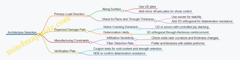
Stacking Strategy That Connects Architecture to Failure Control
A systematic approach is to build the layup from the expected failure mode. If you anticipate mostly in-plane matrix cracking, a UD-dominant stack with carefully chosen ply angles can keep cracks spaced and reduce interlaminar shear. If you anticipate delamination, introduce through-thickness reinforcement early in the stack design rather than treating it as an afterthought.
A concrete example stack logic for a panel:
- Use UD plies aligned with the dominant tensile direction.
- Insert a woven layer where you need in-plane stability across manufacturing tolerances.
- Add 3D orthogonal reinforcement in the regions with the highest thermal gradient and highest interlaminar stress.
Practical Selection Checklist
- If principal loads are directional and you can control fiber alignment, start with UD.
- If you need robust in-plane orientation and handling, add woven layers.
- If delamination is a credible failure mode under thermal cycling, include 3D orthogonal reinforcement in the critical zones.
- Validate with representative coupons that match curvature, thickness, and stacking order, then confirm that void content and residual strength behave consistently across the part.
This is the quiet part of design: architecture selection is less about choosing a “best” weave or layup and more about matching the architecture to the dominant crack and load paths you expect to see.
5.5 Practical Examples of Interphase and Architecture Pairing for Target Failure Modes
The goal of this section is to connect two knobs—interphase design and architecture choice—to one measurable outcome: a specific failure mode that matches the service environment. A practical workflow starts with the failure you want to encourage (or avoid), then selects an interphase that controls crack behavior, and finally chooses an architecture that routes loads and constrains damage growth.
Foundational Mapping from Failure Mode to Design Knobs
- Matrix cracking that stays contained: You want many small cracks, not one runaway fracture. Use an interphase that allows controlled debonding and frictional sliding, and an architecture that redistributes load away from the crack plane.
- Delamination resistance under bending and thermal gradients: You want to slow interlaminar crack growth. Use an interphase that does not create an overly weak interface, and an architecture that increases through-thickness load transfer.
- Oxidation-driven interface weakening: You want the interface to retain enough integrity after exposure so the composite does not lose its damage tolerance. Use an oxidation-stable interphase chemistry and a fiber architecture that limits oxygen access paths.
A useful mental model is: interphase sets the crack tip rules, while architecture sets the damage traffic lanes.
Mind Map: Interphase and Architecture Pairing Logic
Example 1: Contained Matrix Cracking for Leading-Edge Panels
Target: Under repeated thermal cycling, encourage distributed matrix cracking while keeping fibers largely intact.
Interphase choice: A thin, engineered interphase that promotes debonding at the fiber/matrix boundary but still provides frictional resistance during sliding. In practice, the interphase thickness is tuned so that debonding occurs without turning the interface into a near-frictionless hinge.
Architecture choice: A quasi-isotropic laminate with multiple in-plane orientations. When a crack forms in one ply, neighboring plies with different fiber directions change the local stress state and encourage crack deflection rather than straight-through fracture.
Easy-to-understand check: After thermal cycling, examine fracture surfaces. If you see many short crack segments with fiber bridging and limited through-thickness separation, the pairing is doing its job. If you see long, continuous matrix cracks aligned across plies, the interphase is likely too weak or the laminate stacking is too uniform in orientation.
Example 2: Delamination Resistance for Bending Loads with Thermal Gradients
Target: Prevent interlaminar crack growth when the panel experiences bending plus temperature gradients.
Interphase choice: Slightly higher interfacial shear strength than in Example 1. The intent is not to eliminate debonding entirely, but to avoid an interface that allows easy separation under shear.
Architecture choice: A stitched or 3D orthogonal architecture that adds through-thickness reinforcement. Think of it as adding “vertical rebar” so an interlaminar crack has to fight more than just the matrix.
Easy-to-understand check: During flexure testing at elevated temperature, monitor stiffness retention and post-test damage maps. A good pairing shows slower stiffness loss and delamination areas that remain patchy rather than spreading in a single dominant plane.
Example 3: Oxidation-Driven Interface Weakening Under Water Vapor Exposure
Target: Maintain damage tolerance after environmental exposure where oxidation can degrade the interphase and alter frictional behavior.
Interphase choice: An oxidation-stable interphase chemistry that resists conversion into brittle phases. The practical aim is to keep the interface from becoming either too brittle (promoting sudden separation) or too degraded (leading to loss of frictional sliding).
Architecture choice: Place denser, more protective material regions toward the hot face and use architectures that limit continuous oxygen ingress paths. For instance, a surface-near region with reduced through-thickness porosity helps slow the transport of reactive species.
Easy-to-understand check: Compare pre- and post-exposure interfacial fracture behavior. If the composite transitions from gradual, friction-assisted crack growth to abrupt separation, the interphase is not surviving the environment well enough for the intended failure mode.
Case Study: Choosing Between Two Pairings for the Same Panel
Scenario: A hypersonic panel must survive thermal cycling and bending. You can either prioritize contained matrix cracking or delamination suppression.
- Pairing A: Debond-friendly interphase + quasi-isotropic laminate.
- Best when the dominant risk is matrix cracking that must stay distributed.
- Pairing B: Shear-supporting interphase + through-thickness reinforced architecture.
- Best when the dominant risk is interlaminar separation under combined loading.
Decision rule: If inspection after representative tests shows delamination planes dominating the damage area, switch toward Pairing B. If fiber integrity is maintained and damage is mostly in-plane cracking, Pairing A is likely closer to the target.
Practical Mind Map: Test-Driven Refinement

These examples show the same principle in different clothes: interphase and architecture must be selected as a pair, because each one controls a different part of the crack and damage story. When the observed failure mode matches the intended one, the composite behaves less like a collection of brittle parts and more like a controlled damage system.
6. Microstructure Characterization and Property Correlation
6.1 Scanning and Transmission Electron Microscopy for Interface Analysis
Interface analysis in ceramic matrix composites is mostly about answering one question: what exactly is happening at the boundary between fiber, interphase, and matrix? Scanning electron microscopy (SEM) helps you see the interface in context and at useful magnifications, while transmission electron microscopy (TEM) lets you inspect the interface at the scale where bonding, reaction layers, and fine cracks actually live. A good workflow uses both, because each technique compensates for the other’s blind spots.
Foundational Concepts for Interface Imaging
SEM images surface and near-surface features by detecting signals generated when an electron beam interacts with the specimen. For interface work, the practical goal is to locate the interface reliably and preserve it during preparation. TEM images thin regions by transmitting electrons through a specimen slice, which means you must prepare electron-transparent foils without smearing or altering the interface.
A simple way to keep expectations aligned is to treat SEM as “where” and TEM as “what.” SEM tells you where the interface is, where gaps or reaction products appear, and how damage is distributed. TEM tells you what those features are made of and how they are arranged at the atomic-to-nanometer scale.
Sample Preparation That Does Not Lie
Interface artifacts are the most common reason microscopy results become unhelpful. For SEM, polishing and etching can change the apparent interphase thickness or pull out phases. For TEM, ion milling can heat the specimen, induce amorphization, or preferentially remove softer reaction layers.
Best-practice approach:
- Use the same region for both SEM and TEM by marking the specimen and tracking it through preparation.
- For SEM, choose polishing steps that minimize smearing and avoid aggressive etchants; verify with low-magnification scans before high-magnification imaging.
- For TEM, aim for minimal beam damage by using low-dose imaging and short acquisition times, and keep milling parameters conservative.
Example: If you see a “thick interphase” in SEM but TEM shows a much thinner reaction layer, the mismatch often traces back to polishing-induced smearing or etch selectivity rather than true microstructural differences.
SEM Workflow for Interface Mapping
Start with low magnification to find the fiber, then move to higher magnification to inspect the boundary. Use multiple imaging modes when available:
- Secondary electron imaging for topography and edge definition.
- Backscattered electron imaging for compositional contrast between matrix and reaction products.
- Energy-dispersive X-ray spectroscopy (EDS) for elemental maps across the interface.
A systematic SEM interface routine:
- Confirm fiber orientation and locate the interface along a straight, uninterrupted segment.
- Acquire an overview image, then zoom into the interface with consistent working distance and detector settings.
- Collect EDS line scans across the boundary to detect gradients rather than relying on single-point spectra.
- Compare interface features across multiple locations to avoid over-interpreting one “good” spot.
Example: A gradual change in EDS signal across the boundary suggests a reaction zone, while a sharp step suggests limited interdiffusion and a more stable interphase.
TEM Workflow for Interface Structure and Chemistry
TEM requires thin foils, typically prepared by focused ion beam (FIB) milling or mechanical thinning followed by thinning. Once you have an electron-transparent region, you can use:
- Bright-field and dark-field imaging to reveal contrast from thickness and microstructure.
- Selected area diffraction to identify crystalline phases.
- High-resolution TEM to visualize lattice fringes when resolution and sample quality allow.
- Scanning TEM (STEM) with EDS or electron energy loss spectroscopy (EELS) for compositional mapping.
A practical TEM strategy is to first identify the interface region in a STEM overview, then switch to higher-resolution imaging only after you confirm the correct boundary is in view.
Example: If STEM-EDS shows a localized enrichment of an interphase-forming element at the boundary, EELS can be used to distinguish whether it is present as an oxide, silicate, or carbide-like environment, depending on the system and available spectral edges.
Mind Map: Interface Analysis Workflow
Integrated Example from Observation to Mechanism
Consider a composite where SEM shows a narrow dark band at the fiber–matrix boundary after thermal exposure. EDS line scans across the band reveal a compositional gradient rather than a sharp step. TEM then confirms that the band corresponds to a nanometer-scale reaction layer with mixed phases and occasional voids at the outer edge. The voids align with crack paths seen in SEM, explaining why the interface shows improved crack deflection but reduced load transfer.
The key point is the logic chain: SEM identifies the feature and its spatial context, EDS suggests a gradient, and TEM confirms the phase structure and nanoscale morphology. When all three agree, the interface story becomes specific enough to guide interphase design decisions.
Common Pitfalls and How to Avoid Them
- Mistaking preparation damage for service damage: compare multiple locations and look for systematic patterns consistent with the exposure history.
- Over-relying on single-point EDS: gradients matter; line scans and maps reduce misinterpretation.
- Treating SEM thickness contrast as chemistry: SEM contrast can be influenced by topography and atomic number; confirm with EDS.
- Assuming TEM images are representative: thin foils can preferentially sample certain regions; validate with SEM context.
Practical Checklist for Interface Microscopy
- Plan the workflow so SEM locates and TEM confirms.
- Preserve the interface during preparation and verify before high-magnification work.
- Use gradients and maps, not just point measurements.
- Cross-check features across at least two interface locations.
- Record imaging conditions so comparisons remain meaningful.
6.2 X Ray Diffraction and Spectroscopy for Phase and Composition Verification
Phase and composition verification is where “it should be that phase” becomes “it is that phase.” For ceramic matrix composites, this matters because small chemistry shifts can change oxidation behavior, thermal conductivity, and even how cracks propagate. The goal is to connect diffraction and spectroscopy signals to specific phases, quantify composition where possible, and confirm that processing produced the intended microstructure.
Foundational Concepts for Interpreting Signals
X ray diffraction (XRD) measures how a crystal lattice scatters X rays. Each phase has a characteristic set of peak positions determined by lattice spacing, so peak location is the primary phase identifier. Peak intensity and shape carry additional information: preferred orientation, crystallite size, microstrain, and the presence of amorphous or poorly crystalline material.
Spectroscopy in this context typically means energy dispersive X ray spectroscopy (EDS) and sometimes X ray photoelectron spectroscopy (XPS) or Raman. EDS is fast and spatially localized, making it useful for checking elemental ratios and detecting secondary phases at interfaces. XPS is surface sensitive and helps distinguish chemical states, which is important when oxidation products form on the surface. Raman can identify certain bonding environments and some crystalline phases, but it is not a replacement for XRD when crystallography is the key question.
A practical rule: use XRD to identify and quantify crystalline phases, then use spectroscopy to confirm elemental distribution and chemical state at surfaces and interfaces.
Workflow from Sample Preparation to Phase Calls
Start with sample preparation that avoids misleading artifacts. Grinding can introduce strain and contamination, shifting peak widths and sometimes peak positions slightly. Use consistent grinding time and particle size across samples intended for comparison. If the composite contains fibers, be aware that fiber peaks can overlap with matrix peaks; plan the analysis region accordingly.
Next, choose the XRD geometry. For powders or crushed matrix, standard Bragg Brentano geometry often works. For thin coatings or surface layers, grazing incidence XRD can improve sensitivity to near-surface phases. For composites, collecting from multiple regions helps separate matrix signals from fiber contributions.
Then perform peak identification using a reference database and a fitting strategy. Peak fitting should include background modeling and account for instrumental broadening. If the material contains amorphous content, treat it explicitly rather than forcing the fit to explain everything with crystalline peaks.
Finally, validate the phase call by checking whether the implied chemistry is consistent with spectroscopy results. If XRD says “silica-rich” but EDS shows a different Si to O ratio trend, you likely have either overlapping peaks, an incorrect background, or a sampling mismatch.
X Ray Diffraction Details That Matter in CMCs
Peak Positions and Lattice Parameters
Peak positions determine which phase is present. For example, polymorphs of alumina differ in lattice spacing, so their peaks separate cleanly when data quality is sufficient. If peaks are shifted relative to references, consider residual stress and systematic errors from sample displacement or calibration.
Peak Broadening and Crystallite Size
Peak width often reflects crystallite size and microstrain. In processing, incomplete densification or rapid thermal cycles can produce smaller crystallites and higher microstrain. Use a consistent line profile model so that “narrower after processing” means something measurable.
Quantification and Limits
Quantifying phase fractions from XRD requires assumptions about absorption, preferred orientation, and reference intensities. In composites, preferred orientation can be strong if the matrix has texture. If texture is present, use methods that incorporate orientation effects or report semi-quantitatively with clear uncertainty.
Spectroscopy Details for Composition and Chemical State
EDS for Elemental Ratios and Secondary Phases
EDS helps confirm whether a secondary phase is truly present or just a peak overlap. For instance, if XRD indicates a minor spinel-like phase, EDS can check whether the cation ratios match the expected stoichiometry. Use multiple points across the region because segregation can be localized.
XPS for Oxidation States on Surfaces
When oxidation products form, the same element can appear in different chemical states. XPS can distinguish, for example, oxide versus non-oxide bonding environments. This is especially useful when the surface layer is thin and XRD sees mostly the underlying bulk.
Raman as a Complementary Check
Raman can confirm certain bonding motifs and some crystalline phases. It is most useful when XRD is ambiguous due to overlap or when the material includes phases that produce distinctive Raman signatures.
Mind Map: Integrated Verification
Example: Verifying a Matrix After Heat Treatment
Suppose a matrix is processed to form a target crystalline phase and then heat treated for thermal stability. XRD shows the expected main peaks, but one additional weak peak appears. A quick EDS survey across the matrix region finds a small enrichment of a cation consistent with the suspected secondary phase. To confirm chemical state, XPS on the surface indicates an oxide form of that cation, matching the idea that the secondary phase is tied to surface or near-surface reactions rather than bulk transformation.
The verification outcome is not just “extra peak exists.” It becomes: the bulk contains the intended phase, the heat treatment introduced a minor secondary phase localized near surfaces, and the chemistry aligns with oxidation-driven formation.
Practical Quality Checks to Avoid False Confidence
Use replicate measurements from different regions to reduce sampling bias. Confirm instrument calibration before comparing peak positions across batches. When fitting peaks, report uncertainty and avoid forcing the model to explain amorphous contributions with crystalline peaks. If XRD and spectroscopy disagree, treat it as a diagnostic signal: it usually points to overlap, texture, background selection, or region mismatch rather than a mysterious material.
In short, XRD provides the crystallographic identity, spectroscopy provides the chemical story, and the combined interpretation turns processing intent into verified material reality.
6.3 Porosity Measurement and Its Impact on Thermal Conductivity and Strength
Porosity in ceramic matrix composites is not just “empty space.” It changes how heat flows, how stresses concentrate, and how cracks choose their path. Measuring it well means linking three things: what the pores look like, how much there is, and where they sit relative to fibers and interfaces.
What Porosity Does to Heat Flow and Load Bearing
Thermal conductivity drops when pores interrupt the solid conduction network. The effect depends on pore shape and connectivity: isolated spherical pores scatter heat less than interconnected pores that create low-conductivity pathways. Strength also suffers because pores act as stress concentrators and provide initiation sites for matrix cracking. In composites, the story is more specific: pores near fiber surfaces can weaken the local load transfer and promote early debonding, while pores in the matrix away from fibers mainly reduce matrix stiffness and increase crack growth driving force.
A practical way to keep the reasoning straight is to treat porosity as two coupled variables: (1) volume fraction and (2) spatial distribution. Two specimens with the same porosity fraction can show different strength if one has pores clustered near interfaces.
Measurement Targets and Sampling Strategy
Start with clear targets before choosing a method. For thermal conductivity correlation, you typically need bulk porosity fraction and whether pores are open to the surface. For strength correlation, you need pore size distribution and proximity to fiber-rich regions.
Sampling matters because porosity is rarely uniform. A good baseline approach is to measure multiple locations across the panel or coupon, then report mean and spread. If you only measure the “best-looking” region, your correlation will be optimistic and your design decisions will be too.
Mind Map: Porosity Measurement Workflow
Density-Based Porosity from Mass and Volume
The simplest measurement is bulk density. Measure mass, measure geometric volume, and compare to a theoretical density of the fully dense composite. The resulting porosity fraction is useful for quick screening and for checking whether more detailed imaging is consistent.
Easy-to-understand example: if a coupon’s measured density is 2.70 g/cm³ and the theoretical dense density is 3.00 g/cm³, then porosity fraction is
- Porosity fraction ≈ (1 − 2.70/3.00) = 0.10, or 10%.
This method cannot tell you pore size distribution or whether pores are near interfaces, so it should be paired with imaging when strength correlation is the goal.
Image-Based Porosity Using Polished Sections
2D image analysis is practical and fast. After consistent polishing, pores appear as dark or bright regions depending on contrast. You then segment pores using calibrated thresholds and compute area fraction, equivalent diameter, and shape descriptors.
Key best practice: use the same imaging and thresholding workflow across all specimens in a comparison set. If thresholds drift, your “porosity fraction” becomes a measurement artifact.
Limitations are real: 2D area fraction is not identical to 3D volume fraction, especially for elongated pores. Still, 2D is excellent for relative comparisons and for identifying whether pores cluster in certain regions.
3D Tomography for Spatial Distribution
X-ray computed tomography (or similar 3D methods) provides pore connectivity and proximity to fibers. For strength, this is where the correlation often improves: pores that are close to fiber surfaces or form connected networks can dominate crack initiation.
Easy-to-understand example: imagine two samples both at 8% porosity by density. In Sample A, pores are mostly isolated in the matrix interior. In Sample B, pores form a connected network that runs along fiber-rich paths. Sample B typically shows lower strength because cracks can propagate through a weakened, low-stiffness route.
Open vs Closed Porosity and Its Role in Thermal Conductivity
Open pores can allow moisture or reaction products to enter, changing effective thermal behavior and sometimes the mechanical response. Even when the composite is tested dry, open porosity can still reduce conductivity more strongly because it disrupts conduction paths and may increase radiative contributions at higher temperatures.
A practical measurement pairing is to combine density-based porosity with a method that distinguishes open pores, such as controlled infiltration or surface-focused inspection. Report both: total porosity and open fraction.
Correlating Porosity Metrics to Strength Without Hand-Waving
Strength correlation improves when you move beyond a single “porosity percent” number. A systematic approach is:
- Use density to confirm overall porosity level.
- Use 2D imaging to get pore size distribution.
- Use 3D data when available to quantify pore proximity to fibers and connectivity.
- Correlate strength with the pore population that is most relevant to the failure mode observed in testing.
Mind Map: Strength Correlation Logic
Practical Reporting That Makes Measurements Usable
When you report porosity, include: measurement method, sampling locations, sectioning plane (for 2D), segmentation approach (thresholding consistency), and uncertainty or repeatability. Also report both total porosity and the pore characteristics most relevant to the property you’re correlating.
A good rule of thumb: if your report only contains one number, it will be hard to explain why the strength changed. If it contains pore fraction plus size and spatial distribution, the “why” becomes measurable rather than guessed.
6.4 Mechanical Testing Methods Including Flexure Tension and Compression
Mechanical testing for ceramic matrix composites (CMCs) has one job: translate a messy, real microstructure into repeatable numbers you can design with. The trick is choosing a test geometry and loading path that makes the dominant damage mechanisms show up early and clearly—without accidentally measuring the wrong thing.
Foundational Principles for Test Selection
Start with the loading mode that matches service. Flexure is useful when thermal gradients and panel bending create tension on one surface and compression on the other. Tension is the cleanest way to study matrix cracking, fiber bridging, and interphase debonding because the stress state is mostly uniaxial. Compression is essential because CMCs often behave differently in compression due to fiber kinking, frictional effects, and contact conditions.
A second principle is controlling strain rate and temperature. Even at room temperature, CMCs can show rate sensitivity through frictional sliding at interfaces. At elevated temperature, matrix softening and oxidation products can change crack growth resistance. So the test report should always include temperature, hold time, and the method used to control loading rate.
Flexure Testing for Bending Response
Flexure tests are typically run on bar specimens with a controlled span. The simplest interpretation uses beam theory to convert applied load into surface tensile and compressive stresses. For CMCs, that conversion is only the starting point: once cracking begins, the effective stiffness drops, and the load–deflection curve becomes the story.
Key outputs include initial stiffness, first-crack load, peak load, and post-crack load retention. A practical best practice is to record load and deflection at high sampling rate and to mark the deflection at which the first visible crack forms during interrupted testing. For example, if a 3-point bend bar shows a sudden stiffness drop at 1.2 kN and then sustains load while deflection increases, that plateau is consistent with matrix cracking plus fiber bridging rather than catastrophic failure.
To avoid misleading results, ensure consistent specimen surface finish and alignment. Misalignment can introduce shear and twist, which can shift the apparent crack location. A quick check is to compare crack initiation location across multiple specimens; if it wanders widely, the setup is likely the culprit.
Tension Testing for Damage Initiation and Growth
Tension tests for CMCs require grips that do not crush fibers or induce bending. Dog-bone geometries reduce stress concentrations, but gripping remains the main challenge. A common best practice is to use tabs or compliant grip inserts so the load transfers gradually into the gauge section.
Interpretation focuses on the transition from linear response to nonlinearity. In many CMCs, the first deviation corresponds to matrix cracking. Later, the curve may show a rising or plateau region as fibers bridge cracks and the interphase governs debonding. For an easy example, if a unidirectional CMC specimen reaches a modest peak stress and then continues to carry load with increasing strain, the post-peak behavior indicates stable crack growth rather than immediate fiber fracture.
Because CMCs can fail abruptly once fiber fracture dominates, strain measurement matters. Use extensometers or digital image correlation on the gauge length, not on the grip region. If the measured strain jumps while the load is still rising, that usually signals slip at the grips.
Compression Testing for Contact and Kinking Effects
Compression tests are sensitive to end conditions. Friction between specimen ends and platens can create barreling and nonuniform stress. To reduce this, use lubrication or compliant interlayers and verify that failure initiates in the gauge region rather than at the ends.
The stress–strain curve in compression often shows a different nonlinearity than tension. Fiber kinking and matrix crushing can contribute, especially in architectures with strong fiber alignment. A practical example: if a specimen exhibits a gradual stiffness decrease followed by a sudden drop after a localized shear band forms, the failure mode is likely dominated by shear localization rather than uniform matrix cracking.
Report the method used to correct for machine compliance and end effects. If two labs use different end conditions, their “compressive strength” may not be directly comparable even when the material is the same.
Advanced Details That Make Results Comparable
Across flexure, tension, and compression, three practices improve comparability.
- Standardize specimen preparation: consistent cutting, polishing, and cleaning reduce variability in surface flaws that can trigger early cracking.
- Control environment: include oxygen exposure conditions when testing at elevated temperature, since oxidation can change crack growth resistance.
- Use consistent failure definitions: define failure as first crack, peak load, 50 percent load drop, or complete fracture, and apply the same rule to every specimen set.
Mind Map: Mechanical Testing Workflow
Example: Choosing the Right Test for a Given Question
If the design question is “How does the interphase control crack bridging under bending loads?”, flexure is the most direct because it naturally creates tension and compression on opposite faces. If the question is “At what stress does matrix cracking initiate and how stable is crack growth?”, tension provides the clearest stress state. If the question is “Will the material survive compressive thermal stresses without localized shear failure?”, compression testing with controlled end conditions is the appropriate choice.
The point is not to test everything. It is to match the test mode to the dominant damage mechanism you want to observe, then standardize the details that otherwise turn material behavior into setup behavior.
6.5 Correlating Microstructural Metrics to Damage Evolution and Residual Strength
A good correlation starts with a simple rule: measure microstructure in a way that maps to how damage actually grows. For ceramic matrix composites (CMCs), the damage path is typically a sequence—matrix cracking, fiber/matrix debonding, fiber bridging and pullout, and finally stiffness and strength loss. Microstructural metrics should therefore be chosen to represent (1) where cracks form, (2) how they propagate, and (3) how load transfer degrades.
Define the Damage Variables Before Measuring
Residual strength is not one thing; it is the remaining ability to carry load after a specific damage history. Start by defining the damage state using three measurable variables:
- Crack population: crack density, crack spacing, and crack opening distribution.
- Interface condition: debonded length fraction, interphase thickness integrity, and oxidation-related interface changes.
- Load-bearing continuity: fiber bridging effectiveness and effective fiber volume fraction.
Example: In a flexure test after thermal cycling, you can section the specimen at the same distance from the tensile surface for every sample. Then quantify crack density in that region and compare it to residual flexural strength. If you instead measure cracks at random locations, the correlation will look “noisy” for reasons that are purely logistical.
Choose Microstructural Metrics That Track Mechanisms
Use metrics that correspond to the dominant mechanism under your loading and environment.
-
Matrix cracking metrics
- Crack density per unit length or area.
- Crack length distribution and orientation relative to fiber direction.
- Matrix porosity near crack planes.
-
Interface and interphase metrics
- Debonded area fraction from microscopy.
- Interphase thickness and continuity.
- Interphase degradation indicators such as reaction layer thickness.
-
Fiber bridging and pullout metrics
- Bridging length distribution.
- Fiber pullout length after fracture.
- Fiber fracture fraction versus pullout fraction.
Example: If residual strength drops sharply while crack density increases only modestly, the interface may be degrading faster than cracking. In that case, debonded area fraction and reaction layer thickness will correlate better than crack density alone.
Build a Mechanism-Linked Correlation Model
A practical approach is to use a two-stage model: microstructure-to-damage-state, then damage-state-to-strength.
-
Microstructure → Damage state
- Convert crack density and interface condition into a damage index, such as a weighted sum.
- Weights should be assigned based on which mechanism controls load transfer in your architecture.
-
Damage state → Residual strength
- Fit residual strength as a function of the damage index using a monotonic form.
- Validate that the model preserves known trends: more cracking and worse interface should not increase strength.
Example: For a unidirectional CMC under tension-dominated loading, a damage index that emphasizes interface condition often predicts residual strength better than one that emphasizes porosity alone.
Use Consistent Sampling and Measurement Windows
Correlation fails when the measurement window does not match the fracture process zone.
- Match the section location to the stress gradient region.
- Use the same magnification and field-of-view strategy across specimens.
- Record the thermal history and environment exposure for each sample.
Example: If you quantify porosity globally but cracks localize near the tensile surface, the porosity metric will dilute the relationship. Instead, quantify porosity in the same region where crack density is measured.
Validate with Residual Strength and Fracture Morphology
After building the correlation, check it against independent evidence.
- Compare predicted strength ranking with observed fracture mode shifts.
- Confirm that specimens with higher damage index show more pullout-dominated fracture or reduced bridging.
- Ensure the correlation holds across at least two loading conditions (e.g., different hold times or different thermal cycling severities).
Example: If two specimens have similar crack density but different residual strength, inspect fracture surfaces. The one with lower strength should show reduced bridging length or higher fiber fracture fraction, depending on the failure mode.
Mind Map: Microstructural Metrics to Damage Evolution
Worked Example with a Simple Damage Index
Suppose you have three specimens after thermal cycling. You measure:
- crack density: 12, 18, 25 cracks/mm
- debonded area fraction: 0.10, 0.18, 0.30
- average bridging length: 0.45, 0.30, 0.20 mm
A straightforward damage index can be constructed as:
- higher crack density increases damage
- higher debonded fraction increases damage
- shorter bridging increases damage
Then residual strength should decrease as the index increases. If the specimen with the largest crack density does not have the lowest bridging length, revisit the sampling window and confirm that crack quantification and bridging quantification refer to the same region of the fracture process zone.
When the correlation is done carefully, it becomes useful rather than just pretty: it tells you which microstructural lever is actually responsible for strength loss under your specific loading and environment.
7. Thermal Conductivity and Thermomechanical Behavior
7.1 Heat Transfer Modeling Inputs Including Conductivity and Radiative Effects
Heat transfer modeling for ceramic matrix composites (CMCs) starts with a simple question: what carries energy away from the hot surface, and how does that energy move through the material and across interfaces? For hypersonic thermal protection, you typically combine conduction inside the panel with radiation and, at the surface, absorption and emission that depend on temperature and surface state.
Core Modeling Assumptions That Drive Input Choices
Most practical models assume a temperature field T(x,y,z) and compute heat flux q from gradients and radiation terms. You must decide whether the problem is steady or transient, whether material properties are constant or temperature-dependent, and whether the surface is treated as gray or wavelength-dependent. A good baseline is a transient conduction model with temperature-dependent conductivity k(T), density ρ, and specific heat cp(T), coupled to a surface radiation boundary condition.
A quick sanity check: if your predicted surface temperature is extremely sensitive to k(T) but not to cp(T), you likely need better conductivity data. If it swings with cp(T), you need better thermal mass characterization.
Thermal Conductivity Inputs Including Temperature Dependence
Thermal conductivity in CMCs is not a single number. It depends on porosity, fiber volume fraction, fiber orientation, matrix phase, and microcrack or interphase effects. For modeling, you usually provide k(T) as either:
- A scalar effective conductivity for a homogenized material.
- Directional conductivities kx(T), ky(T), kz(T) for orthotropic laminates.
- A layered approach where each ply or region has its own effective k(T).
A concrete example: suppose you have a unidirectional CMC leading-edge panel. Through-thickness conduction controls how quickly the back face heats up, so kz(T) matters more than kx(T). If you only measure in-plane conductivity and reuse it as through-thickness k, you can overpredict heat spreading and underpredict back-face temperature.
To build k(T), use measured conductivity across the relevant temperature range. If you only have discrete points, interpolate smoothly and keep the derivative reasonable; abrupt changes can create artificial thermal gradients in the solver.
Radiative Effects Inputs Including Emissivity and Surface State
Radiation is often the dominant heat transfer mechanism at high surface temperatures, especially when the gas-side convective contribution is moderate or when the surface is relatively transparent to radiation. In a gray-body approximation, the net radiative heat flux at the surface can be written in terms of emissivity ε(T) and the surrounding radiation temperature Tr.
Key inputs:
- Emissivity ε(T): depends on surface roughness, oxidation layer thickness, and whether the surface is fresh or conditioned.
- Radiation temperature Tr: represents the effective environment seen by the surface.
- View factors or geometry: for panels, you may approximate the surroundings as a large enclosure (view factor near 1) or include shielding.
Example: if oxidation increases emissivity from 0.6 to 0.85, the radiative loss term increases strongly because it scales with temperature to the fourth power. In practice, you should couple emissivity to the surface condition used in your thermal exposure scenario, not to a generic handbook value.
Coupling Conduction and Radiation Through Boundary Conditions
In transient conduction, the governing equation uses k(T), ρ(T), and cp(T). The surface boundary condition combines absorbed external radiation, emitted radiation, and any convective heat flux.
A common gray-surface boundary condition structure is:
- Incoming terms: absorbed radiation from the environment and any external heat flux.
- Outgoing terms: emitted radiation based on ε(T) and surface temperature, plus convection if included.
To avoid double-counting, be explicit about what the external heat input represents. If your external solver already provides a net heat flux including radiation, you should not add a second radiation term in the same boundary condition.
Practical Input Workflow from Data to Solver
- Define geometry and coordinate directions aligned with laminate architecture.
- Choose a property model: isotropic effective or orthotropic directional.
- Assemble k(T), ρ(T), and cp(T) for each region or ply.
- Define surface emissivity ε(T) and absorption/reflectance assumptions consistent with the boundary condition.
- Set radiation environment Tr and view factor assumptions.
- Run a baseline case and check energy balance at the surface.
Energy balance check example: integrate the computed heat flux over the surface area and compare it to the rate of change of thermal energy stored in the domain. If the mismatch is large, the issue is usually boundary condition sign conventions or inconsistent property units.
Mind Map: Heat Transfer Modeling Inputs
Example: Building a Minimal Yet Defensible Input Set
Imagine a panel modeled as orthotropic through-thickness conduction with radiation at the hot face. You measure kz(T) from room temperature to the maximum service temperature, and you use cp(T) from differential scanning calorimetry or high-temperature calorimetry. For radiation, you assign ε(T) based on oxidized surface coupons at representative exposure conditions, and you set Tr from the thermal environment model you are using.
Then you run two cases: one with constant emissivity ε=0.7 and one with ε(T) increasing with temperature. If the back-face temperature changes noticeably, you have learned that emissivity modeling is not optional. If it barely moves, conductivity and thermal mass dominate, and you should spend effort there.
The goal is not to make the model complicated; it is to make the inputs match the physics that actually controls the temperature field.
7.2 Thermal Expansion Mismatch and Residual Stress Development
Thermal expansion mismatch is what happens when two materials want to change size by different amounts as temperature rises or falls. In ceramic matrix composites (CMCs), the mismatch is rarely between just two phases; it’s a whole cast: fibers, matrix, interphase, pores, and sometimes coatings. Residual stresses are the “leftover” stresses that remain after cooling from a processing temperature or after a thermal cycle, because the composite cannot freely expand or contract.
Core Concepts That Drive Residual Stress
Start with the simplest picture: a fiber embedded in a matrix. If the fiber’s coefficient of thermal expansion (CTE) differs from the matrix CTE, then a temperature change ΔT produces a strain difference Δε ≈ (α_matrix − α_fiber)ΔT. If the phases were free, each would follow its own strain. Inside a bonded composite, compatibility forces internal stresses to develop so that the overall deformation matches the constraints.
In CMCs, the stress state is also shaped by stiffness contrast. A stiffer phase attracts more load, so even a modest CTE difference can matter if the modulus ratio is large. Temperature dependence adds another layer: α and modulus both change with temperature, so the stress “budget” accumulates unevenly through the thermal history.
From Mismatch to Stress: A Stepwise Mechanism
-
During heating or cooling, mismatch strain is generated. The sign depends on which phase has the larger CTE. If the matrix expands more than the fiber on heating, the fiber tends to be put into tension relative to the matrix.
-
Bonding and interphase behavior determine how strain transfers. A strong fiber-matrix bond forces closer strain compatibility, raising interfacial shear and normal stresses. A designed interphase that allows controlled debonding reduces the effective constraint, lowering residual stress but increasing interfacial damage risk.
-
Microcracking and debonding relieve stress. Once local stresses exceed a threshold, the composite can partially “give” by forming matrix cracks or fiber-matrix debonds. Relief is not free: it changes stiffness and can create new stress concentrations around crack faces.
-
Cooling locks in the remaining stress. Even after damage forms, not all mismatch strain is relieved. The final residual stress distribution depends on how much cracking occurred, how pores and interfaces evolved, and how the thermal cycle ended.
Mind Map: Stress Sources and Relief Paths
Practical Example: Cooling After Infiltration and Consolidation
Imagine a CMC coupon consolidated at a high temperature, then cooled to service temperature. Suppose the matrix has a higher CTE than the fiber over the relevant range. During cooling, the matrix contracts more than the fiber wants to. If the interface remains intact, the matrix near the fiber is forced into tension while the fiber experiences compression relative to the matrix.
Now add a realistic twist: the interphase is engineered to allow debonding at moderate interfacial stresses. As cooling proceeds, interfacial stresses rise until debonding initiates. After debonding, the fiber and matrix no longer enforce full strain compatibility, so the residual stress magnitude drops. However, the debonded regions become compliant, which can shift stress to neighboring intact areas, often increasing local stress heterogeneity.
A simple way to connect this to measurements is to compare two coupons: one with a more compliant interphase and one with a more robust interphase. The compliant-interphase coupon typically shows more interfacial damage after cooling and a lower average residual stress, but it may also show greater stiffness reduction due to damage-induced compliance.
Practical Example: Thermal Gradients Across a Panel
Even if average CTE values match, a temperature gradient through thickness can create mismatch locally. Consider a leading-edge panel where the surface cools faster than the interior during a thermal cycle. The cooler surface wants to contract sooner, but it is constrained by the hotter interior. This generates bending-like residual stresses and can drive surface cracking even when bulk mismatch is small.
In design terms, this means you cannot treat residual stress as a single number. The stress field depends on the thermal history and boundary conditions, so coupon tests should mimic the relevant gradient direction and magnitude.
How to Think About Modeling Without Getting Lost
A useful modeling workflow is to map the thermal history into temperature-dependent material properties, then apply compatibility with an interface model that includes debonding or cracking criteria. If you ignore damage relief, you often overpredict residual stress. If you include damage relief but use thresholds that are too high, you underpredict cracking and still overpredict stress. The best practice is to calibrate thresholds using microstructural observations from thermal cycling, then verify that the predicted residual stress trends match the observed damage patterns.
Key Takeaways for Engineering Decisions
Residual stress in CMCs is not just “CTE mismatch.” It’s mismatch plus constraint plus damage relief, all shaped by temperature-dependent properties and thermal gradients. Interphase design and microcracking behavior are the main levers that control how much mismatch strain becomes residual stress versus how much becomes controlled damage.
7.3 Thermal Cycling Response Including Crack Initiation and Stiffness Degradation
Thermal cycling in ceramic matrix composites (CMCs) is less about “one big failure” and more about a sequence of small damage events that gradually change how the material carries load. Each cycle imposes a temperature swing, which creates thermal expansion mismatch between fibers and matrix, then drives stresses that concentrate at interfaces and defects. Over time, those stresses turn microcracks into a network that reduces stiffness and can eventually change failure mode.
Foundational Mechanisms from Mismatch to Microcracks
Start with the mismatch strain: when temperature changes, fibers and matrix expand differently. The mismatch strain is partially relieved by matrix cracking and by controlled fiber–matrix debonding. The key point is that CMCs are designed so that cracking does not immediately destroy load transfer.
A practical way to picture it is a “load-sharing handshake.” Initially, the matrix and fibers share load. As the matrix cracks, fibers take more of the load, but the interface still allows energy dissipation through debonding and frictional sliding. This is why stiffness drops gradually rather than catastrophically.
Crack Initiation Sites and Threshold Behavior
Crack initiation usually occurs at predictable microstructural locations: matrix-rich regions, near fiber ends, around pores, and at fiber–matrix interface imperfections. Porosity matters because it increases local stress concentration and provides pathways for oxidation-assisted weakening.
Threshold behavior is common. Early cycles may produce microcracks that are short and sparse, with stiffness nearly unchanged. After a critical crack density is reached, crack coalescence becomes easier, and stiffness begins to decline more noticeably.
Example: Consider a coupon cycled between 300°C and 900°C with a fixed hold time at the hot end. If the matrix has low toughness, the first cracks appear sooner and stiffness drops earlier. If the interphase promotes controlled debonding, cracks still initiate, but the stiffness reduction is slower because load transfer remains stable.
Stiffness Degradation Pathways
Stiffness degradation is not a single mechanism. It typically includes:
- Matrix cracking growth: more cracks and larger crack spacing changes the effective modulus.
- Interface evolution: debonded areas increase, reducing shear transfer across the interface.
- Residual stress relaxation: repeated cycling can relax stresses, altering the stress state for subsequent cycles.
- Thermal expansion mismatch redistribution: as damage accumulates, the strain distribution shifts toward fibers.
A useful measurement strategy is to track stiffness at consistent temperatures and loading conditions. If you measure at different temperatures, you may confuse thermal softening with damage.
Example: In a flexure test, measure load–displacement at the same test temperature after each cycling block. A steady downward trend in initial slope indicates damage-driven stiffness loss rather than just temperature effects.
Modeling the Response Without Making It Complicated
A practical modeling workflow links thermal strain to damage variables. Use thermal mismatch to estimate driving stress, then map that stress to an evolving crack density or an effective interface shear transfer parameter.
A simple conceptual model:
- Driving stress scales with mismatch strain and elastic mismatch.
- Crack density increases when driving stress exceeds an initiation criterion.
- Stiffness decreases as crack density and debonded area increase.
This approach is often enough to interpret test trends and compare material/process changes.
Experimental Observables and How to Interpret Them
Common observables include stiffness (initial slope), hysteresis in cyclic loading, crack density from microscopy, and changes in ultrasonic velocity. The interpretation should be consistent: if stiffness drops but crack density appears low, then interface degradation or microcrack closure effects may be dominating.
Example: Suppose microscopy shows many short cracks after 50 cycles, but stiffness drops sharply between 50 and 60 cycles. That pattern suggests a transition from isolated cracking to crack coalescence, where a few new connections strongly reduce effective stiffness.
Mind Map of the Thermal Cycling Chain
Mind Map: Thermal Cycling Response in CMCs
Integrated Example Workflow for a Coupon Program
- Cycle coupons in blocks (for instance, 10-cycle increments) with identical temperature profiles.
- After each block, test stiffness at the same temperature and loading setup.
- Section a subset after early cycles and after the first noticeable stiffness drop.
- Compare crack density and interface condition to identify whether the drop is driven by initiation, coalescence, or interface evolution.
Example: If early cycles show sparse cracks but stiffness is stable, the initiation threshold is not yet exceeded. If stiffness then declines rapidly while crack density increases modestly, interface degradation or crack connectivity is likely the dominant cause.
This systematic chain—from mismatch strain to initiation sites, then to damage evolution and stiffness measurement—keeps thermal cycling interpretation grounded in what the material is actually doing.
7.4 High Temperature Elasticity and Nonlinear Response Under Service Loads
Ceramic matrix composites (CMCs) behave elastically only until damage mechanisms start to matter. At hypersonic service temperatures, “elastic” becomes a moving target: stiffness changes with temperature, thermal gradients create residual stresses, and microcracks plus fiber–matrix interactions introduce nonlinear load–displacement behavior. The goal of this section is to connect those effects to what you actually measure and how you use them in design.
Foundations of High Temperature Elasticity
Temperature Dependent Modulus and Strain Definition
At elevated temperature, the elastic modulus (E(T)) typically decreases, and the effective Poisson response can shift as microcracking evolves. For modeling, define strain consistently: total strain is the sum of mechanical strain and thermal strain. A practical workflow is to treat thermal strain as known from coefficients of thermal expansion and treat mechanical strain as governed by a temperature dependent constitutive law.
Easy example: Suppose a panel experiences a uniform temperature rise ΔT. If the fiber and matrix have different α values, the mismatch strain Δα·ΔT drives internal stresses even with no external load. Those stresses can open microcracks early, so the “initial” modulus you measured at room temperature may not represent the stiffness after heating.
Thermal Expansion Mismatch and Residual Stress
During heating and cooling, mismatch between fiber and matrix expansion creates residual stress fields. These stresses can pre-load the composite in tension or compression locally, changing the subsequent response under service loads. In practice, you can observe this as a shift in the apparent linear region when you run a mechanical test at temperature.
Easy example: If the matrix expands more than the fiber on heating, the matrix may go into compression while the fiber carries tension. When you later apply bending, the first increment of load may close existing cracks rather than increase stress linearly.
Nonlinear Response Mechanisms
Microcracking and Progressive Stiffness Loss
Nonlinearity often begins with matrix cracking. As cracks form and grow, the composite’s load transfer changes: stiffness drops, and the stress–strain curve bends. The curve is not random; it reflects a sequence of events such as crack initiation, crack spacing evolution, and eventual fiber-dominated load sharing.
Easy example: In a unidirectional CMC under tension at temperature, you may see an initially near-linear segment, then a gradual reduction in slope. That slope reduction corresponds to increasing crack density in the matrix and more frequent fiber–matrix debonding events.
Fiber–Matrix Interaction and Nonlinear Load Transfer
Even when the matrix cracks, fibers can carry load through frictional and interfacial mechanisms. Debonding and re-bonding are not perfectly reversible, especially under thermal cycling. The result is hysteresis-like behavior in repeated loading and a nonlinear relationship between applied load and global strain.
Easy example: If you unload and reload during a high-temperature test, the second loading path can be steeper or shallower depending on whether cracks are closing or opening and whether interfacial contact is maintained.
Creep-Like Effects and Time Dependence
At high temperature, some systems show time-dependent deformation under sustained stress. Even if you model it as “nonlinear elasticity with time,” the key design implication is that stiffness and strain evolve during holds. For service loads, this means that a static load case is not truly static at the material level.
Easy example: Under a constant bending moment at temperature, the deflection may increase over time. If you ignore time dependence, you may underpredict deflection and overpredict margin against stress concentrations.
Modeling Strategy That Matches Reality
Choose a Constitutive Level That Fits the Data
A useful hierarchy is:
- Temperature-dependent linear elasticity for early-stage response.
- Nonlinear elastic with damage variables for stiffness degradation from cracking.
- Thermo-mechanical constitutive laws that include thermal strain, damage evolution, and time dependence.
The best practice is to align model complexity with what your tests can identify. If you only have monotonic stress–strain curves at temperature, don’t claim you can predict cyclic hysteresis.
Identify Parameters from Targeted Tests
Use tests that isolate mechanisms:
- Isothermal tension or flexure to capture stiffness loss and nonlinear curvature.
- Thermal cycling with minimal mechanical load to capture residual stress effects.
- Hold-time tests at representative stress levels to quantify time dependence.
Easy example: If your flexure test shows strong curvature but your hold-time test shows minimal additional strain, you can treat time dependence as secondary and focus on damage-driven nonlinearity.
Mind Map: High Temperature Elasticity and Nonlinear Response
Integrated Example for Service Load Use
Consider a heated panel segment under bending during a flight segment. First, compute thermal strains from the temperature history and material expansion mismatch to estimate residual stress state. Next, use isothermal flexure data at the service temperature to obtain an effective nonlinear stiffness curve, not a single modulus. Then, if the flight segment includes a meaningful hold, apply the hold-time strain increment to update deflection and stress redistribution.
The practical check is consistency: the model should reproduce the observed curvature in the flexure test and the measured deflection growth during holds. If it does, you can use the same framework to evaluate margins under combined thermal and mechanical loading without pretending the material is perfectly elastic.
7.5 Practical Test Setups for Measuring Temperature Dependent Properties
Temperature-dependent properties for ceramic matrix composites (CMCs) are measured with a simple goal: reproduce the same thermal history and mechanical boundary conditions that the material sees in service, while controlling the measurement uncertainty. The practical challenge is that heating changes everything at once—geometry, contact conditions, thermal gradients, and even what “strain” means when parts expand.
Start with What You Must Know
Before picking hardware, write down the property list and the required temperature points. For CMCs, common targets include elastic modulus, strength, fracture behavior indicators, thermal conductivity, and thermal expansion. A useful baseline set is 25 °C, a mid temperature (often where matrix softening begins), and the maximum test temperature. If you need a full curve, plan smaller steps near transitions rather than evenly spaced points everywhere.
Example: If your design uses modulus for stiffness and thermal strain for stress prediction, you can run a two-step plan: (1) modulus and CTE at discrete temperatures, (2) a reduced set of mechanical tests at the same temperatures to confirm strength retention.
Choose the Temperature Control Strategy
Two approaches dominate: furnace-based uniform heating and localized heating with a controlled gradient.
- Furnace uniform heating: Best for properties that assume the specimen is isothermal. Use when you care about intrinsic temperature dependence.
- Localized heating: Best when service has strong gradients, such as leading-edge regions. Use when you must capture gradient-driven cracking or stiffness changes.
Example: For measuring tensile strength versus temperature, furnace uniform heating is usually the cleanest. For measuring apparent stiffness under a thermal gradient, localized heating with careful gradient measurement is more honest.
Mechanical Test Setups That Survive Heat
A temperature-dependent mechanical test needs three things: stable grips, a reliable strain measurement method, and a way to prevent thermal expansion from masquerading as deformation.
Strain measurement options
- High-temperature extensometer: Direct and simple, but it must survive the temperature and maintain alignment.
- Optical methods: Useful when contact is risky, but require stable optics and careful calibration.
- Crosshead displacement with correction: Works for trends, but you must subtract machine compliance and thermal expansion of the load train.
Practical best practice: Measure machine compliance at each temperature using a dummy specimen or calibration bar. Then subtract it from the raw displacement.
Example: If your load train expands by 0.05 mm between room temperature and 1200 °C, and your specimen elongates by 0.10 mm under load, the corrected specimen elongation is 0.05 mm. Without the correction, your modulus will look artificially low.
Thermal Conductivity and CTE Measurements
Thermal properties often use separate setups from mechanical tests.
- Thermal conductivity: Commonly measured with steady-state or laser flash methods. For CMCs, ensure the specimen surface preparation is consistent because emissivity and contact resistance can bias results.
- CTE: Use dilatometry with a high-temperature sensor and a reference material. The reference must have a known expansion behavior over your temperature range.
Example: If you measure CTE using a dilatometer and the specimen-to-sensor contact loosens at high temperature, the curve will show a sudden slope change. A simple check is to repeat one temperature point after reloading the specimen with the same contact force.
Controlling Thermal Gradients and Timing
Even in a furnace, gradients can appear due to radiation losses and specimen geometry. Control them by:
- Using a specimen geometry that minimizes edge effects.
- Preheating long enough to reach thermal equilibrium.
- Monitoring temperature at more than one location when possible.
Example: If you heat a dog-bone specimen and only measure temperature at the furnace wall, the gauge section may lag by 30–50 °C. That lag can shift the apparent modulus drop to a lower temperature than reality.
Data Reduction That Respects Temperature
Convert raw signals to properties using temperature-specific calibration.
- Modulus: Use stress and corrected strain at each temperature hold.
- Strength: Define strength at a consistent strain rate or hold time. If the test includes a dwell, report the dwell time and the temperature at the moment of peak load.
- CTE: Use the slope of length change versus temperature over a defined interval, not a single point.
Example: If your modulus is computed from the initial slope of the stress–strain curve, ensure the initial slope is taken after thermal equilibrium and after any seating effects in the grips.
Mind Map: Temperature Dependent Property Test Setups
A Concrete End-to-End Example
Suppose you need modulus and strength from 25 °C to 1200 °C.
- Plan temperature points: 25, 600, 900, 1200 °C.
- Use furnace uniform heating: place thermocouples near the gauge section.
- Run compliance calibration: at each temperature, measure machine response with a calibration bar.
- Perform mechanical tests: apply load after thermal equilibrium; record load, displacement, and temperature.
- Correct strain: subtract compliance and thermal expansion of the load train.
- Compute properties: modulus from the corrected initial slope; strength from peak load at the defined rate.
- Sanity check: repeat one intermediate temperature test to confirm the curve shape is reproducible.
This workflow keeps the measurement honest: temperature is verified where it matters, deformation is corrected for the apparatus, and property extraction uses consistent definitions across the entire range.
8. Oxidation Ablation and Environmental Degradation Mechanisms
8.1 Oxidation Pathways for Oxide and Non Oxide Matrix Systems
Oxidation in ceramic matrix composites is not one process; it is a sequence of coupled events: oxygen transport, chemical reaction at interfaces, formation of new phases, and mechanical consequences of growth and mismatch. The pathway you get depends strongly on whether the matrix is already an oxide or is non oxide (often carbide or nitride). A practical way to think about it is: oxide matrices usually start with an “oxide skin” that can thicken or spall, while non oxide matrices must first convert to oxides, then manage the resulting scale.
Mind Map: Oxidation Pathways Overview
Oxide Matrix Systems
Oxide matrices typically form a surface layer quickly because the matrix itself is chemically compatible with oxygen. The useful question is whether that layer becomes protective or becomes a liability.
Protective scale formation. If the surface layer grows slowly and remains adherent, it reduces oxygen flux. A simple example is a dense alumina rich surface: oxygen must diffuse through a tight, low-permeability layer, so the reaction rate drops. In practice, you can see this as a smaller mass gain after an initial transient.
Scale growth and densification. As the scale thickens, diffusion paths lengthen. However, densification can also create tensile stresses at the scale/substrate boundary. Imagine a thin crust forming on a drying puddle: it can hold until stress exceeds adhesion, then it lifts. In CMCs, that lifting can expose fresh material and restart oxidation.
Spallation and reoxidation. Spallation is more likely when thermal expansion mismatch is large or when the scale grows with significant volume change. Once spalled, oxygen reaches the underlying matrix through cracks and gaps, leading to repeated cycles of growth and loss. The result is often a layered surface with alternating reacted and partially reacted regions.
Volatilization of minor constituents. Even in oxide systems, trace elements can form volatile species under high temperature and reactive atmospheres. A small amount of a glass-former impurity can create a low-viscosity phase that migrates and evaporates, leaving behind a porous residue. The oxidation pathway then shifts from diffusion-limited to reaction-limited at new surfaces.
Non Oxide Matrix Systems
Non oxide matrices must first convert to oxides. That conversion can be beneficial if it produces a stable, adherent scale; it can be harmful if the scale is porous, cracked, or volatile.
Initial conversion to oxides. For carbides and nitrides, oxygen reacts to form oxide products and release gaseous species. A concrete example is a carbide matrix exposed to oxygen: the surface reacts to form an oxide layer while carbon-containing byproducts leave the surface. This creates a moving reaction front and a changing microstructure.
Formation of silica or alumina rich layers. Many non oxide systems rely on forming a protective layer such as SiO2 rich glassy silica or Al2O3 rich alumina. The protective value comes from low oxygen permeability and chemical stability. If the layer is continuous, oxygen diffusion slows dramatically. If it is discontinuous, oxygen finds shortcuts through pores and cracks.
Scale cracking and reoxidation. The oxide scale often grows with volume change and stiffness mismatch relative to the underlying matrix. Thermal cycling adds another stress source because the scale and substrate expand differently. Cracks in the scale act like highways for oxygen, so the pathway becomes: crack formation → oxygen ingress → fresh conversion → new oxide growth. You can observe this as increasing surface roughness and a non-linear mass change over time.
Ongoing recession and mass change. When the protective layer cannot fully seal the surface, material loss continues. Recession rate depends on how quickly the oxide forms, how well it adheres, and whether any reaction products are volatile. A helpful lab-style check is to compare mass change with thickness change: if mass drops while thickness drops, volatilization is likely contributing.
Integrated Controls and Easy Checks
Across both matrix types, the oxidation pathway is governed by transport and by how the composite manages cracks.
- Porosity and permeability: Higher connected porosity increases oxygen flux. A quick example is comparing a “leaky” coupon with a well-consolidated one: the leaky coupon shows faster scale growth because oxygen can penetrate rather than just react at the surface.
- Fiber matrix interfaces and interphases: Interfaces can either slow oxygen ingress or provide fast paths. If an interphase promotes crack deflection and reduces direct contact between oxygen and reactive matrix, oxidation slows even when cracks exist.
- Surface roughness and edges: Edges concentrate oxygen because they expose more area and disrupt scale continuity. A practical example is that a machined edge often oxidizes faster than a polished face under the same conditions.
Example: Interpreting Mass Change and Surface Morphology
Suppose two coupons are exposed under identical conditions. Coupon A shows a small initial mass gain followed by near-plateau behavior and a relatively smooth surface. Coupon B shows continuous mass gain with a rough, layered surface and visible spallation marks. Coupon A likely follows a diffusion-limited pathway with an adherent scale, while Coupon B likely follows a repeated growth–crack–reoxidation pathway where oxygen keeps reaching fresh material.
In both cases, the “pathway” is the story of oxygen movement and where reactions keep happening. Once you can map that story to what you measure—mass change, scale thickness, and surface morphology—you can explain oxidation behavior without guessing.
8.2 Water Vapor and Reactive Gas Effects on Surface and Subsurface Layers
Water vapor and reactive gases shape ceramic matrix composite (CMC) performance in two coupled ways: they change what happens at the surface (scale growth, recession, and bond-line chemistry), and they modify the near-surface microstructure (porosity evolution, phase transformations, and interphase stability). In practice, you can think of the system as three zones: the gas-exposed surface, a reaction-affected subsurface layer, and the bulk material that mostly “feels” the consequences through property loss.
Foundational Mechanisms at the Surface
Water Vapor Transport and Condensation
Water vapor reaches the surface by convection and diffusion through the boundary layer. Whether it reacts immediately or condenses depends on the local temperature and partial pressure. A useful engineering habit is to map the surface temperature distribution first, then compare it to the water stability window for your matrix and any protective scale you expect to form. For example, if the surface temperature is high enough to keep water in the gas phase, reactions tend to be diffusion-limited; if the surface cools locally, condensed water can accelerate hydrolysis and promote deeper penetration along pores.
Reactive Gas Chemistry
Reactive gases such as oxygen, nitrogen species, and combustion products can either cooperate with water or compete with it. Oxygen often drives oxide scale growth, while water can alter scale growth kinetics by changing the dominant transport species (e.g., hydroxyl-mediated pathways) and by affecting the volatility of reaction products. A practical check is to track which species controls the rate: if scale growth thickness increases roughly with time to a power less than one, diffusion through the scale is likely limiting; if it scales more linearly, interfacial reaction may be dominating.
Scale Formation and Protective Behavior
For many CMCs, the “good” outcome is a coherent, adherent oxide scale that slows further transport. The “bad” outcome is a porous, cracked, or spalled scale that exposes fresh material. Water can worsen the bad outcome by increasing scale permeability and by promoting growth stresses through repeated hydration and dehydration cycles. The surface result is often a moving reaction front: the outer layer becomes more oxidized, while the subsurface experiences chemical and structural changes.
Subsurface Effects and Microstructural Consequences
Penetration Along Pores and Cracks
Even when the bulk stays intact, the near-surface region can change because pores and microcracks act as highways for transport. Water vapor can diffuse into these pathways, then react to form new phases or to transform existing ones. The key nuance is that the effective diffusion coefficient is not constant: it increases when cracks open and decreases when pores clog with reaction products.
Phase Transformations and Property Loss
Reactive environments can shift matrix phase equilibria. Common consequences include reduced stiffness, altered thermal expansion, and changes in oxidation resistance. Interphase regions are especially sensitive because their chemistry and bonding are tuned for mechanical damage tolerance; reactive species can weaken the intended debonding behavior by changing interphase composition or by forming reaction products at the interface.
Thermal Cycling Coupling
Water-related reactions are not purely chemical; they are thermomechanical too. Hydration and dehydration change local volume and can drive microcracking. When combined with thermal gradients, this can increase the density of pathways for further transport, creating a feedback loop: more cracks allow more ingress, which enables more reaction.
Mind Map: Water Vapor and Reactive Gas Effects on Surface and Subsurface Layers
Example: Interpreting a Coupon After Exposure
Imagine two coupons with the same layup and processing, but one sees higher water vapor partial pressure while both see similar peak surface temperature. After exposure, you observe that the high-water coupon has a thicker reacted layer and a more porous outer scale.
- Surface observation: The outer scale shows fine cracking and partial spallation, suggesting that protective integrity was lost.
- Subsurface observation: The reacted layer contains new phases and a higher density of microcracks near pores.
- Mechanistic interpretation: Water likely increased transport through the scale and along pores, while hydration/dehydration cycles promoted cracking that opened additional pathways.
- Design implication: Your mitigation focus should be on improving scale adherence and reducing connected porosity near the surface, not just on bulk oxidation resistance.
Example: Interphase Stability Check
If mechanical tests show reduced damage tolerance after water-rich exposure, treat it as an interphase problem until proven otherwise. A straightforward workflow is to compare interphase chemistry and bonding state between exposed and unexposed specimens. If reaction products are present at the interface or if the interphase has become more continuous, the intended controlled debonding can be reduced, shifting failure toward more brittle behavior.
Practical Takeaways for Engineering Control
- Start with a surface temperature map to decide whether water is likely to react in gas phase or via condensation-driven pathways.
- Use exposure observations to infer whether transport through scale or interfacial reaction is rate-limiting.
- Treat connected porosity near the surface as a primary driver of subsurface change, not a minor defect.
- Verify interphase stability under the same environment that drives the surface scale, because mechanical performance depends on what happens at that interface.
8.3 Ablation and Erosion Mechanisms Including Surface Recession and Spallation
Ablation is material loss driven by the coupled action of heat flux, surface chemistry, and mechanical shear from the boundary layer. In ceramic matrix composites (CMCs), the “surface recession” part is usually the visible outcome, while “spallation” is the sudden, patchy removal that can expose fresh material and restart the process. Treat both as linked: spallation accelerates recession by repeatedly resetting the surface to a less-protected state.
Surface Recession Foundations
Surface recession begins when the near-surface region reaches temperatures high enough to activate one or more loss pathways.
- Thermal decomposition or volatilization: Some matrix constituents can break down into gaseous species. The mass loss rate rises sharply with temperature because reaction kinetics are strongly temperature dependent.
- Oxidation-driven mass loss: For systems that oxidize, oxygen transport through pores and cracks controls how fast the reaction front advances. Even when the bulk is stable, a porous surface layer can become the “fast lane” for oxygen.
- Erosion by shear and entrained particles: High-speed flow can physically remove softened or weak surface layers. This is especially relevant when a reaction layer becomes brittle or porous.
A practical way to connect these mechanisms is to track a recession rate curve versus heat flux. If recession scales mainly with temperature, chemistry and decomposition dominate. If recession jumps when flow conditions change, mechanical erosion and boundary-layer effects are likely contributing.
Spallation Mechanisms
Spallation is the detachment of surface or near-surface layers in flakes or plates. In CMCs, it is rarely a single-step event; it is the result of stress buildup plus a weak interface.
Key drivers include:
- Thermal expansion mismatch: Temperature gradients create in-plane and through-thickness stresses. The surface layer wants to expand differently than the underlying material, so cracks form and grow.
- Oxide or reaction-layer growth stresses: As a protective layer forms, its growth can generate compressive or tensile stresses depending on volume change and adhesion.
- Porosity and crack networks: Pores reduce effective stiffness and can concentrate stress at ligament boundaries. Once a crack network percolates, a layer can lift out.
- Bond strength degradation: If the interface between the reaction layer and the substrate weakens due to chemical alteration, spallation becomes easier.
A useful mental model is “stress plus weakness.” Stress comes from gradients and layer growth; weakness comes from interfaces, pores, and pre-existing microcracks.
Coupled Recession and Spallation Workflow
A systematic evaluation treats the surface as a stack of functional layers: substrate, matrix-rich near-surface region, reaction/oxide layer, and any porous scale. The workflow below keeps the cause-and-effect chain intact.
- Define the thermal boundary condition: Use heat flux and surface temperature estimates from the thermal protection system model.
- Identify the dominant chemistry: Determine whether oxidation, water vapor reactions, or decomposition is expected for the specific matrix system.
- Estimate transport limits: Check whether oxygen or vapor transport through pores is likely rate-limiting.
- Assess stress generation: Use thermal expansion mismatch and gradient magnitude to anticipate crack initiation.
- Map likely failure surfaces: Interfaces between layers, regions with high porosity, and areas near fiber/matrix boundaries are common candidates.
- Connect to observable signatures: Recession is measured as thickness loss; spallation is inferred from mass loss intermittency, surface morphology, and crack patterns.
Mind Map: Ablation and Erosion Pathways
Example: Interpreting Test Coupon Results
Example: A coupon is exposed under constant heat flux. Mass loss increases smoothly for the first few minutes, then shows step-like jumps. Post-test microscopy reveals a thin, porous surface scale that cracked into plates.
- The smooth early loss suggests a relatively steady oxidation or decomposition rate.
- The step-like jumps indicate spallation events that remove the scale in chunks.- The porous scale explains why oxygen transport was initially efficient, and the crack plates explain why the layer detached rather than eroding uniformly.
If, instead, the mass loss is steady but surface roughness increases rapidly, that points more toward shear-driven erosion of a weak, softened layer rather than brittle spallation.
Example: What Changes When You Improve Interface Adhesion
Example: Two CMC variants are tested with the same thermal exposure. Variant A has a reaction layer that adheres strongly to the substrate; Variant B shows frequent flaking.
- Variant A tends to maintain a continuous protective layer, so recession proceeds more uniformly.
- Variant B forms a cracked scale with weak bonding, so spallation repeatedly exposes fresh material.
In practice, this means that reducing spallation is not only about making the surface “tougher.” It is about preserving adhesion and controlling the microstructure that governs crack initiation and growth.
Practical Takeaways for Mechanism-Based Design
- Treat recession and spallation as coupled: spallation resets the surface and increases subsequent recession.
- Use morphology and mass-loss timing together; recession rate alone can hide intermittent spallation.
- Focus on the interfaces and porosity that control both transport (chemistry) and stress concentration (mechanics).
8.4 Protective Coatings and Sealants for Reducing Mass Loss and Oxidation
Protective coatings and sealants are the “surface layer” tools for ceramic matrix composites (CMCs) in hypersonic environments. Their job is simple to state and tricky to execute: slow oxygen and water-vapor ingress, reduce surface recession, and keep the underlying composite from turning into a porous, weak sponge.
Foundational Goals and Failure Logic
A coating must survive three coupled realities: heat flux, chemical reactivity, and mechanical strain from thermal gradients. If the coating cracks early, oxygen finds fast paths along crack networks. If it spalls, the exposed substrate oxidizes quickly. If it densifies too much, it can become brittle and fail under cyclic stresses. A useful way to design is to map each expected failure mode to a coating feature.
Coating Types and What They Do
- Oxidation barrier coatings: These aim to form a stable, slow-growing oxide scale. They often rely on glassy or ceramic phases that seal pores and reduce diffusion.
- Erosion resistant top layers: These focus on resisting particle-driven wear and surface recession. They may be harder but still need oxidation stability.
- Bonding or interlayers: These manage thermal expansion mismatch and improve adhesion to the CMC surface.
- Sealants for joints and pores: These target leakage paths at edges, seams, and through-thickness porosity.
A practical rule: if the dominant mass loss comes from surface recession, prioritize erosion resistance; if it comes from subsurface oxidation, prioritize diffusion blocking and sealing.
Mind Map: Coating system design
Surface Preparation and Adhesion Control
Coating performance often hinges on preparation more than chemistry. Rough CMC surfaces can improve mechanical interlocking, but excessive roughness creates stress concentrators that promote cracking. A common best practice is to standardize surface roughness and remove loose fibers or debris before coating. For sealants, the objective is to wet and fill micro-voids without leaving shrinkage gaps.
Interlayers and Thermal Expansion Management
CMCs and coating materials rarely share the same thermal expansion behavior. Interlayers can act like stress buffers by being more compliant or by forming graded microstructures. A simple example is a thin interlayer that partially reacts with the surface to improve bonding while limiting abrupt stiffness changes.
Sealants for Edges, Seams, and Through-Thickness Leakage
Sealants are most valuable where geometry creates leakage paths: panel edges, fastener regions, and stitched or joined interfaces. A sealant that works on a flat coupon can fail at a corner if it pulls away during drying or curing. Best practice is to test sealant performance on representative geometry coupons, not just planar samples.
Example: Designing a Coating Stack for a Leading Edge
Assume a leading edge CMC where oxidation-driven recession dominates. A systematic stack approach is:
- Use a bonding interlayer to improve adhesion and reduce thermal mismatch.
- Apply a top oxidation barrier that forms a slow-growing protective scale.
- Add a sealant at edges and seams to prevent lateral oxygen transport.
Concrete checks during qualification:
- Measure mass change after exposure and compare with an uncoated baseline.
- Section the coating to confirm limited penetration depth of oxidation products.
- Inspect for crack networks that connect to the substrate.
Example: Sealant Application Workflow That Avoids Common Traps
For a seam sealant, a reliable workflow is:
- Clean and dry the seam region to remove moisture that can create voids.
- Apply sealant with controlled thickness to limit shrinkage stress.
- Cure under a schedule that matches the sealant chemistry, not just “time until it feels dry.”
- Verify coverage by cross-section inspection on sacrificial coupons.
Validation Metrics That Actually Matter
Track three metrics together: mass change, recession depth, and oxidation penetration depth. Mass change alone can mislead if a coating densifies without protecting. Recession depth alone can mislead if the coating cracks but the surface still looks intact. Penetration depth ties the coating to the underlying oxidation mechanism.
Mind Map: Failure Mode to Mitigation Mapping
Case Study: Interpreting a “looks fine” coating
If a coating appears intact on the surface after exposure but microscopy shows oxidation products near the interface, the coating likely opened diffusion pathways internally. The fix is usually not “more coating thickness.” It is improving sealing quality, reducing shrinkage-driven porosity, and strengthening the interface so oxygen cannot travel along microgaps.
Practical Integration with the CMC System
Coatings and sealants must be treated as part of the composite design, not an afterthought. Their thermal expansion behavior, adhesion, and permeability interact with the CMC’s own porosity and crack patterns. When these interactions are accounted for in both design and validation, the coating stops being a decorative layer and becomes a functional barrier.
8.5 Practical Exposure Protocols for Coupon Testing and Surface Characterization
Purpose and Scope
Exposure protocols for ceramic matrix composite coupons should answer two questions: what changes on the surface, and how those changes connect to measurable property loss. A good protocol treats the coupon like a small experiment with a controlled thermal history, a defined gas or water vapor environment, and a repeatable way to measure mass, dimensions, and surface chemistry.
Foundational Setup Choices
Start by matching the exposure mode to the service environment. For hypersonic thermal protection, common coupon exposure modes include oxidation-only, oxidation with water vapor, and combined thermal cycling plus gas exposure. Choose coupon geometry to support both mass change and surface imaging: a flat panel with a known exposed area and a thickness that avoids edge-dominated cracking is usually easier to interpret.
Define three baseline measurements before exposure: (1) initial mass with a balance that reports to at least 0.1 mg, (2) initial dimensions using a profilometer or micrometer, and (3) initial surface state using optical microscopy plus a roughness metric. If the surface is polished or coated, record that condition explicitly because it changes the first minutes of oxidation.
Exposure Program Design
A practical exposure program uses a stepwise schedule rather than one long run. For example, use short holds at increasing temperature to capture early oxide growth and later steady-state behavior. Between steps, allow controlled cooling to reduce thermal shock artifacts that would otherwise masquerade as environmental damage.
Control the atmosphere composition and flow rate. If the environment includes water vapor, specify the method used to introduce it and the target partial pressure. Keep the gas flow high enough to avoid boundary-layer depletion, but not so high that it mechanically erodes the surface.
Surface Characterization Workflow
Use a consistent sequence so that measurements remain comparable across coupons.
- Visual and Morphology Survey: optical microscopy to identify cracking, spallation patches, and surface recession.
- Mass and Dimensional Change: post-exposure mass after standardized cleaning that removes loose debris without chemically altering the adherent layer.
- Roughness and Profile: profilometry to quantify recession depth and crater-like features.
- Cross-Section Preparation: sectioning and mounting that preserve the oxide scale and any interfacial reaction zone.
- Chemistry and Phases: SEM-EDS for elemental distributions and XRD or Raman for phase identification of the oxide scale.
A small but important practice: document the cleaning method and duration, because aggressive cleaning can remove weakly bound oxide and bias mass loss downward.
Mind Map: Protocol Elements and Decision Points
Example: Stepwise Oxidation with Water Vapor
Prepare three coupon sets: baseline, oxidation-only, and oxidation with water vapor. For each set, record initial mass and surface roughness. Run a schedule such as: hold at a lower temperature to form an initial oxide layer, then increase to a higher temperature to drive growth and reaction. After each step, cool in the same manner and proceed directly to the same post-step characterization sequence.
When cleaning after exposure, use a standardized approach such as gentle brushing plus solvent rinse, then dry under controlled conditions. If a coupon shows extensive spallation, note it separately rather than forcing the same cleaning intensity across all coupons.
Example: Interpreting Surface Features Systematically
If you observe a network of surface cracks, check whether the cracks align with fiber architecture or with thermal gradients. Then compare roughness and recession depth to mass loss. A coupon can show low mass loss but high recession if the oxide layer breaks into fragments that detach early; the cross-section will reveal whether the adherent scale remained thick or whether the surface layer was repeatedly renewed.
Practical Controls and Replication
Use at least three replicates per condition when possible. Variability often comes from small differences in surface finish, local fiber volume fraction, and initial porosity. Include a reference coupon that is processed and exposed alongside the test coupons so that day-to-day furnace and atmosphere changes are detectable.
Documentation That Prevents Confusion
Record: furnace temperature calibration method, atmosphere composition targets, coupon batch identifiers, and the exact cleaning procedure. Also log the time between removal from the furnace and the first measurement, because oxide scale can continue to evolve during cooling and handling.
A simple timestamp convention helps: label each measurement stage using a consistent format such as “2026-02-18 pre-exposure,” “2026-02-18 post-step 1,” and so on. This keeps the dataset coherent when multiple coupons are processed in a single run.
9. Mechanical Strength Under Combined Thermal and Mechanical Loading
9.1 Strength Retention and Degradation Under Elevated Temperature Hold Times
Ceramic matrix composites (CMCs) rarely fail instantly during a hypersonic mission; more often, they degrade during elevated temperature hold times that occur during ascent, loiter, or repeated thermal cycles. Strength retention is the fraction of baseline mechanical capacity that remains after a controlled thermal exposure, while degradation describes the mechanisms that reduce that capacity. A useful way to keep the analysis grounded is to treat the hold time as a “time-at-temperature experiment” that changes microstructure, interfaces, and residual stress.
Foundational Concepts for Hold-Time Strength Retention
Start with what “strength” means for the test you will run. For CMCs, flexure and tension tests often measure different failure paths because crack opening and fiber bridging evolve differently. Define the baseline at the same specimen geometry and loading rate used for the post-hold test. Then separate two contributors: (1) reversible changes such as thermal expansion mismatch effects that vanish upon cooling, and (2) irreversible changes such as oxidation of fibers or matrix densification changes that persist.
A practical best practice is to report strength as a ratio, such as σ_hold/σ_baseline, and to include scatter metrics. If the scatter grows after exposure, that is not just “noise”; it usually signals more variable damage initiation, such as uneven oxidation along fiber surfaces.
Mechanisms That Drive Degradation During Holds
Elevated temperature holds primarily affect CMCs through oxidation and interphase evolution, matrix property drift, and microcrack growth.
Oxidation and interface chemistry changes. Oxidation can consume fiber coatings and alter the fiber–interphase bond. When the interphase loses its intended debonding behavior, load transfer becomes less controlled, and failure can shift from stable crack growth to more abrupt fracture.
Matrix densification and phase evolution. Some matrices continue to densify or transform during holds, which can reduce crack deflection capability. A denser matrix may carry more load but can also reduce the energy dissipation that comes from controlled cracking.
Residual stress relaxation. Thermal expansion mismatch creates residual stresses during cooling. During holds, stress relaxation can reduce the driving force for crack opening, which may temporarily improve stiffness but can also change the subsequent damage sequence.
Microcrack growth and interface debonding progression. Holds allow slow crack growth and gradual interfacial weakening. Even if the specimen looks intact, the crack population can increase, lowering the effective load-bearing area.
Systematic Testing Strategy for Hold Times
A systematic approach links exposure design to the failure mode you care about.
- Choose temperature levels that match service gradients. Use a uniform furnace temperature for coupon screening, then consider a gradient test for leading-edge-like conditions.
- Select hold times that span the expected kinetics. Include short, intermediate, and long holds so you can observe whether degradation is linear with time or shows early rapid change.
- Control atmosphere and water vapor content. Oxidation is chemistry-driven; even small changes in oxygen partial pressure can shift the dominant mechanism.
- Use consistent cooling protocols. Cooling rate affects residual stress and crack closure, which changes measured strength.
Example: A lab tests a unidirectional CMC coupon at 1200°C for 0, 10, 100, and 1000 hours in air. Flexure strength drops sharply between 10 and 100 hours, then levels off. That pattern suggests an early-stage oxidation or interphase transformation followed by a slower diffusion-limited regime.
Interpreting Strength Retention Data Without Hand-Waving
Strength retention curves should be interpreted alongside stiffness evolution and post-test microscopy.
- If strength decreases while stiffness decreases similarly, matrix cracking and interface weakening are likely dominant.
- If strength decreases but stiffness changes little, damage may be localized to critical regions, such as fiber bundles near the tensile surface.
- If scatter increases strongly, oxidation may be nonuniform, producing variable fiber surface condition.
A simple, effective reporting practice is to pair each strength point with a microstructural metric, such as porosity change, interphase thickness variation, or oxide scale thickness on representative fibers.
Mind Map: Hold-Time Degradation Workflow
Case-Style Example with Integrated Reasoning
Example: A CMC panel coupon is exposed at 1300°C for 200 hours in a humid oxidizing environment, then tested in tension at room temperature. The measured ultimate strength is 70% of baseline, but the failure mode shifts: before exposure, cracks initiate and bridge with stable fiber pullout; after exposure, bridging is shorter and fracture is more catastrophic. Microscopy shows thicker oxide scale on fibers and a less distinct interphase region. The integrated conclusion is that the hold time altered interphase function and reduced controlled debonding, so the composite lost its preferred damage tolerance even though the matrix remained largely continuous.
Practical Best Practices for Reliable Strength Retention Claims
- Use paired specimens from the same batch to separate processing variability from thermal degradation.
- Keep specimen handling consistent between baseline and post-hold tests to avoid surface contamination effects.
- Record failure mode categories, not just peak strength, because hold-time degradation often changes how the specimen fails.
- Report exposure conditions precisely, including atmosphere composition and cooling rate, since these govern oxidation kinetics and residual stress state.
A strength retention result is only as useful as its mechanism linkage. When you connect hold-time exposure conditions to interface and microstructure observations, the numbers stop being just percentages and start being explanations.
9.2 Combined Loading Effects Including Bending Tension and Shear
Ceramic matrix composites (CMCs) in hypersonic thermal protection rarely see a single, clean load. A panel near a leading edge can experience bending from pressure and aerodynamic forces while simultaneously carrying in-plane shear from load transfer, panel curvature, and attachment constraints. The combined effect matters because bending tension drives matrix cracking and fiber/matrix interface damage, while shear accelerates sliding and delamination-like separation along interfaces. Together they change stiffness, strength, and failure sequence.
Foundational Mechanics of Combined Loading
Start with the stress resultants in a laminate or structural subcomponent. Bending produces a through-thickness gradient: one face in tension, the opposite in compression. Shear produces a more uniform interlaminar demand across thickness, depending on the layup and boundary conditions. In a CMC, the tension side is where matrix cracking typically initiates because the matrix is the first phase to reach its tensile limit. Shear then determines how quickly cracked regions can separate and how efficiently load can redistribute.
A practical way to think about it is load sharing. Under bending tension, fibers carry most of the tensile load after matrix cracking, but only if the interface can transfer shear between cracked matrix segments and fibers. Under shear, that transfer is stressed directly. If the interface is already weakened by thermal cycling or oxidation, shear can cause earlier debonding, reducing the effective load transfer length.
Stress Interaction and Failure Sequence
Combined loading changes the order of events. Under pure bending tension, you often see matrix cracking first, followed by progressive stiffness loss and eventual fiber fracture or pullout-limited failure. Under combined bending tension and shear, matrix cracking still starts on the tension face, but shear promotes faster separation between plies or between fiber bundles and matrix regions. That separation can reduce the constraint that would otherwise keep cracks short.
A concrete example: consider a simply supported CMC panel segment with a tensile surface and a shear-heavy edge region near a fastener or stiffener. As bending increases, the tension face cracks form. As shear increases, those cracks open more because shear-driven interlaminar stresses encourage sliding. The result is a shorter path for damage to evolve into a through-thickness separation mode.
Interface-Level View of the Combined Load
At the interface, two mechanisms compete. First, debonding reduces frictional resistance and lowers shear transfer capacity. Second, controlled debonding can still be beneficial if it limits catastrophic fiber fracture by allowing energy dissipation. The combined loading shifts the balance toward debonding because shear directly attacks the interface while tension opens cracks that concentrate shear at crack tips.
This is why the same material can show different failure modes depending on the loading mix. A layup that performs well in tension-dominated tests may underperform when shear is significant, not because the fibers are weaker, but because the interface is asked to do more work per unit time and per unit damage state.
Design Practices for Managing Combined Loading
-
Use tension-face crack control as a design target. Choose architecture and matrix toughness so that matrix cracking is distributed rather than localized. Example: if a unidirectional region shows a single dominant crack band under bending, adjust interphase thickness or fiber spacing so multiple smaller crack bands form, which reduces the shear concentration at any one location.
-
Treat shear transfer as an interface capacity problem. Ensure the interphase and matrix system can sustain shear transfer after initial cracking. Example: in a coupon with a notched tension region, compare two interphase chemistries by measuring post-crack stiffness under a small added shear load; the better system maintains higher stiffness longer.
-
Account for boundary condition induced shear. Attachments and curvature can create shear peaks. Example: when designing a panel with a stiffener, model the load path so that the stiffener does not force a large shear gradient right where bending tension cracks initiate.
-
Verify with tests that include both load components. Example: run a combined loading test where bending moment and shear force are applied proportionally, then confirm that the observed failure mode matches the predicted sequence from stiffness degradation.
Mind Map: Combined Loading Effects
Example: Proportional Loading on a Panel Segment
Imagine a panel segment where bending moment increases linearly with time while shear force increases proportionally. Early on, the tension face cracks appear and stiffness drops modestly. As loading continues, the shear component increases the interlaminar sliding tendency, so the stiffness degradation accelerates compared with a bending-only run. The failure occurs when the interface can no longer transfer shear effectively across the cracked region, leading to a rapid loss of load-carrying capacity.
To make this actionable, compare two layups: one with tighter through-thickness constraint (more effective interlaminar resistance) and one with looser constraint. Under the same proportional loading ratio, the constrained layup typically shows slower stiffness loss because it resists crack opening and delays the interface-driven separation that shear promotes.
Example: Interpreting Test Data Without Guesswork
When you plot load versus displacement for combined loading, focus on changes in slope rather than only peak load. A bending-only test may show a gentle slope reduction after cracking. A combined test often shows an earlier and steeper slope reduction, signaling that shear is activating interface damage sooner. If two specimens have similar peak load but different post-crack slopes, the one with better slope retention is usually the one with stronger shear transfer after cracking—exactly the property that combined loading stresses.
9.3 Damage Accumulation Models Based on Observed Failure Progression
Damage accumulation models connect what you see in tests—crack density, stiffness loss, fiber breakage, delamination—to how you predict strength and life under combined thermal and mechanical loading. The key idea is simple: treat damage as a state that evolves with load history, and calibrate the evolution using failure progression observed in representative coupons.
Start with Observable Damage States
A useful model begins by defining a small set of measurable damage states. For ceramic matrix composites under hypersonic thermal-mechanical environments, a practical set is:
- Matrix cracking tracked by crack density or crack spacing.
- Interfacial debonding tracked by acoustic emission counts, pullout length distributions, or stiffness changes.
- Fiber breakage tracked by post-test fiber strength statistics and fracture surface counts.
- Delamination or interlaminar cracking tracked by NDE indicators and interlaminar shear strength reduction.
Example: In a flexure test with thermal cycling, you can mark the first appearance of surface cracks, then later quantify crack density at fixed intervals. Those two observations become anchors for the early and mid stages of the damage evolution.
Choose a Progression Path from Test Evidence
Observed failure progression usually follows a sequence, but the sequence can branch depending on temperature, heating rate, and stress ratio. Build the model around the dominant path for your configuration.
A common progression for CMCs is:
- Thermal expansion mismatch creates initial matrix cracking.
- Cracks grow and link, increasing load transfer to fibers.
- Interfacial debonding grows to allow energy dissipation and stiffness reduction.
- Fiber breakage occurs when local fiber stress exceeds retained strength.
- Interlaminar damage appears if through-thickness stresses are high.
Mind the “branch points.” If your coupon shows early interfacial debonding before dense matrix cracking, your model should allow interfacial damage to start earlier rather than forcing a single fixed order.
Define State Variables and Evolution Laws
Let damage states be scalar variables that range from 0 (undamaged) to 1 (fully developed for that mode). Typical choices:
- \(D_m\): matrix cracking severity
- \(D_i\): interfacial debonding severity
- \(D_f\): fiber breakage fraction
- \(D_{il}\): interlaminar damage severity
Evolution laws map increments of loading history to increments in damage. A common structure is:
- \(\Delta D = f(\text{driving force}, T, \text{time})\)
Driving forces can be stress, energy release rate, strain, or a proxy like crack density growth rate. The model does not need to be physically perfect at every scale; it needs to be consistent with what the tests show.
Example: If crack density grows roughly linearly with the number of thermal cycles in the early regime, you can use a linear evolution for \(D_m\) until a transition point where growth slows due to crack saturation.
Couple Damage to Stiffness and Strength
Damage variables must affect the quantities you care about: stiffness and strength. A typical coupling approach is to degrade effective moduli and strength with damage.
For instance:
- Effective bending stiffness decreases as matrix cracking and debonding increase.
- Fiber strength degradation can be represented through a fiber breakage fraction \(D_f\) that reduces load-carrying capacity.
Example: If your flexure data show a clear stiffness drop before ultimate failure, fit the stiffness degradation curve using \(D_m\) and \(D_i\). Then fit the ultimate load using \(D_f\) so the model reproduces both the “how it softens” and “how it fails.”
Calibrate Using Failure Progression Data
Calibration should use multiple test types so each damage mode has evidence.
- Thermal cycling coupons for early matrix cracking and stiffness trends.
- Mechanical loading at representative temperatures for interfacial and fiber failure.
- Short-beam or interlaminar tests for \(D_{il}\) if your panel experiences through-thickness shear.
A practical workflow:
- Fit early-stage evolution for \(D_m\) using crack density vs cycle count.
- Fit stiffness degradation using combined \(D_m\) and \(D_i\).
- Fit ultimate strength using \(D_f\) and the measured retained fiber strength distribution.
- Validate by predicting a separate dataset with different heating rate or stress level.
Mind Map of the Modeling Chain
Example: Building a Two-Stage Model That Matches What You See
Suppose thermal cycling produces two regimes in your data: rapid early stiffness loss, then slower degradation until failure.
- Stage A: \(D_m\) grows quickly with cycle count; \(D_i\) starts after a threshold crack density.
- Stage B: \(D_m\) saturates; \(D_i\) continues to grow; \(D_f\) activates near the stress level where fibers begin to fracture.
You can implement this by using thresholded evolution laws: \(D_i\) remains near zero until \(D_m\) exceeds a fitted value, and \(D_f\) remains near zero until a fitted local stress criterion is met. The model stays compact, yet it reproduces the observed “soften then fail” shape without forcing every mechanism to start at the same time.
Common Failure-Progression Pitfalls
- Overfitting one curve: matching stiffness but missing ultimate strength usually means the fiber breakage coupling is wrong.
- Ignoring branching: if your tests show different sequences under different thermal gradients, a single fixed progression order will mispredict.
- Too many damage variables: adding modes without independent measurements makes calibration unstable.
A good model is boring in the right way: it predicts stiffness evolution, then predicts failure location and mode, because each damage variable is tied to a specific observable progression.
9.4 Residual Strength After Thermal Cycling and Environmental Exposure
Residual strength is what you can still count on after the material has lived through heat, oxidation, moisture, and the mechanical loads that come with them. For ceramic matrix composites (CMCs), the key idea is simple: thermal cycling and environment rarely “break everything at once.” Instead, they change the microstructure in small, measurable ways—then those changes add up to a lower strength and a different failure path.
Foundations: What Thermal Cycling Changes
Thermal cycling drives three coupled effects. First, thermal expansion mismatch between fibers and matrix creates residual stresses on cooling, which can open or close microcracks. Second, repeated heating and cooling promotes progressive matrix cracking and interfacial degradation, so the composite’s stiffness and load transfer evolve. Third, oxidation and volatilization can alter the surface chemistry, changing how easily cracks deflect at the interface.
A practical way to think about residual strength is to separate it into two contributions: (1) the remaining load-bearing capability of the fiber network and (2) the ability of the matrix and interface to distribute load without catastrophic fiber failure. If fibers keep their strength but the interface becomes less effective, you often see earlier fiber-dominated failure. If fibers degrade too, strength drops faster and failure becomes less repeatable.
Environmental Exposure Pathways That Matter
Environmental exposure affects both surfaces and internal regions. Oxidation can thicken fiber coatings or consume interphase constituents, reducing controlled debonding. Water vapor can accelerate surface reactions and create additional pathways for damage, especially near the exposed face. Ablation and erosion remove material, which changes the local thickness and stress state during subsequent cycles.
A concrete example: consider a panel coupon exposed on one face to a hot gas stream. After cycling, the exposed face may show a higher crack density and a more oxidized interphase, while the back face remains comparatively intact. When you test flexure, the failure initiation location often shifts toward the exposed face, even if the nominal geometry is unchanged.
Residual Strength Measurement Strategy
Residual strength should be measured with a test plan that matches the damage gradient you expect. If damage is surface-dominated, use specimens that preserve the exposure face orientation and record which side is in tension during bending. Keep the loading mode consistent with your structural use case, because CMCs can show different failure modes under tension versus bending.
A systematic workflow looks like this:
- Define the thermal cycling and environment protocol for the coupon set.
- After exposure, characterize damage indicators that correlate with strength loss.
- Perform mechanical tests at the same temperature as the intended service condition, or at a clearly defined reference temperature.
- Compare residual strength to baseline strength using consistent statistics.
Damage Indicators That Correlate with Strength Loss
Residual strength is best predicted by a small set of microstructural and mechanical indicators rather than a single “damage number.” Common indicators include crack density and crack spacing in the matrix, interphase integrity proxies (for example, oxidation extent or chemistry changes), porosity evolution, and changes in stiffness during the test.
Example: if flexural stiffness drops significantly after cycling, it usually means load transfer efficiency decreased. Even if peak strength does not collapse immediately, you may see a larger scatter in strength because failure initiation becomes more sensitive to local defects.
Mind Map: Residual Strength Drivers
Example: Interpreting Residual Strength Data
Suppose baseline flexural strength is 250 MPa with moderate scatter. After 50 thermal cycles in an oxidizing environment, strength becomes 190 MPa and scatter increases. If microscopy shows higher near-surface matrix cracking and chemistry checks indicate interphase oxidation, the most consistent interpretation is reduced crack deflection and less controlled debonding. The composite still carries load through fibers, but the matrix can no longer distribute stress as effectively, so local stress concentrations reach fiber failure conditions sooner.
Now consider a second scenario: strength drops to 190 MPa, but stiffness during the test remains close to baseline and failure still shows fiber bridging behavior. That pattern suggests the dominant loss mechanism may be surface recession or porosity increase rather than wholesale interphase breakdown. The residual strength is lower because the effective load-bearing cross-section or stress distribution changed, not because the interface stopped doing its job.
Practical Takeaways for Engineering Use
Residual strength should be treated as a property of the exposed condition, not just the material system. Always preserve exposure face orientation, use consistent loading mode, and correlate strength loss with at least one microstructural indicator and one mechanical response indicator. When you do that, the residual strength number becomes explainable, not just measurable—useful for design allowables and for diagnosing why a particular coupon behaved the way it did.
9.5 Practical Design Allowables Development From Test Data and Statistics
Design allowables turn messy test results into numbers engineers can use without guessing. The goal is simple: choose a conservative strength or stiffness value that a specified fraction of parts will exceed, with a stated confidence, under the same conditions used to generate the data. For ceramic matrix composites (CMCs), this is tricky because scatter comes from both material variability and damage evolution, so the workflow must treat statistics as part of the material model—not an afterthought.
Step 1: Define the Allowable Quantity and Service Conditions
Start by writing the allowable definition in plain language. Examples:
- Allowable flexural strength at 1200 °C for a specific layup and fiber architecture.
- Allowable residual strength after a defined thermal cycling profile and environmental exposure.
- Allowable shear modulus or effective stiffness at a temperature range.
Then lock the test-to-service mapping: specimen geometry, loading mode, temperature, hold time, atmosphere, and pre-damage state. A common best practice is to create a one-page “conditions checklist” that must match between coupon tests and the structural analysis inputs.
Step 2: Collect Data with Traceable Provenance
Use a test matrix that separates sources of scatter. At minimum, record:
- Batch or lot identifiers for fibers and matrix precursors.
- Process parameters for infiltration and consolidation.
- NDE results or defect metrics used for acceptance or stratification.
- Failure mode classification (e.g., matrix cracking with fiber pullout vs. catastrophic fiber breakage).
A practical example: if you observe two distinct failure modes, analyze them separately. Mixing them often produces a single “average” that is not physically meaningful and can be either too optimistic or too conservative.
Step 3: Choose a Statistical Model That Matches the Failure Mechanism
For brittle or quasi-brittle failure, strength often follows a Weibull-type distribution because failure initiates at the weakest flaw. For CMCs, the story is more nuanced: damage tolerance can shift the dominant event from initial cracking to fiber-dominated rupture after progressive degradation.
A pragmatic approach is:
- If failure is dominated by a single initiation event, use a Weibull model.
- If failure depends on progressive damage with a measurable precursor (like stiffness drop or acoustic emission onset), consider a two-stage model or treat the precursor as a covariate.
Keep the model selection documented. The best model is the one that fits the data without contradicting the observed failure progression.
Step 4: Compute Characteristic Parameters and Confidence Bounds
For a Weibull model, estimate the shape parameter and scale (or characteristic strength). Then compute a lower confidence bound for the chosen percentile. The allowable is typically a conservative quantile such as the 1st percentile with a specified confidence level.
Concrete example workflow:
- Fit Weibull parameters to failure strengths from a consistent test set.
- Select the target reliability level for design.
- Compute a lower confidence bound for the target percentile.
- Report the allowable as that bound, not the mean.
If sample sizes are small, confidence intervals widen. A best practice is to avoid pretending precision exists: use the confidence bound directly and keep the allowable tied to the actual dataset size.
Step 5: Apply Scaling Rules for Geometry and Volume
Strength depends on the stressed volume or effective flaw population. If you change specimen size or structural panel thickness, apply a scaling rule consistent with the statistical model.
Example: if your coupon is a smaller gauge section than the structural panel, the stressed volume is larger in the panel, so the allowable strength should not increase just because the coupon looked strong.
Step 6: Incorporate Temperature and Environmental Effects
Allowables must be conditional on temperature and exposure. Two common strategies:
- Fit separate distributions at each temperature and exposure state.
- Fit a single model with temperature-dependent parameters, but only if the data support it.
A practical example: if oxidation reduces residual strength after cycling, treat “as-tested” and “cycled” as different populations. Mixing them can hide the degradation mechanism and produce an allowable that fails the intended safety margin.
Step 7: Validate the Allowable Against Independent Data
Validation is not a victory lap; it is a sanity check. Use an independent set of specimens (different batches or different process runs) to verify that the allowable is not systematically violated.
A simple acceptance check: confirm that the number of observed failures below the allowable is consistent with the confidence level you claimed. If not, revisit model choice, condition mapping, or data stratification.
Step 8: Document Assumptions and Produce Usable Outputs
Deliverables should include:
- The allowable value and units.
- The conditions under which it applies.
- The statistical model, parameter estimates, and confidence level.
- The dataset definition and any exclusions.
- The failure mode scope.
Engineers use allowables in analysis, so include the allowable in a form that matches the structural model input (e.g., strength in N/mm², stiffness in GPa, residual strength after cycling).
Mind Map: Allowables Development Workflow
Example: From Test Scatter to a Single Allowable Strength
Suppose you test 30 specimens at 1200 °C in the same atmosphere and record flexural strength. You observe two failure modes: Mode A shows matrix cracking with fiber pullout; Mode B shows rapid fiber-dominated rupture. You split the dataset by mode, fit Weibull distributions to each, and compute a lower confidence bound for a chosen percentile for Mode A only if Mode A matches the structural failure expectation.
Then you apply stressed-volume scaling from the coupon gauge area to the panel effective volume. The final allowable is the scaled lower confidence bound, not the fitted mean. If independent panel subscale tests show more low-strength failures than expected, you revise the stratification or the model rather than averaging the discrepancy away.
Example: Handling Small Sample Sizes Without Making Up Confidence
If only 8 specimens are available for a specific exposure state, the confidence interval is wide. The practical move is to use the lower confidence bound directly and keep the allowable tied to that uncertainty. You also tighten the conditions checklist so the allowable is not accidentally applied outside its evidence envelope.
10. Structural Design Methods for Ceramic Matrix Composite Panels
10.1 Load Paths and Structural Roles in Thermal Protection Systems
Thermal protection systems (TPS) do two jobs at once: they manage heat flow and they survive mechanical loads that come along for the ride. Ceramic matrix composites (CMCs) are often chosen because they can carry load while tolerating high temperatures, but the “how” depends on where stresses travel. Thinking in load paths keeps the design honest: every force has to go somewhere, and every interface has to decide whether it transfers force, limits it, or sacrifices itself in a controlled way.
Foundational Load Path Concepts
A load path is the chain of material regions and interfaces that carry a force from where it is applied to where it is reacted. In TPS, the applied forces typically include aerodynamic pressure, bending from panel curvature, inertia during maneuvers, and local stresses from attachment hardware. The reacted forces are taken by the underlying structure, such as a frame, stiffener, or primary skin.
For CMC TPS, the structural role is rarely “the whole panel is the load-bearing member.” Instead, roles are split across layers:
- Surface layer role: resist heat and erosion while contributing limited structural stiffness.
- Core or backing role: manage through-thickness compliance and distribute loads.
- Interface role: control shear transfer, accommodate thermal expansion mismatch, and prevent stress concentrations.
- Primary structure role: provide the main reaction forces and global stiffness.
A practical way to see this is to imagine a gust bending a leading-edge panel. The panel surface experiences bending stress, but the interface and backing determine how much of that stress reaches the primary structure versus how much is dissipated as interfacial shear or local cracking.
Mapping Loads to Structural Roles
Start by listing load cases, then assign each load to a dominant direction:
- In-plane loads create membrane and bending stresses along the panel.
- Out-of-plane loads create through-thickness compression, tension, and shear at interfaces.
- Thermal loads create stresses from constrained expansion and stiffness gradients.
Next, decide which TPS layer is allowed to be stiff and which must be compliant. A common best practice is to keep the primary structure responsible for global stiffness, while the TPS layers are tuned for thermal protection and controlled mechanical response. This reduces the risk that the TPS becomes a brittle “single point of failure” under bending or attachment loads.
Interface Mechanics That Define the Load Path
Most TPS designs live or die at interfaces. Three interface behaviors matter most:
- Shear transfer: determines how bending moments and in-plane forces pass from TPS to the primary structure.
- Normal stiffness: determines contact pressure levels and the likelihood of gaps or crushing.
- Friction and bonding stability: determines whether the interface slips, debonds, or holds.
A simple example: if a CMC panel is bonded directly to a stiff substrate, thermal expansion mismatch can concentrate stress at the bond line. If the design instead uses a compliant interlayer or a controlled attachment scheme, the load path shifts: thermal strain is absorbed by interlayer deformation, and mechanical loads are transferred more gradually.
Mind Map: Load Paths and Structural Roles
Example: Leading-Edge Panel with Mechanical Attachments
Consider a leading-edge TPS panel made of CMC with mechanical fasteners to a metallic substructure. The aerodynamic pressure creates bending and local shear near the fastener rows. The load path typically looks like this:
- Pressure loads the CMC surface in bending.
- Bending stress drives through-thickness shear toward the fastener locations.
- Fasteners transfer shear into the primary structure.
- The interface between CMC and backing manages normal pressure so the CMC is not forced into high tensile stress during thermal cycling.
A best practice is to design the fastener spacing and backing compliance so that the interface shear stress is distributed rather than concentrated at each fastener. In practice, this often means using a backing that can deform slightly and a surface that maintains contact where needed without over-constraining thermal strain.
Example: Bonded Interface with Controlled Compliance
Now consider a TPS where the CMC is bonded to a compliant interlayer rather than directly to the substrate. The load path shifts from “bond line carries everything” to “interlayer spreads strain and limits peak stresses.” Under thermal gradients, the interlayer deforms, reducing the tensile stress that would otherwise open cracks at the CMC interface. Under mechanical bending, the interlayer still allows gradual shear transfer, keeping the primary structure reaction smooth.
Design Checks That Confirm the Load Path
To ensure the intended load path matches reality, verify three things:
- Force balance: the reaction forces in the primary structure match the applied loads for each case.
- Stress distribution: peak stresses occur where the design expects them, typically near attachments or controlled crack-deflection zones.
- Interface integrity: the interface system maintains the intended contact or slip behavior under thermal cycling and mechanical loads.
When these checks align, the TPS behaves like a system rather than a stack of materials. The CMC can then do its job—thermal protection with structural participation—without being forced into an unintended failure mode.
10.2 Laminate Analysis for Orthotropic and Damage Tolerant Materials
Laminate analysis turns a messy reality—fibers, matrix, interfaces, and cracks—into a set of engineering inputs you can actually compute with. For ceramic matrix composites (CMCs), the key is to treat the laminate as orthotropic in-plane and to represent damage tolerance explicitly, rather than pretending the material stays perfectly elastic.
Orthotropic Lamina Foundations
Start with the lamina coordinate system: 1 along the fiber direction, 2 transverse in-plane, and 3 through-thickness. For an orthotropic lamina, the reduced stiffness matrix \(\mathbf{Q}\) relates in-plane stresses \({\sigma_1,\sigma_2,\tau_{12}}\) to strains \({\epsilon_1,\epsilon_2,\gamma_{12}}\). In practice, you use engineering constants \(E_1, E_2, G_{12}, \nu_{12}\) and enforce \(\nu_{21}=\nu_{12}E_2/E_1\) so the stiffness matrix is consistent.
A concrete example: suppose \(E_1\) is much larger than \(E_2\). Under a bending load that produces mostly \(\epsilon_1\) in the outer fibers, the laminate will carry load efficiently. Under the same load, transverse strains \(\epsilon_2\) can still be significant, which is why damage tolerance often shows up as stiffness loss and strength reduction in the transverse direction.
Laminate Stacking and Classical Laminate Theory
Classical Laminate Theory (CLT) builds the laminate response from lamina properties and ply angles. Each ply contributes a transformed stiffness \(\bar{\mathbf{Q}}\) based on its fiber orientation \(\theta\). The laminate stiffness matrices \(\mathbf{A}\), \(\mathbf{B}\), and \(\mathbf{D}\) are then assembled by summing contributions through the thickness.
A quick sanity check prevents many mistakes: for a symmetric laminate, \(\mathbf{B}=\mathbf{0}\), meaning bending-extension coupling vanishes. If your panel is symmetric about the mid-plane, but your computed \(\mathbf{B}\) is not near zero, you likely mis-ordered ply thicknesses or angles.
Thermal Strains and Hygrothermal Effects
Hypersonic thermal protection systems rarely see uniform temperature. CLT handles this by adding thermal strains \(\boldsymbol{\epsilon}^{th}\) per ply, transformed into the global axes. For orthotropic laminae, thermal expansion coefficients differ by direction, so the same temperature change produces different in-plane strains depending on ply angle.
Example: if \(\alpha_1\) is smaller than \(\alpha_2\), a 0° ply and a 90° ply will try to expand differently. The laminate must reconcile these tendencies through internal stresses, which can drive matrix cracking and interface debonding even before mechanical loads are applied.
Damage Tolerant Modeling Strategy
Damage tolerance is not a single switch; it’s a set of mechanisms that reduce stiffness and alter load transfer. For CMC laminates, common in-plane effects include matrix cracking, fiber/matrix debonding, and progressive delamination-like separation between plies.
A practical approach is to use a stiffness degradation model tied to damage variables. Instead of replacing the entire laminate with a new “damaged material,” degrade only the relevant stiffness terms. For instance, matrix cracking primarily reduces transverse stiffness \(E_2\) and shear stiffness \(G_{12}\), while \(E_1\) may degrade more slowly because fibers still carry much of the axial load.
Example: if transverse cracking increases, you reduce \(E_2\) and \(G_{12}\) in the affected plies. Then recompute \(\mathbf{A}\) and \(\mathbf{D}\) to obtain updated laminate strains and curvatures. This keeps the analysis consistent with what the damage is actually doing.
Failure Criteria and Allowables for Orthotropic Laminates
Once you have laminate strains, you need a failure criterion at the ply level. Common choices include maximum stress or maximum strain criteria in the ply axes, or interaction-based criteria that account for combined normal and shear stresses.
Example: for a ply at angle \(\theta\), compute \(\sigma_1,\sigma_2,\tau_{12}\) from global laminate strains. If \(\sigma_2\) exceeds the transverse tensile or compressive allowable, you trigger a damage update for that ply. The key is to use the criterion consistently with the stiffness degradation you selected.
Mind Map: Laminate Analysis Workflow
Worked Example: Angle-Dependent Load Sharing with Damage Update
Consider a symmetric two-ply laminate: 0°/90° with equal thickness. Under a bending moment, the 0° ply carries most axial strain along fiber direction, so \(\sigma_1\) is high there. The 90° ply experiences higher transverse stress \(\sigma_2\), which is where matrix cracking often initiates.
If you apply a transverse cracking damage update that reduces \(E_2\) and \(G_{12}\) only in the 90° ply, the laminate curvature increases for the same moment because the damaged ply contributes less stiffness. That change then feeds back into the ply stresses: the 0° ply may see a modest increase in \(\sigma_1\) because the remaining stiffness must carry the load. This is the practical reason damage-tolerant laminate analysis is worth doing: it captures redistribution without pretending the material is still pristine.
Practical Checks That Prevent Costly Errors
-
Verify units and sign conventions for \(\theta\) and shear strain \(\gamma_{12}\). A 90° ply with the wrong transformation can look “reasonable” while producing wrong failure locations.
-
Confirm symmetry and thickness ordering before trusting \(\mathbf{B}\) and bending-extension coupling.
-
Keep damage updates local to the mechanism. If you degrade \(E_1\) when transverse cracking is the only trigger, you will underpredict axial load capacity and overpredict curvature.
-
Ensure consistency between failure criterion and stiffness degradation. If the criterion triggers on \(\sigma_2\) but you only degrade \(E_1\), the model will fight itself.
10.3 Stress Concentrations Around Fasteners Joints and Cutouts
Fasteners, joints, and cutouts create local geometry changes that interrupt smooth load flow. In ceramic matrix composites (CMCs), that interruption matters because damage is often interface-driven: cracks, debonding, and fiber fracture can start where stress peaks and constraints change abruptly. The goal of this section is to help you predict where peaks form, estimate their severity, and design details that keep damage progression controlled.
Foundational Concepts for Local Stress Peaks
Start with the idea of load paths. In a panel, global bending or membrane loads distribute through laminate stiffness. Near a hole, notch, or fastener, the load path must detour, which increases local stress and can rotate principal stresses. In CMCs, the detour also changes the mix of tension, shear, and through-thickness stress at interfaces.
A practical way to think about it is with a stress concentration factor, Kt, defined as the ratio of local peak stress to a nominal far-field stress. For isotropic metals, Kt is often estimated from hole geometry. For CMC laminates, Kt is still useful, but the “local peak stress” depends on layup orientation, through-thickness constraints, and whether the peak triggers matrix cracking or interface debonding.
Geometry Features That Drive Concentration
- Cutout edges and notch radii: Sharp corners force high curvature in the stress field. A small increase in fillet radius can noticeably reduce peak stress.
- Hole diameter and edge distance: Too little edge distance makes the remaining ligament act like a narrow bridge under load.
- Fastener shank clearance and bearing fit: Clearance can shift load to one side; tight fits can introduce assembly-induced preload and local crushing.
- Countersinks, chamfers, and step changes: These create abrupt stiffness transitions, which can amplify shear and interlaminar stresses.
- Joints with dissimilar stiffness: If a joint region is stiffer or softer than the surrounding laminate, load transfer becomes uneven.
How CMC Damage Changes the Picture
In CMCs, the first damage event is frequently matrix cracking in tension, followed by interface debonding that redistributes load. That means the stress concentration is not just a peak number; it is a trigger for a specific damage sequence.
A useful design check is to compare the predicted local stress state to damage initiation thresholds for the relevant mechanism. For example, a fastener hole in a quasi-isotropic laminate may cause matrix cracking in the vicinity of the bearing contact, while a cutout in a highly oriented laminate may drive fiber-direction tension and lead to earlier fiber fracture if the interface cannot shed load.
Modeling Strategy from Simple to Detailed
Begin simple, then add realism.
- 2D plate or membrane approximation: Use it to identify where Kt-like behavior is expected and to sanity-check load direction.
- 3D laminate finite element model: Include laminate stacking, orthotropic stiffness, and contact/bearing regions.
- Interface-aware modeling: If you have data for interface debonding or cohesive behavior, incorporate it near the fastener hole and joint.
A common pitfall is modeling the fastener as a perfectly rigid constraint without contact compliance. That can overpredict interlaminar stress and underpredict load shedding through debonding.
Mind Map: Stress Concentrations and Design Levers
Integrated Design Practices with Examples
Practice 1: Use edge distance and radius as first-order controls. Example: If a panel has a circular cutout, compare two designs: one with a sharp corner notch and one with a 2–3× larger fillet radius at the same ligament width. In a 3D orthotropic model, the filleted version typically reduces peak tensile stress near the edge and delays matrix cracking onset in the adjacent plies.
Practice 2: Tailor the local layup to manage the dominant stress direction. Example: For a fastener hole loaded primarily in bearing shear, add plies that place fibers to carry shear-resolved components near the hole wall. In practice, this often means local reinforcement around the hole rather than relying on the global quasi-isotropic stacking alone.
Practice 3: Treat contact as a load-sharing mechanism, not a rigid clamp. Example: If you model a fastener with zero clearance and full rigid contact, the analysis may predict high interlaminar shear at the countersink region. Introducing realistic clearance and contact compliance can show that load transfers to a smaller effective bearing area, which then guides where to place local reinforcement and how to set acceptance criteria for damage.
Practice 4: Verify with a representative coupon, not just a full panel. Example: Build a coupon with the same hole diameter, edge distance, and local layup as the panel. Apply the same load type used in the panel (tension with bending, or shear through the fastener). Use NDE to locate the first damage region; if it appears at a different location than predicted, adjust the model assumptions about contact, clearance, or through-thickness stiffness.
Checklist for Fastener and Cutout Detail Readiness
- Geometry: notch radii and edge distance meet your stress peak reduction targets.
- Layup: local reinforcement aligns with the dominant stress components near the hole.
- Contact: clearance, preload, and bearing compliance are represented consistently with assembly.
- Analysis: 3D orthotropic modeling is used for final estimates, with interface-aware checks where data exist.
- Test: coupon-level verification confirms the predicted damage initiation location and mode.
When these items are satisfied, stress concentration becomes a controlled design variable rather than an unpleasant surprise that shows up only after the first load cycle.
10.4 Joining and Interface Design Including Adhesive and Mechanical Attachments
Joining is where ceramic matrix composites (CMCs) stop being a material and start being a system. The interface must manage three jobs at once: transfer load, survive thermal gradients, and avoid turning small damage into a fast failure. A good design begins with what the joint is allowed to do under heat: slip, redistribute stress, and keep the CMC from seeing sharp tensile peaks.
Core Interface Requirements
First, define the joint’s load path. If the joint is meant to carry shear, design for shear transfer rather than relying on bending stiffness. For example, a leading-edge panel-to-spar joint should be analyzed as a shear-lag problem, not as a rigid clamp, because CMCs tolerate distributed strain better than concentrated tension.
Second, control the thermal mismatch. CMCs and metals expand differently, so the joint must either accommodate differential strain or keep the metal from pulling the CMC into tension. A practical rule: if the interface cannot accommodate at least the expected differential strain during a thermal cycle, expect cracking at the CMC surface or debonding at the interface.
Third, protect the interface from the environment. Oxidation and moisture can change adhesive chemistry and degrade metallic surfaces. Even when the bulk CMC is stable, the joint can be the weak link.
Adhesive Joining Fundamentals
Adhesives can provide smooth load transfer and reduce stress concentrations, but they are sensitive to temperature, surface condition, and thickness uniformity. Start with surface preparation that matches the adhesive’s chemistry: clean, control roughness, and remove weak surface layers. A simple example is bonding a CMC coupon to a coated metal plate: if the CMC surface is polished too aggressively, you may remove the very features that help wetting and mechanical interlock.
Adhesive thickness is not a “set-and-forget” parameter. Thicker adhesive layers can reduce peak stresses but may increase creep and thermal strain accumulation. For a practical check, compare two bondline thicknesses in a small coupon test and track both failure mode and residual strength after thermal cycling.
Cure and post-cure matter because they set residual stresses. If the adhesive cure temperature is much higher than service temperature, the joint can lock in stress that later becomes a crack driver. Use a cure profile that minimizes mismatch stress while still achieving the required glass transition and strength.
Mechanical Attachment Fundamentals
Mechanical attachments avoid adhesive temperature limits, but they introduce their own stress concentrators. Fasteners, clips, and clamps should be designed to limit local bearing stress on the CMC. A common best practice is to use a compliant layer or a load-spreading insert so the CMC sees a distributed contact area.
Preload is a double-edged sword. Too little preload leads to fretting and wear; too much preload pulls the CMC into tension during cool-down. For a concrete example, consider a panel held by bolts: if you tighten bolts at room temperature and the metal shrinks more than the CMC on heating, the joint can unload and then re-load in a way that cycles contact pressure. Measure contact pressure indirectly through slip marks or strain gauges during thermal cycling.
Interface Design Mind Map
Mind Map: Joining and Interface Design for CMCs
Failure Modes and How Design Choices Address Them
Adhesive joints often fail interfacially when surface chemistry is off or when oxidation products form at the interface. If you see a clean adhesive surface after failure, the interface likely debonded; if you see adhesive residue on the CMC, the failure may be cohesive within the adhesive. That distinction guides whether to change surface prep, adhesive selection, or bondline thickness.
Mechanical joints can fail by CMC surface cracking from bearing stress, or by fretting damage at contact surfaces. If cracks initiate near fastener holes, increase local contact area using inserts or redesign the geometry to reduce bending at the hole. If wear marks appear at the interface, adjust preload and add a sacrificial or protective layer that can tolerate sliding without transferring damage into the CMC.
Integrated Example Workflow
- Choose the joint concept based on temperature limits and required load path.
- Define allowable strain at the CMC surface and compute differential expansion across the cycle.
- For adhesive joints, specify surface prep steps and bondline thickness tolerances, then run a coupon test that includes thermal cycling.
- For mechanical attachments, design load spreading and set preload targets, then run a thermal cycle test that includes inspection for slip and cracking.
- Confirm failure mode consistency across specimens so the design is not “strong by accident.”
A good joint is boring in the inspection report: minimal cracking, no widespread debonding, and stable contact behavior. That stability is the real performance metric, not just the initial strength number.
10.5 Practical Panel Design Examples With Layup Selection And Verification Tests
A practical panel design starts with a clear load path, then chooses a layup that can survive the expected thermal gradients without turning every crack into a catastrophic event. The key is to connect three things: (1) structural role of the panel, (2) laminate architecture and layup sequence, and (3) verification tests that reproduce the failure modes you designed for.
Step 1: Define the Panel Job in One Page
Write down the panel’s structural role and environment in plain terms.
- Structural role: load-bearing skin, thermal protection only, or hybrid.
- Critical locations: leading edge, fastener zones, cutouts, and edges where stress concentrates.
- Governing loads: in-plane shear, bending from pressure, and through-thickness thermal stresses.
- Environment: peak surface temperature, thermal cycling frequency, and exposure chemistry.
Example: A windward panel is primarily a thermal protection skin but must carry shear from aerodynamic loads. The design target is to limit stiffness loss after cycling and keep damage localized near the surface rather than propagating through the thickness.
Step 2: Choose a Layup Strategy That Matches the Failure Mode
For ceramic matrix composites, you usually design for controlled damage: matrix cracking, controlled debonding, and fiber-dominated load transfer. That means your layup should provide:
- Fiber directions aligned with dominant in-plane loads.
- Through-thickness architecture that resists delamination under bending and thermal cycling.
- Enough interfaces to dissipate energy without creating a “weak sandwich.”
Mind Map: Panel Layup Selection Logic
Step 3: Build Two Candidate Layups and Keep Them Comparable
Use a baseline and a variant so you can attribute differences to specific design choices.
Layup A: Symmetric Quasi-Isotropic Skin
- Goal: balanced in-plane stiffness and reduced anisotropic stress concentrations.
- Typical sequence: alternating 0°/±45°/90° plies in a symmetric stack.
- Surface strategy: place the most oxidation-tolerant surface ply orientation toward the hot face.
Layup B: Load-Aligned With Edge Reinforcement
- Goal: improve shear and bending performance where loads concentrate.
- Typical sequence: bias the mid-plane plies toward the dominant shear direction (for example, more ±45°), while adding localized reinforcement near edges and fastener regions.
- Surface strategy: keep a consistent hot-face ply orientation to reduce thermal mismatch-driven warping.
Easy-to-understand example: If the panel experiences strong bending, delamination risk increases at interfaces where through-thickness strain peaks. Layup B reduces that risk by placing more energy-dissipating interfaces near the expected delamination plane while keeping the mid-plane balanced for global stiffness.
Step 4: Verification Tests That Actually Exercise the Design
Verification should connect to the failure modes you expect.
Verification Test Set
- Material Allowables Coupons
- Flexure or tension-compression tests at relevant temperatures.
- Thermal cycling on matched coupons to measure strength and stiffness retention.
- Interface And Damage Evolution Checks
- Nondestructive evaluation before and after cycling.
- Use consistent inspection windows so you can compare damage growth rates.
- Subscale Panel Tests
- Bending or shear-dominated loading that matches the panel’s structural role.
- Include thermal exposure that reproduces the gradient, not just the peak temperature.
- Fastener And Cutout Subtests
- Local loading around holes and edges to confirm that stress concentrations do not trigger uncontrolled cracking.
Example Verification Plan For Layup A vs Layup B
- Both layups undergo identical thermal cycling profiles.
- Subscale panels are tested under the same bending moment and boundary conditions.
- Acceptance metrics include: post-cycling stiffness, residual strength, and damage location consistency.
Step 5: Interpret Results with a Simple Decision Rule
After testing, map observed damage to laminate features.
- If failure initiates at the hot face and propagates rapidly, adjust hot-face ply orientation or interface design.
- If stiffness drops early but ultimate strength remains acceptable, the laminate may be accumulating matrix cracking without catastrophic fiber failure; consider increasing through-thickness resistance.
- If failure localizes near edges or fasteners, revise local reinforcement geometry and ply continuity.
Mind Map: Verification Evidence To Design Actions
Example Outcome That Guides the Next Iteration
Suppose Layup B shows higher post-cycling stiffness and delayed edge cracking, while Layup A shows earlier stiffness loss and more interface separation near the mid-plane. The evidence points to a through-thickness and interface placement advantage in Layup B, so the next iteration keeps the ±45° bias but refines the interface spacing near the observed delamination plane.
A good panel design is not the one with the most complex layup; it’s the one where the layup choices explain the test results without hand-waving. When the failure map matches the laminate map, you can trust the design logic enough to move from subscale verification to full panel implementation.
11. Manufacturing Scale Up and Process Control for Flight Hardware
11.1 Preform Fabrication Including Weaving Braiding and 3D Printing of Preforms
A ceramic matrix composite (CMC) preform is the “shape plus architecture” that later receives matrix. Good preform fabrication reduces downstream headaches: it sets fiber volume fraction targets, controls tow alignment, limits fiber distortion during infiltration, and makes defects easier to detect before they become permanent. Think of it as building the skeleton carefully enough that the matrix can do its job without fighting the geometry.
Foundational Concepts That Drive Process Choice
Preform fabrication starts with three decisions. First, choose the architecture that matches the load path: unidirectional for dominant tension or compression, woven for quasi-isotropic in-plane behavior, braided for curved or leading-edge geometries, and 3D printed preforms for complex internal features. Second, set a fiber architecture tolerance budget. For example, a leading-edge panel may tolerate small in-plane waviness but not large out-of-plane buckling, because that changes local fiber spacing and infiltration behavior. Third, define the infiltration strategy early. If infiltration is viscosity-limited, the preform must maintain connected pathways; if it is pressure-driven, the preform can be slightly denser but still must avoid trapped pockets.
Weaving Preforms for Balanced In-Plane Behavior
Weaving lays warp and weft to create controlled crimp and interlacing. The practical best practice is to characterize crimp as a function of yarn tension and loom settings, then keep it consistent across batches. A simple example: if a woven preform is intended to reach a target fiber volume fraction of 0.35 after consolidation, measure the as-woven areal weight and thickness, then adjust yarn spacing rather than relying on “hope” during infiltration. During handling, support the preform on a flat platen to avoid localized fiber migration.
Key checks before matrix infiltration include tow straightness, uniformity of interlacing density, and absence of broken filaments. If you see a region with noticeably tighter crimp, expect that region to infiltrate differently and potentially form local porosity.
Braiding Preforms for Curvature and Through-Thickness Support
Braiding creates interlaced yarns that naturally conform to curved mandrels. The process variables that matter most are braid angle, yarn tension, and mandrel surface finish. A useful rule of thumb: braid angle controls the balance between axial and hoop stiffness, so record the angle distribution along the length rather than only the nominal setting.
Example: for a cylindrical leading-edge segment, choose a braid angle that yields the desired hoop reinforcement. Then verify that the preform maintains that angle after removal from the mandrel. If the braid relaxes significantly, the final fiber architecture may shift, changing both mechanical response and thermal conductivity.
To prevent fiber distortion, use consistent yarn tension and avoid sharp bends during transfer. After braiding, inspect for yarn slippage at ends and for gaps that could become infiltration voids.
3D Printing Preforms for Complex Geometry and Local Features
3D printing preforms are built layer-by-layer, enabling internal channels, graded fiber spacing, and tailored thickness transitions. The foundational concept is that printed “scaffolds” must be compatible with the later infiltration route. If the printed features block flow paths, you will get dry spots even when the matrix chemistry is perfect.
A systematic workflow is: (1) convert the desired fiber architecture into a printable toolpath, (2) set layer height and deposition width to achieve stable geometry, (3) validate that printed spacing supports infiltration without excessive resistance, and (4) confirm that the printed preform can be handled without fiber displacement.
Example: when printing a preform with a local pocket for a sensor lead, keep the pocket walls thick enough to resist collapse during handling. Then ensure the pocket does not create a closed cavity that traps gas during infiltration.
Mind Map: Preform Fabrication Decisions
Integrated Example Workflow for a Panel Preform
Start with a woven base for in-plane balance. Add braided reinforcement along the leading-edge curve to manage curvature-induced stress and to stabilize the geometry during handling. For a cutout region around a fastener, use a 3D printed spacer to maintain a consistent gap so matrix does not bridge the opening.
Before infiltration, build a defect map: record thickness variation, note any localized crimp tightness, and flag regions where printed features could restrict flow. This is the point where rework is cheap and predictable; once matrix is in, the same issues become expensive to diagnose.
Finally, document the preform build parameters as a controlled set: loom settings, braid angle targets and tension settings, and print layer parameters. Consistency is what turns “a good preform” into “a repeatable preform,” which is what qualification actually cares about.
11.2 Infiltration Control Including Viscosity Wetting and Capillary Transport
Infiltration is the step where a matrix precursor moves through a fiber preform and fills the inter-fiber space. For ceramic matrix composites, the goal is simple to state and tricky to execute: achieve full fill with controlled chemistry and minimal defects. The easiest way to control infiltration is to treat it as a coupled problem of flow resistance, wetting, and capillary driving forces.
Foundational Concepts for Flow Through Fiber Preforms
A fiber preform is a porous medium. Its permeability depends on fiber architecture, tow packing, and preform compaction. If permeability is high, the precursor can move quickly, but it may also bypass regions and leave local dry spots. If permeability is low, infiltration can stall even when the precursor is well prepared.
Viscosity sets the resistance to flow. Lower viscosity improves penetration, but it can also increase the risk of fiber washout, segregation, or excessive infiltration depth before gelation. Wetting determines whether the precursor spreads along fiber surfaces instead of forming droplets that block flow.
Capillary transport provides the driving force when the precursor wets the pore walls. The capillary pressure scales with surface tension and the effective pore size. In practice, pore size is not a single number; it varies with local compaction and fiber rearrangement.
Viscosity Control and Practical Targets
Viscosity is controlled by precursor chemistry, solvent content, and temperature. A common best practice is to measure viscosity at the same temperature used in infiltration and to record it with the same shear conditions if the precursor is non-Newtonian.
Example: If a precursor viscosity is reduced from 50 mPa·s to 20 mPa·s, infiltration time through a representative coupon often drops by more than the simple ratio, because flow can shift from being dominated by viscous resistance to being limited by wetting and pore connectivity. The practical takeaway is to run infiltration trials with a fixed preform compaction and only one variable changed at a time.
Wetting and Surface Energy Checks
Wetting is often summarized by contact angle, but the more useful engineering view is whether the precursor can form a stable liquid film on fibers without beading. Wetting improves when surface chemistry is compatible and when the precursor is free of contaminants.
Best practice: preform cleaning and controlled drying reduce trapped air and improve wetting consistency. A simple example is comparing infiltration outcomes for preforms dried under the same schedule but stored for different times; even modest moisture uptake can change wetting behavior and increase void formation.
Capillary Transport and Air Removal
Capillary transport requires that air be displaced as the precursor advances. If air removal is poor, the precursor may advance in fingers or stop at trapped pockets.
Control levers include vacuum level, venting strategy, and infiltration pressure profile. A steady pressure can help, but a staged approach is often more reliable: start with vacuum to evacuate air, then introduce precursor under controlled pressure so the front advances uniformly.
Example: In a leading-edge preform with tight regions near the outer surface, a single-step pressure ramp can trap air at the curvature. A staged ramp allows the front to establish contact and wet the surface before deeper penetration, reducing dry spots.
Coupled Effects and Defect Signatures
Viscosity, wetting, and capillary transport interact. High viscosity can be partially compensated by stronger capillary driving (lower surface tension) or better air evacuation, but compensation has limits.
Defect signatures help diagnose the dominant failure mode:
- Dry spots near the inlet suggest poor wetting or early gelation.
- Voids in the interior suggest trapped air, insufficient vacuum, or permeability bottlenecks.
- Wavy or uneven fill fronts suggest nonuniform preform compaction or premature viscosity increase.
Mind Map: Infiltration Control Logic
Example: A Systematic Infiltration Trial Plan
A practical trial plan keeps the preform and environment fixed while varying one infiltration parameter at a time.
- Baseline characterization: measure precursor viscosity at infiltration temperature and confirm wetting behavior on representative fiber coupons.
- Air removal check: run a vacuum hold without precursor to verify evacuation stability and absence of leaks.
- Staged infiltration: apply vacuum, introduce precursor slowly, then complete fill under a controlled pressure hold.
- Post-fill inspection: section representative coupons and map void locations to connect defects to likely mechanisms.
If voids cluster in tight regions, adjust compaction uniformity or vent placement before changing chemistry. If voids appear throughout, revisit wetting and air displacement rather than only lowering viscosity.
Process Documentation for Repeatability
Repeatability comes from recording the variables that actually move the infiltration front: precursor temperature, viscosity measurement method, vacuum profile, pressure ramp timing, preform drying history, and infiltration duration. When these records are consistent, defect maps become interpretable rather than mysterious. That’s the difference between “it worked once” and “it works on purpose.”
11.3 Consolidation Parameters Including Pressure Temperature and Atmosphere Control
Consolidation turns a fiber preform plus matrix into a dense, load-bearing ceramic matrix composite. The three knobs—pressure, temperature, and atmosphere—work together, so changing one without adjusting the others usually trades one defect for another. A good way to think about it is: pressure controls how well the matrix can move and wet; temperature controls reaction and viscosity; atmosphere controls what reactions are allowed and what surfaces get protected.
Pressure Control and Wetting
Pressure drives infiltration and consolidation by forcing matrix into the fiber architecture and by closing pores during densification. In practice, you set a target pressure profile rather than a single value. Early in the cycle, lower pressure helps avoid fiber distortion and preform “spring-back.” Later, higher pressure supports pore closure once the matrix has softened enough to flow.
Easy example: if you see a “dry” region near the preform edge after processing, the matrix likely did not reach that region before viscosity rose too high. Reducing the temperature ramp rate or holding slightly longer at the infiltration window often fixes it more reliably than simply increasing pressure.
Key checks include thickness uniformity, fiber volume fraction consistency, and void distribution. A common pattern is higher void content near thicker sections, which indicates insufficient pressure transmission or uneven preform compaction.
Temperature Control and Viscosity Timing
Temperature sets the matrix viscosity and the kinetics of densification. For many systems, there is a narrow window where the matrix is fluid enough to infiltrate but not so hot that it reacts too aggressively or causes excessive shrinkage stress.
A systematic approach is to define three temperature stages:
- Preheat stage to equalize the thermal field and reduce thermal gradients.
- Infiltration or softening stage where viscosity is low enough for capillary flow.
- Densification stage where reactions and pore closure occur.
Easy example: if you observe surface cracking after consolidation, the matrix may have densified too quickly while the interior lagged in temperature. Slowing the ramp into the densification stage and adding a short soak can reduce the mismatch.
Temperature uniformity matters as much as the setpoint. Thermocouple placement should represent the thickest and thinnest regions, because the same furnace program can produce different actual profiles.
Atmosphere Control and Surface Chemistry
Atmosphere determines whether oxidation, reduction, or volatilization occurs at the matrix and fiber surfaces. Even when the bulk chemistry looks correct, surface reactions can change wetting and interphase formation.
For oxide-matrix systems, the atmosphere often mainly affects oxidation state and surface oxide growth. For non-oxide systems, atmosphere control is more critical because oxygen ingress can alter phases and degrade properties.
Easy example: if you get unexpected porosity after densification, check whether the atmosphere allowed gas generation during reaction. Gas trapped during pore closure can create fine pores that are hard to remove later.
Practical atmosphere controls include:
- Oxygen monitoring with a sensor appropriate to the temperature range.
- Gas flow management to avoid stagnant boundary layers.
- Vacuum or inert purge steps to remove residual air before heating.
Coupled Parameter Strategy
Because pressure, temperature, and atmosphere are coupled, the most robust process development uses a small matrix of experiments. Start with a baseline cycle that achieves infiltration, then adjust one variable at a time while keeping the others fixed.
A typical workflow:
- Confirm infiltration completeness at the baseline.
- Adjust temperature ramp and soak to reduce voids and cracking.
- Tighten atmosphere control to stabilize phase formation and surface behavior.
Mind Map: Consolidation Parameter Interactions
Example: Interpreting Defects to Tune the Cycle
Suppose a consolidated panel shows a gradient: dense near the tooling surface and porous toward the center. The most common causes are insufficient pressure transmission and temperature non-uniformity.
- If the porous region correlates with lower actual temperature, increase soak time at the infiltration stage or improve furnace uniformity.
- If temperature is uniform but voids persist, adjust the pressure profile: increase late-stage pressure while keeping early-stage pressure moderate to protect fiber architecture.
- If voids are accompanied by fine pores and phase changes, review atmosphere purity and gas generation during reaction; add a purge or tighten oxygen monitoring.
The goal is not to “fix” the defect with a single extreme setting. The goal is to match the matrix flow and reaction timeline to the fiber architecture and the thermal field, while keeping the atmosphere consistent enough that chemistry doesn’t surprise you mid-cycle.
11.4 Defect Management Including Voids Cracks and Fiber Distortion
Defect management starts with a simple rule: you can’t control what you can’t measure, and you can’t measure what you don’t define. For ceramic matrix composites (CMCs), the most common defects—voids, cracks, and fiber distortion—originate from processing steps, then evolve under thermal cycling and oxidation. The goal is to prevent formation where possible, detect early, and control severity so the final part meets strength, stiffness, and environmental performance targets.
Foundational Defect Map and Where They Come From
Voids typically form when infiltration is incomplete or when trapped gases can’t escape during consolidation. Cracks often appear from thermal gradients, shrinkage mismatch, or stress concentration around fibers and interfaces. Fiber distortion—misalignment, waviness, or local buckling—usually traces back to preform handling, layup tension, or differential compaction during consolidation.
A practical way to organize this is to link each defect to its “first moment” in the process. If you know the first moment, you can choose the right countermeasure instead of treating symptoms.
Voids Management with Measurable Acceptance Logic
Start by defining voids in operational terms: size range, spatial distribution, and allowable volume fraction. For example, a simple acceptance approach is to treat voids as “clusters” rather than isolated pixels. If you see a cluster near a surface, it matters more because it shortens the path for oxidation and moisture ingress.
A concrete workflow:
- Before consolidation: verify preform permeability and thickness uniformity. If thickness varies by even a few percent, infiltration front timing changes.
- During infiltration: monitor infiltration pressure and time. A common failure mode is reaching pressure too late—gas pockets form early and remain trapped.
- After consolidation: use density mapping and cross-section imaging. If density is uniform but voids are elongated, that points to flow channeling rather than overall under-infiltration.
Example: Suppose a leading-edge panel shows lower flexural strength in one region. Density mapping reveals normal average density, but microscopy shows elongated voids aligned with flow direction. The fix is not “more infiltration,” but improved wetting and reduced viscosity gradients so the infiltration front doesn’t create preferential channels.
Cracks Management by Controlling Stress, Not Just Appearance
Cracks are not all equal. A matrix crack that stops at an interphase can be less harmful than a crack that crosses interfaces and creates a continuous path for oxidation. Therefore, crack management should classify cracks by location and connectivity.
A systematic approach:
- Thermal schedule control: use conservative heating and cooling rates to reduce thermal gradients. If the part is thick, the center cools later, leaving residual stress.
- Geometry-aware design: sharp corners and abrupt thickness changes concentrate stress. Even with the same material system, a filleted transition can reduce crack density.
- Interface-aware interpretation: when cracks correlate with fiber-rich regions, it suggests mismatch-driven stress at local fiber volume variations.
Example: A coupon set consolidated with the same nominal cycle shows two crack patterns. One has many short matrix cracks; the other has fewer, longer cracks that traverse across fiber bundles. The second pattern often aligns with faster cooling and higher residual stress. Adjusting the cooling profile reduces crack length even if the total number of cracks changes only slightly.
Fiber Distortion Management with Alignment and Compaction Control
Fiber distortion is the defect that quietly changes everything: load paths, local stiffness, and how cracks and oxidation propagate. It’s also the hardest to “repair” after consolidation.
Use a two-stage check:
- Preform stage: confirm fiber architecture placement and waviness using simple measurement tools (templates, gauges, or optical checks). If the preform is already off, consolidation will amplify the error.
- Post-consolidation stage: measure alignment and local thickness changes. If thickness is uniform but fibers are shifted, the issue is compaction mechanics; if both shift, it’s likely preform handling plus tooling.
Example: A braided preform shows acceptable overall density, yet mechanical tests under bending show reduced strength. Cross-sections reveal fiber bundles rotated locally by a few degrees. The density didn’t reveal it because void content was fine; the real problem was compaction-induced shear during tooling closure. Correcting tooling alignment and controlling closure speed restores the intended fiber orientation.
Integrated Defect Response Plan
When defects appear, respond in a structured order: confirm the defect type, locate its spatial pattern, identify the process step most likely responsible, then verify the fix with targeted measurements.
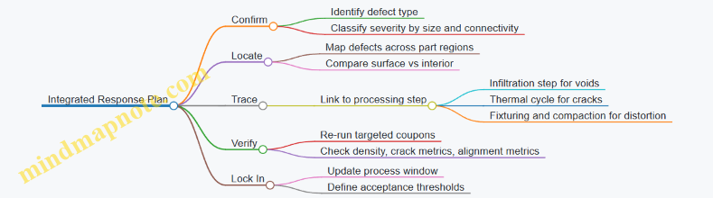
A good defect management system ends with process windows tied to evidence. For instance, if void clusters correlate with a specific infiltration pressure-time segment, you set a minimum dwell time and a pressure ramp constraint. If crack length correlates with cooling rate, you set a maximum cooling gradient. If fiber distortion correlates with tooling closure speed, you set a controlled closure profile. The result is not just fewer defects—it’s fewer surprises.
11.5 Practical Process Qualification Using Representative Coupons and Statistical Sampling
Process qualification answers one question: if you run the process the way you say you will, will the material behave like the material you tested? The practical approach is to qualify the process using representative coupons, then use statistical sampling to keep production inside the qualified envelope.
Foundations of Representative Coupons
Start by defining what “representative” means for your specific CMC system. A coupon should reproduce the critical variables that drive performance: fiber architecture, matrix chemistry, interphase state, infiltration/consolidation quality, and the thermal exposure surface condition.
A useful rule is to map each performance risk to a measurable coupon metric. For example:
- Oxidation resistance risk → coupon surface mass change, oxide scale thickness, and near-surface porosity.
- Strength retention risk → flexure strength after thermal cycling and residual strain response.
- Thermal conductivity risk → through-thickness porosity and phase distribution.
Then choose coupon geometries that make those metrics practical. A simple flexure bar can be more informative than a complex panel when you need tight control of test variability.
Statistical Sampling That Actually Controls Risk
Statistical sampling is not “test more.” It is “test enough, in the right places, with the right acceptance logic.” Begin with a process map that lists steps with the highest sensitivity: preform handling, infiltration viscosity and wetting, consolidation temperature and pressure, and any post-consolidation heat treatment.
Next, define sampling units. A sampling unit can be a single coupon batch from one infiltration run, or a set of coupons cut from one consolidated billet. The key is that all coupons in a unit share the same process history.
Use a two-layer plan:
- Within-Unit Sampling checks uniformity inside one run (e.g., coupons from different locations in the same billet).
- Between-Unit Sampling checks run-to-run stability (e.g., coupons from multiple billets produced on different days or with different operators).
A concrete example: if infiltration is sensitive to preform compaction, take within-unit coupons from the thickest and thinnest regions of the preform. If consolidation is sensitive to furnace loading, take between-unit coupons from billets processed in different furnace loads.
Qualification Workflow from Baseline Runs to Acceptance
Run a baseline qualification series to establish the qualified ranges for key metrics. Keep the number of variables controlled so you can attribute outcomes to process changes.
A systematic workflow:
- Define Metrics and Limits: choose measurable properties and set preliminary limits based on engineering targets and test repeatability.
- Produce Qualification Lots: make multiple units using the intended process window.
- Measure and Analyze: compute mean, variance, and any correlations between microstructure metrics and performance.
- Set Acceptance Criteria: translate qualification results into production acceptance rules.
- Lock the Process Window: document allowable ranges for critical parameters and the actions required when metrics drift.
To avoid “passing tests by accident,” include at least one coupon set that stresses the process near the edge of the parameter window. For instance, if consolidation temperature is allowed within a narrow band, qualify at the low end and high end so you know which failure mode appears first.
Mind Map: Process Qualification Logic
Example Sampling Plan and Decision Rules
Assume each production run produces one consolidated billet. You cut coupons from three locations: center, edge, and corner. For within-unit sampling, test all three locations for microstructure metrics (porosity and phase verification). For performance metrics (flexure after thermal cycling), test two locations that historically show the widest spread, such as edge and corner.
Between-unit sampling: test one billet per day for the first production month, then reduce frequency only after you demonstrate stable variance. Acceptance criteria should be tied to both central tendency and spread. A practical approach is:
- Pass if all required metrics meet the limit.
- Conditional pass if the mean meets the limit but one location shows elevated variance, triggering a focused corrective action.
- Fail if any metric exceeds the hard limit or if traceability indicates a process-history mismatch.
Traceability and Records That Make Results Defensible
Every coupon must carry a traceable identity back to the process history: preform batch, infiltration lot, consolidation schedule, and any deviations. When a coupon fails, you want to know whether it is a material issue, a process issue, or a sampling-location issue.
A simple but effective practice is to store a “coupon decision sheet” per sampling unit. It lists the critical parameters used, the coupon locations, the measured metrics, and the acceptance decision. This turns qualification from a one-time event into a repeatable, auditable method.
12. Testing Standards and Qualification for Hypersonic Use
12.1 Coupon Testing Matrix for Thermal Mechanical and Environmental Properties
A coupon testing matrix is the bridge between “material properties in a lab” and “performance in a hypersonic thermal protection system.” The goal is not to test everything at once, but to cover the dominant physics with a controlled set of specimens, conditions, and acceptance metrics.
Foundational Scope and Test Philosophy
Start by mapping each coupon test to one of three roles: (1) baseline properties, (2) degradation under environment, and (3) property recovery or residual strength after exposure. For ceramic matrix composites, the matrix must also separate fiber-dominated behavior from matrix-dominated behavior, because the failure mode changes with temperature and oxidation.
A practical rule: every test condition should have a matching “as-fabricated” reference coupon from the same manufacturing lot. If you skip that, you end up measuring process variability instead of environment effects. For example, if flexure strength drops after exposure, you need to know whether the drop is due to oxidation or simply because the coupon thickness varied.
Mind Map: Coupon Test Coverage
Matrix Design from Inputs to Outputs
Build the matrix in layers.
Layer 1: Geometry and orientation. Choose coupon types that reflect the structural directions that matter. For instance, a unidirectional or woven CMC will show different crack patterns in the warp and weft directions. A simple example is using two flexure orientations: one aligned with the dominant fiber direction and one transverse. If you only test one orientation, you may miss the direction that controls interfacial debonding.
Layer 2: Temperature ladder. Use a temperature ladder that spans the service-relevant range with enough points to see transitions. A common approach is three levels: a lower level near the onset of significant matrix softening, a mid level where oxidation kinetics are active, and an upper level near the maximum thermal exposure. Keep ramp rates consistent across conditions so that thermal gradients don’t masquerade as material degradation.
Layer 3: Environment pairing. Pair thermal conditions with environment types that represent the dominant chemistry. If the system sees both dry air and water vapor, include at least one exposure where water vapor is present. A concrete example: run identical flexure coupons at the same peak temperature in air-only and in air-plus-water-vapor, then compare strength retention and crack density.
Layer 4: Loading mode and time. Thermal protection systems experience both transient heating and time at elevated temperature. Include at least one test with a hold time at peak temperature. Without a hold-time case, you may underpredict oxidation-driven stiffness loss.
Example Coupon Set with Integrated Metrics
Use a compact set that still answers the key questions.
- Baseline flexure coupons at room temperature and at the mid temperature level. Measure strength, modulus, and failure mode.
- Thermal cycling coupons with a defined number of cycles and controlled ramp rates. After cycling, repeat flexure and record residual strength.
- Oxidation coupons exposed at the upper temperature in the relevant environment for a defined duration. Measure mass change, surface recession, and post-exposure flexure.
- Thermal conductivity coupons measured before and after environmental exposure to quantify property drift.
Acceptance metrics should be explicit and tied to the measured quantities. For example, strength retention could be defined as the ratio of post-exposure flexure strength to baseline flexure strength for the same orientation and thickness band.
Nondestructive Evaluation as a Gatekeeper
Nondestructive evaluation should be used as a gate before destructive testing and as a diagnostic after. A simple workflow is: baseline NDE on as-fabricated coupons, exposure, NDE again, then destructive testing. If ultrasonic velocity drops after exposure, you can correlate that change with later crack density or delamination indicators.
Statistical Plan and Traceability
Replicates prevent single-coupon stories from becoming “results.” Use enough specimens per condition to estimate scatter, and keep the lot and orientation labels consistent across every step. A good practice is to predefine outlier criteria based on measurable defects like thickness out of tolerance or obvious fiber waviness, not on whether the result “fits” the expected trend.
Example Matrix Layout
| Coupon Type | Orientation | Temperature | Environment | Time/Load |
|---|---|---|---|---|
| Baseline Flexure | Fiber-aligned | Mid | Air | Ramp only |
| Baseline Flexure | Transverse | Mid | Air | Ramp only |
| Thermal Cycling | Fiber-aligned | Upper | Air | N cycles |
| Oxidation | Fiber-aligned | Upper | Air + Vapor | Hold time |
| Conductivity | Through-thickness | Upper | Air + Vapor | Pre/Post |
12.2 Subscale Component Testing Including Leading Edge and Panel Simulations
Subscale component testing exists to answer a simple question: do the material and process choices behave like the real part when heat, pressure, and mechanical loads show up together? Coupon tests tell you what a material can do in isolation; subscale tests show how damage forms, spreads, and affects stiffness, strength, and surface integrity in a geometry that actually resembles the hardware.
Foundational Setup from Requirements to Test Articles
Start with the service envelope, not the lab convenience. Define the thermal boundary conditions (surface heat flux or temperature-time history), the mechanical loads (bending, shear, pressure-induced stresses), and the environment (air, water vapor, and any reactive species). Convert these into testable inputs: a leading-edge fixture that reproduces the thermal gradient and a panel fixture that reproduces the load path and constraint conditions.
A practical best practice is to create a “load and heat budget” table before building anything. For each subscale test, list the dominant stress contributors and the dominant degradation mechanisms. Example: for a leading edge, thermal gradient drives matrix cracking and interfacial debonding, while aerodynamic pressure adds bending and local shear near the stagnation region.
Leading Edge Subscale Testing
A leading edge subscale typically uses a curved or wedge-like specimen with a controlled surface heat flux profile. The goal is to reproduce the through-thickness temperature gradient and the resulting mismatch strains between fibers and matrix.
Thermal Gradient Control
Use an instrumented surface and embedded thermocouples or optical pyrometry to verify the temperature field. If the measured gradient differs from the target by more than a pre-set tolerance, stop and adjust heater power distribution or fixture insulation. This is not bureaucracy; it prevents you from attributing failure to “materials” when the real culprit is a mis-shaped temperature field.
Mechanical Loading Integration
Mechanical loading can be applied as bending (cantilever or simply supported beam) or as pressure simulation using a diaphragm or actuator. The key is to align the mechanical load direction with the expected stress state in the real leading edge. A common easy-to-understand example: if the full-scale part experiences tensile stress on the windward surface during peak heating, the subscale should load so that the windward surface is in tension at the same time the thermal gradient peaks.
Observables and Acceptance Metrics
Plan observables before the test. Typical metrics include:
- Surface recession and mass change after exposure.
- Crack density and crack spacing on polished cross-sections.
- Residual flexural stiffness and strength after thermal cycling.
- Nondestructive evaluation signatures such as ultrasonic velocity changes.
A useful practice is to define “decision points.” For instance, after a first thermal cycle, perform NDE and decide whether to continue, modify the fixture, or adjust the thermal profile.
Panel Subscale Testing
Panel subscale tests focus on load transfer and damage tolerance across a larger area. They are especially good at revealing how delamination-like damage and matrix cracking interact with boundary constraints.
Boundary Conditions That Actually Match the Part
Panels fail differently depending on how edges are constrained. Use fixtures that replicate the stiffness of the surrounding structure. If the real panel is supported by a relatively flexible frame, a rigid lab clamp can overestimate stress concentrations and produce unrealistic damage patterns.
Example: a panel with a stiff clamped edge may show early edge cracking, while a panel with a compliant support may show more distributed cracking and later stiffness loss. Both can be correct for their boundary conditions, so the fixture must match the intended constraint.
Thermal Loading Across the Panel
Apply a spatial heat flux pattern that matches the expected aerodynamic heating distribution. Even a simple two-zone pattern (hot center, cooler edges) can be sufficient if it reproduces the dominant gradient that drives differential expansion.
Mechanical Load Paths and Joints
If the full-scale panel includes fasteners, inserts, or bonded interfaces, include them in the subscale design. Otherwise, you risk testing a “perfect panel” that never experiences the real stress concentrations.
Systematic Test Planning Workflow
- Translate flight requirements into thermal and mechanical histories.
- Choose subscale geometry that preserves the dominant stress and temperature gradients.
- Instrument the thermal field and verify it matches the target.
- Apply mechanical loads in the correct phase relative to peak heating.
- Predefine NDE and post-test destructive characterization.
- Use acceptance metrics tied to structural performance, not just survival.
Mind Map: Subscale Component Testing Logic
Example Test Matrix for Practical Coverage
A compact matrix can cover the essentials without exploding the number of specimens. For instance:
- Leading edge: two thermal profiles (milder and peak), each with and without mechanical loading.
- Panel: one representative thermal profile with two boundary conditions (stiffer and more compliant supports).
This structure isolates whether failures are driven primarily by thermal gradients, by mechanical stress, or by their interaction.
Closing the Loop from Subscale Results to Design Decisions
Treat subscale outcomes as inputs to design allowables and process verification. If a subscale shows early stiffness loss correlated with a specific crack pattern or NDE signature, that becomes a measurable indicator for future material batches and manufacturing runs. The goal is consistency: the same material/process choices should produce the same damage progression when the thermal and mechanical histories are matched.
12.3 Nondestructive Evaluation Methods Including Ultrasonic and Thermography
Nondestructive evaluation (NDE) for ceramic matrix composites is about finding the right defect, in the right place, with the right confidence level. The tricky part is that CMC damage can be subtle: a small interfacial change may matter more than a visible surface crack. A systematic NDE plan starts with what you need to protect—load paths, thermal insulation behavior, and environmental sealing—then maps those needs to measurable signals.
Foundations for Choosing NDE Signals
Begin by linking likely damage modes to observable signatures.
- Fiber and interphase degradation often changes elastic response and wave propagation more than surface appearance.
- Matrix cracking and delamination can create discontinuities that affect both ultrasonic travel time and thermal spreading.
- Porosity and near-surface voids influence thermal diffusivity and can also scatter ultrasonic energy.
A practical best practice is to define an “inspection target list” before testing: defect type, approximate size range, depth range, and whether it is expected to be planar (delamination) or volumetric (voids). For example, if you are checking a panel region near a fastener where shear-driven delamination is common, you prioritize methods sensitive to near-surface interfaces.
Ultrasonic Methods for Interface and Internal Defects
Ultrasonic NDE uses acoustic waves to probe internal structure. In CMCs, the goal is usually to detect planar discontinuities (like delaminations) and property changes (like degraded interphases).
Wave Types and What They Reveal
- Pulse-echo ultrasonics measures reflections from interfaces. It is good for locating discontinuities at known depths.
- Through-transmission compares received signal amplitude and time-of-flight across a region. It is useful for mapping attenuation changes.
- Guided waves can scan larger areas efficiently, but require careful calibration because anisotropy and geometry affect dispersion.
Calibration and Coupling Reality Checks
Ultrasonic results depend on coupling between transducer and specimen. A simple example: if you switch from a gel to a dry coupling method, the first backwall echo may shift enough to look like a defect. To avoid that, establish a repeatable coupling protocol and use reference coupons with known artificial defects or controlled thickness variations.
Practical Inspection Workflow
- Baseline scan on an as-manufactured reference panel.
- Scan grid with spacing chosen to match the expected defect size.
- Signal processing focused on time-of-flight and amplitude features rather than only raw images.
- Defect confirmation using a second modality or a destructive check on representative samples.
Thermography for Surface and Subsurface Thermal Signatures
Thermography measures how heat flows through a material. In CMCs, defects alter thermal conductivity and heat capacity locally, which changes the temperature evolution after a controlled heat input.
Active Thermography Basics
Active thermography applies a heat pulse or periodic heating and records surface temperature over time. The key idea is that different defect depths respond at different times.
- Pulse thermography is good for quick screening and depth estimation using time-to-peak or phase analysis.
- Lock-in thermography uses modulated heating to improve sensitivity to subtle subsurface changes.
Example: Detecting Near-Surface Delamination
Suppose you suspect delamination near the surface of a CMC panel after thermal cycling. You can apply a short heat pulse and record the thermal response. A delaminated region tends to slow heat penetration, producing a delayed or reduced temperature rise compared with intact areas. The best practice is to compare against a reference region with similar thickness and layup, because thermal response is strongly influenced by geometry and fiber orientation.
Controlling Variables That Matter
Thermography is sensitive to surface emissivity. If two regions have different surface finishes, the infrared camera may “see” a defect that is really a coating or roughness change. A practical mitigation is to standardize surface preparation for inspection or apply a consistent emissivity treatment across the region of interest.
Integrated Use of Ultrasonic and Thermography
Using both methods reduces ambiguity. Ultrasonics excels at locating discontinuities and mapping elastic contrasts, while thermography highlights thermal transport disruptions.
A cohesive approach is to treat NDE as a two-stage decision system:
- Stage 1: screening: thermography to find suspect regions quickly.
- Stage 2: confirmation: ultrasonics to determine defect depth and planar geometry.
For example, if thermography flags a region with delayed thermal response, ultrasonic pulse-echo can verify whether the delay corresponds to a near-surface interface reflection rather than a surface emissivity artifact.
Mind Map: NDE Planning and Execution
Mind Map: Decision Logic for Defect Calls
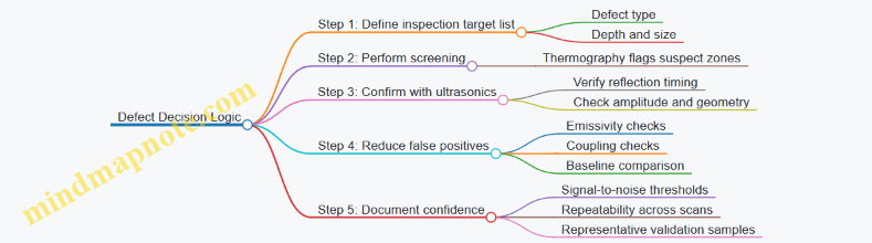
Acceptance and Documentation
A defect call is only useful if it is repeatable. Record the scan settings, coupling method, heating parameters, and the exact signal features used for classification. A simple but effective practice is to require that the same defect signature appears in repeated scans on the same region before it is treated as real. This keeps the NDE results aligned with how engineers actually make decisions: with evidence that survives the next measurement, not just the first one.
12.4 Acceptance Criteria and Traceability for Material and Process Records
Acceptance criteria are the rules that decide whether a ceramic matrix composite (CMC) material lot, coupon batch, or manufactured part is “good enough” to move forward. Traceability is the paperwork and data chain that lets you prove why it is good enough, even months later when someone asks, “Which exact fibers and which exact infiltration run built this panel?” Together, they prevent two common failure modes: accepting parts that should have been rejected, and rejecting parts that were actually fine but can’t be defended.
Foundational Principles for Acceptance
Start with a clear hierarchy: requirements → acceptance criteria → test methods → sampling plan → records. Requirements come from the design allowables and environmental expectations. Acceptance criteria translate those requirements into measurable thresholds, such as density range, porosity limits, fiber volume fraction targets, flexural strength minimums, and oxidation mass change bounds.
A practical way to keep criteria from becoming a random list is to map each criterion to a failure mechanism. For example, if oxidation-driven surface recession is a concern, acceptance criteria should include surface recession metrics and mass change after a defined exposure protocol. If thermal cycling cracking is a concern, include stiffness retention or residual strength after cycling, not just as-manufactured strength.
Traceability That Actually Works
Traceability should cover three layers: material identity, process identity, and test identity.
- Material identity: fiber lot number, fiber diameter distribution, matrix precursor batch IDs, and any interphase coating identifiers.
- Process identity: preform architecture recipe, infiltration/consolidation parameters (temperature, pressure, dwell time, atmosphere), and any deviations logged during the run.
- Test identity: coupon IDs linked to the part or lot, specimen geometry, test temperatures, calibration status, and operator or equipment identifiers.
A simple rule: if a record can’t be tied to a specific lot or run, it can’t support acceptance decisions.
Acceptance Criteria Structure
Use categories so reviewers can find what they need quickly.
- Dimensional and microstructural criteria: density, porosity, fiber volume fraction, and defect counts (e.g., voids above a size threshold).
- Mechanical criteria: strength and modulus at relevant temperatures, plus residual properties after thermal cycling.
- Environmental criteria: oxidation or ablation metrics under defined exposure conditions.
- Process control criteria: evidence that critical parameters stayed within control limits.
Each category should specify: the test method, the acceptance threshold, the number of specimens, and the conditions under which the test is valid.
Sampling and Decision Rules
Acceptance is not “test one coupon and hope.” Define a sampling plan that matches the risk. For example, if infiltration viscosity and wetting are sensitive to precursor batch, sample more coupons from each infiltration run. If fiber lot variability dominates, sample across fiber lots rather than only across parts.
Decision rules should be explicit:
- Pass/Fail based on individual specimen thresholds.
- Lot acceptance based on statistical summaries when variability is expected.
- Rework or containment rules when a criterion is borderline but the rest of the evidence is strong.
A good practice is to require that any nonconformance triggers a traceability check first: confirm whether the issue is isolated to one run, one fiber lot, or one test setup.
Mind Map: Records and Evidence Chain
Example: Linking a Panel to Its Evidence
Suppose a hypersonic leading-edge panel is built from a specific CMC laminate. The acceptance package should include:
- A panel traveler listing the laminate layup recipe, preform ID, and consolidation run ID.
- A materials sheet listing fiber lot numbers and matrix precursor batch IDs used for that run.
- A process record showing actual infiltration temperature and pressure profiles, plus any logged deviations.
- A coupon mapping table showing which coupons were cut from the same consolidated block as the panel, including coupon IDs and test temperatures.
- A test report with calibration status for the load frame and furnace, specimen dimensions, and results against each criterion.
If the panel fails a criterion, traceability helps you answer whether the cause is likely microstructural (e.g., porosity out of range), process-related (e.g., infiltration dwell too short), or test-related (e.g., calibration drift). That’s the difference between guessing and fixing.
Example: Borderline Criterion Handling
Imagine porosity is slightly above the threshold, but strength and oxidation mass change are within limits. The acceptance decision should follow the defined rules: either reject outright, accept with documented risk, or contain the lot for additional inspection. The traceability chain lets you target the investigation: check whether the porosity shift correlates with a specific infiltration run, a specific precursor batch, or a specific equipment condition.
Records That Must Be Complete
At minimum, acceptance and traceability records should be complete enough to reconstruct the “as-built” story: what went in, what was done, what was measured, and how the decision was made. A practical completeness check is to verify that every acceptance criterion has a corresponding record entry and that every record entry points back to a specific lot, run, or coupon ID.
Finally, include a revision-controlled summary page that states the acceptance outcome and lists the exact evidence IDs used. On a review day, that one page saves time and prevents the classic “we have the data somewhere” problem.
12.5 Practical Documentation Packages for Qualification and Production Readiness
A qualification and production readiness package is not a folder of PDFs; it’s a traceable chain from requirements to test evidence to manufacturing control. The goal is simple: if someone asks “why is this acceptable,” the answer should be found in the package without calling three people and waiting a week.
What the Package Must Prove
Start with a requirements map that links each performance requirement to a measurable attribute and then to test methods and acceptance criteria. For ceramic matrix composites, the measurable attributes typically include density and porosity, fiber volume fraction, phase composition, oxidation mass change, retained strength after thermal cycling, and NDE detectability limits.
A practical approach is to define three layers of evidence:
- Material evidence for coupons and subcomponents.
- Process evidence showing the manufacturing route can reproduce the material evidence.
- Component evidence demonstrating the design survives the combined environment.
Mind Map: Documentation Package Structure
Core Contents in a Readiness-Ready Package
Include the following documents, each with a clear owner and revision history.
1. Requirements Traceability Matrix Use a table that maps requirement → attribute → test method → acceptance criterion → evidence document ID. Example: “Retained flexural strength after thermal cycling at 1400°C” maps to “strength retention ratio” measured by a specified flexure test, with a criterion like “≥ 0.70 of baseline,” and points to the exact report section.
2. Test Plans That Prevent Argument Later A good test plan states specimen geometry, conditioning steps, instrumentation, data reduction rules, and how failures are classified. For instance, if a coupon fails early due to handling damage, the plan should define whether it is excluded, replaced, or counted as a process defect.
3. Calibration And Measurement Traceability List calibration status for balances, furnaces, thermocouples, and NDE equipment. Also record how temperature uniformity is verified. This matters because oxidation and ablation outcomes are sensitive to actual specimen temperature, not just furnace setpoint.
4. Manufacturing Travelers With In-Process Checks A traveler is a step-by-step recipe with checkpoints. Example checkpoints:
- Preform mass and dimensions before infiltration.
- Infiltration temperature and viscosity window.
- Consolidation pressure and dwell time.
- Post-consolidation density and dimensional inspection.
When a parameter drifts, the traveler should specify the immediate action: stop, rework, or continue with documented justification.
5. Nonconformance, Waivers, And Rework Rules Define how deviations are handled. Example: if porosity exceeds the target band but remains within an allowable range supported by prior evidence, the package should show the disposition path and the linked evidence.
6. Data Reduction And Uncertainty Statements State how raw measurements become reported values. Example: density from mass and volume measurements should include uncertainty propagation, and strength calculations should specify span length, crosshead rate, and how fracture location is treated.
Example: A Minimal Yet Complete Release Checklist
Use a checklist that can be signed without interpretation.
- Traceability matrix completed and reviewed
- All required coupon tests executed with pass/fail criteria applied
- NDE method qualification evidence included
- Calibration records current for measurement dates
- Manufacturing travelers match the recorded process history
- Deviations documented with disposition and evidence links
- Final component allowables computed from approved data set
- Version control verified for all referenced documents
Version Control and Naming Conventions That Save Time
Adopt a consistent naming scheme for evidence documents and embed traceability IDs in both the traveler and the test report. For example, a lot ID should appear in specimen labels, furnace logs, and final reports. This prevents the classic “same process, different file” problem.
A practical rule: every numeric claim in the package should point to a document ID and a section number. If it can’t, it doesn’t belong in the release package.