Spatial Computing with Lidar and Computer Vision
1. Introduction to Spatial Computing and Autonomous Perception
1.1 Overview of Spatial Computing Concepts
Spatial computing refers to the set of technologies and methods that enable machines to perceive, interpret, and interact with the physical world in three dimensions. At its core, it combines sensing, processing, and acting on spatial information to create systems that understand their environment beyond flat, two-dimensional data.
The foundation of spatial computing lies in capturing spatial data, often through sensors like lidar and cameras, then processing that data to build representations of the environment. These representations can be point clouds, maps, or semantic models that describe objects and their relationships in space.
Key components of spatial computing include:
- Sensing: Acquiring raw spatial data from the environment.
- Perception: Extracting meaningful information from sensor data.
- Localization: Determining the position and orientation of the system within the environment.
- Mapping: Creating spatial models or maps of the environment.
- Interaction: Using spatial understanding to make decisions or control actions.
To visualize these components and their relationships, consider the following mind map:
This map shows that spatial computing is a layered process, starting from raw data and ending with actionable knowledge.
Example: Imagine a warehouse robot tasked with moving goods. It uses lidar to scan its surroundings, creating a 3D point cloud. The perception system segments this cloud to identify shelves and obstacles. Localization algorithms determine the robot’s position relative to the warehouse map. Using this spatial understanding, the robot plans a path to its destination while avoiding obstacles.
Another way to break down spatial computing is by the types of data it handles:
Handling these data types requires different algorithms and processing steps. For example, geometric data might be used for collision avoidance, while semantic data helps the system understand what objects are present.
Example: A self-driving car uses cameras to identify traffic lights (semantic data) and lidar to detect the exact shape and position of nearby vehicles (geometric data). It combines this information to decide when to stop or proceed.
Spatial computing also involves managing uncertainty. Sensors are not perfect; lidar returns can be noisy, and cameras can be affected by lighting. Systems must account for these imperfections through filtering and probabilistic methods.
Example: When a drone navigates indoors, it fuses lidar and camera data to maintain accurate localization despite occasional sensor dropouts or noisy measurements.
In summary, spatial computing is about turning raw spatial data into useful knowledge that machines can use to understand and navigate the physical world. It combines multiple sensing modalities, data processing techniques, and decision-making algorithms to build perception pipelines essential for autonomous robots and mapping applications.
1.2 Role of Lidar and Computer Vision in Autonomous Systems
In autonomous systems, perception is the foundation that allows machines to understand and interact with their environment. Two key technologies enabling this perception are Lidar and computer vision. Each brings unique strengths and challenges, and their combined use often leads to more robust and reliable spatial understanding.
Understanding Lidar’s Role
Lidar (Light Detection and Ranging) uses laser pulses to measure distances to objects, producing precise 3D point clouds that represent the environment’s geometry. This spatial data is critical for tasks like obstacle detection, mapping, and localization.
-
Strengths:
- Provides accurate depth information independent of lighting conditions.
- Captures detailed 3D structure, useful for shape recognition and environment modeling.
- Effective at long ranges, making it suitable for outdoor and large-scale environments.
-
Limitations:
- Produces sparse data compared to images, which can make semantic interpretation harder.
- Sensitive to weather conditions like heavy rain or fog.
- Typically more expensive and power-consuming than cameras.
Understanding Computer Vision’s Role
Computer vision uses cameras to capture images or video, extracting rich semantic information such as colors, textures, and object identities. It excels at recognizing and classifying objects, interpreting scenes, and understanding context.
-
Strengths:
- Provides dense, high-resolution data with rich semantic content.
- Enables recognition of objects, signs, and signals critical for decision-making.
- Cameras are generally affordable and lightweight.
-
Limitations:
- Depth estimation is indirect and less precise without additional sensors.
- Performance varies with lighting and weather conditions.
- Requires significant processing to extract meaningful spatial data.
Complementary Roles in Autonomous Systems
Lidar and computer vision complement each other by balancing geometric accuracy and semantic richness. Lidar offers reliable 3D measurements, while vision provides detailed context. Together, they enable more complete perception pipelines.
Mind Map: Role of Lidar and Computer Vision in Autonomous Systems
Examples Illustrating Their Roles
Example 1: Obstacle Detection
- Lidar detects the shape and distance of obstacles, even in low light.
- Vision identifies what the obstacle is (e.g., pedestrian, vehicle, or static object).
- Combined, the system can decide not only where to avoid but also how to respond appropriately.
Example 2: Mapping and Localization
- Lidar builds accurate 3D maps by scanning surroundings.
- Vision helps recognize landmarks and signs, aiding in place recognition.
- Together, they improve the robot’s ability to localize itself within the environment.
Example 3: Traffic Scene Understanding
- Vision detects traffic lights, road signs, and lane markings.
- Lidar confirms the position and movement of other vehicles and pedestrians.
- Fusion of these inputs supports safe navigation decisions.
Summary
Lidar and computer vision serve distinct but interconnected roles in autonomous systems. Lidar provides the spatial skeleton, while vision adds semantic flesh. Employing both technologies in perception pipelines improves accuracy, reliability, and situational awareness, which are essential for autonomous operation.
1.3 Key Challenges in Perception Pipelines
Perception pipelines in autonomous robots and mapping systems face a variety of challenges that stem from the complexity of interpreting real-world data. These challenges affect the accuracy, reliability, and efficiency of spatial computing tasks. Understanding these difficulties helps in designing better systems and anticipating potential pitfalls.
Sensor Limitations and Data Quality
Sensors like lidar and cameras have inherent constraints. Lidar can struggle with reflective or transparent surfaces, creating gaps or noise in point clouds. Cameras depend heavily on lighting conditions; low light or glare can degrade image quality.
Mind Map: Sensor Limitations
Example: A robot navigating a rainy street might receive noisy lidar returns from wet surfaces and blurry images due to raindrops on the camera lens. This combination can confuse object detection algorithms.
Calibration and Synchronization
Accurate spatial perception requires precise calibration between sensors and synchronization of their data streams. Misalignment leads to errors in sensor fusion and mapping.
Mind Map: Calibration Challenges
Example: If a lidar and camera are not properly calibrated, a detected obstacle in the lidar point cloud might not align with the corresponding image, causing incorrect object identification.
Data Volume and Processing Speed
Lidar and vision sensors produce large amounts of data rapidly. Processing this data in real time demands efficient algorithms and hardware.
Mind Map: Data Handling Challenges
Example: A drone flying at high speed must process lidar scans and camera frames quickly to avoid obstacles. Delays in processing can lead to outdated information and unsafe decisions.
Environmental Complexity
Real-world environments are dynamic and cluttered. Moving objects, varying terrain, and changing lighting complicate perception.
Mind Map: Environmental Challenges
Example: In a busy warehouse, forklifts and workers move unpredictably, creating occlusions and requiring the perception system to distinguish between static and dynamic elements.
Sensor Fusion Difficulties
Combining lidar and vision data improves perception but introduces challenges in aligning and weighting information from different modalities.
Mind Map: Sensor Fusion Issues
Example: A shiny metal surface might produce sparse lidar returns but clear camera images. The fusion algorithm must decide how much to trust each sensor to maintain accurate mapping.
Robustness to Noise and Outliers
Sensor data often contains noise and outliers, which can mislead algorithms if not handled properly.
Mind Map: Noise and Outliers
Example: Dust or insects near sensors can create false points in lidar data. Without filtering, these points might be mistaken for obstacles.
Scalability and Map Management
As robots operate over larger areas or longer times, managing and updating spatial maps becomes challenging.
Mind Map: Scalability Challenges
Example: An autonomous vehicle driving through a city needs to update its map continuously without overwhelming onboard storage or losing track of changes.
Real-Time Constraints
Perception pipelines must deliver timely information to support navigation and decision-making.
Mind Map: Real-Time Processing
Example: A robot avoiding obstacles in a crowded environment cannot afford delays in detecting a suddenly appearing pedestrian.
Summary Mind Map: Key Challenges in Perception Pipelines
Each of these challenges requires careful consideration during system design. Addressing them with appropriate best practices and examples helps build perception pipelines that are both reliable and practical.
1.4 Best Practices for Integrating Multi-Sensor Data
Integrating data from multiple sensors like lidar and cameras is essential for building reliable spatial perception systems. The goal is to combine complementary information to create a richer, more accurate understanding of the environment. However, this integration requires careful attention to several factors to avoid introducing errors or inefficiencies.
Key Principles for Multi-Sensor Data Integration
- Temporal Alignment: Sensors operate at different frame rates and latencies. Synchronizing timestamps ensures data corresponds to the same moment in time.
- Spatial Calibration: Knowing the precise relative positions and orientations of sensors is critical for accurate data fusion.
- Data Representation: Choosing compatible formats and coordinate frames simplifies integration.
- Noise and Uncertainty Management: Each sensor has different noise characteristics; fusion methods must account for this.
- Computational Efficiency: Real-time systems require optimized pipelines to handle large data volumes without lag.
Mind Map: Core Components of Multi-Sensor Integration
Temporal Alignment
Different sensors capture data at different rates and with varying delays. For example, a lidar might produce point clouds at 10 Hz, while a camera captures images at 30 Hz. Without aligning these data streams, fusion can combine mismatched snapshots, leading to errors.
Best practice: Use hardware triggers or software timestamp synchronization to align data. When exact synchronization isn’t possible, interpolate sensor data to estimate values at common timestamps.
Example: Suppose a robot receives a lidar scan at time t=1.0s and camera frames at t=0.97s and t=1.03s. Interpolating between the two camera frames can estimate the image corresponding to the lidar timestamp.
Spatial Calibration
Sensors must be calibrated to a common coordinate system. Intrinsic calibration corrects sensor-specific distortions (like lens distortion for cameras). Extrinsic calibration determines the position and orientation of each sensor relative to a shared frame, often the robot base or lidar frame.
Best practice: Perform regular calibration using known patterns or calibration targets. Automate calibration routines when possible to maintain accuracy over time.
Example: Mounting a camera on a lidar rig requires estimating the rotation and translation between the camera and lidar frames. Using a checkerboard pattern visible to both sensors allows computing this transformation.
Data Representation
Consistent coordinate frames and data formats simplify fusion. Point clouds from lidar are naturally 3D, while camera data is 2D images. Projecting lidar points into the camera frame or back-projecting image pixels into 3D space enables joint processing.
Best practice: Define a clear pipeline for transforming data between frames. Use standard formats like ROS messages or PCL point clouds to maintain compatibility.
Example: Projecting lidar points onto the camera image plane helps associate depth with pixels, enabling depth-enhanced image processing.
Noise and Uncertainty Management
Each sensor has unique noise characteristics. Lidar can have range measurement noise and missing points on reflective surfaces. Cameras suffer from lighting variations and motion blur.
Best practice: Model sensor noise explicitly and incorporate it into fusion algorithms, such as Kalman filters or probabilistic frameworks. Detect and remove outliers before fusion.
Example: When fusing lidar and camera data for obstacle detection, weighting lidar measurements higher in low-light conditions can improve robustness.
Computational Efficiency
Fusing high-resolution lidar and camera data can be computationally expensive. Efficient data handling is necessary for real-time applications.
Best practice: Use downsampling techniques like voxel grids for point clouds and image pyramids for cameras. Employ parallel processing and hardware acceleration where available.
Example: Reducing a 1 million-point lidar scan to 100,000 points via voxel filtering preserves structure while speeding up processing.
Mind Map: Best Practices Summary
Integrated Example: Building a Simple Fusion Pipeline
Imagine a mobile robot equipped with a 16-beam lidar and a monocular camera. The goal is to detect obstacles with both sensors.
- Temporal Alignment: The lidar publishes scans at 10 Hz, the camera at 30 Hz. The system timestamps all data and interpolates camera frames to lidar timestamps.
- Spatial Calibration: A calibration routine determines the camera’s pose relative to the lidar.
- Data Representation: Lidar points are projected onto the camera image plane using the calibration transform.
- Noise Handling: Points with low reflectivity or inconsistent depth are filtered out.
- Fusion: The system combines lidar depth with image features to confirm obstacle presence.
- Efficiency: The point cloud is downsampled before projection to reduce computation.
This approach leverages complementary strengths: lidar provides accurate depth, the camera adds rich texture and color information. Following these best practices ensures the fusion is accurate and efficient.
In summary, integrating multi-sensor data requires attention to timing, calibration, representation, noise, and performance. Applying these best practices with concrete examples helps build perception pipelines that are both reliable and practical.
1.5 Example: Setting Up a Basic Perception Pipeline for a Mobile Robot
Creating a perception pipeline for a mobile robot means connecting sensor inputs to actionable outputs. The goal is to transform raw data from sensors like lidar and cameras into a spatial understanding the robot can use to navigate and interact with its environment.
Step 1: Sensor Setup and Data Acquisition
Start with two primary sensors: a 2D lidar scanner and a monocular camera. The lidar provides distance measurements in a plane around the robot, while the camera captures visual context.
- Lidar Data: Produces a 2D point cloud representing obstacles and free space.
- Camera Data: Provides images for detecting objects and textures.
Mind Map: Sensor Inputs
Step 2: Data Preprocessing
Raw sensor data often contains noise and irrelevant information. Preprocessing cleans and prepares data for further analysis.
-
Lidar Preprocessing:
- Filter out points beyond a maximum range.
- Remove isolated points considered noise.
- Downsample to reduce computational load.
-
Camera Preprocessing:
- Correct lens distortion via calibration parameters.
- Convert images to grayscale if color is unnecessary.
- Resize images for faster processing.
Mind Map: Preprocessing Steps
Step 3: Feature Extraction
Extracting meaningful features helps the robot identify obstacles and landmarks.
-
From Lidar:
- Detect clusters of points representing objects.
- Calculate boundaries and centroids.
-
From Camera:
- Detect edges or corners using algorithms like Canny or Harris.
- Identify simple shapes or colors if relevant.
Example: Use a clustering algorithm such as DBSCAN on the lidar point cloud to group points into obstacle candidates.
Mind Map: Feature Extraction
Step 4: Sensor Fusion
Combine lidar and camera data to improve perception accuracy.
- Align lidar points with corresponding camera pixels using extrinsic calibration.
- Use camera images to classify objects detected by lidar clusters.
Example: If a lidar cluster corresponds to a region in the camera image with a detected pedestrian, label that cluster as a pedestrian.
Mind Map: Sensor Fusion
Step 5: Environment Representation
Build a map or occupancy grid that the robot can use for navigation.
- Convert lidar clusters into obstacles on a 2D occupancy grid.
- Mark free space based on lidar returns.
- Overlay semantic labels from camera data if available.
Example: Create a grid where each cell is marked as free, occupied, or unknown.
Mind Map: Environment Representation
Step 6: Decision Making and Output
The processed perception data feeds into the robot’s navigation and control systems.
- Use the occupancy grid to plan collision-free paths.
- React to detected dynamic obstacles by stopping or rerouting.
Example: If an obstacle cluster is detected within a safety radius, the robot slows down or stops.
Mind Map: Decision Making
Concrete Example: Simple Perception Pipeline in Python-like Pseudocode
# Step 1: Acquire data
lidar_points = get_lidar_scan()
camera_image = capture_camera_frame()

# Step 2: Preprocess
filtered_points = filter_lidar_points(lidar_points, max_range=10.0)
downsampled_points = downsample(filtered_points, factor=2)
corrected_image = undistort_image(camera_image, calibration_params)

# Step 3: Feature Extraction
clusters = cluster_points(downsampled_points, eps=0.5, min_samples=5)
edges = detect_edges(corrected_image)

# Step 4: Sensor Fusion
for cluster in clusters:
    image_region = project_cluster_to_image(cluster, calibration_params)
    if detect_pedestrian(image_region, edges):
        label_cluster(cluster, 'pedestrian')

# Step 5: Environment Representation
occupancy_grid = create_occupancy_grid(downsampled_points, grid_size=0.1)
mark_occupied_cells(occupancy_grid, clusters)

# Step 6: Decision Making
if obstacle_in_path(occupancy_grid):
    stop_robot()
else:
    continue_navigation()
This example outlines the flow from raw sensor data to actionable decisions. Each step can be expanded with more sophisticated algorithms, but this basic pipeline covers the essentials.
By structuring perception this way, the robot gains a layered understanding of its surroundings, balancing raw data processing with higher-level interpretation. The pipeline can be tested and improved incrementally, making it a practical starting point for autonomous robot perception.
2. Fundamentals of Lidar Technology
2.1 Principles of Lidar Sensing and Measurement
Lidar, short for Light Detection and Ranging, is a remote sensing method that uses laser light to measure distances to objects. The core concept is straightforward: a laser pulse is emitted, it travels until it hits an object, then reflects back to the sensor. By measuring the time it takes for the pulse to return, the system calculates the distance to that object. This time-of-flight measurement is the foundation of Lidar’s ability to create detailed 3D maps of environments.
How Lidar Measures Distance
The fundamental formula behind distance measurement in Lidar is:
\[ \text{Distance} = \frac{c \times t}{2} \]
where:
- \( c \) is the speed of light (~299,792,458 meters per second),
- \( t \) is the time taken for the laser pulse to travel to the object and back.
The division by 2 accounts for the round-trip travel of the pulse.
Because light travels extremely fast, the timing measurement must be precise, often in the order of nanoseconds. This precision allows Lidar systems to resolve distances with centimeter or even millimeter accuracy.
Components of a Typical Lidar System
- Laser Emitter: Sends out short pulses of laser light.
- Photodetector/Receiver: Captures the reflected pulses.
- Timing Circuit: Measures the time between emission and reception.
- Scanning Mechanism: Directs the laser pulses across the environment, either mechanically or electronically.
- Processing Unit: Converts raw timing data into distance measurements and constructs point clouds.
Types of Lidar Pulses
Lidar systems typically emit pulses in the near-infrared spectrum, commonly around 905 nm or 1550 nm wavelengths. The choice affects eye safety, range, and atmospheric absorption.
Mind Map: Core Lidar Measurement Process
Example: Calculating Distance from Time-of-Flight
Suppose a Lidar sensor measures a round-trip time of 20 nanoseconds (20 x 10^-9 seconds). The distance to the object is:
\[ \text{Distance} = \frac{3 \times 10^{8} \times 20 \times 10^{-9}}{2} = 3 \text{ meters} \]
This means the object is 3 meters away from the sensor.
Factors Affecting Measurement Accuracy
- Surface Reflectivity: Dark or absorbent surfaces reflect less light, reducing signal strength.
- Atmospheric Conditions: Fog, rain, or dust can scatter or absorb laser pulses.
- Incidence Angle: Grazing angles can cause weaker or distorted returns.
- Multiple Returns: Some pulses reflect off multiple surfaces (e.g., tree leaves), producing multiple distance readings.
Mind Map: Sources of Measurement Variability
Example: Multiple Return Scenario
A Lidar pulse aimed at a tree might first reflect off leaves (returning a close distance), then off branches behind (returning a farther distance). The sensor records both distances, which helps distinguish between objects at different depths.
Scanning and Point Cloud Generation
Lidar sensors scan the environment by sweeping the laser beam across a field of view. Each pulse provides a single distance measurement along a specific direction. Collecting many such measurements builds a dense set of points in 3D space, called a point cloud. This point cloud represents the shape and structure of the environment.
Mind Map: From Pulses to Point Clouds
Example: Converting Polar to Cartesian Coordinates
Given a distance \( r \), azimuth angle \( \theta \), and elevation angle \( \phi \), the 3D point \( (x, y, z) \) is:
\[ x = r \cos \phi \cos \theta \] \[ y = r \cos \phi \sin \theta \] \[ z = r \sin \phi \]
This conversion places each measured point in 3D space relative to the sensor.
Summary
Lidar sensing relies on precise timing of laser pulses to measure distances. The quality of measurements depends on sensor design, environmental factors, and surface properties. Understanding these principles helps in designing robust perception pipelines and interpreting Lidar data effectively.
2.2 Types of Lidar Sensors and Their Applications
Lidar sensors come in several varieties, each with distinct characteristics suited to particular tasks. Understanding these types helps in choosing the right sensor for your autonomous robot or mapping project.
Types of Lidar Sensors
-
Mechanical Lidar
- Uses rotating mirrors or the entire sensor head to scan the environment.
- Produces 360-degree horizontal field of view.
- Common in autonomous vehicles and large-scale mapping.
- Typically bulkier and more power-consuming.
-
Solid-State Lidar
- No moving parts; relies on electronic beam steering.
- More compact and robust.
- Lower cost and easier to integrate.
- Limited field of view compared to mechanical types.
-
Flash Lidar
- Illuminates the entire scene at once, similar to a camera flash.
- Captures depth information in a single shot.
- Useful for short-range applications and high-speed scenarios.
- Limited range and resolution compared to scanning lidars.
-
MEMS Lidar
- Uses micro-electromechanical systems to steer the laser beam.
- Combines some advantages of mechanical and solid-state types.
- Smaller size and moderate field of view.
- Often used in drones and compact robots.
-
Frequency-Modulated Continuous Wave (FMCW) Lidar
- Measures distance by frequency shift rather than time of flight.
- Provides velocity information directly.
- Less susceptible to interference.
- More complex and currently less common.
Mind Map: Lidar Sensor Types
Applications by Sensor Type
-
Mechanical Lidar
- Autonomous cars use them for full-surround environment perception.
- Mapping large outdoor areas where wide coverage is essential.
- Examples: Velodyne HDL-64E, commonly mounted on self-driving cars.
-
Solid-State Lidar
- Suitable for compact robots and drones where size and durability matter.
- Indoor navigation and obstacle avoidance.
- Examples: Quanergy M8, used in warehouse automation.
-
Flash Lidar
- High-speed object detection in industrial automation.
- Short-range collision avoidance in drones.
- Examples: LeddarTech sensors in automotive safety systems.
-
MEMS Lidar
- Small UAVs and delivery robots benefit from MEMS for lightweight sensing.
- Applications requiring moderate scanning angles with compact hardware.
- Examples: AEye’s MEMS-based sensors for adaptive perception.
-
FMCW Lidar
- Emerging in applications needing velocity detection, such as traffic monitoring.
- Situations requiring resistance to interference from other sensors.
Mind Map: Applications of Lidar Types
Example: Choosing a Lidar for a Delivery Robot
Imagine designing a delivery robot for urban sidewalks. The robot needs to detect obstacles, pedestrians, and navigate tight spaces. A mechanical lidar might be too bulky and power-hungry. Flash lidar’s short range might not provide enough reaction time. A solid-state or MEMS lidar offers a good balance: compact size, adequate field of view, and robustness. Choosing a MEMS lidar could provide moderate scanning angles and durability, fitting the robot’s size and operational needs.
Example: Mapping a Forested Area
For mapping large outdoor environments like forests, a mechanical lidar with 360-degree scanning is ideal. It captures detailed point clouds over wide areas. The sensor’s range and resolution help detect tree trunks, canopy structure, and terrain. The Velodyne HDL-64E is a typical choice, mounted on a vehicle or drone flying over the area.
In summary, the choice of lidar sensor depends on the application’s range, field of view, size constraints, and environmental conditions. Matching sensor characteristics to task requirements ensures effective spatial perception.
2.3 Data Characteristics and Formats in Lidar
Lidar sensors produce data that is fundamentally different from traditional camera images. Instead of pixels arranged in a grid, lidar outputs a collection of points in three-dimensional space, known as a point cloud. Each point represents a location where the laser pulse reflected off a surface and returned to the sensor. Understanding the nature of this data and its common formats is essential for effective processing and integration.
Key Characteristics of Lidar Data
-
Sparsity and Density: Unlike images, point clouds are sparse and irregularly distributed. The density of points varies depending on the distance from the sensor, surface reflectivity, and scanning pattern.
-
Dimensionality: Each point typically contains at least three coordinates (x, y, z) in a 3D space. Additional attributes such as intensity (reflectance strength), timestamp, or return number may also be included.
-
Coordinate Frames: Lidar data is often expressed in the sensor’s local coordinate frame. Transformations are required to align data with other sensors or global maps.
-
Noise and Outliers: Measurement errors, environmental conditions, and surface properties introduce noise. Outliers can appear as isolated points far from actual surfaces.
-
Temporal Aspect: Some lidars provide timestamps per point or per scan, enabling temporal analysis and synchronization with other sensors.
Common Lidar Data Formats
Lidar data can be stored and exchanged in various formats, each with its own structure and use cases. Here are some widely used ones:
-
Raw Sensor Data: Proprietary formats from manufacturers, often containing raw measurements and metadata. These are usually converted into standard formats for processing.
-
PCD (Point Cloud Data): Developed by the Point Cloud Library (PCL), PCD files store point clouds with optional fields like intensity and color. They support both ASCII and binary encoding.
-
LAS/LAZ: Standard formats in geospatial applications, storing 3D point data with attributes such as GPS time, classification, and color. LAZ is the compressed version.
-
PLY (Polygon File Format): Originally designed for 3D models, PLY files can represent point clouds with color and other properties.
-
CSV/TXT: Simple text formats listing point coordinates and attributes. Easy to read but inefficient for large datasets.
-
ROS Messages: In robotic systems using the Robot Operating System (ROS), point clouds are typically published as sensor_msgs/PointCloud2 messages, which include metadata and support streaming.
Mind Map: Lidar Data Characteristics
Mind Map: Common Lidar Data Formats
Example: Understanding a Point Cloud Sample
Consider a small snippet of a point cloud stored in CSV format:
x,y,z,intensity
0.5,1.2,2.0,120
0.6,1.3,2.1,115
0.55,1.25,2.05,118
Each row represents a single point with its 3D coordinates and the intensity of the returned laser pulse. Intensity values help distinguish materials or surface types.
Example: Visualizing Data Density Variation
Imagine a lidar scanning a flat wall at varying distances. Points closer to the sensor appear denser, while those farther away are more spread out. This happens because the angular resolution of the lidar translates into larger spatial gaps at greater distances.
Practical Note
When working with lidar data, always check the format and included attributes before processing. Some algorithms rely on intensity or multiple returns, while others only need spatial coordinates. Efficient storage and access methods matter, especially for large-scale mapping or real-time applications.
In summary, lidar data is a cloud of points with spatial and sometimes additional attributes, stored in multiple formats tailored to different applications. Recognizing these characteristics helps in selecting the right tools and strategies for perception pipelines.
2.4 Noise and Error Sources in Lidar Data
Lidar sensors provide valuable 3D information by measuring distances using laser pulses. However, the data they produce is not perfect. Various noise and error sources affect the accuracy and reliability of point clouds. Understanding these issues is essential for building robust perception pipelines.
Types of Noise and Errors in Lidar Data
- Measurement Noise: Random fluctuations in the distance measurements caused by sensor limitations and environmental factors.
- Systematic Errors: Biases introduced by calibration inaccuracies or hardware imperfections.
- Environmental Interference: Effects from weather, ambient light, and reflective surfaces.
- Motion-Induced Errors: Distortions caused by the movement of the sensor platform during scanning.
- Multipath Effects: Laser pulses reflecting off multiple surfaces before returning, causing incorrect distance readings.
Mind Map: Noise and Error Sources in Lidar Data
Measurement Noise
Lidar sensors emit laser pulses and measure the time it takes for the light to return. This time-of-flight measurement is subject to small random variations. Electronic components add noise, and the sensor’s resolution limits how finely it can measure distance. These factors cause jitter in point positions, especially for distant or low-reflectivity targets.
Example: A stationary lidar scanning a flat wall will produce a point cloud with points scattered slightly around the true surface, rather than a perfectly flat plane.
Systematic Errors
Systematic errors are consistent biases rather than random noise. They often stem from imperfect calibration of the lidar sensor or misalignment between sensor components. Over time, sensors can experience drift due to temperature changes or mechanical wear.
Example: If the lidar’s internal timing is off by a fixed amount, all distance measurements may be shifted, causing the entire point cloud to appear closer or farther than reality.
Environmental Interference
Weather conditions like rain, fog, or snow scatter and absorb laser pulses, weakening the return signal or creating false returns. Bright sunlight can introduce noise in sensors that rely on intensity measurements. Highly reflective surfaces, such as glass or polished metal, can cause the laser to reflect unpredictably, while very dark or absorptive surfaces may return little to no signal.
Example: During foggy conditions, the lidar may detect numerous points in the air due to backscatter, creating a noisy point cloud that obscures real objects.
Motion-Induced Errors
When the lidar or the platform it’s mounted on moves during scanning, the resulting point cloud can become distorted. This is especially true for spinning lidars that collect data over a period of time. Vibrations or abrupt movements cause points to be recorded at incorrect positions relative to the environment.
Example: A lidar mounted on a drone flying through turbulent air may produce a warped point cloud where straight edges appear bent or smeared.
Multipath Effects
Multipath occurs when a laser pulse bounces off multiple surfaces before returning to the sensor. This can cause the sensor to register an incorrect distance, often longer than the true distance. Transparent or semi-transparent surfaces, like windows or water, exacerbate this issue.
Example: A lidar scanning a glass window may register points behind the window or ghost points caused by reflections, confusing the mapping algorithm.
Summary Table of Noise and Error Sources
| Error Type | Cause | Effect on Data | Mitigation Strategies |
|---|---|---|---|
| Measurement Noise | Sensor resolution, electronics | Jitter in point positions | Filtering, averaging multiple scans |
| Systematic Errors | Calibration, sensor drift | Consistent bias in distances | Regular calibration, temperature compensation |
| Environmental Interference | Weather, ambient light, surface properties | False or missing points | Sensor fusion, adaptive thresholding |
| Motion-Induced Errors | Platform movement, vibration | Distorted or warped point clouds | Motion compensation, IMU integration |
| Multipath Effects | Multiple reflections, transparency | Incorrect distance readings | Filtering, semantic understanding |
Understanding these noise and error sources is the first step toward designing preprocessing and filtering methods that improve lidar data quality. Each source requires different strategies to detect and mitigate its impact, which will be covered in later chapters.
2.5 Best Practices for Lidar Data Acquisition
Acquiring high-quality lidar data is the foundation of any spatial computing task. Even the best algorithms struggle if the input data is noisy, incomplete, or poorly aligned. Here are practical guidelines to ensure your lidar data collection is reliable and useful.
Understand Your Sensor’s Specifications
- Range and Resolution: Know the maximum and minimum distances your lidar can measure accurately. This affects how you position the sensor relative to objects.
- Field of View (FoV): Understand horizontal and vertical coverage to plan sensor placement and movement.
- Scan Rate: Higher scan rates capture more detail but generate more data.
Example: If your lidar has a 360° horizontal FoV but only 30° vertical, mounting it on a robot with a tilted angle can help capture vertical structures better.
Plan the Environment and Movement
- Static vs. Dynamic Scenes: For static environments, slower, more deliberate scans can improve data quality. In dynamic scenes, faster scans reduce motion artifacts.
- Sensor Placement: Position the lidar to minimize occlusions. Avoid mounting near reflective surfaces that cause false returns.
- Movement Path: Plan paths that cover the environment thoroughly with overlapping scans to fill gaps.
Example: When scanning a cluttered room, moving the lidar in a grid pattern with overlapping passes helps capture hidden corners.
Calibration and Alignment
- Initial Calibration: Perform factory or manual calibration to correct sensor biases.
- Regular Checks: Recalibrate after impacts, temperature changes, or long-term use.
- Coordinate Frames: Ensure the lidar’s coordinate system aligns with other sensors or robot frames.
Example: A robot with both lidar and camera must have a well-defined transformation matrix between the two to fuse data accurately.
Data Quality Control
- Noise Filtering: Use onboard or post-processing filters to remove spurious points caused by dust, rain, or reflective surfaces.
- Intensity Values: Monitor return intensities to detect sensor saturation or weak signals.
- Data Density: Adjust scan resolution or speed to maintain sufficient point density for your application.
Example: In outdoor mapping, filtering out points with very low intensity can reduce noise from rain droplets.
Environmental Considerations
- Lighting Conditions: Lidar is mostly immune to lighting but reflective surfaces can cause multipath errors.
- Weather Effects: Rain, fog, and dust degrade lidar performance; plan data acquisition during favorable conditions.
- Temperature: Extreme temperatures can affect sensor electronics and calibration.
Example: Avoid scanning through glass windows as lidar beams reflect unpredictably, causing ghost points.
Data Storage and Management
- Data Formats: Use standardized formats like LAS or PCD for compatibility.
- Compression: Apply lossless compression to manage large datasets without losing detail.
- Metadata: Record timestamps, sensor pose, and environmental conditions alongside point clouds.
Example: Synchronizing lidar data timestamps with robot odometry helps in accurate map building.
Mind Map: Best Practices for Lidar Data Acquisition
Example: Acquiring Lidar Data in an Indoor Office Environment
Imagine you need to map an office floor with desks, chairs, and glass walls.
- Sensor Choice: Select a lidar with a vertical FoV wide enough to capture desks and chairs without excessive tilt.
- Mounting: Place the sensor on a mobile robot at about 1 meter height to avoid floor clutter and capture furniture.
- Movement: Program the robot to move in a zigzag pattern, ensuring overlapping scans for full coverage.
- Calibration: Before starting, calibrate the lidar with the robot’s odometry and camera system.
- Data Filtering: During acquisition, monitor intensity values to detect reflections from glass walls and apply filters to remove ghost points.
- Storage: Save data in PCD format with timestamps and robot pose for later processing.
This approach reduces blind spots, minimizes noise from reflective surfaces, and produces a dense, accurate point cloud suitable for mapping and navigation.
Following these best practices ensures your lidar data is as clean, complete, and accurate as possible, setting a solid foundation for all downstream spatial computing tasks.
2.6 Example: Collecting and Visualizing Raw Lidar Point Clouds
Collecting and visualizing raw lidar point clouds is a foundational step in spatial computing. It helps you understand the sensor’s output and prepares you for more advanced processing. This example walks through the process using a typical 3D lidar sensor, covering data collection, basic visualization, and some practical tips.
Step 1: Setting Up the Lidar Sensor
Before collecting data, ensure your lidar sensor is properly connected to your system. Most lidars communicate via Ethernet or USB and provide data in packets that you can capture using vendor-specific drivers or open-source libraries.
Best Practice: Confirm the sensor’s firmware and drivers are up to date. This avoids compatibility issues and ensures accurate timestamping.
Step 2: Capturing Raw Point Cloud Data
Raw lidar data typically consists of a stream of points, each with X, Y, Z coordinates and sometimes intensity values. The data may be published as packets or frames.
Example: Using a ROS (Robot Operating System) environment, you can subscribe to the /velodyne_points topic (common for Velodyne lidars) to receive point clouds.
import rospy
from sensor_msgs.msg import PointCloud2

def callback(data):
    rospy.loginfo("Received point cloud with %d points", data.width * data.height)

rospy.init_node('lidar_listener', anonymous=True)
rospy.Subscriber('/velodyne_points', PointCloud2, callback)
rospy.spin()
This snippet logs the number of points in each point cloud frame.
Best Practice: Always check the frame rate and data size to ensure your system can handle the incoming data without lag.
Step 3: Visualizing Point Clouds
Visualization helps verify data quality and sensor orientation. Tools like RViz (for ROS) or standalone viewers can render point clouds.
Example: Using Python’s open3d library for visualization:
import open3d as o3d
import numpy as np

# Load point cloud from a file (e.g., .pcd or .bin)
pcd = o3d.io.read_point_cloud("sample.pcd")

# Visualize
o3d.visualization.draw_geometries([pcd])
If you have raw data in binary format, convert it to a point cloud first:
import numpy as np

# Example: Load binary lidar data (x, y, z, intensity)
points = np.fromfile('sample.bin', dtype=np.float32).reshape(-1, 4)

pcd = o3d.geometry.PointCloud()
pcd.points = o3d.utility.Vector3dVector(points[:, :3])

o3d.visualization.draw_geometries([pcd])
Best Practice: Visualize intensity values by coloring points to spot reflective surfaces or sensor artifacts.
Step 4: Basic Analysis of the Point Cloud
Once visualized, you can perform simple checks:
- Density: Are points evenly distributed?
- Noise: Are there isolated points far from the main cloud?
- Range: Does the point cloud cover the expected distance?
Mind Map: Raw Lidar Data Collection and Visualization
Mind Map: Practical Tips for Handling Raw Lidar Data
Summary Example Workflow
- Connect lidar sensor and confirm communication.
- Use a subscriber or data capture tool to collect raw point clouds.
- Save data in a standard format.
- Load data into a visualization tool like Open3D.
- Inspect the point cloud for quality and coverage.
- Adjust sensor or environment if issues are detected.
This straightforward process establishes a solid foundation for any spatial computing project involving lidar. Understanding raw data early helps prevent headaches during later stages like filtering, segmentation, or fusion.
3. Fundamentals of Computer Vision for Spatial Perception
3.1 Image Formation and Camera Models
Understanding how images are formed and how cameras model the world is fundamental in computer vision. This section covers the physics behind image formation, the mathematical models used to represent cameras, and practical examples to ground these concepts.
Image Formation Basics
An image is a 2D projection of a 3D scene. Light rays from objects in the environment pass through the camera lens and hit the image sensor, creating a pattern of intensities that we interpret as an image.
- Pinhole Camera Model: The simplest model, where light rays pass through a single point (the pinhole) and project onto an image plane.
- Lens Effects: Real cameras use lenses to focus light, which introduces distortions not present in the pinhole model.
Mind Map: Image Formation Overview
The Pinhole Camera Model
This model assumes a single point through which all light passes, projecting 3D points onto a 2D plane. It’s a good starting point for understanding camera geometry.
-
Coordinate Systems:
- World Coordinates: Position of points in the environment.
- Camera Coordinates: Position relative to the camera’s center.
- Image Coordinates: 2D pixel locations on the sensor.
-
Projection Equation:
\[ s \begin{bmatrix} u \ v \ 1 \end{bmatrix} = \mathbf{K} [\mathbf{R} | \mathbf{t}] \begin{bmatrix} X \ Y \ Z \ 1 \end{bmatrix} \]
Where:
- \( (X, Y, Z) \) are 3D world points.
- \( (u, v) \) are pixel coordinates.
- \( s \) is a scale factor.
- \( \mathbf{K} \) is the intrinsic matrix.
- \( \mathbf{R} \) and \( \mathbf{t} \) represent rotation and translation (extrinsics).
Mind Map: Pinhole Camera Model
Camera Intrinsics
The intrinsic matrix \( \mathbf{K} \) encodes internal camera parameters:
- Focal Length (f_x, f_y): Defines how strongly the camera focuses light.
- Principal Point (c_x, c_y): The point where the optical axis intersects the image plane, usually near the center.
- Skew: Usually zero, accounts for non-rectangular pixels.
Example intrinsic matrix:
\[ \mathbf{K} = \begin{bmatrix} f_x & s & c_x \\ 0 & f_y & c_y \\ 0 & 0 & 1 \end{bmatrix} \]
Camera Extrinsics
Extrinsic parameters define the camera’s position and orientation in the world:
- Rotation Matrix (R): Rotates points from world to camera coordinates.
- Translation Vector (t): Translates points to the camera’s coordinate frame.
Together, they transform world points into the camera’s frame before projection.
Lens Distortion
Real lenses introduce distortions:
- Radial Distortion: Causes straight lines to appear curved, especially near edges.
- Tangential Distortion: Results from lens misalignment.
Distortion is modeled and corrected during preprocessing to improve accuracy.
Mind Map: Lens Distortion
Example: Projecting a 3D Point onto the Image Plane
Suppose a 3D point \( P = (2, 3, 10) \) meters in world coordinates. The camera has:
- Focal lengths: \( f_x = 800, f_y = 800 \) pixels
- Principal point: \( c_x = 320, c_y = 240 \)
- No skew
- Camera at origin looking along Z-axis (identity rotation and zero translation)
Intrinsic matrix:
\[ \mathbf{K} = \begin{bmatrix} 800 & 0 & 320 \ 0 & 800 & 240 \ 0 & 0 & 1 \end{bmatrix} \]
Projection:
- Convert point to camera coordinates (same as world here): \( (2, 3, 10) \)
- Compute normalized image coordinates:
\[ x = X/Z = 2/10 = 0.2, \quad y = Y/Z = 3/10 = 0.3 \]
- Apply intrinsics:
\[ u = f_x x + c_x = 800 \times 0.2 + 320 = 480 \\ v = f_y y + c_y = 800 \times 0.3 + 240 = 480 \]
So the 3D point projects to pixel coordinates \( (480, 480) \).
Summary
- Image formation maps 3D points to 2D pixels via projection.
- The pinhole camera model provides a clean mathematical framework.
- Intrinsic parameters describe internal camera properties.
- Extrinsic parameters position and orient the camera in space.
- Real lenses introduce distortions that require correction.
Understanding these concepts is essential before moving on to feature detection, calibration, and sensor fusion.
3.2 Feature Detection and Description Techniques
Feature detection and description form the backbone of many computer vision tasks, especially in spatial computing where understanding the environment is key. Features are distinctive points or patterns in an image that algorithms can reliably identify and match across different views or time frames. Detecting these features and describing them in a way that captures their essence allows systems to recognize objects, track movement, and build maps.
What is Feature Detection?
Feature detection involves locating points, edges, or regions in an image that stand out from their surroundings. These points should be repeatable under changes in viewpoint, scale, and illumination. Common types of features include corners, blobs, and edges.
What is Feature Description?
Once features are detected, they need to be described numerically so that they can be compared across images. Descriptors encode the local appearance around a feature point into a vector or histogram that is robust to noise and transformations.
Mind Map: Overview of Feature Detection and Description
Common Feature Detectors
Harris Corner Detector This classic method detects corners by looking for significant changes in intensity in all directions. It computes a matrix of gradients and finds points where the eigenvalues are both large, indicating a corner. It’s fast and simple but not scale-invariant.
Shi-Tomasi Detector An improvement over Harris, it selects corners based on the minimum eigenvalue of the gradient matrix, often leading to more stable points.
Difference of Gaussians (DoG) Used in SIFT, DoG detects blobs by subtracting two blurred versions of the image. It is scale-invariant, making it useful when objects appear at different sizes.
Canny Edge Detector Detects edges by looking for areas with strong intensity gradients. While edges are not points, they can be useful for certain feature extraction tasks.
Feature Descriptors
SIFT (Scale-Invariant Feature Transform) SIFT describes features by creating histograms of gradient directions around the keypoint, normalized to be invariant to scale and rotation. It produces a 128-dimensional floating-point vector.
SURF (Speeded-Up Robust Features) A faster alternative to SIFT, SURF uses Haar wavelet responses and integral images to speed up computation while maintaining robustness.
BRIEF (Binary Robust Independent Elementary Features) BRIEF creates a binary string by comparing intensities of pairs of pixels around the keypoint. It’s fast but not inherently scale or rotation invariant.
ORB (Oriented FAST and Rotated BRIEF) Combines the FAST corner detector with a rotated version of BRIEF descriptors. ORB is efficient and provides rotation invariance, making it popular in real-time applications.
Mind Map: Feature Detectors and Descriptors Comparison
Example: Detecting and Describing Features with ORB in Python
import cv2

# Load image in grayscale
image = cv2.imread('scene.jpg', cv2.IMREAD_GRAYSCALE)

# Initialize ORB detector
orb = cv2.ORB_create()

# Detect keypoints
keypoints = orb.detect(image, None)

# Compute descriptors
keypoints, descriptors = orb.compute(image, keypoints)

# Draw keypoints on the image
output = cv2.drawKeypoints(image, keypoints, None, color=(0,255,0), flags=0)

cv2.imshow('ORB Features', output)
cv2.waitKey(0)
cv2.destroyAllWindows()
This example shows how to detect keypoints and compute descriptors using ORB. The detected points are then drawn on the image for visualization.
Practical Tips and Best Practices
- Choose detectors and descriptors based on application needs: For real-time systems, ORB or BRIEF might be preferable due to speed, while SIFT or SURF may be better for accuracy-critical tasks.
- Preprocess images: Normalize lighting and apply noise reduction to improve feature detection stability.
- Combine detectors: Sometimes using multiple detectors can improve robustness, especially in complex scenes.
- Use scale and rotation invariant methods when viewpoint changes are expected: This helps maintain feature correspondence across frames.
- Limit the number of features: Too many features can slow down processing; use thresholds or non-maximum suppression to keep the most relevant points.
Summary
Feature detection and description are essential for interpreting visual data in spatial computing. Understanding the strengths and limitations of different methods allows you to tailor your perception pipeline to the task at hand. Whether you prioritize speed, robustness, or invariance, there is a technique suited for your needs. The key is to experiment with these tools and integrate them thoughtfully into your system.
3.3 Image Segmentation and Object Recognition
Image segmentation and object recognition are foundational tasks in computer vision, especially for spatial computing applications like autonomous robots and mapping. Segmentation breaks down an image into meaningful parts, while object recognition identifies and classifies those parts. Both steps are essential for understanding the environment and making informed decisions.
Image Segmentation
Image segmentation partitions an image into regions that share common characteristics. These regions can correspond to objects, surfaces, or other meaningful units. There are two main types of segmentation:
- Semantic Segmentation: Assigns a class label to every pixel, grouping pixels by category (e.g., road, pedestrian, vehicle).
- Instance Segmentation: Differentiates between distinct instances of the same class (e.g., two separate pedestrians).
Mind Map: Image Segmentation
Practical Example: Thresholding and Region Growing
Imagine a simple scenario where a robot needs to identify a flat surface on a table using a grayscale image. Thresholding can separate the surface based on intensity values. After thresholding, region growing can expand the segmented area by including neighboring pixels with similar intensities. This approach is straightforward and fast but limited to simple cases.
Object Recognition
Object recognition involves detecting and classifying objects within an image. It typically follows segmentation or uses bounding boxes to localize objects. Recognition can be broken down into:
- Detection: Locating objects (bounding boxes or masks).
- Classification: Assigning a category label to detected objects.
Mind Map: Object Recognition
Practical Example: Feature Matching for Object Recognition
Suppose a robot needs to recognize a specific tool on a cluttered workbench. Using feature detectors like SIFT, the robot extracts keypoints from both the tool’s reference image and the scene. Matching these keypoints helps locate and identify the tool despite changes in viewpoint or lighting. This method works well for textured objects but struggles with textureless or deformable items.
Integrating Segmentation and Recognition
In many pipelines, segmentation and recognition work hand-in-hand. For example, semantic segmentation can provide pixel-level context, which improves object detection accuracy by focusing on relevant regions. Conversely, recognized objects can refine segmentation by confirming class labels.
Mind Map: Integration of Segmentation and Recognition
Best Practices
- Start Simple: Use classical methods like thresholding or clustering for initial segmentation when possible.
- Calibrate Models: Ensure camera calibration is accurate to avoid segmentation errors caused by distortion.
- Balance Speed and Accuracy: Deep learning models offer accuracy but may require optimization for real-time use.
- Use Context: Incorporate spatial and temporal context to improve recognition reliability.
- Validate with Examples: Test on representative scenes to catch edge cases early.
Example: Semantic Segmentation with U-Net
A mobile robot navigating indoors can use a U-Net architecture to segment floors, walls, and obstacles. The network takes an RGB image and outputs a pixel-wise classification map. The robot then uses this map to plan safe paths. Training the network on annotated indoor scenes and augmenting data with rotations and lighting variations improves robustness.
Example: Object Recognition with YOLO
For real-time object detection, YOLO (You Only Look Once) processes images in a single pass, outputting bounding boxes and class probabilities. A delivery robot can use YOLO to detect pedestrians and vehicles in urban environments, enabling quick reactions. The model balances detection speed and accuracy, making it suitable for embedded systems.
In summary, image segmentation and object recognition are complementary processes that enable robots to interpret visual data effectively. Understanding their methods, challenges, and practical applications is key to building reliable perception pipelines.
3.4 Depth Estimation and Stereo Vision
Depth estimation is a fundamental task in spatial computing, enabling machines to understand the three-dimensional structure of their environment. Stereo vision is one of the most established methods for estimating depth using two or more cameras. It mimics human binocular vision by comparing images from slightly different viewpoints to infer distance.
Principles of Stereo Vision
Stereo vision relies on the concept of disparity, which is the difference in the position of an object’s projection between two camera images. The greater the disparity, the closer the object is to the cameras. Calculating disparity maps from stereo image pairs allows us to estimate depth pixel-by-pixel.
Mind Map: Stereo Vision Workflow
Calibration and Rectification
Calibration ensures the cameras’ internal parameters and their relative pose are known precisely. Without accurate calibration, disparity calculations will be unreliable. Rectification transforms images so that corresponding points lie on the same horizontal line, simplifying the search for matching pixels.
Correspondence Matching Techniques
Finding correspondences between two images is the core challenge. Simple block matching compares small patches, but can struggle with textureless areas. Feature-based methods detect keypoints and match descriptors but may miss dense depth information. Semi-global matching balances accuracy and computational cost by aggregating matching costs over multiple paths.
Depth Calculation
Once disparity is computed, depth is derived using the formula:
\[\text{Depth} = \frac{\text{Baseline} \times \text{Focal Length}}{\text{Disparity}}\]
where baseline is the distance between the two cameras. This inverse relationship means small disparities correspond to far objects.
Example: Simple Stereo Depth Estimation
Imagine two cameras mounted 10 cm apart, each with a focal length of 800 pixels. An object appears at pixel 150 in the left image and pixel 130 in the right image. The disparity is 20 pixels.
Using the formula:
\[\text{Depth} = \frac{0.1 \times 800}{20} = 4 \text{ meters}\]
This calculation places the object 4 meters away.
Best Practices
- Ensure accurate calibration: Small errors in camera parameters can cause large depth errors.
- Use rectification: It simplifies correspondence search and improves accuracy.
- Handle occlusions carefully: Some points visible in one camera may be hidden in the other.
- Filter disparity maps: Apply median or bilateral filters to reduce noise.
- Consider lighting conditions: Shadows and reflections can confuse matching algorithms.
Mind Map: Challenges in Stereo Vision
Example: Depth Estimation in a Corridor
A robot navigating a corridor uses stereo vision to detect obstacles. The walls are mostly textureless, making block matching unreliable. To improve results, the system uses feature-based matching combined with semi-global matching to fill in gaps. After computing the disparity map, a median filter removes speckle noise. The robot then identifies obstacles within 2 meters and plans a safe path.
Integration with Other Sensors
Stereo vision can be combined with Lidar to improve depth accuracy and coverage. While Lidar provides precise but sparse measurements, stereo vision offers dense but noisier depth maps. Fusion of these sources helps build robust perception pipelines.
This section covered the core concepts and practical steps for depth estimation using stereo vision. Understanding these fundamentals is essential for building perception systems that rely on accurate 3D information from cameras.
3.5 Best Practices for Camera Calibration and Image Preprocessing
Camera calibration and image preprocessing form the foundation of reliable computer vision systems. Calibration ensures that the camera’s internal parameters and its position relative to the environment are accurately known. Preprocessing prepares raw images for downstream tasks by improving quality and consistency.
Camera Calibration Best Practices
-
Use a well-designed calibration pattern. Checkerboards are the most common choice due to their high contrast and easily detectable corners. Ensure the pattern is printed flat and is large enough to cover the field of view.
-
Capture diverse views. Take calibration images from multiple angles and distances, covering the entire image frame. This diversity helps estimate intrinsic parameters accurately and reduces bias.
-
Ensure good lighting conditions. Avoid shadows, glare, or reflections on the calibration pattern. Uniform lighting improves corner detection.
-
Maintain a stable setup during calibration. Avoid moving the camera or pattern between shots to prevent inconsistent data.
-
Use sufficient images. Typically, 10-20 well-distributed images provide a good balance between accuracy and effort.
-
Validate calibration results. Check reprojection errors and visualize the projected pattern points on images to confirm accuracy.
-
Repeat calibration periodically. Mechanical shifts or temperature changes can alter parameters over time.
Image Preprocessing Best Practices
-
Apply lens distortion correction early. Use the calibration parameters to correct radial and tangential distortions before any analysis.
-
Normalize image intensity. Adjust brightness and contrast to reduce variability caused by lighting changes.
-
Denoise images carefully. Use filters like Gaussian blur or median filtering to reduce sensor noise without losing important edges.
-
Resize images thoughtfully. Downsampling can speed up processing but may remove critical details. Balance resolution with computational constraints.
-
Convert color spaces when needed. For tasks like segmentation, switching from RGB to HSV or grayscale can simplify processing.
-
Handle image artifacts. Detect and mitigate lens flares, motion blur, or compression artifacts that can mislead algorithms.
-
Maintain consistent preprocessing across datasets. This consistency ensures that models trained on one set generalize well to others.
Mind Map: Camera Calibration
Mind Map: Image Preprocessing
Example 1: Calibrating a Camera Using a Checkerboard Pattern
- Print a checkerboard pattern on a flat surface.
- Capture 15 images of the pattern from different angles and distances, ensuring the entire frame is covered.
- Use a calibration library (e.g., OpenCV) to detect the corners in each image.
- Compute intrinsic parameters (focal length, principal point) and distortion coefficients.
- Validate by projecting the known 3D points back onto the images and measuring reprojection error.
- Apply the calibration parameters to undistort images before further processing.
Example 2: Preprocessing Images for Object Detection
- Start with raw images from a calibrated camera.
- Correct lens distortion using the calibration parameters.
- Convert images from RGB to grayscale to simplify processing.
- Apply a median filter to reduce salt-and-pepper noise.
- Normalize brightness and contrast to reduce lighting variability.
- Resize images to a fixed resolution suitable for the detection algorithm.
- Feed preprocessed images into the object detection pipeline.
These practices and examples help ensure that the camera data feeding into spatial computing systems is accurate and consistent, reducing errors downstream and improving overall system reliability.
3.6 Example: Implementing a Simple Object Detection Pipeline
Object detection is a fundamental task in computer vision, where the goal is to identify and locate objects within an image. This example walks through a straightforward pipeline using classical methods to detect objects, focusing on clarity and practical steps.
Step 1: Input Image Acquisition
Start with a single RGB image captured from a camera. The image should be clear and well-lit for best results.
Step 2: Preprocessing
Preprocessing prepares the image for feature extraction:
- Convert the image to grayscale to simplify processing.
- Apply Gaussian blur to reduce noise and smooth the image.
import cv2
image = cv2.imread('input.jpg')
gray = cv2.cvtColor(image, cv2.COLOR_BGR2GRAY)
gray_blurred = cv2.GaussianBlur(gray, (5, 5), 0)
Step 3: Feature Detection
Detect key features that can represent objects. Here, we use the Histogram of Oriented Gradients (HOG) descriptor, a classic technique for capturing shape and edge information.
- Compute HOG features over the image.
- Use a sliding window approach to scan across the image.
Step 4: Classification
For each window, classify whether it contains the object of interest. A linear Support Vector Machine (SVM) is commonly used.
- Train the SVM on labeled positive and negative samples beforehand.
- Apply the trained SVM to each window’s HOG features.
Step 5: Postprocessing
- Apply Non-Maximum Suppression (NMS) to remove overlapping detections.
- Draw bounding boxes around detected objects.
import numpy as np
from imutils.object_detection import non_max_suppression

# boxes is a list of bounding boxes detected
boxes = np.array([[x, y, x + w, y + h] for (x, y, w, h) in detected_windows])
pick = non_max_suppression(boxes, probs=None, overlapThresh=0.3)

for (xA, yA, xB, yB) in pick:
    cv2.rectangle(image, (xA, yA), (xB, yB), (0, 255, 0), 2)
cv2.imshow('Detections', image)
cv2.waitKey(0)
Mind Map: Simple Object Detection Pipeline
Concrete Example: Detecting Pedestrians
Suppose you want to detect pedestrians in street images. The pipeline would be:
- Use a dataset of pedestrian images and background images to train the SVM.
- Extract HOG features from training images.
- Train the SVM to distinguish pedestrians from non-pedestrians.
- On a test image, slide a window at multiple scales.
- Classify each window.
- Apply NMS to consolidate overlapping detections.
This approach is the basis of the well-known Dalal-Triggs pedestrian detector.
Tips and Best Practices
- Window Size and Step: Choose window sizes matching the expected object size. Smaller steps increase detection accuracy but cost more computation.
- Multi-Scale Detection: Objects appear at different sizes; resizing the image or windows helps detect objects at various scales.
- Balanced Training Data: Ensure the classifier has enough positive and negative samples to avoid bias.
- Threshold Tuning: Adjust the classification threshold to balance false positives and false negatives.
Summary
This example shows a classical object detection pipeline using HOG features and an SVM classifier. While modern methods often use deep learning, understanding this pipeline provides insight into the building blocks of object detection and how preprocessing, feature extraction, classification, and postprocessing fit together.
4. Sensor Calibration and Synchronization
4.1 Intrinsic and Extrinsic Calibration of Lidar and Cameras
Calibration is the process of determining the parameters that describe the relationship between sensors and the environment. For autonomous robots using lidar and cameras, calibration ensures that data from each sensor aligns correctly in space and time. This section covers intrinsic and extrinsic calibration, focusing on practical understanding and examples.
Intrinsic Calibration
Intrinsic calibration refers to the internal parameters of a sensor that affect how it perceives the world. For cameras, this includes focal length, principal point, and lens distortion coefficients. For lidar, intrinsic calibration involves parameters like laser beam angles, timing offsets, and range accuracy.
Camera Intrinsic Parameters
- Focal length (fx, fy): Determines the scale between the image plane and the real world.
- Principal point (cx, cy): The optical center of the camera image.
- Distortion coefficients: Account for lens imperfections causing radial and tangential distortion.
Lidar Intrinsic Parameters
- Vertical and horizontal angular resolution: Defines the spacing between laser beams.
- Range accuracy and noise characteristics: Affect measurement precision.
- Timing offsets: Important for multi-beam lidars to correct point timestamps.
Mind Map: Camera Intrinsic Calibration
Mind Map: Lidar Intrinsic Calibration
Example: Camera Intrinsic Calibration Using a Checkerboard
A common approach is to capture multiple images of a checkerboard pattern at different orientations. Software detects the corners and uses their known geometry to solve for intrinsic parameters. This process corrects lens distortion and defines the camera matrix.
Example: Lidar Intrinsic Calibration
Most lidars come pre-calibrated, but field calibration can be done by scanning known geometric shapes (like planar surfaces) and adjusting parameters to minimize measurement errors.
Extrinsic Calibration
Extrinsic calibration defines the spatial relationship between sensors. It specifies the rotation and translation that transform points from one sensor’s coordinate frame to another’s. This is crucial when fusing lidar and camera data to ensure points align correctly.
Parameters
- Rotation (R): A 3x3 matrix or quaternion describing orientation.
- Translation (t): A 3D vector describing position offset.
Mind Map: Extrinsic Calibration
Methods for Extrinsic Calibration
- Target-Based Calibration: Uses a calibration target visible to both sensors, such as a checkerboard with reflective markers. The sensors observe the target, and correspondences are used to solve for R and t.
- Targetless Calibration: Uses features in the environment, like edges or planes, to align data without a physical target.
- Optimization-Based: Minimizes an error metric, such as reprojection error or point cloud alignment error.
Example: Extrinsic Calibration Between Lidar and Camera Using a Checkerboard
- Place a checkerboard in the field of view of both sensors.
- Capture synchronized data: images from the camera and point clouds from the lidar.
- Detect checkerboard corners in images and corresponding points in the point cloud.
- Use a calibration algorithm (e.g., hand-eye calibration) to compute rotation and translation.
Example: Targetless Extrinsic Calibration Using Plane Fitting
If a calibration target is unavailable, identify planar surfaces visible in both lidar and camera data. Extract planes from the point cloud and corresponding image regions, then optimize the transformation to align them.
Practical Tips and Best Practices
- Use multiple views and diverse poses: More varied data improves calibration robustness.
- Ensure synchronization: Temporal misalignment can degrade calibration quality.
- Check calibration quality: Visualize reprojection errors and point cloud alignment.
- Repeat calibration periodically: Sensor mounting can shift over time.
- Automate where possible: Use scripts and tools to reduce human error.
Summary Mind Map: Calibration Overview
Calibration is foundational for accurate sensor fusion. Intrinsic calibration ensures each sensor’s data is internally consistent, while extrinsic calibration aligns data across sensors. Together, they enable reliable perception pipelines for autonomous robots.
4.2 Temporal Synchronization of Multi-Sensor Data
Temporal synchronization is the process of aligning data streams from multiple sensors in time so that their outputs correspond to the same real-world instant or event. In spatial computing, especially when combining lidar and camera data, this alignment is crucial. Without it, the perception pipeline risks mixing information from different moments, leading to inaccurate maps, object mislocalization, or faulty scene interpretation.
Why Synchronization Matters
Sensors operate at different frequencies and latencies. For example, a lidar might scan at 10 Hz, while a camera captures images at 30 Hz. Additionally, each sensor may have its own internal clock, and data transmission delays can add jitter. If these timing differences aren’t accounted for, the system might fuse a lidar scan from time t with a camera frame from time t + 0.1 seconds, which can be significant when the robot or objects in the environment are moving.
Key Concepts in Temporal Synchronization
- Timestamping: Assigning a precise time label to each sensor measurement.
- Clock Synchronization: Ensuring all sensors share a common time reference.
- Interpolation: Estimating sensor data values at desired timestamps when exact matches are unavailable.
- Latency Compensation: Accounting for delays between measurement and data availability.
Mind Map: Temporal Synchronization Components
Methods of Timestamping
Hardware-generated timestamps come directly from the sensor’s internal clock, often tied to a hardware trigger. These are generally more precise but require the sensor’s clock to be synchronized with the system clock.
Software-generated timestamps are assigned when the data arrives at the processing unit. They are easier to implement but less accurate due to variable communication delays.
Clock Synchronization Techniques
-
GPS Time: Useful outdoors, GPS provides a global time reference. Sensors equipped with GPS receivers can sync their clocks accordingly.
-
Network Time Protocol (NTP): A standard protocol to synchronize clocks over a network, but it has limited precision (milliseconds).
-
Precision Time Protocol (PTP): Offers sub-microsecond accuracy over Ethernet, suitable for high-precision sensor synchronization.
Aligning Data Streams
Once timestamps are reliable, the next step is to align data samples. Because sensors operate at different rates, exact timestamp matches are rare.
-
Nearest Neighbor Matching: Select the sensor data point closest in time to the reference timestamp. Simple but can introduce errors if timing differences are large.
-
Linear Interpolation: Estimate sensor data at the desired timestamp by interpolating between two known samples. Works well for continuous data like images or lidar scans.
-
Spline Interpolation: A more sophisticated approach for smoother estimates, useful when sensor data varies non-linearly over time.
Latency Compensation
Sensors and communication channels introduce delays. For example, a camera might have a rolling shutter delay, or lidar data might be buffered before transmission.
To compensate, measure or estimate these latencies and adjust timestamps accordingly. This often requires calibration and careful measurement.
Mind Map: Synchronization Workflow
Example: Synchronizing a Lidar and Camera
Imagine a robot with a 10 Hz lidar and a 30 Hz camera. The lidar provides point clouds every 100 ms, and the camera captures images every ~33 ms. The goal is to fuse data from both sensors at consistent timestamps.
-
Timestamping: Both sensors generate hardware timestamps synchronized via PTP.
-
Latency Compensation: The camera has a known 10 ms processing delay; lidar data has a 5 ms delay. Adjust timestamps by subtracting these delays.
-
Data Alignment: For each lidar timestamp, find the two camera frames closest in time. Use linear interpolation on the camera frames to estimate an image that matches the lidar timestamp.
-
Fusion: Use the synchronized lidar point cloud and interpolated image for further processing.
Code Snippet (Python-like pseudocode)
# Assume lidar_timestamps and camera_timestamps are sorted lists
# lidar_data and camera_data are corresponding data arrays

def interpolate_camera_frame(target_time, camera_timestamps, camera_data):
    # Find indices surrounding target_time
    for i in range(len(camera_timestamps) - 1):
        t0, t1 = camera_timestamps[i], camera_timestamps[i+1]
        if t0 <= target_time <= t1:
            ratio = (target_time - t0) / (t1 - t0)
            frame0, frame1 = camera_data[i], camera_data[i+1]
            # Simple linear interpolation placeholder
            return frame0 * (1 - ratio) + frame1 * ratio
    return None  # target_time out of range

synchronized_data = []
for lt, ld in zip(lidar_timestamps, lidar_data):
    adjusted_lt = lt - lidar_latency
    interp_frame = interpolate_camera_frame(adjusted_lt,
                                           [t - camera_latency for t in camera_timestamps],
                                           camera_data)
    if interp_frame is not None:
        synchronized_data.append((adjusted_lt, ld, interp_frame))
Common Pitfalls
- Ignoring Latency: Leads to systematic misalignment.
- Assuming Perfect Clocks: Clock drift can accumulate errors over time.
- Using Software Timestamps Only: Can introduce jitter and reduce accuracy.
- Over-Interpolation: Interpolating beyond sensor capabilities can create artifacts.
Summary
Temporal synchronization is a foundational step in multi-sensor perception. It requires precise timestamping, clock alignment, latency compensation, and careful data alignment. Getting it right ensures that lidar and camera data represent the same moment, enabling accurate fusion and reliable spatial understanding.
4.3 Calibration Tools and Frameworks
Calibration Tools and Frameworks
Calibration is a critical step in ensuring that data from lidar sensors and cameras align correctly in space and time. Without proper calibration, sensor fusion and perception pipelines can produce inaccurate or misleading results. This section covers common tools and frameworks used to calibrate lidar and camera systems, highlighting their features, workflows, and practical examples.
Overview of Calibration Types
Before discussing tools, it helps to recall the two main calibration categories:
- Intrinsic Calibration: Determines the internal parameters of a sensor, such as focal length, lens distortion for cameras, or laser beam characteristics for lidar.
- Extrinsic Calibration: Finds the spatial relationship (rotation and translation) between sensors, e.g., the rigid transform from a lidar coordinate frame to a camera coordinate frame.
Mind Map: Calibration Tools and Frameworks
Camera Calibration Tools
OpenCV is the most widely used open-source library for camera calibration. It uses images of a known pattern, typically a checkerboard, to estimate intrinsic parameters. The process involves capturing multiple images from different angles, detecting corners, and running optimization to minimize reprojection error.
Example snippet in OpenCV (Python):
import cv2
import numpy as np

# Prepare object points, like (0,0,0), (1,0,0), ...
objp = np.zeros((6*9,3), np.float32)
objp[:,:2] = np.mgrid[0:9,0:6].T.reshape(-1,2)

objpoints = [] # 3d points in real world space
imgpoints = [] # 2d points in image plane

# For each calibration image:
img = cv2.imread('calib_image.jpg')
gray = cv2.cvtColor(img, cv2.COLOR_BGR2GRAY)
ret, corners = cv2.findChessboardCorners(gray, (9,6), None)
if ret:
    objpoints.append(objp)
    imgpoints.append(corners)

ret, mtx, dist, rvecs, tvecs = cv2.calibrateCamera(objpoints, imgpoints, gray.shape[::-1], None, None)
This outputs the camera matrix and distortion coefficients needed to undistort images and relate pixel coordinates to rays in 3D space.
Lidar Calibration Tools
Lidar intrinsic calibration is less standardized than cameras but often involves verifying range accuracy and beam alignment. Some commercial lidars provide factory calibration, but field checks are still recommended.
Extrinsic calibration between lidar and camera is more involved. It requires finding the rigid transform between their coordinate frames. This is often done using calibration targets visible to both sensors.
Lidar-Camera Extrinsic Calibration Frameworks
Kalibr is a popular open-source toolbox originally designed for camera-IMU calibration but extended to lidar-camera setups. It uses images of calibration targets and lidar scans to jointly optimize intrinsic and extrinsic parameters.
Workflow with Kalibr:
- Collect synchronized data of calibration targets.
- Detect checkerboard corners in images.
- Extract corresponding features from lidar scans.
- Run nonlinear optimization to minimize reprojection and geometric errors.
Kalibr outputs the transformation matrix between sensors, along with covariance estimates.
ROS Calibration Packages also provide tools for extrinsic calibration. For example, the camera_lidar_calibration package uses planar targets and iterative closest point (ICP) algorithms to align lidar point clouds with camera images.
Synchronization Tools
Calibration accuracy depends on proper temporal alignment. Hardware triggers can synchronize sensor captures precisely. When hardware sync is unavailable, software timestamp alignment and interpolation are used.
Example: Calibrating a Lidar-Camera Setup Using a Checkerboard
- Setup: Mount a checkerboard target visible to both the lidar and camera.
- Data Collection: Capture multiple frames with the checkerboard at different positions and orientations.
- Feature Extraction: Detect checkerboard corners in images; extract corresponding planar points from lidar scans.
- Optimization: Use a calibration tool (e.g., Kalibr) to compute the extrinsic transform.
- Validation: Project lidar points into the camera image using the computed transform to verify alignment.
Summary
Calibration tools and frameworks vary in complexity and automation. OpenCV handles camera intrinsics well, while lidar calibration often requires custom procedures or specialized frameworks like Kalibr. Extrinsic calibration between lidar and cameras is crucial for sensor fusion and benefits from well-designed calibration targets and synchronized data. Maintaining calibration accuracy involves periodic checks and proper synchronization.
4.4 Best Practices for Maintaining Calibration Accuracy
Maintaining calibration accuracy for lidar and camera sensors is essential for reliable perception in autonomous systems. Calibration is not a one-time task; it requires ongoing attention to ensure that sensor data remains consistent and trustworthy. Here are best practices to keep calibration precise over time.
Regular Calibration Checks
Calibration parameters can drift due to mechanical vibrations, temperature changes, or physical impacts. Schedule routine checks to detect and correct any deviations early. The frequency depends on your system’s operating environment and usage intensity.
Environmental Considerations
Temperature fluctuations can cause sensor components to expand or contract, affecting calibration. Whenever possible, perform calibration in the same environmental conditions as deployment. If the environment varies, consider temperature compensation methods or recalibrate after significant changes.
Secure Sensor Mounting
Loose or shifting mounts are a common cause of calibration drift. Use robust fixtures and periodically inspect them for wear or loosening. Even small shifts in sensor position or orientation can degrade calibration quality.
Data Quality Monitoring
Monitor the quality of incoming sensor data continuously. Sudden changes in point cloud alignment or image reprojection errors can signal calibration issues. Automated alerts based on error thresholds help catch problems before they impact system performance.
Calibration Validation
After calibration, validate results using known reference targets or patterns. This step confirms that the calibration parameters produce accurate sensor alignment. Validation should be part of every calibration session.
Version Control and Documentation
Keep detailed records of calibration parameters, dates, and procedures. Use version control for calibration files to track changes and revert if needed. Documentation aids troubleshooting and ensures repeatability.
Automated Calibration Pipelines
Where possible, automate calibration routines to reduce human error and increase consistency. Automated tools can run calibration checks during system startup or at scheduled intervals.
Mind Map: Maintaining Calibration Accuracy
Example: Detecting Calibration Drift Using Reprojection Error
Imagine a lidar-camera system mounted on a robot. After initial calibration, the system projects lidar points onto the camera image. Over time, if the calibration drifts, the projected points no longer align with corresponding image features.
By calculating the reprojection error—the average distance between projected lidar points and their expected image locations—you can quantify calibration accuracy. If this error exceeds a threshold, it signals the need for recalibration.
Implementing a monitoring script that computes reprojection error at startup and periodically during operation helps catch calibration issues early. This approach is straightforward and effective.
Example: Securing Sensor Mounts to Prevent Drift
A warehouse robot experienced inconsistent mapping results. Investigation revealed that the lidar sensor mount had loosened slightly after repeated vibrations.
The solution was to replace the mounting hardware with vibration-resistant fasteners and add a locking mechanism. Additionally, a maintenance schedule was established to check mounts weekly. This simple fix stabilized calibration and improved perception reliability.
Mind Map: Example Workflow for Calibration Maintenance
Following these practices helps maintain sensor calibration accuracy, which is foundational for trustworthy spatial perception. Consistent calibration reduces unexpected errors and supports smoother operation of autonomous robots and mapping systems.
4.5 Example: Calibrating a Lidar-Camera Sensor Suite
Calibration is the process of determining the spatial relationship between sensors—in this case, a lidar and a camera—so their data can be accurately combined. Without calibration, fusing 3D point clouds with 2D images leads to misalignment, which can confuse perception algorithms.
Why Calibrate?
- Align lidar points with camera pixels.
- Enable sensor fusion for tasks like object detection and mapping.
- Improve accuracy of localization and environment understanding.
Overview of the Calibration Process
- Intrinsic Calibration of the Camera: Determine camera parameters like focal length, principal point, and distortion.
- Extrinsic Calibration between Lidar and Camera: Find the rotation and translation that relate the lidar coordinate frame to the camera frame.
- Validation: Check the calibration accuracy by projecting lidar points onto images.
Step 1: Camera Intrinsic Calibration
Before aligning sensors, the camera itself must be calibrated. This involves capturing images of a known pattern (usually a checkerboard) from multiple angles.
- Detect checkerboard corners in images.
- Use these points to compute intrinsic parameters and distortion coefficients.
Best Practice: Use a high-contrast checkerboard with known square size. Capture images under different orientations and distances.
Step 2: Lidar-Camera Extrinsic Calibration
This step finds the rigid transformation (rotation R and translation t) from the lidar frame to the camera frame.
Approaches:
- Target-based calibration: Use a calibration target visible to both sensors.
- Targetless calibration: Use features in the environment.
Here, we focus on target-based calibration using a checkerboard with reflective markers or a planar surface.
Mind Map: Extrinsic Calibration Workflow
Step 3: Data Collection
- Place the calibration target in the field of view of both sensors.
- Capture multiple frames with the target in different positions and orientations.
- Synchronize timestamps to pair lidar scans with camera images.
Example:
- Use a checkerboard mounted on a flat board.
- Move the board around to cover different angles and distances.
Step 4: Feature Extraction
- Camera: Detect checkerboard corners using OpenCV’s
findChessboardCorners. - Lidar: Extract points corresponding to the calibration target.
Tip: For lidar, segment points near the target plane by fitting a plane model (e.g., RANSAC). This helps isolate the target from background.
Step 5: Correspondence Matching
- Associate 3D lidar points on the target plane with 2D image points (checkerboard corners).
- Since the checkerboard is planar, use the known geometry to establish correspondences.
Step 6: Optimization
- Formulate a cost function that measures the difference between the projected lidar points and the detected image points.
- Use nonlinear least squares (e.g., Levenberg-Marquardt) to solve for R and t.
Mathematically:
For each lidar point ( P_i ), project it into the image using:
\[ p_i = K (R P_i + t) \]
where ( K ) is the camera intrinsic matrix.
Minimize the sum of squared distances between ( p_i ) and the corresponding image points.
Step 7: Validation
- Project lidar points onto images using the estimated extrinsics.
- Visually inspect the alignment.
- Calculate reprojection error statistics.
Example:
- Overlay projected lidar points on the camera image.
- Points should align with the checkerboard corners or edges.
Practical Example: Step-by-Step
-
Capture Data:
- Take 20 synchronized lidar scans and camera images with the checkerboard in different poses.
-
Camera Calibration:
- Run intrinsic calibration using OpenCV.
- Save camera matrix and distortion coefficients.
-
Extract Lidar Target Points:
- Use RANSAC to fit a plane to the lidar points corresponding to the checkerboard.
-
Detect Checkerboard Corners:
- Use
cv::findChessboardCornerson images.
- Use
-
Match Correspondences:
- Map lidar plane points to 2D corners based on known checkerboard layout.
-
Optimize Extrinsics:
- Initialize R and t.
- Minimize reprojection error.
-
Validate:
- Project lidar points onto images.
- Check alignment visually and compute mean reprojection error.
Mind Map: Troubleshooting Calibration Issues
Summary
Calibrating a lidar-camera suite involves intrinsic calibration of the camera, collecting synchronized data with a shared target, extracting features, matching correspondences, optimizing extrinsic parameters, and validating results. Following systematic steps and best practices ensures accurate sensor fusion, which is critical for autonomous perception tasks.
5. Data Preprocessing and Filtering
5.1 Point Cloud Filtering and Downsampling Techniques
Point cloud data from lidar sensors often contains millions of points, which can be overwhelming for processing and analysis. Filtering and downsampling are essential steps to reduce data size, remove noise, and improve computational efficiency without sacrificing important spatial information.
Why Filter and Downsample?
- Noise Reduction: Raw lidar data includes outliers and measurement errors.
- Data Size Management: Large point clouds slow down algorithms like registration, segmentation, and mapping.
- Focus on Relevant Data: Filtering can isolate regions or features of interest.
Common Filtering Techniques
-
Statistical Outlier Removal (SOR):
- Removes points that deviate significantly from their neighbors.
- Works by computing the mean distance to neighbors and discarding points beyond a threshold.
- Example: Removing isolated points caused by sensor noise.
-
Radius Outlier Removal (ROR):
- Removes points with fewer neighbors within a specified radius.
- Useful for eliminating sparse noise clusters.
- Example: Cleaning up scattered points in open areas.
-
Pass-Through Filtering:
- Filters points based on coordinate ranges along one or more axes.
- Helps to crop the point cloud to a region of interest.
- Example: Extracting points within a certain height range to ignore ground or ceiling.
-
Voxel Grid Filtering (Downsampling):
- Divides space into 3D grids (voxels) and replaces all points in a voxel with their centroid.
- Reduces point count while preserving overall shape.
- Example: Downsampling a dense scan to speed up SLAM.
-
Conditional Removal:
- Removes points based on custom conditions, such as intensity or curvature.
- Example: Filtering out low-intensity points that may be unreliable.
Mind Map: Point Cloud Filtering Techniques
Mind Map: Voxel Grid Downsampling Process
Example: Applying Statistical Outlier Removal
Imagine a lidar scan of a street scene with stray points caused by reflective surfaces or sensor glitches. Applying SOR with a mean neighbor count of 50 and a standard deviation multiplier of 1.0 removes points that are unusually far from their neighbors. This cleans the data, making subsequent segmentation more reliable.
import pcl

cloud = pcl.load_XYZRGB('street_scene.pcd')

sor = cloud.make_statistical_outlier_filter()
sor.set_mean_k(50)
sor.set_std_dev_mul_thresh(1.0)
filtered_cloud = sor.filter()

pcl.save(filtered_cloud, 'street_scene_filtered.pcd')
Example: Voxel Grid Downsampling
A dense indoor scan contains 5 million points, which slows down processing. Using voxel grid filtering with a leaf size of 5 cm reduces the point cloud to about 500,000 points, preserving the room’s geometry while speeding up algorithms.
import pcl

cloud = pcl.load_XYZ('indoor_scan.pcd')

vox = cloud.make_voxel_grid_filter()
vox.set_leaf_size(0.05, 0.05, 0.05)
downsampled_cloud = vox.filter()

pcl.save(downsampled_cloud, 'indoor_scan_downsampled.pcd')
Tips and Best Practices
- Choose filtering parameters based on sensor characteristics and environment.
- Over-filtering can remove important details; under-filtering leaves noise.
- Combine multiple filters for better results (e.g., pass-through followed by SOR).
- Downsampling voxel size should balance detail retention and speed.
- Visualize filtered results to verify effectiveness.
Filtering and downsampling are foundational steps that prepare lidar data for reliable perception. They reduce noise and data volume, enabling faster and more accurate processing downstream.
5.2 Image Noise Reduction and Enhancement
Image noise reduction and enhancement are foundational steps in preparing visual data for spatial computing tasks. Noise can obscure important features, reduce the accuracy of downstream algorithms, and generally degrade the quality of perception. Enhancing images improves contrast and detail, making it easier for algorithms to interpret the scene accurately.
Understanding Image Noise
Noise in images typically arises from sensor limitations, lighting conditions, or environmental factors. Common types of noise include:
- Gaussian noise: Random variations in intensity, often due to sensor electronics.
- Salt-and-pepper noise: Random black and white pixels caused by bit errors or transmission issues.
- Speckle noise: Multiplicative noise common in coherent imaging systems.
Each noise type requires different handling strategies.
Basic Noise Reduction Techniques
-
Spatial Filtering: Applying filters directly on the pixel grid to smooth or sharpen images.
- Mean filter: Simple averaging to smooth noise but can blur edges.
- Median filter: Replaces each pixel with the median of neighbors, effective against salt-and-pepper noise.
- Gaussian filter: Weighted averaging that preserves edges better than mean filter.
-
Frequency Domain Filtering: Transforming the image to frequency space (e.g., via Fourier transform) and attenuating high-frequency noise.
-
Bilateral Filtering: Combines spatial proximity and pixel intensity similarity to smooth while preserving edges.
Image Enhancement Techniques
-
Histogram Equalization: Redistributes intensity values to improve contrast.
-
Adaptive Histogram Equalization (CLAHE): Applies histogram equalization locally to avoid over-amplification.
-
Sharpening Filters: Enhance edges by emphasizing high-frequency components.
-
Gamma Correction: Adjusts brightness non-linearly to enhance details in shadows or highlights.
Best Practices Summary
- Identify the noise type before choosing a filter.
- Use edge-preserving filters (like bilateral) when preserving detail is critical.
- Combine noise reduction with enhancement carefully; over-smoothing can remove useful information.
- Test filters on representative data to balance noise removal and detail retention.
Mind Map: Image Noise Reduction and Enhancement
Example 1: Removing Salt-and-Pepper Noise with Median Filtering
Consider an image captured by a camera on a robot navigating a dusty warehouse. The image shows random black and white pixels due to sensor glitches (salt-and-pepper noise). Applying a median filter with a 3x3 kernel replaces each pixel with the median of its neighbors, effectively removing these isolated noise pixels without blurring edges.
Code snippet (Python, OpenCV):
import cv2

# Load noisy image
noisy_img = cv2.imread('warehouse_noisy.png', cv2.IMREAD_GRAYSCALE)

# Apply median filter
filtered_img = cv2.medianBlur(noisy_img, 3)

cv2.imwrite('warehouse_filtered.png', filtered_img)
This simple step improves the clarity of the image, making object detection more reliable.
Example 2: Enhancing Contrast with CLAHE
A robot mapping an indoor environment may encounter poorly lit corridors. The raw images have low contrast, making it hard to distinguish features.
Applying CLAHE enhances local contrast without amplifying noise excessively.
Code snippet (Python, OpenCV):
import cv2

img = cv2.imread('dim_corridor.png', cv2.IMREAD_GRAYSCALE)

clahe = cv2.createCLAHE(clipLimit=2.0, tileGridSize=(8,8))
enhanced_img = clahe.apply(img)

cv2.imwrite('corridor_enhanced.png', enhanced_img)
This enhancement reveals details in shadowed areas, aiding feature extraction.
Example 3: Combining Bilateral Filtering and Gamma Correction
For outdoor autonomous robots, images may suffer from both noise and uneven lighting. Bilateral filtering smooths noise while preserving edges, and gamma correction adjusts brightness to reveal details.
Code snippet (Python, OpenCV):
import cv2
import numpy as np

def gamma_correction(image, gamma=1.2):
    invGamma = 1.0 / gamma
    table = np.array([((i / 255.0) ** invGamma) * 255
                      for i in np.arange(256)]).astype('uint8')
    return cv2.LUT(image, table)

img = cv2.imread('outdoor_scene.png')

# Apply bilateral filter
filtered = cv2.bilateralFilter(img, d=9, sigmaColor=75, sigmaSpace=75)

# Apply gamma correction
corrected = gamma_correction(filtered, gamma=1.2)

cv2.imwrite('outdoor_processed.png', corrected)
This pipeline reduces noise without losing edge sharpness and brightens the image to improve visibility.
In summary, noise reduction and image enhancement are complementary processes. Choosing the right techniques depends on the noise characteristics and the perception task requirements. Testing and tuning parameters on your specific data is key to achieving the best results.
5.3 Outlier Detection and Removal in Lidar Data
Outliers in lidar data are points that do not correspond to real surfaces or objects in the environment. They can arise from sensor noise, reflective surfaces, atmospheric interference, or even hardware glitches. Removing these outliers is crucial because they can distort maps, confuse object detection algorithms, and degrade localization accuracy.
Why Outlier Removal Matters
- Improves map quality: Outliers can create false obstacles or distort surface geometry.
- Enhances algorithm robustness: Downstream processes like segmentation and tracking rely on clean data.
- Reduces computational load: Filtering out irrelevant points means fewer data to process.
Common Sources of Outliers
- Multi-path reflections (laser bounces causing ghost points)
- Sensor measurement errors (random noise)
- Moving objects or transient phenomena (e.g., rain, dust)
- Range limitations and sensor saturation
Mind Map: Outlier Detection and Removal Techniques
Statistical Outlier Removal (SOR)
SOR calculates the average distance from each point to its k nearest neighbors. Points with a mean distance significantly higher than the global average are considered outliers. This method assumes that true points lie in denser regions, while outliers are isolated.
Example:
- Set k = 20 neighbors
- Compute mean distance for each point
- Calculate global mean and standard deviation
- Remove points with mean distance > mean + 1.5 * std
This is straightforward and effective for removing sparse noise but may struggle near edges or thin structures.
Radius Outlier Removal (ROR)
ROR counts how many neighbors each point has within a fixed radius. Points with fewer neighbors than a threshold are removed. This works well to eliminate isolated points.
Example:
- Radius = 0.5 meters
- Minimum neighbors = 5
- Points with fewer than 5 neighbors within 0.5m are discarded
This method is sensitive to parameter choice; too large a radius may remove valid points, too small may leave noise.
Model-Based Outlier Removal
When the environment contains planar surfaces (walls, floors), fitting a plane model can help identify points that do not belong to that surface.
RANSAC (Random Sample Consensus) is often used here:
- Randomly sample points to fit a plane
- Count inliers within a distance threshold
- Iterate to find the best plane
- Points far from the plane are outliers
Example:
- Fit a plane to a wall segment
- Remove points more than 0.1m from the plane
This method is powerful but requires some prior knowledge of scene geometry.
Clustering-Based Methods
Clustering algorithms like DBSCAN group points into dense clusters and label points that do not belong to any cluster as noise.
Example:
- Use DBSCAN with eps=0.3m and minPts=10
- Points not assigned to any cluster are removed
This is useful in complex scenes but computationally heavier.
Intensity and Reflectivity Filtering
Lidar points carry intensity values representing returned signal strength. Abnormally low or high intensities can indicate unreliable points.
Example:
- Remove points with intensity < 10 (weak returns)
- Remove points with intensity > 200 (possible saturation)
This method complements spatial filtering.
Combined Approach
Often, a combination of these methods yields the best results. For example, first apply intensity filtering, then radius outlier removal, followed by statistical filtering.
Practical Example: Cleaning a Noisy Point Cloud
Suppose you have a point cloud from an outdoor lidar scan with scattered noise.
- Intensity Filter: Remove points with intensity < 15.
- Radius Outlier Removal: Set radius = 0.4m, minimum neighbors = 6.
- Statistical Outlier Removal: k = 20, threshold = mean + 1.5 * std.
This sequence removes weak returns, isolated points, and statistical outliers, resulting in a cleaner point cloud.
Summary
Outlier detection and removal in lidar data is a necessary step to ensure reliable spatial perception. Choosing the right method depends on the environment, sensor characteristics, and computational constraints. Testing and tuning parameters on representative data is essential. Combining multiple methods often leads to better results than relying on a single technique.
5.4 Best Practices for Data Quality Improvement
Improving data quality is a foundational step in building reliable perception pipelines. Both lidar and vision data come with inherent imperfections—noise, missing points, distortions—that can mislead algorithms if not addressed properly. This section outlines practical approaches to enhance data quality, supported by clear examples and structured mind maps.
Mind Map: Key Areas for Data Quality Improvement
Noise Reduction
Noise in lidar data typically appears as random points scattered away from surfaces, while in images it manifests as grain or pixel-level fluctuations. Applying filters helps smooth data without losing important details.
-
Statistical Filters: These analyze the distribution of points or pixels and remove those that deviate significantly from their neighbors. For example, the Statistical Outlier Removal (SOR) filter in point clouds calculates the mean distance to neighbors and removes points beyond a threshold.
-
Spatial Filters: For images, Gaussian or median filters reduce noise by averaging pixel values in a local neighborhood. For lidar, voxel grid filters downsample points to reduce redundancy and noise.
Example: Applying a median filter to a noisy grayscale image of a corridor reduces speckle noise, making edges clearer for subsequent segmentation.
Outlier Removal
Outliers can skew perception results. Removing them improves the reliability of feature extraction and mapping.
-
Radius Outlier Removal: Points with fewer neighbors within a set radius are considered outliers and removed.
-
Statistical Outlier Removal: Points whose average distance to neighbors significantly deviates from the mean are filtered out.
Example: In a lidar scan of an outdoor scene, isolated points caused by rain droplets are removed using radius outlier removal, resulting in a cleaner point cloud.
Data Completeness
Missing data can arise from sensor occlusions or reflections. Filling these gaps helps maintain spatial continuity.
-
Interpolation: For images, missing pixels can be estimated using neighboring pixel values.
-
Hole Filling: In point clouds, small holes in surfaces can be filled by estimating points based on surrounding geometry.
Example: After removing outliers in a point cloud of a room, small holes appear on walls. Applying hole filling reconstructs these areas, improving surface models.
Calibration Accuracy
Accurate calibration ensures that sensor data aligns correctly in space and time.
-
Intrinsic Calibration: Corrects lens distortions and sensor-specific artifacts.
-
Extrinsic Calibration: Aligns multiple sensors in a common coordinate frame.
Example: Recalibrating a camera-lidar setup reduces misalignment errors, improving fusion results.
Synchronization
Temporal misalignment between sensors can cause inconsistencies.
-
Temporal Alignment: Ensures data from different sensors correspond to the same moment.
-
Sensor Fusion Timing: Uses timestamps and buffering to synchronize streams.
Example: Synchronizing lidar scans with camera frames prevents ghosting effects in fused maps.
Data Normalization
Normalizing intensity and color values reduces variability caused by lighting or sensor settings.
-
Intensity Normalization: Scales lidar return intensities to a consistent range.
-
Color Correction: Adjusts image colors to compensate for lighting differences.
Example: Normalizing lidar intensities across scans improves feature matching reliability.
Integrated Example: Preprocessing a Lidar Point Cloud
- Load raw point cloud with noise and outliers.
- Apply Statistical Outlier Removal to discard isolated points.
- Downsample using voxel grid filter to reduce data size while preserving structure.
- Fill small holes on surfaces using interpolation.
- Normalize intensity values to a fixed scale.
- Verify calibration and synchronization with camera data.
This sequence improves data quality, making downstream tasks like segmentation and mapping more robust.
Maintaining high data quality is an ongoing process. Regularly applying these best practices helps perception pipelines produce consistent and accurate results, even in challenging environments.
5.5 Example: Preprocessing Pipeline for Noisy Sensor Data
In this section, we will walk through a practical preprocessing pipeline designed to handle noisy sensor data from both lidar and cameras. The goal is to clean and prepare the data so that downstream perception tasks—like mapping or object detection—can operate more reliably.
Understanding the Noise Sources
Before applying filters, it helps to identify common noise types:
- Lidar noise: random measurement errors, multipath reflections, and environmental interference (rain, dust).
- Camera noise: sensor noise in low light, motion blur, lens distortions.
Each noise type requires tailored handling.
Step 1: Raw Data Inspection
Start by visualizing raw data to identify noise patterns.
- For lidar: visualize point clouds using tools like PCL or Open3D.
- For images: inspect histograms and pixel intensity distributions.
This step informs which filters to apply.
Step 2: Lidar Point Cloud Filtering
Apply these common filters:
- Statistical Outlier Removal (SOR): removes points that deviate significantly from neighbors.
- Voxel Grid Downsampling: reduces point density uniformly to speed up processing.
- Radius Outlier Removal: removes isolated points with few neighbors within a radius.
Mind map for lidar filtering:
Example snippet (Pseudocode):
pc = load_point_cloud('raw.pcd')
pc_filtered = statistical_outlier_removal(pc, mean_k=50, std_dev_mul=1.0)
pc_downsampled = voxel_grid_downsample(pc_filtered, voxel_size=0.05)
pc_clean = radius_outlier_removal(pc_downsampled, radius=0.1, min_neighbors=5)
Step 3: Image Preprocessing
Typical steps include:
- Denoising: using Gaussian blur or median filters to reduce sensor noise.
- Contrast Enhancement: histogram equalization to improve visibility.
- Lens Distortion Correction: applying camera calibration parameters.
Mind map for image preprocessing:
Example snippet (Pseudocode):
img = load_image('raw.jpg')
img_denoised = median_filter(img, kernel_size=3)
img_equalized = histogram_equalization(img_denoised)
img_undistorted = undistort_image(img_equalized, camera_matrix, dist_coeffs)
Step 4: Synchronization and Alignment
If lidar and camera data are collected simultaneously, ensure timestamps align. Misalignment can cause errors in fusion.
- Use hardware triggers or software timestamp synchronization.
- Apply extrinsic calibration to align lidar points with image pixels.
Mind map for synchronization:
Step 5: Data Validation
After filtering, validate data quality:
- Check point cloud density and distribution.
- Verify image sharpness and absence of artifacts.
If problems persist, adjust filter parameters.
Complete Pipeline Summary
Concrete Example: Cleaning a Noisy Urban Dataset
Imagine a mobile robot collecting data on a rainy day. The lidar point cloud contains scattered noise from raindrops, and the camera images are slightly blurred.
- Load raw lidar data.
- Apply Statistical Outlier Removal with mean_k=50 and std_dev_mul=1.0 to remove raindrop noise.
- Downsample with a voxel size of 0.1m to reduce data size.
- Remove isolated points with radius 0.15m and minimum 3 neighbors.
- Load raw images.
- Apply median filter with kernel size 5 to reduce blur-induced noise.
- Perform histogram equalization to improve contrast in cloudy lighting.
- Undistort images using precomputed camera calibration.
- Synchronize timestamps and align lidar points to images using extrinsic calibration.
- Visualize results to confirm noise reduction and alignment.
This pipeline improves data quality, making subsequent tasks like object detection or mapping more reliable.
This example demonstrates a straightforward, modular approach to preprocessing noisy sensor data. Adjust filter parameters based on specific sensor characteristics and environmental conditions. The key is iterative refinement guided by visualization and validation.
6. Point Cloud Processing and Feature Extraction
6.1 Point Cloud Segmentation Methods
Point cloud segmentation is the process of dividing a 3D point cloud into meaningful parts or clusters based on geometric or semantic properties. This step is crucial for interpreting spatial data, enabling tasks such as object recognition, scene understanding, and mapping. Segmentation methods vary in complexity and approach, but they generally fall into a few broad categories: region growing, model fitting, clustering, and graph-based methods.
Mind Map: Overview of Point Cloud Segmentation Methods
Region Growing
Region growing starts with one or more seed points and expands the region by adding neighboring points that satisfy certain criteria, typically based on surface normals or curvature. This method works well when the object surfaces are relatively smooth and continuous.
Example: Suppose you have a point cloud of a tabletop scene. You pick a seed point on the table surface, then add neighboring points whose normals are within a small angle threshold to the seed’s normal. This grows a cluster representing the table surface.
Best Practice: Carefully choose the smoothness threshold. Too tight, and you get fragmented segments; too loose, and different surfaces merge.
Model Fitting
Model fitting involves finding geometric primitives (planes, cylinders, spheres) within the point cloud. The most common technique is RANSAC (Random Sample Consensus), which iteratively fits a model to random subsets of points and selects the best fit.
Example: In an indoor scan, RANSAC can identify planar surfaces like walls and floors by fitting planes to subsets of points. Points fitting the plane within a distance threshold form a segment.
Best Practice: Set the distance threshold according to sensor noise and scene scale. Also, limit the number of iterations to balance accuracy and speed.
Clustering
Clustering groups points based on spatial proximity or density without assuming a specific shape.
-
Euclidean Distance Clustering: Groups points that lie within a certain radius of each other. It’s simple and effective for well-separated objects.
-
Density-Based Spatial Clustering of Applications with Noise (DBSCAN): Groups points based on density, allowing detection of arbitrarily shaped clusters and noise.
Example: For a point cloud of scattered objects on the ground, Euclidean clustering can separate each object if they are spaced apart. DBSCAN can handle unevenly spaced points and remove sparse noise.
Best Practice: Choose clustering parameters (distance thresholds, minimum cluster size) based on the expected object sizes and point cloud density.
Graph-Based Segmentation
Graph-based methods represent the point cloud as a graph where points or supervoxels are nodes connected by edges weighted by similarity measures (e.g., color, spatial distance, normal difference). Segmentation is performed by partitioning this graph.
-
Supervoxel Segmentation: Groups points into small, homogeneous regions (supervoxels) before higher-level segmentation.
-
Spectral Clustering: Uses eigenvalues of the graph Laplacian to find clusters.
Example: In a complex scene with overlapping objects, supervoxel segmentation can reduce complexity by grouping points into manageable chunks, which are then merged based on similarity.
Best Practice: Use supervoxels to speed up processing and improve segmentation quality, especially in large-scale point clouds.
Mind Map: Example Workflow for Point Cloud Segmentation
Concrete Example: Segmenting a Street Scene
Imagine a Lidar scan of a street corner. The goal is to segment the road, sidewalk, vehicles, and pedestrians.
- Preprocessing: Remove isolated noise points and downsample for efficiency.
- Normal Estimation: Compute normals to help distinguish flat surfaces.
- Plane Extraction: Use RANSAC to find the road and sidewalk planes.
- Clustering: Apply Euclidean clustering to remaining points to separate vehicles and pedestrians.
- Refinement: Merge small clusters that belong to the same object based on proximity and shape.
This pipeline balances model fitting for large planar regions and clustering for discrete objects.
Summary
Point cloud segmentation is a toolbox rather than a single tool. The choice depends on the scene, sensor quality, and task requirements. Combining methods often yields the best results. Always tune parameters with your data in mind and validate segments visually or with ground truth when possible.
6.2 Surface Normal Estimation and Curvature Analysis
Surface normals and curvature are fundamental geometric properties extracted from point clouds that help characterize the local shape of surfaces. They play a critical role in tasks like segmentation, object recognition, and registration. Understanding how to estimate these properties accurately and efficiently is essential for building reliable spatial perception systems.
What Are Surface Normals?
A surface normal at a point on a surface is a vector perpendicular to the tangent plane at that point. In the context of point clouds, which are discrete samples of surfaces, the normal approximates the direction the surface is facing locally.
- Normals help differentiate between flat, convex, and concave regions.
- They are used to align point clouds, detect edges, and compute curvature.
What Is Curvature?
Curvature measures how much a surface deviates from being flat around a point. It quantifies the rate of change of the surface normal direction.
- High curvature indicates sharp edges or corners.
- Low curvature corresponds to smooth or planar areas.
Mind Map: Surface Normal Estimation
Mind Map: Curvature Analysis
Step-by-Step Surface Normal Estimation Using PCA
- Select a point in the cloud for which to estimate the normal.
- Define a neighborhood around this point, either by k-nearest neighbors or within a radius.
- Compute the covariance matrix of the neighboring points relative to their centroid.
- Perform eigen decomposition on the covariance matrix.
- Identify the eigenvector associated with the smallest eigenvalue; this vector is the estimated normal.
- Orient the normal consistently, often by ensuring it points towards the sensor or a reference direction.
Example: Estimating Normals on a Simple Plane
Imagine a flat table surface sampled by a lidar. For any point on the table:
- The neighborhood points lie roughly on the same plane.
- The covariance matrix will have two large eigenvalues (directions along the plane) and one near zero (perpendicular).
- The eigenvector with the smallest eigenvalue points straight up, perpendicular to the table.
This normal vector accurately represents the surface orientation.
Curvature Estimation from Eigenvalues
Given the eigenvalues \( \lambda_0 \leq \lambda_1 \leq \lambda_2 \) from the covariance matrix:
-
Surface variation (curvature proxy) can be calculated as: \[ \text{curvature} = \frac{\lambda_0}{\lambda_0 + \lambda_1 + \lambda_2} \]
-
A small curvature value indicates a flat surface; a larger value indicates a corner or edge.
Example: Detecting Edges
On a sharp corner, the smallest eigenvalue \( \lambda_0 \) will be relatively larger compared to a flat surface, increasing the curvature measure. This helps identify edges automatically.
Practical Considerations and Best Practices
- Neighborhood size matters: Too small neighborhoods lead to noisy normals; too large neighborhoods smooth out important details.
- Noise handling: Pre-filtering or robust weighting can improve normal estimation.
- Normal orientation: Consistent orientation is crucial for downstream tasks; flipping normals arbitrarily can cause errors.
- Curvature thresholding: Use adaptive thresholds based on sensor noise and environment.
Example: Implementing Normal and Curvature Estimation in Python (Pseudocode)
import numpy as np
from sklearn.neighbors import NearestNeighbors

def estimate_normals(points, k=20):
    nbrs = NearestNeighbors(n_neighbors=k).fit(points)
    normals = []
    curvatures = []
    for i, point in enumerate(points):
        distances, indices = nbrs.kneighbors([point])
        neighbors = points[indices[0]]
        centroid = neighbors.mean(axis=0)
        cov = np.cov((neighbors - centroid).T)
        eigenvalues, eigenvectors = np.linalg.eigh(cov)
        normal = eigenvectors[:, 0]  # smallest eigenvalue
        curvature = eigenvalues[0] / eigenvalues.sum()
        normals.append(normal)
        curvatures.append(curvature)
    return np.array(normals), np.array(curvatures)
This simple approach can be extended with weighting, normal orientation correction, and noise filtering.
Surface normal estimation and curvature analysis provide a geometric lens to interpret point clouds. They transform raw data into meaningful shape descriptors that underpin many spatial computing applications.
6.3 Feature Descriptors for 3D Data
Feature descriptors are compact representations of local geometric properties in 3D point clouds. They help algorithms recognize, match, and classify parts of the environment by encoding distinctive patterns around points or regions. Unlike 2D image descriptors, 3D descriptors must handle irregular sampling, varying point densities, and the absence of a fixed grid.
Why Use Feature Descriptors?
- Matching: Identify corresponding points or regions across different scans or viewpoints.
- Recognition: Classify objects or surfaces based on local geometry.
- Registration: Align multiple point clouds by finding correspondences.
Key Characteristics of 3D Feature Descriptors
- Invariance: Should be robust to rotation, translation, and scale changes.
- Distinctiveness: Able to differentiate between different geometric structures.
- Efficiency: Computation should be feasible for real-time or large-scale data.
- Robustness: Tolerant to noise, occlusions, and varying point density.
Mind Map: Categories of 3D Feature Descriptors
Local Feature Descriptors
Local descriptors focus on a neighborhood around a keypoint, capturing shape details within a radius or fixed number of points.
Spin Images
- Represent the surface around a point by counting points in bins defined by distance and height relative to a local coordinate frame.
- Rotation invariant because they rely on a local reference frame.
- Example: Used for matching parts of mechanical components scanned from different angles.
Point Feature Histograms (PFH)
- Compute angular relationships between pairs of points in a neighborhood.
- Encodes surface curvature and orientation variations.
- Computationally expensive due to pairwise comparisons.
Fast PFH (FPFH)
- Simplifies PFH by considering only pairs between the query point and its neighbors.
- Faster but slightly less descriptive.
- Example: Useful in real-time robot localization where speed matters.
SHOT (Signature of Histograms of Orientations)
- Divides the local neighborhood into spatial bins and computes histograms of normal orientations.
- Balances descriptiveness and computational cost.
- Often used in object recognition tasks.
Region-based Descriptors
These describe larger patches or segments rather than single points.
Unique Shape Context (USC)
- Extends 2D shape context to 3D by capturing the distribution of points in spherical shells.
- Provides a unique signature for regions.
Rotational Projection Statistics (RoPS)
- Projects local surface patches onto multiple planes and computes statistical measures.
- Effective for distinguishing complex shapes.
Global Feature Descriptors
Global descriptors summarize the entire point cloud or object.
Viewpoint Feature Histogram (VFH)
- Combines surface normals and viewpoint direction to create a global descriptor.
- Useful for object classification.
Ensemble of Shape Functions (ESF)
- Computes multiple shape functions (distances, angles) and aggregates them into a histogram.
- Robust to noise and partial views.
Global FPFH (GFPFH)
- Extends FPFH to describe the whole object.
Example: Extracting and Using SHOT Descriptors
Imagine a robot scanning a cluttered tabletop. To identify objects, it first detects keypoints on surfaces. Around each keypoint, it defines a spherical neighborhood (e.g., radius 0.05 meters). For each neighborhood:
- Compute surface normals for points.
- Establish a local reference frame based on the keypoint’s normal and principal directions.
- Divide the neighborhood into spatial bins.
- For each bin, build a histogram of normal orientations relative to the reference frame.
- Concatenate histograms into a fixed-length descriptor vector.
The robot then compares these descriptors to a database of known objects to find matches. Because SHOT is rotation invariant, the robot can recognize objects regardless of their orientation on the table.
Practical Tips and Best Practices
- Choose descriptor radius carefully: Too small misses context; too large includes irrelevant data.
- Normalize descriptors: Helps with matching under varying conditions.
- Combine descriptors: Sometimes fusing multiple descriptor types improves robustness.
- Pre-filter noisy data: Clean input improves descriptor quality.
- Use approximate nearest neighbor search: Speeds up matching in large datasets.
Mind Map: Workflow for Using 3D Feature Descriptors
Feature descriptors are essential tools in 3D spatial computing. They translate raw point clouds into meaningful, comparable signatures. Understanding their properties and appropriate use cases helps build more reliable perception pipelines for autonomous robots and mapping applications.
6.4 Best Practices for Robust Feature Extraction
Feature extraction from point clouds is a critical step in spatial computing pipelines. It shapes how well subsequent tasks like segmentation, classification, and mapping perform. Here are practical guidelines to ensure your feature extraction is both reliable and effective.
Understand Your Data Characteristics
- Density Variations: Point clouds often have uneven density due to sensor range and occlusions. Features extracted in sparse regions can be noisy or misleading.
- Noise and Outliers: Raw lidar data contains measurement noise and spurious points. Preprocessing to reduce noise improves feature stability.
Choose Features Suited to Your Application
- Geometric Features: Normals, curvature, and shape descriptors work well for structural understanding.
- Intensity and Reflectance: Some lidars provide intensity values that can help differentiate materials or surfaces.
- Multi-Scale Features: Extract features at different neighborhood sizes to capture both fine and coarse structures.
Mind Map: Feature Extraction Workflow
Neighborhood Selection
The choice of neighborhood size directly affects feature quality.
- Fixed Radius: Good for uniform density but may fail in sparse areas.
- k-Nearest Neighbors (k-NN): Adapts to local density but can include distant points in sparse regions.
Example: When extracting normals on a point cloud of a tree, using a small radius captures leaf details but may be noisy; a larger radius smooths noise but loses detail.
Feature Computation Techniques
- Surface Normals: Calculate by fitting a plane to neighboring points. Consistent normals are essential for curvature and descriptor calculations.
- Curvature: Measures local surface variation; useful for distinguishing flat surfaces from edges or corners.
- Descriptors: Fast Point Feature Histograms (FPFH) and Signature of Histograms of Orientations (SHOT) encode local geometry for matching and classification.
Mind Map: Common 3D Feature Descriptors
Validation and Quality Checks
- Visual Inspection: Use visualization tools to check normals and feature distributions.
- Statistical Analysis: Compute feature histograms and check for outliers or unexpected distributions.
Example: Extracting Planar Features from a Room Scan
- Preprocess: Apply voxel grid downsampling to reduce point count.
- Neighborhood: Use a fixed radius of 0.05 meters for normal estimation.
- Normals: Compute normals ensuring consistent orientation towards the sensor.
- Curvature: Calculate curvature to identify flat surfaces.
- Segmentation: Use curvature thresholds to segment walls and floors.
This approach balances detail and noise suppression, enabling reliable plane extraction.
Tips for Robustness
- Always orient normals consistently; inconsistent normals can break downstream algorithms.
- Use adaptive neighborhood sizes if your environment has varying point densities.
- Combine multiple features (e.g., normals and intensity) when available.
- Regularly validate feature quality on representative data samples.
Mind Map: Tips for Robust Feature Extraction
By following these practices, you can improve the reliability of your feature extraction, which in turn strengthens the entire perception pipeline.
6.5 Example: Extracting Planar Surfaces from Lidar Data
Extracting planar surfaces from Lidar data is a foundational step in many spatial computing tasks, including environment modeling, object recognition, and robot navigation. Planes often correspond to walls, floors, ceilings, or flat objects, making them useful landmarks.
Step 1: Understanding the Data
Lidar produces a point cloud — a set of points in 3D space. Each point has coordinates (x, y, z) and sometimes intensity values. Our goal is to find subsets of points that lie on the same plane.
Step 2: Preprocessing
Before extracting planes, clean the data:
- Downsampling: Use voxel grid filtering to reduce point density while preserving structure.
- Noise Removal: Apply statistical outlier removal to discard isolated points.
Step 3: Plane Segmentation Using RANSAC
RANSAC (Random Sample Consensus) is a robust method to fit models to data with outliers.
Algorithm outline:
- Randomly select 3 points to define a candidate plane.
- Calculate the plane equation from these points.
- Count how many points lie within a distance threshold of this plane.
- Repeat for a fixed number of iterations.
- Choose the plane with the highest inlier count.
Best practice: Set the distance threshold based on sensor noise and expected surface roughness. Too tight, and you miss points; too loose, and you get imprecise planes.
Step 4: Extracting Multiple Planes
After detecting one plane, remove its inliers and repeat to find additional planes. Stop when the remaining points are too few or no plane meets the inlier threshold.
Step 5: Refinement
Once planes are identified, refine their parameters by least squares fitting to all inliers for better accuracy.
Mind Map: Plane Extraction Workflow
Concrete Example: Extracting Planes Using Python and Open3D
import open3d as o3d

# Load point cloud
pcd = o3d.io.read_point_cloud("sample_lidar.pcd")

# Downsample
pcd_down = pcd.voxel_down_sample(voxel_size=0.05)

# Remove noise
cl, ind = pcd_down.remove_statistical_outlier(nb_neighbors=20, std_ratio=2.0)
pcd_clean = pcd_down.select_by_index(ind)

planes = []
plane_models = []
remaining_pcd = pcd_clean

while True:
    # Segment plane
    plane_model, inliers = remaining_pcd.segment_plane(distance_threshold=0.02,
                                                       ransac_n=3,
                                                       num_iterations=1000)
    if len(inliers) < 100:  # Minimum points to consider a plane
        break
    planes.append(remaining_pcd.select_by_index(inliers))
    plane_models.append(plane_model)
    remaining_pcd = remaining_pcd.select_by_index(inliers, invert=True)

# Output plane parameters
for i, model in enumerate(plane_models):
    [a, b, c, d] = model
    print(f"Plane {i}: {a:.3f}x + {b:.3f}y + {c:.3f}z + {d:.3f} = 0")
This code:
- Loads a Lidar point cloud.
- Downsamples and removes noise.
- Iteratively extracts planes using RANSAC.
- Prints plane equations.
Notes on Parameters
voxel_size=0.05balances detail and speed.distance_threshold=0.02meters fits typical Lidar noise.num_iterations=1000provides a good chance to find the best plane.- Minimum inlier count prevents spurious planes.
Mind Map: Key Parameters and Their Effects
Tips and Best Practices
- Always visualize intermediate results to verify plane extraction.
- Tune parameters on a representative dataset.
- Use plane normals to classify surfaces (e.g., horizontal floors vs vertical walls).
- Combine planar segmentation with clustering to isolate objects.
Extracting planar surfaces is a practical skill that bridges raw Lidar data and higher-level spatial understanding. With clear steps and parameter tuning, you can reliably identify key structures in your environment.
7. Image Processing and Semantic Understanding
7.1 Semantic Segmentation and Classification
Semantic segmentation and classification are foundational tasks in computer vision, especially when applied to spatial computing for autonomous robots and mapping. The goal is to assign a meaningful label to every pixel in an image (semantic segmentation) or to classify entire regions or objects (classification). This enables robots to understand their environment beyond raw geometry, recognizing roads, pedestrians, vehicles, buildings, and other relevant elements.
What is Semantic Segmentation?
Semantic segmentation partitions an image into segments where each pixel belongs to a predefined class. Unlike object detection, which provides bounding boxes, semantic segmentation offers pixel-level precision. This is crucial for tasks like obstacle avoidance, where knowing exactly which pixels correspond to drivable surfaces or hazards matters.
Classification in the Context of Segmentation
Classification assigns a category to an entire image or a detected object. In spatial computing, classification often complements segmentation by confirming the identity of segmented regions or objects. For example, after segmenting a cluster of pixels as “vehicle,” classification can specify if it is a car, truck, or bicycle.
Mind Map: Semantic Segmentation and Classification Overview
Methods and Approaches
Semantic segmentation typically relies on convolutional neural networks (CNNs) designed to preserve spatial information. Architectures like Fully Convolutional Networks (FCNs), U-Net, and DeepLab are common. These models take an input image and produce an output mask where each pixel is assigned a class label.
Classification often uses similar CNN backbones but focuses on global or region-based features. In spatial computing, classification can be integrated with segmentation in multi-task networks.
Best Practices
- Data Annotation: High-quality, pixel-accurate labels improve model performance. Use tools that support polygonal or brush-based annotation for precision.
- Class Balancing: Some classes (e.g., pedestrians) may be underrepresented. Use weighted loss functions or data augmentation to address imbalance.
- Preprocessing: Normalize images and apply geometric augmentations (rotations, flips) to improve generalization.
- Model Selection: Choose architectures balancing accuracy and inference speed, especially for real-time applications.
- Post-processing: Apply techniques like Conditional Random Fields (CRFs) or morphological operations to refine segmentation masks.
Example: Semantic Segmentation of an Urban Street Scene
Imagine a robot navigating a city street. The input is a camera image capturing the scene. The segmentation model processes the image and outputs a mask with classes such as:
- Road
- Sidewalk
- Vehicle
- Pedestrian
- Building
- Vegetation
Each pixel in the output mask is colored according to its class. The robot uses this mask to determine drivable areas (road), avoid obstacles (vehicles, pedestrians), and understand the environment layout (buildings, sidewalks).
Step-by-step:
- Input image is resized and normalized.
- The segmentation network predicts class probabilities per pixel.
- The highest probability class is assigned to each pixel.
- Post-processing smooths boundaries and removes small isolated regions.
- The robot’s navigation system uses the processed mask to plan a safe path.
Mind Map: Example Workflow for Semantic Segmentation
Example: Classification of Detected Objects
After segmenting a vehicle in the scene, the robot might classify it further:
- Extract the segmented vehicle region.
- Resize and normalize the region image.
- Pass it through a classification network trained to distinguish cars, trucks, and bicycles.
- Use the classification result to adjust navigation behavior (e.g., slower near bicycles).
This two-step approach—segment first, classify second—helps maintain modularity and allows for easier debugging and improvement.
Common Challenges
- Ambiguous Boundaries: Objects with similar colors or textures can cause misclassification.
- Dynamic Objects: Moving pedestrians or vehicles may appear blurred or partially occluded.
- Lighting Variations: Shadows, reflections, and nighttime conditions affect model accuracy.
Addressing these requires diverse training data, robust model architectures, and sometimes sensor fusion with lidar data to complement vision.
Semantic segmentation and classification form the perceptual backbone for spatial understanding in autonomous robots. By combining pixel-level detail with object-level context, these techniques enable machines to interpret complex environments with clarity and precision.
7.2 Object Detection and Tracking in Images
Object detection and tracking form the backbone of many computer vision applications in autonomous systems. Detecting objects means identifying and localizing them within an image, while tracking involves following these objects across multiple frames to understand their motion and behavior.
Object Detection
Object detection typically outputs bounding boxes around objects along with class labels. The process can be broken down into several steps:
- Preprocessing: Resize and normalize images to fit the model input.
- Feature Extraction: Use convolutional layers or handcrafted features to highlight important image characteristics.
- Region Proposal: Identify candidate regions likely to contain objects.
- Classification and Localization: Assign class labels and refine bounding box coordinates.
Mind Map: Object Detection Pipeline
Example: Simple Object Detection with Sliding Windows
Imagine scanning an image with a fixed-size window, classifying each window as object or background. This brute-force approach is straightforward but computationally expensive. To optimize, one can use image pyramids to detect objects at multiple scales.
Object Tracking
Tracking assigns consistent identities to detected objects across frames. It helps in understanding object trajectories and predicting future positions.
Key steps include:
- Detection Association: Match detections frame-to-frame.
- Motion Modeling: Predict object movement using models like Kalman filters.
- Handling Occlusions: Maintain object identity even when temporarily hidden.
Mind Map: Object Tracking Workflow
Example: Tracking with Kalman Filter
Suppose a detected car moves across frames. The Kalman filter predicts its next position based on velocity and updates this prediction with new detections. If the car is briefly occluded, the filter maintains the estimate until the car reappears.
Integrating Detection and Tracking
Detection provides the initial object locations, while tracking maintains their identities over time. Combining these allows for robust perception even in cluttered or dynamic scenes.
Mind Map: Detection and Tracking Integration
Example: Multi-Object Tracking in Urban Scenes
In a busy street scene, multiple pedestrians and vehicles appear and disappear. A detection algorithm identifies them each frame. The tracking system links detections over time, enabling counting, behavior analysis, or collision avoidance.
Best Practices
- Use detection models suited to your environment and computational budget.
- Calibrate detection confidence thresholds to balance false positives and negatives.
- Employ motion models that reflect expected object dynamics.
- Implement robust data association to prevent identity switches.
- Handle occlusions gracefully to avoid losing tracks.
Summary
Object detection and tracking in images require careful coordination between identifying objects and maintaining their identities over time. Practical implementations balance accuracy, speed, and robustness, often tailoring methods to the specific robotic or mapping context.
7.3 Integrating 2D and 3D Semantic Information
Integrating 2D and 3D semantic information is a key step in building a comprehensive understanding of an environment. While 2D images provide rich color and texture details, 3D point clouds offer spatial structure and depth. Combining these data types helps autonomous systems recognize objects more reliably and understand their position in space.
Why Integrate 2D and 3D Semantic Data?
- Complementary strengths: 2D images excel at fine-grained classification and texture recognition, while 3D data excels at shape and spatial relationships.
- Improved robustness: Combining modalities reduces errors caused by occlusions, lighting changes, or sensor noise.
- Contextual awareness: 3D data helps place 2D detections in a spatial context, enabling better scene interpretation.
Common Approaches to Integration
Mind Map: Integrating 2D and 3D Semantic Information
Data Alignment
Before integration, 2D and 3D data must be aligned spatially and temporally. This involves precise calibration of the camera and lidar sensors to establish their relative poses. Temporal synchronization ensures that data corresponds to the same moment.
Example: Using a checkerboard pattern to calibrate camera intrinsics and extrinsics, then applying a calibration target visible to lidar for extrinsic calibration between sensors.
Semantic Projection
One straightforward method is to project 3D points onto the 2D image plane using the camera projection matrix. Each 3D point inherits the semantic label of the pixel it projects onto. Conversely, 2D semantic labels can be back-projected into 3D space to label point clouds.
Example: After segmenting an image into road, vehicle, and pedestrian classes, project lidar points onto the image to assign semantic labels to the point cloud. This helps create a semantically annotated 3D map.
Fusion Strategies
-
Early Fusion: Combine raw or low-level features from both sensors before semantic classification. This requires synchronized and well-aligned data but can yield richer features.
-
Mid-level Fusion: Fuse intermediate embeddings from separate 2D and 3D neural networks. This balances complexity and performance.
-
Late Fusion: Combine final predictions from separate 2D and 3D classifiers. This is simpler but may miss cross-modal correlations.
Mind Map: Fusion Strategies
Practical Example: Semantic Mapping
Consider an autonomous robot navigating an urban environment. The camera detects traffic signs and pedestrians with high accuracy, while lidar provides precise 3D shapes and obstacle distances.
- Calibrate sensors to align lidar points with camera images.
- Run semantic segmentation on images to label pixels.
- Project lidar points onto images to transfer labels.
- Use fused semantic point cloud to build a 3D map with object categories.
This integrated map allows the robot to understand not only where obstacles are but also what they are, improving navigation decisions.
Challenges and Best Practices
-
Occlusions: Some 3D points may project onto image regions without labels due to occlusion or limited camera field of view. Handle these cases by propagating labels from neighboring points or using temporal data.
-
Label Noise: Errors in 2D segmentation can propagate to 3D labels. Use confidence thresholds and probabilistic fusion to mitigate.
-
Computational Load: Fusion can be resource-intensive. Optimize by downsampling point clouds or limiting processing to regions of interest.
Summary
Integrating 2D and 3D semantic information combines the strengths of both modalities. Careful calibration, projection, and fusion strategies enable richer environmental understanding. Practical examples show how this integration supports tasks like semantic mapping and object detection, essential for autonomous robots and mapping systems.
7.4 Best Practices for Real-Time Vision Processing
Real-time vision processing is a balancing act between speed, accuracy, and resource constraints. The goal is to process incoming image data fast enough to inform decisions without sacrificing the quality of perception. Here are some best practices to keep your vision pipeline efficient and reliable.
Prioritize Lightweight Models and Algorithms
- Choose algorithms that offer a good trade-off between accuracy and computational cost.
- Use model pruning, quantization, or knowledge distillation to reduce model size.
- Prefer classical computer vision methods (e.g., edge detection, color thresholding) when applicable, as they often run faster than deep learning models.
Optimize Input Data Size and Format
- Resize images to the smallest acceptable resolution to reduce processing time.
- Convert images to grayscale if color information is not critical.
- Use efficient image formats and avoid unnecessary conversions.
Implement Efficient Data Pipelines
- Use batch processing when possible to leverage parallelism.
- Employ asynchronous data loading and prefetching to keep the processor busy.
- Minimize memory copies by using zero-copy buffers or shared memory.
Leverage Hardware Acceleration
- Utilize GPUs, TPUs, or dedicated vision accelerators for computationally heavy tasks.
- Exploit SIMD instructions and multithreading on CPUs.
- Match your software stack to the hardware capabilities.
Manage Latency and Throughput
- Profile each stage of the pipeline to identify bottlenecks.
- Use early exit strategies in models to reduce computation when confidence is high.
- Consider frame skipping or adaptive frame rates when processing every frame is unnecessary.
Robust Error Handling and Recovery
- Detect and handle dropped frames gracefully.
- Use temporal smoothing or filtering to mitigate noisy detections.
- Implement fallback mechanisms for sensor failures or degraded input quality.
Continuous Monitoring and Logging
- Track processing times and accuracy metrics in real time.
- Log anomalies and performance drops for debugging.
- Use monitoring data to guide iterative optimizations.
Mind Map: Real-Time Vision Processing Best Practices
Example: Real-Time Object Detection Pipeline
Imagine a mobile robot navigating indoors that needs to detect obstacles in real time. Here’s how best practices come together:
- Input Preprocessing: The camera captures 1280x720 images, but the pipeline resizes them to 320x180 to reduce computation.
- Model Choice: A lightweight YOLOv3-tiny model is used for object detection, balancing speed and accuracy.
- Data Pipeline: Images are loaded asynchronously while the previous frame is being processed.
- Hardware: The system runs on an embedded GPU with CUDA support.
- Latency Management: The pipeline processes every other frame, reducing load without missing critical obstacles.
- Error Handling: If a frame is dropped, the last detection is held for one cycle to maintain continuity.
- Monitoring: Processing times and detection confidence scores are logged to identify performance dips.
This setup allows the robot to detect obstacles at roughly 15 frames per second with stable performance.
Mind Map: Example Pipeline Components
Following these practices helps maintain a real-time vision system that is responsive, reliable, and efficient. The key is to keep the pipeline lean, leverage hardware wisely, and monitor performance continuously to catch and fix issues early.
7.5 Example: Semantic Labeling of Urban Scenes
Semantic labeling in urban scenes means assigning a meaningful category to each pixel or region in an image, such as “road,” “building,” “pedestrian,” or “vehicle.” This process helps autonomous robots understand their surroundings at a higher level than just raw pixels or point clouds.
Step 1: Data Preparation
Start with an RGB image captured from a camera mounted on the robot or vehicle. Optionally, depth information or Lidar data can be fused later to improve accuracy, but this example focuses on image-based labeling.
- Input: Urban street scene image
- Goal: Assign semantic labels to each pixel
Step 2: Preprocessing
- Resize the image to a manageable resolution for faster processing.
- Normalize pixel values to standardize input for the model.
- Optionally, apply data augmentation during training (flips, rotations) to improve robustness.
Step 3: Model Selection
Common semantic segmentation architectures include Fully Convolutional Networks (FCNs), U-Net, or DeepLab variants. For this example, consider a U-Net style model due to its balance between accuracy and computational efficiency.
Step 4: Training the Model
- Use a labeled dataset with pixel-wise annotations for urban scenes.
- Define classes such as road, sidewalk, building, vegetation, vehicle, pedestrian, sky, and others.
- Train the model with cross-entropy loss or a similar pixel-wise classification loss.
Step 5: Inference and Postprocessing
- Run the trained model on new images.
- Obtain a probability map for each class per pixel.
- Assign the class with the highest probability to each pixel.
- Apply smoothing or conditional random fields (CRFs) to refine boundaries.
Step 6: Visualization
- Overlay the semantic labels on the original image using distinct colors.
- This helps verify the labeling quality visually.
Mind Map: Semantic Labeling Pipeline
Concrete Example
Imagine a camera image showing a city street with cars parked on the side, pedestrians walking, buildings lining the street, and trees.
- The model processes the image and outputs a segmentation map.
- Pixels corresponding to the road are labeled in gray.
- Sidewalk pixels are labeled in light brown.
- Buildings appear in beige.
- Vehicles are marked in red.
- Pedestrians get a bright green label.
- Trees and vegetation are colored dark green.
This labeling allows the robot to distinguish drivable areas from obstacles and identify dynamic objects like people and cars.
Best Practices Embedded in This Example
- Balanced Class Definitions: Avoid too many fine-grained classes that confuse the model; focus on categories relevant to navigation and safety.
- Data Quality: Use well-annotated datasets to train; poor labels lead to poor predictions.
- Model Complexity vs. Speed: Choose a model that fits the computational budget of the robot.
- Postprocessing: Refining segmentation boundaries improves usability in downstream tasks.
- Visualization: Always verify results visually to catch obvious errors before deployment.
Mind Map: Best Practices for Semantic Labeling
By following these steps and considerations, semantic labeling of urban scenes becomes a manageable task that provides meaningful spatial understanding for autonomous robots. This example ties together practical steps with best practices to build a perception pipeline that is both effective and efficient.
8. Sensor Fusion Techniques
8.1 Principles of Sensor Fusion for Spatial Perception
Sensor fusion is the process of combining data from multiple sensors to produce more accurate, reliable, or comprehensive information than could be obtained from any single sensor alone. In spatial perception, this often means merging data from lidar and cameras to better understand the environment around an autonomous robot.
Why Fuse Sensors?
- Complementary Strengths: Lidar provides precise 3D distance measurements but lacks rich texture or color information. Cameras capture detailed visual data but struggle with depth accuracy.
- Redundancy: Combining sensors can help detect and correct errors or failures in individual sensors.
- Robustness: Fusion can improve perception in challenging conditions, such as poor lighting or partial sensor occlusion.
Core Concepts of Sensor Fusion
- Data Alignment: Before fusion, sensor data must be aligned in space and time. This involves calibration (to align coordinate frames) and synchronization (to match timestamps).
- Representation: Data can be fused at different levels — raw data, features, or decision outputs.
- Uncertainty Handling: Sensor measurements come with noise and uncertainty; fusion algorithms must account for this to avoid misleading results.
Levels of Sensor Fusion
Common Fusion Approaches
- Kalman Filters: Probabilistic filters that estimate the state of a system over time, taking into account sensor noise.
- Particle Filters: Use a set of samples to represent the probability distribution, useful for nonlinear or non-Gaussian problems.
- Bayesian Networks: Model dependencies between variables to fuse uncertain information.
- Deep Learning Fusion: Neural networks that learn to combine sensor data, often at feature or decision levels.
Example: Projecting Lidar Points onto Camera Images
One straightforward fusion technique is to project 3D lidar points into the 2D image plane. This requires knowing the extrinsic calibration between the lidar and camera and the camera’s intrinsic parameters.
- Step 1: Transform lidar points from lidar frame to camera frame using extrinsic calibration matrix.
- Step 2: Use camera intrinsics to project 3D points onto the 2D image plane.
- Step 3: Overlay projected points on the image to combine depth and visual information.
This fusion helps in associating depth with image pixels, enabling tasks like depth-aware object detection.
Mind Map: Sensor Fusion Components
Handling Uncertainty
Each sensor measurement has noise. For example, lidar points may have range errors, and camera images can be affected by lighting. Fusion algorithms weigh sensor inputs based on their estimated uncertainty. Kalman filters explicitly model this by assigning covariance matrices to measurements.
Example: Using a Kalman Filter for Position Estimation
Suppose a robot uses GPS and lidar for localization. GPS provides global position but with high noise; lidar provides relative position with better precision but no global reference.
- The Kalman filter treats GPS as a noisy absolute measurement and lidar as a relative measurement.
- It combines both to produce a smoothed, more accurate position estimate.
Practical Considerations
- Latency: Sensors may have different update rates and delays. Fusion must compensate to avoid stale data.
- Data Association: When fusing object detections, correctly matching detections from different sensors is crucial.
- Computational Load: Fusion algorithms should balance accuracy with real-time constraints.
Mind Map: Challenges in Sensor Fusion
In summary, sensor fusion in spatial perception is about combining complementary data streams to build a clearer picture of the environment. It requires careful calibration, synchronization, uncertainty management, and algorithm selection. Simple examples like projecting lidar points onto images illustrate the basics, while more complex filters handle dynamic, uncertain environments.
8.2 Fusion of Lidar and Camera Data
Sensor fusion combines data from multiple sensors to create a more complete and reliable perception of the environment. When it comes to autonomous robots and mapping, fusing lidar and camera data is a common and effective approach. Lidar provides precise 3D spatial measurements, while cameras offer rich color and texture information. Together, they complement each other and help overcome individual limitations.
Why Fuse Lidar and Camera Data?
- Complementary Strengths: Lidar excels at measuring distances and shapes but lacks color and texture. Cameras capture detailed visual information but struggle with depth estimation and can be affected by lighting conditions.
- Improved Object Recognition: Combining 3D shape from lidar with 2D appearance from cameras enhances object classification accuracy.
- Robustness: Fusion helps maintain perception quality when one sensor is degraded, for example, lidar in rain or camera in low light.
Key Steps in Lidar-Camera Fusion
- Calibration: Accurate intrinsic and extrinsic calibration is essential to relate lidar points to camera pixels.
- Data Synchronization: Temporal alignment ensures data from both sensors corresponds to the same scene moment.
- Projection: Transform lidar points into the camera frame and project them onto the image plane.
- Association: Match lidar points with corresponding image pixels.
- Fusion: Combine features or measurements from both sensors for downstream tasks.
Mind Map: Lidar-Camera Fusion Workflow
Calibration and Projection
The first practical step is to calibrate the sensors. Intrinsic calibration defines the camera’s internal parameters (focal length, principal point, distortion), while extrinsic calibration defines the rigid transformation between lidar and camera coordinate frames. Without accurate calibration, projecting lidar points onto images will be off, leading to incorrect associations.
Once calibrated, each 3D lidar point \(P_{lidar} = (x, y, z)\) is transformed into the camera coordinate frame using the extrinsic matrix \(T_{cam}^{lidar}\). Then, the camera intrinsic matrix \(K\) projects the 3D point onto the 2D image plane:
\[ p_{img} = K \times T_{cam}^{lidar} \times P_{lidar} \]
Points outside the camera’s field of view or behind the camera are discarded.
Example: Projecting Lidar Points onto an Image
Imagine a robot equipped with a Velodyne lidar and an RGB camera. After calibration, you transform lidar points into the camera frame and project them onto the image. The result is a colored point cloud where each lidar point is colored by the pixel it projects onto. This helps visualize how lidar and camera data align and is a first step toward fusion.
Association Techniques
Once lidar points are projected onto the image, the next step is to associate them with image features or regions. Common methods include:
- Nearest Neighbor: Assign each lidar point the pixel color or label of the closest projected pixel.
- Region-Based: Use image segmentation to assign lidar points to semantic regions.
This association enables combining geometric and visual features.
Fusion Strategies
Fusion can happen at different stages:
- Early Fusion (Data Level): Combine raw lidar and image data before feature extraction. For example, augmenting point clouds with color information.
- Mid Fusion (Feature Level): Extract features separately from lidar and images, then concatenate or merge them for joint processing.
- Late Fusion (Decision Level): Process lidar and camera data independently and fuse their outputs, such as combining object detections.
Each approach has trade-offs in complexity, latency, and performance.
Example: Mid-Level Fusion for Object Detection
Consider a pipeline where lidar point clouds are processed to extract 3D shape features, and images are processed with a convolutional neural network to extract visual features. These features are combined in a shared representation to improve object classification and localization. This approach leverages the strengths of both sensors while keeping processing modular.
Practical Considerations and Best Practices
- Calibration Accuracy: Regularly verify and update calibration to avoid drift.
- Time Synchronization: Use hardware triggers or software interpolation to align timestamps.
- Handling Occlusions: Lidar and camera may see different parts of the scene; fusion algorithms should account for missing data.
- Data Density Mismatch: Lidar points are sparse compared to dense images; interpolation or voxelization can help.
- Computational Load: Fusion increases processing requirements; optimize by selecting appropriate fusion level.
Mind Map: Challenges in Lidar-Camera Fusion
Summary
Fusing lidar and camera data involves careful calibration, synchronization, projection, and association steps. Choosing the right fusion strategy depends on the application and system constraints. By combining the precise 3D measurements of lidar with the rich visual information from cameras, autonomous systems gain a more complete understanding of their environment.
Example Summary
A simple example fusion pipeline:
- Calibrate sensors.
- Synchronize data streams.
- Project lidar points onto camera images.
- Assign color to lidar points.
- Use combined data for semantic segmentation or object detection.
This approach can be implemented with open-source tools and provides a solid foundation for more advanced perception tasks.
8.3 Probabilistic Approaches and Filtering Methods
In spatial computing, especially when fusing Lidar and camera data, uncertainty is unavoidable. Sensors have noise, environments change, and measurements can be incomplete or ambiguous. Probabilistic approaches help us manage this uncertainty by representing sensor data and state estimates as probability distributions rather than fixed values. Filtering methods then update these distributions over time as new data arrives.
Key Concepts
- State Estimation: The process of inferring the true state of the system (e.g., robot position, object location) from noisy sensor data.
- Probability Distributions: Instead of a single value, states and measurements are modeled as distributions (e.g., Gaussian) to capture uncertainty.
- Prediction and Update: Filtering methods alternate between predicting the next state based on a model and updating that prediction with new sensor data.
Common Probabilistic Filters
Kalman Filter (KF)
- Assumes linear system dynamics and Gaussian noise.
- Maintains a Gaussian distribution over the state.
- Predicts next state using a motion model.
- Updates state estimate with new measurements.
Extended Kalman Filter (EKF)
- Extends KF to nonlinear systems by linearizing around the current estimate.
- Widely used in robotics for localization and sensor fusion.
Unscented Kalman Filter (UKF)
- Uses deterministic sampling (sigma points) to better capture nonlinearities.
- Often more accurate than EKF for highly nonlinear systems.
Particle Filter (PF)
- Represents the state distribution with a set of weighted samples (particles).
- Can handle arbitrary distributions and nonlinear models.
- Computationally heavier but flexible.
Mind Map: Probabilistic Filtering Methods
Applying Probabilistic Filters in Lidar and Vision Fusion
When combining Lidar and camera data, probabilistic filters help reconcile differences in sensor characteristics and timing. For instance, Lidar provides accurate range measurements but sparse data, while cameras offer dense visual information but less direct depth cues.
A typical approach:
- Prediction: Use a motion model (e.g., robot odometry) to predict the next state.
- Measurement Update: Incorporate Lidar point clouds and camera detections as observations.
- Fusion: Weight each sensor’s contribution based on its uncertainty.
This process reduces noise and improves the reliability of the spatial understanding.
Example: Using an Extended Kalman Filter for Robot Localization
Imagine a robot navigating indoors with a 2D Lidar and a monocular camera. The robot wants to estimate its position (x, y) and orientation (θ).
- State Vector: [x, y, θ]
- Motion Model: Based on wheel encoders, predicts how the robot moves.
- Measurement Model:
- Lidar detects distances to walls.
- Camera identifies landmarks with known positions.
Process:
- Predict the new position using encoder data.
- Update the estimate by comparing expected sensor readings (from predicted position) to actual Lidar and camera measurements.
- The EKF linearizes the nonlinear measurement functions to update the Gaussian estimate.
This method handles sensor noise and occasional mismatches gracefully, providing a smooth and accurate position estimate.
Mind Map: EKF Localization Pipeline
Example: Particle Filter for Object Tracking in 3D
Tracking a moving object using Lidar point clouds can be challenging due to clutter and occlusions. A particle filter can represent multiple hypotheses about the object’s position.
- Initialize particles around the initial detection.
- For each time step:
- Predict particle positions based on assumed motion.
- Weight particles by how well their predicted observations match the current Lidar data.
- Resample particles to focus on high-probability regions.
This approach can track objects even when measurements are noisy or partially missing.
Best Practices
- Model Your Noise: Accurately characterize sensor noise and process uncertainty. Over- or underestimating noise can degrade filter performance.
- Choose the Right Filter: Use KF or EKF for mostly linear problems; UKF or PF when nonlinearities or multimodal distributions dominate.
- Maintain Numerical Stability: Regularly check covariance matrices for positive definiteness.
- Tune Parameters Carefully: Filter gains and noise covariances often require empirical tuning.
- Test with Real Data: Simulations help, but real-world sensor quirks matter.
Probabilistic filtering methods form the backbone of robust perception pipelines. They provide a mathematically sound way to combine uncertain data from Lidar and cameras, enabling autonomous robots to build reliable spatial awareness.
8.4 Best Practices for Synchronization and Data Alignment
Synchronization and data alignment between lidar and camera sensors are foundational for building reliable perception pipelines. Without careful coordination, sensor data can become mismatched in time or space, leading to errors in object detection, mapping, or localization. This section outlines practical approaches and best practices to ensure your lidar and vision data line up correctly.
Understanding the Challenge
Lidar sensors typically operate at different frame rates and capture data in a fundamentally different format than cameras. Lidar produces 3D point clouds over a scan period, while cameras capture 2D images at discrete time points. This mismatch creates two main challenges:
- Temporal synchronization: Ensuring lidar scans and camera images correspond to the same moment in time.
- Spatial alignment: Calibrating the relative positions and orientations of sensors so their data can be fused accurately.
Best Practices for Temporal Synchronization
-
Use hardware triggers when possible: Many lidar and camera systems support external triggers. Using a common trigger signal ensures sensors capture data simultaneously or with a known offset.
-
Timestamp all data precisely: If hardware triggers aren’t available, rely on high-resolution timestamps from synchronized clocks (e.g., GPS-disciplined or PTP-synchronized clocks). Store timestamps with each frame or scan.
-
Account for sensor latency: Different sensors have varying internal processing delays. Measure and compensate for these latencies to align data correctly.
-
Interpolate data when needed: If sensor rates differ (e.g., lidar at 10 Hz, camera at 30 Hz), interpolate the lower-rate data to estimate values at the higher-rate timestamps.
-
Validate synchronization regularly: Use test scenarios where known events appear in both sensors to verify temporal alignment.
Best Practices for Spatial Alignment
-
Perform thorough extrinsic calibration: Determine the rotation and translation between lidar and camera coordinate frames using calibration targets or natural features.
-
Use robust calibration methods: Employ algorithms that minimize reprojection errors and handle noise, such as iterative closest point (ICP) combined with camera pose estimation.
-
Recalibrate periodically: Sensor mounts can shift due to vibration or impacts. Schedule recalibration or implement online calibration checks.
-
Maintain consistent coordinate conventions: Agree on axis directions and units across sensors to avoid confusion during fusion.
-
Visualize alignment results: Overlay projected lidar points onto camera images to inspect calibration quality.
Mind Map: Synchronization and Data Alignment
Example: Synchronizing a 16-beam Lidar and RGB Camera
Imagine a robot equipped with a Velodyne VLP-16 lidar spinning at 10 Hz and a camera capturing images at 30 Hz. The lidar provides a full 360-degree scan every 100 ms, while the camera captures frames every ~33 ms. To synchronize:
-
Timestamping: Both sensors use a shared clock synchronized via Precision Time Protocol (PTP).
-
Latency Measurement: The camera’s internal processing adds a 15 ms delay; the lidar’s delay is negligible.
-
Data Alignment: For each camera frame timestamp, find the closest lidar scan timestamp adjusted by latency. If no exact match, interpolate lidar points between scans.
-
Calibration: Use a checkerboard target visible to both sensors. Capture data and compute the extrinsic transform from lidar frame to camera frame.
-
Verification: Project lidar points onto camera images. Misalignments indicate calibration errors or synchronization offsets.
Mind Map: Example Workflow
Additional Tips
-
When hardware triggers are unavailable, software synchronization can work but requires careful timestamp management.
-
For rotating lidars, consider the exact time each laser beam fires within a scan to improve temporal precision.
-
Use sensor fusion frameworks that support asynchronous data inputs and provide built-in synchronization tools.
-
Document all synchronization parameters and calibration results for reproducibility.
By following these practices, you reduce errors caused by misaligned data and improve the overall reliability of your perception pipeline.
8.5 Example: Building a Fused 3D Semantic Map
Creating a fused 3D semantic map involves combining spatial data from lidar with semantic information extracted from camera images. The goal is to produce a 3D representation of the environment where each point or region is labeled with meaningful categories like “road,” “building,” or “vegetation.” This example walks through the key steps and considerations.
Step 1: Data Collection and Synchronization
- Lidar point clouds provide accurate 3D geometry.
- Camera images provide rich semantic cues.
Synchronize timestamps and align sensor frames to ensure data corresponds to the same scene snapshot.
Step 2: Sensor Calibration
- Use intrinsic calibration to correct camera lens distortions.
- Use extrinsic calibration to find the rigid transform between lidar and camera.
This allows projecting 3D lidar points into the camera image plane.
Step 3: Semantic Segmentation on Images
- Run a semantic segmentation model on the camera images.
- Output is a per-pixel label map (e.g., road, pedestrian, vehicle).
Step 4: Project Lidar Points into Image Space
- For each lidar point, apply the extrinsic transform to the camera frame.
- Project the 3D point onto the 2D image plane using camera intrinsics.
- Assign the semantic label of the corresponding pixel to the lidar point.
Step 5: Construct the 3D Semantic Map
- Combine labeled lidar points to form a colored point cloud.
- Optionally, organize points into voxels or meshes for efficient storage.
Step 6: Post-Processing and Refinement
- Apply spatial smoothing or majority voting within local neighborhoods to reduce label noise.
- Remove outliers or points with uncertain labels.
Mind Map: Workflow Overview
Concrete Example: Urban Scene Mapping
Suppose you have a mobile robot equipped with a 64-beam lidar and a front-facing RGB camera. The robot drives through a city street, collecting synchronized lidar scans and images.
-
Calibration: You perform a checkerboard calibration to find the camera intrinsics and use a calibration target visible to both lidar and camera to estimate the extrinsic transform.
-
Semantic Segmentation: You run a pretrained segmentation model on each camera frame, producing labels such as “road,” “sidewalk,” “car,” “building,” and “tree.”
-
Projection and Labeling: Each lidar point is transformed into the camera frame and projected onto the image. If the projected pixel is within the image bounds, the point inherits the pixel’s semantic label.
-
Map Assembly: The labeled points accumulate over time, building a 3D map where each point carries a semantic tag.
-
Refinement: You apply a radius-based majority voting filter. For each point, you check the labels of neighbors within 0.5 meters and assign the most frequent label to reduce noise.
-
Visualization: The final map can be visualized with points colored by semantic class, helping operators understand the environment quickly.
Mind Map: Label Assignment Process
Notes on Best Practices
-
Calibration Accuracy: Small errors in extrinsic calibration cause misalignment, leading to incorrect labels. Regular calibration checks help.
-
Handling Occlusions: Some lidar points may project onto image areas occluded or outside the camera’s field of view. Mark these points as unlabeled or use alternative methods.
-
Semantic Model Choice: The quality of the semantic segmentation directly affects the fused map. Choose models that balance accuracy and inference speed.
-
Data Synchronization: Time offsets between sensors cause mismatches. Use hardware triggers or software timestamp alignment.
-
Label Confidence: If the segmentation model provides confidence scores, incorporate them to weigh label assignments.
-
Map Storage: For large environments, consider spatial data structures like octrees to store and query the semantic map efficiently.
This example outlines a straightforward approach to fuse lidar geometry with camera semantics into a unified 3D semantic map. The process relies on careful calibration, accurate segmentation, and robust data association. The resulting map can support tasks like navigation, obstacle avoidance, and scene understanding.
9. Localization and Mapping with Lidar and Vision
9.1 Simultaneous Localization and Mapping (SLAM) Fundamentals
Simultaneous Localization and Mapping, or SLAM, is a core problem in robotics and spatial computing. It involves a robot or autonomous system building a map of an unknown environment while simultaneously keeping track of its own position within that map. This dual task is challenging because the system must rely on imperfect sensor data and uncertain motion estimates.
At its heart, SLAM addresses two intertwined questions:
- “Where am I?”
- “What does the environment look like?”
Answering one depends on the other, which creates a chicken-and-egg problem. Without a map, localization is difficult; without knowing the robot’s position, building an accurate map is tough.
Core Components of SLAM
Localization
Localization means estimating the robot’s pose, which includes its position and orientation. This estimate comes from combining motion information (odometry or inertial data) and sensor observations. Motion models predict where the robot should be after a movement, but these predictions accumulate error over time.
Mapping
Mapping involves creating a representation of the environment. This can be a grid map, a feature-based map, or a point cloud. The choice depends on the sensors and the application. For example, lidar sensors produce point clouds that can be used to detect walls or obstacles.
Sensor Inputs
SLAM systems often rely on multiple sensors. Lidar provides precise distance measurements, while cameras offer rich visual information. Inertial sensors add data about acceleration and rotation, helping to smooth pose estimates.
Data Association
A critical step is data association: deciding which measurements correspond to previously seen features. Incorrect associations can cause the map and localization to drift or fail.
State Estimation
SLAM algorithms use statistical methods to fuse sensor data and motion models. Common approaches include:
- Extended Kalman Filter (EKF): A recursive filter that linearizes nonlinear models.
- Particle Filter: Uses a set of samples to represent the probability distribution.
- Graph-Based SLAM: Represents poses and landmarks as nodes in a graph, optimizing their configuration.
Example: Simple 2D SLAM with Lidar
Imagine a robot equipped with a 2D lidar moving through a corridor. It starts with no map and an uncertain position. As it moves, the lidar scans detect walls and obstacles. The robot uses odometry to estimate its movement but knows this estimate drifts over time.
The SLAM system extracts features from lidar scans, such as line segments representing walls. It matches these features to those in the current map estimate. Using an EKF, it updates the robot’s pose and refines the map. Over time, the map becomes more accurate, and the robot’s localization improves.
Mind Map: SLAM Process Flow
Loop Closure
One important concept in SLAM is loop closure. When the robot revisits a location, it can detect this and adjust its map and pose estimates to correct drift accumulated over time. Detecting loop closures improves map consistency.
Example: Loop Closure in Practice
Consider a robot exploring a square-shaped room. After traveling around the perimeter, it returns to its starting point. The SLAM system recognizes the place through matching features or scan similarity. It then adjusts the map and pose estimates to align the start and end positions, reducing errors.
Summary
SLAM is about building a map and localizing within it simultaneously. It requires careful integration of sensor data, motion models, and statistical estimation. Understanding its components and workflow is essential before moving to more advanced algorithms or sensor fusion techniques.
9.2 Lidar-Based SLAM Algorithms
Lidar-based SLAM (Simultaneous Localization and Mapping) algorithms focus on building a map of an unknown environment while simultaneously tracking the sensor’s position within that map using lidar data. Unlike vision-based SLAM, lidar SLAM relies on 3D point clouds or 2D scans, which provide accurate distance measurements but require different processing techniques.
Core Components of Lidar-Based SLAM
- Scan Acquisition: Collect raw lidar scans, typically as point clouds or 2D range scans.
- Preprocessing: Filter noise, downsample points, and remove outliers to improve data quality.
- Scan Matching: Align the current scan with previous scans or a map to estimate relative motion.
- Pose Estimation: Calculate the sensor’s position and orientation based on scan matching results.
- Map Update: Integrate new scans into the map to refine the environment representation.
- Loop Closure Detection: Identify when the sensor revisits a previously mapped area to correct drift.
Mind Map: Lidar-Based SLAM Workflow
Scan Matching Techniques
Two widely used scan matching methods in lidar SLAM are ICP and NDT.
-
ICP (Iterative Closest Point):
- Iteratively aligns two point clouds by minimizing the distance between corresponding points.
- Sensitive to initial pose guess; often combined with odometry or inertial data.
- Example: Aligning consecutive 3D scans to estimate robot movement in a corridor.
-
NDT (Normal Distributions Transform):
- Represents the reference scan as a set of Gaussian distributions over spatial cells.
- Matches the current scan to this probabilistic model, often more robust to noise.
- Example: Mapping an outdoor environment with sparse features where ICP struggles.
Example: Simple 2D Lidar SLAM Using ICP
Imagine a robot equipped with a 2D lidar scanning its surroundings every second. The robot starts with no map.
- The first scan is stored as the initial map.
- The second scan is matched to the first using ICP, estimating the robot’s movement.
- The pose estimate updates the robot’s position.
- The new scan is merged into the map.
- This process repeats, building a map and tracking position.
This simple approach works well in structured environments but can accumulate error over time without loop closure.
Loop Closure and Pose Graph Optimization
Loop closure corrects accumulated drift by recognizing previously visited places. When a loop is detected:
- A constraint is added between the current pose and the earlier pose.
- The entire pose graph (a network of poses connected by constraints) is optimized to minimize errors.
This step is crucial for long-term mapping accuracy.
Mind Map: Loop Closure Process
Best Practices in Lidar-Based SLAM
- Preprocessing: Always filter and downsample scans to reduce computation and improve matching.
- Initial Guess: Use odometry or IMU data to provide a good initial pose estimate for scan matching.
- Robust Matching: Choose scan matching algorithms suited to your environment (e.g., NDT for outdoors).
- Loop Closure: Implement reliable place recognition to prevent map drift.
- Map Representation: Select map types (occupancy grids, point clouds) based on application needs.
Example: Using NDT with Loop Closure in an Outdoor Robot
A robot mapping a park uses NDT for scan matching due to sparse tree features. It also employs a place recognition algorithm based on scan context descriptors to detect loop closures. When the robot returns to the starting point, the system adds loop closure constraints and optimizes the pose graph, correcting accumulated drift and producing a consistent map.
This example highlights how combining robust scan matching with loop closure improves mapping accuracy in challenging environments.
9.3 Visual SLAM and Visual-Inertial Odometry
Visual SLAM (Simultaneous Localization and Mapping) and Visual-Inertial Odometry (VIO) are key techniques for estimating a robot’s position and orientation while building a map of the environment using cameras and inertial sensors. These methods rely on processing visual data, often combined with inertial measurements, to track motion and reconstruct surroundings in real time.
Visual SLAM Overview
Visual SLAM uses images from one or more cameras to detect features, track their movement across frames, and estimate the camera’s trajectory. It simultaneously builds a map of the environment, typically as a sparse or semi-dense 3D point cloud.
Key steps in Visual SLAM include:
- Feature Detection and Matching: Identifying distinctive points (like corners or blobs) in images and matching them across frames.
- Pose Estimation: Using matched features to estimate the camera’s position and orientation relative to previous frames.
- Map Updating: Adding new landmarks to the map or refining existing ones based on new observations.
- Loop Closure: Detecting when the camera revisits a previously mapped area to correct drift errors.
Visual-Inertial Odometry (VIO) Overview
VIO combines visual data with inertial measurements from an IMU (Inertial Measurement Unit), which includes accelerometers and gyroscopes. The IMU provides high-frequency motion data that complements the camera’s lower-frequency but richer spatial information.
This fusion improves robustness, especially in challenging conditions such as rapid motion, low texture, or temporary visual occlusions.
Mind Map: Visual SLAM Components
Mind Map: Visual-Inertial Odometry Workflow
Best Practices
- Camera Calibration: Precise intrinsic and extrinsic calibration is essential. Even small errors can cause drift in pose estimation.
- IMU-Camera Synchronization: Accurate timestamp alignment between camera frames and IMU measurements is critical for effective fusion.
- Feature Selection: Use robust, repeatable features that perform well under varying lighting and viewpoint changes.
- Outlier Filtering: Employ robust methods like RANSAC to reject mismatched features, preventing corrupted pose estimates.
- Loop Closure Detection: Implement place recognition algorithms to detect revisits and reduce accumulated drift.
- Real-Time Optimization: Use efficient solvers and limit the size of optimization windows to maintain real-time performance.
Example: Implementing a Basic Visual-Inertial Odometry Pipeline
Imagine a small ground robot equipped with a monocular camera and an IMU. The goal is to estimate the robot’s trajectory as it moves through an indoor corridor.
-
Initialization: Start by calibrating the camera and IMU. Ensure timestamps are synchronized.
-
Feature Detection: For each incoming camera frame, detect ORB features and extract descriptors.
-
Feature Tracking: Match features to the previous frame to estimate relative motion.
-
IMU Integration: Between frames, integrate IMU accelerations and angular velocities to predict motion.
-
Sensor Fusion: Fuse visual pose estimates and IMU predictions using an Extended Kalman Filter to refine position and orientation.
-
Map Update: Add new landmarks from tracked features to the map.
-
Loop Closure: Periodically check if the robot revisits a known location by comparing current features with stored keyframes.
This pipeline balances the complementary strengths of vision and inertial sensing, improving robustness over pure visual or inertial methods alone.
Example: Handling Rapid Motion with VIO
When the robot accelerates quickly, the camera images may blur or change drastically, making feature tracking unreliable. The IMU, however, provides high-frequency motion data unaffected by lighting or texture.
In this case, the VIO system relies more heavily on inertial data to maintain pose estimates during rapid motion. Once the robot slows down, visual tracking regains prominence, correcting any drift accumulated during inertial-only phases.
This interplay between sensors is a core advantage of VIO.
Visual SLAM and Visual-Inertial Odometry form the backbone of many autonomous systems that require accurate localization and mapping without relying on external infrastructure. Understanding their components, workflows, and practical considerations helps build reliable perception pipelines for robots navigating complex environments.
9.4 Best Practices for Robust Localization in Dynamic Environments
Robust localization in dynamic environments requires strategies that handle moving objects, changing scenes, and sensor noise without losing track of the robot’s position. The key is to separate the static world from the dynamic elements and maintain a reliable estimate of the robot’s pose despite disturbances.
Key Practices for Robust Localization
- Dynamic Object Filtering: Identify and exclude moving objects from sensor data before localization. This reduces false matches and drift caused by transient features.
- Robust Feature Selection: Use features that are stable over time, such as building corners or road markings, rather than transient objects like pedestrians or vehicles.
- Multi-Modal Sensor Fusion: Combine Lidar and vision data to cross-validate observations. For example, Lidar can detect geometry while vision can provide semantic context to filter out dynamic elements.
- Temporal Consistency Checks: Verify that features persist over multiple frames before using them for localization. This helps avoid using temporary or moving objects.
- Adaptive Map Updating: Maintain a map that can adapt by removing or down-weighting features that frequently change or disappear.
- Outlier Rejection in Pose Estimation: Use robust estimation methods like RANSAC or M-estimators to ignore measurements inconsistent with the majority.
- Motion Model Integration: Incorporate the robot’s motion model to predict pose changes and reduce reliance on noisy measurements.
Mind Map: Robust Localization Strategies
Example: Filtering Dynamic Objects in Urban Localization
Imagine a robot navigating a busy street. Pedestrians and vehicles constantly move through its field of view. If the localization algorithm treats these moving objects as fixed landmarks, it will quickly lose accuracy.
A practical approach is to use semantic segmentation on camera images to label dynamic classes (people, cars). Corresponding Lidar points projected into the image can be marked as dynamic and excluded from the localization process. This leaves only static elements like buildings and street signs for pose estimation.
Additionally, the system can track feature persistence over time. If a feature appears only briefly or moves relative to the static background, it is flagged and ignored. This temporal filtering ensures the robot relies on stable references.
Mind Map: Example Workflow for Dynamic Object Filtering
Example: Using Robust Estimation to Handle Outliers
Localization algorithms often use feature correspondences to estimate the robot’s pose. In dynamic environments, some correspondences are incorrect due to moving objects or sensor noise.
Robust estimators like RANSAC repeatedly sample subsets of correspondences to find the largest consensus set. This approach effectively ignores outliers and produces a pose estimate based on consistent, static features.
For instance, if 30% of features correspond to moving objects, RANSAC can still find a reliable pose by focusing on the 70% static features. This prevents the robot from being misled by transient data.
Mind Map: Robust Pose Estimation
Summary
Robust localization in dynamic environments depends on filtering out moving objects, selecting stable features, fusing multiple sensor modalities, and using robust estimation techniques. Temporal consistency and adaptive map management further enhance reliability. Applying these practices ensures the robot maintains accurate positioning even when the world around it is constantly changing.
9.5 Example: Implementing a Lidar-Visual SLAM Pipeline
Implementing a Lidar-Visual SLAM pipeline involves combining the strengths of both lidar and camera sensors to achieve robust localization and mapping. This example walks through the key steps, illustrating how lidar point clouds and visual data can be integrated effectively.
Overview of the Pipeline
The pipeline consists of several stages:
- Data Acquisition: Collect synchronized lidar scans and camera images.
- Preprocessing: Filter and prepare lidar point clouds; undistort and calibrate images.
- Feature Extraction: Detect features in images and extract geometric features from lidar.
- Data Association: Match features across frames and between sensors.
- Pose Estimation: Estimate the robot’s pose using combined sensor data.
- Mapping: Update the map with new observations.
- Loop Closure: Detect revisited areas to correct drift.
Mind Map: Core Components of Lidar-Visual SLAM
Step 1: Data Acquisition and Synchronization
Start by ensuring your lidar and camera data streams are time-synchronized. This can be done via hardware triggers or software timestamp alignment. Without synchronization, associating data from both sensors becomes error-prone, leading to poor pose estimates.
Example: If your lidar runs at 10 Hz and your camera at 30 Hz, interpolate or select the closest camera frame to each lidar scan timestamp.
Step 2: Preprocessing
- Lidar: Remove outliers and downsample the point cloud to reduce computational load. A voxel grid filter is commonly used.
- Camera: Apply intrinsic calibration parameters to undistort images. This step ensures that feature detection is not affected by lens distortion.
Step 3: Feature Extraction
- Visual Features: Use a feature detector like ORB for a good balance between speed and robustness. Extract keypoints and descriptors from each image.
- Lidar Features: Extract geometric features such as edges and planar surfaces. These features help in matching scans and estimating motion.
Step 4: Data Association
Match features between consecutive frames and across sensors. For visual features, use descriptor matching (e.g., brute-force or FLANN). For lidar, match geometric features using nearest neighbor searches.
Cross-modal association can be done by projecting lidar points onto the image plane using calibration parameters and associating lidar features with nearby visual features.
Step 5: Pose Estimation
Combine visual odometry and lidar odometry to estimate the robot’s pose:
- Visual Odometry: Estimate relative camera motion by matching features between frames.
- Lidar Odometry: Use scan matching techniques like ICP (Iterative Closest Point) or NDT (Normal Distributions Transform).
Fuse these estimates using an Extended Kalman Filter (EKF) or pose graph optimization to leverage complementary strengths: lidar provides accurate depth, vision offers rich texture information.
Step 6: Mapping
Update a global map with the new pose and sensor data:
- Accumulate lidar scans into a point cloud map.
- Store visual landmarks for loop closure and relocalization.
Step 7: Loop Closure
Detect when the robot revisits a location by comparing current visual features and lidar scans to previously stored data. Upon detection, optimize the pose graph to reduce accumulated drift.
Mind Map: Pose Estimation and Fusion
Concrete Example: Implementing a Simple Lidar-Visual SLAM Step
Assume you have a lidar scan and a synchronized camera image.
- Preprocess: Downsample the lidar scan and undistort the image.
- Extract Features: Detect ORB features in the image; extract edges from the lidar scan.
- Associate: Project lidar points onto the image and associate nearby ORB keypoints.
- Estimate Motion: Use matched visual features to estimate camera motion; refine with lidar scan matching.
- Fuse: Combine estimates using EKF to get a robust pose.
- Update Map: Add transformed lidar points to the global map.
Mind Map: Example Workflow
This example demonstrates the interplay between lidar and vision data. The key is to maintain accurate calibration and synchronization, extract meaningful features from both sensors, and fuse their information to improve pose estimation and mapping quality. The fusion compensates for limitations in each sensor: lidar handles textureless areas well, while vision provides rich semantic context.
By following these steps and carefully tuning parameters (e.g., feature thresholds, filter sizes), you can build a Lidar-Visual SLAM pipeline that balances accuracy and computational efficiency.
10. 3D Reconstruction and Environment Modeling
10.1 Techniques for 3D Reconstruction from Lidar and Images
3D reconstruction is the process of creating a three-dimensional representation of a scene or object from sensor data. When combining lidar and images, the goal is to leverage the strengths of both: lidar provides accurate depth measurements, while images offer rich color and texture information.
Core Approaches to 3D Reconstruction
- Lidar-Only Reconstruction: Uses point clouds directly to build 3D models. It excels in accuracy and range but lacks color and fine texture.
- Image-Only Reconstruction: Uses photogrammetry or stereo vision to infer depth and build 3D models. It can capture texture but struggles with scale and accuracy compared to lidar.
- Hybrid Reconstruction: Combines lidar depth data with image textures to produce accurate and visually rich 3D models.
Mind Map: Overview of 3D Reconstruction Techniques
Lidar-Based Reconstruction Techniques
Lidar data comes as point clouds—sets of points in 3D space representing surfaces. The main steps include:
- Point Cloud Registration: Align multiple scans into a common coordinate frame.
- Noise Filtering: Remove outliers and reduce measurement noise.
- Surface Reconstruction: Generate surfaces or meshes from points.
Common surface reconstruction methods:
- Voxel Grid Filtering: Downsamples points into a 3D grid to reduce data size.
- Poisson Surface Reconstruction: Creates smooth surfaces by solving a spatial Poisson equation.
- Delaunay Triangulation: Connects points to form triangles, useful for planar or structured scenes.
Example:
Imagine scanning a small statue with a lidar sensor mounted on a turntable. After capturing multiple scans, you register them to align the views, filter noise, and apply Poisson reconstruction to create a watertight mesh. This mesh can then be textured with images.
Image-Based Reconstruction Techniques
Images provide 2D projections of the 3D world. Two popular methods for reconstruction are:
- Stereo Vision: Uses two or more cameras to compute depth by comparing disparities between images.
- Structure from Motion (SfM): Uses multiple images from different viewpoints to estimate camera poses and reconstruct 3D points.
Key steps include:
- Feature Detection and Matching: Identify keypoints (e.g., SIFT, ORB) and match them across images.
- Camera Pose Estimation: Determine relative positions and orientations of cameras.
- Triangulation: Compute 3D point positions from matched features.
Example:
A drone captures overlapping images of a building facade. Using SfM, the system detects features across images, estimates the drone’s trajectory, and triangulates points to form a sparse 3D point cloud.
Hybrid Reconstruction Techniques
Combining lidar and images can overcome limitations of each sensor alone. The typical workflow:
- Sensor Calibration: Precisely align lidar and camera coordinate systems.
- Depth Map Generation: Project lidar points onto images to create sparse depth maps.
- Depth Completion: Use image data and interpolation to densify depth maps.
- Texture Mapping: Apply image textures onto reconstructed surfaces.
This approach yields accurate geometry from lidar and detailed appearance from images.
Mind Map: Hybrid Reconstruction Workflow
Example:
In an autonomous vehicle, lidar scans generate a sparse 3D point cloud of the environment. Cameras capture high-resolution images. After calibration, lidar points are projected onto images to create depth maps. Depth completion algorithms fill gaps using image cues, producing a dense depth map. Finally, surfaces are reconstructed and textured, providing a detailed 3D map for navigation.
Practical Considerations
- Calibration Accuracy: Misalignment between lidar and cameras causes errors in projection and texture mapping.
- Data Density: Lidar point clouds can be sparse; image-based depth completion helps fill missing data.
- Computational Load: Hybrid methods require more processing; real-time applications must balance detail and speed.
- Environmental Conditions: Lighting affects image quality; lidar is less sensitive but can be affected by weather.
Summary
3D reconstruction from lidar and images involves selecting appropriate methods based on sensor data and application needs. Lidar provides precise geometry, images add texture and detail, and hybrid methods combine both for richer models. Understanding each technique’s strengths and limitations helps build effective perception pipelines.
10.2 Mesh Generation and Surface Reconstruction
Mesh generation and surface reconstruction are key steps in converting raw spatial data—usually point clouds—into usable 3D models. These models enable robots and mapping systems to understand and interact with their environments more effectively.
What is Mesh Generation?
Mesh generation is the process of creating a polygonal representation of a surface from discrete data points. The output is typically a network of vertices, edges, and faces (usually triangles) that approximate the shape of the scanned object or environment.
What is Surface Reconstruction?
Surface reconstruction refers to the broader task of inferring a continuous surface from scattered points. It often involves estimating the underlying geometry that best fits the data, filling gaps, and smoothing noise.
Mind Map: Key Concepts in Mesh Generation and Surface Reconstruction
Common Methods Explained
-
Delaunay Triangulation
- Connects points to form triangles without overlapping circumcircles.
- Works well for well-distributed points but can produce poor results with noise or uneven sampling.
-
Poisson Surface Reconstruction
- Treats surface reconstruction as a spatial Poisson problem.
- Produces smooth, watertight surfaces.
- Handles noise better but can smooth out fine details.
-
Ball-Pivoting Algorithm (BPA)
- Rolls a virtual ball over points to form triangles where the ball touches three points.
- Good for dense and uniformly sampled data.
-
Alpha Shapes
- Generalizes the concept of a convex hull.
- Controls detail level with an alpha parameter.
- Useful for capturing shape concavities.
Practical Example: Mesh Generation Using Poisson Surface Reconstruction
Imagine you have a point cloud from a Lidar scan of a small indoor room. The points are dense but include some noise and small gaps near windows and corners.
Step 1: Preprocessing
- Remove obvious outliers using statistical filters.
- Estimate normals for each point, ensuring they are consistently oriented.
Step 2: Apply Poisson Reconstruction
- Use the normals and points as input.
- Choose an appropriate depth parameter balancing detail and computation time.
Step 3: Post-processing
- Crop the mesh to remove artifacts outside the scanned area.
- Simplify the mesh to reduce polygon count for real-time applications.
- Fill small holes to create a watertight surface.
This pipeline results in a smooth 3D mesh representing the room’s surfaces, useful for robot navigation or visualization.
Mind Map: Poisson Surface Reconstruction Workflow
Tips and Best Practices
- Normal Estimation: Accurate and consistently oriented normals are crucial for surface reconstruction quality.
- Noise Handling: Preprocessing to remove noise improves mesh quality and reduces artifacts.
- Parameter Tuning: Adjust reconstruction parameters based on data density and desired detail.
- Mesh Simplification: After reconstruction, simplify meshes to balance detail and computational load.
- Hole Filling: Use hole filling cautiously; large gaps may require additional data acquisition.
Example: Mesh Generation Using Ball-Pivoting Algorithm
Suppose you have a high-resolution point cloud of a mechanical part scanned with a structured light sensor. The data is dense and uniform.
Step 1: Compute normals for each point.
Step 2: Select a ball radius slightly larger than the average point spacing.
Step 3: Run the BPA to form triangles by rolling the ball over the surface.
Step 4: Inspect the mesh for holes or disconnected components and fill or remove them as needed.
This method efficiently creates a detailed mesh suitable for quality inspection or CAD model generation.
Mesh generation and surface reconstruction are foundational for turning raw spatial data into actionable 3D models. Choosing the right method depends on data quality, density, and the application’s needs. Understanding the trade-offs and workflows helps create reliable maps and models for autonomous robots and mapping systems.
10.3 Creating Dense and Sparse Maps
Mapping is a core task in spatial computing, and understanding the difference between dense and sparse maps is essential for choosing the right approach for your application. Both types of maps serve different purposes and come with their own trade-offs in terms of computational cost, memory usage, and the level of detail they provide.
Sparse Maps
Sparse maps consist of a limited set of key points or landmarks that represent the environment. These points are typically distinctive features extracted from sensor data, such as corners, edges, or other salient elements.
- Purpose: Sparse maps are primarily used for localization and tracking. By focusing on a small number of reliable features, they reduce computational load and enable real-time performance.
- Data Representation: Usually stored as a list of 3D points with associated descriptors (e.g., SIFT, ORB) for matching.
- Advantages: Efficient storage and fast matching; robust to changes in the environment if features are well-chosen.
- Limitations: Lack of detailed environmental information; not suitable for tasks requiring full scene understanding.
Example: Sparse Map Creation
Imagine a robot navigating a warehouse. It detects corners of shelves and unique markers as keypoints. These points form a sparse map that the robot uses to localize itself as it moves.
Dense Maps
Dense maps aim to capture the environment comprehensively, representing surfaces and objects with high detail. They often involve reconstructing entire scenes as point clouds, meshes, or volumetric grids.
- Purpose: Dense maps support tasks like obstacle avoidance, path planning, and 3D reconstruction.
- Data Representation: Large point clouds, voxel grids, or mesh models.
- Advantages: Detailed representation of the environment; useful for visualization and interaction.
- Limitations: High computational and memory demands; slower to process and update.
Example: Dense Map Creation
A drone flying indoors uses Lidar and cameras to build a dense 3D model of the room. This model helps it avoid obstacles and plan smooth flight paths.
Mind Map: Sparse vs Dense Maps
Creating Sparse Maps: Key Steps
- Feature Detection: Extract distinctive points from sensor data. For Lidar, this might be edges or corners; for images, keypoints like ORB or SIFT.
- Feature Description: Compute descriptors to uniquely identify features.
- Data Association: Match features across frames to track landmarks.
- Map Update: Add new landmarks and refine existing ones using optimization techniques like bundle adjustment.
Example: Sparse Mapping in Visual SLAM
A robot captures images as it moves. It detects ORB features, matches them between frames, and triangulates their 3D positions to build a sparse point map. This map helps the robot estimate its position relative to the environment.
Creating Dense Maps: Key Steps
- Data Acquisition: Collect dense sensor data, often combining Lidar scans and stereo or RGB-D images.
- Depth Estimation: For vision, compute depth maps using stereo matching or depth sensors.
- Point Cloud Generation: Convert depth data into 3D point clouds.
- Fusion and Registration: Align multiple scans or frames to build a consistent model.
- Surface Reconstruction: Generate meshes or volumetric representations from point clouds.
- Map Refinement: Apply filtering and smoothing to reduce noise.
Example: Dense Mapping with Lidar and Vision
A robot uses a spinning Lidar to collect point clouds and stereo cameras to capture images. It fuses these data streams to create a dense 3D map of an office, including walls, furniture, and obstacles.
Mind Map: Dense Map Creation Pipeline
Practical Considerations
- Computational Resources: Dense mapping requires more CPU/GPU power and memory. Sparse maps are preferable for resource-constrained platforms.
- Update Frequency: Sparse maps can be updated quickly, suitable for fast-moving robots. Dense maps may lag due to processing time.
- Application Needs: Choose sparse maps for localization and navigation; dense maps for detailed environment modeling and interaction.
Summary
Creating sparse and dense maps involves different data representations and processing pipelines. Sparse maps focus on key landmarks for efficient localization, while dense maps capture detailed environmental geometry. Understanding these differences helps in designing perception pipelines that balance accuracy, speed, and resource use.
Both map types can coexist in a system, with sparse maps guiding localization and dense maps providing environmental context.
10.4 Best Practices for Efficient Map Storage and Retrieval
Efficient map storage and retrieval are cornerstones of spatial computing, especially when working with large-scale 3D reconstructions from lidar and vision data. Without careful handling, maps can become unwieldy, slow to access, and costly to maintain. This section outlines practical strategies to keep your maps lean, fast, and reliable.
Understanding the Map Data Types
Before diving into storage methods, it helps to categorize the types of map data you typically handle:
- Sparse Maps: Key features or landmarks, often used for localization.
- Dense Maps: Detailed 3D reconstructions, including point clouds or meshes.
- Semantic Maps: Maps enriched with labels or classifications.
Each type has different storage and retrieval demands.
Best Practices for Efficient Map Storage and Retrieval
Use Appropriate Data Structures
Choosing the right data structure can drastically reduce storage size and speed up queries.
- Octrees: Hierarchical spatial partitioning that compresses point clouds by grouping points into cubic volumes. Great for sparse and dense data.
- Kd-Trees: Useful for nearest neighbor searches, common in feature matching.
- Voxel Grids: Divide space into uniform cubes, simplifying collision checks and occupancy mapping.
Mind Map: Data Structures for Map Storage
Compress Data Without Losing Essential Detail
Raw lidar point clouds can be massive. Compression techniques help:
- Downsampling: Reduce point density while preserving shape (e.g., voxel grid filter).
- Quantization: Store coordinates with reduced precision when ultra-high accuracy isn’t necessary.
- Lossless Compression: Use formats like LASzip for lidar data.
Example: Applying a voxel grid filter to downsample a 10 million point cloud to 1 million points reduces storage and speeds up processing with minimal impact on map quality.
Store Metadata Separately
Keep sensor parameters, timestamps, and semantic labels in separate, indexed files or databases. This separation allows faster access to relevant data without loading the entire map.
Use Incremental and Modular Storage
Instead of storing one giant map file, break maps into tiles or chunks:
- Enables loading only the relevant section.
- Facilitates updates and corrections without rewriting the whole map.
Example: A city-scale map divided into 100m x 100m tiles allows a robot to load only nearby tiles, saving memory.
Mind Map: Modular Map Storage
Index for Fast Retrieval
Implement spatial indexing to quickly locate points or features:
- Use R-trees or bounding volume hierarchies for 2D/3D spatial queries.
- Maintain feature indices for rapid matching during localization.
Example: An R-tree index on map tiles lets the system quickly find all points within a query radius.
Balance Between In-Memory and Disk Storage
Keep frequently accessed map portions in memory for speed, while archiving less critical data on disk.
- Use caching strategies to predict which map parts are needed next.
- Monitor memory usage to avoid overloading.
Optimize File Formats
Choose file formats that support fast read/write and partial loading:
- Binary formats (e.g., PCD, BIN) are faster than text-based (e.g., CSV).
- Use formats supporting partial reads to avoid loading entire files.
Maintain Consistent Coordinate Frames
Store all map data in a unified coordinate system to avoid costly transformations during retrieval.
Implement Robust Backup and Versioning
Keep backups and version histories to recover from corruption or errors without losing entire maps.
Example: Efficient Map Storage Workflow
- Data Acquisition: Collect raw lidar and camera data.
- Preprocessing: Filter noise and downsample point clouds.
- Segmentation: Break the environment into tiles.
- Storage: Save tiles as compressed octrees with associated metadata in a database.
- Indexing: Build R-tree indices for spatial queries.
- Retrieval: Load only tiles within the robot’s vicinity, caching them in memory.
This workflow balances storage size, retrieval speed, and update flexibility.
Mind Map: Efficient Map Storage Workflow
Efficient map storage and retrieval require a combination of smart data structures, compression, modularization, and indexing. These practices reduce resource consumption and improve system responsiveness, which is critical for autonomous robots operating in real-world environments.
10.5 Example: Generating a 3D Model of an Indoor Environment
Creating a 3D model of an indoor space using lidar and computer vision involves several steps, each building on the previous to transform raw sensor data into a usable spatial representation. This example walks through the process, highlighting key decisions and practical tips.
Step 1: Data Collection
Start by capturing lidar scans and synchronized images of the indoor environment. Use a handheld or robot-mounted sensor rig that includes a 3D lidar scanner and an RGB camera. Ensure proper calibration and synchronization between sensors to align data accurately.
Best practice: Move slowly and steadily to minimize motion blur in images and reduce lidar scan artifacts. Overlapping scans help fill gaps and improve completeness.
Step 2: Preprocessing
Raw lidar data often contains noise and outliers. Apply filtering techniques such as Statistical Outlier Removal or Radius Outlier Removal to clean the point cloud. For images, perform color correction and lens distortion removal using intrinsic camera parameters.
Example: Use a voxel grid filter to downsample the point cloud, balancing detail retention and computational load.
Step 3: Registration and Alignment
Register multiple lidar scans to create a unified point cloud. Use algorithms like Iterative Closest Point (ICP) or Normal Distributions Transform (NDT) to align scans based on overlapping features.
Simultaneously, align images to the point cloud using extrinsic calibration parameters. This step enables colorizing the 3D points with image data.
Step 4: Surface Reconstruction
Convert the registered point cloud into a continuous surface. Common methods include:
- Poisson Surface Reconstruction: Produces smooth surfaces but may fill holes.
- Ball Pivoting Algorithm: Good for preserving sharp edges.
Choose based on the environment’s characteristics and desired output.
Step 5: Texturing
Map image data onto the reconstructed surface to add realistic textures. This requires projecting images onto the mesh using camera poses and intrinsic parameters.
Tip: Use multiple images to cover occluded areas and blend textures smoothly.
Step 6: Model Refinement
Clean the mesh by removing artifacts and small disconnected components. Simplify the mesh to reduce complexity while maintaining important details.
Step 7: Export and Visualization
Export the 3D model in standard formats like OBJ or PLY. Use visualization tools to inspect the model and verify accuracy.
Mind Map: Workflow Overview
Concrete Example: Indoor Room Scan
Imagine scanning a small office room with a lidar scanner and a camera mounted on a tripod.
- Data Collection: Perform a 360-degree rotation, capturing overlapping lidar scans and images every 30 degrees.
- Preprocessing: Filter out points beyond 10 meters to remove irrelevant background.
- Registration: Use ICP to align scans, starting from the first scan as reference.
- Surface Reconstruction: Apply Poisson reconstruction to generate a smooth mesh of walls, furniture, and floor.
- Texturing: Project images onto the mesh, using the camera poses recorded during capture.
- Refinement: Remove floating points representing noise and simplify the mesh to reduce polygon count by 30%.
- Export: Save the model as a PLY file and open it in a 3D viewer to verify.
This process results in a detailed, textured 3D model that can be used for navigation, visualization, or further analysis.
Mind Map: Key Algorithms and Tools
Summary
Generating a 3D model of an indoor environment combines lidar’s geometric accuracy with the rich visual detail from cameras. The process requires careful calibration, data cleaning, and alignment before reconstructing and texturing the model. Each step benefits from established algorithms and practical adjustments tailored to the environment and hardware used. The result is a spatially accurate, visually informative 3D representation suitable for autonomous robot navigation or mapping applications.
11. Object Detection and Tracking in 3D Space
11.1 3D Object Detection from Point Clouds
3D object detection from point clouds is a fundamental task in spatial computing, especially for autonomous robots that rely on Lidar data to understand their surroundings. Unlike 2D images, point clouds provide spatial coordinates (x, y, z) for each point, offering a direct representation of the environment’s geometry. This section covers the core concepts, common methods, and practical examples to help you grasp how to detect objects in 3D space using point cloud data.
What is 3D Object Detection in Point Clouds?
At its core, 3D object detection involves identifying and localizing objects within a point cloud. Localization typically means generating bounding boxes around detected objects, often represented as 3D cuboids with position, dimensions, and orientation. The goal is to classify these objects (e.g., car, pedestrian, cyclist) and provide their precise spatial location.
Key Challenges
- Sparsity and Irregularity: Point clouds are sparse and unevenly distributed, unlike dense pixel grids in images.
- Varying Point Density: Points closer to the sensor are denser; farther points are sparser.
- Occlusions: Objects may be partially hidden, leading to incomplete data.
- Computational Complexity: Processing large point clouds in real time requires efficient algorithms.
Common Approaches to 3D Object Detection
-
Projection-Based Methods
- Project the 3D point cloud onto 2D planes (e.g., bird’s eye view, front view).
- Apply 2D detection techniques on these projections.
- Pros: Leverages mature 2D CNN architectures.
- Cons: Loss of 3D information and potential ambiguities.
-
Voxelization-Based Methods
- Divide the 3D space into a grid of voxels (3D pixels).
- Aggregate points within each voxel.
- Apply 3D CNNs or sparse convolutions.
- Pros: Structured data representation.
- Cons: Trade-off between resolution and computational cost.
-
Point-Based Methods
- Directly process raw point clouds without voxelization.
- Use networks designed for unordered point sets (e.g., PointNet, PointNet++).
- Pros: Preserve fine-grained geometric details.
- Cons: Often computationally intensive.
-
Hybrid Methods
- Combine voxel and point-based approaches to balance efficiency and detail.
Mind Map: Overview of 3D Object Detection Methods
Step-by-Step Example: Detecting Cars in a Lidar Point Cloud
Step 1: Data Preparation
- Load raw point cloud data.
- Filter points by region of interest (e.g., within 50 meters).
Step 2: Preprocessing
- Remove ground points using plane segmentation.
- Downsample point cloud to reduce computation.
Step 3: Feature Extraction
- For voxel-based method: voxelize the point cloud into 0.2m cubes.
- Compute features such as point density, mean intensity per voxel.
Step 4: Detection Network
- Use a 3D CNN to process voxel features.
- Network outputs bounding box proposals with class scores.
Step 5: Postprocessing
- Apply non-maximum suppression (NMS) to remove overlapping boxes.
- Refine box orientation and dimensions.
Step 6: Visualization
- Overlay detected bounding boxes on the original point cloud.
Mind Map: Example Pipeline for Voxel-Based 3D Object Detection
Best Practices
- Ground Removal: Separating ground points early reduces false positives and computational load.
- Voxel Size Selection: Smaller voxels capture more detail but increase computation; balance based on application needs.
- Data Augmentation: Apply random rotations, scaling, and translations during training to improve robustness.
- Class Imbalance Handling: Use weighted loss functions or oversampling to handle rare object classes.
- Evaluation Metrics: Use Intersection over Union (IoU) thresholds adapted for 3D boxes to assess detection quality.
Additional Example: Point-Based Detection with PointNet++
- Input raw point cloud directly.
- Use hierarchical feature learning to capture local and global context.
- Predict objectness scores and bounding box parameters per point cluster.
- Aggregate predictions to form final detections.
This approach is particularly useful when voxelization introduces too much quantization error or when fine geometric details matter.
In summary, 3D object detection from point clouds requires careful consideration of data representation and processing techniques. Whether you choose projection, voxel, point-based, or hybrid methods depends on your accuracy needs, computational resources, and application context. The examples and mind maps here provide a foundation to build and experiment with your own detection pipelines.
11.2 Multi-Object Tracking Using Lidar and Vision
Multi-object tracking (MOT) is the process of identifying and following multiple objects over time as they move through a scene. When combining lidar and vision data, the goal is to leverage the strengths of both sensors to achieve more accurate and robust tracking. Lidar provides precise 3D spatial information, while vision offers rich semantic and appearance details.
Core Components of Multi-Object Tracking
- Detection: Identify objects of interest in each sensor frame.
- Data Association: Match detections across frames to maintain consistent object identities.
- State Estimation: Predict and update object positions and velocities.
- Track Management: Initialize, maintain, and terminate object tracks.
Why Fuse Lidar and Vision for Tracking?
- Lidar excels in range accuracy and works well in low-light or textureless environments.
- Vision provides color, texture, and shape cues, useful for distinguishing objects.
- Fusion reduces false positives and improves tracking through complementary data.
Mind Map: Multi-Object Tracking Pipeline
Detection Stage
Lidar Detection: Typically involves segmenting the point cloud to isolate clusters representing objects. Techniques include Euclidean clustering and region growing. The output is a set of 3D bounding boxes or point clusters.
Vision Detection: Uses trained neural networks or classical methods to detect objects in images, producing 2D bounding boxes with class labels.
Best Practice: Calibrate sensors precisely to align 3D lidar points with 2D image pixels. This alignment enables cross-validation and fusion of detections.
Example: Suppose a robot detects a pedestrian with lidar as a cluster of points and with vision as a bounding box. By projecting lidar points onto the image, the system confirms the pedestrian’s presence and refines the bounding box.
Data Association
Data association links detections across time frames to maintain object identities. This step is complicated by occlusions, missed detections, and sensor noise.
Common Approaches:
- Nearest Neighbor: Assigns detections to tracks based on minimum distance.
- Hungarian Algorithm: Solves the assignment problem optimally when multiple objects are involved.
- Joint Probabilistic Data Association (JPDA): Considers multiple hypotheses to handle ambiguous matches.
Fusion Aspect: Use both spatial proximity from lidar and appearance similarity from vision to improve association accuracy.
Example: A vehicle partially occluded in the camera view might still be tracked reliably by lidar. Combining position and visual features reduces identity switches.
State Estimation
Once detections are associated, the system estimates object states (position, velocity). Filters smooth noisy measurements and predict future states.
- Kalman Filter: Suitable for linear motion and Gaussian noise.
- Extended Kalman Filter: Handles nonlinear motion models.
- Particle Filter: Useful when distributions are non-Gaussian or multimodal.
Best Practice: Choose the filter based on object dynamics and sensor characteristics. Incorporate both lidar range and vision-derived position measurements.
Example: Tracking a cyclist involves predicting their curved path. An Extended Kalman Filter can model this nonlinear motion better than a linear Kalman Filter.
Track Management
Tracks must be created when new objects appear and deleted when objects leave the scene or are lost.
- Track Initiation: Requires consistent detections over multiple frames to avoid false positives.
- Track Confirmation: Confirms a track once it meets certain criteria (e.g., minimum age).
- Track Termination: Removes tracks after a set number of missed detections.
Example: A pedestrian briefly occluded behind a parked car may cause missed detections. The system keeps the track alive for a few frames before terminating.
Sensor Fusion Strategies
- Early Fusion: Combine raw data before detection (e.g., project lidar points onto images).
- Feature-Level Fusion: Combine features extracted from each sensor before tracking.
- Late Fusion: Fuse detection results or track outputs.
Best Practice: Late fusion is often simpler and more modular, while early fusion can improve detection but requires tight synchronization.
Example: Tracking Pedestrians and Vehicles in an Urban Scene
- Detection: Use lidar clustering to find objects and a vision-based detector to identify pedestrians and vehicles.
- Calibration: Align lidar points with camera images to associate detections.
- Data Association: Apply the Hungarian algorithm using a cost matrix combining 3D distance and visual appearance similarity.
- State Estimation: Use an Extended Kalman Filter to estimate object positions and velocities.
- Track Management: Confirm tracks after 3 consecutive detections; terminate after 5 missed frames.
This pipeline reduces identity switches and improves tracking robustness in crowded environments.
Summary
Multi-object tracking with lidar and vision requires careful integration of detection, association, state estimation, and track management. Combining the precise spatial data from lidar with the rich semantic information from vision leads to more reliable tracking. Each step benefits from best practices such as accurate calibration, appropriate filtering, and thoughtful fusion strategies. Concrete examples help ground these concepts in real-world applications.
11.3 Data Association and Tracking Filters
Tracking multiple objects in 3D space involves two key challenges: correctly associating sensor detections to existing tracks (data association) and estimating the state of each tracked object over time (tracking filters). Getting these right is crucial for reliable perception in autonomous systems.
Data Association
Data association is the process of matching new sensor measurements to existing tracked objects. In cluttered or dynamic environments, this can be tricky because detections may be noisy, objects may occlude each other, and new objects can appear or disappear.
Common approaches to data association include:
- Nearest Neighbor (NN): Assign each detection to the closest predicted track based on a distance metric, often Euclidean distance in 3D space.
- Global Nearest Neighbor (GNN): Finds the best overall assignment between detections and tracks by minimizing total cost, typically solved using the Hungarian algorithm.
- Probabilistic Data Association (PDA): Assigns detections to tracks probabilistically, accounting for uncertainty and clutter.
- Joint Probabilistic Data Association (JPDA): Extends PDA to multiple targets, considering all possible associations jointly.
- Multiple Hypothesis Tracking (MHT): Maintains multiple possible association hypotheses over time, pruning unlikely ones as more data arrives.
Mind Map: Data Association Methods
Example: Nearest Neighbor Association
Imagine tracking pedestrians with a Lidar sensor. At time t, you have predicted positions of three tracked pedestrians. At time t+1, the sensor detects four points. Using NN, each detection is assigned to the closest predicted pedestrian position. If a detection is too far from any predicted track, it may be considered a new object or clutter.
This method is simple and fast but can fail when objects are close together or when detections are missing.
Tracking Filters
Once detections are associated to tracks, tracking filters estimate the current state (position, velocity, etc.) of each object, smoothing out noise and predicting future states.
Common tracking filters include:
- Kalman Filter (KF): Assumes linear motion and Gaussian noise; provides optimal estimates under these assumptions.
- Extended Kalman Filter (EKF): Handles nonlinear motion models by linearizing around the current estimate.
- Unscented Kalman Filter (UKF): Uses deterministic sampling to better capture nonlinearities.
- Particle Filter: Uses a set of weighted samples to represent arbitrary distributions; useful for highly nonlinear or non-Gaussian problems.
Mind Map: Tracking Filters
Example: Kalman Filter for 3D Object Tracking
Suppose a tracked vehicle moves on a flat plane. The state vector includes position and velocity in x and y. The Kalman filter predicts the vehicle’s next state using a constant velocity model and updates the estimate when a new Lidar detection arrives. This smooths noisy measurements and fills in gaps when detections are missing.
Combining Data Association and Tracking Filters
The typical pipeline:
- Predict the state of all existing tracks using the tracking filter.
- Receive new detections from sensors.
- Perform data association to match detections to tracks.
- Update each track’s state with the associated detection.
- Manage track lifecycle: create new tracks for unmatched detections, delete tracks that have not been updated for some time.
Mind Map: Tracking Pipeline
Example: Multi-Object Tracking with Kalman Filter and Hungarian Algorithm
Consider an autonomous robot tracking multiple moving obstacles. The robot predicts each obstacle’s position using a Kalman filter. New Lidar detections arrive, and the Hungarian algorithm assigns detections to predicted tracks by minimizing total distance. The Kalman filters update their estimates with the assigned detections. Unmatched detections start new tracks, and tracks without updates for several frames are removed.
This approach balances accuracy and computational efficiency, suitable for real-time systems.
Practical Tips and Best Practices
- Use gating to limit associations to detections within a reasonable distance of predicted tracks. This reduces false matches and speeds up computation.
- Tune the process and measurement noise parameters in tracking filters to balance responsiveness and smoothness.
- Handle missed detections gracefully by allowing tracks to persist for a few frames without updates before deletion.
- When objects are close or crossing paths, consider probabilistic or multiple hypothesis methods to avoid track swaps.
- Visualize tracks and associations regularly during development to catch errors early.
In summary, data association and tracking filters form the backbone of multi-object tracking in spatial computing. Choosing the right methods depends on the environment complexity, sensor characteristics, and computational constraints.
11.4 Best Practices for Handling Occlusions and Dynamic Objects
Handling occlusions and dynamic objects is a critical challenge in 3D object detection and tracking for autonomous systems. Occlusions occur when an object is partially or fully hidden by another object or environmental feature, while dynamic objects are those that move independently within the scene. Both factors complicate perception pipelines by introducing uncertainty and potential errors in object localization and identification.
Understanding Occlusions and Dynamic Objects
- Occlusions can be:
- Partial: Only a part of the object is visible.
- Full: The object is completely hidden for some frames.
- Dynamic objects include pedestrians, vehicles, animals, or any moving entity.
Best Practices for Handling Occlusions and Dynamic Objects
Use Temporal Information
Tracking objects over time helps maintain identity and position even when occluded temporarily. When an object disappears behind an obstacle, its last known velocity and trajectory can predict its position until it reappears.
Mind Map: Temporal Handling
Example: A pedestrian walking behind a parked truck disappears from the sensor’s line of sight. A Kalman filter predicts the pedestrian’s path, allowing the system to anticipate their reappearance and avoid misclassifying the object as lost.
Multi-Sensor Fusion
Combining Lidar and camera data reduces blind spots. Cameras can provide texture and color information, while Lidar offers precise 3D geometry. If an object is occluded in one sensor, it might still be visible in the other.
Mind Map: Sensor Fusion
Example: A cyclist partially hidden behind a pole may be obscured in the Lidar point cloud but visible in the camera image. Fusion algorithms combine these inputs to maintain detection.
Use Robust Object Models
Employ object models that tolerate partial observations. Shape completion algorithms can infer missing parts of an object based on visible segments, improving detection under occlusion.
Mind Map: Robust Object Models
Example: A car partially blocked by a tree branch is detected by reconstructing its shape from visible Lidar points and known vehicle dimensions.
Implement Occlusion-Aware Tracking
Trackers that explicitly model occlusion states can switch between visible and occluded modes, adjusting confidence scores accordingly. This prevents premature object disappearance.
Mind Map: Occlusion-Aware Tracking
Example: An autonomous robot tracks a pedestrian who walks behind a wall. The tracker lowers confidence during occlusion but maintains the track, resuming normal updates once the pedestrian reappears.
Leverage Scene Context
Understanding the environment helps predict occlusions. For example, knowing where static obstacles are can help anticipate when and where occlusions might occur.
Mind Map: Scene Context
Example: A delivery robot knows a parked truck blocks its camera’s view near a loading dock. It anticipates occlusions and relies more on Lidar data in that area.
Use Multiple Hypotheses Tracking (MHT)
MHT maintains several possible tracks for ambiguous detections, resolving uncertainties when more data becomes available.
Mind Map: Multiple Hypotheses Tracking
Example: When two pedestrians cross paths and partially occlude each other, MHT keeps multiple track hypotheses until their identities can be confidently separated.
Incorporate Motion Models
Dynamic objects often follow predictable motion patterns. Incorporating these models helps distinguish moving objects from static background and improves tracking during occlusions.
Mind Map: Motion Models
Example: A vehicle slowing down at an intersection is tracked using a constant acceleration model, allowing the system to predict its position even if briefly occluded by another vehicle.
Regularly Update and Validate Tracks
Frequent updates and validation against sensor data reduce drift and false positives. When an object reappears, validation ensures the track corresponds to the same object.
Mind Map: Track Validation
Example: A robot re-identifies a previously occluded pedestrian by matching shape and appearance features, confirming the track before resuming normal updates.
Summary Mind Map
Mind Map: Handling Occlusions and Dynamic Objects
By combining these practices, perception pipelines can maintain reliable object detection and tracking despite occlusions and dynamic environments. The key is to anticipate uncertainty, use complementary data, and maintain flexible models that adapt as objects move and disappear from view.
11.5 Example: Tracking Vehicles and Pedestrians in Urban Scenarios
Tracking vehicles and pedestrians in urban environments requires combining data from lidar and vision sensors to handle dynamic scenes with multiple moving objects. The goal is to maintain consistent identities for detected objects over time, despite occlusions, varying speeds, and sensor noise.
Step 1: Data Acquisition and Preprocessing
- Collect synchronized lidar point clouds and camera images.
- Apply filtering to remove noise and downsample point clouds for efficiency.
- Calibrate sensors to align lidar points with image pixels.
Step 2: Object Detection
- Use lidar clustering algorithms (e.g., Euclidean clustering) to segment point clouds into candidate objects.
- Apply 2D object detectors (e.g., YOLO, SSD) on images to identify vehicles and pedestrians.
- Fuse detections by projecting lidar clusters into image space and matching with bounding boxes.
Step 3: Feature Extraction
- Extract geometric features from lidar clusters: size, shape, centroid, velocity (from consecutive frames).
- Extract appearance features from images: color histograms, texture descriptors.
Step 4: Data Association
- Match detected objects across frames using spatial proximity, motion models, and appearance similarity.
- Use algorithms like the Hungarian method or Joint Probabilistic Data Association (JPDA) for assignment.
Step 5: Tracking
- Implement a tracking filter such as Kalman Filter or Extended Kalman Filter for each object.
- Update object states with new measurements, predict future positions.
- Handle occlusions by maintaining tracks with no detections for a limited number of frames.
Step 6: Track Management
- Initialize new tracks for unmatched detections.
- Delete tracks that have not been updated for a threshold duration.
Mind Map: Urban Object Tracking Pipeline
Concrete Example: Tracking a Vehicle and a Pedestrian
Imagine a busy street scene where a car and a pedestrian cross paths. The lidar sensor detects two clusters: one large and elongated (likely the car), another smaller and more irregular (likely the pedestrian). The camera detects two bounding boxes with class labels “car” and “person”.
- The lidar clusters are projected onto the image plane.
- The car cluster aligns with the car bounding box; the pedestrian cluster aligns with the person bounding box.
- For each detected object, the system extracts the centroid and velocity from lidar data, and color histograms from the image.
- The Kalman Filter predicts the next position of each object based on previous velocity.
- When the pedestrian briefly moves behind a parked vehicle (occlusion), the tracker maintains the pedestrian’s track by predicting position and waiting for re-detection.
- The vehicle continues moving forward; its track updates smoothly with new lidar and vision data.
This example illustrates how combining spatial and appearance information helps maintain accurate tracking in complex urban scenes.
Mind Map: Data Association Considerations
Best Practices Highlighted in This Example
- Always preprocess sensor data to reduce noise before detection.
- Use sensor calibration to accurately project lidar points onto images.
- Fuse lidar and vision detections to improve object classification and localization.
- Employ motion models in tracking filters to handle temporary occlusions.
- Maintain track lifecycle management to avoid false positives and lost tracks.
Tracking vehicles and pedestrians in urban scenarios is a balancing act between accurate detection, reliable data association, and robust tracking under real-world conditions. This example provides a practical framework to build from, emphasizing clarity and incremental complexity.
12. Motion Planning and Obstacle Avoidance Using Perception Data
12.1 Utilizing Spatial Maps for Path Planning
Spatial maps are the backbone of autonomous robot navigation. They represent the environment in a form that the robot can interpret and use to make decisions about where and how to move. Using spatial maps effectively for path planning means converting raw perception data into actionable information.
What Are Spatial Maps?
Spatial maps can take many forms: occupancy grids, point clouds, voxel maps, or semantic maps. Each type encodes information about the environment’s geometry and obstacles differently, influencing how path planning algorithms operate.
- Occupancy Grid: A 2D or 3D grid where each cell indicates free space, occupied space, or unknown.
- Point Cloud: A set of points in 3D space representing surfaces detected by sensors.
- Voxel Map: A volumetric representation dividing space into small cubes (voxels), useful for 3D planning.
- Semantic Map: Adds labels to regions or objects, such as “road,” “building,” or “pedestrian.”
Why Use Spatial Maps for Path Planning?
Path planning requires knowledge of where obstacles are and where free space exists. Spatial maps provide this knowledge in a structured way. They allow the robot to evaluate possible paths, avoid collisions, and optimize for criteria like shortest distance or minimal energy.
Mind Map: Components of Spatial Maps in Path Planning
Integrating Spatial Maps into Path Planning Pipelines
- Map Construction: Combine sensor data (Lidar, vision) to build or update the map.
- Map Representation Selection: Choose a format suited to the environment and robot capabilities.
- Path Search: Use algorithms like A*, D*, RRT, or PRM on the map to find feasible paths.
- Collision Checking: Verify candidate paths against obstacles indicated in the map.
- Path Refinement: Smooth or optimize the path for efficiency and safety.
- Replanning: Update paths dynamically as the map changes.
Example: Occupancy Grid for Indoor Robot Navigation
Imagine a robot navigating an office floor. The Lidar scans produce a 2D occupancy grid where each cell is marked as free, occupied, or unknown. The robot uses A* search on this grid to find a path from its current location to a target desk.
- The occupancy grid simplifies raw Lidar points into a grid where path planning is straightforward.
- Unknown cells are treated cautiously, often as obstacles, to avoid risk.
- The robot updates the grid as it moves, allowing it to replan if new obstacles appear.
Mind Map: Occupancy Grid Path Planning Workflow
Example: Using Semantic Maps to Prioritize Paths
In outdoor autonomous driving, semantic maps can label roads, sidewalks, and obstacles. The path planner can prefer routes on roads and avoid sidewalks or pedestrian zones. This adds a layer of decision-making beyond simple obstacle avoidance.
- Semantic information helps the planner respect traffic rules and social norms.
- The map can flag dynamic objects like pedestrians, prompting the planner to slow down or stop.
Practical Tips and Best Practices
- Choose the right map resolution: Too coarse loses detail; too fine increases computation.
- Keep maps updated: Static maps are insufficient in dynamic environments.
- Fuse multiple sensor inputs: Combining Lidar and vision improves map accuracy.
- Incorporate uncertainty: Represent unknown or uncertain areas explicitly to avoid risky paths.
- Test with real-world data: Simulations can miss edge cases encountered in practice.
Summary
Spatial maps translate sensor data into a structured form that path planners can use to navigate safely and efficiently. Understanding the types of maps and their integration into planning algorithms is essential for building reliable autonomous systems.
12.2 Real-Time Obstacle Detection and Avoidance
Real-time obstacle detection and avoidance is a critical component in autonomous navigation. It ensures that a robot can perceive its surroundings quickly enough to make safe and effective movement decisions. This section covers the core concepts, common techniques, and practical examples to help you implement reliable obstacle avoidance using lidar and computer vision data.
Core Concepts
- Latency: The time between sensing an obstacle and reacting to it. Minimizing latency is essential for safety.
- Detection Accuracy: Correctly identifying obstacles without false positives or negatives.
- Dynamic vs Static Obstacles: Differentiating between moving objects (like pedestrians) and stationary ones (like walls).
- Field of View (FoV): The sensor coverage area; wider FoV helps detect obstacles earlier.
Typical Pipeline for Real-Time Obstacle Detection
Step-by-Step Breakdown
- Sensor Data Acquisition: Collect raw lidar point clouds and camera images at high frequency.
- Preprocessing: Filter noise from lidar data using statistical outlier removal or voxel grid downsampling. For images, apply denoising and correct distortions.
- Obstacle Detection:
- Lidar: Use clustering algorithms like DBSCAN or Euclidean clustering to segment points into obstacle candidates.
- Vision: Apply semantic segmentation or bounding box detection to identify obstacles visually.
- Obstacle Tracking: Use Kalman filters or particle filters to estimate obstacle trajectories, helping distinguish moving obstacles.
- Avoidance Planning: Integrate detected obstacles into a local map and compute safe paths using algorithms such as A*, RRT, or dynamic window approach.
Best Practices
- Balance Speed and Accuracy: Use lightweight algorithms for detection to maintain real-time performance but verify with more accurate methods when possible.
- Sensor Fusion: Combine lidar and vision data to compensate for limitations of each sensor (e.g., lidar struggles with glass, cameras struggle in low light).
- Dynamic Thresholding: Adjust detection thresholds based on environmental conditions to reduce false alarms.
- Continuous Monitoring: Regularly update obstacle information and replan paths to handle moving obstacles.
Example: Simple Real-Time Obstacle Avoidance
Imagine a mobile robot equipped with a 16-beam lidar and a monocular camera navigating a cluttered hallway.
- The lidar scans produce a 3D point cloud every 100 ms.
- A voxel grid filter reduces points to manageable size.
- DBSCAN clusters points to identify obstacles.
- Simultaneously, the camera runs a lightweight object detector to identify humans.
- Detected obstacles are projected onto a 2D occupancy grid.
- The robot uses a dynamic window approach to select a velocity command that avoids obstacles within a 2-second horizon.
- If a moving obstacle (detected via tracking) is on a collision course, the robot slows or stops.
This setup balances responsiveness with computational load, allowing the robot to navigate safely.
Mind Map: Obstacle Avoidance Decision Flow
Additional Example: Handling Sudden Obstacles
A robot moving at 1 m/s detects a sudden obstacle entering its path:
- The lidar immediately registers new points within a 2-meter radius.
- The obstacle tracker flags it as dynamic due to position changes over frames.
- The planner recalculates a path around the obstacle within 100 ms.
- The control system reduces speed to 0.5 m/s and steers away.
- If no safe path exists, the robot executes an emergency stop.
This example highlights the importance of fast detection, reliable tracking, and responsive control.
In summary, real-time obstacle detection and avoidance require a tightly integrated pipeline that processes sensor data efficiently, identifies obstacles accurately, and plans safe paths promptly. Combining lidar’s precise distance measurements with vision’s rich semantic information improves robustness. Following best practices and testing with concrete examples will help build dependable autonomous navigation systems.
12.3 Integration of Perception Pipelines with Control Systems
Integrating perception pipelines with control systems is the bridge that turns sensor data into meaningful action. The perception pipeline processes raw sensor inputs—like lidar point clouds and camera images—into a representation of the environment. The control system then uses this representation to make decisions about movement, speed, and safety. This section breaks down how these two components interact and how to design their integration effectively.
Key Components of Integration
- Data Flow: Perception outputs must be formatted and timed correctly for the control system to use.
- Latency Management: Minimizing delay between sensing and action is critical.
- Feedback Loops: Control decisions can affect perception, creating a loop that must be managed.
- Error Handling: The system should handle perception uncertainties gracefully.
Mind Map: Integration Overview
Data Flow and Interface Design
The perception pipeline typically outputs data such as obstacle locations, free space maps, or object classifications. Control systems expect inputs like waypoints, velocity commands, or collision warnings. Designing a clear interface between these outputs and inputs is essential.
For example, a perception module might output a 2D occupancy grid indicating obstacles. The control system then uses this grid to plan a path. The interface should specify data formats, coordinate frames, and update rates.
Example:
A mobile robot uses lidar to detect obstacles and generates a 10 Hz occupancy grid. The control system requests this grid at the same rate and plans velocity commands accordingly. If the perception pipeline slows down, the control system must handle missing updates by maintaining previous commands or slowing down.
Mind Map: Data Flow Details
Latency and Timing Considerations
Latency is the delay from sensing to actuation. High latency can cause outdated perceptions, leading to unsafe or inefficient control decisions. To manage latency:
- Profile each stage: sensor acquisition, data processing, communication, and control computation.
- Use time stamps to align perception data with control cycles.
- Implement buffering and interpolation to smooth data.
- Prioritize critical data paths to reduce delays.
Example:
In an autonomous drone, lidar data is processed every 50 ms, but control commands are issued every 20 ms. The system interpolates between perception updates to maintain smooth control.
Feedback Loops Between Perception and Control
Control actions can influence perception quality. For instance, rapid robot movements may cause motion blur in cameras or reduce lidar scan quality. Integrating perception and control allows adjusting control parameters based on perception confidence.
Example:
If the perception system detects low visibility due to motion blur, it can signal the control system to reduce speed, improving sensor data quality.
Mind Map: Feedback Loop
Error Handling and Robustness
Perception systems are not perfect; they produce uncertain or incomplete data. Control systems must handle these uncertainties to avoid unsafe behavior.
Strategies include:
- Using probabilistic representations (e.g., occupancy probabilities).
- Implementing fail-safe behaviors like stopping when perception confidence is low.
- Cross-validating sensor data to detect inconsistencies.
Example:
If lidar data is noisy due to rain, the perception pipeline lowers confidence scores. The control system responds by reducing speed and increasing sensor data fusion reliance.
Practical Example: Integrating a Lidar-Based Obstacle Detection Pipeline with a Robot Controller
- Perception Output: The lidar pipeline produces a list of obstacle coordinates relative to the robot frame at 15 Hz.
- Interface: These coordinates are published as a ROS message with timestamps.
- Control Input: The robot controller subscribes to obstacle messages and plans a path avoiding these points.
- Latency Handling: The controller uses the latest available obstacle data and applies a safety margin to account for delays.
- Feedback: If obstacles are detected too close, the controller commands an emergency stop and signals the perception system to increase scan frequency.
This example shows how clear interfaces, timing considerations, and feedback loops work together.
Summary
Integrating perception pipelines with control systems requires careful attention to data formats, timing, feedback, and error management. Clear interfaces and synchronization ensure the control system acts on accurate, timely information. Feedback loops help maintain perception quality by adapting control behavior. Handling uncertainty prevents unsafe actions. Together, these elements create a perception-control partnership that enables autonomous robots to navigate and interact with their environments effectively.
12.4 Best Practices for Safe Navigation in Complex Environments
Safe navigation in complex environments requires a careful balance of perception accuracy, real-time responsiveness, and robust decision-making. Here are best practices to ensure autonomous robots can navigate safely and effectively.
Maintain High-Quality, Up-to-Date Maps
- Continuously update spatial maps to reflect dynamic changes, such as moving obstacles or altered terrain.
- Use sensor fusion to combine Lidar and vision data, improving map completeness and reliability.
Prioritize Real-Time Obstacle Detection and Classification
- Implement fast algorithms to detect obstacles early and classify them (e.g., static vs. dynamic).
- Use semantic segmentation to distinguish between drivable surfaces and hazards.
Design Conservative Safety Margins
- Define buffer zones around detected obstacles to account for sensor noise and prediction uncertainty.
- Adjust margins dynamically based on robot speed and environment complexity.
Integrate Robust Localization with Navigation
- Ensure localization errors are minimized; inaccurate positioning can lead to unsafe path planning.
- Use loop closure and sensor redundancy to correct drift.
Employ Predictive Models for Dynamic Obstacles
- Track moving objects and predict their trajectories to avoid collisions.
- Use motion models appropriate for the environment (e.g., pedestrian vs. vehicle dynamics).
Implement Fail-Safe Behaviors
- Define clear fallback actions such as stopping or rerouting when perception confidence drops.
- Monitor system health and sensor status continuously.
Optimize Path Planning for Complexity and Safety
- Use planners that consider both shortest path and safest path, balancing efficiency and risk.
- Incorporate cost maps that penalize proximity to obstacles and uncertain areas.
Test in Diverse Scenarios
- Validate navigation algorithms in varied environments, including cluttered, narrow, and dynamic spaces.
- Use simulation and real-world trials to identify edge cases.
Mind Map: Safe Navigation Best Practices
Example 1: Dynamic Safety Margins
A mobile robot navigating a busy warehouse adjusts its safety margin around obstacles based on its speed. When moving slowly near workers, it increases the buffer to allow more reaction time. At higher speeds in open areas, it reduces the margin to maintain efficiency without compromising safety.
Example 2: Predictive Obstacle Avoidance
In an urban environment, a delivery robot uses Lidar and vision to track pedestrians crossing its path. By predicting pedestrian trajectories, it slows down preemptively rather than reacting abruptly, ensuring smooth and safe navigation.
Example 3: Fail-Safe Trigger on Sensor Degradation
A robot detects a sudden drop in Lidar data quality due to dust interference. It immediately switches to a conservative mode, reducing speed and increasing obstacle buffer zones until sensor quality recovers or manual intervention occurs.
Mind Map: Fail-Safe Behavior Workflow
By following these practices, autonomous robots can navigate complex environments with a measured approach that balances safety and operational efficiency.
12.5 Example: Autonomous Navigation in a Cluttered Environment
Autonomous navigation in cluttered environments requires a perception pipeline that can reliably detect obstacles, localize the robot, and plan safe paths in real time. This example walks through a practical approach using fused Lidar and camera data to enable a mobile robot to navigate through a room filled with furniture, boxes, and moving people.
Step 1: Environment Sensing and Data Acquisition
The robot is equipped with a 16-beam Lidar sensor and a forward-facing RGB camera. The Lidar provides a 3D point cloud representing the surroundings, while the camera captures visual details useful for semantic understanding.
- Lidar scans at 10 Hz, producing point clouds with approximately 30,000 points each.
- Camera streams at 30 FPS with 1280x720 resolution.
The first task is to synchronize these data streams and preprocess them for downstream tasks.
Step 2: Data Preprocessing
- Lidar Filtering: Remove ground points using a height threshold to focus on obstacles above floor level.
- Downsampling: Apply voxel grid filtering to reduce point cloud density, balancing detail and processing speed.
- Image Enhancement: Apply histogram equalization to improve contrast in shadowed areas.
Step 3: Obstacle Detection and Segmentation
- Point Cloud Clustering: Use Euclidean clustering to segment individual obstacles from the filtered point cloud.
- Semantic Segmentation: Run a lightweight neural network on the camera image to classify pixels into categories like furniture, humans, and walls.
- Fusion: Project clustered point clouds into the camera frame to associate 3D clusters with semantic labels.
This fusion helps distinguish between static obstacles (e.g., chairs) and dynamic ones (e.g., people).
Step 4: Localization and Mapping
- Use a Lidar-based SLAM algorithm to build a 2D occupancy grid map of the environment.
- Fuse visual odometry from the camera to improve pose estimates, especially in feature-rich areas.
The map updates continuously, marking obstacles and free space.
Step 5: Path Planning and Obstacle Avoidance
- The planner uses the occupancy grid to find a collision-free path to the goal.
- Dynamic obstacles detected via semantic segmentation trigger local re-planning.
- The robot slows down or stops when a moving obstacle is too close.
Mind Map: Autonomous Navigation Pipeline
Concrete Example: Navigating Around a Table and Moving Person
Imagine the robot is tasked with moving from one side of a room to another. The room contains a large table and a person walking near it.
- The Lidar detects the table as a large cluster of points at a fixed position.
- The camera semantic segmentation identifies the person as a moving object.
- The fusion step associates the moving cluster with the “person” label.
- The planner generates a path that goes around the table, avoiding the static obstacle.
- When the person moves into the planned path, the local planner recalculates a detour in real time.
- The robot slows down as the person approaches, stopping if necessary to maintain safety.
This example highlights how combining geometric and semantic data improves navigation decisions.
Mind Map: Obstacle Handling
Summary
This example demonstrates a perception pipeline that integrates Lidar and vision data to enable autonomous navigation in cluttered spaces. The key is combining geometric data from Lidar with semantic information from vision to distinguish obstacle types and react appropriately. Preprocessing ensures data quality, while sensor fusion aligns different modalities. Localization and mapping provide a reliable spatial context, and planning algorithms use this information to generate safe paths. Finally, the system adapts in real time to dynamic obstacles, maintaining safety and efficiency.
The approach balances computational demands with practical performance, making it suitable for real-world autonomous robots operating in complex indoor environments.
13. Performance Evaluation and Benchmarking
13.1 Metrics for Assessing Perception Pipeline Accuracy
Evaluating the accuracy of perception pipelines is essential to understand how well your system interprets the environment. Metrics provide quantitative measures to compare algorithms, tune parameters, and ensure reliable performance. Since perception pipelines often combine Lidar and computer vision data, metrics must reflect both spatial and semantic accuracy.
Core Categories of Metrics
- Geometric Accuracy: Measures how closely the reconstructed or detected spatial data matches the real world.
- Semantic Accuracy: Evaluates the correctness of object classification or scene understanding.
- Temporal Consistency: Assesses stability of detection and tracking over time.
- Computational Efficiency: Though not strictly accuracy, it impacts practical usability.
Mind Map: Metrics Overview
Geometric Accuracy Metrics
-
Root Mean Square Error (RMSE)
- Measures average deviation between estimated points and ground truth.
- Example: When aligning two point clouds, RMSE quantifies the average distance between corresponding points after registration.
-
Absolute Trajectory Error (ATE)
- Used in localization and SLAM to measure the difference between estimated and true robot trajectories.
- Example: ATE of 0.05 meters means the robot’s estimated path is on average 5 cm off from the actual path.
-
Relative Pose Error (RPE)
- Focuses on local consistency by comparing relative motion between consecutive poses.
- Useful to detect drift in odometry.
-
Chamfer Distance and Earth Mover’s Distance (EMD)
- Compare two point clouds by measuring how well points from one set match the other.
- Example: In 3D reconstruction, a low Chamfer distance indicates a faithful model.
Semantic Accuracy Metrics
-
Precision and Recall
- Precision: Proportion of correctly identified positives out of all positives detected.
- Recall: Proportion of actual positives correctly detected.
- Example: Detecting pedestrians in images—high precision means few false alarms, high recall means most pedestrians are found.
-
F1 Score
- Harmonic mean of precision and recall, balancing both.
-
Intersection over Union (IoU)
- Measures overlap between predicted and ground truth bounding boxes or segmentation masks.
- Example: An IoU of 0.7 means 70% overlap between detected object and ground truth.
-
Mean Average Precision (mAP)
- Aggregates precision-recall curves over multiple classes and thresholds.
Temporal Consistency Metrics
-
Multiple Object Tracking Accuracy (MOTA)
- Combines false positives, missed targets, and ID switches into one metric.
-
ID Switches
- Counts how often the identity of a tracked object changes.
- Example: In pedestrian tracking, frequent ID switches indicate unstable tracking.
-
Track Fragmentation
- Measures how often tracks are interrupted.
Computational Efficiency Metrics
-
Latency
- Time delay between sensor input and output result.
- Important for real-time systems.
-
Throughput
- Number of frames or point clouds processed per second.
Example: Evaluating a Lidar-Camera Perception Pipeline
Imagine you have a pipeline that detects and tracks vehicles in an urban environment using fused Lidar and camera data. To assess accuracy:
- Use RMSE to evaluate how well the 3D positions of detected vehicles match ground truth GPS data.
- Calculate IoU for bounding boxes on camera images to measure detection quality.
- Measure MOTA and ID switches to evaluate tracking stability over time.
- Record latency to ensure the system meets real-time constraints.
By combining these metrics, you get a comprehensive view of geometric precision, semantic correctness, temporal reliability, and operational speed.
Summary
Choosing the right metrics depends on your pipeline’s goals. Geometric metrics suit mapping and localization tasks, semantic metrics fit object recognition, and temporal metrics are key for tracking. Computational metrics ensure your system runs efficiently. Using a balanced set of these metrics helps identify strengths and weaknesses in perception pipelines and guides improvements.
13.2 Benchmark Datasets for Lidar and Vision
Benchmark datasets are essential for evaluating and comparing perception algorithms in lidar and computer vision. They provide standardized data and ground truth annotations, enabling researchers and engineers to measure performance consistently. Choosing the right dataset depends on the task—whether it’s object detection, segmentation, localization, or mapping—and the sensor modalities involved.
Key Characteristics of Benchmark Datasets
- Sensor Types: Some datasets focus on lidar point clouds, others on images, and many combine both. The sensor setup affects the data format and complexity.
- Environment: Urban, suburban, indoor, or off-road environments influence the challenges present, such as clutter, lighting, or dynamic objects.
- Annotations: Ground truth can include 2D bounding boxes, 3D bounding boxes, semantic labels, or trajectory data.
- Data Volume and Diversity: Larger datasets with varied scenarios help test generalization.
Mind Map: Benchmark Dataset Attributes
Examples of Common Benchmark Datasets
Lidar-Centric Datasets
- Example: A dataset capturing urban driving scenes with high-resolution lidar scans and annotated 3D bounding boxes for vehicles and pedestrians.
- Use Case: Testing 3D object detection algorithms.
- Best Practice: When using such datasets, ensure your preprocessing pipeline handles varying point densities and sensor noise.
Vision-Centric Datasets
- Example: A dataset consisting of street-level images with pixel-wise semantic segmentation labels.
- Use Case: Training and evaluating semantic segmentation models.
- Best Practice: Pay attention to camera calibration data provided to relate image pixels to 3D space.
Multi-Modal Datasets
- Example: Combined lidar and camera data with synchronized timestamps and cross-modal annotations.
- Use Case: Sensor fusion for object detection and mapping.
- Best Practice: Verify temporal alignment and spatial calibration between sensors before fusion.
Mind Map: Example Dataset Use Cases
Practical Example: Evaluating a 3D Object Detection Algorithm
Suppose you want to test a 3D object detection model on a dataset with annotated lidar point clouds. The dataset provides raw point clouds, 3D bounding boxes for cars and pedestrians, and calibration files.
- Start by loading the point clouds and visualizing them to understand sensor coverage and noise.
- Use the calibration files to transform point clouds into a common coordinate frame.
- Run your detection algorithm and compare predicted bounding boxes to ground truth using metrics like Intersection over Union (IoU) and Average Precision (AP).
- Analyze failure cases by visualizing false positives and false negatives.
This hands-on approach helps identify weaknesses in your model and guides improvements.
Summary
Benchmark datasets anchor the development and evaluation of spatial computing algorithms. Understanding their characteristics and how to use them effectively is key to building reliable perception pipelines. Mindful selection and careful handling of dataset specifics—sensor types, environment, annotations—make your evaluations meaningful and reproducible.
13.3 Testing and Validation Protocols
Testing and validation are essential steps in ensuring that perception pipelines for spatial computing perform reliably and accurately. These protocols help identify weaknesses, measure performance, and confirm that the system meets its intended specifications. The process involves systematic procedures to evaluate both individual components and the integrated pipeline.
Key Objectives of Testing and Validation
- Verify sensor data integrity and preprocessing accuracy.
- Confirm correct calibration and synchronization of sensors.
- Assess algorithmic performance on detection, segmentation, and mapping tasks.
- Evaluate robustness under varying environmental conditions.
- Measure computational efficiency and real-time capability.
Testing Levels
Testing can be organized into several levels, each with distinct goals and methods:
- Unit Testing: Focuses on individual modules, such as filtering or feature extraction.
- Integration Testing: Checks how modules work together, for example, sensor fusion.
- System Testing: Validates the entire perception pipeline in controlled scenarios.
- Field Testing: Evaluates performance in real-world environments.
Validation Metrics
Choosing the right metrics is crucial. Common metrics include:
- Accuracy: Percentage of correct detections or classifications.
- Precision and Recall: Measure of false positives and false negatives.
- Intersection over Union (IoU): For segmentation quality.
- Root Mean Square Error (RMSE): For localization and mapping accuracy.
- Latency: Time taken for processing data.
Mind Map: Testing and Validation Protocols Overview
Dataset Selection and Ground Truth
Testing requires datasets that represent the operational environment. Ground truth data—accurate, manually labeled or sensor-verified information—is necessary for comparison. For example, a point cloud with labeled objects or a camera image with annotated bounding boxes.
Example: To validate object detection, run the pipeline on a dataset with known object locations and compare detected bounding boxes against ground truth using IoU and precision-recall curves.
Stress Testing
Stress testing pushes the system beyond normal conditions to observe failure modes. This might include:
- Introducing sensor noise or dropouts.
- Testing in low-light or adverse weather conditions.
- Simulating rapid motion or occlusions.
Example: Add synthetic noise to Lidar scans and verify if segmentation algorithms still correctly identify obstacles.
Regression Testing
Every update or optimization should be followed by regression testing to ensure no new errors are introduced. This involves re-running previous test cases and comparing results.
Example: After improving the feature extraction algorithm, validate that detection accuracy has not dropped on previously tested datasets.
Mind Map: Validation Procedure Steps
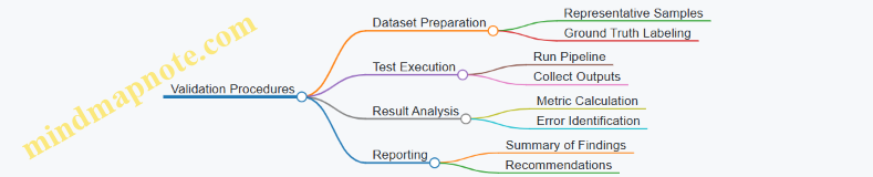
Example: Validating a Lidar-Camera Fusion Pipeline
- Dataset: Use synchronized Lidar and camera data with annotated objects.
- Calibration Check: Verify sensor alignment using checkerboard patterns or calibration targets.
- Run Fusion Algorithm: Combine point clouds with image data for object detection.
- Compare Results: Calculate precision, recall, and IoU against ground truth.
- Stress Test: Introduce partial sensor occlusion and observe detection robustness.
- Report: Document performance metrics and note any failure cases.
This structured approach ensures the perception pipeline is not only accurate but also reliable under different conditions.
Summary
Testing and validation protocols are a backbone of spatial computing development. They provide measurable evidence of system capabilities and highlight areas needing improvement. By combining clear objectives, appropriate metrics, and systematic procedures, developers can build perception pipelines that perform consistently in real-world autonomous applications.
13.4 Best Practices for Continuous Performance Monitoring
Continuous performance monitoring is essential to maintain the reliability and accuracy of perception pipelines in autonomous systems. It ensures that the system behaves as expected over time and under varying conditions. Here are key best practices to keep your perception pipeline in check.
Define Clear Metrics
Start by selecting metrics that reflect the core goals of your perception system. Common metrics include:
- Accuracy: How close are detections or classifications to ground truth?
- Precision and Recall: Particularly for object detection and segmentation.
- Latency: Time taken to process sensor data.
- Robustness: Performance under different environmental conditions.
- False Positive/Negative Rates: To understand error types.
Metrics should be tailored to your application. For example, in obstacle detection, false negatives (missed obstacles) might be more critical than false positives.
Automate Data Collection and Evaluation
Set up automated pipelines that regularly collect sensor data and evaluate system outputs against labeled ground truth or reference data. This reduces manual effort and helps catch regressions early.
Use Visualization Tools
Visualizing results helps spot anomalies that raw numbers might miss. Overlay detected objects on images or point clouds, plot error distributions, or track metric trends over time.
Monitor Environmental and Operational Context
Performance can vary with lighting, weather, sensor degradation, or robot speed. Track these contextual factors alongside metrics to diagnose issues effectively.
Establish Thresholds and Alerts
Define acceptable performance ranges. When metrics cross thresholds, trigger alerts for investigation. This keeps the team informed without constant manual checking.
Maintain Version Control and Logging
Track software versions, sensor calibrations, and configuration changes. Detailed logs help correlate performance shifts with system updates.
Periodic Recalibration and Revalidation
Schedule regular recalibration of sensors and revalidation of algorithms to counter drift and environmental changes.
Mind Map: Continuous Performance Monitoring
Example: Monitoring Object Detection Performance
Imagine an autonomous robot navigating a warehouse. The perception pipeline detects boxes and pallets using lidar and vision.
- Metrics: Precision and recall for box detection, latency of detection pipeline.
- Automation: Every night, the system runs a batch evaluation on logged sensor data with annotated ground truth.
- Visualization: A dashboard shows precision and recall trends over the past month, with example frames where detections failed.
- Context: The system logs ambient light levels and robot speed to correlate with detection performance.
- Alerts: If recall drops below 85%, an alert emails the engineering team.
- Version Control: Each evaluation run records the software version and calibration state.
This setup allows the team to spot gradual performance degradation, perhaps caused by sensor misalignment or software updates, and respond before failures occur in the field.
Example: Latency Monitoring in Real-Time Systems
For a drone using lidar and vision to avoid obstacles, latency is critical.
- The system continuously measures processing time from sensor input to output command.
- A rolling average latency is plotted live.
- If latency exceeds a set threshold, the system logs the event and switches to a fallback mode.
This practice ensures timely responses and maintains safety margins.
Summary
Continuous performance monitoring is a mix of clear metric definition, automation, visualization, context awareness, alerting, and disciplined version control. Together, these practices help maintain a perception pipeline that is both reliable and transparent, reducing surprises during operation.
13.5 Example: Evaluating a Perception System on Public Datasets
Evaluating a perception system on public datasets is a practical way to measure its accuracy, robustness, and real-world applicability. Public datasets provide standardized data and ground truth, enabling objective comparison and reproducibility. This example walks through the key steps and considerations when performing such an evaluation.
Step 1: Selecting the Dataset
Choose a dataset that matches your system’s sensor configuration and target environment. For example, if your system uses a 64-beam Lidar and monocular camera in urban settings, pick a dataset with similar sensors and scenarios.
Step 2: Understanding Dataset Structure and Ground Truth
Familiarize yourself with the dataset’s data format, sensor calibration files, and ground truth annotations. Ground truth may include:
- 3D bounding boxes for objects
- Semantic labels for points or pixels
- Precise robot trajectories or poses
Knowing the ground truth format is essential for meaningful evaluation.
Step 3: Preparing Your System’s Output
Your perception system should produce outputs compatible with the dataset’s ground truth. This might mean:
- Formatting detected objects as 3D bounding boxes with class labels
- Generating semantic segmentation maps aligned with images or point clouds
- Producing pose estimates in the dataset’s coordinate frame
Step 4: Defining Evaluation Metrics
Choose metrics that reflect your system’s goals. Common metrics include:
- Precision and Recall: Measure detection correctness and completeness.
- Intersection over Union (IoU): Quantifies overlap between predicted and ground truth bounding boxes or segments.
- Average Precision (AP): Summarizes precision-recall curve for object detection.
- Root Mean Square Error (RMSE): For pose or depth estimation accuracy.
Step 5: Running the Evaluation
Run your system on the dataset sequences and compare outputs to ground truth using the selected metrics. Automate this process to handle multiple sequences efficiently.
Step 6: Analyzing Results
Break down performance by object class, distance, lighting conditions, or other relevant factors. This helps identify strengths and weaknesses.
Mind Map: Evaluation Workflow
Example: Evaluating Object Detection on a Lidar-Camera Dataset
Suppose your system detects vehicles and pedestrians using fused Lidar and camera data. The dataset provides 3D bounding boxes and class labels.
- Format your detections as a list of bounding boxes with class labels and confidence scores.
- Match detections to ground truth using a 3D IoU threshold (e.g., 0.5) to determine true positives.
- Calculate precision and recall at various confidence thresholds.
- Plot the precision-recall curve and compute Average Precision (AP) for each class.
- Analyze failure cases such as missed detections at far distances or false positives near occlusions.
Mind Map: Object Detection Evaluation
Example: Evaluating SLAM Trajectory Accuracy
If your system outputs a trajectory estimate, compare it to the ground truth trajectory using metrics like Absolute Trajectory Error (ATE) and Relative Pose Error (RPE).
- Align estimated and ground truth trajectories using a rigid-body transformation.
- Compute ATE as the RMSE of positional differences.
- Compute RPE to assess local consistency over fixed time intervals.
- Visualize trajectories to spot drift or jumps.
Mind Map: Trajectory Evaluation
Tips for Effective Evaluation
- Ensure coordinate frames between your output and ground truth match exactly.
- Use consistent units (meters, degrees) throughout.
- Automate metric computation to avoid human error.
- Document evaluation parameters clearly for reproducibility.
- Consider environmental factors such as lighting or weather when interpreting results.
This example demonstrates how to systematically evaluate a perception system using public datasets. The process involves careful preparation, metric selection, and analysis to gain actionable insights into system performance.
14. Deployment and Real-World Integration
14.1 Hardware Considerations for Autonomous Robots
When designing or selecting hardware for autonomous robots, the choices directly influence the effectiveness of perception pipelines, system reliability, and operational efficiency. This section covers the main hardware components, their roles, and practical considerations, illustrated with mind maps and examples.
Key Hardware Components
- Sensors: Lidar units, cameras, IMUs (Inertial Measurement Units), GPS, ultrasonic sensors.
- Processing Units: CPUs, GPUs, FPGAs, embedded systems.
- Power Supply: Batteries, power management units.
- Communication Interfaces: Wired (Ethernet, CAN bus), wireless (Wi-Fi, 5G).
- Mechanical Structure: Mounting points, vibration isolation, environmental protection.
Mind Map: Hardware Components Overview
Sensors
Lidar: Provides accurate 3D spatial data. Consider range, resolution, scanning pattern, and refresh rate. For example, a 16-beam lidar is often sufficient for indoor navigation, while 64-beam units suit outdoor autonomous driving.
Cameras: Offer rich color and texture information. Choose between monocular, stereo, or RGB-D cameras depending on depth requirements. For instance, stereo cameras can provide depth without active illumination, useful in well-lit environments.
IMU: Measures acceleration and rotation, critical for motion estimation and sensor fusion.
GPS: Useful outdoors for global positioning but unreliable indoors.
Ultrasonic Sensors: Simple and cost-effective for short-range obstacle detection.
Example: A warehouse robot might combine a 2D lidar for obstacle detection, a monocular camera for barcode reading, and an IMU for dead reckoning.
Processing Units
Processing hardware must balance computational power, energy consumption, and physical size.
- CPU: General-purpose, handles control logic and moderate perception tasks.
- GPU: Accelerates parallel tasks like image processing and neural networks.
- FPGA: Offers customizable hardware acceleration with low latency.
- Embedded Systems: Compact and energy-efficient, suitable for constrained environments.
Example: An autonomous drone might use an embedded ARM CPU for flight control and an onboard GPU for real-time image segmentation.
Power Supply
Battery capacity and power management affect operational time and system stability. High-performance sensors and processors consume more power, so hardware selection must consider energy budgets.
Example: A delivery robot operating for 8 hours requires batteries sized to support peak power draw plus a safety margin.
Communication Interfaces
Reliable data transfer between sensors, processors, and actuators is essential.
- Wired: Ethernet offers high bandwidth and low latency, common in industrial robots.
- Wireless: Provides flexibility but may introduce latency and interference.
Example: A mobile robot may use CAN bus for motor control and Wi-Fi for remote monitoring.
Mechanical Structure
Physical mounting affects sensor accuracy and durability.
- Ensure sensors are rigidly fixed to maintain calibration.
- Use vibration dampers to reduce noise in IMU and lidar data.
- Protect hardware from dust, moisture, and impacts.
Example: Mounting a lidar on a gimbal can stabilize scanning in bumpy terrains.
Mind Map: Sensor Selection Considerations
Integration Example: Autonomous Delivery Robot Hardware Setup
- Sensors: 16-beam lidar (for obstacle detection), stereo camera (for depth and object recognition), IMU (for pose estimation).
- Processing: Embedded CPU for control, GPU for vision processing.
- Power: Lithium-ion battery sized for 6-hour operation.
- Communication: Ethernet for internal sensor data, Wi-Fi for cloud connectivity.
- Mechanical: Vibration-isolated sensor mounts, weatherproof housing.
This setup balances cost, performance, and operational needs for urban delivery.
Hardware choices shape the perception pipeline’s capabilities and constraints. Understanding each component’s role and trade-offs helps build reliable autonomous robots tailored to their tasks.
14.2 Software Frameworks and Middleware
In autonomous robotics, software frameworks and middleware form the backbone of perception pipelines. They provide the structure and tools to handle sensor data, manage communication between components, and facilitate real-time processing. Choosing the right framework can simplify development, improve maintainability, and ensure scalability.
What Are Software Frameworks and Middleware?
- Software Frameworks are collections of libraries and tools designed to help build applications by providing reusable components and standard ways to solve common problems.
- Middleware acts as a bridge between different software components or between hardware and software, managing communication, data exchange, and sometimes computation.
In spatial computing, middleware often handles sensor data streaming, synchronization, and inter-process communication.
Key Features to Look For
- Modularity: Ability to add, remove, or replace components without disrupting the entire system.
- Real-time capabilities: Support for low-latency data processing and deterministic behavior.
- Multi-sensor support: Built-in tools for handling Lidar, cameras, IMUs, and other sensors.
- Communication protocols: Efficient message passing, often with publish-subscribe patterns.
- Cross-platform compatibility: Runs on various operating systems and hardware architectures.
Common Framework Components
Examples of Frameworks and Middleware
-
Robot Operating System (ROS)
- Provides a modular architecture with nodes communicating via topics and services.
- Supports sensor drivers for Lidar and cameras.
- Offers tools for visualization (RViz) and simulation (Gazebo).
- Best practice: Use ROS message filters to synchronize multi-sensor data streams.
-
ROS 2
- Designed for real-time and embedded systems.
- Uses DDS (Data Distribution Service) for scalable communication.
- Supports Quality of Service (QoS) settings to tune reliability and latency.
- Example: Adjust QoS profiles to prioritize Lidar data over less critical sensor streams.
-
Lidar-specific Middleware
- Some Lidar manufacturers provide SDKs and middleware tailored to their sensors.
- These often include calibration tools and optimized data processing pipelines.
- Best practice: Integrate manufacturer middleware with your main framework to leverage optimized drivers.
-
Computer Vision Libraries
- OpenCV is widely used for image processing tasks.
- Can be integrated into larger frameworks for feature extraction and object detection.
- Example: Use OpenCV within ROS nodes to process camera images in real time.
Integrating Middleware in Perception Pipelines
Practical Example: Setting Up a Middleware Pipeline
Suppose you have a robot equipped with a 3D Lidar and stereo cameras. You want to build a perception pipeline that fuses data for mapping and obstacle detection.
- Step 1: Use ROS 2 to create nodes for each sensor.
- Step 2: Employ message filters to synchronize Lidar point clouds with stereo images based on timestamps.
- Step 3: Process Lidar data in one node to filter noise and extract features.
- Step 4: Process stereo images in another node to generate depth maps.
- Step 5: Fuse the processed data in a dedicated node that aligns point clouds with image-based semantic information.
- Step 6: Publish fused data for downstream modules like mapping and navigation.
This modular approach keeps components independent, making debugging and upgrades easier.
Best Practices
- Keep nodes focused: Each node should handle a specific task to reduce complexity.
- Use standardized message types: This improves interoperability and reduces conversion overhead.
- Monitor system performance: Middleware often provides tools to track latency and throughput.
- Handle sensor failures gracefully: Design middleware to detect and manage sensor dropouts without crashing.
- Document interfaces: Clear definitions of topics, services, and message formats help team collaboration.
Middleware and software frameworks are not just plumbing; they shape how perception pipelines evolve and perform. Selecting and using them wisely can save time and headaches down the road.
14.3 Real-Time Processing and Resource Management
Real-time processing is a cornerstone for autonomous robots relying on lidar and computer vision. The system must handle incoming sensor data, process it, and produce actionable outputs within strict time constraints. Resource management is the balancing act that ensures this happens efficiently without overloading the hardware.
Key Considerations in Real-Time Processing
- Latency: The delay between sensor data capture and system response. Lower latency improves responsiveness but often demands more computing power.
- Throughput: The volume of data processed per unit time. High throughput is necessary for dense lidar scans and high-resolution images.
- Determinism: Predictability in processing times. Systems should avoid unpredictable spikes that can cause missed deadlines.
- Prioritization: Critical tasks (e.g., obstacle detection) must be prioritized over less time-sensitive ones (e.g., map updating).
Resource Management Challenges
- CPU and GPU Load: Balancing workloads between processors to prevent bottlenecks.
- Memory Usage: Managing limited RAM to store sensor data, intermediate results, and models.
- Power Consumption: Especially important for mobile robots with limited battery life.
- Bandwidth: Handling data transfer rates between sensors and processors.
Mind Map: Real-Time Processing Components
Mind Map: Resource Management Strategies
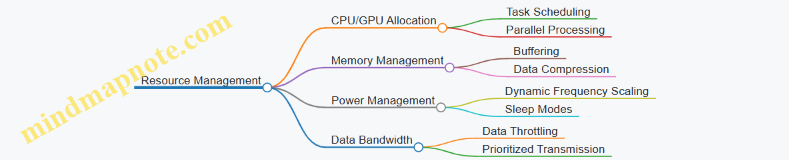
Practical Examples
Example 1: Prioritizing Obstacle Detection Over Mapping
In a mobile robot, obstacle detection must happen faster than map updates. The system can assign higher CPU priority to the obstacle detection thread. Meanwhile, mapping runs at a lower priority or less frequently. This ensures the robot reacts quickly to immediate hazards without sacrificing map quality over time.
Example 2: Using GPU for Parallel Feature Extraction
Feature extraction from images and point clouds can be computationally heavy. Offloading these tasks to the GPU allows parallel processing of multiple data points simultaneously. For instance, running convolutional neural networks on the GPU accelerates image segmentation, freeing the CPU for other tasks.
Example 3: Buffering and Data Throttling
Lidar sensors can produce millions of points per second. To avoid overwhelming the processor, the system can buffer incoming data and process it in chunks. If the processing lags, data throttling reduces the rate of incoming data temporarily, preventing system overload.
Example 4: Dynamic Resource Allocation Based on Task Load
The robot monitors CPU and memory usage in real time. When resource usage spikes, non-critical tasks like logging or map refinement are paused or slowed. This dynamic adjustment keeps critical perception functions running smoothly.
Summary
Real-time processing and resource management require careful balancing of speed, accuracy, and hardware limits. Prioritizing tasks, leveraging parallelism, managing memory, and controlling data flow are all essential. These strategies ensure that autonomous robots can perceive and react to their environments reliably and efficiently.
14.4 Best Practices for Robust Field Deployment
Robust field deployment of perception pipelines for autonomous robots requires careful planning and attention to practical details. The goal is to ensure the system performs reliably outside controlled environments, where unpredictable factors come into play. Here are key best practices to consider:
Sensor Protection and Maintenance
- Physical protection: Use durable housings and covers to shield sensors from dust, moisture, and impacts. Lidar units and cameras are sensitive to dirt and scratches, which degrade data quality.
- Regular cleaning: Establish a routine for cleaning sensor lenses and windows. Even small smudges can cause significant perception errors.
- Environmental considerations: Account for temperature extremes and vibrations. Choose sensors rated for the expected conditions.
Robust Calibration Procedures
- Field calibration: Perform quick calibration checks on-site to catch shifts caused by vibrations or minor collisions.
- Automated calibration aids: Use software tools that can recalibrate or verify calibration during operation.
- Calibration logging: Keep records of calibration states to track sensor health over time.
Data Quality Monitoring
- Real-time diagnostics: Implement monitoring of sensor data quality metrics such as point cloud density, image sharpness, and signal-to-noise ratio.
- Alert systems: Set thresholds that trigger alerts when data quality drops below acceptable levels.
- Fallback strategies: Design perception pipelines to handle degraded data gracefully, for example by switching to alternate sensors or modes.
Software Robustness and Fail-Safes
- Modular design: Build perception components so failures in one module don’t crash the entire system.
- Watchdog timers: Use watchdogs to detect and recover from software hangs or crashes.
- Graceful degradation: Allow the system to reduce functionality rather than fail completely when encountering issues.
Environmental Adaptation
- Dynamic parameter tuning: Adjust processing parameters based on environmental conditions, such as lighting or weather.
- Scene understanding: Use semantic information to ignore irrelevant or misleading data (e.g., reflections, shadows).
Power and Resource Management
- Energy-efficient processing: Optimize algorithms to reduce power consumption, especially for battery-operated robots.
- Resource monitoring: Track CPU, memory, and network usage to prevent overloads that can cause dropped data or delays.
Testing and Validation in Real Conditions
- Incremental deployment: Start with simple, controlled environments and gradually move to more complex scenarios.
- Scenario coverage: Test under different lighting, weather, and terrain conditions.
- Performance logging: Collect detailed logs during field tests to analyze failures and improve robustness.
Mind Map: Key Areas for Robust Field Deployment
Example: Deploying a Perception Pipeline on a Delivery Robot
Imagine a delivery robot navigating urban sidewalks. To ensure robust perception:
- The lidar and cameras are enclosed in weatherproof casings with transparent covers that can be easily wiped.
- Before each deployment, a quick calibration check runs automatically to verify sensor alignment.
- The system continuously monitors point cloud density and image clarity; if dust buildup is detected, the robot alerts maintenance.
- The perception software is modular; if the camera feed fails, the lidar-only mode activates to maintain obstacle detection.
- Parameters like exposure and filtering adjust automatically as the robot moves from bright sunlight to shaded areas.
- CPU and memory usage are tracked to avoid overloads, ensuring real-time processing remains stable.
- Initial tests occur on quiet campus grounds before moving to busy city streets, with logs reviewed after each run to refine the system.
This approach balances technical rigor with practical constraints, helping the robot operate reliably in the real world.
14.5 Example: Deploying a Perception Pipeline on a Mobile Robot Platform
Deploying a perception pipeline on a mobile robot platform involves several concrete steps that connect sensor data acquisition, processing, and actionable output for navigation or mapping. This example walks through a typical deployment scenario, emphasizing practical considerations and clear workflows.
Step 1: Define the Robot Platform and Sensor Setup
Start by specifying the hardware configuration. For this example, the robot is equipped with a 16-beam Lidar sensor mounted on top, a forward-facing RGB camera, an onboard computer (e.g., an NVIDIA Jetson or Intel NUC), and an IMU for inertial measurements.
-
Sensors:
- Lidar: Velodyne VLP-16
- Camera: 1080p RGB, 30 FPS
- IMU: 6-axis inertial measurement
-
Compute:
- CPU: Quad-core, 2.5 GHz
- GPU: CUDA-capable for vision processing
Step 2: Sensor Calibration and Synchronization
Before running the pipeline, calibrate the sensors:
- Intrinsic calibration for the camera (lens distortion, focal length).
- Extrinsic calibration between Lidar and camera to align coordinate frames.
- Time synchronization to ensure sensor data corresponds to the same time frame.
This ensures that data fusion later in the pipeline is accurate.
Step 3: Data Acquisition and Preprocessing
The pipeline begins by collecting raw data streams:
- Lidar point clouds are filtered to remove noise and downsampled for efficiency.
- Camera images undergo undistortion and color correction.
- IMU data is integrated to assist in pose estimation.
Step 4: Perception Pipeline Components
The core pipeline consists of:
- Lidar Processing: Segmentation to identify obstacles and ground plane.
- Vision Processing: Object detection and semantic segmentation.
- Sensor Fusion: Project Lidar points into the camera frame to combine semantic labels with 3D points.
- Localization: Using SLAM algorithms that integrate Lidar and IMU data.
Step 5: Integration with Robot Control
The processed perception data feeds into the robot’s navigation stack:
- Obstacle maps inform path planning algorithms.
- Detected objects trigger behavior modules (e.g., stop for pedestrians).
Mind Map: Perception Pipeline Deployment Overview
Example: Deploying the Pipeline
Consider a warehouse robot tasked with navigating aisles while avoiding obstacles.
- Setup: Mount sensors and connect to onboard computer.
- Calibration: Use checkerboard patterns for camera calibration and calibration targets for Lidar-camera extrinsics.
- Run Data Collection: Start streaming sensor data and verify synchronization.
- Launch Pipeline: Start perception modules in ROS (Robot Operating System) nodes.
- Monitor Outputs: Visualize point clouds with semantic labels and detected objects.
- Test Navigation: Command the robot to move; perception data updates the map and triggers obstacle avoidance.
Mind Map: Example Deployment Workflow
Practical Tips
- Resource Management: Ensure the onboard computer can handle the computational load; consider downsampling or limiting frame rates if necessary.
- Latency: Monitor end-to-end latency from sensor capture to control output; excessive delay can impair navigation.
- Robustness: Implement watchdog timers and fallback behaviors in case perception modules fail or produce inconsistent data.
- Logging: Record sensor data and pipeline outputs for offline analysis and debugging.
Summary
Deploying a perception pipeline on a mobile robot requires careful coordination of hardware setup, sensor calibration, data processing, and integration with control systems. By following a structured workflow and verifying each step with concrete examples, the pipeline can reliably support autonomous navigation and mapping tasks.
15. Troubleshooting and Optimization
15.1 Common Issues in Lidar and Vision Pipelines
When working with lidar and computer vision pipelines, certain issues tend to recur. Recognizing these problems early can save time and improve system reliability. Below is a structured overview of common challenges, accompanied by examples and mind maps to clarify their relationships.
Sensor Noise and Data Quality
Lidar and cameras both produce data that can be noisy or incomplete. Noise in lidar data often appears as random points scattered away from surfaces, while vision data can suffer from poor lighting or motion blur.
- Lidar Noise Sources: atmospheric interference, reflective surfaces, sensor hardware limitations.
- Vision Noise Sources: low light, sensor noise, motion blur, lens distortion.
Example: A lidar sensor scanning a rainy street may return spurious points from raindrops, causing false obstacles in the map.
Calibration Errors
Incorrect intrinsic or extrinsic calibration leads to misalignment between sensors. This causes fused data to be inconsistent, affecting downstream tasks like object detection or mapping.
- Intrinsic calibration errors distort individual sensor data.
- Extrinsic calibration errors misalign sensors spatially.
Example: A camera and lidar mounted on a robot with a few degrees of misalignment will produce point clouds projected incorrectly onto images, confusing semantic labeling.
Synchronization Issues
Temporal mismatch between sensors results in data that does not correspond to the same moment in time. Moving objects appear in different positions, complicating fusion.
Example: A fast-moving vehicle captured by a camera at time t and lidar at time t+100ms will appear shifted, causing tracking errors.
Data Sparsity and Occlusion
Lidar point clouds are often sparse compared to images, and both sensors can miss parts of the environment due to occlusions.
- Sparse data can hinder feature extraction.
- Occlusions cause incomplete object representations.
Example: A pedestrian partially hidden behind a parked car may be visible in the camera but only partially detected by lidar.
Environmental Conditions
Lighting changes, weather, and surface reflectivity affect sensor performance.
- Cameras struggle in low light or glare.
- Lidar performance degrades in rain, fog, or dust.
Example: Direct sunlight can cause camera images to saturate, while fog can scatter lidar beams, reducing effective range.
Computational Load and Latency
Processing high volumes of lidar points and high-resolution images in real time is demanding.
- Excessive latency can make perception outdated.
- Resource constraints limit algorithm complexity.
Example: Running a dense semantic segmentation on a 4K camera feed alongside lidar processing may exceed onboard computer capabilities.
Algorithmic Limitations
Algorithms may fail under certain conditions or assumptions.
- Feature detectors may not be robust to scale or viewpoint changes.
- Segmentation algorithms might misclassify objects in cluttered scenes.
Example: A planar surface extraction algorithm might mistake a glass window for empty space due to low lidar returns.
Mind Maps
Mind Map 1: Sensor Data Issues
Mind Map 2: Temporal and Environmental Factors
Mind Map 3: System and Algorithmic Challenges
Example Scenario: Diagnosing a Perception Pipeline Problem
A mobile robot’s perception pipeline reports frequent false positives for obstacles. Investigation reveals:
- Lidar data contains noise spikes due to reflective surfaces.
- Camera images are slightly out of sync with lidar scans.
- Calibration between sensors is off by a few centimeters.
Addressing these issues involved:
- Applying statistical outlier removal filters on lidar data.
- Implementing hardware-level timestamp synchronization.
- Performing a full extrinsic calibration using checkerboard patterns.
After these fixes, false positives dropped significantly, improving navigation safety.
Understanding these common issues helps in designing more robust perception pipelines and troubleshooting problems effectively.
15.2 Debugging Sensor Data and Algorithms
Debugging sensor data and perception algorithms is a crucial step in ensuring reliable spatial computing systems. Problems often arise from sensor noise, miscalibration, timing issues, or algorithmic assumptions that don’t hold in real-world conditions. This section breaks down common debugging strategies, illustrated with examples and mind maps to clarify the process.
Understanding Sensor Data Issues
Sensor data problems can manifest as missing points, distorted images, misaligned frames, or inconsistent measurements. The first step is to isolate whether the issue originates from the sensor hardware, data acquisition pipeline, or the processing algorithm.
Mind Map: Debugging Sensor Data Issues
Example: A lidar sensor returns sparse point clouds intermittently. Checking the hardware reveals a loose cable connection causing intermittent data loss. Tightening the connection resolves the issue.
Visualizing Raw Data
Before diving into algorithm debugging, visualize raw sensor data. For lidar, use point cloud viewers to inspect density, distribution, and noise. For cameras, display raw images to check exposure, focus, and distortion.
Mind Map: Visualization Steps
Example: A camera image appears washed out. Adjusting exposure settings in the acquisition software improves image quality, which in turn enhances feature detection downstream.
Checking Calibration and Synchronization
Misalignment between sensors often causes errors in fused perception. Verify intrinsic calibration (within a sensor) and extrinsic calibration (between sensors). Also, confirm timestamps are synchronized to avoid temporal mismatches.
Mind Map: Calibration and Synchronization Checks
Example: A fused point cloud appears shifted relative to the camera image. Re-running extrinsic calibration using checkerboard patterns and lidar reflectors corrects the spatial offset.
Algorithmic Debugging
Once sensor data quality is confirmed, focus shifts to the algorithms. Common issues include incorrect assumptions, parameter tuning errors, or unexpected input data.
Mind Map: Algorithm Debugging Workflow
Example: A segmentation algorithm fails to detect objects in low-light images. Testing with brighter images and adjusting contrast normalization parameters improves detection rates.
Logging and Automated Tests
Maintain detailed logs of sensor readings, timestamps, and algorithm outputs. Automated tests that feed known inputs and verify expected outputs help catch regressions early.
Mind Map: Logging and Testing
Example: An intermittent failure in object tracking is traced to dropped data packets logged during operation. Adding packet loss handling in the algorithm improves robustness.
Practical Debugging Example: Tracking a Moving Object
- Symptom: The tracked object’s position jitters erratically.
- Step 1: Visualize raw lidar and camera data to confirm sensor inputs are stable.
- Step 2: Check calibration between lidar and camera; find a small rotational offset.
- Step 3: Verify timestamps; discover a 50 ms lag between sensors.
- Step 4: Adjust synchronization and recalibrate extrinsics.
- Step 5: Tune tracking filter parameters to smooth position estimates.
- Result: Object tracking stabilizes with reduced jitter.
Summary
Debugging sensor data and algorithms requires a systematic approach: start with raw data inspection, verify calibration and synchronization, validate algorithm inputs and parameters, and maintain thorough logs. Visual tools and incremental testing help isolate issues efficiently. Keeping these steps in mind reduces guesswork and accelerates problem resolution.
15.3 Optimization Techniques for Speed and Accuracy
Optimizing perception pipelines requires balancing computational speed with the precision of results. Faster processing enables real-time responses, but cutting corners can degrade accuracy. Conversely, highly accurate methods often demand more resources and time. This section outlines practical techniques to improve both aspects without compromising either unnecessarily.
Mind Map: Key Optimization Areas
Algorithmic Efficiency
Choosing the right algorithms and data structures can drastically reduce runtime. For example, using kd-trees or voxel grids for nearest neighbor searches in point clouds speeds up queries compared to brute force methods. Approximate nearest neighbor algorithms can further cut computation time with minimal accuracy loss.
Example: When segmenting a large point cloud, applying a voxel grid filter first reduces points by averaging within each voxel. This lowers the number of points processed downstream, accelerating segmentation without significant detail loss.
Parallelizing independent tasks also improves throughput. Many Lidar and vision algorithms lend themselves to parallel execution, such as feature extraction on image patches or point clusters.
Data Reduction
Reducing the amount of data processed is a straightforward way to speed up pipelines. Downsampling point clouds or images removes redundant information. Selecting regions of interest (ROIs) focuses computation on relevant areas, avoiding wasted effort on irrelevant data.
Example: In autonomous driving, limiting object detection to the road area rather than the entire image cuts processing time. Similarly, cropping point clouds to a bounding box around the vehicle’s immediate surroundings reduces data volume.
Feature selection techniques help by retaining only the most informative features for tasks like classification or tracking. This reduces dimensionality and speeds up machine learning models.
Hardware Utilization
Leveraging hardware capabilities is essential for real-time performance. GPUs excel at parallel operations common in image and point cloud processing. Multi-threading on CPUs allows simultaneous execution of pipeline stages.
Example: Running convolutional neural networks for image segmentation on a GPU can reduce inference time from seconds to milliseconds. Similarly, using multiple CPU cores to process different sensor streams concurrently improves overall throughput.
Dedicated processors, such as FPGAs or specialized AI chips, can accelerate specific tasks but require additional development effort.
Pipeline Design
Designing the perception pipeline thoughtfully can avoid unnecessary computation. Early filtering removes noise and irrelevant data before heavier processing. Lazy evaluation delays computation until results are needed, preventing wasted effort.
Modular components enable swapping or tuning individual stages without reworking the entire pipeline. This flexibility helps optimize bottlenecks iteratively.
Example: Implementing a fast ground plane removal step early in the Lidar pipeline reduces points passed to object detection, speeding up that stage.
Combined Example: Optimizing a Lidar-Based Object Detection Pipeline
- Downsample the raw point cloud using a voxel grid filter to reduce point count.
- Apply ROI filtering to focus on the drivable area.
- Use a kd-tree for efficient nearest neighbor searches during segmentation.
- Parallelize feature extraction across CPU cores.
- Run classification models on GPU for faster inference.
- Early remove ground points to reduce clutter.
- Modularize pipeline stages to allow easy tuning.
This approach balances speed and accuracy by cutting data volume, using efficient algorithms, and exploiting hardware.
Optimization is an iterative process. Profiling tools help identify bottlenecks, guiding where to apply these techniques. The goal is a pipeline that meets real-time constraints while maintaining reliable perception quality.
15.4 Best Practices for Maintaining System Reliability
Maintaining system reliability in spatial computing pipelines that use lidar and computer vision requires a structured approach to monitoring, diagnosing, and preventing failures. Reliability means the system consistently performs as expected under varying conditions, without unexpected crashes or degraded outputs. Here are key best practices for achieving this, illustrated with mind maps and examples.
Continuous Health Monitoring
Regularly track sensor status, data quality, and processing pipeline metrics. This helps catch issues early before they cascade into failures.
Example: Set up a dashboard that flags when lidar returns drop below a threshold or when camera frames lag behind expected timing. This lets operators intervene before perception degrades.
Robust Error Handling and Fallbacks
Design the system to handle sensor dropouts or corrupted data gracefully, rather than crashing or producing garbage outputs.
Example: If the camera feed is lost, the system temporarily relies on lidar-only localization until the camera recovers, while logging the event for review.
Regular Calibration Checks
Sensors can drift over time, causing errors in perception. Schedule periodic calibration verification and adjustment.
Example: Run an automated routine that compares detected landmarks from lidar and camera data to verify alignment weekly, alerting if discrepancies exceed thresholds.
Redundancy and Diversity
Incorporate multiple sensors or algorithms that can compensate for each other’s weaknesses.
Example: Use both lidar and stereo vision for obstacle detection, cross-checking results to reduce false positives and negatives.
Resource and Performance Management
Monitor CPU, GPU, and memory usage to prevent overloads that cause dropped frames or slow processing.
Example: When CPU usage spikes, temporarily reduce the frequency of semantic segmentation to maintain real-time responsiveness.
Comprehensive Logging and Diagnostics
Keep detailed logs of sensor inputs, processing steps, and system states to aid troubleshooting.
Example: After a system fault, replay logged lidar and camera data to pinpoint whether the issue originated from sensor noise or algorithm failure.
Incremental Updates and Testing
Deploy changes in small increments with thorough testing to avoid introducing new faults.
Example: Before updating the object detection module, run it on recorded datasets to verify performance and then deploy to a test robot before full rollout.
Summary Mind Map
By following these practices, spatial computing systems can sustain reliable operation in real-world conditions. The key is to anticipate failures, detect them early, and respond without interrupting core functionalities. Examples grounded in real scenarios help illustrate how these principles apply in practice.
15.5 Example: Diagnosing and Fixing Perception Pipeline Bottlenecks
In this example, we will walk through a scenario where an autonomous robot’s perception pipeline is running slower than expected, causing delays in navigation and mapping. We will identify bottlenecks, analyze causes, and apply fixes. The goal is to improve throughput without sacrificing accuracy.
Step 1: Identify Symptoms
- The robot’s point cloud processing lags behind the sensor frame rate.
- Object detection on images takes longer than the sensor capture interval.
- Localization updates are delayed, causing navigation jitter.
These symptoms suggest the pipeline cannot keep up with real-time data flow.
Step 2: Map Out the Pipeline
Perception Pipeline Mind Map
This map helps visualize where delays might accumulate.
Step 3: Profile Each Stage
Use timing tools or logging to measure processing time per stage:
| Stage | Time per Frame (ms) |
|---|---|
| Data Acquisition | 5 |
| Preprocessing | 30 |
| Feature Extraction | 60 |
| Sensor Fusion | 15 |
| Localization & Mapping | 40 |
| Object Detection & Tracking | 80 |
| Output | 10 |
The total is 240 ms per frame, but the sensor frame rate requires processing every 100 ms. Clearly, feature extraction and object detection are the biggest time consumers.
Step 4: Analyze Bottlenecks
Bottleneck Analysis Mind Map
Step 5: Apply Fixes
Feature Extraction:
- Replace complex 3D descriptors with faster alternatives (e.g., FPFH to SHOT).
- Use spatial data structures like KD-Trees for neighbor searches.
- Parallelize feature computation using multi-threading or GPU.
Object Detection & Tracking:
- Downscale images moderately to reduce input size.
- Use a smaller or optimized neural network model.
- Enable hardware acceleration (e.g., GPU or TPU).
Step 6: Re-profile After Fixes
| Stage | Time per Frame (ms) |
|---|---|
| Data Acquisition | 5 |
| Preprocessing | 25 |
| Feature Extraction | 25 |
| Sensor Fusion | 15 |
| Localization & Mapping | 35 |
| Object Detection & Tracking | 30 |
| Output | 10 |
Total processing time is now 145 ms per frame. This is a significant improvement, though still above the 100 ms target. Further tuning or hardware upgrades may be needed.
Step 7: Verify Accuracy and Stability
After optimization, verify that:
- Feature extraction still produces reliable descriptors.
- Object detection maintains acceptable precision and recall.
- Localization remains stable without jitter.
If accuracy drops, consider balancing speed and quality by adjusting parameters.
Summary Mind Map
This example shows that diagnosing bottlenecks requires systematic measurement and targeted fixes. Optimizing perception pipelines is often a trade-off between speed and accuracy, and understanding the pipeline’s structure is key to effective troubleshooting.
16. Case Studies and Practical Applications
16.1 Autonomous Driving Perception Pipelines
Autonomous driving relies heavily on perception pipelines that process data from multiple sensors to understand the vehicle’s surroundings. These pipelines transform raw sensor inputs into actionable information for decision-making and control. The core sensors typically include lidar, cameras, radar, and sometimes ultrasonic sensors, but this section focuses on lidar and computer vision components.
Key Components of an Autonomous Driving Perception Pipeline
- Sensor Data Acquisition: Collecting raw data from lidar and cameras.
- Preprocessing: Filtering noise, correcting distortions, and synchronizing data.
- Detection: Identifying objects such as vehicles, pedestrians, cyclists, and road features.
- Classification: Assigning semantic labels to detected objects.
- Tracking: Maintaining consistent identities of objects over time.
- Mapping: Building and updating a representation of the environment.
- Localization: Estimating the vehicle’s position within the map.
Each step builds on the previous one, and best practices ensure smooth data flow and accuracy.
Mind Map: Autonomous Driving Perception Pipeline Overview
Sensor Data Acquisition and Preprocessing
Lidar sensors provide 3D point clouds that capture the geometry of the environment with high accuracy. Cameras supply rich color and texture information but lack direct depth measurements. Combining these modalities compensates for their individual limitations.
Preprocessing includes removing outliers from lidar data and correcting lens distortion in images. Synchronizing timestamps is critical to ensure that data from different sensors represent the same moment in time. Calibration aligns the coordinate frames of lidar and cameras, enabling sensor fusion.
Example: A common preprocessing step is voxel grid filtering on lidar data to reduce point cloud density without losing significant detail. This speeds up downstream processing while maintaining spatial accuracy.
Object Detection and Classification
Detection algorithms identify regions of interest in sensor data. For lidar, clustering methods segment point clouds into candidate objects. For images, convolutional neural networks (CNNs) detect bounding boxes around objects.
Classification assigns semantic labels to detected objects. Combining lidar’s 3D shape information with camera imagery improves classification accuracy. For instance, a cluster of points shaped like a pedestrian and matched with a corresponding image region labeled as a person confirms the detection.
Example: Using a fusion-based detector that projects lidar points onto the image plane allows a CNN to process both modalities simultaneously, improving detection in challenging lighting or weather conditions.
Tracking and Data Association
Tracking maintains object identities across frames, which is essential for understanding motion and predicting future states. Common approaches use Kalman filters or particle filters combined with data association algorithms like the Hungarian method to match detections frame-to-frame.
Tracking benefits from fused data: lidar provides precise 3D positions, while vision offers appearance cues. This combination helps maintain tracks even when one sensor’s data is temporarily unreliable.
Example: Tracking a cyclist moving behind a parked car can be maintained by lidar’s 3D continuity, even if the camera view is partially occluded.
Mapping and Localization
Mapping creates a spatial representation of the environment, often in the form of high-definition (HD) maps that include lane markings, traffic signs, and static obstacles. Localization uses this map to determine the vehicle’s precise position.
Lidar-based SLAM algorithms generate point cloud maps by registering consecutive scans. Visual SLAM complements this by tracking visual features. Combining both improves robustness, especially in GPS-denied environments.
Example: An autonomous vehicle uses lidar SLAM to build a 3D map of an urban street and camera data to recognize traffic lights and signs, integrating this information to localize itself within centimeters.
Practical Example: Building a Basic Autonomous Driving Perception Pipeline
- Data Collection: Capture synchronized lidar scans and camera images while driving a test route.
- Preprocessing: Apply voxel grid filtering to lidar data and undistort images.
- Calibration: Use checkerboard patterns and calibration tools to align sensors.
- Detection: Run a clustering algorithm on the lidar point cloud and a CNN on images.
- Fusion: Project lidar clusters onto the image plane to confirm detections.
- Tracking: Implement a Kalman filter to track detected objects frame-to-frame.
- Mapping: Use lidar SLAM to create a local map of the environment.
- Localization: Match current lidar scans to the map to estimate vehicle pose.
This pipeline can be expanded with more advanced algorithms and additional sensors, but it demonstrates the core steps and integration points.
Mind Map: Example Pipeline Workflow
This section highlights how lidar and computer vision combine to form a perception pipeline tailored for autonomous driving. Each step requires attention to detail and adherence to best practices to ensure reliability and accuracy in real-world scenarios.
16.2 Robotics in Warehouse and Industrial Environments
Warehouse and industrial settings present a unique set of challenges and opportunities for spatial computing using lidar and computer vision. These environments are typically structured but dynamic, with a mix of static infrastructure and moving objects such as forklifts, pallets, and human workers. Autonomous robots operating here must perceive their surroundings accurately to navigate safely, optimize workflows, and interact with objects.
Key Perception Tasks in Industrial Robotics
- Localization and Mapping: Robots need precise localization within often large and complex indoor spaces. Mapping helps create a spatial understanding of aisles, shelves, and workstations.
- Obstacle Detection and Avoidance: Dynamic obstacles like humans and vehicles require real-time detection and path adjustment.
- Object Recognition and Manipulation: Identifying and locating items such as boxes or tools is essential for picking and placing tasks.
- Environment Monitoring: Continuous perception supports safety and operational efficiency.
Mind Map: Core Perception Components in Warehouse Robotics
Lidar and Vision Integration
Lidar sensors provide accurate 3D spatial data, which is invaluable for mapping and obstacle detection. However, lidar alone may struggle with object classification or reading labels. Cameras complement lidar by capturing rich visual information, enabling recognition of text, colors, and textures.
Best practice involves tightly synchronizing lidar and camera data streams and calibrating their relative poses. This fusion allows robots to build detailed semantic maps where geometry and object identity coexist.
Example: Autonomous Pallet Transport Robot
Consider a robot tasked with moving pallets between storage racks and loading docks. It uses a 16-beam lidar to scan its surroundings and a stereo camera pair for visual input.
- Mapping: The robot runs a lidar-based SLAM algorithm to generate a 3D map of the warehouse layout.
- Localization: It localizes itself within this map using scan matching and visual landmarks.
- Obstacle Avoidance: Dynamic obstacles like forklifts are detected by combining lidar point cloud clustering and camera-based object detection.
- Pallet Identification: The stereo cameras identify pallets by shape and barcode labels, confirming the correct item before pickup.
This pipeline ensures the robot navigates efficiently and handles objects accurately.
Mind Map: Perception Pipeline for Pallet Transport Robot
Handling Environmental Challenges
Warehouses often have reflective surfaces, narrow aisles, and varying lighting conditions. Lidar can be affected by reflective floors or glass, causing noisy returns. Cameras may struggle with shadows or glare.
Best practices include:
- Using sensor-specific filters to remove spurious lidar points.
- Employing adaptive exposure and image enhancement techniques for cameras.
- Incorporating redundancy by combining multiple sensor modalities.
Example: In a scenario where a shiny metal shelf causes lidar noise, the system can rely more on visual cues for obstacle detection in that area.
Safety and Human Interaction
Robots must detect and respond to humans reliably. Combining lidar’s range accuracy with vision’s semantic understanding helps identify people and predict their movements.
Best practice involves setting safety zones around detected humans and slowing or stopping the robot accordingly. Continuous monitoring ensures compliance with workplace safety standards.
Example: A robot detects a worker entering its path using lidar clustering and confirms the presence with a vision-based human detector before halting.
Example: Inventory Inspection Robot
An autonomous robot equipped with a high-resolution lidar and RGB-D camera inspects inventory on shelves.
- 3D Reconstruction: The lidar builds a detailed 3D model of shelf geometry.
- Visual Inspection: The RGB-D camera captures images for identifying damaged or misplaced items.
- Semantic Mapping: The system tags shelf locations with item categories.
This approach improves inventory accuracy and reduces manual labor.
Mind Map: Inventory Inspection Perception Workflow
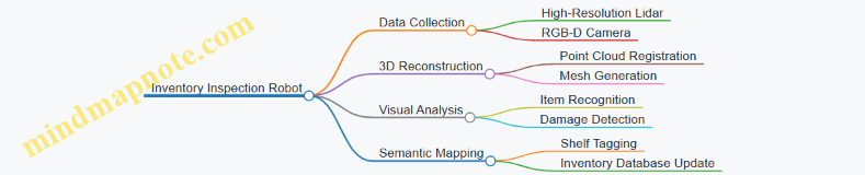
In summary, spatial computing in warehouse and industrial robotics relies on the complementary strengths of lidar and computer vision. Integrating these sensors with robust perception pipelines enables robots to navigate complex environments, interact safely with humans, and perform tasks like transport and inspection effectively. Practical examples and mind maps help clarify how these components fit together in real-world applications.
16.3 Mapping and Surveying with Lidar and Vision
Mapping and surveying are foundational tasks in spatial computing, providing detailed representations of environments for applications ranging from construction to environmental monitoring. Combining lidar and computer vision enhances accuracy, completeness, and semantic richness of maps. This section covers practical approaches, workflows, and examples to build effective mapping and surveying pipelines.
Core Components of Mapping and Surveying
- Data Acquisition: Collecting raw lidar point clouds and images.
- Preprocessing: Filtering noise, aligning sensor data.
- Registration: Aligning multiple scans or images into a unified coordinate frame.
- Reconstruction: Creating 3D models or maps from registered data.
- Semantic Annotation: Adding labels or classifications to map elements.
Mind Map: Mapping and Surveying Workflow
Data Acquisition
Lidar sensors provide precise distance measurements, capturing detailed 3D geometry. Cameras add color and texture, which help interpret the scene. For surveying, it’s important to plan sensor placement and movement to cover the area comprehensively. Overlapping scans and images improve registration and reduce gaps.
Best Practice: Use a combination of static scans and mobile scanning (e.g., handheld or drone-mounted sensors) to balance detail and coverage.
Example: Surveying a construction site with a terrestrial lidar scanner for structural details, supplemented by aerial images for context.
Preprocessing
Raw lidar data often contains noise from reflective surfaces or environmental conditions. Images may suffer from lighting variations or motion blur. Preprocessing steps include:
- Removing outliers from point clouds.
- Downsampling to reduce data size while preserving features.
- Correcting lens distortion in images.
- Synchronizing timestamps between lidar and camera data.
Best Practice: Automate filtering with adjustable thresholds to adapt to different environments.
Example: Applying a statistical outlier removal filter on point clouds collected in a forested area to eliminate stray points caused by leaves.
Registration
Aligning multiple scans or images is critical for building a coherent map. Common methods include:
- ICP (Iterative Closest Point): Aligns point clouds by minimizing distances between corresponding points.
- Feature-Based Matching: Uses distinctive features (corners, edges) detected in both lidar and images.
Combining lidar and vision features improves robustness, especially in feature-poor environments.
Best Practice: Start with coarse alignment using GPS or odometry, then refine with ICP or feature matching.
Example: Registering consecutive lidar scans of a tunnel using planar features, then refining alignment with camera-based feature correspondences.
Reconstruction
Once data is registered, the next step is to reconstruct surfaces or volumetric models:
- Point Cloud Merging: Combine overlapping scans into a single dataset.
- Surface Reconstruction: Generate meshes or volumetric grids representing surfaces.
Color information from images can be projected onto the 3D model to enhance visualization.
Best Practice: Use adaptive meshing techniques to balance detail and computational load.
Example: Creating a textured 3D model of a historic building by merging lidar scans and projecting high-resolution photographs.
Semantic Annotation
Adding semantic labels helps interpret the map beyond geometry:
- Classify regions as ground, vegetation, buildings, water, etc.
- Detect and label objects like poles, vehicles, or signage.
Combining lidar’s geometric precision with vision’s texture and color cues improves classification accuracy.
Best Practice: Use machine learning models trained on combined lidar and image features.
Example: Segmenting a city block into roads, sidewalks, and trees using fused lidar and camera data.
Example Workflow: Surveying a Park
- Plan sensor routes to cover paths, open areas, and dense vegetation.
- Collect data using a mobile lidar unit and synchronized cameras.
- Preprocess data by filtering noise and correcting image distortions.
- Register scans using GPS for initial alignment, refined with ICP.
- Merge point clouds and reconstruct surfaces.
- Project images onto the model for color.
- Classify regions into grass, trees, benches, and water features.
- Export map for use in park maintenance or visitor apps.
Mind Map: Semantic Annotation Process

Mapping and surveying with lidar and vision is a multi-step process that benefits from integrating complementary sensor strengths. Clear planning, careful preprocessing, and methodical registration lead to accurate reconstructions. Adding semantic layers turns raw data into actionable maps. Practical examples demonstrate how these steps come together in real-world scenarios.
16.4 Best Practices Derived from Industry Deployments
Industry deployments of spatial computing systems using lidar and computer vision have provided a wealth of practical insights. These best practices stem from real-world constraints and operational demands, offering guidance that balances technical rigor with field realities.
Calibration and Maintenance
Maintaining sensor calibration is non-negotiable. Frequent recalibration schedules prevent drift that can accumulate from vibrations, temperature changes, or minor impacts. Automated calibration checks embedded in the system can flag deviations early, reducing downtime.
- Mind Map: Calibration and Maintenance
Example: A logistics robot operating in a dusty warehouse environment implemented weekly lidar calibration routines combined with daily sensor lens cleaning. This practice reduced mapping errors by 15% and improved obstacle detection reliability.
Data Quality and Filtering
Raw sensor data is noisy and often incomplete. Industry systems apply layered filtering strategies: spatial filtering to remove outliers, temporal filtering to smooth data over time, and semantic filtering to discard irrelevant information. These filters must be tuned to the operational environment to avoid losing critical details.
- Mind Map: Data Quality and Filtering
Example: An autonomous vehicle project used a combination of voxel grid downsampling and temporal median filtering on lidar data to maintain real-time performance without sacrificing detection accuracy in urban traffic.
Sensor Fusion Strategies
Combining lidar and vision data improves perception but requires careful alignment and confidence weighting. Industry deployments favor probabilistic fusion methods that account for sensor uncertainty and environmental conditions. Fusion pipelines often include fallback modes that rely on a single sensor if the other fails or degrades.
- Mind Map: Sensor Fusion Strategies
Example: A delivery robot used a particle filter-based fusion approach, weighting lidar more heavily in low-light conditions and vision more in open, well-lit areas. This adaptability reduced perception errors by 20%.
Real-Time Processing and Latency Management
Industry systems must balance computational load with latency constraints. Prioritizing critical perception tasks and implementing multi-threaded or hardware-accelerated processing helps maintain responsiveness. Data pipelines are designed to discard stale data and avoid bottlenecks.
- Mind Map: Real-Time Processing and Latency Management
Example: An autonomous forklift system prioritized obstacle detection over map updating during navigation, ensuring immediate hazards were processed first. GPU acceleration was used for image segmentation, reducing latency from 150ms to under 50ms.
Robustness to Environmental Variability
Systems deployed outdoors or in industrial settings face changing lighting, weather, and clutter. Best practices include adaptive algorithms that adjust thresholds based on sensor feedback, and robust feature extraction methods less sensitive to environmental noise.
- Mind Map: Robustness to Environmental Variability
Example: A mining robot adjusted its lidar intensity thresholds dynamically to compensate for dust and fog, maintaining reliable obstacle detection where static thresholds failed.
Continuous Monitoring and Logging
Operational deployments benefit from detailed logging of sensor data, system states, and detected anomalies. This data supports troubleshooting, performance tuning, and compliance with safety standards.
- Mind Map: Continuous Monitoring and Logging
Example: A fleet of autonomous delivery robots logged sensor calibration status and perception confidence scores, enabling remote diagnostics that cut maintenance visits by 30%.
Example Summary: Warehouse Robot Deployment
In a warehouse deployment, a robot combined lidar and vision for navigation and inventory scanning. Key best practices included:
- Weekly sensor calibration with automated drift detection
- Multi-layer filtering tuned for indoor lighting and metallic surfaces
- Probabilistic sensor fusion with fallback to lidar-only mode during camera occlusion
- Prioritized real-time obstacle detection with GPU-accelerated vision processing
- Adaptive algorithms to handle reflective floors and varying shelf arrangements
- Continuous logging for performance monitoring and anomaly detection
This approach resulted in a system that balanced accuracy, robustness, and operational uptime effectively.
These best practices reflect the practical lessons learned from industry deployments. They emphasize maintaining sensor integrity, managing data quality, fusing information thoughtfully, and designing systems that remain responsive and robust under real-world conditions.
16.5 Example: End-to-End Perception Pipeline for an Autonomous Delivery Robot
This section walks through a practical example of building a perception pipeline tailored for an autonomous delivery robot operating in an urban environment. The goal is to illustrate how lidar and computer vision components integrate to enable navigation, obstacle avoidance, and environment understanding.
Overview of the Pipeline
The perception pipeline consists of several stages, each responsible for transforming raw sensor data into actionable information:
- Sensor Data Acquisition
- Calibration and Synchronization
- Preprocessing
- Feature Extraction
- Sensor Fusion
- Localization and Mapping
- Object Detection and Tracking
- Environment Understanding
Below is a mind map summarizing these components:
Step 1: Sensor Data Acquisition
The robot is equipped with a 16-beam lidar and a forward-facing RGB camera. The lidar provides 3D point clouds at 10 Hz, while the camera streams 30 FPS images. IMU data is optional but can improve pose estimation.
Best Practice: Ensure sensors have overlapping fields of view to maximize fusion effectiveness. For example, the camera’s field should cover the lidar’s horizontal scan range.
Step 2: Calibration and Synchronization
Accurate spatial and temporal alignment is critical. Intrinsic calibration corrects camera lens distortions. Extrinsic calibration determines the rigid transform between lidar and camera frames.
Example: Use a checkerboard pattern visible to both sensors to estimate extrinsic parameters. Synchronize timestamps using hardware triggers or software interpolation.
Step 3: Preprocessing
Lidar data often contains noise and outliers. Apply voxel grid downsampling to reduce point cloud density while preserving structure. Remove isolated points using radius outlier removal.
Camera images benefit from histogram equalization to improve contrast under varying lighting.
Example: Downsample a 100,000-point cloud to 20,000 points for real-time processing without losing key features.
Step 4: Feature Extraction
Extract 3D features such as ISS keypoints and FPFH descriptors from the point cloud. On images, detect ORB features for robustness and speed.
Best Practice: Use features invariant to rotation and scale to handle robot motion and varying viewpoints.
Step 5: Sensor Fusion
Project lidar points onto the camera image plane using the extrinsic calibration matrix and camera intrinsics. This allows associating 3D points with 2D image features.
Example: For a detected pedestrian in the image, identify corresponding lidar points to estimate distance and 3D bounding box.
Sensor Fusion Mind Map
Step 6: Localization and Mapping
Implement a lidar-based SLAM algorithm (e.g., LOAM) to estimate the robot’s pose and build a 3D map. Complement with visual odometry to improve robustness in feature-rich areas.
Best Practice: Fuse IMU data if available to reduce drift during rapid movements.
Step 7: Object Detection and Tracking
Run a lightweight 2D object detector on camera images to identify pedestrians, vehicles, and obstacles. Use lidar data to generate 3D bounding boxes around detected objects.
Track objects over time using a Kalman filter or a more advanced multi-object tracking algorithm.
Example: Detect a cyclist crossing the path; track position and velocity to predict trajectory.
Step 8: Environment Understanding
Perform semantic segmentation on images to classify road, sidewalk, and obstacles. Combine with lidar-based free space estimation to identify navigable areas.
Dynamic obstacles are flagged by detecting moving clusters in consecutive lidar scans.
Integrated Example Flow
- Acquire synchronized lidar and camera data.
- Preprocess both data streams to remove noise.
- Extract features and project lidar points onto images.
- Detect objects in images and associate with 3D points.
- Estimate robot pose via SLAM.
- Track objects and update environment map.
- Identify free space and obstacles for navigation.
End-to-End Pipeline Mind Map
This example highlights how each component contributes to a coherent perception system. The integration of lidar and vision data improves accuracy and robustness, enabling the delivery robot to navigate urban environments safely and efficiently.