Advanced Data Engineering with Real Time Streaming and Lakehouse Architectures
1. Introduction to Real-Time Data Engineering and Lakehouse Architectures
1.1 Understanding Real-Time Data Engineering Concepts
Real-time data engineering focuses on processing and managing data as it arrives, rather than after it has been stored. The goal is to enable immediate insights, actions, or transformations on data streams, often within milliseconds to seconds of data generation. This contrasts with batch processing, where data is collected over a period and processed in chunks.
At its core, real-time data engineering involves several key components:
- Data Ingestion: Capturing data continuously from sources such as sensors, applications, logs, or user interactions.
- Stream Processing: Applying computations, transformations, or enrichments on data as it flows through the system.
- Storage: Efficiently storing processed or raw data for querying, analytics, or archival.
- Delivery: Making processed data available to downstream systems, dashboards, or machine learning models.
Mind Map: Core Components of Real-Time Data Engineering
Why Real-Time?
Real-time processing is essential when the value of data diminishes quickly or when immediate responses are required. Examples include fraud detection, monitoring system health, or updating user experiences dynamically.
Example: Real-Time Clickstream Processing
Imagine an e-commerce website tracking user clicks to personalize recommendations instantly. Each click event is sent to a streaming platform like Kafka. A Spark Structured Streaming job consumes these events, aggregates user behavior over short windows, and updates a recommendation engine in near real-time.
This pipeline involves:
- Producing click events to Kafka topics.
- Spark reading from Kafka, filtering irrelevant events, and aggregating clicks by user.
- Writing aggregated results to a fast-access database.
Mind Map: Real-Time Clickstream Pipeline
Characteristics of Real-Time Data Engineering
- Low Latency: Systems must process and deliver data quickly, often within seconds or less.
- Fault Tolerance: Components should handle failures without data loss or duplication.
- Scalability: Ability to handle varying data volumes and velocity.
- Exactly-Once Processing: Ensuring each event is processed once and only once, avoiding duplicates or missed data.
Example: Exactly-Once Processing with Kafka and Spark
Kafka provides message delivery guarantees, and Spark Structured Streaming supports checkpointing and idempotent writes. Together, they enable pipelines where data is processed exactly once, even if failures occur.
Mind Map: Key Characteristics and Challenges
Handling Late and Out-of-Order Data
In real-time systems, data may arrive late or out of order due to network delays or retries. Techniques like watermarking and windowing help manage this by defining how long the system waits for late data before finalizing results.
Example: Windowing with Watermarks in Spark
Suppose you want to count events per minute, but some events arrive late. Watermarks allow Spark to wait for a defined delay (e.g., 5 minutes) before closing the window, balancing completeness and latency.
Summary
Real-time data engineering is about building systems that ingest, process, and deliver data with minimal delay. It requires careful design around latency, fault tolerance, and data consistency. Understanding these concepts lays the foundation for building scalable, reliable streaming pipelines.
1.2 Overview of Lakehouse Architecture Principles
The lakehouse architecture attempts to combine the best features of data lakes and data warehouses into a single, unified system. It aims to provide the flexibility and scalability of data lakes with the data management and performance features traditionally associated with data warehouses.
At its core, a lakehouse stores data in an open file format on low-cost storage, similar to a data lake. However, it adds a layer of metadata and transactional capabilities that enable ACID (Atomicity, Consistency, Isolation, Durability) transactions, schema enforcement, and indexing. This makes it possible to run reliable, performant analytics directly on the data lake.
Key Principles of Lakehouse Architecture
Storage Layer
The storage layer uses open file formats like Parquet or ORC. These formats are columnar, which helps with compression and query performance. The data is stored on cloud object storage or distributed file systems, which are cost-effective and scalable.
Metadata Layer
This layer tracks the state of the data with a transaction log. It records all changes, enabling features like time travel (querying older versions of data) and rollback. Schema enforcement ensures that data written to the lakehouse conforms to expected structures, preventing silent data corruption.
Compute Layer
The compute layer runs queries and transformations. It supports both batch and streaming workloads, allowing real-time analytics alongside traditional reporting. Engines like Apache Spark or Presto can read directly from the lakehouse storage and metadata layers.
Data Management
Lakehouses support ACID transactions, which means multiple users or jobs can read and write data concurrently without conflicts or data loss. This is a major improvement over traditional data lakes, where concurrent writes often cause issues.
Performance Features
To improve query speed, lakehouses implement indexing, caching, and data skipping. Indexing helps locate relevant data files quickly. Caching stores frequently accessed data in memory. Data skipping avoids scanning irrelevant data based on metadata statistics.
Example: Writing Data with Schema Enforcement
Imagine a streaming pipeline writing user activity logs to a lakehouse. The pipeline writes JSON events to Parquet files stored on S3. The lakehouse metadata layer enforces a schema that requires fields like user_id (string), event_type (string), and timestamp (timestamp).
If a malformed event arrives missing the user_id, the write operation will fail or be rejected, preventing bad data from entering the system. This enforcement happens automatically through the transaction log and schema validation.
Example: Time Travel Queries
Suppose a data engineer accidentally deletes a day’s worth of sales data. With a lakehouse, they can query the transaction log to access the previous version of the data before deletion. For example, a SQL query might look like:
SELECT * FROM sales_table TIMESTAMP AS OF '2023-05-15T10:00:00Z'
This query returns the state of sales_table at the specified timestamp, allowing recovery without restoring from backups.
Mind Map: Lakehouse Components and Features
Summary
The lakehouse architecture bridges the gap between data lakes and warehouses by adding structured management and transactional capabilities to open storage formats. It supports diverse workloads, enforces data quality, and improves performance through metadata-driven optimizations. Understanding these principles is essential for building scalable, reliable data platforms that handle both streaming and batch data efficiently.
1.3 Comparing Traditional Data Warehouses, Data Lakes, and Lakehouses
When working with data storage and analytics, it’s important to understand the distinctions between traditional data warehouses, data lakes, and the more recent lakehouse architecture. Each has its own design goals, strengths, and trade-offs. Below, we’ll explore these differences with clear examples and mind maps to clarify their structure and typical use cases.
Traditional Data Warehouses
A data warehouse is a centralized repository designed to store structured data from multiple sources, optimized for reporting and analysis. It typically enforces a strict schema on write, meaning data must conform to a predefined model before entering the warehouse.
Key characteristics:
- Data is cleaned, transformed, and loaded (ETL) before storage.
- Schema-on-write approach.
- Optimized for SQL queries and business intelligence tools.
- Data is usually stored in relational tables.
Example: A retail company collects sales data from various stores. Before loading into the warehouse, data is cleaned and transformed to fit a star schema. Analysts run SQL queries to generate monthly sales reports.
Mind map:
Data Lakes
Data lakes store raw data in its native format, whether structured, semi-structured, or unstructured. They use a schema-on-read approach, meaning the data’s structure is interpreted only when read. This offers flexibility but can complicate governance and performance.
Key characteristics:
- Stores all types of data (logs, images, JSON, CSV, etc.).
- Schema-on-read allows storing data without upfront modeling.
- Typically built on low-cost object storage (e.g., Amazon S3).
- Supports batch and some streaming ingestion.
Example: A social media platform stores raw user activity logs, images, and videos in a data lake. Data scientists query raw logs directly for exploratory analysis.
Mind map:
Lakehouse Architecture
The lakehouse aims to combine the best of data warehouses and data lakes. It stores data in open formats on low-cost storage like a data lake but adds management features such as ACID transactions, schema enforcement, and indexing, which are typical of data warehouses.
Key characteristics:
- Supports both structured and unstructured data.
- Schema enforcement and evolution capabilities.
- ACID transactions for data reliability.
- Enables BI and ML workloads on the same platform.
Example: An e-commerce company uses a lakehouse to store raw clickstream data alongside cleaned sales data. Analysts run SQL queries while data scientists access raw and processed data for model training.
Mind map:
Side-by-Side Comparison
| Feature | Data Warehouse | Data Lake | Lakehouse |
|---|---|---|---|
| Data Types Supported | Structured only | Structured, semi-structured, unstructured | Structured and unstructured |
| Schema Handling | Schema-on-write | Schema-on-read | Schema enforcement with evolution |
| Storage Medium | Proprietary or relational DB | Object storage (e.g., S3) | Object storage with metadata layer |
| Transaction Support | Yes (ACID) | No | Yes (ACID) |
| Query Performance | High for structured queries | Variable, often slower | High with optimizations |
| Use Cases | Business reporting, dashboards | Data science, raw data storage | Unified analytics, real-time ETL |
Practical Example: Sales Data Pipeline
-
Data Warehouse: Sales data is extracted from POS systems, cleaned, and loaded nightly into a relational database. Analysts run reports on daily sales totals.
-
Data Lake: Raw sales logs, customer reviews, and images are dumped into a data lake. Data scientists explore this raw data for insights but face challenges with inconsistent schemas.
-
Lakehouse: The company stores raw logs and cleansed sales data in a lakehouse. They run real-time dashboards and train ML models on the same data platform, benefiting from transaction guarantees and schema enforcement.
In summary, traditional data warehouses excel at structured, reliable reporting but lack flexibility for diverse data types. Data lakes offer flexibility and scale but require more effort to manage data quality and performance. Lakehouses attempt to bridge these gaps by combining flexible storage with data management features, enabling a broader range of analytics on a single platform.
1.4 Key Components of Modern Data Engineering Ecosystems
Modern data engineering ecosystems are built from a set of core components that work together to collect, process, store, and analyze data efficiently. Understanding these components helps in designing systems that are scalable, reliable, and maintainable. Below, we break down the essential parts and illustrate their roles with mind maps and examples.
Core Components Overview
Data Sources
Data sources are the origin points of data. They can be traditional databases, application APIs, IoT sensors, or log files. Each source has its own characteristics such as data format, velocity, and volume.
Example: A retail company might collect sales transactions from a relational database, clickstream data from web servers, and sensor data from in-store devices.
Data Ingestion
This component is responsible for moving data from sources into the processing environment. It can be done in batches or as continuous streams.
- Batch ingestion suits scenarios where data latency is not critical, such as daily sales reports.
- Streaming ingestion is used when data freshness matters, like real-time fraud detection.
Example: Apache Kafka is often used for streaming ingestion, capturing events as they happen.
Data Processing
Processing transforms raw data into usable formats. This includes cleaning, enriching, aggregating, and joining datasets.
- ETL (Extract, Transform, Load) traditionally extracts data, transforms it, then loads it into storage.
- ELT (Extract, Load, Transform) loads raw data first and transforms it later, often within the storage system.
- Stream processing handles data continuously, enabling near real-time insights.
Example: Apache Spark Structured Streaming can process Kafka streams to compute rolling aggregates.
Data Storage
Storage systems hold processed or raw data for analysis and reporting.
- Data Lakes store raw, unstructured data, often in cloud object storage.
- Data Warehouses store structured, cleaned data optimized for queries.
- Lakehouses combine features of lakes and warehouses, supporting both raw and structured data with transactional capabilities.
Example: Using Delta Lake on top of cloud storage allows ACID transactions on data lakes.
Data Orchestration
Orchestration manages the execution and scheduling of data workflows and pipelines.
- Ensures tasks run in the correct order.
- Handles retries and failure recovery.
- Monitors pipeline health.
Example: Apache Airflow schedules ETL jobs and triggers alerts on failures.
Data Governance
Governance covers policies and tools to secure data, ensure compliance, and maintain metadata.
- Security includes authentication, authorization, and encryption.
- Compliance ensures adherence to regulations like GDPR.
- Metadata management tracks data lineage and schema versions.
Example: Using a schema registry with Kafka helps enforce data contracts between producers and consumers.
Analytics and BI
This layer provides tools for querying, reporting, and building machine learning models.
- Enables business users and data scientists to extract insights.
- Often integrates with data warehouses or lakehouses.
Example: Running SQL queries on a lakehouse to generate sales dashboards.
Mind Map: Data Flow Through Components
Data Flow in a Modern Data Engineering Ecosystem
graph TD;
    A0[Data Sources] --> A1[Data Ingestion] --> A2[Data Processing] --> A3[Data Storage] --> A4[Analytics & BI

Data Orchestration oversees Data Ingestion, Processing, and Storage

Data Governance applies across all components]
Concrete Example: Real-Time User Activity Pipeline
- Data Sources: User clicks on a website.
- Data Ingestion: Kafka captures click events in real time.
- Data Processing: Spark Structured Streaming aggregates clicks per user every minute.
- Data Storage: Aggregated data stored in a Delta Lake table.
- Analytics: BI tool queries the Delta Lake to show active users.
- Orchestration: Airflow monitors the pipeline and triggers alerts on failures.
- Governance: Schema registry enforces event format; access controls restrict data.
This example shows how components interact to deliver fresh, reliable data.
Understanding these components and their interplay is foundational to building effective data engineering systems. Each piece has a clear role, and together they form a cohesive ecosystem that supports modern data needs.
1.5 Setting Up Your Development Environment: Tools and Platforms
Setting up a solid development environment is the first practical step in building scalable ETL pipelines with real-time streaming and lakehouse architectures. This section covers the essential tools, platforms, and configurations you need to get started efficiently.
Core Components of the Environment
Your environment should support development, testing, and debugging of streaming data pipelines and lakehouse integrations. Key components include:
- Apache Kafka for message streaming
- Apache Spark for stream processing
- Storage Layer for lakehouse data (e.g., local or cloud object storage)
- Development Tools such as IDEs and command-line utilities
- Containerization and Orchestration for managing services
Mind Map: Development Environment Components
Installing Apache Kafka Locally
For development, running Kafka locally is common. Download Kafka from the official Apache site and follow these steps:
- Extract the Kafka binaries.
- Start Zookeeper (Kafka’s coordination service):
bin/zookeeper-server-start.sh config/zookeeper.properties - Start Kafka broker:
bin/kafka-server-start.sh config/server.properties
This setup allows you to create topics, produce, and consume messages locally.
Example: Creating a Kafka Topic and Producing Messages
bin/kafka-topics.sh --create --topic test-topic --bootstrap-server localhost:9092 --partitions 3 --replication-factor 1

bin/kafka-console-producer.sh --topic test-topic --bootstrap-server localhost:9092
> {"user":"alice","action":"login"}
> {"user":"bob","action":"logout"}
Setting Up Apache Spark
Download and install Apache Spark with Hadoop support. For streaming, ensure you use Spark 2.4 or later for Structured Streaming features.
Run Spark in local mode for development:
./bin/spark-shell --master local[*]
Or use PySpark:
./bin/pyspark --master local[*]
Example: Reading Kafka Stream in Spark
Here’s a minimal Scala snippet to read from Kafka:
val spark = SparkSession.builder.appName("KafkaSparkExample").getOrCreate()

val df = spark
  .readStream
  .format("kafka")
  .option("kafka.bootstrap.servers", "localhost:9092")
  .option("subscribe", "test-topic")
  .load()

val messages = df.selectExpr("CAST(key AS STRING)", "CAST(value AS STRING)")

messages.writeStream.format("console").start().awaitTermination()
Storage Setup for Lakehouse
For local development, you can use the local file system with Delta Lake or Apache Iceberg. For cloud, configure access to S3, Azure Data Lake Storage, or Google Cloud Storage.
Example of writing Delta Lake tables locally:
import io.delta.tables._

val data = spark.range(0, 5)
data.write.format("delta").mode("overwrite").save("/tmp/delta-table")

val deltaTable = DeltaTable.forPath(spark, "/tmp/delta-table")
deltaTable.toDF.show()
Development Tools
- IDEs: IntelliJ IDEA is popular for Scala and Java Spark development. VSCode works well for Python.
- Command Line: Kafka ships with useful CLI tools for topic management and message production/consumption.
- Build Tools: Use Maven or SBT for Scala/Java projects; pip and virtualenv for Python.
Containerization
Docker simplifies managing Kafka and Spark dependencies. Use official images or build custom ones.
Example Docker Compose snippet to run Kafka and Zookeeper:
version: '2'
services:
  zookeeper:
    image: wurstmeister/zookeeper
    ports:
      - "2181:2181"
  kafka:
    image: wurstmeister/kafka
    ports:
      - "9092:9092"
    environment:
      KAFKA_ZOOKEEPER_CONNECT: zookeeper:2181
      KAFKA_ADVERTISED_LISTENERS: PLAINTEXT://localhost:9092
    depends_on:
      - zookeeper
Mind Map: Development Workflow
Summary
A well-prepared environment reduces friction and lets you focus on building data pipelines. Start with local Kafka and Spark instances, add storage for lakehouse tables, and use containerization to simplify setup. Use IDEs and CLI tools to speed development. This foundation supports the examples and best practices in later chapters.
1.6 Best Practices: Designing for Scalability and Maintainability with Examples
Designing data engineering systems that scale and remain maintainable over time requires deliberate choices at every stage. This section focuses on practical guidelines and concrete examples to help you build pipelines that handle growth gracefully and stay manageable.
Key Principles Mind Map
Modularity and Clear Component Boundaries
Break your pipeline into well-defined stages: ingestion, processing, storage, and serving. Each stage should have a clear input and output contract.
Example:
In a Kafka-Spark pipeline, separate the Kafka consumer logic from the Spark transformation logic. For instance, write a Kafka consumer module that reads messages and outputs a DataFrame, then pass that DataFrame to a transformation module. This separation allows you to update transformations without touching ingestion code.
// Kafka consumer module
val kafkaDF = spark.readStream
  .format("kafka")
  .option("kafka.bootstrap.servers", "broker1:9092")
  .option("subscribe", "topic")
  .load()

// Transformation module
def transform(df: DataFrame): DataFrame = {
  df.selectExpr("CAST(key AS STRING)", "CAST(value AS STRING)")
    .filter("value IS NOT NULL")
}

val transformedDF = transform(kafkaDF)
This modularity makes testing and debugging easier.
Loose Coupling Through Asynchronous Communication
Avoid tight dependencies between components. Use message queues or event streams to decouple producers and consumers.
Example:
Instead of having Spark directly call a database, write processed data back to Kafka or a cloud storage bucket. Downstream services can consume from there independently.
[Kafka Topic: Raw Events] --> [Spark Streaming] --> [Kafka Topic: Processed Events] --> [Data Warehouse Loader]
This pattern allows you to scale each component independently and replace parts without affecting others.
Idempotency and Safe Retries
Design your pipeline so that reprocessing the same data does not cause errors or duplicates.
Example:
When writing to a Delta Lake table, use upserts keyed by a unique event ID.
val updates = transformedDF
  .withColumn("event_id", expr("some_unique_id"))

deltaTable.as("t")
  .merge(
    updates.as("u"),
    "t.event_id = u.event_id"
  )
  .whenMatched().updateAll()
  .whenNotMatched().insertAll()
  .execute()
This ensures that if the same batch is processed twice, the table state remains consistent.
Monitoring and Alerting
Collect metrics on throughput, latency, error rates, and resource usage. Set alerts for anomalies.
Example:
Use Spark’s built-in metrics system to expose streaming query progress and integrate with Prometheus.
spark.streams.addListener(new StreamingQueryListener {
  override def onQueryProgress(event: QueryProgressEvent): Unit = {
    println(s"Processed ${event.progress.numInputRows} rows in batch")
  }
  override def onQueryStarted(event: QueryStartedEvent): Unit = {}
  override def onQueryTerminated(event: QueryTerminatedEvent): Unit = {}
})
Set alerts if processing time exceeds thresholds or if input rates drop unexpectedly.
Documentation and Versioning
Maintain clear documentation of data schemas, pipeline logic, and deployment procedures.
Example:
Use a schema registry for Kafka topics to manage schema versions and compatibility.
Topic: user_events
Schema v1: { user_id: string, event_type: string }
Schema v2: { user_id: string, event_type: string, event_time: long }
Document changes and ensure consumers handle schema evolution gracefully.
Testing: Unit and Integration
Write tests for individual components and the pipeline end-to-end.
Example:
Unit test a transformation function with sample data:
val input = Seq(("key1", "value1"), ("key2", null)).toDF("key", "value")
val output = transform(input)
assert(output.count() == 1) // filters out null value
Integration tests can run a mini Kafka cluster and Spark locally to verify the full pipeline.
Resource Management and Autoscaling
Design pipelines to scale resources based on workload.
Example:
Use Spark dynamic allocation to adjust executors:
spark.dynamicAllocation.enabled=true
spark.dynamicAllocation.minExecutors=2
spark.dynamicAllocation.maxExecutors=20
Monitor resource usage and tune accordingly to avoid overprovisioning.
Summary Mind Map
Applying these practices consistently helps keep your streaming and lakehouse pipelines resilient, easier to understand, and ready for growth.
2. Apache Kafka Fundamentals for Real-Time Streaming
2.1 Kafka Architecture and Core Concepts
Apache Kafka is a distributed streaming platform designed to handle real-time data feeds with high throughput and fault tolerance. At its core, Kafka is a messaging system that allows producers to send messages to topics, and consumers to read those messages asynchronously. Understanding Kafka’s architecture is essential for building scalable and reliable streaming pipelines.
Core Components
- Broker: A Kafka server that stores and serves data. Kafka clusters consist of multiple brokers to distribute load and provide fault tolerance.
- Topic: A category or feed name to which records are published. Topics are partitioned for parallelism and scalability.
- Partition: A topic is split into partitions, each an ordered, immutable sequence of messages. Partitions allow Kafka to scale horizontally.
- Producer: The client application that publishes messages to Kafka topics.
- Consumer: The client application that subscribes to topics and processes messages.
- Consumer Group: A group of consumers that coordinate to consume messages from partitions without overlap.
- ZooKeeper: A coordination service Kafka uses to manage cluster metadata and leader election (though newer Kafka versions are moving away from ZooKeeper).
Kafka Architecture Mind Map
How Kafka Stores Data
Kafka stores messages in partitions on disk in a commit log format. Each message in a partition has a unique offset, which acts as its identifier. Consumers track offsets to know which messages they have processed. This design allows Kafka to provide high throughput and durability.
Example: Producing and Consuming Messages
Imagine a simple use case where a sensor device sends temperature readings to a Kafka topic named “sensor-data”.
Producer example (Python pseudocode):
from kafka import KafkaProducer

producer = KafkaProducer(bootstrap_servers='localhost:9092')

for temp in [22.5, 23.0, 22.8]:
    message = str(temp).encode('utf-8')
    producer.send('sensor-data', message)
producer.flush()
Consumer example (Python pseudocode):
from kafka import KafkaConsumer

consumer = KafkaConsumer('sensor-data', bootstrap_servers='localhost:9092', auto_offset_reset='earliest')

for msg in consumer:
    print(f"Received temperature: {msg.value.decode('utf-8')}")
Partitioning and Parallelism
Partitions allow Kafka to scale by distributing data and load across brokers. Each partition is an ordered log, but Kafka does not guarantee ordering across partitions. Producers can specify the partition for a message, often using a key to ensure related messages go to the same partition.
Consumer Groups and Load Balancing
Consumers in the same group divide the partitions among themselves. This means each partition is consumed by only one consumer in the group, ensuring no duplicate processing. If a consumer fails, partitions are reassigned to other consumers.
Fault Tolerance
Kafka replicates partitions across multiple brokers. One broker acts as the leader for a partition, handling all reads and writes. Followers replicate the leader’s data. If the leader fails, a follower takes over, ensuring no data loss.
Mind Map: Kafka Message Flow
Summary
Kafka’s architecture centers on distributed, partitioned logs managed by brokers. Producers write messages to topics, which are split into partitions for scalability. Consumers read messages in groups to balance load and ensure fault tolerance. Replication and offset management provide durability and consistency. This design makes Kafka suitable for building scalable, real-time data pipelines.
2.2 Setting Up Kafka Clusters: Configuration and Deployment
Setting up a Kafka cluster involves several steps, from installing Kafka binaries to configuring brokers and deploying the cluster in a way that balances fault tolerance, scalability, and performance. This section walks through the core concepts and practical examples to get a Kafka cluster up and running.
Kafka Cluster Components
A Kafka cluster consists primarily of brokers, ZooKeeper nodes (for Kafka versions prior to 3.0), and clients (producers and consumers). Brokers handle message storage and serve client requests. ZooKeeper manages cluster metadata and leader election.
Step 1: Installing Kafka
Kafka can be downloaded as a binary package from the Apache Kafka website. After extraction, the directory contains scripts to start brokers and ZooKeeper.
Example (Linux shell):
wget https://downloads.apache.org/kafka/3.4.0/kafka_2.13-3.4.0.tgz
tar -xzf kafka_2.13-3.4.0.tgz
cd kafka_2.13-3.4.0
Step 2: Configuring ZooKeeper
Kafka relies on ZooKeeper for metadata management (until Kafka 3.0+ where KRaft mode is introduced). A ZooKeeper ensemble should have an odd number of nodes (typically 3 or 5) for fault tolerance.
Minimal ZooKeeper config (zookeeper.properties):
# data directory
dataDir=/tmp/zookeeper
# client port
clientPort=2181
# tick time
tickTime=2000
# init limit
initLimit=5
# sync limit
syncLimit=2
Start ZooKeeper:
bin/zookeeper-server-start.sh config/zookeeper.properties
Step 3: Configuring Kafka Brokers
Each Kafka broker requires a unique broker ID and connection info for ZooKeeper.
Sample server.properties snippet:
broker.id=1
listeners=PLAINTEXT://:9092
log.dirs=/tmp/kafka-logs
zookeeper.connect=localhost:2181
num.network.threads=3
num.io.threads=8
socket.send.buffer.bytes=102400
socket.receive.buffer.bytes=102400
socket.request.max.bytes=104857600
log.retention.hours=168
log.segment.bytes=1073741824
log.retention.check.interval.ms=300000
Key parameters:
broker.id: Unique integer per broker.listeners: Network interface and port.log.dirs: Directory for storing logs.zookeeper.connect: ZooKeeper connection string.
Step 4: Starting Kafka Brokers
Start each broker with its respective config:
bin/kafka-server-start.sh config/server.properties
For multiple brokers on the same machine, copy server.properties and change broker.id, listeners, and log.dirs accordingly.
Step 5: Creating Topics
Topics are logical channels for messages. Each topic has partitions and a replication factor.
Example creating a topic with 3 partitions and replication factor 2:
bin/kafka-topics.sh --create --topic my-topic --bootstrap-server localhost:9092 --partitions 3 --replication-factor 2
Deployment Considerations
On-Premises
- Ensure network connectivity between brokers and ZooKeeper.
- Use dedicated disks for Kafka logs to avoid I/O contention.
- Monitor disk usage and broker health.
Cloud
- Managed Kafka services simplify deployment but understanding configuration remains important.
- Use cloud storage and networking features to optimize performance.
Containers
- Kafka can run in Docker or Kubernetes.
- StatefulSets in Kubernetes help maintain stable network IDs.
- Persist data volumes outside containers.
Best Practices with Examples
-
Unique Broker IDs: Avoid conflicts by assigning unique IDs manually or via automation.
-
Replication Factor: Set replication factor to at least 3 in production for fault tolerance.
-
Partition Count: Balance between parallelism and overhead. Example: For 3 brokers, 9 partitions allow good distribution.
-
Log Retention: Adjust retention based on use case. For example,
log.retention.hours=168keeps data for 7 days. -
Listener Configuration: Use separate listeners for internal and external traffic if needed.
Example snippet for multiple listeners:
listeners=INTERNAL://0.0.0.0:9092,EXTERNAL://0.0.0.0:9094
advertised.listeners=INTERNAL://broker1.internal:9092,EXTERNAL://broker1.example.com:9094
listener.security.protocol.map=INTERNAL:PLAINTEXT,EXTERNAL:SSL
inter.broker.listener.name=INTERNAL
-
ZooKeeper Ensemble: Use at least 3 nodes; avoid single-node ZooKeeper in production.
-
Monitoring: Use tools like JMX exporters and Kafka Manager to track broker health.
Example: Minimal Multi-Broker Setup on Single Machine
- Copy
server.propertiestoserver-1.properties,server-2.properties,server-3.properties. - Edit each:
broker.id=1,broker.id=2,broker.id=3listeners=PLAINTEXT://:9092,PLAINTEXT://:9093,PLAINTEXT://:9094log.dirs=/tmp/kafka-logs-1,/tmp/kafka-logs-2,/tmp/kafka-logs-3
- Start ZooKeeper.
- Start each broker with respective config.
This setup simulates a 3-node cluster on one machine, useful for development and testing.
This section covered the essentials of setting up Kafka clusters, including configuration files, deployment options, and practical tips. The next sections will build on this foundation to explore streaming data processing and pipeline construction.
2.3 Kafka Topics, Partitions, and Replication Explained
Apache Kafka organizes data streams primarily through topics, partitions, and replication. Understanding these concepts is essential for building scalable and fault-tolerant streaming systems.
Kafka Topics
A topic in Kafka is a category or feed name to which records are published. Think of it as a logical channel where related messages are grouped.
- Topics are identified by a unique name.
- Producers write data to topics.
- Consumers read data from topics.
Topics are the fundamental abstraction for organizing data streams.
Mind Map: Kafka Topics
Example:
Suppose you have an e-commerce platform. You might create topics like orders, payments, and user-activity to separate different data streams.
# Create a topic named 'orders' with default settings
kafka-topics.sh --create --topic orders --bootstrap-server localhost:9092
Partitions
Each topic is split into one or more partitions. Partitions are the unit of parallelism and scalability in Kafka.
- Each partition is an ordered, immutable sequence of records.
- Records within a partition are assigned sequential offsets.
- Partitions enable Kafka to scale horizontally by distributing data across brokers.
Partitions allow multiple consumers to read from the same topic in parallel, improving throughput.
Mind Map: Kafka Partitions
Example:
If the orders topic has 3 partitions, Kafka distributes incoming order messages across these partitions. This distribution can be round-robin or based on a message key.
// Example: Sending messages with a key to ensure ordering per key
ProducerRecord<String, String> record = new ProducerRecord<>("orders", "customer123", "order details");
producer.send(record);
Using a key ensures all messages for customer123 go to the same partition, preserving order for that customer.
Replication
Replication copies partitions across multiple Kafka brokers to provide fault tolerance.
- Each partition has one leader and zero or more followers.
- The leader handles all read and write requests.
- Followers replicate data from the leader asynchronously.
- If the leader fails, one follower is elected as the new leader.
Replication factor is configured per topic and determines how many copies of each partition exist.
Mind Map: Kafka Replication
Example:
Creating a topic with 3 partitions and replication factor of 2:
kafka-topics.sh --create --topic orders --partitions 3 --replication-factor 2 --bootstrap-server localhost:9092
This means each partition has two copies on different brokers. If one broker goes down, Kafka can continue serving data from the other.
How Topics, Partitions, and Replication Work Together
- Topics group related messages.
- Partitions split topics into parallel logs.
- Replication copies partitions for durability.
Together, they enable Kafka to handle large-scale, fault-tolerant streaming workloads.
Mind Map: Combined View
Additional Details
- Offsets: Each record in a partition has a unique offset, which consumers use to track their position.
- Ordering Guarantees: Kafka guarantees order only within a partition, not across partitions.
- Partition Assignment: When producing without a key, Kafka distributes messages round-robin across partitions.
- Replication Lag: Followers may lag behind the leader; monitoring lag is important for health.
Summary Example
Imagine a user-activity topic with 4 partitions and replication factor 3:
- User events are keyed by user ID to ensure ordering per user.
- Each partition is replicated on 3 brokers.
- If one broker fails, Kafka automatically promotes a follower to leader.
- Consumers can read from partitions in parallel, scaling throughput.
This setup balances scalability, fault tolerance, and ordering guarantees.
Understanding topics, partitions, and replication is foundational for designing Kafka-based pipelines that are scalable, reliable, and performant.
2.4 Producing and Consuming Messages with Kafka Clients
Producing and consuming messages are the fundamental operations in Apache Kafka. This section explains how to use Kafka clients to send data to Kafka topics and read data from them, with practical examples and clear explanations.
Kafka Producer Basics
A Kafka producer is an application or service that publishes messages to Kafka topics. Each message consists of a key, a value, and optional metadata such as headers and timestamps.
Key Concepts:
- Topic: The category or feed name to which messages are published.
- Partition: A topic is divided into partitions for parallelism and scalability.
- Key: Used to determine the partition to which the message is sent.
- Value: The actual data payload.
Producer Workflow Mind Map
Example: Simple Kafka Producer in Java
Properties props = new Properties();
props.put("bootstrap.servers", "localhost:9092");
props.put("key.serializer", "org.apache.kafka.common.serialization.StringSerializer");
props.put("value.serializer", "org.apache.kafka.common.serialization.StringSerializer");

KafkaProducer<String, String> producer = new KafkaProducer<>(props);

String topic = "example-topic";
String key = "user1";
String value = "Hello Kafka!";

ProducerRecord<String, String> record = new ProducerRecord<>(topic, key, value);

try {
    producer.send(record, (metadata, exception) -> {
        if (exception != null) {
            System.err.println("Error sending message: " + exception.getMessage());
        } else {
            System.out.printf("Message sent to topic %s partition %d offset %d\n",
                metadata.topic(), metadata.partition(), metadata.offset());
        }
    });
} finally {
    producer.close();
}
This example demonstrates asynchronous sending with a callback to handle success or failure.
Kafka Consumer Basics
A Kafka consumer reads messages from Kafka topics. Consumers belong to consumer groups, which allow for load balancing and fault tolerance.
Key Concepts:
- Consumer Group: A set of consumers sharing the work of consuming topic partitions.
- Offset: The position of a consumer in a partition.
- Auto-commit: Automatically committing offsets after processing messages.
Consumer Workflow Mind Map
Example: Simple Kafka Consumer in Java
Properties props = new Properties();
props.put("bootstrap.servers", "localhost:9092");
props.put("group.id", "example-group");
props.put("key.deserializer", "org.apache.kafka.common.serialization.StringDeserializer");
props.put("value.deserializer", "org.apache.kafka.common.serialization.StringDeserializer");
props.put("auto.offset.reset", "earliest");

KafkaConsumer<String, String> consumer = new KafkaConsumer<>(props);
consumer.subscribe(Collections.singletonList("example-topic"));

try {
    while (true) {
        ConsumerRecords<String, String> records = consumer.poll(Duration.ofMillis(100));
        for (ConsumerRecord<String, String> record : records) {
            System.out.printf("Received message: key = %s, value = %s, partition = %d, offset = %d\n",
                record.key(), record.value(), record.partition(), record.offset());
        }
    }
} finally {
    consumer.close();
}
This example shows continuous polling and processing of messages.
Best Practices for Producing and Consuming
-
Producer:
- Use appropriate serializers matching your data format.
- Handle exceptions and retries to avoid message loss.
- Consider batching messages to improve throughput.
- Use keys to ensure message ordering within partitions.
-
Consumer:
- Choose the right group ID to control consumption behavior.
- Manage offsets carefully; manual commits offer more control.
- Handle rebalance events to avoid duplicate processing.
- Poll frequently to avoid session timeouts.
Mind Map: End-to-End Message Flow
Summary
Producing and consuming messages with Kafka clients involves configuring serializers/deserializers, managing connections to Kafka brokers, and handling message delivery and processing carefully. The examples above provide a foundation for building reliable Kafka applications. Proper error handling, offset management, and understanding Kafka’s partitioning and consumer group mechanics are key to creating scalable and fault-tolerant data pipelines.
2.5 Kafka Connect: Integrating Data Sources and Sinks
Kafka Connect is a framework for streaming data between Apache Kafka and other systems. It simplifies the process of building and managing scalable, fault-tolerant data pipelines without writing custom code for each integration. Instead, it uses connectors—pre-built or custom—that handle data ingestion (source connectors) or data export (sink connectors).
Why Use Kafka Connect?
- Standardization: Provides a uniform way to move data in and out of Kafka.
- Scalability: Supports distributed mode for scaling connectors across multiple workers.
- Fault Tolerance: Automatically handles retries and offsets to avoid data loss.
- Extensibility: Supports custom connectors if pre-built ones don’t fit your needs.
Core Concepts
Mind Map: Kafka Connect Core Concepts
Setting Up Kafka Connect
Kafka Connect runs as a separate process or cluster of workers. It requires configuration files that specify:
- Kafka bootstrap servers
- Connector class
- Connector-specific settings (e.g., database connection strings, topic names)
Example: Configuring a standalone Kafka Connect worker (connect-standalone.properties):
bootstrap.servers=localhost:9092
key.converter=org.apache.kafka.connect.json.JsonConverter
value.converter=org.apache.kafka.connect.json.JsonConverter
key.converter.schemas.enable=true
value.converter.schemas.enable=true
offset.storage.file.filename=/tmp/connect.offsets
Source Connector Example: File Source Connector
This connector reads data from a file and writes it to a Kafka topic.
Sample connector configuration (file-source.properties):
name=local-file-source
connector.class=FileStreamSource
tasks.max=1
file=/tmp/input.txt
topic=connect-file-topic
Run Kafka Connect in standalone mode:
connect-standalone.sh connect-standalone.properties file-source.properties
This setup reads new lines appended to /tmp/input.txt and publishes them to the connect-file-topic Kafka topic.
Sink Connector Example: File Sink Connector
This connector consumes messages from a Kafka topic and writes them to a file.
Sample connector configuration (file-sink.properties):
name=local-file-sink
connector.class=FileStreamSink
tasks.max=1
topics=connect-file-topic
file=/tmp/output.txt
Run Kafka Connect in standalone mode:
connect-standalone.sh connect-standalone.properties file-sink.properties
Messages from connect-file-topic will be appended to /tmp/output.txt.
Distributed Mode
For production, distributed mode is preferred. It allows multiple worker nodes to share the load and provides fault tolerance.
Key points:
- Workers coordinate via Kafka topics
- Tasks are dynamically assigned
- Connectors can be added or removed via REST API
Managing Connectors via REST API
You can create, update, and delete connectors with HTTP requests.
Example: Create a connector
curl -X POST -H "Content-Type: application/json" --data '{
  "name": "local-file-source",
  "config": {
    "connector.class": "FileStreamSource",
    "tasks.max": "1",
    "file": "/tmp/input.txt",
    "topic": "connect-file-topic"
  }
}' http://localhost:8083/connectors
Best Practices
Mind Map: Kafka Connect Best Practices
Example: Using JDBC Source Connector
Suppose you want to stream data from a relational database into Kafka.
Sample configuration (jdbc-source.properties):
name=jdbc-source
connector.class=io.confluent.connect.jdbc.JdbcSourceConnector
tasks.max=1
connection.url=jdbc:postgresql://localhost:5432/mydb?user=myuser&password=mypassword
topic.prefix=mydb-
mode=incrementing
incrementing.column.name=id
This connector polls the database table(s) and publishes new rows to Kafka topics prefixed with mydb-.
Example: Using Elasticsearch Sink Connector
To index Kafka data into Elasticsearch:
name=es-sink
connector.class=io.confluent.connect.elasticsearch.ElasticsearchSinkConnector
tasks.max=2
topics=mydb-users
connection.url=http://localhost:9200
key.ignore=true
schema.ignore=true
This connector consumes the mydb-users topic and writes documents into Elasticsearch.
Summary
Kafka Connect is a powerful tool to integrate Kafka with external systems without custom coding. It manages the complexities of data ingestion and export, supports scaling and fault tolerance, and offers a REST API for management. Understanding its architecture and best practices helps build reliable, maintainable streaming pipelines.
2.6 Best Practices: Designing Reliable Kafka Producers and Consumers with Code Samples
Designing reliable Kafka producers and consumers is essential for building robust streaming applications. Reliability here means ensuring data is neither lost nor duplicated, and that the system gracefully handles failures. Below, we break down key best practices, supported by mind maps and code snippets.
Mind Map: Key Areas for Reliable Kafka Producers
Mind Map: Key Areas for Reliable Kafka Consumers
Message Delivery Guarantees
Kafka supports three delivery semantics:
- At-most-once: Messages may be lost but never duplicated.
- At-least-once: Messages are never lost but may be duplicated.
- Exactly-once: Messages are neither lost nor duplicated.
For most production systems, at-least-once is the baseline. Exactly-once requires additional configuration and careful design.
Producer Example: Enabling Idempotence for Exactly-Once Semantics
Properties props = new Properties();
props.put("bootstrap.servers", "localhost:9092");
props.put("key.serializer", "org.apache.kafka.common.serialization.StringSerializer");
props.put("value.serializer", "org.apache.kafka.common.serialization.StringSerializer");
// Enable idempotence to avoid duplicates
props.put("enable.idempotence", "true");

KafkaProducer<String, String> producer = new KafkaProducer<>(props);

ProducerRecord<String, String> record = new ProducerRecord<>("topic", "key", "value");
producer.send(record, (metadata, exception) -> {
    if (exception != null) {
        System.err.println("Send failed: " + exception.getMessage());
    } else {
        System.out.println("Message sent to partition " + metadata.partition() + " with offset " + metadata.offset());
    }
});
producer.flush();
producer.close();
Explanation: Enabling enable.idempotence ensures the producer retries safely without duplicating messages.
Retries and Backoff
Producers should retry transient errors but avoid flooding the broker. Use exponential backoff to space retries.
props.put("retries", 5);
props.put("retry.backoff.ms", 100); // 100 ms between retries
Avoid infinite retries; set a max retry count.
Partitioning Strategy
Choosing the right partition key affects ordering and load balancing.
- Use a consistent key for ordering guarantees.
- Use a random or round-robin approach for load balancing when ordering is not critical.
Example:
ProducerRecord<String, String> record = new ProducerRecord<>("topic", "userId123", "message");
Here, all messages for userId123 go to the same partition.
Serialization
Use efficient and schema-compatible serializers like Avro or Protobuf for production. For simplicity, StringSerializer is fine.
Error Handling
Handle exceptions during send and consume operations. For producers, use callbacks to log or retry. For consumers, catch exceptions during processing and decide whether to skip, retry, or send to a dead letter queue.
Consumer Offset Management
Consumers can commit offsets automatically or manually.
- Automatic commit: Easy but risks data loss or duplication if processing fails after commit.
- Manual commit: Safer; commit offsets only after processing succeeds.
Example of manual commit:
consumer.subscribe(Collections.singletonList("topic"));

while (true) {
    ConsumerRecords<String, String> records = consumer.poll(Duration.ofMillis(100));
    for (ConsumerRecord<String, String> record : records) {
        try {
            processRecord(record); // Your processing logic
            consumer.commitSync(Collections.singletonMap(new TopicPartition(record.topic(), record.partition()),
                new OffsetAndMetadata(record.offset() + 1)));
        } catch (Exception e) {
            System.err.println("Processing failed for offset " + record.offset());
            // Optionally send to dead letter queue
        }
    }
}
Handling Rebalances
When a rebalance occurs, consumers lose partition ownership temporarily. Commit offsets before rebalance to avoid reprocessing.
Use a ConsumerRebalanceListener to commit offsets on partition revocation.
consumer.subscribe(Collections.singletonList("topic"), new ConsumerRebalanceListener() {
    public void onPartitionsRevoked(Collection<TopicPartition> partitions) {
        consumer.commitSync(); // commit offsets before losing partitions
    }
    public void onPartitionsAssigned(Collection<TopicPartition> partitions) {
        // Initialization if needed
    }
});
Idempotent Processing on Consumer Side
Since at-least-once delivery can cause duplicates, design consumers to handle repeated messages idempotently.
Example: Use unique message IDs stored in a cache or database to detect duplicates.
Set<String> processedMessageIds = new HashSet<>();

void processRecord(ConsumerRecord<String, String> record) {
    String messageId = record.key();
    if (processedMessageIds.contains(messageId)) {
        System.out.println("Duplicate message detected: " + messageId);
        return; // Skip duplicate
    }
    // Process message
    processedMessageIds.add(messageId);
}
Backpressure and Flow Control
Consumers should handle data at a rate they can process. Use max.poll.records to limit batch size.
props.put("max.poll.records", 500);
Pause consumption if processing lags.
consumer.pause(consumer.assignment());
// Process backlog
consumer.resume(consumer.assignment());
Monitoring and Metrics
Track producer and consumer metrics such as:
- Message send/receive rates
- Error counts
- Latency
- Consumer lag
Use Kafka’s JMX metrics or client libraries.
Summary Table of Producer Configurations for Reliability
| Configuration | Purpose | Example Value |
|---|---|---|
| enable.idempotence | Avoid duplicate messages | true |
| acks | Wait for leader and replicas to ack | all |
| retries | Number of retry attempts | 5 |
| retry.backoff.ms | Time between retries | 100 |
| max.in.flight.requests.per.connection | Limit concurrent requests to maintain order | 5 |
Summary Table of Consumer Configurations for Reliability
| Configuration | Purpose | Example Value |
|---|---|---|
| enable.auto.commit | Whether to auto-commit offsets | false |
| max.poll.records | Max records per poll | 500 |
| session.timeout.ms | Detect consumer failures | 10000 |
| auto.offset.reset | Where to start if no offset found | earliest |
Reliable Kafka producers and consumers require careful configuration and handling of edge cases. The examples above provide a foundation to build upon. Always test your pipelines under failure scenarios to ensure your design holds up.
2.7 Monitoring and Managing Kafka Clusters Effectively
Monitoring and managing Kafka clusters is essential to keep your streaming data pipelines running smoothly. Kafka is designed to handle high throughput and fault tolerance, but without proper oversight, issues can escalate quickly. This section covers key metrics, tools, and practical examples to help you maintain a healthy Kafka environment.
Key Areas to Monitor
Broker Health
Each Kafka broker is a critical node. Monitoring CPU, memory, disk, and network usage helps identify resource bottlenecks. For example, high disk I/O could indicate heavy log segment activity or slow disk performance, which might cause increased request latency.
Example: Using JMX metrics exposed by Kafka, you can track kafka.server:type=BrokerTopicMetrics,name=BytesInPerSec to monitor incoming data volume per broker.
Topic and Partition Metrics
Kafka partitions are the unit of parallelism. Uneven partition distribution can overload certain brokers, causing performance degradation.
- Under-Replicated Partitions: Partitions with fewer in-sync replicas than configured. These increase risk of data loss.
- Offline Partitions: Partitions unavailable due to broker failure.
Example: The metric kafka.server:type=ReplicaManager,name=UnderReplicatedPartitions shows how many partitions are under-replicated.
Consumer Lag
Consumer lag measures how far behind a consumer group is from the latest message in a partition. High lag indicates consumers are not keeping up, which can cause stale data downstream.
Example: Tools like Kafka’s kafka-consumer-groups.sh script provide lag information per consumer group and partition.
Producer Metrics
Monitoring producer request latency and error rates helps detect issues like network problems or broker overload.
Example: The metric kafka.producer:type=ProducerRequestMetrics,name=RequestLatencyMs tracks the latency of produce requests.
Controller Status
Kafka elects a controller broker responsible for managing partition leadership and cluster metadata. Monitoring controller elections and failovers helps ensure cluster stability.
Example: The metric kafka.controller:type=KafkaController,name=ActiveControllerCount should be 1 in a healthy cluster.
ZooKeeper Health (for older Kafka versions)
ZooKeeper manages Kafka metadata. Monitoring session expiries and request latencies can preempt cluster issues.
Practical Monitoring Setup Example
Using Prometheus and Grafana is a common approach. Kafka exposes JMX metrics that Prometheus can scrape.
# Prometheus scrape config snippet
scrape_configs:
  - job_name: 'kafka'
    static_configs:
      - targets: ['broker1:9090', 'broker2:9090']
    metrics_path: /metrics
In Grafana, dashboards can visualize broker CPU, disk usage, under-replicated partitions, consumer lag, and more.
Alerting
Set alerts on critical metrics such as:
- Under-replicated partitions > 0
- Consumer lag exceeding threshold for a sustained period
- Broker CPU or disk usage above 80%
- Controller count not equal to 1
Alerts should trigger automated notifications and include runbook instructions.
Managing Kafka Clusters
Management tasks include:
-
Rebalancing partitions: When brokers are added or removed, use Kafka’s partition reassignment tool to evenly distribute partitions.
-
Rolling restarts: Apply configuration changes or upgrades with minimal downtime by restarting brokers one at a time.
-
Log retention management: Configure retention policies to balance storage costs and data availability.
-
Broker scaling: Add or remove brokers based on throughput and storage needs.
Example: Checking Under-Replicated Partitions and Rebalancing
# Check under-replicated partitions
kafka-topics.sh --describe --zookeeper zk_host:2181 | grep UnderReplicated

# Generate reassignment plan
kafka-reassign-partitions.sh --zookeeper zk_host:2181 --topics-to-move-json-file topics.json --broker-list "1,2,3,4" --generate

# Execute reassignment
kafka-reassign-partitions.sh --zookeeper zk_host:2181 --reassignment-json-file reassignment.json --execute
Summary Mind Map
Effective monitoring and management require a combination of automated metrics collection, alerting, and operational procedures. Regularly reviewing cluster health and responding to alerts keeps Kafka clusters reliable and performant.
3. Stream Processing with Apache Spark Structured Streaming
3.1 Introduction to Spark Structured Streaming Architecture
Apache Spark Structured Streaming is a scalable and fault-tolerant stream processing engine built on the Spark SQL engine. It treats streaming data as a continuously growing table, allowing developers to write streaming computations the same way as batch queries. This unified approach simplifies the development and maintenance of streaming applications.
Core Concepts
- Input Data as a Table: Streaming data is represented as an unbounded table that grows over time.
- Continuous Query: Queries run continuously and incrementally process new data as it arrives.
- Fault Tolerance: Checkpointing and write-ahead logs ensure that the system can recover from failures without data loss.
- Event-Time Processing: Supports handling data based on the time events actually occurred, not just processing time.
Architecture Overview
Mind Map: Spark Structured Streaming Architecture
Data Sources and Sinks
Spark Structured Streaming supports a variety of data sources, including Kafka, file streams, and socket streams. It also supports multiple output sinks such as files, Kafka topics, and console output for debugging.
Micro-Batch Processing
Under the hood, Spark Structured Streaming processes data in small batches, called micro-batches. Each micro-batch processes the new data that arrived since the last batch, applying the query logic incrementally. This approach balances latency and throughput effectively.
Continuous Processing Mode
Spark also offers an experimental continuous processing mode that aims to reduce latency further by processing data row-by-row rather than in micro-batches. However, it currently supports a limited set of operations.
Fault Tolerance and Checkpointing
To guarantee exactly-once processing semantics, Spark Structured Streaming uses checkpointing to save the state and progress of streaming queries. If a failure occurs, the system can recover from the last checkpoint without reprocessing data.
Stateful Processing
Some streaming operations require maintaining state across events, such as aggregations or joins. Spark manages this state in a state store, which is periodically checkpointed to ensure durability.
Example: Reading from Kafka and Writing to Console
import org.apache.spark.sql.SparkSession

val spark = SparkSession.builder.appName("StructuredStreamingExample").getOrCreate()

// Read streaming data from Kafka
val kafkaStream = spark
  .readStream
  .format("kafka")
  .option("kafka.bootstrap.servers", "localhost:9092")
  .option("subscribe", "input_topic")
  .load()

// Convert the binary 'value' column to string
import spark.implicits._
val messages = kafkaStream.selectExpr("CAST(value AS STRING)").as[String]

// Simple transformation: filter messages containing 'error'
val errorMessages = messages.filter(msg => msg.contains("error"))

// Write filtered messages to console
val query = errorMessages.writeStream
  .outputMode("append")
  .format("console")
  .start()

query.awaitTermination()
This example demonstrates the basic flow: reading from Kafka, transforming the data, and writing the results to the console. The streaming query runs continuously, processing new Kafka messages as they arrive.
Summary
Spark Structured Streaming treats streaming data as a continuously growing table, enabling developers to write queries that run incrementally and fault-tolerantly. Its architecture centers on micro-batch processing, with support for stateful operations and fault recovery. Understanding these components helps in designing efficient and reliable streaming applications.
3.2 Setting Up Spark Streaming Environments
Setting up a Spark Streaming environment involves configuring the necessary software, hardware, and infrastructure to process streaming data efficiently. This section covers the key steps and considerations to get a Spark Structured Streaming environment up and running, with examples and mind maps to clarify the process.
Key Components of a Spark Streaming Environment
Step 1: Install Apache Spark
Spark can be installed locally or on a cluster. For development, a local installation suffices, but production requires a cluster manager such as YARN, Mesos, or Kubernetes.
Example: Installing Spark locally on Linux
wget https://archive.apache.org/dist/spark/spark-3.3.2/spark-3.3.2-bin-hadoop3.tgz
sudo tar -xzf spark-3.3.2-bin-hadoop3.tgz -C /opt/
export SPARK_HOME=/opt/spark-3.3.2-bin-hadoop3
export PATH=$PATH:$SPARK_HOME/bin
Step 2: Configure Spark for Streaming
Spark Structured Streaming requires specific configurations to optimize for streaming workloads.
Key configurations include:
spark.sql.shuffle.partitions: Controls the number of partitions during shuffle operations. Lower values reduce overhead for small streams.spark.streaming.backpressure.enabled: Enables dynamic rate control to avoid overwhelming the system.spark.streaming.kafka.maxRatePerPartition: Limits the maximum rate of data ingestion from Kafka.
Example: Setting Spark configurations in code
val spark = SparkSession.builder()
  .appName("StreamingApp")
  .config("spark.sql.shuffle.partitions", "10")
  .config("spark.streaming.backpressure.enabled", "true")
  .config("spark.streaming.kafka.maxRatePerPartition", "1000")
  .getOrCreate()
Step 3: Choose a Cluster Manager
Spark supports multiple cluster managers:
- Standalone: Simple to set up, good for small clusters.
- YARN: Common in Hadoop ecosystems.
- Kubernetes: Container orchestration, flexible for cloud-native deployments.
Example: Starting Spark in standalone mode
$SPARK_HOME/sbin/start-master.sh
$SPARK_HOME/sbin/start-worker.sh spark://<master-hostname>:7077
Step 4: Connect to Streaming Data Sources
Spark Structured Streaming supports various sources. Kafka is the most common for real-time data.
Example: Reading from Kafka in Spark Streaming
val kafkaStream = spark.readStream
  .format("kafka")
  .option("kafka.bootstrap.servers", "localhost:9092")
  .option("subscribe", "topic-name")
  .load()
Step 5: Define Output Sinks
Streaming data needs to be written somewhere, such as files, databases, or dashboards.
Example: Writing streaming output to console
val query = kafkaStream.writeStream
  .format("console")
  .option("truncate", "false")
  .start()

query.awaitTermination()
Step 6: Manage Resources and Monitoring
Resource allocation impacts streaming performance. Use cluster manager tools and Spark UI to monitor job progress and resource usage.
- Resource Management
- CPU and Memory Allocation
- Executor Configuration
- Dynamic Allocation
- Monitoring
- Spark UI
- Logs
- Metrics
Mind Map: Spark Streaming Setup Workflow
Example: Minimal Spark Streaming Application Setup
import org.apache.spark.sql.SparkSession

object SimpleKafkaStream {
  def main(args: Array[String]): Unit = {
    val spark = SparkSession.builder()
      .appName("SimpleKafkaStream")
      .master("local[*]")
      .getOrCreate()

    val kafkaStream = spark.readStream
      .format("kafka")
      .option("kafka.bootstrap.servers", "localhost:9092")
      .option("subscribe", "test-topic")
      .load()

    val stringStream = kafkaStream.selectExpr("CAST(key AS STRING)", "CAST(value AS STRING)")

    val query = stringStream.writeStream
      .format("console")
      .start()

    query.awaitTermination()
  }
}
This example sets up a local Spark session, reads from a Kafka topic, converts the key and value to strings, and prints the output to the console.
Summary
Setting up a Spark Streaming environment requires installing Spark, configuring it for streaming workloads, selecting a cluster manager, connecting to streaming sources like Kafka, defining output sinks, and managing resources. Each step involves configuration choices that impact performance and reliability. The examples above provide a practical foundation to build and run Spark Structured Streaming applications.
3.3 Reading and Writing Streaming Data from Kafka
Reading and writing streaming data from Kafka is a fundamental skill for building real-time data pipelines. Apache Spark Structured Streaming provides native support for Kafka, making it straightforward to integrate Kafka topics as streaming sources and sinks. This section covers how to configure Spark to consume and produce Kafka messages, handle serialization, and manage offsets.
Mind Map: Reading and Writing Streaming Data from Kafka
Reading Streaming Data from Kafka
Spark Structured Streaming reads data from Kafka topics as an unbounded table of records. Each record consists of a key, value, topic, partition, offset, timestamp, and timestamp type.
Basic Example: Reading from Kafka
import org.apache.spark.sql.SparkSession

val spark = SparkSession.builder.appName("KafkaReadExample").getOrCreate()

// Define Kafka source options
val kafkaBootstrapServers = "localhost:9092"
val kafkaTopic = "input_topic"

// Create streaming DataFrame from Kafka
val kafkaStreamDF = spark.readStream
  .format("kafka")
  .option("kafka.bootstrap.servers", kafkaBootstrapServers)
  .option("subscribe", kafkaTopic)
  .option("startingOffsets", "earliest") // or "latest"
  .load()

// kafkaStreamDF schema includes key, value as binary, topic, partition, offset, timestamp

// Convert value from binary to string
import org.apache.spark.sql.functions._
val stringDF = kafkaStreamDF.selectExpr("CAST(key AS STRING)", "CAST(value AS STRING)")

stringDF.printSchema()
Explanation:
kafka.bootstrap.servers: Kafka broker addresses.subscribe: Topic(s) to consume.startingOffsets: Where to start reading; “earliest” reads from beginning, “latest” reads new messages.- The key and value are binary by default; casting is needed to interpret them.
Best Practice: Explicit Schema
If the Kafka message payload is structured (e.g., JSON), define a schema and parse the value accordingly to avoid runtime errors.
import org.apache.spark.sql.types._

val schema = new StructType()
  .add("userId", StringType)
  .add("action", StringType)
  .add("timestamp", LongType)

val parsedDF = stringDF.select(
  col("key"),
  from_json(col("value"), schema).alias("data")
).select("key", "data.*")
This approach improves type safety and query optimization.
Offset Management
Spark manages offsets internally by default, storing them in checkpoints. You can also control offsets manually by specifying startingOffsets or using Kafka’s consumer groups.
Writing Streaming Data to Kafka
Writing data back to Kafka is equally straightforward. Spark Structured Streaming supports writing to Kafka topics as a sink.
Basic Example: Writing to Kafka
val outputTopic = "output_topic"

val query = parsedDF.selectExpr(
  "CAST(userId AS STRING) AS key",
  "to_json(struct(*)) AS value"
).writeStream
  .format("kafka")
  .option("kafka.bootstrap.servers", kafkaBootstrapServers)
  .option("topic", outputTopic)
  .option("checkpointLocation", "/tmp/checkpoints/kafka_sink")
  .start()

query.awaitTermination()
Explanation:
- The key and value must be cast to strings or binary.
checkpointLocationis mandatory for fault tolerance.- The
to_jsonfunction serializes the structured data back to JSON.
Delivery Semantics
Spark guarantees exactly-once semantics when writing to Kafka if checkpointing is enabled. This means messages won’t be duplicated or lost during failures.
Error Handling
Errors during writes can be monitored via Spark logs. It’s good practice to monitor Kafka broker health and configure retries.
Serialization and Deserialization
Kafka messages are byte arrays. Serialization formats like JSON, Avro, or Protobuf are common. Spark does not natively support Avro or Protobuf in Kafka sources/sinks, so you may need to deserialize manually or use libraries.
Example: Deserializing Avro Messages
import org.apache.spark.sql.avro._

val avroDF = kafkaStreamDF.select(from_avro(col("value"), avroSchema).alias("data"))
This requires the Avro schema as a string.
Summary
- Reading from Kafka involves configuring Spark’s Kafka source, casting key/value, and optionally parsing structured data.
- Writing to Kafka requires casting key/value, specifying the topic, and enabling checkpointing.
- Managing offsets and serialization formats carefully is key to reliable pipelines.
This section equips you with the practical steps and considerations to integrate Kafka with Spark Structured Streaming effectively.
3.4 Windowing, Watermarking, and Event-Time Processing Explained
In stream processing, data arrives continuously and often out of order. To make sense of this flow, we need ways to group events and handle timing issues. This section explains three core concepts: windowing, watermarking, and event-time processing. Each plays a crucial role in building reliable, accurate streaming applications.
Windowing
Windowing breaks an unbounded stream into finite chunks, allowing aggregation or analysis over manageable slices of data. Without windows, you’d be trying to process an infinite stream all at once.
Types of Windows:
-
Tumbling Windows
- Fixed-size, non-overlapping
- Example: 5-minute windows from 12:00 to 12:05, 12:05 to 12:10
-
Sliding Windows
- Fixed-size, overlapping
- Example: 5-minute windows sliding every 1 minute
-
Session Windows
- Variable size, based on inactivity gaps
- Example: Group events separated by less than 10 minutes
Mind Map: Windowing Types
Example:
Suppose you want to count page views every 10 minutes. A tumbling window of 10 minutes groups all events in that interval. If you want to see counts every minute for the last 10 minutes, a sliding window with size 10 minutes and slide 1 minute fits.
Event-Time Processing
Event-time is the timestamp when the event actually occurred, as opposed to processing-time, which is when the event is processed by the system. Event-time processing ensures results reflect the true order and timing of events, even if they arrive late or out of order.
Why Event-Time Matters:
- Data can be delayed due to network or system issues.
- Processing-time can misrepresent event sequences.
- Accurate analytics depend on event-time ordering.
Example:
Imagine a sensor sends temperature readings with timestamps. If a reading from 2 minutes ago arrives late, processing-time would place it now, but event-time processing places it correctly in the past.
Watermarking
Watermarks are a way to track progress in event-time. They signal that the system believes it has seen all events up to a certain event-time.
How Watermarks Work:
- Watermarks advance as data arrives.
- They allow the system to close windows and emit results.
- Late data arriving after the watermark is considered “too late” and can be handled separately.
Mind Map: Watermarking Concepts
Example:
If your watermark is at 12:05, the system assumes no more events with timestamps before 12:05 will arrive. It can safely close windows ending at or before 12:05. If an event with timestamp 12:03 arrives late, it’s late data.
Putting It All Together
Consider a streaming application that counts user clicks per 5-minute window using event-time.
- Windowing: Use tumbling windows of 5 minutes.
- Event-Time: Use the timestamp embedded in each click event.
- Watermarking: Define watermarks that lag behind the max event-time seen by a fixed delay, say 1 minute, to allow late arrivals.
This setup lets the system emit counts for each 5-minute window once it believes all relevant events have arrived, while handling late events gracefully.
Code Snippet (Spark Structured Streaming in Scala)
import org.apache.spark.sql.functions._
import org.apache.spark.sql.streaming.Trigger

val clicks = spark.readStream
  .format("kafka")
  .option("kafka.bootstrap.servers", "localhost:9092")
  .option("subscribe", "clicks_topic")
  .load()

// Assume the event timestamp is in the "event_time" field
val clicksWithEventTime = clicks.selectExpr("CAST(value AS STRING)", "timestamp as processing_time")
  .withColumn("event_time", to_timestamp(col("value")))

val windowedCounts = clicksWithEventTime
  .withWatermark("event_time", "1 minute")
  .groupBy(window(col("event_time"), "5 minutes"))
  .count()

val query = windowedCounts.writeStream
  .outputMode("append")
  .format("console")
  .trigger(Trigger.ProcessingTime("1 minute"))
  .start()

query.awaitTermination()
Explanation:
withWatermark("event_time", "1 minute")tells Spark to wait 1 minute for late data before closing windows.window(col("event_time"), "5 minutes")defines tumbling windows of 5 minutes based on event-time.- The query outputs counts every minute.
Summary
- Windowing groups streaming data into finite chunks for analysis.
- Event-time processing ensures results reflect the actual time events occurred.
- Watermarks track event-time progress and manage late data.
Together, these concepts help build streaming applications that are both timely and accurate, even when data arrives late or out of order.
3.5 Stateful Stream Processing: Aggregations and Joins
Stateful stream processing is a core capability in Apache Spark Structured Streaming that allows you to maintain and update information across multiple events or batches. Unlike stateless operations, which treat each event independently, stateful processing keeps track of intermediate results, enabling complex computations such as aggregations over time windows and stream-to-stream or stream-to-batch joins.
Why Stateful Processing Matters
Imagine you’re tracking the total sales per product in real time. Each sale is an event, but to report total sales, you need to remember previous sales and add new ones. This memory is the “state.” Without stateful processing, you’d only see individual sales, not the cumulative picture.
Mind Map: Key Concepts in Stateful Stream Processing
Aggregations in Stateful Streaming
Aggregations summarize data over a group of events. In streaming, these groups often correspond to time windows.
Window Types:
- Tumbling Windows: Fixed-size, non-overlapping intervals. For example, every 5 minutes.
- Sliding Windows: Fixed-size intervals that slide over time, overlapping. For example, a 5-minute window sliding every 1 minute.
- Session Windows: Dynamic windows that group events separated by gaps of inactivity.
Watermarking helps manage late-arriving data by specifying how long to wait before considering a window complete.
Example: Tumbling Window Aggregation
import org.apache.spark.sql.functions._

val salesStream = spark.readStream
  .format("kafka")
  .option("subscribe", "sales_topic")
  .load()

val sales = salesStream.selectExpr("CAST(value AS STRING) as json")
  .select(from_json(col("json"), schema).as("data"))
  .select("data.*")

val windowedSales = sales
  .withWatermark("event_time", "10 minutes")
  .groupBy(
    window(col("event_time"), "5 minutes"),
    col("product_id")
  )
  .agg(sum("amount").as("total_sales"))

windowedSales.writeStream
  .outputMode("update")
  .format("console")
  .start()
  .awaitTermination()
This example groups sales by product and 5-minute windows, summing amounts. Watermarking allows late data up to 10 minutes late.
Joins in Stateful Streaming
Joins combine data from two streams or a stream and a static dataset. Stateful processing is necessary because matching records may arrive at different times.
Stream-Stream Joins: Both inputs are unbounded streams.
- Inner Join: Emits records when keys match in both streams within a time constraint.
- Outer Joins: Include unmatched records from one or both streams.
Stream-Batch Joins: Join a streaming dataset with a static or slowly changing batch dataset.
Example: Stream-Stream Inner Join
val clicks = spark.readStream
  .format("kafka")
  .option("subscribe", "clicks_topic")
  .load()
  .selectExpr("CAST(value AS STRING) as json")
  .select(from_json(col("json"), clicksSchema).as("data"))
  .select("data.*")

val impressions = spark.readStream
  .format("kafka")
  .option("subscribe", "impressions_topic")
  .load()
  .selectExpr("CAST(value AS STRING) as json")
  .select(from_json(col("json"), impressionsSchema).as("data"))
  .select("data.*")

val joinedStream = clicks
  .withWatermark("click_time", "10 minutes")
  .join(
    impressions.withWatermark("impression_time", "10 minutes"),
    expr(
      "clicks.user_id = impressions.user_id AND " +
      "click_time BETWEEN impression_time AND impression_time + interval 5 minutes"
    )
  )

joinedStream.writeStream
  .format("console")
  .outputMode("append")
  .start()
  .awaitTermination()
This join matches clicks and impressions by user ID, where click times fall within 5 minutes after the impression.
State Management Details
Spark manages state internally using a state store, persisting it to disk and checkpointing to recover from failures. You can configure state timeout to clean up old state and avoid unbounded growth.
Example: Setting State Timeout
val aggregated = sales
  .groupByKey(_.product_id)
  .mapGroupsWithState(GroupStateTimeout.ProcessingTimeTimeout()) { (key, values, state) =>
    // update state logic
  }

aggregated.writeStream
  .option("checkpointLocation", "/path/to/checkpoint")
  .start()
Timeouts prevent state from growing indefinitely by removing state for keys that have not received data for a specified period.
Summary
Stateful stream processing in Spark Structured Streaming enables you to perform aggregations and joins that require memory of past events. Understanding window types, watermarking, and state management is essential to build reliable, scalable pipelines. Examples show how to implement these concepts practically, balancing latency, completeness, and resource use.
3.6 Fault Tolerance and Exactly-Once Semantics in Spark Streaming
Fault tolerance and exactly-once semantics are critical for building reliable streaming applications. Without these guarantees, data loss, duplication, or inconsistent results can occur, which can undermine the trustworthiness of your pipelines.
Fault Tolerance in Spark Structured Streaming
Spark Structured Streaming achieves fault tolerance primarily through checkpointing and write-ahead logs (WAL). Checkpointing saves the state of the streaming query, including offsets, metadata, and operator states, to a reliable storage system such as HDFS or cloud storage. If a failure occurs, Spark can restart the query from the last checkpoint, avoiding data loss or reprocessing from the beginning.
Key components of fault tolerance:
- Checkpointing: Periodic snapshots of query state and progress.
- Write-Ahead Logs: Logs of received data before processing, ensuring no data is lost.
- Idempotent Sinks: Output systems that can handle repeated writes without side effects.
Mind Map: Fault Tolerance Components
Exactly-Once Semantics Explained
Exactly-once semantics means each record is processed and reflected in the output exactly one time, even in the presence of failures or retries. Achieving this is tricky because streaming systems often process data in micro-batches or continuous streams, and failures can cause reprocessing.
Spark Structured Streaming provides exactly-once guarantees under certain conditions:
- The source supports offset tracking (e.g., Kafka).
- The sink supports idempotent or transactional writes (e.g., Delta Lake).
- Checkpointing is enabled to track progress.
Mind Map: Exactly-Once Semantics Requirements
Example: Exactly-Once Processing with Kafka and Delta Lake
import org.apache.spark.sql.SparkSession

val spark = SparkSession.builder()
  .appName("ExactlyOnceExample")
  .getOrCreate()

// Read from Kafka with offset tracking
val kafkaStream = spark.readStream
  .format("kafka")
  .option("kafka.bootstrap.servers", "broker1:9092")
  .option("subscribe", "input-topic")
  .option("startingOffsets", "earliest")
  .load()

// Transform data
val transformed = kafkaStream.selectExpr("CAST(key AS STRING)", "CAST(value AS STRING)")
  .withColumnRenamed("value", "data")

// Write to Delta Lake with checkpointing
val query = transformed.writeStream
  .format("delta")
  .option("checkpointLocation", "/delta/checkpoints/streaming_query")
  .outputMode("append")
  .start("/delta/output/table")

query.awaitTermination()
In this example, Spark tracks Kafka offsets and stores them in the checkpoint directory. If the streaming job fails and restarts, it resumes from the last committed offset, avoiding duplicate processing. Writing to Delta Lake ensures transactional writes, so the output reflects exactly-once semantics.
Handling Failures and Recovery
When a failure happens, Spark uses the checkpoint data to resume processing:
- It reads the last committed offsets.
- Restores operator state.
- Replays any uncommitted data from the source.
This process prevents data loss and duplication.
Idempotency and Sink Considerations
Not all sinks support exactly-once semantics natively. For example, writing to a simple file system or a database without transactional guarantees can cause duplicates after retries. To handle this:
- Use sinks with transactional support (Delta Lake, Apache Hudi, Iceberg).
- Implement idempotent writes, where repeated writes of the same data do not change the final state.
- Use deduplication logic in your streaming job, such as watermarking and dropDuplicates.
Mind Map: Sink Strategies for Exactly-Once
Practical Tips
- Always enable checkpointing with a reliable storage path.
- Use Kafka or other sources that support offset commits.
- Prefer sinks that support atomic writes or transactions.
- Monitor your streaming queries for failures and lag.
- Test failure scenarios by killing and restarting jobs to verify recovery.
Summary
Fault tolerance in Spark Structured Streaming relies on checkpointing and write-ahead logs to recover from failures. Exactly-once semantics require careful coordination between source offset tracking, checkpointing, and transactional or idempotent sinks. When these elements align, Spark can provide strong guarantees that each record is processed once and only once, even in the face of failures.
3.7 Best Practices: Building Robust Streaming Applications with Practical Examples
Building streaming applications that run reliably over time requires attention to design, error handling, state management, and resource use. Below are key practices with explanations and code snippets to illustrate each.
Mind Map: Key Areas for Robust Streaming Applications
Fault Tolerance
Fault tolerance ensures your streaming job recovers gracefully from failures without data loss or duplication.
Checkpointing is essential. Spark Structured Streaming supports checkpointing to durable storage (e.g., HDFS, S3). This stores progress and state snapshots.
val query = streamingDF
  .writeStream
  .format("parquet")
  .option("checkpointLocation", "/path/to/checkpoint")
  .start("/path/to/output")
This lets Spark resume from the last checkpoint if the job restarts.
Write-Ahead Logs (WAL) complement checkpointing by logging incoming data before processing, preventing data loss.
Idempotent Writes prevent duplicates when outputs are written multiple times due to retries. For example, writing to a Delta Lake table with upsert logic:
import io.delta.tables._

val deltaTable = DeltaTable.forPath(spark, "/delta/events")

val updatesDF = ... // new batch

deltaTable.as("t")
  .merge(
    updatesDF.as("s"),
    "t.eventId = s.eventId"
  )
  .whenMatched()
  .updateAll()
  .whenNotMatched()
  .insertAll()
  .execute()
This ensures the same event isn’t duplicated.
State Management
Stateful operations (aggregations, joins) require careful handling.
Keep state size manageable by pruning old data. Use watermarking to specify how late data is tolerated:
val withWatermark = streamingDF
  .withWatermark("eventTime", "10 minutes")
  .groupBy(window(col("eventTime"), "5 minutes"))
  .count()
Watermarking allows Spark to drop state for windows older than the watermark.
Regularly clean up state to avoid memory bloat. Avoid storing large objects in state.
Data Quality
Enforce schemas strictly to catch malformed data early.
Example of schema enforcement:
import org.apache.spark.sql.types._

val schema = StructType(Array(
  StructField("userId", StringType, nullable = false),
  StructField("eventType", StringType, nullable = false),
  StructField("eventTime", TimestampType, nullable = false)
))

val streamingDF = spark
  .readStream
  .schema(schema)
  .json("/input/path")
Handle late data by setting appropriate watermarks (see above).
Deduplication is critical when sources may resend data. Use unique event IDs and drop duplicates:
val dedupedDF = streamingDF.dropDuplicates("eventId")
Performance
Tune batch size and trigger intervals to balance latency and throughput.
Example: process every 30 seconds with micro-batches:
query.trigger(Trigger.ProcessingTime("30 seconds"))
Adjust parallelism by setting shuffle partitions:
spark.conf.set("spark.sql.shuffle.partitions", "200")
Allocate sufficient memory and CPU cores, but avoid overprovisioning which wastes resources.
Monitoring & Alerting
Collect metrics like processing rate, latency, and error counts.
Spark exposes metrics via its UI and metrics system. Integrate with monitoring tools to track:
- Input rate
- Processing delay
- Number of failed batches
Set alerts for anomalies, e.g., if processing delay exceeds a threshold.
Log errors with context to simplify debugging.
Testing & Debugging
Write unit tests for transformation logic using Spark’s local mode.
Example unit test snippet in Scala:
import org.scalatest.FunSuite

class StreamingTransformTest extends FunSuite {
  test("filter events by type") {
    val input = Seq(
      ("user1", "click"),
      ("user2", "purchase")
    )
    val df = spark.createDataFrame(input).toDF("userId", "eventType")
    val filtered = df.filter("eventType = 'purchase'")
    assert(filtered.count() == 1)
  }
}
Simulate streaming data locally with memory streams to test end-to-end pipelines.
Use structured logging and Spark UI to trace issues.
Summary
Robust streaming applications rely on fault tolerance, careful state management, data quality enforcement, performance tuning, monitoring, and thorough testing. Applying these practices with concrete examples helps build pipelines that run reliably and scale gracefully.
3.8 Performance Tuning and Resource Optimization
Performance tuning in Spark Structured Streaming is about balancing throughput, latency, and resource usage. The goal is to process data efficiently without wasting compute or memory, while maintaining the correctness and timeliness of results.
Key Areas to Focus On
- Batch Size and Trigger Interval: Controls how often Spark processes data and how much data it processes each time.
- Shuffle and Data Skew: Impacts how data is redistributed across the cluster.
- State Management: Relevant for stateful operations like aggregations and joins.
- Resource Allocation: How CPU, memory, and executors are assigned.
- Serialization and Data Formats: Affect data movement and storage efficiency.
Mind Map: Performance Tuning Factors
Batch Size and Trigger Interval
Spark Structured Streaming processes data in micro-batches. The trigger interval defines how often a batch is started, and batch size is influenced by the volume of incoming data and any limits you set.
Example: If you set trigger(ProcessingTime("10 seconds")), Spark will process data every 10 seconds. If your data volume is high, this might cause long batch processing times, leading to backpressure.
Best Practice: Start with a trigger interval that matches your latency requirements. Use maxOffsetsPerTrigger to limit data per batch if needed.
val kafkaStream = spark
  .readStream
  .format("kafka")
  .option("kafka.bootstrap.servers", "host:port")
  .option("subscribe", "topic")
  .option("maxOffsetsPerTrigger", 10000) // limit batch size
  .load()
  .writeStream
  .trigger(Trigger.ProcessingTime("10 seconds"))
  .start()
Adjusting these parameters helps avoid long batch durations and keeps latency predictable.
Shuffle and Data Skew
Shuffles happen when Spark redistributes data across partitions, such as during aggregations or joins. Excessive shuffles or skewed data can cause some tasks to take much longer.
Example: A join where one key is very common can cause one partition to be huge, slowing down the entire job.
Mitigation Techniques:
- Use salting: add a random prefix to keys to spread skewed keys across partitions.
- Increase the number of shuffle partitions (
spark.sql.shuffle.partitions). - Use broadcast joins when one side is small.
// Increase shuffle partitions
spark.conf.set("spark.sql.shuffle.partitions", "200")

// Broadcast join example
val smallDF = spark.table("small_table")
val largeDF = spark.table("large_table")

val joined = largeDF.join(broadcast(smallDF), "key")
State Management
Stateful operations keep track of data across batches. Large or long-lived state can consume significant memory and slow down processing.
Best Practices:
- Use watermarking to limit how long state is kept.
- Tune state store options to optimize memory and disk usage.
- Periodically compact state to remove obsolete entries.
val streamingDF = inputDF
  .withWatermark("eventTime", "10 minutes")
  .groupBy(window(col("eventTime"), "5 minutes"), col("key"))
  .count()
Watermarking tells Spark to drop state for windows older than the watermark, controlling state size.
Resource Allocation
Proper resource allocation ensures Spark executors have enough memory and CPU to process data efficiently without causing garbage collection pauses or resource contention.
Guidelines:
- Allocate enough executor memory to hold shuffle data and state.
- Assign multiple CPU cores per executor to parallelize tasks.
- Avoid too many small executors or too few large ones; balance is key.
--conf spark.executor.memory=8g \
--conf spark.executor.cores=4 \
--conf spark.executor.instances=10
Monitor executor logs and Spark UI to identify resource bottlenecks.
Serialization and Data Formats
Serialization affects how data is moved between nodes and stored during shuffle.
- Kryo serialization is faster and more compact than Java serialization.
- Use efficient data formats like Parquet or Avro for storage.
spark.conf.set("spark.serializer", "org.apache.spark.serializer.KryoSerializer")
Mind Map: Resource Optimization Techniques
Example: Tuning a Streaming Job
Suppose your streaming job processes Kafka data with a 5-minute trigger interval but experiences latency spikes and executor OOM errors.
Steps to optimize:
- Lower the trigger interval to 1 minute to reduce batch size.
- Set
maxOffsetsPerTriggerto limit data per batch. - Increase shuffle partitions from 200 to 500 to reduce task size.
- Enable Kryo serialization.
- Increase executor memory from 4GB to 8GB and cores from 2 to 4.
- Add watermarking to drop old state.
This combination reduces latency, prevents memory errors, and balances load.
Summary
Performance tuning in Spark Structured Streaming requires attention to batch sizing, shuffle behavior, state management, resource allocation, and serialization. Each adjustment affects others, so iterative testing and monitoring are essential. Use Spark UI and logs to identify bottlenecks, then apply targeted changes. Small tweaks can yield significant improvements when applied thoughtfully.
4. Designing Scalable ETL Pipelines Using Kafka and Spark
4.1 ETL vs. ELT in Streaming Contexts
In the world of data engineering, ETL (Extract, Transform, Load) and ELT (Extract, Load, Transform) are two foundational patterns for moving and processing data. When applied to streaming data, these patterns take on nuances that affect pipeline design, performance, and scalability.
What is ETL in Streaming?
ETL traditionally means you extract data from a source, transform it into the desired format or structure, and then load it into the target system. In streaming, this translates to processing data as it flows in, applying transformations on-the-fly before writing the results downstream.
Example: Imagine a Kafka topic receiving raw sensor readings. An ETL streaming pipeline might consume these messages, filter out invalid readings, enrich them with metadata, and then write the cleaned data to a data warehouse or lakehouse.
What is ELT in Streaming?
ELT flips the order: data is extracted and loaded into the target system first, then transformed inside that system. With streaming, this often means ingesting raw data into a scalable storage layer or lakehouse, then running transformations using batch or streaming compute engines.
Example: The same sensor data is ingested directly into a Delta Lake table. Later, Spark jobs run transformations on this raw data to produce curated views or aggregates.
Key Differences in Streaming Contexts
- Transformation Location: ETL applies transformations before loading, ELT applies them after loading.
- Latency: ETL can offer lower latency since data is transformed before storage, but it requires compute resources upfront. ELT may introduce some delay due to deferred transformations.
- Flexibility: ELT allows storing raw data, which is useful for reprocessing or auditing. ETL pipelines often discard raw data after transformation.
- Complexity: ETL streaming pipelines can be more complex to build and maintain because transformations run in real-time. ELT pipelines separate ingestion from transformation, simplifying ingestion but requiring orchestration of downstream jobs.
Mind Map: ETL vs. ELT in Streaming
When to Use ETL in Streaming
- When you need immediate, clean data for downstream consumers.
- When transformations are simple and can be done efficiently in the streaming layer.
- When storage costs or compliance require discarding raw data.
Example: Fraud detection systems that need to flag suspicious transactions in near real-time often use ETL streaming pipelines to transform and enrich data before analysis.
When to Use ELT in Streaming
- When retaining raw data is important for auditing or reprocessing.
- When transformations are complex or evolving, benefiting from decoupling ingestion and processing.
- When leveraging powerful batch or interactive query engines on stored data.
Example: A marketing analytics platform might ingest all clickstream data raw into a lakehouse, then run various transformation jobs to build different user behavior models.
Concrete Example: ETL Streaming with Kafka and Spark Structured Streaming
val rawStream = spark
  .readStream
  .format("kafka")
  .option("kafka.bootstrap.servers", "broker1:9092")
  .option("subscribe", "raw-sensor-data")
  .load()

val transformedStream = rawStream
  .selectExpr("CAST(value AS STRING) as json")
  .select(from_json(col("json"), sensorSchema).as("data"))
  .filter("data.temperature IS NOT NULL")
  .withColumn("processed_time", current_timestamp())

transformedStream
  .writeStream
  .format("delta")
  .option("checkpointLocation", "/checkpoints/sensor_etl")
  .start("/lakehouse/clean_sensor_data")
Here, data is transformed during ingestion and only clean data lands in the lakehouse.
Concrete Example: ELT Streaming with Kafka and Delta Lake
val rawStream = spark
  .readStream
  .format("kafka")
  .option("kafka.bootstrap.servers", "broker1:9092")
  .option("subscribe", "raw-sensor-data")
  .load()

rawStream
  .writeStream
  .format("delta")
  .option("checkpointLocation", "/checkpoints/sensor_raw")
  .start("/lakehouse/raw_sensor_data")

// Later batch job
val rawData = spark.read.format("delta").load("/lakehouse/raw_sensor_data")
val cleanedData = rawData
  .selectExpr("CAST(value AS STRING) as json")
  .select(from_json(col("json"), sensorSchema).as("data"))
  .filter("data.temperature IS NOT NULL")
  .withColumn("processed_time", current_timestamp())

cleanedData.write.format("delta").mode("overwrite").save("/lakehouse/clean_sensor_data")
In this ELT example, raw data is stored immediately, and transformation happens later.
Summary
ETL and ELT both have places in streaming data engineering. ETL suits scenarios demanding immediate, clean data with minimal storage of raw inputs. ELT fits when raw data retention and flexible, evolving transformations are priorities. Understanding these trade-offs helps design pipelines that balance latency, complexity, and data governance effectively.
4.2 Architecting End-to-End Streaming ETL Pipelines
Streaming ETL pipelines process data continuously, transforming raw input into structured, usable outputs in near real-time. Unlike batch ETL, streaming ETL demands careful design to handle data velocity, volume, and variability without sacrificing reliability or data quality.
Core Components of a Streaming ETL Pipeline
A typical streaming ETL pipeline includes these stages:
- Data Ingestion: Capturing raw data from sources such as application logs, IoT devices, or databases.
- Stream Processing: Applying transformations, filtering, enrichment, and aggregations on the incoming data.
- Data Storage: Writing processed data to persistent storage like data lakes, lakehouses, or data warehouses.
- Serving Layer: Making data available for analytics, dashboards, or downstream applications.
Each stage requires specific architectural considerations to ensure scalability, fault tolerance, and low latency.
Mind Map: Streaming ETL Pipeline Architecture
Example: Simple Streaming ETL Pipeline
Suppose you want to process user click events from a website in real time. The pipeline might look like this:
- Ingestion: User click events are sent to a Kafka topic named
user_clicks. - Processing: Spark Structured Streaming reads from
user_clicks, filters out invalid events, enriches the data with user profile info from a lookup table, and aggregates clicks per user every 5 minutes. - Storage: The aggregated results are written to a Delta Lake table for downstream analytics.
- Serving: BI dashboards query the Delta Lake table to display real-time user engagement metrics.
Code snippet (Spark Structured Streaming read from Kafka):
val kafkaDF = spark
  .readStream
  .format("kafka")
  .option("kafka.bootstrap.servers", "broker1:9092,broker2:9092")
  .option("subscribe", "user_clicks")
  .load()

val clicksDF = kafkaDF.selectExpr("CAST(value AS STRING) as json")
  .select(from_json(col("json"), clickSchema).as("data"))
  .select("data.*")

val filteredClicks = clicksDF.filter("eventType = 'click' AND isValid = true")

val enrichedClicks = filteredClicks.join(userProfilesDF, Seq("userId"), "left")

val aggregatedClicks = enrichedClicks
  .withWatermark("eventTime", "10 minutes")
  .groupBy(window(col("eventTime"), "5 minutes"), col("userId"))
  .count()

aggregatedClicks.writeStream
  .format("delta")
  .option("checkpointLocation", "/checkpoints/user_clicks")
  .outputMode("update")
  .start("/delta/user_clicks_aggregated")
Key Design Considerations
-
Data Ordering and Event Time: Streaming data often arrives out of order. Use event-time processing with watermarks to handle late data gracefully.
-
Fault Tolerance: Use checkpointing and write-ahead logs to recover from failures without data loss or duplication.
-
Idempotency: Design transformations so that reprocessing the same data does not corrupt results.
-
Schema Evolution: Plan for changes in data schema by using schema registries and compatible serialization formats.
-
Backpressure and Load Management: Monitor system load and implement backpressure mechanisms to avoid overwhelming downstream systems.
-
Latency vs. Throughput: Balance the need for low latency with throughput requirements; window sizes and batch intervals affect this tradeoff.
Mind Map: Design Considerations for Streaming ETL
Example: Handling Late Data with Watermarks
Imagine your pipeline aggregates sensor readings every minute. Some readings arrive late due to network delays. Without watermarks, late data might be ignored or cause incorrect results.
Using watermarks in Spark Structured Streaming allows the system to wait for late data up to a threshold before finalizing results.
val aggregated = sensorReadings
  .withWatermark("timestamp", "2 minutes")
  .groupBy(window(col("timestamp"), "1 minute"))
  .agg(avg("temperature"))
This tells Spark to wait up to 2 minutes for late events before closing the window, balancing completeness and latency.
Example: Idempotent Writes to Storage
When writing to a lakehouse, repeated writes due to retries can cause duplicates. Using upserts or merge operations ensures idempotency.
val deltaTable = DeltaTable.forPath(spark, "/delta/sensor_data")

deltaTable.as("t")
  .merge(
    sensorUpdates.as("s"),
    "t.sensorId = s.sensorId AND t.timestamp = s.timestamp"
  )
  .whenMatched().updateAll()
  .whenNotMatched().insertAll()
  .execute()
This merge updates existing records or inserts new ones, preventing duplicates.
Summary
Architecting end-to-end streaming ETL pipelines requires a clear understanding of each stage, from ingestion to serving. Balancing fault tolerance, latency, and data quality is essential. Incorporating best practices like event-time processing, idempotent writes, and schema management ensures pipelines remain reliable and maintainable as data scales.
4.3 Data Ingestion Patterns from Various Sources
Data ingestion is the first step in any ETL pipeline, and the pattern you choose depends heavily on the source system, data velocity, volume, and the desired latency. In streaming ETL pipelines, ingestion must be reliable, scalable, and often real-time or near-real-time. Here, we explore common ingestion patterns, their characteristics, and practical examples.
Mind Map: Data Ingestion Patterns Overview
Batch Ingestion
Batch ingestion involves collecting data in chunks and processing it at intervals. This pattern suits systems where real-time data is not critical or where source systems only expose data in bulk.
Example: A retail company exports daily sales data as CSV files to an SFTP server. A Spark job runs every night to ingest these files into the data lake.
Best Practice: Use atomic file moves or renaming to signal completion of file writes, avoiding partial reads.
Example snippet:
val salesDF = spark.read
  .option("header", "true")
  .csv("s3a://retail-data/sales/daily/*.csv")

salesDF.write.format("delta").mode("append").save("/lakehouse/sales")
Streaming Ingestion
Streaming ingestion captures data continuously, often from event sources or message brokers. It supports low-latency pipelines and real-time analytics.
a. Event Streaming
This pattern uses platforms like Apache Kafka to stream events from producers to consumers.
Example: An e-commerce website sends user click events to Kafka topics. Spark Structured Streaming reads from Kafka and processes events in near real-time.
Example snippet:
val kafkaStream = spark
  .readStream
  .format("kafka")
  .option("kafka.bootstrap.servers", "broker1:9092,broker2:9092")
  .option("subscribe", "click-events")
  .load()

val clicksDF = kafkaStream.selectExpr("CAST(value AS STRING) as json")
  .select(from_json(col("json"), clickSchema).as("data"))
  .select("data.*")

clicksDF.writeStream
  .format("delta")
  .option("checkpointLocation", "/checkpoints/clicks")
  .start("/lakehouse/clicks")
b. Change Data Capture (CDC)
CDC captures changes (inserts, updates, deletes) from source databases and streams them downstream. It enables near real-time replication and incremental updates.
Example: Using Debezium to capture changes from a MySQL database and publish them to Kafka topics.
Best Practice: Ensure idempotency in downstream consumers to handle duplicate or out-of-order events.
Mind Map: Streaming Ingestion Details
Hybrid Approaches
Hybrid ingestion combines batch and streaming to balance latency and throughput.
a. Micro-batching
Micro-batching processes small batches of streaming data at short intervals, often used in Spark Structured Streaming.
b. Lambda Architecture
Lambda architecture separates batch and speed layers to provide both comprehensive and low-latency views.
Example: A pipeline where Kafka streams feed a speed layer for real-time views, while batch jobs periodically recompute aggregates for accuracy.
Source-Specific Patterns
a. File-Based Sources
- Polling directories for new files.
- Using event notifications (e.g., S3 event triggers).
b. Databases
- Full extracts on schedule.
- Incremental extracts using timestamps or CDC.
c. APIs
- Polling REST endpoints.
- Webhooks pushing data.
Example: Polling a REST API every 5 minutes to ingest weather data, then pushing it into Kafka for downstream processing.
Practical Example: Combining CDC and Event Streaming
Suppose you have an orders database and a user activity stream. You want to ingest both into a lakehouse.
- Use Debezium to capture order changes and publish to Kafka.
- Use Kafka producers on the website to send user activity events.
- Spark Structured Streaming reads both topics, joins data, and writes to Delta Lake.
val ordersStream = spark
  .readStream
  .format("kafka")
  .option("subscribe", "orders_cdc")
  .load()

val activityStream = spark
  .readStream
  .format("kafka")
  .option("subscribe", "user_activity")
  .load()

// Deserialize and join streams
// Write to lakehouse
Summary
Choosing the right ingestion pattern depends on source characteristics and business needs. Batch ingestion is simple and reliable but slower. Streaming ingestion supports real-time use cases but requires more infrastructure and careful design. Hybrid approaches offer flexibility. Regardless of pattern, focus on data consistency, fault tolerance, and idempotency to build robust pipelines.
4.4 Data Transformation Techniques in Spark Streaming
Data transformation in Spark Streaming is the process of converting raw streaming data into a structured, enriched, or aggregated form suitable for analysis or downstream consumption. Unlike batch processing, streaming transformations must operate continuously and efficiently on data arriving in small increments.
Core Transformation Types
- Map: Applies a function to each element in the stream, producing a new stream of transformed elements.
- Filter: Selects elements based on a predicate, discarding those that don’t meet criteria.
- FlatMap: Similar to map but allows producing zero or more output elements per input element.
- ReduceByKey: Aggregates data by key, combining values using a specified function.
- Windowed Operations: Perform transformations over a sliding or tumbling window of data.
- Join: Combines two streams based on keys within a time window.
Mind Map: Basic Transformations
Example 1: Simple Map and Filter
Suppose you receive a stream of JSON strings representing user clicks. You want to extract the URL and filter out clicks from bots.
import org.apache.spark.sql.functions._

val rawStream = spark.readStream.format("kafka")
  .option("subscribe", "clicks")
  .load()

val clicks = rawStream.selectExpr("CAST(value AS STRING) as json")
  .select(from_json(col("json"), schema).as("data"))
  .select("data.*")

val filteredClicks = clicks
  .filter(!col("userAgent").contains("bot"))
  .select("url", "timestamp")
Here, the filter removes bot traffic, and select acts like a map extracting fields.
Stateful Transformations
Stateful transformations maintain information across batches, enabling operations like counting occurrences over time or detecting patterns.
- updateStateByKey: Keeps track of state per key.
- mapWithState: More efficient and flexible alternative to updateStateByKey.
Mind Map: Stateful Transformations
Example 2: Counting Events Per User with updateStateByKey
val events = rawStream.selectExpr("CAST(value AS STRING) as event")
  .map(event => (extractUserId(event), 1))

val stateDstream = events.updateStateByKey[Int]((newValues, runningCount) => {
  val newCount = runningCount.getOrElse(0) + newValues.sum
  Some(newCount)
})
This keeps a running count of events per user.
Windowed Transformations
Windowing lets you aggregate data over fixed time intervals, which is essential for summarizing streaming data.
- Tumbling Window: Non-overlapping fixed-size windows.
- Sliding Window: Windows that slide by a specified interval, possibly overlapping.
Mind Map: Windowing
Example 3: Sliding Window Aggregation
Calculate the count of clicks per URL over the last 10 minutes, updated every 1 minute.
val clicksWithTimestamp = clicks.withWatermark("timestamp", "15 minutes")

val windowedCounts = clicksWithTimestamp
  .groupBy(
    window(col("timestamp"), "10 minutes", "1 minute"),
    col("url")
  )
  .count()
Watermarking helps handle late data by specifying how long to wait for late arrivals.
Joining Streams
Joining two streams allows combining related data, such as user profiles with click events.
- Inner Join: Only matching keys in both streams.
- Left/Right Outer Join: Includes all keys from one stream.
Mind Map: Stream Joins
Example 4: Joining Click Stream with User Profile Stream
val userProfiles = spark.readStream.format("kafka")
  .option("subscribe", "user_profiles")
  .load()
  .selectExpr("CAST(value AS STRING) as json")
  .select(from_json(col("json"), userSchema).as("user"))
  .select("user.*")

val enrichedClicks = clicksWithTimestamp
  .join(userProfiles.withWatermark("updateTime", "10 minutes"),
    expr("clicks.userId = userProfiles.userId AND clicks.timestamp BETWEEN userProfiles.updateTime AND userProfiles.updateTime + interval 10 minutes"))
This join enriches click events with user profile data.
Complex Transformations: Combining Techniques
Often, transformations combine multiple steps: filtering, mapping, aggregating, and joining. For example, a pipeline might filter out invalid data, extract fields, aggregate counts over windows, and join with reference data.
Mind Map: Combined Transformation Pipeline
Example 5: Full Pipeline Snippet
val validClicks = clicks.filter(col("url").isNotNull)

val clicksByUrl = validClicks
  .groupBy(window(col("timestamp"), "5 minutes"), col("url"))
  .count()

val enrichedClicks = clicksByUrl.join(referenceData, "url")
This snippet filters, aggregates, and enriches data in a continuous flow.
Summary
Data transformation in Spark Streaming involves applying a variety of operations to streaming data, from simple maps and filters to complex stateful and windowed aggregations. Understanding when and how to use these transformations is key to building efficient, scalable streaming ETL pipelines. Examples and mind maps here illustrate the core concepts and practical applications.
4.5 Handling Data Quality and Schema Evolution in Pipelines
Maintaining data quality and managing schema evolution are critical challenges in streaming ETL pipelines. Data flows continuously, and any disruption or inconsistency can propagate quickly, causing downstream issues. This section covers practical approaches to detect, handle, and adapt to data quality problems and schema changes without halting your pipeline.
Data Quality in Streaming Pipelines
Data quality refers to the accuracy, completeness, consistency, and reliability of data as it moves through your pipeline. In real-time systems, you need automated checks because manual inspection is impractical.
Common Data Quality Issues:
- Missing or null values
- Incorrect data types
- Out-of-range values
- Duplicate records
- Inconsistent formatting
Strategies to Handle Data Quality:
Mind Map: Data Quality Handling
Example: Null and Range Checks in Spark Streaming
import org.apache.spark.sql.functions._

val streamingInputDF = spark
  .readStream
  .format("kafka")
  .option("kafka.bootstrap.servers", "localhost:9092")
  .option("subscribe", "input_topic")
  .load()

// Assuming the value column contains JSON with fields: id (int), temperature (double)
val parsedDF = streamingInputDF.selectExpr("CAST(value AS STRING) as json")
  .select(from_json(col("json"), schema).as("data"))
  .select("data.*")

// Filter out records with null id or temperature outside expected range
val cleanDF = parsedDF.filter(col("id").isNotNull && col("temperature").between(-50, 100))

cleanDF.writeStream
  .format("console")
  .start()
  .awaitTermination()
This example filters out records missing an ID or with temperature values outside a plausible range.
Dead Letter Queues (DLQ)
Records failing validation can be routed to a DLQ topic or storage for later inspection and correction. This prevents pipeline failure and preserves problematic data.
Schema Evolution
Schema evolution refers to the ability of your pipeline to handle changes in data structure without breaking. In streaming, schema changes can happen unexpectedly, for example, when producers add new fields or rename existing ones.
Common Schema Changes:
- Adding new fields
- Removing fields
- Changing data types
- Renaming fields
Handling Schema Evolution:
Mind Map: Schema Evolution Handling
Example: Using Avro with Schema Registry
Kafka producers and consumers can use Avro serialization combined with a schema registry to manage schema versions. The registry enforces compatibility rules and allows consumers to adapt to schema changes.
// Producer example snippet
SpecificRecord record = new User(); // generated from Avro schema
record.setName("Alice");
record.setFavoriteNumber(42);

ProducerRecord<String, SpecificRecord> producerRecord = new ProducerRecord<>("topic", record);
producer.send(producerRecord);
If a new field is added in a later schema version with a default value, older consumers can still read the data without errors.
Schema Compatibility Modes
- Backward Compatibility: New schema can read data produced with the old schema.
- Forward Compatibility: Old schema can read data produced with the new schema.
- Full Compatibility: Both backward and forward compatibility.
Choosing the right mode depends on your pipeline’s consumer and producer update patterns.
Best Practices Summary
- Validate data as early as possible in the pipeline.
- Use dead letter queues to isolate bad data without stopping the pipeline.
- Employ schema registries to manage schema versions and enforce compatibility.
- Design schemas with evolution in mind: use optional fields and default values.
- Automate monitoring and alerting on data quality and schema violations.
- Test schema changes in staging environments before production rollout.
Handling data quality and schema evolution requires a balance between strict validation and flexible adaptation. By combining automated checks, proper serialization formats, and thoughtful pipeline design, you can keep your streaming ETL pipelines resilient and maintainable.
4.6 Best Practices: Implementing Idempotent and Reprocessable Pipelines with Examples
When building streaming ETL pipelines, two qualities often make the difference between manageable systems and headaches: idempotency and reprocessability. Both ensure your pipeline can handle retries, failures, and data inconsistencies without corrupting results or requiring manual fixes.
What Does Idempotency Mean in Streaming Pipelines?
Idempotency means that applying the same operation multiple times yields the same result as applying it once. In data pipelines, this means if a message or batch is processed more than once (due to retries or duplicates), the output does not change or duplicate.
Why Reprocessability Matters
Reprocessability is the ability to re-run parts or all of your pipeline on historical data without breaking downstream systems or producing inconsistent results. This is crucial for correcting bugs, schema changes, or backfilling missing data.
Mind Map: Core Concepts of Idempotent and Reprocessable Pipelines
Practical Techniques and Examples
Deduplication Using Unique Keys
A common approach to idempotency is to identify each event with a unique key and ensure downstream writes use upserts instead of inserts.
Example:
Suppose you have a Kafka topic with user activity events, each with a unique event_id. When writing to a Delta Lake table, use MERGE statements keyed on event_id:
val streamingDF = spark
  .readStream
  .format("kafka")
  .option("subscribe", "user_events")
  .load()
  .selectExpr("CAST(value AS STRING) as json")
  .select(from_json(col("json"), schema).as("data"))
  .select("data.*")

// Upsert logic
streamingDF.writeStream
  .foreachBatch { (batchDF, batchId) =>
    batchDF.createOrReplaceTempView("updates")
    spark.sql(
      "MERGE INTO user_events_table t USING updates s ON t.event_id = s.event_id " +
      "WHEN MATCHED THEN UPDATE SET * " +
      "WHEN NOT MATCHED THEN INSERT *"
    )
  }
  .start()
This ensures that if the same event is processed multiple times, the table state remains consistent.
Atomic Writes and Exactly-Once Semantics
Using transactional sinks like Delta Lake or Apache Hudi allows atomic commits of batches. Spark Structured Streaming supports exactly-once guarantees when writing to such sinks.
Example: Writing streaming output to Delta Lake:
streamingDF.writeStream
  .format("delta")
  .outputMode("append")
  .option("checkpointLocation", "/checkpoints/user_events")
  .start("/delta/user_events")
The checkpoint directory tracks progress, preventing duplicate writes on failure recovery.
Checkpointing and State Management
Spark Structured Streaming uses checkpointing to store offsets and state. This enables reprocessing from the last successful point without data loss or duplication.
Ensure checkpoint locations are reliable and persistent (e.g., cloud storage).
Handling Schema Evolution
Schema changes can break pipelines or cause data loss. Use schema registries and formats supporting evolution (Avro, Parquet with Delta Lake) to maintain compatibility.
Example: Adding a nullable column to a Delta table does not require rewriting existing data.
Replay and Backfill Strategies
Kafka retains data for a configurable period. To reprocess data:
- Reset consumer offsets to an earlier point.
- Restart the pipeline with the same idempotent logic.
This works well only if your sink supports idempotent writes.
Mind Map: Implementing Idempotency in Practice
Example: Idempotent Kafka to Delta Lake Pipeline
- Kafka Producer assigns unique
event_idto each message. - Spark Streaming Job reads from Kafka, parses JSON, and writes to Delta Lake using
MERGEonevent_id. - Checkpointing enabled to track progress.
- Failure Scenario: If Spark job crashes, on restart it reprocesses from last checkpoint, but
MERGEprevents duplicate rows.
This setup ensures exactly-once processing semantics.
Summary
- Idempotency prevents duplicate or inconsistent data when processing retries or duplicates.
- Reprocessability allows rerunning pipelines safely for corrections or backfills.
- Use unique keys, upsert operations, transactional storage, and checkpointing.
- Schema management and replay strategies complement these techniques.
Implementing these practices reduces operational complexity and improves data reliability in streaming ETL pipelines.
4.7 Pipeline Orchestration and Workflow Management
In building scalable ETL pipelines, orchestration and workflow management are essential to ensure that tasks run in the correct order, handle dependencies, and recover gracefully from failures. This section covers the principles, tools, and practical examples for orchestrating streaming ETL pipelines using Apache Kafka, Spark, and cloud platforms.
Why Orchestration Matters
Streaming pipelines often involve multiple stages: data ingestion, transformation, enrichment, validation, and loading into target systems. Each stage may depend on the successful completion of previous steps or external triggers. Without orchestration, pipelines risk running out of order, duplicating work, or missing critical error handling.
Orchestration also helps manage resource allocation, retries, and notifications, making pipelines more reliable and easier to maintain.
Core Concepts in Pipeline Orchestration
- Tasks: Individual units of work, such as running a Spark job or moving data from Kafka to a data lake.
- Dependencies: Relationships between tasks that define execution order.
- Triggers: Conditions that start workflows, e.g., time schedules or event arrivals.
- Retries and Error Handling: Strategies to recover from failures.
- Monitoring: Tracking task status and pipeline health.
Common Orchestration Tools
While this book focuses on Kafka and Spark, orchestration is often handled by dedicated workflow managers. Examples include Apache Airflow, Apache NiFi, and cloud-native schedulers. These tools provide interfaces for defining Directed Acyclic Graphs (DAGs) of tasks.
Mind Map: Pipeline Orchestration Components
Example: Orchestrating a Kafka-to-Spark Streaming Pipeline with Airflow
Suppose you have a pipeline that consumes messages from Kafka, processes them in Spark Structured Streaming, and writes results to a Delta Lake table. You want to run this pipeline daily, ensure it completes successfully, and retry on failure.
from airflow import DAG
from airflow.operators.bash import BashOperator
from airflow.utils.dates import days_ago
from datetime import timedelta

default_args = {
    'owner': 'data_engineer',
    'depends_on_past': False,
    'retries': 3,
    'retry_delay': timedelta(minutes=5),
}

dag = DAG(
    'kafka_spark_etl',
    default_args=default_args,
    description='Kafka to Spark ETL pipeline',
    schedule_interval='@daily',
    start_date=days_ago(1),
    catchup=False,
)

consume_kafka = BashOperator(
    task_id='consume_kafka',
    bash_command='python consume_kafka.py',
    dag=dag,
)

process_spark = BashOperator(
    task_id='process_spark',
    bash_command='spark-submit --master yarn process_spark.py',
    dag=dag,
)

load_delta = BashOperator(
    task_id='load_delta',
    bash_command='python load_delta.py',
    dag=dag,
)

consume_kafka >> process_spark >> load_delta
This DAG defines three tasks with dependencies ensuring order. Retries are configured to handle transient failures.
Mind Map: Example Workflow DAG
Handling Event-Driven Triggers
Instead of time-based scheduling, pipelines can start on events, such as new Kafka messages or file arrivals. Some orchestration tools support sensors or hooks to listen for these events.
Example: Using Airflow’s Kafka sensor to trigger a pipeline when a specific topic receives messages.
Error Handling and Recovery
Good orchestration includes:
- Retries: Automatically retry failed tasks with backoff.
- Alerts: Notify teams on repeated failures.
- Idempotency: Design tasks so re-running does not cause data duplication.
- Checkpoints: Save progress to resume from failure points.
Example: Spark Structured Streaming supports checkpointing to recover stateful computations.
Monitoring and Observability
Orchestration tools provide logs and dashboards. Integrate with monitoring systems to track:
- Task durations
- Failure rates
- Resource usage
This helps identify bottlenecks and maintain pipeline health.
Mind Map: Best Practices in Orchestration
Summary
Pipeline orchestration coordinates complex workflows, ensuring tasks run in the right order and recover from failures. Using tools like Airflow alongside Kafka and Spark helps build reliable, maintainable ETL pipelines. Clear dependencies, error handling, and monitoring are key to smooth operations.
5. Lakehouse Architecture Deep Dive
5.1 Core Components of Lakehouse Systems
A lakehouse system combines elements of data lakes and data warehouses to provide a unified platform for data storage, management, and analytics. Understanding its core components helps clarify how it supports both batch and streaming workloads with transactional guarantees.
Key Components Mind Map
Storage Layer
The storage layer in a lakehouse is typically built on object storage systems such as Amazon S3, Azure Data Lake Storage (ADLS), or Google Cloud Storage (GCS). These systems offer scalable, cost-effective storage for large volumes of data. Unlike traditional data warehouses that store data in proprietary formats, lakehouses use open file formats like Parquet or ORC. These columnar formats optimize storage and query performance.
Example:
Consider a retail company storing daily sales data. The raw data lands in Parquet files on S3. These files are partitioned by date and region to speed up queries and reduce scanning unnecessary data.
# Example: Writing Parquet files partitioned by date in PySpark
sales_df.write.partitionBy('date').parquet('s3://retail-data/sales/')
Metadata Layer
The metadata layer tracks the state of data files and their schema. It maintains a transaction log that records all changes to the data, enabling ACID transactions and data versioning. Popular implementations include Delta Lake, Apache Iceberg, and Apache Hudi.
This transaction log allows the lakehouse to support operations like updates, deletes, and merges on data stored in immutable files.
Example:
Using Delta Lake, you can perform an update on a dataset stored in Parquet files:
from delta.tables import DeltaTable

deltaTable = DeltaTable.forPath(spark, '/mnt/delta/sales')
deltaTable.update(
    condition = "region = 'West'",
    set = {"sales_amount": "sales_amount * 1.1"}
)
This update modifies only the relevant partitions and maintains consistency.
Compute Layer
The compute layer runs queries and data processing jobs. It includes engines capable of handling both batch and streaming workloads. Apache Spark is a common choice, supporting SQL queries, machine learning, and streaming analytics.
The compute layer reads data from the storage layer and consults the metadata layer to understand the current state and schema.
Example:
A Spark Structured Streaming job reads from Kafka and writes to a Delta Lake table:
streaming_df = spark.readStream.format('kafka')
  .option('kafka.bootstrap.servers', 'broker1:9092')
  .option('subscribe', 'sales_topic')
  .load()

parsed_df = streaming_df.selectExpr('CAST(value AS STRING) as json')
  .select(from_json('json', schema).alias('data')).select('data.*')

parsed_df.writeStream.format('delta')
  .option('checkpointLocation', '/mnt/delta/checkpoints/sales')
  .start('/mnt/delta/sales')
Data Management
Lakehouses provide ACID transactions on top of data lakes. This means multiple concurrent readers and writers can operate without corrupting data. Data versioning allows users to query historical snapshots, a feature called time travel.
Example:
Querying a previous version of a Delta Lake table:
SELECT * FROM sales TIMESTAMP AS OF '2023-05-01T00:00:00'
This query returns the state of the sales data as it was at the specified timestamp.
Governance & Security
Governance includes access control, auditing, and encryption. Lakehouses integrate with cloud identity and access management (IAM) systems to enforce permissions at the file or table level.
Auditing tracks who accessed or modified data and when. Encryption protects data at rest and in transit.
Example:
Using AWS IAM policies to restrict access to S3 buckets storing lakehouse data ensures only authorized users or services can read or write data.
Summary
The lakehouse architecture’s core components work together to provide a flexible, scalable, and reliable platform for data engineering:
- Storage Layer: Cost-effective, scalable object storage with open file formats.
- Metadata Layer: Transaction logs and schema management enabling ACID transactions.
- Compute Layer: Engines that support batch and streaming processing.
- Data Management: Versioning, time travel, and transactional guarantees.
- Governance & Security: Access control, auditing, and encryption.
Each component plays a distinct role but integrates tightly to deliver the benefits of both data lakes and warehouses without their traditional limitations.
5.2 Storage Formats: Delta Lake, Apache Iceberg, and Hudi
When building a lakehouse architecture, choosing the right storage format is crucial. It affects how you manage data consistency, schema evolution, query performance, and streaming integration. Three popular open-source formats—Delta Lake, Apache Iceberg, and Apache Hudi—offer similar goals but differ in design and features. Understanding their distinctions helps in selecting the best fit for your use case.
Overview Mind Map
Delta Lake
Delta Lake is a storage layer built on top of cloud object stores or HDFS, designed to bring ACID transactions and reliability to data lakes. It uses a transaction log (a Delta Log) to track all changes to data files.
-
Transaction Log: The Delta Log is a sequence of JSON and Parquet files that record every operation (add, remove, update) on the data. This log enables atomic commits and consistent reads.
-
ACID Compliance: Delta guarantees atomicity, consistency, isolation, and durability. This means concurrent writes won’t corrupt data, and readers see a consistent snapshot.
-
Schema Enforcement and Evolution: Delta enforces schemas on write, preventing accidental writes of incompatible data. It also supports schema evolution by allowing new columns to be added without breaking existing queries.
-
Time Travel: Delta supports querying data as it existed at a previous point in time or version, useful for audits or debugging.
-
Upserts and Deletes: Delta supports MERGE operations, enabling efficient upserts and deletes without rewriting entire datasets.
Example:
import io.delta.tables._

val deltaTable = DeltaTable.forPath(spark, "/delta/events")

// Upsert example
val updatesDF = spark.read.json("/updates/events.json")
deltaTable.as("t")
  .merge(
    updatesDF.as("u"),
    "t.eventId = u.eventId"
  )
  .whenMatched
  .updateAll()
  .whenNotMatched
  .insertAll()
  .execute()
This code merges updates into an existing Delta table, updating matching records and inserting new ones.
Apache Iceberg
Iceberg is a table format designed for high-performance analytic queries on petabyte-scale datasets. It focuses on managing metadata efficiently and supporting complex table operations.
-
Table Metadata: Iceberg stores metadata in a tree of manifest files and manifests lists, which track data files and their statistics. This design allows fast pruning and snapshot isolation.
-
Snapshot Isolation: Each write creates a new snapshot, enabling readers to query consistent data without locking.
-
Partition Evolution: Iceberg supports changing partition schemes without rewriting data, unlike traditional partitioned tables.
-
Hidden Partitioning: Query engines can leverage partition information without exposing it in the table schema.
-
Multi-Engine Support: Iceberg works with Spark, Flink, Presto, and others, making it versatile.
Example:
-- Create an Iceberg table with partitioning
CREATE TABLE events (
  eventId STRING,
  eventType STRING,
  eventTime TIMESTAMP
)
USING iceberg
PARTITIONED BY (days(eventTime))
Iceberg manages partitions internally, allowing you to change partitioning later without rewriting the entire table.
Apache Hudi
Hudi adds streaming ingestion capabilities to data lakes, focusing on incremental processing and near real-time data availability.
-
Storage Modes: Hudi supports Copy-on-Write (CoW) and Merge-on-Read (MoR). CoW rewrites entire files on updates, while MoR stores delta logs for faster writes and compacts later.
-
Incremental Pulls: Hudi enables efficient incremental queries by tracking changes since a given commit.
-
Upserts and Deletes: Like Delta, Hudi supports record-level updates and deletes.
-
Indexing: Hudi maintains indexes (Bloom filters, simple hash) to speed up record lookups during writes.
-
Streaming Integration: Hudi integrates with streaming sources and sinks, making it suitable for real-time pipelines.
Example:
val hudiOptions = Map(
  "hoodie.table.name" -> "events",
  "hoodie.datasource.write.recordkey.field" -> "eventId",
  "hoodie.datasource.write.precombine.field" -> "timestamp",
  "hoodie.datasource.write.operation" -> "upsert",
  "hoodie.upsert.shuffle.parallelism" -> "2",
  "hoodie.insert.shuffle.parallelism" -> "2"
)

val inputDF = spark.read.json("/input/events.json")

inputDF.write.format("hudi")
  .options(hudiOptions)
  .mode(SaveMode.Append)
  .save("s3://data/events_hudi")
This snippet writes data into a Hudi table with upsert semantics.
Comparative Summary Mind Map
Choosing the Right Format
- Use Delta Lake if you want tight Spark integration, strong ACID guarantees, and time travel.
- Choose Iceberg if you need multi-engine support, flexible partitioning, and advanced metadata handling.
- Pick Hudi when streaming ingestion, incremental pulls, and real-time updates are priorities.
Each format supports upserts and deletes, but their internal mechanisms differ, impacting performance and operational complexity.
This section has outlined the core features and examples of Delta Lake, Apache Iceberg, and Apache Hudi. Understanding these will help you design lakehouse architectures that balance consistency, performance, and flexibility.
5.3 Metadata Management and Transactional Guarantees
Metadata management and transactional guarantees are foundational to lakehouse architectures. They ensure data integrity, consistency, and efficient querying, especially when dealing with streaming data and concurrent writes. This section breaks down how metadata is handled and how transactional guarantees are implemented in lakehouse systems.
What is Metadata in a Lakehouse?
Metadata is data about data. In a lakehouse, it includes information about files, partitions, schemas, versions, and transactions. Proper metadata management allows the system to track changes, optimize queries, and maintain consistency.
Key metadata components:
- Table schema: Defines the structure of data (columns, types).
- File manifests: Lists data files that belong to a table or partition.
- Transaction logs: Records of changes made to the data.
- Partition information: Details about data segmentation for efficient access.
Why Metadata Management Matters
Without a robust metadata layer, lakehouses would behave like traditional data lakes — large, unstructured blobs of data with limited transactional support. Metadata enables:
- ACID transactions: Atomicity, Consistency, Isolation, Durability.
- Schema enforcement and evolution: Ensuring data matches expected formats.
- Efficient query planning: Knowing which files to scan.
- Data versioning and time travel: Accessing historical snapshots.
Mind Map: Metadata Components in Lakehouse
Transactional Guarantees in Lakehouses
Lakehouses aim to provide ACID guarantees similar to traditional databases but on top of object storage systems that are inherently eventually consistent and append-only.
How is this achieved?
- Atomic commits: Changes are committed as a single unit.
- Isolation: Concurrent transactions do not interfere.
- Durability: Once committed, changes persist despite failures.
These guarantees rely heavily on the metadata layer, especially transaction logs.
Transaction Log: The Heart of Consistency
The transaction log is an append-only sequence of commit metadata files. Each commit records:
- Files added or removed.
- Schema changes.
- Partition updates.
This log acts as the source of truth for the table state.
Example:
Suppose a streaming job writes new data files to a Delta Lake table. The commit log records the addition of these files atomically. If a failure occurs mid-write, the commit either fully succeeds or is discarded, preventing partial data visibility.
Mind Map: Transactional Guarantees Mechanism
Snapshot Isolation and Concurrency
Lakehouses use snapshot isolation to manage concurrent reads and writes. Readers see a consistent snapshot of the data as of a particular commit. Writers append new commits without overwriting existing data files.
Example:
Two streaming jobs write to the same table:
- Job A commits version 10.
- Job B tries to commit version 11 but detects a conflict if Job A’s commit isn’t visible yet.
The system resolves conflicts by retrying or aborting conflicting commits, ensuring no corrupted or partial data states.
Schema Enforcement and Evolution
Metadata tracks the current schema and enforces it during writes. When schema changes occur (e.g., adding a column), they are recorded as part of the transaction log.
Example:
A streaming pipeline adds a new field to the data. The commit includes the updated schema. Readers querying older snapshots see the previous schema, while newer queries see the updated one.
Practical Example: Committing a Streaming Batch in Delta Lake
import io.delta.tables._
import org.apache.spark.sql.SparkSession

val spark = SparkSession.builder.appName("DeltaCommitExample").getOrCreate()

// Read streaming data
val streamingDF = spark.readStream.format("kafka")
  .option("kafka.bootstrap.servers", "localhost:9092")
  .option("subscribe", "topic")
  .load()

// Transform data
val transformedDF = streamingDF.selectExpr("CAST(value AS STRING) as json")

// Write to Delta Lake table with transactional guarantees
transformedDF.writeStream
  .format("delta")
  .option("checkpointLocation", "/delta/checkpoints/table")
  .outputMode("append")
  .start("/delta/tables/table")
Behind the scenes, each micro-batch commit updates the transaction log atomically, ensuring readers see consistent data.
Summary
Metadata management and transactional guarantees form the backbone of lakehouse reliability. The transaction log maintains a consistent and versioned view of data, enabling ACID properties on distributed storage. Schema enforcement and snapshot isolation ensure data correctness and concurrency control. Understanding these mechanisms helps design robust streaming ETL pipelines that integrate seamlessly with lakehouse architectures.
5.4 Integrating Streaming Data into Lakehouses
Integrating streaming data into lakehouse architectures is a practical challenge that requires balancing real-time ingestion with the consistency and reliability expected from a lakehouse. The goal is to ensure that streaming data flows smoothly into the lakehouse storage layer, enabling downstream analytics and machine learning workloads without sacrificing data quality or performance.
Key Concepts
- Streaming Ingestion: Continuously capturing data from sources such as Kafka topics or event hubs.
- Micro-batching vs. Continuous Processing: Lakehouses often ingest streaming data in micro-batches to maintain transactional integrity.
- Schema Enforcement: Ensuring incoming streaming data conforms to expected schemas to avoid corrupt or inconsistent data.
- Atomicity and Idempotency: Guaranteeing that data writes are atomic and can be retried without duplication.
Mind Map: Streaming Data Integration Workflow
Example: Streaming Data Ingestion Using Spark Structured Streaming and Delta Lake
Suppose you have a Kafka topic named user_events producing JSON messages with user activity data. The goal is to ingest this data into a Delta Lake table named user_events_lakehouse.
import org.apache.spark.sql.SparkSession
import org.apache.spark.sql.functions._

val spark = SparkSession.builder()
  .appName("StreamingToLakehouse")
  .getOrCreate()

// Define schema for incoming JSON
import org.apache.spark.sql.types._

val userEventSchema = new StructType()
  .add("userId", StringType)
  .add("eventType", StringType)
  .add("eventTime", TimestampType)
  .add("metadata", MapType(StringType, StringType))

// Read from Kafka
val kafkaStream = spark.readStream
  .format("kafka")
  .option("kafka.bootstrap.servers", "broker1:9092,broker2:9092")
  .option("subscribe", "user_events")
  .option("startingOffsets", "latest")
  .load()

// Parse the JSON value
val parsedStream = kafkaStream.selectExpr("CAST(value AS STRING) as json_str")
  .select(from_json(col("json_str"), userEventSchema).as("data"))
  .select("data.*")

// Write stream to Delta Lake table
val query = parsedStream.writeStream
  .format("delta")
  .outputMode("append")
  .option("checkpointLocation", "/delta/checkpoints/user_events")
  .start("/delta/tables/user_events_lakehouse")

query.awaitTermination()
Explanation:
- We define a strict schema to enforce data consistency.
- Kafka is the streaming source.
- Data is parsed from JSON and written in append mode to a Delta Lake table.
- Checkpointing ensures fault tolerance and exactly-once delivery semantics.
Mind Map: Ensuring Data Quality in Streaming Integration
Handling Schema Evolution
Streaming data schemas can change over time. Lakehouses like Delta Lake support schema evolution, but it needs to be handled carefully:
- Use explicit schema updates rather than allowing automatic schema inference.
- Validate new schema changes against existing data.
- Use schema registries to track versions.
Example snippet to allow schema evolution in Spark:
parsedStream.writeStream
  .format("delta")
  .option("mergeSchema", "true")
  .outputMode("append")
  .option("checkpointLocation", "/delta/checkpoints/user_events")
  .start("/delta/tables/user_events_lakehouse")
This option merges the incoming schema with the existing table schema.
Idempotency and Exactly-Once Guarantees
To avoid duplicates, especially when retrying writes, the pipeline should be idempotent. Strategies include:
- Using unique event IDs as primary keys.
- Leveraging lakehouse features like upserts (MERGE operations).
Example of a MERGE operation to upsert streaming data:
import io.delta.tables._

val deltaTable = DeltaTable.forPath(spark, "/delta/tables/user_events_lakehouse")

val streamingBatchDF = ... // batch from streaming micro-batch

deltaTable.as("t")
  .merge(
    streamingBatchDF.as("s"),
    "t.eventId = s.eventId"
  )
  .whenMatched()
  .updateAll()
  .whenNotMatched()
  .insertAll()
  .execute()
This approach ensures that repeated events with the same ID update existing records rather than creating duplicates.
Monitoring and Troubleshooting
- Use streaming query listeners to track progress and failures.
- Monitor checkpoint directories for corruption.
- Implement alerting on lag metrics in Kafka and streaming job health.
Summary
Integrating streaming data into lakehouses involves careful orchestration of ingestion, schema management, and transactional writes. Using tools like Spark Structured Streaming with Delta Lake provides a solid foundation for reliable, scalable pipelines. Enforcing schemas, handling evolution, and ensuring idempotency are essential to maintain data quality and consistency. Monitoring and checkpointing complete the picture by providing operational stability.
5.5 Query Engines and Performance Optimization
In lakehouse architectures, query engines are the workhorses that turn raw data into actionable insights. Choosing the right engine and tuning it effectively can make the difference between a sluggish report and a responsive dashboard. This section covers common query engines used in lakehouse setups and practical ways to optimize their performance.
Common Query Engines in Lakehouse Architectures
-
Apache Spark SQL: A distributed query engine that integrates tightly with Spark’s processing capabilities. It supports batch and streaming queries and works well with formats like Delta Lake.
-
Presto / Trino: A distributed SQL query engine designed for fast analytic queries across large datasets. It can query data in various storage systems without moving data.
-
Databricks SQL: Built on Spark but optimized for interactive analytics with features like query caching and workload management.
-
Apache Hive LLAP: Provides low-latency analytical processing on Hadoop data, often used in traditional data lake environments.
-
Dremio: A query engine focused on accelerating analytics through columnar caching and data reflections.
Each engine has strengths and trade-offs related to latency, concurrency, and integration with storage formats.
Key Performance Factors
-
Data Layout and Partitioning: How data is organized on disk affects scan speed. Partitioning data by frequently filtered columns reduces the amount of data read.
-
File Format and Compression: Columnar formats like Parquet or ORC enable predicate pushdown and efficient compression, reducing I/O.
-
Metadata Management: Maintaining up-to-date statistics and indexes helps the query planner make better decisions.
-
Caching and Data Skipping: Some engines support caching hot data in memory or skipping irrelevant data files based on metadata.
-
Query Optimization Techniques: Includes predicate pushdown, join reordering, broadcast joins, and vectorized execution.
Mind Map: Query Engine Performance Optimization
Example: Partitioning and Predicate Pushdown
Imagine a sales dataset partitioned by year and region. A query filtering on year = 2023 and region = 'US' will only scan files in the corresponding partitions. This reduces I/O dramatically.
SELECT product_id, SUM(sales) AS total_sales
FROM sales_data
WHERE year = 2023 AND region = 'US'
GROUP BY product_id;
If the data is stored in Parquet format, the query engine can also apply predicate pushdown, skipping row groups that do not meet the filter criteria inside the files.
Example: Broadcast Join in Spark SQL
When joining a large fact table with a small dimension table, broadcasting the smaller table to all executors avoids expensive shuffles.
val salesDF = spark.read.parquet("/data/sales")
val productsDF = spark.read.parquet("/data/products")

val joinedDF = salesDF.join(broadcast(productsDF), "product_id")
joinedDF.show()
This technique reduces network traffic and speeds up the join operation.
Mind Map: Join Strategies
Vectorized Execution
Many query engines support vectorized execution, processing batches of rows at a time instead of one row at a time. This reduces CPU overhead and improves cache utilization.
For example, Spark SQL’s vectorized Parquet reader reads multiple rows in a batch, speeding up scans.
Metadata and Statistics
Keeping statistics like min/max values, distinct counts, and histograms helps the query planner prune data early and choose efficient join orders.
Delta Lake maintains transaction logs with statistics that Spark SQL can leverage for data skipping.
Resource and Parallelism Tuning
Adjusting the number of shuffle partitions, executor memory, and CPU cores impacts query throughput and latency. For example, increasing shuffle partitions can improve parallelism but may add overhead if set too high.
Summary
Optimizing query engines in lakehouse architectures involves a combination of good data layout, choosing the right file formats, leveraging metadata, and applying query-level optimizations. Understanding how your chosen engine works and tuning it accordingly leads to faster, more efficient data processing.
5.6 Best Practices: Managing Data Consistency and Latency with Sample Implementations
Managing data consistency and latency in lakehouse architectures is a balancing act. Achieving strong consistency often introduces latency, while prioritizing low latency can risk stale or inconsistent data. The goal is to design pipelines that meet your application’s tolerance for delay and inconsistency without compromising reliability.
Understanding Consistency and Latency
- Data Consistency means that all users or systems see the same data at the same point in time or after a defined delay.
- Latency is the time delay from data generation to its availability for consumption or query.
In streaming lakehouse pipelines, these concepts interplay through ingestion, processing, and storage layers.
Mind Map: Key Factors Affecting Consistency and Latency
Best Practice 1: Use Exactly-Once Semantics Where Possible
Kafka and Spark Structured Streaming support exactly-once processing semantics, which help maintain data consistency by preventing duplicates and data loss.
Example:
val kafkaSource = spark
  .readStream
  .format("kafka")
  .option("kafka.bootstrap.servers", "broker1:9092")
  .option("subscribe", "topic")
  .load()

val processed = kafkaSource
  .selectExpr("CAST(key AS STRING)", "CAST(value AS STRING)")
  .withColumn("processed_value", someTransformation(col("value")))

processed.writeStream
  .format("delta")
  .option("checkpointLocation", "/checkpoints/topic")
  .outputMode("append")
  .start("/lakehouse/table")
Here, Spark’s checkpointing and Delta Lake’s transactional writes ensure exactly-once delivery.
Best Practice 2: Employ Watermarking and Windowing to Handle Late Data
Watermarking lets you specify how late data can arrive before it is considered too late to be processed, balancing latency and completeness.
Example:
val streamingDF = spark.readStream.format("kafka")
  .option("subscribe", "events")
  .load()
  .selectExpr("CAST(value AS STRING)", "timestamp")

val windowedCounts = streamingDF
  .withWatermark("timestamp", "10 minutes")
  .groupBy(window(col("timestamp"), "5 minutes"))
  .count()

windowedCounts.writeStream
  .format("console")
  .outputMode("update")
  .start()
This approach waits up to 10 minutes for late events, reducing inconsistencies caused by out-of-order data.
Best Practice 3: Partition Data Thoughtfully to Optimize Latency and Consistency
Partitioning affects how data is distributed and queried. Choosing partitions aligned with query patterns reduces latency and avoids hotspots.
Example:
In Delta Lake, partition by date or event type:
processed.write
  .format("delta")
  .partitionBy("event_date")
  .mode("append")
  .save("/lakehouse/events")
This speeds up queries filtered by date and keeps data organized for efficient compaction.
Best Practice 4: Use Transactional Storage to Ensure Atomicity and Consistency
Lakehouse formats like Delta Lake, Apache Iceberg, and Hudi provide ACID transactions, which prevent partial writes and maintain consistent snapshots.
Example:
Delta Lake’s MERGE operation for upserts:
import io.delta.tables._

val deltaTable = DeltaTable.forPath(spark, "/lakehouse/events")

val updates = spark.read.format("json").load("/updates")

deltaTable.as("t")
  .merge(updates.as("u"), "t.event_id = u.event_id")
  .whenMatched().updateAll()
  .whenNotMatched().insertAll()
  .execute()
This keeps data consistent even when updates arrive out of order or multiple times.
Best Practice 5: Tune File Sizes and Compaction Frequency
Small files increase metadata overhead and query latency. Regular compaction merges small files into larger ones, improving read performance and consistency.
Example:
Schedule a Spark job to compact small files:
val df = spark.read.format("delta").load("/lakehouse/events")
df.repartition(10) // Adjust number based on target file size
  .write
  .format("delta")
  .mode("overwrite")
  .option("overwriteSchema", "true")
  .save("/lakehouse/events")
Automate this during low-traffic periods.
Mind Map: Balancing Consistency and Latency
Best Practice 6: Monitor and Alert on Data Freshness and Consistency
Implement metrics and alerts to detect lag or inconsistencies early.
Example:
- Track Kafka consumer lag with Kafka’s built-in metrics.
- Use Spark’s streaming query progress to monitor processing delays.
- Set alerts if data freshness exceeds thresholds.
This proactive approach helps maintain SLAs and troubleshoot issues before they affect users.
Summary
Managing data consistency and latency requires a combination of architectural choices and operational discipline. Use exactly-once semantics, watermarking, and transactional storage to keep data reliable. Partition and compact data to optimize query latency. Finally, monitor your pipelines continuously to catch issues early. These practices, supported by concrete implementations, help build lakehouse pipelines that are both fast and trustworthy.
5.7 Security and Access Control in Lakehouse Environments
Security and access control are foundational to any data platform, and lakehouse architectures are no exception. The combination of data lakes and data warehouses in a single system means you must protect diverse data types and access patterns. This section covers key concepts, practical controls, and examples to help you secure your lakehouse.
Core Concepts
- Authentication: Verifying the identity of users or services accessing the lakehouse.
- Authorization: Defining what authenticated users can do—read, write, modify, or administer.
- Encryption: Protecting data at rest and in transit.
- Auditing and Monitoring: Tracking access and changes for compliance and troubleshooting.
Access Control Models
Lakehouse environments typically support one or more of the following:
- Role-Based Access Control (RBAC): Permissions assigned to roles rather than individuals.
- Attribute-Based Access Control (ABAC): Access decisions based on attributes like user department, data sensitivity, or time.
- Fine-Grained Access Control: Permissions at the table, column, or even row level.
Mind Map: Security Layers in Lakehouse
Authentication
Most lakehouse platforms integrate with enterprise identity providers (IdPs) such as LDAP, Active Directory, or cloud-native services like AWS IAM or Azure AD. Using SSO simplifies user management and reduces password fatigue.
Example: Configuring Databricks to use Azure AD for authentication enables users to log in with corporate credentials, centralizing identity management.
Authorization
Authorization controls who can access what data and perform which operations. Implementing RBAC involves defining roles such as Data Engineer, Data Scientist, and Analyst, each with specific permissions.
Fine-grained access control is crucial when sensitive data coexists with less sensitive data. For example, you might allow analysts to query sales data but restrict access to personally identifiable information (PII) columns.
Example: Using Apache Ranger with a Delta Lake table to enforce column-level security:
-- Grant select on specific columns only
GRANT SELECT (customer_id, purchase_amount) ON TABLE sales_data TO ROLE analyst_role;
Encryption
Encryption protects data from unauthorized access if storage or network components are compromised.
- At Rest: Data stored in cloud object storage or on-premises disks should be encrypted using keys managed by cloud providers or customer-managed keys.
- In Transit: All communication between clients, brokers, and compute nodes should use TLS/SSL.
Example: Enabling server-side encryption on AWS S3 buckets used by your lakehouse ensures data files are encrypted without additional application changes.
Auditing and Monitoring
Audit logs record who accessed what data and when. This is essential for compliance and forensic analysis.
Lakehouse platforms often integrate with logging services or SIEM tools to collect and analyze audit data.
Example: Enabling audit logging in Databricks captures all SQL queries and user activities, which can be reviewed for suspicious behavior.
Mind Map: Implementing Access Control
Practical Example: Securing a Delta Lake Table
-
Define Roles:
data_engineerwith full read/write accessanalystwith read-only access to non-sensitive columns
-
Create Table:
CREATE TABLE customer_data (
  customer_id STRING,
  email STRING,
  purchase_amount DOUBLE
) USING DELTA;
- Grant Permissions:
GRANT SELECT ON customer_data TO ROLE data_engineer;
GRANT SELECT (customer_id, purchase_amount) ON customer_data TO ROLE analyst;
- Test Access:
- Analyst queries
SELECT * FROM customer_data;— should fail due to restricted columns. - Analyst queries
SELECT customer_id, purchase_amount FROM customer_data;— should succeed.
Best Practices Summary
- Integrate lakehouse authentication with existing enterprise IdPs.
- Use RBAC combined with fine-grained controls to minimize over-permissioning.
- Encrypt data both at rest and in transit without relying solely on application-level encryption.
- Enable detailed audit logging and regularly review logs.
- Regularly test access controls by simulating user roles.
Security in lakehouse environments is about layering controls and verifying them continuously. The goal is to protect data without hindering legitimate access or performance.
6. Cloud Data Platforms for Streaming and Lakehouse Solutions
6.1 Overview of Major Cloud Providers and Their Data Services
When building real-time streaming and lakehouse architectures, choosing the right cloud provider and understanding their data services is crucial. The three major players—Amazon Web Services (AWS), Microsoft Azure, and Google Cloud Platform (GCP)—each offer a broad set of tools tailored for data engineering workloads. This section breaks down their core offerings relevant to streaming, storage, processing, and orchestration.
Amazon Web Services (AWS)
AWS is often the first choice for many enterprises due to its maturity and extensive service catalog.
-
Streaming Services:
- Amazon MSK (Managed Streaming for Kafka): Fully managed Apache Kafka service that handles provisioning, scaling, and maintenance.
- Amazon Kinesis Data Streams: An alternative to Kafka for real-time data ingestion with native AWS integration.
-
Compute and Processing:
- Amazon EMR: Managed Hadoop and Spark clusters for batch and streaming processing.
- AWS Glue Streaming ETL: Serverless ETL service with Spark underpinnings.
-
Storage:
- Amazon S3: Object storage often used as the foundation for lakehouse architectures.
- Amazon Redshift Spectrum: Query data directly in S3 using Redshift.
-
Orchestration and Monitoring:
- AWS Step Functions: Workflow orchestration.
- Amazon CloudWatch: Monitoring and alerting.
Example: Building a Kafka-Spark Pipeline on AWS
A typical pipeline might use Amazon MSK to ingest streaming data, Amazon EMR running Spark Structured Streaming to process data in real time, and store output files in S3. AWS Glue Catalog can manage metadata, enabling querying via Athena or Redshift Spectrum.
Microsoft Azure
Azure integrates well with Microsoft-centric environments and offers competitive data services.
-
Streaming Services:
- Azure Event Hubs: A fully managed, real-time data ingestion service similar to Kafka.
- Azure IoT Hub: Specialized for IoT device data ingestion.
-
Compute and Processing:
- Azure Databricks: Managed Spark platform co-developed with Databricks, optimized for Azure.
- Azure Stream Analytics: Real-time analytics service with SQL-like syntax.
-
Storage:
- Azure Data Lake Storage Gen2: Scalable, hierarchical storage optimized for big data.
- Azure Blob Storage: General-purpose object storage.
-
Orchestration and Monitoring:
- Azure Data Factory: Data integration and pipeline orchestration.
- Azure Monitor: Comprehensive monitoring solution.
Example: Streaming ETL with Azure Event Hubs and Databricks
Data flows from devices into Event Hubs, then Azure Databricks consumes the stream, performs transformations, and writes results to Data Lake Storage Gen2. Data Factory schedules and monitors the pipeline.
Google Cloud Platform (GCP)
GCP emphasizes serverless and fully managed services with strong integration across its ecosystem.
-
Streaming Services:
- Google Cloud Pub/Sub: Messaging service for event ingestion, comparable to Kafka.
-
Compute and Processing:
- Google Cloud Dataflow: Managed Apache Beam service for batch and streaming.
- Dataproc: Managed Spark and Hadoop clusters.
-
Storage:
- Google Cloud Storage: Object storage for lakehouse data.
- BigQuery: Serverless data warehouse with support for querying external data.
-
Orchestration and Monitoring:
- Cloud Composer: Managed Apache Airflow for workflow orchestration.
- Stackdriver Monitoring: Monitoring and logging platform.
Example: Real-Time Analytics Pipeline on GCP
Events are published to Pub/Sub, Dataflow processes the streaming data using Apache Beam, and results are stored in Cloud Storage or BigQuery for analysis. Cloud Composer manages complex workflows.
Mind Map: Cloud Provider Data Services Overview
Mind Map: Typical Streaming Pipeline Components
Summary
Each cloud provider offers a comprehensive set of services that cover ingestion, processing, storage, and orchestration. AWS leans on mature, flexible services like MSK and EMR. Azure provides tight integration with Microsoft tools and a strong Databricks partnership. GCP emphasizes serverless and managed services with Pub/Sub and Dataflow. Understanding these offerings helps in designing pipelines that fit your technical requirements and operational preferences.
The examples illustrate how streaming data can flow through these ecosystems, highlighting the interplay between ingestion, processing, and storage. The mind maps provide a quick visual reference to the components and their relationships, aiding in architecture planning.
6.2 Managed Kafka Services: AWS MSK, Confluent Cloud, Azure Event Hubs
Managed Kafka services simplify running Kafka clusters by handling infrastructure, scaling, and maintenance. This section compares three major managed Kafka offerings: AWS Managed Streaming for Apache Kafka (MSK), Confluent Cloud, and Azure Event Hubs.
Overview Mind Map
AWS Managed Streaming for Apache Kafka (MSK)
AWS MSK provides a fully managed Kafka service that runs Apache Kafka clusters on AWS infrastructure. It manages provisioning, patching, and cluster maintenance.
Key Features:
- Supports Kafka versions compatible with open-source Kafka.
- Integrates with AWS Identity and Access Management (IAM) for authentication.
- Enables encryption at rest and in transit.
- Offers automatic node replacement and monitoring through CloudWatch.
Example Use Case: Imagine a retail company wants to stream purchase events for real-time inventory updates. Using AWS MSK, they create a Kafka cluster in their preferred AWS region, configure topics for purchase events, and connect producers from their point-of-sale systems. The cluster scales automatically as traffic grows, and CloudWatch monitors throughput and latency.
Example: Creating a Topic with AWS CLI
aws kafka create-topic --cluster-arn <cluster-arn> --topic-name purchases --partitions 3 --replication-factor 3
Best Practice: Use IAM roles for secure producer and consumer authentication instead of managing Kafka credentials manually.
Confluent Cloud
Confluent Cloud is a fully managed Kafka service provided by the original Kafka creators. It offers Kafka clusters with additional tools like ksqlDB for streaming SQL, Schema Registry for schema management, and connectors for various data sources.
Key Features:
- Multi-cloud support: AWS, Azure, Google Cloud.
- Advanced security options including role-based access control (RBAC).
- Managed Schema Registry for enforcing data contracts.
- Stream processing with ksqlDB.
Example Use Case: A fintech startup wants to enforce strict schema validation on transaction events and perform real-time fraud detection using SQL queries. They use Confluent Cloud to deploy Kafka clusters with Schema Registry and ksqlDB, enabling them to validate incoming data and run continuous queries without managing infrastructure.
Example: Producing a Message with Schema Validation (Java)
Properties props = new Properties();
props.put("bootstrap.servers", "<confluent-cloud-bootstrap>");
props.put("security.protocol", "SASL_SSL");
props.put("sasl.mechanism", "PLAIN");
props.put("sasl.jaas.config", "org.apache.kafka.common.security.plain.PlainLoginModule required username=\"<API_KEY>\" password=\"<API_SECRET>\";");

KafkaProducer<String, GenericRecord> producer = new KafkaProducer<>(props, new StringSerializer(), new KafkaAvroSerializer());

// Produce messages with Avro schema enforced by Schema Registry
Best Practice: Use Confluent’s Schema Registry to manage schema evolution and avoid compatibility issues.
Azure Event Hubs
Azure Event Hubs is a fully managed event ingestion service that supports the Kafka protocol. It allows Kafka clients to connect without changing code, making it a Kafka-compatible alternative within the Azure ecosystem.
Key Features:
- Kafka protocol support without managing Kafka brokers.
- High throughput and low latency.
- Integration with Azure Stream Analytics and Azure Functions.
- Supports partitioning and consumer groups.
Example Use Case: A media company wants to ingest live streaming telemetry data from millions of devices. Using Azure Event Hubs with Kafka compatibility, they connect existing Kafka producers to Event Hubs, then process data with Azure Stream Analytics.
Example: Connecting a Kafka Producer to Azure Event Hubs
bootstrap.servers=<namespace>.servicebus.windows.net:9093
security.protocol=SASL_SSL
sasl.mechanism=PLAIN
sasl.jaas.config=org.apache.kafka.common.security.plain.PlainLoginModule required username="$ConnectionString" password="<EventHubConnectionString>";
Best Practice: Use Event Hubs Capture to automatically store streaming data into Azure Blob Storage or Data Lake for downstream processing.
Comparative Mind Map
Summary
Managed Kafka services reduce operational overhead by handling cluster provisioning, scaling, and maintenance. AWS MSK is a good fit for AWS-centric workloads requiring native integration. Confluent Cloud adds tools for schema management and stream processing across clouds. Azure Event Hubs offers Kafka compatibility with a focus on high throughput and Azure integration. Choosing between them depends on your cloud environment, feature needs, and integration preferences.
6.3 Cloud-Native Spark: Databricks, EMR, Azure Synapse
Cloud-native Spark platforms have become the go-to choice for running large-scale data processing workloads without the overhead of managing infrastructure. This section compares three major cloud Spark offerings: Databricks, Amazon EMR, and Azure Synapse Analytics, highlighting their architecture, deployment models, and practical usage.
Overview Mind Map
Databricks
Databricks offers a fully managed Spark environment built on top of Apache Spark, with optimizations and additional features tailored for cloud-scale workloads. It provides a collaborative workspace where data engineers, scientists, and analysts can work together.
Key Features:
- Optimized Spark runtime for better performance.
- Interactive notebooks supporting multiple languages (Python, Scala, SQL).
- Built-in job scheduling and monitoring.
- Delta Lake integration for ACID transactions and schema enforcement.
Example: Creating a Spark Job on Databricks
# Sample PySpark code to read from Kafka and write to Delta Lake
from pyspark.sql.functions import *

kafka_df = spark.readStream.format("kafka") \
  .option("kafka.bootstrap.servers", "broker1:9092,broker2:9092") \
  .option("subscribe", "topic_name") \
  .load()

# Extract the value as string
value_df = kafka_df.selectExpr("CAST(value AS STRING) as json_str")

# Parse JSON and select fields
parsed_df = value_df.select(from_json(col("json_str"), schema).alias("data")).select("data.*")

# Write stream to Delta Lake
query = parsed_df.writeStream.format("delta") \
  .option("checkpointLocation", "/delta/checkpoints/topic_name") \
  .outputMode("append") \
  .start("/delta/tables/topic_name")

query.awaitTermination()
Best Practice: Use Delta Lake on Databricks to handle streaming data with ACID guarantees and simplify schema evolution.
Amazon EMR
Amazon EMR provides a managed Hadoop and Spark service that lets you spin up clusters quickly. Unlike Databricks, EMR gives more control over the cluster configuration and software versions.
Key Features:
- Customizable cluster size and instance types.
- Supports multiple big data frameworks beyond Spark (Hive, Presto, HBase).
- Tight integration with AWS services like S3, Glue, and CloudWatch.
- Auto-scaling and spot instance support for cost optimization.
Example: Submitting a Spark Streaming Job on EMR
aws emr add-steps --cluster-id j-XXXXXXXX --steps Type=Spark,Name="KafkaStreamingJob",ActionOnFailure=CONTINUE,Args=[--deploy-mode,cluster,--class,com.example.KafkaStreamingApp,s3://my-bucket/jars/kafka-streaming-app.jar]
Best Practice: Store intermediate and final data on S3 using EMRFS for durability and scalability. Use Glue Data Catalog for schema management.
Azure Synapse Analytics
Azure Synapse Analytics combines big data and data warehousing capabilities. Its Spark pools provide a serverless Spark environment integrated with other Azure services.
Key Features:
- Serverless Spark pools with on-demand scaling.
- Integration with Azure Data Lake Storage Gen2.
- Unified workspace for SQL, Spark, and pipelines.
- Built-in monitoring and security features.
Example: Running a Spark Notebook in Synapse
// Read streaming data from Event Hubs
val eventHubsConf = Map(
  "eventhubs.connectionString" -> "Endpoint=sb://namespace.servicebus.windows.net/;SharedAccessKeyName=keyName;SharedAccessKey=keyValue"
)

val streamDF = spark.readStream.format("eventhubs").options(eventHubsConf).load()

// Process and write to ADLS Gen2
streamDF.writeStream.format("parquet")
  .option("checkpointLocation", "/synapse/checkpoints/eventhub")
  .start("abfss://[email protected]/output")
Best Practice: Leverage Synapse’s integration with Azure Active Directory for fine-grained access control and use serverless pools for cost-effective burst workloads.
Comparative Mind Map
Summary
Choosing between Databricks, EMR, and Synapse depends on your team’s needs and cloud environment. Databricks excels for collaborative, optimized Spark workloads with Delta Lake. EMR suits teams wanting control over cluster configurations and deep AWS integration. Synapse fits organizations invested in Azure seeking unified analytics with serverless Spark capabilities. Each platform supports scalable, real-time ETL pipelines, but the operational model and ecosystem integration vary.
Understanding these differences helps build efficient, maintainable streaming pipelines tailored to your infrastructure and workflow preferences.
6.4 Cloud Storage Options for Lakehouses: S3, ADLS, GCS
Cloud storage is the backbone of any lakehouse architecture. It provides the durable, scalable, and cost-effective foundation to store raw, processed, and curated data. The three major cloud storage options—Amazon S3, Azure Data Lake Storage (ADLS), and Google Cloud Storage (GCS)—each offer unique features and integrations that influence how you design and operate your lakehouse.
Overview of Cloud Storage in Lakehouses
At its core, cloud storage for lakehouses acts as a distributed file system optimized for large-scale data. It supports object storage semantics, allowing you to store files (objects) in buckets or containers. These files can be in formats like Parquet, ORC, or Delta Lake tables.
Key considerations when choosing cloud storage for lakehouses include:
- Durability and availability: How reliably the data is stored and accessible.
- Performance: Latency and throughput for reads and writes.
- Security: Encryption, access control, and compliance features.
- Integration: Compatibility with processing engines like Spark and query engines.
- Cost: Storage pricing, data transfer fees, and request costs.
Amazon S3
Amazon Simple Storage Service (S3) is the most widely used cloud object storage. It offers high durability (11 nines) and availability, making it a solid choice for lakehouses.
- Storage Structure: Uses buckets and objects. Objects are immutable; updates require overwriting.
- Consistency Model: Read-after-write consistency for PUTs of new objects; eventual consistency for overwrite and delete operations.
- Security: Supports bucket policies, IAM roles, encryption at rest (SSE-S3, SSE-KMS), and in transit (TLS).
- Integration: Native support in Apache Spark, Delta Lake, and other lakehouse frameworks.
Example: Writing Delta Lake Tables to S3
val deltaPath = "s3a://my-lakehouse/delta/events/"
spark
  .read
  .json("s3a://my-raw-data/events/*.json")
  .write
  .format("delta")
  .mode("overwrite")
  .save(deltaPath)
Mind Map: Amazon S3 Features
Azure Data Lake Storage (ADLS) Gen2
ADLS Gen2 builds on Azure Blob Storage, adding hierarchical namespace capabilities, which makes it more like a traditional file system.
- Storage Structure: Supports hierarchical directories and files, which simplifies file management.
- Consistency Model: Strong consistency for all operations.
- Security: Integrates with Azure Active Directory (AAD) for fine-grained access control, supports POSIX-like ACLs, encryption at rest and in transit.
- Integration: Works well with Azure Databricks, Synapse Analytics, and Spark.
Example: Reading from ADLS Gen2 in Spark
val adlsPath = "abfss://[email protected]/delta/events/"
val df = spark.read.format("delta").load(adlsPath)
df.show()
Mind Map: Azure Data Lake Storage Gen2 Features
Google Cloud Storage (GCS)
GCS offers unified object storage with strong consistency and global availability.
- Storage Structure: Buckets and objects, similar to S3.
- Consistency Model: Strong global consistency for all read-after-write and read-after-delete operations.
- Security: IAM roles, bucket policies, encryption at rest and in transit.
- Integration: Supported by Dataproc (managed Spark), BigQuery, and open-source lakehouse tools.
Example: Writing Parquet Files to GCS
val gcsPath = "gs://my-lakehouse/events/"
spark
  .read
  .json("gs://my-raw-data/events/*.json")
  .write
  .parquet(gcsPath)
Mind Map: Google Cloud Storage Features
Comparing the Three
| Feature | Amazon S3 | Azure Data Lake Storage Gen2 | Google Cloud Storage |
|---|---|---|---|
| Storage Model | Flat object storage | Hierarchical namespace | Flat object storage |
| Consistency | Read-after-write (new objects), eventual otherwise | Strong consistency | Strong consistency |
| Security | IAM, bucket policies, encryption | AAD, POSIX ACLs, encryption | IAM, bucket policies, encryption |
| Integration | Broad ecosystem support | Optimized for Azure services | Tight GCP integration |
| Cost Model | Storage + requests + data transfer | Storage + transactions + egress | Storage + operations + egress |
Best Practices for Using Cloud Storage in Lakehouses
- Use the appropriate connector (e.g.,
s3a://,abfss://,gs://) to ensure compatibility and performance. - Leverage encryption and fine-grained access controls to secure sensitive data.
- Organize data with partitioning and directory structures to optimize query performance.
- Monitor storage costs by understanding pricing models for storage, requests, and data egress.
- Test read and write performance under expected workloads to tune configurations.
This section covered the core cloud storage options for lakehouses, emphasizing their architecture, consistency models, security features, and integration points. Understanding these details helps in making informed decisions when building scalable and maintainable lakehouse pipelines.
6.5 Setting Up Secure and Scalable Cloud Environments
Setting up secure and scalable cloud environments is a foundational step for building reliable data engineering pipelines. The goal is to create an infrastructure that protects data, supports growth, and remains manageable over time. This section breaks down the core components and practical steps involved.
Core Principles
- Security by Design: Implement security controls from the start rather than as an afterthought.
- Scalability: Design infrastructure that can grow with data volume and user demand.
- Automation: Use automation to reduce human error and speed up deployments.
- Monitoring: Continuously observe system health and security posture.
Key Components of Secure and Scalable Cloud Environments
Cloud Environment Setup Mind Map
Step 1: Network Design
Start by creating isolated virtual networks (e.g., AWS VPC, Azure VNet, GCP VPC) to segment your environment. Use subnets to separate public-facing components from internal services. Apply network access control lists (ACLs) and security groups to restrict traffic.
Example:
- Create a VPC with private and public subnets.
- Place Kafka brokers and Spark clusters in private subnets.
- Use NAT gateways for outbound internet access from private subnets.
This setup limits exposure of critical components to the internet.
Step 2: Identity and Access Management (IAM)
Define roles and permissions following the principle of least privilege. Assign roles to users, services, and applications to control what resources they can access.
Example:
- Create an IAM role for Spark jobs with permissions limited to reading from Kafka topics and writing to the data lake.
- Use temporary credentials or service principals rather than long-lived keys.
This minimizes risk if credentials are compromised.
Step 3: Data Encryption
Encrypt data both at rest and in transit. Most cloud providers offer managed encryption for storage services. For data in transit, use TLS/SSL.
Example:
- Enable server-side encryption on S3 buckets or Azure Blob Storage.
- Configure Kafka brokers and clients to use SSL encryption.
- Use Spark’s built-in support for encrypted shuffle and data transfer.
Encryption ensures data confidentiality and integrity.
Step 4: Scalability Setup
Leverage cloud features like auto-scaling groups and managed services to handle variable workloads.
Example:
- Configure Spark clusters with auto-scaling to add or remove worker nodes based on load.
- Use managed Kafka services that automatically handle partition rebalancing and broker scaling.
This approach avoids overprovisioning and reduces costs.
Step 5: Automation with Infrastructure as Code (IaC)
Use tools like Terraform, AWS CloudFormation, or Azure Resource Manager templates to define your infrastructure declaratively.
Example:
- Write Terraform scripts to provision VPCs, subnets, security groups, Kafka clusters, and Spark clusters.
- Automate deployment pipelines that apply these scripts on demand.
IaC improves reproducibility and reduces manual errors.
Step 6: Monitoring and Alerting
Set up monitoring to track resource utilization, application health, and security events.
Example:
- Use CloudWatch, Azure Monitor, or Google Cloud Monitoring to collect metrics.
- Aggregate logs from Kafka brokers, Spark executors, and cloud infrastructure.
- Define alerts for unusual activity, such as spikes in error rates or unauthorized access attempts.
Proactive monitoring helps detect and resolve issues quickly.
Practical Example: Setting Up a Secure Kafka Cluster on AWS
- Network: Create a VPC with private subnets for Kafka brokers.
- IAM: Define an IAM role for Kafka with permissions limited to EC2 and CloudWatch.
- Encryption: Enable encryption at rest using AWS KMS keys and enable TLS for Kafka communication.
- Scaling: Use AWS MSK with automatic broker replacement and scaling.
- Automation: Use Terraform to script the entire setup.
- Monitoring: Configure CloudWatch alarms for broker CPU and disk usage.
This example demonstrates combining security and scalability features in a real cloud environment.
Summary
Setting up secure and scalable cloud environments requires careful planning across networking, identity, encryption, scalability, automation, and monitoring. Each element supports the others to create a robust foundation for data engineering workloads. By applying these principles and examples, you can build environments that protect data, adapt to changing demands, and remain manageable over time.
6.6 Best Practices: Cost Optimization and Resource Management with Real-World Examples
Cost optimization and resource management are critical when running streaming and lakehouse workloads on cloud platforms. Without careful planning, costs can spiral quickly due to the continuous nature of streaming, storage needs, and compute resource consumption. This section covers practical approaches to controlling expenses while maintaining performance and reliability.
Understanding Cost Drivers
Before optimizing, identify the main cost drivers:
- Compute Resources: Spark clusters, Kafka brokers, and managed services consume CPU and memory.
- Storage: Lakehouse storage (e.g., S3, ADLS) accumulates data continuously.
- Data Transfer: Moving data between services or across regions incurs charges.
- Licensing and Managed Services: Some cloud-managed Kafka or Spark services add premium costs.
Mind Map: Cost Optimization Focus Areas
Compute Resource Optimization
Right-sizing clusters is the first step. Avoid over-provisioning by matching cluster size to workload demand. For example, if your Spark streaming job processes 500 MB/minute, test smaller clusters and scale up only if processing lags.
Auto-scaling helps adjust resources dynamically. Configure Kafka brokers or Spark executors to scale based on CPU load or message lag. This prevents paying for idle capacity during low traffic.
Spot or preemptible instances offer significant savings but come with the risk of sudden termination. Use them for non-critical batch jobs or as auxiliary workers in Spark clusters. Always design your pipelines to handle interruptions gracefully.
Example: Spark Auto-scaling Configuration
spark.conf.set("spark.dynamicAllocation.enabled", "true")
spark.conf.set("spark.dynamicAllocation.minExecutors", "2")
spark.conf.set("spark.dynamicAllocation.maxExecutors", "10")
spark.conf.set("spark.dynamicAllocation.executorIdleTimeout", "60s")
This configures Spark to scale executors between 2 and 10 based on workload.
Storage Cost Management
Storage grows continuously in streaming environments. Implement data retention policies to delete or archive old data. For example, keep raw streaming data for 30 days, then move to cheaper archival storage or delete if no longer needed.
Use efficient file formats like Parquet or Delta Lake with compression (e.g., Snappy) to reduce storage size and improve query performance.
Apply tiered storage by separating hot data (frequently accessed) from cold data (rarely accessed). Store hot data on faster but more expensive storage and cold data on cheaper options.
Example: Retention Policy in Delta Lake
-- Delete data older than 30 days
DELETE FROM events WHERE event_date < date_sub(current_date(), 30)
Minimizing Data Transfer Costs
Data transfer between regions or across cloud services can add up. Design your architecture to keep data processing and storage in the same region.
Where cross-region transfer is unavoidable, batch data movement to reduce frequency or compress data before transfer.
Operational Practices
Monitoring and alerting on resource usage and costs help catch unexpected spikes early. Set alerts on CPU usage, storage growth, or data transfer volumes.
Scheduling workloads to run during off-peak hours can reduce costs if your cloud provider offers lower rates or better resource availability.
Regularly clean up unused resources such as idle clusters, orphaned storage buckets, or stale Kafka topics.
Mind Map: Operational Cost Controls
Real-World Example: Cost Optimization in a Kafka-Spark Pipeline
A company runs a streaming ETL pipeline ingesting IoT sensor data via Kafka into a Delta Lake.
- Initially, the Spark cluster was fixed at 20 executors, leading to high costs during low traffic.
- They enabled Spark dynamic allocation, reducing executors to 3 during off-peak hours.
- Kafka brokers were scaled down from 10 to 5 during nights.
- Data older than 60 days was archived to Glacier storage.
- Compression was enabled on Kafka topics and Delta Lake files.
- Monitoring dashboards alerted the team when storage grew faster than expected.
The result was a 40% reduction in monthly cloud costs without impacting data freshness or pipeline reliability.
Summary
Cost optimization in real-time streaming and lakehouse architectures requires a combination of technical tuning and operational discipline. Focus on right-sizing compute, managing storage intelligently, minimizing data transfer, and maintaining vigilant monitoring. Small adjustments, like enabling auto-scaling or setting retention policies, can lead to significant savings over time.
6.7 Hybrid and Multi-Cloud Data Engineering Strategies
Hybrid and multi-cloud data engineering strategies involve designing data pipelines and architectures that span across multiple cloud providers or combine on-premises infrastructure with cloud services. These approaches help organizations avoid vendor lock-in, optimize costs, meet regulatory requirements, and leverage best-of-breed services from different platforms.
Key Considerations for Hybrid and Multi-Cloud Architectures
- Data Movement and Latency: Transferring data between clouds or between on-premises and cloud environments introduces latency and potential bandwidth costs. Efficient data movement strategies are essential.
- Consistency and Synchronization: Ensuring data consistency across environments can be challenging, especially with streaming data and real-time processing.
- Security and Compliance: Different clouds may have different security models and compliance certifications. Harmonizing policies is necessary.
- Operational Complexity: Managing multiple environments increases operational overhead, requiring automation and centralized monitoring.
Mind Map: Hybrid and Multi-Cloud Data Engineering Strategies
Data Integration Approaches
Batch Transfers: Moving data in scheduled batches between clouds or from on-premises to cloud storage is straightforward but introduces latency. Tools like Apache NiFi or cloud-native data transfer services can automate this.
Real-Time Streaming: Using Kafka clusters that span multiple clouds or federated Kafka setups can enable near real-time data replication. For example, MirrorMaker 2 can replicate Kafka topics between clusters in different clouds.
Change Data Capture (CDC): CDC tools capture database changes and stream them to different environments. This method supports near real-time synchronization with minimal data movement.
Example: Multi-Cloud Kafka Replication
Suppose a company runs Kafka clusters on AWS and Azure. They want to replicate critical topic data from AWS to Azure for analytics.
- Deploy MirrorMaker 2 on a Kubernetes cluster with network access to both Kafka clusters.
- Configure MirrorMaker 2 to replicate selected topics with offset tracking.
- Use schema registry compatible across both environments to maintain schema consistency.
This setup ensures data is available in both clouds with minimal delay.
Storage and Compute Distribution
A lakehouse architecture can be distributed across clouds by storing data in cloud object storage (e.g., AWS S3, Azure Data Lake Storage) and running compute engines close to the data.
Example: Store raw data in AWS S3 and processed data in Azure Data Lake Storage. Run Spark clusters on Databricks in both clouds, with pipelines designed to read/write data appropriately.
This requires careful management of data formats and schemas to ensure compatibility.
Networking and Security
Establishing secure, low-latency connections between clouds or between on-premises and cloud is critical. VPNs, dedicated interconnects (like AWS Direct Connect or Azure ExpressRoute), and cloud peering reduce latency and improve security.
Unified identity management, such as using federated authentication with LDAP or Active Directory, helps maintain consistent access controls.
Encryption of data in transit and at rest must be enforced consistently across environments.
Monitoring and Operational Management
Centralized logging and monitoring platforms that aggregate metrics from all environments simplify troubleshooting. Tools like Prometheus and Grafana can be deployed in a federated manner.
Automated deployment pipelines using Terraform or Kubernetes operators enable consistent infrastructure provisioning across clouds.
Example: Orchestrating a Hybrid Pipeline
- Use Apache Airflow deployed on-premises to orchestrate data ingestion from an on-premises database to a cloud Kafka cluster.
- Spark jobs running on a cloud platform consume Kafka streams, process data, and write results to a lakehouse stored in cloud object storage.
- Airflow monitors job statuses and triggers alerts for failures.
This design leverages on-premises control with cloud scalability.
Summary
Hybrid and multi-cloud data engineering requires balancing trade-offs between latency, cost, complexity, and security. Clear strategies for data movement, consistent schema management, secure networking, and centralized operations are essential. Examples like Kafka replication across clouds and distributed lakehouse storage illustrate practical implementations.
7. Data Modeling and Schema Management in Streaming Pipelines
7.1 Principles of Data Modeling for Streaming Data
Data modeling for streaming data shares some ground with traditional batch data modeling but introduces unique challenges and considerations. The goal is to design data structures and flows that accommodate continuous, often unordered, data arrival while supporting timely and accurate analytics.
Key Principles
1. Event-Centric Design Streaming data typically revolves around events—discrete occurrences that carry meaningful information. Modeling should focus on capturing these events as the primary unit of data.
- Each event should be self-contained with a clear timestamp and context.
- Avoid over-normalization; events often benefit from denormalized or flattened structures for performance.
2. Immutability and Append-Only Data Streaming data is naturally append-only. Models should reflect this by treating data as immutable records rather than mutable state.
- This simplifies concurrency and fault tolerance.
- Historical data remains accessible for reprocessing or auditing.
3. Time and Ordering Awareness Time is central in streaming. Models must account for event time (when the event happened) versus processing time (when the event was processed).
- Include timestamps in your data schema.
- Design for out-of-order events and late arrivals.
4. Schema Evolution and Compatibility Streaming pipelines often run continuously, so data models must accommodate changes without breaking consumers.
- Use schema registries to manage versions.
- Design schemas to be backward and forward compatible.
5. Idempotency and Reprocessing Because streams can be replayed or events reprocessed, models should support idempotent operations.
- Include unique event identifiers.
- Avoid side effects that depend on event order.
6. Partitioning and Keying Data should be modeled to support efficient partitioning and key-based operations.
- Choose keys that align with query patterns.
- Consider data skew and balance.
Mind Map: Core Concepts of Streaming Data Modeling
Example: Modeling Clickstream Events
Consider a web clickstream where each user interaction generates an event.
{
  "event_id": "uuid-1234",
  "user_id": "user-5678",
  "event_type": "page_view",
  "page_url": "https://example.com/home",
  "event_timestamp": "2024-06-15T12:34:56.789Z",
  "session_id": "session-9012"
}
- Event-Centric: Each record is a single event.
- Immutability: Events are never updated, only appended.
- Time Awareness:
event_timestamprecords when the event happened. - Idempotency:
event_idensures uniqueness. - Partitioning: Partitioning by
user_idorsession_idcan optimize queries.
Mind Map: Example Clickstream Event Model
Handling Late and Out-of-Order Events
In streaming, events may arrive late or out of order. The data model should:
- Include event timestamps to allow windowing and watermarking.
- Support buffering or stateful processing to reorder events if necessary.
For example, a late-arriving click event with an earlier timestamp should still be processed correctly within its time window.
Example: Schema Evolution
Suppose you add a new field referrer_url to the clickstream event:
{
  "event_id": "uuid-1234",
  "user_id": "user-5678",
  "event_type": "page_view",
  "page_url": "https://example.com/home",
  "event_timestamp": "2024-06-15T12:34:56.789Z",
  "session_id": "session-9012",
  "referrer_url": "https://google.com"
}
- Older consumers should ignore the new field without failing.
- New consumers should handle missing
referrer_urlgracefully.
This requires a schema registry and compatibility rules.
Summary
Modeling streaming data means focusing on events as immutable, time-aware records that support continuous processing and schema changes. Thoughtful key selection, timestamp inclusion, and idempotency are essential. The model should enable efficient partitioning and handle the realities of late or out-of-order data. Keeping these principles in mind helps build streaming pipelines that are reliable, scalable, and maintainable.
7.2 Schema Evolution and Compatibility Strategies
Schema evolution is the process of modifying a data schema over time without breaking existing systems that rely on it. In streaming pipelines, where data flows continuously and consumers expect consistent formats, managing schema changes is crucial. Without a clear strategy, schema changes can cause data loss, processing errors, or downtime.
Why Schema Evolution Matters
Data schemas often need to change due to new business requirements, bug fixes, or optimization. For example, adding a new field to a user profile, renaming an attribute, or changing data types. In batch systems, schema changes can be handled with downtime or migrations. Streaming systems require backward and forward compatibility to keep pipelines running smoothly.
Key Compatibility Types
- Backward Compatibility: New schema can read data written with the old schema.
- Forward Compatibility: Old schema can read data written with the new schema.
- Full Compatibility: Both backward and forward compatibility are maintained.
These compatibility modes guide how schemas evolve and how consumers and producers interact.
Common Schema Evolution Operations
| Operation | Backward Compatible | Forward Compatible | Notes |
|---|---|---|---|
| Add Field | Yes | Yes | New fields should have default values. |
| Remove Field | No | No | Usually breaks compatibility. |
| Rename Field | No | No | Requires careful handling or aliasing. |
| Change Field Type | Depends | Depends | Compatible if types are promotable. |
| Change Field Default | Yes | Yes | Defaults help maintain compatibility. |
Schema Evolution Mind Map
Practical Strategies for Managing Schema Evolution
-
Use a Schema Registry
- Centralizes schema storage and versioning.
- Enforces compatibility rules automatically.
- Example: Confluent Schema Registry supports Avro, Protobuf, JSON Schema.
-
Version Your Schemas Explicitly
- Assign version numbers to schemas.
- Consumers can handle multiple versions or migrate gradually.
-
Design Schemas for Evolution
- Prefer adding optional fields with defaults over removing or renaming.
- Use nullable fields to avoid breaking changes.
-
Consumer Adaptation
- Consumers should be resilient to unknown fields.
- Implement fallback logic for missing or extra fields.
-
Producer Adaptation
- Producers should serialize data according to the latest compatible schema.
- Avoid sending deprecated fields.
Example: Adding a Field with Avro
Initial schema:
{
  "type": "record",
  "name": "User",
  "fields": [
    {"name": "id", "type": "string"},
    {"name": "name", "type": "string"}
  ]
}
Evolved schema (adding “email” field with default):
{
  "type": "record",
  "name": "User",
  "fields": [
    {"name": "id", "type": "string"},
    {"name": "name", "type": "string"},
    {"name": "email", "type": ["null", "string"], "default": null}
  ]
}
This change is backward and forward compatible because:
- Older data without “email” can be read by new schema (default null).
- New data with “email” can be read by old schema (field ignored).
Example: Renaming a Field
Renaming is tricky because it breaks compatibility. Suppose “name” is renamed to “fullName”.
Options:
- Use aliases in Avro:
{
  "name": "fullName",
  "type": "string",
  "aliases": ["name"]
}
- Consumers must support aliases or map fields manually.
Without aliases, this change breaks backward compatibility.
Handling Schema Evolution in Spark Streaming
- Use schema registries to fetch the latest schema dynamically.
- Deserialize data with schema-aware readers.
- Configure Spark to ignore unknown fields or provide default values.
- Validate schema compatibility during pipeline deployment.
Summary
Schema evolution requires planning and tooling. Favor additive changes with defaults, use schema registries, and version schemas explicitly. Consumers and producers should be designed to handle schema changes gracefully. Compatibility modes guide which changes are safe. Avoid removing or renaming fields without careful coordination.
Managing schema evolution well reduces pipeline failures and eases maintenance in real-time streaming environments.
7.3 Using Avro, Protobuf, and JSON Schema with Kafka
When working with Kafka, data serialization formats are crucial for ensuring that messages are compact, consistent, and interoperable. Avro, Protobuf, and JSON Schema are three widely used serialization frameworks that help define the structure of your messages and enforce schema validation. Each has its strengths and trade-offs, and understanding how to use them effectively with Kafka is key to building reliable streaming applications.
Why Use Schemas with Kafka?
- Data Consistency: Schemas enforce a contract between producers and consumers, reducing errors caused by unexpected data shapes.
- Schema Evolution: They allow you to change message formats over time without breaking existing consumers.
- Interoperability: Different systems can agree on data formats, simplifying integration.
Overview Mind Map
Apache Avro
Avro is a compact, fast, binary serialization format designed for big data. It uses JSON to define schemas and serializes data in a compact binary form.
Key Features:
- Schemas are stored separately (usually in a Schema Registry).
- Supports schema evolution with backward and forward compatibility.
- Compact binary format reduces message size.
Example:
Avro schema (user.avsc):
{
  "type": "record",
  "name": "User",
  "namespace": "com.example",
  "fields": [
    {"name": "id", "type": "int"},
    {"name": "name", "type": "string"},
    {"name": "email", "type": ["null", "string"], "default": null}
  ]
}
Producer code snippet (Java):
Schema schema = new Schema.Parser().parse(new File("user.avsc"));
GenericRecord user = new GenericData.Record(schema);
user.put("id", 1);
user.put("name", "Alice");
user.put("email", "[email protected]");

ProducerRecord<String, GenericRecord> record = new ProducerRecord<>("users", user);
producer.send(record);
Best Practice: Use a Schema Registry to manage Avro schemas centrally, which helps producers and consumers stay in sync.
Protocol Buffers (Protobuf)
Protobuf is a language-neutral, platform-neutral binary serialization format developed by Google. It offers strong typing and efficient serialization.
Key Features:
- Requires .proto files to define message structure.
- Supports backward and forward compatibility.
- Smaller message size compared to JSON.
Example:
Protobuf schema (user.proto):
syntax = "proto3";
package com.example;

message User {
  int32 id = 1;
  string name = 2;
  string email = 3;
}
Producer code snippet (Java):
User user = User.newBuilder()
  .setId(1)
  .setName("Alice")
  .setEmail("[email protected]")
  .build();

ProducerRecord<String, User> record = new ProducerRecord<>("users", user);
producer.send(record);
Best Practice: Use Protobuf when you need strong typing and compact messages, especially in microservices environments.
JSON Schema
JSON Schema defines the structure of JSON data and is often used when human readability is important.
Key Features:
- Text-based, easy to read and debug.
- Flexible and widely supported.
- Larger message size compared to binary formats.
Example:
JSON Schema (user-schema.json):
{
  "$schema": "http://json-schema.org/draft-07/schema#",
  "title": "User",
  "type": "object",
  "properties": {
    "id": {"type": "integer"},
    "name": {"type": "string"},
    "email": {"type": ["string", "null"]}
  },
  "required": ["id", "name"]
}
Producer code snippet (Python):
import json

user = {
    "id": 1,
    "name": "Alice",
    "email": "[email protected]"
}

message = json.dumps(user).encode('utf-8')
producer.send('users', value=message)
Best Practice: Use JSON Schema when you want easy debugging and interoperability, but be mindful of larger payload sizes.
Integrating Schemas with Kafka
- Use Schema Registry (Confluent or alternatives) to store and retrieve schemas.
- Producers serialize data using the schema and register the schema ID in the message.
- Consumers fetch the schema by ID to deserialize messages correctly.
- This process avoids sending full schemas with every message, saving bandwidth.
Schema Registry Mind Map
Schema Evolution
- Backward Compatibility: New schema can read data produced with old schema.
- Forward Compatibility: Old schema can read data produced with new schema.
- Full Compatibility: Both backward and forward.
Example: Adding a new optional field with a default value is backward compatible.
Summary Table
| Feature | Avro | Protobuf | JSON Schema |
|---|---|---|---|
| Encoding | Binary | Binary | Text (JSON) |
| Schema Definition | JSON schema | .proto files | JSON Schema |
| Schema Registry Support | Yes | Yes | Yes |
| Human Readability | No | No | Yes |
| Message Size | Small | Smaller | Larger |
| Schema Evolution | Supported | Supported | Supported |
Using Avro, Protobuf, or JSON Schema with Kafka depends on your use case. Avro and Protobuf offer compact binary formats suited for high-throughput systems, while JSON Schema provides readability and flexibility. Integrating these with a schema registry ensures smooth schema management and evolution, which is essential for long-lived streaming applications.
7.4 Enforcing Schemas in Spark Streaming Applications
In Spark Structured Streaming, schema enforcement is a key step to ensure data consistency, reliability, and easier downstream processing. Unlike batch jobs where schema can be inferred once, streaming data arrives continuously and may vary over time. Explicitly defining and enforcing schemas helps catch errors early, avoid silent data corruption, and maintain pipeline stability.
Why Enforce Schemas?
- Data Consistency: Ensures all incoming data conforms to expected structure.
- Error Detection: Early identification of malformed or unexpected data.
- Performance: Schema inference on streaming data is expensive and can cause runtime issues.
- Compatibility: Facilitates integration with downstream systems expecting fixed schemas.
How Spark Handles Schemas in Streaming
Spark requires a schema when reading streaming data sources like Kafka or files. It does not support schema inference for streaming sources because the data is unbounded and continuously arriving. You must provide a schema explicitly or use a predefined schema.
Mind Map: Schema Enforcement in Spark Streaming
Defining Schemas Explicitly
Spark uses StructType and StructField classes to define schemas. For example, if your streaming data is JSON with fields userId (string), eventTime (timestamp), and action (string), you define:
import org.apache.spark.sql.types._

val schema = StructType(Array(
  StructField("userId", StringType, nullable = false),
  StructField("eventTime", TimestampType, nullable = false),
  StructField("action", StringType, nullable = true)
))
When reading from Kafka, you typically get the message as a byte array or string. You then parse it using this schema:
import org.apache.spark.sql.functions._

val rawStream = spark
  .readStream
  .format("kafka")
  .option("kafka.bootstrap.servers", "localhost:9092")
  .option("subscribe", "events")
  .load()

val parsedStream = rawStream
  .selectExpr("CAST(value AS STRING) as json")
  .select(from_json(col("json"), schema).as("data"))
  .select("data.*")
This approach enforces the schema on every incoming record. If a record does not match the schema, Spark will return null for the offending fields or drop the record depending on how you handle it.
Handling Schema Evolution
Streaming data schemas can evolve over time. For example, new fields may be added or data types may change. Spark does not automatically handle schema evolution in streaming jobs. You must:
- Update your schema definition to include new fields.
- Use nullable fields for backward compatibility.
- Handle missing or extra fields gracefully in your transformations.
Example: Adding an optional deviceType field
val evolvedSchema = StructType(Array(
  StructField("userId", StringType, nullable = false),
  StructField("eventTime", TimestampType, nullable = false),
  StructField("action", StringType, nullable = true),
  StructField("deviceType", StringType, nullable = true) // new field
))
You can then parse with the new schema. Records without deviceType will have null in that field.
Mind Map: Handling Schema Evolution
Validating and Handling Schema Mismatches
When data does not match the schema, Spark returns nulls for fields that cannot be parsed. This can silently introduce bad data if unchecked. To avoid this:
- Use
dropMalformedorfailFastmodes when reading JSON files (not available for Kafka directly). - Add validation logic after parsing to check for nulls in required fields.
- Log or route malformed records to a separate sink for inspection.
Example: Filtering out records with null userId
val cleanStream = parsedStream.filter(col("userId").isNotNull)
Best Practices Summary
- Always define explicit schemas for streaming data.
- Use nullable fields to accommodate schema changes.
- Validate critical fields after parsing.
- Log or isolate malformed data for troubleshooting.
- Keep schema definitions version-controlled and documented.
Example: Complete Spark Streaming Job with Schema Enforcement
import org.apache.spark.sql.SparkSession
import org.apache.spark.sql.types._
import org.apache.spark.sql.functions._

val spark = SparkSession.builder.appName("SchemaEnforcedStreaming").getOrCreate()

val schema = StructType(Array(
  StructField("userId", StringType, nullable = false),
  StructField("eventTime", TimestampType, nullable = false),
  StructField("action", StringType, nullable = true)
))

val kafkaStream = spark
  .readStream
  .format("kafka")
  .option("kafka.bootstrap.servers", "localhost:9092")
  .option("subscribe", "user_events")
  .load()

val parsedStream = kafkaStream
  .selectExpr("CAST(value AS STRING) as json")
  .select(from_json(col("json"), schema).as("data"))
  .select("data.*")

val cleanStream = parsedStream.filter(col("userId").isNotNull && col("eventTime").isNotNull)

val query = cleanStream
  .writeStream
  .format("console")
  .start()

query.awaitTermination()
This example reads JSON messages from Kafka, applies a strict schema, filters out invalid records, and writes the clean data to the console.
Enforcing schemas in Spark Streaming is not just a technical requirement but a practical necessity. It keeps your pipelines predictable and your data trustworthy.
7.5 Best Practices: Managing Schema Registries and Versioning with Code Samples
Managing schemas effectively is crucial in streaming pipelines to ensure data compatibility, maintainability, and smooth evolution. Schema registries serve as centralized repositories for schemas, enabling producers and consumers to agree on data structure and format. Versioning schemas properly prevents breaking changes and supports backward and forward compatibility.
Why Use a Schema Registry?
- Centralized Schema Storage: Avoids schema duplication and inconsistency.
- Compatibility Enforcement: Validates new schema versions against existing ones.
- Decouples Producers and Consumers: Changes can be managed without immediate code updates.
- Supports Multiple Serialization Formats: Avro, Protobuf, JSON Schema, etc.
Schema Versioning Concepts
- Backward Compatibility: New schema can read data produced with the previous schema.
- Forward Compatibility: Old schema can read data produced with the new schema.
- Full Compatibility: Both backward and forward compatible.
- No Compatibility: Any change allowed, risky in production.
Mind Map: Schema Registry and Versioning Essentials
Example: Registering and Using Avro Schemas with Confluent Schema Registry
from confluent_kafka import avro
from confluent_kafka.avro import AvroProducer

# Define Avro schema
value_schema_str = """
{
  "namespace": "example.avro",
  "type": "record",
  "name": "User",
  "fields": [
    {"name": "name", "type": "string"},
    {"name": "favorite_number",  "type": ["int", "null"]},
    {"name": "favorite_color", "type": ["string", "null"]}
  ]
}
"""

value_schema = avro.loads(value_schema_str)

# Producer configuration
producer_config = {
    'bootstrap.servers': 'localhost:9092',
    'schema.registry.url': 'http://localhost:8081'
}

producer = AvroProducer(producer_config, default_value_schema=value_schema)

# Produce a message
value = {"name": "Alice", "favorite_number": 42, "favorite_color": "blue"}
producer.produce(topic='users', value=value)
producer.flush()
This example shows how to define an Avro schema, register it implicitly via the AvroProducer, and produce a message. The schema registry stores the schema and assigns it an ID, which is embedded in the message.
Managing Schema Evolution
Suppose you want to add a new optional field email to the User schema. To maintain backward compatibility:
- Add the new field with a default value or make it nullable.
- Register the new schema version.
- Consumers using the old schema can still read data.
{
  "namespace": "example.avro",
  "type": "record",
  "name": "User",
  "fields": [
    {"name": "name", "type": "string"},
    {"name": "favorite_number",  "type": ["int", "null"]},
    {"name": "favorite_color", "type": ["string", "null"]},
    {"name": "email", "type": ["string", "null"], "default": null}
  ]
}
Mind Map: Schema Evolution Workflow
Enforcing Compatibility Modes
When registering a new schema version, the registry can enforce compatibility rules. For example, using the Confluent Schema Registry REST API:
curl -X PUT -H "Content-Type: application/vnd.schemaregistry.v1+json" \
  --data '{"compatibility": "BACKWARD"}' \
  http://localhost:8081/config/users
This sets the users subject to backward compatibility mode, preventing incompatible schema changes.
Example: Retrieving and Using Schema in Spark Structured Streaming
from pyspark.sql import SparkSession
from pyspark.sql.avro.functions import from_avro

spark = SparkSession.builder.appName("SparkKafkaAvro").getOrCreate()

kafka_df = spark.readStream.format("kafka") \
  .option("kafka.bootstrap.servers", "localhost:9092") \
  .option("subscribe", "users") \
  .load()

# Avro schema as JSON string
avro_schema = '''{
  "type": "record",
  "name": "User",
  "fields": [
    {"name": "name", "type": "string"},
    {"name": "favorite_number", "type": ["int", "null"]},
    {"name": "favorite_color", "type": ["string", "null"]}
  ]
}'''

# Deserialize value column
users_df = kafka_df.select(from_avro(kafka_df.value, avro_schema).alias("user"))

query = users_df.writeStream.format("console").start()
query.awaitTermination()
This snippet shows how to deserialize Avro-encoded Kafka messages in Spark using an explicit schema. In production, you might retrieve the schema dynamically from the registry.
Tips for Managing Schema Registries and Versioning
- Automate Schema Registration: Integrate schema registration into CI/CD pipelines.
- Use Schema IDs: Embed schema IDs in messages to avoid ambiguity.
- Validate Schemas Before Deployment: Prevent incompatible changes.
- Document Schema Changes: Maintain clear changelogs.
- Test Consumers Against Multiple Versions: Ensure backward and forward compatibility.
- Monitor Schema Registry Health: Avoid downtime impacting pipelines.
Summary
Managing schema registries and versioning is a foundational practice for reliable streaming ETL pipelines. Centralized schema storage, clear versioning policies, and compatibility enforcement reduce runtime errors and data inconsistencies. Using tools like Confluent Schema Registry with Avro or Protobuf, combined with proper integration in producers and consumers, keeps your data flowing smoothly even as schemas evolve.
7.6 Handling Late and Out-of-Order Data in Models
Handling late and out-of-order data is a common challenge in streaming data pipelines and real-time analytics. When events arrive after their expected processing time or in a sequence different from their original occurrence, it can cause inaccuracies in aggregations, joins, and other time-sensitive computations. This section explains the causes, implications, and practical strategies to manage such data effectively within data models.
Why Late and Out-of-Order Data Occur
- Network delays: Data packets may be delayed due to network congestion or failures.
- Source system retries: Systems may resend events after failures, causing duplicates or late arrivals.
- Clock skew: Different systems may have unsynchronized clocks, leading to timestamp inconsistencies.
- Batching and buffering: Intermediate systems may buffer data before forwarding, causing reordering.
Implications for Data Models
- Aggregations based on event time can be incorrect if late data is ignored.
- Joins on streaming data may miss matches if one side arrives late.
- Windowed computations may close prematurely, excluding late events.
- Data quality and accuracy degrade without proper handling.
Core Concepts to Manage Late and Out-of-Order Data
Mind Map: Handling Late and Out-of-Order Data
Event Time vs Processing Time
Using event time means computations are based on the timestamp when the event actually happened, not when it was processed. This is crucial for accuracy but introduces complexity because events can arrive late or out of order. Processing time is simpler but less accurate for time-based analytics.
Watermarking Explained
A watermark is a signal that indicates the system believes it has seen all events up to a certain event time. It helps trigger computations like window closures. For example, if the watermark is at 10:00 AM, the system assumes no events with timestamps earlier than 10:00 AM will arrive.
Allowed Lateness
To accommodate late data, systems often define an allowed lateness period. This is a grace window after the watermark during which late events are still accepted and processed. After this period, late data is dropped or handled differently.
Practical Example: Spark Structured Streaming
import org.apache.spark.sql.functions._

val kafkaStream = spark
  .readStream
  .format("kafka")
  .option("subscribe", "events")
  .load()

val events = kafkaStream
  .selectExpr("CAST(value AS STRING)", "timestamp")
  .withColumn("eventTime", col("timestamp"))

val windowedCounts = events
  .withWatermark("eventTime", "10 minutes") // watermark with 10 min delay
  .groupBy(
    window(col("eventTime"), "5 minutes"),
    col("eventType")
  )
  .count()

windowedCounts.writeStream
  .format("console")
  .outputMode("append")
  .start()
  .awaitTermination()
In this example, the watermark allows events up to 10 minutes late to be included in the 5-minute tumbling window aggregation. Late events arriving after 10 minutes are ignored.
Handling Out-of-Order Data
Out-of-order data is handled by buffering events until the watermark passes their event time. The system holds state for windows and updates results if late events arrive within the allowed lateness. This requires careful state management to avoid memory bloat.
Idempotency and Deduplication
Late data may cause duplicates. To avoid double counting, pipelines should be idempotent. Common techniques include:
- Using unique event IDs and maintaining a deduplication state store.
- Leveraging Kafka’s exactly-once semantics combined with Spark’s checkpointing.
Mind Map: Strategies for Late Data Handling
Example: Handling Late Data with Allowed Lateness in Spark
val windowedCountsWithLateness = events
  .withWatermark("eventTime", "10 minutes")
  .groupBy(
    window(col("eventTime"), "5 minutes"),
    col("eventType")
  )
  .count()
  .withColumn("processingTime", current_timestamp())

// Write with update mode to allow late data updates
windowedCountsWithLateness.writeStream
  .format("console")
  .outputMode("update")
  .start()
  .awaitTermination()
This approach updates windowed counts as late data arrives within the allowed lateness. The processing time column helps observe when updates happen.
Summary
Handling late and out-of-order data requires a combination of event-time processing, watermarking, allowed lateness, and state management. Deduplication and idempotency ensure data accuracy despite retries or duplicates. These techniques together maintain the integrity of streaming data models and enable reliable real-time analytics.
8. Data Quality, Validation, and Monitoring in Real-Time Pipelines
8.1 Defining Data Quality Metrics for Streaming Data
Data quality in streaming systems is a moving target. Unlike batch data, streaming data arrives continuously, often in high volumes and varying velocity. This makes defining and measuring data quality metrics more challenging but no less important. Poor data quality in real-time pipelines can lead to incorrect analytics, faulty alerts, and bad business decisions.
Key Dimensions of Data Quality for Streaming
Before jumping into specific metrics, it helps to understand the main dimensions of data quality relevant to streaming data:
- Completeness: Are all expected data points arriving?
- Accuracy: Is the data correct and precise?
- Timeliness: Is the data arriving within an acceptable time window?
- Consistency: Does the data conform to defined schemas and rules?
- Uniqueness: Are duplicate records avoided?
- Validity: Does the data meet predefined formats and constraints?
Each dimension translates into measurable metrics that can be tracked continuously.
Mind Map: Data Quality Dimensions and Metrics
Completeness Metrics
Completeness measures whether all expected data is present. In streaming, this means tracking if any messages or events are missing.
Example: Suppose you have a sensor sending temperature readings every second. If you expect 60 readings per minute but receive only 55, your completeness is 55/60 = 91.7%.
Metric: Missing Data Rate = (Expected Events - Received Events) / Expected Events
Tracking null or empty fields is also part of completeness. For instance, if a critical field like “user_id” is missing in 5% of events, that’s a red flag.
Accuracy Metrics
Accuracy is about correctness of the data values. In streaming, you can’t always verify accuracy immediately, but you can detect anomalies or outliers that suggest errors.
Example: If a temperature sensor normally reports values between -20°C and 50°C, a reading of 500°C is likely inaccurate.
Metric: Error Rate = Number of Detected Erroneous Events / Total Events
Outlier detection algorithms can help flag suspicious values in real time.
Timeliness Metrics
Timeliness measures how quickly data arrives after it is generated. Streaming systems often have Service Level Agreements (SLAs) for latency.
Example: If your SLA requires data to arrive within 5 seconds of generation, you can track the percentage of events that meet this.
Metric: Percentage of Late Events = Number of Events Arriving After SLA / Total Events
Latency distribution (mean, median, percentiles) gives a fuller picture.
Consistency Metrics
Consistency ensures data adheres to expected formats and relationships.
Example: If your schema requires a “timestamp” field in ISO 8601 format, any deviation counts as inconsistency.
Metric: Schema Conformance Rate = Number of Events Matching Schema / Total Events
Referential integrity checks (e.g., foreign keys) can also be applied if relevant.
Uniqueness Metrics
Uniqueness prevents duplicate records from polluting analytics.
Example: If a user event stream accidentally sends the same event twice, duplicates inflate counts.
Metric: Duplicate Percentage = Number of Duplicate Events / Total Events
Deduplication strategies often rely on unique event IDs or timestamps.
Validity Metrics
Validity checks ensure data fields meet defined constraints.
Example: A “price” field should be a positive number; negative values violate validity.
Metric: Constraint Violation Count = Number of Events Violating Rules
Regular expressions or range checks are common validation methods.
Combined Example: Monitoring Data Quality in a Streaming Pipeline
Imagine a streaming pipeline ingesting e-commerce transactions. You might track:
- Completeness: Expect 10,000 transactions per hour; missing data rate should be below 1%.
- Accuracy: Price fields should be within reasonable bounds; error rate under 0.1%.
- Timeliness: Transactions must arrive within 10 seconds; late events under 2%.
- Consistency: All events must conform to the transaction schema; conformance above 99.5%.
- Uniqueness: Duplicate transaction IDs should be zero.
- Validity: Payment method codes must match allowed values; violations under 0.05%.
Each metric can be tracked via streaming monitoring tools and alerts set for threshold breaches.
Mind Map: Example Metrics for E-Commerce Streaming Pipeline
Final Thoughts
Defining data quality metrics for streaming data requires understanding the nature of the data, the business context, and the technical constraints. Metrics should be actionable, measurable in real time, and aligned with the goals of the pipeline. Regularly reviewing and refining these metrics helps maintain trust in streaming data and supports reliable downstream analytics.
8.2 Implementing Data Validation Checks in Kafka and Spark
Data validation is a crucial step in any streaming pipeline to ensure data quality and reliability. When working with Kafka and Spark, validation can happen at multiple points: at ingestion (Kafka producers), during streaming transformations (Spark Structured Streaming), and before data sinks. This section covers practical approaches and examples for implementing data validation checks effectively.
Why Validate Data in Streaming Pipelines?
- Prevents corrupt or malformed data from propagating downstream.
- Enables early detection of anomalies or schema violations.
- Maintains trustworthiness of analytics and business decisions.
Mind Map: Data Validation Checkpoints in Kafka and Spark
Validation at Kafka Producer
Kafka producers are the first gatekeepers. Validating data here reduces the risk of bad data entering the stream.
Example: JSON Schema Validation in Kafka Producer (Java)
import com.networknt.schema.JsonSchema;
import com.networknt.schema.JsonSchemaFactory;
import com.networknt.schema.ValidationMessage;
import com.fasterxml.jackson.databind.ObjectMapper;

// Load schema
JsonSchemaFactory factory = JsonSchemaFactory.getInstance();
JsonSchema schema = factory.getSchema(schemaJsonNode);

// Validate message
Set<ValidationMessage> errors = schema.validate(messageJsonNode);
if (!errors.isEmpty()) {
    // Handle validation errors
    System.out.println("Validation failed: " + errors);
    return;
}
// Send message to Kafka
producer.send(new ProducerRecord<>(topic, key, message));
Best Practice: Keep validation logic lightweight to avoid slowing down producers. Consider asynchronous validation or batching.
Schema Enforcement Using Schema Registry
Using a schema registry (e.g., Confluent Schema Registry) helps enforce consistent schemas across producers and consumers.
- Producers serialize data using Avro, Protobuf, or JSON Schema.
- Consumers validate incoming messages against registered schemas.
Example: Configuring Kafka Avro Deserializer in Spark
val spark = SparkSession.builder.appName("StreamingApp").getOrCreate()

val df = spark
  .readStream
  .format("kafka")
  .option("kafka.bootstrap.servers", "broker:9092")
  .option("subscribe", "topic")
  .load()

import org.apache.spark.sql.avro.functions.from_avro

val avroSchema = "{...}" // Avro schema string

val validatedDf = df.select(from_avro(col("value"), avroSchema).as("data"))
  .select("data.*")
This enforces the schema at the consumer side, filtering out messages that don’t conform.
Row-Level Validation in Spark Structured Streaming
Spark allows you to apply custom validation logic on each row after deserialization.
Example: Filtering Invalid Rows Based on Business Rules
import org.apache.spark.sql.functions._

val streamingDf = spark
  .readStream
  .format("kafka")
  .option("subscribe", "topic")
  .load()
  .selectExpr("CAST(value AS STRING) as json")
  .select(from_json(col("json"), schema).as("data"))
  .select("data.*")

// Define validation UDF
val isValid = udf((age: Int, email: String) => {
  age >= 0 && email.contains("@")
})

val validatedStream = streamingDf.filter(isValid(col("age"), col("email")))

validatedStream.writeStream.format("console").start()
Best Practice: Separate invalid data into a dead-letter queue or error topic for later inspection.
Handling Schema Evolution and Missing Fields
Streaming data often evolves. Spark’s schema enforcement can be configured to handle missing or extra fields gracefully.
Example: Using columnNameOfCorruptRecord to Capture Bad Records
val schemaWithCorrupt = new StructType()
  .add("name", StringType)
  .add("age", IntegerType)
  .add("_corrupt_record", StringType)

val df = spark
  .readStream
  .schema(schemaWithCorrupt)
  .json(inputPath)

val validRecords = df.filter(col("_corrupt_record").isNull)
val corruptRecords = df.filter(col("_corrupt_record").isNotNull)
This approach helps isolate malformed records.
Validation Patterns Summary
Example: End-to-End Validation Flow
- Producer validates JSON against schema before sending.
- Kafka stores data with schema ID.
- Spark Structured Streaming reads data, deserializes with schema registry.
- Spark applies row-level validations (e.g., field ranges, formats).
- Valid data is written to lakehouse; invalid data is sent to an error topic.
Monitoring Validation Results
Track metrics such as:
- Number of invalid records per time window
- Common validation errors
- Latency impact of validation
This helps maintain pipeline health and data quality.
Implementing validation checks in Kafka and Spark requires balancing thoroughness with performance. Lightweight checks at the producer combined with more detailed validations in Spark offer a practical approach. Always plan for how to handle invalid data without disrupting your pipeline.
8.3 Automated Anomaly Detection Techniques
Automated anomaly detection in streaming data pipelines is essential to maintain data quality and operational reliability. Anomalies can indicate data corruption, system faults, or unexpected events. Detecting these issues quickly helps prevent downstream errors and supports timely intervention.
What is Anomaly Detection?
Anomaly detection identifies data points or patterns that deviate significantly from expected behavior. In streaming contexts, this means spotting unusual events in near real-time as data flows through the pipeline.
Categories of Anomalies
- Point anomalies: Single data points that stand out from the rest.
- Contextual anomalies: Data points that are anomalous in a specific context (e.g., time or location).
- Collective anomalies: A sequence or group of data points that together represent an anomaly.
Mind Map: Types of Anomalies
Common Techniques for Automated Anomaly Detection
-
Statistical Methods
- Use statistical properties like mean, standard deviation, or quantiles.
- Example: Flag data points beyond 3 standard deviations from the mean.
- Suitable for simple, univariate data streams.
-
Rule-Based Detection
- Define explicit rules or thresholds.
- Example: Alert if temperature sensor reading exceeds 100°C.
- Easy to implement but inflexible for complex patterns.
-
Machine Learning Approaches
- Supervised: Requires labeled data of normal and anomalous events.
- Unsupervised: Learns normal patterns and flags deviations.
- Examples include clustering, isolation forests, and autoencoders.
-
Time Series Analysis
- Models temporal dependencies.
- Techniques like ARIMA, seasonal decomposition, or moving averages.
- Detect anomalies based on deviations from predicted values.
-
Hybrid Methods
- Combine statistical, rule-based, and ML techniques for robustness.
Mind Map: Anomaly Detection Techniques
Example 1: Statistical Anomaly Detection in Kafka Stream
Suppose you have a Kafka topic streaming sensor temperature readings. A simple anomaly detector flags readings outside the mean ± 3 standard deviations.
from pyspark.sql.functions import mean, stddev

# Read streaming data
streaming_df = spark.readStream.format("kafka")... # simplified

# Calculate running mean and stddev
stats = streaming_df.select(mean("temperature"), stddev("temperature")).collect()[0]
mean_val = stats[0]
stddev_val = stats[1]

# Define anomaly condition
anomalies = streaming_df.filter((streaming_df.temperature > mean_val + 3*stddev_val) |
                                 (streaming_df.temperature < mean_val - 3*stddev_val))

anomalies.writeStream.format("console").start()
This example is straightforward but assumes data distribution is stable and roughly normal.
Example 2: Rule-Based Detection with Thresholds
In a streaming ETL pipeline, you might want to detect if the number of events per minute drops below a threshold, indicating a possible upstream failure.
from pyspark.sql.functions import window, count

# Count events per minute
counts = streaming_df.groupBy(window("timestamp", "1 minute")).count()

# Filter windows with low counts
low_volume = counts.filter(counts['count'] < 100)

low_volume.writeStream.format("console").start()
This simple rule helps catch data ingestion issues early.
Example 3: Unsupervised Machine Learning with Isolation Forest
Isolation Forest isolates anomalies by randomly partitioning data. It works well for multidimensional data.
from pyspark.ml.feature import VectorAssembler
from pyspark.ml.iforest import IsolationForest

# Assemble features
assembler = VectorAssembler(inputCols=["feature1", "feature2"], outputCol="features")
feature_df = assembler.transform(streaming_df)

# Train Isolation Forest
iforest = IsolationForest(contamination=0.01, featuresCol="features", predictionCol="anomaly")
model = iforest.fit(feature_df)

# Predict anomalies
predictions = model.transform(feature_df).filter("anomaly == 1")

predictions.writeStream.format("console").start()
Note: This example assumes batch training or incremental model updates.
Mind Map: Example Techniques
Considerations for Streaming Anomaly Detection
- Latency: Detection algorithms must operate within streaming latency constraints.
- Concept Drift: Data patterns may change over time; models need retraining or adaptation.
- False Positives/Negatives: Balance sensitivity to avoid alert fatigue or missed anomalies.
- Explainability: Simple methods are easier to interpret; complex ML models may require additional tooling.
Integrating Anomaly Detection into Pipelines
Anomalies can trigger alerts, initiate automated remediation, or be logged for later analysis. Common integration points include:
- Kafka Streams processors
- Spark Structured Streaming jobs
- Cloud monitoring and alerting services
Automated anomaly detection is a practical tool to maintain pipeline health and data trustworthiness. Choosing the right technique depends on data characteristics, operational requirements, and resource constraints.
8.4 Monitoring Pipeline Health with Metrics and Alerts
Monitoring the health of real-time data pipelines is essential to ensure data flows smoothly, errors are caught early, and performance stays within expected bounds. Metrics and alerts form the backbone of this monitoring strategy. This section breaks down the key concepts, practical metrics to track, alerting strategies, and examples to help you build a reliable monitoring system.
Why Monitor Pipeline Health?
- Detect data delays or drops before they impact downstream systems.
- Identify resource bottlenecks causing slow processing.
- Catch errors and exceptions early to reduce data loss.
- Ensure SLAs (Service Level Agreements) are met.
Core Monitoring Areas
Key Metrics to Track
-
Throughput: Number of records processed per second. Helps understand pipeline capacity.
- Example: Kafka consumer lag metrics or Spark processed rows per batch.
-
Latency: Time taken from data ingestion to output.
- Example: Event time vs processing time difference.
-
Error Rates: Number or percentage of failed messages or processing errors.
- Example: Count of deserialization failures or Spark job exceptions.
-
Resource Utilization: CPU, memory, disk I/O usage on processing nodes.
- Example: JVM heap usage in Spark executors.
-
Data Quality Metrics: Null counts, schema violations, or duplicate records.
- Example: Number of records failing validation rules.
Setting Up Metrics Collection
- Kafka Metrics: Use JMX exporters to expose broker and consumer metrics.
- Spark Metrics: Enable Spark metrics system to push data to sinks like Prometheus.
- Custom Metrics: Instrument your pipeline code to emit business-specific metrics (e.g., count of processed events by type).
Sample Prometheus Metrics Configuration for Kafka Consumer Lag
kafka_consumer_lag:
  help: "Kafka consumer lag per partition"
  type: gauge
  labels:
    - topic
    - partition
  value: consumer_lag
Alerting Strategies
-
Threshold-Based Alerts: Trigger when a metric crosses a predefined limit.
- Example: Alert if consumer lag > 10,000 messages for more than 5 minutes.
-
Anomaly Detection Alerts: Use statistical methods to detect unusual patterns.
- Example: Sudden spike in error rates compared to baseline.
-
Escalation Policies: Define alert severity and notification channels (email, Slack, PagerDuty).
Example Alert Rule in Prometheus Alertmanager
- alert: HighKafkaConsumerLag
  expr: kafka_consumer_lag > 10000
  for: 5m
  labels:
    severity: critical
  annotations:
    summary: "Kafka consumer lag is high"
    description: "Consumer lag for topic {{ $labels.topic }} partition {{ $labels.partition }} has exceeded 10,000 messages."
Visualizing Metrics
- Use Grafana dashboards to plot throughput, latency, and error trends.
- Create heatmaps for consumer lag across partitions.
- Display resource utilization alongside pipeline metrics to correlate performance issues.
Practical Example: Monitoring a Spark Streaming Job
- Track batch processing time and input rows per batch.
- Monitor failed task counts and executor memory usage.
- Alert if batch processing time exceeds batch interval consistently.
// Example: Emit custom metric for processed records
val processedRecords = spark.sparkContext.longAccumulator("processedRecords")
streamingDF.foreachBatch { (batchDF, batchId) =>
  processedRecords.add(batchDF.count())
  // Additional processing
}
Summary Mind Map
Monitoring pipeline health is a continuous process. Start with essential metrics and simple alerts, then refine based on operational experience. Clear visibility into your pipelines reduces downtime and improves data reliability.
8.5 Best Practices: Building End-to-End Data Quality Frameworks with Examples
Ensuring data quality in real-time streaming pipelines is a continuous process that requires a structured approach. A data quality framework helps catch errors early, maintain trust in data products, and reduce costly rework. This section outlines practical steps and examples to build such frameworks, focusing on streaming environments.
Core Components of a Data Quality Framework
Define Clear Data Quality Rules
Start by specifying what “good” data looks like. This includes schema conformance, value ranges, uniqueness, completeness, and timeliness. For example, if you ingest sensor data, a temperature field should be within a plausible range (e.g., -50 to 150 degrees Celsius).
Example:
# Spark Structured Streaming example for range check
from pyspark.sql.functions import col

streaming_df = spark.readStream.format("kafka")...load()

validated_df = streaming_df.filter((col("temperature") >= -50) & (col("temperature") <= 150))
This filters out records with invalid temperature values early in the pipeline.
Implement Schema Validation and Evolution Handling
Use schema registries or enforce schemas in your streaming jobs to catch structural issues. When schemas evolve, ensure backward or forward compatibility.
Example: Using Confluent Schema Registry with Avro schemas, a consumer can reject messages that don’t comply:
// Java Kafka consumer with schema validation
KafkaConsumer<String, GenericRecord> consumer = new KafkaConsumer<>(props);
consumer.subscribe(Arrays.asList("topic"));
// Schema validation happens automatically when deserializing
Rejecting malformed messages early prevents downstream errors.
Use Automated Data Validation Checks
Automate checks such as null detection, uniqueness, and referential integrity within your streaming jobs or as separate validation layers.
Example:
# Null check example
validated_df = streaming_df.filter(col("user_id").isNotNull())

# Uniqueness check can be approximated using watermark and windowed aggregations
unique_users = validated_df.withWatermark("event_time", "10 minutes")
  .groupBy(window("event_time", "5 minutes"), "user_id")
  .count()
  .filter("count > 1")
This identifies duplicate user events within a time window.
Set Up Monitoring and Alerting
Collect metrics on data quality checks and pipeline health. Use dashboards to visualize trends and alerts to notify when thresholds are breached.
Example: Emit counts of invalid records to a monitoring system:
val invalidCount = streamingDF.filter("temperature < -50 OR temperature > 150").count()
// Push invalidCount metric to Prometheus
Alerts can trigger if invalidCount exceeds a threshold.
Handle Bad Data Gracefully
Redirect invalid or suspicious data to dead letter queues (DLQs) for later inspection and reprocessing. This avoids pipeline failures and data loss.
Example:
val validData = streamingDF.filter(isValid)
val invalidData = streamingDF.except(validData)

invalidData.writeStream
  .format("kafka")
  .option("topic", "dead_letter_topic")
  .start()
This separates bad data for offline analysis without blocking the main pipeline.
Enable Reprocessing and Idempotency
Design pipelines so data can be reprocessed without duplication or inconsistency. Use unique keys and idempotent sinks.
Example: When writing to a Delta Lake table:
validated_df.writeStream.format("delta")
  .option("checkpointLocation", "/checkpoints/streaming")
  .outputMode("append")
  .start("/delta/table")
Delta Lake’s ACID guarantees help avoid duplicates during retries.
Document Data Contracts and Ownership
Define who owns each data stream and what guarantees they provide. Document schemas, quality expectations, and SLAs.
Clear contracts reduce misunderstandings and improve accountability.
Continuous Improvement Through Feedback Loops
Regularly review data quality metrics and incidents. Use findings to refine validation rules and pipeline design.
Example: If a particular field frequently fails validation due to format changes, update the schema or add transformation logic to handle new cases.
Summary
Building an end-to-end data quality framework involves defining explicit rules, automating validation, monitoring results, handling errors gracefully, and maintaining clear governance. The examples provided illustrate how to embed these practices into streaming pipelines using Apache Spark and Kafka. The goal is a resilient system that detects problems early and supports reliable data-driven decisions.
8.6 Troubleshooting Common Data Pipeline Issues
Troubleshooting data pipelines can feel like detective work. You have to track down where data is getting stuck, corrupted, or lost, and figure out why. Here, we’ll cover common issues in streaming ETL pipelines involving Kafka, Spark, and lakehouse architectures, along with practical approaches to identify and fix them.
Mind Map: Common Data Pipeline Issues
Data Loss
Symptoms: Missing records downstream, gaps in data, or incomplete datasets.
Common Causes and Fixes:
-
Kafka Producer Failures: Producers might fail silently if error handling is not implemented. Ensure producers have retry logic and proper error callbacks.
Example: In a Kafka producer, always check the delivery report or use synchronous sends with error catching.
from kafka import KafkaProducer producer = KafkaProducer(bootstrap_servers='localhost:9092') try: future = producer.send('topic', b'message') record_metadata = future.get(timeout=10) except Exception as e: print(f'Error sending message: {e}') -
Consumer Lag: If consumers can’t keep up, data piles up in Kafka but isn’t processed. Monitor consumer lag metrics and scale consumers or optimize processing.
-
Network Partitions: Temporary network failures can cause message loss if producers or consumers are not configured for retries and buffering.
Best Practice: Use Kafka’s built-in durability features (acks=all) and enable producer retries with backoff.
Data Duplication
Symptoms: Duplicate records in the data lake or downstream systems.
Common Causes and Fixes:
-
At-Least-Once Delivery: Kafka guarantees at-least-once delivery, so duplicates can occur if consumers reprocess messages after failure.
-
Reprocessing Without Idempotency: If your Spark transformations are not idempotent, reprocessing the same data causes duplicates.
Example: Use unique keys or deduplication logic in Spark streaming.
val dedupedStream = inputStream
  .withWatermark("eventTime", "10 minutes")
  .dropDuplicates("uniqueId")
Best Practice: Design pipelines to be idempotent or implement deduplication steps.
Data Corruption
Symptoms: Errors during deserialization, schema mismatch exceptions, or malformed data.
Common Causes and Fixes:
-
Schema Mismatches: Producers and consumers using different schema versions cause failures.
-
Serialization/Deserialization Errors: Incorrect use of serializers or corrupted messages.
Example: Use a schema registry and enforce schema compatibility.
// Avro schema example
{
  "type": "record",
  "name": "User",
  "fields": [
    {"name": "id", "type": "string"},
    {"name": "email", "type": ["null", "string"], "default": null}
  ]
}
Best Practice: Validate schemas before deployment and handle schema evolution carefully.
Latency Problems
Symptoms: Delays in data availability, slow processing times, or pipeline backlogs.
Common Causes and Fixes:
-
Backpressure: When downstream systems slow down, upstream components accumulate data.
-
Resource Bottlenecks: CPU, memory, or network constraints limit throughput.
Example: In Spark, monitor task durations and shuffle read/write sizes.
Best Practice: Tune batch sizes, parallelism, and resource allocation. Use autoscaling where possible.
Pipeline Failures
Symptoms: Jobs crash, checkpoints fail, or pipelines restart unexpectedly.
Common Causes and Fixes:
-
Job Crashes: Caused by unhandled exceptions or resource exhaustion.
-
Checkpointing Issues: Corrupted or missing checkpoints cause state loss.
Example: Enable checkpointing in Spark Streaming and handle exceptions gracefully.
val streamingQuery = inputStream
  .writeStream
  .format("delta")
  .option("checkpointLocation", "/path/to/checkpoint")
  .start()
Best Practice: Implement robust error handling and monitor checkpoint health.
Monitoring and Alerting Gaps
Symptoms: Issues go unnoticed until they cause major problems.
Common Causes and Fixes:
-
Missing Metrics: Not collecting critical metrics like consumer lag, processing times, or error rates.
-
Delayed Alerts: Alerts not configured or thresholds set too high.
Best Practice: Set up dashboards and alerts for key metrics. Use tools like Prometheus and Grafana.
Mind Map: Troubleshooting Workflow
Summary
Troubleshooting data pipelines is about systematically identifying where things break and why. Focus on symptoms, gather evidence, isolate components, and test fixes. Use monitoring and logging extensively. Keep your pipelines idempotent and resilient to failures. When you encounter issues, clear thinking and methodical investigation pay off more than guesswork.
9. Security, Compliance, and Governance in Streaming and Lakehouse Architectures
9.1 Security Fundamentals for Streaming Data
Streaming data systems handle continuous flows of information, often sensitive or critical. Securing these systems requires understanding the unique challenges posed by real-time data movement and processing. The goal is to protect data confidentiality, integrity, and availability without introducing latency or complexity that undermines performance.
Key Concepts in Streaming Data Security
- Data Confidentiality: Ensuring that only authorized users or systems can access the data.
- Data Integrity: Guaranteeing that data is not altered or tampered with during transmission or storage.
- Authentication: Verifying the identity of users or systems interacting with the streaming platform.
- Authorization: Controlling what authenticated users or systems can do.
- Encryption: Protecting data both at rest and in transit.
- Auditing and Monitoring: Tracking access and changes to detect and respond to security incidents.
Mind Map: Streaming Data Security Fundamentals
Authentication and Authorization
Authentication confirms who you are; authorization decides what you can do. In streaming systems like Kafka, authentication can be implemented using SASL (Simple Authentication and Security Layer) mechanisms such as SCRAM or Kerberos. For example, SCRAM uses username and password exchanges securely hashed to authenticate clients.
Authorization in Kafka typically uses Access Control Lists (ACLs). ACLs specify which users or groups can perform actions like producing or consuming messages on specific topics.
Example:
# Grant read access to user 'analytics_app' on topic 'user_events'
kafka-acls --add --allow-principal User:analytics_app --operation Read --topic user_events
This command restricts access, ensuring only authorized consumers can read sensitive event streams.
Encryption
Encryption protects data from eavesdropping or tampering. Streaming data needs encryption both in transit and at rest.
-
In Transit: Transport Layer Security (TLS) encrypts data moving between producers, brokers, and consumers. Configuring Kafka with TLS involves setting up keystores and truststores for brokers and clients.
-
At Rest: Data stored in logs or persistent storage should be encrypted using standards like AES-256. Cloud platforms often provide managed encryption for storage layers.
Example: Configuring Kafka broker for TLS (simplified):
ssl.keystore.location=/var/private/ssl/kafka.server.keystore.jks
ssl.keystore.password=changeit
ssl.key.password=changeit
ssl.truststore.location=/var/private/ssl/kafka.server.truststore.jks
ssl.truststore.password=changeit
security.inter.broker.protocol=SSL
Data Integrity
Ensuring data integrity means detecting if data has been altered maliciously or accidentally. Kafka uses checksums on messages to detect corruption during transmission. For stronger guarantees, digital signatures or message authentication codes (MACs) can be applied at the application level.
Example: A producer application can append an HMAC to each message payload, and the consumer verifies it before processing.
Auditing and Monitoring
Tracking who accessed or modified data is critical. Kafka supports audit logging, which records client connections, ACL checks, and authorization failures.
Monitoring tools can alert on unusual access patterns or failed authentication attempts.
Mind Map: Security Layers in Streaming Systems
Practical Example: Securing a Kafka Topic
- Enable TLS on Kafka brokers and clients to encrypt data in transit.
- Configure SASL/SCRAM for client authentication.
- Define ACLs to restrict topic access.
- Enable broker audit logging.
This layered approach ensures that only authenticated clients can connect securely, access is limited by role, and all actions are logged for review.
Summary
Security in streaming data systems is a multi-layered effort. It starts with verifying identities and controlling access, continues with protecting data through encryption and integrity checks, and finishes with monitoring and auditing to detect and respond to issues. Each layer complements the others to build a secure, reliable streaming environment.
9.2 Authentication and Authorization in Kafka and Spark
Authentication and authorization are fundamental to securing data pipelines built with Kafka and Spark. They ensure that only trusted users and applications can access or modify data streams and processing jobs. This section breaks down how these mechanisms work in both systems, with practical examples and mind maps to clarify concepts.
Kafka Authentication and Authorization
Kafka supports multiple authentication methods to verify client identity and authorization mechanisms to control access to resources like topics, consumer groups, and clusters.
Authentication Methods:
- SSL/TLS Client Authentication: Uses certificates to authenticate clients.
- SASL (Simple Authentication and Security Layer): Supports mechanisms like PLAIN, SCRAM, GSSAPI (Kerberos), and OAUTHBEARER.
Authorization: Kafka uses Access Control Lists (ACLs) to define permissions.
Mind Map: Kafka Security Overview
Example: Enabling SASL/SCRAM Authentication in Kafka
- Configure Kafka Broker: Add the following to
server.properties:
listeners=SASL_PLAINTEXT://:9092
sasl.enabled.mechanisms=SCRAM-SHA-256,SCRAM-SHA-512
listener.name.sasl_plaintext.scram-sha-256.sasl.jaas.config=org.apache.kafka.common.security.scram.ScramLoginModule required;
listener.name.sasl_plaintext.scram-sha-512.sasl.jaas.config=org.apache.kafka.common.security.scram.ScramLoginModule required;
- Create SCRAM Credentials: Using Kafka’s
kafka-configs.shtool:
kafka-configs.sh --zookeeper localhost:2181 --alter --add-config 'SCRAM-SHA-256=[password=secret]' --entity-type users --entity-name alice
- Client Configuration: The client must provide JAAS config:
sasl.jaas.config=org.apache.kafka.common.security.scram.ScramLoginModule required username="alice" password="secret";
security.protocol=SASL_PLAINTEXT
sasl.mechanism=SCRAM-SHA-256
Example: Setting ACLs for Authorization
Grant user alice read access to topic orders:
kafka-acls.sh --authorizer-properties zookeeper.connect=localhost:2181 --add --allow-principal User:alice --operation Read --topic orders
Spark Authentication and Authorization
Spark’s security model focuses on authenticating users who submit jobs and controlling access to cluster resources and data.
Authentication:
- Spark Authentication: Uses shared secret tokens to authenticate internal components.
- Kerberos: Common in enterprise environments for user authentication.
- SSL/TLS: Secures communication between Spark components.
Authorization:
- File System Permissions: Access to data in HDFS, S3, or other storage is controlled by underlying file system permissions.
- Spark SQL Authorization: Controls access to tables and views.
- Custom Plugins: Spark supports pluggable authorization frameworks.
Mind Map: Spark Security
Example: Enabling Kerberos Authentication in Spark
- Configure Spark to Use Kerberos: Add to
spark-defaults.conf:
spark.authenticate=true
spark.authenticate.enableSaslEncryption=true
spark.kerberos.principal=spark/[email protected]
spark.kerberos.keytab=/path/to/spark.keytab
- Submit Job with Kerberos Ticket:
kinit [email protected]
spark-submit --principal [email protected] --keytab /path/to/user.keytab --class com.example.App app.jar
Example: Controlling Access to Spark SQL Tables
Using Apache Ranger or similar tools, you can define policies that restrict which users can query or modify specific tables. For example, only users in the data_scientists group can read the customer_data table.
Integrating Kafka and Spark Security
When building pipelines that connect Kafka and Spark, security configurations must align:
- Spark consumers connecting to Kafka must authenticate using Kafka’s configured mechanisms.
- Kafka ACLs must permit Spark’s user or application principal to read/write topics.
- Spark’s internal authentication ensures only authorized users submit jobs.
Mind Map: Kafka-Spark Security Integration
Example: Spark Structured Streaming Reading from Kafka with SASL
val kafkaParams = Map[String, Object](
  "kafka.bootstrap.servers" -> "broker1:9092",
  "subscribe" -> "orders",
  "kafka.security.protocol" -> "SASL_PLAINTEXT",
  "kafka.sasl.mechanism" -> "SCRAM-SHA-256",
  "kafka.sasl.jaas.config" -> "org.apache.kafka.common.security.scram.ScramLoginModule required username=\"alice\" password=\"secret\";"
)

val df = spark
  .readStream
  .format("kafka")
  .options(kafkaParams)
  .load()
This example shows how Spark authenticates to Kafka using SASL/SCRAM, matching Kafka’s security setup.
Summary
Authentication confirms identities; authorization controls what those identities can do. Kafka offers flexible authentication via SSL and SASL, with ACLs for authorization. Spark relies on shared secrets, Kerberos, and file system permissions, with SQL-level controls for data access. When integrating, ensure both sides’ security settings align. Proper configuration avoids unauthorized access and protects sensitive data streams.
The examples provided demonstrate how to configure these mechanisms practically, making security a built-in part of your streaming and lakehouse pipelines.
9.3 Data Encryption at Rest and in Transit
Data encryption is a fundamental part of securing data pipelines, especially in real-time streaming and lakehouse architectures where data flows continuously and is stored across multiple systems. Encryption protects sensitive information from unauthorized access, whether the data is being stored (at rest) or moving between systems (in transit).
Encryption at Rest
Encryption at rest means that data stored on disks, databases, or cloud storage is encrypted. This prevents attackers who gain access to storage media from reading the data without the encryption keys.
Key points about encryption at rest:
- Scope: Applies to files, databases, object storage, and backups.
- Methods: Full disk encryption, file-level encryption, and database encryption.
- Key Management: Secure storage and rotation of encryption keys is critical.
Mind Map: Encryption at Rest
Example: Enabling Encryption at Rest with AWS S3
# Create an S3 bucket with default encryption enabled
aws s3api create-bucket --bucket my-secure-bucket --region us-east-1

# Enable AES-256 encryption by default
aws s3api put-bucket-encryption --bucket my-secure-bucket --server-side-encryption-configuration '{"Rules":[{"ApplyServerSideEncryptionByDefault":{"SSEAlgorithm":"AES256"}}]}'
This ensures that all objects stored in the bucket are encrypted using AES-256 without requiring the client to handle encryption manually.
Example: Transparent Data Encryption (TDE) in Databases
Many cloud data platforms and databases support TDE, which encrypts data files and backups automatically. For example, in Azure SQL Database, TDE is enabled by default, ensuring data at rest is encrypted.
Encryption in Transit
Encryption in transit protects data as it moves between systems, such as between Kafka producers and brokers, or between Spark streaming jobs and storage layers. Without encryption, data packets can be intercepted and read or modified.
Key points about encryption in transit:
- Protocols: TLS (Transport Layer Security) is the standard for encrypting network traffic.
- Mutual Authentication: Both client and server verify each other’s identity.
- Configuration: Proper certificate management and protocol versions matter.
Mind Map: Encryption in Transit
Example: Enabling TLS Encryption in Kafka
Kafka supports TLS for encrypting data between clients and brokers. Here’s a simplified example of configuring a Kafka broker to use TLS:
# server.properties
listeners=SSL://:9093
ssl.keystore.location=/var/private/ssl/kafka.server.keystore.jks
ssl.keystore.password=your_keystore_password
ssl.key.password=your_key_password
ssl.truststore.location=/var/private/ssl/kafka.server.truststore.jks
ssl.truststore.password=your_truststore_password
ssl.client.auth=required
On the client side, the Kafka producer or consumer must be configured to trust the broker’s certificate and use SSL:
# client.properties
security.protocol=SSL
ssl.truststore.location=/var/private/ssl/kafka.client.truststore.jks
ssl.truststore.password=client_truststore_password
ssl.keystore.location=/var/private/ssl/kafka.client.keystore.jks
ssl.keystore.password=client_keystore_password
ssl.key.password=client_key_password
This setup encrypts data moving between clients and brokers and ensures both sides authenticate each other.
Example: Spark Structured Streaming with TLS
When Spark reads from or writes to Kafka over TLS, the Spark configuration must include SSL parameters:
val kafkaParams = Map[String, Object](
  "kafka.security.protocol" -> "SSL",
  "ssl.truststore.location" -> "/path/to/truststore.jks",
  "ssl.truststore.password" -> "truststore_password",
  "ssl.keystore.location" -> "/path/to/keystore.jks",
  "ssl.keystore.password" -> "keystore_password",
  "ssl.key.password" -> "key_password"
)

val df = spark
  .readStream
  .format("kafka")
  .options(kafkaParams)
  .option("subscribe", "topic_name")
  .load()
This ensures that Spark’s streaming job communicates securely with Kafka.
Key Management Considerations
Encryption is only as strong as the management of its keys. Poor key management can lead to data exposure despite encryption.
- Centralized Key Management Systems (KMS): Use cloud provider KMS or dedicated solutions.
- Access Controls: Limit who and what can access keys.
- Rotation: Regularly rotate keys to reduce risk from compromised keys.
- Auditing: Track key usage and access.
Mind Map: Key Management
Summary
Encrypting data at rest and in transit is essential to protect sensitive information in streaming and lakehouse architectures. At rest, encryption secures stored data using methods like full disk encryption or transparent data encryption. In transit, TLS encrypts data moving between components such as Kafka brokers and Spark jobs. Effective key management underpins both, ensuring encryption keys remain secure and properly controlled. Implementing these measures prevents unauthorized data access and helps meet security and compliance requirements.
9.4 Auditing and Compliance Requirements
Auditing and compliance form the backbone of trustworthy data engineering, especially in real-time streaming and lakehouse architectures where data flows continuously and transformations happen on the fly. Auditing means keeping a detailed record of who did what, when, and how. Compliance means ensuring your data practices meet legal, regulatory, and organizational standards.
Why Auditing Matters
Auditing helps detect unauthorized access, data tampering, and operational errors. It also supports forensic investigations when something goes wrong. In regulated industries like finance or healthcare, auditing is often a legal requirement.
Key Auditing Components
- Access Logs: Track who accessed data or systems.
- Change Logs: Record modifications to data, schemas, or configurations.
- Process Logs: Capture pipeline executions, job statuses, and errors.
- Metadata Auditing: Monitor metadata changes in lakehouse tables.
Compliance Requirements Overview
Compliance requirements vary by industry and region, but common themes include:
- Data retention policies
- Data privacy and protection (e.g., GDPR, HIPAA)
- Data lineage and traceability
- Role-based access control (RBAC)
- Encryption and secure transmission
Mind Map: Auditing and Compliance Requirements
Auditing in Kafka and Spark
Kafka provides audit trails through broker logs, consumer offsets, and Kafka Connect logs. For example, enabling broker-level logging captures client connections and authorization attempts. Kafka’s ACLs (Access Control Lists) can be logged to track permission changes.
Example:
# Enable Kafka broker logging for authorization
log4j.logger.kafka.authorizer.logger=INFO, authorizerAppender
In Spark Structured Streaming, audit information can be captured by logging streaming query progress and job execution details. Spark’s event logs provide detailed records of job stages and tasks.
Example:
val query = streamingDF.writeStream
  .format("delta")
  .option("checkpointLocation", "/checkpoints/streamingQuery")
  .start()

query.awaitTermination()
The checkpoint directory stores metadata about the streaming job’s progress, which can be audited to verify processing completeness.
Auditing Data Changes in Lakehouses
Lakehouse technologies like Delta Lake, Apache Iceberg, and Hudi support transaction logs that record every data change. These logs serve as an audit trail for inserts, updates, and deletes.
Example: Delta Lake transaction log entry snippet:
{
  "add": {
    "path": "part-00000-abc123.parquet",
    "size": 123456,
    "modificationTime": 1616161616161
  },
  "remove": {
    "path": "part-00000-def456.parquet",
    "deletionTimestamp": 1616161616162
  }
}
This log helps reconstruct the state of a table at any point in time, supporting both auditing and compliance.
Example: Implementing an Auditing Pipeline
Suppose you want to audit all user data changes flowing through a Kafka topic into a Delta Lake table.
- Capture Metadata in Kafka: Include headers with user ID, timestamp, and operation type (insert/update/delete).
- Stream Processing: Use Spark Structured Streaming to read from Kafka, extract metadata, and write data to Delta Lake.
- Audit Table: Maintain a separate Delta table that stores audit records with metadata and data snapshots.
Sample Spark code snippet:
val kafkaStream = spark.readStream
  .format("kafka")
  .option("kafka.bootstrap.servers", "broker1:9092")
  .option("subscribe", "user-data-topic")
  .load()

val auditStream = kafkaStream.selectExpr(
  "CAST(key AS STRING) as userId",
  "CAST(value AS STRING) as userData",
  "timestamp",
  "headers"
)

// Extract operation type from headers
val withOperation = auditStream.withColumn("operation", expr("headers['operation']"))

// Write to audit Delta table
withOperation.writeStream
  .format("delta")
  .option("checkpointLocation", "/checkpoints/audit")
  .start("/delta/audit_table")
This approach ensures every data change is logged with context, supporting traceability and compliance.
Compliance: Data Retention and Privacy
Auditing is not just about recording data but also about respecting retention policies. For example, GDPR requires that personal data be deleted upon request. Your audit logs should support selective data deletion or anonymization.
Example: In Delta Lake, you can use VACUUM with retention periods:
VACUUM delta.`/delta/audit_table` RETAIN 168 HOURS;
This command removes files older than 7 days, helping enforce retention.
Mind Map: Compliance Enforcement
Final Notes
Auditing and compliance are ongoing efforts. They require careful design of logging, metadata capture, and retention policies. The goal is to create a transparent, traceable data environment that meets regulatory demands without overwhelming your systems or teams. Practical implementation involves leveraging built-in features of Kafka, Spark, and lakehouse platforms, combined with clear policies and automation.
9.5 Data Lineage and Governance in Lakehouse Systems
Data lineage and governance are essential pillars in managing lakehouse systems. They help track data’s journey from ingestion to consumption and ensure that data is reliable, auditable, and compliant with organizational policies.
What is Data Lineage?
Data lineage is a record of the data’s origin, the transformations it undergoes, and where it moves within the system. It answers questions like: Where did this data come from? What processes modified it? Who accessed it? This traceability is crucial for debugging, auditing, and compliance.
What is Data Governance?
Data governance refers to the policies, roles, responsibilities, and processes that ensure data is accurate, secure, and used properly. It includes access controls, data quality standards, and compliance enforcement.
Mind Map: Data Lineage in Lakehouse Systems
Mind Map: Data Governance Components
Implementing Data Lineage in Lakehouse Systems
Lakehouses combine data lakes’ flexibility with data warehouses’ structure. This dual nature means lineage tracking must cover both raw data ingestion and structured transformations.
-
Capture Metadata at Ingestion: When streaming data enters via Kafka, metadata such as topic name, partition, offset, and ingestion timestamp should be recorded. For batch loads, capture file names, sizes, and timestamps.
-
Track Transformations: Spark jobs that process streaming or batch data should log transformation steps. This can be done by embedding lineage information in job metadata or using open-source lineage tools integrated with Spark.
-
Store Lineage Metadata: Use a centralized metadata store or catalog (e.g., Apache Atlas, or a custom metadata database) to keep lineage information accessible.
-
Link Lineage to Data Storage: Delta Lake and similar formats support transaction logs that can be extended or queried to provide lineage details.
Example: Tracking Lineage in a Spark Streaming Job
val rawStream = spark
  .readStream
  .format("kafka")
  .option("subscribe", "source_topic")
  .load()

// Add ingestion metadata
val enrichedStream = rawStream.withColumn("ingestion_time", current_timestamp())

// Transformation
val transformedStream = enrichedStream
  .selectExpr("CAST(value AS STRING) as json_data")
  .withColumn("processed_time", current_timestamp())

// Write to Delta Lake with metadata
transformedStream.writeStream
  .format("delta")
  .option("checkpointLocation", "/checkpoints/streaming_job")
  .start("/delta/processed_data")
In this example, ingestion and processing timestamps serve as simple lineage markers. More detailed lineage can be captured by logging job IDs, input offsets, and schema versions.
Governance Practices in Lakehouse Systems
-
Role-Based Access Control (RBAC): Define roles such as data engineer, analyst, and steward with specific permissions on lakehouse tables and metadata.
-
Data Masking and Encryption: Apply masking on sensitive columns during query time or encrypt data at rest.
-
Audit Logging: Enable logging of data access and modifications at the storage and query layers.
-
Schema Enforcement and Evolution: Use lakehouse features like Delta Lake’s schema enforcement to prevent invalid data writes, while allowing controlled schema evolution.
Example: Enforcing Governance with Delta Lake
-- Enable schema enforcement
ALTER TABLE processed_data SET TBLPROPERTIES ('delta.enableChangeDataFeed' = 'true');

-- Grant read access to analysts
GRANT SELECT ON TABLE processed_data TO ROLE analyst;

-- Mask sensitive column
CREATE OR REPLACE VIEW masked_data AS
SELECT id,
  CASE WHEN current_user() = 'analyst' THEN '****' ELSE ssn END AS ssn_masked
FROM processed_data;
This example shows how to control access and mask sensitive data dynamically.
Why Lineage and Governance Matter Together
Lineage provides the map; governance sets the rules for who can travel where and how. Without lineage, governance decisions lack context. Without governance, lineage data can’t protect or control access effectively.
Together, they enable:
- Auditability: Trace data back to its source and transformations.
- Compliance: Demonstrate adherence to regulations.
- Trust: Ensure users can rely on data quality and security.
In summary, effective data lineage and governance in lakehouse systems require capturing detailed metadata throughout the data lifecycle, enforcing access and quality policies, and integrating these controls into the storage and processing layers. Practical implementation involves combining built-in lakehouse features with external metadata management and access control tools, all supported by clear organizational roles and responsibilities.
9.6 Best Practices: Implementing Secure and Compliant Pipelines with Practical Examples
Implementing secure and compliant data pipelines is essential for protecting sensitive information and meeting regulatory requirements. This section focuses on practical steps and examples to build pipelines that safeguard data without sacrificing performance or flexibility.
Key Areas for Secure and Compliant Pipelines
Authentication and Authorization
Start by ensuring that only authorized users and services can interact with your pipeline components. For Kafka, enable SASL (Simple Authentication and Security Layer) with mechanisms like SCRAM or OAuth. For Spark, integrate with enterprise identity providers or use Kerberos.
Example: Configuring Kafka SASL/SCRAM authentication:
# server.properties
sasl.enabled.mechanisms=SCRAM-SHA-256
sasl.mechanism.inter.broker.protocol=SCRAM-SHA-256
security.inter.broker.protocol=SASL_SSL
On the client side, provide credentials securely, avoiding hard-coded passwords by using environment variables or secret managers.
Set up Role-Based Access Control (RBAC) to restrict topic access. For example, only allow the ETL service to produce to raw data topics and analytics teams to consume from curated topics.
Data Encryption
Encrypt data both at rest and in transit. For data at rest, use encryption features provided by storage systems like AWS S3 SSE (Server-Side Encryption) or Azure Blob Storage encryption. For Kafka, enable SSL encryption for client-broker communication.
Example: Enabling SSL encryption in Kafka:
# server.properties
ssl.keystore.location=/var/private/ssl/kafka.server.keystore.jks
ssl.keystore.password=your_keystore_password
ssl.key.password=your_key_password
ssl.truststore.location=/var/private/ssl/kafka.server.truststore.jks
ssl.truststore.password=your_truststore_password
security.inter.broker.protocol=SSL
For Spark, configure SSL for communication between driver and executors and encrypt shuffle data if supported.
Data Masking and Anonymization
When dealing with sensitive fields like PII, mask or anonymize data before storing or processing it downstream.
Example: Using Spark to mask email addresses in a streaming pipeline:
import org.apache.spark.sql.functions._

val maskedDF = inputDF.withColumn("email_masked", regexp_replace(col("email"), "(?<=.{2}).(?=[^@]*?@)", "*") )
This replaces characters in the email except the first two and the domain with asterisks.
Dynamic masking can be implemented by controlling access at query time, returning masked data based on user roles.
Auditing and Logging
Maintain detailed logs of who accessed or modified data and when. Kafka supports audit logging via broker logs and interceptors. Spark can log job execution details.
Example: Enable Kafka audit logging by configuring broker log4j properties:
log4j.logger.kafka.authorizer.logger=INFO, authorizerAppender
Set up alerts for unusual access patterns or failed authentication attempts.
Compliance Controls
Implement data retention policies that automatically delete or archive data after a specified period.
Example: Using Kafka topic retention settings:
log.retention.hours=168 # 7 days
Track data lineage by capturing metadata about data transformations and movements. Tools like Delta Lake provide built-in transaction logs that help trace data changes.
Pipeline Security
Secure pipeline configurations by avoiding default passwords and limiting network exposure. Use private subnets and VPNs for cloud deployments.
Manage dependencies carefully to avoid vulnerabilities. Regularly update libraries and frameworks.
Practical Example: Secure Kafka-to-Spark Streaming Pipeline
- Authentication: Kafka brokers use SASL_SSL with SCRAM for client authentication.
- Authorization: Kafka ACLs restrict topic access to specific service accounts.
- Encryption: SSL encrypts data in transit; S3 bucket storing output data uses server-side encryption.
- Data Masking: Spark streaming job masks sensitive fields before writing to the lakehouse.
- Auditing: Kafka broker logs record access; Spark logs track job execution.
- Compliance: Kafka topics have retention policies; Delta Lake manages data versioning and lineage.
Summary Mind Map of Best Practices
Following these practices helps build pipelines that protect data integrity and privacy, meet compliance requirements, and maintain operational reliability.
10. Advanced Use Cases and Hands-On Examples
10.1 Real-Time Fraud Detection Pipeline
Detecting fraud in real time requires a pipeline that can ingest, process, analyze, and alert on suspicious activity as it happens. This section walks through building such a pipeline using Apache Kafka for ingestion, Apache Spark Structured Streaming for processing, and a Lakehouse architecture for storage and further analysis.
Core Components of the Pipeline
- Data Sources: Transaction streams from payment gateways, user activity logs, device metadata.
- Ingestion Layer: Kafka topics to capture and buffer incoming events.
- Processing Layer: Spark Structured Streaming jobs to enrich, aggregate, and score transactions.
- Storage Layer: Lakehouse (e.g., Delta Lake) to store raw and processed data.
- Alerting and Dashboarding: Downstream systems or services consuming flagged events.
Mind Map: Real-Time Fraud Detection Pipeline Overview
Step 1: Data Ingestion with Kafka
Kafka acts as the backbone for streaming data ingestion. Each transaction event is serialized (commonly using Avro or JSON) and sent to a Kafka topic dedicated to transaction data.
Example Kafka Producer (Python using confluent-kafka):
from confluent_kafka import Producer
import json

conf = {'bootstrap.servers': 'localhost:9092'}
producer = Producer(conf)

def delivery_report(err, msg):
    if err is not None:
        print(f"Message delivery failed: {err}")
    else:
        print(f"Message delivered to {msg.topic()} [{msg.partition()}]")

transaction_event = {
    "transaction_id": "txn_12345",
    "user_id": "user_678",
    "amount": 250.0,
    "timestamp": "2024-06-01T12:34:56Z",
    "device_id": "device_abc"
}

producer.produce('transactions', key=transaction_event['transaction_id'], value=json.dumps(transaction_event), callback=delivery_report)
producer.flush()
This simple producer sends transaction events to the transactions topic. Partitioning by transaction_id or user_id can help with ordering and parallelism.
Step 2: Stream Processing and Fraud Scoring with Spark Structured Streaming
Spark Structured Streaming reads from Kafka, applies transformations, and outputs results to the Lakehouse or alerting systems.
Key Processing Steps:
- Parse and deserialize Kafka messages.
- Enrich data by joining with user profiles or device reputation data.
- Apply sliding window aggregations to detect anomalies (e.g., multiple high-value transactions in a short time).
- Use a simple rule-based or ML model to assign a fraud score.
- Filter and route suspicious transactions for alerting.
Example Spark Structured Streaming (Scala):
import org.apache.spark.sql.SparkSession
import org.apache.spark.sql.functions._
import org.apache.spark.sql.types._

val spark = SparkSession.builder.appName("FraudDetection").getOrCreate()

// Define schema for incoming JSON
val schema = new StructType()
  .add("transaction_id", StringType)
  .add("user_id", StringType)
  .add("amount", DoubleType)
  .add("timestamp", TimestampType)
  .add("device_id", StringType)

// Read from Kafka
val rawStream = spark.readStream
  .format("kafka")
  .option("kafka.bootstrap.servers", "localhost:9092")
  .option("subscribe", "transactions")
  .load()

// Deserialize and select fields
val transactions = rawStream.selectExpr("CAST(value AS STRING) as json")
  .select(from_json(col("json"), schema).as("data"))
  .select("data.*")

// Enrich with static user data (example)
val userProfiles = spark.read.format("delta").load("/data/user_profiles")
val enriched = transactions.join(userProfiles, Seq("user_id"), "left")

// Define windowed aggregation: count transactions per user in last 10 minutes
val windowedCounts = enriched
  .withWatermark("timestamp", "15 minutes")
  .groupBy(
    window(col("timestamp"), "10 minutes", "5 minutes"),
    col("user_id")
  )
  .agg(count("transaction_id").alias("txn_count"), sum("amount").alias("total_amount"))

// Simple fraud scoring rule: flag if txn_count > 5 or total_amount > 1000
val scored = windowedCounts.withColumn("fraud_score", when(col("txn_count") > 5 || col("total_amount") > 1000, lit(1)).otherwise(lit(0)))

// Filter suspicious transactions
val suspicious = scored.filter(col("fraud_score") === 1)

// Write suspicious events to alert topic
val query = suspicious.selectExpr("CAST(user_id AS STRING) AS key", "to_json(struct(*)) AS value")
  .writeStream
  .format("kafka")
  .option("kafka.bootstrap.servers", "localhost:9092")
  .option("topic", "fraud_alerts")
  .option("checkpointLocation", "/tmp/checkpoints/fraud_detection")
  .start()

query.awaitTermination()
This example shows how to use windowing and watermarking to handle late data and perform aggregations. The fraud scoring here is rudimentary but illustrates the pattern.
Step 3: Storing Data in the Lakehouse
Raw transactions and enriched, scored data should be stored in a Lakehouse for auditing, historical analysis, and model retraining.
Example: Writing to Delta Lake in Spark Streaming:
val rawWrite = transactions.writeStream
  .format("delta")
  .option("checkpointLocation", "/tmp/checkpoints/raw_transactions")
  .outputMode("append")
  .start("/data/lakehouse/raw_transactions")

val scoredWrite = scored.writeStream
  .format("delta")
  .option("checkpointLocation", "/tmp/checkpoints/scored_transactions")
  .outputMode("append")
  .start("/data/lakehouse/scored_transactions")

rawWrite.awaitTermination()
scoredWrite.awaitTermination()
Delta Lake provides ACID transactions and schema enforcement, which helps maintain data integrity.
Step 4: Alerting and Monitoring
Suspicious transactions pushed to the fraud_alerts Kafka topic can be consumed by alerting systems or dashboards. Alerts might trigger emails, SMS, or automated holds on accounts.
Mind Map: Fraud Detection Processing Logic
Best Practices Embedded in the Pipeline
- Idempotency: Use unique transaction IDs as Kafka message keys to avoid duplicates.
- Schema Evolution: Employ schema registries to manage changes in transaction event formats.
- Watermarking: Handle late-arriving data gracefully to avoid missing fraud signals.
- Checkpointing: Enable Spark checkpointing to ensure fault tolerance.
- Partitioning: Partition Kafka topics and Lakehouse tables by user or date for efficient querying.
- Monitoring: Track lag in Kafka consumers and processing delays to maintain pipeline health.
This pipeline provides a foundation for real-time fraud detection that can be extended with more sophisticated models, additional data sources, and integration with operational systems.
10.2 IoT Data Ingestion and Processing Architecture
Internet of Things (IoT) systems generate continuous streams of data from a variety of devices such as sensors, smart appliances, and industrial equipment. Handling this data efficiently requires a robust ingestion and processing architecture that can scale, handle diverse data formats, and provide near-real-time insights.
Core Components of IoT Data Architecture
- Device Layer: The source of data, including sensors and edge devices.
- Data Ingestion Layer: Responsible for collecting data streams reliably.
- Stream Processing Layer: Processes and transforms data in motion.
- Storage Layer: Stores raw and processed data for querying and analysis.
- Serving Layer: Provides access to processed data for downstream applications.
Mind Map: IoT Data Ingestion and Processing Architecture
Data Ingestion: Protocols and Messaging
IoT devices often use lightweight protocols like MQTT due to constrained resources. However, for scalable ingestion, data is typically funneled through a message broker such as Apache Kafka. Kafka acts as a durable buffer that decouples producers (devices or edge gateways) from consumers (processing systems).
Example: An edge gateway collects temperature readings from multiple sensors using MQTT, then publishes batches to Kafka topics for further processing.
Stream Processing: Handling Continuous Data
Apache Spark Structured Streaming is well-suited for IoT data because it supports event-time processing, windowing, and fault tolerance. Processing often involves:
- Filtering out noise or invalid readings.
- Aggregating data over time windows (e.g., average temperature every 5 minutes).
- Enriching data with metadata (device location, type).
Example: A Spark job reads from Kafka, applies a sliding window of 10 minutes to compute rolling averages, and writes results back to a Delta Lake table.
Mind Map: Stream Processing Steps
Storage: Balancing Raw and Processed Data
Raw data is stored in a data lake to preserve original events. Processed and aggregated data is stored in a lakehouse format like Delta Lake to enable ACID transactions and efficient querying.
Example: Raw sensor data lands in S3 as JSON files partitioned by date. Processed aggregates are stored in Delta Lake tables partitioned by device and hour.
Serving Layer: Making Data Accessible
Processed data supports dashboards, alerting systems, and APIs. Low-latency queries on the lakehouse enable near-real-time monitoring.
Example: End-to-End IoT Pipeline
import org.apache.spark.sql.SparkSession
import org.apache.spark.sql.functions._

val spark = SparkSession.builder.appName("IoT Streaming").getOrCreate()

// Read streaming data from Kafka
val rawStream = spark
  .readStream
  .format("kafka")
  .option("kafka.bootstrap.servers", "broker1:9092")
  .option("subscribe", "iot-sensor-data")
  .load()

// Parse JSON payload
val sensorData = rawStream.selectExpr("CAST(value AS STRING) as json")
  .select(from_json(col("json"), schema).as("data"))
  .select("data.*")

// Filter out invalid readings
val filteredData = sensorData.filter(col("temperature").isNotNull && col("temperature") > -50 && col("temperature") < 100)

// Compute 5-minute tumbling window average temperature per device
val aggData = filteredData
  .withWatermark("timestamp", "10 minutes")
  .groupBy(
    window(col("timestamp"), "5 minutes"),
    col("deviceId")
  )
  .agg(avg("temperature").alias("avg_temperature"))

// Write results to Delta Lake
val query = aggData.writeStream
  .format("delta")
  .outputMode("update")
  .option("checkpointLocation", "/checkpoints/iot")
  .start("/mnt/delta/iot/aggregates")

query.awaitTermination()
Best Practices for IoT Data Pipelines
- Edge Aggregation: Perform lightweight processing on edge devices to reduce data volume.
- Schema Enforcement: Use schema registries to manage evolving IoT data formats.
- Watermarking: Handle late-arriving data gracefully with appropriate watermark settings.
- Fault Tolerance: Use checkpointing and idempotent writes to avoid data loss or duplication.
- Partitioning Strategy: Partition storage by device and time to optimize query performance.
Mind Map: Best Practices
This architecture supports scalable ingestion and processing of IoT data, balancing latency, reliability, and cost. The examples show how Kafka and Spark integrate to form a solid foundation for real-time IoT analytics.
10.3 Clickstream Analytics with Kafka and Spark
Clickstream analytics involves capturing, processing, and analyzing user interactions on websites or applications in real time. This data helps businesses understand user behavior, optimize user experience, and make timely decisions. Kafka and Spark together form a solid foundation for building scalable, real-time clickstream analytics pipelines.
Overview of a Clickstream Pipeline
A typical clickstream analytics pipeline consists of these stages:
- Data Ingestion: Collecting raw click events from users.
- Stream Processing: Cleaning, enriching, and aggregating data.
- Storage: Persisting processed data for querying and reporting.
- Analytics and Visualization: Running queries and generating insights.
Kafka acts as the ingestion and messaging backbone, while Spark Structured Streaming handles processing and transformation.
Mind Map: Clickstream Analytics Pipeline
Step 1: Data Ingestion with Kafka
User interactions such as page views, clicks, scrolls, and form submissions are captured on the client side (e.g., JavaScript in browsers). These events are serialized (often as JSON or Avro) and sent to Kafka topics.
Example Kafka Producer (Python):
from kafka import KafkaProducer
import json
import time

producer = KafkaProducer(bootstrap_servers='localhost:9092',
                         value_serializer=lambda v: json.dumps(v).encode('utf-8'))

click_event = {
    'user_id': 'user123',
    'event_type': 'page_view',
    'page_url': '/home',
    'timestamp': int(time.time() * 1000)
}

producer.send('clickstream_topic', click_event)
producer.flush()
This simple producer sends user events to the clickstream_topic. In production, events are generated continuously.
Step 2: Stream Processing with Spark Structured Streaming
Spark reads from Kafka, processes events, and writes results to storage. Processing includes parsing JSON, filtering invalid events, enriching data (e.g., adding geolocation based on IP), and computing aggregates like session counts or popular pages.
Example Spark Structured Streaming Job (Scala):
import org.apache.spark.sql.SparkSession
import org.apache.spark.sql.functions._

val spark = SparkSession.builder.appName("ClickstreamAnalytics").getOrCreate()

// Read from Kafka
val rawStream = spark.readStream
  .format("kafka")
  .option("kafka.bootstrap.servers", "localhost:9092")
  .option("subscribe", "clickstream_topic")
  .load()

// Parse JSON value
val events = rawStream.selectExpr("CAST(value AS STRING) as json_str")
  .select(from_json(col("json_str"), schema_of_click_event).as("data"))
  .select("data.*")

// Filter valid page views
val pageViews = events.filter(col("event_type") === "page_view")

// Aggregate: count page views per URL in 10-minute windows
val agg = pageViews
  .withWatermark("timestamp", "15 minutes")
  .groupBy(window(col("timestamp"), "10 minutes"), col("page_url"))
  .count()

// Write to console for demo
val query = agg.writeStream
  .outputMode("update")
  .format("console")
  .start()

query.awaitTermination()
This job reads click events, filters page views, and counts views per page URL in 10-minute windows. Watermarking handles late data.
Mind Map: Spark Stream Processing Steps
Step 3: Storage and Querying
Processed data can be stored in a data lake using formats like Delta Lake or Parquet. This enables batch queries and integration with BI tools.
Example: Writing Aggregated Data to Delta Lake
agg.writeStream
  .format("delta")
  .option("checkpointLocation", "/tmp/checkpoints/clickstream")
  .outputMode("update")
  .start("/data/clickstream/aggregates")
This writes the aggregation results continuously to a Delta Lake table.
Step 4: Example Use Cases
- Real-Time Popular Pages: Identify trending pages by counting page views in short time windows.
- Sessionization: Group events by user and session to analyze behavior.
- Funnel Analysis: Track user progression through steps (e.g., landing page → product page → checkout).
Best Practices
- Schema Enforcement: Use schema registries to manage event schemas and avoid parsing errors.
- Idempotency: Design consumers to handle duplicate events gracefully.
- Watermarking and Windowing: Properly configure to balance latency and completeness.
- Monitoring: Track lag in Kafka consumers and processing delays.
- Data Quality Checks: Filter or flag malformed or suspicious events early.
Mind Map: Best Practices Summary
This example-driven approach shows how Kafka and Spark combine to build a real-time clickstream analytics pipeline. Each step focuses on practical implementation details and common challenges, making it easier to apply these concepts in your own projects.
10.4 Building a Customer 360 Data Lakehouse
Creating a Customer 360 data lakehouse means assembling a unified, comprehensive view of customer data from multiple sources into a single platform that supports both batch and real-time analytics. The goal is to integrate disparate data—transactional, behavioral, demographic, and interaction data—into a coherent, queryable system that can serve marketing, sales, support, and analytics teams.
Key Components and Workflow
Customer 360 Data Lakehouse Mind Map
Step 1: Ingesting Customer Data
Start by identifying all relevant data sources. For example, CRM systems hold customer contact and account info, while web analytics track behavior. Transactional databases capture purchases, and support logs record interactions.
Use Apache Kafka for streaming ingestion where near-real-time updates are needed, such as capturing website clicks or support chat logs. For batch sources like nightly CRM exports, use Spark batch jobs or cloud-native ETL tools.
Example: Streaming web events into Kafka topics named web_clicks and page_views, while batch loading CRM data daily into a raw data lake folder.
Step 2: Organizing Data Zones in the Lakehouse
Organize data into zones:
-
Raw Zone: Store incoming data as-is, partitioned by source and date. This preserves original data for reprocessing.
-
Cleansed Zone: Apply schema validation, deduplication, and basic transformations. For instance, normalize customer IDs and timestamps.
-
Enriched Zone: Join cleansed data across sources to build unified customer profiles and event timelines.
Example: Use Delta Lake tables to store each zone, enabling ACID transactions and schema enforcement.
Step 3: Building the Unified Customer Profile
The core of Customer 360 is a unified profile keyed by a stable customer identifier. This involves:
-
Resolving multiple identifiers (email, phone, customer ID) to a single entity.
-
Merging attributes from CRM, marketing, and transactional data.
-
Creating a timeline of customer events (purchases, website visits, support tickets).
Example: A Spark job joins cleansed CRM data with streaming web events using a common customer ID, updating the profile in the enriched zone.
Step 4: Handling Data Quality and Schema Evolution
Data quality checks include:
-
Validating required fields (e.g., email format).
-
Removing duplicates based on event IDs or timestamps.
-
Monitoring data freshness and completeness.
Schema evolution is common as sources change. Use schema registries and Delta Lake’s schema enforcement to manage changes without breaking pipelines.
Example: A streaming job rejects or quarantines records that fail validation, logging errors for review.
Step 5: Serving Data for Analytics and ML
Expose the enriched customer profiles and event timelines via SQL query engines like Databricks SQL or Presto. This supports BI dashboards and ad-hoc queries.
For machine learning, export features such as recency of purchase, total spend, or engagement scores.
Example: A marketing team queries the lakehouse to create customer segments for targeted campaigns.
Example: Simple Spark Structured Streaming Pipeline for Customer Events
import org.apache.spark.sql.SparkSession
import org.apache.spark.sql.functions._

val spark = SparkSession.builder.appName("Customer360Streaming").getOrCreate()

// Read streaming data from Kafka
val kafkaStream = spark.readStream
  .format("kafka")
  .option("kafka.bootstrap.servers", "broker1:9092,broker2:9092")
  .option("subscribe", "web_clicks")
  .load()

// Parse JSON payload
val events = kafkaStream.selectExpr("CAST(value AS STRING) as json")
  .select(from_json(col("json"), schema).as("data"))
  .select("data.*")

// Basic cleansing
val cleansed = events.filter(col("customer_id").isNotNull)
  .withColumn("event_time", to_timestamp(col("event_timestamp")))

// Write to Delta Lake in enriched zone
val query = cleansed.writeStream
  .format("delta")
  .option("checkpointLocation", "/checkpoints/web_clicks")
  .outputMode("append")
  .start("/lakehouse/enriched/web_clicks")

query.awaitTermination()
This example shows streaming ingestion from Kafka, basic cleansing, and writing to a Delta Lake table. Similar pipelines can be built for other sources.
Summary
Building a Customer 360 data lakehouse involves careful integration of multiple data sources, organizing data into zones, applying transformations and quality checks, and creating unified customer profiles. Using streaming tools like Kafka and Spark Structured Streaming alongside lakehouse storage formats such as Delta Lake supports scalable, maintainable, and queryable customer data platforms.
10.5 Implementing Change Data Capture (CDC) Pipelines
Change Data Capture (CDC) is a technique to identify and capture changes made to data in a source system and propagate those changes downstream in near real-time. CDC pipelines are crucial when you want to keep data synchronized across systems without full reloads, reducing latency and resource consumption.
What is CDC?
CDC tracks inserts, updates, and deletes on source tables and streams these changes as events. This enables downstream systems to apply only the incremental changes, maintaining an up-to-date view.
Why Use CDC?
- Avoid costly full data reloads.
- Achieve near real-time synchronization.
- Support audit trails and historical data reconstruction.
Core Components of a CDC Pipeline
CDC Pipeline Mind Map
Common CDC Approaches
- Log-Based CDC: Reads database transaction logs (e.g., MySQL binlog, PostgreSQL WAL). This is efficient and non-intrusive.
- Trigger-Based CDC: Uses database triggers to record changes into audit tables. Easier to implement but can impact source performance.
- Timestamp-Based CDC: Polls source tables for rows changed after a certain timestamp. Simple but can miss deletes and is less precise.
Example: Building a CDC Pipeline with Kafka and Spark
Step 1: Capture Changes from MySQL Using Debezium
Debezium is a popular open-source CDC connector that reads MySQL binlogs and publishes change events to Kafka topics.
- Configure Debezium connector to monitor specific tables.
- Debezium emits events with fields like
before,after,op(operation type: c for create, u for update, d for delete).
Step 2: Consume Kafka CDC Events with Spark Structured Streaming
Spark reads the Kafka topics and processes change events.
import org.apache.spark.sql.functions._
import org.apache.spark.sql.streaming.Trigger

val kafkaBootstrapServers = "localhost:9092"
val topic = "dbserver1.inventory.customers"

val rawStream = spark
  .readStream
  .format("kafka")
  .option("kafka.bootstrap.servers", kafkaBootstrapServers)
  .option("subscribe", topic)
  .load()

val jsonSchema = new StructType() // define schema matching Debezium payload

val parsedStream = rawStream.selectExpr("CAST(value AS STRING) as json")
  .select(from_json(col("json"), jsonSchema).as("data"))
  .select("data.payload.*")

// Extract operation type and after state
val changes = parsedStream.select(
  col("op"),
  col("after.*")
)

// Filter only inserts and updates
val upserts = changes.filter(col("op").isin("c", "u"))

// Write to Delta Lake upsert table
upserts.writeStream
  .format("delta")
  .option("checkpointLocation", "/tmp/checkpoints/cdc")
  .foreachBatch { (batchDF, batchId) =>
    batchDF.createOrReplaceTempView("updates")
    spark.sql(
      "MERGE INTO target_table t USING updates u ON t.id = u.id " +
      "WHEN MATCHED THEN UPDATE SET * " +
      "WHEN NOT MATCHED THEN INSERT *"
    )
  }
  .start()
  .awaitTermination()
Step 3: Handle Deletes
Deletes are represented by op = 'd' and the before field contains the row to delete.
Extend the processing logic to delete rows from the target table:
val deletes = parsedStream.filter(col("op") === "d").select(col("before.id").alias("id"))

// In foreachBatch
spark.sql(
  "MERGE INTO target_table t USING deletes d ON t.id = d.id " +
  "WHEN MATCHED THEN DELETE"
)
Best Practices for CDC Pipelines
- Idempotency: Ensure downstream operations can be applied multiple times without side effects.
- Ordering Guarantees: Preserve event order per key to maintain data consistency.
- Schema Evolution: Handle changes in source schema gracefully, using schema registries.
- Error Handling: Implement dead-letter queues for problematic events.
- Monitoring: Track lag and throughput to detect bottlenecks.
CDC Pipeline Mind Map: Best Practices
Summary
Implementing CDC pipelines involves capturing source changes efficiently, transporting them reliably, and applying them correctly downstream. Using Kafka as the messaging backbone and Spark Structured Streaming for processing provides a scalable and flexible solution. The key is to maintain data consistency, handle schema changes, and build pipelines that can recover gracefully from failures.
10.6 Best Practices: Step-by-Step Walkthroughs of Complex Pipelines
Building complex streaming ETL pipelines requires a clear structure and attention to detail. This section walks through practical examples, highlighting best practices at each stage. The goal is to provide a blueprint that balances reliability, scalability, and maintainability.
Example Pipeline: Real-Time Order Processing and Analytics
Scenario: Ingest orders from an e-commerce platform, enrich with customer data, perform fraud detection, and store results in a lakehouse for analytics.
Step 1: Data Ingestion with Kafka
- Design: Use Kafka topics to separate raw orders and customer updates.
- Best Practice: Partition topics by customer ID to ensure message ordering per customer.
- Example:
kafka-topics --create --topic orders --partitions 12 --replication-factor 3 kafka-topics --create --topic customer_updates --partitions 12 --replication-factor 3 - Reasoning: Partitioning by customer ID helps maintain order and enables efficient joins downstream.
Step 2: Schema Management
- Design: Use Avro schemas registered in a schema registry.
- Best Practice: Evolve schemas with backward compatibility to avoid pipeline breaks.
- Example: Define an Avro schema for orders with optional fields for future expansion.
Step 3: Stream Processing with Spark Structured Streaming
- Design: Read from Kafka, join orders with customer updates, apply fraud detection logic.
- Best Practice: Use watermarking to handle late data and avoid state buildup.
- Example:
val orders = spark .readStream .format("kafka") .option("subscribe", "orders") .load() .selectExpr("CAST(value AS STRING)") .select(from_json(col("value"), orderSchema).as("order")) .select("order.*") .withWatermark("order_time", "10 minutes") val customers = spark .readStream .format("kafka") .option("subscribe", "customer_updates") .load() .selectExpr("CAST(value AS STRING)") .select(from_json(col("value"), customerSchema).as("customer")) .select("customer.*") .withWatermark("update_time", "10 minutes") val enriched = orders.join(customers, Seq("customer_id"), "leftOuter") - Reasoning: Watermarking limits state retention, preventing memory leaks.
Step 4: Fraud Detection Logic
- Design: Implement simple rule-based checks (e.g., order amount thresholds).
- Best Practice: Keep logic modular and testable.
- Example:
val flaggedOrders = enriched.filter(col("order_amount") > 10000) - Reasoning: Modular filters allow easy extension and debugging.
Step 5: Writing to Lakehouse (Delta Lake)
- Design: Write enriched and flagged orders to separate Delta tables.
- Best Practice: Use batch writes with checkpointing for fault tolerance.
- Example:
enriched.writeStream .format("delta") .option("checkpointLocation", "/checkpoints/enriched_orders") .outputMode("append") .start("/lakehouse/enriched_orders") flaggedOrders.writeStream .format("delta") .option("checkpointLocation", "/checkpoints/flagged_orders") .outputMode("append") .start("/lakehouse/flagged_orders") - Reasoning: Checkpointing enables recovery from failures without data loss.
Step 6: Monitoring and Alerting
- Design: Track lag in Kafka consumer groups and Spark streaming metrics.
- Best Practice: Set alerts on lag thresholds and failed batch counts.
- Example Mind Map:
- Reasoning: Early detection of issues reduces downtime.
Step 7: Handling Schema Evolution and Data Quality
- Design: Implement schema validation and reject malformed records.
- Best Practice: Use dead-letter queues for problematic messages.
- Example:
val validOrders = orders.filter(schemaValidationUdf(col("value"))) val invalidOrders = orders.except(validOrders) invalidOrders.writeStream .format("kafka") .option("topic", "dead_letter_orders") .start() - Reasoning: Separating bad data prevents pipeline crashes and aids troubleshooting.
Mind Map: Complex Pipeline Components
Summary of Best Practices in Walkthrough
- Partition Kafka topics thoughtfully to maintain order.
- Manage schemas centrally and evolve them carefully.
- Use watermarking in Spark to control state size.
- Keep business logic modular and testable.
- Employ checkpointing for fault tolerance.
- Monitor pipeline health proactively.
- Handle bad data separately to avoid pipeline failures.
This step-by-step approach, supported by concrete examples and clear reasoning, helps build streaming ETL pipelines that are easier to maintain and scale over time.
11. Debugging, Testing, and Deployment Strategies
11.1 Unit and Integration Testing for Streaming Applications
Testing streaming applications requires a different mindset compared to batch processing. The continuous nature of data flow, stateful computations, and event-time semantics introduce unique challenges. This section breaks down practical approaches to unit and integration testing, supported by clear examples and mind maps to organize concepts.
Unit Testing in Streaming Applications
Unit tests focus on isolated components, such as transformations, filters, or small processing units within your streaming job. The goal is to verify that these components behave as expected given specific inputs.
Key points for unit testing:
- Test pure functions or stateless transformations independently.
- Use small, controlled datasets to simulate input streams.
- Mock external dependencies like Kafka or databases.
- Validate output correctness and side effects.
Mind Map: Unit Testing Components
Example: Unit Testing a Filter Function in Spark Structured Streaming
import org.scalatest.flatspec.AnyFlatSpec
import org.apache.spark.sql.{SparkSession, Dataset}
import org.apache.spark.sql.functions._

class FilterTest extends AnyFlatSpec {
  val spark = SparkSession.builder()
    .master("local[*]")
    .appName("UnitTest")
    .getOrCreate()
  import spark.implicits._

  "filterHighValue" should "filter out records below threshold" in {
    val input = Seq(
      ("a", 10),
      ("b", 50),
      ("c", 5)
    ).toDS().toDF("id", "value")

    val threshold = 20
    val filtered = input.filter(col("value") >= threshold)

    val results = filtered.collect().map(_.getString(0))
    assert(results.sameElements(Array("b")))
  }
}
This test isolates a simple filter operation, ensuring it correctly excludes records below a threshold.
Testing Stateful Operations
Stateful operations like windowed aggregations or joins require more setup. Unit tests can still be used by simulating input batches and verifying state updates.
Mind Map: Testing Stateful Logic
Example: Testing a Windowed Count
import org.apache.spark.sql.streaming.Trigger

val spark = SparkSession.builder.master("local[*]").getOrCreate()
import spark.implicits._

val input = Seq(
  ("key1", "2023-01-01T00:00:01"),
  ("key1", "2023-01-01T00:00:02"),
  ("key2", "2023-01-01T00:00:03")
).toDF("key", "timestamp")

val df = input
  .withColumn("eventTime", to_timestamp(col("timestamp")))
  .withWatermark("eventTime", "1 minute")
  .groupBy(
    window(col("eventTime"), "1 minute"),
    col("key")
  ).count()

// Here you would write assertions on df.collect() or use Spark's MemoryStream for more dynamic tests
While this example is simplified, in practice you can use Spark’s MemoryStream to feed data dynamically and assert on streaming output.
Integration Testing
Integration tests verify that multiple components work together as expected. For streaming apps, this means testing the full pipeline or significant parts, including Kafka ingestion, processing, and output sinks.
Key points for integration testing:
- Use embedded Kafka clusters or test containers to simulate Kafka brokers.
- Use in-memory or test versions of sinks (e.g., in-memory databases, files).
- Test end-to-end data flow with realistic input streams.
- Validate correctness, latency, and fault tolerance behaviors.
Mind Map: Integration Testing Workflow
Example: Integration Test Using Embedded Kafka and Spark
import net.manub.embeddedkafka.{EmbeddedKafka, EmbeddedKafkaConfig}
import org.apache.spark.sql.SparkSession
import org.scalatest.flatspec.AnyFlatSpec

class StreamingIntegrationTest extends AnyFlatSpec with EmbeddedKafka {
  implicit val config = EmbeddedKafkaConfig()
  val spark = SparkSession.builder.master("local[*]").getOrCreate()
  import spark.implicits._

  "Streaming pipeline" should "process messages from Kafka and write to sink" in {
    withRunningKafka {
      val topic = "test-topic"
      // Produce test messages
      publishToKafka(topic, "key1", "value1")
      publishToKafka(topic, "key2", "value2")

      // Read from Kafka
      val df = spark
        .readStream
        .format("kafka")
        .option("kafka.bootstrap.servers", "localhost:9092")
        .option("subscribe", topic)
        .load()

      val processed = df.selectExpr("CAST(key AS STRING)", "CAST(value AS STRING)")
        .filter("value LIKE 'value%'")

      // Write to memory sink for testing
      val query = processed.writeStream
        .format("memory")
        .queryName("testOutput")
        .start()

      query.processAllAvailable()

      val result = spark.sql("select * from testOutput").collect()
      assert(result.length == 2)

      query.stop()
    }
  }
}
This test spins up an embedded Kafka broker, produces messages, runs the streaming job, and verifies output in an in-memory sink.
Tips for Effective Testing
- Isolate logic: Keep business logic in testable functions separate from streaming framework code.
- Use test streams: Spark’s MemoryStream allows feeding data programmatically.
- Mock external systems: Avoid dependencies on live systems during unit tests.
- Test failure scenarios: Simulate message loss, duplicates, or schema changes.
- Automate tests: Integrate with CI pipelines for continuous validation.
Testing streaming applications is a layered process. Unit tests catch logic errors early, while integration tests ensure the entire pipeline behaves correctly under realistic conditions. Combining both leads to more reliable and maintainable streaming systems.
11.2 Simulating Streaming Data for Testing Purposes
Testing streaming data pipelines requires generating data that mimics real-world scenarios. Simulated streaming data helps verify pipeline correctness, performance, and fault tolerance without relying on live production data. This section covers practical methods to simulate streaming data, including design considerations, tools, and code examples.
Why Simulate Streaming Data?
- Control: You decide the data shape, volume, and timing.
- Repeatability: Run tests with consistent inputs.
- Edge Cases: Generate rare or error-prone scenarios.
- Isolation: Avoid impacting production systems.
Key Characteristics to Simulate
- Data Schema: Match the expected structure.
- Event Timing: Control event frequency and order.
- Data Variability: Include normal and anomalous values.
- Volume: Scale from small tests to stress tests.
- Latency and Out-of-Order Events: Reflect real network and processing delays.
Mind Map: Simulating Streaming Data Components
Methods to Simulate Streaming Data
Static Dataset Replay
Use a fixed dataset and replay it at a controlled rate. Useful for functional tests where data content is known.
Example: Replaying a CSV file line-by-line into Kafka.
from kafka import KafkaProducer
import time

producer = KafkaProducer(bootstrap_servers='localhost:9092')

def replay_file(file_path, topic, delay=0.1):
    with open(file_path, 'r') as f:
        for line in f:
            producer.send(topic, line.encode('utf-8'))
            time.sleep(delay)
    producer.flush()

replay_file('sample_data.csv', 'test_topic')
Random Data Generation
Generate data on the fly using random or pseudo-random values. Good for load testing and simulating variable data.
Example: Generating JSON events with random user activity.
import json
import random
import time
from kafka import KafkaProducer

producer = KafkaProducer(bootstrap_servers='localhost:9092')

users = ['alice', 'bob', 'carol', 'dave']
actions = ['click', 'view', 'purchase']

def generate_event():
    event = {
        'user': random.choice(users),
        'action': random.choice(actions),
        'timestamp': int(time.time() * 1000)
    }
    return json.dumps(event).encode('utf-8')

for _ in range(100):
    producer.send('user_events', generate_event())
    time.sleep(0.05)

producer.flush()
Patterned or Time-Series Data
Generate data following specific patterns or trends, such as sine waves or spikes, to test how pipelines handle predictable or cyclical data.
Example: Simulating temperature sensor readings with periodic fluctuations.
import math
import json
import time
from kafka import KafkaProducer

producer = KafkaProducer(bootstrap_servers='localhost:9092')

start_time = time.time()

while True:
    elapsed = time.time() - start_time
    temp = 20 + 5 * math.sin(elapsed / 10)  # temperature oscillates
    event = json.dumps({'sensor_id': 'temp_1', 'temperature': temp, 'timestamp': int(time.time() * 1000)})
    producer.send('sensor_data', event.encode('utf-8'))
    time.sleep(1)
Out-of-Order and Late Data Simulation
To test pipeline handling of event-time semantics, deliberately send events with timestamps out of order or delayed.
Example: Sending events with timestamps shifted backward.
import json
import time
from kafka import KafkaProducer

producer = KafkaProducer(bootstrap_servers='localhost:9092')

base_time = int(time.time() * 1000)

for i in range(10):
    # Simulate late event by subtracting 5000 ms for some events
    timestamp = base_time + i * 1000 - (5000 if i % 3 == 0 else 0)
    event = json.dumps({'event_id': i, 'timestamp': timestamp})
    producer.send('events', event.encode('utf-8'))
    time.sleep(0.2)

producer.flush()
Mind Map: Testing Scenarios with Simulated Streaming Data
Tips for Effective Simulation
- Match Production Data: Use realistic schemas and value distributions.
- Control Timing: Use sleeps or timers to mimic event rates.
- Automate Runs: Integrate simulation scripts into CI pipelines.
- Combine Methods: Mix static replay with random or patterned data.
- Monitor Outputs: Validate results downstream to confirm pipeline behavior.
Simulating streaming data is a practical step to ensure your pipelines behave as expected under various conditions. The examples above provide a starting point, but tailoring data to your domain and pipeline specifics will yield the best test coverage.
11.3 Debugging Techniques for Kafka and Spark Pipelines
Debugging streaming pipelines built with Kafka and Spark can be challenging due to their distributed and asynchronous nature. However, a systematic approach combined with the right tools and techniques can make the process manageable and efficient. This section covers practical debugging strategies, common pitfalls, and examples to help identify and resolve issues.
Understanding the Debugging Landscape
Before diving into specific techniques, it helps to visualize the main components and potential failure points in a Kafka-Spark pipeline:
Each node represents an area where bugs or performance issues can arise. Effective debugging requires isolating which component is the source of the problem.
Common Kafka Issues and How to Debug Them
-
Message Loss or Duplication
- Check producer acknowledgments (
ackssetting). - Verify consumer offsets and commit behavior.
- Use Kafka’s consumer group command-line tool to inspect committed offsets.
- Check producer acknowledgments (
-
Consumer Lag
- Monitor consumer lag with tools like
kafka-consumer-groups.sh. - Lag indicates the consumer is not keeping up, possibly due to resource constraints or inefficient processing.
- Monitor consumer lag with tools like
-
Serialization Errors
- Confirm that producer and consumer use compatible serializers/deserializers.
- Look for exceptions in logs indicating deserialization failures.
-
Broker Connectivity Issues
- Verify network connectivity and broker availability.
- Check broker logs for errors or warnings.
Example: Checking Consumer Lag
kafka-consumer-groups.sh --bootstrap-server kafka-broker:9092 --describe --group my-consumer-group
This command shows the current lag per partition. A high lag suggests the consumer is falling behind.
Debugging Spark Structured Streaming
-
Job Failures and Exceptions
- Review Spark driver and executor logs for stack traces.
- Identify whether failures occur during data ingestion, transformation, or output.
-
Checkpointing and State Issues
- Check if checkpoint directories are accessible and not corrupted.
- State store corruption can cause job restarts or incorrect results.
-
Data Skew and Performance Bottlenecks
- Use Spark UI to analyze task durations and shuffle read/write metrics.
- Uneven task durations may indicate data skew.
-
Late or Out-of-Order Data Handling
- Verify watermarking settings.
- Incorrect watermark configurations can cause data to be dropped or delayed.
Example: Reading Spark Logs for Errors
In a Spark cluster, logs can be accessed via the Spark UI or directly on the nodes. Look for lines containing ERROR or Exception.
2024-05-10 14:32:15 ERROR TaskSetManager: Task 5 in stage 12.0 failed 4 times
java.lang.IllegalArgumentException: requirement failed: Checkpoint directory is not accessible
This points to a checkpoint directory permission or availability issue.
Integrated Debugging Workflow
Practical Debugging Tips
- Use Unique Message Keys: Helps track message flow and detect duplicates.
- Enable Detailed Logging Temporarily: Increase log verbosity on producers, consumers, and Spark jobs to capture detailed events.
- Leverage Kafka’s Offset Management: Reset offsets to replay data for testing fixes.
- Isolate Components: Test Kafka producers and consumers independently before integrating with Spark.
- Simulate Failures: Introduce controlled failures (e.g., kill executors) to observe recovery and fault tolerance.
Example Scenario: Debugging Data Skew in Spark Streaming
Problem: Spark streaming job processing Kafka data is slow and uneven.
Steps:
- Open Spark UI and check the stage/task metrics.
- Notice some tasks take significantly longer.
- Investigate the data distribution by key; discover a few keys dominate.
- Modify the Spark job to use salting or repartitioning to distribute load.
- Redeploy and monitor improved task duration balance.
Summary
Debugging Kafka and Spark pipelines requires a methodical approach: understand where the issue manifests, gather relevant logs and metrics, isolate components, and test fixes incrementally. Keeping an eye on offsets, serialization, checkpointing, and resource usage will catch most common problems. The mind maps here can guide your thought process and ensure you cover all bases.
11.4 Continuous Integration and Continuous Deployment (CI/CD) Pipelines
Continuous Integration and Continuous Deployment (CI/CD) pipelines are essential for managing the lifecycle of streaming and batch ETL pipelines, especially when working with complex systems like Kafka, Spark, and cloud data platforms. CI/CD automates the process of building, testing, and deploying code changes, reducing manual errors and accelerating delivery.
Why CI/CD Matters in Data Engineering
Unlike traditional application code, data pipelines often involve multiple components: data ingestion, transformation logic, schema management, and infrastructure configuration. CI/CD ensures that changes in any of these components are validated and deployed consistently, preventing broken pipelines or data quality issues.
Core Components of a CI/CD Pipeline for Streaming ETL
Building the Pipeline: Step-by-Step
-
Source Control Management (SCM)
- Store all code, configuration files, and infrastructure-as-code (IaC) scripts in a version control system like Git.
- Organize repositories to separate streaming logic, schema definitions, and deployment scripts.
-
Automated Build
- Use build tools (e.g., Maven, SBT for Spark) to compile and package your streaming jobs.
- For Kafka connectors or custom clients, package them as JARs or Docker images.
-
Testing
- Unit Tests: Validate individual transformation functions and utility methods.
- Integration Tests: Run tests that simulate Kafka topics and Spark streaming jobs using embedded Kafka or test clusters.
- Schema Validation: Ensure schemas conform to expected formats and compatibility rules.
-
Deployment Automation
- Use IaC tools (Terraform, CloudFormation) to provision or update cloud resources.
- Deploy Spark jobs to clusters via scripts or APIs.
- Update Kafka Connect configurations programmatically.
-
Monitoring and Rollback
- Integrate monitoring to detect failed deployments or pipeline errors.
- Implement rollback strategies, such as reverting to previous container images or configurations.
Example: Simple CI/CD Pipeline Using Jenkins and Docker
- Checkout: Jenkins pulls the latest commit from the Git repository.
- Build: The Spark job is compiled, and a Docker image containing the job and dependencies is built.
- Test: Unit tests run inside the Jenkins environment; integration tests use a local Kafka cluster.
- Deploy: The Docker image is pushed to a container registry; Kubernetes manifests are applied to update the Spark job.
- Notify: Team members receive notifications about the build status.
Best Practices for CI/CD in Streaming Data Pipelines
- Isolate Environments: Maintain separate environments for development, staging, and production to test changes safely.
- Automate Schema Evolution: Integrate schema registry updates into the pipeline to avoid manual errors.
- Use Feature Flags: Control the rollout of new pipeline features or transformations to minimize risk.
- Test with Realistic Data: Use sample datasets that reflect production data characteristics.
- Monitor Deployment Metrics: Track deployment duration, failure rates, and rollback frequency.
- Keep Pipelines Modular: Separate build, test, and deploy stages for easier troubleshooting and maintenance.
Example: Declarative Deployment with Terraform and Spark
- Terraform scripts declare the infrastructure needed for the pipeline.
- Running
terraform planpreviews changes before applying. terraform applyprovisions or updates resources.- Deployment scripts submit Spark jobs and update Kafka connectors accordingly.
This approach reduces manual infrastructure management and ensures consistency across environments.
In summary, CI/CD pipelines for real-time streaming and lakehouse ETL workflows require careful orchestration of code, infrastructure, and configuration. Automating builds, tests, and deployments reduces errors and accelerates iteration. By integrating schema management, environment isolation, and monitoring, teams can maintain reliable and scalable data pipelines.
11.5 Best Practices: Automating Deployment and Rollbacks with Examples
Automating deployment and rollbacks is essential for maintaining reliable streaming and lakehouse data pipelines. Manual deployments are error-prone and slow, which can lead to downtime or data inconsistencies. Automation ensures repeatability, reduces human error, and speeds up recovery when things go wrong.
Key Concepts in Deployment Automation
- Continuous Integration/Continuous Deployment (CI/CD): Automate building, testing, and deploying code changes.
- Infrastructure as Code (IaC): Manage infrastructure setup through code to ensure consistency.
- Version Control: Track changes in code and configurations to enable rollbacks.
- Immutable Deployments: Deploy new versions without modifying running instances, allowing quick rollbacks.
- Blue-Green and Canary Deployments: Techniques to minimize risk by gradually shifting traffic.
Mind Map: Automating Deployment and Rollbacks
Automating Deployment: A Practical Example Using Jenkins and Kubernetes
Imagine you have a Spark Structured Streaming job packaged as a Docker container, deployed on Kubernetes. Here’s a simplified Jenkins pipeline snippet that automates deployment:
pipeline {
  agent any

  stages {
    stage('Build') {
      steps {
        script {
          dockerImage = docker.build("myrepo/spark-streaming:${env.BUILD_NUMBER}")
        }
      }
    }

    stage('Test') {
      steps {
        sh 'pytest tests/'
      }
    }

    stage('Push') {
      steps {
        script {
          docker.withRegistry('https://registry.hub.docker.com', 'docker-credentials') {
            dockerImage.push()
          }
        }
      }
    }

    stage('Deploy') {
      steps {
        sh "kubectl set image deployment/spark-streaming spark-streaming=myrepo/spark-streaming:${env.BUILD_NUMBER}"
      }
    }
  }

  post {
    failure {
      echo 'Deployment failed. Triggering rollback.'
      sh 'kubectl rollout undo deployment/spark-streaming'
    }
  }
}
Explanation:
- The pipeline builds a Docker image tagged with the build number.
- Runs tests to verify code correctness.
- Pushes the image to a Docker registry.
- Updates the Kubernetes deployment with the new image.
- If deployment fails, it automatically rolls back to the previous version.
This example shows how automation can reduce downtime and manual intervention.
Rollback Strategies
- Automated Rollbacks: Triggered by failed health checks or test failures during deployment.
- Manual Rollbacks: Initiated by operators when monitoring detects issues post-deployment.
- Version Pinning: Always keep track of stable versions and deploy those when rolling back.
Mind Map: Rollback Process
Example: Terraform Rollback
When using Terraform to manage infrastructure, rollbacks involve applying a previous state. Suppose a new version of infrastructure causes issues; you can rollback by:
terraform init
terraform apply -var-file=previous_version.tfvars
This command reapplies the configuration from a known good state. To automate this, integrate Terraform commands into your CI/CD pipeline with conditional logic to detect failures and trigger rollback.
Best Practices Summary
- Integrate Testing Early: Include unit, integration, and smoke tests in your pipeline to catch issues before deployment.
- Use Immutable Artifacts: Build once, deploy many times. Avoid rebuilding images during deployment.
- Tag and Track Versions: Use semantic versioning and tags in your version control and container registries.
- Implement Health Checks: Ensure your deployment platform supports readiness and liveness probes.
- Automate Rollbacks: Configure your deployment tools to rollback automatically on failure.
- Monitor Continuously: Use metrics and logs to detect issues quickly.
- Document Rollback Procedures: Even with automation, have clear manual steps documented.
Final Note
Automating deployment and rollbacks is not just about scripting commands; it’s about creating a reliable, repeatable process that minimizes risk and downtime. By combining CI/CD pipelines, version control discipline, and smart deployment strategies like blue-green or canary releases, you can confidently update your streaming and lakehouse pipelines with minimal disruption.
11.6 Managing Version Control and Configuration
Managing version control and configuration is a cornerstone of maintaining reliable, reproducible, and scalable data engineering pipelines. When working with streaming and lakehouse architectures, the complexity of your codebase and infrastructure grows quickly. Without a clear strategy for versioning and configuration management, you risk introducing bugs, inconsistencies, and deployment headaches.
Why Version Control Matters
Version control systems (VCS) like Git track changes in your code, configuration files, and sometimes even data schemas. This tracking allows you to:
- Revert to previous working states when something breaks.
- Collaborate with teammates without overwriting each other’s work.
- Audit changes to understand when and why a modification happened.
For streaming pipelines, where code interacts with external systems like Kafka and cloud services, version control extends beyond just application code. It includes infrastructure-as-code (IaC), deployment scripts, and configuration files.
Configuration Management Essentials
Configurations define how your pipelines behave in different environments (development, staging, production). They include parameters such as Kafka topic names, Spark cluster sizes, database connection strings, and feature toggles.
Hardcoding these values in your code is a recipe for errors and inflexibility. Instead, configurations should be externalized and versioned alongside your code.
Mind Map: Version Control and Configuration Management Overview
Branching Strategies
Using a branching strategy helps organize work and reduce conflicts. Common strategies include:
- Git Flow: Separate branches for features, releases, and hotfixes.
- Trunk-Based Development: Short-lived feature branches merged quickly into the main branch.
For streaming pipelines, trunk-based development often works well because it encourages frequent integration and testing, reducing the risk of long-lived divergent code.
Example: Managing Pipeline Code and Configuration
Imagine you have a Spark Structured Streaming job consuming from Kafka and writing to a Delta Lake table. Your repository structure might look like this:
├── src/
│   └── main.py
├── config/
│   ├── dev.yaml
│   ├── staging.yaml
│   └── prod.yaml
├── scripts/
│   └── deploy.sh
├── Dockerfile
└── README.md
main.pycontains the streaming logic.config/*.yamlfiles hold environment-specific parameters like Kafka bootstrap servers, topic names, checkpoint locations, and Spark configurations.deploy.shautomates deployment steps.
In main.py, you can load the configuration dynamically:
import yaml
import sys

def load_config(env):
    with open(f'config/{env}.yaml') as f:
        return yaml.safe_load(f)

if __name__ == '__main__':
    env = sys.argv[1]  # e.g., 'dev', 'prod'
    config = load_config(env)
    # Use config['kafka_bootstrap_servers'], config['checkpoint_location'], etc.
This approach keeps your code environment-agnostic and your configurations explicit and versioned.
Mind Map: Configuration File Structure Example
Handling Secrets
Never commit sensitive information like passwords or API keys to your repository. Use secrets management tools or environment variables injected at deployment time.
For example, in Kubernetes, you might mount secrets as environment variables or files, and your Spark job reads them at runtime.
Example: Git Commit Hygiene
Good commit messages improve traceability. A simple format:
[component] Short description

Detailed explanation if necessary.
Example:
[streaming] Add support for dynamic topic subscription

This change allows the Spark job to subscribe to multiple Kafka topics
based on configuration, improving flexibility.
Tagging and Releases
Tagging stable versions in Git helps track releases. For example:
git tag -a v1.0.0 -m "Initial stable release"
This tag can be referenced in deployment pipelines to ensure the exact code version is deployed.
Infrastructure as Code and Configuration
Version control should also cover your infrastructure definitions, such as Terraform scripts or Kubernetes manifests. This ensures your environment setup is reproducible and auditable.
Example directory:
├── infra/
│   ├── kafka_cluster.tf
│   ├── spark_cluster.tf
│   └── lakehouse_storage.tf
Changes to infrastructure are reviewed and versioned like application code.
Mind Map: Integrating Version Control with CI/CD
Summary
Managing version control and configuration is about clarity and control. Keep your code, configs, and infrastructure definitions in version control. Separate configuration from code to adapt easily to different environments. Use branching and tagging to organize development and releases. Handle secrets carefully. Integrate these practices with your deployment pipelines to reduce errors and improve reproducibility.
This discipline pays off with smoother deployments, easier debugging, and better collaboration.
12. Performance Optimization and Scalability Techniques
12.1 Identifying Bottlenecks in Streaming Pipelines
In streaming data pipelines, bottlenecks are the points where data processing slows down, causing delays, backlogs, or failures. Identifying these bottlenecks is crucial to maintaining throughput, latency, and reliability. This section breaks down common bottleneck areas, how to spot them, and practical examples to illustrate the process.
Common Bottleneck Categories
Step-by-Step Identification Approach
-
Monitor End-to-End Latency: Measure the time from data ingestion to final output. Sudden increases indicate bottlenecks.
-
Check Kafka Metrics: Look at producer and consumer lag, request rates, and broker CPU usage.
-
Inspect Spark Metrics: Executor CPU and memory usage, task duration, shuffle read/write sizes, and garbage collection times.
-
Analyze Throughput at Each Stage: Compare input and output rates for each pipeline component.
-
Review Logs for Errors or Retries: Frequent retries or errors can signal resource exhaustion or misconfiguration.
-
Profile Network and Disk Usage: High utilization or saturation points to infrastructure bottlenecks.
Mind Map: Bottleneck Identification Workflow
Example 1: Kafka Broker Saturation
A streaming pipeline shows increasing consumer lag and growing end-to-end latency. Kafka broker CPU usage is near 90%, and network I/O is maxed out. The root cause is broker saturation due to insufficient partition count and under-provisioned hardware.
Solution: Increase the number of partitions to distribute load, add brokers to the cluster, and optimize producer batch sizes.
Example 2: Spark Executor Resource Contention
Spark streaming jobs have tasks that take much longer than usual, and executors frequently run out of memory, triggering garbage collection pauses.
Diagnosis: Executors are overloaded with too many concurrent tasks or large stateful operations.
Solution: Adjust executor memory and cores, reduce parallelism to match cluster capacity, and optimize state store usage by pruning unnecessary state.
Example 3: Sink Write Contention
The pipeline writes to a Delta Lake table, but write latencies spike, causing backpressure upstream.
Cause: Multiple concurrent writers causing transaction conflicts or slow cloud storage writes.
Mitigation: Use optimized write modes, reduce write concurrency, and enable data compaction to reduce small files.
Practical Tips
- Use built-in monitoring tools (Kafka’s JMX metrics, Spark UI) to gather real-time data.
- Set up alerts on lag and latency thresholds.
- Regularly profile your pipeline under load to catch bottlenecks early.
- Experiment with partition counts and batch sizes incrementally.
Identifying bottlenecks is a process of elimination combined with metric-driven investigation. Each pipeline is unique, but the categories and methods outlined here provide a solid framework to find and address performance constraints.
12.2 Kafka Performance Tuning: Producers, Brokers, and Consumers
Tuning Kafka performance requires attention to its three main components: producers, brokers, and consumers. Each has its own knobs and levers that influence throughput, latency, and resource usage. This section breaks down key tuning parameters and strategies, supported by mind maps and examples.
Kafka Producers
Producers are the data sources pushing messages into Kafka topics. Their performance impacts how fast data enters the system.
Key Tuning Areas for Producers:
- Batching: Grouping multiple records into a single request reduces network overhead.
- Compression: Compressing batches lowers bandwidth but adds CPU load.
- Retries and Idempotence: Controls reliability and duplicate message handling.
- Buffer Memory: Size of the buffer holding records before sending.
- Acknowledgments (acks): Determines durability guarantees and latency.
Example: Adjusting Producer Batching
Properties props = new Properties();
props.put("bootstrap.servers", "localhost:9092");
props.put("key.serializer", "org.apache.kafka.common.serialization.StringSerializer");
props.put("value.serializer", "org.apache.kafka.common.serialization.StringSerializer");
// Increase batch size to 64KB
props.put("batch.size", 65536);
// Wait up to 10ms to accumulate batch
props.put("linger.ms", 10);
KafkaProducer<String, String> producer = new KafkaProducer<>(props);
Increasing batch.size and linger.ms allows the producer to send larger batches less frequently, improving throughput at the cost of slight latency increase.
Compression
Setting compression.type to snappy, lz4, or zstd reduces network usage. For example:
props.put("compression.type", "lz4");
Choose compression based on CPU availability and latency sensitivity.
Reliability Settings
acks=allensures data is committed to all in-sync replicas before acknowledging.enable.idempotence=trueprevents duplicate messages during retries.
These settings increase durability but may reduce throughput.
Kafka Brokers
Brokers handle message storage and replication. Their configuration affects cluster stability and performance.
Key Tuning Areas for Brokers:
- Log Segment Size: Controls file sizes for topic partitions.
- Retention Policies: How long data is kept impacts disk usage.
- Replication Settings: Number of replicas and ISR (in-sync replicas).
- Network Threads and I/O Threads: Number of threads handling requests.
- Disk Throughput and File System: Underlying hardware and filesystem choice.
Example: Increasing Network and I/O Threads
In server.properties:
num.network.threads=8
num.io.threads=8
Increasing these threads can improve broker throughput, especially under high load.
Log Segment Size
Larger log.segment.bytes (e.g., 1GB) reduces the number of segment files, improving sequential disk writes but may delay log cleanup.
log.segment.bytes=1073741824
Replication and ISR
Setting min.insync.replicas to 2 with acks=all on producers ensures data durability but can impact write latency.
Kafka Consumers
Consumers read and process messages. Their tuning affects how quickly data is processed and how balanced the load is.
Key Tuning Areas for Consumers:
- Fetch Size: Controls how much data is fetched per request.
- Max Poll Records: Number of records returned in each poll.
- Session Timeout and Heartbeats: Controls consumer group stability.
- Parallelism: Number of consumer instances and partitions.
Example: Configuring Fetch and Poll
Properties props = new Properties();
props.put("bootstrap.servers", "localhost:9092");
props.put("group.id", "my-group");
props.put("key.deserializer", "org.apache.kafka.common.serialization.StringDeserializer");
props.put("value.deserializer", "org.apache.kafka.common.serialization.StringDeserializer");
// Fetch at least 1MB per request
props.put("fetch.min.bytes", 1048576);
// Wait up to 500ms if fetch.min.bytes not met
props.put("fetch.max.wait.ms", 500);
// Max records per poll
props.put("max.poll.records", 500);
KafkaConsumer<String, String> consumer = new KafkaConsumer<>(props);
Increasing fetch.min.bytes and fetch.max.wait.ms can improve throughput by reducing the number of fetch requests, but may add latency.
Session Timeout and Heartbeats
Setting session.timeout.ms and heartbeat.interval.ms appropriately avoids unnecessary consumer group rebalances. For example:
session.timeout.ms=30000
heartbeat.interval.ms=10000
Summary Mind Map
Tuning Kafka requires balancing throughput, latency, and resource usage. Adjust producer batching and compression to optimize network and CPU. Configure brokers for efficient disk and network handling. Tune consumers to fetch and process data efficiently while maintaining group stability. Always test changes under realistic workloads to find the right balance.
12.3 Spark Streaming Optimization: Memory, Parallelism, and Shuffle
Optimizing Spark Structured Streaming requires a solid grasp of how memory, parallelism, and shuffle operations interact under the hood. These three areas often dictate whether your streaming job runs smoothly or grinds to a halt.
Memory Management in Spark Streaming
Spark’s memory is divided into two main regions: execution memory (used for shuffles, joins, sorts) and storage memory (used for caching and broadcast variables). In streaming, execution memory is critical because operations like aggregations and joins rely heavily on it.
-
Memory Pressure Causes:
- Large stateful operations (e.g., windowed aggregations) that hold data in memory.
- Excessive caching of streaming data or intermediate results.
- Improperly sized executors leading to frequent garbage collection.
-
Best Practices:
- Tune
spark.memory.fractionandspark.memory.storageFractionto balance execution and storage needs. - Avoid caching large streaming datasets unless necessary.
- Monitor JVM garbage collection logs to detect memory pressure.
- Use Tungsten’s off-heap memory cautiously; it can reduce GC pauses but requires careful configuration.
- Tune
Example:
val spark = SparkSession.builder()
.appName("StreamingMemoryExample")
.config("spark.memory.fraction", "0.6")
.config("spark.memory.storageFraction", "0.3")
.getOrCreate()
val streamingInput = spark.readStream
.format("kafka")
.option("subscribe", "topic")
.load()
// Avoid caching this streaming DataFrame unless necessary
// streamingInput.cache() // Use sparingly
// Perform aggregation with state store
val aggregated = streamingInput
.groupBy(window(col("timestamp"), "10 minutes"), col("key"))
.count()
aggregated.writeStream
.format("console")
.start()
.awaitTermination()
Parallelism in Spark Streaming
Parallelism controls how many tasks run concurrently. In streaming, it affects ingestion rate, processing latency, and resource utilization.
-
Key Parameters:
spark.sql.shuffle.partitions: Number of partitions after shuffle operations.- Kafka partitions: Number of partitions in Kafka topic directly impacts parallelism.
- Number of executors and cores per executor.
-
Guidelines:
- Match Kafka partitions to Spark partitions to maximize parallelism.
- Avoid too few partitions which cause task bottlenecks.
- Avoid too many partitions which increase overhead and small tasks.
- Adjust
spark.sql.shuffle.partitionsbased on data volume and cluster size.
Example:
// Suppose Kafka topic has 12 partitions
// Set shuffle partitions to 12 to align with Kafka
spark.conf.set("spark.sql.shuffle.partitions", "12")
val kafkaStream = spark.readStream
.format("kafka")
.option("subscribe", "topic")
.load()
// Processing logic here
Shuffle Optimization in Spark Streaming
Shuffle operations move data across the cluster, often the most expensive step in terms of time and resources.
-
Common Shuffle Operations:
- Aggregations
- Joins
- Repartitioning
-
Optimization Techniques:
- Use
mapGroupsWithStateorflatMapGroupsWithStatefor incremental stateful processing to reduce shuffle. - Avoid unnecessary shuffles by minimizing wide transformations.
- Use
reduceByKeyoraggregateByKeyinstead ofgroupByKeywhen possible. - Tune shuffle file consolidation with
spark.shuffle.consolidateFiles. - Enable shuffle compression (
spark.shuffle.compress) to reduce network I/O.
- Use
Example:
// Using mapGroupsWithState to maintain state without full shuffle
import org.apache.spark.sql.streaming.GroupState
case class Event(key: String, value: Int)
case class State(count: Int)
val events = spark.readStream
.format("kafka")
.option("subscribe", "topic")
.load()
.selectExpr("CAST(value AS STRING) as json")
.as[String]
.map(json => parseEvent(json)) // parseEvent converts JSON to Event
val stateUpdateFunc = (key: String, values: Iterator[Event], state: GroupState[State]) => {
val sum = values.map(_.value).sum
val previousCount = if (state.exists) state.get.count else 0
val updatedCount = previousCount + sum
state.update(State(updatedCount))
(key, updatedCount)
}
val statefulStream = events
.groupByKey(_.key)
.mapGroupsWithState(GroupStateTimeout.NoTimeout())(stateUpdateFunc)
statefulStream.writeStream
.format("console")
.start()
.awaitTermination()
Mind Maps
Memory Management Mind Map
Parallelism Mind Map
Shuffle Optimization Mind Map
Summary
Optimizing Spark Structured Streaming hinges on balancing memory allocation, setting appropriate parallelism, and minimizing shuffle overhead. Memory tuning prevents bottlenecks caused by stateful operations and caching. Aligning Kafka partitions with Spark shuffle partitions maximizes parallelism without overwhelming the cluster. Reducing shuffle operations through stateful APIs and careful transformation choices cuts down on expensive data movement. These adjustments, combined with monitoring and iterative tuning, help maintain efficient and stable streaming workloads.
12.4 Scaling Lakehouse Storage and Compute Separately
One of the key advantages of lakehouse architectures is the ability to scale storage and compute independently. This separation allows for more efficient resource use, cost control, and flexibility in handling varying workloads. Let’s break down how this works and why it matters.
Why Separate Storage and Compute?
Traditional data warehouses often tie storage and compute tightly together. This means if you need more compute power for a heavy query, you also pay for more storage, even if you don’t need it. Conversely, if you need more storage, you might end up paying for unused compute capacity.
Lakehouses, built on open storage formats like Delta Lake, Apache Iceberg, or Hudi, store data in cloud object storage (e.g., S3, ADLS, GCS) that scales independently and cheaply. Compute clusters (Spark, Presto, etc.) spin up and down as needed, querying the data without owning it.
How Does This Separation Work?
- Storage Layer: Data is stored in a scalable, durable, and cost-effective object store. The data files are immutable or append-only, with metadata layers managing versions and transactions.
- Compute Layer: Compute engines read data from storage, process it, and write back results or updates. Compute clusters can be provisioned on-demand and sized according to workload.
This decoupling means you can:
- Increase storage capacity without touching compute resources.
- Scale compute clusters up or down based on query volume and complexity.
- Optimize costs by paying for storage and compute separately.
Mind Map: Scaling Lakehouse Storage and Compute
Practical Example: Scaling Storage
Imagine your company collects IoT sensor data continuously. Over time, the volume grows from gigabytes to petabytes. Since the data lands in an S3 bucket using Delta Lake format, you simply keep adding data files. The storage scales automatically without any manual intervention or cluster resizing.
Your storage costs increase linearly with data volume, but your compute costs remain stable because you only spin up clusters when running queries or batch jobs.
Practical Example: Scaling Compute
Suppose you have a daily batch job that processes the entire dataset and a set of interactive analysts running ad-hoc queries during business hours. You can configure a small compute cluster for the batch job overnight and a larger, autoscaling cluster during the day to handle the interactive workload.
Because compute is separate, you avoid paying for a large cluster 24/7. You also avoid storage duplication since all compute clusters read from the same underlying data.
Mind Map: Compute Scaling Strategies
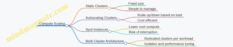
Considerations When Scaling
- Latency: Larger compute clusters can reduce query latency but may increase cost.
- Concurrency: Multiple users or jobs require more compute resources to avoid queuing.
- Data Locality: Since data is in object storage, compute nodes fetch data over the network. Network bandwidth and caching strategies affect performance.
- Metadata Overhead: Managing metadata efficiently is crucial as data scales.
Example: Query Performance Impact
If you run a Spark job on a small cluster with 4 executors, a complex aggregation over a billion records might take hours. Increasing to 32 executors can reduce runtime significantly. However, if your storage throughput or network bandwidth is limited, adding more executors yields diminishing returns.
Summary
Separating storage and compute in lakehouse architectures provides flexibility and cost control. Storage scales automatically in cloud object stores, while compute clusters can be sized and scheduled based on workload demands. Understanding this separation helps you design scalable, efficient, and cost-effective data pipelines.
12.5 Best Practices: Load Testing and Benchmarking with Sample Workflows
Load testing and benchmarking are essential steps to ensure that your streaming and lakehouse pipelines can handle expected workloads while maintaining performance and reliability. This section covers practical approaches, common pitfalls, and sample workflows to guide you through effective load testing and benchmarking.
Understanding Load Testing vs. Benchmarking
- Load Testing: Simulates real-world data volumes and velocity to observe system behavior under expected or peak conditions.
- Benchmarking: Measures system performance under controlled conditions to compare configurations or technologies.
Both are complementary: load testing reveals operational limits, while benchmarking helps optimize components.
Key Metrics to Monitor
- Throughput (messages/records per second)
- Latency (end-to-end processing time)
- Resource utilization (CPU, memory, network, disk I/O)
- Error rates and data loss
- Backpressure and queue sizes
Mind Map: Load Testing Workflow
Sample Load Testing Example: Kafka Producer and Spark Streaming
-
Objective: Test if the pipeline can handle 100,000 messages per second with < 2 seconds end-to-end latency.
-
Test Data Generation: Use a Kafka producer script that generates JSON messages with realistic fields (timestamps, IDs, payload).
-
Load Execution: Ramp up producer rate from 10,000 to 100,000 messages/sec over 10 minutes.
-
Monitoring: Use Kafka’s JMX metrics for producer throughput and consumer lag; Spark UI for batch processing times.
-
Result Analysis: Identify if lag grows, batch durations exceed thresholds, or resource saturation occurs.
-
Optimization: Adjust Kafka partition count, increase Spark executors, or tune batch intervals.
Mind Map: Benchmarking Spark Structured Streaming
Example Benchmark: Stateful Aggregation
- Input: Stream of events with user IDs and timestamps.
- Task: Compute running counts per user over a 10-minute window.
- Setup: Vary executor count from 4 to 16.
- Metrics: Batch processing time, memory usage.
Outcome: Batch time decreases with more executors but plateaus beyond 12 executors due to shuffle overhead.
Tips for Effective Load Testing and Benchmarking
- Use Realistic Data: Synthetic data should mimic production distributions and schema complexity.
- Isolate Variables: Change one parameter at a time to understand its impact.
- Automate Tests: Use scripts and CI pipelines to run tests consistently.
- Monitor Continuously: Collect logs and metrics during tests to catch anomalies.
- Account for Warm-Up: Systems may perform differently after caches and JIT optimizations.
- Test Failure Scenarios: Include broker failures or executor restarts to assess resilience.
Mind Map: Common Pitfalls and How to Avoid Them
Sample Workflow: Automating Load Tests with Apache JMeter and Kafka
- Configure JMeter Kafka Producer plugin with target topic and message schema.
- Define thread groups to simulate concurrent producers.
- Script ramp-up and steady-state load phases.
- Integrate Spark streaming job consuming from Kafka.
- Collect Kafka and Spark metrics via JMX exporters.
- Analyze results with Grafana dashboards.
This setup enables repeatable, automated load tests that reflect production-like conditions.
In summary, load testing and benchmarking are iterative processes that require careful planning, realistic data, and thorough monitoring. By following structured workflows and learning from each test, you can build streaming and lakehouse pipelines that meet performance goals without surprises.
12.6 Cost-Effective Scaling on Cloud Platforms
Scaling data engineering workloads on cloud platforms requires balancing performance needs with budget constraints. Cloud resources are elastic, but without careful planning, costs can quickly spiral. This section focuses on practical strategies to scale streaming and lakehouse architectures efficiently, minimizing waste while maintaining responsiveness.
Understanding Cost Drivers in Cloud Data Platforms
Before optimizing, identify what drives costs:
- Compute Resources: Virtual machines, containers, or serverless functions running Kafka brokers, Spark executors, or orchestration jobs.
- Storage: Object storage for lakehouse data, Kafka topic retention, checkpointing, and logs.
- Data Transfer: Network egress, especially between regions or out of cloud.
- Licensing and Managed Services: Fees for managed Kafka, Spark clusters, or proprietary formats.
Mind Map: Cost Components in Cloud Data Engineering
Strategy 1: Right-Sizing Compute Resources
Avoid over-provisioning by matching resource allocation to workload demands. Use autoscaling features where available but configure sensible minimums and maximums.
Example:
A Spark Structured Streaming job processes Kafka data with fluctuating input rates. Instead of a fixed cluster size, configure dynamic allocation with a minimum of 2 executors and a maximum of 10. Monitor CPU and memory utilization to adjust these boundaries over time.
Best Practice: Use metrics-driven autoscaling policies rather than static thresholds. For instance, scale out when CPU usage exceeds 70% for 5 minutes, scale in when below 30% for 10 minutes.
Strategy 2: Optimize Storage Costs
Storage can be surprisingly expensive if not managed properly. Consider the following:
- Retention Policies: Set Kafka topic retention to keep only necessary data. For example, if downstream consumers only need 7 days of data, avoid 30-day retention.
- Data Compaction: Use compacted topics in Kafka to reduce storage for changelog streams.
- File Formats: Use efficient, compressed columnar formats like Parquet or Delta Lake to reduce storage size.
- Partitioning: Partition lakehouse tables by common query keys to reduce scan costs.
Example:
A lakehouse table storing user events is partitioned by event date. This allows queries to skip irrelevant partitions, reducing compute and storage I/O costs.
Mind Map: Storage Optimization Techniques
Strategy 3: Minimize Data Transfer Costs
Data transfer between cloud regions or out to the internet can be costly.
- Co-locate streaming components and storage in the same region.
- Use VPC peering or private endpoints to avoid public internet egress.
- Compress data before transfer.
Example:
A Kafka cluster and Spark processing cluster are deployed in the same availability zone to avoid cross-zone data transfer fees.
Strategy 4: Leverage Spot and Preemptible Instances
Many cloud providers offer discounted compute instances that can be reclaimed with short notice.
- Use spot instances for non-critical or fault-tolerant workloads, such as batch ETL jobs or Spark executors that can handle interruptions.
- Combine with checkpointing and fault-tolerant streaming to recover gracefully.
Example:
A Spark streaming job checkpointing state to durable storage can safely run executors on spot instances, reducing compute costs by up to 70%.
Mind Map: Compute Cost Reduction Techniques
Strategy 5: Use Serverless and Managed Services Wisely
Serverless services charge based on usage, which can be cost-effective for variable workloads but expensive for sustained heavy loads.
- For steady, high-throughput workloads, dedicated clusters might be cheaper.
- For bursty or unpredictable workloads, serverless can reduce idle resource costs.
Example:
Using a managed Kafka service with pay-per-use pricing for development and testing, then switching to dedicated clusters for production workloads.
Strategy 6: Monitor and Analyze Cost Metrics Regularly
Set up dashboards and alerts for cost anomalies.
- Track cost per pipeline or job.
- Correlate cost spikes with workload changes.
- Use cloud provider cost explorer tools.
Example:
An alert triggers when daily compute costs exceed a threshold, prompting investigation into runaway jobs or misconfigured autoscaling.
Summary Mind Map: Cost-Effective Scaling
Scaling on cloud platforms involves continuous tuning. Start with conservative resource allocations, monitor usage and costs closely, and iterate. The goal is to deliver the required performance without paying for unused capacity or unnecessary overhead.
13. Case Studies and Industry Applications
13.1 Financial Services: Real-Time Risk and Compliance Monitoring
Financial institutions face stringent regulatory requirements and must manage risks continuously. Real-time data streaming combined with lakehouse architectures offers a practical way to monitor transactions, detect anomalies, and ensure compliance without delays.
Key Components of Real-Time Risk and Compliance Monitoring
Example: Monitoring Suspicious Transactions
Imagine a bank wants to detect transactions that exceed a certain amount within a short time frame or originate from flagged accounts.
-
Data Ingestion: Transaction events are published to Kafka topics as they occur.
-
Stream Processing: Spark Structured Streaming reads from Kafka, applying a sliding window of 10 minutes to aggregate transaction amounts per account.
-
Rule Application: If the sum exceeds a threshold or the account matches an external watchlist, the event is flagged.
-
Alerting: Flagged events trigger alerts sent to compliance officers via a messaging system.
-
Storage: All transactions and flags are stored in a Delta Lake table for audit and historical analysis.
Code Snippet: Sliding Window Aggregation in Spark Structured Streaming
import org.apache.spark.sql.functions._
val transactions = spark
.readStream
.format("kafka")
.option("kafka.bootstrap.servers", "broker1:9092")
.option("subscribe", "transactions")
.load()
// Assuming value contains JSON with fields: accountId, amount, timestamp
val parsed = transactions.selectExpr("CAST(value AS STRING) as json")
.select(from_json(col("json"), schema).as("data"))
.select("data.*")
val windowedAgg = parsed
.withWatermark("timestamp", "5 minutes")
.groupBy(
col("accountId"),
window(col("timestamp"), "10 minutes", "5 minutes")
)
.agg(sum("amount").alias("totalAmount"))
val flagged = windowedAgg.filter(col("totalAmount") > 100000) // Threshold example
flagged.writeStream
.format("console") // Replace with alert sink
.start()
.awaitTermination()
Mind Map: Fraud Detection Pipeline
Handling Compliance Reporting
Regulators require detailed reports on transactions and risk events. Lakehouse architectures simplify this by storing both raw and processed data in open formats with ACID guarantees. This enables:
- Efficient querying of historical data for audits.
- Reprocessing data if rules change or errors are found.
- Combining batch and streaming data for comprehensive views.
Example: Schema Evolution for Compliance Data
Financial data schemas often evolve due to new regulations or business needs. Using schema registries with Kafka and enforcing schema validation in Spark ensures pipeline stability.
- Kafka producers register schemas using Avro or Protobuf.
- Spark consumers validate incoming data against the latest schema.
- When schema changes occur, backward or forward compatibility is maintained.
This reduces pipeline failures and supports compliance with minimal downtime.
Security and Governance Considerations
- Encrypt data at rest in lakehouse storage and in transit between Kafka and Spark.
- Implement role-based access controls to restrict sensitive data.
- Maintain audit logs of data access and pipeline changes.
Summary
Real-time risk and compliance monitoring in financial services requires a combination of robust streaming ingestion, flexible processing, reliable storage, and strict governance. Kafka and Spark provide the backbone for ingestion and processing, while lakehouse architectures offer a unified storage solution that supports both streaming and batch workloads. Best practices include designing idempotent pipelines, managing schema evolution carefully, and integrating alerting mechanisms that enable timely responses to risk events.
13.2 Retail: Personalized Recommendations and Inventory Management
In retail, real-time streaming and lakehouse architectures support two critical functions: personalized recommendations and inventory management. Both rely on continuous data flows from customer interactions, sales transactions, and supply chain events. Integrating these data streams efficiently enables retailers to respond quickly to customer preferences and inventory changes.
Personalized Recommendations
Personalized recommendations depend on capturing user behavior in real time—clicks, searches, purchases—and combining this with historical data to suggest relevant products. Streaming pipelines ingest event data from web and mobile apps via Kafka topics, which Spark Structured Streaming processes to generate recommendation scores.
Mind Map: Personalized Recommendations Pipeline
Example: Sessionization and Feature Extraction
A common step is grouping user events into sessions to understand browsing patterns. Using Spark Structured Streaming, you can apply windowing and watermarking to group clicks by user ID within a time frame:
val clicks = spark
.readStream
.format("kafka")
.option("subscribe", "user_clicks")
.load()
import org.apache.spark.sql.functions._
val sessions = clicks
.withColumn("eventTime", col("timestamp").cast("timestamp"))
.groupBy(
col("userId"),
window(col("eventTime"), "30 minutes")
)
.agg(collect_list("productId").as("productsViewed"))
This session data feeds into feature extraction pipelines, where product categories viewed or time spent per product are calculated. These features then feed into recommendation models.
Best Practice: Handling Late Data
Late-arriving events can skew session boundaries. Use watermarking to specify how late data is tolerated:
.withWatermark("eventTime", "10 minutes")
This tells Spark to wait 10 minutes for late data before finalizing session windows.
Inventory Management
Inventory management benefits from real-time visibility into stock levels, sales velocity, and supply chain events. Streaming data from point-of-sale systems and warehouse sensors updates inventory counts continuously.
Mind Map: Inventory Management Pipeline
Example: Real-Time Stock Level Aggregation
Using Spark Structured Streaming, aggregate sales events to update stock levels:
val sales = spark
.readStream
.format("kafka")
.option("subscribe", "sales")
.load()
val salesAggregated = sales
.withColumn("quantitySold", col("value").cast("int"))
.groupBy("productId")
.agg(sum("quantitySold").as("totalSold"))
// Join with current inventory from lakehouse
val inventory = spark.table("lakehouse.inventory")
val updatedInventory = inventory
.join(salesAggregated, Seq("productId"), "left_outer")
.withColumn("newStockLevel", col("stockLevel") - coalesce(col("totalSold"), lit(0)))
This updated stock level can feed alerting systems when thresholds are crossed.
Best Practice: Idempotency in Inventory Updates
Sales events might be duplicated or reordered. Use unique transaction IDs and upsert logic in the lakehouse to ensure stock levels are accurate and not double-counted.
Integration of Recommendations and Inventory
Recommendations should consider inventory availability to avoid suggesting out-of-stock items. This requires joining recommendation scores with current stock levels in the lakehouse.
Mind Map: Integrating Recommendations with Inventory
Example: Filtering Recommendations by Stock
val recommendations = spark
.readStream
.format("kafka")
.option("subscribe", "recommendations")
.load()
val inventory = spark.table("lakehouse.inventory")
val filteredRecommendations = recommendations
.join(inventory, Seq("productId"))
.filter(col("stockLevel") > 0)
This ensures customers only see products available for purchase.
Summary
Retail pipelines for personalized recommendations and inventory management rely on streaming data ingestion, real-time processing, and integration with lakehouse storage. Best practices include sessionization with watermarking, idempotent updates, and cross-checking recommendations against inventory. These approaches help retailers maintain responsiveness and accuracy in their data-driven operations.
13.3 Healthcare: Streaming Patient Data and Analytics
Healthcare systems generate vast amounts of data continuously—from patient vital signs to electronic health records (EHRs), medical imaging, and device telemetry. Streaming this data in real time allows providers to monitor patient status continuously, detect anomalies quickly, and support timely decision-making.
Key Components of Streaming Patient Data Pipelines
- Data Sources: Medical devices (heart rate monitors, infusion pumps), EHR systems, lab results, wearable devices.
- Ingestion Layer: Apache Kafka topics ingest data streams from multiple sources.
- Processing Layer: Apache Spark Structured Streaming processes and transforms data.
- Storage Layer: Lakehouse storage (e.g., Delta Lake) stores raw and processed data.
- Analytics and Alerting: Real-time dashboards and alert systems consume processed data.
Mind Map: Streaming Patient Data Pipeline
Example: Real-Time Heart Rate Monitoring
Imagine a hospital monitoring heart rates from ICU patients. Each device sends a message every second with patient ID, timestamp, and heart rate.
-
Kafka Topic:
patient-heart-rate -
Message Format: JSON
{ "patient_id": "12345", "timestamp": "2024-06-01T12:00:00Z", "heart_rate": 85 } -
Spark Structured Streaming Job: Reads from
patient-heart-rate, applies a sliding window of 1 minute to compute average heart rate per patient, and writes alerts if average exceeds a threshold.
val spark = SparkSession.builder.appName("HeartRateMonitoring").getOrCreate()
val rawStream = spark
.readStream
.format("kafka")
.option("kafka.bootstrap.servers", "broker1:9092")
.option("subscribe", "patient-heart-rate")
.load()
import spark.implicits._
val heartRateStream = rawStream
.selectExpr("CAST(value AS STRING)")
.as[String]
.map { jsonStr =>
val json = spark.read.json(Seq(jsonStr).toDS)
(
json.select("patient_id").as[String].head(),
json.select("timestamp").as[String].head(),
json.select("heart_rate").as[Int].head()
)
}
.toDF("patient_id", "timestamp", "heart_rate")
.withColumn("timestamp", to_timestamp(col("timestamp")))
val avgHeartRate = heartRateStream
.withWatermark("timestamp", "1 minute")
.groupBy(
col("patient_id"),
window(col("timestamp"), "1 minute", "30 seconds")
)
.agg(avg("heart_rate").alias("avg_heart_rate"))
val alerts = avgHeartRate.filter("avg_heart_rate > 100")
alerts.writeStream
.format("console")
.outputMode("update")
.start()
.awaitTermination()
This example shows how to process streaming data with windowing and watermarking to handle late data. The alert triggers when the average heart rate exceeds 100 bpm in a one-minute window.
Mind Map: Heart Rate Monitoring Stream Processing
Handling Data Quality and Schema Evolution
Patient data streams often change schema or contain missing fields. For example, a new device may add a battery_level field. Using schema registries with Avro or JSON Schema helps enforce compatibility.
Example practice:
- Register schemas centrally.
- Validate incoming messages against schema.
- Use default values or nulls for missing fields.
- Version schemas to support backward compatibility.
Example: Schema Validation with Kafka and Spark
Kafka Connect can enforce schema validation on ingestion. In Spark, use from_avro or schema-aware deserialization to catch invalid messages and route them to a dead-letter queue for inspection.
Real-Time Analytics and Alerting
Streaming patient data supports dashboards that update continuously. For example, a dashboard can show:
- Current vital signs per patient.
- Trends over the last hour.
- Alerts for abnormal readings.
Alerts can integrate with paging systems or nurse station monitors.
Mind Map: Real-Time Analytics and Alerting
Privacy and Security Considerations
Patient data is sensitive. Streaming pipelines must:
- Encrypt data in transit and at rest.
- Authenticate and authorize producers and consumers.
- Audit data access.
- Anonymize or mask data where appropriate.
These controls integrate with Kafka ACLs, Spark security configurations, and cloud platform features.
Summary
Streaming patient data pipelines combine multiple technologies to deliver timely insights. Kafka handles ingestion, Spark processes data with windowing and stateful operations, and lakehouse storage preserves data for batch and interactive queries. Schema management and data quality checks ensure reliability. Real-time analytics and alerts improve patient monitoring, while security safeguards protect sensitive information.
This approach enables healthcare providers to respond faster and make data-driven decisions without waiting for batch processes.
13.4 Telecommunications: Network Monitoring and Alerting
Telecommunications networks generate vast amounts of data continuously. Monitoring this data in real time is essential to ensure network reliability, detect faults early, and maintain service quality. Network monitoring and alerting pipelines must handle high throughput, low latency, and complex event correlations. This section covers how to build scalable streaming ETL pipelines tailored for telecom network monitoring using Kafka, Spark, and lakehouse architectures.
Key Components of Telecom Network Monitoring Pipelines
- Data Sources: Network devices (routers, switches, base stations), probes, logs, and performance counters.
- Ingestion Layer: Kafka topics ingest raw telemetry and event streams.
- Stream Processing: Spark Structured Streaming processes, aggregates, and enriches data.
- Storage: Lakehouse stores raw and processed data for historical analysis.
- Alerting: Real-time detection of anomalies triggers alerts.
Mind Map: Telecom Network Monitoring Pipeline Overview
Example: Ingesting SNMP Trap Data into Kafka
SNMP traps are asynchronous notifications from network devices signaling events such as link failures or configuration changes. A lightweight Kafka producer can be built in Python using the pysnmp library to listen for traps and publish them to Kafka.
from pysnmp.hlapi.asyncore import *
from kafka import KafkaProducer
import json
producer = KafkaProducer(bootstrap_servers='kafka-broker:9092', value_serializer=lambda v: json.dumps(v).encode('utf-8'))
def trap_receiver(snmpEngine, stateReference, contextEngineId, contextName, varBinds, cbCtx):
trap_data = {str(name): str(val) for name, val in varBinds}
producer.send('snmp-traps', trap_data)
snmpEngine = SnmpEngine()
ntfrcv.NotificationReceiver(snmpEngine, trap_receiver)
snmpEngine.transportDispatcher.jobStarted(1)
try:
snmpEngine.transportDispatcher.runDispatcher()
except:
snmpEngine.transportDispatcher.closeDispatcher()
raise
This example shows how raw network events enter the streaming pipeline.
Mind Map: Stream Processing for Alerting
Example: Detecting Link Failures with Spark Structured Streaming
Suppose we want to detect if a network link has failed repeatedly within a 5-minute window. We can use Spark to aggregate failure events and trigger alerts when counts exceed a threshold.
import org.apache.spark.sql.functions._
import org.apache.spark.sql.streaming.Trigger
val kafkaDf = spark
.readStream
.format("kafka")
.option("kafka.bootstrap.servers", "kafka-broker:9092")
.option("subscribe", "snmp-traps")
.load()
val eventsDf = kafkaDf.selectExpr("CAST(value AS STRING) as json")
.select(from_json(col("json"), schema).as("data"))
.select("data.*")
val failuresDf = eventsDf.filter(col("eventType") === "linkDown")
val windowedCounts = failuresDf
.withWatermark("timestamp", "10 minutes")
.groupBy(window(col("timestamp"), "5 minutes"), col("deviceId"))
.count()
val alertsDf = windowedCounts.filter(col("count") > 3)
.selectExpr("deviceId", "window.start as windowStart", "window.end as windowEnd", "count")
alertsDf.writeStream
.format("console")
.outputMode("update")
.trigger(Trigger.ProcessingTime("1 minute"))
.start()
.awaitTermination()
This pipeline identifies devices with more than three link failures in five minutes, helping network operators react quickly.
Mind Map: Alerting and Notification
Example: Integrating Alerts with a Notification System
Alerts generated by Spark can be pushed to a Kafka topic dedicated to alerts. A consumer service can then forward these alerts to notification channels.
from kafka import KafkaConsumer
import smtplib
consumer = KafkaConsumer('network-alerts', bootstrap_servers='kafka-broker:9092', value_deserializer=lambda m: json.loads(m.decode('utf-8')))
for message in consumer:
alert = message.value
if alert['count'] > 3:
# Simple email notification example
with smtplib.SMTP('smtp.example.com') as server:
server.sendmail(
'[email protected]',
'[email protected]',
f"Subject: Network Alert\n\nDevice {alert['deviceId']} has {alert['count']} link failures between {alert['windowStart']} and {alert['windowEnd']}"
)
This example demonstrates a straightforward way to notify the network team.
Best Practices Summary
- Partition Kafka Topics by Device or Region: This improves parallelism and reduces consumer lag.
- Use Watermarks and Windowing: Handle late-arriving data gracefully.
- Enrich Events Early: Add metadata like device location or type to simplify downstream logic.
- Implement Idempotent Processing: Ensure alerts are not duplicated due to retries.
- Store Raw and Processed Data: Keep raw data immutable for audits and reprocessing.
- Monitor Pipeline Health: Track lag, throughput, and error rates.
- Design Alert Escalation: Avoid alert fatigue by tuning thresholds and suppressing duplicates.
This section provided a practical look at building telecom network monitoring pipelines using streaming and lakehouse technologies. The examples show how to ingest, process, and alert on network events effectively, combining Kafka and Spark with best practices tailored for telecom environments.
13.5 Manufacturing: Predictive Maintenance Pipelines
Predictive maintenance in manufacturing aims to anticipate equipment failures before they happen, reducing downtime and maintenance costs. The data engineering challenge is to build pipelines that collect, process, and analyze sensor data in near real-time, enabling timely alerts and informed decisions.
Key Components of a Predictive Maintenance Pipeline
Data Ingestion
Manufacturing equipment typically emits data through sensors measuring temperature, vibration, pressure, and other parameters. These sensors often connect to edge devices that aggregate and preprocess data before sending it to a central system. Kafka acts as a buffer and messaging layer, handling high-throughput ingestion with fault tolerance.
Example: A vibration sensor produces readings every second. An edge device batches these readings and pushes them to a Kafka topic named machine-vibration.
from kafka import KafkaProducer
import json
producer = KafkaProducer(bootstrap_servers='localhost:9092')
sensor_data = {'machine_id': 'M123', 'timestamp': 1680000000, 'vibration': 0.02}
producer.send('machine-vibration', json.dumps(sensor_data).encode('utf-8'))
producer.flush()
Stream Processing and Feature Extraction
Spark Structured Streaming consumes Kafka topics, cleans data, and computes features such as rolling averages or anomaly scores. Windowing functions help aggregate data over time intervals.
Example: Calculate a 5-minute rolling average of vibration for each machine.
import org.apache.spark.sql.functions._
val kafkaStream = spark
.readStream
.format("kafka")
.option("kafka.bootstrap.servers", "localhost:9092")
.option("subscribe", "machine-vibration")
.load()
val sensorDF = kafkaStream.selectExpr("CAST(value AS STRING) as json")
.select(from_json(col("json"), schema).as("data"))
.select("data.*")
val rollingAvg = sensorDF
.withWatermark("timestamp", "10 minutes")
.groupBy(
window(col("timestamp"), "5 minutes"),
col("machine_id")
)
.agg(avg("vibration").alias("vibration_avg"))
rollingAvg.writeStream
.format("console")
.start()
.awaitTermination()
Data Storage
Processed data and features are stored in a lakehouse, supporting both batch and streaming queries. Delta Lake or Apache Iceberg provide ACID transactions and schema enforcement, essential for reliable analytics.
Model Scoring and Alerts
A machine learning model, trained offline on historical data, is deployed to score streaming data. Scores indicating potential failures trigger alerts.
Example: A Spark UDF applies a pre-trained model to streaming features.
import org.apache.spark.sql.expressions.UserDefinedFunction
val predictFailure: UserDefinedFunction = udf((vibrationAvg: Double) => {
if (vibrationAvg > 0.05) 1 else 0
})
val scoredStream = rollingAvg.withColumn("failure_risk", predictFailure(col("vibration_avg")))
scoredStream.filter("failure_risk = 1")
.writeStream
.format("console")
.start()
.awaitTermination()
Alerts can be sent to maintenance teams via messaging platforms or integrated with ticketing systems.
Monitoring and Feedback
Data quality checks ensure sensor data completeness and correctness. Monitoring pipeline health includes tracking lag in Kafka consumers and Spark job metrics. Model performance is monitored by comparing predicted failures with actual outcomes.
Mind Map: Data Flow and Components
Best Practices
- Idempotency: Ensure that data ingestion and processing are idempotent to handle retries without duplication.
- Schema Evolution: Use schema registries to manage changes in sensor data formats.
- Latency vs. Accuracy: Balance the frequency of feature computation with the acceptable latency for alerts.
- Resource Allocation: Allocate sufficient resources to Spark streaming jobs to avoid bottlenecks.
- Data Retention: Define retention policies for raw and processed data to manage storage costs.
This section illustrates how real-time streaming and lakehouse architectures combine to support predictive maintenance in manufacturing. The pipeline integrates ingestion, processing, storage, and alerting, all designed with reliability and scalability in mind.
13.6 Best Practices: Lessons Learned and Implementation Insights
Building and maintaining real-time streaming and lakehouse architectures is a complex task that benefits from practical experience. This section summarizes key lessons learned from various implementations, focusing on actionable insights and concrete examples.
Mind Map: Core Lessons Learned
Data Quality: Validate Early and Often
One recurring insight is the importance of catching data issues as close to the source as possible. For example, in a Kafka-based pipeline ingesting IoT sensor data, schema validation using a schema registry prevented malformed messages from propagating downstream. This reduced debugging time and avoided corrupting the lakehouse.
Example: Using Avro schemas with Kafka producers and consumers ensures that only valid data enters the pipeline. When a sensor sends data missing a required field, the producer rejects the message, preventing downstream errors.
Handling late-arriving or duplicate data is another common challenge. Implementing watermarking and deduplication logic in Spark Structured Streaming helps maintain data accuracy without sacrificing latency.
Scalability: Partitioning and Decoupling
Effective partitioning is crucial for scaling Kafka topics and Spark jobs. For instance, partitioning Kafka topics by customer ID or region can distribute load evenly and improve parallelism.
In one retail analytics pipeline, partitioning by store location allowed Spark streaming jobs to process data in parallel without contention.
Decoupling components—such as separating ingestion, processing, and storage layers—makes scaling easier. If the ingestion rate spikes, Kafka can buffer messages without overwhelming Spark jobs.
Example: Using Kafka Connect to ingest data into Kafka, then Spark Structured Streaming to process and write to Delta Lake, creates clear boundaries. Each component can be scaled independently.
Reliability: Idempotency and Checkpointing
Idempotent processing prevents duplicate records when retries occur. For example, implementing idempotent writes to Delta Lake by using unique transaction IDs ensures that reprocessing does not create duplicates.
Checkpointing in Spark Structured Streaming is essential to recover state after failures. Without it, stateful aggregations or joins can produce incorrect results.
Example: Enabling checkpoint directories on durable storage allows Spark to resume from the last committed offset, preserving exactly-once semantics.
Monitoring is not just about alerting on failures but also tracking data freshness and throughput. Setting up dashboards with metrics like Kafka consumer lag and Spark processing time helps catch issues early.
Security & Governance: Access Controls and Auditing
Applying the principle of least privilege reduces risk. For example, restricting Kafka topic permissions so that only authorized producers and consumers can access sensitive data is a straightforward but effective measure.
Encrypting data at rest and in transit is standard practice. Using TLS for Kafka communication and server-side encryption for cloud storage protects data confidentiality.
Auditing access and changes supports compliance. Logging user actions on lakehouse tables and Kafka topics helps trace data lineage and investigate incidents.
Operational Practices: Testing and Deployment
Automated testing for streaming pipelines is often overlooked but critical. Writing unit tests for transformation logic and integration tests that simulate streaming data prevents regressions.
Example: Using embedded Kafka clusters in test environments allows developers to run end-to-end tests without external dependencies.
CI/CD pipelines that automate deployment reduce human error. Incremental rollouts with feature flags or canary deployments minimize impact of new changes.
Version controlling pipeline configurations and infrastructure as code ensures reproducibility and easier troubleshooting.
Summary Mind Map: Implementation Insights
These lessons reflect practical experience across industries and use cases. They emphasize the value of designing pipelines that are not only functional but also maintainable, observable, and secure. Applying these insights can help avoid common pitfalls and build data engineering solutions that stand the test of time.
14. Appendix: Tools, Libraries, and Resources
14.1 Essential Open Source Tools for Streaming and Lakehouse
In building real-time streaming and lakehouse architectures, selecting the right open source tools is crucial. These tools form the backbone of data ingestion, processing, storage, and management. Below, we explore key tools organized by their primary roles, accompanied by mind maps to clarify their relationships and examples to illustrate their practical use.
Core Streaming Platforms
-
Apache Kafka: A distributed event streaming platform designed for high-throughput, fault-tolerant, and scalable message handling. Kafka is often the starting point for real-time data pipelines.
-
Apache Pulsar: An alternative to Kafka, Pulsar offers multi-tenancy and geo-replication with a layered architecture separating storage and serving.
-
Apache Flink: A stream processing framework that supports event-time processing and complex stateful computations.
-
Apache Spark Structured Streaming: Provides micro-batch and continuous processing modes, integrating well with batch workloads.

Example:
A typical real-time pipeline might use Kafka as the message broker and Spark Structured Streaming for processing. For instance, ingesting clickstream data into Kafka topics, then running Spark jobs to aggregate user sessions in near real-time.
Stream Processing Frameworks
-
Apache Beam: Provides a unified programming model for batch and streaming, with runners for Spark, Flink, and Google Dataflow.
-
Kafka Streams: A lightweight Java library for building stream processing applications directly on Kafka topics.
-
ksqlDB: A SQL-based streaming engine built on Kafka Streams for interactive stream processing.
Example:
Using Kafka Streams, you can write a Java application that reads from a topic of sensor readings, filters out invalid data, and writes the cleaned stream to another topic for downstream consumption.
Lakehouse Storage and Formats
-
Delta Lake: Adds ACID transactions and schema enforcement on top of cloud object stores.
-
Apache Iceberg: A table format designed for high-performance analytic queries with support for schema evolution.
-
Apache Hudi: Supports incremental data processing and upserts for data lakes.
Example:
A Spark job writes streaming data into a Delta Lake table. Delta Lake ensures that concurrent writes do not corrupt data and enforces schema consistency, making downstream analytics reliable.
Data Serialization and Schema Management
-
Apache Avro: A compact binary serialization format with schema support.
-
Protocol Buffers (Protobuf): Google’s language-neutral, platform-neutral mechanism for serializing structured data.
-
JSON Schema: A JSON-based format for defining the structure of JSON data.
-
Confluent Schema Registry: Manages schemas for Kafka messages, enabling compatibility checks.

Example:
When producing Kafka messages, Avro serialization combined with a schema registry ensures that consumers can deserialize data correctly even as schemas evolve.
Workflow Orchestration and Monitoring
-
Apache Airflow: A platform to programmatically author, schedule, and monitor workflows.
-
Prefect: A modern workflow orchestration tool with a Python-native API.
-
Prometheus: Monitoring system and time series database.
-
Grafana: Visualization tool for metrics and logs.

Example:
Airflow can schedule batch jobs that complement streaming pipelines, such as periodic data quality checks. Prometheus collects metrics from Kafka brokers and Spark executors, which Grafana visualizes for operational insights.
Example: Building a Minimal Streaming Pipeline
// Spark Structured Streaming reading from Kafka
import org.apache.spark.sql.SparkSession
val spark = SparkSession.builder.appName("StreamingExample").getOrCreate()
val kafkaDF = spark.readStream
.format("kafka")
.option("kafka.bootstrap.servers", "localhost:9092")
.option("subscribe", "input_topic")
.load()
import spark.implicits._
val processedDF = kafkaDF.selectExpr("CAST(key AS STRING)", "CAST(value AS STRING)")
.as[(String, String)]
.filter(_._2.nonEmpty)
val query = processedDF.writeStream
.format("delta")
.option("checkpointLocation", "/tmp/checkpoints")
.start("/tmp/delta_table")
query.awaitTermination()
This example shows reading from Kafka, filtering empty messages, and writing to a Delta Lake table with checkpointing for fault tolerance.
Selecting the right open source tools depends on your specific use case, scale, and operational preferences. The tools above cover the essential layers of a real-time streaming and lakehouse architecture, providing a solid foundation for building scalable and maintainable data pipelines.
14.2 Libraries for Data Serialization and Schema Management
Data serialization and schema management are foundational to building reliable, scalable streaming and lakehouse pipelines. They ensure that data can be efficiently encoded for transport and storage, and that its structure is well-defined and versioned to prevent compatibility issues. This section covers the most widely used libraries in this space, their core features, and practical examples to illustrate their use.
Key Libraries Overview
- Apache Avro
- Protocol Buffers (Protobuf)
- JSON Schema
- Thrift
- Schema Registry (Confluent and alternatives)
Mind Map: Serialization Libraries and Schema Management
Apache Avro
Avro is a popular serialization framework designed for Hadoop but widely adopted in streaming systems. It uses JSON to define schemas and stores data in a compact binary format. Avro’s schema is always stored with the data or referenced externally, enabling readers to understand how to deserialize the bytes.
Example: Avro Schema Definition (user.avsc)
{
"type": "record",
"name": "User",
"namespace": "com.example",
"fields": [
{"name": "id", "type": "string"},
{"name": "age", "type": "int"},
{"name": "email", "type": ["null", "string"], "default": null}
]
}
Using Avro in Java to serialize a User record:
Schema schema = new Schema.Parser().parse(new File("user.avsc"));
GenericRecord user = new GenericData.Record(schema);
user.put("id", "user-123");
user.put("age", 30);
user.put("email", "[email protected]");
ByteArrayOutputStream out = new ByteArrayOutputStream();
DatumWriter<GenericRecord> writer = new GenericDatumWriter<>(schema);
Encoder encoder = EncoderFactory.get().binaryEncoder(out, null);
writer.write(user, encoder);
encoder.flush();
out.close();
byte[] serializedBytes = out.toByteArray();
Best Practice: Always include a schema registry or embed schema references to handle schema evolution gracefully.
Protocol Buffers (Protobuf)
Protobuf is a language-neutral, platform-neutral serialization library developed by Google. It uses .proto files to define message schemas and generates code for multiple languages.
Example: Protobuf schema (user.proto)
syntax = "proto3";
package example;
message User {
string id = 1;
int32 age = 2;
string email = 3;
}
Generating Java classes and serializing:
User user = User.newBuilder()
.setId("user-123")
.setAge(30)
.setEmail("[email protected]")
.build();
byte[] serialized = user.toByteArray();
Protobuf is efficient and strongly typed but less flexible with schema evolution compared to Avro.
JSON Schema
JSON Schema defines the structure and validation rules for JSON data. It is human-readable and widely used for REST APIs and configuration files.
Example: JSON Schema for User
{
"$schema": "http://json-schema.org/draft-07/schema#",
"title": "User",
"type": "object",
"properties": {
"id": {"type": "string"},
"age": {"type": "integer"},
"email": {"type": ["string", "null"]}
},
"required": ["id", "age"]
}
JSON Schema is not a serialization format but is useful for validating data before processing.
Thrift
Thrift is both an interface definition language and a serialization framework. It supports RPC and multiple serialization protocols.
While less common in streaming pipelines compared to Avro and Protobuf, Thrift can be useful in environments requiring RPC and cross-language support.
Schema Registry
A schema registry stores and manages schemas centrally. It enforces compatibility rules (backward, forward, full) and allows producers and consumers to negotiate schema versions.
Typical Workflow:
- Producer registers schema before sending data.
- Consumer fetches schema by ID to deserialize.
Example: Using Confluent Schema Registry with Avro
Properties props = new Properties();
props.put("schema.registry.url", "http://localhost:8081");
KafkaAvroSerializer serializer = new KafkaAvroSerializer();
serializer.configure(props, false);
byte[] serialized = serializer.serialize("topic", userRecord);
Mind Map: Schema Registry Workflow
Summary
Choosing the right serialization and schema management library depends on your use case:
- Use Avro for flexible schema evolution and tight Kafka integration.
- Choose Protobuf for efficient, strongly typed messages and multi-language support.
- Use JSON Schema primarily for validation and human-readable schemas.
- Employ a Schema Registry to centralize schema management and enforce compatibility.
Each library comes with trade-offs in complexity, performance, and flexibility. Practical examples and embedding schema management into your pipelines will reduce errors and improve maintainability.
14.3 Monitoring and Logging Frameworks
Monitoring and logging form the backbone of maintaining healthy streaming and lakehouse data pipelines. They provide visibility into system behavior, help detect anomalies, and support troubleshooting. Without them, diagnosing issues in distributed, real-time environments becomes guesswork.
Why Monitoring and Logging Matter
- Early detection of failures: Streaming pipelines often run continuously; catching errors early prevents data loss or corruption.
- Performance tracking: Monitoring resource usage and throughput helps optimize pipeline efficiency.
- Audit and compliance: Logs provide records of data movement and transformations.
- Root cause analysis: Detailed logs and metrics speed up debugging.
Key Concepts
- Metrics: Quantitative measurements such as throughput, latency, error rates.
- Logs: Detailed, timestamped records of events, errors, and system messages.
- Tracing: Tracking the flow of a data record through multiple components.
- Alerts: Automated notifications triggered by metric thresholds or error patterns.
Mind Map: Monitoring and Logging Components
Common Monitoring and Logging Tools
- Prometheus: Popular open-source metrics collection and alerting system.
- Grafana: Visualization tool often paired with Prometheus.
- Elasticsearch, Logstash, Kibana (ELK Stack): Centralized log aggregation and search.
- Jaeger / Zipkin: Distributed tracing tools.
- Apache Kafka’s JMX metrics: Kafka exposes metrics via Java Management Extensions.
- Spark UI and Metrics: Spark provides its own monitoring interfaces.
Implementing Monitoring in Kafka and Spark Pipelines
Kafka Metrics Example
Kafka brokers expose metrics such as MessagesInPerSec, BytesInPerSec, and UnderReplicatedPartitions. You can scrape these metrics using Prometheus JMX exporter.
# Example Prometheus scrape config snippet
- job_name: 'kafka'
static_configs:
- targets: ['kafka-broker1:7071', 'kafka-broker2:7071']
This setup lets you track message rates and broker health in real time.
Spark Structured Streaming Metrics
Spark exposes metrics via its REST API and JMX. Key metrics include input rate, processing rate, and batch duration.
Example: Accessing streaming query status programmatically:
val query = streamingDataFrame.writeStream.start()
println(query.status)
This returns information about progress and any errors.
Logging Best Practices
- Use structured logging: JSON or key-value pairs enable easier parsing and querying.
- Include context: Add correlation IDs and metadata to link logs across components.
- Set appropriate log levels: Avoid excessive DEBUG logs in production but keep enough detail for troubleshooting.
- Centralize logs: Use aggregation tools to collect logs from all pipeline components.
- Rotate and archive logs: Prevent disk space exhaustion.
Example: Structured Log Entry in Spark Application
{
"timestamp": "2024-06-01T12:00:00Z",
"level": "ERROR",
"component": "SparkStreamingJob",
"message": "Failed to process batch",
"batchId": 42,
"error": "TimeoutException",
"correlationId": "abc123"
}
Distributed Tracing
Tracing helps follow a single data record as it moves through Kafka producers, topics, Spark processors, and sinks. Assigning a unique correlation ID at ingestion and propagating it through logs and metrics is essential.
This practice simplifies root cause analysis when pipelines span multiple services.
Alerting Strategies
- Define thresholds for key metrics (e.g., consumer lag, error rates).
- Use anomaly detection for unusual patterns.
- Configure alerts to notify relevant teams via email, Slack, or PagerDuty.
Example alert rule in Prometheus:
- alert: KafkaConsumerLagHigh
expr: kafka_consumer_lag > 10000
for: 5m
labels:
severity: critical
annotations:
summary: "High Kafka consumer lag detected"
description: "Consumer lag has exceeded 10,000 messages for over 5 minutes."
Visualization and Dashboards
Dashboards provide at-a-glance views of pipeline health.
Grafana is commonly used to build these dashboards by querying Prometheus or Elasticsearch.
Summary
Monitoring and logging frameworks are vital for understanding and maintaining streaming and lakehouse pipelines. Metrics track system health, logs capture detailed events, tracing connects distributed components, and alerts ensure timely responses. Combining these elements with visualization tools creates a comprehensive observability stack. Implementing these practices with clear, structured data and context makes troubleshooting faster and pipelines more reliable.
14.4 Sample Code Repositories and Tutorials
This section provides a structured overview of practical code repositories and tutorials that illustrate key concepts in real-time streaming, ETL pipelines, and lakehouse architectures. Each example is designed to be accessible and instructive, with clear explanations and code snippets that emphasize best practices.
Mind Map: Sample Code Repositories Overview
Kafka Basics: Producer and Consumer Examples
Producer Example (Java):
Properties props = new Properties();
props.put("bootstrap.servers", "localhost:9092");
props.put("key.serializer", "org.apache.kafka.common.serialization.StringSerializer");
props.put("value.serializer", "org.apache.kafka.common.serialization.StringSerializer");
KafkaProducer<String, String> producer = new KafkaProducer<>(props);
for (int i = 0; i < 10; i++) {
ProducerRecord<String, String> record = new ProducerRecord<>("test-topic", "key-" + i, "value-" + i);
producer.send(record);
}
producer.close();
This example demonstrates basic message production with explicit key-value pairs. It’s important to set serializers correctly to avoid runtime errors.
Consumer Example (Python):
from kafka import KafkaConsumer
consumer = KafkaConsumer(
'test-topic',
bootstrap_servers=['localhost:9092'],
auto_offset_reset='earliest',
enable_auto_commit=True,
group_id='my-group'
)
for message in consumer:
print(f"Received message: {message.key} -> {message.value}")
This snippet shows how to consume messages with offset management. Setting auto_offset_reset to earliest ensures no messages are missed on startup.
Spark Structured Streaming: Reading from Kafka and Windowed Aggregations
Reading from Kafka:
val spark = SparkSession.builder.appName("KafkaSparkExample").getOrCreate()
val df = spark.readStream
.format("kafka")
.option("kafka.bootstrap.servers", "localhost:9092")
.option("subscribe", "test-topic")
.load()
val values = df.selectExpr("CAST(value AS STRING)")
This code reads streaming data from Kafka and casts the binary value field to string for further processing.
Windowed Aggregation Example:
import org.apache.spark.sql.functions._
val windowedCounts = values
.withColumn("timestamp", current_timestamp())
.groupBy(window(col("timestamp"), "10 minutes"), col("value"))
.count()
windowedCounts.writeStream
.outputMode("complete")
.format("console")
.start()
.awaitTermination()
This example groups data into 10-minute windows and counts occurrences per value. Using event-time windows with watermarks would be a next step for production.
Lakehouse Integration: Delta Lake Streaming Writes and Schema Evolution
Streaming Write to Delta Lake:
values.writeStream
.format("delta")
.outputMode("append")
.option("checkpointLocation", "/tmp/checkpoints")
.start("/delta/events")
This snippet writes streaming data into a Delta Lake table with checkpointing to ensure fault tolerance.
Schema Evolution Example:
import io.delta.tables._
val deltaTable = DeltaTable.forPath(spark, "/delta/events")
deltaTable.updateExpr("newColumn", "'defaultValue'")
Delta Lake supports adding new columns without rewriting the entire dataset. This example shows how to update existing records with a new column.
Cloud Platform Examples: AWS MSK and EMR Pipeline
Architecture Mind Map:
Example: Reading from MSK in EMR Spark Application (Scala):
val kafkaBootstrapServers = "b-1.mskcluster.xxxx.kafka.us-east-1.amazonaws.com:9092"
val df = spark.readStream
.format("kafka")
.option("kafka.bootstrap.servers", kafkaBootstrapServers)
.option("subscribe", "msk-topic")
.option("kafka.security.protocol", "SSL")
.load()
This example highlights configuring secure connections to a managed Kafka cluster.
End-to-End ETL Pipeline Example
Pipeline Steps Mind Map:
Basic Pipeline Code Snippet:
val rawStream = spark.readStream
.format("kafka")
.option("subscribe", "input-topic")
.load()
val transformed = rawStream
.selectExpr("CAST(value AS STRING) as json")
.select(from_json(col("json"), schema).as("data"))
.select("data.*")
.filter("status = 'active'")
transformed.writeStream
.format("delta")
.option("checkpointLocation", "/checkpoints/etl")
.start("/lakehouse/active_data")
This example filters active records and writes them to a Delta Lake table, demonstrating a simple but scalable ETL flow.
Testing and Monitoring Examples
Unit Testing Spark Structured Streaming (Scala):
import org.apache.spark.sql.streaming.OutputMode
import org.scalatest.FunSuite
class StreamingJobTest extends FunSuite {
test("filter active records") {
val input = Seq(
("{"status":"active","id":1}"),
("{"status":"inactive","id":2}")
).toDS()
val filtered = input.filter(json => json.contains("active"))
assert(filtered.count() == 1)
}
}
This test checks that only records with status “active” pass through the filter.
Simulated Kafka Data for Testing:
Use embedded Kafka or mock Kafka producers to generate test data streams. This approach allows integration testing without a full Kafka cluster.
Monitoring Metrics Example:
Collect metrics such as processing latency, input rate, and error counts using Spark’s built-in metrics system or Kafka’s JMX metrics. These can be exported to dashboards for real-time visibility.
This section aims to provide practical starting points with code and structure to build, test, and monitor real-time streaming and lakehouse pipelines. The examples focus on clarity and applicability, avoiding unnecessary complexity while demonstrating essential techniques.
14.5 Glossary of Key Terms and Acronyms
This glossary collects essential terms and acronyms used throughout the book. Each entry includes a concise definition and, where helpful, a simple example or a mind map in format to clarify relationships.
Apache Kafka (Kafka) A distributed streaming platform used for building real-time data pipelines and streaming apps. It stores streams of records in categories called topics.
Example: A topic named “user-events” collects clicks and page views from a website.
ETL (Extract, Transform, Load) A data pipeline process where data is extracted from sources, transformed into a desired format, and loaded into a target system.
Example: Extract sales data from a database, convert currency values, and load into a data warehouse.
ELT (Extract, Load, Transform) A variant of ETL where data is first loaded into a storage system, then transformed within that system.
Example: Raw logs are loaded into a lakehouse, then SQL queries transform the data.
Lakehouse Architecture A data architecture combining features of data lakes and data warehouses, offering both storage flexibility and structured data management.
Mind map:
Schema Evolution The ability to change the schema of data over time without breaking existing pipelines or queries.
Example: Adding a new optional field to a JSON message without impacting consumers.
Partition A division of a Kafka topic or a dataset that allows parallel processing and scalability.
Example: A topic with 10 partitions can handle 10 parallel consumers.
Watermarking A technique in stream processing to handle late-arriving data by defining a threshold time up to which data is considered on time.
Example: Processing events with timestamps up to 5 minutes behind the current time.
Exactly-Once Semantics (EOS) Guarantee that each message or record is processed exactly one time, avoiding duplicates or data loss.
Example: A payment transaction is recorded once despite retries or failures.
CDC (Change Data Capture) A method to capture and stream changes (inserts, updates, deletes) from a database to downstream systems.
Example: Streaming updates from a customer database to a real-time analytics platform.
Kafka Connect A framework for connecting Kafka with external systems such as databases or file systems.
Example: Using a connector to stream data from MySQL into Kafka topics.
Stateful Stream Processing Stream processing that maintains state across events, enabling operations like aggregations and joins.
Example: Counting the number of clicks per user over a sliding window.
Windowing Grouping streaming data into finite chunks based on time or count for aggregation or analysis.
Mind map:
Avro, Protobuf, JSON Schema Data serialization formats that define how data is structured and encoded for transmission or storage.
Example: Avro schema defines fields and types for Kafka messages.
Metadata Management Tracking information about data, such as schema, location, and version, to enable data governance and efficient querying.
Example: Delta Lake maintains transaction logs to track changes.
Idempotency Ensuring that performing the same operation multiple times results in the same state as performing it once.
Example: Writing a record with a unique key so duplicates are ignored.
Orchestration Automating the scheduling and management of data pipelines and workflows.
Example: Using Apache Airflow to trigger Kafka-to-Spark ETL jobs.
Latency The delay between data generation and its availability for processing or querying.
Example: A pipeline with 5-second latency means data is visible 5 seconds after creation.
Throughput The amount of data processed per unit time in a pipeline.
Example: Processing 10,000 messages per second.
Broker A Kafka server that stores and serves messages to consumers.
Example: A Kafka cluster with three brokers distributes topic partitions among them.
Consumer Group A group of Kafka consumers that share the work of consuming messages from topics.
Example: Three consumers in a group each read from different partitions.
Checkpointing Saving the state of a streaming application periodically to enable recovery after failure.
Example: Spark Structured Streaming saves offsets and state to durable storage.
Data Lineage Tracking the origin and transformations of data through a pipeline.
Example: Knowing which source file contributed to a particular record in the lakehouse.
Serialization Converting data structures into a format suitable for storage or transmission.
Example: Converting a Python dictionary to Avro bytes before sending to Kafka.
Deserialization The reverse of serialization: converting bytes back into usable data structures.
Example: Reading Avro bytes from Kafka and converting them into Spark DataFrame rows.
Fault Tolerance The ability of a system to continue operating properly in the event of failures.
Example: Kafka replicates partitions across brokers to avoid data loss.
Load Balancing Distributing workload evenly across resources to optimize performance.
Example: Kafka partitions spread across brokers to balance consumer load.
Streaming ETL Pipeline A data pipeline that continuously extracts, transforms, and loads data in real time.
Example: Processing clickstream data from Kafka, enriching it in Spark, and storing in a lakehouse.
Batch Processing Processing data in large, discrete chunks rather than continuously.
Example: Running a nightly job to aggregate daily sales.
Hybrid Processing Combining batch and streaming processing to meet different latency and completeness needs.
Example: Using streaming for real-time alerts and batch for historical reports.
Cloud Data Platform A managed service offering storage, compute, and tools for data engineering in the cloud.
Example: AWS S3 for storage, EMR for Spark processing, and MSK for Kafka.
Data Lake A centralized repository storing raw data in its native format.
Example: Storing JSON logs and CSV files in S3.
Data Warehouse A system optimized for structured data storage and fast analytical queries.
Example: Snowflake or Redshift storing cleaned and modeled data.
Transactional Guarantees Assurances about the atomicity, consistency, isolation, and durability (ACID) of operations.
Example: Delta Lake provides ACID transactions on data lakes.
Message Offset A unique identifier for a message within a Kafka partition.
Example: Consumers track offsets to know which messages have been processed.
Backpressure A mechanism to handle situations when data production outpaces consumption.
Example: Spark slowing down Kafka reads to avoid memory overload.
Serialization Formats Mind Map:
This glossary aims to clarify the terminology needed to navigate real-time streaming and lakehouse data engineering. Understanding these terms helps build and maintain scalable, reliable pipelines.