Advanced Industrial Noise and Vibration Control Engineering

1.1 Sources of Machinery Noise and Vibration in Industrial Systems

Industrial noise and vibration rarely come from a single “bad part.” They are usually the combined result of excitation (what shakes or radiates), transmission (how it travels), and response (how structures and enclosures react). This section maps the most common machinery sources so you can connect measurements to likely causes without guessing.

Core Excitation Sources

Rotating machinery generates periodic forces from imbalance, misalignment, and bearing defects. Imbalance acts like a rotating weight, producing a force at the rotation frequency and its harmonics. Misalignment adds a directional component that often shows up strongly at bearing locations and can excite structural modes. Bearing defects create impacts and high-frequency content, which can be heard as a gritty “texture” and measured as broadband vibration spikes.

Reciprocating machinery produces time-varying forces from piston motion, valve events, and crankshaft dynamics. The dominant excitation often includes the fundamental stroke frequency and its harmonics, plus sharp transients from impacts or clearances. A compressor with worn valve seats may still run, but the vibration signature becomes less periodic and more impulsive, which also increases airborne noise through enclosure panel radiation.

Gear trains and transmissions add mesh stiffness variation. Gear tooth contact changes the effective stiffness as teeth engage and disengage, producing vibration at the mesh frequency and sidebands related to shaft speed and load. Backlash and tooth wear can increase amplitude and broaden the frequency content, making the noise less “tonal” and more “hissy” or “buzz-like.”

Hydraulic and pneumatic systems introduce pressure pulsations and flow-induced excitation. In pumps and compressors, pressure ripple couples into piping and supports, turning flexible pipe runs into sound radiators. In pneumatic lines, turbulence and valve switching can generate broadband vibration that excites hangers and nearby structural members.

Impact and clearance events include belt slap, coupling looseness, rubbing, and mechanical contact. These sources are often intermittent, so they may be missed if you only look at steady-state averages. They can also create strong low-frequency components when impacts excite structural resonances.

How Vibration Becomes Noise

Vibration is not automatically noise; it becomes noise when it drives an acoustic radiator. A motor baseplate can vibrate, but the airborne sound level depends on whether panels, covers, ducts, and openings move efficiently. The same excitation can produce different noise outcomes depending on enclosure stiffness, panel size, and damping.

A useful mental model is: force → structural motion → surface radiation → sound pressure at the receiver. For example, a gearbox may generate strong vibration at the mesh frequency, but if the gearbox is fully enclosed with well-sealed panels, the dominant noise at the operator position may shift to duct leakage or flanking paths through the frame.

Transmission Paths That Multiply the Problem

Even when the excitation is localized, transmission can spread it. Common paths include:

• Direct mounting path: machine feet to baseplate to floor.
• Structural coupling: shared beams, skids, and frames that act like bridges.
• Piping coupling: rigid or poorly supported pipe runs that carry vibration into other equipment.
• Flanking through penetrations: cable trays, wall penetrations, and duct interfaces that bypass intended isolation.

This is why two machines with similar vibration levels can produce very different noise levels in the same room.

Concrete Examples You Can Use Immediately

Example 1: Pump with a “clean” tone that grows louder with speed If the dominant vibration and noise increase proportionally with motor speed and show harmonics, imbalance or misalignment is likely. The practical check is to compare vibration at the bearing housing and at the baseplate corners; a strong baseplate response suggests efficient radiation.

Example 2: Gearbox with a repeating buzz plus a rough edge A repeating buzz at mesh frequency with sidebands indicates gear mesh excitation. If the rough edge increases after load changes, backlash or wear may be contributing. Inspecting mounting tightness and gearbox-to-baseplate contact often matters because looseness can amplify radiation.

Example 3: Compressor with intermittent knocks Intermittent knocks often point to clearance, valve issues, or belt/coupling problems. Because these events are transient, time-domain observation and order tracking around operating conditions are more informative than a single averaged spectrum.

Practical Takeaway

When you identify the excitation type—rotating, reciprocating, gear mesh, fluid pulsation, or impact—you narrow the likely transmission and radiation mechanisms. That connection is what turns measurements into design decisions, instead of turning them into a collection of interesting graphs.

1.2 Noise Transmission Paths Through Airborne Structureborne and Flanking Routes

Industrial noise rarely travels in a single, polite line from source to receiver. It usually takes multiple routes at once, and the “loudest” path is often not the one you initially suspect. This section builds a practical map of how machinery noise reaches people, then shows how to use that map to choose effective control measures.

Core Idea: Two Main Routes Plus a Sneaky Third

1. Airborne path: sound radiates into air and reaches the receiver directly.
2. Structureborne path: vibration excites building elements, which radiate sound from their surfaces.
3. Flanking path: sound bypasses the intended barrier by traveling through alternate structural or geometric routes, such as side walls, beams, ducts, or penetrations.

A useful mental model is to treat the building like a set of coupled “sound highways.” If you block one highway, traffic often reroutes.

Airborne Transmission Path

Airborne noise is driven by sound power radiated by the machine and its enclosure gaps. Typical contributors include fan housings, motor vents, compressor discharge openings, and panel seams.

What to look for in the field

• Audible noise that changes strongly with distance and direction.
• Clear “line of sight” from machine to receiver.
• Strong tonal components that match rotational speeds, indicating direct radiation.

Easy example: A small pump in a room with a partially closed cover. If the cover has a gap around the cable entry, you can often hear the same pitch at the receiver even when the cover is otherwise intact. The gap becomes a local airborne radiator.

Engineering implication: Airborne control focuses on reducing sound radiation and improving barrier sound insulation (mass, sealing, and surface continuity).

Structureborne Transmission Path

Structureborne noise starts with vibration. The machine baseplate and mounts transmit dynamic forces into the foundation, beams, and floors. Those elements then vibrate and radiate sound into the air.

Key mechanism

• Vibration energy enters the structure.
• Structural modes shape where and how strongly surfaces radiate.
• Radiation efficiency depends on panel size, boundary conditions, and damping.

Easy example: A gearbox mounted on stiff supports. Even if the gearbox enclosure is reasonably sealed, the floor can become the main radiator. You may feel vibration near the base and hear a broader-band “rumble” at the receiver.

Engineering implication: Structureborne control emphasizes reducing force transmission (isolation) and reducing structural response (damping and stiffness tuning).

Flanking Transmission Routes

Flanking is what happens when the “main barrier” is not the only route. Sound can travel around it through:

• Side walls and adjacent partitions connected to the same frame.
• Beams and columns that bridge the barrier.
• Floor slabs that connect rooms.
• Penetrations like pipe sleeves, cable trays, and anchor bolts.
• Ductwork that carries pressure fluctuations and radiates at openings.

Easy example: You install a heavy acoustic enclosure around a compressor. The enclosure sits on a steel frame that is bolted to the building structure. The compressor’s vibration now couples into the frame and then into the building, bypassing the enclosure’s intended isolation.

Engineering implication: Flanking control requires detailing, not just material selection. Seals, decoupling, and controlled interfaces matter.

Systematic Diagnostic Workflow

1. Start with direction and distance: If noise drops quickly with distance, airborne is likely significant. If it stays strong, structureborne or flanking may dominate.
2. Check vibration at interfaces: Touch and measure near mounts, baseplate edges, and nearby walls. Strong vibration at a wall suggests structureborne radiation.
3. Identify bypass points: Look for rigid connections between the machine support and building structure, and for penetrations that connect rooms.
4. Use targeted “interruptions”: Temporarily add soft isolation at a suspected rigid bridge or seal a suspected gap, then re-check noise and vibration. If the change is immediate and repeatable, you found a path.

Integrated Example: One Machine, Three Paths

A motor-driven fan sits in an equipment bay. The receiver is in an adjacent office.

• Airborne: the fan discharge opening leaks sound through a poorly sealed duct collar.
• Structureborne: the fan’s baseplate excites the floor slab, which radiates a low-frequency component.
• Flanking: a cable tray is bolted to both the bay frame and the office wall, carrying vibration and enabling sound bypass.

A coherent solution combines: sealing the duct collar, adding isolation at the fan mounts, and decoupling the cable tray with resilient supports and proper sleeve detailing. Treating only one path often improves things, but treating all three is what makes the improvement stick.

1.3 Vibration Excitation Types Including Rotating Reciprocating and Impact Loads

Industrial vibration starts with excitation: a force or motion that injects energy into the machine and its support system. The same mounting and isolation hardware can behave very differently depending on whether the excitation is periodic, broadband, or impulsive. A good control and isolation design begins by classifying the excitation type, then mapping it to the dominant frequency content and the likely transmission paths.

Rotating Loads and Periodic Excitation

Rotating equipment produces vibration because rotating elements do not generate perfectly steady forces. Common causes include unbalance, misalignment, gear tooth stiffness variation, and bearing defects. The key feature is periodicity: the excitation repeats every revolution or every gear mesh.

Unbalance is the simplest mental model. Imagine a rotor with its center of mass offset from its rotation axis. As it spins, the centrifugal force rotates with it, creating a harmonic force at the rotational frequency. If the rotor speed is 1800 rpm, that is 30 Hz, so you expect strong response near 30 Hz and often its harmonics. Misalignment and bearing effects can add additional frequency components, including sidebands around the rotational frequency.

A practical example: a pump on elastomer mounts shows a peak at 30 Hz in accelerometer data on the baseplate. When the speed increases to 1500 rpm, the peak shifts to 25 Hz. That tracking with speed is a strong clue that the dominant excitation is rotating and periodic rather than random.

Reciprocating Loads and Strong Harmonic Content

Reciprocating machines—engines, compressors, and some pumps—convert rotational motion into back-and-forth motion. The resulting forces are not purely sinusoidal. Even if the crank rotates smoothly, the piston motion produces acceleration that changes rapidly near dead centers. That creates a force waveform with many harmonics.

A useful way to think about it: the fundamental frequency corresponds to the crank rotation rate, but the force waveform contains higher harmonics that can excite structural modes even when the fundamental is well isolated. For a compressor with a 20 Hz crank frequency, you might see significant response at 40 Hz, 60 Hz, and beyond, depending on geometry and valve dynamics.

Example: a reciprocating compressor exhibits high vibration at a structural resonance near 75 Hz. The crank frequency is 15 Hz, and 5th harmonic lands at 75 Hz. Isolation that targets only the fundamental can miss the real culprit.

Impact Loads and Broadband Excitation

Impact excitation is different because it injects energy in short time intervals. Impacts can come from mechanical clearances closing, loose components, contact between rotating and stationary parts, valve slam, or structural impacts from handling and maintenance. The frequency content is broadband because a sharp impulse contains many frequencies.

In practice, impact events often show up as:

• Time-domain spikes or bursts in acceleration.
• A high-frequency tail in spectra.
• Low coherence between sensors at frequencies where the response is dominated by random impacts rather than a stable periodic source.

Example: a conveyor drive shows occasional high acceleration bursts at the gearbox housing. When you compare spectra from steady operation to spectra during the bursts, the burst periods increase energy across a wide band. That pattern suggests impacts or intermittent contact rather than a clean rotating harmonic.

Excitation Classification Mind Map

Mapping Excitation to Measurement and Design Choices

Once you identify the excitation type, you can choose measurement and design checks that match it.

For rotating loads, confirm speed tracking: peaks should move with rpm. For reciprocating loads, check harmonics against structural modal frequencies; a resonance at a harmonic can dominate even if the fundamental is modest. For impact loads, use time-domain inspection to locate bursts and compare coherence across sensors to distinguish intermittent forcing from stable periodic sources.

A simple integrated workflow looks like this: start with operational speed and load state, record time signals and spectra, then interpret peaks using the excitation classification. If the dominant energy follows rpm, treat it as rotating. If it aligns with harmonic multiples of crank frequency, treat it as reciprocating. If energy appears as bursts with broadband content, treat it as impact. This classification step prevents the common mistake of designing isolation around the wrong frequency story—like tuning a lock to the wrong key shape.

1.4 Modal Behavior of Machine Foundations and Supporting Structures

A machine rarely “vibrates as a whole.” Instead, its foundation and nearby structure respond through a set of vibration shapes called modes. Each mode has a natural frequency, a deformation pattern, and an effective stiffness and damping. Modal behavior matters because the machine’s operating forces excite specific frequencies, and the structure’s mode shapes determine where motion and stress concentrate.

From Rigid Body Motion to Deformation Modes

At very low frequencies, a foundation may behave almost like a rigid block: the baseplate translates and rotates with limited internal strain. As frequency increases, internal deformation becomes significant—columns bend, slabs flex, and anchor regions shear. The transition is not a single cutoff; it’s gradual, and it shows up in measured frequency response functions (FRFs) as peaks and changes in phase.

A practical way to think about modes is to imagine the structure “choosing” a deformation pattern when driven near a natural frequency. If the machine force spectrum overlaps that frequency, the corresponding mode contributes strongly to motion at the machine mounting points.

Modal Parameters That Actually Get Used

For engineering work, you typically need:

• Natural frequencies: where peaks occur.
• Mode shapes: relative motion at the baseplate, anchors, beams, and surrounding floor.
• Modal damping: how quickly peaks decay; it affects resonance amplification.
• Modal participation factors: how strongly the machine input couples into each mode.

Participation factors are the “bridge” between excitation and response. Two modes at similar frequencies can produce very different machine-point motion if one mode barely moves the mounting region.

Boundary Conditions and Why They Change Everything

Modes depend heavily on boundary conditions: how the foundation is connected to the surrounding structure, how anchors are grouted, and whether the baseplate is effectively tied to the slab. A common field surprise is that a “stiff” foundation can still have flexible local modes if the grout thickness, anchor embedment, or interface stiffness is inconsistent.

Even small changes in contact conditions can shift natural frequencies and alter mode shapes. That’s why operational modal analysis (OMA) and FRF-based identification are so useful: they capture the real boundary conditions, not the idealized drawing.

Coupling Between Foundation and Supporting Structure

A foundation is rarely isolated from the building. The slab, beams, columns, and floor system form a coupled dynamic network. This coupling creates two common outcomes:

1. Mode splitting: what would be separate foundation and floor modes become distinct but nearby modes.
2. Energy sharing: motion at the machine can be reduced while motion elsewhere increases, or vice versa.

A useful diagnostic is to compare measured motion at the machine mount and at nearby structural points. If peaks align in frequency but differ in relative amplitude, you’re seeing the same modal family moving through the structure.

How Machine Mounting Interfaces Select Modes

The machine-to-foundation interface includes baseplate stiffness, anchor flexibility, and any isolation elements. These features act like filters. For example, a stiff baseplate can transmit higher-frequency content efficiently, exciting higher modes of the foundation and floor. Conversely, a compliant mount can reduce transmission at some frequencies but may introduce new resonances in the combined system.

A concrete example: consider a pump on a baseplate with four anchor bolts. If the grout is well bonded, the anchors constrain rotation and the foundation modes that involve baseplate rocking may shift upward. If bonding is poor, rocking modes can drop in frequency and show larger motion at the pump feet, even if the foundation mass is unchanged.

Example: Reading Modes from a Frequency Response

Suppose you measure an FRF from a shaker or from operational excitation at the machine mounting point to a nearby floor point. You see a strong peak at 38 Hz and a smaller peak at 41 Hz. The phase at both peaks changes consistently, indicating modal behavior rather than measurement noise.

Next, you compare relative amplitudes: at 38 Hz the mount moves much more than the floor point, suggesting a foundation-dominant mode. At 41 Hz the floor point amplitude becomes comparable, suggesting a coupled floor-foundation mode. That distinction guides mitigation: foundation-local changes (anchor stiffness, baseplate bonding, local damping) target the 38 Hz mode, while broader structural detailing or isolation strategy is more relevant for the 41 Hz mode.

Example: Damping as a Mode-Specific Reality

Engineers sometimes apply one damping value to the whole structure. In practice, damping varies by mode because strain energy distribution changes with the mode shape. A mode that bends the slab heavily may show higher effective damping than a mode dominated by localized shear at grout interfaces.

A practical check is to estimate damping from peak bandwidths for each identified mode. If the damping differs significantly across modes, then a single “global damping” assumption will mispredict which resonance is most problematic.

Summary of the Logical Chain

Modal behavior starts with geometry and boundary conditions, then moves through identification of natural frequencies and mode shapes, and finally connects those modes to machine excitation through participation factors and mounting stiffness. When you treat the foundation and supporting structure as a coupled modal system, you can explain observed peaks, predict where motion concentrates, and choose mitigation actions that target the right deformation patterns.

1.5 Measurement Setup for Noise and Vibration Including Sensor Placement and Reference Levels

A good measurement setup answers two questions: “What is the system doing?” and “Where did the signal come from?” The trick is to make sensor placement and reference levels consistent enough that results from different days, operators, or machines still mean the same thing.

Measurement Goals and What You Must Decide First

Start by choosing the measurement objective, because it dictates sensor type, location, and reference. Common objectives include:

• Identify dominant vibration paths from machine to foundation or structure.
• Quantify airborne noise from an enclosure, duct, or room.
• Correlate vibration to noise using time or frequency relationships.
• Verify isolation performance by comparing before/after levels.

Then decide the primary coordinate system: define axes for accelerometers (e.g., X along the machine length, Y transverse, Z vertical) and define microphone height and orientation rules for repeatability.

Sensor Placement for Vibration Measurements

Vibration sensors typically include accelerometers for structural motion and sometimes velocity or displacement transducers for special cases.

Accelerometer placement rules

1. Measure where the motion matters, not where it is convenient. For machinery, that usually means near the mounting interface: baseplate corners, skid feet, or bearing housing.
2. Use consistent mounting. Surface prep and mounting method (stud, magnet, adhesive) affect high-frequency content. If you must use magnets, document the magnet type and contact condition.
3. Avoid “sensor lies”. Do not place sensors on thin covers that move differently from the load-bearing structure unless the goal is to measure cover radiation.
4. Capture coupling. If you want transmission paths, place sensors on both sides of the interface: machine base and foundation, or foundation and adjacent wall.

Reference placement Pick one location as a reference channel for comparisons. A practical choice is a point that is mechanically stable and representative of the structure’s overall motion, such as a foundation corner away from direct mounting bolts.

Example: A pump on elastomer mounts shows high vibration at the bearing housing. Place accelerometers at:

• Bearing housing (X and Z)
• Baseplate corner (X and Z)
• Foundation reference point (X and Z) This lets you see whether isolation reduces motion at the foundation or merely shifts it within the baseplate.

Sensor Placement for Noise Measurements

Noise measurements use microphones for sound pressure level and sometimes intensity probes for directional studies.

Microphone placement rules

1. Control geometry. Keep distance from the source consistent (e.g., 1 m from the enclosure face) and document the exact location.
2. Control orientation. Point the microphone diaphragm toward the dominant source region unless you are intentionally mapping directionality.
3. Avoid local artifacts. Keep microphones away from reflective edges, cable runs, and operator positions that can create standing waves or shadowing.
4. Use height consistency. For industrial rooms, a common practice is microphone height around ear level for receiver relevance, while still recording the height in your notes.

Example: To evaluate an enclosure retrofit, measure at the same three receiver points before and after: center of the access panel, near the duct outlet, and near the enclosure seam. If only one point improves, the issue is likely flanking through a specific opening or duct connection.

Reference Levels and Calibration Discipline

Reference levels are what make numbers comparable.

Calibration basics

• Perform a microphone calibration before and after the session using the same calibrator and settings.
• For accelerometers, verify sensitivity and mounting integrity. If you use charge amplifiers, confirm the charge sensitivity and polarity.

Reference level choices

• For vibration, you typically report acceleration in g or velocity in mm/s, and you may also compute RMS values over defined bands.
• For noise, you report sound pressure level in dB re 20 µPa, often as A-weighted or unweighted depending on the objective.

Operational reference Record machine operating conditions: speed, load, and any control settings. A measurement at 1480 rpm is not the same as 1500 rpm, even if the difference seems small.

Time, Frequency, and Synchronization

If you want vibration-to-noise correlation, synchronization matters.

• Use tachometer or speed reference for rotating machinery so you can align spectral peaks with orders.
• For transient events (impacts, start-up), capture sufficient pre-trigger and post-trigger time.
• Ensure consistent windowing and averaging settings so the same frequency resolution is used across runs.

Practical Checklist for a Clean Measurement Run

1. Define axes and document sensor coordinates.
2. Choose reference locations for vibration and receiver points for noise.
3. Calibrate microphones before and after.
4. Record operating conditions and speed reference.
5. Verify signal quality on-site: check for clipping, poor contact, or unstable levels.
6. Save raw data with clear naming that includes date, machine ID, and configuration.

A measurement setup is successful when someone else can reproduce your geometry and reference levels and get the same story from the data—even if they do not know your exact intuition about the machine.

2.1 Acoustic Measurement Standards for Industrial Environments

Industrial noise measurements are only useful if they are repeatable. Standards exist to make results comparable across time, teams, and sites. This section explains what those standards typically require, how to set up a measurement so it actually represents the machinery, and how to report results without accidentally measuring the room instead of the machine.

What Standards Are Trying to Control

Most acoustic standards aim to control three things: the source, the path, and the receiver.

• Source control means you measure the machinery under defined operating conditions, not “whatever the plant happened to do today.”
• Path control means you manage reflections, background noise, and geometry so the microphone hears the intended sound field.
• Receiver control means you place and orient the microphone consistently and document the environment so someone else can reproduce the setup.

A practical way to remember this is: if you can’t describe the operating state, microphone position, and environment, you can’t defend the number.

Core Quantities and How They Are Used

Industrial standards commonly revolve around these quantities:

• Sound Pressure Level (SPL) in dB, usually reported as A-weighted (dBA) to reflect human hearing sensitivity.
• Equivalent continuous level (often written as Leq), which converts a time-varying signal into one level that has the same energy.
• Peak levels for impulsive events such as impacts, valve chatter, or hammering.
• Frequency content using octave or third-octave bands, which helps distinguish tonal machinery from broadband noise.

When you measure only overall dBA, you can miss the mechanism. Band data often explains why a control measure worked—or why it didn’t.

Measurement Conditions That Must Be Documented

Standards typically require you to record conditions that affect results:

• Operating state: speed, load, valve positions, and whether the machine is in steady operation or cycling.
• Background noise: the level without the target machine running. If background is too high, your “machine level” becomes a guess.
• Environment: room type, reverberation characteristics, and whether the measurement is in free field or a semi-enclosed space.
• Weather and ground effects for outdoor measurements, including wind shielding and microphone height.

A simple rule of thumb for planning: if background is within a few dB of the target, you need either longer averaging, better separation, or a different measurement approach.

Microphone Placement and Orientation

Standards specify microphone height and placement rules to reduce bias from reflections and human movement.

• Use a consistent height relative to the floor and keep the microphone away from obstacles that can create local reflections.
• Maintain a defined orientation (commonly microphone axis pointing toward the sound source or following the standard’s guidance for the measurement type).
• Avoid placing the microphone where it “sees” only a reflection. If the direct sound is blocked, you may measure the room.

Example: Why One Meter Can Matter

Two measurements taken at the same height but one meter apart can differ noticeably in a reflective industrial bay. If you’re comparing before/after results, keep the microphone location fixed and mark it so the next surveyor doesn’t “improve” the position.

Time Weighting, Averaging, and Impulses

Industrial noise often includes both steady components (fans, motors) and impulsive components (impacts, intermittent flow). Standards define time weighting and averaging so you don’t average away what matters.

• For steady machinery, Leq over an appropriate duration captures typical exposure.
• For impulsive events, peak or impulse-sensitive metrics are needed, because Leq can understate the risk of short-duration high levels.

Example: Valve Chatter vs. Motor Hum

A compressor may show moderate dBA overall, but a valve may generate sharp peaks. If you only report Leq, the chatter can look harmless even when peaks exceed thresholds.

Frequency Analysis and Bandwidth Choices

Frequency analysis is usually done in octave or third-octave bands. The choice affects how clearly you can identify tonal components.

• Octave bands are robust for general characterization.
• Third-octave bands often separate closely spaced tones, which matters for gear mesh and bearing-related components.

If your goal is to select acoustic treatments, band data is more actionable than a single number.

Calibration and Quality Checks

Standards require calibration verification before and after measurements. This is not bureaucracy; it’s how you detect drift, damaged microphones, or recording errors.

A practical workflow is: calibrate, measure, then calibrate again. If the second calibration differs beyond the allowed tolerance, you either repeat the measurement or clearly document the limitation.

Reporting That Lets Others Reproduce the Result

A good report includes:

• the measurement type (overall, band, impulsive)
• microphone location description and height
• operating conditions and measurement duration
• background noise notes and how it was handled
• calibration status

Example: A Minimal but Complete Measurement Note

A measurement note should be specific enough that another team could stand in the same spot, run the same operating state, and expect a similar result. If your note says only “measured near the pump,” it’s not a measurement standard—it’s a memory.

Integrated Example Workflow

1. Record machine operating state and confirm it is stable for the intended measurement window.
2. Measure background with the machine off or in a clearly defined non-target condition.
3. Place the microphone at the standardized height and orientation, keeping the location fixed for comparisons.
4. Choose metrics that match the signal character: Leq for steady components, peak for impulsive events, and band analysis when you need mechanism-level insight.
5. Calibrate before and after, and document any anomalies.
6. Report overall and band results with the conditions checklist so the numbers are interpretable.

This workflow turns standards from a list of rules into a measurement method that produces numbers you can actually use.

2.2 Vibration Measurement Standards for Machinery and Structures

Vibration measurements for machinery and structures are only useful if they are repeatable. Standards define how sensors are mounted, how signals are recorded, and how results are reported so that two teams measuring the same asset can compare apples to apples. In practice, you’ll see three layers of standardization: the physical measurement setup, the signal processing choices, and the reporting format.

Measurement Goals and What Standards Actually Protect

Start by stating the measurement goal in plain terms: identify dominant frequencies, quantify transmissibility, verify isolation performance, or check compliance against acceptance limits. Standards protect you from common failure modes: inconsistent sensor orientation, mismatched bandwidth, uncontrolled mounting conditions, and results reported in incompatible units.

A useful mental model is: standards reduce measurement variability, not engineering uncertainty. You still need good judgment, but the rules remove avoidable chaos.

Sensor and Mounting Standards for Repeatability

Most vibration standards assume that the sensor measures the motion at a defined point and direction. That sounds obvious until you compare a magnet-mounted accelerometer to a properly torqued stud mount.

Key mounting practices:

• Consistent reference direction: define axes relative to machine geometry (e.g., X along the shaft line, Y transverse, Z vertical). If you later rotate the sensor, you must rotate the interpretation too.
• Rigid coupling: use stud mounts or adhesive designed for the temperature and frequency range. Soft interfaces smear high-frequency content.
• Surface preparation: clean, remove paint where required, and ensure flat contact. A thin layer of grime can act like a tiny spring.
• Cable management: route cables to avoid strain on the sensor body and to prevent triboelectric noise.

Easy example: measuring a pump baseplate. If you mount one accelerometer on bare metal and another on painted steel, the painted location often shows lower amplitude at higher frequencies because the mounting compliance changes.

Instrument Settings Standards for Comparable Spectra

Standards typically constrain how you choose sampling rate, record length, windowing, and averaging.

Core choices:

• Sampling rate: must exceed twice the highest frequency of interest, with margin for anti-alias filtering.
• Record length: sets frequency resolution. Short records blur narrow peaks like bearing defect sidebands.
• Windowing and averaging: reduce leakage and stabilize results. Use consistent settings across runs.
• Triggering and synchronization: for rotating machinery, synchronize with tachometer signals when possible so harmonics and order tracking are meaningful.

Easy example: a motor running at 1500 rpm. If you measure with a record length that doesn’t capture an integer number of revolutions, the 25 Hz harmonic energy can spread across bins, making it look weaker than it really is.

Directionality and Coordinate Conventions

Standards emphasize that vibration is vector-valued. Reporting only a magnitude can hide the real problem.

Recommended reporting approach:

• Provide component spectra (e.g., X, Y, Z) and note the physical orientation.
• For machine diagnostics, align axes with known excitation directions: axial for thrust-related issues, radial for imbalance and misalignment, and vertical for foundation coupling.

Easy example: a gearbox with a dominant gear mesh frequency. If the sensor is mounted in the wrong direction, you may still see the mesh frequency but with reduced amplitude, delaying correct interpretation.

Bandwidth, Filtering, and Units

Standards define how to handle filters so you don’t accidentally compare filtered RMS values to unfiltered ones.

Common reporting units:

• Acceleration in m/s² or g
• Velocity in mm/s or in/s
• Displacement in µm or mils

A practical rule: choose the unit that matches the engineering question. Velocity often correlates well with overall vibration severity for many rotating machines, while acceleration is useful for higher-frequency bearing and structural effects.

Easy example: comparing two retrofit results. If one team reports velocity after applying a bandpass and the other reports broadband velocity, the numbers can disagree even if the physical vibration improved.

Time Domain, Frequency Domain, and Order Domain

Standards typically allow multiple domains, but they require consistent processing.

• Time domain: useful for transients, impacts, and verifying sensor health.
• Frequency domain: useful for identifying resonances and steady periodic excitation.
• Order domain: useful when speed varies; it maps spectral content to multiples of rotational speed.

Easy example: a compressor with variable speed during warm-up. Frequency spectra can shift, while order spectra keep the excitation aligned to shaft orders.

Reporting Requirements and Traceability

Standards usually require that you document enough detail to reproduce the measurement.

Minimum reporting checklist:

• Sensor type, sensitivity, and mounting method
• Coordinate system and sensor orientation
• Sampling rate, record length, window, and averaging
• Filter settings and bandwidth
• Tachometer usage and synchronization method
• Operating conditions at the time of measurement

If you need a date for a calibration record, use a date like 2026-03-15 rather than the current day.

Integrated Example Workflow for a Machinery Mount

1. Define axes and mounting plan on the baseplate.
2. Confirm sensor coupling method and surface prep.
3. Set sampling rate and record length to resolve expected harmonics.
4. Use tachometer synchronization for rotating equipment.
5. Process in the chosen domain and report component spectra with units and bandwidth.

The result is not just a spectrum; it’s a measurement that another engineer can repeat and interpret without guessing what changed between runs.

2.3 Time Frequency Analysis for Rotating Machinery and Transient Events

Rotating machinery rarely behaves like a single steady sine wave. Even when the speed is constant, the vibration can change with load, lubrication state, and bearing condition. When speed varies or events occur abruptly—like a startup, coast-down, or a brief rub—time-frequency analysis helps you see what frequency content exists, when it exists, and how it evolves.

Core Idea of Time Frequency Analysis

Time-frequency analysis converts a signal from “what frequency is present” into “what frequency is present at each time.” The practical trade is resolution: you cannot have perfect time and perfect frequency simultaneously. A short time window gives good time localization but blurry frequency detail; a long window gives sharp frequency detail but smears events in time.

A common workflow is:

1. Choose a window length and overlap.
2. Compute a short-time spectrum across time.
3. Interpret ridges, bands, and bursts in relation to rotational orders and transient events.

From Time Signals to Spectra

Start with the basics you already trust: a time waveform and its Fourier spectrum. The Fourier spectrum assumes stationarity, meaning the signal statistics do not change during the analysis window. For rotating machines, stationarity is often violated during transients and sometimes even during steady operation when load or phase relationships shift.

Time-frequency methods relax that assumption by analyzing short segments. The result is a spectrogram-like representation where each pixel corresponds to energy at a frequency and time.

Windowing and Overlap Choices

Windowing reduces spectral leakage, which otherwise makes one frequency smear into neighbors. A Hann window is a safe default because it suppresses leakage without overly distorting peaks.

Overlap improves smoothness and reduces the chance you miss short events. For example, with a 1-second window at 50% overlap, a 0.2-second burst still appears in multiple adjacent time slices, making it easier to localize.

Order Tracking for Rotating Machinery

Rotating components create harmonics tied to rotational speed. Instead of labeling frequency in Hz, order tracking labels content by multiples of shaft speed (1×, 2×, 0.5×, etc.). This matters when speed drifts.

To do order tracking, you need a tachometer or speed reference. Then you map each time sample to an instantaneous angle or order. In practice, you compute an order axis and re-sample the time-frequency representation so that a bearing defect at, say, 3× stays aligned even if RPM changes.

Easy example: A pump runs from 1450 to 1500 RPM during a test. In Hz, the 1× component moves from about 24.2 Hz to 25.0 Hz, so it looks like a slanted band. In order units, it stays horizontal at 1×, making it easier to compare runs.

Interpreting Ridges, Bands, and Sidebands

In a spectrogram or order-tracked map:

• Horizontal ridges suggest stable order content.
• Slanted ridges suggest speed variation or imperfect order tracking.
• Thick bands often indicate broadband excitation, like impacts or looseness.
• Sidebands around a harmonic can indicate modulation, such as bearing defects interacting with shaft rotation.

A useful rule of thumb is to relate observed patterns to physical mechanisms. For instance, a bearing defect often produces periodic impacts that create energy across a range of frequencies, but the repetition rate still maps to an order. That combination produces both a repeating structure and broadband spread.

Transient Events and Burst Detection

Transients show up as localized energy bursts. The key is to avoid averaging them away. If you use too long a window, a 50 ms rub event becomes a faint smear across time. If you use too short a window, frequency peaks become hard to identify.

A systematic approach is to run two analyses:

• A shorter window to localize the event time.
• A longer window to identify the dominant frequencies during the event.

Easy example: During startup, a gearbox shows a brief increase in energy around 2×. A short-window spectrogram pins the burst to 12–14 seconds. Then a longer-window spectrum computed only over that interval confirms whether the burst is dominated by 2× harmonic content or by a resonance excited by the event.

Practical Signal Conditioning for Reliable Maps

Time-frequency results depend on preprocessing:

• Use consistent sensor mounting and orientation.
• Remove obvious DC offsets and trends.
• Ensure sampling rate supports the highest frequency of interest with margin.
• Check for clipping; clipped signals create artificial broadband energy that looks like “mystery events.”

Example: Startup with Speed Drift and a Short Impact

Suppose you record vibration from a motor-driven compressor during startup. The tachometer shows RPM rising nonlinearly. In Hz-based spectrograms, the 1× component appears as a curved band. After order tracking, the 1× band becomes nearly horizontal, confirming correct mapping.

Near the moment of a brief impact, you see a short-lived thick band spanning multiple frequencies. The order-tracked map shows that the burst repeats at a specific order, indicating the impact is synchronized with rotation rather than random noise. A short-window view gives the impact timing; a longer-window view over that interval identifies whether the burst excites a structural resonance or primarily adds harmonic energy.

Example: Loose Coupling Showing Modulation

A loose coupling can produce vibration that is strongest at a main harmonic but varies in amplitude. In the time-frequency map, you may see a main ridge with sidebands that appear and disappear as the looseness “loads and unloads.” If the sidebands align consistently with a modulation order tied to another rotating element, you can separate coupling-related modulation from unrelated broadband disturbances.

Summary of What to Look For

Use time-frequency analysis to answer three questions: which orders are active, when they are active, and whether the behavior is steady, speed-dependent, or burst-like. When you combine order tracking with careful window selection, the map becomes a structured way to connect measured patterns to rotating mechanisms and transient events.

2.4 Calibration Verification and Uncertainty Control for Field Testing

Field testing is where good theory meets messy reality: cables get moved, temperatures drift, and sensors sometimes get installed “just for a minute.” Calibration verification and uncertainty control keep your results defensible. The goal is simple: prove that the measurement chain is behaving as expected, and quantify how much error remains.

Calibration Verification: What You Check and Why

Start with the measurement chain: sensor → cable → signal conditioner or data acquisition (DAQ) → software scaling → output units. Verification happens at two levels.

1. Instrument readiness: confirm the sensor type, range, and sensitivity settings match the test plan. A common failure mode is using the wrong sensitivity value in the acquisition software, which can shift absolute levels without changing relative trends.

2. Chain behavior: verify that the chain produces consistent readings under a known input. For accelerometers, this often means a shaker calibration or a reference vibration source. For microphones, it typically means a calibrator tone at a specified sound pressure level.

A practical workflow is to perform a pre-test check, a mid-test check if the test is long or conditions change, and a post-test check. If pre and post differ beyond your acceptance limits, treat the data as suspect and document the likely cause.

Uncertainty Control: Turning “Good Enough” Into Numbers

Uncertainty is not a single number pulled from thin air. It is the combination of multiple contributions, each tied to a mechanism.

• Type A uncertainty comes from repeatability: how much the readings vary when you repeat the measurement under the same conditions.
• Type B uncertainty comes from specifications and assumptions: sensor calibration certificate tolerances, DAQ gain accuracy, and resolution limits.

Compute uncertainty by combining contributions (typically root-sum-square). Then propagate it through any transformations you apply, such as converting acceleration to velocity, applying weighting, or computing spectral levels.

A useful mindset: if your uncertainty is dominated by one term, fix that term first. For example, if the largest contribution is sensor sensitivity tolerance, improving the calibration method matters more than tweaking windowing in the spectral analysis.

Acceptance Criteria and Documentation

Define acceptance limits before testing. Examples include:

• Microphone calibration tone deviation within a specified dB range.
• Accelerometer sensitivity change between pre and post within a specified percent.
• DAQ scaling consistency checks using a known reference signal.

Document at minimum: sensor serial numbers, calibration dates (use the certificate date, e.g., 2026-03-15), mounting method, cable routing, DAQ settings, environmental conditions, and the exact verification results.

Example: Microphone Calibration Tone and Uncertainty Budget

Suppose a microphone is calibrated with a tone nominally at 94.0 dB re 20 µPa. Your measured level is 93.6 dB pre-test and 93.7 dB post-test.

1. Drift check: the difference between pre and post is 0.1 dB, which is small. If your acceptance limit is ±0.5 dB, the chain passes.

2. Uncertainty contributions: include the calibrator tolerance (from its certificate), the measurement repeatability (Type A from repeated tone readings), and DAQ resolution (Type B). Combine them to get a standard uncertainty for the calibration factor.

3. Apply to results: when you report sound pressure level at a receiver, include the calibration uncertainty as part of the total uncertainty. If you compute A-weighted levels, ensure the weighting transformation is applied consistently, and do not forget that uncertainty in the underlying SPL carries through.

Example: Accelerometer Sensitivity Drift During a Long Run

You mount accelerometers on a pump skid and run a 2-hour test. Pre-test sensitivity verification gives a reference output that matches the expected value within 2%. Post-test shows a 6% change.

• If your acceptance limit is 3%, the post-test indicates drift beyond tolerance.
• The uncertainty budget should reflect that the effective sensitivity during the run is uncertain. A conservative approach is to treat the sensitivity as varying within the observed pre-to-post range, then propagate that into acceleration and any derived quantities.
• If the drift correlates with connector movement or temperature exposure, you can justify a more targeted uncertainty model, but only if you have documented evidence from the test log.

Example: Repeatability Trials for Type a Uncertainty

Before the main run, repeat the same operating condition three times and compute the key metric (for instance, a 1/3-octave band level). If the three values are 78.2, 78.4, and 78.3 dB, the spread is small. Use that spread to estimate Type A uncertainty. If the spread is large, you likely have a setup issue (loose mounting, inconsistent excitation, or unstable operating conditions) rather than a purely statistical problem.

Practical Takeaways That Prevent Most Measurement Headaches

• Verify the chain before and after, and define acceptance limits in advance.
• Build an uncertainty budget that matches your processing steps, not just your sensor.
• Use repeatability to catch setup problems early; use certificates to quantify known tolerances.
• Report uncertainty in a way that supports engineering decisions, not just compliance paperwork.

2.5 Data Reduction Workflows from Raw Signals to Design Inputs

Raw measurements rarely arrive in a form that a design model can use. Data reduction turns time signals into stable, engineering-ready inputs: spectra, transfer functions, coherence, and uncertainty bounds. The workflow below is systematic: it starts with signal hygiene, then moves through feature extraction, then ends with design parameters.

Define Design Targets Before Touching the Data

Start by writing down what the design needs. Typical targets include: (1) dominant vibration orders for rotating machines, (2) transmissibility between mounting points, (3) enclosure sound transmission indicators, and (4) damping-related metrics from decay or FRF shapes. If you cannot state the target in one sentence, you will reduce the data in circles.

Example: For a pump on elastomer mounts, the design model may need the transmissibility magnitude from baseplate acceleration to nearby floor acceleration across 10–200 Hz, plus a damping estimate to tune the isolation system. That dictates the analysis windows, frequency resolution, and whether you need cross-spectral quantities.

Preprocess Signals for Repeatable Analysis

Preprocessing prevents “analysis artifacts” from masquerading as physics.

1. Check units and channel mapping. Confirm accelerometer orientation, microphone calibration factors, and consistent sign conventions. A swapped axis can look like a phase shift that never existed.

2. Remove obvious bad segments. Drop intervals with sensor dropouts, clipping, or operator-caused impacts. Keep a log so later reviewers know what was excluded.

3. Detrend and window. For steady-state runs, detrend each segment to reduce low-frequency drift. Apply a window (commonly Hann) before FFT to control spectral leakage.

4. Set sampling and anti-aliasing expectations. If you see energy near Nyquist, treat it as a warning. Aliasing can create false peaks that survive averaging.

Choose the Right Analysis Mode

Different questions require different transforms.

• Steady-state rotating behavior: Use block averaging with FFT to estimate power spectral density (PSD) and cross-PSD.
• Transient events: Use time-domain segmentation around the event, then compute decay rates or short-time spectra.
• System identification: Use frequency response functions (FRFs) from input-output pairs.

Example: If you are comparing two mount configurations, compute FRFs from an excitation reference (e.g., tach-synchronous force proxy or controlled shaker input) to response accelerations. If you only compute PSDs, you may miss whether the change is due to excitation differences or actual isolation performance.

Compute Spectral Quantities with Coherence Checks

For vibration and acoustic coupling, cross-spectral methods are the backbone.

• PSD estimates how much energy exists at each frequency.
• FRF estimates how output responds relative to input.
• Coherence indicates whether the relationship is consistent or dominated by noise.

A practical rule: if coherence is low in a band where you intend to design, treat the FRF magnitude and phase there as unreliable. You can still report it, but you should not tune a model to it.

Convert Spectra to Engineering Features

Design inputs are usually features, not raw spectra.

Common feature extractions:

• Peak picking with order tracking: Convert frequency peaks to orders using tach data for rotating machines.
• Band-averaged levels: Compute RMS or A-weighted equivalents for sound pressure, or band-limited RMS acceleration for vibration.
• Transmissibility: Ratio of response PSDs or FRF magnitudes between two points.
• Damping indicators: Use FRF curvature, half-power bandwidth, or decay envelopes depending on whether you have forced or free response.

Example: For a gearbox, you may identify sideband peaks around the gear mesh frequency. Those order-based peaks become targets for isolation tuning and enclosure treatment placement.

Estimate Uncertainty and Guard Against Overconfidence

Uncertainty comes from finite averaging, sensor noise, and environmental variability.

• Use the number of averages to estimate confidence in PSD/FRF smoothness.
• Track variability across repeated runs.
• Report coherence alongside FRF so readers can see where the data supports the model.

Example: If transmissibility curves from three runs differ by 6 dB in a band, do not average them into a single “truth” without noting the spread. That spread often becomes the design margin.

Validate Reduced Data Against Physical Expectations

Validation is not a vibe check; it is a consistency check.

• Energy balance sanity: If input energy increases but output decreases across all bands, verify sensor scaling and sign conventions.
• Causality and phase behavior: FRF phase should change smoothly through resonances; abrupt jumps can indicate processing errors.
• Repeatability across operating points: A peak that moves with speed should move with speed.

Example: If a resonance frequency stays fixed while the machine speed changes, it might be a structural mode of the foundation rather than a machine order. That distinction affects how you interpret the isolation system.

Package Design Inputs in a Model-Friendly Format

The final step is turning results into inputs your modeling tools can use.

• Provide frequency vectors and units.
• Provide FRF magnitude and phase (or transmissibility) with confidence notes.
• Provide damping estimates with the method used.
• Provide band-averaged levels for acceptance criteria.

Mini Example from Raw to Design Inputs

Suppose you measure baseplate acceleration (output) and a reference excitation signal (input) from a controlled impact test.

1. Segment the record around the impact and apply a window.
2. Compute cross-PSD and FRF between input and output.
3. Check coherence; if coherence drops below a threshold in a band, mark that band as low-confidence.
4. Convert FRF magnitude to transmissibility relative to a second sensor location.
5. Extract resonance frequencies and damping indicators from FRF shape.
6. Output a table of frequency points with transmissibility magnitude and phase, plus damping estimates for the isolation model.

The design model then uses these reduced quantities directly, rather than re-deriving them from raw signals under time pressure. That is the whole point: fewer surprises, more traceable engineering decisions.

3.1 Lumped Parameter Models for Machine Mounts and Foundations

A lumped parameter model represents a machine and its support as a small set of masses, springs, and dampers. The goal is not to mimic every bolt and weld; it is to predict the dominant dynamic behavior in the frequency range that matters for noise and vibration control.

Core Modeling Idea

Start with the simplest motion that actually couples to the problem. For many machines, the dominant response is vertical translation of the baseplate and foundation. If lateral motion is significant, you add degrees of freedom (DOFs) rather than pretending it does not exist.

A typical 1-DOF vertical model uses:

• Mass (m): effective moving mass of the machine plus baseplate portion that participates in the mode.
• Spring stiffness (k): equivalent stiffness of mounts or foundation compliance.
• Damping (c): energy loss from mounts, soil, and internal friction.

The equation of motion for harmonic excitation is:

\[ m\ddot{x} + c\dot{x} + kx = F_0\cos(\omega t) \]

where (x) is displacement and \(F_0\) is the excitation force transmitted into the support.

From Physical Parts to Equivalent Elements

Lumped parameters come from combining real components into equivalents.

1. Mount stiffness and damping

   • If mounts act in parallel (multiple pads under a baseplate), stiffness adds: \(k_{eq}=\sum k_i\).
   • Damping can be treated similarly when using viscous damping as an approximation.
   • Example: four identical elastomer mounts under a pump baseplate give \(k_{eq}=4k\) and \(c_{eq}=4c\).

2. Foundation compliance

   • A rigid foundation assumption is often wrong when the foundation is tall, slender, or soil is soft.
   • In a lumped model, foundation flexibility can be represented as an additional spring in series with mount compliance.
   • Series combination: \(1/k_{eq}=1/k_{mount}+1/k_{foundation}\).

3. Effective mass

   • The machine does not move as a rigid block in every case, so you use an effective mass based on test data or a consistent assumption.
   • Practical approach: estimate effective mass from measured resonance frequency and known stiffness, then refine with additional measurements.

Governing Quantities That Drive Design

Once you have \(m\), \(c\), and \(k\), the model yields the key metrics.

• Natural frequency: \(\omega_n=\sqrt{k/m}\), \(f_n=\omega_n/(2\pi)\).
• Damping ratio: \(\zeta=c/(2\sqrt{km})\).
• Static deflection: \(\delta_{st}=W/k\), where \(W\) is supported weight.

A useful sanity check: if the calculated static deflection is tiny compared to the mount’s physical travel allowance, you may have overestimated stiffness or ignored compliance elsewhere.

Frequency Response and Isolation Performance

For harmonic force excitation, the displacement transmissibility depends on frequency ratio \(r=\omega/\omega_n\).

• Below resonance, the system moves with the force input.
• Near resonance, response peaks unless damping is sufficient.
• Above resonance, isolation improves: the transmitted force to the foundation decreases relative to excitation.

Example: Suppose a pump mount system has \(f_n=12,Hz\) and the dominant forcing is at 30 Hz (e.g., running speed harmonics). Then \(r=30/12=2.5\). In a lightly damped system, the displacement response may still be moderate, but the transmitted force typically drops compared with operation near resonance. This is why designers often target forcing frequencies well above the system’s natural frequency.

Extending to 2-DOF and 3-DOF Models

When the baseplate can rock or when both vertical and horizontal motions matter, you add DOFs.

• 2-DOF example: vertical translation \(x\) and rocking rotation \(\theta\).

  • The rocking stiffness depends on mount layout geometry and stiffness distribution.
  • Coupling terms appear because rotation changes the effective lever arms of mount forces.

• 3-DOF example: vertical translation plus two orthogonal horizontal translations.

  • This is common for machines with significant lateral excitation or when piping imposes side loads.

A 2-DOF model is still manageable and often captures the “why did it resonate differently than expected?” moments.

Parameter Identification Using Simple Tests

Lumped models are only as good as their parameters. You can identify them with straightforward measurements.

1. Free decay (if safe)

   • Displace the system slightly and release.
   • Measure decay rate to estimate damping ratio.

2. Forced response sweep

   • Apply a known excitation and measure displacement or acceleration.
   • Extract \(f_n\) from the peak or phase change.

3. Operational data refinement

   • Use measured vibration at the machine base and foundation to update effective mass and damping.

Example: If the measured resonance is 10 Hz but the model predicts 12 Hz, you likely overestimated stiffness or underestimated effective mass. Adjusting \(k\) or \(m\) to match resonance often improves predictions across the band.

Practical Example: Building a 1-DOF Model for a Pump

Assume a pump baseplate is supported by four identical elastomer mounts.

1. Determine mount stiffness per mount, \(k\), from manufacturer data or a test.
2. Compute equivalent stiffness \(k_{eq}=4k\).
3. Include foundation compliance as a series spring if soil flexibility is non-negligible.
4. Estimate effective mass \(m\) using measured resonance frequency \(f_n\): \(m=k_{eq}/(2\pi f_n)^2\).
5. Estimate damping ratio \(\zeta\) from decay or from the width of the resonance peak.

With \(m\), \(k\), and \(c\), you can compute expected response at the machine’s forcing frequencies and compare options such as stiffer mounts, softer mounts, or adding damping treatments.

A lumped model is a disciplined shortcut: it keeps the physics that matter and trims the rest. When the model is calibrated to measured resonance and damping, it becomes a reliable engineering tool rather than a guess with equations.

3.2 Finite Element Modeling for Structural Response and Modal Extraction

Finite element modeling (FEM) turns “the structure moves” into a set of equations you can interrogate at specific frequencies. For industrial noise and vibration control, the goal is usually practical: predict where motion concentrates, estimate how changes (mounts, damping layers, baseplate details) shift resonances, and extract modal shapes that guide isolation and damping design.

Core Modeling Workflow

Start with a model that is just detailed enough to represent the physics you care about.

1. Define the modeling objective

   • Modal extraction for resonance locations and mode shapes.
   • Structural response for frequency response functions (FRFs) and transmission paths.
   • Coupling to acoustic or enclosure effects only when needed.

2. Choose the element and representation level

   • Use beam elements for long slender members, shell elements for plates and panels, solid elements for thick regions, and spring-damper elements for mounts.
   • If the structure is mostly rigid in a direction, resist the urge to model every bolt as a solid; that detail often adds cost without improving modal accuracy.

3. Set boundary conditions that match the real support conditions

   • A “fixed” boundary is rarely real. Foundations and surrounding structures provide stiffness and damping.
   • A good compromise is to use spring supports or impedance-like constraints at interfaces.

4. Assemble mass and stiffness consistently

   • Modal results depend on mass distribution. If you lump mass incorrectly, you can get the right mode shapes with wrong frequencies—or the reverse.

5. Run eigenvalue analysis for modal extraction

   • Extract enough modes to cover the frequency band of interest, including the modes that might be excited by machine harmonics.

6. Validate with measurement-backed checks

   • Compare predicted natural frequencies and mode shape correlations with operational modal analysis or impact/hammer tests.

Modeling Choices That Matter Most

Geometry and Mesh Strategy

A mesh is not a decoration; it controls numerical stiffness and mass.

• For shell and plate-like parts, use a mesh density that resolves curvature and expected deformation wavelengths. A common rule is to ensure several elements per half-wavelength in the highest frequency of interest.
• For local features like stiffeners, openings, or baseplate ribs, refine locally rather than globally.

Material Properties and Damping Representation

Modal extraction typically uses undamped eigenmodes, but damping still matters for response.

• Use temperature-appropriate elastic moduli when the machine operates hot.
• For damping, represent it via proportional damping (if it fits the structure) or via modal damping ratios assigned after eigenmodes are extracted.
• If you model constrained layer damping, include the layer geometry and interface behavior; otherwise, treat the damping as an equivalent loss factor on relevant modes.

Mounts and Interfaces

Mounts are often the dominant “design lever,” so model them explicitly.

• Represent elastomer mounts as spring-damper elements with direction-dependent stiffness.
• For baseplate-to-foundation interfaces, include stiffness from grout and contact conditions; a fully fixed interface can overpredict resonance frequencies.

Modal Extraction Details

Eigenvalue analysis yields natural frequencies and mode shapes. The mode shapes are the real workhorses: they tell you where to place sensors, where damping treatments will be effective, and which structural paths carry energy.

Key outputs to extract:

• Natural frequencies for resonance identification.
• Mode shapes for deformation patterns.
• Modal participation factors to estimate which modes are likely to be excited by forces at specific locations.

A practical check is to look for “mode swapping” when you refine the mesh. If two close modes exchange identities as the mesh changes, you may need better mesh consistency or a clearer interface definition.

From Modes to Structural Response

Once you have modes, you can compute frequency response.

• Use modal superposition to estimate FRFs between force application points and measurement points.
• Compare FRF peaks and anti-resonances to identify whether the model captures both stiffness-dominated and mass-dominated behavior.

A simple but effective workflow:

1. Extract modes.
2. Compute FRFs using the same force locations used in testing.
3. Compare peak frequencies and relative amplitudes.
4. Adjust uncertain parameters (interface stiffness, mount stiffness, damping ratios) within physically reasonable bounds.

Example: Pump Baseplate Modal Model

Suppose a pump sits on a baseplate with elastomer mounts, and you want to know which modes will be excited near the pump’s running speed harmonics.

• Model the baseplate as shells, include stiffeners as shell ribs, and represent the pump feet and mount interfaces with spring elements.
• Apply spring supports at the foundation interface with stiffness values derived from grout and contact tests or conservative estimates.
• Extract modes up to the highest harmonic of interest plus a margin.
• After extraction, inspect the first few bending and torsional modes. If a mode shows large rotation of the pump mounting plane, it is a prime candidate for isolation tuning or damping placement.

To connect this to measurements, compare predicted natural frequencies with impact test results at the baseplate corners. If the first bending mode matches but the torsional mode is off, the likely culprit is interface stiffness asymmetry or an under-modeled stiffener detail.

Example: Mount Stiffness Sensitivity Check

Mount stiffness uncertainty is common because installation conditions vary.

• Run a small parameter sweep: increase and decrease mount stiffness by a realistic range.
• Track how natural frequencies shift and which mode shapes remain stable.
• Use the stable modes to guide design decisions, and treat unstable ones as indicators that the model needs better interface definition.

This approach keeps the model honest: it tells you which predictions are robust and which depend on assumptions you should verify with test data.

3.3 Coupled Acoustic Structural Modeling for Enclosures and Ducts

Coupled acoustic structural modeling treats an enclosure or duct as two interacting systems: the structure moves, and that motion changes the air pressure; the air pressure then loads the structure. The goal is not to “predict everything perfectly,” but to produce a model that explains measured behavior and supports design decisions like panel thickness, stiffener spacing, gasket strategy, and duct lining.

Foundational Coupling Concepts

Start with a clear separation of degrees of freedom. The structure is represented by modal coordinates (or finite elements), while the acoustic field is represented by pressure modes (or an equivalent acoustic network). Coupling happens through boundary conditions at interfaces: where the structure forms part of the air domain, normal structural velocity equals the normal particle velocity of the air.

A practical mental model is a two-way energy exchange. Panel motion radiates sound into the air volume and duct, while pressure fluctuations excite panel bending and torsion. If you only model the structure with a “lumped” acoustic load, you miss how the enclosure geometry shapes pressure distribution. If you only model acoustics with rigid walls, you miss how structural compliance changes resonance frequencies and transmission loss.

Modeling Workflow from Geometry to Coupled Equations

1. Define the coupled domain: choose the air region (enclosure interior, duct interior, or both) and the structural region (panels, baseplate, stiffeners, duct shell, end caps). Decide which boundaries are coupled and which are rigid or acoustically absorbing.
2. Choose discretization levels: use structural modes for global behavior and finite elements for local details like stiffener junctions. For acoustics, use pressure modes for simple cavities or a finite element acoustic mesh for complex shapes.
3. Assemble the coupled system: the coupled model typically yields a frequency-domain system where structural dynamics and acoustic pressure are linked by interface terms. In practice, software handles the algebra, but you must still ensure consistent units, consistent boundary definitions, and stable coupling at the interface.
4. Include damping and losses: structural damping can be modal (material loss factors) or Rayleigh-like. Acoustic losses include viscothermal effects (often approximated), lining absorption, and leakage paths if present.
5. Validate with targeted measurements: compare predicted and measured transfer functions such as sound pressure level at a receiver versus excitation at a machine mount, or structural acceleration versus acoustic drive.

Interface Conditions That Actually Matter

The interface between structure and air is where most modeling errors hide. Three details are worth extra attention:

• Normal velocity continuity: the air particle velocity normal to the surface must match the structural surface velocity. If you approximate the interface as “pressure-only,” you can get the right resonance peaks but wrong coupling strength.
• Effective boundary impedance: duct linings and porous absorbers are often modeled as an impedance boundary. The impedance depends on lining thickness, flow resistivity, and frequency. If you treat lining as purely absorbing with a constant coefficient, you may misplace the frequency where coupling changes character.
• Seals and gaps: small leaks can dominate transmission at some frequencies. If you ignore leakage, the model may overestimate isolation and underpredict measured sound levels.

Advanced Details Without the Headaches

Modal truncation: using too few structural modes can miss panel bending shapes that strongly affect radiation. Using too many modes can create numerical noise and slow convergence. A good practice is to include enough modes to cover the frequency band of interest with margin, then check that predicted coupling peaks align with measured ones.

Acoustic mesh strategy: for duct sections, a coarse mesh may smear higher-order modes. If the duct is long relative to wavelength, consider a hybrid approach: treat the duct as an acoustic network for propagation and use detailed modeling only near transitions like bends, expansions, and end connections.

Coupling strength diagnostics: after solving, inspect modal participation factors for both structure and acoustic field. If a structural mode has high participation but the acoustic pressure modes show little response, the interface boundary conditions or impedance settings are likely inconsistent.

Example: Enclosure Panel with Duct Connection

Imagine a pump enclosure connected to a duct that carries air from the enclosure to an exhaust plenum. The pump generates vibration that excites the enclosure walls. A coupled model proceeds like this:

• Model the enclosure walls and stiffeners with structural modes, including the panel region near the duct flange.
• Model the duct interior with acoustic modes and apply an impedance boundary to the duct lining if present.
• Couple the duct flange region to the enclosure wall so that panel motion drives pressure in the duct.
• Add a gasket compliance or a simplified leakage path if field measurements show higher-than-predicted sound at certain frequencies.

A useful check is to compute the predicted sound pressure at a receiver location in the duct and compare it to the predicted structural acceleration at the flange. If both show peaks at the same frequencies, coupling is behaving consistently. If the structural peaks appear but the acoustic response is flat, the acoustic boundary conditions are likely too rigid or the lining impedance is set unrealistically.

Example: Lining Impedance Boundary with Frequency-Dependent Behavior

Suppose you have a duct lining of thickness t and you model it with an impedance boundary. Use a frequency-dependent impedance rather than a constant absorption coefficient. Then, examine how the coupled resonance peaks shift with frequency. If the model shows a sharp change in coupling around the lining’s effective quarter-wave region, that behavior should also appear in measured transfer functions. If it does not, either the lining parameters are off or the interface coupling area is modeled too coarsely.

Practical Output Metrics

For design decisions, focus on metrics that connect directly to engineering actions:

• Transmission loss through the enclosure at duct-relevant bands.
• Sound pressure level at receiver points versus excitation source location.
• Structural response distribution to identify which panel regions need damping treatments or stiffening.
• Sensitivity to boundary assumptions such as gasket stiffness, lining impedance, and leakage area.

A coupled model is successful when it explains why certain frequencies are loud and others are quiet, and when its “knobs” correspond to real construction choices. That’s the difference between a model that looks detailed and one that helps you build the right thing.

3.4 Parameter Identification From Test Data for Model Updating

A model is only as useful as its parameters. In vibration and noise control, those parameters often drift from “as-designed” values due to installation tolerances, material variability, and boundary condition differences. Parameter identification is the disciplined process of adjusting model parameters so the model reproduces measured behavior—typically frequency response functions (FRFs), operational modal analysis (OMA) results, or time-domain responses.

Core Idea and What Gets Identified

Start by separating what you can measure from what you need to predict.

• Measured quantities: FRFs (transfer functions), coherence, modal frequencies and mode shapes, damping estimates, and sometimes sound power or sound pressure spectra.
• Model parameters: stiffnesses, masses, damping coefficients, coupling terms, boundary spring constants, enclosure panel properties, and effective transmission path gains.

A practical rule: identify parameters that strongly influence the outputs you care about. If the goal is mount tuning, focus on mount stiffness and damping; if the goal is enclosure resonance, focus on panel stiffness, damping, and boundary conditions.

Step 1: Define the Updating Problem

Write the updating target as an error between measured and predicted outputs.

• Choose outputs: e.g., receptance FRF at a receiver point, or mobility at a machine base.
• Choose frequency range: include the modes that matter for the control objective; avoid ranges where coherence is poor.
• Choose parameter set: keep it small enough to be identifiable.

A common pitfall is trying to estimate too many parameters at once. If you do, the optimizer can “fit” noise instead of physics. Good updating problems are constrained and interpretable.

Step 2: Prepare Test Data for Identification

Measured FRFs are not automatically ready for updating.

1. Check coherence: low coherence means the model will chase measurement artifacts.
2. Ensure consistent reference frames: sensor orientation and coordinate conventions must match the model.
3. Remove obvious contamination: electrical cross-talk, sensor saturation, and time-window leakage.
4. Convert to the right domain: if your model is modal, use FRFs or modal parameters consistently.

Example: If you measured FRFs with a hammer and the coherence drops above a certain frequency, restrict the identification to the lower band where the structure is excited and observed reliably.

Step 3: Select a Parameterization That Behaves

Parameters should change the model outputs in a smooth, physically meaningful way.

• Use effective stiffness and damping for mounts when detailed material behavior is unknown.
• Use modal damping ratios if the model is modal and you only need damping at specific modes.
• For boundary conditions, use spring constants that represent the foundation interface stiffness.

Keep parameters bounded. For instance, stiffness should not become negative, and damping should remain within plausible ranges.

Step 4: Choose an Identification Strategy

Two common strategies work well in industrial settings.

Frequency-Domain FRF Fitting

Minimize the difference between measured and predicted FRFs over selected frequencies.

• Objective: reduce magnitude and phase error, not just magnitude.
• Weighting: weight frequencies near resonances more heavily if those dominate the control performance.

Modal Parameter Updating

Identify modal frequencies and mode shapes first, then tune parameters to match them.

• Objective: match eigenvalues and modal participation factors.
• Damping handling: damping is often the trickiest part; use consistent damping definitions.

A simple workflow is FRF fitting for stiffness and mass, then modal damping refinement using the same dataset.

Step 5: Solve the Optimization Carefully

Optimization is where good engineering judgment prevents “parameter soup.”

• Use initial guesses from design calculations or prior tests.
• Apply regularization to discourage unrealistic parameter changes.
• Validate with holdout checks: fit on one frequency band or one operating condition, validate on another.

Example: Update mount stiffness using FRFs measured at low speed, then validate the updated model by predicting FRFs at a higher speed where the mount’s effective behavior may differ due to nonlinearities. If the prediction fails, the parameterization needs refinement (e.g., add a nonlinear stiffness term or separate operating regimes).

Step 6: Validate and Interpret the Updated Parameters

Validation is not optional; it is the difference between a model that explains and a model that merely fits.

• FRF prediction check: compare measured vs predicted FRFs at multiple receiver points.
• Mode shape sanity: updated mode shapes should resemble measured shapes in qualitative features (node locations, dominant motion regions).
• Parameter plausibility: updated values should align with installation realities (e.g., baseplate contact conditions).

If the updated parameters look implausible, it often means the model structure is missing something: an overlooked coupling path, incorrect boundary conditions, or an incomplete representation of damping.

Example: Updating a Machine Mount Model from FRFs

Assume a simplified mount model with two parameters: effective vertical stiffness (k) and damping (c). You measure a mobility FRF at the machine base over a band containing the first resonance.

1. Compute the measured FRF \(H_{meas}(f)\) and confirm coherence is high in the band.
2. Predict \(H_{pred}(f; k, c)\) using the current model.
3. Minimize an error metric such as complex FRF error or magnitude-phase error with higher weight near resonance.
4. After convergence, validate by predicting an FRF at a second receiver point (e.g., a nearby structural node). If the updated model matches both points, the parameters are likely identifiable and physically meaningful.

Example: Updating Boundary Stiffness for Foundation Coupling

If the model consistently underpredicts resonance frequency, the foundation interface is likely stiffer in reality than assumed. Update the boundary spring stiffnesses representing the foundation contact. Then re-check not only the resonance frequency but also the relative mode shape participation at the machine base. If the frequency matches but the mode shape does not, the model is missing a coupling path rather than only having the wrong stiffness.

Practical Checklist for Reliable Updating

• Use only frequency ranges with good coherence.
• Keep the parameter set small and interpretable.
• Weight resonances according to control relevance.
• Validate on additional points or conditions.
• Treat implausible parameters as a signal of model incompleteness.

Parameter identification is less about “finding numbers” and more about ensuring the model’s physics aligns with what the structure actually does under test conditions.

3.5 Model Validation Using Frequency Response Functions and Coherence Checks

Model validation answers one question: does the model predict what you measure, at the same frequencies and for the same excitation conditions? Frequency Response Functions (FRFs) and coherence checks provide a practical way to judge that, without pretending the world is perfectly linear.

Core Idea of FRF Based Validation

An FRF describes how the system output responds to a known input at each frequency. For vibration problems, a common choice is the transfer from an excitation force to a measured response such as acceleration at a mounting point or displacement at a panel. If your model is correct, the predicted FRF magnitude and phase should match the measured FRF within reasonable bounds over the frequency band where the model is intended to operate.

A useful mental model: FRFs are like “frequency fingerprints.” When the excitation is consistent and the measurement quality is good, the fingerprints line up; when they don’t, either the model is missing something or the data is contaminated.

Measurement Setup That Makes Validation Possible

Validation is only as good as the input-output pairing. Use the same reference channels in measurement and in the model’s assumed locations. Typical best practices include:

• Use a force reference channel that corresponds to the actual excitation point and direction. If you use a stinger, ensure the force sensor is calibrated and the force direction matches the model DOF.
• Measure outputs at the DOFs you modeled. If the model predicts baseplate vertical motion, don’t validate using a nearby point that is dominated by a different mode.
• Control the operating state. If the machine is running, keep speed steady during each sweep and record speed for later alignment.

A small but common mistake: validating a model built for “free-free” boundary conditions using data collected with a rigidly clamped test rig. The FRF will disagree, and the coherence may still look decent—because the data is clean, just not comparable.

Building the FRF Comparison

Start with a measured FRF and compute the predicted FRF from the model. For linear models, the predicted FRF typically comes from the dynamic stiffness or receptance/accelerance formulation. Then compare:

• Magnitude: usually in dB for clarity.
• Phase: unwrap carefully so discontinuities don’t masquerade as errors.
• Resonance locations: peak frequencies and anti-resonances.
• Bandwidth behavior: whether the model tracks the slope between peaks.

A systematic approach is to validate in stages:

1. Single DOF or substructure checks: verify mount stiffness and damping behavior before adding enclosures and piping.
2. Modal region checks: compare around each dominant mode rather than expecting perfect agreement everywhere.
3. Global checks: after local tuning, compare the full band.

Coherence Checks for Data Quality

Coherence quantifies how much of the output is linearly related to the input at each frequency. High coherence means the FRF estimate is trustworthy; low coherence means the FRF may be dominated by noise, unmeasured inputs, or nonlinearities.

Practical interpretation:

• High coherence across a band: you can trust magnitude and phase trends and use them to tune model parameters.
• Low coherence near a resonance: often indicates poor excitation control, sensor issues, or additional excitation paths.
• Low coherence at specific frequencies: can indicate impacts, backlash, or frictional effects that violate linear assumptions.

When coherence is low, do not “force” the model to match. Instead, fix the measurement or revise the model scope.

Example: Mount and Baseplate Model Validation

Consider a pump mounted on elastomer isolators. The model includes isolator stiffness and damping, baseplate modal behavior, and a simplified foundation interface.

1. Measure: excite the pump baseplate with a force hammer (or shaker) at the pump mounting region. Measure baseplate acceleration at the same location used in the model.
2. Compute FRF: obtain the accelerance FRF from force to acceleration.
3. Check coherence: coherence is high from 20 Hz to 200 Hz, but drops sharply near 145 Hz.
4. Interpret mismatch:
   • In 20–120 Hz, the predicted peak is within 5% frequency and phase trend matches. This suggests the isolator parameters and baseplate boundary conditions are reasonable.
   • Around 145 Hz, the measured FRF shows a peak shift and coherence drops. Instead of tuning damping to force agreement, inspect the excitation control. Often the hammer contact or shaker coupling changes at that frequency due to local compliance.
5. Refine: improve contact repeatability or use a different excitation method, then re-measure. After correction, coherence rises and the peak aligns better.

The key lesson: coherence tells you whether a mismatch is likely model-related or measurement-related.

Example: Running Machinery with Speed-Dependent Effects

For a gearbox, the excitation depends on rotational speed. Validation should focus on narrow speed windows where the FRF estimate is meaningful.

• Align frequency axes using the measured speed so that harmonics fall at the correct frequencies.
• Compare FRFs at harmonics and nearby bands rather than expecting a single static FRF to represent all operating points.
• Use coherence to detect unmodeled inputs such as structural resonances excited by other components. If coherence is low at a harmonic, you may be measuring the combined effect of multiple sources, not the one represented in the model.

Acceptance Criteria That Stay Honest

Define acceptance criteria before tuning. For example:

• Peak frequency error within a chosen tolerance in the target band.
• Phase agreement within a specified range at dominant modes.
• Coherence above a threshold over the band used for tuning.

If the model matches only where coherence is high, you can be confident the agreement is meaningful. If it matches where coherence is low, treat it as a coincidence until the measurement quality is improved.

Practical Decision Rules

• Mismatch + High Coherence: adjust model parameters or boundary conditions; the data is reliable.
• Mismatch + Low Coherence: fix excitation, sensor placement, or operating stability; the data is not reliably tied to the input.
• Good FRF Match + Poor Coherence: don’t celebrate. Improve coherence first so the match is trustworthy.

This combination of FRF comparison and coherence gating turns validation into a controlled engineering process rather than a guessing game with plots.

4.1 Isolation Design Goals Including Sound Power Reduction and Transmission Loss

Isolation design goals should be stated in measurable terms before you pick hardware. For industrial machinery, two outcomes usually matter most: (1) reducing the sound power radiated into the surrounding space, and (2) reducing transmission loss from the machine into the building structure and then to receivers.

Sound Power Reduction Goals

Sound power is the total acoustic energy a source emits per unit time, independent of room geometry. In practice, you estimate it from measurements or manufacturer data, then predict how much of that power reaches receivers after isolation and enclosure effects.

A useful starting point is to separate noise into airborne and structureborne contributions. Airborne noise is what travels through air directly from the machine or enclosure openings. Structureborne noise is what the machine excites in mounts, baseplates, and nearby walls; those vibrating surfaces then radiate sound.

Design goal phrasing that works:

• Reduce radiated sound power by lowering vibration at the radiating surfaces.
• Reduce airborne leakage by improving enclosure sealing and controlling openings.

Easy example: A pump sits on a baseplate with gaps around a sheet-metal guard. Even if the pump itself is quiet, the guard panel can “sing” because it is lightly coupled to the vibrating baseplate. Closing the gaps and adding a constrained damping layer to the guard’s mounting points often reduces radiated sound more than adding a thicker, untreated panel.

Transmission Loss Goals

Transmission loss (TL) describes how much vibration energy is reduced as it passes through an isolation system. For machinery, you care about transmission from the machine to:

• the foundation and floor,
• nearby walls and columns,
• and connected components like piping supports.

A good isolation target is not a single TL number across all frequencies. Instead, you define performance over the operating band: around dominant running speeds, harmonics, and transient events like start-up.

Easy example: A compressor produces strong vibration at 1× running speed and at 2×. If the isolation system’s resonance sits near 1×, TL will be poor right where you need it. Shifting the system’s natural frequency lower (or changing mount stiffness and damping) can improve TL at 1× without making the system worse at higher frequencies.

Linking Sound Power and Transmission Loss

Sound power reduction and transmission loss are connected because structureborne noise is often the dominant path. Lower transmission into the structure reduces surface vibration, which reduces radiated sound power.

A practical way to connect the two goals is to use a chain model:

1. Machine excitation forces act on the mounts.
2. Isolation system shapes the transmitted force spectrum.
3. Foundation and nearby panels respond with specific vibration modes.
4. Those surfaces radiate sound into the room.

This chain is why “just add foam” rarely works. Foam mainly affects airborne absorption; it does not stop the force from entering the structure.

Systematic Goal-Setting Workflow

1. Identify dominant excitations. Use operational measurements to find peaks at running speed, harmonics, and transient windows.
2. Identify dominant paths. Compare accelerometer data on the baseplate and nearby panels with microphone data near likely radiators. If panel vibration rises when airborne levels stay similar, structureborne dominates.
3. Define frequency bands for targets. Choose bands around the dominant peaks rather than a single broadband number.
4. Set separate targets for airborne and structureborne. For airborne, focus on leakage and absorption around openings. For structureborne, focus on TL through mounts and on reducing radiating surface motion.
5. Translate targets into design constraints. Mount natural frequency, allowable deflection, and installation stiffness all constrain what TL and sound power reduction are achievable.

Easy example: Suppose you need lower noise at 250–500 Hz where a gearbox harmonic is strong. You might set a TL target for the machine-to-foundation path in that band, while also setting an enclosure goal to reduce airborne leakage at the same frequencies. If measurements show the floor vibration drops but room noise does not, the remaining contribution is likely airborne leakage or a different radiating surface than you assumed.

Practical Acceptance Metrics

To keep goals from becoming wishful thinking, define acceptance metrics that match the physics:

• Sound power or receiver band levels measured before and after isolation changes.
• Transmitted vibration reduction measured at baseplate and key structural points.
• Coherence checks between machine excitation and structural response to confirm the isolation system is actually breaking the coupling.

When these metrics agree, you can be confident that the isolation design goals are being met for the right reasons, not just because the room got quieter in a way you cannot explain.

4.2 Isolation Mount Selection Based on Stiffness Damping and Load Paths

Isolation mounts are chosen to control how forces travel from a machine into its base and surrounding structure. The core idea is simple: stiffness sets the force-to-motion relationship, damping controls how quickly energy dies out, and load paths determine where the energy actually goes. If you get those three right, the rest of the design becomes a matter of checking details rather than guessing.

Foundational Concepts That Drive Mount Choice

Stiffness sets the isolation frequency. For a single mount group supporting a rigid machine, the natural frequency is roughly proportional to \(\sqrt{k/m}\), where \(k\) is effective stiffness and \(m\) is supported mass. Lower stiffness usually improves isolation at higher frequencies, but it can create large static deflections and risk bottoming or misalignment.

Damping reduces resonance peaks. Without damping, the system can amplify vibration near its natural frequency. With damping, the peak narrows and the transmitted force drops more smoothly across frequency. Damping also affects how the system behaves during start-stop events, where forces sweep through resonance.

Load paths decide what “isolated” really means. A mount can be soft in the vertical direction yet still transmit energy through side loads, anchor bolts, piping connections, or baseplate bridges. Mount selection must therefore include the mechanical routes for force transfer, not just the mount’s vertical spring rate.

Stepwise Selection Workflow

Define the Load Cases and Directions

Start with the machine’s operating loads: steady weight, dynamic forces from rotating elements, and any transient impacts. Then map directions: vertical, horizontal, and moment loads from torque reaction, belt tension, or misalignment.

Easy example: A pump on a skid typically has strong vertical excitation from rotating imbalance and smaller horizontal components from coupling misalignment. If you only size vertical stiffness, the horizontal motion may still couple into the piping and create a “surprise” noise problem.

Choose a Mount Type That Matches the Motion You Need

Common mount families include elastomeric pads, coil springs, air springs, and combinations with snubbers or guides. Elastomeric mounts provide both stiffness and inherent damping, while spring systems often need added damping elements.

Easy example: If the machine must tolerate frequent starts and stops, elastomeric mounts can be attractive because their damping helps control resonance crossings without extra hardware.

Size Stiffness for Target Isolation Without Unacceptable Deflection

Use static deflection \(\delta = W/k\) to check practical limits. A common engineering habit is to keep deflection within a range that preserves alignment and avoids bottoming under maximum load.

Easy example: Suppose a mount group supports 20 kN and the selected effective stiffness is 2 MN/m. Static deflection is \(\delta = 20{,}000/2{,}000{,}000 = 0.01\) m, or 10 mm. If the design clearance to a stop is 8 mm, you either increase stiffness, add travel stops, or change the mount configuration.

Select Damping to Control Peak Transmission

Damping can come from material hysteresis (elastomer), friction elements, or tuned dampers. The goal is not maximum damping everywhere; it is enough damping to reduce the resonance peak and manage transient behavior.

Easy example: Two mount options might have similar stiffness. The one with higher effective damping will typically show lower transmitted vibration near the system natural frequency, which matters if the machine’s operating speed passes through that region.

Build the Load Path Model and Check Bypass Routes

Treat the mount group as the intended compliance path, then identify unintended rigid links: anchor bolts, baseplate-to-floor contact, grout bridges, rigid piping hangers, and cable trays. If these bypass the mount compliance, the isolation benefit shrinks.

Easy example: A “perfect” vertical isolator under the baseplate can still fail to reduce noise if the exhaust pipe is rigidly supported to the building frame. The pipe becomes a structural antenna, carrying vibration into the receiver.

Integrated Example: Pump on a Baseplate with Piping Coupling

A pump skid is mounted on four isolation pads supporting a baseplate. The design target is to reduce transmitted vibration to the building floor in the 100–500 Hz band where the receiver is sensitive.

1. Stiffness: Effective vertical stiffness is selected so the system natural frequency sits below the dominant excitation band, while static deflection stays within alignment limits.
2. Damping: Elastomer selection is based on its effective damping so the resonance peak is not overly sharp when the pump speed sweeps through critical values.
3. Load paths: The piping is checked for rigid hangers that could bypass the isolators. If rigid supports exist, flexible sections or isolated hangers are used so the piping does not reintroduce a stiff path.
4. Mount layout: The mount spacing is reviewed to ensure rotational moments from torque reaction do not cause uneven compression that would change effective stiffness and create side loading.

The result is not just a “soft mount,” but a controlled mechanical system where compliance and energy dissipation occur in the places that matter.

4.3 Enclosure Design for Machinery Noise Control Including Panels Seals and Openings

A machinery enclosure reduces noise by controlling two things: how sound energy reaches the outside (transmission through surfaces) and how it escapes through “short circuits” like gaps, penetrations, and openings. The enclosure is not just a box; it is a system of panels, joints, seals, and airflow paths that must be treated as one acoustic circuit.

Core Principles for Panel-Based Sound Reduction

Start with panel behavior. A panel’s sound insulation depends on its mass, stiffness, and damping, plus how it is mounted. A thin sheet can be light and cheap, but it often has a coincidence region where airborne sound couples efficiently into panel bending waves. Practical best practice is to use a heavier panel for the same footprint, and to add constrained damping or a second layer with an air gap when you need more reduction in the mid frequencies.

Mounting details matter as much as material. If the panel is rigidly welded to a vibrating base, it can act like a loudspeaker diaphragm. Use controlled boundary conditions: isolate the enclosure from the machine base with vibration isolation mounts, and avoid hard bridges that bypass the isolation layer. If you must connect structurally, connect in a way that limits dynamic stiffness at the noise-critical frequencies.

Panel Construction Choices That Actually Change Results

A single-layer panel is straightforward: increase surface mass and ensure good damping. For many industrial machines, a double-wall approach performs better: two panels separated by an air cavity, with the cavity filled using appropriate absorption to reduce cavity resonance. The cavity is not a magic sponge; it mainly helps suppress internal standing waves and reduces the effective coupling between walls.

A useful rule of thumb for design thinking is to treat the enclosure as a set of transmission loss “bottlenecks.” The weakest bottleneck might be a panel with poor mounting, a seam with leakage, or an opening that is acoustically transparent. When you test, you will often find the bottleneck quickly by comparing sound levels near seams and near the largest opening.

Seals and Joints for Preventing Acoustic Short Circuits

Even a high-performance panel can fail if air leaks. Sound travels through gaps by pressure-driven flow, and the enclosure becomes a duct. Therefore, design joints first, then panels.

Common joint types include lap joints, butt joints with backing strips, and door frames. For each joint, specify: contact surfaces, compression method, seal material, and maintenance plan. A seal that works on day one but loses compression after thermal cycling is a design that will eventually teach you humility.

Practical examples:

• Door perimeter seal: Use a continuous gasket and ensure the door closes with consistent compression. If the door is frequently opened, choose a gasket that tolerates repeated cycling without flattening.
• Panel-to-frame seam: Add a backing strip so the seal compresses uniformly along the seam length. Uneven compression creates micro-leaks that show up as “mystery” noise outside the enclosure.

Openings for Airflow, Access, and Service

Openings are unavoidable: cooling air, ventilation, cable routing, and maintenance access. The enclosure should treat each opening as an acoustic component, not a hole.

For ventilation, use ducted paths with acoustic treatment. A simple approach is to route intake and exhaust through baffles or labyrinth sections so that sound must change direction and pass through absorbing material. The goal is to reduce the effective acoustic transmission while keeping pressure drop within the fan’s capability.

For access doors and service panels, use acoustic curtains or double-door arrangements when the process allows. If you cannot use double doors, ensure the single door has robust sealing and that hinges and latches do not create gaps under load.

For cable and pipe penetrations, avoid “fill it with foam and hope” solutions. Use grommets and properly rated fire-stop or acoustic seal systems that maintain integrity after vibration and temperature changes. Penetrations often become the dominant leakage path because they are small but numerous.

Integrated Design Workflow for Panels, Seals, and Openings

1. Define the noise target by frequency. Identify which bands matter most for the receiver.
2. Select panel strategy. Choose single-layer mass, double-wall cavity, and damping approach based on the frequency bands.
3. Design the enclosure boundary. Specify mounting isolation and prevent hard acoustic bridges.
4. Engineer joints and seals. Treat seams and doors as primary acoustic elements.
5. Model and detail openings. Add baffles, labyrinths, and treated ducts; constrain pressure drop.
6. Verify with measurements. Perform before-after checks and inspect for leakage at seams and around penetrations.

Example: Cooling Vent with Minimal Noise Escape

A pump enclosure needs airflow for motor cooling. The first attempt uses a simple louvered opening and achieves only modest reduction because sound leaks through the opening like a chimney. The fix is to add a ducted intake path with a baffle section and lining, and to route exhaust through a similar treated path. The enclosure now reduces noise outside the enclosure while maintaining fan performance by limiting added pressure drop. During commissioning, the team checks for leakage around the duct joints and confirms that the door gasket compression is uniform.

Example: Door That “Looks Sealed” but Isn’t

A service door is installed with a gasket, but the outside noise remains high at low and mid frequencies. Inspection finds that the latch pulls the door slightly out of plane, compressing the gasket strongly at the center but leaving a small gap near the corners. Replacing the latch geometry and adding a backing strip to support uniform compression restores the expected reduction. The lesson is simple: a seal is a system of geometry and compression, not just a material strip.

4.4 Airborne Noise Control Using Barriers Absorbers and Duct Silencers

Airborne noise control starts with one practical question: where does the sound travel before it reaches the receiver? For machinery, the answer is usually a mix of direct radiation from housings and noise carried through openings, ducts, and pipe penetrations. The goal is to reduce sound energy along those paths using barriers, absorbers, and duct silencers—each with a different job.

Foundational Concepts That Drive Design

Sound Transmission Paths in Industrial Layouts

Airborne sound reaches people through three common routes: (1) direct line-of-sight radiation from equipment surfaces, (2) reflections from nearby walls and ceilings, and (3) guided propagation through ducts and openings. Barriers mainly reduce route (1) and part of (2). Absorbers mainly reduce reflections that build up route (2). Duct silencers mainly target route (3), where sound is funneled like a bad idea through a straw.

Frequency Matters More Than People Expect

Barriers are most effective at higher frequencies because they rely on blocking and diffraction limits. Absorbers work across a broader range but depend on material thickness and airflow conditions. Duct silencers are tuned to the duct geometry and flow regime, so the same “silencer” can behave very differently in a 150 mm duct versus a 600 mm duct.

Barriers for Airborne Noise Reduction

What Barriers Actually Do

A barrier reduces sound at the receiver by increasing the path length and forcing diffraction around the obstacle. The effectiveness depends on barrier height relative to the source-receiver geometry and on whether the barrier is continuous without gaps. Even small openings can create a new transmission path that bypasses the barrier’s benefit.

Practical Barrier Design Steps

1. Map the source and receiver positions and identify the likely line-of-sight path.
2. Choose barrier height and placement so the barrier blocks the dominant radiation angle.
3. Seal edges and joints to prevent leakage around the barrier.
4. Treat nearby reflective surfaces if the room is hard-walled, because reflections can “wrap around” the barrier effect.

Easy Example

A compressor sits near a wall. A barrier placed between the compressor and the operator reduces direct sound, but the operator still hears a steady hiss. The hiss is likely traveling through a nearby service opening. Sealing that opening and adding a small absorber panel on the wall behind the operator often yields more improvement than raising the barrier alone.

Absorbers for Controlling Reflections

When Absorption Is the Right Tool

Absorbers are most useful when the room or enclosure has strong reflections that increase overall sound level. If the noise is dominated by reverberant buildup rather than direct radiation, absorption reduces the “echo contribution” and makes the receiver experience a lower average level.

Absorber Types and Selection Logic

• Porous absorbers (fiberglass, mineral wool) convert sound energy to heat through viscous losses. They work best when mounted with an air gap or sufficient thickness.
• Panel absorbers (including perforated face with backing) can target lower frequencies by adding a resonant mechanism.

Installation Practices That Matter

• Maintain airflow and cleanliness requirements for industrial environments; dust loading can reduce performance.
• Use protective facings where fibers would be exposed.
• Avoid compressing porous media, which changes thickness and airflow resistivity.

Easy Example

A pump room has hard concrete walls and a noticeable “ring” at mid frequencies. Adding absorptive panels to the ceiling and upper wall sections reduces the reverberant level. The pump’s direct sound may not change much, but the operator’s measured overall level drops because the reflected energy is reduced.

Duct Silencers for Guided Airborne Noise

Why Ducts Need Special Treatment

In ducted systems, sound is guided by the duct walls, so it can travel long distances with less spreading than free-field radiation. A duct silencer introduces acoustic impedance changes and internal flow paths that reduce sound transmission.

Common Duct Silencer Mechanisms

• Reactive silencers use geometry and resonant elements to create attenuation at specific frequency bands.
• Dissipative silencers use porous media to convert acoustic energy to heat.
• Hybrid designs combine both approaches for broader performance.

Design Steps That Prevent “Looks Right, Works Wrong”

1. Measure or estimate the duct flow rate and temperature, because airflow affects pressure drop and acoustic behavior.
2. Confirm duct dimensions and straight-run availability for mounting and performance.
3. Select silencer type based on the dominant frequency content and acceptable pressure loss.
4. Check for contamination and maintenance access, especially where porous media could foul.
5. Ensure proper sealing at flanges and transitions to avoid bypass leakage.

Easy Example

A ventilation duct carries fan noise. A reactive silencer reduces a narrow band, but the operator still hears broadband noise. Switching to a hybrid silencer (reactive section plus dissipative lining) reduces both the tonal components and the broadband hiss, while keeping pressure drop within the fan’s operating margin.

Integrated Design Mind Map

Quick Verification Checklist

After installing barriers, absorbers, or duct silencers, verify performance in frequency bands rather than only using a single broadband reading. If improvement is missing at a particular band, the cause is usually one of three things: a bypass opening, insufficient absorber thickness or coverage, or a duct silencer mismatch to duct size and flow conditions. In other words, the physics is rarely offended by good measurements.

4.5 Flanking Transmission Control Through Structural Detailing and Penetration Management

Flanking transmission is what happens when vibration or sound energy takes a detour around your intended isolation path. In practice, it usually shows up as “the isolation worked, but the receiver still complains,” because energy travels through structural bridges, imperfect seals, and penetrations that bypass the isolation layer.

Foundational Concept: Identify Where the Detour Starts

Start by separating two flanking routes:

• Structural flanking: vibration travels through frames, baseplates, walls, floors, and fasteners.
• Airborne flanking: sound leaks through gaps, ducts, cable trays, and unsealed openings.

A useful rule of thumb: if a component touches both the “isolated” and “non-isolated” sides with a continuous stiff path, you have a candidate flanking bridge. If you can trace a straight line from the machine to the receiver through rigid connections or unsealed openings, you can usually trace the problem.

Structural Detailing: Break Stiff Paths Without Creating New Ones

1) Baseplate and Frame Interfaces

When a machine sits on isolators, the baseplate should not become a rigid ladder that connects to the building. Common best practices include:

• Use isolation gaps at interfaces: leave a deliberate clearance between the baseplate and surrounding steelwork, then support the baseplate only through the isolators.
• Avoid “helpful” welds: welding the baseplate to adjacent structural members often defeats isolation by creating a direct load path.
• Control anchor behavior: if anchors are required for safety, design them so they restrain only the needed directions while maintaining isolation in the vibration-relevant directions.

Easy example: A pump skid is mounted on elastomer mounts. The installer welds a steel bracket from the skid to the pipe rack “to stop wobble.” The bracket becomes a rigid bridge; vibration levels at the rack rise at the same frequencies as the pump. Removing the rigid bracket and using an isolated restraint restores the expected reduction.

2) Fasteners, Brackets, and Cable Supports

Fasteners are small, but they are often the stiffest elements in the system. Treat them like transmission lines:

• Isolate brackets from the isolated mass using slotted holes, resilient pads, or dedicated isolated supports.
• Keep cable trays off the isolated base. If trays must cross an isolation boundary, use flexible sections and maintain separation.
• Use gaskets and compliant layers under brackets that mount to isolated surfaces.

Easy example: A cable tray is bolted to the machine enclosure frame, which is isolated from the floor. The tray bolts create a stiff path that couples enclosure vibration into the building. Adding resilient pads under the tray supports and maintaining a separation gap at the boundary reduces the coupling.

3) Pipe Supports and Penetrations Through Isolated Floors

Pipes often carry both dynamic forces and acoustic leakage. For flanking control:

• Support piping with isolation-aware hangers so the pipe does not “grab” the building through rigid brackets.
• Use flexible connectors where appropriate to reduce force transfer.
• Seal penetrations with materials that remain compliant under movement.

Easy example: A flexible coupling exists at the pump, but the pipe passes through an unsealed sleeve in the isolated floor. The sleeve is rigidly grouted, creating a hard bridge. Sealing with a compliant fire-rated system and using an isolation-aware sleeve detail reduces both vibration transfer and noise leakage.

Penetration Management: Seal the Air Path and Control the Mechanical Path

Penetrations are where good intentions meet reality: sleeves, firestopping, cable entries, and duct connections. Manage them as two problems—air leakage and mechanical bridging.

1) Sleeve Design and Treatment

• Use sleeves that allow relative movement between isolated and non-isolated sides.
• Avoid rigid fill that spans the isolation boundary unless the design explicitly accounts for the resulting stiffness.
• Maintain continuity of the isolation layer around the penetration.

2) Firestopping and Acoustic Sealing Together

Firestopping systems can be acoustic assets or acoustic liabilities depending on installation.

• Choose systems that accommodate movement and do not crack under expected deflection.
• Ensure proper backer materials and thickness so the seal behaves as intended.
• Seal both sides of the penetration where the boundary is interrupted.

Easy example: A contractor installs a firestopping “plug” that is too rigid and too thin. After thermal cycling, it cracks, creating a narrow air leak that dominates high-frequency noise. Replacing it with the correct thickness and movement-capable system restores the seal.

3) Cable and Conduit Entries

• Use bulkhead-style sealing for groups of cables rather than many small gaps.
• Prevent cable trays from bridging the boundary with rigid clips.
• Seal conduit ends so they do not act like small resonant ducts.

Integrated Example Workflow: From Site Walk to Detail Fix

1. Walk the boundary between isolated equipment and building structure, marking every rigid connection, sleeve, and seal.
2. Classify each item as structural bridge, air leak, or both.
3. Correct the highest-stiffness bridges first (welds, rigid brackets, grouted sleeves spanning the boundary).
4. Then correct sealing continuity (movement-capable firestopping, compliant acoustic seals, bulkhead cable entries).
5. Verify with targeted measurements at the receiver location and at intermediate structural points to confirm the detour path is gone.

This approach keeps the work systematic: you stop the detour at its most direct route, then you close the air leaks that let the remaining vibration “sound louder than it is.”

5.1 Damping Mechanisms Including Viscoelastic Constrained Layer and Friction Damping

Industrial vibration control often fails for a simple reason: the structure keeps storing energy even after the excitation stops. Damping is what turns that stored energy into heat (or, more precisely, into internal energy changes that do not return as useful vibration). Two widely used mechanisms are viscoelastic constrained layer damping and friction damping. They differ in how they dissipate energy, how they behave with frequency and temperature, and how they are installed.

Viscoelastic Constrained Layer Damping

A constrained layer system uses a viscoelastic core sandwiched between two relatively stiff layers, often steel or aluminum. When the host structure bends, the skins try to move differently. That relative motion forces shear deformation in the viscoelastic layer. The viscoelastic material’s internal friction converts the shear energy into heat.

A useful mental model is “shear does the work.” If the viscoelastic layer is too thin, shear strain may be small and the system becomes less effective. If it is too thick, the core can behave less like a shear element and more like a compliant filler, reducing the coupling to the host bending mode. The skins matter too: stiffer skins increase the relative motion that drives shear in the core.

Easy example: treating a vibrating baseplate panel. Suppose a steel baseplate plate vibrates strongly around 200 Hz due to a machine mounting mode. A constrained layer patch is bonded to the underside. If the patch is bonded with full-area adhesive and the skins are stiff, the plate’s bending causes shear in the viscoelastic layer. The result is a lower resonant peak and faster decay of vibration after a transient.

Installation practices that make or break performance.

1. Bond quality controls shear transfer. Voids or poor wetting reduce effective shear strain. A practical check is to ensure adhesive coverage and avoid “dry spots” during curing.
2. Surface preparation prevents debonding. Clean, roughened surfaces improve adhesion and reduce peel stresses.
3. Operating temperature must match the material behavior. Viscoelastic materials have a temperature-dependent loss factor. If the plant runs hot, the damping peak may shift away from the dominant vibration frequency.

Advanced detail without mystery: loss factor and modal damping. In design, you often estimate how the constrained layer changes modal damping by considering strain energy in the host and in the damping layer. The goal is not to maximize damping at every frequency, but to increase damping where the structure actually spends energy—typically near resonances excited by rotating machinery.

Friction Damping

Friction damping dissipates energy through sliding at an interface. Unlike viscoelastic damping, it does not rely on shear deformation of a polymer layer. Instead, it relies on tangential force resisting relative motion. Each small slip event dissipates energy roughly proportional to the normal force, friction coefficient, slip distance, and contact conditions.

Easy example: a bolted joint that refuses to stay quiet. Consider a machine support bracket bolted to a frame. If the bolts are tightened to a controlled preload, the joint may exhibit micro-sliding under vibration. That micro-sliding dissipates energy and reduces the amplitude of the bracket’s bending resonance. If the preload is too low, the joint may slip excessively, causing noise, wear, and loss of stiffness. If preload is too high, the joint may stick and friction damping becomes minimal.

Key design variables.

• Normal force sets the friction level. Preload determines whether the interface reaches the slip threshold during operation.
• Surface condition affects friction stability. Smooth, contaminated, or uneven surfaces can change friction behavior unpredictably.
• Contact area influences energy dissipation. Larger areas can dissipate more energy for the same slip behavior.
• Joint stiffness controls how much relative motion occurs. A very stiff joint may prevent slip; a very flexible joint may cause large motion and instability.

Practical integration with structural design. Friction damping often works best when the joint is designed as a controlled interface rather than an afterthought. For example, adding a friction layer or using a tuned friction damper can convert a problematic connection into a predictable energy sink.

Choosing Between the Two Mechanisms

Viscoelastic constrained layer damping is typically favored when you want damping distributed over a surface and you can manage temperature and bonding quality. Friction damping is typically favored when you can control preload and interface behavior at joints or designed contact points.

A simple selection rule of thumb: if the dominant vibration is driven by bending of plates and you can bond a damping layer reliably, constrained layer damping is often efficient. If the dominant energy transfer occurs through interfaces—bolted connections, clamped overlays, or designed contact surfaces—friction damping can be more directly targeted.

Quick Comparison Mind Map

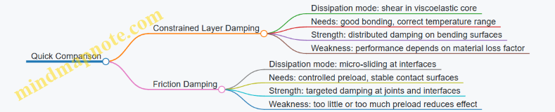
Example Integration into a Damping Plan

For a machine skid supporting a gearbox, you might combine both mechanisms: constrained layer damping on the skid’s underside to reduce panel resonances, and friction damping at a bolted interface where the skid couples to the foundation frame. The constrained layer reduces bending energy in the skid, while friction damping reduces energy that would otherwise feed back through the connection. The combined approach works because each mechanism addresses a different energy path, rather than trying to force one material to solve every problem.

5.5 Installation Practices Including Surface Preparation Bonding and Quality Verification

A damping or isolation system is only as good as what happens at the interface. The goal of this section is simple: make the contact surfaces predictable, make the bond line behave as designed, and prove the result with checks that catch common failure modes before they become maintenance work.

Surface Preparation Principles

Start by treating surface preparation as part of the design, not a housekeeping step. Most bond failures come from contamination, unevenness, or chemistry mismatch.

1. Remove contaminants completely: oil, cutting fluids, dust, paint overspray, and rust all interfere with adhesion. Use the same cleaning method across the whole job so the bond line is consistent.
2. Achieve the right roughness: smooth surfaces reduce mechanical interlock; overly rough surfaces can create voids and thick adhesive pockets. Target a uniform profile that matches the adhesive or damping layer requirements.
3. Control moisture and temperature: many adhesives are sensitive to humidity and cure conditions. Store materials as specified, and avoid installing when surfaces are wet or condensing.
4. Plan for edge effects: damping layers often start failing at edges where stresses concentrate. Clean and prepare edges and corners, not just the center.

Mind Map: Surface Preparation Workflow

- Surface Preparation - Contaminant Removal - Oil and grease - Dust and debris - Paint and coatings - Surface Profile Control - Too smooth reduces grip - Too rough traps voids - Uniformity across area - Environmental Control - Temperature within spec - Humidity and condensation checks - Edge Readiness - Corners and cutouts cleaned - No loose material at boundaries - Documentation - Cleaning method used - Surface condition recorded

Bonding Practices for Damping and Isolation Components

Bonding is where theory meets reality. A bond line that is too thick, too thin, or uneven changes stiffness and damping, which changes the system’s frequency response.

1. Mix and apply adhesives correctly: follow the specified ratio and mixing time. Incomplete mixing creates soft spots that look fine at first and then drift.
2. Use controlled bond-line thickness: spacers, not guesswork, help keep thickness consistent. If the design assumes a thin layer, thick patches can shift resonances.
3. Apply with full wet-out: the adhesive should contact the entire prepared surface without dry islands. For larger areas, work in sections so the adhesive doesn’t skin over.
4. Clamp or press with the right pressure: too little pressure leaves voids; too much can squeeze adhesive out and starve the bond.
5. Prevent movement during cure: vibration from nearby work, foot traffic, or handling can create micro-gaps. Treat cure as a no-surprises period.
6. Seal where needed: some systems require edge sealing to prevent moisture ingress and to keep the bond line from drying unevenly.

Example: Constrained Layer Damping on a Baseplate

A baseplate gets a viscoelastic layer bonded to the underside of a steel plate. The installer cleans the steel to remove rust and oil, then abrades to a uniform profile. Adhesive is mixed to the specified ratio, spread to a controlled thickness using a notched tool, and the assembly is clamped evenly. After cure, the installer checks for adhesive squeeze-out patterns and verifies that edges are fully wetted. If a corner shows a dry line, that area is corrected before the system is put into service.

Quality Verification That Actually Catches Problems

Quality verification should be layered: quick checks to prevent obvious mistakes, and targeted checks to confirm the bond behaves as intended.

Visual and Dimensional Checks

• Bond-line continuity: look for gaps, dry edges, and bubbles.
• Thickness consistency: compare multiple points against the expected range.
• Surface cleanliness at installation: confirm no new contamination occurred between prep and bonding.

Cure and Handling Verification

• Cure time and conditions: record start and end times, temperature, and humidity if required.
• Mechanical handling rules: verify the component wasn’t moved or loaded before the adhesive reached handling strength.

Performance-Oriented Checks

For vibration control systems, the best verification is a measurement that reflects the interface.

• Baseline comparison: if possible, measure before and after installation using the same sensor locations and mounting method.
• Frequency response sanity checks: confirm that expected resonance shifts or attenuation bands appear where the design predicts.
• Repeatability: re-measure at a few points to ensure the result isn’t a one-off.

Mind Map: Quality Verification Layers

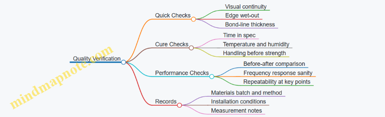
Common Failure Modes and How Installation Prevents Them

• Contamination under the bond: solved by consistent cleaning and avoiding re-contamination before bonding.
• Uneven bond thickness: solved by controlled application tools and spacers.
• Edge debonding: solved by thorough edge preparation and edge sealing where specified.
• Premature loading: solved by cure-time discipline and clear handling rules.
• Inconsistent cure due to environment: solved by installing within specified conditions and recording them.

Practical Checklist for Installers

• Confirm surface is clean, dry, and uniformly prepared.
• Verify adhesive mixing ratio and pot life.
• Apply adhesive to achieve designed bond-line thickness.
• Clamp evenly and prevent movement during cure.
• Record cure conditions and times.
• Perform visual and dimensional checks.
• Run before-after measurements where feasible and document results.

A well-installed damping or isolation interface should look boring: uniform bond lines, no loose edges, and measurements that match the expected behavior. That’s the point—boring is reliable.

6. Vibration Isolation Systems for Machinery Mounting

7. Active and Semi Active Vibration Mitigation Techniques

8. Damping and Isolation for Rotating Machinery and Reciprocating Equipment

9. Structural Modification and Foundation Engineering

9.1 Foundation Design Principles Including Mass Stiffness and Energy Dissipation

A machine foundation is not just “a big block.” It is a tuned system that decides how much vibration stays with the machine and how much travels into the building. The core levers are mass, stiffness, and energy dissipation. Treat them as a set of knobs that trade off against each other, then verify with measurements.

Mass Stiffness and Energy Dissipation as a System

Mass reduces transmitted motion by lowering the acceleration response for a given dynamic force. In practice, it also shifts resonances downward, which can be good or bad depending on where the machine’s excitation frequencies land.

Stiffness controls the static deflection and the natural frequency of the support. Too stiff can couple the machine strongly to the structure, while too soft can place the foundation’s resonance near operating speeds.

Energy dissipation reduces vibration amplitude by converting mechanical energy into heat. This is where many “it should work on paper” designs either succeed or disappoint, because real damping depends on interfaces, grout behavior, soil or slab contact, and material aging.

Mind Map: Foundation Design Levers

- Foundation Design Principles - Mass - Increases inertia - Shifts natural frequencies - Reduces acceleration for given force - Stiffness - Sets static deflection - Determines support natural frequency - Affects load path rigidity - Energy Dissipation - Material damping - Interface damping - Soil or slab contact losses - Design Workflow - Identify excitation frequencies - Choose target separation from resonances - Build model and estimate damping - Detail interfaces and reinforcement - Verify with operational measurements

Step 1: Identify Excitation Frequencies and Critical Modes

Start with the machine’s forcing spectrum: bearing defect orders, gear mesh harmonics, blade pass frequencies, and any reciprocating components. Then identify which foundation modes matter. For many industrial setups, the first few translational and rocking modes dominate transmission. A foundation that is “stiff enough” in one direction can still rock or twist if the geometry and reinforcement allow it.

Example: A pump has dominant forcing at 1× running speed and a weaker component at 2×. If the foundation’s rocking mode sits near 2×, the second harmonic can become the main contributor to floor vibration even when 1× is well separated.

Step 2: Choose a Frequency Separation Strategy

The usual goal is to avoid operating near foundation resonances. A practical approach is to target a natural frequency for the support system that is sufficiently separated from dominant excitation orders, considering uncertainty in stiffness and damping.

Mass and stiffness are linked: increasing mass tends to lower natural frequency, while increasing stiffness raises it. That means “add weight” and “make it rigid” can move the resonance in opposite directions. Decide which direction you need based on where the excitation sits.

Example: If the machine runs at 30 Hz and the foundation resonance is predicted at 28 Hz, adding mass may push it to 22–25 Hz, worsening the overlap with a nearby harmonic. Instead, adjust stiffness through baseplate thickness, reinforcement layout, or isolation interface selection.

Step 3: Estimate Damping Where It Actually Lives

Damping is not a single material property. In foundations, it comes from:

• Concrete and reinforcement internal damping
• Grout and contact damping at the machine baseplate interface
• Soil or slab contact losses if the foundation is supported by ground or a compliant mat
• Frictional slip in any interface that can micro-move under load

A useful engineering habit is to treat damping as an uncertainty band rather than a fixed number. If you assume 5% damping but the interface behaves closer to 1–2%, the predicted response can be far too optimistic.

Example: Two identical baseplates on different grout procedures can show noticeably different decay rates after a controlled impact test. The difference often traces to surface preparation, grout thickness uniformity, and whether voids exist.

Step 4: Detail Interfaces to Control Stiffness and Damping

Foundation performance is heavily influenced by how the machine connects to the concrete.

• Baseplate contact quality: uniform grout thickness and full bearing reduce unintended compliance.
• Anchor and leveling practice: inconsistent tightening can introduce looseness that increases damping variability and reduces repeatability.
• Reinforcement and cracking control: cracks change effective stiffness and can alter mode shapes.

Example: If anchor grout is thin in one corner, the baseplate can tilt slightly under load, increasing rocking response and making the foundation behave “softer” than modeled.

Step 5: Use a Simple Model to Guide Decisions, Then Verify

A foundation model can start simple: lumped mass for the machine and foundation, stiffness representing the support interface, and damping representing energy loss. Use it to check resonance locations and relative sensitivity to mass and stiffness changes. Then verify with operational modal analysis or transfer function measurements.

Example: After installing a revised baseplate thickness, you measure the transfer function from machine mount accelerations to floor vibration. If the resonance peak shifts upward as expected but the peak height stays high, the issue is likely damping or interface behavior rather than stiffness.

Mind Map: Practical Design Checks

Summary of the Foundation “Knobs”

Mass, stiffness, and energy dissipation are not independent. Mass and stiffness set where the system resonates; damping sets how tall the resonance peaks become. Good foundation engineering makes those choices with realistic interface assumptions, then confirms them with measurements so the design stops being a guess and starts being a controlled outcome.

9.2 Stiffness Enhancement and Its Tradeoffs with Resonance and Transmission

Stiffness enhancement means increasing the effective stiffness of a foundation, baseplate, or support interface so the system deflects less under load. In vibration control, that often sounds like a universal good thing—until you remember that stiffness also shifts natural frequencies and changes how forces transmit through the structure. The goal is not “maximum stiffness,” but stiffness that places resonances away from excitation and reduces transmission at the frequencies that matter.

Core Idea: Stiffness Changes Two Things

First, stiffness changes the system’s natural frequencies. For a simple single-degree-of-freedom model, the natural frequency scales roughly with the square root of stiffness. If you increase stiffness, the resonant peaks move upward.

Second, stiffness changes transmission. Even when resonance is avoided, the force-to-response ratio depends on stiffness and damping. A stiffer support can reduce displacement at low frequencies, but it can increase transmitted force into connected structures if the interface becomes a more efficient load path.

Where Tradeoffs Show Up in Real Machinery

Consider a pump on a baseplate. The pump produces periodic forces at running speed and harmonics. If the baseplate-plus-foundation system has a resonance near one of those harmonics, you get large motion and noise. Increasing stiffness can move that resonance upward, reducing motion at the original operating point.

Now consider the building frame connected to the foundation. If the foundation becomes stiffer, it may couple more strongly to the frame. The pump might vibrate less locally, but the frame might vibrate more, shifting the noise problem from “machine bay” to “nearby rooms.” This is why stiffness enhancement must be evaluated as a system, not a component.

Mind Map: Stiffness Enhancement Decision Logic

- Stiffness Enhancement - What Changes - Natural Frequencies - Resonance Peaks Move Up - Mode Shapes May Reorder - Transmission Paths - Force Transfer Through Interface - Coupling to Adjacent Structures - What You Want - Avoid Resonance at Operating Speeds - Reduce Receiver Vibration and Noise - Keep Deflection Within Mechanical Limits - What Can Go Wrong - New Resonances Near Harmonics - Increased Structureborne Transmission - Reduced Damping Effectiveness - How to Decide - Identify Dominant Excitations - Measure or Model FRFs and Coherence - Tune Stiffness Incrementally - Verify with Before After Tests

Step 1: Identify the Excitation Spectrum

Start with the machine’s force content. Rotating equipment typically excites at 1× speed and harmonics, plus bearing-related components. Reciprocating equipment adds strong broadband content and impacts. You do not need a perfect spectrum; you need a credible range of frequencies where excitation is significant.

Easy example: a motor-driven fan at 1800 rpm has 30 Hz fundamental (1×) and 60 Hz (2×). If your foundation resonance sits near 60 Hz, stiffness enhancement might help by pushing that resonance to, say, 80–90 Hz. But if you push it too far, you might land near 120 Hz where a harmonic exists.

Step 2: Determine the Current Resonance and Transmission Behavior

Use either measurement or modeling to answer two questions:

1. Where are the dominant resonances of the machine-support system?
2. How does vibration transmit from the machine into the surrounding structure?

A practical method is to obtain frequency response functions (FRFs) from a reference point on the baseplate or machine to points on the foundation and nearby receivers. Coherence helps confirm that the same source drives both locations.

Easy example: if the FRF from baseplate to a nearby wall shows a strong peak at the same frequency where the baseplate motion peaks, you have a direct transmission path. Stiffness changes should target that frequency behavior.

Step 3: Choose the Type of Stiffness Enhancement

Stiffness can be increased in different ways, and each affects modes differently.

• Massive stiffness increase: thicker baseplate, added ribs, or heavier foundation. This often raises frequencies but can also increase force transmission.
• Local stiffness increase: stiffening only under critical load paths, such as under bearing pedestals. This can reduce relative motion where it matters while limiting global coupling.
• Interface stiffness increase: stiffer grout or improved baseplate-to-foundation contact. This reduces slip and can raise effective stiffness without major structural changes.

Easy example: improving grout quality and eliminating voids can increase effective stiffness and reduce rocking. If the rocking mode was causing misalignment and high vibration, this can help without dramatically changing the entire foundation’s global coupling.

Step 4: Understand the Resonance Tradeoff Mechanism

When you increase stiffness, you typically shift resonant peaks upward. That reduces response at frequencies below the new resonance, but it can increase response near the shifted resonance. The tradeoff is therefore about where the new peaks land relative to operating speed and harmonics.

A useful rule of thumb is to avoid placing a strong resonance within the “excitation band” where the machine produces significant energy. The excitation band is not just 1×; it includes harmonics and sometimes bearing sidebands.

Step 5: Manage Transmission, Not Just Displacement

If stiffness enhancement reduces machine motion but increases transmitted force, you may still fail the receiver requirement. Transmission depends on how the interface couples to other structural elements.

Mitigation pairing is often necessary:

• Increase stiffness where it reduces critical relative motion.
• Add damping or isolation where it reduces transmitted energy.
• Ensure that stiffening does not create a direct rigid bridge to sensitive receivers.

Easy example: adding baseplate ribs can raise local stiffness, but if the ribs connect rigidly into a wall-formwork region, the wall may see higher vibration. Adding damping layers on the rib surfaces or adjusting connection details can reduce that transmission.

Step 6: Use Incremental Verification

Stiffness enhancement is rarely a one-shot decision. Small changes can reorder modes, especially in multi-mode systems like baseplates with multiple supports.

A systematic approach is to:

1. Apply a limited stiffness change.
2. Re-measure or re-check FRFs.
3. Confirm that the resonance peaks moved away from excitation and that receiver points did not worsen.

Easy example: after adding ribs, you might see baseplate displacement drop at 60 Hz, but wall vibration rises at 90 Hz. That tells you the new resonance is now exciting the wall. The fix is not to remove stiffness, but to adjust the stiffening layout or add damping at the coupling interface.

Practical Summary

Stiffness enhancement works when it shifts resonances away from dominant excitation and does not create a stronger transmission bridge to receivers. Treat stiffness as a design variable with measurable consequences: it changes both where the system resonates and how forces travel. The best results come from pairing stiffness changes with damping and connection-detail control, then verifying with FRFs and before-after measurements.

9.3 Isolation Interfaces Between Foundations and Surrounding Structures

A foundation rarely acts alone. It sits inside a web of slabs, walls, soil, pipe racks, and building frames, and that web creates extra paths for vibration and noise. The goal of an isolation interface is simple: control how energy leaves the foundation and how much of the surrounding structure “talks back” into it.

Core Interface Concepts

Start with the two directions of coupling.

1. Foundation to surrounding structure: vibration from the machine base travels into the adjacent slab, columns, and walls. This is often the dominant path for structureborne noise at nearby receivers.

2. Surrounding structure to foundation: building motion from other equipment, foot traffic, or HVAC duct vibration can excite the foundation. Even a well-isolated machine can suffer if the interface transmits building motion efficiently.

In practice, you manage both by treating the interface as a controlled boundary condition. A “good” boundary condition is not necessarily soft everywhere; it is soft in the right directions and stiff enough to keep alignment and safety margins.

Interface Mechanisms You Must Account For

1) Contact stiffness at grout and bearing surfaces Grout and bearing pads set the effective stiffness between foundation and adjacent elements. Higher stiffness increases transmission at many frequencies, but too much softness can create excessive motion and fatigue.

2) Flanking through reinforcements and ties Rebar continuity, anchor bolts, and steel plates can bypass isolation layers. A common failure mode is installing an isolation gap in one place while leaving a solid steel bridge elsewhere.

3) Airborne and structureborne coupling through penetrations Pipe sleeves, cable trays, and duct penetrations can carry vibration and also leak sound. Even if the foundation is isolated, rigid sleeves can create a direct mechanical path.

4) Soil-structure interaction Soil is not a perfect spring. Its stiffness and damping vary with moisture, compaction, and depth. Interface design should assume that the soil will not behave like a neat textbook element.

Systematic Design Workflow

Step 1: Identify the interface boundaries List every element that touches or nearly touches the foundation: adjacent slabs, curb walls, pipe racks, cable trays, and any structural beams. Mark which connections are rigid, semi-rigid, or potentially isolatable.

Step 2: Map coupling paths by frequency Use measured or estimated frequency response functions to see where transmission is strongest. If you do not have data yet, begin with the machine’s dominant excitation orders and harmonics, then check for nearby structural resonances.

Step 3: Choose the isolation strategy by path type

• For direct contact paths, use an isolation layer or controlled gap.
• For steel bridges, break continuity with isolating sleeves or redesign the connection.
• For penetrations, use resilient sleeves and flexible connections.
• For adjacent slabs, consider separation joints and controlled stand-off details.

Step 4: Verify with acceptance checks Confirm that interface changes reduce measured transfer at key frequencies and do not introduce unacceptable base motion, alignment drift, or safety issues.

Practical Details That Work

Isolation gaps and separation joints A separation joint should be continuous where it matters. If the gap is blocked by a cable tray bracket or a grout “bridge,” the isolation layer becomes decorative. A simple field check is to trace every potential contact from the foundation edge to the surrounding slab.

Resilient sleeves for penetrations For pipes and conduits, use sleeves with a resilient liner and seal the annulus to prevent air leakage. The mechanical goal is to prevent rigid contact between the foundation and the surrounding structure through the penetration.

Controlled grout interfaces When grout is required for leveling or load spreading, limit its role in transmission. For example, use grout where it supports load transfer but avoid full-area rigid bonding to adjacent structural elements. If the design requires bonding, add a resilient layer elsewhere in the load path so the interface is not uniformly stiff.

Steel continuity breaks If anchor bolts or plates must pass near an isolation layer, include isolating washers or redesign the bracket so the steel does not create a direct rigid bridge across the interface.

Mind Map: Isolation Interfaces Between Foundations and Surrounding Structures

- Isolation Interfaces Between Foundations and Surrounding Structures - Coupling Directions - Foundation to Surroundings - Surroundings to Foundation - Transmission Mechanisms - Contact Stiffness at Grout and Bearings - Flanking Through Reinforcement and Ties - Penetrations Through Pipes Cables and Ducts - Soil-Structure Interaction - Design Workflow - Identify Interface Boundaries - Map Coupling Paths by Frequency - Select Strategy by Path Type - Verify with Acceptance Checks - Practical Implementation - Separation Joints and Isolation Gaps - Resilient Sleeves and Annulus Seals - Controlled Grout Interfaces - Steel Continuity Breaks - Verification - Transfer Reduction at Key Frequencies - Base Motion and Alignment Limits - Safety and Fatigue Considerations

Example: Retrofitting a Pump Foundation Interface

A pump sits on a baseplate grouted to a foundation block. Nearby, a housekeeping slab is poured flush against the foundation edge. After commissioning, vibration levels at the slab-mounted equipment increase at the pump’s 1× and 2× running speeds.

Diagnosis: the slab is rigidly connected through direct contact and a few steel supports for cable trays. The interface is effectively a stiff bridge.

Fix:

• Cut and remove rigid contact at the foundation edge and install a continuous separation joint with a resilient filler.
• Replace rigid cable tray standoffs near the interface with isolated supports that do not touch the foundation.
• Add resilient sleeves for any remaining penetrations and seal the annulus.

Verification: repeat transfer measurements from foundation accelerometers to receivers on the adjacent slab. The target is a reduction at the pump’s dominant frequencies without increasing base motion beyond the alignment tolerance.

Example: Preventing Building Motion Excitation

A compressor foundation is isolated from the machine using elastomer mounts, but the building has another rotating system nearby. During that system’s operating window, the compressor shows elevated vibration even though its own mounts are unchanged.

Diagnosis: the surrounding structure excites the foundation through rigid connections at the interface, such as grouted bearing pads or continuous steel elements.

Fix: break rigid continuity at the interface by introducing resilient pads or isolating sleeves where structural members connect to the foundation, and ensure penetrations do not create rigid mechanical bridges.

Verification: compare compressor vibration during the other system’s on/off cycles and confirm that the interface modifications reduce the building-to-foundation transfer at the relevant frequencies.

9.4 Grouting Anchors and Baseplate Detailing for Controlled Boundary Conditions

A baseplate is only as good as the boundary conditions it creates. In vibration control, “controlled” means repeatable stiffness, predictable damping contribution, and consistent load transfer from machine feet into anchors and the foundation. Grout and anchor detailing are where those boundary conditions are won or lost.

Foundational Boundary Condition Concepts

Start with what the machine “sees.” The baseplate-foot interface and the foundation interface together define how forces turn into motion. If the grout layer is thin in some areas and thick in others, the local stiffness varies, which shifts resonances and can amplify specific frequency bands. If anchors are over-constrained or poorly aligned, they can introduce bending moments that the machine did not intend to generate.

A practical way to think about it: grout behaves like a stiffness bridge, while anchors behave like force carriers. The baseplate transfers both vertical loads and moments; the foundation must accept them without creating unintended rocking or shear slip.

Grout Selection and Performance Targets

Choose grout based on mechanical properties and constructability. For vibration work, the key targets are compressive strength, low shrinkage, and adequate bond to both baseplate and foundation. Low shrinkage matters because shrinkage can create micro-gaps that reduce effective stiffness right after commissioning.

A simple example: two grouts both meet a 28-day compressive strength spec, but one is formulated for minimal bleeding and shrinkage. During installation, the low-shrinkage grout maintains contact around anchor sleeves, so the baseplate stiffness stays close to the design assumption.

Surface Preparation and Contact Quality

Bond quality is not optional. Remove laitance, dust, and loose concrete; create a surface profile that allows grout to mechanically key. For steel, ensure baseplate surfaces are clean and free of paint or contaminants in the grout contact zone.

Example: if the foundation top is smooth and sealed, grout may cure with good strength but poor bond. Under cyclic loading, the baseplate can micro-slip, increasing vibration levels at the machine’s dominant harmonics.

Baseplate Detailing for Predictable Load Paths

Detail the baseplate so load paths are direct and moments are controlled.

• Use appropriate leveling pads or grout pockets so the baseplate does not “bridge” over voids.
• Provide grout thickness that matches the grout system capability; extremely thin layers can be difficult to place without defects.
• Avoid sharp changes in baseplate thickness near anchor zones; stiffness discontinuities can concentrate stress and alter local modal behavior.

A concrete example: a baseplate with a thickened pad only under the center can cause the outer feet to rely on grout stiffness that is lower than expected. The foundation interface then behaves like a partial support, shifting the rocking mode downward.

Anchor Grouting and Sleeve Management

Anchors must be positioned and grouted so they carry load without creating unintended compliance.

• Keep anchor sleeves aligned and clean so grout can fully surround the shank where required.
• Ensure grout does not trap air around the anchor, especially near the sleeve ends.
• Use procedures that maintain grout flow into corners and around reinforcement.

Example: if grout is poured too quickly, it can trap air bubbles around anchor sleeves. The anchor still holds static load, but under vibration the effective stiffness drops, and the baseplate can show higher response near the foundation’s local modes.

Controlled Boundary Conditions Through Grout Placement

Placement is a boundary condition event. Use methods that promote full contact: proper pour sequence, vibration or flow techniques compatible with the grout, and continuous filling to avoid cold joints.

A systematic checklist for placement quality:

• Confirm baseplate is level and supported during the pour.
• Verify grout mix consistency and temperature.
• Maintain continuous filling until grout reaches the intended thickness everywhere.
• Inspect for voids and honeycombing before cure proceeds.

Verification Using Measurements and Acceptance Logic

After installation, verify that the boundary conditions behave as intended.

• Perform operational vibration checks at the machine’s key speed and harmonic frequencies.
• Compare baseline frequency response or overall vibration metrics to commissioning targets.
• If possible, use impact testing or operational modal analysis to confirm that support stiffness and damping are within expected ranges.

Example: if the dominant resonance peak shifts upward after rework, it suggests improved contact and stiffness. If it shifts downward, it can indicate grout defects, insufficient thickness, or anchor misalignment.

Mind Map: Grouting Anchors and Baseplate Detailing

- Grouting Anchors and Baseplate Detailing - Boundary Conditions - Effective stiffness of interfaces - Damping contribution from grout - Rocking and shear slip control - Grout System - Low shrinkage - Bond strength - Placement compatibility - Surface Preparation - Remove laitance and dust - Steel cleanliness - Mechanical keying - Baseplate Detailing - Grout thickness uniformity - Avoid bridging and voids - Manage stiffness transitions - Anchor Detailing - Sleeve alignment - Full grout surround - Air trap prevention - Placement Process - Continuous filling - Correct pour sequence - Compatible consolidation - Verification - Operational vibration checks - Modal or impact testing - Compare to acceptance targets

Example: Pump Baseplate with Anchor Sleeves

A pump baseplate is installed on a concrete foundation with four anchor groups. The design assumes a uniform grout layer stiffness.

1. Foundation top is roughened and cleaned to ensure bond.
2. Baseplate is leveled using temporary supports, leaving grout pockets fully accessible.
3. Grout is mixed to the specified water ratio and placed continuously, starting from one corner to drive flow through the entire pocket.
4. Anchor sleeves are checked for alignment before grout placement.
5. After cure, operational checks confirm that the dominant harmonic response matches the commissioning baseline within the acceptance band.

If the measured response is higher than expected at a specific frequency, the first suspects are voids, poor bond, or anchor sleeve grout defects—because those directly change the interface stiffness the model assumed.

9.5 Verification Testing After Structural Changes Using Operational Modal Analysis

Structural changes—new baseplates, grouting, added stiffeners, altered boundary conditions—often shift modal frequencies, mode shapes, and damping. Operational Modal Analysis (OMA) verifies those changes using measured responses under normal operating or ambient excitation, without requiring a controlled impact hammer. The goal is not just “did it change,” but “did it change in the way the design assumed,” and “did it introduce new coupling paths.”

Foundational Setup and Planning

Start by defining what “success” means for the specific structural change. Typical targets include reduced transmissibility at machine operating orders, reduced vibration at receiver points, and stable modal behavior across the relevant speed range. Then choose measurement locations that can distinguish local baseplate effects from global foundation effects.

A practical rule: place sensors so that at least one set captures the machine-side structure and another set captures the surrounding building or adjacent equipment frame. If you only measure near the machine, you can confirm improvement locally while missing a flanking path that now dominates.

Measurement Strategy for OMA

Use accelerometers (or velocity sensors) with consistent mounting quality. For baseplate verification, measure vertical and horizontal directions if the change affects rocking or shear. For foundation verification, include at least one sensor on the foundation mass and one on the supporting slab or frame.

Collect data during steady operating conditions when excitation is repeatable. If the machine runs through speed ranges, segment the data by speed bins and treat each bin as its own OMA dataset. This prevents mixing modes that are only present at certain speeds.

Data Conditioning and Quality Checks

Before modal extraction, verify signal quality: check for clipping, excessive noise, and sensor dropouts. Use coherence between channels to confirm that the structure is being excited in a way that supports stable modal identification. Low coherence across many channels usually means either poor mounting, insufficient excitation energy, or a measurement layout that misses the active degrees of freedom.

Windowing and overlap should be chosen to balance frequency resolution and stationarity. If the machine load changes during the record, modal estimates can smear. When in doubt, shorten records and increase the number of segments.

Modal Identification and Model Updating

Apply an OMA method such as frequency domain decomposition or stochastic subspace identification. Extract modal frequencies, damping ratios, and mode shapes. Then compare the “before” and “after” modal sets.

Mode matching is the heart of verification. Use modal assurance criteria (MAC) to pair modes with similar shapes. Frequency shifts alone can mislead: a small frequency change with a large shape change can indicate a boundary condition shift rather than improved stiffness.

Update the structural model if you have one. The verification is strongest when the measured modal changes align with the predicted changes in stiffness and damping distribution.

Interpreting Results with Engineering Meaning

A structural change often increases stiffness, which typically raises natural frequencies. However, damping can also change because grout quality, contact conditions, and added materials alter energy dissipation. If damping decreases while frequencies increase, transmissibility at certain bands may worsen even though the structure feels “stiffer.”

Also watch for new modes. Adding stiffeners can create local modes that were previously outside the operating band. If those new modes couple to the machine base, you may see increased vibration at specific receiver points.

Mind Map: Verification Workflow

# OMA Verification After Structural Changes - Objective - Confirm modal shifts match design intent - Detect new coupling paths - Validate damping and transmissibility behavior - Planning - Define success metrics - Choose sensor layout - Machine-side points - Foundation or building points - Segment data by operating condition - Acquisition - Stable mounting and correct directions - Adequate excitation energy - Multiple records for repeatability - Conditioning - Clipping and dropout checks - Coherence and noise assessment - Windowing and stationarity control - Identification - OMA method selection - Extract frequencies, damping, mode shapes - Mode matching using MAC - Comparison - Before vs after - Frequency shift trends - Mode shape change interpretation - Damping ratio changes and implications - Engineering Decisions - Accept structural change - Adjust design or installation - Plan targeted follow-up measurements

Example: Grouted Anchor and Baseplate Stiffness Change

A pump baseplate was re-grouted and anchor details were tightened to reduce rocking. Measurements were taken before and after the work at four points: two on the baseplate corners and two on the adjacent slab. Data were collected at a steady pump speed, then split into speed bins of ±2%.

After OMA, the dominant vertical mode frequency increased by 18%. MAC pairing showed the mode shape remained consistent, suggesting the stiffness increase was the main effect. Damping decreased slightly, which explained why vibration at a nearby receiver point improved at some frequencies but not all. A follow-up check confirmed that a horizontal rocking mode moved closer to an operating harmonic, so additional constrained-layer damping was added to the baseplate underside.

The verification step prevented a common mistake: declaring success based on the single most visible frequency shift while ignoring the mode that actually aligned with the excitation harmonic.

Example: Detecting a New Flanking Path

In a compressor retrofit, a foundation stiffener reduced vibration at the machine skid. OMA after the change revealed a new mode with a different mode shape, paired by MAC to a previously weakly excited mode. The new mode had higher participation on the adjacent pipe support frame, indicating that the stiffener altered load paths. The fix was not more stiffness; it was improved isolation at the pipe support interface and a revised restraint layout.

Acceptance Criteria and Documentation

Acceptance should be based on consistent modal pairing and engineering relevance. A reasonable set of criteria includes: (1) matched modes show MAC above a chosen threshold, (2) frequency shifts fall within the expected direction and magnitude from the structural change, (3) damping changes do not contradict observed transmissibility trends, and (4) no new modes appear within the critical excitation bands without a mitigation plan.

Document the measurement conditions, sensor locations, data segmentation method, identification settings, and the before/after modal comparison table. If the results are used to sign off installation quality, include the reasoning that links modal changes to the specific structural modification made on site.

11. Industrial Noise Control Integration from Source to Receiver

11.1 Prioritizing Control Measures Using Source Path and Receiver Criteria

Industrial noise and vibration problems rarely have one villain. A gearbox can be the source, but the foundation can be the amplifier, and the receiver can be the limiting factor for compliance. Prioritization is how you spend effort where it actually changes what people and equipment experience.

Step 1: Define the Receiver Requirements First

Start with what must be satisfied: typical receiver criteria include operator hearing limits, equipment functional limits, and process quality constraints. Convert these into measurable targets such as A-weighted sound pressure level at a workstation, octave-band sound pressure level in a room, or vibration velocity at a sensitive component.

Example: If a pump room must meet a workstation limit, you prioritize reductions that affect airborne sound reaching that room. If the constraint is a control cabinet malfunction from vibration, you prioritize transmission to the cabinet mounting points, even if the room is still loud.

Step 2: Map Source Path Mechanisms

Next, identify how energy travels from the machine to the receiver. Use a simple classification:

• Airborne path: sound radiates from casing, ducts, and openings.
• Structureborne path: vibration excites the baseplate, floor, and nearby walls.
• Flanking path: energy bypasses the main barrier through penetrations, shared frames, or cable trays.

Example: A partially enclosed compressor may still fail noise targets because the enclosure is rigidly connected to a wall that becomes a secondary radiator. The source is still the compressor, but the dominant path is flanking.

Step 3: Build a Source Path Receiver Matrix

Create a matrix that links each candidate control measure to each path and receiver. Score each combination by expected impact and feasibility.

Use a practical scoring approach:

• Impact: how strongly the measure reduces the relevant quantity at the receiver (sound level, vibration velocity, or both).
• Coverage: whether it addresses the dominant path or only a minor one.
• Feasibility: installation space, downtime, maintainability, and risk to machine operation.

Example: Adding acoustic absorption inside an enclosure can strongly reduce airborne radiation but may do little for vibration-induced floor noise. Conversely, improving base isolation can reduce structureborne transmission but won’t fix duct-borne tonal noise.

Step 4: Use Measurement to Confirm Dominant Paths

Before committing to hardware, confirm which paths dominate at the frequencies that matter.

• For airborne noise: measure sound pressure near the receiver and around likely radiating surfaces.
• For structureborne noise: measure vibration at the machine mounting, baseplate, and receiver structure.
• Use frequency-domain thinking: tonal components from rotating machinery often dominate at specific orders, while broadband components may come from impacts or airflow.

Example: If vibration at the floor peaks at the same frequency as the receiver’s noise complaint, structureborne coupling is likely. If the receiver shows strong tonal noise but floor vibration is modest, airborne radiation or duct transmission is more likely.

Step 5: Prioritize by “Most Leverage per Constraint”

Rank measures using a rule of thumb: pick the smallest set of actions that changes the dominant path to the receiver.

A common ordering that works in practice:

1. Eliminate or reduce excitation at the source when it is straightforward (alignment correction, balancing, tightening loose parts, fixing airflow leaks).
2. Interrupt the dominant transmission path (isolation mounts for structureborne, sealing and panel treatment for airborne, decoupling penetrations for flanking).
3. Add damping where motion concentrates (baseplate constrained-layer damping, tuned damping for structural modes).
4. Verify with before-after measurements at the receiver, not just at the machine.

Example: If a fan’s blade-pass tone is the main issue, balancing and inlet conditioning can reduce excitation. If the tone persists, then enclosure sealing and duct silencing target the path.

Mind Map: Source Path Receiver Prioritization

- Prioritizing Control Measures - Receiver Requirements - Human comfort and compliance - Equipment functional limits - Process quality constraints - Define measurable targets - Source Mechanisms - Rotating tonal components - Reciprocating impacts - Airflow and leakage noise - Electrical and control-related vibration - Transmission Paths - Airborne radiation - Casing - Ducts - Openings - Structureborne coupling - Mounts - Baseplate - Floor and walls - Flanking routes - Penetrations - Shared frames - Cable trays - Decision Tools - Source Path Receiver Matrix - Impact - Coverage - Feasibility - Measurement confirmation - Receiver sound pressure - Structural vibration points - Frequency-domain dominance - Action Ordering - Reduce excitation at source - Interrupt dominant path - Add damping at motion hotspots - Verify at receiver

Example: Two Competing Constraints

A packaging line has two complaints: operators report high noise near the control room, and the line’s encoder occasionally misreads due to vibration.

• For the encoder: prioritize structureborne transmission to the encoder bracket. Isolation mounts under the machine base and decoupling of the encoder cable routing from the vibrating frame typically give the biggest improvement.
• For the operators: prioritize airborne radiation and flanking. Sealing enclosure seams, adding panel mass where sound leaks, and treating duct openings can reduce sound pressure at the control room.

The key is that the “best” measure for one receiver may not be the best for the other, so the matrix prevents you from optimizing the wrong outcome.

Step 6: Document the Rationale So It Stays Correct

Record the dominant paths, the scoring logic, and the measurement evidence. This matters because later troubleshooting will otherwise treat symptoms as causes, and you’ll end up repeating work with different labels.

11.2 Integrated Design Workflow Combining Isolation Damping and Enclosure Treatments

Integrated control starts by treating the machine, its support, and its noise path as one system. The goal is not just to “reduce vibration” or “quiet the enclosure,” but to reduce the receiver’s exposure at the frequencies that matter, while keeping the design buildable and verifiable.

Step 1: Define Performance Targets and Constraints

Begin with measurable targets: sound pressure level at receiver positions, sound power limits for equipment bays, and vibration limits at mounting points or on critical surfaces. Then list constraints that often decide the outcome: available mounting space, allowable baseplate mass, maintenance access, temperature range, and maximum permissible motion (for example, clearance to piping).

Example: A pump room has a target of 5 dB reduction in the 250–500 Hz band at two operator locations. The pump runs at 30 Hz shaft speed with a strong 2× harmonic. The enclosure must fit around existing ductwork, and the mount travel cannot exceed 6 mm.

Step 2: Map Excitation Sources to Transmission Paths

Identify what excites the structure and what carries it to the receiver. Typical paths include airborne radiation from the machine and enclosure, structureborne transmission through mounts and baseplates, and flanking through walls, floors, and penetrations.

Practical check: If the dominant vibration is at 2× running speed, but the receiver noise peaks at a different band, you likely have a structural resonance or enclosure panel mode shaping the response.

Step 3: Build a System Model That Matches the Decision You Need

Use a model that is detailed enough to guide isolation and enclosure choices. A common workflow is:

• Use a frequency-domain model for mounts and baseplate modes.
• Use panel or enclosure transmission estimates for airborne-to-structure coupling.
• Include damping in the structural model, not just stiffness.

Example: A simple mount model predicts a resonance near 20 Hz. Since the operating speed is 30 Hz, isolation will help, but only if the baseplate and enclosure do not introduce a strong mode near 60 Hz (2×). That becomes a design target.

Step 4: Choose Isolation and Damping as a Coupled Pair

Isolation changes how much force reaches the structure; damping changes how much of that energy stays and rings down.

• If you only isolate: the machine may move more, and the baseplate can still ring if damping is low.
• If you only damp: you reduce ringing, but you still transmit too much force.

Example: For a skid-mounted compressor, elastomer mounts reduce transmitted force above the mount resonance. Adding constrained-layer damping to the baseplate reduces the panel’s modal peaks, lowering the enclosure’s “singing” at the harmonic band.

Step 5: Design the Enclosure for Transmission Loss and Leakage Control

Enclosures work through mass, stiffness, and damping of panels, plus control of openings. The enclosure should be treated as part of the structural system, not a separate box.

Key practices:

• Use double-layer or stiffened panels where panel modes are expected.
• Seal doors, inspection ports, and cable penetrations.
• Decouple the enclosure from the machine support so the enclosure does not become a parallel transmission path.

Example: A “mostly sealed” enclosure still leaks at a cable gland. After sealing and adding a flexible conduit section, the measured receiver noise drops in the same band as the cable penetration’s structural vibration.

Step 6: Integrate Flanking and Penetrations Early

Flanking often defeats otherwise good isolation. Treat walls, floors, and duct interfaces as transmission elements.

Practice: Specify how the enclosure is attached to the building. If rigid brackets connect the enclosure to a vibrating wall, you can lose the benefit of panel damping.

Step 7: Verify with a Measurement Plan That Matches the Model

Before finalizing, plan measurements that confirm each design assumption:

• Mount transmissibility or baseplate vibration at key points.
• Enclosure surface velocity to locate panel modes.
• Receiver sound pressure levels to confirm the noise path reduction.

Example: If the model predicts a baseplate mode at 120 Hz, measure baseplate velocity and enclosure panel velocity near that frequency. If the receiver noise drops but panel velocity does not, you may have reduced airborne leakage rather than structural radiation.

Step 8: Iterate Using Targeted Changes

Iteration should be surgical. Change one element at a time and re-measure the same metrics.

Common iteration moves:

• Adjust mount stiffness or add damping to shift and reduce peaks.
• Add or relocate damping patches to reduce specific modal peaks.
• Improve sealing and decouple enclosure attachments to reduce flanking.

Mind Map: Integrated Workflow for Isolation Damping and Enclosure Treatments

- Integrated Design Workflow - Define Targets - Receiver SPL goals - Vibration limits - Motion and access constraints - Map Paths - Source excitation - Airborne radiation - Structureborne transmission - Flanking and penetrations - Build Model - Mount and baseplate modes - Enclosure panel behavior - Damping representation - Select Isolation and Damping - Isolation reduces force transfer - Damping reduces ringing - Coupled design checks - Enclosure Treatment - Panel mass and stiffness - Damping in panels - Seals and openings control - Decoupling from supports - Flanking Control - Attachment strategy - Penetration detailing - Duct and pipe interfaces - Verification - Mount/baseplate measurements - Enclosure surface velocity - Receiver SPL confirmation - Iterate - Targeted stiffness changes - Damping patch adjustments - Sealing and decoupling improvements

Example: Pump Retrofit with Integrated Isolation and Enclosure

Start with receiver targets in the 250–500 Hz band. Measure pump and baseplate vibration to confirm dominant harmonics. Select mounts so the mount resonance sits well below the operating band, then add constrained-layer damping to the baseplate to reduce modal peaks that coincide with the enclosure panel modes. Finally, seal inspection openings and decouple the enclosure from the baseplate using compliant attachments. Verify by repeating receiver SPL measurements and checking that enclosure surface velocity peaks align with the reduced noise band.

This workflow keeps the design coherent: isolation reduces what reaches the structure, damping controls how the structure behaves, and the enclosure prevents the receiver from seeing the remaining motion—especially through leaks and flanking paths.

11.3 Acoustic Treatment Selection for Rooms Ducts and Equipment Bays

Selecting acoustic treatment for rooms, ducts, and equipment bays is mostly about controlling where sound energy goes after it leaves the source. The practical workflow is: (1) identify dominant noise paths and frequency bands, (2) choose treatments that target those bands with the right placement, (3) verify with measurements that match the acceptance criteria.

Foundational Concepts That Drive Material Choice

Sound in industrial spaces is rarely “one problem.” You typically have a mix of airborne sound from panels, leaks, and openings, plus duct-borne sound that travels with airflow. Acoustic treatment addresses both by controlling absorption, reflection, and transmission.

1. Absorption reduces reverberant build-up. It is most effective when the treatment is placed where sound energy is likely to reach surfaces repeatedly, such as walls and ceilings in rooms.

2. Duct lining reduces sound traveling inside ducts. It works best when the lining is protected from airflow erosion and when the duct geometry doesn’t short-circuit the effect.

3. Barriers and enclosures reduce transmission through openings and weak boundaries. Even strong absorption won’t fix a large leak.

A useful mental model: absorption reduces “how long sound hangs around,” while barriers reduce “how much sound escapes.” Duct lining is absorption applied to the path itself.

Step 1: Determine What You’re Treating

Start with a frequency-resolved measurement plan. Use octave or one-third-octave bands so you can match treatments to band behavior.

• Rooms: If the sound level is dominated by reverberation, you’ll see relatively smooth levels across positions and a strong dependence on distance from the source.
• Ducts: If the noise changes with duct operating conditions and correlates with fan speed or flow, duct-borne paths are likely dominant.
• Equipment bays: If noise is concentrated around doors, cable penetrations, and panel seams, transmission and flanking dominate.

Easy example: A compressor bay shows high levels near the door even when the room is otherwise quiet. Treating the ceiling alone won’t help much; you need sealing and targeted absorption near the opening area.

Step 2: Choose Treatment Type by Frequency Band

Different materials behave differently across frequency.

• Fibrous absorbers (mineral wool, glass wool) are strong at mid to high frequencies. They need an air gap or sufficient thickness to perform well at lower mid bands.
• Membrane or panel absorbers can target specific low-mid bands but require careful mounting and tuning.
• Perforated face with backing combines surface impedance control with fibrous absorption, improving performance where plain fibrous layers would be less effective.

Easy example: If measurements show a peak around 500 Hz, a thin blanket won’t do much. A thicker absorber or a perforated panel with backing can shift effectiveness downward.

Step 3: Select Placement That Matches Sound Field Behavior

Placement matters as much as material.

Rooms

• Treat ceiling and upper walls first because sound energy often reflects there and builds up.
• Avoid covering only small areas. For meaningful reverberation reduction, target a reasonable coverage ratio and keep surfaces continuous.

Easy example: If you line only a small patch above a machine, the rest of the room still provides reflective surfaces, so the overall reverberation time barely changes.

Ducts

• Line straight runs where sound has time to interact with the lining.
• Keep lining away from bends unless you have verified performance; turbulence can reduce effective absorption.
• Use acoustic insulation with protective liners where airflow erosion is a concern.

Easy example: A duct with a 90° elbow right after the fan may show poor benefit from lining near the elbow. Lining the first long straight section downstream often yields better results.

Equipment Bays

• Prioritize absorbing surfaces that are “visible” from the source through openings and internal reflections.
• Combine with sealing at penetrations. Absorption can’t compensate for a poorly sealed cable tray or door gasket.

Easy example: After installing door seals, the noise drops noticeably. Adding absorptive panels on the interior walls then reduces the remaining reverberant component.

Step 4: Check Practical Constraints

Industrial environments add constraints that affect acoustic performance.

• Temperature and humidity: Some adhesives and facings degrade; choose systems rated for the environment.
• Air velocity and dust: Duct linings need protective facings and stable fibers.
• Cleanability and hygiene: Food or clean areas may require specific surface finishes.
• Fire safety: Use rated materials and assemblies consistent with the facility requirements.

Easy example: A bay with frequent washdowns may require sealed, cleanable facings over absorbers; otherwise the absorber becomes a maintenance problem and performance drops.

Step 5: Verify with Acceptance Metrics

Use before-after measurements in the same operating conditions.

• For rooms: compare sound pressure levels at representative receiver points and confirm reverberation reduction trends.
• For ducts: compare levels at duct outlets and near the fan discharge under stable flow.
• For bays: compare receiver points near doors and typical operator locations.

A good acceptance approach is to define target reductions by band where possible, not just broadband totals.

Mind Map: Acoustic Treatment Selection Logic

# Acoustic Treatment Selection - Goal - Reduce airborne noise at receivers - Reduce duct-borne noise along flow paths - Reduce transmission through openings and weak boundaries - Inputs - Frequency-banded measurements - Source type and operating correlation - Geometry and likely flanking paths - Environmental constraints - Room Treatments - Absorption on ceiling and upper walls - Adequate thickness and coverage - Continuous surfaces over small patches - Duct Treatments - Lining on straight runs - Protective facings for erosion - Consider bends and turbulence zones - Equipment Bay Treatments - Absorption visible from source - Seal doors, penetrations, seams first - Combine enclosure integrity with interior absorption - Material Selection - Fibrous for mid/high bands - Perforated face with backing for improved mid performance - Membrane/panel for targeted low-mid bands - Verification - Before-after at same operating conditions - Band-focused acceptance where feasible - Receiver point comparison

Example: Integrated Room and Duct Treatment Plan

A facility reports high broadband noise near a control room wall. Measurements show strong mid-frequency content and a correlation with fan speed.

1. Duct path check: Levels at the duct outlet are high, and the spectrum matches fan harmonics.
2. Duct lining: Install protected fibrous lining on a long straight duct section, avoiding the immediate elbow region.
3. Room absorption: Add ceiling and upper-wall absorbers sized for the dominant mid bands.
4. Receiver verification: After installation, confirm the reduction at receiver points and ensure the door and wall penetrations remain sealed.

The result is typically a combined reduction: duct lining reduces what reaches the room, and room absorption reduces how much remains reverberant once inside.

11.4 Verification Using Before After Measurements and Acceptance Metrics

Verification is where the design stops being a set of good intentions and becomes a measurable outcome. The goal is to confirm that the installed isolation, damping, and acoustic measures reduce noise and vibration at the receiver while staying within mechanical and operational constraints.

Define What “Success” Means Before You Measure

Start by writing acceptance metrics in plain terms and tying them to the physics you expect to change.

• Noise metric: choose a receiver-based quantity such as A-weighted sound pressure level (SPL) at key locations, or a band-limited metric around dominant tones.
• Vibration metric: choose a response quantity such as acceleration RMS or velocity RMS at machine mounts, baseplate, or nearby structural points.
• Transmission metric: if you can, use frequency response functions (FRFs) or transfer functions between a reference input (e.g., bearing housing acceleration) and receiver points.
• Operational constraints: include checks like mount travel margin, temperature limits for damping materials, and no increase in vibration at other critical points.

A practical acceptance statement might read: “At the operator position, the dominant 1/3-octave band containing the gearbox tone decreases by at least 5 dB after installation, and the mount acceleration RMS decreases by at least 30% without exceeding allowable travel.”

Plan the Before After Test Like a Controlled Experiment

Before/after comparisons fail when the test conditions drift. Lock down the essentials.

• Same operating states: match speed, load, and duty cycle. If the process varies, record it and use only comparable windows.
• Same measurement locations: mark sensor coordinates and use consistent mounting methods. A magnet that “works fine” on one day can be a different story on another.
• Same instrumentation settings: sampling rate, bandwidth, averaging time, windowing, and trigger conditions should match.
• Same environmental conditions: note HVAC status, doors open/closed, and background noise. If background changes, document it and use it to interpret results.

Example: For a pump, run three steady-state windows at the same RPM before and after. Use identical sensor mounting on the baseplate corner and the operator-side panel.

Measure with Metrics That Match the Mechanism

Use measurement choices that reflect how the control works.

• Isolation improvements often show up as reduced transmissibility at specific frequency bands, not necessarily across the whole spectrum.
• Damping improvements often reduce resonance peaks and broaden the response reduction around modes.
• Enclosure improvements often reduce airborne contributions at receiver points more than at structural points.

So, if you expect airborne reduction from enclosure sealing, measure both inside/outside enclosure points and at a structural reference. If the receiver drops but the structural point does not, you likely improved airborne paths.

Use Acceptance Metrics with Clear Pass Fail Logic

Convert raw measurements into decision-ready numbers.

• Noise: compute SPL differences at the receiver. For tonal content, compare band levels or tone amplitudes at the same frequency bins.
• Vibration: compute RMS acceleration/velocity in defined bands. Use consistent band edges tied to machine orders or measured peaks.
• Uncertainty and repeatability: include repeat runs and report variability. A 1–2 dB change with high scatter is not the same as a 5 dB change with tight repeatability.

A simple decision rule can be: “Pass if the mean reduction exceeds the acceptance threshold and the after measurement variability overlaps the before variability only within the expected uncertainty.”

Mind Map: Before After Verification

# Before After Verification - Inputs - Operating state match - Sensor locations and mounting - Instrument settings - Environmental notes - Measurements - Receiver noise SPL and band levels - Structural vibration RMS and peak tones - Optional FRFs for transfer insight - Background noise characterization - Processing - Window selection and averaging - Band definitions tied to dominant features - Uncertainty from repeat runs - Acceptance - Noise reduction at receiver - Vibration reduction at mounts and key structure - No constraint violations - Reporting - Before vs after plots - Summary table of metrics - Interpretation linking mechanism to results

Example: Retrofit with Mount Isolation and Panel Sealing

Assume a machine bay where operator complaints focus on a gearbox tone.

1. Before: measure operator SPL at the dominant tone band and acceleration on the baseplate near the gearbox mount. Record three steady windows at the same RPM.
2. Install: replace mounts with tuned elastomer isolators and seal enclosure panel joints.
3. After: repeat the same windows and locations.

Expected pattern:

• If isolation is effective, baseplate acceleration RMS in the tone band drops.
• If sealing is effective, operator SPL at the tone band drops more than the structural point suggests.

Acceptance:

• Operator tone band decreases by at least 5 dB.
• Baseplate acceleration RMS decreases by at least 30%.
• No increase in mount travel beyond the allowable margin.

Reporting That Stays Useful After the Site Walk

A good verification report is short where it can be and specific where it matters.

• Include a table listing each acceptance metric, before mean, after mean, difference, and pass/fail.
• Attach representative plots: SPL spectra at the receiver and vibration spectra at the structural points.
• State the test conditions that made the comparison valid: RPM/load, sensor mounting method, and any background changes.

A final line that helps everyone: “The measured reductions align with the expected control mechanism: airborne paths improved at the receiver, and structural excitation decreased at the mounts.”

11.5 Documentation of Design Assumptions Calculations and Installation Requirements

Good vibration and noise control designs fail most often for boring reasons: someone assumed the wrong operating condition, a calculation used the wrong boundary condition, or installation changed the stiffness path. This section standardizes how to document assumptions, calculations, and installation requirements so the design intent survives real-world work.

Design Assumptions That Must Be Written Down

Start with a short “Assumptions Register” that lists each assumption, its basis, and what would invalidate it.

• Operating condition envelope: Include speed range, load range, duty cycle, and start/stop behavior. Example: if a pump runs at 1450–1750 rpm, document whether the mount tuning targets the midrange or the worst-case resonance.
• Source characterization: State what excitation model or measured spectrum you used (e.g., bearing defect frequencies, gear mesh orders, broadband imbalance). Example: if you used a measured acceleration spectrum, note the measurement location and whether it represents the installed condition.
• Transmission path model: Identify which paths are included (airborne through enclosure, structureborne through baseplate, flanking through walls/ducts). Example: if you assume flanking is “secondary,” document the check you performed (e.g., comparing measured coherence or estimating transmission loss).
• Boundary conditions: Record foundation stiffness assumptions, baseplate anchorage details, and whether piping is treated as rigidly connected or supported. Example: “Anchors installed with specified torque; grout thickness 25–40 mm” is more useful than “properly grouted.”
• Material properties and damping: List damping loss factors or stiffness/damping curves used for elastomers and constrained-layer treatments, plus temperature and frequency context. Example: “Elastomer dynamic stiffness at 20–30°C; installation temperature within 15°C of test condition.”

Calculations That Should Be Traceable

Calculations should be reproducible from the document alone. Use a consistent structure: inputs, method, intermediate results, and outputs.

Minimum calculation set

1. Isolation performance: show transmissibility or dynamic stiffness-based isolation estimates across the operating band.
2. Resonance and clearance checks: confirm that the isolation system avoids excessive motion at start/stop and does not bottom out.
3. Structural damping effectiveness: show how damping placement and expected strain energy participation lead to a predicted reduction.
4. Enclosure and sealing: show expected attenuation for relevant frequency bands and identify leakage points.
5. Coupling checks: for piping and supports, show how hanger stiffness and restraint strategy affect force transfer.

Example calculation documentation snippet

• Inputs: pump speed 1450–1750 rpm; mount static deflection 6 mm; mount stiffness at operating temperature 1.2e6 N/m per mount; number of mounts 4; base mass 4200 kg.
• Method: compute natural frequency and transmissibility at 1× and 2× running speed.
• Output: predicted transmissibility peak at 28 Hz; operating band 24–29 Hz; therefore add damping layer or adjust mount stiffness to shift the peak.
• Validation note: include a plan to measure FRFs after installation and compare peak frequency and slope.

Installation Requirements That Protect the Design

Installation requirements should be written as “do this, verify that” statements.

• Mount installation: specify leveling tolerances, torque values, grout thickness, and whether shims are allowed. Example: “No shims under elastomer; leveling within ±0.5 mm across baseplate; torque per manufacturer spec; verify no side-load from misalignment.”
• Surface preparation for damping treatments: specify cleaning method, primer use, cure time, and bond coverage. Example: “Remove oil/scale; abrade to specified finish; apply primer; cure 24 h before load; verify bond coverage visually and by tap test.”
• Enclosure sealing: specify gasket type, compression range, and treatment of penetrations. Example: “All cable and pipe penetrations sealed with specified elastomeric compound; do not use rigid foam for acoustic sealing.”
• Piping support and restraint: specify hanger stiffness class, snubber placement, and restraint direction. Example: “Allow thermal expansion with sliding support; restrain axial movement with guides; install snubbers to limit relative motion under dynamic loads.”
• Quality verification: define acceptance checks tied to the assumptions. Example: “After installation, measure accelerations at base and machine; confirm peak frequency shift within ±10% of predicted; document any deviations and corrective actions.”

Mind Map: Documentation Flow from Assumptions to Acceptance

# Documentation Flow - Assumptions Register - Operating Envelope - Source Characterization - Transmission Paths - Boundary Conditions - Material Properties and Damping - Calculations Package - Isolation Performance - Resonance and Clearance Checks - Damping Effectiveness - Enclosure Attenuation - Coupling Through Piping - Installation Requirements - Mounting and Leveling - Bonding and Curing - Sealing and Penetrations - Piping Supports and Restraints - Wiring and Sensor Mounting - Verification and Sign-Off - Post-Install Measurements - FRF and Spectrum Comparison - Clearance and Motion Checks - Documentation of Deviations

Mind Map: What to Verify After Installation

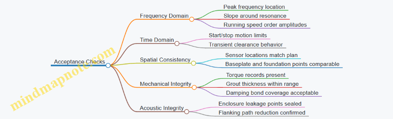
Integrated Example: One Retrofit with Clear Traceability

A retrofit replaces machine mounts and adds constrained-layer damping to the baseplate. The assumptions register states the speed range, base mass estimate, anchor stiffness, and damping loss factor used. The calculations show the predicted transmissibility peak shifts away from the 1× running speed and that the baseplate mode targeted by the damping has sufficient strain energy participation. Installation requirements specify grout thickness, anchor torque, damping surface prep, and curing time. Verification then measures accelerations at the machine and foundation, compares peak frequency and order amplitudes to predictions, and records any mismatch with corrective actions such as re-leveling or rework of a poorly bonded damping patch.

Documentation Format That Keeps Teams Aligned

Use a single document structure: assumptions register first, then calculations, then installation requirements, then verification plan and sign-off. When a new contractor touches the job, they should be able to answer three questions without searching: what we assumed, what we computed, and what we must check before declaring success.

12. Practical Design Examples and Engineering Calculations

12.1 Example Design of Elastomer Mounts for a Pump with Operational Speed Constraints

A pump’s vibration problem usually shows up as a frequency pattern: peaks at running speed and its harmonics, plus sidebands from bearing defects or flow effects. The goal of elastomer mounts is to reduce transmitted vibration to the foundation while keeping the mount natural frequency safely away from the pump’s dominant excitation band.

Step 1: Define the Constraints from Operating Speed

Start with the pump’s speed range and the frequencies you must avoid. Suppose the pump runs from 1450 to 1750 rpm.

• Running speed: 1450/60 = 24.2 Hz to 1750/60 = 29.2 Hz
• First harmonic: 48.3 to 58.3 Hz
• Second harmonic: 72.5 to 87.5 Hz

A practical rule is to place the mount’s natural frequency below the lowest excitation frequency by a margin, so the isolation works where it matters. For elastomer mounts, you typically target a natural frequency around one-third to one-fifth of the lowest forcing frequency, then verify it doesn’t drift upward due to temperature or aging.

Step 2: Estimate Loads and Determine Mount Count

Compute the static load per mount from the pump weight, baseplate weight, and any steady loads from piping and guards. Example assumption:

• Pump plus baseplate mass: 420 kg
• Total static load: 420 × 9.81 = 4120 N
• Add 20% for piping and dynamic margin: 4940 N
• Use 4 mounts for symmetry: 4940/4 = 1235 N per mount

If the pump has a tall center of mass or significant moment, you may need more mounts or a stiffer layout to control rocking. Symmetry reduces cross-coupling between translation and rotation.

Step 3: Choose Mount Type and Target Natural Frequency

Select elastomer mounts with appropriate durometer range and geometry (shear mounts or compression mounts). For a first-pass design, target a natural frequency fn near 8–10 Hz.

• Lowest forcing frequency is 24.2 Hz
• Ratio fn/forcing ≈ 0.33 to 0.41, which is in the isolation-friendly range

To check the target, use the single-degree-of-freedom approximation:

• fn = (1/2π) √(k/m)
• Rearranged: k = (2πfn)^2 m

For one mount, m is the supported mass share. If the 4 mounts share equally, m ≈ 420/4 = 105 kg.

• With fn = 9 Hz: k ≈ (2π×9)^2 × 105 ≈ 3.4×10^5 N/m
• That is 340 N/mm equivalent stiffness per mount

Step 4: Convert Stiffness to Deflection and Verify Operating Travel

Elastomer mounts must not bottom out and must remain in a predictable stiffness region. Static deflection δ is:

• δ = F/k
• With F = 1235 N and k = 3.4×10^5 N/m: δ ≈ 0.0036 m = 3.6 mm

Check two things:

1. Clearance to bottoming: design for at least 2× the static deflection as margin.
2. Dynamic deflection at operating speed: near resonance, motion can grow, but the isolation ratio reduces it away from fn. You still verify that the predicted peak displacement stays within the mount’s allowable strain.

Step 5: Account for Damping and Frequency-Dependent Stiffness

Elastomer damping is not a constant; it depends on excitation level and temperature. Use a conservative damping ratio ζ for preliminary calculations (often in the 5–15% range for elastomer systems) and then confirm with test data or manufacturer curves.

A useful engineering check is to ensure the transmissibility at the running speed is low enough. For a lightly damped isolator, transmissibility drops as frequency ratio r = f/ fn increases. With fn = 9 Hz and f = 24–29 Hz, r ≈ 2.7–3.2, which typically yields meaningful reduction.

Step 6: Validate with a Frequency Response View

Even if the SDOF model looks good, real systems have multiple modes and coupling through the baseplate. Use a simplified frequency response check to confirm that the mount resonance is not accidentally shifted upward by baseplate stiffness or by constrained boundary conditions.

    flowchart TD
A[Inputs] --> B[Operating speed range]
A --> C[Pump and baseplate mass]
A --> D[Static load per mount]
B --> E[Compute forcing frequencies]
C --> F[Choose mount count and share]
D --> G[Target natural frequency fn]
E --> H[Check fn/forcing ratio]
G --> I[Compute mount stiffness k]
I --> J[Compute static deflection]
J --> K[Check travel and strain limits]
K --> L[Apply damping and estimate transmissibility]
L --> M[Confirm no resonance near running speed]
M --> N[Plan verification measurement]

Step 7: Practical Mount Selection and Installation Details

Select mounts whose rated stiffness and allowable deflection match the computed values with margin. Then control installation variables that quietly change stiffness:

• Ensure baseplate leveling so elastomer compression is uniform across mounts.
• Use consistent torque on anchor bolts and avoid over-constraining with rigid shims.
• Keep grout thickness uniform if grouting is used; thick or uneven grout can create stiff paths.
• Route piping with flexible connections near the pump to reduce additional dynamic forces.

Step 8: Verification Plan Using On-Site Measurements

After installation, verify the isolation behavior by measuring vibration at the pump casing and at the foundation. A simple acceptance metric is the reduction in vibration amplitude around running speed compared to a baseline or compared to a reference direction.

Mind Map: Design Workflow for Elastomer Pump Mounts

- Example Design of Elastomer Mounts for a Pump with Operational Speed Constraints - Step 1: Define Constraints - Speed range in rpm - Convert to Hz - Identify forcing harmonics - Step 2: Determine Loads - Pump and baseplate weight - Add piping steady load margin - Choose mount count and symmetry - Step 3: Target Natural Frequency - Choose fn below lowest forcing - Use fn/forcing ratio check - Step 4: Compute Stiffness and Deflection - k from fn and supported mass - δ from F/k - Travel and strain limits - Step 5: Include Damping Effects - Use conservative ζ - Estimate transmissibility at running speed - Step 6: Validate System Behavior - Check for resonance shift - Consider baseplate coupling - Step 7: Installation Quality - Leveling and uniform compression - Anchor bolt torque consistency - Avoid rigid shims and stiff grout paths - Step 8: Verify in Field - Measure casing and foundation - Compare reduction at running speed

This example design is intentionally structured: it starts with the frequencies that matter, turns them into a mount natural frequency target, then converts that target into stiffness, deflection, and installation checks. The final step is measurement, because elastomer systems behave like real systems, not like neat equations on paper.

12.2 Example Enclosure Design for Airborne Noise Reduction With Seal and Flanking Checks

An enclosure reduces airborne noise by adding transmission loss through panels and by preventing leakage at openings. In practice, the enclosure is only as good as its weakest leak path, so the design process should treat sealing and flanking as first-class requirements, not afterthoughts.

Step 1: Define the Noise Target and Operating Conditions

Start with the measured or predicted sound pressure level (SPL) at the receiver location and the frequency range that matters. Suppose a pump room has a dominant tone around 500 Hz and broadband energy from 200 Hz to 2 kHz. The goal is a 10 dB reduction at the nearest operator position.

A useful planning check is to separate airborne reduction needs from vibration-driven radiation. If the pump baseplate radiates strongly, enclosure panels must be treated as structural radiation sources too; otherwise, you may overestimate airborne-only performance.

Step 2: Choose Enclosure Type and Panel Strategy

For a machinery bay, a common approach is a double-wall or single-wall enclosure with constrained damping and stiff framing. The panel strategy should match the dominant frequencies:

• For mid frequencies (roughly 300 Hz to 2 kHz), panel mass and stiffness dominate transmission loss.
• For lower frequencies, panel resonances and flanking paths often dominate, so sealing and structural decoupling become critical.

Example decision: Use 12 mm steel outer panels with a 25 mm mineral wool layer and a 1.5 mm inner liner, mounted to a stiff frame with resilient mounts. The mineral wool improves absorption inside the cavity, reducing internal reflections that otherwise re-radiate through the panel.

Step 3: Design the Sealing System for Real-World Gaps

Airborne noise reduction collapses when there are uncontrolled gaps. Treat every interface as a potential leak: doors, cable penetrations, duct connections, and panel seams.

Door and Access

Use a perimeter gasket with a continuous compression path. A practical rule is to ensure the gasket is compressed when the door is closed, not merely touching. Add a threshold strip to reduce the “bottom gap” that often forms after repeated use.

Example: A door with a 6 mm nominal gasket compression. If the door sags by 2 mm over time, the remaining compression still maintains contact, preventing a new leak frequency.

Seams and Panel Joints

Use overlapping seams or tongue-and-groove details rather than butt joints. If butt joints are unavoidable, use a backing strip and a sealant rated for the operating temperature.

Example: Overlap seams with a 20 mm overlap reduce direct air paths. Even if the sealant cracks slightly, the overlap still forces tortuous leakage.

Penetrations for Power and Control

Cable trays and conduit penetrations are frequent flanking starters. Use grommets or brush seals for small penetrations and fire-rated acoustic sealant for larger ones.

Example: For a conduit bundle, use a single bulkhead penetration with a sealing collar and a backing foam ring. Avoid multiple small penetrations that create many independent leak points.

Step 4: Check Flanking Paths Through Structure and Mounting

Flanking occurs when sound energy bypasses the enclosure panels via the structure. The enclosure frame, floor interface, and any rigid connections to the machine or building can create a low-resistance path.

Frame-to-Floor Interface

Introduce resilient isolation between the enclosure frame and the floor. The goal is to reduce the transmission of vibration that can radiate as airborne noise through the building.

Example: Mount the enclosure frame on elastomer pads with a natural frequency well below the enclosure’s dominant panel resonance range. This keeps the frame from acting like a secondary radiator.

Rigid Connections to Ducts and Piping

If the enclosure connects to ductwork or piping, use flexible connectors and avoid rigid couplings that bridge the isolation gap.

Example: Use a flexible duct section with an acoustic liner and ensure the duct does not touch the enclosure frame at multiple points.

Step 5: Internal Absorption and Airflow Considerations

Enclosures need ventilation. Ventilation openings can become “acoustic short circuits” if not treated.

Example: For an intake and exhaust, use baffles lined with mineral wool and maintain a labyrinth path. Keep the airflow velocity reasonable to avoid generating new noise at the louvers.

Step 6: Verification with Before-After Measurements and Acceptance Checks

Measure at the receiver location with the machine operating in steady conditions. Then repeat with the enclosure installed and sealed.

Acceptance logic:

• If the reduction is strong at mid frequencies but weak at low frequencies, suspect flanking or panel resonance.
• If reduction is inconsistent across frequencies, suspect leakage at doors or penetrations.

A practical diagnostic: temporarily apply controlled sealing tape to suspected seams and re-measure. If SPL drops noticeably, you found the leak class.

Mind Map: Enclosure Design Workflow with Seal and Flanking Checks

- Example Enclosure Design for Airborne Noise Reduction - Step 1: Define Noise Target - Receiver SPL baseline - Dominant frequency bands - Airborne vs vibration radiation check - Step 2: Choose Enclosure Type - Panel mass and stiffness - Internal cavity absorption - Frame stiffness and mounting concept - Step 3: Seal All Interfaces - Door perimeter gasket and threshold - Panel seams overlap or sealed joints - Cable and conduit penetrations bulkhead sealing - Step 4: Evaluate Flanking Paths - Frame-to-floor resilient interface - Avoid rigid bridges to building - Flexible connectors for ducts and piping - Step 5: Ventilation Without Acoustic Short Circuits - Lined baffles and labyrinth paths - Manage airflow velocity - Step 6: Verify and Diagnose - Before-after receiver measurements - Frequency-pattern interpretation - Targeted seam sealing tests

Worked Example Summary

For the pump room case, the combined panel strategy plus internal absorption provides baseline transmission loss, while the sealing package prevents leakage-driven failure. The flanking checks—especially the resilient frame interface and flexible duct connections—address the low-frequency and “mystery” paths that often survive even well-built panels. The final verification step confirms whether the enclosure behaves like a barrier or like a fancy speaker with better manners.

12.3 Example Structural Damping Treatment Design for a Machine Baseplate

A practical baseplate damping design starts with one question: which vibration modes actually matter for the noise and vibration you measure at the receiver? The goal here is to reduce baseplate motion at the dominant operating frequencies while keeping the machine aligned and the installation robust.

Step 1: Define the Design Targets Using Measured Behavior

Begin with operational data from the machine and baseplate. You want frequency bands where motion is both high and correlated with the noise you care about.

• Pick 3–5 target frequencies (or narrow bands) around the operating speed harmonics.
• For each target, note the baseplate response level and the mode shape if you have it (from FRFs or operational modal analysis).

Easy example: If your pump runs at 25 Hz (1500 rpm) and you see peaks at 25 Hz, 50 Hz, and 75 Hz, treat those as targets. If the 50 Hz peak is much sharper than the others, prioritize damping for the mode that drives that peak.

Step 2: Choose a Damping Mechanism and Layout Strategy

For a baseplate, constrained layer damping (CLD) is often effective because it converts bending strain energy into heat using a viscoelastic layer sandwiched between stiff layers.

Core idea: CLD works best where the baseplate experiences bending strain. If a mode is mostly rigid-body motion, CLD won’t help much.

Easy example: If the 50 Hz mode shows strong curvature near the center span, place CLD patches near that region rather than only near the edges.

Step 3: Estimate Strain Energy Hotspots from a Simple Model

You can do this with a finite element model, but a simplified workflow still works.

1. Identify approximate bending regions from mode shapes.
2. Assume strain energy density is proportional to squared curvature.
3. Use that to rank candidate patch locations.

Rule of thumb: Put more damping area where curvature is higher, and avoid areas that are mostly nodal lines for the target mode.

Step 4: Select Materials and Determine Thickness

CLD performance depends on the viscoelastic layer’s complex modulus at your frequencies and temperature.

• Choose a viscoelastic layer with a loss factor that is meaningful in your target band.
• Keep the stiff layers (steel or aluminum) thin enough to allow strain transfer but thick enough to distribute load.
• Use a thickness that does not “lock out” strain transfer by being too stiff.

Easy example: If the viscoelastic layer is too thin, it may not develop shear deformation under bending. If it’s too thick, it can reduce stiffness too much and shift resonances or create excessive compliance.

Step 5: Compute an Effective Damping Increase for the Target Mode

A full derivation is model-dependent, but the engineering workflow is consistent:

• Determine the baseplate’s modal damping ratio ζ0 for the target mode (from FRF bandwidth or curve fitting).
• Estimate the additional damping Δζ contributed by the CLD patches using strain energy participation.
• Ensure the resulting resonance amplitude reduction matches the measured peak reduction you need.

Easy example: If ζ0 is 1% and you can raise it to 3% at 50 Hz, the peak response typically drops noticeably because the resonance becomes less sharp. The exact factor depends on how close you operate to resonance.

Step 6: Verify Resonance Shifts and Alignment Constraints

Damping treatments add mass and stiffness. Even when the intent is “just damping,” the baseplate can shift modal frequencies.

• Check that the new resonance frequencies do not move into a more problematic operating band.
• Confirm that added mass does not overload leveling pads or distort the baseplate.

Easy example: If your 75 Hz target is close to an operating harmonic, a resonance shift of even a few Hz can change the benefit. That’s why you verify after installation.

Step 7: Installation Details That Actually Matter

CLD effectiveness is sensitive to bond quality and surface preparation.

• Prepare surfaces to remove oil, rust, and paint; roughen to promote adhesion.
• Use controlled curing or approved bonding methods; avoid uneven adhesive thickness.
• Ensure the viscoelastic layer is continuous and not pinched at edges.
• Apply uniform clamping pressure during cure.

Easy example: Two patches with the same dimensions can behave very differently if one has a thin, poorly bonded adhesive region. That region can act like a “dead” area with low strain transfer.

Step 8: Acceptance Testing with Before After Measurements

After installation, re-measure the same operational conditions.

• Compare peak amplitudes at the target frequencies.
• Confirm damping ratio increase for the target mode.
• Check that other modes did not worsen significantly.

Easy example: If the 50 Hz peak drops but the 100 Hz peak rises, you may have over-damped one mode and shifted energy into another. Adjust patch placement or area.

Mind Map: Baseplate CLD Design Workflow

- Example Structural Damping Treatment Design for a Machine Baseplate - Step 1: Define Design Targets - Select target frequencies - Identify dominant peaks - Capture mode shapes if available - Step 2: Choose Damping Mechanism - Constrained layer damping - Strain-energy driven placement - Step 3: Find Strain Hotspots - Use mode curvature - Rank candidate patch locations - Avoid nodal regions - Step 4: Select Materials and Thickness - Viscoelastic loss factor in band - Stiff layer thickness for strain transfer - Step 5: Estimate Damping Increase - Baseline modal damping ζ0 - Additional damping Δζ from participation - Predict peak reduction trend - Step 6: Check Side Effects - Resonance frequency shifts - Mass and stiffness changes - Alignment and load path constraints - Step 7: Installation Quality - Surface prep and adhesion - Uniform adhesive thickness - Cure pressure and edge control - Step 8: Verify Performance - Before/after FRF or operational tests - Peak amplitude and damping ratio comparison - Mode-to-mode tradeoff review

Worked Mini-Example with Concrete Numbers

Assume a baseplate with a measured 50 Hz target mode:

• Baseline modal damping ratio ζ0 = 1.2%
• Measured peak amplitude at 50 Hz is 10 units (relative)
• CLD patches are planned in the high-curvature region with total patch area = 12% of plate area
• After installation, ζ1 is estimated to be 3.0% based on strain energy participation

A typical outcome is a reduction in resonance peak amplitude because the resonance becomes less sharp. If the measured peak drops from 10 to about 6 units, that’s a 40% reduction at the target. If instead it only drops to 9 units, the likely causes are poor bonding, insufficient viscoelastic performance at temperature, or patch placement near a nodal line.

Practical Design Checklist

• Target frequencies chosen from real operating data
• Patch locations align with strain energy hotspots
• Viscoelastic layer selected for the actual temperature and frequency band
• Bonding and curing procedures controlled
• Before/after verification confirms both damping increase and acceptable resonance shifts

12.4 Example Vibration Isolation System Verification Using Frequency Response Functions

A good isolation design earns its keep when it performs under real operating conditions. Frequency Response Functions (FRFs) are a practical way to verify that the isolation system attenuates vibration where it matters, and that it does not create surprises like unexpected resonances or weak coupling paths.

Step 1: Define the Verification Targets

Start by writing down what “verified” means in measurable terms.

• Primary target frequency bands: the machine’s dominant orders (e.g., 1×, 2×, blade pass) and the expected structural resonances.
• Primary response points: typically the machine casing/baseplate and the receiver location (nearby floor, duct, or equipment bay).
• Acceptance metric: a ratio such as transmissibility from input to output. For isolation, you often want a low output/input magnitude across the band.

Example: A pump runs at 1800 rpm (30 Hz). You care about 30 Hz (1×), 60 Hz (2×), and nearby harmonics up to 200 Hz. You also care about whether the floor motion near the pump baseplate is reduced relative to the foundation input.

Step 2: Choose Inputs Sensors and Excitation

FRFs need a defined input and a measurable output.

• Input: force (impact hammer or shaker) applied to the foundation or baseplate, or an acceleration reference if you use operational FRFs.
• Sensors: accelerometers on the machine baseplate (output) and on the foundation (input reference). If you suspect rotational coupling, add a second sensor to estimate rocking.
• Coherence check: plan to reject frequency lines with low coherence.

Example: Apply a controlled impact to the foundation at the same location each run. Mount accelerometers at the pump baseplate center and on the foundation block directly under the mount group.

Step 3: Acquire FRFs and Validate Data Quality

Collect FRFs over a frequency range that covers:

• the isolation system’s expected resonance region,
• the machine’s operating band,
• and at least one decade above the highest frequency of interest (so you can see whether behavior changes).

Use these checks:

• Coherence: keep lines above a chosen threshold (commonly 0.8) to trust the FRF.
• Repeatability: compare multiple impacts; the FRF magnitude should be stable.
• Linearity: ensure the response does not scale nonlinearly with excitation level.

Example: If the FRF magnitude changes shape when you increase impact force, you likely hit a nonlinear contact condition like loose grout or a slipping mount.

Step 4: Compute Transmissibility from FRFs

For verification, you want a ratio that reflects isolation performance.

If you have an FRF from foundation force to baseplate acceleration, you can form a transmissibility-like metric:

• Magnitude ratio:
  • output: baseplate acceleration magnitude,
  • input: foundation acceleration magnitude or force-based reference.

A simple and effective approach is to compare before and after installation:

• Isolation improvement:
  • \(\Delta M(f)=20\log_{10}\left(\frac{|H_{after}(f)|}{|H_{before}(f)|}\right)\)

Negative values indicate reduction.

Example: After installing elastomer mounts, the FRF magnitude at 30 Hz drops by 12 dB, while at 95 Hz it increases by 4 dB. That tells you the isolation moved the resonance behavior: good at 1×, but you must check whether 95 Hz aligns with a harmonic or structural mode.

Step 5: Interpret Key Features in the FRF

FRFs are not just numbers; they show system behavior.

• Low-frequency region: isolation often improves as stiffness decreases, but too-soft mounts can increase static deflection and risk bottoming.
• Isolation resonance: expect a peak near the mount system’s natural frequency. A well-designed system places this peak away from dominant excitation orders.
• High-frequency region: damping and structural constraints determine how quickly the response decays.

Example: If you see a sharp peak at 60 Hz, it may mean the mount stiffness is lower than predicted or the baseplate boundary conditions changed during installation.

Step 6: Confirm Mount Behavior with Operational Checks

After the lab-style FRF, verify under operating conditions using operational FRFs or order tracking.

• Compare the FRF-predicted attenuation at 30 Hz and 60 Hz with measured vibration spectra during startup steady-state.
• If the operational spectrum shows a peak where FRFs predicted attenuation, suspect changes in coupling: piping contact, cable trays, or loosened fasteners.

Example: The FRF shows 10 dB attenuation at 30 Hz, but during operation the baseplate acceleration at 30 Hz is unchanged. A quick inspection reveals a rigid pipe support touching the baseplate during thermal expansion.

Mind Map: FRF Verification Workflow

- FRF Verification Using Frequency Response Functions - Define Targets - Frequency bands of interest - Input and output locations - Acceptance metric - Plan Measurement - Input method - Hammer - Shaker - Sensor placement - Foundation reference - Baseplate output - Optional rotational check - Frequency range - Acquire FRFs - Coherence filtering - Repeatability runs - Linearity sanity check - Process Data - Compute FRF magnitude - Form transmissibility ratio - Before vs after comparison - Interpret Results - Isolation resonance peak - Attenuation in operating bands - High-frequency roll-off - Validate Under Operation - Operational spectrum comparison - Identify coupling changes - Correct installation issues

Step 7: Document Evidence and Tie It to Design Assumptions

A verification report should connect the FRF results to what the design assumed.

Include:

• mount natural frequency estimate from FRF,
• damping behavior inferred from peak width and decay,
• measured attenuation at each target order,
• and any deviations with a clear cause.

Example: “At 30 Hz, transmissibility decreased by 12 dB; the mount resonance peak shifted from 52 Hz to 58 Hz, consistent with increased effective stiffness due to improved grout contact. At 95 Hz, transmissibility increased by 4 dB; inspection confirmed a structural mode of the baseplate that was not included in the simplified model.”

Step 8: Quick Numerical Example for Decision Making

Suppose the FRF magnitude ratio (output/input) at 30 Hz is:

• Before: \(|H_{before}(30)| = 0.020\) (m/s² per m/s²)
• After: \(|H_{after}(30)| = 0.006\)

Then:

• \(\Delta M(30)=20\log_{10}(0.006/0.020)=20\log_{10}(0.3)\approx -10.5,\text{dB}\)

If your acceptance threshold is at least 8 dB reduction at 1×, the system passes at 30 Hz. You still check 60 Hz and the resonance region to ensure the improvement is not bought with a new problem.

12.5 Example Integrated Noise and Vibration Retrofit Plan With Measurement and Acceptance Steps

This retrofit plan targets a typical industrial package: a pump skid on a concrete base, with airborne noise from the pump and motor, plus structureborne vibration that travels through the baseplate, grouted anchors, and nearby piping supports. The goal is to reduce both receiver noise and vibration levels at the operating speed range, using isolation, damping, and acoustic containment in a coordinated way.

Step 1: Define Acceptance Targets and Constraints

Start by writing measurable targets before touching hardware. Use existing logs or short surveys to set baseline metrics.

• Noise acceptance: receiver A-weighted sound pressure level reduction at key operating points, plus a limit on tonal components if present.
• Vibration acceptance: limits on overall velocity at the machine housing and on base or nearby structural points, plus a frequency-domain check at dominant orders.
• Constraints: allowable footprint, maintenance access, maximum mount deflection, and any limits on enclosure internal temperature.

A practical trick: define two sets of acceptance criteria—one for “must meet” at the dominant operating point, and one for “should meet” across the speed sweep.

Step 2: Baseline Survey with Coherent Measurement

Measure before modifying so you can attribute improvements.

• Sensor placement: accelerometers on the pump housing and baseplate corners; a reference accelerometer on the foundation; microphones at the receiver and near the enclosure openings.
• Operational points: at least three steady states (low, mid, high speed) and one transient start/stop if the noise is tonal during ramp.
• Data quality checks: verify coherence between excitation and response channels for the frequency bands where you expect isolation to work.

Example: if the dominant vibration peak is at a bearing-related frequency, you want coherence between the housing response and the foundation reference around that peak. Low coherence usually means you are measuring the wrong location or missing the real excitation path.

Step 3: Diagnose Dominant Paths and Failure Modes

Use the baseline to decide what to fix first.

• Airborne path: if microphones show strong levels near openings and the enclosure is leaky, acoustic isolation will be limited until sealing and panel transmission are addressed.
• Structureborne path: if base accelerations track housing accelerations closely at the same frequencies, the mount and foundation interface are the priority.
• Flanking path: if receiver noise remains high even after local enclosure improvements, check ducting, cable trays, and rigid piping connections.

Step 4: Retrofit Package Design with Integrated Logic

Build the retrofit as a linked set of changes, not a pile of parts.

1. Acoustic isolation and containment

   • Add a machine enclosure with treated panels and controlled openings.
   • Seal penetrations around cables and piping sleeves.
   • Use a gasketed access door so the enclosure does not become a “mostly open” box.

2. Structural damping

   • Apply constrained-layer damping to the baseplate or skid panels where feasible.
   • Keep damping treatments away from moving interfaces and ensure surface prep is consistent.

3. Vibration isolation

   • Select mounts based on the required isolation frequency range and static deflection limits.
   • Verify that the mount natural frequency sits below the dominant excitation band but not so low that travel limits are exceeded.

4. Foundation and interface detailing

   • Confirm grouting and anchor contact quality.
   • Ensure piping supports do not bypass the isolation system with rigid connections.

Step 5: Installation Sequence That Preserves Measurement Meaning

Order matters because each change can affect the next.

• Install mounts and verify alignment and travel limits.
• Apply damping treatments.
• Build enclosure and complete sealing.
• Rework piping supports and add restraints or flexible sections where required.

After each major phase, take quick spot checks at the dominant operating point so you do not discover problems only at the end.

Step 6: Post-Retrofit Measurement with Matched Conditions

Repeat the baseline measurement plan using the same operating points and sensor locations.

• Matched conditions: same speed setpoints, same load, same microphone height and orientation.
• Before-after comparison: focus on the dominant frequency bands and tonal components.
• Isolation verification: compare housing-to-foundation transfer behavior at the key peaks.

Example: if enclosure sealing reduces receiver noise but housing vibration remains unchanged, the plan still succeeded for airborne control, but you should not claim full system vibration mitigation.

Step 7: Acceptance Testing and Documentation

Acceptance is not just “it sounds quieter.” Use a structured checklist.

• Noise: confirm receiver reduction meets the must criteria at the dominant operating point.
• Vibration: confirm overall velocity and peak frequency-domain levels meet limits at the housing and base points.
• Operational robustness: verify performance at low and high speed steady states.
• Installation evidence: record mount part numbers, torque checks, damping coverage area, enclosure seal inspection results, and piping support changes.

If a criterion fails, use the measurement deltas to pinpoint the path: airborne failure points to enclosure leakage or panel transmission; vibration failure points to mount tuning, foundation interface, or rigid bypasses.

Mind Map: Integrated Retrofit Plan Flow

- Integrated Retrofit Plan - Define Targets - Noise receiver limits - Vibration housing and base limits - Constraints and access limits - Baseline Measurement - Sensor placement - Operating points - Coherence and data quality - Path Diagnosis - Airborne dominance - Structureborne dominance - Flanking bypass checks - Retrofit Package - Enclosure and sealing - Constrained-layer damping - Isolation mount selection - Foundation and interface detailing - Piping support integration - Installation Sequence - Mounts first - Damping next - Enclosure and sealing - Piping support corrections - Post-Retrofit Measurement - Matched conditions - Before-after frequency comparison - Transfer behavior checks - Acceptance and Closeout - Must meet criteria - Should meet across speed range - Evidence and documentation - Failure attribution logic

Example Acceptance Checklist for One Operating Point

• Receiver noise: meets must reduction at dominant tonal frequency band.
• Housing vibration: peak amplitude reduced by the required margin.
• Base vibration: reduced peak or reduced transfer ratio at the dominant band.
• Enclosure: no visible gaps at penetrations and access door seals.
• Piping supports: no rigid bypass connection that reintroduces the dominant peak.

This checklist keeps the retrofit accountable to measurements, while the integrated logic prevents “improvements” that only move the problem to a different path.