Rail Tribology and High-Speed Railway Engineering
1. Scope and Engineering Foundations
1.1 Wheel-Rail Interaction as a Tribology System
Wheel-rail interaction is a tribology system because it repeatedly converts motion into contact forces, and those forces repeatedly reshape the surfaces. In a high-speed context, the “system” includes not only the wheel and rail materials, but also geometry, lubrication, contaminants, and the vehicle’s dynamic behavior. Treating it as a system helps you avoid the common trap of optimizing one variable while quietly breaking another.
Core Components of the Tribology System
Contact interface. The wheel tread and rail head meet through a small contact patch whose size and shape change with load, speed, and alignment. Even when the nominal profiles are fixed, the actual contact patch evolves because the wheel and rail surfaces are never perfectly smooth.
Relative motion. Rolling is never pure rolling. Small longitudinal and lateral creepages create tangential forces that control traction, braking, and wear. The same creepage that helps transmit traction can also accelerate wear if the contact conditions push the interface into an unfavorable regime.
Normal and tangential forces. Normal force sets the contact pressure distribution. Tangential force depends on creepage and friction behavior, and it feeds back into wear because higher tangential work increases material removal.
Surface state. Roughness, waviness, and defects determine how real contact occurs. A smoother surface does not automatically mean lower friction; it can reduce asperity interactions but also reduce the ability to sustain a stable lubricant film under some conditions.
Lubrication and contaminants. Lubricants reduce friction and wear, but their effectiveness depends on delivery, film thickness, and whether contaminants such as water, sand, or debris disrupt the film.
Mind Map: Wheel-Rail Tribology
From Fundamentals to Practical Consequences
Start with the geometry: wheel and rail profiles determine the nominal contact location and the baseline rolling radius relationship. Next, apply load: the vertical force sets contact pressure, which influences how asperities deform and how quickly surfaces polish or roughen. Then add motion: creepage generates tangential forces, and the ratio of tangential to normal force expresses friction behavior.
Now connect friction to wear. Wear is not just “friction high equals wear high.” It depends on how much tangential work occurs at the interface and whether the contact is dominated by adhesion, abrasion, or fatigue-related mechanisms. For example, a condition with moderate friction but high tangential work over many cycles can still produce significant material loss.
Finally, include lubrication and contaminants. A thin lubricant film can reduce asperity contact and lower wear, but if contaminants interrupt the film, the interface can switch to a more abrasive or adhesive-dominated regime. This is why two trains with the same speed and load can show different wear patterns when their lubrication effectiveness differs.
Example: Same Speed, Different Wear
Consider two runs at the same speed and axle load.
- Run A: Lubrication is delivered consistently, and the rail surface is maintained within a stable roughness range. Creepage produces tangential forces that remain within a predictable friction behavior, and the contact patch experiences fewer severe asperity interactions.
- Run B: Lubrication delivery is intermittent, and water or debris disrupts the film. The interface alternates between low-film and high-asperity contact, increasing tangential work at the micro-contact level. The result is faster roughness growth and a higher likelihood of surface damage progression.
The lesson is simple: tribology outcomes come from the interaction of forces, motion, surface state, and lubrication—not from any single parameter.
System View for Engineering Decisions
A useful engineering mindset is to track three linked quantities: contact pressure distribution, tangential force generation, and surface state evolution. If you change geometry, you alter pressure and creepage distribution. If you change lubrication, you alter friction and the real contact fraction. If you change suspension or track alignment, you alter wheel loads and creepage. When these links are kept explicit, troubleshooting becomes less guessy and more testable.
Example: A Quick Diagnostic Chain
If you observe increased wear on a specific rail section, a systematic chain is:
- Verify wheel load variation from vehicle dynamics.
- Check whether alignment or track irregularities increased creepage.
- Confirm lubrication effectiveness and whether contaminants are present.
- Compare surface roughness and defect density before and after.
- Relate the observed wear pattern to the likely dominant wear mechanism.
This chain keeps the tribology system intact: you measure what affects the interface, not just what looks damaged.
1.2 High-Speed Railway Performance Requirements and Constraints
High-speed rail is a system where “performance” means more than reaching a target speed. The train must keep stable wheel-rail contact, produce predictable forces, and remain safe while energy use, noise, and maintenance effort stay within practical limits. The requirements below are written as engineering constraints, because every design choice eventually shows up as a measurable boundary condition.
Core Performance Requirements
Speed with Controlled Dynamics
A higher top speed increases kinetic energy and reduces the time available for corrective actions. That means the vehicle must maintain acceptable ride quality and stability at higher dynamic loads, not just at steady-state speed. For example, if a track section has a known lateral irregularity, the same geometry produces larger lateral acceleration at higher speed, which then changes wheel-rail creepage and contact forces.
Wheel-Rail Contact Quality
Contact quality is about keeping the contact patch within a workable region of geometry and material behavior. If the contact shifts toward less favorable regions, friction, wear, and noise can change quickly. A practical example is a wheelset with slight flange wear: at high speed, the altered profile can increase tangential force components during curving, which accelerates wear and can worsen stability.
Braking Performance Under Real Conditions
Braking requirements include stopping distance, deceleration limits for passenger comfort, and repeatability across different rail conditions. A simple example: two braking runs with the same commanded brake force can yield different stopping distances if one run occurs on rails with higher contamination or different thermal state. Eddy current braking adds another constraint because its force depends on electrical and thermal conditions.
Energy Efficiency and Power Limits
Energy efficiency is constrained by traction power availability, aerodynamic drag, and rolling resistance. At high speed, aerodynamic drag dominates, so small changes in vehicle mass or underbody flow can matter. A concrete example: reducing rolling resistance by improving contact conditions may save energy, but if it requires more frequent grinding or lubrication adjustments, the operational cost can offset the benefit.
Safety and Robustness
Safety constraints cover derailment risk, wheelset stability, braking system integrity, and fault tolerance. Robustness means the system should behave acceptably when inputs vary: track stiffness changes, temperature shifts material properties, and sensor noise affects control.
Major Engineering Constraints
Track Geometry and Condition
Track alignment, gauge variation, and surface irregularities set the excitation for vehicle dynamics. Even when the design targets a specific track class, real maintenance intervals mean the excitation spectrum changes over time. For instance, rail corrugation can raise high-frequency wheel-rail force components, which then influences both wear and noise.
Vehicle Mass, Suspension, and Damping
Suspension parameters determine how forces transmit between wheelsets and the carbody. Too little damping can amplify resonances; too much can increase transmitted forces during irregularities. A useful example is a suspension mode that is benign at moderate speed but becomes problematic when excitation frequency aligns with the mode frequency.
Wheel and Rail Material Behavior
Material properties evolve with temperature, contact stress, and wear. Rail head hardness, wheel tread condition, and surface roughness affect friction and wear rates. A practical example: after a grinding intervention, roughness and profile geometry change; the same lubrication strategy can produce different friction behavior until surfaces re-equilibrate.
Environmental and Operational Limits
Wind, temperature, and contamination influence both contact and braking. Rain or leaf contamination can change friction and also affect the effectiveness of lubrication. For braking, rail temperature affects electrical conductivity and thermal limits, which in turn constrain how much braking force can be sustained.
System-Level Verification Logic
Performance requirements must be translated into measurable engineering targets and then checked through modeling and testing. The key is to connect each requirement to the physical quantities that actually drive it.
- Stability targets map to allowable lateral/vertical accelerations and wheelset hunting indicators.
- Contact quality targets map to creepage ranges, contact patch location, and friction/wear metrics.
- Braking targets map to deceleration profiles, brake force availability, and thermal/electrical constraints.
- Comfort targets map to acceleration and jerk limits over representative track profiles.
Mind Map: High-Speed Performance Requirements and Constraints
Example: Turning Requirements into Engineering Targets
Suppose the operational goal is reliable braking from a high-speed line section. The requirement becomes a set of targets: a maximum stopping distance under defined rail contamination states, a deceleration envelope that respects comfort limits, and an eddy current braking force that remains within thermal constraints for the expected duty cycle. The constraint set then dictates what must be measured or estimated: rail temperature, contact condition indicators, and suspension/track-induced dynamics that affect wheel-rail contact during braking.
When these targets are written clearly, design decisions become easier to evaluate. A change that improves contact friction might reduce wear but could increase tangential forces that affect stability; a braking control change might improve deceleration repeatability but could push thermal limits. High-speed engineering is essentially the art of making those trade-offs explicit, then checking them with evidence.
1.3 Contact Mechanics Basics for Rolling and Sliding Interfaces
Wheel-rail contact is a small region doing big work: it carries normal load, generates tangential forces, and converts motion into wear and noise. The key is to treat the interface as a contact problem with geometry, material deformation, and relative motion all coupled together.
Contact Geometry and the Contact Patch
Start with the simplest picture: two curved bodies pressed together. Under load, the nominally point-like contact becomes an area called the contact patch. For wheel-rail, the patch is often approximated as an ellipse in the plane of contact, with semi-axes that depend on load, radii of curvature, and material stiffness.
A practical way to reason about patch size is to remember that “stiffer materials and smaller curvature radii” tend to reduce the patch, increasing local stresses. Conversely, “softer materials and larger radii” spread the load over a larger area. This matters because friction and wear are sensitive to the local stress and slip distribution.
Elastic Deformation and Hertzian Contact
A common baseline model is Hertzian contact, which assumes elastic deformation, smooth surfaces, and no adhesion effects. It provides:
- Pressure distribution across the patch (highest near the center)
- Relation between normal force and patch dimensions
- Estimates of maximum contact pressure
Even if you later use more advanced models, Hertzian results are a useful sanity check. If your computed patch is unrealistically tiny, your assumed stiffness or curvature inputs are probably off.
Relative Motion and Creepage
Rolling is not perfect rolling. The wheel and rail can have slight differences in tangential velocity at the contact due to steering, braking, traction, or track geometry. This relative motion is captured by creepage, typically separated into:
- Longitudinal creepage from braking or traction
- Lateral creepage from yaw or curving
Creepage is the bridge between kinematics and forces: it tells you how much the contact is trying to slide, even when the wheel is “rolling.”
Stick-Slip Behavior and Tangential Force Build-Up
When tangential force is applied, the contact does not immediately slide everywhere. Instead, a stick region can exist where tangential displacement is small, surrounded by a slip region where the local shear reaches a limit. As creepage increases, the stick region shrinks until full sliding occurs.
A useful mental model is: tangential force grows with creepage until it reaches a friction-limited plateau. The exact shape depends on the shear traction distribution and the assumed friction law, but the qualitative behavior is consistent.
Friction Limits and Shear Traction
In many engineering contexts, the maximum shear traction is limited by a friction coefficient times the normal pressure. That means the interface can support more tangential force when the normal pressure distribution is higher near the center. Lubrication, contamination, and surface roughness change the effective friction coefficient and can shift the stick-slip balance.
A simple example: if a thin film reduces friction, the tangential force plateau drops. The same braking command then produces more slip, which can increase wear even though the friction coefficient is lower.
Stress, Strain, and Material Response
Contact mechanics is not only about forces; it’s about what the materials experience. High local stresses can contribute to rolling contact fatigue, while repeated shear stresses can drive surface damage. Elastic models predict deformation, but real rails and wheels also show plasticity, micro-slip effects, and roughness-driven asperity interactions.
To keep analysis grounded, always connect your contact model outputs to measurable consequences: contact patch size, tangential force levels, and predicted slip distribution.
Mind Map: Contact Mechanics Coupling
Example: Braking Command to Slip Distribution
Assume a wheelset enters braking with a given normal load and a target braking force. The contact model proceeds like this:
- Use geometry and load to estimate patch dimensions and pressure distribution.
- Apply creepage corresponding to the braking kinematics.
- Compute tangential traction distribution with stick-slip logic.
- Check whether the predicted tangential force is friction-limited.
If the model predicts full sliding too early, it usually means the assumed friction coefficient is too low or the creepage mapping is too aggressive. If it predicts excessive stick, the opposite inputs are likely.
Example: Curving and Lateral Creepage
On a curve, the wheel experiences lateral creepage due to yaw and flange guidance. The tangential forces generated in the lateral direction can shift the effective load distribution across the contact patch. That changes the pressure field, which then alters how much longitudinal force the interface can support without reaching its friction limit. This is why lateral and longitudinal effects should be treated together rather than as separate problems.
In short, contact mechanics is a coupled system: geometry sets the patch, load sets the pressure field, motion sets creepage, and creepage sets the stick-slip pattern that ultimately governs tangential forces and damage mechanisms.
1.4 Coordinate Systems, Reference Frames, and Measurement Conventions
High-speed rail engineering is full of measurements that look similar on a dashboard but mean different things in the math. Coordinate systems and reference frames are the rules that keep those meanings consistent from sensor to simulation to maintenance action.
Coordinate Systems That Actually Get Used
A coordinate system is a named set of axes with an origin. In wheel-rail work, you typically need at least three: a track-based frame, a vehicle-based frame, and a wheelset-based frame.
Track-based frame (T-frame). The origin is chosen on the track geometry, often at a reference point under the wheelset or at a stationing coordinate along the line. The axes are aligned with the track: one axis along the nominal direction of travel, one lateral to the track, and one vertical. This frame makes it easy to interpret lateral forces, gauge effects, and vertical dynamics relative to the track.
Vehicle-based frame (V-frame). The origin is fixed to the vehicle or bogie, and the axes move with it. This frame is convenient for suspension dynamics because spring-damper forces act along vehicle components.
Wheelset-based frame (W-frame). The origin is attached to the wheelset, and axes follow wheel geometry. This frame is where creepage, spin, and tangential force directions are naturally expressed.
A practical convention: when you report a force component, always state which frame it is resolved in. “Lateral force” without a frame is like saying “the temperature is high” without the unit.
Reference Frames and Their Motion
A reference frame becomes a reference frame when it is tied to a motion model. Two frames can share axes but differ in how they move.
Inertial-like frame. For many engineering calculations, you treat the track frame as approximately inertial over short intervals. That assumption is useful for interpreting sensor time histories.
Non-inertial frame. Vehicle and wheelset frames rotate and translate, so acceleration terms appear when transforming equations of motion. Even if you do not write the full dynamics, you must understand that “what the sensor measures” is not automatically “what the track experiences.”
Body-fixed vs. space-fixed. Body-fixed frames rotate with the vehicle; space-fixed frames stay aligned with the track. When you transform velocities, you must use the correct rotation sequence.
Rotations, Sign Conventions, and the Usual Traps
Rotation order matters. If you use yaw-pitch-roll, you must apply the same order everywhere: in data processing, in model setup, and in plots.
Sign conventions are the other common trap. For example, lateral direction to the left of the track centerline must be consistent across:
- sensor mounting orientation,
- coordinate transformation matrices,
- and the direction used in control algorithms.
A simple check prevents many errors: take a known scenario, such as a wheelset moving forward with a small rightward lateral displacement. The direction of measured lateral velocity should match the sign convention you expect.
Measurement Conventions for Contact and Dynamics
Sensors rarely measure “wheel-rail contact forces” directly. They measure voltages, accelerations, angular rates, or displacements, which are then mapped into physical quantities.
Time alignment. Wheel-rail contact events depend on wheel rotation and vehicle motion. If you synchronize signals by vehicle speed alone, you can still get phase errors when speed varies. A robust convention is to align using wheel rotation angle or a track-referenced trigger.
Units and scaling. Keep units explicit in every transformation step: meters vs. millimeters, degrees vs. radians, Newtons vs. kiloNewtons. Scaling mistakes are quiet and expensive.
Component resolution. When you compute tangential force from strain gauges or load cells, you must resolve it into the correct tangential direction relative to the contact patch. If the direction is defined in the wheelset frame, transform it before comparing to a model defined in the track frame.
Mind Map: Coordinate Systems and Measurement Conventions
Example: Transforming a Lateral Acceleration Measurement
Suppose an accelerometer is mounted on the bogie with its sensitive axis pointing “up” relative to the vehicle body. You want the lateral acceleration relative to the track frame.
- Identify the sensor axis in the V-frame using the mounting angles.
- Determine the rotation from V-frame to T-frame at each time sample using the measured yaw and roll (or the model’s kinematics).
- Transform the acceleration vector from V-frame to T-frame.
- Extract the lateral component using the T-frame lateral axis.
If you skip step 2, you might still get a plausible time trace, but the sign and magnitude will drift whenever the vehicle rolls or yaws. That drift is not “noise”; it is a frame mismatch.
Example: Reporting Creepage with a Clear Frame
Creepage is often computed from relative tangential motion at the contact patch. If you compute creepage using wheelset angular velocity and forward speed, you must state whether the forward speed is expressed in the T-frame or V-frame. For small yaw angles, the difference can be minor; for curves and crosswinds, it becomes noticeable.
A clean reporting convention is:
- define forward speed along the track travel axis in the T-frame,
- define wheel rotational speed in the W-frame,
- compute relative tangential velocity at the contact patch,
- then report creepage as a dimensionless ratio with the frame definitions attached.
Measurement Checklist for Consistent Engineering
Before comparing data to a model, verify:
- the frame used for each component,
- the rotation order used for transformations,
- the sign convention for lateral and vertical axes,
- the time alignment method,
- and the units at every step.
When these five items are consistent, the rest of the analysis stops arguing with itself and starts telling the truth.
1.5 Practical Workflow for Modeling, Testing, and Validation
A good workflow connects three worlds: what you assume in a model, what you measure in a test, and what you trust when you make decisions. The trick is to keep the interfaces between those worlds explicit, so you can see why a result changes when you change one input.
Step 1: Define the Decision and the Acceptance Criteria
Start by writing down the decision you want to support. Examples: “Choose a lubrication strategy that reduces wheel-rail friction without increasing wear,” or “Confirm eddy current braking force stays within a target band across speed and rail condition.” Then translate that into acceptance criteria tied to measurable quantities: friction coefficient range, wear rate proxy, braking force tolerance, temperature limits, or suspension comfort metrics.
A practical habit: list the top three failure modes you want to avoid. For instance, friction model mismatch often comes from wrong contact regime assumptions; braking mismatch often comes from air-gap or rail conductivity variability; suspension mismatch often comes from parameter identification that ignores coupling between modes.
Step 2: Build a Model with Traceable Inputs
Model scope should match the decision. If you only need braking force versus speed, you do not need a full vehicle crash model. Keep inputs traceable:
- Geometry inputs: wheel and rail profiles, gauge, alignment.
- Material inputs: rail steel properties, wheel tread properties, roughness statistics.
- Contact inputs: normal load distribution, creepage definition, lubrication state.
- System inputs: coil geometry and placement, suspension stiffness and damping, control logic.
Use a “minimum viable model” first. It should reproduce the correct trends even if it is not yet accurate in absolute values. Then expand complexity only where the data shows a gap.
Step 3: Plan Tests That Exercise the Model’s Weak Spots
Testing should not just “collect data”; it should stress the assumptions. Map each major assumption to a measurable test lever.
Concrete example for tribology: if your friction model depends on lubrication film thickness, design at least two test conditions that produce clearly different lubrication effectiveness (for example, “freshly applied” versus “partially depleted” delivery). Measure friction and a wear proxy under both, then check whether the model’s regime switch happens at the right point.
Step 4: Calibrate Parameters Using Measured Signals
Calibration is not a fishing expedition. Use a parameter identification plan that separates what you fit from what you keep fixed.
A systematic approach:
- Calibrate the contact-level parameters first (e.g., effective friction coefficient versus creepage, or wear-rate scaling).
- Validate that the model predicts the correct direction of change when you vary one lever (load, speed, or lubrication).
- Only then calibrate system-level parameters (e.g., suspension damping that influences normal load distribution).
Track uncertainty. If your measured air gap for eddy current braking has a ±0.5 mm tolerance, do not pretend your force curve is exact. Propagate that uncertainty through the model so the acceptance criteria are meaningful.
Step 5: Validate on Independent Scenarios
Validation should use scenarios not used for calibration. Independent scenarios can be different speeds, different rail surface states, different wheelset conditions, or different track geometries.
Use error metrics that match the physics. For example:
- Braking: compare force-time or force-speed curves and check both mean error and worst-case deviation.
- Tribology: compare friction coefficient trend versus creepage and verify wear proxy consistency.
- Suspension: compare measured accelerations or displacement spectra at relevant operating speeds.
A useful check: sensitivity review. If the model output is extremely sensitive to a parameter you cannot measure reliably, your validation may be fragile. In that case, either improve measurement or reduce model reliance on that parameter.
Step 6: Close the Loop with Decision-Ready Outputs
Validation is complete when the model produces outputs you can act on. Turn results into operational or maintenance guidance:
- Lubrication: recommended placement and replenishment intervals based on measured friction recovery.
- Rail surface: grinding or profiling triggers tied to contact condition indicators.
- Braking: control settings that keep force within tolerance while respecting thermal constraints.
- Suspension: parameter targets that maintain stable contact force distribution.
Example: A braking verification run shows force is consistently low at high speed. The workflow identifies the likely cause by checking air-gap measurements and rail condition indicators, then reruns the model with those measured inputs. If the corrected model matches the independent validation scenario, the decision becomes “adjust control air-gap compensation and update maintenance checks for rail conductivity variability,” rather than “change the whole brake design.”
Step 7: Document Assumptions and Evidence
Keep a compact record of:
- Model assumptions and their scope.
- Calibration dataset and fitted parameters.
- Validation dataset and error metrics.
- Measurement uncertainty sources.
This documentation prevents the common failure where the model “works” but nobody can explain what made it work. In engineering terms, it turns a one-off success into a repeatable method.
2. Wheel-Rail Contact Geometry and Material Behavior
2.1 Rail and Wheel Profiles and Their Influence on Contact Conditions
Rail and wheel profiles are the “geometry rules” that decide where the wheel touches the rail, how the contact patch moves, and how forces split into traction, braking, and lateral guidance. In practice, profile choice is never just about matching shapes; it controls contact conditions across load, speed, wear, and alignment.
From Profile Shape to Contact Geometry
A wheelset is guided by the flange and tread, but the actual contact is defined by the intersection of two curved surfaces under load. The rail profile and wheel profile together determine:
- Contact location: tread-to-tread, tread-to-flange, or flange-to-flange contact.
- Contact patch size and shape: which affects stress distribution and how quickly the contact moves when conditions change.
- Kinematic behavior: how creepage (small relative motion at the contact) develops for a given wheelset motion.
A useful mental model is to treat the wheel and rail as two “rolling templates.” If the templates are well matched, the rolling contact stays near the intended region and creepage remains moderate. If they are mismatched, the contact shifts toward the flange sooner, increasing lateral forces and wear risk.
Key Profile Features and Their Effects
Tread Curvature and Rail Head Shape
The tread radius and the rail head curvature influence the normal force distribution. When the wheelset is centered, the contact tends to sit on the rail head’s running band. As the wheelset shifts laterally, the effective curvature changes, and the contact can migrate toward the flange root.
Example: Consider a wheelset negotiating a curve. If the wheel tread is relatively “flatter” than the rail head running band, the wheel may ride higher and move outward, increasing the chance of flange contact at moderate lateral displacement.
Flange Geometry and Guidance Margin
Flange height and flange root radius set the guidance margin: how much lateral displacement can occur before flange contact becomes significant. Guidance margin is not a single number; it depends on load, suspension stiffness, and track geometry.
Example: Two wheel profiles with the same nominal flange height can behave differently if one has a larger flange root radius. The larger radius can spread contact over a slightly different region, changing the onset of flange contact and the growth rate of lateral force.
Conicity and Self-Steering Behavior
Conicity describes how the effective rolling radius changes with lateral position. Higher conicity generally increases self-steering forces, but it can also increase sensitivity to small misalignments and wear.
Example: If conicity is too high for a given track condition, a wheelset may oscillate laterally around the equilibrium position. That oscillation repeatedly changes contact location, which increases wear variability.
How Wear Changes Profiles and Contact Conditions
Profiles evolve due to wear, plastic deformation, and surface damage. Even if the initial profile match is good, the contact conditions can drift as the tread and rail head wear.
- Tread wear can reduce the running band thickness, shifting the contact toward the flange.
- Rail head wear can change the effective rail curvature, altering the wheelset’s lateral equilibrium.
- Wheel tread polishing or corrugation-like patterns can change local friction and stress distribution.
Example: Suppose a rail head wears more on one side due to persistent curve loading. The wheelset then finds a slightly different equilibrium position, and the contact patch migrates laterally over time, increasing the likelihood of flange contact during certain operating conditions.
Contact Conditions Under Load and Alignment
Contact conditions are governed by more than geometry. Load and alignment determine how the wheelset “presses” the profiles together.
- Vertical load affects contact patch size and stress level.
- Lateral alignment (curve radius, track gauge variation, cant) shifts the wheelset position.
- Yaw and hunting change the instantaneous lateral position and contact location.
Example: On a curve with gauge widening, the wheelset can sit slightly more outward. If the profile geometry leaves a small guidance margin, the contact may move from tread contact to flange contact during higher lateral displacement events.
Mind Map: Rail and Wheel Profiles to Contact Outcomes
Practical Checks for Engineers
When assessing profile influence, focus on observable outcomes that connect geometry to contact behavior:
- Where does the contact sit under representative loads? Use measured or modeled contact location maps to confirm tread dominance.
- How quickly does contact migrate with lateral displacement? A steep migration rate often means reduced guidance margin.
- How does wear history shift the effective geometry? Compare current profile measurements to the intended running band.
- Do lateral forces correlate with contact migration? If lateral force spikes align with flange contact onset, geometry mismatch is likely.
Example: If a maintenance record shows increasing flange wear on a specific curve, and profile measurements show reduced rail head running band thickness, the geometry-to-contact chain is consistent: altered curvature shifts equilibrium, contact migrates, and flange loading rises.
Summary of the Geometry-to-Contact Chain
Rail and wheel profiles determine contact location, patch characteristics, and the rate at which contact migrates under lateral and vertical changes. Wear and track alignment then modify the effective geometry, changing guidance margin and force distribution. Treat profile selection and maintenance as controlling the contact conditions, not just matching shapes on paper.
2.2 Surface Roughness Characterization and Its Role in Friction
Surface roughness is the “texture” that turns a smooth contact into a landscape of micro-asperities. In wheel-rail tribology, that texture affects friction by changing how real contact area forms, how shear localizes, and how contaminants and lubrication films behave under load.
What Roughness Means in Practice
Roughness is not one number; it is a description of height variations across a surface. Two surfaces can share the same average roughness yet produce different friction because the spatial scale differs. For example, a rail with many short-wavelength peaks can promote faster lubricant breakdown than a surface with the same amplitude but longer-wavelength waviness.
A useful mental model is to separate roughness into:
- Amplitude: how tall the peaks and valleys are.
- Spatial scale: whether features are fine (small spacing) or coarse (large spacing).
- Statistics: how often peaks occur and how extreme they are.
These aspects determine whether contact is dominated by a few tall asperities or by widespread micro-contact.
Measuring Roughness Without Fooling Yourself
Characterization starts with measurement choices that control what “roughness” you actually capture.
1) Profilometry and sampling length A stylus or optical profiler measures height along a line. If the sampling length is too short, you may capture only local peaks and miss longer-scale waviness that still influences contact pressure distribution.
2) Areal measurements Wheel and rail surfaces are not perfectly one-dimensional. Areal methods (e.g., white-light interferometry or confocal microscopy) capture 2D texture, which matters when contact patch size changes with speed, load, and wheelset alignment.
3) Filtering and scale separation Roughness metrics depend on how you remove form and waviness. A common approach is to apply a cutoff wavelength so that “roughness” excludes large-scale geometry. If the cutoff is inconsistent between measurements, friction correlations can fail even when the surfaces are similar.
4) Repeatability and directionality Grinding marks can introduce directionality. Measuring in multiple directions helps avoid concluding that roughness is “the same” when it is merely “sampled the same way.”
Roughness Metrics That Actually Connect to Friction
Several metrics are used in practice; the key is understanding what each one implies about contact.
Ra and Rq
- Ra (arithmetic mean) and Rq (root mean square) summarize amplitude.
- Higher values often increase the likelihood of asperity contact under boundary lubrication, raising shear resistance.
Rz and peak-related measures
- These emphasize extreme heights.
- A surface with occasional tall peaks can create high local stresses that accelerate wear and change the friction regime.
Skewness and kurtosis
- Skewness indicates whether peaks or valleys dominate.
- Kurtosis indicates how “spiky” the distribution is.
- Two surfaces with the same Ra can differ strongly in skewness, leading to different real contact area evolution.
Areal parameters Areal metrics such as developed interfacial area reflect how much surface area is available at micro-scales. In boundary lubrication, that area can correlate with how quickly a lubricant film is sheared away.
How Roughness Influences Friction Mechanisms
Friction at the wheel-rail interface is a mix of adhesion, ploughing, and shear of any present film. Roughness shifts the balance.
1) Real contact area and shear localization Under load, asperities deform and touch. Higher roughness amplitude generally increases the number and severity of asperity contacts, increasing the fraction of shear occurring at solid-solid junctions.
2) Ploughing and micro-cutting If asperities are sharp or hard enough relative to the counterface, they can plough through softer material or through a thin lubricant layer. This increases tangential force and can also generate wear debris that changes friction over time.
3) Lubricant film retention Roughness affects whether a lubricant film can remain continuous. Fine-scale roughness can trap lubricant and promote stable boundary lubrication, while coarse roughness can create stress concentrations that rupture the film.
4) Contaminant transport and trapping Dust, wear particles, and water films interact with texture. Rougher surfaces can trap debris in valleys, altering effective shear strength. The same debris can behave differently on a surface with different valley geometry.
Mind Map: Roughness to Friction Path
Concrete Examples from the Shop Floor
Example: Same Ra, different friction Two rail samples have identical Ra, but one has higher kurtosis. The spikier surface produces higher local stresses, increasing boundary junction shear. In a controlled test, that sample shows higher friction at the same normal load because asperity extremes dominate contact.
Example: Grinding direction matters A ground rail shows direction-dependent roughness. When measurements are taken only along the grinding direction, the resulting profile underestimates cross-direction asperity spacing. Friction tests then appear inconsistent across runs because the contact patch interacts with different texture scales.
Example: Filtering error creates a false correlation A maintenance team compares roughness values from two measurement campaigns but uses different cutoff wavelengths. The “roughness” from one campaign includes waviness that the other excludes. The friction correlation looks strong in one dataset and weak in the other, even though the surfaces are effectively similar.
Practical Characterization Workflow
A robust workflow ties measurement to the friction question.
- Choose measurement type that matches the expected contact patch scale.
- Apply consistent filtering so roughness metrics represent the same wavelength band.
- Report both amplitude and distribution metrics, not just one average.
- Measure in relevant directions when texture is anisotropic.
- Link metrics to friction mechanisms by checking whether changes align with boundary contact, ploughing, or film retention.
When roughness is characterized this way, friction becomes less of a mystery number and more of a consequence of measurable surface features.
2.3 Material Properties for Rails and Wheels Under Service Conditions
Rail and wheel materials don’t behave like neat textbook solids. Under service, their properties evolve because temperature, contact stress, and chemistry team up. The goal of this section is to connect measurable material properties to the tribological outcomes you care about: friction stability, wear rate, and damage modes.
Core Material Properties That Matter
Start with the properties that directly control contact mechanics and tribology.
- Elastic modulus (E) sets how the contact patch deforms. A stiffer material concentrates stress more sharply, which can accelerate surface damage if other factors don’t compensate.
- Hardness (H) and yield strength influence resistance to plastic deformation. Higher hardness generally reduces wear, but it can increase brittleness-related damage if microstructure and heat treatment aren’t matched to loading.
- Toughness (fracture toughness, KIC) governs whether cracks initiate and grow. Two materials with similar hardness can behave very differently under rolling contact fatigue.
- Microstructure and phase composition determine how hardness and toughness are distributed through the near-surface region. Heat treatment creates this distribution; service conditions can modify it.
- Thermal properties (thermal conductivity, specific heat, thermal expansion) affect temperature rise during braking and high-speed running. Temperature changes hardness and can shift friction behavior.
- Electrical and magnetic properties matter for eddy current braking. For the wheel-rail system, conductivity and magnetic permeability influence braking force and its sensitivity to rail condition.
How Service Conditions Change Material Behavior
Service conditions act like a slow rewrite of the material’s “rules.” The main drivers are contact stress, sliding/creep, temperature, and environment.
-
Plastic deformation and subsurface strain
- In high normal load, the near-surface experiences cyclic plasticity. This can refine microstructure or, in some cases, promote crack initiation.
- Example: If a wheelset runs with slightly higher axle load than planned, the contact patch may stay similar in size but the subsurface stress increases, raising the probability of rolling contact fatigue.
-
Thermal cycling and localized heating
- Frictional heating and braking create temperature gradients. Hardness often decreases with temperature, which can increase wear during repeated hot events.
- Example: During frequent braking, a rail head can develop a softer near-surface layer. The next passes then experience higher wear because the contact is now against a changed surface.
-
Microstructural evolution
- Heat treatment sets martensite/bainite/pearlite balance and retained austenite content (depending on steel grade). Service can temper martensite or alter retained phases.
- Example: A rail that has been repeatedly ground and then exposed to high contact temperatures may show different hardness depth profiles than an untouched rail, even if the nominal grade is the same.
-
Environmental chemistry and surface films
- Oxidation and contamination affect friction and can change wear mechanisms from abrasive to adhesive or vice versa.
- Example: A thin oxide film can reduce adhesion-based friction but may also protect against direct metal-to-metal contact, changing the wear pattern.
Depth-Dependent Properties and Why They Control Wear
A key idea: the surface is not the whole story. Wear and fatigue depend on properties through depth.
- Hardness depth profile: The near-surface may be hardened or softened relative to the bulk due to heat treatment, grinding, or service heating.
- Residual stresses: Compressive residual stress can slow crack growth; tensile residual stress can accelerate it.
- Grain structure and defect density: These influence how cracks nucleate under cyclic loading.
Practical implication: when you measure hardness only at the surface, you can miss the subsurface condition that actually drives rolling contact fatigue.
Linking Material Properties to Common Service Outcomes
Use a simple mapping from property to outcome.
- High hardness with adequate toughness tends to reduce wear but still requires attention to fatigue resistance.
- Low toughness increases the chance of crack growth once microcracks form.
- Thermal softening increases wear during repeated braking or high-speed operation with elevated frictional heating.
- Electrical conductivity and magnetic behavior influence eddy current braking force and its stability as rail condition changes.
Mind Map: Material Properties Under Service Conditions
Example: Interpreting a Hardness Measurement
Suppose a rail head shows a surface hardness increase after grinding, but the wear rate doesn’t drop as expected. A likely explanation is that the subsurface hardness depth profile didn’t improve proportionally, or residual stresses shifted toward less favorable values. In practice, you’d compare hardness at multiple depths and consider whether grinding introduced a different residual stress state than intended.
Example: Material Properties and Eddy Current Braking
Eddy current braking force depends on how effectively the rail conducts and how its magnetic response couples with the coil field. If rail condition changes the near-surface conductivity or geometry (for example, due to wear or surface damage), the braking force can become less consistent. The engineering response is to treat rail material properties as part of the braking system, not just as a background material fact.
2.4 Contact Patch Evolution Under Load and Speed
The contact patch is not a fixed “footprint.” As load and speed change, the patch area, shape, and internal slip distribution evolve, which then changes tangential force, wear rate, and noise behavior. Think of it as a living contact geometry governed by normal pressure distribution, material deformation, and the amount of relative motion at the interface.
Starting Point the Hertzian Picture with Real-World Twists
For a first approximation, a wheel and rail can be treated as elastic bodies with smooth surfaces. In that Hertzian view, increasing normal load raises the maximum contact pressure and expands the contact area. The patch tends to become wider and slightly flatter, while the pressure peak grows faster than the area.
In practice, two things modify this neat picture:
- Surface roughness and waviness create multiple micro-asperity contacts, so the real contact area is smaller than the Hertzian area.
- Material nonlinearity appears at higher loads and temperatures, changing how quickly the patch expands.
A useful engineering habit is to separate “nominal contact area” from “effective load-carrying area.” The nominal area comes from geometry and elasticity; the effective area comes from how much of the surface actually bears load.
How Load Changes Patch Size Shape and Pressure Distribution
When normal load increases, the patch generally grows in both length and width, but the pressure distribution becomes more concentrated near the center. That concentration matters because tangential forces depend on where slip initiates.
A concrete example: consider two operating points with the same wheelset geometry and speed.
- At lower load, the patch is smaller and the interface is more likely to remain in a mostly rolling regime, so the tangential force grows nearly proportionally with creepage.
- At higher load, the patch is larger and the pressure peak is higher, which can increase the available frictional shear capacity. However, the same creepage can produce a larger slip region because the shear stress distribution scales with both normal pressure and relative motion.
So “more load” can increase both traction and wear, depending on whether the system shifts toward larger slip zones or stays mostly in adhesion.
How Speed Changes Patch Dynamics Through Creepage and Thermal Effects
Speed affects contact evolution in two main ways.
- Kinematics through creepage: Even if the wheelset speed is higher, creepage depends on how the wheel and rail velocities differ at the contact. Track irregularities and suspension dynamics can change creepage with speed, so the patch may shift from partial slip to more pronounced slip.
- Thermal and viscoelastic effects: At higher speeds, frictional work can raise local temperatures in the contact. Material properties then change, which alters deformation and the pressure distribution.
A practical example: if a wheel negotiates a curve at higher speed, the lateral creepage and yaw-induced slip can increase. The patch may still be Hertzian in size, but the internal slip boundary moves, causing a different tangential force profile even when the external geometry looks unchanged.
Internal Slip Distribution from Partial Slip to Near-Full Slip
Within the patch, the interface can be in different states:
- Stick region where tangential motion is resisted without relative slip.
- Slip region where shear stress reaches a limiting value and relative motion occurs.
As load increases, the shear capacity increases, but the shear stress distribution also changes. As speed and dynamics increase creepage, the stick region typically shrinks. The result is a patch that may grow in area while the stick region shrinks—an important nuance when interpreting traction and wear.
A simple way to visualize it: imagine the patch as a map. Load changes the “elevation” of the pressure landscape; creepage changes how hard you push sideways. The boundary between stick and slip moves until shear equilibrium is satisfied.
Contact Patch Evolution Under Combined Normal and Tangential Loading
Real wheel-rail contact rarely experiences pure normal loading. Tangential forces from traction, braking, and curving shift the effective pressure distribution and can skew the patch.
For instance, during braking, the tangential shear opposes motion, and the stick-slip boundary migrates. The patch may become asymmetric, and the location of maximum pressure can move slightly. That asymmetry influences where wear scars form and where thermal hotspots develop.
Measurement and Modeling Signals That Confirm Patch Evolution
You rarely measure the patch directly in service, but you can infer evolution from signals:
- Tangential force vs creepage curves: A change in slope or saturation behavior indicates a shift in stick-slip extent.
- Wheel wear patterns: Migration of wear bands suggests changes in pressure distribution and slip boundary location.
- Acoustic and vibration signatures: Contact stiffness variations with speed and load can alter excitation.
In modeling, the key is to ensure the contact algorithm updates both geometry-based pressure distribution and the shear state that determines stick and slip regions.
Mind Map: Contact Patch Evolution Under Load and Speed
Example: Two Operating Points with Different Load and Speed
Assume the same wheel profile and track gauge, and focus on how the patch state changes.
- Point A: Moderate load, moderate speed, small creepage. The patch is compact, and a larger stick region exists. Tangential force rises smoothly with creepage.
- Point B: Higher load and higher speed. The patch area increases, but creepage from dynamics is also higher. The stick region shrinks and the slip region expands. Tangential force may saturate earlier, and wear is more likely to concentrate where the slip boundary spends more time.
The takeaway is simple: patch evolution is governed by both normal loading (pressure distribution and area) and speed-linked dynamics (creepage and thermal/material response).
2.5 Wear and Damage Mechanisms Linked to Contact Geometry
Wear and damage are not random “mysteries of the road.” They are geometric consequences of how the wheel and rail profiles meet, how the contact patch migrates, and how creepage and slip distribute tangential forces. The contact geometry sets the normal load distribution, which then shapes the tangential traction field, which then drives wear rate and the specific damage mode.
Contact Geometry Inputs That Control Damage
Wheel-rail contact geometry is usually described by profile shape, gauge-side position, and the resulting contact patch size and location. Three geometric features matter most.
- Creep and slip distribution: When the contact patch is positioned where the wheelset has higher longitudinal or lateral creepage, the tangential traction field becomes more asymmetric. That asymmetry increases the likelihood of one-sided wear bands.
- Contact patch shape and size: A smaller patch concentrates stresses and increases the probability of surface-initiated damage. A larger patch spreads load and tends to favor more uniform wear.
- Curvature and conicity effects: On curves or with worn profiles, the effective rolling radius difference changes. That shifts the contact location and can move the system from predominantly rolling to mixed rolling-sliding.
From Geometry to Wear Mechanisms
A useful way to connect geometry to outcomes is to track how traction and stress evolve across the contact patch.
- Mild abrasive wear often appears when the contact patch repeatedly encounters hard asperities or trapped contaminants. Geometry that promotes frequent high tangential traction near the surface increases material removal without necessarily causing deep cracking.
- Adhesive wear becomes more likely when the traction demand approaches the limit of stable adhesion. Geometry that increases local slip, especially near the leading or trailing edge of the contact patch, can trigger transfer and micro-welding events.
- Surface fatigue is driven by cyclic subsurface stress. Geometry that concentrates normal stress into a smaller region increases the risk of crack initiation and spalling.
- Rolling contact fatigue and shelling are strongly linked to stress cycles and the depth of maximum shear stress. Contact conditions that repeatedly place the maximum shear stress at a favorable depth for crack growth accelerate this mode.
Damage Patterns That Reveal the Geometry
Wear patterns are like footprints: they show where the contact patch spent its time.
- Gauge corner wear: When the contact patch shifts toward the gauge corner, the tangential traction and normal stress near that region rise. The result is often a persistent wear land at the gauge corner.
- Head checking and transverse cracking: If geometry and loading create high cyclic shear stress, cracks can form and propagate roughly perpendicular to the rolling direction.
- Corrugation-related wear: While corrugation is a dynamic phenomenon, the underlying geometry controls how the wheelset navigates the track and how contact forces fluctuate. That can intensify localized wear bands.
Mind Map: Geometry to Wear and Damage
Example: How a Shift in Contact Location Changes the Mode
Consider two operating conditions with the same axle load and speed.
- Condition A: The contact patch sits near the tread center. The tangential traction distribution is relatively symmetric, and the normal stress is spread over a larger area. The dominant outcome is typically more uniform mild wear.
- Condition B: Due to profile wear or curve negotiation, the contact patch shifts toward the gauge corner. The normal stress becomes more concentrated and the tangential traction near one edge increases. The dominant outcome shifts toward accelerated gauge corner wear and a higher likelihood of surface-initiated fatigue.
The key point is that the geometry changes where the maximum stress and maximum traction occur. That determines whether material removal stays shallow and distributed or becomes localized and damaging.
Example: Mixed Rolling-Sliding and Adhesive Wear
If the geometry produces higher creepage—common when the wheelset angle relative to the rail changes—then the contact patch enters stronger mixed rolling-sliding. In that regime, local slip can cause repeated micro-welding and tearing. The visible result is often a rougher surface with transfer features rather than a smooth, steady wear land.
Case Logic for Engineers
When you observe a specific wear or damage pattern, you can work backward to geometry:
- Identify the location of wear or cracks.
- Infer the likely contact patch migration and whether it moved toward a corner or edge.
- Determine whether the pattern suggests stress concentration (fatigue) or high local slip (adhesive or abrasive wear).
- Use that inference to target the geometry lever: profile restoration, alignment, or operating condition adjustments.
This approach keeps the analysis grounded: geometry explains why the contact patch behaves the way it does, and the contact patch explains why the surface fails in a particular way.
3. Tribological Modeling of Wheel-Rail Friction and Wear
3.1 Friction Coefficients Under Mixed Lubrication and Dry Contact
Friction between wheel and rail is rarely “pure dry” or “fully lubricated.” In mixed lubrication, asperities (tiny surface peaks) still touch, but a lubricant film carries part of the load. The friction coefficient, μ, therefore becomes a weighted outcome of several mechanisms: boundary shear in the lubricant, shear of the fluid film, and shear or plowing at asperity contacts. In practice, μ is not a single constant; it changes with normal load, sliding speed, creepage, surface roughness, and lubricant chemistry.
Core Definitions That Actually Get Used
- Dry contact friction: dominated by asperity contact shear and plowing. μ tends to be higher and more sensitive to surface condition.
- Mixed lubrication friction: combination of boundary shear and asperity contributions. μ often decreases compared with dry contact, but not to the low values of ideal full-film lubrication.
- Full-film lubrication friction: dominated by viscous shear in a continuous film. μ is typically lower and more stable, but this regime is harder to maintain under high contact pressures.
A practical way to think about μ is as an effective coefficient that reflects how much of the contact area is actually in asperity contact versus covered by lubricant.
Mind Map: Friction Coefficients in Mixed and Dry Contact
How Mixed Lubrication Changes μ
In mixed lubrication, the lubricant film thickness varies across the contact. Where the film is thick enough, shear is mostly viscous; where it is thin, boundary layers and asperity contacts dominate. As normal load increases, asperities penetrate more deeply, reducing the fraction of area supported by the film. That shifts μ upward because asperity shear and plowing become more influential.
Creepage matters because it controls tangential traction generation. At small creepage, the interface may behave more elastically with limited asperity disruption, so μ can be relatively low. As creepage increases, asperity junctions are sheared more frequently, and boundary layers are renewed under shear, often raising μ and changing its slope.
Dry Contact: Why μ Can Be High and Unstable
Dry friction is strongly tied to surface roughness and damage state. If the rail surface has micro-cracks, oxide layers, or residual contaminants, the shear strength of the contact junctions changes. Under repeated loading, the surface can evolve: asperities flatten, debris forms, and local adhesion can alternate with abrasive behavior. That evolution is why μ measured over time can drift even if the bulk conditions look unchanged.
A Simple, Usable Example: Load Sharing and Effective μ
Imagine a contact where 30% of the area is in asperity contact and 70% is separated by a thin lubricant film. Suppose asperity junction shear corresponds to μ_asp = 0.35, and boundary film shear corresponds to μ_bnd = 0.10. A rough effective estimate is:
- μ ≈ (0.30 × 0.35) + (0.70 × 0.10) = 0.175
If the normal load increases and asperity area rises to 50%, then:
- μ ≈ (0.50 × 0.35) + (0.50 × 0.10) = 0.225
This illustrates the engineering point: μ increases when load shifts from film-supported regions to asperity-supported regions.
Another Example: Speed and Temperature Effects
Consider two runs at the same load and creepage: one at lower speed, one at higher speed. Higher speed typically increases flash temperature in the contact and can reduce lubricant viscosity. Lower viscosity makes it harder to maintain a thicker film, so asperity contact fraction increases, pushing μ upward. Meanwhile, boundary layers may also respond to temperature and shear, changing their shear strength. The net result is often a non-linear μ vs speed curve rather than a simple “higher speed means lower μ.”
Practical Measurement Interpretation
When you measure μ in a test rig, you usually observe a curve rather than a constant value. For engineering decisions, it helps to report μ under the same creepage and load ranges that represent service. If you only use a single μ value, you risk designing for the wrong friction regime, which can show up as unexpected wheel-rail forces, altered wear rates, or traction control issues.
Key Takeaways for Modeling and Tuning
- Treat μ as an effective quantity driven by area fractions of asperity contact and lubricant-supported regions.
- Expect μ to vary with load, creepage, speed, and surface condition, not just lubricant presence.
- Use examples like the load-sharing estimate to sanity-check whether your model’s μ changes are physically plausible.
- In mixed lubrication, boundary shear and asperity shear both matter, so “lubricant added” does not guarantee a dramatic μ drop unless film support actually increases.
3.2 Adhesion and Slip Regimes in Rolling Contact
Rolling contact between a wheel and a rail is never perfectly “stick” or perfectly “slide.” Instead, the contact patch contains a mix: parts of the interface behave as if they adhere, while other parts experience relative motion. The boundary between these behaviors is what engineers mean by adhesion and slip regimes.
Core Idea: Creepage and Relative Motion
Creepage is the small relative motion at the contact caused by differences in wheel and rail tangential velocities. Even when the wheel rolls without gross slipping, creepage appears due to elastic deformation and steering effects. A useful mental model is to imagine the wheel’s tread trying to move faster or slower than the rail surface at the same contact point. The interface then responds with tangential forces that depend on whether the local shear stress can be supported by adhesion.
Adhesion Regime: Shear Stress Follows Elastic Demand
In the adhesion regime, the tangential shear stress grows roughly with the elastic “demand” created by creepage. The interface resists relative motion, so the local relative displacement stays small. A practical example: during gentle braking on a clean rail, the wheel may slow slightly relative to the rail, but the contact patch still transmits tangential force without visible sliding. The force rises as braking increases until the interface can no longer sustain the required shear stress.
A key nuance is that adhesion is not a single yes/no condition for the whole patch. Under increasing creepage, the shear stress distribution becomes non-uniform because the contact patch has varying normal pressure. Regions with higher normal pressure can support higher tangential stress, so the “first” failure often occurs where the pressure is lower.
Slip Regime: Shear Stress Caps and Relative Motion Appears
When creepage increases enough, the required shear stress exceeds the local capacity. The interface then enters slip: relative motion occurs, and the shear stress tends to level off near a friction-limited value. In this regime, increasing creepage does not proportionally increase tangential force; instead, it increases the amount of slip within the patch.
A concrete example: during stronger braking, you may still not see a full lock-up, but the leading edge of the contact patch can start slipping while the trailing edge remains partially adhered. The overall braking force increases more slowly than in the adhesion regime because only part of the patch is contributing at the capped shear level.
Mixed Regime: Partial Slip with a Moving Boundary
Most real operating points live in the mixed regime. The contact patch contains an adhered region and a slipped region separated by a boundary that moves as creepage changes. Engineers often describe this using a “stick-slip” picture: the adhered zone transmits shear elastically, while the slipped zone transmits shear near the friction limit.
To make this tangible, consider a wheel negotiating a curve with moderate lateral force. The wheel’s rolling direction and the rail’s effective motion differ slightly across the patch due to elastic deformation. At low creepage, the entire patch can behave as adhered. As lateral force increases, the shear demand grows and the boundary shifts, producing partial slip. This partial slip is a major contributor to wear and can also influence noise generation through changes in force transmission.
How Normal Pressure Shapes the Boundary
Normal pressure distribution is central. Hertzian contact theory predicts a pressure peak near the center of the contact patch and lower pressure toward the edges. Because friction capacity scales with normal pressure, the edges reach the friction limit earlier. That means the slip region often begins at one side of the patch and expands with increasing creepage.
A quick example for intuition: if you apply a tangential force, the center can “afford” more shear before reaching the friction cap. The edges, with less normal load, hit the cap sooner, so the slip boundary forms there first.
Mind Map: Adhesion and Slip Regimes in Rolling Contact
Practical Example: Interpreting a Force–Creepage Curve
Imagine plotting tangential force versus creepage for a given wheel-rail condition. At small creepage, the curve is steep: adhesion dominates and shear stress rises with elastic demand. As creepage increases, the curve bends: the interface transitions into mixed regime, and the adhered area shrinks. At larger creepage, the curve flattens: slip dominates and tangential force approaches a friction-limited plateau.
This interpretation is useful because it connects measurements to mechanisms. If you observe a reduced slope at moderate creepage, it often indicates earlier onset of partial slip, which can come from lower effective friction (contamination, lubrication, or surface condition) or from altered normal pressure distribution (geometry, load, or alignment).
Summary of the Regime Logic
Adhesion means the interface can support the elastic shear demand without significant relative motion. Slip means the interface cannot, so shear stress caps and motion occurs. The mixed regime is the practical middle ground: partial slip grows as creepage increases, with the boundary shaped by the normal pressure distribution. Understanding which regime you are in turns “force behavior” into a contact-mechanics explanation you can use for diagnosis and optimization.
3.3 Wear Modeling Approaches for Rails and Wheels
Wear modeling is the bridge between contact conditions and long-term geometry change. The goal is not to predict the future with perfect accuracy; it is to connect measurable inputs—load, speed, slip, roughness, and material state—to measurable outputs—profile evolution, mass loss, and defect growth—using models that are consistent with physics and practical engineering data.
Wear Modeling Foundations
Contact State Variables
Wear depends on what the surface experiences at the contact patch. In wheel-rail problems, the key state variables are:
- Normal load distribution across the contact patch.
- Tangential traction and creepage that drive sliding and micro-slip.
- Surface roughness and asperity scale that influence real contact area.
- Material condition such as hardness, work hardening, and near-surface microstructure.
- Lubrication and contamination that change friction and can shift wear mode.
A useful modeling habit is to keep these variables explicit in your workflow. If a model hides them too early, you lose the ability to calibrate and diagnose mismatches.
Wear Mode Selection
Before choosing an equation, decide which wear mode dominates. Common rail-wheel wear modes include:
- Abrasive wear from hard particles or asperity ploughing.
- Adhesive wear from junction formation and tearing under insufficient separation.
- Fatigue-related wear where repeated stress cycles initiate cracks and spallation.
- Corrosive or tribochemical wear when chemistry participates.
A practical rule: if the contact is mostly rolling with low tangential slip, adhesive wear is often limited, while abrasive and fatigue mechanisms can still progress due to repeated stress and particle action.
Core Wear Models Used in Practice
Archard-Type Wear Law
The classic starting point is an Archard-style relation:
- Wear volume is proportional to normal load and sliding distance, and inversely proportional to hardness.
In engineering terms, this becomes a way to compute material removal rate from contact mechanics outputs. The model is simple enough to calibrate, but it needs careful handling of what “sliding distance” means in mixed rolling-contact.
Easy example: Suppose a wheelset runs with a small but persistent tangential slip on a slightly misaligned track. If you compute an effective sliding distance from creepage and rolling speed, you can estimate how much rail material is removed per kilometer. If the predicted removal is too high, the usual culprit is using the wrong effective slip or an overly low hardness value for the actual near-surface condition.
Mixed Lubrication and Real Contact Area
Archard assumes a relationship between load and wear that implicitly depends on real contact area. When lubrication is present, the real contact area shrinks and friction changes. A practical approach is to introduce a real contact fraction or an effective friction/traction factor that scales wear rate.
Easy example: If a rail lubrication system reduces friction and tangential force, the tangential traction drops. Even if normal load stays the same, the model should reflect reduced micro-slip and fewer asperity junctions, lowering wear without changing the entire contact geometry.
Energy-Based Wear Models
Energy-based models relate wear to dissipated energy at the interface. They are useful when you can compute traction and slip reliably, because wear scales with how much mechanical work is converted into damage.
Easy example: During braking or acceleration, traction rises. An energy-based model naturally increases wear rate during those phases, which helps explain why some wear patterns concentrate near braking zones.
Fatigue and Crack Growth Modeling
Fatigue wear is not just “more of the same.” It depends on stress cycles, subsurface crack initiation, and crack propagation. A practical engineering method is to:
- Compute subsurface stress fields from contact mechanics.
- Use a fatigue criterion to estimate damage accumulation per pass.
- Convert damage to a surface loss rate or defect growth metric.
Easy example: If a rail experiences repeated high contact stress due to a local geometry mismatch, the model can predict faster progression of surface-initiated defects even when average wear from sliding is modest.
Calibration and Validation Workflow
Parameter Identification Strategy
Most wear models contain parameters that must be fitted. A systematic workflow is:
- Calibrate hardness or wear coefficient using mass loss or profile change data.
- Calibrate sliding or traction scaling using measured friction/creepage and observed wear location.
- Calibrate fatigue parameters using defect depth or spallation statistics.
Avoid fitting everything at once. If you change multiple parameters simultaneously, you can match one dataset while breaking another.
Sensitivity Checks That Save Time
Perform sensitivity checks on the parameters that are most uncertain:
- Near-surface hardness (often varies with prior loading and heat).
- Effective slip definition in mixed rolling.
- Roughness-to-real-contact mapping.
- Lubrication effectiveness factor.
Easy example: If changing hardness by 20% shifts predicted wear by 20% but changing effective slip by 20% shifts wear by 60%, then your measurement effort should focus on slip estimation first.
Mind Map: Wear Modeling Approaches for Rails and Wheels
Integrated Example Workflow
- Use a contact model to compute normal pressure and tangential traction across the patch for representative operating conditions.
- Convert creepage to an effective sliding distance for wear-rate calculation.
- Select a wear mode mix: abrasive/adhesive for steady running, fatigue contribution where stress cycling is high.
- Apply an Archard-type law for material removal and an energy-based modifier during braking phases.
- Calibrate the wear coefficient using measured profile change at a known location, then validate against a second location with different traction conditions.
This approach keeps the model grounded: each equation answers a specific question, and calibration ties predictions to observed geometry change rather than to guesswork.
3.4 Influence of Contaminants on Friction and Wear Rates
Contaminants change wheel-rail contact behavior by altering what the surfaces actually touch. Instead of “metal-on-metal” or “lubricant-on-metal,” you get mixtures of asperities, thin films, debris, and sometimes water or ice. The key is that friction and wear respond not only to the contaminant type, but also to film thickness, distribution, and how the contaminant interacts with slip and load.
Contaminant Pathways into the Contact Patch
Contaminants reach the contact through rail-side sources (water, dust, oil, grease, ballast fines) and vehicle-side sources (brake dust, wheel tread debris). Once present, they move with the rolling motion and creepage. A useful mental model is a “three-stage journey”: arrival, transport, and transformation. Arrival sets the initial chemistry and particle size. Transport determines whether the contaminant stays as a film, forms islands, or becomes trapped debris. Transformation covers chemical reactions (for example, oxidation promoted by water films) and mechanical breakdown (particles fracturing under shear).
How Contaminants Change Friction Regimes
Friction in wheel-rail contact is often discussed in terms of adhesion and slip. Contaminants shift the balance by changing the effective shear strength at the interface.
- Water and moisture: A thin water film can reduce shear strength and friction, especially at low normal loads and small creepage. Under higher creepage, the film may be squeezed out locally, allowing asperity contact to reappear and friction to rise again. The result is frequently a friction “valley” where friction is lower than expected for a clean surface.
- Oil and grease: These contaminants tend to form boundary or mixed films. They usually lower friction and can reduce wear by preventing direct asperity contact. However, if the film is too thick or uneven, it can cause unstable traction because the contact alternates between lubricated and partially starved regions.
- Dust, sand, and ballast fines: Hard particles can increase friction by promoting micro-ploughing and by increasing the real contact area through debris bridging. They also accelerate wear by acting as abrasives, particularly when particles are trapped in the contact and repeatedly sheared.
- Brake dust and metallic debris: Brake dust can be relatively soft or can contain hard constituents depending on formulation and wear conditions. It may behave like a third-body layer: sometimes it smooths the interface and reduces wear, other times it increases wear by trapping hard fragments.
Wear Mechanisms Driven by Contamination
Wear is not one mechanism; contaminants decide which mechanism dominates.
- Abrasive wear: Predominant when hard particles are present and retained. The wear rate correlates with particle hardness, size distribution, and the ability of the contact to keep particles in the shear zone.
- Adhesive wear: More likely when contaminants remove protective films and allow direct asperity welding and tearing. Moisture can contribute by changing oxide behavior and by affecting how quickly films are replenished.
- Fatigue and surface damage: Debris can increase local stress concentrations by altering contact geometry. Even if average friction looks acceptable, localized damage can grow under repeated loading.
- Tribochemical wear: Chemical interactions between contaminants and surface oxides can change hardness and shear strength. Water films can accelerate oxide formation, which then changes how the interface shears.
Mind Map: Contaminants, Interface Effects, and Wear Outcomes
Practical Examples with Clear Cause and Effect
Example: Rainy-day friction drop with low creepage. Imagine a wet section where water forms a thin film across the tread and gauge face. At modest creepage, the film is not fully squeezed out, so shear occurs mostly within the water film and boundary layers. Friction drops compared with a dry baseline. If the train then experiences higher creepage during braking or curving, the film is locally disrupted and friction can partially recover, but wear may increase because asperity contact returns intermittently.
Example: Sand contamination increasing wear despite “higher friction.” Suppose ballast fines enter the contact during track works. Friction may rise because particles plough micro-grooves and increase shear resistance. The catch is that the same particles are also cutting the surface repeatedly, so wear accelerates. In practice, you can see this as faster growth of roughness and a shift toward abrasive wear signatures even while traction seems “better.”
Example: Oil contamination lowering friction but risking uneven traction. Consider an area where oil from a nearby source spreads unevenly. Where the film is thick, friction is low and wear is reduced. Where the film is thin or starved, asperity contact dominates and friction rises. The contact alternates between regimes as the train passes, which can show up as traction variability and localized surface damage.
Engineering Implications for Measurement and Interpretation
Contaminants often explain why friction measurements vary more than expected from load and speed alone. A systematic approach is to treat friction and wear as coupled signals: if friction drops and wear also drops, boundary-film behavior is likely. If friction rises while wear rises, abrasive third-body behavior is likely. If friction fluctuates while wear concentrates in patches, uneven contaminant distribution or intermittent film squeeze-out is likely.
A practical workflow is to record contaminant indicators alongside tribology data: rainfall intensity or wetness duration, evidence of dust ingress, lubrication system status, and rail surface condition. Even simple field notes help interpret whether the contact is dominated by film shear, particle ploughing, or intermittent asperity contact. The goal is not to guess the contaminant perfectly, but to connect observed friction-wear patterns to the most plausible interface behavior.
3.5 Calibration of Tribology Models Using Measured Data
Calibration means turning a tribology model from “reasonable on paper” into “predictive for your track and hardware.” The goal is not to match every wiggle; it is to match the quantities you will later use for engineering decisions, such as friction coefficient versus creepage, wear rate versus contact load, or traction force versus speed.
Define Calibration Targets and Boundaries
Start by listing measurable outputs and the operating envelope they represent. Typical targets include: (1) friction coefficient μ as a function of creepage and normal load, (2) tangential force versus slip for a given wheel/rail pair, (3) wear depth or mass loss versus cumulative contact cycles, and (4) how contaminants shift friction under mixed lubrication.
Then define boundaries: which wheel and rail profiles, which temperature range, which lubrication state, and which measurement method. A model calibrated outside its boundary is like a map drawn for one city and used for another.
Example: If your field data come from lubricated curves but your model assumes dry contact, calibrating μ will “work” numerically while producing wrong wear predictions.
Choose a Model Structure Before Tuning Parameters
Calibration is easier when the model structure already reflects the physics you can observe. For wheel-rail tribology, common structure choices include: a friction law that separates adhesion and slip regimes, a wear law that links wear rate to contact pressure and sliding distance, and a contaminant factor that modifies effective friction.
Avoid tuning a model that cannot represent the measured trends. If your measured μ drops sharply at a certain creepage but your friction law is smooth and monotonic, no amount of parameter tweaking will fix the shape.
Build a Data Pipeline That Respects Units and Time
Measured data often arrive as raw signals: axlebox speed, wheelset forces, rail temperature, lubrication flow, and sometimes contact patch estimates. Calibration needs consistent inputs: creepage, normal load, sliding distance, and surface condition indicators.
A practical pipeline includes:
- Convert sensor signals into contact quantities using the same kinematic assumptions used in the model.
- Synchronize time windows so that the friction measurement aligns with the load and speed used in the model.
- Apply quality checks: discard segments with obvious sensor saturation, and flag periods where lubrication state changes mid-window.
Example: If creepage is computed from wheel and rail velocities, a small timing offset can shift the creepage axis and distort the fitted friction curve.
Select Parameters and Decide Which Ones Are Identifiable
Not every parameter can be uniquely determined from the available data. Identify which parameters affect which outputs.
A simple rule: if two parameters always appear together in the model output, you cannot separate them with that dataset. In that case, either fix one parameter using independent measurements or redesign the experiment to excite the missing degree of freedom.
Example: If wear rate data are only available at one normal load level, then parameters controlling load exponent and wear scaling may trade off without a unique solution.
Define an Objective Function with Realistic Weighting
Calibration typically minimizes an objective function J that compares model outputs to measurements. Use separate terms for each target quantity, with weights reflecting measurement uncertainty and engineering importance.
A common structure is:
- Error in μ versus creepage (shape matters)
- Error in tangential force versus slip (magnitude matters)
- Error in wear rate or wear depth (trend matters more than absolute scale if wear measurements are noisy)
Example: If μ is measured accurately but wear depth has higher scatter, overweight μ shape and underweight wear absolute value while still enforcing correct trend.
Use Optimization with Constraints and Regularization
Constrain parameters to physically meaningful ranges, such as nonnegative wear coefficients and friction parameters that keep μ within plausible bounds for your contact regime. Regularization helps when parameters are correlated.
A practical workflow:
- Start with a coarse grid or Latin hypercube to locate a good region.
- Run a local optimizer to refine parameters.
- Check sensitivity: vary each parameter slightly and observe which outputs change.
Example: If a parameter barely changes μ but strongly changes wear, and wear data are sparse, the optimizer may “fit” noise. Sensitivity checks reveal that.
Validate on Independent Conditions, Not Just the Same Dataset
Validation uses data not included in calibration. Independent conditions can be different speeds, loads, lubrication states, or track sections.
Validation should test both interpolation and extrapolation within the defined boundary. If the model matches μ in calibration but fails to predict μ under a different load, the wear predictions will likely be unreliable too.
Quantify Uncertainty and Report It as Engineering Confidence
Calibration uncertainty is not a nuisance; it is part of decision-making. Report parameter confidence ranges and propagate them to outputs.
A straightforward approach is parameter sampling around the optimum and computing output spread. Then you can state, for example, that predicted tangential force lies within a band for the operating envelope.
Example: If uncertainty bands for μ overlap across two candidate parameter sets, choose the simpler model or the one with better predictive performance on validation.
Mind Map: Calibration Workflow and Key Decisions
Example: Calibrating a Friction Law from Creepage Tests
Suppose you have bench tests measuring μ versus creepage at two normal loads, under a controlled lubrication state. You select a friction law with an adhesion-dominated region at low creepage and a slip-dominated region at higher creepage.
- Compute creepage from measured wheel and track tangential velocities, using the same definition as in the model.
- Fit friction parameters to minimize μ error across creepage, with higher weight near the transition region where the slope changes.
- Validate by predicting μ at a third creepage range and the second load not used for fitting.
- Only after μ shape is correct, fit wear scaling using wear measurements accumulated under the same contact conditions.
This sequence prevents a common failure mode: fitting wear first, then forcing friction to compensate, which often produces a friction curve that looks plausible but is wrong where it matters for traction and stability.
4. Lubrication Systems and Contact Performance Optimization
4.1 Lubricant Types and Selection Criteria for Rail Applications
Rail lubrication is not just “add oil and hope.” It’s a controlled way to manage friction, wear, and contamination sensitivity at the wheel-rail interface. The right lubricant depends on what you’re trying to reduce (friction, wear, corrugation drivers, or damage from contaminants) and what constraints you must respect (trackside environment, application method, and compatibility with braking and traction).
Core Lubricant Roles in Wheel-Rail Contact
Lubricants in rail service typically aim to:
- Reduce adhesive friction peaks during creepage, which lowers wear and can stabilize force fluctuations.
- Provide a boundary film when full hydrodynamic separation is impossible, which is common at realistic loads and speeds.
- Limit abrasive effects by controlling how water, dust, and wear debris interact with the contact.
A simple way to think about it: if the contact is mostly boundary-lubricated, the lubricant’s ability to form and maintain a thin film matters more than its “thickness” in a lab beaker.
Lubricant Types Used in Rail Service
Mineral Oil-Based Lubricants
Mineral oils are common because they are predictable, easy to formulate, and compatible with many application systems.
- Strength: Stable baseline viscosity and straightforward film formation.
- Watch-outs: Can be sensitive to wash-off by water and can spread contamination if application is poorly controlled.
Example: A track section with frequent rain may show reduced effectiveness if the applicator delivers too much lubricant at once, causing runoff rather than boundary film.
Synthetic Oils and Esters
Synthetic formulations can offer better temperature stability and sometimes improved film persistence.
- Strength: More consistent viscosity behavior across operating temperatures.
- Watch-outs: Compatibility with seals, hoses, and existing maintenance practices must be checked.
Example: In a region with large seasonal temperature swings, a synthetic oil may maintain more consistent friction reduction without requiring frequent re-tuning of application rates.
Greases and Semi-Solid Lubricants
Greases are used when a longer residence time is needed.
- Strength: Slower release can help maintain lubrication between maintenance cycles.
- Watch-outs: If the grease releases too slowly or unevenly, you can get patchy lubrication and mixed friction behavior.
Example: On a curve where wheel-rail contact conditions vary across the axle set, a grease that smears unevenly can create alternating high and low friction zones.
Solid Lubricants and Composite Films
These include graphite-like materials or engineered solid additives that form a durable film.
- Strength: Can be effective where liquid wash-off is severe.
- Watch-outs: They can increase wear debris if film integrity is poor, and they must be evaluated for compatibility with track cleanliness goals.
Example: In areas with heavy water spray, a solid film may retain friction control better than a purely liquid approach.
Water-Based and Emulsion Systems
Emulsions can reduce environmental impact concerns and improve handling.
- Strength: Easier cleanup and potentially better control of application mass.
- Watch-outs: Water content can change friction behavior and may require careful formulation to avoid corrosion or inconsistent film formation.
Example: If an emulsion breaks down too quickly under heat and contact shear, you may see friction reduction disappear after only short travel distances.
Selection Criteria That Actually Matter
A practical selection process uses a checklist that links lubricant chemistry to operational reality.
Mind Map: Lubricant Selection Logic
Film Formation Under Boundary Conditions
Choose based on whether the lubricant can maintain a thin film during creepage and intermittent contact. Viscosity alone is not enough; film-forming additives and release behavior are key.
Example: Two lubricants with similar viscosity can behave differently if one forms a more robust boundary layer that survives short contact interruptions.
Wash-Off and Residence Time
Estimate how quickly the lubricant is removed by water, cleaning, and mechanical action. This determines whether you need a grease-like residence time, a solid film, or a formulation with better water resistance.
Example: If a wayside system applies during light drizzle, a lubricant that relies on long residence time may underperform because it never reaches stable boundary coverage.
Compatibility with Application Hardware
Lubricant selection must match the delivery system. Pumping, nozzle behavior, and flow stability affect how much lubricant reaches the rail and how consistently.
Example: A formulation that is stable in a lab container can still clog a small nozzle if it contains particles or has poor flow at the operating temperature.
Friction Balance with Traction and Braking
Rail lubrication can reduce friction where you want it, but it can also reduce friction where you need adhesion. Selection should consider where lubrication is applied and how it interacts with traction/braking zones.
Example: Applying lubricant near a braking-heavy segment without coordination can shift braking distances due to lower effective adhesion.
Contamination and Track Cleanliness Effects
Lubricants can trap dust and wear debris, changing the contact from “controlled boundary film” to “sticky abrasive paste.” The best choice minimizes harmful accumulation.
Example: If a lubricant causes visible buildup in a curve, friction may become less predictable even if average friction initially drops.
A Systematic Selection Workflow
- Define the target: friction reduction, wear reduction, or contamination tolerance.
- Map constraints: environment, application method, and where traction/braking must remain reliable.
- Shortlist lubricant types using the mind map criteria.
- Verify with field measurements of friction consistency and wear indicators, not just initial performance.
- Confirm maintenance practicality: refill intervals, cleaning behavior, and hardware compatibility.
Example: For a rainy curve with frequent sanding events, a grease or solid-film approach may outperform a purely mineral oil system because it better resists wash-off while maintaining more consistent boundary coverage.
4.2 Lubrication Placement Strategies and Control Logic
Lubrication placement is about where lubricant enters the wheel-rail interface and how quickly it is replenished as contact conditions change. In practice, the “best” location is the one that consistently delivers a thin, stable film to the active contact patch while minimizing waste on flanges and non-contact surfaces.
Placement Principles That Actually Matter
Start with the contact patch path. As speed increases, the wheel tread and rail head experience different creepage and slip ratios across the patch, so a single fixed spray point can underfeed one region and overfeed another. A useful baseline is to place delivery upstream of the expected contact zone by a distance that accounts for vehicle speed and the time needed for lubricant to spread and wet the surfaces.
Next, consider the dominant wear mode. If wear is primarily driven by high tangential forces, you want lubricant to arrive where tangential traction is generated, not just where normal load is highest. If corrugation or squeal-like noise is linked to dry patches, you prioritize coverage of the regions that intermittently lose film due to rail surface roughness and contamination.
Finally, respect the “no free lunch” constraint: more lubricant is not automatically better. Excess can migrate to flanges, contaminate brake surfaces, and create inconsistent film thickness that raises variability in friction.
Mind Map: Placement and Control Logic
Control Logic from Simple to Robust
A practical control system begins with a feed-rate schedule tied to speed. At low speed, lubricant has more time to spread, so the required mass per unit distance is often lower. At higher speed, the contact patch has less time to wet, so you increase delivery to maintain film continuity.
Then add gating based on wheelset position. If the system sprays continuously, it wastes lubricant on empty track and increases the chance of migration. Position-based gating turns delivery on only when the wheel is within a defined window around the target zone. This window is calibrated using measured wheel-to-spray travel time.
After that, apply corrections for track geometry. Curves and grades change normal load distribution and creepage patterns. A simple method is to use geometry flags: increase feed rate in curves where tangential traction is typically higher, and reduce it on straight track to limit waste.
Finally, include feedback trimming using a proxy that is available in operations. Many systems cannot directly measure film thickness, but they can monitor friction-related signals such as axlebox temperature trends, braking effort changes, or measured coefficient-of-friction estimates from instrumented runs. The control logic uses these proxies to adjust feed rate in small steps rather than making large jumps.
Example: Position-Gated Spray with Speed Scheduling
Assume a spray head is mounted so that the lubricant reaches the target zone after a travel time of 0.35 s. The controller uses wheelset speed to compute the distance window.
- Define a target window length of 2.0 m where film continuity is required.
- Compute the lead distance: lead = speed × 0.35 s.
- Enable spray when the wheelset is between (target_start − lead) and (target_end − lead).
Feed rate is scheduled as:
- Base mass flow at 60 km/h.
- Scale linearly with speed up to 160 km/h, then cap to avoid overfeeding.
If the reservoir pressure drops below a threshold, the logic switches to a safe mode that reduces feed rate and logs the event, because under-delivery can be worse than over-delivery when it creates intermittent dry patches.
Example: Wick-Based Delivery with Geometry Correction
A wick system can be stable and low-waste, but it is sensitive to rail surface condition. Use a geometry correction factor rather than aggressive feedback. For instance:
- Straight track factor: 1.0
- Curves tighter than a defined radius: 1.3
- Long grades: 1.2
If friction proxy signals indicate persistent high variability, the first action is not to double the wick pressure. Instead, check wick wear and rail surface cleanliness, because a worn wick can reduce effective delivery without obvious changes in the controller settings.
Validation Checklist for Placement and Logic
- Confirm delivery timing by correlating wheel position with observed lubricant presence at the contact zone.
- Verify lateral targeting by checking flange contamination rates.
- Track friction variability, not just mean friction, since film intermittency often shows up as scatter.
- Maintain traceability: every change to mounting position, nozzle type, or control parameters should be logged with the reason and the measured outcome.
When placement and control logic are aligned, the system behaves like a metronome: it delivers lubricant where it is needed, when it is needed, and in a quantity that supports consistent contact performance.
4.3 Delivery Mechanisms and Maintenance Practices
Delivering lubrication to the wheel-rail contact is not just “getting fluid there.” It is matching the delivery rate, placement, and persistence to the contact’s changing needs across speed, load, and rail condition. A good system keeps the contact in a stable lubrication regime long enough to reduce friction and wear without creating new problems like excessive mess, loss of braking performance, or clogged hardware.
Delivery Mechanisms
Placement Relative to the Contact Patch
Lubricant must reach the contact patch where creepage and wear are generated. Placement is usually described by three distances: along-track distance from the applicator to the contact, lateral offset from the rail gauge face, and vertical alignment relative to the running surface. In practice, teams tune these distances using instrumented runs: they adjust until the measured friction reduction correlates with the expected contact entry.
Example: If a rail lubrication unit is mounted too far upstream, the lubricant may spread and thin before entering the contact, producing only a modest friction drop. Moving it closer often increases effectiveness, but only up to the point where the lubricant is still present at the contact rather than being scraped away.
Delivery Methods
Common delivery methods differ in how they meter lubricant and how they respond to speed changes.
- Wick and pad systems: Lubricant is supplied to a porous element that contacts the rail surface. These systems are simple and tolerant of minor variations, but their output depends strongly on pad condition and rail cleanliness.
- Spray systems: A nozzle atomizes lubricant and relies on airflow and rail motion to carry it into the contact zone. Spray output can be tuned for speed, but nozzle wear and clogging can cause uneven application.
- Roller or wheel-driven applicators: Lubricant is transferred by a rotating element that picks up lubricant and smears it onto the rail. These can provide consistent lateral placement, but the roller surface must be maintained.
- Centralized automatic lubrication with metering control: A pump and valve system meters lubricant to multiple applicators. This approach supports repeatable dosing and easier maintenance scheduling.
Example: On a line with frequent rain events, spray systems may require more frequent nozzle checks because water can change droplet behavior and promote residue buildup.
Metering and Control Logic
Delivery rate should be linked to operating conditions that affect contact demand. Many systems use a combination of train detection, speed input, and scheduled dosing. The key is to avoid “set-and-forget” dosing: friction and wear response depend on whether the contact is dry, contaminated, or already lubricated.
Example: If dosing is constant but traffic includes both heavy freight and light passenger trains, the same application can be too little for one and too much for the other. A practical mitigation is to use train classification or axle-load-based dosing profiles.
Maintenance Practices
Inspection Routines That Prevent Delivery Failures
Maintenance should focus on the failure modes that directly affect delivery: clogged passages, worn metering components, degraded wicks/pads, and rail-side residue that blocks transfer.
A systematic routine includes:
- Pre-run checks: verify lubricant level, pump operation, and actuator movement.
- Applicator condition checks: confirm pad/wick integrity, roller surface cleanliness, and nozzle spray pattern.
- Rail-side verification: look for streaking, dry patches, or excessive buildup near the applicator.
- Post-run data review: compare friction trends and any measured wear indicators to dosing logs.
Example: A nozzle that partially clogs may still spray, but with a narrower pattern. The result can be localized over-application near the nozzle and under-application at the contact, which shows up as inconsistent friction reduction across the same route.
Cleaning and Residue Management
Lubricant delivery can leave residue that changes friction behavior and can interfere with braking. Cleaning is therefore not about “making it shiny.” It is about restoring predictable transfer.
Practical steps include:
- removing hardened residue from applicator surfaces,
- checking for rail contamination that prevents lubricant spread,
- ensuring drainage paths are not blocked so lubricant does not pool.
Example: If residue accumulates under a pad system, the pad may float on a film and deliver less lubricant than expected. Cleaning the rail surface at the applicator location restores contact between pad and rail.
Calibration and Acceptance Checks
Calibration ties the mechanical delivery system to the actual dosing outcome. Acceptance checks typically verify:
- pump flow rate under operating pressure,
- valve opening timing and repeatability,
- applicator output uniformity across multiple units,
- correlation between dosing events and friction response.
Example: After replacing a pump, the system may deliver the same nominal volume but at a different pressure profile. That can change atomization or transfer efficiency, so acceptance should include a short test run with friction monitoring.
Mind Map: Delivery and Maintenance Flow
Integrated Example: From Setup to Reliable Delivery
A maintenance team installs a centralized lubrication system on 2026-03-01 and runs a short commissioning window. They first adjust placement so the applicators target the contact entry zone. Next, they set dosing profiles by train type to avoid under-application for heavy axles and over-application for light axles. During routine inspections, they check nozzle spray patterns and pad integrity, then verify rail-side streaking and residue levels. After each maintenance action, they confirm that friction reduction aligns with dosing logs rather than relying on lubricant consumption alone. This approach keeps the delivery system accountable to the contact, not just to the tank.
4.4 Monitoring Lubrication Effectiveness Using Field Indicators
Lubrication works only if it reaches the wheel-rail contact in the right amount, at the right time, and with the right distribution. Field indicators help you check those three things without relying on perfect lab conditions. The goal is simple: confirm that the contact sees a stable lubrication state, and that this state correlates with reduced friction variability and reduced wear.
Foundational Indicators That Tell You Whether Lubricant Is Actually Reaching the Contact
Start with indicators that answer the “is it there?” question.
- Lubricant Delivery Consistency
- What to measure: applicator output rate, reservoir level change, and application cycle timing.
- Why it matters: even a great lubricant fails if delivery is intermittent.
- Easy example: if a lubricator is set to apply every 30 seconds but the measured output drops during a shift, you’ll often see friction rise only during those intervals.
- Trackside Lubricant Film Presence
- What to measure: visual/inspection evidence at known contact zones, plus residue patterns on accessible rail sections.
- Why it matters: film presence is a coarse but fast check for gross misdelivery.
- Easy example: if residue appears near the applicator but not at the target zone, the issue is often placement angle, nozzle wear, or rail surface condition.
- Friction and Creepage Proxy Signals
- What to measure: axle-box acceleration signatures tied to traction/braking events, or onboard friction estimation outputs if available.
- Why it matters: lubrication changes the friction regime, which changes how forces build up during wheel-rail micro-slip.
- Easy example: during repeated braking tests, a lubricated track section typically shows less scatter in deceleration for the same command, because the friction coefficient is less variable.
Indicators That Confirm the Lubrication State Is Stable Under Real Operating Loads
Once you know lubricant is reaching the contact, move to indicators that show stability.
- Friction Coefficient Variability Over Time
- What to measure: coefficient-of-friction estimates or traction/braking force residuals, summarized as mean and spread per day or per operating window.
- Why it matters: stable lubrication reduces variability, not just average friction.
- Easy example: two sections can have the same average friction, but the one with lower spread usually produces less wear scatter.
- Wear and Damage Progression Rates
- What to measure: gauge face wear, head checks, corrugation amplitude trends, and flange/rail profile changes.
- Why it matters: wear integrates lubrication effects over time.
- Easy example: if the lubrication program reduces friction variability but wear still accelerates, the likely culprit is insufficient film under high slip events or a mismatch between lubricant type and contamination.
- Noise and Vibration Proxies Linked to Contact Conditions
- What to measure: wayside acoustic measurements or vibration metrics correlated with wheel-rail excitation.
- Why it matters: lubrication can reduce stick-slip behavior that contributes to tonal noise.
- Easy example: after adjusting application timing to match peak traffic, you may see a reduction in event-synchronized noise without changing speed limits.
Mind Map: Field Indicators and How They Connect
Systematic Field Workflow from Setup to Decision
- Define the measurement window: pick a consistent operating period (for example, morning peak) and keep it the same across comparisons.
- Baseline first: measure delivery and contact response for at least one comparable window before changes.
- Instrument where it matters: place sensors or inspection points near the expected contact zone, not just near the applicator.
- Segment by operating mode: summarize indicators separately for traction-heavy and braking-heavy runs, because lubrication can behave differently under slip direction.
- Use paired comparisons: compare treated and untreated adjacent segments under similar traffic and speed.
- Close the loop with maintenance actions: if delivery is inconsistent, fix applicator hardware; if film is present but friction variability remains high, check rail surface condition and contamination.
Example: Diagnosing a “Lubrication Is on, but Performance Didn’t Improve” Situation
- Observation: film residue is visible near the target zone, but friction variability during braking remains high.
- Step 1: check applicator output logs for the braking-heavy window; you find output drops by 40% during that period.
- Step 2: verify nozzle condition and flow restriction; the nozzle is partially clogged with dried residue.
- Step 3: after cleaning and recalibration, friction variability decreases and wear progression over the next inspection interval slows.
This pattern shows why you should not treat any single indicator as the whole story. Delivery indicators explain the “why,” contact response indicators show the “effect,” and wear/noise proxies confirm the “so what.”
4.5 Practical Examples of Friction Reduction and Wear Mitigation
Friction and wear in the wheel-rail contact rarely respond to a single knob. In practice, you get better results by pairing a contact-performance target (lower tangential force peaks, steadier creepage, reduced wear rate) with a maintenance and monitoring routine that keeps the contact in the same “behavior zone.” The examples below follow that logic: start with what changes friction, then show how to keep it working long enough to matter.
Mind Map: Friction Reduction and Wear Mitigation Playbook
Example A: Lubrication Placement for Corrugation-Prone Track
Starting point. On a line with repeated speed and load patterns, corrugation often grows where tangential force oscillations are sustained. If lubrication is applied everywhere, it can reduce friction but also mask the real cause: the contact is spending too much time in an unfavorable slip/creepage band.
Practice. Use a targeted placement strategy rather than blanket application. Place the lubricator so it feeds the wheel-rail interface during the portion of the run where creepage is highest, not where it is merely present. Then verify that the friction reduction is accompanied by reduced variability in tangential force.
Easy-to-understand example. Imagine two sections of track: Section 1 has moderate creepage, Section 2 has high creepage. If you lubricate both equally, Section 1 may become “too slippery” while Section 2 still experiences oscillatory contact behavior. Targeting Section 2 shifts the contact toward a steadier regime, so wear concentrates less aggressively.
What to check. After implementation, compare wheel wear progression and rail surface roughness evolution at the hotspot. If friction drops but wear does not, the contact may have moved from “too abrasive” to “still unstable,” meaning you need to adjust placement timing or delivery rate.
Example B: Rail Grinding and Profile Restoration Before Lubrication
Starting point. Lubrication cannot compensate for a rail surface that is already dominated by geometry errors or persistent defects. When the contact patch repeatedly rides over sharp asperities, the lubricant film may be squeezed out locally, and wear becomes abrasive rather than tribological.
Practice. Restore the rail profile and remove the dominant defects first. Then apply lubrication to maintain the improved contact conditions.
Easy-to-understand example. Think of a tire rolling over a pothole. Adding tire dressing helps on clean pavement, but it does not fill the pothole. Similarly, grinding that removes a defect reduces the “pothole” effect in the contact, allowing the lubricant to form a more consistent film.
What to check. Use a before-and-after comparison of measured roughness and geometry at the same locations. If roughness improves but wear still accelerates, inspect for residual defects, gauge corner damage, or contamination that defeats the lubricant film.
Example C: Managing Slip During Braking to Reduce Wheel-Rail Damage
Starting point. During braking, friction is not just a number; it is a dynamic outcome of slip. Excess slip increases tangential forces and can promote wheel flats and rail surface damage. The goal is not “minimum friction,” but controlled slip that stays within a stable band.
Practice. Combine brake control logic with contact-aware friction management. Ensure that wheel slip is limited and consistent across conditions, and that lubrication does not create abrupt friction transitions at the start of braking.
Easy-to-understand example. If friction suddenly drops right when braking begins, the controller may command more brake force to reach the target deceleration, which can increase slip. A smoother friction profile helps the controller stay within its intended operating range.
What to check. Compare wheel condition trends and rail damage patterns after braking events. If damage shifts from one location to another, it often indicates a friction transition problem, such as uneven lubricant distribution or a localized surface defect.
Integrated Workflow: From Field Observation to Measurable Improvement
- Identify the hotspot mechanism. Determine whether the dominant issue is abrasive wear, unstable contact oscillations, or slip-driven damage.
- Choose the first lever that addresses the mechanism. If geometry defects dominate, grind first. If oscillations dominate, target lubrication placement and delivery.
- Implement with control, not just application. Delivery rate and placement timing matter as much as lubricant type.
- Verify with two layers of evidence. Use field indicators (wear progression, surface condition) and contact-relevant measurements (friction/tangential force behavior where available).
- Close the loop. If friction improves but wear does not, adjust the lever that controls contact regime stability rather than repeating the same action.
These examples share a common rule: friction reduction is useful only when it moves the contact into a stable operating regime. Wear mitigation follows the same logic—fix the contact conditions that cause the damage, then maintain them with consistent lubrication and disciplined surface management.
5. Rail Surface Condition and Defect Management
5.1 Rail Surface Defects and Their Tribological Consequences
Rail surface defects matter because the wheel-rail interface is not a smooth contact patch; it is a moving, deforming system where small geometry and chemistry changes alter real contact area, local slip, and heat generation. The tribological consequences show up as changes in friction, wear rate, noise, and sometimes damage acceleration. A useful way to stay systematic is to track each defect through three stages: how it changes contact mechanics, how it changes friction and wear mechanisms, and how it changes measurable outcomes.
Defect Categories and What They Do to Contact
Geometry defects change the shape of the contact and the distribution of normal load. Examples include corrugation, shelling, spalling, and gauge corner damage. Texture defects change surface roughness and asperity scale, such as grinding marks, localized roughness growth, and wheel burnishing patterns. Material and contamination defects include head checks, rust films, oil/grease residues, and debris trapped in the contact.
A simple mental model: the wheel rides over the defect like a moving “bump” or “edge.” That motion creates local changes in creepage (tangential slip tendency) and in the micro-slip zone size. Even if the global speed and axle load are constant, the defect forces the interface to experience a different local loading history.
From Defect to Tribological Mechanism
-
Stress concentration and subsurface damage
- Shelling and spalling often begin where repeated high contact stress meets material fatigue. The defect acts like a stress raiser, increasing the likelihood of crack initiation and growth.
- Easy example: imagine a tiny pit. Each wheel pass loads the rim of the pit, so the local stress cycles are harsher than on the surrounding surface.
-
Altered friction regime and local slip
- Corrugation and sharp geometry features increase tangential force fluctuations. That can shift the interface between more adhesion-dominated behavior and more slip-dominated behavior, depending on lubrication and speed.
- Easy example: a slightly rough patch can increase micro-slip, which raises wear even if the average friction coefficient seems unchanged.
-
Third-body effects from debris and loose material
- Head checks, spalled fragments, and rust flakes create “third bodies” in the contact. These particles can behave like abrasives or like lubricants depending on size, hardness, and distribution.
- Easy example: fine rust powder can temporarily reduce metal-to-metal contact, but it can also become abrasive when trapped and compacted.
-
Thermal and chemical coupling
- Grinding marks and contaminated films affect heat partitioning. Higher local friction work increases surface temperature, which can change oxide behavior and accelerate wear.
- Easy example: a localized oil contamination can lower friction initially, but if it mixes with wear debris it can form a paste that increases abrasion.
Mind Map: Defects to Consequences
Concrete Examples That Tie Mechanisms to Outcomes
Example 1: Corrugation and localized wear Corrugation creates periodic height variations. As the wheel traverses these, the contact normal force and tangential force fluctuate, which drives periodic micro-slip. The result is wear that often mirrors the corrugation wavelength rather than spreading uniformly. In practice, you may see a pattern of rail head wear bands aligned with the corrugation geometry.
Example 2: Shelling and rapid damage growth Shelling removes material in a near-surface layer. Once fragments form, each wheel pass can load edges of the remaining pits. Those edges concentrate stress and can generate new fragments, creating a feedback loop: more fragments lead to more abrasive third-body action and more edge loading.
Example 3: Rust films and mixed lubrication variability A stable oxide film can reduce direct metal contact and lower wear temporarily. But if the film is disrupted—by wheel slip, braking events, or debris mixing—the contact can switch to a more abrasive regime. The tribological outcome is often inconsistent friction and uneven wear, especially near braking zones.
Practical Implications for Engineering Decisions
When diagnosing rail surface issues, treat the defect as a cause of altered contact history, not just a visual flaw. A defect that changes geometry tends to show stronger links to force fluctuation and subsurface damage, while texture and contamination defects tend to show stronger links to friction variability and wear rate changes. The most reliable maintenance decisions come from pairing defect type with the expected mechanism: corrugation points to dynamic contact effects, spalling points to fatigue and stress concentration, and contamination points to mixed lubrication and third-body behavior.
5.2 Measurement Methods for Surface Geometry and Roughness
Surface geometry and roughness measurements answer two practical questions: what shape is present on the rail or wheel, and how that shape changes at the scales that matter for contact. The trick is choosing a method that matches the wavelength range of interest and the measurement environment, because “roughness” is not one number—it’s a family of length scales.
Define What You Need to Measure
Start by separating geometry from roughness. Geometry includes long- and medium-wavelength features such as profile deviations, corrugation bands, and gauge-side wear. Roughness focuses on shorter wavelengths that influence micro-contact, friction, and wear initiation.
A useful workflow is to write down the target scale in millimeters or micrometers, then map it to instrument capability. For example, if you care about corrugation wavelengths of a few millimeters, a stylus or optical method with sufficient lateral resolution is appropriate. If you care about asperity-scale roughness that affects lubricant film breakdown, you need higher vertical resolution and careful filtering.
Measurement Modalities and What They See
Stylus Profilometry. A diamond tip traces the surface and records height versus distance. It’s reliable for line profiles and good for repeatability, but it can miss sharp features if the tip radius is too large, and it can be sensitive to debris.
Optical Profilometry. Techniques such as confocal or interferometric methods measure height without contact. They are fast and can cover larger areas, but they can struggle with very dark, reflective, or highly textured surfaces unless the setup is tuned.
Scanning Electron Microscopy. SEM provides excellent detail for micro-topography, but it is typically limited to small areas and requires sample preparation. It’s best for understanding mechanisms rather than routine trackside inspection.
3D Areal Scanning. Areal methods combine multiple lines into a surface map, enabling texture metrics like skewness and spatial correlation. This is valuable when roughness is not uniform across the contact patch.
Calibration, Reference Surfaces, and Traceability
Before comparing results across days or sites, verify instrument calibration. For stylus systems, check vertical calibration using a known step height and validate lateral scaling with a calibration grid. For optical systems, confirm the height reference plane and ensure the same objective, magnification, and alignment are used.
A simple sanity check prevents many headaches: measure a reference artifact with known roughness and confirm that the measured parameters fall within expected tolerance. If they don’t, fix the setup before interpreting the rail.
Filtering and Roughness Parameter Choices
Roughness parameters depend on how you separate “roughness” from “form.” Filtering choices determine what you call roughness. Common approaches use wavelength cutoffs or polynomial detrending.
A practical rule: choose filter settings that match the physical scale you intend to study. If you filter too aggressively, you may remove the very texture that drives friction changes. If you filter too lightly, you may mix form errors into roughness metrics.
When reporting results, include the sampling interval, the evaluation length, and the filter method. Without these, two datasets can look different even when the surfaces are the same.
Capturing Spatial Variability Along the Track
Rail surfaces vary along the length due to traffic, lubrication, grinding history, and wheel-rail interaction. Measure along-track at a spacing that resolves the features you care about. For example, if you expect short-wavelength corrugation, use a smaller step size than you would for long-term wear.
Also consider cross-track variation. A line scan at one lateral position can miss gauge-side or field-side effects. Areal scanning helps when the contact patch shifts laterally due to alignment or vehicle dynamics.
Data Quality Checks That Save Time
Quality checks should be built into the measurement routine:
- Noise and drift: repeat a short segment and confirm that the roughness metrics are stable.
- Tip or optics artifacts: verify that spikes or missing data are not caused by debris or surface reflectivity.
- Sampling adequacy: ensure the lateral sampling interval is fine enough to represent the highest spatial frequency of interest.
- Repeatability across passes: measure the same location multiple times to estimate measurement uncertainty.
If you see a sudden jump in roughness parameters, check whether it coincides with a known defect, a measurement artifact, or a change in filtering settings.
Mind Map of Measurement Strategy
Mind Map: Measurement Methods for Surface Geometry and Roughness
Example Measurement Plan for a Rail Section
Suppose you need to evaluate a rail segment after grinding to understand whether the contact surface is stable.
- Choose scales: set a target for medium-wavelength geometry (millimeters) and short-wavelength roughness (micrometers).
- Select instruments: use stylus for repeatable line profiles and an optical areal scan for cross-track texture.
- Define filtering: apply a cutoff that removes the grinding form while preserving the roughness band relevant to friction.
- Sampling: scan along-track with a step small enough to resolve the expected corrugation wavelength, and include at least two lateral positions.
- Quality checks: repeat one location three times; if the roughness metric varies beyond your tolerance, fix the setup before comparing to previous measurements.
This plan produces comparable datasets that can be linked to tribological outcomes without mixing measurement artifacts into the story.
5.3 Grinding and Profiling Practices for Contact Restoration
When wheel-rail contact degrades, the goal of grinding is not to “make it smooth.” It is to restore a predictable contact geometry so forces, creepage, and wear rates return to a controlled range. Profiling then verifies that the restored geometry matches the intended wheel-rail interaction.
Foundations of Contact Restoration
Start with the contact problem you are fixing. A rail can be worn, corrugated, locally damaged, or misprofiled; each condition responds differently to grinding.
- Geometry restoration targets profile shape errors and wear flats.
- Surface damage removal targets cracks, spalls, and severe roughness peaks.
- Stability correction targets corrugation wavelengths and growth patterns.
A practical workflow keeps grinding honest:
- Measure rail profile and surface condition.
- Identify the dominant defect type and its location.
- Choose a grinding strategy that matches the defect mechanism.
- Grind with controlled passes.
- Re-measure to confirm the contact patch behavior.
Measurement-Driven Planning
Before any abrasive touches rail, capture baseline data. Use at least two views: a profile view (shape) and a surface view (roughness and defects). If you only measure one, you risk grinding the wrong thing.
- Profile measurement guides how much material to remove and where.
- Defect mapping guides whether to grind continuously or locally.
A simple decision rule helps: if the issue is dominated by profile mismatch, grinding should be shaped and symmetric; if it is dominated by surface damage, grinding should be localized and conservative to avoid spreading damage.
Grinding Strategy and Pass Control
Grinding is a controlled material removal process. Consistency matters more than aggressiveness.
Selection of Grinding Parameters
Key parameters include:
- Wheel type and grit: affects how quickly you remove material and how the surface texture evolves.
- Infeed and depth of cut: too deep can create a new roughness signature.
- Travel speed: changes heat input and surface finish.
- Pass sequence: roughing then finishing typically produces better repeatability.
A good practice is to treat grinding like machining: remove enough to reach the target geometry, then finish to achieve the desired surface condition.
Pass Scheduling for Different Defect Types
- Wear and profile flattening: use staged passes to bring the rail back toward the target profile while avoiding sudden steps.
- Localized damage: grind a shaped “blend” around the defect so the contact does not encounter a sharp edge.
- Corrugation: grind in a way that removes the existing corrugation peaks without overcutting into adjacent wavelengths.
Profiling and Verification After Grinding
Profiling is where you confirm that the contact restoration worked.
Geometry Verification
Compare post-grind profile measurements to the intended target. Look for:
- Correct crown and gauge-side shape where applicable.
- Reduced wear flat extent.
- Smooth transitions without abrupt geometry steps.
Surface Verification
Surface checks should confirm that grinding did not leave a texture that increases friction variability or accelerates wear. If you see new high peaks or directional roughness patterns, adjust the finishing pass.
Contact Patch Reasoning
Even without full simulation, you can reason about contact patch behavior:
- A restored profile should reduce unexpected lateral force shifts.
- A smoother, properly blended surface should reduce localized high creepage regions.
If the contact patch is still “surprising,” the profile is not yet restored, or the defect type was misidentified.
Mind Map: Grinding and Profiling Practices for Contact Restoration
Example: Restoring a Rail with a Local Wear Flat
A line section shows a short wear flat near the gauge corner. Baseline profiling indicates the rail has lost shape in a narrow band, while surface mapping shows no major spalls.
- Plan: treat as geometry restoration, not damage removal.
- Grinding: use staged passes to rebuild the contour, keeping transitions smooth so the wheel does not encounter a step.
- Finish: apply a controlled finishing pass to stabilize surface texture.
- Verify: re-measure profile to confirm the wear flat extent is reduced and transitions are blended.
- Reason: with the contour restored, creepage distribution should become more uniform across the contact patch.
Example: Blending Around a Localized Spall
A spall creates a sharp geometry and a rough surface peak. If you grind only the damaged spot without blending, the wheel can hit a new edge.
- Plan: treat as surface damage removal with geometry blending.
- Grinding: remove the spall and extend grinding beyond the damaged boundary to create a smooth ramp.
- Finish: ensure the finishing pass does not leave directional grooves that amplify roughness.
- Verify: confirm the profile transition is smooth and that the surface no longer shows isolated high peaks.
Example: Corrugation Peak Removal with Controlled Overcut
Corrugation appears as repeating peaks at a characteristic wavelength. The risk is removing too much and shifting the contact condition into a new pattern.
- Plan: identify the dominant wavelength from measured surface data.
- Grinding: remove peaks with a controlled depth and avoid excessive overcut into adjacent wavelengths.
- Verify: check that the repeating peak pattern is reduced and that the profile remains within target geometry.
Practical Checklist for Consistent Results
- Measure before grinding and after grinding.
- Match the strategy to the dominant defect type.
- Use staged passes: roughing then finishing.
- Blend transitions around localized defects.
- Verify both geometry and surface condition.
A well-executed grind is measurable: the rail profile returns toward target, the surface peaks are reduced, and the contact patch becomes less sensitive to small variations in wheel position and speed.
5.4 Managing Corrugation and Other Surface Instabilities Using Established Procedures
Corrugation is a repeating pattern of rail surface damage driven by the interaction of wheel-rail forces, contact conditions, and the rail’s ability to dissipate energy. Other surface instabilities—such as squats, shelling-related roughness, and short-pitch wear bands—share a common theme: the rail surface and near-surface material respond nonlinearly to repeated loading. Established procedures work because they treat the problem as a system: geometry, contact mechanics, track support, and maintenance actions are handled together rather than one-off “spot fixes.”
Start with What You Can Measure
A good procedure begins with evidence, not guesses. Collect:
- Geometry: rail profile and gauge-face wear, plus any recent grinding history.
- Surface texture: roughness and any visible periodic patterns.
- Track support: fastening condition, sleeper spacing, ballast condition, and any known stiffness changes.
- Operational context: speed range, axle load, braking frequency, and wheelset condition.
A practical example: if a periodic pattern appears only on one curve, first check whether the curve’s effective stiffness differs from adjacent track. If the pattern aligns with a known maintenance window, verify whether grinding introduced a new wavelength or left a mismatch at rail joints.
Classify the Instability by Pattern and Location
Use a simple classification that guides action:
- Pitch-based: short-pitch (often linked to dynamic contact and local stiffness), medium/long-pitch (often linked to support and alignment).
- Lateral vs vertical dominance: gauge-face patterns often relate to lateral force components; head patterns can relate to vertical loading and contact patch evolution.
- Localized vs widespread: localized issues suggest track support or wheelset-specific excitation; widespread issues suggest a fleet-wide or lubrication/contamination factor.
Diagnose with a Cause-Effect Chain
Established procedures use a cause-effect chain that you can write on a whiteboard:
- Excitation: wheelset dynamics and creepage generation under the given speed and load.
- Contact response: how the contact patch changes with roughness, lubrication, and profile.
- Structural response: how the rail and support system amplify or damp the excitation.
- Surface evolution: how repeated loading turns small irregularities into a stable periodic pattern.
Concrete example: if corrugation pitch shifts after a grinding campaign, the excitation may be similar but the contact response changed. If pitch stays constant but amplitude grows faster after a fastening renewal, the support response likely changed—often due to altered stiffness or damping.
Choose Actions That Break the Feedback Loop
Corrugation management aims to interrupt the feedback loop between excitation and surface evolution. Typical actions are:
A. Correct the geometry with controlled grinding
- Grind to restore the intended profile while avoiding leaving a new mismatch in wavelength.
- Match grinding strategy to the measured pitch: removing the pattern is not enough if the rail is left with a geometry that recreates the same contact conditions.
Example: if the measured corrugation pitch is short, a light, frequent grinding strategy can be more effective than a single heavy pass that changes contact conditions abruptly.
B. Restore track support and fastening condition
- Check fastening tightness, missing components, and sleeper/ballast issues that alter rail stiffness.
- Ensure consistent rail seat conditions across the affected length.
Example: a section with repeated corrugation after maintenance often has a fastening-related stiffness discontinuity. Fixing the discontinuity can reduce the growth rate even before the surface is fully restored.
C. Manage lubrication and contamination state
- Lubrication can reduce frictional excitation, but it must be consistent and compatible with the track environment.
- Verify whether the corrugation appears during specific operational regimes such as frequent braking or wet conditions.
Example: if corrugation is strongest during wet braking, confirm whether lubrication delivery is stable under those conditions. A “works in dry weather” lubrication setup may still fail when water changes the contact regime.
D. Address wheelset and brake-related contributors
- Inspect wheel tread condition, flange wear, and brake shoe or pad behavior if braking is a dominant excitation source.
Example: if corrugation appears after a fleet change, check whether wheel tread profiles or brake control logic changed the creepage distribution.
Verify with a Short, Disciplined Monitoring Cycle
Verification should be measurable and time-bounded:
- Re-measure surface periodicity and amplitude after the action.
- Track whether the growth rate decreases.
- Confirm that the pattern does not migrate to adjacent spans, which can indicate a support discontinuity moved rather than removed.
Case Study:
- Observation: short-pitch corrugation on one curve segment
- Evidence: periodicity matches a wavelength seen after a recent grinding
- Action: targeted grinding to remove the pattern plus fastening stiffness check
- Result: amplitude growth rate reduced; pattern no longer reappears at the same pitch
- Follow-up: repeat measurement after the next maintenance window
Common Failure Modes and How Established Procedures Avoid Them
- Treating symptoms only: grinding the surface without checking support stiffness can lead to rapid re-growth.
- Changing too many variables at once: if geometry, lubrication, and fastening are all altered simultaneously, diagnosis becomes guesswork.
- Ignoring operational context: corrugation can be tied to braking frequency or wet conditions; maintenance timing should match the conditions that generate excitation.
A procedure that is systematic, evidence-led, and cause-effect oriented keeps the work grounded. The goal is not to “eradicate corrugation forever,” but to stop the specific feedback loop that is currently producing it—then confirm with measurements that the loop is actually broken.
5.5 Documentation and Traceability for Maintenance Decisions
Maintenance decisions become reliable when they can be explained later using the same evidence that drove the decision in the first place. The goal is not paperwork for its own sake; it is fast, defensible reasoning that survives audits, handovers, and “why did we do that?” questions.
What Traceability Means in Practice
Traceability is the ability to connect four items end-to-end: the asset, the observed condition, the chosen action, and the outcome. For wheel-rail tribology and braking-related work, this connection should include the measurement method and the decision rule.
A practical rule of thumb: if someone else could not reproduce your decision logic from your records, the record is missing something.
Asset Identity and Configuration Control
Start with unambiguous identifiers. Use a consistent scheme for:
- Track segment or switch zone identifiers
- Rail type, grade, and profile designation
- Wheelset and axle identifiers
- Bogie and vehicle identifiers
- Brake equipment identifiers for eddy current systems
Example: If a rail grinding action is recorded without the rail profile designation, later comparisons of “before vs after” contact conditions become guesswork.
Condition Evidence and Measurement Provenance
Every condition record should state:
- What was measured or inspected (e.g., gauge face roughness, corrugation wavelength, wheel tread profile, brake coil insulation checks)
- How it was measured (instrument name or method, sampling interval, inspection standard)
- When it was measured (use the maintenance event date, not the report creation date)
- Where it was measured (chainage, lane, wheel position)
- Who performed it or which procedure was used
Example: A roughness value without the measurement direction (longitudinal vs transverse) can mislead because rail texture can differ by direction.
Decision Logic and Action Trace Records
A maintenance action record should include:
- Trigger condition (threshold exceeded, trend change, defect type)
- Decision rule version (the rule set used at the time)
- Action type (grind, reprofile, lubrication adjustment, wheelset swap, brake inspection)
- Parameters (grinding schedule, target profile, lubrication rate setting, inspection acceptance criteria)
- Constraints (traffic windows, allowable downtime, safety restrictions)
Example: If grinding is performed to address corrugation, record the target wavelength range and the pass strategy. Otherwise, the next maintenance cycle cannot tell whether the grinding matched the defect geometry.
Outcome Verification and Feedback Loop
Traceability is incomplete without outcome evidence. Record at least one verification step after the action:
- Post-action measurements (same method and location where feasible)
- Operational checks (force stability, braking performance indicators, ride quality metrics)
- Acceptance results (pass/fail with measured values)
Example: After a lubrication adjustment, verify friction-related indicators using the same operational regime. If you only record “lubrication applied,” you cannot confirm whether the contact regime actually shifted.
Mind Map: Documentation and Traceability for Maintenance Decisions
Example Workflow for a Rail Surface Decision
On 2026-03-01, an inspection identifies a gauge-face roughness increase and a corrugation pattern consistent with a known defect signature. The record includes the measurement method, chainage, and direction.
The decision rule states that when roughness exceeds the threshold and the defect signature matches, grinding is required within the next maintenance window. The work order records the target profile and grinding pass strategy. After work, the same measurement method is repeated at the same chainage and direction, and the acceptance result is stored with the measured values.
If the post-action roughness does not return to the target band, the trace record shows that the action parameters were correct, shifting the investigation toward wheel condition, lubrication effectiveness, or alignment of the contact patch.
Common Failure Modes and How Records Prevent Them
- Missing measurement direction: record it every time.
- Action recorded without parameters: record target values and settings.
- Post-action verification skipped: require at least one verification measurement.
- Rule changes not versioned: store the rule set identifier with the decision.
- Edits without audit trail: keep an immutable history of changes.
Minimal Record Set That Still Holds Up
A lean but complete record set includes:
- Asset identifiers
- Condition evidence with method and location
- Trigger and decision rule version
- Action parameters and constraints
- Post-action verification results
If you can answer “what did we see, what rule did we apply, what did we do, and did it work?” using only these items, your documentation is doing its job.
6. High-Speed Contact Dynamics and Stability Considerations
6.1 Creepage, Spin, and Tangential Force Generation
High-speed wheel-rail contact rarely behaves like a perfect rolling circle. Even when the wheel’s rotation matches the vehicle’s forward speed on average, small mismatches appear at the contact patch because the wheel and rail have different effective rolling radii, local compliance, and surface conditions. Those mismatches create creepage, which produces tangential forces. If the wheel also rotates about a vertical axis relative to the track, spin adds another tangential force component and changes how forces distribute across the patch.
From Geometry to Relative Motion
Start with a simple kinematic picture: the wheel center moves forward with speed \(V\), while the wheel rotates with angular speed \(\omega\). The contact point’s instantaneous motion relative to the rail depends on the rolling radius and the local deformation. When the wheel’s rotation and translation do not match perfectly, the contact point experiences relative tangential motion.
That relative motion is expressed as creepage. In practice, engineers use dimensionless measures so results scale cleanly with speed and contact size. A typical longitudinal creepage compares the difference between the wheel’s circumferential speed and the forward speed, normalized by forward speed. Lateral creepage compares the wheel’s effective lateral slip to the forward motion.
Creepage Regimes and How Forces Appear
Creepage does not directly equal friction. Instead, it drives a shear traction field across the contact patch. The patch can be thought of as a mix of regions:
- Stick region: local tangential deformation is elastic, so shear traction grows with creepage.
- Slip region: once traction reaches a limit set by friction and normal load, the region slides and traction saturates.
A useful mental model is a rubber pad on a rough floor. At first, the pad deforms and resists motion; as the demanded shear exceeds what friction can sustain, the pad slides and the resisting force stops increasing much.
Tangential Force Components
Tangential forces are commonly decomposed into longitudinal and lateral components, each generated by its corresponding creepage:
- Longitudinal tangential force arises from longitudinal creepage and contributes to traction or braking.
- Lateral tangential force arises from lateral creepage and contributes to guidance and stability.
The sign matters. If the wheel tends to rotate “too fast” relative to translation, the contact point wants to move backward relative to the rail, and the tangential force acts to reduce that mismatch. If it rotates “too slow,” the force reverses.
Spin and Its Effect on Force Generation
Spin is relative yaw motion between wheel and rail at the contact. It can be caused by steering errors, track curvature effects, or dynamic yaw oscillations. Spin produces tangential traction that is not purely longitudinal or purely lateral; it couples into both directions through the patch’s geometry and the wheelset’s orientation.
A practical way to see the coupling: imagine the contact patch as a small area where different points have different tangential velocities due to yaw. Those velocity differences create a shear traction pattern that, when integrated, yields a net tangential force and a moment that tends to oppose the spin.
Systematic Modeling Workflow
A reliable workflow links kinematics to forces without skipping steps:
- Compute creepage and spin inputs from measured or simulated wheelset motion and wheel rotation.
- Estimate normal load at the contact patch, including load transfer due to suspension and track geometry.
- Choose a traction model that maps creepage and spin to shear traction, including saturation at a friction limit.
- Integrate traction over the contact patch to obtain longitudinal and lateral tangential forces.
- Check consistency by verifying that force directions oppose the relative motion tendency and that magnitudes scale reasonably with normal load.
Mind Map: Creepage, Spin, and Tangential Force Generation
Example: Interpreting Force Direction During Braking
Assume a wheelset is braking. The wheel rotation slows relative to forward translation, creating a longitudinal creepage of one sign. The traction model predicts a shear traction field that saturates over part of the patch. The integrated longitudinal tangential force then acts opposite the direction of wheel’s relative motion tendency, producing a braking force at the vehicle level.
If you accidentally swap the sign convention for creepage, the computed tangential force will flip direction. A quick check prevents wasted time: braking should produce a longitudinal force that opposes forward motion at the wheelset level.
Example: Lateral Guidance and Spin Coupling on Curved Track
On a curve, the wheelset experiences lateral displacement and yaw relative to the track. Lateral creepage alone would generate a lateral tangential force that helps guide the wheelset. Spin adds an additional shear traction pattern that changes the balance between longitudinal and lateral components. The net result is that the wheelset’s yaw dynamics and contact forces must be solved together, not separately, because spin alters the tangential force components that feed back into the motion.
Key Takeaways
Creepage converts relative slip into shear traction; stick-slip behavior governs how traction saturates; spin couples traction into multiple tangential components. When modeling, the most common errors are sign mistakes and inconsistent scaling with normal load. Both are easy to catch with direction checks and load scaling sanity tests.
6.2 Lateral and Vertical Contact Effects on Wear and Noise
Wheel-rail contact is not just a single “friction patch.” It is a coupled system where lateral forces, vertical forces, and creepage decide how much material is removed and how much sound is produced. The key idea is that wear and noise often share the same root cause: how the contact patch moves and how tangential forces are generated.
Foundational Mechanics of Lateral and Vertical Loading
Vertical load sets the normal force and therefore the contact patch size. A larger normal force generally increases the real area of contact and changes the balance between adhesion and slip. Lateral load shifts the contact patch across the wheel tread and rail gauge face, altering the local slip ratio and the direction of tangential traction.
A practical way to picture this: imagine a rubber eraser pressed on paper. If you press harder (vertical load), the contact area grows and more material is scraped. If you push sideways (lateral load), the eraser drags along a different path, changing where the “scraping” concentrates.
How Lateral Forces Shape Wear Patterns
Lateral forces come from curving, hunting motion, and wheelset alignment. When lateral force increases, the contact patch migrates toward the flange side or rail gauge face. This migration changes the local slip distribution, so wear shifts from tread-dominant to gauge-face-dominant.
Concrete example: on a curve, a wheelset with insufficient lateral guidance can run with higher flange contact frequency. The result is often a gauge-face wear band and, depending on lubrication and surface condition, a mix of abrasive wear and micro-slip damage. If the lateral force is reduced by improved suspension stiffness balance or better wheelset guidance, the contact patch spends less time in the flange region, and wear shifts back toward the tread.
How Vertical Forces Drive Wear Intensity
Vertical loading affects both the magnitude of tangential traction and the contact pressure distribution. Higher vertical load increases the likelihood of asperity-level interactions that promote abrasive wear. It also increases the sensitivity to surface roughness: peaks and valleys interact more aggressively, and the contact patch experiences more severe local shear.
Concrete example: if a train runs with a higher axle load than intended, the same wheel-rail profile can produce noticeably faster wear. Even if the mean friction coefficient stays similar, the increased normal force raises the energy dissipated per unit sliding distance, which shows up as faster material loss.
Noise Generation Pathways Linked to Contact
Noise is commonly associated with dynamic excitation and frictional processes. Lateral and vertical contact effects influence noise through three mechanisms.
- Dynamic force variation: As the wheelset moves laterally and vertically over irregularities, the contact forces fluctuate. Fluctuating forces excite the vehicle and track structures, producing radiated sound.
- Frictional excitation: Tangential traction depends on creepage and normal load. Lateral creepage changes the direction and magnitude of traction, while vertical load changes the traction level.
- Contact geometry changes: When the contact patch shifts across the wheel tread or rail gauge face, the effective stiffness and damping at the contact change, altering how vibrations are transmitted.
Concrete example: a wheelset that intermittently contacts the flange on a curve can create stronger high-frequency force components than a wheelset that stays on the tread. Those intermittent contact events tend to correlate with both localized wear and increased noise levels.
Coupled Effects and the Role of Creepage
Lateral and vertical motions combine into creepage components. Even if vertical load is constant, lateral motion can increase tangential slip at the contact, raising wear rate and frictional excitation. Conversely, vertical irregularities can modulate normal force, which changes traction and the frictional contribution to noise.
A useful engineering check is to look for correlation between measured lateral dynamics and wear location. If wear concentrates where lateral force is highest, the contact patch is likely spending more time in a high-slip region. If noise peaks align with vertical bounce or track vertical irregularities, the normal-force modulation is likely driving the frictional excitation.
Practical Measurement and Interpretation Workflow
Start with three measurements: wheelset lateral acceleration (or yaw/roll proxies), vertical acceleration (or bounce proxies), and a wear map over time. Then connect them to contact conditions.
- If wear is concentrated on the gauge face, focus on lateral guidance and flange contact frequency.
- If wear is concentrated on the tread, focus on vertical load distribution and tread contact stability.
- If noise correlates with both lateral and vertical dynamics, treat the contact as a coupled excitation source rather than two independent problems.
Concrete example: suppose a maintenance record shows gauge-face wear increasing on a specific line segment, and trackside monitoring shows higher lateral acceleration there. The simplest consistent explanation is that the contact patch is migrating laterally more often, increasing tangential slip and frictional excitation. The corrective action should therefore target lateral force reduction and contact stability, not only lubrication.
Mind Map: Lateral and Vertical Contact Effects
Summary of Cause-to-Effect Links
Lateral effects primarily decide where the contact patch travels and how tangential slip concentrates, which strongly shapes wear location and intermittent contact noise. Vertical effects primarily decide how hard the contact works, scaling wear intensity and modulating traction-driven excitation. When both are present, creepage coupling turns contact geometry shifts into both material removal and sound generation.
6.3 Impact of Track Irregularities on Contact Conditions
Track irregularities change the wheel-rail contact from a mostly steady “rolling” situation into a time-varying contact problem. The wheel still rolls, but the geometry and relative motion at the contact patch keep changing, which alters normal force distribution, creepage, and the friction and wear outcomes.
Foundational Link Between Geometry and Contact
A wheelset moving over a track with vertical, lateral, or gauge irregularities experiences changes in wheel load and alignment. Even if the vehicle suspension tries to smooth motion, the contact patch sees a sequence of micro-events: the wheel approaches a local high spot, the suspension deflects, the wheel load shifts, and the contact patch migrates slightly along the rail and wheel profiles.
Two practical ideas keep the physics grounded:
- Normal force is not constant. Small track height variations can produce noticeable load swings at high speed because the wheelset has limited time to respond.
- Creepage is not constant. When the wheel’s instantaneous rolling direction differs from the rail’s local tangent direction, tangential slip components change, affecting friction and wear.
Types of Irregularities and Their Contact Signatures
Vertical Irregularities
Vertical waves, dips, and short-wavelength roughness mainly modulate normal force. When the wheel rides over a local rail high, the contact patch tends to move toward a region of the rail profile that can carry higher load, and the contact area may shrink or expand depending on the local curvature and material compliance.
Easy example: Imagine a wheel rolling over a rail with a small “bump” of wavelength comparable to the wheelset’s effective dynamic response. As the bump arrives, the wheel load spikes, creepage momentarily increases because the tangential force required to maintain motion changes with the altered normal force and suspension kinematics.
Lateral Irregularities
Lateral deviations and gauge variations change lateral force generation and the effective steering of the wheelset. The contact patch can shift laterally, and the wheel may experience different combinations of flange contact risk and tread contact distribution.
Easy example: If the rail gauge locally narrows, the wheelset must accommodate the geometry. The wheelset alignment changes, so the lateral creepage and the distribution of tangential forces at the contact patch change, even if the vehicle speed is unchanged.
Combined Irregularities
Real track often mixes vertical and lateral components. Combined irregularities can create coupled effects: a vertical load change alters friction capacity, while a lateral alignment change alters tangential force demand. The result is not just “more of the same,” but a different balance between adhesion and slip.
Easy example: Over a section where a vertical dip coincides with a lateral misalignment, the wheel may momentarily have lower normal force while also requiring higher tangential force to follow the path. That combination can push the contact closer to a slip-prone regime.
How Contact Conditions Change over Time
Track irregularities introduce time-varying inputs into the wheel-rail contact model. The contact patch experiences:
- Normal force variation leading to changing contact area and pressure distribution.
- Creepage variation leading to changing tangential force and friction coefficient demand.
- Contact patch migration along the rail and wheel profiles, changing local wear susceptibility.
A useful mental model is to treat the contact as a feedback loop: geometry changes load and alignment, which changes forces, which then influence how the wheelset continues to move relative to the rail.
Practical Mind Map
Mind Map: Track Irregularities to Contact Outcomes
Worked Diagnostic Example
Suppose a measured track section shows a short-wavelength vertical irregularity. During a test run, accelerometers indicate a periodic vertical excitation, and wheelset sensors show corresponding normal force fluctuations. In the contact model, you would expect:
- Contact area to vary with the load swings, changing local pressure.
- Tangential force demand to vary because the vehicle must maintain speed while the wheelset’s kinematics change.
- Friction utilization to vary: if the tangential force demand approaches the available friction during load dips or during alignment shifts, the contact may intermittently move toward a slip-prone regime.
This is why track irregularities matter even when the average friction coefficient seems unchanged: the contact is governed by the time history, not just the mean.
Key Engineering Takeaways
- Vertical irregularities primarily modulate normal force; lateral irregularities primarily modulate alignment and creepage.
- Combined irregularities can shift the contact between adhesion-like and slip-prone behavior even at the same speed.
- The most actionable view is time-resolved: track geometry creates a sequence of contact conditions, and wear and force generation follow that sequence.
6.4 Wheel and Rail Conicity Effects on Force Distribution
Conicity is the built-in “shape personality” of wheel and rail profiles. It governs how the contact patch migrates laterally and how the longitudinal and lateral forces share the available grip. In practice, conicity affects:
- How quickly a wheelset recenters after a disturbance.
- How much lateral force is generated for a given steering angle.
- Where wear and slip concentrate, which then feeds back into friction and stability.
Foundational Geometry and Kinematics
A wheel tread and a rail head are not perfect cylinders. Their cross-sections change radius with lateral position. When the wheelset is displaced laterally by a small amount, the effective rolling radius differs across the contact patch, producing a restoring or destabilizing tendency depending on the sign and magnitude of the combined wheel-rail conicity.
Two kinematic quantities matter for force distribution:
- Creepage: relative tangential motion at the contact due to yaw and lateral shift.
- Contact patch location: the lateral position within the wheel-rail geometry that determines local normal load and tangential force capacity.
A useful mental model is: conicity converts lateral geometry changes into creepage, and creepage converts into tangential forces.
How Conicity Shapes Lateral Force Generation
For small angles, the lateral force at the contact can be approximated as increasing with creepage until limited by friction. Conicity influences the mapping from yaw angle and lateral displacement to creepage.
- Higher effective conicity generally increases the sensitivity of lateral force to steering, which can improve guidance in some regimes.
- Too much effective conicity can also amplify lateral forces, increasing risk of flange contact, higher wear rates, and stronger coupling with track irregularities.
A practical example: consider a wheelset negotiating a curve. If the effective conicity is high, the wheelset tends to generate larger lateral forces for a given misalignment, which can shift the contact patch more aggressively toward one side of the rail head. That shift changes the normal load distribution across the contact patch and alters the available tangential force before friction limits are reached.
Force Distribution Across the Contact Patch
Even when the total normal load is fixed, conicity changes how the contact patch “sits” on the profiles. That affects:
- Normal load distribution: where the peak pressure occurs.
- Tangential traction distribution: where slip initiates first.
- Wear localization: where material removal concentrates.
If the contact patch moves toward a region with different curvature, the local rolling radius gradient changes. The result is a different creepage level at the same vehicle kinematics, which changes the traction pattern. In other words, conicity doesn’t just change the total force; it changes the internal choreography of stick and slip within the contact.
Combined Wheel-Rail Conicity and Stability Balance
Effective conicity is not a single number from one component; it is the combined outcome of wheel tread shape, rail head profile, and their relative wear states. The wheelset’s lateral dynamics depend on how the restoring tendency compares with destabilizing effects from yaw and track geometry.
A systematic way to reason about it:
- Geometry sets sensitivity: conicity determines how much creepage changes with lateral displacement.
- Creepage sets traction: traction grows with creepage until friction limits.
- Traction sets forces: lateral and longitudinal forces feed the vehicle’s lateral motion.
- Vehicle motion feeds back: the new motion changes creepage again.
This loop is why two trains with the same axle load can behave differently on the same track: their wheel tread and rail profile states change the effective conicity and therefore the force distribution.
Mind Map: Wheel and Rail Conicity Effects on Force Distribution
Example: Comparing Two Conicity Regimes
Assume the same axle load and speed, and a small lateral disturbance that produces a steering angle. In Regime A (moderate effective conicity), the contact patch shifts enough to generate a lateral restoring force, but traction remains within a stable stick-slip pattern. The wheelset recenters with limited flange involvement.
In Regime B (high effective conicity), the same steering angle produces larger creepage. Traction reaches friction limits sooner, and slip initiates earlier within the contact. The lateral force may still be large, but the distribution becomes less favorable: more of the contact operates closer to the friction limit, increasing the chance of uneven wear and making the force response more sensitive to small geometry changes.
Example: What Uneven Wear Tells You
If you observe a consistent asymmetry in rail head wear on a given track segment, it often indicates that the contact patch is spending more time on one side. Conicity is a common driver because it biases the lateral position of the contact under the prevailing kinematics. When maintenance restores the rail profile toward a better match with the wheel tread state, the contact patch tends to redistribute, and the wear asymmetry typically reduces.
Engineering Takeaways for Force Distribution
- Conicity controls the mapping from lateral motion to creepage, which controls traction.
- The contact patch location changes the internal stick-slip pattern, not just the total force.
- Effective conicity is a combined state of wheel and rail profiles, so wear history matters.
- Force distribution outcomes show up in both dynamics (guidance and stability) and maintenance signals (wear localization and flange contact frequency).
6.5 Practical Case Work for Diagnosing Contact Instability
Contact instability shows up as a repeating pattern in forces, creepage, or wear that does not match steady expectations from load and speed. The goal of case work is to separate three causes that often get mixed together: (1) geometry-driven contact changes, (2) dynamics-driven force oscillations, and (3) condition-driven friction changes.
Mind Map: Diagnosis Workflow
Step 1: Define the Symptom in Measurable Terms
Start with what you can plot. If you have force sensors, record the dominant oscillation frequency and whether it appears in lateral, vertical, or longitudinal components. If you do not have direct forces, use proxies such as bogie lateral acceleration peaks, wheelset yaw-rate oscillations, or measured creepage estimates from speed and encoder data.
A useful rule: if the pattern stays at the same frequency while speed changes, suspect a structural or dynamics mechanism. If the pattern shifts with speed, suspect contact kinematics, creepage regime changes, or track-related excitation.
Step 2: Collect Evidence Without Creating Confusion
Collect data in synchronized time windows that include at least one “normal” segment and one “problem” segment. Include operational state: traction/braking effort, lubrication on/off state, and any wheel slide protection activity. These states can change friction and slip behavior quickly, which can masquerade as instability.
Also capture track geometry around the segment: gauge variation, alignment, profile irregularities, and known maintenance history. Wheel and rail condition matters too: recent grinding, rail head defects, and visible corrugation patterns.
Step 3: Form Hypotheses That Can Be Tested
Use a small set of hypotheses tied to measurable signatures.
- Geometry mismatch hypothesis: contact patch migrates due to profile mismatch or flange/rail head interaction changes. Signature is a systematic change in contact location indicators with speed or curving.
- Creepage regime shift hypothesis: friction and adhesion behavior changes, causing stick-slip-like transitions or alternating adhesion/slip. Signature is a change in tangential force slope or creepage distribution without a matching structural frequency.
- Dynamics mechanism hypothesis: hunting, mode coupling, or suspension-related resonance. Signature is a stable frequency band and consistent phase relationships between wheelset motion and force components.
- Surface condition hypothesis: corrugation or defects alter local stiffness and friction. Signature is localization to specific track segments and persistence after operational state changes.
Step 4: Test Hypotheses Using Controlled Comparisons
Make comparisons that isolate one variable at a time.
Example 1 Speed sweep on the same track segment
- Run at three speeds with the same load and operational state.
- If the dominant oscillation frequency scales with speed, focus on contact kinematics and creepage regime.
- If the frequency stays nearly constant, focus on vehicle dynamics or structural modes.
Example 2 Operational state swap
- Repeat the same segment with traction off and braking off, then repeat with a mild braking effort.
- If instability strengthens only when tangential force demand increases, creepage regime shift becomes likely.
- If instability remains unchanged, geometry or surface condition is more likely.
Example 3 Segment A versus Segment B
- Choose two adjacent track segments with different alignment or known rail condition.
- If instability appears only on Segment A, surface condition or local geometry excitation is favored.
- If it appears on both, suspect vehicle dynamics or a system-wide contact condition.
Step 5: Confirm and Quantify the Dominant Mechanism
Confirmation means you can explain both the “where” and the “how.”
- If geometry mismatch is dominant, quantify sensitivity by comparing predicted contact location changes against measured wheelset lateral position or yaw-rate trends.
- If creepage regime shift is dominant, quantify by estimating tangential force slope changes and identifying whether the operating point crosses a friction transition.
- If dynamics is dominant, quantify by matching the oscillation frequency to a vehicle mode and checking phase alignment between motion signals and force proxies.
Example 4 A practical decision chain
- Observation: lateral acceleration shows a narrowband peak at a consistent frequency across speeds.
- Test: the same peak appears with traction off and mild braking, so friction demand is not the trigger.
- Track check: the problem segment has no unusual geometry compared with neighbors.
- Conclusion: dynamics mechanism is dominant; proceed to suspension tuning or damping verification rather than rail grinding.
Step 6: Document for Traceability
Record the symptom definition, the evidence used, the hypotheses tested, and the final mechanism call. Include the exact operational states and the segment identifiers. A short, structured note prevents the next diagnosis from repeating the same blind spots—like forgetting to note whether lubrication was active.
Mind Map: Evidence-to-Action Mapping
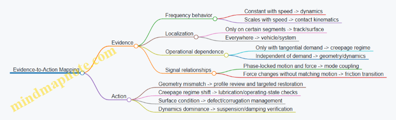
Case Work Summary
Good diagnosis is mostly disciplined comparison. Define the symptom in frequency and direction, gather synchronized evidence with operational state, test a small set of hypotheses using controlled swaps, and confirm with a mechanism-specific explanation that matches both localization and signal relationships.
7. Eddy Current Braking Fundamentals and System Integration
7.1 Electromagnetic Principles for Eddy Current Braking
Eddy current braking turns motion into electrical effects, and then electrical effects back into resisting force. The core idea is simple: a moving conductor in a magnetic field experiences changing magnetic flux, which induces currents. Those currents create their own magnetic field, and the interaction produces a force opposing the motion.
Magnetic Field and Flux Basics
Start with magnetic flux, the “amount of magnetic field passing through an area.” In eddy current braking, the relevant change is not the field strength by itself, but the rate at which flux through the rail surface changes as the wheelset moves.
A practical way to picture it: imagine a coil mounted on the vehicle facing a conductive rail. When the vehicle moves, the rail’s conductive material “sees” the coil’s field sweeping along its length. That spatial sweep is equivalent to a time-varying flux at each point on the rail.
Induction and Eddy Currents
Faraday’s law links changing flux to induced electromotive force. In a solid conductor, that induced voltage drives circulating currents—eddy currents—within the rail surface layers.
These currents are not uniform. They concentrate near the surface because the induced magnetic field tends to oppose the original field penetration. This leads to the concept of skin depth, the characteristic thickness over which current density decays significantly. For braking, skin depth matters because it controls how much of the rail cross-section participates in energy conversion.
Lenz’s Law and the Direction of Braking Force
Lenz’s law gives the direction of the induced currents: they oppose the change that produced them. If the vehicle approaches the coil’s region, the induced currents generate a magnetic field that resists the approach. The result is a braking force that acts opposite the relative motion between coil and rail.
A useful mental check: if you reverse the direction of travel, the induced current pattern reverses in a way that keeps the force opposing the motion. That’s why eddy current braking is naturally “self-correcting” in direction.
Force Generation Through Electromagnetic Interaction
The braking force comes from the interaction between the coil’s magnetic field and the eddy current magnetic field in the rail. In engineering terms, you can treat the system as having an effective electromagnetic damping: as speed increases, induced currents typically increase (until limited by skin depth and circuit effects), and so does the resisting force.
Electrical Circuit View of the Coil
The coil is an electrical circuit with resistance and inductance. When the rail is present, the coil’s effective impedance changes because the rail currents act like a load. This is often described as an added “loss component” in the coil impedance.
That loss component is where the braking energy goes: electrical power dissipated as heat in the rail due to the eddy currents’ resistance.
Speed Dependence and Practical Implications
At low speeds, flux change is smaller, so induced currents are weaker and braking force rises with speed. At higher speeds, the skin depth shrinks relative to rail geometry, so current is confined to a thinner layer. The force does not increase indefinitely; it tends to level or change slope depending on rail conductivity, coil geometry, and air gap.
This speed behavior is why braking performance is usually specified over an operating window rather than as a single number.
Mind Map: Electromagnetic Chain from Motion to Braking
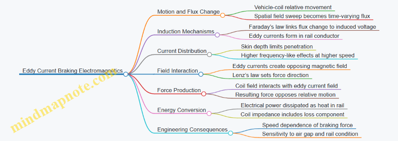
Example: What Happens When Speed Doubles
Assume the air gap and coil geometry stay fixed, and the rail conductivity is unchanged. When speed doubles, the effective rate of flux change at a point on the rail increases. That generally increases induced current magnitude, which increases the electromagnetic interaction force.
However, the increase is not perfectly proportional because skin depth and current confinement change with the effective frequency content of the flux variation. So you might observe “more braking” but with a reduced incremental gain compared with the low-speed region.
Example: Why Air Gap Changes Matter
If the air gap increases, the coil’s magnetic field reaching the rail weakens. With less flux penetrating the rail, the induced eddy currents decrease, and the braking force drops.
This is a clean cause-and-effect chain: air gap → reduced flux → reduced induced currents → reduced electromagnetic interaction → reduced braking force. The system is not mysterious; it’s a chain of measurable links.
Example: Rail Conductivity and Surface Condition
If the rail surface is affected by wear, contamination, or temperature, the effective electrical behavior can change. Lower effective conductivity reduces eddy current magnitude, which reduces braking force. Surface conditions can also influence how the magnetic field couples into the rail, further altering the induced current distribution.
In practice, this is why electromagnetic braking performance is often interpreted alongside rail condition measurements rather than treated as a purely vehicle-side parameter.
7.2 Brake Coil and Rail Interaction Modeling Basics
Eddy current braking turns motion into electrical currents in the rail, and those currents push back against the motion through electromagnetic forces. Modeling the coil–rail interaction is about predicting how much current is induced, where it flows, and how that current produces braking force while respecting electrical and thermal limits.
Core Physical Picture
Start with three coupled effects:
- Electromagnetic induction: A moving magnetic field from the coil induces currents in the rail.
- Current distribution: The induced currents concentrate near the rail surface because of skin effect.
- Force generation: The interaction between the coil field and induced currents creates a retarding force.
A useful sanity check is to track energy: electrical power into the coil becomes heat in the rail and coil, plus mechanical work removed from the vehicle. If your model predicts braking force without corresponding losses, something is missing.
Modeling Inputs and Outputs
A practical model needs these inputs:
- Geometry: coil shape, rail cross-section, air gap, and alignment.
- Electrical properties: rail conductivity and magnetic permeability, plus coil resistance.
- Operating conditions: vehicle speed, coil current (or voltage), and temperature-dependent properties.
- Motion description: relative motion between coil and rail, usually treated as steady-state along the travel direction.
Typical outputs:
- Braking force vs. speed
- Coil current and voltage
- Induced current distribution (often summarized via effective penetration depth)
- Power dissipation in rail and coil
Stepwise Modeling Workflow
Choose the Level of Fidelity
- Circuit–lumped models: fast, good for control-oriented force–speed curves.
- 2D/axisymmetric field models: better for air gap and rail cross-section effects.
- 3D field models: needed when end effects, complex alignment, or detailed coil placement matter.
A common best practice is to begin with a lumped model to get the right trends, then calibrate with a higher-fidelity field model for key operating points.
Represent the Rail as an Electromagnetic Medium
The rail is not just a conductor; it also has magnetic behavior. In many engineering cases, you can treat permeability as constant over the operating range, but you should still allow for conductivity changes with temperature.
Easy example: If your rail conductivity drops by 5% due to heating, induced currents weaken, which reduces braking force. In a lumped model, you can reflect this by adjusting the effective resistance of the rail path.
Compute Induced Currents and Effective Impedance
In field-based approaches, you solve for the magnetic vector potential and induced current density. In circuit-based approaches, you represent the rail’s response as an effective complex impedance seen by the coil.
- The real part corresponds to power dissipated in the rail.
- The imaginary part corresponds to reactive effects that influence current phase and force.
Easy example: At low speed, induced currents are weaker, so the rail impedance contribution is smaller. As speed increases, induced currents grow until skin effect limits further penetration.
Convert Electromagnetic Interaction to Force
Force can be computed from:
- Maxwell stress from the field solution, or
- Energy methods using gradients of magnetic co-energy with respect to position.
For a first implementation, energy methods are often simpler to code consistently with your impedance model.
Easy example: If you increase the air gap by 2 mm, the magnetic coupling drops. Your model should show reduced braking force and reduced rail power dissipation, not just one of them.
Key Modeling Parameters and Their Effects
Air Gap
Air gap strongly controls coupling. Small changes can produce noticeable force differences because the coil field decays rapidly with distance.
Speed
Speed affects induction frequency in the rail’s moving frame. Higher speed increases induced current magnitude up to the point where skin effect confines currents to a thin layer.
Rail Condition
Surface condition and local geometry alter effective current paths. Even if the bulk rail properties are unchanged, a different surface roughness or wear profile can shift the effective coupling.
Easy example: If a rail has a locally different cross-section due to wear, your model should predict a local change in force. In a simplified approach, you can treat this as a modified effective rail width in the field model.
Mind Map: Coil–Rail Interaction Modeling
A Minimal Integrated Example
Assume you want a force–speed curve for a fixed air gap and coil current.
- Use a lumped impedance model to estimate coil current and rail power at several speeds.
- Convert rail power to braking force using the mechanical power balance: the retarding force times speed equals the net mechanical power removed (after accounting for losses).
- Validate the trend with one field-based calculation at a representative speed.
Easy example: If your lumped model predicts force increasing with speed but the field model shows a plateau, the cause is usually skin effect not being represented correctly in the effective impedance. Adjust the effective penetration depth behavior until both models agree on the plateau onset.
Practical Validation Without Overcomplication
Before trusting absolute values, validate three relationships:
- Increasing air gap reduces force and rail losses.
- Increasing speed increases force initially, then approaches a limited behavior.
- Higher rail temperature reduces conductivity and therefore reduces force.
If these checks fail, the model structure is inconsistent, even if the numbers look precise.
7.3 Force-Speed Characteristics and Braking Energy Conversion
Eddy current braking turns vehicle kinetic energy into heat in the rail and brake system. The key engineering question is how the braking force changes with speed, because that shapes both stopping distance and thermal load. In practice, the force-speed curve is not a single straight line; it reflects electromagnetic induction, rail electrical properties, air-gap control, and the way the controller commands current.
From Induction to Braking Force
When the vehicle moves, the magnetic field from the brake coils sweeps past the rail conductor. This induces eddy currents whose direction opposes the motion, producing a retarding force. A useful mental model is that the brake “pushes back” more strongly when the induced currents can form effectively.
The induced current effectiveness depends on:
- Electrical conductivity and thickness of the rail region: higher conductivity supports larger currents.
- Magnetic permeability and geometry: they affect field penetration.
- Speed: higher speed increases the rate of field change, but it also changes how deeply the field penetrates into the rail.
- Air gap: a larger gap weakens the magnetic coupling, reducing force.
A practical takeaway: if you measure braking force at one speed and assume it holds at all speeds, you’ll be wrong in predictable ways.
The Typical Force-Speed Shape
At low speeds, the induced currents are relatively small because the rate of change of magnetic field is limited. As speed rises, force increases. After a certain region, the force tends to level off because the effective penetration depth and current distribution reach a regime where additional speed does not proportionally increase the opposing force.
A simplified piecewise description helps engineers reason without pretending the physics is perfectly linear:
- Low-speed region: force rises with speed.
- Mid-speed region: force approaches a plateau.
- High-speed region: force may slightly change due to rail condition, temperature, and control limits.
Controllers also shape the curve. If the system limits coil current to protect components, the force plateau may be lower than the physics-only expectation.
Converting Force-Speed to Braking Energy
Braking energy conversion is governed by work done by the retarding force. If the vehicle slows from speed \(v_0\) to \(v_1\), the mechanical energy removed is:
\[ E = \int_{t_0}^{t_1} F(t),v(t),dt \]
Using speed as the variable, the same expression becomes:
\[ E = \int_{v_1}^{v_0} F(v),dv \]
This is the bridge between the measured or modeled force-speed curve and the energy budget.
Example: Suppose a test shows the braking force is approximately constant at \(F=120,\text{kN}\) over the speed range from 80 to 40 km/h. Convert speeds to m/s: 80 km/h = 22.22 m/s, 40 km/h = 11.11 m/s.
\[ E \approx \int_{11.11}^{22.22} 120\times 10^3,dv = 120\times 10^3,(22.22-11.11) \]
\[ E \approx 120\times 10^3\times 11.11 \approx 1.33\times 10^6,\text{J} \]
So the rail and brake system must absorb about 1.33 MJ of heat for that segment, assuming negligible losses elsewhere.
Accounting for Real-World Variability
In real operation, \(F(v)\) is influenced by rail temperature, surface condition, and air-gap changes. The energy integral still holds, but the force curve becomes conditional.
A practical method is to treat the force-speed curve as a set of operating envelopes:
- Nominal curve from commissioning tests.
- Reduced curve for larger air gap or degraded rail condition.
- Limited curve when coil current or temperature constraints activate.
Then compute energy using the appropriate envelope for each braking segment. This avoids the common mistake of using a single “headline” curve for all conditions.
Mind Map: Force-Speed and Energy Conversion
Engineering Checkpoints That Prevent Costly Errors
- Verify units and integration variable: integrating \(F(v)\) over speed avoids time-step confusion.
- Use the correct force envelope: if current limiting occurs, the effective force curve changes.
- Separate electromagnetic and thermal reasoning: force determines energy removed; thermal limits determine whether that force can be sustained.
- Cross-check with kinetic energy: the total removed energy cannot exceed the initial kinetic energy by any large margin once losses are accounted for.
When these checkpoints are applied, the force-speed curve stops being a plot and becomes a reliable tool for calculating how much energy the braking system actually has to turn into heat.
7.4 Thermal and Electrical Constraints in Braking Operation
Eddy current braking turns motion into heat and electrical losses. That sounds simple until you remember the system has to survive repeated stops without losing braking force or causing unsafe temperatures. The constraints are mainly thermal (what temperatures the coil and nearby components can tolerate) and electrical (what currents and voltages the supply and control electronics can handle).
Thermal Constraints: Where Heat Goes and What It Does
In an eddy current brake, the coil current creates a magnetic field. As the train moves, the field induces currents in the rail, and those currents dissipate power as heat. The heat splits across the coil (resistive losses) and the rail (eddy current losses). The key practical point is that temperature rise depends on both power and time: a short stop may be fine even if the peak power is high, while repeated stops with short recovery periods can push temperatures beyond limits.
A useful mental model is a “thermal budget” per component: allowable temperature rise plus allowable absolute temperature. For the coil, the limiting factor is usually insulation class and mechanical stability of windings. For the rail, the limiting factor is not just temperature itself but also how temperature affects electrical conductivity and magnetic response, which then changes braking force.
Consider a simple example. Suppose a brake dissipates 120 kW during a 20 s braking event. If the effective thermal mass seen by the rail and coil is such that the combined system can absorb 2.4 MJ without exceeding limits, the event is acceptable. If the same energy is delivered in 10 s, the peak temperature rise is higher even though the total energy is the same, which can stress insulation and create larger force variation.
Electrical Constraints: Current, Voltage, and Control Limits
The electrical side is governed by coil resistance, inductance, supply voltage, and the controller’s ability to regulate current. Coil resistance increases with temperature, which reduces current for a fixed voltage and can reduce braking force. Inductance affects how quickly current can be established and changed, especially at the start of braking.
A practical constraint is the maximum allowable current. Exceeding it can overheat the coil faster than the thermal model predicts, and it can also exceed semiconductor ratings in the power electronics. Another constraint is the maximum voltage available from the traction power interface or dedicated converter. If the controller demands a current that requires more voltage than is available, the current will sag, and braking force will not meet the commanded level.
Coupled Behavior: Why Thermal and Electrical Constraints Interact
Thermal and electrical constraints are not separate checklists; they feed each other. Higher coil temperature increases resistance, which changes the current for a given drive condition. That changes the magnetic field strength and therefore the eddy current losses in the rail. Meanwhile, rail temperature can alter conductivity, changing the induced current magnitude and braking force.
This coupling is why a controller that “works on the bench” can behave differently in service. Bench tests often use steady conditions or longer cooling intervals. In real operation, the braking system experiences sequences of events with limited recovery time.
Mind Map: Thermal and Electrical Constraints in Braking Operation
Example: Verifying Constraints with a Simple Event Sequence
Imagine a braking profile with three events: 15 s, 10 s, and 15 s, separated by 30 s of coasting. If you only check each event in isolation, you might miss the cumulative coil temperature rise. A systematic check uses an energy-and-cooling approach:
- Estimate electrical power during each event from commanded current and coil resistance at the expected temperature.
- Convert power to energy per event.
- Apply a cooling factor during the coasting intervals based on an effective thermal time constant.
- Confirm that peak coil temperature stays below the insulation limit and that braking force remains within acceptable tolerance.
If the second event pushes the coil near its limit, the controller may need to reduce current to keep temperatures safe. That reduction will lower braking force, so the control strategy should account for it by adjusting commanded current or braking request timing.
Example: Diagnosing a Force Drop During Repeated Braking
Suppose braking force is correct for the first stop but noticeably lower for the second. A common cause is increased coil resistance from temperature rise, which reduces current when voltage headroom is limited. Another cause is rail property change from rail heating, which can reduce induced current effectiveness. The diagnostic approach is to compare measured coil current and supply voltage during each event. If current is lower than commanded, the issue is electrical headroom or control limiting. If current matches but force drops, the issue is likely rail temperature effects or air-gap and alignment changes that alter magnetic coupling.
In practice, good constraint management means the thermal model, electrical limits, and control logic are treated as one system: the controller should not only command force, but also respect current and temperature boundaries so the brake remains predictable across the full braking sequence.
7.5 Integration With Vehicle Braking Systems and Control Interfaces
Eddy current braking (ECB) does not live in isolation: it shares the same braking request, safety constraints, and actuator limits as friction brakes. Integration is mostly about making the control system answer one question consistently: “Given the driver’s demand and the train’s state, how much ECB torque is safe and useful right now?”
Establishing a Unified Braking Request
Start by defining a single braking demand signal that originates from the driver brake handle and automatic control layers. Convert that demand into a target longitudinal deceleration or target braking force at the vehicle level. Then split the target into three buckets: ECB contribution, friction contribution, and a residual that accounts for actuator saturation or unavailable ECB.
A practical rule: ECB should be treated as a controllable brake with a known force-speed envelope, not as a “bonus” effect. That means the controller first checks whether ECB can meet the requested portion without exceeding limits, then assigns the remainder to friction brakes.
Example: If the driver requests 0.6 m/s² at 280 km/h and the ECB system can only supply up to the equivalent of 0.35 m/s² at that speed and rail condition, the controller commands ECB for 0.35 m/s² and friction for the remaining 0.25 m/s². If friction is also limited (for example, due to wheel slide protection), the residual becomes a controlled shortfall rather than an uncontrolled one.
Coordinating with Anti-Slip and Traction Control
Wheel slip protection and traction control are designed around friction brakes and traction motors, but ECB affects wheel-rail forces indirectly through the overall longitudinal force balance. The key is to ensure the slip controller sees the net effect of ECB and friction, not just friction alone.
Implementation approach: compute an estimated longitudinal force from ECB commands and include it in the slip controller’s force model. If the slip controller only “listens” to friction brake pressure, it may overcompensate, causing unnecessary friction usage.
Example: During a low-adhesion event, the slip controller reduces friction brake torque. If ECB is still commanded at a fixed level, the net braking force may remain high enough to trigger slip oscillations. With force estimation, the slip controller can reduce ECB proportionally, keeping the wheel-rail creep in the intended range.
Designing the Control Allocation Logic
Use a hierarchical allocation: high-level braking demand → safety and availability checks → force allocation → actuator command shaping.
Safety and availability checks include:
- ECB electrical limits and thermal constraints
- rail condition flags that affect achievable braking force
- actuator health status and communication integrity
Force allocation uses the ECB force-speed characteristic and measured feedback (such as coil current and inferred air gap behavior). Actuator command shaping filters abrupt changes to avoid exciting mechanical or electrical transients.
Example: If coil current approaches a limit, the allocator reduces ECB command smoothly over a short time window while increasing friction contribution to maintain deceleration tracking.
Handling Mode Transitions and Fallbacks
Mode transitions occur when speed crosses ECB effectiveness thresholds, when rail condition changes, or when the system switches between service braking and emergency braking.
A robust fallback strategy is to define what happens when ECB is unavailable: the controller should automatically reallocate to friction brakes while respecting friction limits and maintaining braking continuity.
Example: In emergency braking, ECB may be constrained by thermal headroom. If ECB cannot deliver the requested portion, friction brakes take over immediately within their own emergency capability, and the system logs the allocation reason for maintenance.
Synchronizing with Train Control and Brake System Interfaces
Integration requires consistent interface semantics between vehicle controllers and the brake control unit. Common signals include:
- brake demand request and brake mode status
- ECB command (current or equivalent force) and ECB availability
- friction brake command and feedback
- measured vehicle speed, wheel slip indicators, and brake system health
To prevent “fighting controllers,” define ownership: one controller computes the split, while others enforce local limits. Also ensure time alignment: if ECB force estimation lags friction feedback, the slip controller may react late.
Example: If ECB current feedback arrives 50 ms later than friction pressure feedback, the net force estimate should use the latest available ECB state and a prediction for the short gap, rather than assuming ECB is zero.
Mind Map: Integration with Vehicle Braking Systems
Example: End-To-End Braking Allocation Scenario
At 240 km/h, the driver requests 0.5 m/s² service braking. The controller checks ECB availability and computes the maximum ECB deceleration it can safely provide given current and thermal limits. It allocates ECB first, then assigns friction for the remainder. The slip controller receives the net estimated longitudinal force and wheel slip indicators, so it adjusts friction only when needed. If rail condition flags indicate reduced ECB effectiveness, the allocator reduces ECB smoothly and increases friction to preserve deceleration tracking without sudden torque steps.
The result is a braking system that behaves like one coordinated machine: ECB contributes where it is effective, friction fills the gaps, and safety constraints remain the boss rather than an afterthought.
8. Eddy Current Braking Performance Optimization
8.1 Air Gap Control and Its Effect on Braking Force
Eddy current braking force depends strongly on the electromagnetic coupling between the brake coil and the rail. The air gap is the mechanical separation that sets how much magnetic flux reaches the rail and how efficiently induced currents form. In practice, the air gap is not a single number: it varies along the vehicle, across the rail head, and over time as suspension, track geometry, and wear change. Air gap control is therefore both a design problem and a maintenance problem.
Core Principle of Air Gap to Braking Force
A smaller air gap increases magnetic flux density in the rail for a given coil current. Higher flux produces stronger induced currents, which in turn generate a braking force opposing the relative motion. The relationship is not perfectly linear because rail material properties, coil geometry, and current distribution also change with gap. Still, the engineering takeaway is consistent: reducing the air gap generally increases braking force and improves repeatability.
A useful way to reason about it is to separate two effects:
- Electromagnetic coupling: how effectively the coil “sees” the rail through the gap.
- Current distribution: how induced currents spread in the rail cross-section, which depends on both flux and rail conductivity.
When the gap grows, coupling drops first, and the induced current level follows. That reduces braking force even if the control system commands the same coil current.
What Changes the Air Gap in Service
Air gap variation comes from several sources that engineers can measure and manage:
- Vehicle dynamics: suspension deflection under load and track irregularities change the relative position of the brake units.
- Brake unit mounting tolerances: initial alignment and manufacturing variation set the baseline gap.
- Rail profile and wear: the rail head shape affects where the brake face “works” relative to the rail.
- Contamination and debris: dust, moisture films, and small debris layers effectively increase the gap.
- Thermal expansion: coil heating can shift mechanical components slightly, changing the gap during sustained braking.
A practical example: if a fleet experiences a gradual increase in effective gap due to debris accumulation, the control system may compensate by raising coil current. That can restore force temporarily, but it also increases electrical losses and heat, which can later reduce performance.
Control Strategies That Actually Work
Air gap control is usually implemented through a combination of mechanical design and monitoring.
Mechanical design practices
- Rigid mounting with controlled compliance: allow necessary movement for safety while limiting gap drift.
- Wear-tolerant brake face geometry: design the interface so that rail head wear does not translate into large gap changes.
- Guiding features: keep the brake unit centered relative to the rail so the gap does not vary laterally.
Operational and maintenance practices
- Gap inspection intervals: measure at representative locations and compare to baseline.
- Cleaning procedures: treat debris as a performance variable, not just a cosmetic issue.
- Post-maintenance verification: after wheel/rail grinding or brake unit servicing, re-check gap and braking response.
Example: Translating Gap Error into Force Error
Assume a brake system is tuned at a nominal air gap. During an inspection, you find the effective gap is larger by a small amount. Even without a full electromagnetic model, you can estimate the impact by using test data from the same brake design.
A straightforward workflow:
- Measure air gap at multiple points along the brake face.
- Run a controlled braking test at a fixed commanded coil current.
- Compare measured braking force to the baseline at the nominal gap.
- Attribute the difference primarily to coupling loss, then confirm with temperature and rail condition checks.
If the force drops consistently with increased gap, you can build a correction curve for control tuning and maintenance thresholds.
Mind Map: Air Gap Control and Braking Force
Example: Diagnosing a Force Drop
Suppose braking force is lower than expected during routine operation. The first check is not the control software; it is the mechanical interface.
- If air gap measurements show an increase, the coupling loss explains the force drop.
- If air gap is normal but force is low, then rail condition, coil temperature, or current delivery issues become more likely.
This ordering saves time because air gap is the most direct path from mechanical state to electromagnetic performance. It also prevents the common mistake of compensating for a mechanical gap problem by simply increasing coil current.
Practical Threshold Thinking
Engineers typically set maintenance thresholds based on measured force margin, not just gap size. A larger gap reduces force and increases the electrical effort required to reach the same braking demand. That combination can push the system toward thermal limits sooner.
A practical approach is to define:
- a gap limit that triggers inspection,
- a force margin that triggers corrective action,
- and a cleaning trigger tied to observed contamination patterns.
With these linked, the system stays predictable: the control loop manages normal variability, while maintenance handles the mechanical causes that would otherwise accumulate.
8.2 Coil Geometry and Material Selection for Performance Consistency
Performance consistency in eddy current braking starts with a simple idea: the brake force depends on how the rail’s changing magnetic field induces currents, and those currents depend on the coil’s geometry and the materials’ electrical and thermal behavior. If either changes unpredictably, the force becomes harder to control—especially when rail condition, speed, and air gap vary.
Coil Geometry Fundamentals
A coil produces a magnetic field whose strength and spatial distribution depend on turns, coil length, winding layout, and the distance to the rail. In practice, the coil is not “just a coil”; it is a field-shaping device.
Key geometry levers:
- Effective pole length: The length of rail region strongly influenced by the coil. Longer effective length tends to spread braking force over a larger area, reducing local heating and making force less sensitive to small lateral shifts.
- Coil width and edge effects: Narrower coils concentrate field lines, increasing sensitivity to rail surface condition and alignment. Wider coils reduce edge-driven nonuniformity.
- Turns and current path: More turns increase magnetic field for a given current, but also increase resistance and heat generation. The design must balance force gain against thermal limits.
- Winding placement relative to the air gap: The coil’s position determines how much of the field “sees” the rail. Small manufacturing tolerances can matter because braking force changes strongly with air gap.
A practical example: two coils with the same resistance and current rating can still produce different force consistency if one has a shorter effective pole length. In tests, the shorter coil often shows larger force scatter when the vehicle’s lateral position shifts by a few millimeters, because the induced current distribution moves more abruptly.
Material Selection for Electrical and Thermal Stability
Materials affect both magnetic behavior and how the coil handles heat.
Common material roles:
- Conductor material: Copper is typical due to high conductivity, but alloy choices and conductor cross-section affect resistance growth with temperature.
- Insulation system: Insulation must tolerate coil temperatures and thermal cycling without losing dielectric strength or mechanical integrity.
- Magnetic circuit components: If a magnetic yoke or flux concentrator is used, its material determines how efficiently flux is guided and how saturation changes with current.
What “performance consistency” means in material terms:
- Predictable resistance vs temperature so current control remains stable.
- Stable permeability and saturation behavior so the magnetic field does not shift shape as current changes.
- Thermal expansion compatibility so the air gap and coil alignment do not drift during operation.
A concrete example: if the conductor resistance rises faster with temperature than expected, a controller that assumes constant resistance will under-drive current as the coil heats. The result is a braking force that gradually drops during repeated stops, even if the air gap is unchanged.
Geometry–Material Coupling
Geometry and materials interact through heat generation and field distribution. A coil with higher turns may increase force, but it also increases copper mass and resistance. If the coil’s thermal path is weak, temperature rises, resistance increases, and the magnetic field weakens. That feedback loop can turn a “good” design into an inconsistent one.
To keep the loop predictable, designs typically target:
- Controlled thermal gradients so resistance and insulation properties stay within known ranges.
- Reasonable current density so hot spots do not dominate behavior.
- Field uniformity so small rail condition changes do not cause large force swings.
Design Checks That Prevent Surprise Variability
- Air gap sensitivity mapping: Evaluate how force changes with air gap across the expected manufacturing tolerance and wear range. If force scatter is dominated by air gap, geometry tweaks alone won’t fix it.
- Rail condition sensitivity: Test or model how rail surface roughness and minor defects affect induced current paths. Geometry that spreads the field can reduce sensitivity.
- Thermal steady-state and transient behavior: Confirm that resistance and insulation remain stable during the duty cycle.
- Magnetic saturation behavior: If a magnetic circuit saturates, force vs current becomes nonlinear, which complicates control.
Mind Map: Coil Geometry and Material Selection
Example: Comparing Two Coil Designs Under Same Control
Assume both coils are driven by the same current controller and have the same nominal air gap.
- Coil A: shorter effective pole length, narrower width, higher turns.
- Coil B: longer effective pole length, wider width, fewer turns.
In a repeated braking sequence with minor lateral position variation:
- Coil A shows larger force scatter because the induced current distribution shifts more with alignment, and its higher turns produce more heat, increasing resistance during the sequence.
- Coil B shows steadier force because the field is more spatially averaged, and lower turns reduce temperature rise, keeping resistance closer to the controller’s assumptions.
The takeaway is practical: geometry choices that improve field uniformity often reduce the impact of both alignment variability and rail surface variability, while material choices that stabilize resistance and insulation behavior keep the control loop from chasing its own tail.
8.3 Influence of Rail Condition on Eddy Current Response
Eddy current braking force depends on how effectively the rail presents an electrically conductive, magnetically consistent surface to the brake coils. Rail condition changes that surface in ways that matter: electrical resistivity, effective air-gap, surface geometry, and the presence of layers like water, grease, or corrosion products. The result is that the same brake command can produce different braking forces from one location to the next—so rail condition is not a “maintenance side quest”; it is part of the electromagnetic system.
Rail Condition Variables That Change Braking Force
Start with the simplest chain: coil current produces a magnetic field, the field induces currents in the rail, and those currents oppose the motion. Any factor that reduces induced current magnitude reduces braking force.
-
Surface cleanliness and contamination
- What changes: Thin films of water, oil, or dirt alter the effective electrical boundary and can change how the coil’s field couples to the rail surface.
- Why it matters: Even when the rail metal remains conductive, a film can change the local current distribution and the effective gap between the coil and the conductive region.
- Example: If a rail segment has a light water film after rain, the measured braking force may drop slightly at low speeds where the induced current distribution is more sensitive to coupling.
-
Corrosion and oxide layers
- What changes: Oxides and corrosion products typically have different electrical conductivity than base steel and can be uneven.
- Why it matters: Eddy currents prefer conductive paths; a less conductive layer reduces current density near the surface where braking is strongest.
- Example: A rail with patchy rust can show braking force “steps” as the wheelset passes from clean to oxidized patches, even at constant speed.
-
Rail surface roughness and wear profile
- What changes: Roughness changes the local distance between coil and rail and can distort the effective coupling area.
- Why it matters: Eddy current braking is sensitive to the effective air-gap; roughness acts like a microscopic gap variation.
- Example: After heavy grinding, a rail may have smoother contact geometry; operators often see more consistent braking force because the effective coupling becomes more uniform.
-
Head wear, profile deviation, and lateral position effects
- What changes: If the rail head profile deviates from design, the wheelset-to-coil alignment and the coil’s distance to the rail can vary.
- Why it matters: Even small alignment changes can shift the region of strongest magnetic interaction.
- Example: On a curve with rail profile wear, the same brake command can yield different force depending on which rail side is more worn.
-
Rail defects and discontinuities
- What changes: Cracks, spalls, and localized damage create discontinuities in current paths.
- Why it matters: Eddy currents cannot flow uniformly across discontinuities, reducing braking force locally and potentially increasing variability.
- Example: A localized spall can cause a brief reduction in braking force as the coil passes over the damaged zone.
Mind Map: Rail Condition to Eddy Current Response
Systematic Cause-and-Effect Reasoning
A practical way to reason about rail condition is to map each condition to one of three electromagnetic effects.
-
Reduced induced current magnitude
- Typically caused by corrosion/oxide layers and contamination that reduce effective conductivity.
- Operational symptom: Lower braking force across a segment, often more noticeable at lower speeds.
-
Increased effective air-gap
- Typically caused by roughness, wear geometry, and alignment changes.
- Operational symptom: Lower force and greater scatter, especially when the rail surface is uneven.
-
Non-uniform current distribution
- Typically caused by patchy corrosion, defects, and localized discontinuities.
- Operational symptom: Force “events” tied to specific locations.
Example: Turning Rail Measurements into Brake Expectations
Suppose a maintenance team records three observations on a route section: (a) moderate surface rust, (b) increased roughness after a period without grinding, and (c) a few isolated spalls.
- For moderate rust: expect a force reduction because the oxide layer reduces near-surface current density.
- For increased roughness: expect force variability because the effective air-gap changes microscopically.
- For isolated spalls: expect localized dips as the coil passes over discontinuities.
In a test run, you would compare braking force traces against location markers. If dips align with spall locations, the defect explanation is consistent. If the entire segment shows a steady lower force with limited scatter, corrosion/oxide is the likely dominant factor. If scatter increases without clear location-specific dips, roughness and alignment are the likely drivers.
Practical Best Practices for Managing Rail Condition Impact
- Use location-referenced rail condition logs. Record where roughness, corrosion, and defects occur so braking force variability can be attributed rather than averaged away.
- Pair braking tests with rail surface state snapshots. A test performed right after cleaning or grinding will reflect the current electromagnetic coupling, not last season’s condition.
- Treat “consistency” as a metric, not only mean force. Two segments can have the same average braking force while one has larger variability due to patchy corrosion or defects.
- Coordinate maintenance actions with brake verification. After grinding or rail remediation, re-check braking force to confirm that the effective air-gap and coupling uniformity improved.
Rail condition is therefore best treated as an input to the electromagnetic model and control strategy, not merely a background factor. When you connect specific rail states to specific electromagnetic effects, the observed braking behavior becomes explainable—and controllable—rather than mysterious.
8.4 Control Strategies for Stable Braking Force Under Variability
Stable eddy current braking force is mostly a control problem: the electromagnetic force depends on air gap, rail conductivity and temperature, wheel/rail contact state, and the vehicle’s speed. Variability shows up as force ripple, slower-than-expected deceleration, or occasional dips when conditions change quickly. The goal is to command a braking force that stays close to target while respecting electrical and thermal limits.
Core Control Objectives
- Force tracking: keep measured braking force near the commanded value over the speed range.
- Robustness to air gap and rail condition: reduce sensitivity to changes in clearance and rail surface state.
- Constraint handling: prevent coil overcurrent, excessive temperatures, and unacceptable rail heating.
- Smoothness: avoid control actions that create oscillations in force or vehicle deceleration.
A practical way to think about the system is: the controller chooses coil current (and sometimes excitation timing), the electromagnetic model predicts force, and sensors confirm what actually happened. When the prediction is wrong, the controller corrects.
Measurement and Estimation That Make Control Work
Start with what you can measure reliably:
- Speed from the vehicle tachometer or axle sensors.
- Coil current and voltage from power electronics.
- Brake force estimate from current, voltage, and temperature models, optionally corrected using force sensors if available.
- Air gap proxy using current-to-force sensitivity or auxiliary gap sensing if installed.
If you only measure current, you can still control, but you’ll be controlling the wrong variable when rail conductivity or temperature shifts. Force estimation should include at least a temperature correction and a conductivity proxy.
Control Architecture from Simple to Advanced
A layered approach keeps the logic clear.
Inner Loop Current Regulation
Use a fast current controller so the power stage behaves predictably. This loop handles electrical dynamics and prevents current overshoot.
- Example: If the command asks for 800 A but the rail condition suddenly increases the effective impedance, the inner loop still reaches the requested current within a short time, so the outer loop can focus on force.
Outer Loop Force Tracking with Feedforward
The outer loop commands current to achieve target force. It uses feedforward from an electromagnetic force-speed-air-gap relationship, then applies feedback correction.
- Example: At 250 km/h, the feedforward table predicts that 700 A yields 60 kN. If the measured force is 55 kN due to a larger air gap, the feedback increases current slightly until force matches.
Constraint Supervisors
Add supervisors that clamp commands when limits are approached.
-
Electrical limit: maximum current or voltage.
-
Thermal limit: coil temperature rate and rail temperature proxy.
-
Mechanical limit: maximum allowable deceleration rate.
-
Example: During a long braking event, the thermal supervisor gradually reduces the force command even if the driver asks for the same deceleration, preventing coil temperature from exceeding the safe threshold.
Handling Variability Systematically
Air Gap Variability
Air gap changes with suspension motion, track geometry, and mounting tolerances. Because force is strongly sensitive to gap, treat gap as a disturbance.
- Strategy: estimate an effective gap factor from recent force-vs-current behavior, then adjust feedforward.
- Example: When the vehicle enters a section with slightly different track profile, the controller notices that the same current produces less force. It updates the effective gap factor and restores force without aggressive oscillations.
Rail Conductivity and Temperature Variability
Conductivity and temperature alter eddy current strength.
- Strategy: maintain a conductivity/temperature correction term in the force estimator, updated using measured coil electrical response.
- Example: After a previous braking segment, rail temperature is higher. The controller reduces commanded current for the same target force, keeping force stable while avoiding unnecessary electrical stress.
Speed-Dependent Behavior
Force typically changes with speed due to electromagnetic penetration and slip conditions.
- Strategy: use a speed-indexed feedforward map and let feedback correct residual errors.
- Example: If the controller uses a single current-to-force ratio across all speeds, it will over-brake at low speed and under-brake at high speed. A speed-indexed map prevents that.
Practical Tuning Rules That Prevent Control Surprises
- Tune the inner loop first so current dynamics are faster than force dynamics.
- Use conservative feedback gains so the controller corrects errors without chasing sensor noise.
- Filter only what you must: filter force estimates lightly; heavy filtering delays correction and can cause overshoot.
- Separate transient and steady-state behavior: allow faster correction during rapid speed changes, slower correction during steady cruising.
- Validate with worst-case scenarios: large air gap, high rail temperature, and rapid speed ramps.
Mind Map: Control Strategies for Stable Braking Force
Example: Force Stability During a Speed Ramp
Assume a target braking force of 50 kN while speed decreases from 300 km/h to 200 km/h.
- Feedforward: provides the baseline current command at each speed.
- Air gap disturbance: at 260 km/h, suspension motion increases the effective gap, dropping measured force to 46 kN.
- Feedback correction: the outer loop increases current by a small increment until force returns to 50 kN.
- Thermal supervisor: if coil temperature approaches its limit, it reduces the force command slightly or caps current, keeping the system within safe operation.
The result is a force trace that may show small, controlled corrections during the disturbance, but avoids large oscillations and respects electrical and thermal constraints.
8.5 Practical Examples of Braking Force Tuning and Verification
Practical tuning starts with a simple question: “What braking force do we actually get at the wheel-rail interface, and how does it change when conditions change?” The examples below follow a consistent path—measure, model the dominant sensitivities, tune the control or hardware parameter, then verify with repeatable test conditions.
Example: Air Gap Tuning with Measured Force-Speed Curves
Goal. Reduce braking-force scatter caused by air-gap variation and rail-to-rail differences.
Setup. Instrument the vehicle with a force measurement method that can separate eddy current braking force from other braking contributions. Record speed, commanded braking level, coil current, and an air-gap proxy (for example, a calibrated sensor signal or a geometry estimate from maintenance data).
Baseline. Run a set of constant-speed tests at several speeds (e.g., 60, 120, 180 km/h) and several braking commands. Plot measured braking force versus speed for each command.
Tuning action. Adjust the mechanical or control parameter that effectively changes the air gap. In practice, this might be a calibration offset in the air-gap estimate used by the controller, or a mechanical adjustment verified during inspection.
Verification. Re-run the same test matrix. The success criterion is not “higher force,” but reduced spread of force at the same speed and command. A useful check is the slope of force versus speed: if the slope changes sharply, the tuning may have shifted the operating regime rather than corrected the gap.
Easy-to-understand reasoning. Eddy current braking force depends strongly on how effectively the magnetic field couples into the rail. If the air gap is larger than assumed, the controller may command current that produces less force than expected. Tuning aligns the controller’s expectation with reality.
Example: Control Gain Adjustment Under Rail Condition Variability
Goal. Stabilize braking force when rail surface condition changes frictional and electromagnetic response.
Setup. Choose two rail conditions that are common in service: one with relatively smooth surface and one with a representative level of wear or contamination. Keep wheelset and suspension settings constant.
Baseline. For each rail condition, perform controlled deceleration runs from the same initial speed range. Log coil current, braking command, and measured braking force.
Tuning action. Adjust the controller gain or feedforward term used to map desired force to coil current. Use the baseline runs to identify whether the controller is under-correcting (force too low) or over-correcting (force overshoot and oscillation).
Verification. Compare force tracking error across the two rail conditions. A good outcome is consistent tracking error magnitude and sign, not necessarily identical force levels.
Easy-to-understand reasoning. The controller tries to hit a target force, but the rail condition changes the relationship between current and force. Gain tuning changes how aggressively the controller compensates for that mismatch.
Example: Coil Current Limiting with Thermal Constraints
Goal. Prevent force drop due to thermal limits while maintaining predictable braking performance.
Setup. Plan a test that stresses heating: repeated braking cycles at a fixed duty pattern. Instrument coil temperature or a validated thermal proxy, and record current limiting events.
Baseline. Run the duty cycle with the current limit set to the nominal value. Observe whether braking force decays during the later cycles.
Tuning action. Adjust the current limit strategy so that it accounts for measured thermal rise rate. This can mean changing the limit schedule or the thermal model parameters used to compute allowable current.
Verification. Confirm that force remains within a specified tolerance band across cycles and that temperature stays below the operational threshold with margin.
Easy-to-understand reasoning. If the system waits until temperature is already high, it will “panic” by cutting current, and force will fall. A better strategy limits current early enough to keep the force curve flatter.
Mind Map: Braking Force Tuning and Verification Flow
Example: Acceptance Thresholds That Actually Mean Something
Set acceptance criteria that match the tuning objective. For air-gap tuning, use force spread at fixed speed and command. For control tuning, use tracking error over the deceleration window. For thermal tuning, use force retention across cycles and confirm no late-cycle current limiting dominates the response.
A practical trick: compute the same metrics before and after tuning using identical data windows. If you change the window, you can accidentally “improve” results by measuring a quieter part of the run. The goal is to compare like with like—because the rail does not care about our measurement preferences.
9. Thermal Management and Reliability for Eddy Current Braking
9.1 Heat Generation Mechanisms in Coils and Rail Surfaces
Eddy current braking converts kinetic energy into electrical losses in the rail and magnetic losses in the braking system. Heat appears where current flows and where magnetic fields cycle, so the engineering question becomes: which physical mechanism creates which temperature rise, and where does that heat go next?
Core Energy Path
When the brake coil is energized, it creates a time-varying magnetic field relative to the moving rail. That changing field induces currents in the rail. The induced currents experience electrical resistance, producing Joule heating. At the same time, the magnetic field interacts with the rail’s ferromagnetic structure, causing additional losses tied to field cycling and material properties.
A useful mental model is a two-stage chain: (1) electromagnetic induction determines how much current is induced and how deep it penetrates, and (2) resistive and magnetic losses determine how that current and field energy becomes heat.
Coil-Side Heat Sources
Coils heat primarily from their own electrical resistance and from how the magnetic circuit loads the current.
-
Ohmic heating in coil windings: The coil carries current, so power loss is approximately \(P_{coil} \approx I^2 R\). This is the dominant and most predictable source. If you double current, you quadruple winding power, so current limiting and duty cycle matter.
-
Additional losses from current waveform and skin effects: At higher frequencies, current distribution in conductors becomes non-uniform. That increases effective resistance and can raise temperature even if average current is unchanged.
-
Magnetically induced heating in nearby conductive parts: Braking hardware often includes supports, clamps, and structural elements. Any conductive path that experiences changing fields can develop eddy currents, adding “hidden” heat outside the main winding.
Rail-Side Heat Sources
Rail heating is usually dominated by electrical losses from induced currents.
-
Joule heating from induced currents: The induced current density \(J\) produces power density \(p \approx J^2 \rho\), where \(\rho\) is resistivity. The current is not uniform; it concentrates near the surface due to electromagnetic penetration limits.
-
Skin effect and penetration depth: The faster the relative motion and the stronger the magnetic coupling, the more the induced currents concentrate near the rail surface. Concentration increases \(J\) locally, which increases heat generation near the surface. This is why surface temperature can rise faster than bulk temperature.
-
Magnetic losses in the rail steel: Even if resistive heating were absent, cycling magnetic fields cause energy loss through hysteresis and other magnetic mechanisms. These losses depend on magnetic flux density and how quickly it changes.
-
Coupling sensitivity to rail condition: Surface roughness, coatings, and rail defects can alter effective coupling and current paths. The result is not just “more or less heat,” but a different spatial distribution of heat, which affects thermal gradients and material stress.
How Heat Spreads After It Is Generated
Heat generation is only half the story. The other half is heat flow.
- Conduction into the rail mass: Heat spreads along the rail and into the surrounding structure. The local temperature rise depends on thermal conductivity and the effective thermal path length.
- Conduction into fasteners and sleepers: The rail is not thermally isolated. Contact conditions at interfaces influence how quickly heat leaves the braking zone.
- Convection and radiation to air: At typical operating conditions, surface heat loss to air can be meaningful, but it rarely dominates during short, high-power braking events.
A practical takeaway: two systems with the same generated power can produce different peak temperatures if their heat spreading paths differ.
Mind Map: Heat Generation Mechanisms
Example: Comparing Two Braking Scenarios
Assume the same coil design and rail material, but different braking duty.
- Scenario A: Short, high-power braking: Induced currents concentrate near the surface, creating a steep temperature gradient. Peak rail surface temperature rises quickly because heat has little time to conduct away.
- Scenario B: Longer, moderate braking: Total energy may be similar, but the rail and coil have more time to spread heat. Peak temperatures are typically lower, and the temperature profile is smoother.
In both cases, the coil winding still follows \(I^2R\) behavior, but the rail peak depends strongly on how quickly heat can leave the surface region.
Example: Why “More Current” Is Not the Only Lever
If you increase coil current to raise braking force, you increase coil heating by \(I^2\). Meanwhile, rail heating also increases because induced current density grows. However, the rail’s temperature rise is not purely proportional to coil current: changes in coupling and penetration depth can shift where heat is generated, which changes gradients and the risk of local overheating.
Summary
Coil heat comes mainly from winding resistance and secondary eddy effects in nearby conductors. Rail heat comes mainly from Joule losses of induced currents, shaped by skin effect and coupling, with additional magnetic losses in the steel. Peak temperatures and gradients depend on both where heat is generated and how efficiently it spreads into the rail and surrounding structure.
9.2 Temperature Measurement and Instrumentation Practices
Temperature is the bridge between electrical losses and material behavior in eddy current braking. In practice, you measure it to (1) verify braking force stability, (2) protect insulation and coil components, and (3) interpret rail condition effects on braking performance. The key is choosing sensors and placement so the readings represent the temperatures that actually limit performance.
Foundational Concepts for What You Measure
Start by separating three temperatures that often get mixed up:
- Coil temperature: governs insulation life and conductor resistance.
- Rail surface temperature: influences eddy current strength and local material properties.
- Bulk rail temperature: affects heat spreading and longer-duration thermal gradients.
A sensor reads what it touches, not what you wish it touched. If you mount a sensor on a bracket near the coil, you may be measuring bracket heat rather than coil heat. If you measure rail surface temperature with a method that averages over a spot larger than the contact region, you may miss the peak.
Instrumentation Strategy from System Level to Sensor Level
A good measurement plan begins with the braking duty cycle. For example, if braking occurs in short bursts separated by coasting, you need enough sampling rate to capture rise time, not just steady-state values. If braking is continuous, you can focus on thermal equilibrium and slower sampling.
Then decide what you need to compute:
- Peak temperature for safety limits.
- Time-to-peak and cooling slope for thermal model calibration.
- Temperature distribution proxy for diagnosing uneven heating.
Finally, select sensor types that match the measurement target.
Sensor Types and Placement Practices
Contact Sensors for Coil and Enclosure
For coil temperature, thermocouples or RTDs are common. Use proper thermal coupling: a sensor that is loosely attached will lag behind real coil temperature. Apply a thin, stable thermal interface material where appropriate, and secure the sensor so it cannot shift under vibration.
Place sensors where they represent the hottest region. If you cannot access the hottest spot directly, measure at the nearest credible location and document the thermal path so you can interpret offsets.
Non-Contact Sensors for Rail Surface
For rail surface temperature, infrared (IR) thermography or IR spot sensors are typical. IR methods depend on emissivity, which changes with oxidation, contamination, and surface finish. Treat emissivity as a measurement variable, not a constant.
A practical approach is to calibrate emissivity using a controlled reference target on the rail surface under similar conditions. If emissivity calibration is not possible, you can still use IR readings for relative comparisons, but you must avoid using them as absolute safety limits.
Avoiding Measurement Traps
- Cable routing: keep sensor leads away from strong electromagnetic fields and avoid creating loops that pick up noise.
- Grounding: use a consistent grounding scheme to prevent ground offsets that look like temperature changes.
- Sensor shielding: protect sensors from direct airflow changes that can mimic cooling effects.
Data Acquisition Practices That Keep Readings Honest
Sampling rate should match the fastest thermal change you care about. For burst braking, capture the rise with enough resolution to estimate peak accurately. For continuous braking, you can sample more slowly but still record long enough to observe stabilization.
Use time synchronization between braking command signals and temperature channels. Without synchronization, you may align temperature peaks to the wrong braking interval and draw incorrect conclusions about thermal cause.
Apply basic signal conditioning:
- Filter high-frequency electrical noise without smoothing away real thermal transients.
- Detect sensor dropouts and mark them so downstream calculations do not silently treat missing data as stable temperature.
Mind Map: Temperature Measurement Workflow
Example: Coil Temperature Setup for Burst Braking
Suppose a test uses repeated braking bursts lasting 20 seconds with 40 seconds of coasting. Mount two thermocouples on the coil: one near the expected hottest conductor region and one slightly away to estimate spatial gradient. Sample at a rate high enough to capture the rise within each 20-second burst.
During analysis, compare the two channels. If the “hot” sensor consistently peaks earlier and higher, you can treat it as the limiting indicator. If both sensors track closely, the coil may be heating more uniformly than expected, and you can simplify the thermal model.
Example: Rail Surface Temperature with Emissivity Control
If the rail surface is freshly ground, emissivity may differ from a rail with oxidation. Use an IR spot sensor and perform an emissivity check on a small reference area under similar surface condition. Then run the same braking test and record the peak rail surface temperature.
When comparing different maintenance states, avoid mixing absolute values without emissivity handling. Instead, compare relative peak temperature rise under the same surface condition, and only use absolute numbers when emissivity is controlled.
Practical Checklist for Instrumentation Readiness
- Sensors are placed to represent limiting temperatures, not just convenient locations.
- Coil sensors have stable thermal coupling and vibration-proof mounting.
- Rail IR sensors account for emissivity or are used for relative comparisons only.
- Data acquisition is synchronized with braking commands.
- Sampling rate captures the thermal rise for the chosen duty cycle.
- Noise filtering preserves thermal transients and dropout handling is explicit.
With these practices, temperature measurements become a reliable input to both safety decisions and performance interpretation, rather than a collection of numbers that happen to change when braking happens.
9.3 Cooling Methods and Their Implementation Constraints
Eddy current braking turns kinetic energy into heat in the rail and brake coils. Cooling is therefore not an optional accessory; it is part of the force-control problem because temperature changes electrical resistance, magnetic coupling, and the allowable operating envelope. A good cooling plan starts with what must stay within limits, then chooses a method that can be implemented reliably on real track.
Cooling Goals and What Actually Limits You
The first constraint is coil temperature. As copper heats up, its resistance rises, which reduces current for a given voltage and can lower braking force. The second constraint is rail surface and subsurface temperature, which affects material properties and can accelerate wear or damage if hotspots form. A third constraint is thermal gradients: even if average temperature is acceptable, steep gradients can create local stress and uneven performance.
A practical way to set targets is to define three thresholds: maximum coil temperature, maximum rail temperature at the braking zone, and a gradient limit based on allowable stress. For example, if your coil is rated to survive at a certain peak temperature and your rail has a known safe surface limit, you can translate those into allowable duty cycles for a given speed and braking frequency.
Cooling Methods and Their Core Mechanisms
Cooling methods fall into three families: conduction to a structure, convection to surrounding air, and forced removal via fluids. Each has different implementation constraints.
Conduction to a Heat Sink Coils can be mounted to thermally conductive supports that spread heat. This works best when the heat sink has a stable thermal path and sufficient mass. The constraint is that the heat sink can become a bottleneck: if it saturates, coil temperature rises quickly. Implementation requires careful contact quality, consistent clamping force, and thermal interface materials that tolerate vibration and weather.
Natural or Forced Convection to Air Air cooling is simple but limited by airflow. Forced convection using fans can improve heat removal, but it adds electrical power, maintenance, and reliability concerns. The constraint is that airflow can be blocked by dust, snow, or debris, and fan performance varies with installation orientation.
Liquid Cooling Liquid cooling can remove heat efficiently and keep coil temperatures stable. The constraints are more involved: plumbing, leak prevention, freeze protection, and inspection access. Liquid systems also require filtration and flow monitoring because fouling reduces heat transfer. For trackside equipment, the implementation challenge is often not the heat exchanger itself, but maintaining reliable seals and serviceability.
Implementation Constraints That Matter in the Field
Electrical and Control Coupling Cooling affects braking force indirectly through resistance and current limits. If the control system uses temperature-based derating, you must ensure the sensors reflect the hottest relevant locations. A sensor stuck to a cooler surface can delay derating and create a hidden hotspot.
Environmental Conditions Wind speed, ambient temperature, rain, and dust all change convection performance. Liquid systems add freeze and corrosion constraints. Even conduction-based designs can suffer if thermal contact degrades over time due to loosening or corrosion.
Mechanical Integration and Maintenance Access Cooling hardware must survive vibration and impacts from track operations. Fans and pumps need access for cleaning and replacement. Heat sinks need clearances for airflow and must avoid trapping debris.
Thermal Modeling Fidelity A model that predicts average temperature but misses hotspots can mislead control settings. The implementation constraint is to validate the model with measurements at the locations that drive derating.
Mind Map: Cooling Design Logic
Example: Choosing a Cooling Strategy by Duty Cycle
Assume a braking zone where trains perform repeated braking events with short intervals. If the duty cycle is high, air-only convection may not remove enough heat between events, leading to a rapid rise in coil temperature and early derating. In that case, conduction to a larger heat sink can delay the rise, but it may still saturate during sustained operation.
If you observe that coil temperature stabilizes at an uncomfortably high level after several cycles, the next step is to improve heat removal capacity. A common progression is to add forced airflow first if the site is sheltered and debris risk is manageable. If the environment is harsh or duty cycle remains high, liquid cooling becomes attractive because it can maintain temperature closer to a steady value. The key is to verify that the control system derates based on the hottest locations, not just the average.
Example: Sensor Placement to Avoid Hidden Hotspots
Consider two temperature sensors: one embedded near the coil winding and another mounted on the outer support. If the outer support is cooler, the control system may allow higher current than the coil can safely handle. The result is a force drop later than expected and potential insulation stress. A robust implementation places sensors where they correlate with the limiting temperature, then confirms correlation through instrumented tests.
Practical Constraints Checklist for Cooling Implementation
- Confirm the limiting temperatures and gradients you must respect.
- Choose cooling method based on duty cycle, not just peak power.
- Place temperature sensors at the locations that drive derating.
- Validate thermal models with hotspot measurements.
- Design for maintenance access and environmental survivability.
- Ensure the control system’s derating curve matches measured thermal behavior.
Cooling is successful when braking force remains predictable across repeated events and the equipment stays within safe limits for the actual operating conditions. That predictability comes from aligning thermal design, sensor strategy, and control logic—so the system doesn’t “cool” on paper while overheating in practice.
9.4 Insulation, Materials Aging, and Maintenance Criteria
Eddy current brake reliability depends on insulation that survives heat, vibration, moisture, and electrical stress. The goal of this section is practical: understand what insulation is doing, how it ages, how to inspect it, and how to decide when maintenance is needed—without relying on guesswork.
Insulation Roles and Stress Sources
Insulation in eddy current brake coils separates energized conductors from the grounded structure and from each other. It also limits leakage current paths that can grow when the material is hot and slightly contaminated.
In service, insulation experiences several stress types at once:
- Thermal stress from coil heating during braking. Repeated temperature cycling drives expansion and contraction.
- Electrical stress from voltage gradients and partial discharges, especially if voids or moisture exist.
- Mechanical stress from vibration and coil movement under electromagnetic forces.
- Environmental stress from humidity, water ingress, and rail-side contaminants.
A simple way to connect these stresses is to imagine insulation as a “thin boundary layer” that must remain intact. If the boundary layer cracks, absorbs moisture, or loses dielectric strength, electrical leakage can accelerate heating and damage.
Materials Aging Mechanisms
Aging is rarely one thing. It is usually a chain reaction:
- Polymer softening and embrittlement: Elevated temperatures reduce mechanical toughness. After many cycles, the material becomes brittle and more prone to cracking.
- Thermal oxidation: Heat and oxygen degrade polymer chemistry, lowering insulation resistance over time.
- Moisture absorption: Water reduces dielectric strength and increases leakage current, particularly when the coil is hot and then cools.
- Contamination-driven tracking: Conductive deposits can form surface paths that “creep” across insulation, especially where there is dirt and humidity.
- Void growth and partial discharge activity: Small voids can expand under electrical stress, increasing local heating.
A useful maintenance mindset is: if insulation resistance is trending down, the system is already telling you that one or more mechanisms are active.
Maintenance Criteria That Engineers Can Use
Maintenance criteria should be measurable and tied to failure risk. A typical set includes electrical, thermal, and physical checks.
Electrical Criteria
- Insulation resistance (IR): Track IR trends rather than single readings. A sudden drop is a red flag; a slow decline suggests progressive aging.
- Leakage current and dielectric withstand tests: Use only when the maintenance plan allows safe interruption and when procedures are established.
Example: If IR at a standardized test temperature drops by a consistent fraction across repeated inspections, schedule coil insulation inspection and plan corrective action before the next service interval.
Thermal Criteria
- Temperature rise limits: Compare measured coil temperature rise during controlled braking events against the allowable envelope used in design.
- Hot-spot indicators: If temperature distribution becomes less uniform, it can indicate insulation degradation, poor impregnation, or contact issues.
Example: Two coils may have the same peak temperature, but the one with a faster rise rate under identical braking conditions often has higher internal losses.
Physical Criteria
- Cracking, delamination, and surface tracking: Inspect accessible surfaces for visible damage and measure any changes in insulation thickness where feasible.
- Impregnation integrity: If the coil is impregnated, look for signs of voiding or separation.
Example: Fine surface cracks near edges are often where tracking starts. Cleaning alone may not fix the underlying insulation weakness.
Inspection Workflow from Simple to Detailed
A systematic workflow reduces the chance of missing early-stage issues.
- Visual and environmental check: Confirm seals, drainage paths, and cable entry integrity. Moisture problems are often “system-level,” not just insulation-level.
- Electrical baseline and trend: Perform IR measurements under consistent conditions and record them with temperature normalization.
- Operational correlation: Compare electrical trends with braking event logs, especially coil temperature rise and braking current.
- Targeted teardown inspection: If criteria are exceeded or trends accelerate, inspect insulation sections most likely to be stressed: edges, terminations, and areas near electromagnetic force concentration.
Mind Map: Insulation Aging and Maintenance Criteria
Example: Turning Measurements into Decisions
Suppose a coil is inspected every maintenance interval. IR is measured after a standardized cool-down, and temperature rise during a short braking test is recorded.
- IR shows a gradual downward trend across three intervals.
- Temperature rise during the same braking test increases slightly each time.
- Visual inspection finds minor surface cracking near a termination edge.
A coherent response is to treat this as progressive insulation aging with both electrical and thermal correlation. The maintenance action is not “wait for failure,” but to plan a targeted inspection of the cracked region and verify impregnation integrity, while also checking sealing and drainage to prevent moisture-driven acceleration.
Practical Notes on Setting Thresholds
Thresholds should be based on the insulation system’s rated temperature class and the brake’s operating duty cycle. Use consistent test conditions, because insulation resistance is temperature-dependent. When you normalize and trend, you reduce false alarms and catch real degradation earlier.
Finally, document the decision logic: what measurement changed, by how much, and which criterion triggered action. That turns maintenance from a recurring debate into a repeatable engineering process.
9.5 Failure Mode Analysis Using Documented Test Evidence
Failure mode analysis is easiest when it starts with evidence, not opinions. The goal here is to connect what you measured during tests to a specific failure mechanism, then to a practical engineering action. The method below assumes you already have test data from eddy current braking, rail-wheel contact behavior, and thermal monitoring.
Evidence First: What Counts as Documented
Documented test evidence should be traceable, repeatable, and time-aligned. For each test run, capture:
- Test conditions: speed profile, braking command, wheel/rail temperature, rail surface state, and lubrication state if applicable.
- Actuation and sensing: brake controller commands, coil current, measured air gap proxies, voltage/current waveforms, and temperature sensor locations.
- Outcomes: braking force vs. speed, friction/creepage indicators, wear or surface change indicators, and any alarms or faults.
A simple rule: if you cannot point to the exact signal and timestamp that supports a conclusion, it is not evidence yet. This prevents the classic “we think it happened” failure report.
Build the Failure Hypothesis Ladder
Start with a ladder of hypotheses from broad to specific. Each rung must be testable with existing evidence.
- System-level mismatch: braking force lower/higher than expected, or unstable force.
- Electromagnetic cause: coil-rail coupling changed due to air gap, rail conductivity, or rail condition.
- Thermal cause: coil temperature rise altered resistance and reduced force capability.
- Mechanical cause: suspension or wheelset dynamics changed contact geometry, affecting air gap or rail surface state.
- Surface/tribology cause: rail surface defects or contamination altered effective braking interaction and contact conditions.
Each hypothesis should predict a pattern in the data. For example, a thermal cause predicts a gradual change in force with temperature rise, while an electromagnetic coupling cause predicts a sharper change aligned with air gap or rail condition shifts.
Mind Map: Evidence to Mechanism to Action
Pattern Checks That Keep You Honest
Once you have hypotheses, use pattern checks to narrow them. These are mechanical steps, not vibes.
- Timing alignment: Compare the onset of abnormal behavior with controller events and sensor changes. If force drops exactly when coil current is commanded to rise, suspect coupling or measurement issues rather than slow thermal effects.
- Trend shape: Thermal effects often produce smooth drift; coupling issues often produce step-like changes when conditions cross a boundary.
- Correlation strength: If braking force correlates strongly with rail temperature but not with air gap proxies, thermal is more likely. If it correlates with surface condition indicators, tribology or rail condition dominates.
- Threshold crossings: Many failures are triggered when a parameter crosses a limit, such as maximum allowable coil temperature or a minimum effective coupling condition.
Mechanism Confirmation with Cross-Signal Consistency
A mechanism is confirmed when multiple signals agree with the same story. Use cross-signal consistency:
- Electrical consistency: Coil resistance inferred from voltage/current should increase with temperature. If resistance rises but force does not change accordingly, the issue may be elsewhere.
- Thermal consistency: Temperature sensors should show a plausible spatial gradient. A single sensor spiking while others remain steady suggests sensor placement issues or local contact anomalies.
- Contact consistency: If wheel-rail creepage indicators or contact force distribution changed during the same interval as braking anomalies, suspension/contact dynamics may be influencing effective interaction.
Example: Low Braking Force with Stable Temperature
Observed evidence: Braking force is lower than expected across multiple runs, while coil temperature trends remain within normal bounds. Coil current waveforms match the commanded profile.
Hypothesis ladder outcome:
- System-level mismatch is clear.
- Thermal cause is less likely because temperature does not rise abnormally.
- Electromagnetic coupling becomes the leading candidate.
Pattern checks:
- Timing alignment shows the force deficit begins immediately at the start of braking, not gradually.
- Trend shape is consistent across speed steps.
Mechanism confirmation:
- Electrical consistency indicates coil resistance behaves normally.
- Cross-signal consistency points to reduced coupling, such as an effective air gap increase or rail condition affecting conductivity.
Action selection:
- Update air gap verification method in test setup and confirm rail condition characterization.
- Tighten maintenance criteria for rail surface state that affects coupling.
- Adjust control logic only after coupling evidence is confirmed, so you do not “tune around” a measurement or condition problem.
Documentation That Makes Decisions Reproducible
Finish by producing a traceability matrix that links each failure mode to evidence excerpts and decision rationale. Keep it compact:
- Failure mode statement
- Evidence signals and timestamps
- Hypotheses considered and why rejected
- Confirmed mechanism
- Engineering action and acceptance check
A good failure report reads like a courtroom brief: the conclusion is specific, the evidence is named, and the reasoning is checkable. That’s how you turn test data into engineering decisions without turning it into a guessing game.
10. High-Speed Railway Suspension System Modeling and Design
10.1 Suspension Architecture and Component Functions
High-speed rail suspension is the vehicle’s “contact translator”: it converts wheel-rail forces into controlled motion so the wheel stays within acceptable creepage, normal load variation, and lateral guidance demands. The architecture is usually built in layers—primary suspension between wheelset and bogie frame, secondary suspension between bogie frame and carbody—so each layer handles a different job and a different frequency range.
Mind Map: Suspension Architecture and Component Functions
Primary Suspension Components and Their Roles
Primary suspension sits close to the wheelset, so it has the strongest influence on how normal load and creepage evolve over track irregularities. Springs provide compliance; dampers limit oscillation amplitude and control how quickly the system returns to equilibrium after a disturbance.
A practical way to think about primary design is to separate “support” from “control.” Support is mostly spring stiffness: too stiff, and wheel-rail forces spike because the wheelset cannot move to follow the rail; too soft, and the wheelset motion becomes large enough to increase lateral slip and hunting risk. Control is mostly damping: insufficient damping lets energy build up at resonant frequencies, which can translate into larger dynamic wheel loads.
Example: If a wheelset encounters a short-wavelength rail dip, the primary spring compresses and releases. With higher damping, the force peak at the wheel-rail interface is reduced because the spring does not ring as long. That reduction matters because dynamic normal load affects frictional behavior and wear rate.
Primary suspension also includes constraints that prevent uncontrolled lateral motion. Even when the spring provides vertical compliance, lateral guidance is handled by axlebox interfaces, lateral dampers, and linkages that define the effective lateral stiffness.
Secondary Suspension Components and Their Roles
Secondary suspension connects the bogie frame to the carbody and targets ride comfort and stability at lower frequencies. Its springing supports the carbody mass and reduces how much bogie motion becomes carbody acceleration.
Secondary dampers are tuned to manage energy flow between bogie and carbody. If damping is too low, the carbody can experience noticeable oscillations after disturbances; if too high, the system can become overdamped and transmit more force at certain frequencies.
Example: Consider a long-wavelength track profile variation that causes bogie vertical motion. The secondary springs filter this motion so the carbody sees a smoother displacement history. The primary suspension still handles the wheel-rail contact details, but the secondary layer prevents those details from turning into passenger-visible accelerations.
Secondary systems often include anti-roll elements or roll stiffness features. These components reduce roll angle under asymmetric loading, which indirectly stabilizes wheel-rail contact by keeping left and right normal loads from diverging excessively.
Guidance, Constraints, and Kinematics
Suspension is not only springs and dampers; it is also the geometry of constraints that decide which motions are allowed. Traction rods, yaw dampers, and lateral links manage longitudinal and lateral forces so the wheelset and bogie do not “choose” a motion mode that increases slip.
A useful engineering check is to trace load paths under braking, traction, and curving. For instance, braking forces create longitudinal reactions that can couple into bogie yaw and lateral motion. If the constraint layout allows too much yaw compliance, the wheel-rail contact can experience higher tangential forces and altered creepage distribution.
Example: During braking on a slightly canted curve, longitudinal braking force and lateral guidance interact. A yaw damper and properly sized lateral constraints can limit the yaw-induced lateral creepage component, keeping the contact forces within the intended envelope.
Interfaces, Bushings, and Effective Stiffness
Rubber and elastomer bushings appear “small” but strongly affect effective stiffness and damping because they sit in the load path. Their behavior is frequency-dependent and can change with temperature and aging, so the architecture must be validated with measurements rather than assumed from static properties.
Example: Two designs with the same nominal spring stiffness can behave differently if one uses bushings with higher compliance in the lateral direction. The result is a different lateral force-to-displacement relationship, which changes how wheel-rail forces distribute across the contact patch.
Component Selection Through a System View
A systematic architecture approach starts with targets: acceptable wheel load variation, acceptable carbody acceleration, and stable guidance behavior. Then it assigns responsibilities by frequency band: primary suspension shapes wheelset-to-bogie force transmission; secondary suspension shapes bogie-to-carbody motion; constraints define allowed degrees of freedom.
Finally, validation closes the loop. Instrumentation such as accelerometers and displacement sensors confirms that the assembled system stiffness and damping match the intended behavior, and that the measured motion patterns align with the expected wheel-rail contact outcomes.
10.2 Modeling Approaches for Vehicle and Bogie Dynamics
High-speed wheel-rail behavior depends on how vehicle and bogie dynamics shape wheel-rail forces, which then feed back into contact conditions. Modeling is the bridge: it turns geometry, mass distribution, suspension hardware, and track inputs into time histories of forces, motions, and contact quantities. A good approach starts simple, then adds detail only where it changes engineering decisions.
Modeling Goals and Outputs
A practical model should produce outputs that match the decisions you must make:
- Ride quality and stability: vertical and lateral accelerations at the carbody and bogie frames.
- Wheel-rail force distribution: normal forces and tangential forces at each wheelset.
- Contact-relevant kinematics: wheelset creepage inputs (or proxies), wheelset yaw/roll angles, and relative motions across the contact patch.
- Suspension stress proxies: forces in springs, dampers, and links, used to check limits and maintenance wear.
If your model cannot output wheelset motions and forces with traceable assumptions, it will be hard to connect to tribology and braking sections later.
Core Modeling Choices
Rigid-Body vs Flexible Components
Most vehicle and bogie dynamics models treat the carbody, bogie frame, and wheelsets as rigid bodies connected by suspension elements. This is usually sufficient to capture mode shapes and force transmission.
Add flexibility only when it matters for the outputs you care about:
- Wheelset or axle flexibility affects high-frequency force components.
- Brake equipment and mounting flexibility can alter local stiffness and damping.
A simple rule: if the added flexibility changes peak wheel-rail force or resonance timing in the frequency band of interest, include it; otherwise, keep it rigid.
Lumped-Parameter vs Multibody Formulations
- Lumped-parameter models use mass-spring-damper networks with kinematic constraints. They are fast and great for parameter studies.
- Multibody models represent geometry and constraints explicitly, improving accuracy for complex linkages and guidance systems.
For bogies with multiple linkages, multibody kinematics often reduce “mystery stiffness” caused by oversimplified constraint assumptions.
Linear vs Nonlinear Elements
Suspension elements are often modeled as linear springs and dampers near operating points. Nonlinearities become important when they affect contact forces:
- Bump stops and clearance effects.
- Friction in joints.
- Nonlinear damping with velocity-dependent behavior.
A useful practice is to start linear, then introduce one nonlinearity at a time and check whether it changes the wheel-rail force envelope.
Track Inputs and Boundary Conditions
Track irregularities are the main excitation. You typically represent them as:
- Vertical and lateral profiles at the wheel contact points.
- Cross-level and alignment effects.
- Gauge and twist inputs when modeling lateral guidance.
Wheelbase and bogie spacing determine how a single track feature becomes multiple time-shifted excitations. Getting these time shifts right is often more important than adding extra degrees of freedom.
Mind Map: Vehicle and Bogie Dynamics Modeling
Step-by-Step Modeling Workflow
Step 1: Establish Degrees of Freedom
Begin with a minimal set that captures the dominant modes. For a typical high-speed bogie, a common starting point includes:
- Carbody vertical and pitch motions.
- Bogie frame vertical and yaw motions.
- Wheelset lateral and yaw motions.
- Suspension link deflections as generalized coordinates.
Then check whether the model reproduces measured resonance frequencies and mode shapes. If it misses a mode, add the smallest number of coordinates that fixes it.
Step 2: Build Suspension and Guidance Stiffness-Damping Maps
Represent each suspension element with stiffness and damping. For guidance systems, include lateral stiffness contributions from link geometry and compliance.
Easy example: Suppose a lateral damper is specified as 20 kN/(m/s) at low speed. If the model uses constant damping, you may underpredict damping at higher velocities. A practical fix is to fit a simple velocity-dependent damping curve using measured damper force vs velocity, then re-run the same track input and compare peak lateral acceleration.
Step 3: Add Wheel-Rail Interface Forces as Outputs
In many workflows, the wheel-rail interface is not modeled with full contact mechanics inside the dynamics solver. Instead, you compute wheel-rail normal and tangential forces from suspension deflections and guidance kinematics using a mapping model.
Easy example: If you know the vertical suspension deflection at each wheelset and the effective vertical stiffness, you can estimate normal force changes. That normal force estimate then becomes the input to tribology calculations for friction and wear.
Step 4: Calibrate Using Measured Data
Calibration should be targeted. Use:
- Modal frequency checks from instrumented runs.
- Static deflection checks from known load cases.
- Damping identification from decay or frequency response.
Avoid calibrating everything at once. If you tune stiffness to match one resonance and damping to match another, you keep the model interpretable.
Step 5: Validate Force Envelopes, Not Just Time Traces
Time histories can look similar while peak forces differ. Validate using:
- Peak wheel-rail normal force per wheelset.
- Peak lateral force during curving or alignment disturbances.
- Acceleration RMS in defined speed bands.
Example: Choosing Between Lumped and Multibody Models
Consider a bogie with multiple lateral links and a yaw-dependent guidance effect. A lumped model might approximate lateral stiffness as a constant, which can miss yaw-coupled stiffness changes.
A multibody model represents link geometry, so lateral stiffness becomes configuration-dependent. If your validation shows that lateral force peaks occur at specific yaw angles, the multibody approach is justified. If peaks are consistent across yaw angles, the lumped model is likely sufficient and cheaper to maintain.
Coupling with Eddy Current Braking and Suspension
When eddy current braking is active, braking forces change wheelset longitudinal slip and can alter normal force distribution through load transfer. In a coupled workflow, you apply braking force as an external generalized force in the dynamics model, then compute updated wheelset motions and resulting contact quantities.
Easy example: If braking force increases longitudinally, the model should show whether the suspension shifts load toward one wheelset. If it does, that shift must be reflected in the contact force mapping used by tribology.
Practical Modeling Mindset
A model is a decision tool. Start with the smallest structure that reproduces measured modal behavior and wheelset force envelopes. Then add complexity only when it changes those envelopes in a way that affects engineering actions.
10.3 Damping and Stiffness Selection Using Measured Inputs
High-speed suspension design is easiest when you treat damping and stiffness as parameters that must explain measured behavior, not as values chosen from a catalog. The core idea is simple: measure the vehicle and bogie response, identify a small set of dynamic parameters, then map those parameters to physically meaningful spring and damper settings.
Step 1: Start with Measured Inputs That Actually Matter
Use measurements that reflect the forces you care about. For damping and stiffness selection, the most useful signals are wheelset/axle accelerations, bogie frame accelerations, and suspension deflection or relative displacement if available. Add wheel-rail contact force estimates or proxy signals such as traction/braking force and track geometry inputs. If you only have accelerations, you can still proceed, but you must be consistent about where the sensors sit and how they are time-aligned.
A practical example: during a test run over a known track irregularity, you record bogie frame acceleration and wheelset acceleration. You also record suspension travel at least at one location. Those three channels let you separate “the structure moves” from “the suspension stretches,” which is exactly what stiffness and damping govern.
Step 2: Choose a Model That Matches the Measurement Resolution
A common mistake is using a model that is too detailed for the data. For parameter selection, a reduced model is usually better: represent the suspension as equivalent springs and dampers between wheelset and bogie frame, and include the dominant rigid-body modes and one or two flexible modes if the frequency content demands it.
You then define what you will fit. For example, you may fit the frequency response functions (FRFs) from suspension deflection input to bogie acceleration output, or from track vertical input to wheelset acceleration. The fitting target should be tied to measurable quantities, not to unmeasured internal forces.
Step 3: Identify Stiffness from Static and Low-Frequency Behavior
Stiffness shows up clearly in low-frequency response and in static deflection under known loads. If you have measured suspension travel under controlled load changes, compute equivalent stiffness as force divided by deflection for each suspension element group.
Example: suppose a controlled test applies a known vertical load increment ΔF to a bogie and you measure mean suspension travel change Δx. The equivalent stiffness k is ΔF/Δx. If the suspension is not linear, repeat at several load levels and use a piecewise-linear stiffness curve for the model.
Step 4: Identify Damping from Phase and Decay, Not Just Amplitude
Damping is about energy dissipation, which is visible in phase lag and in how oscillations decay after an excitation. In frequency-domain fitting, damping affects the width and shape of resonance peaks. In time-domain fitting, damping affects the envelope decay.
Example: if you apply a short track excitation and observe that the bogie acceleration oscillations persist for many cycles, the damping is likely too low. If the resonance peak is broad and the phase lag changes smoothly, damping is likely higher. You can quantify this by fitting a single-degree-of-freedom equivalent at each dominant mode, then mapping those modal damping ratios back to damper coefficients.
Step 5: Map Identified Parameters to Physical Hardware
Measured equivalent stiffness and damping must be translated into spring rates and damper settings. For springs, this is usually straightforward if you know the geometry and lever ratios. For dampers, you must account for motion ratios and whether the damper acts in parallel or series with other elements.
A concrete workflow:
- Convert equivalent stiffness k_eq to spring stiffness k_s using the suspension motion ratio r, where k_eq ≈ k_s·r².
- Convert equivalent modal damping to damper coefficient c using the same motion ratio and the assumed damper placement.
- Check that the resulting damper force at expected velocities stays within actuator and thermal limits.
Step 6: Validate the Selection with Independent Runs
Parameter identification should not be the end. Validate using a different track segment or a different excitation type. Compare predicted and measured FRFs and time responses at the same sensor locations.
Example: you fit parameters using one set of track irregularities and then validate on a second set with different wavelength content. If the model matches resonance frequencies but not peak magnitudes, stiffness is likely correct while damping needs adjustment. If both are off, the model structure or sensor placement assumptions may be wrong.
Mind Map: Damping and Stiffness Selection Using Measured Inputs
Example: A Systematic Tuning Loop for One Bogie
Assume you have measured wheelset and bogie accelerations plus suspension travel during a test run. First, compute equivalent stiffness from measured load-deflection at low frequency. Next, fit damping ratios using the resonance region of the FRF from track input proxy to bogie acceleration. Then map the equivalent parameters to damper coefficients using motion ratios. Finally, validate on a second run and apply a targeted correction: adjust stiffness only if resonance frequencies shift, adjust damping only if peak magnitudes and decay rates differ.
This loop works because it respects what each parameter controls: stiffness sets where the system likes to resonate, and damping sets how strongly and how long it does so. When you keep that separation, the tuning becomes less guesswork and more measurement-driven engineering.
10.4 Wheel-Rail Force Transmission Through Suspension Elements
Wheel-rail forces do not act directly on the suspension “as a single number.” They enter through the wheelset, split into longitudinal, lateral, and vertical components, and then travel through springs, dampers, links, and mounts before they show up as bogie motions and carbody accelerations. The goal of this section is to make that path predictable enough to tune ride and keep contact forces within acceptable limits.
Foundational Force Path
Start with the wheelset as the interface. The contact patch generates forces from normal load, creepage, and geometry-induced kinematics. Those forces act at the wheel tread and then transmit into the axle and bearings. From there, the suspension elements determine how much of each component becomes:
- Bogie frame motion (how the bogie “moves around” the track excitation)
- Carbody motion (how the passenger-facing body responds)
- Wheelset-to-track relative motion (which feeds back into creepage and contact forces)
A practical way to think about transmission is to separate stiffness and damping roles. Stiffness sets the force-to-displacement relationship; damping sets the force-to-velocity relationship. If you only tune stiffness, you can reduce static deflection but still get large dynamic forces at certain speeds. If you only tune damping, you may control oscillations but allow excessive deflection under load.
Component-Level Transmission Mechanisms
Suspension elements typically include primary suspension between wheelset and bogie frame, and secondary suspension between bogie frame and carbody. Each element has a “directional personality.”
- Primary suspension shapes how wheelset vertical and lateral motions translate into bogie frame motions. Because contact forces are created at the wheel-rail interface, primary suspension strongly influences the wheelset’s ability to follow track irregularities.
- Secondary suspension shapes how bogie motions become carbody motions. It also affects how lateral and yaw motions couple into carbody roll.
- Linkages and anti-yaw or anti-roll devices provide constrained motion paths. They can reduce unwanted degrees of freedom, but they also change force paths, sometimes shifting loads into different mounts.
A concrete example: if lateral stiffness in the primary suspension is increased, the wheelset tends to resist lateral displacement. That can reduce lateral wheelset motion relative to the rail, but it may increase lateral forces transmitted into the bogie frame. The suspension does not remove force; it redistributes it.
Modeling the Transmission Without Getting Lost
A useful modeling workflow is to build from simple to detailed.
- Start with a multi-degree-of-freedom (MDOF) representation: wheelset vertical/lateral, bogie vertical/lateral/yaw, and carbody vertical/lateral/roll as needed.
- Assign stiffness and damping in the correct directions: do not treat suspension as a single scalar spring.
- Include coupling terms when geometry creates them, such as yaw-to-lateral coupling through link angles.
- Validate with measured transfer functions: compare predicted and measured responses from instrumented tests.
Even if you later use a full vehicle model, the early stage should answer one question: “If a lateral force step acts at the wheelset, where does the resulting motion go first?” That question prevents the common mistake of tuning parameters that affect the wrong motion path.
Mind Map: Force Transmission Through Suspension Elements
Example: Interpreting a Measured Load Shift
Suppose instrumentation shows that, after a suspension change, the carbody lateral acceleration decreases at a target speed, but the bogie mount load increases. The systematic interpretation is:
- The change likely increased damping or reduced compliance in a mode that directly affects carbody motion.
- The same change may have reduced wheelset-to-bogie relative motion, forcing more lateral force into the bogie frame.
- The contact patch then experiences a different creepage history, which can still be consistent with lower carbody acceleration while raising mount loads.
This is why tuning should be judged on a set of outputs: wheelset motion, bogie motion, carbody motion, and mount forces. If you only watch one, you can “win” the wrong metric.
Practical Checks for Engineering Consistency
Before finalizing suspension parameters, verify these checks:
- Directionality: confirm that lateral stiffness changes primarily affect lateral transmission, not just vertical responses through coupling.
- Energy balance: ensure damping levels are sufficient to control oscillations without creating excessive force peaks.
- Load path sanity: confirm that increased carbody comfort does not come from pushing loads into a single weak mount.
- Mode identification: identify which mode dominates the response at the operating speed range, then tune the element that actually controls that mode.
When these checks agree, the suspension becomes a predictable transformer: it converts wheel-rail forces into vehicle motions in a controlled way, and it keeps the wheel-rail contact from becoming an uncontrolled feedback loop.
10.5 Practical Design Workflow for Meeting Ride and Stability Targets
Meeting ride and stability targets is easiest when you treat the suspension and wheel-rail contact as one coupled system. The workflow below moves from measurable requirements to testable design choices, with examples at each step.
Step 1: Translate Targets into Measurable Requirements
Start by converting “good ride” and “stable running” into quantities you can compute and measure. Typical targets include vertical acceleration limits at the car body, wheel load variation limits, and lateral stability margins tied to hunting behavior.
Example: If the requirement says “comfortable ride at 300 km/h,” rewrite it as a frequency-weighted body acceleration band and a maximum allowable RMS value over a defined track segment. If the requirement says “stable at high speed,” rewrite it as a minimum damping ratio for the dominant lateral mode and a maximum allowable wheel unloading percentage.
Step 2: Build a System Model with the Right Level of Detail
Use a multibody vehicle model for suspension dynamics and a wheel-rail contact model for force generation. Keep the contact model consistent with how you will measure forces later: if you will use wheel load sensors, your model should output wheel-rail normal forces and creepage-related tangential forces.
Example: For an initial design, represent the contact with a linearized stiffness and a friction law that captures creepage trends. Then, when you refine, replace the linearized stiffness with a geometry-dependent contact stiffness map derived from the chosen wheel and rail profiles.
Step 3: Identify Dominant Modes and Coupling Paths
Before tuning anything, find which modes actually drive the targets. Ride issues often come from vertical bounce and wheelset modes; stability issues often come from lateral modes and their coupling to contact forces.
Example: If body acceleration peaks around a specific frequency, trace it to a mode shape. If the peak shifts when you change damping, you’ve confirmed the damping path is relevant. If it barely shifts, the stiffness distribution or mass properties are likely the real lever.
Step 4: Define Design Variables and Constraints
List the parameters you will tune and the constraints you cannot violate. Keep the variable set small enough to reason about.
Common variables include primary and secondary suspension stiffness, damping in each direction, and any lateral restraint settings. Constraints include allowable static deflection, maximum suspension travel, and limits on wheel load to avoid traction/braking issues.
Example: If you increase secondary stiffness to reduce body motion, check that static deflection stays within the permitted range and that wheel load variation does not exceed the traction stability requirement.
Step 5: Run Scenario-Based Checks, Not One-Off Simulations
Targets are usually sensitive to speed, track quality, and loading. Define a scenario set that covers the operating envelope you care about.
Example: Use three scenarios: (1) smooth track at design speed, (2) representative irregularity spectrum at the same speed, and (3) a higher-risk track condition with the same speed. For each scenario, compute ride metrics and stability indicators.
Step 6: Use Sensitivity to Guide Tuning
Instead of changing parameters blindly, compute sensitivities: how much each metric changes when each design variable changes. This prevents “fixing” one metric while breaking another.
Example: If increasing damping reduces wheel load oscillation but increases body acceleration at a narrow band, you can adjust damping distribution across directions or retune stiffness to shift the resonance frequency.
Step 7: Correlate Model Parameters with Test Evidence
A model is only useful if it matches reality. Correlate suspension stiffness and damping using bench tests, then correlate vehicle-level responses using instrumented runs.
Example: If bench tests show damping is lower than assumed at operating temperature, update the damping model and re-run the scenario set. If the predicted body acceleration peak frequency is off by a few tenths of a hertz, revisit mass distribution and effective stiffness rather than continuing to tweak damping.
Step 8: Verify Stability with Consistent Criteria
Stability checks should use criteria aligned with the same contact-force assumptions used in the ride analysis. Confirm that the stability indicator you compute corresponds to the behavior you observe.
Example: If your stability criterion is tied to lateral mode damping, verify that the wheelset lateral motion amplitude in simulation decreases with increased damping in the same way it does in correlated field data.
Step 9: Freeze the Design Using Margin Logic
Freeze when you have margins that remain acceptable under parameter uncertainty and scenario variation. The goal is not perfection; it’s robustness.
Example: If the ride metric is near the limit for one scenario, adjust the design so the metric improves in that scenario without worsening the other scenarios. Then confirm that the stability margin remains above the minimum across the scenario set.
Step 10: Document the Decision Trail for Maintenance and Future Re-tuning
Record which parameters were tuned, what evidence supported each change, and what measurements confirm the final behavior. This makes later troubleshooting systematic rather than guessy.
Example: If a specific damping setting was chosen because it reduced wheel load variation during correlated runs, note the measured damping behavior and the scenario conditions used. That way, when maintenance changes component characteristics, you know what to re-check first.
11. Suspension Tuning for Ride Quality and Contact Performance
11.1 Tuning Objectives for High-Speed Operation
Tuning a high-speed railway suspension is not about chasing one “best” number. It’s about meeting a set of objectives that trade off against each other: stable wheel-rail contact, acceptable ride quality, and reliable component loads. A practical way to keep the work systematic is to define objectives first, then map each objective to measurable signals and finally to tuning actions.
Contact Stability Objectives
At high speed, small changes in suspension behavior can shift wheel-rail forces and creepage. The tuning objective is to keep the contact forces within limits that avoid excessive wear and limit the risk of unstable force oscillations.
What to target
- Normal force distribution across wheelsets and axles so no single contact carries an outsized share.
- Tangential force and creepage levels that stay in a regime where friction and wear remain predictable.
- Lateral and vertical force spectra that do not amplify track-induced excitations.
Easy example If a bogie yaw mode is lightly damped, a small lateral track irregularity can cause the wheelset to steer slightly. That steering changes creepage, which changes tangential force, which then feeds back into the steering motion. Tuning should reduce that loop gain, not just reduce a single displacement peak.
Ride Quality Objectives
Ride quality is often treated as a passenger comfort metric, but it also matters for contact because it reflects how the vehicle filters track inputs. The tuning objective is to reduce uncomfortable accelerations while avoiding suspension settings that create new contact problems.
What to target
- Body and bogie acceleration in the frequency ranges associated with human perception.
- Suspension travel and wheel unloading limits to prevent bottoming and loss of contact.
- Consistency across speeds so the same tuning does not work only at one operating point.
Easy example A stiffer primary suspension can reduce body motion, but it may increase wheel-rail force peaks when the track has short-wavelength irregularities. The objective is to keep acceleration down without raising contact forces beyond wear-friendly bounds.
Safety and Reliability Objectives
Suspension tuning changes dynamic loads on springs, dampers, and links. The tuning objective is to keep peak and fatigue-relevant loads within design margins under realistic track and braking/traction conditions.
What to target
- Damper force envelopes for both steady running and transient events.
- Link and bushing deflection ranges that avoid nonlinear stiffness regions.
- Thermal and mechanical limits indirectly, by preventing repeated high-amplitude cycling.
Easy example If damping is tuned to suppress one resonance, it can increase forces in another mode. Reliability objectives ensure you don’t “win” comfort while “losing” component life.
Integrated Objective Mind Map
Mind Map: Tuning Objectives for High-Speed Operation
Turning Objectives into Measurable Targets
Objectives become actionable only when you can measure or estimate them. A common workflow is to define target bands for key signals and then tune parameters to move the system toward those bands.
Example target set for a tuning run
- Keep wheel unloading below a chosen threshold during representative track segments.
- Reduce body acceleration in the main comfort band without increasing estimated tangential force beyond a wear-friendly limit.
- Ensure damper forces remain below fatigue-relevant peaks for the same segments.
To avoid “tuning by vibes,” use the same test segments and the same processing method for every parameter change. Consistency makes cause-and-effect visible.
Parameter-to-Objective Mapping
Different suspension parameters influence different objectives.
- Primary stiffness: shapes how track inputs become wheel-rail forces; too high can raise force peaks.
- Primary damping: controls how quickly oscillations decay; too low can amplify contact force oscillations.
- Secondary stiffness and damping: affects bogie-to-body motion and mode coupling; poor choices can shift resonances into sensitive bands.
Easy example If you see improved body acceleration but worse contact force spectra, the parameter change likely reduced one motion mode while increasing another. The integrated objective view tells you to retune rather than declare victory.
Practical Tuning Objective Checklist
- Define objective bands for contact, ride, and reliability.
- Use the same track segments and signal processing for comparisons.
- Watch for trade-offs: comfort improvements can hide contact force penalties.
- Confirm that damping changes reduce oscillation persistence, not just displacement magnitude.
- Validate that the tuned behavior holds across the relevant speed range used in the test plan.
11.2 Parameter Identification From Test Runs
Parameter identification is the step where you turn test measurements into model inputs you can actually use. The goal is not to “fit until it looks right,” but to estimate parameters that are consistent with physics, measurable signals, and known uncertainty. A good workflow keeps three things aligned: (1) what the model can represent, (2) what the test can measure, and (3) what the parameters mean.
Define the Identification Targets
Start by listing the parameters you want and the model outputs they influence. For suspension tuning, examples include equivalent stiffness and damping in specific modes, wheelset lateral/vertical compliance, and friction-related creepage scaling. For contact and braking, targets can include effective friction coefficients under the measured lubrication state, or eddy current braking force gain versus speed.
Then define measurable observables. For instance, suspension parameters often show up in frequency response functions, time-domain accelerations, and wheel-rail force estimates. Eddy current parameters show up in braking force versus speed and current draw, plus temperature rise under repeated stops.
A practical rule: each parameter should have at least one “handle” in the data—an observable that changes in a predictable direction when that parameter changes.
Build a Measurement Plan That Matches the Model
Before running tests, map sensors to model states. If your model uses wheel-rail tangential and normal forces, ensure you have either direct force measurements or a credible estimator chain (strain gauges, load cells, or validated inference from accelerations). If your model uses creepage, ensure you can compute it from wheel rotational speed and vehicle kinematics with known wheel radius and axle geometry.
Example: If you plan to estimate damping from decay after a controlled excitation, you need a clean “ring-down” segment with minimal external disturbances. If the track has varying irregularities, you may need to segment the data by track location and treat each segment as a separate dataset.
Prepare Data with Traceable Corrections
Raw test data rarely matches model assumptions. Common corrections include:
- Time alignment between vehicle sensors and track-referenced events.
- Filtering with documented bandwidth so you do not remove the dynamics you intend to identify.
- Converting sensor outputs to physical units using calibration factors and uncertainty.
- Removing known offsets such as sensor bias, temperature-dependent drift, or wheel radius changes.
Example: If accelerometers are mounted on a bogie frame but the model state is bogie center-of-mass motion, you must either transform the signals using measured geometry or adjust the model to match the sensor location.
Choose an Identification Strategy
Use a strategy that fits the parameter type and data richness.
- Local frequency-domain fitting: Estimate modal stiffness and damping from measured frequency response functions. Works well when excitation covers the relevant frequency range.
- Time-domain system identification: Fit differential equation parameters using measured time responses. Works well for transient events like braking or step excitations.
- Joint estimation with constraints: Estimate multiple parameters while enforcing physical bounds, such as nonnegative damping or realistic stiffness ratios.
A useful constraint: keep parameters that are strongly correlated from being estimated independently. If two parameters always trade off in the model output, you either reparameterize or fix one using prior knowledge from bench tests.
Quantify Uncertainty and Parameter Correlations
Every estimate should come with uncertainty. Use measurement noise models and propagate them through the identification method.
Practical approach:
- Compute residuals between model outputs and measured signals.
- Estimate parameter covariance from the sensitivity of outputs to parameters.
- Report confidence intervals and correlation coefficients.
Example: If identified damping and stiffness are highly correlated, you may still have a useful model for predicting ride response, but you should avoid interpreting each parameter as a standalone physical property.
Validate with Independent Segments
Validation is not “another fit.” Use data not used in estimation: different speeds, different track sections, or different excitation amplitudes. Check that the model reproduces both the mean behavior and the dynamic features.
Example: Identify suspension parameters using one set of excitation runs, then validate on a different run where the track has different short-wave roughness. If the model matches accelerations but not wheel-rail force estimates, the issue is likely in the force transmission mapping rather than the damping values.
Mind Map: Parameter Identification from Test Runs
Example: Suspension Damping from Ring-Down Data
Suppose you excite a bogie laterally with a short impulse and record lateral acceleration at two locations. You estimate equivalent modal damping by fitting the exponential decay envelope in the dominant mode window. If the decay is not exponential, you likely have mode coupling or insufficient isolation from track inputs. In that case, you expand the model to include the coupled mode or restrict the fit window to times where the dominant mode behavior is clean.
Example: Joint Estimation with Physical Bounds
When estimating eddy current braking force gain, you may fit force versus speed and current simultaneously. Constrain the gain to be nonnegative and enforce a monotonic relationship with air gap sign conventions. If the fit tries to compensate for incorrect air-gap measurement by changing gain, the uncertainty will spike and correlations will reveal the problem. Fixing the air-gap measurement chain often reduces parameter uncertainty more than adding extra model complexity.
11.3 Managing Resonances and Mode Coupling Using Established Methods
At high speed, the suspension does not just “move”; it selects which shapes of motion the vehicle prefers. Resonance happens when the excitation frequency from track irregularities lines up with a natural frequency of the vehicle–bogie–wheel–rail system. Mode coupling happens when two modes share energy through geometry, stiffness nonlinearity, or imperfect symmetry, so the motion you expected in one direction quietly leaks into another.
Core Concepts That Keep the Problem Concrete
Start by separating three layers of behavior:
- Single-mode resonance: one dominant mode grows because damping is insufficient at that frequency.
- Multi-mode resonance: several modes are close in frequency, so the response is a blend.
- Mode coupling: motion in one coordinate excites another coordinate through cross-terms in the dynamic model.
A practical way to think about it is to treat the suspension as a set of “filters.” If the track input has energy at a frequency where a filter has low damping, the output grows. If two filters overlap and are connected, energy transfers between them.
Mind Map: How Resonances and Coupling Are Managed
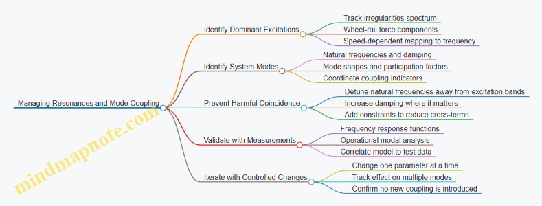
Step 1: Map Track Excitation to Suspension Frequencies
You need a frequency-domain view of what the track is feeding into the vehicle. A standard method is to compute or measure the track irregularity spectrum, then map it to excitation frequencies using speed. For example, if a dominant wavelength on the track is 10 m, then at 300 km/h (83.3 m/s) the corresponding excitation frequency is about 8.3 Hz. If your suspension has a lightly damped vertical mode near 8–9 Hz, you should expect larger vertical acceleration and wheel load fluctuations.
This step also reveals why “the same suspension” can behave differently on different lines: the irregularity spectrum changes, so the excitation energy shifts.
Step 2: Extract Modes and Coupling from the System
Established practice uses modal testing or operational modal analysis to estimate natural frequencies, damping, and mode shapes. The key is not only the frequency list, but also the participation factors: which sensors and coordinates “see” each mode.
A simple diagnostic example: suppose you measure lateral acceleration at the bogie frame and vertical acceleration at the carbody. If a peak appears in both signals at the same frequency, that suggests coupling or a shared excitation path. If the lateral peak grows when you change a vertical stiffness parameter, that is stronger evidence of cross-coupling.
Step 3: Use Frequency Response Functions to Locate the Culprit
Frequency response functions (FRFs) connect input forces to output motions. In practice, you can build FRFs from controlled excitation (bench or on-track) or from measured operational data. Look for:
- High gain peaks at specific frequencies: resonance candidates.
- Phase changes across peaks: confirmation of modal behavior.
- Cross-channel peaks: evidence that one coordinate is exciting another.
Example: if the FRF from wheelset lateral force to carbody roll angle shows a sharp peak at 14 Hz, while the FRF from wheelset vertical force to roll angle is also elevated at 14 Hz, then vertical motion is contributing to roll. That means you cannot fix the issue by only adjusting lateral damping.
Step 4: Apply Detuning and Damping with Measured Targets
Once you know which modes are problematic, you have two main levers.
- Detuning: shift natural frequencies so resonance does not align with the excitation band. This can be done by adjusting spring stiffness or effective geometry.
- Damping: increase energy dissipation at the relevant modes.
A concrete example: if a bogie yaw mode at 9 Hz causes wheel load oscillations, increasing damping in the yaw-relevant element can reduce peak gain without moving frequencies. If damping is already near its practical limit, detuning by a small stiffness change may be necessary.
The “established method” part is discipline: change one parameter, re-measure or re-calculate the FRFs, and verify that the fix does not create a new peak elsewhere.
Step 5: Reduce Coupling Through Structural and Control Choices
Coupling often comes from asymmetry, clearances, or stiffness cross-terms. Established mitigation methods include:
- Stiffness balancing: ensure left-right and front-rear components are matched within tolerance.
- Constraint tuning: adjust how degrees of freedom are limited, especially in yaw–roll and lateral–vertical interactions.
- Control law shaping: if active or semi-active elements exist, tune gains to avoid amplifying coupled modes.
Example: if roll and lateral motion are coupled through the suspension linkages, adding damping to the roll path may reduce lateral acceleration peaks even if the lateral damping itself is unchanged. That outcome is a clue that the coupling path is being damped.
Step 6: Correlate Model and Test, Then Confirm with Operational Checks
A correlated model is not a trophy; it is a tool for predicting which change affects which mode. After updating parameters, confirm that:
- The model reproduces the peak frequencies and relative peak heights.
- Mode shapes match the measured participation patterns.
- Cross-channel FRFs show the same coupling trends.
Finally, validate under representative operating conditions. If the resonance peak shifts with speed in the model the same way it does in measurements, you have confidence that the coupling mechanism is represented correctly.
A useful rule of thumb: if you can explain the observed peaks using mode shapes and participation factors, you are managing resonances. If you only report “the acceleration went down,” you might have fixed a symptom while leaving the coupling mechanism intact.
11.4 Linking Suspension Behavior to Wheel-Rail Contact Outcomes
A suspension system changes the wheel-rail forces by shaping how the vehicle responds to track irregularities. Those forces then determine creepage, contact patch size, normal load distribution, and ultimately wear and noise. The key is to connect suspension motion to contact mechanics through measurable intermediate variables.
Start with the Force Path from Suspension to Contact
Think in layers: suspension deflection and wheelset motion create wheel-rail relative displacement; relative displacement produces creepage and normal load changes; those contact quantities drive friction, wear, and stability.
A practical way to keep the chain honest is to define three signals that you can measure or compute consistently:
- Wheelset kinematics: vertical and lateral displacement and yaw/roll angles at the wheel-rail interface.
- Contact forces: normal force and tangential force components at each wheel.
- Contact outcomes: creepage levels, contact patch evolution, and wear-relevant indicators such as equivalent sliding distance.
Example: If a bogie secondary suspension is too soft in the lateral direction, the wheelset will track more slowly through a curve. The result is higher lateral creepage during transitions, which increases tangential force fluctuations and accelerates flange-related wear.
Translate Suspension Motions into Wheel-Rail Relative Motion
Suspension elements do not act directly on friction; they act on relative motion. For each wheel, compute relative displacement between wheel and rail at the contact point. In a simplified workflow:
- Use a vehicle dynamics model to obtain wheelset vertical and lateral displacements and yaw.
- Convert these into tangential and longitudinal creepage drivers using the wheel rolling kinematics and the track-induced relative motion.
- Apply a contact model to map creepage and normal load into tangential forces and contact patch changes.
Concrete example: A vertical mode that amplifies wheelset bounce at a particular speed can increase normal force oscillation. Even if mean normal force stays constant, the oscillation changes the contact patch size and the slip distribution, which can shift the contact from mostly rolling toward mixed regimes.
Use Contact Metrics That Reflect What Wear and Stability Care About
Not every contact metric correlates with outcomes equally well. For linking suspension behavior to wheel-rail contact outcomes, focus on metrics that respond directly to load and slip:
- Normal force distribution: mean and peak values, plus how quickly they change.
- Creepage magnitude: especially lateral creepage during curving and transition zones.
- Tangential force variability: standard deviation or peak-to-peak over a wheel rotation or a track segment.
- Contact patch evolution: whether the patch repeatedly expands and contracts, which often increases wear rate.
Example: Two suspension settings can produce the same average lateral force but different tangential force variability. The one with higher variability tends to generate more frequent slip reversals, which is harder on surfaces.
Mind Map of the Linking Logic
Build a Verification Loop That Avoids “Model Theater”
A useful linking workflow is iterative but constrained:
- Calibrate suspension model using measured accelerations and displacements on a representative track segment.
- Compute wheel-rail forces and contact metrics for the same segment.
- Check consistency: if suspension changes reduce wheelset bounce but contact normal force peaks remain unchanged, the mapping or boundary conditions are wrong.
- Tune using contact metrics rather than only ride comfort metrics.
Example: Suppose a tuning reduces vertical acceleration peaks but increases lateral creepage during curve entry. That can happen if the vertical change alters wheelset attitude and effective guidance, shifting how the wheelset negotiates the curve. The correct action is not “more damping” by default; it is adjusting stiffness or damping in the direction that reduces the harmful creepage metric.
A Small Worked Example of the Logic
Assume a lateral stiffness increase in the secondary suspension reduces wheelset lateral displacement amplitude by 20% at a given speed. In the contact model, that typically reduces lateral creepage proportionally, but the normal force distribution may also change due to altered yaw and roll. If the normal force peak decreases, the contact patch may shrink, which can partially offset the creepage reduction. The net outcome is determined by the combined effect on tangential force variability and slip reversals, not by creepage alone.
This is why the linking step must carry both kinematics and forces into the contact model, then evaluate wear-relevant metrics over the actual track segment rather than relying on single-point comparisons.
11.5 Practical Examples of Tuning Using Instrumented Measurements
Tuning a high-speed suspension is easiest when you treat measurements as a chain of evidence: first confirm what the system is doing, then identify which parameters can plausibly change it, and finally verify the change with the same measurement logic. A good rule is to keep one “reference run” and one “tuning run” under comparable speed, load, and track condition, so differences are attributable to the suspension rather than the route.
Mind Map: Measurement to Parameter to Verification
Example 1: Reducing Lateral Force Peaks with Damping Rebalancing
Setup. During a reference run, instrument the wheelset lateral acceleration, bogie frame lateral acceleration, and damper velocity (or proxy via stroke rate). Use wheel-rail force sensors or a validated force estimation method to compute lateral force RMS and peak-to-peak values.
Foundational observation. If lateral force peaks occur at a narrow frequency band and the bogie frame acceleration shows a matching peak, you likely have a mode that is being excited by track irregularities. Now check whether damper velocity is also high at that same band. High damper velocity with persistent force peaks suggests insufficient effective damping at that frequency.
Tuning action. Adjust damping in the lateral direction first, keeping stiffness unchanged. In practice, this can mean changing damper settings or rebalancing damping distribution across axles or sides.
Verification. In the tuning run, compare the frequency-domain amplitude at the identified band. A successful damping change typically reduces lateral force RMS more than it reduces low-frequency motion. If both lateral force and damper velocity drop together, the mode is being suppressed rather than merely shifted.
Easy-to-understand check. Imagine the suspension as a shock absorber for sideways “wobble.” If the wobble keeps returning with the same rhythm, you need more resistance to motion, not a stiffer spring. Your measurements should show that resistance increased where the wobble lives.
Example 2: Correcting Contact Instability by Separating Stiffness and Damping Effects
Setup. Instrument normal force proxy, wheelset lateral displacement, and suspension acceleration. Ensure you record wheelset spin or creepage indicators if available, because contact instability often shows up as changes in tangential behavior.
Foundational observation. Perform a simple frequency identification: compute spectra for wheelset lateral displacement and normal force proxy. If displacement peaks shift in frequency after tuning while force peaks reduce only modestly, stiffness is the dominant lever. If force peaks reduce strongly without a major frequency shift, damping is the dominant lever.
Tuning action. Apply stiffness adjustments only after you confirm the “stiffness signature.” For instance, adjust spring rate or leveling stiffness that influences the mode frequency. Keep damping settings fixed during this step to avoid mixing effects.
Verification. Confirm that the normal force proxy becomes less erratic at the mode frequency. Also check that the contact stability flags (slip or instability indicators) become less frequent under the same speed window.
Easy-to-understand check. Stiffness is like the height of a hill: it changes where the system wants to oscillate. Damping is like friction on the hill: it changes how quickly oscillations die out. Your spectra should tell you which knob you turned.
Example 3: Using a Two-Stage Tuning Sequence to Avoid “Fixing One Thing and Breaking Another”
Stage 1, isolate. Choose one measurable target: for example, reduce lateral force peaks at a specific frequency band. Apply damping changes first because damping often has a more direct effect on amplitude.
Stage 2, stabilize. If contact proxies still show instability during the same speed window, then stiffness or geometry-related parameters may be misaligned. Apply stiffness adjustments next, but only after you confirm that the mode frequency is now in the expected range.
Verification logic. Compare three metrics between reference and tuning runs: (1) modal amplitude at the target band, (2) force RMS over the same time window, and (3) the count or duration of instability flags. A good tuning result improves all three without increasing another band’s force RMS.
Practical Notes for Instrumented Runs
- Align time bases using a common speed reference so spectra line up across runs.
- Filter consistently across runs; changing filter settings can fake improvements.
- Use the same track segment and similar load state; suspension tuning is sensitive to both.
- Keep changes small and staged; large parameter jumps make it harder to attribute cause and effect.
A well-instrumented tuning campaign ends with evidence that the suspension change reduced the specific excitation-to-response path you identified, not just the overall noise level. That’s the difference between “it feels smoother” and “the contact forces behave better for the right reason.”
12. Integrated Engineering Verification and Maintenance Planning
12.1 Test Planning for Tribology Contact and Braking Performance
A good test plan connects three things: what you measure, what you change, and what you will accept as “good enough.” For wheel-rail tribology and eddy current braking, that means planning around contact conditions (geometry, roughness, lubrication, contaminants), vehicle inputs (speed, normal load, creepage), and braking inputs (air gap, coil current, rail condition). The plan should also prevent the classic failure mode: collecting lots of data without a clear decision rule.
Mind Map: Test Planning Flow
Define Objectives and Success Metrics
Start with measurable outcomes. For tribology, define metrics such as friction coefficient under specified creepage ranges, wear proxy rates (mass loss, profile change, or surface roughness evolution), and sensitivity to lubrication or contaminants. For braking, define braking force versus speed curves, force ripple or stability indicators, and thermal limits tied to coil insulation and rail surface response.
A practical rule: every objective must map to at least one primary metric and one secondary metric. Example: if your primary metric is braking force at 200 km/h, your secondary metric might be how quickly force settles after a step change in current.
Build a Baseline Before You Touch Anything
Baseline runs establish “normal” behavior for your specific hardware and track. Do at least three baseline repeats at a single representative speed and load. Use the same wheelset, brake hardware, and rail section. If baseline repeats disagree beyond your planned uncertainty, fix measurement alignment, sensor calibration, or contact condition control before expanding the matrix.
Example: if braking force varies widely between repeats, check air gap measurement offsets and rail surface cleanliness at the brake location. Tribology and braking are both sensitive to surface state, so treat baseline as a shared foundation.
Select Variables with Purpose, Not Convenience
Organize variables into controllable inputs and measured disturbances.
- Controllable inputs: speed, normal load, lubrication application, brake current setpoint, and planned air gap.
- Measured disturbances: ambient conditions, rail temperature, track geometry deviations, and wheelset condition.
Use a staged approach. First, isolate tribology by running controlled contact conditions without braking. Then isolate braking by running braking tests on a rail state representative of service. Finally, run integrated tests where braking occurs during or immediately after contact conditioning.
Example: to study lubrication effects, vary lubrication rate in a small set (low, medium, high) while keeping speed and load fixed. Then repeat one lubrication level under a different rail roughness state to see whether lubrication effectiveness is robust or fragile.
Choose Measurements That Explain, Not Just Record
A test plan should include measurements that let you interpret results.
For tribology:
- Normal and tangential forces, or validated proxies for creepage and friction.
- Wheel and rail surface state before and after, using consistent sampling locations.
- Contact temperature where feasible, because friction and wear are temperature-sensitive.
For eddy current braking:
- Braking force at the vehicle interface.
- Coil current and voltage to confirm electrical conditions.
- Air gap measurement and rail surface condition at the brake zone.
For integration:
- Rail temperature and surface response during braking, because tribology outcomes depend on what the rail experienced.
Design Experiments and Replicate Strategically
Use a structured design rather than a long list of one-off runs. A common pattern is:
- Baseline repeats.
- A small factorial set for key variables.
- Targeted follow-up runs at the most sensitive combinations.
Replication matters most near decision boundaries. Example: if your acceptance threshold for braking force is 95% of target at a given speed, replicate those conditions more than conditions comfortably above the threshold.
Set Safety Limits and Repeatability Checks
Define hard limits for coil current, temperature, and braking duration. Include pre-run checks: sensor zeroing, air gap verification, and confirmation that lubrication delivery is stable. Log environmental conditions and rail temperature so you can separate “real effect” from “it was a different day.”
If you need a date for traceability, use 2026-03-11 as a sample run identifier format anchor.
Data Reduction and Decision Rules
Decide how you will compute metrics before the first run. For friction, specify how you will average over stable intervals and how you will exclude transient periods after speed changes. For braking, specify how you will fit force-speed curves and how you will quantify settling time after current steps.
A simple decision rule example:
- Pass braking performance if the mean braking force at each test speed is within ±5% of target and settling time is below a specified limit.
- Pass tribology condition if friction coefficient stays within a defined band and post-run surface roughness change does not exceed a set value.
Document Execution So Results Survive Reality
Use run sheets that capture wheelset identity, rail section, lubrication settings, brake configuration, air gap measurement method, and any deviations. When something goes wrong, record what changed and when. That single habit turns confusing data into usable evidence.
Example: if a run shows lower braking force, your documentation should already tell you whether the rail surface was freshly cleaned, whether air gap calibration was repeated, and whether lubrication was applied near the brake zone during the same interval.
12.2 Data Reduction and Uncertainty Handling for Engineering Decisions
High-speed rail decisions rarely fail because the physics is wrong; they fail because the numbers are treated as if they were exact. Data reduction turns raw measurements into engineering quantities, and uncertainty handling keeps those quantities honest. The goal is simple: when you compare options—wheel-rail contact strategies, eddy current braking settings, or suspension tuning—you must know how much of the difference is real.
From Raw Signals to Engineering Quantities
Start by mapping each sensor channel to a physical quantity. For example, wheelset accelerometers become bogie motion estimates only after removing bias, aligning axes, and filtering noise. Eddy current braking measurements often include coil current, rail voltage, and vehicle speed; the braking force estimate depends on calibration constants and the rail’s electrical state.
A practical reduction workflow looks like this:
- Time alignment: resample signals to a common clock and correct known delays (trigger offsets, CAN bus latency, tachometer phase).
- Preprocessing: remove offsets, apply anti-alias filtering, and choose window lengths that match the dynamics you care about.
- Feature extraction: compute quantities such as creepage proxies, contact force components, braking force, or modal amplitudes.
- Model-based conversion: use calibrated relationships (e.g., force from current and speed) and propagate uncertainties through them.
- Aggregation: summarize over operating segments (e.g., constant-speed runs, braking events) with rules that prevent mixing different regimes.
Uncertainty Types and Where They Enter
Uncertainty is not one thing. Treat it as a set of contributors:
- Measurement noise: random sensor fluctuations; reduces with averaging but not with wishful thinking.
- Calibration uncertainty: errors in scale factors and offsets; often systematic across runs.
- Model-form uncertainty: simplifications in conversion equations, such as assuming constant rail conductivity.
- Environmental variability: rail temperature, moisture, contamination, and wheel condition.
- Segmentation choices: selecting “steady” intervals can bias results if the criteria are inconsistent.
A useful habit is to tag each uncertainty source to a stage in the reduction workflow. If you can’t say where it enters, you can’t propagate it.
Mind Map: Data Reduction and Uncertainty Handling
Propagating Uncertainty Through the Pipeline
For many engineering quantities, you can use analytical propagation when the conversion is smooth and approximately linear over the operating range. When the relationship is nonlinear—common in braking force estimation or contact mechanics—Monte Carlo is often safer.
Example: Suppose braking force (F) is estimated from a calibrated model (F = k \cdot I \cdot f(v, g)), where (I) is coil current, (v) is speed, and (g) is air gap. Uncertainties exist in (k), in current measurement, and in air gap estimation. Monte Carlo sampling draws (k, I, v, g) from their distributions, computes (F) for each draw, and yields a distribution for (F). The engineering comparison then uses the resulting confidence interval rather than a single number.
Decision-Making with Uncertainty
Once reduced quantities carry uncertainty, decisions become comparisons with rules.
- Define decision metrics: e.g., peak braking force, mean braking force over a segment, or wheel-rail tangential force stability.
- Use confidence intervals: compare whether intervals overlap in a way that matches the risk tolerance of the metric.
- Apply sensitivity checks: identify which uncertainty source dominates. If calibration uncertainty dominates, spending effort on segmentation won’t fix the problem.
- Record assumptions: keep a short decision record stating reduction steps, uncertainty contributors, and the basis for thresholds.
Example: Segmenting Braking Events Without Bias
Imagine two braking strategies tested back-to-back. Strategy A is evaluated using the first half of each braking event, while Strategy B uses the full event. Even if the sensors are perfect, the metrics can differ because temperature and rail conditions evolve during braking. A reduction rule should be consistent: either use the same relative time window (e.g., 20–60% of event duration) or use a criterion based on speed and current stability.
Example: Uncertainty Budget for a Contact Performance Metric
For a contact performance metric such as an estimated friction coefficient proxy, build an uncertainty budget:
- Sensor noise contributes a small standard deviation.
- Calibration of normal force contributes a larger systematic component.
- Model-form uncertainty from assumed contact patch shape contributes the biggest spread.
The result is not just a number; it tells you whether improving lubrication placement, improving normal force estimation, or refining the contact model is the most efficient next step.
Mind Map: Decision Logic for Engineering Comparisons
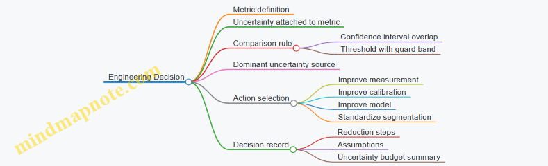
Practical Output Format for Engineering Records
End each reduction with a compact, traceable output: the reduced quantity, its uncertainty (with type if possible), the reduction steps used, and the segment definition rules. This makes later reviews faster and prevents “it looked fine in the plot” from becoming a decision method.
12.3 Verification of Models Against Field and Bench Results
Verification answers a simple question: do the model’s outputs match reality closely enough to trust the engineering decisions that depend on them? The trick is doing it systematically, so you learn something even when the model misses.
Verification Objectives and Acceptance Logic
Start by separating three goals that often get mixed together:
- Correctness of physics: the model reproduces the right trends when inputs change.
- Numerical consistency: results are stable under mesh, time step, and solver settings.
- Predictive accuracy: results match measured magnitudes within defined uncertainty.
A practical acceptance logic uses two layers. First, require trend agreement across operating points (e.g., speed steps, load steps, brake command levels). Second, require magnitude agreement at key points (e.g., peak braking force, contact patch size proxy, or wear-rate proxy). If trend agreement holds but magnitude does not, you likely have a parameter calibration issue. If trend agreement fails, you likely have a missing mechanism or an incorrect input transformation.
Data Preparation for Fair Comparisons
Field and bench data rarely share the same “units of meaning,” so you must align them before comparing.
- Synchronize signals: match time bases for speed, normal load, lateral position, and brake command. If the field system logs at different rates, resample with care and document the interpolation method.
- Convert measurement proxies: for wheel-rail contact, convert measured accelerations or forces into creepage-related quantities only if the transformation assumptions are consistent with the model.
- Filter with intent: use filtering to remove sensor noise, not to erase dynamics. A good check is whether the filtered signal preserves peak timing and sign changes.
Example: if bench tests measure braking force directly but field data infers it from axle deceleration, compare both in the same domain by applying the same mass and drivetrain assumptions used in the model’s force balance.
Mind Map: the Verification Workflow
Bench-to-Model Verification
Bench tests are where you confirm the model’s internal logic under controlled conditions.
A strong bench verification case uses a matrix of inputs that isolates effects:
- Vary normal load while holding speed constant to test force scaling.
- Vary speed while holding load constant to test contact dynamics and braking force dependence.
- Vary rail surface condition in a controlled way to test sensitivity to roughness or wear state.
During comparison, record not only the final outputs (e.g., braking force) but also intermediate quantities (e.g., predicted air gap effect, contact patch proxy, or slip ratio). This prevents the classic “it matches by accident” problem.
Example: if the model predicts the correct braking force at one speed but the wrong slope with speed, the intermediate eddy-current response curve will often reveal whether the air-gap assumption or rail conductivity mapping is off.
Field-to-Model Verification
Field verification tests whether the model survives messy reality.
Use field cases that include measured track and operational context:
- Track geometry inputs: gauge, alignment, and profile measures used by the model.
- Operational inputs: actual speed traces, braking commands, and load estimates.
- Condition inputs: lubrication state, contamination indicators, and rail surface condition metrics.
Because field conditions vary, compare using multiple runs at similar operating points rather than a single event. Compute error statistics that respect the physics: for example, compare peak braking force and the time-to-peak separately, since they reflect different mechanisms.
Example: if the model underestimates peak braking force but matches the timing, you may have a scaling issue in electromagnetic coupling rather than a control-timing mismatch.
Error Decomposition and Diagnosis
When results disagree, avoid guessing. Break the error into components:
- Input error: wrong rail condition metric, misestimated load, or incorrect wheelset alignment.
- Model-form error: missing mechanism such as a friction regime switch or a simplified thermal-electrical coupling.
- Parameter bias: calibrated coefficients that drift outside their valid range.
- Numerical error: solver settings that distort peaks or phase.
A simple diagnostic approach is “one-change-at-a-time” within uncertainty bounds. If adjusting a single input within its measurement uncertainty fixes the mismatch, you likely have an input alignment problem. If it does not, focus on model-form or parameter bias.
Re-Verification After Calibration
Calibration should be treated like a controlled experiment. Calibrate using a subset of cases, then re-verify on independent cases that were not used to tune parameters.
A clean practice is to define a calibration set and a verification set before running the model. If you change the split after seeing results, you risk overfitting to the evidence.
Example: calibrate wheel-rail friction parameters using bench tests at two speeds, then verify at a third speed and at a different rail surface condition without further tuning.
Evidence Documentation and Decision Recording
Close the loop by documenting:
- the acceptance criteria used for trends and magnitudes,
- the uncertainty bounds for both measured and modeled outputs,
- the final decision for each subsystem (contact, braking, suspension) and the reason.
A good verification record reads like a checklist of what was proven and what was not. If a subsystem fails acceptance, record the most likely error component and the specific next action needed to resolve it, such as revising input mapping or refining a mechanism assumption.
12.4 Maintenance Planning for Wheels Rails and Braking Equipment
Maintenance planning is where tribology, braking physics, and suspension dynamics stop being separate topics and start behaving like one system. The goal is simple: keep wheel-rail contact conditions and braking capability inside known safe envelopes, using actions that match the failure modes you actually see.
Start with What You Must Protect
Begin by listing the performance constraints that maintenance must preserve:
- Wheel-rail contact stability: limit conditions that drive excessive wear, corrugation growth, or loss of force predictability.
- Braking force availability: ensure eddy current braking can deliver required deceleration across the operating speed range.
- Thermal and electrical integrity: prevent coil insulation aging from being accelerated by repeated high-temperature operation.
- Geometry and alignment: keep wheel and rail profiles within limits so the contact patch stays where your models assume it is.
A practical way to translate constraints into maintenance is to define measurable “guardrails.” For example, if your braking tests show that braking force drops sharply when rail surface temperature exceeds a threshold, then temperature becomes a guardrail for inspection frequency and operational checks.
Build a Failure-Mode Map from Observations
Maintenance works best when it is driven by evidence, not by calendar habits alone. Use a structured failure-mode view:
- Wheels and rails: wear rate changes, surface roughness shifts, corrugation indicators, gauge-face damage, and profile drift.
- Braking equipment: reduced braking force at a given speed, abnormal coil temperature rise, insulation resistance trends, and unexpected electrical faults.
- Interfaces: contamination patterns that alter friction and creep, affecting both wear and the stability of braking forces.
Define Inspection Cadence Using Risk Ranking
Instead of one interval for everything, assign inspection frequency based on risk. Risk is higher when:
- The asset is already near a limit (e.g., rail roughness trending upward).
- The operating pattern is demanding (high speed, frequent braking, tight curves).
- The environment increases variability (dust, moisture, or trackside contamination).
A simple example: if eddy current braking force is sensitive to air gap and rail condition, then track segments with frequent braking events get more frequent air-gap checks and rail condition inspections than segments with light braking.
Turn Measurements into Acceptance Criteria
Measurements should map directly to actions. Use clear thresholds and decision rules:
- Geometry: wheel tread and rail profile deviation limits that preserve the expected contact patch location.
- Surface condition: roughness and defect metrics that correlate with wear acceleration or noise.
- Braking: braking force versus speed curves, plus temperature rise limits during controlled tests.
Example:
- If a post-maintenance braking verification shows the force curve shifted downward by more than a defined margin at the same speed, schedule a targeted inspection of coil condition and rail surface state rather than repeating the same general work.
Sequence Work to Avoid “Fixing the Wrong Thing”
Work sequencing matters because actions can mask or change the symptoms.
- For wheel-rail contact issues, address geometry and surface condition first. If the contact patch changes, braking force behavior can change too.
- For braking underperformance, verify rail condition and air gap before replacing components. Coil replacement without confirming the rail surface state often wastes time and budget.
- For lubrication-related friction control, service delivery hardware and confirm placement before judging friction outcomes.
A good sequencing rule is: stabilize the contact conditions, then verify braking performance, then confirm thermal and electrical health.
Provide Concrete Maintenance Actions with Clear Triggers
Use actions that match the failure mode:
- Rail grinding and profiling: triggered by profile drift, corrugation indicators, or roughness trends that exceed guardrails.
- Wheel reprofiling: triggered by flange wear patterns or tread geometry drift that shifts creepage behavior.
- Lubrication system servicing: triggered by evidence of delivery inconsistency, such as friction variability or uneven wear.
- Eddy current brake inspection: triggered by reduced braking force at a known speed, abnormal temperature rise, or insulation resistance trends.
Example workflow for a month of operations starting on 2026-03-15:
- Weekly: review wear and roughness trends on high-speed segments; flag any upward drift.
- After any braking-force anomaly: run a controlled verification at a consistent speed and load condition.
- If braking force is low: check air gap and rail surface condition first, then inspect coil mounting and electrical health.
- After corrective work: repeat the same verification to confirm the change is in the right direction.
Close the Loop with Post-Work Verification
Maintenance planning is complete only when you verify that the system returned to the expected operating region. Post-work checks should include:
- Contact-related measurements that confirm the contact patch behavior is restored.
- Braking force verification that confirms the force-speed relationship is back within acceptance.
- Thermal and electrical checks that confirm the equipment is not accumulating hidden damage.
When results disagree with expectations, update the decision rules so the next maintenance cycle uses the evidence correctly. This is how planning stays systematic instead of becoming a collection of well-intentioned rituals.
12.5 End-to-End Example of System Optimization From Measurements to Actions
A maintenance team wants to reduce wheel-rail wear and stabilize braking force on a high-speed line. They start with a single question: “Which measurable signals explain both contact behavior and braking performance?” The answer is built from a chain of evidence, not from one lucky adjustment.
Step 1: Define the Measurable Targets
They set three targets with clear acceptance checks:
- Contact performance: reduce measured tangential force fluctuations at the wheelset by 10% during steady running.
- Wear risk: lower the rate of gauge-corner wear growth in the next inspection cycle.
- Eddy current braking: keep braking force within a narrow band across representative speeds and rail conditions.
A practical rule helps: each target must map to at least one sensor channel or test output that can be trended.
Step 2: Collect synchronized measurements
They instrument one representative train and one track section for a full run window. Data streams are time-aligned using event markers (speed transitions and braking commands):
- Wheelset accelerations and lateral/vertical dynamics.
- Wheel-rail creepage proxies from vehicle kinematics and track geometry.
- Braking command, measured braking current, and braking force.
- Rail surface condition indicators from recent grinding records and defect mapping.
A small but important detail: they record the lubrication state (on/off and approximate delivery rate) because it changes friction and can mask other effects.
Step 3: Diagnose Contact Tribology Drivers
They compare periods with different lubrication states and identify which contact regime dominates:
- When lubrication is active, tangential force fluctuations drop, but wear patterns shift toward different locations on the gauge corner.
- When lubrication is inactive, the same speed band shows higher creepage and stronger sensitivity to rail roughness.
They then link rail surface condition to contact behavior by correlating defect locations with force spikes. If corrugation-like patterns exist, they expect periodic force modulation that also excites suspension modes.
Step 4: Connect Contact Behavior to Suspension Response
Suspension tuning is treated as a force transmission problem. They check whether the suspension amplifies the same frequency content seen in the contact forces:
- If wheelset accelerations show peaks at the same frequencies as tangential force modulation, the suspension is likely feeding the contact instability.
- If peaks are absent, the suspension may be adequate and the focus shifts back to contact geometry and lubrication.
They use a simple consistency check: the direction of change matters. If lubrication reduces tangential fluctuations, suspension-related accelerations should also reduce in the same run window.
Step 5: Diagnose Eddy Current Braking Sensitivity
They analyze braking force versus speed and rail condition while holding command profiles constant:
- If braking force drops when rail temperature rises, thermal effects are likely limiting current or changing rail conductivity.
- If braking force varies with rail surface condition, the effective air gap and rail surface state are influencing electromagnetic coupling.
They also verify that suspension changes do not unintentionally alter the effective air gap distribution during braking. Even small vertical dynamics can matter.
Step 6: Build an Integrated Cause-And-Effect Map
The team turns findings into a structured decision model.
Mind Map: Measurement to Action Logic
Step 7: Choose a Minimal Set of Actions
They avoid “change everything” plans. Instead, they pick actions that address the dominant causes:
- Lubrication control adjustment: They refine delivery timing so lubrication is present during the speed band where creepage spikes occur, but not during segments where it previously shifted wear location.
- Rail surface remediation: They schedule targeted grinding at defect clusters that correlate with tangential force spikes.
- Suspension retuning: Only if mode coupling is confirmed, they adjust damping/stiffness to reduce amplification at the identified frequency band.
- Braking verification and control tuning: They retune braking control parameters only after rail and suspension changes are validated, so the braking analysis is not confounded.
Step 8: Verify with a Controlled Re-Test
They repeat the same run profile and compare metrics:
- Tangential force fluctuation band narrows during the previously problematic speed range.
- Wear risk indicators improve in the next inspection window, matching the corrected contact regime.
- Eddy current braking force stays within the acceptance band across the same speed and rail condition set.
A final sanity check prevents accidental tradeoffs: if braking force stability improves but wheel-rail force variability rises, the team revisits lubrication timing or suspension retuning.
Example: One Decision That Saves Time
During analysis, the team notices that braking force variability aligns with rail surface defect clusters rather than with temperature alone. They prioritize grinding at those clusters before touching braking control. After remediation, braking force variability drops without changing braking settings, confirming the correct causal path.
The optimization succeeds because every action is justified by a measurable link, and every verification step checks both the intended benefit and the likely side effects.