Cryogenic Space Propulsion
1. Fundamentals of Cryogenic Propulsion for Spacecraft
1.1 Mission Requirements for Cryogenic Propellants
Cryogenic propellants are not chosen because they sound cool; they are chosen because the mission needs the performance and the system can tolerate the storage and handling penalties. Mission requirements translate into concrete constraints on tank boil-off, feed reliability, engine start behavior, and allowable contamination.
Mission Drivers That Set the Cryogenic Envelope
Start with the mission’s “why,” then convert it into numbers.
- Delta-V and thrust level determine whether cryogenic propellants are worth the complexity. Higher specific impulse can reduce propellant mass, but only if the mission can keep enough usable propellant at the right conditions.
- Burn schedule matters as much as total burn time. A short, single burn is easier than multiple starts separated by long coast periods because boil-off and settling requirements accumulate.
- Coast duration and attitude constraints define how long the propellant must remain in a usable liquid state. If the spacecraft cannot maintain favorable ullage conditions, the feed system must compensate.
- Thermal environment and power availability set how much heat the tank will absorb and how much active control can be provided. Even a small heat leak becomes significant over long durations.
- Orbit and gravity regime affect propellant management. In microgravity, “liquid acquisition” depends on ullage control and line design rather than natural settling.
A practical way to connect these drivers is to write a requirement chain: mission timeline → tank heat load exposure → boil-off rate → remaining propellant mass → feed conditions at each start → engine ignition margin.
Key Requirements Expressed as System Constraints
Cryogenic missions typically specify requirements in terms of measurable system behavior.
- Usable propellant fraction: The mission needs a minimum mass of liquid available at each engine start. This requirement directly constrains insulation quality, allowable heat leak, and the permitted venting strategy.
- Boil-off rate and total boil-off: Requirements often include both a steady-state boil-off limit and a transient limit after maneuvers or thermal events.
- Subcooling or saturation margin: The feed system must deliver liquid with enough margin to avoid excessive flashing in lines and valves. The margin is usually expressed as a temperature difference relative to saturation at the local pressure.
- Start reliability: The mission specifies acceptable probabilities for successful ignition and stable operation. That translates into bounds on valve timing, settling duration, and acceptable two-phase behavior during the start sequence.
- Pressure management limits: Tanks and feed lines must remain within pressure bounds under normal operation and off-nominal events, including regulator behavior and relief valve setpoints.
- Contamination tolerance: Trace impurities and water ingress can freeze, block, or alter heat transfer. Requirements define allowable impurity levels and acceptable cleanliness verification outcomes.
Example: Turning a Timeline into a Cryogenic Requirement
Suppose a spacecraft needs three engine starts: one at launch day plus 2 days, another at day 10, and a final one at day 18. If the tank heat leak and insulation are such that boil-off reduces usable propellant by 12% by day 10, but the mission needs only 8% margin, then the insulation and/or active boil-off control must be improved. The key point is that the “day 10” requirement is not abstract; it is the point where feed conditions must still meet subcooling and liquid acquisition needs.
Mind Map: Mission Requirements to Cryogenic Design Inputs
Practical Requirement-Setting Workflow
- List every engine start with its time after launch and expected duty cycle.
- Assign thermal exposure windows for each phase, including coast and any attitude or power changes.
- Translate exposure into boil-off budget and derive usable propellant mass at each start.
- Convert usable mass into feed conditions by specifying subcooling margin and allowable two-phase behavior.
- Lock start sequence constraints by mapping valve timing and settling needs to the derived feed conditions.
- Add safety and quality constraints so the design cannot meet performance while violating pressure or contamination limits.
This approach keeps the requirements coherent: the mission timeline drives thermal exposure, thermal exposure drives boil-off, boil-off drives feed conditions, and feed conditions drive start reliability. When those links are explicit, design tradeoffs become straightforward rather than mysterious.
1.2 Thermodynamic Properties of Common Cryogens
Cryogenic propulsion lives and dies by how fluids behave when temperature drops below normal boiling points. For spacecraft systems, the key thermodynamic properties are not just “numbers,” but the way those numbers govern phase change, pressure, heat leak response, and feed reliability.
Core Thermodynamic Quantities
Start with the property set that repeatedly shows up in calculations.
- Saturation temperature and pressure: For a given cryogen, there is a temperature where liquid and vapor coexist at equilibrium. That temperature corresponds to a saturation pressure. In practice, tank pressure is strongly tied to the saturation curve because boil-off produces vapor.
- Latent heat of vaporization: This is the energy required to convert liquid to vapor at saturation. A larger latent heat means more energy must enter the liquid before a comparable mass of propellant turns into vapor.
- Specific heat capacities: These govern how much temperature changes when heat enters a liquid or a solid. They matter for subcooling and for warming during transient events.
- Density of liquid and vapor: Liquid density affects mass flow and settling behavior; vapor density affects pressurization and ullage dynamics.
- Thermal conductivity and viscosity: Thermal conductivity influences heat transfer through insulation supports and internal structures. Viscosity affects pressure drop and flow regime in lines and injectors.
A useful mental model: heat leak → temperature and phase response → pressure and mass availability. Each property controls one link in that chain.
Common Cryogens and What Their Properties Imply
Liquid Oxygen (LOX)
LOX has strong oxidizer chemistry, but thermodynamically it is often treated as a “high-boiling” cryogen relative to the very cold fuels. Its saturation pressure at a given temperature is typically higher than for colder cryogens, which means tank pressure can be more sensitive to temperature changes. LOX also tends to have higher density than many hydrocarbon fuels at comparable temperatures, which helps with liquid acquisition but increases the energy stored in the liquid mass.
Example: If a tank warms by a small amount, LOX will generate vapor according to the saturation relationship. The latent heat determines how much liquid mass is consumed per unit heat leak.
Liquid Hydrogen (LH2)
LH2 is extremely cold and has very low liquid density. Thermodynamically, that combination makes boil-off mass fraction and feed system pressure drop both more challenging. Because LH2’s vapor density is low, small absolute vapor volumes can still correspond to meaningful pressure changes depending on tank volume and venting.
Example: During a cold soak, LH2 lines may show large temperature gradients even when the tank bulk temperature appears stable. Viscosity and thermal conductivity then influence how quickly the line reaches equilibrium.
Liquid Methane (LCH4)
LCH4 sits between LOX and LH2 in temperature scale and has properties that often make it easier to manage than LH2 while still benefiting from cryogenic performance. Its latent heat and density support practical feed system sizing, and its viscosity is generally more forgiving than LH2 for pressure drop.
Example: In a feed line with modest heat leak, LCH4 is less likely than LH2 to create severe two-phase pressure losses for the same thermal disturbance.
Phase Behavior and Subcooling
Cryogenic systems rarely operate exactly at saturation. Subcooling means the liquid temperature is below the saturation temperature corresponding to the local pressure. Subcooling provides margin against immediate flashing when heat enters.
- If the liquid is subcooled, added heat first raises temperature toward saturation.
- Once near saturation, additional heat converts liquid to vapor using latent heat.
Example: Suppose a line segment experiences a heat input. If the liquid enters subcooled, the first portion of heat increases temperature without generating much vapor. After reaching saturation, further heat produces vapor quickly, which can change flow regime and pressure drop.
Property Tables and How to Use Them Correctly
Thermodynamic property data are usually presented as functions of temperature (and sometimes pressure). The practical workflow is:
- Choose operating state: tank pressure or expected saturation temperature.
- Read saturation properties: saturation temperature, latent heat, and densities.
- Apply off-saturation corrections: use sensible heat (specific heat) for subcooled or warmed states.
- Check consistency: ensure the implied phase state matches the assumed model (single-phase liquid, two-phase mixture, or vapor).
A common mistake is treating “boiling point” as a fixed constant. For cryogens, it is a pressure-dependent equilibrium temperature, so the system pressure model must be consistent with the property model.
Mind Map: Thermodynamic Properties for Cryogenic Systems
Worked Micro-Example: Heat Leak to Boil-Off
Imagine a small heat leak rate into a tank. The mass boil-off rate is governed by the latent heat once the liquid is near saturation. If the liquid is initially subcooled, the early time response is dominated by sensible heating until saturation is reached.
Example: If you know the heat leak and latent heat, you can estimate how quickly the system consumes liquid mass. If you also know the initial subcooling, you can estimate the time before the tank enters a near-saturation regime where boil-off accelerates.
That’s the thermodynamic story in one line: properties determine how heat turns into temperature change and phase change, and phase change determines how much propellant remains available for propulsion.
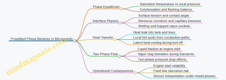
1.3 Propellant Phase Behavior in Microgravity
In microgravity, “liquid” and “gas” still exist, but the usual gravity-driven separation stops doing the heavy lifting. Phase behavior becomes dominated by surface tension, wetting, heat transfer, and the geometry of the tank and feed system. The practical result is that the propellant can form bubbles, stratify by temperature rather than height, and intermittently starve the engine even when the tank contains plenty of liquid.
Core Concepts of Phases Without Buoyancy
Start with the equilibrium idea: at a given pressure, a cryogenic liquid has a saturation temperature. If the local temperature rises above that saturation point, some liquid flashes into vapor; if it falls below, vapor tends to condense. In microgravity, the key twist is that vapor does not automatically rise away from the liquid. Instead, vapor can remain near the liquid surface, migrate along walls, or get trapped in pockets.
Surface tension then becomes the “gravity substitute.” It shapes interfaces so that liquid prefers to wet certain surfaces and avoid others. This matters because tank walls and feed lines are not neutral: coatings, roughness, and material choice change the contact angle, which changes how easily vapor forms and how easily liquid can spread to where the engine needs it.
Two Phase Flow and Interface Motion
A cryogenic tank typically contains liquid plus vapor in the ullage. Heat leak from the environment drives boil-off, creating vapor and cooling the remaining liquid through latent heat. In microgravity, the interface can move in complex ways because there is no buoyant rise to smooth it out.
Consider a simple feed line connected to a tank. If vapor enters the line, the engine may ingest a mixture rather than liquid. That mixture can cause unstable injector behavior and reduced thrust because the injector’s atomization and evaporation depend strongly on the liquid fraction.
A useful mental model is to track three coupled states:
- Thermal state: local temperatures relative to saturation.
- Phase state: liquid fraction and where the interface sits.
- Flow state: whether the line sees mostly liquid, mostly vapor, or a changing mixture.
Ullage, Subcooling, and Flashing
Subcooling means the liquid is below its saturation temperature at the local pressure. Subcooling provides a buffer: small heat inputs or pressure drops do not immediately produce vapor. In microgravity, subcooling is especially valuable because pressure transients during valve motion can trigger flashing right where the feed system is trying to deliver liquid.
A concrete example: suppose a valve opens quickly and the downstream pressure drops. If the liquid in the line is only slightly subcooled, the new saturation temperature may be higher than the liquid temperature, and vapor can nucleate. The result is a short “vapor slug” that can persist until the interface re-establishes.
Wetting, Meniscus Formation, and Capillary Effects
When liquid contacts a wall, it forms a meniscus. The meniscus curvature sets a pressure difference across the interface through the Laplace relation. In microgravity, this capillary pressure can dominate over buoyancy, meaning the liquid can be held against a wall or pulled into small gaps.
This is why feed system design often emphasizes surface finish and geometry: a small change in corner radius or wall coating can shift where the liquid prefers to sit. For operations, that translates into different start reliability margins because the engine inlet may or may not be “wet” at the moment of ignition.
Heat Leak Patterns and Temperature Stratification
Even without gravity, heat leak is not uniform. Radiative heating, conduction through supports, and local conduction through instrumentation mounts can create temperature gradients. The saturation condition then varies spatially, so vapor generation can be localized.
Example: if a sensor mount conducts heat into one region of the tank, that region can reach saturation earlier. Vapor forms there, and because vapor can remain near the interface, the tank may develop a persistent two-phase region that does not behave like a simple top-vapor layer.
Advanced Details That Matter in Practice
- Nucleation sites: micro-bubbles and surface imperfections can seed boiling at lower superheat than expected.
- Two-phase pressure drop: flow resistance changes with vapor fraction, so the same valve command can yield different inlet conditions.
- Transient interface topology: during slosh-like motions from maneuvers or venting, the interface can break into patches, not a smooth surface.
- Thermal coupling to hardware: cold straps, insulation seams, and line supports can create local “cold spots” that encourage condensation.
Mind Map: Phase Behavior Drivers in Microgravity
Example: Valve Opening and Inlet Phase Quality
Assume the tank liquid is subcooled by a small margin. During a start sequence, a valve opens to establish flow. The downstream pressure drop increases the likelihood that the local saturation temperature rises above the liquid temperature. If vapor nucleates in the line, the inlet sees a mixture; the injector then experiences delayed evaporation because the vapor fraction reduces the available liquid mass.
A practical mitigation is to ensure the feed path is sufficiently subcooled and to sequence valve operations so that pressure changes are gradual enough for the interface to remain stable. In other words, you manage phase behavior by managing thermal margin and transient pressure history, not by hoping gravity will do the sorting.
1.4 Performance Metrics for Cryogenic Engines and Tanks
Performance metrics connect physics to decisions. For cryogenic propulsion, the “performance” of an engine is inseparable from the “performance” of its tanks, because heat leak, phase state, and feed conditions determine whether the engine can deliver the commanded thrust and mixture ratio.
Core Engine Metrics
Thrust and Thrust Coefficient quantify how much force the engine produces under specific chamber pressure and mixture ratio. In cryogenic systems, thrust is often limited indirectly: if the feed line flashes or the mixture ratio drifts, combustion efficiency drops even when the chamber hardware is healthy.
Specific Impulse measures propellant efficiency. Use it with context: two tests can show the same average specific impulse while having different start transients, different injector inlet conditions, and different propellant utilization. A practical approach is to report both steady-state specific impulse and the time history during ignition and throttle-like transients.
Mixture Ratio Accuracy is critical for cryogenic propellants because small feed imbalances can shift combustion temperature and stability margins. A simple example: if oxidizer line heat leak causes earlier vapor formation, the oxidizer mass flow can fall first, pushing the mixture ratio toward fuel-rich operation.
Chamber Pressure Stability is measured by mean value and allowable ripple. Cryogenic feed instabilities can couple into injector pressure drop, creating oscillations that show up as chamber pressure ripple. Metrics should therefore include both chamber pressure and feed pressure signals.
Tank Metrics That Actually Matter
Boil-Off Rate is the rate at which liquid turns into vapor due to heat leak. Report it as a function of time and tank pressure, not just a single number. Example: a tank with good insulation can still show a higher initial boil-off if the insulation is not fully settled after cooldown.
Heat Leak Budget expresses how much thermal power enters the tank. Break it into contributions such as conduction through supports, radiation through multilayer insulation gaps, and plumbing conduction. This makes troubleshooting possible: if boil-off rises after a mechanical change, you can identify which heat path likely changed.
Ullage and Liquid Level Behavior affects feed reliability. Metrics include ullage pressure, ullage temperature, and the time it takes for liquid to re-establish after maneuvers. In microgravity, “liquid acquisition” is not guaranteed by gravity, so the tank must be evaluated with the same operational sequence used in flight.
Pressurization Efficiency describes how effectively pressurant gas maintains tank pressure without wasting propellant. A useful metric is the fraction of pressurant mass that ends up as vented mass versus useful pressure support.
Coupled Metrics for System-Level Performance
Start Capability is a system metric: the engine start is successful only if the propellants reach the injector with acceptable phase state and temperature. Define measurable criteria such as minimum liquid subcooling at the inlet, maximum allowable vapor quality, and valve timing windows.
Feed Line Flashing Margin quantifies how close the system is to two-phase flow in lines and manifolds. A practical metric is the minimum margin between local pressure and the saturation pressure corresponding to measured or estimated fluid temperature.
Propellant Utilization measures how much of the tank inventory can be consumed while meeting mixture ratio and stability constraints. Example: if boil-off increases vapor fraction near end-of-burn, utilization can drop even though the tank still contains liquid.
Mind Map: Performance Metrics for Cryogenic Engines and Tanks
Example Metric Set for a Test Report
A coherent test report lists metrics in the same order the system experiences them: cooldown and tank stabilization, then feed conditioning, then start, then steady operation.
For instance, during a start test you can report:
- Tank boil-off rate over the final cooldown interval.
- Ullage pressure and temperature at the moment each valve opens.
- Feed line inlet temperature and estimated vapor quality at the injector.
- Valve opening and closure timing relative to chamber pressure rise.
- Chamber pressure mean and ripple during the first few seconds.
- Mixture ratio error over a defined steady window.
This structure prevents a common failure mode: collecting many numbers without linking them to the decision they support. When metrics are defined with clear measurement points and acceptance criteria, the data becomes usable rather than just interesting.
1.5 System Level Mass And Energy Accounting For Ultra-Cold Fuels
Ultra-cold propulsion is mostly an accounting problem: every kilogram and every watt of heat has to be paid for somewhere. This section builds a practical workflow that starts with what you must deliver to the engine and ends with a system-level mass and energy balance you can actually use in design trades.
System Boundaries and What You Must Deliver
Define the “contract” between tanks, feed, and engine. At minimum, you need:
- Required propellant mass to meet mission delta-v and margins.
- Required engine inlet conditions at each start and steady segment: pressure, temperature, and phase state.
- Allowable boil-off and vent losses so the delivered propellant matches the mission requirement.
A useful habit is to write the delivered propellant as a function of losses:
- Delivered mass = Initial tank liquid mass − Boil-off loss − Vent loss − Residuals in lines and unusable tank regions.
Mass Accounting Framework
Break total propellant system mass into components that scale differently with mission duration and operating mode:
- Propellant mass (liquid and any trapped gas).
- Tank structure mass (shell, domes, supports).
- Insulation mass and support hardware.
- Feed system mass (lines, valves, regulators, manifolds).
- Pressurization hardware mass (pressurant tanks, regulators, relief valves).
- Power and control mass (valves actuation, heaters, sensors, controller).
- Thermal management mass (heat switches, radiation shields, cold straps).
A key nuance: insulation reduces heat leak, which reduces boil-off, which reduces required initial propellant. That means insulation mass can “pay back” by shrinking propellant mass. The trade is not one-directional.
Energy Accounting Framework
Energy accounting tracks where heat enters and what you do with it:
- Heat leak into the tank through insulation and supports.
- Heat added by active components such as heaters or warm-up cycles.
- Heat removed by venting or by consuming energy in phase change.
For boil-off, the central relationship is simple: boil-off rate is driven by the net heat into the liquid and ullage, divided by an effective latent heat term. In practice, you also include sensible heating of liquid and gas before it reaches the phase-change condition.
Stepwise Workflow for a Design Trade
- Set mission segments: coast, attitude changes, engine starts, and dwell periods.
- Compute heat leak per segment: use a heat transfer model for conduction through supports and radiation through insulation gaps.
- Convert heat to propellant loss: apply latent heat and include any temperature rise effects.
- Update tank inventory: subtract losses to get remaining liquid mass and ullage conditions.
- Check feed requirements: verify that the remaining liquid can meet engine inlet pressure and subcooling needs.
- Size hardware: adjust insulation thickness, tank geometry, and pressurization capacity until constraints are satisfied.
- Recompute mass: update total mass and iterate.
This workflow prevents the common failure mode where you size insulation from a boil-off-only view, then discover feed conditions are wrong because the system’s pressure and temperature trajectory drifted.
Mind Map: Mass and Energy Accounting
Concrete Example: Insulation Trade with a Payback Check
Assume a design baseline with a predicted heat leak of 12 W into a cryogenic tank during cruise. If the effective latent heat term is 200 kJ/kg, the boil-off mass rate is approximately:
- Boil-off rate ≈ 12 W / 200,000 J/kg = 6e-5 kg/s Over 30 days (2.592e6 s), boil-off is about 155 kg.
Now consider adding insulation that increases insulation mass by 18 kg but reduces heat leak to 9 W. The new boil-off is:
- 9 W / 200,000 J/kg = 4.5e-5 kg/s Over the same period, boil-off is about 117 kg.
Net effect on propellant inventory is a reduction of roughly 38 kg of boil-off. Even before considering any feed condition improvements, the insulation mass “pays back” by reducing required initial propellant by more than its own mass. In a full system model, you would also check whether the reduced boil-off changes ullage pressure enough to affect feed valve settings and start sequence timing.
Concrete Example: Energy Budgeting for Start Reliability
Suppose engine starts require a minimum subcooling at the inlet. If tank boil-off raises ullage temperature and reduces liquid temperature, the feed system may enter a two-phase regime earlier than expected. The energy accounting then must include not only tank heat leak but also heat picked up by feed lines and regulators during the time between valve opening and stable injector conditions. A design that looks fine on total boil-off can still fail a start constraint if the energy path to the inlet is ignored.
Practical Output Metrics
To keep the accounting actionable, report results as:
- Delivered propellant mass with explicit loss breakdown.
- Heat leak and boil-off per mission segment.
- Tank pressure and temperature at each engine start.
- Total system mass with sensitivity to insulation and pressurization sizing.
When these metrics agree with the engine inlet constraints, the mass and energy model stops being a spreadsheet exercise and becomes a design tool.
2. Cryogenic Propellant Selection and Compatibility
2.1 Candidate Propellants and Their Operational Tradeoffs
Cryogenic propulsion usually means you are managing two things at once: the chemistry that produces thrust, and the physics that keeps a liquid cold enough to stay liquid. Candidate propellants differ in how they store, feed, and combust, so “best” depends on what your mission values most: start reliability, tank mass, engine simplicity, or thermal control margin.
Core Tradeoff Dimensions
Start by sorting candidates along four operational axes.
-
Storage temperature and boil-off pressure: Lower temperature generally reduces vapor pressure, which can ease pressure control but increases insulation and materials challenges.
-
Density and tank volume: Higher liquid density reduces tank volume for a given impulse, which can lower structural mass and simplify plumbing routing.
-
Feed system behavior: Some propellants tolerate two-phase flow better than others. If your feed line sees flashing or vapor ingestion, you need margins in valve response, pump inlet conditions, or regulator stability.
-
Combustion characteristics: Ignition ease, mixture ratio sensitivity, and combustion stability determine how strict your injector and start sequence must be.
A practical way to think about it: storage and feed determine whether you can deliver the right phase at the right pressure; combustion determines whether that delivery turns into stable thrust.
Common Cryogenic Propellant Families
Liquid Oxygen and Liquid Hydrogen
LOX/LH2 is the classic high-performance pair. Hydrogen’s low density means large tank volume, but its high specific impulse potential can reduce propellant mass for a given mission delta-v. The trade is operational: hydrogen systems often require careful insulation and leak-tightness because small heat leaks can create significant boil-off and vapor ingestion risk.
LOX is denser and easier to package than hydrogen, so the oxygen side often has more forgiving tank volume. However, oxygen’s oxidizing nature makes contamination control and material selection non-negotiable.
Easy example: If your mission demands long coast time, hydrogen boil-off can dominate your propellant budget. You may respond by improving insulation, increasing subcooling, or accepting a more complex boil-off management strategy.
Liquid Oxygen and Liquid Methane
LOX/LCH4 sits between LOX/LH2 and more storable options. Methane has higher density than hydrogen, which reduces tank volume and can simplify feed line layout. It also has a relatively manageable cryogenic temperature compared with hydrogen, which can ease some thermal design pressure.
Combustion behavior is typically more forgiving than hydrogen in terms of ignition and handling, while still offering strong performance. The trade is that methane systems still require strict thermal and contamination discipline, and injector design must handle methane’s specific atomization and mixture ratio sensitivity.
Easy example: If you want a compact tank compared with hydrogen while keeping a cryogenic engine architecture, LOX/LCH4 often reduces the “how big is the tank?” problem without forcing the most extreme insulation.
Liquid Oxygen and Liquid Nitrogen
LOX/LN2 is attractive for its operational simplicity in some respects because nitrogen is less demanding than hydrogen. Nitrogen’s lower performance compared with hydrogen means you may need more propellant mass or accept lower efficiency.
The trade is straightforward: you gain easier cryogenic handling and potentially lower thermal stress, but you pay in thrust efficiency. This can still be useful for testbeds, demonstrations, or missions where reliability and simplicity outweigh peak performance.
Easy example: If your priority is repeatable engine starts during ground testing, LOX/LN2 can reduce the “cryogenic drama” while still exercising the feed and ignition hardware.
Propellant Pairing Tradeoffs by Operational Goal
If You Care About Long Duration Storage
Hydrogen-containing pairs often require the most attention to boil-off and thermal gradients. Methane-containing pairs usually reduce tank volume and can improve thermal margin, but you still must budget heat leak carefully.
If You Care About Feed Reliability
Pairs that are prone to flashing in the feed line demand stronger control of subcooling, line pressure drops, and valve timing. A reliable feed design treats two-phase behavior as a first-class requirement, not an afterthought.
Easy example: Suppose your valve opens and the line pressure briefly drops. If your propellant flashes easily, you may ingest vapor right when the engine needs liquid. Mitigation can include preconditioning, pressure margin, and sequencing that avoids the worst pressure dips.
If You Care About Engine Start Robustness
Ignition and start transients depend on mixture ratio control and injector response. Hydrogen systems can require careful start sequencing to avoid unstable combustion during the transition from ignition to steady operation.
Mind Map: Candidate Propellants and Operational Tradeoffs
Quick Selection Heuristic
When comparing candidates, start with the mission’s constraint that hurts most: tank volume, boil-off budget, feed stability, or start reliability. Then choose the propellant pair whose tradeoffs align with that constraint, and design the system so the “weak link” has margin rather than hope.
2.2 Freezing and Boiling Constraints for Storage and Feed
Cryogenic storage and feed systems are governed by two competing phase risks: freezing of the liquid and uncontrolled boiling that steals liquid inventory and can introduce two-phase flow where you do not want it. The trick is to treat both risks as constraints in the same operating envelope, then design hardware and procedures so the system stays inside that envelope during every mission phase.
Core Phase Constraints
A cryogen is “safe” only when the local temperature and pressure keep it in the intended phase. Freezing happens when the liquid temperature drops below the cryogen’s freezing point at the local pressure. Boiling happens when the liquid temperature rises above the saturation temperature for the local pressure, or when pressure drops enough that the saturation temperature falls below the liquid temperature.
A practical way to think about this is to track two temperatures at each location: the actual liquid temperature and the saturation temperature corresponding to the local pressure. If actual temperature is below saturation by a margin, you are subcooled; if it crosses saturation, you start boiling. If you cross the freezing line, you are in trouble.
Freezing Constraints in Storage and Lines
Freezing is usually driven by heat leak plus pressure conditions that can shift the freezing point. In a tank, the bulk liquid temperature is set by the boil-off behavior and thermal gradients. If insulation performance degrades or a localized cold spot forms, the liquid near that spot can approach the freezing point.
In feed lines, freezing risk increases when a cold liquid is exposed to a colder-than-expected environment or when pressure transients cause rapid temperature changes. Even if the bulk system is warm enough, a small region can freeze first because freezing is sensitive to local conditions.
A simple example: suppose a cryogen has a freezing point at a given pressure of 90 K. If your tank liquid is at 92 K with a healthy margin, you are fine. But if a valve closure causes a pressure rise in a small manifold volume and the local saturation temperature shifts, the liquid temperature relative to the freezing point can change faster than your control system can react.
Boiling Constraints in Storage and Feed
Boiling is more common than freezing because heat leak is persistent and pressure can vary with ullage dynamics. Boil-off increases ullage pressure and reduces liquid mass, which then affects engine start readiness.
In storage, boiling is often acceptable within limits because it provides a controlled pressure source and can be managed with venting or active boil-off control. The constraint is that the system must maintain sufficient liquid quality and level for the required feed conditions.
In feed systems, boiling is constrained by the need for stable single-phase liquid delivery. Two-phase flow can cause vapor ingestion into pumps, unstable valve behavior, and mixture ratio errors at the injector.
A simple example: if a line pressure drops due to a pressure drop across a filter, the saturation temperature drops. If the liquid temperature is unchanged, it can cross into the boiling regime. The result is flashing at the restriction, which then propagates downstream as a bubbly mixture.
Integrated Operating Envelope
Design work becomes systematic when you combine constraints into one checklist: (1) keep temperatures above freezing with margin everywhere liquid can exist, (2) keep pressure and temperature combinations below boiling onset in single-phase segments, and (3) allow boiling only in explicitly managed regions like ullage or controlled vent paths.
Practical Examples for Design Decisions
Example 1: Tank insulation and freezing margin If your thermal model predicts a worst-case liquid temperature of 91 K and the freezing point at operating pressure is 90 K, you have a 1 K margin. That margin may be too tight if sensor uncertainty and gradient effects are significant. A better approach is to increase insulation performance or adjust operating pressure so the freezing constraint has a comfortable buffer.
Example 2: Line pressure drop and flashing Assume a feed line experiences a pressure drop of 0.2 MPa across a filter during a high-flow phase. If the saturation temperature at the upstream pressure is 95 K and at the downstream pressure is 90 K, while the liquid temperature is 92 K, then flashing is likely downstream. The fix is to reduce pressure drop (larger flow area, different filter strategy) or to ensure the line segment is designed to tolerate two-phase flow.
Verification Logic That Prevents Surprises
Constraint checking should be done at three levels: steady-state, start/transient, and worst-case disturbances. Steady-state confirms the baseline envelope. Transient analysis catches valve operations, pump start, and pressure regulator behavior. Disturbances include sensor offsets and realistic heat leak variations so you do not rely on a single “perfect” condition.
When you treat freezing and boiling as paired constraints rather than separate topics, the design becomes easier to reason about: every component gets a clear job description—either maintain single-phase conditions with margin, or intentionally host phase change in a controlled location.
2.3 Material Compatibility With Cryogens and Trace Impurities
Cryogenic compatibility is not just “will it freeze?” It’s a chain of interactions: the bulk material properties, the surface chemistry, the presence of trace impurities, and the way the system is cleaned, assembled, and operated. A practical way to reason about it is to separate mechanical integrity, chemical stability, and contamination-driven failures.
Foundational Concepts for Compatibility
Start with temperature-dependent behavior. Many polymers, elastomers, and adhesives change modulus and permeability as temperature drops, which can turn a “works in a lab” seal into a “leaks after cooldown” seal. Metals also shift: thermal contraction can increase stress at joints, and some alloys become more susceptible to brittle cracking under certain environments.
Next, consider phase and wetting. Cryogens can be liquid, vapor, or a mix, and compatibility differs across these states. A surface that is safe in vapor can fail when it is wetted by liquid containing dissolved or suspended impurities.
Finally, treat impurities as part of the material system. Even at low concentrations, trace water, oxygen, hydrocarbons, and particulates can change corrosion rates, promote freezing of unwanted species, or alter ignition behavior in combustion hardware.
Material Classes and What Usually Breaks
Metals: Compatibility is often limited by corrosion and stress effects. Stainless steels and nickel alloys are common because they form stable oxide films, but those films can be disrupted by chloride contamination, water-assisted corrosion, or oxygen-starved conditions. Aluminum alloys can be sensitive to certain impurity chemistries and to galvanic coupling when paired with dissimilar metals.
Elastomers and Polymers: Failures often come from shrinkage, loss of elasticity, swelling, or embrittlement. Swelling is frequently driven by hydrocarbons or plasticizers; embrittlement can be driven by oxygen exposure and aging. Permeation matters too: even if a seal doesn’t leak immediately, permeation can raise local impurity levels at the interface.
Welds, Brazes, and Coatings: Interfaces are where surprises hide. Weld heat-affected zones can have different microstructures than the base metal, changing corrosion resistance. Coatings may crack under thermal cycling, exposing fresh substrate to cryogen and impurities.
Trace Impurities and Their Mechanisms
Trace impurities typically enter through cleaning residues, atmospheric exposure during assembly, outgassing from nearby materials, or imperfect gas handling. The key is to map each impurity to a mechanism.
- Water: In cryogenic service, water can freeze on cold surfaces, blocking flow paths or altering heat transfer. In some cases it also accelerates corrosion by enabling electrochemical reactions.
- Oxygen: Oxygen can react with certain materials, especially at interfaces where the cryogen film is thin and diffusion is limited. Oxygen also changes the behavior of other impurities by affecting oxidation pathways.
- Hydrocarbons: Hydrocarbons can dissolve into cryogens and later deposit as temperatures drop, forming sticky residues that trap particulates or foul valves and injectors.
- Chlorides and salts: These are notorious for localized corrosion. Even small amounts can create pitting, particularly in stainless steels.
- Particulates: Dust and machining debris can become ice-like solids at cryogenic temperatures, acting as abrasives or as initiation points for leaks.
A useful rule of thumb: the colder and more stagnant the region, the more likely impurities will freeze out and accumulate.
Mind Map: Compatibility Drivers and Failure Modes
Example: Designing a Compatibility Check That Actually Finds Problems
Imagine a feed system using stainless steel tubing with a polymer-lined section and elastomer seals. A compatibility plan should include:
- Material screening at temperature: Verify seal compression set and swelling behavior after exposure to the cryogen and any expected impurity levels.
- Surface and cleanliness verification: Use a cleaning standard that controls ionic residues (for chloride risk) and hydrocarbon residues (for swelling and deposition risk). A simple wipe test is not enough; you need a method that measures residue type.
- Wetted-surface testing: Test components in conditions that mimic liquid wetting, not just vapor exposure. Many impurity-driven failures require liquid contact.
- Two-phase and cooldown simulation: Include cooldown and stabilization steps so frozen deposits have time to form where they would in the real system.
A concrete outcome to look for is whether deposits form at the same locations every time. If they do, you can correlate them to surface temperature gradients and impurity sources.
Example: Trace Water and the “Cold Spot” Problem
Suppose a valve body has a small region that runs colder due to thermal bridging. Even if the bulk cryogen is dry enough, water can freeze preferentially at that cold spot. The result can be a gradual increase in flow resistance or a change in valve response. The fix is not only “dry the cryogen more,” but also to reduce cold-spot severity by adjusting insulation, improving thermal uniformity, or redesigning the flow path to avoid stagnant pockets.
Practical Compatibility Checklist
- Confirm material behavior at service temperature, including seals and adhesives.
- Control ionic residues to reduce localized corrosion risk.
- Control hydrocarbon residues to reduce swelling and deposition.
- Minimize atmospheric exposure during assembly and transfer.
- Validate behavior under liquid wetting and cooldown, not just steady vapor.
- Identify and mitigate cold spots where impurities can freeze out.
Compatibility is a systems property: the “best” material can still fail if the cleanliness and impurity control are sloppy, and a “good enough” material can perform reliably when the contamination pathways are managed.
2.4 Seal and Elastomer Selection for Low Temperature Service
Cryogenic seals are less about “choosing a rubber” and more about matching materials to a specific temperature range, fluid chemistry, pressure cycle, and allowable leakage. The key idea is that elastomers and seal geometries must survive three simultaneous stresses: cold contraction, chemical exposure, and mechanical cycling.
Foundational Constraints and Failure Modes
Start with the service envelope. Define minimum and maximum liquid temperatures at the seal location, including worst-case cold soak and warm-up during operations. Then list the fluids that contact the seal: the cryogen itself, any pressurant gas, and any trace contaminants such as water or oxygen. Finally, specify duty cycle: static sealing, reciprocating motion, valve actuation, or rotating shafts.
At low temperature, common failure modes include:
- Hardening and loss of elasticity: elastomers become glassy, so they can’t follow surface irregularities.
- Shrinkage and extrusion: reduced volume can open gaps; pressure can push soft material into clearance.
- Swelling or embrittlement: some fluids and additives change polymer structure.
- Thermal cycling fatigue: repeated contraction and relaxation cracks seals or damages mating surfaces.
A practical rule: if the seal must remain compliant at the lowest temperature, you’re selecting for low-temperature mechanical behavior first, compatibility second.
Material Selection Logic
Elastomer selection should be systematic. Use a two-step screen: (1) temperature capability and (2) chemical compatibility.
-
Temperature capability
- Identify the elastomer’s usable range based on glass transition behavior and compression set performance.
- For dynamic seals, also consider rebound and friction stability at low temperature.
-
Chemical compatibility
- Evaluate compatibility with the cryogen and with any likely impurities.
- Water contamination is a frequent “silent” problem: it can freeze, change local thermal gradients, and accelerate degradation.
-
Mechanical and geometric fit
- Seal design must prevent extrusion under pressure. This is where backup rings, proper gland dimensions, and correct squeeze matter as much as the elastomer itself.
-
Surface and installation effects
- Elastomers can be damaged during assembly if parts are not clean and if installation temperatures are too high or too low.
- Mating surface finish and waviness influence how much compression is needed to achieve leak-tight contact.
Seal Geometry and Gland Design
Even a “perfect” elastomer can fail with poor gland design. For static O-rings, the goal is stable compression that maintains contact after thermal contraction. For dynamic seals, the goal is controlled contact pressure that avoids excessive friction and wear.
Key parameters to control:
- Compression (squeeze): too little leads to leakage; too much increases compression set and extrusion risk.
- Gland fill and squeeze distribution: uneven squeeze can create leak paths.
- Extrusion clearance: keep clearance small enough for the pressure differential and seal hardness.
- Backup support: use backup rings when pressure can drive elastomer into the gap.
A simple example: if a cryogenic valve sees pressure spikes, the seal may survive steady pressure but extrude during spikes. Adding a backup ring and tightening gland clearance can convert a “mysterious intermittent leak” into a stable seal.
Testing and Qualification Practices
Qualification should mirror the actual thermal and pressure history. A good test plan includes:
- Cold soak at the minimum seal temperature while holding representative pressure.
- Thermal cycling through the expected operating range to measure compression set and leakage growth.
- Chemical exposure using the same fluid and impurity assumptions as the system.
- Dynamic cycling for moving seals, including start-stop sequences that replicate real valve operation.
Measure outcomes that matter: leakage rate, compression set, hardness change, and evidence of cracking or surface damage. If you only measure leakage at room temperature, you’ll miss the failure mechanism that happens when the elastomer stiffens.
Mind Map: Seal and Elastomer Selection Flow
Example: O-Ring Static Seal on a Cryogenic Feedthrough
Assume a static O-ring seals a feedthrough flange exposed to liquid temperature at the seal interface. Start by selecting an elastomer rated for the minimum temperature with acceptable compression set. Next, verify compatibility with the cryogen and with any expected water/oxygen traces. Then confirm gland squeeze and extrusion clearance using the maximum pressure differential, and add a backup ring if the clearance is nontrivial.
During qualification, perform a cold soak at the minimum temperature while applying the same bolt preload and internal pressure. After thermal cycling, re-check leakage at the operating temperature, not just at ambient. If leakage increases, inspect for extrusion marks or cracking; those observations point directly to either gland geometry issues or elastomer embrittlement.
Example: Dynamic Seal in a Cryogenic Valve Stem
For a valve stem seal, the elastomer must remain compliant enough to maintain contact under low-temperature stiffness. Choose material based on low-temperature friction and wear behavior, not only static compatibility. Ensure the gland supports the seal to prevent extrusion during pressure transients. Qualification should include repeated open-close cycles with realistic actuation speed and dwell times.
If the seal shows early wear, reduce contact pressure by adjusting gland geometry or using a design that supports the seal with a more rigid element. If it shows cracking after cycles, revisit thermal contraction mismatch between seal and gland materials and confirm that the assembly process avoids damaging the elastomer during installation.
Practical Checklist for Low Temperature Seal Decisions
- Confirm minimum seal temperature and thermal cycling range.
- Identify all contacting fluids and likely impurities.
- Select elastomer for low-temperature mechanical behavior and compression set.
- Verify gland squeeze, extrusion clearance, and backup support.
- Use qualification tests that replicate thermal and pressure history.
- Evaluate results at operating temperature and after cycling.
2.5 Contamination Control for Water Oxygen and Particulates
Cryogenic systems fail in boring ways: a tiny amount of water freezes where it shouldn’t, oxygen reacts with materials or fuels, and particles scratch seals or block small passages. Contamination control is therefore less about one heroic filter and more about a chain of controls that starts at material selection and ends at verification.
Foundational Concepts for Contamination Control
Contaminants enter a cryogenic feed system through three main paths: (1) they are present in the propellant or pressurant, (2) they are introduced during assembly and maintenance, or (3) they migrate from surfaces as temperature changes. Water and oxygen are especially tricky because they can be present at low levels yet still cause disproportionate effects.
A useful mental model is to separate contamination into three categories by behavior at cryogenic temperatures:
- Water: condenses, freezes, and can form ice plugs or block orifices.
- Oxygen: can react chemically or accelerate oxidation of metals and elastomers.
- Particulates: move with flow, lodge in narrow gaps, and damage seals or valves.
Water Control Strategy
Water control begins with understanding where water can hide. In practice, the biggest sources are humid air trapped in lines, moisture absorbed by hoses and elastomers, and residues left after cleaning.
Core practices
- Dry assembly and controlled atmosphere: Keep components capped and purge with dry gas during assembly. A simple example is capping a valve manifold immediately after installation and purging the internal volume before connecting to the tank.
- Cleaning with residue control: Cleaning is not just “remove dirt.” It must leave low residue that won’t outgas and condense later. For example, if a wipe leaves a detergent film, that film can become a water source after cold soak.
- Bakeout and material conditioning: Some materials hold moisture. Bakeout reduces the internal reservoir. A practical check is to weigh a suspect elastomer before and after bakeout; a measurable mass change indicates moisture removal.
Cryogenic verification
Use a moisture measurement method appropriate to your environment. For example, if you can’t measure directly inside the cold hardware, you can measure purge gas dew point during cooldown and verify it stays below your target threshold.
Oxygen Control Strategy
Oxygen control is about limiting reactive exposure and preventing oxygen from being carried into cold sections where it can participate in oxidation or other reactions.
Core practices
- Purge before cold exposure: Replace air in lines and tanks with an inert gas. A straightforward example is performing a multi-stage purge: initial purge to remove bulk air, then a slower purge to reduce the remaining oxygen concentration.
- Avoid oxygen ingress during maintenance: If a line is opened, treat it like a new contamination event. Cap quickly, purge before reconnecting, and confirm with oxygen monitoring where feasible.
- Material compatibility checks: Some materials tolerate oxygen better than others at low temperatures. Even with good purging, small oxygen levels can persist, so compatibility still matters.
Particulate Control Strategy
Particles are the “mechanical” contamination problem. They can be introduced by machining debris, thread sealant fragments, gasket shedding, or wear debris.
Core practices
- Cleanliness levels and handling discipline: Use controlled packaging and clean-room-like handling for critical components. For example, keep caps on until the moment of connection, and avoid touching sealing surfaces.
- Filtration with a plan: Filters are not magic; they must match particle size distribution and flow conditions. A practical approach is to place a coarse filter upstream to protect finer elements, then verify differential pressure behavior during tests.
- Flush and verify: Perform a controlled flush with an appropriate fluid or gas to remove loose debris. Verification can be as simple as inspecting filter media after a flush to confirm it captured expected debris without shedding.
Integrated Control Logic
Contamination control works best when each stage has a clear purpose and a measurable outcome.
Mind Map: Contamination Control Flow
Example: A Practical Sequence for a Cryogenic Feed Manifold
- Pre-assembly: Confirm component cleanliness documentation and cap all openings. Handle sealing surfaces with clean gloves.
- Assembly purge: After assembly, purge the manifold with dry inert gas to remove trapped air. Monitor purge gas dew point until stable.
- Cold-soak readiness: Perform a controlled cooldown while maintaining purge or inert cover where design allows. Watch dew point trends and ensure they remain below the system’s moisture tolerance.
- Particulate protection: Install the planned filtration stack and confirm differential pressure during a representative flow test. Inspect filter media after the test to confirm it captured debris rather than shedding.
- Operational checks: During engine feed tests, track pressure drop across filters and monitor for signs of blockage such as unexpected flow restriction.
This sequence turns contamination control from a checklist into a chain of evidence: each step reduces a specific risk, and each verification step confirms the reduction before moving to the next stage.
3. Cryogenic Tank Design and Thermal Management
3.1 Tank Geometry Selection and Structural Load Paths
Cryogenic tank geometry is not just a shape choice; it sets the stress pattern, the insulation layout, the plumbing routing, and the way the tank survives handling and launch loads. A good starting point is to treat the tank as a pressure vessel first, then add cryogenic-specific details like thermal contraction, boil-off-driven pressure changes, and slosh-induced loads.
Foundational Geometry Choices
Most spacecraft cryogenic tanks use either spherical, cylindrical, or “cylindrical with hemispherical ends” forms. Spheres distribute membrane stress most evenly under internal pressure, which is why they are structurally efficient. Cylinders are easier to package with launch vehicle fairings and to integrate with common feed system layouts. Cylindrical tanks also simplify manufacturing and inspection access, especially for long weld seams.
A practical rule: if mass efficiency dominates and packaging allows, favor shapes with lower peak membrane stress. If integration dominates, favor cylinders and manage the stress concentrations at ends and nozzles.
Load Paths Under Pressure and Acceleration
Internal pressure creates membrane stress that flows through the shell to the end caps and then into the support structure. In a cylindrical tank, the axial load path typically goes from the shell to the end closures through welds and then into the tank’s support ring or skirt. Radial load path goes from the shell into circumferential stiffening features and then into the supports.
Launch loads add another layer. Acceleration produces inertial forces on the propellant mass, which can be partially coupled to the tank wall through slosh and through the liquid’s pressure distribution. Even if the propellant is mostly liquid, the ullage gas and the moving liquid surface can shift where loads act.
To keep the load path predictable, geometry should support controlled stiffness transitions. Sudden changes in diameter, thickness, or insulation support stiffness can create local bending and stress risers.
Nozzle and Support Geometry
Nozzles are where “simple pressure vessel” becomes “real structure.” The nozzle neck and its weld region experience combined bending from misalignment, thermal contraction, and dynamic loads from valve and line reactions. A geometry that places nozzles near regions of lower bending moment helps, but the real win comes from designing the nozzle-to-shell transition with smooth thickness changes and adequate reinforcement.
Tank supports also matter. Common approaches include ring supports, bipod-like struts, or a skirt that transfers loads to the spacecraft structure. The support geometry should align with the dominant load direction so the tank sees mostly axial forces rather than large shear and bending.
Slosh Coupling and Internal Features
Geometry interacts with internal baffling and propellant management devices. Baffles change the effective hydrodynamic added mass and can reduce slosh amplitude, but they also add structural attachments that must be load-rated. If the tank is cylindrical, baffles often attach to the shell; the attachment design must transfer both hydrodynamic forces and thermal contraction without creating fatigue-prone stress concentrations.
A simple example: if a baffle is welded directly to a thin shell, the weld toe can become a fatigue hotspot under repeated slosh cycles. Adding a local doubler plate or using a bolted interface can spread stress, but it must still maintain leak-tightness and thermal performance.
Thermal Contraction Effects on Structural Integrity
Cryogenic contraction changes the geometry slightly, but the structural load path must still close. The shell, end caps, and nozzle regions contract by different amounts depending on material, thickness, and temperature gradients. If the insulation system constrains parts unevenly, it can introduce bending moments.
A geometry that supports symmetric thermal gradients reduces these moments. In practice, that means careful placement of insulation seams, consistent wall thickness where possible, and feedline routing that avoids forcing the tank to “follow” the line.
Mind Map: Tank Geometry and Load Paths
Example: Choosing Between Two Cylindrical Layouts
Consider two cylindrical tanks with the same volume and material. Layout A uses a single thickened end ring and places nozzles near the mid-height. Layout B uses thinner shell thickness with local reinforcements around each nozzle and places nozzles closer to the end caps.
Under internal pressure, both layouts carry membrane stress similarly. Under launch acceleration, Layout B tends to experience higher bending near the end caps because nozzle locations sit closer to regions where end-cap stiffness changes. Layout A typically shows lower peak bending at nozzle welds, but it may concentrate stress in the thickened end ring if the support ring stiffness is mismatched.
The decision becomes a load-path closure problem: you want pressure to flow smoothly into supports, and you want dynamic loads to avoid creating sharp stiffness jumps at nozzle-to-shell transitions.
Practical Checklist for Geometry Decisions
- Confirm the dominant load case set: internal pressure, handling, launch acceleration, and slosh-induced bending.
- Map the membrane and bending load paths from shell to end closures to supports.
- Evaluate nozzle-to-shell transition smoothness and reinforcement adequacy.
- Check support stiffness alignment to minimize unintended bending.
- Verify thermal contraction compatibility across shell, end caps, nozzles, and insulation constraints.
- Ensure internal features like baffles do not create fatigue-prone attachment details.
When these items are satisfied, the tank geometry stops being a drawing exercise and becomes a predictable structure that can be analyzed, tested, and built with fewer surprises.
3.2 Insulation Systems Including Multilayer Insulation and Supports
Cryogenic insulation is the art of slowing heat flow without creating new failure paths. The goal is simple: reduce heat leak into the propellant while keeping the structure strong, the vacuum stable, and the materials compatible with cold temperatures and repeated thermal cycling.
Foundational Heat Transfer Model
Heat leaks into a tank mainly through three paths: conduction through supports, radiation across gaps, and any residual gas conduction where vacuum is imperfect. A practical design starts with a heat-leak budget that assigns limits to each path. For example, if your allowable boil-off corresponds to 5 W total heat leak, you might allocate 1 W to supports, 3 W to radiation, and 1 W to parasitic conduction through penetrations.
Radiation dominates when surfaces “see” each other across a vacuum gap. That is why multilayer insulation (MLI) is so effective: it replaces one large radiative exchange with many small exchanges, each with a lower effective emissivity.
Multilayer Insulation Architecture
MLI is typically built as alternating layers of reflective foils and spacer materials. The reflective layers reduce emissivity, while spacers prevent foil-to-foil contact that would create conductive bridges and local shorts.
A systematic MLI stack design includes:
- Layer count and spacing: More layers generally reduce radiative transfer, but diminishing returns appear when spacers and compression effects start to matter.
- Foil material choice: Foils must tolerate handling, vacuum exposure, and thermal contraction without tearing or wrinkling.
- Spacer selection: Spacers control conduction and maintain separation; they also influence how the stack behaves under vibration and launch loads.
A concrete example: if a tank experiences frequent handling, choose a spacer that resists shedding and maintains separation after compression. Then verify that the stack still meets the emissivity target after cold soak.
Vacuum Jacket and Surface Preparation
MLI works best inside a vacuum space bounded by a jacket. The jacket must be leak-tight and mechanically compatible with the tank. Surface preparation matters: dust, fingerprints, and machining residues can raise effective emissivity and increase heat leak.
A simple shop-floor practice: treat MLI surfaces like optical surfaces. Use controlled cleaning, avoid touching foils, and document any rework so you can correlate changes to measured heat leak.
Supports and Conduction Control
Even with excellent MLI, supports can dominate heat leak because they are solid paths from warm structure to cold tank. Support design therefore focuses on minimizing thermal conduction while meeting stiffness, alignment, and load requirements.
Common conduction-control strategies include:
- Reduce cross-sectional area: Thinner supports conduct less heat.
- Use low-conductivity materials: Materials with lower thermal conductivity reduce conduction.
- Increase effective length: Longer conduction paths reduce heat transfer.
- Introduce thermal breaks: Interrupt continuous conductive paths.
A practical example: if you need three-point support, you can use slender struts with thermal breaks at the warm end. Then check that the struts do not buckle under launch loads and that their contraction does not misalign feedline interfaces.
Mechanical Integration and Thermal Contraction
Thermal contraction is not just a structural detail; it changes insulation geometry. If the MLI stack shifts, gaps can open, contact can increase, and radiative performance can degrade.
Design integration steps:
- Define allowable movement: Specify how much the insulation can shift without losing separation.
- Use compliant attachment methods: Springs, clamps, or standoffs can accommodate contraction.
- Avoid hard points: Hard contacts can create localized conduction paths.
Example: if the tank shrinks more than the jacket, a rigidly bonded MLI blanket can wrinkle and touch the tank wall. Instead, use attachment points that allow relative motion while keeping the stack separated.
Edge Effects and Penetrations
MLI performance often drops near edges, seams, and penetrations where the geometry changes and surfaces may “see” each other more directly. Penetrations for feedlines, wiring, and sensors must be insulated without creating conductive shortcuts.
A systematic approach:
- Model view factors near edges: Treat seams as distinct regions with their own heat-leak allowance.
- Insulate penetrations with staged barriers: Use nested insulation around penetrations so each stage reduces radiative exchange.
- Seal vacuum interfaces carefully: Small leaks can turn radiation control into gas conduction problems.
Mind Map: Insulation System Design Logic
Example Workflow for a Tank Insulation Build
Start with a heat-leak target tied to allowable boil-off. Allocate budgets to radiation, supports, and penetrations. Choose an MLI stack concept that meets the radiation allocation under expected compression and contraction. Then design supports to meet the conduction allocation while passing stiffness and buckling checks.
Finally, verify with a cold-soak test that measures total heat leak and inspects for insulation contact, spacer degradation, and vacuum integrity. If measured heat leak is high, the first suspects are usually support conduction and edge/penetration regions, not the center of the MLI blanket.
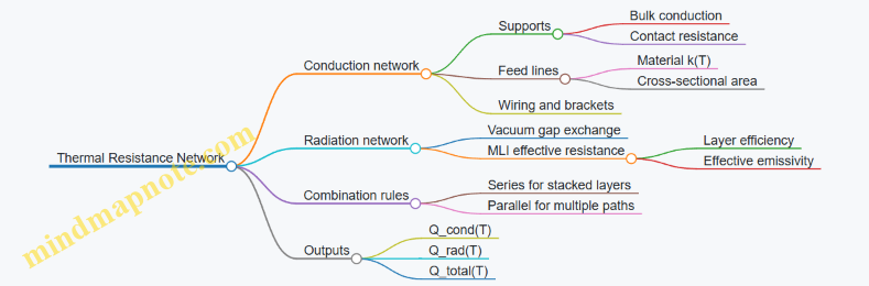
3.3 Heat Leak Budgeting and Thermal Resistance Modeling
Cryogenic systems fail in boring ways: too much heat gets in, propellant warms, boil-off rises, and feed conditions drift. Heat leak budgeting and thermal resistance modeling give you a disciplined way to predict that chain of events before hardware exists.
Foundations of Heat Leak Budgeting
Heat leak budgeting starts with a simple statement: the net heat flow into the cold region equals the sum of conductive, radiative, and sometimes convective contributions, minus any intentional heat removal. In most spacecraft cryogenic tanks, convection is suppressed by vacuum, so the model focuses on conduction through supports and plumbing, plus radiation across the vacuum gap.
A practical workflow is to define:
- Cold boundary: the tank wall or propellant interface temperature you care about.
- Warm boundary: the external structure temperature driving heat in.
- Thermal resistances: each path gets its own resistance, then resistances combine like electrical circuits.
- Heat leak budget: the total heat into the cold boundary, used later to estimate boil-off and ullage evolution.
Mind Map: Heat Leak Budgeting Flow
Thermal Resistance Modeling Basics
Conduction Through Supports and Hardware
For a conduction path with roughly constant thermal conductivity over the temperature range, the heat flow is:
- Q = (T_hot − T_cold) / R
- R = L / (k A)
Where L is the effective length, A is cross-sectional area, and k is thermal conductivity. In reality, k changes with temperature, especially for metals and polymers. When k varies, you replace k with an effective conductivity or integrate k(T) across the temperature span. A simple engineering approach is to compute two bounding values using k at the cold and warm ends, then use the average as an estimate and keep the uncertainty in mind.
Contact resistance is the silent tax on conduction models. If a support is bolted or clamped, the interface can dominate the effective resistance. You can model this by adding a contact resistance term in series with the bulk conduction resistance. A quick example: if the bulk resistance predicts 0.5 W but the interface resistance is comparable, the total might drop to 0.3 W or rise to 0.8 W depending on surface condition and preload.
Radiation Across Vacuum Gaps
Radiation heat transfer between surfaces depends on emissivity, geometry, and temperature. With multiple surfaces and insulation, the model becomes a network of radiative exchanges. The most common spacecraft approach uses multilayer insulation (MLI), where the effective radiative heat transfer is reduced by many thin layers that interrupt line-of-sight exchange.
A workable modeling strategy is:
- Treat the MLI as an effective thermal resistance between the warm and cold surfaces.
- Use an empirical form where heat transfer decreases with layer count and increases with temperature.
- Include effective emissivity and layer efficiency as parameters calibrated from representative coupons or prior builds.
Even without perfect calibration, you can still do meaningful budgeting by separating the radiation budget into a baseline estimate and a conservative margin.
Combining Resistances into a Heat Leak Budget
Thermal networks combine like circuits:
- Series paths add resistances: R_total = R1 + R2 + …
- Parallel paths add conductances: 1/R_total = 1/R1 + 1/R2 + …
A tank typically has multiple parallel conduction paths (supports, feed lines, instrumentation wiring) and one dominant radiation path (MLI and view factors). So you compute:
- Q_cond_total from the parallel conduction network
- Q_rad_total from the radiation exchange model
- Q_total = Q_cond_total + Q_rad_total
Example: Support Conduction vs Radiation Dominance
Assume a tank with:
- Support conduction predicts Q_cond = 0.9 W
- Radiation through MLI predicts Q_rad = 1.6 W
Then Q_total = 2.5 W. If you later reduce support cross-section by 20% and conduction drops to 0.7 W, the total becomes 2.3 W. That tells you the radiation path is the bigger lever. This is why heat leak budgeting is useful: it prevents you from spending effort where it won’t move the needle.
Temperature Dependence and Model Discipline
Heat leak models should reflect that temperatures are not constant. If the cold wall warms from 20 K to 25 K, both conduction and radiation change. For conduction, k(T) changes; for radiation, the driving term grows with temperature. A disciplined method is to compute heat leak at a few representative temperatures (for example, start, mid, and end of a test window) and then use the resulting heat leak trend in downstream boil-off calculations.
Mind Map: Thermal Resistance Network
Sanity Checks That Catch Common Errors
- Units: resistances in K/W, heat in W, temperatures in K.
- Dominant path: identify whether conduction or radiation is larger; if they’re within a factor of two, both need careful attention.
- Magnitude check: if the model predicts tens of watts for a well-insulated tank, re-check emissivity assumptions and MLI effectiveness.
- Geometry realism: view factors and effective areas matter; using “full area” when only part of the surface is exposed can overestimate radiation.
A good heat leak budget is not just a number. It’s a map of where the watts come from, which assumptions control the outcome, and how sensitive the total is to each modeling choice.
3.4 Slosh Dynamics and Propellant Distribution Control
Cryogenic tanks rarely behave like perfectly still buckets. Even in microgravity, the liquid surface can move, the ullage gas can redistribute, and the engine feed system can see changing inlet conditions. Slosh dynamics matter because they directly affect whether the feed line receives liquid, how stable the mixture ratio is, and how repeatable engine starts are.
Foundational Concepts of Slosh in Microgravity
Slosh is the coupled motion of liquid and tank geometry under acceleration. In microgravity, the dominant “push” is not gravity but spacecraft maneuvers, reaction wheel disturbances, and thrust transients. The liquid responds with modes shaped by tank boundaries: for a simple cylindrical tank, the lowest mode often resembles a single bulge; for more complex geometries, multiple lobes can appear.
A practical way to think about it is to separate two effects. First, the liquid free surface moves relative to the tank. Second, the feed system experiences a time-varying liquid fraction at its inlet due to that surface motion and due to local boiling or flashing.
Key Variables That Drive Propellant Distribution
Three variables typically dominate distribution control.
- Acceleration history: The magnitude and direction of acceleration determine which slosh modes are excited. A short, sharp maneuver can excite higher modes; a long, smooth burn tends to excite lower modes.
- Tank geometry and fill level: The same acceleration produces different slosh behavior at different fill fractions. Near-empty tanks can expose the inlet to gas; near-full tanks can trap liquid away from the inlet.
- Internal features: Baffles, vanes, and screens change flow paths and damp certain modes. They also add pressure drop and can trap vapor if not designed carefully.
Modeling Approach from Simple to Useful
Start with a reduced-order view: treat the tank as having a few slosh modes with effective masses and natural frequencies. This lets you predict when the liquid surface will likely reach the inlet during a maneuver.
Then add realism where it matters for operations. For distribution control, the most useful outputs are not the full fluid field but the inlet liquid fraction and the time window of acceptable inlet conditions. You can estimate these by combining mode amplitudes with a geometric mapping from free-surface elevation to inlet submergence.
Finally, validate the model with tests that reproduce the relevant acceleration spectrum. A model that matches natural frequencies but misses damping can still fail at predicting inlet liquid fraction.
Control Objectives and Acceptance Criteria
A distribution control strategy should define what “good” means. Typical acceptance criteria include:
- Minimum inlet liquid fraction during engine start and steady operation.
- Maximum allowable vapor ingestion rate, because vapor can cause feed pressure oscillations and mixture ratio excursions.
- Maximum allowable inlet pressure drop across screens or baffles, to avoid starving the engine.
A simple operational example: if the engine requires liquid at the inlet within the first 2 seconds of start, the control system must ensure that the predicted surface elevation keeps the inlet submerged during that interval, even under worst-case maneuver timing.
Passive Distribution Control with Baffles and Screens
Passive devices reduce slosh energy or guide liquid toward the outlet.
- Baffles break up large-scale motion by increasing effective flow resistance between regions. They reduce the amplitude of certain modes, but they can also create trapped vapor pockets if the local flow reverses.
- Vane or screen outlet devices help maintain liquid at the outlet by promoting liquid preferential transport. The key design trade is pressure drop versus vapor rejection.
Example: Suppose a tank experiences repeated short attitude adjustments. A baffle that reduces the lowest slosh mode may not help if higher modes dominate during those adjustments. In that case, a screen near the outlet can be more effective because it filters the inlet region even when the global surface moves.
Active Distribution Control with Maneuver Timing and Feed Sequencing
Active control usually means coordinating spacecraft maneuvers with propellant management.
- Maneuver phasing: Schedule burns so that the acceleration direction during critical feed windows aligns with a mode shape that keeps the inlet submerged.
- Feed sequencing: Delay valve opening until the predicted liquid fraction rises above a threshold.
Example: During a coast-to-burn transition, the spacecraft may perform a small attitude correction. If that correction excites a slosh mode that lifts the free surface away from the outlet, then opening the feed valve immediately can ingest vapor. A better approach is to open the valve after the correction settles, using onboard estimates of slosh state derived from recent acceleration and tank fill.
Advanced Details That Commonly Break Designs
- Damping assumptions: Damping depends on temperature, surface conditions, and internal feature wetting. A model calibrated at one fill level can mispredict at another.
- Two-phase coupling: Boil-off and flashing can change effective liquid density and alter slosh response. Even modest vapor generation can reduce liquid momentum transfer to the outlet.
- Nonlinear free-surface behavior: At higher slosh amplitudes, the free surface can contact internal structures, changing flow paths abruptly.
Example: A baffle that looks fine in a single-phase flow test may trap vapor during a cold start when local temperatures are lower and flashing is more likely. The result is a delayed liquid arrival at the outlet, even though the global surface elevation seems acceptable.
Mind Map: Slosh Dynamics and Propellant Distribution Control
Example Workflow for Designing Distribution Control
- Define the critical engine windows and required inlet liquid fraction.
- Choose a reduced-order slosh model with a small set of modes relevant to expected maneuvers.
- Compute inlet submergence probability across the operational fill range.
- Add passive features to reduce the most harmful modes and verify pressure drop limits.
- Plan active sequencing rules that delay feed until predicted inlet conditions are met.
- Confirm with tests that reproduce the acceleration profile and thermal state, then adjust damping and two-phase coupling parameters.
This workflow keeps the focus on what the engine actually sees: liquid availability at the inlet, not just the motion of the free surface.
3.5 Pressure Relief and Venting Architecture for Safe Operation
Cryogenic systems don’t fail because pressure exists; they fail because pressure has nowhere predictable to go. Pressure relief and venting architecture turns “somewhere” into a designed path with known flow behavior, known thermal conditions, and known consequences. The goal is simple: keep tank and feed hardware within allowable limits during credible off-nominal events, while preventing unsafe propagation such as line rupture, oxygen enrichment, or uncontrolled venting into sensitive areas.
Core Principles for Relief and Venting
Start with a clear boundary between relief and vent functions. Relief devices protect pressure vessels from overpressure by discharging when pressure exceeds set limits. Vent systems manage normal or abnormal boil-off and purge needs by providing controlled discharge routes. In practice, both are often present, but they should not be treated as interchangeable.
A useful mental model is a “pressure ladder.” First, design for low heat leak so boil-off stays within operating margins. Second, use pressure control (regulators and pressurant management) to avoid drifting upward. Third, rely on relief devices as the last line of defense. If you skip step one or two, the relief system becomes a routine operating mode, which is a great way to discover that seats, orifices, and downstream hardware are not designed for frequent cycling.
Relief Device Placement and Sizing Logic
Relief devices should be mounted where they sense the pressure that matters. For a tank, that usually means direct connection to the vapor space or a representative pressure takeoff that avoids long, thermally stratified runs. Avoid placing relief sensing points behind valves or long manifolds that could trap pressure or delay response.
Sizing follows the energy and mass balance of the worst credible overpressure scenario. For cryogenic tanks, common drivers include blocked vent paths, regulator malfunctions, external heat input during a thermal event, or rapid pressurant release into a constrained volume. The sizing process should include:
- Maximum credible mass generation rate from heat leak and phase change.
- Discharge capacity of the relief device at the set pressure and expected backpressure.
- Downstream pressure effects so the device can actually flow.
Backpressure is the quiet saboteur. If the discharge line ends in a region where pressure builds, the relief device may lift later than expected or flow less than calculated. That’s why discharge routing, termination geometry, and any flow restrictions must be treated as part of the relief system, not as afterthought plumbing.
Discharge Routing and Thermal Management
Discharge piping must handle two competing realities: cryogenic fluids can cause embrittlement and icing, while warm ambient conditions can flash and increase mass flow. Use routing that minimizes long horizontal runs where liquid can collect. Provide insulation or thermal breaks where needed to prevent excessive heat transfer into the tank through the discharge line.
A practical example: if a relief discharge line runs near structural members, the line can freeze them into a brittle state or create ice buildup that blocks nearby vents. A better approach is to route the discharge away from critical structures and include a termination that promotes stable vaporization rather than liquid impingement.
Venting Architecture for Normal and Abnormal Operations
Venting should be designed for predictable states: normal boil-off, controlled purge, and emergency vent. Normal venting often uses a regulated path to maintain tank pressure within a narrow band. Emergency venting should be capable of handling higher flow rates without causing backpressure spikes.
Separate vent lines by function when possible. Mixing purge gas with relief discharge can create unexpected phase behavior and complicate downstream safety analysis. If shared manifolds are unavoidable, include flow conditioning elements and ensure the manifold can tolerate the highest credible discharge conditions.
Backpressure Control and Termination Design
Termination design is where “safe operation” becomes physical. The vent outlet should prevent re-ingestion of discharged gas into intakes or crew-accessible areas. It should also avoid locations where condensed cryogen can accumulate and later re-evaporate.
Consider a simple termination check: if the discharge jet can impinge on a nearby surface, you may get localized icing and a changing flow area that alters backpressure. A termination that directs flow upward and away from obstacles reduces the chance of liquid impingement and makes backpressure more stable.
Materials, Seals, and Leak Tightness
Relief and vent components experience thermal cycling and occasional high-flow events. Select materials and seals that maintain integrity at cryogenic temperatures and during repeated cycling. For example, elastomer seals that work at operating temperatures may harden after relief events that expose them to colder transient conditions.
Also consider that relief discharge can carry trace contaminants. If oxygen is present in the system, venting can create localized oxygen enrichment in the discharge region. That’s why contamination control and vent placement must be considered together, not separately.
Mind Map: Pressure Relief and Venting Architecture
Example: Designing for a Blocked Vent Scenario
Assume a tank has a normal vent line that could become partially blocked by ice formation. The relief system must be sized for the resulting pressure rise rate, not the nominal boil-off rate. Then check the discharge line for backpressure: if the relief outlet is near a structure that can accumulate ice, the discharge may become less effective over time. A robust design routes the relief discharge to a termination that stays clear of surfaces and includes thermal considerations to reduce ice growth near the outlet. Finally, verify that the relief discharge does not create a new hazard by directing cold gas toward sensitive hardware or oxygen-sensitive zones.
Verification Checks Before Hardware Release
Before integration, validate the architecture with checks that map directly to failure modes: relief lift timing under expected backpressure, discharge line thermal behavior during a representative cold soak, and leak tightness of relief and vent interfaces after cycling. The best systems don’t just “have a relief valve”; they have a relief path that stays predictable when the rest of the system is not.
4. Boil Off Control and Cryogenic Feed System Architecture
4.1 Boil Off Mechanisms and Their Drivers
Boil off is the slow conversion of stored liquid cryogen into vapor because heat leaks into the tank. The vapor then raises ullage pressure and can vent, wasting propellant and changing feed conditions. The key idea is simple: boil off rate is set by the heat entering the liquid, and the heat entering is set by the thermal path from the surroundings to the cryogen.
Mind Map: Boil Off Mechanisms and Drivers
Heat Input Pathways
Radiation is often the largest contributor when insulation is imperfect. Even with multilayer insulation (MLI), some energy reaches the cold surfaces. The practical driver is the combination of surface emissivity, the number and quality of insulation layers, and how well the insulation is supported without gaps. A useful mental model: MLI reduces radiative transfer by forcing energy to bounce through many thin layers, but any “short circuit” path—like a support that touches both warm and cold regions—lets radiation and conduction team up.
Conduction comes from solid connections that bridge temperature differences. Typical culprits include tank supports, mounting hardware, instrument wiring, and feed line penetrations. Conduction scales with cross-sectional area and temperature gradient, so a thick bracket or a poorly designed penetration can dominate the heat leak even if the rest of the tank is well insulated. For example, if a support strut is made of a higher-conductivity material than planned, the boil off can increase noticeably because the strut becomes a direct thermal highway.
Convection is usually smaller than radiation and conduction for well-controlled ullage, but it can matter when ullage gas pressure is high enough for meaningful gas motion. Convection is also affected by stratification: if warmer vapor sits above colder liquid, buoyancy-driven circulation can transport energy downward. Venting can temporarily change ullage conditions, which can either suppress or amplify convective heat transfer depending on the direction and timing of pressure changes.
Phase Conversion Physics
Once heat reaches the liquid, boil off depends on how much energy is required to change phase. The energy per unit mass is the latent heat of vaporization, so the boil off rate is roughly proportional to the heat leak divided by that latent heat. This is why two cryogens with different latent heats can show different boil off behavior under the same thermal load.
Subcooling matters too. If the liquid is colder than its saturation temperature, additional heat must first raise it to saturation before net vapor generation becomes significant. That means a tank that is “pre-cooled” before a long coast can show a slower initial boil off, even if the steady-state heat leak is unchanged.
Tank and System State
Boil off is not just a tank property; it is tied to the tank’s operating state. As vapor forms, ullage pressure rises toward the saturation pressure corresponding to the liquid temperature. That pressure rise can affect feed system behavior, especially if regulators or valves are sensitive to inlet conditions.
Ullage volume and geometry influence how quickly vapor accumulates and how evenly temperature and pressure distribute. A larger ullage can buffer pressure changes, but it can also increase the surface area exposed to warmer regions, depending on design.
Slosh and mixing can change local conditions. If liquid motion repeatedly brings warmer liquid or vapor-contacting regions into contact with colder bulk liquid, the effective heat transfer can shift. The driver here is not “more motion equals more boil off” in a simple way; it’s how motion changes the contact patterns between phases and surfaces.
Operational Drivers and Practical Examples
Mission duration is the obvious driver: even a small heat leak integrated over days becomes a meaningful propellant loss. For an easy example, imagine a heat leak that produces a steady mass loss rate; doubling the coast time doubles the boil off mass, even though nothing “new” happens thermally.
Thermal environment and attitude drive how much radiation reaches the tank. Sun-facing surfaces can raise effective radiative heat input, while a shaded attitude reduces it. A practical check is to compare boil off behavior during different attitude profiles and verify that the thermal model’s view factors match the observed trends.
Ground handling and pre-cool history affect initial conditions. If the tank enters the mission with warmer liquid, it will reach saturation sooner and begin producing vapor at a higher rate earlier in the timeline.
Quick Diagnostic Mindset
When boil off is higher than expected, the systematic approach is to ask which term in the heat budget grew: radiative, conductive, or convective. Then check whether the tank entered the phase-change regime earlier due to reduced subcooling. Finally, verify that operational conditions—attitude, venting events, and handling—did not change the thermal paths or ullage state.
4.2 Passive Boil Off Reduction Techniques
Passive boil off reduction means you slow down heat entering the cryogenic tank without relying on active control. The core idea is simple: boil off happens when heat leak raises the liquid’s temperature and drives vaporization. Passive methods reduce either (1) the heat leak rate, (2) the fraction of heat that reaches the liquid, or (3) the time the tank spends in the “unhappy” thermal conditions right after launch.
Foundational Heat Leak Logic
Heat enters through conduction (solid paths), radiation (line-of-sight and surfaces), and sometimes gas conduction through residual ullage gas. In a well-designed cryogenic system, radiation and conduction dominate, while gas conduction is minimized by low-pressure ullage and careful venting.
A practical way to reason about passive performance is to treat the tank as a thermal network:
- Insulation layers provide thermal resistance.
- Supports provide conduction paths.
- Internal surfaces and MLI blankets determine radiative exchange.
- The liquid surface and ullage define where the energy ends up.
If you reduce total heat leak by 30%, you don’t just reduce boil off by 30% in every case, because the tank’s pressure, saturation temperature, and liquid level also change. Still, for engineering comparisons, heat leak reduction is the right first-order metric.
Insulation That Actually Works
Multilayer insulation (MLI) is the workhorse. Its effectiveness comes from many thin layers that interrupt radiative transfer and reduce effective emissivity. The details matter:
- Layer density and spacing: Too loose wastes radiative blocking; too tight increases conduction through contact points.
- Surface cleanliness and coating choices: Dust or poor surface finishes can raise emissivity and degrade performance.
- Thermal shorts: Any strap, bracket, or support that bridges layers becomes a shortcut for heat.
A concrete example: if you replace a continuous metal strap across the insulation with a segmented support that breaks conduction paths, you often get a larger improvement than adding a small thickness increase to the MLI. The “weak link” is usually the geometry, not the insulation thickness.
Minimizing Conduction Paths
Conduction is carried by tank supports, feedthroughs, wiring harnesses, and any structural members that connect warm and cold regions.
Passive conduction reduction techniques include:
- Low-conductivity materials for supports and standoffs.
- Geometric throttling such as reducing cross-sectional area and increasing length.
- Thermal intercepts where feasible, using intermediate cold stages to “catch” heat before it reaches the tank.
Example: consider three support designs with the same total load. The one with the smallest product of cross-sectional area and thermal conductivity divided by length yields the lowest conduction heat leak. Even if the material is only slightly better, the geometry can dominate.
Radiation Control with Surface Management
Radiation heat transfer depends on view factors and surface emissivity. Passive radiation control is achieved by:
- Using low-emissivity surfaces on the cold side of insulation.
- Ensuring good vacuum quality so gas conduction doesn’t undo the gains.
- Avoiding gaps that create direct line-of-sight from warm surfaces to cold surfaces.
Example: a small uninsulated window around a penetrator can create a radiative “tunnel.” The heat leak through that tunnel can exceed the surrounding insulation contribution, especially when the penetrator is near the tank’s hottest external region.
Tank Geometry and Liquid Surface Effects
Boil off is influenced by where heat ends up. If heat primarily warms the ullage, it may increase vapor pressure with less immediate liquid vaporization than if heat reaches the liquid directly. Passive design choices that help include:
- Reducing direct thermal coupling between external structures and the liquid region.
- Managing internal surfaces so that heat absorbed by vapor or walls doesn’t efficiently transfer into the liquid.
Example: routing a structural member so it contacts the tank wall near the upper region rather than near the liquid pool can reduce the rate at which energy reaches the liquid, even if the total heat leak is similar.
Early-Phase Thermal Conditioning
Even passive systems experience a “startup” thermal period after deployment or during ascent. Passive strategies reduce the duration and severity of that period:
- Pre-cooling and cold soak before final tank loading.
- Limiting warm-up exposure by minimizing time between tank cool-down and mission-relevant operations.
Example: if a tank sits for hours in a warmer environment before integration, the insulation may be saturated with heat. Later passive performance can’t fully compensate because the tank begins closer to saturation at a higher temperature.
Mind Map: Passive Boil Off Reduction Techniques
Example Workflow for Engineering Tradeoffs
- Estimate heat leak budget by splitting conduction and radiation contributions.
- Identify dominant paths by inspecting supports, penetrators, and any insulation discontinuities.
- Apply passive fixes in the order of highest leverage: remove thermal shorts first, then tune MLI and surface conditions.
- Validate with a simple thermal model that includes saturation behavior so you can translate heat leak into expected boil off.
A good rule of thumb: if you can point to a single physical feature that bridges warm and cold regions, you can usually get more improvement by redesigning that feature than by adding more insulation everywhere else.
4.3 Active Boil Off Management Using Heaters and Control Loops
Active boil-off management means you add controlled heat to reduce the net boil-off rate, or to keep the propellant within a safe temperature and pressure envelope during operations. The key idea is simple: boil-off is driven by heat leak into the tank. If you can’t eliminate the leak, you can shape how and where that energy goes.
Foundational Control Targets
Start by defining what “good” looks like in measurable terms:
- Tank pressure margin: keep ullage pressure below relief setpoints with enough margin for sensor error and transients.
- Propellant temperature: maintain a stable saturation temperature corresponding to the desired pressure band.
- Liquid acquisition reliability: ensure the liquid level and subcooling are sufficient for feed system inlet conditions.
A practical rule of thumb is to treat boil-off control as a pressure-temperature regulation problem. Heaters are the actuator; insulation heat leak and ambient conditions are disturbances.
Heater Placement and What It Really Changes
Heaters can be placed to influence different parts of the thermal system:
- Ullage heaters add energy to the gas space, raising pressure faster but often with less direct impact on liquid subcooling.
- Liquid or wall heaters add energy closer to the liquid, reducing subcooling loss and potentially lowering net boil-off if the control objective is to keep saturation conditions stable.
An easy example: if your tank is trending toward higher pressure because of a large heat leak, ullage heating can make it worse. In that case, the controller should either reduce heater power or switch to a strategy that prioritizes liquid temperature stability.
Control Loop Architecture
A robust loop typically includes:
- Sensors: tank pressure, liquid temperature (or a proxy), and heater current/voltage for power verification.
- Actuator: heater power command with limits that respect electrical and thermal constraints.
- Logic: mode selection for coast, maneuver, and start-prep phases.
A common approach is a two-layer structure:
- Outer loop regulates tank pressure to a setpoint band.
- Inner loop shapes heater power to achieve the commanded thermal effect while preventing overshoot.
Modeling the Thermal Balance
Even a simplified energy balance helps avoid “mystery oscillations.” Consider:
- Heat leak into the tank: \(Q_{leak}\)
- Heater power delivered effectively to the relevant region: \(\eta Q_{heater}\)
- Net boil-off energy demand: \(\dot{m}*{boil} h*{vap}\)
When \(\eta Q_{heater} \) is used to counteract the effective energy that would otherwise drive phase change, the controller can reduce \(\dot{m}_{boil}\). If the heater adds energy in the wrong region, it may increase boil-off even while pressure control looks temporarily stable.
Practical Control Law Example
Below is a conceptual discrete-time controller that uses pressure error and rate limiting to avoid aggressive heater cycling.
Inputs: P, dPdt, P_set, P_band, Qmax
State: mode, Qcmd

if P < P_set - P_band:
  mode = "heat_up"
elif P > P_set + P_band:
  mode = "hold_or_reduce"
else:
  mode = "hold"

if mode == "heat_up":
  Qcmd = clamp(Qcmd + Kp*(P_set - P), 0, Qmax)
elif mode == "hold_or_reduce":
  Qcmd = clamp(Qcmd - Kp*(P - P_set), 0, Qmax)
else:
  Qcmd = Qcmd - Kd*dPdt

Apply slew limit to Qcmd to prevent heater power steps.
A concrete example: during a long coast, pressure slowly rises. The controller increases heater power only if pressure drops below the lower band. If pressure is already high, it reduces power and uses the pressure rate term to damp motion, which prevents the classic “hunt” where heaters chase the sensor noise.
Handling Transients and Mode Switching
Transients come from valve operations, attitude changes, and changing external heat flux. Mode switching should be explicit:
- Start-prep mode: prioritize liquid acquisition conditions, often by limiting heater action that would reduce subcooling.
- Coast mode: prioritize pressure stability with minimal heater cycling.
A simple operational example: if you know a propellant transfer will temporarily disturb ullage conditions, you can freeze heater commands for a short window and then resume closed-loop control once measurements settle.
Verification with a Small Test Matrix
Before committing to flight-like operations, verify with a compact set of scenarios:
- nominal heat leak with small heater power steps
- increased heat leak (simulated by higher external temperature)
- sensor bias test to confirm the controller doesn’t saturate
Success criteria should include: no heater saturation for normal cases, bounded pressure excursions, and stable temperature behavior without repeated overshoot.
Mind Map: Active Boil Off Management Using Heaters and Control Loops
Integrated Example Scenario
Imagine a tank with steady heat leak that would normally raise pressure over time. You command a pressure setpoint band. When pressure drifts low, the controller increases heater power, but it does so with slew limits to avoid sudden saturation changes. When pressure drifts high, it reduces heater power and uses pressure rate feedback to damp the trend. The result is a controlled saturation environment that supports feed system inlet conditions without constant heater cycling.
4.4 Feed System Layouts for Ullage and Liquid Acquisition
Cryogenic engines care about one thing more than most: getting the right phase to the right place at the right time. “Ullage” is the gas space above the liquid, and “liquid acquisition” is the hardware and flow path that ensures the engine inlet sees liquid rather than vapor. A good layout starts with a simple question: where will the liquid be when the spacecraft is accelerating, coasting, or settling after a maneuver?
Foundational Layout Concepts
A typical cryogenic feed system has three functional zones: tank ullage management, transfer and conditioning, and engine inlet supply. Ullage management is about controlling where the liquid surface sits and how stable it is. Liquid acquisition is about collecting liquid through a device that can tolerate slosh and two-phase conditions.
A practical mental model is to treat the tank as a moving container with a “liquid surface” that shifts with acceleration. If the engine inlet line connects to the tank through a dip tube or acquisition device, the line must remain connected to liquid even when the surface tilts. The layout therefore couples tank geometry, acquisition hardware, and line routing.
Tank Geometry and Ullage Stability
Most layouts rely on one of two strategies. The first is to reduce surface motion using internal baffles and propellant management devices. The second is to make the acquisition device robust to surface motion by using a settling volume and a controlled inlet.
A simple example: imagine a tank with a straight outlet line. During a thrusting phase, the liquid surface leans away from the outlet, and the line ingests vapor. Now add a downcomer dip tube that extends below the expected minimum liquid level. During the same thrusting phase, the tube still sees liquid because it reaches into the region that remains filled.
Liquid Acquisition Devices
Common acquisition devices include dip tubes, standpipes, and surface-following concepts. Dip tubes are straightforward: a tube extends into the liquid and the outlet is taken from the tube. Standpipes are similar but often paired with a settling volume or a controlled inlet to reduce vapor ingestion.
For two-phase tolerance, the acquisition device is usually designed to create a “liquid-dominant” zone near the outlet. That zone is protected by geometry that discourages vapor bubbles from reaching the inlet. A practical example is a standpipe with a perforated or baffled inlet that slows incoming flow and encourages bubbles to rise away from the pickup.
Feed Line Routing and Thermal Considerations
Line routing affects both phase behavior and reliability. Long, cold lines can create unwanted thermal gradients that change local saturation conditions. A layout typically uses a pressure drop budget and a thermal budget together.
A concrete approach: route the feed line so it avoids sharp bends near the tank outlet, because bends can trap vapor pockets during transient conditions. Then use insulation where heat leak would raise local temperature enough to increase vapor fraction. If the line is intentionally warmed to prevent freezing, the warm section is kept short and controlled so it does not destabilize the rest of the line.
Ullage Control Through Settling and Venting
Even with good acquisition hardware, many systems use a settling step before engine start. Settling is a controlled period where acceleration is reduced or managed so the liquid surface returns to a predictable position.
Venting and pressure equalization also matter. If the ullage pressure is too high, vapor volume can increase and reduce the effective liquid head at the pickup. If it is too low, flashing can occur in the line due to local pressure drops. A layout therefore includes a vent path and a controlled way to manage ullage pressure during both normal operation and start preparation.
Advanced Layout Details That Prevent Two-Phase Ingestion
Once the basic geometry is chosen, the layout details focus on minimizing vapor ingestion and stabilizing inlet conditions.
- Inlet elevation control: The pickup location is set relative to the minimum expected liquid level under worst-case acceleration. This is often paired with a margin for manufacturing tolerances.
- Flow regime management: The line diameter and length are selected to keep pressure drops within a range that does not trigger excessive flashing.
- Bubble management: Acquisition devices may include internal baffles or flow straighteners to reduce swirling and bubble entrainment.
- Transient sequencing: Valve timing is coordinated so the system does not open a path that would immediately expose the pickup to vapor.
A small example ties these together. Suppose the system uses a settling step, then opens a valve to feed the engine. If the valve opens too quickly, the sudden pressure change can cause flashing near the pickup. Slowing the valve opening or adding a controlled prefill path can keep the inlet dominated by liquid during the first seconds.
Mind Map: Ullage and Liquid Acquisition Layout
Example: Two-Phase Safe Start Sequence
Consider a layout with a standpipe pickup and an insulated feed line. Before start, the spacecraft performs a settling phase so the liquid surface returns near the standpipe inlet elevation. During settling, ullage pressure is adjusted using the vent/equalization path to keep the liquid head stable. At start, the system opens the feed valve with a controlled ramp to avoid a sudden pressure drop that would flash vapor near the pickup. The engine inlet then receives liquid-dominant flow, and the system monitors inlet pressure and temperature to confirm stable conditions before transitioning to steady operation.
Summary of Layout Logic
A reliable cryogenic feed layout treats ullage and liquid acquisition as a coupled problem: tank geometry sets the liquid surface behavior, acquisition hardware sets what the pickup sees, and line routing plus sequencing sets whether two-phase conditions appear during the moments that matter most.
4.5 Instrumentation for Detecting Thermal and Phase States
Cryogenic systems fail in boring ways: a sensor reads “liquid” when it’s actually two-phase, a wall temperature lags behind the propellant, or a pressure transducer gets fooled by flashing in a line. Good instrumentation treats thermal state and phase state as separate measurements that must agree within known tolerances.
Core Measurements and Why They Matter
Start with three foundational signals.
- Temperature of propellant and hardware: A thermocouple on a tank wall tells you about heat soak and insulation performance, not directly the phase at the sensor location.
- Pressure of ullage and feed lines: Pressure anchors the saturation condition. If pressure is stable but temperature drifts, you’re likely seeing subcooling changes or sensor lag.
- Phase indicators: Phase is inferred from behavior—density, capacitance, optical response, or differential pressure across a known restriction. The key is choosing a method whose failure modes are understood.
A practical rule: phase state is confirmed by at least two independent cues (for example, pressure-based saturation plus a phase sensor or flow regime indicator).
Temperature Sensing Strategy
Use temperature sensors to build a thermal model you can trust.
- Where to place sensors: Put one set on the tank wall (to validate heat leak and insulation effectiveness) and another set on feed hardware (to detect line warm-up that can trigger flashing).
- How to interpret readings: Expect thermal gradients. A wall sensor might show 90 K while the liquid near the surface is closer to saturation at a slightly different pressure. Treat temperature as a boundary condition for your model, not a direct phase verdict.
Example: During a cold soak, wall temperature falls quickly at first, then slows as insulation resistance dominates. If a feed-line temperature drops much later than the tank wall, you likely have a thermal bridge or poor contact at a clamp.
Pressure Measurement and Saturation Anchoring
Pressure sensors should be installed to represent the correct control volume.
- Ullage pressure: Use it to compute saturation temperature for the cryogen. Ensure the sensor is not directly exposed to flashing jets.
- Feed-line pressure: Use it to detect pressure drops from two-phase flow. If pressure oscillates while commanded flow is steady, you may be cycling between liquid and vapor in the line.
Example: A regulator holds average pressure, but the feed pressure shows high-frequency ripple. That ripple often matches valve stroking or flashing events, which can confuse phase inference if you only look at averages.
Phase Detection Methods
Phase detection methods fall into categories based on what they respond to.
- Capacitance or dielectric sensors: Liquid and vapor have different permittivity. These work best when the sensor is designed for cryogenic dielectric behavior and when wiring and insulation are stable.
- Optical or fiber methods: Useful when optical access exists and contamination is controlled. They can be sensitive to window frosting.
- Differential pressure across restrictions: Two-phase flow changes effective density and flow regime, altering ΔP. This is robust when the restriction geometry is stable.
- Flow regime inference from combined signals: Combine pressure, temperature, and flow (or pump speed) to infer phase quality.
Example: If a capacitance sensor indicates “liquid present” but ΔP across a restriction increases sharply, the system may be seeing stratified two-phase near the sensor. The disagreement is valuable: it points you to a specific location where phase is not uniform.
Sensor Placement Logic for Integrated Interpretation
Think in layers: tank, ullage, feed line, and injector interface.
- Tank layer: Wall temperatures validate insulation and heat leak budgeting.
- Ullage layer: Pressure plus ullage temperature supports saturation calculations.
- Feed layer: Feed-line temperatures and pressure drops reveal flashing risk.
- Engine interface layer: Local pressure and phase cues confirm start readiness.
Calibration, Uncertainty, and Failure Modes
Instrumentation must be calibrated for the operating environment.
- Temperature calibration: Cryogenic sensors can drift after thermal cycling. Use calibration curves that cover the expected range and include uncertainty bands.
- Pressure calibration: Account for sensor hysteresis and mounting strain from cooldown.
- Phase sensor validation: Validate with controlled conditions that mimic expected vapor quality ranges.
Example: A phase sensor might read “mostly liquid” during a start transient because bubbles are small and intermittent. If you also track ΔP across a restriction, you can distinguish “liquid with entrained vapor” from “fully two-phase flow.”
Integrated Example Workflow for Start Readiness
- During cold soak, verify wall temperature trends match the expected heat leak.
- At ullage pressure stability, compute saturation temperature and compare to ullage and nearby liquid temperatures.
- Before valve opening, check feed-line temperature and pressure for signs of incipient flashing.
- During start, confirm phase state using at least two cues, such as saturation agreement plus a phase sensor or ΔP regime shift.
- If cues disagree, treat it as a diagnostic: the location of disagreement usually indicates where thermal gradients or phase stratification are occurring.
This approach keeps the system honest. Temperature tells you about heat flow, pressure tells you about thermodynamic state, and phase indicators tell you about what the fluid is actually doing where it matters.
5. Propellant Conditioning for Reliable Engine Start
5.1 Subcooling Requirements and Practical Methods
Subcooling means keeping a cryogenic liquid colder than its saturation temperature at the local pressure. In a feed system, that extra margin reduces the chance of flash boiling inside lines and valves, and it makes engine start sequences more repeatable. The key idea is simple: if the liquid enters a region where pressure drops or heat leaks in, subcooling gives you time before vapor forms.
Subcooling Requirements from First Principles
Start by defining the local saturation temperature, Tsat(P). Then define subcooling as ΔT = Tsat(P) − Tactual. For a practical requirement, you need three layers of margin:
- Thermal margin: heat leak into the line or injector during the start window. A warmer liquid reduces ΔT, so you size ΔT to survive the worst-case heat input.
- Pressure margin: pressure drops across fittings, filters, and valves. Even a modest drop changes Tsat, so the same absolute temperature can become less subcooled.
- Two-phase margin: sensors and control logic must tolerate small vapor fractions without destabilizing flow. Subcooling is your buffer against that vapor fraction growing.
A useful way to reason about it is to treat the start as a short “budget period.” If the system can guarantee that ΔT stays positive across the most sensitive segment—often the last few meters before the engine—then you avoid the messy regime where vapor locks, unstable valve behavior, and erratic mixture formation show up.
Practical Methods to Achieve Subcooling
There are three common approaches, often combined.
Cold-Source Subcooling Through Controlled Feed Conditions
If the tank is well managed, the liquid leaving the tank can be subcooled by ensuring the tank ullage pressure and liquid temperature are aligned. In practice, you regulate pressurant pressure and manage heat leak so the liquid temperature stays below Tsat at the outlet pressure. A simple check is to compare measured tank liquid temperature with the saturation temperature computed from the outlet pressure at the same time.
Example: During a cold start, the outlet pressure is 3.0 bar and the measured liquid temperature is 90 K. If Tsat at 3.0 bar is 92 K, then ΔT = 2 K. If your start window allows only 1 K of heat gain in the critical line segment, you have a 1 K margin.
Subcooling Using Heat Exchangers or Internal Cooling
A heat exchanger can remove heat from the propellant stream, increasing ΔT before the engine. The design goal is to keep the exchanger from becoming a vapor generator. That means you size the approach temperature so the cold side never crosses into boiling conditions.
Example: A small pre-cooler is placed upstream of a metering valve. If the valve is sensitive to vapor, you target a minimum ΔT at the valve inlet rather than at the tank outlet. This often leads to tighter control of exchanger duty and flow rate.
Operational Subcooling by Start Sequencing
Even without extra hardware, you can create subcooling by controlling when you open valves and when you allow pressure transients. For instance, you can delay the high-flow phase until the feed line has reached a stable thermal state, or you can ramp pressures in a way that avoids sudden Tsat shifts.
Example: If a regulator causes a pressure step that drops outlet pressure quickly, Tsat falls and the liquid may become more subcooled, but the same step can also trigger flashing if heat leak dominates during the transient. Sequencing is about balancing these effects with measured temperatures and pressures.
Mind Map: Subcooling Logic and Implementation
Verification Checklist for the Critical Segment
- Identify the most sensitive location, usually the last segment before the engine or the inlet to the metering valve.
- Measure pressure and temperature at that location during representative start conditions.
- Compute Tsat(P) and ΔT in real time or in post-processing.
- Confirm ΔT remains above zero with a margin that covers sensor uncertainty and transient heat leak.
If ΔT approaches zero near the end of the start sequence, the fix is usually not “more subcooling everywhere,” but targeted: reduce heat leak in the final segment, reduce pressure drop, or adjust sequencing so the critical region is fed under the most favorable conditions.
5.2 Managing Two Phase Flow in Feed Lines
Two phase flow in cryogenic feed lines means liquid and vapor move together. In practice, it shows up as pressure oscillations, unstable engine inlet conditions, and “mystery” start failures where the engine expects liquid but receives a vapor-rich mixture. The goal is not to eliminate two phase flow at all costs; it is to control where it forms, how it moves, and what the engine actually sees.
Foundational Picture of Two Phase Flow
Start with the simplest mental model: along a feed line, pressure drops due to friction and elevation changes, while heat leaks add energy. When local saturation conditions are met, some liquid flashes into vapor. The mixture then travels as alternating bubbles and slugs, or as a more uniform mist, depending on flow rate, line diameter, and surface roughness.
A practical way to reason is to track three quantities along the line: (1) local pressure, (2) local temperature relative to saturation, and (3) vapor quality, meaning the fraction of mass that is vapor. If vapor quality rises near the engine inlet, injector performance and mixture ratio control become harder.
Where Two Phase Flow Starts
Two phase formation typically begins at one of three locations:
- Downstream of a pressure drop: A valve throttling event or an orifice can drop pressure faster than heat can be removed, triggering flashing.
- In warmer sections: A section with higher heat leak, such as a poorly insulated run near a bulkhead, can push the liquid toward saturation.
- At geometry changes: Sudden expansions, sharp bends, or small-to-large diameter transitions can promote local boiling and vapor trapping.
A useful check during design is to compare the expected pressure drop budget to the allowable saturation margin. If the line is “close to the edge,” even small heat leak changes can tip it into two phase.
Managing Vapor Formation with Line Design
Keep throttling gentle where possible. If you must throttle, place the throttling element where the downstream line can tolerate some vapor without starving the engine. For example, a common approach is to throttle upstream of a mixing volume or a liquid acquisition region so the engine inlet sees a more stable condition.
Control heat leak paths. Insulation is not just about average heat leak; it is about avoiding hot spots. If a clamp or support creates a thermal bridge, the local saturation point can be reached even when the rest of the line remains subcooled. A simple example is a feed line routed through a region with intermittent insulation coverage: the exposed segment becomes the boiling trigger.
Avoid vapor traps. Vertical runs can collect vapor in high points, then release it in bursts. In a feed line that rises and then dips, a high point can act like a “pocket” where vapor accumulates. When the pocket finally vents, the downstream inlet can momentarily become vapor-rich.
Managing Two Phase Flow with Operating Strategy
Use subcooling as a buffer. Subcooling means the liquid is below its saturation temperature at the local pressure. It provides time and distance before flashing begins. In a start sequence, a practical rule is to ensure the line is sufficiently subcooled before opening valves that create large pressure drops.
Sequence valves to prevent sudden flashing. If a fast valve opening causes a rapid pressure drop, vapor quality can spike. A more stable approach is to open in a controlled manner or to stage the pressure reduction so the system crosses saturation gradually.
Respect minimum inlet conditions. Even if two phase exists upstream, the engine inlet should be protected with criteria such as minimum liquid fraction or minimum pressure above saturation. In testing, you can verify this by correlating inlet pressure and temperature with measured flow stability.
Instrumentation That Actually Helps
Two phase flow is hard to “see” directly, so instrumentation must be placed where it informs control decisions.
- Temperature sensors near the engine inlet help determine whether the fluid is approaching saturation.
- Pressure sensors upstream and downstream of throttling elements reveal whether the line is crossing saturation due to pressure drop.
- Flow measurement (when available) can be paired with pressure and temperature to infer vapor quality trends.
A concrete example: if inlet temperature rises while inlet pressure stays nearly constant, the cause is likely heat leak or poor insulation rather than throttling-induced flashing.
Mind Map: Two Phase Feed Management
Example: Diagnosing a Start Instability
Suppose an engine start shows oscillatory chamber pressure during the first seconds. During the same interval, inlet pressure is stable but inlet temperature increases. That pattern points to boiling driven by heat leak rather than a throttling event. The next step is to check insulation coverage and thermal bridges along the last segment of the feed line. If a clamp region is warmer than expected, it can raise local saturation, creating vapor that reaches the injector. After improving insulation continuity and reducing the thermal bridge, the inlet temperature rise slows, and the start becomes steady.
Example: Preventing Vapor Trapping in a Vertical Run
Consider a feed line that rises to a high point before descending to the engine. During steady operation, vapor can accumulate at the high point, then intermittently migrate downward. The engine inlet sees alternating vapor-rich and liquid-rich conditions. A mitigation is to re-route to eliminate the high point or to redesign the geometry so vapor can be carried without forming a pocket. In testing, you can confirm improvement by observing reduced inlet temperature swings and smoother pressure traces at the engine interface.
5.3 Settling and Ullage Strategies for Liquid Acquisition
Liquid acquisition is the moment you stop “hoping the liquid is there” and start proving it. In cryogenic feed systems, the challenge is that the tank may contain a mix of liquid and vapor, and the interface can move due to slosh, boil-off, and acceleration. Settling and ullage strategies aim to create a predictable, repeatable liquid surface position at the inlet so the downstream valve and engine see liquid rather than vapor.
Core Concepts for Liquid Acquisition
Ullage is the vapor space above the liquid. If the inlet is located in the ullage region, vapor ingestion becomes likely. Settling is the controlled reduction of interface motion so the liquid surface stabilizes near the inlet pickup. The two ideas are linked: settling changes where the interface ends up; ullage management defines how much vapor margin remains.
A practical way to think about it: treat the tank like a “moving target” whose position depends on acceleration and heat input. Settling reduces the target’s motion; ullage margin ensures the inlet stays on the right side of the target.
Settling Methods That Work in Real Hardware
-
Coast-and-settle before opening the engine path After a maneuver or attitude change, stop forcing large accelerations and allow time for the interface to damp. The key is to use a settling window tied to measured tank conditions, not a fixed guess. For example, if the tank is warmer (higher boil-off), vapor generation can keep the interface active, so the settling window must be longer.
-
Attitude control to bias the liquid toward the pickup In microgravity, “gravity” is whatever acceleration the spacecraft creates. By holding a specific attitude, you create a small effective acceleration that drives liquid toward the lowest point of the tank and toward the inlet pickup. A simple example: if the pickup is on the tank’s lower sidewall, orient the tank so the effective acceleration points toward that wall during the settling interval.
-
Use of internal acquisition devices Standpipes, vanes, and collector cones can reduce sensitivity to interface motion. A standpipe pickup, for instance, can be positioned so that even if the bulk interface sloshes slightly, the standpipe remains fed by liquid. The trade is added complexity and potential sensitivity to two-phase flow during the transition.
-
Controlled feed line preconditioning Before the engine start sequence, you can establish a known pressure and temperature state in the feed line. This doesn’t replace settling, but it reduces the consequences if the first seconds include some vapor. For example, if the start valve opens into a line that is already at the expected subcooled liquid conditions, the system tolerates minor interface uncertainty better.
Ullage Margin and Interface Uncertainty
Ullage margin is not just a geometric number; it’s a combined uncertainty from interface location, sensor placement, and thermal state. A systematic approach is to define an acquisition criterion such as: “inlet pressure and tank ullage temperature indicate the interface is below the pickup.” Then you map that criterion to a required ullage margin.
Concrete example: suppose the pickup is 30 mm above the nominal liquid surface. If interface motion during settling can be ±15 mm and sensor uncertainty adds ±5 mm, your effective margin is 30 − (15 + 5) = 10 mm. If that margin is too small for reliable acquisition, you either increase settling time, change attitude bias, or redesign pickup geometry.
Two-Phase Transition Management
Even with good settling, the system may pass through a transition where vapor fraction at the inlet changes quickly. The goal is to avoid valve and pump actions that amplify that transition.
- Sequence valve timing to avoid “first-open vapor”: open valves in a way that allows the inlet region to be purged of vapor before full flow demand. For instance, a staged opening can start with a small flow that encourages liquid to occupy the pickup path.
- Limit aggressive pressure drops during acquisition: large pressure reductions can flash liquid into vapor, worsening two-phase ingestion. A controlled pressure ramp keeps the system closer to the intended phase state.
Instrumentation and Verification Logic
Settling strategies should be tied to measurable signals. Common signals include ullage pressure, ullage temperature, and sometimes differential pressure across a known restriction. The verification logic is straightforward: confirm that the tank has reached a stable thermal state and that pressure behavior matches the expected boil-off trend.
Example logic: if ullage pressure is decreasing at the expected rate and ullage temperature is within a narrow band, then the interface is likely stable enough to proceed. If pressure behavior deviates, extend settling or adjust attitude bias rather than starting the engine path.
Mind Map: Settling and Ullage Strategies for Liquid Acquisition
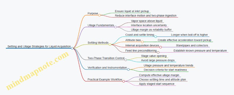
Integrated Example Workflow
- Define pickup geometry and required ullage margin based on interface motion estimates.
- Plan an attitude bias that drives liquid toward the pickup during settling.
- Set a settling window that depends on measured ullage temperature and pressure trends.
- Use a staged valve sequence to minimize vapor ingestion during the first seconds.
- Gate engine start on verification signals that indicate stable thermal and pressure behavior.
This approach keeps the system from treating settling as a ritual. It becomes a controlled, measurable process that turns tank physics into a repeatable acquisition outcome.
5.4 Start Sequence Design for Valves and Pumps
A cryogenic engine start is mostly a choreography problem: each valve and pump action must match the fluid’s current phase state, the available pressure margins, and the thermal condition of the hardware. A good sequence reduces two common failure modes—starting with vapor where you need liquid, and commanding flow rates that exceed what the feed system can supply without flashing.
Start Sequence Foundations
Start sequences are easiest to design when you treat them as three layers that must agree with each other.
- Energy and thermal layer: what temperatures and subcooling levels exist at the tank, feed lines, and engine inlet.
- Hydraulic layer: what pressures exist at each node, and how pressure drops evolve as valves open.
- Control layer: what commands are issued, in what order, and with what interlocks.
A practical rule: every command that changes flow or phase risk should be gated by a measurement that indicates the system is in the expected state. For example, if you plan to open a liquid acquisition valve, you should confirm that the ullage pressure and line temperatures are consistent with liquid being available at the pickup.
Valve and Pump Roles in the Sequence
Valves usually define the “path” for pressure and flow, while pumps define the “ability” to move liquid. That means valve timing often determines whether the pump sees liquid or vapor.
- Preconditioning valves route propellant through warm-up or recirculation paths, or they isolate components to prevent unwanted boil-off migration.
- Acquisition valves connect the tank or settling device to the engine feed path.
- Start valves establish the final feed path to the engine.
- Purge or vent valves remove trapped gas pockets and manage ullage pressure during transitions.
For pumps, the key is avoiding cavitation inception and preventing dry running. A pump start command should be treated like a “permission slip” that requires the feed system to be ready.
Interlock Logic That Prevents Phase Mistakes
Interlocks should be simple, measurable, and specific. A typical set includes:
- Temperature window: confirm line and inlet temperatures indicate subcooled or at least non-flashing conditions for the expected pressure.
- Pressure margin: ensure inlet pressure exceeds the minimum required to avoid flashing at the pump inlet.
- Valve position confirmation: verify commanded positions match actual actuator feedback.
- Two-phase indicators: use differential pressure trends and flow/temperature consistency to detect vapor ingestion.
Example: If the pump inlet differential pressure rises sharply while flow is still low, that can indicate vapor pockets. In that case, the sequence should pause before increasing pump speed or opening additional valves.
Systematic Sequence Flow
A robust sequence can be organized into phases that map directly to physical events.
- Stabilize: verify tank pressure, ullage pressure, and sensor health; ensure no unintended valve leakage paths.
- Prime and purge: establish a controlled path that removes trapped gas from the feed line and manifold.
- Acquire liquid: open acquisition valves in a way that promotes liquid at the pickup; keep engine start valves closed until acquisition is confirmed.
- Start pump: command pump speed only after inlet conditions meet minimum criteria.
- Establish feed: ramp valve openings and pump speed together to follow a pressure-drop budget without exceeding flashing thresholds.
- Engine start: once injector inlet conditions are within limits, proceed with ignition and mixture ratio control.
- Transition to steady: hold valves and pump at their steady-state setpoints; monitor for drift and stop conditions.
Example Sequence with Concrete Timing
Assume a liquid-feed system with a pump and three key valves: a purge/vent valve (V1), an acquisition valve (V2), and an engine start valve (V3).
- T0: confirm sensor validity; verify V1 closed, V2 closed, V3 closed.
- T0+10 s: open V1 to a controlled vent path for a short purge interval; hold until line pressure stabilizes.
- T0+30 s: close V1; open V2 to connect tank liquid to the feed line.
- T0+45 s: wait for acquisition confirmation using ullage pressure and line temperature consistency.
- T0+55 s: start pump at low speed; monitor inlet pressure and differential pressure.
- T0+65 s: open V3 in small increments while ramping pump speed to maintain the desired inlet pressure.
- T0+75 s: when injector inlet conditions are met, proceed to ignition and then continue the ramp to steady.
If acquisition confirmation is not achieved by a defined timeout, the sequence should abort to a safe state: close V2, stop pump, and return to a vented or isolated configuration.
Mind Map: Start Sequence Design for Valves and Pumps
Practical Design Checklist
Before committing to a sequence, verify that each step has: (1) a measurable condition, (2) a clear action, and (3) a defined abort path. A sequence that “works on paper” but lacks abort logic is just a longer way to fail. The best sequences are boring in the right places: they pause when the system is uncertain and proceed only when the measurements agree with the intended phase and pressure state.
5.5 Verification Tests for Start Readiness Criteria
Start readiness is not a single checkbox; it’s a chain of evidence that the engine will see the right propellant phase, composition, and pressure conditions at the right time. The verification plan should move from “can we feed liquid?” to “can we ignite and hold stable combustion?” while keeping the test article representative of flight hardware.
Define Start Readiness Criteria in Measurable Terms
Begin by translating system goals into testable thresholds. A practical set includes: tank ullage temperature and pressure limits, acceptable subcooling or saturation margin at the feed inlet, maximum allowable two-phase fraction in the inlet line, valve response timing, and ignition readiness based on chamber inlet conditions.
Example: If the engine requires liquid at the injector face, set a measurable proxy such as “feed line temperature below saturation by at least X K” plus “inlet pressure above flashing threshold by at least Y kPa.” Then verify those proxies during the same sequence used for start.
Build a Verification Ladder from Components to System
Use a ladder so failures are diagnosable.
- Component checks: valve leak-tightness at cryogenic temperature, actuator stroke timing, sensor calibration drift under cold soak.
- Subsystem checks: feed line thermal equilibrium, boil-off control behavior, settling performance in representative ullage conditions.
- Integrated start tests: full sequence from pressurization through valve transitions to ignition and early steady operation.
This prevents the classic “it failed, but we don’t know why” outcome.
Instrumentation and Data Integrity Checks Before Cryogenic Runs
Before any cryogenic start sequence, confirm that measurements will remain trustworthy.
- Verify temperature sensor placement relative to expected thermal gradients, and confirm wiring thermal contraction does not strain connectors.
- Confirm pressure transducers are within operating temperature range and that any correction factors are applied consistently.
- Validate flow or phase proxies using a controlled warm test where saturation behavior is predictable.
Example: If you use a differential pressure method to infer two-phase presence, run a non-cryogenic calibration to confirm the signal-to-phase mapping still holds after cold soak.
Cold Soak and Equilibrium Verification
Start readiness depends on the state at the moment of valve opening. Cold soak should be long enough to reach stable tank and line conditions.
Verification steps:
- Monitor ullage pressure and representative wall temperatures until their rates of change fall below a preset limit.
- Confirm feed line temperature has approached the expected profile from insulation and heat leak budgeting.
Example: If your heat leak model predicts a 0.5 K/min drift at the feed inlet, set an equilibrium criterion like “drift < 0.1 K/min for 10 minutes” before initiating the start sequence.
Feed System Start Sequence Tests
Run the same timing logic that flight uses, but with controlled variations to test margins.
Key checks during the sequence:
- Valve timing: ensure commanded open/close events match measured position or flow response.
- Pressure transients: verify no sustained underpressure that would trigger flashing.
- Phase behavior: confirm the feed inlet sees the intended liquid condition during the critical window.
Example: Perform a baseline start, then repeat with a slightly higher ullage temperature and slightly lower pressurant pressure to confirm the system still meets the liquid proxy thresholds.
Ignition and Early Combustion Verification
Even perfect feeding can fail at ignition if inlet conditions are off.
Verification steps:
- Confirm ignition system timing relative to injector supply conditions.
- Check that chamber pressure rise rate and mixture ratio indicators fall within acceptable bands.
- Define a “no-go” window: if ignition does not occur within a specified time after reaching inlet conditions, abort and record the state.
Example: If ignition requires a minimum chamber inlet pressure, verify that the measured injector supply pressure crosses that threshold before the ignition command.
Acceptance Testing Logic and Pass-Fail Criteria
Use a structured decision rule.
- Hard limits: any violation of safety or leak-tightness requirements fails the test.
- Soft limits: if a proxy like subcooling is slightly low, allow a limited retest with documented adjustments.
- Sequence integrity: if sensor dropouts or timing mismatches occur, treat the run as invalid.
Example Test Matrix for Practical Coverage
A compact matrix often beats a huge number of random tests.
- Baseline: nominal ullage temperature and pressurant pressure.
- Margin Low: slightly warmer ullage and reduced subcooling margin.
- Margin High: slightly colder ullage and increased density to confirm no overpressure or cavitation-like symptoms.
- Timing Stress: small valve timing offsets within actuator tolerance.
Each run should record the exact state at valve opening and ignition command, so you can tie outcomes to the measured conditions rather than to assumptions.
Documenting Evidence for Readiness Review
Close the loop by summarizing results in a way reviewers can audit.
Include: the measured values at critical timestamps, which criteria were met or violated, sensor health logs, and a short explanation of any deviation tied to a specific subsystem. If the test passes, the evidence should show that the system reached the required propellant state before ignition and maintained it through the early combustion window.
6. Valves Actuators and Cryogenic Fluid Control
6.1 Valve Types and Selection Criteria for Cryogenic Service
Cryogenic valves are not just “cold-rated” versions of common hardware. In ultra-cold service, the valve must manage three coupled problems: sealing at low temperature, reliable actuation despite thermal contraction, and stable flow behavior when flashing or two-phase conditions appear. A good selection starts with the operating envelope, then matches valve type to the dominant failure mode.
Start with the Operating Envelope
Define these inputs before choosing hardware:
- Propellant and temperature range: e.g., LOX at ~90 K or LH2 at ~20 K. The colder the fluid, the more sealing and material choices dominate.
- Pressure range and allowable pressure drop: throttling valves can waste pressure head; on small engines that matters.
- Flow regime: single-phase liquid, saturated mixture, or two-phase flashing during start and transients.
- Cycle count and duty: cryogenic systems often need long dwell times with occasional moves; that changes lubrication and wear assumptions.
- Leak tolerance: some valves can tolerate a tiny seep; others must be effectively bubble-tight.
A practical way to make this concrete: if your feed line can see flashing during a valve opening, prioritize designs that avoid trapped vapor pockets and minimize dead volume.
Map Valve Types to Their Best Jobs
Different valve families handle different “jobs” well. Use the map below to avoid mismatches.
Mind Map: Valve Types and Their Roles
Selection Criteria That Actually Matter
Seal Material and Geometry
At cryogenic temperatures, seals can lose elasticity and shrink away from mating surfaces. Selection criteria include:
- Seal material compatibility with the cryogen and any trace contaminants.
- Compression set behavior after repeated cold cycles.
- Seal geometry that maintains contact pressure as parts contract.
Example: a valve that uses a soft elastomer seal may work at moderate cryogenic temperatures but fail at very low temperatures where the seal becomes too stiff. For LOX service, elastomer choices also must consider oxygen compatibility and swelling behavior.
Thermal Contraction and Mechanical Alignment
Valves experience differential contraction between body, bonnet, stem, and seats. If alignment shifts, the valve may either leak or stick.
Selection criteria:
- Matched materials and clearances designed for the full cooldown profile.
- Stem and seat design that preserves concentricity.
- Actuator coupling that does not overload the stem during contraction.
Example: if a stem seal is designed for room-temperature alignment, a small offset at 90 K can translate into a large reduction in sealing contact area.
Two-Phase Flow Tolerance and Flashing Control
During opening, pressure can drop fast enough to flash liquid into vapor. That vapor can cause:
- Erosion at high-velocity regions.
- Unstable flow that makes control difficult.
- Stiction if vapor forms and collapses in a way that changes forces on moving parts.
Selection criteria:
- Valve internal flow path that limits sudden pressure drops.
- Seat and trim materials resistant to cavitation/erosion.
- Positioning strategy for start sequences that avoids long dwell in unstable regimes.
Example: for a start valve, a two-step opening (crack then full open) can reduce the time spent in the most problematic flashing window.
Actuation Type and Cold Soak Behavior
Common actuation options include solenoid, motor/gear, and pneumatic. In cryogenic service, the key is whether the actuator can deliver required force after cooldown.
Selection criteria:
- Power and force margin at minimum temperature.
- Electrical insulation and coil performance for solenoids.
- Pneumatic supply temperature and dryness to prevent ice formation.
- Fail-safe behavior (what happens on power loss) aligned with mission safety.
Example: a solenoid that meets force at room temperature may lose stroke margin after cooldown if the linkage stiffens or if clearances change.
Leak Rate and Testing Method
Leak requirements should be paired with a realistic test plan. Selection criteria include:
- Specified leak class appropriate to the consequence of leakage.
- Acceptance test conditions that match cryogenic operation as closely as practical.
- Instrumentation plan for verifying seat integrity.
Example: a valve used as a propellant isolation element may require a tighter leak class than a valve used only for flow regulation, because the isolation valve must hold pressure during long coasts.
Practical Selection Workflow
- Classify the valve function: isolation, throttling, metering, check, or relief.
- Determine the dominant flow regime across the full mission timeline, including start and shutdown.
- Set leak and cycle requirements to narrow seal and trim choices.
- Check thermal contraction compatibility between valve and connected hardware.
- Validate actuation margins at the coldest expected condition.
- Confirm flashing and pressure-drop behavior with a flow-path review.
Example Decision: Isolation vs Metering
- Isolation valve: choose a design optimized for long dwell and tight sealing. Prioritize seal geometry, contraction compatibility, and leak class.
- Metering valve: choose a design that can handle throttling without excessive flashing instability. Prioritize trim characteristics, flow stability, and control authority.
If you treat both as “just on/off,” you may end up with a metering valve that chatters during control or an isolation valve that leaks after cooldown. The selection criteria above are the antidote: match the valve’s strengths to the job it must do.
6.2 Actuation Methods Including Solenoid Piezo and Motor Driven
Cryogenic valves and regulators need actuation that stays reliable at low temperatures, across long dwell times, and under tight leak and timing requirements. The actuation method is not just a “how it moves” choice; it determines force margin, thermal contraction behavior, power draw, control bandwidth, and how you handle failures.
Core Actuation Requirements for Cryogenic Service
Start with the job the actuator must do. First, it must generate sufficient stem force to overcome pressure loads and friction at cold temperatures. Second, it must position the valve repeatably enough to meet flow or pressure targets. Third, it must tolerate thermal cycling without binding. A practical way to reason about this is to separate the actuator into three links: electrical or mechanical input, transmission to the stem, and the stem-to-seat interface. If any link loses margin, you get slow response, incomplete closure, or excessive leakage.
Solenoid Actuation Fundamentals
A solenoid converts electrical energy into linear motion. In cryogenic systems, the key issues are coil insulation, magnetic circuit performance at temperature, and the mechanical design that prevents the armature from sticking when materials contract.
A useful mental model is a force budget: electromagnetic force minus spring preload and friction must exceed the maximum required closing force at the worst-case pressure. For example, if a valve needs 120 N at cold and your design provides 160 N at nominal coil temperature, you still need to account for reduced force due to coil temperature rise during repeated cycles. That’s why solenoid designs often include a conservative force margin and a defined duty cycle.
Example: A normally closed cryogenic valve is commanded open for 2 seconds every minute. If the coil heats and the magnetic force drops, the valve might open partially. The fix is not “turn it up forever,” but to ensure the minimum force at the end of the duty cycle still clears the stem friction and pressure load.
Piezo Actuation Fundamentals
Piezoelectric actuators produce motion from electric field changes, typically with very fine displacement resolution. They excel when you need precise small movements, fast response, or tight control of a metering element.
The practical constraint is that piezo motion is small, so you almost always use a mechanical amplification stage such as a flexure lever or a stack-to-stem linkage. Another constraint is that piezo performance depends on temperature and drive voltage stability. In cryogenic service, the drive electronics are usually kept warm, while the actuator is cold; that means you must manage cable thermal contraction and ensure the linkage does not introduce side loads.
Example: A metering valve uses a piezo-driven needle for fine flow trimming. If the linkage introduces lateral friction, the needle may not return fully, causing drift in mixture ratio. The design response is to use symmetric flexures and verify return force with the needle at operating temperature.
Motor Driven Actuation Fundamentals
Motor-driven actuators use a motor plus gearing or a lead screw to translate rotation into stem travel. They are common for larger valves because they can provide high force with controllable positioning.
The main cryogenic concerns are backlash, gear lubrication, and the thermal path between the cold valve and warm motor. Many motor systems use a mechanical transmission that avoids relying on lubricants that can thicken at low temperatures. You also need a strategy for position feedback: open-loop step counts can drift if friction changes with temperature.
Example: A motor-driven isolation valve is cycled during commissioning. After several cold cycles, the valve takes longer to reach the commanded position. If the controller assumes the same friction every time, it may stop early. The fix is to include limit sensing or position verification at least at the end stops, then use those references to correct subsequent moves.
Thermal and Mechanical Integration Across Actuation Types
Regardless of actuator type, cryogenic integration is where reliability is won or lost. Thermal contraction can change clearances, preload, and alignment. A good practice is to design the transmission so that contraction does not create bending moments on the stem. Another practice is to keep the actuator’s moving parts from being exposed to excessive boil-off flow if that flow carries contaminants.
A simple checklist helps: (1) confirm the actuator can reach the required stroke at cold temperature, (2) verify the force margin at maximum differential pressure, (3) ensure the return path is not friction-limited, and (4) validate electrical insulation and connector strain relief for the thermal gradient.
Control and Timing Considerations
Actuation method affects control bandwidth. Solenoids can be fast but are often used in discrete open/close modes unless you add position sensing and closed-loop control. Piezo systems can support fine modulation, but the drive waveform and hysteresis compensation matter. Motor systems support smooth positioning, but their response time is typically slower due to mechanical travel and gearing.
A practical approach is to match actuation to the control objective. If the valve only needs to isolate, discrete solenoid control with robust end-stop detection is often sufficient. If the valve must meter precisely, piezo or a motor with a well-characterized position loop is a better fit.
Mind Map: Actuation Methods for Cryogenic Valves
Example: Choosing Between Solenoid, Piezo, and Motor Driven
Suppose you need an isolation valve for a cryogenic feed line and a separate metering element for mixture ratio control. The isolation valve must reliably seat under pressure and only needs infrequent cycling. A solenoid with end-stop sensing and a verified cold force margin is a straightforward choice. The metering element must adjust flow in small increments with repeatable positioning. A piezo-driven needle with a flexure linkage can provide that fine control, provided the return behavior is validated at temperature. If the metering range requires a larger stroke than piezo can practically provide, a motor-driven actuator with a position loop and cold-verified friction model becomes the safer path.
Summary of System-Level Integration
Solenoids, piezos, and motor-driven actuators each solve a different part of the cryogenic actuation problem. Solenoids emphasize force for discrete moves, piezos emphasize precision for small strokes, and motors emphasize travel and controllability for larger valves. The integrated best practice is to design around the cold-temperature force, stroke, and friction realities, then verify the full actuation chain under representative thermal and pressure conditions.
6.3 Cavitation and Flashing Risks in Valve Manifolds
Cavitation and flashing are two ways cryogenic valve manifolds can misbehave when local pressure drops below the liquid’s saturation pressure. The difference is mostly about what phase forms: cavitation is vapor bubbles forming in a liquid flow field, while flashing is bulk liquid turning to vapor once pressure falls below saturation along a flow path. Both can erode surfaces, destabilize flow, and complicate start and steady operation.
Foundational Pressure Conditions
Start with the pressure budget across the manifold. A valve manifold typically includes upstream tank pressure, line pressure losses, valve pressure drop, and downstream pressure at the engine inlet or regulator. The key check is whether the minimum static pressure anywhere in the manifold falls below the cryogen saturation pressure at the local fluid temperature.
A practical rule: if you can sketch the pressure drop path and mark the lowest-pressure point, you can predict where risk concentrates. In many designs, that point is inside the valve seat region, at sharp area changes, or in a small-volume cavity where flow accelerates.
Cavitation Mechanisms in Valve Geometry
Cavitation begins when the local pressure drops enough for vapor bubbles to form. As the flow moves downstream into higher-pressure regions, bubbles collapse. Collapse near a solid surface is what turns “small bubbles” into “surface damage.”
In valve manifolds, common geometry triggers include:
- Sudden contractions and expansions that create high local acceleration.
- Orifice edges that generate strong vena contracta behavior.
- Dead volumes where recirculation lowers pressure.
A simple example: imagine a cryogenic line feeding a normally closed valve. During a partial opening, the effective flow area grows quickly, but the seat region still forces a high velocity jet through a small gap. That jet can create a low-pressure core just downstream of the seat, where vapor bubbles form even if the upstream and downstream pressures look safe.
Flashing Mechanisms and Two-Phase Consequences
Flashing occurs when the pressure along a path crosses the saturation line for the fluid temperature. Unlike cavitation, which is often tied to local pressure minima in a mostly liquid flow field, flashing can produce a larger vapor fraction that changes the flow regime.
Once vapor fraction rises, the manifold behaves differently:
- Pressure losses increase because two-phase friction is higher than single-phase friction.
- Valve effective flow coefficient can shift because the flow is no longer purely liquid.
- Downstream pressure can oscillate as vapor generation and condensation interact with control actions.
Example: during a start sequence, a controller may command a valve opening to achieve a target inlet pressure. If the manifold flashes, the valve may “appear” to underperform because the same commanded opening yields less liquid mass flow. The controller then compensates by opening further, which can deepen flashing and create a feedback loop.
Risk Indicators and How to Locate the Minimum Pressure
Risk is not just about average pressure; it is about the minimum static pressure. To find it, combine three inputs:
- Valve and fitting loss coefficients across expected openings.
- Line pressure drops from flow rate and fluid properties.
- Thermal state, because saturation pressure depends on temperature.
A useful operational indicator is whether the manifold shows signs of two-phase behavior at the same valve opening and flow rate. For instance, if inlet pressure to the engine feed oscillates while valve position is steady, that often points to vapor generation in the manifold rather than sensor noise.
Design Practices That Reduce Cavitation and Flashing
-
Avoid excessive pressure drop concentration in one element. Spread losses across multiple components so the minimum pressure does not plunge below saturation.
- Example: instead of putting all throttling in a single valve, use a combination of a larger-area control valve plus downstream restriction.
-
Use smooth flow paths and reduce sharp area changes. Streamlined transitions lower local acceleration peaks.
- Example: replacing a sharp-edged reducer with a contoured reducer can reduce the vena contracta intensity.
-
Maintain adequate inlet pressure margin at the valve seat. Set operating limits so the worst-case opening and flow condition still keeps the minimum pressure above saturation.
- Example: if the valve must open to 30% during start, compute the seat-region pressure drop at that opening and verify margin for the coldest expected fluid temperature.
-
Control thermal gradients that change saturation conditions. A colder liquid has lower saturation pressure, which can increase margin; a warmer liquid reduces margin.
- Example: if a manifold section warms during a long hold, the same commanded valve opening can become riskier later.
-
Size lines to limit velocity spikes. High velocity increases local pressure losses and intensifies cavitation tendencies.
- Example: if a small-diameter branch feeds a larger main, ensure the branch does not create a narrow throat at the junction.
Testing and Verification for Valve Manifolds
Verification should reproduce the pressure drop and flow regime that cause the minimum pressure condition. During tests, measure at least:
- Upstream and downstream pressures around the valve.
- Valve position versus flow rate.
- Temperatures near the manifold sections where saturation margin is tight.
A concrete acceptance approach is to define “no two-phase signatures” windows for each critical valve opening. If you observe pressure oscillations, abnormal flow coefficient shifts, or rapid temperature changes consistent with vapor formation, treat that as a sign that the minimum pressure is crossing saturation.
Mind Map: Cavitation and Flashing Risks in Valve Manifolds
Example: Seat-Region Margin Check During Start
Assume a start condition where the valve is commanded to a partial opening. Compute the expected pressure drop across the valve at that opening using the valve’s flow coefficient data, then subtract line losses to estimate the minimum pressure near the seat region. Compare that minimum to the saturation pressure corresponding to the local fluid temperature. If the minimum is within a small margin of saturation, treat that opening as a cavitation/flashing risk zone and adjust the manifold so the throttling is less concentrated or the upstream pressure margin is increased.
6.4 Leak Tightness Requirements and Acceptance Testing
Leak tightness for cryogenic valves and manifolds is not a single number; it’s a chain of evidence. The chain starts with what “leak” means for your mission, then moves through test methods that can actually detect the relevant leak rates, and ends with acceptance criteria tied to the hardware’s intended service.
Foundational Concepts for Cryogenic Leak Tightness
A leak is any unintended path that allows fluid to escape or enter. For cryogenic systems, the practical concern is usually loss of propellant, loss of pressure margin, and contamination of components that must stay clean and dry. Because cryogens boil, even a small leak can create a visible frost pattern and a measurable pressure change.
Leak tightness requirements should be expressed in terms of allowable leak rate and allowable leak location. A common mistake is specifying only a global leak rate without identifying whether the leak can be tolerated at a flange, a valve stem, or a sensor port. Those locations behave differently under thermal cycling and vibration.
Defining Requirements That Match Service
Start by mapping each potential leak path to its consequence.
- External leakage at flanges and fittings can cause propellant loss and ice formation.
- Internal leakage across a closed valve can bypass isolation and upset mixture ratio.
- Stem and actuator leakage can allow cryogen ingress into seals and bearings.
- Porosity or microcracks can be invisible until cold soak or pressure cycling.
A useful acceptance approach is to set separate criteria for: (1) external leakage, (2) internal leakage across critical shutoff elements, and (3) leak growth after thermal and mechanical stress.
Test Strategy Overview
Acceptance testing should be staged so that you don’t “pass” a part that only works at room temperature. A systematic sequence is:
- Baseline leak check at ambient conditions to catch obvious defects.
- Cold-relevant conditioning such as cold soak or thermal cycling to reveal seal contraction issues.
- Pressure and actuation tests to verify leak tightness under realistic pressure gradients.
- Post-test verification to confirm no leak growth.
Mind Map: Leak Tightness Evidence Chain
Selecting a Leak Test Method
Different methods detect different leak sizes and require different assumptions.
- Helium mass spectrometry is sensitive and widely used for small leaks. It works best when helium can reach the leak path and when the test volume and background are controlled.
- Pressure decay is simple but less sensitive for extremely small leaks unless the setup is carefully instrumented and the volume is stable.
- Bubble tests are qualitative and not ideal for acceptance of ultra-tight cryogenic hardware.
For cryogenic propulsion, helium mass spectrometry is often the backbone because it can detect small leak rates that matter for boil-off and long coasts.
Acceptance Criteria That Engineers Can Defend
Acceptance criteria should include:
- A maximum allowable leak rate at a specified test pressure.
- A maximum allowable leak growth after thermal cycling or actuation.
- A location rule stating whether any leak at certain interfaces is automatically disqualifying.
A practical example: if a valve is required to isolate two propellant volumes, internal leakage across the seat might be limited to a tighter threshold than external leakage at a non-critical flange. That prevents “passing” a part that still leaks internally while staying externally clean.
Example Acceptance Workflow for a Cryogenic Valve
Consider a valve intended for liquid feed isolation.
- Ambient helium sniffing around flanges, stem area, and actuator interfaces.
- Seat leakage check by pressurizing one side and monitoring the other at ambient.
- Cold soak to the target cryogenic temperature, then repeat the seat leakage check.
- Actuation under pressure to ensure the seal doesn’t relax after movement.
- Final ambient helium check to confirm no new leak path formed.
If the valve passes ambient checks but fails after cold soak, the failure points are usually seal material contraction, surface finish mismatch, or trapped contamination that becomes mobile at low temperature.
Instrumentation and Calibration Discipline
Leak testing is only as good as the measurement chain. Acceptance should require:
- Calibration traceability for pressure gauges and mass spectrometer response.
- Background leak characterization so the system can distinguish real signals from noise.
- Verification of vacuum or test chamber stability during the measurement window.
A small but important detail: if the test setup includes long tubing runs, thermal gradients can change the effective volume and bias pressure decay results.
Data Reduction and Pass Fail Logic
Document the measurement window, the stabilization time, and the method used to compute leak rate from raw signals. Pass/fail should be based on the computed leak rate and on whether the leak location matches the allowed set.
Case Study: Interpreting a Borderline Result
A part shows a helium signal near a flange during the baseline test, but the signal disappears after tightening to the specified torque.
- If the acceptance plan allows rework and retest, the part can be re-tested.
- If the signal persists after rework, it suggests a surface defect, gasket damage, or misalignment.
- If the signal appears only after cold soak, it points to contraction mismatch or gasket behavior at low temperature.
This logic keeps the decision tied to physical causes rather than “it looks fine today.”
Documentation Requirements for Acceptance Records
Acceptance records should include:
- Test configuration diagram and identification of all interfaces.
- Calibration certificates and instrument settings.
- Raw data plots and the calculation method.
- Clear statements of leak location and whether it is acceptable.
When the record is complete, the next team can reproduce the reasoning without guessing what was assumed during the test.
6.5 Control Valve Characterization for Pressure and Flow Regulation
Control valves are the “translation layer” between your control commands and the cryogenic reality of two-phase flow, flashing, and thermal contraction. Characterization turns a valve from a black box into a predictable component you can model, schedule, and test.
Foundational Concepts for Valve Behavior
A control valve’s job is to convert pressure drop into flow. For cryogenic systems, the key is that the valve’s effective flow area changes with stem position, while the fluid’s density and vapor fraction change with temperature and pressure.
Start with the static relationship: for a given fluid state, flow depends on pressure drop and valve opening. Then add dynamics: the valve moves with actuator lag, and the process responds with line and tank compressibility plus flashing delays.
A practical rule: characterize at the same approximate pressure and temperature range you will regulate, or at least bracket the extremes. If you only test at room temperature, your “model” will be accurate in the same way a map is accurate if the roads are made of fog.
Measurement Setup and Test Points
Use a test rig that can hold upstream pressure, downstream pressure, and fluid temperature stable long enough to measure steady behavior. For cryogenic valves, include a way to prevent uncontrolled flashing upstream of the valve during characterization.
Define a grid of test points:
- Valve position: choose enough points to capture nonlinearity near closed and near full open.
- Pressure drop: cover the range expected in operation.
- Temperature: at least two levels if the valve will see significant subcooling changes.
For each point, record:
- Upstream and downstream pressures.
- Fluid temperature at least upstream of the valve.
- Mass flow rate (or volumetric flow with density correction).
- Stem position and actuator command.
Static Characterization for Flow Coefficients
Characterization typically extracts a flow coefficient such as Cv or its cryogenic-friendly equivalent, plus a relationship between stem position and effective area.
- Determine the valve’s effective flow area curve.
- Plot measured flow versus stem position at fixed pressure drop.
- Expect the curve to be nonlinear because seat geometry and flow regime change with opening.
- Determine the flow coefficient versus pressure drop.
- Repeat at multiple pressure drops.
- If the coefficient changes, it usually indicates regime shifts like flashing or cavitation-like behavior.
- Fit a usable model.
- Use a piecewise-linear or polynomial fit over the operating range.
- Keep the model simple enough that your control engineer can actually implement it.
Example: Building a Usable Cv Map
Suppose you test at two temperatures and three pressure drops. You find that at low pressure drop the valve behaves smoothly, but at high pressure drop the flow increases less than expected. That tells you the valve is entering a regime where vapor formation or throttling losses dominate. In your model, you keep one Cv curve for low drop and a second curve for high drop, rather than forcing one curve to do everything.
Dynamic Characterization for Control Stability
Static curves don’t guarantee stable regulation. Dynamics come from actuator motion and process lag.
Measure:
- Valve step response: command a position change and record actual stem position.
- Flow response: record flow and pressure transients after the step.
From these data, estimate:
- Actuator time constant and any dead time.
- Valve hysteresis between opening and closing.
- Any oscillation tendency caused by compressibility and flashing.
A useful test is a small-amplitude sinusoidal sweep around a nominal operating point. It reveals whether the valve-process loop has phase lag that will fight your controller.
Cavitation, Flashing, and Regime Boundaries
Cryogenic throttling can create vapor at the valve inlet or within the seat region. This changes the effective flow area and can increase noise in pressure and flow signals.
During characterization, watch for:
- Non-repeatability between runs at the same nominal conditions.
- Sudden slope changes in flow versus pressure drop.
- Increased scatter in temperature measurements near the valve.
When you identify a regime boundary, treat it explicitly in the model. Controllers hate surprises, and valves are excellent at producing them.
Hysteresis, Deadband, and Repeatability
Stem-to-area mapping often differs for increasing versus decreasing commands due to friction, seat contact, and thermal contraction effects.
Characterize hysteresis by running paired sweeps:
- Sweep from 0 to 100% opening.
- Sweep back from 100% to 0%.
Quantify deadband by finding the smallest command change that produces a measurable stem movement. In control design, deadband translates into limit cycles or sluggish response unless compensated.
Mind Map: Control Valve Characterization Workflow
Integrated Example: From Data to Control Parameters
Imagine a valve regulating LOX feed where the controller targets a constant downstream pressure. You characterize static behavior and find two regimes: subcooled throttling and flashing-limited throttling. You then fit two Cv curves and include a hysteresis offset in the stem-position mapping.
Next, you measure a step response and find a dead time of 0.2 s and a time constant of 0.6 s for stem motion. In the control model, you add this actuator lag so the controller doesn’t overreact to delayed flow changes. Finally, you validate by running a closed-loop test at a pressure drop near the regime boundary and confirm that the controller remains stable and tracks without hunting.
Acceptance Criteria for Characterized Valves
A characterization is “done” when it supports engineering decisions:
- The static model predicts flow within a defined error band across the operating grid.
- The dynamic model reproduces measured transient timing and damping.
- Hysteresis and deadband are quantified so control logic can account for them.
- Regime boundaries are identified so the model doesn’t silently fail when flashing begins.
When these conditions are met, your pressure and flow regulation stops being a guessing game and becomes a controlled experiment with numbers that behave.
7. Pumps and Turbomachinery for Ultra Cold Propellants
7.1 Pumping Concepts for Cryogenic Liquids
Cryogenic pumping is the art of moving a liquid that is cold enough to behave like a stubborn material: it can flash to vapor, contract the hardware, and punish poor sealing. The goal is simple—deliver the required mass flow and inlet conditions to the engine—but the path is constrained by thermodynamics, two-phase flow, and mechanical limits.
Core Pumping Goals and Constraints
A cryogenic pump must achieve three things at once: (1) provide the required pressure rise, (2) maintain stable inlet conditions to avoid cavitation or flashing, and (3) do so with acceptable leakage and power consumption. For an easy mental model, treat the pump as a pressure converter: it turns shaft power into fluid pressure, but only if the inlet pressure stays above the liquid’s vapor pressure plus a safety margin.
In practice, the inlet margin is often the limiting factor. If the net positive suction head available (NPSHa) drops below the pump’s required NPSH (NPSHr), vapor bubbles form and collapse, damaging surfaces and causing flow oscillations. In cryogenic service, the vapor pressure is higher than you might expect at warmer local spots, so “cold enough” is not a single number—it’s a distribution.
Pumping Architectures and Where They Fit
Cryogenic systems typically use one of three pumping approaches.
- Pressure-fed systems rely on tank pressurant to push liquid through the engine. They avoid pump cavitation issues but can require large pressurant mass and tank pressure.
- Pump-fed systems use a pump to raise pressure at the inlet, improving control of mixture ratio and enabling lower tank pressures.
- Hybrid systems combine modest pressurization with pumping to reduce inlet risk and manage transients.
A practical selection rule is to compare the required pressure rise to the available tank head and the allowable inlet margin. If the engine needs a high inlet pressure and the tank cannot supply it without excessive boil-off, pumping becomes the sensible choice.
Inlet Conditions and Two-Phase Reality
Even when the tank is mostly liquid, the pump inlet can see vapor due to heat leak, flashing in lines, or poor ullage management. Two-phase flow reduces effective density and can change the pump’s operating point. The pump may still spin, but the flow can become unsteady.
A useful example: imagine a line with a small heat leak into a subcooled liquid. As the fluid warms, its temperature approaches saturation at the local pressure. If the line pressure drops slightly due to fittings or control valves, the same warmed fluid may cross into partial flashing. The pump then receives a mixture, and the pressure rise can fluctuate because the pump is now compressing a changing vapor fraction.
Cavitation and Flashing Mechanisms
Cavitation is vapor bubble formation and collapse driven by local pressure dropping below vapor pressure. Flashing is similar in origin but often occurs due to bulk pressure reduction and thermodynamic crossing into two-phase conditions.
To prevent both, designers manage:
- Pressure losses in suction lines and fittings
- Thermal gradients that create warmer pockets
- Flow path geometry that avoids vapor traps and stagnant regions
- Subcooling so the liquid has room to absorb heat without reaching saturation
A simple operational check is to compute the worst-case suction pressure at the pump inlet during the most demanding phase of the mission profile, then compare it to vapor pressure at the highest plausible liquid temperature.
Pump Types and Cryogenic-Specific Considerations
Common pump categories include centrifugal and positive-displacement designs.
- Centrifugal pumps are compact and efficient over a range of flows, but they are sensitive to inlet conditions and can experience cavitation if NPSHa is insufficient.
- Positive-displacement pumps can tolerate some inlet variability and provide predictable volumetric flow, but they may be harder to seal and can impose higher mechanical loads.
Cryogenic service adds constraints: materials must remain ductile at low temperature, seals must handle contraction and differential thermal shrinkage, and bearings must manage lubrication behavior when the fluid is extremely cold.
System Integration Practices That Make Pumping Work
Good pumping is not only about the pump. It’s about the plumbing and the control logic.
- Suction line design: keep suction runs short, minimize fittings, and avoid high points where vapor can accumulate.
- Thermal management: route suction lines to reduce heat leak into the liquid; insulate and support them to limit conduction through structures.
- Start sequencing: ramp conditions so the pump does not ingest vapor during the earliest moments of operation.
- Instrumentation placement: measure suction pressure and temperature close to the pump inlet to detect margin loss before it becomes damage.
Mind Map: Pumping Concepts for Cryogenic Liquids
Example: Estimating Suction Margin in a Simple Case
Assume a pump inlet pressure of 3.0 bar absolute and a worst-case liquid temperature of 90 K. If the vapor pressure of the cryogen at 90 K is 2.2 bar absolute, the margin is 0.8 bar before reaching saturation. Now subtract suction line pressure losses—say 0.3 bar under peak flow—leaving 0.5 bar margin at the pump inlet. If the pump requires a larger margin to avoid cavitation, the design must improve suction conditions by reducing heat leak, lowering losses, or increasing subcooling.
This kind of margin arithmetic is the backbone of cryogenic pumping: it turns “keep it cold” into a measurable inlet condition that can be verified and controlled.
7.2 NPSH Margin Analysis for Low Temperature Feed
NPSH margin analysis answers one practical question: will the feed system stay safely above the condition where vapor bubbles form and collapse in the pump? In cryogenic service, the answer depends on temperature, pressure, line losses, and how “cold” the fluid actually is at the pump inlet. A good analysis starts with definitions, then builds a margin that matches your hardware and test conditions.
Foundations of NPSH and Cavitation
NPSH available (NPSHa) is the energy head at the pump inlet expressed as an equivalent pressure head above the liquid’s vapor pressure. NPSH required (NPSHr) is the pump manufacturer’s threshold where performance degradation begins, typically tied to a specified cavitation index.
For low temperature feed, vapor pressure rises quickly with temperature, so small inlet temperature errors can shrink NPSH margin. Also, cryogenic lines often include long runs, bends, filters, and heat leaks that change both pressure and temperature before the pump.
Step 1: Define the Operating Point
Pick the most demanding condition for cavitation risk. Common choices are:
- Lowest tank pressure during the burn.
- Highest inlet temperature due to boil-off, warm-up, or incomplete subcooling.
- Highest flow rate, because friction losses scale with flow.
- Worst-case configuration, such as a partially restricted strainer or a valve at a less favorable position.
Example: If your mission has a long coast before engine start, the “coldest” tank may not be the “coldest” pump inlet. Use the inlet temperature you expect at the pump, not the tank temperature.
Step 2: Compute NPSH Available
A typical NPSHa expression in pressure terms is:
NPSHa = (P_in − P_vap(T_in))/ρg + (velocity head terms) − (any additional losses expressed as head)
In practice, you compute it from measured or modeled pressures and the vapor pressure at the inlet temperature. For cryogenic liquids, treat P_vap as a function of T_in using your selected property model.
Key inputs:
- P_in: static pressure at the pump inlet flange or sensor location, corrected for any elevation difference.
- T_in: liquid temperature at the same location, after accounting for heat leak and flashing risk in the line.
- ρ: density at T_in and the local pressure range.
Example: Suppose P_in is 3.2 bar(a), and P_vap at T_in is 2.1 bar(a). The pressure head above vapor is only 1.1 bar. If line losses increase by 0.3 bar at high flow, your margin can collapse quickly even though the tank pressure looked healthy.
Step 3: Include Line Losses and Two-Phase Effects
Line losses reduce P_in. Use a pressure drop budget that includes:
- Straight pipe friction.
- Fittings and elbows.
- Filters/strainers.
- Valve throttling and check valves.
- Any additional drop across inlet manifolds.
For cryogenic feed, two-phase behavior can appear near the inlet if local pressure approaches vapor pressure. Even if the bulk remains liquid, micro-flashing can change effective density and friction, and it can alter the inlet conditions seen by the pump.
A conservative approach is to ensure the analysis uses the lowest credible P_in and the highest credible T_in simultaneously. If you have evidence of subcooled liquid throughout the inlet line, you can justify using single-phase losses; otherwise, treat the inlet as potentially near-saturation and tighten the margin.
Step 4: Determine NPSH Required
NPSHr comes from pump curves at your operating speed and flow. Cryogenic pumps may be tested at representative conditions, but your analysis should still map the curve to your actual speed and flow point.
If you interpolate between curve points, do it consistently and keep track of uncertainty. NPSHr is sensitive to operating point, so don’t average across a range that includes the worst flow.
Step 5: Define Margin and Acceptance Criteria
A common engineering rule is to require NPSHa to exceed NPSHr by a safety margin that accounts for uncertainties in temperature, pressure measurement, property data, and modeling of losses. The exact number is project-specific, but the logic is consistent:
- Temperature uncertainty affects P_vap strongly.
- Pressure uncertainty affects P_in directly.
- Loss modeling uncertainty affects the difference between tank pressure and pump inlet pressure.
Example: If your computed NPSHa − NPSHr is 0.4 m, and your combined uncertainty could plausibly be ±0.3 m, you should not treat the result as comfortably safe. Instead, re-evaluate with worst-case T_in and P_in and confirm the margin remains positive with the chosen criterion.
Mind Map: NPSH Margin Analysis Workflow
Worked Example in One Pass
Assume a high-flow start condition. You estimate:
- Pump inlet pressure: P_in = 3.0 bar(a)
- Inlet temperature: T_in = 90 K
- Vapor pressure at 90 K: P_vap = 2.2 bar(a)
- Density at 90 K: ρ = 800 kg/m³
Compute the pressure head above vapor: (P_in − P_vap)/(ρg). With ΔP = 0.8 bar = 8e4 Pa, the head is about 8e4/(800×9.81) ≈ 10.2 m.
If the pump curve at your speed and flow gives NPSHr = 7.0 m, then NPSHa − NPSHr ≈ 3.2 m. Now apply uncertainty: if inlet temperature could rise enough to increase P_vap by 0.3 bar, ΔP becomes 0.5 bar and the head drops to about 6.4 m. The margin becomes negative (6.4 − 7.0), meaning the design or operating condition needs adjustment.
This is why cryogenic NPSH analysis must treat temperature and pressure as coupled, not independent checkboxes.
7.3 Cavitation Inception and Prevention Techniques
Cavitation starts when local pressure in a cryogenic feed line drops below the liquid’s vapor pressure, allowing vapor bubbles to form. In practice, the pressure drop is rarely uniform: it spikes at restrictions, bends, valve seats, and sensor ports. The key idea is to prevent the minimum pressure anywhere in the flow path from crossing the vapor pressure at the local temperature.
Cavitation Inception Foundations
Begin with the pressure margin concept. For a given operating condition, compare the lowest expected static pressure at the most critical location to the vapor pressure corresponding to the local liquid temperature. If the margin is small, small disturbances—like valve throttling changes or a slightly warmer inlet—can trigger bubble formation.
Next, connect inception to flow regime. Two-phase behavior can appear even before classic “bubbles everywhere” cavitation. When flashing begins, vapor volume fraction rises quickly, which then increases local slip between phases and can amplify pressure oscillations. This is why a system can feel stable at one flow rate and suddenly misbehave at another.
Finally, recognize that cryogenic liquids add extra sensitivity. Temperature gradients along a line mean vapor pressure varies with position. A line that is “cold enough” at the inlet can still have a warmer section near an elbow or a poorly insulated valve body, creating a local weak spot.
Where Cavitation Usually Starts
Most cavitation events originate at predictable geometry and control points:
- Throttling elements: control valves, orifices, and partially closed shutoffs create high local velocity and pressure drop.
- Sharp transitions: sudden area changes and short-radius bends increase turbulence and local minima.
- Instrumentation ports: small cavities around pressure taps or flow straighteners can become low-pressure pockets.
- Thermal bridges: metal supports or uninsulated sections warm the fluid, raising vapor pressure.
A practical example: if a feed valve is used to regulate mixture ratio, the valve may spend long periods near a particular opening. That opening sets a repeatable pressure drop pattern, so cavitation can become a “routine” problem at one operating point rather than a rare accident.
Prevention Techniques That Actually Work
1. Increase Available Pressure Margin Raise the upstream pressure or reduce downstream losses so the minimum pressure stays above vapor pressure. In a feed system, this often means:
- Rebalancing the pressure drop budget across filters, lines, and valves.
- Using larger line diameters where mass and thermal constraints allow.
- Selecting valve trims that reduce throttling losses at the required flow range.
2. Reduce Local Throttling and Velocity Peaks Cavitation is driven by local minima, not average pressure. Techniques include:
- Avoiding unnecessary throttling by using control strategies that keep valves closer to their efficient operating region.
- Using flow conditioners or smoother transitions to reduce turbulence-induced pressure dips.
- Ensuring bends use appropriate radii and alignment to avoid secondary flows.
3. Manage Temperature Uniformity Because vapor pressure depends on temperature, thermal control is cavitation control.
- Improve insulation continuity around the most critical components.
- Minimize thermal bridges near valves and sensor locations.
- Route lines so the warmest sections are not also the most restrictive.
A simple check: map the expected temperature profile along the line under steady boil-off and insulation conditions, then identify where vapor pressure is highest. Those locations deserve the most conservative pressure margin.
4. Use Proper Start and Transient Handling Cavitation often appears during transients when pressures and temperatures lag.
- Sequence valves so the system reaches a safe pressure margin before throttling to the final operating point.
- Avoid rapid valve movements that create momentary low-pressure pockets.
- Confirm that the start transient does not pass through a “danger window” of flow rate and inlet temperature.
Example: during engine start, if the feed valve closes slightly to stabilize mixture ratio while pump speed is still ramping, the combined effect can momentarily increase pressure drop. A control tweak that delays that closure until pressure margin is established can eliminate cavitation without changing hardware.
Mind Map: Cavitation Inception and Prevention
Verification and Operational Checks
To confirm prevention measures, verify both steady and transient conditions. Use a pressure-drop model that includes fittings, valves, and filters, then identify the predicted minimum pressure location. Pair that with a temperature model or conservative thermal assumptions to compute vapor pressure at the worst-case point.
Instrumentation placement matters: if you only measure inlet pressure, you can miss the local minimum. Even a single additional pressure measurement near the most restrictive component can turn “mystery cavitation” into a traceable pressure margin problem.
Operationally, treat cavitation as a condition that can be mapped. If you observe performance degradation or unstable behavior at a specific valve opening or flow rate, that pattern usually points to a consistent local pressure minimum. Adjusting the control point or hardware loss distribution at that operating region is often the fastest path to stable, repeatable feed behavior.
7.4 Bearing Sealing And Shaft Dynamics Under Cryogenic Conditions
Cryogenic pumps ask two things of their rotating hardware: keep cryogenic liquid where it belongs, and keep the shaft stable enough that the seals and clearances survive. The tricky part is that “cold” changes both the fluids and the mechanics at the same time.
Foundations of Cryogenic Shaft Dynamics
Start with what the shaft “feels.” At cryogenic temperatures, bearing materials contract, clearances shrink, and lubricant behavior changes. Even if the bearing is designed for a specific cold clearance, the shaft’s effective stiffness can shift because the housing and bearing outer ring may contract at different rates. That means the same rotor speed can produce different vibration amplitudes after cooldown.
A simple way to reason about it is to track three coupled quantities: (1) radial clearance between rotating and stationary parts, (2) squeeze film thickness in any fluid film bearing, and (3) rotor unbalance forces. If the clearance shrinks, the rotor may run closer to the seal faces, increasing the risk of rubbing during transients. If the film thickness drops too far, you can lose hydrodynamic support and move toward mixed or boundary lubrication.
Sealing Goals and Failure Modes
Cryogenic seals must block two pathways: liquid leakage and gas migration. Liquid leakage can cause local freezing at seal interfaces, which increases friction and can trap debris. Gas migration can carry heat into the cold region and increase boil-off, while also changing pressure gradients that drive leakage.
Common failure modes map cleanly to physical causes:
- Rubbing and heat generation from reduced clearances or shaft whip.
- Seal face deformation from thermal contraction mismatch.
- Leak growth from seal material embrittlement or microcracking.
- Contamination-driven wear when ice or particulates form in the seal cavity.
A practical design habit is to treat the seal cavity as a controlled environment: define expected temperatures, pressures, and allowable leakage rates, then ensure the bearing and shaft dynamics do not push the system outside those bounds.
Bearing Types and How Cryogenic Conditions Change Them
For cryogenic pumps, bearings are often selected to match the lubrication strategy.
Rolling element bearings can be attractive because they tolerate low viscosity better than many fluid-film designs, but they still need careful attention to preload and thermal contraction. If preload increases too much at cold temperature, friction rises and the bearing can overheat locally even when the bulk fluid is cold.
Fluid film bearings rely on maintaining a stable film. Cryogenic liquids can alter viscosity and can also introduce two-phase behavior if vapor forms near the bearing region. Two-phase flow can reduce film stiffness and increase vibration.
A useful rule of thumb for analysis is to separate steady-state operation from cooldown and start/stop transients. Many seal and bearing problems happen during those transitions, not at the final operating point.
Shaft Dynamics Under Cooldown and Start Transients
During cooldown, the rotor and housing contract differently, which changes alignment and can shift the rotor’s critical speeds. During start, the shaft may pass through critical speeds while clearances are still settling and seal faces are not yet at their intended temperatures.
To manage this, designers typically combine:
- Thermal sequencing that brings the bearing region and seal faces toward equilibrium before high-speed operation.
- Speed ramps that reduce time spent near critical speeds.
- Runout and alignment control that accounts for cold-state geometry.
A concrete example: if a pump is started immediately after reaching tank pressure but before the bearing housing has cooled to its target temperature, the shaft may experience a larger effective eccentricity. That increases seal face contact probability, especially if the seal uses a spring-loaded element whose force changes with temperature.
Sealing Architecture Coupled to Bearing Behavior
Seals and bearings should be designed as one system. The bearing determines shaft motion; the seal determines allowable motion.
A common integrated approach is:
- Primary seal blocks bulk leakage from the pump fluid.
- Secondary seal provides additional containment and a buffer volume.
- Seal cavity management uses controlled pressure (often via a small barrier flow or gas management) to keep the pressure gradient from driving unwanted leakage.
If the bearing allows excessive shaft orbit, the seal faces see alternating contact pressure. That can create uneven wear and localized freezing. Therefore, seal design targets should include dynamic metrics like allowable shaft displacement amplitude, not just static runout.
Mind Map: Cryogenic Bearing Sealing and Shaft Dynamics
Example: Designing for Cold-State Clearance Without Surprises
Suppose a pump uses a spring-loaded seal and a bearing housing that contracts more than the shaft. At room temperature, the seal spring provides a comfortable contact force. At cryogenic temperature, the shaft-to-housing spacing shrinks, increasing the likelihood of seal face contact even if the spring force drops slightly.
A systematic fix is to compute cold-state geometry and then set acceptance criteria around displacement. For instance, define a maximum allowable shaft orbit at the seal location during the first seconds of operation. Then verify through test that the speed ramp and thermal soak achieve that orbit while leakage stays within the target. This turns “it seems fine” into a measurable condition.
Verification Checklist for Integrated Bearing and Seal Performance
- Confirm cold-state alignment and runout using representative thermal conditions.
- Measure vibration during cooldown-to-start transitions, not only at steady speed.
- Validate seal cavity pressure management so the pressure gradient does not drive leakage.
- Check for rubbing indicators such as friction rise, temperature spikes at seal interfaces, and changes in leakage rate.
- Ensure acceptance criteria include dynamic displacement limits at the seal location.
When bearing dynamics and sealing are treated as a coupled problem, cryogenic hardware becomes less mysterious: the shaft motion sets the seal stress, the seal stress sets friction and heat, and both are governed by thermal timing and geometry.
7.5 Performance Mapping and Test Planning for Cryogenic Pumps
A cryogenic pump’s “performance map” is more than a chart of head versus flow. In practice, it is a set of relationships that let you predict how the pump behaves when inlet pressure, liquid temperature, vapor fraction, and line pressure losses all shift together. A good map also tells you what you cannot trust—usually the parts of the operating envelope where two-phase flow or cavitation dominate.
Foundations of Performance Mapping
Start with the variables that actually move during a cryogenic mission test. For most systems, the primary axes are flow rate and pump speed, while the key dependent outputs are head rise, efficiency, and inlet pressure margin. Then add the cryogenic-specific modifiers: inlet liquid subcooling, ullage pressure, and the likelihood of flashing in the suction line.
A practical mapping workflow uses a consistent test definition:
- Define flow rate at a measurable boundary (often the discharge line) and correct for known line losses.
- Define head rise as the measured discharge total pressure minus suction total pressure, corrected for elevation and sensor offsets.
- Record temperatures at suction, discharge, and key line segments to interpret whether the pump is seeing single-phase liquid or a mixture.
Test Planning Logic from Simple to Complex
Plan tests in layers so you can attribute changes to one cause at a time.
-
Baseline single-phase mapping: Use the coldest stable liquid condition that still guarantees suction is fully liquid. Sweep speed across the intended operating range and step flow through a few points that cover low, mid, and high flow.
-
Inlet condition stress: Keep speed and discharge pressure targets fixed while reducing inlet subcooling or raising ullage pressure. This reveals how the pump curve shifts when suction becomes more prone to flashing.
-
System integration mapping: Add representative upstream and downstream line restrictions. Now the pump map becomes a system map: the operating point is where pump head rise intersects system pressure losses.
A simple example: if your discharge valve throttling increases line losses, the system curve rotates upward. The pump will move to a lower flow point even if speed is unchanged. If you only tested with a fixed discharge pressure, you might miss that shift.
Instrumentation and Data Quality Checks
Cryogenic pump data is only as good as its pressure and temperature integrity.
- Use fast-response pressure transducers near suction and discharge to capture transient pressure dips during valve transitions.
- Calibrate temperature sensors for cryogenic ranges and verify wiring thermal conduction paths so sensor readings reflect fluid temperature, not wall temperature.
- Log differential pressure across suction strainers or filters if present, since clogging or thermal contraction can change effective NPSH.
Before plotting curves, apply sanity checks:
- Verify mass balance between inlet and outlet flow measurements.
- Confirm that head rise trends smoothly with flow at constant speed; jagged plots often indicate sensor timing mismatch or two-phase interference.
Building the Map and Interpreting It
Construct curves for each speed setting: head rise versus flow, efficiency versus flow, and inlet margin versus flow. Then overlay stability and cavitation indicators.
Cavitation is not just “bad sound.” In data terms, it often shows up as:
- A head curve that flattens or drops at a particular flow.
- Efficiency falling faster than expected.
- Increased vibration or pressure oscillation amplitude near suction.
A useful interpretation method is to mark the first consistent deviation from the baseline single-phase trend as the onset region. Then define a conservative operating limit that stays away from that onset by a margin tied to your uncertainty.
Example Test Matrix for a Cryogenic Pump
Assume you test at three speeds: 70%, 85%, and 100% of nominal. For each speed, you test five flow points and two inlet subcooling levels.
| Speed Setting | Flow Points | Inlet Subcooling Levels | Total Runs |
|---|---|---|---|
| 70% | 5 | 2 | 10 |
| 85% | 5 | 2 | 10 |
| 100% | 5 | 2 | 10 |
If each run includes a short stabilization period and a steady sampling window, you can estimate total test time and ensure the cryogenic facility can maintain stable conditions without drifting.
Mind Map: Performance Mapping and Test Planning
Practical Acceptance Criteria for the Map
A map is “usable” when it reproduces measured operating points under at least one integrated condition set. For example, after building the map from baseline runs, run one integrated test with a different discharge restriction and verify that the predicted flow at the chosen speed matches within your defined uncertainty band. If it does not, the likely causes are unmodeled line losses, sensor offsets, or suction two-phase effects that were not captured in the mapping phase.
8. Pressurization Systems and High Pressure Gas Management
8.1 Pressurant Selection and Thermodynamic Behavior
Pressurization systems keep cryogenic tanks and feed lines within safe pressure limits while ensuring the engine receives the right propellant phase and pressure. Pressurant choice is mostly about thermodynamics: how the gas temperature and density change as it expands, how it interacts with cold hardware, and how much pressure margin it can maintain without turning into a liquid problem.
Foundational Requirements for Pressurant Gases
A pressurant must (1) provide sufficient initial tank pressure, (2) maintain pressure during the mission’s propellant drawdown, (3) avoid freezing or condensing inside the tank and lines, and (4) remain chemically compatible with materials and any trace contaminants.
A practical way to reason is to treat the tank as a control volume with a gas space (ullage) that shrinks as liquid level rises. As propellant is used, the ullage volume increases, and the pressurant expands. Expansion cools the gas, which can reduce pressure faster than you’d expect from volume change alone. That coupling is why thermodynamic behavior matters.
Core Thermodynamic Model for Tank Pressurization
For many preliminary designs, assume the pressurant behaves approximately as an ideal gas and the ullage process is quasi-adiabatic over short intervals. Then pressure and temperature are linked through the gas law and the expansion relation.
A useful mental model: if the ullage expands from V1 to V2, the pressure drops. If the gas also cools from T1 to T2, the pressure drop is amplified. In real systems, heat transfer from the tank wall and insulation can partially offset cooling, so the effective behavior lies between fully adiabatic and fully isothermal.
Selecting Pressurant Based on Condensation and Freezing Risk
The biggest “gotcha” is phase change. Even if the pressurant is a gas at room temperature, it can cool enough in the tank to condense or freeze, especially near cold surfaces. Condensation reduces the available gas moles, causing pressure to fall more than predicted by simple expansion.
Selection criteria therefore include:
- Saturation margin: compare expected ullage temperatures to the pressurant’s saturation curve.
- Thermal coupling: estimate how quickly the gas temperature approaches wall temperature.
- Impurity sensitivity: trace water or oxygen can create freezing or chemical issues at cryogenic temperatures.
A concrete example: suppose you start with a high-pressure nitrogen bottle and feed it into a tank with a very cold wall. If the ullage temperature drops close to nitrogen’s saturation conditions, a small amount of condensation can occur. Even a modest loss of gas moles can noticeably change the pressure-time curve during long coast phases.
Comparing Common Pressurants by Behavior
Nitrogen (N₂) is widely used because it is inert, has manageable saturation behavior for typical cryogenic tank temperatures, and is relatively easy to source and handle. Its thermodynamic properties are well characterized, which helps with modeling and test correlation.
Helium (He) has higher thermal conductivity and lower molecular weight, which affects heat transfer and expansion behavior. It tends to be less prone to condensation at cryogenic temperatures, but it can leak more readily through small clearances due to its small molecular size.
Argon (Ar) can be attractive for some temperature ranges, but its condensation behavior must be checked carefully against the tank’s coldest regions and expected ullage temperatures.
The selection is not “which is best,” but “which stays in the gas phase with acceptable leakage and acceptable pressure margin.”
Heat Transfer and Why Insulation Changes Pressure
Even if you model expansion correctly, heat leak through insulation changes the gas temperature. If heat flows into the ullage, the gas warms, slowing the pressure decay. If heat flows out, the gas cools, accelerating pressure decay.
A simple example helps: two tanks have the same initial pressure and same propellant draw profile. The better-insulated tank keeps the ullage warmer, so pressure stays higher for longer. That means insulation performance can be traded against pressurant mass or initial pressure, but only if you model the coupled thermal-pressure behavior.
Regulator and Blowdown Effects on Thermodynamic State
Pressurization hardware often includes regulators and relief devices. When the regulator opens, the incoming gas can be at a different temperature than the ullage. Mixing changes the ullage temperature and therefore pressure.
During blowdown or venting, the escaping gas carries enthalpy away. That can cool the remaining ullage, again affecting pressure beyond volume change. For accurate pressure margin, include regulator flow temperature and vent enthalpy in the mass and energy balance.
Practical Design Workflow for Thermodynamic Behavior
- Define ullage temperature bounds using tank thermal models and expected heat leak.
- Estimate expansion path from propellant drawdown and ullage volume change.
- Check phase-change margins by comparing predicted ullage states to saturation conditions.
- Include mixing and regulator temperature if active pressurization is used.
- Validate with a pressure-time model and confirm with cold tests using representative fill levels.
Mind Map: Pressurant Selection and Thermodynamic Behavior
Example: Pressure Margin Check with Condensation Risk
Assume a tank starts at a known ullage pressure and temperature. As propellant is consumed, ullage volume increases and the gas cools due to expansion. If the predicted ullage temperature approaches the pressurant’s saturation temperature, the model should be adjusted to account for possible condensation. A practical check is to compute the saturation pressure at the predicted ullage temperature; if the tank pressure falls below that saturation pressure while the system is still cold, condensation is likely. The fix is usually one of: increase initial pressure, improve insulation to keep ullage warmer, reduce thermal coupling to cold surfaces, or select a pressurant with a safer gas-phase margin.
8.2 Regulator Design for Cryogenic Compatible Pressure Control
Cryogenic pressure control is mostly about keeping the regulator from becoming a temperature-driven chemistry experiment. The regulator has to sense pressure accurately, move fluid reliably at low temperatures, and avoid creating new heat paths that worsen boil-off or cause two-phase surprises.
Foundational Requirements for Cryogenic Regulators
Start with what “pressure control” means in this context: the regulator must maintain a target downstream pressure while the upstream tank pressure and fluid properties change as the system cools and boils. In practice, the downstream pressure is often the feed header or a pressurant line that supplies a tank ullage.
Two constraints dominate. First, cryogenic fluids can flash when local pressure drops below saturation, so the regulator’s internal pressure losses must be managed. Second, materials and seals must tolerate thermal contraction and differential shrinkage without losing tightness.
A useful mental model is to treat the regulator as three coupled subsystems: (1) a flow restriction that sets pressure drop, (2) a control element that modulates that restriction, and (3) a thermal and mechanical environment that determines how the element behaves as temperatures change.
Sensing and Control Strategy
Pressure sensing can be direct (sensor at the regulated side) or inferred (sensor at upstream with a modeled drop). Direct sensing is usually more robust because it captures the actual pressure seen by the downstream hardware.
For control stability, decide whether you are regulating a gas pressurant or a liquid feed. Gas regulation tolerates more compressibility and can show slower dynamics; liquid regulation can be fast but is sensitive to flashing and two-phase flow. A regulator that “works” on a bench with warm gas may behave differently when the same valve sees cold, partially vaporizing fluid.
Example: If you regulate helium pressurant to keep tank ullage pressure near a setpoint, place the sensor close to the ullage volume or the ullage manifold. If you instead sense upstream, the regulator may chase its own pressure drop and oscillate as the tank pressure falls.
Flow Path Geometry and Pressure Drop Budgeting
Regulators are not magic; they are controlled pressure drops. Build a pressure-drop budget that includes the regulator, downstream lines, fittings, and any filters. Then ensure the minimum pressure anywhere in the regulator body stays above the saturation pressure for the fluid at the local temperature.
This is where “cryogenic compatible” becomes concrete. A regulator with a narrow throttling section can create localized cooling and flashing. Even if the bulk line pressure is safe, the throttling region can cross into two-phase territory, changing flow resistance and causing control hunting.
Practical approach: Use a larger effective flow area where possible, and keep throttling lengths short. If you must use a fine restriction for stability, add a design margin so that the throttling region does not reach saturation during worst-case heat leak and transient conditions.
Thermal Design and Heat Leak Management
A regulator can add heat to the system through conduction along its body, through radiation to cold surfaces, and through heat carried by the flowing fluid. Thermal design is therefore part of pressure control.
Key tactics include minimizing conductive bridges between warm and cold structures, using thermal breaks, and selecting mounting strategies that reduce direct metal-to-metal paths. Also consider that the regulator body temperature may lag the line temperature during cold soak, so the control element may not be at the temperature assumed by your flow model.
Example: During cold soak, a regulator mounted on a warm bracket may stay warmer than the adjacent cryogenic line. The resulting density and viscosity differences can shift the effective flow resistance, so the downstream pressure may drift until thermal equilibrium.
Materials, Seals, and Cryogenic Mechanical Behavior
Regulator performance depends on seal integrity and actuator motion. Elastomers can harden at cryogenic temperatures, so seal selection must match the minimum operating temperature and the expected thermal cycling count.
Also account for differential contraction. If the valve seat, stem, and actuator components contract at different rates, the setpoint may shift or the valve may stick. Design for predictable clearances at operating temperature, not at room temperature.
A simple check: compute the expected contraction over the relevant temperature range for each critical interface. Then verify that the resulting clearances still allow full travel and maintain sealing contact under pressure.
Actuation and Control Element Choices
Common cryogenic regulator approaches include spring-loaded pressure regulators and actively controlled valves. Spring-loaded regulators can be compact and reliable, but their setpoint can drift with temperature if the spring and sensing element are not thermally managed.
Actively controlled valves can compensate for drift by using feedback, but they require careful attention to sensor placement, actuator thermal effects, and control loop tuning.
Example: If you use an actively controlled regulator for a liquid feed line, tune the loop with the expected two-phase sensitivity in mind. A controller that is too aggressive can drive the valve into a flashing regime, which then changes the flow resistance and makes the loop chase its own tail.
Verification Testing and Acceptance Criteria
Testing should confirm both pressure control and cryogenic survivability. Use cold-soak tests to verify that the regulator maintains setpoint without sticking, leaking, or producing unstable oscillations.
Acceptance criteria typically include:
- Setpoint accuracy over the expected upstream pressure range
- Stability metrics such as overshoot and oscillation amplitude
- Leak rate at operating temperature
- Response time within the mission’s transient envelope
Mind Map: Regulator Design for Cryogenic Compatible Pressure Control
Integrated Design Example for Ullage Pressurization
Consider a system regulating helium pressurant into a tank ullage. Choose a regulator that senses ullage-side pressure directly. Budget pressure drop so the regulator throttling region does not fall below helium saturation at the coldest expected local temperature. Add thermal breaks to reduce conduction from warm structures into the cryogenic line. Select seals rated for the minimum temperature and verify contraction clearances at operating conditions.
During cold soak, expect a temporary setpoint drift if the regulator body temperature lags the line. Use test data to confirm that the control loop (or spring setpoint) settles within the allowed time window, and verify that stability remains acceptable as upstream pressure decreases.
8.3 Blowdown Analysis and Pressure Stability Requirements
Blowdown systems use stored pressurant to push cryogenic propellant through the feed system as tank pressure falls over time. The job of blowdown analysis is to predict how pressure, flow, and temperatures evolve together, then set stability requirements so the engine sees acceptable inlet conditions from first start through the end of the burn.
Foundational Model of Blowdown Behavior
Start with a simple energy-and-mass picture: pressurant expands, tank pressure drops, and the propellant flow rate changes because the pressure difference across valves and lines changes. A practical first model treats the pressurant as a compressible gas and the tank as a control volume with a known ullage volume. Even if you later use a higher-fidelity model, this baseline is useful because it exposes which assumptions dominate.
A common workflow is:
- Define initial tank pressure, ullage volume, and pressurant mass.
- Specify the propellant mass flow demand profile (constant mixture ratio or measured engine demand).
- Compute pressurant expansion and resulting tank pressure versus time.
- Convert tank pressure into feed-line pressure at the engine inlet using pressure-drop budgets.
Pressure stability requirements then translate into bounds on engine inlet pressure and, for cryogenic systems, bounds on feed conditions that prevent flashing or two-phase ingestion.
Pressure Stability Requirements That Actually Matter
Engine hardware cares about pressure at specific interfaces, not about tank pressure in isolation. Set requirements at the engine inlet and at any sensitive valve or regulator outlet.
Typical stability constraints include:
- Minimum inlet pressure to maintain adequate margin over vapor pressure and avoid cavitation/flash in downstream components.
- Maximum inlet pressure to protect regulators, valves, and injector manifolds from exceeding design limits.
- Rate-of-change limits so control valves and regulators can respond without hunting or saturating.
- Mixture ratio stability indirectly enforced by keeping the propellant feed pressure within the range where flow coefficients remain predictable.
A concrete example: if your injector requires at least 2.5 bar at the inlet to keep liquid acquisition reliable, then your blowdown analysis must show that the feed-line pressure stays above 2.5 bar for the entire burn segment where the engine is throttled or where ullage conditions are worst.
Pressure Drop Budgeting from Tank to Engine
Pressure stability is only as good as the pressure-drop model. Build a budget that includes:
- Static head and acceleration terms (small in microgravity but not always negligible in long lines).
- Friction losses in straight runs.
- Local losses from bends, tees, filters, and valve throttling.
- Additional losses when the flow regime changes, such as when flashing begins.
A useful habit is to compute pressure drops at several representative points: start, mid-burn, and end-of-burn. If the pressure margin is tight only at one point, you can focus design changes there rather than overbuilding everywhere.
Blowdown Thermodynamics with Practical Assumptions
Pressurant expansion can be modeled as isothermal, adiabatic, or polytropic. Real systems often land between extremes because heat transfer occurs through tank walls and insulation supports.
To keep the analysis systematic, treat the thermodynamic model as a parameterized choice:
- Use an adiabatic assumption for a conservative lower-bound on pressure at a given time.
- Use a near-isothermal assumption for an upper-bound.
- If you have measured or estimated heat transfer coefficients, use a polytropic exponent to interpolate.
Then validate the chosen model against a simple ground test where tank pressure decay is measured with no propellant flow. That test isolates the pressurant behavior so the later end-to-end feed test can focus on flow-induced effects.
Mind Map: Blowdown Analysis and Stability
Example Margin Check with a Simple Budget
Assume a blowdown tank starts at 30 bar with ullage volume fixed. Your feed-line budget at nominal flow shows that when tank pressure is 10 bar, engine inlet pressure is 2.6 bar. Your stability requirement is a minimum inlet pressure of 2.5 bar.
Now run the blowdown model to find the time when tank pressure drops to 9.6 bar. If the model predicts that 9.6 bar occurs after the planned burn end, you have margin. If it occurs early, you have options that are analysis-driven:
- Reduce pressure drops by revising line sizing or filter restriction.
- Adjust valve opening schedules to reduce throttling losses early.
- Increase initial pressurant mass or initial tank pressure within design limits.
The key is that each action changes a specific term in the budget, so the next iteration is targeted rather than guessy.
Advanced Details That Prevent “It Worked on Paper”
- Two-phase onset coupling: If flashing begins in the feed line, pressure drops can increase sharply and flow can become less predictable. Include a criterion based on local pressure relative to saturation conditions and check it along the line.
- Valve coefficient variation: Valve flow coefficients can change with temperature and pressure. Use characterization data at relevant conditions or apply conservative coefficients.
- Sensor placement effects: If your inlet pressure sensor is upstream of a restriction, the measured pressure may look stable while the engine-facing pressure is not. Align stability requirements with the true interface.
Summary of What to Deliver
A complete blowdown analysis package should produce time histories of tank pressure, engine inlet pressure, and flow rate, plus a margin table that shows compliance with minimum and maximum inlet pressure limits and any rate-of-change constraints at the critical burn segments.
8.4 Gas Storage Tanks and Safety Relief Design
Cryogenic propulsion pressurization usually relies on a stored gas that warms, expands, and feeds the tank ullage. The tank and relief system must handle three realities at once: cryogenic compatibility, pressure transients, and credible failure modes. A good design starts with what the gas is allowed to do, then works backward to the hardware.
Foundational Requirements for Stored Pressurant
A gas storage tank must meet pressure containment and leak tightness requirements across the mission profile. Even if the tank sits “quiet” most of the time, it experiences thermal cycling, regulator cycling, and occasional valve events. Begin by defining:
- Maximum allowable pressure at every downstream interface, including regulators and relief valves.
- Normal operating pressure range so regulators do not chatter or drift into unstable control.
- Permissible leak rate for the pressurant path, since small leaks can change ullage pressure and mixture ratio.
A practical example: if your regulator outlet is specified for 2.0 MPa nominal with a 2.2 MPa upper limit, the relief system must ensure the regulator never sees above its limit even during regulator failure or blocked outlet scenarios.
Tank Types and Selection Logic
Stored gas tanks are typically either high-pressure composite cylinders or metallic pressure vessels. Selection is driven by mass, allowable stress, manufacturing maturity, and compatibility with the pressurant gas.
- Composite cylinders often reduce mass but require careful handling of burst margins, liner integrity, and valve attachment details.
- Metallic vessels can be robust for repeated thermal cycles and are easier to inspect internally, but may be heavier.
Whichever type is chosen, the design must include a valve and fitting plan that avoids trapped volumes and minimizes dead legs. Dead legs matter because they can accumulate condensable contaminants and later release them as pressure changes.
Thermal and Pressure Behavior That Drives Design
Gas temperature determines pressure through the ideal gas law as a first approximation, but real systems deviate due to non-ideal behavior and heat transfer limits. The design process should include:
- Worst-case warm-up: assume the tank reaches the highest credible temperature from environment or heat leak.
- Regulator and line heat soak: account for how quickly the gas warms after a valve opens.
- Blowdown event: estimate pressure drop when a regulator fails open or a relief event occurs.
Example: if a helium tank is stored at 20 K and can warm to 300 K, pressure can increase by roughly the temperature ratio. Even if the regulator limits normal operation, the relief system must protect against the tank reaching its own allowable limits.
Safety Relief Design Principles
Relief devices exist to prevent overpressure of the tank and connected components. The key is to ensure the relief path is sized and located so it actually relieves the right volume at the right time.
Relief Valve Placement and Isolation
Relief valves should be installed so that any credible overpressure source can discharge to a safe direction without being blocked by check valves, closed isolation valves, or trapped segments. If you use isolation valves for maintenance, ensure they cannot accidentally isolate the relief path during normal operation.
A simple rule of thumb: if a failure could raise pressure in a segment, that segment needs a relief path that bypasses the failure.
Sizing for Mass Flow and Backpressure
Sizing depends on the maximum relieving pressure and the required discharge mass flow. The calculation must consider:
- Choked flow possibility for gases at high pressure ratios.
- Discharge coefficient and flow losses through piping and fittings.
- Backpressure at the discharge location, which can reduce effective relieving pressure.
Example: if the discharge plenum is restrictive, backpressure can rise during a relief event, increasing the pressure seen by the protected component. The relief system must be evaluated as a full flow path, not just the valve.
Burst Disks and Redundancy
Burst disks can provide a predictable rupture pressure and are sometimes used in combination with relief valves. If used, ensure the burst disk does not create a hazardous fragment hazard or block the downstream relief route.
Redundancy should be functional, not just numerical. Two relief devices that share the same blocked discharge path do not provide meaningful protection.
Integrated Example Workflow
Consider a pressurant tank feeding a regulator. You can structure the design workflow like this:
- Determine tank allowable pressure and relief set pressure with margins.
- Compute worst-case warm-up pressure and identify whether normal operation ever approaches set pressure.
- Define failure cases: regulator stuck closed, regulator stuck open, blocked outlet, and valve leakage.
- For each case, evaluate which segment overpressures and where relief must act.
- Size relief devices using the maximum relieving scenario and verify discharge piping backpressure.
If the regulator outlet is blocked, the tank pressure may rise until the tank relief opens. That means the tank relief must be sized for the maximum credible mass flow into the blocked segment, including any heat-driven expansion.
Mind Map: Gas Storage Tanks and Safety Relief Design
Quick Design Example for Relief Set Pressure
Suppose a tank has an allowable pressure of 25 MPa. Choose a relief set pressure below that limit with margin for measurement tolerance and transient overshoot. Then verify that, under the worst credible warm-up and failure case, the relief valve opens before the tank approaches its allowable limit. Finally, confirm that the discharge piping can handle the relieving mass flow without excessive backpressure.
This approach keeps the system grounded: you are not just picking a number for a relief set, you are ensuring the entire flow path and failure logic actually prevent overpressure where it matters.
8.5 Integration of Pressurization with Tank and Feed Hardware
Pressurization is not a standalone subsystem; it is the “muscle” that moves propellant through the feed system while keeping tank conditions inside safe limits. Integration means coordinating three interfaces: (1) tank ullage and relief behavior, (2) feed line pressure and phase state, and (3) valve and regulator control logic.
Foundational Coupling Between Tank and Pressurant
A pressurant system typically supplies gas to the tank ullage. That gas pressure must be high enough to overcome static head, line losses, and any throttling needed for stable injector conditions. A simple way to reason about it is to write a pressure budget at the engine inlet: tank ullage pressure minus tank-to-feed pressure drops minus any intentional regulator drop equals required inlet pressure. If you treat the regulator as a “black box,” you’ll eventually discover that its drop changes with flow, temperature, and upstream pressure.
Example: Suppose the engine needs 2.5 MPa at the injector inlet. The feed line losses at the target flow are 0.15 MPa, and the regulator drop at that flow is 0.05 MPa. Then the tank ullage pressure must be about 2.70 MPa. If the tank pressure is only 2.55 MPa, the engine may start but will likely drift toward mixture ratio errors as the system settles.
Hardware Interfaces That Must Agree
Integration is mostly about matching assumptions across components.
- Regulator setpoint and tank pressure range: The regulator must remain in its intended control region across the tank’s pressure decay or blowdown profile.
- Relief valve sizing and vent path: Relief devices must relieve the correct energy source, whether it is heat leak causing boil-off, regulator malfunction, or blocked vent scenarios.
- Check valves and backflow paths: A check valve prevents pressurant from migrating into lines where it can cause unwanted phase changes or contaminate measurement points.
- Thermal contraction and line routing: Gas lines often see different thermal gradients than liquid lines. If you mount them rigidly without accounting for contraction, you can create stress that later shows up as leaks.
Example: If a check valve is placed after a pressure sensor, a stuck-open check can bypass the sensor’s location and make the sensor read “normal” while the downstream manifold sees a different pressure.
Control Logic Integration for Stable Feed
Pressurization control usually targets tank pressure (or tank pressure plus a feed condition proxy). The feed system then uses valves to meter liquid to the engine. The key integration rule is to avoid fighting loops: if both tank pressure control and feed throttling try to correct the same variable, you can get oscillations.
A practical approach is to choose one “primary” loop and one “secondary” loop.
- Primary loop: Regulate tank ullage pressure using the pressurant regulator and/or heater strategy.
- Secondary loop: Use feed valves to achieve the commanded engine mixture ratio and thrust profile.
Example: During start, you may temporarily bias ullage pressure higher to ensure liquid acquisition and avoid two-phase ingestion. After ignition stabilizes, you return to the steady setpoint so the regulator doesn’t continuously chase a transient.
Phase State Awareness at the Tank-to-Feed Boundary
Even if the tank pressure is correct, the feed can still misbehave if the liquid is not in the right phase state when it reaches the inlet. Integration therefore includes ensuring that ullage pressure and tank thermal conditions keep the liquid subcooled enough to prevent flashing in sensitive sections.
Example: If a regulator causes a sudden pressure drop at the tank outlet, the local pressure in a downstream line segment can fall below the saturation pressure corresponding to the local liquid temperature. The result is flashing that looks like “mysterious” flow instability. The fix is not only changing setpoints; it may require revising regulator placement, adding a small buffer volume, or adjusting line thermal management.
Sizing and Budgeting with Integrated Assumptions
Integrated sizing uses the same operating scenarios across tank, regulator, and feed.
- Mass flow balance: Pressurant mass flow must cover boil-off and any leakage while maintaining ullage pressure.
- Energy balance: Heat leak drives boil-off; regulator and line temperatures affect gas density and therefore pressure response.
- Pressure drop budget: Include regulator drop, check valve losses, and manifold losses at the same flow points used in engine inlet requirements.
Example: If you size the regulator for nominal flow but ignore that the feed valves open in steps, the regulator may momentarily saturate. That saturation can create a tank pressure dip that is large enough to trigger a start abort, even though steady-state calculations look fine.
Mind Map: Pressurization Integration with Tank and Feed
Example Integration Walkthrough
Consider a typical sequence: prepressurize, start, steady burn, and shutdown.
- Prepressurize: Raise tank ullage pressure to a level that ensures the feed line remains single-phase up to the acquisition point. Confirm that relief valves remain closed and that no unexpected venting occurs.
- Start: Command feed valves to establish liquid flow while holding tank pressure under the primary loop. If the engine requires a higher inlet pressure during ignition, apply a short ullage bias and then remove it once combustion stabilizes.
- Steady Burn: Keep regulator control within its stable region. Monitor pressure trends at both tank and feed-side measurement points to detect mismatch caused by unexpected pressure drops.
- Shutdown: Reduce feed flow first, then manage ullage pressure decay according to the tank’s allowable limits. Ensure that check valves prevent reverse migration when pressures equalize.
This sequence works because each step uses consistent pressure budgets and coordinated loop roles, so the tank, regulator, and feed hardware are solving the same problem at the same time.
9. Engine Feed Manifolds and Injector Interface Design
9.1 Manifold Layouts for Minimizing Thermal Gradients
Cryogenic feed manifolds are basically heat-exchange machines that you want to control rather than fight. Thermal gradients matter because they change local phase state, shift pressure drops, and can create uneven mixture ratio at the injector. The goal is to keep the manifold “thermally boring”: predictable temperatures along each flow path, with minimal hot spots and minimal cross-flow mixing through the structure.
Foundational Principles for Gradient Control
Start with the heat-leak budget. Every watt entering the manifold must go somewhere: warming the liquid, generating vapor, or raising the wall temperature. If one branch receives more heat than another, its vapor fraction rises first, which changes effective density and pressure drop. A practical layout rule is to treat each branch as a thermal twin: similar length, similar insulation thickness, similar support conduction paths, and similar exposure to radiation.
Next, separate the manifold into functional zones. A typical zone set is:
- Acquisition zone near the tank outlet where ullage and liquid interface conditions can vary.
- Distribution zone where flow splits to multiple injector lines.
- Conditioning zone near the engine interface where final pressure and phase requirements must be met.
Thermal gradients are worst at zone boundaries because geometry changes and conduction paths change. So you design those boundaries to be smooth in both shape and insulation continuity.
Layout Strategies That Work in Practice
1. Symmetry and equal hydraulic paths If two injector lines see different pressure drops, the mixture ratio shifts even when the control system commands the same setpoint. Use equalized line lengths and diameters from the manifold split to each injector connection. Then check that the thermal environment is also similar: same insulation wrap, same standoff to warm structures, and same support bracket pattern.
Example: For a 6-injector engine, route three pairs of lines in mirrored positions around the manifold centerline. Keep the split point centered so each pair has matching conduit length and matching bend count. Even if the engine bay has a “warm side,” the mirrored routing reduces the chance that only one half of the manifold gets extra radiation.
2. Minimize conduction through supports Supports can be the dominant heat path if they bridge from warm structure to cold manifold. Use low-conductivity standoffs, reduce cross-sectional area, and avoid continuous metal straps. If you must use metal, interrupt it with thermal breaks and keep support contact areas small.
Example: Replace a single continuous mounting ring with three discrete pads spaced around the manifold. The pads carry load, while the gaps reduce conduction area. Then verify that the pads do not create localized hot spots by checking wall temperature near each pad during a cold-soak test.
3. Control radiation with geometry and insulation continuity Radiation doesn’t care about your flow symmetry; it cares about view factors. Use reflective multilayer insulation where appropriate, but also ensure insulation is continuous across joints. A small gap at a flange can create a direct line-of-sight to a warmer surface, producing a localized hot spot.
Example: If the manifold attaches to a flange that is partially uninsulated for assembly access, keep the uninsulated window small and place it where it affects all branches similarly. Otherwise, one branch becomes the “uninsulated favorite child” and warms first.
4. Avoid sharp thermal transitions Sudden changes in diameter or wall thickness create local conduction bottlenecks and temperature spikes. Use gradual tapers and consistent wall thickness where possible. Also avoid placing the manifold split right next to a thick structural boss.
Example: If you need a larger-diameter distribution section, taper over a length that keeps the wall thickness change gradual. Then place the split downstream of the taper so each branch starts from a region with more uniform wall temperature.
Advanced Details for Distribution and Phase Stability
Phase-sensitive equalization When vapor generation occurs, the manifold’s effective density changes. To reduce branch-to-branch phase differences, keep the distribution zone short and keep each branch’s thermal exposure matched. If you have to include a longer run to one injector, compensate by adding insulation thickness or adjusting standoff distance so the heat input per branch is comparable.
Thermal decoupling from engine interface The engine interface often has different thermal boundary conditions than the manifold body. Use a short “decoupling” section—either a flexible coupling region or a controlled insulation transition—so the manifold doesn’t inherit a steep gradient from the engine.
Instrumentation placement for gradient diagnosis Put temperature sensors where gradients would be informative: near the split, mid-branch, and near the injector connection. Pressure taps should be paired with temperature points so you can distinguish “pressure drop changed because of flow” from “pressure drop changed because phase changed.”
Mind Map: Manifold Thermal Gradient Minimization
Integrated Example Layout Walkthrough
Imagine a manifold feeding six injector lines. You start with a centered split into two mirrored halves, each with three branches. The split is placed downstream of a tapered transition from the tank outlet so the wall temperature is already more uniform. Each branch has the same length, the same number of bends, and the same insulation thickness. Support pads are discrete and placed symmetrically to avoid a conduction “hot spot ring.” Finally, temperature sensors are installed at the split, at the midpoint of each branch group, and at the injector connection region. During cold-soak, you confirm that mid-branch temperatures track closely across all branches; if one branch lags or warms faster, you trace it to insulation gaps, radiation exposure, or an unbalanced support contact area.
9.2 Line Sizing and Pressure Drop Budgeting
Line sizing starts with a simple goal: deliver the required propellant mass flow to the injector at the required inlet pressure, while keeping pressure losses predictable and compatible with cryogenic two-phase behavior. In cryogenic feed systems, “predictable” matters because a small sizing mistake can turn a stable start into a long, messy hunt for the right phase and pressure.
Foundational Inputs for Line Sizing
Begin by writing the pressure requirement as an equation:
- Injector inlet pressure requirement (minimum during steady operation and during start transient)
- Allowable pressure margin for uncertainties (sensor error, valve position tolerance, thermal contraction)
- Sum of pressure drops from tank outlet to injector inlet
Then list the flow conditions you must cover:
- Nominal steady flow at the target mixture ratio
- Start flow (often lower, with different ullage and subcooling)
- Transient valve throttling states
A practical habit: size the line for the worst-case combination of flow rate and fluid state you expect at the injector. If you only size for nominal liquid, you may underpredict losses when flashing occurs.
Pressure Drop Budgeting Method
Treat the feed path as a chain of resistances. Total drop is the sum of:
- Frictional loss in straight pipe
- Minor losses from fittings, bends, expansions, contractions, strainers, and flow conditioners
- Local losses across valves and regulators (often dominant)
- Two-phase contributions when vapor quality is nonzero
For single-phase liquid, frictional loss can be estimated using Darcy–Weisbach with an appropriate friction factor. For cryogenic liquids, you should also account for how viscosity changes with temperature, because the line may not be isothermal.
For two-phase flow, the “effective” pressure drop depends on slip between phases and void fraction. A common engineering approach is to use a conservative two-phase multiplier on the single-phase liquid drop, calibrated to your expected vapor fraction range. The key is to keep the multiplier tied to a defined quality band rather than treating it as a magic number.
Mind Map: Line Sizing and Pressure Drop Budgeting
Velocity and Diameter Choices That Actually Matter
Line diameter influences both frictional loss and the likelihood of problematic phase behavior. Smaller diameters increase velocity and frictional loss, which can drop local pressure enough to trigger flashing. Larger diameters reduce friction but can increase thermal gradients and dead volume, which complicates start behavior.
A useful rule of thumb is to set a target velocity range that balances friction and phase stability. Then verify that the resulting pressure profile does not create a low-pressure “dip” downstream of a valve or at a contraction where flashing could start.
Worked Example: Budgeting a Feed Line
Assume you need 0.80 kg/s of liquid propellant to the injector. The injector inlet minimum is 3.0 bar absolute during steady operation. Your tank outlet pressure is 6.0 bar absolute. That gives a 3.0 bar total allowable drop, before margins.
- Allocate margins: reserve 0.5 bar for uncertainties, leaving 2.5 bar for line and component losses.
- Estimate straight-pipe friction: using Darcy–Weisbach with the line diameter you selected, compute friction loss for the nominal liquid temperature.
- Add minor losses: sum K-factors for bends, fittings, and a strainer. If the strainer is expected to partially load with ice or debris, treat its K-factor as a worst-case value.
- Add valve loss: use the valve’s characterized loss coefficient at the expected opening. If the valve is throttled during start, compute the start-state loss separately.
- Two-phase correction: if your start-state quality band allows some vapor, apply a conservative two-phase multiplier to the friction and minor losses, but keep it bounded to your defined quality range.
If the resulting total drop is 2.3 bar, you have 0.2 bar remaining margin. If it is 2.7 bar, you must change something: increase diameter, reduce minor losses, adjust valve sizing/position strategy, or improve thermal control to reduce vapor formation.
Advanced Detail: Pressure Profile Checks
After the budget passes, compute a pressure profile along the line rather than only a total drop. This catches local minima caused by:
- throttling at a valve
- contractions into smaller sections
- sensor ports that create local disturbances
Those minima often govern flashing risk and can also invalidate your assumption of single-phase flow in the first place. A line that “balances” on paper can still fail if the pressure dip occurs where the fluid is warmest or where vapor nucleation is easiest.
Practical Output of the Budget
The final deliverable is a table that ties each segment to a pressure loss and a confidence level. For example:
| Segment | Assumption | Loss (bar) | Notes |
|---|---|---|---|
| Tank outlet to first valve | Liquid, 90 K | 0.40 | Temperature model used |
| Valve at start opening | Throttled | 1.10 | Based on characterized K |
| Downstream pipe | Quality band 0–5% | 0.60 | Two-phase multiplier applied |
| Injector inlet manifold | Liquid | 0.20 | Minor losses included |
When the numbers are consistent with the assumed fluid state, the rest of the feed system design becomes much easier—especially when you later compare start transients to steady operation.
9.3 Injector Supply Conditions and Mixture Ratio Control
Injector performance is mostly decided before the propellant reaches the injector face. “Supply conditions” means the state of each feed stream—pressure, temperature, phase fraction, and composition—at the injector inlet. “Mixture ratio control” means keeping the oxidizer-to-fuel mass ratio on target despite boil-off, line losses, valve dynamics, and sensor noise. In a cryogenic engine, these two topics are inseparable: the injector can only meter what the feed system delivers.
Supply Conditions That Actually Matter
Start with the injector inlet pressure. If inlet pressure is too low, the injector may enter a different flow regime, changing effective discharge coefficient and atomization quality. If it is too high, you can increase flashing risk in lines and manifolds, especially when local pressure drops below saturation pressure.
Next is temperature and phase state. For cryogens, “temperature” is not just a number; it indicates how close the liquid is to saturation. A small rise in temperature can turn a mostly-liquid stream into a two-phase mixture, which then changes both flow rate and effective metering. A practical way to think about this is to treat the feed as having a “liquid fraction budget”: the control system must ensure enough liquid reaches the injector to behave predictably.
Finally, consider composition. For most cryogenic propellants, composition drift is usually dominated by contamination and dissolved gases rather than intentional mixing. Even trace impurities can alter saturation behavior and wetting, which shows up as changes in pressure drop and injector response.
Mixture Ratio Control Fundamentals
Mixture ratio is typically controlled by regulating oxidizer and fuel mass flow rates. Mass flow rate depends on valve position, upstream pressure, downstream pressure, and fluid state. In cryogenic systems, the same valve command can yield different mass flow if the inlet pressure or liquid fraction changes.
A robust control approach uses a feed-forward term plus feedback correction. Feed-forward estimates required valve commands from measured tank pressure and expected line losses. Feedback corrects mixture ratio using injector inlet pressure and flow-related measurements. The key is to avoid “fighting” the physics: if the controller assumes single-phase liquid but the stream is two-phase, it will chase errors that are really phase dynamics.
Practical Control Variables and Constraints
Common control variables include valve command (or duty cycle), pressurant regulator setpoints, and sometimes pump speed. Constraints include minimum inlet pressure to avoid cavitation or flashing, maximum allowable temperature to limit two-phase formation, and actuator rate limits to prevent oscillations.
A simple example: suppose oxidizer tank pressure drops during a long burn due to boil-off. Feed-forward would predict reduced oxidizer mass flow. Feedback can compensate by slightly opening the oxidizer valve, but only if the injector inlet remains above the saturation threshold for the expected temperature. If not, the controller may increase valve opening and still get less useful liquid, worsening mixture ratio.
Integrated Example with Numbers
Assume target mixture ratio is O/F = 2.50 by mass. During a start transient, measured injector inlet pressures show oxidizer inlet pressure is 5% lower than nominal, while fuel inlet pressure is unchanged. If oxidizer discharge coefficient effectively drops due to phase fraction increase, oxidizer mass flow might fall by 3% for the same valve command. The resulting mixture ratio becomes approximately 2.50 × (1 − 0.03) = 2.43.
A practical correction is to adjust oxidizer valve command to restore oxidizer mass flow, but only after verifying that the oxidizer inlet temperature indicates sufficient liquid fraction. If temperature is near saturation, the controller should first reduce the rate of change (slower valve motion) or adjust feed conditioning so the stream stays liquid-dominant.
Mind Map: Injector Supply Conditions and Mixture Ratio Control
Operational Checks That Prevent “Good Commands, Bad Results”
Before trusting mixture ratio control, verify that the measured injector inlet conditions are consistent with the control model. A quick sanity check is to compare expected saturation margin from measured temperature and pressure against the minimum margin used in the controller tuning. If the margin is shrinking, the controller should prioritize stabilizing feed state over chasing mixture ratio error.
Another check is to examine the correlation between valve command changes and mixture ratio response. If mixture ratio lags valve motion more than expected, it often indicates that the feed system is changing phase state or that line pressure dynamics dominate. In that case, the control law should be adjusted to account for the additional delay, rather than increasing controller aggressiveness.
Summary of the Section
Injector supply conditions determine how metering behaves, and mixture ratio control determines how well the engine stays on target. In cryogenic propulsion, the most reliable control strategy treats pressure, temperature, and phase state as first-class inputs, not afterthoughts. When the controller respects those constraints, mixture ratio becomes a controlled variable rather than a surprise outcome.
9.4 Thermal Contraction and Mechanical Alignment Considerations
Cryogenic feed hardware rarely fails because someone forgot to tighten a bolt. More often, it fails because parts shrink by different amounts, then the assembly quietly “finds” a new geometry—usually one that makes seals unhappy or flow paths misaligned. Thermal contraction and mechanical alignment are therefore design topics, not assembly chores.
Foundational Concepts That Drive Alignment
Start with three basics: coefficient of thermal expansion (CTE), temperature gradients, and constraint conditions.
CTE tells you how much a material length changes per degree. If two parts are made of different materials, their relative motion is not zero even when both reach the same final temperature. Temperature gradients matter because a component can be colder on one side than the other, causing bending rather than uniform shrinkage. Constraints matter because “free to move” parts behave differently from parts clamped to a rigid structure.
A practical example: a stainless steel manifold bolted to an aluminum mounting plate. If the manifold cools from room temperature to cryogenic temperature, it contracts more or less than the plate depending on the materials. Even if the average contraction seems small, the bolt pattern can create shear loads that distort the manifold face and shift the injector interface by fractions of a millimeter—enough to stress a gasket.
Modeling Contraction as a Geometry Problem
Treat alignment as a stack-up of tolerances plus thermal offsets. Build a simple chain: reference datum to mounting interface, interface to seal plane, seal plane to flow centerline. Then add thermal terms for each segment.
Use two temperatures in the model: the “bulk” temperature of the part and the “interface” temperature at the seal or coupling. Interface temperature is often lower because it sits near cold fluid or insulation edges. If you only model bulk temperature, you can underpredict distortion.
A systematic approach:
- Identify the datums that matter for sealing and flow.
- Assign material properties and CTE values for the relevant temperature range.
- Apply thermal loads as temperature fields, not just uniform temperature.
- Include boundary conditions that match the real mounting method.
- Compute relative displacement at the seal plane and at the flow centerline.
Constraint Management with Kinematic Thinking
When you bolt parts together, you create constraints that can overconstrain motion. A good cryogenic design aims for controlled degrees of freedom: allow contraction where it is harmless, constrain where it is necessary.
A common tactic is to use a compliant feature at one interface and a rigid feature at another. For instance, a flange can be designed with a thin section that flexes slightly under thermal load, while the opposite side uses dowel pins to maintain repeatable positioning.
Example: Suppose you need to keep an injector face aligned to within 0.10 mm at cryogenic temperature. If the thermal model predicts 0.25 mm of differential contraction across the bolt circle, you can’t “torque your way out.” Instead, introduce a sliding or flexure element so the assembly accommodates differential shrinkage without forcing the seal plane to move.
Seal Plane Alignment and Load Path Control
Seals are sensitive to both position and load. Thermal contraction can change the seal compression, the face parallelism, and the bolt preload distribution.
Design checks should include:
- Relative face displacement at the seal plane
- Face tilt or angular change due to bending
- Bolt preload change from thermal mismatch
- Shear load introduced into the seal by lateral shifts
A concrete example: a knife-edge seal between a cryogenic line and an engine manifold. If the line contracts more than the manifold, the seal may experience reduced compression, leading to leakage. If it contracts less, the seal may be overcompressed, increasing the risk of damage during cooldown.
Mitigation strategies include using a seal that tolerates small misalignment, selecting materials with matched contraction where possible, and designing the bolt pattern to maintain preload consistency across temperature.
Thermal Gradients and Bending Distortion
Uniform cooling is a fantasy. In reality, insulation thickness, heat leak paths, and local contact with cold hardware create gradients.
To handle this, model temperature distribution and then compute structural response. Even a modest gradient can cause bending that shifts the seal plane more than uniform contraction would.
Example: A manifold with one side exposed to a colder feed line can warp so that the far edge moves away from the mating face. The resulting gap change can be larger than the centerline shift, which is why you should evaluate both edge and center displacements.
Practical Alignment Techniques During Integration
Integration methods should reflect the physics.
- Use alignment pins or dowels to define repeatable positioning at room temperature.
- Verify alignment at the relevant cold condition using a representative cooldown procedure.
- Mark reference points so you can measure relative motion after cooldown without guessing.
- Avoid relying on “final tightening” to correct thermal mismatch; it only changes where the stress goes.
A simple measurement example: before cooldown, measure the gap at three points around a flange using feeler gauges. After cooldown, repeat the same measurements. If the gap change is not uniform, you likely have bending distortion, not just contraction.
Mind Map: Thermal Contraction and Mechanical Alignment
Example: Manifold-to-Line Interface with Differential Contraction
Assume a cryogenic line made of stainless steel connects to an aluminum manifold flange. The line contracts more than the manifold. If you rigidly bolt the interface, the seal plane can shift and the seal compression can drop.
A robust solution is to add a flexure ring or a controlled compliance feature that allows the line to contract relative to the manifold while keeping the seal plane within tolerance. During integration, align using dowels, then confirm at cold condition by measuring seal-plane gap at multiple points. If the center gap changes but the edge gaps stay nearly constant, the issue is likely uniform contraction; if edges change differently, bending distortion is dominating and the thermal model needs refinement.
Summary of What to Verify
At the end of the process, verify three outcomes at cryogenic temperature: seal-plane position, seal-plane parallelism, and preload consistency. If any of these are outside tolerance, adjust the constraint scheme or compliance features rather than treating the problem as a tightening or machining issue.
9.5 Instrumentation Placement for Feed Verification
Feed verification is mostly a geometry problem wearing a measurement hat. The goal is to prove that the engine sees the intended inlet conditions—liquid availability, pressure level, and temperature—despite thermal gradients, flashing risk, and line holdup. Good placement makes the measurements interpretable; bad placement turns every reading into a guess.
Foundational Placement Rules
Start with where the fluid state changes. In cryogenic feed systems, the most informative locations are near phase-sensitive boundaries: tank outlet, subcooled liquid acquisition region, any two-phase choke points, and the injector inlet plane. Place sensors so they “see” the same fluid parcel the engine uses, not the upstream average.
Next, respect thermal gradients. A temperature sensor mounted on a line wall measures wall temperature, not bulk fluid temperature. If you must infer fluid state, mount the sensor where wall-to-fluid coupling is strong: short straight runs, good thermal contact, and minimal insulation discontinuities. Keep sensor leads thermally managed so they don’t become unintended heaters or heat sinks.
Finally, protect signal integrity. Long runs of wiring in cryogenic environments can create thermal offsets and noise pickup. Route cables with strain relief, avoid sharp bends, and separate sensor wiring from actuator power where practical.
Sensor Set and What Each One Proves
A practical feed verification set typically includes: pressure at the engine inlet reference plane, differential pressure across a known restriction or filter, temperature at tank outlet and at the injector inlet, and a flow measurement method that matches the expected regime.
- Injector inlet pressure verifies the engine supply margin against flashing and cavitation. Place it as close as possible to the injector inlet while still allowing a stable mounting surface.
- Tank outlet pressure helps interpret boil-off and pressurant behavior. It also supports mass balance checks when combined with tank level or ullage indicators.
- Differential pressure across a restriction flags partial blockage or vapor formation that reduces effective flow area. Choose a restriction with stable geometry so the interpretation stays consistent.
- Temperature at two points—upstream of any phase change risk and at the injector inlet—lets you distinguish “cold but two-phase” from “warm and single-phase.”
- Flow measurement should be selected based on expected phase. If two-phase is likely, a method that assumes single-phase density can mislead; instead, use a measurement approach that tolerates regime changes or rely on pressure-drop-based inference.
Placement Logic from Tank to Injector
- Tank outlet region: Place pressure and temperature where the liquid acquisition line transitions from tank influence to line influence. If there is a settling or ullage management feature, place sensors upstream and downstream of it to see whether stratification is working.
- Feed line straight sections: Mount temperature sensors on the line where flow is expected to be well mixed and where insulation is continuous. Avoid placing them near valve bodies unless you also account for local conduction through the valve.
- Near restrictions and filters: Differential pressure sensors should reference the same fluid path and be connected with equal-length impulse lines when possible. Unequal impulse lines can create apparent differential pressure that is really a thermal artifact.
- Injector inlet plane: Pressure and temperature here are the “decision inputs” for engine start and steady operation limits. Keep the distance short and the internal volume minimal so the sensor reflects the same conditions the injector experiences.
Mind Map: Feed Verification Instrumentation Placement
Example: Interpreting a “Good Pressure, Bad Start” Event
Suppose injector inlet pressure is within limit, but start fails due to unstable combustion. With well-placed instrumentation, you can test the most likely causes without guessing.
- If injector inlet temperature is higher than expected while tank outlet temperature is normal, the issue likely sits in the feed line thermal coupling or a localized heat leak near a valve or manifold.
- If differential pressure across the filter rises while injector inlet pressure stays nominal, the restriction may be partially blocked or intermittently vaporizing, reducing effective liquid delivery.
- If tank outlet pressure drops during the start sequence while injector inlet pressure remains stable, the pressurization system may be compensating, but the liquid acquisition may be failing due to ullage mixing or insufficient settling.
The key is that each sensor answers a distinct question, and the placement makes the questions answerable.
Example: A Simple Cross-Check Using Two Temperatures
During a start, compare the temperature rise between tank outlet and injector inlet. If the rise exceeds the expected line heat leak effect, you likely have either increased heat transfer at a specific hardware location or a shift toward two-phase flow that changes effective thermal behavior. When the rise is small but differential pressure increases, focus on restriction health and vapor formation rather than thermal conduction.
Practical Placement Checklist
- Injector inlet pressure is mounted at the engine reference plane with minimal intervening volume.
- Temperature sensors are mounted where wall-to-fluid coupling is strong and insulation is continuous.
- Differential pressure taps reference the same flow path and use matched impulse line geometry.
- Sensor wiring is strain-relieved and thermally managed to avoid acting like heaters.
- Every sensor has a stated purpose that can be tested against at least one other measurement.
10. Combustion Chamber and Injector Considerations with Cryogenic Inputs
10.1 Injector Flow Regimes and Atomization with Cryogenic Feeds
Cryogenic feeds change injector behavior because the liquid can be colder than its saturation temperature, the line may contain a two-phase mixture, and the fluid properties shift with temperature. The result is that “atomization” is not a single outcome; it depends on which flow regime reaches the injector and how quickly the liquid flashes or heats during injection.
Flow Regimes at the Injector Face
Start with what the injector actually sees at its inlet: a mostly liquid stream, a stratified liquid-ullage mixture, or a dispersed two-phase flow. In cryogenic systems, the same hardware can experience different regimes across the mission because tank pressure, heat leak, and settling conditions vary.
- Subcooled single-phase liquid: The liquid temperature is below saturation at the local pressure. Atomization tends to be more repeatable because there is no immediate flashing inside the injector passages.
- Near-saturation single-phase liquid: The liquid is close to saturation; small pressure drops can trigger flashing. This regime often produces sensitivity to valve position and line pressure ripple.
- Two-phase flow with separated phases: Liquid and vapor occupy different regions, especially in manifolds with poor orientation or during transient maneuvers. The injector may receive intermittent liquid slugs.
- Two-phase flow with dispersed bubbles: Vapor exists as bubbles within the liquid. The bubbles can collapse downstream, changing local pressure and effective viscosity.
- Annular or slug-like behavior in small passages: In narrow injector inlets, vapor can form an annular film around liquid cores or create slugging. This can lead to uneven droplet sizes and spray angle.
A practical way to connect regime to hardware is to track the pressure drop from tank to injector and the expected saturation temperature along the path. If the pressure drop is large enough that the fluid crosses its saturation line, flashing becomes likely before the injector or within the injector inlet.
Atomization Mechanisms with Cryogenic Liquids
Atomization is driven by relative velocity, pressure drop, and the injector geometry. Cryogenic feeds add a phase-change mechanism that can either help or hurt.
- Shear-driven breakup: Common in pressure-swirl and coaxial designs. Subcooled liquid supports stable shear breakup; near-saturation feeds can flash during breakup, increasing droplet number but also increasing vapor content that can reduce liquid penetration.
- Hydraulic breakup: For pressure atomizers, the liquid experiences strong acceleration and pressure reduction. If flashing occurs early, the effective liquid density drops, which can change the breakup length and spray cone.
- Flash-assisted atomization: When controlled flashing occurs after the liquid exits the orifice, vapor generation can fragment the spray. The benefit is finer droplets; the risk is that too much vapor reduces the liquid mass fraction reaching the combustion zone.
A useful mental model is to separate “where flashing starts” from “where breakup happens.” If flashing starts upstream, the injector may deliver a lower liquid mass flow even when the commanded valve position is constant.
Regime Transitions During Start and Throttling
During engine start, the feed system experiences rapid pressure changes and thermal gradients. Even if the tank is well controlled, the injector inlet can move between regimes.
- Start transient: Early flow may be dominated by ullage entrainment or by vapor pockets that were harmless in the line but become problematic when pressure drops at the injector.
- Throttling: Lower mass flow can reduce liquid residence time in passages, increasing the chance that flashing occurs before the liquid reaches the atomizing element.
To keep behavior predictable, designers often set operating envelopes that ensure the injector inlet remains in a known regime. For example, specifying a minimum subcooling at the injector inlet reduces the probability of flashing inside the atomizing element.
Geometry and Operating Parameters That Matter
Three parameters usually control the regime-to-atomization mapping.
- Injector inlet pressure margin: Larger margin against saturation reduces in-injector flashing.
- Orifice and passage size: Smaller passages increase pressure drop per unit length and can promote two-phase instabilities.
- Swirl and mixing intensity: Higher swirl can improve breakup but also increases local pressure gradients that may trigger flashing.
A concrete example: consider a pressure-swirl injector fed by liquid oxygen. If the inlet pressure is only slightly above the saturation pressure, a modest increase in line pressure drop can push the fluid into near-saturation. The spray may become finer, but penetration can shorten because vapor reduces the effective liquid momentum.
Diagnostics and Acceptance Checks
Because regime changes can be subtle, acceptance testing should verify both flow regime indicators and spray outcomes.
- Inlet thermometry and pressure: Use temperature and pressure at the injector inlet to estimate subcooling margin.
- High-speed imaging or surrogate spray measurements: Confirm spray angle, cone structure, and droplet size distribution under representative inlet conditions.
- Mass flow consistency: Compare commanded and measured mass flow during start to detect vapor ingestion or flashing losses.
Mind Map: Injector Flow Regimes and Atomization with Cryogenic Feeds
Example: Predicting Flashing Location from Inlet Conditions
Suppose the injector inlet pressure is known and the measured inlet temperature is close to saturation. If the injector inlet pressure drop is expected to be large, flashing is likely to begin inside the injector inlet passages. That typically increases vapor fraction before the atomizing element, which can reduce liquid penetration even if the spray becomes visually finer. If instead the inlet temperature is safely subcooled, flashing shifts downstream, and the injector behaves more like a conventional atomizer with predictable breakup length.
Example: Interpreting Spray Changes During Throttling
During throttling, a drop in mass flow can reduce liquid momentum and change residence time in the feed lines. If the spray cone angle narrows while penetration shortens, the likely cause is not just “less fuel,” but a regime shift toward higher vapor fraction at the injector inlet. The fix is to adjust the operating point so the injector inlet returns to a subcooled or controlled near-saturation regime, rather than relying on the same valve command to produce the same spray.
10.2 Ignition Systems and Start Transients
Cryogenic engines rarely fail because ignition is “hard.” They fail because the first seconds combine changing mixture ratio, evolving feed conditions, and hardware that has never seen those exact temperatures together. Start transients are therefore treated as a controlled sequence: establish stable propellant state, deliver the intended mixture, ignite, then transition to steady combustion.
Ignition System Foundations
Ignition hardware must tolerate cryogenic plumbing, thermal contraction, and the fact that propellants may arrive as a mix of liquid and vapor. The ignition chain is usually split into three functions: energy delivery, reliable propellant contact, and timing logic.
Energy delivery can be spark, torch, or pyrotechnic assist depending on engine architecture. Spark systems are sensitive to local mixture and electrode wetting; torch systems are sensitive to heat transfer and ignition delay caused by atomization quality.
Propellant contact depends on injector behavior at the start. If the injector produces poor atomization during the first milliseconds, the ignition energy may be wasted heating vapor rather than igniting droplets.
Timing logic coordinates valve motion, pressurization, and ignition trigger. A common best practice is to trigger ignition only after feed instrumentation indicates the mixture is within a narrow band and the chamber pressure is rising, not just after a fixed time.
Start Transient Timeline
A practical way to reason about transients is to map them to phases. Each phase has a dominant cause and a measurable indicator.
- Pre-ignition feed conditioning: valves move, lines cool, and ullage conditions evolve. Indicators include line temperature trends and feed pressure stability.
- Ignition window: ignition energy is applied while the injector is producing a repeatable spray and the chamber is ready to sustain combustion. Indicators include mixture ratio estimate and chamber pressure rise rate.
- Light-up and ramp: combustion begins, then mixture ratio and chamber pressure are brought toward target. Indicators include injector differential pressure and stable combustion oscillation limits.
- Steady transition: control loops settle and boil-off or pressurant effects stop dominating the mixture.
A simple example: if hydrogen and oxygen are used, the oxygen line may reach its target temperature earlier than the hydrogen line. If ignition is triggered at the first “looks good” moment, the hydrogen may still be partially vaporizing, shifting mixture ratio and increasing ignition delay.
Managing Mixture Ratio During Light-Up
Mixture ratio errors during ignition come from two places: changing propellant densities and changing flow paths as valves and regulators settle. The fix is not only better sensors; it is better sequencing.
A robust approach is to compute an expected mixture ratio from measured upstream pressures and temperatures, then compare it to the commanded value. If the estimate is outside tolerance, ignition is delayed until the estimate converges.
Example: Suppose the oxidizer valve opens first. The chamber sees an oxidizer-rich mixture until the fuel line reaches its liquid acquisition condition. If ignition is delayed until both feed lines show stable temperatures and the estimated mixture ratio crosses the target band, the ignition energy is more likely to ignite a mixture that can sustain.
Injector and Atomization Effects
Cryogenic feeds can flash in injector passages if local pressure drops below saturation pressure. Flashing changes droplet size distribution and can turn a reliable ignition into a “hot start” where energy goes into vaporization.
Best practices include:
- Line and manifold pressure budgeting so injector inlet pressure stays above the flashing threshold.
- Avoiding abrupt valve steps that create pressure transients and momentary low-pressure regions.
- Using start-specific flow schedules rather than reusing steady-state valve commands.
Example: A valve commanded from 0% to 30% instantly may cause a brief pressure dip at the injector inlet. Even if average flow is correct, that dip can trigger flashing and lengthen ignition delay.
Ignition Timing and Control Logic
Ignition timing is often treated like a single event, but it is better treated like a decision rule. The decision rule uses sensor trends rather than a single threshold.
A practical decision rule might require three conditions: (1) estimated mixture ratio within tolerance for a short dwell time, (2) injector inlet pressure above a minimum margin, and (3) chamber pressure derivative positive, indicating combustion is starting rather than just heating.
Instrumentation for Transient Diagnosis
Ignition transients are easiest to fix when you can classify the failure mode. Instrumentation should therefore support diagnosis, not just reporting.
Key measurements include:
- Chamber pressure with high sampling rate to capture the rise shape.
- Injector inlet pressures for flashing and cavitation risk assessment.
- Line temperatures to track thermal equilibrium and liquid acquisition.
- Valve position feedback to correlate command vs actual motion.
Example: If chamber pressure rises slowly and injector inlet pressure shows a dip, the likely cause is flashing during the ignition window. If chamber pressure rises quickly but mixture estimate is off, the issue is sequencing or flow calibration rather than atomization.
Start Transient Acceptance Criteria
Acceptance criteria should be stated in terms that map to hardware behavior. Common criteria include maximum ignition delay, maximum overshoot in chamber pressure, and bounds on mixture ratio error during the ramp.
A good practice is to define criteria separately for phases. For instance, allow a larger mixture ratio error during the first few hundred milliseconds if chamber pressure rise remains within limits, then tighten the bounds as the control loops settle.
Example: During light-up, a short oxidizer-rich period may be acceptable if it does not exceed pressure limits and the mixture converges quickly. During steady transition, the same error would be unacceptable because it can drive combustion instability.
Integrated Example Start Sequence
Consider a two-propellant cryogenic engine with separate oxidizer and fuel feed lines.
- Pre-ignition: open oxidizer valve first, then fuel valve after fuel line temperature indicates liquid acquisition.
- Monitor: wait until estimated mixture ratio is within tolerance and injector inlet pressure has recovered from valve motion transients.
- Ignite: trigger spark or torch when chamber pressure derivative is positive.
- Ramp: follow a start-specific flow schedule that reduces valve step sizes to avoid injector inlet pressure dips.
- Verify: confirm that chamber pressure rise shape and mixture convergence meet phase-based criteria.
This structure turns ignition from a gamble into a sequence of checks, each tied to a measurable physical mechanism.
10.3 Cooling Strategies Including Regenerative and Film Cooling
Cryogenic propellants arrive cold, but the chamber and injector hardware still see intense heat flux. Cooling strategies aim to keep material temperatures within allowable limits while preserving stable combustion. The key design move is to decide where the heat goes: into the propellant before it enters the injector, into a boundary layer that reduces wall contact, or into a combination of both.
Cooling Foundations That Drive Design Choices
Start with a heat budget. Estimate heat flux at the wall from chamber pressure, mixture ratio, and combustion regime, then convert it into a wall temperature rise using thermal resistance through the wall and any cooling channels. A practical check is to compare the predicted wall temperature to the maximum allowable for the material and any coatings or brazes.
Next, decide what “cooling” means for your system. In regenerative cooling, the propellant absorbs heat as it flows through passages near the wall. In film cooling, a thin sheet of propellant is injected along the wall to form a protective layer. Both reduce wall temperature, but they do it differently and they impose different constraints on feed conditions and injector layout.
Regenerative Cooling with Internal Heat Pickup
Regenerative cooling uses the main propellant flow as the coolant. The wall-to-propellant heat transfer depends on channel geometry, surface roughness, and whether the flow remains single-phase. If the coolant warms too much, it can approach saturation and start flashing, which changes heat transfer and can introduce two-phase pressure losses.
A simple way to reason about it is to treat the cooling circuit as a thermal resistor network. The wall temperature is higher when thermal resistance from wall to coolant is high, and lower when heat transfer coefficient is high. Increasing mass flow generally lowers wall temperature, but it also changes mixture ratio because the coolant is the same propellant that feeds combustion.
Regenerative cooling is often paired with careful channel design. Narrow channels increase heat transfer area but raise pressure drop. Larger channels reduce pressure drop but may reduce heat transfer coefficient. Designers typically balance these effects against available pump margin and allowable feed pressure.
Example: Suppose a chamber wall needs a 200 K temperature reduction relative to an uncooled case. If the coolant mass flow is fixed by mission mixture ratio, you can estimate the required enthalpy rise of the coolant. If the propellant can absorb that enthalpy without reaching saturation, regenerative cooling is feasible. If it would saturate early, you either increase coolant flow (which changes mixture ratio), reduce heat flux by changing chamber geometry or operating point, or switch to a hybrid approach.
Film Cooling with a Wall-Protecting Boundary Layer
Film cooling injects a portion of propellant through small holes or slots aimed to spread along the wall. The injected layer reduces direct contact between hot gas and the wall by lowering the effective heat transfer coefficient at the surface.
Film cooling is sensitive to injection momentum and mixing. Too little momentum and the film may detach or be swept away. Too much momentum and the film can mix aggressively with the core flow, increasing local heat loads and potentially disturbing combustion.
The design also depends on where the film is applied. Early in the chamber, the gas is hotter and the flow is still developing, so the film must survive strong shear. Near the throat and downstream, the gas velocity and pressure gradients change, which affects how the film spreads and how long it remains protective.
Example: If you allocate 5% of a propellant to film injection, you can estimate the wall heat reduction by comparing the effective heat transfer coefficient with and without a boundary layer. If the film injection temperature is low enough, the film can absorb heat while staying liquid longer, but the same injection can still flash if the local pressure and heat flux drive it to saturation.
Hybrid Cooling That Uses Both Mechanisms
Hybrid cooling combines regenerative cooling for bulk wall heat removal with film cooling for additional protection where heat flux peaks or where regenerative coverage is limited. A common integration pattern is to use regenerative channels along most of the chamber and reserve film injection for the highest-risk regions such as the throat vicinity.
The integration challenge is consistency. Regenerative cooling changes the coolant temperature entering the injector, while film cooling changes the local mixture and wall heat transfer. If you ignore these couplings, you can end up with a design that meets wall temperature targets but causes injector flow instabilities or mixture ratio errors.
A systematic approach is to iterate between thermal and flow models. First, compute regenerative wall temperature and coolant outlet conditions. Second, compute film injection effectiveness and resulting wall heat flux reduction. Third, update injector and chamber performance with the modified propellant distribution.
Cooling Strategies Mind Map
Practical Design Workflow That Stays Grounded
- Build a heat flux map along the chamber wall for the intended operating point.
- Choose regenerative coverage and channel geometry, then verify coolant stays within a safe phase margin.
- Identify regions where regenerative cooling alone cannot meet wall limits.
- Add film cooling to those regions, then verify injection conditions support a stable boundary layer.
- Reconcile propellant allocation with injector supply conditions and mixture ratio control.
When these steps are followed, regenerative and film cooling stop being separate “features” and become a single, coherent thermal strategy. The wall gets cooled where it needs cooling, and the propellant gets used in a way that matches the physics instead of just the wish list.
10.4 Combustion Stability Constraints for Cryogenic Propellants
Cryogenic propellants can support stable combustion, but the stability margins are tighter because the feed system delivers a mixture that may not be perfectly steady. Combustion stability is usually treated as a set of constraints: the injector must supply the right local mixture ratio, the chamber must damp pressure oscillations, and the ignition and start transient must not seed large acoustic modes.
Foundational Stability Mechanisms
Start with the two most common drivers of instability. First, mixture ratio sensitivity: small variations in oxidizer-to-fuel ratio can change heat release, which then changes chamber pressure. Second, acoustic coupling: pressure waves in the chamber interact with unsteady flow and atomization, producing a feedback loop.
A practical way to reason about this is to track the chain from feed to heat release. Feed system dynamics create fluctuations in inlet pressure, temperature, and phase fraction. Those fluctuations alter injector flow rates and spray characteristics. The altered spray changes droplet evaporation and mixing times, which shifts where and how fast energy is released. If the timing aligns with the chamber’s acoustic response, the loop can grow.
Injector-Level Constraints
Injector design determines how strongly the chamber “hears” the feed. Three constraints matter most.
-
Flow-rate linearity near the operating point: If small pressure changes cause large changes in flow, the injector becomes an amplifier. For example, a valve or regulator that behaves nonlinearly can create a bigger oxidizer flow ripple than the chamber pressure ripple itself.
-
Atomization and evaporation time alignment: Cryogenic feeds can be subcooled or partially two-phase. If the injector sees two-phase flow, the effective droplet size distribution and evaporation rate can change with time, which can shift heat release timing. A simple check is to compare characteristic evaporation time to the period of the dominant chamber acoustic mode; when they are similar, coupling is more likely.
-
Mixture ratio distribution: Even if the average mixture ratio is correct, nonuniform distribution can create local hot spots that respond quickly to pressure oscillations. A common example is an injector with uneven pressure drop across elements; during oscillations, some elements “steer” more of the propellant, changing local equivalence ratio.
Chamber-Level Constraints
The chamber contributes damping and sets the acoustic mode structure.
-
Acoustic mode spacing and geometry: The chamber length-to-diameter ratio and injector face shape influence which modes are present. If an injector’s unsteady response has a strong frequency content near a chamber mode, stability margin shrinks.
-
Wall heat transfer and damping: Heat loss to the wall can either damp or, in some regimes, modify the effective combustor response. For cryogenic propellants, wall temperatures can be affected by cold soak and by how the cooling system interacts with the chamber.
-
Combustion product properties: Effective speed of sound and gas composition affect mode frequencies. Mixture ratio variations from the injector shift gas properties, which can move the system toward or away from resonance.
Start Transient Constraints
Ignition and early operation are where stability problems often begin. The ignition system can create a short-lived but strong pressure perturbation. If the propellant feed is still settling—especially if ullage conditions or phase behavior are changing—then the injector response during the first seconds can be strongly time-dependent.
A concrete example: during start, if oxidizer temperature rises as the feed warms from a cold soak, the injector flow may increase slightly. That changes mixture ratio and heat release, which can amplify the initial pressure oscillation. The fix is not “more ignition power,” but ensuring the feed reaches a repeatable thermal and phase state before the main combustion regime is established.
Stability Metrics and Practical Limits
Engineers often use a stability margin concept based on whether perturbations decay or grow. In practice, you constrain the system by limiting the combination of unsteady heat release sensitivity and acoustic coupling strength.
A useful operational approach is to define acceptance criteria tied to measurable signals: chamber pressure oscillation amplitude, frequency content, and correlations between pressure and injector flow or valve position. If pressure oscillations increase rapidly after a known event (valve opening, regulator transition, or pump speed change), that event is likely injecting energy into the feedback loop.
Mind Map: Combustion Stability Constraints
Example: Diagnosing a Pressure Oscillation During Start
Suppose chamber pressure shows a growing oscillation at a frequency matching a known acoustic mode shortly after the oxidizer valve opens. The first hypothesis is that the oxidizer flow ripple is being amplified by injector nonlinearity. The second hypothesis is that two-phase behavior is changing evaporation timing during the same window.
A systematic test logic is to compare runs where only one variable changes. If the oscillation growth reduces when the oxidizer feed is held at a more repeatable subcooled condition, then phase-driven timing changes are likely. If the oscillation growth reduces when the valve opening profile is smoothed, then the injector flow-rate response is the dominant coupling path. Either way, the constraint becomes clear: you must control the feed state and the valve transition shape so that the injector does not inject energy at the chamber’s dominant acoustic frequencies.
10.5 Post Start Steady Operation Monitoring and Limits
Once the engine has started, the job shifts from “get it running” to “keep it running the same way every time.” Post-start monitoring focuses on three questions: Are the propellants in the expected phase state at the injector? Are the feed system conditions staying inside safe margins? Are combustion and structural temperatures behaving consistently with the start transient you just survived?
Core Steady State Targets
Steady operation is not a single number; it’s a band around a target. Define bands for mixture ratio, chamber pressure, injector inlet pressures, and key temperatures. For cryogenic systems, phase state matters as much as pressure: a small temperature drift can turn a stable liquid supply into a two-phase supply, changing effective flow area and mixture ratio.
A practical approach is to separate monitoring into “fast” and “slow” loops. Fast signals catch immediate problems after ignition—like valve misposition, line flashing, or sensor wiring errors. Slow signals catch thermal drift—like insulation degradation, gradual boil-off changes, or creeping regulator offsets.
Monitoring Signals That Actually Matter
Use a minimal set of high-value measurements, then add redundancy where risk is high.
- Injector inlet pressure and temperature for each propellant: track both absolute values and trends.
- Chamber pressure and thrust proxy (if available): confirm combustion is stable and not throttling unintentionally.
- Line differential pressure across filters and restrictors: rising drop can indicate partial blockage or ice formation.
- Ullage pressure and tank temperatures: confirm the pressurization system is not driving unexpected boil-off.
- Valve position feedback and actuator current: detect sticking or incomplete travel.
Example: If chamber pressure is steady but injector inlet temperature slowly rises while line differential pressure increases, the likely culprit is not combustion instability—it’s feed-side restriction growth, often from contamination or thermal contraction issues.
Limits and How to Set Them
Limits should be tied to physical failure modes, not just “what looks safe.” Common limit categories include:
- Phase and flashing limits: constrain injector inlet subcooling and allowable temperature rise rates.
- Pressure stability limits: bound allowable oscillation amplitude in chamber pressure and feed pressures.
- Thermal limits: cap wall temperatures and temperature gradients that drive stress.
- Flow quality limits: bound mixture ratio error and allowable two-phase indicators.
- Actuation limits: cap valve cycling frequency and actuator current thresholds.
To set bands, start from the start transient data. Measure the actual settling time and the typical steady-state variance. Then widen the band slightly for sensor noise and calibration uncertainty, but keep the limit tight enough that a real deviation triggers action before it becomes a hardware problem.
Fault Detection Logic That Avoids False Trips
A good monitoring system distinguishes “measurement noise” from “system change.” Use layered logic:
- Range checks: immediate trip if a parameter exceeds a hard limit.
- Rate-of-change checks: trip if temperature or pressure changes faster than the feed system can plausibly explain.
- Consistency checks: compare chamber pressure trends with injector inlet pressures and valve positions.
Example: If injector inlet pressure drops but valve feedback shows no movement, a range check alone might not be enough. A consistency check can flag a likely leak, regulator malfunction, or sensor fault by comparing expected pressure response to the observed one.
Mind Map: Post Start Monitoring and Limits
Example Steady Operation Scenarios
Scenario A: Gradual Loss of Subcooling Injector inlet temperature rises slowly while ullage pressure remains stable. Line differential pressure stays constant. This pattern points to increased heat leak into the feed line or reduced thermal contact in an insulation/support area. The appropriate response is to enforce a temperature-rise-rate limit and verify subcooling margin before allowing continued operation.
Scenario B: Two-Phase Supply Without Chamber Instability Injector inlet pressure and temperature drift toward a flashing condition, but chamber pressure remains steady for a short period. This can happen when the injector tolerates some variation. Still, the system should not “wait for trouble.” Use phase-related limits and flow-quality indicators to trigger corrective action early.
Scenario C: Rising Differential Pressure Line differential pressure increases while injector inlet pressure remains near target and valve positions are unchanged. The most likely cause is filter loading or partial blockage. Enforce a differential-pressure limit and require a controlled shutdown if the trend continues past the threshold.
Practical Limits for “Keep Running” Decisions
Define three decision levels:
- Level 1: Informational when a parameter is within the warning band.
- Level 2: Corrective when a parameter approaches a limit, requiring a controlled adjustment or a brief hold.
- Level 3: Protective when a hard limit is exceeded or multiple consistency checks fail, triggering shutdown or safe mode.
The key is that Level 2 actions must be reversible and Level 3 actions must be decisive. That keeps the monitoring system from becoming a guessing game while still giving the engine a fair chance to stabilize after the start transient.
11. Instrumentation Data Acquisition and Health Monitoring
11.1 Temperature Sensing for Cryogenic Liquids and Walls
Temperature sensing in cryogenic propulsion is less about “measuring a number” and more about proving that the number is meaningful for the phase state, the heat leak, and the feed conditions. A good system distinguishes three targets: the bulk liquid temperature, the wall temperature near heat-transfer paths, and the local temperature gradients that reveal where heat is actually going.
Foundational Concepts for What You Measure
Bulk liquid temperature is tied to saturation conditions when the liquid is near equilibrium. In practice, you often infer equilibrium indirectly: if the liquid is subcooled, the sensor reads below saturation; if it is flashing or stratified, the sensor reads a mix of states depending on where it sits.
Wall temperature is not the same as liquid temperature. Wall readings help you estimate heat flux through insulation supports, penetrations, and interfaces. The key is placement: a sensor embedded in a thick wall can lag behind the true surface temperature, while a sensor bonded to the inner surface can be more responsive but may disturb local flow or be affected by condensation and frosting.
Local gradients matter because cryogenic systems rarely behave like ideal tanks. A small heat leak can create a warm spot that drives boil-off locally, even when the average tank temperature looks uniform. That’s why wall sensors are often paired with liquid sensors at known distances.
Sensor Types and Their Cryogenic Behavior
Resistance temperature detectors are common because they are stable and easy to calibrate. At cryogenic temperatures, the resistance-temperature curve can become nonlinear, so calibration must cover the operating range and account for lead wire effects.
Thermocouples can work when you need ruggedness and fast response, but they typically require careful cold-junction handling and have lower accuracy than well-characterized RTDs. For cryogenic liquids, thermocouples are often used for wall or structural monitoring rather than precise bulk liquid temperature.
Diode-based sensors can be sensitive and compact, but they require stable excitation and careful wiring to avoid self-heating. In cryogenic service, even small excitation power can create a local temperature bias if the sensor is poorly thermally anchored.
Placement Strategy That Prevents Misleading Readings
A practical placement rule is to separate “where heat enters” from “where you want the phase answer.” For example, if you want to know whether the liquid is subcooled enough for a start sequence, place a liquid sensor where it samples the liquid that will be acquired by the feed system. If you place it near a vent or a warm wall, you may measure a region that is not representative.
For wall sensors, map the thermal path. Put sensors near: (1) insulation support interfaces, (2) penetrations through the insulation, and (3) known high-conductivity brackets. Then compare those readings to the liquid sensor to estimate whether the wall is acting as a heat source or a heat sink.
Wiring, Mounting, and Error Control
Lead wires can conduct heat into the sensor. Use thin, low-thermal-conductivity wiring and route it to minimize thermal bridges. Strain relief matters too: mechanical stress during cooldown can change sensor resistance or break bond wires.
Mounting method controls response time. A sensor pressed against a surface with a thin thermal interface can respond quickly but may drift if the interface changes with contraction. A sensor embedded in a pocket can be more stable but may lag during transient events.
Calibration is not a one-time activity. You need to verify sensor behavior after integration, because adhesives, mounting pressure, and wiring changes can shift the effective calibration.
Data Interpretation for Phase and Heat Leak Clues
A single temperature reading rarely tells the whole story. Use trends and consistency checks. If wall temperature rises while liquid temperature stays flat, the heat may be confined to a local path. If both rise together, the heat leak is likely increasing or the system is losing insulation performance.
When you see oscillations, check whether they correlate with valve cycles, pump starts, or pressurant regulator behavior. Temperature sensors can reveal two-phase activity: flashing often produces faster, noisier signals near the affected region.
Mind Map: Temperature Sensing Workflow
Example: Tank Cooldown with Two Sensors
Imagine a tank with one RTD in the liquid acquisition region and two wall RTDs near insulation supports. During cooldown, the liquid RTD drops smoothly toward saturation. The wall sensors drop more slowly, but the support-adjacent wall sensor reaches a plateau earlier than the other. That pattern suggests one support path is conducting heat more effectively, creating a localized thermal bottleneck. If later the feed system shows higher boil-off during a start attempt, you can connect the start behavior to the earlier thermal asymmetry rather than blaming the feed hardware.
Example: Detecting a Local Warm Spot
Suppose the average tank temperature looks acceptable, but a wall sensor near a penetration shows a persistent offset above its neighbors. The liquid sensor remains steady, yet the wall offset grows during steady operation. This combination points to a heat leak concentrated at the penetration rather than a global insulation failure. A useful operational check is to compare the wall sensor offset with the measured boil-off rate; if they track together, the wall sensor is acting as a reliable proxy for the heat leak location.
Practical Output for Health Monitoring
Temperature sensing should produce actionable signals: subcooling margin indicators from the liquid sensor, heat path indicators from wall sensors, and consistency checks that flag sensor disagreement. A simple rule is to treat large wall-liquid discrepancies as a prompt to verify mounting integrity, wiring continuity, and sensor calibration stability, because those are the most common causes of “temperature that doesn’t match the physics.”
11.2 Pressure Measurement Techniques in Cryogenic Environments
Cryogenic pressure measurement is mostly about not lying to yourself. The sensor must survive low temperatures, the measurement must represent the correct location in the fluid system, and the reading must stay meaningful when the fluid flashes or stratifies. In practice, you treat pressure measurement as a chain: physical pressure at a point → transducer response → signal conditioning → calibration validity.
Core Measurement Requirements
Start with where the pressure is defined. In a cryogenic tank, “pressure” might mean ullage gas pressure, liquid hydrostatic pressure at a dip tube, or a dynamic pressure near a valve. Each location has different temperature and phase conditions, so the sensor’s mounting and impulse line matter.
Next, define the measurement mode. Static pressure is relatively steady and suits direct gauge readings. Dynamic pressure captures fast transients during valve actuation or engine start, where line compliance and sensor resonance can smear the waveform. A simple rule: if you need transient shape, you must minimize dead volume and keep the sensing path short and stiff.
Finally, confirm the sensor’s operating envelope. Cryogenic service can push sensors beyond their specified temperature range, even if the electronics are warm. The sensing element and any wetted parts must be rated for the cryogen and for thermal cycling.
Sensor Types and How They Behave
Capacitive and piezoresistive transducers are common for cryogenic systems because they can be packaged compactly. Their output depends on temperature, so you either use temperature-compensated designs or you calibrate across the expected cryogenic range.
Strain-gauge pressure sensors can work well when properly thermally anchored, but they are sensitive to mounting stress. In cryogenic hardware, contraction can preload the sensor body. A good practice is to mount using a defined interface and include a mechanical compliance feature so the sensor doesn’t become an accidental thermometer.
Absolute versus gauge pressure matters for boil-off and pressurization analysis. Absolute sensors simplify comparisons across test setups. Gauge sensors require a stable reference, which is tricky if the reference side is exposed to changing ambient conditions.
Impulse Lines and Mounting Geometry
Impulse lines are where accuracy goes to hide. A long, narrow line filters pressure changes through fluid inertia and compressibility. For cryogenic liquids, the line can also trap vapor bubbles, creating a two-phase “pressure spring.”
A practical approach is to keep impulse lines short, minimize bends, and avoid upward loops that encourage vapor pockets. If you must route around obstacles, use a layout that maintains a consistent phase path to the sensor. During installation, verify that the sensing point is at the intended elevation relative to the liquid level.
Thermal anchoring is equally important. If the impulse line is not thermally managed, it can warm, partially vaporize the fluid, and shift the effective pressure seen by the transducer.
Calibration and Traceability Under Cryogenic Conditions
Calibration is not just a number; it’s a validity claim. You need to know whether the calibration was performed with the same cryogen, similar temperature, and comparable mounting constraints.
For cryogenic systems, two calibration strategies are common:
- Temperature-compensated calibration where the sensor is characterized at multiple temperatures and the system uses compensation during operation.
- System-level calibration where the full measurement chain, including impulse line and fittings, is validated under representative thermal conditions.
A simple example: if a sensor is calibrated at room temperature with a gas, then installed to measure ullage pressure at cryogenic temperature, the reading may drift due to temperature-dependent diaphragm behavior and changes in reference pressure. The fix is to calibrate the sensor in the relevant temperature regime or to apply compensation based on measured temperature.
Handling Two-Phase and Flashing Effects
Cryogenic feed systems often experience flashing near throttling points. When vapor forms, the pressure at the sensor can differ from the “ideal” single-phase pressure because the vapor fraction changes the local compressibility.
To reduce ambiguity, place sensors where the phase is controlled or where the measurement intent is explicit. For example, if you measure ullage pressure, ensure the sensor is in the gas space and not connected through a line that can intermittently flood with liquid. If you measure liquid pressure, design the sensing path to remain wetted and avoid vapor ingestion.
Signal Conditioning and Noise Control
Cryogenic environments can introduce noise through microphonics, cable contraction, and grounding differences. Use shielded cabling, strain relief, and consistent grounding practices. Keep excitation currents and wiring consistent with the sensor’s specifications.
For transient measurements, sampling rate and filtering must match the dynamics. A low-pass filter that is fine for steady-state can distort valve-opening waveforms. A practical method is to start with minimal filtering, then add filtering only if it demonstrably improves signal quality without erasing the features you care about.
Mind Map: Pressure Measurement Chain in Cryogenic Systems
Example: Choosing a Sensor Placement for Ullage Pressure
Suppose you need ullage pressure to predict boil-off rate and regulator behavior. Place the sensor in the gas space with a short, thermally anchored connection. Avoid routing the connection through a region that can intermittently fill with liquid during slosh or valve operations. Then calibrate the sensor at cryogenic temperature conditions or apply validated temperature compensation. The result is a reading that tracks the gas pressure the regulator actually “sees,” rather than a blended pressure influenced by two-phase behavior.
Example: Transient Pressure During Engine Start
If you need to capture the pressure dip and recovery when valves open, use a sensor with a fast response and minimize the impulse line volume. Mount the sensing element close to the manifold and keep the path stiff. Validate the transient response during a representative start test, checking that the measured waveform changes when you intentionally vary valve timing. If the waveform shape stays the same while timing changes, the measurement path is likely dominating the dynamics rather than the engine.
11.3 Flow Measurement Methods and Calibration Approaches
Cryogenic flow measurement is mostly about two things: measuring the right quantity (mass flow, not just “something moving”) and proving that the sensor still behaves when cold, wet, and slightly grumpy. The workflow below moves from fundamentals to practical calibration steps used in cryogenic feed systems.
What You Measure and Why It Matters
Start by choosing the measurement target:
- Mass flow rate is the most useful for engine mixture ratio control because it accounts for density changes with temperature and pressure.
- Volumetric flow rate is easier to measure but must be converted using a fluid model, which is sensitive to two-phase conditions.
- Phase state matters because many sensors assume single-phase flow; a small fraction of vapor can bias readings.
A simple example: if a line warms from 90 K to 95 K, liquid density drops. A volumetric sensor would report the same “volume per second” while the mass flow actually decreases.
Measurement Methods for Cryogenic Feed Lines
-
Differential Pressure Across Restrictors
- Use an orifice or venturi with a differential pressure transducer.
- Works best in single-phase liquid or well-characterized two-phase regimes.
- Example: an orifice plate with a calibrated discharge coefficient converts ΔP to mass flow; you verify the coefficient at cryogenic temperature.
-
Turbine or Paddle Flowmeters
- Provide direct volumetric flow in single-phase service.
- Cryogenic challenges include bearing friction changes, icing, and cavitation-like flashing near the rotor.
- Example: if the rotor sees vapor bubbles, the meter may under-read because the effective density drops.
-
Ultrasonic Transit-Time or Doppler
- Can be used where moving parts are undesirable.
- Two-phase flow can scatter sound and reduce signal quality.
- Example: transit-time meters may still work if vapor fraction stays low and the signal-to-noise ratio remains acceptable.
-
Correlating Sensors with System Models
- Combine pressure, temperature, and valve position to infer flow.
- Useful when direct flow measurement is unreliable.
- Example: a valve flow coefficient model plus upstream/downstream pressures can estimate mass flow during start transients.
Mind Map: Flow Measurement and Calibration
Calibration Approaches That Actually Close the Loop
Calibration is not a single event; it’s a chain of evidence.
-
Choose a Reference Standard
- Gravimetric calibration is common: collect cryogenic propellant over a known time and weigh it.
- If gravimetry is impractical, use a cryogenic flow loop with a trusted reference meter and controlled conditions.
-
Calibrate at Representative Conditions
- For differential pressure meters, calibrate discharge coefficient vs Reynolds number and include temperature effects.
- For ultrasonic meters, calibrate signal quality thresholds and document how readings degrade as vapor fraction increases.
-
Separate Single-Phase and Two-Phase Behavior
- If your system can enter two-phase flow during start, you must either:
- calibrate in that regime, or
- define a “do not trust” window and switch to indirect estimation.
- Example: during valve opening, you may rely on mass balance until ΔP-based flow becomes stable.
- If your system can enter two-phase flow during start, you must either:
-
Build an Uncertainty Budget
- Include transducer accuracy, temperature/pressure measurement uncertainty, and model uncertainty (like discharge coefficient fit error).
- Example: if ΔP uncertainty is 0.5% and coefficient fit adds 0.7%, the combined uncertainty is not just 1.2%—you combine contributions properly.
-
Verify with Mass Balance Cross-Checks
- Use tank pressure change, known pressurant behavior, and measured temperatures to compute expected mass flow.
- Example: if the flowmeter says 10.0 g/s but tank mass balance implies 9.6 g/s consistently, the sensor or assumptions need attention.
Sensor Placement and Installation Details
Good calibration can be undone by bad installation. Practical rules:
- Provide straight pipe run upstream of restrictors or meters to reduce swirl and non-uniform velocity profiles.
- Avoid placing sensors where local heat leak creates vapor pockets.
- Ensure lines are oriented so that trapped vapor does not sit permanently near the sensor.
Example Calibration Workflow for an Orifice-Based Flowmeter
- Step 1: Establish single-phase liquid flow at multiple temperatures and pressures.
- Step 2: Record ΔP, upstream/downstream temperatures, and reference mass flow.
- Step 3: Fit discharge coefficient and verify residuals.
- Step 4: Repeat at a second set of conditions to check transferability.
- Step 5: Define an operational validity range for the engine feed system.
A final sanity check: after calibration, run a short “known” test where you can predict flow from independent measurements. If the predicted and measured values agree within the uncertainty budget, you can trust the sensor to do its job—cold, wet, and all.
11.4 Leak Detection and Contamination Monitoring Methods
Leak detection in cryogenic propulsion is really two problems wearing the same coat: finding where something escapes, and proving that what remains is still clean enough to behave. Contamination monitoring is the second half of the proof, because a “no leak” result can still be wrong if trace water, oxygen, or particulates quietly enter and then change valve behavior, ignition margins, or sensor readings.
Core Concepts and What You Can Actually Measure
Start with what leaks do to the system. A leak changes mass balance (propellant or pressurant inventory), changes local thermodynamics (cooling or warming near a leak path), and often changes gas composition in a way that can be inferred from pressure transients. Contamination changes fluid properties and surface conditions, which then show up as altered boil-off behavior, unexpected freezing, sensor drift, or degraded ignition repeatability.
A practical mindset is to separate detection into three layers:
- Bulk accounting: compare expected and measured inventories using pressure, temperature, and known tank volumes.
- Local sensing: measure near likely leak paths using temperature, pressure, and sometimes gas sampling.
- Functional evidence: confirm that valves, regulators, and engine start sequences behave within limits.
Leak Detection Methods by Mechanism
Mass Balance and Pressure-Temperature Consistency
For cryogenic tanks, the simplest “leak detector” is often the system model. If the tank pressure and temperature evolution cannot be explained by heat leak and normal boil-off, you investigate. Example: during a long coast, the tank temperature stays stable but pressure drops faster than predicted; that points to propellant loss through a leak or vent path, or to an unmodeled change in ullage composition.
To keep this method honest, you must calibrate sensor offsets and account for stratification. A common best practice is to use multiple temperature points (top, mid, bottom) and treat them as a sanity check on the assumed ullage and liquid distribution.
Helium Tracing and Vacuum-Based Localization
When you need to locate a leak, helium tracing is the workhorse. You pressurize the suspect volume with helium, apply a vacuum outside, and measure helium concentration at the outside side. Example: after a leak test fails, you isolate subassemblies (valve manifold, feedline sections, tank penetrations) and repeat tracing on each. The first pass tells you whether the assembly is leaky; the second pass tells you where.
Cryogenic hardware complicates this because materials contract and seals behave differently at low temperatures. A best practice is to perform leak checks at representative temperatures when feasible, or at least validate that the leak rate does not change dramatically between room temperature and cold soak.
Pressure Decay and Controlled Volume Methods
For small volumes like regulator cavities or valve bodies, pressure decay tests can be effective. You isolate the volume, record pressure decay over time, and infer leak rate from the slope. Example: if a regulator cavity should hold pressure within a specified decay curve but shows a faster decay after thermal cycling, you likely have a seal integrity issue that only appears when elastomers or metal interfaces contract.
Contamination Monitoring Methods by Contaminant Type
Water and Oxygen in Cryogenic Fluids
Water is the troublemaker because it can freeze, block small passages, and promote corrosion on cold surfaces. Oxygen can react with materials or affect ignition behavior depending on propellant pairing.
A systematic approach is to monitor contamination at the interfaces where it enters: fill lines, vent lines, and purge gas paths. Example: if a system uses a purge to keep lines dry, you verify purge effectiveness by checking that downstream sensor baselines return to expected values after purge cycles.
Particulates and Surface Deposits
Particulates show up as flow restriction, valve sticking, or altered injector behavior. Monitoring focuses on filtration integrity and differential pressure across filters.
Example: during acceptance testing, you track differential pressure across a cryogenic filter over repeated thermal cycles. If the differential pressure rises faster than expected, you likely have particulate loading or filter migration.
Mind Map: Leak Detection and Contamination Monitoring
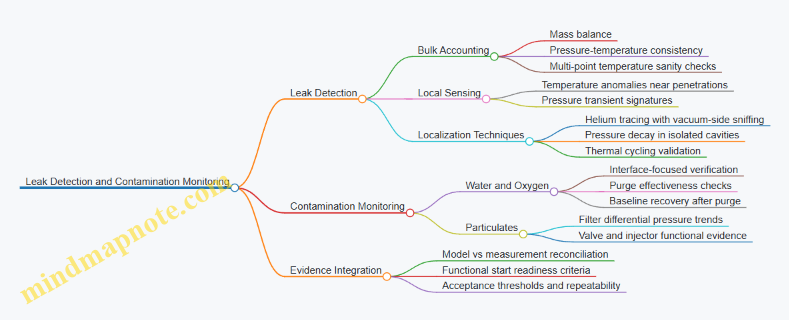
Integrated Example Workflow for a Cryogenic Feed System
- Baseline model run: establish expected pressure and temperature evolution during a representative hold.
- Bulk discrepancy check: if pressure drift exceeds the model envelope, flag a possible leak or unmodeled venting.
- Localize by subassembly: isolate tank penetrations, manifold sections, and valve bodies; repeat targeted tests.
- Confirm with contamination indicators: verify purge performance and filter differential pressure trends during the same test campaign.
- Functional confirmation: run engine start readiness checks that are sensitive to contamination, such as stable valve response and predictable feed conditions.
This workflow prevents a common failure mode: treating “leak-free” as a single yes/no result. In practice, you want a consistent story across accounting, localization, and functional behavior, so the system passes for the right reasons rather than by accident.
11.5 Fault Detection Logic for Valves Pumps and Sensors
Fault detection logic is the part of the system that turns messy measurements into clear actions. The goal is not to catch every tiny anomaly; it is to detect faults early enough, with enough confidence, that the engine can be protected without triggering unnecessary scrubs.
Foundational Concepts for Cryogenic Fault Logic
Start with a simple chain: symptom → hypothesis → evidence → decision. A symptom is what you measure (for example, a valve position sensor reading that doesn’t match commanded motion). A hypothesis is the likely cause (stiction, leak, wiring fault, sensor drift). Evidence is the set of checks you apply (range checks, rate checks, correlation checks). The decision maps evidence to outcomes such as “continue,” “de-rate,” or “safe shutdown.”
A second foundation is time alignment. Cryogenic systems have delays: valves take time to move, pumps spool up, and temperatures lag due to thermal mass. If you compare signals without accounting for these delays, you will either miss real faults or flag normal behavior.
Signal Conditioning and Sanity Checks
Before logic rules, condition signals so they are comparable.
- Unit and scaling checks: confirm sensor scaling matches expected ranges (e.g., pressure in Pa vs kPa).
- Range checks: reject impossible values immediately (temperature below sensor minimum, flow negative when it cannot be).
- Rate checks: detect abrupt jumps that exceed physical plausibility.
- Staleness checks: if a sensor stops updating, treat it as a fault with a distinct signature.
Example: if a cryogenic liquid temperature sensor reports a sudden step upward during a phase where heat leak should cause a slow drift, the logic should mark “sensor jump” rather than “propellant warming.” That distinction matters for downstream decisions.
Model-Based Consistency Checks
Once signals pass sanity checks, use consistency rules that tie together what should move together.
- Command vs feedback for valves: compare commanded position (or current) to measured position. Use a tolerance band and a movement window.
- Pressure-flow consistency: if pump speed is steady, a large pressure drop without a corresponding flow change suggests a restriction or cavitation onset.
- Thermal consistency: if ullage temperature rises while liquid temperature stays flat, the logic should consider stratification or sensor placement effects rather than a uniform thermal fault.
Example: during a start sequence, the logic expects a characteristic pressure rise after pump spool-up. If pressure remains flat while pump speed increases, the hypothesis shifts toward a blocked inlet, severe leakage, or a sensor fault on the pressure transducer.
Fault Hypotheses for Valves
Valves typically fail in a few repeatable ways, and the logic should reflect that.
- Stiction or sluggish motion: feedback lags command beyond the movement window.
- Leak-through: valve is commanded closed, but downstream pressure or flow continues to change.
- Actuator electrical fault: commanded current is present but motion feedback is absent.
- Position sensor fault: feedback remains constant across multiple commands.
Decision rule example: if the valve is commanded from 10% to 90% open and the measured position does not cross 50% within the expected travel time plus margin, classify “stiction/sluggish.” If the same sensor is also stuck during other valve cycles, classify “position sensor fault” instead.
Fault Hypotheses for Pumps
Pump faults are often tied to flow quality and cavitation risk.
- Cavitation onset: pressure at the inlet drops while pump speed rises, and temperature signals may show rapid changes.
- Low net positive suction margin: consistent underperformance across operating points.
- Seal or leakage issues: unexpected pressure decay patterns and abnormal temperature gradients near the seal.
- Speed control failure: commanded speed differs from measured speed beyond tolerance.
Example: if inlet pressure oscillates with pump speed and correlates with a rise in downstream vapor indicators (or inferred two-phase behavior), the logic should treat it as cavitation rather than a generic “pressure sensor drift.”
Fault Hypotheses for Sensors
Sensor faults are common enough that they should be first-class citizens in the logic.
- Bias or drift: slow deviation from expected trends.
- Noise or intermittent dropout: high variance or missing samples.
- Calibration mismatch: consistent offset across the full operating range.
- Cross-sensitivity: sensor responds to something it should not (for instance, a wall sensor influenced by local heat conduction changes).
Example: if two redundant temperature sensors show the same slow drift, the logic should consider real thermal change. If only one drifts while the other tracks expected behavior, classify “single-sensor bias.”
Decision Logic and Confidence Scoring
Use a structured decision approach:
- Detect: trigger when evidence exceeds thresholds.
- Classify: map evidence to a fault mode.
- Confirm: require a second independent check when possible.
- Act: choose the least disruptive safe action.
A practical confidence score can be built from evidence types. For instance, command-feedback mismatch plus staleness plus correlation failure yields high confidence. Single evidence type with weak correlation yields low confidence and may only request a controlled hold.
Mind Map: Fault Detection Logic Flow
Integrated Example: Start Sequence Fault Handling
During a cryogenic engine start, the logic runs in phases.
- Phase 1: Pre-start checks sensor sanity and staleness. If a key temperature sensor is stale, the logic should avoid using it for readiness criteria.
- Phase 2: Valve actuation applies command-feedback timing windows. If a valve fails to reach the expected position, the logic should confirm with downstream pressure response; if downstream pressure also fails to move, classify “valve motion fault,” otherwise classify “position sensor fault.”
- Phase 3: Pump spool-up checks speed tracking and inlet pressure behavior. If speed rises but inlet pressure does not, classify “inlet restriction or sensor fault” and confirm with correlated downstream pressure and inferred flow.
The action mapping should be conservative but not chaotic: a single low-confidence sensor anomaly may trigger a hold and re-check, while a high-confidence valve motion failure during a critical step should trigger a safe shutdown path.
Practical Threshold Tuning Without Guesswork
Thresholds should be tuned using the same timing windows and operating envelopes used in the logic. A good tuning workflow is to start with conservative thresholds, then adjust based on observed normal variability. The key is to separate “normal scatter” from “rule-breaking behavior” so the logic does not become a false-alarm machine.
12. Ground Testing and Verification for Cryogenic Propulsion Systems
12.1 Test Objectives and Acceptance Criteria Definition
A good cryogenic propulsion test plan starts with a simple question: what must be true at the end of the test for the system to be considered “ready to fly”? The answer should be written as measurable objectives, then translated into acceptance criteria that map directly to hardware behavior.
Define Objectives from System Functions
Begin at the function level, not the component level. For a cryogenic feed and start sequence, the core functions usually include propellant availability, thermal state control, leak tightness, and stable engine operation.
Objective examples with clear intent
- Propellant availability: The feed system must deliver liquid at the required inlet conditions during the commanded engine start window.
- Thermal state control: Tank and feed line temperatures must remain within limits that prevent excessive boil-off or freezing hazards.
- Leak tightness: No unacceptable leakage rate is allowed across valves, seals, and interfaces under cryogenic conditions.
- Start reliability: The engine must reach stable combustion without exceeding allowable transient pressures, temperatures, or valve timing errors.
A practical way to keep objectives grounded is to attach each objective to a specific test phase: cold soak, pressurization, feed conditioning, start, and steady operation.
Translate Objectives into Acceptance Criteria
Acceptance criteria are the “pass/fail rules.” They should be expressed as thresholds on measured quantities, plus timing and sequence constraints.
Acceptance criteria structure
- Quantitative limits: e.g., maximum allowable leak rate, maximum line temperature gradient, minimum inlet pressure.
- Timing windows: e.g., valve command-to-response must occur within a defined tolerance.
- Sequence correctness: e.g., pressurization must precede feed valve opening; engine start must occur only after liquid acquisition criteria are met.
- Data sufficiency: e.g., required sensor sampling rates and minimum duration of steady-state measurement.
Easy-to-understand example If the objective is propellant availability, an acceptance criterion might require that the feed line temperature indicates liquid presence (not just “cold”), and that the engine inlet pressure stays above a minimum for the entire start transient. This prevents a common failure mode: “cold enough” hardware that still delivers vapor.
Build a Traceability Map from Requirements to Measurements
Acceptance criteria should not float in isolation. Create a trace from each system requirement to the specific sensors and derived metrics used to judge it.
Mind Map: Test Objectives and Acceptance Criteria Traceability
Use Evidence Types That Match Cryogenic Reality
Cryogenic systems often involve indirect indicators. For example, “liquid acquisition” may be inferred from a combination of temperature stratification, pressure behavior, and valve response timing.
To keep criteria defensible, specify which evidence types are allowed:
- Direct evidence: measured leak rate, measured pressure, measured temperature at defined locations.
- Derived evidence: computed heat leak from boil-off rate, inferred phase state from multi-sensor trends.
- Exclusion rules: define what invalidates a result, such as sensor dropout during the start window.
Define Uncertainty Handling and Margin
Acceptance criteria should include how measurement uncertainty is treated. A simple rule is to require that the measured value plus uncertainty still meets the limit. This avoids borderline outcomes caused by sensor noise.
Example: If the maximum allowable leak rate is 1×10⁻⁶ std cc/s, and the measurement uncertainty is ±0.2×10⁻⁶, then the criterion can be stated as: measured leak rate + 0.2×10⁻⁶ must be ≤ 1×10⁻⁶.
Lock the Criteria to the Test Matrix
Finally, acceptance criteria must be consistent across the test matrix. If you test multiple operating points, define which criteria are universal and which scale with conditions.
Example:
- Universal: leak tightness limits and valve response timing tolerances.
- Condition-dependent: inlet pressure minimums and allowable thermal gradients that vary with commanded thrust level.
A clean practice is to record the criteria in a single checklist format used by the test conductor and the reviewer. That checklist should be complete enough that two people can independently decide pass/fail from the same dataset without arguing about interpretation.
12.2 Cryogenic Test Facility Setup and Safety Procedures
A cryogenic test facility is really three systems working together: the hardware that handles cold fluids, the controls that keep it stable, and the safety layers that make “oops” survivable. Setup starts with a clear test boundary, then builds outward from utilities to propellant path, and finally locks in procedures that match the facility’s actual failure modes.
Facility Boundary and Roles
Define the test boundary as a physical and procedural perimeter: what valves, lines, and instruments are considered “in scope,” and what is treated as “support only.” Assign roles before any cold work begins: test conductor (sequence authority), safety officer (stop authority), and instrumentation lead (data integrity authority). A simple rule prevents confusion: only the test conductor can advance the sequence; everyone else can request holds.
Utilities and Environmental Controls
Cryogenic tests depend on stable utilities. Confirm chilled water or electrical cooling for instrumentation, stable power quality for controllers, and adequate ventilation capacity for any expected venting. If the facility uses a cryogenic liquid supply cart or dewar, verify that transfer hoses and quick-disconnects are rated for the temperature range and pressure class. A practical check is to run a “warm dry” utility test first: cycle valves, confirm pressure transducers read sensibly, and verify that emergency shutdown logic triggers without touching the cryogenic path.
Propellant Path Configuration
Build the propellant path from the tank or supply to the test article and back to the vent or recovery system. Keep the coldest components closest to the cryogen source to reduce condensation risk on warmer surfaces. Route drain and vent lines so they cannot trap liquid; trapped liquid can later flash and overpressure a line. Before cooling, perform a leak check at ambient temperature using the facility’s standard method for the specific fluid class.
Instrumentation Readiness
Instrumentation setup should be treated like part of the hardware. Calibrate or verify sensors for the expected ranges: liquid temperature, ullage temperature, line pressure, and differential pressure across filters or orifices. Confirm sensor placement matches the test intent; for example, a line pressure sensor should be upstream of any restriction whose behavior you want to measure. Validate data acquisition timing so that valve commands, pressure changes, and temperature responses align in the recorded timeline.
Cold Soak and Thermal Equilibrium
Cold soak is not just “wait until it’s cold.” Establish a soak plan that includes minimum soak time and acceptance criteria such as stable temperatures at key locations and no unexpected pressure drift. A common mistake is to start the test sequence when only the tank is cold while the feed line remains warmer, causing phase changes that look like control problems. Use a stepwise approach: cool the propellant path, monitor stabilization, then proceed to the next stage.
Safety Procedures for Cryogenic Hazards
Safety procedures should cover four hazard categories: oxygen displacement, thermal burns, pressure hazards, and toxic or reactive contaminants if applicable.
- Oxygen displacement: Verify oxygen monitoring coverage in occupied and near-vent areas. Establish alarm thresholds and a clear action plan for each alarm level.
- Thermal burns: Use cryogenic PPE and enforce controlled access during cooling and venting. Mark exclusion zones around cold surfaces and any lines that can become cold during transients.
- Pressure hazards: Ensure relief devices are correctly installed and not bypassed. Confirm vent routing is unobstructed and that any rupture disk or relief discharge path cannot impinge on personnel or sensitive equipment.
- Contamination control: If the test fluid is sensitive to water or particulates, specify purge and handling steps that match the facility’s actual cleanliness level.
Emergency Shutdown Logic and Drills
Emergency shutdown must be deterministic. Define what “stop” means: which valves close, which pumps stop, and whether the system transitions to a safe vent state. Test the shutdown sequence during warm conditions so that the logic is proven without cryogenic risk. Then rehearse the human side: the safety officer calls the stop, the test conductor executes the defined safe state, and the instrumentation lead records the final data window.
Mind Map: Test Facility Setup and Safety
Example: Warm Dry Run to Prove the Sequence
Run a warm dry test that cycles the same valves and control logic you will use later. Confirm that pressure transducers respond to commanded valve positions, that data acquisition logs every command, and that the emergency shutdown transitions to the planned vent state. Only after this passes do you proceed to cooling, because it proves the control system and wiring before cryogenic conditions add complexity.
Example: Cold Soak Acceptance Criteria
Set acceptance criteria such as “line temperature within a defined band for a sustained interval” and “pressure drift below a threshold.” If the tank stabilizes but the feed line does not, hold the sequence and extend the soak rather than forcing the start. This keeps the test results tied to intended physics instead of unintended thermal gradients.
12.3 Cold Soak Procedures and Thermal Equilibrium Verification
Cold soak is the controlled period where cryogenic hardware reaches a stable temperature distribution before you start a test sequence. The goal is not just “getting cold,” but making the thermal state repeatable so that later measurements reflect the propulsion system, not the warm-up history.
Cold Soak Objectives and Success Criteria
Start by defining what “equilibrium” means for your setup. For a tank and feed system, equilibrium typically includes: (1) bulk propellant temperature near the measurement points, (2) wall temperatures that stop drifting, and (3) stable pressure behavior under a defined boil-off or recirculation condition. A practical success criterion is a drift limit, such as temperature change below a chosen threshold over a fixed window (for example, a few hours), paired with consistent pressure trends.
A useful mental model is to treat the system as multiple thermal masses connected by heat leaks. The cold soak ends when the slowest thermal path has settled. If you only watch the fastest sensor, you can declare victory early and later see feed line temperatures still migrating.
Instrumentation Setup for Meaningful Equilibrium
Before any cryogen enters, verify sensor functionality at ambient conditions. Then plan sensor placement so each thermal mass has at least one representative measurement: tank bulk liquid or proxy, tank wall near insulation interfaces, feed line segments near valves and bends, and ullage or vapor space pressure. Calibrate or at least confirm zero offsets so that drift calculations are trustworthy.
Example: If your feed line has a long run with a valve mid-span, place temperature sensors upstream and downstream of the valve. During soak, the valve region often lags because it adds thermal resistance and internal volume. That lag is exactly what you want to measure.
Stepwise Cold Soak Procedure
- Pre-chill and leak check: Cool the external surfaces and verify no abnormal pressure rise during initial cooldown. If you see rapid pressure changes inconsistent with expected heat leak, stop and correct the issue.
- Controlled fill to a known level: Introduce propellant to a target fill fraction that matches your test configuration. Keep the fill rate consistent across runs; changing fill rate changes how quickly ullage and walls cool.
- Establish a defined thermal boundary condition: Decide whether the system is allowed to boil off naturally, is held with a controlled recirculation, or is supported by active heating. The boundary condition must remain constant during the equilibrium window.
- Hold and monitor drift: Continue the soak while recording temperatures and pressures at a fixed sampling interval. Use the same data reduction method each run.
- Equilibrium verification: Apply drift limits to each critical measurement channel and confirm that pressure behavior is consistent with the chosen boil-off mode.
- Transition readiness: Only after equilibrium is verified, proceed to start sequence steps. If you must open valves or change flow paths, treat that as a new thermal transient and document the time of change.
Thermal Equilibrium Verification Logic
Thermal equilibrium is rarely “one number.” Use a structured checklist:
- Bulk temperature stability: Temperature at liquid-representative sensors shows minimal drift.
- Wall temperature stability: Insulation interface and structural wall sensors stop trending.
- Pressure stability: Ullage pressure remains within a narrow band for the defined mode.
- Consistency across segments: Upstream and downstream feed line sensors show either both stable values or a stable gradient that matches your expected heat leak.
Example: Suppose tank wall temperature stabilizes but feed line downstream of a valve continues to drift downward. That indicates the downstream segment is still absorbing heat. Starting the engine feed anyway can cause two-phase behavior earlier than expected.
Mind Map: Cold Soak and Equilibrium Verification
Example Cold Soak Plan for a Feed System
Assume a tank with a feed line that includes a valve and a long insulated run. You set the fill fraction to match your expected liquid acquisition behavior. During the hold, you maintain the same boil-off handling mode throughout. You then compute drift for each sensor over a fixed window and require that all critical sensors meet the drift limit. Finally, you confirm that ullage pressure trends align with the expected saturation behavior for the measured bulk temperature.
If one sensor fails the drift test, you do not “average it out.” You extend the soak and identify the thermal lag source by comparing gradients across segments. That turns equilibrium verification into a diagnostic step rather than a yes/no gate.
Data Handling and Decision Discipline
Use consistent time windows and consistent filtering rules. Record the exact moment any operational change occurs, such as valve actuation or a change in boil-off management. When you document the equilibrium result, include which sensors passed, which failed, and the measured drift magnitude. That level of detail prevents the next run from repeating the same confusion with different numbers.
12.4 End-to-End Feed and Start Tests With Representative Conditions
End-to-end tests prove that the whole chain—thermal state, propellant acquisition, conditioning, valve sequencing, and engine start—works as one system. “Representative conditions” means the test reproduces the same limiting factors you design around: heat leak and subcooling margins, ullage behavior, line pressure drops, and sensor-to-actuator timing. A good test plan starts with a clear pass/fail definition, then builds a sequence that isolates failure modes without breaking realism.
Test Objectives and Representative Condition Targets
Set measurable objectives before hardware is touched. Typical objectives include: (1) stable liquid acquisition at the engine inlet, (2) no unexpected two-phase ingestion during the start transient, (3) valve timing that matches control logic under cold temperatures, and (4) chamber start parameters that stay within allowable limits for pressure rise and mixture ratio.
Representative condition targets should be expressed as ranges, not single values. For example, define allowable inlet liquid subcooling as a band, not a point, because insulation performance and boil-off rate vary across the tank. Similarly, define acceptable ullage pressure and temperature ranges so the test covers the “worst plausible” combination rather than only the nominal case.
System-Level Test Sequence from Cold Soak to Stable Run
Begin with a cold soak that reaches thermal equilibrium in the tank and the feed lines. Use a heat-leak budget to decide how long the soak should be, then verify with sensor trends: temperatures should flatten within a defined tolerance, and pressure behavior should match the expected pressurization response.
Next, run a controlled feed conditioning phase. The goal is to establish liquid at the acquisition device, confirm that the feed line is not trapped with vapor pockets, and verify that the conditioning method produces the intended subcooling. A simple example is a “settle and verify” step: hold propellant acquisition conditions steady for a fixed time, then check that inlet temperature and pressure indicate liquid-dominant flow.
Then execute the start sequence exactly as flight logic would. Record valve commands, actuator positions, and sensor readings at high time resolution. The key is to confirm that the first liquid reaches the injector interface before ignition criteria are met, and that any transient flashing stays inside the allowable window.
Finally, transition to a short stable run at a representative throttle or mixture ratio point. This is where you confirm that the feed system remains stable after the initial transient, not just during it.
Mind Map: End-to-End Feed and Start Test Flow
Concrete Example: Two-Phase Ingestion Check During Start
Suppose your acceptance criterion is “no more than 5% vapor volume fraction at injector inlet during the first 0.3 s.” In practice, you may not measure vapor fraction directly. Instead, you infer it from a combination of inlet temperature drop rate and pressure oscillation signatures.
A practical workflow is: (1) run a conditioning step that establishes a known inlet subcooling band, (2) start with ignition inhibited until inlet pressure and temperature cross the liquid-expected thresholds, and (3) compare the measured pressure transient shape to a baseline run where liquid ingestion was confirmed. If the pressure transient shows earlier-than-expected flashing behavior, you adjust the conditioning timing or acquisition strategy and rerun.
Evidence Collection and Data Reduction That Actually Helps
Use synchronized time bases for every signal that can influence the transient: valve commands, actuator feedback, tank and line temperatures, ullage pressure, feed pressures at multiple points, and engine chamber pressure. Then reduce data into “event markers” such as valve open/close times, first liquid arrival indicators, ignition command time, and chamber pressure rise milestones.
Acceptance should be tied to event markers, not only to averaged values. Averaging can hide a brief vapor ingestion spike that still matters for combustion stability.
Example Acceptance Criteria Set
- Cold soak: tank and line temperatures within ±2 K of the target trend plateau.
- Conditioning: inlet temperature and pressure indicate liquid-dominant flow before ignition is allowed.
- Start transient: chamber pressure rise rate and mixture ratio proxy remain within defined bands.
- Valve timing: commanded and measured valve positions match within a specified delay tolerance.
- Stable run: feed pressures remain within the pressure drop budget without oscillatory behavior.
Practical Notes for Repeatability
Repeat the test at least twice for the same representative condition set. If results differ, check whether the difference comes from thermal equilibrium timing, pressurant regulator behavior, or valve actuation under cold conditions. A repeatable system is one where the event markers line up, not just where final pressures look similar.
12.5 Data Reduction Methods and Uncertainty Analysis for Test Results
Cryogenic propulsion tests generate data that are easy to collect and surprisingly easy to misinterpret. Data reduction is the step where you turn raw sensor streams into physically consistent quantities, then attach uncertainty so decisions have a measurable basis. A good workflow starts with definitions, then corrections, then propagation.
Establish Measurement Definitions and Units
Before touching numbers, lock down what each reported variable means. For example, decide whether “tank pressure” is the ullage pressure at a specific transducer port or an average of multiple ports. Define reference temperatures for density calculations and specify whether flow is reported as mass flow, volumetric flow at line conditions, or equivalent engine mixture ratio.
A practical habit: create a one-page “signal dictionary” listing sensor ID, location, raw units, conversion formula, and the physical quantity it represents. When a later anomaly appears, you can trace it to a specific conversion rather than guessing.
Clean and Correct Raw Signals
Raw data often need three categories of correction.
-
Time alignment: Different channels may be sampled at different rates or with different trigger delays. Align using a known event, such as a valve command edge or ignition trigger, then resample to a common time grid.
-
Calibration and scaling: Apply calibration curves for pressure transducers, thermocouples, and flow meters. If a sensor has a non-linear response, use the calibrated model rather than a linear approximation.
-
Thermal and electrical effects: Cryogenic tests can create sensor-specific artifacts. Thermocouples can show lead-wire conduction effects; pressure lines can damp fast transients; and heater power can couple into nearby temperature sensors.
Example: If a temperature sensor is mounted on a valve body, its reading may lag the fluid temperature. In reduction, treat it as a “wall temperature” measurement and avoid using it directly as the fluid inlet temperature unless you have a validated correction.
Compute Derived Quantities with Consistent Assumptions
Derived quantities include mass flow from differential pressure, mixture ratio from two propellant mass flows, and heat leak estimates from boil-off rate.
A systematic approach is to write each derived equation in the same order every time:
- Convert raw signals to primary physical quantities.
- Apply fluid property models using the same assumptions for phase and composition.
- Compute derived values and store intermediate terms.
Example: For mass flow from a differential pressure element, compute upstream density using the measured upstream pressure and temperature, then apply the discharge coefficient model. If the discharge coefficient depends on Reynolds number, compute Reynolds number using the same density you used for mass flow, not a separately computed density from a different time window.
Uncertainty Budget Construction
Uncertainty analysis should be explicit and traceable. Separate uncertainty into Type A (statistical, from repeated samples) and Type B (systematic, from calibration, model assumptions, and resolution).
Typical contributors:
- Sensor calibration uncertainty and linearity.
- Measurement resolution and quantization.
- Temperature-to-density model uncertainty.
- Flow model parameters such as discharge coefficient or pump efficiency.
- Time alignment error affecting transient values.
A simple rule: if a quantity is computed from multiple inputs, propagate uncertainty using sensitivity (partial derivatives) or Monte Carlo sampling. Sensitivity analysis is often enough for steady segments; Monte Carlo is useful when non-linear models and thresholds are involved.
Propagate Uncertainty Through Reduction Steps
For a derived quantity \(y=f(x_1, x_2, …)\), propagate uncertainties using either:
- Linearized propagation: \(u_y^2 \approx \sum (\partial f/\partial x_i)^2 u_{x_i}^2\) assuming uncorrelated inputs.
- Monte Carlo: sample \(x_i\) from their distributions, compute \(y\) for each sample, then report mean and spread.
Example: Mixture ratio \(MR=\dot m_{ox}/\dot m_{fuel}\). If both mass flows have uncertainties, the ratio uncertainty increases when one flow is small. That’s not a bug; it’s a real measurement limitation. Report uncertainty as a function of operating point, not as a single constant number.
Report Results with Context and Operating Segments
Tests include phases: pre-cold soak, steady feed, start transient, and post-start stabilization. Uncertainty should be reported per segment because sensor behavior changes with temperature and flow regime.
A clean reporting pattern:
- Provide reduced time histories for key variables.
- Provide segment-averaged values with uncertainty bars.
- Include a short note describing which uncertainty sources dominate in each segment.
Example: During start, time alignment and valve actuation delay may dominate mixture ratio uncertainty; during steady operation, calibration and model parameter uncertainty may dominate.
Mind Map: Data Reduction and Uncertainty Analysis
Mini Example: From Raw to Uncertainty-Tagged Mixture Ratio
Suppose you measure oxidizer and fuel mass flows using two differential pressure elements. You reduce each channel by converting differential pressure to flow using calibrated discharge coefficients and fluid properties at the measured line conditions. Then you compute \(MR=\dot m_{ox}/\dot m_{fuel}\).
Uncertainty steps:
- Assign \(u_{\Delta P}\) from transducer calibration and resolution.
- Assign \(u_T\) from thermocouple calibration and mounting effects.
- Assign \(u_{C_d}\) from calibration spread.
- Propagate to \(u_{\dot m_{ox}}\) and \(u_{\dot m_{fuel}}\).
- Propagate to \(u_{MR}\), noting that if \(\dot m_{fuel}\) is near a lower limit during a transient, \(u_{MR}\) will inflate.
Finally, report MR for the steady segment only, with uncertainty bars, and keep transient MR as a diagnostic quantity rather than a decision metric.