Scramjet Propulsion for Defense Platforms
1. Mission Requirements and System Interfaces
1.1 Defining Defense Platform Mission Profiles for Scramjet Use
A scramjet is not a generic “high-speed engine.” It is a tightly coupled system whose usable performance depends on how the platform flies, how long it stays in the right inlet and combustor conditions, and how reliably it can start and remain stable. Mission profiling is the step where you translate operational intent into measurable flight segments that the propulsion design can actually satisfy.
Start with Mission Tasks and Flight Segments
Defense platforms typically execute a sequence: approach, acceleration, sustained high-speed operation, and terminal maneuvers. For scramjet use, you break the mission into segments with distinct boundary conditions:
- Approach segment: airspeed and altitude where the inlet is not yet in its best operating regime.
- Acceleration segment: rapid changes in Mach number and dynamic pressure that stress inlet starting and combustor ignition.
- Sustained segment: the portion where thrust is expected and where thermal margins are most challenged.
- Terminal segment: often shorter, but it can include aggressive bank or pitch that changes inlet angle of attack and effective capture.
A practical best practice is to define each segment with a time history of Mach number, altitude, angle of attack, sideslip, and throttle demand. Even if you later refine the trajectory, this first pass prevents “designing to a single point” and then being surprised by off-nominal operation.
Convert Operational Needs into Propulsion Requirements
Once segments exist, map each segment to propulsion-relevant quantities:
- Inlet operating window: where the inlet can maintain stable compression and avoid unstart.
- Combustor ignition and stability window: where fuel-air mixing and residence time support sustained combustion.
- Thermal load window: where wall heat flux and material limits constrain allowable duration.
- Thrust and specific fuel consumption targets: where the mission needs net acceleration or range.
A useful example: suppose the mission requires a sustained acceleration for 40 seconds at high dynamic pressure. If your thermal model shows the combustor liner reaches its allowable heat soak in 25 seconds, you can’t fix that with “more thrust.” You must either shorten the sustained segment, reduce heat flux via cooling strategy, or adjust the trajectory so the engine spends less time at the worst combination of Mach and altitude.
Define “Scramjet Usable Time” as a First-Class Metric
Scramjet performance is often limited by how long the system can remain within stable inlet and combustor conditions. Define usable time as the duration during which:
- inlet pressure recovery stays within a stability band,
- combustor pressure oscillations remain below a chosen limit,
- wall temperatures remain below allowable margins,
- fuel metering stays within controllable bounds.
This metric becomes the bridge between mission profiles and engine design. If the mission profile yields only 10 seconds of usable time, the design must be optimized for that reality rather than for an idealized steady-state point.
Use Constraints to Bound the Design Space Early
Mission profiles include constraints that directly affect scramjet feasibility:
- Angle-of-attack and sideslip limits: these change effective inlet capture and shock/boundary-layer interactions.
- Acceleration limits: rapid throttle or flight changes can outpace control authority.
- Start conditions: the engine may need a minimum stagnation temperature or pressure to ignite reliably.
- Environmental variability: density and temperature variations shift the operating window.
A concrete example: if the platform can only tolerate a narrow range of inlet capture angles during acceleration, then the mission profile should reflect that by using a trajectory that keeps the inlet aligned. Otherwise, the propulsion design will be forced to compensate with aggressive control or geometry changes that may not be manufacturable or testable.
Mind Map: Mission Profile to Scramjet Requirements
Example: Turning a Trajectory into Design Points
Take a simplified acceleration segment: Mach increases from 3.0 to 4.5 over 30 seconds while altitude drops slightly, causing dynamic pressure to rise. You can sample the segment at 5-second intervals and compute inlet stagnation conditions, combustor inlet temperature, and expected residence time. Then you tag each sample as:
- Start-critical: near the first point where ignition is expected.
- Stability-critical: where inlet pressure recovery is most sensitive to angle of attack.
- Thermal-critical: where wall heat flux peaks.
This produces a small set of design points that represent the whole segment. Instead of testing every second of the mission, you validate the engine where it is most likely to fail—then confirm that the rest of the segment stays inside margins.
Deliverables That Make the Mission Profile Actionable
A mission profile for scramjet design should end with concrete artifacts:
- A segmented trajectory with time histories of key flight variables,
- A table of propulsion-relevant quantities per segment,
- A definition of usable time and the stability/thermal criteria that govern it,
- A list of constraints that the propulsion design must respect,
- A set of representative design points for analysis and test.
When these are in place, later chapters can connect inlet geometry, combustor architecture, cooling, and controls to the actual mission rather than to a convenient fantasy flight condition.
1.2 Translating Mission Constraints into Propulsion Requirements
Mission constraints rarely arrive as “build a scramjet.” They show up as ranges, timelines, survivability limits, payload mass, and allowable risk. Translating them into propulsion requirements means converting each constraint into an engine-level quantity you can design, test, and verify.
Start with a Requirements Map
Create a two-layer view: mission-level constraints and propulsion-level requirements. Mission constraints include Mach range, altitude band, acceleration or loiter needs, and duty cycle. Propulsion requirements become target thrust, allowable inlet unstart margin, fuel consumption limits, and thermal protection limits.
A practical way to keep the mapping honest is to write each propulsion requirement as a measurable statement with a test condition. For example, “Maintain stable combustion at 3.5 km/s equivalent inlet conditions” is better than “combust reliably at high speed.” The first version implies a specific inlet total pressure/temperature window and stability criteria.
Convert Flight Envelope into Operating Points
Scramjets are sensitive to inlet pressure ratio, residence time, and wall heat flux. So you should discretize the mission envelope into operating points rather than treating it as a continuous curve.
- Choose representative points across the mission: entry, mid-mission, and terminal segments.
- For each point, compute inlet conditions from the airframe state: freestream Mach, static pressure, and temperature.
- Translate those into engine inlet total conditions and required mass flow.
Example: If the mission requires sustained operation between two altitudes, you may end up with three inlet total pressure levels and two inlet total temperature levels. That becomes your “design grid” for inlet starting, combustor stability, and thermal margins.
Translate Thrust Needs into Component-Level Targets
Mission thrust demand comes from acceleration and drag balance. Once you have required net thrust, you can allocate it across inlet pressure recovery, combustor pressure loss, and nozzle expansion.
A simple allocation model helps you avoid chasing the wrong knob. Net thrust is driven by:
- Inlet momentum capture and pressure recovery
- Combustor heat addition and resulting mass-weighted exhaust conditions
- Nozzle expansion ratio and effective area
Example: Suppose the mission needs 120 kN net thrust at a mid-mission point. If preliminary cycle estimates show the nozzle can only deliver 150 kN gross under thermal limits, then the inlet-plus-combustor must not waste more than 30 kN worth of effective thrust through pressure losses or incomplete heat addition.
Turn Stability Constraints into Inlet and Combustor Limits
Defense platforms often require predictable operation under disturbances: angle-of-attack changes, manufacturing tolerances, and fuel property variation. These become stability limits.
Key stability requirements to derive:
- Inlet starting margin: the maximum adverse pressure gradient or minimum total pressure ratio where the inlet remains started.
- Unstart recovery behavior: how quickly the system returns to a stable state after a perturbation.
- Combustor stability: acceptable ranges of equivalence ratio, ignition delay, and flameholding effectiveness.
Example: If the mission allows only brief thrust dropouts, you can set a maximum allowable unstart duration and a minimum acceptable probability of stable restart within a defined time window. That turns “stability” into a testable operational envelope.
Convert Thermal and Structural Limits into Cooling Requirements
Thermal constraints usually come from allowable material temperatures, heat flux limits, and life-cycle maintenance assumptions. Translate them into cooling design requirements by following a chain:
- Determine worst-case heat flux at leading edges and combustor walls for each operating point.
- Convert heat flux into required heat removal capacity.
- Allocate that capacity across cooling mechanisms: film cooling, regenerative paths, or internal convection.
Example: If the mission includes a terminal segment with higher stagnation temperature, you may find that the combustor wall heat flux peaks there even if thrust demand is lower. The propulsion requirement then becomes “meet wall temperature limits at the thermal peak,” not “optimize only for thrust.”
Mind Map: Mission Constraints to Propulsion Requirements
Example Workflow from Constraints to Requirements
Assume a mission requires sustained operation across a Mach band with a strict fuel budget and a limited allowable thrust dropout.
- Discretize the Mach-altitude band into three operating points.
- For each point, compute inlet total conditions and required mass flow.
- Set thrust targets from net force balance and allocate losses to inlet and combustor.
- Define stability acceptance criteria: maximum unstart duration and minimum stable combustion window.
- Compute thermal peak heat flux across the same points and set cooling capacity requirements.
- Produce a test matrix that mirrors the operating point grid and includes disturbance cases.
The result is a set of propulsion requirements that are not just numbers, but numbers tied to conditions. That linkage is what makes design decisions traceable and test results interpretable.
1.3 Vehicle Integration Interfaces for Inlet Exhaust and Mounting
Scramjet performance is won or lost at interfaces: where the inlet meets the airframe, where the combustor hands flow to the exhaust, and where loads travel through mounts into structure. This section treats those interfaces as a set of engineering contracts—geometry, flow quality, thermal protection, and mechanical stiffness—each with measurable acceptance criteria.
Interface Foundations for Inlet and Exhaust
Start with the flowpath “datum.” Define a centerline and reference surfaces that every subsystem uses: inlet cowl, isolator, combustor, and nozzle. If the datum shifts by even a small amount, the inlet shock system and boundary-layer behavior change, which then changes where combustion starts. A practical best practice is to lock the datum early using a physical mockup or a 3D-printed alignment fixture, then carry that datum into CAD and test hardware.
Next, define the interface planes. For the inlet, the forward plane typically controls external aerodynamic alignment and internal capture area. For the exhaust, the aft plane controls nozzle exit area, expansion ratio, and the location of any afterbody flow features. Acceptance criteria should include:
- Geometric tolerances on alignment and area (flatness, concentricity, and step height).
- Surface finish targets on flow-critical walls.
- Sealing requirements to prevent leakage paths that bypass the intended flowpath.
A simple example: if a mounting bracket introduces a 2 mm step at a wall junction, the local pressure gradient can thicken the boundary layer, reducing effective combustor entry conditions. The fix is not “smoother is better” in general; it is to specify allowable step height and verify it with metrology.
Mechanical Mounting and Load Paths
Mounting must handle three load categories: aerodynamic pressure loads, thermal gradients, and vibration. The interface design should separate these loads so thermal expansion does not fight structural stiffness.
A useful approach is to classify mounts by their degrees of freedom:
- Kinematic mounts constrain only what must be constrained, reducing stress from thermal growth.
- Guided mounts allow controlled sliding or expansion while maintaining alignment.
- Stiff mounts are reserved for locations where alignment is critical and thermal growth is small.
Example: Suppose the inlet cowl grows more than the combustor liner during a hot run. If the mount is fully rigid, the structure may bow and misalign the internal flowpath. A better practice is to allow one controlled expansion direction using slots or compliant features, while keeping the centerline constraint through a reference bearing surface.
Thermal Protection Interfaces and Cooling Continuity
Thermal protection layers must not create new flow problems. If insulation or cooling manifolds protrude into the flowpath, they can trigger separation or alter heat flux distribution.
Define thermal interfaces with three checks:
- Heat-flux continuity across joints so hot spots do not concentrate at seams.
- Cooling passage continuity so flow does not dead-end or leak.
- Gap management so thermal expansion does not close a gap in a way that blocks cooling.
Concrete example: A liner-to-cowl joint often uses a gasket or metallic seal. If the seal compresses unevenly, it can create a local leakage jet that changes combustor inlet conditions. Specify seal compression range and verify it with a representative thermal-mechanical test article.
Sealing, Leakage, and Boundary-Layer Integrity
Leakage is easiest to underestimate because it can be small in mass flow yet large in effect. A bypass leak can reduce the effective pressure recovery and change the isolator behavior.
Best practices:
- Use labyrinth or stepped seals where possible to reduce direct leakage.
- Specify leak-rate acceptance at the interface, not just “no visible gaps.”
- Ensure seals survive thermal cycling without cracking that opens new paths.
Example: If a flange seal fails after a few cycles, the inlet may still “start,” but the combustor may not sustain because the effective inlet-to-combustor pressure ratio is altered. Interface qualification should therefore include cycle-relevant conditions.
Instrumentation and Verification at the Interface
Interfaces should be instrumented to prove they behave as designed. Place sensors where they answer interface-specific questions:
- Pressure taps near the inlet capture and near the combustor entry.
- Thermocouples or thin-film gauges near joint lines to detect seam hot spots.
- Strain gauges on mounts to confirm load path assumptions.
A practical verification workflow is to run a component test with the same mounting hardware used in the vehicle. If you test the inlet without its real mount, you may measure “perfect” alignment that the vehicle cannot reproduce.
Mind Map: Vehicle Integration Interfaces
Example: Interface Checklist for a Jointed Inlet-to-Combustor Assembly
- Confirm the internal flowpath datum using a physical alignment fixture.
- Specify allowable step height and concentricity at the joint.
- Choose a mount strategy that permits controlled thermal expansion.
- Verify cooling passage continuity and seal compression range.
- Instrument the joint with pressure and temperature sensors.
- Qualify the interface using the same mounting hardware as the vehicle.
When these items are treated as measurable contracts, the inlet and exhaust stop being “attached parts” and become a single integrated flow system—exactly what the engine needs to behave predictably.
1.4 Performance Metrics for Thrust Drag and Specific Fuel Consumption
Scramjet performance is usually summarized with three linked quantities: thrust, drag, and specific fuel consumption. The trick is that thrust and drag are not independent; they share the same inlet and nozzle physics, and fuel consumption depends on how much of the captured air actually gets heated and accelerated.
What Thrust Means in a Scramjet
Thrust is the net momentum exchange between the engine and the flow. In practice, you compute it from measured or predicted pressure and mass-flow at the inlet and exhaust. A useful mental model is: inlet compression raises stagnation pressure, combustor adds energy, and the nozzle converts that energy into directed exhaust velocity. If the nozzle expansion is off-design, you can lose thrust even when the combustor is doing its job.
A practical decomposition is:
- Gross thrust from exhaust momentum plus pressure at the exit plane.
- Net thrust after accounting for inlet pressure losses and any external pressure effects.
Example: If the combustor increases exhaust temperature but the nozzle is under-expanded, the exit pressure stays high and the flow may separate. You can end up with higher thermal energy but lower net thrust because the nozzle fails to turn that energy into useful axial momentum.
How Drag Enters the Same Story
Drag is not just “airframe drag.” For propulsion metrics, you track propulsive drag and inlet losses because they determine how much of the freestream momentum becomes useful thrust.
Key contributors:
- Inlet pressure loss reduces the stagnation pressure available to the combustor and nozzle.
- Unstart or shock-induced losses can increase total pressure loss abruptly.
- Skin friction and form drag matter for overall vehicle performance, but for engine-level comparisons you often focus on inlet and exhaust contributions.
Example: Two inlet geometries might deliver the same captured mass flow, but one produces a smoother shock pattern with lower total pressure loss. The smoother one typically yields higher thrust even if both meet the same overall pressure recovery target.
Specific Fuel Consumption and Why It’s Not Just “Fuel Used”
Specific fuel consumption (SFC) measures fuel flow normalized by thrust. For scramjets, you must be careful about the reference basis because different teams use different denominators.
Common forms:
- SFC by thrust: fuel mass flow divided by net thrust.
- Fuel–air ratio: fuel mass flow divided by captured air mass flow.
SFC is sensitive to both combustion efficiency and how effectively the added energy becomes axial momentum. A combustor can burn well but still yield poor SFC if the nozzle expansion wastes energy.
Example: Suppose two operating points have the same net thrust. The one with higher combustor exit temperature but worse nozzle performance may require more fuel to overcome losses, increasing SFC even though thrust matches.
The Metric Chain from Inputs to Numbers
To keep the metrics consistent, build a chain that ties together mass flow, energy addition, and momentum conversion.
- Captured mass flow depends on inlet compression and boundary layer state.
- Energy addition depends on fuel–air ratio, mixing quality, and combustion completeness.
- Momentum conversion depends on nozzle expansion and any flow separation.
- Net thrust follows from exhaust momentum and pressure terms.
- SFC follows from fuel flow divided by net thrust.
If any link is inconsistent—like using a thrust computed with one exit plane definition and SFC computed with another—you get misleading comparisons.
Mind Map: Metric Relationships and What Drives Them
Advanced Details That Matter in Real Data
Reference plane discipline is the unglamorous hero. Decide where thrust is evaluated (engine exit plane, external cowl plane, or test rig datum) and keep it consistent across inlet and combustor tests.
Normalization choices also matter. If you compare SFC across conditions, ensure the thrust is net of inlet drag effects in the same way each time. Otherwise, you might attribute differences to combustion when they actually come from inlet loss variations.
Uncertainty propagation is practical, not theoretical. Thrust uncertainty often comes from pressure transducer calibration and force balance repeatability. SFC uncertainty then inherits thrust uncertainty and fuel metering uncertainty. A small systematic bias in thrust can look like a large SFC change because SFC divides by thrust.
Example: If thrust is underestimated by 5% due to force balance offset, SFC computed as fuel/thrust will be overestimated by about 5% even when fuel metering is perfect.
A Worked Mini-Example for Consistency
Assume a test point with:
- Fuel mass flow: 0.8 kg/s
- Net thrust: 12.0 kN
- Captured air mass flow: 40 kg/s
Then:
- Fuel–air ratio = 0.8 / 40 = 0.020
- SFC by thrust = 0.8 / 12,000 = 6.67e-5 kg/(N·s)
If you later recompute thrust using a different exit plane definition and get 11.4 kN, the SFC becomes 0.8/11,400 = 7.02e-5 kg/(N·s). The physics may be unchanged, but the metric changed because the denominator changed. That’s why reference discipline is part of performance engineering, not paperwork.
1.5 Ground and Flight Test Requirements for Verification
Verification for a scramjet defense platform is mostly about proving that the modeled physics and control logic match reality under the same constraints the vehicle will face. The goal is not to “show it works,” but to demonstrate traceable agreement between requirements, measured quantities, and acceptance criteria—component by component, then integrated.
Define Verification Scope and Evidence Chain
Start by mapping each propulsion requirement to a measurable evidence item. For example, if a requirement states “stable inlet operation over a Mach range,” the evidence chain should include inlet pressure recovery, unstart margin indicators, and combustor light-off behavior at corresponding conditions. Keep the chain explicit: requirement → test article → instrumentation → data reduction method → acceptance metric.
A practical best practice is to use a verification matrix that lists: (1) operating points (Mach, dynamic pressure, inlet total temperature), (2) configuration states (fuel on/off, control mode), and (3) expected signatures (pressure oscillation bands, thrust trends, heat flux levels). This prevents the common failure mode where tests measure interesting data but not the specific quantities that tie back to requirements.
Ground Test Requirements for Inlet and Combustor
Ground testing typically starts with component-level rigs because they isolate variables and reduce risk. For inlet verification, the minimum set of measurements usually includes static and total pressures along the inlet, wall pressure taps near expected shock locations, and boundary-layer indicators if available. For combustor verification, measure fuel flow, injector pressure drop, combustor inlet/outlet temperatures, and wall heat flux or surface temperatures.
A concrete example: to verify pressure recovery and shock stability, instrument a 2D or axisymmetric inlet model with a pressure tap grid. During a run, compute pressure recovery as the ratio of measured combustor inlet total pressure to inlet total pressure, then compare it to the model prediction at the same boundary conditions. If the model predicts a smooth recovery but the test shows intermittent pressure spikes, the evidence points to inlet unsteadiness or boundary-layer separation rather than “combustor issues.”
For combustor light-off, define acceptance in terms of repeatability and controllability. Instead of a single “lit” event, require that ignition occurs within a specified fuel flow window and that stable operation persists for a defined dwell time. This makes the test a verification of control-relevant behavior, not just a demonstration of ignition.
Ground Test Requirements for Thermal and Structural Limits
Thermal verification must connect heat flux measurements to material limits and cooling effectiveness. Use a heat-flux gauge or calibrated thermography where feasible, and ensure the test replicates the relevant wall boundary conditions. A useful practice is to run a thermal calibration step: apply known heating to validate sensor response and data reduction before using the scramjet hardware.
Structural verification focuses on whether thermal gradients and pressure loads stay within allowable stress and deformation. Instrument strain where possible, or at least record temperature fields with enough spatial coverage to estimate thermal stress. Acceptance criteria should be stated as margins against allowable limits, not as “no visible damage,” because damage can be delayed and subtle.
Ground Test Requirements for Integrated Engine and Exhaust
Integrated engine tests verify coupling effects: inlet-to-combustor alignment, exhaust backpressure, and overall thrust generation. Measure thrust directly when possible, or use a calibrated force balance with uncertainty budgets. Also record nozzle pressure ratios and expansion conditions because thrust sensitivity to backpressure can be large.
A concrete example: if thrust is lower than predicted, check whether the nozzle is operating off-design by comparing measured nozzle pressure ratio to the predicted map. If the nozzle is correct but thrust still drops, the evidence shifts toward combustor efficiency or inlet total pressure losses.
Flight Test Requirements for System-Level Verification
Flight tests verify the integrated system under real atmospheric and vehicle dynamics. The key requirement is that flight data must be reducible to the same metrics used in ground tests. That means consistent definitions for inlet total pressure, combustor operating state, and thrust proxies.
Instrumentation should include: engine bay pressures for inlet/exhaust coupling, fuel system telemetry, and vehicle-level accelerations for thrust inference. Use time synchronization across sensors so that events like inlet starting, ignition, and control transitions can be aligned to within a few milliseconds.
For acceptance, require that the measured signatures fall within uncertainty bounds of the verification model. For example, if the model predicts a specific frequency band of pressure oscillations during stable combustor operation, acceptance can be based on whether the measured band energy and amplitude remain within limits.
Uncertainty, Repeatability, and Test Readiness
Every acceptance metric needs an uncertainty statement that includes sensor accuracy, calibration drift, and data reduction assumptions. Repeatability requirements should be explicit: define how many runs are needed to establish that the observed behavior is not a one-off.
A simple readiness gate is to run a “known condition” check before the main test campaign. For instance, verify that the fuel metering system reproduces commanded mass flow within tolerance at a representative pressure and temperature. If that fails, the rest of the campaign becomes hard to interpret.
Mind Map: Ground and Flight Verification Evidence
Example: Verification Matrix Row for Inlet Starting
- Operating point: Mach 4.5 equivalent, specified inlet total temperature
- Configuration: fuel off, control mode “start”
- Measurements: inlet static pressure taps, wall pressure near expected shock, inlet total pressure
- Data reduction: compute unstart indicator as peak-to-mean wall pressure ratio
- Acceptance: unstart indicator below threshold for N consecutive seconds with repeatability across runs
Example: Acceptance Metric for Combustor Stability
- Condition: ignition achieved, fuel flow held constant
- Measurements: combustor inlet/outlet temperatures, wall heat flux, fuel flow
- Metric: stability score based on temperature standard deviation and mean heat flux within bounds
- Acceptance: stability score meets threshold for a defined dwell time with uncertainty accounted for
2. Fundamentals of Scramjet Aerothermodynamics
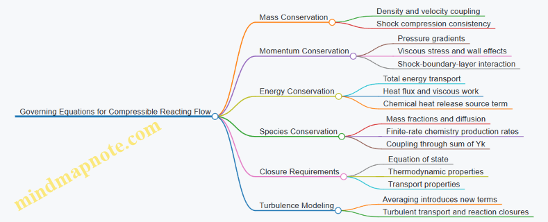
2.1 Governing Equations for Compressible Reacting Flows
Scramjet flowfields are compressible, often shock-containing, and chemically reacting. The governing equations are the same ones used in many high-speed problems; what changes is the coupling between compressibility, turbulence, and finite-rate chemistry. A practical way to stay sane is to start with conservation laws, then add the smallest set of physics needed for reacting, compressible flow.
Conservation of Mass
For a continuum with velocity u, density ρ, and time t, the mass conservation equation is
\[ \frac{\partial \rho}{\partial t}+\nabla\cdot(\rho\mathbf{u})=0. \]
In a steady inlet, this says that any local increase in density must be matched by a change in volumetric flow. In a scramjet inlet, shocks can compress the flow quickly, so the mass equation is what keeps the post-shock state consistent with the pre-shock flow.
Conservation of Momentum
Momentum conservation in compressible flow is
\[ \frac{\partial (\rho\mathbf{u})}{\partial t}+\nabla\cdot(\rho\mathbf{u}\otimes\mathbf{u})=-\nabla p+\nabla\cdot\boldsymbol{\tau}+\rho\mathbf{f}. \]
Here p is pressure, τ is the viscous stress tensor, and f represents body forces (usually gravity is negligible for scramjet scales). The key point for high-speed inlets is that pressure gradients and viscous stresses must balance acceleration, especially near walls and in shock-boundary-layer interactions.
Conservation of Energy
A common form uses total energy E per unit mass:
\[ \frac{\partial (\rho E)}{\partial t}+\nabla\cdot\big(\mathbf{u}(\rho E+p)\big)=\nabla\cdot\big(\boldsymbol{\tau}\cdot\mathbf{u}-\mathbf{q}\big)+\dot{\omega}_T. \]
E includes internal energy and kinetic energy. q is the heat flux (often modeled with Fourier’s law using an effective thermal conductivity), and \dot{\omega}_T is the energy source from chemical reactions. In reacting flow, the energy equation is where heat release shows up, and it is also where you must be careful: if your chemistry model adds heat but your thermodynamics are inconsistent, the solution will misbehave.
Species Conservation and Finite-Rate Chemistry
For each chemical species k with mass fraction Y_k and molecular diffusion flux j_k:
\[ \frac{\partial (\rho Y_k)}{\partial t}+\nabla\cdot(\rho\mathbf{u}Y_k)= -\nabla\cdot\mathbf{j_k}+\dot{\omega}_k. \]
\dot{\omega}_k is the net production rate from reactions. The sum of all species mass fractions is 1, so the species equations are coupled through both chemistry and diffusion. In combustors, this coupling is the reason that “mixing first, then burning” is not always a safe assumption; shocks and turbulence can create strong gradients that affect reaction rates.
Thermodynamic Closure
The equations above are not closed until you relate p, ρ, temperature T, and composition. A typical closure uses an equation of state and mixture properties:
- Ideal gas: \(p=\rho R_{mix}T\)
- Mixture molecular weight and \(R_{mix}\) from composition
- Transport properties (viscosity, conductivity, diffusion) as functions of T and composition
In scramjet combustors, temperatures can be high enough that transport properties vary strongly with temperature, so using constant properties is usually a shortcut that breaks quantitative predictions.
Turbulence and Averaging
Real scramjets operate with turbulent flow. Most practical models use Reynolds-averaged or density-weighted averaging, which introduces additional unknowns. The result is that viscous terms and reaction terms require closure models. A common structure is:
- Replace instantaneous fields with averaged ones
- Model turbulent viscosity and turbulent diffusion
- Use a combustion model to relate averaged reaction rates to mean quantities
Even if you do not write the full averaged equations here, the governing-equation takeaway is clear: turbulence changes both transport and effective reaction progress.
Mind Map: Governing Equations for Compressible Reacting Flow
Example: One-Dimensional Reacting Flow with Heat Release
Consider a steady 1D flow along x with species k. The mass equation reduces to
\[ \frac{d}{dx}(\rho u)=0 \Rightarrow \rho u=\text{constant}. \]
The species equation becomes
\[ \frac{d}{dx}(\rho u Y_k)= -\frac{d j_k}{dx}+\dot{\omega}_k. \]
If you assume negligible diffusion for a first estimate, then \(\frac{d}{dx}(\rho u Y_k)\approx \dot{\omega}_k\). The energy equation then links the temperature rise to the reaction source term \(\dot{\omega}_T\). This simple chain—mass sets \(\rho u\), chemistry sets \(\dot{\omega}_k\), and energy sets \(T\)—is exactly the coupling you must preserve in higher-fidelity models.
Example: Why Closure Matters
Suppose two models use the same \(\dot{\omega}*k\) but different thermodynamic closures. The reaction rates might be computed from the same temperature, yet the pressure and density fields differ because \(p=\rho R*{mix}T\) uses \(R_{mix}\) from composition. The result is a different shock strength and different residence time, which feeds back into chemistry. In other words, the governing equations are only as good as the closure that ties them together.
2.2 Shock Wave Formation and Interaction in High Speed Inlets
At high Mach numbers, the inlet does not “smoothly compress” the flow. Instead, it forces the flow to obey conservation laws across thin regions where pressure, temperature, and density change abruptly. Those regions are shock waves. In an inlet, shocks are not just events; they are moving structures that must be positioned and managed so the downstream combustor sees a usable pressure and temperature.
Foundational Mechanisms of Shock Formation
Shock formation begins when the flow attempts to pass through a region where the required downstream conditions cannot be met smoothly. A useful mental model is to compare the flow’s ability to communicate changes upstream with the speed of the flow itself. When the local flow becomes supersonic, pressure disturbances cannot travel upstream, so the flow “chooses” a discontinuity that satisfies the jump conditions.
For a normal shock, the key effects are immediate: static pressure rises, static temperature rises, and Mach number drops to a subsonic value (for the idealized case). In a real inlet, the shock is rarely perfectly normal. Oblique shocks form when the flow is turned by a ramp or wedge, producing a shock angle that depends on the upstream Mach number and the turning angle.
Oblique Shocks and Turning Limits
An inlet forebody often creates a sequence of oblique shocks. Each shock turns the flow toward the desired direction while increasing pressure. The turning angle cannot be increased arbitrarily. If the required turning is too large, the oblique shock system can no longer remain attached to the surface. The result is a detached bow shock or a separated shock system.
A practical example: imagine a wedge inlet operating at a fixed geometry. As Mach number increases, the same wedge turning angle demands a different shock angle. If the inlet is designed for a lower Mach number, the shock may move upstream and become less attached, which changes the effective capture area and can trigger unstart.
Shock Interaction Pathways in Inlets
Once multiple shocks exist, they interact. Interaction means one shock changes the upstream conditions seen by another shock, which alters its strength and position. Common interaction patterns include:
- Shock–shock interaction: Two shocks meet, producing a new set of waves. The downstream region after the interaction has a different pressure and Mach number than either shock alone would predict.
- Shock–boundary-layer interaction: A shock compresses the boundary layer, increasing pressure near the wall. If the adverse pressure gradient is strong enough, the boundary layer separates, creating a recirculation zone that can move and thicken.
- Shock–expansion interaction: If a shock is followed by an expansion region, the pressure can drop rapidly. The combined effect can reduce the net pressure recovery and alter the inlet’s operating margin.
A concrete example is a compression ramp followed by a cowl. The ramp generates an oblique shock that raises pressure. If the pressure rise is large, the boundary layer may separate at the ramp corner. The separated region changes the effective flow turning, so the next shock in the sequence can become stronger or shift position.
Shock Train Behavior and Pressure Recovery
Many inlets use a “shock train” concept: several oblique shocks and small regions of nearly uniform flow between them. The goal is to raise pressure gradually enough that the flow remains attached and the boundary layer stays thin. The pressure recovery is not just about the final pressure; it is also about how much total pressure is lost across each wave.
In idealized terms, stronger shocks increase entropy and reduce total pressure more than weaker shocks. In practice, the inlet designer balances shock strength against the need to fit the required compression into the available length. Shorter inlets tend to require stronger shocks, which increases the risk of separation and unstart.
Advanced Details That Matter in Design
Shock angle sensitivity: Small changes in upstream Mach number shift shock angles. That shift changes the location where shocks intersect the wall or internal surfaces.
Triple points and wave topology: When shocks meet surfaces and other shocks, triple points can form where three wave families intersect. These points can anchor the wave system, making it more stable—or more sensitive—depending on geometry.
Unstart linkage: Inlet unstart is often associated with a shock system moving upstream until it blocks the inlet throat. Shock interaction with the boundary layer can accelerate this by changing separation extent and effective throat area.
Mind Map: Shock Formation and Interaction in High Speed Inlets
Example: Predicting a Separation Trigger from Shock Strength
Suppose an inlet uses two compression ramps. At a nominal condition, the first ramp produces an oblique shock that raises wall pressure moderately, and the boundary layer remains attached. If the vehicle accelerates and the upstream Mach increases, the same ramp turning angle yields a stronger oblique shock. The stronger shock increases the post-shock pressure and the adverse pressure gradient over the boundary layer. If the boundary layer cannot overcome that gradient, it separates near the ramp corner. Once separated, the effective flow area shrinks and the next shock in the train can shift upstream, changing the inlet’s pressure recovery and stability.
Example: Shock–Shock Interaction Changing Throat Conditions
Consider a cowl lip that generates an oblique shock and a downstream internal feature that generates another shock. If the first shock moves due to a change in operating condition, it alters the Mach number and pressure entering the second shock. The second shock then becomes stronger or weaker than expected, which changes the pressure at the throat. That throat pressure directly affects whether the inlet can maintain stable compression into the combustor.
In short, shock formation is governed by the inability of supersonic flow to adjust smoothly, while shock interaction is governed by how each wave reshapes the conditions seen by the next. Managing both is what turns “compression” into a controllable inlet behavior.
2.3 Boundary Layer Behavior Under Extreme Pressure Gradients
A scramjet inlet and combustor see pressure changes so steep that the boundary layer can no longer rely on “gentle” assumptions. The boundary layer is still a thin region where viscosity matters, but its thickness, velocity profile, and even its ability to stay attached become functions of the local pressure gradient. In practice, you can treat the boundary layer as a pressure-gradient interpreter: it converts external pressure forcing into wall shear, separation risk, and mixing quality.
Core Concepts That Control the Boundary Layer
The starting point is the momentum balance in the near-wall region. When the external pressure gradient is favorable (pressure decreases along the flow), the boundary layer tends to thin and the wall shear often increases. When the pressure gradient is adverse (pressure increases along the flow), the fluid near the wall is asked to slow down. Viscosity then becomes a double-edged tool: it transmits the deceleration into the near-wall region, reducing wall shear and making separation more likely.
A useful nondimensional measure is the pressure-gradient parameter often expressed through the Clauser form of the adverse gradient strength. You do not need to memorize symbols to use the idea: stronger adverse gradients correspond to lower wall shear and higher separation probability. Another practical quantity is the boundary-layer shape, captured by the velocity profile through the shape factor. Higher shape factor generally signals a fuller profile and reduced resistance to separation.
How Extreme Gradients Change the Boundary Layer
Under extreme pressure gradients, three effects dominate.
First, the boundary layer thickens rapidly. The outer flow decelerates, and the near-wall region cannot “keep up” without a large viscous stress. As the wall shear drops, the boundary layer grows in thickness and the velocity gradient at the wall weakens.
Second, the boundary layer can transition from attached to separated flow even without a long, gradual ramp. In high-speed inlets, shocks and shock-induced expansions can create localized adverse gradients. The boundary layer may separate in a short region, then reattach downstream if the pressure gradient relaxes.
Third, compressibility alters the wall-normal structure. Density changes and compressible turbulence behavior modify how momentum is transported. A boundary layer that would remain attached in an incompressible estimate can separate earlier when compressibility effects are included.
Separation Mechanics with a Concrete Picture
Separation occurs when the wall shear stress approaches zero and then reverses sign. In a compressible, high-speed environment, this is not just a “stall” of the mean flow. The near-wall turbulence and pressure fluctuations interact with the mean adverse gradient, so the separation point can be sensitive to small changes in geometry, surface roughness, and shock location.
A concrete example: consider a boundary layer encountering a shock train in an inlet. The shock raises pressure abruptly, creating a strong adverse gradient immediately downstream. If the boundary layer is already thick (for example, due to a long forebody or a previous adverse region), the wall shear may collapse quickly, producing a separated pocket. That pocket can then alter the effective inlet capture area, changing the subsequent shock pattern and the pressure recovery.
Mind Map: Boundary Layer Under Extreme Pressure Gradients
Example: Using Pressure Distribution to Predict Separation on a Wall
Suppose you have a wall pressure trace along an inlet internal surface. If the pressure rises smoothly, the adverse gradient is spread out; separation may or may not occur depending on boundary-layer thickness. If the pressure rises sharply over a short distance, the adverse gradient is localized and the boundary layer has less time to adjust. A simple workflow is:
- Identify regions of rapid pressure rise from the wall pressure distribution.
- Check whether the boundary layer is already thick upstream (from prior gradients or geometry).
- Expect the separation point to occur near where wall shear would be driven to zero by the combined effect of adverse gradient strength and boundary-layer state.
In CFD, you can validate this by examining wall shear stress contours and the near-wall velocity profile. In experiments, you can infer separation from wall pressure behavior: separated flow often produces a pressure plateau or altered gradient because the effective flow path changes.
Practical Best Practices for Design and Analysis
Use pressure-gradient “hot spots” as first-order design constraints. When you place shocks, ramps, or expansions, treat them as boundary-layer forcing events, not just inviscid flow features. Aim to keep adverse gradients either mild or sufficiently short that the boundary layer does not reach a separation-prone state. When you cannot avoid strong gradients, design the inlet and combustor so that any separation is either minimized in extent or managed so it does not destabilize the overall pressure recovery and mixing.
2.4 Combustion Regimes in Scramjet Combustors
Scramjet combustors operate in a narrow window where the flow is fast, the residence time is short, and the inlet already did the hard work of compressing the air. “Combustion regime” is the practical way to describe what the fuel–air mixture is doing: whether ignition is reliable, whether the reaction is limited by chemistry, mixing, or heat loss, and whether the flame stays attached to a stable structure.
Foundational View of Regime Drivers
Three knobs largely determine the regime.
- Ignition and early reaction: At scramjet conditions, ignition delay can be comparable to the entire combustor residence time. If the mixture ignites late, the combustor behaves like a high-speed duct with heat addition that never fully develops.
- Mixing rate: Even if chemistry is fast, poor mixing can prevent reactants from meeting. Mixing limitations show up as incomplete burning and strong sensitivity to injection pattern.
- Thermal and flow losses: Wall heat transfer, finite pressure recovery, and nonuniform velocity profiles can quench reactions or shift the effective equivalence ratio.
A useful mental model is to compare chemical timescales to flow timescales. When chemistry is slower, you get chemistry-limited behavior; when chemistry is fast but reactants don’t meet, you get mixing-limited behavior. When both are fast enough to ignite but the flame cannot stay anchored, you get blowoff-like behavior.
Regime 1: No Ignition or Weak Reaction
In this regime, the combustor does not sustain a reaction zone. You may see small temperature rises near the injection but little pressure rise and no persistent heat-release region.
What causes it
- Mixture too lean locally, so ignition delay is long.
- Insufficient initial temperature or residence time.
- Injection momentum that produces strong dilution before ignition.
Easy example Imagine injecting fuel into a fast stream with a low local equivalence ratio. Even if the average mixture is “near stoichiometric,” the fuel may remain in thin streaks that never reach the temperature needed for ignition before the flow exits.
Regime 2: Ignition-Limited Combustion
Here, the reaction starts, but ignition timing is the bottleneck. The combustor may show a delayed rise in temperature downstream of the injection.
What it looks like
- Strong dependence on inlet temperature and equivalence ratio.
- Sensitivity to ignition assist features such as pilot zones, recirculation bubbles, or localized heating.
Best-practice example If you use a flameholder that creates a recirculation region, you are effectively increasing local residence time and temperature. A practical check is to compare pressure and temperature rise locations: if they shift significantly with small changes in equivalence ratio, you are likely ignition-limited.
Regime 3: Mixing-Limited Combustion
In this regime, ignition can occur, but complete burning is limited by how quickly fuel and air mix. The flame may exist as a distributed reaction zone rather than a sharply anchored structure.
What it looks like
- Incomplete conversion with strong sensitivity to injection geometry and spray breakup.
- Temperature rise that spreads over a longer axial distance.
Easy example Consider two injectors delivering the same total fuel flow. The one with better atomization and penetration creates smaller fuel-rich pockets that mix faster, producing higher overall heat release. The “coarser” injector can ignite but still leave pockets unburned.
Regime 4: Flameholder-Associated Combustion
This is the regime designers often aim for: a stable reaction zone anchored by a flow feature. Recirculation zones, bluff bodies, or cavities can hold hot products and radicals near the injection region.
What it looks like
- A relatively repeatable location of peak heat release.
- More robust operation across a range of conditions.
Best-practice example When testing, vary equivalence ratio in small steps and monitor where the temperature rise begins. If the onset location stays near the flameholder, the combustor is behaving as flameholder-associated rather than purely distributed.
Regime 5: Quenching and Partial Burning
At high heat flux or unfavorable local conditions, reactions can be quenched near walls or in low-temperature pockets. The result is partial burning even when ignition occurs.
What causes it
- Wall temperatures and heat transfer that remove energy faster than reactions can sustain.
- Strong gradients in equivalence ratio leading to locally lean or locally overcooled zones.
Easy example If a combustor has a hot core but thin boundary layers with strong heat flux, the near-wall region can become chemically inactive. You may still get a significant centerline temperature rise while overall efficiency remains limited.
Mind Map: Combustion Regimes
Integrated Example: Reading Regime Transitions
Suppose a combustor is tested at constant inlet conditions while equivalence ratio is increased. At low values, you observe weak reaction with no sustained heat release (Regime 1). As you raise equivalence ratio, ignition begins but occurs downstream of injection (Regime 2). With further increase, the reaction becomes more complete but spreads axially, indicating mixing limitation (Regime 3). When a flameholder is effective, the peak heat release locks near the flameholder and becomes less sensitive to small operating changes (Regime 4). At the highest heat flux or most aggressive operating points, near-wall quenching can reduce overall conversion even though the core remains hot (Regime 5).
This progression is not magic; it is the combustor telling you which constraint dominates at each operating point. The most useful design habit is to map those constraints to measurable signals—where the temperature rises, how pressure responds, and how sensitive the behavior is to mixture strength.
2.5 Nozzle Expansion and Thrust Generation Mechanisms
A scramjet nozzle turns the combustor’s high-pressure, high-temperature flow into useful momentum. The key idea is simple: thrust comes from changing the flow’s momentum, and nozzle expansion is the main tool for shaping that momentum change.
Core Thrust Mechanism
Thrust is the net force from two contributions: momentum flux and pressure acting on the nozzle exit area. In an idealized form, you can think of it as “how much mass flow you accelerate, and how different the exit velocity and pressure are from the surroundings.” A nozzle that expands too little leaves high exit pressure, which can help or hurt depending on whether the exit pressure is above or below ambient. A nozzle that expands too much can choke or separate, reducing effective thrust even if the pressure at the exit looks “nice” on paper.
A practical way to reason is to track three states: combustor exit (total pressure and temperature), nozzle throat (where the flow chokes), and nozzle exit (where the flow either remains attached or separates). Each state determines whether the nozzle is doing controlled expansion or causing losses.
Expansion Regimes and Choking
As the nozzle area decreases toward the throat, the flow accelerates and the static temperature drops. If the back pressure is high, the nozzle may not fully expand; if the back pressure is low enough, the flow reaches sonic conditions at the throat and becomes choked. Once choked, further reductions in back pressure mostly change the exit pressure rather than the mass flow.
For scramjets, this matters because the inlet and combustor can deliver a wide range of total pressure depending on operating condition. The nozzle must handle that variation without producing large separation regions that waste pressure recovery.
Pressure Matching and Exit Conditions
The “best” exit pressure depends on whether you include pressure thrust. If the nozzle exit pressure equals ambient, pressure thrust is near zero and thrust is dominated by momentum. If exit pressure is higher than ambient, pressure thrust adds positive force but only if the flow remains well-behaved. If exit pressure is lower than ambient, pressure thrust becomes negative and can reduce net thrust.
In practice, designers aim for robust performance across a range of inlet conditions. That means the nozzle contour and expansion ratio are chosen so that, over expected total pressure variations, the nozzle either stays close to attached expansion or transitions predictably.
Flow Losses from Separation and Shocks
Nozzle expansion is not just geometry; it is also about how the boundary layer responds to adverse pressure gradients. When the pressure recovery is too aggressive, the boundary layer can separate. Separation reduces effective area, increases losses, and can create unsteady shock/boundary-layer interactions.
At high Mach numbers, shocks can appear inside the nozzle when the flow is overexpanded relative to the ambient. These shocks convert kinetic energy into internal energy, lowering exit velocity. The result is a nozzle that may show a lower exit Mach number and higher exit pressure than expected, with reduced net thrust.
Nozzle Geometry Choices
A common baseline is a convergent-divergent nozzle. The convergent section helps establish a throat and stabilize choking. The divergent section provides expansion. For scramjets, the contour is often shaped to manage pressure gradients and reduce separation risk.
A useful rule-of-thumb example: suppose combustor exit total pressure is fixed, but ambient pressure varies with flight condition. If the nozzle expansion ratio is set for a “mid” ambient pressure, then at higher ambient the nozzle is underexpanded (exit pressure too high), and at lower ambient it is overexpanded (shocks and separation risk). The design goal is to keep both cases within acceptable loss margins.
Mind Map: Nozzle Expansion and Thrust
Example: Interpreting Two Nozzle Outcomes
Consider two operating points with the same combustor exit total temperature but different total pressure. In the first point, higher total pressure increases available pressure ratio, so the nozzle can expand more effectively before encountering separation. In the second point, lower total pressure reduces the pressure ratio, so the nozzle may not reach the intended expansion level; exit pressure rises, and pressure thrust may partially compensate while exit velocity drops.
Now add ambient variation: if the nozzle is overexpanded at the second point, shocks can form, increasing losses and making the compensation from pressure thrust unreliable. The net effect is that thrust is not determined by exit pressure alone; it depends on how the flow got there.
Example: A Simple Accounting Workflow
- Estimate combustor exit total pressure and temperature.
- Determine whether the nozzle is choked by comparing back pressure to the choking threshold.
- For the expected regime, predict exit pressure and exit Mach using an expansion model.
- Apply a loss factor for separation or shock losses based on pressure gradient severity and boundary-layer state.
- Compute net thrust from momentum plus pressure terms.
This workflow keeps the reasoning grounded: geometry sets the expansion path, operating conditions set the pressure ratio, and losses decide how much of the ideal momentum change survives to the exit.
3. Inlet Design for High Mach Operation
3.1 Inlet Flowpath Geometry and Internal Aerodynamic Goals
A scramjet inlet is not just a duct; it is a controlled argument between shocks, boundary layers, and pressure recovery. The flowpath geometry sets where compression happens, how much total pressure survives, and whether the inlet can deliver a usable, nearly uniform core to the combustor.
Mind Map: Inlet Flowpath Geometry and Internal Aerodynamic Goals
Foundational Geometry Choices
Start with the external shape because it determines the initial shock pattern. A forebody contour that creates the right oblique shock angles at the design Mach number helps keep the shock system anchored inside the inlet rather than wandering into the forebody or spilling downstream.
Next, define the internal area distribution. For a typical inlet, the goal is to compress the flow while limiting adverse pressure gradients that thicken the boundary layer. A practical way to think about it is to treat the inlet as a sequence of small “pressure recovery steps” rather than one big diffuser. Each step should be gentle enough that the boundary layer can remain attached.
Internal Aerodynamic Goals
Shock Train Location and Stability
The inlet often uses a shock train to gradually reduce Mach number while maintaining pressure recovery. Geometry controls where those shocks sit by shaping the effective streamlines and the local area ratio. If the shocks are too far upstream, they can over-compress the boundary layer and trigger early separation. If they are too far downstream, the combustor may see a nonuniform inlet total pressure and a distorted Mach profile.
A simple diagnostic is to compare expected shock positions with the inlet’s internal length. If the inlet is short, the geometry must avoid relying on many weak shocks that require distance to form.
Boundary Layer Growth and Separation Avoidance
Boundary layer growth is the inlet’s quiet performance killer. As the flow decelerates, the wall pressure rises, and the boundary layer needs momentum to resist separation. Geometry that produces a strong adverse gradient—often from an overly aggressive diffuser angle or contraction mismatch—can cause separation even if the inviscid pressure recovery looks fine.
A concrete example: consider two diffuser schedules that both achieve the same overall area ratio. The schedule with a front-loaded aggressive angle creates a steep pressure rise early, which increases separation risk. The schedule that spreads the diffusion more evenly tends to preserve attachment, even if it looks less “efficient” on a single snapshot.
Pressure Recovery and Core Uniformity
Pressure recovery is not just about total pressure magnitude; it is also about distribution. The combustor typically tolerates some nonuniformity, but large circumferential or radial gradients can lead to uneven equivalence ratios, local overheating, and unstable ignition.
Geometry influences uniformity through how shocks and boundary layers interact. When shocks impinge on the boundary layer, they can thicken it and create a low-total-pressure region near the wall. If the combustor inlet plane is placed too close to that interaction region, the combustor sees a distorted profile.
Matching to the Combustor Interface
The interface plane should be treated as a contract. Define target conditions such as captured mass flow, acceptable total pressure loss, and a maximum allowable nonuniformity metric. Then choose the inlet’s internal length and diffusion rate so that the flow has time to relax after the final shock interaction.
A practical example: if the inlet’s last compression occurs right at the interface, the combustor may receive a strong radial Mach gradient. Moving the interface slightly downstream of the final shock interaction can reduce that gradient, but only if the added length does not reintroduce separation risk.
Design Workflow for Geometry Decisions
- Choose the external shape to set the primary shock angles at the design condition.
- Build an internal area schedule that limits adverse gradients and spreads diffusion.
- Estimate shock train behavior and check whether shocks remain inside the inlet across the intended operating range.
- Evaluate boundary layer attachment risk using wall pressure gradient trends and separation indicators.
- Set the interface plane location to balance relaxation of the core with avoidance of late separation.
Example: Two Inlet Flowpaths with Different Diffuser Schedules
Path A uses a large diffuser angle early, then a mild recovery section. Path B uses a mild angle early, then a stronger recovery later. Both can meet the same overall area ratio, but Path A tends to create a thicker near-wall low-total-pressure region because the early adverse gradient accelerates boundary layer growth. Path B often delivers a more uniform core at the interface because the boundary layer experiences a gentler pressure rise before the stronger recovery begins.
The key takeaway is simple: geometry must manage not only the inviscid compression, but also the viscous consequences of that compression. In a scramjet inlet, the boundary layer is part of the flowpath design, not an afterthought.
3.2 Starting and Unstart Considerations for Inlet Stability
A scramjet inlet is stable only when the internal pressure field matches what the vehicle can physically support. “Starting” is the transition from an unstarted or weakly started state into a condition where the inlet captures and delivers flow to the combustor with predictable pressure recovery. “Unstart” is the reverse: the shock system moves, the capture pattern degrades, and the inlet can no longer maintain the intended internal compression.
Core Stability Concepts
Start with the inlet’s shock train and boundary layer. At high Mach, compression is achieved through oblique shocks and a terminal normal or quasi-normal shock. The inlet is stable when the terminal shock location and the downstream pressure it imposes remain within an acceptable range. Boundary layers matter because they reduce effective flow area and change how shocks interact with the wall and with each other.
A practical way to think about stability is as a feedback loop: the inlet geometry sets how much compression is demanded; the combustor and engine backpressure determine how much pressure the inlet must deliver; the mismatch shifts shocks upstream or downstream. If the shock system shifts upstream far enough, it can spill outside the inlet capture region, causing unstart.
Mind Map: Starting and Unstart Mechanisms
Starting Sequence: From Weak Compression to Captured Shocks
A common starting problem is that the inlet initially behaves like a “cold” duct with insufficient downstream pressure support. If the combustor is not yet producing the pressure rise the inlet expects, the terminal shock can sit too far downstream or oscillate. The fix is not magic; it is sequencing and matching.
- Establish a baseline backpressure: During early operation, the combustor may be in a low-heat state. Designers often use a controlled ignition or a staged fuel schedule so that backpressure rises smoothly rather than abruptly.
- Avoid sudden area-demand changes: Fueling changes heat release and can alter effective compressibility and pressure distribution. If fuel is introduced faster than the inlet can respond, the shock system can jump.
- Use a controlled ramp of operating point: In practice, the vehicle’s flight condition changes continuously. A stable inlet tolerates gradual changes; it struggles when the demanded compression changes faster than the shock system can settle.
Example: Suppose the inlet is designed for a terminal shock near a specific axial station. If ignition is delayed until the vehicle is already at a higher dynamic pressure, the combustor backpressure arrives late. The terminal shock then migrates upstream during the delay, and when backpressure finally rises, the shock may overshoot the target location. A staged fuel ramp that begins earlier at a lower heat release rate can keep the terminal shock within a narrow band.
Unstart Triggers and What They Look Like
Unstart is usually triggered by one or more of these conditions:
- Backpressure mismatch: Too high backpressure can push the terminal shock upstream; too low backpressure can let the shock system drift and lose capture.
- External condition shifts: Changes in Mach number or angle of attack alter the effective compression demand.
- Boundary layer separation: When shocks interact with a thickened boundary layer, separation can create a low-momentum region that changes shock behavior and promotes spillover.
Example: Consider a small misalignment that increases effective angle of attack. The inlet’s compression becomes asymmetric, and the terminal shock may move upstream on one side first. That asymmetry can reduce overall capture and trigger a full unstart even if the average conditions seem acceptable.
Stability Margins and Practical Design Levers
Stability margins are the difference between “where the inlet wants the shock to be” and “where it can safely be.” You can widen margins by:
- Shaping the internal area ratio so the pressure recovery curve is less sensitive to small operating changes.
- Providing controlled bleed or bypass so the inlet can relieve pressure when the shock system begins to migrate.
- Designing for boundary layer robustness using surface treatments, careful ramping, and geometry that reduces adverse pressure gradients.
Example: If a combustor produces backpressure that varies strongly with fueling, the inlet sees a moving target. A combustor design that yields a smoother backpressure response reduces the likelihood of shock migration. In the inlet, a modest bleed can prevent the terminal shock from marching upstream when the backpressure temporarily spikes.
Diagnostics and Acceptance Criteria
Inlet stability is verified with measurements that indicate shock location and pressure recovery quality. Common signals include:
- Static pressure taps along the inlet to infer shock position.
- Total pressure trends to detect capture loss.
- High-frequency pressure fluctuations that correlate with oscillatory unstart behavior.
Example: During a test, if the upstream static pressure rises while downstream static pressure drops, the terminal shock likely moved upstream and the inlet is losing effective compression. Acceptance criteria can be defined as limits on shock location range and on allowable fluctuation amplitude.
Integrated Takeaway
Starting and unstart are not separate events; they are two sides of the same pressure-feedback problem. Stable operation requires matching the inlet’s compression demand to the combustor’s pressure support while keeping boundary layer behavior predictable. When that match is maintained through geometry, sequencing, and control, the shock system stays captured and the inlet behaves like a tool rather than a surprise.
3.3 Shock Train Design and Pressure Recovery Optimization
A scramjet inlet often needs a controlled sequence of shocks to slow the flow to a speed where the combustor can do useful work. The goal is not “maximum compression,” but “useful compression with minimal losses.” A shock train is the practical compromise: multiple oblique shocks (and sometimes a terminal normal shock) that gradually raise static pressure while keeping the boundary layer from separating.
Foundational Picture of Shock Trains
Start with what a single oblique shock does: it turns the flow by a small angle, increases pressure and temperature, and reduces Mach number. If the required total turning is large, one big shock would demand an angle that is hard to realize and would likely trigger separation. A shock train spreads the turning across several shocks, each operating closer to its stable range.
Pressure recovery depends on two competing effects:
- Thermodynamic gain: shocks raise static pressure.
- Irreversibility and losses: shocks also create entropy, and boundary-layer thickening reduces effective area.
A good design keeps the shocks strong enough to achieve the needed Mach reduction, but weak enough to avoid large separation bubbles.
Geometry Choices That Control Shock Strength
Shock strength is tied to the local flow deflection and the local Mach number. In practice, you shape the inlet so that each ramp or wedge produces a deflection that matches the expected upstream Mach.
A systematic approach:
- Choose a target Mach at combustor entry based on combustor operability and thermal limits.
- Estimate the required total turning to reach that Mach from the expected freestream condition.
- Distribute turning across multiple shocks so each shock sees a manageable deflection.
A concrete example: suppose the inlet must reduce Mach from 3.0 to about 2.0 at a design condition. A single deflection large enough to do this in one step would likely exceed the stable oblique-shock range. Splitting the turning into three smaller deflections keeps each shock closer to its “sweet spot,” where pressure rise is meaningful but the boundary layer remains attached.
Shock Train Placement and Interaction
In a multi-shock inlet, shocks do not exist in isolation. Their downstream positions affect the flowfield that the next shock “sees.” If the shocks are placed too far apart, the flow between them can expand or develop nonuniformities that weaken subsequent compression. If they are too close, the shocks can interact strongly, producing local regions of high gradients and potential separation.
Two practical placement rules:
- Maintain a consistent effective flow angle at each shock location by controlling forebody curvature and ramp transitions.
- Avoid abrupt area changes that can reflect shocks and create unwanted secondary wave systems.
Boundary Layer and Separation Risk
Even if the inviscid shock pattern looks correct, the viscous flow can ruin the party. Across a shock, the adverse pressure gradient can thicken the boundary layer. If the pressure rise is too abrupt, the boundary layer may separate, causing a loss of effective capture area and a drop in pressure recovery.
Design best practices that follow directly from this physics:
- Use gradual ramp transitions so the boundary layer experiences a smoother pressure history.
- Keep shock-induced pressure gradients within what the boundary layer can tolerate for the expected Reynolds number.
- Account for inlet roughness and manufacturing waviness because they increase boundary-layer thickness and reduce separation margin.
A simple diagnostic mindset: if pressure recovery is lower than predicted, check whether the shock train is shifting upstream or downstream with condition changes, which often signals separation or strong viscous interaction.
Pressure Recovery Metrics That Actually Matter
Pressure recovery is often reported as a ratio of total pressure at combustor entry to freestream total pressure. For optimization, it helps to separate two contributors:
- Inviscid compression performance: how well the shock pattern achieves the desired Mach reduction.
- Viscous loss performance: how much total pressure is lost to entropy generation and boundary-layer effects.
A useful optimization objective is to maximize pressure recovery subject to constraints:
- no inlet unstart behavior in the operating envelope
- no sustained separation at the design condition
- acceptable thermal loads on leading edges and ramps
Mind Map: Shock Train Design and Pressure Recovery
Example: Optimizing a Three-Shock Train
Assume a three-ramp inlet at a design Mach where you need a moderate Mach reduction. You start with equal deflections, then test sensitivity.
- Baseline: equal deflections produce the correct terminal Mach in an inviscid model.
- Observation: the predicted pressure recovery is lower than expected when viscous effects are included.
- Adjustment: reduce the first shock deflection slightly and increase the last shock deflection so the strongest adverse gradient occurs later, where the boundary layer is thinner due to upstream compression.
This is not magic; it’s boundary-layer timing. The first shock sets the early pressure history. If it is too aggressive, it thickens the boundary layer early and reduces the ability of later shocks to compress without separation.
Advanced Details Without the Mystery
Two advanced considerations often decide whether the design behaves well across conditions:
- Shock position drift: as freestream Mach changes, the oblique-shock solution shifts. If the shocks drift toward a ramp corner, local separation risk increases.
- Terminal shock choice: if a normal shock is used, its location relative to the combustor entrance affects both pressure recovery and the uniformity of the flow entering the combustor.
A disciplined optimization therefore includes condition sweeps and checks that the shock train remains in the intended geometric “comfort zone,” where compression is achieved without turning the boundary layer into a separation event.
3.4 Boundary Layer Control Methods for Inlet Performance
At scramjet inlet speeds, the boundary layer is not a side character—it decides whether the internal shocks land where you want them. Boundary layer growth increases displacement thickness, which effectively reduces the inlet’s usable area and shifts the shock system. The result can be higher total pressure loss, earlier unstart, and reduced combustor stability. Boundary layer control aims to keep the boundary layer thin, stable, and predictable across the operating Mach range.
Foundational Concepts That Drive Control Choices
A boundary layer thickens because the near-wall fluid has lower momentum and the pressure gradient does work on the flow. In an inlet, the pressure gradient is often adverse near compression ramps and in regions approaching the shock train. If the wall pressure rises faster than the fluid can respond, the boundary layer can separate. Separation is especially harmful because it changes the effective geometry and can create a new shock pattern.
A practical way to think about control is to track three quantities: displacement thickness (how much area the boundary layer “steals”), momentum thickness (how much energy the near-wall region has), and the wall shear stress (a proxy for whether the flow is attached). Control methods either reduce growth, energize the near-wall flow, or manage the pressure gradient so separation is less likely.
Passive Methods for Thin, Predictable Layers
Surface shaping and pressure gradient management. Smooth, carefully contoured forebody and inlet internal walls reduce abrupt adverse gradients. Even when the overall compression is fixed by mission requirements, the distribution of compression along the length can be tuned so the boundary layer sees a gentler gradient.
Roughness and trip placement. A controlled transition to turbulence can sometimes help by increasing mixing and delaying separation. The trick is to place the trip where the boundary layer is thick enough to respond but not so early that it causes excessive drag or total pressure loss. For inlet design, the goal is not “more turbulence,” but “turbulence where it improves attachment.”
Boundary layer bleed or suction. Suction removes low-momentum fluid from the wall region, reducing displacement thickness. Bleed adds mass and can thicken the layer, so suction is the usual choice when the inlet must stay compact. Suction effectiveness depends on having enough suction mass flow and a wall permeability or slot geometry that does not disturb the outer flow.
Active Methods for Robust Attachment
Wall transpiration control. Active suction can be modulated with operating condition. When the inlet approaches a higher compression state, increasing suction can prevent separation. The control logic typically uses measured wall pressure or inferred separation indicators.
Boundary layer blowing. Blowing injects momentum near the wall. It can re-energize the boundary layer and suppress separation, but it also adds mass and can disturb the shock system if the jet penetrates too far. In practice, blowing is tuned to be just strong enough to maintain attachment while keeping jet penetration shallow.
Plasma and electromagnetic forcing. These methods can alter near-wall momentum through body forces. They are complex to integrate and require power and diagnostics, so they are usually evaluated at component scale with careful attention to how the forcing changes the shock-boundary layer interaction.
Shock-Boundary Layer Interaction as the Core Design Problem
In inlets, the boundary layer often meets shocks. A compression shock can increase wall pressure and drive the boundary layer toward separation. A key best practice is to design the shock train so that the strongest shocks do not strike a thick boundary layer. That means controlling both the external shock location and the internal boundary layer thickness.
A useful rule of thumb is to treat boundary layer control as part of the shock design, not an afterthought. If you change the boundary layer thickness, you change the effective geometry, which can move the shock system. Therefore, control hardware must be included in the same analysis loop as the inlet flowpath.
Integrated Example: Choosing Between Suction and Surface Shaping
Suppose an inlet shows increasing total pressure loss as Mach rises, and wall pressure traces indicate intermittent separation near a compression ramp. You first check whether the adverse pressure gradient is too steep for the current boundary layer thickness. If the ramp contour is fixed by external packaging, suction becomes attractive.
A systematic approach is:
- Estimate displacement thickness growth from a baseline model.
- Identify the location where the wall pressure rise is most adverse.
- Evaluate suction effectiveness by targeting a reduction in displacement thickness at that location.
- Recompute the shock pattern with the modified boundary layer.
If suction reduces separation but the shock train shifts upstream, you may need to adjust suction location or strength so the shock system remains in the intended region.
Mind Map: Boundary Layer Control Methods for Inlet Performance
Practical Design Checklist
- Place any boundary layer control hardware where it influences the region of strongest adverse pressure gradient or the expected shock interaction.
- Treat boundary layer control as part of the inlet aerodynamics model, not a separate add-on.
- Validate with instrumentation that can detect separation onset, such as wall pressure distributions and near-wall flow indicators.
- Ensure the chosen method does not introduce new disturbances that move the shock train into a less stable configuration.
3.5 Inlet Instrumentation and Data Reduction for Validation
Validation starts with a simple question: did the inlet produce the flowfield you designed, at the conditions you tested? Answering it requires instrumentation that can measure the right quantities, plus data reduction that turns raw signals into comparable, physics-based metrics.
Foundational Measurements That Tie to Inlet Physics
Begin by mapping inlet phenomena to measurable observables. For high-Mach inlets, the key behaviors are shock structure, boundary-layer state, and pressure recovery. Pressure taps provide the fastest path to shock location and overall recovery. Fast-response pressure transducers capture unstart dynamics, where the inlet oscillates between stable and unstable states.
Boundary-layer health is harder. Wall pressure and wall heat flux correlate with separation and reattachment, but they are indirect. If you can add surface oil-film interferometry or temperature-sensitive coatings, you gain spatial separation maps. For internal flow, schlieren or shadowgraph imaging shows shock geometry and helps confirm whether the shock train is attached and steady.
Fuel-free validation still needs thermal context. Even without combustion, inlet compression heats the flow and changes density, which affects shock strength and boundary-layer thickness. Thermocouples or thin-film temperature sensors on the outer mold line support thermal boundary conditions for CFD correlation.
Instrumentation Layout and Practical Placement
A good layout avoids “measurement theater,” where sensors are present but not interpretable. Place pressure taps along the expected shock train axis so that pressure gradients reveal shock steps. Use a denser spacing near predicted shock locations, then widen spacing downstream where gradients smooth out.
For fast transients, mount pressure transducers with short tubing and consistent routing to reduce phase lag. If you must use longer lines, calibrate the frequency response so your unstart timing is not an artifact of plumbing.
Optical diagnostics need line-of-sight windows aligned with the inlet centerline and at least one off-axis plane. If the window distorts the beam path, correct it using a calibration target placed at the same optical distance as the test article.
Calibration and Synchronization
Before reducing data, calibrate every sensor in the operating range. Pressure transducers should be checked for zero drift and linearity. Temperature sensors require both offset and gain verification, especially if they sit near strong thermal gradients.
Synchronization matters because inlet events are fast. Use a common trigger for pressure transducers, imaging cameras, and any flow-control signals. Then verify alignment by checking that a known event, such as a valve actuation, appears at the same time across channels.
Data Reduction from Signals to Validation Metrics
Raw pressure signals become validation metrics through consistent processing. First, convert transducer readings to static pressure using calibration curves. Next, compute nondimensional pressure ratios relative to a reference station upstream of the inlet.
Shock location can be estimated by finding steep pressure gradients along the wall or by using image-derived shock edges. For each test condition, report shock position as a function of inlet capture area and back pressure. This makes results comparable across runs even when absolute pressures drift.
Pressure recovery is computed as the ratio of downstream static pressure to upstream total pressure, corrected for reference station definitions. Use the same station definitions as in CFD so that “good agreement” is not just a naming mismatch.
Boundary-layer indicators benefit from a simple, repeatable approach. For example, define a separation proxy from wall pressure behavior: a sustained adverse pressure gradient combined with a characteristic pressure plateau suggests separation. Pair this with heat-flux or surface temperature trends to reduce false positives.
Example Workflow for One Test Point
Example: A Mach 3.2 inlet test at a fixed back pressure.
- Select the stable interval using pressure transducer criteria: reject segments where oscillation amplitude exceeds a threshold.
- Average pressure taps over the stable interval and compute nondimensional pressure ratios.
- Determine shock train attachment by combining wall pressure gradients with schlieren shock edges.
- Compute pressure recovery and compare to CFD using identical reference stations.
- Produce a compact validation report: shock positions, recovery, and separation proxy location.
This workflow keeps the analysis honest: it separates “what happened” from “how we interpret it.”
Mind Map: Inlet Instrumentation and Data Reduction
Common Failure Modes and How to Avoid Them
A frequent issue is reference mismatch: if CFD uses a different upstream station than the experiment, recovery comparisons become misleading. Another is phase lag in pressure lines, which can shift apparent shock timing and distort unstart characterization. Finally, averaging over mixed stable and unstable intervals hides the very signatures you are trying to validate. Use stable-interval selection before computing recovery and shock metrics.
A validation dataset should read like a coherent story: sensor calibration, synchronized acquisition, stable-interval selection, then physics-based metrics that can be compared directly to inlet design intent.
4. Combustor Architecture and Fueling Strategies
4.1 Combustor Layout Choices for Residence Time Management
Residence time management is the art of making the gas spend the right amount of time in the combustor so that ignition and heat release happen where you can actually use them. In a scramjet, the flow is already moving fast, so “right amount” is mostly about geometry, not heroics. The layout choices below connect directly to how long the mixture stays hot enough and mixed enough to burn.
Foundational Concepts for Residence Time
Residence time is often approximated as
- τ ≈ L / U, where L is the effective combustor length and U is the local axial velocity.
That simple relation hides two practical realities. First, U changes along the combustor because of pressure gradients and heat addition. Second, the “effective length” is not the same as the physical length when mixing is incomplete. A layout that shortens the physical length can still increase effective residence time if it creates recirculation zones that trap hot products and promote mixing.
A useful mental model is to separate the job into two clocks:
- Ignition clock: time until a combustible mixture reaches conditions for sustained reaction.
- Burning clock: time to convert enough reactants to raise temperature and pressure for thrust.
Residence time management means balancing both clocks without letting the combustor become a pressure-loss machine.
Layout Options and Their Mechanisms
Straight-Through Combustor with Controlled Mixing
A straight-through combustor uses a relatively simple flowpath and relies on fuel injection and aerodynamic shaping to create mixing. Residence time is mainly controlled by length and local velocity. Best practice is to design the injection so that mixing starts early, because late mixing forces the burning clock to run out before the nozzle.
Example: If the inlet delivers a high-speed core with a thin boundary layer, a straight-through combustor can still work by placing injectors near the shear layer so that jets entrain core gas quickly. The effective residence time increases because the reacting mixture forms sooner along the axis.
Recirculation-Based Combustor with Flameholding Regions
Recirculation zones create a low-velocity region where hot products persist. This increases effective residence time without requiring a long combustor. The layout typically includes a cavity, step, or swirl-assisted recirculation that generates a stable recirculation bubble.
Example: A cavity flameholder can be sized so that the recirculation bubble occupies a predictable fraction of the cross-section. Even if the bulk flow is fast, the trapped region keeps radicals alive and provides a continuous ignition source for downstream mixing.
Multi-Pass or Staged Combustion Layouts
Staging splits the combustor into segments with different roles, such as ignition in the first stage and bulk heat release in the second. This can reduce the risk of overdriving one region while still meeting overall residence time needs.
Example: Stage 1 can be shorter and optimized for ignition using stronger local mixing, while Stage 2 uses gentler mixing and longer effective interaction time. The layout reduces the chance that the first stage consumes reactants too aggressively and starves the second stage.
Advanced Details That Actually Move Residence Time
- Cross-Section Area Variation: Expanding area can lower axial velocity, increasing τ, but it also affects pressure and mixing. A small controlled expansion can help without causing excessive pressure loss.
- Mixing Layer Growth: Residence time is wasted if mixing is slow. Layouts that promote shear-layer growth often outperform layouts that only increase length.
- Thermal Feedback to Ignition: Hot products in recirculation zones raise local temperatures, effectively shortening the ignition clock even if τ is unchanged.
- Pressure Loss Budget: Every feature that increases residence time also risks adding drag and reducing mass flow. A good layout manages both clocks while keeping total pressure loss within the inlet-combustor-nozzle system budget.
Mind Map: Residence Time Management in Combustor Layout
Integrated Example Layout Decision Flow
A systematic way to choose a layout is to start from where you need heat release to occur.
- If heat release must start early, prefer recirculation-based or staged layouts that shorten the ignition clock.
- If heat release can start later but must be sustained, prefer straight-through with early mixing and sufficient effective length.
- If pressure loss is tight, use staging to concentrate features where they do the most work, instead of spreading complex geometry everywhere.
Example: Suppose the combustor must fit within a constrained length. A straight-through design may not provide enough τ for the burning clock. A recirculation-based design can recover effective residence time by trapping hot products, while staging can prevent the first region from consuming too much reactant before the second region contributes to thrust.
4.2 Fuel Injection Schemes for Mixing and Ignition Support
Fuel injection in a scramjet combustor has two jobs that fight each other: it must mix fast enough to reach a combustible mixture, and it must do so while the flow is already under severe time pressure. The scheme you choose determines droplet or jet breakup, penetration into the hot core, local equivalence ratio, and how ignition-support features survive heat soak.
Core Mixing Requirements
Start with the mixing target: you want a near-uniform equivalence ratio in the region where ignition is expected, but you also need local pockets that are easier to ignite. A practical way to think about it is in three zones.
- Entry zone: fuel must be introduced without immediately quenching the flow with overly rich pockets.
- Ignition-support zone: fuel concentration and temperature must align so that ignition kernels can form and grow.
- Burning zone: mixing must continue so that the combustor does not rely on a single “lucky” location.
A simple example: if the combustor residence time is short, a scheme that produces long fuel streaks will leave some streamlines too lean to burn, even if the overall average equivalence ratio looks fine.
Injection Hardware Choices
Central Jet Injection
A central injector sends a fuel jet into the core. It tends to give strong penetration and can create a relatively coherent mixing pattern. The best use case is when you can tolerate higher local equivalence ratio near the centerline.
Easy example: imagine a single fuel jet aimed slightly upward. At low fuel flow, the jet may remain too concentrated and fail to mix before the ignition-support region ends. At higher flow, the same geometry can overshoot and create rich pockets that increase soot risk and wall heat flux.
Annular Injection Around the Core
Annular injection distributes fuel along a ring, reducing the chance of a single rich plume. It also offers a more symmetric mixing field, which helps when the combustor has a strong cross-sectional temperature gradient.
Easy example: if the inlet delivers a nonuniform temperature profile, an annular ring can “average out” the local mixture strength so that ignition-support features do not have to compensate for one hot or cold side.
Staged Injection for Controlled Equivalence Ratio
Staging splits fuel into two or more axial locations. The upstream stage can support ignition, while the downstream stage can improve mixing and reduce wall heat flux.
Easy example: inject 60% of the fuel upstream to ensure ignition-support conditions, then inject the remaining 40% downstream to complete mixing. If you instead inject all fuel upstream, you may ignite reliably but end up with incomplete mixing and higher peak temperatures.
Ignition Support Through Local Enrichment
Ignition support is not just “more fuel.” It is fuel placement that creates a region where ignition energy can trigger a self-sustaining reaction. For hydrocarbon fuels, the key is to create a mixture that is neither too lean nor too rich in the ignition-support zone.
Pilot-Like Enrichment Using a Small Upstream Fraction
Use a small upstream fraction to create a stable ignition region, then rely on downstream injection and mixing for the bulk.
Easy example: if the combustor is marginal at the lowest operating condition, increase only the upstream fraction slightly. This can raise local reactivity without flooding the entire combustor with rich mixture.
Co-Flow and Counter-Flow Injection Effects
Injection direction changes relative velocity and thus breakup and mixing rate.
- Co-flow injection often yields smoother penetration but can under-mix if the relative velocity is low.
- Counter-flow injection can enhance breakup and mixing but may increase aerodynamic losses and disturb the inlet recovery.
Easy example: if you see ignition delay that grows as Mach number increases, check whether the injection relative velocity is dropping. A small change in injection angle can restore breakup quality.
Atomization, Breakup, and Spray Penetration
Fuel may be injected as liquid droplets or as a gaseous stream. For liquid injection, atomization quality determines droplet size distribution, which controls evaporation time.
A systematic approach:
- Choose injection pressure or gas assist to achieve target droplet sizes.
- Estimate evaporation time relative to residence time.
- Verify penetration so droplets reach the ignition-support zone before they evaporate completely.
Easy example: if droplets are too large, they may not evaporate before the ignition-support zone ends, leaving a locally cold mixture. If droplets are too small, they may evaporate early and form a lean mixture that is hard to ignite.
Mind Map: Fuel Injection Scheme Logic
Integrated Example: Choosing a Two-Stage Scheme
Suppose the combustor must operate over a range where ignition becomes difficult at the low end. A two-stage scheme can be tuned without redesigning the entire injector.
- Stage 1 (upstream): inject a smaller fraction with geometry that promotes penetration into the ignition-support zone.
- Stage 2 (downstream): inject the remaining fuel farther aft to finish mixing and reduce peak temperature.
Validation is straightforward: compare measured pressure rise and wall heat flux trends against predicted local equivalence ratio. If ignition occurs but wall heat flux spikes, reduce upstream fraction or adjust injection angle to avoid overly rich pockets near the walls.
Practical Best Practices
- Design for local mixture, not just average mixture. Average equivalence ratio can look correct while ignition-support pockets remain too lean.
- Use staging to separate ignition and mixing responsibilities. This reduces the coupling between “can it ignite?” and “does it burn cleanly?”
- Match atomization quality to residence time. Droplet size distribution is a mixing tool, not a detail.
- Tune injection direction with relative velocity in mind. If breakup weakens at higher Mach, ignition support will degrade even when total fuel flow is unchanged.
4.3 Ignition Methods and Their Integration With Hardware
Scramjet ignition is less about “starting a flame” and more about creating a short, repeatable region where the fuel–air mixture reaches ignition conditions while the inlet and combustor are already doing their high-speed jobs. Hardware integration matters because ignition energy, timing, and thermal environment are coupled to inlet pressure, combustor residence time, and wall heat flux.
Foundational Constraints for Ignition
Ignition must work across a range of inlet states, including cases where the combustor inlet is hot but not yet chemically ready. The ignition system therefore needs (1) a reliable energy source, (2) a way to place that energy where mixing and temperature are favorable, and (3) a thermal and mechanical design that survives repeated cycles.
A practical way to reason about ignition is to treat it as a local event inside a global flow. The local event requires sufficient radical production and mixture stratification, which depends on fuel injection pattern and equivalence ratio near the ignition zone. The global flow determines how long that zone stays within the ignition window.
Ignition Method Families
Spark ignition uses an electrical discharge to initiate a flame kernel. It is straightforward to integrate but can struggle when the mixture is too lean, too cold, or too diluted by strong shear. Spark systems also require careful electrode placement to avoid erosion and to prevent the electrode from acting like an unwanted heat sink.
Pyrotechnic or chemical igniters provide a rapid heat and species source. They can be effective in difficult conditions, but they introduce packaging complexity, one-time consumables, and thermal shock loads. For defense platforms, the integration challenge is often not “can it ignite?” but “can it be safely stored, handled, and verified?”
Laser ignition can target a small region with minimal hardware intrusion. It offers precise spatial control, but integration includes optical access, alignment retention, and protection from soot and thermal distortion.
Hot-surface ignition relies on a heated element to promote ignition. It can be robust once at temperature, but it requires preheating logic and thermal isolation so the element does not overheat or crack under cyclic loads.
Hardware Integration Principles
Ignition hardware must be designed as part of the combustor, not as an add-on.
-
Placement relative to mixing: If the ignition source sits where the mixture is still mostly air, the discharge energy mostly heats nitrogen and oxygen. If it sits where fuel is already well mixed, ignition is easier but the local heat release can increase wall loading. A common best practice is to align the ignition zone with the first strong mixing feature, such as a shear layer created by the injector geometry.
-
Timing with fuel metering: Ignition should occur after fuel injection begins but before the mixture becomes too diluted by downstream expansion. A simple control approach is to trigger ignition at a fixed delay from the first fuel command, then adjust that delay using measured inlet pressure and combustor inlet temperature.
-
Thermal protection and electrode survival: For spark systems, electrode materials and geometry must manage both conduction into the wall and radiative heating from the nascent flame. A practical design uses a recessed electrode with a protective liner so the discharge sees the flow while the wall sees less direct flame exposure.
-
Electrical integration and safety: Ignition circuits need isolation, robust connectors, and fault detection that can inhibit firing if sensors indicate unsafe conditions. Even a “simple” spark system benefits from a built-in continuity check of the electrode path.
Mind Map: Ignition Integration Logic
Example: Spark Ignition with Recessed Electrode
Assume a combustor where fuel is injected to form a shear layer that thickens downstream. Place the recessed electrode so the discharge spans the shear layer centerline. Trigger ignition shortly after fuel flow starts, when the local equivalence ratio near the shear layer is high enough to support a flame kernel.
A useful integration check is to compare two configurations: electrode flush with the wall versus recessed behind a liner. The recessed design typically reduces direct flame impingement on the wall, improving electrode life and lowering the risk of local hot spots that can distort the liner.
Example: Chemical Igniter Placement for Difficult Starts
For cases where the mixture near the injector is too lean or too cold for spark reliability, a chemical igniter can be placed upstream of the main mixing region. The goal is to raise local temperature and provide reactive species before the mixture reaches the equivalence ratio where sustained combustion can occur. Hardware integration focuses on minimizing backflow into the igniter cavity and ensuring the igniter does not become a persistent flow obstruction.
Validation Through Instrumented Evidence
Ignition integration is validated by confirming not only “light-off,” but also the transition to stable combustion. Instrument the combustor with pressure taps near the ignition zone and temperature measurements downstream of the expected flameholding region. Repeat tests across the intended operating envelope to verify that ignition timing and placement remain effective when inlet conditions shift.
A good rule of thumb: if the ignition system works only when the wall is already hot, it is not integrated well enough. The hardware should be designed so ignition success does not depend on accidental thermal conditions.
4.4 Flameholding Features and Aerodynamic Stabilization
Flameholding in a scramjet combustor is the job of creating a stable region where hot products and fresh reactants can repeatedly meet long enough for combustion to sustain. The key constraint is that scramjet flow is fast and compressible, so “staying lit” is mostly about residence time, mixing quality, and local recirculation—not about making the flame look pretty.
Foundational Stabilization Mechanisms
A flame can be stabilized when the flowfield produces a recirculation zone that traps hot gases and provides a continuous ignition source for incoming mixture. In practice, designers aim for three coupled outcomes:
- A persistent recirculation region that survives changes in inlet pressure and fuel flow.
- Sufficient mixing between fuel and air so that the mixture reaches ignitable proportions within the combustor length.
- A controlled shear layer that feeds the recirculation with fresh reactants while keeping the hot core from being swept downstream.
A simple mental model is a “hot anchor” plus a “fresh delivery.” The anchor is the recirculation zone; the delivery is the shear layer and any induced crossflow.
Flameholder Geometries and What They Do
Cavity Flameholders
Cavities create a low-pressure region and a shear layer that rolls up into a recirculation bubble. The cavity depth and length set the bubble size, which affects how much hot gas is available to ignite new mixture.
Easy example: If you reduce cavity depth while keeping the same combustor inlet conditions, the recirculation bubble shrinks. The anchor becomes smaller, so the flame is more sensitive to fuel mass flow and inlet Mach number.
Bluff-Body Flameholders
Bluff bodies generate a wake with a recirculation region behind the obstacle. They are often compact and effective, but they can increase total pressure loss.
Easy example: A larger bluff body increases wake size and residence time, but it also raises drag and can push the combustor toward unstart-like inlet conditions if the overall pressure budget is tight.
Ramp and Step Stabilizers
Steps and ramps can create separation and reattachment patterns that form a stable shear layer. These are useful when the combustor must maintain a mostly smooth internal contour.
Easy example: A step that is too small may not separate enough to form a robust recirculation zone; a step that is too large can cause excessive separation and wall heat flux.
Aerodynamic Stabilization Through Flow Control
Flameholding is not only about the flameholder itself; it is about how the entire combustor flowfield supports it.
Shear Layer Management
The shear layer between recirculating hot products and incoming mixture is where mixing and ignition often happen. Designers tune the shear layer by adjusting:
- local area changes,
- injector placement,
- and the geometry that sets separation strength.
Best practice: Treat shear layer thickness as a design variable. A thicker shear layer can improve mixing but may reduce the sharpness of the recirculation anchor.
Boundary Layer and Wall Heat Flux
Recirculation can increase near-wall residence time, which can raise heat flux. Cooling and thermal protection must be coordinated with flameholder-induced flow.
Easy example: If a cavity increases wall heat flux near the cavity lip, the cooling design cannot be “generic.” The cooling channels and materials must match the actual hot-spot location.
Pressure Recovery and Backpressure Coupling
A flameholder changes local pressure distribution. If the combustor backpressure rises too much, the inlet may deliver less mass flow or shift shock structures upstream.
Best practice: Allocate pressure budget explicitly. When you add a flameholder, you should account for its pressure loss in the same spreadsheet as inlet and nozzle margins.
Mind Map: Flameholding Features and Aerodynamic Stabilization
Integrated Design Example: Choosing a Stabilizer
Suppose you need stable combustion at a fixed combustor length while maintaining acceptable pressure loss. A cavity offers strong recirculation but can create a localized heat-flux peak at the cavity lip. A bluff body offers a wake anchor but may consume more total pressure.
A systematic approach is:
- Start with the required residence time based on your combustor inlet conditions and fuel injection strategy.
- Select a flameholder class that can plausibly produce the needed recirculation size without exceeding the pressure budget.
- Place the injector relative to the shear layer so that fuel arrives where the recirculation and mixing are strongest.
- Check thermal implications by mapping expected hot-spot locations to cooling coverage.
- Use validation signatures: stable operation typically shows consistent pressure distributions across the flameholder region and heat-flux patterns that do not wander dramatically with small operating changes.
If the flame is unstable, the first questions are practical: Is the recirculation zone shrinking, is the shear layer mixing too slow, or is the pressure coupling shifting the inlet delivery? The answers point directly back to geometry, injection placement, and pressure budgeting—no guesswork required, just good bookkeeping and a few well-chosen measurements.
4.5 Combustor Cooling and Thermal Protection Integration
Scramjet combustors see a mix of heat sources: hot compressed air, chemical heat release, and intense wall heating driven by high-speed boundary layers. Cooling and thermal protection are not separate tasks; they are a coupled design problem involving heat flux, material limits, and how the cooling system changes the flow and structural behavior.
Start with Heat-Flux Reality
Begin by defining wall heat flux along the combustor length and around the circumference. A practical approach is to compute or measure heat flux at representative axial stations, then map it to a thermal model that includes conduction through the wall and convection to the cooling channel. A simple sanity check helps: if the peak heat flux occurs near the flameholding region, your cooling design must handle both high heat load and local flow disturbances.
Example: Suppose the inlet boundary layer is thicker than expected. The combustor wall then sees higher convective heating earlier, shifting the peak heat flux upstream. Your thermal protection thickness and cooling flow allocation must follow that shift, not the original geometry-only assumption.
Choose the Cooling Architecture
Cooling architectures typically fall into two buckets: internal cooling that uses a coolant flowing through channels, and external thermal protection that relies on low-conductivity layers or ablation. For defense platforms, internal cooling is often favored for repeatable operation, while thermal protection layers can be used where cooling access is limited.
Key integration rule: the cooling system must not steal too much pressure or mass flow from the combustor cycle. If cooling uses fuel as coolant, you also change fuel temperature and potentially mixture preparation.
Example: Using fuel for film cooling can reduce wall heat flux, but it also preheats the fuel. That can improve ignition margin in some cases, while worsening stability if the combustor becomes too hot too quickly.
Model the Wall as a Heat-Transfer Stack
Represent the wall as a stack of layers: hot-side surface, structural material, insulation or thermal barrier (if present), and cooling-side boundary. For each axial location, solve energy balance:
- Heat conducted through the wall equals heat convected to the coolant plus any heat stored in the structure.
- Coolant-side convection depends on channel geometry, roughness, and whether the flow is single-phase or two-phase.
A good best practice is to compute both steady-state and transient heating for the expected duty cycle. Even if the mission is short, start-up and throttling can create thermal gradients that drive stress.
Manage Thermal Stress and Structural Integrity
Cooling reduces average wall temperature but can increase thermal gradients, which raise thermal stress. Treat the combustor liner as a structural component under combined mechanical loads and temperature-dependent material properties.
Practical checks include:
- Ensure the maximum principal stress stays below allowable limits for the chosen material and temperature.
- Verify that thermal expansion does not bind seals, mounts, or interfaces.
- Confirm that cooling channel walls do not buckle under pressure and temperature.
Example: If cooling channels are narrow, they may raise local heat transfer coefficients, which is good for cooling, but they also create higher temperature gradients across the channel-to-liner thickness. The stress analysis may then force a thicker structural wall, reducing available cooling effectiveness.
Integrate Thermal Protection Without Breaking Flow
Thermal protection features—coatings, liners, or inserts—must be integrated so they do not create flow separation or excessive pressure loss. Surface roughness changes boundary layer behavior and can increase heating.
Best practice: treat thermal protection as part of the aerodynamic surface, not as a removable layer. If you add a thermal barrier, re-evaluate inlet-to-combustor matching and the expected boundary layer thickness at the flameholding region.
Example: A thicker thermal barrier near the flameholder might protect the wall, but if it increases roughness, it can thicken the boundary layer and raise heat flux further. The net result can be worse than the baseline.
Validate with Instrumented Thermal Tests
Thermal validation should include heat flux measurement and temperature mapping. Use instrumentation that can survive the environment and provide data aligned with your model assumptions.
Recommended measurement set:
- Surface temperature at multiple axial stations.
- Heat flux or inferred heat transfer coefficient on representative panels.
- Coolant inlet/outlet temperatures and pressures.
Example: If measured wall temperatures are lower than predicted but coolant outlet temperatures are also lower, you may have overestimated coolant heat pickup or underestimated heat flux. Matching both sides of the energy balance quickly reveals which model input is off.
Mind Map: Cooling and Thermal Protection Integration
Example: A Systematic Integration Workflow
- Compute or estimate heat flux along the combustor and identify peak locations.
- Select cooling architecture based on available coolant mass flow and pressure margin.
- Build a wall stack thermal model and run steady-state plus transient duty cases.
- Perform coupled thermal-stress analysis using temperature-dependent properties.
- Re-check aerodynamic impact of thermal protection features on boundary layer and pressure loss.
- Validate with instrumented thermal tests and reconcile energy balance on both hot and coolant sides.
This sequence keeps the design grounded: you protect the wall by matching heat flux, coolant capacity, and structural limits, while ensuring the cooling hardware does not quietly sabotage the flow that makes the combustor work.
5. Materials Thermal Management and Cooling Design
5.1 Thermal Loads from Aerothermodynamic Heating and Combustion
Scramjet thermal loads come from two main sources: the hot external flow heating the vehicle surfaces, and the internal hot gas plus combustion products heating the inlet, combustor, and nozzle. In design, it helps to treat these as separate load paths that later merge into one thermal-stress and material-margin picture.
Foundational Heating Mechanisms
External aerothermodynamic heating is driven by stagnation temperature, surface heat transfer coefficient, and how the boundary layer behaves along the forebody and inlet. A simple mental model is: higher recovery temperature and stronger near-wall gradients increase heat flux. For a quick example, compare two trajectories with the same Mach number but different atmospheric density. The denser case typically yields higher convective heating because the boundary layer has more mass flow to carry heat to the wall.
Internal heating is driven by hot gas temperature, pressure, and residence time in the inlet and combustor. In the combustor, combustion adds both sensible heat and chemical energy release, raising gas temperature and often increasing radiative participation if soot or particulates exist. Even without particulates, radiation from hot gases can matter at high temperatures because the wall “sees” a hot volume.
Conduction and thermal spreading inside the structure determine how surface heat flux turns into internal temperature gradients. A thin wall with low conductivity can produce steep gradients and high thermal stress; a thicker wall spreads heat but increases mass and may shift peak temperatures deeper into the structure.
Load Decomposition into Design Inputs
A practical workflow starts by expressing thermal loads as boundary conditions for a thermal model.
- Surface heat flux: often computed from correlations or CFD-derived wall heat flux.
- Gas-side temperature and pressure: used to compute convection and radiation.
- Wall emissivity and roughness: affect radiative exchange and effective heat transfer.
- Cooling boundary conditions: if active cooling exists, the coolant temperature and heat transfer coefficient become additional constraints.
A useful example is a combustor wall segment where you know the local gas temperature from a cycle model and the local heat transfer coefficient from CFD. If you also have a cooling channel with a measured coolant inlet temperature, you can estimate whether the wall reaches a material limit before the coolant warms too much.
Aerothermodynamic Heating Along the Flowpath
External heating is not uniform. Leading edges and regions with strong compression typically see higher heat flux. Inside the inlet, shocks and boundary-layer compression can create local spikes in wall heating. The key design habit is to map heating to geometry features rather than averaging over the whole surface.
Example: if an inlet has a ramp that causes a stronger shock/boundary-layer interaction, the local heat flux peak can dominate the maximum wall temperature even when the mean heat flux is moderate. That’s why thermal margin is usually governed by a few hot spots.
Combustion Heating and Its Spatial Structure
Combustion heating is shaped by where ignition occurs, how quickly the mixture reaches a near-stoichiometric or fuel-lean condition, and how mixing progresses. Heat release tends to be concentrated in a reaction zone, so wall heating often follows the combustor’s effective reaction location.
Example: consider two fueling strategies that deliver the same total fuel mass flow. If one strategy produces earlier mixing and ignition, the reaction zone moves upstream, increasing heat flux near the forward combustor wall. The other strategy may shift heat release downstream, trading forward wall heating for downstream heating and potentially changing where cooling is most stressed.
Radiation Contribution and When It Matters
Radiation becomes more significant at high gas temperatures and when the optical thickness is high enough for the gas to absorb and emit strongly. A design-friendly approach is to treat radiation as a correction to convection rather than assuming it dominates everywhere.
Example: if CFD provides wall heat flux that is consistently higher than a convection-only estimate, radiation or additional mechanisms like turbulent mixing enhancement may be responsible. You can then refine the model by including radiative exchange with appropriate emissivity assumptions.
Coupling to Thermal Stress and Material Limits
Heat flux alone does not determine failure. The wall temperature distribution drives thermal strain, and the resulting stress depends on constraints, material properties, and cooling gradients.
A simple stress intuition: if the wall heats quickly on one side, the hot layer wants to expand but is restrained by cooler material, creating tensile or compressive stress depending on the temperature gradient direction. This is why transient heating matters. A steady-state peak can be less critical than a short-duration spike if it produces a steep gradient.
Mind Map: Thermal Loads from Aerothermodynamic Heating and Combustion
Integrated Example from Inputs to Hot Spots
Suppose you have a combustor section with three axial locations: A near the expected ignition/mixing region, B mid-combustor, and C near the exit. If cycle modeling and CFD indicate the gas temperature peaks at A and the heat transfer coefficient also rises due to stronger turbulence, then A becomes the likely maximum wall temperature location. Even if B has a longer residence time, the combined convection-plus-radiation boundary condition at A can still dominate. The design check is therefore to compute wall temperatures and stresses at A, B, and C using the same cooling assumptions, then confirm which location controls the thermal margin.
5.2 Material Selection Criteria for High Temperature Components
Scramjet combustors and inlets ask materials to do three jobs at once: survive high heat flux, keep their shape under pressure and vibration, and avoid chemistry that turns “strong” into “crumbly.” Material selection criteria should therefore be treated as a set of coupled constraints, not a single “pick the hottest alloy” decision.
Start with the Load Map
Begin by translating the engine environment into material-relevant loads.
- Thermal load: estimate wall heat flux and temperature gradients along the flow direction. A leading edge can see steep gradients even when average wall temperature looks moderate.
- Mechanical load: include internal pressure, thermal expansion mismatch between parts, and cyclic stresses from start/stop or throttle changes.
- Chemical load: identify oxidizing species, fuel-rich or steam-rich regions, and the likelihood of soot or deposits that change surface reactions.
- Erosion load: account for particle-laden flow, droplets, or coking risk near injection and mixing zones.
A practical best practice is to rank surfaces by “most likely failure mode,” then select materials per surface rather than assuming one material fits the whole hot section.
Choose Candidate Families by Dominant Failure Mode
At scramjet temperatures, the failure mode often determines the material family more than the peak temperature alone.
- Oxidation and hot corrosion control: prioritize alloys and coatings that form stable protective scales. If the environment is fuel-rich, the scale chemistry can differ from air-like oxidation.
- Creep resistance: if the component spends long dwell times near high temperature, creep becomes a time-dependent deformation problem. Short pulses shift the emphasis toward thermal shock and fatigue.
- Thermal shock and fatigue resistance: if the engine cycles rapidly, focus on low thermal strain accumulation and crack resistance.
- Erosion and deposit tolerance: if surfaces see impingement or coking, choose materials and surface treatments that resist roughening and maintain heat transfer performance.
Evaluate Material Properties with the Right Metrics
Use metrics that match the loads you mapped.
- High-temperature strength: tensile and creep properties at the expected operating temperature range, not just room-temperature strength.
- Thermal conductivity and emissivity: these influence wall temperature distribution. A material with lower conductivity can run hotter locally even if its allowable temperature is similar.
- Thermal expansion coefficient: mismatch drives stress at joints, brazes, and interfaces with liners.
- Oxidation kinetics: compare mass gain or scale growth rates under representative gas compositions.
- Fracture toughness and fatigue crack growth: these help estimate whether cracks will stay small or propagate during thermal cycling.
A simple example: if two candidate alloys have similar creep strength, the one with higher thermal conductivity may reduce peak hot-spot temperature, lowering oxidation rate and extending coating life.
Treat Coatings and Interfaces as First-Class Citizens
For many scramjet components, the coating system is the real oxidation barrier.
- Coating adhesion and thermal cycling stability: a coating that cracks early can expose fresh substrate to rapid oxidation.
- Diffusion and interfacial reactions: at high temperature, elements can migrate across interfaces, changing both oxidation behavior and mechanical properties.
- Surface roughness evolution: oxidation and erosion can increase roughness, altering heat transfer and potentially accelerating further degradation.
Best practice: specify coating performance in terms of measurable outcomes—scale thickness growth, spallation resistance, and post-test surface condition—rather than only coating “max temperature.”
Mind Map: Material Selection Criteria
Work Through a Concrete Example
Suppose a combustor wall sees high heat flux near the flameholding region and a more oxidizing environment downstream.
- Map loads: identify a hot-spot band with steep gradients and a downstream band with longer dwell at temperature.
- Pick base material by creep vs fatigue: if dwell dominates, choose a base alloy with strong creep resistance; if cycling dominates, emphasize fatigue and crack resistance.
- Add a coating for oxidation control: select a coating system whose scale growth rate remains low under the downstream gas composition.
- Check interface compatibility: ensure thermal expansion and diffusion behavior won’t undermine adhesion during cycling.
The “gotcha” is that a base alloy that looks excellent on creep charts can still fail early if the coating spalls due to thermal strain mismatch.
Verification That Closes the Loop
Material selection is not complete until you can connect property data to the engine environment.
- Coupon oxidation tests in representative gas compositions and temperatures.
- Thermal cycling tests that reproduce gradient-driven stress, not just uniform heating.
- Erosion or deposit tests if injection and mixing create surface fouling.
- Post-test characterization: scale morphology, spallation patterns, and crack locations.
When these results align with the load map, the selection becomes defensible rather than hopeful. In scramjet hardware, that difference matters—because the wall doesn’t care what the datasheet says, only what the environment does to it.
5.3 Cooling Concepts for Walls and Leading Edges
Scramjet walls and leading edges face a double hit: aerodynamic heating from compression and shocks, and additional heat from combustion gases. Cooling design starts with a simple question: which surfaces must stay within material limits, and for how long? The answer drives the thermal path from hot gas to structure to coolant, and it also determines how much complexity you can afford in plumbing, seals, and manufacturing.
Foundational Heat Transfer Picture
Begin with a heat-flux budget. Treat the wall as a thermal resistor network: hot gas convection and radiation feed heat into the wall; conduction spreads it through thickness; the coolant removes it at the inner surface. A practical design uses three inputs: (1) external heat flux or wall heat transfer coefficient, (2) wall material thermal conductivity and allowable temperature, and (3) internal coolant-side heat transfer coefficient and temperature rise.
A useful rule of thumb is to separate “peak” and “average” heating. Leading edges often see short-duration peaks tied to shock/boundary-layer interactions, while sidewalls may see steadier loads. Cooling must handle both, but the design strategy can differ: leading edges often need stronger local protection, while sidewalls may rely on distributed cooling.
Cooling Objectives and Constraints
Cooling is not only about keeping temperature below a limit. It must also preserve structural integrity and aerodynamic shape. Thermal gradients create stress; uneven cooling can warp panels; and aggressive cooling can starve the engine of fuel needed for combustion. For defense platforms, reliability matters: designs should tolerate manufacturing variation and sensor/valve drift without turning a small deviation into a thermal runaway.
Cooling Concepts and How They Work
- Film Cooling
Film cooling injects a thin layer of cooler fluid along the surface to reduce the effective heat transfer coefficient. The idea is to keep the hot gas from directly contacting the wall. In practice, film cooling effectiveness depends on injection momentum, hole geometry, and local pressure gradients. A concrete example: if you inject fuel through small angled holes near a leading edge, the injected jets can both cool and slightly modify the boundary layer, which may improve thermal margins but can also change drag and inlet performance.
- Transpiration Cooling
Transpiration cooling passes coolant through a porous or micro-perforated wall. It creates a continuous protective layer and can be excellent for leading edges, but it is harder to manufacture and seal. A practical example is a porous leading-edge insert where coolant flow is metered to maintain a stable surface mass flux; the design must ensure the insert does not clog and that the coolant distribution remains uniform.
- Internal Convection Cooling
Internal cooling channels remove heat by forcing coolant through passages in the structure. This is the most common approach because it integrates well with fuel systems and is manufacturable with established methods. The key design variables are channel hydraulic diameter, spacing, coolant mass flow, and surface roughness. Example: smaller channels increase heat transfer coefficient but raise pressure drop; if your fuel pump budget is limited, you may accept lower heat transfer and compensate with thicker walls or better external heat transfer assumptions.
- Heat Sinks and Thermal Spreading
Some designs use high-heat-capacity materials or thicker sections to absorb heat during a short event. This can be effective when the mission duration is brief and the heating pulse is limited. Example: a leading edge with a thicker metal section can survive a short high-heat interval while internal convection catches up afterward. The trade is weight and the risk of exceeding allowable temperatures if the heating is longer than expected.
Leading Edge Versus Wall Strategy
Leading edges benefit from a layered approach: local protection (film or transpiration) plus internal convection for bulk heat removal. Sidewalls can often rely on internal convection with careful channel layout to match the external heat-flux distribution. A systematic method is to map expected heat flux along the span and then assign cooling intensity where it matters most.
Design Workflow That Avoids Surprises
-
Define Thermal Limits Set allowable wall temperatures and maximum stress/strain limits based on material and joining method. Include limits for coatings and brazed interfaces.
-
Estimate External Heat Flux Use inlet and combustor flowfield results to obtain local heat flux or heat transfer coefficients. Identify peak regions tied to shocks and boundary-layer behavior.
-
Choose Cooling Architecture Select film/transpiration for leading edges and internal convection for walls, or a single concept if constraints are tight. Ensure the concept matches manufacturability and available coolant.
-
Size Channels and Flow Rates Compute coolant-side heat transfer and temperature rise. Pressure drop must fit within the fuel system capability. If pressure drop is too high, adjust channel geometry or redistribute flow.
-
Check Wall Temperature and Stress Solve for through-thickness temperature gradients and estimate thermal stress. Validate that peak temperatures do not occur at joints or thin sections.
-
Plan for Off-Nominal Conditions Account for coolant flow reduction, inlet temperature variation, and manufacturing tolerances. Cooling designs should fail gracefully, not catastrophically.
Mind Map: Cooling Concepts for Walls and Leading Edges
Example: Channel Layout Decision for a Sidewall Panel
Suppose a sidewall shows a heat-flux hotspot near a shock impingement line. If you use uniform channels, the hotspot may exceed allowable temperature because coolant-side heat transfer scales with local velocity and wetted area. A better practice is to increase channel density or reduce channel spacing only in the hotspot region, keeping total coolant flow similar. This local redistribution reduces peak temperature without paying the full pressure-drop penalty across the entire panel.
Example: Leading Edge Protection with Film Cooling and Internal Convection
For a leading edge, you can allocate a small fraction of coolant to film injection near the stagnation region while the rest flows through internal channels. The film reduces the effective external heat transfer coefficient at the most critical location, and internal convection handles the remaining heat load. The design check is to ensure the film coolant does not overcool the surface so much that it creates large thermal gradients that increase stress at the leading-edge root.
A good cooling design is therefore not a single “cooling choice,” but a coordinated thermal strategy: protect peaks locally, remove heat efficiently in the structure, and keep the mechanical consequences within limits.
5.4 Heat Transfer Modeling for Design and Margining
Heat transfer modeling turns “the engine will get hot” into numbers you can design around. For scramjet combustors and inlets, the model must connect three things: the external heating environment, the internal wall heat flux response, and the material limits that define allowable margins.
Start with the Heat-Transfer Map of the Problem
Begin by separating the wall into regions that share similar physics: leading edges, sidewalls, combustor liner, and any cooling-channel walls. Each region gets its own heat-flux path: external convection and radiation feed the wall, internal convection and conduction remove it, and the wall temperature field determines stress and thermal protection effectiveness.
A practical modeling best practice is to define a “minimum viable model” first: steady-state 1D conduction through a wall thickness plus a single effective convection coefficient on each side. Once that baseline reproduces measured heat flux trends at one condition, you add complexity only where it changes the answer.
Governing Relations That Actually Get Used
For a thin wall, the core conduction relation is one-dimensional:
- Heat flux continuity at the interfaces
- Temperature drop across the wall thickness
- Material thermal conductivity as a function of temperature
On the hot side, the heat flux is typically expressed as convection plus radiation. Convection uses a form like q" = \(h(T_g − T_w)\). Radiation can be handled with an effective emissivity and view factor approach, or with a simplified net radiation term if the gas temperature is high enough that radiation matters.
On the cold side, cooling channels usually require a convection correlation tied to Reynolds number and hydraulic diameter. If the coolant is liquid, include boiling onset if relevant; if it is gas, use property variation with temperature.
A key nuance: the wall temperature appears inside both the driving temperature differences and the material properties. That means you solve iteratively, not once.
Coupling with Flow and Combustion Models
Heat transfer coefficients come from the flow solution. If you are using CFD, you can extract near-wall quantities (velocity, turbulence scale, density, temperature) and compute h using a selected turbulence-to-wall heat transfer model. If you are using a cycle model, you may use empirical correlations for h based on Mach number, Reynolds number, and recovery temperature.
Design margining depends on consistency: the same assumptions that produce gas temperature and residence time must also produce the wall heating environment. If the gas temperature is from a simplified model but h is from a detailed one, the mismatch can quietly dominate the margin.
Radiation and Emissivity Without the Headache
Radiation modeling is often the biggest source of “it depends” behavior. A workable approach is to treat emissivity as an effective parameter calibrated to one dataset. Then you keep it fixed while you vary operating conditions within the validated range.
When you include radiation, ensure you do not double-count energy. If your gas temperature already reflects radiative losses in a reduced-chemistry model, adding a separate radiation term can overcool the gas and underpredict wall heating.
From Heat Flux to Wall Temperature and Stress Margin
Once you have q"(x) along the wall, compute the wall temperature distribution T_w(x). Then translate temperature into allowable limits using thermal stress and material strength models.
A simple margin workflow is:
- Compute steady-state T_w(x) from coupled convection, radiation, and conduction.
- Convert T_w(x) into thermal strain and stress using an elastic or thermoelastic model.
- Compare predicted stress and peak temperature to allowable values with a safety factor.
If the engine experiences transients, repeat the workflow in time using a transient conduction model through the wall thickness. For many design decisions, the worst-case occurs when heating ramps faster than the wall can equilibrate, so you should not assume steady-state is always conservative.
Uncertainty Quantification for Margining
Margining is not just “add a number.” Identify uncertain inputs: gas temperature, h correlation choice, emissivity, coolant properties, and wall thickness tolerances. Propagate these uncertainties through the heat transfer model to obtain a distribution of peak wall temperature.
A useful engineering practice is to compute sensitivity coefficients: how much peak T_w changes per percent change in each input. That tells you which measurement or test effort reduces the dominant uncertainty.
Example: Liner Wall with Cooling Channels
Assume a combustor liner with thickness t = 3 mm, coolant flowing in channels, and a hot-side gas temperature T_g = 2200 K. Let the hot-side convection coefficient be h_h = 800 W/m²-K and the effective radiation term be represented as an equivalent h_r = 200 W/m²-K at the relevant emissivity.
Then the net hot-side heat flux is driven by (h_h + h_r)(T_g − T_w). On the cold side, suppose h_c = 3000 W/m²-K with coolant bulk temperature T_c = 600 K. The wall conduction drop is q" t / k(T_w), where k is temperature-dependent.
You solve for T_w iteratively so that:
- q" = (h_h + h_r)(T_g − T_w)
- q" = h_c(T_w − T_c)
- q" also satisfies conduction through the wall
If the resulting peak T_w is 1150 K and the allowable is 1200 K with a safety factor, you have a margin of (1200 − 1150)/1200 = 4.2%. If emissivity uncertainty shifts h_r by ±30%, rerun the iteration; the margin will likely shrink more than the simple 30% suggests because T_w appears in both driving terms and k(T_w).
Mind Map for Heat Transfer Modeling
Modeling Discipline That Prevents “Good Looking Wrong Answers”
Keep the model auditable: every heat-flux term should trace back to a defined assumption, correlation, or extracted field. When you change a modeling detail, record whether it affects gas-side heating, coolant-side removal, or wall conduction. That separation makes it easier to interpret why a margin improved or disappeared, and it keeps design decisions grounded in physics rather than hope.
5.5 Structural Considerations for Thermal Stress and Fatigue
Scramjet hardware lives in a world where temperature changes are fast, gradients are steep, and loads are rarely “steady.” Structural design for thermal stress and fatigue starts with a simple rule: treat temperature as a load, not a background condition. Then you can connect material behavior, structural geometry, and duty-cycle usage into one consistent stress-and-life picture.
Foundations: Thermal Stress from Temperature Fields
Thermal stress arises when expansion is restrained. In a combustor wall, the hot gas side wants to expand more than the cooler backside, so the wall develops bending and membrane stresses. The key inputs are (1) the through-thickness temperature distribution, (2) the constraint conditions at supports and interfaces, and (3) the temperature-dependent elastic modulus and thermal expansion coefficient.
A practical way to reason about it is to separate stress into components:
- Membrane stress from average temperature change under global restraint.
- Bending stress from temperature gradients across thickness.
- Local stress from features like cooling holes, ribs, and fillets.
Example: If a wall segment is clamped at its edges and the hot face heats rapidly, the average expansion is blocked, creating in-plane tensile stress on one side and compressive stress on the other. If the gradient is large, bending dominates and can drive cracking even when average temperature is moderate.
Thermal Strain Compatibility and Boundary Conditions
Structural models often fail because boundary conditions are too idealized. A “fixed” support in a finite element model may not represent the real stiffness of mounts, seals, or compliant layers. For thermal stress, you want compatibility: the structure should be allowed to expand where the real system allows it, and restrained where the real system restrains it.
Best practice: model the engine mount and adjacent structure with stiffness rather than absolute constraints. Even a simplified spring representation can prevent nonphysical stress spikes at artificial clamps.
Temperature-Dependent Material Behavior
At scramjet temperatures, material properties change with temperature, and that changes both stress and fatigue. Elastic modulus typically decreases as temperature rises, so the same thermal strain can produce lower elastic stress at high temperature, but the structure may still accumulate damage because creep-like deformation and cyclic plasticity can occur.
For fatigue, you need to decide which regime matters:
- Low-cycle fatigue when plastic strain cycles dominate due to large thermal excursions.
- High-cycle fatigue when elastic strain cycles dominate, often driven by vibration plus thermal expansion.
Example: A cooling passage wall might see small mean stress but large cyclic strain at the hot face during start/stop sequences. That can push the design toward low-cycle fatigue even if the peak temperature is below the “melting” intuition.
Stress Concentrations at Cooling Features
Cooling holes, impingement jets, and internal channels create geometric discontinuities. Thermal gradients across these features can be sharper than the surrounding wall, and the local stress concentration factor can be much higher than what a coarse mesh suggests.
Best practice: refine the mesh around fillets, hole edges, and junctions, and verify that results are mesh-convergent. Also check that the thermal model and structural model use consistent geometry and contact assumptions; a mismatch can create artificial stress.
Fatigue Life Modeling with Thermal Cycles
Thermal fatigue is driven by the strain history at critical locations, not just peak temperature. A typical workflow is:
- Compute temperature histories for representative operating points.
- Convert temperature histories into strain histories using structural analysis with temperature-dependent properties.
- Extract local strain ranges at hot spots.
- Apply a fatigue relation appropriate to the strain regime.
Example: Suppose the engine cycles through several inlet start events during a mission. Even if each event is short, the repeated thermal gradient can produce a consistent strain range at a combustor corner. Life can be limited by that corner even when the rest of the wall appears safe.
Mean Stress, Relaxation, and Load Sequence Effects
Thermal cycles can include hold times where stresses relax through time-dependent deformation. If your analysis assumes purely elastic behavior, you may overpredict stress range. Conversely, if you assume full relaxation without evidence, you may underpredict damage.
A useful check is to compare two simplified cases:
- Elastic-only response to estimate an upper bound on stress range.
- Time-dependent response with a conservative relaxation model to estimate a lower bound.
If the predicted life changes by orders of magnitude, you know the design is sensitive and needs better characterization of material behavior and boundary conditions.
Mind Map: Thermal Stress and Fatigue Structure
Example: Corner Hot Spot with Cooling Passages
Consider a combustor corner where a cooling passage turns a sharp internal angle. The thermal model shows a steep gradient near the turn during peak operation. In structural analysis, the corner experiences bending plus local stress concentration at the passage junction. A design fix is not only “add more cooling,” but also to adjust the internal fillet radius and ensure the mount stiffness allows controlled expansion. After changes, you re-run the temperature-to-strain workflow and confirm that the strain range at the corner drops, not just the peak temperature.
Design Verification Checklist
- Confirm temperature gradients are captured with adequate spatial resolution.
- Use boundary conditions that reflect mount and interface stiffness.
- Include temperature-dependent elastic properties and assess time-dependent effects when hold times exist.
- Refine around cooling features and verify mesh convergence.
- Base fatigue life on local strain ranges from representative thermal cycles.
- Check sensitivity to relaxation assumptions and load sequence.
When these steps are consistent, the structure stops being a passive container and becomes a predictable mechanical system under thermal loading—exactly what you want when the engine is doing its job at the edge of physics.
6. Propulsion Cycle Modeling and Performance Prediction
6.1 Cycle Modeling Assumptions and Model Fidelity Levels
Cycle modeling is where you decide what physics to keep, what to simplify, and how to quantify the damage. For scramjet defense platforms, the goal is not perfect truth; it’s consistent, testable predictions of thrust, fuel burn, and operating margins across a mission envelope.
Modeling Assumptions That Matter First
Start with assumptions that directly affect inlet-combustor-nozzle coupling.
-
One-dimensional versus quasi-one-dimensional flow: A 1-D cycle treats each component as a control volume with averaged properties. A quasi-1-D model adds area change and losses more explicitly. Example: if you model inlet pressure recovery with a single efficiency, you can match overall thrust trends, but you may miss how unstart-prone conditions shift with geometry.
-
Thermochemical equilibrium versus finite-rate chemistry: Equilibrium assumes reactions complete instantly at local conditions. Finite-rate chemistry accounts for reaction time scales. Example: at low combustor residence time, equilibrium can overpredict heat release, leading to optimistic thrust and underestimated wall heat flux.
-
Mixing and dissociation treatment: Many cycle models lump mixing into an effective combustion efficiency and treat dissociation via equilibrium or simplified correlations. Example: if you use a constant combustion efficiency, you’ll likely fit one operating point but mis-handle partial fuel vaporization or poor mixing at off-design.
-
Loss modeling: Losses include inlet pressure losses, combustor friction, heat losses, and nozzle discharge losses. Example: using a single “total pressure loss coefficient” is convenient, but you must ensure it stays consistent when inlet Mach number changes.
-
Heat transfer closure: Wall heat transfer can be modeled with an overall effectiveness, a heat transfer coefficient correlation, or an adiabatic-wall assumption. Example: adiabatic-wall cycles can predict thrust reasonably while hiding thermal protection margins.
Fidelity Levels That Map to Decisions
Think of fidelity as a ladder tied to what you need to decide.
-
Level 0: Performance bookkeeping
- Assumes ideal gas, simplified losses, and either equilibrium or fixed combustion efficiency.
- Best for early sizing and sensitivity screening.
- Example: vary combustor inlet temperature by ±50 K and observe thrust sensitivity; you’ll learn which inputs dominate.
-
Level 1: Component-matched cycle
- Uses calibrated component maps or reduced-order models for inlet pressure recovery, combustor efficiency, and nozzle performance.
- Best for design space exploration with controlled error.
- Example: calibrate inlet pressure recovery using a set of wind-tunnel points, then reuse the same correlation across nearby angles of attack.
-
Level 2: Thermochemical cycle with finite-rate options
- Adds finite-rate chemistry or improved combustion efficiency models tied to residence time and mixing proxies.
- Best for off-design operation where equilibrium breaks down.
- Example: compare two cases at the same total temperature but different combustor length; finite-rate modeling should show reduced heat release when residence time drops.
-
Level 3: Coupled reduced-order inlet-combustor-nozzle
- Includes stronger coupling of flow properties, losses, and thermal effects, often using quasi-1-D relations and consistent property evaluation.
- Best for margining and when component interactions drive risk.
- Example: include how combustor backpressure affects nozzle expansion and how nozzle choking limits combustor pressure.
A Systematic Workflow for Choosing Assumptions
- Define the outputs and tolerances: thrust accuracy target, fuel burn accuracy, and thermal margin sensitivity.
- List dominant error sources: inlet recovery, combustor heat release, and nozzle discharge are usually top three.
- Pick the minimum fidelity that captures those sources: if thrust is dominated by inlet recovery, don’t spend effort on detailed chemistry.
- Calibrate with consistent data: use the same assumptions when fitting efficiencies and losses.
- Validate across conditions: check trends, not just point matches.
Mind Map: Assumptions and Fidelity Knobs
Example: How One Assumption Changes the Story
Assume a cycle model uses equilibrium chemistry and a constant combustor efficiency of 0.9. At design point, it matches thrust within 3%. Now move to an off-design condition with shorter effective residence time due to higher inlet mass flow.
- With equilibrium chemistry, heat release may remain high because equilibrium doesn’t “care” about time.
- With finite-rate chemistry or residence-time-based efficiency, heat release drops, which reduces thrust and increases the fraction of energy that must be carried by the flow.
- The nozzle then sees different total temperature and pressure, changing expansion and potentially shifting whether the nozzle is near choking.
The practical lesson: when you change operating conditions, you must ensure the closure you used still represents the physics that limits performance.
Example: A Simple Consistency Check
Before trusting results, verify that the model uses a consistent property basis. For instance, if you compute combustor heat release using one gas property set but compute nozzle expansion using another, you can get a “good” thrust match at one point and a misleading trend elsewhere. A quick check is to hold total temperature and pressure fixed at a station and confirm that the same thermodynamic model predicts consistent enthalpy and speed-of-sound behavior across the cycle.
Summary of What to Document
A credible cycle model records: the flow dimensionality, thermochemistry assumption, combustion closure form, loss coefficient definitions, and heat transfer closure. It also records which parameters were calibrated and which were kept fixed. That documentation is what turns a model from a calculator into an engineering tool.
6.2 Component Level Performance Models for Inlet Combustor and Nozzle
Component-level models predict how much useful thrust you get from each part of the engine, under the actual inlet conditions the vehicle provides. The trick is to model enough physics to be credible, but not so much that every run becomes a CFD thesis.
Modeling Goal and Inputs
Start with a consistent set of “state” inputs at the component boundaries: total pressure and total temperature at inlet face, mass flow rate, fuel-to-air ratio (for combustor), and an operating condition indicator such as flight Mach number or external pressure. For inlet and nozzle, you also need geometry parameters (area ratios, effective lengths, roughness or loss coefficients). A good best practice is to define a single mass-flow variable that flows through the entire chain so conservation is never re-decided differently in each component.
Inlet Performance Model
For a scramjet inlet, the model usually focuses on pressure recovery and total pressure losses. A common structure is:
- Compute ideal pressure recovery from shock/expansion relations or an empirical map.
- Apply losses using a loss coefficient that depends on boundary-layer state and shock strength.
- Enforce mass conservation with an effective capture area.
A concrete example: suppose the inlet face delivers 1.0 MPa total pressure and 900 K total temperature at a given flight condition. If the model predicts 0.85 pressure recovery and a 5% additional total pressure loss from boundary-layer and spillage, the combustor face total pressure becomes 1.0×0.85×0.95 = 0.8075 MPa. The corresponding total temperature is adjusted for compressibility and dissipation, often with a small temperature rise tied to the same loss coefficient.
Combustor Performance Model
The combustor model maps inlet conditions and fuel addition to combustor exit conditions and heat release. At component level, you typically separate three effects: mixing and residence, ignition/combustion efficiency, and pressure loss.
-
Combustion efficiency: represent how much of the available fuel energy actually turns into gas-phase thermal energy. A practical approach is an efficiency function of equivalence ratio, residence time proxy, and inlet total temperature.
-
Residence time proxy: use an effective mixing length or an empirical “combustion effectiveness” parameter that scales with combustor length and bulk velocity.
-
Pressure loss: include a pressure drop coefficient that accounts for friction, shocks, and any flameholding hardware.
Example: if the inlet provides 0.81 MPa and 900 K, and the fuel-to-air ratio is set to reach a target equivalence ratio, the model computes a heat release based on efficiency. If efficiency is 0.7, only 70% of the stoichiometric energy contributes to raising the gas temperature. The combustor exit total temperature might rise from 900 K to, say, 1400 K, while total pressure drops from 0.81 MPa to 0.74 MPa due to the modeled loss.
Nozzle Performance Model
The nozzle model converts combustor exit total conditions into thrust-producing static pressure and velocity. Component-level nozzle models usually use:
- A choking or non-choking check based on area ratio and effective specific heat.
- Isentropic expansion with a nozzle efficiency or an additional total pressure loss.
- A correction for imperfect expansion when the ambient pressure differs from the design point.
A concrete example: if combustor exit total pressure is 0.74 MPa and total temperature is 1400 K, the nozzle model determines whether the nozzle is choked. If choked, exit static pressure is tied to the critical pressure ratio; if not, it is adjusted to match the back pressure with an expansion efficiency. Thrust then follows from momentum plus pressure terms using the nozzle exit area and predicted exit velocity.
Coupling and Consistency Rules
To avoid “model drift,” enforce these rules across components:
- Single mass flow: compute mass flow once from inlet face conditions and carry it through.
- Energy accounting: combustor heat release must be consistent with the temperature rise used downstream.
- Pressure bookkeeping: inlet and combustor pressure losses must be applied before nozzle expansion.
- Area effects: use effective flow areas rather than nominal areas when boundary layers or spillage reduce capture.
Mind Map: Component Model Structure
Example Integrated Workflow
- Use flight condition to estimate inlet face total conditions.
- Apply inlet pressure recovery and losses to get combustor face total P and T.
- Choose fuel-to-air ratio and compute combustor heat release using efficiency and residence proxy; apply combustor pressure loss.
- Expand through nozzle using choking logic and expansion efficiency; compute exit velocity and static pressure.
- Compute thrust from momentum and pressure terms, then compute a fuel consumption metric from the fuel mass flow.
This workflow stays systematic because each component produces the exact boundary states the next component expects, with losses and efficiencies applied in one consistent accounting scheme.
6.3 Chemical Kinetics and Thermochemistry Inputs for Calculations
Scramjet performance models only look “simple” until you decide what chemistry and thermodynamics to feed them. The inputs you choose determine ignition delay, heat release rate, species composition, and therefore thrust and fuel burn. The goal is not perfect realism; it is consistent, defensible inputs that match the operating regime you are modeling.
Start with the Thermochemistry Backbone
Thermochemistry inputs define how energy and composition relate at each step of a kinetics calculation. You typically provide:
- Species thermodynamic properties (e.g., enthalpy, entropy, heat capacity) as functions of temperature.
- Formation enthalpies and reference states.
- Mixture rules for computing mixture properties from species properties.
A practical way to sanity-check thermochemistry is to compute equilibrium composition at representative inlet-combustor temperatures and compare the resulting heat release trend against what your intuition expects. If equilibrium predicts almost no reaction where you know ignition should occur, the thermodynamic dataset or temperature range is likely mismatched.
Choose a Kinetics Representation That Matches Your Use Case
Chemical kinetics inputs specify reaction rates and how they depend on temperature, pressure, and composition. Common representations include:
- Global one-step or few-step reaction schemes for fast cycle models.
- Detailed reaction mechanisms for CFD or higher-fidelity studies.
- Reduced mechanisms that preserve key ignition and major species trends.
For defense platform calculations, you often need repeatable results across many design points. That pushes you toward mechanisms that are stable numerically and have clear parameterization. A global scheme can be surprisingly useful if your model is calibrated to the same fuel and oxidizer conditions.
Map Reaction Rates to the Solver’s Expectations
Most kinetics models use Arrhenius-type rate expressions:
- Forward rate constants depend on temperature via an exponential term.
- Reaction rates depend on reactant concentrations through reaction orders.
Your solver may require either:
- Mass-action form with species mass fractions.
- Molar form with molar concentrations.
- Pressure-dependent formulations for certain pathways.
A common best practice is to verify units and scaling by running a tiny “single-cell” test: initialize a mixture at a chosen temperature and composition, apply one timestep, and confirm that the predicted heat release direction is correct (exothermic where expected, endothermic where expected). This catches silent unit mismatches.
Account for Pressure Dependence and Third-Body Effects
At scramjet conditions, pressure affects reaction pathways through third-body collisions and falloff behavior. If your mechanism includes pressure-dependent reactions, you must provide:
- Effective third-body efficiencies for relevant species.
- Parameters for falloff curves or Troe-like formulations.
Easy example: consider a simplified hydrocarbon oxidation scheme where a key radical-forming step is pressure-sensitive. If you run the same mixture at two pressures and your model predicts identical ignition delay, you likely omitted pressure dependence or used third-body efficiencies that are inappropriate for the mixture.
Select the Species Set and Ensure Consistency
The species list is not just a bookkeeping choice. It controls:
- Which intermediate radicals exist in the model.
- Whether soot precursors or heavy species are represented.
- How accurately the model predicts CO, CO2, H2O, and unburned fuel.
For hydrogen-fueled scramjets, a smaller species set can work well because the chemistry is comparatively fast and clean. For hydrocarbon fuels, you usually need additional intermediates to avoid underpredicting ignition delay or overpredicting complete burnout.
Consistency matters: thermochemistry data must match the same species definitions used in kinetics. If the thermodynamic dataset and mechanism disagree on species names, reference states, or temperature validity ranges, the solver can produce unphysical results without obvious warnings.
Provide Temperature Ranges and Numerical Safeguards
Thermodynamic polynomials are valid only over specified temperature intervals. Kinetics rate expressions also have valid ranges. In practice:
- Clamp temperatures to the dataset bounds when appropriate.
- Use smooth switching or extrapolation rules that preserve continuity.
- Prevent negative species mass fractions by enforcing solver constraints.
A small but effective check is to plot heat release rate versus temperature for a fixed mixture composition. The curve should be smooth and monotonic in the ignition region; jagged behavior often indicates discontinuities from clamping or inconsistent polynomial ranges.
Validate Inputs with Targeted Benchmarks
Before trusting full engine calculations, validate chemistry inputs with minimal tests:
- Constant-pressure ignition delay simulations at representative mixture conditions.
- Adiabatic flame temperature checks for the same fuel-air equivalence ratio.
- Species evolution at fixed time for a chosen temperature ramp.
Example workflow: pick three operating points spanning low, mid, and high combustor inlet temperatures. Run ignition delay with your chosen mechanism and compare the ordering of ignition timing. If the ordering is wrong, you can still tune mixing or residence time in the combustor model, but you will be compensating for chemistry errors.
Mind Map: Chemical Kinetics and Thermochemistry Inputs
Example: Single-Cell Chemistry Input Verification
Initialize a mixture at a chosen equivalence ratio with a fixed temperature and pressure. Run one timestep with the chemistry-only source term. Confirm three things: (1) the temperature change direction matches expected exothermicity, (2) the dominant species shift toward products rather than away, and (3) total mass is conserved. If any of these fail, fix units, species mapping, or temperature bounds before moving to full combustor simulations.
6.4 Uncertainty Quantification for Thrust and Fuel Burn Estimates
Uncertainty quantification (UQ) answers a practical question: “How wrong could our thrust and fuel burn be, given imperfect inputs and models?” In scramjet cycle modeling, the inputs are messy—measured inlet conditions, uncertain component efficiencies, and thermochemistry that depends on assumptions. UQ turns that mess into quantified ranges so design decisions can be made with eyes open.
Start with What You Mean by Uncertainty
Separate uncertainty into three buckets:
- Input uncertainty: measured or estimated quantities like inlet total temperature, pressure recovery, fuel lower heating value, and wall heat transfer coefficients.
- Model-form uncertainty: errors from using simplified physics, such as assuming a single combustion efficiency or using a reduced reaction scheme.
- Numerical uncertainty: sensitivity to discretization or solver settings, usually handled earlier in the workflow for CFD-based component models.
A good first practice is to write a short “uncertainty ledger” that lists each uncertain quantity, its source, and whether it is treated as random, bounded, or both. For example, inlet total pressure might be treated as random with a standard deviation from test instrumentation, while a pressure recovery factor might be treated as bounded because it is known to vary with unmodeled flow features.
Build a Sensitivity Map Before Running Full UQ
Before you spend compute time, identify which inputs actually move thrust and fuel burn. Use local sensitivity (derivatives) or global sensitivity (variance-based methods).
A simple local approach: perturb one input at a time around the nominal value and observe the change in outputs. If a 1% change in inlet total temperature shifts thrust by 0.2% but a 1% change in combustor efficiency shifts thrust by 1.5%, you know where to focus.
Mind Map: Uncertainty Quantification for Thrust and Fuel Burn
Choose Output Metrics That Don’t Hide Errors
For scramjet cycle modeling, define outputs carefully:
- Net thrust: include inlet momentum effects, combustor pressure losses, and nozzle expansion.
- Fuel burn: use fuel mass flow integrated over the modeled operating segment, not just a single-point estimate.
- Specific fuel consumption: compute from fuel burn and thrust consistently, using the same time or distance basis.
A common pitfall is mixing bases. If thrust is computed per unit time but fuel burn is per unit distance, the ratio can look stable while both numerator and denominator are wrong in different ways.
Represent Uncertainty with Distributions or Bounds
You need a representation that matches how the uncertainty behaves.
- Use normal or lognormal distributions for quantities that fluctuate around a mean due to measurement noise, like inlet total temperature.
- Use uniform or triangular bounds when you only know plausible limits, like a pressure loss coefficient that varies with flow regime.
- Use correlations when errors share a cause. For instance, if inlet pressure and temperature are measured by the same sensor suite, treat their errors as correlated rather than independent.
Example: Suppose inlet total temperature \( T_t \) has ±2% uncertainty and inlet total pressure \(p_t\) has ±1.5% uncertainty, with a correlation coefficient of 0.6 because both are derived from the same calibration. If you ignore correlation, you may overestimate the spread in thrust.
Propagate Uncertainty Through the Cycle Model
Three propagation strategies are common:
- Monte Carlo: straightforward but can be expensive if each cycle evaluation is costly.
- Latin hypercube sampling: reduces variance for the same number of samples.
- Surrogate modeling: fit a fast emulator (like a polynomial chaos or regression model) to the cycle model, then sample the surrogate.
A practical workflow is to start with Latin hypercube sampling using a modest sample count, then increase samples or refine the surrogate only if the output confidence intervals are too wide.
Handle Correlations and Coupled Physics
In scramjet models, coupled inputs are the rule, not the exception.
- Combustor efficiency often depends on inlet conditions and residence time, so treat efficiency parameters as conditional on those inputs.
- Heat transfer correlations can affect both wall temperature limits and effective combustor performance, so don’t treat thermal and flow losses as independent.
Example: If wall heat transfer coefficient uncertainty changes wall temperature, it may also change effective combustion efficiency through altered reaction rates. In UQ, represent this by linking the uncertain thermal parameter to the combustion efficiency mapping rather than sampling them separately.
Quantify Results in a Way Engineers Can Use
Report results as:
- Confidence intervals for thrust and fuel burn (e.g., 5th to 95th percentile).
- Contribution analysis showing which inputs dominate output variance.
- Worst-case bounds if the design requires guaranteed limits.
Example: If the 90% interval for net thrust is ±6% but the fuel burn interval is ±15%, the design margin should focus on fuel metering and combustion efficiency uncertainty rather than only inlet aerodynamics.
A Concrete Mini-Example with Sensible Numbers
Assume a cycle model with uncertain inputs:
- Inlet total temperature: ±2% (normal)
- Pressure recovery factor: ±3% (triangular)
- Combustor efficiency scale: ±10% (lognormal)
- Correlation between inlet temperature and pressure recovery: 0.3
Run Latin hypercube sampling with 2000 samples. Compute net thrust and fuel burn for each sample. Then report:
- Thrust 5th–95th percentile range
- Fuel burn 5th–95th percentile range
- The top three variance contributors
If combustor efficiency scale accounts for 70% of thrust variance and 80% of fuel burn variance, you have a clear, testable target: improve combustor efficiency characterization or reduce its uncertainty through better component-level validation.
Common Failure Modes to Avoid
- Treating all inputs as independent when measurement errors are correlated.
- Using a single-point uncertainty estimate for a model that is highly nonlinear across operating conditions.
- Reporting only mean values without intervals, which hides the risk that matters for margins.
UQ is not about producing a single “best” number. It is about producing a trustworthy range and explaining which assumptions create that range.
6.5 Example Workflow From Requirements to Predicted Engine Performance
This workflow turns mission and interface requirements into a predicted thrust and fuel-burn estimate, with traceable assumptions at every step. The goal is not a single number; it is a chain of calculations you can audit when test data disagrees.
Step 1: Start with Mission Requirements and Operating Envelope
Define the flight condition grid your engine must cover: Mach number, altitude, inlet capture area, and required thrust level. For a defense platform, you often also need an operating envelope that respects inlet start limits and combustor stability margins.
Example requirement set:
- Target: 80 kN net thrust at a design point
- Flight condition: Mach 4.5, 12 km altitude
- Throttle range: 60% to 100% of design fuel flow
- Constraints: maximum allowable inlet pressure loss and maximum wall heat flux
Best practice: record the “why” behind each requirement. If thrust is net of drag, state the reference area and whether you include inlet drag.
Step 2: Convert Mission Conditions into Inlet and Engine Boundary Conditions
Translate the flight condition into stagnation properties at the inlet face using standard atmosphere and inlet capture assumptions. Then set boundary conditions for the cycle model: inlet mass flow, total pressure at inlet entry, and allowable pressure recovery.
Example:
- Compute inlet stagnation temperature from freestream static temperature and Mach number
- Estimate inlet mass flow using capture area and an assumed spillage fraction
- Set an inlet pressure recovery target, such as 0.85 of ideal, to reflect real losses
Best practice: keep the inlet model and the cycle model consistent about what “mass flow” means. A common failure mode is double-counting losses.
Step 3: Build a Component Chain with Explicit Interfaces
Use a component-by-component structure: inlet → combustor → nozzle. Each component passes forward a small set of state variables (typically total temperature, total pressure, and species composition or an effective heat addition).
A practical interface list:
- Inlet output: total pressure at combustor face, total temperature, and flow uniformity factor
- Combustor output: exit total temperature, combustor pressure loss, and effective fuel-air ratio
- Nozzle output: expansion ratio, exit pressure, and thrust coefficient
Best practice: define pressure losses as separate terms rather than hiding them inside “efficiency.” It makes trade studies readable.
Step 4: Choose Modeling Fidelity and Lock Assumptions
Select the level of physics for each component. For a first-pass prediction, you might use:
- Inlet: semi-empirical shock/pressure recovery model or reduced-order CFD-informed correlations
- Combustor: equilibrium or finite-rate chemistry with a mixing/combustion effectiveness factor
- Nozzle: isentropic expansion with real-gas corrections if needed
Example assumption set:
- Combustion effectiveness ηc = 0.9 at design point
- Combustor pressure loss Δpc/p0 = 0.06
- Nozzle discharge coefficient Cd = 0.98
Best practice: write assumptions in the same units and naming scheme you’ll use in the spreadsheet or script. If the model uses “ηc” but the report uses “combustion efficiency,” you will waste time later.
Step 5: Run the Cycle Calculation and Compute Net Thrust
Compute gross thrust from mass flow and momentum change, then compute net thrust by subtracting inlet drag and any installation losses.
Example calculation outline:
- Determine combustor exit total temperature Tt3 from fuel-air ratio and ηc
- Determine combustor exit total pressure Pt3 from inlet Pt2 minus pressure losses
- Expand through nozzle to ambient pressure, using nozzle efficiency factors
- Compute thrust: F = mdot*(Vexit − V0) + (pexit − p0)*Aexit
- Apply netting: Fnet = F − Finlet_drag − installation penalties
Best practice: verify that the computed thrust coefficient trends correctly with throttle. If thrust rises while mass flow falls in your model, you have an interface mismatch.
Step 6: Quantify Uncertainty and Produce a Predicted Range
Instead of a single predicted value, propagate uncertainty from key inputs: inlet pressure recovery, combustor effectiveness, and discharge coefficient.
Example uncertainty bands:
- Inlet pressure recovery ±5%
- Combustor effectiveness ±0.05 absolute
- Nozzle Cd ±0.01
Use a simple sensitivity approach first: perturb one parameter at a time, then combine the effects. This keeps the uncertainty story grounded.
Step 7: Validate Against Component-Level Checks
Before trusting the full engine prediction, check each component’s outputs against what you would expect from test-like behavior.
Example checks:
- Inlet: predicted total pressure loss matches the order of magnitude from prior inlet tests
- Combustor: predicted exit temperature does not exceed thermal limits implied by cooling design
- Nozzle: predicted expansion ratio yields exit pressure near ambient at the design point
Best practice: if a check fails, fix the component interface or assumption before re-tuning the whole model.
Mind Map: Requirements to Predicted Performance
Example: One Design Point Walkthrough
Assume the model predicts mdot = 22 kg/s at the combustor face, combustor exit total temperature Tt3 = 1850 K, and nozzle expansion yields Vexit = 1650 m/s. With V0 from the flight condition and a small pressure term, gross thrust comes out near 92 kN. After subtracting inlet drag of 10 kN and installation penalties of 2 kN, net thrust is 80 kN, matching the requirement at the design point.
The predicted fuel flow might be 1.05 kg/s, giving a specific fuel consumption consistent with the mission’s fuel budget. The uncertainty range might be 76–84 kN, driven mostly by inlet pressure recovery and combustor effectiveness.
This is the key habit: every number is tied to a component assumption, and every assumption has a reason you can defend in a design review.
7. Computational Methods for Scramjet Design
7.1 CFD Setup for Compressible Reacting Flows
A scramjet CFD setup is mostly about choosing what to model, what to measure, and how to keep the numerics from lying. For compressible reacting flows, that means consistent thermodynamics, a stable turbulence–chemistry strategy, and boundary conditions that match the physical test or inlet/combustor segment you are simulating.
Mind Map: CFD Setup for Compressible Reacting Flows
Geometry and Domain Choices That Prevent “Good Looking Wrong Answers”
Start by deciding whether you model the full engine or a component segment. For inlet–combustor studies, include enough upstream length to let the shock/boundary-layer state develop, and enough downstream length to observe heat release and expansion. Place the outlet boundary where the flow is mostly one-way influenced by upstream conditions; if you cut through a recirculation bubble, you will fight the boundary condition.
Governing Models and Thermochemistry Consistency
Use compressible reacting flow equations with species mass fractions and an energy equation consistent with your thermodynamic package. The reaction model must match the chemistry representation: a reduced mechanism for feasibility, or a detailed mechanism if the domain is small and the cost is acceptable. Ensure the same species list is used across transport properties, reaction kinetics, and thermodynamic data; mismatches often show up as negative mass fractions or nonphysical heat release.
A practical best practice is to run a nonreacting case first with the exact same grid and boundary conditions. If pressure recovery and wall heat flux trends look reasonable without chemistry, you have a baseline that the numerics and boundary conditions are not broken.
Turbulence and Turbulence–Chemistry Coupling
For most scramjet combustor segments, RANS is common because cost matters and the flow is strongly three-dimensional but not always well suited to LES resolution. Choose a turbulence model appropriate for compressible separated flows; then decide how chemistry couples to turbulence.
If you use an eddy-dissipation style approach, verify that the limiting step behaves sensibly by checking the distribution of reaction rates versus mixture fraction. If you use a finite-rate approach with a mixing model, confirm that the model does not produce ignition everywhere at once. A simple sanity check is to plot heat release rate contours and ensure they align with the expected mixing and residence-time regions rather than the numerical diffusion layer.
Numerics That Stay Stable Under Shocks and Stiff Chemistry
Shocks demand robust compressible discretization. Use a shock-capturing scheme with appropriate limiters to prevent spurious oscillations near discontinuities. For stiff chemistry, time stepping and under-relaxation matter: too aggressive a step can cause the solver to “converge” to a state that violates conservation.
A systematic approach is:
- Start with first-order accuracy to reach a stable flow field.
- Switch to higher-order once the solution is steady enough.
- Tighten convergence criteria gradually, especially for species residuals.
Boundary Conditions That Match the Physical Setup
Inlet conditions should be total pressure and total temperature for the freestream state, plus turbulence quantities consistent with the assumed turbulence model. For reacting cases, specify fuel injection as either a mass-flux boundary, a velocity boundary, or a source term depending on whether you resolve the injector geometry.
At walls, choose an energy condition that matches the test article. If you do not model conjugate heat transfer, use an adiabatic wall or a prescribed heat flux/temperature. For scramjet combustors, adiabatic walls can overpredict temperatures; prescribed heat flux can be more realistic if you have thermal protection data.
Outlet boundaries should be pressure-based for compressible flows. If you see reflections, move the outlet farther downstream or adjust the boundary formulation.
Initialization and Continuation That Reduce Solver Whiplash
A reliable workflow is nonreacting warm start, then ignition. For ignition, ramp the reaction source term or fuel equivalence ratio over a short physical time so the solver does not attempt to satisfy stiff source terms instantly.
Example: ignition ramp logic in a steady solver
Step 0: Solve nonreacting until residuals and key monitors stabilize.
Step 1: Enable chemistry but set reaction rate multiplier = 0.
Step 2: Increase multiplier linearly to 1 over N iterations.
Step 3: Keep turbulence and transport settings unchanged.
Step 4: Switch to tighter residual targets after heat release appears.
Verification Checks That Catch Setup Errors Early
Before trusting thrust-relevant metrics, verify:
- Mass conservation across inlet and outlet.
- Energy balance consistency by comparing integrated heat release with temperature rise.
- No negative species mass fractions beyond small tolerances.
- Grid independence by repeating the case with at least two mesh densities, focusing refinement near shocks, injector regions, and expected reaction zones.
If your pressure trace matches the expected inlet behavior but your combustion location is wrong, the issue is usually mixing representation, turbulence–chemistry coupling, or injector boundary specification—not the mesh alone. That’s good news: it narrows the problem quickly, and it keeps the solver from blaming your physics for your numerics.
7.2 Turbulence Modeling Choices and Applicability Limits
Scramjet inlet and combustor flows are turbulent, compressible, and often reacting. Turbulence models must therefore do two jobs at once: represent momentum transport and provide a credible path from mean flow to mixing and heat release. The catch is that “turbulence model” is not one knob; it’s a bundle of assumptions about eddy viscosity, near-wall behavior, compressibility effects, and how turbulence interacts with combustion.
Foundational Concepts for Model Selection
Start with what the model is allowed to “see.” Most Reynolds-averaged models solve for mean quantities and add a closure for turbulent stresses. That closure typically uses an eddy viscosity concept, meaning the model assumes turbulence acts like an enhanced viscosity. This is usually fine for attached flows with moderate pressure gradients, but scramjets love strong gradients, shocks, and separation—places where eddy viscosity can become a blunt instrument.
Next, decide whether you need a turbulence time scale. Two-equation models (like k–ω or k–ε variants) introduce transport equations for turbulence kinetic energy and a dissipation or specific dissipation rate. This gives them a better handle on how turbulence grows and decays than one-equation models. However, they still rely on empirical constants and wall functions or near-wall resolution strategies.
Finally, check whether the model can represent anisotropy. In shock–boundary-layer interactions, turbulence becomes directionally dependent. Isotropic eddy viscosity models smear that anisotropy, which can shift predicted separation length and thus inlet pressure recovery.
Applicability Limits by Flow Feature
Shock-dominated regions: Inlets experience oblique shocks, shock trains, and rapid pressure changes. Standard two-equation closures can underpredict or overpredict post-shock turbulence levels depending on how compressibility corrections are handled. A practical rule: if the flow contains repeated shocks and strong gradients, expect sensitivity to compressibility terms and near-wall treatment.
Near-wall turbulence and heat flux: Combustor walls see high heat flux and steep thermal gradients. If you use wall functions, you’re effectively assuming the first grid point sits in a log layer. If your grid resolves the viscous sublayer, you can use low-Re or near-wall formulations. Mixing up these assumptions is a common way to get plausible-looking velocity fields and untrustworthy heat flux.
Separated or recirculating zones: Flameholding often relies on recirculation. In separated flow, eddy viscosity models may predict too much or too little turbulence production, which changes residence time and mixing rates. If the recirculation bubble size is a key driver of performance, you should treat turbulence-model uncertainty as a first-order design risk.
Turbulence–chemistry interaction: For reacting flows, turbulence models must couple with a combustion model. If you use an eddy dissipation concept or similar approach, the turbulence time scale directly influences reaction rates. That means turbulence modeling errors can masquerade as chemistry errors.
Model Families and Practical Tradeoffs
One-equation models: They are computationally cheaper and can work for simple, attached, non-reacting flows. In scramjet contexts, they often struggle with adverse pressure gradients and near-wall accuracy.
Two-equation eddy viscosity models: These are the workhorse choice for many engineering studies. They balance cost and robustness, but their accuracy depends strongly on wall treatment and compressibility corrections.
Reynolds stress models: These solve transport for stress components, allowing anisotropy. They can better handle shock–boundary-layer interactions and complex separation, at higher cost and with more sensitivity to boundary conditions.
Large eddy simulation: LES resolves large turbulent structures and models only the subgrid scales. It can capture unsteadiness and mixing more directly, but it demands fine grids and careful subgrid modeling, especially in compressible, reacting flows.
Mind Map: Turbulence Modeling Decision Logic
Example: Choosing a Model for an Inlet Shock–Boundary-Layer Interaction
Suppose you simulate an inlet segment where an oblique shock impinges on a turbulent boundary layer, followed by a short separation bubble. If you use a two-equation eddy viscosity model with wall functions but your mesh places the first cell too far from the wall, the model will “see” an incorrect near-wall turbulence state. The result is often a separation bubble that is too long, which then changes downstream pressure recovery.
A systematic approach is to run two configurations: one with near-wall resolution appropriate for the chosen formulation, and one with wall-function placement consistent with that formulation. Compare separation length and wall pressure distribution, not just bulk mass flow. If the separation prediction changes significantly, treat the turbulence model and wall strategy as coupled uncertainty.
Example: Reacting Combustor with Flameholding Recirculation
In a combustor where a cavity stabilizes a recirculation zone, the turbulence model influences how quickly the flow mixes fuel and how long hot products remain in the recirculation region. If you switch from a standard two-equation model to a Reynolds stress model, you may see changes in predicted bubble size and scalar mixing rates. Those changes can shift ignition location and flameholding strength.
To keep the comparison meaningful, hold the combustion model and chemistry inputs constant, and focus on turbulence-sensitive outputs: residence time proxies (like recirculation extent), scalar dissipation indicators, and heat flux distribution along the cavity walls. If only the turbulence model changes and the heat flux pattern changes in the same direction as the recirculation geometry, you’ve identified a turbulence-model-driven mechanism rather than a random numerical artifact.
Bottom-Line Applicability Checklist
Before trusting results, verify that the turbulence model’s assumptions match the flow: near-wall strategy consistent with your grid, compressibility handling consistent with shock strength, and stress isotropy assumptions consistent with separation and shock–boundary-layer interactions. When these checks fail, the model can still be useful—but it becomes a tool for bounding behavior rather than delivering a single “correct” answer.
7.3 Turbulent Mixing and Combustion Modeling Approaches
Scramjet combustors sit in a narrow band of conditions where turbulence, finite-rate chemistry, and strong compressibility all matter at once. A practical modeling approach starts by separating what you must capture from what you can approximate. Mixing controls how quickly reactants reach each other; chemistry controls how quickly they react once they meet; turbulence-chemistry interaction controls whether those two processes stay coupled or decouple.
Mind Map: Modeling Building Blocks
From Mixing to Reaction: What Each Model Must Represent
In a combustor, the local reaction rate is limited by either how fast reactants mix or how fast they react. A useful mental check is to compare a mixing timescale to a chemical timescale. If mixing is slow, the model should focus on scalar transport and turbulence-chemistry interaction. If chemistry is slow, the model should focus on finite-rate kinetics and accurate temperature fields.
For turbulent mixing, scalar transport models typically solve for species mass fractions with an added turbulent diffusion term. A common baseline is gradient diffusion: the turbulent flux of a scalar is proportional to the mean gradient. This works best when turbulence is sufficiently homogeneous and gradients are not too sharp. In scramjet combustors, strong shear and recirculation can create steep gradients near flameholding features, so gradient diffusion often underpredicts mixing-limited burning unless scalar dissipation is handled more carefully.
RANS Approaches with Practical Turbulence-Chemistry Coupling
RANS models are attractive because they are computationally efficient and stable for full-engine geometries. The trade is closure fidelity: you must represent unresolved mixing and its effect on reaction.
A widely used turbulence-chemistry interaction framework is the Eddy Dissipation Concept. It assumes that the reaction rate is controlled by the rate at which turbulence brings reactants together, using a turbulent timescale derived from the turbulence model. In practice, EDC needs a consistent mapping between the turbulence timescale and the chemical source term. For hydrocarbon fuels, reduced chemistry is usually required so that the chemical source term is not prohibitively expensive.
A limitation to watch is that EDC can over-smooth reaction zones when the turbulence model produces overly diffusive scalar fields. When that happens, the heat release region becomes too thick, and ignition appears earlier or later than expected depending on how the turbulence timescale is calibrated.
LES Approaches When You Need Spatial Structure
LES resolves the largest turbulent eddies, which improves the representation of mixing layers, shear-driven vortices, and recirculation dynamics. Species transport still needs a subgrid closure for turbulent diffusion and scalar dissipation. The key benefit is that the model has less work to do on the largest mixing structures, so the chemistry coupling can be more local.
In LES, the subgrid model often supplies an effective turbulent viscosity and a subgrid scalar diffusivity. If the subgrid scalar dissipation is too low, the simulation can produce overly thin reaction zones and excessive peak temperatures. If it is too high, the reaction zone spreads out and the predicted heat release weakens. A good modeling practice is to tune subgrid parameters using a combustor-relevant benchmark where you can compare both ignition behavior and the spatial heat release distribution.
PDF and Stochastic Mixing Views of Turbulence-Chemistry Interaction
Probability Density Function methods treat the uncertain mixture state statistically. Instead of assuming a single mean composition, a PDF approach represents how temperature and species fluctuate due to turbulence. This is especially helpful when chemistry is highly nonlinear in temperature, as it is for many ignition and oxidation pathways.
A common practical implementation uses a presumed PDF shape and solves transport equations for moments or mixture fraction statistics. The advantage is better handling of local extinction and re-ignition in partially mixed regions. The downside is increased complexity and sensitivity to the assumed PDF form.
Flamelet and Manifold Ideas for Efficient Chemistry
Flamelet-style approaches reduce the chemistry cost by precomputing solutions of a simplified structure, then mapping those solutions into the flow simulation using a controlling variable such as mixture fraction or scalar dissipation. This can be efficient when the flame structure is thin compared to the flow scales and when the controlling variable correlates well with the reaction progress.
In scramjet combustors, the controlling variable may not be mixture fraction alone because compressibility and pressure variations can shift reaction pathways. A robust practice is to ensure the flamelet parameterization includes the relevant pressure and enthalpy ranges used in the combustor, otherwise the mapped chemistry can be systematically biased.
Example: Choosing a Modeling Stack for a Fuel-Air Mixing Test
Suppose you simulate a combustor section with a fuel injection plate and a recirculation zone. If your primary goal is to match where heat release begins and how it spreads, start with RANS plus a turbulence-chemistry interaction model that explicitly limits reaction by turbulent mixing. Use a reduced mechanism that preserves ignition delay and major heat release species.
Then run a second simulation with LES on the same geometry but with the same reduced chemistry. Compare the predicted heat release location and scalar profiles near the shear layer. If LES shows a much thinner reaction zone than RANS, the RANS scalar diffusion is likely too strong or the turbulence-chemistry coupling is too diffusive. If both models place heat release similarly but differ in ignition timing, the issue is more likely chemical kinetics or temperature field accuracy than mixing closure.
Example: A Sanity Check Using Scalar Dissipation
For any mixing-limited case, compute a scalar dissipation rate proxy from the turbulence model outputs and compare it to the chemical timescale implied by the reduced mechanism at the local temperature. If scalar dissipation is high but reaction remains weak, the model may be underestimating temperature or overestimating mixing timescale. If scalar dissipation is low but reaction is strong, the model may be over-permitting reactant contact, often due to an overly optimistic turbulent flux closure.
This kind of check keeps the modeling honest: it ties the closure choice to a physical bottleneck rather than treating turbulence and chemistry as two independent knobs.
7.4 Mesh Strategy and Numerical Stability Practices
A scramjet inlet-combustor simulation lives or dies by mesh quality and numerical discipline. The goal is not “more cells,” but a mesh that resolves the physics you care about while keeping the solver stable enough to produce repeatable answers.
Foundational Mesh Goals
Start with three non-negotiables: (1) capture shocks and expansions without excessive smearing, (2) resolve boundary-layer gradients where they drive separation and heat transfer, and (3) keep combustion-relevant gradients from being artificially flattened.
A practical way to think about this is to assign each region a job. In the inlet, the job is shock fidelity and pressure recovery. In the combustor, the job is mixing and heat release location. Near walls, the job is accurate shear and wall heat flux. If your mesh does not have a clear job per region, you will end up “fixing” results with solver knobs instead of geometry.
Mesh Topology Choices
Use structured or block-structured meshes when you can, because they make it easier to control growth rates and alignment with flow features. Use unstructured meshes where geometry forces it, but then be stricter about quality metrics.
For scramjets, common topology patterns include:
- Inlet shock regions with moderate skewness control and enough refinement along expected shock paths.
- Combustor mixing regions with refinement that follows fuel injection jets and shear layers.
- Wall-adjacent layers with smooth stretching and consistent y+ targets.
Boundary Layer Resolution and y+ Discipline
If you use wall functions, aim for y+ in the wall-function validity range and keep the first cell thickness consistent across the model. If you use low-Re or resolved-wall approaches, target y+ near unity and ensure the near-wall grid is smooth enough that the turbulence model is not fighting numerical artifacts.
A simple sanity check: plot wall-normal spacing along a representative spanwise line. If the first-cell height jumps abruptly, expect spurious heat flux spikes and pressure oscillations.
Shock Capturing Without Over-Refinement
Shocks are thin, but they are not infinitely thin on a grid. Over-refining everywhere can waste cost while still producing oscillations if the solver is too aggressive.
Instead:
- Refine where shocks are expected (based on preliminary runs or design geometry).
- Use appropriate reconstruction and limiter settings so the shock is captured within a few cells.
- Avoid sudden changes in cell size across shock paths; a shock crossing a refinement boundary can trigger nonphysical ringing.
Growth Rates and Quality Metrics
Mesh growth rate matters because it controls how quickly gradients can change between cells. Keep growth smooth in the boundary layer and in any region with strong pressure gradients.
Track these metrics:
- Skewness: high skewness often correlates with solver instability.
- Orthogonality: poor orthogonality can degrade pressure-velocity coupling.
- Aspect ratio: high aspect ratio is fine near walls, but not everywhere.
If you see instability that disappears when you locally smooth the mesh, you have learned the hard way that “physics” was not the culprit.
Numerical Stability Practices
Mesh quality is necessary, but stability also depends on solver settings and staged solution strategy.
- Start with a simpler physics level: begin with non-reacting flow to establish inlet shock structure and boundary-layer behavior.
- Use staged coupling: enable turbulence modeling first, then add combustion models, then add any additional source terms.
- Control time stepping for unsteady runs: choose a time step that resolves the dominant unsteadiness without making the CFL number wildly inconsistent.
- Monitor residuals and physical signals: residual drop alone is not enough; watch mass flow balance, inlet/outlet pressure trends, and wall heat flux stability.
A useful rule of thumb: if the solution changes dramatically when you halve the time step or tighten convergence criteria, the mesh is probably too coarse for the gradients you are asking it to represent.
Systematic Mesh Convergence Workflow
Convergence should be systematic, not random. Use at least two refinement levels and compare the same metrics.
Example metrics for scramjet simulations:
- Inlet pressure recovery and shock position
- Mass flow rate through the combustor
- Wall heat flux distribution along key panels
- Combustion location proxy such as integrated heat release or species mass fraction contours
If the shock location shifts but pressure recovery converges, you may be capturing the overall thermodynamics but not the detailed shock geometry. If heat flux converges but thrust does not, check nozzle boundary conditions and how you compute thrust from pressure and momentum flux.
Mind Map: Mesh Strategy and Stability Checks
Example: Diagnosing a “Looks Stable but Is Wrong” Case
Suppose wall heat flux shows oscillations while inlet pressure looks reasonable. First check the near-wall spacing: a small region with abrupt y+ variation can cause turbulence model stress spikes. Next check skewness in that same patch; high skewness can create pressure-velocity coupling noise. Finally, verify that the refinement transition near the wall is smooth, because a coarse-to-fine jump can seed unphysical gradients even when residuals behave.
A stable solver is not automatically a correct solver. The mesh strategy is what makes stability meaningful.
7.5 Verification and Validation Using Benchmarks and Test Data
Verification answers “Did we build what we said we built?” Validation answers “Does it predict reality closely enough for the job?” For scramjet design, both matter because small inlet or combustor modeling errors can turn into large thrust and thermal load errors.
Establishing the Benchmark Ladder
Start with a ladder of increasing realism so you can attribute errors instead of guessing. Use three rungs: (1) canonical physics benchmarks, (2) component-scale test correlations, and (3) integrated engine or representative system tests.
A practical example: before trusting a full combustor CFD model, compare predicted shock/boundary-layer interaction patterns in a simplified inlet geometry against published or in-house measurements. If the shock location is consistently off by, say, 2–3% of inlet length, you can correct inlet boundary conditions or refine the mesh strategy before adding combustion.
Verification Through Numerical and Modeling Checks
Numerical verification focuses on whether the solver behaves predictably.
- Grid convergence: run at least three mesh densities and track key outputs such as pressure recovery, wall heat flux, and combustor exit temperature. If the change from medium to fine is smaller than your uncertainty budget, you can justify the chosen mesh.
- Time-step sensitivity: for unsteady cases like inlet starting, reduce the time step and confirm that integral quantities (mean thrust proxy, average heat flux) stabilize.
- Boundary condition consistency: confirm that inlet total pressure/temperature and back pressure match the test configuration. A mismatch of a few percent in back pressure can shift unstart margins.
Model verification checks whether the physics models are used correctly. For instance, if a turbulence model is used, ensure wall treatment and near-wall resolution match the model’s assumptions. A common “looks fine” failure mode is a near-wall setup that silently violates the turbulence model’s intended regime.
Validation Against Test Data
Validation requires mapping predictions to what the test actually measures.
- Define observables: thrust, inlet pressure distribution, combustor pressure, wall heat flux, and species or temperature proxies. Choose observables that are sensitive to the specific modeling choice you want to trust.
- Align operating points: match Mach number, equivalence ratio, fuel type, and injection conditions. If the test uses a specific injector spray pattern, represent it with the same effective injection parameters rather than only the bulk fuel mass flow.
- Quantify error: compute bias and scatter across repeated runs. For example, if predicted combustor exit temperature is consistently 50–80 K high while wall heat flux matches within 10%, the issue may be chemistry or mixing, not thermal protection.
Using Uncertainty Budgets Instead of “Good Enough”
Create an uncertainty budget that separates sources:
- measurement uncertainty (pressure transducers, thermocouples, heat flux gauges)
- test-to-model mapping uncertainty (calibration, alignment, boundary condition reconstruction)
- modeling uncertainty (turbulence, combustion closure, radiation assumptions)
- numerical uncertainty (residual discretization error)
A simple rule: if the prediction error is smaller than the combined uncertainty, you can treat the model as validated for that observable. If it is larger, you refine the most influential source first.
Mind Map of Verification and Validation Workflow
Mind Map: Verification and Validation Using Benchmarks and Test Data
Example: From Inlet Benchmarks to Combustor Validation
Assume you have inlet pressure taps and wall heat flux sensors on a test article.
- Inlet-only validation: run CFD without combustion and compare pressure distribution along the inlet. If the predicted peak pressure is too high and occurs upstream, adjust shock-capturing settings or inlet boundary layer treatment, then re-check grid convergence.
- Add combustor without changing inlet: keep the inlet setup fixed and enable combustion. Now compare combustor pressure and wall heat flux. If combustor pressure matches but wall heat flux is high, the mixing or flameholding representation is likely too aggressive.
- Use uncertainty to decide: if the heat flux error exceeds the combined uncertainty by a clear margin, refine the combustion model inputs (e.g., effective mixing time or injection representation) and repeat the validation loop.
Practical Data Handling for Repeatable Conclusions
Treat test data like an input model, not a trophy.
- Use consistent preprocessing: filter pressure signals with the same method across runs.
- Record calibration states and sensor offsets used during reduction.
- Store the exact mapping from test coordinates to model coordinates so you can reproduce the comparison.
A small but effective habit: keep a “comparison sheet” per test point listing predicted vs measured values, uncertainty components, and the dominant suspected error source. It prevents the classic failure where every iteration improves something but no one knows what actually fixed the problem.
8. Experimental Methods for Inlet Combustor and Engine Testing
8.1 Test Facility Selection and Boundary Condition Control
A scramjet test is only as good as the flow conditions you can reproduce. Facility selection and boundary condition control are therefore not administrative steps; they determine whether the engine sees the same inlet pressure ratio, turbulence level, and thermal environment you designed for.
Facility Selection Foundations
Start by matching the facility to the scramjet subsystem you need to validate.
- Inlet-only tests: Use a blowdown or continuous-flow wind tunnel with a representative forebody and inlet capture. The goal is to reproduce external shocks, boundary layer state, and pressure recovery without the combustor adding complexity.
- Combustor tests: Use a facility that can provide stable high-enthalpy air and controlled fuel injection timing. The facility must support optical access if you need flameholding diagnostics.
- Integrated engine tests: Use a facility capable of sustaining the required total pressure and temperature while accommodating the full inlet-to-nozzle geometry and its instrumentation.
A practical rule: if your facility cannot match the inlet total pressure and inlet Mach number within your test tolerance, treat the results as component-level trends rather than direct performance validation.
Boundary Condition Control Strategy
Boundary conditions include what the facility provides and what the model changes. Control them in a chain: supply conditions → external flow → internal geometry effects → measurement corrections.
-
Supply conditions
- Control total pressure and total temperature at the facility plenum or stagnation reservoir.
- Control gas composition if you use seeded air or special mixtures for diagnostics.
- Control flow quality by monitoring settling chamber pressure, temperature uniformity, and upstream valve dynamics.
-
External flow and inlet capture
- Ensure the model is mounted so that the forebody boundary layer and shock pattern match the intended configuration.
- Use flow straighteners or screens only if they do not erase the boundary layer characteristics you need to preserve.
- Verify that the inlet lip sees the intended angle-of-attack and yaw; even small misalignments can shift the shock train.
-
Internal geometry effects
- Maintain model surface roughness and gap tolerances. A roughness change can alter boundary layer thickness enough to move separation onset.
- Control cooling flow if the hardware includes thermal protection. Cooling mass flow becomes part of the boundary condition seen by the combustor walls.
-
Measurement corrections
- Calibrate pressure transducers and thermocouples for the expected range and response time.
- Correct for facility wall interference and for any pressure losses in instrumentation lines.
Mind Map: Test Facility and Boundary Condition Control
Example: Choosing a Facility for Inlet Starting
Suppose you need to validate inlet starting behavior at a target inlet Mach number and a specific pressure ratio. If your facility can reach the required total pressure but only provides a lower total temperature, you can still test shock structure and unstart thresholds, but you must interpret thrust-related outcomes cautiously because density and viscosity change the boundary layer and separation behavior.
To keep the test meaningful, you would:
- instrument the inlet with fast-response pressure taps to capture shock movement,
- match the model alignment and forebody boundary layer state,
- record facility settling conditions immediately before each run,
- and apply corrections for facility-to-model pressure losses.
Example: Boundary Condition Control for Combustor Fueling
For combustor tests, boundary conditions include the timing and distribution of fuel injection relative to the incoming flow. A common failure mode is assuming that “same fuel mass flow” implies “same mixture.” In reality, atomization quality and injection pressure depend on upstream stagnation conditions.
A controlled approach is to:
- log injection pressure and valve timing for every run,
- verify spray pattern repeatability with a non-reacting check at representative pressures,
- and ensure the facility provides consistent total temperature so ignition delay and mixing time remain comparable.
Practical Acceptance Checks
Before trusting a dataset, confirm:
- the facility achieved the intended total pressure and temperature within specified tolerances,
- the inlet shock pattern is repeatable run-to-run under identical alignment,
- the model surface and cooling configuration match the test plan,
- and the instrumentation response times are fast enough to capture the events you claim to measure.
A good test plan ends with a simple question: “If the result changes, do we know whether it changed because the engine changed or because the boundary conditions did?”
8.2 Instrumentation for Pressure Temperature and Heat Flux
Scramjet testing lives and dies by measurement quality. Inlet unstart events, combustor ignition timing, and thermal protection margins can all hinge on whether your sensors survive the environment and whether your data reduction matches the physics. This section builds a practical measurement chain: what to measure, where to measure it, how to instrument safely, and how to convert raw signals into engineering quantities.
Foundational Measurements and Why They Matter
Pressure tells you about flow structure and component health. Temperature indicates reaction progress and wall-to-gas energy exchange. Heat flux is the direct input to thermal protection design, because it drives material response more directly than temperature alone.
A useful mental model is to treat the engine as three coupled systems: the flowfield (pressure), the thermochemical state (temperature), and the thermal boundary condition (heat flux). If one system is measured poorly, the others become harder to interpret.
Pressure Instrumentation
For scramjets, pressure taps must be flush, well aligned, and protected from shock-induced damage. Use static pressure ports with short, smooth passages to minimize damping and phase lag. Place ports along the inlet centerline and near expected shock locations so you can track pressure recovery and shock movement.
Example: If you place three inlet ports at increasing axial stations, a stable shock train typically shows a consistent pressure rise pattern across runs. During an unstart, the upstream port often spikes first, followed by a reorganization of the downstream pressure gradient.
For dynamic behavior, consider fast-response pressure transducers. Their value is not just higher sampling rate; it is the ability to capture transient pressure oscillations that correlate with inlet starting and combustor blowout.
Temperature Instrumentation
Temperature measurement is trickier because the gas is hot, fast, and often chemically active. Choose between thermocouples for wall or near-wall measurements and optical methods for gas-phase temperature.
Wall temperature sensors are straightforward but must be interpreted carefully. A thermocouple embedded near the surface measures a solid temperature that depends on conduction into the structure and local heat flux. That is still useful: with a calibrated thermal model, wall temperature becomes a proxy for heat flux.
Optical temperature approaches can reduce conduction artifacts, but they require careful line-of-sight alignment and accounting for soot, luminosity, and species effects. In practice, optical temperature is most reliable when paired with pressure and heat flux so you can cross-check consistency.
Example: During ignition, wall temperature may lag gas temperature because heat must conduct through the boundary layer and surface. If you only look at wall temperature, ignition timing can appear delayed. Pairing it with pressure rise and heat flux onset helps separate “gas got hot” from “wall got hot.”
Heat Flux Instrumentation
Heat flux is usually measured with thin-film gauges, heat flux sensors, or embedded foil/thermopile concepts. The key is calibration under conditions that resemble the test environment: similar surface finish, similar thermal contact, and similar radiation assumptions.
Radiation matters at scramjet temperatures. A heat flux sensor that measures only conductive heat into the gauge can undercount total heat load if radiative exchange is significant. Data reduction should include a radiation model or an empirical correction based on calibration.
Example: If two sensors are placed at the same axial station but one is closer to a cooling feature, the measured heat flux can differ even when gas conditions are similar. The difference is not necessarily “bad data”; it may be the cooling system changing the local boundary condition. That is why sensor placement relative to cooling passages and film-cooling holes must be documented precisely.
Sensor Placement Strategy
A systematic placement plan prevents “measurement holes” where you cannot interpret events. Use a grid logic:
- Along the flow direction: capture gradients from inlet entry to combustor exit.
- Across the span: detect asymmetry from misalignment, inlet distortion, or fueling nonuniformity.
- Near interfaces: place sensors near shock impingement regions, flameholding features, and cooling transitions.
Data Reduction Integrity
Raw signals rarely equal engineering quantities. Pressure channels require calibration and drift checks. Temperature channels require cold-junction compensation and, for optical methods, emissivity or species corrections. Heat flux channels require calibration and radiation correction.
A practical best practice is to define a “minimum consistent set” for each test point: at least one pressure distribution, one temperature indicator, and one heat flux measurement (or a validated wall-temperature-to-heat-flux mapping). If any element is missing, interpretability drops sharply.
Mind Map: Instrumentation Chain for Scramjet Tests
Example: Building a Coherent Measurement Set for One Test Condition
- Select three inlet pressure stations spanning expected shock locations.
- Add a combustor pressure sensor near the flameholding region to detect ignition-associated pressure rise.
- Place wall thermocouples at the same axial stations as heat flux sensors to enable heat-flux inference when direct measurement is unavailable.
- Use heat flux sensors on the thermal protection surface at locations that correspond to maximum expected heating and near cooling transitions.
- During analysis, align time histories: ignition is identified by the earliest consistent pressure change, heat flux onset confirms energy deposition, and wall temperature validates conduction and thermal response.
This approach keeps the story consistent: pressure explains flow structure, heat flux explains energy transfer to hardware, and temperature ties the two together through thermal response. When the three agree within uncertainty, you can trust the conclusions; when they do not, you know exactly which measurement chain to investigate.
8.3 Optical Diagnostics for Flowfield and Combustion Characterization
Optical diagnostics answer a simple question: what does the flow and reaction zone actually look like inside the inlet-combustor-nozzle system? In scramjet hardware, the answer is complicated by shocks, strong gradients, and intense thermal radiation. The best practice is to treat optical measurements as a chain: choose a target observable, pick a measurement principle, design the optical path and calibration, then convert raw images or spectra into quantitative fields.
Start with Observables and Measurement Goals
Begin by listing what you need to know. For flowfield characterization, common targets are shock location, boundary-layer thickness, separation onset, and mixing quality. For combustion characterization, targets include ignition location, heat-release distribution, and equivalence-ratio trends. A practical rule: if the observable cannot be tied to a physical quantity (pressure, temperature, species concentration, or heat release), the diagnostic will likely stay qualitative.
Example: If you need to verify that the combustor flameholding anchors near a specific cavity lip, the observable is the spatial position of a luminous region or a chemiluminescence band. That choice dictates the optical bandpass filters, exposure time, and whether you need time-resolved imaging.
Choose the Optical Principle That Matches the Physics
Optical methods generally fall into three buckets.
-
Imaging of intensity: You measure brightness patterns from scattering or emission. This is fast and intuitive, but intensity depends on optical thickness, soot or particulates, and viewing geometry.
-
Spectroscopy: You measure wavelength-resolved emission or absorption. This can separate overlapping species signals and supports quantitative temperature or species inference when calibration is solid.
-
Interferometry or phase methods: You infer refractive-index changes linked to density and temperature. These are powerful for nonreacting or weakly emitting flows, but combustion radiation can overwhelm the phase signal.
Best practice: match the method to the expected signal-to-background ratio. In a hot combustor, emission can dominate; in that case, spectroscopy with narrow bandpass filtering often beats broadband imaging.
Design the Optical Path for Scramjet Reality
Optical access is rarely perfect. Windows must survive heat flux, resist thermal stress, and avoid distorting the wavefront. You also need to manage stray light from the inlet shocks and from wall reflections.
Key practices:
- Use a baffled optical train so the camera sees only the intended region.
- Select window materials based on transmission at the diagnostic wavelengths and on thermal expansion behavior.
- Plan for alignment drift by referencing a fixed target or using calibration lamps before and after runs.
Example: If you observe a “moving” flame boundary that correlates with camera exposure changes, suspect stray light or window reflections rather than actual flow motion.
Mind Map: Optical Diagnostics Workflow
Calibration and Data Reduction Without Hand-Waving
Raw images are not results. Convert them into physical meaning through a repeatable pipeline.
-
Radiometric calibration: Correct camera response and filter transmission so intensity comparisons across conditions are meaningful.
-
Background subtraction: Remove contributions from window emission, wall glow, and ambient light. A simple approach is to record “no-fuel” or “no-flow” frames under the same optical settings.
-
Geometric mapping: Correct lens distortion and perspective so pixel coordinates map to physical coordinates. This matters when you track shock motion or flame anchoring along the combustor axis.
Example: If you compute an emission centroid to quantify flameholding location, but your mapping is off by a few pixels, the centroid shift can masquerade as a real change in anchoring.
Time Resolution and Synchronization
Scramjet flows can change quickly during starting, unstart events, or fuel ramping. If you use time-resolved imaging, synchronize camera triggers with engine control signals and with any pulsed illumination source.
Best practice: verify timing using a visible reference event, such as a controlled light pulse through the optical path, rather than assuming trigger alignment.
Practical Examples of Integrated Use
Example: Shock and boundary-layer coupling
- Use narrowband imaging of scattered light to locate shock position.
- Use the same optical access to infer boundary-layer thickness from intensity gradients near the wall.
- Correlate the shock location with the onset of separation seen in the intensity profile.
Example: Combustion zone characterization
- Use spectroscopy to isolate a chemiluminescence band associated with the reaction zone.
- Compute an emission centroid and width as a proxy for reaction-region location and spread.
- Compare “no-fuel” and “fuel-on” backgrounds to ensure the signal is reaction-driven rather than window-driven.
Common Failure Modes and How to Avoid Them
- Overexposure: Saturation destroys quantitative intensity relationships; reduce exposure or add attenuation.
- Filter mismatch: A filter that leaks broadband light can make flame signals look stronger than they are.
- Window distortion: Thermal gradients can warp images; monitor window temperature and re-check mapping.
- Assuming intensity equals heat release: Emission depends on species chemistry and optical thickness; treat intensity-based metrics as calibrated proxies unless you have a validated conversion.
Optical diagnostics work best when they are treated as measurement systems, not just cameras and filters. Define the observable, engineer the optical path, calibrate rigorously, and reduce data with a pipeline you can repeat across test points.
8.4 Data Reduction Methods for Thrust and Efficiency Metrics
Purpose and Inputs
Data reduction turns raw measurements—pressures, temperatures, wall heat flux, fuel flow, and sometimes thrust stand signals—into consistent performance metrics. For scramjet testing, the tricky part is that the engine is not a steady, simple duct; inlet starting, combustor unstart, and mixing transients can all show up as short-lived features in the data. The goal is to compute thrust and efficiency in a way that is repeatable across test points and robust to those transients.
Start by listing the measured channels and their roles:
- Pressure taps for inlet and combustor static pressure, plus total pressure where available.
- Temperature sensors for total temperature estimates and wall temperature for thermal protection checks.
- Fuel mass flow from a calibrated flowmeter or weigh tank.
- Thrust from a force balance or calibrated load cell.
- Heat flux sensors on representative walls when available.
Then define the reduction “contract”: what time window, what averaging rule, and what reference conditions are used for each metric.
Time Alignment and Quality Gating
Before any physics, align signals in time. Fuel flow often lags injection command; pressure transients can lead or lag thrust depending on instrumentation placement. A practical approach is:
- Choose a reference event, such as a stable inlet pressure plateau or a thrust stand trigger.
- Apply known sensor delays if characterized.
- Use a moving window to compute mean and variance.
Quality gating prevents bad data from contaminating averages. A simple rule set:
- Reject windows where inlet total pressure drops below a threshold indicating partial unstart.
- Reject windows where combustor pressure oscillation exceeds a set band.
- Flag windows where fuel flow deviates from commanded value beyond calibration uncertainty.
Thrust Metric Construction
If thrust is directly measured, reduce it to a corrected thrust by accounting for:
- Ambient pressure and nozzle exit pressure effects using the standard balance relationship.
- Mass flow imbalance if the test article has known leakage or purge flows.
- Calibration drift of the force balance.
If thrust is not directly measured, compute it from momentum and pressure terms using measured inlet and exit conditions. In either case, keep the same reference area and coordinate system across all test points.
A concrete example:
- Suppose the force balance reports an average thrust of 12.4 kN over a 0.2 s stable window.
- Ambient pressure is 101 kPa, and the nozzle exit static pressure estimate is 98 kPa.
- Apply the pressure correction term ( (p_e - p_a)A_e ) using the nozzle exit area.
- The corrected thrust might become 12.3 kN, a small but non-negligible adjustment when comparing across conditions.
Efficiency Metrics That Actually Close
For scramjets, “efficiency” can mean several things. Use metrics that match the available data and close the energy balance.
Common choices:
- Thrust efficiency: compares useful propulsive power to chemical power input.
- Thermal efficiency: compares kinetic energy gain to heat released.
- Overall efficiency: combines the above with losses.
A systematic reduction workflow:
- Compute chemical power input from fuel mass flow and lower heating value (or the value consistent with your thermochemistry model).
- Compute propulsive power from thrust and reference velocity. For a test article, use the freestream velocity at the inlet reference station.
- Compute specific impulse if needed for mission comparisons.
Example with numbers:
- Fuel flow: 0.85 kg/s.
- Heating value: 43 MJ/kg.
- Chemical power: 36.6 MW.
- Corrected thrust: 12.3 kN.
- Reference velocity: 1,600 m/s.
- Propulsive power: 19.7 MW.
- Thrust efficiency: 19.7/36.6 = 0.54.
This number is only meaningful if the same reference velocity and fuel definition are used everywhere.
Uncertainty Propagation and Reporting
Efficiency comparisons without uncertainties are like comparing two thermometers without calibration. Propagate uncertainty from:
- Sensor calibration (pressure, temperature, flow, force).
- Averaging window selection.
- Model assumptions used to estimate exit conditions.
A practical method is Monte Carlo sampling with distributions based on calibration specs. If you prefer a simpler approach, use root-sum-square propagation for each derived metric and report a combined standard uncertainty.
Mind Map: Data Reduction Flow
Example: From Raw Window to Final Metrics
Assume a test point with a stable inlet window:
- Choose a 0.2 s window where inlet total pressure variance is low.
- Compute mean thrust from the force balance and apply pressure correction.
- Compute chemical power from mean fuel flow.
- Use the inlet reference velocity to compute propulsive power.
- Compute thrust efficiency and attach uncertainty from force calibration, fuel flow calibration, and reference velocity uncertainty.
The final output for each test point should include: corrected thrust, reference velocity, chemical power, propulsive power, thrust efficiency, and uncertainty bounds. That set is enough to compare across conditions without hiding assumptions.
8.5 Example Test Plan for Component Level Verification
This example test plan verifies a scramjet inlet-combustor module at component scale. The goal is simple: prove that the inlet delivers the expected flow to the combustor, the combustor produces the expected heat release and pressure rise, and the thermal loads stay within design limits. The plan is organized from setup fundamentals to advanced correlation checks, so you can stop early if a prerequisite fails.
Test Objectives and Acceptance Criteria
Define measurable outcomes before touching hardware.
- Inlet performance: total pressure recovery and distortion metrics within specified bounds across a Mach and backpressure grid.
- Combustor performance: ignition success rate, combustor pressure drop, and integrated heat release proxy (e.g., wall heat flux and/or gas temperature rise) within uncertainty margins.
- Thermal protection: leading-edge and wall heat flux below allowable limits with margin for sensor uncertainty.
- Stability: no sustained unstart, no persistent blowout, and no recurring pressure oscillation beyond a defined threshold.
A practical acceptance approach is to set two tiers: a “go/no-go” threshold for safety and a “model correlation” threshold for deeper analysis.
Test Article and Instrumentation
Use a representative module geometry with controlled interfaces.
- Inlet section: pressure taps along the external and internal walls, plus a rake for total pressure and yaw/pitch distortion.
- Combustor section: wall thermocouples or thin-film gauges, heat flux sensors on selected panels, and optical access if available.
- Fuel system: calibrated mass flow measurement, injector pressure/temperature monitoring, and purge capability.
- Data system: synchronized acquisition with a single time base for pressure, temperature, heat flux, and flow.
Example instrumentation layout: place heat flux sensors at three streamwise stations and two spanwise locations to capture both peak and average loads.
Facility and Boundary Conditions
Select a facility that can reproduce the inlet inlet conditions at the module face.
- Flow conditioning: ensure consistent stagnation temperature and pressure, and document settling time.
- Backpressure control: use a controllable exhaust or dump to set combustor inlet/outlet pressure ratio.
- Alignment control: verify module centerline and yaw with a mechanical survey before any hot tests.
A good practice is to run a “cold flow” matrix first to confirm that the inlet delivers the expected pressure recovery without combustion.
Test Matrix and Sequencing
Run tests in phases so each phase reduces uncertainty for the next.
Phase 1: Cold Flow Verification
- Sweep inlet Mach and backpressure ratio.
- Confirm shock location trends and pressure recovery.
- Validate boundary layer behavior indicators using wall pressure and, if available, schlieren or surface oil patterns.
Phase 2: Ignition and Low Power Combustion
- Start with the lowest fuel flow that can ignite reliably.
- Step fuel flow in small increments while holding backpressure constant.
- Record ignition delay and stability metrics.
Phase 3: Rated Power and Thermal Limit Checks
- Increase to the target fuel-air ratio and repeat the backpressure sweep.
- Monitor heat flux and wall temperatures continuously.
- Stop or reduce power if any sensor approaches its allowable limit.
Phase 4: Interface and Correlation Runs
- Repeat a subset of points with additional diagnostics enabled.
- Use these points to tune or validate the component-level models.
Example schedule: complete cold flow first, then ignition, then rated power, then correlation. This avoids spending time on combustion when the inlet is still misbehaving.
Data Reduction and Uncertainty Handling
Convert raw measurements into acceptance metrics.
- Pressure recovery: compute from measured stagnation pressures at inlet face and downstream stations.
- Heat release proxy: integrate heat flux over instrumented areas and combine with measured mass flow to estimate effective energy addition.
- Uncertainty budget: include sensor calibration, time synchronization error, and facility boundary condition uncertainty.
A practical rule: if uncertainty is dominated by one term, fix that term before adding more test points.
Safety and Stop Criteria
Set explicit triggers.
- Thermal: any heat flux sensor exceeding its allowable limit for more than a defined dwell time.
- Stability: sustained pressure oscillations beyond the threshold or repeated unstart events.
- Fuel system: any deviation in mass flow calibration beyond a set tolerance.
Mind Map: Component Level Verification Flow
Example Test Point Definition
Pick a point that exercises the full chain: inlet shocks, combustor ignition, and thermal load.
- Inlet condition: Mach 3.5 at module face, fixed stagnation temperature.
- Backpressure ratio: set to a value that yields near-target combustor pressure rise.
- Fuel flow: start at the lowest igniting value, then step to the rated value.
- Duration: long enough to reach quasi-steady wall temperatures, with a shorter pre-ignition segment for baseline.
Record baseline cold-flow data at the same boundary conditions, then compare pressure recovery and wall heat flux deltas. The difference is the cleanest sanity check that combustion is doing what you think it is.
Example Run Sheet Structure
Run Sheet Template
- Date: 2026-03-05
- Test Phase: Phase 2 Ignition
- Inlet Mach: 3.5
- Backpressure Ratio: 0.62
- Fuel: JP-10 surrogate
- Fuel Flow Steps: 3 levels
- Pre-Ignition Segment: 2 s
- Combustion Segment: 6 s
- Sensors Active: pressures, thermocouples, heat flux
- Stop Criteria: heat flux limit or oscillation threshold
- Notes: alignment check, purge verification
This structure keeps the run auditable and makes it easier to compare across phases without reinterpreting the whole experiment each time.
9. Controls and Operational Sequencing for Engine Stability
9.1 Control Objectives for Inlet Starting and Combustor Operation
Scramjet control has two jobs that must happen in the right order: first, make the inlet flowfield behave predictably; second, make the combustor produce stable heat release without destroying itself. The controller’s objectives are therefore written as measurable outcomes tied to physical limits.
Control Objectives from First Principles
-
Achieve inlet start with stable pressure recovery. The inlet must transition from an unstarted or partially started state to a started state where the internal shock system and boundary layer are repeatable. A practical objective is to keep inlet internal pressure oscillations within a band while maintaining the target mass-flow capture.
-
Prevent unstart and mode switching. Unstart is not just “bad performance”; it is a structural and thermal risk. Control must avoid operating points that trigger large shock motion, inlet buzz, or rapid changes in effective capture area.
-
Establish combustor ignition and maintain light-off. Ignition requires local conditions that support reaction, but light-off must persist as the flow accelerates and residence time changes. The objective is to reach and hold a minimum combustor heat-release indicator while staying within allowable wall heat flux.
-
Regulate fuel–air mixing to avoid blowout and flashback. Too little fuel or poor mixing yields blowout; too much fuel or overly aggressive injection can create upstream propagation or excessive local equivalence ratios. Control objectives include keeping mixture quality within a safe window across the operating envelope.
-
Respect thermal and mechanical limits. Inlet and combustor hardware have different thermal time constants, so the controller must manage both instantaneous and accumulated heating. A common objective is to enforce heat-flux and temperature-rate limits using conservative margins.
-
Provide robust fault handling. If sensors disagree or actuators saturate, the controller must move to a safe state that avoids repeated start attempts and prevents sustained off-nominal combustion.
System Signals and Actuators
Inlet starting is typically influenced by variables such as inlet geometry actuation (if present), bleed or bypass flows (if available), and throttle-like control via fuel scheduling that indirectly affects combustor backpressure. Combustor operation is influenced by fuel metering, injection pressure, injection timing, and sometimes staged injection.
Sensors that matter for control objectives include inlet and combustor pressure taps, wall or near-wall temperature proxies, exhaust pressure, and fuel flow measurement. Because scramjet dynamics are fast, the controller must use signals that respond quickly enough to detect instability before it grows.
Mind Map: Control Objectives and How They Connect
Example: A Practical Start Sequence Objective Set
Consider a controller that uses a staged fuel schedule. The objectives can be written as a sequence of checks.
-
Phase 1: Inlet readiness. The controller waits until inlet pressure ratios indicate a started condition. Example criterion: internal inlet pressure oscillation amplitude stays below a threshold for a short dwell time.
-
Phase 2: Ignition attempt. Fuel is injected at a rate that is high enough to achieve light-off but limited by a maximum allowable combustor pressure rise. Example criterion: exhaust pressure does not exceed a set limit during the first ignition window.
-
Phase 3: Light-off maintenance. Fuel is reduced or redistributed to keep the heat-release indicator steady. Example criterion: wall heat-flux proxy remains below the thermal limit while maintaining stable combustor pressure.
-
Phase 4: Steady operation. The controller tracks a target thrust proxy by adjusting fuel while enforcing mixing and thermal constraints. Example criterion: if the inferred equivalence ratio drifts high, injection is staged to reduce local peaks.
If any phase fails, the controller does not “try harder” indefinitely. It transitions to a safe state, typically by cutting fuel and returning to a condition that allows the inlet flowfield to recover.
Advanced Details Without the Mystery
A key nuance is that inlet and combustor controls interact through backpressure. Increasing fuel can raise combustor pressure, which can in turn alter inlet shock structure and move the system toward unstart. Therefore, control objectives must be coupled: ignition objectives are never evaluated in isolation from inlet stability objectives.
Another nuance is time-scale separation. Inlet shock motion can occur faster than thermal sensors respond, so the controller uses fast pressure-based indicators for immediate stability and slower thermal proxies for damage prevention. This split keeps the controller responsive without pretending it can measure wall stress directly.
Finally, fault handling should be objective-driven. For example, if fuel flow measurement disagrees with commanded flow beyond a tolerance, the controller should assume the combustor may be operating at an unknown mixture ratio and move to a conservative safe state rather than continuing the same schedule.
9.2 Fuel Metering and Injection Control Logic
Fuel metering and injection control logic is the part of the engine that turns “we want stable combustion” into concrete actuator commands. For scramjets, the logic must coordinate three things at once: inlet state (started or unstarted), combustor conditions (mixing and ignition margin), and hardware limits (valve authority, pressure drops, and thermal constraints). A good design treats fuel control as a closed-loop system with clear fallback paths, not as a single fixed schedule.
Foundational Control Variables and Signals
Start by defining the minimum set of signals that determine how much fuel to inject and where. Typical inputs include:
- Inlet state indicators: pressure rise pattern, inlet total pressure trend, and unstart detection flags.
- Combustor state indicators: combustor pressure, wall heat flux proxies, and exhaust temperature estimates.
- Fuel system state: tank/rail pressure, valve position feedback, and injector differential pressure.
- Ambient and vehicle state: dynamic pressure and estimated freestream Mach number.
From these, compute two core control outputs:
- Fuel mass flow command \(\dot{m}_f\)
- Injection distribution command across injector banks or stages (for example, pilot vs main).
A practical best practice is to separate the logic into layers: a mode selector (what regime are we in?) and a metering controller (how do we achieve the commanded fuel flow?). This prevents “one controller to rule them all” problems.
Mode Selection and Safety Interlocks
The mode selector chooses among regimes such as inlet starting, combustor ignition, steady operation, and inlet recovery. Each mode has allowed ranges for fuel flow and injection distribution.
Safety interlocks should be explicit and early in the decision chain:
- Unstart or inlet instability flag forces fuel to a safe low value or cutback.
- Valve authority check ensures the commanded flow is achievable given current rail pressure and injector pressure drop.
- Thermal protection limits cap injection if wall heat flux proxies exceed thresholds.
A simple example: if combustor pressure oscillation exceeds a limit while inlet pressure recovery is incomplete, the logic reduces main injection to avoid feeding a poor mixing state.
Metering Control Structure
Use a two-loop structure:
- Outer loop: regulates a combustion-relevant variable to maintain stability. Common choices are combustor pressure tracking or an exhaust temperature proxy.
- Inner loop: regulates valve actuation to achieve the requested fuel flow based on injector hydraulics.
Hydraulics matter because injector flow is not linear with valve position. A common approach is to compute \(\dot{m}_f\) from an orifice-like model using injector differential pressure \(\Delta P\) and an effective flow coefficient \(C_d\). Then the inner loop adjusts valve position to match the target \(\dot{m}_f\).
Example: Pilot and Main Injection Staging
A staging strategy improves ignition reliability without overfeeding fuel.
- Pilot stage: small flow to establish a stable reaction zone.
- Main stage: larger flow only after indicators show sustained combustion.
Example logic:
- If inlet is started but combustor pressure is below a threshold, command pilot flow = 20% of the steady target.
- When combustor pressure rises and oscillation amplitude drops, ramp main flow from 0% to 100% over a fixed time window.
This avoids the classic failure mode where main injection tries to do ignition work and ends up creating a messy, unstable mixture.
Injection Distribution Logic
For engines with multiple injector banks, distribution logic prevents local over-temperature and supports mixing.
A robust rule set:
- Balance banks to keep injector differential pressure within authority limits.
- Bias toward the region with better mixing indicated by pressure gradients or temperature proxies.
- Limit bank-to-bank flow rate changes to avoid sudden changes in equivalence ratio that can trigger instabilities.
Even if you do not have detailed equivalence ratio measurement, you can enforce conservative constraints on how quickly the commanded distribution changes.
Mind Map: Fuel Metering and Injection Control Logic
Integrated Decision Flow Example
Below is a compact logic sketch showing how the pieces connect.
-
Read sensors: inlet state, combustor pressure, oscillation proxy,
rail pressure, valve feedback, injector ΔP, heat flux proxy. -
If unstart flag is true:
command fuel cutback (pilot-only or minimum flow)
hold until inlet recovery criteria are met. -
Else select mode:
if combustor not ignited -> ignition mode
else if steady criteria met -> steady mode
else -> transition mode -
Compute achievable flow:
use ΔP and valve authority to cap requested \(\dot{m}_f\). -
Outer loop computes target \(\dot{m}_f\) for stability variable tracking.
-
Apply staging rules:
pilot fraction in ignition mode
ramp main fraction when stability indicators pass. -
Inner loop converts \(\dot{m}_f\) to valve position targets.
-
Enforce distribution constraints:
bank balancing and rate limits. -
Output commands and log mode transitions for validation.
This structure keeps the logic explainable: every command has a reason, every fallback is deterministic, and the fuel system never “guesses” its way into an unsafe operating point.
9.3 Sensor Selection for Real Time Operating State Estimation
Real-time operating state estimation is the job of turning messy measurements—pressures, temperatures, flow indicators—into a consistent picture of what the inlet and combustor are doing right now. For scramjet defense platforms, the picture must be stable during fast transients (starting, throttle steps, and unstart recovery) and robust to sensor dropouts.
Foundational Concepts for State Estimation
Start by defining the state vector you actually need for control and protection. A practical state vector for scramjet operation often includes: inlet mode (started/unstarted), inlet shock stability index, combustor equivalence ratio proxy, combustor thermal margin proxy, and nozzle/exit condition proxy. You do not measure these directly; you infer them from sensor features.
Next, map each state component to observables. For example, inlet unstart typically shows up as a rapid rise in inlet face pressure oscillations and a change in downstream pressure phase relationships. Combustor operation shows up as heat release signatures: pressure rise across the combustor, temperature increase trends, and sometimes optical emission if available.
Finally, choose sensors based on three constraints: bandwidth, survivability, and observability. Bandwidth determines whether you can detect shock motion and combustion instability. Survivability determines whether the sensor survives the thermal and vibration environment long enough to be useful. Observability determines whether the sensor actually distinguishes between likely operating modes.
Sensor Categories and What They Tell You
Inlet pressure sensors: Use a distributed set along the inlet and at the isolator interface. A minimum useful set is inlet face, a mid-inlet station, and an isolator/combustor inlet station. The best practice is to compute features like pressure ratio and cross-correlation lag between stations; those features are more robust than raw pressure.
Wall temperature and heat flux sensors: These are your thermal margin workhorses. Thermocouples can be slower and drift; thin-film heat flux sensors can be faster but require careful calibration. A common practice is to estimate heat flux trends and compare them to a precomputed allowable envelope tied to material limits.
Fuel system sensors: Mass flow or pressure-based metering sensors enable equivalence ratio proxy estimation. Even when flow meters are imperfect, combining fuel pressure with injector differential pressure and actuator command improves estimation consistency.
Exhaust or nozzle pressure sensors: Exit pressure helps distinguish whether thrust changes come from inlet performance or combustor heat release. If you can only afford one additional sensor beyond inlet and combustor, prioritize a station that best separates these effects.
Optical sensors: If included, use them for combustion presence and stability indicators rather than absolute temperature. Optical signals can be noisy in harsh environments, so treat them as mode classifiers that complement pressure-based inference.
Mind Map: Sensor Selection Logic
Data Quality Practices That Make Sensors Usable
Sensor selection fails most often at the data layer. Align sensor time bases so that pressure features correspond to the same flow event. Use filtering that preserves transients; for unstart detection, overly aggressive smoothing can erase the very oscillations you need.
Plan for calibration drift. Wall temperature sensors are especially prone to drift under thermal cycling. A best practice is to include a calibration schedule tied to test campaigns and to use estimator residuals to flag when a sensor’s behavior no longer matches expected patterns.
Add fault detection logic. Simple checks work: stuck-at detection for pressure channels, plausibility bounds for fuel metering, and consistency checks between inlet pressure rise and combustor pressure rise. When a sensor fails, the estimator should degrade gracefully by switching to a reduced measurement set.
Example: Minimal Sensor Set for Stable Starting
Assume you need to detect inlet starting and confirm combustor light-off with limited instrumentation. A minimal set could be:
- Inlet face pressure (high bandwidth)
- Isolator interface pressure (high bandwidth)
- One wall heat flux sensor near the combustor entrance region
- Fuel metering pressure and injector command position
Estimation logic: inlet starting is inferred from the transition from low-frequency, low-amplitude pressure behavior to higher-amplitude oscillatory patterns that settle into a stable pressure ratio. Light-off is inferred when isolator pressure rise correlates with a sustained increase in heat flux trend and fuel command indicates sufficient injection.
If the heat flux rises but isolator pressure rise does not, the estimator can flag a likely mismatch such as partial ignition or local hot spots. If isolator pressure rises without heat flux increase, it may indicate pressure coupling without sustained combustion, prompting the controller to adjust fuel metering rather than assuming full light-off.
Example: Feature Engineering That Improves Robustness
Instead of using a single pressure value, compute a shock stability index from two stations:
- Pressure ratio feature: \( R_p = P_{mid}/P_{face} \)
- Oscillation feature: standard deviation of (P_{mid}) over a short window
- Phase feature: cross-correlation lag between (P_{face}) and (P_{mid})
These features are more stable across operating conditions than raw pressure because they capture relationships that reflect flow physics. The estimator can then classify inlet stability states and feed control actions with fewer false triggers.
Integrating Sensors into the Estimator Loop
Once sensors are selected, the final step is integration: define measurement-to-feature transforms, time alignment, and fault handling. The estimator output should be used for both control and protection, but with different thresholds and response times. Control needs smooth estimates; protection needs fast, conservative detection. A good sensor set supports both without forcing the estimator to choose between speed and reliability.
9.4 Fault Detection and Safe Operating Limits
Scramjet operation lives in a narrow band where inlet compression, combustor residence time, and thermal limits all cooperate. Fault detection and safe operating limits are the system’s way of keeping that cooperation from turning into a physics problem. The goal is not to predict everything; it is to detect the few failure signatures that matter quickly and to move the engine to a condition where hardware stress and unstart risk are reduced.
Foundational Concepts for Fault Detection
Start with a clear fault taxonomy. Use three layers: (1) sensor faults, (2) control/actuation faults, and (3) physical faults in the flowpath. Sensor faults include stuck or drifting pressure transducers and temperature sensors that lag during rapid transients. Actuation faults include fuel valve stiction or injector flow mismatch. Physical faults include inlet unstart, combustor blowout, and abnormal thermal rise at the combustor wall.
Next, define safe operating limits as constraints tied to measurable signals. For example, inlet unstart risk often correlates with rapid pressure oscillations and a sudden drop in inlet pressure recovery. Thermal limits correlate with wall heat flux proxies such as inferred wall temperature from coolant outlet temperature and flow rate. Fueling limits correlate with mixture strength proxies like combustor pressure and exhaust temperature rise rate.
Finally, decide the response strategy for each fault class. A sensor fault may trigger estimator fallback. A fueling fault may trigger immediate fuel cutoff. A physical fault may trigger inlet mode change or controlled shutdown.
Mind Map: Detection Logic and Limits
Detection Methods That Work in Practice
Use layered detection so one bad sensor does not cause a shutdown. Begin with simple health checks: range checks catch impossible values, and rate-of-change checks catch stuck signals during rapid inlet starting. Then add cross-sensor consistency. For instance, if fuel valve position indicates commanded flow but fuel flow sensor reads near zero, treat it as an actuation fault even if combustor pressure looks normal.
For physical faults, rely on signatures that change quickly and measurably. Inlet unstart often shows up as growing high-frequency pressure oscillations and a collapse in pressure recovery. A practical rule is to compute an oscillation metric from internal pressure sensors and require it to exceed a threshold for a short confirmation window, such as tens of milliseconds, before triggering an unstart response.
Combustor blowout is trickier because it can mimic other conditions. A robust approach is to compare commanded fueling with temperature rise rate. If fuel flow continues but the combustor temperature proxy stops increasing, treat that as blowout rather than “normal low performance.”
Overtemperature detection should use thermal proxies that reflect wall stress drivers. Coolant outlet temperature and coolant mass flow are usually available quickly. Convert them to a heat-load estimate using a calibrated relationship, then compare to a limit that includes margin for sensor lag and model error.
Safe Operating Limits and Response Actions
Safe operating limits should be expressed as constraints with hysteresis and time windows. Hysteresis prevents chattering when signals hover near thresholds. Time windows prevent reacting to brief noise spikes.
A typical priority ordering is: (1) hardware protection limits, (2) inlet stability limits, (3) performance-related limits. If the thermal proxy exceeds a hard limit, cut fuel immediately and command a safe shutdown path. If inlet unstart signatures trigger, reduce or cut fuel first to remove the combustion-driven pressure disturbances, then execute an inlet restart sequence that returns the inlet to a stable shock configuration.
For sensor faults, avoid unnecessary shutdowns. If a single temperature sensor fails, switch to an estimator that uses other available signals such as coolant flow, combustor pressure, and fuel schedule. If multiple sensors disagree beyond a consistency band, escalate to a conservative action.
Example Fault Scenarios
Example: Fuel Valve Stiction During Starting
- Symptom: Valve position commands flow, but fuel flow sensor stays low.
- Detection: Cross-sensor consistency fails; fuel flow rate rate-of-change is near zero during commanded ramp.
- Action: Freeze the fueling schedule, declare actuation fault, and hold combustor at a non-igniting condition to avoid unstart-like transients from partial ignition.
Example: Inlet Unstart Signature Growth
- Symptom: Internal pressure oscillation metric rises sharply; inlet pressure recovery drops.
- Detection: Oscillation metric exceeds threshold for confirmation window.
- Action: Cut fuel, hold inlet control in a restart-friendly mode, and only re-enable fueling after oscillations fall below a lower hysteresis threshold.
Example: Thermal Proxy Exceeds Limit
- Symptom: Coolant outlet temperature rises faster than expected for the current fuel schedule.
- Detection: Heat-load proxy exceeds hard limit for a short confirmation window.
- Action: Immediate fuel cutoff and shutdown; keep coolant flow at maximum allowable setting to reduce thermal gradients.
Verification Checklist for the Logic
Validate each detection rule with targeted tests. Sensor health checks should be exercised with injected faults and known transients. Unstart signatures should be confirmed in integrated inlet tests where oscillation metrics can be measured reliably. Thermal proxy limits should be calibrated against component-level heat flux measurements so the proxy tracks the real stress driver, not just a correlated signal.
9.5 Example Control Sequence for Stable Combustion Across Conditions
Stable scramjet combustion is mostly about sequencing: you start the inlet in the right state, you bring the combustor to a controllable thermal and mixing condition, and you keep it there while the flight condition shifts. The sequence below is written as an example for a throttleable fuel system with inlet starting logic and combustor stability monitoring.
Foundational Control Concepts
- State-based control beats continuous guessing. The controller should treat “inlet started,” “combustor lit,” and “combustor stable” as distinct states with explicit entry and exit criteria.
- Use fast measurements for fast actions. Inlet unstart risk is driven by pressure oscillations and flow separation, so inlet actuation and fuel ramping should respond to those signals quickly.
- Use slower thermal limits for protection. Wall heat flux and metal temperature estimates change more slowly than pressure, so they gate fuel and actuation to prevent thermal runaway.
Mind Map: Control Sequence Logic
Example Sequence with Concrete Steps
Step 0: Pre-start checks (controller arms, no fuel).
- Verify cooling system flow status is nominal.
- Confirm fuel system pressure is within operating range.
- Ensure inlet actuators are in a known safe position.
- Example practice: if cooling flow is low, the controller refuses ignition even if inlet pressure looks ready.
Step 1: Inlet starting (fuel remains off).
- Command inlet actuation to achieve pressure recovery.
- Monitor an unstart indicator such as a rapid rise in inlet pressure gradient or a spike in pressure oscillation metric.
- Example practice: if the unstart indicator triggers, revert to a recovery position and hold until the indicator returns to baseline for a dwell time.
Step 2: Inlet stabilized gate.
- Declare “inlet stabilized” only when pressure recovery stays within a band for a short window.
- Also require that the mass-flow proxy does not show a sustained drop.
- Example practice: this prevents lighting a combustor on a marginal flow condition that would later cause blowout.
Step 3: Ignition initiation.
- Enable ignition source or ignition-favoring injection mode.
- Keep fuel at a small pilot level rather than jumping to target equivalence ratio.
- Example practice: pilot fuel is metered with a strict rate limit so that pressure oscillations do not spike.
Step 4: Ignition confirmation.
- Confirm combustion using a flame presence proxy or a consistent rise in exhaust temperature estimate.
- Require that combustion pressure oscillation metric stays below a stability threshold.
- Example practice: if temperature rises but oscillations exceed the threshold, the controller reduces pilot fuel and adjusts injection timing or pattern.
Step 5: Fuel ramp to target.
- Ramp fuel in small increments while continuously checking three gates:
- Stability gate: oscillation metric remains below limit.
- Thermal gate: wall heat flux estimate stays within margin.
- Inlet gate: inlet remains in stabilized state.
- Example practice: if thermal gate approaches the limit, the controller reduces ramp slope rather than stopping abruptly.
Step 6: Stable operation maintenance.
- Hold fuel command at the target value.
- Apply small trim adjustments based on measured exhaust temperature and inlet pressure.
- Example practice: trim is rate-limited to avoid exciting oscillations; the controller prefers gradual correction over fast swings.
Disturbance Recovery and Shutdown
Disturbance recovery trigger:
- If unstart indicator rises or oscillation metric crosses a threshold, the controller enters recovery.
Recovery actions:
- Reduce fuel to pilot level immediately (fast action).
- Command inlet back toward a stable recovery position (fast action).
- Keep ignition enabled only if stability metrics improve.
- Example practice: recovery is not a full shutdown; it’s a controlled retreat that preserves hardware margin.
Shutdown sequence:
- When commanded or when thermal margin is exhausted, ramp fuel down to zero with a controlled slope.
- Maintain inlet actuation in a safe configuration until inlet pressure trends normalize.
- Example practice: do not abruptly cut fuel if the inlet is still transitioning; abrupt changes can worsen pressure dynamics.
Minimal Example State Machine Table
| State | Entry Criteria | Main Actions | Exit Criteria |
|---|---|---|---|
| Pre-start | System armed, cooling OK | Inlet safe position | Start command |
| Inlet Starting | Start command | Inlet actuation, monitor unstart | Inlet stabilized |
| Ignition | Inlet stabilized | Pilot fuel + ignition | Combustion confirmed |
| Fuel Ramp | Combustion confirmed | Rate-limited fuel increments | Stable operation or recovery |
| Stable Operation | Gates satisfied | Trim fuel and injection | Disturbance or shutdown |
| Recovery | Stability or unstart violation | Fuel to pilot, recover inlet | Back to stable or shutdown |
| Shutdown | Commanded or thermal limit | Fuel ramp down, safe inlet | Fuel off, system safe |
10. Integration with Airframe and Launch Systems
10.1 Mechanical Integration of Engine Inlets and Exhaust Paths
Mechanical integration is where aerodynamic intent meets metal reality. For scramjet defense platforms, the inlet and exhaust paths must preserve the designed flow conditions while surviving severe thermal gradients, vibration, and alignment drift. The goal is simple: keep the inlet delivering the expected pressure recovery and keep the exhaust producing the expected thrust without creating new flow losses.
Foundational Interfaces and Load Paths
Start by defining the physical interfaces that transfer loads and constrain geometry. The inlet cowl, internal duct, isolator region, and exhaust duct share a common coordinate system tied to the airframe reference datum. Best practice is to lock down three things early: (1) datum definition, (2) allowable misalignment, and (3) how loads flow into the structure.
A practical example: if the inlet lip is allowed to move radially by ±2 mm under thermal expansion, the internal shock pattern can shift enough to change pressure recovery. You can treat this as a mechanical tolerance budget problem: allocate displacement limits to each mounting feature so the combined worst-case stays within the aerodynamic sensitivity envelope.
Mounting Strategies for Thermal and Aerodynamic Stability
Inlets experience heating that is not uniform across the cowl thickness. Rigid mounts can over-constrain the structure and cause warping that changes the effective capture area. A better approach is to use kinematic mounting concepts where one set of features controls location and another set accommodates differential expansion.
Example: use a sliding interface or compliant feature at the aft mount to allow axial growth, while a separate set of pins controls lateral position. This prevents the inlet from “bowing” into the flowpath when temperatures rise.
Alignment Control and Tolerance Stack-Up
Alignment is not just a measurement; it’s a chain of assumptions. The inlet-to-forebody alignment affects external compression, while the internal duct alignment affects boundary layer development and combustor entry conditions.
A systematic method is to perform a tolerance stack-up in the same coordinate directions that matter aerodynamically: yaw, pitch, and vertical offset. Then map each tolerance contributor to a measurable inspection point. For instance, if the exhaust duct centerline must stay within 1.0 mrad of the design axis, translate that into allowable flange bolt-hole tolerances and assembly fixture accuracy.
Exhaust Path Geometry and Backpressure Management
The exhaust path must avoid creating unwanted pressure waves that propagate upstream. Mechanical design choices—duct diameter transitions, flange steps, and support struts—can introduce local losses or flow separation.
Example: a step at a flange joint that is only a few millimeters high can act like a small diffuser discontinuity. Under high dynamic pressure, that discontinuity can thicken the boundary layer and reduce effective nozzle expansion. The mechanical fix is straightforward: ensure smooth transitions, control joint flushness, and specify surface finish requirements at joints.
Structural Supports and Vibration Considerations
Supports must hold alignment under vibration while not acting as flow blockers. Place supports where the flow is less sensitive, and design them so they do not create sharp edges in the main stream.
Example: if a support strut is unavoidable near the duct wall, fair it with a streamlined profile and keep its leading edge radius consistent with the duct boundary layer thickness. Also include a vibration check for the support’s natural frequency relative to expected excitation from engine operation and airframe modes.
Sealing, Leakage, and Access Panels
Seals prevent unwanted bypass flows that can alter inlet mass capture and combustor entry conditions. However, seals also add stiffness and thermal complexity. The mechanical design should specify seal type, compression range, and thermal expansion behavior.
Example: a gasket that compresses too much when hot can distort the duct and create a gap elsewhere. A robust practice is to define seal performance across the full thermal range and to test representative assemblies for leak rate and dimensional change.
Thermal Protection Integration and Mounting Clearances
Thermal protection systems change the effective geometry. If insulation or reusable thermal protection is used, the mechanical design must account for its thickness tolerance and its effect on mounting clearances.
Example: if the thermal liner thickness varies by ±0.5 mm, the duct cross-sectional area changes and can shift the operating point. Treat liner thickness as a first-class tolerance in the same stack-up used for metal structure.
Instrumentation Mounting Without Flow Penalties
Pressure and temperature sensors are useful only if their installation does not disturb the flow. Sensor ports should be located to minimize disturbance and should include provisions for thermal expansion and wiring strain relief.
Example: a flush pressure port with a controlled hole diameter can reduce local perturbations compared to a protruding probe. Mechanically, ensure the port insert is bonded or mechanically fixed in a way that prevents it from loosening under thermal cycling.
Mind Map: Mechanical Integration of Inlets and Exhaust Paths
Example Workflow for a Mechanical Integration Review
- Define datums and allowable misalignment targets for inlet and exhaust centerlines.
- Build a tolerance stack-up that includes mounting hardware, thermal protection thickness, and assembly fixture accuracy.
- Choose mounting features that constrain location without over-constraining thermal growth.
- Specify joint flushness, surface finish, and transition geometry at inlet-to-duct and duct-to-exhaust interfaces.
- Verify sealing performance across thermal conditions and confirm that access panels do not create new leakage paths.
- Confirm support strut geometry and vibration characteristics so alignment survives operational excitation.
When these steps are done in order, the mechanical design stops being a late-stage “fit check” and becomes a controlled contributor to the propulsion performance you designed in the first place.
10.2 Aerodynamic Coupling with Forebody and Fins
Scramjet performance is rarely limited by the engine alone. At high Mach, the forebody and fins shape the inlet inflow, the inlet shapes the combustor entry conditions, and the resulting pressure field feeds back into the airframe. Aerodynamic coupling means you design the engine and the airframe as one pressure system, not as separate parts with a handshake at the interface.
Foundational Coupling Mechanisms
Start with three flow features that dominate coupling:
-
Pressure recovery and spillage at the inlet plane. Forebody curvature and fin-induced crossflow change the static pressure distribution entering the inlet. Even if the inlet internal geometry is perfect, a shifted pressure pattern can move the shock system and reduce effective capture.
-
Boundary layer thickness and skew. The forebody sets the boundary layer state at the inlet. Fins can thicken the boundary layer locally and introduce spanwise velocity gradients. That matters because inlet shock/boundary-layer interaction is sensitive to both thickness and skew.
-
Unsteady pressure transmission. Engine starting, throttling, and combustor pressure oscillations can couple to the external flow through the inlet lip and forebody pressure field. The airframe then changes the inlet operating margin by altering the external-to-internal pressure ratio.
A practical way to keep this systematic is to define a coupling map: which external variables the inlet cares about (pressure, flow angle, boundary layer state), and which engine variables the airframe feels (inlet capture losses, backpressure, and unsteady loads).
Forebody Geometry Effects on Inlet Inflow
Forebody design influences inlet inflow through curvature, length, and cross-sectional area distribution. A useful best practice is to treat the forebody as an “inflow conditioner” with measurable outputs.
-
Curvature and shock placement. If the forebody creates a weak external compression ahead of the inlet, the inlet may start more easily because the internal shock train has less work to do. If the forebody compression is too strong, the inlet can ingest a boundary layer already near separation.
-
Cross-sectional area distribution. Area changes affect local Mach and static pressure. For example, a slightly larger forebody area near the inlet can reduce the inlet lip pressure gradient, which can help keep the inlet boundary layer attached during off-design angles.
-
Surface roughness and waviness. Small surface imperfections can trip or thicken the boundary layer. In coupling terms, roughness is not just a drag issue; it changes the inlet’s shock/boundary-layer interaction threshold.
Fin-Induced Flow and Crossflow Management
Fins introduce spanwise pressure gradients and can generate crossflow at the inlet. The coupling goal is to ensure the inlet sees a flow field it can tolerate without excessive distortion.
-
Fin placement and forebody wake. If a fin places its wake directly into the inlet capture region, the inlet may experience nonuniform total pressure and flow angle. A concrete example: moving a fin root fairing slightly upstream can shift the wake so that the inlet shock system remains centered rather than skewed.
-
Yaw and sideslip sensitivity. At nonzero sideslip, fin-generated vortices can either energize the boundary layer (sometimes beneficial for attachment) or increase separation risk (often harmful). The design practice is to evaluate inlet performance across the expected sideslip envelope, not just at nominal.
-
Control surface deflection coupling. If fins include movable elements, deflection changes the external pressure field and can alter inlet starting margins. Treat deflection as an inlet operating condition, not an afterthought.
Interface Definition and Data Exchange
Aerodynamic coupling becomes manageable when the interface is explicit. Define an inlet “inflow plane” and specify what must be transferred from the airframe model to the inlet model.
A typical interface package includes:
- Total pressure and temperature distributions across the inlet capture area.
- Flow angle distribution (including spanwise variation).
- Boundary layer indicators such as momentum thickness or a proxy from wall-resolved data.
- External static pressure at the inlet lip region.
Best practice: validate the interface using a simplified coupled test. For instance, run a forebody-only simulation to extract inflow statistics, then apply them as boundary conditions to an inlet model. If the inlet response is highly sensitive to one variable (often flow angle or boundary layer thickness), prioritize accurate measurement or modeling of that variable.
Unsteady Coupling and Load Paths
Even when mean performance looks fine, unsteady coupling can drive instability or structural load spikes.
-
Backpressure effects. Combustor pressure changes can alter the external pressure near the exhaust and inlet region through global pressure balance. This can shift the inlet operating point.
-
Inlet lip separation and oscillations. If the forebody and fin geometry create a marginal boundary layer state, small unsteady pressure changes can trigger lip separation. That separation then feeds back into inlet capture and thrust.
A systematic mitigation practice is to compute load paths: identify which external panels experience the largest pressure fluctuations during engine transients, then ensure the structural and thermal design can handle those loads.
Mind Map: Aerodynamic Coupling with Forebody and Fins
Example: Coupling-Driven Geometry Adjustment
Suppose a coupled analysis shows reduced inlet pressure recovery at a specific sideslip angle. The forebody-only model predicts acceptable attachment, but the coupled model reveals that fin-generated crossflow skews the boundary layer toward the inlet wall. A targeted adjustment is to reshape the fin root fairing to reduce the crossflow component at the inlet plane while keeping the overall forebody compression unchanged. After the change, the inlet shock train recenters, and the pressure recovery returns to the expected level without requiring internal inlet redesign.
Example: Interface Validation with a Two-Step Workflow
First, compute forebody-plus-fins flow to obtain total pressure and flow angle distributions at the inlet inflow plane. Second, run the inlet model using those distributions as boundary conditions and compare predicted starting behavior and pressure recovery. If the inlet results match closely, the coupling interface is trustworthy. If not, refine the inflow plane location or improve boundary layer characterization, because the inlet is often more sensitive to boundary layer skew than to small differences in mean Mach.
10.3 Separation and Alignment Tolerances for High Speed Flow
At scramjet speeds, “alignment” is not just a mechanical nicety—it determines whether the inlet delivers the pressure recovery you designed, or whether the flow separates and refuses to cooperate. Separation is driven by adverse pressure gradients, boundary-layer growth, and geometric mismatches that change the local shock/boundary-layer interaction. Tolerances therefore need to be treated as flowfield inputs, not paperwork.
Foundational Concepts That Tie Geometry to Separation
A high-speed inlet typically relies on controlled shock formation to compress the flow. If the forebody-to-inlet alignment shifts, the shock system can move relative to the inlet walls. That changes the pressure gradient seen by the boundary layer. When the gradient becomes adverse, the boundary layer can thicken, transition earlier, and eventually separate.
Two tolerance mechanisms dominate:
- Angular misalignment: a small yaw or pitch error changes the effective incidence angle. The inlet then “thinks” it is operating at a different condition, shifting shock positions.
- Translational and step errors: gaps, offsets, and surface steps create local disturbances that can trigger separation, especially near compression ramps and cowl lips.
A practical rule of thumb is to treat tolerances as causing a distribution of effective incidence and local wall contour errors. The flow doesn’t care about the nominal value; it cares about the worst-case combination that produces the strongest adverse gradient.
How to Convert Tolerances into Flow Risks
Start with a tolerance stack that yields bounds on:
- Effective inlet incidence at the capture plane
- Local wall normal error along the flowpath
- Cowl lip and ramp step heights
- Exhaust alignment affecting back pressure and inlet operating point
Then map those bounds to separation risk using a simple chain:
- Geometry error changes local pressure distribution.
- Pressure distribution changes wall shear and boundary-layer momentum.
- Boundary-layer momentum loss increases separation probability.
A useful engineering check is to compute the pressure gradient severity along the wall. Even without full CFD, you can identify where the design already runs close to separation by looking for regions where the model predicts high adverse gradients.
Mind Map: Separation Drivers and Tolerance Effects
Example: Angular Misalignment and Shock/Boudary-Layer Interaction
Assume a nominal inlet is designed for a specific capture incidence. If the platform experiences a yaw misalignment of +0.3°, the effective incidence increases. The compression system typically moves upstream, raising the local pressure gradient near the first compression surface. The boundary layer then experiences stronger shock/boundary-layer interaction.
A concrete way to test this in design is to run a small set of incidence cases (for example, nominal, ±0.2°, ±0.4°) and compare:
- Wall pressure rise location
- Wall shear proxy or skin-friction trend
- Separation indicators such as reversed flow regions or rapid wall pressure oscillations
If separation appears only at the upper bound, you can allocate tighter tolerances to the alignment features that control incidence, while leaving other dimensions looser.
Example: Step Errors at a Ramp Corner
Consider a ramp with a nominally smooth junction. A step error of 0.5 mm at a high-speed corner can create a local separation bubble that grows with adverse gradient. The bubble can then alter the effective throat area, shifting the inlet operating point and potentially causing unstart-like behavior.
To manage this, allocate tolerances to:
- Step height at junctions
- Flushness of mating panels
- Surface finish in the disturbed region
Verification can include a simple “as-built contour” measurement and then a targeted flow analysis using the measured contour as input.
Alignment Verification That Actually Predicts Separation
A verification plan should include both geometry checks and flow checks:
- Geometry: measure angular alignment and local contour errors at the same locations that the flow is sensitive to.
- Flow: perform an incidence sweep in a facility that can reproduce the inlet pressure boundary conditions. Use wall pressure taps or equivalent diagnostics to locate where the shock system shifts.
When the measured wall pressure patterns match the predicted shock displacement trends, you can trust the tolerance-to-separation mapping. When they don’t, the mismatch usually points to an unmodeled error source—often a step, a gap, or a misalignment axis.
Practical Tolerance Allocation Strategy
Allocate tolerances in this order:
- Incidence-controlling features that set the effective capture angle.
- Flowpath contour continuity at ramps, lips, and junctions.
- Mounting and exhaust alignment that affects back pressure and inlet operating point.
This ordering prevents the common mistake of tightening a dimension that looks important on a drawing while leaving the real separation trigger—often incidence and local steps—too loose.
10.4 Electrical and Plumbing Integration for Fuel and Actuation
Scramjet fuel and actuation hardware live at the intersection of aerodynamics, thermal protection, and safety. Electrical wiring and plumbing are not “support” items; they shape routing, mass, maintainability, and even inlet/compressor stability because they occupy space, change surface roughness, and create heat paths.
Foundational Interfaces and Design Rules
Start by locking the interface contract between propulsion, airframe, and safety systems. Define where the engine harness enters the vehicle, where fuel lines cross structural members, and which components are allowed to share bundles or manifolds. A practical rule: treat every penetration through a thermal boundary as a system-level event that requires a sealing concept, a strain-tolerant mounting concept, and a leak-check concept.
Next, map the actuation chain end to end. For example, a typical sequence is: controller output → power electronics → actuator driver → valve/actuator → flow path change → combustor operating state. Each step has its own failure modes, so integration must include electrical protection (fusing, current limiting, shielding) and plumbing protection (check valves, relief paths, and controlled venting).
Fuel Plumbing Architecture
Fuel plumbing usually includes a tank outlet, filters, metering valves, regulators, and injector supply lines. Integration best practice is to minimize long, unsupported runs that can vibrate and fatigue. Route lines so they follow structural members, use clamps with known torque limits, and include expansion loops where thermal growth is significant.
A concrete example: if the combustor uses multiple injector banks, avoid a single manifold with many small branches unless you can guarantee equal pressure distribution. Instead, use a primary manifold with short, matched-length feeds to each bank, then verify distribution by measuring injector inlet pressure during a ground test.
Plumbing also needs a thermal strategy. Fuel can be a coolant, but it is not magic; it can heat up and change viscosity, which shifts valve response and metering accuracy. Integration therefore pairs thermal modeling with valve sizing and sensor calibration.
Electrical Harnessing and Signal Integrity
Electrical integration has two jobs: deliver power reliably and preserve signal quality. For power, use separate routing for high-current actuator lines and low-level sensor lines. For signal integrity, maintain consistent grounding topology and avoid running sensor leads parallel to high-current switching lines.
A concrete example: if an ignition system shares a harness bundle with fuel metering valve drivers, the ignition pulse can couple into the metering feedback signal. The fix is usually mechanical and routing-based: separate bundles, use shielded twisted pairs for feedback, and terminate shields at a defined point to prevent ground loops.
Actuation Hardware Integration
Actuation components include valves, actuators, and any position sensing. Integration best practice is to design for “known position” behavior when power is lost. For instance, a metering valve should fail to a safe flow state using a spring return or a controlled hydraulic/thermal mechanism.
Also plan for mechanical alignment. Valve stems, linkages, and mounting pads must tolerate thermal expansion without binding. Use kinematic mounts where appropriate and specify allowable misalignment in the mechanical drawing set.
Penetrations, Seals, and Thermal Boundaries
Every penetration through a pressure boundary or thermal barrier needs a sealing system that survives vibration and thermal cycling. For fuel lines, consider double containment where feasible, with a monitored leak path. For electrical penetrations, use strain relief and potting or grommets that maintain insulation integrity under heat soak.
A practical example: if a harness passes near a hot combustor wall, the insulation rating alone is not enough. You also need to manage radiant heat with standoffs or reflective barriers, and you need to ensure that the connector backshell does not become the hottest point.
Safety, Diagnostics, and Testability
Integration should make faults diagnosable. Add sensors where they reduce ambiguity: fuel inlet pressure near the metering stage, valve position feedback, and temperature at the hottest electrical junction. Pair these with electrical protections such as overcurrent detection and with plumbing protections such as check valves to prevent backflow.
Testability matters during integration. Provide access for leak checks, connector inspection, and harness continuity verification. A good rule: if a technician cannot reach a connector without removing a thermal panel, the design will eventually force a workaround.
Mind Map: Electrical and Plumbing Integration for Fuel and Actuation
Example Integration Walkthrough
Assume a combustor with two injector banks and a metering valve per bank. Route each bank’s feed from a shared primary manifold using matched-length lines, then place a pressure sensor at each bank inlet. For electrical, run metering valve power leads in a dedicated bundle, and route position feedback as shielded twisted pairs back to the controller ground reference.
During ground testing, command a step change in metering demand and record: valve position, bank inlet pressure, and any ignition-related electrical noise on the feedback channels. If the feedback shows spikes correlated with ignition pulses, adjust routing separation and shield termination before changing control gains. This keeps the fix tied to the physical coupling mechanism rather than treating symptoms.
10.5 Example Integration Checklist for Design Reviews
A design review checklist should do two things at once: confirm the engine can survive the airframe environment, and confirm the airframe can survive the engine’s needs. The best checklists are structured from interfaces outward, so you catch mismatches early instead of discovering them during test.
Integration Review Mind Map
Step 1: Confirm the Review Scope and Ground Rules
Start by stating what “integrated” means for this review. For example, you might require that the inlet flowpath alignment, cooling plumbing, and control wiring are represented by hardware mockups or detailed models. Then verify the mission envelope used for the review matches the latest requirements set.
Example check: If the engine model assumes a specific inlet capture area but the airframe forebody drawing uses a different reference plane, you will get thrust and thermal predictions that look consistent internally yet disagree with installation reality.
Step 2: Mechanical Integration Checks
Mechanical integration is mostly about load paths and alignment tolerances.
- Mounting loads: Confirm the engine mount can carry thrust and bending moments without exceeding allowable interface stresses.
- Alignment tolerances: Verify inlet centerline and cowl geometry tolerances are compatible with the airframe assembly process.
- Vibration and shock: Check that mounting hardware and any flexible couplings have defined stiffness and fatigue margins.
Example check: If a cooling manifold is rigidly tied to the engine casing, thermal expansion can induce misalignment at the inlet lip. A simple tolerance stack-up often reveals this before it becomes a test-only problem.
Step 3: Aerodynamic Integration Checks
Aerodynamic integration focuses on flow quality at the inlet and flow behavior at the exhaust.
- Inlet/forebody alignment: Confirm the inlet lip plane and forebody curvature produce the expected capture angle.
- Boundary layer effects: Ensure the forebody boundary layer state used in inlet design matches the installed configuration.
- Exhaust interaction: Verify that nozzle plume expansion does not create unacceptable base heating or flow recirculation.
Example check: A small change in forebody leading-edge radius can shift shock/boundary-layer interaction behavior. The checklist should require that the installed forebody geometry is used in the inlet assessment, not just the nominal engine geometry.
Step 4: Thermal Integration Checks
Thermal integration is where “it works on the bench” often stops being true.
- Heat soak paths: Confirm predicted heat flux into nearby structure and fasteners stays within limits.
- Cooling routing: Verify supply/return routing avoids kinks, trapped air, and flow restrictions.
- Thermal protection interfaces: Confirm insulation gaps, coatings, and seals are compatible with assembly tolerances.
Example check: If the cooling supply line passes near a structural member with a different thermal expansion coefficient, the checklist should require a clearance and support strategy that prevents rubbing under thermal cycling.
Step 5: Propellant and Fluids Integration Checks
Fluids integration should be checked as a system, not as isolated components.
- Line routing and supports: Confirm lines are supported to prevent vibration fatigue.
- Valving and filtration: Verify valve placement supports required pressure drops and accessible maintenance.
- Venting and purge: Ensure purge paths prevent vapor lock and trapped volumes.
Example check: A filter that is “good enough” in a component test can become a flow restriction in the installed pressure environment. The checklist should require installed pressure-drop verification.
Step 6: Electrical and Controls Integration Checks
Controls integration should verify both functionality and survivability.
- Power distribution: Confirm wiring gauge, connectors, and fusing match current draw and fault conditions.
- Sensor placement: Verify sensors measure the intended quantities despite installation-induced offsets.
- Actuation interfaces: Confirm actuator stroke, travel limits, and mechanical stops are consistent with the installed geometry.
Example check: If a pressure sensor is mounted in a region with local recirculation, the control logic may interpret noise as operating state. The checklist should require sensor location review against the expected flowfield.
Step 7: Verification Evidence and Traceability Checks
A good review ends with evidence that ties back to requirements.
- Requirements mapping: Confirm each critical requirement has at least one evidence source.
- Model-to-test correlation: Verify that cycle/CFD/thermal models are consistent with component test data for the same installation assumptions.
- Acceptance criteria: Confirm pass/fail metrics are defined for integrated conditions, not only component conditions.
Example check: If thrust margin is claimed using a model calibrated to a standalone combustor, the checklist should require an installation correction or an integrated test condition.
Step 8: Risk Closure and Action Management
Finally, ensure every open item has an owner, a due date, and a closure path.
- Open items: Categorize by severity and integration impact.
- Mitigation: Require a concrete mitigation plan, such as a design change, a test, or a revised analysis.
- Readiness: Confirm the next build or test can proceed without unresolved interface blockers.
Example check: An unresolved inlet alignment tolerance should block acceptance if it affects shock position or cooling inlet conditions; otherwise it can be treated as a controlled manufacturing variation.
Example Review Output Format
Use a single table per interface so everyone sees the same truth.
| Interface | What We Verified | Evidence Type | Status | Owner |
|---|---|---|---|---|
| Inlet alignment | Centerline and lip plane within tolerance | Drawing + analysis | Open | A. Patel |
| Cooling routing | No kinks, verified pressure drop | Plumbing model | Closed | J. Kim |
| Controls wiring | Sensor signal integrity and connector rating | Harness review | Closed | S. Rivera |
| Exhaust interaction | Base heating within limit | CFD + thermal | Open | M. Chen |
11. Design for Manufacturability and Maintainability
11.1 Manufacturing Processes for High Temperature Structures
High-temperature scramjet hardware lives where heat flux, thermal gradients, and mechanical loads all show up at once. Manufacturing choices therefore affect not only shape accuracy, but also cooling passage integrity, coating adhesion, and how reliably the part survives repeated thermal cycles.
Start with the Material and the Heat Path
A good process begins by mapping the heat path: where heat enters, where it spreads, and where it must be removed by cooling. For example, a leading-edge panel typically has a thin hot face, a thicker structural body, and internal cooling channels. If the manufacturing method leaves pores or misaligned channels, the cooling effectiveness drops and local hot spots appear.
Common material families include nickel-based superalloys, refractory alloys, and high-temperature ceramics or composites for specific zones. Each family comes with different constraints:
- Nickel-based superalloys tolerate high temperatures and can be welded or brazed, but require careful control of grain structure and residual stresses.
- Refractory metals offer high melting points but are sensitive to oxidation and can be difficult to join without cracking.
- Ceramics can handle heat well, but they demand strict control of surface finish and bonding layers.
Choose a Primary Forming Route
Manufacturing routes can be grouped by how they create the hot structure and cooling features.
Casting is useful when complex internal passages are needed. A typical best practice is to use investment casting for near-net shapes, then machine critical surfaces. Example: a combustor wall with intricate internal ribs can be cast with sacrificial cores, then finish-machined where cooling channel dimensions must match test data.
Forging and machining are common for thicker structural sections. Example: a nozzle support frame may be forged for strength, then machined to tight tolerances where it mates to the inlet/exhaust structure.
Additive manufacturing helps when cooling channels are too complex for conventional tooling. Example: a lattice-like channel layout can be printed, then hot-face surfaces are machined to remove surface roughness that would otherwise raise heat transfer unpredictably.
Build Cooling Features Without Creating Hidden Weakness
Cooling passages are the part’s “plumbing,” but they also become stress concentrators. Manufacturing defects that matter include:
- Porosity in channel walls that reduces thermal conductivity and can trap coolant vapor.
- Surface roughness that changes friction losses and alters coolant temperature rise.
- Dimensional drift that causes partial blockage or uneven flow distribution.
A practical workflow is to define acceptance criteria by function, not just geometry. Example: instead of only specifying channel diameter, specify allowable pressure drop range across a coupon test that mimics the expected coolant flow rate.
Join and Seal with Thermal Cycling in Mind
High-temperature structures often require joining: brazing, welding, or diffusion bonding.
- Brazing can create smooth joints but depends heavily on surface cleanliness and braze gap control. Example: if the braze gap varies, the joint thickness varies, leading to uneven stiffness and stress during heating.
- Welding can introduce residual stresses and heat-affected zones. Example: for a superalloy panel, a controlled weld sequence and post-weld heat treatment can reduce cracking risk around the weld toe.
- Diffusion bonding offers strong joints with minimal melting, but it requires tight control of pressure, temperature, and surface preparation. Example: diffusion bonding of thin liners benefits from careful fixturing to prevent local gaps.
Sealing methods must also account for thermal expansion mismatch. Example: a gasket-like seal between a cooled panel and a manifold may work at room temperature but leak under thermal cycling if the seal compression changes.
Surface Preparation and Thermal Protection Layers
Thermal protection layers—coatings, bond coats, or oxidation-resistant finishes—are sensitive to the as-manufactured surface.
Best practices include:
- Consistent surface roughness before coating so adhesion and oxidation behavior are repeatable.
- Controlled cleaning to remove residues from machining or additive processes.
- Heat treatment alignment so the coating sees the intended microstructure.
Example: if a hot-face coating is applied over a surface with deep tool marks, coating thickness can vary and spallation can start at the thinnest regions.
Inspection and Process Qualification That Actually Catches Failures
Inspection should target the failure modes that manufacturing can introduce.
Common methods:
- Dimensional metrology for channel geometry and mating surfaces.
- Non-destructive evaluation such as X-ray or ultrasonic testing to detect internal voids.
- Surface inspection for cracks, delamination risk, and coating defects.
A useful practice is to qualify the process using representative coupons that include the same cooling features and joining steps as the real part. Example: a coupon with a short section of the same channel layout can be pressure-tested and thermally cycled to validate that manufacturing defects do not grow into leaks.
Mind Map: Manufacturing Processes for High Temperature Structures
Example: Process Selection for a Cooled Combustor Wall
A practical approach is to cast or print the wall with internal channels, then machine the hot face and critical channel exits. Join the wall to a manifold using brazing with controlled braze gap, then apply a thermal protection layer after surface preparation. Finally, qualify using a coupon that matches the channel layout and joint type, verifying pressure drop, leak tightness, and coating adhesion after thermal cycling.
11.2 Tolerances and Surface Finish Effects on Aerodynamic Performance
Scramjet inlets and combustors live in a world where small geometric errors can become big flow errors. Tolerances and surface finish matter because the flow is mostly compressible, often shock-dominated, and sensitive to boundary-layer thickness and separation. The goal of this section is to connect what you can measure on a drawing to what the flow does inside the engine.
Foundational Concepts for Tolerance Sensitivity
Start with three linked ideas: (1) boundary-layer growth, (2) shock/boundary-layer interaction, and (3) effective roughness.
-
Boundary-layer growth depends on wall shear and pressure gradients. A slightly rougher wall increases skin friction, which thickens the boundary layer. In a high-speed inlet, that extra thickness can shift where shocks land.
-
Shock/boundary-layer interaction is where the inlet stops being forgiving. If a shock impinges on a thicker boundary layer, separation becomes more likely, and pressure recovery drops.
-
Effective roughness is not just “Ra.” In compressible flow, roughness can behave differently depending on whether it is fully submerged in the viscous sublayer or protrudes into the buffer region. That’s why two surfaces with the same Ra can produce different drag and different separation behavior.
A practical way to think about tolerances is: they change the geometry, while surface finish changes the near-wall physics. Both end up altering the same flow outcomes.
Tolerances That Commonly Drive Aerodynamic Performance
Inlet Internal Geometry
Key dimensions include forebody-to-inlet alignment, ramp angles, cowl lip shape, and internal cross-sectional area. A small angle error changes the local shock location. If the shock train is designed to sit at a particular station, a mismatch can move it forward or aft, altering pressure recovery and inlet starting margin.
Example: Suppose a ramp angle is off by 0.2°. In a typical high-Mach inlet, that can shift the impingement point by enough to change whether the boundary layer remains attached through the interaction region. The symptom in test data is often a change in inlet pressure ratio at the same external Mach number.
Wall Alignment and Step Heights
Steps from machining, assembly, or coating thickness can trip the boundary layer and create localized separation. The effect depends on step height relative to boundary-layer thickness and the local pressure gradient.
Example: A 0.3 mm step on a wall where the boundary layer is only a few millimeters thick can behave like a deliberate roughness element. If the step sits near a shock foot, it can worsen separation more than the same step in a calmer region.
Combustor Liner Concentricity and Fuel Manifold Offsets
Even if the inlet delivers the right pressure, combustor performance can degrade when the liner is not concentric or when injection hardware shifts. Misalignment changes the effective mixing length and can alter where recirculation zones form.
Example: If the liner is slightly eccentric, one side experiences higher local wall heat flux and different mixing effectiveness. That can reduce combustion efficiency and increase thermal margin consumption.
Surface Finish Effects and How They Show Up
Surface finish influences aerodynamic performance through increased friction, altered transition behavior, and modified separation thresholds.
Roughness Metrics That Actually Help
Use multiple metrics rather than a single number. Ra is easy to specify, but it doesn’t capture peak-to-valley distribution. Consider:
- Ra for general roughness level.
- Rz or peak height for worst-case protrusions.
- Lay direction for anisotropic machining marks.
Example: Two parts with the same Ra can differ in Rz. The one with higher peaks can trip the boundary layer earlier, increasing drag and changing shock/boundary-layer interaction.
Where Finish Matters Most
Finish effects are strongest where the boundary layer is thin and where pressure gradients are steep. In inlets, that often means near ramps, cowl lips, and shock interaction regions. In combustors, it matters around flameholding features and near injection zones where mixing and recirculation are sensitive.
Systematic Design and Verification Workflow
- Map flow sensitivity to geometry. Identify stations where shocks interact with walls and where boundary-layer thickness is small.
- Translate drawing tolerances into flow-relevant variations. Convert angular and positional tolerances into expected changes in shock location and effective area.
- Define finish requirements by functional region. Use tighter finish where roughness can protrude into the near-wall region or where separation is likely.
- Control the process, not just the part. Specify machining method, tool marks, and allowable rework. Rework can change lay direction and peak height even if Ra stays similar.
- Validate with targeted tests. Use component-level inlet/combustor tests that measure pressure recovery, wall pressure distribution, and separation indicators.
Mind Map: Tolerances and Surface Finish to Aerodynamic Outcomes
Example: Turning Requirements into Practical Acceptance Criteria
A workable acceptance approach is to tie tolerances and finish to the risk of separation and shock misplacement.
Example: For an inlet ramp region, set a geometric tolerance on ramp angle and a step-height limit for any machining transitions. Pair that with a finish requirement that limits peak height (not just Ra). During inspection, measure both the geometry and the roughness metrics on representative locations, then correlate those measurements with inlet pressure ratio trends from a small set of parts.
The key is consistency: if the inspection metrics don’t match the flow sensitivity, you can pass parts that still fail in the engine, or reject parts that would have performed fine.
11.3 Assembly Techniques for Cooling Passages and Seals
Cooling passages in scramjet engines are small, hot, and unforgiving. Assembly is where good thermal design meets real-world tolerances, surface roughness, and leakage paths. The goal is simple: keep coolant where it belongs, keep hot gas out of places it should not reach, and maintain performance after vibration, thermal cycling, and handling.
Foundational Assembly Principles
Start with a clear stack-up plan. Cooling passage performance depends on the as-built hydraulic diameter, wall thickness, and alignment between manifolds and internal channels. Treat the assembly like a flow system, not just a mechanical one: coolant must enter, distribute, and exit with predictable pressure losses.
Next, control surfaces. Seals and joints rely on mating flatness, surface cleanliness, and controlled roughness. A practical rule is to keep handling steps consistent: same gloves, same cleaning method, same drying time, and the same inspection criteria. If you change any of these, you change leak behavior.
Finally, plan for thermal growth. Components expand differently. Assembly must allow for differential expansion without crushing seals or overstressing joints. That means designing clearances and choosing seal materials that tolerate the expected temperature range and cycling.
Cooling Passage Assembly Workflow
1. Pre-assembly inspection: Verify passage geometry with go/no-go gauges where possible, and confirm manifold port locations. Even a small misalignment can force coolant into a corner, increasing local heat flux.
2. Cleaning and contamination control: Remove machining debris from passages and seal grooves. Debris can block small orifices, create local hot spots, and seed corrosion under coolant exposure.
3. Dry fit and alignment: Perform a dry fit to confirm that coolant paths connect without steps or obstructions. Use witness marks to track alignment through the build.
4. Controlled joining: Select joining methods that preserve internal geometry. For example, brazing can be excellent for leak tightness, but it can also warp thin walls if thermal cycles are not controlled. Mechanical fastening can avoid heat distortion but may require careful torque control and seal compression management.
5. Post-assembly verification: Confirm leak integrity and flow passage continuity. A pressure decay test is often more informative than a visual inspection because it measures the actual leakage path.
Seals and Compression Management
Seals in cooling systems usually face two enemies: extrusion under pressure and loss of compression after thermal cycling. The assembly technique must therefore set the initial compression correctly and avoid over-tightening.
A useful practice is to define a compression window. For each seal type, determine the minimum compression needed to prevent leakage and the maximum compression that avoids permanent deformation. During assembly, use calibrated torque tools or controlled clamp loads rather than “tighten until it feels right.”
Also, protect seal grooves. Scratches in a groove can create a leak channel even if the seal material is intact. When assembling, avoid dragging seals across rough edges; instead, use alignment features and gentle insertion tools.
Mind Map: Assembly Techniques for Cooling Passages and Seals
Example: Manifold-to-Channel Seal Assembly
Imagine a manifold feeding multiple parallel cooling channels. The manifold face includes a seal groove, and the channel block has corresponding ports.
- Dry fit: Align the manifold to the channel block without the seal. Confirm that each manifold port overlaps the channel inlet without steps.
- Seal placement: Install the seal using a fixture that centers it in the groove. This prevents twisting, which can create uneven compression.
- Controlled clamp: Tighten in a star pattern to distribute load. Use a torque sequence that reaches the target compression window.
- Leak test: Perform a pressure decay test at a level appropriate for the seal and joint. If leakage is detected, inspect for groove damage and verify alignment marks before repeating assembly.
This example matters because the most common “mystery leaks” come from assembly-induced misalignment or seal damage, not from the seal material itself.
Example: Preventing Debris-Driven Blockage
Suppose a small orifice distributes coolant into a cooling passage. During assembly, debris from machining can lodge at the orifice entrance.
A systematic approach is to flush passages with a compatible cleaning fluid, then dry and cap open ports to prevent recontamination. After assembly, verify flow continuity by measuring pressure drop across the passage set at a controlled test condition. If the pressure drop is higher than expected, treat it as a blockage indicator and inspect the passage inlet region.
Assembly Documentation That Actually Helps
Record the assembly parameters that influence leakage and thermal contact: cleaning batch ID, seal lot, clamp load or torque sequence, and leak test results. When a build fails, these records let you identify whether the issue is geometry, cleanliness, seal compression, or joining method—without guessing.
Practical Checklist for the Shop Floor
- Confirm passage alignment with dry fit and witness marks.
- Clean and cap passages to prevent recontamination.
- Use fixtures for seal centering and controlled insertion.
- Apply clamp loads or torque using a defined sequence.
- Verify with pressure decay leak testing and flow continuity checks.
- Log seal lot, assembly parameters, and test outcomes for traceability.
11.4 Inspection Methods for Thermal Protection and Structural Integrity
Thermal protection on scramjet defense platforms is not just a “hot surface.” It is a coupled system: the thermal protection material, the bond layer, the substrate structure, and the cooling hardware all interact under pressure, vibration, and thermal cycling. Inspection methods therefore need to answer two questions: what changed, and where did the change start.
Foundational Inspection Goals and Acceptance Logic
Start with a clear map from requirements to measurable indicators. For thermal protection, typical indicators include surface recession, coating cracking, delamination, bond-layer degradation, and cooling-channel blockage. For structural integrity, indicators include crack initiation, fastener or attachment loosening, deformation beyond limits, and loss of stiffness due to thermal damage.
A practical best practice is to define acceptance criteria in terms of inspection observables. For example, if a design limit is “no delamination beyond X,” then the inspection method must reliably detect delamination size and location with a known probability of detection. If the method cannot do that, the acceptance logic must be revised or the inspection plan must add complementary techniques.
Inspection Planning from Access to Risk
Inspection planning begins with access. Some areas are reachable only during maintenance windows, while others can be checked during engine bay inspections. Next comes risk ranking: prioritize locations with high heat flux gradients, high stress concentration, and complex interfaces such as leading edges, panel seams, and attachment regions.
A simple workflow helps avoid gaps:
- Identify thermal protection interfaces and structural load paths.
- Assign inspection methods to each interface based on detectability.
- Define sampling rules for large areas and full coverage rules for critical zones.
- Specify pre- and post-test inspection cadence.
Visual and Dimensional Inspection
Visual inspection is the fastest gate. Use consistent lighting, magnification, and reference photos so that “looks worse” becomes “shows crack density increase at seam A.” Dimensional checks should include warpage and gap measurements near thermal protection edges, because small geometry shifts can amplify thermal stress.
Example: After a test campaign, a leading-edge panel shows a new network of fine surface cracks. Visual inspection alone cannot confirm depth, but it can trigger targeted subsurface inspection and help correlate crack patterns with local heat-flux nonuniformity.
Surface Condition and Noncontact Measurements
Noncontact methods reduce the chance of damaging fragile coatings. Common tools include profilometry for recession and thickness loss, and thermographic screening for anomalies in thermal response.
Best practice: treat thermography as a screening tool, not a final verdict. A thermal contrast anomaly might indicate coating thinning, bond-layer voids, or surface contamination. Follow up with a subsurface method before accepting the anomaly as “delamination.”
Subsurface Inspection for Bond Integrity
Bond integrity is often the critical failure mode. Ultrasonic testing is frequently used to detect delamination or loss of coupling at interfaces. The key is calibration on representative coupons and establishing thickness and coupling conditions that match the real hardware.
Example: Ultrasonic scans show reduced signal amplitude at a bond-layer interface under a cooling channel. The inspection report should include scan parameters, region coordinates, and a confidence level tied to calibration data.
Crack Detection and Structural Integrity Checks
For structural integrity, the inspection focus shifts to cracks in the substrate, attachment hardware, and load-bearing features. Methods may include dye penetrant for accessible surfaces, eddy current for conductive components, and magnetic particle testing where applicable.
Best practice: choose methods based on material and geometry. Dye penetrant works well for surface-breaking cracks on accessible metallic surfaces, while eddy current is useful for detecting near-surface flaws in conductive parts with limited access.
Cooling Hardware and Thermal Protection Interface Verification
Cooling-channel performance affects thermal protection life, so inspection must include cooling hardware condition. Techniques include borescope inspection for visible blockage, pressure decay checks for leaks, and flow verification where feasible.
Example: A panel exhibits localized coating degradation near a cooling inlet. Borescope inspection reveals partial blockage consistent with the degradation location. The inspection record should link the cooling finding to the thermal protection anomaly so maintenance actions are targeted.
Documentation, Traceability, and Data Quality
Inspection results must be traceable to the exact component, location, and condition. Use a consistent coordinate system and include method settings, calibration references, and environmental conditions. Data quality checks should be part of the workflow, such as verifying probe coupling quality for ultrasonics and confirming dye penetrant dwell time.
Mind Map: Inspection Methods and Decision Flow
Example Inspection Record Structure
A good report makes it easy to act. Include: component ID, inspection date, method, scan/measurement grid, anomaly description, estimated size, confidence level, and recommended follow-up method.
Example: “Panel 3, leading-edge zone, coordinate grid L3–L7: surface crack density increased; thermography shows localized thermal contrast; ultrasonic indicates bond-layer discontinuity with estimated area 18–25 mm²; confidence medium due to coupling variability.”
Practical Integration of Methods Without Gaps
The most common failure in inspection programs is method mismatch: using a screening tool as a final decision, or using a subsurface tool without confirming surface context. Integration means each method has a job. Visual and dimensional checks flag where to look. Noncontact screening prioritizes anomalies. Subsurface methods confirm interface damage. Structural crack methods verify load-bearing integrity. Cooling inspections explain why the damage happened.
When the inspection plan follows that logic, maintenance actions become targeted rather than guessy, and the hardware returns to service with evidence instead of hope.
11.5 Maintenance Planning for Component Replacement and Turnaround
Maintenance planning for scramjet defense platforms is mostly about controlling uncertainty: thermal damage, wear-out mechanisms, and the time it takes to restore the engine to a known configuration. A good plan starts with what “ready” means, then builds a repeatable path from inspection results to parts replacement, reassembly, and verification.
Foundations for Turnaround Readiness
Turnaround planning begins by defining acceptance criteria at three levels: component condition, installed configuration, and system performance. Component condition criteria translate into measurable limits such as allowable heat-flux exposure, maximum surface roughness after cleaning, and verified cooling-channel integrity. Installed configuration criteria cover alignment, fastener torque ranges, seal compression, and correct routing of fuel and instrumentation lines. System performance criteria are typically expressed as inlet-to-nozzle flowpath leak checks, sensor health, and a short functional test that confirms control authority and actuation response.
A practical best practice is to maintain a “maintenance bill of materials” that links each critical part to its inspection method and replacement trigger. For example, if a combustor wall panel is cooled by discrete channels, the plan should specify whether replacement is triggered by measured wall thickness loss, by cooling-channel blockage indicators, or by heat-exposure accounting.
Maintenance Interval Logic
Intervals should be driven by operating hours and thermal cycles, not calendar time. Start with a baseline interval derived from design margins, then adjust using actual usage metrics recorded during each flight or test. A simple example: if the platform logs combustor inlet temperature and estimated residence-time, you can compute an accumulated thermal index and compare it to the threshold that corresponds to your allowable material property degradation.
To keep the plan systematic, separate tasks into three categories:
- Condition-based tasks: inspections that decide whether replacement is needed.
- Preventive tasks: cleaning, seal replacement, and calibration that reduce the chance of hidden degradation.
- Corrective tasks: actions taken after a fault or out-of-limit measurement.
Replacement Strategy That Minimizes Risk
Replacement planning should reduce the probability of “right part, wrong state.” That means controlling part identity, surface condition, and cooling-path cleanliness.
A concrete workflow for a combustor module replacement:
- Disassemble with traceability: record fastener IDs, torque history if available, and the exact module serial number.
- Inspect mating surfaces: check for fretting, coating spallation, and residue that could affect thermal contact.
- Verify cooling-path cleanliness: use a standardized inspection method such as borescope checks plus a flow/pressure test appropriate to the design.
- Install with controlled interfaces: apply specified seal materials and compression targets; verify alignment marks.
- Perform post-install checks: leak test, sensor continuity, and a controlled functional run that exercises the relevant valves and control logic.
This approach prevents the common failure mode where the hardware is new but the interface is not.
Turnaround Scheduling and Resource Planning
Turnaround time is constrained by three things: access to components, availability of test equipment, and the time required for verification steps. Build a task network that includes “waiting states,” such as cure times for sealants or drying times after cleaning.
Example schedule logic for a 10-day turnaround:
- Days 1–2: disassembly and incoming inspection of removed parts.
- Days 3–4: cleaning and cooling-path verification.
- Days 5–6: replacement installation and interface checks.
- Days 7–8: leak testing and sensor verification.
- Days 9–10: functional test and documentation sign-off.
If any step fails, the plan should specify whether you rework, replace again, or stop and escalate. The escalation criteria should be written in measurable terms, such as “cooling-path flow test below threshold” or “heat-flux surrogate measurement out of limit.”
Documentation and Configuration Control
Every maintenance action must update the configuration record so the next team starts with the same truth. Track: part serials, inspection results, replacement reasons, and the verification outcomes that confirm the engine is in an accepted state.
A lightweight but effective practice is to use a standardized “maintenance closure checklist” that requires sign-off for each acceptance level: component condition, installed configuration, and system performance. When a checklist item is skipped, the record must include the reason and the compensating verification performed.
Mind Map: Maintenance Planning Flow
Example: Decision Rule for a Cooling-Channel Blockage
Suppose a cooling-path flow test indicates reduced flow compared to the baseline. The plan should specify a decision sequence: first confirm measurement validity (repeat test), then inspect for blockage indicators (borescope), then choose corrective action (cleaning or replacement). If the blockage persists after cleaning or if inspection shows structural damage, replacement becomes mandatory. This keeps the decision consistent across teams and avoids “interpretation drift.”
A well-run turnaround ends with a configuration record that matches the physical engine, plus verification evidence that matches the acceptance criteria. That’s the whole trick: make the next maintenance cycle start from a known state, not a guess.
12. Engineering Trade Studies and Design Case Studies
12.1 Trade Study Methodology for Inlet Combustor and Nozzle Parameters
A trade study is a structured way to choose inlet, combustor, and nozzle parameters that satisfy mission requirements while staying within physical, thermal, and operational limits. The goal is not to find a single “best” design in isolation; it’s to find a design that remains workable across the relevant operating envelope.
Step 1: Define the Decision Space
Start by listing the parameters you will vary and the constraints you must not violate.
Inlet parameters often include ramp/forebody angles, cowl geometry, internal length, bleed locations, and boundary-layer control choices. Combustor parameters include combustor length, cross-sectional area ratio, fuel injection placement and pattern, residence-time targets, and cooling scheme selection. Nozzle parameters include expansion ratio, throat area, nozzle contour, and whether the nozzle is fixed or variable.
Constraints should be explicit and measurable: maximum allowable wall heat flux, maximum pressure loss across the combustor, minimum combustor pressure for stable ignition, and inlet unstart margin. A practical example is setting a hard limit on peak heat flux at the leading edge of the combustor liner, then letting the optimization trade combustor length against cooling mass flow.
Step 2: Choose Performance Metrics That Match the Physics
Use metrics that connect directly to what the engine must do.
- Thrust and specific impulse: computed from inlet capture, combustor pressure gain/loss, and nozzle expansion.
- Pressure recovery and total pressure loss: inlet and combustor losses determine how much energy is available for thrust.
- Combustion effectiveness: fraction of fuel energy released in the combustor volume.
- Thermal margin: wall temperature and heat flux relative to material limits.
- Operational robustness: sensitivity of ignition and stable operation to inlet conditions.
A concrete example: if two inlet geometries yield similar thrust, but one produces a combustor inlet total pressure that is 10% lower at the same Mach number, the lower-pressure option may still lose because the combustor cannot reach the same flameholding conditions.
Step 3: Build a Modeling Stack with Clear Fidelity Levels
Use a tiered approach so you don’t pay CFD costs for every trial.
- 1D/0D cycle models for quick screening of parameter ranges.
- Component quasi-1D models for inlet pressure recovery and combustor residence-time checks.
- Higher-fidelity CFD for the final shortlist, focusing on flow separation, shock/boundary-layer interaction, and mixing/combustion sensitivity.
Best practice: keep the same thermochemical and boundary-condition assumptions across tiers where possible. If the screening model uses one set of reaction assumptions and the CFD uses another, the ranking can become meaningless.
Step 4: Define Operating Points and Weighting
Pick representative conditions that reflect how the defense platform actually flies and how the engine is used.
For each operating point, define inlet Mach number, altitude/ambient pressure, required thrust level, and allowable throttle range. Then assign weights based on mission importance and test feasibility.
Example: weight the “starting” condition more heavily if the platform requires repeated relights, even if the steady-state cruise point dominates total time.
Step 5: Generate Candidate Designs Systematically
Use a design-of-experiments style sweep rather than random guessing.
- Start with a coarse grid for inlet geometry and combustor length.
- Add nozzle expansion ratio as a secondary sweep.
- Use constraints to prune candidates early.
A simple rule: if a candidate violates a thermal limit in the screening model, don’t waste CFD time on it.
Step 6: Evaluate Tradeoffs with a Decision Rule
Turn results into a ranking using a decision rule that reflects priorities.
A common approach is a weighted score with hard constraints:
- Hard constraints: heat flux limit, minimum combustor pressure for stable operation, maximum allowable pressure loss.
- Soft objectives: maximize thrust, maximize specific impulse, minimize total pressure loss, maximize combustion effectiveness.
Example decision rule: “Select the design with the highest thrust among those that keep peak liner heat flux below the limit and maintain stable ignition margin across all weighted operating points.”
Step 7: Sensitivity Analysis and Robustness Checks
After selecting a shortlist, test how small parameter changes affect outcomes.
Sensitivity can be done by perturbing one parameter at a time (local sensitivity) or by sampling around the chosen design (robustness sensitivity). This catches cases where a design looks great at one point but fails with realistic manufacturing tolerances or sensor/control errors.
Step 8: Close the Loop Between Inlet, Combustor, and Nozzle
In scramjet-like systems, inlet performance changes combustor conditions, which changes nozzle expansion behavior. A best practice is to evaluate coupled metrics rather than optimizing each component separately.
Example: increasing inlet pressure recovery might raise combustor exit total pressure, but if it also increases combustor wall heat flux due to higher residence-time requirements, the net system thrust could drop after cooling penalties.
Mind Map: Trade Study Workflow
Example: A Minimal Parameter Sweep That Still Teaches You Something
Assume you vary three parameters: combustor length (L), nozzle expansion ratio (ER), and inlet internal length (Lin). You run a screening model at five operating points.
- Prune any design where peak liner heat flux exceeds the limit at any weighted point.
- Among the survivors, rank by thrust while requiring a minimum combustor pressure for stable flameholding.
- For the top three designs, run a sensitivity check by perturbing L by ±5% and ER by ±3%.
You’ll typically see one of two outcomes: either thrust ranking stays consistent (good robustness), or the ranking flips under small perturbations (meaning the design is too sensitive and needs geometry or control changes). Either result is useful because it tells you whether the next design iteration should focus on performance or on stability.
12.2 Case Study: Inlet Geometry Selection Using Pressure Recovery Metrics
Selecting an inlet geometry is mostly about managing pressure recovery without accidentally inviting flow separation to the party. This case study shows a systematic path from foundational inlet physics to a geometry choice using pressure recovery metrics, with concrete numbers and practical checks.
Foundational Setup
Assume a defense platform scramjet inlet operating at a design flight condition of Mach 4.5 with a target internal combustor entry Mach near 2.0. The inlet’s job is to convert freestream stagnation pressure into usable static pressure at the combustor face while keeping the internal flow attached.
Two geometry levers dominate pressure recovery:
- External compression via forebody shape and ramp/strake angles, which sets the shock system.
- Internal diffusion via internal cowl/sidewall angles and throat area, which controls how quickly the flow decelerates.
A key reminder: pressure recovery is not just “higher is better.” If you raise recovery by forcing stronger diffusion, you may trigger boundary-layer thickening and separation, which then collapses effective recovery.
Pressure Recovery Metrics
Use metrics that separate “ideal” from “effective” performance.
-
Total Pressure Recovery \(\eta_t = \frac{p_{t,\text{avg, exit}}}{p_{t,\text{inlet}}}\) where averages are taken over a defined cross-section at combustor entry.
-
Static Pressure Recovery \(\eta_s = \frac{p_{\text{avg, exit}}}{p_{\text{ref}}}\) where \(p_{\text{ref}}\) is the freestream static pressure mapped to the same streamtube.
-
Effective Recovery With Separation Penalty Define a separation indicator such as the fraction of the cross-section with wall shear below a threshold. Then compute: \(\eta_{t,\text{eff}} = \eta_t \times (1 - f_{\text{sep}})\)
This makes the metric behave like reality: if separation grows, recovery drops even if shocks look “good” on paper.
Geometry Candidates
Consider three inlet geometries that share the same overall length and capture area but differ in internal diffusion angle and external compression strength.
- Candidate A: Mild external compression, moderate internal diffusion.
- Candidate B: Stronger external compression, slightly steeper internal diffusion.
- Candidate C: Strong external compression with gentler internal diffusion.
All candidates are designed to produce a stable shock pattern near the inlet cowl region at the design Mach.
Mind Map: Geometry Selection Logic
Example Computation at Design Condition
From CFD or a validated reduced model, compute cross-section averages at combustor entry.
Assume the following results at Mach 4.5:
- Candidate A: \(\eta_t = 0.78\), separation fraction \(f_{\text{sep}} = 0.05\)
- \(\eta_{t,\text{eff}} = 0.78 \times 0.95 = 0.741\)
- Candidate B: \(\eta_t = 0.84\), separation fraction \(f_{\text{sep}} = 0.18\)
- \(\eta_{t,\text{eff}} = 0.84 \times 0.82 = 0.689\)
- Candidate C: \(\eta_t = 0.82\), separation fraction \(f_{\text{sep}} = 0.08\)
- \(\eta_{t,\text{eff}} = 0.82 \times 0.92 = 0.754\)
By raw \(\eta_t\), Candidate B looks best. By effective recovery, Candidate C wins. The interpretation is straightforward: Candidate B’s stronger diffusion improves pressure in the attached regions, but the shock/boundary-layer interaction grows a separated patch that steals more total pressure than it gains.
Off-Design Robustness Check
Repeat the same metric set at Mach 4.2 and Mach 4.8.
Suppose:
- At Mach 4.2: \(\eta_{t,\text{eff}}\) is 0.70 (A), 0.66 (B), 0.69 (C)
- At Mach 4.8: \(\eta_{t,\text{eff}}\) is 0.73 (A), 0.67 (B), 0.76 (C)
Candidate C stays near the top across the range, which matters because inlet shock position shifts with Mach. A geometry that only “wins” at one point tends to be fragile when the platform experiences small trajectory changes.
Advanced Detail: Why Pressure Recovery Fails Gracefully or Not
Pressure recovery depends on where the shocks land relative to the boundary layer. If the shock system moves upstream, the boundary layer has less time to thicken before encountering the next compression event, which can reduce separation. If it moves downstream, the boundary layer thickens and the same diffusion angle becomes more aggressive, increasing separation fraction.
That is why \(\eta_{t,\text{eff}}\) is a better selection metric than \(\eta_t\) alone: it ties geometry choice to the flow attachment state.
Final Selection and Rationale
Select Candidate C because it provides the highest effective total pressure recovery at the design point and maintains strong performance across off-design Mach values. The decision is metric-driven and physically consistent: it balances external compression strength with internal diffusion gentleness to keep shock/boundary-layer interaction from turning into separation.
Practical Best Practices Embedded in the Case
- Define pressure recovery at a consistent cross-section and averaging method.
- Include a separation penalty tied to wall shear or an equivalent attachment indicator.
- Compare candidates using the same shock-stability criteria so you don’t reward a geometry that only works in a narrow operating window.
- Treat tolerances as part of the geometry selection, not an afterthought, because small angle errors shift shock position and change \(f_{\text{sep}}\).
12.3 Case Study: Combustor Fueling and Flameholding Configuration
This case study walks through a practical combustor fueling and flameholding configuration for a defense scramjet combustor operating over a limited Mach band. The goal is stable ignition and sustained combustion without turning the hardware into a heat-flux art project.
Starting Point and Constraints
Assume a combustor with a fixed inlet total temperature range and a combustor length constrained by airframe packaging. The design must:
- Provide reliable ignition at the low end of the operating envelope.
- Maintain flameholding when residence time shortens at higher Mach.
- Limit wall heat flux by keeping the reaction zone away from the liner.
A useful first principle is that flameholding is not “keeping a flame in place”; it is creating a controlled recirculation region that continuously supplies hot products to the incoming mixture.
Fueling Strategy Selection
Fueling is chosen to balance mixing speed, ignition support, and thermal protection.
Step 1: Choose fuel injection location relative to the flameholding feature.
- Inject too far upstream and droplets may impinge on hot surfaces or evaporate prematurely in the wrong place.
- Inject too far downstream and the mixture may not reach flammability before the flow exits.
Step 2: Choose injection pattern to promote mixing without excessive pressure loss. A common configuration is a set of small-angle injectors aimed to create shear layers that feed the recirculation zone.
Easy example: If the combustor is 0.8 m long and the effective residence time at design condition is 2.5 ms, then the fuel must evaporate and mix on the order of 1–2 ms to leave margin for ignition. If your injector produces droplets that evaporate in 3 ms, you will likely see incomplete combustion and higher wall heating.
Flameholding Feature Configuration
A flameholder can be a cavity, strut, or ramp-induced recirculation. For this case study, use a cavity flameholder because it naturally creates a stable recirculation bubble and provides a sheltered region for ignition.
Key design variables:
- Cavity depth and length determine recirculation strength.
- Cavity leading-edge angle affects shock/boundary-layer interaction and how the bubble couples to the main flow.
- Cavity position sets the distance between fuel injection and the hottest zone.
Best-practice rule of thumb: Place the fuel injection so that the initial mixing occurs upstream of the cavity shear layer, while the bulk of evaporation and reaction occurs within or just downstream of the recirculation bubble.
Integrated Configuration Walkthrough
- Inlet to combustor transition: Ensure the flow arriving at the cavity is not already separated in an uncontrolled way. A stable boundary layer helps the cavity recirculation behave predictably.
- Fuel injection: Use a staged approach: a small pilot fraction aimed to enter the cavity shear layer, plus a main fraction injected slightly downstream to complete mixing.
- Ignition support: The pilot fraction increases local equivalence ratio in the cavity region, where hot products recirculate.
- Sustained combustion: As the main fraction mixes, the recirculation bubble continues to provide ignition kernels and hot radicals.
Easy example: If the pilot is 10% of total fuel flow and the main is 90%, then at low throttle the pilot can keep the cavity active while the main fraction may remain partially mixed. At higher throttle, the main fraction’s increased mass flux shortens mixing time, so the pilot can be reduced to avoid over-rich pockets.
Mind Map: Combustor Fueling and Flameholding Configuration
Verification Plan Using Concrete Signals
To confirm the configuration works, validate three things: recirculation stability, mixing/evaporation timing, and where the reaction happens.
- Pressure signature: A stable cavity should produce a repeatable pressure rise and avoid large oscillations. If pressure oscillations grow with fuel flow, the recirculation bubble may be intermittently collapsing.
- Heat flux mapping: Expect lower peak heat flux near the cavity floor if the reaction zone is anchored in the bubble rather than on the liner.
- Combustion completeness: Look for a consistent temperature rise across the combustor length and reduced unburned products at the exit.
Easy example: If heat flux peaks shift upstream when you increase pilot fraction, that suggests the pilot is overfeeding the cavity and moving the reaction toward the liner. Reducing pilot or moving injection slightly downstream typically restores the reaction zone location.
Final Configuration Summary
This case study configuration uses a cavity flameholder paired with staged fueling: a pilot fraction aimed into the cavity shear layer for ignition support and a main fraction injected to complete mixing and sustain reaction. The design is validated by pressure stability, heat-flux distribution, and combustion completeness, with explicit checks that evaporation and mixing times align with the combustor residence time.
12.4 Case Study: Thermal Protection Design Using Heat Flux and Stress Limits
A defense scramjet thermal protection design starts with two numbers that refuse to be ignored: the allowable heat flux at the material interface and the allowable stress in the structure. In this case study, the goal is to protect a combustor wall and leading-edge region while keeping the structure intact through repeated engine cycles.
Step 1: Define Interfaces and Limits
First, map the thermal interfaces: external aerodynamic heating on the inlet/forebody, internal combustor wall heating, and any cooling passages. Then set limits from material behavior and allowable deformation.
- Heat flux limit: choose a maximum surface heat flux that the thermal protection system can absorb without exceeding temperature limits at the hot-side material.
- Stress limit: set allowable stress based on yield margin, creep/relaxation behavior, and fatigue strain range for the expected cycle count.
Example: If the hot-side coating can tolerate a peak hot-side temperature of 1250 K and the substrate can tolerate a maximum tensile stress of 180 MPa, the design target becomes “keep the predicted temperature and stress below those values at every operating condition.”
Step 2: Build a Heat Flux Budget
Heat flux is not one monolithic villain; it is the sum of mechanisms. For a combustor wall, a practical budget includes:
- Convective heating from the hot gas boundary layer.
- Radiative heating from combustion products and any soot or participating species.
- Conduction into the wall and any thermal protection layers.
- Heat removal by cooling if present.
A systematic budget uses the CFD or test-derived wall heat flux as the starting point, then checks whether radiation is significant. If radiation is small compared to convection, you can keep it as a correction term; if not, it must be included in the thermal model.
Example: Suppose the predicted convective wall heat flux peaks at 2.5 MW/m². A radiation estimate adds 0.4 MW/m². The total becomes 2.9 MW/m², which directly drives the temperature rise and stress.
Step 3: Convert Heat Flux to Temperature Through a Thermal Model
Use a layered thermal model that represents the wall stack: hot-side material, insulation or coating, substrate, and cooling boundary. The model should include:
- Thermal conductivity and thickness for each layer.
- Temperature-dependent properties when they matter.
- Boundary conditions: hot-side heat flux and cooling-side heat transfer coefficient or coolant temperature.
Example: A 2 mm hot-side layer with conductivity 10 W/m·K and a 6 mm insulation layer with conductivity 0.8 W/m·K will produce a large temperature drop across the insulation. That drop is useful, but it also means the insulation must survive thermal gradients without cracking.
Step 4: Translate Temperature to Stress with a Structural Model
Thermal stress comes from temperature gradients and constrained expansion. A structural model should include:
- Elastic and inelastic behavior appropriate to the temperature range.
- Constraints from mounting, stiffeners, and cooling passage geometry.
- Thermal expansion coefficients per material.
A common best practice is to run a coupled workflow: thermal analysis produces temperature fields, and structural analysis computes stresses from those fields.
Example: If the hot-side layer is much hotter than the substrate, the hot-side tries to expand more. If the interface is bonded and the substrate resists, tensile stress can appear at the hot-side interface even when average temperature looks acceptable.
Step 5: Apply Limits and Margining
Now compare predictions to limits at critical locations: leading edge, combustor wall midspan, and near cooling passage transitions.
- Heat flux margin: ensure peak heat flux does not exceed the limit after accounting for uncertainty.
- Stress margin: ensure predicted peak stress stays below allowable stress with a safety factor.
Example: If the allowable hot-side stress is 180 MPa and the model predicts 162 MPa at peak condition, you still need to check uncertainty. If heat flux uncertainty is ±15%, the peak could rise enough to erase the margin.
Step 6: Iterate Design Variables with Cause-and-Effect Checks
Thermal protection design variables typically include coating thickness, insulation thickness, cooling channel geometry, and bonding strategy.
- Increasing insulation thickness can reduce hot-side temperature but may increase thermal gradients and mechanical mismatch.
- Improving cooling heat transfer can reduce both temperature and stress, but it may raise coolant-side constraints and manufacturing complexity.
Example: If stress is dominated by hot-side tensile stress at the interface, increasing insulation thickness may worsen gradients. In that case, adjusting the insulation conductivity (or adding an intermediate layer) can reduce gradient without requiring more thickness.
Mind Map: Heat Flux to Stress Design Flow
Example Outcome: A Coherent Decision
After iteration, the design should show a consistent story: the peak heat flux condition produces a temperature field that stays under the hot-side temperature limit, and the resulting stress field stays under the allowable stress at the interface and substrate.
Example: The final stack uses a slightly thicker insulation layer to reduce hot-side temperature, while a revised cooling passage spacing reduces the temperature gradient near the interface. The predicted peak hot-side stress drops from 198 MPa to 171 MPa, restoring margin without pushing the insulation beyond its acceptable gradient-driven strain.
The key is that heat flux and stress limits are not separate tasks. They are linked through temperature fields, and the best designs keep that linkage explicit at every step.
12.5 Case Study: End-to-End Performance Correlation With Test Data
A practical correlation exercise starts by deciding what “end-to-end” means. In this case study, the goal is to match measured thrust and inlet-to-exhaust efficiency across a set of engine operating points, using the same component models used in earlier chapters. The workflow is systematic: align definitions, build a consistent data pipeline, correlate component losses first, then lock the full-engine model.
Step 1: Define the Correlation Targets
Targets are chosen so they can be computed from both test data and the model without hidden assumptions. The primary targets are:
- Net thrust at the test stand reference conditions.
- Total pressure loss across inlet and combustor.
- Fuel-to-air ratio and effective heat addition inferred from measured temperatures.
A simple but effective best practice is to create a “units and reference conditions” sheet before touching equations. For example, if the test stand reports thrust at one ambient pressure but the model uses another, the mismatch can masquerade as physics.
Step 2: Build a Consistent Data Pipeline
Test data usually arrives as time series with sensor-specific delays and calibration factors. The correlation-ready dataset is produced by:
- Converting raw sensor signals to thermodynamic quantities using the same gas property model as the cycle code.
- Applying time alignment so inlet pressure and combustor temperature correspond to the same operating moment.
- Averaging over a stable window where inlet mode and combustor behavior are steady.
Example: if the combustor thermocouples lag by 30 ms, averaging them without shifting can bias inferred heat addition low, which then forces the model to “invent” extra losses elsewhere.
Step 3: Correlate Inlet Losses Before Combustor Effects
Inlet performance is correlated using measured inlet total pressure and static pressure taps. The key is to separate two error sources: geometric mismatch and flow-state mismatch.
- Geometric mismatch shows up as a consistent pressure recovery offset across conditions.
- Flow-state mismatch shows up as a condition-dependent deviation, often tied to shock position or boundary layer state.
Best practice example: if the model underpredicts inlet pressure recovery by 2% at all Mach numbers tested, adjust an inlet loss coefficient (or effective friction factor) rather than changing shock geometry. That keeps the model physically interpretable.
Step 4: Correlate Combustor Heat Addition and Losses
Combustor correlation uses measured combustor exit temperature and pressure. The model is tuned using two knobs that map cleanly to physics:
- Effective heat addition efficiency, capturing incomplete mixing and finite-rate effects.
- Additional pressure loss coefficient, capturing non-ideal flow turning and mixing losses.
Example: suppose measured exit temperature is 40 K higher than predicted at the same fuel-to-air ratio. If pressure loss matches, the discrepancy likely sits in heat addition efficiency rather than combustor blockage. Adjusting only the heat addition efficiency avoids breaking inlet correlation.
Step 5: Close the Loop with Nozzle and Exhaust Expansion
Even when inlet and combustor match, thrust can still miss due to nozzle expansion and discharge conditions. Correlate nozzle performance using measured exhaust pressure (or inferred from back pressure and flow continuity) and compare:
- Predicted nozzle exit Mach number.
- Predicted thrust coefficient.
Best practice example: if thrust is low but exhaust pressure is correct, the issue may be mass flow mismatch. That points back to inlet capture or combustor choking assumptions, not nozzle geometry.
Step 6: Perform End-to-End Model Calibration with Minimal Degrees of Freedom
Calibration should use as few parameters as possible, and each parameter should be tied to a component-level discrepancy. A clean approach is staged fitting:
- Fit inlet loss parameter using inlet-only measurements.
- Fit combustor heat addition and pressure loss using combustor exit measurements.
- Fit nozzle discharge coefficient only if the previous steps leave a systematic thrust bias.
Step 7: Evaluate Residuals and Diagnose Patterns
After calibration, plot residuals versus operating condition (Mach number, fuel-to-air ratio, or inlet total temperature). Residual patterns are more informative than a single error metric.
- If residuals grow with fuel-to-air ratio, heat addition efficiency is still off.
- If residuals grow with inlet total temperature, property models or heat transfer assumptions may be inconsistent.
- If residuals flip sign across conditions, the model may be using the wrong choking or unstart boundary.
Example: a consistent negative thrust residual at high fuel-to-air ratio with correct inlet pressure recovery suggests the combustor model is underpredicting effective heat addition, not inlet losses.
Step 8: Document the Correlation in a Reproducible Form
A correlation report should include:
- The exact reference conditions and averaging windows.
- The parameter values and which measurements justified each.
- A table of predicted vs measured thrust and the component-level contributors to the difference.
Example table structure:
- Operating point ID
- Measured thrust
- Predicted thrust
- Inlet loss contribution
- Combustor heat addition contribution
- Nozzle discharge contribution
- Total residual
This structure makes the model’s “why” visible, so the next iteration can change the right assumption instead of chasing symptoms.