Space Warfare and Military Space Systems Essentials
1. Foundations of Military Space Power
1.1 Defining Military Space Power and Mission Sets
Military space power is the ability to use space systems to achieve operational objectives on the ground, at sea, in the air, and in cyberspace. It is not just “having satellites.” It is the full chain: sensing, communications, navigation, control, data processing, and the procedures that turn outputs into decisions and effects.
A useful way to define it is by outcomes. Space power supports missions that require persistent awareness, reliable timing, resilient communications, and coordinated action. When those needs are mapped to specific mission sets, planners can design architectures that fit the job rather than the other way around.
Core Mission Sets and What They Require
-
Intelligence, Surveillance, and Reconnaissance
- What it needs: collection planning, tasking, downlink, processing, and geolocation.
- Why it matters: commanders need timely, accurate information about targets and activity patterns.
- Example: A maritime task force requests imagery of a suspected logistics route. The system selects an orbit pass, schedules collection, downlinks raw data, runs detection and geolocation, and delivers a target report with confidence levels.
-
Command and Control Communications
- What it needs: link availability, bandwidth management, encryption and authentication, and network routing.
- Why it matters: forces must coordinate even when terrestrial networks are degraded.
- Example: During a contested communications window, a unit shifts from a wide-area broadcast to narrow, authenticated point-to-point messaging. The mission succeeds because link budgets and authentication procedures were designed for that mode.
-
Navigation, Timing, and Positioning
- What it needs: signal quality, integrity monitoring, and user equipment compatibility.
- Why it matters: navigation errors cascade into targeting, maneuver, and synchronization failures.
- Example: A precision strike plan depends on consistent timing across platforms. If timing integrity checks flag anomalies, the operation uses an alternate solution path rather than trusting bad inputs.
-
Space Situational Awareness
- What it needs: detection coverage, track management, cataloging, and conjunction analysis.
- Why it matters: awareness reduces collision risk and supports responsible maneuvering.
- Example: A satellite operator receives a conjunction warning. The team evaluates track uncertainty, confirms whether the predicted miss distance is acceptable, and schedules a maneuver if required.
-
Orbital Defense and Counterspace Support
- What it needs: defensive posture, response planning, and protected control paths.
- Why it matters: defense is about maintaining mission continuity under interference or attack.
- Example: If telemetry integrity degrades, operators switch to a preplanned safe mode that preserves command authority and maintains essential housekeeping until the issue is resolved.
From Mission Needs to System Requirements
Mission sets translate into requirements through three steps.
- Define the operational question. For example: “Where are the assets, and when will they be there?”
- Specify the decision cadence. Intelligence may require minutes; navigation integrity may require seconds; collision avoidance may require hours.
- Set performance thresholds. Planners choose acceptable error bounds, latency limits, and availability targets.
A common best practice is to document each mission set as a “decision chain,” not a list of capabilities. The chain identifies inputs, processing, decision rules, and outputs. This prevents a classic failure mode: building a sensor that produces great data but arrives too late for the decision.
Mind Map: Military Space Power to Mission Sets
Integrated Example: One Operation, Multiple Mission Sets
Consider a scenario on 2026-04-10 where a joint force must track a moving maritime threat, coordinate maneuver, and avoid operational disruption from space hazards.
- ISR provides updated target tracks and confidence-scored identification.
- C2 communications carries tasking and coordination messages with authenticated control.
- Navigation and timing ensure synchronized maneuver and consistent geospatial references.
- Space situational awareness supports conjunction risk checks for relevant satellites.
- Orbital defense support prepares degraded-mode procedures so essential telemetry and command links remain usable.
The key point is integration: each mission set contributes a piece of the decision chain, and the architecture must align their timing, interfaces, and performance thresholds. When they do, space power becomes measurable in operational outcomes rather than satellite counts.
1.2 Space System Roles in Command Control Communications Computers Intelligence Surveillance and Reconnaissance
Space systems support five mission functions that map cleanly to how forces plan, coordinate, and act: command, control, communications, computers, and intelligence, surveillance, and reconnaissance. The key idea is that each function has a job, a set of interfaces, and a failure mode. When you design roles this way, integration becomes less mysterious and more testable.
Command
Command is the authority to decide and direct actions. In space systems, command roles usually show up as tasking orders that must reach the right satellite, payload, or ground service at the right time. A practical example is a tasking message that schedules a satellite to switch from routine imaging to a specific collection window. Best practice is to treat command as a constrained action: define exactly what can be commanded, what parameters are allowed, and what confirmations are required.
Example: A ground operator issues a “collect” command with a target identifier and time window. The satellite acknowledges receipt, reports payload readiness, and logs the command for later correlation with observed data.
Control
Control is the execution discipline that keeps operations on track. Space control includes monitoring health, managing resources, and adjusting plans when reality changes. This is where you see feedback loops: telemetry indicates power margin, thermal limits, or pointing status, and control logic decides whether to proceed, throttle, or reschedule.
Example: If a payload’s power margin drops below a threshold due to eclipse operations, the control system automatically reduces duty cycle and updates the schedule so the next contact remains usable.
Communications
Communications provide the transport for command and data. Space communications roles include link establishment, routing, and link adaptation so that payload outputs and control messages arrive with the required reliability and latency. The “role” framing helps because communications is not just a radio link; it is also the path that carries meaning.
Example: A satellite downlinks processed detections rather than raw imagery during a congested pass. The communications role here is prioritization: ensure the highest-value packets arrive first, even if lower-priority data is delayed.
Computers
Computers are the processing and decision-support layer that turns signals into usable information and turns plans into executable workflows. In space systems, computers span onboard processing, ground processing, and the software that coordinates tasking and data handling. A good mental model is: computers manage state. They track what the system believes is happening, what it has already sent, and what it still needs to verify.
Example: Onboard software performs quick-look classification and tags each product with a confidence score. Ground computers then route products to analysts or to follow-on collection planning based on those tags.
Intelligence, Surveillance, and Reconnaissance
ISR is the mission outcome: collecting, processing, and delivering information about objects, activities, or conditions. Space ISR roles include sensing, measurement, exploitation, and dissemination. The integration point with command and control is that ISR outputs must be taskable and controllable: you need to know what the sensor can measure, under what conditions, and how measurement quality affects downstream decisions.
Example: A surveillance task requires tracking a moving object. The system must schedule appropriate observation geometry, ensure pointing accuracy, and deliver measurements with uncertainty estimates so analysts can fuse tracks reliably.
Mind Map: Space System Roles in C2C4ISR
How the Roles Interlock Without Hand-Waving
Integration works when you define interfaces and timing constraints. Command requires a clear contract with communications: the message format, authentication expectations, and delivery confirmation. Control requires a contract with computers: telemetry fields, thresholds, and decision logic. ISR requires a contract with both control and computers: what collection parameters are adjustable, how quality is measured, and how uncertainty travels with the product.
Example: During a time-critical collection, the command layer requests a specific observation mode. The communications layer ensures the mode change command arrives before the pass begins. The control layer verifies power and pointing readiness. The computers layer configures processing and tags outputs. ISR exploitation then uses the delivered uncertainty to decide whether additional observations are needed.
Common Failure Modes and What Each Role Should Do
A useful way to stay systematic is to list what goes wrong per role.
- Command failure: wrong target or invalid parameters. Mitigation is strict validation and explicit acknowledgments.
- Control failure: health limits ignored or thresholds mis-set. Mitigation is conservative gating and auditable decisions.
- Communications failure: partial delivery or excessive latency. Mitigation is packet prioritization and time-bounded acceptance.
- Computers failure: inconsistent state or missing metadata. Mitigation is schema checks and end-to-end traceability.
- ISR failure: unusable measurements due to geometry or sensor constraints. Mitigation is quality checks before dissemination and uncertainty-aware workflows.
When each role has a defined job, a defined interface, and a defined fallback, the overall system behaves like a set of coordinated professionals rather than a pile of components hoping for the best.
1.3 Space Operating Concepts and Mission Assurance Requirements
A space operating concept explains how a mission actually runs: who does what, when, with which data, and what happens when reality refuses to cooperate. Mission assurance requirements then translate that concept into measurable expectations for performance, safety, security, and reliability. Think of it as the bridge between “how we plan to operate” and “how we prove we can operate.”
Operating Concepts from End to End
Start with the mission thread: tasking leads to command generation, command leads to spacecraft actions, actions lead to payload observations, observations lead to downlink, downlink leads to processing, and processing leads to decisions. Each handoff creates a failure mode, so the operating concept should explicitly define:
- Roles and responsibilities: mission planners, operators, surveillance analysts, and data exploiters. Example: if a track quality drops, the concept should say whether operators request new sensor passes or analysts adjust correlation thresholds.
- Timing and contact strategy: when contacts occur, what must be received during each pass, and what can wait. Example: if a payload needs calibration data before imaging, the concept should require a calibration downlink before the first tasking window.
- Data flow and interfaces: which systems produce which data products, and what formats and latency expectations apply. Example: a command uplink system should publish a receipt status that downstream processing can treat as authoritative.
- Operational modes: nominal, degraded, and safe states. Example: if a power budget constraint is detected, the concept should specify whether the spacecraft autonomously reduces duty cycle or the ground issues a new schedule.
Mission Assurance Requirements That Match Operations
Mission assurance requirements should be traceable to operating concept steps. A good requirement is testable and tied to an operational consequence.
- Performance assurance: link budgets, pointing accuracy, timing accuracy, and processing throughput. Example: if attitude control jitter exceeds a threshold, the requirement should state the maximum allowable image smear and the operational action when exceeded.
- Reliability and availability: mean time to restore, redundancy coverage, and acceptable downtime. Example: if a redundant receiver fails, the requirement should specify how quickly the ground switches to the backup and what data gaps are acceptable.
- Safety and constraint management: propellant limits, thermal margins, and collision-avoidance constraints. Example: a requirement can mandate that maneuver planning must respect a maximum propellant expenditure per month and that the ground must verify constraint compliance before uplink.
- Security and command integrity: authentication, authorization, and protection of command paths. Example: the operating concept should require that only approved operators can generate certain command classes, and mission assurance should define the audit trail and verification steps.
- Data integrity and provenance: checksums, metadata completeness, and track-to-product traceability. Example: if a downlinked file fails integrity checks, the requirement should define whether it is discarded, re-requested, or flagged for partial use.
Mind Map: Operating Concepts to Assurance Requirements
Example: From Concept Steps to Requirements
Consider a surveillance mission where tasking depends on timely track updates.
- Operating concept step: analysts publish updated track estimates after correlating sensor detections.
- Assurance requirement: track update latency must be within a defined window so that the command planning team can generate pointing schedules before the next contact.
- Test method: run end-to-end simulations using recorded sensor streams and measure the time from detection ingestion to finalized track product.
- Operational consequence: if latency exceeds the threshold, the concept specifies that the next imaging task is either rescheduled to a later pass or executed with a reduced confidence mode.
This pattern prevents vague statements like “be timely.” Instead, it ties timing to a concrete decision point and defines what changes when the system cannot meet the expectation.
Example: Degraded Mode That Still Serves the Mission
A common operating concept includes a degraded mode for partial payload capability. Example: if a payload’s calibration routine cannot run fully due to power constraints, the concept should state whether the mission continues with reduced-quality products or pauses until calibration is restored. Mission assurance requirements then specify the acceptable degradation level, the metadata that must accompany reduced products, and the operator actions required to prevent mixing calibrated and uncalibrated outputs without clear labeling.
When operating concepts and mission assurance requirements are aligned this way, the mission becomes easier to run under stress. The ground team knows what to do, the spacecraft knows what it can safely attempt, and the data consumers know what they can trust.
1.4 Threat Environments and Mission Impact Pathways
Military space missions face threats that rarely act in isolation. A single adversary action can ripple through sensing, communications, navigation, and command authority. The key is to map threats to mission impact pathways: what the adversary does, what it breaks, and how that break shows up in operational outcomes.
Threat Environments as Operating Conditions
Threat environments include more than hostile intent. They also include the practical constraints of operating in shared or contested orbital and electromagnetic spaces. Consider three environment layers:
- Orbital environment: objects, debris, and maneuvering behavior that change geometry and timing.
- Electromagnetic environment: interference, jamming, spoofing, and signal degradation.
- Cyber and control environment: unauthorized access, data manipulation, and disruption of command and telemetry paths.
A useful best practice is to treat each layer as a set of measurable conditions. For example, “degraded link” becomes a measurable reduction in carrier-to-noise ratio and increased packet loss, not a vague feeling of trouble.
Mission Impact Pathways from Action to Outcome
A mission impact pathway connects an adversary action to a mission-level consequence through intermediate technical effects. A systematic pathway has four steps:
- Adversary action: what changes in the environment.
- System effect: what the space system experiences (sensor saturation, loss of lock, corrupted data).
- Functional degradation: what capability drops (tracking continuity, command authority, navigation accuracy).
- Operational consequence: what the mission team cannot do (missed task windows, unsafe maneuvers, delayed response).
This structure prevents a common failure mode: focusing on the action (“jammed”) without tracing the operational consequence (“cannot maintain track quality for conjunction assessment”).
Core Threat Categories and Their Pathways
Below are integrated examples showing how threats map to mission impacts.
1. Interference and Denial of Service
- Action: uplink jamming during command windows.
- System effect: command frames fail authentication or cannot be decoded.
- Functional degradation: loss of timely attitude control updates.
- Operational consequence: payload pointing drifts, reducing data quality and forcing rescheduling.
Easy example: If a satellite needs a 10-minute pointing window to collect a target pass, and jamming causes a 3-minute command delay, the ground team may still collect data but with reduced geometry quality, which can lower exploitation confidence.
2. Spoofing and Integrity Attacks
- Action: falsified timing or corrupted telemetry streams.
- System effect: incorrect state estimation inputs.
- Functional degradation: orbit determination uncertainty grows.
- Operational consequence: conjunction assessment becomes conservative, increasing maneuver frequency or causing missed avoidance opportunities.
Easy example: A track pipeline that assumes telemetry timestamps are trustworthy may compute a biased relative position. Even if the bias is small, it can shift risk metrics enough to trigger a different decision threshold.
3. Physical and Orbital Manipulation
- Action: close approach by an object intended to force evasive maneuvers.
- System effect: increased conjunction risk and operational workload.
- Functional degradation: reduced maneuver margin and disrupted scheduling.
- Operational consequence: mission tasks slip because the satellite must prioritize safety over collection.
Easy example: A spacecraft with limited propellant may have to trade between station-keeping and avoidance. If avoidance consumes margin early, later tasks may require more frequent ground interventions.
4. Cyber Compromise of Ground and Control
- Action: unauthorized access to tasking or track management services.
- System effect: incorrect task commands or corrupted track associations.
- Functional degradation: wrong objects get prioritized or wrong data gets correlated.
- Operational consequence: defensive actions are delayed or misdirected.
Easy example: If a track association service merges two similar objects, the system may report a single “clean” track. The defense team then underestimates uncertainty and delays escalation.
Mind Map: Threat to Mission Impact
Turning Pathways Into Operational Requirements
To make these pathways actionable, define mission-critical functions and attach measurable triggers. For example, “track continuity” can be tied to minimum track age, maximum gap length, and acceptable covariance growth. Then map each threat category to which triggers it is likely to violate.
A practical workflow is to run a tabletop event using a single concrete scenario: a scheduled collection pass that depends on timely command uplink and reliable track updates. Start with the adversary action, propagate it through system effects, and end at the operational consequence. If the team cannot state a clear decision—such as “execute avoidance first, then reschedule collection”—the pathway is incomplete.
Integrated Example Scenario
Assume a satellite must perform a maneuver to maintain safe geometry while collecting data during a narrow window. An adversary jams the uplink during the first half of the command window and attempts to spoof timing inputs during the same period. The immediate system effects are failed command decoding and increased state-estimation uncertainty. Functionally, attitude control updates arrive late and orbit determination confidence drops. Operationally, the defense team chooses a conservative maneuver plan and the collection window is shortened, reducing data quality but maintaining safety. The pathway is clear because each step is tied to a measurable condition and a decision-relevant outcome.
2. Space System Architecture and Mission Design
2.1 Segmenting Space Systems Into Space Ground and User Components
A military space system is easiest to reason about when you split it into three cooperating parts: space, ground, and user. This segmentation is not about organizational charts; it’s about separating responsibilities so you can design interfaces, test behaviors, and manage risk without guessing what happens elsewhere.
Space Components
Space components include everything that operates in orbit or in space: payloads, spacecraft bus functions, onboard processing, and onboard timing. Their job is to turn mission intent into measurable outputs.
A practical way to segment space responsibilities is by data flow:
- Sensing or mission execution: the payload collects raw measurements (images, spectra, signals, or navigation observables).
- Onboard processing: the spacecraft may compress, filter, or package data to fit downlink capacity.
- Control and health: attitude control, power management, thermal control, and fault handling keep the payload usable.
- Timing and state awareness: onboard clocks and navigation state support consistent tagging of measurements.
Example: A reconnaissance satellite might capture high-resolution imagery, then onboard-select only the most relevant frames based on a coarse onboard classifier, reducing downlink load while preserving mission value.
Ground Components
Ground components include the systems that communicate with the spacecraft, process incoming data, and generate commands. Ground is where you translate “what the mission needs” into “what the spacecraft can execute.”
Segment ground responsibilities into three layers:
- Communications and control: antennas, modems, command generation, and telemetry monitoring.
- Data processing and exploitation: calibration, geolocation, track association, and conversion into user-ready products.
- Operations and assurance: scheduling, contingency handling, configuration control, and performance monitoring.
Example: If telemetry indicates a payload temperature drift, ground processing can adjust calibration parameters so the final imagery remains geometrically consistent.
User Components
User components are the systems that consume products and turn them into decisions or actions. Users may be analysts, operators, or automated mission partners.
Segment user responsibilities by decision loop:
- Tasking and requirements: users specify what they need, with constraints like priority, time windows, and acceptable uncertainty.
- Product consumption: users ingest processed outputs and apply domain-specific interpretation.
- Feedback to the system: users report quality, relevance, or anomalies that affect future tasking and processing.
Example: A space surveillance operator uses processed track data to decide whether to request additional observations, then feeds back that the track quality was insufficient for a specific maneuver planning step.
Interfaces and Contracts Between Components
Segmentation only works if you define interfaces as contracts. Each contract should specify inputs, outputs, timing expectations, and failure behavior.
Key interface contracts:
- Command interface: command meaning, parameter ranges, and validation rules.
- Telemetry interface: what each telemetry field represents, units, update rates, and loss handling.
- Data product interface: product schema, provenance, calibration assumptions, and quality indicators.
- Timing interface: how timestamps are generated, synchronized, and corrected.
A simple best practice is to write an “interface truth table” for each boundary: what happens when data arrives late, when a field is missing, or when uncertainty exceeds thresholds.
Mind Map: Space Ground User Segmentation
Example: End-to-End Segmentation Walkthrough
Consider a mission that must support both imagery exploitation and operational tasking.
- User submits a task with a time window and required ground sample distance.
- Ground schedules contacts and converts the task into spacecraft command parameters.
- Space executes the imaging plan, tags outputs with timing, and packages data to match downlink constraints.
- Ground receives telemetry, validates health, calibrates imagery, and produces a quality-tagged product.
- User consumes the product and either accepts it or requests a follow-on task if quality indicators fail the mission threshold.
Notice what each segment owns: the user owns intent and acceptance criteria, space owns execution and measurement integrity, and ground owns translation, processing, and operational control. When those ownership boundaries are clear, troubleshooting becomes concrete: you can ask whether the problem is in command meaning, onboard execution, downlink loss, calibration assumptions, or user interpretation—without mixing responsibilities.
2.2 Payload Functionality and Performance Tradeoffs for Military Missions
A payload is the mission’s “job site”: it senses, measures, communicates, or processes. In military space systems, payload choices rarely optimize everything at once. You trade performance against constraints like power, mass, thermal limits, bandwidth, pointing stability, and the operational timeline. The trick is to make those tradeoffs explicit so the rest of the system can be designed without surprise.
Payload Functionality as a Chain of Capabilities
Think of payload functionality as a chain:
- Acquisition: find the target or scene within the payload’s field of view.
- Measurement: produce the raw observables (range, angle, spectrum, imagery pixels, signal samples).
- Processing: convert observables into usable products (tracks, detections, classifications, maps).
- Delivery: move products to the ground or user within latency and bandwidth limits.
- Verification: confirm the product quality meets mission thresholds.
A common best practice is to define mission thresholds at each link. For example, if the mission needs “identify a vehicle class,” you must specify what measurement quality supports that classification, not just the final label.
Performance Dimensions You Actually Trade
Payload performance is multi-dimensional. The most frequent tradeoffs are:
- Resolution vs. Swath: higher resolution usually reduces the area captured per pass.
- Sensitivity vs. Data Rate: better detection often increases processing load and/or requires more samples.
- Latency vs. Quality: faster downlink may require lower-fidelity products.
- Coverage vs. Pointing Requirements: narrow beams or high-resolution modes demand tighter pointing.
- Power vs. Duty Cycle: high-power modes can be limited to short windows.
A practical way to keep this systematic is to map each payload mode to a resource budget: power, thermal headroom, data volume, and pointing tolerance.
Payload Modes and Mode Switching
Most military payloads operate in multiple modes. Mode switching is not just a software feature; it changes the physical demands on the spacecraft.
- Example: Imaging payload
- Wide-area mode: lower resolution, larger swath, minimal processing.
- Targeted mode: higher resolution, smaller swath, heavier onboard processing.
- Verification mode: intermediate resolution with stricter calibration.
Best practice: define mode transition rules that include both spacecraft constraints and mission intent. For instance, if the spacecraft is already slewing for a communications contact, the imaging mode schedule should avoid starting a high-stability exposure that would conflict with attitude control.
Measurement Quality and Calibration Requirements
Performance is only as good as measurement quality. Calibration requirements often dominate payload design.
- Radiometric calibration affects how reliably brightness maps to physical properties.
- Geometric calibration affects how accurately pixels map to angles and locations.
- Timing calibration affects phase-based measurements and multi-sensor fusion.
A concrete example: if a payload uses spectral bands to separate materials, small bandpass shifts can mimic the effect of different materials. That means the payload’s filter stability, thermal control, and calibration schedule must be treated as part of performance, not as maintenance trivia.
Onboard Processing vs. Downlink Bandwidth
Onboard processing reduces downlink volume, but it consumes power and introduces algorithmic assumptions.
- If you downlink raw data: you preserve flexibility for ground processing, but you may saturate bandwidth.
- If you downlink products: you save bandwidth, but you must ensure the onboard algorithms meet quality thresholds.
Best practice: design a “quality ladder.” For example, downlink a low-fidelity detection product quickly, then downlink higher-fidelity imagery only when bandwidth and mission priorities allow. This keeps the system responsive without pretending every pass can be perfect.
Tradeoff Mind Map
Worked Example: Choosing Between Two Payload Configurations
Assume a mission needs to detect and then confirm objects during a limited number of passes.
-
Configuration A emphasizes high resolution at all times.
- Pros: strong confirmation capability.
- Cons: narrow swath means fewer opportunities to find objects; downlink volume is high.
-
Configuration B emphasizes wide-area detection with targeted high-resolution confirmation.
- Pros: more detections per pass; downlink can prioritize detections first.
- Cons: confirmation depends on successful tasking and stable pointing during targeted mode.
A systematic decision process is to compare both configurations against the chain thresholds: detection probability (acquisition + measurement), confirmation probability (processing + verification), and delivery feasibility (processing + downlink). If confirmation requires a specific pointing stability window, then the spacecraft attitude control and scheduling constraints become payload requirements.
Summary of the Integrated Logic
Payload functionality is not a single spec sheet. It is a chain of capabilities constrained by resources. Performance tradeoffs become manageable when you (1) define quality thresholds for each chain link, (2) express payload modes as resource budgets, and (3) ensure calibration, processing, and delivery are designed together rather than patched later.
2.3 Ground Segment Design for Data Flow and Control
A military space ground segment is easiest to reason about when you treat it as two coordinated systems: data flow and control flow. Data flow moves measurements, images, and telemetry to users and analysts. Control flow sends commands, configuration updates, and operational status back to the space segment. If you design them together, you avoid the classic failure mode where the data pipeline is fast but the control path is slow, or vice versa.
Core Principles for Data Flow
Start with the question: what must arrive, where it must arrive, and how quickly it must be usable. “Usable” matters because raw downlink is rarely the same thing as an operational product.
-
Define interfaces by contracts, not by convenience. A contract specifies message formats, timing expectations, and error handling. For example, a sensor downlink contract might state that each frame includes a sequence number and a checksum, and that missing frames must be flagged rather than silently dropped.
-
Separate transport from meaning. Use a transport layer to move bytes reliably, then a processing layer to interpret them. This separation lets you swap codecs or processing algorithms without rewriting the entire network.
-
Design for traceability end to end. Every unit of work should carry identifiers: pass ID, frame ID, processing job ID, and product ID. When a user asks, “Why does this track look wrong?”, you can follow the chain without guessing.
-
Plan for latency budgets. Break the total time from downlink to decision into stages: ingest, decode, time-tag alignment, calibration, quality checks, and product publication. A simple rule is to measure each stage and set thresholds for acceptable delay.
Mind Map: Ground Segment Data Flow
Core Principles for Control Flow
Control flow should be conservative: it must prevent invalid commands, detect transmission issues, and confirm that the spacecraft state matches intent.
-
Use command templates with strict parameter validation. Instead of letting operators type arbitrary values, define templates like “Set payload mode” with allowed ranges and required dependencies. Example: a template might require that the spacecraft is in a safe attitude mode before enabling a high-rate downlink.
-
Implement a two-step verification loop. First, verify uplink success at the ground transmitter level. Second, verify spacecraft acceptance using telemetry that confirms mode change or configuration state.
-
Treat configuration as versioned data. If you change a calibration table or a command parameter set, you need to know which version was used for which pass and which product.
Example: Data Flow with Quality Gates
Assume a pass produces raw frames that must become a track-quality product. A practical pipeline might look like this:
- Ingest stores frames with sequence numbers.
- Decode converts frames into measurement records.
- Time alignment maps each record to a common time base.
- Calibration applies instrument corrections.
- Quality checks compute residuals and flag outliers.
- Only then does the system publish a track-quality product.
If quality checks fail, the system should mark the product as degraded and optionally trigger a reprocessing job using alternate calibration parameters. The key is that “degraded” is a first-class status, not an afterthought.
Data Flow Architecture Choices
A ground segment typically uses a layered architecture:
- Reception layer: handles RF capture, demodulation, and initial framing.
- Ingest and message bus: moves decoded records to processing services.
- Processing services: perform calibration, correlation, and product generation.
- Publication and access: provides products to operators and downstream systems.
A useful design tactic is to make each layer stateless where possible, with state stored in explicit databases or job stores. That makes recovery simpler: if a processing service crashes, you can rerun jobs from stored inputs rather than reconstructing hidden internal state.
Control Flow Architecture Choices
For control flow, the architecture should emphasize safety and auditability:
- Command authoring: operator-facing UI that only allows valid template selections.
- Command validation service: checks dependencies, ranges, and required preconditions.
- Uplink scheduler: sequences transmissions and enforces timing constraints.
- Telemetry monitor: watches for confirmation and raises alerts when expected state changes do not occur.
Example: Preventing a Bad Command
Suppose a command template sets a payload to a high-rate mode. The validation service checks three things before allowing uplink:
- The spacecraft mode telemetry indicates the spacecraft is in the required attitude.
- The predicted link margin for the scheduled contact meets a minimum threshold.
- The command parameters match the currently loaded payload software version.
If any check fails, the system blocks uplink and records the reason in the audit log. Operators then choose a different plan or request a different contact.
Time Synchronization and Control Coupling
Time is the glue. Data flow uses time tags to align measurements; control flow uses time to schedule uplink and to interpret telemetry confirmations. A common best practice is to maintain a single authoritative time source for the ground segment and to propagate time metadata through every stage.
When time alignment is wrong, you get subtle errors: tracks that drift, products that appear inconsistent across passes, and confirmation logic that thinks a spacecraft ignored a command when the issue was actually timing.
Operational Readiness Through Testable Interfaces
Design your ground segment so that each interface can be tested in isolation. For example, you should be able to:
- Replay a stored downlink pass into the processing pipeline.
- Validate that the same inputs produce the same outputs for a given configuration version.
- Simulate telemetry confirmations for a command and verify the state reconciliation logic.
This turns “it seems to work” into measurable behavior, which is exactly what you want when the ground segment is the nervous system of the mission.
2.4 User Terminal Integration and Data Exploitation Workflows
User terminals are where space data turns into decisions. Integration is the engineering work of making that happen reliably: the terminal must receive the right signals, interpret them correctly, and deliver usable products to operators and mission systems with traceable quality.
Terminal Integration Foundations
Start with a clear data contract. Define what the terminal must output (for example, track updates, imagery products, or command acknowledgments), the expected latency, and the acceptable error rates. A useful practice is to write the contract as three layers: physical link behavior, message semantics, and operational meaning.
Example: A terminal receives downlinked sensor packets. The physical layer contract might specify demodulation success rate and bit error tolerance. The message semantics contract specifies packet format, sequence numbering, and checksum rules. The operational meaning contract specifies that only packets with valid sequence continuity may be used to update a track.
Next, map the terminal’s interfaces to the mission workflow. Terminals rarely operate alone; they feed a chain that includes ingest, processing, and operator display. Integration is easiest when you treat the terminal as a producer with well-defined timestamps, identifiers, and status signals.
Data Exploitation Workflow from Reception to Action
A systematic exploitation workflow has five stages.
- Reception and link validation: Confirm signal lock, decode frames, and verify integrity checks. Record link health metrics such as loss-of-lock events and packet error rates.
- De-framing and normalization: Convert raw frames into canonical message objects. Normalize units, coordinate frames, and time formats so downstream systems do not guess.
- Quality gating: Apply rules that decide whether data is usable. Quality gating should use measurable indicators, not vibes.
- Product generation: Transform normalized data into operator-facing outputs such as detections, tracks, or imagery overlays.
- Distribution and audit: Publish products to the right consumers and retain enough metadata to explain what happened during the event.
Example: For space surveillance, the terminal downlinks measurement packets. The workflow de-frames them into measurement records, normalizes timestamps to a common time standard, gates out records with invalid uncertainty fields, then forwards accepted measurements to a track processing service.
Time, Identity, and Coordinate Consistency
Time is the glue. If timestamps drift or are interpreted inconsistently, correlation fails even when the data is correct. Integration best practice is to enforce a single time interpretation rule at the terminal boundary and to propagate both the received time and the measurement time.
Identity matters too. Terminals must preserve identifiers such as satellite IDs, sensor IDs, and message sequence numbers. When sequence gaps occur, the exploitation workflow should mark the affected products with a traceable “incomplete input” status.
Coordinate consistency prevents subtle errors. A terminal should output measurements in a declared frame and document the transformation chain used. If the terminal applies a transformation, it should also output the parameters or references used so the same transformation can be reproduced.
Interface Design and Operational Integration
Design the terminal’s software interfaces around explicit states: initializing, receiving, degraded, and faulted. Each state should correspond to a predictable behavior in the exploitation pipeline.
Example: In degraded mode, the terminal may still deliver partial data but must flag increased uncertainty. Downstream processing can then widen gating thresholds or reduce confidence in the resulting products.
For operator usability, include a compact status summary alongside data products. A practical approach is to attach a small “data provenance” block to each product: source terminal ID, link health snapshot, time interpretation method, and quality gating outcome.
Mind Map: User Terminal Integration and Data Exploitation
Worked Example: Surveillance Measurements to Track Updates
Assume a terminal receives measurement packets from a space surveillance sensor. The terminal validates integrity checks and logs packet loss events. It then de-frames packets into measurement records and normalizes timestamps to the agreed interpretation rule.
Quality gating checks three items: uncertainty fields are present and within bounds, sequence continuity is acceptable for the time window, and the measurement frame matches the declared output frame. Accepted measurements are forwarded with provenance metadata.
Downstream, the track processor correlates measurements into track candidates. When the terminal flags incomplete input due to sequence gaps, the track processor reduces confidence or delays confirmation rather than pretending the data is complete. The operator display shows the resulting tracks along with a short explanation of why confidence may be lower.
Practical Checklist for Integration
- Define the data contract at the terminal boundary.
- Enforce one time interpretation rule and propagate both time types.
- Preserve identifiers and sequence numbers end-to-end.
- Output measurements in a declared coordinate frame with traceability.
- Implement explicit terminal states and predictable pipeline behavior.
- Gate data using measurable quality indicators.
- Attach provenance metadata to every product for auditability.
Example: Minimal Status Summary Format
A terminal can publish a compact status block with each product batch:
- Terminal ID
- Link health snapshot (loss-of-lock count, packet error rate)
- Time interpretation method
- Quality gating outcome (accepted count, rejected count)
- Sequence continuity flag
This keeps operators informed without forcing them to read raw logs, and it helps engineers reproduce the same outcome during troubleshooting.
2.5 End-to-End Link Budgeting for Operational Planning
End-to-end link budgeting answers one practical question: can the system deliver the required data quality and timeliness from a specific satellite geometry to a specific user or ground receiver under realistic losses? “End-to-end” matters because the limiting factor is often not the space-to-ground radio itself, but the chain around it—pointing, coding, processing gain, atmospheric effects, polarization mismatch, and receiver noise figure.
Core Inputs and Outputs
Start with the operational requirement, not the hardware. Define:
- Data rate and modulation/coding mode for the mission phase (acquisition, routine downlink, emergency telemetry, etc.).
- Required Eb/N0 or SNR at the receiver to meet bit error rate or packet success targets.
- Geometry and time windows: elevation angle, range, relative velocity, and expected pointing error.
- Antenna parameters: gains, beamwidth, polarization, and pointing loss model.
- System losses: feeder loss, implementation loss, atmospheric attenuation, rain loss, and any additional margins.
The output is a set of budgets that can be compared across modes:
- Link margin (how much extra margin you have at the worst-case time).
- Availability (fraction of time windows meeting the requirement).
- Operational constraints (minimum elevation, maximum pointing error, or required coding mode).
Step-by-Step Budget Flow
- Compute free-space path loss using slant range for the planned pass.
- Apply antenna gains and pointing loss: effective gain drops when the pointing error grows relative to beamwidth.
- Include polarization mismatch and any cross-polar discrimination effects.
- Add atmospheric losses appropriate to the frequency band and elevation angle.
- Model transmitter power and implementation losses: power amplifier back-off, feeder/combiner losses, and any waveguide losses.
- Convert to received carrier power and then to C/N0 or Eb/N0 using bandwidth and data rate.
- Apply coding and processing gains: coding gain depends on the selected mode and receiver implementation.
- Compare to receiver requirement and compute margin.
A good budgeting practice is to keep the chain in the same order as the signal experiences it. That makes it easier to debug when a margin disappears.
Mind Map: Link Budget Building Blocks
Example: Budgeting a Downlink Mode for a Pass
Assume a downlink mode with a required Eb/N0 = 6.5 dB for packet success. During a planned pass, the worst-case time occurs near 15° elevation.
Use the following simplified chain (values shown as placeholders for method clarity):
- Slant range yields free-space path loss = 196 dB.
- Satellite transmit power after back-off and implementation losses gives EIRP = 62 dBW.
- Ground receive antenna gain is G/T equivalent captured via receiver noise figure and effective gain; in practice you compute C/N0 from received power and receiver noise.
- Pointing loss at 15° elevation is -1.8 dB due to expected pointing error.
- Polarization mismatch loss is -0.7 dB.
- Atmospheric attenuation at 15° is -2.5 dB.
Compute received carrier power (conceptually):
- Start with EIRP, subtract path loss, subtract pointing/polarization/atmospheric losses, and subtract any additional feeder losses.
Then convert to Eb/N0 using:
- Eb/N0 = (C/N0) − 10log10(Rb), where Rb is the bit rate.
Finally, compare:
- If the computed Eb/N0 = 7.9 dB, then link margin = 1.4 dB.
Operationally, that margin is not just a number. It tells you whether you can keep the same mode at 15° elevation or whether you must switch to a more robust coding mode earlier.
Sensitivity Analysis That Actually Helps
After the first pass budget, vary the biggest uncertain terms and see which one moves the margin most:
- Pointing loss (beamwidth and error model quality)
- Atmospheric attenuation (rain statistics and elevation dependence)
- Receiver noise figure (temperature and implementation)
- Coding/processing gain (mode configuration and demodulator behavior)
A practical rule: if a 0.5 dB change in one term flips the margin from positive to negative, that term deserves better measurement or tighter operational constraints.
Operational Planning Integration
To use the budget in planning, produce a small decision table for each mode:
- Minimum elevation for each mode
- Expected margin at that elevation
- Fallback mode if the margin is insufficient
For example, if routine downlink requires 1 dB margin and the budget shows only 0.6 dB at 15°, you set the planning minimum elevation to the next time where the margin returns above 1 dB. That turns link budgeting from a spreadsheet exercise into an operational rule.
Validation with Operational Data
Budgets are models, so validate them with recorded telemetry:
- Compare predicted and observed received signal strength or demodulator metrics.
- Reconcile systematic offsets by adjusting the loss terms that are most likely to be modeled inaccurately (often pointing loss and atmospheric attenuation).
A clean validation approach is to keep the same geometry inputs used in planning and only adjust the loss model parameters. That prevents “fixing” the budget by accidentally changing the scenario.
3. Satellite Orbits and Orbital Mechanics for Operations
3.1 Common Orbit Types and Their Operational Characteristics
Military space missions pick orbits the way planners pick routes: based on where you need to be, how often you need to be there, and what you must avoid. Orbit type is the shorthand for those tradeoffs.
Orbit Basics That Drive Operational Behavior
An orbit is defined by geometry and timing. The key geometry terms are altitude, inclination, and eccentricity. Altitude affects signal delay, coverage footprint size, and how much atmosphere drag matters. Inclination controls which latitudes you can see or serve. Eccentricity determines whether the satellite spends more time near perigee (closest point) or more evenly along the path. Timing is captured by period and by how the orbit repeats relative to Earth’s rotation.
A practical way to think about operational characteristics is to map them to three questions:
- Where can the satellite see or communicate?
- How often does it revisit the same region?
- How predictable is its ground track for planning?
Low Earth Orbit
Low Earth Orbit typically means altitudes roughly from 160 to 2,000 km. LEO moves fast, so it revisits a given point frequently, but it does not stay over one place. That makes LEO a strong fit for imaging, signals intelligence collection, and rapid tasking when you can schedule passes.
Operational characteristics:
- Coverage is pass-based: you plan windows, not continuous service.
- Ground track shifts with time due to Earth rotation and orbital period.
- Atmospheric drag can be significant, so station keeping and orbit maintenance are routine.
Easy example: A reconnaissance satellite in a near-circular LEO can be tasked to image a target area when it passes overhead. The operations team uses predicted passes to schedule downlink and to coordinate with other sensors so the target is observed from multiple angles.
Medium Earth Orbit
Medium Earth Orbit generally spans about 2,000 to 35,786 km, though many mission planners treat “MEO” as a band where navigation-like coverage and longer dwell times are common. Compared with LEO, MEO moves more slowly, so revisit intervals are longer and planning can be less pass-fragmented.
Operational characteristics:
- Coverage is still not continuous, but dwell times can be longer than LEO.
- Link budgets often improve relative to LEO because the satellite is higher, though free-space loss still matters.
- Radiation environment and long-term perturbations become more prominent with altitude.
Easy example: A communications relay in MEO can support scheduled connectivity for regions that need fewer handovers than LEO, reducing the number of times operators must switch terminals or routing configurations.
Geostationary Earth Orbit
Geostationary Earth Orbit sits at about 35,786 km altitude with an orbital period matching Earth’s rotation. A satellite in a near-zero inclination geostationary orbit appears fixed over one longitude, which is operationally convenient.
Operational characteristics:
- Continuous coverage of a fixed footprint is possible for a chosen longitude.
- Coverage is limited by elevation angle at the edges of the footprint, which affects link quality.
- Station keeping is required to counter perturbations that would otherwise change longitude and inclination.
Easy example: A persistent communications satellite can provide steady command and telemetry paths to a ground network without frequent re-pointing or handover planning. Operators still monitor link margins, but they do not plan “passes” in the same way as LEO.
Highly Elliptical Orbits
Highly elliptical orbits trade uniform coverage for time-on-station near apogee or perigee. The satellite moves quickly near perigee and slowly near apogee, so the ground track and visibility pattern are strongly non-uniform.
Operational characteristics:
- Coverage is concentrated: you get longer dwell over certain regions.
- Planning must account for changing elevation angles and varying link geometry.
- Orbit determination and maneuver planning are essential because small errors can shift where and when the satellite spends its slow segment.
Easy example: A sensor designed to repeatedly observe a specific region can use the slow apogee portion to increase the number of useful observation minutes per orbit, while accepting that other regions are only briefly visible.
Polar and Sun-Synchronous Orbits
Inclination determines latitude access. Polar orbits (near 90° inclination) pass over high latitudes and can cover the whole Earth over time. Sun-synchronous orbits are a special case: they are engineered so the orbital plane precesses at a rate that keeps the local solar time of the ground track nearly constant.
Operational characteristics:
- Polar orbits enable global coverage with frequent revisit at high latitudes.
- Sun-synchronous orbits support consistent lighting conditions, which helps when comparing observations across days.
- The precession rate depends on altitude and Earth’s gravity field, so maintaining the desired geometry is part of operations.
Easy example: An Earth observation mission that needs consistent illumination can use a sun-synchronous orbit so that imaging passes occur at roughly the same local solar time, reducing variability caused by changing sun angles.
Mind Map: Orbit Types and Operational Traits
Choosing an Orbit Type for a Mission Need
A simple selection workflow helps teams avoid “orbit shopping” without operational consequences:
- Identify whether you need continuous coverage or scheduled windows.
- Determine the latitude band and whether global coverage is required.
- Estimate how often you must revisit the same region.
- Check whether the mission can tolerate pass-based operations or needs a fixed footprint.
- Confirm that the orbit’s maintenance burden fits the mission’s operational tempo.
Easy example: If a mission requires frequent imaging of mid-latitude targets and can coordinate downlink during passes, LEO is usually the straightforward fit. If the mission needs steady communications to a fixed region with minimal handovers, geostationary becomes the natural candidate.
Operational Characteristics Summary
Orbit type is not just a math label. It determines how often you can see, how long you can stay, how predictable planning is, and what maintenance you must budget for. Once those characteristics are clear, the rest of the system design—sensor scheduling, ground segment workflows, and link planning—falls into place with fewer surprises.
3.2 Coverage Geometry and Revisit Rate Planning
Coverage geometry answers a simple question: where can a sensor see, and for how long? Revisit rate planning answers the follow-up: how often does it get back to the same kind of place with usable quality? Together, they turn orbit selection into an operational schedule rather than a diagram.
Coverage Geometry Basics
Start with the sensor’s line of sight. For a satellite at altitude, the Earth blocks part of the view, so visibility depends on elevation angle. A common planning rule is to set a minimum elevation (for example, 10–30°) to avoid low-angle paths that degrade range, Doppler, and pointing stability.
Next, define the coverage footprint. For a nadir-pointing sensor with a given field of view, the footprint is the set of ground points where the sensor can maintain the required pointing and sensitivity. For off-nadir or scanning sensors, the footprint becomes a moving shape across the pass.
Finally, translate geometry into time. A pass is not just “visible” or “not visible.” You typically care about a usable interval where the elevation stays above the threshold and the ground track stays within the sensor’s pointing or swath limits.
Revisit Rate Planning Foundations
Revisit rate is usually expressed as either:
- Time to next opportunity for a specific target region.
- Average revisit for a class of targets, such as a latitude band.
The key planning step is to define the target set. If you plan for a single coordinate, you will get one distribution of revisit times. If you plan for a latitude band and longitude window, you get a different distribution. Good planning is explicit about which one you mean.
A practical method is to compute opportunities over a planning horizon and then summarize them. For each opportunity, record start time, end time, maximum elevation, and whether the sensor meets a minimum performance metric (for example, minimum signal-to-noise or maximum pointing error).
Mind Map: Coverage Geometry to Revisit Rate
From Geometry to Scheduling: A Systematic Workflow
-
Choose the target set. Example: “Track objects in a 20° latitude band centered at 35°N during working hours.” This immediately determines which passes matter.
-
Set the elevation and performance thresholds. Example: require minimum elevation of 20° and a minimum dwell time of 60 seconds to support a measurement quality requirement.
-
Generate candidate passes from orbit ground tracks. Even before detailed sensor modeling, you can estimate pass times by projecting the orbit onto the Earth and checking when the satellite is geometrically above the elevation mask.
-
Compute usable intervals. For each candidate pass, determine the time span when elevation stays above 20° and the sensor can maintain pointing. This converts “pass” into “opportunity.”
-
Summarize revisit behavior. Count opportunities per day and compute the distribution of gaps. Averages hide the operational reality: the longest gap often drives staffing and contingency planning.
-
Iterate with constraints. If revisit is too slow, adjust orbit parameters or tasking strategy. If usable dwell is too short, revisit rate might look fine on paper but fail the measurement requirement.
Worked Example: Latitude Band Revisit
Assume a sensor with a minimum elevation of 20° and a requirement of at least 60 seconds of usable dwell. You plan for a latitude band from 25°N to 45°N.
- If the orbit inclination is near the band’s center, many passes will cross the band, but the usable interval depends on how quickly the satellite moves relative to the ground point and how the sensor’s footprint intersects the band.
- If the inclination is lower than the band’s edge, opportunities may exist only near the extremes of the orbit’s ground coverage, creating longer gaps.
A simple way to see this: compute opportunities for each day, then list the time gaps between opportunities that meet the dwell requirement. If you find that most gaps are 2–3 hours but one gap is 8 hours, you have a scheduling problem even if the average looks acceptable.
Practical Planning Checks
- Elevation threshold sensitivity: Raise the minimum elevation by 5° and re-run the opportunity calculation. The revisit rate often drops faster than expected because the Earth limb constraint tightens.
- Dwell time requirement: A sensor might be “visible” for 5 minutes but only “usable” for 30 seconds due to pointing limits or scan timing. Always apply the dwell filter before counting opportunities.
- Tasking overlap: If multiple tasks require the same sensor mode, count mode-specific opportunities rather than generic visibility.
Common Pitfalls and How to Avoid Them
A frequent mistake is counting every geometric pass as a revisit opportunity. That inflates revisit rate and underestimates operational gaps. Another mistake is using a single metric like average revisit time without examining the worst-case gap distribution. Coverage planning is an engineering problem: measure the intervals you can actually use, then schedule around them.
3.3 Conjunction Geometry and Relative Motion Basics
Conjunction assessment starts with a simple question: how close will two objects get, and how fast will they move relative to each other at that closest approach. Geometry tells you where the objects are in space; relative motion tells you how the distance changes over time. Together, they turn a messy orbital world into a measurable risk problem.
Core Geometry: Position, Separation, and Closest Approach
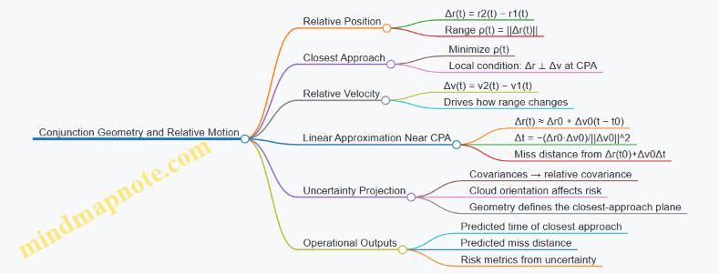
At any time, each object has a position vector in an Earth-centered frame. The instantaneous separation is the relative position vector \(\Delta \mathbf{r}(t)=\mathbf{r}_2(t)-\mathbf{r}_1(t)\). The range is \(\rho(t)=|\Delta \mathbf{r}(t)|\). Closest approach occurs when the range is minimized, which (in a local linearized sense) corresponds to the relative velocity being orthogonal to the relative position at the time of closest approach.
A practical way to think about this is to imagine a moving “miss distance” point. Even if the objects never collide, the miss distance and its uncertainty drive the risk calculation.
Relative Motion: Relative Position and Relative Velocity
Relative motion uses \(\Delta \mathbf{r}(t)\) and \(\Delta \mathbf{v}(t)=\mathbf{v}_2(t)-\mathbf{v}_1(t)\). Over short windows around the predicted closest approach, you can approximate the relative position as:
\(\Delta \mathbf{r}(t) \approx \Delta \mathbf{r}(t_0) + \Delta \mathbf{v}(t_0)(t-t_0)\)
This is not a replacement for orbit propagation, but it is a useful mental model for why small changes in track timing or state estimates can shift the predicted miss distance.
The Linear Miss-Distance Model
Let \(t_0\) be a reference time near closest approach. Define \(\Delta \mathbf{r}_0=\Delta \mathbf{r}(t_0)\) and \(\Delta \mathbf{v}_0=\Delta \mathbf{v}(t_0)\). The time offset to closest approach in the linear model is:
\(\Delta t = -\frac{\Delta \mathbf{r}_0\cdot \Delta \mathbf{v}_0}{|\Delta \mathbf{v}_0|^2}\)
Then the predicted miss distance is the norm of \(\Delta \mathbf{r}(t_0)+\Delta \mathbf{v}_0\Delta t\). The dot product term is the key intuition: if relative motion points mostly toward the other object, the dot product is strongly negative and \(\Delta t\) moves you toward the minimum range.
Uncertainty Meets Geometry
Real tracks come with uncertainty. Instead of a single \(\Delta \mathbf{r}\), you have a distribution of possible relative positions. In practice, the uncertainty is often represented by covariance matrices for each object’s state estimate, which combine into a relative covariance. The geometry then determines how that uncertainty projects onto the plane where closest approach happens.
A helpful mental picture: the miss distance is a scalar, but uncertainty is a cloud. The cloud’s shape and orientation relative to the line-of-approach matter.
Mind Map: Conjunction Geometry and Relative Motion
Worked Example: Two Objects with a Near-Approach Geometry
Assume at a reference time \(t_0\), the relative position is \(\Delta \mathbf{r}_0=[200,\ 50,\ -30]\) meters and the relative velocity is \(\Delta \mathbf{v}_0=[-2.0,\ 0.5,\ 0.1]\) meters per second. Compute:
- \(\Delta \mathbf{r}_0\cdot \Delta \mathbf{v}_0 = 200(-2.0)+50(0.5)+(-30)(0.1)=-400+25-3=-378\)
- \(|\Delta \mathbf{v}_0|^2 = (-2.0)^2+0.5^2+0.1^2=4+0.25+0.01=4.26\)
So \(\Delta t = -(-378)/4.26 \approx 88.7\) seconds. The linear model then gives \(\Delta \mathbf{r}(t_{CPA}) \approx \Delta \mathbf{r}_0 + \Delta \mathbf{v}_0\Delta t\). That becomes:
- \(x: 200 + (-2.0)(88.7) \approx 22.6\)
- \(y: 50 + (0.5)(88.7) \approx 94.4\)
- \(z: -30 + (0.1)(88.7) \approx -21.1\)
Miss distance \(\rho_{CPA} \approx \sqrt{22.6^2+94.4^2+(-21.1)^2} \approx 98\) meters. Notice what happened: even though the objects were 206 meters apart at \(t_0\), the relative velocity geometry pulled them closer.
Common Pitfalls That Geometry Reveals
If you see a predicted closest approach time far from the reference window, the linear approximation is probably being stretched. If the relative velocity is nearly perpendicular to relative position for most of the window, the range changes slowly, and uncertainty can dominate the miss distance distribution. In both cases, the geometry is telling you where the math is stable and where it is fragile.
3.4 Maneuver Planning for Station Keeping and Repositioning
Maneuver planning turns orbital mechanics into a repeatable workflow. The goal is simple: keep the spacecraft where it needs to be, and move it when it must, while protecting propellant, power, thermal margins, and mission timing. A good plan starts with constraints, then builds a maneuver sequence that respects both physics and operations.
Core Inputs and Constraints
Begin with the current state and the mission’s required geometry. You typically need:
- Current orbit estimate and uncertainty (position, velocity, and covariance).
- Target orbit or target geometry (e.g., along-track phasing, altitude band, or ground-track repeat).
- Propulsion model (thrust, specific impulse, thrust vector alignment, minimum impulse bit).
- Spacecraft constraints (attitude pointing limits, power availability, thermal limits, safe-mode rules).
- Operational constraints (communication windows, command authority, crewless autonomy rules).
A practical best practice is to write constraints in “must” and “cannot” form. For example, “must maintain nadir pointing within 0.5° during burn” is a must; “cannot transmit commands during a high-power heater cycle” is a cannot. This prevents later “clever” solutions that fail operational reality.
Station Keeping Versus Repositioning
Station keeping maintains an orbit against natural perturbations. Repositioning changes the orbit intentionally to meet mission geometry or coverage needs. The planning differences are mostly about objectives and timing:
- Station keeping often uses small, frequent corrections to stay inside a tolerance box.
- Repositioning uses larger, less frequent maneuvers to shift phase, altitude, or inclination-related geometry.
A helpful mental model is to treat station keeping as “keeping the clock hands aligned” and repositioning as “moving the clock to a different time zone.” Both use the same physics, but the tolerances and cadence differ.
Step 1: Define the Target and Tolerances
Targets should be expressed as tolerances, not single numbers. For example, instead of “altitude equals 550 km,” specify “altitude within ±2 km and local time within ±10 minutes at the next planning epoch.” This matters because uncertainty and modeling errors will otherwise force unnecessary propellant use.
Example: A communications satellite needs a minimum elevation angle to a ground station. Rather than planning for a perfect orbit, you plan for the elevation constraint to be satisfied for the next N contacts, using a margin that accounts for track uncertainty.
Step 2: Choose Maneuver Strategy
Common strategies include:
- Single-burn correction at a chosen epoch.
- Two-burn schemes for phasing or plane-related adjustments.
- Split burns to respect attitude or power constraints.
A simple rule: if you cannot point the spacecraft the way the ideal burn requires, split the maneuver into segments that each satisfy attitude and power limits. The math changes slightly, but the operational feasibility improves dramatically.
Step 3: Propagate and Plan with Uncertainty
You should propagate the orbit forward using the best available force model (drag, J2 effects, solar/lunar perturbations as applicable). Then propagate uncertainty to see how likely you are to meet the target tolerances.
Best practice: plan using a “risk-aware” approach. For instance, if the probability of meeting the elevation constraint drops below an acceptable threshold, increase the maneuver magnitude or shift the burn epoch. This avoids the classic failure mode where the nominal solution works on paper but misses in operations.
Step 4: Compute Delta-V and Burn Geometry
Delta-v planning depends on where and how you apply thrust. Key considerations:
- Thrust direction relative to the desired velocity change.
- Burn duration and resulting attitude evolution.
- Rocket equation effects for finite burns.
For station keeping, you often compute a required delta-v in a convenient frame (e.g., along-track and radial components), then map it to the spacecraft’s thrust vector capabilities.
Example: If drag is lowering the orbit, the along-track component of the correction is often less intuitive than the radial component. You still compute in the appropriate frame, but you validate the resulting ground-track and contact geometry after the burn.
Step 5: Sequence, Timing, and Contact Management
Maneuver planning must fit within operational windows. Typical sequencing steps:
- Pre-burn checks and attitude stabilization.
- Burn execution with command timing and autonomy limits.
- Post-burn calibration and orbit determination updates.
- Resume mission operations.
If a burn overlaps a critical downlink, you may need to reorder tasks. A practical approach is to schedule burns so that post-burn orbit determination improves the next contact’s pointing and tasking.
Step 6: Validate with End-to-End Checks
Validation should confirm more than “delta-v achieved.” Check:
- Attitude feasibility during the entire burn.
- Power and thermal margins.
- Communication availability for command and telemetry.
- Predicted orbit and geometry at the next few key epochs.
A good sanity check is to compare the predicted change in orbital elements to the expected physical driver. If drag dominates, altitude should trend upward after a corrective maneuver; if it doesn’t, you likely mapped the delta-v incorrectly.
Mind Map: Maneuver Planning Workflow
Worked Example: Station Keeping with a Contact Constraint
Assume a satellite must maintain a minimum elevation angle to a ground station for contacts over the next two weeks. Natural drag is predicted to reduce altitude, shrinking the elevation margin.
- Define tolerances: elevation constraint must be met for each contact with a margin of 1°.
- Propagate: run orbit propagation with uncertainty to estimate probability of meeting the constraint.
- Plan maneuver: compute a small corrective delta-v at an epoch when the thrust direction best produces the needed altitude increase.
- Validate: confirm that after the burn, the predicted elevation margin stays above the threshold for the scheduled contacts.
- Sequence: ensure attitude stabilization and telemetry coverage cover the entire burn and immediate post-burn orbit determination.
If the probability of meeting the constraint is too low, the fix is not “more delta-v blindly.” First adjust burn epoch to improve geometry, then increase magnitude if needed. This keeps propellant use aligned with the actual constraint driver.
Worked Example: Repositioning for Coverage Geometry
A repositioning maneuver aims to shift the ground-track timing so that a sensor’s best viewing windows align with tasking.
- Target geometry: specify the desired local time or phasing angle at the next task window.
- Strategy: choose a two-burn phasing approach if a single burn would violate attitude limits.
- Uncertainty-aware planning: evaluate how track uncertainty affects the phasing at the task epoch.
- Timing: schedule burns so that post-burn orbit determination refines the phasing estimate before tasking begins.
The key idea is that repositioning is not just “move the orbit.” It is “move the orbit so the mission geometry lands in the right place at the right time,” with uncertainty explicitly accounted for.
3.5 Time Management for Scheduling Contacts and Tasking
Time management in space operations is mostly about turning orbital geometry into a reliable sequence of actions. The goal is simple: when a satellite is in view or a link is usable, the system should already know what to do, who decides it, and how to recover if reality disagrees with the plan.
Core Concepts for Contact Scheduling
A contact is a window when a specific service is feasible, such as downlinking telemetry, uploading commands, or collecting sensor data. A task is the work you want to accomplish during that window, such as “send 30 minutes of payload data” or “perform a calibration sequence.” Time management connects them through three layers: predicted opportunity, prepared execution, and verified completion.
Start with the prediction inputs: orbit state, Earth orientation, sensor pointing constraints, ground station availability, and link budgets. Then add operational constraints: command authorization windows, crew or automation availability, data processing capacity, and any required handshakes between control and analysis teams.
A practical best practice is to treat time as a resource with buffers. For example, if a pass is predicted from 10:00:00 to 10:12:00 UTC, you might schedule command uplink from 09:58:30 to 10:11:30 to account for clock offsets, slewing delays, and late track refinement. The buffer is not wasted time; it prevents “perfect plan, unusable execution.”
Building a Contact Plan That Survives Reality
A contact plan is a structured schedule that maps each opportunity to actions and decision points. Use a consistent timeline model:
- T0: earliest time when the system can safely begin the activity
- Tstart: earliest time when the link or pointing is expected to meet thresholds
- Tstop: latest time when the activity can still complete
- Tend: earliest time when you must stop to avoid losing control or data integrity
An easy example: you schedule a downlink of a recorded image. If the downlink rate drops near the edge of the pass, you compute Tstop based on the remaining data volume and expected throughput, not just on visibility time.
Tasking Workflow and Decision Ownership
Tasking should be planned so that the decision authority is clear before the pass begins. A common workflow is:
- Task definition: payload mode, data volume, and required command sequence
- Feasibility check: orbit and pointing constraints, link capacity, and timing
- Authorization: who approves the task and under what conditions
- Command preparation: generate command sets and verify checksums
- Execution: uplink at the planned times with monitoring
- Verification: confirm acceptance telemetry and data receipt
A best practice is to define “decision gates” tied to measurable events. For instance, if track quality or link margin falls below a threshold by a certain time, the system should automatically switch to a reduced-rate downlink or skip nonessential payload operations.
Handling Uncertainty with Time Buffers and Replanning
Uncertainty comes from track errors, station motion, and timing offsets. Instead of treating uncertainty as a nuisance, convert it into schedule structure.
- Pre-pass buffer: time to refine track and confirm pointing
- In-pass buffer: time for contingency actions like rate changes
- Post-pass buffer: time to verify acceptance and log outcomes
Example: Suppose a satellite is expected to pass over a station for 12 minutes. You schedule a 9-minute data downlink plus 1 minute for rate stabilization and 2 minutes for verification and any retransmission requests. If the first minute shows lower-than-expected link margin, you still have time to adjust without missing the verification step.
Mind Map: Time Management for Contacts and Tasking
Worked Example: Scheduling a Downlink and a Payload Mode Change
Assume a satellite has a predicted pass from 10:00 to 10:12. You want to (1) switch the payload to a recording mode and (2) downlink the recorded data.
- Command uplink window: schedule from 09:58:30 to 10:11:30 so the payload mode change can be confirmed even if slewing or track refinement takes longer.
- Recording-to-downlink timing: include the payload’s internal processing time. If recording starts at 10:02:00 and the payload needs 90 seconds to package data, the downlink can begin at 10:03:30.
- Downlink completion deadline: compute Tstop based on expected throughput. If the remaining data fits in 7 minutes at nominal rate but only 5 minutes at worst-case, set Tstop to 10:08:30 and leave time for verification.
- Verification gate: require acceptance telemetry by 10:09:30. If it doesn’t arrive, the system should avoid assuming the data exists and should log the failure for later analysis.
This example shows the core principle: time management is not just scheduling; it is engineering the schedule so that each action has a measurable success condition and a fallback path.
4. Space Surveillance Fundamentals and Data Pipelines
4.1 Surveillance Objectives and What Must Be Measured
Military space surveillance exists to answer a few practical questions fast enough to matter: What is out there? Where is it now? What will it do next? How confident are we? And what does that confidence mean for decisions like tasking, conjunction assessment, and defensive actions?
Core Surveillance Objectives
-
Detect and track objects reliably
- Objective: maintain continuous tracks for resident space objects and other relevant emitters.
- What to measure: detection confidence, track continuity, and track update rate.
- Example: if a sensor sees a target for three passes but loses it between, you measure the gap length and the predicted uncertainty growth during the gap.
-
Estimate accurate state information
- Objective: produce position, velocity, and uncertainty at specific times.
- What to measure: orbit determination residuals, state covariance size, and time-tag accuracy.
- Example: two sensors may both “track” the same object, but one yields smaller residuals and tighter covariance; that difference directly affects maneuver risk.
-
Characterize objects for operational relevance
- Objective: infer what an object is likely doing and how it might affect friendly missions.
- What to measure: classification confidence, behavioral indicators (e.g., maneuver signatures), and identification stability over time.
- Example: a sudden change in estimated mean motion with a consistent pattern across updates is measured as a maneuver event with an uncertainty envelope.
-
Support decision-grade risk assessment
- Objective: translate surveillance outputs into decision inputs with traceable assumptions.
- What to measure: conjunction risk metrics, probability-of-collision inputs, and sensitivity to track-quality changes.
- Example: you measure how much the risk metric shifts when you widen covariance by a realistic factor; if it swings wildly, the system needs better measurements or tighter processing.
-
Maintain data integrity and timeliness
- Objective: ensure the right data reaches the right place at the right time, with integrity preserved.
- What to measure: latency from observation to usable track, data completeness, and integrity checks on command and telemetry paths.
- Example: if latency increases during a busy observation window, you measure end-to-end delay and confirm that decision thresholds still align with the actual update cadence.
What Must Be Measured and Why
Surveillance is only as good as the measurements feeding the estimation chain. The measurement set should cover three categories: geometry, dynamics, and quality.
-
Geometry measurements capture where something appears relative to a sensor.
- Examples: angles (azimuth/elevation), range where available, and time-of-arrival.
- Why it matters: geometry drives the initial orbit fit and the shape of uncertainty.
-
Dynamics measurements capture how the object is changing.
- Examples: Doppler shift, successive position changes, and signatures consistent with maneuvers.
- Why it matters: dynamics determine whether the track can extrapolate safely between updates.
-
Quality measurements capture how trustworthy each observation is.
- Examples: signal-to-noise ratio, calibration status, pointing accuracy, and residuals after fitting.
- Why it matters: quality controls how much weight the estimator gives each data point.
A useful mental model is: measurements create uncertainty; uncertainty drives decisions. If you measure quality poorly, you may produce confident-looking tracks that are wrong in the ways that matter.
Surveillance Objectives and Measurement Targets
Mind Map: Surveillance Objectives
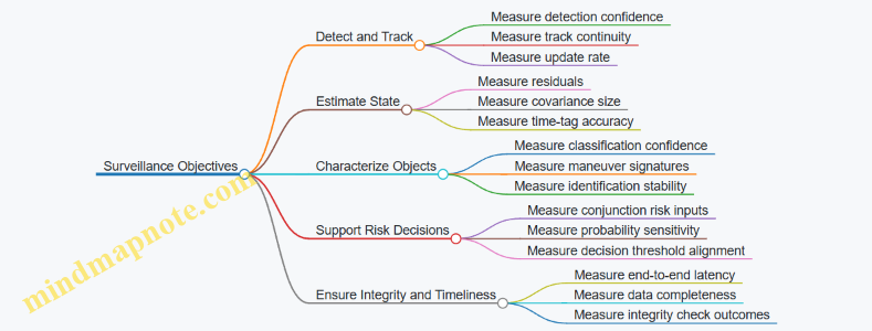
Mind Map: Measurement Categories
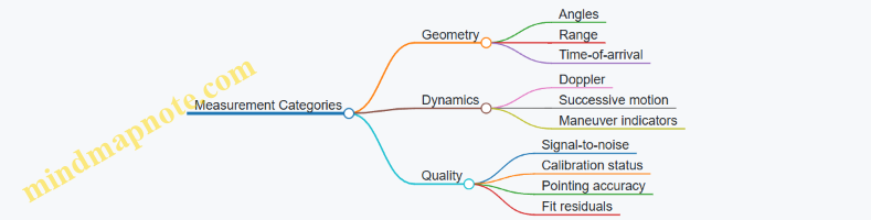
Example: From Observation to Decision Input
Assume a ground sensor produces a sequence of angle measurements with timestamps. The system first computes a track candidate, then performs orbit determination to estimate state at a decision time. To make the output decision-grade, it also computes residuals and covariance.
- If residuals are small but covariance is large, the system measures that the geometry is weak (for example, limited viewing angles), so the estimator is uncertain even if the fit looks tidy.
- If covariance is small but residuals are large, the system measures a mismatch between assumed dynamics and observed behavior, which may indicate a maneuver or calibration issue.
- If latency is high, the system measures whether the decision time still matches the track’s validity window; otherwise, the risk metric may be computed from stale information.
Practical Measurement Checklist
When defining surveillance objectives, list each output you need and attach the measurement that justifies it:
- Track exists continuously → measure continuity and gap duration.
- State is accurate at time T → measure residuals and time-tag accuracy.
- Uncertainty is honest → measure covariance behavior and quality weights.
- Risk metric is stable → measure sensitivity to track-quality changes.
- Outputs arrive on time → measure end-to-end latency and completeness.
This approach keeps objectives grounded in observable quantities. It also prevents a common failure mode: treating “good results” as a feeling rather than a measurable property.
4.2 Sensor Types and Measurement Outputs for Space Situational Awareness
Space Situational Awareness (SSA) depends on sensors that measure something physical and turn it into usable information: detections, tracks, and object characterization. The trick is to understand what each sensor can measure directly, what it must estimate, and what that implies for accuracy, latency, and operational use.
Measurement Outputs You Actually Use
SSA pipelines typically consume five kinds of outputs, each with a different role in the workflow.
- Detections: time-stamped observations in sensor coordinates. Example: a telescope reports a bright spot at a specific right ascension/declination for a given time.
- Tracklets: short track segments formed from a few detections. Example: three measurements within minutes become a preliminary path.
- Tracks: longer-lived correlated track estimates with uncertainty. Example: a track that persists across multiple passes.
- Attributes: characterization parameters derived from measurements. Example: brightness trend, angular size, or radar cross-section estimates.
- Quality metrics: numbers that tell you how much to trust the output. Example: residuals, covariance, and confidence scores.
A practical best practice is to treat these outputs as separate contracts. A detection is not a track; a track is not a characterization; and a characterization without uncertainty is just a story.
Sensor Types and What They Measure
Optical Sensors
Optical sensors measure angles (and sometimes brightness) by imaging the sky. They are strong for detecting objects in favorable lighting and for producing precise angular measurements when pointing and timing are well controlled.
Typical measurement outputs
- Angular position in an inertial or Earth-fixed frame after calibration
- Apparent magnitude or intensity
- Image-based features such as centroid and sometimes shape proxies
Operational implication: optical performance depends heavily on geometry, weather, and background clutter. A common workflow uses optical detections to seed tracklets, then correlates them with other sensors to reduce ambiguity.
Easy example: A ground telescope sees a streaked object during twilight. The centroid is still usable, but the uncertainty grows because the streak spreads the light. The SSA system should carry that increased uncertainty into the track fit.
Radar Sensors
Radar sensors measure range and angle (and often Doppler), producing direct information about distance and relative motion.
Typical measurement outputs
- Slant range
- Azimuth/elevation angles
- Radial velocity from Doppler
- Sometimes waveform-derived features that support classification
Operational implication: radar can operate in darkness and through some atmospheric conditions, but it has constraints on power, beamwidth, and target size. Radar measurements often provide strong constraints on orbit determination because range and Doppler reduce the “many orbits fit the same angles” problem.
Easy example: A radar returns a strong echo at a known time with a measured Doppler shift. Even if the angular resolution is coarse, the range-rate constraint can sharply narrow the set of candidate trajectories.
Infrared Sensors
Infrared sensors measure thermal radiation, often producing detections and sometimes coarse angular information.
Typical measurement outputs
- Detection coordinates
- Intensity or temperature proxies
- Tracklets based on repeated sightings
Operational implication: IR can be useful when optical is degraded by lighting or when objects have thermal signatures. Measurement uncertainty depends on background sources and calibration stability.
Easy example: An IR sensor detects a point source near the horizon. The system should avoid treating intensity as a direct size estimate; instead, it uses intensity as a supporting attribute while orbit fitting relies on angles and timing.
Passive Radio Frequency Sensors
Passive RF sensors measure signals of opportunity or emissions from satellites. They can provide timing and frequency-related measurements.
Typical measurement outputs
- Time of arrival or time difference of arrival
- Frequency offset
- Angle estimates from interferometry or direction finding
Operational implication: passive RF is powerful for tracking cooperative or emitting objects, but it depends on signal availability and may be less effective for non-emitting targets.
Easy example: Multiple receivers detect the same beacon. By comparing arrival times, the system estimates a direction or location constraint, which then supports track correlation.
Space-Based Sensors
Space-based sensors observe from above the atmosphere, reducing weather and atmospheric distortion effects.
Typical measurement outputs
- Optical or IR angular measurements with stable viewing conditions
- Radar measurements if equipped
- Higher revisit opportunities for certain geometries
Operational implication: space-based sensors can provide consistent measurement quality across many passes, but they require careful calibration and precise time synchronization.
Easy example: A satellite sensor images a target repeatedly during a single overflight. The system can form a tracklet quickly because the geometry changes smoothly and the timing is stable.
Measurement Models and Output Formats
Sensors do not “hand you orbits.” They provide measurements that must be mapped into a common reference frame using a measurement model.
A systematic approach is to define, for each sensor type:
- Measurement space: what the sensor reports (angles, range, Doppler, intensity)
- Reference frames: sensor frame, Earth-fixed, inertial
- Time basis: the exact time standard used for measurement timestamps
- Uncertainty representation: covariance or error bounds per measurement
Easy example: If one sensor timestamps in UTC and another in a different time basis, the track fit can degrade even when the geometry is perfect. SSA systems therefore treat time conversion as a first-class step, not an afterthought.
Mind Map: Sensor Types and Outputs
Integrated Example Workflow
Consider a target first detected by optical angles during a short window. The optical system produces detections with angle uncertainty and a time stamp. Those detections form a tracklet, but the track remains ambiguous because angles alone can fit multiple trajectories.
Next, a radar pass measures range and Doppler for the same time window. The SSA system correlates the optical tracklet with the radar measurements, then refits the track using a combined measurement model. The resulting track has tighter uncertainty because radar constrains distance and radial motion. Finally, the pipeline attaches attributes such as brightness trend (from optical) and radar-derived features (from radar), each with quality metrics so operators know what is solid and what is merely suggestive.
The key idea is simple: each sensor contributes different constraints, and the measurement outputs must carry their uncertainty all the way into decisions.
4.3 Data Ingestion and Normalization Across Sensor Networks
Military space surveillance depends on many sensors that do not speak the same language. Ingestion is the process of pulling measurements from each sensor reliably and on time. Normalization is the process of converting those measurements into a consistent internal form so downstream tracking, correlation, and defense decision logic can treat them as comparable inputs. If you skip normalization, you get tracks that look confident but are actually built from mismatched units, coordinate frames, and time bases.
Foundational Concepts for Ingestion
Start with three invariants: time, reference frames, and measurement meaning.
Time invariants mean every measurement must carry a precise timestamp and a declared time standard. A common failure mode is mixing UTC-like timestamps with onboard time that has drift or different leap-second handling. Best practice is to store both the sensor-reported time and the system-converted time, along with the conversion method and uncertainty.
Reference-frame invariants mean each sensor measurement must state which coordinate system it uses. For example, an optical sensor might output right ascension and declination in an Earth-centered inertial context, while a radar sensor outputs range and range-rate in a local topocentric frame. Normalization converts everything into the internal frames required by the track estimator.
Measurement-meaning invariants mean you must know what the numbers represent. “Angle” is not always the same angle: some sensors report apparent angles, others report angles after internal refraction corrections. Normalization records measurement type, calibration status, and any quality flags that affect interpretation.
Ingestion Pipeline Structure
A practical ingestion pipeline has five stages.
- Acquisition: Receive measurement packets from sensors through a defined interface. Include sequence numbers and integrity checks so missing or duplicated packets are detectable.
- Validation: Verify schema, units, and required metadata. Reject or quarantine records that fail basic checks.
- Time Alignment: Convert timestamps to the system time standard and compute time uncertainty. If the sensor provides a latency estimate, incorporate it.
- Frame and Unit Conversion: Convert coordinates and units into the internal canonical representation.
- Normalization Output: Emit a standardized measurement record for the track management system.
A simple example: a radar sensor sends slant range in meters and range-rate in meters per second, while an optical sensor sends angles in degrees. During ingestion, you convert degrees to radians and meters to the internal unit set, then attach a measurement model identifier so the estimator knows how to interpret each type.
Normalization Rules That Prevent Silent Errors
Normalization should be deterministic and auditable. Use explicit rules rather than “best guess” conversions.
- Unit normalization: Convert all distances to a single unit and all angles to a single unit. Store the original values for traceability.
- Frame normalization: Convert to canonical frames using declared transforms. If transforms depend on Earth orientation parameters or ephemerides, record the parameter set used.
- Uncertainty normalization: Convert covariance or error estimates into a consistent representation. If a sensor provides only a scalar accuracy, map it into the appropriate covariance structure with documented assumptions.
- Measurement model tagging: Attach a tag that identifies the measurement equation used later. A normalized record without a model tag is like a recipe without ingredients.
Mind Map: Data Ingestion and Normalization Across Sensor Networks
Example: Mixed Sensor Measurement Record
Imagine two sensors observing the same object during a single tasking window.
- Radar reports: slant range = 820000 m, range-rate = -145 m/s, timestamp T1.
- Optical reports: right ascension = 12.345 deg, declination = -1.234 deg, timestamp T2.
During ingestion:
- Convert angles to radians and store original degrees.
- Convert radar measurements into the internal canonical coordinate representation required by the estimator.
- Convert both timestamps into the same system time standard, using the sensor-specific conversion method.
- Attach measurement model tags: one for radar range/range-rate, one for optical angle measurements.
- Map uncertainties into a common covariance format. If radar provides a range accuracy but not a full covariance, generate a covariance consistent with the measurement model.
The normalized output is two comparable measurement records that the track estimator can fuse without guessing what each number means.
Example: Normalization Quality Checks
Normalization quality is not just “did it convert.” It is “did it convert correctly.” Use checks that catch mismatches early.
- Range sanity: Reject radar measurements outside physically plausible bounds for the sensor geometry.
- Angle sanity: Check that optical angles fall within expected limits for the sensor pointing and field of view.
- Uncertainty sanity: Flag records with zero or negative uncertainties, or uncertainties that are orders of magnitude larger than typical for that sensor.
- Frame consistency: Verify that the declared sensor frame matches the transform chain used.
When these checks trigger, quarantine the record and continue processing. Quarantine beats silent corruption every time; your track logic should be able to operate with partial data rather than being poisoned by a few bad conversions.
Integrated Takeaway
Ingestion and normalization are the bridge between raw sensor outputs and the shared language of tracking and defense architectures. Treat time, frames, and measurement meaning as first-class data. Convert units and uncertainties deterministically, tag measurement models explicitly, and validate aggressively. The result is a measurement stream that is consistent enough for correlation and robust enough for operational use, even when sensors disagree about the details of reality.
4.4 Track Management From Detection to Correlation and Maintenance
Track management turns raw sensor detections into stable, usable object tracks. The pipeline has three jobs: (1) decide what a detection might be, (2) associate detections over time into coherent tracks, and (3) keep those tracks accurate as new data arrives.
Detection to Track Initiation
A detection is a measurement candidate with a time tag and uncertainty. Track initiation starts by grouping detections that are close in time and consistent with a plausible motion model. A practical best practice is to require both temporal proximity and kinematic consistency, not just “nearby points.”
Example: A radar reports two detections 20 seconds apart with similar range-rate and bearing-rate. If the implied motion fits a constant-velocity model within the reported uncertainties, the system creates a tentative track. If the detections are close in time but imply wildly different motion, the system holds them as unassociated detections.
Initiation also sets a confidence level. Tentative tracks are allowed to grow only if subsequent detections support them. This prevents one-off clutter from becoming a “real” track.
Correlation and Association
Correlation answers: which detections belong to which track? The core mechanism is gating, where each track predicts where it expects the next detection to appear. Gating uses uncertainty to define an acceptance region.
Example: A track prediction says the next azimuth should be 12.0° with a standard deviation of 0.3°. A detection at 12.8° might be outside a 3-sigma gate and therefore rejected for that track, even if it is the closest detection in absolute terms. This is how the system avoids “sticky” wrong associations.
When multiple detections fall within a gate, association becomes a selection problem. A common approach is to compute association scores using residuals between predicted and observed measurements, then choose the best combination under constraints.
Track Filtering and State Estimation
Once detections are associated, the track filter updates the estimated state. The filter blends prediction and measurement using their uncertainties. A well-tuned filter prevents two failure modes: overreacting to noisy measurements and underreacting to real maneuvers.
Example: If a sensor’s range noise increases during a pass, the filter should automatically reduce the measurement weight. If the object truly maneuvers, the residuals will grow consistently across multiple updates, prompting the filter to adjust the state and uncertainty.
Track maintenance includes covariance management. If uncertainty shrinks too quickly, the gate becomes too tight and the track loses detections. If uncertainty grows too quickly, the gate becomes too wide and the track starts accepting clutter.
Track Maintenance and Quality Control
Maintenance keeps tracks coherent over time, even when data is missing or degraded.
Key maintenance actions:
- Update cadence checks: If updates arrive slower than expected, the filter propagates forward and uncertainty increases.
- Track confirmation and deletion: Tentative tracks become confirmed only after enough consistent associations. Tracks are deleted after repeated missed detections beyond a threshold.
- Identity continuity: The system avoids track swaps by using association history and motion consistency.
Example: A confirmed track misses two updates due to a sensor outage. The filter propagates the state, uncertainty expands, and the gate widens. When detections return, the system can re-acquire the track without creating a duplicate.
Mind Map: Track Management Pipeline
Worked Example: One Object Through the Pipeline
Assume a sensor produces detections at times t1, t2, t3.
- At t1, the system sees a single detection and stores it as unassociated.
- At t2, a second detection appears within the initiation time window and implies motion consistent with the model. A tentative track is created.
- At t3, the track predicts a measurement region. One detection falls inside the gate with a small residual; another falls inside a wider gate but has a larger residual. The association logic selects the small-residual detection.
- The filter updates the state and tightens uncertainty appropriately.
- If the next update is missed, the system propagates and increases uncertainty rather than immediately deleting the track.
This example shows why gating, association scoring, and filter uncertainty are not separate steps. They are the same idea expressed at different points in time: “Does the new information fit the track we already believe?”
Practical Checklist for Robust Track Management
- Use gating derived from covariance, not fixed tolerances.
- Require multiple consistent detections before confirmation.
- Monitor residuals to detect sensor degradation or real maneuvers.
- Handle missed detections with propagation and controlled uncertainty growth.
- Prevent duplicates by enforcing identity continuity during re-acquisition.
4.5 Quality Metrics for Track Accuracy and Data Latency
Quality metrics for space surveillance tracks answer two practical questions: “How wrong is the track?” and “How late is the information?” If you can measure both, you can manage risk instead of arguing about it.
Track Accuracy Metrics
Track accuracy is about the difference between the estimated object state and the true state. Because the true state is rarely known, quality is expressed using residuals, covariances, and consistency checks.
1. Residual Statistics
Residuals compare what the sensor measured to what the filter predicted. For a simple example, imagine a radar range-rate measurement. If the predicted range-rate is 7.2 km/s and the sensor reports 7.0 km/s, the residual is -0.2 km/s. Over many updates, you track the mean (bias) and spread (variance).
Best practice: compute residuals per sensor, per measurement type, and per geometry regime (for example, near-zenith vs low-elevation). A system that looks “good on average” can still fail at the edges where operators actually need it.
2. Normalized Innovation Squared Consistency
A filter that is properly tuned should produce residuals that match its stated uncertainty. One common consistency metric is the normalized innovation squared (often written as NIS). Conceptually, it asks whether the residual is “reasonable” given the filter covariance. If NIS is consistently too high, the filter is overconfident or the model is missing effects. If it is too low, the filter may be underconfident.
Easy example: if a track’s covariance says a measurement should be within ±0.5 units for most updates, but residuals frequently exceed that by a wide margin, NIS will spike and operators will see growing track-to-track disagreement.
3. Position and Velocity Error Proxies
When truth is unavailable, you can still estimate error using covariance and cross-sensor agreement. Two practical proxies are:
- Predicted 1-sigma bounds from the filter covariance, summarized as percent-of-time coverage.
- Track-to-track disagreement for the same object from independent processing chains.
Best practice: require that independent chains agree within their combined uncertainty. If Chain A says the object is at 10 km ±2 km and Chain B says it is at 20 km ±2 km, the disagreement is not “noise,” it is a quality failure.
Data Latency Metrics
Latency is the time from measurement capture to the moment the data is usable for decisions. Latency has multiple components, and each component has different failure modes.
1. End-to-End Latency
Define end-to-end latency as:
- measurement time stamp to ingestion completion
- ingestion to track update completion
- track update completion to availability in the operator interface
Easy example: a sensor can deliver data quickly, but if correlation waits for a slow batch job, the end-to-end latency becomes unacceptable even though the sensor itself is fast.
2. Component Latency and Jitter
Track quality depends on both mean latency and jitter. Jitter is variation in latency that makes scheduling and fusion harder. If one update arrives 2 seconds late and the next arrives 20 seconds late, the system may still meet an average requirement while producing inconsistent track freshness.
Best practice: measure latency distributions (percentiles), not just averages. A 95th percentile latency is often the number that matters during time-critical conjunction assessment.
3. Staleness at Decision Time
Even if latency is stable, the track can become stale relative to the decision moment. Staleness is the effective age of the information when it is used. A simple operational rule is to compute staleness as decision time minus measurement time stamp, then compare it to the time window where the filter’s uncertainty growth remains acceptable.
Integrated Quality Mind Map
Mind Map: Track Accuracy and Data Latency Quality Metrics
Practical Example Workflow
Consider a conjunction assessment pipeline that uses tracks from two sensor networks. You set three gates:
- Residual Gate: residual mean near zero and spread within expected limits for each sensor.
- Consistency Gate: NIS stays within a defined band for most updates.
- Freshness Gate: end-to-end latency percentiles and staleness at decision time remain under thresholds.
If the system fails gate 1 but passes gate 2, the filter may be consistent but the measurement model is wrong for that geometry. If it fails gate 2 but passes gate 1, the filter tuning or process model is likely off. If it fails gate 3, the track may be accurate when computed but unusable when needed.
The key is that these metrics are not separate dashboards; they are linked diagnostics. Accuracy tells you whether the track is trustworthy, and latency tells you whether it is timely. Together, they define whether the operator can act with confidence.
5. Tracking and Characterization of Orbital Objects
5.1 Orbit Determination Methods and State Estimation Concepts
Orbit determination is the process of estimating an object’s state—typically position and velocity—using measurements such as angles, ranges, Doppler shifts, or radar returns. State estimation is the broader framework that turns noisy, incomplete measurements into a best estimate with quantified uncertainty. In military space operations, the goal is not just a number, but a number with a defensible confidence level that downstream tasks can use.
Core State Representation
A common starting point is the state vector in an Earth-centered inertial frame:
- Position: \(\mathbf{r} = [x,y,z]\)
- Velocity: \(\mathbf{v} = [\dot{x},\dot{y},\dot{z}]\)
The state evolves under a dynamics model \(\dot{\mathbf{x}} = f(\mathbf{x}, t)\), where \(\mathbf{x} = [\mathbf{r},\mathbf{v}]\). For practical systems, the dynamics model includes gravity (often with perturbations), atmospheric drag when relevant, solar radiation pressure, and sometimes empirical terms to absorb modeling gaps.
Measurement Models and Residuals
Measurements rarely observe \(\mathbf{r}\) and \(\mathbf{v}\) directly. Instead, they relate to the state through a measurement function \(\mathbf{z} = h(\mathbf{x}) + \boldsymbol{\epsilon}\), where \(\boldsymbol{\epsilon}\) is measurement noise. For example:
- Optical angles: right ascension and declination depend on line-of-sight geometry.
- Radar: range and range-rate depend on relative position and velocity.
- Two-way Doppler: frequency shift depends on projected relative velocity.
A residual is the difference between an observed measurement and the predicted measurement from the current state estimate. Residuals are the “feedback” that tells the estimator whether the current orbit guess is too high, too low, or simply wrong in a way that the uncertainty should reflect.
Batch Least Squares Orbit Determination
Batch methods estimate the state by minimizing a cost function over a set of measurements. A typical objective is the weighted sum of squared residuals:
\(J(\mathbf{x}) = \sum_i \mathbf{r}_i^T \mathbf{W}_i \mathbf{r}_i\)
where \(\mathbf{W}_i\) is derived from measurement covariance. The weighting matters: a precise radar range should influence the solution more than a noisy angle measurement. Batch least squares is conceptually straightforward and works well when you have a fixed set of measurements and can afford repeated computation.
Easy example: Suppose you track an object with three radar passes. Each pass gives range and range-rate with known uncertainties. If one pass has twice the uncertainty, its residuals get half the weight, so the solution doesn’t “chase” that noisier pass.
Sequential Estimation with Kalman Filters
Sequential methods update the state as measurements arrive. The Kalman filter is the standard workhorse when the dynamics and measurement models can be approximated as linear (or linearized). It maintains:
- A state estimate \(\hat{\mathbf{x}}\)
- An error covariance \(\mathbf{P}\)
The filter alternates between:
- Prediction: propagate \(\hat{\mathbf{x}}\) forward using the dynamics model and propagate \(\mathbf{P}\) using the model’s sensitivity.
- Update: incorporate new measurements by computing a gain that balances model uncertainty against measurement uncertainty.
Easy example: If the dynamics model is uncertain (large \(\mathbf{P}\)), the filter trusts measurements more. If the sensor is uncertain (large measurement covariance), the filter trusts the model more. This is why covariance tuning is not paperwork—it changes behavior.
Linearization and Extended Kalman Filters
Orbital dynamics and measurement mappings are nonlinear. The extended Kalman filter (EKF) handles this by linearizing around the current estimate. The practical implication is that EKF performance depends on having a reasonably good initial guess. If the initial state is far off, linearization error can cause the filter to “lock onto” the wrong explanation.
Easy example: Start with an orbit that predicts the object passes near a sensor’s field of view, but the true pass is several degrees away. The residuals will be large, and the linearized update may not correct the estimate cleanly. In that case, you need a better initial orbit from a batch method or a dedicated initial orbit determination step.
Unscented and Particle Approaches
When linearization is too crude, alternatives exist. The unscented Kalman filter (UKF) propagates a set of sigma points through nonlinear functions to better capture mean and covariance. Particle filters represent the posterior with samples, which can handle non-Gaussian uncertainty but typically cost more computation.
Easy example: If measurement noise is heavy-tailed (occasional outliers), a particle approach can represent that uncertainty more faithfully than a pure Gaussian assumption.
Practical Orbit Determination Workflow
A typical operational workflow is:
- Initial orbit determination: produce a starting state from a limited set of measurements.
- Track refinement: run sequential estimation to update the state and covariance.
- Quality checks: validate residuals, consistency with covariance, and stability across updates.
- Propagation: carry the estimated state forward for scheduling and conjunction assessment.
Quality checks are essential because a mathematically “best” fit can still be inconsistent with the stated uncertainties.
Mind Map: State Estimation Building Blocks
Worked Mini-Example: From Measurements to a Refined State
Imagine a sensor provides three measurements at times \(t_1, t_2, t_3\): an angle pair at \(t_1\), range-rate at \(t_2\), and range at \(t_3\). An initial orbit is computed from the first two measurements, producing \(\hat{\mathbf{x}}_0\) and \(\mathbf{P}_0\). The filter predicts the state to \(t_3\), computes predicted measurements \(h(\hat{\mathbf{x}})\), and forms residuals. The update then adjusts both position and velocity components that best explain the residuals, while the covariance shrinks where the measurements add information and stays large where they do not.
The key idea is consistency: if the residuals are small but the covariance is large, the system is conservative. If residuals are large but covariance is tiny, the system is overconfident. Good orbit determination keeps those two in reasonable agreement.
5.2 Covariance Handling and Uncertainty Propagation
Uncertainty is not a nuisance; it is the bookkeeping that keeps decisions honest. In orbit determination and conjunction assessment, you rarely care about a single “best” state alone. You care about how wrong it might be, and in which directions. That directionality lives in the covariance matrix.
What Covariance Means in Practice
Covariance is a matrix that describes spread and correlation among state components. For a simple 2D example, imagine estimating position and velocity along one axis. If the position error and velocity error tend to grow together, the covariance will show correlation rather than treating them as independent.
A useful mental model: covariance is the shape of an error cloud. If you propagate that cloud through dynamics and measurement updates, you get a new cloud. The math is linear-algebra heavy, but the workflow is systematic: predict uncertainty forward, then shrink it when measurements arrive.
State, Errors, and Linearization
Most operational pipelines use a state vector x and an error model. The filter assumes small deviations around a nominal trajectory. That assumption matters: if the system is highly nonlinear over the time step, linearization error can dominate and covariance can become overconfident.
A practical best practice is to choose time steps and update rates so that the linear approximation remains reasonable. For example, if you propagate a track for 10 minutes with a coarse step, you may see covariance that looks “too tight” compared to residuals. Reducing the step can restore consistency.
Prediction Step Uncertainty Propagation
In a typical filter, the prediction step uses a state transition model. If the dynamics are approximated as linear over the step, the covariance update looks like this conceptually:
- Start with prior covariance P
- Apply the transition Jacobian F to map errors forward
- Add process noise Q to represent unmodeled effects
So the predicted covariance becomes larger because dynamics and modeling imperfections spread the error cloud.
Easy example: Suppose your drag model is imperfect. Even if the position estimate is good at the start, drag uncertainty grows with time. That growth should appear as increasing covariance, especially in along-track components.
Measurement Update Uncertainty Shrinking
When you incorporate a measurement, you reduce uncertainty where the sensor is informative. The measurement model maps state to predicted observations, and the filter compares predicted measurements to actual ones.
Key idea: the measurement update depends on both measurement noise R and the sensitivity of the measurement to the state. If the sensor geometry makes the measurement insensitive to a particular state direction, covariance in that direction will not shrink much.
Concrete example: A radar range measurement strongly constrains distance along the line of sight, but it may constrain cross-range poorly if the aspect angle is unfavorable. Covariance should reflect that imbalance.
Consistency Checks That Prevent “Overconfident” Covariance
A covariance can be mathematically correct yet operationally inconsistent if assumptions fail. Consistency checks compare normalized residuals (innovation terms) against expected statistical behavior.
If residuals are larger than predicted, your covariance is too small or your noise model is too optimistic. If residuals are consistently tiny, your covariance may be too large, which can lead to conservative decisions and unnecessary maneuvers.
A simple operational habit: track the innovation statistics per sensor and per geometry regime. If a particular sensor mode produces systematically larger innovations, adjust the effective R or revisit calibration rather than forcing the filter to “pretend” the sensor is perfect.
Mind Map: Covariance Handling and Uncertainty Propagation
Advanced Details Without the Pain
Cross-Correlation Matters
Many systems treat position and velocity independently, but that can break conjunction risk calculations. Correlations influence how uncertainty projects into miss distance. Ignoring cross terms can distort the effective uncertainty ellipse.
Frame Choices Affect Interpretation
Covariance is frame-dependent. A covariance that looks reasonable in an Earth-fixed frame might be awkward in an orbital frame. For conjunction assessment, you typically want covariance expressed in a frame aligned with relative motion so that miss distance uncertainty is computed cleanly.
Numerical Stability
Covariance matrices can become ill-conditioned due to repeated updates and finite precision. Stabilization techniques such as enforcing symmetry and using numerically robust matrix operations help keep the covariance physically meaningful.
Worked Example: From Prior to Predicted Covariance
Assume you have a prior covariance P0 for a track at time t0. You propagate to t1 using a transition model with Jacobian F and add process noise Q that represents drag and maneuver uncertainty. The predicted covariance P1 is computed from these ingredients.
Now a sensor provides a measurement at t1. The measurement update uses the measurement Jacobian H and measurement noise R. If H indicates the sensor is sensitive mainly to range, the updated covariance will shrink mostly along the range-sensitive direction, leaving other directions comparatively unchanged.
The result is not just “a better state,” but a covariance that correctly describes what the sensor did and did not learn. That is the foundation for uncertainty-aware conjunction decisions.
5.3 Cataloging Practices and Object Identification Workflows
Cataloging turns raw measurements into stable, named objects that operators can trust. Object identification is the step that decides whether a new track belongs to an existing catalog entry or starts a new one. The workflow below is systematic: it starts with measurement hygiene, moves through orbit and identity logic, and ends with catalog updates that preserve traceability.
Core Concepts That Drive Good Identification
A “track” is a time-ordered set of measurements with an estimated state and uncertainty. A “catalog entry” is a maintained object record with an orbit model, identification metadata, and a history of updates. Identification is not a single yes/no test; it is a chain of evidence: measurement quality, track-to-catalog consistency, and operational plausibility.
A practical rule: if you cannot explain why a track is assigned to an object, you cannot defend the assignment during an audit or a collision-avoidance decision.
Measurement Hygiene Before Identity Logic
Start by ensuring the inputs are fit for purpose.
- Time alignment: Convert all sensor timestamps to a common time standard and verify clock offsets. Example: if one sensor’s timestamps are consistently 0.8 s late, the same object can appear to “jump” between catalog candidates.
- Coordinate consistency: Confirm frame transformations (sensor frame to inertial frame) are correct and versioned. Example: a swapped axis can still produce a plausible-looking orbit, but it will fail correlation later.
- Outlier handling: Use residual checks to downweight or remove measurements that disagree with the current state estimate. Example: a single bad range measurement can inflate uncertainty and cause the track to match multiple catalog entries.
Track-to-Catalog Correlation Workflow
The identification workflow typically follows these steps.
- Initial orbit fit: Use a short arc to estimate a preliminary state and covariance.
- Candidate generation: Propagate the preliminary state to catalog epochs and compute gating metrics.
- Association scoring: Compare predicted and observed measurements using uncertainty-aware metrics.
- Identity decision: Choose the best candidate if it clears thresholds; otherwise create a new provisional object.
- Refinement and confirmation: Refit with additional measurements and re-evaluate the association.
- Catalog update: Commit changes with provenance, including which measurements and algorithms drove the decision.
A simple example: a new track appears near the predicted position of Object A. If the residuals are small relative to covariance and the track’s uncertainty shrinks as more measurements arrive, the association is strengthened. If residuals remain large or uncertainty grows, the system should avoid forcing a match.
Mind Map: Object Identification Workflow
Catalog Update Rules That Prevent Identity Drift
Catalogs fail when updates blur the line between “better orbit” and “different object.” Use explicit rules.
- Provenance-first updates: Store which tracks and measurement sets contributed to an orbit update. Example: if two sensors disagree, the catalog record should show which sensor drove the final fit.
- Model versioning: Keep orbit model and estimation settings tied to the update. Example: changing force models without recording it can make two catalog versions look inconsistent.
- Uncertainty sanity checks: Require that uncertainty decreases or behaves predictably after adding measurements. Example: if uncertainty increases after adding high-quality data, something is wrong with weighting or frames.
- Ambiguity handling: When multiple candidates score similarly, mark the association as tentative and wait for additional measurements. Example: two catalog entries in similar orbits can both pass a loose gate; the system should not “flip a coin” when residuals are nearly tied.
Example: From Ambiguous Track to Confirmed Identity
A radar provides a track with moderate uncertainty. Optical follow-up arrives later with tighter angular measurements.
- Step 1: The initial fit yields a preliminary state with a covariance that is large enough to overlap two catalog entries.
- Step 2: Candidate generation produces Object A and Object B. Gating metrics show both are plausible, but Object A’s predicted residuals are consistently lower across sensors.
- Step 3: Association scoring incorporates uncertainty, not just raw distance. Object A’s score improves as the optical measurements are added; Object B’s score does not.
- Step 4: The workflow confirms the association to Object A after the longer arc reduces uncertainty in a consistent way.
- Step 5: The catalog update records the measurement provenance and the estimation settings used for the refined orbit.
Example: Provisional Entry Creation with Guardrails
If a track fails to match any catalog entry within gating thresholds, create a provisional object rather than forcing a match.
Guardrails include:
- Minimum measurement count: Require enough measurements to support a stable preliminary orbit.
- Minimum arc length: Avoid short arcs that can fit many orbits.
- Confirmation window: Keep the provisional entry active until a later track either confirms it or shows it was a transient.
This approach keeps the catalog honest: it grows when evidence supports it, and it stays stable when evidence does not.
Quality Checks Operators Can Actually Use
Identification quality should be visible in operational terms.
- Residual behavior: Are residuals shrinking as more data arrives?
- Uncertainty behavior: Does covariance decrease in the expected directions?
- Cross-sensor consistency: Do independent sensors agree on the same association?
- Decision traceability: Can you point to the exact measurements and thresholds that produced the assignment?
When these checks pass, cataloging becomes more than record-keeping. It becomes a disciplined way to keep object identity aligned with the measurements that justify it.
5.4 Maneuver Detection and Attribution of Track Changes
Maneuver detection answers a simple question: did the object change its motion in a way that is consistent with a planned thrust, a natural perturbation, or a measurement artifact? Attribution goes one step further: if it looks like a maneuver, what kind of maneuver is most consistent with the observed track change, and how confident are we?
Core Idea from Residuals to Hypotheses
Track updates arrive as a time-ordered sequence of measurements. Orbit determination turns those measurements into an estimated state and a set of residuals—differences between what the sensor reported and what the current model predicts.
A practical workflow is to treat maneuver detection as a hypothesis test:
- No-maneuver hypothesis: the object follows the current dynamical model (including drag, solar radiation pressure, and gravity harmonics as configured).
- Maneuver hypothesis: at some time interval, an impulsive or finite-duration change in velocity occurred.
- Data-quality hypothesis: the apparent change is explained by sensor bias, timing error, or correlation mistakes.
A good system does not jump straight to “maneuver.” It first checks whether the residual pattern is coherent across sensors, geometries, and passes.
Step 1: Detect Change Using Consistent Residual Patterns
Residuals that grow smoothly can indicate model mismatch (for example, drag coefficient error). Residuals that show a sharp change near a specific epoch suggest a maneuver or a measurement issue.
Best practice: compute residual statistics in sliding windows (e.g., 2–4 passes or a fixed time span) and compare the windowed residual norm against a baseline built from recent “normal” behavior.
Easy example: Suppose a satellite is tracked for three consecutive passes. Pass 1 and 2 residual norms are stable. In pass 3, residuals jump by a factor of 3 and the direction of the residuals rotates consistently across multiple sensors. That pattern is harder to explain with random noise than with a real change in motion.
Step 2: Estimate Maneuver Parameters with Minimal Assumptions
Once you suspect a maneuver, estimate parameters that explain the track change with the least complexity:
- Maneuver time: the epoch or interval where the state transition is applied.
- Maneuver type: impulsive Δv (common for short burns) or finite-duration thrust (for longer burns).
- Direction: along-track, cross-track, radial, or a general 3D Δv vector.
Best practice: start with an impulsive model even if the real burn is finite. If the impulsive fit is poor, refine to a finite-duration model.
Easy example: A track shows a sudden along-track drift. An impulsive fit yields a Δv vector mostly aligned with the along-track direction, and the post-maneuver residuals drop back to baseline. That supports a small velocity change rather than a timing bias.
Step 3: Attribute the Cause by Comparing Competing Explanations
Attribution is about ruling out alternatives.
-
Measurement artifact checks
- Verify time tags and propagation delays.
- Check for sensor-specific biases.
- Confirm track association: did the track swap to a nearby object?
-
Natural dynamics checks
- Recompute with updated environmental inputs (e.g., solar activity proxies for drag).
- Test whether a plausible drag adjustment could mimic the observed change.
-
Maneuver plausibility checks
- Compare estimated Δv magnitude and direction to what the object’s propulsion system could reasonably produce.
- Look for consistency across multiple orbital elements (not just one).
Easy example: If the estimated Δv is tiny but the residual jump is large and localized to one sensor, a sensor bias is more plausible than a real burn.
Step 4: Quantify Confidence and Produce Actionable Outputs
Confidence should be expressed as a score or probability derived from the fit quality and the separation between hypotheses.
Common outputs include:
- Maneuver likelihood: how much better the maneuver model fits than the no-maneuver model.
- Δv estimate: magnitude and vector components.
- Time window: the epoch range where the maneuver is most consistent.
- Attribution label: maneuver vs measurement issue vs model mismatch.
Best practice: require that the maneuver explanation improves residuals across at least two independent data sources or geometries. This reduces “single-sensor miracles.”
Mind Map: Maneuver Detection and Attribution Flow
Example: From Track Change to Attributed Maneuver
A tracked object shows a residual spike starting at 14:20 UTC during a pass. Windowed residual norms rise sharply compared to the previous two passes. A no-maneuver fit leaves structured residuals, while an impulsive maneuver fit at 14:19:50 UTC reduces residuals back to baseline.
Next, you check sensor timing metadata and find no timing anomalies. You also verify track association by confirming that the object’s predicted position remains consistent with the same catalog identity before and after the epoch. Finally, you test whether a drag-only adjustment could reproduce the same change; it reduces residuals slightly but fails to match the post-epoch residual direction.
Attribution result: a maneuver is the best explanation, with a small Δv primarily in the along-track component and a maneuver epoch constrained to a narrow window around 14:20 UTC. Confidence is moderate-to-high because the improvement appears across multiple sensors and the alternative explanations do not match both magnitude and direction of the residual change.
5.5 Characterization Inputs for Risk Assessment and Planning
Risk assessment for orbital defense starts with a simple question: “What could happen, to which object, in what geometry, and with what uncertainty?” Characterization inputs answer that question by turning raw surveillance and system knowledge into quantities you can compare against decision thresholds.
Core Characterization Inputs
Object identity and classification
You need a stable way to refer to the same object across time. Inputs typically include catalog association confidence, object type hypotheses, and any known operational status. A practical example: if two track clusters repeatedly correlate to the same catalog entry with high confidence, you can treat the object as “known” for planning; if confidence is low, you plan with larger uncertainty and more conservative thresholds.
State estimates and uncertainty
The state estimate is usually a position-velocity vector at a reference epoch. The uncertainty is captured as covariance (or an equivalent uncertainty representation). For planning, you don’t just use the mean; you use the spread. Example: two conjunctions may have the same closest approach distance, but the one with larger covariance produces a wider probability distribution, so your risk metric will be higher even if the nominal geometry looks similar.
Maneuver and behavior indicators
Characterization includes evidence that an object is maneuvering, decaying, or otherwise behaving differently than a simple propagator assumes. Inputs can include residuals from orbit determination, changes in estimated velocity, and time-tagged maneuver flags. Example: if residuals spike after a specific time window, you treat the post-window propagation as less reliable and widen the uncertainty for that interval.
Physical and operational properties
Risk depends on what the object is likely to do and what it might collide with. Inputs include size estimates, shape assumptions, attitude or tumbling indicators when available, and operational constraints like expected maneuver capability. Example: a small, high-mass object with a well-modeled drag environment may still pose high risk because it’s hard to “miss” in probability space; a larger but poorly characterized object may drive risk through uncertainty rather than nominal size.
Environmental and propagation context
Propagation accuracy depends on the environment: gravity model choice, drag assumptions, solar activity proxies, and Earth orientation parameters. Characterization inputs include the environment state used for orbit propagation and its uncertainty. Example: if the drag model is calibrated poorly for a particular altitude band, you inflate uncertainty growth rates, which increases the risk window.
From Inputs to Risk-Relevant Quantities
Risk assessment typically converts characterization inputs into three planning-ready products: relative geometry, collision probability inputs, and decision constraints.
Relative geometry
Compute relative position and velocity between the primary and secondary objects over the relevant time window. Characterization inputs determine the reference epoch, propagation span, and how you handle time alignment. Example: if tracks are time-tagged with different latency, you align them to a common epoch before computing relative motion.
Collision probability inputs
Collision probability models require uncertainty representations for both objects and sometimes additional parameters like hard-body radius or effective cross-section. Characterization inputs supply those parameters and their uncertainty. Example: if size estimates are uncertain, you represent the effective radius as a distribution rather than a single value, which prevents overconfident risk scores.
Decision constraints
Planning also needs constraints that are not purely orbital: maneuver feasibility, control authority, and operational limits on when and how you can act. Characterization inputs include your own spacecraft’s maneuver capability and the timing of command opportunities. Example: a low-probability conjunction might still trigger action if the only feasible maneuver window is early and narrow.
Mind Map: Characterization Inputs for Risk Assessment
Worked Example: Building Inputs for a Conjunction Window
Assume you are assessing a conjunction between a primary satellite and a secondary object.
- Associate tracks to objects: You confirm the secondary track cluster matches a catalog entry with moderate confidence. You record that confidence because it affects how tightly you trust the secondary’s state.
- Generate state estimates: You compute state vectors for both objects at a common reference epoch and attach covariance from the orbit determination process.
- Check behavior: You observe increased residuals for the secondary after a specific time. You treat the post-window propagation as less reliable and inflate uncertainty accordingly.
- Set physical parameters: You estimate an effective cross-section for the secondary using available size information and represent it with uncertainty. For the primary, you use a known hard-body radius.
- Incorporate environment: You apply the drag and gravity assumptions used by the propagation engine and include environment uncertainty effects in the covariance growth.
- Produce risk inputs: You compute relative geometry time series and feed the uncertainty representations and effective radii into the collision probability calculation.
- Apply decision constraints: You check whether your own maneuver capability supports an avoidance action within the available command windows. If the feasible window is early, you may need to act even when risk is borderline.
This workflow keeps characterization grounded: every input either improves the fidelity of relative motion, the realism of uncertainty, or the practicality of decisions. When any input is weak, you don’t hide it—you carry its uncertainty forward into the risk calculation and the action planning logic.
6. Threat Modeling for Space Systems and Ground Operations
6.1 Threat Taxonomy for Space and Counterspace Activities
A threat taxonomy is a practical way to sort “what can go wrong” into categories that map to effects, targets, and responses. For space and counterspace activities, the most useful taxonomy starts with the mission chain: sensing and communications, command and control, navigation timing, and ground processing. Then it classifies threats by how they interfere with that chain.
Foundational Building Blocks
Targets are the things you must protect or sustain: space payloads, satellite buses, ground stations, network links, user terminals, and the data products that operators rely on.
Actors are the entities that generate the threat: state or non-state operators, contractors acting under coercion, or third parties whose infrastructure can be abused.
Means describe the mechanism: cyber intrusion, electronic interference, physical disruption, deception, or exploitation of operational procedures.
Effects are the measurable outcomes: loss of telemetry, corrupted tracking data, degraded link margin, delayed tasking, or incorrect object identification.
Constraints include what the attacker needs to succeed: access to frequencies, proximity for physical effects, knowledge of your procedures, or time to observe patterns.
A good taxonomy keeps these dimensions separate so you can reason from a specific incident to a specific mitigation.
Taxonomy by Activity Type
Space Threats
Space threats aim at spaceborne assets and their immediate support chain.
-
Kinetic disruption: physical impact or fragmentation that damages payloads or bus subsystems. Example: a close approach that forces a satellite to execute an emergency avoidance maneuver, consuming propellant and reducing future coverage.
-
Non-kinetic physical effects: mechanisms that alter performance without direct impact, such as thermal or charging stress. Example: sustained high-energy particle exposure that increases detector noise and forces shorter integration times.
-
Electronic interference: jamming or spoofing of uplinks, downlinks, or ranging signals. Example: a ground receiver sees a sudden drop in signal-to-noise ratio during a critical contact window.
-
Cyber and supply-chain compromise: unauthorized access to satellite software, ground systems, or mission planning tools. Example: a command pipeline is altered so that valid commands are routed to the wrong spacecraft or executed at the wrong time.
-
Deception and data manipulation: falsified sensor inputs, altered ephemerides, or corrupted catalogs that mislead operators. Example: track correlation assigns a new object to the wrong catalog entry, shifting conjunction risk.
Counterspace Threats
Counterspace threats target the ability to observe, decide, and respond.
-
Counter-surveillance: actions that reduce the quality of space situational awareness. Example: interference that increases track latency, causing operators to act on stale information.
-
Counter-communications: disruption of the pathways that move commands and data. Example: selective interference that affects only certain modulation modes, breaking specific command types.
-
Counter-control: interference with command authorization, timing, or automation logic. Example: spoofed authentication tokens that trigger a “safe mode” response.
-
Counter-maneuver enablement: constraints that prevent timely orbit changes. Example: ground scheduling is disrupted so maneuver windows are missed, even though the spacecraft is healthy.
Taxonomy by Effect Pathway
To avoid category confusion, map each threat to an effect pathway through the mission chain.
- Sensing pathway: detection quality → track quality → object identification.
- Communications pathway: link availability → command/telemetry integrity.
- Navigation and timing pathway: timing accuracy → pointing and ranging correctness.
- Processing pathway: data ingestion → correlation → decision support.
This pathway view helps you choose the right test. If the problem is “wrong object,” you test correlation and catalog integrity, not just radio link performance.
Mind Map: Threat Taxonomy for Space and Counterspace Activities
Worked Example: Classifying a Realistic Incident
Assume operators notice that conjunction assessments suddenly show higher risk for multiple objects, but spacecraft telemetry and downlink quality remain normal.
- Identify the affected pathway: sensing and processing, not communications.
- Choose the taxonomy branch: deception or data manipulation, or counter-surveillance causing track latency.
- Narrow the means: check whether track correlation inputs changed (catalog version, sensor calibration parameters, or time tags).
- Select the likely target: ground processing chain or surveillance data ingestion.
- Pick a mitigation test: run a replay of raw sensor measurements through an independent correlation pipeline and compare track outputs.
If the replay reproduces the risk increase, the issue is upstream of correlation; if it disappears, the issue is likely in correlation inputs or catalog mapping.
Practical Rules for Using the Taxonomy
- Classify by effect pathway first, then by means.
- Keep targets specific enough to drive engineering decisions, like “ground receiver chain” rather than “ground segment.”
- Require each threat entry to state an observable effect and a verification method so the taxonomy stays testable, not just descriptive.
A taxonomy that follows these rules turns “threats” into a set of concrete checks and response options that match how space systems actually fail.
6.2 Modeling Effects on Payload Links and Ground Control
Modeling the effects on payload links and ground control means translating “what the threat does” into “what the system experiences” across the full chain: space-to-ground propagation, receiver behavior, waveform and coding, and ground control processing. A good model is not just physics; it also includes operational constraints like scheduling, command formatting, and latency budgets.
Link Modeling Foundations
Start with a baseline link model that predicts received signal quality under nominal conditions. Represent the chain as:
- Transmit power and antenna gains
- Path loss and propagation effects
- Atmospheric losses and pointing losses
- Receiver noise figure and bandwidth
- Waveform parameters such as symbol rate, modulation, coding, and interleaving
- Demodulation and decoding performance
A practical way to keep this manageable is to separate “channel effects” from “implementation effects.” Channel effects include attenuation, fading, and interference. Implementation effects include receiver saturation, automatic gain control behavior, tracking loop errors, and decoder failure modes.
Easy example: If a command uplink uses a coded waveform at a fixed rate, then a jammer that raises the noise floor by 6 dB may not just reduce margin; it can push the decoder from “works reliably” to “fails intermittently,” which changes how often the ground system must retransmit or re-acquire.
Ground Control Modeling Foundations
Ground control modeling converts link outcomes into control outcomes. Build a state machine for the ground segment:
- Contact start and acquisition
- Telemetry reception and time synchronization
- Command preparation and uplink
- Command verification and confirmation
- Fault handling and fallback modes
Then attach link-dependent probabilities to each transition. For instance, telemetry loss affects time sync quality, which affects command timing windows, which affects whether the spacecraft accepts the command.
Easy example: If telemetry is used to estimate spacecraft clock drift, then a brief telemetry outage can widen the predicted command acceptance window. That can increase the chance of acceptance but also increases the chance of sending at a time when the spacecraft is in a different mode.
Modeling Effects on Payload Links
Model threat effects as perturbations to measurable link quantities. Common categories include:
- Interference and jamming: Represent as increased noise spectral density or as a structured interferer that overlaps the signal bandwidth.
- Spoofing and false signals: Represent as additional signals that can confuse acquisition, tracking, or decoding.
- Co-channel interference: Represent as partial overlap from other legitimate emitters or adversary emitters.
- Physical degradation: Represent as pointing errors, antenna pattern changes, or thermal effects that reduce effective gain.
To keep the model grounded, map each category to parameters you can compute:
- Carrier-to-interference-plus-noise ratio (C/(I+N))
- Signal-to-noise ratio (SNR)
- Bit error rate (BER) or block error rate (BLER)
- Probability of successful frame decode
Easy example: If a receiver uses a threshold-based frame acceptance rule, then BLER alone is not enough. You also need the distribution of frame errors across time, because the ground system may require N consecutive good frames before it trusts the data.
Modeling Effects on Ground Control
Ground control effects often appear as “process failures,” not just link failures. Model these explicitly:
- Command acceptance probability as a function of uplink quality and timing
- Verification latency when confirmation depends on downlink telemetry
- Retransmission behavior including maximum attempts and backoff
- Mode-dependent command validity where a command is syntactically correct but operationally rejected
A useful modeling trick is to treat the ground segment as a set of gates. Each gate has an input quality requirement and an output action.
Easy example: Gate A might require decoded telemetry to update predicted ephemeris. If Gate A fails, Gate B still sends commands, but with conservative timing. That reduces command acceptance probability but avoids sending commands outside the spacecraft’s safe window.
Integrated Mind Map
Mind Map: Modeling Effects on Payload Links and Ground Control
Worked Example with Numbers
Assume an uplink command frame requires a decoded success probability of at least 0.95 to meet operational timing constraints. Under nominal conditions, the model predicts BLER = 0.01, so success ≈ 0.99.
Now model a jammer that increases noise by 5 dB, reducing effective C/(I+N). The waveform model predicts BLER = 0.08, so success ≈ 0.92. If the ground system sends one command and waits for confirmation, the expected confirmation delay increases because failed frames trigger retransmissions. If the system allows only two attempts within the spacecraft’s mode window, then the probability of acceptance within that window becomes:
- P(accept within 2 attempts) = 1 − (1 − 0.92)² = 0.9936
But if the mode window is shorter and only one attempt is allowed, acceptance drops to 0.92. The key modeling insight is that the same link degradation can have very different operational impact depending on ground control timing rules.
Modeling Validation Using Operational Observables
Validate the model by comparing predicted outcomes to what the ground segment actually records: frame success rates, acquisition times, telemetry gaps, and command confirmation statistics. If the model predicts “intermittent failures,” check whether the ground system’s retry logic matches the observed pattern. If it predicts “continuous failure,” verify that the receiver saturation or tracking loss mechanisms are included, not just average SNR.
Easy example: If logs show frequent loss of lock during interference bursts, then a model that only changes average noise will miss the dominant effect. Add a tracking loop failure probability tied to interference duration and frequency offset.
6.3 Modeling Effects on Navigation Timing and Synchronization
Navigation timing and synchronization modeling answers a simple question: if timing is off, how does that error propagate into position, velocity, and ultimately mission decisions? In military space systems, the “timing” problem is rarely just one clock. It is a chain: onboard timekeeping, ranging and Doppler observables, ground processing, network transport, and the reference time used by users.
Core Timing Model Components
Start with a measurement model. A typical receiver uses pseudorange and Doppler (or carrier phase) to estimate state. Each observable depends on time tags:
- Transmit time at the satellite or transmitter.
- Receive time at the user or ground station.
- Propagation delay through space and media.
- Clock offsets and drifts in each endpoint.
A practical modeling approach treats timing errors as additive terms on the time tags. For example, if the receiver’s local clock has an offset \(\Delta t_r\), then the measured pseudorange error is approximately \(c,\Delta t_r\), where \(c\) is the speed of light. Doppler errors map to frequency-rate errors, which then map to velocity bias.
Synchronization Error Sources
Model timing errors as a mixture of deterministic and stochastic effects:
- Deterministic biases: known delays in hardware paths, fixed processing latency, or calibration constants that drift slowly.
- Stochastic noise: oscillator phase noise, jitter in timestamping, and random network delay variation.
- Model mismatch: incorrect relativistic corrections, imperfect ephemeris, or unmodeled tropospheric/ionospheric terms.
A useful rule: if you can measure it in a lab or characterize it in operations, model it explicitly; otherwise, represent it statistically and track its impact on uncertainty.
Propagation from Timing Error to Navigation Error
To avoid hand-waving, connect timing error to navigation outputs through linearization.
- Linearize the measurement equations around a nominal state and nominal time offsets.
- Build a sensitivity matrix that maps small timing perturbations into observable perturbations.
- Propagate into state covariance using the estimator’s measurement noise model.
For pseudorange-based estimation, the sensitivity to receiver clock offset is direct. For Doppler-based estimation, the sensitivity depends on the time derivative of the clock error and the observation interval length.
A concrete example: suppose a receiver clock offset of 50 ns exists and is not corrected. The pseudorange error is \(c\times 50\text{ ns}\approx 15\text{ m}\). If the navigation solution relies on multiple satellites, geometry may reduce the position impact, but the clock term still biases the solution unless the estimator includes a clock state.
Modeling Timing in the Presence of Relativistic Effects
Relativity matters because it couples to timing. Even if you do not need full general relativity in every operational context, you must include the standard corrections used by the system’s navigation solution. Model mismatch here behaves like a systematic timing bias.
A practical workflow:
- Compute relativistic corrections using the system’s reference model.
- Treat residuals as either a bias term (if stable) or a noise term (if variable).
- Include those residuals in the measurement noise budget so the filter does not pretend the world is perfect.
Ground Processing and Network Timing
In integrated architectures, the ground segment often timestamps data, forwards it, and performs correlation and tracking. Timing errors can enter through:
- Timestamping granularity in acquisition hardware.
- Variable transport delay in message passing.
- Asynchronous processing where data from different sources are fused later.
Model these as time-tag errors attached to each data stream. When fusing streams, represent the relative time alignment error between them. If two streams are misaligned by \(\Delta t\), the effective range-rate or phase history can be biased, depending on the observable.
Mind Map: Timing and Synchronization Modeling
Example: Building a Timing Error Budget for a Filter
Assume a receiver estimates position and a receiver clock offset state. You model:
- Receiver clock offset noise: \(\sigma_{t}\)
- Timestamp jitter: \(\sigma_{j}\)
- Residual relativistic correction: \(\sigma_{rel}\)
Combine them into an effective timing uncertainty \(\sigma_{eff}\) using a root-sum-square approach when sources are independent:
- \(\sigma_{eff} = \sqrt{\sigma_{t}^2 + \sigma_{j}^2 + \sigma_{rel}^2}\)
Then convert to pseudorange measurement noise:
- \(\sigma_{\rho} \approx c,\sigma_{eff}\)
This does two things: it prevents the filter from being overconfident, and it makes the effect of each timing component visible in the final position uncertainty.
Example: Relative Misalignment Between Two Data Streams
Suppose a ground station fuses tracking data from two sensors. Sensor A and B have a relative time alignment error of 20 ns due to different timestamp sources. If the fused solution uses pseudorange-like observables, the relative range bias is about \(c\times 20\text{ ns}\approx 6\text{ m}\). If the estimator assumes perfect alignment, the residuals will show systematic structure, and the covariance may understate risk. Modeling the relative time alignment as a parameter or as additional measurement noise keeps the estimator honest.
Practical Modeling Checklist
- Include clock offset and clock drift states when the architecture supports them.
- Attach timing errors to the correct time tags and to the correct data streams.
- Convert timing uncertainty into observable uncertainty using the measurement sensitivity.
- Use a measurement noise budget that includes residuals from propagation and relativistic corrections.
- Validate with residual analysis: timing errors often reveal themselves as structured residuals rather than random scatter.
6.4 Modeling Effects on Data Integrity and Command Authenticity
Modeling data integrity and command authenticity is about tracing how information changes as it moves from a decision to a spacecraft and back again. In practice, you model three things together: what the system expects, what the environment does to signals and data, and how the software and procedures detect or tolerate those changes. A good model is testable: you can map each modeled effect to a measurable symptom in telemetry, command logs, or operator displays.
Data Integrity Foundations for Command and Telemetry
Start with a simple end-to-end data path model. Commands originate in a planning or operator interface, pass through a ground control system, are encoded and transmitted, then are decoded and executed onboard. Telemetry follows the reverse direction: onboard measurement generation, onboard formatting, downlink transmission, ground reception, decoding, and finally storage and display.
For each hop, define the integrity properties you care about:
- Bit-level correctness: did the received bits match what was sent?
- Message-level correctness: did the message structure, fields, and checks pass?
- Semantic correctness: does the content make sense for the current spacecraft state?
- Provenance correctness: can you attribute the message to the intended source and time?
A practical modeling habit is to attach an “integrity contract” to each interface. For example, the ground-to-space command interface might require a valid authentication tag, a correct command sequence number, and a checksum that covers the command payload. Telemetry might require a CRC plus a schema version match.
Modeling Effects on Data Integrity
Data integrity breaks in predictable ways. Model them as classes of effects, then connect each class to symptoms.
- Transmission errors: noise, fading, and interference flip bits or corrupt frames. Symptom: CRC failures, missing fields, or sudden spikes in decoded values.
- Loss and reordering: packets drop or arrive out of order. Symptom: gaps in sequence numbers, stale telemetry used for decisions, or repeated command acknowledgments.
- Partial corruption: only some fields are wrong. Symptom: header passes but payload fields fail range checks or cross-field consistency checks.
- Timing distortion: clocks drift or timestamps are inconsistent. Symptom: mismatched event times, inconsistent correlation between telemetry and command execution windows.
To keep the model systematic, represent each effect as a transformation on a message object. For instance, “bit flip” changes specific fields; “loss” removes the message; “reordering” changes the arrival order; “timing distortion” alters timestamps. Then define detection points: where CRC checks, schema validation, sequence checks, and plausibility checks occur.
Modeling Effects on Command Authenticity
Command authenticity is not just “was the message uncorrupted.” It is “was it authorized by the correct source for the correct context.” Model authenticity using three layers.
- Cryptographic authenticity: authentication tags and key identifiers verify the sender and message integrity.
- Context binding: the command is tied to mission context such as spacecraft identity, operational mode, and command validity window.
- Operational authorization: the ground system enforces that only approved operators and workflows can generate specific command types.
Model failure modes that look similar to integrity failures but behave differently. For example, a corrupted authentication tag will fail verification, while a valid tag from an authorized but wrong workflow might pass cryptographic checks yet fail context rules. Symptom: “authentication verified” but “authorization policy rejected,” which is exactly the kind of distinction you want in a model.
Mind Map: Integrity and Authenticity Modeling
Example: Modeling a Command with Replay and Partial Corruption
Assume a command message includes a sequence number, a validity window, and an authentication tag. You model two effects:
- Replay: an attacker or faulty system resends an older command.
- Partial corruption: the sequence number field is altered but the authentication tag check is still evaluated.
In the model, replay produces a message that passes authentication if the tag is still valid, but fails the sequence freshness check and validity window check. Partial corruption produces a message that either fails authentication verification (if the tag covers the sequence field) or fails semantic checks (if the tag does not cover that field, which your design should avoid). The key is that your model must specify where each check occurs and what it rejects.
A concrete symptom mapping helps operators and engineers. For replay, you expect an “authentication success, freshness failure” pattern in command logs. For partial corruption, you expect either “authentication failure” or “authentication success, schema or plausibility failure,” depending on coverage.
Example: Telemetry Integrity Affecting Command Authenticity Decisions
Telemetry integrity can indirectly affect authenticity because ground systems often decide whether to send commands based on received state. Model a scenario where telemetry shows a plausible but incorrect mode due to partial corruption.
If the ground system uses telemetry to select a command template, then a corrupted mode can lead to sending a command that is cryptographically authentic but contextually wrong. Your model should include semantic plausibility checks that compare telemetry-derived mode against independent indicators, such as expected power levels or recent command acknowledgments. The detection point is not the authentication layer; it is the context selection layer.
Case-Style Summary of What the Model Must Produce
A complete model produces more than “it fails.” It outputs a structured result: which integrity property was violated, which detection mechanism triggered, what the operator would see, and whether the system prevented unsafe action. When you can answer those questions with a consistent mapping, you have a model that supports both engineering verification and operational confidence.
6.5 Operational Scenarios for Mission Degradation and Recovery
Operational degradation rarely arrives as a single failure. It shows up as a chain: a sensor quality drop, a delayed track, a command path interruption, or a timing mismatch that makes otherwise correct data unusable. Recovery is therefore not one action; it is a sequence of decisions that preserves safety, maintains mission value, and restores confidence in the data.
Scenario Design Principles
Start with three questions for every scenario: What capability is lost? What capability still works? What is the earliest observable signal that the system is degrading? For example, a payload may still downlink telemetry, but the ground processor may start producing tracks with larger uncertainty. That difference matters because it changes which recovery steps are safe and which are urgent.
A useful scenario template is:
- Trigger: the first measurable deviation (latency spike, increased residuals, loss of lock).
- Impact: what downstream function breaks (tasking delays, reduced classification confidence, missed conjunction windows).
- Constraints: what cannot change quickly (propellant limits, operator staffing, approved maneuver windows).
- Recovery Actions: steps ordered by reversibility and safety.
- Verification: how you confirm the system is back to an acceptable operating state.
Mind Map: Degradation and Recovery Flow
Example Scenario 1: Track Latency Spike During Routine Tasking
Trigger: The track management system reports a latency increase from seconds to minutes while detection counts remain normal.
Impact: Tasking decisions arrive too late for time-critical contacts, and conjunction assessment windows shrink.
Recovery sequence:
- Freeze high-risk decisions: continue monitoring but pause any maneuver approvals that depend on the degraded track stream.
- Localize the fault: compare sensor-level timestamps to processing output timestamps to determine whether the delay is in ingestion, correlation, or downstream distribution.
- Reconfigure processing: switch to a simpler correlation mode that prioritizes timely track updates over fine characterization.
- Use alternate data paths: if available, route critical track updates through a lower-latency service while the full pipeline catches up.
- Verification: confirm that latency returns below the operational threshold and that track residuals remain within the acceptable uncertainty envelope.
A practical detail: operators should not wait for a full “green” system state. They need a measurable criterion that indicates the specific capability required for safe decisions has returned.
Example Scenario 2: Time Sync Drift Between Ground Services
Trigger: Command acknowledgements are received, but the system flags inconsistent time tags in telemetry and derived products.
Impact: Even accurate measurements can become misleading when time alignment is wrong, which can distort orbit determination and degrade conjunction assessments.
Recovery sequence:
- Stop time-dependent fusion: keep raw telemetry collection active, but suspend fusion steps that assume synchronized clocks.
- Resynchronize clocks: correct the ground timing reference and validate offsets using a known-good telemetry source.
- Rebuild critical products: regenerate time-tagged state estimates and re-run correlation for the affected time window.
- Verification: compare redundant time-tag fields and confirm that orbit determination residuals return to baseline.
The key nuance is that “communications are up” does not mean “data is trustworthy.” Time alignment is a data integrity requirement, not a convenience.
Example Scenario 3: Partial Loss of Command Path with Continued Telemetry
Trigger: Telemetry downlink continues, but command uplink acknowledgements stop for one ground interface.
Impact: The system cannot execute defensive actions that require that interface, even though it can still observe.
Recovery sequence:
- Switch to alternate control path: reroute commands to a redundant interface if available.
- Constrain actions: during the transition, avoid maneuvers that require tight execution timing unless the alternate path is confirmed.
- Maintain observation continuity: increase monitoring cadence using the still-working telemetry pipeline to preserve situational awareness.
- Verification: confirm command acknowledgements and telemetry response consistency before resuming normal tasking.
A small but important operational habit: document which interface is currently authoritative. Confusion about authority is a common way to turn a manageable outage into a messy one.
Operational Recovery Checkpoints
Recovery should end with checkpoints that match the scenario’s impact:
- Safety checkpoint: conjunction-related decisions use track data that meets uncertainty and latency bounds.
- Mission checkpoint: tasking and exploitation resume at a rate the system can sustain without re-triggering the failure.
- Integrity checkpoint: time tags, authentication status, and telemetry consistency are verified.
- Learning checkpoint: record the trigger-to-recovery timeline and the exact configuration changes applied.
On 2026-04-06, a useful way to run these scenarios in training is to require teams to state the trigger, the affected capability, and the verification metric before they attempt any fix. It keeps the response grounded in evidence rather than hope.
7. Orbital Defense Architecture and Defensive Posture
7.1 Defensive Objectives and Defensive Measures in System Terms
Defensive objectives describe what you want to preserve, and defensive measures describe how the system behaves to preserve it. In system terms, that means mapping objectives to measurable outcomes across sensing, decision, control, and communications. A useful starting point is to treat defense as a set of constraints the system must satisfy during normal operations and during stress.
Defensive Objectives in System Terms
-
Preserve mission function
- Outcome: the payload continues to provide usable data or the system degrades gracefully with known impact.
- Example: if a ground receiver is jammed, the system switches to an alternate receiver chain and maintains telemetry for at least critical commands.
-
Preserve control integrity
- Outcome: commands and control states remain authentic, timely, and consistent with operator intent.
- Example: a command is accepted only after authentication and cross-checking against expected state, such as “satellite is in safe mode” or “ground station is authorized for this time window.”
-
Preserve space asset survivability
- Outcome: the system reduces the probability of loss due to collision, harmful interference, or physical effects.
- Example: conjunction assessment triggers a maneuver only when risk exceeds a defined threshold and when the maneuver budget still supports later mission needs.
-
Preserve situational awareness quality
- Outcome: track accuracy and latency remain within limits required for decisions.
- Example: if sensor geometry worsens, the system flags reduced confidence so downstream decision logic uses conservative thresholds.
-
Preserve continuity under degraded conditions
- Outcome: the system maintains a minimum set of functions even when parts fail.
- Example: if the primary data pipeline fails, the system stores observations locally and later forwards them for correlation.
Defensive Measures as System Behaviors
Defensive measures should be written as behaviors tied to system components. That keeps “defense” from becoming a vague label.
-
Detect: identify relevant events early.
- Example: monitor link quality indicators and command authentication failures; treat repeated anomalies as a potential interference or spoofing pattern.
-
Assess: convert observations into decision-relevant quantities.
- Example: translate sensor reports into track uncertainty and compute risk metrics rather than relying on raw detections.
-
Decide: apply thresholds and policies.
- Example: require two independent checks for a high-impact action like a maneuver that changes pointing or consumes propellant.
-
Act: execute the response safely.
- Example: when a defensive action is triggered, the system selects a pre-approved maneuver profile and verifies constraints such as attitude limits and thermal margins.
-
Recover: restore normal operation.
- Example: after a defensive communications mode, the system returns to nominal settings only after link quality and authentication checks meet acceptance criteria.
Mind Map: Objectives to Measures Mapping
Example: A Single Defensive Loop Written End to End
Consider a scenario where a satellite’s command link shows intermittent corruption.
- Detect: the ground segment flags rising bit error rate and repeated authentication rejects.
- Assess: the system correlates the timing of anomalies with known pass geometry and compares track quality to the required decision thresholds.
- Decide: policy selects a defensive communications mode and blocks non-critical commands until integrity is restored.
- Act: the system switches to a hardened receiver configuration and schedules a limited set of safe commands, such as maintaining attitude hold.
- Recover: once authentication succeeds and link quality stabilizes for a defined window, the system resumes normal command processing.
The key is that each step produces an explicit input to the next step: detection outputs drive assessment, assessment outputs drive decision thresholds, and decision outputs drive constrained actions.
System-Level Design Rules for Coherent Defense
- Write objectives as measurable outcomes so they can be tested during integration.
- Bind measures to interfaces between sensing, analysis, and control rather than to organizational roles.
- Use constraints to prevent “defense by accident” such as maneuvers that satisfy one objective while violating another.
- Ensure traceability from objective to requirement to procedure so operators know what the system is allowed to do when conditions degrade.
When defensive objectives and measures are expressed this way, the architecture becomes easier to reason about: defense is not a separate activity, it is the system’s behavior under defined stress conditions.
7.2 Layered Defense Using Detection Assessment and Response Loops
Layered defense is a practical way to avoid treating every space event as an emergency. The core idea is to run repeated loops that (1) detect, (2) assess, and (3) respond at multiple levels of confidence and urgency. Each layer uses different evidence, different decision thresholds, and different response actions, so the system can act quickly when it must and stay calm when it can.
Detection Layer: Getting Signals Into a Usable Form
Detection starts with turning raw sensor outputs into candidate events. A good best practice is to define what “detection” means in your system requirements, not just in sensor terms. For example, a radar track update might be a detection for the tracking system, while a “possible conjunction” is a detection for the defense workflow.
A simple example: a ground sensor reports a new track fragment. The detection layer checks whether it can be associated with existing objects using gating rules (position, velocity, and timing consistency). If it passes, the system promotes it to a maintained track; if it fails, it stays in a quarantine list for later correlation.
Assessment Layer: Turning Evidence Into Risk
Assessment converts candidate events into risk levels using uncertainty, context, and operational constraints. The key is to separate “what happened” from “what it means for the mission.”
Use a two-stage assessment:
- Fast triage estimates whether the event could matter soon. It uses coarse uncertainty and conservative assumptions.
- Refined assessment recomputes risk with improved track quality, better covariance, and any available characterization.
Example: A conjunction candidate appears. Fast triage flags it as “potentially relevant” because the miss distance distribution overlaps your safety region. Refined assessment then updates the track using additional sensor passes and produces a probability-of-collision metric with a confidence level. If the refined result drops below the action threshold, the response loop can downgrade from “plan maneuver” to “monitor.”
Response Layer: Choosing Actions That Match the Risk
Response actions should be pre-defined and tied to assessment outcomes. This prevents ad hoc decisions under time pressure.
A layered response typically includes:
- Administrative response: increase observation cadence, request additional sensor data, or pause nonessential tasks.
- Operational response: adjust tasking, replan contacts, or switch to a backup control mode.
- Physical response: plan and execute a maneuver or protective configuration change.
Example: If assessment indicates a low probability of collision but high uncertainty, the response might be to schedule extra tracking opportunities and keep the satellite in a configuration that preserves maneuver authority. If assessment indicates a high probability, the response escalates to maneuver planning with explicit constraints on fuel, attitude limits, and communication windows.
The Detection Assessment Response Loop Structure
Each layer runs a loop, but the loops are coordinated so they do not fight each other. A common pattern is “evidence-driven escalation.”
- Loop trigger: new sensor data, updated track, or a time-to-event milestone.
- Escalation rule: promote the event to the next layer only when specific criteria are met.
- De-escalation rule: demote or close events when refined evidence reduces risk.
A practical rule set: require two independent confirmations for escalation to physical response, unless the time-to-event is inside a defined control latency window.
Mind Map: Layered Defense Loop
Worked Example: Conjunction from First Detection to Closure
Assume a satellite is scheduled for a communications pass. A new sensor update arrives and creates a candidate conjunction.
- Detection: The system associates the candidate with an existing object and updates the maintained track. It tags the event as “candidate conjunction” and computes a rough time-to-closest-approach.
- Fast triage: The system estimates risk quickly and marks it “potentially relevant” because the miss-distance distribution overlaps the safety region.
- Refined assessment: Additional track updates reduce uncertainty. The probability-of-collision falls below the maneuver threshold but remains above the “monitor-only” threshold.
- Response: The system escalates to administrative and operational actions: it increases tracking cadence, protects maneuver authority by limiting nonessential attitude changes, and replans the communications pass to maintain link availability.
- Closure: As new data tightens the track further, the risk drops below the monitoring threshold. The event is closed with an audit record showing the assessment stage that drove the decision.
This loop structure keeps the system responsive without turning every sensor update into a full-scale response. The layers exist so evidence quality and operational urgency can be handled separately, which is exactly what you want when time is short and uncertainty is real.
7.3 Defensive Planning for Conjunction Avoidance and Reconfiguration
Defensive planning for conjunction avoidance starts with a simple question: what can you change, when can you change it, and what must remain true while you change it? The answer becomes a set of constraints, actions, and checks that connect surveillance inputs to maneuver decisions and then to safe reconfiguration of operations.
Core Concepts and Planning Inputs
A conjunction plan is only as good as its inputs. You typically begin with:
- Track set and uncertainty from space surveillance, including how often tracks are updated.
- Object catalog context to understand whether the other object is known, unknown, or behaving oddly.
- Your own spacecraft state and maneuver capability, including propellant margin, attitude control limits, and timing constraints.
- Operational requirements, such as minimum pointing for payloads, ground contact windows, and command link availability.
A practical best practice is to treat each input as a “contract” with a confidence level. For example, if track updates are infrequent, you plan for a larger uncertainty envelope and you schedule earlier decision points. If your spacecraft can only slew at certain rates, you bake that into the maneuver design rather than hoping operations will cooperate later.
Decision Loop from Risk to Action
Conjunction avoidance planning is a loop with three gates: assess, select, and verify.
- Assess: Convert track uncertainty into a risk metric and identify the time window where risk is highest. You also compute whether the risk is sensitive to your own maneuver timing errors.
- Select: Choose an action that reduces risk while respecting spacecraft and mission constraints.
- Verify: Recompute risk after applying maneuver assumptions, including execution error models.
A useful mental model is “risk is a moving target.” If you only compute risk once, you’re assuming the world stays still. Defensive planning instead schedules recomputation after key updates, like a new track update or a confirmed maneuver execution time.
Maneuver Planning and Reconfiguration Strategy
Conjunction avoidance often requires more than a single burn. Reconfiguration covers how you adjust the spacecraft’s operational mode so the maneuver and its aftermath don’t break mission-critical functions.
Common defensive actions include:
- Single-impulse avoidance: A burn that changes the relative geometry enough to reduce close approach risk.
- Two-impulse or split strategies: When timing constraints make a single burn awkward, you can use an initial change plus a later correction.
- Phasing changes: Adjusting along-track timing to shift the encounter location.
Reconfiguration tasks typically include:
- Attitude and pointing changes so the spacecraft can execute burns safely.
- Payload mode transitions to avoid operating in a configuration that requires stable pointing during a maneuver.
- Ground segment scheduling to ensure command and telemetry coverage during the maneuver window.
- Autonomy and safing logic checks so the spacecraft doesn’t interpret the maneuver as an anomaly.
Best practice: define a “minimum viable operations” mode. For instance, if a payload needs precise pointing, you predefine a mode where the payload is safely paused while the bus performs the maneuver and then resumes once attitude is within limits.
Mind Map: Defensive Planning Workflow
Example: Avoidance with Limited Pointing Margin
Assume a spacecraft must maintain payload pointing within a narrow cone for imaging, but the conjunction window requires a burn at a specific time. The plan could look like this:
- Assess: Risk peaks at T+2 hours with high sensitivity to maneuver timing.
- Select: Choose a single-impulse burn that reduces relative velocity at the encounter point.
- Verify: Run risk recomputation using a timing error model of ±30 seconds and attitude-dependent thrust pointing error.
- Reconfigure:
- At T-45 minutes, transition payload to a safe paused mode.
- At T-10 minutes, slew the bus to the burn attitude and confirm thruster alignment.
- During the burn, ensure telemetry is within the downlink schedule so you can confirm execution.
- At T+20 minutes, return to the imaging pointing profile and resume operations only after attitude settles within the payload requirement.
The key detail is that the plan doesn’t treat payload pause as an afterthought. It is scheduled as a constraint-driven step, so the spacecraft isn’t forced into a last-minute compromise.
Example: Reconfiguration for a Split Strategy
When a single burn would violate attitude or thermal constraints, a split strategy can help. For example:
- First burn at T-3 hours performs a modest along-track adjustment.
- Second burn at T-1 hour refines the geometry.
Reconfiguration then includes two operational mode transitions: one for the first burn and another for the second. A common best practice is to keep the spacecraft in a stable “maneuver-ready” configuration between burns, with monitoring thresholds that detect whether the first burn achieved the expected state change.
Execution Monitoring and Post-Event Checks
Defensive planning ends with verification that the maneuver behaved as planned. Monitoring should confirm:
- Command execution occurred at the intended time.
- Telemetry indicates attitude and thruster performance within expected bounds.
- The achieved state change matches the assumptions used in the post-maneuver risk computation.
After the event, you compare predicted versus observed outcomes and update the next plan’s assumptions. This is how you prevent the same planning mistake from showing up again—like reusing a map with the same wrong turn, but with better math.
7.4 Defensive Communications and Control Path Protection
Defensive communications and control path protection focuses on keeping command and control usable when the environment is hostile. “Usable” means the right party can send the right message to the right system at the right time, even if parts of the network are degraded or spoofed. The control path includes the links, protocols, routing logic, authentication, and the operator workflows that turn messages into actions.
Control Path Basics and Trust Boundaries
Start by mapping the control path into trust zones: operator consoles, mission planning services, message brokers, ground segment interfaces, satellite command interfaces, and the satellite’s command processing. Each boundary is a place where integrity can fail. A practical best practice is to label every message with three properties: origin identity, intended recipient, and command type. For example, a “repoint antenna” command should carry a recipient identifier for the specific ground controller and a command type that the satellite can validate before acting.
A second foundational practice is to define what “failure” looks like. If authentication fails, the system should reject the command and raise an operator-visible alarm. If telemetry is missing, the system should avoid blind execution and request confirmation through an alternate channel or a safe mode procedure.
Threats to Communications and Control
Common control path problems are not always dramatic. They include replayed commands, modified command fields, misrouted messages, and denial of service that causes timeouts. A simple way to reason about these is to classify threats by where they act:
- At the sender: compromised credentials or insider misuse.
- In transit: interception, replay, or modification.
- At the receiver: spoofed endpoints, confused routing, or weak validation.
- In the workflow: operator confusion caused by ambiguous status or missing acknowledgements.
Defensive Design Principles
- Authenticate before authorize: verify identity and message integrity first, then check whether the sender is allowed to issue that command type.
- Bind commands to context: include mission identifiers, target identifiers, and a freshness mechanism so a valid command can’t be reused later.
- Minimize trust in routing: treat network paths as untrusted; validate at the application layer.
- Fail safe with clear operator cues: rejection should be explicit, not silent.
A concrete example: when issuing a command to change a satellite’s operating mode, the message should include the satellite ID, the mode change request ID, and a freshness value. The satellite validates the signature and freshness, then checks that the mode transition is allowed from the current state.
Freshness, Replay Resistance, and Acknowledgements
Freshness can be implemented with nonces or time windows. The key is to make freshness verifiable by the receiver without relying on perfect clocks. If time synchronization is degraded, a nonce-based approach with a short-lived cache of seen nonces can work. Pair this with acknowledgements: the receiver sends a signed acknowledgement that includes the request ID and the resulting state.
Example workflow:
- Operator issues “Request Mode A” with request ID
R-1842. - Ground system signs and transmits the command.
- Satellite validates signature and freshness, changes state, then returns “Ack R-1842 Mode A confirmed.”
- Ground system correlates the acknowledgement to the original request and updates the operator display.
If the acknowledgement never arrives, the system should not automatically retry indefinitely. Instead, it should retry within a bounded policy and then escalate to a human decision with the last known state.
Link Hardening and Control Channel Separation
Hardening is about reducing the chance that interference or jamming causes incorrect actions. One practical approach is to separate the control channel from high-rate data paths. Even if the data path is noisy, the control path should remain narrow, robust, and prioritized.
Also consider diversity in transport. If the architecture supports it, use multiple ground gateways or alternate routing so a single compromised or jammed path doesn’t block all command delivery.
Access Control and Least Privilege
Least privilege applies to both humans and services. Operators should not have direct ability to issue raw commands; they should request actions that pass through a policy-enforcing service. That service checks command type, target, and time window, then produces a signed command.
Example: an operator can request “safe antenna configuration,” but only the policy service can generate the signed command that the satellite accepts.
Operational Monitoring and Incident Handling
Monitoring should focus on control path health, not just link metrics. Track authentication failures, rejected commands, acknowledgement delays, and unusual command rates. When an incident occurs, the response should be procedural:
- Freeze new high-impact commands.
- Confirm last known satellite state using telemetry.
- Validate whether failures are due to authentication, routing, or link conditions.
- Resume only after the system returns to a known-good condition.
Example: Control Path Message Checklist
- Origin identity is present and verifiable.
- Recipient identifier matches the intended ground controller or satellite.
- Command type is explicit and allowed for the current state.
- Freshness value is included and validated.
- Signature covers all command fields and request ID.
- Receiver returns a signed acknowledgement with the request ID.
- Ground correlates acknowledgement to the operator request.
- Rejection triggers an operator-visible reason code.
This checklist turns protection into a repeatable engineering and operations habit, so the control path behaves predictably even when the environment does not.
7.5 Defensive Governance Interfaces Between Operators and Analysts
Defensive governance is the set of rules, roles, and handoffs that keeps space defense actions consistent, timely, and accountable. The interface between operators and analysts is where “we saw something” becomes “we will do something,” and where the system avoids both paralysis and reckless action.
Governance Goals and Interface Boundaries
Start by defining what the interface must accomplish:
- Decision clarity: Analysts provide assessments in a form operators can act on without guessing intent.
- Action traceability: Every defensive action links back to data sources, assumptions, and approvals.
- Operational continuity: When data quality drops, the interface still produces bounded, safe decisions.
A practical boundary is to separate assessment responsibility from execution responsibility. Analysts own interpretation and risk framing; operators own tasking, authorization, and execution within approved constraints.
Roles, Responsibilities, and Authority Levels
Use a small set of role types to prevent “everyone owns everything” confusion:
- Sensor and track owners: Ensure track quality gates are met before data enters the decision stream.
- Analyst leads: Produce threat and risk assessments with explicit confidence and uncertainty.
- Defense coordinators: Translate assessments into candidate defensive actions and constraints.
- Operators and duty officers: Approve and execute actions, including communications with other control nodes.
Authority levels should be explicit. For example, a conjunction avoidance maneuver might require analyst concurrence plus operator approval, while a non-maneuver defensive posture change might require only operator approval under pre-approved rules.
Interface Data Products and Decision Formats
The interface should standardize what analysts deliver. A good defensive assessment package includes:
- Event summary: What happened, when it was detected, and which tracks or measurements support it.
- Uncertainty statement: What is known, what is uncertain, and how uncertainty affects risk.
- Risk framing: A small set of risk metrics mapped to operational impact categories.
- Recommended actions: Candidate actions with prerequisites, expected effects, and constraints.
- Confidence and gating: Which track quality or sensor coverage conditions must hold for the recommendation to remain valid.
Operators then respond with one of a few decision outcomes: approve, request clarification, defer, or reject. Each outcome should have a defined next step so the workflow doesn’t stall.
Workflow from Detection to Defensive Action
A systematic workflow reduces surprises:
- Ingest and validate: Track quality gates filter obvious issues and flag missing metadata.
- Correlate and characterize: Analysts correlate tracks, identify likely object behavior, and estimate uncertainty.
- Assess and propose: Analysts produce a risk package and candidate defensive actions.
- Coordinate and approve: Defense coordinators check constraints, then operators authorize execution.
- Execute and monitor: Operators task systems; analysts monitor whether new data invalidates assumptions.
- Record and review: The governance layer logs decisions, rationale, and any deviations.
A simple example: if a track shows a possible maneuver by an unknown object near a protected satellite, analysts compute conjunction risk under multiple uncertainty realizations. They recommend either a planned avoidance maneuver or a temporary protected-mode configuration. Operators approve the option that meets both the risk threshold and the mission constraints, then analysts confirm after execution that the track behavior matches the assessment.
Mind Map: the Governance Interface
Practical Governance Controls That Prevent Common Failure Modes
- Quality gating before assessment: If track uncertainty exceeds a defined limit, analysts must label the assessment as “bounded” and restrict recommendations to low-risk actions.
- Assumption tracking: Analysts list key assumptions, such as object identification confidence or sensor coverage. Operators see what would invalidate the plan.
- Time-boxed clarification: If operators request clarification, the interface should specify a response window and fallback action so the system doesn’t wait forever.
- Deviation rules: If execution differs from the recommendation, the log must capture why, such as mission priority conflicts or communications constraints.
Example Decision Packet and Operator Response
Analyst packet fields (example):
- Event: “Possible maneuver detected on Object X near Protected Satellite Y.”
- Evidence: “Track set A and B correlated; sensor coverage gap noted.”
- Uncertainty: “Relative miss distance distribution spans two risk bands.”
- Recommendation: “Option 1 avoidance maneuver if track quality remains above gate Q; Option 2 protected-mode configuration otherwise.”
- Confidence: “Medium; sensitive to correlation between A and B.”
Operator response (example):
- Outcome: Approve Option 1 because current track quality meets gate Q and mission constraints allow the maneuver window.
- Execution note: “Proceed with maneuver plan P1; monitor for track divergence and reassess if new measurements arrive.”
This interface design keeps defensive governance grounded: analysts explain risk in operational terms, operators act within authority and constraints, and both sides share a common record of what was assumed, what was decided, and what was done.
8. Conjunction Assessment and Collision Avoidance Operations
8.1 Building Conjunction Assessment Workflows From Tracks to Decisions
A conjunction assessment workflow turns raw track data into an actionable maneuver recommendation. The key is to treat every step as a transformation with explicit inputs, outputs, and quality checks, so the final decision is traceable.
From Tracks to Assessment Inputs
Start with a track set that includes position, velocity, covariance (or an uncertainty model), timestamps, and an object identifier. Best practice is to enforce a consistent time base: convert all tracks to a common reference frame and epoch before any propagation. A simple example: if one sensor reports at 12:00:05 UTC and another at 12:00:12 UTC, you either re-propagate both to a shared epoch or run propagation in each track’s native epoch and then align results for the risk computation.
Next, select the candidate pairs. Use a gating rule to avoid wasting compute on obviously distant objects. For instance, if the minimum predicted miss distance is guaranteed to exceed a safety envelope given current uncertainty bounds, you can skip detailed risk calculations.
Propagation and Relative Geometry
For each candidate pair, propagate both objects over the assessment window. Use a consistent dynamics model and include maneuver assumptions. If you assume “no maneuver,” document it and ensure the uncertainty model reflects that assumption.
Compute relative geometry in a local encounter frame. The workflow should produce a time series of relative position and relative velocity, plus the propagated covariance for the relative state. A practical detail: if covariance is provided in an inertial frame, transform it carefully into the encounter frame using the correct Jacobian; otherwise, the risk metric will be subtly wrong.
Uncertainty Handling and Risk Metrics
Conjunction risk depends on uncertainty, not just nominal trajectories. A common approach is to compute a probability of collision (Pc) using the relative position uncertainty at closest approach. The workflow should include:
- Covariance validation: check that covariance matrices are positive semidefinite and scaled plausibly.
- Correlation treatment: if you have cross-covariances, include them; if not, use a documented approximation.
- Time-of-closest-approach determination: compute the time that minimizes the nominal miss distance, then evaluate Pc around that time.
Example: Suppose the nominal miss distance is 2 km, but the 3-sigma uncertainty radius is 3 km. The workflow should not treat the 2 km as “safe.” Instead, it should compute Pc and show how it changes if you shift the closest approach time by a few seconds within the uncertainty model.
Decision Thresholds and Action Selection
Convert risk metrics into decisions using thresholds tied to operational policy. The workflow should separate “assessment” from “authorization.” A typical structure is:
- Generate candidate actions (e.g., small avoidance maneuver options).
- Recompute risk after each candidate action.
- Apply thresholds for approval, considering both risk reduction and operational constraints.
Operational constraints include propellant limits, attitude constraints, and contact impacts. Example: a maneuver that reduces Pc from 1e-4 to 1e-6 might still be rejected if it breaks a critical downlink window and the mission can’t tolerate the data loss.
Data Quality Gates and Human-Readable Outputs
Before any decision is issued, run quality gates. These gates catch issues like stale tracks, inconsistent frames, or unrealistic covariance growth. Then produce an output package that an operator can read quickly:
- Encounter summary: closest approach time, nominal miss distance, and Pc.
- Uncertainty summary: key uncertainty dimensions and how they evolved.
- Assumptions list: propagation model, maneuver assumptions, and any approximations.
- Recommended action: the maneuver option that meets thresholds with acceptable constraints.
A slightly playful rule of thumb: if the output can’t answer “what changed the risk?” in one screen, the workflow is missing a link.
Mind Map: Tracks to Decisions Workflow
Example: End-to-End Pair Processing
Assume two objects, A and B, with tracks updated within the last 30 minutes. The workflow aligns both to a shared epoch, then gates candidate pairs using a coarse miss-distance envelope. It propagates both over a 48-hour window, computes relative geometry in the encounter frame, and evaluates Pc at the predicted closest approach time.
If Pc exceeds the “assessment-only” threshold but not the “automatic action” threshold, the workflow generates two maneuver options: one that slightly changes along-track velocity and another that changes cross-track. It recomputes Pc for each option, then checks propellant and contact impacts. The final decision package includes the exact assumptions used for propagation and the before/after risk numbers so the operator can verify the logic without re-running the math.
Example: Quality Gate That Prevents a Bad Decision
Imagine covariance for object B is missing cross-correlation terms and is unusually small compared to recent track history. The workflow’s covariance validation gate flags the inconsistency and either inflates uncertainty using a conservative rule or requests track reprocessing. This prevents a misleadingly low Pc that could otherwise trigger an incorrect “no action” outcome.
8.2 Computing Risk Metrics and Interpreting Uncertainty
Risk in conjunction assessment is not a single number; it’s a chain of quantities that start with uncertain tracks and end with an operational decision. The goal of this section is to compute risk metrics consistently and interpret uncertainty in a way that operators can act on without guessing.
Risk Metrics from Tracks to Decisions
A typical workflow starts with two objects, A and B, each represented by a state estimate and an uncertainty model. The system then predicts their relative motion at the closest approach time and computes how likely they are to come within a defined separation.
Core ingredients
- Relative geometry: predicted closest approach position and time.
- Uncertainty: how uncertain the predicted states are, often expressed as covariance matrices.
- Collision model: what “too close” means, including hard-body radius and any operational safety margin.
- Decision metric: a scalar risk value derived from the collision model and uncertainty.
A common metric is the probability of collision (Pc). Another is a miss distance with uncertainty bounds. Pc is usually more informative when uncertainty is large or non-Gaussian, while miss distance is easier to communicate when uncertainty is small.
Uncertainty Models That Actually Matter
Uncertainty is not just “noise.” It changes the shape of the predicted separation distribution. If you treat uncertainty as a single number, you lose the directionality that comes from tracking geometry.
Practical interpretation of covariance
- Large covariance along the line of sight often means poor range knowledge.
- Large covariance perpendicular to the line of sight often means poor cross-track knowledge.
- Correlations matter because they can stretch the uncertainty ellipse in a tilted direction.
Easy example
Imagine two conjunctions with the same nominal miss distance of 50 meters. In Conjunction 1, uncertainty is tight and mostly radial; in Conjunction 2, uncertainty is broad and cross-track. Conjunction 2 will typically yield a higher Pc because the separation distribution overlaps the collision threshold more often.
Computing Pc with a Standard Collision Threshold
Pc computation depends on the assumed distribution of relative position at closest approach. A widely used approach assumes the relative position error is approximately Gaussian in a local encounter frame.
Step-by-step
- Propagate both tracks to the candidate closest approach time.
- Compute relative state and transform into an encounter frame.
- Combine uncertainties to get relative covariance.
- Define collision threshold using hard-body radii and safety margin.
- Compute Pc by integrating the probability mass inside the threshold region.
Encounter frame intuition
- One axis aligns with relative velocity direction.
- Another axis lies in the orbital plane geometry.
- The remaining axis completes the right-handed frame.
This frame makes the uncertainty geometry easier to reason about because the collision region is defined in physical space.
Interpreting Uncertainty Without Overpromising
A risk metric is only as trustworthy as the uncertainty model and the track quality feeding it.
What to look for
- Track age: older tracks often increase covariance.
- Observation cadence: sparse updates can inflate uncertainty.
- Sensor geometry: unfavorable angles can create elongated uncertainty.
- Model mismatch: unmodeled maneuvers or biases can make covariance optimistic.
Operational rule of thumb
If Pc is high but uncertainty is also clearly underconstrained (for example, covariance seems inconsistent with recent residuals), treat the result as “needs refinement,” not “definitely collides.” Refinement usually means reprocessing tracks, updating with additional observations, or recomputing with improved covariance.
Mind Map: Risk Metrics and Uncertainty Interpretation
Example: Two Conjunctions with Different Uncertainty Shapes
Assume the collision threshold corresponds to a sphere of radius 10 meters in the encounter frame.
- Conjunction A: nominal closest approach is 12 meters, relative covariance yields a tight uncertainty ellipse.
- Pc is low because most probability mass lies outside the 10-meter sphere.
- Conjunction B: nominal closest approach is also 12 meters, but covariance is larger and cross-track oriented.
- Pc is higher because a larger fraction of the probability mass overlaps the collision sphere.
The key point is that the same miss distance can produce different Pc values because Pc integrates over the uncertainty distribution, not just the nominal point.
Example: How Decision Thresholds Use Pc and Confidence
Suppose an operator uses two thresholds:
- Advisory: Pc above a lower limit triggers additional monitoring.
- Action: Pc above a higher limit triggers a defensive maneuver review.
If Pc is near the advisory threshold but uncertainty diagnostics show covariance is likely optimistic, the correct interpretation is to request track refinement rather than treat the Pc as definitive. Conversely, if Pc is well above the action threshold and uncertainty diagnostics look consistent, the metric is more actionable.
Summary
Computing risk metrics means propagating uncertain tracks into an encounter geometry, combining covariance correctly, and integrating a collision model to produce Pc. Interpreting uncertainty means checking whether the covariance is realistic and understanding how its geometry changes the overlap between predicted separation and the collision threshold. When these pieces align, the risk metric becomes a decision tool rather than a guess.
8.3 Decision Thresholds and Approval Processes for Maneuvers
A maneuver decision is really a chain of smaller decisions: what risk means, what data you trust, what options you can execute, and who is allowed to spend the satellite’s limited resources. Thresholds turn that chain into something repeatable under time pressure.
Foundational Concepts for Thresholds
Start with the risk inputs you already have: track state estimates, their uncertainty, and the predicted miss distance over a time window. A threshold is a rule that maps those inputs to an action category. For example, you might define:
- No action when predicted risk is low and uncertainty is stable.
- Plan action when risk is moderate or uncertainty is growing.
- Execute action when risk is high and the maneuver can be completed with acceptable impact.
A practical best practice is to separate risk thresholds from resource thresholds. Risk thresholds answer “Is this close enough to matter?” Resource thresholds answer “Can we afford to change the orbit right now?” These two are often conflated, which leads to either unnecessary maneuvers or stalled responses.
Choosing Decision Metrics That Operators Can Use
Operators need metrics that behave consistently as data quality changes. Common metrics include probability of collision, minimum predicted separation, and time-to-closest-approach. The key is to define how uncertainty affects the metric.
Example: If two conjunctions have the same minimum predicted separation but one has tighter covariance, the higher-confidence case should generally require less conservative action. That means your threshold logic should reference both the nominal miss distance and the uncertainty-derived risk metric.
A simple, operator-friendly approach is to use a two-part gate:
- Risk gate: probability or risk score must exceed a threshold.
- Data quality gate: track quality must meet a minimum standard, or you must request updated tracking before deciding.
This avoids “acting on bad tracks” while still allowing timely action when the clock is running.
Threshold Design with Clear Tradeoffs
Thresholds should reflect operational priorities: safety of the spacecraft, protection of critical missions, and preservation of maneuver capability. You can express tradeoffs explicitly by adding categories for maneuver impact.
Example:
- If the maneuver consumes propellant needed for attitude control later, you might require a higher risk threshold to execute.
- If the maneuver can be done using a low-impact burn window, you can allow execution at a lower risk threshold.
To keep the logic from becoming a spreadsheet jungle, define a small set of action categories and map them to operator-visible outcomes.
Approval Processes That Match Time Constraints
Approval processes should be designed around decision latency: how long it takes to confirm data, compute options, and authorize execution. A common pattern is a layered authority model.
- Automated recommendation: computes candidate maneuvers and their expected outcomes.
- Conjunction review authority: verifies track quality, checks assumptions, and selects an action category.
- Execution authority: authorizes the burn based on resource and safety constraints.
When time is short, you still want human oversight, but you want it to be targeted. That means the reviewer should not re-derive the math; they should verify that the system used the correct inputs, that the selected option meets constraints, and that the predicted post-maneuver risk is acceptable.
Mind Map of Thresholds and Approvals
Mind Map: Decision Thresholds and Approval Processes for Maneuvers
Worked Example for a Realistic Flow
Assume a conjunction window with a predicted close approach in 36 hours.
- Initial assessment: The system computes a probability of collision that crosses your moderate threshold, but track quality is only marginal.
- Data quality gate check: Because the track quality is below the minimum for execution, the process moves to Plan action rather than Execute action.
- Update tracking: The system requests additional observations and recomputes risk. After updates, the probability rises above the high threshold and uncertainty tightens.
- Option generation: Two maneuver options are available: a small burn with limited risk reduction and a larger burn that reduces risk more but consumes additional propellant.
- Execution authority decision: The reviewer confirms that the larger option meets safety constraints and that the propellant impact stays within the maneuver budget for the next operational cycle.
- Approval and command release: Execution authority authorizes the selected burn, and the system verifies that the predicted post-maneuver risk falls below the acceptable threshold.
The “slightly playful” part here is that the process is designed so the satellite doesn’t get bullied into a maneuver just because a number is scary. It moves from scary to actionable only when the data quality and constraints line up.
Operational Checks That Prevent Common Failure Modes
- Threshold drift: Ensure thresholds are version-controlled and tied to the metric definitions used by the risk engine.
- Inconsistent assumptions: Confirm that the maneuver planner uses the same time window and uncertainty model as the risk computation.
- Approval bottlenecks: Predefine who can approve which action category so the process doesn’t stall during contact loss.
A good threshold and approval design makes the system predictable: the same inputs lead to the same action category, and the human role is verification, not re-invention.
8.4 Maneuver Execution Planning and Contact Reoptimization
Maneuver execution planning turns a conjunction decision into a concrete, timed sequence that preserves safety margins and operational goals. The core idea is simple: you plan the maneuver so that the post-maneuver track uncertainty, not just the nominal orbit, yields an acceptable miss distance.
Execution Planning Inputs
Start with the same ingredients used to compute the maneuver recommendation, then add the operational details needed to fly it.
- Track state and uncertainty: Use the latest correlated track estimate and its covariance at the maneuver epoch.
- Object and conjunction geometry: Include relative position and velocity, plus the predicted time of closest approach.
- Spacecraft maneuver capability: Thruster resolution, minimum impulse, attitude constraints, and achievable delta-v direction.
- Operational constraints: Power, thermal limits, comm windows, safe-mode rules, and ground contact timing.
- Decision thresholds: The acceptance criteria that map risk metrics to “go” or “no-go.”
A practical best practice is to freeze a “planning snapshot” of these inputs at a defined time, then document what changes are allowed after that snapshot. For example, if the planning snapshot is taken at 2026-04-06T18:00Z, you can require that any track update after that time triggers a re-check of the maneuver solution rather than silently changing it.
Maneuver Timeline Construction
Build a timeline backward from the key events.
- Closest Approach Window: Identify the time interval where the risk is highest.
- Maneuver Epoch: Choose a maneuver time that provides sufficient separation growth while respecting spacecraft constraints.
- Attitude and Pointing Lead Time: Ensure the spacecraft can point for the burn and handle any stabilization delays.
- Command Uplink and Verification: Schedule uplink, command acceptance, and telemetry confirmation.
- Downlink and Post-Maneuver Tracking: Plan for immediate tracking to validate the achieved delta-v.
A concrete example: if the predicted closest approach is at TCA = 12:40:00, and the spacecraft needs 20 minutes of attitude settling plus 5 minutes of command uplink, you might schedule the maneuver at T = 11:55:00 to allow both execution and early post-burn tracking.
Contact Reoptimization Logic
Contact reoptimization adjusts when and how you use ground and sensor resources after you commit to a maneuver. The goal is to maximize the quality of the post-maneuver track while minimizing operational disruption.
- Shift contacts toward the maneuver: Prioritize downlink and sensor passes that bracket the burn with enough geometry to improve state estimation.
- Recompute tasking windows: If a sensor pass no longer provides good geometry due to the maneuver timing, replace it with the next best pass.
- Preserve critical command windows: Do not sacrifice uplink opportunities needed for the maneuver confirmation and any follow-on actions.
A simple rule of thumb: if post-maneuver tracking quality is poor, your uncertainty grows, and the same maneuver can look riskier in the next assessment cycle. So reoptimization is not just convenience; it directly affects the next risk calculation.
Planning the Maneuver Solution
A maneuver solution is more than a single delta-v number. It includes how you will implement it and how you will verify it.
- Delta-v magnitude and direction: Choose a burn that is feasible with thruster limits and attitude constraints.
- Execution mode: Single burn versus split burns, with clear rules for when to stop or continue.
- Propellant and margins: Confirm that the maneuver does not violate remaining propellant reserves or contingency margins.
- Verification plan: Define what telemetry indicates successful execution (e.g., attitude change, thruster current signatures, orbit determination residuals).
Example: If the computed delta-v requires a direction that is slightly outside the attitude pointing envelope, you can plan a two-step maneuver: a small pre-burn to rotate the relative geometry, followed by the main burn during the best pointing window.
Decision Gates and Execution Checks
Use gates to prevent “plan drift” from turning into execution surprises.
- Pre-commit gate: Confirm that the maneuver solution still meets acceptance criteria using the latest track snapshot.
- Pre-execution gate: Re-check thruster readiness, power status, and comm availability.
- Post-execution gate: Validate achieved delta-v using tracking residuals and update the track estimate.
- Contingency gate: If verification fails, define the next action (hold, reattempt, or switch to a safe operational mode).
Mind Map: Maneuver Execution and Contact Reoptimization
Worked Example: From Decision to Reoptimized Contacts
Assume a maneuver is approved to reduce risk at TCA. The initial plan schedules a burn at 11:55:00 and uses a downlink pass at 12:10:00 for early tracking.
After contact reoptimization, you find that the 12:10:00 pass has poor viewing geometry for the post-burn state update. You replace it with a 12:05:00 pass that provides better line-of-sight diversity, while keeping the uplink window at 11:50:00 unchanged.
Result: the post-maneuver track update arrives sooner and with lower uncertainty, so the next conjunction assessment uses tighter covariance. That reduces the chance that the maneuver “works on paper” but looks risky after the real-world track update.
The planning takeaway is consistent: execute the maneuver with a verifiable solution, then reoptimize contacts to improve the measurements that feed the next decision gate.
8.5 Post Event Review and Lessons Learned for Track Quality
A good post-event review turns “the maneuver happened” into “we know why the track quality changed.” The goal is not to assign blame; it is to identify which parts of the track pipeline produced the right (or wrong) uncertainty, at the right time, for the right decision.
Define the Review Scope and Success Criteria
Start by pinning down the event type and the decision it supported. Examples include a conjunction assessment that triggered a planned avoidance maneuver, a re-tasking that changed observation priorities, or a sensor outage that forced a fallback track solution.
Success criteria should be measurable and tied to track quality outputs:
- Track stability: Did the track state and covariance evolve smoothly between the last pre-event update and the first post-event update?
- Uncertainty realism: Did the reported covariance match observed residuals (innovation statistics)?
- Decision consistency: Did the maneuver timing and geometry align with the track used for the decision?
A practical rule: if the decision was made using track data at time T, then the review window should cover roughly from T minus the last major update interval to T plus the first post-maneuver re-convergence interval.
Capture the Timeline with Evidence, Not Opinions
Build a single timeline that includes:
- Sensor observations and their timestamps
- Track updates and correlation events
- Catalog or identity assignments used by the system
- Maneuver execution time and any telemetry confirmation
- Operator actions that changed tasking or processing modes
Example: During a conjunction campaign, a radar sensor produced detections with a known timing offset. The track solution still looked “reasonable,” but the innovation residuals spiked right after the first update using those detections. The timeline lets you connect the spike to the sensor mode change rather than to the maneuver itself.
Diagnose Track Quality Changes Using a Structured Checklist
Use a checklist that maps symptoms to likely causes.
Symptom to check mapping:
- Large residuals after update: verify measurement time tags, coordinate transforms, and sensor calibration state.
- Covariance too tight: check whether process noise was reduced unintentionally, or whether maneuver modeling was missing.
- Covariance too loose: check whether data association created track fragmentation or excessive gating.
- Track jump or drift: check correlation logic, catalog constraints, and any identity swaps.
Keep the checklist grounded in what the system actually computed. If the track filter used a maneuver model, confirm whether the model parameters came from telemetry, operator input, or a default profile.
Validate Uncertainty with Residuals and Consistency Tests
Track quality is often “right for the wrong reasons.” Consistency checks help prevent that.
Use at least three views:
- Innovation residuals over time: look for step changes at specific updates.
- Normalized residuals: confirm they behave like expected distributions rather than clustering at extremes.
- Covariance vs. observed spread: compare predicted uncertainty envelopes to the actual scatter of subsequent estimates.
Example: After a maneuver, the track covariance expanded as expected, but the normalized residuals remained biased in one direction. That pattern suggests a systematic modeling error (often a frame transform or a bias in measurement interpretation), not random noise.
Separate Maneuver Effects from Sensor and Processing Effects
A maneuver can change dynamics; it should not silently change measurement handling. To separate effects:
- Compare pre-event and post-event behavior for the same sensor modes.
- Compare behavior across multiple sensors at overlapping times.
- Check whether the correlation and filtering settings changed at the same moment as the maneuver.
If only one sensor shows the quality drop, suspect that sensor’s measurement chain. If all sensors degrade simultaneously, suspect a shared dependency such as time synchronization, common ephemeris inputs, or a processing configuration switch.
Produce Actionable Lessons Learned with Ownership and Verification
Convert findings into actions that can be verified.
A lesson learned should include:
- Finding: what changed in track quality and when
- Cause hypothesis: what mechanism likely produced it
- Corrective action: what will be changed in the pipeline
- Verification method: how you will prove the improvement
- Owner: who runs the fix and who signs off
Example action set:
- Finding: covariance too tight after maneuver confirmation
- Cause hypothesis: maneuver model used default parameters instead of telemetry-derived ones
- Corrective action: enforce telemetry-to-model mapping before the next track update
- Verification: run a replay using the same event window and confirm normalized residuals return to baseline
Mind Map for Post Event Review Workflow
Worked Example with a Clean Closure
On 2026-04-10, a conjunction event triggered an avoidance maneuver. The post-event review found that track covariance expanded correctly after maneuver confirmation, but the predicted miss distance distribution was narrower than observed.
Timeline inspection showed a processing mode switch at the first post-maneuver update. The switch reduced assumed process noise for a short interval, assuming steady dynamics. The maneuver modeling input was present, but the process noise override remained active.
Corrective action: tie the process noise override to maneuver state confidence rather than to a fixed time window. Verification: replay the same event window and confirm that normalized residuals return to baseline and that covariance envelopes match observed spread.
Closure is achieved when the verification method passes and the action is integrated into the standard operating procedure for future events.
9. Resilience Engineering for Military Space Systems
9.1 Mission Assurance Requirements and Resilience Attributes
Mission assurance is the discipline of making sure a space mission does what it must, when it must, under realistic conditions. Resilience is the ability to keep doing that work when parts of the system fail, degrade, or get attacked. In practice, mission assurance requirements translate operational needs into measurable engineering and operational constraints, then resilience attributes describe how the system behaves when things go wrong.
Mission Assurance Requirements from Operational Needs
Start with mission outcomes, not components. For example, if an ISR satellite must deliver imagery to a theater command within 30 minutes of downlink, then requirements must cover the full chain: orbit availability, pointing and capture, onboard processing, downlink capacity, ground reception, and data handoff.
A systematic way to write requirements is to include five elements:
- Operational trigger: what event starts the requirement (scheduled pass, target acquisition, emergency command).
- Performance envelope: what “good enough” means (image resolution, latency, command success rate).
- Resource limits: power, thermal margin, bandwidth, operator time.
- Failure tolerance: what failures can occur without violating the envelope.
- Verification method: how you prove it (test, analysis, simulation, operational rehearsal).
Example: A requirement might state that during a single ground station outage, the system must still deliver time-critical telemetry within 45 minutes using a preplanned alternate station and routing. That single sentence forces design decisions in scheduling, data buffering, and ground automation.
Resilience Attributes That Map to Real Failure Modes
Resilience attributes should be observable in operations. Common attributes include:
- Graceful degradation: the mission continues at reduced capability rather than stopping.
- Fault containment: one subsystem failure does not cascade into total loss.
- Recovery speed: the time to restore required functions after a failure.
- Adaptability: the ability to reconfigure procedures when conditions change.
- Robustness to data issues: the ability to handle missing, delayed, or corrupted data.
To keep this concrete, tie each attribute to a failure mode. If onboard processing fails, graceful degradation could mean switching to lower-rate downlink with reduced metadata. If ground authentication fails, robustness could mean rejecting unauthenticated commands while continuing safe telemetry collection.
Mind Map: Mission Assurance Requirements and Resilience Attributes
From Requirements to Design Constraints
Requirements become engineering constraints through traceability. For each requirement, identify which subsystem contributes and what evidence supports compliance. A useful pattern is to create a “requirement-to-evidence” chain:
- Requirement: time-critical telemetry delivered within 45 minutes during one station outage.
- Contributing design: onboard buffering for X hours, ground routing automation, contact scheduling rules.
- Evidence: link budget analysis, storage capacity test, rehearsal logs.
This prevents the classic failure mode where the requirement exists on paper, but the system cannot actually meet it because a buffer overflows or a manual step takes too long.
Example: Degraded Mode That Still Supports Defense Decisions
Consider a satellite that provides sensor data used for conjunction assessment. A resilience-focused approach defines a degraded mode that preserves the minimum data needed for risk screening.
- Requirement: even with reduced downlink bandwidth, the system must deliver track-relevant measurements within a defined latency.
- Resilience attributes: graceful degradation (lower sample rate), fault containment (processing pipeline isolation), recovery speed (automated switch to degraded mode).
- Operational procedure: operators confirm the system state, verify integrity checks, and trigger a re-request only when the integrity score indicates it is worthwhile.
The key is that the degraded mode is not a vague “safe mode.” It is a defined operating point with measurable outputs.
Example: Recovery Speed with Clear Stop Conditions
Recovery speed is often undermined by unclear stop conditions. A practical requirement includes both a target and a boundary.
Example: After a command authentication failure, the system must enter a telemetry-only safe configuration within 10 minutes, and it must stop attempting command execution after three failed authentication cycles. That boundary reduces the chance of repeated operator interventions and limits log noise that can hide the real cause.
Verification That Proves Resilience, Not Just Function
Verification should include scenarios that stress the system’s ability to keep operating. End-to-end tests should cover:
- contact interruptions and re-acquisition,
- partial data loss and integrity failures,
- ground automation failures and manual fallback,
- software component restarts without losing mission context.
A good test ends with evidence that the system met the performance envelope and that the resilience attributes behaved as intended. If the system “works” but only after a long manual scramble, the requirement was not actually met.
Integrated Summary for Engineering and Operations
Mission assurance requirements define what must be achieved and how you will know. Resilience attributes define how the system behaves under stress. When you connect them with traceability and verification evidence, you get a system that does not just survive failures—it continues to produce the right outputs at the right time, with operators spending their effort on decisions rather than troubleshooting the same preventable issue.
9.2 Redundancy Strategies for Payloads and Ground Subsystems
Redundancy is not just “more hardware.” It is a set of design choices that keeps mission-critical functions available when something fails, degrades, or behaves unexpectedly. The goal is to preserve the ability to sense, process, and control—at the right performance level—long enough for operators to recognize the issue and execute a safe recovery.
Foundational Concepts for Redundancy
Start by separating redundancy into three layers:
- Functional redundancy keeps the same mission function available through alternate components or paths.
- Data redundancy preserves the ability to reconstruct or validate information when a stream is missing or corrupted.
- Operational redundancy ensures the system can continue under degraded procedures, not just degraded hardware.
A simple rule of thumb: if the failure mode can be detected but not corrected, you need operational redundancy; if it can be corrected but not detected quickly, you need data redundancy and better monitoring; if it can be neither detected nor corrected, you need functional redundancy.
Payload Redundancy Strategies
Payloads typically fail in predictable ways: power issues, thermal stress, radiation damage, component drift, or software faults. Redundancy should match those realities.
1. Duplicate critical subsystems
- Example: A satellite imaging payload uses two redundant high-voltage power modules feeding the same sensor chain. If one module trips a protection threshold, the controller switches to the other and continues imaging with the same exposure settings.
- Best practice: design the switch-over so it does not require a full reboot. A reboot is a “hard reset,” and hard resets often cost you the contact window.
2. Cross-strapped processing
- Example: Two onboard processors can both run the same signal processing pipeline. One is active, the other is warm standby. If the active processor’s health checks fail, the system promotes the standby and resumes processing using the latest valid configuration.
- Best practice: keep configuration state consistent. If the standby cannot match the active configuration, you trade a hardware failure for a software mismatch.
3. Redundant sensors or channels
- Example: A space surveillance payload uses two receiver channels for the same frequency band. If one channel’s front-end gain drifts beyond limits, the system flags it and continues using the other channel.
- Best practice: define acceptance thresholds that are tied to mission performance, not just component specs. “Still works” is not the same as “still useful.”
4. Fault-tolerant software and watchdogs
- Example: A payload controller uses a watchdog timer plus health monitors on key loops (timing, buffer fill level, calibration parameters). If a loop stalls, the controller restarts only that loop and returns to a safe mode.
- Best practice: ensure the recovery path is tested under realistic load. A recovery routine that works in the lab can fail when buffers are full and downlink is constrained.
Ground Subsystem Redundancy Strategies
Ground systems often fail due to network issues, storage corruption, operator workflow errors, or single points in data routing. Redundancy should protect both the control path and the data path.
1. Redundant command and control paths
- Example: Two independent ground stations can both uplink commands. The primary station handles routine operations; the secondary is ready with pre-approved command sets.
- Best practice: keep command sets synchronized and versioned. If the secondary lags behind, redundancy becomes a “backup that can’t actually back up.”
2. Redundant data ingestion and storage
- Example: Downlink data is received by two separate ingest services that write to mirrored storage. If one ingest service fails, the other continues capturing frames and metadata.
- Best practice: store enough metadata to support later validation. Without timestamps, frame counters, and calibration tags, you can lose the ability to interpret the data even if you still have the raw bits.
3. Redundant processing pipelines
- Example: Track processing runs on two compute nodes with a shared job scheduler. If one node fails mid-task, the scheduler reassigns the job using the same input set.
- Best practice: make jobs restartable. Restartable jobs require deterministic inputs and clear boundaries between stages.
4. Redundant operator workflows and approvals
- Example: A runbook defines who can authorize a switch to a redundant path, what telemetry must be checked first, and how to document the event.
- Best practice: practice the workflow with realistic constraints. Redundancy that depends on “someone will remember” is not redundancy.
Redundancy Strategies Mind Map
Mind Map: Redundancy Design Choices
Integrated Example: Coordinated Failover
Consider a scenario where a payload’s receiver front-end begins to drift. The payload health monitor compares measured gain and noise metrics against mission thresholds. When the drift exceeds the limit, the payload controller switches to the redundant receiver channel without rebooting the payload. Meanwhile, the ground ingest system continues receiving downlink frames and preserves the frame counters and calibration tags. On the processing side, the track pipeline uses the metadata to select the correct calibration set for the active channel. Operators see a clear status change, confirm telemetry sanity, and then execute a planned maintenance action during the next suitable contact.
This example shows why redundancy must be coordinated across layers: switching hardware alone is not enough if the ground cannot interpret the new channel, and processing alone is not enough if commands cannot be uplinked during the same window.
Practical Checklist for Building Redundancy
- Identify mission-critical functions and map them to payload and ground responsibilities.
- For each redundancy mechanism, specify: what fails, how it is detected, what switches, and what performance level is maintained.
- Ensure configuration and calibration state are consistent across active and standby paths.
- Test failover during realistic contact constraints, including limited downlink and time pressure.
- Verify that logs and metadata support post-event correlation so the team can learn without guessing.
9.3 Cybersecurity Controls for Space Ground and Data Services
Military space ground and data services sit at the intersection of safety-critical operations and high-value information. Cybersecurity controls here must protect three things at once: the ability to command and monitor spacecraft, the integrity of telemetry and derived products, and the availability of services during degraded conditions. A good control set starts with clear boundaries, then enforces identity, integrity, and least privilege, and finally proves itself through monitoring and rehearsed response.
Foundational Control Goals for Space Ground
- Command integrity: Ensure only authorized operators and software can issue commands, and that commands are not altered in transit.
- Telemetry integrity: Ensure received data is authentic, uncorrupted, and correctly associated with the right spacecraft and time.
- Service availability: Ensure critical services keep running or fail safely when networks, sensors, or operators are stressed.
- Accountability: Ensure every sensitive action is traceable to a human or system identity with time and context.
A practical way to remember this is the “C-T-A” triad: Command, Telemetry, Availability. If a control doesn’t support at least one of these, it probably belongs elsewhere.
Identity and Access Controls for Operators and Systems
Start with strong identity and tight authorization. Use multi-factor authentication for privileged access to ground systems, and separate operator roles from engineering roles. Enforce least privilege so a user who can view telemetry cannot also modify command scripts.
Example: A mission planner needs to task observations, but not to change command templates. The planner’s account can select from approved templates; only a configuration manager can publish new templates after review.
For service-to-service access, use short-lived credentials and mutual authentication where possible. Avoid shared accounts; they make investigations feel like detective work with missing clues.
Network Segmentation and Secure Data Paths
Segment the environment so a compromise in one area cannot freely reach command and control. A common pattern is:
- User and analyst networks for viewing and processing
- Control networks for command generation and uplink
- Data ingestion networks for telemetry reception
- Management networks for patching and configuration
Between segments, enforce allowlisted traffic flows and inspect where feasible. Use firewalls and access control lists as policy enforcement points, not as “set and forget” decorations.
Example: Telemetry ingestion servers can send normalized data to downstream processing, but they cannot initiate connections to command generation hosts.
Data Integrity Controls for Telemetry and Derived Products
Telemetry is not just data; it is evidence for decisions. Protect it with:
- Cryptographic integrity checks for received streams
- Replay protection using sequence numbers and time windows
- Schema validation to detect malformed or unexpected fields
- Provenance tagging so derived products carry their input lineage
Example: If a telemetry packet arrives with an unexpected frame counter, the pipeline flags it and quarantines it for operator review rather than silently merging it into the track database.
Command Security Controls for Uplink and Execution
Command paths should be treated like a high-integrity workflow:
- Command authorization: require explicit approval for sensitive command types
- Command signing: ensure commands are signed and verified end-to-end
- Two-person control for high-impact actions
- Dry-run validation: simulate command effects against current state models
Example: A “repoint antenna” command requires approval by an operator and verification by a second role. The system runs a simulation using the latest attitude constraints; if the predicted pointing violates limits, it blocks execution.
Logging, Monitoring, and Forensic Readiness
Controls fail quietly if you cannot see them. Implement:
- Centralized logging with tamper-evident storage
- Time synchronization so events align across systems
- Alerting on policy violations such as unexpected access patterns
- Audit trails for configuration changes, template updates, and command approvals
Example: If a user account that normally only reads telemetry suddenly attempts to access command template repositories, the system raises an alert and records the full access path.
Resilience and Secure Degraded Modes
Availability is a security property in space operations. Design degraded modes that preserve safety:
- If authentication services fail, allow only pre-approved offline workflows.
- If data integrity checks fail, switch to quarantine and operator review.
- If network links degrade, ensure command execution paths remain isolated and protected.
Example: During a telemetry feed outage, the system stops updating derived products and marks them as stale rather than mixing partial data with fresh data.
Mind Map: Cybersecurity Controls for Space Ground and Data Services
Putting It Together with a Worked Control Flow
A secure end-to-end flow for a typical operation looks like this: an operator authenticates, selects an approved command template, the system validates inputs and simulates effects, the command is signed and verified, and the uplink system executes only after authorization checks. In parallel, telemetry ingestion validates integrity and provenance, and downstream services refuse to update critical products when integrity checks fail.
Example: During a scheduled contact, the ground system receives telemetry with a frame counter gap. The pipeline quarantines the affected segment, continues with unaffected segments, and marks the derived track confidence accordingly. Meanwhile, command execution proceeds only through the signed and approved path, with logs capturing every decision point.
9.4 Resilient Data Handling for Integrity and Availability
Resilient data handling means the system keeps working when parts of the chain misbehave: a sensor drops packets, a database slows down, a network link flaps, or a command message arrives with the wrong identity. The goal is simple: preserve integrity (data is what it claims to be) and availability (data is still usable when you need it).
Core Principles
- Validate early, fail safely. As soon as data enters a pipeline, check structure, identity, and basic consistency. If it fails, quarantine it instead of letting it contaminate tracks or decisions.
- Separate concerns. Keep ingestion, validation, storage, and dissemination loosely coupled so a slowdown in one stage does not stall the rest.
- Design for partial truth. In space operations, “missing” is normal. Systems should degrade gracefully by using the best available subset rather than blocking on perfect completeness.
- Make integrity measurable. Integrity controls should produce observable outcomes: verification pass/fail, provenance tags, and audit trails.
Data Lifecycle with Control Points
Think of the data path as four stages, each with specific checks.
- Ingest: Receive telemetry, sensor measurements, or derived products.
- Normalize: Convert to canonical formats, units, and time scales.
- Store: Persist raw and processed data with provenance.
- Serve: Provide data to track management, fusion, and operator displays.
At each stage, apply controls that match the failure mode.
Integrity Controls That Catch Real Problems
Identity and provenance. Every message should carry a verifiable identity: sensor ID, message type, and a cryptographic or operational trust mechanism appropriate to the environment. For example, if two sensors report similar angles, provenance prevents a “correct-looking” but wrong-source measurement from being fused.
Schema and semantic validation. Structural checks catch corrupted payloads; semantic checks catch plausible-but-wrong values. Example: a time tag that jumps backward by 30 seconds should be rejected or routed to a correction workflow.
Time consistency. Normalize to a common time base and enforce monotonic expectations within a stream. If a stream violates ordering, buffer briefly and then mark the gap rather than forcing a misleading sequence.
Cross-field consistency. Validate relationships such as units, coordinate frames, and required metadata. Example: if a measurement claims Earth-centered inertial coordinates but includes a frame flag for a local topocentric frame, quarantine it.
Availability Controls That Keep Operations Moving
Backpressure and buffering. When downstream systems slow, ingestion should not collapse. Use bounded queues and explicit overflow handling. Example: if the track service is overloaded, store measurements for later while still serving the last known good track set to operators.
Redundant paths. Provide alternate routes for data delivery. Example: if one ground network segment fails, allow ingestion to switch to a secondary link and continue buffering within limits.
Graceful degradation. Define what “minimum viable data” looks like. Example: if high-rate measurements are unavailable, the system can still support conjunction assessment using lower-rate updates, but it must label the reduced fidelity.
Operational timeouts. Avoid indefinite waits. Example: if a validation service does not respond within a set window, route data to a degraded validation mode that checks only the most critical fields.
Mind Map: Resilient Data Handling
Example: Quarantine with Continued Service
Suppose a sensor begins sending measurement packets where the frame flag is intermittently wrong. Without resilience, fusion might quietly ingest inconsistent data and degrade track quality.
A resilient approach:
- Ingest validates schema and frame flag.
- Semantic validation detects frame mismatch.
- The system quarantines those packets and increments a “frame mismatch” counter.
- Track management continues using prior validated measurements and marks the affected time window with reduced confidence.
Operators still see a usable track set, while engineers get a clear, actionable integrity signal.
Example: Bounded Buffer During a Network Flap
During a brief ground link interruption, measurements arrive late in bursts. A bounded buffer prevents memory exhaustion.
- Ingest continues writing to a queue up to a defined limit.
- If the limit is reached, the system drops only the lowest-priority stream segments (for example, non-critical auxiliary products) while preserving core measurement types.
- When the link returns, the system replays buffered data and labels any gaps.
The key is that availability is maintained without pretending the missing data never happened.
Practical Checklist for Implementation
- Define validation rules per message type, including time and frame checks.
- Assign quarantine destinations and ensure quarantined data is searchable by reason.
- Use provenance tags on every stored product.
- Set queue sizes and overflow policies explicitly.
- Implement degraded service modes with clear fidelity labels.
- Monitor integrity outcomes (verification pass rates, validation failure reasons) and availability outcomes (queue depth, replay lag, last-known-good age).
Resilient data handling is not a single feature; it’s a set of guardrails placed at the right points in the pipeline so the system can keep producing trustworthy information under stress.
9.5 Operational Continuity Procedures for Degraded Modes
Operational continuity means you can keep doing the mission when parts of the system misbehave. In space operations, “degraded” usually shows up as missing data, delayed updates, reduced pointing or link margin, partial automation, or degraded trust in commands. The goal is not to preserve every capability; it is to preserve the minimum set of functions needed to keep operators safe, maintain situational awareness, and avoid unsafe actions.
Core Concepts for Degraded Mode Continuity
Start with a simple chain: detect degradation → assess impact → switch to a safe operating mode → execute constrained procedures → recover and validate. Each step should have explicit triggers and explicit exit criteria.
A practical way to define “minimum mission” is to list the decisions the team must still make. For example: continue monitoring conjunction-relevant tracks, maintain basic telemetry health, and keep command authentication checks running even if higher-level automation is down. If you cannot name the decisions, you cannot define the degraded mode.
Degraded Mode Taxonomy and Triggers
Use a small set of mode categories so procedures stay readable:
- Data Degraded: sensor feeds missing, latency increased, or track quality below threshold.
- Control Degraded: command path available but reduced throughput, intermittent uplink, or partial ground station availability.
- Navigation Degraded: timing offsets, ephemeris mismatch, or loss of reference frames.
- Automation Degraded: decision support tools unavailable, but manual workflows remain possible.
- Trust Degraded: authentication failures, integrity checks failing, or suspicious command telemetry.
Triggers should be measurable. Instead of “link looks bad,” use conditions like “telemetry packet success rate below X for Y minutes” or “track covariance exceeds Z for N consecutive updates.”
Safe Operating Modes and Constrained Actions
When a trigger fires, the system should move to a mode with constrained behavior. A good degraded mode is conservative in two ways: it reduces the chance of unsafe maneuvers and it reduces the chance of acting on untrusted data.
Common constrained actions include:
- Reduce maneuver cadence: allow only pre-approved maneuver types with verified inputs.
- Freeze critical baselines: hold reference ephemerides or attitude targets until navigation quality returns.
- Limit command scope: permit only health, safing, and essential control commands.
- Switch to manual verification: require two-person checks for any action that changes orbit or attitude.
Example: If track quality drops, you may still support routine monitoring, but you pause any maneuver planning that depends on high-confidence conjunction geometry. You can keep the spacecraft stable while you rebuild the track picture.
Operational Continuity Mind Map
Example Workflows That Stay Usable
Example 1: Track Quality Degraded During Conjunction Monitoring
- Detection: track covariance exceeds the configured limit for N updates.
- Assessment: conjunction decision support cannot meet the required risk confidence.
- Mode switch: enter “Monitoring Only” for conjunction actions.
- Constrained execution: continue telemetry health checks and maintain track ingestion, but pause maneuver planning.
- Recovery: once covariance returns below threshold and correlation stability improves, re-run the conjunction assessment and require approval to resume.
Example 2: Command Authentication Trust Degraded
- Detection: authentication verification fails on incoming command acknowledgements.
- Assessment: you cannot trust that commands correspond to authorized intent.
- Mode switch: enter “Safing Priority” with strict command allowlists.
- Constrained execution: permit only commands that restore safe spacecraft configuration using pre-validated parameters.
- Recovery: verify keying material and ground system integrity, then re-enable full command set.
Recovery, Exit Criteria, and Validation
Recovery should not be “it seems better.” Define exit criteria that match the degraded trigger. If the trigger was track quality, the exit requires track quality and correlation stability to return to acceptable ranges. If the trigger was timing, the exit requires timing reference alignment and consistent ephemeris agreement.
Validation should include both data validation (quality metrics, consistency checks) and action validation (command path trust, parameter sanity, and confirmation telemetry). Only after both validations should the team resume normal automation.
Documentation and Continuity Evidence
Continuity procedures fail when they cannot be audited. Log the trigger condition, the selected mode, the constrained actions, and the validation results used to exit the mode. A short, structured event record helps the next operator understand what happened without guessing.
A final practical rule: every degraded mode should have a one-page checklist and a clear “who decides” line. When the system is stressed, clarity beats cleverness, and checklists beat memory.
10. Space Electronic Warfare and Communications Protection
10.1 Electronic Warfare Effects on Satellite Links and Ground Receivers
Electronic warfare (EW) affects satellite communications by changing what the receiver sees: signal power, timing, frequency, modulation fidelity, and the reliability of the control path. The practical goal is to map EW effects to link-layer outcomes so operators can predict when a link degrades from “works” to “works with constraints” to “doesn’t work.”
Link and Receiver Basics That EW Attacks
A satellite link is usually modeled as a chain: transmitter → channel → receiver front end → demodulation/decoding → higher-layer processing. EW can interfere at any stage.
Key receiver sensitivities include:
- Carrier frequency and phase: errors reduce coherent combining and increase bit errors.
- Signal-to-noise ratio: jamming raises the noise floor.
- Dynamic range: strong interference can drive nonlinearities, causing distortion even if the desired signal is still present.
- Timing and synchronization: spoofing or deceptive signals can break lock.
- Channel estimation: interference that changes over time can make equalization inaccurate.
A simple mental model: if the receiver can’t keep its “mental picture” of the signal stable, decoding becomes guesswork.
Common EW Effects on Satellite Links
-
Noise-like jamming increases effective noise, lowering SNR. Example: a ground receiver tuned to a narrowband telemetry carrier experiences broadband interference; the demodulator sees higher variance and the decoder needs more margin.
-
Tone or narrowband interference creates spectral lines that can fall into the signal band. Example: a continuous-wave interferer sits near the symbol bandwidth; even with decent average SNR, the receiver’s front end may saturate or the demodulator’s filters may pass the interferer.
-
Swept-frequency interference causes time-varying overlap. Example: an interferer sweeps across the transponder band during a command window; the receiver might briefly regain lock between sweeps, producing intermittent command success.
-
Spoofing and deceptive signals aim to mislead acquisition and tracking. Example: a counterfeit uplink signal causes the receiver to lock onto the wrong carrier phase, leading to authentication failures or incorrect command interpretation.
-
Pulse or burst interference targets specific time slots. Example: a burst jammer activates only during scheduled ranging or synchronization periods, so the link fails only when timing-critical exchanges occur.
Ground Receiver Failure Modes
EW effects translate into observable failure modes:
- Loss of lock: carrier tracking or symbol timing fails.
- Increased bit error rate: decoding still runs but with more errors.
- Frame loss: CRC checks fail even if some symbols are correct.
- Command rejection: higher-layer checks block unsafe commands.
- False acquisition: the receiver locks to interference that resembles the expected signal.
Operators should treat these as distinct, because the mitigation differs. For instance, raising transmit power may help against noise-like jamming but won’t fix a synchronization deception.
Systematic Mitigation Mapping
Mitigation works best when it is tied to the failure mode.
-
Against SNR loss: increase link margin through coding rate selection, adaptive modulation, or antenna gain. Example: if telemetry uses a robust coding mode during high interference, the system can keep producing usable data even when command margins are tighter.
-
Against nonlinear distortion: improve front-end linearity, add filtering, and manage automatic gain control behavior. Example: if the receiver saturates when interference exceeds a threshold, a front-end limiter or better bandpass filtering can preserve demodulation.
-
Against frequency/phase errors: tighten frequency reference quality and tracking loop parameters. Example: a stable local oscillator reduces the receiver’s sensitivity to small interferer-induced offsets.
-
Against synchronization disruption: use resilient acquisition strategies and schedule critical exchanges when interference is least likely. Example: perform ranging and lock acquisition earlier in the contact window, then execute commands after tracking is stable.
-
Against deceptive signals: enforce authentication and sanity checks on command content and timing. Example: even if a receiver demodulates a plausible command, it rejects it when the command sequence number or expected timing pattern doesn’t match.
Mind Map: EW Effects to Receiver Outcomes
Worked Example for Operators
Assume a telemetry downlink uses a modulation and coding scheme that requires a minimum SNR for acceptable frame error rate. During a scheduled pass, the receiver reports rising BER and then CRC failures clustered around the beginning of the contact.
A structured response:
- Check whether the issue is timing-specific by comparing error timestamps to acquisition and tracking phases.
- Determine the likely EW type: clustered early failures suggest burst or swept interference during acquisition; steady degradation suggests noise-like jamming.
- Apply the matching mitigation: switch to a more robust coding mode if SNR is the limiting factor; adjust receiver gain and filtering if front-end saturation is suspected.
- Protect command integrity by ensuring command windows only start after lock quality meets thresholds and authentication checks pass.
This approach keeps the team from treating every failure as “the link is jammed” and instead ties symptoms to causes, which is where the real operational leverage lives.
10.2 Link Hardening Techniques for Robust Command and Telemetry
Robust command and telemetry links are the difference between “we can see it” and “we can act on it.” Link hardening means designing for degraded conditions—interference, loss, latency, and partial compromise—while keeping command execution safe and telemetry usable.
Core Principles for Command and Telemetry
Start with two separate but connected goals.
- Command safety: A receiver must not execute the wrong command, at the wrong time, or with corrupted parameters.
- Telemetry usefulness: A ground system must reconstruct enough state to support tracking, health monitoring, and decision support, even when some packets are missing.
A practical way to keep this systematic is to harden the link in layers: waveform and RF, coding and framing, authentication and authorization, network transport, and operational procedures.
Link Hardening Mind Map
Mind Map: Link Hardening Techniques for Robust Command and Telemetry
RF and Waveform Hardening
Begin with the physical layer because it determines how much error correction you can realistically fix.
- Link margin discipline: If a command requires a bit error rate of 1e-6 after decoding, you must budget margin for worst-case antenna pointing, temperature drift, and interference. Example: if your nominal Eb/N0 is 10 dB and interference can drop it by 4 dB, you may need a more robust modulation and coding pair to keep the decoded frame error rate acceptable.
- Frequency agility: Use pre-planned channels and switch based on measured interference. Example: the ground selects among three known frequencies; the spacecraft listens on a scheduled dwell pattern, reducing the chance that a single jammer tone blocks everything.
- Receiver robustness: Configure AGC behavior and filtering to avoid saturating under strong out-of-band signals. Example: if a receiver saturates at high interference, telemetry demodulation fails even when the desired signal is still present.
Coding, Framing, and Error Handling
Hardening is not just “more coding.” It is choosing coding and framing that match the error patterns.
- Forward error correction (FEC): Select FEC that tolerates burst errors. Example: interleaving spreads a burst across multiple codewords so that a short interference event does not wipe an entire command.
- Soft-decision decoding: If hardware supports it, soft-decision improves performance at the same transmit power. Example: two demodulators may both output bits, but soft metrics let the decoder correct borderline frames.
- Framing with sequence numbers: Every command frame carries a sequence number and a time tag. The receiver rejects frames that are out of order or outside the allowed command window.
Example: Safe Command Framing
A spacecraft command packet includes:
cmd_id(what to do)params_hash(integrity of parameters)seq(monotonic counter)valid_fromandvalid_to(time window)mac(authentication)
If any field fails validation, the spacecraft does not execute; it logs the reason and waits for the next valid command.
Authentication and Authorization
Security hardening prevents “wrong command” failures.
- Message authentication codes (MACs): Authenticate command frames so corrupted or spoofed frames are rejected. Telemetry can use integrity checks too, but command authentication is usually the highest priority.
- Anti-replay counters: The spacecraft tracks the last accepted
seqper command type or per key context. Example: if an attacker records a valid command and retransmits it later, the spacecraft rejects it because theseqis not greater than the stored threshold. - Key separation: Use different keys for command and telemetry to limit blast radius. Example: if a telemetry key is compromised, command execution still requires the command key.
- Least-privilege authorization: Map commands to roles and require the ground system to request only what is needed. Example: a “repoint antenna” command is authorized only for the operator role that has that specific capability.
Transport and Acknowledgment Strategy
Hardening includes how you recover from loss.
- End-to-end acknowledgments: For critical commands, require an acknowledgment that includes the executed command identifier and a status code.
- Telemetry store-and-forward: If downlink is intermittent, buffer telemetry and transmit when the link returns. Example: health monitoring packets are stored with timestamps so ground can reconstruct a timeline.
- Rate limiting: Prevent command floods from overwhelming the spacecraft command processor. Example: enforce a maximum number of command frames per minute per channel.
Operational Procedures That Actually Matter
Even perfect engineering fails without procedures.
- Loss of signal runbooks: Define what the spacecraft does when it misses acknowledgments or telemetry cadence. Example: if no valid telemetry frames arrive for a threshold, the spacecraft enters a conservative monitoring mode and continues safe housekeeping.
- Degraded-mode telemetry: Ensure telemetry includes enough fields to support tracking and health even when higher-rate data is unavailable.
- Test with fault injection: Run bit-error and packet-loss tests that mirror realistic interference patterns. Example: inject 1% random packet loss plus burst errors during specific time windows to verify that command windows and telemetry reconstruction behave as intended.
Worked Example: Robust Command Under Interference
Scenario: the ground must send a “change mode” command while interference intermittently reduces link quality.
- Ground selects a frequency channel with the best measured interference profile.
- Command is encoded with FEC and framed with
seqand a narrowvalid_from/valid_towindow. - Receiver authenticates the MAC, checks anti-replay, and verifies the time window.
- If the frame fails decoding, the spacecraft does nothing; ground retries with the next scheduled opportunity.
- Ground confirms execution via acknowledgment, and telemetry confirms the mode transition.
This approach keeps the spacecraft from guessing, while giving the ground a deterministic path to recover.
10.3 Authentication and Anti Spoofing Measures for Control Messages
Control messages are the “steering wheel” of a satellite system. If an attacker can forge commands, spoof telemetry, or replay old instructions, the system can be pushed into unsafe modes or denied legitimate control. Authentication and anti-spoofing measures aim to ensure three properties: the message is from an authorized sender, the message is fresh, and the message has not been altered in transit.
Core Concepts for Control Message Trust
Start with a simple model: a ground controller sends a command; a spacecraft verifies it; the spacecraft then executes. Authentication answers “who sent this?” Integrity answers “was it changed?” Freshness answers “is it new?” Anti-spoofing is the operational bundle that makes these properties hold under realistic link conditions like delays, intermittent connectivity, and partial loss.
A practical way to think about it is to treat each command as a small package containing: a command type, target identifier, parameters, a time or sequence indicator, and a cryptographic tag. The tag is computed over the package so that any change breaks verification.
Message Structure and Verification Flow
A robust command packet typically includes:
- Sender identity: which control authority issued the command.
- Target identity: which spacecraft and subsystem should accept it.
- Command payload: the actual action and parameters.
- Freshness field: either a monotonically increasing sequence number or a timestamp.
- Anti-replay metadata: often the same as freshness, but may include windowing info.
- Authentication tag: a cryptographic MAC or signature.
On receipt, the spacecraft performs checks in a deliberate order: parse and validate fields, verify the authentication tag, then verify freshness, then authorize the command against a policy table.
Symmetric Authentication with Anti Replay
For many command links, symmetric cryptography is common because it is efficient. The spacecraft and ground share a secret key (managed securely). The ground computes a MAC over the packet; the spacecraft recomputes and compares.
Anti-replay is handled with a sequence number. The spacecraft stores the highest accepted sequence number and rejects anything older. Example: if the spacecraft last accepted sequence 1042, a resent command with sequence 1039 is rejected even if the MAC is valid.
Operational best practice: define a clear acceptance window for out-of-order delivery. If the link can reorder packets, allow a small gap (for example, accept sequences within a limited range above the last accepted value) while still rejecting clearly stale messages.
Asymmetric Authentication for Multi Authority Control
When multiple authorities must issue commands or when key distribution is constrained, asymmetric signatures can be used. Each authority has a private signing key; the spacecraft stores the corresponding public keys.
Example: two mission roles—operations and safety—may both sign different command classes. The spacecraft verifies the signature and then checks whether the command class is permitted for that signer. This prevents a valid signature from being used for the wrong kind of action.
Best practice: separate keys by command class or subsystem so that compromise of one signing key does not automatically grant broad control.
Time Based Freshness and Clock Discipline
Timestamp-based freshness is useful when sequence numbers are hard to manage across multiple paths. The spacecraft checks whether the timestamp falls within an allowed window.
Example: if the allowed window is ±30 seconds, a command stamped 2 minutes earlier is rejected. This requires the spacecraft clock to be disciplined enough to make the window meaningful.
Best practice: combine timestamp checks with a lightweight replay cache for commands that pass the window. That way, an attacker cannot resend the same “fresh” command repeatedly within the window.
Policy Authorization Beyond Cryptography
Authentication proves the sender is legitimate; it does not guarantee the command is appropriate. Add policy authorization rules such as:
- Command allowlists per mode (for example, only certain actions allowed in safe mode).
- Parameter constraints (for example, bounds on burn duration or pointing angles).
- Rate limits (for example, no more than N critical commands per minute).
Example: a command to change attitude control gains might be authenticated, but rejected if the gains exceed safe limits or if the spacecraft is not in the correct control mode.
Mind Map: Authentication and Anti Spoofing for Control Messages
Example: End-to-End Command Handling
Assume a symmetric MAC scheme with sequence numbers.
- Ground creates command: target SAT-1, action SET_MODE, parameters SAFE, sequence 1043.
- Ground computes MAC over the full packet including sequence 1043.
- Spacecraft receives packet, verifies MAC, then checks sequence 1043 is within the acceptance window.
- Spacecraft consults its policy: SET_MODE to SAFE is allowed from the current mode.
- Spacecraft executes and logs the accepted sequence.
If an attacker replays an older packet with sequence 1038, the MAC verification might still pass only if the attacker has the key; however, the spacecraft rejects it due to freshness. If the attacker forges a new packet without the key, MAC verification fails and the command is discarded before any policy checks.
Operational Considerations That Matter
Authentication must be paired with disciplined key management and clear failure behavior. Define what happens on repeated authentication failures: for example, ignore commands, increment an internal counter, and require a safe recovery procedure for operator re-synchronization. Also ensure that the spacecraft logs enough context to support troubleshooting without exposing sensitive key material.
Finally, treat anti-spoofing as a system property: link-layer protections, cryptographic checks, and authorization rules all contribute. When one layer is imperfect, the others still prevent “valid-looking” but harmful commands from being executed.
10.4 Spectrum Management and Interference Mitigation Practices
Military satellite links live inside a crowded electromagnetic neighborhood. Spectrum management is the disciplined way to choose where you transmit, how you shape the signal, and how you coordinate with others. Interference mitigation is the set of practices that keep the link usable when the neighborhood gets noisy.
Spectrum Management Foundations
Start with a clear map of responsibilities: the mission owner defines what performance is needed, the RF engineer defines how to meet it, and the operations team defines how to run it day-to-day. A practical best practice is to maintain a single “link-to-spectrum” worksheet per waveform and mission mode. It should list center frequency, bandwidth, modulation and coding, transmit power, antenna pointing assumptions, and expected EIRP at the receiver. When a change happens—new terminal, different pointing, updated power limits—you can see immediately which spectrum assumptions are affected.
Next, treat spectrum as a constraint on scheduling. If your downlink needs a specific frequency window for a particular ground station pass, then tasking must include RF availability, not just orbital visibility. A simple example: two ground stations can see the same satellite at overlapping times, but only one has clearance for the downlink band. The operations plan should route the pass accordingly, rather than assuming both can receive.
Interference Threats and Their Signatures
Interference comes in several operationally distinct forms. Co-channel interference is another transmitter using the same or nearly the same frequency; it often shows up as a persistent floor in measured SINR. Adjacent-channel interference is energy spilling from nearby channels; it tends to be frequency-offset dependent and can vary with filter settings. In-band spurious interference is narrow and can be intermittent, often tied to specific equipment states.
A useful practice is to record interference signatures alongside link metrics. For each contact, log measured noise temperature, estimated SINR, and any detected spectral lines. If a spike appears only when a particular transmitter is active, you can correlate quickly without guessing.
Planning and Coordination Practices
Before operations, perform a coordination pass that translates mission requirements into spectrum actions. Use three layers of control:
- Frequency plan: choose center frequencies and guard bands that match your filter roll-off and expected Doppler.
- Power plan: set transmit power to meet link budget while avoiding unnecessary emissions.
- Timing plan: schedule transmissions to reduce overlap with known sensitive receivers.
Concrete example: suppose your uplink waveform has a 2 MHz occupied bandwidth and you expect Doppler shifts up to ±30 kHz. If you select a channel with only a 10 kHz guard band, adjacent-channel energy can creep into your passband during edge-of-coverage Doppler. Increasing guard band or adjusting the frequency plan for the Doppler range prevents avoidable degradation.
Receiver Front-End and Filtering Tactics
Interference mitigation starts at the receiver. Front-end linearity matters because strong out-of-band signals can cause desensitization even if they are far from the nominal channel. Filtering reduces this risk, but it must be designed for the actual operating range: temperature drift, aging, and tuning tolerances all change filter behavior.
A best practice is to validate filter performance with a “worst-case” test matrix: maximum expected signal levels, minimum expected desired signal levels, and representative interferer offsets. For example, if your ground terminal uses a tunable bandpass filter, test at the extremes of tuning range and verify that the passband attenuation at the interferer offset stays within the required margin.
Waveform Shaping and Link Robustness
Waveform choices affect how interference turns into errors. Wider bandwidth increases susceptibility to adjacent-channel energy, while certain modulation and coding schemes tolerate interference differently. The practical approach is to run link simulations that include realistic interference models, not just thermal noise.
Example: two coding rates might both meet the thermal-noise link budget, but under co-channel interference the higher-rate mode could collapse first because it needs a higher SINR to maintain the same block error performance. Your operational modes should therefore include an interference-aware mode selection rule, such as “if measured SINR drops below threshold X for two consecutive frames, switch to the more robust mode.”
Operational Monitoring and Mitigation Loops
During operations, treat spectrum as a continuously monitored resource. A simple monitoring loop looks like this: measure spectral occupancy and received SINR, compare against thresholds, apply a mitigation action, and then verify improvement.
Common mitigation actions include:
- retuning to a different frequency within the approved plan,
- adjusting transmit power within limits,
- changing modulation and coding mode,
- narrowing bandwidth if the waveform supports it,
- altering antenna pointing to improve desired-signal dominance.
Example: if a ground station sees a persistent adjacent-channel interferer, you can switch to a pre-approved alternate frequency that keeps the interferer outside the effective passband after Doppler. Then confirm by checking that the measured SINR improves and that the demodulator maintains lock.
Mind Map: Spectrum Management and Interference Mitigation
Example: End-to-End Mitigation Workflow
- Before the pass: confirm the approved frequency plan covers expected Doppler and that the ground terminal filter settings match the planned channel.
- During acquisition: monitor spectral lines and track SINR trend from the first frames.
- If degradation appears: check whether the interferer aligns with a known equipment state or a specific time window.
- Apply mitigation: retune to the alternate approved frequency and, if supported, switch to a more robust modulation and coding mode.
- Verify: confirm demodulator lock stability and improved SINR for at least two consecutive measurement intervals.
This workflow keeps decisions grounded in measurements, not assumptions, and it turns interference from a surprise into a manageable operational condition.
10.5 Operational Playbooks for Loss of Signal and Recovery
Loss of signal (LoS) is not one event; it is a chain of failures across link geometry, RF performance, timing, and control authorization. A good playbook treats LoS as a structured diagnostic problem with clear stop conditions, so operators do not “chase ghosts” while the system quietly drifts into a worse state.
Core Principles for LoS Playbooks
Start with three invariants: (1) protect the spacecraft by defaulting to safe command sets, (2) preserve evidence by logging every action and measurement, and (3) minimize time spent in ambiguous states. If you cannot explain why the link is missing, you cannot reliably fix it.
A practical playbook uses a decision ladder:
- Confirm whether LoS is real or a local receiver issue.
- Localize the failure to one segment: space-to-ground RF, ground processing, or command/control path.
- Recover using the smallest change that restores the link.
- Stabilize by verifying telemetry continuity, time alignment, and command acceptance.
Mind Map: LoS and Recovery Workflow
Step-by-Step Playbook Text
Step 1: Confirm the Scope
Begin by stating what “lost” means in operational terms: no carrier, no demodulated frames, or frames present but failing CRC. Operators should also confirm whether the issue is limited to one station or affects multiple stations. Example: if Station A sees no carrier while Station B still receives telemetry, the spacecraft is likely fine and the problem is local to Station A.
Step 2: Capture Evidence Before Changing Anything
Record the last known good telemetry timestamp, receiver configuration, and antenna tracking mode. Example: if the receiver was recently switched to a different intermediate frequency (IF) plan, LoS may be a configuration mismatch rather than a link failure. Evidence capture prevents “fixing” the wrong layer.
Step 3: Apply Triage Levels
Use triage to avoid random actions.
- Level 0 Local Receiver: Check power, clock reference, and demod settings. Example: a clock drift can shift symbol timing enough to break decoding even when the carrier is present.
- Level 1 Ground Processing: Verify that the correct decoder and frame synchronization are active. Example: telemetry may be arriving but routed to the wrong processing pipeline.
- Level 2 RF Link Degraded: Re-check pointing, Doppler compensation, and polarization. Example: a small ephemeris mismatch can create a Doppler error that pushes the signal outside the acquisition window.
- Level 3 Control Path Compromised: Confirm command authentication status, uplink authorization, and ground-to-control routing. Example: if command acceptance fails while telemetry is healthy, the issue is likely in the command path rather than the spacecraft.
Step 4: Execute Recovery Actions in the Smallest-Change Order
- Reacquire tracking: verify antenna lock and tracking mode. Example: if the antenna is in manual slewing, it may appear “locked” but not actually follow the predicted path.
- Verify frequency and Doppler: confirm the frequency plan and the predicted Doppler used by the receiver. Example: if the system uses a stale ephemeris set, the receiver may tune to the wrong offset.
- Switch receiver modes: try an alternate polarization or modulation mode only after confirming frequency and pointing. Example: switching polarization can restore link when the spacecraft attitude changed.
- Restart the decoder chain: reboot or restart only the affected processing components, not the entire station, to preserve logs.
- Reissue safe command set: if telemetry is absent for a defined interval, send a minimal safe command sequence to restore normal operations. Example: use a command that requests a known telemetry mode rather than a complex state transition.
- Re-establish time sync: once telemetry returns, verify time correlation so subsequent command windows and scheduling remain valid.
Step 5: Use Decision Gates and Stop Conditions
Define thresholds such as “telemetry frames restored within X minutes” and “command acceptance confirmed by Y consecutive acknowledgments.” Example: if telemetry returns but acknowledgments do not, stop further uplink retries and escalate to control-path triage.
Example: A Clean Recovery Scenario
A spacecraft loses telemetry at 14:10. Station A reports no demod frames; Station B still receives carrier but with low SNR. The playbook triggers Level 2 RF Link Degraded. Operators confirm antenna pointing and update Doppler using the latest ephemeris. After reacquisition, Station A regains demod frames and CRC success. Command acceptance is then verified by a single safe-mode query acknowledgment. The post-recovery review records that the ephemeris update lag caused the Doppler mismatch.
Example: A Local Receiver False Alarm
At 09:35, both operators see LoS on one station only. Evidence shows the receiver clock reference was switched during maintenance. Triage Level 0 Local Receiver is applied: the clock reference is restored, demod frames return immediately, and no spacecraft commands are sent. The playbook prevents unnecessary uplink activity.
Post-Recovery Review That Produces Action
After link restoration, document the most likely cause, the exact actions taken, and which measurements changed. Then update the playbook parameters that matter: acquisition windows, Doppler margins, and decoder routing checks. A playbook that cannot be improved is just a checklist with good intentions.
11. Integration of Surveillance and Defense Decision Making
11.1 Requirements Traceability From Mission Need to Surveillance Outputs
Requirements traceability is the discipline of proving that what you ask for at the mission level is what you actually measure, process, and deliver at the surveillance level. Done well, it prevents the classic mismatch: operators need timely, trackable object behavior, while the surveillance system delivers pretty pictures with the wrong latency or uncertainty.
Mission Need to Capability Requirements
Start with a mission need stated in operational terms. Example: “Provide early warning of potential conjunction risk for high-value assets during scheduled operations.” Convert that into capability requirements that surveillance must support, such as:
- Timeliness: risk assessment must be available before a decision window closes.
- Coverage: the surveillance system must observe relevant orbital regimes for the asset’s operational timeline.
- Accuracy and uncertainty: track uncertainty must be quantified well enough to support risk metrics.
- Continuity: service must degrade gracefully when sensors drop or data quality changes.
A practical best practice is to define each capability requirement with a measurable acceptance criterion. For instance, “risk assessment available 30 minutes before maneuver approval” is testable; “timely warning” is not.
Capability Requirements to Surveillance Requirements
Next, map capability requirements to surveillance requirements that describe what the sensors and processing must produce. A clean mapping uses a consistent structure:
- What: detection, track, characterization, or catalog update.
- How well: measurement accuracy, track quality, and uncertainty bounds.
- How fast: latency from observation to usable output.
- Under what conditions: geometry, illumination, weather, interference, and data gaps.
Example mapping:
- Mission need: early warning of conjunction risk.
- Capability requirement: decision-ready risk assessment.
- Surveillance requirement: maintain track continuity for objects in the asset’s conjunction search volume with quantified covariance and update latency under the decision window.
Surveillance Requirements to Data Products
Surveillance requirements become data products with explicit schemas and semantics. Typical products include:
- Detections: time-tagged sensor measurements with metadata.
- Tracks: correlated state estimates with covariance.
- Catalog or ephemeris updates: refined orbital states and provenance.
- Event outputs: conjunction assessments with risk metrics and decision-relevant flags.
Each product should state its “contract”: units, coordinate frames, time standards, uncertainty representation, and validity intervals. A small but common failure is mixing time standards or coordinate frames between components; traceability catches this because the mission need depends on correct timing and geometry.
Data Products to Processing Functions
Now trace from data products to processing functions. For each function, specify inputs, outputs, and quality gates.
- Ingestion and normalization: converts raw measurements into a common format.
- Correlation and tracking: associates detections into tracks.
- Orbit determination: estimates states and covariances.
- Quality monitoring: checks residuals, track stability, and uncertainty realism.
- Event computation: uses tracks to compute conjunction metrics.
Example: If the mission need requires quantified risk, then orbit determination must output covariance, and quality monitoring must validate that covariance is neither overconfident nor wildly pessimistic.
Processing Functions to Verification Evidence
Traceability is only convincing when each requirement has verification evidence. Evidence can be:
- Test results from representative scenarios.
- Simulation runs with known truth states.
- Operational trials with measured latency and track quality.
- Interface checks confirming schema and unit correctness.
A useful rule: every requirement should have at least one verification method that directly measures the acceptance criterion, not just a proxy.
Mind Map: Traceability Chain
Worked Example: Conjunction Risk Decision
Assume the mission need is “support maneuver decisions for a protected asset during a 6-hour operation.”
- Capability requirement: conjunction risk assessment must be updated at least every 10 minutes with uncertainty suitable for risk thresholds.
- Surveillance requirement: track updates must deliver state estimates with covariance and time tags consistent with the event computation module.
- Data product: conjunction assessment output includes risk metric, decision flag, and validity interval tied to the latest track update.
- Processing functions: orbit determination must compute covariance; quality monitoring must reject tracks with inconsistent residuals.
- Verification evidence: scenario tests measure end-to-end latency from observation to conjunction output and confirm covariance realism against truth.
Traceability Artifacts That Keep Teams Aligned
To make traceability operational, maintain a small set of artifacts:
- A requirements table linking mission need → capability → surveillance requirement → data product → verification.
- Interface definitions for each data product contract.
- A quality budget that allocates acceptable error and latency across processing stages.
When these artifacts exist, engineers can answer a straightforward question during integration: “Which mission need is this output satisfying, and what evidence proves it?” That question is boring in the best way—because it prevents surprises later.
11.2 Interface Design Between Space Surveillance Centers and Operators
A space surveillance center (SSC) produces tracks, assessments, and recommended actions; operators consume them as decisions, tasks, and control messages. Interface design is the discipline that makes those handoffs reliable, timely, and understandable under stress. The goal is simple: the operator should know what the SSC knows, what it does not know, and what to do next—without guessing.
Interface Foundations
Start with a shared operational picture. Define the “unit of work” for the interface: a track update, a conjunction assessment, a maneuver recommendation, or an event alert. Each unit must carry the same minimum fields so operators can route it correctly.
Best practice: Use a consistent event taxonomy across SSC and operator systems. For example, “Track Quality Degraded” should always map to the same operator workflow, whether it is triggered by sensor dropouts or correlation issues.
Next, design for time. Every message needs a reference time base (e.g., UTC) and a clear meaning for each timestamp: when the observation occurred, when the track was computed, and when the message was issued. If these are mixed, operators may treat stale information as current.
Easy example: An operator sees a conjunction risk value computed at 10:00:05 but receives it at 10:12. If the interface shows both “computed time” and “received time,” the operator can immediately judge whether to trust the risk for an imminent maneuver window.
Data Contract and Semantics
Define a data contract that specifies fields, units, coordinate frames, and uncertainty representation. Tracks are not just positions; they are state estimates with covariance or equivalent uncertainty. Operators need uncertainty in a form they can use for thresholds and approvals.
Best practice: Include uncertainty with the same granularity as the decision. If the operator’s decision threshold is based on miss distance probability, the interface should provide that probability and the inputs used to compute it, not only the final number.
Also define semantics for identifiers. Object IDs, sensor IDs, and track IDs must be stable enough to support audit trails. If an object is re-identified, the interface should show the mapping from old to new identifiers.
Easy example: A track labeled “Obj-17” becomes “Obj-17A” after catalog correlation. The interface should show the re-identification event and preserve the lineage so operators can interpret prior actions.
Workflow Integration and Decision Hooks
Operators rarely act on raw tracks. They act on workflow outputs: “approve maneuver,” “request additional data,” “hold and re-evaluate,” or “escalate for human review.” Interface design should therefore include decision hooks—structured fields that indicate recommended action, required operator confirmation, and any constraints.
Best practice: Separate “recommendation” from “authorization.” The SSC can recommend; the operator system authorizes. This prevents accidental execution when a recommendation is based on incomplete context.
Easy example: For a conjunction, the SSC recommends a small plane change. The interface includes a field “requires operator approval = true” and lists constraints such as attitude limits and contact windows. The operator sees exactly what must be confirmed.
Human-Readable Summaries with Machine-Readable Detail
Operators need fast comprehension, especially during degraded conditions. Provide a short summary that mirrors the decision logic: risk level, key drivers, and confidence indicators. Underneath, include the machine-readable payload for the operator’s tools.
Best practice: Make the summary deterministic. If two operators see the same message, they should interpret it the same way. Avoid free-text fields for critical values.
Error Handling and Degraded Modes
Interfaces must define what happens when data is missing or late. Include explicit status codes for each message: complete, partial, delayed, or invalid. Provide “reason codes” so operators can choose the correct fallback workflow.
Easy example: If covariance is unavailable, the interface should not silently omit it. It should mark the message as partial and trigger a “use conservative threshold” workflow.
Mind Map: Interface Design Between SSC and Operators
Example: Conjunction Message End-to-End
An SSC sends a conjunction assessment message with: object lineage, the relevant track IDs, computed time, received time, miss distance probability, uncertainty basis, and a recommended action with constraints. The operator interface renders a summary such as “High probability, computed 10:00:05, received 10:12:30; requires approval; constraint: keep attitude within limits.” The operator system then logs the message ID, displays the exact threshold inputs, and blocks execution until authorization is recorded.
Verification and Auditability
Finally, treat the interface like a safety-critical component. Test that fields arrive with correct units, timestamps are consistent, uncertainty is present when required, and decision hooks enforce the recommendation/authorization separation. Ensure every operator action can be traced back to the exact SSC message that informed it, including versioned schemas and message IDs.
11.3 Decision Support Tools for Tasking and Defensive Actions
Decision support tools turn surveillance and defense requirements into concrete actions: what to look at, when to look, what to do if risk crosses a threshold, and how to keep operators and systems aligned. The core idea is simple: every recommendation must trace back to a measurable input (tracks, uncertainties, link status, rules) and end in an auditable output (tasking, alerts, maneuver plans, or control actions).
Foundational Inputs and Outputs
A useful tool starts by defining its I/O contract.
- Inputs: track sets with covariance, object identity confidence, sensor health, contact opportunities, predicted conjunction metrics, communications status, and command authorization state.
- Outputs: tasking orders for sensors and payloads, defensive action recommendations (e.g., avoidance maneuver proposals), operator alerts with rationale, and execution packages with constraints.
A practical best practice is to separate estimation from decision. Estimation produces state and uncertainty; decision consumes them. For example, if a conjunction risk rises, the tool should not silently “fix” the track. Instead, it can recommend reprocessing with additional sensors while simultaneously preparing a conservative action plan.
Tasking Logic for Surveillance and Data Quality
Tasking tools typically operate in two loops.
- Quality loop: maximize the usefulness of data for the next decision. If track uncertainty is high, the tool prioritizes sensors that reduce uncertainty in the dimensions that matter for the next event.
- Coverage loop: maintain operational continuity. If a planned contact window is at risk due to link degradation, the tool proposes alternate windows or alternate sensors.
Easy example: A ground operator needs a reliable characterization of an object before a defensive decision. The tool compares predicted contact windows and selects the sensor that improves the specific metric tied to the decision, such as radial miss distance uncertainty or identification confidence.
Defensive Action Selection and Constraint Handling
Defensive actions usually include assessment, recommendation, and execution planning. The tool should treat constraints as first-class citizens.
- Safety constraints: maneuver limits, propellant budgets, attitude constraints, and keep-out regions.
- Operational constraints: mission priorities, time windows, and ground station availability.
- Governance constraints: authorization levels, approval workflows, and audit requirements.
A systematic approach is to model each candidate action as a set of predicted outcomes. For instance, a proposed avoidance maneuver can be evaluated for its effect on conjunction metrics, its impact on future coverage, and its feasibility under current spacecraft constraints. The tool then ranks actions using a decision policy that is explicit, not hidden in code.
Decision Policies and Thresholds
Policies define what “good enough” means. They should be expressed in terms of measurable quantities and uncertainty.
- Risk thresholds: based on conjunction probability and uncertainty bounds.
- Confidence thresholds: based on identity confidence or sensor quality.
- Time thresholds: based on maneuver lead time and contact opportunities.
Example: If the tool sees a high conjunction probability but the track covariance is large, it can recommend a two-step plan: request additional observations to tighten uncertainty, while preparing a conservative maneuver that remains feasible if the tightened estimate still triggers action.
Human-Machine Interaction and Auditability
Operators need clarity, not a wall of numbers. The tool should present decisions as structured explanations.
- Why this action: which inputs drove the recommendation.
- What would change the decision: which measurements or constraints would lower or raise risk.
- What is required from the operator: approval, confirmation of constraints, or selection among ranked options.
Auditability matters because defensive actions are operationally sensitive. A good tool records the policy version, the input snapshot used for the decision, and the exact execution package generated.
Mind Map: Decision Support Tool Workflow
Example: Integrated Tasking and Avoidance Workflow
Consider a scenario where a satellite is approaching a conjunction event.
- The tool ingests updated tracks and computes conjunction risk with uncertainty.
- It checks whether the current uncertainty is sufficient for a confident decision. If not, it schedules additional sensor observations during the next feasible contact window.
- In parallel, it generates a ranked set of avoidance maneuver options that satisfy spacecraft constraints and governance rules.
- The operator receives a concise briefing: the top option, the expected risk reduction, the feasibility checks passed, and the specific observations that would change the ranking.
- After approval, the tool produces an execution package tied to the policy version and the input snapshot used.
The result is a workflow where surveillance improvements and defensive planning reinforce each other, instead of competing for attention. The tool’s job is not to replace judgment, but to make the next judgment easier to make and easier to justify.
11.4 Data Sharing and Coordination Across Command and Control Domains
Military space operations rarely fail because someone forgot a sensor exists. They fail because the right data arrives at the wrong place, in the wrong format, at the wrong time, or with the wrong confidence. This section explains how to share surveillance and defense-relevant data across command and control (C2) domains so decisions stay consistent from detection to action.
Foundational Concepts for Shared Space Data
Start with three invariants that every domain must respect.
- Common object identity: Tracks, catalog entries, and maneuver events must refer to the same “thing” using a shared identifier strategy. A practical approach is to maintain a canonical object ID in the surveillance domain and propagate it through downstream systems.
- Common time discipline: Every message needs a time reference. Use a single time standard for timestamps and include both event time and processing time so latency can be measured, not guessed.
- Common meaning of uncertainty: Confidence is not a vibe. Share covariance or equivalent uncertainty descriptors, plus the method used to compute them, so risk calculations remain comparable.
A simple example: if Domain A reports “risk high” using one uncertainty model and Domain B uses another, the combined workflow can trigger unnecessary maneuvers or, worse, suppress needed ones.
Data Products and Ownership Boundaries
Define what each domain produces and what it consumes.
- Surveillance domain produces detections, correlated tracks, and orbit determination outputs with uncertainty.
- Assessment domain consumes tracks to compute conjunction risk, classify events, and propose actions.
- C2 domain consumes assessment outputs to task operators, authorize responses, and record decisions.
Best practice: treat each data product as a contract with fields, units, and validity windows. For instance, a “track update” should include position, velocity, uncertainty, reference frame, and validity time.
Coordination Workflow from Track to Decision
Use a staged pipeline so each handoff has a clear check.
- Ingest and normalize: Convert sensor reports into a normalized track representation. Example: if one sensor reports in an Earth-fixed frame and another in inertial coordinates, the normalization step must be explicit and repeatable.
- Correlate and maintain tracks: Apply correlation rules consistently. Example: if correlation thresholds differ by domain, two systems may create separate tracks for the same object.
- Assess risk: Compute conjunction metrics using shared uncertainty inputs. Example: risk thresholds should be tied to the same definition of miss distance and time-of-closest-approach.
- Recommend and authorize: Assessment proposes; C2 authorizes. Example: the authorization record should capture who approved, what thresholds were used, and which track version drove the decision.
- Execute and close the loop: After action, record the maneuver plan, execution status, and post-event track quality. Example: if the post-event track shows large residuals, the system should flag the decision chain for review.
Mind Map: Cross-Domain Data Sharing
Example: Coordinating a Conjunction Event Across Domains
Assume a surveillance domain correlates a new track update for an object near a protected asset.
- The surveillance system publishes a Track Update message with: object ID, track version, state vector, uncertainty, reference frame, event time, and validity window.
- The assessment domain subscribes to track updates and computes conjunction metrics. It includes the uncertainty model identifier used for the risk computation.
- The C2 domain receives an Assessment Package containing miss distance, time-of-closest-approach, risk classification, and the exact track version used.
Coordination checks prevent common errors:
- If the C2 domain receives an assessment package referencing a track version it does not have, it requests the missing track update rather than proceeding.
- If the assessment package uses an uncertainty model that differs from the one C2 expects for thresholding, C2 flags the mismatch and routes the package to a compatibility check step.
Practical Rules for Interfaces and Message Handling
- Version everything that can change: track versions, schema versions, and uncertainty model identifiers.
- Use explicit validity windows: a message should declare when it is safe to use.
- Log handoff metadata: record message IDs, routing paths, and processing timestamps so latency and drop rates can be diagnosed.
- Fail safely on missing context: if required fields are absent, do not “best effort” risk calculations.
Coordination Outcomes That Matter
When these practices are applied, the system produces three operational benefits: consistent object identity across domains, measurable end-to-end latency, and decisions that can be audited down to the exact track version and uncertainty semantics used. That’s the difference between coordination that looks good in a diagram and coordination that holds up when the clock is running.
11.5 Training and Exercise Design for Integrated Space Operations
Integrated space operations training should connect three things that often get trained separately: surveillance data quality, decision workflows, and the physical execution of defensive actions. The goal is not to “win” an exercise; it is to prove that the end-to-end chain produces correct, timely, and authorized outcomes under realistic friction.
Training Foundations That Make Integration Possible
Start with a shared operational picture. Define what each role must see and when: surveillance analysts need track confidence and object identity cues; operators need tasking status and constraints; mission planners need maneuver windows and contact impacts. A simple rule keeps teams aligned: every training scenario includes (1) a data state, (2) a decision state, and (3) an execution state.
Next, standardize the interfaces. If one team labels a “track update” while another labels it “correlation refresh,” you will spend exercise time arguing about words instead of practicing decisions. Use a common event taxonomy and require every exercise inject to map to it.
Finally, practice authorization. Defensive actions are not just calculations; they are controlled operations. Build training around the approval path: who can request, who can authorize, what evidence is required, and what happens when evidence is incomplete.
Exercise Design Method That Prevents Common Failure Modes
Use a three-layer exercise structure.
-
Tabletop workflow tests reasoning and coordination. Participants step through a scenario using pre-generated tracks and logs. The focus is on whether the team asks for the right data, applies the right thresholds, and documents the decision.
-
Functional exercise tests system behavior without full dynamics. Real software components run with simulated inputs: track management services, conjunction assessment tools, and command generation modules. The focus is on timing, data transformations, and error handling.
-
Operational exercise tests execution. It includes realistic communications delays, operator workload, and procedure timing. The focus is on whether the team can carry out the authorized plan without breaking constraints.
A practical best practice: include at least one “boring” inject that is still operationally hard, such as a delayed sensor update or a partial telemetry gap. These are the failures that show up in real life.
Scenario Construction with Integrated Injects
Each scenario should include a chain of causality.
- Data inject: a new sensor pass arrives with increased uncertainty or a conflicting measurement.
- Assessment inject: the conjunction assessment output changes classification or risk metric due to updated covariance.
- Decision inject: the decision threshold is near the boundary, forcing the team to justify the choice.
- Execution inject: a maneuver plan must be re-timed because a contact window shifts.
To keep the exercise systematic, predefine success criteria for each stage. For example, track quality is “acceptable” only if the team can explain why uncertainty is within bounds for the decision being made.
Mind Map: Training and Exercise Flow
Example Exercise Walkthrough
Scenario: A satellite operator receives a conjunction assessment that is initially “monitor” but becomes “avoid” after a late sensor update.
- Tabletop phase: The team reviews the initial track and decides whether to request additional characterization. They must state what evidence would move the case from monitor to avoid.
- Functional phase: The system ingests the late update. The track manager updates covariance, and the assessment tool recalculates risk. The team verifies that the decision support output is consistent with the updated uncertainty.
- Operational phase: Communications experience a short delay. The authorized maneuver plan must be re-timed to preserve a critical downlink contact. The team executes the revised plan and records the authorization trail.
Success criteria: the decision is authorized with correct evidence, the maneuver timing respects constraints, and the post-event review identifies whether the track update quality drove the outcome.
Debrief Structure That Produces Fixes
Debriefs should be evidence-based and stage-specific.
- Stage 1: Data asks whether the team trusted the right quality metrics and whether any normalization or correlation step behaved unexpectedly.
- Stage 2: Decision asks whether thresholds were applied consistently and whether missing data was handled with defined rules.
- Stage 3: Execution asks whether procedures were followed, whether timing constraints were met, and whether command preparation matched the authorized plan.
A useful closing practice is to assign each finding to a single owner with a single corrective action, such as updating a procedure step, adjusting an interface mapping, or refining an evidence checklist. If a finding cannot be turned into an action, it is usually a symptom of unclear criteria rather than a training failure.
A Simple Scheduling Template
Plan for a short cycle that still covers the chain end-to-end.
- Pre-brief: roles, event taxonomy, and success criteria
- Tabletop: one data-to-decision path
- Functional: one interface and timing stress
- Operational: one execution with a realistic delay
- Debrief: stage-specific evidence and corrective actions
This structure keeps the exercise focused: every segment tests a different link in the integrated workflow, and the debrief turns observed behavior into concrete improvements.
12. Practical Implementation and Documentation for Fielded Systems
12.1 System Engineering Documentation for Space Surveillance and Defense
System engineering documentation is what turns “we can do this” into “we can do this reliably, safely, and with traceable decisions.” For space surveillance and defense, the documentation set must connect mission needs to sensor measurements, track products, decision thresholds, and operator actions—without leaving gaps where assumptions quietly breed.
Documentation Goals and Boundaries
Start by stating what the documentation must prove. A good set answers four questions: what is required, what is built, how it behaves under stress, and how operators use it during real events. Boundaries prevent confusion: define which documents govern space segment behavior, which govern ground segment processing, and which govern operational decision making.
A practical best practice is to maintain a single “requirements spine” that every other artifact references. For example, if a defense workflow requires a maximum decision latency, that latency requirement must trace to ingestion timing, track update rates, and the user interface response time.
Requirements Traceability and Interface Contracts
Write requirements in testable terms. “Improve accuracy” is not testable; “maintain 1-sigma cross-track error below X for Y object classes under Z sensor geometries” is. Then create interface contracts that specify data products, formats, timing, and semantics.
Example: A sensor-to-tracking interface should define not only fields like timestamp and measurement uncertainty, but also the meaning of those uncertainties. If one subsystem reports covariance in a local frame and another assumes an inertial frame, you will get confident wrong answers.
System Architecture Documentation
Use architecture views that match how teams reason. Include a functional view (what happens), an allocation view (which component does it), and a data flow view (how information moves). For defense, also document the control loop boundaries: where assessment ends and response begins.
A helpful rule: every function that affects safety or authorization must have a documented owner, an input contract, and an output contract. If a function can be bypassed in degraded mode, document the bypass conditions and the resulting change in risk posture.
Verification, Validation, and Evidence
Verification proves the system meets its stated requirements; validation proves the system meets mission needs in operational context. For surveillance and defense, evidence often comes from end-to-end scenarios, not isolated unit tests.
Example: To validate conjunction assessment, run scenarios that include realistic track uncertainty, sensor dropouts, and time-tag errors. Then record whether the workflow produces the expected decision category and whether the operator sees the right explanation at the right time.
Configuration Management and Change Control
Space systems change: software patches, sensor calibration updates, orbit model revisions, and threshold tuning. Configuration management must treat these as first-class items.
Best practice: version every artifact that influences decisions, including track model parameters and decision threshold tables. When an operator reports “the system behaved differently,” you need a deterministic way to map that behavior to a specific configuration.
Operational Documentation for Defense Workflows
Operational documents should be readable under stress. They must describe the workflow steps, the data products used at each step, and the decision criteria that trigger actions.
Example: A procedure for conjunction assessment should state what to do when track quality degrades. It should specify whether the system requests additional sensor data, whether it widens uncertainty bounds, and what the operator must confirm before authorizing a maneuver recommendation.
Mind Map: Documentation Set and Traceability
Example Documentation Package Structure
A compact package can still be complete if it is organized around traceability and evidence. One workable structure is:
- System Requirements Specification: mission needs to testable requirements.
- Interface Control Documents: schemas, frames, units, timing, and uncertainty meaning.
- System Architecture Description: functional, allocation, and data flow views.
- Verification and Validation Plan: how each requirement is proven.
- Configuration Management Plan: what is versioned and how changes are approved.
- Operations Concept and Procedures: step-by-step workflows for surveillance and defense.
- Risk and Safety Artifacts: hazard analyses tied to mitigations and constraints.
Worked Example: Tracing a Decision Latency Requirement
Suppose the defense workflow requires a decision within 60 seconds after a new sensor track update. Trace it like this:
- Requirement: “Decision latency ≤ 60 s for object class A under sensor geometry B.”
- Interface contract: define ingestion time budget and track update timestamp accuracy.
- Architecture: identify which processing stages run in parallel and which are sequential.
- Verification: create scenario tests with controlled sensor delays and measure end-to-end latency.
- Configuration control: ensure timing parameters and scheduling policies are versioned.
- Operations: document what the operator sees if the system cannot meet the budget (for example, a “degraded decision” category with explicit uncertainty handling).
When these links exist, the system becomes explainable. If performance slips, you can point to the exact stage and configuration that caused it—no guessing, no hand-waving, and no mystery meat in the middle of the workflow.
12.2 Configuration Management for Orbits Sensors and Software Components
Configuration management keeps the system knowable under pressure. In space surveillance and defense, “knowable” means you can reproduce what was running, what it saw, and what it decided—down to the orbit model version, sensor calibration set, and software build that produced a track.
Core Concepts and Scope
Start by defining what counts as a configuration item (CI). For this section, treat CIs as three families: orbit models, sensor assets, and software components.
- Orbit models include propagators, force models, Earth orientation parameters, and maneuver priors used by orbit determination.
- Sensor assets include antenna patterns, timing offsets, measurement noise parameters, and calibration products.
- Software components include track processing pipelines, correlation logic, data validation rules, and command/telemetry interfaces.
A practical best practice is to create a “configuration manifest” that lists each CI, its version, and the role it plays in the end-to-end chain. Example: a manifest might state that the track pipeline uses Propagator v3.1, SensorCal v2025-04-12, and Software Build 7.4.0.
Configuration Identification and Versioning
Identification answers: “Which exact thing produced this output?” Use consistent naming and versioning rules across orbit, sensor, and software.
For orbit models, version the assumptions, not just the code. If you change Earth orientation inputs or drag parameters, that is a new CI even if the propagator executable is unchanged.
For sensors, version calibration products by their validity window and measurement basis. A calibration derived from a specific test campaign should not be silently reused after hardware changes.
For software, version both the executable and the configuration files that tune behavior. A common failure mode is updating a parameter file without recording it, leading to “mystery differences” in track quality.
Change Control and Approval Flow
Change control is the discipline that prevents accidental drift. A simple flow works well:
- Request: describe the change, affected CIs, and expected impact.
- Assess: identify dependencies, required tests, and rollback plan.
- Approve: authorize by role, typically engineering plus operations.
- Implement: apply changes in a controlled environment.
- Verify: run acceptance checks tied to operational metrics.
- Release: publish the new baseline and update the manifest.
A slightly playful rule of thumb: if the change could alter a decision threshold, it needs the same seriousness as a code change.
Baselines, Environments, and Reproducibility
A baseline is a frozen set of CIs that defines a system state. Maintain at least two environments: integration and operational.
- Integration is where you test new orbit/sensor/software combinations.
- Operational is where you run the live pipeline.
Reproducibility depends on capturing inputs. For example, if a track set is produced from sensor measurements, store the measurement batch identifier and the time window boundaries used by the pipeline.
Mind Map: Configuration Management Structure
Verification Metrics That Actually Matter
Verification should connect configuration changes to operational outcomes. Use metrics that reflect the pipeline’s job:
- Track accuracy: compare residuals against known reference objects or truth sources used in test.
- Data latency: ensure the pipeline still meets time constraints after changes.
- Association behavior: watch for increased false correlations when correlation logic is modified.
- Interface consistency: confirm command/telemetry parsing still matches expected schemas.
Example: if you update a sensor timing offset, you should expect measurable changes in track residuals and possibly in correlation stability. Verification should check both.
Worked Example: A Controlled Update
Suppose you need to update a sensor calibration product after a hardware adjustment on 2025-04-12.
- You create a new CI: SensorCal v2025-04-12 with its validity window.
- You submit a change request listing affected sensors and the track pipeline stages that consume calibration.
- In integration, you run the pipeline on a fixed measurement batch and compare:
- residual distributions,
- track continuity across the batch,
- latency.
- If metrics stay within agreed bounds, you approve and release.
- You update the configuration manifest used by operational runs.
The key detail is that you do not just “deploy the new calibration.” You prove that the new configuration produces acceptable outputs for the same input set, then you record the exact CI set used.
Audit Trail and Traceability
Finally, maintain an audit trail that answers four questions: who, what, when, and why. Tie each release to the manifest and to the change requests that produced it. When an operator asks, “Why did track quality change last week?” the system should point to a specific baseline and its CI differences, not a vague recollection.
Configuration management is not paperwork for its own sake. It is how you keep orbit models, sensor measurements, and software behavior aligned so decisions remain explainable when the data gets messy.
12.3 Operational Procedures for Routine Monitoring and Event Response
Routine monitoring is what keeps your defensive posture boring in the best way: predictable, measurable, and fast to correct. Event response is what you do when the boring routine stops working—because a sensor disagrees, a track quality drops, a link behaves oddly, or a conjunction risk crosses a decision threshold.
Routine Monitoring Foundations
Start with a clear cadence and a clear definition of “normal.” Normal is not a feeling; it is a set of measurable baselines.
1) Establish monitoring baselines
- Track quality baselines: typical residuals, covariance growth rates, and track age distributions.
- Sensor baselines: detection counts per pass, false track rates, and time-tag consistency.
- Communications baselines: loss-of-signal frequency, command/telemetry turnaround time, and authentication failure counts.
Easy example: If your radar usually produces 200–260 detections per 10-minute window and suddenly drops to 40, you treat it as a sensor health event, not an orbital event.
2) Define monitoring ownership
Assign each monitoring stream to a role with authority to act. For example:
- Sensor operator: validates sensor health and calibration status.
- SSA analyst: validates track quality and correlation.
- Spacecraft/ground controller: validates link health and command/telemetry integrity.
- Watch supervisor: coordinates cross-team decisions and approvals.
3) Use a layered escalation ladder
Escalation should be based on impact and confidence, not on who noticed first.
- Level 0: informational anomaly with no action.
- Level 1: investigate within the team.
- Level 2: cross-team review and temporary mitigation.
- Level 3: formal decision workflow with approvals.
Mind Map: Monitoring and Response Loop
Routine Monitoring Procedures
A) Continuous checks
- Track stream health: ensure updates are arriving on schedule and time tags are consistent.
- Sensor feed integrity: verify calibration state, clock synchronization, and data completeness.
- Link status: monitor loss-of-signal events, command acknowledgements, and telemetry sanity checks.
B) Periodic reviews
- Daily: compare current residual distributions to baseline.
- Weekly: review correlation stability and catalog update impacts.
- Monthly: audit procedure adherence and verify that thresholds still match observed performance.
Easy example: If telemetry sanity checks show a recurring “range out of expected bounds” pattern only during a specific ground pass, you suspect a ground processing configuration issue rather than a spacecraft anomaly.
Event Response Procedures
Use a consistent sequence so teams do not improvise under time pressure.
1) Detect
Trigger on objective signals:
- Track quality drops below a defined threshold.
- Conjunction risk metrics exceed a decision threshold.
- Data integrity flags indicate possible corruption or spoofing.
- Link health shows repeated authentication failures or abnormal turnaround.
2) Assess
Goal: determine whether the event is a sensor/ground issue, a data issue, or a space event.
- Compare at least two independent sources when available (e.g., different sensors or different processing pipelines).
- Validate time tags and metadata before changing any orbital conclusions.
- Check whether the anomaly aligns with a known operational change (maintenance window, software release, antenna re-pointing).
Easy example: If two sensors disagree on a track but both show consistent time-tag integrity, you focus on correlation logic and measurement weighting rather than assuming a time synchronization failure.
3) Contain
Containment prevents bad data from driving bad decisions.
- Pause automated defensive actions if confidence falls below the agreed minimum.
- Switch to alternate feeds or processing modes if they exist.
- Restrict command changes to what is necessary for safety and recovery.
4) Resolve
Resolution is the corrective work.
- Reprocess tracks with updated calibration parameters.
- Re-run correlation with adjusted gating rules.
- Validate command authentication and telemetry decoding.
- If needed, coordinate a conjunction assessment re-run using the corrected track set.
5) Closeout
Closeout turns events into better routine.
- Record a timeline: detection time, assessment actions, decisions, and outcomes.
- Capture which baseline comparisons were decisive.
- Update thresholds only when evidence supports it, and document the rationale.
Worked Example: Track Quality Degradation During Routine Monitoring
On 2026-04-06, a watch team notices that a previously stable track’s covariance growth rate increases and residuals widen beyond baseline. The sensor operator confirms the sensor clock is synchronized and calibration state is unchanged. The SSA analyst compares two processing pipelines and finds correlation confidence dropped due to a gating mismatch. Containment is applied by pausing any defensive maneuver recommendations tied to that track. The team reprocesses with corrected gating parameters, residuals return to baseline, and the conjunction assessment is re-run using the updated state. The closeout notes that a configuration parameter change in the correlation service coincided with the onset, so the weekly audit checklist is updated to catch it earlier.
Operational Checklists for Consistency
Keep checklists short enough to use during stress.
- Event intake: what triggered, what time, what stream, who owns it.
- Assessment: independent source comparison, time-tag validation, metadata checks.
- Containment: what actions are paused, what alternate feeds are used.
- Resolution: what reprocessing or validation steps were performed.
- Closeout: timeline, decision record, baseline or threshold updates.
12.4 Metrics and Acceptance Criteria for Operational Readiness
Operational readiness for a military space surveillance and defense system is proven, not declared. The goal of this section is to define measurable criteria that connect sensor performance, data quality, decision latency, and defensive execution safety. The best metrics are the ones that can be checked repeatedly under realistic operating conditions.
Readiness Outcomes and What They Must Prove
Start by stating the outcomes your system must deliver during normal operations and during degraded modes. Typical outcomes include:
- Reliable track continuity for relevant objects during scheduled and unscheduled events.
- Timely, traceable decisions that operators can verify and act on.
- Safe defensive actions that respect conjunction risk constraints and command integrity.
- Resilient operation when links, sensors, or compute services degrade.
A practical acceptance approach uses a “chain of evidence”: each outcome maps to measurable inputs, processing behaviors, and operator-facing outputs.
Metric Categories and How They Connect
Use four metric families so you can reason from raw measurements to mission-level readiness.
Sensor and Measurement Quality
Measure what sensors produce before any fusion.
- Detection completeness: fraction of expected detections for a test set.
- Measurement accuracy: residual statistics against truth or high-quality reference.
- Measurement latency: time from measurement time to ingestion time.
Example: If a sensor campaign expects 1,000 observable passes and you record 930 detections, completeness is 93%. If residuals show a consistent bias, you treat it as a calibration issue rather than blaming fusion.
Track Quality and Fusion Behavior
Measure what the system estimates.
- Track continuity: percentage of time tracks remain unbroken over a scenario window.
- Uncertainty realism: whether reported covariance matches observed errors.
- Correlation stability: rate of identity swaps or track reassignments.
Example: If covariance is consistently too optimistic, conjunction risk will be underestimated. Acceptance criteria should therefore include uncertainty calibration checks.
Decision and Workflow Performance
Measure the operational loop.
- End-to-end latency: time from measurement to decision recommendation.
- Tasking throughput: number of defensive assessments completed per unit time.
- Decision traceability: ability to reproduce the decision from recorded inputs.
Example: If assessments are produced in 90 seconds but cannot be reproduced due to missing configuration logs, readiness fails because operators cannot validate what happened.
Defensive Execution Safety and Integrity
Measure whether actions are safe and commands are trustworthy.
- Conjunction risk compliance: fraction of events meeting approved risk thresholds.
- Maneuver safety margins: adherence to planned constraints on timing and geometry.
- Command authenticity success rate: percentage of accepted commands that pass authentication and policy checks.
Example: A “successful” maneuver that violates a safety margin is not acceptance-worthy. Safety metrics should be treated as hard gates.
Acceptance Criteria Design Principles
Good criteria are specific, testable, and tied to operational intent.
- Use scenario-based thresholds: set different limits for routine monitoring versus high-tempo events.
- Separate hard gates from soft targets: hard gates block readiness; soft targets guide improvement.
- Require evidence for each gate: logs, metrics reports, and reproducible runs.
- Include degraded-mode tests: readiness must survive realistic partial failures.
Mind Map: Operational Readiness Evidence Chain
Worked Example: Conjunction Assessment Readiness Gate
Assume an acceptance gate for conjunction assessment during routine monitoring.
- Input gate: measurement completeness ≥ 95% for the scenario object set.
- Track gate: track continuity ≥ 98% over the assessment window; uncertainty realism within an approved tolerance band.
- Decision gate: end-to-end latency ≤ 120 seconds for 95% of assessments; traceability requires that the system can replay the decision from recorded inputs.
- Safety gate: for events requiring action, risk compliance must be 100% with maneuver safety margins within limits.
If latency meets the target but traceability fails, the system is not operationally ready because operators cannot verify the basis for the action.
Evidence Package and Sign-Off Checklist
Operational readiness should be supported by a consistent evidence package:
- Metric summary tables for each metric family.
- Scenario descriptions and object sets used.
- Reproducibility artifacts: configuration snapshots and run identifiers.
- Exception reports listing any gate failures and their root causes.
- Operator verification records showing that outputs are interpretable and actionable.
A system is ready when every hard gate passes and the remaining soft targets meet agreed thresholds under both nominal and degraded conditions. This keeps readiness grounded in measurable behavior, not in hope.
12.5 Worked Examples for End-to-End Integration Workflows
This section shows two end-to-end workflows that connect surveillance, track management, conjunction assessment, and defensive action into one operational chain. Each example uses the same integration logic: define the decision, trace inputs to outputs, and keep uncertainty visible until the moment a threshold is applied.
Mind Map: End-to-End Integration Workflow
Example: Routine Conjunction Assessment with Monitoring-Only Decision
Scenario. A surveillance network detects an object of interest near a protected satellite’s predicted path. The goal is to determine whether a collision-avoidance maneuver is required or whether monitoring is sufficient.
Step 1: Ingest and normalize detections. Detections arrive with sensor identifiers, timestamps, and measurement types. Best practice is to normalize units and time standards immediately, then attach a measurement-quality flag. Example: if one sensor reports a larger angle uncertainty than others, the pipeline keeps that uncertainty rather than averaging it away.
Step 2: Correlate detections into tracks. Track management correlates new detections with existing track candidates using gating based on predicted position and uncertainty. Example: if the candidate’s covariance is wide, the gate expands, but the system also increases the likelihood of false associations; the workflow compensates by requiring consistent residual patterns across multiple sensors.
Step 3: Estimate orbit state and covariance. Orbit determination produces a state estimate and covariance for both the protected satellite and the conjunction object. Example: if the protected satellite’s last maneuver was recent, the covariance reflects maneuver uncertainty; the workflow ensures this uncertainty is carried into the conjunction calculation.
Step 4: Compute conjunction risk. Conjunction assessment uses relative motion to compute miss distance and a probability metric that accounts for covariance. Example: two conjunctions may share the same miss distance, but the one with tighter covariance yields a higher confidence in risk ranking.
Step 5: Apply decision thresholds. The decision module compares risk metrics against configured thresholds and checks operational constraints such as available propellant margins and attitude limits. Example: if risk is near the threshold, the system can select “monitor-only with re-tasking” by scheduling additional observations to reduce uncertainty.
Step 6: Re-task and confirm. The workflow issues observation requests to improve track quality during the critical window. Example: it prioritizes sensors that reduce along-track uncertainty, not just those that maximize raw detection count.
Step 7: Document and close the loop. After the window passes, the system records track residual statistics and whether the monitoring-only choice remained valid. This is where integration becomes practical: if residuals were consistently biased, the next run adjusts sensor calibration handling.
Example: Defensive Reconfiguration with Maneuver Execution and Post-Event Verification
Scenario. A higher-risk conjunction is identified with insufficient time to rely on monitoring-only. The workflow must plan a maneuver, execute it, and verify that the risk is reduced.
Step 1: Lock the decision package. The system packages the relevant tracks, covariance snapshots, and the computed risk metrics used for authorization. Example: the authorization record includes the exact covariance inputs so later disputes about “why the decision was made” can be resolved without re-running everything from scratch.
Step 2: Plan a maneuver under constraints. Maneuver planning converts the desired risk reduction into a burn plan that respects constraints like maximum thrust duration and pointing limits. Example: if the primary plan requires a burn that violates a thermal constraint, the planner selects an alternative that achieves smaller but sufficient risk reduction.
Step 3: Generate commands and verify. Command generation produces uplink-ready messages and includes sanity checks such as parameter ranges and expected state transitions. Example: if the predicted post-burn state differs from the planned state beyond a tolerance, the workflow flags it for operator review before uplink.
Step 4: Execute and confirm. After uplink, the ground segment confirms receipt and monitors telemetry for expected attitude and orbit changes. Example: confirmation includes both “command accepted” and “telemetry matches expected trend,” because accepted commands can still fail in effect.
Step 5: Re-run conjunction assessment with updated tracks. Post-maneuver tracking updates the state and covariance, then the system recomputes risk for the same conjunction window. Example: the workflow compares pre- and post-maneuver risk metrics and records the delta, not just the final value.
Step 6: Close with verification metrics. The final step reports whether the maneuver achieved the intended risk reduction and whether track quality improved. Example: if risk reduction occurred but covariance remained too optimistic, the workflow marks the orbit determination tuning for review.
Mind Map: Data and Control Interfaces

These workflows emphasize a single integration principle: every stage must preserve uncertainty and traceability so the final decision is explainable, repeatable, and operationally safe.